review of snapshot spectral imaging technologies

Review of snapshot spectral imagingtechnologies

Nathan HagenMichael W. Kudenov

Downloaded From: https://www.spiedigitallibrary.org/journals/Optical-Engineering on 16 Nov 2021Terms of Use: https://www.spiedigitallibrary.org/terms-of-use

Review of snapshot spectral imaging technologies

Nathan HagenRebellion Photonics Inc.7547 South FreewayHouston, Texas 77021E-mail: [email protected]

Michael W. KudenovNorth Carolina State UniversityDepartment of Electrical & Computer Engineering2410 Campus Shore DriveRaleigh, North Carolina 27606

Abstract. Within the field of spectral imaging, the vast majority of instru-ments used are scanning devices. Recently, several snapshot spectralimaging systems have become commercially available, providing newfunctionality for users and opening up the field to a wide array of new appli-cations. A comprehensive survey of the available snapshot technologies isprovided, and an attempt has been made to show how the new capabilitiesof snapshot approaches can be fully utilized. © The Authors. Published by SPIEunder a Creative Commons Attribution 3.0 Unported License. Distribution or reproduction of thiswork in whole or in part requires full attribution of the original publication, including its DOI. [DOI:10.1117/1.OE.52.9.090901]

Subject terms: snapshot; imaging spectrometry; hyperspectral imaging; multispec-tral imaging; advantage; throughput; remote sensing; standoff detection.

Paper 130566V received Apr. 15, 2013; revised manuscript received Jul. 30, 2013;accepted for publication Aug. 1, 2013; published online Sep. 23, 2013.

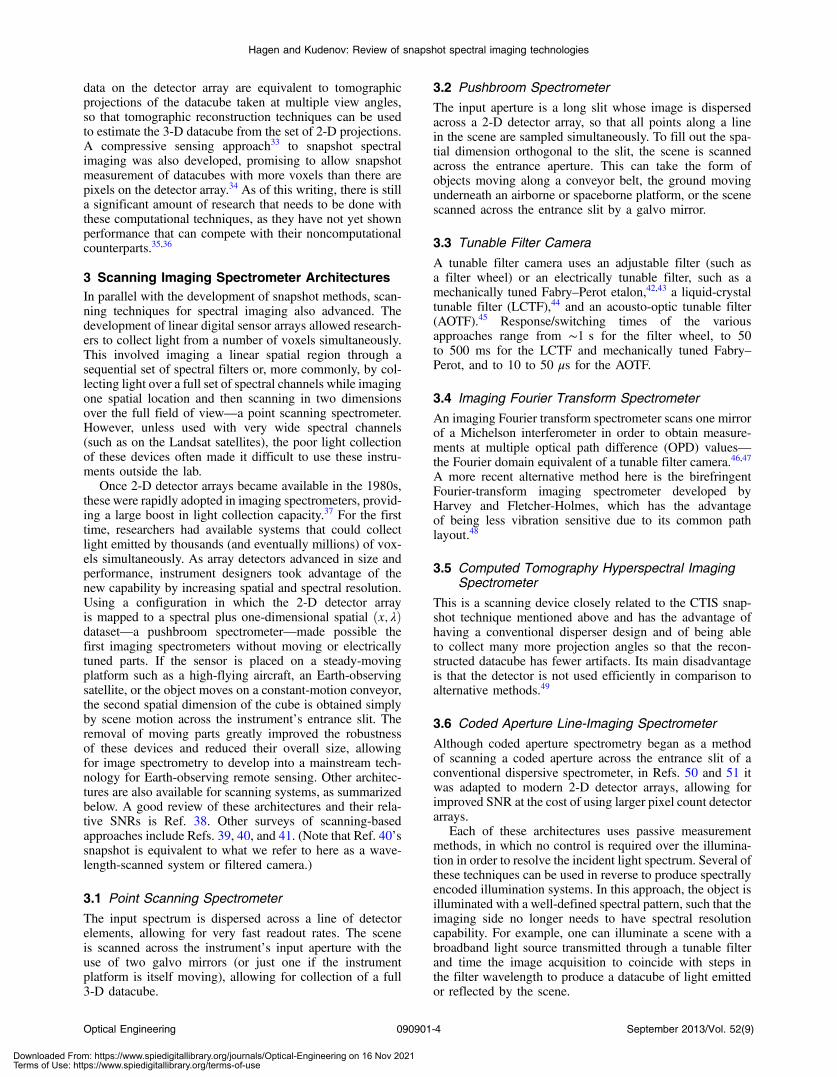
1 IntroductionSpectral imaging sensors sample the spectral irradianceIðx; y; λÞ of a scene and thus collect a three-dimensional(3-D) dataset typically called a datacube (see Fig. 1). Sincedatacubes are of a higher dimensionality than the two-dimensional (2-D) detector arrays currently available, systemdesigners must resort to either measuring time-sequential2-D slices of the cube or simultaneously measuring allelements of the datacube by dividing it into multiple 2-Delements that can be recombined into a cube in postpro-cessing. These two techniques are described here as scanningand snapshot.

The use of imaging spectrometers was rare beforethe arrival of 2-D CCD arrays in the 1980s, but steadilygrew as detector technology advanced. Over the following30 years, better optical designs, improved electronics,and advanced manufacturing have all contributed toimproving performance by over an order of magnitudesince that time. But the underlying optical technology hasnot really changed. Modified forms of the classic Czerny-Turner, Offner, and Michelson spectrometer layouts remainstandard. Snapshot spectral imagers, on the other hand,use optical designs that differ greatly from these standardforms in order to provide a boost in light collection capacityby up to three orders of magnitude. In the discussionbelow, we provide what we believe is the first overviewof snapshot spectral imaging implementations. After pro-viding background and definitions of terms, we presenta historical survey of the field and summarize each individ-ual measurement technique. The variety of instrumentsavailable can be a source of confusion, so we use ourdirect experience with a number of these technologies[computed tomography imaging spectrometer (CTIS),coded aperture snapshot spectral imager (CASSI), multi-aperture filtered camera (MAFC), image mapping spec-trometry (IMS), snapshot hyperspectral imaging Fouriertransform (SHIFT) spectrometer, and multispectral Sagnacinterferometer (MSI)—each described in Sec. 4 below] toprovide comparisons among them, listing some of theiradvantages and disadvantages.

1.1 Definitions and Background

The field of spectral imaging is plagued with inconsistent useof terminology, beginning with the field’s name itself. Oneoften finds spectral imaging, imaging spectrometry (or im-aging spectroscopy), hyperspectral imaging, and multispec-tral imaging used almost interchangeably. Some authorsmake a distinction between systems with few versus manyspectral bands (spectral imaging versus imaging spectrom-etry), or with contiguous versus spaced spectral bands(hyperspectral versus multispectral imaging). In the discus-sion below, we use spectral imaging to refer simply to anymeasurement attempting to obtain an Iðx; y; λÞ datacube of ascene, in which the spectral dimension is sampled by morethan three elements. In addition, we use the term snapshot asa synonym for nonscanning—i.e., systems in which theentire dataset is obtained during a single detector integrationperiod. Thus, while snapshot systems can often offer muchhigher light collection efficiency than equivalent scanninginstruments, snapshot by itself does not mean high through-put if the system architecture includes spatial and/or spectralfilters. When describing a scene as dynamic or static, ratherthan specifying the rate of change in absolute units for eachcase, we simply mean to say that a dynamic scene is one thatshows significant spatial and/or spectral change during themeasurement period of the instrument, whether that periodis a microsecond or an hour. Since snapshot does not by itselfimply fast, a dynamic scene can blur the image obtainedusing either a snapshot or a scanning device, the differencebeing that whereas motion induces blur in a snapshot system,in a scanning system, it induces artifacts. In principle, blur-ring and artifacts are on a similar footing, but in practiceone finds that artifacts prove more difficult to correct inpostprocessing.

When describing the various instrument architectures,“pixel” can be used to described an element of the 2-D detec-tor array or a single spatial location in the datacube (i.e., avector describing the spectrum at that location). While someauthors have tried introducing “spaxel” (spatial element) todescribe the latter,1 this terminology has not caught on, so wesimply use “pixel” when describing a spatial location whosespectrum is not of interest, and “point spectrum” when it is.

Optical Engineering 090901-1 September 2013/Vol. 52(9)

Optical Engineering 52(9), 090901 (September 2013) REVIEW


http://dx.doi.org/10.1117/1.OE.52.9.090901

http://dx.doi.org/10.1117/1.OE.52.9.090901

http://dx.doi.org/10.1117/1.OE.52.9.090901

http://dx.doi.org/10.1117/1.OE.52.9.090901

http://dx.doi.org/10.1117/1.OE.52.9.090901

http://dx.doi.org/10.1117/1.OE.52.9.090901

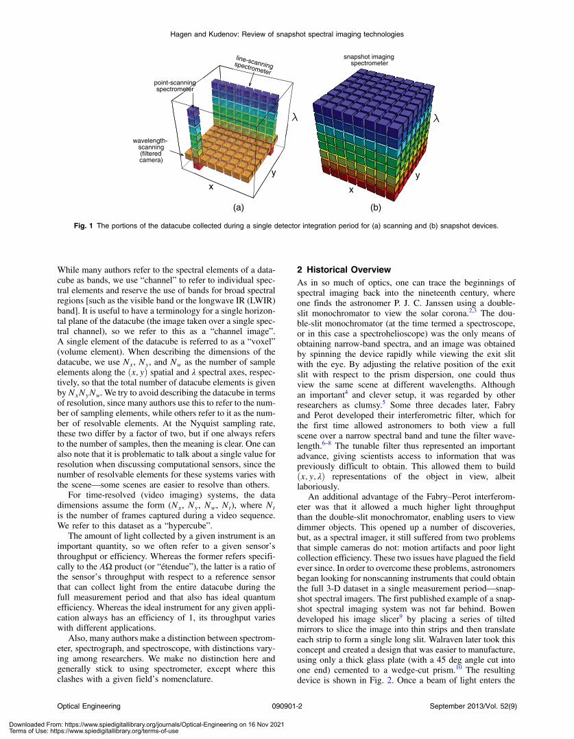
While many authors refer to the spectral elements of a data-cube as bands, we use “channel” to refer to individual spec-tral elements and reserve the use of bands for broad spectralregions [such as the visible band or the longwave IR (LWIR)band]. It is useful to have a terminology for a single horizon-tal plane of the datacube (the image taken over a single spec-tral channel), so we refer to this as a “channel image”.A single element of the datacube is referred to as a “voxel”(volume element). When describing the dimensions of thedatacube, we use Nx, Ny, and Nw as the number of sampleelements along the ðx; yÞ spatial and λ spectral axes, respec-tively, so that the total number of datacube elements is givenbyNxNyNw. We try to avoid describing the datacube in termsof resolution, since many authors use this to refer to the num-ber of sampling elements, while others refer to it as the num-ber of resolvable elements. At the Nyquist sampling rate,these two differ by a factor of two, but if one always refersto the number of samples, then the meaning is clear. One canalso note that it is problematic to talk about a single value forresolution when discussing computational sensors, since thenumber of resolvable elements for these systems varies withthe scene—some scenes are easier to resolve than others.

For time-resolved (video imaging) systems, the datadimensions assume the form (Nx, Ny, Nw, Nt), where Ntis the number of frames captured during a video sequence.We refer to this dataset as a “hypercube”.

The amount of light collected by a given instrument is animportant quantity, so we often refer to a given sensor’sthroughput or efficiency. Whereas the former refers specifi-cally to the AΩ product (or “étendue”), the latter is a ratio ofthe sensor’s throughput with respect to a reference sensorthat can collect light from the entire datacube during thefull measurement period and that also has ideal quantumefficiency. Whereas the ideal instrument for any given appli-cation always has an efficiency of 1, its throughput varieswith different applications.

Also, many authors make a distinction between spectrom-eter, spectrograph, and spectroscope, with distinctions vary-ing among researchers. We make no distinction here andgenerally stick to using spectrometer, except where thisclashes with a given field’s nomenclature.

2 Historical OverviewAs in so much of optics, one can trace the beginnings ofspectral imaging back into the nineteenth century, whereone finds the astronomer P. J. C. Janssen using a double-slit monochromator to view the solar corona.2,3 The dou-ble-slit monochromator (at the time termed a spectroscope,or in this case a spectrohelioscope) was the only means ofobtaining narrow-band spectra, and an image was obtainedby spinning the device rapidly while viewing the exit slitwith the eye. By adjusting the relative position of the exitslit with respect to the prism dispersion, one could thusview the same scene at different wavelengths. Althoughan important4 and clever setup, it was regarded by otherresearchers as clumsy.5 Some three decades later, Fabryand Perot developed their interferometric filter, which forthe first time allowed astronomers to both view a fullscene over a narrow spectral band and tune the filter wave-length.6–8 The tunable filter thus represented an importantadvance, giving scientists access to information that waspreviously difficult to obtain. This allowed them to buildðx; y; λÞ representations of the object in view, albeitlaboriously.

An additional advantage of the Fabry–Perot interferom-eter was that it allowed a much higher light throughputthan the double-slit monochromator, enabling users to viewdimmer objects. This opened up a number of discoveries,but, as a spectral imager, it still suffered from two problemsthat simple cameras do not: motion artifacts and poor lightcollection efficiency. These two issues have plagued the fieldever since. In order to overcome these problems, astronomersbegan looking for nonscanning instruments that could obtainthe full 3-D dataset in a single measurement period—snap-shot spectral imagers. The first published example of a snap-shot spectral imaging system was not far behind. Bowendeveloped his image slicer9 by placing a series of tiltedmirrors to slice the image into thin strips and then translateeach strip to form a single long slit. Walraven later took thisconcept and created a design that was easier to manufacture,using only a thick glass plate (with a 45 deg angle cut intoone end) cemented to a wedge-cut prism.10 The resultingdevice is shown in Fig. 2. Once a beam of light enters the

x

y

point-scanningspectrometer

line-scanningspectrometer

wavelength-scanning(filteredcamera)

x

y

snapshot imaging spectrometer

(a) (b)

Fig. 1 The portions of the datacube collected during a single detector integration period for (a) scanning and (b) snapshot devices.


Hagen and Kudenov: Review of snapshot spectral imaging technologies


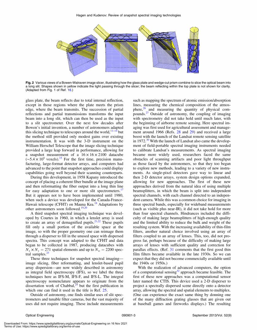
glass plate, the beam reflects due to total internal reflection,except in those regions where the plate meets the prismedge, where the beam transmits. The succession of partialreflections and partial transmissions transforms the inputbeam into a long slit, which can then be used as the inputto a slit spectrometer. Over the next few decades afterBowen’s initial invention, a number of astronomers adaptedthis slicing technique to telescopes around the world,11–14 butthe method still provided only modest gains over existinginstrumentation. It was with the 3-D instrument on theWilliam Herschel Telescope that the image slicing techniqueprovided a large leap forward in performance, allowing fora snapshot measurement of a 16 × 16 × 2100 datacube(∼5.4 × 105 voxels).15 For the first time, precision manu-facturing, large-format detector arrays, and computers hadadvanced to the point that snapshot approaches could displaycapabilities going well beyond their scanning counterparts.

During this development, in 1958 Kapany introduced theconcept of placing a coherent fiber bundle at the image planeand then reformatting the fiber output into a long thin linefor easy adaptation to one or more slit spectrometers.17

But it appears not to have been implemented until 1980,when such a device was developed for the Canada-France-Hawaii telescope (CFHT) on Mauna Kea.18 Adaptations byother astronomers soon followed.19,20

A third snapshot spectral imaging technique was devel-oped by Courtes in 1960, in which a lenslet array is usedto create an array of demagnified pupils.21,22 These pupilsfill only a small portion of the available space at theimage, so with the proper geometry one can reimage themthrough a disperser to fill in the unused space with dispersedspectra. This concept was adapted to the CFHT and databegan to be collected in 1987, producing datacubes withNx × Ny ¼ 271 spatial elements and up to Nw ¼ 2200 spec-tral samples.23

These three techniques for snapshot spectral imaging—image slicing, fiber reformatting, and lenslet-based pupilarray dispersion—are now widely described in astronomyas integral field spectroscopy (IFS), so we label the threetechniques here as IFS-M, IFS-F, and IFS-L. The integralspectroscopy nomenclature appears to originate from thedissertation work of Chabbal,24 but the first publication inwhich one can find it used in the title is Ref. 25.

Outside of astronomy, one finds similar uses of slit spec-trometers and tunable filter cameras, but the vast majority ofuses did not require imaging. These include measurements

such as mapping the spectrum of atomic emission/absorptionlines, measuring the chemical composition of the atmos-phere,26 and measuring the quantity of physical com-pounds.27 Outside of astronomy, the coupling of imagingwith spectrometry did not take hold until much later, withthe beginning of airborne remote sensing. Here spectral im-aging was first used for agricultural assessment and manage-ment around 1966 (Refs. 28 and 29) and received a largeboost with the launch of the Landsat remote sensing satellitein 1972.30 With the launch of Landsat also came the develop-ment of field-portable spectral imaging instruments neededto calibrate Landsat’s measurements. As spectral imagingbecame more widely used, researchers faced the sameobstacles of scanning artifacts and poor light throughputas those faced by the astronomers, so that they too beganto explore new methods, leading to a variety of new instru-ments. As single-pixel detectors gave way to linear andthen 2-D detector arrays, system design options expanded,allowing for new approaches. The first of these newapproaches derived from the natural idea of using multiplebeamsplitters, in which the beam is split into independentspectral channels, with each channel directed to an indepen-dent camera. While this was a common choice for imaging inthree spectral bands, especially for wideband measurements(such as visible plus near-IR), it did not take hold for morethan four spectral channels. Hindrances included the diffi-culty of making large beamsplitters of high-enough qualityand the limited ability to reduce the bulk and weight of theresulting system. With the increasing availability of thin-filmfilters, another natural choice involved using an array offilters coupled to an array of lenses. This, too, did not pro-gress far, perhaps because of the difficulty of making largearrays of lenses with sufficient quality and correction forparallax effects. (Ref. 31 comments that the first good thinfilm filters became available in the late 1930s. So we canexpect that they did not become commercially available untilthe 1940s or 1950s.)

With the realization of advanced computers, the optionof a computational sensing32 approach became feasible. Thefirst of these new approaches was a computational sensorlater named the CTIS. This device used a 2-D disperser toproject a spectrally dispersed scene directly onto a detectorarray, allowing the spectral and spatial elements to multiplex.(One can experience the exact same thing by donning oneof the many diffraction grating glasses that are given outat baseball games and fireworks displays.) The resulting

Fig. 2 Various views of a Bowen-Walraven image slicer, illustrating how the glass plate and wedge-cut prism combine to slice the optical beam intoa long slit. Shapes shown in yellow indicate the light passing through the slicer; the beam reflecting within the top plate is not shown for clarity.(Adapted from Fig. 1 of Ref. 16.)




data on the detector array are equivalent to tomographicprojections of the datacube taken at multiple view angles,so that tomographic reconstruction techniques can be usedto estimate the 3-D datacube from the set of 2-D projections.A compressive sensing approach33 to snapshot spectralimaging was also developed, promising to allow snapshotmeasurement of datacubes with more voxels than there arepixels on the detector array.34 As of this writing, there is stilla significant amount of research that needs to be done withthese computational techniques, as they have not yet shownperformance that can compete with their noncomputationalcounterparts.35,36

3 Scanning Imaging Spectrometer ArchitecturesIn parallel with the development of snapshot methods, scan-ning techniques for spectral imaging also advanced. Thedevelopment of linear digital sensor arrays allowed research-ers to collect light from a number of voxels simultaneously.This involved imaging a linear spatial region through asequential set of spectral filters or, more commonly, by col-lecting light over a full set of spectral channels while imagingone spatial location and then scanning in two dimensionsover the full field of view—a point scanning spectrometer.However, unless used with very wide spectral channels(such as on the Landsat satellites), the poor light collectionof these devices often made it difficult to use these instru-ments outside the lab.

Once 2-D detector arrays became available in the 1980s,these were rapidly adopted in imaging spectrometers, provid-ing a large boost in light collection capacity.37 For the firsttime, researchers had available systems that could collectlight emitted by thousands (and eventually millions) of vox-els simultaneously. As array detectors advanced in size andperformance, instrument designers took advantage of thenew capability by increasing spatial and spectral resolution.Using a configuration in which the 2-D detector arrayis mapped to a spectral plus one-dimensional spatial ðx; λÞdataset—a pushbroom spectrometer—made possible thefirst imaging spectrometers without moving or electricallytuned parts. If the sensor is placed on a steady-movingplatform such as a high-flying aircraft, an Earth-observingsatellite, or the object moves on a constant-motion conveyor,the second spatial dimension of the cube is obtained simplyby scene motion across the instrument’s entrance slit. Theremoval of moving parts greatly improved the robustnessof these devices and reduced their overall size, allowingfor image spectrometry to develop into a mainstream tech-nology for Earth-observing remote sensing. Other architec-tures are also available for scanning systems, as summarizedbelow. A good review of these architectures and their rela-tive SNRs is Ref. 38. Other surveys of scanning-basedapproaches include Refs. 39, 40, and 41. (Note that Ref. 40’ssnapshot is equivalent to what we refer to here as a wave-length-scanned system or filtered camera.)

3.1 Point Scanning Spectrometer

The input spectrum is dispersed across a line of detectorelements, allowing for very fast readout rates. The sceneis scanned across the instrument’s input aperture with theuse of two galvo mirrors (or just one if the instrumentplatform is itself moving), allowing for collection of a full3-D datacube.

3.2 Pushbroom Spectrometer

The input aperture is a long slit whose image is dispersedacross a 2-D detector array, so that all points along a linein the scene are sampled simultaneously. To fill out the spa-tial dimension orthogonal to the slit, the scene is scannedacross the entrance aperture. This can take the form ofobjects moving along a conveyor belt, the ground movingunderneath an airborne or spaceborne platform, or the scenescanned across the entrance slit by a galvo mirror.

3.3 Tunable Filter Camera

A tunable filter camera uses an adjustable filter (such asa filter wheel) or an electrically tunable filter, such as amechanically tuned Fabry–Perot etalon,42,43 a liquid-crystaltunable filter (LCTF),44 and an acousto-optic tunable filter(AOTF).45 Response/switching times of the variousapproaches range from ∼1 s for the filter wheel, to 50to 500 ms for the LCTF and mechanically tuned Fabry–Perot, and to 10 to 50 μs for the AOTF.

3.4 Imaging Fourier Transform Spectrometer

An imaging Fourier transform spectrometer scans one mirrorof a Michelson interferometer in order to obtain measure-ments at multiple optical path difference (OPD) values—the Fourier domain equivalent of a tunable filter camera.46,47

A more recent alternative method here is the birefringentFourier-transform imaging spectrometer developed byHarvey and Fletcher-Holmes, which has the advantageof being less vibration sensitive due to its common pathlayout.48

3.5 Computed Tomography Hyperspectral ImagingSpectrometer

This is a scanning device closely related to the CTIS snap-shot technique mentioned above and has the advantage ofhaving a conventional disperser design and of being ableto collect many more projection angles so that the recon-structed datacube has fewer artifacts. Its main disadvantageis that the detector is not used efficiently in comparison toalternative methods.49

3.6 Coded Aperture Line-Imaging Spectrometer

Although coded aperture spectrometry began as a methodof scanning a coded aperture across the entrance slit of aconventional dispersive spectrometer, in Refs. 50 and 51 itwas adapted to modern 2-D detector arrays, allowing forimproved SNR at the cost of using larger pixel count detectorarrays.

Each of these architectures uses passive measurementmethods, in which no control is required over the illumina-tion in order to resolve the incident light spectrum. Several ofthese techniques can be used in reverse to produce spectrallyencoded illumination systems. In this approach, the object isilluminated with a well-defined spectral pattern, such that theimaging side no longer needs to have spectral resolutioncapability. For example, one can illuminate a scene with abroadband light source transmitted through a tunable filterand time the image acquisition to coincide with steps inthe filter wavelength to produce a datacube of light emittedor reflected by the scene.




Finally, when comparing scanning and snapshot devices,we can note that the division between the two is not as blackand white as one might expect. For example, designers haveproduced sensor architectures that mix both snapshot andscanning techniques, so that the number of scans requiredto gather a complete dataset is significantly reduced. The ear-liest example of this of which we are aware (although itseems likely that astronomers had tried this well beforethis time), is a patent by Busch,52 where the author illustratesa method for coupling multiple optical fibers such that eachfiber is mapped to its own entrance slit within a dispersivespectrometer’s field of view. More recently, we can findexamples such as Chakrabarti et al., who describe a gratingspectrometer in which the entrance slit is actually four sep-arate slits simultaneously imaged by the system.53 Therespective slits are spaced apart such that the dispersed spec-tra do not overlap at the image plane. This setup can be usedto improve light collection by a factor of four, at the expenseof either increasing the detector size or reducing the spectralresolution by a factor of four. Ocean Optics’ SpectroCam isanother example of a mixed approach, in which a spinningfilter disk is combined with a pixel-level spectral filter array(more detail on the latter is given in Sec. 4.8) to improve thespeed of multispectral image acquisition.

In addition, the fact that a given instrument is snapshot doesnot in itself imply that the device is fast. Scanning devices canhave very short measurement times, and snapshot devices canpotentially havevery long ones. The essential difference is thatsnapshot devices collect data during a single detector integra-tion period, and whether this is short or long depends on theapplication. For large-format snapshot spectral imagers in par-ticular, the frame readout rate can also be rather long in com-parison to the exposure time, so that a video sequence (orhypercube) can be time-aliased due to poor sampling if thetwo rates are not forced to be better matched.

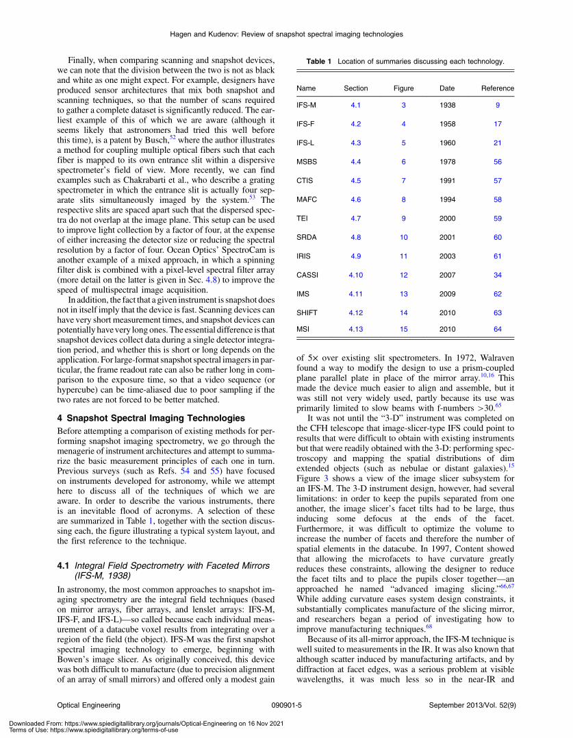
4 Snapshot Spectral Imaging TechnologiesBefore attempting a comparison of existing methods for per-forming snapshot imaging spectrometry, we go through themenagerie of instrument architectures and attempt to summa-rize the basic measurement principles of each one in turn.Previous surveys (such as Refs. 54 and 55) have focusedon instruments developed for astronomy, while we attempthere to discuss all of the techniques of which we areaware. In order to describe the various instruments, thereis an inevitable flood of acronyms. A selection of theseare summarized in Table 1, together with the section discus-sing each, the figure illustrating a typical system layout, andthe first reference to the technique.

4.1 Integral Field Spectrometry with Faceted Mirrors(IFS-M, 1938)

In astronomy, the most common approaches to snapshot im-aging spectrometry are the integral field techniques (basedon mirror arrays, fiber arrays, and lenslet arrays: IFS-M,IFS-F, and IFS-L)—so called because each individual meas-urement of a datacube voxel results from integrating over aregion of the field (the object). IFS-M was the first snapshotspectral imaging technology to emerge, beginning withBowen’s image slicer. As originally conceived, this devicewas both difficult to manufacture (due to precision alignmentof an array of small mirrors) and offered only a modest gain

of 5× over existing slit spectrometers. In 1972, Walravenfound a way to modify the design to use a prism-coupledplane parallel plate in place of the mirror array.10,16 Thismade the device much easier to align and assemble, but itwas still not very widely used, partly because its use wasprimarily limited to slow beams with f-numbers >30.65

It was not until the “3-D” instrument was completed onthe CFH telescope that image-slicer-type IFS could point toresults that were difficult to obtain with existing instrumentsbut that were readily obtained with the 3-D: performing spec-troscopy and mapping the spatial distributions of dimextended objects (such as nebulae or distant galaxies).15

Figure 3 shows a view of the image slicer subsystem foran IFS-M. The 3-D instrument design, however, had severallimitations: in order to keep the pupils separated from oneanother, the image slicer’s facet tilts had to be large, thusinducing some defocus at the ends of the facet.Furthermore, it was difficult to optimize the volume toincrease the number of facets and therefore the number ofspatial elements in the datacube. In 1997, Content showedthat allowing the microfacets to have curvature greatlyreduces these constraints, allowing the designer to reducethe facet tilts and to place the pupils closer together—anapproached he named “advanced imaging slicing.”66,67While adding curvature eases system design constraints, itsubstantially complicates manufacture of the slicing mirror,and researchers began a period of investigating how toimprove manufacturing techniques.68

Because of its all-mirror approach, the IFS-M technique iswell suited to measurements in the IR. It was also known thatalthough scatter induced by manufacturing artifacts, and bydiffraction at facet edges, was a serious problem at visiblewavelengths, it was much less so in the near-IR and

Table 1 Location of summaries discussing each technology.

Name Section Figure Date Reference

IFS-M 4.1 3 1938 9

IFS-F 4.2 4 1958 17

IFS-L 4.3 5 1960 21

MSBS 4.4 6 1978 56

CTIS 4.5 7 1991 57

MAFC 4.6 8 1994 58

TEI 4.7 9 2000 59

SRDA 4.8 10 2001 60

IRIS 4.9 11 2003 61

CASSI 4.10 12 2007 34

IMS 4.11 13 2009 62

SHIFT 4.12 14 2010 63

MSI 4.13 15 2010 64




shortwave IR, and the image slicing method has been shownto excel in these spectral bands.69 As confidence in manufac-turing techniques increased, Content later introduced theconcept of microslicing (or IFS-μ), a technique that com-bines design elements of IFS-M with IFS-L. This enabledone to measure many more spatial elements in the datacube,

at the expense of reduced spectral sampling.70 The basic ideaof microslicing is to use the same slicing mirror as IFS-M,but with larger facets. The slicer allows the various strips inthe image to be physically separated, and each is then passedthrough an anamorphic relay, such that one axis is stretched.This gives some extra space so that further down the optical

(b)

slicer mirror

(a)

optical axis

pupil

arra

y

pupil

arra

y

fold

mirr

ors

fold

mirr

ors

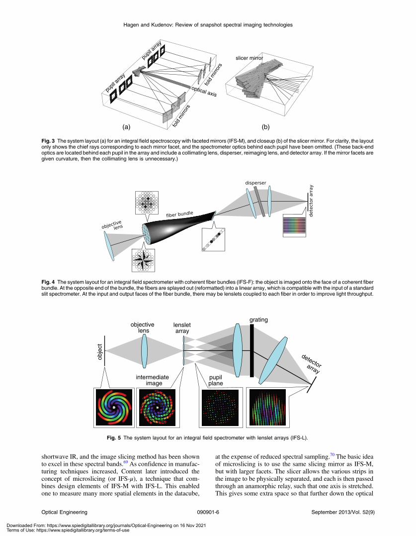
Fig. 3 The system layout (a) for an integral field spectroscopy with facetedmirrors (IFS-M), and closeup (b) of the slicer mirror. For clarity, the layoutonly shows the chief rays corresponding to each mirror facet, and the spectrometer optics behind each pupil have been omitted. (These back-endoptics are located behind each pupil in the array and include a collimating lens, disperser, reimaging lens, and detector array. If the mirror facets aregiven curvature, then the collimating lens is unnecessary.)

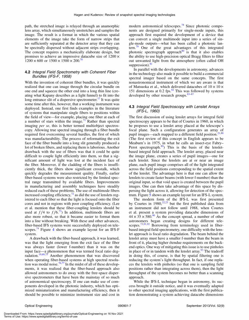
Fig. 4 The system layout for an integral field spectrometer with coherent fiber bundles (IFS-F): the object is imaged onto the face of a coherent fiberbundle. At the opposite end of the bundle, the fibers are splayed out (reformatted) into a linear array, which is compatible with the input of a standardslit spectrometer. At the input and output faces of the fiber bundle, there may be lenslets coupled to each fiber in order to improve light throughput.

obje

ct

objectivelens

lensletarray

grating

detectorarrayintermediate

imagepupilplane

Fig. 5 The system layout for an integral field spectrometer with lenslet arrays (IFS-L).




path, the stretched image is relayed through an anamorphiclens array, which simultaneously unstretches and samples theimage. The result is a format in which the various spatialelements of the image take the form of narrow strips thatare sufficiently separated at the detector array that they canbe spectrally dispersed without adjacent strips overlapping.The concept requires a mechanically elaborate design, butpromises to achieve an impressive datacube size of 1200 ×1200 × 600 or 1500 × 1500 × 200.70

4.2 Integral Field Spectrometry with Coherent FiberBundles (IFS-F, 1958)

With the invention of coherent fiber bundles, it was quicklyrealized that one can image through the circular bundle onone end and squeeze the other end into a long thin line (cre-ating what Kapany describes as a light funnel) to fit into thelong entrance slit of a dispersive spectrometer.17 It was quitesome time after this, however, that a working instrument wasdeployed. Instead, one first finds examples in the literatureof systems that manipulate single fibers to positions withinthe field of view—for example, placing one fiber at each ofa number of stars within the image.71 Rather than spectralimaging per se, this is better termed multiobject spectros-copy. Allowing true spectral imaging through a fiber bundlerequired first overcoming several hurdles, the first of whichwas manufacturability. The process of reformatting the exitface of the fiber bundle into a long slit generally produced alot of broken fibers, and replacing them is laborious. Anotherdrawback with the use of fibers was that it could be quitedifficult to couple light efficiently into them, so that a sig-nificant amount of light was lost at the incident face ofthe fiber. Moreover, if the cladding of the fibers is insuffi-ciently thick, the fibers show significant crosstalk, whichquickly degrades the measurement quality. Finally, earlierfiber-based systems were also restricted by the limited spec-tral range transmitted by available fibers. Improvementsin manufacturing and assembly techniques have steadilyreduced each of these problems. The use of multimode fibersincreased coupling efficiency,72 as did the use of lenslets reg-istered to each fiber so that the light is focused onto the fibercores and not in regions with poor coupling efficiency. (Leeet al. mention that these fiber-coupling lenslets should beused at f∕4 to f∕6.73) In addition, multimode fibers arealso more robust, so that it became easier to format theminto a line without breaking. With these and other advances,fiber-based IFS systems were successfully deployed on tele-scopes.74 Figure 4 shows an example layout for an IFS-Fsystem.

A drawback with the fiber-based approach, it was learned,was that the light emerging from the exit face of the fiberwas always faster (lower f-number) than it was on theinput face—a phenomenon that was termed focal ratio deg-radation.19,69,75 Another phenomenon that was discoveredwhen operating fiber-based systems at high spectral resolu-tion was modal noise.76,77 In the midst of all of these develop-ments, it was realized that the fiber-based approach alsoallowed astronomers to do away with the free-space disper-sive spectrometers that have been the mainstay of so muchof astronomical spectroscopy. If one can make use of com-ponents developed in the photonic industry, which has opti-mized miniaturization and manufacturing efficiency, then itshould be possible to minimize instrument size and cost in

modern astronomical telescopes.78 Since photonic compo-nents are designed primarily for single-mode inputs, thisapproach first required the development of a device thatcan convert a single multimode input into a series of sin-gle-mode outputs—what has been called a photonic lan-tern.79 One of the great advantages of this integratedphotonic spectrograph approach80 is that it also enablesthe ability to use high-precision optical Bragg filters to filterout unwanted light from the atmosphere (often called OHsuppression).81

In parallel with the developments in astronomy, advancesin the technology also made it possible to build a commercialspectral imager based on the same concepts. The firstnonastronomical instrument of which we are aware is thatof Matsuoka et al., which delivered datacubes of 10 × 10 ×151 dimensions at 0.2 fps.82 This was followed by systemsdeveloped by other research groups.83–87

4.3 Integral Field Spectroscopy with Lenslet Arrays(IFS-L, 1960)

The first discussion of using lenslet arrays for integral fieldspectroscopy appears to be that of Courtes in 1960, in whichhe proposes to use a lenslet array placed at the telescope’sfocal plane. Such a configuration generates an array ofpupil images—each mapped to a different field position.21,88

(The first review of this concept in English appears to beMeaburn’s in 1975, in what he calls an insect-eye Fabry–Perot spectrograph.89) This is the basis of the lenslet-based integral field approach. The lenslet array, placed nearthe image plane, creates a series of pupil images—one foreach lenslet. Since the lenslets are at or near an imageplane, each pupil image comprises all of the light integratedacross the field positions corresponding to the spatial extentof the lenslet. The advantage here is that one can allow thelenslets to create faster beams (with lower f-number) than theoriginal input, so that void space is created between the pupilimages. One can then take advantage of this space by dis-persing the light across it, allowing for detection of the spec-trum. Figure 5 shows an example layout for an IFS-L system.

The modern form of the IFS-L was first presentedby Courtes in 1980,22,23 but the first published data froman instrument did not follow until 1988, when Courteset al. present a system providing datacube dimensions of44 × 35 × 580.90 As the concept spread, a number of otherastronomers began creating designs for different tele-scopes.73,91,92 Borrowing from terminology used in fiber-based integral field spectrometry, one difficulty with the lens-let approach is focal ratio degradation. The beam behind thelenslet array must have a smaller f-number than the beam infront of it, placing higher étendue requirements on the back-end optics. One way of mitigating this issue is to use pinholesin place of or in tandem with the lenslet array.93 The tradeoffin doing this, of course, is that by spatial filtering one isreducing the system’s light throughput. In fact, if one repla-ces the lenslets with pinholes (so that one is sampling fieldpositions rather than integrating across them), then the lightthroughput of the system becomes no better than a scanningapproach.

While the IFS-L technique began in astronomy, its suc-cess brought it outside notice, and it was eventually adaptedto other spectral imaging applications, with the first publica-tion demonstrating a system achieving datacube dimensions




of 180 × 180 × 20, measured at 30 fps and f∕1.8 using a1280 × 1024 CCD.94,95

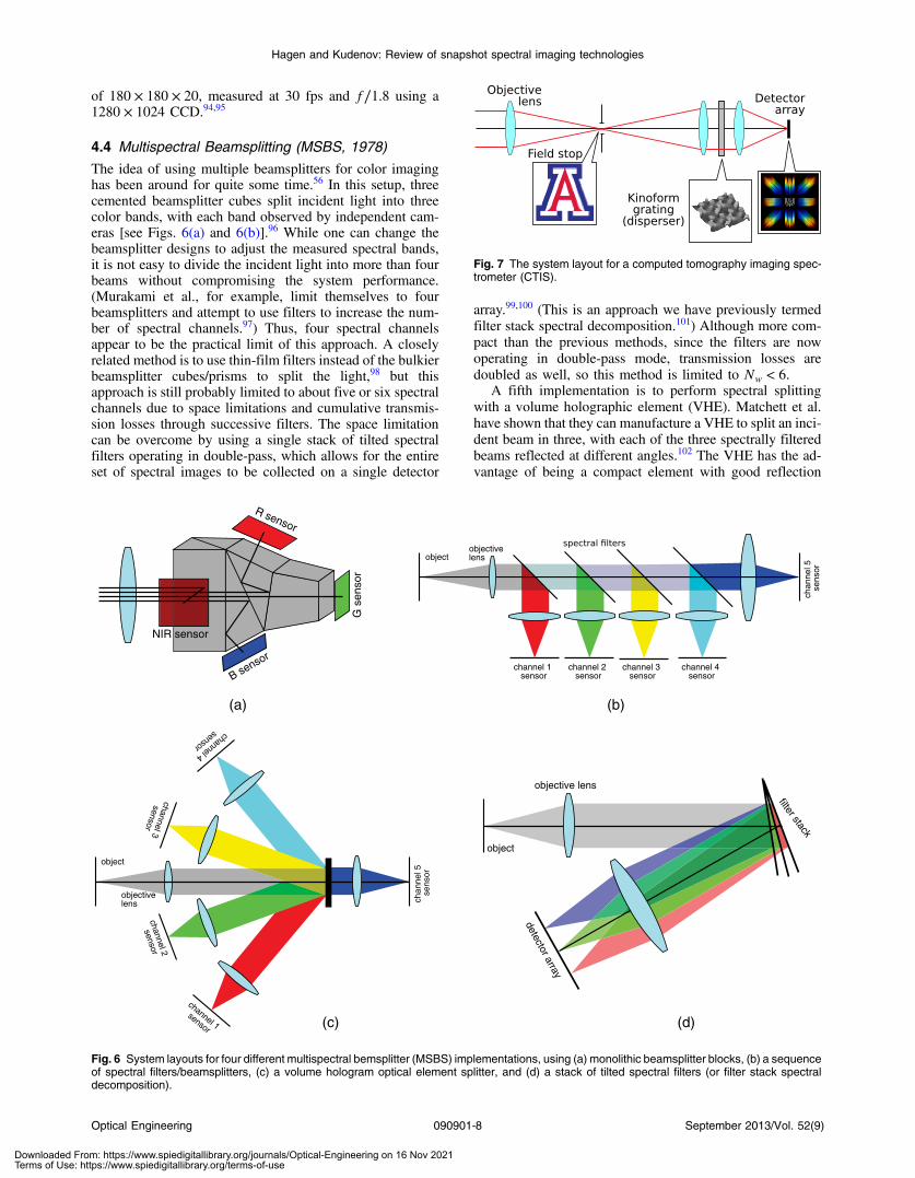
4.4 Multispectral Beamsplitting (MSBS, 1978)

The idea of using multiple beamsplitters for color imaginghas been around for quite some time.56 In this setup, threecemented beamsplitter cubes split incident light into threecolor bands, with each band observed by independent cam-eras [see Figs. 6(a) and 6(b)].96 While one can change thebeamsplitter designs to adjust the measured spectral bands,it is not easy to divide the incident light into more than fourbeams without compromising the system performance.(Murakami et al., for example, limit themselves to fourbeamsplitters and attempt to use filters to increase the num-ber of spectral channels.97) Thus, four spectral channelsappear to be the practical limit of this approach. A closelyrelated method is to use thin-film filters instead of the bulkierbeamsplitter cubes/prisms to split the light,98 but thisapproach is still probably limited to about five or six spectralchannels due to space limitations and cumulative transmis-sion losses through successive filters. The space limitationcan be overcome by using a single stack of tilted spectralfilters operating in double-pass, which allows for the entireset of spectral images to be collected on a single detector

array.99,100 (This is an approach we have previously termedfilter stack spectral decomposition.101) Although more com-pact than the previous methods, since the filters are nowoperating in double-pass mode, transmission losses aredoubled as well, so this method is limited to Nw < 6.

A fifth implementation is to perform spectral splittingwith a volume holographic element (VHE). Matchett et al.have shown that they can manufacture a VHE to split an inci-dent beam in three, with each of the three spectrally filteredbeams reflected at different angles.102 The VHE has the ad-vantage of being a compact element with good reflection

channel 4

sensor

channel 1sensor

channel 2

sensor

channel 3sensor

object

objectivelens ch

anne

l 5se

nsor

R sensor

G s

enso

r

B sensor

NIR sensor

(a)

(c)

channel 1sensor

channel 2sensor

channel 3sensor

channel 4sensor

chan

nel 5

sens

or

objectobjectivelens

(b)

objective lens

filter stack

object

detector array

(d)

Fig. 6 System layouts for four different multispectral bemsplitter (MSBS) implementations, using (a) monolithic beamsplitter blocks, (b) a sequenceof spectral filters/beamsplitters, (c) a volume hologram optical element splitter, and (d) a stack of tilted spectral filters (or filter stack spectraldecomposition).

Fig. 7 The system layout for a computed tomography imaging spec-trometer (CTIS).




efficiency over a reasonable range of field angles. But itappears to be difficult to design the VHE for more thanthree channels. For example, Matchett et al. divided the sys-tem pupil in four, using a different VHE for each of the foursections, in order to produce a system that can measure 12spectral channels. Matchett et al. state that this system hasachieved 60 to 75% throughput across the visible spectrum.

4.5 Computed Tomography Imaging Spectrometry(CTIS, 1991)

As with every other snapshot spectral imaging technology,CTIS can be regarded as a generalization of a scanningapproach—in this case a slit spectrometer. If one openswide the slit of a standard slit spectrometer, spectral resolu-tion suffers in that spatial and spectral variations across thewidth of the slit become mixed at the detector. However, ifinstead of a linear disperser one uses a 2-D dispersion pat-tern, then the mixing of spatial and spectral data can be madeto vary at different positions on the detector. This allowstomographic reconstruction techniques to be used to estimatethe datacube from its multiple projections at different viewangles. Figure 7 shows the CTIS system layout. The CTISconcept was invented by Okamoto and Yamaguchi57 in 1991and independently by Bulygin and Vishnyakov103 in 1991/1992, and was soon further developed by Descour, whoalso discovered CTIS’s missing cone problem.35,104,105 Theinstrument was further developed by using a custom-designed kinoform disperser and for use in the IRbands.106 The first high-resolution CTIS, however, wasnot available until 2001, providing a 203 × 203 × 55 data-cube on a 2048 × 2048 CCD camera.107 Although theCTIS layout is almost invariably shown using a transmissivedisperser, Johnson et al. successfully demonstrated a reflec-tive design in 2005.108

A major advantage of the CTIS approach is that the systemlayout can be made quite compact, but a major disadvantagehas been the difficulty in manufacturing the kinoform dispers-ing elements. Moreover, since its inception, CTIS has had todeal with problems surrounding its computational complexity,calibration difficulty, and measurement artifacts. These form acommon theme among many computational sensors, and thegap they create between ideal measurement and field measure-ments forms the difference between a research instrumentand a commercializable one. While CTIS has shown a lotof progress on bridging this gap, it has not shown the abilityto achieve a performance level sufficient for widespread use.

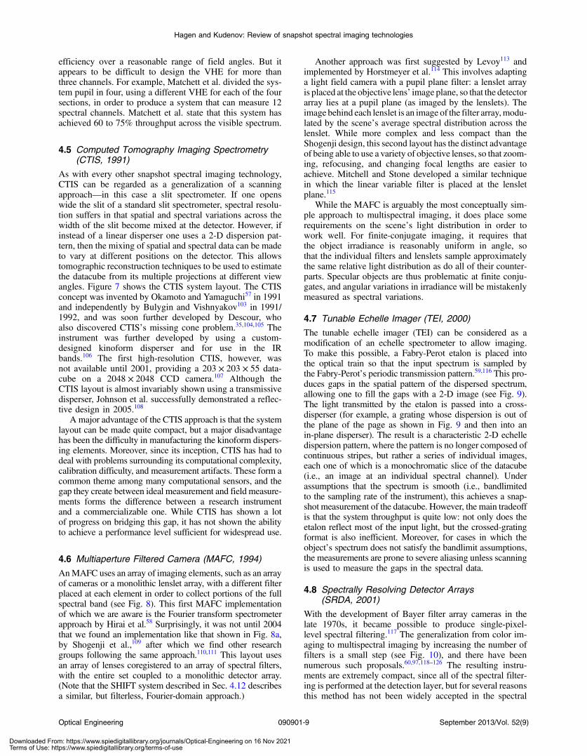
4.6 Multiaperture Filtered Camera (MAFC, 1994)

AnMAFC uses an array of imaging elements, such as an arrayof cameras or a monolithic lenslet array, with a different filterplaced at each element in order to collect portions of the fullspectral band (see Fig. 8). This first MAFC implementationof which we are aware is the Fourier transform spectrometerapproach by Hirai et al.58 Surprisingly, it was not until 2004that we found an implementation like that shown in Fig. 8a,by Shogenji et al.,109 after which we find other researchgroups following the same approach.110,111 This layout usesan array of lenses coregistered to an array of spectral filters,with the entire set coupled to a monolithic detector array.(Note that the SHIFT system described in Sec. 4.12 describesa similar, but filterless, Fourier-domain approach.)

Another approach was first suggested by Levoy113 andimplemented by Horstmeyer et al.114 This involves adaptinga light field camera with a pupil plane filter: a lenslet arrayis placed at the objective lens’ image plane, so that the detectorarray lies at a pupil plane (as imaged by the lenslets). Theimage behind each lenslet is an image of the filter array,modu-lated by the scene’s average spectral distribution across thelenslet. While more complex and less compact than theShogenji design, this second layout has the distinct advantageof being able to use a variety of objective lenses, so that zoom-ing, refocusing, and changing focal lengths are easier toachieve. Mitchell and Stone developed a similar techniquein which the linear variable filter is placed at the lensletplane.115

While the MAFC is arguably the most conceptually sim-ple approach to multispectral imaging, it does place somerequirements on the scene’s light distribution in order towork well. For finite-conjugate imaging, it requires thatthe object irradiance is reasonably uniform in angle, sothat the individual filters and lenslets sample approximatelythe same relative light distribution as do all of their counter-parts. Specular objects are thus problematic at finite conju-gates, and angular variations in irradiance will be mistakenlymeasured as spectral variations.

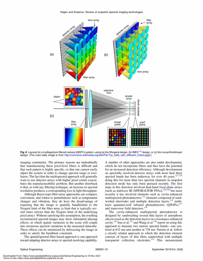
4.7 Tunable Echelle Imager (TEI, 2000)

The tunable echelle imager (TEI) can be considered as amodification of an echelle spectrometer to allow imaging.To make this possible, a Fabry-Perot etalon is placed intothe optical train so that the input spectrum is sampled bythe Fabry-Perot’s periodic transmission pattern.59,116 This pro-duces gaps in the spatial pattern of the dispersed spectrum,allowing one to fill the gaps with a 2-D image (see Fig. 9).The light transmitted by the etalon is passed into a cross-disperser (for example, a grating whose dispersion is out ofthe plane of the page as shown in Fig. 9 and then into anin-plane disperser). The result is a characteristic 2-D echelledispersion pattern, where the pattern is no longer composed ofcontinuous stripes, but rather a series of individual images,each one of which is a monochromatic slice of the datacube(i.e., an image at an individual spectral channel). Underassumptions that the spectrum is smooth (i.e., bandlimitedto the sampling rate of the instrument), this achieves a snap-shot measurement of the datacube. However, the main tradeoffis that the system throughput is quite low: not only does theetalon reflect most of the input light, but the crossed-gratingformat is also inefficient. Moreover, for cases in which theobject’s spectrum does not satisfy the bandlimit assumptions,the measurements are prone to severe aliasing unless scanningis used to measure the gaps in the spectral data.

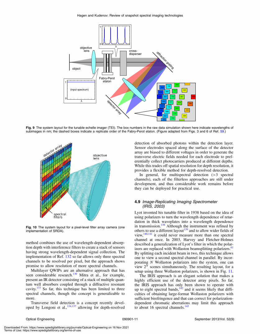
4.8 Spectrally Resolving Detector Arrays(SRDA, 2001)

With the development of Bayer filter array cameras in thelate 1970s, it became possible to produce single-pixel-level spectral filtering.117 The generalization from color im-aging to multispectral imaging by increasing the number offilters is a small step (see Fig. 10), and there have beennumerous such proposals.60,97,118–126 The resulting instru-ments are extremely compact, since all of the spectral filter-ing is performed at the detection layer, but for several reasonsthis method has not been widely accepted in the spectral




imaging community. The primary reasons are undoubtedlythat manufacturing these pixel-level filters is difficult andthat each pattern is highly specific, so that one cannot easilyadjust the system in order to change spectral range or reso-lution. The fact that the multispectral approach will generallywant to use detector arrays with higher pixel counts exacer-bates the manufacturability problem. But another drawbackis that, as with any filtering technique, an increase in spectralresolution produces a corresponding loss in light throughput.

Although Bayer-type filter-array approaches are compact,convenient, and robust to perturbations such as temperaturechanges and vibration, they do have the disadvantage ofrequiring that the image is spatially bandlimited to theNyquist limit of the filter array (a limit that is typically sev-eral times stricter than the Nyquist limit of the underlyingpixel array). Without satisfying this assumption, the resultingreconstructed spectral images may show substantial aliasingeffects, in which spatial variations in the scene will coupleinto erroneous spectral variations in the measured datacube.These effects can be minimized by defocusing the image inorder to satisfy the bandlimit constraint.

The spatial/spectral filter-based approach is one approachtoward adapting detector arrays to spectral resolving capability.

A number of other approaches are also under development,which do not incorporate filters and thus have the potentialfor an increased detection efficiency. Although developmenton spectrally resolved detector arrays with more than threespectral bands has been underway for over 40 years,127,128

doing this for more than two spectral channels in snapshotdetection mode has only been pursued recently. The firststeps in this direction involved dual-band focal plane arrays[such as midwave IR (MWIR)/LWIR FPAs],129,130 but morerecently it has involved elements such as cavity-enhancedmultispectral photodetectors,131 elements composed of sand-wiched electrodes and multiple detection layers,132 multi-layer quantum-well infrared photodetectors (QWIPs),133

and transverse field detectors.134

The cavity-enhanced multispectral photodetector isdesigned by sandwiching several thin layers of amorphoussilicon (used as the detection layers) in a resonance-enhancedcavity.135 Sun et al.131 and Wang et al.136 report on using thisapproach to measure two narrow spectral bands—one cen-tered at 632 nm and another at 728 nm. Parrein et al. followa closely related approach in which the detection elementconsists of layers of thin films sandwiched with multipletransparent collection electrodes.132 This measurement

detector a

rray

lens array

filter array

(a)

(c) dete

ctor

arr

ay

objectivelens

lensletarray

imageplane

pupilplane

object

filterarray

lens array

filterarray

detector a

rray

(b)

Fig. 8 Layouts for a multiaperture filtered camera (MAFC) system, using (a) the Shogenji design, (b) IMEC112 design, or (c) the Levoy/Horstmeyerdesign. (The color balls image is from http://commons.wikimedia.org/wiki/File:Toy_balls_with_different_Colors.jpg#.)




http://commons.wikimedia.org/wiki/File:Toy_balls_with_different_Colors.jpg#




method combines the use of wavelength-dependent absorp-tion depth with interference filters to create a stack of sensorshaving strong wavelength-dependent signal collection. Theimplementation of Ref. 132 so far allows only three spectralchannels to be resolved per pixel, but the approach showspromise to allow resolution of more spectral channels.

Multilayer QWIPs are an alternative approach that hasseen considerable research.130 Mitra et al., for example,present an IR detector consisting of a stack of multiple quan-tum well absorbers coupled through a diffractive resonantcavity.133 So far, this technique has been limited to threespectral channels, though the concept is generalizable tomore.

Transverse field detection is a concept recently devel-oped by Longoni et al.,134,137 allowing for depth-resolved

detection of absorbed photons within the detection layer.Sensor electrodes spaced along the surface of the detectorarray are biased to different voltages in order to generate thetransverse electric fields needed for each electrode to pref-erentially collect photocarriers produced at different depths.While this trades off spatial resolution for depth resolution, itprovides a flexible method for depth-resolved detection.

In general, for multispectral detection (>3 spectralchannels), each of the filterless approaches are still underdevelopment, and thus considerable work remains beforethey can be deployed for practical use.

4.9 Image-Replicating Imaging Spectrometer(IRIS, 2003)

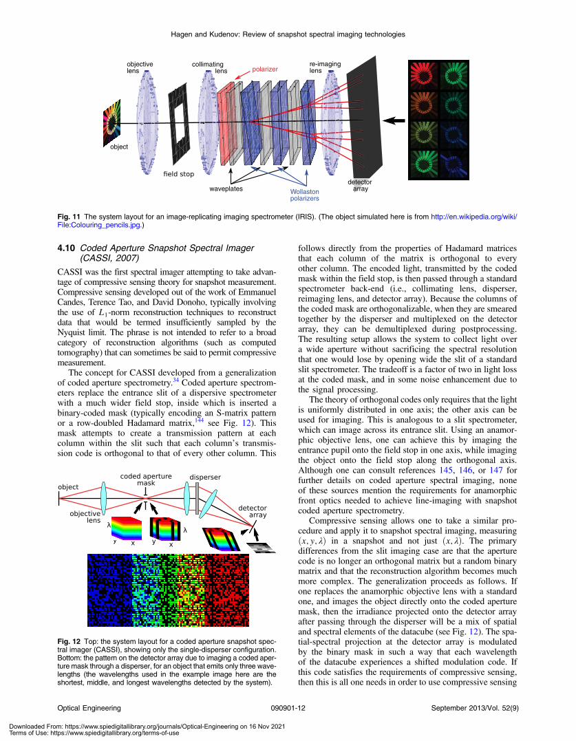
Lyot invented his tunable filter in 1938 based on the idea ofusing polarizers to turn the wavelength dependence of retar-dation in thick waveplates into a wavelength dependencein transmission.138 Although the instrument was refined byothers to use a different layout139 and to allow wider fields ofview,140,141 it could never measure more than one spectralchannel at once. In 2003, Harvey and Fletcher-Holmesdescribed a generalization of Lyot’s filter in which the polar-izers are replaced with Wollaston beamsplitting polarizers.61

By splitting each incident beam in two, this technique allowsone to view a second spectral channel in parallel. By incor-porating N Wollaston polarizers into the system, one canview 2N scenes simultaneously. The resulting layout, for asetup using three Wollaston polarizers, is shown in Fig. 11.

The IRIS approach is an elegant solution that makes ahighly efficient use of the detector array pixels. So far,the IRIS approach has only been shown to operate withup to eight spectral bands,142 and it seems likely that diffi-culties of obtaining large-format Wollaston polarizers withsufficient birefringence and that can correct for polarization-dependent chromatic aberrations may limit this approachto about 16 spectral channels.143

detector array

object

objectivelens cross-

disperser

Fabry-Perotetalon

diffraction grating

750

774

800

828 960

923

889

649

667

686

706

727

600

615

632

649

667

686

706632

615

600 750 857 1000

774 889

800

0

1

0

1

(input spectrum)

Fig. 9 The system layout for the tunable echelle imager (TEI). The box numbers in the raw data simulation shown here indicate wavelengths ofsubimages in nm; the dashed boxes indicate a replicate order of the Fabry-Perot etalon. (Figure adapted from Figs. 3 and 6 of Ref. 59.)

Fig. 10 The system layout for a pixel-level filter array camera (oneimplementation of SRDA).




4.10 Coded Aperture Snapshot Spectral Imager(CASSI, 2007)

CASSI was the first spectral imager attempting to take advan-tage of compressive sensing theory for snapshot measurement.Compressive sensing developed out of the work of EmmanuelCandes, Terence Tao, and David Donoho, typically involvingthe use of L1-norm reconstruction techniques to reconstructdata that would be termed insufficiently sampled by theNyquist limit. The phrase is not intended to refer to a broadcategory of reconstruction algorithms (such as computedtomography) that can sometimes be said to permit compressivemeasurement.

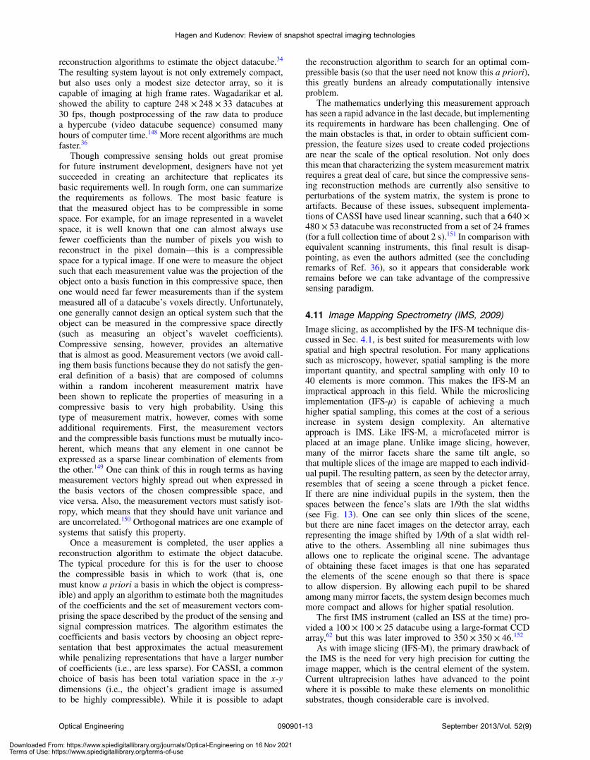
The concept for CASSI developed from a generalizationof coded aperture spectrometry.34 Coded aperture spectrom-eters replace the entrance slit of a dispersive spectrometerwith a much wider field stop, inside which is inserted abinary-coded mask (typically encoding an S-matrix patternor a row-doubled Hadamard matrix,144 see Fig. 12). Thismask attempts to create a transmission pattern at eachcolumn within the slit such that each column’s transmis-sion code is orthogonal to that of every other column. This

follows directly from the properties of Hadamard matricesthat each column of the matrix is orthogonal to everyother column. The encoded light, transmitted by the codedmask within the field stop, is then passed through a standardspectrometer back-end (i.e., collimating lens, disperser,reimaging lens, and detector array). Because the columns ofthe coded mask are orthogonalizable, when they are smearedtogether by the disperser and multiplexed on the detectorarray, they can be demultiplexed during postprocessing.The resulting setup allows the system to collect light overa wide aperture without sacrificing the spectral resolutionthat one would lose by opening wide the slit of a standardslit spectrometer. The tradeoff is a factor of two in light lossat the coded mask, and in some noise enhancement due tothe signal processing.

The theory of orthogonal codes only requires that the lightis uniformly distributed in one axis; the other axis can beused for imaging. This is analogous to a slit spectrometer,which can image across its entrance slit. Using an anamor-phic objective lens, one can achieve this by imaging theentrance pupil onto the field stop in one axis, while imagingthe object onto the field stop along the orthogonal axis.Although one can consult references 145, 146, or 147 forfurther details on coded aperture spectral imaging, noneof these sources mention the requirements for anamorphicfront optics needed to achieve line-imaging with snapshotcoded aperture spectrometry.

Compressive sensing allows one to take a similar pro-cedure and apply it to snapshot spectral imaging, measuringðx; y; λÞ in a snapshot and not just ðx; λÞ. The primarydifferences from the slit imaging case are that the aperturecode is no longer an orthogonal matrix but a random binarymatrix and that the reconstruction algorithm becomes muchmore complex. The generalization proceeds as follows. Ifone replaces the anamorphic objective lens with a standardone, and images the object directly onto the coded aperturemask, then the irradiance projected onto the detector arrayafter passing through the disperser will be a mix of spatialand spectral elements of the datacube (see Fig. 12). The spa-tial-spectral projection at the detector array is modulatedby the binary mask in such a way that each wavelengthof the datacube experiences a shifted modulation code. Ifthis code satisfies the requirements of compressive sensing,then this is all one needs in order to use compressive sensing

objectivelens

collimatinglens

waveplates Wollastonpolarizers

polarizerre-imaginglens

detectorarray

object

Fig. 11 The system layout for an image-replicating imaging spectrometer (IRIS). (The object simulated here is from http://en.wikipedia.org/wiki/File:Colouring_pencils.jpg.)

Fig. 12 Top: the system layout for a coded aperture snapshot spec-tral imager (CASSI), showing only the single-disperser configuration.Bottom: the pattern on the detector array due to imaging a coded aper-ture mask through a disperser, for an object that emits only three wave-lengths (the wavelengths used in the example image here are theshortest, middle, and longest wavelengths detected by the system).




http://en.wikipedia.org/wiki/File:Colouring_pencils.jpg.






reconstruction algorithms to estimate the object datacube.34

The resulting system layout is not only extremely compact,but also uses only a modest size detector array, so it iscapable of imaging at high frame rates. Wagadarikar et al.showed the ability to capture 248 × 248 × 33 datacubes at30 fps, though postprocessing of the raw data to producea hypercube (video datacube sequence) consumed manyhours of computer time.148 More recent algorithms are muchfaster.36

Though compressive sensing holds out great promisefor future instrument development, designers have not yetsucceeded in creating an architecture that replicates itsbasic requirements well. In rough form, one can summarizethe requirements as follows. The most basic feature isthat the measured object has to be compressible in somespace. For example, for an image represented in a waveletspace, it is well known that one can almost always usefewer coefficients than the number of pixels you wish toreconstruct in the pixel domain—this is a compressiblespace for a typical image. If one were to measure the objectsuch that each measurement value was the projection of theobject onto a basis function in this compressive space, thenone would need far fewer measurements than if the systemmeasured all of a datacube’s voxels directly. Unfortunately,one generally cannot design an optical system such that theobject can be measured in the compressive space directly(such as measuring an object’s wavelet coefficients).Compressive sensing, however, provides an alternativethat is almost as good. Measurement vectors (we avoid call-ing them basis functions because they do not satisfy the gen-eral definition of a basis) that are composed of columnswithin a random incoherent measurement matrix havebeen shown to replicate the properties of measuring in acompressive basis to very high probability. Using thistype of measurement matrix, however, comes with someadditional requirements. First, the measurement vectorsand the compressible basis functions must be mutually inco-herent, which means that any element in one cannot beexpressed as a sparse linear combination of elements fromthe other.149 One can think of this in rough terms as havingmeasurement vectors highly spread out when expressed inthe basis vectors of the chosen compressible space, andvice versa. Also, the measurement vectors must satisfy isot-ropy, which means that they should have unit variance andare uncorrelated.150 Orthogonal matrices are one example ofsystems that satisfy this property.

Once a measurement is completed, the user applies areconstruction algorithm to estimate the object datacube.The typical procedure for this is for the user to choosethe compressible basis in which to work (that is, onemust know a priori a basis in which the object is compress-ible) and apply an algorithm to estimate both the magnitudesof the coefficients and the set of measurement vectors com-prising the space described by the product of the sensing andsignal compression matrices. The algorithm estimates thecoefficients and basis vectors by choosing an object repre-sentation that best approximates the actual measurementwhile penalizing representations that have a larger numberof coefficients (i.e., are less sparse). For CASSI, a commonchoice of basis has been total variation space in the x-ydimensions (i.e., the object’s gradient image is assumedto be highly compressible). While it is possible to adapt

the reconstruction algorithm to search for an optimal com-pressible basis (so that the user need not know this a priori),this greatly burdens an already computationally intensiveproblem.

The mathematics underlying this measurement approachhas seen a rapid advance in the last decade, but implementingits requirements in hardware has been challenging. One ofthe main obstacles is that, in order to obtain sufficient com-pression, the feature sizes used to create coded projectionsare near the scale of the optical resolution. Not only doesthis mean that characterizing the system measurement matrixrequires a great deal of care, but since the compressive sens-ing reconstruction methods are currently also sensitive toperturbations of the system matrix, the system is prone toartifacts. Because of these issues, subsequent implementa-tions of CASSI have used linear scanning, such that a 640 ×480 × 53 datacube was reconstructed from a set of 24 frames(for a full collection time of about 2 s).151 In comparison withequivalent scanning instruments, this final result is disap-pointing, as even the authors admitted (see the concludingremarks of Ref. 36), so it appears that considerable workremains before we can take advantage of the compressivesensing paradigm.

4.11 Image Mapping Spectrometry (IMS, 2009)

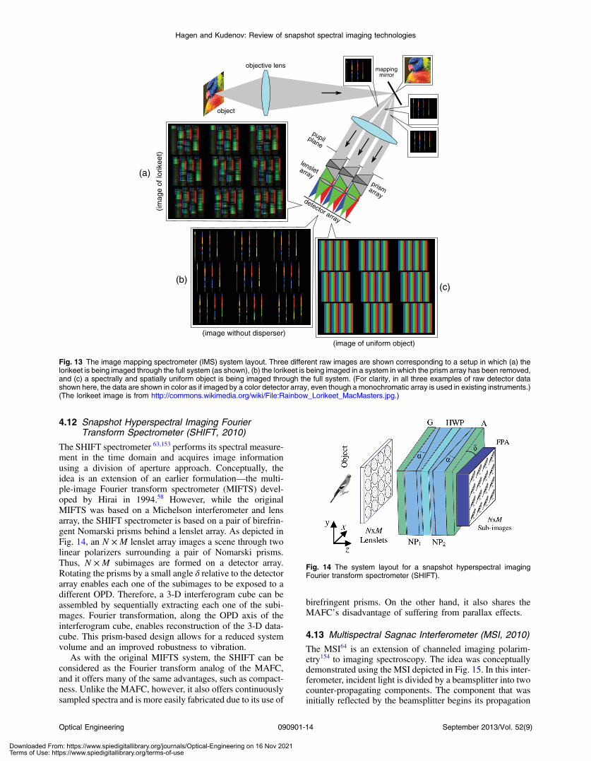
Image slicing, as accomplished by the IFS-M technique dis-cussed in Sec. 4.1, is best suited for measurements with lowspatial and high spectral resolution. For many applicationssuch as microscopy, however, spatial sampling is the moreimportant quantity, and spectral sampling with only 10 to40 elements is more common. This makes the IFS-M animpractical approach in this field. While the microslicingimplementation (IFS-μ) is capable of achieving a muchhigher spatial sampling, this comes at the cost of a seriousincrease in system design complexity. An alternativeapproach is IMS. Like IFS-M, a microfaceted mirror isplaced at an image plane. Unlike image slicing, however,many of the mirror facets share the same tilt angle, sothat multiple slices of the image are mapped to each individ-ual pupil. The resulting pattern, as seen by the detector array,resembles that of seeing a scene through a picket fence.If there are nine individual pupils in the system, then thespaces between the fence’s slats are 1/9th the slat widths(see Fig. 13). One can see only thin slices of the scene,but there are nine facet images on the detector array, eachrepresenting the image shifted by 1/9th of a slat width rel-ative to the others. Assembling all nine subimages thusallows one to replicate the original scene. The advantageof obtaining these facet images is that one has separatedthe elements of the scene enough so that there is spaceto allow dispersion. By allowing each pupil to be sharedamong many mirror facets, the system design becomes muchmore compact and allows for higher spatial resolution.

The first IMS instrument (called an ISS at the time) pro-vided a 100 × 100 × 25 datacube using a large-format CCDarray,62 but this was later improved to 350 × 350 × 46.152

As with image slicing (IFS-M), the primary drawback ofthe IMS is the need for very high precision for cutting theimage mapper, which is the central element of the system.Current ultraprecision lathes have advanced to the pointwhere it is possible to make these elements on monolithicsubstrates, though considerable care is involved.




4.12 Snapshot Hyperspectral Imaging FourierTransform Spectrometer (SHIFT, 2010)

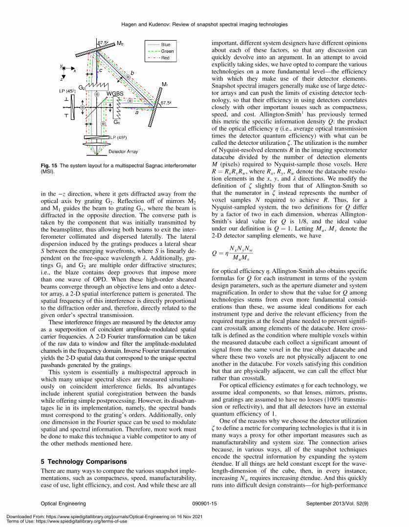
The SHIFT spectrometer 63,153 performs its spectral measure-ment in the time domain and acquires image informationusing a division of aperture approach. Conceptually, theidea is an extension of an earlier formulation—the multi-ple-image Fourier transform spectrometer (MIFTS) devel-oped by Hirai in 1994.58 However, while the originalMIFTS was based on a Michelson interferometer and lensarray, the SHIFT spectrometer is based on a pair of birefrin-gent Nomarski prisms behind a lenslet array. As depicted inFig. 14, an N ×M lenslet array images a scene through twolinear polarizers surrounding a pair of Nomarski prisms.Thus, N ×M subimages are formed on a detector array.Rotating the prisms by a small angle δ relative to the detectorarray enables each one of the subimages to be exposed to adifferent OPD. Therefore, a 3-D interferogram cube can beassembled by sequentially extracting each one of the subi-mages. Fourier transformation, along the OPD axis of theinterferogram cube, enables reconstruction of the 3-D data-cube. This prism-based design allows for a reduced systemvolume and an improved robustness to vibration.

As with the original MIFTS system, the SHIFT can beconsidered as the Fourier transform analog of the MAFC,and it offers many of the same advantages, such as compact-ness. Unlike the MAFC, however, it also offers continuouslysampled spectra and is more easily fabricated due to its use of

birefringent prisms. On the other hand, it also shares theMAFC’s disadvantage of suffering from parallax effects.

4.13 Multispectral Sagnac Interferometer (MSI, 2010)

The MSI64 is an extension of channeled imaging polarim-etry154 to imaging spectroscopy. The idea was conceptuallydemonstrated using the MSI depicted in Fig. 15. In this inter-ferometer, incident light is divided by a beamsplitter into twocounter-propagating components. The component that wasinitially reflected by the beamsplitter begins its propagation

objective lensmapping

mirror

object

lensletarray

pupilplane

prismarraydetector array

(image without disperser)(image of uniform object)

(imag

e of

lorik

eet)

(a)

(b)(c)

Fig. 13 The image mapping spectrometer (IMS) system layout. Three different raw images are shown corresponding to a setup in which (a) thelorikeet is being imaged through the full system (as shown), (b) the lorikeet is being imaged in a system in which the prism array has been removed,and (c) a spectrally and spatially uniform object is being imaged through the full system. (For clarity, in all three examples of raw detector datashown here, the data are shown in color as if imaged by a color detector array, even though a monochromatic array is used in existing instruments.)(The lorikeet image is from http://commons.wikimedia.org/wiki/File:Rainbow_Lorikeet_MacMasters.jpg.)

Fig. 14 The system layout for a snapshot hyperspectral imagingFourier transform spectrometer (SHIFT).




http://commons.wikimedia.org/wiki/File:Rainbow_Lorikeet_MacMasters.jpg.





in the −z direction, where it gets diffracted away from theoptical axis by grating G2. Reflection off of mirrors M2

and M1 guides the beam to grating G1, where the beam isdiffracted in the opposite direction. The converse path istaken by the component that was initially transmitted bythe beamsplitter, thus allowing both beams to exit the inter-ferometer collimated and dispersed laterally. The lateraldispersion induced by the gratings produces a lateral shearS between the emerging wavefronts, where S is linearly de-pendent on the free-space wavelength λ. Additionally, gra-tings G1 and G2 are multiple order diffractive structures;i.e., the blaze contains deep grooves that impose morethan one wave of OPD. When these high-order shearedbeams converge through an objective lens and onto a detec-tor array, a 2-D spatial interference pattern is generated. Thespatial frequency of this interference is directly proportionalto the diffraction order and, therefore, directly related to thegiven order’s spectral transmission.

These interference fringes are measured by the detector arrayas a superposition of coincident amplitude-modulated spatialcarrier frequencies. A 2-D Fourier transformation can be takenof the raw data to window and filter the amplitude-modulatedchannels in the frequency domain. Inverse Fourier transformationyields the 2-D spatial data that correspond to the unique spectralpassbands generated by the gratings.

This system is essentially a multispectral approach inwhich many unique spectral slices are measured simultane-ously on coincident interference fields. Its advantagesinclude inherent spatial coregistration between the bandswhile offering simple postprocessing. However, its disadvan-tages lie in its implementation, namely, the spectral bandsmust correspond to the grating’s orders. Additionally, onlyone dimension in the Fourier space can be used to modulatespatial and spectral information. Therefore, more work mustbe done to make this technique a viable competitor to any ofthe other methods mentioned here.

5 Technology ComparisonsThere are many ways to compare the various snapshot imple-mentations, such as compactness, speed, manufacturability,ease of use, light efficiency, and cost. And while these are all

important, different system designers have different opinionsabout each of these factors, so that any discussion canquickly devolve into an argument. In an attempt to avoidexplicitly taking sides, we have opted to compare the varioustechnologies on a more fundamental level—the efficiencywith which they make use of their detector elements.Snapshot spectral imagers generally make use of large detec-tor arrays and can push the limits of existing detector tech-nology, so that their efficiency in using detectors correlatesclosely with other important issues such as compactness,speed, and cost. Allington-Smith1 has previously termedthis metric the specific information density Q: the productof the optical efficiency η (i.e., average optical transmissiontimes the detector quantum efficiency) with what can becalled the detector utilization ζ. The utilization is the numberof Nyquist-resolved elements R in the imaging spectrometerdatacube divided by the number of detection elementsM (pixels) required to Nyquist-sample those voxels. HereR ¼ RxRyRw, where Rx, Ry, Rw denote the datacube resolu-tion elements in the x, y, and λ directions. We modify thedefinition of ζ slightly from that of Allington-Smith sothat the numerator in ζ instead represents the number ofvoxel samples N required to achieve R. Thus, for aNyquist-sampled system, the two definitions for Q differby a factor of two in each dimension, whereas Allington-Smith’s ideal value for Q is 1/8, and the ideal valueunder our definition is Q ¼ 1. Letting Mu, Mv denote the2-D detector sampling elements, we have

Q ¼ ηNxNyNw

MuMv

for optical efficiency η. Allington-Smith also obtains specificformulas for Q for each instrument in terms of the systemdesign parameters, such as the aperture diameter and systemmagnification. In order to show that the value for Q amongtechnologies stems from even more fundamental consid-erations than these, we assume ideal conditions for eachinstrument type and derive the relevant efficiency from therequired margins at the focal plane needed to prevent signifi-cant crosstalk among elements of the datacube. Here cross-talk is defined as the condition where multiple voxels withinthe measured datacube each collect a significant amount ofsignal from the same voxel in the true object datacube andwhere these two voxels are not physically adjacent to oneanother in the datacube. For voxels satisfying this conditionbut that are physically adjacent, we can call the effect blurrather than crosstalk.

For optical efficiency estimates η for each technology, weassume ideal components, so that lenses, mirrors, prisms,and gratings are assumed to have no losses (100% transmis-sion or reflectivity), and that all detectors have an externalquantum efficiency of 1.

One of the reasons why we choose the detector utilizationζ to define a metric for comparing technologies is that it is inmany ways a proxy for other important measures such asmanufacturability and system size. The connection arisesbecause, in various ways, all of the snapshot techniquesencode the spectral information by expanding the systemétendue. If all things are held constant except for the wave-length-dimension of the cube, then, in every instance,increasing Nw requires increasing étendue. And this quicklyruns into difficult design constraints—for high-performance

Fig. 15 The system layout for a multispectral Sagnac interferometer(MSI).




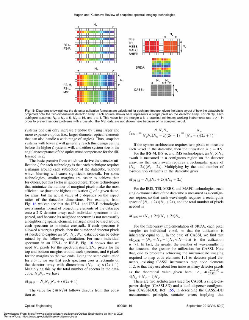
systems one can only increase étendue by using larger andmore expensive optics (i.e., larger-diameter optical elementsthat can also handle a wide range of angles). Thus, snapshotsystems with lower ζ will generally reach this design ceilingbefore the higher ζ systems will, and either system size or theangular acceptance of the optics must compensate for the dif-ference in ζ.

The basic premise from which we derive the detector uti-lization ζ for each technology is that each technique requiresa margin around each subsection of the datacube, withoutwhich blurring will cause significant crosstalk. For sometechnologies, smaller margins are easier to achieve thanfor others, but this factor is ignored here. Those technologiesthat minimize the number of marginal pixels make the mostefficient use (have the highest utilization ζ) of a given detec-tor array, but the actual value of ζ depends on the aspectratios of the datacube dimensions. For example, fromFig. 16 we can see that the IFS-L and IFS-F technologiesuse a similar format of projecting elements of the datacubeonto a 2-D detector array: each individual spectrum is dis-persed, and because its neighbor spectrum is not necessarilya neighboring spatial element, a margin must be used aroundeach spectrum to minimize crosstalk. If each spectrum isallowed a margin s pixels, then the number of detector pixelsM needed to capture an (Nx, Ny, Nw) datacube can be deter-mined by the following calculation. For each individualspectrum in an IFS-L or IFS-F, Fig. 16 shows that weneed Nw pixels for the spectrum itself, 2Nw pixels for thetop and bottom margins around each spectrum, and 6 pixelsfor the margins on the two ends. Doing the same calculationfor s > 1, we see that each spectrum uses a rectangle onthe detector array with dimensions ðNw þ sÞ × ð2sþ 1Þ.Multiplying this by the total number of spectra in the data-cube, NxNy, we have

MIFS-F ¼ NxNyðNw þ sÞð2sþ 1Þ:

The value for ζ ≡ N∕M follows directly from this equa-tion as

ζIFS-F ¼ NxNyNw

NxNyðNw þ sÞð2sþ 1Þ ¼Nw

ðNw þ sÞð2sþ 1Þ :

If the system architecture requires two pixels to measureeach voxel in the datacube, then the utilization is ζ ¼ 0.5.

For the IFS-M, IFS-μ, and IMS technologies, an Ny × Nwswath is measured in a contiguous region on the detectorarray, so that each swath requires a rectangular space ofðNw þ 2sÞðNy þ 2sÞ. Multiplying by the total number ofx-resolution elements in the datacube gives

MIFS-M ¼ NxðNy þ 2sÞðNw þ 2sÞ:

For the IRIS, TEI, MSBS, and MAFC technologies, eachsingle-channel slice of the datacube is measured as a contigu-ous region, so that each wavelength requires a rectangularspace of ðNx þ 2sÞðNy þ 2sÞ, and the total number of pixelsneeded is

MIRIS ¼ ðNx þ 2sÞðNy þ 2sÞNw:

For the filter-array implementation of SRDA, each pixelsamples an individual voxel, so that the utilization isinherently equal to 1. In the case of CASSI, we find thatMCASSI ¼ ðNx þ Nw − 1ÞNy < N—that is, the utilizationis >1. In fact, the greater the number of wavelengths inthe datacube, the greater the utilization for CASSI. Notethat, due to problems achieving the micron-scale imagingrequired to map code elements 1∶1 to detector pixel ele-ments, existing CASSI instruments map code elements1∶2, so that they use about four times as many detector pixels

as the theoretical value given here, i.e., MðpracticalÞCASSI ¼

4ðNx þ Nw − 1ÞNy.There are two architectures used for CASSI: a single-dis-

perser design (CASSI-SD) and a dual-disperser configura-tion (CASSI-DD). Ref. 155, in describing the CASSI-DDmeasurement principle, contains errors implying that

IFS-L,IFS-F:

Nw

Ny

IFS-M,

IMS:

Nx

Ny

IRIS,TEI,MSBS,MAFC,SHIFT:

CASSI: Ny

Nx Nw

SRDA:

Nw

Fig. 16 Diagrams showing how the detector utilization formulas are calculated for each architecture, given the basic layout of how the datacube isprojected onto the two-dimensional detector array. Each square shown here represents a single pixel on the detector array. For clarity, eachsubfigure assumes Nx ¼ Ny ¼ 5, Nw ¼ 16, and s ¼ 1. This value for the margin s is a practical minimum; working instruments use s ≥ 1 inorder to prevent serious problems with crosstalk. The MSI data are not shown here because of its complex layout.




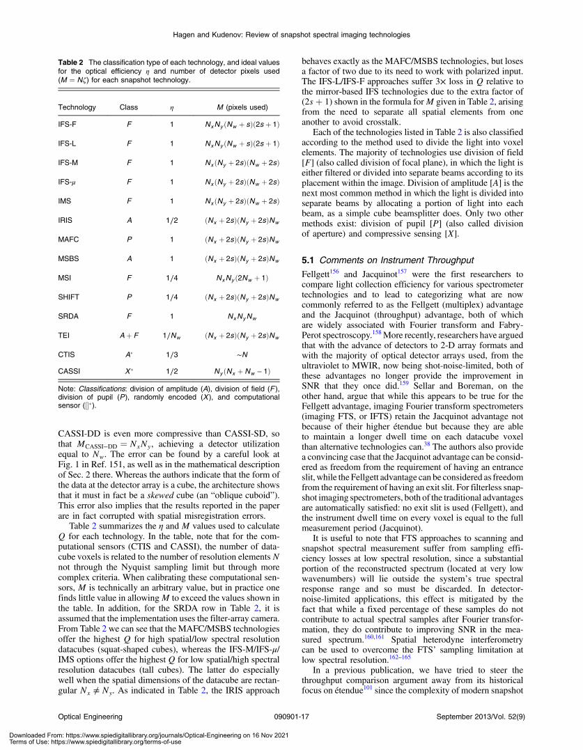
CASSI-DD is even more compressive than CASSI-SD, sothat MCASSI−DD ¼ NxNy, achieving a detector utilizationequal to Nw. The error can be found by a careful look atFig. 1 in Ref. 151, as well as in the mathematical descriptionof Sec. 2 there. Whereas the authors indicate that the form ofthe data at the detector array is a cube, the architecture showsthat it must in fact be a skewed cube (an “oblique cuboid”).This error also implies that the results reported in the paperare in fact corrupted with spatial misregistration errors.

Table 2 summarizes the η and M values used to calculateQ for each technology. In the table, note that for the com-putational sensors (CTIS and CASSI), the number of data-cube voxels is related to the number of resolution elements Nnot through the Nyquist sampling limit but through morecomplex criteria. When calibrating these computational sen-sors, M is technically an arbitrary value, but in practice onefinds little value in allowingM to exceed the values shown inthe table. In addition, for the SRDA row in Table 2, it isassumed that the implementation uses the filter-array camera.From Table 2 we can see that the MAFC/MSBS technologiesoffer the highest Q for high spatial/low spectral resolutiondatacubes (squat-shaped cubes), whereas the IFS-M/IFS-μ/IMS options offer the highest Q for low spatial/high spectralresolution datacubes (tall cubes). The latter do especiallywell when the spatial dimensions of the datacube are rectan-gular Nx ≠ Ny. As indicated in Table 2, the IRIS approach

behaves exactly as the MAFC/MSBS technologies, but losesa factor of two due to its need to work with polarized input.The IFS-L/IFS-F approaches suffer 3× loss in Q relative tothe mirror-based IFS technologies due to the extra factor of(2sþ 1) shown in the formula forM given in Table 2, arisingfrom the need to separate all spatial elements from oneanother to avoid crosstalk.

Each of the technologies listed in Table 2 is also classifiedaccording to the method used to divide the light into voxelelements. The majority of technologies use division of field[F] (also called division of focal plane), in which the light iseither filtered or divided into separate beams according to itsplacement within the image. Division of amplitude [A] is thenext most common method in which the light is divided intoseparate beams by allocating a portion of light into eachbeam, as a simple cube beamsplitter does. Only two othermethods exist: division of pupil [P] (also called divisionof aperture) and compressive sensing [X].

5.1 Comments on Instrument Throughput

Fellgett156 and Jacquinot157 were the first researchers tocompare light collection efficiency for various spectrometertechnologies and to lead to categorizing what are nowcommonly referred to as the Fellgett (multiplex) advantageand the Jacquinot (throughput) advantage, both of whichare widely associated with Fourier transform and Fabry-Perot spectroscopy.158More recently, researchers have arguedthat with the advance of detectors to 2-D array formats andwith the majority of optical detector arrays used, from theultraviolet to MWIR, now being shot-noise-limited, both ofthese advantages no longer provide the improvement inSNR that they once did.159 Sellar and Boreman, on theother hand, argue that while this appears to be true for theFellgett advantage, imaging Fourier transform spectrometers(imaging FTS, or IFTS) retain the Jacquinot advantage notbecause of their higher étendue but because they are ableto maintain a longer dwell time on each datacube voxelthan alternative technologies can.38 The authors also providea convincing case that the Jacquinot advantage can be consid-ered as freedom from the requirement of having an entranceslit, while the Fellgett advantage can be considered as freedomfrom the requirement of having an exit slit. For filterless snap-shot imaging spectrometers, both of the traditional advantagesare automatically satisfied: no exit slit is used (Fellgett), andthe instrument dwell time on every voxel is equal to the fullmeasurement period (Jacquinot).

It is useful to note that FTS approaches to scanning andsnapshot spectral measurement suffer from sampling effi-ciency losses at low spectral resolution, since a substantialportion of the reconstructed spectrum (located at very lowwavenumbers) will lie outside the system’s true spectralresponse range and so must be discarded. In detector-noise-limited applications, this effect is mitigated by thefact that while a fixed percentage of these samples do notcontribute to actual spectral samples after Fourier transfor-mation, they do contribute to improving SNR in the mea-sured spectrum.160,161 Spatial heterodyne interferometrycan be used to overcome the FTS’ sampling limitation atlow spectral resolution.162–165

In a previous publication, we have tried to steer thethroughput comparison argument away from its historicalfocus on étendue101 since the complexity of modern snapshot

Table 2 The classification type of each technology, and ideal valuesfor the optical efficiency η and number of detector pixels used(M ¼ Nζ) for each snapshot technology.

Technology Class η M (pixels used)

IFS-F F 1 NxNy ðNw þ sÞð2s þ 1Þ

IFS-L F 1 NxNy ðNw þ sÞð2s þ 1Þ

IFS-M F 1 Nx ðNy þ 2sÞðNw þ 2sÞ

IFS-μ F 1 Nx ðNy þ 2sÞðNw þ 2sÞ

IMS F 1 Nx ðNy þ 2sÞðNw þ 2sÞ

IRIS A 1∕2 ðNx þ 2sÞðNy þ 2sÞNw

MAFC P 1 ðNx þ 2sÞðNy þ 2sÞNw

MSBS A 1 ðNx þ 2sÞðNy þ 2sÞNw

MSI F 1∕4 NxNy ð2Nw þ 1Þ

SHIFT P 1∕4 ðNx þ 2sÞðNy þ 2sÞNw

SRDA F 1 NxNyNw

TEI Aþ F 1∕Nw ðNx þ 2sÞðNy þ 2sÞNw

CTIS A� 1∕3 ∼N

CASSI X � 1∕2 Ny ðNx þ Nw − 1Þ

Note: Classifications: division of amplitude (A), division of field (F ),division of pupil (P), randomly encoded (X ), and computationalsensor (½��).




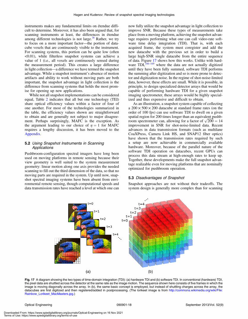
instruments makes any fundamental limits on étendue diffi-cult to determine. Moreover, it has also been argued that, forscanning instruments at least, the differences in étendueamong different technologies is not large.38 Rather, we tryto focus on a more important factor—the portion of data-cube voxels that are continuously visible to the instrument.For scanning systems, this portion can be quite low (often<0.01), while filterless snapshot systems can achieve avalue of 1 (i.e., all voxels are continuously sensed duringthe measurement period). This creates a large differencein light collection—a difference we have termed the snapshotadvantage. While a snapshot instrument’s absence of motionartifacts and ability to work without moving parts are bothimportant, the snapshot advantage in light collection is thedifference from scanning systems that holds the most prom-ise for opening up new applications.

While not all snapshot implementations can be consideredequal, Table 2 indicates that all but one technology (TEI)share optical efficiency values within a factor of four ofone another. For most of the technologies summarized inthe table, the efficiency values shown are straightforwardto obtain and are generally not subject to major disagree-ment. Perhaps surprisingly, MAFC is the exception. Asthe argument leading to our choice of η ¼ 1 for MAFCrequires a lengthy discussion, it has been moved to theAppendix.

5.2 Using Snapshot Instruments in ScanningApplications

Pushbroom-configuration spectral imagers have long beenused on moving platforms in remote sensing because theirview geometry is well suited to the system measurementgeometry: linear motion along one axis provides the neededscanning to fill out the third dimension of the data, so that nomoving parts are required in the system. Up until now, snap-shot spectral imaging systems have been absent from envi-ronmental remote sensing, though computational speeds anddata transmission rates have reached a level at which one can

now fully utilize the snapshot advantage in light collection toimprove SNR. Because these types of measurements takeplace from a moving platform, achieving the snapshot advan-tage requires performing what one can call video-rate soft-ware time delay integration (TDI). That is, with eachacquired frame, the system must coregister and add thenew datacube with the previous set in order to build alarge high-SNR single datacube from the entire sequenceof data. Figure 17 shows how this works. Unlike with hard-ware TDI,166–169 where the data are not actually digitizeduntil they have been fully summed, software TDI performsthe summing after digitization and so is more prone to detec-tor and digitization noise. In the regime of shot-noise-limiteddata, however, these effects are small. While it is possible, inprinciple, to design specialized detector arrays that would becapable of performing hardware TDI for a given snapshotimaging spectrometer, these arrays would be highly special-ized and thus expensive and difficult to obtain.

As an illustration, a snapshot system capable of collectinga 200 × 500 × 200 datacube at standard frame rates (on theorder of 100 fps) can use software TDI to dwell on a givenspatial region for 200 times longer than an equivalent pushb-room spectrometer can, allowing for a factor of

ffiffiffiffiffiffiffiffi

200p ¼ 14

improvement in SNR for shot-noise-limited data. Recentadvances in data transmission formats (such as multilaneCoaXPress, Camera Link HS, and SNAP12 fiber optics)have shown that the transmission rates required by sucha setup are now achievable in commercially availablehardware. Moreover, because of the parallel nature of thesoftware TDI operation on datacubes, recent GPUs canprocess this data stream at high-enough rates to keep up.Together, these developments make the full snapshot advan-tage realizable even for moving platforms that are nominallyoptimized for pushbroom operation.

5.3 Disadvantages of Snapshot

Snapshot approaches are not without their tradeoffs. Thesystem design is generally more complex than for scanning

Fig. 17 A diagram showing the two types of time-domain integration (TDI): (a) hardware TDI and (b) software TDI. In conventional (hardware) TDI,the pixel data are shuttled across the detector at the same rate as the image motion. The sequence shown here consists of five frames in which theimage is moving diagonally across the array. In (b), the same basic concept is employed, but instead of shuttling charges across the array, thedatacubes are first digitized and then registered/added in postprocessing. (The lorikeet image is from http://commons.wikimedia.org/wiki/File:Rainbow_Lorikeet_MacMasters.jpg.)










systems and makes use of recent technology such aslarge FPAs, high-speed data transmission, advancedmanufacturing methods, and precision optics. Moreover,the snapshot advantage in light collection often can befully realized only by tailoring the design to its application.For example, we have taken outdoor measurements with anðNx; Ny; NwÞ ¼ ð490;320; 32Þ snapshot imaging spectrom-eter that reads out at 7 fps, but used an exposure time ofonly 6 ms to avoid saturation. This exposure time is poorlymatched to the readout rate, so that most of the snapshot sys-tem’s light collection advantage is thrown away. An appli-cation for which these are much better matched wouldrequire a much dimmer scene or a much faster readout rate.

It is also important to recognize that there are measure-ment configurations for which snapshot spectral imagingis actually impossible to realize. Confocal microscopy is aclear example. Here the light is confined by a small aperturein order to reject light emerging from unwanted regions ofthe sample (i.e., outside the focal volume).170 Thus, thismethod for rejecting unwanted light means that only onespatial point is in view at any given time, and one mustscan the optics about the sample in raster fashion in orderto generate a complete ðx; y; λÞ spectral image. By its naturethis prevents a snapshot implementation. On the otherhand, for the case of volumetric imaging microscopy, thereexists an alternative technique—structured illuminationmicroscopy—that is compatible with widefield imaging, andthus with snapshot spectral imagers, and that in some casescan achieve better SNR than can confocal microscopy.152,171

An additional difficulty with using snapshot systems isthe sheer volume of data that must be dealt with in orderto take full advantage of them. Only recently have commer-cial data transmission formats become fast enough to fullyutilize a large-format snapshot imaging spectrometer for day-light scenes. (Multi-lane CoaXPress is an example of such aformat.) There are ways of reducing the data glut. For mov-ing platforms, performing software TDI prior to transmittingthe data allows high SNR data without requiring any band-width beyond those used by scanning systems. For targetdetection and tracking systems, one can process filter detec-tion algorithms onboard prior to transmitting the data, so thatrather than the full cube, one only needs to transmit thedetection algorithm result. For transmitting complete data-cubes, one can also resort to onboard compression.172

6 ConclusionsOver the past 30 years, scanning techniques have seen animpressive improvement in performance parameters, includ-ing calibration stability, SNR, and spatial, spectral, or tem-poral resolution. This trend can be attributed to largerdetector arrays, reduced detector noise, improved systemdesign, and better optical/optomechanical manufacturing;but the underlying technology and concepts have notchanged significantly in this time period.

The advent of large-format (4 megapixel) detector arrays,some 20 years ago, brought with it the capability to measuremillions of voxels simultaneously, and it is this large-scale measurement capacity that makes snapshot spectralimaging practical and useful. Almost all research in snapshotspectral imagers use novel 2-D multiplexing schemes, eachof which involve fundamental tradeoffs in detector pixelutilization, optical throughput, etc. While many advantages

can be realized for these snapshot systems over their tempo-rally scanned counterparts, it is only by making use of largearrays of detector elements that these advantages can beachieved. And it is only in the past 10 years that the spatialand spectral resolution achieved by snapshot imaging sys-tems has become sufficient that the devices are now commer-cially viable. We can anticipate that the snapshot advantagewill open up a number of new applications that leveragethe improvements in light collection, temporal resolution, orruggedness. The next 10 years should see further improve-ments in the technologies reviewed here with continuedadvancements in detector array technology, optical fabrica-tion, and computing power.

Appendix: Optical Efficiency of MAFCSystemsIn order to explain our choice of η ¼ 1 for MAFC’s effi-ciency factor, we attempt to provide an argument fromtwo sides and explain why we feel one perspective shouldbe given more weight.

One way to view the optical throughput is from a voxel’sview of the system. That is, we consider a voxel emittinglight as a Lambertian source and thus fully and uniformlyilluminating the instrument’s pupil. When comparing eachinstrument, if we set the pupil area and system focal length(and thus the f-number) to be the same for all instruments,then the efficiency is simply the fraction of light entering thepupil that reaches the detection layer. For the MAFC, lightemitted by the object voxel illuminates the system pupil, butonly one of the Nw lenses in the MAFC objective lens arraycan transmit the voxel’s light to the detection layer. Theremaining Nw − 1 lenses have to reject this voxel’s light,so from the voxel perspective, the MAFC is effectively per-forming spatial filtering of the pupil, so that the transmittedlight flux is reduced by 1∕Nw. And thus this perspectiveargues for giving the MAFC an efficiency η ¼ 1∕Nw.

A second way to view the optical efficiency is to see howthe system’s optical efficiency scales with a change in thenumber of wavelengths Nw. For the MAFC, increasingNw means increasing the number of lenses in the objectivelens array, and with them the number of filters as well. Whenscaling a lens array like this, if one momentarily ignores thefilters, it can be readily observed that the irradiance on thedetector is invariant to scale when viewing extended objects.This contradicts the previous voxel view—a fact that can beexplained as follows.

When we increase the number of lenses in the array by ascale factor S2 (e.g., S ¼ 2 increases the number of lenses byfour), the lens focal lengths drop by the factor S. If the scaled,smaller lenslets have the same f-number that the unscaled,larger lenslets had, then we should find that the irradianceat the focal plane (ignoring filters) is independent of the num-ber of lenslets when imaging an extended object. But thiswould appear to conflict with the voxel view expressedabove. The feature that is easy to miss is that by scalingthe lenses we have changed the magnification, so that thevoxel we were imaging in the unscaled system is now1∕S2 of a voxel in the scaled system. The scaled versionis effectively integrating across larger regions of the object.One can also explain this as an increase in the étendue of thepupil. That is, after scaling the system, the maximum range




of angles passed by the pupil (what may be called the pupilacceptance angle) has increased by S in each axis. And this isthe difference between the two perspectives on how to mea-sure the system’s efficiency: the pupil étendue of the scaledsystem is S2 times that of the unscaled system, effectivelycancelling out the 1∕Nw optical efficiency factor. Thus,although increasing Nw means that the spectral filters inthe system will transmit a smaller fraction of the incidentlight, the shorter focal length lenses allow a higher étendue,and the two effects cancel to give η ¼ 1.

At this point, neither of the two views can be described asthe correct view—they both simply describe different prop-erties of the system. So we make use of some empiricalobservations. In general, one finds that MAFC systemshave a substantially larger system pupil (the pupil of eachindividual objective lens multiplied by the number of lensesin the array) than do the objective lenses of other instrumentssuch as CTIS, IRIS, IMS, etc. Moreover, one can observethat the MAFC also has a larger acceptance angle of thepupil than do the other systems. However, if we compareMAFC’s pupil étendue with, say, IMS’s étendue—measurednot at the IMS objective lens pupil but rather at the systempupil of the IMS’s back-end lenslet array—then we obtaincomparable values. Thus, the limiting étendue of these sys-tems is generally determined not by their monolithic front-optics but rather by their optical arrays. Although thisstretches the definition of optical efficiency from a systemperformance perspective, it is clear that we should choosethe system scaling view over the voxel view, so that MAFC’sefficiency factor η is 1 and not 1∕Nw.

References

1. J. Allington-Smith, “Basic principles of integral field spectroscopy,”New Astron. Rev. 50(4–5), 244–251 (2006).

2. P. J. C. Janssen, “Sur la méthode qui permet de constater la matièreprotubérantielle sur tout le contour du disque solaire [On a method tosee the entire solar corona],” Comptes Rendus Acad. Sci. 68, 713–715(1869). (In French)

3. P. J. C. Janssen, “Sur l’étude spectrale des protubérances solaires[Spectral study of solar prominences],” Comptes Rendus Acad. Sci.68, 93–95 (1869). (In French)

4. A. A. Michelson, “On the conditions which affect the spectro-photog-raphy of the sun,” Astrophys. J. 1(1), 1–10 (1895).

5. G. E. Hale, “The spectrohelioscope and its work. Part I. History, instru-ments, adjustments, and methods of observation,” Astrophys. J. 70(5),265–327 (1929).

6. C. Fabry and A. Pérot, “Sur les franges des lames minces argentées etleur application à la mesure de petites épaisseurs d’air [On the fringesof thin layers of silver and their application to the measurementof small thicknesses of air],” Annales de Chimie et de Physique 12,459–501 (1897). (In French)

7. A. Perot and C. Fabry, “Sur l’application de phénomènesd’interférence à la solution de divers problèmes de spectroscopie etde métrologie [On the application of interference phenomena to thesolution of various problems in spectroscopy and metrology],”Bulletin Astronomique, Serie I 16, 5–32 (1899). (In French)

8. C. Fabry and A. Perot, “On a new form of interferometer,” Astrophys.J. 13, 265–272 (1901).

9. I. S. Bowen, “The image slicer, a device for reducing loss of light at slitof stellar spectrograph,” Astrophys. J. 88(2),113–124 (1938).

10. T. Walraven and J. H. Walraven, “Some features of the Leidenradial velocity instrument,” in Auxiliary Instrumentation for LargeTelescopes, S. Laustsen and A. Reiz, Eds., pp. 175–183, EuropeanSouthern Observatory (1972).

11. A. K. Pierce, “Construction of a Bowen image slicer,” Publ. Astron.Soc. Pac. 77(456), 216–219 (1965).

12. E. H. Richardson, “An image slicer for spectrographs,” Publ. Astron.Soc. Pac. 78(465), 436–437 (1966).

13. E. H. Richardson, “The spectrographs of the dominion astronomicalobservatory,” J. Roy. Astron. Soc. Canada 62(6), 313–330 (1968).

14. D. Hunten, “Reshaping and stabilization of astronomical images,”Chapter 4 in Astrophysics Optical and Infrared. Series: Methods ofExperimental Physics, N. Carleton, Ed., Vol. 12, pp. 193–220,Academic Press, New York (1974).

15. L. Weitzel et al., “3D: the next generation near-infrared imagingspectrometer,” Astron. Astrophys. Suppl. Ser. 119, 531–546(1996).

16. G. Avila and C. Guirao, “A Bowen-Walraven image slicer withmirrors,” http://spectroscopy.wordpress.com/2009/05/12/inexpensive-image-slicer-with-mirrors/ (January 2013).

17. N. S. Kapany, “Fiber optics,” in Concepts of Classical Optics,J. Strong, Ed., pp. 553–579, Dover, Mineola, NY (2004).

18. C. Vanderriest, “A fiber-optics dissector for spectroscopy of nebulos-ities arounds quasars and similar objects,” Publ. Astron. Soc. Pac.92(550), 858–862 (1980).

19. S. C. Barden and R. A. Wade, “DensePak and spectral imaging withfiber optics,” in Fiber Optics in Astronomy. Volume 3 of AstronomicalSociety of the Pacific Conference Series, S. C. Barden, Ed., pp. 113–124, Astronomical Society of the Pacific (1988).

20. S. Arribas, E. Mediavilla, and J. L. Rasilla, “An optical fiber system toperform bidimensional spectroscopy,” Astrophys. J. 369(1), 260–272(1991).

21. G. Courtès, “Méthodes d’observation et étude de l’hydrogène interstel-laire en émission,” Annales d’Astrophysique 23(2), 115–244 (1960).(In French)

22. G. Courtes, “Le télescope spatial et les grands télescope au sol,” inApplication de la Photométrie Bidimensionelle à l’Astronomie,pp. 241–269, Astropresse, Toulouse (1980). (In French)

23. R. Bacon et al., “The integral field spectrograph TIGER,” in VeryLarge Telescopes and Their Instrumentation, M. H. Ulrich, Ed., Vol. 2,pp. 1185–1194, European Southern Observatory (1988).

24. R. Chabbal, “Recherches expérimentales sur la généralisation de l’em-ploi du spectromètre Fabry-Perot aux divers domaines de la spectro-scopie [Experimental research on widening the use of Fabry-Perotspectrometer to the various fields of spectroscopy],” Ph.D. Thesis,University of Paris (1958). (In French)

25. J. M. Helbert, P. Laforie, and P. Miche, “Nouveau spectromètreintégral haute résolution à étalon Fabry-Pérot utilisable dans tout ledomaine visible et proche U. V.,” Rev. Phys. Appl. (Paris) 12(3),511–522 (1977). (In French)

26. C. Fabry and H. Buisson, “L’absorption de l’ultraviolet par l’ozoneet la limite du spectre solaire [The ultraviolet absorption by ozoneand the limit of the solar spectrum],” J. Physique 3, 196–206 (1913).(In French)

27. C. V. Raman, “The nature of the liquid state,” Current Sci. 11, 303–310(1942).

28. J. Braithwaite, “Dispersive multispectral scanning.,” Technical ReportNASA-65, National Aeronautics and Space Administration (1966).

29. D. A. Landgrebe, “Multispectral land sensing: where from, where to?,”IEEE Trans. Geosci. Rem. Sens. 43(3), 414–421 (2005).

30. A. F. H. Goetz, “Three decades of hyperspectral remote sensing ofthe earth: a personal view,” Rem. Sens. Environ. 113, S5–S16 (2009).

31. H. A. Macleod, Thin Film Optical Filters, 3rd ed., Institute of Physics,Philadelphia (2001).

32. T. Kanade and R. Bajcsy, “Computational sensors,” in Proceedingsof the DARPA Image Understanding Workshop, Morgan Kaufmann,San Mateo, CA (1993).

33. R. G. Baraniuk, “Compressive sensing,” IEEE Sign. Proc. Mag. 24(4),118–124 (2007).

34. M. E. Gehm et al., “Single-shot compressive spectral imaging with adual-disperser architecture,” Opt. Express 15(21), 14013–14027(2007).

35. N. Hagen and E. L. Dereniak, “Analysis of computed tomographicimaging spectrometers. I. Spatial and spectral resolution,” Appl. Opt.47(28), F85–F95 (2008).

36. Q. Zhang et al., “Joint segmentation and reconstruction of hyper-spectral data with compressed measurements,” Appl. Opt. 50(22),4417–4435 (2011).

37. A. F. H. Goetz et al., “Imaging spectrometry for Earth remote sensing,”Science 228(4704), 1147–1153 (1985).

38. R. G. Sellar and G. D. Boreman, “Comparison of relative signal-to-noise ratios of different classes of imaging spectrometer,” Appl.Opt. 44(9), 1614–1624 (2005).

39. M. T. Eismann, Hyperspectral Remote Sensing, SPIE Press,Bellingham, WA (2012).

40. A. R. Harvey et al., “Technology options for imaging spectrometry,”Proc. SPIE 4132, 13–24 (2000).

41. X. Prieto-Blanco et al., “Optical configurations for imaging spectrom-eters,” Comput. Intell. Rem. Sens. 133, 1–25 (2008).

42. P. D. Atherton et al., “Tunable Fabry-Perot filters,” Opt. Eng. 20(6),806–814 (1981).

43. J. Antila et al., “Spectral imaging device based on a tuneable MEMSFabry-Perot interferometer,” Proc. SPIE 8374, 83740F (2012).

44. N. Gupta, “Hyperspectral imager development at Army ResearchLaboratory,” Proc. SPIE 6940, 69401P (2008).

45. S. Poger and E. Angelopoulou, “Multispectral sensors in computervision,” Technical Report CS 2001-3, Stevens Institute of Techno-logy (2001).

46. A. E. Potter, “Multispectral imaging system,” U.S. Patent No.3702735 (1972).




http://dx.doi.org/10.1016/j.newar.2006.02.024

http://dx.doi.org/10.1086/140001

http://dx.doi.org/10.1086/143226

http://dx.doi.org/10.1086/140817

http://dx.doi.org/10.1086/140817

http://dx.doi.org/10.1086/143964

http://dx.doi.org/10.1086/128199

http://dx.doi.org/10.1086/128199

http://dx.doi.org/10.1086/128382

http://dx.doi.org/10.1086/128382

http://dx.doi.org/10.1051/aas:1996266

http://spectroscopy.wordpress.com/2009/05/12/inexpensive-image-slicer-with-mirrors/




http://dx.doi.org/10.1086/130764

http://dx.doi.org/10.1086/169757

http://dx.doi.org/10.1051/rphysap:01977001203051100

http://dx.doi.org/10.1109/TGRS.2004.837327

http://dx.doi.org/10.1016/j.rse.2007.12.014

http://dx.doi.org/10.1109/MSP.2007.4286571

http://dx.doi.org/10.1364/OE.15.014013

http://dx.doi.org/10.1364/AO.47.000F85

http://dx.doi.org/10.1364/AO.50.004417

http://dx.doi.org/10.1126/science.228.4704.1147

http://dx.doi.org/10.1364/AO.44.001614

http://dx.doi.org/10.1364/AO.44.001614

http://dx.doi.org/10.1117/12.406592

http://dx.doi.org/10.1117/12.7972819

http://dx.doi.org/10.1117/12.919271

http://dx.doi.org/10.1117/12.777110

47. M. R. Descour, “The throughput advantage in imaging Fourier-transform spectrometers,” Proc. SPIE 2819, 285–290 (1996).

48. A. R. Harvey and D. W. Fletcher-Holmes, “Birefringent Fourier-trans-form imaging spectrometer,” Opt. Express 12(22), 5368–5374 (2004).

49. J. M. Mooney, “Angularly multiplexed spectral imager,” Proc. SPIE2480, 65–77 (1995).

50. C. Fernandez et al., “Longwave infrared (LWIR) coded aperturedispersive spectrometer,” Opt. Express 15(9), 5742–5753 (2007).

51. M. E. Gehm et al., “High-throughput, multiplexed pushbroom hyper-spectral microscopy,” Opt. Express 16(15), 11032–11043 (2008).

52. K. W. Busch, “Multiple entrance aperture optical spectrometer,”U.S. Patent No. 4375919 A (1985).

53. S. Chakrabarti et al., “High-throughput and multislit imaging spectro-graph for extended sources,” Opt. Eng. 51(1), 013003 (2012).

54. P. Connes and E. le Coarer, “3-D spectroscopy: the historical and log-ical viewpoint,” in 3D Optical Spectroscopic Methods in Astronomy,G. Comte and M. Marcelin, Eds., Vol. 71 of ASP Conference Series,pp. 38–49, Astronomical Society of the Pacific, San Francisco (1995).

55. M. A. Bershady, “3D spectroscopic instrumentation,” in XVII CanaryIsland Winter School of Astrophysics, E. Mediavilla et al., Eds.,pp. 87–125, Cambridge University Press, Cambridge, England (2009).

56. J. Stoffels et al., “Color splitting prism assembly,” U.S. 4084180 A(1978).

57. T. Okamoto and I. Yamaguchi, “Simultaneous acquisition of spectralimage information,” Opt. Lett. 16(16), 1277–1279 (1991).

58. A. Hirai et al., “Application of multiple-image Fourier transformspectral imaging to measurement of fast phenomena,” Opt. Rev. 1(2),205–207 (1994).

59. I. K. Baldry and J. Bland-Hawthorn, “A tunable echelle imager,” Publ.Astron. Soc. Pac. 112(774), 1112–1120 (2000).

60. G. L. Bilbro, “Technology options for multi-spectral infrared cam-eras,” Technical Report AD-A396058, North Carolina State University(2001).

61. A. R. Harvey and D. W. Fletcher-Holmes, “High-throughput snapshotspectral imaging in two dimensions,” Proc. SPIE 4959, 46–54 (2003).

62. L. Gao, R. T. Kester, and T. S. Tkaczyk, “Compact image slicingspectrometer (ISS) for hyperspectral fluorescence microscopy,” Opt.Express 17(15), 12293–12308 (2009).

63. M. W. Kudenov and E. L. Dereniak, “Compact snapshot birefringentimaging Fourier transform spectrometer,” Proc. SPIE 7812, 781206(2010).

64. M. W. Kudenov et al., “White-light Sagnac interferometer for snapshotmultispectral imaging,” Appl. Opt. 49(21), 4067–4075 (2010).

65. O. Cardona, A. Cornejo-Rodríguez, and P. C. García-Flores, “Starimage shape transformer for astronomical slit spectroscopy,” Rev.Mex. Astron. Astrof. 46(2), 431–438 (2010).

66. R. Content, “A new design for integral field spectroscopy with 8-mtelescopes,” Proc. SPIE 2871, 1295–1305 (1997).

67. R. Content, “Image slicer for integral field spectroscopy with NGST,”Proc. SPIE 3356, 122–133 (1998).

68. F. Laurent, “Etude et modelisation des performances de systemesdecoupeurs d’images pour l’astronomie: application a l’instrumenta-tion du JWST et du VLT [Modelling image slicer performance forastronomy. Application to JWST and VLT],” Ph.D. Thesis, JeanMonnet University at Saint Etienne (2006). (In French)

69. D. Ren and J. Allington-Smith, “On the application of integral fieldunit design theory for imaging spectroscopy,” Publ. Astron. Soc.Pac. 114(798), 866–878 (2002).

70. R. Content, S. Morris, and M. Dubbeldam, “Microslices and low costspectrographs for million element integral field spectroscopy,” Proc.SPIE 4842, 174–182 (2003).

71. J. M. Hill et al., “Multiple object spectroscopy: the Medusa spectro-graph,” Astrophys. J. 242(2), L69–L76 (1984).

72. J. Bland-Hawthorn et al., “Hexabundles: imaging fiber arrays forlow-light astronomical applications,” Opt. Express 19(3), 2649–2661(2011).

73. D. Lee et al., “Characterization of lenslet arrays for astronomical spec-troscopy,” Publ. Astron. Soc. Pac. 113(789), 1406–1419 (2001).

74. S. C. Barden, J. A. Arns, and W. S. Colburn, “Volume-phase holo-graphic gratings and their potential for astronomical applications,”Proc. SPIE 3355, 866–876 (1998).

75. J. Allington-Smith and R. Content, “Sampling and background sub-traction in fiber-lenslet integral field spectrographs,” Publ. Astron.Soc. Pac. 110(752), 1216–1234 (1998).

76. C.-H. Chen, R. O. Reynolds, and A. Kost, “Origin of spectral modalnoise in fiber-coupled spectrographs,” Appl. Opt. 45(3), 519–527(2006).

77. U. Lemke et al., “Modal noise prediction in fibre spectroscopy—I.Visibility and the coherent model,” Mon. Not. Roy. Ast. Soc. 417(1),689–697 (2011).

78. J. Allington-Smith and J. Bland-Hawthorn, “Astrophotonic spectros-copy: defining the potential advantage,” Mon. Not. Roy. Ast. Soc.404(1), 232–238 (2010).

79. S. G. Leon-Saval, A. Argyros, and J. Bland-Hawthorn, “Photoniclanterns: a study of light propagation in multimode to single-modeconverters,” Opt. Express 18(8), 8430–8439 (2010).

80. N. Cvetojevic et al., “Characterization and on-sky demonstration of anintegrated photonic spectrograph for astronomy,” Opt. Express 17(21),18643–18650 (2009).

81. J. Bland-Hawthorn, “In search of first light: new technologies and newideas,” New Astron. Rev. 50(1–3), 75–83 (2006).

82. H. Matsuoka et al., “Single-cell viability assessment with a novelspectro-imaging system,” J. Biotech. 94(3), 299–308 (2002).

83. D. W. Fletcher-Holmes and A. R. Harvey, “Real-time imaging with ahyperspectral fovea,” J. Optics A 7(6), S298–S302 (2005).

84. N. Gat et al., “Development of four-dimensional imaging spectrome-ters (4D-IS),” Proc. SPIE 6302, 63020M (2006).

85. J. Kriesel et al., “Snapshot hyperspectral fovea vision system (hyper-video),” Proc. SPIE 8390, 83900T (2012).

86. R. M.Wentworth et al., “Standoff Raman hyperspectral imaging detec-tion of explosives,” in Laser Applications to Chemical, Security andEnvironmental Analysis, pp. 4925–4928, IEEE Press, Hoboken NJ(2008).

87. M. P. Nelson and P. J. Treado, “Raman imaging instrumentation,”Chapter 2 in Raman, Infrared, and Near-Infrared ChemicalImaging, S. Šašic and Y. Ozaki, Eds., pp. 23–54, Wiley, Hoboken,NJ (2010).

88. G. Monnet, “Application des méthodes interférentielles à la mesure desvitesses radiales. I. Montages optiques [Interference methods for themeasurements of radial velocities. I. Optical mountings],” Astron.Astrophys. 9(3), 420–435 (1970). (In French).

89. J. Meaburn, “Versatile nebular insect-eye Fabry-Perot spectrograph,”Appl. Opt. 14(2), 465–469 (1975).

90. G. Courtes et al., “A new device for faint objects high resolutionimagery and bidimensional spectrography—first observational resultswith TIGER at CFHT 3.6-meter telescope,” in Instrumentation forGround-Based Optical Astronomy, L. B. Robinson, Ed., p. 266,Springer, New York (1988).

91. R. Bacon et al., “The Sauron project—I. The panoramic integral-fieldspectrograph,” Mon. Not. Roy. Ast. Soc. 326(1), 23–35 (2001).

92. R. F. Peletier et al., “SAURON: integral-field spectroscopy of gal-axies,” New Astron. Rev. 45(1–2), 83–86 (2001).

93. H. Sugai et al., “The Kyoto tridimensional spectrograph II on Subaruand the University of Hawaii 88-in telescopes,” Publ. Astron. Soc. Pac.122(887), 103–118 (2010).

94. A. Bodkin et al., “Snapshot hyperspectral imaging—the hyperpixelarray camera,” Proc. SPIE 7334, 73340H (2009).

95. A. Bodkin et al., “Video-rate chemical identification and visualizationwith snapshot hyperspectral imaging,” Proc. SPIE 8374, 83740C(2012).

96. B. A. Spiering, “Multi spectral imaging system,” U.S. Patent No.5900942 (1999).

97. Y. Murakami, M. Yamaguchi, and N. Ohyama, “Hybrid-resolutionmultispectral imaging using color filter array,” Opt. Express 20(7),7173–7183 (2012).

98. W. E. Ortyn and D. A. Basiji, “Imaging and analyzing parameters ofsmall moving objects such as cells,” U.S. Patent No. 6211955 B1(2003).

99. T. C. George et al., “Distinguishing modes of cell death using theimagestream multispectral imaging flow cytometer,” Cytometry A59(2), 237–245 (2004).

100. W. E. Ortyn et al., “Blood and cell analysis using an imaging flowcytometer,” U.S. Patent No. 7925069 B2 (2009).

101. N. Hagen et al., “Snapshot advantage: a review of the light collectionimprovement for parallel high-dimensional measurement systems,”Opt. Eng. 51(11), 111702 (2012).

102. J. D. Matchett et al., “Volume holographic beam splitter for hyperspec-tral imaging applications,” Proc. SPIE 6668, 66680K (2007).

103. F. V. Bulygin and G. N. Vishnyakov, “Spectrotomography—a newmethod of obtaining spectrograms of two-dimensional objects,”Proc. SPIE 1843, 315–322 (1992).

104. M. R. Descour, “Non-scanning imaging spectrometry,” Ph.D. Thesis,University of Arizona (1994).

105. M. Descour and E. Dereniak, “Computed-tomography imaging spec-trometer: experimental calibration and reconstruction results,” Appl.Opt. 34(22), 4817–4826 (1995).

106. C. E. Volin et al., “Midwave-infrared snapshot imaging spectrometer,”Appl. Opt. 40(25), 4501–4506 (2001).

107. B. K. Ford, M. R. Descour, and R. M. Lynch, “Large-image-formatcomputed tomography imaging spectrometer for fluorescence micros-copy,” Opt. Express 9(9), 444–453 (2001).

108. W. R. Johnson, D. W. Wilson, and G. Bearman, “All-reflective snap-shot hyperspectral imager for ultraviolet and infrared applications,”Opt. Lett. 30(12), 1464–1466 (2005).

109. R. Shogenji et al., “Multispectral imaging using compact compoundoptics,” Opt. Express 12(8), 1643–1655 (2004).

110. B. A. Hooper et al., “Time-series imaging of ocean waves with anairborne RGB and NIR sensor,” in OCEANS, Proc. of MTS/IEEE,pp. 1–8, IEEE Press (2005).

111. S. A. Mathews, “Design and fabrication of a low-cost, multispectralimaging system,” Appl. Opt. 47(28), F71–F76 (2008).

112. IMEC, www.imec.be (2013).




http://dx.doi.org/10.1117/12.258075

http://dx.doi.org/10.1364/OPEX.12.005368

http://dx.doi.org/10.1117/12.210909

http://dx.doi.org/10.1364/OE.15.005742

http://dx.doi.org/10.1364/OE.16.011032

http://dx.doi.org/10.1117/1.OE.51.1.013003

http://dx.doi.org/10.1364/OL.16.001277

http://dx.doi.org/10.1007/BF03254863

http://dx.doi.org/10.1086/pasp.2000.112.issue-774


http://dx.doi.org/10.1117/12.485557

http://dx.doi.org/10.1364/OE.17.012293

http://dx.doi.org/10.1364/OE.17.012293

http://dx.doi.org/10.1117/12.864703

http://dx.doi.org/10.1364/AO.49.004067

http://dx.doi.org/10.1117/12.269020

http://dx.doi.org/10.1117/12.324521



http://dx.doi.org/10.1117/12.456693

http://dx.doi.org/10.1117/12.456693

http://dx.doi.org/10.1364/OE.19.002649


http://dx.doi.org/10.1117/12.316806



http://dx.doi.org/10.1364/AO.45.000519

http://dx.doi.org/10.1111/mnr.2011.417.issue-1

http://dx.doi.org/10.1364/OE.18.008430

http://dx.doi.org/10.1364/OE.17.018643

http://dx.doi.org/10.1016/j.newar.2005.11.005

http://dx.doi.org/10.1016/S0168-1656(01)00431-X

http://dx.doi.org/10.1088/1464-4258/7/6/007

http://dx.doi.org/10.1117/12.678082

http://dx.doi.org/10.1117/12.918643

http://dx.doi.org/10.1364/AO.14.000465

http://dx.doi.org/10.1046/j.1365-8711.2001.04612.x

http://dx.doi.org/10.1016/S1387-6473(00)00134-2

http://dx.doi.org/10.1086/648997

http://dx.doi.org/10.1117/12.818929

http://dx.doi.org/10.1117/12.919202

http://dx.doi.org/10.1364/OE.20.007173

http://dx.doi.org/10.1002/(ISSN)1097-0320

http://dx.doi.org/10.1117/1.OE.51.11.111702

http://dx.doi.org/10.1117/12.733778

http://dx.doi.org/10.1117/12.131904

http://dx.doi.org/10.1364/AO.34.004817

http://dx.doi.org/10.1364/AO.34.004817

http://dx.doi.org/10.1364/AO.40.004501

http://dx.doi.org/10.1364/OE.9.000444

http://dx.doi.org/10.1364/OL.30.001464

http://dx.doi.org/10.1364/OPEX.12.001643

http://dx.doi.org/10.1364/AO.47.000F71

113. M. Levoy et al., “Light field microscopy,” ACM Trans. Graph. 25(3),924–934 (2006).

114. R. Horstmeyer et al., “Flexible multimodal camera using a light fieldarchitecture,” in IEEE Int. Conf. on Computational Photography,pp. 1–8, IEEE Press (2009).

115. T. A. Mitchell and T. W. Stone, “Compact snapshot multispectral im-aging system,” U.S. Patent No. 8027041 B1 (2011).

116. E. le Coarer et al., “PYTHEAS: a multi-channel Fabry Perot spectrom-eter for astronomical imaging,” Astron. Astrophys. Suppl. Ser. 111(2),359–368 (1995).

117. B. E. Bayer, “Color imaging array,”U.S. Patent No. 3971065 A (1976).118. P. E. Buchsbaum and M. J. Morris, “Method for making monolithic

patterned dichroic filter detector arrays for spectroscopic imaging,”U.S. Patent No. 6,638,668 B2 (2003).

119. L. Miao, H. Qi, and W. Snyder, “A generic method for generating mul-tispectral filter arrays,” in Int. Conf. on Image Processing, Vol. 5,pp. 3343–3346, IEEE Press (2004).

120. G. A. Baone and H. Qi, “Demosaicking methods for multispectralcameras using mosaic focal plane array technology,” Proc. SPIE6062, 60620A (2006).

121. J. Brauers and T. Aach, “A color filter array based multispectralcamera,” presented at 12. Workshop Farbbildverarbeitung, pp. 5–6,Ilmenau, Germany (October 2006).

122. R. Shrestha, J. Y. Hardeberg, and R. Khan, “Spatial arrangement ofcolor filter array for multispectral image acquisition,” Proc. SPIE7875, 787503 (2011).

123. S.-W. Wang et al., “Concept of a high-resolution miniature spectrom-eter using an integrated filter array,” Opt. Lett. 32(6), 632–634 (2007).

124. J. Mercier, T. Townsend, and R. Sundberg, “Utility assessmentof a multispectral snapshot LWIR imager,” in 2nd Workshop onHyperspectral Image and Signal Processing: Evolution in RemoteSensing, pp. 1–5, IEEE, Hoboken, NJ (2010).

125. J. M. Eichenholz et al., “Real time megapixel multispectral bioimag-ing,” Proc. SPIE 7568, 75681L (2010).

126. N. Gupta, P. R. Ashe, and S. Tan, “Miniature snapshot multispectralimager,” Opt. Eng. 50(3), 033203 (2011).

127. H. Halpert and B. L. Musicant, “N-color (Hg,Cd)Te photodetectors,”Appl. Opt. 11(10), 2157–2161 (1972).

128. A. Rogalski, J. Antoszewski, and L. Faraone, “Third-generation infra-red photodetector arrays,” J. Appl. Phys. 105(9), 091101 (2009).

129. G. C. Gerhard, “A multispectral image sensor array,” Proc. IEEE59(12), 1718 (1971).

130. M. N. Abedin et al., “Multicolor focal plane array detector technology:a review,” Proc. SPIE 5152, 279–288 (2003).

131. X. C. Sun et al., “Multispectral pixel performance using a one-dimen-sional photonic crystal design,” App. Phys. Lett. 89(22), 223522 (2006).

132. P. Parrein et al., “Multilayer structure for a spectral imaging sensor,”Appl. Opt. 48(3), 653–657 (2009).

133. P. Mitra et al., “Multispectral long-wavelength quantum-well infraredphotodetectors,” Appl. Phys. Lett. 82(19), 3185–3187 (2003).

134. A. Longoni et al., “The transverse field detector (TFD): a novel color-sensitive CMOS device,” IEEE Electron Device Lett. 29(12), 1306–1309 (2008).

135. K. Kishino et al., “Resonant cavity-enhanced (RCE) photodetectors,”IEEE J. Quant. Electron. 27(8), 2025–2034 (1991).

136. J. Wang et al., “Cavity-enhanced multispectral photodetector usingphase-tuned propagation: theory and design,” Opt. Lett. 35(5), 742–744 (2010).

137. F. Zaraga, G. Langfelder, and A. Longoni, “Implementation of aninterleaved image sensor by means of the filterless transverse fielddetector,” J. Electron. Imaging 19(3), 033013 (2010).

138. B. Lyot, “Un monochromateur à grand champ utilisant lesinterférences en lumière polarisée [Wide field monochromator usingpolarized light interference],” Comptes Rendus de l’Academie desSciences 197, 1593–1595 (1933).

139. A. Title and W. Rosenberg, “Research on spectroscopic imaging, vol.2: reference literature,” NASA Tech. Report NSAA-CR-158702,Lockheed Palo Alto Research Laboratories, California (1979).

140. B. Lyot, “Le filtre monochromatique polarisant et ses applications enphysique solaire,” Ann. d’Astrophysique 7, 31–79 (1944).

141. J. W. Evans, “The birefringent filter,” J. Opt. Soc. Am. 39(3), 229–242(1949).

142. A. Gorman, D. W. Fletcher-Holmes, and A. R. Harvey,“Generalization of the Lyot filter and its application to snapshot spec-tral imaging,” Opt. Express 18(6), 5602–5609 (2010).

143. G. Wong, R. Pilkington, and A. R. Harvey, “Achromatization ofWollaston polarizing beam splitters,” Opt. Lett. 36(8), 1332–1334(2011).

144. A. A. Wagadarikar, M. E. Gehm, and D. J. Brady, “Performance com-parison of aperture codes for multimodal, multiplex spectroscopy,”Appl. Opt. 46(22), 4932–4942 (2007).

145. S. B. Mende et al., “Hadamard spectroscopy with a two-dimensionaldetecting array,” Appl. Opt. 32(34), 7095–7105 (1993).

146. S. T. McCain et al., “Coded aperture Raman spectroscopy for quanti-tative measurements of ethanol in a tissue phantom,” Appl. Spectrosc.60(6), 663–671 (2006).

147. M. E. Gehm and D. J. Brady, “High-throughput hyperspectral micros-copy,” Proc. SPIE 6090, 609007 (2006).

148. A. A. Wagadarikar et al., “Video rate spectral imaging using a codedaperture snapshot spectral imager,” Opt. Express 17(8), 6368–6388(2009).

149. V. Studer et al., “Compressive fluorescence microscopy for biologicaland hyperspectral imaging,” Proc. Nat. Acad. Sci. U.S.A. 109(26),E1679–E1687 (2012).

150. E. J. Candès and Y. Plan, “A probabilistic and RIPless theory of com-pressed sensing,” IEEE Trans. Inf. Theory 57(11), 7235–7254 (2011).

151. D. S. Kittle, D. L. Marks, and D. J. Brady, “Design and fabrication ofan ultraviolet-visible coded aperture snapshot spectral imager,” Opt.Eng. 51(7), 071403 (2012).

152. L. Gao et al., “Depth-resolved image mapping spectrometer (IMS)with structured illumination,” Opt. Express 19(18), 17439–17452(2011).

153. M. W. Kudenov and E. L. Dereniak, “Compact real-time birefringentimaging spectrometer,” Opt. Express 20(16), 17973–17986 (2012).

154. K. Oka and T. Kaneko, “Compact complete imaging polarimeter usingbirefringent wedge prisms,” Opt. Express 11(13), 1510–1519 (2003).

155. C. F. Cull et al., “Identification of fluorescent beads using a codedaperture snapshot spectral imager,” Appl. Opt. 49(10), B59–B71(2010).

156. P. B. Fellgett, “The theory of infra-red sensitivities and its applicationto investigations of stellar radiation in the near infra-red,” Ph.D. Thesis,University of Cambridge (1951).

157. P. Jacquinot, “The luminosity of spectrometers with prisms, gratings,or Fabry-Perot etalons,” J. Opt. Soc. Am. 44(10), 761–765 (1954).

158. P. Griffiths, H. J. Sloane, and R. W. Hannah, “Interferometers vsmonochromators: separating the optical and digital advantages,”Appl. Spectrosc. 31(6), 485–495 (1977).

159. L. W. Schumann and T. S. Lomheim, “Infrared hyperspectral imagingFourier transform and dispersive spectrometers: comparison of signal-to-noise based performance,” Proc. SPIE 4480, 1–14 (2002).

160. R. G. Sellar, G. D. Boreman, and L. E. Kirkland, “Comparison of sig-nal collection abilities of different classes of imaging spectrometers,”Proc. SPIE 4816, 389–396 (2002).

161. R. A. Keller and T. S. Lomheim, “Imaging Fourier transform spec-trometer (IFTS): parametric sensitivity analysis,” Proc. SPIE 5806,267–287 (2005).

162. J. Harlander, R. J. Reynolds, and F. L. Roesler, “Spatial heterodynespectroscopy for the exploration of diffuse interstellar emissionlines at far-ultraviolet wavelengths,” Astrophys. J. 396(2), 730–740(1992).

163. J. M. Harlander et al., “Shimmer: a spatial heterodyne spectrometer forremote sensing of Earth’s middle atmosphere,” Appl. Opt. 41(7),1343–1352 (2002).

164. S. Watchorn et al., “Sunlight fluorescence observations at 589 nm withthe SHIELDS spectrometer system: a progress report,” Proc. SPIE7812, 781207 (2010).

165. M. W. Kudenov et al., “Spatial heterodyne interferometry with polari-zation gratings,” Opt. Lett. 37(21), 4413–4415 (2012).

166. D. F. Barbe, “Time delay and integration image sensors,” in Solid StateImaging, pp. 659–671, NATO Advanced Science Institutes (ASI),Leyden, Netherlands (1975).

167. H.-S. Wong, Y. L. Yao, and E. S. Schlig, “TDI charge-coupled devices:design and applications,” IBM J. Res. Devel. 36(1), 83–106 (1992).

168. G. Lepage, J. Bogaerts, and G. Meynants, “Time-delay-integrationarchitectures in CMOS image sensors,” IEEE Trans. Electron Devices56(11), 2524–2533 (2009).

169. X.-F. He and O. Nixon, “Time delay integration speeds up imaging,”Photon. Spectra 46(5), 50–53 (2012).

170. J. B. Pawley, ed., Handbook of Biological Confocal Microscopy,3rd ed., Springer, New York (2006).

171. N. Hagen, L. Gao, and T. S. Tkaczyk, “Quantitative sectioning andnoise analysis for structured illumination microscopy,” Opt. Express20(1), 403–413 (2012).

172. J. E. Sánchez et al., “Review and implementation of the emergingCCSDS recommended standard for multispectral and hyperspectrallossless image coding,” in 2011 First Int. Conf. on DataCompression, Communications and Processing, pp. 222–228, IEEEPress (2011).

Nathan Hagen graduated with a PhD degreein optical sciences at the University ofArizona in 2007, studying snapshot imagingspectrometry and spectropolarimetry (includ-ing CTIS). From 2007 to 2009, he worked asa postdoc at Duke University, developing im-aging and spectrometry techniques (includ-ing CASSI). From 2009 to 2011 he workedas a research scientist at Rice University,continuing work on imaging and spectrom-etry, including development work on the




http://dx.doi.org/10.1145/1141911

http://dx.doi.org/10.1117/12.642425

http://dx.doi.org/10.1117/12.872253

http://dx.doi.org/10.1364/OL.32.000632

http://dx.doi.org/10.1117/12.842563

http://dx.doi.org/10.1117/1.3552665

http://dx.doi.org/10.1364/AO.11.002157

http://dx.doi.org/10.1063/1.3099572

http://dx.doi.org/10.1109/PROC.1971.8535

http://dx.doi.org/10.1117/12.505887

http://dx.doi.org/10.1063/1.2400069

http://dx.doi.org/10.1364/AO.48.000653

http://dx.doi.org/10.1063/1.1573354

http://dx.doi.org/10.1109/LED.2008.2006284

http://dx.doi.org/10.1109/3.83412

http://dx.doi.org/10.1364/OL.35.000742

http://dx.doi.org/10.1117/1.3483905

http://dx.doi.org/10.1364/JOSA.39.000229

http://dx.doi.org/10.1364/OE.18.005602

http://dx.doi.org/10.1364/OL.36.001332

http://dx.doi.org/10.1364/AO.46.004932

http://dx.doi.org/10.1364/AO.32.007095

http://dx.doi.org/10.1366/000370206777670693

http://dx.doi.org/10.1117/12.644828

http://dx.doi.org/10.1364/OE.17.006368

http://dx.doi.org/10.1073/pnas.1119511109

http://dx.doi.org/10.1109/TIT.2011.2161794

http://dx.doi.org/10.1117/1.OE.51.7.071403

http://dx.doi.org/10.1117/1.OE.51.7.071403

http://dx.doi.org/10.1364/OE.19.017439

http://dx.doi.org/10.1364/OE.20.017973

http://dx.doi.org/10.1364/OE.11.001510

http://dx.doi.org/10.1364/AO.49.000B59

http://dx.doi.org/10.1364/JOSA.44.000761

http://dx.doi.org/10.1366/000370277774464048

http://dx.doi.org/10.1117/12.453326

http://dx.doi.org/10.1117/12.451649

http://dx.doi.org/10.1117/12.605885

http://dx.doi.org/10.1086/171756

http://dx.doi.org/10.1364/AO.41.001343

http://dx.doi.org/10.1117/12.863173

http://dx.doi.org/10.1364/OL.37.004413

http://dx.doi.org/10.1147/rd.361.0083

http://dx.doi.org/10.1109/TED.2009.2030648

http://dx.doi.org/10.1364/OE.20.000403

IMS imaging spectrometer. In 2011 he joined the newly formedRebellion Photonics, to help develop snapshot imaging spectrome-ters as commercial products.

Michael W. Kudenov completed his BSdegree in electrical engineering at theUniversity of Alaska in 2005 and his PhDin optical sciences at the University ofArizona in 2009. He is currently an assistantprofessor in the Electrical and ComputerEngineering Department at North CarolinaState University. His research focuses on vis-ible-light and thermal-infrared spectrometer,interferometer, and polarimeter systemsdevelopment and calibration. Applications

span disease detection, chemical identification, remote sensing, fluo-rescence imaging, polarimetry, spectroscopy, polarization ray tracingand aberrations, and profilometry.




review of snapshot spectral imaging technologies

Documents