review of residential sector hot water requirements for
TRANSCRIPT

EEIS Legislation update – Technical Supporting Documentation, May 2016 i
Review of Residential Sector Hot Water Requirements for South Australia
Final Report
October 2020
Prepared by Energy Efficient Strategies with George Wilkenfeld & Associates and Common Capital

2
Review of Residential Sector Hot Water Requirements for South Australia Report prepared for: The Department for Energy and Mining, South Australia Report Authors: Dr Lloyd Harrington, Energy Efficient Strategies with Dr George Wilkenfeld, George Wilkenfeld & Associates John Denlay, Common Capital Final Report, 30 October 2020 (V3-final) This version will support the DEM consultation on demand response issues. Disclaimer: The views, conclusions and recommendations expressed in this report are those of Energy Efficient Strategies. While reasonable efforts have been made to ensure that the contents of this publication are factually correct, Energy Efficient Strategies give a warranty regarding its accuracy, completeness, currency or suitability for any particular purpose and to the extent permitted by law, does not accept any liability for loss or damages incurred as a result of reliance placed upon the content of this publication. This publication is provided on the basis that all persons accessing it undertake responsibility for assessing the relevance and accuracy of its content. Energy Efficient Strategies, PO Box 515, Warragul VIC 3820 Telephone: +61 (03) 5626 6333 www.energyefficient.com.au

3
Executive Summary This report reviews current water heater policies in South Australia and examines three new policy options specified by the South Australian Department for Energy and Mining. The projected impacts of these new policies are examined relative to continuation of the current policy (Business as Usual). The tasks specified in the project brief were:
1. Assessment of trends in hot water ownership in South Australia and other
jurisdictions
2. Net cost & benefits of three new water heater policy options in South Australia
3. Sensitivity analysis of alternative policy options
4. Quantification of costs and benefits to householders from a range of hot water
equipment combinations.
The key findings with respect to the specified tasks are summarised in the following sub-sections. Task 1: Assessment of trends in hot water ownership in South Australia and other jurisdictions The objective of the current water heater policy in South Australia is: “To stimulate a transition to low emission water heater technology in the residential sector, while ensuring that households are not burdened with unacceptable costs associated with the transition”. This review assesses water heater requirements against the following, revised policy objective:
The South Australian water heater requirements aim to improve energy productivity for households and the broader energy system. This ‘productivity’ objective recognises:
• energy efficiency benefits; • demand response benefits; and • benefits to all consumers from use of electric resistive water heaters as energy
storage during times of excess solar PV export.
This review is to consider whether any changes should be made to the existing requirements for residential water heaters to reflect these revised objectives. The current policy (BAU) specifies that water heaters installed in new Class 1 houses1 and existing Class 1 houses with mains gas connections must be of a “low emissions” type (gas, solar or heat pump) at the time of new installation or replacement. Electric storage water heaters may be installed in existing Class 1 dwellings without a mains gas connection provided the capacity (called the hot water delivery capacity) is not greater than 250 litres. There are no restrictions regarding the type of water heater that can be installed in Class 2 dwellings (flats and apartments). Electric water heaters have become less prevalent in South Australia since around 2000. The rate of decline has been fairly steady over that 20 year period and this trend is also obvious in NSW, ACT, Western Australia and Victoria. Since 2009, the share of gas water heaters has been quite stable, but it has started growing slowly in recent years. Solar share increased significantly from 2005 to 2008 (from a low base), in part driven by federal
1 Class 1 houses include detached dwellings and attached dwellings such as row terraces and town
houses.

4
subsidies during that period. All of the South Eastern states have seen a slow and steady increase in solar share over the past 15 years. Victoria is the state with the fastest increase in solar systems over the past 10 years, increasing at about 1% per annum. This appears to be driven by state policy and their faster population growth and household formation rate. There is no doubt that the existing South Australian water heater requirements for new and established homes are driving these overall trends for all water heater types (increase in solar and gas, decrease in electric).
Task 2: Net cost & benefits of three water heater policy options in South Australia The proposed policy options in this study are considered in a broader policy context: the Council of Australian Governments (COAG) Energy Council2 agreed in late 2019 that all electric water heaters registered in Australia from 2023 must have specified Demand Response (DR) capability (each specific function is called a Demand Response Mode or DRM). South Australia is considering an accelerated implementation timetable for DR controls. The two main types of DRM relevant to electric storage water heaters are DRM1 (load shedding) and DRM43 (increasing energy consumption). The broader policy context also includes high and rising ownership of grid connected rooftop photovoltaic (PV) systems, and an increasing number and duration of low-demand periods associated with this form of distributed generation. Three new policy options were specified by the Department for examination in this report. For one of the options, several variants were developed by the consultants. In summary, these policy options are:
� Option A: no restrictions on the installation of electric water heaters.
� Option B: no restrictions on the installation of electric water heaters that have
specified DRM capability. The sub-variants of Option B are:
o Option B1 – DRM1 only electric water heaters, COAG Energy Council
timetable
o Option B2 – DRM1 only electric water heaters, accelerated timetable
o Option B3 – DRM1 and DRM4 electric water heaters, COAG Energy Council
timetable
o Option B4 – DRM1 and DRM4 electric water heaters, accelerated timetable
o Option B5 – DRM1 and DRM4 electric water heaters, accelerated timetable
for a minimum tank size of >160 litres.
� Option C: Option B but only where a grid connected PV system is installed.
Given that the COAG Energy Council decision will affect all electric storage water heaters, the BAU case (continuation of current policy) and Option A will both have DRM1 demand response available over time (same as Option B1). The COAG Energy Council timetable will result in a slow diffusion of DR technology into the market because only new water heaters registered after July 2023 will be required to be DRM1 capable. Existing registration of models without DRM1 capability have a five year expiry, so sales of some non DRM1 electric storage water heaters may continue up to 2028 and such water heaters may remain installed up to 2038, if not longer. The accelerated timetable proposed for South Australia in
2 The COAG Energy Council is a Ministerial forum for the Commonwealth, States and Territories and
New Zealand, to work together in the pursuit of national energy reforms. The Council was established by the Council of Australian Governments (COAG) in December 2013 as part of a decision to streamline the COAG council system and refocus it on COAG’s priorities. See http://www.coagenergycouncil.gov.au/ High level administrative changes in governments in mid-2020 may replace this with other arrangements into the future. 3 DRM4 works by topping up the stored hot water temperature to a second higher thermostat
temperature that is above the default setting.

5
Options B2, B4 and B5 may require water heaters supplied or installed by 2021 to have DR capability. There are some significant risks associated with the accelerated timetable in that no complying products may be available prior to 2023 and suppliers may elect to temporarily withdraw from the South Australian market. The share of electric storage water heaters in the total South Australian stock of water heaters has been declining slowly since around 2008, and is expected to continue under BAU. The projected impact of adopting any of Options A to B5 will be to slow, but not reverse, the decline in the stock share of electric storage water heaters. This conclusion is based on considering the relative capital costs of the water heater options available to owner-occupiers and owners of rental houses, and the extent to which they value energy savings and energy operating costs under existing tariff structures. Option C would result in a large and rapid decline in the stock share of electric storage water heaters. It would effectively restrict electric storage water heaters to households that already have a grid connected PV system (around 27% of Class 1 dwellings) or those who were going install a PV system in any case. For other households, the requirement to install a PV system solely to install an electric water heater makes this option considerably more expensive than all other options, including solar and heat pump water heaters. The technical DR capability of a water heater is not effective unless it is “activated” – connected to a Demand Response Service Provider’s (DRSP’s) communication system. Various rates of activation have been modelled for both the COAG Energy Council timetable as well as an accelerated South Australian timetable. The level of activation will ultimately be dictated by the rate of development of the market for DR services, which is still somewhat uncertain as final rules have just been released and do not commence until late 2021 for large users (timetable for smaller users or aggregators is still unclear). Therefore, a low, medium and high activation rate was modelled under each of the implementation timetables. The potential value of DR can be realised in the wholesale energy market and by reducing the capital investment needed to meet network peak demands and to maintain grid stability and power quality during low-demand events. Extensive analysis of the wholesale electricity market in South Australia was undertaken in order to better understand the role that DR capability in electric storage water heaters may be able to provide (noting that similar DR capability would also be present in air conditioners, pool pump controllers and other appliances). The prevalence of high price events (over $1000/MWh) has been decreasing since 2016 as more supply enters the system, but the average event duration is increasing. The prevalence of low price events (less than $0/MWh) has increased markedly since 2018 and the average event duration is also increasing. One of the main observations was that both high price and low price events are somewhat random in nature and it is not easy to predict when these are likely to occur4. This makes it difficult for these events to be reflected in retail tariffs, which tend to be static for several years. In this respect, DR in electric storage water heaters, which allows more dynamic control by DRSPs in response to real time market changes, has the technical potential to make an important contribution to the wholesale electricity market. As most electric storage water heaters in South Australia are currently operated as controlled loads (off peak), it is estimated that relatively few large water heaters will be drawing power during system peaks. Therefore, the load shedding capacity of all electric water heaters under DRM1 is relatively small even by 2030 (somewhat less than 10MW). This level of DRM1 control would still be valuable if aggregated with DR functions from other
4 Price extremes may be driven by combinations of generation and transmission issues,
interconnector limitations, changes in loads and weather. Requirements for frequency control and voltage stability may also have some impact on prices.

6
appliances such as air conditioners. Activation of the DRM1 load shedding function is likely to be only required 10 to 20 times a year on average for up to a few hours for each event. The prevalence of larger electric storage systems operating on off peak tariffs in South Australia (in the context of this report, these are 160 litres and above) means that there is a significant potential for electric water heaters to act as a so-called “solar sponge” using the DRM4 function. This has the technical potential to deliver more than 100MW of additional load to the South Australian system and could represent additional storage of more than 300MWh during any one event by 2030 in the high activation scenario. DRM4 controls could be used several hundred times a year. The DRM4 storage capacity of small electric storage water heaters operating on continuous tariff is negligible. The potential benefits of DRM1 to avoid emergency load shedding are relatively clear and are likely to be worth around $10,000 per MWh for around 20 hours per year (NPV of benefits to 2030 of up to $5m in the high activation scenario). In addition, there are network benefits from the deferral of transmission and distribution upgrades with an NPV of benefits to 2030 of up to $15m in the high activation scenario. The potential benefits for DRM4 are more difficult to estimate. The main type of benefit will accrue from arbitrage if a service provider can shift energy consumption from a period where wholesale prices are higher to a period where they are lower (the value is a function of the difference between these prices). This can only normally be done when future prices over the coming 12 hours are forecast. Any increase in load where prices are negative will result in some benefit to the service provider. An initial estimate of potential earnings for a service provider is an NPV of benefits to 2030 of up to $10m in the high activation scenario, but this is very uncertain and could be less than $1m in some cases. There are a number of major uncertainties that need to be considered when examining the potential impact of these policies. Firstly, the electricity market in South Australia has been through major changes in the past 8 years and more change into the future is very likely. South Australia is already close to 60% renewables in electricity generation and the government has announced an aspiration to reach net 100% renewables by 2030. So, an historical analysis of the wholesale electricity market does not provide any guarantee of future market trends. The Australian Energy Market Commission (AEMC) released a new rule that moves the wholesale market from 30 minute settlements to five minute settlements in 20215. The effect of this is still unclear, but it may make short term prices more volatile, which may increase opportunities for short term water heater DR activities for both DRM1 and DRM4 functions. The Australian Energy Regulator (AER) approved ElectraNet’s Regulatory Investment Test for Transmission (RIT-T) application for the new SA-NSW interconnector in January 20206. This interconnector may be completed as early as 2022. This will provide a nominal import/export capacity of 800MW in addition to the current interconnector with Victoria. This increased capacity is likely to both reduce the frequency and severity of wholesale market high price events and negative price events in the short to medium term. The other consideration is that the AEMC has just released its rules for a Wholesale Demand Response Mechanism (WDRM) that will start operating on 24 October 2021. It is still unclear exactly how energy retailers and independent DRSPs will be able to bid into the wholesale market and whether the incentives will be sufficient to harvest water heater demand response, or whether there are barriers that may block or discourage participation of particular approaches or technologies.
5 The AEMC released a final determination on 9 July 2020 that five minute settlements would be
delayed by three months and would commence on 1 October 2021. 6 ElectraNet must now make an application to the AER for contingent project funding for the SA-NSW
interconnector prior to commencing construction.

7
One major technical issue is the commercial arrangements between a DRSP and a customer with respect to DRM4 functions. The amount of energy that could be consumed in response to regular DRM4 requests is quite large and could be equal to the total energy consumption of the water heater without DRM4 requests. Conceptually, under DRM4, the water heater is being asked to consume energy when this is most cost effective in the context of real price changes in the wholesale electricity market. However, the energy that the water heater consumes will still be metered as per normal under the existing householder tariff arrangements. For example, if an off peak water heater is asked by DRM4 to consume energy in the middle of the day7 due to low wholesale electricity prices when the off peak circuit is turned off by the time clock, this energy may be metered at the normal domestic tariff, depending on how the meter is configured. The amount of additional energy consumed by each water heater will be very different in response to a DRM4 request and this will depend on the tank temperature (water consumed earlier in the day), the tank size and even if the water heater is on. For DRM4 to be effective, energy consumed by the water heater would have to be separately metered or estimated so that bill adjustments could be made according to the energy consumed and the value of that energy in the wholesale market. This could be a separate channel on an existing meter. The overall cost impact on householders of each of the policies was generally small and the difference from the business as usual was generally minimal (noting that this excludes the additional benefits to householders that may be paid from their participation in DR programs – these are not costed). The exception was for Option C, where the overall cost was greater due to the cost of a new PV system, where an existing system was not already installed (note that this analysis did not take into account other associated benefits from the PV system – this was examined in Task 4).
Task 3: Sensitivity analysis of alternative policy options The issue of increased Minimum Energy Performance Standards (MEPS) levels for electric storage water heaters was also examined as a separate policy option. While there are potentially some benefits from this policy option, estimating the costs is very complex due to the large fixed tooling costs borne by manufacturers each time a model configuration is changed. Enacting a policy of more stringent MEPS in South Australia alone has very high risks and is not likely to succeed. The cost benefit case for improved MEPS for electric storage water heaters is further undermined where systems will be operated on the new time of use tariff, which will have much lower energy costs and therefore reduce the benefits from future energy savings. Task 4: Quantification of benefits to householders from a range of hot water equipment combinations Given the wide scope of Task 4 and the large number of systems covered, EES developed a hot water analysis tool for use by DEM to inform their policy deliberations with respect to overall hot water costs using different equipment and tariff permutations and combinations. The tool is based on results from TRNSYS simulations to AS/NZS4234 for a wide range of system types. Importantly, these simulations were undertaken across a wide range of hot water loads (typically from 0MJ/day to 60MJ/day), which enabled a detailed correlation model to be developed for different usage parameters. As the impact of PV generation was to be assessed, it was necessary to select a whole house electricity consumption profile as a
7 It is important to note that DRM4 controls must be connected to an active circuit in order to
communicate and response to DRM requests.

8
base for analysis in order to assess the internal consumption versus export on an hour by hour basis. The hot water analysis tool allows the parallel assessment of 27 water heater types so that they can all be directly compared for identical operating conditions, tariffs and hot water demands. The project brief specifies hot water demands of 40, 120 and 200 litres per day. The brief also specifies 3 kW, 6 kW and 9 kW PV systems. Together with no PV system (0 kW, which is still, by far, the most common configuration in South Australia), this makes a total of 12 scenarios that were modelled for the 27 types of water heater. While energy consumption was calculated as a primary model output, the main parameter used to assess ranking was total hot water costs, made up of energy costs and amortised capital costs. The first observation from modelling was that the size of PV system does not have a large impact on the relative cost ranking of most systems. Unsurprisingly, electric instantaneous and electric storage on continuous tariff improve their ratings slightly as the PV system size increases because PV energy is directly displacing some hot water energy use. Small electric continuous and instantaneous electric systems have very limited ability to shift boost times and PV can only displace hot water energy where hot water is used during the day. It was found that the hot water load has a substantial impact on cost ranking for different water heaters. In particular, low capital cost water heaters with higher energy costs (like electric storage on continuous tariff and instantaneous electric) look reasonable at very low hot water loads, but rank poorly at higher hot water loads. To clearly illustrate the impact of hot water demand on total hot water cost, data was modelled using the hot water analysis tool for hot water loads of 40, 80, 120, 160, 200, 240 and 280 litres per day with a 3 kW PV system. The overall results are illustrated in Figure ES-1.
Figure ES-1: Total hot water costs for all systems for a range of hot water loads Figure notes: Hot water load is indicated on X axis and is based on a winter peak hot water volume. For South Australia, summer hot water energy is around 50% of the winter peak. PV system size of 3 kW. Discount rate of 3%. All other parameters are as set out in the beginning of Section 8.3. Assumes historical tariff structures and controls. A full explanation of the abbreviation by system type is in Table
$0
$200
$400
$600
$800
$1,000
$1,200
$1,400
$1,600
$1,800
$2,000
40 80 120 160 200 240 280
Annu
al co
st o
f ene
rgy
Hot water demand (litres per day, winter)
Elec instantEWH 80L (new)LPGSWH 4*ILPGWH 5*LPGSWH 5.5*ILPGWH 6*ILPGWH 7*GSWH 4*IGWH 5*GSWH 5.5*IGWH 6*EWH 315L (new)IGWH 7*ST StdSTLPG StdST HESTLPG HESTG StdST Std OPSTG HEHP HEST HE OPHP StdHP HE OPHP Std OP
9
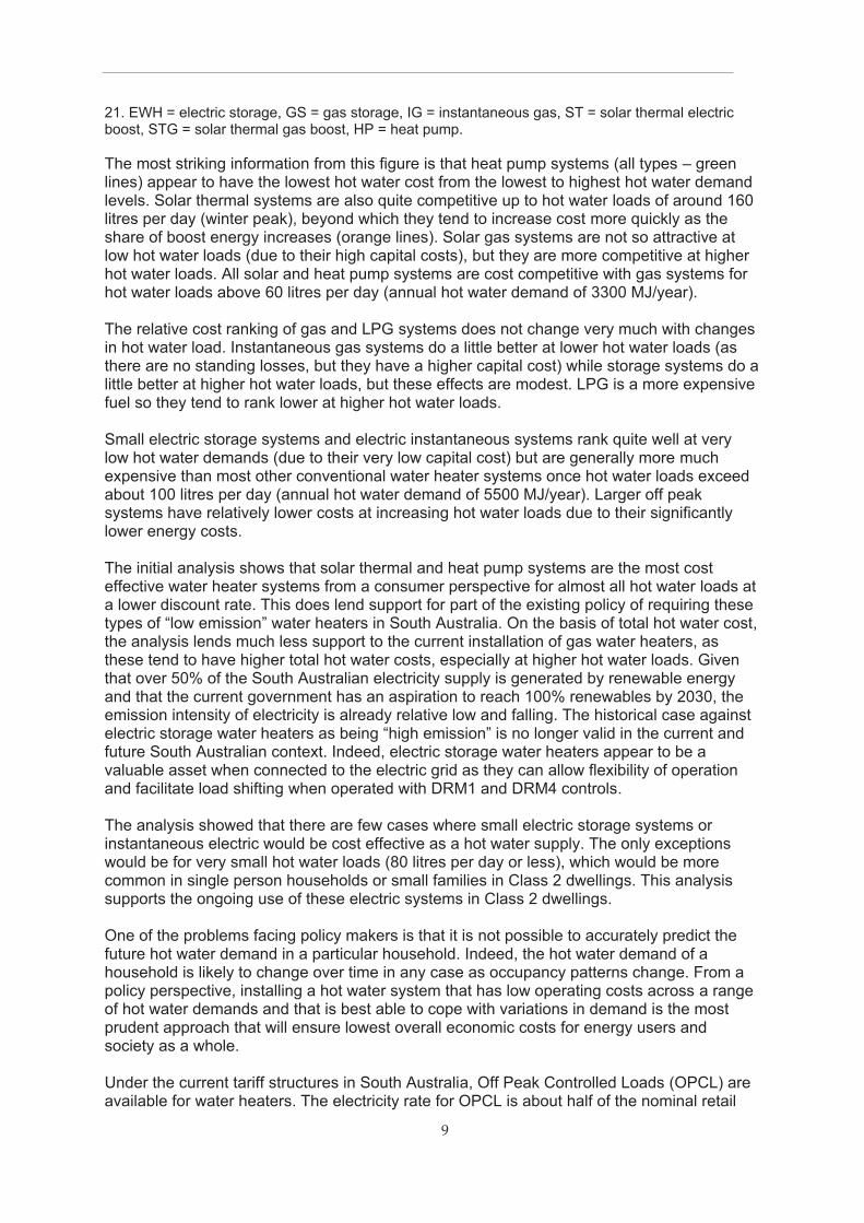
21. EWH = electric storage, GS = gas storage, IG = instantaneous gas, ST = solar thermal electric boost, STG = solar thermal gas boost, HP = heat pump.
The most striking information from this figure is that heat pump systems (all types – green lines) appear to have the lowest hot water cost from the lowest to highest hot water demand levels. Solar thermal systems are also quite competitive up to hot water loads of around 160 litres per day (winter peak), beyond which they tend to increase cost more quickly as the share of boost energy increases (orange lines). Solar gas systems are not so attractive at low hot water loads (due to their high capital costs), but they are more competitive at higher hot water loads. All solar and heat pump systems are cost competitive with gas systems for hot water loads above 60 litres per day (annual hot water demand of 3300 MJ/year). The relative cost ranking of gas and LPG systems does not change very much with changes in hot water load. Instantaneous gas systems do a little better at lower hot water loads (as there are no standing losses, but they have a higher capital cost) while storage systems do a little better at higher hot water loads, but these effects are modest. LPG is a more expensive fuel so they tend to rank lower at higher hot water loads. Small electric storage systems and electric instantaneous systems rank quite well at very low hot water demands (due to their very low capital cost) but are generally more much expensive than most other conventional water heater systems once hot water loads exceed about 100 litres per day (annual hot water demand of 5500 MJ/year). Larger off peak systems have relatively lower costs at increasing hot water loads due to their significantly lower energy costs. The initial analysis shows that solar thermal and heat pump systems are the most cost effective water heater systems from a consumer perspective for almost all hot water loads at a lower discount rate. This does lend support for part of the existing policy of requiring these types of “low emission” water heaters in South Australia. On the basis of total hot water cost, the analysis lends much less support to the current installation of gas water heaters, as these tend to have higher total hot water costs, especially at higher hot water loads. Given that over 50% of the South Australian electricity supply is generated by renewable energy and that the current government has an aspiration to reach 100% renewables by 2030, the emission intensity of electricity is already relative low and falling. The historical case against electric storage water heaters as being “high emission” is no longer valid in the current and future South Australian context. Indeed, electric storage water heaters appear to be a valuable asset when connected to the electric grid as they can allow flexibility of operation and facilitate load shifting when operated with DRM1 and DRM4 controls. The analysis showed that there are few cases where small electric storage systems or instantaneous electric would be cost effective as a hot water supply. The only exceptions would be for very small hot water loads (80 litres per day or less), which would be more common in single person households or small families in Class 2 dwellings. This analysis supports the ongoing use of these electric systems in Class 2 dwellings. One of the problems facing policy makers is that it is not possible to accurately predict the future hot water demand in a particular household. Indeed, the hot water demand of a household is likely to change over time in any case as occupancy patterns change. From a policy perspective, installing a hot water system that has low operating costs across a range of hot water demands and that is best able to cope with variations in demand is the most prudent approach that will ensure lowest overall economic costs for energy users and society as a whole. Under the current tariff structures in South Australia, Off Peak Controlled Loads (OPCL) are available for water heaters. The electricity rate for OPCL is about half of the nominal retail

10
general domestic tariff. Devices on OPCL tariffs are separately metered and are mostly controlled by time clocks (the current average OPCL tariff offered by large South Australian retailers is 19.7c/kWh). SAPN has recently released a new residential time of use tariff (also called the “solar sponge” tariff) as set out in their 2020-25 revised tariff structure statement, which has been reviewed and approved by the Australian Energy Regulator. The structure of the new “solar sponge” tariff, which offers off peak rates from 1am to 6am (at comparable rates to current OPCL tariffs) and a solar sponge tariffs at half the off peak rate from 10am to 3pm each day, provides an opportunity for all end users with larger electric storage water heaters (160 litres and above) to take full advantage of this tariff. This could effectively halve the energy cost for these storage systems, which would make them cost competitive with the total hot water costs for heat pumps, making them one of the most cost effective systems available. Heat pump systems, and to a lesser extent solar thermal systems with electric boost, would also enjoy a modest reduction in total energy costs with this tariff, although the existing energy costs are already a relatively small part of the total hot water cost for these systems, so the impacts are much smaller. To achieve this cost reduction, water heating boosting would have to be controlled so that most boosting falls within the day time solar sponge window (with the lowest energy rate). This can easily be achieved by using a local household energy management system (HEMS), but it would require a whole new approach to locally managing these water heater systems. This could complement the operation of a DRM4 control to some extent, although there could be some complex interactions that may reduce DRM4 capacity. These complexities are the same as any system where there is a local energy management system that (potentially) diverts energy into an electric storage water heater during the day. The solar sponge tariff could make larger electric storage water heaters one of the cheapest forms of water heater in South Australia. However, to achieve this, the electric storage system must be large enough to provide sufficient hot water storage to meet demand whenever it occurs while allowing the hot water boost energy consumption to occur at times that are optimal for the grid. This is only possible with larger electric storage water heaters (160 litres and above). A minimum tank size is specified in Policy Option B5. Any relaxation of current rules to permit installation of DRM4 capable water heaters should consider applying the DRM4 requirements to tanks >160 litres only and look at measures to encourage tanks >160 litres as the preferred option for Class 1 and 2 dwelling wherever possible. Under most scenarios, heat pumps operating on off peak provide lowest lifetime costs. Electric storage water heaters also offer lifetime advantages when operating during the middle of the day on the new ‘time of use’ tariff. As such, there is a place for policies to drive targeted use of ESWH, particularly where it is connected to a solar sponge tariff or a Virtual Power Plant using DRM4 or other enabling technology. It is important to note that the scale of benefits of this policy option is uncertain given:
• the likely slow diffusion of the technology, and
• other initiatives such as SA-NSW interconnector and wholesale demand
mechanism may provide the main support for low-demand situations.
Gas water heating has transitioned to a situation where it is (or soon will become) a relatively high lifetime cost water heater option.
Overall report findings The electricity market and network conditions impacting on water heater policy will change in the coming years. Periods of high and low wholesale prices have certainly been apparent in South Australia in recent years, but their incidence and magnitude are likely to change in the

11
near future once the interconnector with NSW is completed. Demand response capability in electric storage water heaters could help to address these issues to some extent, but there are uncertainties regarding how the market will operate and how consumers will be fairly compensated. The new time of use tariff will also increase energy consumption during the day, which will address system minimum system load issues to some extent. Overall, our project findings are that:
� The current policy has assisted South Australian households reduce lifetime costs of
water heating, but some elements should now be updated.
� No significant change in the mix of water heater types installed would be anticipated
under any of Policy Options A or B1 to B5, compared with a continuation of the
current policy (BAU) if current tariff arrangements were to persist. A significant
decline in electric water heater use would be anticipated for Policy Option C. The
new time of use tariff could result in an increase in the share of electric storage water
heaters, arresting the current decline, if a range of adjustments were made to the
current policy restrictions for electric systems.
� Water heaters have the technical potential to contribute up to 10MW of peak demand
reduction by 2030 using DRM1 controls. This could be substantially higher once a
significant number of electric storage water heaters move onto the new time of use
tariff.
� Water heaters have the technical potential to contribute up to 100MW of demand
increase by 2030 at times of low-demand, though to realise this would require
significant uptake of DMR4 enabled water heaters and a business model that offers
end-users with tariffs/incentives to particulate.
� The actual contribution from water heaters depends on the uptake and activation rate
of demand response controls. The market rules for Wholesale Demand Response
Mechanism have just been released (June 2020) and do not commence operation
until October 2021, so the level of future market activity is unclear.
� The net benefits from DRM1 are modest. Under a medium activation rate and a 7%
discount rate, the net benefits over a short time horizon to 2030 for Policy Option B4
are +$2.25m. Benefits increase significantly with higher activation rates and over
long time periods. DRM1 net benefits are likely to increase further once a significant
number of electric storage water heaters move onto the new time of use tariff.
� The net benefits from DRM4 are negative at a medium activation rate and a 7%
discount rate over a short time horizon to 2030. For Policy Option B4, the net benefits
are -$1.8m. Benefits increase dramatically with higher activation rates, with net
benefits of +$2.9m under a high activation rate, with larger net benefits over longer
time periods8. DRM4 net benefits are likely to decrease further once a significant
number of electric storage water heaters move onto the new time of use tariff.
� The most important conclusion from the analysis in this report is that the activation
rate is absolutely critical to making this policy cost effective. If the decision is made to
adopt mandatory DRM1 and DRM4 on an accelerated timetable in South Australia,
which does look promising under high activation rates, then the government needs to
consider actively stimulating the market for these DRM services.
� DR is a new and innovative technology that can bring much needed flexibility in the
end use load on the electricity network and will be an important part of the future
8 A separate analysis by Wilkenfeld (2020) using slightly different assumptions to 2035 finds that the
net benefits of DRM4 are positive for South Australia under medium activation rates.

12
smart grid as we move to higher proportions of unscheduled renewable generation.
While there are some risks in moving early to this sort of technology, the long term
benefits are clear.
� There are several emerging systems and pieces of infrastructure that offer the
potential to help manage peak and minimum demand challenges in South Australia,
most notably the recently approved SA-NSW interconnector and the future impacts of
these on DRM cost effectiveness are unclear.
� The new time of use tariff now approved in South Australia has the potential to make
electric storage water heaters one of the most cost effective forms of hot water
supply if energisation can be mostly contained within the five hour daytime solar
sponge window. This could cut energy costs for existing off peak electric storage
water heaters by 50%. Widespread connection of larger electric storage water
heaters to the new ‘time of use’ tariff could reduce the potential benefits from DRM4
controls proposed for water heaters in South Australia by reducing the DRM4
available storage capacity in larger electric water heaters at each site but also by
reducing the prevalence of low prices on the wholesale market during the day (and
hence the need for DRM4).
A revised residential sector water heater policy would maximise productivity benefits by:
� Removing the current restrictions on the installation of electric storage water heaters
in Class 1 dwellings, specifically for new homes and homes with an existing gas
connection.
� Removing the current 250 litres size restriction for electric water heaters in Class 1
dwellings without a gas connection. There should be encouragement of the
installation of larger electric storage systems (160+ litres) to allow these types of
households to significantly reduce their hot water energy costs by using on-site
controllers and time of use tariffs.
� No change to the Class 2 dwellings, which currently have no restrictions on the type
of water heater installed. However, there should be encouragement of the installation
of larger electric storage systems (160+ litres) to allow these types of households to
significantly reduce their hot water energy costs by using on-site controllers and ‘time
of use’ tariffs.
� Actively pursue policies that maximise the activation rate of DRM1 and DRM4
controls for electric storage water heaters in South Australia.
� Encourage the connection of all larger electric storage water heaters (new and
existing OPCL customers) to the new ‘time of use’ tariff, with on-site controllers to
maximise energy consumption during the daytime solar sponge window and to
reduce overall hot water costs for households.
� Provide clear information to consumers on the relative costs of all water heaters to
encourage the selection of low cost water heating options.
� Continue support for solar thermal and heat pump water heaters as the most cost
effective water heater supply options. Heat pump systems operating to maximise
energy during low cost windows in the time of use tariff are by far the lowest cost
form of water heating available.

13
Table of Contents
11 INTRODUCTION ................................................................................................................... 19
1.1 Request for Quote ......................................................................................................................... 19
1.2 Report structure ............................................................................................................................ 20
1.3 Acknowledgements ....................................................................................................................... 20
2 ASSESSMENT OF TRENDS IN HOT WATER OWNERSHIP IN SOUTH AUSTRALIA AND OTHER JURISDICTIONS (TASK 1) .............................................................................................................. 21
2.1 Current and revised policy objectives ............................................................................................. 21
2.2 Residential hot water requirements for South Australia ................................................................. 21 2.2.1 Background to the current requirements ........................................................................................... 21 2.2.2 Current requirements ......................................................................................................................... 22
2.3 Data sources for current stock of residential water heaters ............................................................ 24
2.4 Detailed comparison with other jurisdictions ................................................................................. 24 2.4.1 Trends in electric water heating ......................................................................................................... 25 2.4.2 Trends in gas water heating ................................................................................................................ 26 2.4.3 Trends in solar water heating ............................................................................................................. 27
2.5 Discussion and conclusions ............................................................................................................ 27
3 NET COST & BENEFITS OF THREE WATER HEATER POLICY OPTIONS IN SOUTH AUSTRALIA (TASK 2) ....................................................................................................................................... 30
3.1 Summary of business as usual ........................................................................................................ 30
3.2 Summary of Option A – no restrictions on electric water heaters ................................................... 31
3.3 Summary of Option B – electric water heaters must have DRM controls ......................................... 34
3.4 Summary of Option C – DRM electric water heaters can only be used in conjunction with on-site photovoltaic systems ................................................................................................................................. 37
3.5 Summary of ownership impacts by policy option ........................................................................... 41
4 DEMAND RESPONSE FOR ELECTRIC STORAGE WATER HEATERS ........................................ 42
4.1 Background ................................................................................................................................... 42
4.2 DRM function availability versus activation .................................................................................... 44
4.3 DRM management potential by water heater type and size ........................................................... 47
4.4 Discussion on DRM impacts ........................................................................................................... 49

14
55 ANALYSIS OF NEM LOAD AND PRICE DATA ......................................................................... 51
5.1 Background ................................................................................................................................... 51
5.2 Context of demand response in the National Electricity Market ..................................................... 51
5.3 Source of NEM data ....................................................................................................................... 52
5.4 Analysis of wholesale electricity prices ........................................................................................... 53 5.4.1 Analysis of average pool prices and trends in South Australia ........................................................... 53 5.4.2 High price events ................................................................................................................................. 56 5.4.3 Low prices events ................................................................................................................................ 64
5.5 Discussion on NEM analysis ........................................................................................................... 72
6 COST AND BENEFITS ............................................................................................................ 78
6.1 Energy modelling for end users ...................................................................................................... 78
6.2 Overall impacts by energy policy for end users ............................................................................... 81
6.3 Network benefits ........................................................................................................................... 84 6.3.1 RERT potential benefits ....................................................................................................................... 85 6.3.2 Network infrastructure deferral benefits ............................................................................................ 86 6.3.3 Costs associated with accessing DRM1 benefits and net benefits ...................................................... 86
6.4 Value of load shifting using DRM4 .................................................................................................. 88 6.4.1 Costs associated with accessing DRM4 benefits and net benefits ...................................................... 90
6.5 Policy discussion ............................................................................................................................ 91
7 SENSITIVITY ANALYSIS OF ALTERNATIVE POLICY OPTIONS (TASK 3) ................................... 92
7.1 Scope ............................................................................................................................................ 92
7.2 Quantification of the impacts ......................................................................................................... 92
7.3 Discussion on the policy proposal .................................................................................................. 94
8 QUANTIFICATION OF COSTS AND BENEFITS TO HOUSEHOLDERS FROM A RANGE OF HOT WATER EQUIPMENT COMBINATIONS (TASK 4) .......................................................................... 95
8.1 Brief requirements ......................................................................................................................... 95
8.2 EES hot water analysis tool ............................................................................................................ 95
8.3 Initial results from analysis tool ....................................................................................................104
8.4 Discussion on initial results ...........................................................................................................113
8.5 Impact of the new residential time of use tariff in South Australia .................................................117
8.6 Conclusions from cost comparisons ...............................................................................................119

15
99 APPENDIX: UPDATE OF DATA SOURCES FOR CURRENT STOCK OF RESIDENTIAL WATER HEATERS IN SOUTH AUSTRALIA ................................................................................................ 121
10 APPENDIX: DETAILED ANALYSIS OF NEM DATA FOR SOUTH AUSTRALIA ...................... 126
11 REFERENCES .................................................................................................................. 140
Index of Figures Figure 1: Decision flow chart on the type of water heater that can be installed in South Australia ................................................................................................................................ 23 Figure 2: Trends in electric share of water heaters by state and territory ............................. 26 Figure 3: Trends in gas share of water heaters by state and territory .................................. 26 Figure 4: Trends in solar share of water heaters by state and territory................................. 27 Figure 5: Updated share of water heater types for South Australia from 1990 to 2020 ........ 28 Figure 6: Projected impact of future water heater stock share to 2030 of various policy options .................................................................................................................................. 41 Figure 7: Activation rate scenarios under the COAG Energy Council implementation timetable ............................................................................................................................... 46 Figure 8: Activation rate scenarios under an accelerated implementation timetable for South Australia ................................................................................................................................ 46 Figure 9: Annual AEMO wholesale settlement prices for South Australia by weekday and weekend ................................................................................................................................ 53 Figure 10: Monthly AEMO wholesale settlement prices for South Australia by weekday and weekend ................................................................................................................................ 54 Figure 11: Time of day AEMO wholesale settlement prices for South Australia by weekday and weekend, 2012-2020 ..................................................................................................... 54 Figure 12: Monthly wholesale electricity prices by year: weekdays ...................................... 55 Figure 13: Monthly wholesale electricity prices by year: weekends ...................................... 55 Figure 14: Settlement price for each half hour for South Australia, calendar 2018 (high price events) .................................................................................................................................. 56 Figure 15: Net load versus settlement price for each half hour for South Australia, calendar 2018 ...................................................................................................................................... 57 Figure 16: Count of 30 min periods by month with a settlement price >$1000/MWh ............ 58 Figure 17: Analysis of settlement price, net load and PV generation for events >$1000/MWh, weekdays .............................................................................................................................. 59 Figure 18: Analysis of settlement price, net load and PV generation for events >$1000/MWh, weekends .............................................................................................................................. 59 Figure 19: Count of 30 min periods by time of day with a settlement price >$1000/MWh, 2012 to 2020, day of week .................................................................................................... 60 Figure 20: Count of 30 min periods by time of day with a settlement price >$1000/MWh, 2012 to 2020, by season ....................................................................................................... 61 Figure 21: Count of separate events over selected price thresholds by year ....................... 62 Figure 22: Total annual hours for events over selected price thresholds by year ................. 62 Figure 23: Average duration of events over selected price thresholds by year .................... 63 Figure 24: Count of shorter duration events by year for a threshold of >$1000/MWh .......... 64 Figure 25: Count of longer duration events by year for a threshold of >$1000/MWh ........... 64 Figure 26: Settlement price for each half hour for South Australia, calendar 2018 (low price events) .................................................................................................................................. 65 Figure 27: Count of 30 min periods by month with a settlement price <$0/MWh .................. 66 Figure 28: Analysis of settlement price, net load and PV generation for events <$0/MWh, weekdays .............................................................................................................................. 67

16
Figure 29: Analysis of settlement price, net load and PV generation for events <$0/MWh, weekends .............................................................................................................................. 67 Figure 30: Count of 30 min periods by time of day with a settlement price <$0/MWh, 2012 to 2020, day of week ................................................................................................................. 68 Figure 31: Count of 30 min periods by time of day with a settlement price <$0/MWh, 2012 to 2020, by season .................................................................................................................... 69 Figure 32: Count of separate events under selected price thresholds by year ..................... 70 Figure 33: Total annual hours for events under selected price thresholds by year............... 70 Figure 34: Average duration of events under selected price thresholds by year .................. 71 Figure 35: Count of shorter duration events by year for a threshold of <$0/MWh ................ 72 Figure 36: Count of longer duration events by year for a threshold of <$0/MWh ................. 72 Figure 37: AS/NZS4234 simulations used to estimate energy input ..................................... 80 Figure 38: Count of households in the SAPN general domestic sample for 2018-2019 ....... 97 Figure 39: Normalised TOD load shape for each of the consumption bins, SAPN sample .. 97 Figure 40: Count of households in the SAPN residential OPCL sample for 2018-2019 ....... 98 Figure 41: Seasonal profile of the SAPN residential OPCL sample for 2018-2019 by bin ... 99 Figure 42: Monthly energy ratio for the SAPN residential OPCL sample for 2018-2019 by bin .............................................................................................................................................. 99 Figure 43: Average seasonal profile for OPCL sample with heat loss correction ............... 100 Figure 44: Average seasonal profile for water heating – various sources .......................... 101 Figure 45: Normalised TOD load shape for each of the consumption bins, SAPN OPCL sample ................................................................................................................................ 101 Figure 46: Sample PV hourly output for a year for Adelaide, 3kW system ......................... 102 Figure 47: Comparison on monthly hot water energy demand with PV output for Adelaide 103 Figure 48: Annual energy by fuel for all water heater types: Scenario 5 ............................ 107 Figure 49: Annual energy costs by capital and fuel for all water heater types: Scenario 5 . 107 Figure 50: Annual energy costs by capital and fuel for all water heater types: Scenario 1 . 108 Figure 51: Annual energy costs by capital and fuel for all water heater types: Scenario 2 . 108 Figure 52: Annual energy costs by capital and fuel for all water heater types: Scenario 3 . 109 Figure 53: Annual energy costs by capital and fuel for all water heater types: Scenario 4 . 109 Figure 54: Annual energy costs by capital and fuel for all water heater types: Scenario 6 . 110 Figure 55: Annual energy costs by capital and fuel for all water heater types: Scenario 7 . 110 Figure 56: Annual energy costs by capital and fuel for all water heater types: Scenario 8 . 111 Figure 57: Annual energy costs by capital and fuel for all water heater types: Scenario 9 . 111 Figure 58: Annual energy costs by capital and fuel for all water heater types: Scenario 10 112 Figure 59: Annual energy costs by capital and fuel for all water heater types: Scenario 11 112 Figure 60: Annual energy costs by capital and fuel for all water heater types: Scenario 12 113 Figure 61: Capital cost impacts: 3% discount (left) and 10% discount (right); Scenario 5 .. 113 Figure 62: Total hot water costs for all systems for a range of hot water loads .................. 116 Figure 63: Comparison of ABS and BIS water heater data for NSW .................................. 123 Figure 64: Comparison of ABS and BIS water heater data for South Australia .................. 124 Figure 65: Half hourly load data for South Australia, 2013 to 2020 .................................... 127 Figure 66: Half hourly wholesale electricity market settlement price for South Australia, 2013 to 2020 (high prices) ........................................................................................................... 128 Figure 67: Half hourly wholesale electricity market settlement price for South Australia, 2013 to 2020 (low prices) ............................................................................................................. 129 Figure 68: Half hourly total photovoltaic generation for South Australia, 2013 to 2019 ...... 130 Figure 69: Half hourly load versus market settlement price for South Australia, 2013 to 2020 ............................................................................................................................................ 131 Figure 70: Average wholesale electricity prices by month for 2013, weekdays .................. 132 Figure 71: Average wholesale electricity prices by month for 2013, weekends .................. 132 Figure 72: Average wholesale electricity prices by month for 2014, weekdays .................. 133 Figure 73: Average wholesale electricity prices by month for 2014, weekends .................. 133 Figure 74: Average wholesale electricity prices by month for 2015, weekdays .................. 134 Figure 75: Average wholesale electricity prices by month for 2015, weekends .................. 134

17
Figure 76: Average wholesale electricity prices by month for 2016, weekdays .................. 135 Figure 77: Average wholesale electricity prices by month for 2016, weekends .................. 135 Figure 78: Average wholesale electricity prices by month for 2017, weekdays .................. 136 Figure 79: Average wholesale electricity prices by month for 2017, weekends .................. 136 Figure 80: Average wholesale electricity prices by month for 2018, weekdays .................. 137 Figure 81: Average wholesale electricity prices by month for 2018, weekends .................. 137 Figure 82: Average wholesale electricity prices by month for 2019, weekdays .................. 138 Figure 83: Average wholesale electricity prices by month for 2019, weekends .................. 138 Figure 84: Average wholesale electricity prices by month for 2020, weekdays .................. 139 Figure 85: Average wholesale electricity prices by month for 2020, weekends .................. 139
Index of Tables Table 1: Summary of DRM modes for water heating ............................................................ 43 Table 2: Summary of activation rate scenarios and applicable policy options ...................... 45 Table 3: Energy storage potential for large and small water heaters in response to low energy prices ........................................................................................................................ 48 Table 4: Key parameters for the calculation of annual hot water energy .............................. 78 Table 5: Residential electricity retail tariffs offered in South Australia .................................. 79 Table 6: System purchase and installation costs collated in 2019 ........................................ 79 Table 7: Calculations to compare lifetime operating and capital costs of different water heater options, replacement ................................................................................................. 80 Table 8: Comparison of total lifetime cost of operation for main water heater types, sensitivity analysis ................................................................................................................................. 81 Table 9: Assessment of overall customer cost impacts for the various water heater policies assessed by 2030 ................................................................................................................. 83 Table 10: Estimated available DRM1 load reduction (MW) from small electric water heaters to 2030, medium activation ................................................................................................... 85 Table 11: Net present value ($m) of RERT contracts from 2020 to 2030 under a range of scenarios ............................................................................................................................... 85 Table 12: Net present value ($m) of network investment deferrals from 2020 to 2030 under a range of scenarios ................................................................................................................ 86 Table 13: Summary of costs and benefits for DRM1 controls to 2030: medium activation and 7% discount rate ................................................................................................................... 87 Table 14: Summary of costs and benefits for DRM1 controls to 2030: high activation and 3% discount rate ......................................................................................................................... 88 Table 15: Net present value ($m) of load shifting from 2020 to 2030 under a range of scenarios ............................................................................................................................... 89 Table 16: Summary of costs and benefits for DRM4 controls to 2030: medium activation and 7% discount rate ................................................................................................................... 90 Table 17: Summary of costs and benefits for DRM1 controls to 2030: high activation and 3% discount rate ......................................................................................................................... 91 Table 18: MEPS for electric storage water heaters with calculated reduction for increased stringency .............................................................................................................................. 93 Table 19: Impact of more stringent MEPS levels .................................................................. 93 Table 20: Hot water scenarios modelled for initial cost comparison ................................... 105 Table 21: Ranking of annual energy costs by water heater type: Scenario 5 ..................... 106 Table 22: Cost ranking of all water heater types for all scenarios (1 is lowest cost) ........... 114 Table 23: Impact of solar sponge tariff on electric water heater operating costs ................ 118 Table 24: Mains gas households in South Australia by region ........................................... 121 Table 25: Prevalence of gas water heaters in different dwelling types in South Australia, 2008 .................................................................................................................................... 122
18
Glossary and Abbreviations ABS Australian Bureau of Statistics (federal)
AEMC Australian Energy Market Commission
AEMO Australian Energy Market Operator
AER Australian Energy Regulator
AS Australian Standard
BAU Business as Usual
BCA Building Code of Australia (now NCC)
CEC Comparative Energy Consumption (energy on an energy label)
COAG Council of Australian Governments (state, federal and NZ)
CSIRO Commonwealth Scientific & Industrial Research Organisation
DEM SA Department for Energy and Mining
DISER Department of Industry, Science, Energy and Resources (federal)
DNSP Distribution Network Service Providers
DR Demand Response
DRM Demand Response Mechanism (in a water heater usually DRM1 or DRM4)
DRSP Demand Response Service Providers
E3 Equipment Energy Efficiency program (state, federal and NZ)
EE Energy Efficiency
EES Energy Efficient Strategies (consultants)
EV Electric Vehicle
FCAS Frequency Control and Ancillary Services (AEMO)
GEMS Greenhouse and Energy Minimum Standards (federal law)
GWh Gigawatt hour (unit of energy)(Wh × 109)
kWh kilowatt hour (unit of energy)(Wh × 103)
MEPS Minimum Energy Performance Standards (regulated efficiency levels)
MW Megawatt (unit of power)(watts × 106)
NCC National Construction Code (Australian Building Codes Board)
NEM National Electricity Market (interconnected east coast grid of Australia)
NPV Net Present Value (calculated with a specified discount rate)
OPCL Off Peak Controlled Load (residential, usually water heating)
PV Rooftop photovoltaic system (distributed generation)(usually grid connected)
REES Retailer Energy Efficiency Scheme (South Australia)
RERT Reliability and Emergency Reserve Trader (AEMO)
RIS Regulatory Impact Statement
W watt (unit of power)
WDRM Wholesale Demand Response Mechanism (AEMC)

19
1 Introduction 1.1 Request for Quote A proposal was prepared in response to a Request for Quote (RFQ) received from the Department for Energy and Mining by email on 15 January 2020 (Reference Number 18190280). The RFQ was seeking a review of hot water requirements in the state of South Australia (SA). Specific work items included:
• Task 1: Assess household penetration trends of electric resistive storage water
heaters in SA (including data since 2009, compared to other jurisdictions).
• Task 2: Quantify, against a business as usual (BaU) scenario, the net cost
benefits (including direct cost benefits to householders, network cost saving
benefits and wholesale electricity cost benefits) under the following three options:
o Option 1 – no requirements
� A scenario removing the current requirements and allowing electric
resistive storage water heaters to be installed throughout SA, with no
local requirements.
o Option 2 – electric heaters with demand response capability
� Option 1, but installation of electric resistive storage water heaters is
restricted to heaters that are demand response capable under
AS/NZS 4755.3.3:2014 or AS/NZS 4755.2 (when published).
o Option 3 – electric heaters with demand response capability and on-site roof
top solar PV
� Option 2, but installation of electric resistive storage water heaters is
also restricted to heaters installed in homes with on-site rooftop solar
PV.
• Task 3: Undertake a sensitivity analysis for each option, calculating the impact on
costs, benefits and currently available models and sales of electric resistance
water heaters by reducing in SA by 10%, 20% or 30%, the maximum allowable
heat loss (kWh/24hrs) permitted under minimum energy performance standards
(MEPS).
• Task 4: Quantify direct cost benefits to householders, including capital, running
and lifetime costs for a full range of replacement/installation scenarios and water
heater systems, in new and established homes. Energy obtained from an existing
on-site PV will be considered as ‘free’ energy in calculating energy consumption. This task covers a wide range of water heater system types and hot water
demand.
Additional tasks to support DEM during stakeholder consultations and in the delivery of stakeholder workshops were also included in the contract scope. The course of COVID-19 during 2020 and subsequent border closures into SA have meant that these tasks had to be delivered remotely. A contract to undertake the work was issued on 26 February 2020. Interim reports for Tasks 1, 2 and 3 have been submitted and reviewed by DEM. This report addresses all tasks specified in the brief and forms the basis for initial stakeholder consultations.

20
1.2 Report structure The report structure generally mirrors the tasks set out in the project brief as follows:
� Section 2 examines the current residential water heater policy for South Australia and
compares ownership trends by water heater type with data from other states and
territories.
� Section 3 sets out detailed analysis of the specified new water heater policy options
and sets out a basis for their assessment.
� Section 4 examines the issue of demand response for water heaters and explores
the issues for implementation in some detail.
� Section 5 looks at AEMO load and wholesale price data for South Australia from
2012 to 2020 and makes an assessment of low price and high price events and their
trends over time to support the quantification of potential DRM costs and benefits.
� Section 6 compiles data on costs and benefits from a consumer perspective and for
the electricity supply system as a whole, particularly with reference to the potential
costs and benefits associated with demand response functions.
� Section 7 makes a preliminary assessment of the feasibility of more stringent MEPS
levels for electric storage water heaters and the associated uncertainties.
� Section 8 provides some documentation on the new hot water analysis tool
developed by EES for DEM and provides some initial results regarding energy and
cost comparisons for 27 types of water heaters under a wide range of operating
conditions. This section also examines the impact of the new residential time of use
tariff for South Australia and how this affects relative cost ranking of different types of
water heaters, as well as its likely future impacts.
� Section 9 (Appendix) provides more detailed analysis of trends in ownership by water
heater type in South Australia, including a review of various data sources that are
used to support the analysis in Section 2.
� Section 10 (Appendix) includes a series of figures that provide a range of
perspectives on AEMO load and wholesale price data from 2012 to 2020 to provide
additional support to the analysis in Section 5.
� Section 11 is a list of report references.
1.3 Acknowledgements The authors would like to thank the following people who assisted with this project:
� Craig Walker at the Department for Energy and Mining who managed the project and
provided a range of supporting and background documents.
� James Simmonds at the Department for Energy and Mining who provided a range of
tariff and metering information specific to South Australia.
� James Bennett from South Australian Power Networks who provided advice on
metering, information about tariff connection policies and data sources.

21
2 Assessment of trends in hot water ownership in South Australia and other jurisdictions (Task 1)
Task 1 has been split into several components for this project. Firstly, the current hot water requirements for South Australia are documented. There is a review of data sources that have been used to update the estimated stock by water heater type in South Australia. Finally, a detailed comparison of water heater types by jurisdiction with some related discussion has been undertaken.
2.1 Current and revised policy objectives The objective of the current water heater policy in South Australia is: “To stimulate a transition to low emission water heater technology in the residential sector, while ensuring that households are not burdened with unacceptable costs associated with the transition”. This current review is assessing water heater requirements against the following, revised objective: The South Australian water heater requirements aim to improve energy productivity for households and the broader energy system. This ‘productivity’ objective recognises:
• energy efficiency benefits; • demand response benefits; and • benefits to all consumers from use of electric resistive water heaters as energy
storage during times of excess solar PV export.
This review is to consider whether any changes should be made to the existing residential water heater requirements to reflect these revised objectives.
2.2 Residential hot water requirements for South Australia
2.2.1 Background to the current requirements Rules relating to domestic water heater installations have been in place in South Australia since July 2008. Under the initial requirements, plumbers were required in many situations to install low-emission water heaters, such as high efficiency gas, solar or electric heat pump systems, when installing new or replacement water heaters. The requirements applied to new homes and to established homes when their existing water heaters were replaced. Different rules applied in different parts of South Australia. A review of the requirements, conducted during 2012-2013 (Department for Manufacturing, Innovation, Trade, Resources and Energy 2013), found that:
“the requirements have achieved their objective of promoting a transition to low emission water heaters and making a substantial contribution to South Australia’s Strategic Plan target relating to residential energy efficiency.”
The review recommended changes to significantly simplify the requirements and provide a greater number of options, especially for smaller households, to comply without incurring unreasonably high upfront installation costs. In response to the review, the requirements were changed in 2014. These requirements continue to apply today (in 2020). The requirements were initially implemented, for established homes, by an SA Water Direction issued under the Waterworks Act 1932, with SA Water responsible for compliance.

22
For new homes the requirements were established through the Building Code of Australia, with local government responsible for compliance. In January 2013, a new Water Industry Act 2012 replaced the legislation governing the operations of SA Water and responsibility for plumbing regulation was subsequently transferred to the Office of the Technical Regulator. Details of the requirements for new homes and established homes are in the National Construction Code Volume Three - Plumbing Code of Australia (Australian Building Codes Board 2019a). In 2019, South Australia published a verification method to allow for electric storage water heaters supplied by photovoltaic solar in new homes to demonstrate compliance of these systems with the Performance Requirement in the National Construction Code (SA Government 2020) with details on the government website https://www.sa.gov.au/topics/energy-and-environment/energy-efficient-home-design/water-heater-requirements.
2.2.2 Current requirements The objectives of the requirements are to lower household energy use and greenhouse gas emissions. The requirements apply state wide. There is no difference between metropolitan and regional areas (SA Office of the Technical Regulator 2019). The requirements are described in the National Construction Code. The Code sets out requirements for water heaters as part of a heated water service via the following:
� An Objective statement that include the objectives of “safeguard the environment” and “reduce greenhouse gas emissions” (Section BO2 (d) and (e))
� A Functional Statement that includes “efficiently using energy” and obtaining heating energy from “a low greenhouse gas intensity energy source or an onsite renewable energy source or another process as reclaimed energy” (Section BF2.3)
� Performance requirements that includes ensuring the “efficient use of energy” (Section BP2.6) and describes performance requirements for energy sources
(Section BP2.6(c)).
� Ways of verifying compliance with Section BP2.6(c) (Section BV2.1).
The Code also provides Deemed-To-Satisfy provisions (Section B2.2, with South Australia variations shown in Section SA B2.2) that can be used to satisfy the Performance requirements. This is the most common way used to comply with the NCC requirements. The SA Deemed-To-Satisfy provisions specify the type of water heaters that can be installed to service a Class 19 building as follows:
� For new homes, the water heater needs to be a low-emission type;
� For established homes with a connection to the reticulated gas supply, a new or
replacement water heater needs to be a low-emission type;
9 The NCC (Australian Building Codes Board 2019b) defines the main classes of buildings as follows:
Class 1a(a): Single dwelling, detached house. Class 1a(b): Single attached dwellings, each being a building, separated by a fire-resisting wall, including a row house, terrace house, town house or villa unit. Class 1b(a): Boarding house, guest house, hostel Class 1b(b): four or more single dwellings located on one allotment used for short-term holidays Class 2: Containing two or more sole-occupancy units, each is a separate dwelling located above one another.

23
� For established homes without a connection to the reticulated gas supply, a new or
replacement water heater needs to be
o A low-emission type,
o An electric water heater with a rated hot water delivery of no greater than 250
litres, or
o An electric instantaneous water heater, having a water storage capacity no
greater than one litre and total electrical input no greater than 15.0 kW.
There are no requirements for Class 2 dwellings (multi-level flats and apartments). This is the same in all states. The decision-making process is set out in Figure 1. These are also set out on the government website https://www.sa.gov.au/topics/energy-and-environment/electrical-gas-and-plumbing-safety-and-technical-regulation/plumbing-trades/water-heater-installation-requirements
Figure 1: Decision flow chart on the type of water heater that can be installed in South Australia Source: SA Office of the Technical Regulator (2019).
In Section SA B2.2 of the NCC, a low-emission type water heater is defined as one of the following types:
(a) A natural gas or LPG water heater, either instantaneous, continuous flow or storage, that has an energy rating of 5 stars or more.
(b) A natural gas or LPG boosted solar water heater, with a total tank volume of not more than 700 litres, that is eligible for any number (one or more) of STCs.
(c) An electric boosted solar water heater or electric heat pump water heater (air source or solar boosted), with a single tank, that:

24
(i) for systems with a tank volume of 400 litres or more and not more than 700 litres, is eligible for at least 38 Small-scale Technology Certificates (STCs) in Zone 3 as defined by the Clean Energy Regulator [CER] and / or eligible for at least 36 STCs in CER Zone 4, or
(ii) for systems with a tank volume of more than 220 litres and less than 400 litres, is eligible for at least 27 STCs in CER Zone 3 and / or eligible for at least 26 STCs in CER Zone 4, or
(iii) for systems with a tank volume of not more than 220 litres, is eligible for at least 17 STCs in CER Zone 3 and / or eligible for at least 16 STCs in CER Zone 4.
(d) A wood combustion water heater, with no additional heating mechanisms, with a total tank volume of not more than 700 litres.
(e) A wood combustion boosted solar water heater, with no additional heating mechanisms, with a total tank volume of not more than 700 litres.
Section SA B2.2 states that these requirements do not apply to: (a) Water heaters serving buildings other than Class 1 (b) Repairs to water heaters including:
(i) Like for like replacements that are the result of manufacturer, supplier or installer warranty arrangements
(ii) Replacement of a single major component of a solar or electric heat pump water heater (for example, a heat pump compressor/evaporator unit, a solar collector, or a storage tank).
(c) Secondary electric water heaters of up to 55 litres rated delivery, which do not serve a shower or bath
(d) Temporary electric water heaters of up to 55 litres rated delivery, for a period not exceeding 60 days, pending installation of a complying water heater
(e) An electric or gas vented (gravity fed) water heater, located in a roof space of an established Class 1 building, of no greater than 250 litres rated hot water delivery
(f) A gas water heater installed entirely within a fully enclosed roof space, room or attached garage of an established Class 1 building, providing the water heater has an energy rating of 3 stars or more.
Source: South Australia Appendix Section B: Water services of the NCC (Australian Building Codes Board 2019a).
2.3 Data sources for current stock of residential water heaters A detailed review of current data sources regarding the ownership of water heaters by type in South Australia was undertaken in order to update historical estimates to 2020. These data sources are set out in detail in the appendix included as Section 9.
2.4 Detailed comparison with other jurisdictions As far as possible, trends in water heater share by type have been updated for all other jurisdictions based on ABS data (Australian Bureau of Statistics 2014) and the BIS report (BIS Oxford Economics 2018), where applicable (NSW, VIC, QLD, SA and WA)(refer to Section 9 for detailed data sources). Detailed estimates of the stock of different water heater types are available (such as boost type for solar, share of heat pump (included in solar in these charts) and the split of gas storage and instantaneous). For this high level review, the three main fuel types are shown: electric, gas and solar. Note that electric includes storage tanks on controlled tariff, storage tanks on continuous tariff and electric instantaneous. Gas includes gas storage and gas instantaneous. Solar includes solar thermal with gas or electric

25
boost (in tank or in line) as well as heat pump. Note that in ABS surveys a small number of households in each state have a water heater energy type of “other” – this is primarily wood and is generally less than 2%. It is now assumed that all households have some form of water heater. More detail is included in the discussion below.
2.4.1 Trends in electric water heating Figure 2 illustrates the trend in the share of electric water heaters by state and territory from 2000 to 2020. The absolute differences in share of electric water heaters by state are the inverse, to a fair extent, of the availability of mains gas in residential households. Electric water heaters are less common in Victoria and South Australia, which have substantial mains gas networks, while electric water heaters are very common in Tasmania and Queensland, which have very limited availability of gas. NSW, Victoria, South Australia and the ACT are all showing a steady downward decline in the share of electric water heaters of all types, all at a similar rate (all at around 0.75% per annum decrease). Note that the split between controlled tariff storage, continuous tariff storage and instantaneous does vary somewhat by state, but the available data on this split is rather sporadic. Tasmania and Queensland are showing little change in electric water heating share over time (for the past 10 years). Both Western Australia and the Northern Territory have shown a strong trend towards electric water heating since 2008 – it is unclear what is driving this trend. It would appear that South Australia is following the same general trends in electric water heating that is evident in the neighbouring South-Eastern states for the past 10 years or more. While the overall trends for NSW and Victoria appear similar to South Australia, there are some underlying differences. Victoria has a more aggressive policy for new homes that results in around 70% of new homes installing a solar thermal system (homes with a gas connection must install solar-gas, otherwise solar-electric). The household formation rate in Victoria is quite high, so this drives the overall increase in solar water heaters. NSW has a lower gas penetration rate (around 40%) and gas is being strongly promoted in urban areas. The household formation rate in NSW is lower than Victoria but higher than South Australia. The water heater requirements for new homes under BASIX are much more complex and this allows a wider range of water heater types to be selected so fewer solar systems are installed. For South Australia, the household formation rate is quite low (1%) and probably a high proportion of new houses will have a gas connection, so the lowest capital cost option for a “low emissions” water heater (under the current policy requirements) will be gas for most households. For those without a gas connection, the option of an electric storage water heater (maximum 250L) is always available and this is certainly the lowest capital cost option and would be the preferred option in most rental premises. So it is technically possible for a scenario to exist where no new households would select a solar system in South Australia. Given these circumstances, it is somewhat surprising that the electric penetration is still falling as quickly as it is in South Australia.

26
Figure 2: Trends in electric share of water heaters by state and territory
2.4.2 Trends in gas water heating Figure 3 illustrates the trend in the share of gas water heaters by state and territory from 2000 to 2020. This reflects the general availability of gas distribution networks in each state, with Victoria and South Australia having the largest gas networks. Note that this includes LPG.
Figure 3: Trends in gas share of water heaters by state and territory
0%
10%
20%
30%
40%
50%
60%
70%
80%
90%
100%
20
00
20
05
20
10
20
15
20
20
Share
Year
Electric
NSW
VIC
QLD
SA
WA
TAS
NT
ACT
0%
10%
20%
30%
40%
50%
60%
70%
80%
2000
2005
2010
2015
2020
Share
Year
Gas
NSW
VIC
QLD
SA
WA
TAS
NT
ACT

27
The share of gas in South Australia, ACT and NSW is gradually increasing. Interestingly, the share of gas in Victoria has remained fairly static since 2014. This is largely due to more aggressive policies with respect to solar water heaters for new homes (note that solar with gas boost is counted as solar in this data). Queensland, Northern Territory and Tasmania have few gas water heaters and the share is static. Interestingly, Western Australia has been declining for many years despite the wide availability of mains gas (being displaced by electric storage). Around 95% (or more) of gas water heaters in NSW, Victoria, South Australia, ACT and Western Australia use mains gas (rather than LPG), reflecting the more extensive gas networks in those states and the relatively high cost of LPG. The share of LPG (for all gas water heaters) was around 50% in Queensland, Tasmania and the Northern Territory. The share of instantaneous gas water heaters (as a share of all gas water heaters) has been increasing in all states. The stock is currently around 60% in Victoria, Western Australia and Tasmania, just over 70% in NSW and Queensland and 83% in South Australia.
2.4.3 Trends in solar water heating Figure 3 illustrates the trend in the share of solar water heaters by state and territory from 2000 to 2020. Note that this includes solar thermal systems and heat pump water heaters.
Figure 4: Trends in solar share of water heaters by state and territory Figure notes: Solar includes solar thermal electric boost, solar thermal gas boost and heat pump.
Of the Eastern states, Queensland historically had the highest penetration (driven by climate), but this has not really changed much for more than 10 years. The South Eastern states have all seen a slow and steady increase in solar share over time. However, Victoria is the state with the fastest increase in solar systems over the past 10 years, increasing at about 1% per annum.
2.5 Discussion and conclusions A summary of the updated trend data for water heaters by type for South Australia is illustrated in Figure 5. The original requirements for water heaters in South Australia came into force in 2009 and were changed in 2014. Electric water heaters have been in decline in
0%
10%
20%
30%
40%
50%
60%
2000
2005
2010
2015
2020
Share
Year
Solar
NSW
VIC
QLD
SA
WA
TAS
NT
ACT

28
South Australia since around 2000. The rate of decline has been fairly steady over that 20 year period, but there were periods that appeared to have a faster decline (e.g. 2011-2015)10. Since 2009, the share of gas water heaters has been quite stable, but it has started growing slowly in recent years. Solar share increased significantly from 2005 to 2008. This is likely to be the result of large federal subsidies that operated over that period. Since 2009, there has been fairly steady growth in solar share over time. There is no doubt that the existing South Australian water heater requirements for new and established homes are driving these overall trends for all water heater types (increase in solar and gas, decrease in electric).
Figure 5: Updated share of water heater types for South Australia from 1990 to 2020 Victoria’s faster solar growth is driven by several factors. The Victorian National Construction Code Requirements for plumbing (Australian Building Codes Board 2019a) mandate a gas solar water heater or a fresh water storage tank for new Class 1 buildings in gas reticulated areas (83% of households in Victoria had mains gas and probably a much higher percentage of new homes will be connected to gas). It is understood from Sustainability Victoria that around 60% of new Class 1 homes select the solar gas water heater option. The new household formation rate for Victoria was the fastest in Australia at 2.2% per annum over the period 2010 to 2020 (Australian Bureau of Statistics 2019), so this alone would account for almost a 1% per annum increase in solar share over the last decade (given the significant share of new Class 2 dwellings in Victoria), which is consistent with the observed data. In Victoria, for new Class 1 dwellings without gas reticulation, a solar electric water heater or a water tank is mandatory (selection of heat pump water heaters for new homes is quite restrictive). Victoria also has an active program of water heater replacement under the Victorian Energy Upgrades Program (VEU) (formerly the Victorian Energy Efficiency Targets or VEET)(DELWP 2019a, 2019b). This has seen significant numbers of heat pump water heaters installed in recent years (almost 40,000 in the past decade)(Essential Services
10
The introduction of water heater rules in 2009 rules is likely to have resulted in the initial decline in electric penetration after 2011. The slower rate of decline from 2015 is likely to be a result of the simplification of the rules that allowed 250 litre electric storage heaters to be installed where mains gas was not available.
0%
10%
20%
30%
40%
50%
60%
1990
1993
1996
1999
2002
2005
2008
2011
2014
2017
2020
Shar
e
Year
Waterheat Gas
Waterheat Electric
Waterheat Solar
Waterheat Other

29
Commission of Victoria 2020), which accounts for just under 0.1% per annum increase in solar over the period. VEU incentives are in addition to credits earned as part of the Renewable Energy Target Small Scale Renewable Energy Scheme (Clean Energy Regulator 2019, 2020a). In South Australia, the household formation rate is relatively low at around 1% per annum for the past decade (Australian Bureau of Statistics 2019). Based on trend data analysis over the past 10 years, Class 2 buildings now make up about a 21% share of new housing construction, leaving about 79% of new Class 111 buildings that have to comply with the current water heater requirements (Australian Bureau of Statistics 2020). The vast majority of new dwellings in South Australia will be in Adelaide and, on average, over 70% of existing houses in Adelaide have a gas connection. The availability of mains gas for new homes is likely to be well over 80% in Adelaide. This means that most new houses have the option of selecting a gas water heater to comply with the South Australian water heater requirements. The available trend data shows an increase in solar penetration of around 0.4% per annum over the past 10 years. The Retailer Energy Efficiency Scheme (REES) has installed just under 4,000 solar and heat pump water heaters over the period 2012 to 2018 (around 600 per annum), which is an increase in solar share of about 0.08% per annum or a 0.5% increase in solar penetration for the years that REES has been in operation (comparable but slightly less than VEU in Victoria). So the balance of the increase in solar and heat pump of around 0.3% can be attributed to the current South Australian water heater requirements. The main focus of the current South Australian water heater requirements is the restriction of conventional electric resistance water heating in favour of low emission water heaters (nominally some form of solar or heat pump water heater or a minimum 5 star gas water heater). Given the relatively high prevalence of mains gas availability in Adelaide and the relatively lower capital cost of gas water heaters (relative to solar water heaters), it would appear that at least half of households are using the gas water heater option to comply with the SA water heater requirements. This is resulting in a small but slow increase in the total penetration of gas water heaters in South Australia. The penetration of electric resistance water heating is declining slowly (6% over the past decade) and is primarily being replaced equally by solar/heat pump (+3%) and gas (+3%). These trends are broadly consistent with what would be expected under the current policy settings. The federal Minimum Energy Performance Standards (MEPS) level for gas water heaters is a minimum of 4 stars (Department of the Environment and Energy 2017). However, in practice, there are few gas water heater models that rate less than 5 stars and the minimum requirement for South Australia is for a minimum 5 stars, so the GEMS requirements are of no relevance. There are almost no instantaneous gas water heaters that rate less than 5 stars and most gas water heaters installed in South Australia are instantaneous. Over the past decade, the emission intensity of electricity has declined dramatically in South Australia and in 2018 some 53% of all electricity generation was from renewable sources (Clean Energy Council 2019). The share of renewable energy electricity generation is likely to increase as the state implements its plan to reach “net 100 per cent renewable energy” by around 2030 (Renew Economy 2020a). So the current review of water heater policy with less emphasis on greenhouse emissions makes sense in the South Australian context.
11
Internal analysis by EES puts the share of Class 1a(b) new dwellings in South Australia at 11%.

30
3 Net cost & benefits of three water heater policy options in South Australia (Task 2)
3.1 Summary of business as usual The South Australia Deemed-To-Satisfy provisions in the National Construction Code specify the type of water heaters that can be installed to service a Class 1 building as follows:
� For new homes, the water heater needs to be a low-emission type;
� For established homes with a connection to the reticulated gas supply, a new or
replacement water heater needs to be a low-emission type;
� For established homes without a connection to the reticulated gas supply, a new or
replacement water heater needs to be:
o A low-emission type,
o An electric water heater with a rated hot water delivery of no greater than 250
litres, or
o An electric instantaneous water heater, having a water storage capacity no
greater than one litre and total electrical input no greater than 15.0 kW.
There are no requirements for Class 2 dwellings (multi-level flats and apartments). Section 2 sets out details of the likely business as usual trends for water heater ownership and stock in South Australia. This showed a persistent and ongoing downward trend in the share of electric water heaters in the stock (a decline of approximately 6% per decade) and an increase in the share of gas systems (predominantly instantaneous water heaters)(an increase of about 3% per decade) and heat pump and solar thermal systems (also an increase of about 3% per decade). It is certain that the requirement for all new houses to have a low emission water heater (gas, solar, heat pump) under the current policy is continuing to drive the increase in these water heater types over time, although the rate of house building is lower in South Australia than other states. These trends can be considered to be partly driven by technology and economics and partly driven by policy, although attributing the impact to each of these factors is difficult with the current data set. The trend data to 2020 allows the installed stock of all water heater types under a business as usual scenario to be projected for South Australia to 2030 with some confidence. An important consideration in the business as usual case is the COAG Energy Council decision of November 2019 that accepted the recommendations of the Regulation Impact Statement for Decision (DRIS) ‘Smart’ Demand Response Capabilities for Selected Appliances (E3 2019; COAG Energy Council 2019). This included requirements for water heaters as follows:
Electric Storage Water Heaters (Resistive Heating) 6. Electric Storage Water Heaters to comply with either of the following standards:
� AS/NZS 4755.3.3:2014; or � AS 4755.2 (when published).
7. Compliance with demand response mode 1 (DRM1) to be required, for electric storage water heaters of 50 to 710 litres (inclusive) nominal capacity subject to MEPS (excluding heat exchange water heaters), registered after 1 July 2023. (Other DRMs are optional). 8. A Determination to give effect to the above to be made by 1 July 2021.

31
In effect, this means that from mid-2023, at least some new electric water heaters will be DRM112 capable. It appears that the COAG Energy Council decision only means that new water heaters registered after 1 July 2023 will need to comply with DRM1 requirements. This means that products that are registered just before July 2023 could, in theory, be registered without DRM1 and remain on the market until mid-2028 (given the 5 year registration expiry in Australia). There are a range of possible scenarios regarding take-up rates for DRM1 in the base case. These are examined in detail in the recent internal report by George Wilkenfeld for the Department titled Demand Response Capabilities for Selected Appliances – South Australia Specific Analysis (George Wilkenfeld and Associates 2020). For the purposes of comparing the existing water heater policy as a base case against the three policy options specified for this project, both a slower case (most electric storage water heaters sold are compliant with DRM by 2028) and rapid case (most water heaters sold are compliant with DRM by 2023) are examined to give a range of possible impacts. Low, medium and high activation rates for DRM controls are also examined. There are currently no water heaters on the market which are compliant with DRM113 and the relevant standard (DR AS4755.2 2019; AS/NZS4755.3.3 2014). However, both the slow (COAG) implementation rate and a more rapid rate are both feasible, although there are some risks associated with the rapid implementation approach. Activation rates of DRM controls are dependent on a range of factors, including the presence of suitable Demand Response Service Providers (DRSPs) who can aggregate water heater demand response (DR) and offer sufficient incentive for customers to participate. DRSPs will also need to monetise their activities, whether through SA-specific incentives (such as the SA Retailer Energy Efficiency Scheme (REES)) or through bidding demand response into the National Electricity Market14. The demand response regulatory impact statement puts the base cost of the COAG Energy Council decision (mandatory inclusion of DRM1) at around $70 per larger water heater (E3 2019; George Wilkenfeld and Associates 2020). This will apply to all water heaters, including business as usual, even if there is no policy change in South Australia.
3.2 Summary of Option A – no restrictions on electric water heaters This policy option would be a significant change for those parts of the residential sector where electric storage water heaters are not currently permitted or are restricted in size. There would be no change for Class 2 dwellings, which already have no restrictions on the use of electric storage water heaters. All water heaters will eventually have DRM1 capability under the COAG Energy Council decision, so there is no difference in product cost between the base case and Option A. Under this option, the rate of increase of DRM controls in the stock would be somewhat slower than all Option B variants, as this option would not require DRM in water heaters on supply or installation15.
12
DRM1 means the ability to shed load when requested by a remote agent. DRM codes are explained in full later in the report. 13
DRM1 is primarily about load shedding in the interests of the electricity network as a whole. Without a regulatory framework, there will be no demand and no market for DRM1 like controls and these would not have appeared in the market. 14
On 11 June 2020 the AEMC published its determination on the National Electricity Amendment (Wholesale Demand Response Mechanism) (Australian Energy Market Commission 2020a). This does not permit the direct participation of small consumers, and while it creates a new class of demand response aggregators, it is not clear whether they can contract with small consumers without involving the consumer’s retailer. 15
This is equivalent to the Base Case in the Wilkenfeld analysis (George Wilkenfeld and Associates 2020).

32
Section 9 found that the rate of installation of gas water heaters in Class 2 dwellings was quite high (nearly 70%). Existing Class 1 dwellings in areas without gas reticulation would see little change, except that there may be some relaxation of the current size limit of electric storage systems, which is currently 250 litres. The most significant changes as a result of this policy option would be:
� Removal of the requirement for a low emissions water heater in new residential Class
1 dwellings;
� Removal of the requirement for a low emissions water heater in existing residential
Class 1 dwellings with a mains gas connection.
These two cases are discussed in turn. The household formation rate in South Australia over the period 2010 to 2020 was relatively modest at about 1% per annum, and this is expected to drop further to about 0.75% per annum in the period 2020 to 2030 (Series II)(Australian Bureau of Statistics 2019). Historically the rate of new gas connections in South Australia has been increasing at about 0.3% per annum, meaning that only 30% of new houses were being connected to mains gas in the years to 2020. Given that gas is relatively difficult to connect to existing houses, it would be expected that almost all new residential gas connections will be for new houses, leaving the remaining 70% of new houses built in recent years without a gas connection. The change in policy is unlikely to affect this element of the market to a great extent, as gas has been seen as a relative cheap and clean water heating option (even though it is a fossil fuel) and a gas water heater is still likely to be used if mains gas is available. However, a very small increase in stock share of electric storage water heaters would be expected, particularly in new display homes where capital cost is being minimised. It is estimated that the electric storage rate would increase at 0.05% per annum relative to the base case and the gas installation rate would decrease at 0.05% per annum as a result of this policy change from 2020 to 203016. The change for households living in existing Class 1 dwellings will possibly be the most significant impact of this policy option, but this is still likely to be small. According to the 2016 census, around 71% of households in Class 1 dwellings were occupier owned, leaving 29% of Class 1 households as renting17. For all dwelling types, there are a range of possible tenure types under renting. For households in Class 1 dwellings, just under half of the rental properties were classified as private landlords, with the balance being a range of organisations and other arrangements such as public housing, institutions, churches, cooperatives and so on. In terms of policy impacts, only the private dwelling landlords are likely to take advantage of such a policy change. It is expected that most public and institutional landlords would have the welfare of clients, and therefore the operating cost of the water heater, as a primary consideration18, which would reduce the prospect of fuel switching towards electric storage. Given that only 12.7% of households in Class 1 dwellings are classified as private rentals, with an average electric water heater lifetime of some 10 years in South Australia, just over 1% of all water heaters sold each year would fall into this category and may be subjected to a potential fuel switch. Changing the fuel type for a water heater can be expensive in some
16
It is possible to blend hydrogen into natural gas networks to reduce emission intensity where green hydrogen is available, although this concentration is limited to around 5% to 15% (depending on the network and gas composition) without the need to modify end use equipment, so this will most likely have a small impact on long term gas supply (Melaina, Antonia & Penev 2013). 17
In stark contrast, only 26% of Class 2 dwellings were owner occupied. 18
A later section in this report calculates the lifetime cost of all water heater types and this illustrates that small electric systems on continuous tariff are substantially more expensive than all other types of water heaters.

33
cases, so this provides some disincentive for fuel switching from solar/heat pump/gas to electric storage. While there is little data available, it is expected that the share of solar or heat pump water heaters in private rental properties will be very low in any case. Most of the impact of this policy change would be a small shift from gas to electric storage (generally to small electric systems operating on continuous tariff to minimise installation cost). It is estimated that this policy could result in an increase in the stock share of electric storage of as much as 0.15% per annum out to 2030. In summary, the expected impacts of Policy Option A in terms of stock share for electric storage water heaters are:
� No change in Class 2 dwellings (policy does not affect this segment).
� Existing Class 1 dwellings without gas connection – negligible changes in share of
stock (as electric storage is already permitted and used in many cases), but there
may be a very small increase in average tank size if the size restriction is released.
� Existing Class 1 dwellings with gas connection – little change for owner occupied
dwellings (most will continue with gas or solar/heat pump at replacement, driven by
energy operating costs), small increase in electric storage share of stock, mainly in
private rental dwellings, estimated at 0.15% per annum above business as usual.
This includes a very small share of households that drop their gas connection for
environmental reasons or to avoid the gas supply charge.
� New Class 1 dwellings – significant increase in share of stock of electric storage
water heaters in new homes, but given the relatively small projected household
formation rate of 0.75% per annum to 2030 and that some of these new dwellings will
continue to have a gas connections, the rate of increase of electric storage is
expected to be around 0.05% per annum in stock share increase above business as
usual.
� Given that some of these changes in electric stock share will be driven by capital cost
alone (landlords in rental properties), some of the additional electric water heaters
installed as a result of this policy change will be small electric storage systems
operating on a continuous domestic tariff, which will have higher customer operating
costs.
It is important to note that the detailed segment analysis above suggests that the rate of electric storage water heater stock will increase in aggregate at 0.2% per annum above BAU across all housing types as a result of this policy. But this needs to be considered in the context of an ongoing long-term downward trend in electric storage hot water systems stock in South Australia, which is projected to continue at a reduction of 0.45% per annum into the future under BAU. With this policy change, the overall effect will be a slowing of the rate of decline in electric storage water heaters and a corresponding increase in the share of gas water heaters to an almost static share over the period. It is unlikely that this policy will have any significant impact on the trend in the stock share of solar or heat pump water heaters19 in South Australia.
19
A few households with solar or heat pump systems may elect to revert to an electric storage water heater at the time of replacement, but this case is likely to be rare. This may be more prevalent if credits from either South Australian REES or SRES under the Renewable Energy Target are withdrawn in the future, but these scenarios have not been modelled here.

34
3.3 Summary of Option B – electric water heaters must have DRM controls
While the difference between Option A and Option B is that Option B requires demand response capability, in practice there might be little difference between these policies, depending on the DRM requirements included in Option B. As noted earlier, COAG Energy Council has agreed to mandate that new electric storage water heaters be DRM1 capable by July 2023, so these controls will be included in the business as usual case and Option A on a relatively slow timetable. The study by Wilkenfeld for the Department (George Wilkenfeld and Associates 2020) notes that the rate of installation of electric storage water heaters with DRM controls under the COAG Energy Council program could vary considerably, as existing registrations are valid for 5 years so non-DRM products, in theory, could be validly supplied to market up to 2028. There are four possible variants of this policy option that have been initially developed for consideration:
� Option B1: Compliance with the COAG DRM1 requirements and COAG timing (2023)
but with more rapid uptake from compliance at supply or installation (Wilkenfeld
Option 3).
� Option B2: Compliance with the COAG DRM1 requirements with faster
implementation (2021) but with more rapid uptake from compliance at supply or
installation (Wilkenfeld Option 2).
� Option B3: Compliance with DRM1+DRM4 requirements with COAG timing (2023)
but with more rapid uptake from compliance at supply or installation (Wilkenfeld
Option 3).
� Option B4: Compliance with DRM1+DRM4 requirements with faster implementation
(2021) but with more rapid uptake from compliance at supply or installation
(Wilkenfeld Option 2).
Under Option B1 and B3, even though they follow the nominal COAG timetable, the take-up rate is faster than the default COAG Energy Council timetable as South Australia proposes a local compliance regime that will ensure demand response controls will be present when the product is supplied or installed. Options B2 and B4 have the same approach but with a faster timetable (2021). The Wilkenfeld report (George Wilkenfeld and Associates 2020) notes that there are some significant risks associated with a faster timetable than the COAG Energy Council start date in South Australia (Options B2 and B4), given the relatively small number of suppliers and their associated market (and political) power. While industry is likely to comply with the DRM1 requirements within the COAG Energy Council mandated time frame (at least some models should appear by 2023), there are currently no models on the market and it appears that industry is quite resistant to the proposal, so an accelerated regime based on installation such as Option B2 or B4 may lead to a withdrawal of product for the South Australian market, at least temporarily. DRM4-like functionality has already been developed by Rheem (Solahart 2019) in a product that can divert local PV energy to an electric storage water heater, but this is not certified to AS/NZS4755 and is a proprietary system that does not allow external control, so has no DRM4 functionality that can be accessed by the NEM. Additional products may appear on the market as the use of a water heater as an excess PV energy store has some appeal where electricity export prices are low. However, future availability of compliant DRM4 products is not assured. The main driver for a change in ownership trends under this option would be a cost increase associated with the inclusion of DRM controls. All new electric storage water heaters will include DRM1 capability in the base cost for the business as usual policy, Option A and Option B1, so there will be no differential cost impact between these policy options. An

35
accelerated requirement of DRM1 under Option B2 could have a very small cost increase in product costs, but these are likely to be limited to negligible after a year or two, especially once the COAG Energy Council requirements come into force, so the incremental cost of Option B2 is set to $0 relative to the base case and Option B1 (even though it has an accelerated timetable). The inclusion of DRM4 controls will certainly have a cost impact, with the regulatory impact statement estimating a total cost of $120 per unit for a larger water heater under the COAG Energy Council timetable and $150 per unit for a larger water heater under an accelerated timetable (E3 2019; George Wilkenfeld and Associates 2020), giving a marginal cost difference between policies of $50 for the COAG Energy Council timetable (Option B3) or $80 per unit for the accelerated timetable (Option B4). Given the analysis in this report and in George Wilkenfeld & Associates (2020), we would recommend that South Australia mandate DRM4 for electric storage water heaters of 160 litres or more for Policy Options B3, B4 and B5, if adopted. However, we believe that there would be no market (and virtually no penetration) for DRM4 products if this were not mandated in South Australia (BAU, Policy Options A, B1 and B2). There may be some increase in market demand for so called solar diverters as the prevalence of photovoltaic generation increases and if export electricity tariffs remain low, but these are not necessarily DRM4 compliant. There will also be a market for on-site controllers that can take advantage of low tariff periods that will be available under the new SAPN time of use tariff (SA Power Networks 2020). In terms of a policy context, one of the key objectives of this water heater policy review is to increase flexibility of demand on the grid as well as control consumer energy costs (the overall energy productivity objective). It is understood that the preferred policy option at this stage is Option B4 (mandatory inclusion of DRM1 and DRM4 on an accelerated timetable for South Australia). Later analysis in this report shows that low or negative wholesale electricity prices are becoming very prevalent in South Australia in recent years, indicating that the DRM4 could play an important future role in increasing the flexibility of demand on the grid. This could ultimately help reduce consumer energy costs by shifting some demand into these periods when they occur. Separate analysis in a later section shows that the greatest flexibility (and energy capacity) in terms of DRM4 is attained when used in larger water heaters that are operated on controlled loads tariffs (off peak). In the light of the analysis in this report, an additional variant to Policy Option B has been included for reference. This variant only allows electric storage water heaters of a specified minimum size with DRM to be connected20. For the purposes of this report, this is called Policy Option B5. Given that Option B4 is the preferred option at this stage, Option B5 would be Option B4 (DRM1+DRM4 on an accelerated implementation schedule) with a minimum tank size of 160 litres. It is understood that there may be no installation controls in South Australia in future (so tank size may be unenforceable), but Option B5 has been modelled on the basis that 160 litres is mandatory and provides an additional reference point in the benefit cost analysis. Later analysis shows that, in the absence of installation controls, there should be strong encouragement of the installation of larger electric storage systems (160+ litres) to allow these types of households to significantly reduce their hot water energy costs by using on-site controllers and time of use tariffs. This applies to Class 1 and Class 2 dwellings. Current connection policies in South Australia allow any electric storage water of 125 litres or more to be connected to off peak (SA Power Networks 2019) (see controlled load tariff –Section 4.2.4). However, except for the smallest of frugal households, 125 litres on off peak
20
The current proposal is to regulate sale of water heaters to require DRM1 for electric storage system of 50 litres and above. It is recommended that DRM1+DRM4 be required for electric storage system of 160 litres and above in South Australia. Ensuring that only 160 litre systems and larger are installed in Class 1 dwellings cannot be effectively controlled through a sales requirement, which is the current regulatory approach proposed.

36
would not provide a satisfactory energy service, especially in a Class 1 dwelling. A tank size of 160 litres may be satisfactory for a small household (depending whether there was a top element and/or several windows with lower energy rates, such as the proposed time of use tariff). A minimum tank size of 250 litres would provide a good hot water service to most households. A minimum tank size of 160 to 200 litres may also be workable for smaller houses (for example, 1 or 2 bedroom dwellings). So the recommended policy option variation would also allow (or even encourage) the water heater to be connected to a controlled tariff (or the new time of use tariff), thus allowing householders to access lower cost off peak energy for hot water. Installation of a minimum tank size under Option B5 would maximise the DRM4 capacity on the system and provide greater flexibility to respond to low wholesale electricity prices21. Connection to off peak controlled load would also mean that the water heater would rarely be on during periods when high price events are likely to occur and so these systems would rarely contribute to system peaks that cause high wholesale electricity prices. Of most concern regarding the “install any electric water heater” policy (Option A and Options B1 to B4) is that a small proportion of rental properties and a small share of new houses may have small, cheap and expensive to operate electric water heaters installed without any protection for the tenant or future owner from high energy costs. Policy variant Option B5 assumes the installation of electric storage water heaters, but with some minimum size restrictions (as a point of comparison). The main impact of this variant would be to require the purchaser of the water heater (most likely the landlord or builder) to buy a slightly more expensive water heater than they would have otherwise done22. It also allows greater DRM4 capacity to be accessed as there is negligible DRM4 capacity available for electric water heaters that operate on continuous tariff. The net impact of this policy (say relative to no restriction) would mostly be very small. Where there was already mains gas in a new or existing home, a requirement for a minimum tank size may push the upfront cost of the larger electric system to be more in line with a comparable gas system (most gas systems in South Australia are instantaneous), which may reduce fuel switching from gas to electric by a very small margin. Where there is no gas available, a larger electric storage system will still be cheaper than a heat pump or solar system (in terms of purchase and installation cost), so this minimum tank size requirement would have no practical impact. In summary, the expected impacts of Policy Option B in terms of market share for electric storage water heaters are:
� Option B1 DRM1 COAG Energy Council timetable – same as Option A (an increase
of 0.2% per annum above BAU).
� Option B2 DRM1 faster timetable – same as Option A in terms of share, but with
increased DRM1 benefits from accelerated implementation and activation.
� Option B3 DRM1+DRM4 COAG Energy Council timetable – an increase of 0.13%
per annum for electric above business as usual for rental properties and of 0.04% per
annum for electric above business as usual for new homes, driven by the incremental
cost of DRM4 only.
21
There is an argument that if the DRM market is operating well, then Demand Response Service Providers will offer incentives to users for larger tanks on off peak or time of use tariffs, so there is no need for a minimum tanks size. However, it will still be some years before a DRSP market is established and this still does not address the landlord tenant split incentives issue. Many users will install water heaters first and then find out about demand response after the installation is complete. 22
The additional capital cost for a larger water heater is relatively small and the additional heat loss for a larger tank is also relatively small. The overall operating cost is substantially lower for a larger tank where this is operated on an off peak controlled load tariff or time of use tariff. As noted previously, Option B5 would be unenforceable if the regulations were changed from an installation requirement (currently in force) to a sales requirement.

37
� Option B4 DRM1+DRM4 faster timetable – an increase of 0.12% per annum for
electric above business as usual for rental properties and of 0.03% per annum for
electric above business as usual for new homes, driven by the incremental cost of
DRM4 only.
� Option B5 DRM1+DRM4 faster timetable, minimum tank size – an increase of 0.08%
per annum for electric above business as usual for rental properties and of 0.02% per
annum for electric above business as usual for new homes, driven by the incremental
cost of DRM4 only and the more expensive larger electric tank.
3.4 Summary of Option C – DRM electric water heaters can only be used in conjunction with on-site photovoltaic systems
Nominally this option is Option B (one of the five possible options defined above) with the additional requirement of on-site photovoltaic generation. Limiting electric water heaters only to those houses with on-site photovoltaic will be somewhat restrictive. Around 25% of households in South Australia currently have a photovoltaic system installed (as of June 2020 there were just over 279,000 small PV systems installed (Clean Energy Regulator 2020b), with some of these at commercial building sites) While the rate of PV installation is still quite high (around 20,000 new systems a year in South Australia), it would be expected that this option would be less available to lower income households that cannot afford PV or those in rental properties, which are two cohorts of general concern. In fact the main rationale for this policy option is to provide some energy operating cost protection to householders by providing on-site generation. For example, where a landlord installs an electric storage water heater to reduce water heater installation costs, they would then be obliged to install PV with this system (or else move to some other low emission water heater like gas, solar or heat pump). However, in all likelihood, this policy option, if adopted, would strongly supress the demand for electric water heaters. There are a number of nuances with respect to this policy that need to be clarified. Firstly, what size of PV system would be required to qualify? It is suggested that a 1.5kW PV system would be the minimum size to qualify – anything smaller would be fairly meaningless in terms of generation of energy to displace internal consumption. Another consideration is whether the PV system is grid connected: this is taken as given so should be stated explicitly. A related issue is whether households with an existing grid connected PV system should also qualify, not just new PV systems installed with the electric hot water system. It would be logical to allow households with an existing PV system access to an electric water heater if desired23. However, households with PV systems are likely to be more environmentally and/or energy cost conscious, so an electric storage water heater is unlikely to be the first choice for these households, although there may be some that want minimise capital cost or take advantage of an internal energy management system. For an electric water heater to act as a so called “solar sponge” for the network, there is no need to have local on-site PV generation. Indeed, local PV generation may in fact reduce capacity of the electric storage water heater to act as a solar sponge for the network generally. The critical issue here is that any “solar sponge” function only generates benefit for the network where it can be activated during times of low energy prices (or where there are larger price differences) via the operation of a dynamic DRM4 function, or through small amounts of marginal load shifting using the hold and release approach of the DRM1 function (much smaller effect). As later analysis will show, the timing of low price events on the network cannot be readily predicted and are largely random in nature, so any demand response system has to be dynamic and flexible.
23
This is just an interpretation of the policy option to be assessed. If the Department meant that only new PV systems are eligible, then this would be far more restrictive than assumed.
38
In terms of optimising the PV – electric water heater configuration for the consumer, this will be maximised if the system is connected to and coordinated by some form of on-site energy management system that can maximise PV utilisation in house and divert excess PV generation into hot water storage, battery storage (if present) or grid export, whichever is more cost effective24. Internal energy management will optimise customer energy costs and this will be active on a continuous basis throughout the year. As household energy costs and electric tariffs are fully insulated from real time changes in wholesale electricity costs, high or low wholesale costs will have no influence on the behaviour or operation of local energy management systems. External control of any DRM capability by a remote agent and/or Demand Response Service Provider would deliver network benefits during specific events with low or high energy prices as they occur, if the water heater system is able to respond on request. In the case of DRM1, a water heater element, if operating, can be disconnected for short periods with no significant loss of energy service for the user and this will provide significant network benefits. This is only likely to be relevant to water heaters connected to continuous load tariffs. Little or no additional DRM1 benefits will be available for water heaters operated on controlled load tariffs as they will rarely, if ever, be operating on system peaks where DRM1 support is required. For DRM4, network benefits only accrue if the water heater is able to increase its energy consumption on receipt of a DRM4 request. If there is a local energy management system in operation that is already dumping excess PV energy into the storage water heater (to optimise local energy costs) before any DRM4 request is sent, then the water heater DRM4 capacity may be greatly reduced. Reduced capacity would also occur if there was widespread connection of electric storage water heaters to the new time of use tariff (SA Power Networks 2020), which would maximise user benefits (lower energy costs) by concentrating most energy consumption into the lowest cost energy tariff window from 10am to 3pm each day. It may be possible to control or ameliorate this effect to some extent if, for example, low energy prices were anticipated for the next day between selected hours and a DRSP could communicate this in a meaningful way to every individual local energy management system. If this were possible, it may maximise the available DRM4 storage during those anticipated hours. However, this is far from a trivial task. The outcomes of such a forecast could be complex if the “forecast” prices do not occur and the DRM4 storage is not used by the DRSP (or it is used at a different time) or if there is a real time increase drop in prices without any warning. With an unscheduled price drop into negative values there is an economic imperative to increase load, but there may be little or no DRM4 storage capacity available. Having an electric storage water heater with a PV system only makes sense in terms of optimising user energy costs where a larger water heater is used. Having a PV system with say an 80 litre electric water heater would be a fairly meaningless and pointless combination as the capacity is so small and the element needs to be run on a continuous tariff to ensure that there is always adequate hot water supply, leaving no DRM4 storage. Small water heaters have very little spare heat storage capacity and PV generation could only then really displace other internal electricity consumption during the day. In this case the PV would only be offsetting a small amount of general daytime energy use. So it is recommended that this option be redefined as:
24
A range of service providers can connect local systems such as PV generation and batteries and coordinate these into a virtual power plant. This is a similar but different function to on-site management to optimise local energy costs.

39
� Installation of a minimum size of electric storage water heater (200 litre or 250 litre)
� Installation of a minimum 1.5kW grid connected PV system
� Potentially a local energy management system that could communicate with a DRSP
if DRM4 benefits are to be accessed.
There is no doubt that if demand response services become valuable, packages of electric water heaters with DRM1/DRM4 with or without PV may be offered by a supplier/financier linked to a demand response service provider, which would reduce overall energy costs for the householder. As the previous discussion indicates, the availability of DRM1/DRM4 capacity is much more certain for a DRSP if there is no local energy management system with PV in combination with an electric storage water heater. For modelling purposes, it is assumed that the DRM4 capacity under Policy Option C is only 50% of that in other policy options due to the risks associated with local energy management systems using up available DRM4 storage. The impact of this policy would be quite dramatic. The installed cost of a 1.5kW PV system in Adelaide is around $3,500 net after the deduction of current STC credits in early 2020 (ITP Renewables 2020). The cost of a 1kW PV system would still be approximately $2,800 installed as there are significant fixed costs in each system (inverter, installation etc.). While PV purchase and installation costs are expected to fall over time, STC (REC) credits are also being reduced as the Renewable Energy Target winds down over time (STC benefits are now calculated from the time of installation to 2030, so will ramp down in future years), so the net price of PV systems installed is expected to be stable for some years (nominal cost). With the cost of an electric storage water heater (around $1,400), the overall PV+electric storage system cost would be more than triple the cost of any gas system and also more than most heat pump and solar systems (less STC credits). So in effect this policy option would effectively drive the installation of new or replacement electric storage water heaters to be close to zero where there was no existing PV system. There will be a small cohort of users with existing PV that may be interested in switching from gas or solar/heat pump to electric storage (or replacing their existing electric storage system), but these are likely to be very few in number (technically savvy users who want to operate their own energy management and a small proportion of people who have legacy electric storage systems). For new houses where the builder was going to install a PV system in any case, then they may elect to install an electric storage water heater as a low cost option. But this combination is slightly odd in terms of how it would be marketed (green and not so green). There is little data on the prevalence of water heater type for households that have and don’t have PV systems, so estimating the impact is based on an educated guess. Around 25% of all households in South Australia currently have a PV system. If it is assumed that only Class 1 dwellings have PV installed, based on a projected estimate of 8% Class 2 dwellings (this is slightly above current levels), this gives an implied ownership of PV systems in Class 1 dwellings of 27.2% (assuming that few Class 2 dwellings have PV). In the absence of better data, it is assumed that 27.2% of households with electric water heaters in Class 1 dwellings would have an existing PV system and would therefore be eligible to replace these under this policy option25. Detailed analysis in Section 9 estimated that 32% share of all water heaters were electric storage on controlled tariffs with a further 6% electric storage on continuous tariff in 2020. Section 9 also found that around 70% of Class 2 households have gas water heating, with the balance likely to be electric. This suggests that around 2.5% of all water heaters are electric storage on continuous tariff in Class 2 dwellings. This means that 32% of all water heater are off peak electric storage in
25
Environmentally conscious households are more likely to have both PV and solar/heat pump hot water, so the share of existing households with electric storage water heaters and PV may well be less than 27.2%.

40
Class 1 plus 3.5% electric continuous in Class 1, giving a total of 35.5% in Class 1 dwellings26. Under this policy option only 9.7% of households are estimated to have an electric storage water heater in a Class 1 dwelling and also have an existing eligible grid connected PV system and would therefore be eligible to replace the electric storage system. In notional terms, under the current policy (business as usual), 45% of Class 1 dwellings do not have a mains gas connection and are therefore eligible to install an electric storage water heater. Under Policy Option C, around 27% of households are likely to have grid connected PV and would therefore be eligible to install or replace an electric storage water heater. In theory, all electric storage water heaters in Class 1 dwellings should be in households that do not have a mains gas connection. However, many of the households with a PV system will also have mains gas. In round figures, the number of eligible households that could install or replace an electric storage system is only 60% of the current eligible base under this policy option. However, the exact impact is difficult to estimate as the two criteria are not mutually exclusive or mutually inclusive. As an initial estimate, much less than 50% of the current installed electric water heater base would be eligible to be replaced under this policy as they will not have a grid connected PV system. Any households with a mains gas connection and with PV is unlikely to switch to electric storage under this policy as there would be little cost advantage (capital or operating). There may be a few households with PV that may elect to replace an existing solar or heat pump system with an electric storage system to reduce capital cost, but these are likely to be very few in number. The overall impact of this policy would be a much more rapid decline in the electric storage water heater stock of 1.5% per annum below business as usual. This is a very strong decline. The most interesting consideration is the allocation of those users who can no longer install an electric storage water heater under this policy option. Given the constraints on the gas network, it is estimated that, at the most, 0.25% per annum of the stock above business as usual would transfer to gas (this is perhaps overly optimistic as most households with gas available currently have to use gas and extending the gas network to existing households is usually extremely constrained). This means that the balance (1.25% per annum) would have no option other than to install a heat pump or solar system. A low end heat pump system would certainly be much less expensive that a new PV system plus an electric storage water heater, so this would be the most likely solution selected by many households. In summary, the expected impacts of Policy Option C in terms of market share for electric storage water heaters are:
� Existing Class 1 dwellings with a PV installed that wish to install an electric system –
due to the high capital cost, few users would elect to install a new PV system in order
to be able to install an electric storage water heater. Only households with existing
PV (or who are installing PV in any case) would be eligible to install an electric
storage water heater. The overall impact is estimated to be a change in the stock of
electric storage water heaters of 1.45% per annum below business as usual, with
+0.20% per annum shifting to gas and +1.25% per annum shifting to solar or heat
pump.
� New Class 1 dwellings – The projected household formation rate in South Australia
is 0.75% per annum to 2030 (Australian Bureau of Statistics 2019). In the absence of
other data, if it is assumed that 27% of these will have PV connected as they are
26
There may be some off peak water heaters in Class 2 dwellings, which would mean slightly more electric storage water heaters on continuous tariff in Class 2 dwellings. This notional tariff split is not critical for modelling of this specific policy option – the main parameter of interest is the total electric water heaters in Class 1 dwellings, which appears fairly certain based on the available data.

41
being built, this would mean that 0.2% of new households per annum could be
permitted to install an electric storage water heater under this policy. Given the
current mixed messages that such a combination currently suggests, it would be
expected that only a small proportion (say one quarter) of these eligible new houses
would have the PV – electric storage water heater option, resulting in an estimated at
0.05% per annum increase in electric storage system under this policy in new homes,
with 0.02% per annum coming from gas and 0.03% per annum coming from
solar/heat pump.
3.5 Summary of ownership impacts by policy option Figure 6 illustrates the impact of the policy options under investigation on the stock share of electric water heaters to 2030. All policy options only have a minor impact on the projected stock share, except for Option C (which requires grid connected PV to enable an electric storage water heater to be installed). Option C will strongly supress demand of electric storage water heaters in the near future. This will gradually ease up to, and beyond 2030, as the share of households with grid connected PV increases.
Figure 6: Projected impact of future water heater stock share to 2030 of various policy options Figure notes: Policy Option A, B1 and B2 are projected to be the same in terms of water heater share.
0%
5%
10%
15%
20%
25%
30%
35%
40%
45%
50%
2011
2012
2013
2014
2015
2016
2017
2018
2019
2020
2021
2022
2023
2024
2025
2026
2027
2028
2029
2030
Elec
tric
stor
age
shar
e
Year
SA Policy Options
Option A
Option B3
Option B4
Option B5
BAU
Option C

42
4 Demand response for electric storage water heaters 4.1 Background Before undertaking detailed analysis of each policy option, it is important to understand the meaning and potential impacts of demand response modes as they pertain to water heaters. The relevant standards define the required responses for specific appliances in order to comply with national DRM requirements. Standard AS/NZS 4755.3.3:2014 defines specific requirements for electric storage water heaters. These are summarised in Table 1. Water heaters complying with this standard must have a physical interface which can connect to a Demand Response Enabling Device (DRED) or a Home Energy Management System (HEMS). AS 4755.2 (2019), which is still in draft form, specifies the same DRMs, but also defines the communications framework between electrical appliance and a so-called Remote Agents, who may be distribution network service providers (DNSPs), retailers or other Demand Response Service Providers (DRSPs), who aggregate the demand response of a large number of customers in order to realise value in one or more energy or capacity markets. Each of the relevant demand response modes for water heaters are set out in Table 1. DRM1 (load shedding) and DRM4 (increase energy consumption) are the only DRMs likely to be used in electric storage water heaters to any extent so they are the two modes examined in this report. In simple terms, DRM1 is primarily a load shedding option, which is mainly used to reduce peak demand during very high system peaks. The water heater responds to a command to disconnect the heating element for a limited period, which based on a diversified demand, will reduce overall system demand. Smaller water heaters have a very limited ability to shed load or shift load (in terms of time) before it potentially impacts on the energy service provided to consumers (consumers may run out of hot water). Larger water heaters can stay off for longer periods. Operation of DRM1 by a remote agent (RA) runs the risk of preventing reheat for so long that the user runs out of hot water. If the controller can also monitor the water temperature, and perhaps predict hot water demand based on learning from past draw-off patterns, it would be possible to increase DRM1 periods without increasing the energy service risk. This would probably involve a local HEMS rather than a RA.

43
Table 1: Summary of DRM modes for water heating
Demand response mode (DRM)
Description of operation in this mode
Mandatory for conformance to AS/NZS 4755.3.3 or AS 4755.2
DRM 1 No electric heating of water (whether by resistive heating element, heat pump or any other electrical device).
Yes
DRM 2 (a) The water heater shall continue to be capable of heating water during the demand response event; and
No
(b) When heating water, the energy consumed shall be between 40 % and 60 % of reference value.
DRM 3 (a) The water heater shall continue to be capable of heating water during the demand response event; and
No
(b) When heating water, the energy consumed shall be between 60 % and 80 % of reference value.
DRM 4 The water heater initiates a period of higher storage mode operation, which continues until the DR event terminates or the required level of heat storage under this mode of operation is reached (whichever occurs first).
No
Source: Appendix 3 of George Wilkenfeld & Associates (2020).
DRM1 can also be used to a very limited extend to shift small amounts of demand by an hour or two. For example, where a low pool settlement price is anticipated for a specific period, DRM1 could be used to pull off electric water heaters for a short period prior to the anticipated low price period and then released during the low price period to soak up some demand. Generally only smaller water heaters that operate on a continuous tariff will be operating during the day and evening when system peaks are most likely to occur. Larger electric water heaters are mostly operated on off peak tariffs and generally they are not operating during likely system peaks (South Australia permits water heaters of 125 litres or more to be connected to off peak (SA Power Networks 2019), but in practical terms, a 250 litre tank is typically required to provide adequate energy service on off peak for many households). But this limited capacity load shedding can still be very valuable during system peaks. In contrast, DRM4 is where a water heater can respond to a request to use more energy, typically where there are low wholesale electricity prices driven by excess supply from non-despatchable renewables. There are a range of approaches, but essentially DRM4 can turn heating elements on when they would otherwise be off27. For smaller electric water heaters on continuous tariff, the DRM4 thermostat cut-out temperature is set higher to increase the total energy storage, but there is only a limited volume of water that can be heated in small tanks. In addition, most tanks have a very limited capacity to increase temperatures. All
27
The DRM4 controller has to be energised to work. For tanks on off peak circuits, DRM4 would need to be connected to a second element on continuous supply. A good option is for households to be on a time of use tariff.

44
enamel glass lined mild steel tanks will be damaged at storage temperatures above 75°C so there are strict temperature limits for most tanks28. Larger tanks have substantial capacity to soak up additional energy. Tanks operated on centrally switched off peak circuits29 could be activated at any time after normal reheat stops, once the storage temperature falls enough to restart energy consumption through activation of their normal thermostats.
There is also the option of increasing the DRM4 thermostat cut-out temperature to a higher level to further increase the total energy storage (within the temperature limits of the enamel glass lining, if applicable, or where stainless steel or copper tanks are used). The energy storage potential for DRM4 in large tanks is quite large.
4.2 DRM function availability versus activation There are several nuances regarding how much DRM capacity can be deployed in different events. In terms of the availability of products with the functions present in the water heaters, the COAG Energy Council timetable (registrations of new products after July 2023) will mean that availability of DRM controls may be slow, and it may be as late as 2028 before all new products are DR capable. Under an accelerated timetable based on supply or installation that is being considered in South Australia, most new products would have to be DR capable by 2023, considerably quicker than the proposed COAG Energy Council timetable – provided that the manufacturers were able and willing to comply with SA-only requirements. A DR-capable appliance can only provide benefits to the network if it is connected to a Demand Response Service Provider or some other Remote Agent that can remotely coordinate operation of DRMs in response to changing conditions on the electricity network. This means that suitable DRSPs have to exist, they have to successfully recruit customers to participate in their program and there have to be mechanisms in the National Electricity Market for these services to be bid in competition with other generation and demand management services and for DRSPs to be paid for these services. All of these conditions need to be met before wide spread activation and operation of DRM functions in water heaters will be possible. AS/NZS4755 includes a definition of “activation”: this means that a command received in accordance with AS/NZS4755 overrides all other settings (excluding safety or maintenance functions, which are carefully defined in the standard). The term activation is used throughout this report and the meaning is as defined by AS/NZS4755. To model the costs and benefits associated with DRM for electric storage water heaters, it is necessary to estimate the activation rate: this is the proportion of water heaters with suitable DRM controls that have been successfully recruited by a DRSP for participation in the NEM. The overall activation rate is limited by the number of water heaters with DRM functions that are actually installed by year (DRM available) plus the proportion of these suitable water heaters that are successfully recruited into a demand response program. The recent report by Wilkenfeld on demand response capability for selected appliances in South Australia (George Wilkenfeld and Associates 2020) maps out several scenarios for activation rate for the COAG Energy Council timetable, and an accelerated timetable for South Australia. There are three different activation levels examined (low, medium and high) and two implementation timetables, giving 6 activation scenarios to model. The activation
28
The enamel glass lining of mild steel tanks breaks down more quickly at hotter temperatures – the rate of degradation varies with temperature but accelerates rapidly over 75°C for most coatings commonly used. While most manufacturers allow the temperature to rise up to 75°C for short periods, there are limits on the permitted hours at higher temperature within the warranty specification. 29
Topping up during the day is already commonly used where the DNSP controls off peak energisation using remote utility switching such as ripple control. This cannot be done if off peak energisation is only controlled by an on-site time-clock (e.g. in SA).

45
levels are slightly different for small water heaters (assuming DRM1 only) and for large water heaters (assuming DRM1 and DRM4). These 12 activation schedules are used for modelling of costs and benefits for water heaters in this report. Electric water heaters installed in Class 2 dwellings are not within the scope of this study. However, about 30% of Class 2 households use an electric storage water heater and over time most of these will have DRM1 capability. As Class 2 dwellings currently make up around 6.5% of households in South Australia, some additional DRM1 capacity will be available from these Class 2 households. Clearly, the benefits of DRM for electric water heaters will be highest if the activation rate is as high as possible. High levels of activation will only be achieved if DRSPs offer attractive packages that encourage eligible consumers to participate. This could be in the form of up-front payments, lower energy rates or payment per event. It is beyond the scope of this study to speculate about the form of such commercial arrangement between DRSPs and consumers. However, without some notion of the arrangements, it is difficult to quantify benefits for consumers. As noted previously, to be able to offer a preferential tariff for additional energy consumed under a DRM4 command (the most attractive option for users) may require separate metering of some form for the water heater and an arrangement between the energy retailer and the DRSP about energy supplied during these periods. Interval meters with a separate channel for the water heater energy consumption could provide such a platform, but it is unclear how widespread this technology option is in South Australia. It may be necessary to install that type of meter (or a meter with equivalent capability) when water heaters with DRM4 capability are activated, depending on the program design. A summary of the activation scenarios modelled, and the applicable policy options assessed against these activation rates, are listed in Table 2. These are illustrated in Figure 7 and Figure 8. Note the Y axis scale is the same to allow direct comparison. Table 2: Summary of activation rate scenarios and applicable policy options Tank Size Activation Timetable
Applicable policy 2020 2022 2024 2025 2030
Large Low COAG A, B1, B2 0.0% 0.0% 0.5% 1.1% 7.3%
Large Medium COAG A, B1, B2 0.0% 0.0% 0.7% 1.4% 9.7%
Large High COAG A, B1, B2 0.0% 0.0% 1.0% 2.2% 14.4%
Small Low COAG A, B1, B2 0.0% 0.0% 0.6% 1.3% 8.4%
Small Medium COAG A, B1, B2 0.0% 0.0% 0.8% 1.7% 11.2%
Small High COAG A, B1, B2 0.0% 0.0% 1.2% 2.5% 16.6%
Large Low Fast B3, B4, B5, C 0.0% 0.5% 1.9% 2.9% 11.1%
Large Medium Fast B3, B4, B5, C 0.0% 0.7% 2.5% 3.8% 14.7%
Large High Fast B3, B4, B5, C 0.0% 1.0% 3.7% 5.7% 21.8%
Small Low Fast B3, B4, B5, C 0.0% 0.6% 2.2% 3.3% 12.7%
Small Medium Fast B3, B4, B5, C 0.0% 0.8% 2.9% 4.4% 16.9%
Small High Fast B3, B4, B5, C 0.0% 1.2% 4.3% 6.6% 25.0% Table notes: Activation rates in this table and in Figure 7 and Figure 8 based on modelling by George Wilkenfeld & Associates (2020).

46
Figure 7: Activation rate scenarios under the COAG Energy Council implementation timetable Figure notes: Assumes a local requirement for DRM on supply or installation in South Australia.
Figure 8: Activation rate scenarios under an accelerated implementation timetable for South Australia Figure notes: Assumes a local requirement for DRM on supply or installation in South Australia.
0%
5%
10%
15%
20%
25%
30%
35%
40%
45%
50%
2020
2021
2022
2023
2024
2025
2026
2027
2028
2029
2030
2031
2032
2033
2034
2035
2036
Activ
atio
n ra
te
Year
Small High COAG
Large High COAG
Small Medium COAG
Large Medium COAG
Small Low COAG
Large Low COAG
0%
5%
10%
15%
20%
25%
30%
35%
40%
45%
50%
2020
2021
2022
2023
2024
2025
2026
2027
2028
2029
2030
2031
2032
2033
2034
2035
2036
Activ
atio
n ra
te
Year
Small High Fast
Large High Fast
Small Medium Fast
Large Medium Fast
Small Low Fast
Large Low Fast

47
4.3 DRM management potential by water heater type and size In order to estimate the network benefits from operation of DRM controls it is necessary to estimate the potential response of electric water heaters to a DRM request. The nature and magnitude of DRM1 and DRM4 are quite different, so these are examined separately. DRM1 is a load shedding request that is usually only actuated for short periods (perhaps up to an hour). Effectively, the water heater receives a command to turn off the heating element if it is operating until it receives a release command to release the DRM1 command (or the command times out30). The most important parameter is the instantaneous load reduction that can be achieved by activation of a DRM1 command. Small water heaters generally have 2.4kW or 3.6kW heating elements, but not all elements will be operating at the same time. There will be element operation to cover heat loss (constant through the day) and some element operation to respond to hot water demand. Wilkenfeld puts the average diversified demand for a water heater on a continuous tariff at 0.6kW when a DRM1 command is received (George Wilkenfeld and Associates 2020) based on AUSGRID end use metering data (AUSGRID 2014). This broadly aligns with older end use data measured by Pacific Power (Pacific Power 1994). However, this may be slightly overstated in the summer period during peaks. For a larger water heater operating on an off peak tariff, most will not be operating during the day when DRM1 commands are most likely to be issued as the vast bulk of their energy consumption occurs overnight (from 11pm to 7am CST). However, a small number of units may have manual override boost switches or they may have dual elements with the top element operating on a continuous tariff (or a special off peak boost tariff). For larger water heaters, Wilkenfeld estimates the average diversified demand to be 0.1kW when a DRM1 command is received. This may also be overstated somewhat for tanks running on off peak. DRM4 is a completely different function and is much more complex to quantify. DRM4 is a request to increase energy consumption where possible as a response to low wholesale electricity prices. There are a number of sub-cases that need to be considered and these are briefly outlined below. Case 1 - No DRM control but with utility remote load control: This case is where a utility can remotely control certain loads on a minute by minute basis using technologies like ripple control31 to turn large banks of load on or off. This case is not applicable to South Australia as most electric water heaters on controlled loads are currently operated using time clocks. If this type of control was available, the Distribution Network Service Provider could turn off electric storage water heaters with remote load control prior to an anticipated low price event and then release these controlled loads to operate during the low price event (so called “hold and release” strategy)32. This effectively shifts a small amount of energy consumption from the current time to a slightly later time.
30
AS4755.2 states that a DR event can be no longer than 2 hrs and the product must revert to normal settings unless it receives a separate command to start a new event (which can be received before current event terminates). 31
Ripple control is a utility operated technology that is used to turn specific customer loads on and off on a real time basis. Ripple control involves superimposing a higher-frequency signal (usually between 500 and 1600 Hz) onto the standard 50 Hz of the main power signal. When a ripple control receiver located at the customer premises receives this signal, it turns the specified load on or off as requested. This technology is quite old but is used extensively for water heaters and other types of loads in NSW and Queensland. Millions of individual loads can be controlled in this way. Different frequencies can be used to turn smaller banks of load on or off making transitions smoother. These signals can interfere with some LED lights. 32
There are a range of interested parties that may wish to operate different types of demand response for different purposes. These are discussed in the section called “Context of demand response in the National Electricity Market”.

48
Case 2 – DRM1 control only used to hold and release: Conceptually this is similar to Case 1 in that a hold and release strategy is used, but in this case the water heater is controlled directly by any DRSP via its DRM1 function, so a general utility load control function is not required (can function where time clocks are used). Case 3 – DRM4 control only used to increase energy consumption of the water heater: In this case, the water heater receives a request to increase energy consumption. For a larger water heater, this would be achieved initially by topping up the water heater energy consumption to its normal thermostat setting (nominally 60°C). This is effective as the average tank temperature of an off peak water heater typically falls throughout the day as hot water is consumed (and not replenished immediately) plus the effect of heat loss on the tank temperature throughout the day. A second stage of boosting can be achieved by having a higher thermostat set point that is activated on receipt of a DRM4 command to allow additional energy to be stored33. For a mild steel tank with vitreous enamel lining, a temperature limit of 75°C is typically specified by suppliers, with some cap on the number of hours per year that the tank is permitted to remain at 75°C for the maintenance of warranty. Higher storage temperatures (and larger capacity) would be possible for copper or stainless steel tanks, but these are not very common and are more expensive. Case 4 – DRM1 and DRM4 controls used together: This is a combination of Case 2 and Case 3 combined using both DRM control to increase the available energy storage capacity during a low price event. Case 2 and Case 4 is only applicable where a low price event is anticipated in advance. To estimate the potential load and energy that could be consumed by Case 1 to 4, some engineering estimates have been compiled for a large water heater and a small water heater, as set out in Table 3. The energy storage potential using DRM1 alone (Case 2) for a large water heater is small and for a small water heater is negligible. The energy storage potential using DRM1+4 (Case 4) for a large water heater is large and for a small water heater is small. This suggests that there is little value in mandating DRM4 controls for small water heaters. Table 3: Energy storage potential for large and small water heaters in response to low energy prices Case 1
large 2
large 3
large 4
large 1
small 2
small 3
small 4
small
Control ULC DRM1 DRM4 DRM1+4 ULC DRM1 DRM4 DRM1+4
Volume (L) 310 310 310 310 50 50 50 50
Element (kW) 3.6 3.6 3.6 3.6 3.6 3.6 3.6 3.6
Cold temp (°C) 18 18 18 18 18 18 18 18
Upper t/stat (°C) 60 60 60 60 60 60 60 60
Standing temp (°C) 50 45 50 45 60 55 60 55
Temp rise (°C) 32 27 32 27 42 37 42 37
Energy stored (MJ) 41.5 35.0 41.5 35.0 10.6 7.8 8.8 7.8
Energy stored (kWh) 11.5 9.7 11.5 9.7 2.9 2.2 2.4 2.2
Max t/stat (°C) 60 60 75 75 60 60 75 75
Extra energy (kWh) 3.6 5.4 9.0 10.8 0.0 0.3 0.9 1.2
Heating time (hrs) 1.0 1.5 2.5 3.0 0.0 0.1 0.2 0.32
Max absorption hrs/year 365 548 914 1096 0 29 88 118
Source: Table 33 from George Wilkenfeld and Associates (2020). Notes: ULC is utility load control. Assumes large tank is operated on an off peak controlled load tariff. Large tank DRM4 storage more or less scales with tank size.
33
As noted previously, the DRM4 circuited must be energised to receive a command.

49
The case of a locally managed PV system that can dump energy into an electric storage water heater to optimise local energy costs (under Policy Option C) has not been specifically modelled. However, given the complexity of communicating to all local energy management systems in a clear way about an anticipated forthcoming low price event where additional storage may be required, it is assumed for modelling purposes that the available capacity for these systems will be only half of the estimated capacity in Table 3.
4.4 Discussion on DRM impacts A critical element in estimating the benefits from DRM capability is both the number of water heaters that are DRM capable and the assumed activation rate. A range of scenarios are modelled in this report to cover the range of policies examined and the likely range of market responses. While mandatory activation appears to be a difficult option for South Australia, higher activation levels will need to be supported by government marketing, and consistent messaging about the benefits to the state and merits from a consumer perspective. While electric storage water heaters in Class 2 buildings are not within the scope of this study, in accordance with the COAG Energy Council decision they too will have DRM1 capability and so could provide additional support to the grid if activated34. It would appear that mandating DRM4 controls for small water heaters that are likely to be on continuous electricity supply will provide very little additional capability. The main policy question to be addressed is the tank size below which DRM4 is not required. An initial recommendation is that tank sizes of 160 litres or more be required to have DRM4 capability. The calculations in the previous section are based on a hot water storage temperature limit of 75°C. This is based on the maximum permitted hot water temperature in mild steel tanks with an enamel glass lining. As noted, stainless steel or copper tanks could store water at higher temperatures (as much as 90°C). All hot water supply temperatures above 50°C can scald, so ensuring compliance with the relevant standard (AS3498 2020) by fitting a tempering valve to limit the temperature of supply for ablution purposes is critical. We are aware that some parts of South Australia (outside of Adelaide) may have water quality issues that limit the use of stainless steel tanks, so this is by no means a simple issue to address35. However, tanks that can operate at a higher temperature with a larger storage temperature should be rewarded by the DRSP with a greater benefit, so the commercial arrangements between the customer and the DRSP should reflect the capability of the specific equipment installed. Another consideration is the additional heat losses that will occur when the tank is operating at a higher storage temperature. While heat losses in the standard are actually measured at a storage temperature of 75°C (the highest hot water – air temperature difference makes the measurement as accurate as possible), most storage tanks, including those with DRM4 capability, will limit the normal storage temperature to around 60°C. This extends the tank life (in the case of glass lined mild steel tanks) and reduces heat losses by around 20% (noting that ambient air temperatures during normal use are usually lower than the standard test temperature). While heat losses are generally only a fraction of the total energy consumption (of the order of 25%), a 20% increase in heat losses resulting from DRM4 activation, even for a limited number of hours each day, is small but not totally insignificant. This is a good illustration of how load shifting can generate substantial benefits for the
34
The COAG decision is to mandate DRM1 controls in electric storage water heaters with a capacity of 50 litres or more. 35
Rheem publish maps which show where the installation of stainless steel tanks is restricted in terms of the warranty they offer: https://assets.ctfassets.net/phagqs82lusw/2OGNQxDb1I2wpK2o4dnIyC/13934a32e146525f771448a28e955583/SS_PRODUCTS_MAPS_March_2020_inc_solar_V2.pdf

50
network in some cases, but this usually comes with some energy cost. Similarly, using an off peak tariff can reduce overall energy bills but larger tanks are required and these have a slightly higher heat loss, so there is also a small energy cost associated with this type of load shifting (of the order of a few percent). Inevitably there will be some end users that install a local energy management system to optimise local energy consumption patterns to minimise energy costs. This many involve a range of elements such as local PV generation, battery storage, scheduling appliance operation and using an electric storage water heater as an excess energy heat store. Local energy management systems will operate on a continuous basis over the years (nominally 8,760 hours). In contrast, DRM1 and DRM4 are external controls that are activated in response to high or low wholesale electricity prices, which end users do not see. It is expected that local energy management systems will not affect the operation or effectiveness of DRM1 controls operated by a Remote Agent or DRSP. However, local energy management systems could adversely affect the response of DRM4 if they have been dumping excess energy into the storage water heater before DRM4 is activated36. While it may be possible to ameliorate this to some extent with some management and coordination of the local energy management systems located in each household with respect to anticipated DRM4 operation, this is by no means a simple task. The picture analysed may be complicated if there is widespread take-up of the new SAPN time of use tariff. This will result in a significant shift of energy consumption from overnight to the middle of the day. This may increase the DRM1 potential for these water heaters but reduce the DRM4 potential, but the effects are complex as the prevalence of high price and low price events on the NEM vary considerably and are difficult to predict.
36
While DRM commands can override local management and operation of a device, they have to remain within the operating and safety parameters for each product. If an electric storage water heater has been storing additional energy in the hours before a DRM4 call is made, there will be little or no capacity remaining within the defined temperature storage limits permitted in the water heater, so the response may be small.

51
5 Analysis of NEM load and price data 5.1 Background In order to examine the costs and benefits of a change in water heater policy in South Australia, a detailed analysis of National Energy Market (NEM) data has been undertaken. The objective of this analysis was to:
� Assess trends in wholesale electricity prices over the past 8 years
� Look at the frequency and duration of high price events on the NEM in order to
assess the potential benefits from DRM1
� Look at the frequency and duration of low price events on the NEM in order to assess
the potential benefits from DRM4
� Look at the contribution of local solar photovoltaic generation to these trends.
This section only looks at wholesale electricity prices. While wholesale pool prices are a good indicator of wholesale energy costs, it is important to note that there are many fixed costs in an electricity network such as transmission, distribution and metering. The final retail tariff paid by consumers has to cover both wholesale electricity costs as well amortisation of fixed transmission and distribution assets. It is also important to note that only a small proportion of the energy sales are at the wholesale market spot price – most energy is traded through the pool via contracts, which are affected little by changes in wholesale prices.
5.2 Context of demand response in the National Electricity Market An issue of particular importance is the economic framework within which each option is assessed. One framework is the perspective of the consumer, which is to minimise overall operating costs (taking into account external electricity energy purchases, PV generation, energy exports), where the water heater and other smart devices are managed locally to best match demand to the expected availability of energy at lowest cost. However, what is optimum for each consumer may not correlate with broader grid requirements as most tariffs remain static over time and do not reflect changing conditions in the grid. While TOU tariffs are more cost-reflective than flat tariffs, they are still limited in their ability to signal rapid change in the costs of supply. Therefore, the other perspective of interest for this project is the state wide costs and benefits, including transmission, distribution and energy supply costs. Demand response can be used to support the grid through short term load shedding during peak load events (or potentially in response to local T&D constraints) through DRM1 and also through the maximisation of PV exports. Similarly, the grid can be supported through increasing demand (DRM4) during periods of minimum demand when pool prices are close to zero or negative. Support during these times can also be provided by curtailing any PV export. In fact within the grid there are four separate components that need to be considered (as set out in the RIS (E3 2019)):
1. Network Demand Response — employed to manage peak demand within a
particular transmission or distribution network, or localised part of a network;
2. Wholesale Demand Response — used to reduce the quantity of electricity bought in
the wholesale market, either to reduce prices, to help market participants manage
their contract market positions, or defer investment in new generation capacity;
3. Ancillary services Demand Response — sourced by the system operator to maintain
grid frequency within its technical operating range; and
4. Emergency Demand Response — sourced by the system operator when there are
predicted supply shortfalls to avoid involuntary load shedding.

52
It is important to note that groups responsible for each of these grid elements may require demand response devices to be operated in a different manner and in different areas in order to get the most benefit. The challenge in coordinating grid-wide operation of these devices is the development of contractual arrangements (via tariffs or other incentives) that can share the system wide benefits with participating end users37. While time of use tariffs are generally available (less so at this stage in South Australia), these are unable to reflect short term variations in the wholesale electricity price (which would drive system use of demand response capability) so other approaches are required. As noted in the RIS, having a device that is demand response capable is of no value unless that capability is deployed (activated). With respect to each of the four main components of demand response set out above, the following point apply to this study:
1. Network demand response – limited to specific regions, can be difficult to cost,
mainly involves activation of DRM1 to limit peak loads on the network as a whole or
in specific regions – close coordination with network operators required.
2. Wholesale demand response – demand response can play a role in the market by
providing demand responses to changes in wholesale electricity prices. This can be
realised through the activation of DRM1 or DRM4 controls via some form of remote
agent or DRSP, which aggregates end users and responds in a coordinated and
strategic manner to changes in price in the wholesale market (both anticipated and
real time).
3. Ancillary services – it is technically possible for DRM1 or DRM4 to provide some very
short term responses if there were requests for these services. However, generally
such responses need to be very rapid and of short duration (seconds to minutes).
DRM capability in water heaters may not be all that well suited for that purpose, at
least in the short term.
4. Emergency load shedding – DRM1 is the main option and this can reduce system
load for short periods in an emergency. The response is similar to that of a very high
wholesale market price.
Most of the analysis in this section focuses on the role of demand response in relation to wholesale electricity prices. However, general peak load response and avoidance of load shedding is also a valuable service that can be provided.
5.3 Source of NEM data For this study, publicly available AEMO data on 30 minute pool settlement price for South Australia and net state load was downloaded from the AEMO website38. In addition, AEMO kindly allowed access to an existing data set that estimated state wide photovoltaic generation at 30 minute intervals from residential systems, business systems and larger so called PV non-scheduled generation (PVNSG in the range 100kW-30MW). The analysis for this report concentrates on calendar years 2013 to 2019 and January 2020 to May 2020
37
“Proof of response” to specific events is not necessary, and indeed very difficult to monitor. For EWH/PV households that exercise their own control, the value comes from the optimisation of purchase and feed-in tariffs (which are static). For water heaters controlled by a demand response service provider (DRSP), payments can be based on availability alone, i.e. once someone has signed up to a contract they get their money. This is based on the assurance that the water heater will perform as specified (in AS/NZS 4755) and statistical estimates based on monitoring a representative subset. It is in fact harder for a user to defeat DR in a DR-activated water heater than just about any other appliance. 38
See Aggregated price and demand data available at https://aemo.com.au/energy-systems/electricity/national-electricity-market-nem/data-nem/aggregated-data

53
inclusive (most data sets are available from 1 July 2012). The AEMO PV data was available from 1 July 2012 to 30 June 2019 only. Note that times shown in this section are NEM times, which is effectively Eastern Standard Time (Brisbane time) all year. This means that in winter Central Standard Time (on the clock) is 30 minute behind NEM time and in summer Central Daylight Saving Time is 30 minute ahead of NEM time.
5.4 Analysis of wholesale electricity prices All data was compiled in sequence in a single large data set to allow detailed analysis. The following parameters were examined in detail:
� Data was generally split into weekdays and weekends as these have quite different
characteristics;
� Data was split by month
� Data was examined by time of data
� The analysis looked for the frequency and duration of high price and low price events
in order to make an assessment of the potential impacts from demand response in
electric storage water heaters.
5.4.1 Analysis of average pool prices and trends in South Australia The initial analysis calculated the average pool price by month over the period July 2012 to May 2020, split into weekday and weekend. This is illustrated in Figure 9 and Figure 10. This illustrates that there appeared to be some supply constraints from mid-2016 to mid-2019 (reflected as high prices) but these have now eased. Note that wholesale prices for weekdays are quite volatile with the left monthly peak in Figure 10 being in winter and the three right peaks being in summer.
Figure 9: Annual AEMO wholesale settlement prices for South Australia by weekday and weekend
$0
$20
$40
$60
$80
$100
$120
2012
2013
2014
2015
2016
2017
2018
2019
2020
Who
lesa
le p
rice
$/M
Wh
Year
WEEKDAY
WEEKEND

54
Figure 10: Monthly AEMO wholesale settlement prices for South Australia by weekday and weekend Figure 11 examines whole electricity costs by time of day over the period July 2012 to May 2020. Wholesale prices for weekdays and weekends are the same during off peak periods (midnight to 7am) but there is a persistent cost premium for weekdays during the day (correlated with increased business demand). Note the consistent spike in prices at midnight associated with switching of off peak electric storage water heaters controlled by time clocks.
Figure 11: Time of day AEMO wholesale settlement prices for South Australia by weekday and weekend, 2012-2020
0
50
100
150
200
250
300
350
2012
-07
2012
-10
2013
-01
2013
-04
2013
-07
2013
-10
2014
-01
2014
-04
2014
-07
2014
-10
2015
-01
2015
-04
2015
-07
2015
-10
2016
-01
2016
-04
2016
-07
2016
-10
2017
-01
2017
-04
2017
-07
2017
-10
2018
-01
2018
-04
2018
-07
2018
-10
2019
-01
2019
-04
2019
-07
2019
-10
2020
-01
2020
-04
Aver
age
pool
pric
e $/
MW
h
Month
Weekday
Weekend
$0
$20
$40
$60
$80
$100
$120
$140
$160
0.5
1.5
2.5
3.5
4.5
5.5
6.5
7.5
8.5
9.5
10.5
11.5
12.5
13.5
14.5
15.5
16.5
17.5
18.5
19.5
20.5
21.5
22.5
23.5
Who
lesa
le p
rice
$/M
Wh
Half hour ending
Average weekday
Average weekend

55
Wholesale price data is also examined by month for each year as illustrated in Figure 12 (weekdays) and Figure 13 (weekends). The same scale has been used to allow direct comparison. Note that weekdays are more volatile. Neither weekdays nor weekends exhibit any consistent strong seasonal pattern.
Figure 12: Monthly wholesale electricity prices by year: weekdays
Figure 13: Monthly wholesale electricity prices by year: weekends
$0
$50
$100
$150
$200
$250
$300
Who
lesa
le p
rice
$/M
Wh
Month
WEEKDAY
2012
2013
2014
2015
2016
2017
2018
2019
2020
$0
$50
$100
$150
$200
$250
$300
Who
lesa
le p
rice
$/M
Wh
Month
WEEKEND
2012
2013
2014
2015
2016
2017
2018
2019
2020

56
Average prices provide some information about the trends in wholesale electricity prices in South Australia. This data could be used, for example, to inform the development of cost reflective tariffs. However, the main focus of this report is the potential flexibility that demand response could bring to the operation of the grid network and the potential benefits that this could bring. This is split into an analysis of high price events, the traditional focus of demand response activities, and analysis of low price events. Low price events are likely to be more prevalent as the system integrates higher proportions of non-scheduled renewable energy such as large scale wind and PV systems.
5.4.2 High price events The simplest way to examine the frequency and duration of high price events is to examine the half hour settlement prices for each year of interest. A sample year for 2018 is shown in Figure 14. Review of this year and all other years suggests that high price events are most prevalent in summer and winter, but can happen at any time of the year. Note that the maximum settlement price is limited by the so called Market Cap Price (MCP) and the Cumulative Price Threshold, which are set by AEMO (AEMO 2009). From 1 July 2019 to 30 June 2020 the MCP was capped at $14,700/MWh and this occurred for two half hour periods in December 2019. Previous years had lower MCP values, as this value is reviewed each year. Since July 2012 there have been 28 settlement periods that have been over $10,000/MWh, with most of these occurring since 2017. AEMO are revising the MCP up to $15,000/MWh from 1 July 2020 for the following year (AEMO 2020a). Detailed figures illustrating half hourly data by year for state load, PV generation, settlement price for all years are provided in Appendix A.
Figure 14: Settlement price for each half hour for South Australia, calendar 2018 (high price events) It is possible to plot South Australian net state load in MW versus settlement price as in Figure 15.
$0
$2,000
$4,000
$6,000
$8,000
$10,000
$12,000
$14,000
$16,000
148
897
514
6219
4924
3629
2334
1038
9743
8448
7153
5858
4563
3268
1973
0677
9382
8087
6792
5497
4110
228
1071
511
202
1168
912
176
1266
313
150
1363
714
124
1461
115
098
1558
516
072
1655
917
046
Sett
lem
ent p
rice
$/M
Wh
30 min period (year)
2018

57
Figure 15: Net load versus settlement price for each half hour for South Australia, calendar 2018 This figure illustrates that settlement prices that are around $1000/MWh or more are relatively rare and can be considered as exceptional events for analysis purposes. Figure 15 also shows that while many of the high price events occur when the state load is higher (say over 2500MW), there are many significant high price events that occur when the state load is between 1000MW and 2500MW. This data suggests that a threshold of $1000/MWh is a useful benchmark against which to assess the potential benefits of demand response in electric storage water heaters. Taking a threshold of $1000/MWh as a benchmark for more detailed analysis, it is possible to investigate further. Figure 16 shows the frequency of higher price settlements over the period July 2012 to May 2020. Most of the months with more than 5 half hour periods per month that exceed $1000/MWh are in winter or summer. Note that weekends experience very few high price events (but they only make up less than 30% of all days).
-$2,000
$0
$2,000
$4,000
$6,000
$8,000
$10,000
$12,000
$14,000
$16,000
0 500 1000 1500 2000 2500 3000 3500
Sett
lem
ent p
rice
$/M
Wh
SA system net load MW
2018

58
Figure 16: Count of 30 min periods by month with a settlement price >$1000/MWh By examining all events where the settlement price is over $1000/MWh, the typical load, price and PV generation data can be examined to look for trends and influences. These are illustrated in the following figures. Figure 17 shows that for weekdays, the system load is typically of the order of 2000MW when these higher price events occur and that average prices are around $2000/MWh with a sprinkling of higher priced events. Higher priced events may be occurring in recent times (although these are less frequent). Figure 18 shows that for weekends, much higher price events are rare, the system load is similar (slightly less) and the average of these higher price events are not changing substantially over time (may be falling slightly). Both figures show that PV generation during high price events is generally quite low. Note that these figures have the same Y axis scales to allow direct comparison.
0
10
20
30
40
50
60
2012
-07
2012
-10
2013
-01
2013
-04
2013
-07
2013
-10
2014
-01
2014
-04
2014
-07
2014
-10
2015
-01
2015
-04
2015
-07
2015
-10
2016
-01
2016
-04
2016
-07
2016
-10
2017
-01
2017
-04
2017
-07
2017
-10
2018
-01
2018
-04
2018
-07
2018
-10
2019
-01
2019
-04
2019
-07
2019
-10
2020
-01
2020
-04
Coun
t of 3
0 m
in p
erio
ds o
ver $
1000
/MW
h
Month
Weekday
Weekend

59
Figure 17: Analysis of settlement price, net load and PV generation for events >$1000/MWh, weekdays
Figure 18: Analysis of settlement price, net load and PV generation for events >$1000/MWh, weekends Figure 19 illustrates the distribution of higher priced events by time of day. Most occur on weekdays and there is some prevalence of events in the morning (most likely associated with winter heating and to a small extent, continuous electric water heaters) and a higher
0
2000
4000
6000
8000
10000
12000
2012
-07
2012
-11
2013
-03
2013
-07
2013
-11
2014
-03
2014
-07
2014
-11
2015
-03
2015
-07
2015
-11
2016
-03
2016
-07
2016
-11
2017
-03
2017
-07
2017
-11
2018
-03
2018
-07
2018
-11
2019
-03
2019
-07
2019
-11
2020
-03
Pric
e $/
MW
h : L
oad
MW
: PV
MW
Month
Events >$1000/MWh
Av, Price Weekday
Av. Load Weekday
Av. PV Weekday
0
2000
4000
6000
8000
10000
12000
2012
-07
2012
-11
2013
-03
2013
-07
2013
-11
2014
-03
2014
-07
2014
-11
2015
-03
2015
-07
2015
-11
2016
-03
2016
-07
2016
-11
2017
-03
2017
-07
2017
-11
2018
-03
2018
-07
2018
-11
2019
-03
2019
-07
2019
-11
2020
-03
Pric
e/M
Wh
: Loa
d M
W :
PV M
W
Month
Events >$1000/MWh
Av, Price Weekend
Av. Load Weekend
Av. PV Weekend

60
prevalence in the afternoon and evening (a mix of summer cooling and winter heating). Note the high count of events at midnight when the off peak time clocks activate.
Figure 19: Count of 30 min periods by time of day with a settlement price >$1000/MWh, 2012 to 2020, day of week This same data is split into season to reveal whether there are seasonal drivers. Figure 20 shows that high price events are most prevalent on winter mornings, in summer in the mid afternoon and on winter evenings.
0
5
10
15
20
25
30
0.5
1.5
2.5
3.5
4.5
5.5
6.5
7.5
8.5
9.5
10.5
11.5
12.5
13.5
14.5
15.5
16.5
17.5
18.5
19.5
20.5
21.5
22.5
23.5
Coun
t of e
vent
s > $
1000
/MW
h
Half hour ending
July 2012 to May 2020
Weekdays
Weekends

61
Figure 20: Count of 30 min periods by time of day with a settlement price >$1000/MWh, 2012 to 2020, by season These figures give some insight into the nature of events on the grid that generate higher settlement prices. However, these figures do not really indicate, in practical terms, how often or for how long a demand response system may be called on to ameliorate wholesale electricity prices. A detailed sequential analysis was undertaking looking at events above and below a range of threshold settlement prices to examine the persistence of high price events and low price events. Within each calendar year, each event over the specified threshold was examined and the number of events by their duration was quantified. The allowed some more detailed analysis on the likely demand response required. Once details of all the events over a specified threshold were compiled, it was possible to calculate the number of separate events, the total duration of events and average time per event. These are illustrated in Figure 21 to Figure 23. For 2020, values for count and total duration was scaled pro rata by 12 over 5 to approximate an equivalent annual figure as only data to the end of May 2020 was available. This will mostly likely understate the final value for 2020 calendar year as more high price events occur in winter as a general rule, so 2020 values need to be considered as indicative only.
0
2
4
6
8
10
12
14
16
18
0.5
1.5
2.5
3.5
4.5
5.5
6.5
7.5
8.5
9.5
10.5
11.5
12.5
13.5
14.5
15.5
16.5
17.5
18.5
19.5
20.5
21.5
22.5
23.5
Coun
t of e
vent
s >$1
000/
MW
h
Half hour ending
July 2012 to May 2020
Summer
Autumn
Winter
Spring

62
Figure 21: Count of separate events over selected price thresholds by year Figure notes: In this figure, events that last 30 min are counted the same as events that last 6 hours.
Figure 22: Total annual hours for events over selected price thresholds by year
0
10
20
30
40
50
60
70
80
90
100
2013 2014 2015 2016 2017 2018 2019 2020
Coun
t of e
vent
s
Year
>$500/MWh
>$1000/MWh
>$2500/MWh
>$5000/MWh
>$7500/MWh
>$10000/MWh
0
10
20
30
40
50
60
70
80
90
100
2013 2014 2015 2016 2017 2018 2019 2020
Annu
al h
ours
Year
>$500/MWh
>$1000/MWh
>$2500/MWh
>$5000/MWh
>$7500/MWh
>$10000/MWh

63
Figure 23: Average duration of events over selected price thresholds by year Figure 21 suggests that, on average, there are around 40 events a year over $1000/MWh and the prevalence may be declining in more recent years. The actual number in a particular year is quite volatile, as expected, and will depend on a wide range of factors, many of which cannot be readily predicted. Figure 22 shows that the total hours per year of all events over $1000/MWh is of the order of 30 hours, but again, this is fairly volatile from year to year. Figure 23 shows the average duration of each event that is over $1000/MWh. Effectively, this figure combines data from the previous two figures. This shows a distinct trend towards longer events. Earlier in the period, the average high price event was close to 0.5 hours (given the data resolution is 0.5 hours, this is the shortest possible event length), while by 2019, this had increased to almost 1.5 hours. While total hours per year and typical event length are useful parameters to take into account, a clearer picture can be obtained by looking at the distribution of event sizes by year as shown in Figure 24 and Figure 25. Figure 24 shows a distinct reduction in shorter events of 0.5 or 1 hour duration from 2013 to 2020. Figure 25 shows that later years have some events that are quite long in duration, with 2016 and 2019 having high price events with a duration of 4.5, 5. 5.5 and 6 hours duration. A few longer events not shown exceed 6 hours. It is important to note as DRM1 in electric water heaters is unlikely to be able to provide support for 6 hours, but there will be DRM capability in other products that could contribute to these longer events. However, these types of events are still quite rare.
0.0
0.5
1.0
1.5
2.0
2.5
2013 2014 2015 2016 2017 2018 2019 2020
Aver
age
dura
tion
per e
vent
(hou
rs)
Year
>$500/MWh
>$1000/MWh
>$2500/MWh
>$5000/MWh
>$7500/MWh
>$10000/MWh
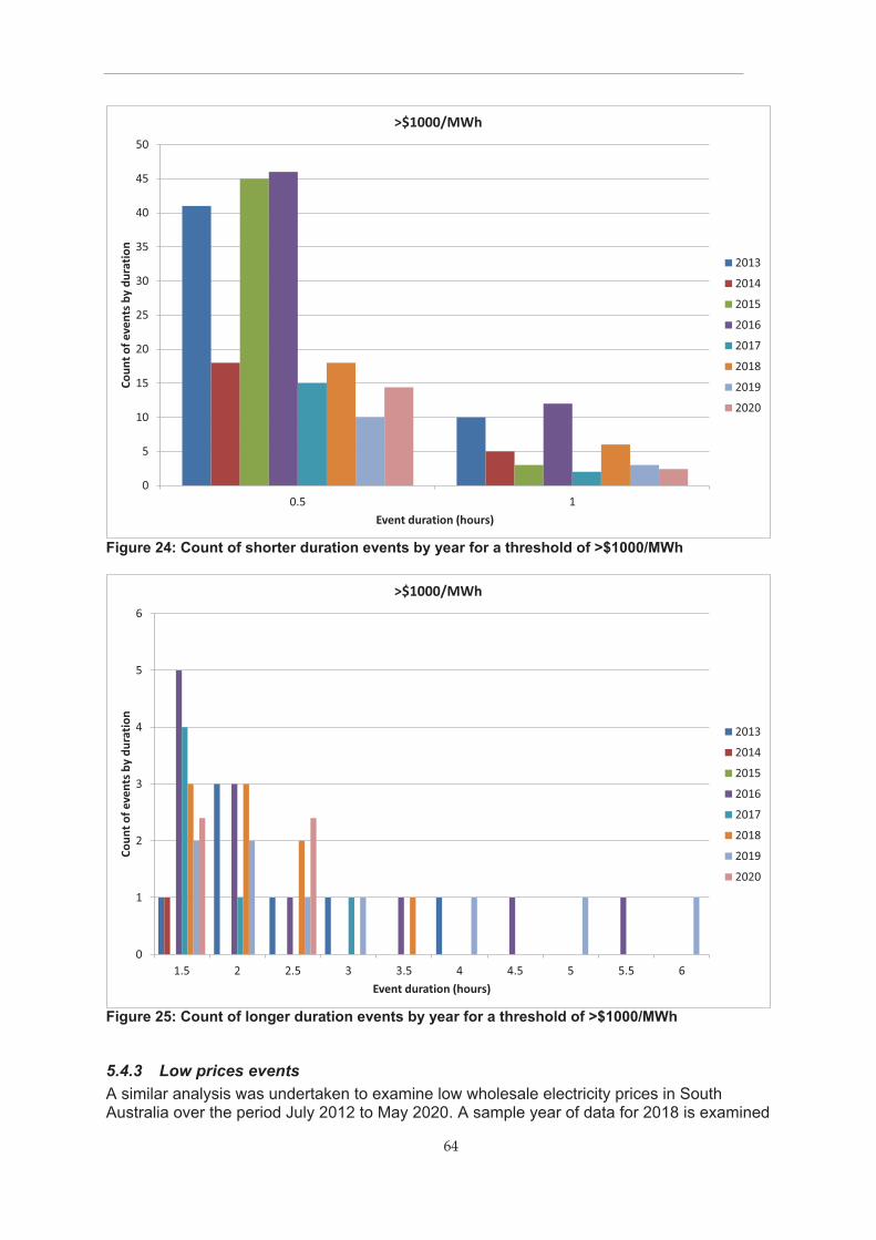
64
Figure 24: Count of shorter duration events by year for a threshold of >$1000/MWh
Figure 25: Count of longer duration events by year for a threshold of >$1000/MWh
5.4.3 Low prices events A similar analysis was undertaken to examine low wholesale electricity prices in South Australia over the period July 2012 to May 2020. A sample year of data for 2018 is examined
0
5
10
15
20
25
30
35
40
45
50
0.5 1
Coun
t of e
vent
s by
dura
tion
Event duration (hours)
>$1000/MWh
2013
2014
2015
2016
2017
2018
2019
2020
0
1
2
3
4
5
6
1.5 2 2.5 3 3.5 4 4.5 5 5.5 6
Coun
t of e
vent
s by
dura
tion
Event duration (hours)
>$1000/MWh
2013
2014
2015
2016
2017
2018
2019
2020

65
to illustrate the approach for low price events. The data in Figure 26 focuses on wholesale settlement prices in the lower range between +$200/MWh and -$200/MWh. Negative prices are shown as brown, while positive prices are shown in green. Note that this is exactly the same data as shown in Figure 14 but with a different scale.
Figure 26: Settlement price for each half hour for South Australia, calendar 2018 (low price events) Figure 26 shows that there are frequent short duration periods where prices are well below zero. Taking a threshold of less than $0/MWh as a benchmark for more detailed analysis, it is possible to investigate further. Figure 27 shows the frequency of lower price settlements over the period July 2012 to May 2020. It appears that low price settlements can occur at any time of the year, with no strong seasonal pattern evident. It is also obvious that the number of periods with a settlement price of less than $0/MWh appears to be increasing over time. Weekends experience a similar absolute number of low price events when compared to weekdays, but as weekends only make up less than 30% of all days, this suggests that low price events on weekends are more common in relative terms.
-200
-150
-100
-50
0
50
100
150
200
146
392
513
8718
4923
1127
7332
3536
9741
5946
2150
8355
4560
0764
6969
3173
9378
5583
1787
7992
4197
0310
165
1062
711
089
1155
112
013
1247
512
937
1339
913
861
1432
314
785
1524
715
709
1617
116
633
1709
5
Sett
lem
ent p
rice
$/M
Wh
30 min period (year)
2018
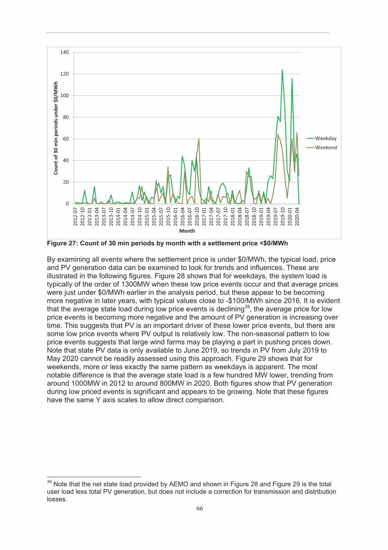
66
Figure 27: Count of 30 min periods by month with a settlement price <$0/MWh By examining all events where the settlement price is under $0/MWh, the typical load, price and PV generation data can be examined to look for trends and influences. These are illustrated in the following figures. Figure 28 shows that for weekdays, the system load is typically of the order of 1300MW when these low price events occur and that average prices were just under $0/MWh earlier in the analysis period, but these appear to be becoming more negative in later years, with typical values close to -$100/MWh since 2016. It is evident that the average state load during low price events is declining39, the average price for low price events is becoming more negative and the amount of PV generation is increasing over time. This suggests that PV is an important driver of these lower price events, but there are some low price events where PV output is relatively low. The non-seasonal pattern to low price events suggests that large wind farms may be playing a part in pushing prices down. Note that state PV data is only available to June 2019, so trends in PV from July 2019 to May 2020 cannot be readily assessed using this approach. Figure 29 shows that for weekends, more or less exactly the same pattern as weekdays is apparent. The most notable difference is that the average state load is a few hundred MW lower, trending from around 1000MW in 2012 to around 800MW in 2020. Both figures show that PV generation during low priced events is significant and appears to be growing. Note that these figures have the same Y axis scales to allow direct comparison.
39
Note that the net state load provided by AEMO and shown in Figure 28 and Figure 29 is the total user load less total PV generation, but does not include a correction for transmission and distribution losses.
0
20
40
60
80
100
120
140
2012
-07
2012
-10
2013
-01
2013
-04
2013
-07
2013
-10
2014
-01
2014
-04
2014
-07
2014
-10
2015
-01
2015
-04
2015
-07
2015
-10
2016
-01
2016
-04
2016
-07
2016
-10
2017
-01
2017
-04
2017
-07
2017
-10
2018
-01
2018
-04
2018
-07
2018
-10
2019
-01
2019
-04
2019
-07
2019
-10
2020
-01
2020
-04
Coun
t of 3
0 m
in p
erio
ds u
nder
$0/
MW
h
Month
Weekday
Weekend

67
Figure 28: Analysis of settlement price, net load and PV generation for events <$0/MWh, weekdays
Figure 29: Analysis of settlement price, net load and PV generation for events <$0/MWh, weekends Figure 30 illustrates the distribution of lower priced events by time of day. Both weekday and weekend low price events appear to be occurring overnight (from midnight to 7am) with a
-200
0
200
400
600
800
1000
1200
1400
1600
1800
2012
-07
2012
-11
2013
-03
2013
-07
2013
-11
2014
-03
2014
-07
2014
-11
2015
-03
2015
-07
2015
-11
2016
-03
2016
-07
2016
-11
2017
-03
2017
-07
2017
-11
2018
-03
2018
-07
2018
-11
2019
-03
2019
-07
2019
-11
2020
-03
Pric
e $/
MW
h : L
oad
MW
: PV
MW
Month
Events <$0/MWh
Av, Price Weekday
Av. Load Weekday
Av. PV Weekday
-200
0
200
400
600
800
1000
1200
1400
1600
1800
2012
-07
2012
-11
2013
-03
2013
-07
2013
-11
2014
-03
2014
-07
2014
-11
2015
-03
2015
-07
2015
-11
2016
-03
2016
-07
2016
-11
2017
-03
2017
-07
2017
-11
2018
-03
2018
-07
2018
-11
2019
-03
2019
-07
2019
-11
2020
-03
Pric
e @
/MW
h : L
oad
MW
: PV
MW
Month
Events <$0/MWh
Av, Price Weekend
Av. Load Weekend
Av. PV Weekend

68
second peak occurring during the mid-afternoon. The prevalence of overnight low priced events peaks are likely to be driven by the (lack of) management of controlled loads, possibly in combination with high output from large scale wind generators. Daytime low price events are likely to be driven by PV output. As weekends only make up less than 30% of all days, the overnight prevalence of low priced events is relatively comparable on weekdays and weekends. However, the relative prevalence of low priced events during the middle of the day appears to be much higher on weekends.
Figure 30: Count of 30 min periods by time of day with a settlement price <$0/MWh, 2012 to 2020, day of week This same data is split into season to reveal whether there are seasonal drivers. Figure 31 reveals that the occurrence of low price events is remarkably spread out across all seasons. The overnight prevalence in low prices is associated with management of controlled loads applies to all seasons with the least impact in summer. The prevalence of low prices in the early afternoon is also occurring in all seasons with spring standing out as the season with the most numerous low price events during the day. Day time low price events are probably being driven in part by PV generation, but there are likely to be other factors as well.
0
10
20
30
40
50
60
70
80
90
0.5
1.5
2.5
3.5
4.5
5.5
6.5
7.5
8.5
9.5
10.5
11.5
12.5
13.5
14.5
15.5
16.5
17.5
18.5
19.5
20.5
21.5
22.5
23.5
Coun
t of e
vent
s < $
0/M
Wh
Half hour ending
July 2012 to May 2020
Weekdays
Weekends

69
Figure 31: Count of 30 min periods by time of day with a settlement price <$0/MWh, 2012 to 2020, by season These figures give some insight into the nature of events on the grid that generate low settlement prices. However, these figures do not really indicate, in practical terms, how often or for how long demand response may be called on during low wholesale electricity price events. Low/negative wholesale price is not an immediate problem for consumers – on the contrary, they can benefit through arbitrage by shifting load into those periods and so taking that load out of a higher price period if there is a mechanism to share the benefits (but most end users are not directly exposed to wholesale prices). Another benefit to consumers is to reduce the investment required in managing the network to avoid/ accommodate reverse flows (e.g. grid-scale batteries). In the longer term, negative prices may reduce the economic returns to scheduled generation. As for high price events, a detailed sequential analysis was undertaken looking at events below a range of threshold settlement prices to examine the persistence of low price events. Within each calendar year, periods below the specified threshold were examined and the number of events was quantified by their duration. This allowed more detailed analysis on the likely demand response required. Once details of all the events under a specified threshold were compiled, it was possible to calculate the number of separate events, the total duration of events and average time per event. These are illustrated in Figure 32 to Figure 34. For 2020, values for count and total duration was scaled pro rata by 12 over 5 to approximate an equivalent annual figure as only data to the end of May 2020 was available. Therefore, 2020 values need to be considered as indicative only.
0
5
10
15
20
25
30
35
40
45
50
0.5
1.5
2.5
3.5
4.5
5.5
6.5
7.5
8.5
9.5
10.5
11.5
12.5
13.5
14.5
15.5
16.5
17.5
18.5
19.5
20.5
21.5
22.5
23.5
Coun
t of e
vent
s <$0
/MW
h
Half hour ending
July 2012 to May 2020
Summer
Autumn
Winter
Spring

70
Figure 32: Count of separate events under selected price thresholds by year
Figure 33: Total annual hours for events under selected price thresholds by year
0
100
200
300
400
500
600
700
2013 2014 2015 2016 2017 2018 2019 2020
Coun
t of e
vent
s
Year
<$0/MWh
<$-25/MWh
<$-50/MWh
<$-75/MWh
<$-100/MWh
0
200
400
600
800
1000
1200
1400
2013 2014 2015 2016 2017 2018 2019 2020
Annu
al h
ours
Year
<$0/MWh
<$-25/MWh
<$-50/MWh
<$-75/MWh
<$-100/MWh

71
Figure 34: Average duration of events under selected price thresholds by year Data illustrated in Figure 32 to Figure 34 indicates that the number of low price events is increasing over time, the total duration of low priced events is increasing significantly and the average length of each event is also increasing somewhat. Figure 32 suggests that the number of events that are less than $0/MWh has increased from almost nothing in 2013 to more than 500 separate events in 2020 (pro rata in 2020). While the number of low price events by year is somewhat variable, there is a clear trend. Figure 33 shows that the total hours per year of all events under $0/MWh is increasing and is likely to exceed 1000 hours in 2020 (pro rata) from a base of close to zero in 2013. Figure 34 effectively combines data from the previous two figures. This shows a distinct trend towards longer low priced events. Earlier in the period, the average low priced event was close to 0.5 hours, while by 2019, this had increased to almost 1.5 to 2 hours. While total hours per year and typical event length are useful parameters to take into account, a clearer picture can be obtained by looking at the distribution of event sizes by year as shown in Figure 35 and Figure 36. Figure 35 shows a distinct increase in shorter events of 0.5 or 1 hour duration from 2013 to 2020. Figure 36 shows a similar type of increase in the prevalence of longer lower priced event in later years. In 2019 and 2020 it is estimated that there are around 10 separate events that persist for at least 6 hours duration. This is important to note as DRM4 in electric water heaters has limited capability to respond for very long periods. But again, they are only one of several appliances with DRM capabilities that can be used to respond to these events.
0.0
0.5
1.0
1.5
2.0
2.5
2013 2014 2015 2016 2017 2018 2019 2020
Aver
age
dura
tion
per e
vent
(hou
rs)
Year
<$0/MWh
<$-25/MWh
<$-50/MWh
<$-75/MWh
<$-100/MWh

72
Figure 35: Count of shorter duration events by year for a threshold of <$0/MWh
Figure 36: Count of longer duration events by year for a threshold of <$0/MWh
5.5 Discussion on NEM analysis The previous section sets out the detailed analysis that examines the prevalence and duration of high price and low price events on the South Australian network. The number of
0
50
100
150
200
250
0.5 1
Coun
t of e
vent
s by
dura
tion
Event duration (hours)
<$0/MWh
2013
2014
2015
2016
2017
2018
2019
2020
0
10
20
30
40
50
60
70
80
1.5 2 2.5 3 3.5 4 4.5 5 5.5 6
Coun
t of e
vent
s by
dura
tion
Event duration (hours)
<$0/MWh
2013
2014
2015
2016
2017
2018
2019
2020

73
high price events (over $1000/MWh) appear to be falling as increased capacity is added to the system. There are of the order of 30 such events in a year and their duration is on average 1 to 1.5 hours. DRM1 is likely to be able to provide valuable support to the grid to help cope with these events. In contrast to high price events, low price events appear to be increasing quite quickly over recent years. The total time where prices are below $0/MWh appears to be over 1000 hours a year (projected for 2020) and the average time of these events is approaching 2 hours. While 400 of these events are 2 hours duration or less, there are a significant number of long duration events where prices are low. While this analysis provides a solid quantitative basis for examining the potential costs and benefits for this policy document, it needs to be noted that data for the past eight years does not necessarily reliably reflect the trends in or influences on the market into the future, even though there are some obvious trends for some parameters. South Australia already has well over 50% renewable electricity generation (Clean Energy Council 2019) and the government has announced plans to reach 100% renewable sources by 2030 (Renew Economy 2020a, 2020b; Government of South Australia 2020). Also, the recently approved interconnector with NSW (Maisch 2020; Australian Energy Regulator 2020) will most likely change the frequency and duration of both high price events (by allowing South Australia to import more power) and low price events (by allowing South Australia to export renewables that are in excess). The analysis in this section looks at the 30 minute settlement price (in $/MWh) and the average state net load (in MW). It is important to note that the settlement price is the marginal cost of the most expensive generator on the system in a particular period – this is the price that all generators receive for energy in that period. However, AEMO do not provide public data on the bid cost for all generators on the system in each settlement period (this determines the operating merit order) so it is not possible to estimate how much the wholesale price may change when a certain amount of capacity is delivered into the system (or taken out of the system) by something like a coordinated demand response supplied by water heaters. A better price impact could be estimated if the MW contributed by each generator and their bid price was analysed, but this is very complex, not publicly available and is likely to change a lot into the future. Another factor is the flexibility of each generator to response to changes in demand (either to increase or decrease from their despatched output). Some types of generation can be quite slow to change output and are unable to respond to short term changes in demand. The other thing to consider is that settlement prices may be driven by a range of factors, not just the merit order of available generators. Low energy prices are typically driven by an excess of non-scheduled generation such as wind and solar PV and/or constraints on export of excess energy interstate40. While the analysis in this section appears to indicate that low prices are being driven to some extent by increased PV capacity, this is not the whole picture and there are many factors that need to be considered. High prices may be caused by a range of factors such as a short term surge in demand (typically very hot or cold conditions), the loss of key generation assets, constraints on interstate interconnectors or other constraints on the intrastate transmission network. The response to high prices can
40
Some generators are required to stay on to provide system stability or other service like FCAS. However, most of the low price events appear to be driven by larger renewable generators that routinely bid very low prices into the market (as low as -$1000/MWh, which is the current AEMO price floor) to ensure that they always despatched to generate at maximum output. The output of these generators is supplied under power purchase agreements, so these generators are fairly insensitive to changes in real time wholesale electricity prices. To some extent this is true for all generators that contract their output directly.

74
include bringing expensive generation capacity on line and load shedding, including demand response. An additional consideration is that in the future the AEMC has finalised a rule to move to 5 minute settlements rather than the current 30 minute (Australian Energy Market Commission 2017). This was originally scheduled to start 1 July 2021, but has recently been delayed by three months and will now start on 1 October 2021 (Australian Energy Market Commission 2020b). Many commentators believe that this will make prices in the short term even more volatile than they have been in the past, but the intent is to provide a better price signal to fast response sources such as batteries and demand response. In some ways, 5 minute settlements may be advantageous to demand response generally as there may be larger price swings for shorter durations, which may well match more closely the technical capabilities of demand response for electric storage water heaters, enabling DRSPs to earn greater revenue. The impact on settlement price that a DRM1 response may have in a particular event is difficult to estimate as there is no data on generator incremental bid costs and merit order in the public domain. If there is a substantial pool of electric storage water heaters that can have DRM1 activated, then a coordinated response could well have a downward impact on high price events. The average settlement price for all individual high price events over $1000/MWh was typically $2000/MWh or more. A higher estimate of benefits would be to assume that the demand response from electric water heaters would be able to keep the wholesale settlement price at $1000/MWh for all high price events. A lower estimate would be to assume that the demand response from electric water heaters would only reduce wholesale prices by a small margin, say $1000/MWh, and only for events over $2000/MWh. If electric water heater demand response is able to reduce settlement prices during high cost events, then this will result in benefits to many participants. If the demand response from electric water heaters was able to cap wholesale settlement prices at $1000/MWh, this would result in clear overall savings in terms of wholesale energy costs for energy retailers. However, as these savings are somewhat uncertain and irregular in nature, it is not clear how these savings would be shared with customers. It would also mean that some specialised generators (such as quick start diesel generators) may no longer receive income by responding to very high price events. Ironically, it also means that the benefits that could be aggregated by a demand response service provider would also be limited if the market was flooded with capacity. Again, it is also unclear how any such payment for services collected by DRSPs would be shared with participating customers41. If electric water heater (and other) demand response has only a limited impact on settlement prices, the overall benefits to customers will be smaller but the financial motivation for DRSPs will be higher. It is difficult to predict where things would settle in such a dynamic supply and demand balancing exercise without more data and analysis. It is important to note that $1000/MWh is equivalent to $1.00/kWh in terms of electricity tariffs, and this is much higher than all retail energy tariffs and about a factor of 10 higher than the normal wholesale electricity cost, so there are strong financial incentives to respond to high prices if the correct tools are in place to allow this to occur. However, only a small proportion of all electricity is traded on the spot market. Most energy is purchased under contracts, which limits the exposure of electricity purchasers to volatility in wholesale electricity prices. The issue of low price events is somewhat different to high price events. When prices are negative, all generators that are exporting energy into the grid have to pay for each MWh they generate. This should result in strong curtailment of generators where their despatch can be controlled. Smaller scale PV tends not have their despatch controlled (except if there
41
This is not an issue for the policy to resolve, but business model options are not currently clear. The case of DRM1 is simpler, but DRM4 business models are potentially more complex.

75
is local high voltage on the distribution network, where they automatically disconnect42) and they are not exposed to wholesale electricity prices in any case, so are totally insensitive to negative wholesale prices. Some larger PV and wind generators will have despatch controls, but not all (many have their output fully contracted so are insensitive to wholesale prices). Some fossil fuel generators may have limited ability to reduce output during periods of low prices, depending on their ramp rates and whether they are required to provide other services (e.g. frequency control or spinning reserve). The potential issue of declining minimum load in South Australia is of some concern and this could introduce some instability into the system if not addressed. AEMO have examined this in some detail and propose a range of measures to deal with the impending issues (AEMO 2020b). During a low price event (below $0/MWh), the activation of a large scale DRM4 response should consume more power and should move the settlement price closer to $0/MWh. As with high cost events, it is difficult to know how much the settlement price will change per MW of load delivered to the system – this will depend on what generators are on the system and how they respond to price changes (if at all). The cost benefit analysis for DRM4 is a bit more complex as more negative prices should flow through to an overall reduction in wholesale electricity prices, so any activity that increases the negative price (such as DRM4) could be argued will reduce benefits to electricity retailers, at least. As with high price events, low price events are somewhat unpredictable and they are difficult to reflect in average electricity costs to generate tariffs, so electricity retailers may well be taking these reduced energy costs as a windfall. However, the more energy that retailers can shift load into those low price periods, the larger the windfall, so retailer and consumer interests align against those of the generators. From the perspective of a DRSP, negative costs provide an opportunity to get payment by increasing load on the system during negative prices. Again, it depends on how the DRSP shares these potential benefits with the end users. When DRM4 is activated, the water heater will increase energy consumption, so it depends on how this energy is metered and charged to the customer. Retail tariffs are made up of wholesale electricity costs plus a range of costs associated with fixed assets such as transmission, distribution, metering and administration. Even if the wholesale energy cost is close to free, some additional charges for this DRM4 energy supplied would need to be added. The other consideration is that energy consumed under DRM4 would displace energy that would normally be consumed under the normal supply tariff used for the water heater, so this may reduce retailer income at other times. It may be necessary to have a separate metering or other ways of adjusting changes in energy associated with DRM4 requests. For example, consider a customer that has an off peak water heater with DRM4 capability activated and they have a time of use energy tariff that is say 30c/kWh peak and 20c/kWh off peak (overnight and weekends). If a DRM4 request results in additional energy consumption during a non off peak period, the consumer will pay more for this energy if metered through the normal metering channel unless the energy consumed as a result of the request is separately metered and a separate rate is applied to that energy or some rebate is applied. The main point of this discussion is to point out that consideration also needs to be given to the technology framework required in order to facilitate and enable DRM4 in electric storage water heaters. DRM1 is different as the frequency and duration of requests are relatively few and the energy impacts for consumers are generally small to negligible, so there is no need to separately track of energy impacts. So, from a DNSP perspective, they only need to provide some up front incentive to encourage consumers to participate in DRM1 and then the DRSP can hope that they accrue sufficient revenue from subsequent demand response activities to cover their ongoing fixed and variable program costs.
42
There is some discussion about centrally controlling and disconnecting (curtailing) small PV through DRM5.

76
In additional to demand response in electric storage water heaters, air conditioners, pool pumps and EV charging43, there are numerous technologies that currently, or could in future, participate in the electricity network to reduce load during high price events and to soak up energy during low price events. These types of technologies could include batteries of all sizes (household, electric vehicles, utility scale, which can be aggregated into Virtual Power Plants), other types of load shedding and new technologies such as large scale variable hydrogen production, which could be deployed to effectively manage excess generation. There are also plans to introduce DRM5 to small PV inverters to allow these systems to be occasionally disconnected during periods of critical low state load. These and many other options are set out in the recently released Energy Solutions document (Government of South Australia 2020). As noted previously, changes to the NEM interconnectors with Victoria and NSW will also have a significant impact on settlement prices in South Australia, most likely by increasing low prices and reducing high prices. The key points of this NEM analysis are:
� There have been significant changes in the wholesale electricity price over the past 8
years and it is unclear and is difficult to predict how things will change into the future.
� High price events on the South Australian grid may be reducing, but there is still a
case for improving load response through DRM1.
� Low priced events broadly correlate with lower load periods and these appear to be
increasing a lot, so there is some opportunity for DRM4 in electric water heaters to
take advantage of this trend, but in South Australia DRM4 for water heaters on its
own is unlikely to be able to deal with all negative price events, especially those of
longer duration.
� To at least some extent, low price events are driven by PV generation, which is
forecast to increase substantially in the future (based on current installation rates and
AEMO forecasts).
� Implementing DRM1 in electric storage water heaters is technically simple.
� Implementing DRM4 in electric storage water heaters is more complex as changes in
energy consumption resulting from DRM4 responses (increased energy when
requested) need to be taken into account (by metering or other means), resulting in
some net benefits to consumers (at least no net costs of participation).
� Given the unpredictable nature of low cost and high cost events, it is not possible to
reflect these in any meaningful way in wholesale prices, other than at the very
broadest and crudest level (average annual prices, for example). Special fixed tariffs
(such as the proposed time of use tariff) are likely to be of very limited value with
respect to wholesale process as they cannot reflect dynamic real time changes in
wholesale electricity prices from day to day. The time of use tariff will address the
looming daytime minimum demand issue to some extent but may exacerbate
overnight low wholesale prices as load is shifted.
� For any demand response benefits to accrue to the electricity network, DRSPs
and/or customers from the activation of DRM in electric storage water heaters, there
needs to be a dynamic system that allows DRSPs to aggregate large numbers of
water heaters and bid these in real time into the wholesale electricity market,
43
The decision regulatory impact statement on 'Smart' demand response capabilities included recommendations to investigate requirements for home energy management systems (that could
control a wide range of appliances), photovoltaic inverters and battery systems (E3 2019).

77
currently at 30 minute intervals. A more dynamic control may be required once the
NEM moves to 5 minute settlements.
� Better demand flexibility would be attainted in South Australia if hot water controlled
loads were moved from the current time clocks to a system that allows better real
time management of these loads44, while meeting minimum service obligations
(minimum hours of supply per day). Control though DRM1 and DRM4 would be more
flexible than control of the hot water power circuit (whether by time clock or other
means).
� While there appears to be a good case for demand response in electric storage water
heaters in South Australia to address minimum demand challenges, there could be
other new technologies that may enter the market over time that could provide
greater flexibility of load and generation at lower cost, which may reduce the benefits
available to DRSPs who manage water heaters. There are a range of other
technologies that can complement water heaters with respect to demand response.
44
Controlled load periods experienced both low price and high price events.

78
6 Cost and Benefits The scope of works specifies that the net cost benefits (including direct cost benefits to householders, network cost saving benefits and wholesale electricity cost benefits) be assessed for each of the proposed policy options when compared to a business as usual policy (no change to the current requirements). The first step in this process for householder costs and benefits is to estimate the energy consumption and associated energy costs for water heaters under each of the policy options. The differences in capital cost and operating cost over the system lifetime can then be compared on the basis of an annualised cost at a specified discount rate. Note that detailed energy modelling for different system types and different hot water demands is documented as part of Task 4 in Section 8, which covers the purchase cost and operating cost of a wide range of system types in combination with photovoltaic systems using a specially developed hot water analysis tool. The brief analysis in this section is comparable to the analysis in Section 8, but that analysis examines critical parameters in more detail. For the network benefits and wholesale electricity costs, the previous analysis provides a solid basis against which to assess these benefits.
6.1 Energy modelling for end users To undertake an initial assessment of the policy options proposed for water heaters in South Australia, it is necessary to make an estimate of the differences in capital cost and energy operating costs for householders. In order to make a higher level assessment of the energy policy, an average hot water consumption will be assumed of 120 litres of hot water per day. The key parameters for the calculation of annual energy consumption are set out in Table 4. Table 4: Key parameters for the calculation of annual hot water energy Parameter Value Units Hot water use 120 litres/day/HH (ann. average)
Cold water temp 18 °C
Hot water temp 60 °C
Hot water demand 21.1 MJ/day
Hot water demand 5.860 kWh/day
Hot water demand 7701 MJ/year Table notes: This hot water demand is the medium level specified in Task 4 and is broadly consistent with an average household in South Australia (Whaley et al. 2014). A seasonal and cold water profile as per AS/NZS4234 has been used for this analysis.
In order to look at the overall impacts of each policy, the overall costs of an average hot water energy service have been calculated. This is made up of installed capital costs and energy operating costs. A survey of major energy retailers in early 2020 documented typical retail energy prices on standard residential tariffs in South Australia as shown in Table 5. These values were consistent with the Federal government’s Energy Made Easy website45 and a market survey undertaken by the Australian Energy Market Commission46 in 2019 (Australian Energy Market Commission 2019).
45
See https://www.energymadeeasy.gov.au/ 46
This survey converted standing changes to an average energy rate, so direct comparison required some calculations and assumptions.

79
Table 5: Residential electricity retail tariffs offered in South Australia
Supplier Peak OPCL Feed-
in AGL 35.12 19.24 14.2
Origin 40.24 21.84 10
Alinta 33.17 18.28 9.5
Average 36.18 19.79 11.23 Table notes: All values in c/kWh, EES survey in 2020.
A survey of gas retailers in South Australia showed that the most common residential tariff had a two block structure, with the first block charged at a higher rate of 4.46c/MJ (on average) with the second block charged at 3.31c/MJ. Both rates have been modelled for comparison purposes. A range of typical water heater costs were compiled to allow an assessment of energy service costs for each type of water heater. These are summarised in Table 6. Table 6: System purchase and installation costs collated in 2019
System type System cost
New installation
Replace installation
Large electric off peak $980 $510 $230
Small electric continuous $690 $510 $230
Gas storage 5 star $1,165 $374 $235
Gas instant 5 star $875 $632 $470
Gas instant 6 star $1,242 $872 $495
Heat pump average * $3,650 $930 $455
Flat plate solar medium * $4,150 $1,780 $985 Table notes: * Solar and heat pump systems are still currently eligible for STCs (REC)s, which are currently worth around $1000 for these systems and this is deducted from the installed capital cost when calculating the lifetime hot water cost. Large and small electric systems include an additional $70 for mandatory DRM1 controls, which are likely to reduce over time. Instant gas 6 star operate in the condensing range so require separate drain line for condensate.
As different energy systems have different lifetimes, the only fair way to compare the relative cost is to compare on an annualised energy basis. This effectively spreads the capital cost of purchase and installation over the expected lifetime, adjusted by the specified discount rate. A formula to convert an up-front capital cost to an equivalent annual value is:
Annual factor = 1 (1 ) n
C rr �
�� �
Where C is the capital cost, r is the discount rate (annual) and n is the lifetime in years (number of intervals). As r approaches zero, the formula converges to C/n. Where the discount rate is 0%, the above formula is replaced by C/n. There are a number of parameters that can be varied in this type of analysis. The main ones examined in this specific analysis are:
� Discount rate: base value of 7% with sensitivity of 3% and 10%
� Replacement or new installation cost
� Gas price for the initial consumption block or the second lower block rate.
To estimate the energy operating cost of different water heater types, simulations to AS/NZS4234 in Zone 3 (which covers the bulk of South Australia) to were used to estimate

80
energy inputs required to meet the specified hot water demand set out in Table 4. The AS/NZS4234 simulations were used to estimate annual energy requirements for different water heaters are set out in Figure 37. Second or third order polynomials were used to closely match the simulated energy across a range of hot water demand values. Seasonal variations in hot water demand, temperatures and other parameters were used to get an accurate estimate of annual energy consumption. This approach is largely compatible with the analysis in Section 8, but the hot water analysis tool breaks down performance by month for solar and heat pump systems to allow the impact of different seasonal and hot water profiles to be examined.
Figure 37: AS/NZS4234 simulations used to estimate energy input An example set of calculations is set out in Table 7. Table 7: Calculations to compare lifetime operating and capital costs of different water heater options, replacement
System type Purchase & install Lifetime
Energy in MJ $/kWh $/MJ
Energy $/year
Capital $/year
Total $/year
Large electric off peak $1,260 10 10639 $0.1979 $0.0550 $585 $162 $757
Small electric continuous $920 10 9697 $0.3618 $0.1005 $974 $121 $1,105
Gas storage 5 star $1,400 12 12135 $0.0446 $541 $176 $717
Gas instant 5 star $1,345 12 12172 $0.0446 $543 $169 $712
Gas instant 6 star $1,737 12 10937 $0.0446 $488 $219 $706
Heat pump average * $3,106 12 2987 $0.1979 $0.0550 $164 $391 $555
Flat plate solar medium * $4,099 15 1949 $0.3618 $0.1005 $196 $450 $646
PV panel 1.5kW $3,500 20 $330
Table notes: * Solar and heat pump systems have STC credits deducted based on $37/STC. Hot water output is 7701 MJ/year. Install costs are based on replacement in this example. Green shaded cells are also shaded in Table 8. Discount rate 7%. Includes an additional system cost of $70 for DRM1 controls for large and small electric storage water heaters, which equates to $10 per year lifetime cost. For the case of DRM1+DRM4 for larger electric storage water heaters (not shown above), the additional lifetime cost is $7 per annum on top of the cost for DRM1 alone (shown above).
0
5000
10000
15000
20000
25000
30000
35000
0 6600 13190 19770
Inpu
t ene
rgy
MJ/
year
Hot Water Demand MJ/year
Total Energy Input by System Type - AS/NZS4234 Zone 3
Gas storage (3* ref)
Gas storage (4* ref)
Gas storage (5* ref)
Gas Instant 5*
Gas storage 5*
Electric Storage (ref large)
Electric Storage (ref small)
Solar thermal
Gas in-line-solar
Heat Pump

81
A range of cases for comparison have been compiled in Table 8. Table 8: Comparison of total lifetime cost of operation for main water heater types, sensitivity analysis
System type Total
$/year Total
$/year Total
$/year Total
$/year Total
$/year Total
$/year Total
$/year Total
$/year Total
$/year Discount rate 7% 3% 10% 7% 3% 10% 7% 3% 10%
Installation type New New New Replace Replace Replace Replace Replace Replace
Gas price Block 1 Block 1 Block 1 Block 1 Block 1 Block 1 Block 2 Block 2 Block 2
Large electric off peak $797 $759 $827 $757 $727 $782 $757 $727 $782
Small electric continuous $1,145 $1,115 $1,170 $1,105 $1,082 $1,124 $1,105 $1,082 $1,124
Gas storage 5 star $735 $696 $767 $717 $682 $747 $578 $542 $607
Gas instant 5 star $733 $694 $764 $712 $678 $740 $572 $538 $600
Gas instant 6 star $754 $700 $798 $706 $662 $743 $581 $537 $617
Heat pump average $615 $524 $690 $555 $476 $620 $555 $476 $620
Flat plate solar medium $733 $606 $839 $646 $539 $735 $646 $539 $735
Table notes: Hot water output is 7701 MJ/year. Discount rate, installation type and gas price as shown. Green shaded cells are from example in Table 7. Includes cost of DRM1 controls for electric storage systems. Add an additional $7/year for large electric off peak to estimate the cost of DRM1+DRM4 controls at 7% discount rate.
Under most of the parameters modelled for sensitivity, larger electric off peak and gas are broadly comparable in terms of annual operating cost (energy costs plus annualised capital cost). Solar and heat pump systems are generally lower cost than conventional systems, except at higher discount rates. Of most note in this analysis is that small electric systems on continuous tariff are considerably more expensive to operate under all the combinations of parameters examined. The capital component of the total cost is as low as 14% for a small electric system to as much as 75% for solar and heat pump systems (7% discount rate, new installation). Off peak system capital cost is around 25% of the total annual operating cost and for gas systems this is typically 30% to 40%. A rational householder would not normally install a small electric hot water system operating on continuous tariff due to the high energy cost (in a permanently occupied site). However, there are two points to note: firstly the current hot water policy limits tank sizes to 250 litres and there are some cases where this sized tank would need to operate on continuous tariff to provide adequate service (or where dual elements with a top boost may be needed), thus proving an obstacle to access off peak in some cases. Secondly, in the case of tenants and landlords, there is a clear split incentive, where the landlord wishes to minimise capital and installation costs but the tenant ends up paying the bills of the high cost water heater. The current policy, as well as most of the proposed policies, do little to alleviate this issue.
6.2 Overall impacts by energy policy for end users The main impacts of the proposed policy changes are a small increase in the ownership of electric storage water heaters compared to the BAU scenario, except for Scenario C, which is likely to result in a large fall in the ownership of electric storage water heaters. In 2020 in South Australia, electric storage water heaters make up about 37.5% of all water heaters (including around 2.5% in Class 2 dwellings and an estimated 35% in Class 1 dwellings). The BAU scenario sees the share of electric water heaters fall to 32.9% by 2030. The current requirements for low emission water heaters where an existing household is connected to mains gas or for new houses puts ongoing downward pressure on the future ownership trends. The current policy allows households without mains gas to install an electric storage water heater of a maximum capacity of 250 litres. Currently 16% of electric

82
storage water heaters operate on continuous tariff, with the remainder being off peak. 250 litres can be connected to off peak in South Australia47 and this size of tank on off peak is suitable for smaller and medium households. Households that are capital cost sensitive (e.g. rental properties where the water heater purchaser does not pay the energy bills – split incentive) will tend to install smaller tanks and operate these continuous tariff. The current policy is expected to very slowly reduce the share of off peak water heaters as some consumers may need to run their tanks on continuous tariff (very large households) when electric systems are replaced or move to a different low emission water heater if they already have gas connected. Some landlords may already be replacing off peak tanks with smaller tanks on continuous tariffs to save capital costs. By 2030 the stock share of electric water heaters on continuous tariff is expected to rise to 21%. The recent approval of the new time of use tariff may change this base case somewhat by providing additional flexibility to existing water heaters to meet larger hot water loads and low cost. Figure 6 maps out the overall expected ownership trends as a result of the policy options considered in this paper. Policy Options A to B5 all result in a small increase in the projected ownership of electric storage systems relative to BAU, with most of the share difference coming from gas. Policy Option A, B1, B2, B3 and B4 place no restrictions on tank size or tariff, so the additional stock share above BAU will be a mixture of small tanks operating on continuous tariff (for cost sensitive segments like rentals) plus mostly larger tanks on off peak (for home owners concerned with operating costs). It is expected that all of these policy options will slow the decline in off peak share significantly from the BAU case. Policy Option B5 specifies a minimum tank size with the objective of allowing new electric storage systems to be connected to off peak tariffs. In this case off peak share is expected to increase from current levels. Policy Option C, as discussed earlier, will severely restrict the installation of electric storage water heaters by requiring a grid connected PV system. This limits electric storage water heaters to those households that already have a qualifying PV system or are going to install one in any case. The economics of installing a new PV system to allow the installation of an electric storage water heater does not stack up. Under this option, it is expected that the stock share of off peak systems will be stable or fall slightly. In order to assess the overall impacts of the different policies on users, the share of different hot water types under each of the different scenarios has been compiled to allow comparison of overall costs from the user perspective. These are summarised in Table 9.
47
The minimum permitted tank size for connection to residential off peak controlled load tariff in South Australia is 125 litres.
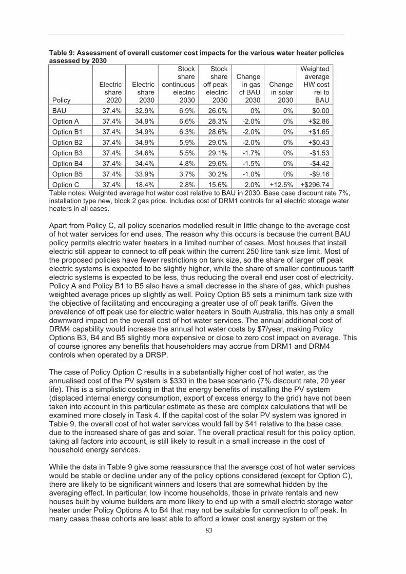
83
Table 9: Assessment of overall customer cost impacts for the various water heater policies assessed by 2030
Policy
Electric share 2020
Electric share 2030
Stock share
continuous electric
2030
Stock share
off peak electric
2030
Change in gas
cf BAU 2030
Change in solar
2030
Weighted average HW cost
rel to BAU
BAU 37.4% 32.9% 6.9% 26.0% 0% 0% $0.00
Option A 37.4% 34.9% 6.6% 28.3% -2.0% 0% +$2.86
Option B1 37.4% 34.9% 6.3% 28.6% -2.0% 0% +$1.65
Option B2 37.4% 34.9% 5.9% 29.0% -2.0% 0% +$0.43
Option B3 37.4% 34.6% 5.5% 29.1% -1.7% 0% -$1.53
Option B4 37.4% 34.4% 4.8% 29.6% -1.5% 0% -$4.42
Option B5 37.4% 33.9% 3.7% 30.2% -1.0% 0% -$9.16
Option C 37.4% 18.4% 2.8% 15.6% 2.0% +12.5% +$296.74
Table notes: Weighted average hot water cost relative to BAU in 2030. Base case discount rate 7%, installation type new, block 2 gas price. Includes cost of DRM1 controls for all electric storage water heaters in all cases.
Apart from Policy C, all policy scenarios modelled result in little change to the average cost of hot water services for end uses. The reason why this occurs is because the current BAU policy permits electric water heaters in a limited number of cases. Most houses that install electric still appear to connect to off peak within the current 250 litre tank size limit. Most of the proposed policies have fewer restrictions on tank size, so the share of larger off peak electric systems is expected to be slightly higher, while the share of smaller continuous tariff electric systems is expected to be less, thus reducing the overall end user cost of electricity. Policy A and Policy B1 to B5 also have a small decrease in the share of gas, which pushes weighted average prices up slightly as well. Policy Option B5 sets a minimum tank size with the objective of facilitating and encouraging a greater use of off peak tariffs. Given the prevalence of off peak use for electric water heaters in South Australia, this has only a small downward impact on the overall cost of hot water services. The annual additional cost of DRM4 capability would increase the annual hot water costs by $7/year, making Policy Options B3, B4 and B5 slightly more expensive or close to zero cost impact on average. This of course ignores any benefits that householders may accrue from DRM1 and DRM4 controls when operated by a DRSP. The case of Policy Option C results in a substantially higher cost of hot water, as the annualised cost of the PV system is $330 in the base scenario (7% discount rate, 20 year life). This is a simplistic costing in that the energy benefits of installing the PV system (displaced internal energy consumption, export of excess energy to the grid) have not been taken into account in this particular estimate as these are complex calculations that will be examined more closely in Task 4. If the capital cost of the solar PV system was ignored in Table 9, the overall cost of hot water services would fall by $41 relative to the base case, due to the increased share of gas and solar. The overall practical result for this policy option, taking all factors into account, is still likely to result in a small increase in the cost of household energy services. While the data in Table 9 give some reassurance that the average cost of hot water services would be stable or decline under any of the policy options considered (except for Option C), there are likely to be significant winners and losers that are somewhat hidden by the averaging effect. In particular, low income households, those in private rentals and new houses built by volume builders are more likely to end up with a small electric storage water heater under Policy Options A to B4 that may not be suitable for connection to off peak. In many cases these cohorts are least able to afford a lower cost energy system or the

84
temptation of lower capital costs is too strong. In particular, landlords have no incentive to consider the energy operating costs for hot water services paid by tenants and invariably will select the lowest capital cost option. Policy Option B5 attempts to overcome this issue by mandating a minimum size tank that makes it suitable for connection to off peak tariffs, thus reducing overall energy costs. Larger tanks operating on off peak tariffs have other potential benefits in that they rarely contribute to peak network loads and offer a substantial reservoir of energy for DRM4 controls. This initial analysis is for existing tariff and configurations only. The very recent availability of the new time of use tariff for South Australia does change these cost comparisons to some extent. This is quite complex and is examined in Section 8. However, in summary, larger electric systems operating on off peak controlled load could switch to the new time of use tariff and this could reduce energy costs by 50% if all consumption could be shifted to the daytime solar sponge window. This would make larger electric storage water heaters one of the lowest cost water heating options available in South Australia, particular at higher discount rates.
6.3 Network benefits There are two main elements of a water heater demand response program that can deliver network benefits. The first is the so called Reliability and Emergency Reserve Trader (RERT). This is a contract that AEMO offers to maintain power system reliability and system security using reserve contracts (effectively a reserve generation supply contract). RERT contracts are based on customer load that can be curtailed and restored on demand. This can be large industrial load or a group of aggregated smaller loads (such as water heaters). To be eligible, reserves provided under a reserve contract must not be available to the market through any other arrangements48 (AEMO 2020c). AEMO criteria to assess the suitability for RERT contracts are:
� The availability of the reserve over the summer period
� Whether the reserve can be activated as a block of not less than 10MW
� Whether the reserve can be activated continuously for at least 30 minutes.
Note that these requirements apply to the whole RERT contracted load, not just the water heater component. The RERT contract is currently $10,000/MWh in South Australia for availability for a nominal 20 hours per year. A minimum 10MW of capacity under this type of RERT reserve contract could earn $2m per year. These values may change once the interconnector between South Australia and NSW is completed in a few years. The second main network benefit is associated with peak load reductions, mainly associated with the transmission system and some parts of the distribution system. The benefits only accrue if demand response can reduce the maximum system demand on the transmission and distribution system at specific times and sometimes in specific places. This would only be achieved by very careful coordination with the network operator (AEMO and SA Power Networks). Effectively the value of a demand response is only realised if demand reductions can be orchestrated to allow near term investments in the transmission and distribution system to be deferred. This could be achieved by delivering significant demand reductions only during a handful of critical peak load events per year, and targeting them to areas with high marginal $/kVA investment costs. This can be done with the AS/NZS 4755 framework.
48
It is not entirely clear, but if a DRSP bids for a RERT contract it is possible that the load reduction capacity (DRM1) could not be used outside that contract for the duration, but DRM4 could still be used.
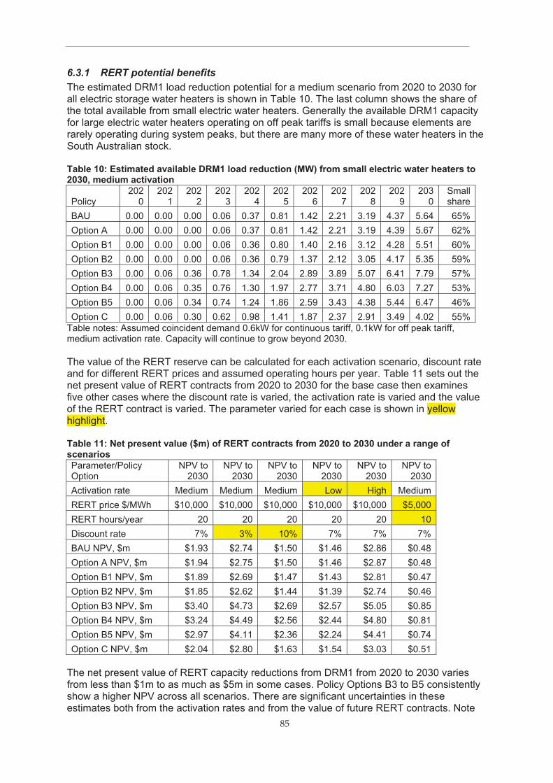
85
6.3.1 RERT potential benefits The estimated DRM1 load reduction potential for a medium scenario from 2020 to 2030 for all electric storage water heaters is shown in Table 10. The last column shows the share of the total available from small electric water heaters. Generally the available DRM1 capacity for large electric water heaters operating on off peak tariffs is small because elements are rarely operating during system peaks, but there are many more of these water heaters in the South Australian stock. Table 10: Estimated available DRM1 load reduction (MW) from small electric water heaters to 2030, medium activation
Policy 202
0 202
1 202
2 202
3 202
4 202
5 202
6 202
7 202
8 202
9 203
0 Small share
BAU 0.00 0.00 0.00 0.06 0.37 0.81 1.42 2.21 3.19 4.37 5.64 65%
Option A 0.00 0.00 0.00 0.06 0.37 0.81 1.42 2.21 3.19 4.39 5.67 62%
Option B1 0.00 0.00 0.00 0.06 0.36 0.80 1.40 2.16 3.12 4.28 5.51 60%
Option B2 0.00 0.00 0.00 0.06 0.36 0.79 1.37 2.12 3.05 4.17 5.35 59%
Option B3 0.00 0.06 0.36 0.78 1.34 2.04 2.89 3.89 5.07 6.41 7.79 57%
Option B4 0.00 0.06 0.35 0.76 1.30 1.97 2.77 3.71 4.80 6.03 7.27 53%
Option B5 0.00 0.06 0.34 0.74 1.24 1.86 2.59 3.43 4.38 5.44 6.47 46%
Option C 0.00 0.06 0.30 0.62 0.98 1.41 1.87 2.37 2.91 3.49 4.02 55%
Table notes: Assumed coincident demand 0.6kW for continuous tariff, 0.1kW for off peak tariff, medium activation rate. Capacity will continue to grow beyond 2030.
The value of the RERT reserve can be calculated for each activation scenario, discount rate and for different RERT prices and assumed operating hours per year. Table 11 sets out the net present value of RERT contracts from 2020 to 2030 for the base case then examines five other cases where the discount rate is varied, the activation rate is varied and the value of the RERT contract is varied. The parameter varied for each case is shown in yellow highlight. Table 11: Net present value ($m) of RERT contracts from 2020 to 2030 under a range of scenarios Parameter/Policy Option
NPV to 2030
NPV to 2030
NPV to 2030
NPV to 2030
NPV to 2030
NPV to 2030
Activation rate Medium Medium Medium Low High Medium
RERT price $/MWh $10,000 $10,000 $10,000 $10,000 $10,000 $5,000
RERT hours/year 20 20 20 20 20 10
Discount rate 7% 3% 10% 7% 7% 7%
BAU NPV, $m $1.93 $2.74 $1.50 $1.46 $2.86 $0.48
Option A NPV, $m $1.94 $2.75 $1.50 $1.46 $2.87 $0.48
Option B1 NPV, $m $1.89 $2.69 $1.47 $1.43 $2.81 $0.47
Option B2 NPV, $m $1.85 $2.62 $1.44 $1.39 $2.74 $0.46
Option B3 NPV, $m $3.40 $4.73 $2.69 $2.57 $5.05 $0.85
Option B4 NPV, $m $3.24 $4.49 $2.56 $2.44 $4.80 $0.81
Option B5 NPV, $m $2.97 $4.11 $2.36 $2.24 $4.41 $0.74
Option C NPV, $m $2.04 $2.80 $1.63 $1.54 $3.03 $0.51
The net present value of RERT capacity reductions from DRM1 from 2020 to 2030 varies from less than $1m to as much as $5m in some cases. Policy Options B3 to B5 consistently show a higher NPV across all scenarios. There are significant uncertainties in these estimates both from the activation rates and from the value of future RERT contracts. Note

86
that these are gross benefits and no attempt has been made to estimate the costs to retailers or DRSPs in harvesting these benefits and how these benefits may be shared with end users. There will obviously be benefits that accrue past 2030 as activation rates continue to rise. However, the value of benefits far into the future have only a small impact at medium discount rates.
6.3.2 Network infrastructure deferral benefits An estimate of the value of peak load reductions on different parts of the South Australian network were provided by SA Power Networks (George Wilkenfeld and Associates 2020). The average value of such peak load reductions is put at $675/kVA49 capacity reduction. This a network wide average value, with the value at specific sites or network elements potentially being much higher at times. The assumption is that all available demand reduction through DRM1 is available for use to defer investment in transmission and distribution assets, even for just a short period. A summary of the value of network infrastructure investment deferral is set out in Table 12 sets out the net present value of network infrastructure investment deferral from 2020 to 2030 for the base case then examines five other cases where the discount rate is varied, the activation rate is varied and the value of the deferral is varied. The parameter varied for each case is shown in yellow highlight. Table 12: Net present value ($m) of network investment deferrals from 2020 to 2030 under a range of scenarios
Parameter NPV to
2030 NPV to
2030 NPV to
2030 NPV to
2030 NPV to
2030 NPV to
2030
Activation rate Medium Medium Medium Low High Medium
Network value $/kVA $675 $675 $675 $675 $675 $350
Discount rate 7% 3% 10% 7% 7% 7%
BAU NPV, $m $6.52 $9.26 $5.06 $4.92 $9.67 $3.38
Option A NPV, $m $6.53 $9.29 $5.08 $4.93 $9.69 $3.39
Option B1 NPV, $m $6.38 $9.07 $4.96 $4.81 $9.47 $3.31
Option B2 NPV, $m $6.23 $8.85 $4.84 $4.70 $9.24 $3.23
Option B3 NPV, $m $11.49 $15.95 $9.09 $8.67 $17.03 $5.96
Option B4 NPV, $m $10.92 $15.14 $8.65 $8.24 $16.19 $5.66
Option B5 NPV, $m $10.03 $13.88 $7.96 $7.57 $14.87 $5.20
Option C NPV, $m $6.89 $9.46 $5.50 $5.20 $10.22 $3.57
The net present value of network infrastructure investment deferral from DRM1 from 2020 to 2030 varies from $3m to as much as $15m in some cases. The value of network infrastructure investment deferral appears to be significantly more valuable than RERT. Policy Options B3 to B5 consistently show a higher NPV across all scenarios.
6.3.3 Costs associated with accessing DRM1 benefits and net benefits There are two main costs associated with being able to access DRM1 functionality in electric storage water heaters. The first is the additional cost of installing the DRM1 control in the water heater. This has been estimated at $70 per unit in the regulatory impact statement (E3 2019). A more up to date estimate in the report for South Australian on demand response capabilities in appliances (George Wilkenfeld and Associates 2020) puts this cost at $60 initially, falling to $45 by 2036. This cost is paid for by consumers as part of the purchase price. In some respects, this can be considered as a sunk cost as COAG has already made
49
As water heater load is resistive with a power factor of 1.0, it is assumed that kW=kVA for this calculation.
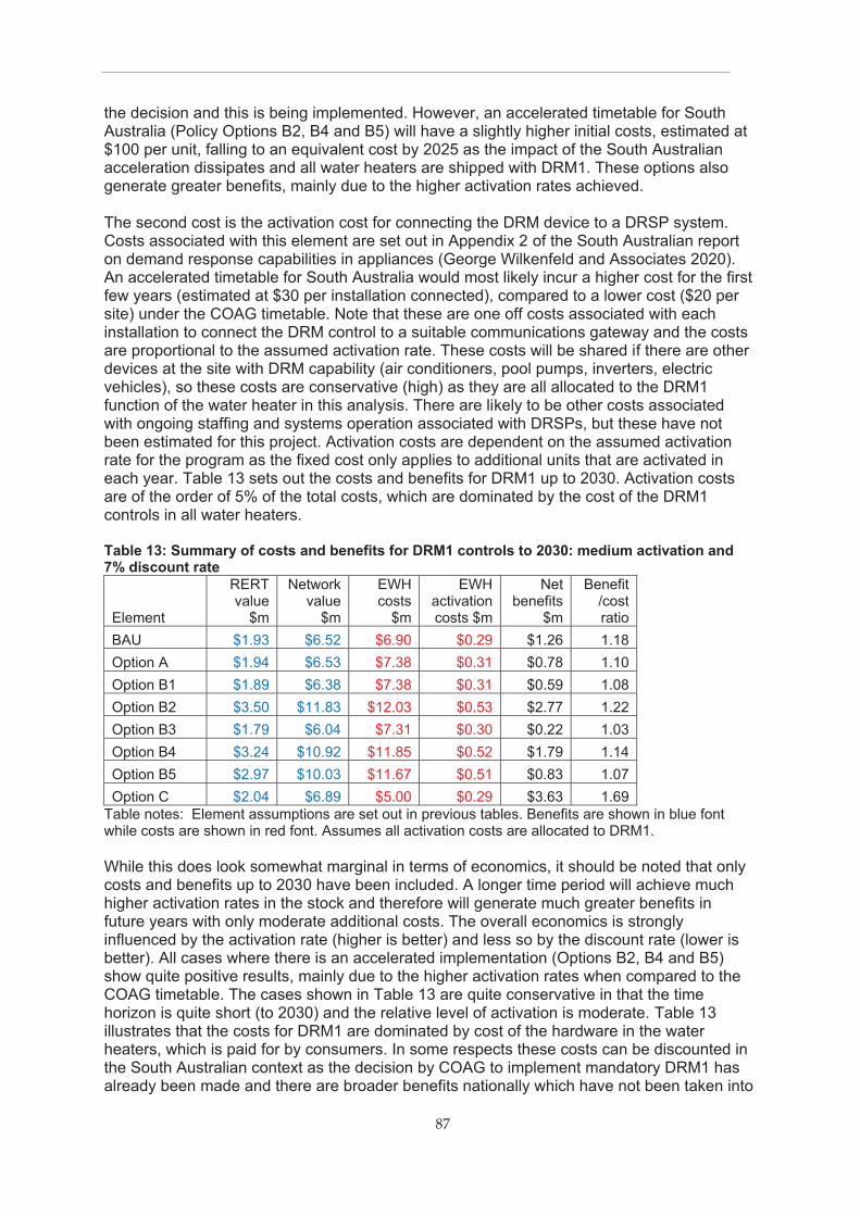
87
the decision and this is being implemented. However, an accelerated timetable for South Australia (Policy Options B2, B4 and B5) will have a slightly higher initial costs, estimated at $100 per unit, falling to an equivalent cost by 2025 as the impact of the South Australian acceleration dissipates and all water heaters are shipped with DRM1. These options also generate greater benefits, mainly due to the higher activation rates achieved. The second cost is the activation cost for connecting the DRM device to a DRSP system. Costs associated with this element are set out in Appendix 2 of the South Australian report on demand response capabilities in appliances (George Wilkenfeld and Associates 2020). An accelerated timetable for South Australia would most likely incur a higher cost for the first few years (estimated at $30 per installation connected), compared to a lower cost ($20 per site) under the COAG timetable. Note that these are one off costs associated with each installation to connect the DRM control to a suitable communications gateway and the costs are proportional to the assumed activation rate. These costs will be shared if there are other devices at the site with DRM capability (air conditioners, pool pumps, inverters, electric vehicles), so these costs are conservative (high) as they are all allocated to the DRM1 function of the water heater in this analysis. There are likely to be other costs associated with ongoing staffing and systems operation associated with DRSPs, but these have not been estimated for this project. Activation costs are dependent on the assumed activation rate for the program as the fixed cost only applies to additional units that are activated in each year. Table 13 sets out the costs and benefits for DRM1 up to 2030. Activation costs are of the order of 5% of the total costs, which are dominated by the cost of the DRM1 controls in all water heaters. Table 13: Summary of costs and benefits for DRM1 controls to 2030: medium activation and 7% discount rate
Element
RERT value
$m
Network value
$m
EWH costs
$m
EWH activation costs $m
Net benefits
$m
Benefit /cost ratio
BAU $1.93 $6.52 $6.90 $0.29 $1.26 1.18
Option A $1.94 $6.53 $7.38 $0.31 $0.78 1.10
Option B1 $1.89 $6.38 $7.38 $0.31 $0.59 1.08
Option B2 $3.50 $11.83 $12.03 $0.53 $2.77 1.22
Option B3 $1.79 $6.04 $7.31 $0.30 $0.22 1.03
Option B4 $3.24 $10.92 $11.85 $0.52 $1.79 1.14
Option B5 $2.97 $10.03 $11.67 $0.51 $0.83 1.07
Option C $2.04 $6.89 $5.00 $0.29 $3.63 1.69
Table notes: Element assumptions are set out in previous tables. Benefits are shown in blue font while costs are shown in red font. Assumes all activation costs are allocated to DRM1.
While this does look somewhat marginal in terms of economics, it should be noted that only costs and benefits up to 2030 have been included. A longer time period will achieve much higher activation rates in the stock and therefore will generate much greater benefits in future years with only moderate additional costs. The overall economics is strongly influenced by the activation rate (higher is better) and less so by the discount rate (lower is better). All cases where there is an accelerated implementation (Options B2, B4 and B5) show quite positive results, mainly due to the higher activation rates when compared to the COAG timetable. The cases shown in Table 13 are quite conservative in that the time horizon is quite short (to 2030) and the relative level of activation is moderate. Table 13 illustrates that the costs for DRM1 are dominated by cost of the hardware in the water heaters, which is paid for by consumers. In some respects these costs can be discounted in the South Australian context as the decision by COAG to implement mandatory DRM1 has already been made and there are broader benefits nationally which have not been taken into

88
account in this analysis. Also the hardware costs assumed by Wilkenfeld are also likely to be fairly conservative, in that they are generous to suppliers and actual costs may be less once they move into mass production (George Wilkenfeld and Associates 2020). Table 14 sets out the costs and benefits for DRM1 up to 2030 for a more optimistic case with a low discount rate and a high activation rate. This illustrates that the overall economics are quite sensitive to activation rate in particular. Table 14: Summary of costs and benefits for DRM1 controls to 2030: high activation and 3% discount rate
Element
RERT value
$m
Network value
$m
EWH costs
$m
EWH activation costs $m
Net benefits
$m
Benefit /cost ratio
BAU $4.07 $13.74 $9.05 $0.60 $8.17 1.85
Option A $4.08 $13.77 $9.69 $0.63 $7.53 1.73
Option B1 $3.99 $13.45 $9.69 $0.63 $7.12 1.69
Option B2 $7.22 $24.35 $14.93 $1.04 $15.60 1.98
Option B3 $3.77 $12.72 $9.60 $0.62 $6.27 1.61
Option B4 $6.65 $22.44 $14.69 $1.02 $13.38 1.85
Option B5 $6.09 $20.57 $14.46 $1.00 $11.20 1.72
Option C $4.16 $14.03 $6.32 $0.57 $11.29 2.64
Table notes: Element assumptions are set out in previous tables. Benefits are shown in blue font while costs are shown in red font. The apparent high benefit/cost ratio for Option C has occurred as this does not include the cost of the PV array (which will apply in some cases).
6.4 Value of load shifting using DRM4 The potential value of DRM4 is that it allows load to be moved from a period with higher wholesale electricity prices to a period with lower prices. Using this price difference between different periods is called arbitrage. For an appliance like an electric storage water heater, normally this load shifting can only be practically done within a 24 hour window each day. The previous analysis of the National Electricity Market data for South Australia showed that the prevalence of low priced events (below $0/MWh) appears to be increasing. There are two basic scenarios where activating DRM4 could generate benefits. The first is where wholesale prices are negative – in this case any additional energy consumption will be paid at the negative settlement price (assuming the load provided does not shift the settlement price very much). This type of strategy does not require much forewarning, but if prices are projected to be more negative at different times of the day, then most value will be achieved by targeting the most negative prices. While it was found in the NEM analysis that some low priced events have quite a long duration, there is certainly opportunity to consume more energy during these periods at low cost if there is DRM4 energy storage available. Of course, energy consumed by a water heater during these periods will displace energy consumed at other times, so it will result in some shifting of load and a small increase in total energy consumption in most cases. The second scenario is where there is planned coordination of the end use to move its energy consumption from a period where there are higher wholesale energy prices to a period where there are lower wholesale energy prices. In this case, the lower prices don’t have to be negative, but more negative prices can generate a larger difference. The overall value is a function of the energy consumed and the differences in whole energy prices between when energy would normally have been consumed and when it is consumed. Most of the capacity from DRM4 is from the additional energy storage offered by off peak storage tanks. Typically these are recharged overnight. To be most effective, the wholesale energy price overnight (when it would normally be operating) would have to be somewhat higher than the anticipated lower price (this may be through the middle of the day, but only on some

89
days). The water heater would have to be held back so it only partly heats overnight and then released to heat during the low price period. To maximise these benefits would take planning and careful coordination. An estimate of the benefits that could be obtained from load shifting and additional energy consumption using DRM4 controls was calculated for a range of parameters. Table 15 sets out the net present value of load shifting from 2020 to 2030 for the base case then examines six other cases where the discount rate is varied, the activation rate is varied, value of shifted energy and the available storage is varied. The parameter varied for each case is shown in yellow highlight. It is important to note the assumption that there will effectively be no DRM4 controls present in the market if this is not mandated by the South Australian government (or some other state government). This means that BAU and Policy Options A, B1 and B2 have no costs associated with DRM4 and no associated benefits. Table 15: Net present value ($m) of load shifting from 2020 to 2030 under a range of scenarios
Parameter NPV to
2030 NPV to
2030 NPV to
2030 NPV to
2030 NPV to
2030 NPV to
2030 NPV to
2030
Activation rate Medium Medium Medium Low High Medium Medium
Value shifting load $/MWh $80.00 $80.00 $80.00 $80.00 $80.00 $80.00 $40.00
Hours available per event 2 2 2 2 2 1 1
Days per year activated 150 150 150 150 150 150 100
Discount rate 7% 3% 10% 7% 7% 7% 7%
BAU $0.00 $0.00 $0.00 $0.00 $0.00 $0.00 $0.00
Option A $0.00 $0.00 $0.00 $0.00 $0.00 $0.00 $0.00
Option B1 $0.00 $0.00 $0.00 $0.00 $0.00 $0.00 $0.00
Option B2 $0.00 $0.00 $0.00 $0.00 $0.00 $0.00 $0.00
Option B3 $3.33 $4.73 $2.59 $2.51 $4.93 $1.66 $0.55
Option B4 $6.45 $8.96 $5.10 $4.87 $9.55 $3.22 $1.07
Option B5 $6.55 $9.10 $5.18 $4.94 $9.70 $3.27 $1.09
Option C $1.97 $2.70 $1.57 $1.48 $2.91 $0.98 $0.33
Table notes: Option C has a much lower electric water heater penetration and also has the DRM4 storage potential discounted by 50% to account for interactions between a local user energy management system, the PV installation and the electric water heater.
The net present value of load shifting and taking advantage of negative network prices using DRM4 from 2020 to 2030 varies from $0.55m to as much as $9.7m in some cases. The value of load shifting is generally higher than the value of RERT but less than network infrastructure investment deferral. Policy Options B4 and B5 consistently show a higher NPV across all scenarios. The expected penetration of DRM4 controls under BAU and Policy Options A, B1 and B2 is zero (non-mandatory inclusion of DRM4 controls), so there are no costs and no benefits. This technology relies on wholesale market price differences at different times of the day in order to be cost effective. While the number of low priced events in South Australia have been increasing in the past few years (with over 1,000 hours with a price of $0/MWh or less projected for 2020), their occurrence has been somewhat erratic in nature, so this makes it harder to reliably harvest this potential value. However, using DRM4 provides an opportunity to deal with erratic and somewhat random wholesale price changes on a day to day basis. If there were highly predictable wholesale price differences throughout the day across all seasons, then these would eventually be reflected in tariffs offered to different end users, reducing the potential value of this arbitrage using DRM4.

90
The significant medium term uncertainty in terms of quantifying costs and benefits for DR technology is that the interconnector between NSW and South Australia will reduce peak price events and will also reduce the frequency of low price events. If this occurs, the difference in energy prices will be smaller and the events per year where DRM4 could be cost effectively applied would be fewer. However, the overall flexibility this type of control brings to the national electricity market is likely to be very valuable in other ways in the future.
6.4.1 Costs associated with accessing DRM4 benefits and net benefits The main cost associated with being able to access DRM4 functionality in electric storage water heaters is the additional cost of installing the DRM4 control in the water heater. This has been estimated at $50 per unit over and above the cost of DRM1 controls in the regulatory impact statement (E3 2019). However, the recent South Australian report on demand response capabilities in appliances (George Wilkenfeld and Associates 2020) has revised this cost to $40 falling gradually to $5 by 2036. Note that this is the incremental cost on top of the installation of the DRM1 control in the water heater, which all water heaters will have. DRM4 controls are only installed in larger water heaters (160 litres and above). This cost is paid for by consumers as part of the purchase price. In the accelerated timing scenarios for South Australia, this cost increases to $50 per unit for the first two years before dropping back to the base case cost. The cost of activation is assumed to be zero for DRM4 as the same activation system would be used for DRM1 and DRM4 and any water heater connected to DRM4 would also be connected to DRM1, so the marginal cost is zero. Table 16: Summary of costs and benefits for DRM4 controls to 2030: medium activation and 7% discount rate
Element DRM4
benefits DRM4 costs
Net benefits
$m Benefit/
cost ratio
BAU $0.00 $0.00 $0.00 #N/A
Option A $0.00 $0.00 $0.00 #N/A
Option B1 $0.00 $0.00 $0.00 #N/A
Option B2 $0.00 $0.00 $0.00 #N/A
Option B3 $3.33 $3.43 -$0.11 0.97
Option B4 $6.45 $5.40 $1.05 1.20
Option B5 $6.55 $5.40 $1.15 1.21
Option C $1.97 $2.30 -$0.34 0.85
The economics of DRM4 for the base case looks fairly weak. However, it should be noted that this only includes costs and benefits up to 2030. A longer time period will achieve much higher activation rates in the stock and therefore will generate much greater potential benefits with only moderate additional costs. The overall economics is strongly influenced by the activation rate (higher is better) and less so by the discount rate (lower is better). The cases that have an accelerated implementation (Options B4 and B5) have larger benefits and larger costs. The cases shown in Table 16 are quite conservative in that the time horizon is quite short and the relative level of activation is moderate. By way of comparison, the case with a high activation rate and a discount rate of 3% is shown in Table 17. Under these conditions, Policy Options B4 and B5 both show very positive net benefits.

91
Table 17: Summary of costs and benefits for DRM1 controls to 2030: high activation and 3% discount rate
Element DRM4 benefits
DRM4 costs
Net benefits $m
Benefit/ cost ratio
BAU $0.00 $0.00 $0.00 #N/A
Option A $0.00 $0.00 $0.00 #N/A
Option B1 $0.00 $0.00 $0.00 #N/A
Option B2 $0.00 $0.00 $0.00 #N/A
Option B3 $7.00 $4.45 $2.55 1.57
Option B4 $13.27 $6.68 $6.58 1.99
Option B5 $13.47 $6.69 $6.79 2.01
Option C $4.00 $2.90 $1.11 1.38
6.5 Policy discussion The most important conclusion from this analysis is that the activation rate is absolutely critical to making this policy cost effective. This is certainly not a set and forget type of policy. If the decision is made to adopt mandatory DRM1 and DRM4 on an accelerated timetable in South Australia, which does look promising under high activation rates, then the government should consider actively stimulating the market for these DRM services. It may even contemplate being directly involved in some shape or form (e.g. through the DNSP) or by actively supporting new DRSPs into this space. The majority of the DRM costs will be borne by consumers, which will have to pay for the cost of these controls in the water heaters that they purchase. The benefits from DRM1 and DRM4 can only accrue to the state in general, the electricity network and end users if these controls are activated and are actively used to manage the load on the electricity system. While this initial analysis does look somewhat marginal for DRM4, the time horizon is quite short (to 2030) and the benefits will certainly grow over time, especially with higher activation rates after total costs stabilise. To some extent, other factors will also have some influence on the cost effectiveness of these measures, such as the new interconnector with NSW and the precise market rules associated with the newly released Wholesale Demand Response Mechanism, which starts in 2021 (Australian Energy Market Commission 2020a). These impacts are difficult to predict. However, these external factors are often unknown and it is necessary to make some value judgement about the potential role of these types of controls in the greater context of the national electricity market. This is a new and innovative technology that can bring much needed flexibility in the end use load on the electricity network and will be an important part of the future smart grid as we move to higher proportions of unscheduled renewable generation. While there are some risks in moving early to adopt this sort of technology, the long term benefits are clear. In all likelihood, the future costs will decline as new technologies evolve and the equipment becomes more mainstream. There is also a potential increase in benefits from a move to five minute settlement and even participation in other types of services such as FCAS, which have not been assessed. There is little doubt that new and innovative application of these types of controls will evolve once they are established in the market. However, for it to be a success, there must be a very active roll out of these controls and active use of these controls to deliver benefits to all parties.

92
7 Sensitivity analysis of alternative policy options (Task 3) 7.1 Scope The scope of works defines Task 3 as:
Task 3: Undertake a sensitivity analysis for each option, calculating the impact on costs, benefits and currently available models and sales of electric resistance water heaters by reducing in South Australia by 10%, 20% or 30%, the maximum allowable heat loss (kWh/24hrs) permitted under minimum energy performance standards (MEPS). This task requests that the impact of more stringent MEPS be assessed in the South Australian context. To undertake this task, the following steps were undertaken:
• Under the base case, data on the distribution of currently installed tank sizes
connected to continuous tariff and off peak tariff (controlled load) in South Australia
are estimated. The heat loss values specified in the relevant standard under MEPS
were extracted. A range of factors are applied to the measured heat loss values to
reflect energy consumption in normal use in the local context.
• The energy impacts of an increase in MEPS of 10%, 20% and 30% as specified are
estimated, including the impact of in use adjustments applicable to South Australia.
• The benefits of this option are then calculated in terms of reduced energy
consumption and annual savings based on current retail electricity tariffs in South
Australia. Existing studies and research are used to make a preliminary assessment
of the impact on purchase price.
It is important to note that most suppliers to the Australian market manufacture their products to just meet the mandatory MEPS levels. There is very little variation across regulated products so there are currently no options to select and encourage the sale of models with lower heat losses.
7.2 Quantification of the impacts The impact of increased MEPS can be readily calculated from the existing standing heat loss requirements specified in AS1056.1 and AS/NZS4692.2 (AS1056.1 1991; AS/NZS4692.1 2005; AS/NZS4692.2 2005). MEPS levels for electric storage water heaters were introduced in October 1999, with the requirements for small water heaters (<80 litres) tightened in 2005. There were a number of studies that examined the costs and benefits of improving MEPS levels from 1999 to 2005 for small tanks. Maximum permitted heat loss for unvented electric storage water heaters is obtained from the standard AS/NZS4692.2 Table A1. This is shown in Table 18 together with calculations of reduced heat loss for increased MEPS levels as proposed.

93
Table 18: MEPS for electric storage water heaters with calculated reduction for increased stringency
Tank size litres
MEPS 1999
kWh/d
MEPS 2005
kWh/d
TPR/ element
kWh/d
Off peak
factor MEPS kWh/d
MEPS * 0.9
kWh/d
MEPS * 0.8
kWh/d
MEPS * 0.7
kWh/d
Adjust SA
size share
40 1.66 1.18 0.2 1 1.38 1.262 1.144 1.026
50 1.76 1.25 0.2 1 1.45 1.325 1.200 1.075 3%
63 1.96 1.39 0.2 1 1.59 1.451 1.312 1.173
80 1.53 1.53 0.2 1 1.73 1.577 1.424 1.271 8%
100 1.67 1.67 0.2 1 1.87 1.703 1.536 1.369
125 1.81 1.81 0.2 1 2.01 1.829 1.648 1.467 4%
160 2.02 2.02 0.2 1 2.22 2.018 1.816 1.614 15%
200 2.23 2.23 0.2 1 2.43 2.207 1.984 1.761
250 2.44 2.44 0.4 0.9 2.84 2.596 2.352 2.108 33%
315 2.72 2.72 0.4 0.85 3.12 2.848 2.576 2.304 22%
400 2.93 2.93 0.4 0.75 3.33 3.037 2.744 2.451 15%
Table notes: Tank size is hot water delivery capacity in AS/NZS4692.1. In addition to MEPS, tanks are permitted an additional 0.2kWh/day for a hot side temperature/pressure relief valve (the most common configuration) plus an additional 0.2 kWh/day for each additional element. Off peak adjustment factor takes into account reduced heat loss from restricted energisation of OPCL tanks as per AS1056.4. MEPS adjustments are only applied to specified heat loss limits, not fitting adders. Share of tank size in South Australia is based on data reported in BIS Oxford and Wilkenfeld Table 32 adjusted to fit available sizes defined in the standard (BIS Oxford Economics 2018; George Wilkenfeld and Associates 2020).
By weighting the share of tank sizes estimated to be present in South Australia, it is possible to calculate an average weighted heat loss as shown in Table 19. Table 19: Impact of more stringent MEPS levels
Policy
MEPS per
standard
MEPS in use
SA Watts
equivalent
Annual energy
reduction kWh
MEPS 2.718 2.125 88.6 0
MEPS * 0.9 2.481 1.939 80.8 68
MEPS * 0.8 2.243 1.753 73.1 136
MEPS * 0.7 2.005 1.567 65.3 204
Table notes: Weighted tank size as per Table 18 applied. In use adjustment based on an ambient outdoor air temperature for Adelaide of 17.001°C as per the 2016 TMY AccuRate climate files and a hot water temperature of 60°C.
This data suggests that a 30% reduction in MEPS would reduce heat losses for all electric water heaters in South Australia by 0.558 kWh/day or 204 kWh/year. Smaller water heaters are usually installed indoors, so if an average indoor temperature was applied to the calculation for a 30% reduction in MEPS, small tanks would have a weighted average heat loss reduction of 0.39kWh/day. At current continuous tariffs in South Australia, this would generate savings of $51.40 per year. A similar calculation for larger tanks (that are typically installed outdoors or in unconditioned parts of the house) results in a weighted average heat loss reduction of 0.62 kWh/day for a 30% reduction in MEPS, which would generate savings of $44.60 per year on current average off peak tariffs. The value of these savings would be about half if the larger electric storage water heater was operated mostly during the daytime period of the new time of use tariff (around $22 per year savings).

94
The cost of achieving these reductions in MEPS are quite complex to estimate. The main cost will be the increased volume of foam. A draft regulatory impact statement was released in 2013, but this has little data on the cost of more stringent MEPS (E3 2013) and it did not proceed to a regulation. Early RIS studies estimated that foam costs accounted for around 75% of the cost of increasing MEPS. Other material costs include additional steel casing, modified and longer fittings, packaging, storage and transport (E3 2003; George Wilkenfeld and Associates 1993). It is difficult to reassess the likely increase in manufacturing cost without a detailed technical study to update the details. A lot of work and analysis went into small water heaters to support the proposed increase in MEPS from 1999 to 2005 for tanks less than 80 litres. Based on earlier studies, the current retail price impact may be in the range $200 to $400 of a 30% increase in MEPS level for a smaller tank, but this is dependent on a wide range of assumptions as well as tank size. The Net Present Value of energy savings calculated above is $360 peak and $315 off peak (7% discount rate), so more than likely the overall benefits for householders may be similar to the costs for smaller tanks, but the results are uncertain for larger tanks, especially if a significant proportion of systems move to the new time of use tariff with a lower energy rate. However, there are a number of complexities in this equation, which are discussed in the following section.
7.3 Discussion on the policy proposal The impact of increased MEPS level on water heater retail purchase costs is highly uncertain. There is the complexity of material costs (increased volume of polyurethane foam, increased materials, packaging, storage, transport etc.). This could be quantified and updated. For an electric storage water heater, there are not many technical options to reduce heat loss other than to increase foam thickness. The main difficulty is that changing a tank design to reduce heat loss will incur a tooling cost of the order of $0.5 million per model and amortising this up front capital cost is complex. Manufacturers are unlikely to maintain two production lines for different MEPS levels for the same size of tank and so will be highly resistant to any proposal to change MEPS levels and may elect to withdraw from the local market if this was a South Australian only regulation. The other complexity in assessing the costs is that increased dimensions will mean that there are more cases where the same sized water heater cannot be installed into the same space. Electric water heaters currently have around 75mm of polyurethane insulation encasing them, and a 30% reduction in heat loss would require an additional 45mm to 50mm of foam (accounting for fixed losses through penetrations), adding 90mm to 100mm to the diameter (Energy Partners 2000). Studies in preparation for increased MEPS for small water heaters found that a 40mm increase in insulation thickness for small water heaters meant that 31% of installations would need to be altered at a cost of some $350 per installation, or a smaller water heater selected (Taylor Nelson Sofres 2000). Note that this study focused on small systems installed indoors. Larger water heaters have constraints on their diameter and they must be able to fit through standard doors, limiting overall diameter to around 750mm. Large water heaters already have a diameter of 730mm (Rheem 400 litre electric storage). It is possible to re-engineer the units to reduce diameter and increase height, but this is even more expensive. So while the benefit cost ratio may appear to be neutral to positive on initial review, there are many complexities to assess. The material costs to improve heat loss levels for larger water heaters are substantially higher than small water heaters but the value of energy savings are much lower, especially if a significant proportion of units are operating on the new time of use tariff, which has a daytime energy rate that is half the current off peak rate.

95
8 Quantification of costs and benefits to householders from a range of hot water equipment combinations (Task 4)
8.1 Brief requirements The brief sets out the tasks to be covered by Task 4 as follows:
Quantify direct cost benefits to householders, including capital, running and lifetime costs for a full range of replacement/installation scenarios and water heater systems, in new and established homes. Energy obtained from an existing on-site PV will be considered as ‘free’ energy in calculating energy consumption. This task covers a wide range of water heater system types and hot water demand.
The main parameters to be covered are:
� On site PV ranging from small (3kW) to large (9kW)
� Hot water demand, ranging from small (40 L/day) to heavy (200 L/day)
� A wide range of system types including conventional electric, gas and LPG water
heaters as well as heat pump, solar thermal electric boost and solar thermal gas
boost.
8.2 EES hot water analysis tool Given the wide scope of this work and the large number of systems covered, EES developed a hot water analysis tool for use by DEM to inform their policy deliberations with respect to overall hot water costs under a range of different equipment and tariff permutations and combinations. The tool is based on results from TRNSYS simulations to AS/NZS4234 for a wide range of system types. Importantly, these simulations were undertaken across a wide range of hot water loads (typically from 0MJ/day to 60MJ/day), which enabled a detailed correlation model to be developed for different usage parameters. As the impact of PV generation was to be assessed, it was necessary to select a whole house electricity consumption profile as a base for analysis in order to assess the internal consumption versus export on an hour by hour basis. The EES hot water analysis tool allows the user to set the following parameters for analysis:
� Selection of climate zone (Adelaide, Mount Lofty or Mount Gambier)
� Details of energy tariffs including any future escalation (increase in real terms)
� Selection of discount rate for financial analysis
� Selection of a PV system from zero to 10kW with options for specifying
orientation share and power limits to export (if required)
� A range of options for house base load including sample SA and NSW houses
and modelled bottom-up South Australian data for selected parameters
� A range of hot water related usage options such as cold water temperature
profiles, seasonal variation in hot water demand profiles, weather profiles, time of
use profiles and specified hot water demand
� Performance parameters for a wide range of water heater systems.
The hot water analysis tool allows the parallel assessment of 27 water heater types so that they can all be directly compared for identical operating conditions, tariffs and hot water demands in the selected household.

96
Hourly energy input profiles are generated for each water heater type. The electricity consumption (if any) is then added to the selected base load electricity profile to allow analysis of hourly PV generation that is climate specific. PV generation is assumed to displace internal consumption initially, with any excess exported (within the boundaries of any pre-defined export power limits). Any excess generation is exported at the specified export tariff. This allows an analysis of energy and energy costs as follows:
� Energy consumption for each water heater type by fuel and hour for the year
� Net energy import or export for electricity by hour for the year
� Electricity costs for import or export by hour for the year
� Total energy costs for the year for each fuel type, broken into import, export and net
costs for electricity.
Total energy and energy costs for each of the water heater types modelled are then summed for the year to allow more detailed comparison. Capital and installation costs, as well as the value of any STCs earned, are compiled to give a total capital cost. The analysis tool then undertakes some financial analysis by calculating the levelised annual equivalent of the total capital cost at the selected discount rate over the estimated lifetime for each water heater type. This annualised capital cost equivalent can be added to the energy purchase cost to provide an initial estimate of the annual cost of hot water. The assumed discount rate has some impact on the overall costing and potential ranking of different water heater types as a higher discount rate penalises higher capital costs and devalues or discounts higher energy costs into the future. So higher discount rates tend to favour low capital cost water heaters with high energy costs (typically conventional water heaters) while low discount rates tend to favour high capital cost water heaters with low energy costs (solar and heat pump water heaters). The hot water analysis tool has a number of innovative new elements. Residential load data for South Australia was obtained from a sample of 295 interval meters from FY 2018-2019 which had data at 30 min intervals for a year. The sample average energy consumption was 4760 kWh/year. The annual energy was broken into 14 separate consumption bins (labelled from A to N) and this was used to generate 14 annual load profiles of 8760 hours). The count of households in each energy bin of 1000 kWh/year is illustrated in Figure 38.

97
Figure 38: Count of households in the SAPN general domestic sample for 2018-2019 An analysis of the load shape was undertaken and it was found, reassuringly, that all bins had a very similar load shape (even if the absolute energy consumption varied substantially). The normalised load shape (shown as hourly energy as a ratio of daily average energy) is illustrated in Figure 39.
Figure 39: Normalised TOD load shape for each of the consumption bins, SAPN sample
0
10
20
30
40
50
60
A =
<100
0
B =
1000
-200
0
C=20
00-3
000
D=30
00-4
000
E=40
00-5
000
F=50
00-6
000
G=60
00-7
000
H=70
00-8
000
I=80
00-9
000
J=90
00-1
0000
K=10
000-
1100
0
L=11
000-
1200
0
M=1
2000
-130
00
N=>
1300
0
Coun
t of h
ouse
hold
s
0.0
0.2
0.4
0.6
0.8
1.0
1.2
1.4
1.6
1.8
2.0
1 2 3 4 5 6 7 8 9 10 11 12 13 14 15 16 17 18 19 20 21 22 23 24
Nor
mal
ised
load
(rat
io o
f ave
rage
)
Hour ending
Average
A
B
C
D
E
F
G
H
I
J
K
L
M
N

98
The data illustrated in Figure 39 overwhelmingly does not include any water heating as off peak controlled loads were separately metered and gas water heaters do not use electricity for heating. Gas and off peak controlled loads account for more than 85% of water heaters in South Australia. Analysis of the OPCL data, which is predominantly used for electric storage water heating, showed that the average consumption was 2059 kWh/year. A few of these had very low energy, so are likely to be solar or heat pump water heaters or some other type of product. The distribution of energy is shown in Figure 40. Note that the bin size was reduced to 400 kWh for the OPCL analysis.
Figure 40: Count of households in the SAPN residential OPCL sample for 2018-2019 The OPCL data showed a strong seasonal profile as shown in Figure 41.
0
10
20
30
40
50
60
70
A=<4
00
B=40
0-<8
00
C=80
0-<1
200
D=12
00-<
1600
E=16
00-<
2000
F=20
00-<
2400
G=24
00-<
2800
H=28
00-<
3200
I=32
00-<
3600
J=36
00-<
4000
K=40
00-<
4400
L=44
00-<
4800
M=4
800-
<520
0
N=>
5200
Coun
t of h
ouse
hold
s

99
Figure 41: Seasonal profile of the SAPN residential OPCL sample for 2018-2019 by bin Data for month and each consumption bin was normalised back to a ratio of the maximum winter value (with the maximum shown as 1.0). This is illustrated in Figure 42. This type of analysis is useful as AS./NZS4234 defines hot water demand in terms of the winter peak. All consumption bins showed a similar seasonal load shape.
Figure 42: Monthly energy ratio for the SAPN residential OPCL sample for 2018-2019 by bin
0
0.1
0.2
0.3
0.4
0.5
0.6
0.7
0.8
0.9
1
1 2 3 4 5 6 7 8 9 10 11 12
Aver
age
pow
er in
kW
Month
Average
C
D
E
F
G
H
I
J
K
L
M
N
0
0.1
0.2
0.3
0.4
0.5
0.6
0.7
0.8
0.9
1
1 2 3 4 5 6 7 8 9 10 11 12
Mon
thly
ene
rgy
as a
ratio
of m
axim
um m
onth
Month
Average Energy
C
D
E
F
G
H
I
J
K
L
M
N

100
Note that the OPCL data includes hot water demand as well as tank heat losses through the year. Some engineering analysis on the likely heat losses by month for OPCL systems in South Australia was undertaken, resulting in the seasonal profile shown in Figure 43. This is important to understand as it suggests that hot water demand in South Australia is possibly more seasonal than other states. AS/NZS4234 assumes a summer hot water demand of 0.7 compared to the winter peak. The stronger seasonal profile found in the OPCL sample data exists for total OPCL sales in South Australia and is also confirmed by the Uni SA water heater study in 2013 that undertook detailed monitoring of 12 water heaters for a year (Whaley et al. 2014). For comparison the water heating seasonal profile from the three South Australian sources is compared to AS/NZS4234 in Figure 44. The 15 year SAPN load profile has not been corrected for heat loss. All of the South Australian sources show a very consistent pattern with a summer hot water demand of around 0.5 of the winter peak value.
Figure 43: Average seasonal profile for OPCL sample with heat loss correction
0
0.1
0.2
0.3
0.4
0.5
0.6
0.7
0.8
0.9
1
1 2 3 4 5 6 7 8 9 10 11 12
Seas
onal
pro
file
Month
Metered energy
Hot water (corr. For heat loss)

101
Figure 44: Average seasonal profile for water heating – various sources Analysis of the time of day load for the SAPN OPCL sample allowed generic load shapes to be derived for off peak systems, as illustrated in Figure 45. This shows most energy consumption occurs at midnight and falls until 8am, with a small increase driven by morning hot water demand at 7am. There is little or no consumption during the day, as expected.
Figure 45: Normalised TOD load shape for each of the consumption bins, SAPN OPCL sample
0
0.1
0.2
0.3
0.4
0.5
0.6
0.7
0.8
0.9
1
1 2 3 4 5 6 7 8 9 10 11 12Month
AS/NZS4234 All zones
SAPN OPCL 15 years (all)
SAPN sample 295 2018/19
Uni SA WH profile
0
1
2
3
4
5
6
7
8
9
10
1 2 3 4 5 6 7 8 9 10 11 12 13 14 15 16 17 18 19 20 21 22 23 24
Nor
mal
ised
load
(rat
io o
f ave
rage
)
Hour ending
Average
C
D
E
F
G
H
I
J
K
L
M
N

102
In addition to the South Australian meter data, load data from NSW has been obtained and broken up into similar energy bins (AUSGRID 2012). In general terms, these showed similar load shapes to the South Australian data. EES has also modelled end use data from bottom-up using house and appliance simulations for several house and climate types in South Australia. In summary the selectable elements cover:
� A range of house sizes from 100 m2 to 300 m2
� Options for different heating systems and whether non-living areas are conditioned
� Options for different cooling systems and whether non-living areas are conditioned
� Older (pre-2006) or newer building shell
� Typical selection of appliances and equipment
� Option to include a pool
� Selection of Adelaide, Mount Lofty for Mount Gambier climate zones.
Any selected hourly load profile can be scaled to the specified electricity consumption value for a particular house, if desired. PV data was modelled using 2016 TMY climate files for Adelaide, Mount Lofty and Mount Gambier climate zones. Modelling was undertaken by ITP Renewables as a sub-contractor and simulated output using Pvsyst software. The assumed angle is 20 degrees from horizontal with hourly output generated for 1kW system. This is scaled depending on the selected system size. The user can select the proportion of panels that are oriented in each of the 4 cardinal directions (North, East, South, West – must sum to 100%). Inverter costs were estimated from analysis from ITP Renewables that estimated total system installed costs by city in Australia in May 2020 (ITP Renewables 2020). An example of the hourly output is illustrated in Figure 46.
Figure 46: Sample PV hourly output for a year for Adelaide, 3kW system
0.0
0.5
1.0
1.5
2.0
2.5
3.0
123
246
369
492
511
5613
8716
1818
4920
8023
1125
4227
7330
0432
3534
6636
9739
2841
5943
9046
2148
5250
8353
1455
4557
7660
0762
3864
6967
0069
3171
6273
9376
2478
5580
8683
1785
48
PV o
utpu
t kW
Hour of year
PV system size 3 kW

103
There is a strong seasonal pattern in average PV output as illustrated in Figure 43, with a peak output in summer and a minimum output in winter (as expected). The demand for hot water is the opposite of this overall trend, with a peak in winter and a minimum demand in summer, as illustrated in Figure 44. This suggests that even large amounts of PV have a limited capacity to eliminate electricity consumed by electrically power hot water systems. The relative energy demand for hot water in South Australia and output for photovoltaics are illustrated in Figure 47.
Figure 47: Comparison on monthly hot water energy demand with PV output for Adelaide Figure notes: PV monthly average energy from Figure 46, seasonal hot water demand from Uni SA and Figure 44 (Whaley et al. 2014).
While the new hot water analysis tool is an innovative approach to modelling and analysing water heater performance, there are a few limitations that need to be considered when applying the results. Most of the water heater performance data underpinning the tool was modelled in accordance with AS/NZS4234 using TRNSYS simulations using Zone 3 (Sydney) and Zone 4 (Melbourne) TMY climate files developed for water heaters. Monthly performance data was extracted and used to develop accurate correlation models for systems types that are highly dependent on ambient conditions, such as solar thermal and heat pump systems (based on performance per MJ of water delivered by month). The electricity consumption profiles for South Australia were based on measured load data for a sample of houses from July 2018 to June 2019, so this does not match the weather files used for hot water simulation. In addition, the PV simulation and the bottom-up house load simulation data used TMY files for Adelaide, Mount Lofty and Mount Gambier, so there is a potential mismatch in PV as well in some cases. However, the modelling approach in the hot water tool has generated generic curves for each type of water heater and climate across a wide range of hot water demand levels, so this should provide a robust basis for the estimation of energy for comparative purposes. As the performance data for solar water heaters (in particular) was generated using different climate files to the PV simulation, the correlation model will show lower alignment between solar performance and PV output that you would expect in reality. Days of high PV output should also result in days of high solar
0.0
0.1
0.2
0.3
0.4
0.5
0.6
0.7
0.8
0.9
1.0
Jan Feb Mar Apr May Jun Jul Aug Sep Oct Nov Dec
Seas
onal
ene
rgy
ratio
Month
PV energy
HW demand

104
thermal contribution and little or no electric boosting, so the current model (which uses different climate files for PV and hot water simulations) will slightly overestimate the amount of boosting that PV can displace in solar thermal systems. The other issue to consider is that the modelling approach used in the hot water analysis tool (and indeed all modelling tools for water heaters) assumes a static constant daily demand every day for each month, with adjustment of load (and cold water temperature) by month as specified in the selected seasonal profile. It is known from limited end use metering data that the actual hot water demand varies significantly from day to day (Sustainability Victoria 2016; E3 2012; Energy Efficient Strategies 2012; Whaley et al. 2014). Currently there is no data analysis to show whether there are any short term weather drivers for hot water demand (as opposed to seasonal demand variations, which are reasonably well documented – see the next section). If there are weather drivers for hot water use (within a month), then a future project may examine the impact of these on overall system performance. If there are no clear weather drivers, the impact of random variations in daily hot water demand should also be assessed on overall performance as a kind of resilience assessment. Some early hot water metering data showed variation in hot water demand between weekdays and weekends, so this is an additional consideration. Simulation software like TRNSYS can do simulations where hot water load is varied day to day, but at this stage there is little data upon which to generate realistic daily variations. Sample off peak metering data for South Australia and NSW could provide a useful data set to explore the magnitude of these daily variations. In all likelihood, the performance of conventional and heat pump systems will be largely unaffected by variations in hot water demand. The impact on solar systems could be important.
8.3 Initial results from analysis tool In order to undertake the comparisons specified in the project brief, the following general settings were selected for all modelling runs:
� Climate file for Adelaide
� Flat tariff structure and PV export tariffs based on the average of three major South
Australian retailers as in early 2020 (see Table 5)
� Gas prices based on South Australian retailers, LPG prices based on available swap-
and-go style retail prices, assume zero supply charge for gas and LPG
� Lower discount rate of 3%
� Base electricity consumption profile for South Australian SAPN load analysis Bin F
(5474 kWh/year)
� University of South Australia cold water and seasonal energy profiles for Adelaide
(Whaley et al. 2014)
� Flat hot water drawoff profile as per AS/NZS4234
� Outdoor temperature profile based on Adelaide climate (AccuRate)
� All system efficiency, performance and cost assumptions as per default setting in the
hot water analysis tool
� No cost associated with the purchase or operation of the PV system, export not
limited
� A total of 27 water heater systems are modelled in parallel.
The brief specifies hot water demand of 40, 120 and 200 litres per day. It is assumed that this is a winter peak demand. The brief also specifies 3, 6 and 9 kW PV systems. The additional option of no PV system (0 kW) makes a total of 12 scenarios to model. These are set out in Table 20.

105
Table 20: Hot water scenarios modelled for initial cost comparison Scenario ID PV system kW Hot water demand
L/day (winter peak)
Scenario 1 0 40
Scenario 2 0 120
Scenario 3 0 200
Scenario 4 3 40
Scenario 5 3 120
Scenario 6 3 200
Scenario 7 6 40
Scenario 8 6 120
Scenario 9 6 200
Scenario 10 9 40
Scenario 11 9 120
Scenario 12 9 200
For initial comparisons, detailed outputs for Scenario 5 have been prepared as this represents an average hot water load and an average PV system size (although only around 25% of households currently have a PV system in South Australia). For this scenario, the ranking of annual energy costs (including levelised capacity cost) is listed in Table 21. The energy consumption by fuel is shown in Figure 48 while the energy cost by fuel is shown in Figure 49.

106
Table 21: Ranking of annual energy costs by water heater type: Scenario 5
Rank Sub-Cat Short Descr. Description - detailed Ann En Cost 1 Solar03 HP Std OP Heat pump (Standard, off peak) $352
2 Solar04 HP HE OP Heat pump (High efficiency off peak) $395
3 Solar01 HP Std Heat pump (Standard, peak) $399
4 Solar12 ST HE OP Solar electric (High efficiency, off peak) $417
5 Solar10 ST HE Solar electric (High efficiency, peak) $420
6 Solar02 HP HE Heat pump (High Efficiency, peak) $432
7 Solar11 ST Std OP Solar electric (Standard, off peak) $434
8 Solar09 ST Std Solar electric (Standard, peak) $443
9 Solar18 STG HE Gas solar high efficiency $501
10 Solar17 STG Std Gas solar standard $504
11 Solar20 STLPG HE LPG solar high efficiency $505
12 Solar19 STLPG Std LPG solar standard $514
13 CV10 IGWH 7* Gas instantaneous (7 star) $569
14 CV9 IGWH 6* Gas instantaneous (6 star) $593
15 CV8 IGWH 5* Gas instantaneous (5 star) $597
16 CV4 EWH 315L (new) Electric storage 315L (Post MEPS 1999 – off peak) $641
17 CV15 ILPGWH 7* LPG instantaneous (7 star) $651
18 CV7 GSWH 5.5* Gas storage (5.5 star) $682
19 CV14 ILPGWH 6* LPG instantaneous (6 star) $686
20 CV3 EWH 315L (old) Electric storage 315L (Pre MEPS 1999 – off peak) $693
21 CV13 ILPGWH 5* LPG instantaneous (5 star) $699
22 CV6 GSWH 4* Gas storage (4 star) $750
23 CV2 EWH 80L (new) Electric storage 80L (Post MEPS 1999 - Peak) $760
24 CV5 Elec instant Electric instant $765
25 CV12 LPGSWH 5.5* LPG storage (5.5 star) $807
26 CV1 EWH 80L (old) Electric storage 80L (Pre MEPS 1999 - Peak) $815
27 CV11 LPGSWH 4* LPG storage (4 star) $895
Table notes: Annual energy cost includes annualised capital cost at the specified discount rate (3%). Other parameters as set out at the beginning of Section 8.3.

107
Figure 48: Annual energy by fuel for all water heater types: Scenario 5
Figure 49: Annual energy costs by capital and fuel for all water heater types: Scenario 5 Figure notes: Refer to Table 21 for a more detailed description of system types.
Given that the primary focus of this project is the overall cost of hot water supply, figures showing the breakdown of capital and fuel costs (converted to an annual basis) have been prepared for the remaining 11 scenarios. Note that Y axis scale varies for each figure.
0
2000
4000
6000
8000
10000
12000
14000
16000
EWH
80L
(old
)EW
H 80
L (n
ew)
EWH
315L
(old
)EW
H 31
5L (n
ew)
Elec
inst
ant
GSW
H 4*
GSW
H 5.
5*IG
WH
5*IG
WH
6*IG
WH
7*LP
GSW
H 4*
LPGS
WH
5.5*
ILPG
WH
5*IL
PGW
H 6*
ILPG
WH
7*HP
Std
HP H
EHP
Std
OP
HP H
E O
PST
Std
ST H
EST
Std
OP
ST H
E O
PST
G St
dST
G HE
STLP
G St
dST
LPG
HE
Annu
al e
nerg
y M
J
System type
Annual hot water demand 6575 MJ
LPG
Gas
Electricity
Scenario 5: 3 kW PV, 120 L/day HW
$0
$100
$200
$300
$400
$500
$600
$700
$800
$900
$1,000
EWH
80L
(old
)EW
H 80
L (n
ew)
EWH
315L
(old
)EW
H 31
5L (n
ew)
Elec
inst
ant
GSW
H 4*
GSW
H 5.
5*IG
WH
5*IG
WH
6*IG
WH
7*LP
GSW
H 4*
LPGS
WH
5.5*
ILPG
WH
5*IL
PGW
H 6*
ILPG
WH
7*HP
Std
HP H
EHP
Std
OP
HP H
E O
PST
Std
ST H
EST
Std
OP
ST H
E O
PST
G St
dST
G HE
STLP
G St
dST
LPG
HE
Annu
al h
ot w
ater
ene
rgy
cost
System type
Annual hot water demand 6575 MJ
LPG
Gas
Electricity
Capital
Scenario 5: 3 kW PV, 120 L/day HW

108
Figure 50: Annual energy costs by capital and fuel for all water heater types: Scenario 1
Figure 51: Annual energy costs by capital and fuel for all water heater types: Scenario 2
$0
$100
$200
$300
$400
$500
$600
$700
EWH
80L
(old
)EW
H 80
L (n
ew)
EWH
315L
(old
)EW
H 31
5L (n
ew)
Elec
inst
ant
GSW
H 4*
GSW
H 5.
5*IG
WH
5*IG
WH
6*IG
WH
7*LP
GSW
H 4*
LPGS
WH
5.5*
ILPG
WH
5*IL
PGW
H 6*
ILPG
WH
7*HP
Std
HP H
EHP
Std
OP
HP H
E O
PST
Std
ST H
EST
Std
OP
ST H
E O
PST
G St
dST
G HE
STLP
G St
dST
LPG
HE
Annu
al h
ot w
ater
ene
rgy
cost
System type
Annual hot water demand 2192 MJ
LPG
Gas
Electricity
Capital
Scenario 1: 0 kW PV, 40 L/day HW
$0
$200
$400
$600
$800
$1,000
$1,200
EWH
80L
(old
)EW
H 80
L (n
ew)
EWH
315L
(old
)EW
H 31
5L (n
ew)
Elec
inst
ant
GSW
H 4*
GSW
H 5.
5*IG
WH
5*IG
WH
6*IG
WH
7*LP
GSW
H 4*
LPGS
WH
5.5*
ILPG
WH
5*IL
PGW
H 6*
ILPG
WH
7*HP
Std
HP H
EHP
Std
OP
HP H
E O
PST
Std
ST H
EST
Std
OP
ST H
E O
PST
G St
dST
G HE
STLP
G St
dST
LPG
HE
Annu
al h
ot w
ater
ene
rgy
cost
System type
Annual hot water demand 6575 MJ
LPG
Gas
Electricity
Capital
Scenario 2: 0 kW PV, 120 L/day HW

109
Figure 52: Annual energy costs by capital and fuel for all water heater types: Scenario 3
Figure 53: Annual energy costs by capital and fuel for all water heater types: Scenario 4 Figure notes: Scenario 5 is included as Figure 49.
$0
$200
$400
$600
$800
$1,000
$1,200
$1,400
$1,600
EWH
80L
(old
)EW
H 80
L (n
ew)
EWH
315L
(old
)EW
H 31
5L (n
ew)
Elec
inst
ant
GSW
H 4*
GSW
H 5.
5*IG
WH
5*IG
WH
6*IG
WH
7*LP
GSW
H 4*
LPGS
WH
5.5*
ILPG
WH
5*IL
PGW
H 6*
ILPG
WH
7*HP
Std
HP H
EHP
Std
OP
HP H
E O
PST
Std
ST H
EST
Std
OP
ST H
E O
PST
G St
dST
G HE
STLP
G St
dST
LPG
HE
Annu
al h
ot w
ater
ene
rgy
cost
System type
Annual hot water demand 10958 MJ
LPG
Gas
Electricity
Capital
Scenario 3: 0 kW PV, 200 L/day HW
$0
$100
$200
$300
$400
$500
$600
$700
EWH
80L
(old
)EW
H 80
L (n
ew)
EWH
315L
(old
)EW
H 31
5L (n
ew)
Elec
inst
ant
GSW
H 4*
GSW
H 5.
5*IG
WH
5*IG
WH
6*IG
WH
7*LP
GSW
H 4*
LPGS
WH
5.5*
ILPG
WH
5*IL
PGW
H 6*
ILPG
WH
7*HP
Std
HP H
EHP
Std
OP
HP H
E O
PST
Std
ST H
EST
Std
OP
ST H
E O
PST
G St
dST
G HE
STLP
G St
dST
LPG
HE
Annu
al h
ot w
ater
ene
rgy
cost
System type
Annual hot water demand 2192 MJ
LPG
Gas
Electricity
Capital
Scenario 4: 3 kW PV, 40 L/day HW

110
Figure 54: Annual energy costs by capital and fuel for all water heater types: Scenario 6
Figure 55: Annual energy costs by capital and fuel for all water heater types: Scenario 7
$0
$200
$400
$600
$800
$1,000
$1,200
$1,400
EWH
80L
(old
)EW
H 80
L (n
ew)
EWH
315L
(old
)EW
H 31
5L (n
ew)
Elec
inst
ant
GSW
H 4*
GSW
H 5.
5*IG
WH
5*IG
WH
6*IG
WH
7*LP
GSW
H 4*
LPGS
WH
5.5*
ILPG
WH
5*IL
PGW
H 6*
ILPG
WH
7*HP
Std
HP H
EHP
Std
OP
HP H
E O
PST
Std
ST H
EST
Std
OP
ST H
E O
PST
G St
dST
G HE
STLP
G St
dST
LPG
HE
Annu
al h
ot w
ater
ene
rgy
cost
System type
Annual hot water demand 10958 MJ
LPG
Gas
Electricity
Capital
Scenario 6: 3 kW PV, 200 L/day HW
$0
$100
$200
$300
$400
$500
$600
$700
EWH
80L
(old
)EW
H 80
L (n
ew)
EWH
315L
(old
)EW
H 31
5L (n
ew)
Elec
inst
ant
GSW
H 4*
GSW
H 5.
5*IG
WH
5*IG
WH
6*IG
WH
7*LP
GSW
H 4*
LPGS
WH
5.5*
ILPG
WH
5*IL
PGW
H 6*
ILPG
WH
7*HP
Std
HP H
EHP
Std
OP
HP H
E O
PST
Std
ST H
EST
Std
OP
ST H
E O
PST
G St
dST
G HE
STLP
G St
dST
LPG
HE
Annu
al h
ot w
ater
ene
rgy
cost
System type
Annual hot water demand 2192 MJ
LPG
Gas
Electricity
Capital
Scenario 7: 6 kW PV, 40 L/day HW

111
Figure 56: Annual energy costs by capital and fuel for all water heater types: Scenario 8
Figure 57: Annual energy costs by capital and fuel for all water heater types: Scenario 9
$0
$100
$200
$300
$400
$500
$600
$700
$800
$900
$1,000
EWH
80L
(old
)EW
H 80
L (n
ew)
EWH
315L
(old
)EW
H 31
5L (n
ew)
Elec
inst
ant
GSW
H 4*
GSW
H 5.
5*IG
WH
5*IG
WH
6*IG
WH
7*LP
GSW
H 4*
LPGS
WH
5.5*
ILPG
WH
5*IL
PGW
H 6*
ILPG
WH
7*HP
Std
HP H
EHP
Std
OP
HP H
E O
PST
Std
ST H
EST
Std
OP
ST H
E O
PST
G St
dST
G HE
STLP
G St
dST
LPG
HE
Annu
al h
ot w
ater
ene
rgy
cost
System type
Annual hot water demand 6575 MJ
LPG
Gas
Electricity
Capital
Scenario 8: 6 kW PV, 120 L/day HW
$0
$200
$400
$600
$800
$1,000
$1,200
$1,400
EWH
80L
(old
)EW
H 80
L (n
ew)
EWH
315L
(old
)EW
H 31
5L (n
ew)
Elec
inst
ant
GSW
H 4*
GSW
H 5.
5*IG
WH
5*IG
WH
6*IG
WH
7*LP
GSW
H 4*
LPGS
WH
5.5*
ILPG
WH
5*IL
PGW
H 6*
ILPG
WH
7*HP
Std
HP H
EHP
Std
OP
HP H
E O
PST
Std
ST H
EST
Std
OP
ST H
E O
PST
G St
dST
G HE
STLP
G St
dST
LPG
HE
Annu
al h
ot w
ater
ene
rgy
cost
System type
Annual hot water demand 10958 MJ
LPG
Gas
Electricity
Capital
Scenario 9: 6 kW PV, 200 L/day HW

112
Figure 58: Annual energy costs by capital and fuel for all water heater types: Scenario 10
Figure 59: Annual energy costs by capital and fuel for all water heater types: Scenario 11
$0
$100
$200
$300
$400
$500
$600
$700
EWH
80L
(old
)EW
H 80
L (n
ew)
EWH
315L
(old
)EW
H 31
5L (n
ew)
Elec
inst
ant
GSW
H 4*
GSW
H 5.
5*IG
WH
5*IG
WH
6*IG
WH
7*LP
GSW
H 4*
LPGS
WH
5.5*
ILPG
WH
5*IL
PGW
H 6*
ILPG
WH
7*HP
Std
HP H
EHP
Std
OP
HP H
E O
PST
Std
ST H
EST
Std
OP
ST H
E O
PST
G St
dST
G HE
STLP
G St
dST
LPG
HE
Annu
al h
ot w
ater
ene
rgy
cost
System type
Annual hot water demand 2192 MJ
LPG
Gas
Electricity
Capital
Scenario 10: 9 kW PV, 40 L/day HW
$0
$100
$200
$300
$400
$500
$600
$700
$800
$900
$1,000
EWH
80L
(old
)EW
H 80
L (n
ew)
EWH
315L
(old
)EW
H 31
5L (n
ew)
Elec
inst
ant
GSW
H 4*
GSW
H 5.
5*IG
WH
5*IG
WH
6*IG
WH
7*LP
GSW
H 4*
LPGS
WH
5.5*
ILPG
WH
5*IL
PGW
H 6*
ILPG
WH
7*HP
Std
HP H
EHP
Std
OP
HP H
E O
PST
Std
ST H
EST
Std
OP
ST H
E O
PST
G St
dST
G HE
STLP
G St
dST
LPG
HE
Annu
al h
ot w
ater
ene
rgy
cost
System type
Annual hot water demand 6575 MJ
LPG
Gas
Electricity
Capital
Scenario 11: 9 kW PV, 120 L/day HW

113
Figure 60: Annual energy costs by capital and fuel for all water heater types: Scenario 12 Note that these figures include the amortised capital and installation cost of the appliance, shown as capital (purple), at a discount rate of 3%. The capital component would be higher as the discount rate increases. The energy cost is unaffected in this calculation. A comparison between a 3% discount rate (default used above) and a 10% discount rate is shown below in Figure 61 for Scenario 5. The impact of a higher discount rate is larger for more expensive water heater types like solar and heat pump systems. Over the product lifetime, a higher discount rate also values future energy savings (reduced future energy costs) from these types of systems as of lower benefit. Therefore, a higher discount rate favours conventional water heaters that have a lower capital cost and higher energy costs. Figure 61: Capital cost impacts: 3% discount (left) and 10% discount (right); Scenario 5
8.4 Discussion on initial results Overall rankings for all scenarios are set out in Table 22. This uses a traffic light colour coding for ranking the overall cost of hot water (green best, red worst).
$0
$200
$400
$600
$800
$1,000
$1,200
$1,400
EWH
80L
(old
)EW
H 80
L (n
ew)
EWH
315L
(old
)EW
H 31
5L (n
ew)
Elec
inst
ant
GSW
H 4*
GSW
H 5.
5*IG
WH
5*IG
WH
6*IG
WH
7*LP
GSW
H 4*
LPGS
WH
5.5*
ILPG
WH
5*IL
PGW
H 6*
ILPG
WH
7*HP
Std
HP H
EHP
Std
OP
HP H
E O
PST
Std
ST H
EST
Std
OP
ST H
E O
PST
G St
dST
G HE
STLP
G St
dST
LPG
HE
Annu
al h
ot w
ater
ene
rgy
cost
System type
Annual hot water demand 10958 MJ
LPG
Gas
Electricity
Capital
Scenario 12: 9 kW PV, 200 L/day HW
$0
$100
$200
$300
$400
$500
$600
$700
$800
$900
$1,000
EWH
80L
(old
)EW
H 80
L (n
ew)
EWH
315L
(old
)EW
H 31
5L (n
ew)
Elec
inst
ant
GSW
H 4*
GSW
H 5.
5*IG
WH
5*IG
WH
6*IG
WH
7*LP
GSW
H 4*
LPGS
WH
5.5*
ILPG
WH
5*IL
PGW
H 6*
ILPG
WH
7*HP
Std
HP H
EHP
Std
OP
HP H
E O
PST
Std
ST H
EST
Std
OP
ST H
E O
PST
G St
dST
G HE
STLP
G St
dST
LPG
HE
Annu
al h
ot w
ater
ene
rgy
cost
System type
Annual hot water demand 6575 MJ
LPG
Gas
Electricity
Capital
Scenario 5: 3 kW PV, 120 L/day HW

114
Tabl
e 22
: Cos
t ran
king
of a
ll w
ater
hea
ter t
ypes
for a
ll sc
enar
ios
(1 is
low
est c
ost)
Syste
m a
bb
rev.
Sce
n 1
S
ce
n 2
S
ce
n 3
S
ce
n 4
S
ce
n 5
S
cen 6
S
ce
n 7
S
ce
n 8
S
ce
n 9
S
cen 1
0
Scen 1
1
Scen 1
2
kW
PV
+ L
/da
y H
W
0kW
+40
L
0kW
+120
L
0kW
+200
L
3kW
+40
L
3kW
+120
L
3kW
+200
L
6kW
+40
L
6kW
+120
L
6kW
+200
L
9kW
+40
L
9kW
+120
L
9kW
+200
L
Mean
rank
EW
H 8
0L
(o
ld)
26
27
26
18
26
26
18
24
23
17
20
21
22.7
EW
H 8
0L (
ne
w)
23
25
25
16
23
24
14
19
20
10
17
18
19.5
EW
H 3
15
L (
old
) 18
20
18
22
20
18
22
22
18
22
23
19
20.2
EW
H 3
15
L (
ne
w)
16
16
15
17
16
15
17
16
15
18
18
15
16.2
Ele
c insta
nt
15
26
27
4
24
27
1
18
24
1
16
22
17.1
GS
WH
4*
24
22
20
25
22
20
25
25
21
25
25
23
23.1
GS
WH
5.5
* 17
18
17
19
18
17
19
20
17
19
21
17
18.3
IGW
H 5
* 2
15
16
2
15
16
4
15
16
4
15
16
11.3
IGW
H 6
* 3
14
14
5
14
14
5
14
14
5
14
14
10.8
IGW
H 7
* 4
13
13
6
13
13
6
13
13
6
13
13
10.5
LP
GS
WH
4*
27
24
24
27
27
25
27
27
27
27
27
27
26.3
LP
GS
WH
5.5
* 25
23
23
26
25
23
26
26
26
26
26
26
25.1
ILP
GW
H 5
* 6
21
22
7
21
22
7
23
25
7
24
25
17.5
ILP
GW
H 6
* 10
19
21
11
19
21
11
21
22
12
22
24
17.8
ILP
GW
H 7
* 9
17
19
10
17
19
10
17
19
11
19
20
15.6
HP
Std
7
7
9
3
3
4
3
2
3
2
2
2
3.9
HP
HE
13
8
11
9
6
5
9
4
4
9
4
4
7.2
HP
Std
OP
1
1
1
1
1
1
2
1
1
3
1
1
1.3
HP
HE
OP
5
2
2
8
2
2
8
3
2
8
3
3
4.0
ST
Std
11
6
12
13
8
11
13
7
9
14
7
8
9.9
ST
HE
14
5
6
15
5
7
16
5
6
16
5
6
8.8
ST
Std
OP
8
4
4
12
7
6
12
8
7
13
8
7
8.0
ST
HE
OP
12
3
3
14
4
3
15
6
5
15
6
5
7.6
ST
G S
td
19
10
8
20
10
10
20
10
11
20
10
11
13.3
ST
G H
E
21
9
5
23
9
8
23
9
8
23
9
9
13.0
ST
LP
G S
td
20
12
10
21
12
12
21
12
12
21
12
12
14.8
ST
LP
G H
E
22
11
7
24
11
9
24
11
10
24
11
10
14.5

115
Table notes for Table 22: Hot water load and PV system size as indicated. Discount rate of 3%. All other parameters are as set out in the beginning of Section 8.3. Rank 1 to 5 = green, rank 5 to 10 = yellow, rank 11 to 20 = orange, rank 21 to 27 = red. See Table 21 for a more detailed description of each system type.
In each scenario, each system type is ranked from 1 to 27 in order of total hot water cost, which includes energy costs plus amortised capital costs at the specified discount rate (3%). While the pattern across all of the scenarios appears to be fairly similar, there are some underlying patterns that are not so obvious. The first observation is that the size of PV system does not have a large impact on the relative cost ranking of most systems (no PV for Scenarios 1 to 3, 9kW for Scenarios 10 to 12). Unsurprisingly, electric instantaneous and electric storage on continuous tariff improve their ratings slightly as the PV system size increases as PV energy is directly displacing some hot water energy use. Note that this is based on a flat hot water profile, which has more consumption during the day. The evening or morning peak profiles would not be as favourable to these systems with large PV. Off peak systems are not affected as their consumption is overnight when there is no PV generation. Solar thermal systems also improve ranking slightly with increased PV, for the same reasons. The ranking of heat pump systems are largely unaffected as they are the lowest cost systems for virtually all hot water loads and all PV system sizes. Note that for this initial analysis, the cost of the PV system has not been included in the overall cost (as specified in the project brief) – this PV energy is to be considered as “free”. For a 9kW system, the amount of energy generated each year is about 50GJ, which is about double the total household energy consumption for many of the cases examined. Boost times for all electric storage systems could be adjusted to take advantage of available energy where there is a large PV system, which would result in very low energy costs for off peak electric systems. This has been examined in detail later in this section. Small electric continuous and instantaneous electric systems have very limited ability to shift boost times and PV can only displace hot water energy while hot water is used during the day. What is more apparent from Table 22 is that hot water load has a substantial impact on cost ranking. In particular, low capital cost water heaters with higher energy costs (like electric storage on continuous tariff and instantaneous electric) look reasonable at very low hot water loads, but rank poorly at higher hot water loads. To clearly illustrate the impact of hot water demand on total hot water cost, data was modelled using the hot water analysis tool for hot water loads of 40, 80, 120, 160, 200, 240 and 280 litres per day with a 3 kW PV system and with the same other settings for the previous comparisons (in general terms, these cover Scenarios 4 to 6, plus some higher hot water loads). The overall results are illustrated in Figure 62.

116
Figure 62: Total hot water costs for all systems for a range of hot water loads Figure notes: Hot water load as indicated. PV system size of 3 kW. Discount rate of 3%. All other parameters are as set out in the beginning of Section 8.3. See Table 21 for a more detailed description of each system type.
The most striking information from this figure is that heat pump systems (all types – green lines) appear to have the lowest total hot water cost for pretty much any hot water demand level. These systems are well suited to act as a controlled load and would be well positioned to take full advantage of the new time of use (solar sponge) tariff, which offers a very low energy rate during the day between 10am and 3pm. This would further reduce the overall cost of these systems. Solar thermal systems are also quite competitive up to hot water loads of around 160 litres per day (winter peak), beyond which they tend to increase cost as the share of boost energy increases (orange lines). Solar gas systems are not so attractive at low hot water loads (due to their high capital costs), but they are more competitive at higher hot water loads. All solar and heat pump systems are cost competitive with all gas systems for hot water loads above 80 litres per day (annual hot water demand of 4400 MJ/year). The relative cost ranking of gas and LPG systems does not change very much with changes in hot water load. Instantaneous gas systems do a little better at lower hot water loads (as there are no standing losses, but they have a higher capital cost) while storage systems do a little better at higher hot water loads, but these effects are modest. LPG is a more expensive fuel so tends to rank lower at higher hot water loads. Small electric storage systems and electric instantaneous systems rank quite well at very low hot water demands (due to their very low capital cost) but are generally more expensive than most other conventional water heater systems once hot water loads exceed about 100 litres per day (annual hot water demand of 5500 MJ/year). Larger off peak systems have relatively lower costs at increasing hot water loads due to their significantly lower energy costs. In terms of operating cost, an off peak electric storage system is quite similar to a 5 star gas storage water heater across the range of hot water demands examined. Larger electric storage systems that currently use off peak tariffs would also be well placed to take
$0
$200
$400
$600
$800
$1,000
$1,200
$1,400
$1,600
$1,800
$2,000
40 80 120 160 200 240 280
Annu
al co
st o
f ene
rgy
Hot water demand (litres per day, winter)
Elec instantEWH 80L (new)LPGSWH 4*ILPGWH 5*LPGSWH 5.5*ILPGWH 6*ILPGWH 7*GSWH 4*IGWH 5*GSWH 5.5*IGWH 6*EWH 315L (new)IGWH 7*ST StdSTLPG StdST HESTLPG HESTG StdST Std OPSTG HEHP HEST HE OPHP StdHP HE OPHP Std OP

117
advantage of the new solar sponge tariff if end use devices are programmed to take advantage of this tariff. It is important to note that the relativity of cost in Figure 62 is driven by energy costs as well as capital costs. High efficiency variants may not be more cost effective overall if the value of energy savings are not offset by the increased capital cost. Of course this is a complex relationship that varies by water heater type and by hot water demand. The relative impact of this parameter is also affected by discount rate.
8.5 Impact of the new residential time of use tariff in South Australia Under the current tariff structures in South Australia, Off Peak Controlled Loads (OPCL) are available for connection to water heaters. The electricity rate for OPCL is about half of the nominal retail general domestic tariff. Devices on OPCL tariffs are separately metered and are mostly controlled by time clocks (the current average OPCL tariff offered by large South Australian retailers is 19.7c/kWh – see Table 5). SAPN has recently released a new residential time of use tariff (the so called solar sponge tariff) as set out in their 2020-25 revised tariff structure statement, which has been reviewed and approved by the Australian Energy Regulator (SA Power Networks 2020). In summary, this tariff offers a three tiered energy rate as follows (see Table 17A-2):
� Off peak: Five-hour off peak block every day: 1:00am to 6:00am (local time) at 50%
of the single rate price
� Solar Sponge: Five-hour solar sponge block every day: 10:00am to 3:00pm (local
time) at 25% of the single rate price
� Peak Pricing: for the 14 hours per day not captured in the off peak/solar sponge
windows at 125% of the single rate price.
This would effectively offer energy during the day between 10:00 and 15:00 at half the current off peak rate. For all types of water heaters that have significant storage (in particular, larger electric storage water heaters, which are quite prevalent in South Australia – around 35% of households), this presents a substantial opportunity to reduce energy costs. For most larger electric storage water heaters, the element rating is typically 3.6kW, and if operated for 5 hours during the solar sponge window, this could generate 18 kWh of hot water (or 64.8 MJ of hot water), which is extremely large (based on SAPN sample interval meter data, an average hot water load in South Australia is 20 MJ/day in winter, about half of this in summer). The maximum energy storage capacity for a 315 litre electric storage water heater (calculated from a cold water base of 15°C) is 59.3 MJ, so this sized tank could easily be fully charged from cold within the nominal five hour window. A 250 litre tank could be fully recharged from cold within 3.6 hours. In order to compare the potential impact of the solar sponge tariff, the hot water analysis tool was configured to assess the changes in operating costs. For Scenario 2 above (average hot water use of 120 litres per day, no PV system), the operating cost of electric boost systems was calculated for the current flat rate and for the new time of use tariff. For the flat tariff rate, the current OPCL load profile was assumed (see Figure 45). Off peak water heaters are mostly controlled by time clock in South Australia and this ensures that OPCL water heaters do not normally operate during the day. For the time of use tariff, two usage profiles were developed. The first alternative profile (called Profile 2) assumes that around 65% of energy is supplied in the “solar sponge” window during the day and about 30% in the overnight off peak period, with the remaining 5% during the peak period. The second alternative profile (called Profile 3) assumes that around 100% of energy is supplied in the

118
solar sponge window during the day. The annual hot water cost for the main systems of relevance are summarised in Table 23. Table 23: Impact of solar sponge tariff on electric water heater operating costs
System
Flat tariff, current
OPCL profile
Flat tariff Rank
TOU tariff,
Profile 2 Rank
Diff. Flat=>
TOU Prof 2
TOU tariff,
Profile 3 Rank
Diff. Flat=>
TOU Prof 3
EWH 80L (old) $1,019 27 $1,026 27 $7 $1,026 27 $7 EWH 80L (new) $954 25 $968 25 $14 $968 25 $14 EWH 315L (old) $697 20 $530 14 -$166 $395 6 -$301 EWH 315L (new) $644 16 $493 8 -$150 $371 3 -$272 Elec instant $955 26 $997 26 $41 $997 26 $41 HP Std $472 7 $485 7 $12 $485 9 $12 HP HE $491 8 $501 9 $10 $501 10 $10 HP Std OP $352 1 $314 1 -$38 $283 1 -$69 HP HE OP $396 2 $365 2 -$31 $340 2 -$55 ST Std $471 6 $477 6 $6 $477 8 $6 ST HE $435 5 $438 5 $3 $438 7 $3 ST Std OP $434 4 $407 4 -$27 $385 4 -$49 ST HE OP $417 3 $404 3 -$13 $393 5 -$24
Table notes: Hot water demand 120 litres per day (winter). No PV system installed. See Table 21 for a listing of system abbreviations. Profile 2 assumes 65% of energy in the daytime solar sponge window and 30% in off peak overnight. Profile 3 assumes 100% of energy supplied in the solar sponge window.
The largest impact occurs for larger electric storage systems, such as the 315 litre electric water heater (abbreviation EWH 315L (new)). Moving from the current off peak arrangement to a time of use tariff using Profile 2 results in an annual reduction in hot water energy costs of $150/year, or a 23.5% reduction. Moving from the current off peak arrangement to a time of use tariff using Profile 3 results in an annual reduction in hot water energy costs of $272/year, or more than a 40% reduction in annual energy costs. Under this arrangement, the larger electric storage water heater ranks 3 out of 27 in terms of operating cost, with lower costs only being achieved by heat pump systems operating on off peak. It is important to note that $142 of this annual cost is amortised capital cost for the 315 litres electric storage water heater, so this component is unaffected by the change in energy tariff. Heat pump systems still rank as the lowest cost hot water supply under both tariff arrangements, but those that can be controlled according to Profile 3 would result in an annual energy reduction of around $55 to $70 per year (around 15% to 20% reduction in total hot water energy costs). Solar thermal systems would have smaller energy reductions for off peak systems. Systems operating on continuous tariff with little ability to shift load would experience an increase in energy costs under the time of use tariff if there was no change to the hot water consumption pattern. The reduction in energy cost is more than 50% for systems that can shift load from the current off peak window to the solar sponge window. This occurs because the solar sponge window tariff is around half of the current off peak tariff, so there will be a strong incentive for consumers to move energy consumption into this window. As noted previously, this will require connection of the water heater to the general household tariff and the use of a local load management system to control the operating times.

119
Where there is a PV system present, this PV generation will displace any hot water consumption that occurs during the day, assuming that this is operating as part of the general household load. While this could be considered “free” energy, as the PV system cost is not included in this initial analysis, the hot water analysis tool looks at PV exports as well as energy imports. Current average export tariffs in South Australia are around 11c/kWh, so energy diverted from PV export to an electric water heater will have an opportunity cost as the amount of energy being exported is reduced. Currently the solar sponge energy purchase tariff is around 9c/kWh, so there will be a “loss” of 2c/kWh for energy diverted from PV export to internal use in a water heater. However, this arrangement will still result in a substantial overall reduction in energy costs under the time of use tariff. The presence of PV within a household setting does make the economics a bit more complex under the new time of use tariff.
8.6 Conclusions from cost comparisons The initial analysis shows that solar thermal and heat pump systems are the most cost effective water heater systems from a consumer perspective for almost all hot water loads at a lower discount rate. This does lend ongoing support for the existing policy of requiring these types of low emission water heaters in South Australia. On the basis of total system cost, the analysis lends much less support to the current installation of gas water heaters, as these tend to have higher total hot water costs, especially at higher hot water loads (even though they nominally do have “lower emissions” than an electric storage system when the electricity supply is highly emissions intensive). Note that the cost comparison for gas omits the gas connection standing charge, so gas costs would be even higher if the water heater was the only gas appliance in the house, or even if a share of the connection fee was added. Given that over 50% of the South Australian electricity supply is generated by renewable energy and that the current government has an aspiration to reach 100% renewables by 2030, the emission intensity of electricity is already relative low and falling. The historical case against electric storage water heaters as being “high emission” is no longer valid in the current and future South Australian context. Indeed, electric storage water heaters appear to be a valuable asset when connected to the electricity grid as they can allow flexibility of operation and facilitate load shifting. The analysis in this section shows that there are few cases where small electric storage systems or instantaneous electric would be cost effective as a hot water supply. The only exceptions would be for very small hot water loads (80 litres per day or less), which would be more common in single person households or small families in Class 2 dwellings. This analysis supports the ongoing use of these electric systems in Class 2 dwellings. One of the problems facing policy makers is that it is not possible to accurately predict the future hot water demand in a particular household. Indeed, the hot water demand of a household is likely to change over time in any case as occupancy patterns change. From a policy perspective, installing a hot water system that has low total hot water costs across a range of hot water demands and that is best able to cope with variations in demand is the most prudent approach that will ensure lowest overall economic costs for energy users and society as a whole. The structure of the new solar sponge tariff, which offers off peak rates from 1am to 6am (at comparable rates to current OPCL tariffs) and a solar sponge tariff at half the off peak rate from 10am to 3pm each day, provides an opportunity for all end users with larger electric storage water heaters (160 litres and above) to take full advantage of this tariff. This could effectively cost energy costs by half for these storage systems, which would bring them into line with the total hot water costs for heat pumps, making them one of the most cost effective systems available. Heat pump systems, and to a lesser extent solar thermal systems with electric boost, would also enjoy a more modest reduction in total energy costs with this tariff,

120
although the existing energy costs are already a relatively small part of the total hot water cost for these systems, so the impacts are much smaller. To achieve this cost reduction, water heating boosting would have to be controlled so that most boosting falls within the day time solar sponge window (with the lowest rate) with possibly some limited overnight boosting on off peak. This can easily be achieved by using a local household energy management system (HEMS), but it would require a whole new approach to locally managing these systems. It is understood that the exact metering configuration for the new time of use tariff is still under discussion. The new time of use tariff could complement the operation of a DRM4 control to some extent, although there could be some complex interactions. These complexities are the same as any system where there is a local energy management system that (potentially) diverts energy into an electric storage water heater during the day (e.g. excess PV energy), as discussed in Section 4.4. Diversion of local PV generation in combination with the solar sponge tariff could make larger electric storage water heaters one of the cheapest forms of water heater in South Australia. However, to achieve this, electric storage system must be large enough to allow hot water use and boost energy consumption to occur at different times during the day. This is only possible with larger electric storage water heaters (160 litres and above). A minimum tank size is specified in Policy Option B5. Any relaxation of rules for electric storage water heaters for Class 1 dwellings should be on the basis that a minimum system size is encouraged to facilitate use of the new time of use tariff. Having two potential recharge windows in the time of use tariff (off peak overnight and solar sponge in the day) has the potential to allow the use of smaller tanks (around 125 litres) in smaller homes to be controlled to reduce overall hot water costs. The solar sponge tariff would offer no advantage to small electric systems (80 litres or less) or electric instantaneous systems and would not impact on the overall costs to gas or LPG systems (while some of these do use a small amount of electricity, this cannot be shifted to different times during the day).

121
9 Appendix: Update of data sources for current stock of residential water heaters in South Australia
The most comprehensive long-term data set for water heater ownership by type in the residential sector is from the series of Australian Bureau of Statistics surveys from 1994 to 2014 ABS4602.0 Environmental Issues: Energy Use and Conservation (Australian Bureau of Statistics 2014). This provides detailed data for each state and territory, and in some cases, at capital city and balance of state sub-regions. EES has undertaken detailed analysis of this data for many years and has also obtained detailed private cross tabs to provide a more detailed picture of water heater data at a state level as illustrated below. This is the best and most reliable long term data set for water heater stock by type in all states. The 2016 Census provides some overall statistics for South Australia that are useful in this review given that water heater requirements vary by dwelling structure. There were a total of 638,782 occupied private dwellings in South Australia on census night, with a further 92,242 unoccupied dwellings (Australian Bureau of Statistics 2017). Of the occupied private dwellings, 77.8% were Class 1a(a), 14.8% were Class 1a(b) and 6.6% (42,000) were Class 2. Other types of residential dwellings made up 0.6% of the total in the state. This effectively means that the current water heater requirements in South Australia apply to more than 93% of all dwellings. For Class 2 dwellings, more than 91% were located in the greater Adelaide area, as defined by the census (Greater Capital City Statistical Area). In terms of mains gas supply, the ABS Environmental Issues: Energy Use and Conservation survey in March 2014 documented fuel sources by state and sub-region (Australian Bureau of Statistics 2014). The overall results are set out in Table 24. This shows that over 70% of households in greater Adelaide had access to a mains gas connection, while less than 20% of households outside of greater Adelaide had mains gas available. Of the households with a mains gas connection in 2014, some 87% used a gas water heater. More than 40 years ago, a few households had no water heating system. It can safely be assumed that today all households have at least one water heater. A small number of households have multiple water heaters (less than 5%). The way that ABS collects data is to record all fuels used for water heating; for example, a solar thermal water heater with electric boost would be recorded as both solar and electric. Some small adjustments to the data are therefore required to estimate the overall share of water heater by type. Table 24: Mains gas households in South Australia by region
Region Households
'000
Mains gas households
'000 Share
Adelaide 498.3 357.1 71.7%
Balance of SA 193.5 34.8 18.0%
Whole SA 691.4 392.1 56.7% Source: Table 1, ABS Environmental Issues: Energy Use and Conservation (Australian Bureau of Statistics 2014).
This 2014 data does not tell us how gas supplies or gas water heaters map to the type of dwelling, which is an important consideration for the current SA water heater requirements. EES commissioned some internal cross tabs of dwelling type versus fuel used for water heating from the 2008 ABS Environmental Issues: Energy Use and Conservation survey. The key results for South Australia are shown in Table 25. This shows that the prevalence of gas water heaters is greater in higher density housing, which is unsurprising. The same

122
cross tabs also revealed that 87% of households with a mains gas connection used gas for hot water in South Australia in 2008, which is the same share as the 2014 data above. This indicates that this figure is quite stable over time. So there is a reasonable basis for assuming that the share of households connected to gas with a gas water heater by dwelling type is unlikely to have changed much in recent years. Based on the differences between the 2008 ABS survey and the 2016 Census, it would appear that the share of higher density housing is increasing slightly over time (Class 1a(b) up 1%, Class 2 up 2%, Class 1(a)a down 3%). Table 25: Prevalence of gas water heaters in different dwelling types in South Australia, 2008
Dwelling type Households
'000 Share
households
Mains gas for water
heating '000
Share HH with GWH
Separate houses Class 1a(a) 498.6 80.6% 242.3 48.6%
Semi-detached Class 1a(b) 94.1 15.2% 51.3 54.5%
Flats Class 2 24.7 4.0% 17.2 69.6%
Other 1.1 0.2% 0.4 36.4%
Total 618.6 100.0% 311.2 50.3% Source: Internal cross tabs, ABS Environmental Issues: Energy Use and Conservation, 2008. Figures in red are author estimates. Unfortunately, the Australian Bureau of Statistics ceased collecting household ownership data in 2014 and has not conducted any related surveys on appliance ownership since that year. The only other source of data on household water heaters in recent years is a 2018 report by BIS Oxford Economics titled The Hot Water Systems Market in Australia (BIS Oxford Economics 2018). This provides detailed data on the installed stock across 5 states (NSW, Victoria, Queensland, South Australia and Western Australia) as well as data on fuels used and sales. The 2018 report gives data on type of system installed for years 2014, 2016 and 2018. Each survey is based on a national sample size of around 4,000 to 5,000 households, with around 400 of these being located in South Australia. Water heater system types documented are electric storage, gas instantaneous, gas storage, solar thermal electric boost, solar thermal gas boost, heat pump and electric instantaneous. While this survey is a little bit on the small side in terms of sample size, it is the only data available in recent years across all water heater types. The other consideration is that water heater surveys (conducted by phone or online) are notoriously difficult as many people don’t have any idea what sort of hot water system they have installed. The BIS Oxford Economics data provides a direct point of comparison with ABS data in 2014. The overall historical ABS data from 2008 to 2014 for the 3 major types of water heater (electric, gas and solar) were compared to BIS Oxford Economics data. As an example, data for NSW is shown Figure 63. The ABS projections from 2014 to 2020 have been adjusted as much as possible to mirror the trends evident in the BIS data.

123
Figure 63: Comparison of ABS and BIS water heater data for NSW Source: Author analysis of ABS Environmental Issues: Energy Use and Conservation (Australian Bureau of Statistics 2014) and BIS Oxford Economics (2018).
NSW is the largest BIS sample size with around 1,700 households covered. Even with this large sample size, it appears that the absolute estimates of share by fuel type in the BIS data are some way off the ABS estimates, which appear to be more reliable. The BIS data seems to systematically underestimate electric and overestimate gas and solar in NSW. The values reported are too high/low for both metropolitan and balance of state data. The mismatches appear to vary by fuel and state. Despite the absolute anomalies in the data sets, the BIS data in NSW does suggest that the historical trends in ownership by fuel type largely continue, but with a faster increase in gas and a slower increase in solar. The case of South Australia was examined closely. The BIS data showed some significant discontinuities in 2014 with the ABS data. The BIS data also showed that gas water heating was much higher and declining in South Australia, which was contrary to other data. In order to establish a more realistic trend with respect to gas, data from the Australian Energy Regular was examined for residential gas connections in South Australia (Australian Energy Regulator 2019) from 2014 to 2019. Given that the share of mains gas households with a gas water heater has been stable for many years, this provides a reasonable basis for projecting the gas water heater share in South Australia after the ABS data series. The AER data and ABS data had a difference of less than 2% in 2014, which could be explained by small differences in household classifications, mixed use connections as well as some differences in timing (ABS March 2014, AER June 2014). The data is illustrated in Figure 64.
0
0.1
0.2
0.3
0.4
0.5
0.6
0.7
2008
2009
2010
2011
2012
2013
2014
2015
2016
2017
2018
2019
2020
Shar
e of
wat
er h
eate
r by
type
Year
NSW
BIS Electric
BIS Gas
BIS Solar
ABS Electric
ABS Gas
ABS Solar
ABS proj Electric
ABS proj Gas
ABS proj Solar

124
Figure 64: Comparison of ABS and BIS water heater data for South Australia Source: Author analysis of ABS Environmental Issues: Energy Use and Conservation (Australian Bureau of Statistics 2014), household projections from ABS (Australian Bureau of Statistics 2019), gas connection data from the Australian Energy Regulator (2019) and BIS Oxford Economics (2018) with author analysis.
Figure 64 shows that residential gas connections in South Australia have been increasing at 1.77% per annum since 2014 (Australian Energy Regulator 2019) and this is likely to be reflected in the share of gas water heaters since 2014. The estimates based on AER data also match well with the historical trends from ABS so ABS projections have been adjusted to closely match the AER trend data. For electric water heaters, data on controlled load electric connections were obtained from South Australian Power Networks customer data and analysed (South Australian Power Networks 2020). This showed that 37.8% of electricity customers had an off peak controlled load connection in early 2020. These connections are likely to be overwhelmingly used for water heating of various types. The BIS Oxford Economics report shows that around 50% to 60% of solar thermal electric boost and heat pump water heaters are operated on off peak tariffs, so these would account for around 6% of all connections in South Australia. Given that the estimated overall share of electric water heating in South Australia in 2020 is around 38%, this suggests that approximately 32% are off peak electric storage and about 6% are continuous electric storage or electric instantaneous. This breakdown is generally very consistent with the overall ABS trends, ABS projections and the SA Power Networks data, once gas customer numbers are taken into account. The BIS data reflects the historical trend in solar systems (which include solar thermal electric boost, solar thermal gas boost and heat pumps), with a small offset. As for NSW, the BIS data seems to overestimate the gas and solar penetration and underestimate the electric penetration. The BIS data on its own does suggest a significant decline in gas ownership from 2014 to 2018 in South Australia, which appears to be counter to other available sources. Similarly, the BIS data for electric does seem to be problematic as it is going up substantially (and varies significantly from 2014 to 2018) and also strongly deviates from the historical ABS trend and is inconsistent with the SA Power Networks data. The
0
0.1
0.2
0.3
0.4
0.5
0.6
0.7
2008
2009
2010
2011
2012
2013
2014
2015
2016
2017
2018
2019
2020
Shar
e of
wat
er h
eate
r by
type
Year
SA
BIS Gas
AER gas Cust
ABS proj Gas
ABS Gas
ABS Electric
ABS proj Electric
BIS Electric
BIS Solar
ABS proj Solar
ABS Solar

125
significant changes in the BIS ownership data from 2014 to 2018 for gas and electric are just not possible (given that these are supposed to reflect changes in the installed stock), so this suggests that there are some issues with the data (sampling and weighting). For this analysis, the BIS data has been somewhat de-emphasised. However, the BIS data does provide a useful breakdown of water heater sub-types, such as the share of instantaneous and storage gas water heaters and boost fuel for solar water heaters.

126
10 Appendix: Detailed Analysis of NEM data for South Australia
This appendix provides more detail on the trends in load, energy prices and PV generation in South Australia over the period July 2012 to May 2020. Note that PV data was provided by AEMO and was only available to June 2019 at the time of writing. A common Y axis scale is used for all years to allow direct comparison. The purpose of this appendix is to provide a qualitative impression of changes in the wholesale electricity market over time in order to better quantify the factors that will influence the operation of demand response controls.

127
0
500
1000
1500
2000
2500
3000
3500
147
594
914
2318
9723
7128
4533
1937
9342
6747
4152
1556
8961
6366
3771
1175
8580
5985
3390
0794
8199
5510
429
1090
311
377
1185
112
325
1279
913
273
1374
714
221
1469
515
169
1564
316
117
1659
117
065
Syst
em d
eman
d M
W
30 min period (year)
2013
Figure 65: Half hourly load data for South Australia, 2013 to 2020
0
500
1000
1500
2000
2500
3000
3500
147
594
914
2318
9723
7128
4533
1937
9342
6747
4152
1556
8961
6366
3771
1175
8580
5985
3390
0794
8199
5510
429
1090
311
377
1185
112
325
1279
913
273
1374
714
221
1469
515
169
1564
316
117
1659
117
065
Syst
em d
eman
d M
W
30 min period (year)
2014
0
500
1000
1500
2000
2500
3000
147
594
914
2318
9723
7128
4533
1937
9342
6747
4152
1556
8961
6366
3771
1175
8580
5985
3390
0794
8199
5510
429
1090
311
377
1185
112
325
1279
913
273
1374
714
221
1469
515
169
1564
316
117
1659
117
065
Syst
em d
eman
d M
W
30 min period (year)
2016
0
500
1000
1500
2000
2500
3000
3500
147
594
914
2318
9723
7128
4533
1937
9342
6747
4152
1556
8961
6366
3771
1175
8580
5985
3390
0794
8199
5510
429
1090
311
377
1185
112
325
1279
913
273
1374
714
221
1469
515
169
1564
316
117
1659
117
065
Syst
em d
eman
d M
W
30 min period (year)
2018
0
500
1000
1500
2000
2500
3000
3500
147
594
914
2318
9723
7128
4533
1937
9342
6747
4152
1556
8961
6366
3771
1175
8580
5985
3390
0794
8199
5510
429
1090
311
377
1185
112
325
1279
913
273
1374
714
221
1469
515
169
1564
316
117
1659
117
065
Syst
em d
eman
d M
W
30 min period (year)
2020
0
500
1000
1500
2000
2500
3000
3500
147
594
914
2318
9723
7128
4533
1937
9342
6747
4152
1556
8961
6366
3771
1175
8580
5985
3390
0794
8199
5510
429
1090
311
377
1185
112
325
1279
913
273
1374
714
221
1469
515
169
1564
316
117
1659
117
065
Syst
em d
eman
d M
W
30 min period (year)
2015
0
500
1000
1500
2000
2500
3000
3500
147
594
914
2318
9723
7128
4533
1937
9342
6747
4152
1556
8961
6366
3771
1175
8580
5985
3390
0794
8199
5510
429
1090
311
377
1185
112
325
1279
913
273
1374
714
221
1469
515
169
1564
316
117
1659
117
065
Syst
em d
eman
d M
W
30 min period (year)
2017
0
500
1000
1500
2000
2500
3000
3500
147
594
914
2318
9723
7128
4533
1937
9342
6747
4152
1556
8961
6366
3771
1175
8580
5985
3390
0794
8199
5510
429
1090
311
377
1185
112
325
1279
913
273
1374
714
221
1469
515
169
1564
316
117
1659
117
065
Syst
em d
eman
d M
W
30 min period (year)
2019

128
Figure 66: Half hourly wholesale electricity market settlement price for South Australia, 2013 to 2020 (high prices)
$0
$2,000
$4,000
$6,000
$8,000
$10,000
$12,000
$14,000
$16,000
148
897
514
6219
4924
3629
2334
1038
9743
8448
7153
5858
4563
3268
1973
0677
9382
8087
6792
5497
4110
228
1071
511
202
1168
912
176
1266
313
150
1363
714
124
1461
115
098
1558
516
072
1655
917
046
Sett
lem
ent p
rice
$/M
Wh
30 min period (year)
2014
$0
$2,000
$4,000
$6,000
$8,000
$10,000
$12,000
$14,000
$16,000
148
897
514
6219
4924
3629
2334
1038
9743
8448
7153
5858
4563
3268
1973
0677
9382
8087
6792
5497
4110
228
1071
511
202
1168
912
176
1266
313
150
1363
714
124
1461
115
098
1558
516
072
1655
917
046
Sett
lem
ent p
rice
$/M
Wh
30 min period (year)
2016
$0
$2,000
$4,000
$6,000
$8,000
$10,000
$12,000
$14,000
$16,000
148
897
514
6219
4924
3629
2334
1038
9743
8448
7153
5858
4563
3268
1973
0677
9382
8087
6792
5497
4110
228
1071
511
202
1168
912
176
1266
313
150
1363
714
124
1461
115
098
1558
516
072
1655
917
046
Sett
lem
ent p
rice
$/M
Wh
30 min period (year)
2018
$0
$2,000
$4,000
$6,000
$8,000
$10,000
$12,000
$14,000
$16,000
148
897
514
6219
4924
3629
2334
1038
9743
8448
7153
5858
4563
3268
1973
0677
9382
8087
6792
5497
4110
228
1071
511
202
1168
912
176
1266
313
150
1363
714
124
1461
115
098
1558
516
072
1655
917
046
Sett
lem
ent p
rice
$/M
Wh
30 min period (year)
2013
$0
$2,000
$4,000
$6,000
$8,000
$10,000
$12,000
$14,000
$16,000
148
897
514
6219
4924
3629
2334
1038
9743
8448
7153
5858
4563
3268
1973
0677
9382
8087
6792
5497
4110
228
1071
511
202
1168
912
176
1266
313
150
1363
714
124
1461
115
098
1558
516
072
1655
917
046
Sett
lem
ent p
rice
$/M
Wh
30 min period (year)
2015
$0
$2,000
$4,000
$6,000
$8,000
$10,000
$12,000
$14,000
$16,000
148
897
514
6219
4924
3629
2334
1038
9743
8448
7153
5858
4563
3268
1973
0677
9382
8087
6792
5497
4110
228
1071
511
202
1168
912
176
1266
313
150
1363
714
124
1461
115
098
1558
516
072
1655
917
046
Sett
lem
ent p
rice
$/M
Wh
30 min period (year)
2017
$0
$2,000
$4,000
$6,000
$8,000
$10,000
$12,000
$14,000
$16,000
148
897
514
6219
4924
3629
2334
1038
9743
8448
7153
5858
4563
3268
1973
0677
9382
8087
6792
5497
4110
228
1071
511
202
1168
912
176
1266
313
150
1363
714
124
1461
115
098
1558
516
072
1655
917
046
Sett
lem
ent p
rice
$/M
Wh
30 min period (year)
2019
$0
$2,000
$4,000
$6,000
$8,000
$10,000
$12,000
$14,000
$16,000
148
897
514
6219
4924
3629
2334
1038
9743
8448
7153
5858
4563
3268
1973
0677
9382
8087
6792
5497
4110
228
1071
511
202
1168
912
176
1266
313
150
1363
714
124
1461
115
098
1558
516
072
1655
917
046
Sett
lem
ent p
rice
$/M
Wh
30 min period (year)
2020

129
Figure 67: Half hourly wholesale electricity market settlement price for South Australia, 2013 to 2020 (low prices)
-200
-150
-100
-50
0
50
100
150
200
146
392
513
8718
4923
1127
7332
3536
9741
5946
2150
8355
4560
0764
6969
3173
9378
5583
1787
7992
4197
0310
165
1062
711
089
1155
112
013
1247
512
937
1339
913
861
1432
314
785
1524
715
709
1617
116
633
1709
5
Sett
lem
ent p
rice
$/M
Wh
30 min period (year)
2014
-200
-150
-100
-50
0
50
100
150
200
146
392
513
8718
4923
1127
7332
3536
9741
5946
2150
8355
4560
0764
6969
3173
9378
5583
1787
7992
4197
0310
165
1062
711
089
1155
112
013
1247
512
937
1339
913
861
1432
314
785
1524
715
709
1617
116
633
1709
5
Sett
lem
ent p
rice
$/M
Wh
30 min period (year)
2016
-200
-150
-100
-50
0
50
100
150
200
146
392
513
8718
4923
1127
7332
3536
9741
5946
2150
8355
4560
0764
6969
3173
9378
5583
1787
7992
4197
0310
165
1062
711
089
1155
112
013
1247
512
937
1339
913
861
1432
314
785
1524
715
709
1617
116
633
1709
5
Sett
lem
ent p
rice
$/M
Wh
30 min period (year)
2018
-200
-150
-100
-50
0
50
100
150
200
146
392
513
8718
4923
1127
7332
3536
9741
5946
2150
8355
4560
0764
6969
3173
9378
5583
1787
7992
4197
0310
165
1062
711
089
1155
112
013
1247
512
937
1339
913
861
1432
314
785
1524
715
709
1617
116
633
1709
5
Sett
lem
ent p
rice
$/M
Wh
30 min period (year)
2019
-200
-150
-100
-50
0
50
100
150
200
146
392
513
8718
4923
1127
7332
3536
9741
5946
2150
8355
4560
0764
6969
3173
9378
5583
1787
7992
4197
0310
165
1062
711
089
1155
112
013
1247
512
937
1339
913
861
1432
314
785
1524
715
709
1617
116
633
1709
5
Sett
lem
ent p
rice
$/M
Wh
30 min period (year)
2020
-200
-150
-100
-50
0
50
100
150
200
146
392
513
8718
4923
1127
7332
3536
9741
5946
2150
8355
4560
0764
6969
3173
9378
5583
1787
7992
4197
0310
165
1062
711
089
1155
112
013
1247
512
937
1339
913
861
1432
314
785
1524
715
709
1617
116
633
1709
5
Sett
lem
ent p
rice
$/M
Wh
30 min period (year)
2013
-200
-150
-100
-50
0
50
100
150
200
146
392
513
8718
4923
1127
7332
3536
9741
5946
2150
8355
4560
0764
6969
3173
9378
5583
1787
7992
4197
0310
165
1062
711
089
1155
112
013
1247
512
937
1339
913
861
1432
314
785
1524
715
709
1617
116
633
1709
5
Sett
lem
ent p
rice
$/M
Wh
30 min period (year)
2015
-200
-150
-100
-50
0
50
100
150
200
146
392
513
8718
4923
1127
7332
3536
9741
5946
2150
8355
4560
0764
6969
3173
9378
5583
1787
7992
4197
0310
165
1062
711
089
1155
112
013
1247
512
937
1339
913
861
1432
314
785
1524
715
709
1617
116
633
1709
5
Sett
lem
ent p
rice
$/M
Wh
30 min period (year)
2017

130
Figure 68: Half hourly total photovoltaic generation for South Australia, 2013 to 2019
0
100
200
300
400
500
600
700
800
900
146
392
513
8718
4923
1127
7332
3536
9741
5946
2150
8355
4560
0764
6969
3173
9378
5583
1787
7992
4197
0310
165
1062
711
089
1155
112
013
1247
512
937
1339
913
861
1432
314
785
1524
715
709
1617
116
633
1709
5
PV g
ener
atio
n M
W
30 min period (year)
2016
0
100
200
300
400
500
600
700
800
900
146
392
513
8718
4923
1127
7332
3536
9741
5946
2150
8355
4560
0764
6969
3173
9378
5583
1787
7992
4197
0310
165
1062
711
089
1155
112
013
1247
512
937
1339
913
861
1432
314
785
1524
715
709
1617
116
633
1709
5
PV g
ener
atio
n M
W
30 min period (year)
2018
0
100
200
300
400
500
600
700
800
900
146
392
513
8718
4923
1127
7332
3536
9741
5946
2150
8355
4560
0764
6969
3173
9378
5583
1787
7992
4197
0310
165
1062
711
089
1155
112
013
1247
512
937
1339
913
861
1432
314
785
1524
715
709
1617
116
633
1709
5
PV g
ener
atio
n M
W
30 min period (year)
2015
0
100
200
300
400
500
600
700
800
900
146
392
513
8718
4923
1127
7332
3536
9741
5946
2150
8355
4560
0764
6969
3173
9378
5583
1787
7992
4197
0310
165
1062
711
089
1155
112
013
1247
512
937
1339
913
861
1432
314
785
1524
715
709
1617
116
633
1709
5
PV g
ener
atio
n M
W
30 min period (year)
2017
0
100
200
300
400
500
600
700
800
900
146
392
513
8718
4923
1127
7332
3536
9741
5946
2150
8355
4560
0764
6969
3173
9378
5583
1787
7992
4197
0310
165
1062
711
089
1155
112
013
1247
512
937
1339
913
861
1432
314
785
1524
715
709
1617
116
633
1709
5
PV g
ener
atio
n M
W
30 min period (year)
2019
0
100
200
300
400
500
600
700
800
900
146
392
513
8718
4923
1127
7332
3536
9741
5946
2150
8355
4560
0764
6969
3173
9378
5583
1787
7992
4197
0310
165
1062
711
089
1155
112
013
1247
512
937
1339
913
861
1432
314
785
1524
715
709
1617
116
633
1709
5
PV g
ener
atio
n M
W
30 min period (year)
2014
0
100
200
300
400
500
600
700
800
900
132
665
197
613
0116
2619
5122
7626
0129
2632
5135
7639
0142
2645
5148
7652
0155
2658
5161
7665
0168
2671
5174
7678
0181
2684
5187
7691
0194
2697
5110
076
1040
110
726
1105
111
376
1170
112
026
1235
112
676
1300
113
326
1365
113
976
1430
114
626
1495
115
276
1560
115
926
1625
116
576
1690
117
226
PV g
ener
atio
n M
W
30 min period (year)
2013

131
Figure 69: Half hourly load versus market settlement price for South Australia, 2013 to 2020
-$2,000
$0
$2,000
$4,000
$6,000
$8,000
$10,000
$12,000
$14,000
$16,000
0 500 1000 1500 2000 2500 3000 3500
Sett
lem
ent p
rice
$/M
Wh
SA system net load MW
2014
-$2,000
$0
$2,000
$4,000
$6,000
$8,000
$10,000
$12,000
$14,000
$16,000
0 500 1000 1500 2000 2500 3000
Sett
lem
ent p
rice
$/M
Wh
SA system net load MW
2016
-$2,000
$0
$2,000
$4,000
$6,000
$8,000
$10,000
$12,000
$14,000
$16,000
0 500 1000 1500 2000 2500 3000 3500
Sett
lem
ent p
rice
$/M
Wh
SA system net load MW
2018
-$2,000
$0
$2,000
$4,000
$6,000
$8,000
$10,000
$12,000
$14,000
$16,000
0 500 1000 1500 2000 2500 3000 3500
Sett
lem
ent p
rice
$/M
Wh
SA system net load MW
2020
-$2,000
$0
$2,000
$4,000
$6,000
$8,000
$10,000
$12,000
$14,000
$16,000
0 500 1000 1500 2000 2500 3000 3500
Sett
lem
ent p
rice
$/M
Wh
SA system net load MW
2017
-$2,000
$0
$2,000
$4,000
$6,000
$8,000
$10,000
$12,000
$14,000
$16,000
0 500 1000 1500 2000 2500 3000 3500
Sett
lem
ent p
rice
$/M
Wh
SA system net load MW
2019
-$2,000
$0
$2,000
$4,000
$6,000
$8,000
$10,000
$12,000
$14,000
$16,000
0 500 1000 1500 2000 2500 3000 3500
Sett
lem
ent p
rice
$/M
Wh
SA system net load MW
2013
-$2,000
$0
$2,000
$4,000
$6,000
$8,000
$10,000
$12,000
$14,000
$16,000
0 500 1000 1500 2000 2500 3000 3500
Sett
lem
ent p
rice
$/M
Wh
SA system net load MW
2015
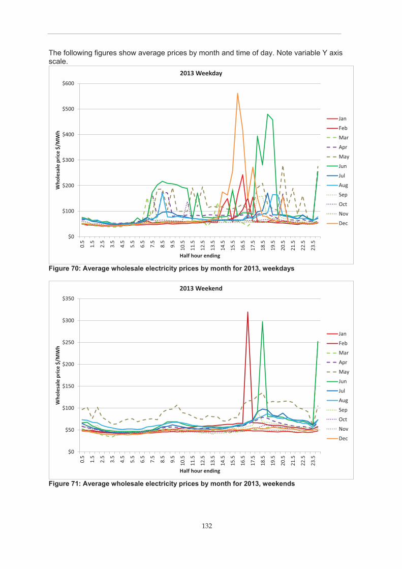
132
The following figures show average prices by month and time of day. Note variable Y axis scale.
Figure 70: Average wholesale electricity prices by month for 2013, weekdays
Figure 71: Average wholesale electricity prices by month for 2013, weekends
$0
$100
$200
$300
$400
$500
$6000.
5
1.5
2.5
3.5
4.5
5.5
6.5
7.5
8.5
9.5
10.5
11.5
12.5
13.5
14.5
15.5
16.5
17.5
18.5
19.5
20.5
21.5
22.5
23.5
Who
lesa
le p
rice
$/M
Wh
Half hour ending
2013 Weekday
Jan
Feb
Mar
Apr
May
Jun
Jul
Aug
Sep
Oct
Nov
Dec
$0
$50
$100
$150
$200
$250
$300
$350
0.5
1.5
2.5
3.5
4.5
5.5
6.5
7.5
8.5
9.5
10.5
11.5
12.5
13.5
14.5
15.5
16.5
17.5
18.5
19.5
20.5
21.5
22.5
23.5
Who
lesa
le p
rice
$/M
Wh
Half hour ending
2013 Weekend
Jan
Feb
Mar
Apr
May
Jun
Jul
Aug
Sep
Oct
Nov
Dec
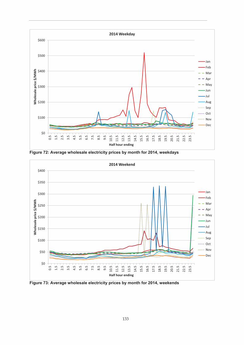
133
Figure 72: Average wholesale electricity prices by month for 2014, weekdays
Figure 73: Average wholesale electricity prices by month for 2014, weekends
$0
$100
$200
$300
$400
$500
$600
0.5
1.5
2.5
3.5
4.5
5.5
6.5
7.5
8.5
9.5
10.5
11.5
12.5
13.5
14.5
15.5
16.5
17.5
18.5
19.5
20.5
21.5
22.5
23.5
Who
lesa
le p
rice
$/M
Wh
Half hour ending
2014 Weekday
Jan
Feb
Mar
Apr
May
Jun
Jul
Aug
Sep
Oct
Nov
Dec
$0
$50
$100
$150
$200
$250
$300
$350
$400
0.5
1.5
2.5
3.5
4.5
5.5
6.5
7.5
8.5
9.5
10.5
11.5
12.5
13.5
14.5
15.5
16.5
17.5
18.5
19.5
20.5
21.5
22.5
23.5
Who
lesa
le p
rice
$/M
Wh
Half hour ending
2014 Weekend
Jan
Feb
Mar
Apr
May
Jun
Jul
Aug
Sep
Oct
Nov
Dec

134
Figure 74: Average wholesale electricity prices by month for 2015, weekdays
Figure 75: Average wholesale electricity prices by month for 2015, weekends
$0
$50
$100
$150
$200
$250
$300
$350
$400
$450
$500
0.5 1.5 2.5 3.5 4.5 5.5 6.5 7.5 8.5 9.5 10.5 11.5 12.5 13.5 14.5 15.5 16.5 17.5 18.5 19.5 20.5 21.5 22.5 23.5
Who
lesa
le p
rice
$/M
Wh
Half hour ending
2015 Weekday
Jan
Feb
Mar
Apr
May
Jun
Jul
Aug
Sep
Oct
Nov
Dec
$0
$100
$200
$300
$400
$500
$600
$700
0.5
1.5
2.5
3.5
4.5
5.5
6.5
7.5
8.5
9.5
10.5
11.5
12.5
13.5
14.5
15.5
16.5
17.5
18.5
19.5
20.5
21.5
22.5
23.5
Who
lesa
le p
rice
$/M
Wh
Half hour ending
2015 Weekend
Jan
Feb
Mar
Apr
May
Jun
Jul
Aug
Sep
Oct
Nov
Dec

135
Figure 76: Average wholesale electricity prices by month for 2016, weekdays
Figure 77: Average wholesale electricity prices by month for 2016, weekends
$0
$200
$400
$600
$800
$1,000
$1,200
0.5
1.5
2.5
3.5
4.5
5.5
6.5
7.5
8.5
9.5
10.5
11.5
12.5
13.5
14.5
15.5
16.5
17.5
18.5
19.5
20.5
21.5
22.5
23.5
Who
lesa
le p
rice
$/M
Wh
Half hour ending
2016 Weekday
Jan
Feb
Mar
Apr
May
Jun
Jul
Aug
Sep
Oct
Nov
Dec
$0
$50
$100
$150
$200
$250
$300
$350
$400
0.5
1.5
2.5
3.5
4.5
5.5
6.5
7.5
8.5
9.5
10.5
11.5
12.5
13.5
14.5
15.5
16.5
17.5
18.5
19.5
20.5
21.5
22.5
23.5
Who
lesa
le p
rice
$/M
Wh
Half hour ending
2016 Weekend
Jan
Feb
Mar
Apr
May
Jun
Jul
Aug
Sep
Oct
Nov
Dec

136
Figure 78: Average wholesale electricity prices by month for 2017, weekdays
Figure 79: Average wholesale electricity prices by month for 2017, weekends
$0
$200
$400
$600
$800
$1,000
$1,200
$1,400
0.5
1.5
2.5
3.5
4.5
5.5
6.5
7.5
8.5
9.5
10.5
11.5
12.5
13.5
14.5
15.5
16.5
17.5
18.5
19.5
20.5
21.5
22.5
23.5
Who
lesa
le p
rice
$/M
Wh
Half hour ending
2017 Weekday
Jan
Feb
Mar
Apr
May
Jun
Jul
Aug
Sep
Oct
Nov
Dec
$0
$50
$100
$150
$200
$250
$300
$350
$400
0.5
1.5
2.5
3.5
4.5
5.5
6.5
7.5
8.5
9.5
10.5
11.5
12.5
13.5
14.5
15.5
16.5
17.5
18.5
19.5
20.5
21.5
22.5
23.5
Who
lesa
le p
rice
$/M
Wh
Half hour ending
2017 Weekend
Jan
Feb
Mar
Apr
May
Jun
Jul
Aug
Sep
Oct
Nov
Dec

137
Figure 80: Average wholesale electricity prices by month for 2018, weekdays
Figure 81: Average wholesale electricity prices by month for 2018, weekends
$0
$100
$200
$300
$400
$500
$600
$700
$800
$900
$1,000
0.5
1.5
2.5
3.5
4.5
5.5
6.5
7.5
8.5
9.5
10.5
11.5
12.5
13.5
14.5
15.5
16.5
17.5
18.5
19.5
20.5
21.5
22.5
23.5
Who
lesa
le p
rice
$/M
Wh
Half hour ending
2018 Weekday
Jan
Feb
Mar
Apr
May
Jun
Jul
Aug
Sep
Oct
Nov
Dec
-$100
$0
$100
$200
$300
$400
$500
$600
0.5
1.5
2.5
3.5
4.5
5.5
6.5
7.5
8.5
9.5
10.5
11.5
12.5
13.5
14.5
15.5
16.5
17.5
18.5
19.5
20.5
21.5
22.5
23.5
Who
lesa
le p
rice
$/M
Wh
Half hour ending
2018 Weekend
Jan
Feb
Mar
Apr
May
Jun
Jul
Aug
Sep
Oct
Nov
Dec

138
Figure 82: Average wholesale electricity prices by month for 2019, weekdays
Figure 83: Average wholesale electricity prices by month for 2019, weekends
-$100
$0
$100
$200
$300
$400
$500
$600
$700
$800
$900
0.5
1.5
2.5
3.5
4.5
5.5
6.5
7.5
8.5
9.5
10.5
11.5
12.5
13.5
14.5
15.5
16.5
17.5
18.5
19.5
20.5
21.5
22.5
23.5
Who
lesa
le p
rice
$/M
Wh
Half hour ending
2019 Weekday
Jan
Feb
Mar
Apr
May
Jun
Jul
Aug
Sep
Oct
Nov
Dec
-$150
-$100
-$50
$0
$50
$100
$150
$200
$250
$300
$350
0.5
1.5
2.5
3.5
4.5
5.5
6.5
7.5
8.5
9.5
10.5
11.5
12.5
13.5
14.5
15.5
16.5
17.5
18.5
19.5
20.5
21.5
22.5
23.5
Who
lesa
le p
rice
$/M
Wh
Half hour ending
2019 Weekend
Jan
Feb
Mar
Apr
May
Jun
Jul
Aug
Sep
Oct
Nov
Dec

139
Figure 84: Average wholesale electricity prices by month for 2020, weekdays Figure note: Data for 2020 only includes January to May.
Figure 85: Average wholesale electricity prices by month for 2020, weekends
-$100
$0
$100
$200
$300
$400
$500
$600
$700
0.5
1.5
2.5
3.5
4.5
5.5
6.5
7.5
8.5
9.5
10.5
11.5
12.5
13.5
14.5
15.5
16.5
17.5
18.5
19.5
20.5
21.5
22.5
23.5
Who
lesa
le p
rice
$/M
Wh
Half hour ending
2020 Weekday
Jan
Feb
Mar
Apr
May
Jun
Jul
Aug
Sep
Oct
Nov
Dec
-$100
-$50
$0
$50
$100
$150
$200
0.5 1.5 2.5 3.5 4.5 5.5 6.5 7.5 8.5 9.5 10.5 11.5 12.5 13.5 14.5 15.5 16.5 17.5 18.5 19.5 20.5 21.5 22.5 23.5
Who
lesa
le p
rice
$/M
Wh
Half hour ending
2020 Weekend
Jan
Feb
Mar
Apr
May
Jun
Jul
Aug
Sep
Oct
Nov
Dec

140
11 References
AEMO 2009, NEM Settlements Process, Australian Energy Market Operator, Sydney, Australia, retrieved from https://www.aemo.com.au/Electricity/National-Electricity-Market-NEM/Settlements-and-payments/Prudentials-and-payments/-/media/E426F899A8124D988815A96DEF0FF298.ashx
AEMO 2020a, ‘Revised - CHG0059311 : Planned System Change - 2020/21 update in EMMS Pre-Production - MPC/CPT/TLFs/DLFs values’, retrieved from https://www.aemo.com.au/Market-Notices?marketNoticeQuery=market+price+cap&marketNoticeFacets=VOLL%2CMARKET+SYSTEMS%2CPRICES+UNCHANGED%2CLOR1+ACTUAL
AEMO 2020b, Minimum operational demand thresholds in South Australia, Australian Energy Market Operator, Sydney, Australia, retrieved from https://aemo.com.au/-/media/files/electricity/nem/planning_and_forecasting/sa_advisory/2020/minimum-operational-demand-thresholds-in-south-australia-review.pdf?la=en
AEMO 2020c, ‘Reliability and Emergency Reserve Trader (RERT)’, retrieved from https://aemo.com.au/en/energy-systems/electricity/emergency-management/reliability-and-emergency-reserve-trader-rert
AS1056.1 1991, Storage water heaters Part 1: General requirements, Standards Australia, Sydney, Australia.
AS3498 2020, Safety and public health requirements for plumbing products - Water heaters and hot-water storage tanks, Standards Australia, Sydney, Australia, retrieved from https://infostore.saiglobal.com/en-au/Standards/AS-3498-2020-123135_SAIG_AS_AS_2816032/
AS/NZS4692.1 2005, Electric water heaters - Part 1: Energy, consumption, performance and general requirements, Standards Australia, Sydney, Australia.
AS/NZS4692.2 2005, Electric water heaters - Part 2: Minimum Energy Performance Standard (MEPS) requirements and energy labelling, Standards Australia, Sydney, Australia.
AS/NZS4755.3.3 2014, Demand response capabilities and supporting technologies for electrical products Interaction of demand response enabling devices and electrical products - Operational instructions and connections for electric storage and electric-boosted storage water heaters, Standards Australia, Sydney, Australia.
AUSGRID 2012, ‘Solar home electricity data’, retrieved July 20, 2019, from https://www.ausgrid.com.au/Industry/Innovation-and-research/Data-to-share/Solar-home-electricity-data
AUSGRID 2014, Demand Management operating expenditure plan - submission to the Australian Energy Regulator.
Australian Building Codes Board 2019a, National Construction Code Volume Three: Plumbing Code of Australia, Canberra, Australia, retrieved from https://www.abcb.gov.au/-/media/Files/ABCB-NCC/NCC_2019_Volume_Three.pdf

141
Australian Building Codes Board 2019b, National Construction Code Volume Two: Technical design and construction requirements for certain residential and non-habitable buildings and structures, Canberra, Australia.
Australian Bureau of Statistics 2014, ABS4602.0 Environmental Issues: Energy Use and Conservation, Canberra, Australia, retrieved from https://www.abs.gov.au/AUSSTATS/[email protected]/DetailsPage/4602.0.55.001Mar%202014?OpenDocument
Australian Bureau of Statistics 2017, ‘Australian Census Quickstats’, retrieved from http://www.abs.gov.au/websitedbs/D3310114.nsf/Home/2016%20QuickStats
Australian Bureau of Statistics 2019, ABS3236.0 Household and Family Projections, Australia, 2016 to 2041, Canberra, Australia, retrieved from http://www.abs.gov.au/ausstats/[email protected]/mf/3236.0
Australian Bureau of Statistics 2020, ABS8731.0 - Building Approvals, Australia, Canberra, Australia, retrieved from https://www.abs.gov.au/ausstats/[email protected]/mf/8731.0
Australian Energy Market Commission 2017, Market Rule: Five Minute Settlement, Sydney, Australia, retrieved from https://www.aemc.gov.au/rule-changes/five-minute-settlement
Australian Energy Market Commission 2019, Final Report: Residential Electricity Price Trends 2019, Sydney, Australia, retrieved from https://www.aemc.gov.au/sites/default/files/2019-12/2019%20Residential%20Electricity%20Price%20Trends%20final%20report%20FINAL.pdf
Australian Energy Market Commission 2020a, Wholesale demand response mechanism - final determination, retrieved from https://www.aemc.gov.au/rule-changes/wholesale-demand-response-mechanism
Australian Energy Market Commission 2020b, Delayed implementation of five minute and global settlement, Sydney, Australia, retrieved from https://www.aemc.gov.au/rule-changes/delayed-implementation-five-minute-and-global-settlement
Australian Energy Regulator 2019, Retail energy market performance update for Quarter 4, 2018-19, Canberra, Australia, retrieved from https://www.aer.gov.au/retail-markets/performance-reporting/retail-energy-market-performance-update-for-quarter-4-2018-19
Australian Energy Regulator 2020, ‘ElectraNet - SA Energy Transformation regulatory investment test for transmission (RIT-T) (including AER Determination)’, retrieved from https://www.aer.gov.au/networks-pipelines/determinations-access-arrangements/contingent-projects/electranet-sa-energy-transformation-regulatory-investment-test-for-transmission-rit-t
BIS Oxford Economics 2018, The Hot Water Systems Market in Australia.
Clean Energy Council 2019, Clean Energy Australia Report 2019, Melbourne, Australia, retrieved from https://www.cleanenergycouncil.org.au/resources/resources-hub/clean-energy-australia-report

142
Clean Energy Regulator 2019, ‘Register of Solar Water Heaters’, retrieved from http://www.cleanenergyregulator.gov.au/RET/Scheme-participants-and-industry/Agents-and-installers/Small-scale-systems-eligible-for-certificates/Register-of-solar-water-heaters
Clean Energy Regulator 2020a, ‘About the Renewable Energy Target’, retrieved from http://www.cleanenergyregulator.gov.au/RET/About-the-Renewable-Energy-Target
Clean Energy Regulator 2020b, ‘Postcode data for small-scale installations’, retrieved from http://www.cleanenergyregulator.gov.au/RET/Forms-and-resources/Postcode-data-for-small-scale-installations#Smallscale-installations-by-installation-year
COAG Energy Council 2019, ‘Smart Demand Response Decision RIS Approved’, retrieved from https://www.energyrating.gov.au/news/smart-demand-response-decision-ris-approved
DELWP 2019a, Victorian Energy Upgrades: Specifications 2018 - Version 2.0, Department of Environment, Land, Water and Planning, Melbourne, Australia, retrieved from https://www.energy.vic.gov.au/energy-efficiency/victorian-energy-upgrades/specifications
DELWP 2019b, Regulatory Impact Statement: Victorian Energy Efficiency Target Amendment (Prescribed Customers and Targets) Regulations 2020, Department of Environment, Land, Water and Planning, Melbourne, Australia, retrieved from https://engage.vic.gov.au/victorian-energy-upgrades/targets
Department for Manufacturing, Innovation, Trade, Resources and Energy 2013, Report of the Review of South Australia’s Water Heater Installation Requirements, Adelaide, South Australia, retrieved from https://www.sa.gov.au/__data/assets/pdf_file/0006/35259/Water-Heater-Review-Report-Oct-2013.pdf
Department of the Environment and Energy 2017, Greenhouse and Energy Minimum Standards (Gas Water Heaters) Determination, retrieved from https://www.legislation.gov.au/Details/F2017L01608
DR AS4755.2 2019, Demand response capabilities and supporting technologies for electrical products Demand response framework and requirements for Communications between Remote Agents and Electrical Products, Standards Australia, Sydney, Australia.
E3 2003, Revised Regulatory Impact Statement: Revised Minimum Energy Performance Standards and Alternative Strategies for Small Electric Storage Water Heaters, Canberra, Australia.
E3 2012, Water Heating Data Collection and Analysis - Residential End Use Monitoring Program (REMP), retrieved from http://www.energyrating.gov.au/sites/new.energyrating/files/documents/REMP-water-heating_0.pdf
E3 2013, Consultation RIS: Electric Storage Water Heaters, Canberra, Australia, retrieved from https://www.energyrating.gov.au/document/consultation-regulation-impact-statement-electric-storage-water-heaters

143
E3 2019, Regulation Impact Statement for Decision: ‘Smart’ Demand Response Capabilities for Selected Appliances, COAG Energy Council, Canberra, Australia, retrieved from https://www.energyrating.gov.au/document/regulation-impact-statement-decision-smart-demand-response-capabilities-selected-appliances
Energy Efficient Strategies 2012, Proof of Concept: Residential Energy Monitoring Program Final Report (REMP), Department of Climate Change and Energy Efficiency, retrieved from http://www.energyrating.gov.au/document/proof-concept-residential-energy-monitoring-program-final-report
Energy Partners 2000, Improving on Electric Water Heater Efficiency - options to reduce heat losses for small electric storage water heaters <80L, Australian Greenhouse Office, Canberra, Australia.
Essential Services Commission of Victoria 2020, ‘Victorian Energy Upgrades: Register of Activities’, retrieved from https://www.veu-registry.vic.gov.au/Public/ActivitiesPostcodeSearch.aspx
George Wilkenfeld and Associates 1993, Benefits and Costs of Implementing Minimum Energy Performance Standards for Household Electrical Appliances in Australia, State Electricity Commission of Victoria, Melbourne, Australia.
George Wilkenfeld and Associates 2020, Demand Response Capabilities for Selected Appliances – South Australia Specific Analysis, SA Department for Energy and Mining, Sydney, Australia.
Government of South Australia 2020, South Australia’s Energy Solution: A secure transition to affordable renewable energy, Adelaide, South Australia, retrieved from https://www.energymining.sa.gov.au/__data/assets/pdf_file/0009/364266/200615_Energy_Solution_Action_Plan_final_spreads_rs.pdf
ITP Renewables 2020, Current Residential PV Costs, Canberra, Australia.
Maisch, M 2020, ‘SA-NSW interconnector gets regulatory go-ahead to unlock slew of renewable energy projects’, PV Magazine Australia, retrieved from https://www.pv-magazine-australia.com/2020/01/24/sa-nsw-interconnector-gets-regulatory-go-ahead-to-unlock-slew-of-renewable-energy-projects/
Melaina, MW, Antonia, O & Penev, M 2013, Blending Hydrogen into Natural Gas Pipeline Networks: A Review of Key Issues, National Renewable Energy Laboatory (US), retrieved from https://www.nrel.gov/docs/fy13osti/51995.pdf
Pacific Power 1994, The Residential End-Use Study, Pacific Power.
Renew Economy 2020a, ‘South Australia to accelerate transition, emissions cuts, after bushfires’, retrieved from https://reneweconomy.com.au/south-australia-to-accelerate-transition-emissions-cuts-after-bushfires-70921/
Renew Economy 2020b, ‘South Australia minister aiming for 100 per cent renewables before 2030’, retrieved from https://reneweconomy.com.au/south-australia-minister-aiming-for-100-per-cent-renewables-before-2030-2030/

144
SA Government 2020, Verification Method for an Electric Resistance Storage Water Heater Supplied by On-Site Renewables (Supply), Adelaide, South Australia, retrieved from https://www.sa.gov.au/__data/assets/pdf_file/0003/500754/190515-ESWH-for-new-homes.pdf
SA Office of the Technical Regulator 2019, South Australian residential water heater requirements: Plumbing Advisory Note, Adelaide, South Australia, retrieved from https://www.sa.gov.au/__data/assets/pdf_file/0018/35262/190515-Water-heater-requirements.pdf
SA Power Networks 2019, Tariff Information, Adelaide, South Australia.
SA Power Networks 2020, 2020-25 Tariff Structure Statement Part A (AER Edited), Adelaide, South Australia, retrieved from https://www.sapowernetworks.com.au/public/download.jsp?id=9508
Solahart 2019, Solahart Powerstore Electric Water Heater - Owner’s Guide and Installation Instructions, Sydney, Australia, retrieved from https://www.solahart.com.au/media/5163/install-instruct-solahart-powerstore-electric-pvv-122273-rev-b-2019-may.pdf
South Australian Power Networks 2020, South Australian Electricity Customer Numbers by Connection Type at 29 February 2020, Adelaide, South Australia.
Sustainability Victoria 2016, Gas Water Heater Retrofit Trial, retrieved from https://www.sustainability.vic.gov.au/About-Us/Research/Household-retrofit-trials
Taylor Nelson Sofres 2000, Implications of Further Insulating Small Hot Water Heaters, Australian Greenhouse Office.
Whaley, D, Liddle, R, Mudge, L, Harmer, E & Saman, W 2014, Residential Water Heater Baseline Data, Department for Manufacturing Innovation Trade Resources and Energy, South Australia, retrieved from https://www.sa.gov.au/__data/assets/pdf_file/0017/215162/Residential-water-heater-baseline-study.pdf