review of natural gas models of... · review of natural gas models 0 september ... pipeline cost...

Review of Natural Gas Models 0 September 2014

September 2014

Review of Natural Gas Models In Support of U.S. Energy Information Administration Natural Gas Transmission and Distribution Module (NGTDM) Redesign Effort

Lauren K. Busch


Introduction The Natural Gas Transmission and Distribution Module (NGTDM), a component of the U.S. Energy Information Administration’s (EIA’s) National Energy Modeling System (NEMS), is currently undergoing a redesign. In support of the redesign effort, this report provides a review of other natural gas models, both domestic and international. These model reviews are intended to be concise summaries of the salient features of the models as they pertain to the NGTDM redesign. In some instances, over one hundred pages of supporting documentation were reviewed and in other instances only scant documentation was available. In either case, a model overview was prepared with a focus on formulation approach, network detail, pipeline cost representation, capacity expansion methods, and calibration. For those interested in more model details, documentation sources are provided in the bibliography.

This report is divided into two sections: (1) the model summaries, including the current NGTDM, and (2) a comparison across models of key areas of interest, such as mathematical formulation, aggregation, and capacity expansion.

Although numerous models, some dating back to the 1970s, were reviewed at some level, only those deemed most relevant (Table 1-1) were chosen for inclusion in this review.

Table 1-1. Reviewed Models

Model Developer Gas Market Model (GMM) ICF International Natural Gas Model (INGM) EIA GPCM RBAC, Inc. Tanner Prototype Model EIA MarketBuilder - North American Gas Model Deloitte MarketBuilder - World Gas Model Deloitte MarketBuilder - RWGTM/BIWGTM Rice University World Gas Model Gabriel-University of Maryland

Model Overviews This section begins with an overview of the NGTDM and then provides summaries of the models in Table 1-1. These summaries represent the author’s best understanding of the models based on available documentation and feedback provided by some of the model developers.

1.1 Natural Gas Transmission and Distribution Module (NGTDM) The NGTDM, a module of NEMS, is EIA’s forecasting model of the domestic natural gas market. The NGTDM models a regional network representation of production regions in the continental United States, liquefied natural gas (LNG) terminals, pipelines, and end-use demand to determine prices and flows of natural gas. These prices and flows are determined through a heuristic algorithm which


balances supply and demand. Due to the level of aggregation in the model, which does not lend itself to a strictly competitive representation, the algorithm starts with historical flows and progressively shifts flow patterns based on lower cost options while balancing supply and demand throughout the network.

Key aspects of the model network are listed below:

• 2 seasons • 12 regions for continental United States • 2 Canadian regions • 3 Mexican border crossings • 7 Canadian border crossings • 7 LNG terminals plus potential terminals representing the Bahamas, eastern and western

Canada, and western Mexico, if the LNG is intended to be transported to the United States • 5 demand sectors (residential, commercial, industrial , electric generation, and transportation

(or natural gas vehicles)

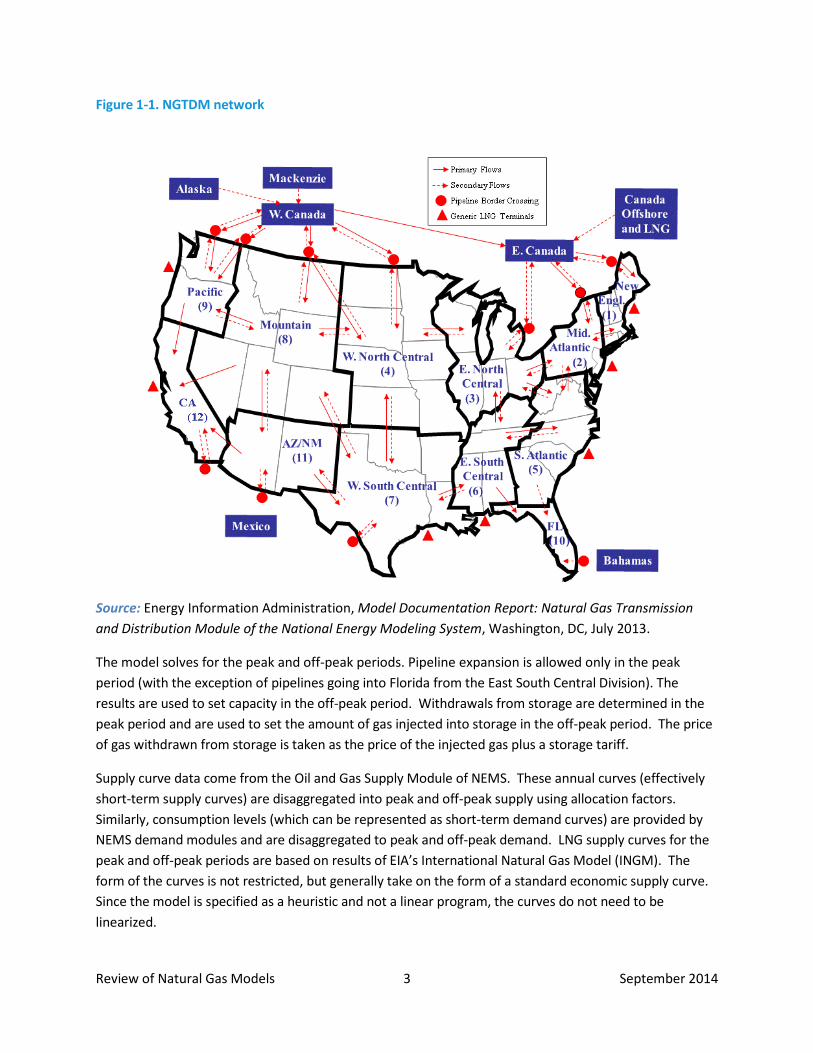
The resulting network is shown in Figure 1-1. Each region contains a transshipment node representing flows into and out of the region to/from other regions, supply points, demand points, and storage points.


Figure 1-1. NGTDM network

Source: Energy Information Administration, Model Documentation Report: Natural Gas Transmission and Distribution Module of the National Energy Modeling System, Washington, DC, July 2013.

The model solves for the peak and off-peak periods. Pipeline expansion is allowed only in the peak period (with the exception of pipelines going into Florida from the East South Central Division). The results are used to set capacity in the off-peak period. Withdrawals from storage are determined in the peak period and are used to set the amount of gas injected into storage in the off-peak period. The price of gas withdrawn from storage is taken as the price of the injected gas plus a storage tariff.

Supply curve data come from the Oil and Gas Supply Module of NEMS. These annual curves (effectively short-term supply curves) are disaggregated into peak and off-peak supply using allocation factors. Similarly, consumption levels (which can be represented as short-term demand curves) are provided by NEMS demand modules and are disaggregated to peak and off-peak demand. LNG supply curves for the peak and off-peak periods are based on results of EIA’s International Natural Gas Model (INGM). The form of the curves is not restricted, but generally take on the form of a standard economic supply curve. Since the model is specified as a heuristic and not a linear program, the curves do not need to be linearized.


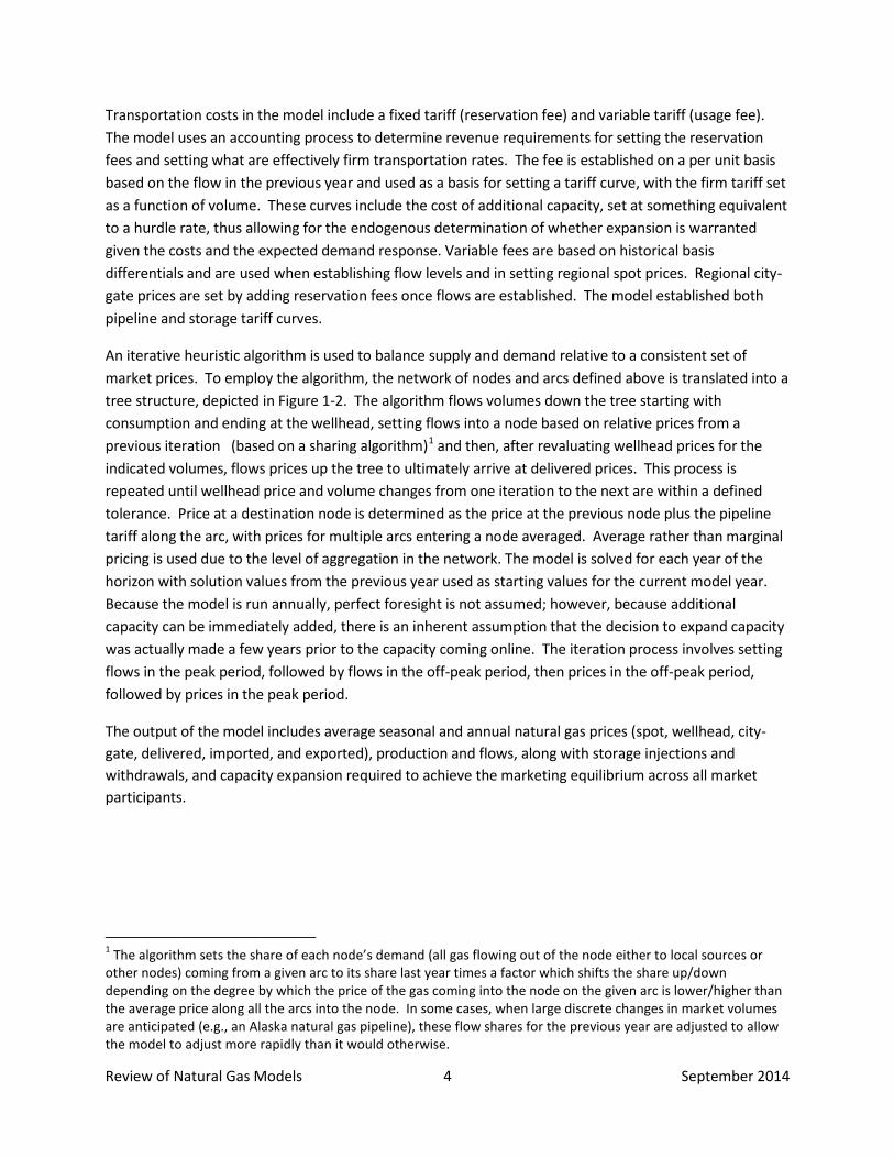
Transportation costs in the model include a fixed tariff (reservation fee) and variable tariff (usage fee). The model uses an accounting process to determine revenue requirements for setting the reservation fees and setting what are effectively firm transportation rates. The fee is established on a per unit basis based on the flow in the previous year and used as a basis for setting a tariff curve, with the firm tariff set as a function of volume. These curves include the cost of additional capacity, set at something equivalent to a hurdle rate, thus allowing for the endogenous determination of whether expansion is warranted given the costs and the expected demand response. Variable fees are based on historical basis differentials and are used when establishing flow levels and in setting regional spot prices. Regional city-gate prices are set by adding reservation fees once flows are established. The model established both pipeline and storage tariff curves.

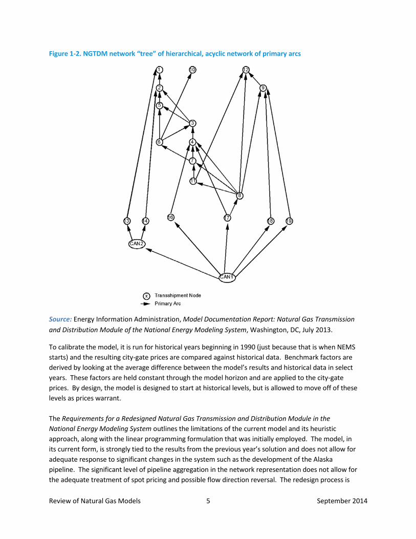
An iterative heuristic algorithm is used to balance supply and demand relative to a consistent set of market prices. To employ the algorithm, the network of nodes and arcs defined above is translated into a tree structure, depicted in Figure 1-2. The algorithm flows volumes down the tree starting with consumption and ending at the wellhead, setting flows into a node based on relative prices from a previous iteration (based on a sharing algorithm)1 and then, after revaluating wellhead prices for the indicated volumes, flows prices up the tree to ultimately arrive at delivered prices. This process is repeated until wellhead price and volume changes from one iteration to the next are within a defined tolerance. Price at a destination node is determined as the price at the previous node plus the pipeline tariff along the arc, with prices for multiple arcs entering a node averaged. Average rather than marginal pricing is used due to the level of aggregation in the network. The model is solved for each year of the horizon with solution values from the previous year used as starting values for the current model year. Because the model is run annually, perfect foresight is not assumed; however, because additional capacity can be immediately added, there is an inherent assumption that the decision to expand capacity was actually made a few years prior to the capacity coming online. The iteration process involves setting flows in the peak period, followed by flows in the off-peak period, then prices in the off-peak period, followed by prices in the peak period.

The output of the model includes average seasonal and annual natural gas prices (spot, wellhead, city- gate, delivered, imported, and exported), production and flows, along with storage injections and withdrawals, and capacity expansion required to achieve the marketing equilibrium across all market participants.

1 The algorithm sets the share of each node’s demand (all gas flowing out of the node either to local sources or other nodes) coming from a given arc to its share last year times a factor which shifts the share up/down depending on the degree by which the price of the gas coming into the node on the given arc is lower/higher than the average price along all the arcs into the node. In some cases, when large discrete changes in market volumes are anticipated (e.g., an Alaska natural gas pipeline), these flow shares for the previous year are adjusted to allow the model to adjust more rapidly than it would otherwise.


Figure 1-2. NGTDM network “tree” of hierarchical, acyclic network of primary arcs

Source: Energy Information Administration, Model Documentation Report: Natural Gas Transmission and Distribution Module of the National Energy Modeling System, Washington, DC, July 2013.

To calibrate the model, it is run for historical years beginning in 1990 (just because that is when NEMS starts) and the resulting city-gate prices are compared against historical data. Benchmark factors are derived by looking at the average difference between the model’s results and historical data in select years. These factors are held constant through the model horizon and are applied to the city-gate prices. By design, the model is designed to start at historical levels, but is allowed to move off of these levels as prices warrant. The Requirements for a Redesigned Natural Gas Transmission and Distribution Module in the National Energy Modeling System outlines the limitations of the current model and its heuristic approach, along with the linear programming formulation that was initially employed. The model, in its current form, is strongly tied to the results from the previous year’s solution and does not allow for adequate response to significant changes in the system such as the development of the Alaska pipeline. The significant level of pipeline aggregation in the network representation does not allow for the adequate treatment of spot pricing and possible flow direction reversal. The redesign process is


intended to address these issues, but also to identify any other market factors that ideally should be captured (e.g., contract versus spot sales). Source: Energy Information Administration, Model Documentation Report: Natural Gas Transmission and Distribution Module of the National Energy Modeling System, Washington, DC, July 2013.

1.2 Gas Market Model (GMM) The Gas Market Model (GMM) is ICF’s model of the North American gas market. It was developed by Energy and Environmental Analysis, Inc. (EEA), now owned by ICF. It is a market equilibrium model that uses a nonlinear (specifically, quadratic) programming formulation. The model solves for market-clearing prices, flows, production, consumption, and storage injection and withdrawal.

Key aspects of the model are listed below:

• Monthly time periods • 121 regions and roughly 400 pipeline corridors throughout the United States and Canada • Supply components (i.e., gas deliverability, storage withdrawals, supplemental gas, LNG imports,

and Mexican imports) • Demand components (i.e., end-use demand, power generation gas demand, LNG exports, and

Mexican exports) • Exogenous pipeline and storage capacity expansion

Nodes are defined based on the physical location of supply, storage, and demand centers and pipelines. In cases where there are multiple demand nodes within a state, it is necessary to disaggregate the available state level data. Although the transportation network is fairly detailed, data have been aggregated to pipeline corridors. Nodes have been chosen in an attempt to avoiding masking any pipeline bottlenecks. Overall, the level of spatial detail used in the model is largely driven by ICF’s clients’ analytical needs to support strategic planning decisions.

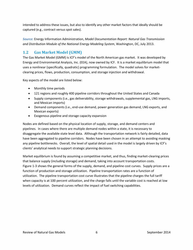
Market equilibrium is found by assuming a competitive market, and thus, finding market-clearing prices that balance supply (including storage) and demand, taking into account transportation costs. Figure 1-3 shows the general forms of the supply, demand, and pipeline cost curves. Supply prices are a function of production and storage utilization. Pipeline transportation rates are a function of utilization. The pipeline transportation cost curve illustrates that the pipeline charges the full tariff when capacity is at 100 percent utilization, and the charge falls until the variable cost is reached at low levels of utilization. Demand curves reflect the impact of fuel switching capabilities.

7

Figure 1-3. GMM natural gas supply and demand curves

Source: ICF, 2010 Natural Gas Market Review, August 2010.

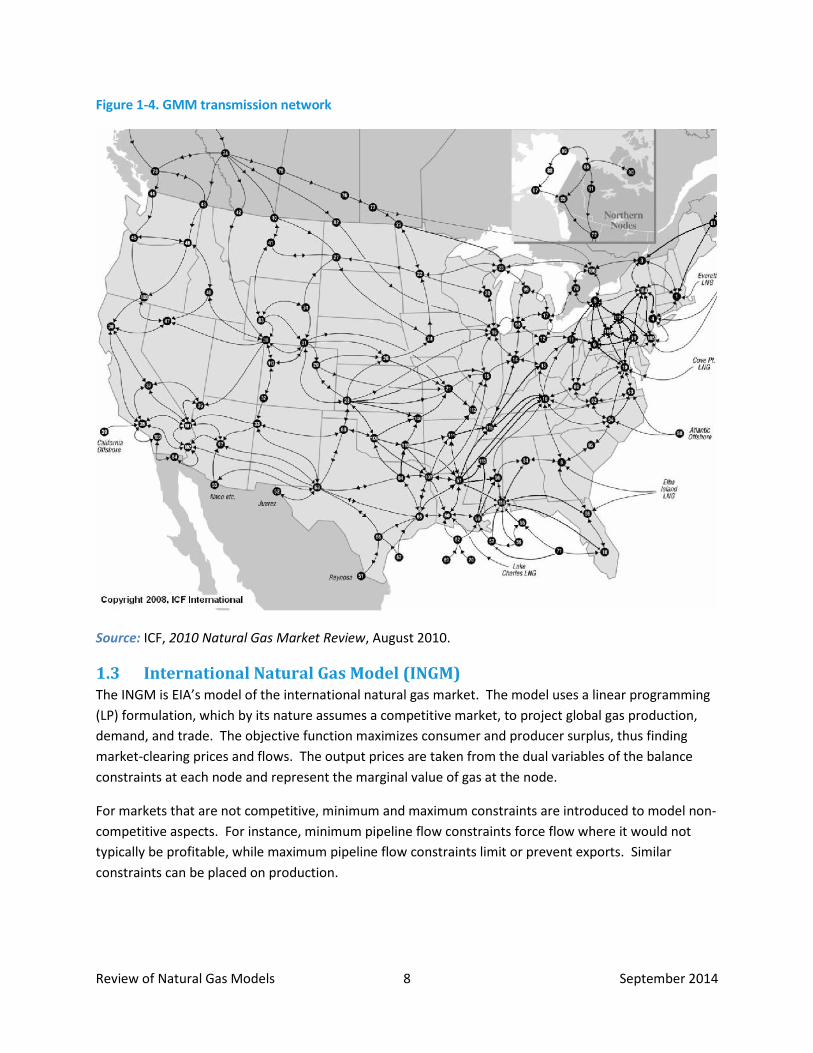
Figure 1-4 shows the transportation network of the model. The direction of flow may change from one month to the next, and where this occurs, the network is labeled to indicate bidirectional flows. Within a time period, flow is in a single direction with no minimum constraints forcing flow the opposite direction. The model is solved for each monthly time period without foresight. Capacity expansion is done outside of the model and is based on announced projects and analyst judgment on the needs of the market areas.

ICF maintains all of the data necessary to run the model, but also enables users to change assumptions on many variables that influence supply and demand, such as weather, economic growth, oil prices, and gas supply deliverability. ICF runs the model each month to update its base case with additional data and any necessary changes to assumptions to calibrate the model; however, no benchmarking factors are used in the forecast.


Figure 1-4. GMM transmission network

Source: ICF, 2010 Natural Gas Market Review, August 2010.

1.3 International Natural Gas Model (INGM) The INGM is EIA’s model of the international natural gas market. The model uses a linear programming (LP) formulation, which by its nature assumes a competitive market, to project global gas production, demand, and trade. The objective function maximizes consumer and producer surplus, thus finding market-clearing prices and flows. The output prices are taken from the dual variables of the balance constraints at each node and represent the marginal value of gas at the node.

For markets that are not competitive, minimum and maximum constraints are introduced to model non-competitive aspects. For instance, minimum pipeline flow constraints force flow where it would not typically be profitable, while maximum pipeline flow constraints limit or prevent exports. Similar constraints can be placed on production.


Key aspects of the model are listed below:

• 61 regions • 3 seasons • 7 demand sectors (residential, commercial, industrial feedstocks, industrial cogeneration, other

industrial, transportation, electric power generation) • 5 supply types (conventional onshore, conventional offshore, tight gas, shale gas, coal bed

methane) • Supply curves consider government take • Demand curves from the World Energy Projection System Plus (WEPS+) and NEMS for United

States • Endogenous capacity expansion decisions

The INGM assumes that LNG contracts will only have a short-term impact on the market and that, in the long-term, LNG will flow based on marginal prices. Thus, the model does not include contractual flows or prices.

Supply and demand curves are linearized and unit transportation costs are used, which keeps the model linear.

Both capacity and cost data are required for infrastructure (processing, shipping, pipelines, and storage). Minimum and maximum capacity limits are set differently for the near-term, mid-term, and long-term. In the near-term, minimum and maximum capacities are both set as the current capacity, expansion already under construction, and projections deemed highly likely to be completed. In the mid-term, minimum capacity is not set and maximum capacity includes projects that are reasonably likely to be completed during the time period. This enables the model to determine the optimal capacity expansion up to the set maximum. In the long-term, no maximum capacity is set, enabling the model to determine optimal capacity expansion based on investment required and operating and maintenance costs. To properly model the capacity expansion decision, asset operator profit is included as a component of the objective function, thus maximizing revenue from the asset minus investment and operating costs along with consumer and producer surplus.

The model can be run over the entire time horizon at once (perfect foresight) or with rolling optimization. In rolling optimization, the model solves annually in the early years of the forecast and then solves for groups of years at a time.

1.4 GPCM The GPCM is RBAC, Inc.’s network partial equilibrium model of the North American natural gas market; this model is used by many pipeline, storage, consulting, and other players in the industry. In addition, the Federal Energy Regulatory Commission (FERC) and Sandia National Laboratories are licensees. RBAC provides the model and an associated database that is updated quarterly. Users are then free to alter the data to create their own scenarios. Some of the data, particularly regarding Mexico and Canada,


come from RBAC’s industry sources. Statistics Canada (Stats Canada) and provincial sources are also used for Canada and Secretaría de Energía (SENER) and Petróleos Mexicanos (Pemex) for Mexico.

This North American model includes Alaska, the continental United States, Canada, Mexico, and LNG terminals. The base case data provided by RBAC contains information on:

• 89 supply areas (basins and other areas). Basins may be broken into sub-areas so that no sub-area expands over more than one state. This allows results to be aggregated to the state level.

• 5 supply types (shale, coal-bed methane, conventional [including tight sands], synthetic natural gas, LNG)

• 12 shale plays (Barnett, Haynesville, Marcellus, Eagle Ford, etc.)

• 24 LNG terminals (14 import, 2 export, and 8 import/export)

• 210 pipelines (interstate, intrastate, Gulf of Mexico gathering)

• 443 storage areas

• 110 demand areas. Demand curves are developed for each or sub-state and sector.

• 5 demand sectors (residential, commercial, industrial, electric power generation, vehicle)

• 95 market points (Gas Daily)

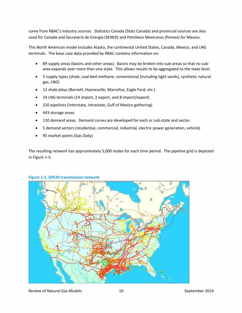
The resulting network has approximately 5,000 nodes for each time period. The pipeline grid is depicted in Figure 1-5.

Figure 1-5. GPCM transmission network


Source: RBAC, GPCM Natural Gas Forecasting System Presentation, May 2014.

The model uses monthly time periods and solves over the entire time horizon at once (perfect foresight). The direction of pipeline flow can change from one month to the next on specific pipeline segments that are modeled to be able to do so. The current version of the model sets the supply curves at the beginning of the forecast so past production does not impact future supply. However, a version of the model in development would operate more like a simulation model: compute a market-clearing solution for a period of 2–3 years, but only save the first year’s results, adjust the supply curves based on the resulting depletion and new drilling, and then run the model for 2–3 years, saving the first year’s results, and so on until the end of the time horizon. This approach allows for greater modeling flexibility of supply without being computationally intractable.

The model assumes perfect competition and seeks to find a market-clearing solution, i.e., a competitive equilibrium where no opportunities for arbitrage exist. A variant of the simplex algorithm is used to find the market equilibrium prices and flows and ensure that the no-arbitrage conditions are met. Specifically, flow between two nodes is adjusted until one of these conditions is met: (1) the price differential is exactly equal to the unit cost, including fuel; (2) the price differential is greater than the unit cost, including fuel, but flow has reached capacity and cannot be increased; or 3) the price differential is less than the cost plus fuel, but flow is at minimum and cannot be reduced.

Source: Brooks, Robert, The Theory and Practice of Modeling with GPCM, RBAC, Inc.

RBAC’s Network Optimizer is based on University of Southern California Professor Emeritus Richard McBride’s EMNET solver, which was designed to efficiently solve generalized networks with unlimited side constraints and side variables. This specialized linear programming algorithm has been extended to handle linearized cost functions for any variable, allowing the use of linearized transportation cost functions in addition to linearized supply and demand curves. (EMNET is no longer being maintained, so RBAC will be moving to GUROBI, a commercial solver that is being regularly maintained and improved.)

In GPCM, transportation costs curves are modeled so that the cost can be a function of the flow, as shown in Figure 1-6. In other words, the demand for transportation influences its cost. To model this relationship, RBAC provides values for a set of parameters: FDQ (full discount quantity), ZDQ (zero discount quantity), and NDQ (negative discount quantity). These parameters are derived using a proprietary algorithm that considers historical basis differentials, actual tariffs, and the capacity release market. Minimum and maximum prices are assigned based on tariffs. Compressor fuel use (plus fuel lost and unaccounted for) is modeled as a fractional loss of flow. This results in an imputed fuel cost on each pipeline segment. If the flow is less than the FDQ, the transportation cost is the minimum price plus fuel. If the flow is greater than the ZDQ, the transportation cost is the maximum price plus fuel. If the demand for pipeline transportation is between the FDQ and ZDQ, then the market value for transportation will be between the minimum and maximum rate (plus fuel), resulting in a “discount” to the maximum rate. On the other hand, if demand is high and there is congestion on the pipeline, the market rate can be above the maximum, resulting in “economic rent.” In solving the model, the cost curves are linearized.



Capacity expansion is handled endogenously after the time horizon of announced expansions (which are built into the GPCM model) with the “auto-expansion” module, which increases the capacity of existing pipelines when it determines the expansion to be economically beneficial. This is an optional parametric function that the analyst can decide to employ. The analyst can decide a beginning date for the auto-expansion to become effective, the hurdle cost for expansion, and the maximum percentage of expansion allowed. The analyst can also turn the function off to produce a solution that will give evidence of the most severely constrained or underutilized capacity in the network as supply and demand conditions change over time.


Figure 1-6. GPCM transportation cost curve


Storage is modeled by creating arcs between storage nodes of consecutive time periods. Storage injection and withdrawal costs and compressor fuel use are estimated based on tariffs when it is available and best judgment otherwise. These costs are not based on capacity utilization. They can change over time based on actual changes in the tariff or an analyst’s scenario design.

Benchmarking, referred to as “calibration” by RBAC, is done by running the model iteratively from January 2006 to the present and comparing the results to historical data. A specialized algorithm is used to find values for the FDQ, ZDQ, and other parameters that best replicate actual historical data on


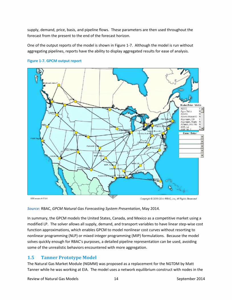
supply, demand, price, basis, and pipeline flows. These parameters are then used throughout the forecast from the present to the end of the forecast horizon.

One of the output reports of the model is shown in Figure 1-7. Although the model is run without aggregating pipelines, reports have the ability to display aggregated results for ease of analysis.

Figure 1-7. GPCM output report


In summary, the GPCM models the United States, Canada, and Mexico as a competitive market using a modified LP. The solver allows all supply, demand, and transport variables to have linear step-wise cost function approximations, which enables GPCM to model nonlinear cost curves without resorting to nonlinear programming (NLP) or mixed integer programming (MIP) formulations. Because the model solves quickly enough for RBAC’s purposes, a detailed pipeline representation can be used, avoiding some of the unrealistic behaviors encountered with more aggregation.

1.5 Tanner Prototype Model The Natural Gas Market Module (NGMM) was proposed as a replacement for the NGTDM by Matt Tanner while he was working at EIA. The model uses a network equilibrium construct with nodes in the


model representing aggregate supply or demand and edges (arcs) representing aggregate pipelines. A fundamental assumption of the model is that the U.S. natural gas market is competitive (with regulation), and thus, no arbitrage opportunities exist.

A system of equations arises that a solution must satisfy; these equations are as follows:

1. Flow balance: supply, demand, and flows are balanced at each node. 2. No arbitrage:

a. if the flow from i to j is equal to the flow capacity, then the price at node i + transportation cost from i to j ≤ the price at node j

b. if the flow from i to j is equal to the minimum flow, then the price at node i + transportation cost from i to j ≥ the price at node j

c. if the flow from i to j is not at a bound, then the price at node i + transportation cost from i to j = the price at node j

3. Prices and quantities are non-negative.

Note that this formulation can accommodate nonlinear functions. Nonlinear transportation cost functions where cost is a function of flow were intended to be used. An iterative approach was taken for finding the solution of this NLP model. According to Proposed Natural Gas Market Module, the solution algorithm finds prices and quantities that are a network equilibrium. The inputs to the algorithm are initial nodal prices. The output is the network equilibrium values. Iterations are made over an inner and outer loop. The outer loop of the method updates nodal supply and demand from prices and matches total supply with total demand using a line search algorithm. The inner loop defines the network flows and updates the prices to lower the amount of arbitrage in the system using a minimum cost flow algorithm. Since the model is formulated as a nonlinear program, multiple optima may exist and global convergence may not be achieved. Some other characteristics of the model are summarized below.

• Four seasons • NGTDM regions with the addition of Mexico and Canadian regions. • Representation of sectors purchasing gas as “wholesale, by contract, or on the spot market” is

handled via markups off the hub prices, rather than being explicitly represented in the network. • The minimum cost flow algorithm minimizes transportation costs and does not take supply costs

into account. • Capacity expansion would not be endogenous to the solution algorithm, but would occur after

the fact. • Bi-directional flows are not addressed. • Storage is modeled as pipeline to the future, connecting storage as future pipeline availability.

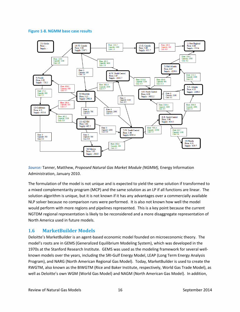
The network representation is shown in Figure 1-8 with the base case results depicted.


Figure 1-8. NGMM base case results

Source: Tanner, Matthew, Proposed Natural Gas Market Module (NGMM), Energy Information Administration, January 2010.

The formulation of the model is not unique and is expected to yield the same solution if transformed to a mixed complementarity program (MCP) and the same solution as an LP if all functions are linear. The solution algorithm is unique, but it is not known if it has any advantages over a commercially available NLP solver because no comparison runs were performed. It is also not known how well the model would perform with more regions and pipelines represented. This is a key point because the current NGTDM regional representation is likely to be reconsidered and a more disaggregate representation of North America used in future models.

1.6 MarketBuilder Models Deloitte’s MarketBuilder is an agent-based economic model founded on microeconomic theory. The model’s roots are in GEMS (Generalized Equilibrium Modeling System), which was developed in the 1970s at the Stanford Research Institute. GEMS was used as the modeling framework for several well-known models over the years, including the SRI-Gulf Energy Model, LEAP (Long Term Energy Analysis Program), and NARG (North American Regional Gas Model). Today, MarketBuilder is used to create the RWGTM, also known as the BIWGTM (Rice and Baker Institute, respectively, World Gas Trade Model), as well as Deloitte’s own WGM (World Gas Model) and NAGM (North American Gas Model). In addition,


ArrowHead Economics has two models, the North American Gas Model and the Global Gas Model, which have their roots in MarketBuilder.

The table below depicts developmental milestones from the creation of GEMS to today and shows how some older models, which are not reviewed for this document but which the reader may be familiar with, relate to the current generation of agent-based models.

Source: Deloitte Market Point, Pioneering the Energy Resource Economics Future, Generalized Equilibrium Modeling System (GEMS), 2013.

MarketBuilder Methodology MarketBuilder uses an agent-based microeconomic approach where each agent (producer, transporter, consumer, distributor, or aggregations of any of these) is a distinct unit seeking to maximize its own profit. Thus, each agent is represented by its own optimization problem where the constraints are based on both physical and behavioral relationships. The interconnections between agents and competition among agents give rise to market prices. In other words, the model decomposes the


market into thousands of process models connected by a network. A feature of this approach is that it allows for imperfect market behavior.

Supply of depletable resources has two components: proved reserves, for which fixed costs are already sunk, and new reserves, for which they are not. Additionally, the production of a tranche of resources declines over time. New reserves are assumed to have increasing marginal costs over time, and producers maximize their profit over time according to the Hotelling Theory of depletable resources. That is, given an exogenous expected time series of interest (or other appropriate discount) rates, the producer maximizes profit by removing the possibility of arbitrage over time. By doing so, the price accepted by producers in the next time increment is the current price plus the opportunity cost of producing an incremental amount now. Even competitive producers produce at the marginal cost plus the scarcity rent, with the price accepted by the producers tending toward the marginal cost as the resource is depleted.

Demand is modeled using nonlinear multi-variate demand curves for each sector: generally taken as an isoelastic function of lagged demand, price, GDP, and population.

Storage is modeled endogenously with storage operators attempting to maximize their profit by buying gas in the off-peak period and selling in the peak period, taking into consideration the present value of the profit, storage costs, interest rates, and physical characteristics such as injection rates, withdrawal rates, and storage capacity.

Capacity expansion is modeled endogenously, taking into account the interdependency of future prices and capacity additions.

Transportation costs are based on tariffs, embedded costs, and discounting behavior.

Emission credits are endogenously modeled through a representation of the emission credit market, which impacts the cost of energy.

Source: Choi, Thomas, Dale Nesbitt, and Brad Barnds, Analysis of Freeport LNG Export Impact on U.S. Markets, Altos Management Partners Inc., December 2010.

Once the network model has been built, equilibrium is found via the tâtonnement (Walrasian auction) process. At each node in the network, a set of input and output prices for all times of interest are guessed. If demands are higher than supplies at these prices, the prices are raised. If the reverse is true, prices are lowered. This continues until supplies and demands equilibrate across the network for all times. This allows the algorithm to be easily parallelized since each node at the network only needs local information plus communication with a small number of adjacent nodes.

Some Models that Use MarketBuilder MarketBuilder can be used to create unique models by allowing users to input their own data and equations that describe agent behavior.


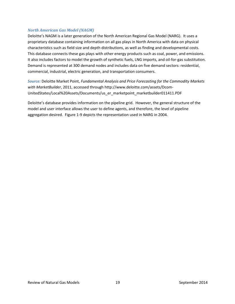
North American Gas Model (NAGM) Deloitte’s NAGM is a later generation of the North American Regional Gas Model (NARG). It uses a proprietary database containing information on all gas plays in North America with data on physical characteristics such as field size and depth distributions, as well as finding and developmental costs. This database connects these gas plays with other energy products such as coal, power, and emissions. It also includes factors to model the growth of synthetic fuels, LNG imports, and oil-for-gas substitution. Demand is represented at 300 demand nodes and includes data on five demand sectors: residential, commercial, industrial, electric generation, and transportation consumers.

Source: Deloitte Market Point, Fundamental Analysis and Price Forecasting for the Commodity Markets with MarketBuilder, 2011, accessed through http://www.deloitte.com/assets/Dcom-UnitedStates/Local%20Assets/Documents/us_er_marketpoint_marketbuilder011411.PDF

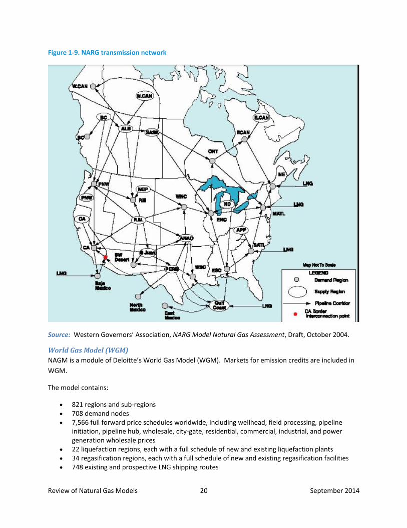
Deloitte’s database provides information on the pipeline grid. However, the general structure of the model and user interface allows the user to define agents, and therefore, the level of pipeline aggregation desired. Figure 1-9 depicts the representation used in NARG in 2004.


Figure 1-9. NARG transmission network

Source: Western Governors’ Association, NARG Model Natural Gas Assessment, Draft, October 2004.

World Gas Model (WGM) NAGM is a module of Deloitte’s World Gas Model (WGM). Markets for emission credits are included in WGM.

The model contains:

• 821 regions and sub-regions • 708 demand nodes • 7,566 full forward price schedules worldwide, including wellhead, field processing, pipeline

initiation, pipeline hub, wholesale, city-gate, residential, commercial, industrial, and power generation wholesale prices

• 22 liquefaction regions, each with a full schedule of new and existing liquefaction plants • 34 regasification regions, each with a full schedule of new and existing regasification facilities • 748 existing and prospective LNG shipping routes


• 1,910 transportation links, including pipeline routes and LNG routes

The resulting network contains over 5,500 nodes. Source: Deloitte Market Point, How MarketBuilder Works, 2014, accessed through http://www.deloitte.com/view/en_US/us/Industries/oil-gas/Deloitte-Center-for-Energy-Solutions/marketpoint-home/marketpoint-marketbuilder/ 76c07c4886549210VgnVCM200000bb42f00aRCRD.htm.

The information reviewed on MarketBuilder did not provide detail on equations used to model each agent’s behavior, how non-competitive market behavior is modeled, what equations are used to link agents in the network, or how capacity expansion is handled.

Rice World Gas Trade Model (RWGTM) The Rice World Gas Trade Model (RWGTM), also known as the Baker Institute World Gas Trade Model (BIWGTM), was developed at Rice University’s Baker Institute. This model is an example of a case in which a user licensed MarketBuilder and modified the network structure and data.

Rice characterizes the model as a dynamic spatial equilibrium model. Each agent (supplier, demand sector, and transportation provider) in the market seeks to maximize its profit (or minimize its cost). An equilibrium solution requires that all possibilities of arbitrage have been eliminated. A key feature of the model, and agent-based models in general, is that the solution is not required to be economically efficient.

Specifically, producers maximize the net present value of resource extraction, considering current and future prices. Producers will accelerate or delay resource extraction based on anticipated prices.

Capacity expansion is endogenous to the model with investment occurring to maximize the net present value of the expansion given the impact on current and future prices.

Producer and consumer agents are linked through the transportation network. These links transmit prices and flows. A link from a supplier to a market with high prices will raise prices back to the supply node.

Inputs to the model are non-stochastic. The model outputs include nodal prices, supply, demand, pipeline, and LNG capacity expansion and flows, and growth in reserves (both from existing fields and undiscovered deposits).

Source: Hartley, Peter, Kenneth Medlock, and Jill Nesbitt, Rice University World Gas Trade Model, James A. Baker III Institute of Public Policy, Rice University, accessed through http://bakerinstitute.org/ media/files/event/3f421216/GSP_WorldGasTradeModel_Part1_05_26_04.pdf.

Detailed information on the development of supply and demand curves used in the model can be found in The Baker Institute World Gas Trade Model, Geopolitics of Gas Working Paper Series, March 2005.


In addition to the aforementioned MarketBuilder models, ArrowHead Economics has developed North American and global gas models that use the agent-based methodology. Limited information was available on these models, but the main area of development appears to have been in adding uncertainty to the model to provide probability distributions on all outputs, thus moving to a fully probabilistic economic model.

1.7 World Gas Model Summary The World Gas Model is an MCP, developed by Steve Gabriel at the University of Maryland with funding from the National Science Foundation. The model allows for market power by including elements of game theory (Nash-Cournot).

The model includes:

• 41-80 production/consumption nodes covering 80 countries, with the United States, Canada, and Russia subdivided

• 2 seasons • 3 demand sectors – residential/commercial, industrial, and power generation – represented by

inverse demand functions • Producers, traders, liquifiers, regasifiers, and storage operators represented by individual

maximization problems with operational constraints • Pipeline and storage capacity are determined endogenously. • Traders act as the marketing arm of producers via the pipeline grid and may exercise market

power by withholding supplies. • LNG contracts set minimum constraints but are gradually phased out to represent further

development of the LNG spot market in the future. • Regasifiers are considered to be Nash-Cournot players with respect to storage operators and

end users. • Pipeline operators charge traders a regulated price to move gas. A congestion fee in the model

ensures that pipeline capacity is allocated optimally.

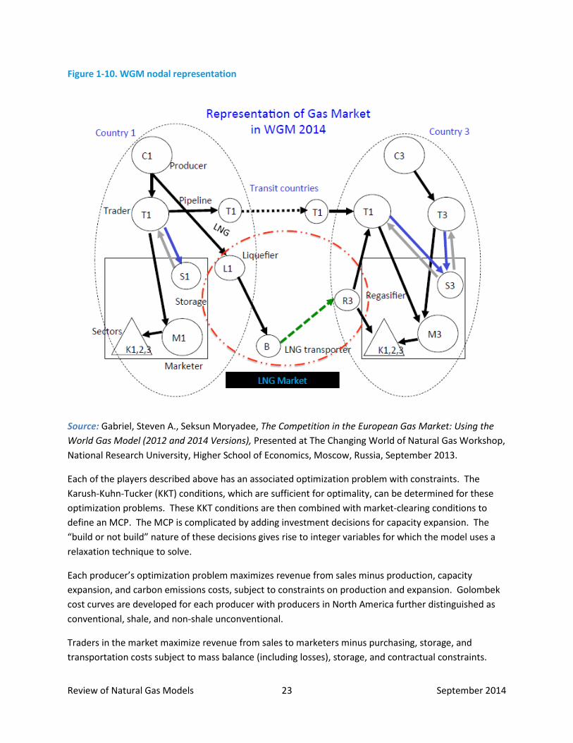
The nodal representation is shown in Figure 1-10.


Figure 1-10. WGM nodal representation

Source: Gabriel, Steven A., Seksun Moryadee, The Competition in the European Gas Market: Using the World Gas Model (2012 and 2014 Versions), Presented at The Changing World of Natural Gas Workshop, National Research University, Higher School of Economics, Moscow, Russia, September 2013.

Each of the players described above has an associated optimization problem with constraints. The Karush-Kuhn-Tucker (KKT) conditions, which are sufficient for optimality, can be determined for these optimization problems. These KKT conditions are then combined with market-clearing conditions to define an MCP. The MCP is complicated by adding investment decisions for capacity expansion. The “build or not build” nature of these decisions gives rise to integer variables for which the model uses a relaxation technique to solve.

Each producer’s optimization problem maximizes revenue from sales minus production, capacity expansion, and carbon emissions costs, subject to constraints on production and expansion. Golombek cost curves are developed for each producer with producers in North America further distinguished as conventional, shale, and non-shale unconventional.

Traders in the market maximize revenue from sales to marketers minus purchasing, storage, and transportation costs subject to mass balance (including losses), storage, and contractual constraints.


There are two components to the transportation costs: a regulated fee and a congestion fee. Sales price is a weighted average of the competitive price and the price from the inverse demand function with the weights depending on the level of market power the trader has at a given demand node. For a perfectly competitive market, just the competitive price is used. At the other extreme of an oligopoly, only the inverse demand function is included. In practice, a trader may have some but not complete market behavior at a node, and thus, weights on the inverse demand function and competitive price are included.

Liquefiers maximize sales revenue minus purchasing, expansion, and liquefication costs subject to capacity and expansion constraints.

LNG shippers maximize revenue minus capacity expansion costs, shipping costs, and canal fees subject to shipping capacity, canal capacity (Panama and Suez), and expansion constraints.

The transmission system operator maximizes revenue of sales of pipeline capacity to traders minus pipeline expansion costs, subject to constraints on available capacity and capacity expansion. The model makes a simplifying assumption that costs will be recovered from regulated fees, and introduces a congestion fee as a mechanism for allocating capacity.

Finally, storage operators are modeled similarly to transmission system operators and seek to maximize their revenues from selling storage capacity minus costs subject to capacity constraints.

Again, these individual optimization problems are combined by using the KKT conditions and market-clearing (mass balance) constraints and inverse demand curves to formulate the equilibrium MCP model.

The primary advantage to this model is its ability to include non-competitive market behavior, which is required for an international model. It can also handle nonlinear functions as long as the functions are convex. The resulting network, as defined above, yields over 78,000 variables and solves in approximately four hours.

Source: Appendix A in Gabriel, Steven A., K.E. Rosendahl, Ruud Egging, Hakob G. Avetisyan, Sauleh Siddiqui, “Cartelization in Gas Markets: Studying the Potential for a ‘Gas OPEC’,” Energy Economics 34(1): 137–152, January 2012.

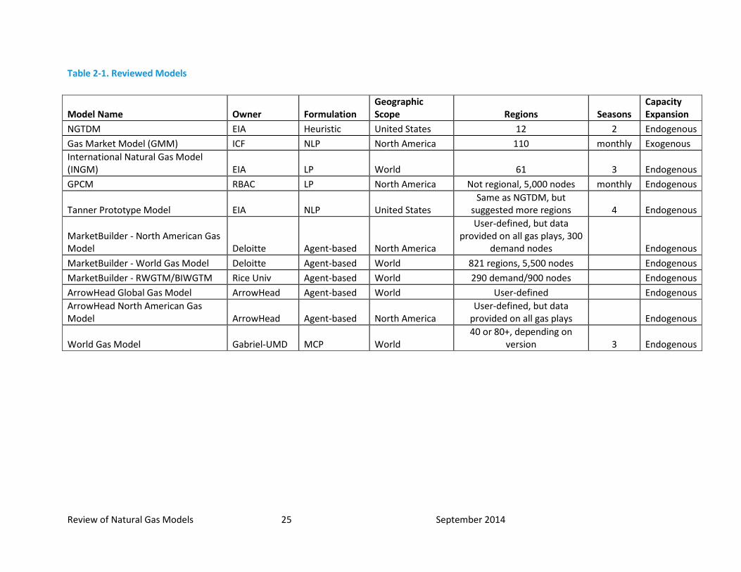
Model Comparisons This section provides a look across models at approaches to areas of prime interest in the NGTDM redesign, including model formulation, regional aggregation, seasonality, benchmarking, and capacity expansion. Table 2-1 summarizes key elements of the models.


Table 2-1. Reviewed Models

Model Name Owner Formulation Geographic Scope Regions Seasons

Capacity Expansion

NGTDM EIA Heuristic United States 12 2 Endogenous Gas Market Model (GMM) ICF NLP North America 110 monthly Exogenous International Natural Gas Model (INGM) EIA LP World 61 3 Endogenous GPCM RBAC LP North America Not regional, 5,000 nodes monthly Endogenous

Tanner Prototype Model EIA NLP United States Same as NGTDM, but

suggested more regions 4 Endogenous

MarketBuilder - North American Gas Model Deloitte Agent-based North America

User-defined, but data provided on all gas plays, 300

demand nodes Endogenous MarketBuilder - World Gas Model Deloitte Agent-based World 821 regions, 5,500 nodes Endogenous MarketBuilder - RWGTM/BIWGTM Rice Univ Agent-based World 290 demand/900 nodes

Endogenous

ArrowHead Global Gas Model ArrowHead Agent-based World User-defined

Endogenous ArrowHead North American Gas Model ArrowHead Agent-based North America

User-defined, but data provided on all gas plays

Endogenous

World Gas Model Gabriel-UMD MCP World 40 or 80+, depending on

version 3 Endogenous


2.1 Formulations All of the models represent the natural gas market in North America or the world as a system of nodes and arcs and find prices and flows that give an equilibrium solution to the network. They differ in the mathematical formulation of the models and solution approaches: linear programming (LP), nonlinear programming (NLP), mixed complementarity programming (MCP), or agent-based economic modeling. While the current NGTDM is also a network equilibrium model, it uses a heuristic approach to find the market equilibrium solution. Some of the pros and cons to each of these approaches are summarized here.

The LP and NLP approaches both assume a competitive market and find an optimal network equilibrium solution that maximizes consumer plus producer surplus while taking transportation costs into account. The difference lies in the types of functions that can be modeled and the resulting implications for convergence and solution time.

As its name implies, the LP can only be used with a linear objective function and linear constraints. Specialized algorithms that take advantage of network structures can solve very large problems quickly. Supply and demand curves, as well as transportation cost curves, can be incorporated into the formulation by approximating any non-linearities with piece-wise linear functions. An argument can be made that any definition lost by linearizing these functions is not significant enough to warrant the added complexity of solving a nonlinear problem.

One potential drawback of an LP is that it allows for flows to change dramatically (the so called “knife-edge effect”) from year to year to achieve optimality; whereas in the real world there may be established contracts and relationships in place that keep players in the market from making changes quickly. This issue is often referred to as “over-optimization” and can become particularly apparent when comparing model results to historical data. One method often used to overcome this problem is to add minimum constraints on flows. However, if these constraints are binding, unusual pricing behavior may be seen.

The NGTDM was initially formulated as an LP, but the results did not track well to history and adding constraints did not yield realistic results. Eventually a heuristic algorithm was developed instead, allowing for suboptimal behavior while still assuming a competitive market with no opportunities for arbitrage.

Energy Ventures Analysis (EVA) also used an LP in the past in a model that is not presented in this report. EVA found that the model did not give reasonable results for the reasons described above. Now, the company projects flows and prices based on analyst judgment (essentially a heuristic algorithm). The “knife-edge” effect has also been seen in the INGM, but the impact is mitigated by the fact that the model is run under many different demand scenarios and then regression analysis on the results is carried out to formulate supply curve for use in WEPS.

RBAC has not encountered the type of problems mentioned above with its LP formulation in the GPCM model. The supply, demand, and transportation cost curves are all linearized and a generalized network solver is employed. RBAC had been using the EMNET solver with extensions that included the ability to


handle convex, nonlinear supply, demand, and transportation cost functions; joint capacity constraints and other non-network equations; and variables with discrete values (MIP).

Source: Brooks, Robert, GPCM® (RBAC) vs NARG (Deloitte/Altos) and GMM (ICF/EEA), RBAC, Inc., 2014.

Because the EMNET solver is no longer being supported by its developer, Richard McBride, RBAC has begun using the GUROBI solver and has been satisfied with its results and the speed with which it can solve large generalized network problems.

The nonlinear formulation in the model proposed by Matt Tanner directly includes a nonlinear representation of transportation costs in the objective function. An iterative algorithm was designed by Tanner to find a model equilibrium solution. ICF’s GMM also uses a nonlinear formulation to accommodate transportation as a function of capacity utilization in the objective function, but a commercial solver is employed. An issue encountered in solving NLPs is the existence of alternate optima. However, NLPs use a starting value and solution algorithms attempt to find the closest optimum to the starting point, which may help keep flows from changing dramatically from one year of the forecast to the next, which is an advantage over an LP formulation. Unfortunately, there is no guarantee that the closest optimum to the starting values will be found, and different optimizers may find a different local optimum even given the same starting values, so it is important that a sensitivity analysis be done on the solution. (This could also be an issue with an LP if there are non-unique solutions.) A disadvantage to an NLP is that its increased complexity can significantly increase run-time and the chances of non-convergence. One of the questions to consider when comparing an LP and NLP is whether the introduction of nonlinear curves as opposed to piecewise linear functions yields model results that are significantly better and more accurate than the simpler LP approach. A key characteristic in addressing this question is whether the functions are convex.

The MCP formulation takes a somewhat different approach. Although this type of approach can model perfect competition, it also allows for the addition of constraints that model market power and elements of game theory (Nash-Cournot). This type of market behavior is assumed to exist in international markets but not in North America. Even so, an MCP formulation may have some advantages in modeling the North American market by allowing the inclusion of behavior that is not strictly competitive such as occurs when players in the market do not act quickly in shifting from established patterns, thus avoiding the “knife-edge” effect. In general, the MCP differs from an LP or NLP by simultaneously solving a set of conditions that includes equations, inequalities, and complementarity that are derived from the KKT conditions instead of maximizing an objective function subject to constraints. The power of the MCP is in its ability to explicitly include prices in the formulation, as well as have a significant amount of feedback between the sectors/players.

All of the above approaches do not allow arbitrage. This is either inherent to the formulation (LP) or is done explicitly through no-arbitrage constraints (the KKT conditions of the MCP). (Although not of interest for a North American model, an MCP formulation could include an arbitrageur optimization problem.)


Agent-based models use a microeconomic approach where each player is autonomous and seeks to maximize its profit subject to constraints. The main implication of this method is that instead of optimizing a single, system-wide objective function, each agent is represented by its own optimization problem with linking relationships to other agents in the network. This is a more real-world approach where each agent acts in its own best interest and not for the greater good of the energy system. Once each agent’s optimization problem is formulated and the relationship between agents is defined, the formulation allows for linear or nonlinear functions. The resulting system is solved using an iterative algorithm to find an equilibrium solution. Under certain conditions, the solution will be identical to system-wide optimal solution; however, once constraints are introduced that model market power and other non-competitive elements, the solution will differ. An advantage of the agent-based model over an LP is that allocation factors can be used to influence flow through the network to achieve a smoother solution. This is similar to the heuristic currently employed in the NGTDM. Source: Nesbitt, Dale, “The Economic Foundation of Generalized Equilibrium Modeling,” Operations Research 32(6): 1240–1267, December 1984.

There are many similarities between the MCP/Nash approach and the agent-based approach. Both model players in the market as entities seeking to maximize their profit or minimize their cost. Each player is modeled with a set of conditions and equations, and linked together with additional equations to create a network for which an equilibrium solution is found. Both methodologies have an advantage over an LP by addressing market inefficiencies to avoid unrealistically abrupt changes in flow patterns.

2.2 Regional Aggregation The models reviewed employ varying levels of aggregation in creating a network of nodes and arcs. For this discussion, we will focus solely on North American models. At one extreme is the NGTDM, which has just 12 regions in the lower 48 states. The ICF GMM contains 110 regions. At the other extreme is the GPCM, which does not aggregate the interstate pipeline network at all, resulting in a network of over 5,000 nodes. Similarly, MarketBuilder and ArrowHead have data on all gas plays and can be run with or without aggregation.

In the case of GPCM and MarketBuilder/Arrowhead, the decision to solve the model at the most detailed level of data available is driven in part by their industry clients’ needs, which may be more locally focused. Both GPCM and MarketBuilder/ArrowHead provide the customers with data and a sophisticated user interface, which enables aggregation of model results for easier analysis of the bigger picture. The challenge with these disaggregated models is data availability and maintenance. In some cases data are being obtained from industry sources and may not be readily available to EIA. Although this is a highly important factor in model design, it is not within the scope of this report. Another potential difficulty arising from a highly detailed network is the impact of size on run-time. Fortunately, both RBAC (GPCM) and MarketBuilder/Arrowhead have found algorithms that solve quickly and run-time has not been an issue. Finally, greater detail in output data can require much more analyst time to decipher and debug.

There are several concerns to be taken into consideration when aggregating the pipeline network. The potential to miss bottlenecks in the system increases as the level of aggregation increases. There may be plenty of capacity to flow between regions but not within the region. This impacts prices, flows, and


expansion decisions. In reality some pipeline capacity may even be used within a region to flow in the opposite direction of the primary flows between regions. The initial formulation of the NGTDM as a linear program encountered these types of problems, contributing to the decision to move to a heuristic algorithm that used average pricing instead of marginal pricing. It stands to reason that a finer level of detail is closer to a real-world representation of the market, and thus, would yield results that more closely match history and expected market behavior.

In summary, in deciding how to represent the network, one has to weigh the data availability, run-time, and analyst time against the increased accuracy of results. The modelers that have chosen not to aggregate the interstate pipeline system feel strongly that the benefits outweigh the costs.

2.3 Temporal Representation The current NGTDM models the peak and off-peak periods, as well as peak day volumes. Other models have three, four, or monthly time periods. Some of the same considerations must be addressed when deciding on temporal granularity as with spatial granularity, namely data availability and impact on run-time and analyst time. At a minimum, two seasons are required because of the seasonal nature of demand and the use of storage. However, monthly intervals better capture the impact of changes in pipeline flow direction.

2.4 Capacity Expansion Capacity expansion decisions are determined endogenously in most of the models. The approach taken is to include the cost of expansion in the pipeline tariff curve reflecting a hurdle rate required for expansion to be considered profitable. Those models that use exogenous inputs on capacity expansion rely more heavily on analyst judgment in determining expansion, which is not as easily documented or as robust as including capacity expansion decision-making directly in the model.

2.5 Benchmarking A few different approaches to benchmarking the models to history have been taken in the models reviewed. One approach is to run the model for a set of historical years and compare the results to the available data for those years. Multiplicative factors are then derived at each node based on the average differences between model results and history. These factors are usually held constant throughout the forecast. The limitation of this approach is that unusual weather from historical years will impact the forecast.

In the GMM and GPCM, the models are run for historical years and model parameters are adjusted so that the results best match historical data. These parameters are then used throughout the forecast.

Regardless of how benchmarking is done, an acceptable calibration tolerance must be determined.

2.6 Foresight

Models take different approaches to foresight. In some instances, perfect foresight is assumed and the model is solved over its entire horizon at once. (The model is usually run for a few years beyond the


horizon to avoid end-of-horizon effects.) Some models assume no foresight and run each period of the model successively. Others run groups of periods at a time.

Prototype Development The next step in the development of a revised NGTDM is to test different formulations and configurations on a small sample network in order to make final decisions on the key elements addressed above.

The initial sample network will be taken from the Nesbitt/Scotcher paper, “Spatial Price and Quantity Relationships in World and Continental Commodity Markets,” The Energy Journal, International Association of Energy Economics, 2009 Special Issue. In their paper, a network of two supply regions and two demand regions is formulated as an agent based model and solved by finding a Walrasian equilibrium. The example uses linear supply and demand curves and unit transportation rates and will serve as a base case. The following tests will then be performed using GAMS.

1. Formulate the base case as an NLP, maximizing consumer and producer surplus minus transportation costs, and as an MCP and compare results to the base case.

2. Test behavior with pipeline capacity constraints. 3. Include transportation cost curves. 4. Expand the network to different levels of detail and compare results and run time. 5. Expand the model to include multiple seasons and compare results and run time. 6. Include a representation of storage. 7. Include capacity expansion.

The test runs should not be limited to the above. The runs will serve as a basis for identifying limitations in approaches and designing the revised NGTDM.


Bibliography Brooks, Robert, GPCM® (RBAC) vs NARG (Deloitte/Altos) and GMM (ICF/EEA), RBAC, Inc., 2014.

Brooks, Robert, The Theory and Practice of Modeling with GPCM, RBAC, Inc.

Cazalet, Edward G., Generalized Equilibrium Modeling: The Methodology of the SRI-Gulf Energy Model, Decision Focus, Inc., May 1977.

Choi, Thomas, Dale Nesbitt, and Brad Barnds, Analysis of Freeport LNG Export Impact on U.S. Markets, Altos Management Partners Inc., December 2010.

Deloitte Market Point, Fundamental Analysis and Price Forecasting for the Commodity Markets with MarketBuilder, 2011.

Deloitte Market Point, Pioneering the Energy Resource Economics Future, Generalized Equilibrium Modeling System (GEMS), 2013.

Deloitte Market Point, How MarketBuilder Works, 2014, accessed through http://www.deloitte.com/ view/en_US/us/Industries/oil-gas/Deloitte-Center-for-Energy-Solutions/marketpoint-home/ marketpoint-marketbuilder/76c07c4886549210VgnVCM200000bb42f00aRCRD.htm.

Egging, Ruud, Franziska Holz, and Steven A. Gabriel, “The World Gas Model: A Multi-Period Mixed Complementarity Model for the Global Natural Gas Market,” Energy 35(10): 4016–4029, October 2010.

Egging, Ruud, Franziska Holz, Christian von Hirschhausen, Daniel Huppmann, Sophia Ruester, and Steven A. Gabriel, The World Gas Market in 2030: Calculation of Development Scenarios Using the World Gas Model, Presented at the 7th Infraday, Berlin, October 2008.

Energy Information Administration, Model Documentation Report: Natural Gas Transmission and Distribution Module of the National Energy Modeling System, Washington, DC, July 2013.

Energy Information Administration, Model Documentation Report: International Natural Gas Model 2011, Washington, DC, August 2013.

Energy Information Administration, Requirements for a Redesigned Natural Gas Transmission and Distribution Module in the National Energy Modeling System, Washington, DC, July 2014.

Gabriel, Steven A., Draft International Expert Report (IER) on the International Natural Gas Model, Task Order Contract #: DE---DT0001734, January 2013.

Gabriel, Steven A., Seksun Moryadee, The Competition in the European Gas Market: Using the World Gas Model (2012 and 2014 Versions), Presented at The Changing World of Natural Gas Workshop, National Research University, Higher School of Economics, Moscow, Russia, September 2013.

Gabriel, Steven A., K.E. Rosendahl, Ruud Egging, Hakob G. Avetisyan, Sauleh Siddiqui, “Cartelization in Gas Markets: Studying the Potential for a ‘Gas OPEC’,” Energy Economics 34(1): 137–152, January 2012.


Hartley, Peter, and Kenneth Medlock, The Baker Institute World Gas Trade Model, Geopolitics of Gas Working Paper Series, March 2005.

Hartley, Peter, Kenneth Medlock, and Jill Nesbitt, Rice University World Gas Trade Model, James A. Baker III Institute of Public Policy, Rice University, accessed through http://bakerinstitute.org/media/files/ event/3f421216/GSP_WorldGasTradeModel_Part1_05_26_04.pdf.

ICF, 2010 Natural Gas Market Review, August 2010.

ICF, North American Midstream Infrastructure Through 2035: Capitalizing on Our Energy Abundance, INGAA Foundation Report, March 2014.

Moryadee, Seksun, Steven A. Gabriel, and Hakob G. Avetisyan, “Investigating the Potential Effects of U.S. LNG Exports on Global Natural Gas Markets,” Energy Strategy Reviews 2(3–4): 273–288, February 2014.

Moryadee, Seksun, Steven A. Gabriel, and F. Rehulka, “The Effects of Panama Canal Tariffs on LNG Markets,” accepted, Journal of Natural Gas Science & Engineering, June 2014.

Nesbitt, Dale, “The Economic Foundation of Generalized Equilibrium Modeling,” Operations Research 32(6): 1240–1267, December 1984.

Nesbitt, Dale, and Jill Scotcher, “Spatial Price and Quantity Relationships in World and Continental Commodity Markets,” The Energy Journal, International Association of Energy Economics, 2009 Special Issue.

Tanner, Matthew, Proposed Natural Gas Market Module (NGMM), Energy Information Administration, January 2010.

Western Governors’ Association, NARG Model Natural Gas Assessment, Draft, October 2004