review of materials property data for nondestructive
TRANSCRIPT

Graduate Theses and Dissertations Iowa State University Capstones, Theses andDissertations
2015
Review of materials property data fornondestructive characterization of pipelinematerialsLucinda Jeanette SmartIowa State University
Follow this and additional works at: https://lib.dr.iastate.edu/etd
Part of the Materials Science and Engineering Commons, Mechanical Engineering Commons,and the Mechanics of Materials Commons
This Thesis is brought to you for free and open access by the Iowa State University Capstones, Theses and Dissertations at Iowa State University DigitalRepository. It has been accepted for inclusion in Graduate Theses and Dissertations by an authorized administrator of Iowa State University DigitalRepository. For more information, please contact [email protected].
Recommended CitationSmart, Lucinda Jeanette, "Review of materials property data for nondestructive characterization of pipeline materials" (2015).Graduate Theses and Dissertations. 14860.https://lib.dr.iastate.edu/etd/14860
Review of materials property data for nondestructive characterization of pipeline
materials
by
Lucinda Jeanette Smart
A thesis submitted to the graduate faculty
in partial fulfillment of the requirements for the degree of
MASTER OF SCIENCE
Major: Mechanical Engineering
Program of Study Committee:
Leonard Bond, Major Professor
Tim Bigelow
Stephen Holland
Iowa State University
Ames, Iowa
2015
Copyright © Lucinda Jeanette Smart. 2015. All rights reserved.

ii
TABLE OF CONTENTS
Page
LIST OF FIGURES ................................................................................................... iv
LIST OF TABLES ..................................................................................................... vii
GLOSSARY .............................................................................................................. viii
ACKNOWLEDGEMENTS ....................................................................................... x
ABSTRACT………………………………. .............................................................. xii
CHAPTER I INTRODUCTION .......................................................................... 1
Current Situation: Regulatory Driver ................................................................... 5
Motivation: Historical Failures ............................................................................ 6
Motivation: Regulatory Action ............................................................................ 7
CHAPTER II PROPERTIES OF PIPELINE STEEL ........................................... 9
Yield and Tensile Strength................................................................................... 9
Fracture Toughness and Transition Temperature ................................................ 11
Grain Size and Microstructure ............................................................................. 13
Chemical Composition......................................................................................... 20
Hardness ......................................................................................................... 25
Manufacturing Processes ..................................................................................... 31
CHAPTER III DESTRUCTIVE TESTS ................................................................ 35
Yield & Tensile Tests .......................................................................................... 35
Bend Tests ......................................................................................................... 40
Fracture Toughness Tests and Transition Temperatures ..................................... 41
CHAPTER IV NONDESTRUCTIVE TESTS ........................................................ 42
Magnetic Flux Leakage........................................................................................ 42
Eddy Current ........................................................................................................ 47
Ultrasound ......................................................................................................... 49
Chemical Composition......................................................................................... 53
Hardness Testing .................................................................................................. 54

iii
Grain Size Determination .................................................................................... 56
Microstructure ...................................................................................................... 56
CHAPTER IV CASE STUDY AND CONCLUSIONS ......................................... 57
Sample Data Information ..................................................................................... 57
General Correlations ............................................................................................ 58
Toughness and Chemical Content Correlations ................................................... 65
Conclusions ......................................................................................................... 73
REFERENCES .......................................................................................................... 76
APPENDIX. REFERENCE MATERIALS ............................................................... 84

iv
LIST OF FIGURES
Page
Figure 1.1 Percentage of Pipe Mileage Installed by Decade .................................. 2
Figure 1.2 U.S. Natural Gas Pipeline Network displaying over 305,000 miles of
pipeline .................................................................................................. 3
Figure 1.3 Map of PG&E’s Line 132 which ruptured near San Bruno. ................. 6
Figure 2.1 Engineering stress-strain curve. Intersection of the dashed line with the
curve determines the offset yield strength ............................................ 10
Figure 2.2 The characteristics of the transition-temperature range for Charpy
V-notch testing of low-carbon (0.18% C) steel .................................... 13
Figure 2.3 Microstructure of pipe steels for different cooling methods. ................ 14
Figure 2.4 Comparison of the microstructure of linepipe material within the base
metal (top) and the HAZ (bottom) ........................................................ 15
Figure 2.5 Dependency of fracture toughness of pipe steels on the grain size
produced during fabrication .................................................................. 16
Figure 2.6 Effect of plate thickness on grain size of the pipe steel ........................ 17
Figure 2.7 Variation of yield point with temperature. The theoretical curve is
fitted to the experimental value of σ/σo at 195oK ................................. 18
Figure 2.8 Forecasting achievable chemical contents in ppm ................................ 21
Figure 3.1 Schematic of stress-strain curves illustrating the sources of variability 37
Figure 3.2 Example of flattening using a 4-point bending method with image of
tensile round bar sample shown in green .............................................. 38
Figure 3.3 Relationship between Modulus (MPa) and YS (MPa) ......................... 39
Figure 4.1 B-H curve for a typical sample of pipeline steel. .................................. 43
Figure 4.2 B-H curves of different hardness generated for natural logarithmic
fit to extrapolated measured data from the GRI study of pipeline
steels ...................................................................................................... 45

v
Figure 4.3 Data from the 18 inch multiple data sets (MDS) tool for the heat
treated spot in 0.375-inch wall thickness at 1700° F. The first column
is for the air cooled spot and the second column for the quenched,
starting from the top row down are the hardness, high-field, low-field,
IDOD, internal deformation geometry, and DEF ................................. 46
Figure 4.4 Eddy current response shown in arbitrary units versus yield strength
and ultimate tensile strength. ................................................................ 48
Figure 4.5 Comparison of average YS and TS per joint measured with the tool
(ILI) with the corresponding values in the manufacturer’s certificates 49
Figure 4.6 Image of Ernst Handy Esatest. Provided by ApplusRTD Norway ....... 54
Figure 4.7 Image of On-site Hardness HB100 Digital Microscope. ...................... 55
Figure 5.1 Frequency of pipe properties available from Kiefner sample data set.. 58
Figure 5.2 Linear regression plot comparisons for Yield, Hardness, Grain Size,
Vintage, %Mn, %C, %Si, %S. .............................................................. 61
Figure 5.3 Linear regression plots comparisons for Yield, Hardness, Grain Size,
%Mn, %C, %Si, %S. Vintage is provided via a color scale as shown
within the figure – blue indicates newer vintage, red indicates older ... 62
Figure 5.4 Linear regression plots comparisons for Yield, Hardness, Grain Size,
%Mn, %C, %Si, %S. Vintage is filtered for pipe older than 1980 and
is provided via a color scale as shown within the figure – blue indicates
newer vintage, red indicates older. ....................................................... 63
Figure 5.5 Linear regression plots comparisons for Yield, Hardness, Grain Size,
%Mn, %C, %Si, %S. Vintage is filtered for pipe newer than 1980 and is
provided via a color scale as shown within the figure – blue indicates
newer vintage, red indicates older ........................................................ 64
Figure 5.6 Linear regression plots comparisons for FSE, %Mn, %C, %S, %Si,
and %Al. Vintage is provided via a color scale as shown within the
figure – blue indicates newer vintage, red indicates older. ................... 66
Figure 5.7 Linear regression plots comparisons for FSE, %Ca, %Nb, %P, %Ti,
and %V. Vintage is provided via a color scale as shown within the
figure – blue indicates newer vintage, red indicates older. .................. 66
Figure 5.8 Linear regression plots comparisons for FSE, %B, %Ca, %Cr, %Cu,
%Sn, and %Zr. Vintage is provided via a color scale as shown within
the figure – blue indicates newer vintage, red indicates older .............. 67

vi
Figure 5.9 Linear regression plots comparisons for Yield Strength, %Mn, %C,
%S, %Si, and %Al. Vintage is provided via a color scale as shown
within the figure – blue indicates newer vintage, red indicates older. .. 68
Figure 5.10 Linear regression plots comparisons for Yield Strength, %Mn, %C,
%S, %Si, and %Al for pipe older than 1980. Vintage is provided via
a color scale as shown within the figure – blue indicates newer
vintage, red indicates older. .................................................................. 69
Figure 5.11 Linear regression plots comparisons for Yield Strength, %Mn, %C,
%S, %Si, and %Al for pipe newer than 1980. Vintage is provided
via a color scale as shown within the figure – blue indicates newer
vintage, red indicates older. .................................................................. 70
Figure 5.12 Wall thickness versus (a) grain size and (b) transition temperature ..... 71
Figure 5.13 Grain size (ASTM) versus transition temperature (°F) ........................ 72
Figure A.1 Hazardous Liquid Integrity Verification Process Flowchart ................ 86
Figure A.2 Gas Transmission Integrity Verification Process Flowchart ................ 87

vii
LIST OF TABLES
Page
Table 2.1 Pipe grade and composition/alloying .................................................... 22
Table 2.2 Typical Supplementary Specification for X90-X100 Steel
Compositions ........................................................................................ 23
Table 2.3 Major effects of alloying elements in high strength line pipe steels ..... 24
Table 2.4 Historical Summary of Steel Manufacturers ......................................... 33
Table 3.1 Effect of Flattening on Mechanical Properties ..................................... 40
Table 4.1 Correlation coefficients for each variable against all others as listed
(shaded boxes indicate higher correlations) .......................................... 44
Table 5.1 Correlation coefficients for linear models of each variable against all
others (darker shaded boxes indicate higher correlations) .................... 60
Table 5.2 Correlation coefficients for FSE-CVN energy to chemical content ..... 65
Table 5.3 Correlation coefficients for Yield Strength to %Mn, %C, %S, %Si,
and %Al. ............................................................................................... 68
Table 5.4 Correlation coefficients for Yield Strength to %Mn, %C, %S, %Si,
and %Al for pipe older than 1980. ........................................................ 69
Table 5.5 Correlation coefficients for Yield Strength to %Mn, %C, %S, %Si,
and %Al for pipe newer than 1980. ...................................................... 70
Table A.1 Correlation coefficients for linear models of each variable against all
others (darker shaded boxes indicate higher correlations) .................... 85

viii
GLOSSARY
Acicular The characteristic of a crystal shape to be composed of radiating,
slender, needle-like crystals
Allotrope The concept of chemical elements to exist in two or more forms, or
different structural modifications of the element
Austenite A metallic, non-magnetic allotrope of iron or a solid solution of iron,
with an alloying element
Banite Acicular microstructure or phase morphology (not an equilibrium
phase) that forms in steels at temperatures of 250–550 °C (depending
on alloy content); may be a decomposition product when austenite is
cooled past a critical temperature
Cementite Commonly known as iron carbide is a chemical
compound of iron and carbon; in its purest form is known as a ceramic
Coercivity The ability for a ferromagnetic material to withstand an external
magnetic or electric field
DOT Department of Transportation
ERW Electric Resistance Welding
Ferrite A materials science term for pure iron, with a body-centered
cubic crystal structure; gives material magnetic properties
ILI In-line Inspection
Magnetic Hysteresis The concept when a material encounters a magnetic field, it has a sort
of memory, even after removing the source of the field. The
relationship is nonlinear, following a curve
Martensite A very hard form of steel crystalline structure formed by rapidly
cooling austenite at an extremely high rate (quenching)
Pearlite A two-phased, lamellar (or layered) structure composed of alternating
layers of alpha-ferrite (88 wt%) and cementite (12 wt%)

ix
Permeability The degree of magnetization of a material in response to a magnetic
field
PHMSA Pipeline and Hazardous Materials Safety Administration
Remanence Magnetization left behind in a ferromagnetic material after an external
magnetic field is removed
Saturation The state at which an increase in applied external magnetic field stops
increasing the magnetization of the material; where total magnetic flux
density levels off
Spiral Pipe Large diameter pipe formed by spiraling sheets of metal that are
smaller in width than the diameter required
U&O Formed Steel forming method using a large U die to press plate steel into a U
shape, followed by an “O”ing machine to close the U into an almost
closed cylindrical shape ready for welding

x
ACKNOWLEDGEMENTS
I would like to thank my many colleagues at Kiefner and Applus RTD for their
guidance and support throughout the course of this research. In particular I would like to
recognize Martin Fingerhut for supporting the broad scope vision for this project, Casper
Wassink for supporting the fundamental background in determining the area of research, and
finally, Harvey Haines, for his continued support and mentorship in my academic studies and
ongoing work activities. He was also an integral point of contact for the times when
everything became overwhelming. There are many others at Kiefner to thank for their
general support either through conversations on the subject matter, or through helping me
obtain research material: Michael Rosenfeld, Carolyn Kolovich, Bruce Nestleroth, Greg
Morris, John MacKenzie, and Dyke Hicks. I want to also offer my appreciation to those at
Pacific Gas & Electric (PG&E), Benjamin Wu and Francois Rongere, for their funding and
support of this research.
I would like to thank the Department of Transportation (DoT) and the Pipeline and
Hazardous Materials Safety Administration (PHMSA) and the Competitive Academic
Agreement Program (CAAP) for providing the momentum for this research through funding
and research support. Steve Nanney and James Merritt provided valuable input during our
monthly conference calls that aided in my understanding of the historical background for this
research topic.
In addition, I would also like to thank my friends, colleagues, the department faculty
and staff for making my time at Iowa State University a wonderful experience. I thank Dr.

xi
Leonard Bond for his support as my major professor and offering his advice and technical
experience in these studies.
Finally, thanks to my husband and his encouragement in supporting my work and
sanity, and taking care of our two beautiful daughters while I spent countless hours at the
office. I could not have done any of this without his help and I admire the patience he has had
with me, and his ability to help me stay on top of my homework, research, and everything
else going on over the course of this program.

xii
ABSTRACT
The oil and gas industry relies on an aging infrastructure of pipeline for transportation
and distribution of product; therefore, it is important to assess the condition of the pipeline,
using accurate material and mechanical properties, to ensure failures are minimized.
Nondestructive evaluation techniques are currently being used to assess pipeline, but
necessary mechanical properties (yield strength, tensile strength, fracture toughness, and
ductile-to-brittle transition temperature) are not yet able to be adequately characterized by
these methods.
There are many issues to consider when addressing this problem. There is variability
within the manufacturing processes due to simple inaccuracies in the processes themselves,
and changes in practices over the years. There is also variability in the destructive techniques
used for assessment of mechanical properties before the pipe is put into service. Current
focus in the industry tends to be on pipe installed in the 1950’s and 1960’s because about half
of the pipe currently in service was installed during these time periods, but it is equally
important to verify the properties of modern pipe Therefore, nondestructive methods of
measurement are commonly used for determining defect severity (e.g. magnetic flux leakage
and ultrasonic) are being explored to determine what other properties can be measured to
relate to mechanical properties. For future activities, it is advised to compare the accuracies
of both destructive and nondestructive methods of determining properties, should some
method of nondestructive evaluation become a more viable technique for mechanical
property measurements, either directly or indirectly.

xiii
The relationships between what can be measured (chemical content, grain size,
microstructure, hardness, coercivity, permeability, etc) and the mechanical properties desired
listed previously, show that there is a strong relationship between hardness and yield
strength. This is already well known in the industry. Other important relationships to evaluate
further include the percent content of various alloying elements, most notably including
manganese and carbon in relation to the yield strength, fracture toughness, and grain size.
Magnetic properties such as permeability and coercivity are also important, as these showed
stronger correlations within research, but are not available in the available sample data set.
In this thesis, research has been performed to establish the current state of the art,
highlighting some of the areas of difficulties in terms of obtaining consistent data sets. Linear
correlations were performed on the sample data available to observe the results for yield
strength and fracture toughness determination. Similar characteristics were also compared to
historical studies and generally the conclusions were well reflected by both data sets. For
future study, it would be of use to obtain saturation, permeability, coercivity, and remanence
measurements on the sample data to see if the correlations are similar to what was developed
shown in historical studies. Additionally, creating a chart of the various ultrasound
measurements such as velocity, attenuation, and backscatter grain noise could open up more
insight as to how effective ultrasonic measurements are in determining the desired
mechanical properties. From this information, the potential for application of nondestructive
methods of evaluation prove to be beneficial in supporting pre-existing destructive methods,
and eventually developing for field application.
1
CHAPTER I: INTRODUCTION
Nondestructive evaluation (NDE) techniques are used widely in the oil and gas industry
to assess the current condition of pipelines. No pipeline fails unless it contains a defect, but
pipelines are an aging infrastructure that must be continually monitored to determine remediation
requirements due to threats of corrosion, cracking, mechanical damage, or other integrity threats.
Using modern procedural guidelines, manufacture and the construction processes can be
performed such that the installed pipeline has theoretically stable defects which exist below the
tolerance as specified by API-5L for pipe manufacturing, where true defects are defined to be
flaws or anomalies that require repair according to the industry guidelines or government
regulations. Material quality and design has improved much in recent years. Various quality
inspections are conducted during both the manufacturing and construction processes to ensure a
pipeline is adequately characterized and these methods have also improved significantly.
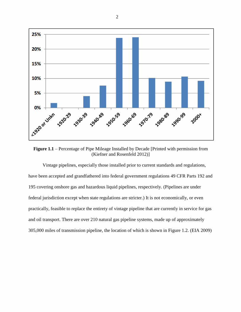
However, a pipeline with structurally insignificant defects is less certain with older
vintage pipelines that have not had the benefit of modern manufacturing and construction
processes. Moreover, in-line inspection (ILI) was not available until relatively recently and some
older pipelines are still not configured appropriately to enable the use of ILI tools. Seventy-
percent (70%) of all pipelines were installed prior to 1980, with almost half installed during the
1950s and 1960s, shown in Figure 1.1. (Kiefner and Rosenfeld 2012)
2
Figure 1.1 – Percentage of Pipe Mileage Installed by Decade [Printed with permission from
(Kiefner and Rosenfeld 2012)]
Vintage pipelines, especially those installed prior to current standards and regulations,
have been accepted and grandfathered into federal government regulations 49 CFR Parts 192 and
195 covering onshore gas and hazardous liquid pipelines, respectively. (Pipelines are under
federal jurisdiction except when state regulations are stricter.) It is not economically, or even
practically, feasible to replace the entirety of vintage pipeline that are currently in service for gas
and oil transport. There are over 210 natural gas pipeline systems, made up of approximately
305,000 miles of transmission pipeline, the location of which is shown in Figure 1.2. (EIA 2009)

3
Figure 1.2 – U.S. Natural Gas Pipeline Network displaying over 305,000 miles of pipeline.
[Printed with permission from (EIA 2009)]
The total mileage at the close of 2008, for interstate pipeline is 217,306 miles, with 73%
of that made up of diameters larger than 16-inches, whereas the 88,648 miles of intrastate
pipeline has 34% of the diameters larger than 16-inches. (EIA 2008) This results in a total of
188,774 miles of pipeline out of the 305,954 miles, or 62% of all pipelines having a diameter
greater than 16-inches.
Some of these vintage pipelines have accurate records of their material properties, but
unfortunately many do not. Even if records for material properties had originally been available,
there is potential over time, often due to changing ownership, that these records have been lost or

4
misplaced. Inadequate characterization of pipeline materials can lead to inaccurate remediation
decisions based on discovered defects.
Several pipeline failures have occurred in the past decade (FracDallas 2013). A pipeline
failure with severe consequences occurred September 9, 2010 in San Bruno, California that
highlighted this problem and has resulted in an increased desire to determine the material
properties of these vintage pipelines. (NTSB 2011) The material properties desired for adequate
characterization of the pipe include the mechanical properties of yield stress, tensile strength,
fracture toughness, and ductile-to-brittle transition temperature. The pipe properties desired are
outside diameter and wall thickness, which can be accurately determined using current
technologies such as magnetic flux leakage (MFL) and ultrasonic thickness (UT) measurements
using in-line inspections (ILI) tools. The seam weld type is also pertinent knowledge, as the
structural integrity of the line may depend on the toughness or reliability of the seam weld.
However, there is not one single nondestructive method which exists to evaluate every material
property required. There are various destructive techniques which are used to determine these
properties, and these may be used to determine relationships between material properties and
currently available NDE techniques. These tests require that pipe samples be cut from the
pipeline, which is costly and undesirable for bulk sampling of pipe. Therefore, it is important to
determine both what material conditions we are able to measure currently and what we may be
able to measure in the near future, and to develop possible relationships between these conditions
and the above listed mechanical material properties. Material conditions that could potentially be
measured and correlated with the required mechanical material properties include anisotropy,
microstructure, grain size, voids, porosity, phase composition, hardening depth, residual stresses,
heat treatments, and fatigue damage. NDE techniques have been successfully developed to

5
measure some of these defect types and microstructural features. But except for gross mechanical
damage, corrosion and cracking anomalies, such techniques have not yet been applied to
pipelines. These NDE techniques include determination of grain size; texture; nucleation and
growth of second phases; tensile, creep, and fatigue properties; and deformation and damage.
(Raj, et al. 2003) Obtaining a greater understanding of the relationships inherent among the
above listed material conditions, their relationship to mechanical material properties and what
can be measured by NDT on a carbon steel pipeline either during in-ditch examination or
possibly with ILI, has considerable potential to improve upon current methods of determining
material properties. Exploration of these potential relationships is the focus of this paper.
Current Situation: Regulatory Driver
In-line inspections have become the primary tool for determining the severity of integrity
threats to a pipeline, due to both ease of applicability in increasing sophistication. “Smart” or
“intelligent” pigs, as they are commonly called, use NDE technologies such as magnetic flux
leakage (MFL) or ultrasonic techniques (UT). In-line inspections are performed to assess the
current condition of the line, focusing on threats due to corrosion, cracking, mechanical damage,
or other anomalies able to be detected by a particular NDE technology.
However, to apply these tools for assessing the condition of a pipeline and to ensure the
pipeline has the proper pressure rating, the mechanical material properties of the pipelines must
be known. The National Transportation Safety Board (NTSB) has recently recommended a
detailed verification and engineering critical assessment process be implemented, if pipe
properties are unknown. The most pertinent mechanical properties are listed and defined in the
following section.

6
Motivation: Historical Failures
The previously referenced pipeline failure on Pacific Gas and Electric Company’s
(PG&E) natural gas transmission Line 132 occurred on September 9, 2010. The rupture occurred
in a residential area in San Bruno, California, creating a crater about 72 feet long by 26 feet
wide. (NTSB 2011) This failure in particular has motivated the oil and gas industry to develop
new material characterization and related nondestructive methods. (NTSB 2011)
The San Bruno pipeline segment failed during a replacement of a nearby uninterruptable
power supply, a map of which is shown in Figure 1.3. The pressure in the pipe had steadily
increased from 2461 kPa (357 psi) to 2661 kPa (386 psi), where the maximum allowable
operating pressure (MAOP) per regulation was 2758 kPa (400 psi). (Hart 2013)
Figure 1.3 – Map of PG&E’s Line 132 which ruptured near San Bruno. [Printed with permission
from (Hart 2013)]

7
The pipeline was originally installed in 1956, and a fracture originated in the partially
welded longitudinal seam in a short pipe section. According to Hart, this weld was deficient in
quality, noting a single weld instead of a double weld, and general poor workmanship
surrounding the weld. Inadequate records were kept of the installation process for which the
NTSB concluded was the primary cause of the failure. Additionally, the records for this pipe
indicated seamless pipe, but segments contained longitudinal welds. (Hart 2013) This lack of
knowledge combined with the unknown weld defect, and inadequate examination methods that
were performed but could assess seam weld defects, the failure became almost inevitable. This
failure could have been avoided by performing a more appropriate assessment using either in-
line inspection tools or high pressure hydrostatic testing. However the severe consequences of
this failure led to an extensive regulatory review of what is known, or rather not known, of all the
material properties that can affect the integrity of vintage pipelines. (NTSB 2011) This resulted
in the publication by PHMSA of an Integrity Verification Process (IVP) flow chart that was
subsequently revised in September 10, 2013 (see Appendix A). This chart contains both MAOP
verification and engineering critical assessment (ECA) components, both of which are relevant
to this paper.
Motivation: Regulatory Action
There are now several teams working on approaches for solving the problem of unknown
pipe properties. (Nestleroth and Haines 2013), (Belanger and Narayanan 2006), (Amend 2012)
There are also recommendations by the National Transportation Safety Board (NTSB),
which were followed by the US Department of Transportation Pipeline and Hazardous Materials
Safety Administration (US DOT PHMSA) developing new regulations regarding their integrity

8
verification processes (IVP). PHMSA describes their IVP as a multidisciplinary engineering
approach to verify the gas transmission pipeline properties are adequate for continued operation
for a period of time. (Nanney 2013)
Through the Pipeline Research Council International (PRCI), many projects and research
topics have been initiated, one of which has outlined the approach for obtaining information on
vintage pipelines and is currently in progress to continue developing technologies and methods
to do so. (Haines and Nestleroth 2013) An earlier report was published through the Interstate
Natural Gas Association of America (INGAA) Foundation that investigates incidents reported to
the DOT PHMSA showed that incidents do not correlate with pipeline age, indicating that pipe
properties do not change over time and therefore if we know the initial properties of the steel, we
can make integrity decisions based on that knowledge throughout the lifetime of the pipeline.
(Kiefner and Rosenfeld 2012) It follows that if the initial properties are unknown, that
determination of the current properties will be sufficient for this purpose.

9
CHAPTER II: PROPERTIES OF PIPELINE STEEL
Steel pipelines are most commonly characterized in terms of grade, which is simply an
estimate of their lower bound yield strength. Less is commonly known regarding the fracture
toughness (impact resistance and ductile-to-brittle transition temperature). But this is changing as
more pipeline operators seek to characterize the allowable size of flaws in operating pipelines
which are highly dependent on both toughness and operating pressure. A major factor to
increase the toughness in pipeline steels is developing steels with a small grain size, which also
tends to increase the strength of the steel. These properties are inter-related for and adjusting the
chemical composition undoubtedly will have an effect on the grain size and microstructure
during the manufacturing process. The review of the mechanical and material properties required
to adequately characterize pipeline mechanical behavior follows.
Yield and Tensile Strength
First we define stress as the internal resistance offered by a unit area of the material,
measured after a load is externally applied. This force can be in any direction, but it is typical to
state stress in terms of normal forces or shear forces. (Chandramouli 2013)
For pipelines, lower bound (approximate) yield strength determines the pipe grade which
is a key parameter in the federal regulations for determining pipeline operating pressure. Yield
strength is the point where the stress load causes plastic deformation to begin. This value at
which permanent deformation occurs is important to identify accurately in pipelines so safe
pressure ratings can be applied to the pipeline. The diagram in Figure 2.1 indicates where each
point occurs. Although there is no exact point at which yielding begins, for general engineering
design the yield strength is chosen when 0.2% plastic strain has taken place. However for older

10
pipes, a 0.5% elongation under load is typically still used. (API 2007) It is critically important to
not exceed an operating pressure which would cause a pipeline to exceed its yield strength. In the
yielding stage, the material deforms with little increase in force load, but with the additional
load, strain hardening will occur which results in changes to the atomic and crystalline structure
of the steel.
Tensile strength, or ultimate strength, corresponds to the maximum tensile stress a
material can withstand before it fails as indicated in Figure 2.1.
Figure 2.1 – Engineering stress-strain curve. Intersection of the dashed line with the
curve determines the preeminent offset yield strength. [Printed with permission from (ASM
International 2000)]
Yield and tensile strengths can be affected by varying such material properties as
chemical properties, heat treatments, microstructure, and grain size. Methods have been and are
currently being developed to determine yield strength through nondestructive measurements of
material properties.
11
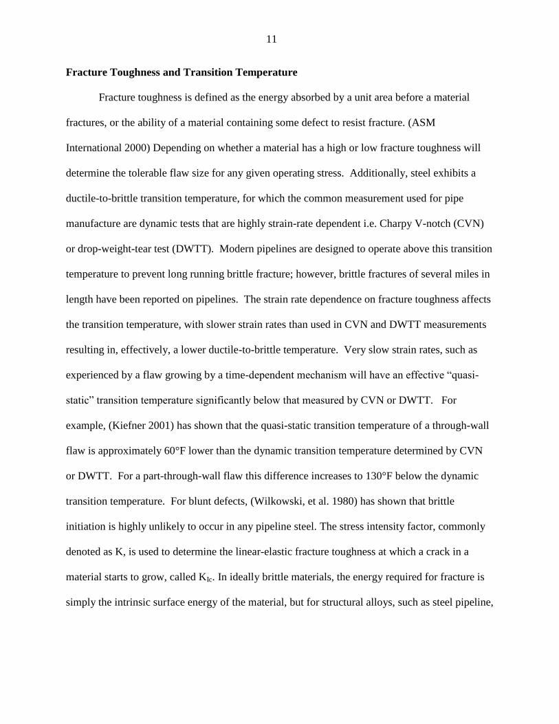
Fracture Toughness and Transition Temperature
Fracture toughness is defined as the energy absorbed by a unit area before a material
fractures, or the ability of a material containing some defect to resist fracture. (ASM
International 2000) Depending on whether a material has a high or low fracture toughness will
determine the tolerable flaw size for any given operating stress. Additionally, steel exhibits a
ductile-to-brittle transition temperature, for which the common measurement used for pipe
manufacture are dynamic tests that are highly strain-rate dependent i.e. Charpy V-notch (CVN)
or drop-weight-tear test (DWTT). Modern pipelines are designed to operate above this transition
temperature to prevent long running brittle fracture; however, brittle fractures of several miles in
length have been reported on pipelines. The strain rate dependence on fracture toughness affects
the transition temperature, with slower strain rates than used in CVN and DWTT measurements
resulting in, effectively, a lower ductile-to-brittle temperature. Very slow strain rates, such as
experienced by a flaw growing by a time-dependent mechanism will have an effective “quasi-
static” transition temperature significantly below that measured by CVN or DWTT. For
example, (Kiefner 2001) has shown that the quasi-static transition temperature of a through-wall
flaw is approximately 60°F lower than the dynamic transition temperature determined by CVN
or DWTT. For a part-through-wall flaw this difference increases to 130°F below the dynamic
transition temperature. For blunt defects, (Wilkowski, et al. 1980) has shown that brittle
initiation is highly unlikely to occur in any pipeline steel. The stress intensity factor, commonly
denoted as K, is used to determine the linear-elastic fracture toughness at which a crack in a
material starts to grow, called KIc. In ideally brittle materials, the energy required for fracture is
simply the intrinsic surface energy of the material, but for structural alloys, such as steel pipeline,

12
considerably more energy is required for fracture due to the effects of plastic deformation.
(Griffith 1921)
A notched specimen is used for testing because the notch toughness represents the ability
of the material to absorb energy determined under impact loading. This can be done in a variety
of ways, including Charpy V-notch, dynamic-tear specimen, and plane-strain fracture toughness.
Charpy V- notch impact specimens are most commonly used throughout industry; including the
pipeline industry for determine fracture toughness. This test will determine the ductile to brittle
transition behavior.
The transition temperature is defined at the point at which a material changes from one
crystal state to another, or where the material changes its potential for a brittle fracture to a
ductile fracture, shown in Figure 2.2. However, the transition temperature is most commonly
determined through fracture impact tests, as described previously within the Charpy V-notch
impact test. The relationship can be seen in the diagram following, where in (a) one can note the
characteristics of the transition temperature range determined by fracture energy, in (b) it is
determine by fracture appearance, and in (c) it is determined by fracture ductility.

13
Figure 2.2 – The characteristics of the transition-temperature range for Charpy V-notch
testing of low-carbon (0.18% C) steel. [Printed with permission from (ASM International 2000)]
Grain Size and Microstructure
Grain size refers to the size of microscopic crystals within a material, and each grain has
external boundaries known as grain boundaries. These grain boundaries tend to be higher energy
than the grain itself and often chemistry segmentation and flaws occur at grain boundaries. These
crystallites can be oriented randomly and would consequently be approximately isotropic, or
lacking in texture. However, most materials have a certain alignment to their grain structure, a
directional dependence, and are considered anisotropic. Furthermore, the rolling process of steel
plate, especially when conducted below the austenite transition temperature, tends to result in

14
grains elongated in the rolling direction. This structure and its alignment can affect the
mechanical properties of a material, including its fracture toughness, yield strength, and tensile
strength.
The manufacturing process differences contribute to the differences in the microstructure.
(Boulgar and Hansen 1965) shows some various methods of cooling and how those significantly
change the grain size and ferrite and pearlite content, shown in Figure 2.3.
Figure 2.3 Microstructure of pipe steels for different cooling methods. (Boulgar and Hansen
1965)
For pipeline steels, grain sizes can range anywhere from 10 to 20 𝜇m (ASTM G 8-10) for
cold-rolled steels where no transformation annealing is applied, all the way down to 4-5 𝜇m
(ASTM G 12.5) for modern, higher strength, steels which have been microalloyed and processed
using hot-rolling and thermo-mechanical treatments. (Shukla, et al. 2013) (Ghosh and Mondal
2013) An example micrograph showing the microstructure of pipeline steel is shown in Figure
2.4, and indicates the differences in grain size and microstructures depending on heat treatments.
Advancements in manufacturing processes indicate that a microstructure consisting of tempered

15
bainite and/or tempered martensite is required in high-grade pipeline steels to achieve high
strengths. (Zong, et al. 2012) A study analyzing the microstructure of modern microalloyed
steels was performed to show the grain size of the base metal is typically below 10 𝜇m and may
contain fractions of ferrite, bainite, and martensite/austenite (M/A)-constituents. (Stallybrass, et
al. 2014) Based on these investigations, it is possible to continue to refine the alloy design and
processing parameters in order to improve the low-temperature toughness of the base metal for
high strength materials, as well as the longitudinal seam welds.
Figure 2.4 Comparison of the microstructure of linepipe material within the base metal
(top) and the HAZ (bottom). [Printed with permission (Stallybrass, et al. 2014)]

16
There is extensive literature on grain size, crystallographic texture, and inclusion content,
and how these relate to the mechanical properties of a material. (Wilson, et al. 1975),
(Baczynski, et al. 1999), (Joo, et al. 2012), (Hwang, et al. 2005) There is an obvious dependence
on the toughness when performing a Charpy V-notch test for the alignment of the material, either
in the longitudinal or circumferential direction (Pessard, et al. 2011). A (Boulgar and Hansen
1965) report indicates that the total area ferrite grain size has a significant impact upon the
fracture toughness, where the transition temperature is defined on the basis of two-thirds the
maximum energy. This trend is shown in Figure 2.5.
Figure 2.5 Dependency of fracture toughness of pipe steels on the grain size produced during
fabrication. (Boulgar and Hansen 1965)
A trend between the average ASTM grain size and the plate thickness was shown by
(Boulgar and Hansen 1965) where the thicker the plates, the coarser the average through-wall
microstructure, or larger grain sizes, shown in Figure 2.6.

17
Figure 2.6 Effect of plate thickness on grain size of the pipe steel. (Boulgar and Hansen 1965)
Fracture tests on these samples confirmed the effect the grain size has on toughness.
Manufacturing processes now exist to help deter this affect by improving the normalization
(Chancellor 1935) and other post-weld heat treatment processes. The process of normalizing
reheats the material to a specified temperature, holds it for a time, and then cools in still air. This
allows for the grain size to become more consistent throughout the material.
Microstructural dislocations within iron have an effect on the yield point of the material.
(Cottrell and Bilby 1948) This is also closely related to the temperature of the material, prior
work hardening, and at what point the material will reach its yield point. Cottrell found the
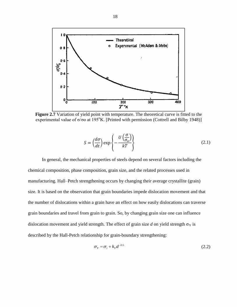
following trend shown in Figure 2.7 for the applied stress (yield point), σ/σo, to the temperature,
T, assuming testing rates, t, stay constant, where U is the activation energy. In formula 2.1, the
point at which yield should occur is listed in terms of the energy released from the dislocations,
U, providing the Figure 2.7 values when U/kT is held constant, and theoretical values when σ/σo
is held constant.
18
Figure 2.7 Variation of yield point with temperature. The theoretical curve is fitted to the
experimental value of σ/σo at 195oK. [Printed with permission (Cottrell and Bilby 1948)]
𝑆 = (𝑑𝜎
𝑑𝑡) exp {−
𝑈 (𝜎𝜎𝑜
)
𝑘𝑇} (2.1)
In general, the mechanical properties of steels depend on several factors including the
chemical composition, phase composition, grain size, and the related processes used in
manufacturing. Hall–Petch strengthening occurs by changing their average crystallite (grain)
size. It is based on the observation that grain boundaries impede dislocation movement and that
the number of dislocations within a grain have an effect on how easily dislocations can traverse
grain boundaries and travel from grain to grain. So, by changing grain size one can influence
dislocation movement and yield strength. The effect of grain size d on yield strength Y is
described by the Hall-Petch relationship for grain-boundary strengthening:
5.0 dkYiY (2.2)

19
which has been extended to include the effects of phase composition and alloying elements. For
example in the case of low-carbon (up to 0.25 wt% C), predominantly ferritic steels, the yield
strength Y, tensile strength T and impact transition temperature (ITT), as measured by CVN or
DWTT, are related to the ferrite grain size dF, volume fraction of pearlite VP and alloy content
(e.g., % of Mn, Si and free nitrogen Nf) as (Llewellyn 1992).
Y (MPa) = 53.9 + 32.3% Mn + 83.2% Si + 354% Nf + 17.4d-0.5
(2.3)
T (MPa) = 294 + 27.7% Mn + 83.2% Si + 3.85% VP + 7.7d-0.5
(2.4)
ITT (ºC) = -19 + 44% Mn + 700%Nf + 2.2% VP – 11.5d-0.5
(2.5)
These empirical equations highlight (i) the beneficial effects of reducing ferrite grain size
in improving yield and tensile strengths as well as depressing the transition temperature; (ii) an
increase in tensile strength and a loss of toughness with pearlite but the relative insignificance of
pearlite content in yield strength; (iii) beneficial effects of Mn and Si on strengths and the
detrimental effect of free nitrogen on transition temperature. Empirical equations have also been
established for medium-to-high carbon steels (Gladman, et al. 1972), which show that in high-
carbon steels, the volume fraction of pearlite and the inter-lamellar spacing have significant
effects on both the yield and tensile strengths.
There is also a significant relationship based on fully pearlitic microstructures, based on
the inter-lamellar spacing, S, the pre-austenitic grain size, d, and the pearlite colony size, P, and
relating these parameters to the yield strength, as shown in equation 2.6. (ASM International
2005)
YS (yield strength) = 2.18(S-1/2
) – 0.40(P-1/2
) – 2.88(d-1/2
) + 52.30 (2.6)

20
This relationship has similar characteristics to the Hall-Petch relationship, but is only
valid for fully pearlitic microstructures. Although pipeline steels are not fully pearlitic, a similar
relationship may be able to be determined using this foundational knowledge and applying to
other microstructures.
Chemical Composition
The chemical composition of any material plays a highly significant a role in its
mechanical properties. Early understanding of pipe properties leads to a known relationship
between chemical content, particularly that of carbon (C), and the strength, hardness, and
toughness. Increasing the percentage of C increases strength and hardness, while decreasing
toughness and weldability, leading to a higher likelihood for cracking when heated and cooled
rapidly. (Nichols 2011) Increasing C also raises the tensile strength more than it does the yield
strength. These reasons are primarily why there is a maximum allowed value for carbon levels.
(Boulgar and Hansen 1965) Manganese can help to increase the strength of the steel as well, but
not to the same degree as C, and must be found in larger quantities for the same strength
contribution. Sulfur is introduced into the steel during the melting process. Sulfur and
phosphorus are impurities which may create hook cracks or other defects, and must be kept to a
minimum.
A report by (Gray and Siciliano 2009) presents a good summary of the microalloying
process and its developments over the years. Vanadium and niobium were initially introduced
with reports in the literature as early as 1945 and 1938, respectively. These microalloying
elements introduced their own problems into the steel, however, and therefore it was not refined
until other microalloying elements were managed, such as manganese, molybdenum, and
aluminum. Controlled rolling and other thermochemical processing methods also needed to be

21
refined to manage austenite grain size and the formation of cementite networks on ferrite grain
boundaries.
Recent advancements in manufacturing processes have shown that lower carbon contents
are acceptable (as low as 0.03-percent), and more advancements in subsequent processing and
secondary refining can lead to high-strength steels with grades as high as X120 (Hammond
2007) Carbon is typically known for its strengthening properties, so removing it requires the use
of other strengthening mechanisms during the manufacturing process, such as micro alloying,
solute alloys, and post-rolling accelerated water cooling practices. Furthermore, to maintain high
toughness, sulfur must be reduced to create cleaner steels. (Bannenberg 2001) discusses the
recent developments of steelmaking in regards to the chemical content desired. The estimated
average contents in parts per million (ppm) are shown in Figure 2.8 below, and forecast into the
future what is likely to be seen.
Figure 2.8 Forecasting achievable chemical contents in ppm. (Bannenberg 2001)
Table 2.1 of a steel alloying approach for various pipe grades, from 5LB to X120,
indicates both chemical content and microstructure design, where F/P indicates ferrite/pearlite
microstructures, F/AF indicates ferrite/acicular ferrite microstructures. Acicular ferrite is defined
as low carbon bainite formed by intragranular nucleation. (Stalheim, et al. 2006) Note that all

22
grades except “B” grade shown have less than 0.10 carbon, considerably less than that typical
with vintage pipeline steels.
Table 2.1 Pipe grade and composition/alloying. (Stalheim, et al. 2006)
API
Grade Steel Alloying Approach
X120 AF/Bainite/Martensite, C <0.10, Mn<2.0, Si<0.40, Nb<0.06, Cu, Ni, Cr, Mo, V, B,
Pcm≤0.25
X100 AF/Bainite, C<0.06, Mn<2.0, Si<0.40,Nb<0.06, Cu, Ni, Cr, Mo, V, Pcm≤0.23
X80 F/AF, C≤0.06, Mn<1.70, Si<0.40, Nb≤0.10, Cu, Ni, Cr, Mo, V, B, Pcm≤0.18
F/AF, C≤0.06, Mn<1.70, Si<0.40, Nb≤0.10, Cu, Ni, Cr, Mo, V, B, Pcm≤0.21
X70
D/t<50: F/AF, C≤0.06, Mn≤1.65, Si<0.40, Nb≤0.10 only, or Nb+Mo, Pcm≤0.18 or
0.21
D/t>50: F/P, C≤0.10, Mn≤1.65, Si<0.40, Nb≤0.065 only, or Nb+V, Pcm≤0.20
X65 F/P, C≤0.10, Mn≤1.65, Si<0.40, Nb≤0.065 only, or Nb+V≤0.15 Pcm≤0.23
X60 F/P, C≤0.10, Mn≤1.50, Si<0.40, Nb≤0.065 only, or Nb+V≤0.12, Pcm≤0.23
X52 F/P, C≤0.10, Mn≤1.20, Si<0.40, Nb≤0.050 only, Pcm≤0.17
X42 F/P, C≤0.10, Mn≤1.00, Si<0.40, Nb≤0.050 only, Pcm≤0.16
API 5LB F/P, C≤0.20, Mn≤1.00, Si<0.40, Pcm≤0.16
Several other alloying elements are added in small quantities into the base material of
iron to improve various factors of the steel pipe. Typical “micro-alloying” elements may include
molybdenum (Mb) silicon (Si), calcium (Ca), titanium (Ti), niobium (Nb), aluminum (Al), and
vanadium (V).
Typical carbon content for steels ranges from 0.07wt% to 0.30wt% (Battelle, 1997).
Modern steels are now relying on improved manufacturing methods to obtain steels with ultra-
low carbon contents, as low as 0.01wt% (Shukla, et al. 2012). By decreasing the carbon content,
the steel weldability improves. The microalloying elements which must be then be considered to

23
improve strength by being strong carbide formers include Ti, Nb, and V. (Shukla, et al. 2012)
There exists a wide variety of steel grades for pipeline applications, with selection depending on
the specific operation conditions and requirements. For high strength steels with yield strengths
in the range of 90 – 100 ksi, carbon content is much lower, with a typical chemical composition
is shown in Table 2.2.
Table 2.2 Typical Supplementary Specification for X90-X100 Steel Compositions. (Hammond
2007)
Element Wt %
Carbon 0.10% maximum
Manganese 0.80% - 2.00%
Silicon 0.05% - 0.35%
Sulphur 0.005% maximum
Phosphorus 0.015% maximum
Nitrogen 0.008% maximum
Vanadium 0.08% maximum
Niobium 0.05% maximum
Titanium 0.03% maximum
Aluminum 0.010 – 0.055%
Copper 0.50% maximum
Boron 0.0005% maximum
Calcium 0.006% maximum
Nickel plus Copper 1.00% maximum
Chromium plus Molybdenum 0.35% maximum
Vanadium plus Niobium 0.12% maximum
A report by Rosado presents a table of the element and their effect and reason for the
inclusion and has been recreated in Table 2.3.

24
Table 2.3 Major effects of alloying elements in high strength line pipe steels. [Reproduced with
permission from (Rosado, et al. 2013)]
Element (wt%) Effect and reason of adding
Carbon (0.03-0.10) Matrix strengthening (by precipitation)
Manganese (1.6-2.0)
Delays austentite decomposition during AcC;
Substitutional strengthening effect;
Decreases ductile to brittle transition temperature;
Indispensable to obtain a fine-grained lower bainite
microstructure
Silicon (up to 0.6) Improvement in strength (solid solution)
Niobium (0.03 – 0.06)
Reduces temperature range in which recrystallization is
possible between rolling passes;
Retard recrystallization and inhibit austenite grain growth
(improves strength and toughness by grain refinement)
Titanium (0.005-0.03)
Grain refinement by suppressing the coarsening of austenite
grains (TiN formation);
Strong ferrite strengthener;
Fixes the free Ni (prevent detrimental effect of Ni on
hardenability)
Nitrogen (0.2-1.0)
Improves the properties of low-carbon steels without
impairing field weldability and low temperature toughness;
In contrast to Mg and Mo, Ni tends to form less hardened
microstructural constituents detrimental to low temperature
toughness in the plate (increases fracture toughness)
Vanadium (0.03-0.08)
Leads to precipitation strengthening during the tempering
treatment;
Strong ferrite strengthener
Molybdenum (0.2-0.6) Improves hardenability and thereby promotes the formation
of the desired lower bainite microstructure
Recent pipes have much higher standards due to the advancements in knowledge and
technology to that have enabled the production of these materials. The majority of pipes (1950-
1970 vintage) will not have such specific measurements of the chemical composition other than
the major elements, and in many cases, those records have been lost or misplaced, including the

25
variety of alloying elements, which lead to lower strength pipe. There may also be more
variability, leading to potentially different relationships between new and old pipe, relative to
their chemical content.
Hardness
Hardness is defined as the ability of a material to withstand surface indentation from
another material. The term “hardness” is not a reference to any specific material property, and is
typically defined in terms for which the industry hardness measurements are desired. (Frank
2002) For the metallurgical industry, hardness is generally regarded as a material’s resistance to
penetration causing formation of a plastic indentation. The quantitative value of hardness is
relative to the type of measurement performed. Several methods exist to obtain hardness values,
and there is no one fundamental expression to convert one hardness value to another. Conversion
tables do exist, but they are based on the material type, and differ from one hardness
measurement technique to another. (ASTM 1997)
Examples of hardness measurements include scratch, indentation, and rebound. The most
common scratch test is done applying the Mohs scale, a comparison of increasingly hard
materials. However, this does not apply well to steel since the typical range of hardness lies from
5 to 6.5, and Mohs does not provide adequate discrimination for the various hardnesses of steel.
Therefore, indentation test methods are much more common in relation to steel hardness
measurements. Common indentation hardness scales include Rockwell, Vickers, Shore, and
Brinell, and function by measuring the resistance and resulting indentation dimensions to the
material by a certain load placed on the indenter. Rebound hardness measures the height of the
bounce from a particular hammer object, and so is also related to elasticity. A common scale for
measuring rebound hardness is the Leeb rebound hardness test.

26
The earliest hardness measurements were done simply using a scratch-test technique,
e.g., a comparison test, to determine if one material is harder than the other. A test bar was used
as a comparison, and the material being tested scratched each comparison material at increasing
levels of hardness until the test material no longer made a scratch. (O'Neill 2011) This method is
qualitative, and does not provide much information about the material, but it was a good first
step in understanding material properties.
The Brinell measurement was developed in 1900 and presents the first widely used and
accepted procedure for quantifying hardness. Brinell’s method uses an indentation measurement
by applying a hard steel ball indenter at specified loads. The hardness value is determined based
on the measured dimensions of the remaining permanent deformation.
As an alternative to the Brinell method, the Vickers hardness test was developed in 1921,
which uses a pyramid diamond shaped indenter rather than the ball indenter used by Brinell, and
could be used for all materials regardless of hardness. (Sandland and Smith 1922) The Knoop
test was later introduced to use with lower test forces in order to measure more brittle or thinner
test materials. (Knoop, et al. 1939) The Rockwell hardness test was developed as a way to take
measurements quickly to determine the effects of heat treatment on steel. (Rockwell 1919)
Advantages of this method include the elimination of secondary calculations to produce results
and a very small indentation area.
Advancements in technology and hardness measurement techniques gave way to closed
loop systems, which are stated to have high accuracy and repeatability. Closed loop systems are
defined in that they must electronically measure the force applied during every test and send this
information back to a computer acquisition system. This method was implemented into the
aforementioned hardness test methods beginning in the early 1990s. (O'Neill 2011)

27
A recent advancement to the concept of hardness testing is observing dynamic changes in
the material using micro-indenter techniques. This technique applies loads from the indenter at
successive, increasing loads, with partial unloading at each step, until a maximum load value is
reached as defined by the inspector. This data is collected continuously by a data acquisition
system, and measurements of yield strength, stress-strain curves, strength coefficients, and strain
hardening exponents are outputs. (Sharma, et al. 2011) One specific example of this process is
the automated ball indentation (ABI) test carried out by the Portable/In-Situ Stress-Strain
Microprobe System, which is stated to provide actual yield strength value, true stress-true strain
curves, strain-hardening exponent, Luders strain, elastic modulus, and an estimate of the local
fracture toughness. (Haggag 2001)
The foundation for relating the applied load of a hardness test to the indentation area was
developed by Meyer in 1908, resulting in Meyer’s Law where P is load pressure, k is resistance
of material to initial penetration, n is Meyer’s index, and d is the diameter of the indentation
(Meyer 1908):
𝑃 = 𝑘𝑑𝑛 (2.7)
Meyer’s equation is only valid for values where the material is not plastically deformed.
It was developed by applying multiple successive loads, each one greater than the previous, and
maintaining that load until equilibrium was reached. This is the basis for how the automated ball
indenter method is performed.
For mild steel materials, a method was developed to relate the plastic regime of a true
stress-true strain curve to the plastic zone created by the spherical hardness indentation. A ratio

28
was also developed and the equation for the true plastic strain,𝜀𝑝 where 𝑑𝑝 is the plastic
indentation diameter, and 𝐷 is the diameter of the ball indenter, was empirically determined as:
𝜀𝑝 = 0.2 (𝑑𝑝
𝐷) (2.8)
An empirical relationship based was developed for tensile strength and the Brinell Hardness
Number (BHN) (Tabor 1951):
𝑇𝑒𝑛𝑠𝑖𝑙𝑒 𝑆𝑡𝑟𝑒𝑛𝑔𝑡ℎ = 𝐶𝑜𝑛𝑠𝑡𝑎𝑛𝑡 𝑥 𝐵𝐻𝑁 (2.9)
There are several sources which show the relationship between yield strength and hardness data.
One method is done using the Vickers hardness test value. The expression is valid for brass, steel
in either cold rolled or tempered condition, and aluminum alloys in the cold rolled or aged
condition (Cahoon, et al. 1971). The expression for the yield strength, 𝜎𝑦, is as follows for steel,
where H is Vickers hardess, m is the Meyer’s hardness coefficient:
𝜎𝑦 =𝐻
30.1𝑚−2
(2.10)
The ABI test presents several equations which uses variables that are specific to the type of test
method it performs. The following is a derivation from Haggag to illustrate the relationship
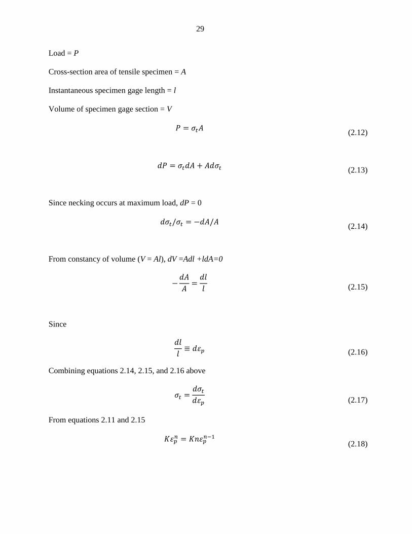
between true uniform elongation and strain-hardening exponent (Haggag, et al. 1993):
The homogenous plastic flow portion of the true-stress (σt)/true-plastic-strain (εp) curve can be
represented by the power law equation
𝜎𝑡 = 𝐾𝜀𝑝𝑛
(2.11)
where n = strain-hardening exponent and K = strength coefficient.
29
Load = P
Cross-section area of tensile specimen = A
Instantaneous specimen gage length = l
Volume of specimen gage section = V
𝑃 = 𝜎𝑡𝐴 (2.12)
𝑑𝑃 = 𝜎𝑡𝑑𝐴 + 𝐴𝑑𝜎𝑡 (2.13)
Since necking occurs at maximum load, dP = 0
𝑑𝜎𝑡/𝜎𝑡 = −𝑑𝐴/𝐴 (2.14)
From constancy of volume (V = Al), dV =Adl +ldA=0
−𝑑𝐴
𝐴=
𝑑𝑙
𝑙 (2.15)
Since
𝑑𝑙
𝑙≡ 𝑑𝜀𝑝 (2.16)
Combining equations 2.14, 2.15, and 2.16 above
𝜎𝑡 =𝑑𝜎𝑡
𝑑𝜀𝑝
(2.17)
From equations 2.11 and 2.15
𝐾𝜀𝑝𝑛 = 𝐾𝑛𝜀𝑝
𝑛−1 (2.18)

30
At necking, the true-plastic strain (𝜀𝑝) equals the true uniform elongation (𝜀𝑢)
𝑛 = 𝜀𝑢 (2.19)
Hence, the true uniform elongation is numerically equal to the strain-hardening exponent.
The micro-indenter method as presented using the ABI by Haggag was investigated and
determined reasonably positive results. (Benamar, et al. 2008) The study was performed on pipe
steels from Grade B to X70. The transverse and longitudinal yield strength calculated values
resulted in a maximum non-conservative discrepancy of about 11%, and an uncertainty of 11%.
The parameters used for this calculation were fitted to get yield strength in the transverse
direction, leading to non-conservative results in the longitudinal direction. The ultimate tensile
strength (UTS) value was obtained with an accuracy of 8%, using the correlation between UTS
and hardness given by the micro-indenter tool. The estimate of toughness obtained in this study
was too non-conservative for ductile steels with a low transition temperature. Additional
comments on the use of this tool indicate that it is promising in the industry, but that it has some
advancements that need to be overcome before it is practical for field use, such as additional
industry testing to prove validity for low to high grade steels as well as varying age of steels,
additional tests for calibration of master curves in order to obtain fracture toughness parameters
on modern steels, and the anisotropic effect of toughness on these types of tests. (Sharma, et al.
2011)
A project performed in 1999 by ASME resulted in a report that supports the use of
hardness measurements to obtain a lower bound yield stress for in-service pipe. (Burgoon, et al.
1999) It uses a correlation of hardness to yield stress values at various confidence levels for pipe
rated as Grade X52 or lower, manufactured prior to 1980, and of diameter 4-inches or greater.

31
The final results are in the form of tables and reports, an estimated lower tolerance bound on
yield strength based on the targeted percentile, and the confidence level desired. Work is
currently being done in the industry to improve this method, making it more usable for in-ditch
applications (Amend 2012). Linear relationships between hardness and tensile and yield
strengths have been studied to be true for steels with yield strengths of 325 MPa to over 1700
MPa (47 ksi and 246 ksi) and tensile strengths between 450 MPa and 2350 MPa (65 ksi to 340
ksi). (Pavlina and Van Tyne 2008) Additional studies provide similar linear relationships, only
varying in the coefficients due to differences in microstructure and compositions. (Pavlina and
Van Tyne 2008)
Manufacturing Processes
Although manufacturing processes are not a mechanical or material property, these
practices greatly affect the final outcome of a steel pipeline material in terms of strength,
toughness, and the material properties in general. There is known variability in the tensile
property based on the manufacturing process. That variability in the finished pipe is a function of
the know-how and processing skill of the steel producer, meaning the pipe making process does
not introduce much more variability, but new compositions and rolling practices may do so.
(Gray, et al. 1999)
One should consider the historical manufacturing processes, because it has been an
evolution as new technology and new understanding about steel making has been discovered.
Beginning as early as 1812, machines were being invented to take plates of iron and form them
into tubes, in processes known as “hammer lap-welding.” (Kiefner and Clark 1996) The
development of modern methods of steel manufacturing began in the 1900s, with low-frequency
electric resistance welding (ERW) taking root in 1924 through a process known as the “Johnson”

32
process. High frequency ERW pipe was introduced in 1955 and superseded low-frequency ERW
pipe by 1970 as an understanding of material properties continued to advance. Submerged arc
welding was first attempted in the 1930’s, and eventually became the standard for making large-
diameter (larger than 24-inches) by the 1950’s. Additional methods of steel manufacturing
include furnace butt-welded pipe (continuous-weld), furnace lap-welded pipe (hammer-weld),
seamless pipe, flash-welded pipe, and spiral weld pipe. The reason for understanding the history
of pipe manufacturing is that some pipes can be identified using what information may be
known. For instance, the only manufacturer to use flash-welded pipe is the A.O. Smith
Corporation. Other manufacturers have other specific key characteristics regarding the grades
they used, or specific diameters they were limited to manufacture within. The report by Kiefner
and Clark provides a table for API 5L line pipe manufacturing; Table 2.4 is a summary of the
text which precedes that table. (Kiefner and Clark 1996)

33
Table 2.4 Historical Summary of Steel Manufacturers (Kiefner and Clark 1996)
Manufacturer Dates of Production Grades Diameters
(inch) Weld Type
American 1963 – not given Grade B min
(35ksi) 10.75 - 20 HF-ERW
A.O. Smith 1930-1969 Grade A min
(30ksi) ≤36 Flash Welded
A.O. Smith 1969-1973 Grade A min
(30ksi) ≤36 DSAW
Bethlehem 1957-1963 Grade A min
(30ksi) 5.5625 - 16 LF-ERW
Bethlehem 1963-1982 Grade A – X52 2.375 – 6.625 HF-ERW
Bethlehem 1970-1982 Grade A – X60 5.562 - 16 HF-ERW
Geneva 1991 Grade B min Not given HF-ERW
Interlake Prior to 1980 Grade A – X52 4.5 – 8.625 LF-ERW
Jones &
Laughlin 1957-1964 Grade A – X60 6.625 – 12.75 Seamless & LF-ERW
Jones &
Laughlin 1965-1985 Grade A – X60 4.5 – 12.75 Seamless & HF-ERW
Kaiser 1950-1964 Grade A – X52 4.5 - 20 LF-ERW
Lone Star 1953-1969 Grade A – X52 6.625-16 LF-ERW
Lone Star 1969 – not given Grade B – X65 8.625-16 HF-ERW
LTV 1986 Grade B – X65 2.375-16 HF-ERW
National Tube <1943 Grade A min Not given Lap-welded & Seamless
National Tube 1946-1964 Grade A min Not given Seamless
Newport 1950-1983 Grade A – X52 4.5-8.625 LF-ERW
Newport 1983- not given Grade B – X52 4.5-16 HF-ERW
Republic 1929-1961 Grade A – X52 2.375-16 LF-ERW
Republic 1961 Grade B – X52 2.375-16 HF-ERW
Stupp Not given Grade A – X80 8.625-24 HF-ERW
Tex Tube 1951-1954 Grade A min - 8.625 LF-ERW
Tex Tube 1954 –not given Grade A min - 8.625 HF-ERW
US Steel Not given Grade A min <24 Seamless or HF-ERW
Youngstown 1945-1978 Grade A min 2.375-14 Seamless and D.C.ERW
Current manufacturers are producing pipe to stricter specifications and are continuing to
improve their understanding of pipe properties as it relates to their manufacturing processes. One
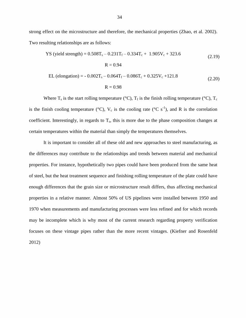
study determined a relationship between the thermo-mechanical processing effects, showing a
34
strong effect on the microstructure and therefore, the mechanical properties (Zhao, et al. 2002).
Two resulting relationships are as follows:
YS (yield strength) = 0.508Ts – 0.231Tf – 0.334Tc + 1.905Vc + 323.6 (2.19)
R = 0.94
EL (elongation) = - 0.002Ts – 0.064Tf – 0.086Tc + 0.325Vc +121.8 (2.20)
R = 0.98
Where Ts is the start rolling temperature (°C), Tf is the finish rolling temperature (°C), Tc
is the finish cooling temperature (°C), Vc is the cooling rate (°C s-1
), and R is the correlation
coefficient. Interestingly, in regards to Ts, this is more due to the phase composition changes at
certain temperatures within the material than simply the temperatures themselves.
It is important to consider all of these old and new approaches to steel manufacturing, as
the differences may contribute to the relationships and trends between material and mechanical
properties. For instance, hypothetically two pipes could have been produced from the same heat
of steel, but the heat treatment sequence and finishing rolling temperature of the plate could have
enough differences that the grain size or microstructure result differs, thus affecting mechanical
properties in a relative manner. Almost 50% of US pipelines were installed between 1950 and
1970 when measurements and manufacturing processes were less refined and for which records
may be incomplete which is why most of the current research regarding property verification
focuses on these vintage pipes rather than the more recent vintages. (Kiefner and Rosenfeld
2012)

35
CHAPTER III: DESTRUCTIVE TESTS
Currently, the most accurate determination of yield strength has been obtained through
destructive testing. (Garcia, et al. 2014) API Specification 5L presents a spectrum of destructive
tests required on a sample before a pipeline is deemed suitable for service. This specification
references several other standards, the most relevant to this literature review being ASTM A370:
“Standard Test Methods and Definitions for Mechanical Testing of Steel Products. One crucial
unknown is the accuracy of these methods. Many are used as standards, but do not have
accompanying performance specifications. However, recent research is being performed by
several steel manufacturers to improve their testing methods to observe the effects of the
differences in procedures, which will be discussed within later sections of this chapter.
Yield and Tensile Tests
The yield point is defined as the first stress in a material that exists where strain occurs
without an increase in the stress, which is only defined for materials that show increases in strain
without increases in stress. (ASTM 1997) The yield point can be determined by a few different
methods. One is known as “drop of the beam” or “halt of the pointer method,” which applies a
uniformly increasing load until the yield point is reached, at which time the beam of the machine
will stop for a brief moment. The corresponding stress measured is the yield point. The
“autographic diagram method” simply uses the stress-strain diagram obtained by an autographic
recording device, and then takes the stress corresponding to the top of the sharp-knee, or where
the curve drops, to be the yield point. There is the potential that the tests above will not provide a
well-defined measurement, in which case a “total extension under load (EUL) method” can be
employed. This method, as described in the ASTM A370 standard, attaches a Class C or better
36
extensometer to the specimen and as the load is applied, once a certain extension is reached, the
stress corresponding to this load is given as the yield point. This is commonly used for pipeline
steel, and is referred to as such in following sections for strength tests.
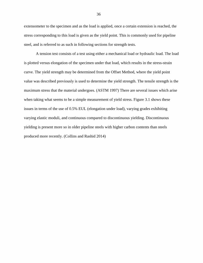
A tension test consists of a test using either a mechanical load or hydraulic load. The load
is plotted versus elongation of the specimen under that load, which results in the stress-strain
curve. The yield strength may be determined from the Offset Method, where the yield point
value was described previously is used to determine the yield strength. The tensile strength is the
maximum stress that the material undergoes. (ASTM 1997) There are several issues which arise
when taking what seems to be a simple measurement of yield stress. Figure 3.1 shows these
issues in terms of the use of 0.5% EUL (elongation under load), varying grades exhibiting
varying elastic moduli, and continuous compared to discontinuous yielding. Discontinuous
yielding is present more so in older pipeline steels with higher carbon contents than steels
produced more recently. (Collins and Rashid 2014)

37
Figure 3.1 Schematic of stress-strain curves illustrating the sources of variability.
[Printed with permission (Collins and Rashid 2014)]
A flattened strap test or round bar test is most commonly used in engineering facilities for
determining yield and tensile strength due to its relative ease of use and requirement for less
specialized equipment. The flattened strap test is done by performing a three or four-point
bending method to flatten the rounded pipe, shown in Figure 3.2. Any residual spring back from
the flat press should be avoided to gain optimal results.

38
Figure 3.2 Example of flattening using a 4-point bending method with image of tensile
round bar sample shown in green [Printed with permission (Cooreman, et al. 2014)]
The flattening operation is not a standard procedure, and an unknown variability tends to
be introduced into the samples as a result. A recent study performed shows that variability in
properties can be introduced by the method used and how exactly the procedures are performed,
with a standard deviation of test results at as high as 26.2 MPa (3800 psi). (Collins and Rashid
2014) A previous study examined the effect of testing methods on high strength steel pipe, and
found similar variability, where differences could occur between different test labs even while
using the same procedure, differences could occur within test specimens and pressurized pipe,
and that the Bauschinger effect should be considered. (Millwood, et al. 2004) The Bauschinger
effect is a result of cold-flattening the material producing a lower measured yield strength, which
is known to be more pronounced in higher strength steel pipe. (Knoop, et al. 2001)
A round bar test has to overcome challenges of its own, because the diameter of the
sample is substantially less than the material from which it was machined, and therefore the
results may not be reflective of the properties of the through thickness properties of the pipe.
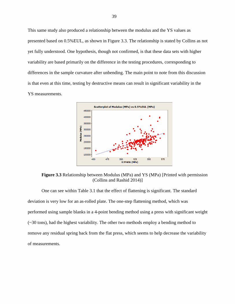
39
This same study also produced a relationship between the modulus and the YS values as
presented based on 0.5%EUL, as shown in Figure 3.3. The relationship is stated by Collins as not
yet fully understood. One hypothesis, though not confirmed, is that these data sets with higher
variability are based primarily on the difference in the testing procedures, corresponding to
differences in the sample curvature after unbending. The main point to note from this discussion
is that even at this time, testing by destructive means can result in significant variability in the
YS measurements.
Figure 3.3 Relationship between Modulus (MPa) and YS (MPa) [Printed with permission
(Collins and Rashid 2014)]
One can see within Table 3.1 that the effect of flattening is significant. The standard
deviation is very low for an as-rolled plate. The one-step flattening method, which was
performed using sample blanks in a 4-point bending method using a press with significant weight
(~30 tons), had the highest variability. The other two methods employ a bending method to
remove any residual spring back from the flat press, which seems to help decrease the variability
of measurements.

40
Table 3.1 Effect of Flattening on Mechanical Properties [Printed with permission
(Collins and Rashid 2014)]
Condition Average
YS (MPa)
YS Std Dev
(MPa)
Average
UTS (MPa)
UTS Std
Dev (MPa)
Modulus
(GPa)
Modulus
Std Dev
(GPa)
Plate 558 5.9 630 2.7 252 2.45
One Step
Flattening 528 26.2 647 4.0 196 17.0
Two Step
Flattening 531 16.3 646 5.4 209 17.1
Three Point
Bend 535 7.9 647 4.7 205 15.8
A ring expansion test is considered by the industry to be the most accurate way to
measure yield strength. This test is carried out by measuring the diameter and stress values of a
short ring of pipe that is then expanded. The data obtained from this test can be used to create the
stress-strain curve for determining yield stress. (ASTM 1997) While these tests are more
accurate, it is more difficult to perform, and testing is cumbersome and time consuming,
particularly for samples with large diameters. A finite element analysis (FEA) was performed in
a study to find that ring expansion tests yield the highest values for yield strength and tests on
round bar sample yield the lowest values, whereas flattened samples are seeing much more
variability in general. (Cooreman, et al. 2014)
Bend Tests
The bend test is a measure of ductility, but is not quantitative for predicting service
performance. The specimen is bent to certain inside diameter specifications, and is then
examined for any cracking on the outside of the material. (ASTM 1997)
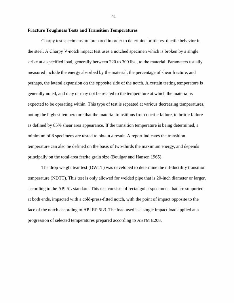
41
Fracture Toughness Tests and Transition Temperatures
Charpy test specimens are prepared in order to determine brittle vs. ductile behavior in
the steel. A Charpy V-notch impact test uses a notched specimen which is broken by a single
strike at a specified load, generally between 220 to 300 lbs., to the material. Parameters usually
measured include the energy absorbed by the material, the percentage of shear fracture, and
perhaps, the lateral expansion on the opposite side of the notch. A certain testing temperature is
generally noted, and may or may not be related to the temperature at which the material is
expected to be operating within. This type of test is repeated at various decreasing temperatures,
noting the highest temperature that the material transitions from ductile failure, to brittle failure
as defined by 85% shear area appearance. If the transition temperature is being determined, a
minimum of 8 specimens are tested to obtain a result. A report indicates the transition
temperature can also be defined on the basis of two-thirds the maximum energy, and depends
principally on the total area ferrite grain size (Boulgar and Hansen 1965).
The drop weight tear test (DWTT) was developed to determine the nil-ductility transition
temperature (NDTT). This test is only allowed for welded pipe that is 20-inch diameter or larger,
according to the API 5L standard. This test consists of rectangular specimens that are supported
at both ends, impacted with a cold-press-fitted notch, with the point of impact opposite to the
face of the notch according to API RP 5L3. The load used is a single impact load applied at a
progression of selected temperatures prepared according to ASTM E208.

42
CHAPTER IV: NONDESTRUCTIVE TESTS
In-Line Inspection Technology
In-line inspections (ILI) are a common form of nondestructive test currently performed
on pipelines. This is due in part to their relative ease of use, feasibility to inspect many miles of
pipeline within a manageable time frame, and the improvement in technology over the years.
(Barbian, et al. 2007) Magnetic flux leakage (MFL) is used most commonly for determining
metal loss and other similar defects on the pipelines, and ultrasonic inspections are useful in
determining crack-like indications as well as metal loss. Therefore, it is reasonable to explore
these technologies and what recent advancements have shown to provide in determining pipe
properties.
Magnetic Flux Leakage
A number of in-line inspection companies are beginning to use a low-field magnetization
(LFM) technique instead of, or in addition to, their now traditional high resolution MFL tools to
locate hard spots in older pipe and areas of mechanical equipment damage in all pipe as these are
both potentially serious threats to integrity. An example of a hysteresis curve is shown in Figure
4.1, and indicates the relationship between magnetic induction and the applied magnetic field for
a typical pipeline steel.

43
Figure 4.1 B-H curve for a typical sample of pipeline steel. [Printed with permission
(Belanger and Narayanan 2006)]
The catalyst to using this mode of measurement was determining a relationship shown
between the Gauss measurements and the wall thicknesses. The first inspections using this
technology utilized one tool to magnetize the pipe and one to measure the residual
magnetization. (Crump and Papenfuss 1991) A study by Nestleroth and Crouch show that
hardness is strongly correlated to the magnetic coercivity of pipeline steel, which has a
correlation coefficient of 0.83. Furthermore, the relationship between hardness is shown to have
a correlation coefficient of 0.86 with yield strength, and 0.96 with ultimate tensile strength. The
table with correlations coefficients has been recreated in Table 4.1.
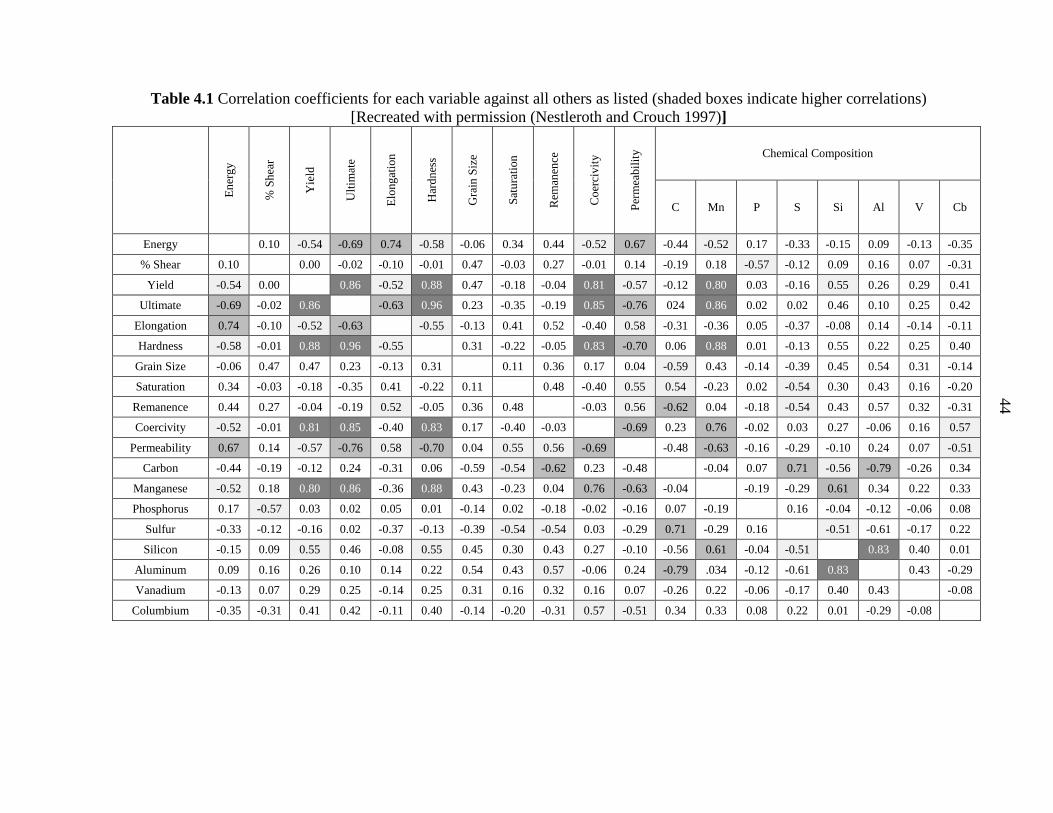
44
Table 4.1 Correlation coefficients for each variable against all others as listed (shaded boxes indicate higher correlations)
[Recreated with permission (Nestleroth and Crouch 1997)]
En
erg
y
% S
hea
r
Yie
ld
Ult
imat
e
Elo
ng
atio
n
Har
dn
ess
Gra
in S
ize
Sat
ura
tion
Rem
anen
ce
Co
erci
vit
y
Per
mea
bil
ity
Chemical Composition
C Mn P S Si Al V Cb
Energy 0.10 -0.54 -0.69 0.74 -0.58 -0.06 0.34 0.44 -0.52 0.67 -0.44 -0.52 0.17 -0.33 -0.15 0.09 -0.13 -0.35
% Shear 0.10 0.00 -0.02 -0.10 -0.01 0.47 -0.03 0.27 -0.01 0.14 -0.19 0.18 -0.57 -0.12 0.09 0.16 0.07 -0.31
Yield -0.54 0.00 0.86 -0.52 0.88 0.47 -0.18 -0.04 0.81 -0.57 -0.12 0.80 0.03 -0.16 0.55 0.26 0.29 0.41
Ultimate -0.69 -0.02 0.86 -0.63 0.96 0.23 -0.35 -0.19 0.85 -0.76 024 0.86 0.02 0.02 0.46 0.10 0.25 0.42
Elongation 0.74 -0.10 -0.52 -0.63 -0.55 -0.13 0.41 0.52 -0.40 0.58 -0.31 -0.36 0.05 -0.37 -0.08 0.14 -0.14 -0.11
Hardness -0.58 -0.01 0.88 0.96 -0.55 0.31 -0.22 -0.05 0.83 -0.70 0.06 0.88 0.01 -0.13 0.55 0.22 0.25 0.40
Grain Size -0.06 0.47 0.47 0.23 -0.13 0.31 0.11 0.36 0.17 0.04 -0.59 0.43 -0.14 -0.39 0.45 0.54 0.31 -0.14
Saturation 0.34 -0.03 -0.18 -0.35 0.41 -0.22 0.11 0.48 -0.40 0.55 0.54 -0.23 0.02 -0.54 0.30 0.43 0.16 -0.20
Remanence 0.44 0.27 -0.04 -0.19 0.52 -0.05 0.36 0.48 -0.03 0.56 -0.62 0.04 -0.18 -0.54 0.43 0.57 0.32 -0.31
Coercivity -0.52 -0.01 0.81 0.85 -0.40 0.83 0.17 -0.40 -0.03 -0.69 0.23 0.76 -0.02 0.03 0.27 -0.06 0.16 0.57
Permeability 0.67 0.14 -0.57 -0.76 0.58 -0.70 0.04 0.55 0.56 -0.69 -0.48 -0.63 -0.16 -0.29 -0.10 0.24 0.07 -0.51
Carbon -0.44 -0.19 -0.12 0.24 -0.31 0.06 -0.59 -0.54 -0.62 0.23 -0.48 -0.04 0.07 0.71 -0.56 -0.79 -0.26 0.34
Manganese -0.52 0.18 0.80 0.86 -0.36 0.88 0.43 -0.23 0.04 0.76 -0.63 -0.04 -0.19 -0.29 0.61 0.34 0.22 0.33
Phosphorus 0.17 -0.57 0.03 0.02 0.05 0.01 -0.14 0.02 -0.18 -0.02 -0.16 0.07 -0.19 0.16 -0.04 -0.12 -0.06 0.08
Sulfur -0.33 -0.12 -0.16 0.02 -0.37 -0.13 -0.39 -0.54 -0.54 0.03 -0.29 0.71 -0.29 0.16 -0.51 -0.61 -0.17 0.22
Silicon -0.15 0.09 0.55 0.46 -0.08 0.55 0.45 0.30 0.43 0.27 -0.10 -0.56 0.61 -0.04 -0.51 0.83 0.40 0.01
Aluminum 0.09 0.16 0.26 0.10 0.14 0.22 0.54 0.43 0.57 -0.06 0.24 -0.79 .034 -0.12 -0.61 0.83 0.43 -0.29
Vanadium -0.13 0.07 0.29 0.25 -0.14 0.25 0.31 0.16 0.32 0.16 0.07 -0.26 0.22 -0.06 -0.17 0.40 0.43 -0.08
Columbium -0.35 -0.31 0.41 0.42 -0.11 0.40 -0.14 -0.20 -0.31 0.57 -0.51 0.34 0.33 0.08 0.22 0.01 -0.29 -0.08

45
Simple analytical models were examined to determine what relationship would be most
accurate, with the resulting best-fit model incorporating a natural logarithmic fit to determine the
hardness of a steel sample given its applied magnetic field and the magnetic induction, as shown
in Figure 4.2.
Figure 4.2 B-H curves of different hardness generated for natural logarithmic fit to
extrapolated measured data from the GRI study of pipeline steels. [Printed with permission from
(Belanger and Narayanan 2006)]
Within the results shown in Figure 4.2, there is still room for improvement by improving
the resolution of the applied field. It should also be noted that the curves are quite close together,
and depending on the error inherent within magnetic measurements, it may prove difficult to
obtain measurements with enough precision, but this may be overcome in time with further
understanding of the remanence relationship to hardness, and looking at saturation points where
harder materials become less permeable. Recent advancements in tools now apply a
magnetization at a level near the maximum permeability region to differentiate the material
property differences using a single tool. (Pollard, et al. 2004) By using these methods,
quantifiable hardness measurements are becoming a possibility, rather than simply observing a
qualitative difference. There are also distinguishable differences observed between the methods
by which the material was hardened, either by heat treatments or quenching of the material.
46
(Belanger and Barker 2014) Figure 4.3 provides the c-scans from the various modes of
measurement, indicating the measureable differences in air-cooled steel on the left, and the
quenched steel on the right. The air-cooling process softens the steel whereas quenching will
create a highly localized region of hardness, which is very well detected by the tool.
Figure 4.3 Data from the 18 inch multiple data sets (MDS) tool for the heat treated spot
in 0.375-inch wall thickness at 1700° F. The first column is for the air cooled spot and the
second column for the quenched, starting from the top row down are the hardness, high-field,
low-field, IDOD, internal deformation geometry, and DEF. [Printed with permission from
(Belanger and Barker 2014)]
There appears to be a relationship between the Gauss measurements for the high-field
MFL tool and the hardness based on the reduction of a dependence on material properties, and

47
the lower resolution MFL is able to detect this based on its higher saturation level. Using these
concepts, this tool could detect differences in the hardness of pipe and relate this to the yield
strength. If able to determine distinct differences, fewer verification digs would need to be
performed to determine the properties of the pipe. Improvements in this technology may lead to
more precise measurements, which in turn, could lead to better understanding of the relationship
between these material measurements and mechanical measurements. However, more work
needs to be done to fully understand how hardness, permeability, remanance, and coercivity
relate to yield strength.
Eddy Current
Eddy current technology is used minimally for in-line inspections due to its limitations in
penetration depth. It has been shown that eddy current can be used, with certain mathematical
models, to obtain mechanical materials properties for sheet metal to an accuracy of with +/-2%
for tensile strength and +/-4% for breaking elongation. (Heingartner, et al. 2009) Eddy current
systems have a high sensitivity to changes in the microstructure of a material, and are therefore a
valuable measurement method for evaluating the mechanical properties, if a correlation between
these properties exists. (Schwind 1998); (Maass 2001) Currently, however, only material
differences can be clearly identified, not a quantitative strength value.
One ILI vendor has recently developed an approach to determining pipe grade through
eddy current testing with pre-magnetization which is claimed to increase the penetration depth of
the eddy currents, minimize possible fluctuations, and result in a more stable response from the
measurement system. (Molenda and Thale 2014) By applying an appropriate excitation
frequency, the depth penetration is small enough that the effects of wall thickness are negligible
down to wall thicknesses of 3 to 4 mm. Once decent levels of excitation frequency and pre-

48
magnetization levels were applied, a good correlation is shown from the measurements taken and
the yield strength and tensile strength, shown in Figure 4.4.
Figure 4.4 Eddy current response shown in arbitrary units versus yield strength and ultimate
tensile strength. [Reproduced with permission (Molenda and Thale 2014)]
The preliminary pull tests of the technology on an ILI tool indicate that accuracies of ±40
MPa (5801 psi) for the electromagnetic determination can be achieved; however, accuracies of
±9 MPa (1305 psi) may be considered for tensile strength and ±14 MPa (2030 psi) for yield
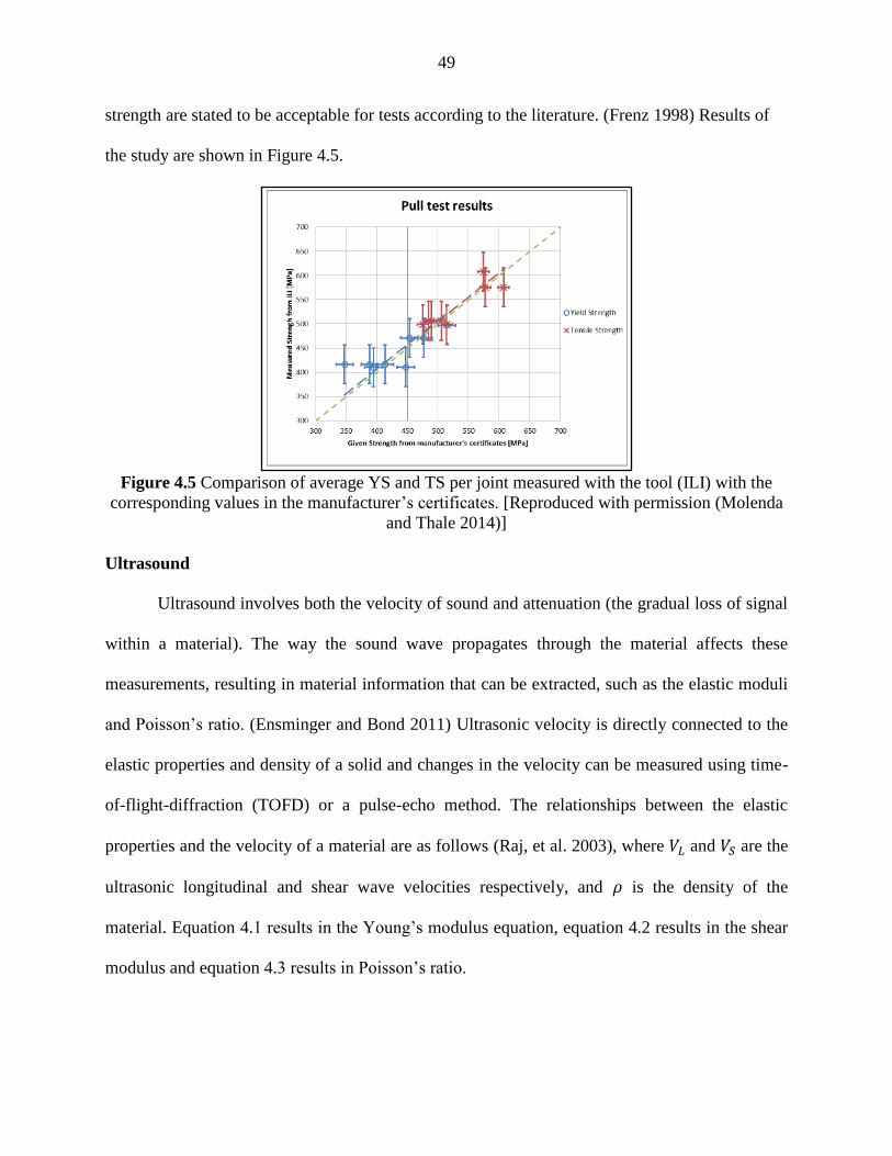
49
strength are stated to be acceptable for tests according to the literature. (Frenz 1998) Results of
the study are shown in Figure 4.5.
Figure 4.5 Comparison of average YS and TS per joint measured with the tool (ILI) with the
corresponding values in the manufacturer’s certificates. [Reproduced with permission (Molenda
and Thale 2014)]
Ultrasound
Ultrasound involves both the velocity of sound and attenuation (the gradual loss of signal
within a material). The way the sound wave propagates through the material affects these
measurements, resulting in material information that can be extracted, such as the elastic moduli
and Poisson’s ratio. (Ensminger and Bond 2011) Ultrasonic velocity is directly connected to the
elastic properties and density of a solid and changes in the velocity can be measured using time-
of-flight-diffraction (TOFD) or a pulse-echo method. The relationships between the elastic
properties and the velocity of a material are as follows (Raj, et al. 2003), where 𝑉𝐿 and 𝑉𝑆 are the
ultrasonic longitudinal and shear wave velocities respectively, and 𝜌 is the density of the
material. Equation 4.1 results in the Young’s modulus equation, equation 4.2 results in the shear
modulus and equation 4.3 results in Poisson’s ratio.

50
𝐸 = 𝜌𝑉𝑠2(3𝑉𝐿
2 − 4𝑉𝑆2)/(𝑉𝐿
2 − 𝑉𝑆2) (4.1)
𝐺 = 𝜌𝑉𝑆2 (4.2)
𝑣 =1
2(𝑉𝐿
2 − 2𝑉𝑆2)/(𝑉𝐿
2 − 𝑉𝑆2) (4.3)
Using acousto-elastic principles, the ultrasonic velocity changes linearly with elastic
strain, where 𝑉 and 𝑉𝑜 are the ultrasonic velocities in the stressed and unstressed conditions, 𝜎 is
the stress, and 𝐴 is the acousto-elastic constant.
𝑉 = 𝑉𝑜 + 𝐴𝜎 (4.4)
The Young’s modulus 𝐸 and ultrasonic velocity 𝑉 can then be related to the volume
fraction of porosity as:
𝐸 = 𝐸𝑜exp (−𝑏𝑝) (4.5)
𝑉 = 𝑉𝑜exp (−𝑏𝑝) (4.6)
Looking at these property relationships, it is obvious that the velocity measurement is
useful for determining material properties such as moduli, Poisson’s ratio, stresses, texture,
porosity, and microstructure characterization. (Raj, et al. 2003) These measurements, in turn, can
provide useful information about the strength and toughness properties of the pipe material.
Ultrasonic measurements have been used in estimating average grain sizes for austenitic
stainless steel using the pulse-echo-overlap technique and relating the velocity with
metallographically obtained grain sizes. (Palanichamy, et al. 1995)
Ultrasonic backscatter measurements methods, which are similar to those of the pulse-
echo method, are able to provide measurements which can produce the grain size quantitatively
and microstructural information qualitatively. (Willems and Goebbels 1981)

51
Freitas showed that the ultrasonic measurements of velocity and attenuation are capable
of identifying microstructures in steels. These measurements can also identify changes in the
microstructure produced by heat treatments, but are not as sensitive to chemical content changes
in terms of carbon content. Elastic constants (E and G) were also calculated from ultrasonic
measurements via the equations (4.1) and (4.2), and show consistency with dynamic and static
methods. (Freitas, et al. 2010) The relationship between elastic moduli and the wave velocity
was also supported by an earlier work by Vary. (Vary 1980)
Stanke and Kino showed a relationship between ultrasonic attenuation and grain size by
using a second-order, multiple-scattering theory to determine the attenuation and change in phase
velocity due to the grain scattering. (Stanke and Kino 1984) Palanchamy provides an
experimental relationship between velocity and grain size for stainless steel. (Palanichamy, et al.
1995) Other conclusions from this work showed that velocity measurements likely give more
accurate grain size measurements compared to attenuation measurements, and shear waves are
more sensitive to grain size estimation as compared with longitudinal waves.
Backscattered grain noise can be used to characterize the microstructure for metallic
materials. (Margetan, et al. 1999) The noise is analyzed to determine a backscatter coefficient,
which provides information about the grain size and orientation within the overall
microstructure. Knowing the backscatter coefficient also allows an estimate of the level of noise
present in an inspection, helping to determine the probability of detecting a defect, as well.
While methods of ultrasonic inspection are being applied and developed for managing
current integrity threats, there has not been as much work done in advancing ultrasonic
technology for the determination of pipeline properties specifically. However, the ground work

52
for understanding and applying the knowledge base shows that opportunities exist for
development.
A project was recently initiated with one task involving determining the viability of using
ultrasonic measurements for determining grain size on pipeline in order to verify pipeline
properties. (Engle, et al. 2014) The longitudinal velocity, attenuation, and backscattered grain
noise were all measured for the preliminary measurements. The samples provided for the study
included grain size measurements obtained by traditional metallographic techniques to correlate
with the grain size results obtained through the use of UT.
The results of this study, although quite preliminary, may show some promising results.
For the velocity measurements of the three samples, there was a positive correlation noted
between the yield strength of the pipe and velocity, as well as the tensile strength of the pipe and
velocity. An inverse relationship was found between the percent ferrite content and the velocity.
The attenuation was measured for the three samples, but the amount of variation in the
measurements was too great to determine any valid relationships with the limited data set. This is
likely due to curvature within one of the pipe samples not able to be accounted for in these
preliminary measurements, but the study does mention that this measurement should still be
considered once a larger data set is obtained.
The backscattered grain noise was measured and evaluated using a series of calculations
and processing algorithms to determine grain size. The results of this mode of measurement were
also promising, but more work needs to be done to the samples themselves to eliminate any
potential cause of variation to the measurements, such as the surface roughness.

53
In-Ditch Inspection Technology
Chemical Composition
Typical methods for determining the chemical composition of a carbon steel material are
based on positive material identification (PMI), and may include x-ray fluorescence (XRF) or
optical emission spectroscopy (OES). XRF uses a beam of x-rays which are emitted into the
material, the atoms of the material absorb the x-rays, and each element emits x-rays in return at a
unique energy. The characteristic energy reported back to the detector can then determine what
the chemical make-up of the material is. (Pyromation 2014) These instruments are relatively easy
to use, and the material does not require much preparation in order to obtain a good result,
however, the XRF cannot measure ‘light’ metal elements such as carbon. OES excites the atoms
of a material using a spark formed between the sample and electrode, which then emits a light.
That light, or, the intensity of the peaks of the spectrum of light produced, is analyzed according
to its spectral pattern. OES instruments are typically larger than XRF devices, but they will
typically be able to measure carbon, silicon, chromium, molybdenum, nickel, aluminum, copper,
and niobium chemical contents. A drawback to this technique is that the OES instruments are
typically larger, require the use of argon gas for decent accuracy, and a burn mark is left on the
pipe surface. However, some companies are working on more portable devices.
[http://www.oxford-instruments.com/products/spectrometers/optical-emission-
spectroscopy/smart], [http://www.verichek.net/product/pmi-master-pro-mobile-oes] There is also
a PMI spectrograph method using a UV probe to measure the chemical contents of nitrogen,
carbon, phosphorous, sulfur, tin, arsenic, and boron. With normal arc probes, one can measure
iron, aluminum, copper, nickel, titanium, magnesium, cobalt, and zinc alloys. [Communication
with Nedim Kaniza A+Norway]
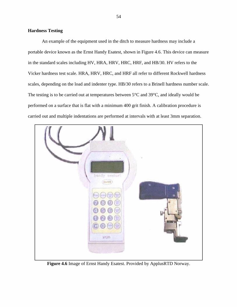
54
Hardness Testing
An example of the equipment used in the ditch to measure hardness may include a
portable device known as the Ernst Handy Esatest, shown in Figure 4.6. This device can measure
in the standard scales including HV, HRA, HRV, HRC, HRF, and HB/30. HV refers to the
Vicker hardness test scale. HRA, HRV, HRC, and HRF all refer to different Rockwell hardness
scales, depending on the load and indenter type. HB/30 refers to a Brinell hardness number scale.
The testing is to be carried out at temperatures between 5°C and 39°C, and ideally would be
performed on a surface that is flat with a minimum 400 grit finish. A calibration procedure is
carried out and multiple indentations are performed at intervals with at least 3mm separation.
Figure 4.6 Image of Ernst Handy Esatest. Provided by ApplusRTD Norway.

55
A digital version is also available, known as the HB100 Portable Digital Microscope,
shown in Figure 4.7. This equipment must be used in a dry environment, and surface preparation
is done according to the hardness procedure. A calibration process is performed, and indentations
are collected at intervals spaced not less than 8mm. The test temperature should be between -5°C
and 45°C.
Figure 4.7 Image of On-site Hardness HB100 Digital Microscope. Provided by
ApplusRTD Norway.

56
Grain Size Determination
Microscopy may be used to determine grain size on site and in the ditch, after a
metallographic sample is prepared using mechanical polishing. There are a wide variety of
international standards for analyzing the grain sizes and structures, but ASTM E112 is the
standard most widely used in North America. Standard optical microscopy is used to view the
grain structure and analyze the average grain size. Micro and macro investigation can be
performed for most materials using this approach. (Brinson, et al. 2004) This is admittedly much
easier to perform in a laboratory setting, and has significant challenges in the ditch, as conditions
may not always be ideal.
Microstructure
Nondestructive testing techniques are valuable and becoming more developed to
determine the microstructure of a material, beyond the optical methods commonly used, and
currently being used for in-situ examination of pipeline. For instance, ultrasonic methods can be
used to determine the microstructure, using ultrasonic velocity ratios to correlate with various
microstructural parameters. (Ramuhalli, et al. 2012) The application of this technique to the
steels found in pipeline material has yet to be solidified, however.
Magnetic methods have been used to characterize microstructure; in particular, the testing
method using Barkhausen noise (BN) can provide very useful information about the
microstructure. One study presents the potential that barkhausen noise can identify
microstructural changes and microcracking, and that these changes can be correlated with the
mechanical behavior and modification of the microstructure. (Zergoug, et al. 2006)

57
CHAPTER V: CASE STUDY AND CONCLUSIONS
Sample Data Information
A set of 94 sample data test coupons were evaluated at the Kiefner and Associates, Inc
lab and are used here for preliminary evaluation of potential relationships between material and
mechanical properties. Measurements taken on the test coupons included grain size, percent
ferrite, percent inclusion content, yield strength, tensile strength, elongation, hardness, full size
equivalent (FSE) Charpy v-notch (CVN) energy (toughness), transition temperature, and
chemical content (C, Mn, S, P, Al, Si, Nb, V, Ti, Cr, Mo, Cu, Ca, Ni, Sn, Zr, Co, B). Information
such as pipe diameter, wall thickness, grade, seam weld type, and vintage was also provided.
However, not all samples have a complete set of measurements and information available for
comparison. The samples currently encompass the following range of pipeline steels:
Vintage: 1939 to 2013
Diameter: 4-inch to 24-inch
Wall Thickness: 0.156-inch to 0.500-inch
Grade: Grade B to X65
Seam Types: ERW -DC, -LF, -HF; Flashweld; Lapweld; Seamless
Grain Size: ASTM 5.9 to ASTM 13.7
It should be noted that approximately half of the samples available have unknown
original specified properties as described above, leaving a remaining 47 samples with full
property characterization. This information was obtained through traditional techniques,
including destructive and non-destructive testing. The bar charts in Figure 5.1 indicate at what
frequency each specific grade, seam weld, diameter, wall thickness, or vintage is present in the

58
samples. The most common pipe attributes for the data set include grade X52 pipe, ERW seam
welds, and wall thicknesses of 0.25-inch, with the rest of the properties fairly evenly distributed
among the samples. Grain sizes range from 5.9 to 13.7 ASTM, with sizes predominantly between
10 and 12.5 ASTM.
Figure 5.1 Frequency of pipe properties available from Kiefner sample data set.
The data was collected from an assortment of sources, but all were from in-service pipe.
Some may have been failure pieces, others may have been from replacement cut-out sections of
pipe. Any tests performed on these pieces would have been from far enough away from the
failure site that the fracture origin will not have an effect on the base metal. The testing carried
out provided the data for the following conclusions.
General Correlations
Trends were observed in the available data by plotting each variable against the other,
shown in Figure 5.2. These correlation plots were created to relate the most likely property
relationships as understood by the background information given to determine yield and tensile

59
strength. There are stronger linear relationships between, yield strength and hardness, and yield
strength and %Mn than the other variables present.
Based on the background knowledge of the advancements in manufacturing processes
over the years causing potential for variability in trends, particularly with regards to chemical
content, the data was filtered by vintage as opposed to using this variable as a comparison within
the relationships. Figure 5.3 shows the same plots with vintage listed instead on the color scale
so that features can be picked out as to what general timeframe they are within on the correlation
plots. Differing vintages tend to be clustered in certain locations within the plots. For example,
the blue data points (pipe installed post-1980) tend to be clustered, and occasionally isolated
from the majority of the red and grey data points (pipe installed pre-1980). The newer pipe
(indicated by the blue data points) tends to not fit the trends as often, and appears to show a
different trend than the older pipe. This occurs for nearly all the correlations shown in this Figure
5.3.
After filtering the data to remove pipe that is newer than 1980, in Figure 5.4 we can see
that the %C content relationships are improved. We are also seeing quite a bit more scatter in the
%Mn to yield strength relationship than was observed previously, indicating our linear
relationship was primarily based on the vintage and secondarily based on the correlation between
%Mn and yield strength.
In Figure 5.5, the filter has been applied to show only pipe newer than 1980. This data set
is considerably smaller, making it more difficult to be confident in the trends shown. However,
the correlation between yield strength and hardness, yield strength to %Mn, yield strength to
%C, %Mn to hardness, and grain size to hardness are all improved.

60
Correlation coefficients for the primary relationships discussed above are shown in Table
5.1, as separated by vintage. It is interesting to note the shift in correlation with regards to %C.
The correlation is quite poor for yield strength to %C and %C to hardness for the entire data set,
but is greatly improved upon the division of vintages. This indicates a difference in the
relationship in %C for older pipe material versus newer pipe material, and thus when developing
and applicatory result, vintage will need to play a role in determining yield strength if one is to
include carbon content.
Table 5.1 Notable correlation coefficients for yield strength, grain size, hardness %Mn, %C
Variables R
2 for <1980
Vintages
R2 for All
Vintages
R2 for >1980
Vintages
YS to
Hardness 0.65 0.72 0.95
YS to Grain
Size 0.15 0.34 0.28
YS to %Mn 0.32 0.50 0.61
YS to %C 0.24 0.17 0.46
%Mn to
Hardness 0.41 0.54 0.69
%C to
Hardness 0.52 0.01 0.43
Grain Size
to Hardness 0.16 0.28 0.34

61
Figure 5.2 Linear regression plot comparisons for Yield, Hardness, Grain Size, Vintage, %Mn, %C, %Si, %S.

62
Figure 5.3 Linear regression plots comparisons for Yield, Hardness, Grain Size, %Mn, %C, %Si, %S. Vintage is provided via a
color scale as shown within the figure – blue indicates newer vintage, red indicates older.

63
Figure 5.4 Linear regression plots comparisons for Yield, Hardness, Grain Size, %Mn, %C, %Si, %S. Vintage is filtered for pipe
older than 1980 and is provided via a color scale as shown within the figure – blue indicates newer vintage, red indicates older.

64
Figure 5.5 Linear regression plots comparisons for Yield, Hardness, Grain Size, %Mn, %C, %Si, %S. Vintage is filtered for pipe
newer than 1980 and is provided via a color scale as shown within the figure – blue indicates newer vintage, red indicates older.

65
Chemical Content Correlations
Toughness is more strongly correlated to chemical content than the other available
material properties. The increase of carbon tends to have opposite effects on the strength as it
does toughness and weldability. (Boulgar and Hansen 1965)
The chemical content for all available sample data was observed in relation to the FSE
CVN energy. Table 5.2 provides the correlation coefficients for comparison. The strongest
correlations lie within %C, %Si, and %Ti. Figure 5.6, Figure 5.7, and Figure 5.8 provide the
plots of the data according to chemical content with color scale gradient again indicating pipe
vintage. As one would expect, there appears to be some segregation of data between the older
and newer vintage pipes. This is likely the result of improved manufacturing processes
increasing toughness while maintaining weldability through the addition of alloying elements
and process improvements.
Table 5.2 Correlation coefficients for FSE-CVN energy to chemical content.
Chemical R2 for FSE Chemical R
2 for FSE
%Mn 0.05 %Ca 0.13
%C 0.46 %Nb 0.23
%S 0.27 %P 0.02
%Si 0.49 %Ti 0.43
%Al 0.38 %V 0.16
%B 0.00 %Cu 0.03
%Co 0.03 %Sn 0.01
%Cr 0.09 %Zr 0.10

66
Figure 5.6 Linear regression plots comparisons for FSE, %Mn, %C, %S, %Si, and %Al. Vintage is provided via a color
scale as shown within the figure – blue indicates newer vintage, red indicates older.
Figure 5.7 Linear regression plots comparisons for FSE, %Ca, %Nb, %P, %Ti, %V. Vintage is provided via a color scale
as shown within the figure – blue indicates newer vintage, red indicates older.
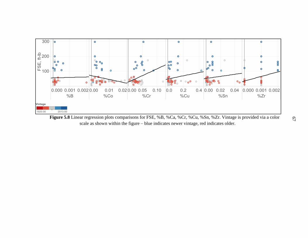
67
Figure 5.8 Linear regression plots comparisons for FSE, %B, %Ca, %Cr, %Cu, %Sn, %Zr. Vintage is provided via a color
scale as shown within the figure – blue indicates newer vintage, red indicates older.

68
The chemical properties were also correlated with the yield strength, shown in Figure 5.9.
There appears to be a very good positive linear relationship between the %Mn and yield strength.
There is also trending in the %Si and %C content versus yield strength, but there are likely other
factors to consider, as the correlation is not extremely strong. There seems to be a negative
relationship between %C and yield strength based on the data available, which contradicts our
understanding the increasing carbon content should increase strength. However, the blue data
points represent the newer pipe, and are skewing the data set. The correlation coefficients are
provided in Table 5.3.
Figure 5.9 Linear regression plots comparisons for Yield Strength, %Mn, %C, %S, %Si, and
%Al. Vintage is provided via a color scale as shown within the figure – blue indicates newer
vintage, red indicates older.
Table 5.3 Correlation coefficients for Yield Strength to %Mn, %C, %S, %Si, and %Al.
Chemical R2
%Mn 0.705
%C 0.416
%S 0.388
%Si 0.688
%Al 0.616
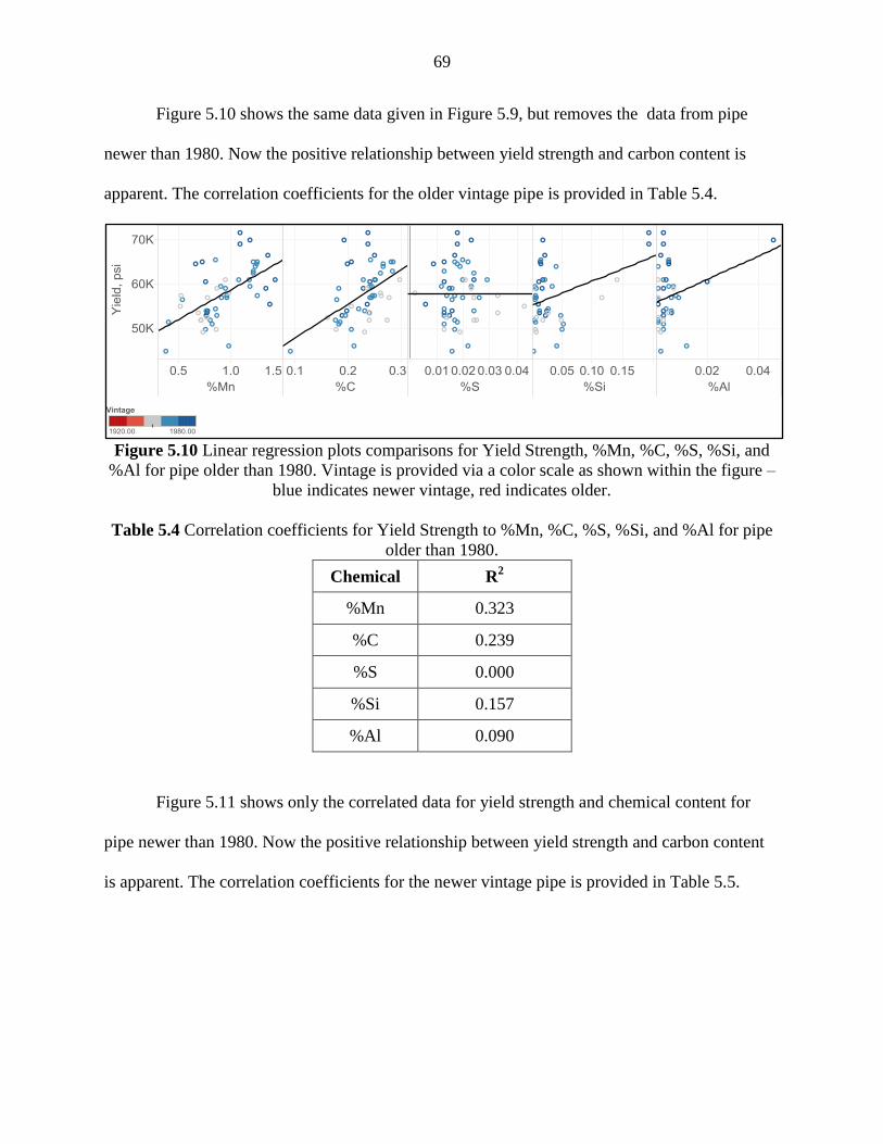
69
Figure 5.10 shows the same data given in Figure 5.9, but removes the data from pipe
newer than 1980. Now the positive relationship between yield strength and carbon content is
apparent. The correlation coefficients for the older vintage pipe is provided in Table 5.4.
Figure 5.10 Linear regression plots comparisons for Yield Strength, %Mn, %C, %S, %Si, and
%Al for pipe older than 1980. Vintage is provided via a color scale as shown within the figure –
blue indicates newer vintage, red indicates older.
Table 5.4 Correlation coefficients for Yield Strength to %Mn, %C, %S, %Si, and %Al for pipe
older than 1980.
Chemical R2
%Mn 0.323
%C 0.239
%S 0.000
%Si 0.157
%Al 0.090
Figure 5.11 shows only the correlated data for yield strength and chemical content for
pipe newer than 1980. Now the positive relationship between yield strength and carbon content
is apparent. The correlation coefficients for the newer vintage pipe is provided in Table 5.5.

70
Figure 5.11 Linear regression plots comparisons for Yield Strength, %Mn, %C, %S, %Si, and
%Al for pipe newer than 1980. Vintage is provided via a color scale as shown within the figure –
blue indicates newer vintage, red indicates older.
Table 5.5 Correlation coefficients for Yield Strength to %Mn, %C, %S, %Si, and %Al for pipe
newer than 1980.
Chemical R2
%Mn 0.611
%C 0.458
%S 0.000
%Si 0.000
%Al 0.105
The minimized amount of carbon in the newer pipe appears to be a direct result of
improved alloying processes in newer pipe. The pipe is increasing strength while removing
carbon content and replacing with other alloying elements.
The manufacturing processes are a key component of the resulting mechanical properties
of the steel. To address the variable of wall thickness and its potential to affect the grain size and
consequently the transition temperature, these were correlated to observe any trends in the data.
However, as seen in Figure 5.12, there is no correlation apparent based on the data available. It
may be that there is not enough wall thickness variation in the samples to see a difference in
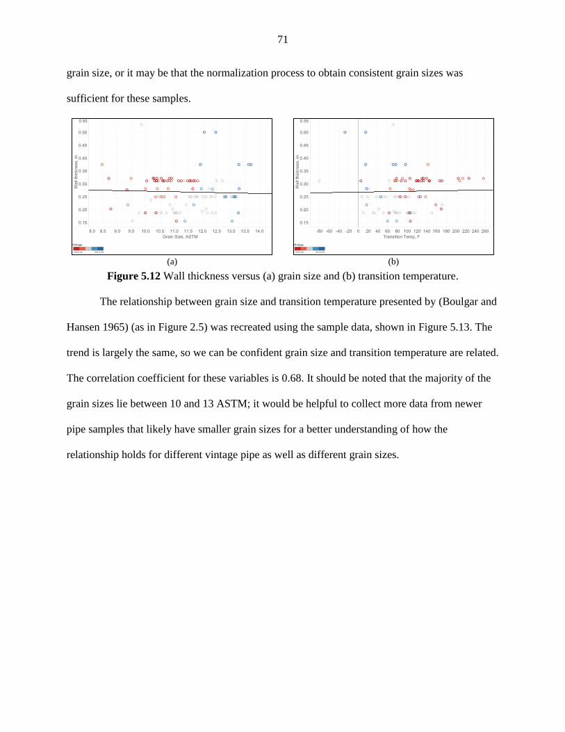
71
grain size, or it may be that the normalization process to obtain consistent grain sizes was
sufficient for these samples.
(a) (b)
Figure 5.12 Wall thickness versus (a) grain size and (b) transition temperature.
The relationship between grain size and transition temperature presented by (Boulgar and
Hansen 1965) (as in Figure 2.5) was recreated using the sample data, shown in Figure 5.13. The
trend is largely the same, so we can be confident grain size and transition temperature are related.
The correlation coefficient for these variables is 0.68. It should be noted that the majority of the
grain sizes lie between 10 and 13 ASTM; it would be helpful to collect more data from newer
pipe samples that likely have smaller grain sizes for a better understanding of how the
relationship holds for different vintage pipe as well as different grain sizes.

72
Figure 5.13 Grain size (ASTM) versus transition temperature (°F).
The entire data set was observed for potential correlations as shown in the appendix in
Table A.1, and tabulated in a similar format to Table 4.1 to allow for a more straightforward
comparison. The correlation coefficients provided in Table A.1 provides some insight as to
which measurements should be focused on in future research. Hardness is the most important
material property to obtain, which is known by the industry in that current studies are being
centered on determining a more precise relationship between hardness and YS and UTS.
Interestingly, the correlation coefficients for Mn to YS, UTS, and hardness are also quite high.
Toughness values are perhaps the most difficult to obtain, and require chemical content, and
likely more information regarding texture and microstructure based on the literature review. The
other alloying elements which show a slightly higher correlation to YS, UTS, and Hardness
include Si, Nb, V, and Zr. However, Nb, V, and Zr are both relatively recent additions to the
73
alloying process (see Figures 5.6, 5.7 and 5.8) and therefore likely indicate the result of recent
vintage pipe being manufactured using a process that leads to higher a YS and UTS, and
consequently, a higher hardness. It is likely, therefore, that a relationship between three or more
variables would be required for a multi-variate model approach to obtaining a more accurate YS,
UTS, and toughness value. By incorporating the %Mn, %C, and the hardness measurements, it
may be possible to obtain a higher correlation coefficient, and a model which relates these two
measurements to the desired mechanical property of YS, UTS, and/or toughness.
Conclusions
To understand the properties of a steel pipe, it is important to understand that many inter-
related variables are simultaneously present. The preceding material should have brought light to
the current practices used to determine material properties, both destructively and
nondestructively, and the limitations of each. In summary, the solution of determining material
properties of pipe, particularly that which is buried, is not a simple solution using a single
measurement or single technology. It will require a knowledge and understanding of several
different material properties, how those are currently able to be obtained, whether destructively
or nondestructively, and how they relate to desired mechanical properties.
Pipe has been manufactured for over a century, and manufacturing processes have vastly
changed over time. Therefore, it is reasonable to expect that the relationships expected from a
certain vintage range of pipe would be different from much newer pipe. This is shown by the
sample data set, and is most notable in the differences in chemical content and its impact on yield
and tensile strengths. What is not observed due to inadequate information on the sample data set,
however, is the difference in manufacturing processes: whether the heat treatments applied, or
the basic mechanics of how the plate is rolled, the pipe assembled; U&O formed, spiral welded,
74
seamless, or any of the other practices. Testing practices within the steel manufacturing facilities
can also bring in variability in what has been deemed acceptable for service. According to
various studies, the same flattening technique carried out at different facilities can cause different
yield strengths to result. For future studies, it is recommended that more evaluation is performed
as to the nature of the accuracy and repeatability of the destructive testing to determine its
measurement error range. Without this knowledge, using nondestructive measurements and
justifying their improved accuracy will be difficult, if not impossible.
For the magnetic measurements and possibility of using either eddy current or magnetic
flux leakage as is currently being explored by ILI companies, it would be of use to obtain
saturation, permeability, coercivity, and remanence measurements on the sample data to see if
the correlations are similar to what was developed shown in Table 4.1. More information on
more recent vintage pipe would be helpful as well, to better understand the differences of vintage
and pipe manufacturing practices. Additionally, creating a chart of the various ultrasound
measurements such as velocity, attenuation, and backscatter grain noise could open up more
insight as to how effective ultrasonic measurements are in determining the desired mechanical
properties. However, measurements first need to be compiled, and then related in a similar
manner.
Based on the results of this preliminary literature review and sample data analysis, there
is promise for correlating the results of NDE measurement modalities to the information required
to develop relationships between those measurements and the mechanical measurements desired
of pipelines to ensure proper response to defects which are of significant threat. A multivariate
approach is the next step to determine which of the many variables may interact to result in a

75
more accurate estimation of the true yield strength, tensile strength, fracture toughness, and
transition temperature.

76
REFERENCES
Amend, B. "Using Hardness to Estimate Pipe Yield Strength; Field Application of ASME
CRTD - Vol. 91." 2012 9th International Pipeline Conference. Calgary, Alberta:
ASME, 2012.
American Petroleum Institute. "Specification for Line Pipe." ANSI/API Specification 5L.
American Petroleum Institute, 2007.
ASM International. "ASM Handbook Vol 8." In Introduction to the Mechanical Behavior of
Metals, by T.M. and Rigney, J.D. Osman, 3-12. ASM International, 2000.
ASM International. "Mechanical Properties of Fully Pearlitic Microstructures." Chap. 15 in
Steels: Processing, Structure and Performance, by George Krauss, 282-283. ASM
International, 2005.
ASM International. Mechanical Testing and Evaluation. Vol. 8, in Mechanical Behavior
Under Tensile and Compressive Loads, by G.E. Dieter, 99-108. ASM International,
2000.
ASTM. "Standard Test Methods and Definitations for Mechanical Testing of Steel Products."
ASTM Standard A 370 - 97a. Vol. A370. West Conshohocken, PA: ASTM, 1997.
Baczynski, G. J., J. J. Jonas, and L. E. Collins. "The influence of rolling practice on notch
toughness and texture development in high-strength linepipe." Metallurgical and
Materials Transactions A (Springer) 30 , no. 12 (December 1999): 3045-3054.
Bannenberg, N. Recent Developments in Steelmaking and Casting. International Symposium
on Niobium 2001, Dillingen, Germany: CBMM, 2001.
Barbian, A., M. Beller, and U. Schneider. "Advanced Pipeline Inspection Utilizing
Ultrasound: Special Applications." Pipeline Technology Conference 2007. Hannover,
Germany: Euro Institute for Information and Technology Transfer in Environmental
Protection, 2007. 1-10.
Belanger, A., and R. Narayanan. "Calculation of Hardness Using High and Low Magnetic
Fields." ECNDT 2006 - Tu.4.1.1, 2006.
Belanger, A., and T. Barker. "Multiple Data Inspection of Hard Spots and Cracking." 2014
10th International Pipeline Conference. Calgary, AB, Canada: ASME, 2014.
Benamar, A., A. Le Bastard, R. Batisse, and V. Gaschignard. "Investigation of a Non-
Destructive Method to Characterize Material Mechanical Properties of Pipelines In
Service." International Gas Union Research Conference. Paris: IGRC, 2008.

77
Boulger, F.W., and W.R. Hansen. "Role of Manufacturing Variables on The Properties of
Line Pipe." AGA 3rd Line Pipe Symposium. 1965. 161-196.
Brinson, L.C., I. Schmidt, and R. Lammering. "Stress-induced transformation behavior of a
polycrystalline NiTi shape memory alloy: micro and macromechanical investigations
via in situ optical microscopy." Journal of the Mechanics and Physics of Solids 52,
no. 7 (2004): 1549-1571.
Burgoon, D.A., O.C Chang, R.B. Francini, B.N. Leis, and S.W. Rust. Determining the Yield
Strength of In-Service Pipe. ASME International CRTD, 1999.
Cahoon, J.R., W.H. Broughton, and A.R. Kutzak. "The determination of yield strength from
hardness measurements." Metallurgical Transactions, July 1971: 1979-1983.
Chancellor, W.C. Washington, DC Patent 2,025,016. 1935.
Chandramouli, P.N. Fundamentals of Strength of Materials. Delhi: PHI Learning Private
Limited, 2013.
Collins, L.E., and M. Rashid. "Best Practices for Yield Stress Determination Using the
Flattened Strap Tensile Test." 2014 10th International Pipeline Conference. Calgary,
AB, Canada: ASME, 2014.
Cooreman, S., D.V. Hoecke, M. Liebeherr, P. Thibaux, and M.Y. Enderlin. "Measurement of
Mechanical Properties on Line Pipe: Comparison of Different Methodologies." 2014
10th International Pipeline Conference. Calgary, AB, Canada: ASME, 2014.
Cosham, A., P. Hopkins, and B. Leis. "CRACK-LIKE DEFECTS IN PIPELINES: THE
RELEVANCE OF PIPELINE-SPECIFIC METHODS AND STANDARDS."
PROCEEDINGS OF THE 9TH INTERNATIONAL PIPELINE CONFERENCE,
2012, VOL 2. Calgary, Canada: ASME, 2013. 713-726.
Cottrell, A.H., and B.A. Bilby. "Dislocation Theory of Yielding and Strain Ageing of Iron."
Proceedings of the Physical Society 62, no. 1 (1948): 49-62.
Crump, H.M., and S. Papenfuss. "Utilization of Magnetic Flux Leakage Inspection Pigs for
Hard Spot Detection and Repair." Corrosion 91. 1991. 366.
Energy Information Administration. EIA - Natural Gas Pipeline Network - Natural Gas
Pipeline Mileage by Region/State. 2008.
http://www.eia.gov/pub/oil_gas/natural_gas/analysis_publications/ngpipeline/mileage
.html (accessed 12 1, 2014).
Energy Information Administration. EIA - Natural Gas Pipeline Network - U.S. Natural Gas
Pipeline Network Map. 2009.

78
http://www.eia.gov/pub/oil_gas/natural_gas/analysis_publications/ngpipeline/ngpipeli
nes_map.html (accessed 12 1, 2014).
Engle, B.E., L.J. Smart, and L.J. Bond. "Nondestructive Characterization of Pipeline
Materials." 41st Annual Review of Progress in Quantitative Nondestructive
Evaluation Conference. Boise, Idaho, 2014.
Ensminger, D., and L.J. Bond. "Determining Properties of Materials." In Ultrasonics:
Fundamentals, Technologies, and Applications, Third Edition, 219-257. Boca Raton,
Florida: CRC Press, 2011.
FracDallas. Pipeline Explosions Since 2001. February 26, 2013.
http://fracdallas.org/docs/pipelines.html (accessed December 2, 2014).
Frank, S. "Portable Hardness Testing - Principles and Applications." The e-Journal of
Nondestructive Testing 7, no. 10 (2002).
Freitas, Vera Lúcia de Araújo, Victor Hugo C. de Albuquerque, Edgard de Macedo Silva,
Antonio Almeida Silva, and João Manuel R.S. Tavares. "Nondestructive
characterization of microstructures and determination of elastic properties in plain
carbon steel using ultrasonic measurements." Materials Science and Engineering A
527, 2010: 4431–4437.
Frenz, H. "Results of an Interlaboratory Comparison Test with 91 European Testing
Laboratories." Material Testing, 1998: 40.
Garcia, T.E., C. Rodriguez, F.J. Belzunce, and C. Suarez. "Estimation of mechanical
properties of metallic materials by means of the small punch test." Journal of Alloys
and Compounds (University Institute of Industrial Technology of Asturias), 2014:
708-717.
Ghosh, K.S., and D.K. Mondal. "Mechanical and Electrochemical Behavior of a High
Strength Low Alloy Steel of Different Grain Sizes." Metallurgical and Materials
Transactions A (The Minerals, Metals & Material Society and ASM International)
44A (August 2013): 3608-3621.
Gladman, T., I.D. McIvor, and F.B. Pickering. "Some Aspects of the Structure-Property
Relationships in High-Carbon Ferrite-Pearlite Steels." Journal of the Iron and Steel
Institute 210 (1972): 916-930.
Gray, J.M. and F. Siciliano. High Strength Microalloyed Linepipe: Half a Century of
Evolution. Houston, TX: Microalloyed Steel Institute L.P., 2009.
Gray, M.J., R.L. Fazackerley, and W.J. Fazackerley. Tensile Property Variation in DSAW
and ERW Line Pipe. Final Report PR-187-9602, Line Pipe Supervisory Committee,

79
Microalloying International, Inc., Houston: Pipeline Research Council International,
Inc, 1999.
Griffith, A.A. "The phenomena of rupture and flow in solids." (Philosophical Transactions of
the Royal Society of London) 221 (1921): 163-198.
Haggag, F.M. "In-Situ Nondestructive Measurements of Key Mechanical Properties of Oil
and Gas Pipelines." Residual Stress Measurement and General Nondestructive
Evaluation. ASME, 2001. 99-104.
Haggag, F.M., W.R. Corwin, and W.L. Server. In-Situ Measurements of Mechanical
Properties Using Novel Auotmated Ball Indentation System. ASTM STP 1204,
Philadelphia: American Society for Testing and Materials, 1993, 27-44.
Haines, H. and B. Nestleroth. "NDE-4A Pipeline Discrepancy Analysis Using an ILI - An
Approach for Meeting the Need for Traceable, Verifiable & Complete Records for
Vintage Pipelines." 2013 PRCI Research Exchange Meeting. Dallas, Texas: PRCI,
February 5, 2013.
Hammond, J. "Development of Standards & Specifications for High Strength Line Pipe."
International Symposium on Microalloyed Steels for the Oil and Gas Industry. Araxa,
MG, Brazil: TMS (The Minerals, Metals & Materials Society), 2007. 43-63.
Hart, C.A. "Importance of Integrity Verification." National Transportation Safety Board,
August 7, 2013.
Heingartner, J., M. Born, and P. Hora. "Eddy Current Measurement for the Nondestructive
Acquisition of the Mechanical Properties of Sheet Metal." NDT Article Prague 2009
Proceedings. Prague: NDT, 2009.
Hwang, B., Y.G. Kim, S. Lee, Y.M. Kim, and N.J. Kim. "Effective Grain Size and Charpy
Impact Properties of High-Toughness X70 Pipeline Steels." redOrbit. August 5, 2005.
www.redorbit.com/news/science/194647/effective_grain_size_and_charpy_impact_pr
operties_of_hightoughness_x70/ (accessed January 14, 2014).
Joo, M.S., D.W. Suh, J.H. Bae, N.S. Mourino, R. Petrov, L.A.I. Kestens, H.K.D.H.
Bhadeshia. "Experiments to separate the effect of texture on anisotropy of pipeline
steel." Materials Science & Engineering A, 2012: 601-606.
Kiefner, J.F. and E.B. Clark. History of Line Pipe Manufacturing in North America. Gas
Pipeline Safety Research Committee, ASME, 1996.
Kiefner, J.F. and M.J. Rosenfeld. The Role of Pipeline Age in Pipeline Safety. INGAA
Foundation, Inc, 2012.

80
Knoop, F., C.G. Peters, and W.B. Emerson. "A Sensitive Pyramidal-Diamond Tool for
Indentation Measurements." Journal of Research of the National Bureau of Standards
(U.S. Department of Commerce) 23 (July 1939): 39-61.
Knoop, F., G. Hohl, and G. Knauf. "The effect of specimen type on tensile test results and its
implications for line pipe testing." 3R International 40 (2001): 655-661.
Llewellyn, D.T. Steels: metallurgy and applications. Boston: Butterworth Heinemann, 1992.
Maass, M. Bestimmung von richtungsabhängigen Werkstoffeigenschaften und. VDI Verlag,
2001.
Margetan, F.J., B.R. Thompson, and T.P. Lerch. "An Analytical Approximation for a
Common Ultrasonic Grain Noise Diffraction Integral." In Review of Progress in
Quantitative Nondestructive Evaluation 18A, 45-52. Snowbird, UT: Springer-Verlag
US, 1999.
Meyer, E. Untersuchungen über Härteprüfung und Härte Brinell Methoden. 1908.
Millwood, N.A., G.C. Morgan, A.M. Wood, and A.D. Batte. "The influence of tensile testing
method on the measured properties of high-strength steel linepipe." Pipeline
Technology Conference. Loughborough, UK: Advantica Ltd, 2004. 1857-1879.
Molenda, D. and W. Thale. "A Novel Approach for Pipe Grade Determination Through In-
Line Inspection (ILI)." 2014 10th International Pipeline Conference. Calgary, AB,
Canada: ASME, 2014.
Nanney, S. "Overview of Integrity Verification Process (IVP) Workshop." Arlington,
Virginia: PHMSA, August 7, 2013.
Nestleroth, J.B. and A.E. Crouch. Variation of Magnetic Properties in Pipeline Steels.
Washington, D.C.: U.S. Department of Transportation, 1997.
Nestleroth, J.B. and H.H. Haines. NDE-4A Pipeline Discrepancy Analysis Using an ILI.
Research Project, Houston: Pipeline Research Council International, 2013.
Nichols, R.K. "The Effects of Steel Mill Practice on Pipe and Tube Making." Thermatool
Corp. 2011. http://www.thermatool.com/information/papers/quality/EFFECTS-OF-
STEEL-MILL-PRACTICES-ON-PIPE-AND-TUBE-MAKING.pdf (accessed March
21, 2014).
National Transportation Safety Board. Pacific Gas and Electric Company Natural Gas
Transmission Pipeline Rupture and Fire San Bruno, California September 9, 2010.
Washington D.C.: National Transporation Safety Board, 2011.

81
National Transportation Safety Board. "Safety Recommendation P-11-14." Eliminating
Grandfather Clause. Washington, D.C.: PHMSA, September 26, 2011.
O'Neill, B. "50 Years of Quality: History of Hardness Testing." Quality Magazine. July 26,
2011. http://www.qualitymag.com/articles/88218-50-years-of-quality-history-of-
hardness-testing (accessed 3 18, 2014).
Palanichamy, P., A Joseph, T Jayakumar, and B. Raj. "Ultrasonic velocity measurements for
estimation of grain size in austenitic stainless steel." NDT & E International 28.3.
1995. 179-185.
Pavlina, E.J. and C.J. Van Tyne. "Correlation of Yield Strength and Tensile Strength with
Hardess for Steels." Journal of Materials Engineering and Performance 17, no. 6
(December 2008): 888-893.
Pavlina, E.J. and C.J. Van Tyne. "Correlation of Yield Strength and Tensile Strength with
Hardness for Steels." Journal of Materials Engineering and Performance (ASM
International) 17, no. 6 (2008): 888-893.
Pessard, E., F. Morel, C. Verdu, L. Flacelièrec, and G. Baudry. "Microstructural
heterogeneities and fatigue anisotropy of forged steels." Materials Science and
Engineering A (Elsevier) 529 (November 2011): 289-299.
Pollard, L., A. Belanger, and T. Clarke. "Managing HIC Affected Pipelines Utilizing MFL
Hard Spot Technology." Corrosion 2004. New Orleans, LA, 2004.
Pyromation. "PMI - Comparing Two Test Methods." Pyromation, Inc. 2014.
http://www.pyromation.com/TechInfo/WhitePapers/PMI_Comparing_Two_Test_Met
hods.aspx (accessed March 12, 2014).
Raj, B., V. Moorthy, T. Jayakumar, and K.B.S. Rao. "Assessment of microstructures and
mechanical behavior of metallic materials through non-destructive characterisation."
International Materials Review 48, no. 5 (October 2003): 273-325.
Ramuhalli, P., R.M. Meyer, A.D. Cinson, T.L. Moran, M. Prowant, B. Watson, M.T.
Anderson. "In-situ Characterization of Cast Stainless Steel Microstructures." In
Proceedings of the Eighth International Conference on NDE in Relation to Structural
Integrity for Nuclear and Pressurized Components. Berlin, Germany, 2012.
Rockwell, H.M. Rockwell and S.P. Hardness-Tester. U.S. Patent 1,294,171. February 1919.
Rosado, D.B., W. De Waele, D. Vanderschueren, and S. Hertele. "Latest Development in
Mechanical Properties and Metallugical Features of High Strength Line Pipe Steels."
Sustainable Construction and Design 2013. Soete Laboratory, 2013.

82
Sandland, R.L. and G.E. Smith. "An Accurate Method of Determining the Hardness of
Metals, with Particular Reference to Those of a High Degree of Hardness."
Proceedings of the Institute of Mechanical Engineers. 1922. 623-641.
Schwind, M. Zerstörungsfreie Ermittlung mechanischer Eigenschaften von. Meisenback,
1998.
Sharma, K., P.K. Singh, V. Bhasin, and K.K. Vaze. "Application of Automated Ball
Indentation for Property Measurements of Degraded Zr2.5Nb." Journal of Minerals &
Materials Characterization & Engineering 10, no. 7 (2011): 661-669.
Shukla, R., S.K. Das, B.R. Kumar, S.K. Ghosh, S. Kundu, and S. Chatterjee. An Ultra-low
Carbon, Thermomechanically Controlled Processed Microalloyed Steel:
Microstructure and Mechnical Properties. The Minerals, Metal & Materials Society
and ASM International, 2012.
Shukla, R., S.K. Ghosh, D. Chakrabarti, and S. Chatterjee. "Microstructure, texture, property
relationship in thermo-mechanically." Materials Science & Engineering A 587, 2013:
201-208.
Stalheim, D.G., K.R. Barnes, and D.B. McCutcheon. "Alloy Designs for High Strength Oil
and Gas Transmission Linepipe Steels." International Symposium on Microalloyed
Steels for the Oil and Gas Industry. Brazil: CBMM/TMS, 2006.
Stallybrass, C., M. Frommert, J. Konrad, and H. Meuser. "Modern Approach to the
Microstructure Characterization of Large Diameter Linepipes." 2014 10th
International Pipeline Conference. Calgary, AB, Canada: ASME, 2014.
Stanke, F.E., and G.S. Kino. "A unified theory for elastic wave propagation in polycrystalline
materials." The Journal of the Acoustical Society of America 75, no. 3 (1984): 665-
681.
Tabor, D. The Hardness of Metals. UK: Oxford University Press, 1951.
Technology, Products, and Processes. Yield Strength and Heat Treatment. 2006.
http://www.tppinfo.com/defect_analysis/yield_strength.html (accessed March 20,
2013).
Vary, A. "Research Techniques in Nondestructive Testing, Vol IV." In Ultrasonic
Measurement of Material Properties. R.S. Sharpe, ed., 1980.
Wilkowski, G.M, W.A. Maxey, and R.J. Eiber. "Use of the DWTT Energy for Predicting
Ductile Fracture Behavior in Controlled-Rolled Steel Line Pipes." Edited by
Pergamon Press Ltd. Canadian Metallurgial Quarterly (Canadian Institute of Mining
and Metallurgy) 19 (1980): 59-77.

83
Willems, H., and K. Goebbels. "Characterization of microstructure by backscattered
ultrasonic waves." Vol. 15. no. 11-12. November 1, 1981. 549-553.
Wilson, P.C., Y.V. Murty, T.Z. Kattamis, and R. Mehrabian. "Effect of homogenization on
sulphide morphology and mechanical properties of rolled AISI 4340 steel." Metals
Technology, June 1975: 241-244.
Zergoug, M., A. Haddad, O. Bourdjam, and R.D.D. Ibrahim. Micro-Structure
Characterization by Micro Magnetic Methods. Centre de soudage et de contrôle,
Laboratoire d'Electronique et d'Electrotechnique, Algeria: ECNDT, 2006.
Zhao, M.C., K. Yang, and Y. Shan. "The effects of thermo-mechanical control process on
icrostructures and mechanical properties of a commercial pipeline steel." Materials
Science and Engineering A335, 2002: 14-20.
Zong, C., G. Zhu, and W. Mao. "Effect of crystallographic texture on the anisotropy of
Charpy impact behavior in pipeline steel." Materials Science & Engineering A 563,
2012: 1-7.

84
APPENDIX. REFERENCE MATERIALS

85
Table A.1 Correlation coefficients for linear models of each variable against all others (darker shaded boxes indicate higher correlations)
% F
erri
te
% I
ncl
usi
on
Yie
ld
Ten
sile
Elo
ng
atio
n
Har
dn
ess
Gra
in S
ize
FS
E (
ft-l
b)
Tra
nsi
tion
Tem
per
atu
re (
F)
Vin
tag
e
OD
WT
Chemical Composition
C Mn S P Al Si Nb V Ti Cr Mo Cu Ca Ni Sn Co B Zr
% Ferrite 0.328 0.118 0.441 0.248 0.360 0.047 0.341 0.195 0.310 0.001 0.130 0.614 0.403 0.074 0.292 0.221 0.133 0.200 0.089 0.409 0.001 0.149 0.146 0.062 0.288 0.163 0.248 0.073 0.249
% Inclusion 0.328 0.088 0.101 0.239 0.137 0.181 0.370 0.083 0.311 0.036 0.146 0.381 0.179 0.244 0.384 0.340 0.263 0.254 0.037 0.357 0.246 0.135 0.127 0.299 0.017 0.070 0.154 0.077 0.169
Yield 0.118 0.088 0.826 0.257 0.851 0.581 0.511 0.140 0.679 0.287 0.132 0.416 0.705 0.388 0.095 0.616 0.688 0.772 0.716 0.389 0.242 0.385 0.125 0.103 0.088 0.058 0.046 0.149 0.699
Tensile 0.441 0.101 0.826 0.342 0.960 0.508 0.239 0.147 0.401 0.392 0.096 0.024 0.743 0.206 0.358 0.435 0.568 0.617 0.557 0.283 0.153 0.374 0.207 0.098 0.203 0.179 0.111 0.204 0.634
Elongation 0.248 0.239 0.257 0.342 0.274 0.211 0.400 0.209 0.246 0.315 0.427 0.364 0.149 0.195 0.227 0.151 0.164 0.035 0.003 0.491 0.031 0.013 0.065 0.104 0.017 0.001 0.109 0.056 0.134
Hardness 0.360 0.137 0.855 0.960 0.274 0.532 0.326 0.143 0.458 0.397 0.156 0.084 0.735 0.235 0.395 0.523 0.676 0.650 0.690 0.325 0.147 0.406 0.280 0.083 0.255 0.244 0.111 0.235 0.686
Grain Size 0.047 0.181 0.581 0.508 0.211 0.532 0.589 0.488 0.690 0.269 0.039 0.441 0.416 0.431 0.094 0.621 0.574 0.646 0.440 0.463 0.134 0.289 0.059 0.313 0.002 0.053 0.004 0.044 0.360
FSE (ft-lb) 0.341 0.370 0.511 0.239 0.400 0.326 0.589 0.410 0.808 0.383 0.432 0.761 0.265 0.519 0.163 0.646 0.731 0.541 0.513 0.655 0.240 0.409 0.082 0.415 0.073 0.117 0.198 0.040 0.326
Trans Temp
(F) 0.195 0.083 0.140 0.147 0.209 0.143 0.488 0.410 0.298 0.170 0.049 0.298 0.109 0.198 0.066 0.139 0.156 0.319 0.142 0.225 0.106 0.364 0.211 0.043 0.246 0.108 0.230 0.060 0.170
Vintage 0.310 0.311 0.679 0.401 0.246 0.458 0.690 0.808 0.298 0.208 0.241 0.804 0.553 0.496 0.192 0.798 0.799 0.677 0.653 0.691 0.085 0.212 0.152 0.418 0.244 0.260 0.252 0.024 0.485
OD 0.001 0.036 0.287 0.392 0.315 0.397 0.269 0.383 0.170 0.208 0.332 0.190 0.266 0.092 0.156 0.276 0.264 0.217 0.216 0.345 0.165 0.084 0.118 0.155 0.200 0.216 0.054 0.152 0.086
WT 0.130 0.146 0.132 0.096 0.427 0.156 0.039 0.432 0.049 0.241 0.332 0.341 0.119 0.118 0.029 0.375 0.264 0.160 0.059 0.601 0.037 0.040 0.009 0.158 0.017 0.101 0.237 0.032 0.083
Carbon 0.614 0.381 0.416 0.024 0.364 0.084 0.441 0.761 0.298 0.804 0.190 0.341 0.187 0.441 0.369 0.667 0.611 0.694 0.593 0.709 0.187 0.144 0.134 0.166 0.215 0.196 0.263 0.011 0.417
Manganese 0.403 0.179 0.705 0.743 0.149 0.735 0.416 0.265 0.109 0.553 0.266 0.119 0.187 0.317 0.206 0.521 0.531 0.610 0.642 0.311 0.098 0.258 0.018 0.186 0.124 0.070 0.036 0.048 0.706
Sulfur 0.074 0.244 0.388 0.206 0.195 0.235 0.431 0.519 0.198 0.496 0.092 0.118 0.441 0.317 0.286 0.355 0.494 0.439 0.543 0.358 0.188 0.147 0.054 0.367 0.104 0.161 0.017 0.000 0.438
Phosphorus 0.292 0.384 0.095 0.358 0.227 0.395 0.094 0.163 0.066 0.192 0.156 0.029 0.369 0.206 0.286 0.051 0.099 0.178 0.151 0.146 0.142 0.053 0.235 0.186 0.129 0.101 0.011 0.058 0.030
Aluminum 0.221 0.340 0.616 0.435 0.151 0.523 0.621 0.646 0.139 0.798 0.276 0.375 0.667 0.521 0.355 0.051 0.658 0.722 0.479 0.756 0.027 0.145 0.254 0.328 0.292 0.142 0.322 0.007 0.492
Silicon 0.133 0.263 0.688 0.568 0.164 0.676 0.574 0.731 0.156 0.799 0.264 0.264 0.611 0.531 0.494 0.099 0.658 0.527 0.584 0.555 0.124 0.317 0.163 0.562 0.112 0.215 0.031 0.196 0.520
Niobium 0.200 0.254 0.772 0.617 0.035 0.650 0.646 0.541 0.319 0.677 0.217 0.160 0.694 0.610 0.439 0.178 0.722 0.527 0.723 0.158 0.079 0.082 0.150 0.154 0.168 0.300 0.267 0.076 0.706
Vanadium 0.089 0.037 0.716 0.557 0.003 0.690 0.440 0.513 0.142 0.653 0.216 0.059 0.593 0.642 0.543 0.151 0.479 0.584 0.723 0.026 0.257 0.342 0.038 0.056 0.028 0.103 0.228 0.211 0.995
Titanium 0.409 0.357 0.389 0.283 0.491 0.325 0.463 0.655 0.225 0.691 0.345 0.601 0.709 0.311 0.358 0.146 0.756 0.555 0.158 0.026 0.046 0.156 0.206 0.058 0.268 0.224 0.268 0.086 0.224
Chromium 0.001 0.246 0.242 0.153 0.031 0.147 0.134 0.240 0.106 0.085 0.165 0.037 0.187 0.098 0.188 0.142 0.027 0.124 0.079 0.257 0.046 0.319 0.435 0.041 0.210 0.155 0.046 0.041 0.071
Molybdenum 0.149 0.135 0.385 0.374 0.013 0.406 0.289 0.409 0.364 0.212 0.084 0.040 0.144 0.258 0.147 0.053 0.145 0.317 0.082 0.342 0.156 0.319 0.513 0.069 0.593 0.316 0.065 0.207 0.198
Copper 0.146 0.127 0.125 0.207 0.065 0.280 0.059 0.082 0.211 0.152 0.118 0.009 0.134 0.018 0.054 0.235 0.254 0.163 0.150 0.038 0.206 0.435 0.513 0.120 0.762 0.711 0.368 0.022 0.121
Calcium 0.062 0.299 0.103 0.098 0.104 0.083 0.313 0.415 0.043 0.418 0.155 0.158 0.166 0.186 0.367 0.186 0.328 0.562 0.154 0.056 0.058 0.041 0.069 0.120 0.089 0.124 0.026 0.035 0.103
Nickel 0.288 0.017 0.088 0.203 0.017 0.255 0.002 0.073 0.246 0.244 0.200 0.017 0.215 0.124 0.104 0.129 0.292 0.112 0.168 0.028 0.268 0.210 0.593 0.762 0.089 0.681 0.295 0.301 0.042
Tin 0.163 0.070 0.058 0.179 0.001 0.244 0.053 0.117 0.108 0.260 0.216 0.101 0.196 0.070 0.161 0.101 0.142 0.215 0.300 0.103 0.224 0.155 0.316 0.711 0.124 0.681 0.296 0.070 0.101
Cobalt 0.248 0.154 0.046 0.111 0.109 0.111 0.004 0.198 0.230 0.252 0.054 0.237 0.263 0.036 0.017 0.011 0.322 0.031 0.267 0.228 0.268 0.046 0.065 0.368 0.026 0.295 0.296 0.011 0.123
Boron 0.073 0.077 0.149 0.204 0.056 0.235 0.044 0.040 0.060 0.024 0.152 0.032 0.011 0.048 0.000 0.058 0.007 0.196 0.076 0.211 0.086 0.041 0.207 0.022 0.035 0.301 0.070 0.011 0.048
Zirconium 0.249 0.169 0.699 0.634 0.134 0.686 0.360 0.326 0.170 0.485 0.086 0.083 0.417 0.706 0.438 0.030 0.492 0.520 0.706 0.995 0.224 0.071 0.198 0.121 0.103 0.042 0.101 0.123 0.048

86
Figure A.1 Hazardous Liquid Integrity Verification Process Flowchart

87
Figure A.2 Gas Transmission Integrity Verification Process Flowchart