review of best practices in labour market forecasting … · centre for the study of living...

CENTRE FOR

THE STUDY OF

LIVING

STANDARDS

REVIEW OF BEST PRACTICES IN

LABOUR MARKET FORECASTING

WITH AN APPLICATION TO THE

CANADIAN ABORIGINAL

POPULATION

October 2015

Jasmin Thomas

CSLS Research Report 2015-16

October 2015

Prepared for the National Association of Friendship Centers

151 Slater Street, Suite 710

Ottawa, Ontario K1P 5H3

Tel: 613-233-8891

Fax: 613-233-8250

[email protected]

2

Review of Best Practices in Labour Market Forecasting

with an Application to the Canadian Aboriginal Population

Abstract

The Friendship Centres in Canada play a pivotal role in community and economic

development by providing training and employment opportunities, facilitating social

development, and building human and resource capacity for Aboriginal Canadians. The

availability of occupational projections may facilitate the work of the Friendship Centres by

providing valuable information concerning future labour market outcomes, allowing their

programs to more appropriately prepare Aboriginal Canadians with the required skills, training

and education to meet expected labour demand. By surveying the best practices in labour market

demand and supply modeling used by national, sub-national and sectoral organizations, this

report will help provide a stronger understanding of the potential power of labour market

forecasting, while acknowledging the difficulties and obstacles inherent in any projection process.

Furthermore, this report will discuss methodologies that could be implemented by the Friendship

Centres to estimate the prospective occupational labour supply and demand facing Aboriginal

Canadians.

3



Table of Contents

Abstract 2

Table of Contents 3

Executive Summary 6

I. Introduction 10

A. Purpose of the Report 11

B. Structure of the Report 12

II. General Labour Market Supply and Demand Projections 13

A. Manpower Requirements Approach 14 i. Projecting Occupational Demand 14 ii. Projecting Occupational Supply 17 iii. Balancing Supply and Demand 20

B. Manpower Requirements Approach Modifications and Simplifications 20

C. Manpower Requirements Approach Assumptions 21

D. Manpower Requirements Approach Critiques 22

E. Usage of Occupational Forecasting Results 25

F. Summary 26

III. Examples of Occupation Forecasting Models 27

A. Canadian Occupational Projection System (COPS) 27 i. Demand Side under COPS 28 ii. Supply Side under COPS 32 iii. Balancing Supply and Demand under COPS 37

B. United States Bureau of Labor Statistics 38 i. BLS Occupational Labour Demand Estimation Methodology 39 ii. Education and Training Requirements 44 iii. Assumptions 46 iv. BLS Occupational and Industry Forecasts (2012-2022) 46 v. Summary 47

C. Other Examples 48 i. Other National and International Models 48 ii. Other Canadian Models 55

D. Summary 67

IV. Best Practices in Occupational Forecasting 69

A. General Best Practices 70

4

B. Specific Best Practices 71

C. Qualifications 72

V. Modeling the Canadian Aboriginal Labour Market 75

A. Labour Demand Estimation 76 i. Top-down manpower requirements approach 76 ii. Inclusion of Set Asides 78 iii. Alternative Projection Methodology for Occupational Labour Demand (Bottom-Up Approach) 79

B. Canadian Aboriginal Labour Supply Estimation 80 i. Canadian Aboriginal Population Projections 80 ii. Potential Obstacles and Important Considerations 81

VI. Conclusion 83

VII. References 84

Appendix 1: Annotated Guide to Occupational Forecasting and Occupational Forecasts 94

A. Additional Examples of Occupational, Educational and Training Needs Forecasting 94

B. Guides and Additional Methods to Occupational Forecasting 94

C. Occupational Forecasts 95

D. Other 95

Appendix 2: Detailed Methodology on Projecting Canadian Population Growth in Canada 96

A. Base Population 96

B. Fertility 97

C. Mortality 98

D. International Immigration 99

E. Emigration 99

F. Non-Permanent Residents 100

G. Final Population Projections 100

Appendix 3: Canadian Microsimulation Model for Projecting Labour Force Participation in

Canada 101

Appendix 4: Canadian Methodology and Microsimulation Model for Enrolment and

Educational Attainment Projections 103

A. Post Secondary Enrolment Trends 103

B. Education Modeling Under Demosim 104

Appendix 5: Canadian Aboriginal Population Projection Methodology 106

Appendix 6: COPS Labour Market Imbalances (2013-2022) 109

A. Overview 109

B. Finance and Insurance Clerks (NOC: 143) 115

5

C. Civil, Mechanical, Electrical and Chemical Engineers (NOC: 213) 115

D. Health Care and Social Assistance Industry 116

Appendix 7: National Occupational Classification 2011 117

A. Overview 117

B. Management Occupations 119

C. Business, Finance, and Administrative Occupations 119

Appendix 8: Canadian Aboriginal Employment by Occupation and Industry 121

Appendix 9: Assessment of Future Labour Market Imbalances 127

6



Executive Summary



development, and building human and resource capacity for Aboriginal Canadians. The


providing valuable information concerning future labour market developments, allowing their

programs to more appropriately prepare Aboriginal Canadians with the required skills, training

and education to meet expected labour demand.

By surveying the best practices in labour market demand and supply modeling used by

national, sub-national and sectoral organizations, this report provides a stronger understanding of

the potential power of labour market forecasting, while acknowledging the difficulties and

obstacles inherent in any projection process. Furthermore, this report discusses possible

methodologies that could be implemented to estimate the prospective occupational labour supply

and demand facing Aboriginal Canadians.

This report finds that the most crucial foundation for any labour market forecasting

model is the manpower requirements approach. This approach forecasts occupational demand

and occupational supply separately. When forecasting occupational demand, the manpower

requirements approach follows six main steps:

(1) Forecasting the macroeconomic reference scenario: developing an estimate of

future economic conditions.

(2) Projecting future demand by industry: estimating future output by industry using

input-output matrices.

(3) Projecting employment by industry: applying estimates of labour productivity to

the estimates of future output by industry.

(4) Projecting future employment or expansion demand by occupation: applying

occupational coefficients (the share of an occupation in a particular industry) to

the projections of employment by industry.

(5) Projecting separations and replacement demand by occupation: developing

estimates of the total number of people leaving an occupation due to retirement,

injury, stress leave or parental leave, and the total number of people entering the

occupation; if there is a net loss of workers, an additional step will be necessary to

determine the total number of people required by the industry, which will not

necessarily equal the net loss of workers.

(6) Calculating total demand by occupation: combining the estimates of the total

number of individuals required from expansions demand in step (4) and

replacement demand in step (5).

7

Once occupational demand has been forecasted, the manpower requirements approach

forecasts occupational supply, which also has six steps:

(1) Projecting the number of graduates and dropouts: estimating the number of

individuals who will graduate by level of education or field of study or both and

applying education to occupation matrices to place the estimated number of

graduates into specific occupations.

(2) Estimating labour force participation rates: applying labour force participation

rates to the number of graduates in each occupation to determine exactly how

many of the graduates will actually be working of those available to work in each

occupation.

(3) Projecting interprovincial and interregional migration: determining the number of

individuals who will enter an occupation in a specific area because they migrated

from another area of the country; this step is unnecessary at the national level.

(4) Projecting future immigration: determining the number of individuals who will

enter an occupation through immigration.

(5) Projecting future labour market re-entrants: estimating of the number of

individuals entering the labour force after temporary departure; the nature of this

estimate will depend on how replacement demand was calculated during

occupational demand estimation.

(6) Calculating labour supply by occupation: aggregating estimates of graduates,

migrants, immigrants and net re-entrants by occupation.

The final step of the manpower requirements approach is to compare the estimates for

occupational demand and occupational supply and determine if there will be a surplus or a

shortage of workers in each individual occupation.

The manpower requirements approach can be modified, extended and simplified in a number

of ways. This report discusses both the Canadian Occupational Projection System and the Bureau

of Labor Statistics occupational projection model to highlight some of the major alterations that

can be implemented when undertaking a labour market forecasting model. This report also

discusses a number of other occupational demand and supply systems from Canadian provinces

and Canadian industries, as well as other countries around the globe.

This review of labour market forecasting theory and practice highlighted a number of best

practices. The more general best practices include:

Forecasting future labour supply, as opposed to only labour demand, since this

indicates where imbalances will occur.

Projecting both expansion demand and replacement demand to generate total labour

demand, since replacement demand represents a large proportion of overall

occupational demand.

Replacement demand estimation including more than retirements since individuals

are likely to move in and out of the labour force throughout their careers for a variety

of reasons.

The use of the most up-to-date data for occupational demand and occupational supply

projections since this is the only way to develop the most accurate picture possible.

8

The incorporation of bottom-up information for both occupational demand and

occupational supply projections since this will ensure consistency between the data

and the real world.

Projection horizons over the medium-term (5 to 10 years), repeated every two to three

years, since this will provide labour market information that individuals can actually

use to guide their labour market behaviour.

Aside from these broad guidelines, the literature also suggests that there are a number of

specific best practices that should be implemented whenever possible when performing labour

market forecasts, including the following:

Occupational mobility adjustments should be included in any study of occupational

demand and supply, since there is the potential for a tremendous amount of

movement between occupations both horizontally and vertically. This can be done by

either accounting for occupational mobility in the estimates or by developing an

indicator of risk that highlights which occupations are the most likely to be influenced

by the business cycle or by interoccupational mobility.

The estimation of future labour demand and labour supply by hours because of

increasing reliance on part time work and casual labour. Estimates based on the

number of jobs will inaccurately account for this recent development in the labour

market.

Analysis of both stocks and flows since this increases the accuracy and completeness

of the final results and allows for the potential application of behavioural models

through flows analysis.

Estimation of occupational and qualification shares through multinomial logistic

regression rather than the simple extrapolation of past trends since multinomial

logistic regressions constrain the summation of the shares of employment across

occupations to one, whereas simpler methods of estimation do not have this feature.

This entire discussion of labour market forecasting concludes by suggesting a potential

labour market forecasting model for the Canadian Aboriginal population. Essentially, a

forecasting model for Canadian Aboriginal occupational supply would proceed identically to the

manpower requirements approach and to occupational supply models used elsewhere. However,

there are two particular challenges that must be considered when estimating Canadian Aboriginal

labour supply through a labour market forecasting model.

First, when estimates of future Canadian Aboriginal labour supply are developed by age

group and gender, the projection assumptions must take into consideration the impact of

intragenerational ethnic mobility (a shift in ethnic affiliation of a given individual throughout

their lifetime) and intergenerational ethnic mobility (a shift in ethnic affiliation between children

and parents). Both types of ethnic mobility present serious challenges to Canadian Aboriginal

labour market forecasting and analysis. Second, there is a considerable education gap between

the Canadian Aboriginal population and their non-Aboriginal counterparts (Calver, 2015). Hence,

any projections of future Canadian Aboriginal educational attainment must consider the potential

for rapid catch-up. This catch-up could be caused by a variety of factors, which may not be

identifiable at the beginning of the projection period.

9

The ease of forecasting Canadian Aboriginal occupational supply is in sharp contrast with

the obstacles encountered during Canadian Aboriginal occupational demand projections. The

biggest impediment to labour demand forecasting for the Canadian Aboriginal population is that

there is not a “demand” for Canadian Aboriginal workers, excluding set asides for Aboriginal

workers and demand for workers on reserves. Quite simply, labour demand by employers cannot

be identity-specific, as this would be considered an illegal hiring practice. Moreover, employers

should in practice choose the most qualified candidate, independent of their background.

Hence, projecting Canadian Aboriginal occupational demand will essentially break

aggregate Canadian occupational demand into an Aboriginal component and a non-Aboriginal

component by using their respective population and occupation shares. For estimates of

retirement and net re-entry and exit, similar approaches would be used to ensure that the numbers

reflect the Canadian Aboriginal population’s labour market behaviour.

The methodology for forecasting Canadian Aboriginal occupational demand presented in

this report also includes a discussion of the potential inclusion of set asides. This could be done

by appropriately adjusting the occupational demand estimates derived through the manpower

requirements approach methodology. Since detailed set aside information is often difficult to

obtain, an alternative would be to add basic set aside information as an addendum to forecasting

results.

An alternative projection methodology for Canadian Aboriginal occupational demand is a

bottom up approach. Essentially, organizations can be consulted in a given regional area

concerning a variety of factors, especially future economic activity, employment requirements by

occupation and skill level, and the expected impacts of future technological changes. In general,

by consulting with various groups to obtain information on future hiring requirements and

skilled-labour needs, insight into future labour demand by occupation and skill within a given

geographic location can be developed.

A significant drawback to this approach is that it assumes that Aboriginal workers will be

willing to work at the firms that are surveyed and that they will be willing to acquire the skills

needed to undertake the job vacancies these firms foresee arising. It also assumes that the firms

will be willing to hire Canadian Aboriginal workers. Moreover, the limited scope of the bottom-

up approach may not provide information on a diverse array of occupational opportunities,

especially when data on future employment prospects are collected regionally or concentrated

within certain industries. However, this largely depends upon the extent and depth of the survey

performed. It is quite possible that the results could provide a variety of occupational listings,

with information on requisite training, education and skills.

In summary, this report gives the impression that forecasting Canadian Aboriginal occupational

demand and occupational supply may be feasible, but there are obstacles worth considering. On

the supply side, challenges include intragenerational and intergenerational ethnic mobility, and

the possibility of rapid increases in the educational attainment of the Canadian Aboriginal

population. On the demand side, the main challenge is that there is not a specific labour demand

for Canadian Aboriginal peoples; there is only labour demand in general.

10



I. Introduction



development, and building human and resource capacity for Aboriginal Canadians.1

The


providing valuable information concerning future labour market outcomes, enabling programs to

more appropriately prepare Aboriginal Canadians with the required skills, training and education

to meet expected labour demand and supply needs.

Labour market forecasting is a valuable resource because it has the potential to show the

impact of a variety of different factors, including short-term business cycle fluctuations and long-

term structural adjustments, on labour market conditions. In the face of uncertainty regarding

short- and long-term patterns, labour market participants (workers, employers, unions,

organizations, policymakers, governments, etc.) must make informed decisions concerning their

education, training, hiring practices and investments (El Achkar, 2010: iii). Hence, occupational

forecasting models can smooth the decision-making process of both potential and current labour

market participants, perhaps alleviating or minimizing the burden of future labour market

imbalances.

More specifically, by informing employers, employees and policymakers, occupational

forecasting facilitates the clearance of labour markets by reducing the adjustment costs required

to attain balanced labour markets, and the potential social and economic costs that may arise due

to imbalanced labour markets. Governments can also use the labour market information (LMI)

from occupational forecasts to develop incentives that will encourage investment in appropriate

education or training programs. Finally, productivity and efficiency gains can result from

occupational forecasts through skills matching across occupations, ensuring that workers are

employed in positions that correspond to their particular knowledge and ability characteristics

(El Achkar, 2010:5).

1 This report was written by Jasmin Thomas under the supervision of Andrew Sharpe. The author would like to

thank Matthew Calver (Economist, Centre for the Study of Living Standards) for useful editorial comments;

Souleima El Achkar for useful critiques and information during the early stages of the report; Jonathan Brown, for

his editorial work; Rosemary Sparks (Executive Director, Build Force Canada) for her information on Build Force

Canada’s net in-mobility estimates; Erwin Gomez (Senior Research Advisor, Labour Market Research Division,

Employment and Social Development Canada), for his support in understanding the detailed estimation procedures

used by the Canadian Occupational Projection System; and Ray Gormley (Ontario Ministry of Training, Colleges

and Universities), for his help in understanding the occupational projection system implemented by the Ontario

Ministry of Training, Colleges and Universities and how it differs from the Canadian Occupational Projection

System. The author would also like to thank the following people for comments on the final draft: Sonya Howard

(Policy Analyst, National Association of Friendship Centres); Wayne Simpson (Professor of Economics, University

of Manitoba); Sarah Gauen (MiHR); Donna Feir (Associate Professor of Economics, University of Victoria); Torben

Drewes (Trent University); Gustave Goldmann (Adjunct Professor, School of Sociological and Anthropological

Studies, University of Ottawa); Erin Sawatzky (Employment and Social Development Canada); and David M. Gray

(Full Professor, Department of Economics, University of Ottawa).

11

In summary, labour markets can often be imbalanced due to a range of factors. To

overcome these imbalances, labour market adjustments are necessary. However, an assortment of

obstacles, including information acquisition, personal availability, financial requirements, and

institutional red tape can prevent labour market adjustments from occurring. Hence, occupational

forecasting is a useful tool, as it can help labour market participants partially overcome one

obstacle: information shortages concerning labour market conditions. Through the provision of

labour market information, labour supply and demand modeling indirectly encourages and

facilitates the adjustments required to avoid predicted imbalances.

By tapping into the labour market information provided by labour market forecasts, the

Friendship Centres may be able to reduce future unemployment among the Canadian Aboriginal

population. In particular, by ensuring that both current and successive cohorts of labour market

participants are equipped with essential skills and education, the Friendship Centres can facilitate

access to employment and guide individuals toward achieving career goals.

A. Purpose of the Report

This report is part of a large, long-term study, entitled Development and Design of a

Feasibility Study to Consolidate Labour Market Supply Data on Canada’s Urban and Off-

Reserve Aboriginal Population, undertaken by the National Association of Friendship Centres.

The basic goal of this feasibility study is to develop a methodological framework and detailed

implementation plan to understand the changing skills supply and demand among Aboriginal

Canadians. By providing a methodology for obtaining detailed labour market information, this

feasibility study can contribute to improving labour market outcomes for Aboriginal Canadians.

The Centre for the Study of Living Standards has been commissioned by the National

Association of Friendship Centres to assist with the development of this feasibility study. At this

stage of the feasibility report, the main tasks include assessing the scope and quality of urban

Aboriginal labour market supply and demand information in Canada and reviewing the best

practices of existing approaches to labour market supply and demand modeling. Once completed,

an investigation of the feasibility and costs associated with data gathering, reporting and

implementation will be undertaken.

The first issue, data availability, has already addressed by the Centre for the Study of

Living Standards on behalf of the National Association of Friendship Centres in a forthcoming

report entitled Aboriginal Labour Market Information in Canada: An Overview (McKellips,

2015). The second component will be addressed in this report. It focuses on describing the

foundation behind occupational forecasting, the manpower requirements approach, before

delving into specific examples of occupational forecasting models. To provide the Friendship

Centres with a potential framework to model the changing skills supply and demand among

Aboriginal Canadians, a suggested methodology for Canadian Aboriginal occupational

employment projections is presented. This methodology acts as a crucial contribution to the

feasibility report. The final component, an investigation of the feasibility and costs associated

with data gathering, reporting and implementation, will be undertaken in the next months as a

separate report.

12

B. Structure of the Report

After the introduction, this report consists of five sections. Section 2 describes the

foundational model behind many occupational forecasting systems: the manpower requirements

approach (MRA). This section also highlights the assumptions required to undertake

occupational forecasting based on this foundational methodology. Moreover, it details the main

critiques of the manpower requirements approach and discusses the proper usage and

interpretation of the resulting labour market information. Section 3 provides an overview of the

various occupational forecasting models used globally. This section includes detailed discussions

of the methodologies used by the Canadian federal government and the United States Bureau of

Labor Statistics. It also describes the procedures implemented by other nations, such as Germany

and New Zealand, as well as some models used by sub-national units and sectoral organizations,

including the Province of Alberta and Build Force Canada, respectively. Section 4 discusses best

practices in the field of labour market supply and demand modeling. Section 5 describes a

potential application of occupational forecasting to the Aboriginal population in Canada. It

focuses on a brief outline of a projection methodology, highlighting issues that may arise during

implementation. Section 6 concludes the report.

To supplement the main body of the report, supporting appendices are provided.

Appendix 1 is an annotated bibliography to occupational forecasting, briefly describing the

information provided in a number of selected resources. Appendices 2 and 5 describe population

projection methodologies in Canada, which can often be crucial for supply side estimation

procedures. Appendices 3 and 4 outline the estimation of Canadian educational attainment and

labour force participation rates. These estimations are essential to the implementation of the

manpower requirements approach. Appendix 6 presents results from the most recent COPS

projections, covering the 2013-2022 time horizon. Appendix 7 describes the National

Occupational Classification (NOC) system used in Canada. Appendix 8 provides tables of

Canadian Aboriginal employment by occupation and industry in 2011. Finally, Appendix 9

provides tables from the 2008-2017 COPS projections, which help to highlight each component

of the manpower requirements approach, while equally demonstrating the difference between ex-

ante and ex-post labour market projection scenarios.

13

II. General Labour Market Supply and Demand Projections

The procedures used in occupational forecasting vary in complexity both across time and

space, falling into three broad categories. Some of the current techniques used during the

forecasting process simply extrapolate historical trends to the end of the projection period,

without controlling for other economic and social factors. For example, in many forecasting

methodologies, future labour market participation rates, used to estimate the size and

composition of the future labour force, are generated by simply linearly extending historical

trends. Some alternative labour market forecast methods involve simple regressions relating

changes in dependent variables to changes in other crucial, predictive variables. For example,

future enrolment rates, used to generate estimates of school leavers, are often treated as

dependent variables, constructed by referencing explanatory variables, including unemployment

rates, population size, demography, and personal disposable income levels. Other models are

more complicated, requiring sophisticated econometric techniques. These allow for a variety of

interactive behaviour between different variables. For example, the macroeconomic reference

scenario, used to predict future levels of output by expenditure category, is constructed by

implementing complex statistical procedures. Clearly, there are important distinctions between

the models that fall under each of these three categories. Generally, as model complexity

decreases so does accuracy, however as complexity increases, cost and professional time

required to maintain the model increases too. Consequently, there is an inherent trade-off

between accuracy and cost. As such, the occupational forecasting method selected by any

particular entity crucially depends on the resources available and the purpose of forecast results

(El Achkar, 2010:7).

Despite the variety of approaches highlighted above, almost all of the best practices in

labour market supply and demand modeling find their foundations within the manpower

requirements approach (MRA). In this section, a brief discussion of this most basic methodology

is presented, as are the assumptions and critiques of the MRA. Finally, a discussion of the usage

of the resultant labour market information is provided. In the next section, a detailed explanation

of the methodology of the Canadian Occupational Projection System (COPS) is presented. Close

attention is given to the COPS model because it is one of the most advanced occupational

forecasting models. In particular, with three decades of experience, access to an immense amount

of data, extensive human and capital resources and strong support from the federal government,

the COPS model has evolved into a rigorous set of procedures, producing valuable labour market

information used across Canada by various labour market participants. The detailed descriptions

of the COPS model presented in the next section prove useful for clarifying some of the more

opaque aspects of the MRA. The subsequent section concludes with a discussion of the US

Bureau of Labor Statistics’ method, as well as a brief overview of some of the other models that

are used elsewhere in the world.

14

A. Manpower Requirements Approach

The most important foundational model in the history of occupational modeling and

forecasting is the manpower requirements approach (MRA).2 Widely used starting in the early

1960s, the MRA achieved great prominence after being included in the OECD’s Mediterranean

Regional Project addressing social objectives in education planning. In 1964, the International

Institute for Educational Planning published an educational planning bibliography with 553

annotated sources. Clearly, by the mid- to late-1960s, there was already a substantial body of

literature concerning manpower projections. Since then, the MRA has undergone extensive

alterations, evolving into a much more complex set of forecasting and projection procedures. The

current methodology of the manpower requirements approach follows three basic, broad steps,

namely:

1) Projecting occupational demand

2) Projecting occupational supply

3) Identifying potential labour market imbalances

Each of these steps, taken individually, has various components and considerations, as

discussed below.

i. Projecting Occupational Demand

There are many subcomponents to the development of a projection of occupational

demand, namely:

1) Forecasting the macroeconomic reference scenario

2) Projecting future demand by industry

3) Projecting employment by industry

4) Projecting future employment or expansion demand by occupation

5) Projecting separations and replacement demand by occupation

6) Calculating total demand by occupation

These steps must be followed sequentially and often require the application of advanced

econometric techniques in order to be performed with a high degree of accuracy and precision.

The data requirements also tend to be substantial. Occasionally, accessing data may simply be

too onerous, if not impossible, in instances where there have not been consistent or persistent

collection procedures.3

Step (1): Forecasting the macroeconomic reference scenario

When projecting occupational demand, it is essential to have an estimate of the future

economic conditions, referred to as the macroeconomic reference scenario. This macroeconomic

reference scenario should ideally be estimated in terms of expenditure categories,4 as this greatly

2 The information in this section was taken from El Achkar (2010:7).

3 The information in this section was taken from El Achkar (2010:9).

4 Economists disaggregate GDP into four components: consumption, investment, government purchases and net

exports. These four categories are called expenditure categories.

15

facilitates the succeeding steps. If aggregate output growth5

is given, as opposed to the

compositional growth of output6, additional assumptions concerning industry shares are required.

In general, the future macroeconomic reference scenario is often estimated by an external

source, as it involves extensive forecasting experience. Sometimes it is best to base the

macroeconomic reference scenario on a consensus of different economic forecasts produced by a

variety of organizations.7

Step (2): Projecting future output by industry

In order to estimate future output by industry, it is essential to consider the changing

structure of the economy. Often, the projection of future output by industry is performed using

input-output matrices, which translate demand by expenditure category into output by industry.

Mathematically, the economy can be expressed as follows:

where x is the vector of total output, I is the identity matrix8, A is a matrix of coefficients

representing how many units of one good9 are required in the production of another good, and d

is the vector of final demand.

Solving for x in the above equation will determine the output necessary to produce a

given final demand:

Step (3): Projecting future employment by industry

In order to estimate future industry-specific employment, it is crucial to have information

on labour productivity within an industry. These estimates of labour productivity are often

obtained by extrapolating historical rates of productivity growth. By applying these measures of

labour productivity to the information from Step (2): Projecting future output by industry an

estimate of future employment demand by industry is developed.10

Step (4): Projecting future employment or expansion demand by occupation

5 Output growth is defined as an increase in an economy’s capacity to produce goods and services over time.

6 Compositional output growth refers to output growth broken down by expenditure categories. In other words,

aggregate growth is broken down by consumption growth, investment growth, government spending growth and net

export growth. 7 When models are developed for industries, sectors, or for small open economics, extremely large projects that

greatly influence economic activity may be explicitly considered. The actual economic effect and composition of

demand for these large projects must be properly analyzed and predicted, especially since these projects often

require individuals with specific skill sets or capabilities. 8 An identity matrix is a square matrix where each element along the principal diagonal is one, while every other

element is zero. 9 A good refers to a consumable item, e.g. tires.

10 When measures of labour productivity are expressed in terms of person-hours per unit of output, to determine

labour demand by industry, data would need to be collected on the average number of hours worked per employee.

16

The simplest way to unpack future industry employment levels into occupational

employment levels is to use occupation coefficients, which are the shares of an occupation in a

particular industry. To obtain these coefficients, the use of an industry-occupation matrix is

suggested. By applying these industry-specific occupational coefficients to the projected

employment of their respective industries, estimates of labour demand by occupation, subdivided

by industry can be acquired. Using the disaggregated occupational employment information

obtained from this step, identical occupations can be summed across industries to obtain a

projection of total future occupational employment. This component of future occupational

employment is referred to as expansion demand (ED) and it represents the net change in

occupational employment resulting from growth in the economy.11

If there is not enough data to perform the next step, this will be the final result for the

projection of future labour demand. However, if there is sufficient data to estimate separations

(also referred to as replacement demand), then one more step can be performed before obtaining

a final estimate of future occupational demand.

11

In general, expansion demand growth is largest for occupations with the largest output growth, as these are the

most likely to have the largest employment growth.

Projecting occupational demand

• Step 1: Forecasting future macroeconomic

reference scenario

• Step 2: Projecting future demand by

industry

• Step 3: Projecting employment by industry

• Step 4: Projecting future employment or expansion demand by

occupation

• Step 5: Projecting replacement demand

and separations

• Step 6: Calculating occupational demand

Projecting occupational supply

• Step 1: Projecting the number of graduates and

drop outs

• Step 2: Estimating labour force participation

rates

• Step 3: Projecting interprovincial and

interregional migration

• Step 4: Projecting future immigration

• Step 5: Projecting future re-entrants

• Step 6: Calculating labour supply by

occupation

Interpreting potential labour market imbalances

• The projection of future labour market

imbalances is done by comparing measures of occupational supply and

demand, and determining where any potential shortages or surpluses may arise.

Figure 1: Manpower Requirements Approach (MRA)

Source: CSLS

17

Step (5): Projecting separations and replacement demand by occupation

The total number of people leaving an occupation is referred to as separations. These

separations can occur for many different reasons, including retirements, deaths, migrations,

illnesses, disabilities, occupational mobility, and maternity leaves, among others. By taking the

difference between the total number of people leaving an occupation and the total number of

individuals entering an occupation, it is possible to measure net separations.

Replacement demand (RD) refers to the number of workers required to replace the

individuals who have left an occupation. Depending on whether employers want to maintain

current employment levels, or adjust them, replacement demand may be equal to, greater than or

less than separations.

The procedure for generating estimates of replacement demand and separations is quite

rigorous, involving highly advanced statistical techniques. Moreover, developing accurate

estimates requires tremendous amounts of statistical information. In many instances, estimates of

future labour demand do not include measures of replacement demand (or separations), as the

data requirements are too burdensome.

In cases where the unit of analysis is a province or a region, interprovincial migration and

interregional migration are included in replacement demand projections. However, this again

depends very highly on the data and resource availability.

Step (6): Calculating total demand by occupation

Assuming that there is sufficient data to undertake the estimations in Step (5): Projecting

separations and replacement demand by occupation, then this is the final step in the projection

of labour demand by occupation according to the very basic MRA approach. Quite simply, gross

occupational employment demand (OD) is the sum of expansion demand from step 4 and

separations from step 5.

These eight steps will result in an estimate of future occupational labour demand using

the manpower requirements approach.

ii. Projecting Occupational Supply

Similarly to projecting occupational demand, there are many important steps to projecting

occupational supply.12

Interestingly, projecting occupational supply can prove to be a much more

data intensive and methodologically rigorous task. There are a number of important steps,

namely:13

12

The information in this section was taken from El Achkar (2010:10-11). 13

Occasionally, the future working-age population (including immigrants, re-entrants and migrants) is estimated,

and labour force participation rates are applied to this estimate. Afterwards, educational attainment rates are applied

to the final estimates to obtain an understanding of the actual working-age population available for employment in

18

1) Projecting the number of graduates and dropouts

2) Estimating labour force participation rates

3) Projecting interprovincial and interregional migration

4) Projecting future immigration

5) Projecting future labour market re-entrants

6) Calculating labour supply by occupation

As in the case of occupational demand estimation, it is wise to follow most of these steps

sequentially. However, unlike occupational demand, many of these estimates are independent of

one another. Unfortunately, as previously discussed in the case of occupational demand

projections, many of these estimation procedures require advanced statistical techniques and

econometric modeling. Moreover, the tremendous amount of data required to attain proper

labour supply projections is a considerable obstacle.

Step (1): Projecting the number of graduates and dropouts

Educational attainment projections are performed by level of education or field of study,

or both. Essentially, the number of graduates is estimated by age and gender for a variety of

educational attainment categories. In many cases, the models that forecast educational attainment

are completely separate from occupational supply models.

Generally, historical data on educational attainment by age and gender can be used to

determine trends in graduation rates. These trends can be projected into the future using

extrapolation techniques. Often, these extrapolative methods can become highly complex,

requiring a strong econometric foundation.

Once estimates of the number of graduates and discontinuants have been derived,

education to occupation matrices are applied to obtain a measure of school leavers by occupation.

The education to occupation matrices can be either field of study to occupation matrices or level

of education to occupation matrices, depending on data availability. The matrices essentially

allocate graduates and dropouts into occupations by using fixed shares, which are typically based

on previously observed career paths.14

Step (2): Estimating labour force participation rates

The trends in labour force participation rates by age, gender and educational level are

calculated using historical data. Similarly to the process used in Step (1): Projecting the number

of graduates and dropouts, these trends are often projected into the future by extrapolation.

Alternatively, these labour force participation rates can be modeled by using econometric

equations that consider a number of explanatory variables.

each educational category. Education to occupation translations can then be undertaken. Both methods lead to an

estimate of labour supply and should yield approximately similar forecasts. 14

It might be important to consider occupations that are regulated from within. In these instances, it is not only the

educational qualification that matters but also where those qualifications were acquired.

19

By applying these estimated or extrapolated education-specific labour force participation

rates to the number of graduates by demographic group, it is possible to find a projection for the

number of labour force participants by educational category.

Step (3): Projecting interprovincial and interregional migration

Whether this step is included or not depends on the unit of analysis. At the national level,

this step is unnecessary, but at the sub-national level, this is a crucial part of the estimation

procedure, since in-migration can be an important source of increasing labour supply. In general,

migratory changes are assumed to be determined separately from the other factors mentioned

here. Hence, migration is an exogenous variable in terms of the size of the labour force.

If estimates of migration away from the sub-national unit of analysis were included in

replacement demand, then estimates of migration into the region, province or state must be

included in the labour force. The number of in-migrants, broken down by age, education and

labor force activity status, can be added to the estimates obtained from Step (2): Estimating

labour force participation rates. By using education to occupation matrices, these in-migrants

can be allocated across occupations.

If estimates of migrations into and out of the sub-national unit of analysis were included

in the replacement demand estimates, then this step is not required.

Step (4): Projecting future immigration

In some models, immigration is included in the estimates of occupational labour supply.

Generally, this is accomplished by using fixed immigrant occupation shares obtained from

census data and applying these to the aggregate flow of immigrants into the labour force. It is

crucial to distinguish between those immigrants who enter the labour force and those who do not,

so obtaining estimates of immigrant labour force participation is very important. Immigrants can

be allocated to occupations by determining their educational attainment and applying education

to occupation matrices.

Step (5): Projecting future labour market re-entrants

Some individuals will re-enter the labour force after a period of non-employment. This

re-entry rate can be estimated by occupation and included as part of the projection of future

occupational labour supply. Depending on the model in consideration, this may be a net measure

or a gross measure. In particular, if individuals leaving the labour market for reasons other than

retirement were included in replacement demand, this measure will be a gross estimate of those

re-entering the labour market. In contrast, if individuals leaving the labour market for reasons

other than retirement were not considered in replacement demand, this measure will be a net

measure, namely the difference between those entering and those leaving the labour market.

Depending on labour market conditions, this net measure could be negative.

Step (6): Calculating future labour supply by occupation

20

Depending on data availability, these four, or possibly six, steps will result in an estimate

of future occupational labour supply using the manpower requirements approach. In particular,

by combining the occupation-specific estimates of school leavers, namely graduates and

dropouts (SL), migrants (MG), immigrants (IM), and re-entrants (NR), an estimate of future

labour supply by occupation (OS) is derived.

iii. Balancing Supply and Demand

With estimates for both the future occupational labour supply and labour demand, it is

possible to develop indicators for labour market imbalances.15

There are a variety of indicators

used in the field of occupational forecasting, many of which are published online by the

organization undertaking the forecast. As each model tends to implement a different labour

market indicator, detailed descriptions will be found in Section 3. However, one of the most

commonly implemented indicators is simply a measure of the cumulative shortage (CS), namely

subtracting supply from demand. When the cumulative shortage is negative, there is a surplus.

Often, these quantitative labour market indicators are accompanied by qualitative

assessments of the extent and projected severity of future occupational imbalances. For example,

some labour market information systems supplement their labour market indicators with a

qualitative assessment of whether the future labour market conditions for a given occupation will

be poor, fair or good. Sometimes these qualitative assessments consider more than simply the

quantitative forecast, taking into account bottom-up information collected from practitioners,

employers, and researchers, as well as additional indicators of risk, such as occupational

sensitivity to the business cycle.16

B. Manpower Requirements Approach Modifications and Simplifications

The MRA approach described above is a basic outline and, as previously mentioned,

there are many variants to this foundational procedure. In general, variations are developed by

omitting steps, such as immigrant estimates, replacement demand estimates, or re-entrant

estimates.17

Some variations are obtained by implementing basic assumptions that help to

simplify certain calculations. For example, consider calculations for replacement demand.

Occasionally, re-entrants on the supply side and separations on the demand side are assumed to

perfectly balance, leaving replacement demand solely a function of deaths and retirements. By

assuming away other forms of re-entry and separation, replacement demand calculations are

massively simplified. In contrast, the model can be expanded or enhanced by including

15

The information in this section was taken from El Achkar (2010:11). 16

There is an informal labour market that has an impact on the formal labour market. The informal labour market is

very difficult to measure. One element of the impact is that the informal labour market removes both labour supply

and labour demand. The inability of this model to measure this impact is an important limitation. The likelihood of

informality in the labour market for an occupation should influence the qualitative assessments that accompany any

quantitative assessment. 17

The information in this section was taken El Achkar (2010:12-13).

21

additional steps, or by beefing up the information included in pre-existing steps. For example,

more information could be included in the calculations of separation or replacement demand as

these are very broad categories.

In addition to all of the potential modifications, simplifications and additions, each step

of the MRA can be performed using a variety of approaches that all demonstrate differing levels

of complexity. For example, estimating future employment by occupation based on future

employment by industry can be undertaken using differing methods. In one method, calculations

of fixed coefficients or shares are performed with regard to historical data. This method assumes

that the occupational distribution is constant over time. In another technique, these same

coefficients are allowed to change over time. This is typically accomplished by extrapolating

historical data over the projection period. In an alternative approach, the future coefficients or

shares are estimated by “accounting for [the] various factors that may influence the occupational

structure of the industries over time” (El Achkar, 2010:13). This last method often requires more

advanced economic knowledge.

A much more challenging and complex consideration would be to permit interactions

between demand and supply. Due to the resource intensity and knowledge requirements of this

approach, it has seen very limited use and most methodologies continue to project demand and

supply independently. Another equally challenging modification would be to allow for “feedback

effect[s] from occupational demand and supply into the underlying macroeconomic [reference]

scenario” (El Achkar, 2010:13). This technique is probably especially relevant in smaller studies

at a regional or sub-national level. It may also find appropriate applications in studies where the

macroeconomic reference scenario explicitly accounts for larger projects, especially when the

completion of these larger projects depends on labour availability.

Clearly, the MRA can be easily manipulated to more adequately address any given

modeling situation. However, before uncovering some useful examples of this inherent

flexibility, it is important to emphasize the role of modeling assumptions in the MRA

methodology. Moreover, it is equally essential to highlight relevant critiques, which indicate

areas where the MRA could undergo serious improvement. Finally, a brief overview of

interpretations and uses of the ensuing quantitative and qualitative results is provided to allow for

a fuller comprehension of the MRA’s potential in providing useful labour market information

(LMI).

C. Manpower Requirements Approach Assumptions

Due to the nature of projections, many assumptions must be made, as there is no way to

ascertain what the future may hold. Typically, the most important assumptions relate to a

particular procedure within the MRA methodology. For example, in order to determine labour

force participation, assumptions are made concerning the projected trend of current labour force

participation rates. Now, consider a country that currently has low levels of female labour force

participation. If there were to be a massive shift in attitudes toward women in the workplace,

labour force participation rates would be drastically different than those predicted using simple

extrapolation techniques on historical data. This is only one example of the many instances

where historical trends can be misleading in the development of occupational forecasts.

22

Another assumption crucial to the MRA is that the “elasticity of substitution between

different kinds of labour is equal to (or near) zero” (Centre for Spatial Economics, 2008:15).

Since the elasticity of substitution between different kinds of labour is a measurement of the

relationship between the supply of workers across occupations, this assumption amounts to a

belief that the “potential supply of workers in other occupations, even occupations requiring

similar skill sets” is not important in the determination of future imbalances in a specific

occupation (El Achkar, 2010:6). This assumption may be slightly deceptive, since in practice,

workers can, and often do, switch occupations. Their substitutability is not perfect, but to a

certain extent, “there is some overlap in skills across occupations, particularly in cases where the

occupations fall within the same occupational group” (El Achkar, 2010:6-7). Despite the well-

known inapplicability of this assumption, it is generally made based on the principle of

simplicity. Due to the importance of this assumption for occupational forecasts, major attempts

have been made to account for this weakness in recent models. Thus, advanced labour supply

and demand models typically consider inter-occupational mobility, although the development of

a standard approach has yet to arise.

To summarize, caution should be used when analyzing the information obtained from any

occupational forecast. Errors can creep into occupational projections quite easily due to the

complex estimation methodology (Figure 2). The final result will crucially depend on the data

available and the assumptions that were inherently made in each step of the projection process.

Depending on how any given organization plans on using occupational forecast information, it

may be wise to closely examine and understand the assumptions that were made in the

estimation process.

Figure 2: Main Components of Error in Developing Occupational Projections

Source: Cedefop (2012:95)

D. Manpower Requirements Approach Critiques

The critiques of the MRA typically fall into the following areas:

23

Accuracy of resultant labour market information

Independent estimation of supply and demand

Immense data requirements

Neglecting workers’ ability levels within occupations

Construction of assumptions

Validity of national-level projections

Implementation of occupational forecasts to educational policies

Soundness of education to occupation linkages

Conversion of sectoral forecasts into occupational forecasts

Accuracy of disaggregated employment data and forecasts

The first and foremost concern for many analysts and users of occupational forecasting

results is the accuracy of the MRA approach (or any approach that closely follows these steps),

especially since there have been considerable forecasting errors associated with many previous

projections. In many ways, this may clearly demonstrate how the accuracy of any forecast

depends upon the quality of the underlying assumptions, including those pertaining to the

macroeconomic reference scenario, fixed industry shares and occupational distributions, among

others. For example, an incorrect measure of the fixed industry shares or the occupational

structure can result in considerable error in the labour market forecast. Quite simply, any

“measurement error or inappropriate assumption” introduced into the model through any of the

variables used in the estimation will result in “inaccurate forecasts” (El Achkar, 2010: iii).

Nevertheless, to some degree, there is an important trade-off in occupational forecasting:

measurement errors and inappropriate assumptions can occasionally be avoided by investing

further time and money in the development of a more complex model, but this may not be an

efficient allocation of resources (El Achkar, 2010: iii).

In general, to keep these concerns to a minimum, it is to possible perform occupational

forecasts at the highest possible level of aggregation. For example, labour market indicators tend

to be more accurate in studies of occupational groups, rather than detailed occupations, or in

studies forecasting occupational employment at the national level, as opposed to the sub-national

level. However, a higher level of aggregation may not be as useful.

Another important limitation of “existing occupational forecast models is that they do not

allow for supply and demand interactions, and [they] do not take into account the responses of

workers and firms to changing occupational prospects” (El Achkar, 2010:14). However, this

critique ignores an important feature of occupational forecasting: occupational forecasting

provides information about where future imbalances might occur; occupational forecasting does

not demonstrate which imbalances will occur.

A practical critique of occupational forecasting is that the data requirements necessary for

the development of accurate results are often onerous if not unattainable. This critique is

important because it points to the inaccessibility of occupational forecasting for smaller

organizations with limited resources and minimal funding.

In addition to these concerns, the MRA approach has often been criticized for foregoing

differentiation between workers in the same occupation or skill group with different ability levels,

or between workers whose qualifications and training do not directly correspond to their

24

occupations. There have been a few attempts to rectify this critique in more recent adaptations of

the model, particularly the COPS model. Nevertheless, these remedies are highly econometric,

require extremely detailed information and are often based on numerous additional assumptions

(Centre for Spatial Economics, 2008:15).

Many attempts have also been made to rectify the concerns about accuracy. In particular,

issues of accuracy have encouraged organizations to reduce their forecasting horizons. Instead of

projecting long-term labour market supply and demand (ten to twenty years), analysts are

focusing on projections in the short- to medium-term (five to ten years) (C4SE, 2008:15). In

addition, reducing the time frame helps limit the potential for drastic changes in the economic

assumptions that were made during any of the extrapolation and projection procedures. Even so,

a time period of five to ten years is still a long enough for individuals, employers and

governments to alter their decisions concerning education and training, investment and hiring

procedures, and labour market policies, respectively (C4SE, 2008:15).

Many critiques have focused on the construction of assumptions, arguing that a number

of assumptions are developed in a highly questionable fashion, including those concerning GDP

forecasts, employment growth rates and skill ratios (Castley, 1996). Some critics have argued

that detailed long-term national projections are neither necessary nor useful. Castley (1996)

argues that most “recruiting is done regionally, and national forecasts may not be relevant to

specific regions” (Canadian Council on Learning [CCL], 2007:25). For example, the national

forecast may predict a shortage of accountants nationally, but any given region or city may

experience a surplus or a balance. Other critics have claimed that there is “no evidence…linking

manpower forecasts to actual educational policy decisions” (Hopkins, 2000). Even if there were

evidence that occupational projections influenced policy decisions, there is a limit to their impact:

“policy makers can open up more spaces in educational facilities, [but] they cannot really plan to

produce a specific number of people trained for a certain occupation” (CCL, 2007:25). This

critique is especially relevant because of the difficulty of determining the education required for

any given occupation. Often, the link between education and occupation is vague, and for many

occupations, the linkage is non-existent (Castley, 1996).

Additional critiques have focused on whether occupational forecasting is using the

appropriate level of aggregation or disaggregation. Projections based on extremely disaggregated

data can be extremely volatile to changes in assumptions, compromising forecasting accuracy,

while projections that use extremely aggregated data are much less useful. Determining the

appropriate balance is difficult, and often the level of aggregation or disaggregation is restricted

by data availability. Finally, Campbell (1997) suggests that mistaken assumptions can arise when

converting sectoral-level projections into occupational-level projections. Hence, another

potential limitation of the manpower requirements approach is that sectoral-level forecasts are

“used to make occupational forecasts” (CCL, 2007:81).

This is only a brief discussion of the limitations of labour market projections. There are

many other critiques of the art of occupational forecasting (Amjad, 1987; Psacharopoulos, 1991;

Richter, 1986). There is also a substantial discussion concerning whether the practice of labour

market forecasting should continue. Some individuals and organizations subscribe to the view

that the “market will correct itself as individuals and employers respond to labour market signals

and decide what sort of skills merit the investment of training or increased wages” (CCL,

25

2007:5). If this belief is correct, occupational forecasting has little use. Indeed, occupational

forecasting could be potentially harmful if bad decisions are made on the basis of erroneous

forecasts of occupational supply and demand. Other practitioners argue that an appropriate

interpretation of labour market shortages and surpluses in manpower forecasting does not

exclude a full functioning of the market’s ability to reconcile supply and demand through the

market clearing mechanism (Borghans and Willems, 1998). This would suggest that economic

labour market models which foster the belief in labour market flexibility through wage

adjustments should be thought of in tandem with the more rigid structure of labour market

forecasting models.

Regardless, the information provided by projecting labour demand and labour supply is

often undervalued, especially because, in reality, there is typically imperfect information

concerning labour markets. Hence, occupational forecasting can potentially overcome gaps in

labour market information. In particular, by indicating where future shortages or surpluses may

be, governments, employers and individuals can undertake training, retraining or education to

facilitate future employment and reduce potential skills mismatch or unemployment growth.

E. Usage of Occupational Forecasting Results

In order to properly use the information provided by occupational forecasts, it is essential

to understand what the forecasts are fundamentally describing. Most importantly, the projections

are ex ante imbalances. As previously discussed, the MRA approach, for simplicity, does not

allow for interactions between labour supply and demand other than through the inherent

interactions that occur in the macroeconomic reference scenario. In short, labour supply and

labour demand are, for the most part, determined separately, and hence “occupational projection

models do not account for the response of firms and workers to changing occupational outlooks”

(El Achkar, 2010:12). More specifically, the projections performed under the MRA model

provide information about imbalances that would occur if employers, workers and governments

did not respond to changing labour market conditions. By understanding this crucial feature of

occupational forecasting, individuals will not be surprised when predicted labour market

shortages or surpluses do not actually arise.

Additionally, because the labour market information (LMI) developed is a measure of

change in the quantity of labour supply and demand over time, it does not consider any potential

labour market imbalances that may have been present at the outset of the forecasting period.

Hence, indicators that are the final result of any occupational forecast must be interpreted

carefully. An indication of excess supply should generally be understood instead as a “movement

toward excess supply,” while an indication of excess demand should be interpreted as a

“movement towards excess demand” (El Achkar, 2010:12). Clearly, the LMI produced by an

occupational forecast may be slightly misleading at times. Thus, qualitative interpretations of the

results are always relevant, and more often than not they are included as part of the occupational

forecast. Occasionally, this qualitative information can be more useful and less cumbersome to

interpret than the quantitative information, especially for employers and individuals seeking to

better understand the labour market for their particular industry or occupation.

26

F. Summary

Despite the often critical view of the art of occupational forecasting, its addition to the

stock of labour market information (LMI) can provide valuable direction to many individuals,

organizations, employers and policymakers who all participate in the labour market.

Occupational forecasts can be used for many things, but most importantly, they can identify the

“implications of existing occupational trends and provide information on the current state of

labour markets and expected changes” to specific occupations (Centre for Spatial Economics,

2008:16). Moreover, they can aid policymakers in the evaluation of the varying effects that

different policies may exert on the “level and structure of employment in the future” (Centre for

Spatial Economics, 2008:16). Finally, individuals can use the information to make knowledge-

driven decisions about their investments in new skills, training and education.

In the next section, a variety of models used by countries, sub-national units and

industries alike will be reviewed. Both the Canadian Occupational Projection System (COPS)

and the method used by the US Bureau of Labor Statistics are examined in extreme detail in

order to develop a very sound understanding of the steps of the MRA described above. The other

methodologies employed by various entities will be examined in less detail, but are included to

highlight some of the alterations, additions and extractions that have occurred to the MRA

worldwide.

27

III. Examples of Occupational Forecasting Models

Occupational forecasting models have been used in a variety of national contexts,

including such countries as the United Kingdom, Australia, Germany, Kuwait, the Netherlands,

and New Zealand. These modeling systems have also been used sub-nationally by provinces

within Canada, most notably by British Columbia and Alberta. In addition, a number of

Canadian industry-level organizations have developed systems for occupational forecasting in

Canada, including the Mining Industry Human Resources Council (MiHR), Build Force Canada,

and the Construction Owners Association of Alberta.

Each of these models will be briefly reviewed in the following section. The Canadian

Occupational Projection System (COPS) and the model used by the US Bureau of Labor

Statistics (BLS) will be thoroughly examined, as they are among the more highly advanced

occupational forecasting systems. The discussion of the other models will proceed in less detail,

focusing mainly on outlining the steps involved in each models’ forecast. As these models have a

strong foundation in the MRA, the detailed description of the COPS and the BLS model can act

as a guide for unpacking the steps in the other models.

A. Canadian Occupational Projection System (COPS)

The COPS model has been used in Canada for over 30 years. Developed by Employment

and Social Development Canada (ESDC), the COPS model was conceived to generate

occupational outlooks based on the National Occupation Classification (NOC) system.18

Every

two years, the Policy Research Directorate of ESDC produces detailed 10-year labour market

forecasts at the national level. These projections are typically made for 140 occupations at the 3-

digit NOC level. Occasionally they are made at the 4 digit-level where smaller occupations are

organized into occupational groupings. This results in 283 occupational projections. Similarly to

the MRA, the COPS model was developed with the goal of identifying ex-ante labour market

imbalances by occupation. In other words, ESDC uses a forecasting model similar to the MRA to

provide a “forward-looking analysis of occupational trends” over the medium term (Ignaczak,

2011:2). Their medium term projections identify the potential level, composition and source of

labour demand and labour supply in the future Canadian labour market. At the beginning, only

the demand side was modeled, but in the mid-1990s, the COPS model was expanded to include

supply side projections (El Achkar, 2010:24). 19

18

Employment and Social Development Canada was previously known as Employment and Immigration Canada

(EIC), after which it has been referred to as Human Resources and Social Development Canada, Human Resources

and Skills Development Canada, and Employment and Skills Development Canada. 19

For a discussion of the history and development of the COPS model in Canada, see Ignaczak (2011).

28

Briefly, the COPS methodology begins by taking into account the projected

macroeconomic reference scenario for 33 industries, which it then uses as a foundation to

estimate future occupational demand. This projection, by considering both expansion demand

and replacement demand, results in a predicted path of labour requirements for each occupation

(Ignaczak, 2011:4). Additionally, the COPS model estimates occupational supply by combining

projections for immigrants, graduates, dropouts and re-entrants with forecasts for labour force

participation rates. Occupational mobility is another crucial source of occupational supply.

However, occupational mobility only alters existing compositions of employment by occupation;

it does not generate any new labour supply in the aggregate (Ignaczak, 2011:5). By combining

and analyzing these projections for demand and supply by occupation, the COPS model can

determine whether the future Canadian labour market will aggregately be in equilibrium, or

whether it will face a shortage or a surplus in any particular occupation (El Achkar, 2010:24).

i. Demand Side under COPS

The demand side of the COPS model consists of three broad steps:

a) Development of a macroeconomic reference scenario

b) Projection of expansion demand by occupation

c) Projection of replacement demand by occupation

Each of these steps is subsequently discussed.20

20

The COPS model studies occupational demand at the national level, hence, interregional migration is ignored.

Occupational demand estimation

• Step 1: Estimation of the macroeconomic reference scenario. A conversion of GDP by final demand categories into output by industry is performed using input-output matrices.

• Step 2: Expansion demand estimation begins with an estimate of aggreagte industry employement, determined by combining forecasts of industry output with labour productivity measures. A conversion of employment by industry into occupational demand is undertaken by using occuaption coefficients.

• Step 3: Replacement demand estimation is undertaken, which combines estimates for retirement, in-service mortality and emigration by occupation.

• Step 4: Aggregation of replacement demand and expansion demand by occupation to determine occupational demand.

Occupational supply estimation

• Step 1: School leaver projections are determined by first estimating future enrolments and then applying projected graduation and drop out rates. Field of study vectors are applied to postsecondary graduates. Education to occupation matrices are applied to determine new, student-based occupational supply.

• Step 2: Immigrant estimation uses both labour force participation rates and occupational allocation information to generate a measure of future immigrant labour supply by occupation.

• Step 3: Other occupational flows, like net occupational mobility, net re-entrants and the unemployment add factor are also measured by occupation.

• Step 4: By combining the results from the three previous steps, an estimate of occupational supply is derived.

Labour market shortage and surplus identification

• Step 1: A normalized future labour market indicator is used to assess potential labour market imbalances.

• Step 2: A qualitative assessment is added to each occupations' forecast. For example, the severity or likelihood of any shortage or surplus is often discussed.

Figure 3: Canadian Occupational Projection System (COPS)

Source: CSLS

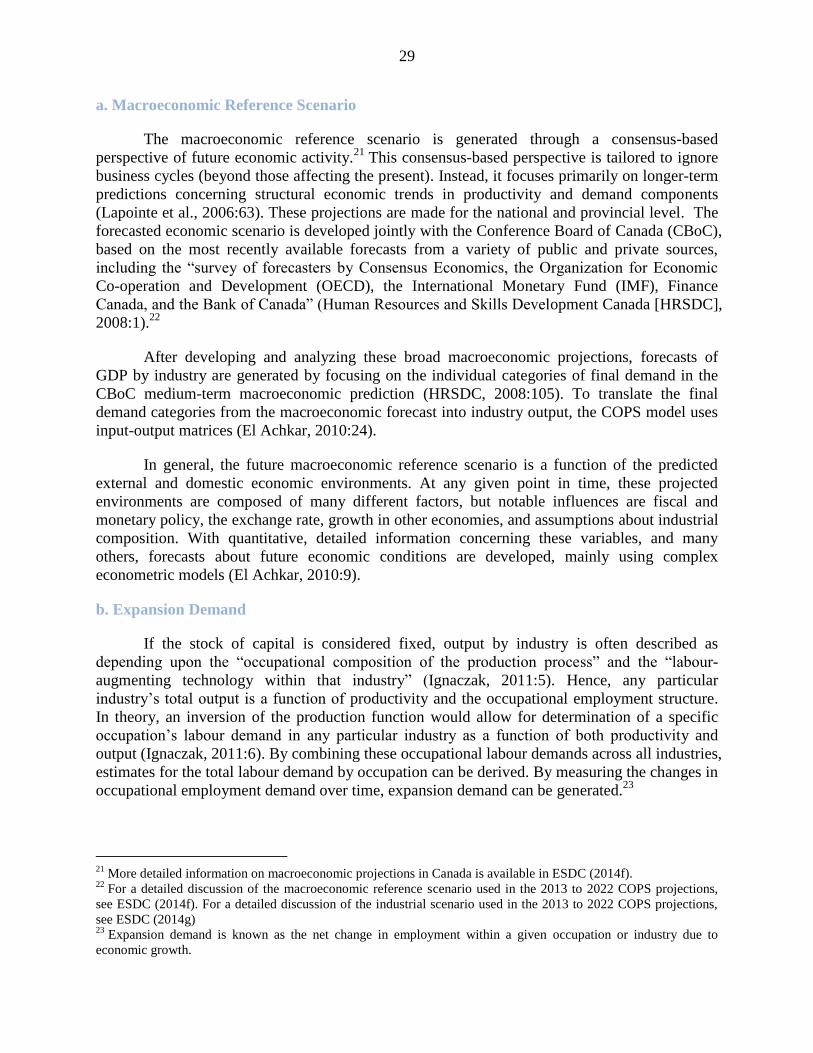
29

a. Macroeconomic Reference Scenario

The macroeconomic reference scenario is generated through a consensus-based

perspective of future economic activity.21

This consensus-based perspective is tailored to ignore

business cycles (beyond those affecting the present). Instead, it focuses primarily on longer-term

predictions concerning structural economic trends in productivity and demand components

(Lapointe et al., 2006:63). These projections are made for the national and provincial level. The

forecasted economic scenario is developed jointly with the Conference Board of Canada (CBoC),

based on the most recently available forecasts from a variety of public and private sources,

including the “survey of forecasters by Consensus Economics, the Organization for Economic

Co-operation and Development (OECD), the International Monetary Fund (IMF), Finance

Canada, and the Bank of Canada” (Human Resources and Skills Development Canada [HRSDC],

2008:1).22

After developing and analyzing these broad macroeconomic projections, forecasts of

GDP by industry are generated by focusing on the individual categories of final demand in the

CBoC medium-term macroeconomic prediction (HRSDC, 2008:105). To translate the final

demand categories from the macroeconomic forecast into industry output, the COPS model uses

input-output matrices (El Achkar, 2010:24).

In general, the future macroeconomic reference scenario is a function of the predicted

external and domestic economic environments. At any given point in time, these projected

environments are composed of many different factors, but notable influences are fiscal and

monetary policy, the exchange rate, growth in other economies, and assumptions about industrial

composition. With quantitative, detailed information concerning these variables, and many

others, forecasts about future economic conditions are developed, mainly using complex

econometric models (El Achkar, 2010:9).

b. Expansion Demand

If the stock of capital is considered fixed, output by industry is often described as

depending upon the “occupational composition of the production process” and the “labour-

augmenting technology within that industry” (Ignaczak, 2011:5). Hence, any particular

industry’s total output is a function of productivity and the occupational employment structure.

In theory, an inversion of the production function would allow for determination of a specific

occupation’s labour demand in any particular industry as a function of both productivity and

output (Ignaczak, 2011:6). By combining these occupational labour demands across all industries,

estimates for the total labour demand by occupation can be derived. By measuring the changes in

occupational employment demand over time, expansion demand can be generated.23

21

More detailed information on macroeconomic projections in Canada is available in ESDC (2014f). 22

For a detailed discussion of the macroeconomic reference scenario used in the 2013 to 2022 COPS projections,

see ESDC (2014f). For a detailed discussion of the industrial scenario used in the 2013 to 2022 COPS projections,

see ESDC (2014g) 23

Expansion demand is known as the net change in employment within a given occupation or industry due to

economic growth.

30

To obtain these estimates in practice, measures of industry-specific labour productivity

must be calculated. In general, these are estimated by using a Hodrick-Prescott filter that

extrapolates historical trends from the past two decades throughout the projection period

(HRSDC, 2008:105). Future industry employment levels are thus calculable by using the

projected output by industry and the forecasted labour productivity by industry. These forecasts

of industry-specific employment are broken down into occupational classes by using industry-

occupation employment matrices. These matrices are constructed using data from past Censuses

and Labour Force Surveys (El Achkar, 2010:24).24

Labour Force Survey data were implemented

in the construction of these matrices to ameliorate the previous methodology, which only relied

on census data. In particular, by including information from the Labour Force Survey, cyclical

influences can be incorporated in the projection of occupational share coefficients (Papps,

2001:20). In addition, the occupational share coefficients obtained from the industry-occupation

employment matrices are allowed to evolve over time by specifically accounting for the

development patterns of past industry-occupation matrices (Papps, 2001; 20). In the end, by

applying these industry-specific occupational coefficients to employment estimates by industry,

occupational employment demand by industry is obtained. By combining the occupational

employment estimates from each occupation across industries, total occupational employment

demand is determined (El Achkar, 2010:24). For the sake of simplicity during analysis, the

occupational expansion demand estimation process is disaggregated into an industrial effect,

which reflects employment changes due to industry performance, and an occupational effect,

which reflects the changes arising from “the trend path of the occupational share in the industry”

(Ignaczak, 2011:6). Once the results have been obtained, the occupational employment shares

undergo evaluation and adjustment to ensure normalization to the industry total.

c. Replacement Demand

Replacement demand broadly refers to employment that is generated by workplace

departures. The COPS model considers replacement demand generated by four types of

departures: retirements, in-service mortality, emigration or otherwise.25

Retirements, in-service

mortality and emigration are captured on the demand side, while other types of separations are

measured under the net re-entrants category of the supply side estimations. In cases where there

are more leavers than entrants, it is considered “negative supply” (Ignaczak, 2011:6). Despite

being slightly counterintuitive, emigration is captured on the demand side because when workers

leave certain occupations to move to different countries or regions, vacancies are created which

need to be filled.

24

An alternative method to disaggregating industry employment is to develop current estimations of industry-

specific occupational shares by referencing the historical evolution and development of industry occupation shares.

To undertake this approach appropriately, it is necessary to ensure that the occupation shares within each industry

sum to one. Often, occupational shares are projected under this methodology by using simple functional forms, like

trends and an output gap measure (HRSDC, 2008:140). 25

Papps (2001:20) claims that replacement demand forecasts are obtainable through a simulation of a “regression

equation of the share of replacement demand in employment.” The equations, Papps (2001:20) argues, include a

“cyclical variable to allow for the fact that the flows of workers in and out of particular industries vary widely over

the business cycle.” This methodology for estimating replacement demand seems widely divergent from the

methodologies claimed in other sources, which are described in the body of the report.

31

The retirement model dominates the projections of replacement demand, since 80 per

cent of replacement demand originates from retirements.26

The COPS model considers both

voluntary and involuntary retirements. This is done with a benchmarking model where the

component of voluntary retirements is generated through the self-reported data in the Labour

Force Survey.27

The involuntary retirements are proxied by a “constant and cyclical

unemployment component” (Ignaczak, 2011:6-7).

More specifically, annual retirement probabilities are calculated by using the

Longitudinal Administrative Databank data on individuals over the age of 50 who are separated

from a job and have remained unemployed for at least three consecutive years. These

probabilities are computed for each single age and gender combination by dividing the number

of retirements by the number of employed persons for each group (HRSDC, 2008:142). These

age- and gender-specific probabilities can be projected into the future by referencing crucial

behavioural influences, including primarily detailed information on the unemployment rate,

household net worth holdings, potential crowding effects from excess labour supply, and implicit

subsidies for retirement and birth-cohort effects. By applying the “projected age- and gender-

specific retirement probabilities to the projected age- and gender-specific employment levels”,

forecasted retirement levels can be obtained (HRSDC, 2008:142).

By following these steps, the model generates three different projections of single age-

and gender-specific rates of retirement.28

All three of these projections are then examined,

weighted and pooled to generate final estimates of future retirement rates by age and gender.

After finding internal agreement between these three forecasts, the aggregate retirement

benchmark is derived by applying these age-specific and gender-specific retirement rates to the

population and employment rate projections (Ignaczak, 2011:7).

Finally, an age distribution model is used to turn occupational employment by single age

into the median age of retirement and a distribution of ages across occupations. By determining

the proportion of the distribution in any given occupation within a benchmark number of years of

the median age of retirement, a “normalized potential retirement pool” is produced (Ignaczak,

2011:7). To ensure accuracy, the spread in the number of years beyond the benchmark retirement

age is increased as the projection horizon is widened so that the potential pool of retirees grows

with the projection period. More specifically, by using this aggregate retirement benchmark and

information from the Labour Force Survey, an estimate of retirement levels by occupation can be

generated by determining the number of individuals approaching the median retirement age in

each occupation.29

Quite simply, after the Labour Force Survey employment profile of an

26

Retirements are defined as permanent withdrawal from the labour force for those aged 50 and over (Ignaczak,

2011:6). 27

A benchmarking model is required because the model’s definition of retirement creates a lag of three years prior

to the projection period. More specifically, as there is no consistent definition of retirement, the current model

assumes that “tax filers over the age of 50 who have been away from paid work for 3 years or more are very unlikely

to return to the labour market” (HRSDC, 2008:141). By making this assumption, this method “creates a lag of

several years prior to the start of the projection period” (Ignaczak, 2011:7). 28

The first projection naively assumes no change. The second projection is an “autoregressive forecast of order 1”,

while the third, and final, projection, “propagates retirement rates mathematically by birth cohort” (Ignaczak,

2011:7) 29

This method does not capture actual retirement levels. Instead, it develops an estimate of potential retirements

(HRSDC, 2008:142).

32

occupation has been aged forward, the estimate of potential retirements is obtained by

calculating the “average annual number of employed workers within five years of that

occupation’s median retirement age” (HRSDC, 2008:142). Subsequently, the estimates of

occupational retirement generated from the Labour Force Survey data are normalized to ensure

that they sum to the aggregate estimate of retirements from the Longitudinal Administrative

Databank (Lapointe et al., 2006:87).30

In summary, estimates for future aggregate retirements are generated through three broad

steps (Lapointe et al., 2006, p. 87):

1) Forecasts of aggregate employment by gender and age are calculated by assuming

specific gender and age employment rates;

2) Gender- and age-based retirement rates are forecasted by using an econometric

technique that models how a variety of explanatory variables, including wealth

education, and labour demand, affect retirement rates;

3) Projections of retirement levels are derived by applying age- and gender-specific

retirement rate projections to forecasts of age- and gender-specific employment.

In-service mortality estimates show how currently occupied positions will be affected by

death. Initially, death rates by age are derived by calculating the deaths to population ratio.31

To

determine projections of occupational vacancies due to deaths, these age-specific death rates are

applied to single-age occupational employment forecasts. This method develops a “projected age

distribution [of deaths] by occupation” (Ignaczak, 2011:7). By summing the final results across

ages, an estimate of in-service mortality by occupation is generated.

Emigration models are primarily based on demographic factors. The COPS model uses a

very simple projection of emigration. Initially, estimates of the number of emigrants are obtained.

Subsequently, labour force participation rates for emigrants are determined. By applying the

labour force participation rates to the projected number of emigrants, an estimate of aggregate

labour requirements due to this departure path is derived. Labour demand by occupation can be

determined by filtering aggregate labour demand through an “average occupational share vector”

(Ignaczak, 2011:7).

After completing these three estimations, simple accounting generates replacement

demand. In particular, replacement demand by occupation can be calculated by combining

retirements, in-service mortality and emigration by occupation. By combining replacement

demand by occupation and expansion demand by occupation, an estimate of occupational

demand is obtained (El Achkar, 2010:25).

ii. Supply Side under COPS

The supply side of the COPS model consists of three steps:

30

For a more detailed analysis of aggregate retirement flows estimates in Canada, see Dunn (2005). 31

The potential complication of higher death rates among the non-working population by single age is partially

overcome by applying the employment rate to estimates of the number of deaths by single age prior to calculating

the death to population ratio.

33

a) Estimation of school leaver labour force entrants by occupation

b) Projection of immigrants by occupation

c) Projection of other occupational flows

Each of these will be subsequently discussed in detail.

a. School Leavers

The supply side of the COPS model generally begins with an attempt to capture the “new

inflows into the labour market from the education system,” referred to as school leavers

(Ignaczak, 2011:8). This model generally assumes that “students invest in education and attempt

to find work in an area related to their field of study” (Ignaczak, 2011:8). A variety of steps are

needed to develop aggregate and occupational graduation and discontinuation flows. Initially,

enrolments are forecasted over the projection period.32

In the past, this has been performed by

considering four major classes of educational attainment: high school, trade and vocational,

community college (including university certificates below a Bachelor’s degree), and university

(including Bachelor’s degrees, university certificates above a Bachelor’s degree, Master’s

degrees, and Doctorates) (HRSDC, 2008:148).33

The rate of enrolment in these programs is

based upon a variety of influences, including unemployment rates, previous enrolment rates,

government funding for education, source population size and per capita real personal disposable

income. Thus, each of these factors is carefully considered during projections of enrolments.34

In

the next stage, projections of graduation are based upon enrolment levels. In general, enrolments

figures are positively correlated with the number graduates (HRSDC, 2008:149).35

In the subsequent step, the number of drop outs is estimated. In this step, there is also

usually an additional filter for individuals who graduate from one program but decide to pursue

further education and forego labour market participation until later in the future. An example

would be an individual who completes a Bachelor’s degree but decides to pursue the completion

of a Master’s degree or PhD before joining the labour force (Lapointe et al, 2006:95). In order to

estimate the number of high school dropouts, the “number of graduates in the current year is

subtracted from the number of students enrolled in grade nine four years earlier” (HRSDC,

32

Part-time students are not considered in the projections. In general, this is done in order to “exclude persons

working part-time or returning to school for re-training” (Lapointe et al, 2006:95). If these individuals were included

in these estimates, then the results would be misleading. In particular, since these estimates are meant to capture the

number of new entrants into the labour force, including part-time students or re-entrants may fudge the projections.

The most prominent exclusion in the past has been “undergraduate or graduate students enrolled in programs leading

to a certificate or diploma” (Lapointe et al, 2006:95). 33

Administrative data is obtained from the Postsecondary Student Information System (PSIS), which encompasses

and replaces the University Student Information System (USIS), the Community College Student Information

System (CCSIS) and the Trade and Vocational Enrolment System (TVOC). Data is also retrieved from the

Elementary and Secondary Education Statistics Project (ESESP) (HRSDC, 2008:148). 34

Generally, it is “expected that an increase in per capita real personal disposable income will drive up demand for

education, and thus enrolments, as education is a normal good” (HRSDC, 2008:148). Moreover, “an increase in the

unemployment rate also boosts enrolments, as it lessens the probability of employment in the labour market, thus

reducing the opportunity cost of pursing education” (HRSDC, 2008:148). Furthermore, as the government increases

investment in the education system, enrolments increase, since education becomes more accessible to a greater

proportion of the population (HRSDC, 2008:148). Lastly, enrolments generally increase with the size of the source

population (HRSDC, 2008:148). 35

The length of the program is taken into account. In cases of uncertainty, average program length is used.

34

2008:149). For post-secondary dropout rates, a fixed coefficient is used, which remains

unchanged throughout the projection period.

In total, the previous steps generate estimates of aggregate discontinuation and graduation

flows over the projection period for four broad educational categories. These estimates can next

be disaggregated into occupational supply projections by the use of education to occupation

matrices. In the past, those with post-secondary education were broken down into field of study

before the application of an education to occupation matrix. This ensured stronger, more accurate

translations from educational attainment into occupational classes. This step is typically

performed by using a “fixed share vector of field of study choices” (Ignaczak, 2011:8). A vector

of field of study choices is allocated to each level of post-secondary education. No field of study

is assigned to individuals who did not attain post-secondary education degrees or diplomas.

Individuals who discontinued their education are allocated to their “immediately preceding level

of education for the field of study transition vector” (Ignaczak, 2011:8). If the immediately

preceding educational class does not have a field of study vector, no field of study vector is

applied. In the last step, participation rates and education to occupation matrices (or field of

study to occupation matrices) are applied to those who have chosen to enter the labour force.

In general, the COPS model uses two field of study to occupation transition matrices to

create two distinct supply alternatives: ex-ante, before labour market resolution, and ex-post,

after labour market resolution. In the “ex-ante scenario, an analyst constrained set of matrices is

applied which only permits employment in a related occupation” (Ignaczak, 2011:8). Leniency in

the development of the constrained matrices is considered crucial, and labour force participants

are permitted a significant amount of movement. The matrices essentially allow for movement to

any occupation in an equivalent skill level, as defined by the required level of study. In addition,

the matrices allow for movement into a number of similar occupations in other skill levels

(Ignaczak, 2011:8). The structure of the ex-ante approach is based on attempts to limit post-

secondary graduate employment in low-skilled occupations by restricting “new school leavers to

seeking employment in occupations directly related to their field of study” (HRSDC, 2008:150).

The ex-ante analysis of new labour supply from school leavers is crucial for some analysts

because it reflects a system where investments in education are embarked upon with the intention

of working in a related or high-skilled occupation. In addition, the supply flow derived from an

ex-ante perspective tends to better reflect the career goals of school leavers over the long term

(HRSDC, 2008:150).

More specifically, by using administrative data, the ex-ante approach breaks down post-

secondary graduates by field of study before translating them into occupational classes.36

Since

the fields of study available to students are relatively stable over time, the breakdown by fields of

study remains unchanged throughout the projection period. The data used by the COPS model

for this process is obtained from the National Graduate Survey performed by Statistics Canada.37

Those surveyed were broken down by field of study and educational level. In the ex-ante

36

There are 162 fields of study: 49 fields of study for trade and vocational graduates, 55 for college graduates and

58 for university graduates (HRSDC, 2008:150). 37

The survey contacts recent graduates to develop an understanding of the number of postsecondary graduates who

were able to find employment after they graduated. The most recent survey was completed in 2007, contacting

graduates from 2005. A new survey conducted in 2013 will be available soon. This survey contacted graduates from

2010.

35

approach, only those occupations that pertained to the individual’s field of study were

preserved.38

This scenario “reflects the difficulties graduates may face early on in their career, by

allowing graduates to fall back on less qualified occupations, if they are directly related to their

field of study” (HRSDC, 2008:150). Hence, with this detailed information, occupational

distributions by field of study and education level can be constructed and applied to projections

of school leavers by education and field of study.39

In stark contrast, the ex-post approach models the “actual outcomes that post-secondary

graduates face in the labour market upon graduation” (Ignaczak, 2011:8). In particular, the ex-

post scenario reflects the difficulties that recent graduates may encounter in their attempts to

access particular occupational paths (HRSDC, 2008:149). Labour Force Survey data from the

past three years are used to construct a distribution of school leavers by occupation for each

education level. To ensure more accurate estimates, the data used to construct different

distributions varies by education level. As an example, the distribution of occupations for

individuals with a high school diploma is based upon Labour Force Survey data for students

from age 15 to 24. In contrast, the occupational distribution for individuals with a Bachelor’s

degree is constructed with data from older individuals as well. In summary, this ex-post scenario

does not confine graduates to employment in an occupation that is directly associated with their

field of study (HRSDC, 2008:149).40

By not restricting the data to occupations that correspond to

field of study, broader occupational distributions are developed and applied to school leaver

projections to determine school leavers by occupation.

The goal of undertaking these two scenarios is to facilitate analysis of any potential

education-occupation mismatches, since ex-ante results predict outcomes that educational

investment would bring, while ex-post results predict outcomes that labour market resolution

would bring (Ignaczak, 2011:8).41

Hence, the final results are two very different projections of

new occupational labour supply coming from recent graduates and dropouts, each providing

valuable insights.42

Beginning with the 2013-2022 projections, the COPS model now considers both part-

and full-time students as channels of new labour supply. The flow of students is projected by

estimating the share of students in each occupation by age and education level. These shares are

then applied to the number of employed individuals by age and education level from the

38

“For example, someone with a Bachelor’s degree in nursing may seek work…as a nursing sciences professional,

health care [technician], or health sciences technologist. However, [that same graduate is] restricted to not seeking

employment as a cashier, even though in reality some graduates may end up in such an occupation” (HRSDC,

2008:150). 39

The model uses data concerning youth from the Labor Force Survey “for graduates who have not completed

postsecondary education, [including] individuals with less than high school, high school graduates and individuals

with only some post-secondary education” (HRSDC, 2008:150). 40

In particular, an individual with a Bachelor’s degree in nursing is permitted access to occupations in entirely

different fields, such as marketing or finance (HRSDC, 2008:149). 41

Many individuals who intended to work in particular occupations ex-ante are limited to other occupations ex-post.

Hence, this two-stage ex-post and ex-ante approach generates a solid beginning for analyzing occupational-skills

mismatches (Ignaczak, 2011:8). 42

See Appendix 9 for the 2008 to 2017 COPS projections that permit comparison of the ex-ante and ex-post results.

The 2013 to 2022 projections take an ex-post approach. Ex-ante results were calculated internally by the COPS

team.

36

demographic projections. This student component is not a major element in the COPS model.

The turn-over in the number of students working might be high, but the net change in the stock

of students, the flow, is expected to be quite low.

To summarize, the education sub-model forecasts graduation levels in any given year

using historical data on age- and gender-specific enrolment rates for various different classes of

educational attainment. In particular, the trends in the historical rates are used to forecast future

rates of enrolment. In order to derive graduation rates for any particular forecast year, a fixed rate

is applied to the number of enrolments that were observed (or forecasted) during the year when

graduates would have normally started the program.43

Forecasts for discontinuants are similarly

estimated. Finally, field of study to occupation transition matrices are used to translate

projections of graduation by education and field of study into projections of labour force entrants

by occupation (El Achkar, 2010:25).

b. Immigration

The COPS immigration model is extremely simple and “lacks many of the interesting

dynamics of other more developed models” within COPS, but it meets the purposes of long-term

trends (Ignaczak, 2011:8). It assumes that “a fixed proportion of the current population will enter

the country every year” (Ignaczak, 2011:8). Over the past few years, the proportion of

immigration out of the total population has been about 0.75 per cent, remaining relatively stable.

The potential available immigrant labour force is estimated by applying their respective

labour force participation rates observed in the last census to the proportion of immigrants who

are not expected to be attending educational programs. To model occupational choices, a fixed

vector of recent immigrant occupational outcomes is assumed, based upon Statistics Canada

surveys that identify immigrant occupational choices (HRSDC, 2008:151).44

Recent improvements have been made to the immigration model. Immigrants used to be

distributed according to the census data on new immigrants (one year after arrival). However, it

is known that immigrants change jobs quickly after arrival, before securing more permanent

positions. Hence, occupational data on “recent immigrants” from the most recent census has now

been implemented. Recent immigrants include those individuals that have arrived over the

previous five years.

c. Other Occupational Flows

The COPS model supplements the above supply side considerations by capturing

additional occupational flows in the form of net occupational mobility, net re-entrants or the

unemployment add factor through a stock-flow reconciliation process. This stock-flow

reconciliation process is performed using a labour market entry cohort model by education,

43

For example, “for a four-year program, the projected number of graduates in 2010 is obtained by applying the

fixed graduation rate last observed to the enrolment numbers in 2006” (El Achkar, 2010:25). 44

In general, statements of intended occupation at time of arrival are considered inaccurate, as there does not appear

to be a statistically significant relationship between intended occupation before arrival and actual occupation after

arrival. Hence, factual data concerning immigrant occupations is obtained to perform these estimates. Education and

geographic location are also “important determinants of occupation” for immigrants (HRSDC, 2008:151).

37

labour force status and single age. All of the reconciliation models use “net measures obtained

from an already existing stock model” (Ignaczak, 2011:9). The idea behind the stock-flow

reconciliation process is to link the changes in the labour force participation rate model,

assumptions about unemployment, and demographics (stock of employed workers) to the

occupational flows generated by the COPS component models. By reconciling these, it is

possible to account for all of the COPS components, and therefore ensure that they all add up

coherently to the macro and demographic projections.

Net occupational mobility captures individuals “currently in the labour force moving

between occupations” (HRSDC, 2008:151). Vertical mobility covers worker movement between

occupations that require different skill levels. This includes both upward occupational mobility,

where workers who have “gained labour force experience move up to management positions,”

and downward occupation mobility, where “workers choose to enter low-skilled occupations as

part of their transition towards retirement” (HRSDC, 2008:151).45

Horizontal mobility considers

workers who display movement between occupations of the same skill level.

Net re-entrant measures and the unemployment add factor “capture the net inflows into

the economy stemming from the anticipated rise in age- and gender-specific participation rates,”

as well as the net inflows caused by the declining unemployment rates due to demographic shifts

(Ignaczak, 2011:9).46

These two components, along with net occupational mobility, are

accounted for on the supply side of the COPS model due to the historical developments of the

Canadian projection system. However, it would make more sense to include negative supply

flows on the demand side.

Hence, in summary, the stock-flow accounting process reconciles historical and projected

data: estimates from the COPS model system are compared to actual historical changes. This

historical analysis develops a benchmark against which the stock-flow reconciliation of the

projection estimates can be compared. While it is not essential that the future closely mirror the

historical data, this approach provides a “reasonable benchmark as to the expected flows and

their magnitude” (Ignaczak, 2011:9).

iii. Balancing Supply and Demand under COPS

After completing both demand and supply side projections by occupation, it is possible to

undertake qualitative and quantitative assessments of future labour market conditions.

Imbalances in the COPS model are measured by subtracting occupational supply from

occupational demand. Quantitatively, the model will always generate some measure of excess

demand or excess supply (Ignaczak, 2011:10). In order to appropriately evaluate this, the

45

In 2008, calculations of vertical mobility were performed at the 3-digit occupational level (HRSDC, 2008:155-

161). 46

One source states that “re-entrants are measured as the observed outflows from an occupation minus the number

of permanent withdrawals, resulting from retirement” (Papps, 2001:20). Furthermore, Papps (2001:20) affirms that

“projections for both retirements and outflows are [based] on regressions of historical values, including a cyclical

term.” Another source states that the “trend, adjusted for the business cycle, in historical data of the flow from

employment to non-employment, expressed as a proportion of employment, [can be] obtained from a simple

regression model” (El Achkar, 2010:25), after which, it is possible to project the flow from employment to non-

employment into the future by applying the projected proportion to the estimated future employment levels.

38

normalized future labour market situation indicator has been developed. To generate this

measure, excess labour demand by occupation is “divided by base year employment and by the

number of years in the projection” (Ignaczak, 2011:10). In the past, a two-standard deviation

bound has been used to indicate occupations that are at risk for excess supply or excess demand.

Unfortunately, this indicator assumes that the labour market is balanced in the base year in each

occupation. Hence, a “current labour market conditions assessment is also used to revise any

occupations which cannot be considered balanced in the base year” (Ignaczak, 2011:10). Given

the difficulties of interpreting these quantitative results, the labour market information that is

made available to the public also offers a rating for each occupation: poor, fair, or good.

The COPS model, in summary, produces detailed occupation-specific and skill-specific

assessments of ex-ante occupational imbalances. Due to its “coherent…consistent assessments of

the demand for and supply of new and existing labour market entrants” (Ignaczak, 2011:15),

many organizations within Canada have adapted the COPS model in order to provide forecasts at

the sub-national level.47

Nevertheless, this overview of the COPS model is not conclusive

because its methodology and procedures are constantly undergoing revision and improvement to

surmount the diverse structural, conceptual and technical obstacles that prevent a completely

efficient and effective production of future labour supply and demand forecasts.

B. United States Bureau of Labor Statistics

The Bureau of Labor Statistics undertakes occupational forecasting through a program

called Employment Projections (EP). The EP program develops 10-year forecasts of the national

labour market. These projections are performed every other year. The most recent projections are

for the period 2012 to 2022, with final projections reflecting the state of the labour market in

2022. The results of the analysis were published in December 2013. The final publication, the

Occupational Outlook Handbook, provides information on worker activities; working

environments; education, training, and other qualifications; wages; job prospects; similar

occupations; and additional resources for 334 occupational profiles, covering approximately 84

per cent of available jobs in the US economy. Each US State also undertakes projections of

industry and occupational employment by using input from the BLS National projections.

Methodologically, the Bureau of Labor Statistics (BLS) undertakes six interconnected

steps to generate forecasts of industry and occupational employment. Each step requires different

procedures, models and assumptions (US Bureau of Labor Statistics, 2014). Briefly, these are

centered on economic projections, an input-output matrix, and an industry-occupation matrix,

called the National Employment Matrix, which “depicts the distribution of employment by

industry and occupation” (Bureau of Labor Statistics [BLS], 2013a:1). The six steps consist of:

1) The size and demographic composition of the labour force

47

The Ontario Ministry of Training, Colleges and Universities has implemented an altered version of the COPS

model at the sub-national level, resulting in their Job Futures publication. Some important changes include altering

assumptions concerning death rates, retirement rates and industry structures (some of this is an internal exercise

only, undertaken as a simple sensitivity analysis). In addition, the Ontario Ministry of Training, Colleges and

Universities obtains more expansive, detailed industry forecasts prior to its projection process from Stokes

Economics Consulting. These disaggregated industry forecasts are re-aggregated to match the 33 industries used by

the COPS model. A number of other provinces and territories have equally adapted the COPS model.

39

2) Aggregate economic growth

3) Commodity final demand

4) Input to output patterns by industry

5) Industry output and employment

6) Occupational employment and openings

i. BLS Occupational Labour Demand Estimation Methodology

a. Labour Force Size and Demographic Composition Estimation

Estimates of aggregate future labour supply are necessary for the BLS estimation of a

macroeconomic reference scenario. The projections of the future supply of labour are determined

by applying projections of the labour force participation rate to projections of the working-age

population. The population projections are generated by the Census Bureau, while forecasts of

the labour force participation rate are undertaken by the Bureau of Labor Statistics. The long-

term projections of the US population are based on the “current size and composition of the

population” (BLS, 2013a:2). In order to have accurate projections, assumptions are made about

future “fertility, mortality and net international migration” (BLS, 2013a:2). In order to convert

the census population information to data that can be used by the BLS, the population of children

aged 16 and under must be subtracted from the total resident population. In addition, the

population of the armed forces and the civilian institutional population are both subtracted by age,

gender, race and ethnic category (BLS, 2013a:1).

Labour force participation rates are taken from the Current Population Survey for various

race, age, gender and ethnic groups. Analysts at the BLS examine trends in these participation

rates for each category. They undertake three steps to generate participation rate projections.

First, the “historical participation rates for each group are smoothed” (BLS, 2013a:2). Second,

the “smoothed data are transformed into logits, [also known as] the natural logarithm of the odds

ratio” (BLS, 2013a:2). Finally, the “logits of the participation rates are extrapolated linearly by

regressing them against time and then extending the fitted series to or beyond the target year”

(BLS, 2013a:2). When the fitted series is transformed from logits back into rates of participation,

the forecasted trends are nonlinear.

In addition to these rigorous estimation techniques, the projected labour force

participation rates undergo a vetting process, where they are reviewed for consistency by the

BLS officials. Once the rates have been carefully analyzed and confirmed, they are applied to the

projected civilian non-institutional population in order to generate projections of labour force

participation by age, gender, race and ethnic group. The individual groups are combined to

obtain the total civilian labour force, which becomes an important addition to the next step: the

construction of the macroeconomic reference scenario.

b. Macroeconomic Reference Scenario

In the next stage, projections about the future macroeconomic scenario are undertaken,

focusing on US gross domestic product and on the chief income and demand categories. The

two models used in the projection process have similar foundations: consumption is founded

upon a life-cycle model, while neo-classical models serve as the foundation for investment (BLS,

40

2013a:2). The estimates for the foreign sector rely on forecasts from Oxford Economics. The

model used by the BLS assumes full employment in the target year, implying that any

unemployment is frictional and not the consequence of a deficit demand (BLS, 2013a:2).48

There

are many other critical components involved in the economic forecasting process, including

projected energy prices, and fiscal and monetary policy assumptions.

Since the macroeconomic model above provides broad projections of final demand

sectors, including “personal consumption expenditures, private investment in equipment and

software, residential and non-residential structures, changes in private inventories, exports and

imports of goods and services, and consumption and investment of federal, state and local

governments,” the next stage strives to further disaggregated the results into the commodity

types purchased within each category (BLS, 2013a:2). There are 76 detailed product categories

included in the consumption expenditure estimates. The historical relationship between each

product type and a set of variables, including disposable income, prices, and a state variable

capturing inventory or habit formation, guide the generation of consumption estimates for each

product type. Similarly, private investment in equipment and software is modeled for 28 asset

categories using a model that predicts investment based on GDP, capital stock, and the rental

cost of capital. The controls for “non-residential and residential structures, exports and imports

of goods and services, as well as consumption and investment within federal defence, federal

non-defence, and state and local government are supplied directly from the macro model” (BLS,

2013a:3).

48

A sub-model estimates prospective nonfarm business output. The forecast is based on “full employment estimates

of the sector’s hours worked and output per hour” (BLS, 2013a:2).

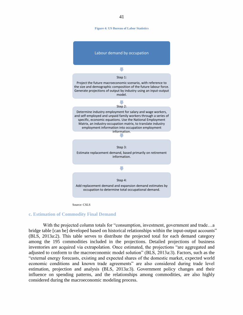
41

Source: CSLS

c. Estimation of Commodity Final Demand

With the projected column totals for “consumption, investment, government and trade…a

bridge table [can be] developed based on historical relationships within the input-output accounts”

(BLS, 2013a:2). This table serves to distribute the projected total for each demand category

among the 195 commodities included in the projections. Detailed projections of business

inventories are acquired via extrapolation. Once estimated, the projections “are aggregated and

adjusted to conform to the macroeconomic model solution” (BLS, 2013a:3). Factors, such as the

“external energy forecasts, existing and expected shares of the domestic market, expected world

economic conditions and known trade agreements” are also considered during trade level

estimation, projection and analysis (BLS, 2013a:3). Government policy changes and their

influence on spending patterns, and the relationships among commodities, are also highly

considered during the macroeconomic modeling process.

Labour demand by occupation

Step 1:

Project the future macroeconomic scenario, with reference to the size and demographic composition of the future labour force. Generate projections of output by industry using an input-output

model.

Step 2:

Determine industry employment for salary and wage workers, and self-employed and unpaid family workers through a series of

specific, economic equations. Use the National Employment Matrix, an industry-occupation matrix, to translate industry

employment information into occupation employment information.

Step 3:

Estimate replacement demand, based primarily on retirement information.

Step 4:

Add replacement demand and expansion demand estimates by occupation to determine total occupational demand.

Figure 4: US Bureau of Labor Statistics

42

In order to complete the forecast of the macroeconomic scenario, data is converted from

purchaser value to producer value.49

This producer value data ensures that output from the

wholesale sector, the retail sector and the transportation sector are separated from the remaining

economy. At the very end, the macroeconomic forecast, a detailed distribution of GDP, provides

the demand component of an inter-industry model of the US economy (BLS, 2013a:2).

d. Output Projections by Industry

In the next stage, the BLS projections use an input-output model, developed with

reference to historical time series data.50

The input-output model is composed of “two basic

matrices for each year: a “use” table and a “make” table” (BLS, 2013a:4). After being

appropriately balanced, each table undergoes a conversion to coefficient form. The “converted

use table, or the direct requirements table, shows the use of commodities by each industry as

inputs into its production process” (BLS, 2013a:4). The columns of the direct requirements table

show “the pattern of commodity inputs per dollar of industry output” (BLS, 2013a:4). The

“converted make table, or the market share table, shows the commodity output of each industry”

(BLS, 2013a:4). This table “allocates commodity output to the industry in which it is the primary

commodity output and to those industries in which it is secondary” (BLS, 2013a:2). The “market

share table also shows the industry distribution of production for each commodity” (BLS,

2013a:4). Using historical relationships and the projected final demand tables, initial

approximations of the projected input-output tables are developed. A vetting process where

results are revised and reviewed allows for the recognition of industry-level changes in the way

goods are produced or services are provided, namely productivity changes. In the event of error,

adjustments can be made.

When projected values of the use and make relationships are available, the BLS uses a

specific relationship to convert the projections of commodity demand developed in the preceding

steps into a projection of domestic industry output. Briefly, by taking the “matrix product of the

inverse of the coefficient forms of the make and use tables”, and subsequently subtracting a

vector of final demand commodity distributions, industry outputs can be determined (BLS,

2013a:4).51

e. Industry Employment Estimates

The extremely detailed industry output derived in the preceding steps is used to generate

the employment estimates by industry required to produce the specified level of output. Similar

to many other approaches, the BLS models employment by industry as a function of wages,

prices and industry output; approximated historical relationships between these variables are

used. To provide as much information as possible, industry employment is projected in both

49

To do this, margin columns are projected for each component of final demand based upon distributional

relationships from historical time series. Summing across the rows of a particular component with its related margin

columns, consisting of transport costs as well as wholesale and retail markups, results in a vector of producer value

data by detailed commodity. 50

Input-output tables recently underwent significant changes in the US in the face of expanded data sources. For

more information see BLS Handbook of Methods (2013a). 51

g = D(I – BD) – e where g is a vector of domestic industry output by sector, D is the make table in coefficient

form, B is the use table in coefficient form, I is the identity matrix, e is the vector of final demand by commodity

sector (BLS, 2013a:4).

43

numbers of jobs and hours worked for wage and salary workers and for self-employed and

unpaid family workers.

In order to project employment for each industry for all of these categories, there are

multiple steps. The projections for wage and salary workers requires a system of equations that

relates total hours of labour demand within an industry to that industry’s output and wage rate, as

well as a trend variable that captures industry-specific technological change (BLS, 2013a:4-5).

Another separate set of equations “describing average weekly hours for each industry, is

estimated as a function of [a] time [trend] and the unemployment rate” (BLS, 2013a:5). Together,

the two sets of equations are capable of predicting the average weekly hours of work within a

given industry over the forecasting period. To finish this estimation process, an identity that

relates “average weekly hours, total hours and employment” is used to generate the number of

wage and salary jobs by industry (BLS, 2013a:5).52

f. Occupational Employment Projections

Similarly to the COPS model, the BLS constructs industry-occupation matrices to

translate industry-level employment forecasts into occupational employment projections. The

BLS approach consists of a “base-year employment matrix and a projected year employment

matrix” (BLS, 2013a:5). The matrices, collectively referred to as the National Employment

Matrix, provide the BLS with a comprehensive database that is capable of generating

occupational employment from industry employment estimates. The aggregate base-year

employment for any particular occupation is determined by pooling employment across all

occupations and worker categories, namely wage and salary, self-employed or unpaid. To

determine the occupational distribution ratios required for the forecasts of occupational

employment by industry, the occupational employment by industry is divided by the total wage

and salary employment within that industry. These ratios, once determined measure staffing

patterns, or occupational utilization, within any particular industry (BLS, 2013a:5).

Initially, projected-year employment is calculated at a higher level of aggregation, after

which it is distributed across the corresponding detailed National Employment Matrix industries

and classes of workers. The BLS analysts take base-year occupational utilization trends and

subject them to iterative processes of quantitative and qualitative analysis. By referencing

historical industry-specific staffing patterns, the economists at the BLS can identify variables

that may influence these staffing patterns over the forecasting horizon. In the past, notable

variables have been “shifts in [the] product mix and changes in technology or business practices”

(BLS, 2013a:5). After identification, these variables can be used to derive “numerical change

52

The BLS undertakes estimation of the number of self-employed and family workers as well. It is “derived by first

extrapolating the ratio of self-employed to the total employment for each industry” (BLS, 2013a:5). The resulting

extrapolated ratio is a function of the unemployment rate and time. The ratio can then be used to estimate self-

employment levels and unpaid family worker levels, given the level of wage and salary work within an industry. To

estimate total self-employment and unpaid family worker hours, the estimated average annual weekly hours is

applied to the levels of employment within each industry. To obtain the estimate of total hours for each industry, the

hours for wage, salary, self-employed and unpaid family workers by industry can be pooled (BLS, 2013a:5). By

combining industry output projections with employment results, a measure of labour productivity can be developed.

Where discrepancies exist with historical trends in labour productivity and employment, appropriate adjustments are

made. The finalized “estimates of projected employment…are then used as inputs to determine the occupational

employment” over the forecasting period (BLS, 2013a:5).

44

factors”, which provide estimates of the “proportional change in an occupation’s share of

industry employment” during the forecasting period (BLS, 2013a:5). By applying these

numerical change factors to base-year occupational utilization patterns, projections of staffing

patterns can be developed. Depending on the underlying rationales, assumptions, models and

historical data used to estimate the numerical change factors, any particular occupation’s share of

industry employment may increase, decrease or remain the same. By multiplying the projected-

year occupational ratio and the projected-year employment, an estimate of future wage and

salary occupational employment can be obtained for each industry. Estimates of self-employed

and unpaid family workers are done separately. Hence, projected total occupational employment

in any given year is the sum of the “projected employment figures for wage and salary workers

and the self-employed and unpaid family workers” (BLS, 2013a:5-6).

g. Replacement Demand Estimation

Similarly to the COPS model, the BLS model forecasts replacement needs. These

estimates of replacement needs are added to the estimates of openings due to economic growth to

derive total job openings over the forecasting horizon (BLS, 2013a:5).

The BLS references historical data on employment by occupation in order to calculate

replacement needs rates by age. By applying these historical replacement rates by age to base

year occupational age distributions, estimates of replacement demand for the projection period

can be generated. This method of forecasting replacement requirements relies on the assumption

that workers will retire and exit from occupations at comparable ages to those individuals from

recent past data. The final result is an “occupation-specific replacement needs [estimate] that

captures the impact of demographic, but not behavioural, changes” (BLS, 2013a:6).53

With the completion of the estimates for replacement demand and expansion demand, an

extensive review process is undertaken to ensure consistency across all of the projections. After

this intensive vetting, the projection process generates “an internally consistent set of

employment projections across all industries and occupations” (BLS, 2013a:6).

ii. Education and Training Requirements

In addition to estimating occupational employment demand, information concerning

training and education requirements is provided by the BLS for the labour force as a whole and

for occupations with various types of education and training needs. The BLS provides these

estimates by focusing on each occupation’s typical training and education requirements. In

addition, data on educational attainment within each occupation are presented to show current

workers’ levels of educational attainment (BLS, 2013a:6).

More specifically, BLS implements a system where it examines categories for entry-level

education requirements, requisite work experience in related occupations, and typical on-the-job

training for each occupation within the BLS projection system.54

By grouping occupations

according to the values they receive in each category, education and training needs for the entire

53

For a more detailed discussion of replacement demand estimates, see the technical document on the Employment

Projections Program website, http://www.bls.gov/emp/ep_replacements.htm. 54

This system replaces an incomparable system used between 1995 and 2008.

45

labour force are equally generated (BLS, 2013b). Within the category of typical education

needed for entry, there are eight designations: less than high school, high school diploma or

equivalent, some college or no degree, postsecondary non-degree award, Associate’s degree,

Bachelor’s degree, Master’s degree, and Doctoral or professional degree. The category for work

experience in a related occupation indicates if work experience is “commonly considered

necessary by employers for entry into the occupation, or is commonly accepted as a substitute for

formal types of training” (BLS, 2013b). The designations in this category include no training,

less than five years, and five years or more. For the typical on-the-job training category, an

assessment of typical on-the-job training needed to attain competency in the requisite

occupational skills is undertaken. The category contains six assignments: no on-the-job training,

short-term on-the-job-training (one month or less), moderate-term on-the-job training (more than

one month and up to twelve months), long-term on-the-job-training (more than twelve months),

apprenticeship, and internship or residency.

The assignment of education, training and experience to each of the BLS occupations can

be straightforward for certain occupations because they are governed by legal regulations that

give “clear guidelines regarding the education or training required for a given occupation” (BLS,

2013b). However, there are other occupations where it is less obvious. In these cases, the BLS

economists determine the typical path of entry into an occupation. If there are multiple paths of

entry, the most frequently chosen path is assigned to the occupation, as this system of education

and training needs does not permit multiple entry pathways. Alternative pathways are described

in their Occupation Outlook Handbook. The assignment of occupations to these categories is

based upon both qualitative and quantitative information. Quantitative data are obtained from the

Census Bureau’s American Community Survey, the Occupational Information Network, and the

National Centre for Education Statistics, while qualitative information is gathered from

“educators, employers, workers in given occupations, training experts, and representatives of

professional and trade associations and unions” (BLS, 2013b).

The educational attainment data complements the above education and training needs

information by allowing users to better “discern whether there are multiple education and

training possibilities” through the provision of the per cent distribution of “workers employed in

an occupation, broken down by their highest level of education attained” (BLS, 2013b).55

The

data for these educational attainment profiles are obtained from the American Community

Survey.56

For example, consider financial analyst occupations. In the Occupational Outlook

Handbook, employment is projected to grow 16 percent from 2012 to 2022, faster than the

average for all occupations (BLS, 2014). The occupational profile suggests that the education

and training requirement to become a financial analyst is a Bachelor’s degree, but that Master’s

degrees are often required for more advanced positions (BLS, 2014). By referring to the

educational attainment data, this is confirmed, since 86.1 per cent of all financial analysts have a

Bachelor’s degree or higher. 10.4 per cent of financial analysts have some college or an

Associate’s degree, while only 3.5 per cent have a high school degree or less (BLS, 2013c).

55

If 76.9 per cent of nurses have a Bachelor’s degree, this clearly indicates that obtaining a Bachelor’s degree is the

most typical pathway to this occupation, but there are alternative methods to entering the field of nursing. 56

The educational attainment table by occupation is available at: http://www.bls.gov/emp/ep_table_111.htm

46

However, this information also indicates that there may be alternative pathways to this

designation.

Despite the usefulness of this additional information, the BLS does not provide a final

assessment of where there may be potential labour market imbalances. Instead, it focuses solely

on measuring aggregate occupational demand and the prospective education and training

requirements for various occupations.

iii. Assumptions

In general, there are a number of assumptions involved in the development of the BLS

projections. Some are explicit, while others are implicit. Each analytical model used during the

BLS methodology assumes that previous, historical patterns will continue to maintain their

trends throughout the projection period. In particular, statistical and econometric models

“formally project historical relationships on a mathematical basis”, while “subjective analysis

projects current and historical behaviour into the future on the basis of analogous past

experiences” (BLS, 2013a:6). The accuracy and efficacy of these projections rely heavily on

concrete historical knowledge, as much as they rely on the expectation that extrapolations of the

past provide strong predictors of the future.

In addition, the BLS methodology assumes that (BLS, 2013a:6):

Broad social and demographic trends will continue

New major armed conflicts will not develop

There will be no major natural disasters

The projected US economy will be at approximately full employment

Existing laws and policies with significant impacts on economic trends will continue to

persist

In general, just like in the MRA, the BLS results are projections; they are not forecasts.

Although often labeled forecasts, in this report and in many others, the denotative distinction is

crucial. Projections are focused on the underlying long-term trends. In contrast, forecasts focus

primarily on calculating actual, predicted outcomes. Moreover, users of forecasting information

are typically concerned with the resultant forecast values, due to their prophetic powers. In

contrast, users of projections are typically more interested in analyzing the plausible scenarios so

as to better understand the ramifications of the long-term trends (BLS, 2013a:6).

iv. BLS Occupational and Industry Forecasts (2012-2022)

The BLS employment projections for 2012 to 2022 indicate that occupations and

industries related to “healthcare are projected to add the most new jobs” (BLS, 2013d). In total,

15.6 million jobs are expected to be added to the economy during the decade, which implies an

increase of 10.8 per cent.

In terms of industries, the health care and social assistance sector is projected to add 5.0

million positions throughout the forecasting period, which is nearly one-third of all positions

added to the economy. This growth reflects “the demand for healthcare to address the needs of

47

an aging population” (BLS, 2013d). Five industries are forecasted to face employment losses:

manufacturing; federal government; agriculture, forestry, fishing and hunting; information; and

utilities.

In terms of occupations, of the thirty occupations projected to have the “largest increase

between 2012 and 2022, fourteen are related to health care and five are related to construction”

(BLS, 2013d). These thirty occupations with the largest increases account for nearly half of total

employment growth forecasted over the period, namely 7.4 million new employment

opportunities. There are four occupations that are projected to demonstrate more than twenty

percent employment increases: health care support occupations (28.1 per cent), health care

practitioners and technical occupations (21.5 per cent), construction and extraction occupations

(21.4 per cent), and personal care and service occupations (20.9 per cent)”. Every major

occupational group, save farming, fishing, and forestry occupations, is forecasted to gain

employment opportunities between 2012 and 2022 (BLS, 2013d).

Surprisingly, occupations that do not “typically require postsecondary education are

projected to add 8.8 million jobs between 2012 and 2022, accounting for more than half of all

new jobs” (BLS, 2013d). Given the breakdown of occupational employment, however, this

becomes clear: most jobs opening up in the health care sector do not seem to involve direct

diagnosis or treatment; instead they provide personal and personnel services or technical support.

In addition to expansion demand, replacement demand was also estimated for the 2012-

2022 period. It is forecasted that throughout this period, 50.6 million total job openings will

result from the need to replace workers who retire or otherwise permanently leave an occupation.

Growth will clearly lead to many job openings, but replacement requirements represent a much

more substantial source of new employment opportunities, accounting for more than two-thirds

of forecasted total occupational demand. Similarly to employment growth from economic

expansion, almost two-thirds of all “job openings are expected to be in occupations that typically

do not require post-secondary education for entry” (BLS, 2013d).

v. Summary

In summary, there is a clear contrast between the COPS model and the model undertaken

by the BLS. The BLS model does not carry out supply side estimations during its occupational

forecasting procedure, choosing instead to focus solely on demand side estimation. Interestingly,

the BLS has added an additional dimension to demand, where educational and training needs are

estimated for each occupation and the entire labour market. Nevertheless, it is not possible to use

the resultant labour market information to predict where potential future labour market

imbalances may occur, since the BLS assumes a labour market in equilibrium, and therefore,

there is no supply side estimation in their model,

These two models, used in Canada and the US respectively, were described in extreme

detail to provide a deeper understanding of the manpower requirements approach, presented in

Section 2. Both the Canadian and the US models of occupational forecasting are heavily based

upon this foundational process. In order to ensure a broad coverage of many different techniques,

the next section will cover models used by various countries and industry groups. Each of these

48

models is also built on the MRA, and applies and adapts it to suit a specific situation, whether it

is unique in its data availability, economic structure or demography.

C. Other Examples

In this section, there will be a brief discussion of the methodologies used by various

organizations and countries in their attempts to estimate future labour demand and labour supply.

Unlike the previous section, less detail will be provided about each specific model, focusing

more on the basic outline of the methodology. As the models described in the following section

are based on the MRA, specific details about particular methodologies can be obtained by

referring to the COPS or US BLS examples, or by referring to additional resources. This section

will consider models developed by various countries, including the United Kingdom, Australia,

Germany, Kuwait, the Netherlands, and New Zealand. Moreover, a sub-national perspective on

modeling prepared by two Canadian provinces, Alberta and British Columbia, will be presented.

Finally, this section will discuss models presented by various industry groups, including the

Mining Industry Human Resources Council (MiHR), Build Force Canada, and the Construction

Owners Association of Alberta.

i. Other National and International Models

a. New Zealand Department of Labour

The New Zealand Department of Labour (NZDoL) produces medium-term forecasts over

both a 5-year and 10-year horizon (Ministry of Business, Innovation and Employment [MBIE],

2010). These projections are updated every six months, in order to more accurately reflect the

current economic situation, wherever it may be in the business cycle. They are produced at the 3-

digit level, for 96 occupations.

The general idea behind the NZDoL method is a top-down approach. Specifically, by

using aggregate economic industry-level forecasts developed by the New Zealand Institute of

Economic Research, the NZDoL is able to generate forecasts for occupational growth (MBIE,

2010).

Essentially, the NZDoL uses GDP growth forecasts and productivity assumptions at the

industry level to derive employment forecasts for each industry. By combining these results with

the occupational shares of industries (generally determined by the census), the NZDoL is able to

generate predictions of employment by occupation (MBIE, 2010).

There are a few pieces of information that are crucial in the development of these

estimates of future employment by occupation. In particular, the NZDoL must have (1) accurate

information on the industry-level economic growth forecasts, (2) statistically sound techniques

for predicting trends in occupational shares within industries, and (3) appropriate assumptions

about productivity growth (MBIE, 2010).

There are clear advantages to this top-down methodology. Most notably, it can be easily

updated and comparisons between industries, across occupations and over time are extremely

straightforward given the consistency of the methodology. Unfortunately, there are also some

49

striking disadvantages. In particular, the supply side is excluded, so there is no method for

determining potential future labour market imbalances. Furthermore, there are only occupational

forecasts for 96 occupations. This is a very low level of disaggregation, which can limit the

usefulness of the resultant projection of labour demand (MBIE, 2010).

The NZDoL has informed the public that over time, they plan to expand their

methodology to include bottom-up approaches of information retrieval, as well as estimates of

occupational supply (MBIE, 2010).

In 2014, the NZDoL released an Occupational Outlook for 50 featured occupations that

looks ahead to both 2016 and 2021. In the construction and infrastructure industry, they find that

job prospects are positive. Of the nine featured occupational categories, only one category

featured negative growth throughout the entire period: floor finishers and painting trades’

workers. Building and engineering technicians; and plumbers demonstrate negative growth over

parts of the period, but positive or stagnant employment growth over the rest of the period. Every

other occupation featured in the report under the construction industry demonstrates positive

growth throughout the entire horizon, including electricians; architects, designers, planners and

surveyors; and construction and mining labourers (MBIE, 2014:6). The job prospects in the

science, technology, engineering and mathematics occupations are even more positive, showing

employment growth for every occupation throughout the forecasting period, including

mechanical and engineering trades; engineering professionals; ICT managers and database and

system administrators (MBIE, 2014:8). The NZDoL also published information on the

manufacturing and technology occupations, primary industry occupations, service industry

occupations, creative industry occupations, and social and community service occupations,

which all demonstrate much more variable job prospects (MBIE, 2014:9-11).

b. Netherlands

The Research Centre for Education and the Labour Market (ROA) was established in

1986 and is a research institute of the Maastricht University School of Business and Economics

in the Netherlands. The institute’s goal is to improve the understanding of the relationship

between education and the labour market.

The ROA uses “two econometric models to produce labour supply and demand forecasts

for 127 occupational groups and 104 education types” (El Achkar, 2010:29).57

By referring to

sectoral employment forecasts released by the Dutch Central Planning Bureau, the

macroeconomic reference scenario is produced. Expansion demand is “broken down by

industrial sectors, occupations and type of education” (El Achkar, 2010:29). Shifts in

occupational structure are captured with a “random coefficient approach” (El Achkar, 2010:29).

One additional step in the ROA model of expansion demand accounts for substitution effects per

type of education. In other words, the ROA model uniquely accounts for issues that arise from

individuals switching jobs.

57

For an extremely detailed description of the Dutch model, see Grip and Heijke (1998). Also, additional

information is found in Covers and Hensen (2004).

50

Replacement demand is generated by type of education, age, and gender based on

expected outflows of workers from the labour force. By calculating changes in stock measures,

flow data for net inflows and outflows are calculated. In general, future net outflow rates are

derived based on “historical rates and adjusted for business cycle fluctuations” (El Achkar,

2010:29). The future net outflow rates by age and gender are “combined with population group

projections for each occupation or education category” to obtain an estimate of future

replacement demand (El Achkar, 2010:30). By combining expansion demand and replacement

demand, the ROA model generates projections of future occupational demand.

The supply side of the model only considers school leavers. In particular, educational

forecasts are prepared at an aggregate level depicting the “flow of school leavers by age and

gender from formal education system[s]” (El Achkar, 2010:30). By using a “matrix of full-time

education and educational attainment”, the ROA model can project the “number of students by

educational category” (El Achkar, 2010:30). To determine occupational supply, the number of

students by educational category is translated into the number of workers by occupation. The

ROA model uses data concerning newcomers from the educational accounts of Statistics

Netherlands to perform this step of the process.

As always, once estimates for the future demand and supply of labour have been

completed, labour market information indicators are developed. The ROA model uses a labour

gap indicator. Essentially, labour supply is subtracted from labour demand, where labour supply

is composed of expected new supply and the number of people unemployed for less than a year

with the same educational background, while labour demand is composed of expansion demand,

replacement demand and passive substitution effects. The final outlook and qualitative

assessment indicates whether prospects for new workers are good, reasonable, moderate or poor

(El Achkar, 2010:30).

As mentioned above, the ROA model takes occupational substitutability into account. In

order to consider this labour market flexibility thoroughly, the ROA model undertakes the

construction of a risk indicator, which measures workers’ ability to move between occupations

and industries (Papps, 2001:19). In addition, another “risk indicator provides an assessment of

the cyclical sensitivity of employment in a given occupation” (Papps, 2001:19). Long-term

occupational properties underlie the use of these two indicators, as their short-term predictions

are less sound. Nevertheless, these indicators allow users of the resultant labour market

information to understand in which cases employment forecasts are likely to be less valid. In

particular, “employment forecasts for groups with high levels of mobility or cyclical sensitivity

will be less valid” (Papps, 2001:19).58

Hence, these indicators are widely seen as an important

addition to the ROA model.59

58

For example, suppose a certain occupation is projected to have strong growth in employment in the medium term.

However, also suppose that this occupation is highly sensitive to the business cycle. In that case, it is quite possible

that employment growth may be substantially weaker, or even, negative in the long term (Papps, 2001:19). 59

The ROA model may have undergone significant revisions since 2001. Unfortunately, there are no recent

resources available in English concerning the methodology used by the ROA.

51

c. Kuwait Occupational Projection System (KOPS)

The Kuwait Occupational Projection System (KOPS) is a work in progress, being

undertaken within the “framework of the World Bank and Central Statistics Bureau technical

cooperation project aimed at enhancing labour market information systems” (Hilal, 2014a:2). 60

It widely follows the MRA, but has a very important distinction from other models: it takes into

account the specific dualistic economic structure of the Kuwaiti labour market.61

When projecting occupational demand, the KOPS systems uses a “macroeconomic

reference scenario obtained from the Economist Intelligence Unit” (EIU) (Hilal, 2014a:6). These

projections are “translated into final demand projections by industry” (Hilal, 2014a:6). These

final demand projections are translated into output using an input-output matrix, which “captures

inter-industry linkages”, allowing for “spill-over effects from growth in one industry [into]

related sectors” (Hilal, 2014a:6). By using an iterative solution, the KOPS model generates

projected output by industry.

In order to determine actual employment levels, projections for labour productivity must

be derived. In the KOPS model, extrapolating historical trends throughout the forecasting

horizon generates these labour productivity projections. Once the predicted labour productivity

by industry is applied to the output projections by industry, levels of projected employment by

industry can be obtained. In order to convert these industry measures into occupational demand

projections, the KOPS model uses industry-occupation-firm matrices.62

To obtain total

employment by occupation, occupational demand figures are summed across industries. By

measuring the change in employment levels over the projection period, expansion demand is

obtained. A unique feature of the KOPS model is that expansion demand for Kuwaitis and Non-

Kuwaitis is also determined separately by “using Kuwaiti and Non-Kuwaiti shares of

occupational employment from the 2008 [Labour Force Survey], and exogenous assumptions

regarding the trend of those shares” (Hilal, 2014a:6). Due to data limitations, the KOPS system

only projects expansion demand; it does not develop forecasts of replacement demand.

When projecting occupational supply, the KOPS model first begins by estimating the

overall population for Kuwaitis and Non-Kuwaitis, after which it develops estimates of the future

working-age population. Next, the KOPS model projects “educational attainment distribution

shares for the working-age population for both Kuwaitis and non-Kuwaitis” (Hilal, 2014a:7).

After obtaining these projections by using their previous growth trends, they can be “applied to

the working-age population of each group”, which generates the “projected number of working-

age persons at each level of educational attainment” (Hilal, 2014a:7). Subsequently, to obtain the

60

This model is currently under review. The methodology could undergo alterations before finalization. The

information used in this review is from a draft prepared in September 2014. 61

A dual economy is characterized by two distinct economic sectors within the same country. Each sector can be

characterized by different demand patterns, development levels and technology implementation. 62

The type of firm variable is included in the KOPS model due to the dualistic structure of the Kuwaiti economy.

The KOPS model distinguishes between the private, public and domestic sectors. In forthcoming versions,

employment in the household sector (family firms) will be treated separately, outside the main input-output model

framework. This is because in Kuwait, the domestic sector is a large employer of expatriate labour, and employment

in the sector is driven primarily by social and demographic factors. Joint and cooperative firms are included in the

private sector.

52

“educational attainment distribution and composition of the labour force”, the rates of labour

force participation for “Kuwaitis and Non-Kuwaitis by educational attainment [are applied] to

the projected working-age population by educational attainment” (Hilal, 2014a:8). Finally, an

education to occupation matrix for both the Kuwaitis and Non-Kuwaitis is applied to the “labour

force by educational attainment to obtain the projected occupational supply for Kuwaitis and

Non-Kuwaitis” (Hilal, 2014a:8). To generate a flow measure of occupational supply, the change

in occupational supply over the projection period is calculated. In order to obtain total

occupational supply, the two groups, Kuwaitis and Non-Kuwaitis, can be summed by occupation.

The third and final stage of the KOPS involves comparing the occupational supply and

demand projections generated in the two previous exercises. The difference between

occupational supply and demand is used to “generate two labour market indicators” (Hilal,

2014a:8). These indicators take on “qualitative values and represent the occupational outlook or

employment prospects for each occupation” (Hilal, 2014a:8). The first labour market indicator

uses an absolute measure, which is the number of additional workers in excess demand or excess

supply for an occupation. It provides information on the projected vacancies or employment

opportunities for each occupation for each year of the forecast period. The accompanying

qualitative information describes the intensity of a labour shortage or surplus in the following

way: “low” if the difference between the supply and demand of workers is less than 500,

“medium” if the difference lies between 500 and 5000 workers, and “high” if the difference is

predicted to lie above 5000 workers. These qualitative and quantitative predictions are produced

for each occupation for Kuwaitis, Non-Kuwaitis and for both groups combined. The second

labour market indicator uses a “relative measure, which is the number of additional workers in

excess demand or excess supply divided by the flow measure of occupational supply” (Hilal,

2014a:9). This indicator “compares the number of work opportunities (excess demand or supply)

for an occupation with the number of new entrants into the labour force of an occupation” (Hilal,

2014a:9). It was developed to be a proxy for the probability of a job-seeker finding employment.

The indicator can take three different values: “low”, when the ratio is negative or lower than five

per cent; “medium”, when the ratio is between five and ten per cent; and “high”, when the ratio

is over ten percent. Each of these indicators is developed for Kuwaitis, Non-Kuwaitis and for

both groups combined.

This model was developed for Kuwait to address “a number of labour market challenges,

such as the shortage of qualified Kuwaiti workers for certain occupations” (Hilal, 2014b:3). As is

very clear in the above description, the MRA is used heavily as a foundation for the KOPS. The

adaptations undertaken by the KOPS, however, are unique. In particular, it takes into

consideration the dual economic structure of the Kuwaiti economy and considers two distinct

groups: Kuwaitis and Non-Kuwaitis. Hence, this model could provide substantial guidance for

other entities seeking to provide occupational forecasts based on a variety of other demographic

features, including ethnicity and identity. The KOPS model could also prove useful in guiding

projections when the economy in consideration demonstrates peculiar dualistic features.

d. European Centre for the Development of Vocational Training (Cedefop)

The European Centre for the Development of Vocational Training (Cedefop) was

founded in 1975. It has been based in Greece since 1995, where it supports the development of

53

European vocational training and education policies, while equally contributing to their

implementation.

The European Centre for the Development of Vocational Training (Cedefop) produced its

first pan-European skill needs forecasts in 2008, for the 2008 to 2015 projection period. These

forecasts covered all EU Member States, plus Norway and Switzerland. Skill demand was

forecast by sector, occupation and qualification. In 2009, projections of the supply of skills by

gender, age group and qualification were produced. Cedefop does not measure occupational

supply because they argue that it is exceedingly difficult to assign individuals to occupations

based on their qualifications, especially since occupations consistently change throughout a

lifetime. The independent studies of skill needs and skill supply in 2008 and 2009 respectively

were combined in 2010 to generate the first pan-European projection of European skills supply

and demand. All of these pan-European projections for the demand and supply of skills were

founded upon the macroeconomic multi-sectoral and multi-country model, E3ME, developed by

Cambridge Econometrics.

The current Cedefop approach for measuring labour supply is based upon an analysis of

the changing patterns over time in the “stocks of people in the population and in the labour force,

defined by highest qualification held and by country” (Cedefop, 2012:46). The stock model for

the supply of qualifications would ideally be estimated by referring to individual microdata, but

this is not available. Hence, estimates of educational attainment are performed at the aggregate

level. It is important to note that the accuracy of the results is slightly more questionable, as there

is less room for descriptive variables, like income and marital status.

More specifically, the Cedefop model focuses on the qualification patterns displayed in

the current Labour Force Survey, where the trends in the propensity to hold a given level of

qualification are estimated using multinomial logit models. With limited data, only a handful of

explanatory variables are considered, including the unemployment rate, expenditure on education

as a percentage of GDP, and financial aid to students defined as a percentage of total public

expenditure on public education. These data are available at the country level (Cedefop,

2012:49).

By applying the projected probabilities of the logistic specification to the labour force

and working-age population by gender and age, projections of the working-age population and

labour force by highest qualification held can be derived by gender and by age. The projections

of the labour force are “obtained by applying the estimated activity rates to the projections of the

working age population” (Cedefop, 2012:50).

The demand side component of the current Cedefop model focuses on projected trends in

demand at the pan-European level by sector, occupation and qualification. Replacement demand

by qualification and occupation are also estimated. Forecasts for the number of job openings by

skill, measured by occupation and qualification, are produced by combining net employment

changes with replacement demand. In their projections, Cedefop considers 41 industries based on

the NACE classification, 27 occupations based on the ISCO classification and three broad levels

of qualification based on the ISCED classification.

54

In the expansion demand module, projected employment by economic sector is based on

the results of the pre-existing pan-European macroeconomic model, E3ME, which delivers a “set

of consistent sectoral employment projections” (Cedefop, 2012:11). Explicit country-specific

assumptions about the main external factors, including the impact of globalization and

technological change, are made. Industry to occupation matrices of employment are constructed

by referring to the Labour Force Survey data. Occupational employment forecasts are performed

by applying these matrices to the sectoral employment projections.

Occupational employment patterns are only “one way of measuring skills” (Cedefop,

2012:11). Qualifications are equally important from the education and training policy and

planning perspective, since qualifications represent the qualities of individuals occupying

positions and the selection criteria for filling a particular job. As such, qualification dimensions

are included in Cedefop’s quantitative results. This is done by creating employment matrices by

occupation cross-classified by qualification from the Labour Force Survey. To avoid difficulties

across countries in the classification of qualifications, only three broad categories of qualification

are considered. Despite only having access to weak data, estimates of future qualifications

demand have been inferred. The focus is generally on the shares of “people in employment who

hold [one of these three qualifications] as their highest qualification, without any reference to

supply side developments” (Cedefop, 2008:34).

In addition to occupation and qualification employment levels, it is important to consider

replacement demand arising from retirements, net migration, interoccupational mobility and in-

service mortality. Replacement demand data is mainly extracted from the Labour Force Survey.

The idea behind the replacement demand model is a cohort-component analysis, where the rates

of outflow are determined by comparing “estimates of the number of people in successive

pseudo cohorts” (Cedefop, 2008:37). After describing historical inflow and outflow patterns by

occupational grouping, these patterns are translated into rates or percentages. These inflow and

outflow percentages are next converted into replacement demand by occupational class. Once

these historically measured net occupational replacement demand rates by age and gender group

are calculated, they are applied to the age and gender structure of workers at the beginning of the

forecasting period. Finally, a projection is undertaken, where estimated outflow or inflow

coefficients are combined with changes in the rates of participation and applied to the age and

gender structure of the occupation, as predicted by participation and demographic forecasts

(Cedefop, 2012:65). These projections of replacement demand are combined with projections of

expansion demand by qualification and occupation.

It is possible to compare Cedefop’s future supply and demand estimates by qualification.

However, because there are many adjustment mechanisms that operate in reality to reconcile

labour market imbalances, any projected gaps must be taken with a grain of salt.

55

Source: Cedefop (2012)

ii. Other Canadian Models

a. Mining Industry Human Resources Council (MiHR)

The Mining Industry Human Resources Council (MiHR) is a national industry group for

the Canadian metals and minerals industry. The mining industry is defined as including the

following “phases of the mining cycle: exploration, development, extraction, processing and

reclamation” (Mining Industry Human Resources Council [MiHR], 2013:11). MiHR has

developed its own methodology for forecasting labour demand (undertaken since 2007) and

labour supply (introduced in 2013) in the mining industry in Canada. In addition to providing a

national outlook, MiHR provides “customized forecasting and analysis for provincial and

regional stakeholders in separate reports” (MiHR, 2013:11).63

In principle, MiHR’s forecasting

63

The Saskatchewan Mining Association produces the Saskatchewan Mining Industry Hiring Requirements and

Talent Forecasts in conjunction with MiHR. They identically follow the MiHR method (Saskatchewan Mining

Association, n.d.). Hiring Requirements and Available Talent Forecasts have also been produced for the Yukon,

Figure 5: European Centre for the Development of Vocational Training (Cedefop)

56

model uses “economic factors to predict [industry and occupational] employment and calculates

replacement requirements due to retirement and other attrition factors” for four industries and 66

occupations under three economic scenarios over a 10-year horizon: baseline, contractionary and

expansionary. MiHR’s available talent model equally projects all new entrants for each of these

66 crucial mining occupations. Their methodology has eight crucial steps (MiHR, n.d.), namely:

1) Collect and analyze data that may potentially explain changes in the number of

jobs in the mining industry in each region;

2) Determine the driver(s) that explain the greatest level of variation in employment

in each region by testing various model specifications through regression analysis;

3) Produce baseline, contractionary and expansionary forecasts in the aggregate and

by industry for each driver determined in step 2;

4) Produce forecasts of retirement and separations based on age, level of education

and participation status;

5) Combine forecasts of employment changes from step 3, with retirement and

separations forecasts from step 4 to determined hiring requirement forecasts;

6) Calculate and apply occupational coefficients to produce estimates of hiring

requirements by occupation for mining;

7) Determine factors influencing available talent (education flows, immigration, and

labour market entry) and forecast future requirements for each occupation;

8) Examine and analyze gaps and trends in hiring requirements and available talent.

These basic steps follow the MRA approach closely for both labour supply and labour

demand. Nevertheless, MiHR has added a unique feature, particularly its dual approach to labour

demand projections. More specifically, in order to determine future labour demand by

occupation, MiHR divides employment into two categories: the mining industry and other

industries. Once disaggregated, MiHR ties its mining industry occupation-specific employment

projections to MiHR employment forecasts, while estimates of future employment by occupation

in other sectors are determined in relation to non-mining sector projections produced by the

Conference Board of Canada. The results are then combined to generate total employment by

occupation. The employment by occupation results are used to estimate migration patterns in the

model, discussed below. The crucial assumption underlying this methodology is that

“occupational employment in the mining industry will grow at the same pace as the mining

industry, and that occupational employment outside the mining sector will grow at the same pace

as the entire [economy]” (MiHR, 2014:25).

In the past, MiHR’s employment projections by industry have treated employment as the

dependent variable, while considering multiple explanatory variables, such as real compensation

per hour worked, real level of production, industrial materials commodity price indices, mineral

price indices, selected commodity price indices and labour productivity. Throughout their

analyses, MiHR has tended to find that the “number of mining jobs in each region is strongly

related to commodity price levels, labour productivity levels and the previous year’s employment”

(MiHR, 2010:50). In particular, there seems to be a “positive correlation between commodity

prices and employment, and a negative correlation between labour productivity and employment”

British Columbia, and Ontario. Labour market trends and human resources challenges have also been studied for

Canada’s Oil Sands. See http://www.mihr.ca/en/publications/Publications_by_Subject_LMI.asp.

57

(MiHR, 2010:50). Moreover, they have found that “metal and mineral prices in conjunction with

labour productivity are the most statistically significant in explaining variations in the mining

employment series” (MiHR, 2010:50). With these analytical findings, MiHR has been able to

base occupational employment projections within the mining industry upon its own forecasted

macroeconomic reference scenarios, which explicitly includes mineral prices.

On the supply side, the MiHR model for each occupation begins with existing supply, to

which new entrants are added and departures are subtracted. Three sources of entrants are

examined: school leavers, immigrants, and others. The other category consists mainly of

individuals switching occupations or re-entering the labour force after a temporary leave. Three

sources of departure are equally considered: “emigration, retirement, and separation for a variety

of reasons, including temporary leaves, maternity leaves, stress leaves, illnesses, injuries,

disability and death” (MiHR, 2013:55-56).64

Migration is an important source of entry and departure. Net international migration

forecasts are based on estimates of net international migration for Canada by occupation, taken

from the COPS model. Net interprovincial migration is based on the “balance of supply and

demand of workers in a particular occupation”, which assumes that a surplus of workers will lead

to outward migration, while a shortage of workers will lead to a inward migration in any

particular region (MiHR, 2013:55). The Conference Board of Canada has determined that

unemployment rates are crucial determinants of migration flows. Gaps between labour demand

and supply serve as a proxy for the unemployment rate for each occupation. Here, the forecasts

of employment by occupation, discussed above, are used to “generate net migration estimates for

each occupation” (MiHR, 2013:56).

Interprovincial and international immigration by occupation are obtained from the

Canadian Census performed every five years. To forecast immigration, the “share of immigrants

by occupation, relative to total immigration, is kept constant over the forecast period, and applied

to the [CBoC’s] provincial forecast for immigration by province (MiHR, 2013:56).

School leavers are forecasted in two different ways. In one method, projections are based

on the occupation’s historical “ability to attract people leaving school” (MiHR, 2014:26). MiHR

assumes that if a “certain share of the population under the age of 25 has historically entered a

particular occupation [then that] share of entrants will be similar in the future” (MiHR, 2014:26).

Hence, new entrant levels depend on the labour force’s age profile. The second approach

attempts to project school leaver levels by occupation. In particular, for workers between 25 and

34 years of age, educational attainment and employment data are capable of establishing

occupation-specific education profiles. To develop these profiles, census data are used, as it

provides “the most recent data on the number of workers by age group, occupation, and highest

certificate, diploma or degree obtained” (MiHR, 2014:26). By combining demographic

information with these education profiles, occupation-specific school leaver projections can be

developed. School leaver estimates are “calculated for three broad levels of education: high

school, diploma, or lower; trade, college or other post-secondary education below the bachelor’s

64

The detailed nature of these supply models means that there are enormous data requirements. MiHR tends to use

census data. Due to the infrequent collection of census data, supply forecasts made in 2013 used census data from

2006, while supply forecasts for 2014 used census data from 2011. The Labour Force Survey, conducted monthly,

is often used to “verify and validate estimates” (MiHR, 2014:25).

58

degree; and university degree” (MiHR, 2014:26). School leaver estimates by occupation can now

be added to existing supply, alongside migration.

The first component of departures is retirement. Methodologically, the levels of

retirement are estimated using province-specific forecasted retirement rates that “combine labour

force participation rates by age and level of education” (MiHR, 2014:26). This method heavily

relies on the census profile of the industry, which provides age and educational attainment data

for industries across Canada.

The last estimates required for MiHR’s projections of labour supply and labour demand

are the other categories found on both sides of the equation. These categories consist of “new

people entering from other occupations or re-entering the workforce” on the supply side and of

people “moving to other occupations…temporarily leaving the workforce, and dying” on the

demand side (MiHR, 2014:26). For simplicity, “the number of new entrants is assumed to be a

certain percentage of the existing labour force” (MiHR, 2014:26). This percentage, or rate, is “set

equal to the other leavers’ rate that MiHR uses as part of its existing models” (MiHR, 2014:26).

These rates remain unchanged across all occupations. By implementing this assumption, “other

entrants are precisely equal to and offset other leavers” (MiHR, 2014:26).

By using these methods, it is possible for MiHR to develop an estimate of future labour

supply and hence generate forecasts of potential imbalances in the mining industry by comparing

these occupational supply projections with the occupational demand projections discussed earlier.

MiHR’s most recent projections for the Canadian mining industry were undertaken in

2014, covering the period between 2014 and 2024. Expansion demand (net change in

employment due to economic growth) is expected to generate “modest gains or remain stable

over the forecast period, depending on whether the macroeconomic scenario is baseline (19,130

jobs), contractionary (2,980 jobs) or expansionary (29,973 jobs). Retirement is expected to

generate the most employment opportunities, ranging from 50,730 openings under a

contractionary perspective to 55,170 under an expansionary perspective. Non-retirement

separation creates a similarly high number of job openings, between 46,000 and 50,800, again

depending on whether the macroeconomic scenario is contractionary or expansionary. Non-

retirement separations capture permanent leaves of absence that are not related to retirement,

such as movement to other sectors or other countries, and injury or mortality. A constant non-

retirement separation rate of 2 percent each year was assumed. Thus, total hiring requirements

under the contractionary circumstances are forecasted at 99,685, while for a baseline scenario

they are projected at 121,150. The expansionary situation generates predictions of employment

requirements of 135,910 (MiHR, 2014:10). MiHR also undertakes short-term projections, over a

two-year and five-year period, to 2016 and 2019 respectively (MiHR, 2014:11).

Shifting focus from the industry to the occupational level, by broad occupational category,

the mining industry is projected to require 36,465 workers in trades and production occupations,

6,380 individuals in professional and physical science occupations, 3,100 individuals in human

resources and financial occupations, 3,205 support workers, 3,470 persons in technical

occupations, and 6,600 supervisors, coordinators and foreman. The top ten occupations with the

greatest forecasted hiring requirements under the baseline scenario include underground

production and development miners; heavy equipment operations (except crane); construction

59

millwrights and industrial mechanics (except textile); truck drivers; welders and related operators;

primary production managers (except agriculture); machine operators, mineral and metal

processing; heavy-duty equipment mechanics; industrial electricians; and, supervisors, mining

and quarrying (MiHR, 2014:12).

At the aggregate labour supply level, MiHR undertakes projection measurements over 2-,

5- and 10-year horizons. They measure both the total number of entrants into 66 occupations

across all industry sectors, as well as the share of these entrants for the mining industry, which

assumes the historical rate for each occupation per year. In 2016, 256,180 individuals are

projected to be available to work in the 66 occupations across all industries, with 11,035 of these

individuals forecasted to work in the mining industry. In 2024, 1,264,330 individuals are

forecasted to enter one of the 66 occupations in any industry, with 58,210 entering these

occupations in the mining industry (MiHR, 2014:14). In 2024, by broad occupational category,

the mining industry is projected to have 36,040 individuals in trades and production occupations,

6,610 persons in professional and physical occupations, 2,380 workers in human resources and

financial occupations, 3,180 support workers, 4,130 individuals in technical occupations and

5,840 supervisors, coordinators and foremen (MiHR, 2014:15). MiHR also undertakes

projections at a lower level of aggregation.

By broad occupational category, trades and production occupations, human resources

and financial occupations, and supervisors, coordinators and foremen are projected to face excess

demand. In contrast, professional and physical science occupations, and technical occupations

are forecasted to be in excess supply. Finally, the mining industry labour market for support

worker occupations is expected to be balanced. At a more disaggregated level, the mining

industry is expected to face shortages in a variety of occupations, including underground

production and development miners; mine labourers; industrial machine operators, mineral and

metal processing; supervisors, mineral and metal processing; and supervisors, mining and

quarrying. At this disaggregated level, occupational surpluses are projected to exist in a number

of occupations, including geologists, geochemists and geophysicists; mining engineers; industrial

and manufacturing engineers; metallurgical and materials engineers; central control and process

operators, mineral and metal processing; and geological and mineral technologists and

technicians (MiHR, 2014:17-21).

b. Build Force Canada (Construction Sector Council)

“Residential and non-residential investment spending is the key determinant of the level of

construction activity and the demand for construction trades and occupations, while the

population and overall labour force drive the supply of labour”

- Build Force Canada

Build Force Canada, originally created as the Construction Sector Council in 2001, is a

national industry-led organization committed to working with the construction industry to

provide information and resources to assist with its management of workforce requirements. One

of its aims is to provide accurate and timely labour market information to advance the needs of

the entire construction industry (BFC, n.d.). The annual Construction and Maintenance Looking

Forward publication offers 10-year outlooks of the supply and demand of labour by trade,

60

province and region. The labour market information system tracks 33 trades and occupations.

These trades and occupations are directly involved with building activity and represent two-

thirds to three-quarters of the total construction workforce; a large portion of office,

administrative and support occupations are excluded from their analysis.

The labour market information program undertaken by Build Force Canada, formerly

known as the Construction Sector Council, has been in operation since 2005. This organization

uses one of the most highly developed and detailed industry models available in order to

generate forecasts for the demand and supply of construction labour in Canada both nationally

and sub-nationally. Their model is based on a version “pioneered [by] the Construction Owners

Association of Alberta and the Commission de la Construction du Quebec” (BFC, n.d.). In brief,

their forecast and report provides answers to “which trades and occupations are required to meet

the needs of the construction industry, how many workers are needed and where these workers

can be found” (BFC, n.d.).

Build Force Canada uses economic models, trade demand models and occupation

demand models to develop its projections. The trade and occupational demand models use the

outputs of the economic models, namely investment and employment projections, in order to

translate investment in construction into employment.

Build Force Canada breaks down the demand for trades and occupations by each sector

of the economy, “including the construction sector and other industries that employ the trades”

(BFC, n.d.).

The forecasting system even has the capacity to further disaggregate the

employment information to show how the demand for an array of trades and occupations varies

among the different types of construction activity. The four main types of construction activity

explored by Build Force Canada’s projections are residential construction (excluding apartments

five floors or over); apartments five floors and over plus government, institutional and

commercial construction; industrial construction plus the installation of production machinery

and equipment; and engineering construction.

Such a detailed analysis essentially links “employment in each trade and occupation to

spending by specific building types” (BFC, n.d.). Each link is “defined by a measure of labour

required for each million dollars of building” (BFC, n.d.). Beyond these additions, labour

demand in construction follows a similar breakdown to the MRA, since occupational labour

demand is composed of expansion demand and replacement demand.

One important distinction relative to other models is that major preplanned projects

provide an important source of information for the economic forecasts created by Build Force

Canada. In general, the preplanned nature of construction greatly facilitates forecasting long-

term employment requirements, as the intention to invest allows for less estimation and guess

work about future economic activity. Nevertheless, the organization recognizes that it is “still

necessary to provide forecasts for major [unannounced] projects…smaller projects, maintenance

and repair expenditures” (BFC, n.d.).

In summary, Build Force Canada creates a macroeconomic reference scenario that

accounts for building requirements related to construction projects that are large and small,

announced and unannounced, or only concerned with maintenance and repair. They estimate

61

expansion demand by combining investment and employment forecasts with a set of coefficients

concerning labour demand by trade. Due to the crucial observation that many projects require

different trade requirements, "these coefficients vary according to the macroeconomic forecast”

(El Achkar, 2010:28). The forecasted labour demand by trade is broken down by construction

sector and by other sectors that employ trades workers. Build Force Canada forecasts

replacement demand by calculating the number of retirements, as measured by death rates and

changes in the labour force participation rate for workers over 55 years of age. Just as in the

MRA approach, “labour requirements by trade for construction and other industries” is the sum

of expansion demand and replacement demand (El Achkar, 2010:28).

The demand side of Build Force Canada’s forecasting system is straightforward, but

extremely rigorous and data intensive. Similarly, the supply side is equally advanced. In

particular, the “LMI forecast system tracks labour force, apprenticeship, and mobility for more

than 30 selected trades and occupations” (BFC, n.d.). The estimates are based on a variety of data,

compiled mainly from the 2006 Census and the 2011 National Household Survey undertaken by

Statistics Canada, as well as input from the industries themselves. In general, with their intensive

data and procedures, Build Force Canada is able to estimate the “number of first-time work force

entrants aged 30 and younger, the flows of apprentices coming out every year, recent immigrants,

and people re-entering the job market” (BFC, n.d.).

In summary, the supply side forecasts developed by Build Force Canada are composed of

school leavers, immigrants, re-entrants and mobility. School leavers is simply a projection of the

“number of graduates from apprenticeship programs”, combined with information on “labour

force [participation] by age group” (El Achkar, 2010:28). Of particular importance is the

inclusion of women, immigrants, Aboriginal Canadians and youth in the initial “calculation of

the population available to enroll in the training and apprenticeship programs” (El Achkar,

2010:28). This gives an “estimate of the labour force by trade” (El Achkar, 2010:28). Re-entrants

are simply the “number of people entering the labour market after a period of non-participation”,

and they are also included in Build Force Canada’s supply side estimates (El Achkar, 2010:28).

In an effort to tackle one of the major criticisms of the MRA approach, Build Force Canada has

included an adjustment for the mobility of workers across sector, industry and region, mostly

accounting for in-mobility, the movement of workers into construction from outside the local

construction industry (BFC, 2014:4).65

Hence, the occupational supply is calculated from the

population and the training and apprenticeship data available to Build Force Canada.

When Build Force Canada generates its employment projections by occupation in the

construction sector, it uses extreme caution because of the cyclical nature of the construction

65

The BFC LMI system calculates net in-mobility as the residual from total labour force change, which is calculated

as described in the body of this report. Data limitations do not allow BFC to identify all of the individual

components of net in-mobility, namely (1) net in-migration and (2) other net in-mobility. Other net in-mobility is

composed of (1) inter-occupation mobility, (2) inter-industry mobility and (3) labour force participation rate induced

mobility. The BFC lacks information on net in-migration (international and interprovincial) because they cannot

identify to which province individuals move and from which province or country they are coming from. The BFC

also lacks data on other sources of net in-mobility, including inter-occupation mobility and inter-industry mobility,

since they cannot identity from which occupation or industry an individual exits and to which occupation or industry

an individual enters. Finally, data limitations also affect the last source of other net in-mobility: the BFC does not

have data on the rate of entry or exit into occupations or industries resulting from changes in the labour force

participation rate.

62

industry. At the time of this report, Build Force Canada was supplementing their quantitative

information with a qualitative assessment called a Labour Market Ranking. It ranged from one,

which indicated excess supply, to five, which indicated excess demand. This labour market

indicator includes information on the employment growth, unemployment and net in-mobility,

where net in-mobility measures the mobility of the workforce across regions, industries and

construction sectors. Net in-mobility has recently begun to spark more interest in construction

industry forecasts because the number of individuals reporting employment in one province and

residence in another is growing.

Clearly, Build Force Canada has developed a very detailed and rigorous forecasting

system over the last decade, which has been a useful resource for “helping to increase the

efficiency of the construction labour market over the long term by maintaining an experienced

workforce, attracting experienced workers back to the industry, adjusting the flow of new

apprentices to meet industry needs, and recruiting qualified workers by offering more stable

employment” (BFC, n.d.).

Build Force Canada’s most recent forecasts cover the period between 2014 and 2023.

During this period, expanding construction activity is projected to add 64,000 jobs by 2023,

52,000 of which are in the non-residential sector, while 12,000 are in residential construction

(BFC, 2014:1). Replacement requirements due to retirement are projected to reach 235,000 over

the forecasting period, much higher than expansion demand employment growth (BFC, 2014:2).

On the supply side, the estimated number of entrants sits at 167,000, which is not nearly

sufficient to meet projected cumulative labour demand. Approximately 132,000 workers will

need to be attracted from other industries in Canada, those out of the labour force, or other

countries. Build Force Canada has projected that carpenters, commercial installers, electricians,

painters and decorators, plasterers and drywall installers, plumbers, refrigeration and air

conditioning mechanics, sheet metal workers, and tilesetters will find a steady rise in

employment in commercial, institution and government projects, adding half of the jobs created

across the scenario period, with steady gains between 2013 and 2019. In contrast, drillers and

blasters, trades helpers and labourers, and truck drivers who are specialized in highways, bridges

and other civil work are expected to have lower employment requirements (BFC, 2014:1-2).

More detailed national and provincial information is available from Build Force Canada for a fee.

c. British Columbia’s Labour Market Scenario Model (WorkBC)

WorkBC is the Government of British Columbia’s point of access to the world of work in

the province. It was created with the intention of facilitating British Columbians’ labour market

access and navigation. Quite simply, WorkBC helps people find jobs, explore career options and

improve their skills, while equally helping employers fill jobs, find the right talent and grow their

businesses. In order to tackle these objectives, WorkBC has a system of labour market

information that provides monthly data on labour force activity (including trends in employment,

unemployment and participation rates), as well as provincial and regional labour market outlooks

and forecasts for British Columbia.

The provincial report for British Columbia includes information on the expected number

of job openings, which regions will have the fastest-growing demand for workers, which

occupations will be the highest in demand, what level of education will be needed for the

63

predicted job openings, and how the aging workforce will affect employment across the province.

Information at the provincial level is provided at both the broad one-digit National Occupation

Classification (NOC) skill level and the three-digit NOC occupation subdivision.66

The regional reports provide overviews of recent, current and expected labour market

trends, as well as labour market forecasts by industry and occupation. In addition to these

publications, WorkBC generates a list of high opportunity occupations, as well as specific

outlooks for the trades’ occupations.67

The current provincial, regional, and high opportunity and

trade occupation reports cover the period from 2010 to 2022. In 2014, WorkBC will publish new

forecast data for the 2012 to 2022 period.

To perform its projections, WorkBC employs the BC Labour Market Scenario Model.

This model uses two key sub-models: a regional macroeconomic model and a regional

occupational model. The results of each regional model are combined to generate provincial

estimates.

The regional macroeconomic models are “fixed-price general equilibrium models, which

employ an input-output structure that links different sectors of the economy together” (WorkBC,

2010:13). As in every economy, economic growth and industry expansion drive labour demand

in each region. As these regional models are small enough geographic units, certain major

projects are incorporated to capture regional changes in economic activities.

The regional occupational models “provide demand and supply information for a total of

140 occupations at the 3-digit NOC level” (WorkBC, 2010:13). Similarly to the previous models,

demand is determined by expected industry and economic performance, as well as by labour

productivity. Moreover, supply and its components are “primarily driven by demographic shifts

and economic performance” (WorkBC, 2010:13).

The key assumptions that underlie this model concern (WorkBC, 2010:13):

GDP and employment growth: it is assumed that GDP and employment growth will

be consistent with the medium-term economic outlooks released by the BC Ministry

of Finance;

BC’s major trading partners’ economic outlooks: assumptions are formed concerning

the economic outlooks of Japan, the United States, and the European Union;

British Columbian regional industry productivity growth;

Population growth by age and gender, and a variety of other sub-classifications: it is

assumed that population growth by age and gender will be consistent with the

population projections produced by BC Stats;

Age and gender participation rates: it is expected that age and gender participation

rates will drop for most groups over the outlook period, except for women aged 55

and over where it is expected to increase;

Occupation-specific median retirement ages and labour force age structure;

Age and gender-specific death rates;

66

For more information on the NOC system, see Appendix 7. 67

For more details on the high opportunity occupations and the trades’ occupations outlook in British Columbia,

visit: http://www.workbc.ca/Statistics/Labour-Market/Forecasting-the-Labour-Market.aspx

64

Labour force adjustments: it is assumed that labour supply generally follows labour

demand; that an occupation’s labour force is determined by demand in the long run;

that occupations compete for new labour supply; and, that as an occupation’s share in

the economy increases, so does the share of new entrants

Each of these assumptions is crucial to the final forecasting results.

As WorkBC only recently began forecasting occupational supply and demand, they

sought guidance from “ministries, external industry associations, business and professional

groups, and other organizations” (WorkBC, 2010:13). By incorporating this additional industry

intelligence and expertise, WorkBC strongly believes that their methodology is sound. The

Conference Board of Canada has equally concluded that the BC Labour Market Scenario Model

is likely to be reliable. In summary, WorkBC was wise to seek advice and critiques from such a

wide array of sources, and this is recommended as a strategy for new entrants into the forecasting

community.

The Labour Market Outlook for 2010-2020 suggests that 1,027,400 job openings are

expected throughout British Columbia, approximately two-thirds of which will arise from

replacement demand due to deaths and retirements. The Northeast is predicted to face the largest

employment opportunity growth at 1.7 per cent annually, followed by the Mainland and

Southwest, and the North Coast and Nechako, respectively at 1.6 per cent and 1.3 per cent

annually. The largest number of job openings is found in the Mainland and Southwest, followed

by Vancouver Island and the Coast and Thompson-Okanagan. These three regions account for

approximately 90 per cent of projected new employment opportunities (WorkBC, 2010:3).

The occupations with the most expected job openings from both expansion demand and

replacement demand are sales and services occupations (224,600), business, finance and

administrative occupations (182,000) and trades, transport, and equipment operators and related

occupations (153,300). The three occupations with the strongest growth in demand are the health

occupations (2.4 per cent), natural and applied sciences and related occupations (1.6 per cent),

and occupations in art, culture, recreation and sport (1.6 per cent). The three occupations with the

lowest growth in demand are occupations unique to primary industries (0.8 per cent), trades,

transport, and equipment operators and related occupations (1.1 per cent), and occupations

unique to processing, manufacturing and utilities (1.2 per cent) (WorkBC, 2010:3).

In terms of education and training requirements, 78 per cent of job openings are

forecasted to require some post-secondary education and training or a university degree. The

aging population has the largest replacement demand impacts in management occupations,

occupations unique to primary industry and occupations unique to processing, manufacturing and

utilities (WorkBC, 2010:3).

From the supply side, labour supply will need to increasingly rely on new migrants to

British Columbia, especially as the number of new labour market entrants declines steadily

throughout the period due to the demographic shift to an older population. Tight labour markets

are predicted over the outlook period because the “demand for workers is expected to outgrow

the available supply by 61,500 workers” (WorkBC, 2010:4).

65

d. Alberta Occupational Demand and Supply Outlook Models

The Ministry of Jobs, Skills, Training and Labour in Alberta has developed a system

called the Alberta Occupational Demand and Supply Outlook.68

The system consists of two

models, each separately determined. They are referred to as the Alberta Occupational Demand

Outlook Model (AODOM) and the Alberta Occupational Supply Outlook Model (AOSOM)

(Government of Alberta [GoA], 2013:5-7). The information obtained from these models is

released every two years with information on forecasted occupational labour surpluses and

shortages in Alberta over the next ten-year horizon for both 127 three- and 286 four-digit NOC

occupations.

The AODOM expansion demand portion has an economic component and an

occupational component. The economic component uses an outlook for the economy. It is based

on a macroeconomic forecast, which is a projection of output by industry. The occupational

component derives employment data from the forecasted output growth in order to translate

estimates of employment by industry into employment by occupation. These two components

generate expansion demand.

The AODOM also considers replacement demand, where retirement rates and other

separations are “determined from the Alberta Labour Force Survey at an aggregate occupational

level” (El Achkar, 2010:26). In general, retirement rates rise over the projection period because

of the aging population. However, separation rates are assumed to “remain constant over the

forecasting period” (El Achkar, 2010:26). For any particular age and gender group, the

“emigration, out-migration and death rates are assumed to be the same for the employed

population as they are for the general population” (GoA, 2013:7). This covers replacement

demand. By adding expansion demand and replacement demand, an estimate for projected

occupational demand is obtained.

The AOSOM begins with a demographic outlook, continues to an education component,

and ends with an estimate of occupational supply. The demographic component forecasts the

population by single year age cohorts and gender, taking into consideration a variety of

assumptions concerning migration, Aboriginal Canadians, visible minorities and individuals with

activity limitations.69

The education component starts by assuming that secondary and post-secondary school

enrolment rates follow historical trends. Next, “graduation rates are calculated by level of

schooling, field of study, age and gender, and they are kept constant” over the projection period

(El Achkar, 2010:26). In addition, discontinuation rates and mature student rates are generated

according to level and field of study. The migration rates by field of study are adjusted to reflect

demand conditions in the province of Alberta. With the information obtained above, the

educational attainment of the population by age, gender and field of study is projected. By

applying the historical distributions of occupation to education attainment, it is possible to obtain

68

There is an updated model, where demand and supply are allowed to interact. In particular, “changes in demand

affect the coefficients of occupation by education” (El Achkar, 2010:28). 69

For more information on these assumptions, see GoA (2013).

66

estimates of the potential future occupational supply. By next applying projections of future

labour force participation, it is possible to obtain an estimate of actual future occupational supply.

As a final step in the Alberta Occupational Demand and Supply Outlook Model, a labour

market information indicator is developed to measure labour market imbalances. It is calculated

as labour demand minus labour supply. There is a shortage if the value is positive and a surplus

if it is negative. In 2013, cumulative shortages were calculated using 2012 employment as the

base year (GoA, 2013:42).

The Ministry of Jobs, Skills, Training and Labour in Alberta recently released a forecast

for the 2013 to 2023 period. Over this projection horizon, Alberta’s labour market is forecasted

to experience a shortage of approximately 96,000 workers, which results in an annual shortage of

about 4,913 individuals.

At the three-digit National Occupational Classification (NOC) level, shortages and

surpluses are distributed annually.70

Most occupations at both the three-digit and four-digit NOC

level demonstrate some amount of cumulative shortage. A number of occupations indicate

potential surpluses, but often these surpluses are not present for each year of the projection and

none of them exceed 250 workers by 2023 (GoA, 2013:8-42). Occupations at the three-digit

level with forecasted shortages of more than 1000 workers by 2023 include managers in retail

trade; clerical occupations, general office skills; civil mechanical, electrical and chemical

engineers; computer and information systems professionals; physicians, dentists and

veterinarians; nurse supervisors and registered nurses; chefs and cooks; occupations in food and

beverage services; heavy equipment operators; motor vehicle and transit drivers; and trades

helpers and labourers (GoA, 2014). Regional forecasts for 140 occupations over a five-year

period are also available from the Ministry of Jobs, Skills, Training and Labour in Alberta.

e. Construction Owners Association of Alberta (COAA)

The Construction Owners Association of Alberta (COAA) has undertaken the role of

releasing projections for the heavy industrial construction workforce in Alberta since 1996.

COAA began working with the Construction Sector Council in the mid-2000s, and continues to

work with its successor Build Force Canada. The heavy industrial construction projects in

Alberta have faced “tight availability of skilled trades for most of the past two decades”

(Construction Owners Association of Alberta [COAA], n.d.:1). Their forecasts of workforce

demand have been crucial for companies that desire a more thorough understanding of tight

labour markets and their “potential impact on planned project execution” (COAA, n.d.:1).

The forecasts that are produced alongside Build Force Canada are top-down

macroeconomic forecasts, “driven by expected levels of capital investment and reviewed for

their reasonableness by COAA’s Workforce Forecast Committee” (COAA, n.d.:1). Build Force

Canada’s approach is outlined above.

In addition to the top-down method, COAA has undertaken bottom-up approaches to

workforce projections by partnering with the Government of Alberta’s Oil Sands Labour Force

70

See Appendix 7 for a discussion of the National Occupational Classification System (NOC).

67

Group (OSLFG) since 2011. The bottom-up method is “driven by current and announced major

capital projects” (COAA, n.d.:1). In particular, there is a “network of contacts in owner

companies that has been assembled to gather up-to-date project information” (COAA, n.d.:1).

With this information, a numerical model has been “developed to translate the planned scope of

each project to the number of trades required” (COAA, n.d.:1). In order to further ensure the

accuracy of this bottom-up approach, the COAA and OSLFG “cooperate and coordinate with

other groups, like the Rose Committee and ENFORM, for information on shutdowns, and

petroleum operations and maintenance”, respectively (COAA, n.d.:1).

In sum, the COAA and OSLFG projections are based on the preplanned “scope and

timing of Alberta projects” (COAA, n.d.:1). Using numerical models, the scope is translated into

expected labour demand for Alberta. The results are displayed for 18 construction trades. In

general, the forecast focuses on the oil sands, although it has recently expanded to include “all

types of heavy industrial construction, such as petrochemicals, natural gas, power transmission,

upgraders, pipelines, and modular construction” (COAA, n.d.:1).

The COAA currently does not have a supply model for work in heavy industrial

construction, but efforts are being made to generate one for the 18 construction trades currently

examined on the demand side. With this supply model, the COAA will be better able to identify

potential workforce gaps. In the meantime, to better “understand the supply and demand for

skilled trades in the heavy industrial sector,” the COAA consults the supply and demand

information available from each of the major industry sectors that employ the same trades

(COAA, n.d.:1).

According to COAA’s most recent forecast for the period between 2013 and 2021,

Alberta’s residential construction labour requirements demonstrate modest gains, adding 1,700

employment opportunities, with growth of 4,600 jobs in the 2013-2014 period and losses of

4,000 jobs as the cycle declines in 2015-2016. Housing activity rises later in the period, bettering

job prospects. In non-residential construction, the oil sands are the main driver of growth. The

current economic situation and the projected increases in oil sands projects for 2016-2018 will

create shortages for boilermakers, bricklayers, carpenters, contractors and supervisors, crane

operators and insulators, ironworkers, sheet metal workers, steamfitters and pipefitters and

welders (Construction Sector Council, 2012:2).

In general, the Alberta labour force is projected to face an expansion demand of 14,000

workers across the 2013 to 2021 scenario, while replacement demand adds requirements

estimated at approximately 30,000 workers. Since new entrants to the labour market are

estimated at 23,000, there will be a gap of about 21,000 individuals in the construction industry.

Labour force gains will likely be made by individuals migrating from other provinces,

occupations, industries or countries (Construction Sector Council, 2012:2).

D. Summary

Clearly, there are many different approaches to modeling future labour demand and

labour supply, and the methodologies adopted in any particular situation depend crucially on data

availability, economic structure and information usage. Since the needs and uses of the resultant

labour market information vary dramatically across organizations, nations and sub-national units,

68

the structure of the output is also highly variable. Equally variable are the resources and data

availability. The most crucial observation to be taken from this broad survey is that each method,

through strongly rooted in the MRA approach, adapts, adds or extracts steps to ensure both

forecast feasibility, and social and economic consistency.

Despite their unique approaches to MRA, none of the models described above have the

intention of generating definitive projections of the future. In particular, these models are

incapable of predicting future outcomes because they assume “constant wages, skills and fixed

productivity per worker over the forecast period,” or some combination of the above (CCA,

2014:56). Assuming that there are no adjustments undertaken by labour market participants,

these models can provide an indication of what may occur. However, if adjustments are

undertaken, including investments in education by prospective and current employees,

investments in training by employers, and adjustments to immigration policy by governments,

then the projected imbalances may very well not transpire. Moreover, none of the models were

created to generate annual projections. Instead, they generate projections of overall trends across

the projection period or of the labour market conditions at the end of the projection horizon

(CCA, 2014:56). Thus, these models are meant to complement pre-existing sources of labour

market information by indicating anticipated future trends in labour supply and labour demand

by occupation. They are not meant to entirely replace and overtake alternative approaches,

especially given their restrictive assumptions and analytical procedures. Some flexibility must be

maintained by continuing to assess the labour market qualitatively.

69

IV. Best Practices in Occupational Forecasting

As this report has made clear, there are a variety of distinct adaptations to the manpower

requirements approach, undertaken for a variety of reasons. With such an array of methodologies,

it may seem like there is no standard best practice in labour market supply and demand modeling.

Even in instances where models have the same structure, the analytical techniques used in each

step can vary significantly. However, there are certain general principles in labour market

forecasting that can be defined as best practices, namely:

Forecasting future labour supply (the supply side of the manpower requirements

approach), as opposed to only labour demand

Projecting both expansion demand and replacement demand to generate total labour

demand (the demand side of the manpower requirements approach)

Replacement demand estimation including more than retirements

The use of the most up-to-date data

The incorporation of bottom-up information

Projection horizons over the medium-term (5 to 10 years), repeated every two to three

years

In addition, there are also certain specific principles in labour market projections that are equally

considered best practices, such as:

Occupational mobility adjustments

The estimation of future labour demand and labour supply by hours, instead of by the

number of jobs

Analysis of both stocks and flows, as opposed to just stocks or flows

Estimation of occupational and qualification shares through multinomial logistic

regression

Each of these will be subsequently discussed in more detail.

In a very general sense, the model that most closely approximates these best practices for

both the supply and demand side was developed by the European Centre for the Development of

Vocational Training. However, this is not surprising as the European Union has large databases

and massive resources in comparison to many of the other entities undertaking projections. The

Canadian Occupational Projection System (COPS) has a similarly advanced supply and demand

projection methodology, equally incorporating many of the best practices mentioned above. In

terms of expansion demand and replacement demand, the US Bureau of Labor Statistics has an

extremely rigorous model that is also strongly linked to a number of these best practices.

Before proceeding, it is important to note that analysts will weigh the relative importance

of the different best practices differently. For example, some analysts will believe that it is

absolutely crucial that replacement demand estimates include other outflows besides retirement,

while another analyst will deem that it is absolutely essential that projections consider

occupational mobility. In this hypothetical scenario, both analysts recognize the importance of

each of the above best practices, but they put different weights on which best practices are most

70

important. Hence, these analysts would identify different models as most closely representing the

best practices of the art of occupational forecasting.

A. General Best Practices

The models discussed above have an unmistakable foundation in the manpower

requirements approach, which is a top-down approach to both labour demand and labour supply

modeling. The methodology of each model may have altered, adapted or extended this basic

foundational procedure, but the fundamental characteristics of the model have been maintained

across every example. Hence, the top-down manpower requirements approach (which includes

expansion demand, replacement demand, and occupational supply, in addition to any steps

relevant to the forecast’s unit of analysis) is, in a very broad sense, a best practice in labour

supply and demand modeling. The Canadian Occupational Projection System is an example of a

labour market forecasting model that follows this best practice.

A comprehensive approach to the estimation of replacement demand would include

retirements, deaths and other sources of departure from the labour market or specific occupations,

including voluntary quits and involuntary firings. Most models consider all of these channels of

departure in their replacement demand estimates, but some models only incorporate retirements

and death. Including other departure pathways is important because individuals leave the labour

force or specific occupations for a variety of reasons, including injury, stress leaves and

maternity leaves. Hence, comprehensive replacement demand estimates, accounting for more

than simply retirements and deaths, are considered best practice. Whether gross or net estimates

of these additional channels of departure from the labour market are calculated depends on the

available data, but their inclusion is most definitely a best practice in labour market forecasting.

Neglecting to include them could significantly bias occupational demand and supply results,

particularly in occupations that have high injury rates, invoke high levels of anxiety or have an

age structure that is concentrated around individuals likely to have children. Again, the Canadian

Occupational Projection System (COPS) is an occupational forecasting system that implements

this best practice.

Implementing the most up-to-date data ensures that assumptions and projections are as

accurate as possible, since outdated data could significantly bias results, depending on how

rapidly the economic, social and political structure is changing. Surprisingly, some models are

relying on extremely outdated information to perform their estimates, because there has not been

continuous or consistent collection, or information is simply unavailable. Hence, using the most

recently available data sets is certainly considered a best practice.

The accuracy and reliability of top-down models can be improved by the implementation

of bottom-up labour market information, also known as prior information or add-factoring. In

particular, survey data and information from employers, practitioners, educators, researchers,

industry groups and trainers should be used to better understand and project trends in labour

force participation, mortality, interoccupational mobility, etc. By doing so, the entire forecasting

process is less mathematical, maintaining instead a connection to real world circumstances and

developments. Furthermore, this bottom-up information is also extremely useful when reviewing

forecast estimates for inconsistencies. Essentially, prior information allows a researcher to

update the model’s parameters or adjust the forecasts according to specific information that is

71

gathered from outside the database upon which the model is estimated. Hence, in any instance

where possible, obtaining both bottom-up information and top-down data is certainly a best

practice. The Construction Owners’ Association of Alberta is an example of an entity that

undertakes this best practice in their forecasting procedures.

Lastly, the most appropriate time horizon for labour market projections is five to ten

years in the future, often referred to as the medium-term. It is considered the most appropriate

horizon for a number of reasons. First, by implementing this projection horizon, individuals have

the capacity to potentially alter their investment decisions based on projected labour market

imbalances, which greatly improves the potential uses of labour market forecasting results.

Second, using a medium-term forecasting horizon reduces negative consequences from

employing inaccurate assumptions. In particular, a time horizon beyond ten years is too uncertain

because the likelihood that assumptions will prove correct decreases as the projection horizon is

increased. Finally, the quality of any forecast is known to decrease as the length of the horizon

increases (Canadian Council on Learning [CCL], 2007:3). Hence, for all of these reasons,

ensuring that projections are over the medium-term is a best practice as it maintains a balance

between potential policy impacts, assumption validity and accuracy. Most of the models

discussed above use the medium-term. Some models, like the one implemented in New Zealand,

include additional short- and long-term projections (two years and twenty years respectively),

but these are not deemed as important as the medium-term projections. Updating the results

every two to three years is essential, as this will ensure that any structural changes are captured

in the time trends used in the estimation process, while equally allowing for the alteration of any

assumptions in the face of new economic and social developments. Moreover, frequent forecasts

allow for the potential to update the implemented methodology to reflect recent improvements in

the art of occupational forecasting.

B. Specific Best Practices

Incorporating interoccupational mobility can also be considered a best practice because

there is the potential for much movement, both horizontally and vertically, between many

occupations, especially when projections are performed at an extremely disaggregated

occupational level. This movement should necessarily be accounted for in estimates of labour

supply by occupation. The actual format, i.e. whether estimates are net or gross, or included on

the supply or demand side, has minimal effects on results. In the Canadian Occupational

Projection System (COPS), horizontal and vertical mobility are both modeled using a stock-flow

reconciliation process. Alternatively, in cases where data concerning movement between

occupations is limited, indicators of risk can be used, such as those used in the Dutch model.

These indicators of risk can help identify occupations that are highly influenced by the business

cycle or by interoccupational movement. The measure of interoccupational mobility chosen by

any forecasting entity will necessarily be a product of the available information, as no standard

has yet developed. Despite the lack of consensus in the labour market forecasting community,

implementing an analytically sound methodology for estimating future occupational mobility is

certainly a best practice.

In recent history, in many economies, there has been an increasing reliance on part-time

workers and casual labour due to structural, political, behavioural and legal changes. This has

rendered labour demand and supply projections by the number of jobs slightly misleading. Hence,

72

a preferred practice would be to express labour supply and labour demand by the number of

hours, to account for the increasing prominent of part-time work. The US Bureau of Labor

Statistics forecasts labour demand by both hours and number of job openings.

On the supply side, since “stocks in one period are related to stocks in an earlier period,

plus inflows and less any outflows,” performing a full analysis of both stocks and flows is an

equally important best practice (Cedefop, 2012:46). In general, the inflows and outflows of

labour supply can often be “linked to demographic developments and to a range of behavioural

drivers, including economic and social factors” (Cedefop, 2012:46). By analyzing both stocks

and flows as a function of a variety of exogenous variables, the accuracy of the final labour

supply results is increased. For example, a linked stock-flow model should be used when

analysing the supply of skills or qualifications. In this type of model, future stocks would be

related to past ones by an accounting relationship that includes separate analysis of all relevant

inflows (flows of people into education and of those obtaining formal qualifications) and

outflows (flows of people out of the labour force due to mortality, migration, etc.). With suitable

data, the flows could be projected by behavioural models, such as the human capital theory.

Unfortunately, in many cases, the historical data required to model flows with behavioural

models is unavailable. Hence, in practice, simple extrapolative procedures, which require less

detailed historical data, are often used to obtain projections. Despite the fact that most models do

not perform this step, it can still be considered a best practice.

Rather than the “simple extrapolation of past trends”, a best practice for developing

estimates of future occupational shares would be the use of multinomial logistic regressions.

These types of multinomial logistic regression models constrain the summation of the shares of

employment across occupations to one, whereas the other simpler methods estimate the share of

each occupational group separately, after which the estimates are constrained to sum to unity.

Therefore, a multinomial logit regression ensures a “consistent picture across all occupations (all

probabilities summing to one hundred percent)…without having to impose an external constraint”

(Cedefop, 2012:62). A multinomial logit regression is also suggested as a best practice for

projecting the shares of qualification levels within a labour force. The European Centre for the

Development of Vocational Training has implemented this type of estimation procedure.

C. Qualifications

After outlining these best practices, it is immediately clear that none of the models

discussed in the previous section completely satisfy the criteria highlighted above. In reality, no

model can “accurately forecast labour market needs in all situations” (CCL, 2007:3). This is

because all models are constructed under a given set of circumstances surrounding data

availability, social and economic structures, analytical capabilities, perspectives and beliefs, and

resource accessibility. Hence, it is difficult to draw unambiguous conclusions about the best

occupational forecasting models for the labour market, but it is possible to discuss best practices

in labour market forecasting (CCL, 2007:78).

In practice, implementing many of the best practices is difficult, if not impossible. Hence,

directly comparing any of these models is subjective because people will naturally put different

weights on different best practices. For example, the Kuwaiti model does not measure

replacement demand, whereas the Canadian model does undertake this estimation. Neglecting to

73

include replacement demand, however, does not make the Kuwaiti model less useful, since

limited data resources implied that this could not be estimated in Kuwait. In contrast, Canadian

data sources are much more sophisticated and accessible, allowing estimates of replacement

demand to be developed. The Canadian model will objectively provide better projections of

future occupational supply and demand, but the Kuwaiti model is still a valuable addition to

labour market information systems despite not being a best practice.

As another example, the US Bureau of Labor Statistics does not estimate occupational

supply, whereas the Canadian Occupational Projection System includes detailed analysis of

future labour supply by occupation. Despite ignoring the supply side evaluation, the US Bureau

of Labor Statistics’ model is not brought into disrepute, as it continues to provide valuable labour

market information and unique statistical approaches to estimation procedures based on

expansion and replacement demand. The model itself may not necessarily represent a complete

best practice in the field of occupational forecasting, but it nevertheless facilitates a more

comprehensive understanding of labour market trends in the US economy.

Thus, in summary, there are clear best practices in labour market forecasting, but

implementing them can be easier said than done. A good guideline is that a model that closely

approximates the manpower requirements approach in its fullest detail is a viable and complete

methodology. However, some models cannot estimate certain components of labour supply and

labour demand due to insufficient data, while other do not have the requisite financial or human

resources to undertake complex analytical procedures. By simply implementing a model with the

largest set of components, estimated with the most intricate extrapolation procedures, directly

following the manpower requirements approach, a key factor might potentially be neglected:

aggregate and occupational labour supply and demand modeling methodologies are necessarily

heavily influenced by their particular, unique economic environment. Moreover, some of the

models have distinctive approaches or additions that provide valuable insight into specific

economic and social constructs, ones that were not explicitly present in the manpower

requirements approach. Finally, occupational forecasting is constantly undergoing improvement.

Hence, these advances must be considered in the development of any new model in order to

ensure that any estimation procedures used are as up-to-date as possible. Moreover, any

forecasting methodology must itself constantly undergo improvement in the face of innovative

techniques and improved data.

The top-down manpower requirements approach serves as a very broad best practice and

a guide in the industry of occupational forecasting, as there are many adaptations to this

foundational model, each reflecting careful analysis of the surrounding constraints, whether

economic, social, or analytical. In addition, there are many other best practices that are not

discussed in the manpower requirements approach. In particular, using the most recent data,

providing results in the form of hours, and incorporating bottom-up sources of information are

all equally considered best practices Nevertheless, labour market forecasting is constantly

changing and evolving in the face of newly acquired data, innovative statistical procedures,

altered economic circumstances or shifted social behaviour. Hence, rigidly structuring

occupational forecasting around the steps provided by the manpower requirements approach is

not necessarily the most appropriate way to project labour market conditions. Instead, it is

suggested that any occupational forecasting methodology is continually updated by referring to

the most recent analytical and technical advances in the industry. In summation, determining the

74

most adept route for any particular entity requires acknowledgement of the best practices in the

art of occupational forecasting and detailed consideration of the surrounding circumstances. In

some instances, achieving occupational forecasting’s best practices may not be possible.

75

V. Modeling the Canadian Aboriginal Labour Market

The aim of this section is to discuss the potential for developing occupational forecasts

for the Canadian Aboriginal population. As there is no one ideal approach for occupational

forecasting, the following questions should be addressed before attempting to construct any

model of future labour demand and supply (El Achkar, 2010:6):

1) Who are the end users of the forecast? Whose perspective does the model need to

convey? How should the final results be presented? What is the desired output format?

2) How many resources are required for this task? How many resources have currently

been committed to this task? Which resources are currently available and accessible

for this task?

3) What is the extent of the data available for undertaking this project? What is the level

of detail or aggregation required in the forecast?

Many of these issues have been addressed in a previous documents produced by the Centre

for the Study of Living Standards (CSLS) on behalf of the Friendship Centres as part of the

CSLS-NAFC contribution to the labour market supply data on the Canadian, urban, off-reserve

Aboriginal population. In particular, the possible end uses of the forecast information were

discussed in the document entitled Potential End Uses of Aboriginal Labour Market Supply and

Demand Information created in 2014. The issues of data availability and accessibility have been

addressed in Aboriginal Labour Market Information in Canada: An Overview developed by

CSLS (McKellips, 2015). In this section, the discussion of a potential methodology for

forecasting occupational demand and Canadian Aboriginal occupational supply will hopefully

provide the information crucial to answering any of the remaining questions, such as the

modeling perspective, final result presentation and desired output format.71

As this project is the first feasibility study of the possibility within Canada to build an

occupational forecasting system for Aboriginals, it will be useful to seek guidance from the

manpower requirements approach, while referring to the specific methodologies used by the

various organizations discussed in Section 3. Hence, each step of the manpower requirements

approach will be subsequently examined, with particular reference to the Canadian Aboriginal

population. In the process, issues and obstacles will be highlighted. In particular, Section A will

discuss two approaches to projecting occupational demand, namely the top-down manpower

requirements approach and the bottom-up approach. This section will also discuss set asides for

Aboriginal workers, commonly used employment tools for major projects undertaken in rural

and remote parts of Canada where Aboriginals represent a significant share of the population.

Section B will suggest a potential methodology for projecting Canadian Aboriginal occupational

supply.

71

The output format includes a number of factors, such as whether occupational forecasting results are presented in

terms of the number of job openings and job seekers, or the number of hours, and at which level of aggregation or

disaggregation the occupational forecasting results are presented, among others.

76

A. Labour Demand Estimation

It is important to note before proceeding that there is not a “demand” for Aboriginal

workers, as opposed to a demand for workers in general, excluding set asides for Aboriginal

workers and demand for workers on reserves. Labour demand by employers cannot be identity-

specific, as this would be considered an illegal hiring practice. Moreover, employers will

naturally choose the most qualified candidate, independent of their background.72

As such, in this

potential methodology, measurements of aggregate occupational labour demand will be broken

down into an Aboriginal component and their non-Aboriginal counterpart by using their

respective population and occupation shares, which would be subjected to updating when

appropriate.73

i. Top-down manpower requirements approach

The manpower requirements approach, or any version derived from it, begins with an

estimation of the future macroeconomic reference scenario for the economy. The future

macroeconomic reference scenario for GDP is then used to derive an estimate of total

employment demand, which is later broken down by industry and by occupation.

In the case of the Canadian Aboriginal population, it would be extremely challenging to

estimate a specific future macroeconomic reference scenario for a variety of reasons. In one

method, it would be possible to simply measure Aboriginal output produced on reserves,

similarly to GDP, subsequently constructing a model that would extrapolate these historical

estimates over the long-term, taking into consideration the many economic variables that would

affect Aboriginal production (Tsiroulnitchenko and Hazell, 2011).

However, there is a huge drawback to this method: on-reserve Aboriginals represent only

part of the Aboriginal community. In particular, in 2011, approximately 50 per cent of the

registered First Nations individuals lived off reserve (Statistics Canada, 2013b). Another concern

is poor data collection and the lack of economic activity on reserves. Moreover, there is likely to

be large differences across reserves by region and by remoteness. There have been attempts to

estimate production by Aboriginally-owned businesses, but these are equally subject to

difficulties.74

In particular, it is hard to break down output produced within an organization into

the output produced by individuals of Canadian Aboriginal identity and output produced by their

non-Aboriginal counterparts. Production processes are often extremely intertwined, without any

clear designation of which specific individuals are responsible for the output produced. Hence,

72

Note that there is evidence that employers are more likely to respond to resumes that have Caucasian sounding

names (Oreopoulos, 2011). However, this feature is probably quite minimal and obtaining data would be impossible.

It will be ignored for the time being. 73

There may be issues associated with forecasting labour demand for a particular subset of the population, since the

degree of substitutability between Aboriginal and non-Aboriginal workers is unknown, but likely quite high

(although it is certainly not zero). Some of the comments received on the first draft suggested that the substitutability

between Aboriginal and non-Aboriginal workers may, in fact, be quite low. There does not seem to be any

consensus. More research is definitely needed in this area. 74

Production by Aboriginally-owned businesses may be undertaken by non-Aboriginal workers. In addition, many

Aboriginals do not work for Aboriginally-owned businesses, and their production would be excluded from such

estimates.

77

any estimate of a macroeconomic forecast based upon on- and off-reserve Canadian Aboriginal

production would be severely inaccurate. Unless more reliable on-reserve production estimates

and a more accurate system for estimating Aboriginal production off-reserve were devised, it

would be impossible to project future Canadian Aboriginal output in this manner. Thus, the

initial step of the manpower requirements approach presents an extreme obstacle to the

development of a labour demand projection for Canadian Aboriginal employment.

Nevertheless, there are potential alternatives. In particular, it could be possible to generate

labour demand for Canadian Aboriginals by making a series of assumptions, similar to those in

the Kuwaiti model. Instead of developing a particular macroeconomic reference scenario for

Canadian Aboriginals, a general macroeconomic reference scenario could be generated from a

survey of available forecasts concerning Canada’s economic future. This macroeconomic

projection would present final demand categories. With these final demand projections, input-

output matrices could be used to develop estimates of output by industry. At this stage, estimates

of labour productivity could be used to translate output by industry into employment by industry.

Occupational-level estimates of employment could be obtained by using occupational shares or

industry-occupation matrices. Thus far, no Aboriginal specific assumptions were made; the

above steps would develop an aggregate estimate of employment by occupation.

Similarly to the Kuwaiti model, it would be possible to estimate Aboriginal occupational

employment demand by determining the future shares of Aboriginal and non-Aboriginal

employment by occupation in Canada. To do so, historical shares of Aboriginal and non-

Aboriginal employment by occupation in Canada would need to be obtained.75

These shares

could be projected over the forecast period and then applied to the aggregate level of

employment estimated above. Alternatively, these shares could be assumed to remain constant.76

This information can be obtained from the 2011 National Household Survey.

75

See Appendix 8 for data on Aboriginal employment by occupation and industry in 2011. 76

One important concern with using a trend series of Aboriginal occupational shares based on historical Aboriginal

employment by occupation is that it would be extremely difficult to generate an accurate time series of Aboriginal

occupational employment shares. This difficulty stems from inter- and intra-generational ethnic mobility. Inter- and

intra-generational ethnic mobility are the result of the continuing changes to legislation concerning legal Aboriginal

identity and the rights of Aboriginals, the alterations to the social perception of Aboriginal status, and the slight

manipulations of language in surveys concerning Aboriginal affiliation. In particular, as the Canadian government

has changed the wording of the survey question concerning Aboriginal status over time, individuals have

increasingly begun to identify themselves as Aboriginals, despite declining to do so in the past. Similarly, since

pride in Aboriginal identity and heritage has increased across Canada, individuals may be more likely to indicate

their Aboriginal status than they would have in the past. These two identification concerns are collectively referred

to as intragenerational ethnic mobility. Finally, as legislation has changed concerning Aboriginal status, more

individuals have qualified under the definition. For these reasons, the Canadian Aboriginal population has increased

by 20.1 per cent between 2006 and 2011, in comparison with only a 5.2 per cent increase for the rest of the

population (Statistics Canada, 2013b). An important caveat is that a portion of this increase is due to the higher

fertility rates exhibited by the Aboriginal population, especially on-reserve. In summary, any attempt to construct

time series data on Aboriginal occupational employment would require adjustments that take these three identity

factors into consideration. If adjustments are appropriately undertaken, the time series data generated could be used

to derive estimates of future Aboriginal occupational employment shares, and hence, future Aboriginal occupational

employment due to expansion demand. As mentioned above, in cases where it is not possible to undertake such

statistical manipulation, the latest data can be assumed to remain constant.

78

An important advantage of this top-down methodology is that, by altering the projections at

the macroeconomic level estimates of total Aboriginal employment and Aboriginal employment

by occupation and by industry, a variety of growth projections can be developed. This would

help determine the sensitivity of Aboriginal employment to output growth for two output

scenarios: changes in output growth and changes in the composition of final demand for a given

output growth. For example, Canadian Aboriginal occupational employment could be monitored

in the face of a forecasted commodity boom or a forecasted export boom to better understand

how changes in final demand categories affect employment prospects for Canadian Aboriginals.

Moreover, changes in forecasted output growth rates, without changing the composition of final

demand, can provide insight into how Canadian Aboriginal occupational employment responds

to aggregate economic growth.

Once estimates of employment demand by occupation are completed and broken down into

Canadian Aboriginal and non-Aboriginal shares, estimates of replacement demand by Canadian

Aboriginal and non-Aboriginal shares need to be undertaken. Similarly to expansion demand, by

using pre-existing estimates of aggregate Canadian replacement demand by occupation, it could

be possible to generate estimates of the proportion of replacement demand facing Canadian

Aboriginals by applying Aboriginal occupational employment shares. Once computed, however,

Aboriginal replacement demand by occupation can be added to Aboriginal expansion demand by

occupation to generate estimates of future Aboriginal labour demand by occupation.77

The previous components, expansion demand and replacement demand, could also be

combined. Since aggregate expansion demand and aggregate replacement demand are summed

to generate total Canadian occupational demand, Aboriginal and non-Aboriginal occupational

shares, obtained from the NHS, could be applied to total Canadian occupational demand instead.

Each approach should produce nearly identical results.

ii. Inclusion of Set Asides

An interesting adjustment to the above methodology would be the inclusion of set asides

information in the occupational share data. Set asides are agreements, explicit or implicit, that

require a certain number or proportion of positions within any given firm be filled by individuals

with Aboriginal identity. Often, these agreements are linked to organizations undertaking

projects on or near Aboriginal land, where they have a duty to consult the community which has

an interest in fostering local economic development and employment opportunities. If enough

firms use set asides for a given occupation or industry, then this may greatly facilitate entry of

Aboriginal workers and boost demand for Canadian Aboriginal workers.

There are two ways that set aside information could be used. For the first method, suppose

that set asides are widespread within a given occupation and that they take a proportional form.78

In this case, the information on set asides could be used to either adjust the occupational shares

77

Job tenure may be an issue for certain groups within society. Acknowledging and investigating these issues would

be crucial to understanding labour demand. It is likely that the lower the average job tenure for a certain group

within society, the less likely an employer is to hire individuals from that group, given the advantages of learning-

by-doing. 78

For example, suppose that, on average, across all the firms that use carpenters, 10 per cent of the available

positions are set aside for Aboriginal workers. An alternative method is to set aside a given number of positions.

79

figures or complement the resultant labour market information. In particular, suppose the

resultant occupational share for any particular occupation is less than the average set asides for

all firms that employ persons in that occupation. In this case, it would be prudent to increase the

occupational share, to inform future Aboriginal labour market participants that there are “extra”

Aboriginal opportunities in that occupation. In the reverse case, where set aside proportions are

lower than the occupational share, adjusting occupational shares would be unnecessary.79

A

second alternative or potentially supplementary method would be to add the information and an

indicator on set asides to the resultant labour market information on occupational forecasts to

indicate where Aboriginals will find easier access to labour market opportunities and how those

opportunities might be accessed.80

Unfortunately, the information concerning set asides is generally not publicly available.

Firms and organizations that undertake set aside agreements do not publish or release this

information widely, in an effort to avoid scrutiny. Hence, any endeavor to undertake this addition

to occupational forecasting might not be possible or would require overwhelming financial

investment in data collection, as well as rigorous techniques to ensure consistent reporting by

those surveying ,and legitimate and honest responses on the part of those surveyed.

iii. Alternative Projection Methodology for Occupational Labour Demand (Bottom-

Up Approach)

In contrast to the use of top-down approaches to labour demand estimation, there is an

additional methodology, often referred to as a bottom-up approach. Essentially, organizations are

consulted in a given regional area concerning a variety of factors, especially future economic

activity, employment requirements by occupation and skill level and the expected impacts of

future technological changes. In general, by consulting with various groups to obtain information

on future hiring requirements and skilled-labour needs, insight into future labour demand by

occupation and skill within a given geographic location can be developed. Bottom-up data

collection techniques are implemented alongside top-down methodologies by a variety of

sectoral councils, including Build Force Canada, the Construction Owners’ Association of

Alberta and the Mining Industry Human Resources Council.

This bottom-up methodology is currently being undertaken by the Aboriginal Human

Resources Council (AHRC), a non-profit organization run out of Saskatoon, Saskatchewan, in

order to help provide information on improving labour market outcomes for Canadian

Aboriginals.81

The AHRC is focusing primarily on Western Canada, especially the impact of major projects

close to areas of high Aboriginal unemployment. In this way, the AHRC can better inform

Aboriginal leaders, employment centres and Friendship Centres about education and training

programs that can be undertaken by the unemployed in order to facilitate individual job prospects.

A significant drawback to this approach is that it assumes that Aboriginal workers will be willing

to work at the firms that are surveyed and that they will be willing to acquire the skills needed to

79

In the case where set asides are in the form of levels, this method may be more difficult to undertake. 80

This method is amenable to both proportions and target levels. 81

For more information on the Aboriginal Human Resources Council, visit: https://aboriginalhr.ca/en

80

undertake the job vacancies these firms foresee arising. It also assumes that the firms will be

willing to hire Canadian Aboriginal workers. Moreover, the limited scope of bottom-up

approaches may not provide information on a diverse array of occupational opportunities,

especially when data on future employment prospects are collected regionally or concentrated

within certain industries.82

However, this largely depends upon the extent and depth of the

surveys performed by the AHRC. It is quite possible that the results could provide a variety of

occupational listings, with information on requisite training, education and skills.

B. Canadian Aboriginal Labour Supply Estimation

In the art of labour market forecasting, there are two distinct approaches used to estimate

supply. One approach begins with population projections by age group and gender. Subsequently,

labour force participation rate projections and educational attainment rate projections by age and

gender are applied to the population projections by age and gender. Finally, the available labour

force by age, gender and educational attainment is converted into occupation-specific supply

estimates using education to occupation matrices.

Another approach begins with an estimate of the new supply of workers generated by the

education system. It then adjusts measures of existing supply for a variety of departure paths,

including mortality, emigration, immigration, re-entry, and additional education. It also includes

measures of immigration. Each method is valid and used by a variety of different organizations.

In general, the two approaches should give similar results, but the first method is more conducive

to long-term projections, while the second method is more amenable to disaggregated

perspectives of labour supply over a shorter time frame (Papps, 2001:16).

In terms of the available resources for the Aboriginal population, the first estimation

method is the most accessible. In particular, almost all of the required information for the first

method is readily available.

i. Canadian Aboriginal Population Projections

Detailed projections for the Canadian Aboriginal population are undertaken by Statistics

Canada using a microsimulation model, called Demosim. The projections include information on

age, marital status, Aboriginal identity, Registered Indian status, place of birth, place of

residence and immigrant status, among others. Most importantly, the Demosim model is capable

of projecting labour force participation rates and educational attainment at the territorial and

provincial level, as well as at the national level.83

These estimates are all done based on a

82

In Western Canada, especially Alberta and Saskatchewan, this technique will put heavy emphasis on trades and

vocational education due to the strong influence of the oil, mining, and gas industries on labour markets. 83

One study manipulated the projected labour force participation rate and educational attainment of Aboriginal

Canadians to quantify the impact of additional education on Aboriginal labour force participation (Spielauer, 2014).

This study found that “about half of the observed difference in labour force participation rates between Aboriginal

peoples and the Canadian-born population belonging neither to an Aboriginal nor a visible minority group can be

attributed to educational differences” (Spielauer, 2014:144). It also finds that “while the impact of educational

improvements on the future labour force is significant, the change is found to be a slow and gradual process, as

successive young school-age cohorts have yet to enter the labour market and renew the workforce” (Spielauer,

2014:144).

81

complex set of assumptions concerning the trends in future parameters.84

Some results from the

National Household Survey in 2011 are presented in Appendix 8.

Given the vast quantitative capabilities of the microsimulation model, Demosim, the only

missing piece of information is the education to occupation matrices used to convert educational

attainment information into occupational information. This information may be substantially

more difficult to generate. Nevertheless, by using data from the 2011 National Household Survey

(NHS), it may be possible to construct rough estimates of these matrices, as the census dataset

includes information on occupations, Aboriginal identity and education. However, since the NHS

is only performed every five years, the education to occupation matrices may be slightly

distorted or inaccurate, so accessing additional information may be crucial to the production of

accurate estimates.

If it were possible to construct such education to occupation matrices, occupational

supply forecasts for the Canadian Aboriginal population could be developed.85

By comparing

these estimates to those developed for occupational demand for Aboriginals, it would be possible

to determine where potential labour market shortages or surpluses could arise in the Aboriginal

labour market, and appropriately redirect human resource investment towards reducing these

projected imbalances.

If education to occupation matrices are not developed, due to data restrictions, it would

be possible to simply compare aggregate projections of Canadian Aboriginal labour supply with

aggregate projections of Aboriginal labour demand. However, the resultant labour market

information would be much less valuable. Without detailed information on where shortages and

surpluses are actually arising, investing in appropriate education and training programs would be

extremely difficult. Thus, a best case scenario would permit the development of education to

occupation matrices using a variety of resources, including primarily census data. In practice, it

would also be possible to simply implement education to occupation matrices that currently exist

for the general population if Aboriginal-specific education to occupation matrices could not be

developed. A worst case scenario may only permit examination of occupational demand, or an

aggregate comparison of labour demand and supply.

ii. Potential Obstacles and Important Considerations

When estimates of future Canadian Aboriginal labour supply are developed by age group

and gender, the projection assumptions must take into consideration the continually changing

definition of a Canadian Aboriginal. For example, as the language used in previous censuses has

varied, certain individuals may have indicated Aboriginal identity in one year, but not in another.

This is an example of intragenerational ethnic mobility in Aboriginal identity, which can pose

extremely challenging obstacles to forecasting, alongside intergenerational ethnic mobility,

which is a shift in ethnic affiliation between children and parents. These issues, equally

84

For more information on Demosim’s estimates of educational attainment and labour force participation, see

Appendix 3 and Appendix 4. For an overview of the assumptions, methodologies and parameters used to forecast

Aboriginal and non-Aboriginal characteristics in Canada , see Appendix 5. For specific Aboriginal applications of

Demosim, as well as extremely detailed information on methodologies, assumptions, parameters and scenarios, see

Statistics Canada (2011). 85

These education to occupation matrices already exist for the total population in the COPS model.

82

mentioned on the demand side, must be carefully considered in the construction of time series

data, as they could heavily bias final results.86

Furthermore, when using estimates of Canadian Aboriginal labour supply by age, gender

and education, another crucial factor must be considered: the Canadian Aboriginal education gap.

There is a considerable education gap between Canadian Aboriginals and their non-Aboriginal

counterparts (Calver, 2015). Hence, any projections of future Canadian Aboriginal educational

attainment must consider the potential for rapid catch-up. This catch-up could be caused by a

variety of factors, which may not be identifiable at the beginning of the projection period. For

example, social and cultural attitudes toward additional education in the Aboriginal population

may dramatically shift, resulting in the completion of high school and the pursuit of higher

education by a larger segment of this subpopulation.

If all of these obstacles are carefully considered, reasonably sound estimates of Canadian

Aboriginal occupational supply could be developed. Hence, in summation, estimating Aboriginal

occupational supply and demand in Canada is feasible, but it could be extremely time consuming

and data intensive. A variety of issues would need to be clearly and concisely managed, either

through additional data collection or through methodological assumptions.87

86

In Appendix 5, there is a brief discussion of how Demosim overcomes this obstacle. More detail is available in

Malenfant and Morency (2011). 87

If this method proves to be too resource intensive and is deemed not feasible, rather than undertaking studies that

are specifically tailored for the Canadian Aboriginal labour force, it would be possible to instead provide guidance

as to the future availability of jobs in regions where these people reside, or in occupations to which they aspire, or

both. However, due to small sample sizes in the Labour Force Survey, regional studies can be quite statistically

noisy and additional information would need to be sought from secondary sources.

83

VI. Conclusion

Forecasting labour supply and labour demand has been an ongoing practice worldwide at

the national, sub-national, regional and sectoral levels since the early 1960s. The art and science

of labour market projection has vastly changed since its humble beginning. Due to the fact that

labour market forecasting is wrought with assumptions, many critics claim that the information

provided by these forecasting processes is of little use. Despite this, governments, employers and

individuals have found a variety of applications for the results that are produced by the cautious

efforts of analysts.

As statistical techniques, innovative approaches and unique resources become

increasingly accessible and available over the coming decades, labour market forecasting has the

potential to become more useful to those individuals and organizations who currently value its

informative power. In addition, individuals and organizations who were previously skeptical of

the potential it held for pinpointing predicted labour market imbalances may begin to implement

the labour market information it provides in their decision-making processes. Hence,

occupational demand and supply forecasting may have a bright future, where it could usefully

redirect individual, governmental and employer energies toward more balanced labour market

outcomes.

As this report has made clear, there is no single entity that is able to completely perform a

best practice in occupational forecasting due to circumstantial constraints, but there are most

definitely best practices that should be used whenever possible. However, the procedures behind

labour supply and labour demand modeling, and the uses and applications of the resultant labour

market information, are constantly evolving. Hence, any attempt to construct an occupational

employment forecasting model must acknowledge this continual evolution, while still

maintaining integrity toward the specific economic, social and political context that serves as a

background to the model’s development. Quite simply, situational individuality implies that new

models of occupational employment projection may demand their own unique alterations,

additions or extractions to the best practices and the existing methodologies in the field.

Hence, in order to appropriately and accurately generate estimates of future labour supply

and labour demand by occupation, any Canadian Aboriginal occupational forecasting model

must recognize the social, cultural and economic situation presented to this subpopulation, in

addition to acknowledging potential data limitations and necessarily adjusting procedures to

address any foreseeable obstacles.

84

VII. References

Aboriginal Affairs and Northern Development Canada. Aboriginal Demography: Population,

Household and Family Projections, 2006-2013. Planning, Research and Statistics

Branch. Aboriginal Affairs and Northern Development Canada.

Alam, M. (1985). Forecasting Occupational Structure in a Developing Economy: A Case Study

of India. Concept Publishing Company.

Amjad, R. (1987). Human Resource Planning: An Asian Experience. ARTEP. Geneva:

International Labour Organization.

Archambault, R. (1999). New COPS Occupational Projection Methodology. Applied Research

Branch. Hull: Human Resources Development Canada.

Bohnert, N., Chagnon, J., Coulombe, S., Dion, P., & Martel, L. (2014). Population Projections

for Canada (2013 to 2063), Provinces and Territories (2013 to 2038): Technical Report

on Methodology and Assumptions. Ottawa: Statistics Canada. Retrieved from Statistics

Canada: http://www.statcan.gc.ca/pub/91-620-x/91-620-x2014001-eng.htm.

Borghans, L. & Willems, E. (1998). Interpreting Gaps in Manpower Forecasting Models.

Labour, 12(4), 633-641.

Brisbois, R., Orton, L., & Saunders, R. (2008). Connecting Supply and Demand in Canada's

Youth Labour Market. Canadian Policy Research Networks. Retrieved from Canadian

Policy Research Networks: http://www.cprn.org/documents/49679_EN.pdf

Build Force Canada [BFC]. (n.d.). Construction Forecasts: Methodology. Retrieved from Build

Force Canada: https://www.constructionforecasts.ca/en/reference/methodology

Build Force Canada. (2014). Construction and Maintenance Looking Forward: National

Summary (2014-2023). Build Force Canada. Retrieved from

http://www.buildforce.ca/en/system/files/products/2014_National_Constr_Maint_Lookin

g_Forward2.pdf

Bureau of Labor Statistics [BLS]. (2013a). Employment projections. In Bureau of Labor

Statistics, BLS Handbook of Methods. Bureau of Labor Statistics: Office of Publications

and Special Studies. Retrieved from Bureau of Labor Statistics:

http://www.bls.gov/opub/hom/

Bureau of Labor Statistics. (2013b, December 19). Employment Projections: Measures of

Education and Training. Retrieved from Bureau of Labor Statistics:

http://www.bls.gov/emp/ep_education_tech.htm

Bureau of Labor Statistics. (2013c, December 19). Employment Projections: Educational

attainment for workers 25 years and older by detailed occupation. Retrieved from

Bureau of Labor Statistics: http://www.bls.gov/emp/ep_table_111.htm

85

Bureau of Labor Statistics. (2013d, December 13). Economic News Release: Bureau of Labor

Statistics. Retrieved from Employment Projections: 2012-2022 Summary:

http://www.bls.gov/news.release/ecopro.nr0.htm

Bureau of Labor Statistics. (2014, January 8). Occupational Outlook Handbook: Financial

Analysts. Retrieved from Bureau of Labor Statistics: http://www.bls.gov/ooh/business-

and-financial/financial-analysts.htm

Calver, M. (2015). Closing the Aboriginal Education Gap in Canada: Assessing Progress and

Estimating the Economic Benefits. Centre for the Study of Living Standards. AANDC.

CSLS Research Report 2015-03.

Campbell, C. P. (1997). Workforce projection and forecasting approaches. Journal of European

Industrial Training, 21(8/9), 281-283.

Canadian Council on Learning [CCL]. (2007). Is it Possible to Accurately Forecast Labour

Market Needs? Canadian Council on Learning. Retrieved from Canadian Council on

Learning: http://www.ccl-

cca.ca/pdfs/SystematicReviews/IsitPossibletoAccuratelyForecastLabourMarketNeedsFin

alReport.pdf

Castley, R. J. (1996). Policy-focused approach to manpower planning. International Journal of

Manpower, 17(3), 15-24.

Centre for Spatial Economics. (2008). Future Labour Supply and Demand 101: A Guide to

Analysing and Predicting Occupational Trends. Milton: Centre for Spatial Economics.

Retrieved from Forum of Labour Market Ministers: http://www.flmm-

lmi.org/CMFiles/Publications/C4SE per cent20FLMM per cent20Users per cent20Guide

per cent20- per cent20final per cent20Version.pdf

Centre for the Study of Living Standards [CSLS]. (2014). Potential End Uses of Aboriginal

Labour Market Supply and Demand Information. Ottawa: Centre for the Study of Living

Standards.

Construction Owners Association of Alberta [COAA]. (n.d.). Heavy Industrial Construction

Workforce Projections. Retrieved from Construction Owners Association of Alberta:

http://www.coaa.ab.ca/Default.aspx?alias=www.coaa.ab.ca/workforceforecast&

Construction Sector Council. (2012). Construction Looking Forward: 2013-2021 Key Highlights

in Alberta. Construction Sector Council. Retrieved from

http://www.coaa.ab.ca/portals/WorkforceForecast/AB_2013_CLF_highlights.pdf

Council of Canadian Academies [CCA]. (2014). Report on the Assessment of STEM Skills for the

Future. Expert Panel on STEM Skills for the Future.

Covers, F., & Hensen, M. (n.d.). Forecasting regional labour market developments by occupation

and education. In F. van Oort, L. van Wissen, & M. Thissen, A Survey of Spatial-

86

Economic Planning Models in the Netherlands: Theory, Application and Evaluation.

Retrieved from European Centre for the Development of Vocational Training:

http://www.cedefop.europa.eu/etv/Upload/Projects_Networks/Skillsnet/Publications/Coer

vers.pdf

Denton, F. T., Feaver, C. H., & Spencer, B. G. (1989). MEDS--Models of Economic-

Demographic Systems: A Report on the Project and Some Preliminary Analysis.

Hamilton: McMaster University, Faculty of Social Sciences, Program of Quantitative

Studies in Economics and Population. Retrieved from PopLine:

http://www.popline.org/node/369061

Dorich, J., Johnston, M., Mendes, R., Murchison, S., & Zhang, Y. (2013). ToTEM II: An

Updated Version of the Bank of Canada's Quarterly Projection Model. Ottawa: Bank of

Canada. Retrieved from Bank of Canada:

http://www.bankofcanada.ca/2013/10/technical-report-100/

Dunn, K. (2005). Estimating and Forecasting Aggregate Retirement Flows in the Canadian

Labour Market. Policy Research and Coordination Directorate. Gatineau: Human

Resources and Social Development Canada. Retrieved from Government of Canada

Publications: http://www.publications.gc.ca/site/eng/310332/publication.html

El Achkar, S. E. (2010). A Companion Guide to Analyzing and Projecting Occupational Trends.

Ottawa: Centre for the Study of Living Standards. Retrieved from CSLS:

http://www.csls.ca/reports/csls2010-07.pdf.

Employment and Social Development Canada [ESDC]. (2014a, Septmber 16). Imbalances

Between Labour Demand and Supply (2013-2022). Canadian Occupational Projection

System: 2013 Projections. Retrieved from Employment and Social Development Canada:

http://www23.hrsdc.gc.ca/[email protected]?cid=52&lang=en&preview=1#fig25

Employment and Social Development Canada [ESDC]. (2014b, October 8). Imbalances Between

Labour Demand and Supply (2013-2022). Canadian Occupational Projection System.

Retrieved from Employment and Social Development Canada:

http://www23.hrsdc.gc.ca/l.3bd.2t.1ilshtml@-

eng.jsp?preview=1&lid=29&fid=1&lang=en#fig11

Employment and Social Development Canada [ESDC]. (2014c, October 8). Finance and

Insurance Clerks (143). Canadian Occupational Projection System. Retrieved from

Employment and Social Development Canada:

http://www23.hrsdc.gc.ca/occupationsummarydetail.jsp?&tid=26

Employment and Social Development Canada [ESDC]. (2014d, October 8). Civil, Mechanical,

Electrical and Chemical Engineers (213). Canadian Occupational Projection System.

Retrieved from Employment and Social Development Canada:


Employment and Social Development Canada [ESDC]. (2014e, October 8). Health Care and

Social Assistance. Canadian Occupational Projection System. Retrieved from

87

Employment and Social Development Canada:


Employment and Social Development Canada [ESDC]. (2014f, September 4). Macroeconomic

Reference Scenario 2013-2022. Canadian Occupational Projection System. Retrieved

from Employment and Social Development Canada:

http://www23.hrsdc.gc.ca/[email protected]?cid=51&lang=en&preview=1#fig1

Employment and Social Development Canada [ESDC]. (2014g, September 4). Industrial

Scenario (2013-2022). Canadian Occupational Projection System. Retrieved from

Employment and Social Development Canada: http://www23.hrsdc.gc.ca/c.4nt.2nt@-

eng.jsp?cid=50&lang=en&preview=1#fig1

Employment and Social Development Canada [ESDC]. (2014h, September 4). Job Seeker (2013-

2022). Canadian Occupational Projection System. Retrieved from Employment and

Social Development Canada: http://www23.hrsdc.gc.ca/c.4nt.2nt@-

eng.jsp?preview=1&cid=48#fig1

Employment and Social Development Canada [ESDC]. (2014i, October 10). Job Openings

(2013-2022). Canadian Occupational Projection System. Retrieved from Employment

and Social Development Canada: http://www23.hrsdc.gc.ca/l.3bd.2t.1ilshtml@-

eng.jsp?lid=22&fid=1&lang=en

European Centre for the Development of Vocational Training [Cedefop]. (2012). Skills supply

and demand in Europe. Luxembourg: Publications Office of the European Union.

Retrieved from European Centre for the Development of Vocational Training:

http://www.cedefop.europa.eu/EN/Files/5525_en.pdf

European Centre for the Development of Vocational Training [Cedefop]. (2008). Future skill

needs in Europe. Luxembourg: Publications Office of the European Union. Retrieved

from http://www.cedefop.europa.eu/EN/Files/4078_en.pdf

Fauvel, Y., Paquet, A., & Zimmerman, C. (1999). Short-term forecasting of national and

provincial employment in Canada. Applied Research Branch of Strategic Policy. Hull,

Quebec: Human Resources Development Canada.

Foot, D. K., & Meltz, N. M. (1992). An ex-post evaluation of Canadian occupational projections,

1961-1981. Relations industrielles, 47(2), 268.

Gervais, O., & Gosselin, M.-A. (2014). Analyzing and Forecasting the Canadian Economy

through the LENS Model. Ottawa: Bank of Canada. Retrieved from Bank of Canada:

http://www.bankofcanada.ca/2014/07/technical-report-102/

Government of Alberta. (2013). Alberta's Occupational Demand and Supply Outlook, 2013-

2023. Government of Alberta. Retrieved from

http://work.alberta.ca/documents/occupational-demand-and-supply-outlook-2013-

2023.pdf

88

Government of Alberta. (2014). Alberta's Occupational Demand and Supply Outlook, 2013-

2023. Government of Alberta. Retrieved from http://work.alberta.ca/labour/occupational-

demand-and-supply-forecast.html

Grip, A., & Heijke, H. (1998). Beyond Manpower Planning: ROA’s Labour Market Model and

its Forecasts to 2002. Research Centre for Education and the Labour Market. Faculty of

Economics and Business Administration. Maastricht University. Retrieved from

Maastricht University: http://arno.unimaas.nl/show.cgi?fid=679

Hango, D., & de Broucker, P. (2007). Postsecondary Enrolment Trends to 2031: Three

Scenarios. Culture, Tourism and the Centre for Education Statistics. Ottawa: Statistics

Canada. Retrieved from Statistics Canada: http://www.statcan.gc.ca/pub/81-595-m/81-

595-m2007058-eng.htm

Heijke, J. A. (1994). Forecasting the Labour Market by Occupation and Education: The

Forecasting Activities of Three European Labour Market Research Institutes. Springer

Science and Business Media.

Helmrich, R., Wolter, M. I., Zika, G., & Maler, T. (2013). Future Skilled-Labour Markets in

Germany: from Model-Based Calculations to Scenarios. Statistika, 93(3), 70-90.

Retrieved from Czech Statistical Office:

http://www.czso.cz/csu/2013edicniplan.nsf/engt/EC00288FBC/$File/180213q3070.pdf

Hilal, S. E. (2014a). The Kuwait Occupational Projections System (KOPS): A methodology

paper and user guide. Central Statistics Bureau. The World Bank.

Hilal, S. E. (2014b). The Kuwait Occupational Projections System: Preliminary results and

analysis. Central Statistics Bureau. The World Bank.

Hopkins, M. (2000). Manpower planning revisited. Geneva: Faculty of Economics and Social

Sciences, University of Geneva. Dissertation. Retrieved from:

http://www.unige.ch/cyberdocuments/theses2000/HopkinsM/these_body.html

Hughes, G. (1993). Projecting the Occupational Structure of Employment in OECD Countries.

Paris: Oragnisation for Economic Co-operation and Development. Retrieved from

OECD: http://www.oecd.org/els/emp/34805842.pdf

Human Resources and Skills Development Canada [HRSDC]. (2008). Looking-Ahead: A 10-

Year Outlook for the Canadian Labour Market (2008-2017). Strategic Policy and

Research Branch, Policy Research Directorate. Hull: Human Resources and Skills

Development Canada.

Human Resources and Skills Development Canada [HRSDC]. (2012, December 17).

Introduction to the National Occupational Classification (NOC) 2011. Human Resources

and Skills Development Canada . Retrieved from Human Resources and Skills

Development Canada: http://www5.hrsdc.gc.ca/noc/english/noc/2011/introduction.aspx

89

Human Resources and Skills Development Canada [HRSDC]. (2013, October 29). Occupational

Structure by Skill Type. Human Resources and Skills Development Canada. Retrieved

from Human Resources and Skills Development Canada:

http://www5.hrsdc.gc.ca/NOC/English/NOC/2011/OccupationIndex.aspx

Ignaczak, L. (2011). Projecting Labour Market Needs in Canada: The COPS National Model

After 30 Years. Hull: Human Resources and Skills Development Canada. Retrieved from

the University of Warwick:

http://www2.warwick.ac.uk/fac/soc/ier/research/forecast/forecastingsymposium/agenda/d

raft_luke_ignaczak_warwick_cops.pdf

Lapointe, M., Dunn, K., Tremblay-Cote, N., Bergeron, L.-P., & Ignaczak, L. (2006). Looking-

Ahead: A 10-Year Outlook for the Canadian Labour Market (2006-2015). Strategic

Policy Research Directorate, Labour Market and Skills Forecasting and Analysis Unit.

Gatineau: Human Resources and Social Development Canada. Retrieved from Thunder

Bay District Labour Market Information: http://nwolabourmarketinfo.ca/wp-

content/uploads/2011/05/Looking_ahead.pdf

Lunn, P., Doyle, N., & Hughes, G. (2007). Occupational Employment Forecasts (2012). ERSI.

Maier, T. (2011, February 17). Methods and Results of Skills Demand and Supply Forecasting:

The Case of Germany. Bonn: Federal Institute for Vocational Education and Training.

Retrieved from Federal Institute for Vocational Education and Training:

http://www.bibb.de/dokumente/pdf/A22_Vortraege_Maier_Thessaloniki2011.pdf

Malenfant, E. C., Lebel, A., & Martel, L. (2010). Projections of the Diversity of the Canadian

Population (2006 to 2031). Ottawa: Statistics Canada. Retrieved from Statistics Canada:

http://www.statcan.gc.ca/pub/91-551-x/91-551-x2010001-eng.htm

Malenfant, E. C., & Morency, J.-D. (2011). Population Projections by Aboriginal Identity in

Caanda, 2006 to 2031. Demosim Team. Ottawa: Statistics Canada. Retrieved from

Statistics Canada: http://www.statcan.gc.ca/pub/91-552-x/91-552-x2011001-eng.htm

Martel, L., Malenfant, E. C., Morency, J.-D., Lebel, A., Belanger, A., & Bsatien, N. (2011).

Projected trends to 2031 for the Canadian labour force. Ottawa: Statistics Canada.

Retrieved from http://www.statcan.gc.ca/pub/11-010-x/2011008/part-partie3-eng.htm

McCormick, W. W., & Franks, C. M. (n.d.). A Method for Forecasting Regional Industry and

Occupational Employment Levels. Institute of Behavioral Science. Bureau of Economic

Research, University of Colorado. Office of Manpower, Automation and Training.

Denver: US Department of Labor.

McKellips, F. (2015). Aboriginal Labour Market Information in Canada: An Overview. Ottawa:

Centre for the Study of Living Standards. CSLS Research Report 2015-05.

McGuinness, S., & Bennett, J. (2008). An Assessment of International Trends in Occupational

Forecasting and Skills Research: How Does Northern Ireland Compare? Priority Skills Unit.

90

Belfast: The Economic Research Institute of Northern Ireland. Retrieved from the Department

for Employment and Learning: uk/an_assessment_skill_trends_report_1_final.pdf

Mining Industry Human Resources Council [MiHR]. (n.d.) MiHR's Labour Market Information

Methodology. Retrieved from Mining Industry Human Resources Council:

http://www.mininghrforecasts.ca/en/hiring-requirements-and-available-talent/MiHRs-

Labour-Market-Information-Methodology.asp

Mining Industry Human Resources Council [MiHR]. (2010). Canadian Mining Industry

Employment and Hiring Forecasts 2010. Mining Industry Workforce Information

Network Report: Mining Industry Human Resources Council. Retrieved from:

http://www.mihr.ca/en/publications/National_Outlook.asp


Employment and Hiring Forecasts 2011. Mining Industry Workforce Information

Network Report: Mining Industry Human Resources Council. Retrieved from:



Employment, Hiring Requirements, and Available Talent 2013: 10-Year Outlook. Mining

Industry Human Resources Council. Retrieved from:



Employment, Hiring Requirements, and Available Talent 2014: 10-Year Outlook. Mining

Industry Human Resources Council. Retrieved from:


Ministry of Business, Innovation and Employment [MBIE]. (2010). Skills Insight: Overview of

Labour Market Forecasting. Government of New Zealand. Ministry of Business,

Innovation and Employment. Retrieved from:

http://www.dol.govt.nz/services/LMI/tools/skillsinsight/forecasting-

narratives/overview.asp

Ministry of Buisness, Innovation and Employment [MBIE]. (2014). Occupational Outlook 2014.

Ministry of Buisness, Innovation and Employment. Retrieved from

http://www.dol.govt.nz/publications/lmr/occupational-outlook/occupation-outlook-

report-2014.pdf

National Observatory of Vocational Training and Labour Market. (1999, April 9-10).

Forecasting Education and Training Needs in Transition Economies: Lessons from the

Western European Experience. Prague: National Observatory of Vocational Education

Training and Labour Market. Retrieved from the Economic and Social Research Institute:

http://www.esri.ie/pdf/The per cent20FAS_ESRI per cent20Occupational per

cent20Forecasting per cent20Model per cent20for per cent20Ireland_App per

cent203.pdf

91

Oreopoulos, Philip (2011). Why Do Skilled Immigrants Struggle in the Labour Market? A Field

Experiment with Thirteen Thousand Resumes. American Economic Journal: Economic

Policy, 3, 148-171. Retrieved from the University of Toronto:

http://oreopoulos.faculty.economics.utoronto.ca/wp-content/uploads/2014/03/Why-Do-

Skilled-Immigrants-Struggle-in-the-Labor-Market.pdf

Papps, K. L. (2001). Occupational and Skills Forecasting: A Survey of Overseas Approaches

with Applications for New Zealand. Labour Market Policy Group. Wellington: New

Zealand Department of Labour. Retrieved from the Ministry of Business, Innovation and

Employment: http://www.dol.govt.nz/publication-view.asp?ID=40

Psacharopoulos, G. (1991). Manpower planning to labour market analysis. International Labour

Review, 130(4).

Richter, L. (1986). Training Needs Assessment and Monitoring. Geneva: International Labour

Organization.

Saskatchewan Mining Association. (n.d.). Saskatchewan Mining Industry Hiring Requirements

and Talent Availability Forecasts 2011. Mining Industry Workforce Information

Network Report: Mining Industry Human Resources Council. Retrieved from Mining

Industry Human Resources Council:

http://www.mihr.ca/en/publications/resources/4256_MiHR_SMA_Study_PrintFINAL.pd

f

Shaienks, D. & Gluszynski, T. (2007). Participation in Postsecondary Education: Graduates,

Continuers, and Drop Outs, Results from YITS Cycle 4. Ottawa: Statistics Canada and

Human Resources and Social Development Canada. Retrieved from Statistics Canada:

http://www.statcan.gc.ca/pub/81-595-m/81-595-m2007059-eng.htm

Sharpe, A., Arsenault, J.-F., & Lapointe, S. (2007). The Potential Contribution of Aboriginal

Canadians to Labour Force, Employment, Productivity and Output Growth in Canada

(2001-2017). Ottawa: Centre for the Study of Living Standards. Retrieved from the

Centre for the Study of Living Standards: http://www.csls.ca/reports/csls2007-04.pdf

Smith, D. A. (2002). Forecasting future skill needs in Canada. Forecasting labour markets in

OECD countries: Measuring and tackling mismatches, 66-89.

Spalletti, S. (2008). The History of Manpower Forecasting in the Modelling Labour Market.

Macareta: University of Macareta. Working Paper No. 18. Retrieved from the University

of Macareta: http://www.unimc.it/sviluppoeconomico/wpaper/wpaper00018/filePaper

Spielauer, M. (2014). The relation between education and labour force participation of

Aboriginal peoples: A simulation analysis using the Demosim population projection

model. Canadian Studies in Population, 41(1-2), 144-164. Retrieved from the University

of Alberta: http://ejournals.library.ualberta.ca/index.php/csp/article/view/22095

92

Statistics Canada. (2010). Population Projections for Canada, Provinces and Territories (2009

to 2036). Ottawa: Statistics Canada. Retrieved from Statistics Canada:

http://www.statcan.gc.ca/pub/91-520-x/91-520-x2010001-eng.pdf

Statistics Canada. (2013a). Population and Family Estimation Methods at Statistics Canada. (S.

Loh, Ed.) Ottawa: Statistics Canada. Retrieved from Statistics Canada:

http://www5.statcan.gc.ca/olc-cel/olc.action?objId=91-528-

X&objType=2&lang=en&limit=0

Statistics Canada. (2013b). Aboriginal Peoples in Canada: First Nations People, Metis and Inuit.

National Household Survey, 2011. Ottawa: Statistics Canada. Retrieved from:

http://www12.statcan.gc.ca/nhs-enm/2011/as-sa/99-011-x/99-011-x2011001-eng.cfm

Statistics Canada. (2014a, June 18). Estimates of Total Population, Canada, Provinces and

Territories. Retrieved from Statistics Canada:

http://www23.statcan.gc.ca/imdb/p2SV.pl?Function=getSurvey&SDDS=3601

Statistics Canada. (2014b, September 16). Imbalances Between Labour Demand and Supply

(2013-2022). Retrieved from Statistics Canada: http://www23.rhdcc-

hrsdc.gc.ca/[email protected]?cid=52&lang=en&preview=1#fig1

Toossi, M. (2011). A behavioral model for projecting the labor force participation rate. Monthly

Labor Review, 25-42. Retrieved from the Bureau of Labor Statistics:

http://www.bls.gov/opub/mlr/2011/05/art3full.pdf

Tsiroulnitchenko, E. & Hazell, E. (2011). Economic Activity of the On-Reserve Aboriginal

Identity Population in Canada: Gross Domestic Product Estimates for Indian Reserves,

2000 and 2005. Centre for the Study of Living Standards. Retrieved from the Centre for

the Study of Living Standards: http://www.csls.ca/reports/csls2011-08.pdf

US Bureau of Labor Statistics. (2014, January 2). Employment Projections: Projections

Methodology. Retrieved from Bureau of Labor Statistics:

http://www.bls.gov/emp/ep_projections_methods.htm

Varnado, D. A. (2014). Evaluating Alternative Techniques for Forecasting Industrial and

Occupational Employment. Louisiana State University Department of Agricultural

Economics. Retrieved from Louisiana State University:

http://etd.lsu.edu/docs/available/etd-04092014-

110652/unrestricted/Varnado_Dissertation.pdf

Willems, E. J., & de Grip, A. (1993). Forecasting replacement demand by occupation and

education. International Journal of Forecasting, 9, 173-185.

Wong, J. M., Chan, A. P., & Chiang, Y. H. (n.d.). A critical review of forecasting models to

predict manpower demand. The Australian Journal of Construction Economics and

Building, 4(2), 43-55. Retrieved from International Cost Engineering Council:

http://www.icoste.org/ICMJ per cent20Papers/AJCEBVol4No2Wong.pdf

93

WorkBC. (2010). British Columbia Labour Market Outlook (2010-2020). WorkBC. Retrieved

from: http://www.workbc.ca/statistics/labour-market/forecasting-the-labour-market.aspx

Youdi, R. V., & Hinchliffe, K. (Eds.). (1985). Forecasting skilled-manpower needs: the

experience of eleven countries. International Institute for Educational Planning. Paris:

UNESCO. Retrieved from UNESCO:

http://unesdoc.unesco.org/images/0007/000773/077328eo.pdf

94

Appendix 1: Annotated Guide to Occupational Forecasting and

Occupational Forecasts

Full bibliographic information for the following resources can be found under Section 7:

References.

A. Additional Examples of Occupational, Educational and Training Needs

Forecasting

For an extremely detailed description of the European skills forecasting methodology, see

Skills supply and demand in Europe by the European Centre for Development of Vocational

Training (2008).

For an overview of the forecasting methods and occupational classifications used in

Ireland see Occupational Employment Forecasts 2012 by Peter Lunn, Nicola Doyle and Gerard

Hughes (2007).

For information on labour market projections in Northern Ireland, see An Assessment of

International Trends in Occupational Forecasting and Skills Research: How Does Northern

Ireland Compare? by Seamus McGuinness and Jessica Bennett (2008).

For information on forecasting education and training needs in France, Ireland, Czech

Republic, Slovenia and Poland, see Forecasting Education and Training Needs in Transition

Economies: Lessons from the Western European Experience by the National Observatory of

Vocational Training and Labor Market (1999).

For more imformation concerning employment projections in Australia, visit

http://lmip.gov.au/default.aspx?LMIP/EmploymentProjections.

For more information on the methodology used by the United Kingdom and the results

from the most recent projections, see https://www.gov.uk/government/publications/working-

futures-2012-to-2022.

For more information on one particular method of German occupational forecasting, see

Helmrich et al. (2013).

B. Guides and Additional Methods to Occupational Forecasting

An extremely useful guide to the development of an occupational forecasting model is

Future Supply and Demand 101: A Guide to Analysing and Predicting Occupational Trends by

the Centre for Spatial Economics (2008).

For information on a method for forecasting regional industry and occupational

employment levels, see A Method for Forecasting Regional Industry and Occupational

Employment Levels by William W. McCormick and Charles M. Franks (n.d.).

95

For detailed descriptions of forecasting regional labour markets, see Forecasting

Regional Labour Market Developments by Occupation and Education by Frank Covers and

Maud Hensen (n.d.).

C. Occupational Forecasts

The Canadian Occupational Projection System results by occupation and industry are

available at http://www23.hrsdc.gc.ca/[email protected].

Manpower Group offers a resource on global employer hiring plans, available at

http://www.manpowergroup.com/wps/wcm/connect/manpowergroup-en/home/thought-

leadership/meos/#.VBstkPk7equ. This resource can provide information on where employer

hiring confidence is highest and where is it lowest.

The Commission de la construction du Quebec (Construction Commission of Quebec)

has a resource that indicates current regional labour shortages in given trades or occupations

across the province. They define a labour shortage as an instance where the data indicate that

“fewer than 5 per cent of workers holding a competency certificate-apprentice issued for a trade

in a particular region are available for work.” For more detailed information on the state of

Quebecois vocational labour pools, visit http://www.ccq.org/en/Medias/E08_EtatBassinsMO.

The Commission de la construction du Quebec has published detailed job prospects

between 2014 and 2017. The methodology used classifies the need for workers into five broad

categories according to the results of five parameters. For more information, see

http://www.ccq.org/en/Medias/H_Metiers/H01_ActiviteIndustrie/H01_1_PerspectivesEmploisPa

rMetier.

The Occupational Outlook Handbook produced by the Bureau of Labor Statistics is

available at: http://www.bls.gov/ooh/

D. Other

For a an analysis of current and prospective Canadian Aboriginal educational attainment

and a detailed application of the Demosim microsimulation model to the educational attainment

of the Canadian Aboriginal population, see Closing the Aboriginal Education Gap in Canada:

Assessing Progress and Estimating the Economic Benefits by Calver (2015).

Population projections from the US Census Bureau are available at

http://www.census.gov/population/projections.

Population projections by Aboriginal identity in Canada from 2006 to 2031 are available

at: http://www.statcan.gc.ca/pub/91-552-x/2011001/ana-eng.htm

96

Appendix 2: Detailed Methodology on Projecting Canadian Population

Growth in Canada

Population projections are important because they help determine the long-term labour

supply by generating estimates of the future working-age population. In addition, population

projections are crucial to many macroeconomic forecasts. Aside from occupational forecasting,

population projections are important for policy analysis, especially with the acceleration of the

Canadian population’s aging process. Hence, Statistics Canada undertakes population projections

for Canada, the provinces and the territories roughly every five years, following each census. It

has been publishing these forecasts for the past forty years.

Briefly, estimates for population growth in Canada are determined by using a

components method. This method can project particular characteristics of a population, including

age, sex and place of residence (Statistics Canada [StatsCan], 2010:19).88

There are certain

assumptions that must be properly prepared for each component of population growth prior to

generating an estimate. In particular, assumptions regarding births, deaths, immigration and

emigration must be outlined. When these are applied to the base population, an estimate for the

projected population can be determined by simple accounting procedures, where births and

immigrations are added to the base population, while deaths and emigrants are subtracted from

the base population.89

In general, Canadian and provincial population estimates are developed.

To ensure consistency, Canadian estimates are compared with the summation of the provincial

estimates (StatsCan, 2010:19).90

91

A. Base Population

The base population can be determined by accessing data posted by the Demography

Division of Statistics Canada. Quarterly information concerning the total Canadian population,

provincial populations and territorial populations is provided by their estimates program. The

88

Much of this methodology can also be performed by a microsimulation model, Demosim. For more information

on Demosim, see Appendix 3 and Appendix 4. 89

If projected population growth by province is of interest, interprovincial migration patterns must be determined. In

this case, provincial or territorial estimates for each of the categories discussed above would be generated and

combined to create an estimate of the future population by province or territory. In addition to accounting for

changes in the non-permanent resident population of the province or territory in consideration, the projected changes

in the interprovincial migrants’ category would also need to be included. The methodology for this estimation can be

found in Chapter 8 of Bohnert et al. (2014). In this section, only the methodology for Canadian population

projections is discussed. 90

In addition to the above approach, a transition matrix can be applied to the base population, in order to allow for

potential interactions among demographic characteristics. This transition matrix “combines the various rates

associated with events”, such as “births, deaths, immigration, emigration and internal migration” (StatsCan,

2010:19; Bohnert et al., 2014). When this transition matrix is used in conjunction with the population at the

beginning of a projection period, the detailed breakdown of the population at the end of the projection period is

obtained. Mid-year population figures can also be obtained through this method. These estimates are useful for

calculating events that occur during any given year. 91

Equation extracted from Bohnert et al. (2014).

97

target population for these estimates is similar to that covered by the census. The data used for

these estimates is retrieved from administrative files or extracted from other Statistics Canada

information (StatsCan, 2014; Bohnert et al., 2014).

There is an interesting distinction between postcensal estimates and intercensal estimates.

Postcensal estimates use the information from the most recent census, but adjust for potential

census net undercoverage (CNU). Further, an adjustment is included for “incompletely

enumerated Indian reserves (IEIR)” (StatsCan, 2014). In particular, by using the population

estimate from the most recent census adjusted by CNU and IEIR, it is possible to obtain an

updated estimate of the population by doing simple accounting for the most recent births, deaths,

immigration and emigration. For provincial or regional estimates, a very similar methodology is

used, except that interprovincial or interregional migrations need to be taken into consideration

in this adjustment process (StatsCan, 2014; Bohnert et al., 2014).

Intercensal estimates are produced after each census in an effort to correct the most recent

postcensal estimates (StatsCan, 2013a). They are determined by using the information from the

most recent census (adjusted for CNU and IEIR), as well as the information from the postcensal

estimate created on Census Day. Intercensal estimates are crucial for maintaining and assuring

the “internal consistency of the estimation system” (StatsCan, 2013a). In order to create the

intercensal estimates, the postcensal estimates are updated by using the CNU and IEIR adjusted

counts from the new census. There are two basic steps. First, the “error of closure” is calculated

as the difference between the postcensal estimate from the day of the most recent census and the

population count from that census (StatsCan, 2013a). Second, the error of closure is linearly

distributed according to the number of days between the censuses. With the assumption that the

coverage studies following each population count are unbiased, the between census postcensal

estimates are updated and henceforward considered accurate (StatsCan, 2013a; Bohnert et al.,

2014).

In terms of timeliness, the “postcensal estimates are more up-to-date than data from the

most recent,” CNU and IEIR adjusted census, but unfortunately, as the temporal distance

between the postcensal estimate and the most recent census grows, the accuracy of the postcensal

estimates begins to vary (StatsCan, 2013a; Bohnert et al., 2014).

B. Fertility

Projected fertility rates are slightly more challenging to estimate, but are also available

through Statistics Canada. Due to the large impact of fertility on the distribution of age in the

Canadian population, there are some key assumptions that must be made prior to projecting

future fertility rates (StatsCan, 2010:19; Bohnert et al., 2014). These assumptions are carefully

constructed by undertaking detailed examinations of the previous trends in fertility, with a

careful focus on the most recent fertility patterns in the regional, provincial, territorial and

national contexts of Canada, with occasional reference to international trends as well. The

assumptions also rely on the results acquired from the Opinion Survey on Future Demographic

Trends and on evidence obtained from scientific literature. Using this information, fertility trends

are detailed using “many different indicators from the perspectives of age, parity, period and

cohort” (Bohnert et al., 2014). In general, three assumptions concerning fertility have been

prepared in the past: high, medium and low.

98

The fertility rate can be analyzed in terms of a period total fertility rate (PTFR) or a

cohort total fertility rate (CTFR), sometimes referred to as cohort completed fertility. The PTFRs

are obtained by observing age-specific fertility rates during specific periods. In contrast, CTFRs

observe age-specific fertility rates over the course of the reproductive life of a cohort of women

(Bohnert et al., 2014). In general, projections are usually written in terms of PTFRs because

projections use yearly age-specific fertility rates as inputs and because CTFRs are only

calculable for cohorts of women who have completed their reproductive cycle. Interestingly,

CTFRs are more appropriate for projections of fertility rates because they are more stable over

time. In particular, when women delay childbirth until later in their lives, this greatly influences

the PTFR measure, typically trending it downwards. However, a downtrend trend in the PTFR

could have virtually no implications on the CTFR if women continue to have the same number of

children, only altering the timing of those children in their reproductive cycle. Thus, the main

issue is that cohort fertility is being estimated and examined through a period perspective,

namely with data that is collected annually (Bohnert et al., 2014). There have been attempts to

overcome this challenge, using “tempo-adjusted measures”, but critical literature surrounding the

effectiveness of these adjustments continues to grow (Bohnert et al., 2014). Given these concerns,

several individuals have advocated for the employment of cohort fertility projections to estimate

the “ultimate mean family size of cohorts not having [yet] reached the end of their reproductive

cycle” (Bohnert et al., 2014). Canadian literature has undertaken several CTFR projections, but

unfortunately, PTFRs are still the most widely available form of fertility projections.

Since attempts to estimate PTFRs are highly advanced econometrically and

mathematically, they prove too complicated to discuss in this report, but they are briefly

overviewed in Chapter 3 of Bohnert et al. (2014).

As a cautionary note, estimates of fertility at the regional and provincial level are

substantially more challenging, as the concerns about PTFR volatility are only more pronounced

under smaller population sizes. Hence, as the unit of consideration decreases in size, careful

consideration of the assumptions used to generate the fertility projections is in order.

C. Mortality

Similar to the case of fertility estimation, assumptions must be formulated regarding the

mortality rates of future Canadians. This demographic component can have major impacts on the

size of Canada’s elderly population (StatsCan, 2010:23). The methodology used to project

mortality rates draws on a parametric model, generating mortality rates by age and sex in a

“consistent manner for each province” (StatsCan, 2010:23). The parameters used in the

parametric model are developed by observing the change in mortality rates over a given

historical period. In the current Canadian context, this period covers 1981 to 2006. The mortality

of the territories is approached differently, using a method that is “based on recent differences in

relation to the national average, since the populations of these regions are too small to obtain

reliable parameters for the parametric model used above” (StatsCan, 2010:23). In general, two

assumptions are made, reflecting low life expectancies and high life expectancies.

Generating assumptions about life expectancies is challenging, especially given the

inability to predict how much life expectancies can grow before they stabilize, either due to

scientific and medical constraints or simple human conditions (StatsCan, 2010:23; Bohnert et al.,

99

2014). Moreover, concerns about obesity (and the unhealthy habits and illnesses that accompany

it) among the newer generations have led some to believe that life expectancies may begin to

track downwards. In another vein, some people believe that technical capabilities and medical

science will continue to facilitate longer life as treatments and cures for some of the leading

causes of death are developed. Hence, there is widespread disagreement about future trends in

life expectancies and mortality rates, which makes predictions surprisingly difficult. In summary,

projections for mortality rates rely very heavily on historical information (StatsCan, 2010:23;

Bohnert et al., 2014).

D. International Immigration

In order to develop low, medium and high immigration predictions, analysts refer to both

short-term and long-term trends in Canadian immigration, “the estimates and views provided by

respondents of the Opinion Survey on Future Demographic Trends, as well as recent

developments in Canadian immigration policy” (Bohnert et al., 2014). This hybrid top-down and

bottom-up approach ensures that more accurate projections can be developed.

At the beginning, assumptions are formed at the national level. Subsequently, specific

assumptions are generated at the provincial and territorial levels. Over the course of the

projection, recently landed immigrants are added to the Canadian population using provincial

and territorial immigration rates. The historical average annual rates of immigration in each

province and territory for the 2007-2008 and 2011-2012 periods serve as the starting point.

These rates are “diminished or raised, depending on the assumptions, in order to match the initial

rate of immigration desired at the national level” (Bohnert et al., 2014). By using linear

interpolation, the rates for the first ten years of the projection are generated, following the

changes envisioned at the Canadian level throughout the period.

This provincial rates approach has a few disadvantages, mainly surrounding the

“substantial shifts in historical provincial and territorial immigration rates” (Bohnert et al., 2014).

In particular, many diverse factors continually influence a migrant’s provincial or territorial

destination, including economic trends and political events, and changes, closures or additions to

the various national and sub-national immigration programs.

As a result, there is an alternative method, which uses national rates with constant

provincial and territorial distribution patterns. However, this implies a mechanical evolution to

immigrations rates by province and territory, which can be a substantial disadvantage, especially

given the incompatibility of fixed distribution patterns with information and data collected

through a bottom-up approach. Hence, the provincial-rates based method is used for projections

of the Canadian population by Statistics Canada (Bohnert et al., 2014).

E. Emigration

Statistics Canada projects three aspects of emigration: “emigrants, returning emigrants

and net temporary emigrants” (Bohnert et al., 2014). These contribute very minimally to recent

population changes in Canada. Unfortunately, these estimates are some of the most difficult to

obtain, as there is no “legal provision in Canada to maintain records for persons leaving the

country” (Bohnert et al., 2014).

100

Initially, emigration assumptions are based on age and gender specific rates, estimated

with regard to past trends within a given reference period (StatsCan, 2010:29; Bohnert et al.,

2014). Under each assumption, adjustment factors are developed through a variety of

methodologies that change frequently based on data and resource availability. These adjustment

factors are used to “modify the number of emigrants estimated’ in the given reference period

(Bohnert et al., 2014). After modifying the estimated counts of emigrants using these adjustment

factors, average emigration rates by age, sex and province or territory are calculable. In

provinces or territories where there is a sufficient lack of data, these emigration projections are

based on average emigration rates in previous periods. This emigration rate is held constant

throughout the population projection. Similar to the case of emigration rates, return emigration

rates are also held constant throughout the projection period. For net temporary emigration, the

assumption is “formulated using the average rate observed over the period by age, sex, province

and territory” (Bohnert et al., 2014).

In the final stage, net emigration is then calculated at emigrants, minus return emigrants,

plus net temporary emigrants (Bohnert et al., 2014).

F. Non-Permanent Residents

The non-permanent resident population is “projected in parallel with the permanent

resident population” (Bohnert et al., 2014). In contrast to the permanent resident population,

however, the non-permanent resident population is not exposed to death or emigration. Moreover,

the tally of non-permanent residents is unaffected by immigration, since immigrants are

considered permanent residents by definition. Interestingly, the fertility of non-permanent

resident females is also irrelevant, because “children born in Canada are automatically Canadian

citizens, regardless of their parents’ status”, and thus, these children are included in the birth

projections for the permanent resident population (Bohnert et al., 2014). Hence, the growth of

the non-permanent resident population is solely the difference between the number of individuals

who enter Canada under this definition and the number of individuals who leave Canada under

this definition. In general, the projection assumptions regarding non-permanent residents, like

most other sections, are based on current and historical demographic situations and recent

Canadian policies that pertain to this group (Bohnert et al., 2014).

An interesting feature is that the non-permanent resident population is assumed to be

stable demographically. More specifically, “every person who leaves is assumed to be replaced

by a person of the same sex and age and living in the same province or territory” (Bohnert et al.,

2014). Hence, the non-permanent resident population can become a stationary population in

years when the “projected annual net number is zero” (Bohnert et al., 2014).

G. Final Population Projections

With projections for each of these categories, it is possible to determine the overall

projection for population growth in Canada by using simple accounting. More specifically by

adding projected births and immigrations, and subtracting deaths and emigrations, from the base

population it is possible to attain a reasonably accurate estimate of future population counts. If

there were changes in the non-permanent resident population, this net figure can be added as well.

101

Appendix 3: Canadian Microsimulation Model for Projecting Labour

Force Participation in Canada

Labour force participation rate projections are important for occupational supply

projections, since they help determine the potential working-age population available in the

future. In Canada, a microsimulation model for population projections, Demosim, is used to

forecast a variety of demographic characteristics simultaneously, such as place of birth, labour

force participation, immigrant status, education level and visible minority status. In addition, it

permits behavioural variability between population subgroups. For example, it is possible to

include higher labour force participation rates for the most highly educated individuals, and

lower labor force participation rates for the newly landed immigrants. Finally, microsimulation

allows for the development of a number of diverse projections and trends by simply altering

basic assumptions within the model’s framework (Martel, et al., 2011; Malenfant et al., 2010:4-

8).92

The microdata file from the long form sample census performed in 2006 provides the

starting population for Demosim microsimulations, after adjustments have been made to remove

net undercoverage concerns. This microdata file contains detailed information that is extremely

pertinent to projections under the Demosim model, including education level, and immigrant and

minority statuses. In general, by projecting single individuals over time, adding new individuals

through birth and immigration channels, and removing individuals by means of emigration and

death, the Demosim microsimulation model is capable of estimating detailed population statistics

over the relevant projection period (Martel, et al., 2011; Malenfant et al., 2010:4-8).

Each individual in the Demosim microsimulation model is subject to the possibility of

undergoing a variety of demographic events, including primarily changes in education level, the

birth of a child, interprovincial migration, emigration, death, changes in labor force activity

status, and changes in marital status. After each event occurs, the individual’s specific

probabilities for each event are recalculated to more appropriately embody the individual’s new

simulated scenario (Martel, et al., 2011; Malenfant et al., 2010:4-8).

To generate labour force participation, annually imputed activity statuses are assigned to

every person residing within a Canadian province. In order to impute activity statuses as

accurately as possible, participation rates are generated in two steps. Initially, a simulated

individual’s participation rate is determined based upon his or her age, gender, educational

attainment and provincial residence status. Historical participation rates are obtained from the

Labour Force Survey and they are extrapolated into the future as a function of either continuing

trends from 1990 to 2008, continuing trends from 1999 to 2008, or constant 2008 levels (Martel,

et al., 2011; Malenfant et al., 2010:4-8).

92

The COPS model does not use Demosim for the calculation of labour force participation rates in its

macroeconomic reference scenario. Instead, it uses a cohort approach. The participation rates are projected by single

age groups, student status, gender and educational attainment. The projections use equations mainly based on the

time-trend. Yet, for some groups, adjustments based on different assumptions are undertaken, especially for the

older age category where historical data are less reliable. The COPS model combines all of this, after which the

cohort approach is used to account for the effect of demographic change. The COPS model does not use any

economic explanatory variables, since the models are very disaggregated and finding a significant relation would be

difficult.

102

Subsequently, by using a ratio method, the previously assigned participation rate is

increased or decreased to more appropriately reflect additional characteristics, such as immigrant

status, immigration period, Aboriginal identity and visible minority status. With information

from the most recent census, the ratios for the ratio method can be generated for a variety of

combinations of age, sex and education level. After calculating the ratios, they are applied to

each Canadian province in the simulation and to the entire simulated Canadian population as a

whole, under the assumption that these ratios do not vary provincially (Martel, et al., 2011;

Malenfant et al., 2010:4-8).

Hence, projections of the labour force participation rate in Canada developed under the

Demosim model consider explicitly the compositional evolution of the Canadian population with

respect to many crucial variables, such as educational attainment, visible minority group status,

gender, age, and immigrant status.93

93

For more information on Demosim’s labour force participation rate projections, see Spielauer (2014:150). In the

baseline scenario, the labour force participation rate for non-registered NAI and Métis generally follows the labour

force participation rate of their Canadian born counterparts over the period from 2011 to 2056. In particular, the

labour force participation rate is projected to stay stable for the 25-44 year old age group, while it is expected to

increase for the 45-64 year old age group. This results in an increase in the labour force participation rate for the

entire age range. In contrast, the registered NAI and Inuit peoples are projected to stay flat or even slightly decrease

(Spielauer, 2014:159). For more information on the phased 50 per cent convergence scenario and the immediate 100

per cent convergence scenario, see Spielauer (2014:160).

103

Appendix 4: Canadian Methodology and Microsimulation Model for

Enrolment and Educational Attainment Projections

Educational attainment projections are crucial for certain occupational labour supply

projection methodologies because they help indicate potential rates of entry into the labour

market. Statistics Canada has published two methodologies for projecting educational attainment

in Canada. One methodology, published by the Division of Culture, Tourism and the Centre for

Education Statistics within Statistics Canada, focuses primarily on historical extrapolations of

post-secondary enrolment trends under three different scenarios. The second methodology

pertains to the use of Demosim’s education modeling component.94

A. Post Secondary Enrolment Trends

In order to carry out educational attainment projections, two primary sources of

information are required. Initially, historical and projected information on Canadian demography

is gathered.95

This data is typically obtained from the Demography Division of Statistics Canada.

In general, data is retrieved for the years 1990 up to and including the year of the most recent

projection. For the years of the projection period, the methodology assumes a scenario where

fertility, interprovincial migration, life expectancy and immigration each embody medium levels

of growth (Hango & de Broucker, 2007:9).96

Subsequently, historical information regarding

postsecondary participation rates is obtained. These estimates are generated from the enrolment

to population ratio, published in the Labour Force Survey (LFS).97

By averaging total enrolments

over the Canadian eight-month school year, which ranges from September to April, academic

year enrolments are captured (Hango & de Broucker, 2007:9).

To make the projections more significant, Statistics Canada analysts focus only on the

birth-cohorts most likely to participate in college or university. Hence, postsecondary education

participation is analyzed for the population between the ages of 17 and 29, which is further split

into three subgroups: 17 to 19, 20 to 24 and 25 to 29 (Hango & de Broucker, 2007:10).98

National and provincial projections are both undertaken to ensure that the simulations are

sensitive to Canadian geographic patterns, whether they may be cultural, economic, political or

social. In order to generate these forecasts, past trends in enrolment are extrapolated to the end of

94

Demosim is a microsimulation model for population projections used in Canada. 95

For a detailed understanding of the population projections methodology in Canada, see Appendix 2. Additionally,

refer to information concerning Demosim in Appendix 3. 96

The profound economic growth in Alberta has encouraged large demographic flows to Western Canada. Hence, in

recent years, medium levels of interprovincial immigration are likely an inaccurate assumption. More specifically, in

the short-term, medium levels of growth in interprovincial migration will probably underestimate the true flows

westwards; however, the assumption may have validity in the long-term (Hango & de Broucker, 2007:9). 97

Since the LFS survey covers only ten provinces, the population considered in these estimations only consists of

those ten provinces. Moreover, the enrolment figures derived from the LFS might be slightly above those figures

reported in administrative data. This is, presumably, because student status is self-reported in the LFS. 98

Individuals who are 17 are included in Canadian estimates since students in Quebec begin CEGEP at this time.

Furthermore, children born later in the year occasionally reach postsecondary education by this age if they decide to

go directly into their studies or training after high school graduation (Hango & de Broucker, 2007:10). In order to

ensure that lifelong learners, those pursuing longer educational paths, are captured in the projections, data

concerning individuals in their late-20s is included.

104

the projection period using a linear trend (Hango & de Broucker, 2007:13). In this particular

methodology, three scenarios are examined:

(1) Participation rates for both college and university remain at the average level that

existed during the previous observation period, namely from 1990 to the present

(Hango & de Broucker, 2007:48)

(2) Historical trends in national postsecondary participation rates are maintained until the

end of the projection, remaining constant thereafter (Hango & de Broucker, 2007:82)

(3) Male participation rates in postsecondary education increase to more closely match

the most recent female participation rates in postsecondary education, representing a

closure of the gender gap (Hango & de Broucker, 2007:87).

In general, college and university estimates are developed independently of one another,

since these two approaches to postsecondary education vary dramatically in terms of financial

investment and time commitment. When data is aggregated nationally, trends in both full-time

and part-time studies can be analyzed. Provincially, due to data restrictions, analysis must be

constrained to full-time studies. In the last stage, to more fully analyze present and projected

postsecondary enrolment gaps between males and females, trends are generated separately by

gender (Hango & de Broucker, 2007:11).

B. Education Modeling Under Demosim

Demosim is a microsimulation model for population projections.99

The education

modeling methodology under Demosim focuses on four particular levels: less than a high school

diploma, high school diploma only, post-secondary diploma below the Bachelor’s degree, and

Bachelor’s degree or higher (Martel, et al., 2011).100

By modeling education on the basis of graduating probabilities, it is possible to vary the

probabilities by birth cohort, age, sex, place of birth and visible minority status. By

disaggregating the probabilities in this way, geographic diversity, and cultural and social norms

are accounted for in the determination of educational paths. The most recent graduating

probabilities were calculated using data from the 2006 Census and the 2001 General Social

Survey (Martel, et al., 2011).

The first assumption implemented by analysts concerning graduating probabilities is that

the previous increases in educational attainment will slow over the next two decades. This

assumption is generally made due to the belief that the previous rates of rising education levels

are unsustainable and cannot be maintained for much longer, especially for certain segments of

the population. The second assumption suggests that gaps in the educational attainment of

different ethno-cultural groups will continue throughout the projection period. In particular,

visible minorities have typically demonstrated higher graduating probabilities than the rest of the

population (Martel, et al., 2011).

99

For a more detailed description of Demosim, see Appendix 3. 100

For an application of Demosim’s educational attainment capabilities to the Canadian Aboriginal population, see

Calver (2015). This report does not undertake projections.

105

Hence, with the above assumptions, it is possible to generate forecasts concerning

graduating probabilities across birth cohort, age, sex, place of birth and visible minority status.

By using these current and projected graduating probabilities as parameters in the Demosim

microsimulation model, projected trends in the educational attainment of the Canadian labor

force are generated (Martel, et al., 2011).

106

Appendix 5: Canadian Aboriginal Population Projection Methodology

When determining occupational supply, projections of the future working-age population

are crucial, as the working-age population is the basis for long-term supply. Hence, when

projecting Canadian Aboriginal occupational supply, projections of the Canadian Aboriginal

population will be equally useful. Fortunately, Statistics Canada undertakes projections of the

Canadian Aboriginal population. Similar to the case of labour force participation rates and the

educational attainment of the general Canadian population, the Demosim microsimulation model

is used to forecast detailed characteristics concerning the future Canadian Aboriginal

population.101

In order to project the characteristics of the future Aboriginal population, the Demosim

model includes an additional categorical variable of Aboriginal identity. This variable can take

on the following values: North American Indian, Métis, Inuit, other Aboriginal and non-

Aboriginal. The inclusion of the non-Aboriginal option is vital because it permits a deeper

analysis of the final forecasts. More specifically, by taking into consideration both the non-

Aboriginal and the Aboriginal population, the Demosim model allows for the calculation of the

overall percentage of Aboriginal people within Canada, as well as the calculation of various

performance and outcome gaps between Aboriginals and non-Aboriginals. Moreover, the

inclusion of Aboriginal identity, in conjunction with the general population, allows for

intergenerational and intragenerational ethnic mobility (Malenfant and Morency, 2011).102

In the Demosim model, there are many parameters. These parameters are used to develop

the probabilities of certain events occurring to certain individuals in specific scenarios.

Throughout the projection period, the individuals in the Demosim model are subjected to these

probabilistic events, which can include the birth of a child, death, marriage, divorce, and

additional education, among others. Statistics Canada, which implements Demosim, must

generate appropriate forecasts for a variety of parameters to ensure that the resultant detailed

population projections are as accurate as possible. Some major parameters that are particularly

important to the inclusion of Aboriginal status in the Demosim projections are fertility,

intergenerational and intragenerational ethnic mobility, death, and the transmission of Registered

Indian status. Each of these parameters and their estimation procedures will be discussed below

(Malenfant and Morency, 2011).

In regards to fertility, there is a significant lack of direct information on Aboriginals.

Hence, Statistics Canada uses the two-stage own-children method to determine this parameter.

Initially, the base risks of childbirth for both the Aboriginal and non-Aboriginal population are

determined with reference to fertility rates, age and number of children in the home.

Subsequently, the relative risks of childbirth are estimated by implementing log-log regressions

that are stratified by age, number of children in the home and Aboriginal status. These estimates

are then used to increase or decrease the base risks of childbirth estimated in the first stage


101

For a detailed description of the microsimulation model, Demosim, please see Appendix 3 and 4. 102

Intergenerational mobility is the idea that a child may not have the same ethnic status as their parents.

Intragenerational mobility is the idea that one particular individual may change his ethnic affiliation over time.

107

Intergenerational ethnic mobility is a parameter that attempts to model the transmission

of Aboriginal identity to children born during the simulation. A simple cross-tabulation of the

mother’s identity with that of the child’s was used in the most recent estimations. This parameter

estimation procedure allows some women who are Aboriginals to give birth to children who will

not possess an Aboriginal identity, or who will possess an identity different than theirs


The rules of the Indian Act are vital to the derivation of the parameters for

intergenerational transmission of Registered Indian status. To ensure that the parameter is

appropriately assigning Registered Indian statuses to children based on the rules of the Indian

Act, matrices are constructed that link the mother’s Aboriginal status with a variable that

indicates the nature of the union between mother and father, namely whether the mother’s spouse

is a Registered Indian and whether the mother was married to that individual during childbirth


Similar to the case of fertility, there is not a solid system of data collection for Aboriginal

mortality. Therefore, Statistics Canada must refer to several data sources to generate estimates of

this parameter for the microsimulation process (Malenfant and Morency, 2011).

The parameters for interregional migration are produced in two stages. Initially, the

probability of leaving any geographical unit is determined by using log-log regressions, which

include a variety of explanatory variables. Subsequently, origin-destination matrices are

developed that consider Aboriginal identity, Registered Indian status, age, birthplace, and

language. These matrices allocate interregional migrants across all of the potential destinations.

Additional procedures are implemented to develop parameters that indicate whether or not

individuals will move to reserve or Inuit land upon arrival in their new region. Intraregional

migration parameters, which monitor the movements of individuals between reserve and off-

reserve geographic areas, are also included in the Demosim model (Malenfant and Morency,

2011).

Finally, intragenerational ethnic mobility is forecasted on the “basis of results from a

cohort flow analysis” (Malenfant and Morency, 2011). Quite simply, this method compares the

total number of a certain identity population at time t with the total number of that same identity

population at time t+x, where x is the number of years between observations. The difference

between these values is considered ethnic mobility, whether positive or negative (Malenfant and

Morency, 2011).

Once each of these parameters has been carefully developed, they can be included in

Demosim, Statistics Canada’s microsimulation model. The inclusion of these parameters permits

the derivation of detailed information concerning the projected Canadian Aboriginal population.

The most recent projections for the Canadian Aboriginal population are from 2006 to

2031. The results were presented for the population as a whole and for individual Aboriginal

identity groups, including North American Indians, Métis, and Inuit. The analysis deals with

population growth, age structure and geographic distribution (Malenfant and Morency, 2011).

For the aggregate Canadian Aboriginal population, the projection results indicate that

Canadian Aboriginal people will continue to increase as a share of the total population, reaching

108

5.3 per cent in 2031 from 4.0 per cent in 2006. North American Indians represent the majority of

this growth, mainly attributable to high fertility rates, followed by Métis and Inuit. If fertility

gaps between Canadian Aboriginals and their non-Aboriginal counterparts were to diminish, the

average annual growth rate would be 0.1 per cent lower than if fertility rates were to remain

constant until 2031 (Malenfant and Morency, 2011). Geographically, the provinces of

Saskatchewan and Manitoba have the largest proportion of Canadian Aboriginal people, ranging

from 21 per cent to 24 per cent and 18 per cent and 21 per cent, depending on the assumptions of

the projection. Compared with non-Aboriginals, Canadian Aboriginals are less likely to live in a

census metropolitan area (CMA). In terms of the age structure, by 2031, the median age of

Aboriginal Canadians will rise from 26.6 years to somewhere between 35.0 years and 36.7 years,

depending upon fertility and ethnic mobility assumptions. Thus, the Canadian Aboriginal

population is demonstrating rapid demographic changes and it is aging much more quickly than

the rest of the Canadian population. Nevertheless, due to their low starting point, Aboriginal

Canadians will continue to be younger than their non-Aboriginal counterparts under every

scenario that was modeled (Malenfant and Morency, 2011).

109

Appendix 6: COPS Labour Market Imbalances (2013-2022)

The most recent projections under the COPS model are for 2013 to 2022.103

A brief

overview of the projection results will be undertaken in this section. In addition, this section will

include detailed discussions for two three-digit occupational groupings and one industry

category.104

By reviewing the latest projection results, a better understanding of the informative

capabilities of labour market forecasting can be developed.

A. Overview

To appropriately assess future trends in labour market conditions, the COPS model

begins by analyzing whether recent and current labour market imbalances are expected to persist

over time. This assessment essentially considers whether there are signs of occupational

shortages or surpluses in Canada by referring to a number of labour market indicators, including

the unemployment rate, wage growth, employment growth, and the proportion of employment

insurance recipients and paid workers working overtime hours. The three primary labour market

indicators are the unemployment rate, wages and employment. Secondary information is

obtained from job vacancies, overtime and employment insurance information. The COPS model

assumes that “if the indicators in a particular occupation behave similarly to all occupations, no

signs of broad imbalances are said to be found” (Employment and Social Development Canada

[ESDC], 2014a). In contrast, if the “indicators are significantly different than the average for all

occupations” this demonstrates “the presence of imbalanced labour markets” (ESDC, 2014a).

Once these recent and current conditions have been examined, the COPS model projects the

number of job openings and the number of job seekers for each occupation, as outlined above.

This helps identify whether there will be projected gaps between labour supply and labour

demand. Finally, the results are pooled to determine the projected labour market conditions for

each occupation, identifying whether potential labour market imbalances are expected to persist

or develop.

Over the period between 2010 and 2012, out of 283 occupations, there were 32

occupations demonstrating shortages (11 per cent of occupations; 9 per cent of employment),

there were 210 occupations with balanced labour markets (74 per cent of occupations; 80 per

cent of employment), and there were 41 occupations reporting surpluses (15 per cent of

occupations; 11 per cent of employment) at the national level.105

Signs of shortages were seen in

a variety of occupational categories, including ten health-related occupations, five occupations

related to trades and construction, and five engineering occupations. Shortages were also

reported in two technical occupational groupings related to applied sciences, two occupations

related to oil and mining, as well as one education-related occupation, one information

technology occupation, and six other occupations. Signs of surpluses were reported in six clerical

and office occupations, six sales and service occupations, seven trades, eleven manufacturing-

103

Unless otherwise indicated, the information in this Appendix is taken from ESDC (2014a). 104

For a deeper understanding of the National Occupation Classification 2011 system, see Appendix 7. 105

The National Occupation Classification has 500 occupations, but many of them are small in terms of

employment, which can present analytical difficulties. To overcome this issue, smaller occupations were pooled into

broader groupings according to the specific tasks of each occupation (ESDC, 2014a). This resulted in a total of 283

occupations of sufficient size for the occupational analysis.

110

related occupations, five occupations in non-mineral primary sectors, two managerial

occupations, and four other occupations. In general, most of the occupations demonstrating signs

of shortages require some type of post-secondary education or apprenticeship, while those

occupations showing signs of surpluses typically only require a high-school diploma or on-the-

job training.

Between 2013 and 2022, the COPS model projects that there will be 5.8 million gross job

openings, of which approximately 1.5 million come from expansion demand (approximately 26

per cent), 3.6 million come from retirements (approximately 62 per cent) and 0.7 million come

from other types of replacement demand (approximately 12 per cent). Two-thirds of these

positions will require post-secondary education or management skills.106

Occupations requiring

high school education and on-the-job training represent approximately one-third of the job

openings.

In terms of supply, it is expected that there will be 5.7 million new individuals available

for work between 2013 and 2022. School leavers account for approximately 5 million job

seekers (88 per cent), immigrants account for approximately 1 million job seekers (19 per cent),

net mobility accounts for approximately 0.05 million job seekers (less than 1 per cent), while

other forms of supply actually reduce the number of job seekers by 0.4 million (negative 7 per

cent). Two-thirds of these individuals are projected to enter positions requiring post-secondary

education or management training.107

Occupational mobility is also “expected to add job seekers

to high-skilled occupations from lower-skilled ones,” referred to as upward vertical mobility. In

general, upward mobility results when higher-than-required-skilled workers in low-skilled

occupations seek employment in occupations that more closely match their skill set. Upward

vertical mobility also results from promotion into high-skilled and management occupations.

Overall, this projection of labour demand and supply by skill level suggests that the labour

market will be balanced throughout the 2013-2022 projection period since the number of

individuals seeking employment in occupations requiring post-secondary education or

management skills is approximately equal to the number of job openings expected in this type of

employment.108

In addition, the indicators used to assess recent labour market conditions

(discussed briefly above) demonstrated occupational trends that were similar to the average of all

occupations. The only differences were that the unemployment rate in on-the-job training

occupations was slightly higher than the average unemployment rate across all occupations and it

was slightly lower than average for jobs typically requiring university education. These results

106

71.1 per cent of jobs created by economic expansion are expected to be in occupations generally requiring post-

secondary education or in management. 64.8 per cent of job openings due to replacement also require these skills

levels. High-skilled and management occupations accounted for 60.7 per cent of total employment in 2012 (ESDC,

2014a). 107

Although 69.3 per cent of school leavers will have post-secondary education, 19 per cent of them are expected to

seek work in occupations that require a lower level of education (ESDC, 2014a). 108

There are five skill levels: management, skill level A (jobs typically requiring university education), skill level B

(jobs typically requiring college education), skill level C (jobs typically requiring high school education), and skill

level D (jobs that require on-the-job training).

111

further suggest that there are no signs of significant labour market imbalances at the broad skill

level.109

Despite being balanced across skill groups, the labour market could still potentially be

imbalanced across occupations. Hence, a visual analysis may help unpack which occupations are

likely to face shortages or surpluses. In Figure 5, each point corresponds to one of the 283

occupations analyzed by the COPS model. They are coded by color according to their skill level.

Points close to the 45-degree line indicate that the projected labour supply and labour demand

are similar. In these occupations, no major imbalances are expected to occur. In contrast, points

that are situated outside the boundary lines (dotted) indicate potential labour market imbalances.

The lower right corner of the figure represents excess supply, while the upper left corner

represents excess demand. The boundary lines are determined by the overall distribution of the

growth in the supply and demand of labour.

Most occupations are situated within the boundaries, close to the 45-degree line, which

suggests that the labour market conditions by occupation are generally balanced. However, there

are clearly a few occupations showing excess demand, while others show excess supply. Quickly

identifying common colors, it is clear that occupations in excess supply are overrepresented by

occupations that usually require college education or apprenticeship training (skill level B), and

occupations requiring secondary school and occupation-specific training (skill level C).

Figure 6: Projected Job Openings and Job Seekers by Occupation over the Period 2013-2022 as Annual Average

Percentage of 2012 Employment

Source: ESDC (2014b)

Nevertheless, projected labour market conditions are “determined by combining

information on conditions in recent years with projected labour market trends” (ESDC, 2014a).

109

An additional analysis calculating the proportion of job openings and job seekers by skill level over the period

2013-2022 relative to 2012 employment provides a further confirmation of balanced labour markets by skill level

(ESDC, 2014a).

112

Hence, Table 1 combines recent labour market conditions, determined by referring to the

indicators discussed above, with projected gaps between job openings and job seekers,

determined by referring to the output of the COPS model.

Throughout the period between 2013 and 2022, analysis suggests that 172 occupations

will be balanced, 47 occupations will face shortages, while 64 occupations will demonstrate

surpluses.110

The occupations most likely to face shortages are mainly high-skilled and in the

health sector, while the occupations most likely to face surpluses are low-skilled and in

manufacturing, trade and primary industries. The occupations projected to experience shortages

represented 13.6 per cent of employment in 2012, while the occupations projected to experience

surpluses accounted for 18.4 per cent of employment in 2012.

Table 1: Projected Labour Market Conditions (2013-2022)

Projected Gap Between Job Openings and Job Seekers

(2013-2022)

Openings

significantly

higher than

seekers

(projected

shortage)

Openings

similar to

seekers

(projected to

balance)

Openings

significantly

less than

seekers

(projected

surplus)

TOTAL

Recent Labour

Market

Conditions

(2010-2012)

Shortage 11 21 - 32

Balanced 15 172 23 210

Surplus - 29 12 41

TOTAL 26 222 35 283

Source: ESDC (2014a)

In addition to shortages in the health sector, a number of the occupations that are

forecasted to report labour shortages throughout 2013 to 2022 are in management, trades,

transport and equipment, as well as the primary sector. Nearly all of these shortages will be

experienced in high-skilled occupations. Furthermore, many of the occupations facing shortages

have less than 50 per cent of their employees as women.

110

“In a diversified economy such as Canada’s, with different regions having quite different industrial mixes and

demographics, a national-level assessment of pressures in occupational labour markets could easily mask major

differences across regions. Some parts of the country may be facing a labour shortfall in an occupation while other

regions may have excess supply in that same occupation. Lastly, it is also important to remember that the analysis is

based on broad occupational groupings. Therefore, although the projections show shortage conditions for all

university professors, there might be some particular fields of study facing balanced or surplus conditions. For

example, there might be a shortage of engineering professors but a sufficient number of mathematics professors”

(ESDC, 2014a).

113

Table 2: Occupations in Shortage (2013-2022)

Skill type (one-digit NOC level) Occupation (four-digit NOC level)

Management occupations (0)

Insurance, Real Estate and Financial Brokerage Managers; Information Systems and Data

Processing Managers; Managers in Health Care; Residential Home Builders and Renovators;

Primary Production Managers (except Agriculture)

Business, Finance, and Administration

Occupations (1)

Financial and Investment Analysts and Securities Agents, Investment Dealers and Traders; Professional Occupations in Business Services to Management; Administrative Officers and

Executive Assistants; Property Administrators; Payroll Clerks

Natural and Applied Sciences and Related Occupations (2)

Life Science Professionals; Civil Engineers; Electrical and Electronics Engineers; Aerospace

Engineers; Other Professional Engineers; Software Engineers; Mechanical Engineering Technologists and Technicians; Construction Estimators; Industrial Instrument Technicians and

Mechanics and Aircraft Instrument, Electrical and Avionics Mechanics, Technicians and Inspectors

Health Occupations (3)

Specialist Physicians; General Practitioners and Family Physicians; Dentists; Dietitians and

Nutritionists; Audiologists and Speech-Language Pathologists; Other Professional Occupations in Therapy and Assessment; Head Nurses and Supervisors; Registered Nurses; Animal Health

Technologists; Opticians; Registered Nursing Assistants

Occupations in Education, Law and

Social, Community and Government Services (4)

University Professors; College and Other Vocational Instructors; Psychologists

Sales and Service Occupations (6) Chefs; Fire-fighters; Funeral Directors and Embalmers; Other Occupations in Protective Service;

Elementary and Secondary School Teacher Assistants

Trades and Transport and Equipment Operators and Related Occupations (7)

Contractors and Supervisors, Electrical Trades and Telecommunications Occupations; Contractors

and Supervisors, Heavy Construction Equipment Crews; Supervisors, Railway And Motor Transportation Occupations; Industrial and Power System Electricians; Welders and Related

Machine Operators

Natural Resources, Agriculture and

Related Production Occupations (8)

Supervisors, Mining, Oil And Gas; Oil and Gas Well Drillers, Servicers, Testers and Related

Workers; Mine Labourers and Oil and Gas Drilling, Servicing and Related Labourers

Occupations in Manufacturing and Utilities (9)

Aircraft Assemblers and Aircraft Assembly Inspectors


Furthermore, a large number of occupations are projected to face surpluses, most

prominently in manufacturing and utilities, and, surprisingly, the trades. These occupations are

mostly low-skilled, requiring less than post-secondary education. In general, international

competition for primary products, globalization of manufacturing industries, technological

progress in clerical work and spiked interests in certain employment have resulted in these

surpluses.

114

Table 3: Occupations in Surplus (2013-2022)

Skill type (one-digit NOC

level) Occupation (four-digit NOC level)

111

Business, Finance, and

Administration Occupations

(1)

Secretaries (except Legal and Medical); General Office Clerks and Records and File Clerks; Office

Equipment Operators; Tellers, Financial Services; Banking, Insurance and Other Financial Clerks and

Collectors; Library, Correspondence and Related Information Clerks; Couriers and Messengers

Natural and Applied Sciences

and Related Occupations (2)

Mechanical Engineers; Computer Programmers and Interactive Media Developers; Web Designers and

Developers; Electronic Service Technicians (Household and Business Equipment); User Support

Technicians and Systems Testing Technicians

Health Occupations (3) Dental Assistants

Occupations in Education,

Law and Social, Community

and Government Services (4)

Natural and Applied Science Policy Researchers, Consultants and Program Officers; Other Instructors

and Teachers and Religious Occupations

Occupations in Art, Culture,

Recreation and Sport (5)

Graphic Arts Technicians and Technical Occupations in Motions Pictures, Broadcasting and the Performing Arts; Graphic Designers and Illustrating Artists; Athletes, Coaches, Referees and Related

Occupations

Sales and Service

Occupations (6)

Cooks; Bakers; Sales Representatives, Wholesale Trade (Non-Technical); Maîtres d'Hôtel and Hosts or

Hostesses; Estheticians, Electrologists and Related Occupations; Service Station Attendants and Other Elemental Sales Occupations; Other Attendants in Travel, Accommodation and Recreation; Other

Elemental Service Occupations

Trades and Transport and

Equipment Operators and

Related Occupations (7)

Roofers and Shinglers; Glaziers and Insulators; Painters and Decorators; Upholsterers, Tailors, Shoe Repairers, Jewellers and Related Occupations; Printing Press Operators and Other Trades, and Related

Occupations; Longshore Workers and Material Handlers; Public Works and Other Labourers.

Natural Resources,

Agriculture and Related

Production Occupations (8)

Fishing Vessel Masters and Skippers and Fisherpeople; Agriculture and Horticulture Workers; Landscaping and Grounds Maintenance Labourers

Occupations in

Manufacturing and Utilities

(9)

Chemical Plant Machine Operators and Water and Waste Plant Operations; Plastics and Rubber Processing Machine Operators; Machine Operators and Related Workers in Fabric, Fur And Leather;

Motor Vehicle Assemblers, Inspectors and Testers; Other Assembly and Related Occupations;

Labourers in Textile Processing and Other Labourers; Labourers in Food, Beverage and Tobacco Processing and in Fish Processing


The rest of the occupations (172) are projected to be balanced, which indicates that there

is not a substantial difference between new labour supply and new job openings. Below, specific

examples of occupational supply and demand projections are given for two 3-digit occupational

111

Some of these occupational groupings may actually be combinations of four-digit occupations. For example,

Printing Press Operators, Commercial Divers and Other Trades, and Related Occupations receive the code 7380.

This code is not specifically a four-digit code in the NOC classification. 7381 is Printing Press Operators, while

7384 is other trades and related occupations. This is a result of the combination of certain smaller occupations

discussed at the beginning of this Appendix.

115

categories. In addition, a projection for labour demand in the health care and social assistance

industry is provided.112

B. Finance and Insurance Clerks (NOC: 143)

The occupations that fall under this category include accounting and related clerks,

payroll clerks, tellers and financial services, banking, insurance and other financial clerks, and

collectors. 113

These occupations typically require high school education. In 2012, there were a

total of 395,258 individuals employed in these occupations. The median age of employees in

2012 was 41 years, while the average age of retirement in 2012 was 62 years.

During the 2010 to 2012 period, there was a minor decline in employment in these

occupational groupings, but unemployment remained constant at approximately 6.0 per cent,

which is lower than the national average of 7.2 per cent. The growth in hourly average wages

across these occupations was comparable to the growth experienced by all occupations. This

comparability suggests that there were not any significant shortages or surpluses in the labour

market for these occupations.

For the finance and insurance clerks, the COPS model projects that there will be a total of

122,585 job openings resulting from both expansion and replacement demand between 2013 and

2022. Retirements generate approximately 71 per cent of the new job openings, while expansion

demand is responsible for approximately 15 per cent. Other replacement demand and emigration

result in the rest of the job openings. In contrast, there are expected to be 137,708 individuals

seeking employment in these occupations. This includes school leavers, immigrants and new

supply from vertical mobility. School leavers account for 77 per cent of new supply, while

immigration accounts for 17 per cent. Other channels of new supply account for the remaining 6

per cent.

Based on the analysis of current and projected labour market conditions for this

occupational grouping, finance and insurance clerk occupations will continue to be balanced

over the 2013 to 2022 period. The occupations that compose this three-digit occupational

grouping are too small to analyze individually. Nevertheless, a few expectations have been

formed concerning four-digit occupational supply and demand within this three-digit category.

Specifically, accounting and related clerks are expected to be balanced, while a shortage is

forecasted to exist for payroll clerks. In contrast, labour surpluses are projected among tellers,

financial services, banking, insurance and other financial clerks and collectors.

C. Civil, Mechanical, Electrical and Chemical Engineers (NOC: 213)

The occupations falling under this category include civil engineers, mechanical engineers,

electrical and electronics engineers and chemical engineers. These jobs typically require

112

For more information on job seekers under the COPS projections for 2013 to 2022, see ESDC (2014h). For more

information on job openings under the COPS projections for 2013 to 2022, see ESDC (2014i). 113

Unless otherwise indicated, the information in this section is from ESDC (2014c).

116

university education. 114

In 2012, there were 141,231 individuals employed in these occupations.

Moreover, the median age was 42 years, while the average age of retirement was 63 years.

Between 2010 and 2012, the number of jobs within this occupational category greatly

increased. The rate of unemployment dropped rapidly to 3.9 per cent in 2012, which is

considerably below the average at the national level. The growth in average hourly wages was

similar to the growth experienced by all other occupations, but the wage rate is well above

average. The COPS methodology indicates that this suggests that there was a labour market

shortage. In other words, the analysis of recent labour market conditions implies that the

“number of job seekers was insufficient to fill the job openings in this occupational grouping”

(ESDC, 2014d).

Between 2013 and 2022, the COPS model forecasts that there will be 48,168 new

employment opportunities. Expansion demand creates 38 per cent of these new job openings,

while retirements are responsible for 50 per cent. The remainder arises from other types of

replacement demand and emigration. The COPS models also projects that there will be 61,347

individuals seeking work within this occupational class. 84 per cent of these new workers will

arrive from the education channel, while 33 per cent are immigrants. Individuals who represent

other channels of new supply rectify these numbers, as they embody negative 17 per cent.

Based on the analysis of recent labour market indicators and the projections of the COPS

model, this occupational class will continue to suffer from labour market shortages throughout

the 2013 to 2022 period. Detailed analysis suggests that this shortage arises mainly in the civil,

electrical and electronics engineering occupations. Chemical engineers are expected to have

balanced labour markets, while mechanical engineers may actually demonstrate a surplus.

D. Health Care and Social Assistance Industry

This industry essentially comprises any occupations that provide health care via diagnosis

or treatment. 115

It also includes occupations that provide residential care for medical and social

reasons. Social assistance occupations, such as counselling, welfare, child protection, community

housing and vocational rehabilitation, are equally included. There are four major categories,

including ambulatory health care services (24 per cent), hospitals (35 per cent), nursing and

residential care facilities (18 per cent), and social assistance (24 per cent). This industry is

basically immune to fluctuations in the economy resulting from the business cycle, but it is

extremely influenced by demographic changes, and it relies heavily on government expenditures.

For a variety of reasons, including a changing demography and efforts to reduce wait

times, labour demand will be high in this industry. However, growth will be slower than in the

past, due to increased technological implementation and cuts to health care spending aimed at

deficit reduction. In particular, employment growth between 2013 and 2022 is projected at 1.8

per cent, lower than the 2.8 per cent experienced between 2010 and 2012 for this industry, but

higher than the aggregate national projection.

114

Unless otherwise indicated, the information in this section is from ESDC (2014d). 115

Unless otherwise indicated, the information in this section is from ESDC (2014e).

117

Appendix 7: National Occupational Classification 2011

The National Occupation Classification (NOC) 2011 is a broadly accepted reference for

occupations within Canada. It has organized 40,000 types of employment into 500 occupational

groupings. The system includes nine broad skill types: management occupations; business,

finance and administration occupations; natural and applied sciences and related occupations;

health occupations; occupations in education, law and social, community and government

services; occupations in art, culture, recreation and sport; sales and service occupations; trade,

transport and equipment operators and related occupations; natural resources, agriculture and

related production occupations; occupations in manufacturing and utilities (HRSDC, 2013).

A. Overview

The management occupations are broken down into four major two-digit groups, 19

three-digit categories and 48 four-digit unit group titles.116

The business, finance and

administrative occupations are subdivided into five major two-digit groups, 13 three-digit

categories and 54 four-digit unit group titles. The natural and applied sciences and related

occupations are broken down into two major two-digit groups, 15 three-digit categories and 62

four-digit unit group titles. The health occupations are subdivided into four major two-digit

groups, nine three-digit categories and 36 four-digit unit group titles. The occupations in

education, law and social, community and government services are broken down into five major

two-digit groups, ten three-digit categories and 38 four-digit unit group titles. The occupations in

art, culture, recreation and sport are subdivided into two major two-digit groups, eight three-digit

categories, and 33 four-digit unit group titles. The sales and service occupations are broken down

into six major two-digit groups, 21 three-digit categories and 54 four-digit unit group titles. The

trades, transport and equipment operators and related occupations are subdivided into five major

two-digit groups, 21 three-digit categories and 80 four-digit unit group titles. The natural

resources, agriculture and related production occupations are broken down into three major two-

digit groups, 11 three-digit categories and 24 four-digit unit group titles. The occupations in

manufacturing and utilities are subdivided into four major two-digit groups, 13 three-digit

categories and 71 four-digit unit group titles (HRSDC, 2013).

116

There are actually ten two-digit groups within the management occupations. However, the NOC system has

aggregated them into four groups: 00, 01-05, 06, 07-09.

118

Table 4: NOC Classification Breakdown

Skill Type Number of two-

digit major groups

Number of three-

digit categories

Number of four-

digit unit group

titles

Management

occupations 4 19 48

Business, finance

and administrative

occupations

5 13 54

Natural and applied

sciences and related

occupations

2 15 62

Health occupations 4 9 36

Occupations in

education, law and

social, community

and government

services

5 10 38

Occupations in art,

culture, recreation

and sport

2 8 33

Sales and service

occupations 6 21 54

Trades, transport

and equipment

operators and

related occupations

5 21 80

Natural resources,

agriculture and

related production

occupations

3 11 24

Occupations in

manufacturing and

utilities

4 13 71

TOTAL 40 140 500

Source: HRSDC (2012); HRSDC (2013)

To provide a stronger understanding of this classification system, two skill type

categories will be discussed in detail (HRSDC, 2013).

119

B. Management Occupations

Management occupations receive a first digit of 0. Within this skill category, there are ten

subgroups, ranging from a second digit of 0 to 9. Subsequently, these subgroups are further

broken down into a third and fourth digit. For example, senior managers in construction,

transportation, production and utilities receive the code of 0016. The initial 0 indicates that these

are management occupations, while the second 0 indicates that these are senior management

positions. The third digit, 1, indicates that these belong to the legislators and senior management

grouping, while the final digit 6 identifies these management occupations as belonging to the

construction, transportation, production and utilities category (HRSDC, 2013). In this segment,

there are 19 three-digit occupational groupings and 48 four-digit occupational categories

(HRSDC, 2013).

Source: CSLS

C. Business, Finance, and Administrative Occupations

Business, finance and administrative occupations receive a first digit of 1. Within this

skill category, there are five subgroups, ranging from 1 to 5. Subsequently, these subgroups are

further broken down into a third and fourth digit. For example, administrative assistant

occupations receive the code 1241. The initial 1 signifies that this occupation resides within the

business, finance, and administration occupations skill category. The second digit, 2, signifies

that these occupations lie within the administrative and financial supervisors and administrative

occupations subcategory. The third digit, 4, identifies this subgroup as belonging to the office

administrative assistants (general, legal and medical) class. Finally, the fourth digit, 1, refers to

the subgroup of administrative assistant occupations (HRSDC, 2013).

Management occupations (0)

Senior management occupations (00)

Legislators and senior management (001)

Senior managers in construction,

transportation, production and utilities

(0016)

Figure 7: NOC Classification of Senior Managers in Construction, Transportation,

Production and Utilities Occupations

120

Source: CSLS

In this segment, there are 13 three-digit occupational groupings and 54 four-digit

occupational categories (HRSDC, 2013).

Clearly, this system was designed to facilitate analysis at many levels of disaggregation.

Quantitative occupational forecasting under the COPS system is undertaken for the three-digit

level, but it appears that the four-digit level is used in qualitative analysis.

As a general rule in occupational forecasting, the more disaggregated the data, the less

accurate the results will be. However, as forecasting results are performed at more aggregate

levels, the resultant labour market information becomes less useful. For example, if COPS were

to use four-digit occupational groupings, as opposed to three-digit categories, the quantitative

projections would tend to be less accurate on average. Hence, this partially explains the use of

three-digit occupational groupings in the past. In contrast, if they were to use two-digit

occupational groupings, the resultant information would be extremely vague, and many labour

market participants would find the results uninformative.

In many occupational forecasting procedures, the choice of aggregation is implicit in the

data that is available to the entity undertaking the study. Nevertheless, in the presence of data

that permits multiple levels of aggregation, there will be a fundamental trade-off between

accuracy and usefulness. This trade-off will need to be carefully addressed to ensure that a

balance is obtained between these two characteristics.

Business, finance, and administrative occupation (1)

Administrative and finanical supervisors and administrative

occupations (12)

Office administrative assistants - general,

legal and medical (124)

Administrative assistants (1241)

Figure 8: NOC Classification of Administrative Assistant Occupations

121

Appendix 8: Canadian Aboriginal Employment by Occupation and

Industry

Table 5: Aboriginal Employment by NAICS Two-Digit Sectors, 2011

NAICS (2007) Code and Description Aboriginal

Employment

Non-

Aboriginal Employment

Total

Employment

Aboriginal

Share of

Employment in Industry

(per cent)

Industry

Share of


(per cent)

Industry

Share of non-

Aboriginal

Employment (per cent)

11 Agriculture, forestry, fishing and hunting 11,652 374,935 386,587 3.01 2.38 2.36

21 Mining, quarrying, and oil and gas extraction 13,202 214,607 227,809 5.80 2.70 1.35

22 Utilities 4,184 128,428 132,611 3.15 0.86 0.81

23 Construction 44,302 1,041,552 1,085,854 4.08 9.06 6.55

31-33 Manufacturing 28,898 1,487,848 1,516,746 1.91 5.91 9.36

41 Wholesale trade 11,639 674,200 685,838 1.70 2.38 4.24

44-45 Retail trade 57,151 1,860,381 1,917,532 2.98 11.69 11.70

48-49 Transportation and warehousing 24,400 756,787 781,187 3.12 4.99 4.76

51 Information and cultural industries 6,629 373,801 380,430 1.74 1.36 2.35

52 Finance and insurance/ 55 Management of companies and enterprises

10,628 730,540 741,168 1.43 2.17 4.60

53 Real estate and rental and leasing 6,274 290,574 296,848 2.11 1.28 1.83

54 Professional, scientific and technical services

15,127 1,162,928 1,178,055 1.28 3.09 7.32

56 Administrative and support, waste

management and remediation services 17,676 620,830 638,506 2.77 3.61 3.91

61 Educational services 33,695 1,202,004 1,235,699 2.73 6.89 7.56

62 Health care and social assistance 66,358 1,821,837 1,888,195 3.51 13.57 11.46

71 Arts, entertainment and recreation 9,566 296,378 305,944 3.13 1.96 1.86

72 Accommodation and food services 34,804 994,821 1,029,625 3.38 7.12 6.26

81 Other services (except public administration) 19,856 735,420 755,276 2.63 4.06 4.63

91 Public administration 72,939 1,127,617 1,200,556 6.08 14.92 7.09

Total 488,979 15,895,488 16,384,467 2.98 100.00 100.00

Source: Calculated using the 2011 National Household Survey Public Use Microdata File (PUMF). Individuals for which data on sector are

unavailable are excluded from the calculation of total values and employment shares.

122

Table 6: Aboriginal Employment by NOC Broad Occupational Categories, 2011

NOCS Code and Description Aboriginal

Employment

Non-


Total

Employment

Aboriginal

Share of

Employment in Occupation (

per cent)

Occupation

Share of

Aboriginal Employment (

per cent)

Occupation

Share of non-

Aboriginal Employment (

per cent)

A Management occupations 29,661 1,643,137 1,672,798 1.77 0.20 10.94

B Business, finance and administrative occupations

71,828 2,878,051 2,949,879 2.43 0.48 19.17

C Natural and applied sciences and related occupations

18,188 1,146,479 1,164,667 1.56 0.12 7.64

D Health occupations 25,617 1,042,231 1,067,848 2.40 0.17 6.94

E Occupations in social science, education, government service

and religion

46,713 1,478,476 1,525,189 3.06 0.31 9.85

F Occupations in art, culture,

recreation and sport 9,749 492,395 502,144 1.94 0.06 3.28

G Sales and service occupations 128,434 3,654,586 3,783,020 3.40 0.85 24.34

H Trades, transport and equipment operators and related

occupations

96,454 2,250,945 2,347,399 4.11 0.64 14.99

I Occupations unique to primary

industry 19,229 477,942 497,170 3.87 0.13 3.18

J Occupations unique to

processing, manufacturing and

utilities

13,635 671,393 685,028 1.99 0.09 4.47

Total 459,509 15,735,634 16,195,143 2.84 3.15 104.81

Source: Calculated using the 2011 National Household Survey Public Use Microdata File (PUMF). Individuals for which data on sector are unavailable are excluded from the calculation of total values and employment shares.

123

Table 7: Aboriginal Employment by NOC Major Occupational Groups, 2011

NOC (2011) Codes and Description Aboriginal

Employment

Non-

Aboriginal

Employment

Total

Employment

Aboriginal Share

of Employment in

Occupation

Occupation Share

of Aboriginal

Employment

Occupation Share

of non-Aboriginal

Employment

00 Senior management occupations 2,835 192,165 195,001 1.45 0.62 1.22

01-05 Specialized middle management occupations 10,922 608,469 619,390 1.76 2.38 3.87

06 Middle management occupations in retail and wholesale trade and customer services 11,406 582,028 593,434 1.92 2.48 3.70

07-09 Middle management occupations in trades, transportation, production and utilities 6,916 436,315 443,232 1.56 1.51 2.77

11 Professional occupations in business and finance 5,701 527,694 533,395 1.07 1.24 3.35

12 Administrative and financial supervisors and administrative occupations 27,076 922,789 949,865 2.85 5.89 5.86

13 and 15 Finance, insurance, distribution, tracking, scheduling and related business administrative occupations 12,347 505,557 517,904 2.38 2.69 3.21

14 Office support occupations 20,674 694,043 714,717 2.89 4.50 4.41

21 Professional occupations in natural and applied sciences 6,362 634,535 640,897 0.99 1.38 4.03

22 Technical occupations related to natural and applied sciences 11,826 510,541 522,367 2.26 2.57 3.24

30-31 Professional occupations in health (including nursing) 8,063 515,298 523,361 1.54 1.75 3.27

32-34 Technical and assisting occupations in health or in support of health services 17,620 529,285 546,905 3.22 3.83 3.36

40 Professional occupations in education services 14,641 661,957 676,598 2.16 3.19 4.21

41 Professional occupations in law and social, community and government services 13,170 414,140 427,310 3.08 2.87 2.63

42 Paraprofessional occupations in legal, social, community and education services 18,327 363,143 381,470 4.80 3.99 2.31

43-44 Public protection, care providers, educational, legal and protection support occupations 20,762 416,211 436,973 4.75 4.52 2.65

51-52 Professional and technical occupations in art, culture, recreation and sport 9,075 439,649 448,725 2.02 1.98 2.79

62 Retail sales supervisors and specialized sales occupations 5,391 317,720 323,111 1.67 1.17 2.02

63 Service supervisors and specialized service occupations 16,147 491,031 507,178 3.18 3.51 3.12

64 Sales representatives and salespersons – wholesale and retail trade 16,365 761,276 777,641 2.10 3.56 4.84

65 Service representatives and other customer and personal services occupations 23,097 737,817 760,913 3.04 5.03 4.69

66 Sales support occupations 19,959 482,568 502,527 3.97 4.34 3.07

67 Service support and other service occupations, n.e.c. 34,589 788,951 823,540 4.20 7.53 5.01

72 Industrial, electrical and construction trades 32,523 798,882 831,405 3.91 7.08 5.08

73 Maintenance and equipment operation trades 14,264 443,282 457,546 3.12 3.10 2.82

74 and 76 Trade helpers, construction labourers, installers, repairers and related occupations 19,257 374,857 394,113 4.89 4.19 2.38

75 Transport and heavy equipment operation and related maintenance occupations 28,051 580,375 608,427 4.61 6.10 3.69

82-86 Supervisors, technical occupations and workers in natural resources, agriculture and related production 17,039 306,955 323,994 5.26 3.71 1.95

92-94 Supervisors and operators in processing, manufacturing and utilities 8,374 345,292 353,666 2.37 1.82 2.19

95-96 Assemblers and labourers in processing, manufacturing and utilities 6,729 352,810 359,539 1.87 1.46 2.24

Total 459,509 15,735,634 16,195,143 2.84 100.00 100.00

Source: Calculated using the 2011 National Household Survey Public Use Microdata File (PUMF). Individuals for which data on occupation are unavailable are excluded from the calculation of total values and

employment shares.

124

Table 8: Aboriginal Employment in the Public Administration Sector by NOC Broad Occupational Categories, 2011

NOCS Code and Description Aboriginal

Employment

Non-


Total

Employment

Aboriginal

Share of Employment

in

Occupation (per cent)

Occupation

Share of


(per cent)

Occupation

Share of non-

Aboriginal

Employment (per cent)

A Management occupations 4,977 114,961 119,938 4.15 0.46 10.04

B Business, finance and administrative occupations 18,716 355,122 373,838 5.01 1.72 31.01

C Natural and applied sciences and related occupations 3,895 140,992 144,887 2.69 0.36 12.31

D Health occupations 992 21,669 22,661 4.38 0.09 1.89

E Occupations in social science, education, government service and religion

7,701 130,311 138,012 5.58 0.71 11.38

F Occupations in art, culture, recreation and sport 551 35,441 35,992 1.53 0.05 3.10

G Sales and service occupations 13,912 211,527 225,439 6.17 1.28 18.47

H Trades, transport and equipment operators and

related occupations 7,869 76,392 84,262 9.34 0.72 6.67

I Occupations unique to primary industry 1,423 13,931 15,354 9.27 0.13 1.22

J Occupations unique to processing, manufacturing

and utilities 190 2,824 3,014 6.30 0.02 0.25

Total 60,226 1,103,171 1,163,397 5.18 5.54 96.34

Source: Calculated using the 2011 National Household Survey Public Use Microdata File (PUMF). Individuals for which data on sector or occupation

are unavailable are excluded from the calculation of total values and employment shares. The reader may notice that the total of 60,226 Aboriginal workers is inconsistent with the total of 72,939 reported in the table entitled Aboriginal Employment by NAICS Two-Digit Sectors. This is because

occupational data is unavailable for many of the individuals within the sector. Note that public administration is the Two-Digit NAICS sector with the

highest Aboriginal employment.

125

Table 9: Aboriginal Employment in the Public Administration Sector by NOC Major Occupational Groups, 2011

NOC (2011) Codes and Description Aboriginal

Employment

Non-

Aboriginal

Employment

Total

Employment

Aboriginal Share

of Employment in

Occupation

Occupation Share

of Aboriginal

Employment

Occupation Share

of non-Aboriginal

Employment

00 Senior management occupations 1,235 19,671 20,906 5.91 2.05 1.78

01-05 Specialized middle management occupations 3,419 86,296 89,715 3.81 5.68 7.82

06 Middle management occupations in retail and wholesale trade and customer services 32 1,407 1,439 2.25 0.05 0.13

07-09 Middle management occupations in trades, transportation, production and utilities 359 8,004 8,363 4.29 0.60 0.73

11 Professional occupations in business and finance 1,483 58,115 59,598 2.49 2.46 5.27

12 Administrative and financial supervisors and administrative occupations 9,044 153,336 162,380 5.57 15.02 13.90

13 and 15 Finance, insurance, distribution, tracking, scheduling and related business administrative occupations 1,088 23,750 24,838 4.38 1.81 2.15

14 Office support occupations 6,771 111,506 118,277 5.72 11.24 10.11

21 Professional occupations in natural and applied sciences 1,737 73,061 74,798 2.32 2.88 6.62

22 Technical occupations related to natural and applied sciences 2,158 67,640 69,797 3.09 3.58 6.13

30-31 Professional occupations in health (including nursing) 440 12,273 12,712 3.46 0.73 1.11

32-34 Technical and assisting occupations in health or in support of health services 552 9,429 9,981 5.53 0.92 0.85

40 Professional occupations in education services 420 6,357 6,777 6.20 0.70 0.58

41 Professional occupations in law and social, community and government services 5,004 100,415 105,419 4.75 8.31 9.10

42 Paraprofessional occupations in legal, social, community and education services 2,245 21,310 23,555 9.53 3.73 1.93

43-44 Public protection, care providers, educational, legal and protection support occupations 9,497 174,809 184,306 5.15 15.77 15.85

51-52 Professional and technical occupations in art, culture, recreation and sport 486 26,393 26,878 1.81 0.81 2.39

62 Retail sales supervisors and specialized sales occupations 32 1,526 1,558 2.08 0.05 0.14

63 Service supervisors and specialized service occupations 319 4,862 5,181 6.17 0.53 0.44

64 Sales representatives and salespersons – wholesale and retail trade 189 1,881 2,069 9.11 0.31 0.17

65 Service representatives and other customer and personal services occupations 1,233 29,729 30,962 3.98 2.05 2.69

66 Sales support occupations 32 1,455 1,487 2.18 0.05 0.13

67 Service support and other service occupations, n.e.c. 3,069 17,315 20,383 15.06 5.10 1.57

72 Industrial, electrical and construction trades 1,620 8,688 10,307 15.71 2.69 0.79

73 Maintenance and equipment operation trades 937 15,327 16,263 5.76 1.56 1.39

74 and 76 Trade helpers, construction labourers, installers, repairers and related occupations 2,364 25,658 28,022 8.44 3.93 2.33

75 Transport and heavy equipment operation and related maintenance occupations 2,755 25,563 28,317 9.73 4.57 2.32

82-86 Supervisors, technical occupations and workers in natural resources, agriculture and related production 1,355 13,513 14,869 9.12 2.25 1.22

92-94 Supervisors and operators in processing, manufacturing and utilities 227 2,697 2,923 7.76 0.38 0.24

95-96 Assemblers and labourers in processing, manufacturing and utilities 125 1,187 1,312 9.54 0.21 0.11

Total 60,226 1,103,171 1,163,397 5.18 100.00 100.00

Source: Calculated using the 2011 National Household Survey Public Use Microdata File (PUMF). Individuals for which data on sector or occupation are unavailable are excluded from the calculation of total

values and employment shares. The reader may notice that the total of 60,226 Aboriginal workers is inconsistent with the total of 72,939 reported in the table entitled Aboriginal Employment by NAICS Two-Digit Sectors. This is because occupational data is unavailable for many of the individuals within the sector. Note that public administration is the Two-Digit NAICS sector with the highest Aboriginal

employment.

126

Table 10: Aboriginal Employment in Service Support and Other Service Occupations not Elsewhere Classified by NAICS

Two-Digit Sector, 2011

NAICS Code and Description Aboriginal

Employment

Non-


Total

Employment

Aboriginal Share of

Employment

in Industry

Industry Share of

Aboriginal

Employment

Industry

Share of

non-Aboriginal

Employment

11 Agriculture, forestry, fishing and

hunting 130 2,642 2,771 4.68 0.40 0.34

21 Mining, quarrying, and oil and gas extraction

227 1,936 2,162 10.49 0.70 0.25

22 Utilities 157 1,629 1,786 8.77 0.48 0.21

23 Construction 374 10,918 11,292 3.32 1.16 1.40

31-33 Manufacturing 375 17,604 17,978 2.08 1.16 2.26

41 Wholesale trade 230 5,369 5,599 4.11 0.71 0.69

44-45 Retail trade 1,201 34,215 35,416 3.39 3.72 4.39

48-49 Transportation and warehousing 546 8,368 8,914 6.13 1.69 1.07

51 Information and cultural industries 324 7,081 7,405 4.37 1.00 0.91

52 and 55 Finance and insurance, and management of companies and

enterprises

0 1,988 3,117 0.00 0.00 0.26

53 Real estate and rental and leasing 1,129 27,248 27,280 4.14 3.50 3.50

54 Professional, scientific and technical

services 32 3,520 8,018 0.40 0.10 0.45

56 Administrative and support, waste

management and remediation services 4,498 135,737 137,868 3.26 13.93 17.41

61 Educational services 2,132 50,974 55,061 3.87 6.60 6.54

62 Health care and social assistance 4,086 93,996 95,249 4.29 12.65 12.06

71 Arts, entertainment and recreation 1,253 32,154 43,265 2.90 3.88 4.12

72 Accommodation and food services 11,111 284,945 286,369 3.88 34.40 36.55

81 Other services (except public administration)

1,424 41,870 44,162 3.23 4.41 5.37

91 Public administration 3,069 17,315 49,612 6.19 9.50 2.22

Total 32,297 779,508 843,325 3.83 100.00 100.00

Source: Calculated using the 2011 National Household Survey Public Use Microdata File (PUMF). Individuals for which data on sector or occupation are unavailable are excluded from the calculation of total values and employment shares. The reader may notice that the total of

32,297 Aboriginal workers is inconsistent with the total of 34,589 reported in the table entitled Aboriginal Employment by NOC Major

Occupational Groups. This is because occupational data is unavailable for many of the individuals within the sector. Note that service support and other service occupations n.e.c. is the NOC Major Occupational Group with the highest Aboriginal employment.

127

Appendix 9: Assessment of Future Labour Market Imbalances

Table 11: Assessment of Future Labour Market Imbalances by Occupation, 2008-2017 (Ex-Post Scenario)

Source: HRSDC (2008)

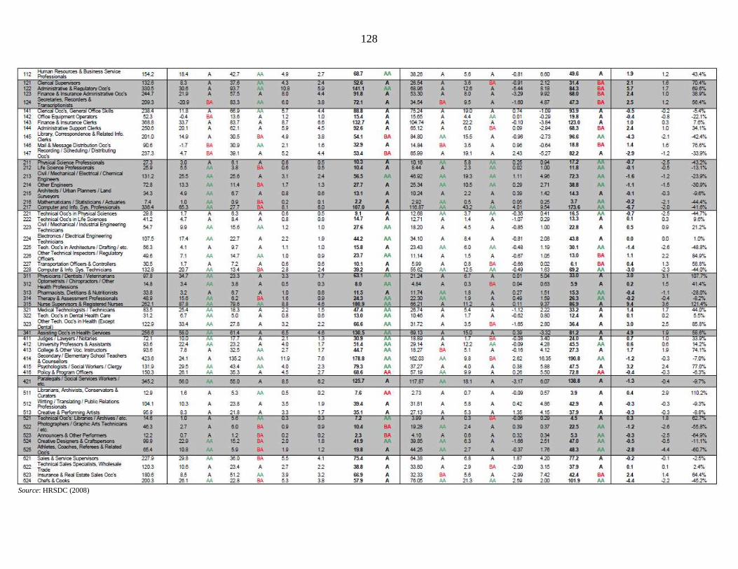
128


129


130

Source: HRSDC (2008

131

Table 12: Assessment of Future Labour Market Imbalances by Occupation, 2008-2017 (Ex-Ante Scenario)


132


133


review of best practices in labour market forecasting … · centre for the study of living...

Documents