Review High Resolution Modeling of Steric Sea-level Rise

Tatsuo Suzuki (FRCGC,JAMSTEC)

Understanding Sea-level Rise and Variability

6-9 June, 2006

Paris, France

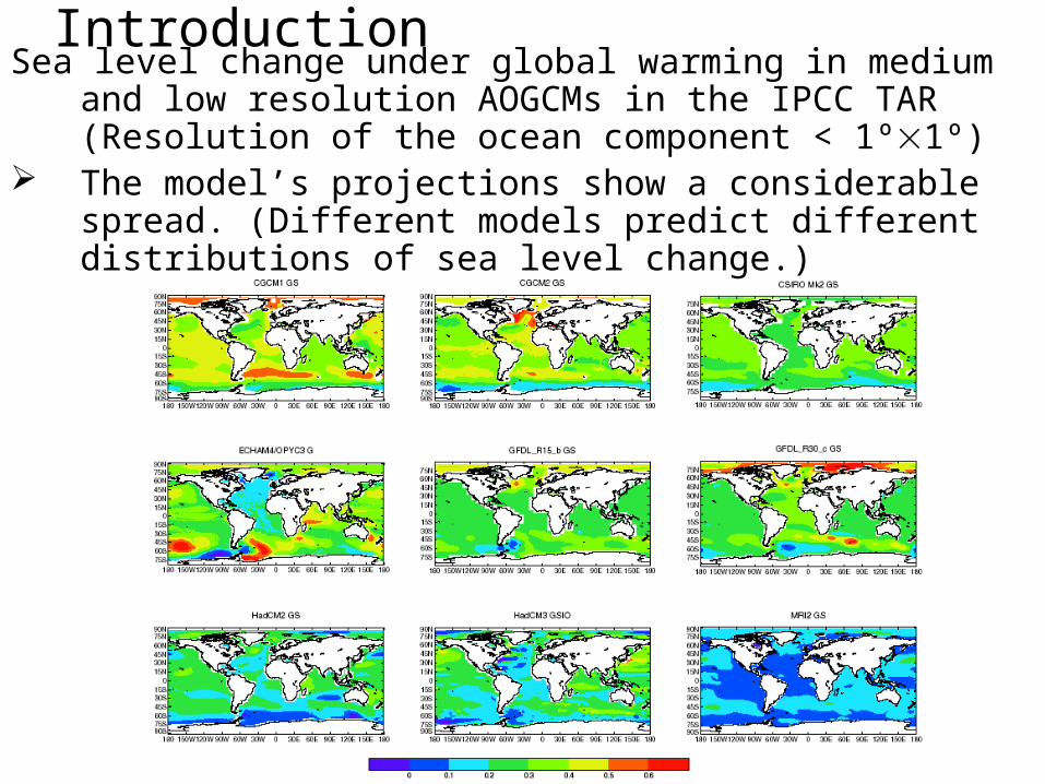
IntroductionSea level change under global warming in medium and low

resolution AOGCMs in the IPCC TAR (Resolution of the ocean component < 1º1º)

The model’s projections show a considerable spread. (Different models predict different distributions of sea level change.)

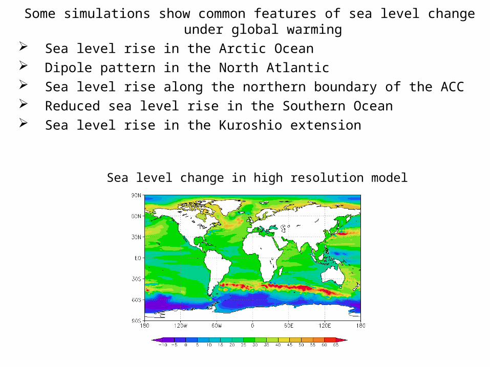
Some simulations show common features of sea level change under global warming

Sea level rise in the Arctic Ocean Dipole pattern in the North Atlantic Sea level rise along the northern boundary of the ACC Reduced sea level rise in the Southern Ocean Sea level rise in the Kuroshio extension

Sea level change in high resolution model

Model for Interdisciplinary Research on Climate (MIROC) version 3.2

• MIROC_hi– Atmosphere: T106, 56 vertical levels– Ocean: 0.28125º0.1875º, 48 vertical levels

• MIROC_med– Atmosphere: T42, 20 vertical levels– Ocean: 1.4º0.56º(near equator), 44 vertical lev

els

In both models, the same physics have been used.

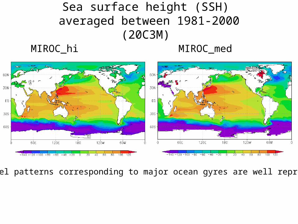
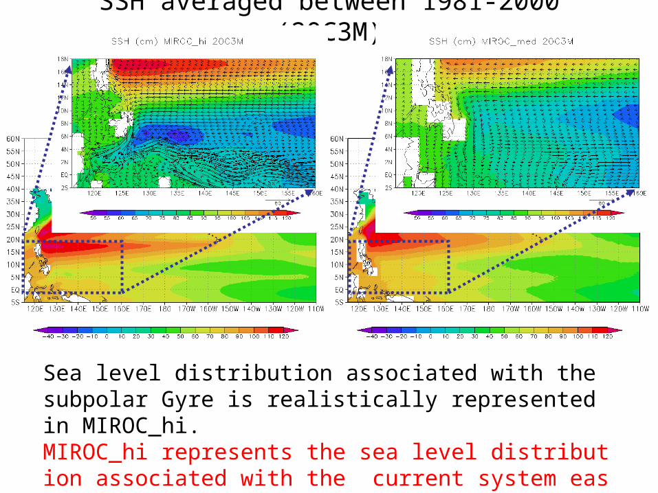
Sea surface height (SSH) averaged between 1981-2000

(20C3M)

MIROC_hi MIROC_med

Sea level patterns corresponding to major ocean gyres are well reproduced.

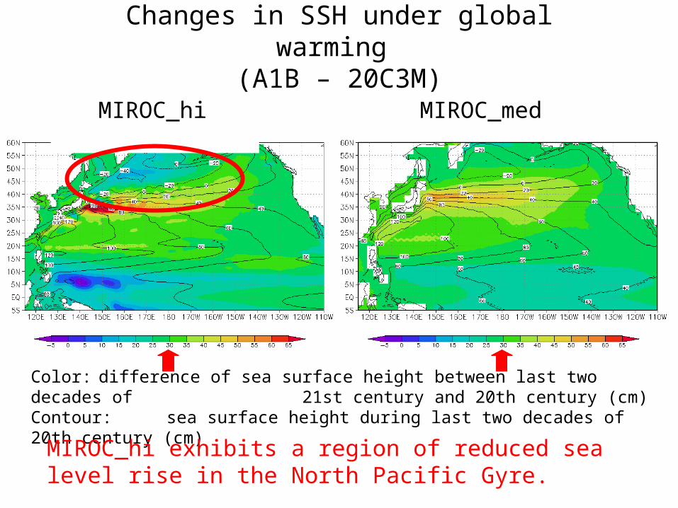
Changes in SSH under global warming (A1B – 20C3M: difference between the last two

decades of the 21st century and 20th century ) MIROC_hi MIROC_med

The regions with large sea level changes are more restricted to specific areas and the magnitudes are more pronounced in MIROC_hi than MIROC_med.These differences are caused by representation of the detailed ocean structure.

SSH averaged between 1981-2000 (20C3M)

MIROC_hi MIROC_med

Sea level distribution associated with the subpolar Gyre is realistically represented in MIROC_hi

SSH averaged between 1981-2000 (20C3M)

MIROC_hi MIROC_med

Sea level distribution associated with the subpolar Gyre is realistically represented in MIROC_hi.MIROC_hi represents the sea level distribution associated with the current system east of the Philippines.

Changes in SSH under global warming (A1B – 20C3M)

MIROC_hi MIROC_med

Color: difference of sea surface height between last two decades of 21st century and 20th century (cm)

Contour: sea surface height during last two decades of 20th century (cm)

MIROC_hi exhibits a region of reduced sea level rise in the North Pacific Gyre.

MIROC_hi MIROC_med

Changes in SSH under global warming (A1B – 20C3M)

MIROC_hi exhibits a region of reduced sea level rise in the North Pacific Gyre.In MIROC_hi, there is a reduced sea level rise east of the Philippines.

SSH averaged between 1981-2000 (20C3M)

MIROC_hi MIROC_med

SSH and Surface current vector averaged between 1981-2000 (20c3m)

MIROC_hi MIROC_med

The Kuroshio and the Kuroshio extension in MIROC_hi is realistically represented.

Changes in SSH under global warming (A1B – 20c3m)

Kuroshio acceleration is caused by changes in wind stress and the consequential spin-up of the Kuroshio recirculation (Sakamoto et al., 2005).

MIROC_hi

MIROC_med

There was a reduced sea level rise north of the Kuroshio Current and an enhanced sea level rise to the south in MIROC_hi.

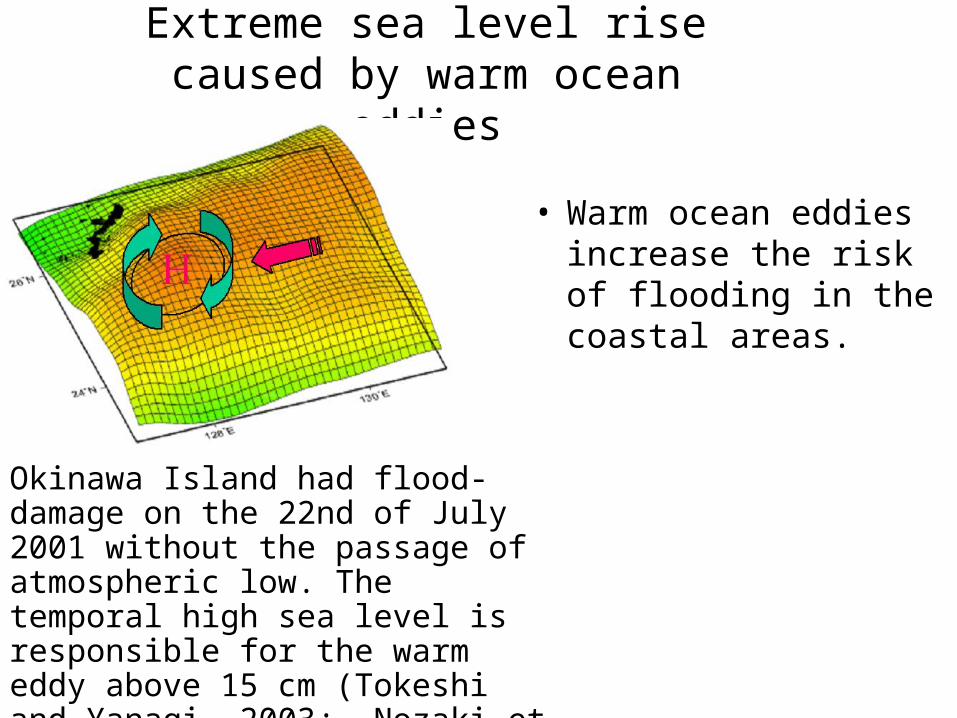
Extreme sea level rise caused by warm ocean eddies

• Warm ocean eddies increase the risk of flooding in the coastal areas.

Okinawa Island had flood-damage on the 22nd of July 2001 without the passage of atmospheric low. The temporal high sea level is responsible for the warm eddy above 15 cm (Tokeshi and Yanagi, 2003; Nozaki et al 2003, etc.).

RMS of sea level variability (eddy component) during the 20th century

(cm)

The regional distribution of sea level variability is well represented in MIROC_hi.

MIROC_hi (20C3M) TOPEX/POSEIDON 1991-2001

Changes in RMS of sea level variability (eddy component)

under global warming (A1B -20C3M)

The enhanced eddy activities are confined to specific areas.Those area are overlapped with the enhanced sea level rise around some coastal regions and Islands.

0.3cm

-12 -3 3 12cm

Globally averaged RMS of sea level variability (cm)

Flood risk increases.

Summary

Sea level changes in MIROC_hi are similar to that in MIROC_med on a large scale.

High resolution model presents more detailed ocean structure changes under global warming.

High resolution model can estimate changes in extreme sea level variability associated with ocean eddies.

Experiments Spin-up

109-years integration forced by fixed external condition for 1900 for MIROC_hi

560-years integration forced by fixed external condition for 1850 for MIROC_med

Control-run 100-years integration for MIROC_hi 400-years integration for MIROC_med

20C3M-run Forced by historical data during the 20th century

A1B-run IPCC SRES A1B scenario

B1-run IPCC SRES B1 scenario

Some trends are shown in control runs.So, we subtract these control trends from 20C3M run and scenario runs.

1. Steric contribution (thermal expansion and haline contraction) to Globally averaged sea level

riseestimated indirectly from density changes as the equivalent volume change under mass conservation as the Boussinesq approximation was adapted in the ocean model :

　

H : globally averaged sea level rise, S: surface area of the ocean, Z: ocean depth, : in situ density, : difference from the reference state

€

H = −1

S

Δρ

ρ−Z

0

∫S

∫ dzdS

2. Contributions of ice-sheet melt estimated using the methods of Wild et al. [2003]

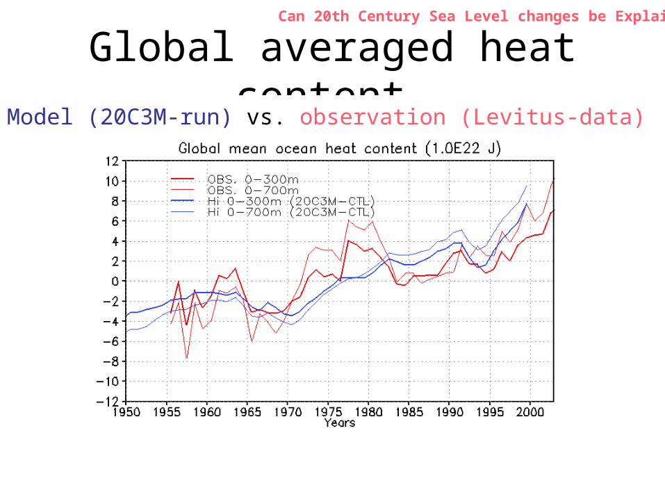
Global averaged heat content

Can 20th Century Sea Level changes be Explained?

Model (20C3M-run) vs. observation (Levitus-data)

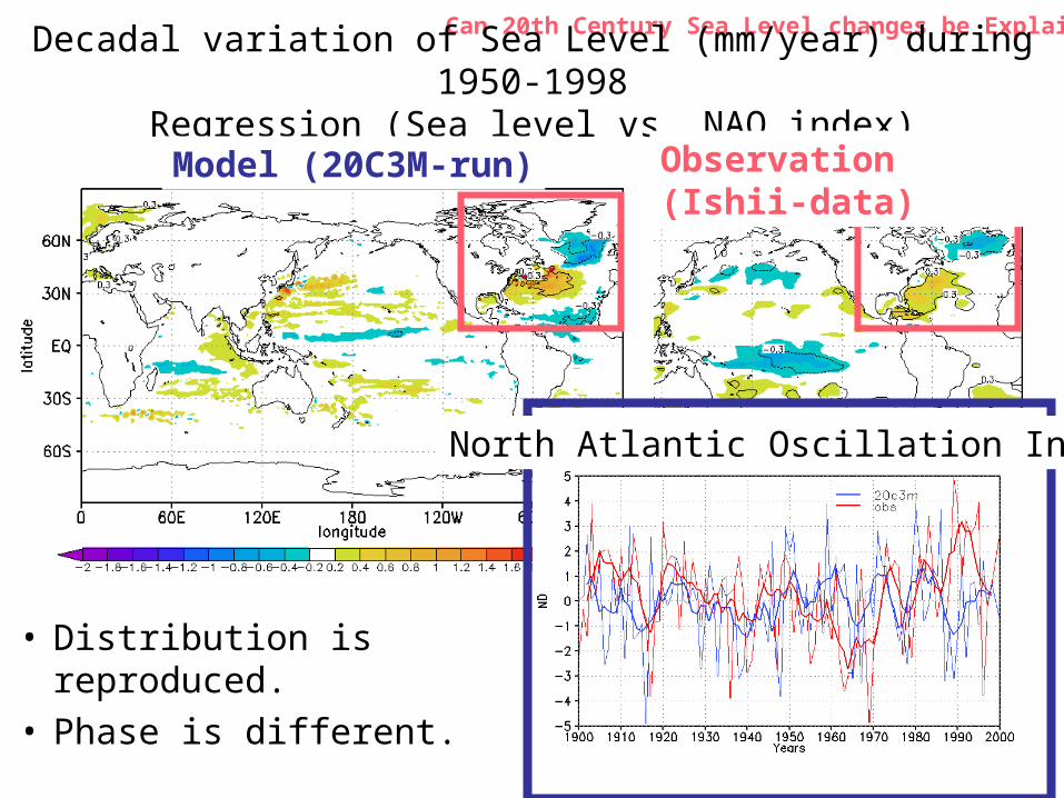
Can 20th Century Sea Level changes be Explained?

Decadal variation of Sea Level (mm/year) during 1950-1998Regression (Sea level vs. NAO index)

North Atlantic Oscillation Index

Observation (Ishii-data)Model (20C3M-run)

• Distribution is reproduced.

• Phase is different.

Can 20th Century Sea Level changes be Explained?

Decadal variation of Sea Level (mm/year) during 1950-1998Regression (Sea level vs. NP index)

Observation (Ishii-data)Model (20C3M-run)

North Pacific Index

• Distribution is reproduced.

• Phase is different.

• Sea level rise along North boundary ACC and Kuroshio-extension is reproduced.

• Decadal pattern of sea level is overlapped. (NAO etc.)

Can 20th Century Sea Level changes be Explained?

Sea level trend (mm/year) during 1993-2003Model vs. Observation (TOPEX/POSEIDON)

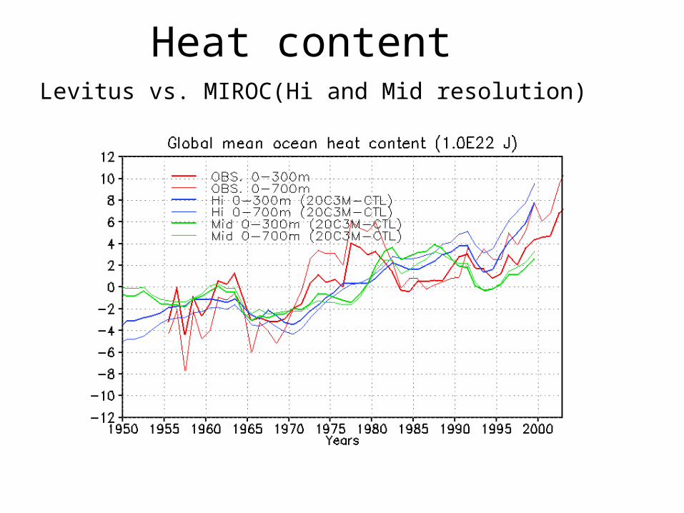
Heat content Levitus vs. MIROC(Hi and Mid resolution)

Globally averaged sea level rise The steric contribution during 21st century

in MIROC_hi is similar to that in MIROC_med.

The contributions of the Greenland and Antarctic ice-sheet exhibited opposite tendencies in both models, as in previous estimations [Church et al., 2001]

The amplitude of ice-sheet melt in MIROC_hi was larger than that in MIROC_med

A1B run induced global warming of about 4.0C in MIROC_hi and 3.4C in MIROC_med at the end of the 21st century, respectively.

Different sensitivity

Why steric contribution in MIROC_hi is similar to that in MIROC_med in spite of the different sensitivity?

• Total heat flux into the ocean for the 21st century is similar in the both models

• The upper ocean in MIROC_hi warms up more than that in MIROC_med (different heat uptake?).

The reasons for these differences are current problems.

difference of sea level distribution between 2080-2100 in A1B run and

1980-2000 in 20C3M run

Spatial standard deviation of the decadal-mean field of sea level change with respect to the control run

Sea level rise trend (thermo-steric contribution) CO2 1% increase run

total upper 450m

lower 450m

Sea level rise trend (halo-steric contribution) CO2 1% increase run

total upper 450m

lower 450m

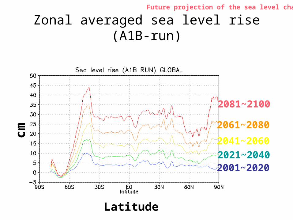
Zonal averaged sea level rise (A1B-run)

Future projection of the sea level change

2001~20202021~2040

2041~2060

2061~2080

2081~2100

Latitude

cm