review article ...downloads.hindawi.com/journals/aav/2012/214839.pdf · underwater acoustic...
TRANSCRIPT
Hindawi Publishing CorporationAdvances in Acoustics and VibrationVolume 2012, Article ID 214839, 28 pagesdoi:10.1155/2012/214839
Review Article
Advanced Applications for Underwater Acoustic Modeling
Paul C. Etter
Northrop Grumman Corporation, P.O. Box 1693, Baltimore, MD 21203, USA
Correspondence should be addressed to Paul C. Etter, [email protected]
Received 29 October 2011; Accepted 30 January 2012
Academic Editor: Jafar Saniie
Copyright © 2012 Paul C. Etter. This is an open access article distributed under the Creative Commons Attribution License, whichpermits unrestricted use, distribution, and reproduction in any medium, provided the original work is properly cited.
Changes in the ocean soundscape have been driven by anthropogenic activity (e.g., naval-sonar systems, seismic-explorationactivity, maritime shipping and windfarm development) and by natural factors (e.g., climate change and ocean acidification).New regulatory initiatives have placed additional restrictions on uses of sound in the ocean: mitigation of marine-mammalendangerment is now an integral consideration in acoustic-system design and operation. Modeling tools traditionally used inunderwater acoustics have undergone a necessary transformation to respond to the rapidly changing requirements imposed by thisnew soundscape. Advanced modeling techniques now include forward and inverse applications, integrated-modeling approaches,nonintrusive measurements, and novel processing methods. A 32-year baseline inventory of modeling techniques has been updatedto reflect these new developments including the basic mathematics and references to the key literature. Charts have been providedto guide soundscape practitioners to the most efficient modeling techniques for any given application.
1. Introduction
Over the past several decades, the soundscape of themarine environment has responded to changes in bothnatural and anthropogenic influences. A soundscape is acombination of sounds that characterize, or arise from, anocean environment. The study of a soundscape is sometimesreferred to as acoustic ecology. The idea of a soundscaperefers to both the natural acoustic environment (consistingof natural sounds including animal vocalizations, the soundsof weather, and other natural elements) and anthropogenicsounds (created by humans) including sounds of mechanicalorigin associated with the use of industrial technology. Thedisruption of the natural acoustic environment results innoise pollution.
This paper is concerned with the underwater soundscape.The field of underwater acoustics enables us to observequantitatively and predict the behavior of this soundscapeand the response of the natural acoustic environment tonoise pollution. Specifically, underwater acoustics entail thedevelopment and employment of acoustical methods toimage underwater features, to communicate information viathe oceanic waveguide, or to measure oceanic properties.In the present context, underwater acoustics encompasses
both the science and the technology necessary to deployfunctioning acoustical systems in support of naval andcommercial operations.
Broadly defined, modeling is a method for organizingknowledge accumulated through observation or deducedfrom underlying principles. Modeling applications fall intotwo basic categories: prognostic and diagnostic. Prognosticapplications include prediction and forecasting functionswhere future oceanic conditions or acoustic sensor perfor-mance must be anticipated. Diagnostic applications includesystem-design and analysis functions typically encounteredin engineering tradeoff studies.
The challenges of managing the underwater soundscapeare being met by enabling technologies and by emergingsolutions. Throughout this paper, the utility of the availableinventory of models is stressed and relevant examples fromthe recent literature are provided in support.
After a brief background in Section 1, the balance ofthis paper is divided into three main sections. Section 2addresses evolving challenges. Section 3 discusses enablingtechnologies. Section 4 reviews emerging solutions. Finally,Section 5 summarizes the notable advances in underwateracoustic modeling that support management of the under-water soundscape.
2 Advances in Acoustics and Vibration
2. Evolving Challenges
2.1. Background. The soundscape baseline is defined byambient noise, which is the prevailing background of soundat a particular location in the ocean at a given time of theyear. It does not include transient sounds such as the noiseof nearby ships and marine organisms, or of passing rainshowers. In practice, ambient noise excludes all forms of self-noise, such as the noise of current flow around the sonar.For sonar processing, however, it is the background of noise(including interfering sounds), typical of the time, location,and depth against which an acoustic signal must be detected.
2.2. Naval Operations in Coastal Environments
2.2.1. The Coastal Environment. Coastal environments aregenerally characterized by high spatial and temporal variabil-ities. When coupled with attendant acoustic spectral depen-dencies of the surface and bottom boundaries, these naturalvariabilities make coastal regions very complex acousticenvironments. Specifically, changes in the temperature andsalinity of coastal waters affect the refraction of sound in thewater column. These refractive properties have a profoundimpact on the transmission of acoustic energy in a shallow-water waveguide with an irregular bottom and a statisticallyvarying sea surface. Thus, accurate modeling and predictionof the acoustic environment is essential to understandingsonar performance in coastal oceans.
Physical processes controlling the hydrography of shelfwaters often exhibit strong seasonal variations. Annual cyclesof alongshore winds induce alternating periods of upwellingand downwelling. The presence of coastal jets and thefrictional decay of deep-water eddies due to topographicinteractions further complicate the dynamics of coastalregions. Episodic passages of meteorological fronts fromcontinental interiors affect the thermal structure of theadjacent shelf waters through intense air-sea interactions.River outflows create strong salinity gradients along theadjacent coast. Variable bottom topographies and sedimentcompositions with their attendant spectral dependenciescomplicate acoustic bottom boundary conditions. At higherlatitudes, ice formation complicates acoustic surface bound-ary conditions near the coast. Waves generated by localwinds under fetch-limited conditions, together with swellsoriginating from distant sources, conspire to complicateacoustic surface boundary conditions and also create noisysurf conditions. Marine life, which is often abundant innutrient-rich coastal regions, can generate or scatter sound.Anthropogenic sources of noise are common in coastal seasincluding fixed sources such as drilling rigs and mobilesources such as merchant shipping and fishing vessels.Surface weather, including wind and rain, further contributeto the underwater noise field. Even noise from low-flyingcoastal aircraft can couple into the water column and add tothe background noise field.
2.2.2. Littoral Operations. Over the past decade, naval mis-sion requirements have shifted from open-ocean operationsto shallow-water (or littoral) scenarios. For convenience,
shallow water will be defined by water depths less than200 meters. This has not been an easy transition forsonar technologists since sonar systems that were origi-nally designed for operation in deep water seldom workoptimally in coastal regions. This has also held true formodeling and simulation (M&S) technologies, which haveundergone a redefinition and refocusing to support a newgeneration of multistatic naval systems that are intendedto operate efficiently in littoral regions while still retaininga deepwater capability. Shallow-water geometries increasethe importance of boundary interactions, which diminishacoustic energy through scattering and also complicatelocalization of diesel submarines and coastal mines dueto multipath propagation. Moreover, the higher levels ofinterfering noises encountered in coastal regions combinedwith higher levels of boundary reverberation mask signalsof interest. In advance of naval deployments, synopticmeteorological and oceanographic (METOC) measurementsare often required in remote or hostile (i.e., harsh or heavilydefended) coastal environments to forecast acoustic sensorperformance. Coupled atmosphere-ocean-acoustic modelscould reduce the need for hazardous in situ data collectionby numerically computing initial states for the embeddedacoustic models.
In support of naval operations in littoral regions,acoustical oceanographers have employed ocean-acousticmodels as adjunct tools that can be used to conduct rapidenvironmental assessments (REAs) in remote locations. Dueto an increased awareness of the potential technologicalimpacts on marine life, naval commanders and acousticaloceanographers must also be aware of new environmentalregulations governing the acoustic emissions of their sonarsystems.
In shallow water, interactions of the acoustic fields withthe sea bed require an understanding of the sedimentarystructure of the bottom to a level of detail that is usuallynot required in deep-water environments. In the forward-propagation case, this means that a significant amount ofinformation is necessary to properly characterize the bottomboundary to ensure the generation of high-fidelity modeloutputs. This generally requires a good understanding ofthe physics of bottom-interacting acoustics in diverse oceanenvironments.
Sonar clutter, particularly in shallow-water environ-ments, introduces false targets that change the statisticsof the reverberation signal. Specifically, clutter increasesthe probability of false alarm for a given probability ofdetection. This is because clutter adds to the length ofthe tails of the reverberation-envelope PDF (probabilitydistribution function), moving the statistics away from theRayleigh canonical form. Clutter can be caused by target-likefeatures, either natural or man-made, or by non-Gaussiandistributions of the scatterers. Typically, high-bandwidth orhighly directive systems (or both) have more problems withclutter since, as the size of the scattering patch is reduced,the PDF of the generally non-Gaussian scatterer distributionsbecomes resolved by the system [1].
2.2.3. Training Ranges. At issue here is operational navaltraining with active sonars. These high-power multistatic

Advances in Acoustics and Vibration 3
sonars have become more important in the face of improveddiesel-electric submarine threats operating in complexcoastal environments.
The US Navy has explored the environmental conse-quences of installing and operating an undersea warfaretraining range (USWTR) in conjunction with appropriatecoordination and consultation with the National MarineFisheries Service (NMFS) and in compliance with applicablelaws and executive orders including the Marine MammalProtection Act (MMPA), the Endangered Species Act (ESA),the National Environmental Policy Act (NEPA), and theCoastal Zone Management Act (CZMA).
2.2.4. Underwater Networks. Ocean-bottom sensor nodes areused for oceanographic data collection, pollution monitor-ing, offshore exploration, tactical surveillance applications,and rapid environmental assessments [2, 3]. Factors thatdetermine the temporal and spatial variability of the acousticchannel also limit the available bandwidth of the oceanchannel and make it dependent on range and frequency.Specifically, long-range systems (∼10 km) have bandwidthsof a few kilohertz while short-range systems (∼0.1 km) havebandwidths on the order of a hundred kilohertz. A moored-buoy ocean observatory system comprising oceanographicsensors was linked by acoustic communications to retrievedata from sensors in the water column at ranges of approxi-mately 3 km [4]; the observatory was deployed off VancouverIsland in the northeastern Pacific Ocean in May 2004 (for 13months) to study the correlation of seismicity and fluid flowin a seep area along the Nootka fault.
Underwater networks consist of variable numbers ofsensors and vehicles deployed in concert to perform collabo-rative monitoring tasks over a given area. Underwater sensornetworks comprise nodes that communicate via acousticwaves over multiple wireless hops to perform collaborativetasks such as environmental monitoring, naval surveillance,and oceanic exploration. Nodes in underwater sensor net-works are constrained by harsh physical environments. Datadelivery schemes originally designed for terrestrial sensornetworks are unsuitable for use in the underwater environ-ment. Relatively few new schemes have been proposed forunderwater use, and no single scheme has yet emerged as thede facto standard.
Underwater acoustic communications are influenced byspreading loss, noise, multipath discrimination, Dopplerspread, and high and variable propagation delays. More-over, underwater acoustic channels normally have low datarates and time-varying fading. These factors determine thetemporal and spatial variability of the acoustic channel andmake the available bandwidth of the ocean channel bothlimited and dependent on range and frequency. Challengesdue to the presence of fading, multipath, and refractive prop-erties of the sound channel necessitate the development ofprecise underwater-channel models. Some existing channelmodels are simplified and do not consider multipaths orfading. Multipath interference due to boundary reflectionin shallow-water acoustic communications poses majorobstacles to reliable high-speed underwater communicationsystems.
Cooperative transmission is a new wireless communica-tion technique in which diversity gain can be achieved byutilizing relay nodes as virtual antennae. These transmissiontechniques have been investigated for underwater acousticcommunications. First, the performance of several cooper-ative transmission schemes was studied in an underwaterscenario. Second, by taking advantage of the relatively lowpropagation speed of sound in water, a new wave cooperativetransmission scheme was designed in which the relay nodesamplified the signal received from the source node andthen forwarded the signal immediately to the intendeddestination. The goal was to alter the multipath effect atthe receiver. Third, the upper bound of performance wasderived for the proposed wave cooperative transmissionscheme. The simulation results showed that the proposedwave cooperative transmission had significant advantagesover both the traditional direct transmission and the existingcooperative transmission schemes originally designed forradio wireless networks [5].
Localization algorithms are relevant to underwater sen-sor networks, but there are challenges in meeting require-ments imposed by emerging applications for such networksin offshore engineering [6]. Localization algorithms can bebroadly categorized into range-based and range-free schemes.Range-based schemes use precise distance or angle measure-ments to estimate the location of nodes in a network. Range-free schemes are simpler than range-based schemes, but theyonly provide a coarse estimate of a node’s location.
Underwater networking is an enabling technology for theoperation of autonomous underwater vehicles. In particular,ad hoc networks entail wireless communications for mobilehosts called nodes. In these networks, there is no fixed infras-tructure. Mobile nodes that are within range communicatedirectly via wireless links, while those that are far apart relyon other nodes to relay messages as routers. Node mobilityin an ad hoc network causes frequent changes of the networktopology. Since ad hoc networks can be deployed rapidlywith relatively low cost, they are attractive for military,emergency, commercial and scientific applications [2, 3]. Achannel simulator was developed for testing the performanceof unmanned undersea vehicle (UUV) communications [7].
2.2.5. Unmanned Underwater Vehicles. Autonomous under-water vehicles (AUVs), or unmanned undersea vehicles(UUVs), constitute part of a larger group of undersea systemsknown as unmanned underwater vehicles, a classificationthat includes nonautonomous remotely operated vehicles(ROVs) that are controlled and powered from the surface byan operator (or pilot) via an umbilical connection.
Underwater gliders actually constitute a new class ofautonomous underwater vehicles that glide by controllingtheir buoyancy and attitude using internal actuators [8].Gliders have useful applications in oceanographic sensingand data collection because of their low cost, autonomy, andcapability for long-range extended-duration deployments.They serve as adjuncts to ship-based hydrographic casts,towed sensors, UUV/AUV and satellite-based sensors, butthey also present challenges in communications common toall untethered subsurface sensors.
4 Advances in Acoustics and Vibration
2.3. Marine Seismic Operations
2.3.1. Seismic Exploration. Marine seismic surveys are usedto assess the location of hydrocarbon resources, includinggas and oil. There are two acquisition methods: 2D and 3D.The 2D method tows a single seismic cable (or streamer)behind the seismic vessel, together with a single source.The reflections from the subsurface of the sea floor areassumed to lie directly below the path (sail line) of thevessel. In a 3D survey, groups of sail lines (or swathes)are used to acquire orthogonal or oblique lines relative tothe acquisition direction. By utilizing more than one sourcetogether with many parallel streamers towed by the seismicvessel, the acquisition of many closely spaced subsurface 2Dlines can be achieved by a single sail line. Computationallyintensive processing is necessary to produce a 3D imageof the subsurface of the sea floor. The source arrays arepowered by high-pressure air that is compressed onboard theseismic vessel. These compressors are capable of rechargingthe airguns rapidly and continuously, enabling the airgunsource arrays to be fired at approximately 10-second intervalsfor periods of up to 12 hours. Typical towing depths rangefrom 4-5 meters for shallow high-resolution surveys or 8–10 meters for deeper penetration, lower-frequency targetsin open waters. Typical source outputs are approximately220 dB re 1 μPa/Hz at 1 m. Other types of seismic sourcesinclude water guns and marine vibrators.
2.3.2. Marine Mammal Impacts. In 2002, the InternationalAssociation of Geophysical Contractors (IAGC) hosted aninformal meeting to discuss future Acoustics Research rele-vant to seismic operations related to the effects of seismicexploration on sperm whales in the Gulf of Mexico [9].The IAGC offered its support for sperm-whale researchthrough the contribution of a seismic-source vessel forcontrolled-exposure experiments. In response, a proposedsperm whale seismic study (SWSS) was approved by theMinerals Management Service (MMS) in 2002. (The MMS isnow the Bureau of Ocean Energy Management, Regulationand Enforcement, or BOEMRE.) In subsequent years, IAGCwas joined by a number of oil and gas companies to formthe Industry Research Funders Coalition (IRFC) that hascontinued to provide contributions in support of SWSSstudies.
Long-term (monthly to seasonal) movements and distri-butions of sperm whales were studied using satellite-trackedradio telemetry tags (S-tags). Short-term (hours) divingand swimming behavior and vocalizations of sperm whaleswere examined using recoverable digital-recording acoustictags (D-tags) that logged whale orientation (i.e., pitch, roll,heading) and depth, as well as the sounds made by the whaleand received at the whale from the environment. Divingdepths and movements were examined using 3D passiveacoustic tracking techniques.
To examine potential changes in the behavior of spermwhales when subjected to seismic airgun sounds, controlledexposure experiments (CEEs) were conducted using the D-tags in conjunction with a seismic-source vessel. The locationand level of airgun sounds delivered at the tagged sperm
whales were controlled by the science team. These CEEsprovided data on the immediate and short-term (hours)response of sperm whales to airgun sounds. Longer-termavoidance or displacement behaviors of sperm whales toseismic vessel airgun sounds were examined using locationdata from the S-tags and from proprietary commercialseismic shot data.
The 3D tracking method requires at least two widelyseparated hydrophones to obtain the horizontal range anddepth of acoustically active sperm whales and would thus besuited for eventual use on a standard seismic vessel, where thepassive acoustic arrays (streamers) can be over a kilometerlong. Instead of relying on four hydrophones deployedas a three-dimensional array (which would be difficult todeploy and process), the method used here exploited surfacemultipath (or “ghosts”) to reduce the number of requiredhydrophones to three and further permitted the phonesto be deployed along a single towed cable. The horizontalseparation between the widely-spaced hydrophones neededto be at least 200 m in order to obtain adequate range anddepth resolution at 1 km horizontal ranges. The method didnot require the use of multipath from the ocean bottom, butwhen such bottom returns were detected they could providean independent confirmation of these tracking procedures[10].
2.4. Shipping Activity. Shipping lanes, a term used to indicatethe general flow of merchant traffic between two ports, areroutes that historically have been optimized for shortestdistances and travel times, and which are modified to avoidextreme weather events [11]. Noise from distant shippinggenerally occupies the frequency band 20–500 Hz.
A comparison of time-series measurements of oceanambient noise over two periods (1963–1965 and 1994–2001) revealed that noise levels from the latter periodexceeded those of the earlier period by about 10 dB in thefrequency ranges 20–80 Hz and 200–300 Hz, and by about3 dB at 100 Hz [12]. The observed increase was attributed toincreases in shipping. Ambient noise measurements collectedat the same site but separated by an interval of nearly 40years (1964–1966 and 2003–2004) revealed an average noiseincrease of 2.5–3 dB per decade in the frequency band 30–50 Hz [13, 14].
2.5. Windfarm Development. Wind power, as an alternativeto fossil fuels, is plentiful, renewable, widely distributed,clean, and produces no greenhouse gas emissions duringoperation. A wind farm, which is a group of wind turbinesin the same location used for production of electric power,may be located offshore. The installation of ocean wind farmsrequires medium water depths (<30 m) and constructionlogistics such as access to specialized vessels to install theturbines. Economic wind generators require wind speeds of16 km/h or greater.
A concerted effort has been made by industry tominimize any undesirable effects relating to windfarm devel-opment and operation [15]. One potential effect of offshorewindfarm development is the creation of underwater noise.

Advances in Acoustics and Vibration 5
Knowing the length of time the marine environment isexposed to an underwater noise source is useful whenassessing environmental effects. Measurements of offshorewind turbine noise showed low-frequency sound levels witha maximum of 153 dB re 1 μPa at 1 m at 16 Hz. Thesemeasurements were of individual turbines of a relativelylow power (less than 1 MW). Despite the low-level andlow-frequency nature of the sound, behavioral reactions ofmarine mammals have been observed in response to thereproduction of wind-turbine noise.
2.6. Ocean Acidification. Climate change also affects theocean soundscape. The emission of carbon into the atmo-sphere through the effects of fossil-fuel combustion andindustrial processes increases atmospheric concentrations ofcarbon dioxide (CO2). Ocean acidification, which occurswhen CO2 in the atmosphere reacts with water to createcarbonic acid (H2CO3), is increasing.
The attenuation of low-frequency sound in the sea is pHdependent; specifically, the higher the pH, the greater theattenuation. Thus, as the ocean becomes more acidic (lowerpH) due to increasing CO2 emissions, the attenuation willdiminish and low-frequency sounds will propagate farther,making the ocean noisier.
Recent investigations modeled what effect the increasingacidity of the ocean would have on ambient-noise levels inshallow water in the presence of internal waves [16]. Thismodel assumed an isotropic distribution of noise sources.Exploring a scenario typical of the East China Sea, the noiseat 3 kHz was predicted to increase by 30%, or about onedecibel, as the pH decreased from 8.0 to 7.4. These resultsare representative of other contemporaneous investigationsinto this matter.
3. Enabling Technologies
3.1. Background
3.1.1. Regulatory Initiatives. An examination of anthro-pogenic sound in a global context considered the need fornew regulatory initiatives to deal with the conflicting uses ofocean space related to noise [17]. This study identified theexisting legal, economic, and political barriers to the creationand implementation of a new international regime designedto manage anthropogenic noise in the ocean.
The Committee on Potential Impacts of Ambient Noisein the Ocean on Marine Mammals was charged by the OceanStudies Board of the US National Research Council to assessthe state of our knowledge of underwater noise and recom-mend research areas to assist in determining whether noisein the ocean adversely affects marine mammals [18]. Oneof the findings of this committee was that models describingocean noise are better developed than are models describingmarine mammal distribution, hearing, and behavior. Thebiggest challenge lies in integrating the two types of models.The National Research Council [19] also examined whatconstitutes biologically significant in the context of LevelB harassment as used in the latest amendments to the
US Marine Mammal Protection Act (MMPA). The MMPAseparates harassment into two levels. Level A harassmentis defined as “any act of pursuit, torment, or annoyancewhich has the potential to injure a marine mammal ormarine mammal stock in the wild.” Level B harassmentis defined as “any act of pursuit, torment, or annoyancewhich has the potential to disturb a marine mammal ormarine mammal stock in the wild by causing disruption ofbehavioral patterns, including, but not limited to, migration,breathing, nursing, breeding, feeding, or sheltering.” TheMMPA, enacted in 1972, was the first legislation that calledfor an ecosystem approach to natural-resource managementand conservation; it specifically prohibited the take (i.e.,hunting, killing, capture, and/or harassment) of marinemammals.
The ocean biogeographic information system (OBIS)is an on-line worldwide atlas for accessing, modelingand mapping marine biological data in a multidimen-sional geographic context [20]. Also see the website athttp://www.iobis.org/home.
3.1.2. Modeling Uncertainty. Uncertainty has been definedas a quantitative measure of our lack of knowledge of thesound-speed field and boundary conditions constitutingthe waveguide information necessary for simulation of theacoustic field [21]. This uncertainty is distinct from anyerrors related to numerical solution of the wave equation.Existing methods typically solve a deterministic wave equa-tion separately over many realizations, and the resulting setof pressure fields is then used to estimate statistical momentsof the field. Proper sampling may involve the computationof thousands of realizations to ensure convergence of thestatistics.
A study of the effects of uncertainty in the modeling ofanthropogenic impacts suggested a precautionary approachto regulation [22]. It was further noted that due to thecomplex patterns of sound propagation encountered indiverse shelf regions, some marine mammals may notnecessarily encounter the average sound exposure conditionspredicted for any given seismic survey.
3.2. Numerical Modeling Techniques. Four types of modelswill be discussed: propagation, noise, reverberation, andsonar performance. The order of presentation will followthat indicated in Figure 1. This box-type format will beused throughout the text to present compact summaries ofmethods that have been developed in detail elsewhere [23].
3.2.1. Propagation Models. As sound propagates through theocean, the effects of spreading and attenuation diminish itsintensity. Spreading loss includes spherical and cylindricalspreading losses in addition to focusing effects. Attenuationloss includes losses due to absorption, leakage out of ducts,scattering, and diffraction. Propagation losses increase withincreasing frequency due largely to the effects of absorption.Sound propagation is profoundly affected by the conditionsof the surface and bottom boundaries of the ocean as wellas by the variation of sound speed within the ocean volume.

6 Advances in Acoustics and Vibration
Data
Environment
Systems
Targets
Propagation
Ray theory Normal mode Parabolicequation
Multipathexpansion
Fast field(wavenumberintegration)
Noise
Ambientnoise
Beam noisestatistics
Analytic Simulation
Reverberation
Cellscattering
Pointscattering
Sonar performance
Active sonarperformance
Modeloperating
system
Tacticaldecision aids
Figure 1: Flow of underwater acoustic modeling from propagation, through noise and reverberation, to sonar performance.
Sound-speed gradients introduce refractive effects that mayfocus or defocus the propagating acoustic energy.
Formulations of acoustic propagation models gener-ally begin with the three-dimensional, time-dependentwave equation. For most applications, a simplified linear,hyperbolic, second-order, time-dependent partial differen-tial equation is used:
∇2Φ = 1c2
∂2Φ
∂t2, (1)
where ∇2 = (∂2/∂x2) + (∂2/∂y2) + (∂2/∂z2) is the Laplacianoperator, Φ is the potential function, c is the speed of sound,and t is the time.
Subsequent simplifications incorporate a harmonic(single-frequency, continuous wave) solution in order toobtain the time-independent Helmholtz equation. Specif-ically, a harmonic solution is assumed for the potentialfunction Φ:
Φ = φe−iωt, (2)
where φ is the time-independent potential function, ω is thesource frequency (2π f ), and f is the acoustic frequency.Then the wave equation (1) reduces to the Helmholtzequation:
∇2φ + k2φ = 0, (3)
where k = (ω/c) = (2π/λ) is the wavenumber and λ isthe wavelength. Equation (3) is referred to as the time-independent (or frequency-domain) wave equation.
Propagation models are integral to the higher-levelmodeling of noise, reverberation, and, ultimately, sonarperformance. The graphic in Figure 1 shows the flow of sonarmodeling from propagation, through noise and reverber-ation, through to sonar performance. Estimates of passive
sonar performance would require the input of propagationand noise while active sonar performance would requireinputs of both noise and reverberation.
Propagation models can be categorized into five distincttechniques [23].
(a) Ray-theoretical models calculate propagation loss onthe basis of ray tracing.
(b) Normal-mode solutions are derived from an integralrepresentation of the wave equation.
(c) Multipath expansion techniques expand the acousticfield integral representation of the wave equationin terms of an infinite set of integrals, each ofwhich is associated with a particular ray-path family.Thus, each normal mode can then be associated withcorresponding rays.
(d) In underwater acoustics, fast-field theory is alsoreferred to as “wavenumber integration.” In seis-mology, this approach is commonly referred to asthe “reflectivity method” or “discrete-wavenumbermethod.”
(e) The parabolic approximation approach replaces theelliptic reduced wave equation with a parabolicequation (PE). Use of the parabolic approximationin wave propagation problems can be traced back tothe mid-1940s when it was first applied to long-rangetropospheric radio wave propagation.
As shown in Figure 2, a further division can be madeaccording to range-independent (1D, or depth-dependenceonly) or range-dependent environmental specifications,where environmental range-dependence can be 2D (depthand range) or 3D (depth, range, and azimuth). Since all fivetechniques are derived from the wave equation by restrictingsolutions to the frequency domain, the resulting models

Advances in Acoustics and Vibration 7
Ray theory
Normal mode
Multipath expansion
Parabolic equation
Fast field/wavenumber integration
Environmental range dependence
Range independent (1D)
Range dependent (2D, 3D)
Frequency-domain solutions ∇2φ + k2φ = 0
φ = F(x, y, z) eiG(x,y,z)
φ = F(z) ·G(r)
φ = F(r, θ, z) ·G(r)
f (z)
f (z, r), f (z, r, θ)
y
z
xθ
(r, θ, z)
Figure 2: Organization of propagation models into five distinct techniques. A further division is made according to range-independent (1D)or range-dependent (2D or 3D) environmental specifications.
are appropriate for traditional sonar applications. (Solutionsobtained in the time domain would be appropriate, e.g.,for modeling shock propagation in the ocean.) Each ofthe five techniques has a unique domain of applicabilitythat can be defined in terms of acoustic frequency andenvironmental complexity. These domains are determinedby the assumptions that were invoked in deriving eachsolution. Hybrid formulations obtained by combining twoor more different techniques are often developed to improvedomain robustness.
Table 1 provides a summary of stand-alone propagationmodels. Superscript letters identify those models that havebeen added to the inventory since 2003. These lettersrefer to a brief summary and appropriate documentation.Model documentation can range from informal program-ming commentaries to journal articles to detailed technicalreports containing a listing of the actual computer code.Corresponding information on the legacy models is providedin the 2003 baseline [23] and is not repeated here.
In Table 1: (Propagation models), (a) FeyRay wasdeveloped to accommodate the speed, fidelity, and im-plementation requirements of sonar trainers and simu-lators. It is a broadband, range-dependent, point-to-pointpropagation model optimized for computa-tional efficiency.FeyRay utilizes the Gaussian-beam approximation, whichreduces the acoustic wave equation (a partial differentialequation) to a more tractable system of ordinary differentialequations [24–28], (b) PlaneRay provides a unique sortingand interpolation routine for efficient determinationof a large number of eigenrays in range-dependentenvironments. No rays are traced into the bottom sincebottom interaction is modeled by plane-wave reflectioncoefficients. The bottom structure is modeled as a fluidsediment layer over a solid half-space. This approachbalances two conflicting requirements: ray tracing is validfor high frequencies while plane-wave reflection coefficientsare valid for low frequencies where the sediment layersare thin compared with the acoustic wavelength [29–33],(c) PWRC is a ray-based model that performs geoacousticinversions in range-dependent ocean waveguides. Thepressure field is modeled approximately by separatingthe ocean propagation ray paths from the layered bottominteraction. The bottom interaction is included by using a
full-wave description, making PWRC a hybrid model, incontrast to a full-ray theory approach that traces rays intothe bottom layers. The field contribution from the bottominteractions partially includes beam-displacement effectsassociated with internally reflected or refracted returnsfrom the sediment since the complex bottom reflectioncoefficients are obtained from a full-wave solution. Thismethod is comparable in accuracy to normal mode andanalytic solutions (in range-dependent environments) forfrequencies >100 Hz [34], (d) Ray5, developed by TrondJenserud at the Forsvarets forskningsinstitutt (NorwegianDefence Research Establishment), uses direct integrationin a sound-speed field specified either analytically or byinterpolation from measured data. The Ray5 program iswell suited for ray-tracing calculations in acoustic fieldsdescribed analytically. It needs the sound-speed values, theirspatial derivatives and second derivatives at all points withinthe field. Hence, if these values can be given analytically asfunctions of the oceanographic and bathymetric parameters,no interpolation is necessary and the program reducesits computing time. Further developments in Ray5 havemade it possible to calculate eigenrays. This allows phaseinformation to be retained for a given frequency so thatcoherent pressure values can be summed for the rays arrivingat the receiver. The actual pressure values for the individualrays are calculated by assuming the pressure distribution inthe direction normal to the ray to have a Gaussian behavior(i.e., Gaussian beams). It is also possible to calculate theincoherent sound levels [35]. A separate report includes theMATLAB code for Ray5 [36], (e) RAYSON was developedby Semantic (France) to solve the Helmholtz equationusing a ray-theoretic approximation for high frequencies.In a stratified (range-independent) environment, analyticsolutions are obtained for ray paths that are portions ofcircles. In range-dependent environments, the ray equationsare numerically integrated using a fourth-order Runge-Kuttamethod to propagate the rays along the range axis. Thebottom composition can vary with range and the state of thesea surface can vary in time as well as in range. The softwareis coded in C++ and is available commercially [37–40], (f)XRAY combines ray tracing in a range-dependent watercolumn with local full-field modeling of interactions with aseabed composed of multiple range-dependent layers of fluid

8 Advances in Acoustics and Vibration
Ta
ble
1:Su
mm
ary
ofu
nde
rwat
erac
oust
icpr
opag
atio
nm
odel
s.Su
per
scri
ptle
tter
sid
enti
fyth
ose
mod
els
that
hav
ebe
enad
ded
toth
ein
ven
tory
sin
ce20
03.
Tech
niq
ue
Ran
gein
depe
nde
nt
Ran
gede
pen
den
tC
APA
RA
YP
LRA
YA
CC
UR
AY
GR
AB
LYC
HPe
ders
enR
AY
WAV
E
Ray
theo
ry
FAC
TR
AN
GE
RB
ELL
HO
PG
RA
SSM
ED
USA
Pla
neR
ayb
RP-
70FL
IRT
Coh
eren
tD
ELT
AH
AR
OR
AY
MIM
ICP
WR
Cc
SHA
LFA
CT
GA
MA
RA
YFA
CT
EX
HA
RP
OM
PC
Ray
5dT
RIM
AIN
ICE
RA
YFe
yRay
aH
AR
VE
STM
PP
RA
YSO
Ne
XR
AY
f
Nor
mal
mod
e
AP-
2/5
MO
DE
LAB
OR
CA
AD
IAB
CO
UP
LEK
RA
KE
NP
RO
SIM
WK
BZ
BD
RM
NE
ME
SIS
PO
PP
gA
SER
TC
PM
SM
OA
TL
SHA
ZA
MW
RA
PC
OM
OD
EN
LN
MP
RO
TE
US
AST
RA
LFE
LM
OD
EM
OC
TE
SUM
ASN
AP
/C-S
NA
P3D
ocea
nD
OD
GE
NO
RM
OD
3SH
EA
R2
CE
NT
RO
IEC
Mh
NA
UT
ILU
SSW
AM
Pi
FNM
SSN
OR
M2L
Stic
kler
CM
M3D
Kan
abis
PR
OLO
SW
ED
GE
Mu
ltip
ath
Exp
ansi
onFA
ME
NE
PB
RIn
tegr
ated
mod
ej
MU
LER
AY
MO
DE
Fast
fiel
dor
wav
enu
mbe
rin
tegr
atio
n
FFP
OA
SES
SAFA
RI
CO
RE
RD
-OA
SES
SAFR
AN
Ku
tsch
ale
FFP
puls
eFF
PSC
OO
TE
RO
ASE
S-3D
kR
DO
ASP
MSP
FFP
RP
RE
SSSP
AR
CR
DFF
PR
DO
AST
Para
bolic
equ
atio
n
AM
PE
/CM
PE
FEP
ES
MO
NM
3Dm
PE
-FFR
AM
ETw
o-W
ayP
EC
arte
sian
3DP
El
FOR
3DM
OR
EP
EP
ESO
GE
NU
LE
TAC
CU
B/S
PL
N/C
NP
1H
AP
EN
SPE
nP
E-S
SF(U
MP
E/M
MP
E)
UN
IMO
DU
sesi
ngl
een
viro
nm
enta
lspe
cifi
cati
onco
rrec
ted
PE
HY
PE
RO
S2IF
DR
AM
/RA
MS/
RA
MG
EO
p3D
PE
(NR
L-1)
DR
EP
IFD
wid
e-an
gle
OW
WE
oR
MP
Eq
3DP
E(N
RL-
2)
FDH
B3D
IMP
3DPA
RE
QSN
UP
E3D
TD
PAFE
PE
LOG
PE
PD
PE
Spec
tral
PE
3DW
AP
Er
FEP
E-C
MM
aCh
1P
EC
anT
DP
E

Advances in Acoustics and Vibration 9
or solid materials [41], (g) POPP is a range-independentversion of the PROLOS normal-mode propagation model[42], (h) IECM is a two-way coupled-mode formalismthat provides an exact solution to the wave equation [43].This model was used to establish a benchmark solutionthat is an exact numerical solution for the reverberationtime series for an environment with a range-dependent,fine-scale rough bottom boundary that induces modecoupling and generates a scattered field. The solutionincludes scattering effects to all orders in that it sums theinfinite series of forward and backward contributions at eachrange point and maintains energy conservation, (i) SWAMPis a range-dependent normal-mode model that containsclosed-analytical forms of the vertical mode functions,which facilitate computation of one-way mode-couplingcoefficients between adjacent range-independent regionsby neglecting weak backscattering components [44, 45].The model was used to understand the physics of pulsepropagation in double-ducted shallow-water environmentswhere precursors have been observed. The pulse temporalresponse is modeled using Fourier synthesis in the frequencydomain. The model accounts for scattering events alongthe acoustic signal propagation path and has been extendedto model acoustic pulse scattering by spherical elastic-shelltargets in inhomogeneous waveguides within the T-matrixapproach [46], (j) Integrated Mode extends the multipathexpansion method to range-dependent environments [47].This approach accounts for horizontal variations in bottomdepth, bottom type, and sound speed using the stationaryphase approximation, (k) OASES-3D target modelingframework is used to investigate scattering mechanisms offlush buried spherical shells under evanescent insonification[48–51], (l) The Cartesian 3D parabolic equation programimplements a split-step Fourier algorithm with a wide-anglePE approximation, and is thus a 3D variant of the PEmodel of Thomson and Chapman [52]. The advantage ofemploying Cartesian coordinates in the numerical scheme isthat the model resolution is uniform over the computationaldomain [53, 54], (m) MONM3D incorporates techniquesthat reduce the required number of model grid points.The concept of tessellation (i.e., covering the plane witha pattern in such a way as to leave no region uncovered)is used to optimize the radial grid density as a functionof range, reducing the required number of grid pointsin the horizontal planes of the grid. The model marchesthe solution out in range along several radial propagationpaths emanating from a source position. Tessellation, asimplemented in MONM3D, allows the number of radialpaths in the model grid to depend on range from thesource. In addition, the model incorporates a higher-order azimuthal operator which allows a greater radialseparation and reduces the required number of radialpropagation paths [55], (n) NSPE, the Navy Standard PEmodel, consists of two methods of solving the acousticparabolic wave equation: split-step Fourier parabolicequation model (SSFPE); and split-step Pade (finite-element) parabolic equation (SSPPE) known as RAM.[http://www.nrl.navy.mil/content.php?P=03REVIEW212],(o) OWWE [56] is based on the innovative one-way wave
equation developed by Godin [57]. This equation wasgeneralized by Godin to include the source terms and alsoto account for motion of the medium. The solutions ofthe differential OWWE are strictly energy conserving andreciprocal. The derivation presented for the multiterm PadePE model is applicable to a broad class of finite-differencePE models, (p) RAMGEO is a version of RAM modifiedto handle sediment layers that are range dependent andparallel to the bathymetry [58], (q) RMPE is a ray-modeparabolic-equation solution that is expressed in terms ofnormal modes in the vertical direction and mode coefficientsin the horizontal direction. The model is based on the beam-displacement ray-mode (BDRM) theory and the parabolicequation (PE) method. The BDRM theory is used to analyzethe local normal modes. The PE method is used to solve thewave equations for mode coefficients [59], and (r) 3DWAPEincorporates higher-order finite-difference schemes tohandle the azimuthal derivative term in a three-dimensional(3D) parabolic equation model [60]. Broadband pulsepropagation problems were solved in a 3D waveguide using aFourier synthesis of frequency-domain solutions (3DWAPE)in a penetrable wedge-shaped waveguide [61]. The 3DWAPEmodel includes a wide-angle paraxial approximation for theazimuthal component. This version of 3DWAPE was usedto investigate broadband sound pulse propagation in twoshallow-water waveguides: the 3D ASA benchmark wedgeand the 3D Gaussian canyon [62].
The specific utility of these categories is further explainedbelow. In applying ocean-acoustic propagation models, theanalyst is normally faced with a decision matrix involvingwater depth (deep versus shallow), frequency (high ver-sus low), and range-dependence (range-independent ver-sus range-dependent ocean environments). The followingassumptions and conditions were imposed in constructionof Figure 3, which was originally adapted from F. B. Jensen(see [23]).
(1) Shallow water includes those water depths for whichthe sound can be expected to interact significantlywith the sea floor. Typically, a maximum depth of200 m is used to delimit shallow water regions. Amore accurate definition of shallow water wouldbe expressed in terms of water depth and acousticwavelength [23].
(2) The threshold frequency of 500 Hz is somewhat arbi-trary, but it does reflect the fact that above 500 Hz,many wave-theoretical models become computation-ally intensive. Also, below 500 Hz, the physics of someray-theoretical models may become questionable dueto restrictive assumptions.
(3) A solid circle indicates that the modeling approachis both applicable (physically) and practical (compu-tationally). Distinctions based on speed of executionmay change as progress is made in computationalcapabilities. A partial circle indicates that the mod-eling approach has some limitations in accuracy orin speed of execution. An open circle indicates thatthe modeling approach is neither applicable norpractical.

10 Advances in Acoustics and Vibration
RI RD RI RD RI RD RI RD
Ray theory
Normal mode
Multipath expansion
Fast field
Parabolic equation
Modeling approach is both applicable (physically) and practical (computationally)
Limitations in accuracy or in speed of execution
Neither applicable or practical
Model type
Applications
Shallow water Deep waterLow frequency High frequency Low frequency High frequency
Low frequency (<500 Hz)
High frequency (>500 Hz)
RI: range-independent environment
RD: range-dependent environment
Figure 3: Domains of applicability of underwater acoustic propagation models.
To provide compact summaries, propagation modelsare arranged in categories reflecting the basic modelingtechnique employed (i.e., the five canonical approaches) aswell as the ability of the model to handle environmentalrange dependence (Figure 3). Such factors define what istermed domains of applicability. Hybrid models occasionallycompromise strict categorization, and some arbitrariness hasbeen allowed in this classification process. The environmen-tal range dependence considers variations in sound speedor bathymetry. Other parameters may be considered to berange dependent by some of the models, although they arenot explicitly treated in this paper.
Figure 3 has been modified in two important respectsrelative to previous versions [23]. Specifically, a range-dependent capability has been added to the multipath-expansion and to the fast-field (or wavenumber integration)approaches. This change is warranted by the substantialprogress made by modelers over the past several years.
Taken together, Figure 3 and Table 1 provide a usefulmechanism for selecting a subset of candidate models oncesome preliminary information is available concerning theintended applications. Note that range-dependent modelscan also be used for range-independent environments byinserting a single environmental description to represent theentire horizontal range.
3.2.2. Noise Models. Noise is the prevailing, unwanted back-ground of sound at a particular location in the ocean at aparticular time. The local noise field is thus characterizedby temporal, spatial, and spectral variabilities. The noisegenerated by natural or anthropogenic point sources isdiminished through the effects of propagation to the sonarreceiver.
Noise models can be segregated into two categories:ambient-noise models and beam-noise statistics models, as
illustrated in Box 1. Ambient-noise models are applicableover a broad range of frequencies and consider noise origi-nating from surface weather, biologics, shipping, and othercommercial activities [63]. Beam-noise statistics models[64] predict the properties of low-frequency shipping noiseusing either analytic (deductive) or simulation (inductive)methods. Table 2 provides a summary of noise models.Superscript letters identify those models that have beenadded to the inventory since 2003. These letters refer toa brief summary and appropriate documentation. Modeldocumentation can range from informal programmingcommentaries to journal articles to detailed technical reportscontaining a listing of the actual computer code. Corre-sponding information on the legacy models is provided inthe 2003 baseline [23] and is not repeated here.
In Table 2: (Noise models), (a) ARAMIS consists ofa number of FORTRAN, C++ and MATLAB codes thatintegrate US Navy standard databases with user-providedsonar system parameters to assess the performance ofpassive spatial processors [65], (b) DANM is the successorto ANDES. DANM predicts the azimuthal dependence ofnoise in the 25–5,000 Hz band [18]. The dynamic ambientnoise model (DANM) provides a realistic simulation of thetemporal noise field in which a passive receive array operates.The total noise field is obtained by separately calculatingwind and shipping noise. The temporal variability of thenoise field is simulated by moving merchant ships alongmajor shipping lanes. Shipping databases provide seasonalinformation about shipping lanes between the world’s majorports, as well as the type and number of ships that move inthe lanes, (c) ISAAC uses a Gaussian ray-tracing approachto determine the acoustic ray paths between source andtarget, including those reflected from the sea surface and seabed. The ray paths may refract with changes in bathymetry,water density, salinity, temperature, and sea-bed type. ISAAC

Advances in Acoustics and Vibration 11
Ambient noiseGiven: the directional noise intensity per unit solid angle [Ns(θ,φ)].
(i) The horizontal noise directionality [N(φ)] is calculated from [Ns(θ,φ)] as:N(φ) = ∫ π/2−π/2 Ns(θ,φ) cos θ dθ.
(ii) The vertical noise directionality [N(θ)] is calculated from [Ns(θ,φ)] as:N(θ) = (1/2π)
∫ 2π0 Ns(θ,φ)dφ.
(iii) The omnidirectional noise level (N) is then calculated as:N = ∫ 2π
0
∫ π/2−π/2 Ns(θ,φ) cos θ dθ dφ,
orN = ∫ 2π
0 N(φ)dφ.(iv) The horizontal angle (φ) is measured positive clockwise from true North while the vertical angle (θ) is measured
positive upward from the horizontal plane. No receiver beam patterns were convolved with the noise levels N(θ)and N(φ).Beam-noise statistics
The averaged noise power at the beamformer output (Y) can be expressed as:
Y =∑mi=1
∑nj=1
∑Aij
k=1 Si jkZi jkBi jk ,where m: number of routes in the basin; n: number of ship types; Aij : number of ships of type j on routei (a random variable); Si jk : source intensity of the kth ship of type j on route i (a random variable that isstatistically independent of the source intensity of any other ship); Zijk : intensity transmission ratio fromship i jk to the receiving point; Bijk : gain for a plane wave arriving at the array from ship i jk
Box 1: Organization of underwater acoustic noise models into two categories.
Table 2: Summary of underwater acoustic noise models. Super-script letters identify those models that have been added to theinventory since 2003.
Ambient noise Beam-noise statistics
ANDES Analytic
AMBENT BBN shipping noise
ARAMISa BTL
CANARY Sonobuoy noise
CNOISE USI Array noise
DANES
DANMb Simulation
DINAMO BEAMPL
DUNES DSBN
FANM NABTAM
ISAACc SIAM-I/IIe
MONMd
Normal mode ambient noise
RANDI-I/II/III
allows sensitive marine areas such as marine mammal loca-tions, migratory routes and fisheries to be displayed in theGIS alongside acoustic propagation results. Noise impacts onindividual species can be assessed by comparing the soundpressure levels generated from anthropogenic activities withsensitivity thresholds to perform environmental risk assess-ments. The system has been configured specifically for use byoffshore industries, environmental agencies, regulators andothers to help assess the environmental impact of underwaternoise. The dBht (species) approach provides a measurementof sound that accounts for interspecies differences in hearing
ability by passing the sound through a filter which mimics thehearing ability of the species. (The dBht (species) metric is apan-specific metric incorporating the concept of “loudness”by using a frequency-weighted curve based on the species’hearing threshold as the reference unit for a dB scale.A large number of both field and controlled-laboratorymeasurements have been made of the avoidance of a range ofidealized noises, using fish with greatly different hearing as amodel. All data, irrespective of source or species, indicate adependence of avoidance reaction on the dBht(species) level.The data indicate three regions: no reaction below 0 dBht(i.e., below the species’ threshold of hearing), a cognitiveavoidance region where increasing numbers of individualswill avoid the noise from 0 to 90 dBht, and instinctivereaction at and above 90 dBht where all animals will avoidthe noise. This probabilistic model allows the behavioralimpact of any noise source to be estimated [66].) Thisapproach provides an indication of the noise level that willbe received for the species at various distances from the noisesource. These values can then be compared to publisheddata to indicate distances at which a species will demon-strate a strong avoidance reaction, a temporary elevationof hearing threshold or a permanent elevation of hearingthreshold [67], (d) MONM (marine operations noise model)incorporates a range-dependent, split-step parabolic equa-tion acoustic model including a shear-wave computationcapability. MONM has been used for precise estimationof noise produced by subsea construction noise, marinefacilities operation, and seismic exploration, particularly incomplex coastal regions. The core algorithm in MONMcomputes frequency-dependent acoustic transmission lossparameters along fans of radial tracks originating from eachpoint in a specified set of source positions. The modelingis performed in individual one-third octave spectral bands

12 Advances in Acoustics and Vibration
covering frequencies from 10 Hz to several kHz, which coversthe overlap between the auditory frequency range of marinemammals and the spectral region in which sound propagatessignificantly beyond the immediate vicinity of the source.The MONM software makes use of geo-referenced databasesto automatically retrieve the bathymetry and acoustic-environmental parameters along each propagation traverse,and incorporates a tessellation algorithm that increases theangular density of modeling segments at greater rangesfrom a source to provide more computationally efficientcoverage of the area of interest. The grid of transmission-loss values produced by the model for each source locationis used to attenuate the spectral acoustic output levels ofthe corresponding noise source to generate absolute receivedsound levels at each grid point. These are then summedacross frequencies to provide broadband levels. A furtherstep of Cartesian resampling and summing of the receivednoise levels from all the sources in a modeling scenarioyields the aggregate noise level for the entire operation ona regular grid from which contours can be drawn on aGIS map. The model can either generate contours at evenlyspaced levels or draw boundaries representing biologicallysignificant threshold levels [68], and (e) SIAM II (S.C.Wales, unpublished manuscript) was designed to providemany replications of surface-ship noise for horizontal arraysystems, particularly narrow-beam systems, but could alsobe used for omnidirectional systems. Its predecessor, SIAMI [69, 70], predicted ship-generated noise over the band 20–120 Hz by generating many replications so that ensemblestatistics could be examined. A review report provides moredetails on SIAM (I/II) in addition to other legacy beam-noise statistics models [71]. Plotting packages for SIAM weredescribed elsewhere [72].
3.2.3. Reverberation Models. Reverberation is sound thatis scattered by the ocean boundaries (sea surface and seafloor) or by the volumetric inhomogeneities. Reverberationis produced by the sonar itself; therefore, the spectralcharacteristics are essentially the same as the transmittedsonar signal. The intensity of reverberation varies with therange of the scatterers (due to propagation loss) and also withthe intensity of the transmitted signal.
Most traditional active sonars are configured in what istermed a monostatic geometry, meaning that the source andreceiver are at the same position. In some sonar systems,however, the source and receiver are separated in range ordepth, or both, in what is termed a bistatic configuration.Bistatic geometries are characterized by a triangle of source,target and receiver positions, and by their respective veloci-ties. Such geometries are commonly employed in sonobuoyapplications and also in active surveillance applications.Geometries involving multiple sources and receivers aretermed multistatic.
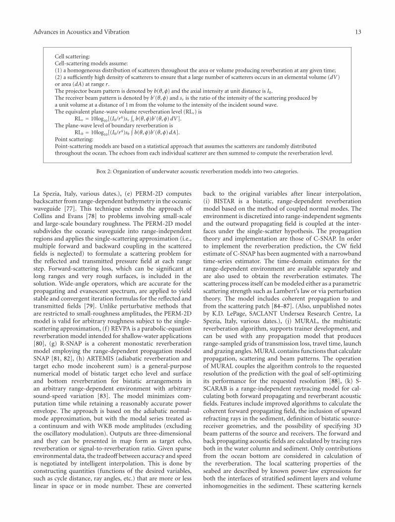
Reverberation models can be categorized according tocell-scattering or point-scattering techniques (Box 2). Cell-scattering formulations divide the ocean into cells, whereeach cell contains a large number of uniformly distributed
scatterers [73]. Point-scattering formulations assume a ran-dom distribution of (point) scatterers. Table 3 provides asummary of stand-alone reverberation models. Superscriptletters identify those models that have been added to theinventory since 2003. These letters refer to a brief summaryand appropriate documentation. Model documentation canrange from informal programming commentaries to journalarticles to detailed technical reports containing a listing ofthe actual computer code. Corresponding information onthe legacy models is provided in the 2003 baseline [23] andis not repeated here.
In Table 3: (Reverberation models), (a) C-SNAP-REVcomputes reverberation using the C-SNAP range-dependentnormal-mode model. Range dependence of the environmentis treated as a one-way coupled-mode solution. Surfaceand bottom reverberation is obtained by integrating thereceived intensity over the area insonified by the emittedpulse and that contributes to the reverberation at a giventime. An average sound speed is assumed for all thepaths (i.e., no group-velocity dependence). The scattering isdescribed by a mode-coupling matrix that is equivalent to theplane-wave scattering function evaluated at discrete anglescorresponding to the modes. The incident and scatteredmode angles are modified to take into account the localslope and are given by the local phase velocity and thesound speed at the interface. Coherent summation of modecontributions is used to correctly model the effects of deep-water convergent zones. The empirical scattering functionis based on Lambert’s rule. The model deals mainly withthe monostatic case, though the technique is extendable tobistatic geometries. (Unpublished notes by Ellis, SACLANTUndersea Research Centre, La Spezia, Italy, various dates.)(b) HYREV is a high-frequency, monostatic reverberationmodel suitable for shallow-water environments. Arrivaltimes and transmission losses from the source to scatterersare obtained from the appropriate eigenrays. The composite-roughness theory is used to predict the boundary scattering[74], (c) NOGRP first runs the normal-mode programPOPP (a variant of PROLOS), which calls the normalmode subprogram MODES and writes out a binary fileof mode information that is then read by the monostaticreverberation code. ROSELLA, an extension of NOGRP, isused to execute the reverberation calculations with beampatterns [75, 76], (d) PAREQ-REV is a range-dependentwave-theory model based on the parabolic approximation ofthe wave equation. The numerical method uses the split-stepFourier marching solution with automatic interpolation ofenvironmental data with range. The code allows a choice ofeither the standard Tappert-Hardin parabolic equation or thewide-angle equation of Thomson-Chapman. Several choicesof starting fields are provided, including a Gaussian sourcebeam of varying width and tilt with respect to the horizontal.Reverberation from the ocean boundaries is computed usingstandard scattering laws: Lambert’s rule for bottom backscat-ter, and either Chapman-Harris curves or Lambert’s rule forsea-surface backscatter. The computational scheme uses reci-procity of propagation to compute the reverberation field forarbitrary receiver depths at the source range. (Unpublishednotes by Schneider, SACLANT Undersea Research Centre,
Advances in Acoustics and Vibration 13
Cell scattering:Cell-scattering models assume:(1) a homogeneous distribution of scatterers throughout the area or volume producing reverberation at any given time;(2) a sufficiently high density of scatterers to ensure that a large number of scatterers occurs in an elemental volume (dV)or area (dA) at range r.The projector beam pattern is denoted by b(θ,φ) and the axial intensity at unit distance is I0.The receiver beam pattern is denoted by b′(θ,φ) and sv is the ratio of the intensity of the scattering produced bya unit volume at a distance of 1 m from the volume to the intensity of the incident sound wave.The equivalent plane-wave volume reverberation level (RLv) is
RLv = 10log10[(I0/r4)sv∫v b(θ,φ)b′(θ,φ)dV].
The plane-wave level of boundary reverberation isRLb = 10log10[(I0/r4)sb
∫b(θ,φ)b′(θ,φ)dA].
Point scattering:Point-scattering models are based on a statistical approach that assumes the scatterers are randomly distributedthroughout the ocean. The echoes from each individual scatterer are then summed to compute the reverberation level.
Box 2: Organization of underwater acoustic reverberation models into two categories.
La Spezia, Italy, various dates.), (e) PERM-2D computesbackscatter from range-dependent bathymetry in the oceanicwaveguide [77]. This technique extends the approach ofCollins and Evans [78] to problems involving small-scaleand large-scale boundary roughness. The PERM-2D modelsubdivides the oceanic waveguide into range-independentregions and applies the single-scattering approximation (i.e.,multiple forward and backward coupling in the scatteredfields is neglected) to formulate a scattering problem forthe reflected and transmitted pressure field at each rangestep. Forward-scattering loss, which can be significant atlong ranges and very rough surfaces, is included in thesolution. Wide-angle operators, which are accurate for thepropagating and evanescent spectrum, are applied to yieldstable and convergent iteration formulas for the reflected andtransmitted fields [79]. Unlike perturbative methods thatare restricted to small-roughness amplitudes, the PERM-2Dmodel is valid for arbitrary roughness subject to the single-scattering approximation, (f) REVPA is a parabolic-equationreverberation model intended for shallow-water applications[80], (g) R-SNAP is a coherent monostatic reverberationmodel employing the range-dependent propagation modelSNAP [81, 82], (h) ARTEMIS (adiabatic reverberation andtarget echo mode incoherent sum) is a general-purposenumerical model of bistatic target echo level and surfaceand bottom reverberation for bistatic arrangements inan arbitrary range-dependent environment with arbitrarysound-speed variation [83]. The model minimizes com-putation time while retaining a reasonably accurate powerenvelope. The approach is based on the adiabatic normal-mode approximation, but with the modal series treated asa continuum and with WKB mode amplitudes (excludingthe oscillatory modulation). Outputs are three-dimensionaland they can be presented in map form as target echo,reverberation or signal-to-reverberation ratio. Given sparseenvironmental data, the tradeoff between accuracy and speedis negotiated by intelligent interpolation. This is done byconstructing quantities (functions of the desired variables,such as cycle distance, ray angles, etc.) that are more or lesslinear in space or in mode number. These are converted
back to the original variables after linear interpolation,(i) BISTAR is a bistatic, range-dependent reverberationmodel based on the method of coupled normal modes. Theenvironment is discretized into range-independent segmentsand the outward propagating field is coupled at the inter-faces under the single-scatter hypothesis. The propagationtheory and implementation are those of C-SNAP. In orderto implement the reverberation prediction, the CW fieldestimate of C-SNAP has been augmented with a narrowbandtime-series estimator. The time-domain estimates for therange-dependent environment are available separately andare also used to obtain the reverberation estimates. Thescattering process itself can be modeled either as a parametricscattering strength such as Lambert’s law or via perturbationtheory. The model includes coherent propagation to andfrom the scattering patch [84–87]. (Also, unpublished notesby K.D. LePage, SACLANT Undersea Research Centre, LaSpezia, Italy, various dates.), (j) MURAL, the multistaticreverberation algorithm, supports trainer development, andcan be used with any propagation model that producesrange-sampled grids of transmission loss, travel time, launchand grazing angles. MURAL contains functions that calculatepropagation, scattering and beam patterns. The operationof MURAL couples the algorithm controls to the requestedresolution of the prediction with the goal of self-optimizingits performance for the requested resolution [88], (k) S-SCARAB is a range-independent raytracing model for cal-culating both forward propagating and reverberant acousticfields. Features include improved algorithms to calculate thecoherent forward propagating field, the inclusion of upwardrefracting rays in the sediment, definition of bistatic source-receiver geometries, and the possibility of specifying 3Dbeam patterns of the source and receivers. The forward andback propagating acoustic fields are calculated by tracing raysboth in the water column and sediment. Only contributionsfrom the ocean bottom are considered in calculation ofthe reverberation. The local scattering properties of theseabed are described by known power-law expressions forboth the interfaces of stratified sediment layers and volumeinhomogeneities in the sediment. These scattering kernels
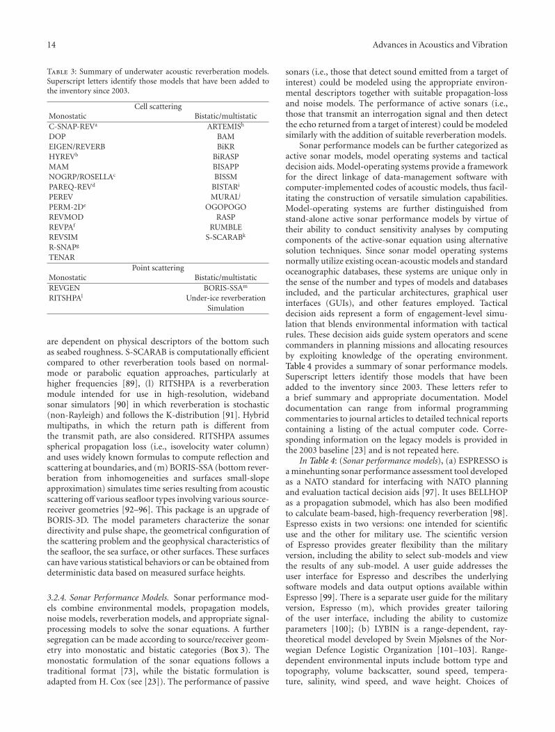
14 Advances in Acoustics and Vibration
Table 3: Summary of underwater acoustic reverberation models.Superscript letters identify those models that have been added tothe inventory since 2003.
Cell scatteringMonostatic Bistatic/multistaticC-SNAP-REVa ARTEMISh
DOP BAMEIGEN/REVERB BiKRHYREVb BiRASPMAM BISAPPNOGRP/ROSELLAc BISSMPAREQ-REVd BISTARi
PEREV MURALj
PERM-2De OGOPOGOREVMOD RASPREVPAf RUMBLEREVSIM S-SCARABk
R-SNAPg
TENARPoint scattering
Monostatic Bistatic/multistaticREVGEN BORIS-SSAm
RITSHPAl Under-ice reverberationSimulation
are dependent on physical descriptors of the bottom suchas seabed roughness. S-SCARAB is computationally efficientcompared to other reverberation tools based on normal-mode or parabolic equation approaches, particularly athigher frequencies [89], (l) RITSHPA is a reverberationmodule intended for use in high-resolution, widebandsonar simulators [90] in which reverberation is stochastic(non-Rayleigh) and follows the K-distribution [91]. Hybridmultipaths, in which the return path is different fromthe transmit path, are also considered. RITSHPA assumesspherical propagation loss (i.e., isovelocity water column)and uses widely known formulas to compute reflection andscattering at boundaries, and (m) BORIS-SSA (bottom rever-beration from inhomogeneities and surfaces small-slopeapproximation) simulates time series resulting from acousticscattering off various seafloor types involving various source-receiver geometries [92–96]. This package is an upgrade ofBORIS-3D. The model parameters characterize the sonardirectivity and pulse shape, the geometrical configuration ofthe scattering problem and the geophysical characteristics ofthe seafloor, the sea surface, or other surfaces. These surfacescan have various statistical behaviors or can be obtained fromdeterministic data based on measured surface heights.
3.2.4. Sonar Performance Models. Sonar performance mod-els combine environmental models, propagation models,noise models, reverberation models, and appropriate signal-processing models to solve the sonar equations. A furthersegregation can be made according to source/receiver geom-etry into monostatic and bistatic categories (Box 3). Themonostatic formulation of the sonar equations follows atraditional format [73], while the bistatic formulation isadapted from H. Cox (see [23]). The performance of passive
sonars (i.e., those that detect sound emitted from a target ofinterest) could be modeled using the appropriate environ-mental descriptors together with suitable propagation-lossand noise models. The performance of active sonars (i.e.,those that transmit an interrogation signal and then detectthe echo returned from a target of interest) could be modeledsimilarly with the addition of suitable reverberation models.
Sonar performance models can be further categorized asactive sonar models, model operating systems and tacticaldecision aids. Model-operating systems provide a frameworkfor the direct linkage of data-management software withcomputer-implemented codes of acoustic models, thus facil-itating the construction of versatile simulation capabilities.Model-operating systems are further distinguished fromstand-alone active sonar performance models by virtue oftheir ability to conduct sensitivity analyses by computingcomponents of the active-sonar equation using alternativesolution techniques. Since sonar model operating systemsnormally utilize existing ocean-acoustic models and standardoceanographic databases, these systems are unique only inthe sense of the number and types of models and databasesincluded, and the particular architectures, graphical userinterfaces (GUIs), and other features employed. Tacticaldecision aids represent a form of engagement-level simu-lation that blends environmental information with tacticalrules. These decision aids guide system operators and scenecommanders in planning missions and allocating resourcesby exploiting knowledge of the operating environment.Table 4 provides a summary of sonar performance models.Superscript letters identify those models that have beenadded to the inventory since 2003. These letters refer toa brief summary and appropriate documentation. Modeldocumentation can range from informal programmingcommentaries to journal articles to detailed technical reportscontaining a listing of the actual computer code. Corre-sponding information on the legacy models is provided inthe 2003 baseline [23] and is not repeated here.
In Table 4: (Sonar performance models), (a) ESPRESSO isa minehunting sonar performance assessment tool developedas a NATO standard for interfacing with NATO planningand evaluation tactical decision aids [97]. It uses BELLHOPas a propagation submodel, which has also been modifiedto calculate beam-based, high-frequency reverberation [98].Espresso exists in two versions: one intended for scientificuse and the other for military use. The scientific versionof Espresso provides greater flexibility than the militaryversion, including the ability to select sub-models and viewthe results of any sub-model. A user guide addresses theuser interface for Espresso and describes the underlyingsoftware models and data output options available withinEspresso [99]. There is a separate user guide for the militaryversion, Espresso (m), which provides greater tailoringof the user interface, including the ability to customizeparameters [100]; (b) LYBIN is a range-dependent, ray-theoretical model developed by Svein Mjølsnes of the Nor-wegian Defence Logistic Organization [101–103]. Range-dependent environmental inputs include bottom type andtopography, volume backscatter, sound speed, tempera-ture, salinity, wind speed, and wave height. Choices of

Advances in Acoustics and Vibration 15
Active sonar equations (monostatic)
(i) Noise background
SL− 2TL + TS = NL−DI + RDN .
(ii) Reverberation background
SL− 2TL + TS = RL + RDR.
Passive sonar equation
SL− TL = NL−DI + RD.
SL: source level; TL: transmission loss; TS: target strength; NL: noise level; DI: receiving directivity index;
RL: reverberation level; RD: recognition differential.
Active sonar equations (bistatic)
The signal excess (SE) can be represented as:
(i) SE = ESL− TL1 − TL2 − [(N0 − AGN )⊕
R0] + TS−Λ− L,
the energy source level (ESL) is related to the intensity source level (SL) as:
(ii) ESL = SL + 10log10T
where T is the duration of the transmitted pulse,
The echo energy level (EEL) received from the target at a hydrophone on the receiver array is then:
(iii) EEL = ESL− TL1 − TL2 + TS,
where TS is the target strength, N0 is the noise spectral level, R0 represents the reverberation spectral level, AGN is the array
gain against noise, Λ is the threshold on the signal-to-noise ratio (SNR) required for detection,
L is a loss term to account for time spreading and system losses,⊕
represents power summation, TL1 is the transmission loss from source (S) to target (T),
and TL2 is the transmission loss from target (T) to receiver (R).
Box 3: Sonar performance models are based upon the sonar equations, which are the basic building blocks for both monostatic and bistaticsonar geometries.
calculation outputs include ray trace, transmission loss,reverberation (surface, volume, and bottom), noise, signalexcess, probability of detection, travel time, and impulseresponse. The transmission-loss module was evaluated byNURC [104]. LYBIN is available commercially from theForsvarets forskningsinstitutt (FFI), (c) MOC3D [105] is a3D model developed from the 2D model MOCASSIN [106].MOC3D was used to investigate the importance of out-of-plane sound propagation in a shallow-water experimentin the Florida Straits [107], (d) MODRAY was developedin conjunction with DSTO (Australia) to simulate thepropagation of sound through the underwater environment[108, 109]. MODRAY uses classical ray-tracing theory toproduce sound-pressure time series at one or more receivers.The marine environment is range-independent. Seafloorcomposition can be specified, the sound-speed profile canbe arbitrary, noise includes wind, rain, biological andshipping sources, and scattering by marine organisms isincluded. MODRAY can model an arbitrary number ofsound sources, reflectors and receivers stationed on movingplatforms. MODRAY has been used extensively to modelthe effectiveness of underwater communications algorithms
[110, 111], (e) SUPREMO is a multistatic sonar performancemodel that includes propagation, target echoes, reverbera-tion and noise, all plotted as a function of delay time andbearing using an equivalent map projection. A modularpropagation section makes it possible to separate the effectsof propagation modeling (e.g., theoretical basis and range-dependence) from those of scattering computations (e.g.,computational efficiency, bottom slope and scattering law).Special attention is paid to problems of interference frommultiple sources firing in sequence, target aspect dependencefrom multiple receivers, mixed FM and CW, mismatchedsource and receivers, multiple displays (one for each bistaticpair), and presentation of results [82, 112–115]. Predictionsof acoustic reverberation and target echo intensity made bythe SUPREMO sonar performance model were comparedwith measured data gathered in the Malta Plateau region ofthe Mediterranean Sea. The observed model-measurementagreement demonstrated the suitability of SUPREMO foruse with an environmentally adaptive, low-frequency, activesonar system [116]. Version 2.0 of SUPREMO has beendocumented [117, 118], (f) SWAMI models range-and-azimuth dependence (N × 2D) via adiabatic modes [119].
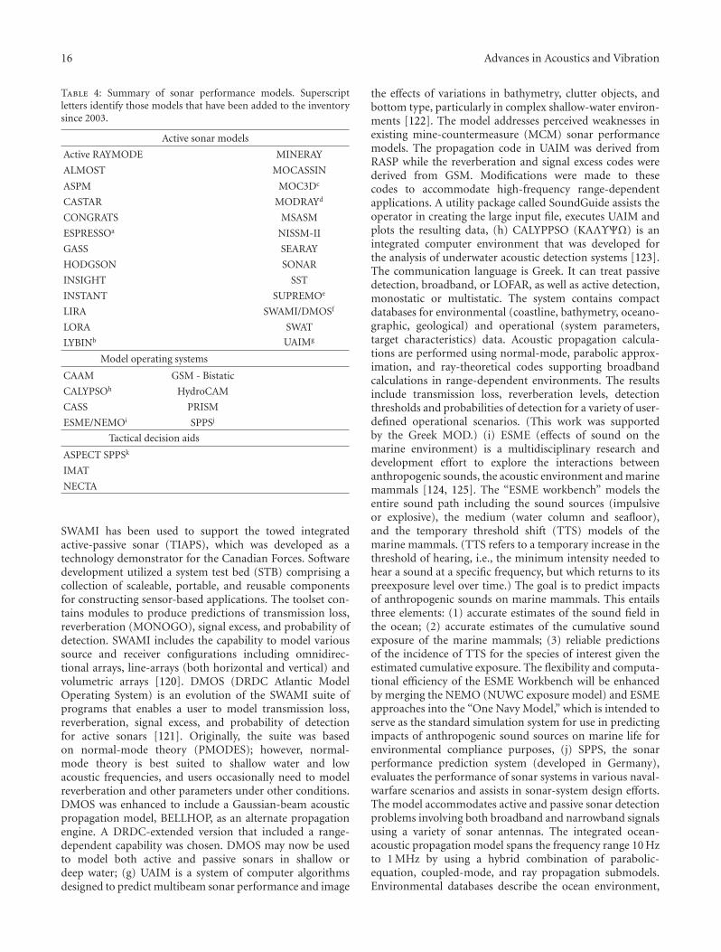
16 Advances in Acoustics and Vibration
Table 4: Summary of sonar performance models. Superscriptletters identify those models that have been added to the inventorysince 2003.
Active sonar models
Active RAYMODE MINERAY
ALMOST MOCASSIN
ASPM MOC3Dc
CASTAR MODRAYd
CONGRATS MSASM
ESPRESSOa NISSM-II
GASS SEARAY
HODGSON SONAR
INSIGHT SST
INSTANT SUPREMOe
LIRA SWAMI/DMOSf
LORA SWAT
LYBINb UAIMg
Model operating systems
CAAM GSM - Bistatic
CALYPSOh HydroCAM
CASS PRISM
ESME/NEMOi SPPSj
Tactical decision aids
ASPECT SPPSk
IMAT
NECTA
SWAMI has been used to support the towed integratedactive-passive sonar (TIAPS), which was developed as atechnology demonstrator for the Canadian Forces. Softwaredevelopment utilized a system test bed (STB) comprising acollection of scaleable, portable, and reusable componentsfor constructing sensor-based applications. The toolset con-tains modules to produce predictions of transmission loss,reverberation (MONOGO), signal excess, and probability ofdetection. SWAMI includes the capability to model varioussource and receiver configurations including omnidirec-tional arrays, line-arrays (both horizontal and vertical) andvolumetric arrays [120]. DMOS (DRDC Atlantic ModelOperating System) is an evolution of the SWAMI suite ofprograms that enables a user to model transmission loss,reverberation, signal excess, and probability of detectionfor active sonars [121]. Originally, the suite was basedon normal-mode theory (PMODES); however, normal-mode theory is best suited to shallow water and lowacoustic frequencies, and users occasionally need to modelreverberation and other parameters under other conditions.DMOS was enhanced to include a Gaussian-beam acousticpropagation model, BELLHOP, as an alternate propagationengine. A DRDC-extended version that included a range-dependent capability was chosen. DMOS may now be usedto model both active and passive sonars in shallow ordeep water; (g) UAIM is a system of computer algorithmsdesigned to predict multibeam sonar performance and image
the effects of variations in bathymetry, clutter objects, andbottom type, particularly in complex shallow-water environ-ments [122]. The model addresses perceived weaknesses inexisting mine-countermeasure (MCM) sonar performancemodels. The propagation code in UAIM was derived fromRASP while the reverberation and signal excess codes werederived from GSM. Modifications were made to thesecodes to accommodate high-frequency range-dependentapplications. A utility package called SoundGuide assists theoperator in creating the large input file, executes UAIM andplots the resulting data, (h) CALYPPSO (KAΛΥΨΩ) is anintegrated computer environment that was developed forthe analysis of underwater acoustic detection systems [123].The communication language is Greek. It can treat passivedetection, broadband, or LOFAR, as well as active detection,monostatic or multistatic. The system contains compactdatabases for environmental (coastline, bathymetry, oceano-graphic, geological) and operational (system parameters,target characteristics) data. Acoustic propagation calcula-tions are performed using normal-mode, parabolic approx-imation, and ray-theoretical codes supporting broadbandcalculations in range-dependent environments. The resultsinclude transmission loss, reverberation levels, detectionthresholds and probabilities of detection for a variety of user-defined operational scenarios. (This work was supportedby the Greek MOD.) (i) ESME (effects of sound on themarine environment) is a multidisciplinary research anddevelopment effort to explore the interactions betweenanthropogenic sounds, the acoustic environment and marinemammals [124, 125]. The “ESME workbench” models theentire sound path including the sound sources (impulsiveor explosive), the medium (water column and seafloor),and the temporary threshold shift (TTS) models of themarine mammals. (TTS refers to a temporary increase in thethreshold of hearing, i.e., the minimum intensity needed tohear a sound at a specific frequency, but which returns to itspreexposure level over time.) The goal is to predict impactsof anthropogenic sounds on marine mammals. This entailsthree elements: (1) accurate estimates of the sound field inthe ocean; (2) accurate estimates of the cumulative soundexposure of the marine mammals; (3) reliable predictionsof the incidence of TTS for the species of interest given theestimated cumulative exposure. The flexibility and computa-tional efficiency of the ESME Workbench will be enhancedby merging the NEMO (NUWC exposure model) and ESMEapproaches into the “One Navy Model,” which is intended toserve as the standard simulation system for use in predictingimpacts of anthropogenic sound sources on marine life forenvironmental compliance purposes, (j) SPPS, the sonarperformance prediction system (developed in Germany),evaluates the performance of sonar systems in various naval-warfare scenarios and assists in sonar-system design efforts.The model accommodates active and passive sonar detectionproblems involving both broadband and narrowband signalsusing a variety of sonar antennas. The integrated ocean-acoustic propagation model spans the frequency range 10 Hzto 1 MHz by using a hybrid combination of parabolic-equation, coupled-mode, and ray propagation submodels.Environmental databases describe the ocean environment,

Advances in Acoustics and Vibration 17
targets, platforms and sonar-system characteristics. Thereverberation model predicts volume, surface and bottomcomponents. Noise sources include ambient, biological, rain,shipping, ice, seismic exploration, and self-noise [126],and (k) ASPECT, the active system performance estimatecomputer tool, is a multistatic tactical decision aid (TDA). Itcomputes estimates of system performance for active under-water acoustic sensors. ASPECT was originally designed tosatisfy the requirements of mission planning software for theIEER (improved extended echo ranging) system. However,virtually any multistatic or monostatic active acoustic systemcan be modeled using this software package. ASPECT usesthe FAME (fast multipath expansion) model for range-independent calculations of transmission loss and ASPM(active system performance model) for range-dependenttransmission loss and reverberation. These computations arethen fed into MSASM, which is capable of estimating theperformance of active sonar systems for multiple sources,receivers, and targets. It simulates target motion includingsuch features as normal and uniform probability distribu-tion, various speed, and course distributions, as well as targetevasion modeling to a limited degree. ASPECT version 2.0(and beyond) supersedes the MSASM Interactive Executionand Optimization System (MINEOS), which was the firstversion of mission planning software developed for the IEERprogram. ASPECT also exists as a standalone version [127].
3.3. Inversion Techniques
3.3.1. Adjunct Tools for Oceanographers. Inverse acousticsensing techniques presently constitute adjuncts to directmeasurement methods. However, the application of inverseacoustic sensing techniques to dynamical studies of theoceans’ boundaries and interior show great promise forthree reasons. First, such data can be used to establishcomparative baselines for other remote sensors, such assatellites, by providing synoptic portraitures of the interioroceans together with concurrent ground-truth data at thesea surface. Second, inverse acoustic techniques often afforduseful insights into a broad class of oceanic phenomenasince their successful employment relies heavily on the use ofnumerical models first to understand the role of the oceansas an acoustic medium. Third, inverse data provide estimatesof spatially integrated and temporally averaged oceanicconditions that are not readily available from traditionaloceanographic sensors.
Recently, acoustical oceanographers have employedunderwater-acoustic models as adjunct tools for inverse-sensing techniques that can be used to obtain synopticportraitures of large ocean areas or to monitor long-termvariations in the ocean.
Useful information about the ocean can be derivedfrom both forward and inverse applications of underwatersound. Direct (or forward) methods include traditionalsonar applications. Inverse methods extract informationfrom direct measurements of the physical properties of theocean. These inverse methods combine the direct physi-cal measurements with theoretical models of underwater
acoustics. The objective is to estimate detailed underwater-acoustic fields from sparse physical measurements usingthe theoretical models as guides. Inversions of controlled-source, noise, and reverberation fields have been performedsuccessfully (Box 4).
Inverse sensing techniques that employ acoustics havebeen used in several subdisciplines of geophysics includingseismology, meteorology, and oceanography. In oceanog-raphy, inverse acoustic data provide estimates of spatiallyintegrated and temporally averaged oceanic conditions thatare not readily available from a traditional constellation ofpoint sensors. Forward (or direct) models are important insolving inverse problems.
3.3.2. Propagation (Acoustic Field Measurements). Acousticpropagation characteristics in the deep oceans are deter-mined largely by the refractive properties of the watercolumn and, to a lesser extent, by the surface and bottomboundary conditions. Propagation measurements can beused to infer bulk properties of the water column suchas temperature, sound speed, density, and currents. Inshallow-ocean areas, where propagation characteristics canbe strongly affected by the bottom boundary, propagationmeasurements can be used to infer properties of the seafloor such as composition and scattering characteristics. Awide spectrum of inverse problems has been addressed inunderwater acoustics including estimation of geoacousticparameters, acoustic thermometry, and shallow-water char-acterization. Inverse acoustic sensing methods utilizing thepropagation characteristics of the oceans include matchedfield processing, ocean acoustic tomography and deductivegeoacoustic inversion [23]. A new technique known as atime reversal mirror (TRM) uses inverse methods to refocusreceived signals back to the source.
Range-dependent ray-theoretical models are typicallyused for deep-water applications involving tomographicexperiments as well as for high-frequency experiments inshallow water. Range-dependent wave-theoretical modelsbased on normal-mode, fast-field (wavenumber integra-tion), or parabolic-equation approaches are preferred forlow-frequency experiments in shallow water.
3.3.3. Noise. The ambient noise field in the oceans isdescribed by the spectral, spatial, and temporal character-istics of sound generated by both natural and industrialsources. Measurements of these characteristics can provideuseful information regarding the nature of the noise sourcesthemselves as well as physical features within the oceans.Examples of inverse applications of the noise field includewind speed determination, rainfall measurements, objectimaging (acoustic daylight), and geoacoustic inversion.
3.3.4. Reverberation. The reverberation field in the oceansis the product of acoustic scattering by the surface andbottom boundaries and by inhomogeneities within theoceans. The utility of the reverberation field as an inversesensing technique is analogous to that of the ambient noisefield. For example, the reverberation field can be inverted to

18 Advances in Acoustics and Vibration
Propagation(i) Matched field processing:
(a) source localization,(b) marine environment characterization.
(ii) Ocean acoustic tomography:(a) density field (eddies, currents),(b) temperature (climate monitoring).
(iii) Deductive geoacoustic inversion:(a) sediment parameters,(b) sea-floor scattering characteristics.
(iv) Time reversal mirror (TRM):(a) signal refocusing.
Noise(i) Field inversion:
(a) wind speeds,(b) rainfall rates.
(ii) Acoustic daylight:(a) object imaging.
(iii) Geoacoustic inversion:(a) seabed acoustics.
Reverberation(i) Field inversion:
(a) sea-floor imaging.(ii) TRM nulling:
(a) reverberation attenuation.
Box 4: Summary of inverse ocean acoustic sensing techniques.
image the sea floor. A new development uses time reversalmirror (TRM) methods to attenuate reverberant returns.
4. Emerging Solutions
4.1. Background. This section addresses advanced processingmethods in addition to novel methods by which to maximizethe interpretation, and thus utility, of archival and experi-mental data.
4.2. Advanced Integrated Modeling Approaches
4.2.1. Acoustic Integration Model. The acoustic integra-tion model (AIM) combines a movement simulator withunderwater acoustic models to predict (and thus minimizeand mitigate) the potential effect of sound on marinemammals [128]. Simulated sound sources and animals areprogrammed to move in location and depth over time ina realistic fashion. AIM is a Monte Carlo statistical modelbased on a whale movement and tracking model and anunderwater acoustic backscattering model for a movingsource. Currently, AIM incorporates the BELLHOP and PEpropagation models in addition to the ETOP05 bathymetryand GDEM sound-speed profile databases. The ETOP05 dataset is the highest resolution topographic data set with globalcoverage that is publicly available, with elevations postedevery 5 arc minutes (approximately 10 km) for all land andsea floor surfaces. ETOP05 is distributed without restrictionby the National Oceanic and Atmospheric Administration
(NOAA) through its National Geophysical Data Center(NGDC).
4.2.2. Marine Mammal Movement Models. A method hasbeen developed for modeling marine mammal movementand behavior (3MB) for use in environmental impact assess-ments [129]. Estimating the impact of anthropogenic soundon marine animals entails consideration of animal locationand behavior at the time of sound exposure. The ESMEmodel (see Table 4) incorporates 3MB to provide fine-scalecontrol over simulated marine-animal (animat) movementand behavior. Control over the animats is scaleable tothe information available regarding the species of concern.Movement and behavior are stochastically determined bysampling from distributions describing rates of movementin the horizontal and vertical planes, direction of travel, timeat the surface between dives, time at depth, and time in andtransition between behavioral states. Influence of behaviorover each of the other distributions is also permitted.
As part of the NATO Undersea Research Centre(NURC) broadband environmentally adaptive concept, theSUPREMO sonar performance model was incorporatedwithin a feedback mechanism for sonar-parameter opti-mization for any specified ocean environment [130]. Thefeasibility of using active sonars to monitor the movementof marine mammals was investigated in order to recommendstand-off distances within which an acoustic source shouldnot be deployed [131].
4.2.3. Energy Flux Models. Some applications, such as workrelating to acoustic impacts on marine mammals, do notrequire extremely high-fidelity model outputs. Transmissionlosses averaged over depth, for example, are often adequate.
An approach referred to as energy-flux models [132]is useful for rapid calculation of transmission loss wherethe propagation conditions are dominated by numerousboundary-reflected multipaths and when only the coarsecharacteristics of the acoustic field are needed.
In specific configurations, especially at long ranges inshallow-water environments, the transmitted field can beviewed as being composed of many paths propagating bysuccessive reflections from the surface and bottom bound-aries. Here, the acoustic energy will remain trapped betweenthese two boundaries. Furthermore, if the acoustic frequencyis high enough that the field oscillations can be considered tobe random, then an average intensity can be calculated usingsimple algebraic formulas [23].
This concept can be extended to ocean environmentswhere the sound speed is not constant, or where there areslight losses at the boundaries. In such cases, the transmittedfield cannot be taken as a volumetric average. Rather, it hasto be decomposed into its angular components and the cycliccharacteristics of the various beams must be detailed [133].
This approach is very useful for predicting incoherenttransmission losses in cases where there are a large numberof modes (≥6). These flux models are fast because there is norequirement to find modes or eigenrays. They can also lead to

Advances in Acoustics and Vibration 19
very simple and intuitive expressions. This method has beenextended for reverberation [134].
4.2.4. Waveguide Invariant Models. In weakly range-dependent ocean environments, it has been observedthat the acoustic wavefield can be described in terms ofray-based or mode-based approaches [135, 136]. Usingray-based descriptions, distributions of the ray amplitudeand phase (travel time) are largely controlled by theso-called stability parameter (α). Alternatively, using mode-based descriptions in either purely range-independentenvironments or in range-independent environments uponwhich weak (range-dependent) perturbations have beensuperimposed, many wavefield properties are controlled bythe so-called waveguide invariant (β). When β is evaluatedusing asymptotic mode-theoretical results (in a stratifiedenvironment), it was found that β = α, which is consistentwith the well-known ray-mode duality. In weakly range-dependent environments, however, α was found to controlray stability and several measures of travel-time dispersionwhile β controlled the spread of modal-group delays due tomode coupling.
In essence, the waveguide invariant (β) summarizes thepattern of constructive and destructive interference betweenacoustic modes propagating in the ocean waveguide. Itmanifests itself as interference fringes (or striations) in aplot of frequency versus source-receiver separation. Thewaveguide invariant summarizes in a single scalar parameterthe dispersive propagation characteristics in a waveguide.
4.3. Advanced Nonintrusive Measurement Approaches
4.3.1. Acoustic Transmission Options. In acoustic probing,transmit signals can be adapted according to in situ estimatesof channel conditions. Waveform characteristics could be setusing returns from the previous transmission as an indicatorof channel response. Rapidly modifying processing param-eters by analyzing previously received signals addresses theproblem of fluctuating acoustic channel response owing tovariations in environmental factors. Such optimal matchingto the estimated channel response would improve target-echo stability [137].
Since sound level, frequency, and duration are criticalparameters in causing physical damage to marine life,transmitting over a wider frequency spectrum using spread-spectrum techniques or noise-like signals could avoid tissuedamage by reducing the time spent (or energy transmitted)in particular frequency bands. Spread-spectrum techniquesuse a pseudorandom spreading code to produce a wide-band source signature. Signals must possess high rangeand Doppler resolution and minimize cross-talk betweendifferent users.
Noise-like signals emulate ambient noise by covertlyadapting to the fluctuating ambient noise field. Designerscould model pseudo-random signals based on bioacousticnoise, surf noise (when high-frequency broadband transientsshould be useful [138]) or shipping noise (when near CWwould be more useful).
Advances in sonar technologies have rendered modernsonar systems useful for in situ measurements of theambient marine environment. For example, through-the-sensor measurements of the ocean impulse response haveenabled modern sonars to perform collateral functions astactical environmental processors.
A recent through-the-sensor remote-sensing technique foracoustic-parameter estimation has been referred to as SABLE(sonar active boundary loss estimation) [139]. Bottomscattering strengths were derived from active hull-mountednaval sonar data by using eigenray paths modeled by CASSand GRAB to associate sonar-signal attributes with specificpropagation paths.
4.3.2. Collision Avoidance. Cetaceans are prone to collisionswith fast-moving vessels. In areas of high cetacean and vesseldensities, the sperm whale (Physeter macrocephalus) is ofgreat concern. Sperm whales are highly vocal and can belocalized with passive sonar; however, when at or near thesurface (i.e., when they are at greatest risk of collision), theytend to stop vocalizing. Techniques employing active sonarshave proved to be inefficient due to short detection rangesand high closing speeds. The efficiency of a passive-sonarsolution was evaluated that used vocalizing whale clicks (atdepth) as acoustic sources to detect silent whales [140]. Thissolution could serve as a noninvasive complement to a morecomplex passive localization and collision-avoidance system.A wideband N × 2D (range-and-azimuth-dependent) raymodel was used to simulate a passive solution comprisingan arbitrary number of active acoustic sources (vocalizingwhales), an illuminated object (silent whale) and a passive-sonar receiver, all positioned in three-dimensional space witharbitrary bathymetry. Both curved-line and straight-lineray solutions were implemented, with the latter providinggreater computational speeds at the expense of temporaland angular fidelity. The simulation recreated the resultantmixture of direct, reverberated and target-backscatteredsignals arriving at the receiver for any array configuration,any number of sources and one target. In the vicinityof the Canary Islands, the simulations demonstrated theapplicability of the concept with a maximum detection rangeon the order of 1 km.
4.4. Advanced Processing Methods
4.4.1. Adjoint Modeling. The principal application of adjointmodels is sensitivity analysis. When quantitative estimatesof sensitivity are desired, a mathematical model of thephenomenon or relationship is required. While models havebeen used to assess the impacts of perturbations and thusestimate sensitivity, a more efficient approach is to use themodel’s adjoint to determine optimal solutions. The adjointoperates backward in the sense that it determines a gradientwith respect to input from a gradient with respect to output.In a temporally continuous model, this would appear asintegration backwards in time. If there are no numericalinstabilities associated with irreversible processes in thetangent linear model acting forward in time, there will be

20 Advances in Acoustics and Vibration
none in the adjoint acting backward in time (a tangent linearmodel provides a first-order approximation to the evolutionof perturbations in a nonlinear forecast trajectory). Thegreatest limitation to the application of adjoints is that theresults are useful only when the linearized approximation isvalid. The adjoint operator (matrix transpose) back-projectsinformation from data to the underlying model. Geophysicalmodeling calculations generally use linear operators thatpredict data from models. The usual task is to find the inverseof these calculations, that is, to find models (or make maps)from the data. The adjoint operator tolerates imperfectionsin the data and does not demand that the data provide fullinformation.
The concept of adjoint modeling was introduced inshallow water acoustics for solving inverse problems [141]. Inrelated work, the concept of backpropagation was reviewedin the context of adjoint modeling [142]. The differentimplementations of this concept were compared and dis-cussed in the framework of experimental acoustic inver-sion in shallow water with application to source localiza-tion, ocean acoustic tomography, geoacoustic inversion andunderwater communications. Well-established inversion (orfocalization) methods based on matched-field processing,model-based matched filter and time-reversal mirror arerelated to lesser known techniques such as acoustic retroga-tion and other variants of backpropagation. In contrast to thelatter, adjoint-based variational inversion approaches makeuse of the adjoint of a forward model to backpropagate themodel-data mismatch at the receiver toward the source.
An adjoint model was derived from a forward-propaga-tion model (e.g., normal mode or parabolic equation)to propagate data-model misfits at the observation pointback through the medium to the site of those mediumperturbations that were not accounted for in the forwardmodel and which gave rise to the observed data-modelmisfits [143]. This property makes adjoint models attractivefor use in acoustic inversion experiments.
4.4.2. Stochastic Resonance. Stochastic resonance refers toa phenomenon that is manifested in nonlinear systemswhereby weak signals can be amplified in the presence ofnoise [144]. Three components are necessary: a threshold,a periodic signal and a source of noise. The response ofthe system undergoes resonance-like behavior as the noiselevel is varied [145]. Stochastic resonance was applied toenhance the detection of target signals masked by shallow-water reverberation [146]. Specifically, parameter-inducedstochastic resonance was used to tune system parameters torecover the spatial signal that was corrupted by Gaussiannoise. This method also has applicability when processingspatial signals that are corrupted by K-distributed envelopenoise (a standard model for radar clutter).
4.4.3. Optimization Techniques. Ant colony optimization(ACO) has elements in common with genetic algorithms[147]. Both are population-based algorithms that searcha discrete space and provide uncertainty analyses. The
main difference is the mechanism that handles and recom-bines components of better candidate solutions (i.e., ant-pheromones trails versus genetic operators). Ant colony opti-mization is further distinguished by having a form of mem-ory (the ant pheromone trails), while genetic algorithmsare without memory. Specifically, when the pheromonesevaporate, identifiers of paths with above-average qualityfade out. Thus, high rates of evaporation mean that onlyrecent information can be retrieved (typical for short-term memory); alternatively, low rates of evaporation allowrecollection of much older information (typical for long-term memory). When applied to inversion, the world of theants acts as an analogy for the geoacoustic environment.
An efficient and reliable method was proposed forperforming the inversion of a neural-network underwateracoustic model to obtain sea-floor parameters [148]. Twodifferent versions of a modified particle-swarm optimizationwere used: two-step gradient approximation and hierarchicalcluster-based approximation. Both approaches worked well.
Tabu search has traditionally been applied to combina-tional optimization problems [149, 150]. The tabu searchbegins by marching to a local minimum. This approachavoids entrapment in cycles by forbidding (tabu), or penal-izing, moves that take the solution in the next iteration topoints in the solution space previously visited.
4.4.4. Chaos. In the presence of weak fluctuations in thesound-speed field, it has been observed that ray trajectoriesin ocean waveguides exhibit a chaotic behavior in whichthe travel times along eigenrays form compact clusters,the center of which is close to the arrival time of anunperturbed ray with similar geometry [151]. The deep-water acoustic waveguide was modeled by an unperturbedsound-speed profile [c0(z)] combined with weak fluctuationsof sound speed [δc(r, z)] caused by a random field of internalwaves conforming to the Garrett-Munk spectrum. Formally,ray equations in a random inhomogeneous medium canbe considered as stochastic equations whose parametersare determined by a random function δc. Such nonlinearequations can be solved in the framework of ordinaryperturbation theory, but only for short ranges. Instead,the ray structure was analyzed by using the Hamiltonianformalism in terms of action-angle canonical variables whosevariation was small under conditions of weak perturbations.It was estimated that ray arrival times at a distance r occupiedan interval whose average width increased in proportion withr1.5, in agreement with previous investigators. Moreover, forr < 103 km, the ray trajectories forming the cluster deviatedonly slightly from the unperturbed ray trajectory and thecluster width grew in proportion with r0.5. For r > 103 km,the width of the cluster grew in proportion with r2.
Chaotic and stochastic nonlinear ray dynamics canoccur in underwater-acoustic waveguides with longitudinalvariations in the sound speed caused by internal waves[152]. This situation was investigated using a model of a“frozen” medium in which the temporal variations in theenvironment were neglected and only the spatial variationsdue to the comparatively small propagation time of sound
Advances in Acoustics and Vibration 21
in the ocean were considered. Coherent ray clusters wereobserved in which large fans of rays with close initialconditions preserved close current dynamical characteristicsover long distances. The cluster structure could be consideredto consist of statistical and coherent parts. Rays belongingto the statistical part propagated in the same areas of phasespace with the same value of the Lagrangian, but did notcorrelate with each other and demonstrated exponential sen-sitivity to initial conditions. Rays belonging to the coherentpart did not demonstrate sensitivity to initial conditions.This coherent clusterization might be a useful propertyfor acoustic tomography in terms of determining spatio-temporal variations in the hydrological environment underconditions of ray chaos [153].
5. Summary
This paper has reviewed changes in the ocean soundscape,changes that have been driven by both anthropogenicactivity and natural factors. New regulatory initiatives haveplaced additional restrictions on uses of sound in theocean, and mitigation of marine-mammal endangermentis now an integral consideration in acoustic-system designand operation. Emphasis has been placed on leveragingadvanced modeling methods to solve emerging scientific andengineering challenges in this field.
Naval sonars have been redesigned as high-power mul-tistatic systems capable of operating in complex coastalenvironments against quiet submarines. Littoral trainingranges to support this new generation of sonar systemsmust comply with more stringent environmental regula-tions. Such compliance is often assessed using advancedmodeling techniques coupled with in situ data collection.Oceanographic data collection is supported by underwaternetworks consisting of sensors and vehicles deployed inconcert. These networks employ nodes that communicate viaacoustic channels that have low data rates and time-varyingfading.
Seismic exploration has ventured into deeper waters insearch of diminishing energy resources using source arraysthat are powered by high-pressure air. Controlled-exposureexperiments have studied changes in the behavior of nearbywhales due to these powerful sources; however, modelinguncertainty complicates the regulatory interpretation ofaverage sound-exposure conditions.
Increased merchant shipping activity has had a mea-sureable impact on the ocean soundscape over the pastfour decades: the average noise has increased by 2.5–3 dBper decade in the frequency band 30–50 Hz. Moreover,the growing number of wind farms in coastal waters ofmedium depth (<30 m) has added to the soundscape at lowfrequencies and resulted in behavioral reactions of nearbymarine mammals.
Climate change has also affected the ocean soundscape.The emission of carbon into the atmosphere through theeffects of fossil-fuel combustion and industrial processeshas increased atmospheric concentrations of carbon dioxide(CO2). Ocean acidification, which occurs when CO2 inthe atmosphere reacts with water to create carbonic acid
(H2CO3), has increased. The attenuation of low-frequencysound in the sea is pH dependent; specifically, the higherthe pH, the greater the attenuation. Thus, as the ocean hasbecome more acidic (lower pH) due to increasing CO2 emis-sions, the attenuation has diminished and low-frequencysounds propagate farther, making the ocean noisier. Recentinvestigations have estimated that the noise at 3 kHz wouldincrease by 30% if the pH decreased from 8.0 to 7.4.
Modeling tools traditionally used in underwateracoustics have undergone a necessary transformation;these tools include propagation, noise, reverberation, andsonar-performance models. Advanced modeling techniquesnow include forward and inverse applications, integrated-modeling approaches, nonintrusive measurements andnovel processing methods. The flow of the sonar modelingprocesses was used to demonstrate advances in modelingtechnology relevant to assessments of the ocean soundscape.A 32-year baseline inventory of modeling techniques wasupdated with the latest developments, including basicmathematics and references to the key literature, to guidesoundscape practitioners to the most efficient modelingtechniques for any given application.
Advanced processing methods included integrated mod-eling approaches that combine marine-mammal movementsimulators with underwater acoustic models to predict (andthus minimize and mitigate) the potential effect of soundon marine mammals. Advances have been achieved usingenergy-flux and waveguide-invariant techniques that cansimplify interpretation of channel models. Nonintrusivemeasurement approaches included new acoustic transmis-sion options to minimize marine-mammal impacts. Colli-sion avoidance techniques have proved useful in areas ofhigh cetacean and vessel density. Finally, adjoint modeling,stochastic resonance, optimization techniques, and chaoswere shown to facilitate understanding of advance underwa-ter acoustic modeling results.
Abbreviations
1D: One-dimensional2D: Two-dimensional3D: Three Dimensional3DWAPE: 3D wide-angle parabolic equation3MB: Marine mammal movement and
behaviorACM: Association for computing machineryACO: Ant colony optimizationAIM: Acoustic integration modelARAMIS: Array response advanced modal
integrated simulatorARTEMIS: Adiabatic reverberation and target echo
mode incoherent sumASA: Acoustical Society of AmericaASPECT: Active system performance estimate
computer toolAUV: Autonomous underwater vehicleBISTAR: Incoherent bistatic reverberation for
range-dependent environments

22 Advances in Acoustics and Vibration
BLM: Bureau of Land Management (nowBOEMRE)
BMT: British Maritime Technology LtdBOEMRE: Bureau of Ocean Energy Management,
Regulation and Enforcement (formerlyBLM)
BORIS-SSA: Bottom reverberation frominhomogeneities andsurfaces-small-slope approximation
CALYPSO: Model operating systemCartesian 3DPE: 3DPE Employing Cartesian
Coordinates in the Numerical SchemeCEE: Controlled exposure experimentsCiSE: Computational intelligence and
software engineeringCMM: Caracterisation du Milieu MarinCORDA: Centre for Operational Research and
Defence AnalysisCOWRIE: Collaborative Offshore Wind Energy
Research Into the EnvironmentC-SNAP-REV: Reverberation using the C-SNAP
Normal-Mode ModelCW: Continuous waveCZMA: Coastal zone Management ActDANM: Dynamic ambient noise modeldB: DecibelDMOS: DRDC Atlantic model operating systemDRDC: Defence Research and Development
CanadaDREA: Defence Research Establishment
Atlantic (Canada)DSTO: Defence Science and Technology
Organisation (Australia)EIA: Environmental impact assessmentESA: Endangered Species ActESME: Effects of sound on the marine
environmentESPRESSO: Extensible performance and evaluation
suite for sonarETOP05: Earth topography five-minute gridFeyRay: Broadband, range-dependent
Gaussian-beam propagation modelFFI: Forsvarets forskningsinstitutt
(Norwegian Defence ResearchEstablishment)
FFP: Fast field programFM: Frequency modulationFORTRAN: Formula translationGDEM: Generalized digital environmental
modelGIS: Geographic information systemGmbH: Gesellschaft mit beschrankter HaftungGOATS: Generic Ocean Array Technology SonarGUI: Graphical User InterfaceHYREV: HanYang University Reverberation
ModelIAGC: International Association of
Geophysical Contractors
IARIA: International Academy, Research, andIndustry Association
ICC: International Conference onCommunications
IECM: Integral equation coupled-modeIEEE: Institute of Electrical and Electronics
EngineersIEER: Improved extended echo rangingIntegrated Mode: Multipath expansion method extended
to range-dependent environmentsIOMEDEX: Ionian Sea/Mediterranean Sea Exercise
(part of LRAPP)IRFC: Industry Research Funders CoalitionISAAC: Impact on Species from Anthropogenic
Acoustic ChannelsJASA: Journal of the Acoustical Society of
AmericaLRAPP: Long Range Acoustic Propagation
ProjectLSMS: Life system modeling and simulationLYBIN: Range-dependent ray-theoretical
propagation modelMATLAB: Matrix Laboratory
(Mathworks, Inc.)MCM: Mine countermeasuresMETOC: Meteorology and oceanographyMINEOS: MSASM interactive execution and
optimization systemMMPA: Marine Mammal Protection ActMMS: Minerals Management ServiceMOC3D: 3D Version of MOCASSINMOCASSIN: Monte Carlo Schall-Strahlen
Intensitaten (Monte Carlo Sound RayIntensities)
MOD: Ministry of DefenceMODRAY: Maritime Operations Division
Ray-tracerMONM: Marine Operations Noise ModelMONM3D: 3D PE Model for MONMMONOGO: Reverberation Module in SWAMIM&S: Modeling and SimulationMTS: Marine Technology SocietyMURAL: Multistatic reverberation algorithmN× 2D: Quasi-3D modeling approachNATO: North Atlantic Treaty OrganizationNEMO: NUWC Exposure ModelNEPA: National Environmental Policy ActNGDC: National Geophysical Data CenterNMFS: National Marine Fisheries ServiceNOAA: National Oceanic and Atmospheric
AdministrationNOGRP: Fast normal mode (monostatic)
reverberation modelNSPE: Navy Standard Parabolic EquationNTNU: Norwegian University of Science and
TechnologyNURC: NATO Undersea Research Centre
(formerly SACLANTCEN)

Advances in Acoustics and Vibration 23
NUSC: Naval Underwater Systems Center (nowNUWC)
NUWC: Naval Undersea Warfare Center(formerly NUSC)
OASES: Ocean acoustics and seismicexploration synthesis
OASES-3D: Version of OASES incorporating 3Dscattering effects
OBIS: Ocean biogeographic informationsystem
OCS: Outer continental shelfONR: Office of Naval ResearchOWWE: One-way wave equationPAREQ: Parabolic equation modelPAREQ-REV: Reverberation using the PAREQ
parabolic equation modelPDF: Probability density (or distribution)
functionPDPE: Pseudo-differential PEPE: Parabolic equationPERM-2D: Reverberation modelPlaneRay: Eigenray Model for range-dependent
environmentsPMODES: Range-independent normal-mode
transmission-loss module in SWAMIPOPP: Range-independent version of PROLOSPWRC: Plane wave reflection coefficientRAM: Range-dependent acoustic modelRAMGEO: RAM modified for range-dependent
sediment layersRay5: Range-dependent ray modelRAYSON: Range-dependent ray-theoretic model
for high frequenciesRDS: Rapidly deployable systemREA: Rapid environmental assessmentREVPA: Parabolic-equation reverberation
modelRITSHPA: Reverberation including the statistics of
hybrid path arrivalsRMPE: Ray-Mode Parabolic Equation ModelROSELLA: Extension of NOGRP to handle beam
patternsROV: Remotely operated vehicleR-SNAP: Coherent monostatic reverberation
modelSABLE: Sonar active boundary loss estimationSACLANT: Supreme Allied Commander, AtlanticSACLANTCEN: SACLANT Undersea Research CentreSIAM: Simulated ambient noise modelSIGBED: Special Interest Group on Embedded
Systems (ACM)SPPS: Sonar performance prediction systemS-SCARAB: SACLANTCEN-scattering
reverberation and backscatterSSF: Split-step FourierSSFEPE: SSF PE ModelSSPPE: Split-step Pade PE modelSTB: System test bed
SUPREMO: Multistatic sonar modelSWAMI: Shallow Water Active-Sonar Modelling
InitiativeSWAMP: Shallow Water Acoustic Modal
PropagationSWSS: Sperm Whale Seismic StudyTDA: Tactical decision aidTIAPS: Towed integrated active-passive sonarTRM: Time-reversal mirrorTTS: Temporary threshold shiftUAIM: Underwater acoustic imaging modelUDT: Undersea defence technologyUSWTR: Undersea warfare training rangeUUV: Unmanned undersea vehicleWHOI: Woods Hole Oceanographic InstitutionWKB: Wentzel, Kramers, and BrillouinWUWNet: Workshop on Underwater NetworksXRAY: Range-dependent ray theoretical model
combined with full-field modeling ofseabed interactions.
References
[1] K. D. LePage, P. Neumann, and C. W. Holland, “Broad-bandtime domain modeling of sonar clutter in range dependentwaveguides,” in in Proceedings of the MTS/IEEE Oceans 2006Conference (OCEANS’06), Boston, Mass, USA, September2006.
[2] I. F. Akyildiz, D. Pompili, and T. Melodia, “Challengesfor efficient communication in underwater acoustic sensornetworks,” ACM SIGBED Review, vol. 1, no. 2, pp. 3–8, 2004.
[3] I. F. Akyildiz, D. Pompili, and T. Melodia, “Underwateracoustic sensor networks: research challenges,” Ad HocNetworks, vol. 3, no. 3, pp. 257–279, 2005.
[4] D. Frye, L. Freitag, R. Detrick et al., “An acousticallylinked moored-buoy ocean observatory,” EOS, Transactions,American Geophysical Union, vol. 87, no. 22, pp. 213–218,2006.
[5] Z. Han, Y. L. Sun, and H. Shi, “Cooperative transmission forunderwater acoustic communications,” in Proceedings of theIEEE International Conference on Communications, (ICC ’08),pp. 2028–2032, Beijing, China, 2008.
[6] V. Chandrasekhar, W. K. G. Seah, Y. S. Choo, and H. V.Ee, “Localization in underwater sensor networks—surveyand challenges,” in Proceedings of the 1st ACM InternationalWorkshop on Underwater Networks (WUWNet’06), pp. 33–40, Los Angeles, Calif, USA, September 2006.
[7] J. Wang, P. Cai, and D. Yuan, “An underwater acousticchannel simulator for UUV communication performancetesting,” in Proceedings of the IEEE International Conferenceon Information and Automation, pp. 2286–2290, Harbin,China, 2010.
[8] J. G. Graver, Underwater gliders: dynamics, control and design,PhD dissertation, Department of Mechanical and AerospaceEngineering, Princeton University, Princeton, NJ, USA, 2005.
[9] A. Jochens, D. Biggs, D. Engelhaupt et al., “Sperm whaleseismic study in the Gulf of Mexico,” Summary Report, 2002–2004 OCS Study MMS 2006-034, US Department of theInterior, Minerals Management Service, Gulf of Mexico OCSRegion, New Orleans, La, USA, 2006.

24 Advances in Acoustics and Vibration
[10] A. Thode, D. K. Mellinger, S. Stienessen, A. Martinez, and K.Mullin, “Depth-dependent acoustic features of diving spermwhales (Physeter macrocephalus) in the Gulf of Mexico,”Journal of the Acoustical Society of America, vol. 112, no. 1,pp. 308–321, 2002.
[11] W. M. Carey and R. B. Evans, Ocean Ambient Noise:Measurement and Theory, Springer, New York, NY, USA,2011.
[12] R. K. Andrew, B. M. Howe, J. A. Mercer, and M. A. Dzieciuch,“Ocean ambient sound: comparing the 1960s with the 1990sfor a receiver off the California coast,” Acoustic ResearchLetters Online, vol. 3, pp. 65–70, 2002.
[13] M. A. McDonald, J. A. Hildebrand, and S. M. Wiggins,“Increases in deep ocean ambient noise in the NortheastPacific west of San Nicolas Island, California,” Journal of theAcoustical Society of America, vol. 120, no. 2, pp. 711–718,2006.
[14] M. A. McDonald, J. A. Hildebrand, S. M. Wiggins, and D.Ross, “A 50 year comparison of ambient ocean noise near SanClemente Island: a bathymetrically complex coastal regionoff Southern California,” Journal of the Acoustical Society ofAmerica, vol. 124, no. 4, pp. 1985–1992, 2008.
[15] J. Nedwell and D. Howell, “A review of offshore windfarmrelated underwater noise sources,” Report 544R0308, Sub-acoustech Ltd, commissioned by COWRIE (CollaborativeOffshore Wind Research Into the Environment), Hampshire,UK, 2004.
[16] D. Rouseff and D. Tang, “Internal waves as a proposedmechanism for increasing ambient noise in an increasinglyacidic ocean,” Journal of the Acoustical Society of America, vol.127, no. 6, pp. EL235–EL239, 2010.
[17] E. McCarthy, International Regulation of Underwater Sound:Establishing Rules and Standards to Address Ocean NoisePollution, Kluwer Academic Publishers, Dordrecht, TheNetherlands, 2004.
[18] National Research Council, Ocean Noise and Marine Mam-mals, The National Academies Press, Washington, DC, USA,2003.
[19] National Research Council, Marine Mammal Populations andOcean Noise: Determining When Noise Causes Biologically Sig-nificant Effects, The National Academies Press, Washington,DC, USA, 2005.
[20] J. F. Grassle, “The ocean biogeographic information system(OBIS): an on-line, worldwide atlas for accessing, modelingand mapping marine biological data in a multidimensionalgeographic context,” Oceanography, vol. 13, no. 3, pp. 5–7,2000.
[21] S. Finette, “Embedding uncertainty into ocean acousticpropagation models,” Journal of the Acoustical Society ofAmerica, vol. 117, no. 3 I, pp. 997–1000, 2005.
[22] J. W. Lawson, “The use of sound propagation modelsto determine safe distances from a seismic sound energysource,” Research Document 2009/060, Department of Fish-eries and Oceans, Canadian Science Advisory Secretariat,2009.
[23] P. C. Etter, Underwater Acoustic Modeling and Simulation,Spon Press, London, UK, 3rd edition, 2003.
[24] R.J. Howard, T. Foreman, and D. Clark, “Architectural anddesign considerations in propagation model selection anddesign, simulation interoperability standards organization,”in Proceedings of the Simulation Interoperability Workshop, no.00S-SIW-054, 2000.
[25] F. C. Newman, A. C. Biondo, M. D. Mandelberg, C. C.Matthews, and J. R. Rottier, “Enhancing realism in computer
simulations: environmental effects,” Johns Hopkins APL Tech-nical Digest, vol. 23, no. 4, pp. 443–453, 2002.
[26] J. Collins, T. Foreman, and D. Speicher, “A new designfor a sonar environmental effects server,” in Proceedings ofthe Simulation Interoperability Workshop, no. 02F-SIW-114,Simulation Interoperability Standards Organization, 2002.
[27] T. Foreman and D. Speicher, “Expanded sonar environ-mental acoustic effects server capabilities for fleet battleexperiments,” in Proceedings of the Simulation InteroperabilityWorkshop, no. 03F-SIW-062, Simulation InteroperabilityStandards Organization, 2003.
[28] J. B. Collins and C. G. Scannell, “Natural environment dataservices in distributed modeling and simulation,” in Net-Centric Approaches to Intelligence and National Security, R.Ladner and F. E. Petry, Eds., pp. 149–174, Springer, New York,NY, USA, 2005.
[29] J. M. Hovem, “PlaneRay: an acoustic underwater propaga-tion model based on ray tracing and plane-wave reflectioncoefficients,” FFI-rapport 2008/00610, Forsvarets forskn-ingsinstitutt/Norwegian Defence Research Establishment(FFI), 2008.
[30] J. M. Hovem, S. Yan, X. Bao, and H. Dong, “Modelingunderwater communication links,” in Proceedings of the 2ndInternational Conference on Sensor Technologies and Applica-tions (SENSORCOMM ’08), pp. 679–686, IEEE ComputerSociety, 2008.
[31] J. M. Hovem and H. Dong, “PlaneRay: an underwateracoustic propagation model using ray tracing and plane wavereflection coefficients,” Journal of the Acoustical Society ofAmerica, vol. 120, p. 3221, 2006.
[32] J. M. Hovem and D. P. Knobles, “A range-dependentpropagation model based on a combination of ray theory andplane-wave reflection coefficients,” Journal of the AcousticalSociety of America, vol. 112, p. 2393, 2002.
[33] J. M. Hovem and D. P. Knobles, “A range dependentpropagation model based on a combination of ray theory andplane wave reflection coefficients,” in Proceedings of the 10thInternational Congress on Sound and Vibration, pp. 2593–2600, Stockholm, Sweden, July 2003.
[34] S. A. Stotts, D. P. Knobles, R. A. Koch, D. E. Grant, K.C. Focke, and A. J. Cook, “Geoacoustic inversion in range-dependent ocean environments using a plane wave reflectioncoefficient approach,” Journal of the Acoustical Society ofAmerica, vol. 115, no. 3, pp. 1078–1102, 2004.
[35] U. Kristiansen, “Sound propagation in regions of variableoceanography—a summary of student work at NTNU,” FFI-rapport 2010/00812, Norwegian Defence Research Establish-ment, 2010.
[36] H.S. Olsen, “Lydutbredelse i havomrader med avstand-savhengig oseanografi,” Norges teknisk-naturvitenskapeligeuniversitet, Institutt for elektronikk og telekommunikasjon,Trondheim, Norway, 2008.
[37] T. S. Semantic, “RAYSON: underwater acoustic rays soft-ware,” Product description literature, Semantic TS , Sanary,France, 2002.
[38] C. Viala, C. Noel, and G. Lapierre, “RAYSON: a real timeunderwater communication simulator and performanceestimator,” in Proceedings of the 7th French Workshop onUnderwater Acoustics, Brest, France, 2004.
[39] C. Viala, C. Noel, Y. Stephan, and M. Asch, “Real-time geo-acoustic inversion of large band signals,” in Proceedings of theIEEE Oceans 2005 Europe Conference, pp. 1392–1395, Brest,France, 2005.
[40] C. Viala, C. Noel, Y. Stephan, and M. Asch, “Real-time geo-acoustic inversion of broad band signals in deep water,”

Advances in Acoustics and Vibration 25
in Proceedings of the Caracterisation du Milieu Marin(CMM’06), Brest, France, 2006.
[41] E. Svensson, I. Karasalo, and J.-P. Hermand, “Hybrid raytracemodelling of an underwater acoustics communication chan-nel,” in Proceedings of the 7th European Conference on Under-water Acoustics, pp. 1211–1216, Delft, The Netherlands, 2004.
[42] D. D. Ellis, “A two-ended shooting technique for calculatingnormal modes in underwater acoustic propagation,” DREAReport 85/105, Defence Research Establishment Atlantic,Nova Scotia, Canada, 1985.
[43] S. A. Stotts, D. P. Knobles, and R.A. Koch, “Scattering ina Pekeris waveguide from a rough bottom using a two-waycoupled mode approach,” Journal of the Acoustical Society ofAmerica, vol. 129, no. 5, pp. EL172–EL178, 2011.
[44] N. A. Sidorovskaia, “A new normal mode program SWAMPas a tool for modeling scattering effects in oceanic waveg-uides,” in Modelling and Experimental Measurements inAcoustics III, D. Almorza, C. A. Brebbia, and R. Hernandez,Eds., pp. 267–275, WIT Press, Southampton, UK, 2003.
[45] N. A. Sidorovskaia, “Systematic studies of pulse propagationin ducted oceanic waveguides in normal mode representa-tion,” The European Physical Journal, Applied Physics, vol. 25,no. 2, pp. 113–131, 2004.
[46] I. M. Tamendarov and N. A. Sidorovskaia, “Unified acousticmodel for simulating propagation and scattering effects inoceanic waveguides,” Journal of the Acoustical Society ofAmerica, vol. 116, p. 2527, 2004.
[47] C. A. Clark, “Acoustic wave propagation in horizontallyvariable media,” IEEE Journal of Oceanic Engineering, vol. 30,no. 1, pp. 188–197, 2005.
[48] H. Schmidt, A. Maguer, E. Bovio et al., “Generic oceano-graphic array technologies (GOATS) ’98 – Bistatic seabedscattering measurements using autonomous underwatervehicles,” Report SR-302, SACLANT Undersea ResearchCentre, La Spezia, Italy, 1998.
[49] H. Schmidt, I. Veljkovic, and M. Zampolli, “Bistatic scatter-ing from buried targets in shallow water—experiment andmodelling,” in Proceedings of the 7th European Conference onUnderwater Acoustics, Delft, The Netherlands, 2004.
[50] H. Schmidt, “Bistatic scattering from buried targets inshallow water,” in Proceedings of the Autonomous UnderwaterVehicle and Ocean Modelling Networks (GOATS’00), E. Bovio,R. Tyce, and H. Schmidt, Eds., no. CP-46, SACLANTUndersea Research Centre, 2001.
[51] H. Schmidt, “OASES Version 3.1 user guide and referencemanual,” Department of Ocean Engineering, MassachusettsInstitute of Technology, Cambridge, Mass, USA, 2004.
[52] D. J. Thomson and N. R. Chapman, “WIDE-angle split-step algorithm for the parabolic equation,” Journal of theAcoustical Society of America, vol. 74, no. 6, pp. 1848–1854,1983.
[53] T. F. Duda, “Initial results from a Cartesian three-dimensional parabolic equation acoustical propagationcode,” Tech. Rep. WHOI-2006-14, Woods Hole Oceano-graphic Institution, Woods Hole, Mass, USA, 2006.
[54] L. Y. S. Chiu, Y.-T. Lin, C.-F. Chen, T. F. Duda, and B. Calder,“Focused sound from three-dimensional sound propagationeffects over a submarine canyon,” Journal of the AcousticalSociety of America, vol. 129, no. 6, pp. EL260–EL266, 2011.
[55] M. E. Austin and N. R. Chapman, “The use of tessellation inthree-dimensional parabolic equation modeling,” Journal ofComputational Acoustics, vol. 19, pp. 221–239, 2011.
[56] D. Mikhin, “Exact discrete nonlocal boundary conditions forhigh-order Pade parabolic equations,” Journal of the Acou-stical Society of America, vol. 116, no. 5, pp. 2864–2875, 2004.
[57] O. A. Godin, “Reciprocity and energy conservation withinthe parabolic approximation,” Wave Motion, vol. 29, no. 2,pp. 175–194, 1999.
[58] L. T. Fialkowski, J. F. Lingevitch, J. S. Perkins, D. K. Dacol,and M. D. Collins, “Geoacoustic inversion using a rotatedcoordinate system and simulated annealing,” IEEE Journal ofOceanic Engineering, vol. 28, no. 3, pp. 370–379, 2003.
[59] L. Zhang, L. Da, and Y. Zhou, “A new ocean acoustic modelin computational oceanographic physics,” in in Proceedingsof the International Conference on Computational Intelligenceand Software Engineering, CiSE’09, Wuhan, China, December2009.
[60] F. Sturm and J. A. Fawcett, “On the use of higher-orderazimuthal schemes in 3-D PE modeling,” Journal of the Acou-stical Society of America, vol. 113, no. 6, pp. 3134–3145, 2003.
[61] F. Sturm, “Examination of signal dispersion in a 3-D wedge-shaped waveguide using 3DWAPE,” Acta Acustica United withAcustica, vol. 88, no. 5, pp. 714–717, 2002.
[62] F. Sturm, “Numerical study of broadband sound pulse prop-agation in three-dimensional oceanic waveguides,” Journal ofthe Acoustical Society of America, vol. 117, no. 3 I, pp. 1058–1079, 2005.
[63] W. Renner, “User’s guide for the ANDES model,” Tech. Rep.version 4.2, Science Applications International Corp., 1995.
[64] M. Moll, R. M. Zeskind, and W. L. Scott, “An algorithmfor beam noise prediction,” Report 3653, Bolt, Beranek andNewman, 1979.
[65] J. Arvelo, “Array response advanced modal integrated sim-ulator (ARAMIS) user’s guide, STX-98-010,” Johns HopkinsApplied Physics Laboratory, Laurel, Md, USA, 1998.
[66] J. R. Nedwell, J. Lovell, and A. W. H. Turnpenny, “Experimen-tal validation of a species-specific behavioral impact metricfor underwater noise,” Journal of the Acoustical Society ofAmerica, vol. 118, p. 2019, 2005.
[67] BMT Cordah EIA and Environmental Services, OffshoreRenewables. Noise Assessment and Modelling, Product Descrip-tion Literature, Aberdeen, UK, 2010.
[68] M. H. Laurinolli, C. D. S. Tollefsen, S. A. Carr, and S.P. Turner, “Assessment of the effects of underwater noisefrom the proposed Neptune LNG project. Part (3): noisesources of the Neptune project and propagation modeling ofunderwater noise,” LGL Report TA4200-3, JASCO ResearchLtd for LGL Ltd, Ontario, Canada, 2005.
[69] S. W. Marshall and J. J. Cornyn, “Ambient-noise prediction.Vol. 1–Model of low-frequency ambient sea noise,” Report7755, Naval Research Laboratory, Washington, DC, USA,1974.
[70] S. W. Marshall and J. J. Cornyn, “Ambient-noise prediction.Vol. 2–Model evaluation with IOMEDEX data,” Report 7756,Naval Research Laboratory, Washington, DC, USA, 1974.
[71] Science Applications Inc., “Review of models of beam-noisestatistics,” SAI-78-696-WA, McLean, Va, USA, 1977.
[72] D. Long, “FANM/SIAM noise plot program,” Ocean DataSystems Inc., Rockville, Md, USA, 1974.
[73] R. J. Urick, Principles of Underwater Sound, McGraw-Hill,New York, NY, USA, 3rd edition, 1983.
[74] J. W. Choi, K.-S. Yoon, J. Na, J.-S. Park, and Y.N. Na,“Shallow water high-frequency reverberation model,” Journalof the Acoustical Society of Korea, vol. 21, pp. 671–678, 2002(Korean).
[75] D.D. Ellis, Measurements and Analysis of Reverberationand Clutter Data, DRDC Atlantic ECR 2007-065, DefenceResearch and Development Canada, Atlantic, 2007.
[76] D. D. Ellis, “Normal-mode models OGOPOGO and NOGRPapplied to the 2006 ONR reverberation modeling workshop

26 Advances in Acoustics and Vibration
problems,” DRDC Atlantic TM 2006-289, Defence Researchand Development Canada, Atlantic, 2008.
[77] J. F. Lingevitch, “A parabolic equation method for modelingrough interface reverberation,” in Proceedings of the Interna-tional Symposium on Underwater Reverberation and Clutter,P. L. Nielsen, C. H. Harrison, and J.-C. LeGac, Eds., Lerici,Italy, 2008.
[78] M. D. Collins and R. B. Evans, “A two-way parabolic equationfor acoustic backscattering in the ocean,” Journal of theAcoustical Society of America, vol. 91, no. 3, pp. 1357–1368,1992.
[79] F. A. Milinazzo, C. A. Zala, and G. H. Brooke, “Rationalsquare-root approximations for parabolic equation algo-rithms,” Journal of the Acoustical Society of America, vol. 101,no. 2, pp. 760–766, 1997.
[80] G. Bouchage and K. D. LePage, “A shallow-water reverbera-tion PE model,” Acta Acustica United with Acustica, vol. 88,no. 5, pp. 638–641, 2002.
[81] K. LePage, “Monostatic reverberation in range dependentwaveguides: the R-SNAP model,” Report SR-363, SACLANTUndersea Research Centre, La Spezia, Italy, 2003.
[82] M. K. Prior, C. H. Harrison, and K. D. LePage, “Reverbera-tion comparisons between RSNAP, SUPREMO and analyticalsolutions,” Report SR-361, SACLANT Undersea ResearchCentre, La Spezia, Italy, 2002.
[83] C. Harrison, “ARTEMIS: a fast general environment rever-beration model,” in Proceedings of the International Sympo-sium on Underwater Reverberation and Clutter, P. L. Nielsenand C. H. Harrison and J.-C. LeGac, Eds., p. 2008, Lerici,Italy, 2008.
[84] K. LePage, “Bottom reverberation in shallow water: coherentproperties as a function of bandwidth, waveguide character-istics, and scatterer distributions,” Journal of the AcousticalSociety of America, vol. 106, no. 6, pp. 3240–3254, 1999.
[85] K. D. LePage, “Bistatic reverberation modeling for range-dependent waveguides,” Journal of the Acoustical Society ofAmerica, vol. 112, pp. 2253–2254, 2002.
[86] K. D. LePage and C. H. Harrison, “Bistatic reverberationbenchmarking exercise: BiStaR versus analytic formulas,”Journal of the Acoustical Society of America, vol. 113, pp.2333–2334, 2003.
[87] K. D. LePage and C. Harrison, “Effects of refraction onthe prediction of bistatic reverberation in range dependentshallow water waveguides,” Journal of the Acoustical Society ofAmerica, vol. 114, p. 2302, 2003.
[88] D. M. Fromm, “A computationally efficient multistaticreverberation algorithm,” Journal of the Acoustical Society ofAmerica, vol. 129, p. 2631, 2011.
[89] V. Marconi, P. L. Nielsen, and C. Holland, “S-SCARAB:SACLANTCEN-Scattering reverberation and backscatteruser guide and reference manual, NURC/SM-418,” NATOUndersea Research Centre, La Spezia, Italy, 2004.
[90] F.-P. A. Lam, N. J. Konijnendijk, J. Groen, and D. G.Simons, “Non-Rayleigh wideband sonar reverberation mod-eling including hybrid multi-paths,” in Proceedings of the TheOceans’06 MTS/IEEE-Boston Conference, Boston, Mass, USA,2006.
[91] D. A. Abraham and A. P. Lyons, “Simulation of non-Rayleigh reverberation and clutter,” IEEE Journal of OceanicEngineering, vol. 29, no. 2, pp. 362–374, 2004.
[92] E. Pouliquen, A. P. Lyons, and N. G. Pace, “The Helmholtz-Kirchhoff approach to modeling penetration of acousticwaves into rough seabeds,” Journal of the Acoustical Societyof America, vol. 104, p. 1762, 1998.
[93] G. Canepa and C. Berron, “Characterization of seafloor geo-acoustic properties from multibeam data,” in Proceedings ofthe MTS/IEEE Oceans Conference, Boston, Mass, USA, 2006.
[94] R. J. Soukup, G. Canepa, H. J. Simpson, J. E. Summers, andR. F. Gragg, “Small-slope simulation of acoustic backscatterfrom a physical model of an elastic ocean bottom,” Journalof the Acoustical Society of America, vol. 122, no. 5, pp. 2551–2559, 2007.
[95] P. Staelens, Defining and modeling the limits of high-resolutionunderwater acoustic imaging,, Doctoral dissertation, Univer-siteit Gent, Belgium, 2009.
[96] P. Blondel and N. G. Pace, “Bistatic sonars: sea trials,laboratory experiments and future surveys,” Archives ofAcoustics, vol. 34, no. 1, pp. 95–109, 2009.
[97] G. L. Davies, “Project 03F–1: phase I completion report,”Memo SM-399, SACLANT Undersea Research Centre, LaSpezia, Italy, 2002.
[98] M. Meyer and G. L. Davies, “A beam-based high-frequencyreverberation model,” Report SR-365, SACLANT UnderseaResearch Centre, La Spezia, Italy, 2002.
[99] G. L. Davies and E. P. Signell, “Espresso—scientificuser guide,” Report NURC-SP-2006-003, NATO UnderseaResearch Centre, La Spezia, Italy, 2006.
[100] G. L. Davies and E. P. Signell, “Espresso(m)—user guide,”Report NURC-SP-2006-002, NATO Undersea Research Cen-tre, La Spezia, Italy, 2006.
[101] S. Mjølsnes, LYBIN SGP-180(C)—Model Description, TheRoyal Norwegian Navy Materiel Command, Bergen, Norway,2000.
[102] K.T. Hjelmervik and G.H. Sandsmark, “In ocean evaluationof low frequency active sonar systems,” in Proceedings of theAcoustics ’08 Conference, pp. 2839–2843, Paris, France, 2008.
[103] E. Dombestein, A. Gjersøe, and M. Bosseng, “LybinCom6.0—description of the binary interface,” FFI-rapport2009/02267, Forsvarets forskningsinstitutt/NorwegianDefence Research Establishment, 2010.
[104] C. M. Ferla, C. Isoppo, G. Martinelli, and F. B. Jensen,“Performance assessment of the LYBIN-2.0 propagation-loss model,” Memo SM-384, SACLANT Undersea ResearchCentre, La Spezia, Italy, 2001.
[105] S. M. Ivansson, “Stochastic ray-trace computations of trans-mission loss and reverberation in 3-D range-dependentenvironments,” in Proceedings of the 8th European Conferenceon Underwater Acoustics, pp. 131–136, Carvoeiro, Portugal,2006.
[106] H. G. Schneider, “MOCASSIN: sound propagation and sonarrange prediction model for shallow water environments.User’s guide,” Tech. Rep. 1990–9, Forschungsanstalt der Bun-deswehr fur Wasserschall- und Geophysik, Kiel, Germany,1990.
[107] F. Sturm, S. Ivansson, Y.-M. Jiang, and N. R. Chapman,“Numerical investigation of out-of-plane sound propagationin a shallow water experiment,” Journal of the AcousticalSociety of America, vol. 124, no. 6, pp. EL341–EL346, 2008.
[108] K. Frith, “MODRAY underwater sound simulator user man-ual, Version 5.0,” Australia Department of Defence, DefenceScience and Technology Organisation, Maritime OperationsDivision, Aeronautical and Maritime Research Laboratory,Edinburgh, South Australia, 2003.
[109] Ebor Computing, “MODRAY, product description litera-ture,” Mile End, South Australia, 2005.
[110] R. Alksne, “Rapidly deployable systems (RDS) underwateracoustic telemetry trials report,” Tech. Rep. DSTO-TN-0259, Australia Department of Defence, Defence Science and

Advances in Acoustics and Vibration 27
Technology Organisation, Maritime Operations Division,Aeronautical and Maritime Research Laboratory, Victoria,Australia, 2000.
[111] D. McCammon, “Active sonar modelling with emphasis onsonar stimulators,” Report CR 2004-130 Defence Researchand Development Canada—Atlantic, 2004.
[112] A. Baldacci and C. H. Harrison, “SUPREMO prototype ver-sion 01 user’s guide, M-141,” SACLANT Undersea ResearchCentre, La Spezia, Italy, 2002.
[113] C. H. Harrison, “Scattering strength uncertainty,” Journal ofthe Acoustical Society of America, vol. 112, p. 2253, 2002.
[114] C. H. Harrison, “SUPREMO: a multistatic sonar per-formance model, Memo SM-396,” SACLANT UnderseaResearch Centre, La Spezia, Italy, 2002.
[115] C. H. Harrison, “Closed-form expressions for ocean rever-beration and signal excess with mode stripping and Lam-bert’s law,” Journal of the Acoustical Society of America, vol.114, no. 5, pp. 2744–2756, 2003.
[116] M. K. Prior and A. Baldacci, “Comparison between pre-dictions made by the SUPREMO sonar performance modeland measured data,” Report SR-429, SACLANT UnderseaResearch Centre, La Spezia, Italy, 2005.
[117] M. K. Prior, “SUPREMO v.2.0 user guide,” Report NURC-FR-2007-009, NATO Undersea Research Centre, La Spezia,Italy, 2007.
[118] M. K. Prior, “SUPREMO v.2.0 program description,” ReportNURC-FR-2007-011, NATO Undersea Research Centre, LaSpezia, Italy, 2007.
[119] J. A. Theriault and D. D. Ellis, “Shallow-water low-frequency active sonar modelling issues,” in Proceedings ofthe MTS/IEEE Oceans ‘97 Conference, p. 678, 672, Halifax,Canada, 1997.
[120] J. A. Theriault, S. Pecknold, N. Collison, and C. Calnan,“Modelling multibeam reverberation with an N×2D model,”in Proceedings of the 8th European Conference on UnderwaterAcoustics, Carvoeiro, Portugal, 2006.
[121] C. Calnan, “DMOS—Bellhop Extension,” Tech. Rep. CR2006-005, DRDC Atlantic, Defence Research and Develop-ment Canada—Atlantic, 2006.
[122] M. D. Wagstaff, R. W. Meredith, and H. A. Terrill-Stolper,“Multi-beam high frequency imaging in a range-dependentenvironment,” in Proceedings of the MTS/IEEE Oceans ’97Conference, pp. 927–931, Halifax, Canada, 1997.
[123] M. A. Kalogerakis, E. K. Skarsoulis, J. S. Papadakis et al.,“An integrated computer system for underwater acousticdetection analysis,” in Proceedings of the Undersea DefenceTechnology Conference, (UDT’04), Nice, France, 2004.
[124] H. J. Shyu and R. Hillson, “A software workbench forestimating the effects of cumulative sound exposure inmarine mammals,” IEEE Journal of Oceanic Engineering, vol.31, no. 1, pp. 8–21, 2006.
[125] M. Siderius and M. B. Porter, “Modeling techniques formarine-mammal risk assessment,” IEEE Journal of OceanicEngineering, vol. 31, no. 1, pp. 49–60, 2006.
[126] “Applied Radar & Sonar Technologies GmbH, Sonar per-formance prediction system (SPPS),” product descriptionliterature, Bremerhaven, Germany, 2002.
[127] Applied Hydro-Acoustics Research Inc., “ASPECT user’sguide,” Version 2.0.1 Build 664, Centreville, VA, USA, 2001.
[128] A. S. Frankel, W. T. Ellison, and J. Buchanan, “Applicationof the Acoustic Integration Model (AIM) to predict andminimize environmental impacts,” in in Proceedings of theMTS/IEEE Oceans ‘02 Conference, pp. 1438–1443, Biloxi,Miss, USA, October 2002.
[129] D. S. Houser, “A method for modeling marine mammalmovement and behavior for environmental impact assess-ment,” IEEE Journal of Oceanic Engineering, vol. 31, no. 1, pp.76–81, 2006.
[130] G. Haralabus and A. Baldacci, “Impact of seafloor and watercolumn parameter variations on signal-to-background ratioestimates—a sensitivity analysis based on sonar performancemodeling,” in Proceedings of the 8th European Conference onUnderwater Acoustics, 2006, Carvoeiro, Portugal.
[131] P. D. Ward, P. Varley, and T. Clarke, “Detecting marinemammals using active sonar—a theoretical consideration,”in Proceedings of the Institute of Acoustics, vol. 26, part 6, no.Symposium on Bio-Sonar Systems and Bioacoustics, 2004.
[132] D. E. Weston, “Acoustic flux formulas for range-dependentocean ducts,” Journal of the Acoustical Society of America, vol.68, no. 1, pp. 269–281, 1980.
[133] X. Lurton, An Introduction to Underwater Acoustics: Principlesand Applications, Springer, New York, NY, USA, 2002.
[134] C. W. Holland, “Propagation in a waveguide with range-dependent seabed properties,” Journal of the AcousticalSociety of America, vol. 128, no. 5, pp. 2596–2609, 2010.
[135] M. G. Brown, F. J. Beron-Vera, I. Rypina, and I. A. Udovy-dchenkov, “Rays, modes, wavefield structure, and wavefieldstability,” Journal of the Acoustical Society of America, vol. 117,no. 3, pp. 1607–1610, 2005.
[136] K. L. Cockrell and H. Schmidt, “A relationship between thewaveguide invariant and wavenumber integration,” Journalof the Acoustical Society of America, vol. 128, no. 1, pp. EL63–EL68, 2010.
[137] R. McHugh, D. McLaren, M. Wilson, and R. Dunbar, “Theunderwater environment—a fluctuating acoustic mediumrich in marine life. Implications for active military sonar,”Acta Acustica United with Acustica, vol. 91, no. 1, pp. 51–60,2005.
[138] G. B. Deane and M. D. Stokes, “Model calculations of theunderwater noise of breaking waves and comparison withexperiment,” Journal of the Acoustical Society of America, vol.127, no. 6, pp. 3394–3410, 2010.
[139] W. E. Brown and M. L. Barlett, “Midfrequency ’through-the-sensor’ scattering measurements: a new approach,” IEEEJournal of Oceanic Engineering, vol. 30, no. 4, pp. 733–747,2005.
[140] E. Delory, M. Andre, J. L. Navarro Mesa, and M. Van DerSchaar, “On the possibility of detecting surfacing spermwhales at risk of collision using others’ foraging clicks,”Journal of the Marine Biological Association of the UnitedKingdom, vol. 87, no. 1, pp. 47–58, 2007.
[141] J.-P. Hermand, M. Meyer, M. Asch, and M. Berrada,“Adjoint-based acoustic inversion for the physical charac-terization of a shallow water environment,” Journal of theAcoustical Society of America, vol. 119, no. 6, pp. 3860–3871,2006.
[142] M. Meyer and J.-P. Hermand, “Backpropagation techniquesin ocean acoustic inversion: time reversal, retrogation andadjoint modeling—a review,” in Acoustic Sensing Techniquesfor the Shallow Water Environment: Inversion methods andexperiments, A. Caiti, N. R. Chapman, J.-P. Hermand, andS.M. Jesus, Eds., pp. 29–46, Springer, New York, NY, USA,2006.
[143] P. Hursky, M. B. Porter, B. D. Cornuelle, W. S. Hodgkiss, andW. A. Kuperman, “Adjoint modeling for acoustic inversion,”Journal of the Acoustical Society of America, vol. 115, no. 2, pp.607–619, 2004.

28 Advances in Acoustics and Vibration
[144] L. Gammaitoni, P. Hanggi, P. Jung, and F. Marchesoni,“Stochastic resonance,” Reviews of Modern Physics, vol. 70,no. 1, pp. 223–287, 1998.
[145] H. Zhang, B. Xu, Z.-P. Jiang, and X. Wu, “Target detectionin shallow-water reverberation based on parameter-inducedstochastic resonance,” Journal of Physics A, vol. 41, no. 10,Article ID 105003, 2008.
[146] B. Xu, L. Zeng, and J. Li, “Application of stochastic resonancein target detection in shallow-water reverberation,” Journal ofSound and Vibration, vol. 303, no. 1-2, pp. 255–263, 2007.
[147] A. V. van Leijen, The sound of sediments: acoustic sensing inuncertain environments, PhD dissertation, Universiteit vanAmsterdam, The Netherlands, 2010.
[148] B. B. Thompson, R. J. Marks, M. A. El-Sharkawi, W. J. Fox,and R. T. Miyamoto, “Inversion of neural network underwa-ter acoustic model for estimation of bottom parameters usingmodified particle swarm optimizers,” in in Proceedings of theIEEE International Joint Conference on Neural Networks, pp.1301–1306, Portland, Ore, USA, July 2003.
[149] Z.-H. Michalopoulou and U. Ghosh-Dastidar, “Tabu formatched-field source localization and geoacoustic inversion,”Journal of the Acoustical Society of America, vol. 115, no. 1, pp.135–145, 2004.
[150] F. Glover and M. Laguna, Tabu Search, Kluwer AcademicPublishers, Dordrecht, The Netherlands, 1997.
[151] A. L. Virovlyansky, “Signal travel times along chaotic raysin long-range sound propagation in the ocean,” AcousticalPhysics, vol. 51, no. 3, pp. 271–281, 2005.
[152] D. V. Makarov, M. Y. Uleysky, and S. V. Prants, “Ray chaosand ray clustering in an ocean waveguide,” Chaos, vol. 14, no.1, pp. 79–95, 2004.
[153] D. Makarov, S. Prants, A. Virovlyansky, and G. Zaslavsky, Rayand Wave Chaos in Ocean Acoustics: Chaos in Waveguides,World Scientific Publishing, Singapore, 2010.

International Journal of
AerospaceEngineeringHindawi Publishing Corporationhttp://www.hindawi.com Volume 2010
RoboticsJournal of
Hindawi Publishing Corporationhttp://www.hindawi.com Volume 2014
Hindawi Publishing Corporationhttp://www.hindawi.com Volume 2014
Active and Passive Electronic Components
Control Scienceand Engineering
Journal of
Hindawi Publishing Corporationhttp://www.hindawi.com Volume 2014
International Journal of
RotatingMachinery
Hindawi Publishing Corporationhttp://www.hindawi.com Volume 2014
Hindawi Publishing Corporation http://www.hindawi.com
Journal ofEngineeringVolume 2014
Submit your manuscripts athttp://www.hindawi.com
VLSI Design
Hindawi Publishing Corporationhttp://www.hindawi.com Volume 2014
Hindawi Publishing Corporationhttp://www.hindawi.com Volume 2014
Shock and Vibration
Hindawi Publishing Corporationhttp://www.hindawi.com Volume 2014
Civil EngineeringAdvances in
Acoustics and VibrationAdvances in
Hindawi Publishing Corporationhttp://www.hindawi.com Volume 2014
Hindawi Publishing Corporationhttp://www.hindawi.com Volume 2014
Electrical and Computer Engineering
Journal of
Advances inOptoElectronics
Hindawi Publishing Corporation http://www.hindawi.com
Volume 2014
The Scientific World JournalHindawi Publishing Corporation http://www.hindawi.com Volume 2014
SensorsJournal of
Hindawi Publishing Corporationhttp://www.hindawi.com Volume 2014
Modelling & Simulation in EngineeringHindawi Publishing Corporation http://www.hindawi.com Volume 2014
Hindawi Publishing Corporationhttp://www.hindawi.com Volume 2014
Chemical EngineeringInternational Journal of Antennas and
Propagation
International Journal of
Hindawi Publishing Corporationhttp://www.hindawi.com Volume 2014
Hindawi Publishing Corporationhttp://www.hindawi.com Volume 2014
Navigation and Observation
International Journal of
Hindawi Publishing Corporationhttp://www.hindawi.com Volume 2014
DistributedSensor Networks
International Journal of