Review

… and the hits just keep on coming

Consumer and Producer Surplus in the Market Equilibrium

Copyright©2003 Southwestern/Thomson Learning

Producersurplus

Consumersurplus

Price

0 Quantity

Equilibriumprice

Equilibriumquantity

Supply

Demand

A

C

B

D

E

Public Goods

• Most important factor is that everyone gets the same amount.

• We have to get some agreement as to how much we’ll want (we’ll discuss that a lot).

• We’ll have to get some agreement as to how to pay for it (we’ll discuss that a lot, also).

Sum of Marginal Benefits = Marginal Cost

If you don’t believe me ...

60

60

Bread

Sch

ools

• Suppose another politician promises s2. Person 3 won’t be happy anymore because you’re providing MORE school resources than he wants … so he’ll vote against it.

• KEY POINT !!! The median voter is decisive. Eq’m school will be at s3. Each voter will pay 60 - b3 in taxes and get s3.

s1

s2

s3

s4

s5

1

2

3

4

5

b3

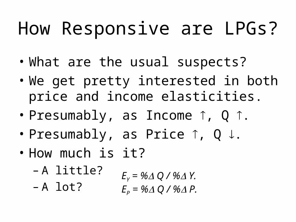
How Responsive are LPGs?

• What are the usual suspects?

• We get pretty interested in both price and income elasticities.

• Presumably, as Income , Q .• Presumably, as Price , Q .• How much is it?

– A little?– A lot?

EY = % Q / % Y.EP = % Q / % P.

Tiebout Model• Assumptions

– Jurisdictional Choice -- Households shop for what local governments provide.

– Information and Mobility -- Households have perfect information, and are perfectly mobile.

– No Jurisdictional Spillovers -- What is produced in Southfield doesn’t affect people in Oak Park.

– Community size – City manager seeks to reach average minimum cost of producing goods.

– Head Taxes -- Pay for things with a tax per person.

• We get an equilibrium. People’s preferences are satisfied.

Eq’m occurs when people stop moving!

What happens if people keep movingFrom Community 1 to Community 2?

Plethora of Studies

• If you do a citation search, you will find that this article was like Helen of Troy, the face that launched 1000 ships.

• All kinds of follow-ups. – Was this really what Tiebout

meant?– Was the econometrics right?– Did this work at the individual house

level, as opposed to the community level?

Instability

• Tax financing generates inherent instability.

• Need not be solely property tax. Happens with any tax other than a pure benefit tax or a head (per/person) tax.

• Incentive for one family to move to take advantage of fiscal surplus will lead other (or all) families to move.

Baumol’s Cost Hypothesis

• Consider two sectors. He calls them– Progressive – subject to productivity

improvements.– Traditional – Generally more labor intensive

and not subject to productivity improvements.

• What happens?

10

Degrees of Public and Private Involvement

Case Choice Financing Production Example1 Public Public Public Police

2 Public Public Private Trash

3 Public Private PrivateSidewalks

4 Private Private Private Private Goods

Privatization

• Definition: Transfer production of government services to private firms.

Degrees of Public and Private Involvement

Case Choice Financing Production Example1 Public Public Public Police

2 Public Public Private Trash

3 Public Private PrivateSidewalks

4 Private Private Private Private Goods

Think of some of your own examples!

Think of some of your own examples!

Impacts of Grants – General v. Matching

• Suppose, instead, you were given a matching grant, where every $ you raised would be matched with a $ from the government.

• Slope is now -0.5. Why?

Education

All Other

Slope = -0.5, why?

E1

A1• Leads to much more E and relatively less A.

E2

A2

E3

Fungibility

• P. 211 has a good example.

• You have a budget of $30 per week for entertainment. You spend:– $10 on Pizza– $10 on Movies– $10 on Pepsi

• Your parents come to visit and give you a $20 gift certificate to Pizza Hut.

Taxes and Efficiency

• Excise Tax– Tax on a particular

good.– Look at a unit (as

oppose to percentage) tax.

• $1 Tax Collected on DEMANDERS

$

Q

D S

Q0

P0

What’s DW$

P1

Q1

Prod.

Con.DW

$1

3.0

Proposal A in MichiganProposal A Spreadsheet

Tax RateRate 1.5%

Value % CPI Taxable Effective Taxes on MobilityYear Value Increase Inflation Value Taxes Rate Value Tax

1994 200,000 200,000 3,000 1.50% 3,000 01995 220,000 10.0% 2.5% 205,017 3,075 1.40% 3,300 2251996 240,000 9.1% 2.8% 210,808 3,162 1.32% 3,600 4381997 255,000 6.3% 2.9% 216,992 3,255 1.28% 3,825 5701998 265,000 3.9% 2.2% 221,766 3,326 1.26% 3,975 6491999 275,000 3.8% 1.3% 224,704 3,371 1.23% 4,125 7542000 290,000 5.5% 2.2% 229,723 3,446 1.19% 4,350 9042001 300,000 3.4% 3.5% 237,686 3,565 1.19% 4,500 9352002 320,000 6.7% 2.7% 244,183 3,663 1.14% 4,800 1,1372003 360,000 12.5% 1.4% 247,581 3,714 1.03% 5,400 1,6862004 400,000 11.1% 2.2% 253,131 3,797 0.95% 6,000 2,2032005 420,000 5.0% 2.6% 259,713 3,896 0.93% 6,300 2,4042006 420,000 0.0% 3.5% 268,868 4,033 0.96% 6,300 2,2672007 400,000 -4.8% 3.2% 277,516 4,163 1.04% 6,000 1,8372008 375,000 -6.3% 2.9% 285,472 4,282 1.14% 5,625 1,343

15

Property tax … what do we have?

• The tax differentials between jurisdictions function as excise taxes (if there is a “national” property tax of 2%, then a jurisdiction w/ taxes of 3% will incur excise tax effects).

• The overall weighted property tax functions as a national tax on capital and land.

Is Property Tax Progressive, Regressive?

• This has long been debated.

• The “traditional” view was the property tax as an excise tax.

• If so, it is passed forward to the purchasers of the goods that are produced.

• If this is the case, it might be thought to be regressive. Why?

Optimal Sales Tax Analysis• We could be more efficient if we could raise same revenue with

less DW loss.• How can we do that?• Raise tax on A so price ↑ by 1%. This leads revenue to ↑ by a

lot, and quantity to decrease by a little so DW ↑ by a little. • Reduce tax on B (more than 1% - why?) to make revenue

constant and it decreases DWB by more than DWA increased.

Good A

$

Good B

Price B

1 1

DA

DB

RA RB DWB

CS loss ↑

CS loss ↓

Rb’

1+t + tA

1+t - tB

18

Is it a prisoner’s dilemma

• Do we give 50% tax abatement?

• In boxes we have total expected tax receipts for the municipalities.

No Yes

No

Yes

TS = 2MTW = 2M

TS = 2.5MTW = 0.5M

Warren

TS = 1MTW = 1M

TS = 0.5MTW = 2.5M

Southfield

Elasticities

• Elasticity of intermetropolitan business activity (A) with respect to local tax [(A/A)/ (t/t)] varies between -0.1, and -0.6.

• Elasticity of intrametropolitan business activity with respect to local tax varies between -1.0, and -3.0.

• Why are they so different?

A Little!

A Lot!!

GTB Formula (and worksheet)Consider a formula of the type:

Gi = B + (V* - Vi) Ri, where:

Gi = 0 + ($200,000 – $50,000) ($40/$1,000), where:

Gi = grantB = Basic or Foundation GrantV* = Guaranteed per-pupil tax baseVi = Per pupil tax base in district i.Ri = Tax rate per thousand dollars in district i.

Gi = $6000; own effort = $2000

If you raise R by $1 in your district, it is raised by (V* - V)/V times; Here (200 – 50)/50. So a $1 tax gets a $3 match.Implicit tax price = 1/(1+3) or 25%. Let’s look at spreadsheet.

What’s the most cost-effective place?

• Thought experiment. Most cost effective place is where we get the highest mean score. Why?

10

10

30

20

Ed

Harry

45o

• We can draw a line with a slope of –1. This line gives us places with equal totals. Start with S = SE + SH = 10.

SE+SH=10

SE+SH=20

SE+SH= max

Mean = (0+10)/2 = 5

Mean = (8+8)/2 = 8

Mean = (20+0)/2 = 10

Highest mean!

Labor Migration

wage

Labor force

Demand SupplyMichigan

Labor force

Demand SupplyElsewhere

LM

wM

LE

wE

wM > wE.

This implies that people will move from E to M

23

Transportation System

• Our roads – they suck.

• Why?– We don’t spend enough– We abuse them

• We allow VERY heavy trucks• We under-fund them

– Weight isn’t the only thing – Contrast a heavy oriental carpet with 4 inch high heeled shoes.

We talked aboutthis a little bit

before

24

“Take-up” and “Crowd-out”

• What are the net impacts of social insurance program implementation?

• Are people who are now insured, previously uninsured (take-up), or are the new programs simply crowding out other forms of insurance?

Year RateRank (1 is highest)

Per Capita Taxes Paid to

Own State

Per Capita Taxes Paid to Other States

Total State and

Local Per

Capita Per Capita

Income RatePer Capita

Income

1977 10.0% 27 $573 $240 $813 $8,117 10.3% $7,787

1980 9.8% 14 $750 $285 $1,034 $10,605 9.5% $10,431

1985 10.3% 8 $1,137 $417 $1,554 $15,154 9.7% $15,349

1990 9.8% 23 $1,395 $553 $1,948 $19,860 9.9% $20,465

1995 9.6% 32 $1,709 $700 $2,409 $25,057 10.2% $24,587

2000 9.4% 24 $2,219 $805 $3,024 $32,300 9.5% $32,707

2001 9.3% 25 $2,243 $820 $3,062 $32,776 9.5% $33,725

2002 9.3% 23 $2,176 $854 $3,030 $32,432 9.5% $33,172

2003 9.6% 22 $2,292 $872 $3,164 $33,126 9.7% $33,644

2004 9.6% 24 $2,358 $919 $3,278 $34,273 9.8% $35,576

2005 9.7% 24 $2,466 $995 $3,461 $35,860 9.8% $38,206

2006 9.6% 27 $2,466 $1,130 $3,596 $37,264 9.9% $40,643

2007 9.5% 28 $2,489 $1,162 $3,651 $38,427 9.9% $42,817

2008 9.4% 27 $2,536 $1,158 $3,694 $39,273 9.7% $44,254Source: Tax Foundation calculations based on data from the Bureau of Economic Analysis, the Census Bureau, the Council on State Taxation, the Travel Industry Association, Department of Energy, and others.

Michigan State-Local Tax Burden Compared to U.S. Average

1977-2008

State U.S. Average

… and remember

Good Luck