Joint Defra/EA Flood and Coastal ErosionRisk Management R&D Programme

Review and formalisation ofgeomorphological concepts andapproaches for estuaries R&D Technical Report FD2116/TR2

PB11207-CVR.qxd 1/9/05 11:42 AM Page 1

Defra / Environment Agency Flood and Coastal Defence R&D Programme Review and formalisation of geomorphological concepts and approaches for estuaries R&D Technical Report FD2116/TR2 December 2006 Authors: HR Wallingford ABPmer Professor J Pethick

- xii -

Figure 10.4 Velocity variations downstream calculated for the channel widths shown in Figure 10.1 132

Figure 10.5 Holocene infilling of the Humber basin (from ABPmer, 2004b) 139

Figure 11.1 Inlet cross-sectional area related to tidal prism, for tidal inlets in the UK, USA, Japan and China 195

Figure 11.2 Relationships between inlet cross-secitonal area at mid-tide and mean spring tidal prism for eight groups of estuary inlets on the New Zealand coast 196

Figure 11.3 Prism-area data for UK estuaries by estuary type, from Townend (2005) 197

Figure 11.4 Observed and predicted evolution of the Frisian inlet following basin closure, after van de Kreeke (1992) 197

Figure 11.5 Escoffier’s diagram, after van de Kreeke (1992) 198

Figure 11.6 Uncertainty in the Regime relationship 198

Figure 11.7 The Lune training walls (after Inglis and Kestner, 1958) 199

Figure 11.8 Summary of method used for long-term prediction 199

Figure 11.9 Tollesbury Creek and flow model cross-sections 200

Figure 12.1 Variation in energy flux, and difference from most probable distribution 220

Figure 12.2 Influence of boundaries on most probable distribution 221

Figure 12.3 Variation in energy flux in the Bristol Channel 222

Figure 12.4 Variation in energy flux taking account of internal constraint 223

Figure 12.5 Variation in energy flux for tide only, river only and river & tide on the Humber 225

Figure 12.6 Energy flux as a result of different forcing conditions 227

Figure 12.7 Historical variation for the Humber Estuary 228

Figure 12.8 Difference from most probable state for the Humber Estuary as a whole 229

Figure 12.9 Influence of various large-scale interventions on the Humber Estuary 230

Figure 12.10 Difference in the total work done (for whole estuary) from theoretical most probable (%) for a range of cases (Townend & Pethick, 2002) 231

Figure 13.1 The Stour and Orwell Estuaries 248

Figure 14.1 Friedrichs and Aubreys schematisation 253

Figure 15.1 The Skeffling intertidal profile. Reproduced from Black and Paterson (1998) in Geological Society Special Publication 139, with permission 289

Figure 15.2 Comparison between measured and modelled mudflat profile at Skeffling (from Roberts et al, 2000, Continental Shelf Research, Pergamon) 290

- xiii -

Figure 15.3 Variation in modelled intertidal profile with tidal range (Whitehouse and Roberts, 1999) 291

Figure 15.4 Variation in modelled intertidal profile with sediment concentration at boundary (Whitehouse and Roberts, 1999) 291

Figure 15.5 Effect of wave action on the modelled profile (Whitehouse and Roberts, 1999) 292

Figure 15.6 Hindcast prediction of intertidal response using Mudpack model (from Pethick, 2002, produced for the Environment Agency) 295

Figure 15.7 Predictions of 50 year evolution of the intertidal at Wrangle Flats in the Wash, showing the influence of sea level rise on future morphological response (data from Pethick, 2002) 296

Boxes Box 4.1 Identification of key mechanisms for Poole Harbour 30

Box 4.2 Building confidence in model results 34

Box 5.1 Summary of approach to data 39

Box 5.2 What data might be available? 41

Box 5.3 Example of effect of maintenance dredging and disposal on upstream intertidal areas 44

Box 5.4 Example of effect of error in current data on estimate of future morphological change 44

Box 5.5 Effect of survey error on estimate of future morphological change 45

Box 7.1 Example application procedure for HTA using bathymetric data 70

Box 12.1 Example of energy transfer between states 203

Box 12.2 Some useful definitions 205

Box 15.1 Summary of conditions experienced by mudflats in three UK estuaries 276

Box 15.2 Example estimations of current speeds 277

Plates Plate 15.1 The mudflats at Skeffling on the Spurn Bight, Humber Estuary 289

Appendices Appendix 1 Langbein’s proof of estuary regime theory on the basis of entropy 310

Appendix 2 Regime Theory as sediment transport (Sandy estuary) 314

Appendix 3 Regime Theory as sediment transport (Muddy estuary) 319

Appendix 4 Second order solution to the strongly convergent 1D equations 325

- 1 -

PART 1 – INTRODUCTION

The Exe Estuary, Devon (Photograph copyright Environment Agency)

- 2 -

- 3 -

1. BACKGROUND TO THE RESEARCH This report presents the results of research project FD2116 on the review and formalisation of geomorphological concepts and approaches in estuaries. The project was undertaken as part of Phase 2 of the Estuaries Research Programme (ERP). This research study forms one of three contracts instigated under ERP Phase 2. The other Phase 2 studies are FD2107: Development of Estuary Hybrid Morphological Models and FD2117: Development and Demonstration of Systems Based Estuary Simulators. The Estuaries Research Programme is part of an agreed programme of scientific research developed and funded within the joint Defra/Environment Agency Modelling and Risk Theme. There are three phases to the ERP:

• Phase 1 evaluated existing morphological modelling approaches. This was completed in 2000 and delivered the first version of an Estuary Impact Assessment System (EIAS) (EMPHASYS, 2000a and 2000b);

• Phase 2 includes the three projects described in the opening paragraph with the purpose of developing the most promising approaches examined in Phase 1; and,

• It is anticipated that Phase 3 will seek to incorporate prior ERP research into an updated EIAS and deliver an integrated Estuary Management System.

1.1 Research Objectives The main objectives of the FD2116 study were:

• To review critically the current geomorphological understanding and concepts related to the medium (years to decades) to long term (decades to centuries) behaviour of estuaries; and,

• Through formalisation of Expert Geomorphological Assessment and Historical Trend Analysis, to provide a resource for the end user so that s/he can substantially increase the quality of their analysis.

The benefits arising from this project are that a consistent and formalised approach to the use of geomorphology in estuarine prediction has been established. This has been achieved by an intensive assessment of the methods, their scientific background and their applicability in solving estuary problems. The results will inform the quality and effectiveness of studies associated with estuarine morphology, whether related to flood defence or estuarine impact. Additionally this project has sought opportunities to support, link and integrate with the Modelling and Risk Theme projects FD21071 and FD21172 . In particular the results are expected to directly contribute to the development of the hybrid model envisaged in FD2107 and to the development of the estuary simulator which is the focus of FD2117. Relevant work on hydrobiosedimentary (hydraulic + biological + sediment transport) processes in estuaries has been completed recently as part of ERP Phase 23. 1 Defra project FD2107 Development of estuary morphological models led by Proudman Oceanographic Laboratory. 2 Defra project FD2117 Development and demonstration of system based estuary simulators led by ABPmer. 3 Defra project FD1905 Estuary Process Research Project (EstProc) led by HR Wallingford (reports available from www.estproc.net as well as www.defra.gov.uk )

- 4 -

1.2 Report structure Chapter 2 describes the purpose and scope of the study and Chapter 3 provides an introduction to estuary types. The remainder of the report then comprises fourteen further chapters subdivided into two further parts: Part 2 – Framework for assessment of estuary geomorphology – comprises a framework for Expert Geomorphological Assessment which is presented and discussed in Chapter 3. Issues surrounding data are examined in Chapter 4. Part 2 of the report is intended to provide the reader with the context in which Part 3 of the report can be read. In Part 3 – Geomorphological tools and methods is first presented an introduction to the geomorphological tools examined within the study (Chapter 5). Chapters 6 to 14 discuss and critique the methods and tools themselves. Part 3 of the report, by its nature of being a technical document, contains a lot of detailed description and assessment of the methods and tools. This means the report may be “heavy going” in places. These sections are included for the technical reader but are accompanied by sections on guidance which are less technically explicit. Finally, recommendations for further study are presented in Chapter 15 and Chapter 16 contains a Bibliography, whilst Chapter 17 lists the index of case studies and examples. 1.3 References EMPHASYS (2000a) A guide to prediction of morphological change within estuarine systems, Version 1B, produced by the EMPHASYS consortium for MAFF project FD1401, Estuaries Research Programme, Phase 1, December 2000. Report TR 114, HR Wallingford. Download from http://www.hrwallingford.co.uk/projects/ERP/index.html as well as www.defra.gov.uk EMPHASYS (2000b) Modelling Estuary Morphology and Process, produced by the EMPHASYS consortium for MAFF project FD1401, Estuaries Research Programme, Phase 1, December 2000. Report TR 111, HR Wallingford. Download from http://www.hrwallingford.co.uk/projects/ERP/index.html as well as www.defra.gov.uk 1.4 Acknowledgements The authors (Nick Cooper, John Pethick, Jeremy Spearman, Ian Townend and Richard Whitehouse) acknowledge the assistance of their colleagues and Dan Fox during the preparation of this report. Andy Parsons and Marcel Stive provided peer review comments which helped improve an earlier draft.

- 5 -

2. PURPOSE AND SCOPE 2.1 Purpose One of the over-riding aims of the Estuaries Research Programme (ERP) is to meet the needs of users and managers through the provision of appropriate technical and decision-support tools (French et al, 2002). Townend (2002) observed that this does not merely mean the provision of new tools but the translation of model outputs and the interpretation of data into information that can inform the decision-making process. Though much of the ERP is targeted towards development of new tools a need was identified to bridge the gap between current scientific understanding of the applicability of the presently available geomorphological tools and the practical needs of estuary managers. In particular the need to strengthen and formalise the use of “top-down” modelling approaches and concepts currently used in Expert Geomorphological Analysis and Historical Trend Analysis was highlighted in EMPHASYS (2000a) and re-iterated by French et al (2002) as a core project in the Research and Development Plan. It should be remembered that “top-down” methods are just one of a whole suite of methods available – as is discussed in Section 2.3 below. 2.2 Continuity of research The research described in this report follows a strand of continuity from the consistent approach taken in the Estuaries Research Programme Phase 1B Guide (EMPHASYS, 2000b) produced by the EMPHASYS consortium (led by HR Wallingford and including ABPmer and John Pethick) and by HR Wallingford in the Phase 2 Uptake Project (FD2110). The output from both these projects highlighted the benefits of a rigorous approach to the use of data and modelling techniques and the need for careful construction of a robust conceptual model. The research approach developed by the project team extends this rigorous scientific approach within the Defra Modelling and Risk Theme. Phase 1 of the Estuaries Research Programme benchmarked the current level of understanding and capabilities for predicting morphological change in estuaries. A range of tools and models were applied during the project (top-down, hybrid and bottom-up models) and the performance assessed against common datasets. The research recommendations delivered by Phase 1 of the Estuaries Research Programme included a recommendation to strengthen and formalise the use of top down modelling approaches and concepts currently used in Expert Geomorphological Analysis and Historical Trend Analysis. This same recommendation was highlighted in the Estuaries Research Programme Phase 2 Research Plan as a core project. The programme of research undertaken has delivered a rigorous approach to Expert Geomorphological Analysis and Historical Trend Analysis which should lead to improvements in the quality and effectiveness of morphological studies associated with flood defence and estuarine impact.

- 6 -

2.3 Definitions Expert Geomorphological Analysis (EGA) is a term attributed by the authors to Pye and Van der Waal (2000) who coined it for the Estuaries Phase 1B Uptake project to describe those activities undertaken in geomorphological assessment which were not directly associated with either numerical or physical modelling or field measurement, i.e. assessment activities concerning top-down concepts and background experience in both an estuary system and the discipline of geomorphology. In practice EGA is an imprecise term because it can be applied to geomorphological assessment undertaken without accompanying modelling/field studies but also to activities that take place within modelling/field studies as a pre-cursor to, or overall framework for, such modelling and fieldwork. EGA encompasses the use of Historical Trend Analysis and other geomorphological tools but also uses knowledge and/or modelling of estuarine process, usually physical but also chemical and biological, to establish an understanding of the underlying functioning of the system. This understanding is then used as the basis for predicting quantitatively or qualitatively the impacts of natural or anthropogenic change using the relevant geomorphological tools. Historical Trend Analysis (HTA) is a geomorphological tool involving the analysis of time series data to identify trends and features in estuarine process and/or evolution. HTA can be used for all types of data (e.g. tidal levels, wind or wave records) but more frequently is used to evaluate the past and current trends in morphology. The use of HTA is explored further in Chapter 6 of the present report. EGA and HTA can be summarised as the analysis and application of data together with a knowledge of estuarine processes and specific geomorphological tools blended by experience. The basis of the processes and techniques are often well known but can be misapplied if the methodology is not clear, if the range of applicability of the technique is exceeded, or if there are shortcomings with the data which the technique requires. Furthermore, the assessment of uncertainty in prediction, a vital part of evaluating risk in estuary management, is frequently lacking from EGA studies. Experience plays an important role in allowing the investigator to reduce the risk of misapplication of EGA techniques, but the end user is not always aware that they are benefiting from this attribute. The formalisation of the process as described in this report has led to a clear framework which provides the end user with the opportunity to appreciate and realise such benefits. Available tools: There is a range of tools available to investigate estuary process and morphology, as described for example in EMPHASYS (2000b). These tools can be generally divided into two types of approach: (1) “bottom-up” or process-based approaches and (2) “top-down” or systems approaches. The “bottom-up” approaches employ models which are based on a representation of physical principles (processes) and give short-term predictions of morphological change. The credibility of these types of approach is increased with calibration and validation using appropriate site specific measurements of relevant processes. The value of bottom-up models is the explicit representation of hydrodynamic and sediment transport processes, leading to morphological change, within the system. However, the long-term predictive capacity of these methods is not always sound as numerical errors can accumulate with long model run times. Methods to improve the application of

- 7 -

process-based models to medium to long term morphological prediction have been investigated in the Defra funded EstProc project (EstProc Consortium, 2006). The “top-down” approaches employ models which do not in general predict the sediment transport process directly to reach a prediction of morphology. Instead they take more general conceptual or systems based approaches to determining the relationship between forcing variables and the resulting characteristic morphology; a good example is the regime type approach (Chapter 11) which is based on empirical correlations between a measure of the capacity of the system to move sediment (e.g. tidal prism) and a characteristic feature such as cross-section area at the mouth of the estuary. However, whilst there are many features of top-down models which make them attractive for examining the state and response of a particular estuary morphology, the conceptual nature of the methods means they are more appropriate usually for general rather than detailed assessments. Results from both bottom-up and top-down approaches require careful analysis, validation and expert interpretation. There is a third category of methods, the so called “hybrid” approach. These methods are based on the combined use of “bottom up” and “top down” techniques. The bottom-up component provides an understanding of forcing processes and the top-down component provides information on the system state and how that wants to change as the forcing is changed. The majority of the methods presented in this report are of the top-down type. Some of them are used in a hybrid way to provide predictive capability. 2.4 Scope In order to fulfil the overall objectives (Section 1.2) this study has focused upon developing a rigorous methodology for undertaking estuary morphological assessments involving Expert Geomorphological Analysis. This has involved defining more clearly the procedure which such assessments should follow and examining in detail the applicability of the available models/tools which such assessments currently can deploy. This study does not attempt to be exhaustive on the subject of estuary geomorphology itself. There are many resources dealing with this topic and some of them are listed in the bibliography given in Chapter 17. The scope of the present study can be summarised as follows: 1. To provide a framework for Expert Geomorphological Assessment (EGA) and in

particular for the systematic development of the conceptual models of estuarine systems in geomorphological studies and their use as a basis for prediction. This has been done in Chapter 4.

2. To review the use and application of data used in EGA. This has been done in Chapter 5.

3. To review critically, and produce guidance in, the use and application of assessment tools that may be considered for use in EGA. This has been done in Chapters 6 to 15. The critique includes the tools listed below which have been selected from the top-down methodologies investigated during the

- 8 -

Estuaries Phase 1B Report “Modelling Estuary Morphology and Process” (EMPHASYS, 2000b and c).

• Historical Trend Analysis (Chapter 7) • Sediment budget modelling (Chapter 8) • Rollover model (Chapter 9) • Geological methods for estuarine studies (Chapter 10) • Regime theory (Chapter 11) • Entropy-based relationships (Chapter 12) • Asymmetry relationships (Chapter 13) • Analytical solutions (Chapter 14) • Intertidal form (Chapter 15)

4. To illustrate the application of the assessment tools using case studies. A full index of the examples of application of the tools listed above is given.

2.5 References EMPHASYS (2000a.) Recommendations for Phase 2 of the Estuaries Research Programme, produced by the EMPHASYS consortium for MAFF project FD1401, Estuaries Research Programme, Phase 1, December 2000. Report TR 113, HR Wallingford. Download from http://www.hrwallingford.co.uk/projects/ERP/index.html

EMPHASYS (2000b). A guide to prediction of morphological change within estuarine systems, Version 1B, produced by the EMPHASYS consortium for MAFF project FD1401, Estuaries Research Programme, Phase 1, December 2000. Report TR 114, HR Wallingford. Download from http://www.hrwallingford.co.uk/projects/ERP/index.html

EMPHASYS (2000c). Modelling Estuary Morphology and Process, produced by the EMPHASYS consortium for MAFF project FD1401, Estuaries Research Programme, Phase 1, December 2000. Report TR 111, HR Wallingford. Download from http://www.hrwallingford.co.uk/projects/ERP/index.html

EstProc Consortium (2006). Integrated Research Results on Hydrobiosedimentary Processes in Estuaries. Final Report of the Estuary Process Research Project (EstProc). R&D Technical Report prepared by the Estuary Process Consortium for the Defra and Environment Agency Joint Flood and Coastal Processes Theme. Report No FD1905/TR3 – Algorithms and Scientific Information. Download from www.estproc.net

French, J., Reeve, D. and Owen, M. (2002). Estuaries Research Programme, Phase 2 Research Plan FD2115, Report prepared for Defra and the Environment Agency, April 2002.

Pye, K. and Van Der Waal, D. (2000). Expert Geomorphological Assessment (EGA) as a tool for long-term morphological prediction in estuaries. Paper 15 in EMPHASYS (2000c).

Townend, I. (2002). Marine Science for strategic planning and management: The requirement for estuaries. Journal of Marine Policy, 26(3), 209 – 219.

- 9 -

3. AN INTRODUCTION TO ESTUARIES 3.1 Introduction The UK has a particularly large number of estuaries (in excess of a hundred). Indeed, more than a quarter of northwestern European estuaries (by area) occurs in the UK. One of the most well known definitions of an estuary is by Pritchard (1952) who defines an estuary as “a semi-enclosed body of water which has a free connection to the open sea and within which seawater is measurably diluted by fresh water derived from land drainage”. However this definition lacks a reference to tidal action. Though it is possible for rivers to flow into a non-tidal sea, such systems are usually not referred to as estuaries. For this reason we will use the following definition of an estuary as “the downstream part of a river valley, subject to the tide and extending from the limit of brackish water” (JNCC, 2001). 3.2 Different types of estuaries 3.3 Introduction A number of attempts have made over the years to classify estuaries into sub-groups. Any reader familiar with estuary classification will immediately recognise the difficulties inherent in trying to group together such complex and varied systems. Of the various methods of classification the most useful tend to be the simplest. There are two methods of classification of particular note. Both of these methods were proposed by Pritchard but are representative of a number of similar approaches:

• Classification by topography/geomorphology; and • Classification by salinity structure. 3.4 Classification by topography/geomorphology Pritchard (1952) classified estuaries into the following sub-groups:

• Coastal plain estuaries; • Bar-built estuaries; • Fjords; and, • Others. Coastal plain estuaries. These estuaries were formed when pre-existing river valleys were flooded at the end of the last ice age. They usually widen and deepen towards the mouth, giving a large width-to-depth ratio; their outline and cross-section is often triangular. Many systems have extensive sediment flats and saltmarsh throughout. Sediment type varies from mud in the upper reaches becoming increasing sandy towards the entrance. This is the main type of estuary, by area, in the UK (JNCC, 2001).

Thames Estuary. © HR Wallingford

- 10 -

Examples of coastal plain estuaries are the Thames Estuary, Southampton Water and the Mersey Estuary (Dyer, 1997).

Rias are one particular type of coastal plain estuary or drowned river valley (Pethick, 1984), sometimes included as a separate class their own (e.g. JNCC, 2001). They are characterised by a low sediment availability and a resulting rocky aspect. Rias in the UK are found mainly in SW England - for instance the Fal and the Tamar Estuaries.

Bar-built estuaries. These estuaries characteristically have a sediment bar across their mouths and are partially drowned river valleys that have subsequently been partially infilled with sediment (JNCC, 2001). These estuaries are generally shallow and often have extensive lagoons and shallow waterways near the mouth. In order for them to form the tidal range must be restricted and there must be large volumes of sediment available. The river flow is generally large and seasonally variable and can sweep the bar away during floods – only for the bar to re-establish when the flood subsides (Dyer, 1997). Estuaries with an extensive spit formation at the mouth would also come under this category, although a true barrier may never actually occur. The best examples of bar-built estuaries are generally found in tropical areas or areas with active coastal deposition. In the UK examples include the Exe (see cover photograph to Part 1), the Ore/Alde Estuaries in Suffolk or the Drigg Estuary which is fed by the Irt, Mite and Esk Rivers.

Fjords. Fjords were formed in areas covered by Pleistocene ice sheets. The pressure of the ice overdeepened and widened the pre-existing river valleys but left rock sills in places, particularly at the fjord mouths, which can be very shallow. Fjords have a small width-depth ratio, steep sides and an almost rectangular cross-section. They have rocky floors or very thin veneers of sediment. Their occurrence is restricted to high latitudes in mountainous areas and is restricted to certain lochs in Scotland in the UK.

Fal Estuary. © P.Channon

Teign Estuary © South West Water

Loch Etive. Photo reproduced with permission from www.fishing-argyll.co.uk

- 11 -

Others. These include estuaries that do not conveniently fit elsewhere, such as tectonically produced estuaries, estuaries formed by faulting, landslides and those formed by volcanic eruptions. There are few examples of this type of estuary in the UK. 3.4.1 Classification by salinity structure Pritchard (1955) classified estuaries into the following sub-groups: • Salt-wedge estuaries; • Fjord-type estuaries; • Partially mixed estuaries; and, • Well mixed estuaries. Salt-wedge estuaries. These estuaries are characterised by high fluvial flow and a small tidal range. Under these conditions mixing between seawater and freshwater is small. The freshwater, being less dense than saltwater, flows in a seaward direction over the saline layer beneath. Some of the lower saline layer is entrained into the upper fresh layer and the fluid lost is replaced by a residual landward flow in the saline layer (Dyer, 1997). There are no examples of salt-wedge estuaries in the UK. An example of a salt-wedge estuary is the Mississippi in the USA. Fjord-type estuaries. This type are similar to the salt wedge type except that fjords exhibit three layers instead of the two commonly associated with salt-wedge estuaries (Dyer, 1997). The freshwater flows seawards across the surface of the fjord with a saline layer beneath. This saline layer experiences a small amount of entrainment into the fresh layer setting up a landward residual. However underneath this saline layer is another even more saline layer, which, because it is lower than the sill of the estuary, experiences little movement and little mixing with the less saline layer above it. Renewal of this layer is so infrequent that anoxic conditions can develop near the bottom. As stated in Section 3.2.2 this type of estuary is limited to Scotland in the UK. Partially mixed estuaries. Partially mixed estuaries essentially represent a half-way house between well-mixed estuaries (see below) and salt-wedge estuaries (see above). The difference between the salt-wedge and partially-mixed estuaries is that the latter experiences larger tides and therefore much more mixing. The increased mixing results in a more saline surface layer and therefore, in order to discharge a similar volume of freshwater, the surface layer has to be correspondingly enhanced. Consequently a distinct two-layer residual flow is set up in the estuary known as gravitational flow (Dyer, 1997). UK examples of partially mixed estuaries are the Mersey Estuary, the Tees Estuary and Southampton Water.

Tees Estuary. © PD Teesport

- 12 -

Well-mixed estuaries. In this type of estuary the tidal range is larger and the fluvial flow smaller. As a consequence mixing is strong enough to mix saline and freshwater through the water depth. However, due to the horizontal salinity gradient there is still some small amount of gravitational circulation. If the estuary is wide enough there may also be lateral circulations, known as ebb and flood channels, set up as a response to the Coriolis force (Dyer, 1997). An example of the latter is the Firth of Forth.

3.5 Processes in Estuaries Estuaries are complicated systems and a description of all of the relevant processes is outside of the scope of this report. A list of relevant processes to be considered with respect to estuary geomorphology is given in Table 4.1. Furthermore, there are a number of very good books that are already available on this subject and these are listed in Section 17.1. The reader is pointed to these resources for a background knowledge of estuary processes. 3.6 References Dyer, K. R. (1997). Estuaries. A Physical Introduction. 2nd Edition. John Wiley and Sons, Chichester. JNCC. (2001). Natura: 2000 Marine Monitoring Handbook. Davies, J., Baxter, J., Bradley, M., Connor, D., Khan, J., Murray, E., Sanderson, W., Turnbull, C. and Vincent, M. (eds), Joint Nature Conservation Committee, http://www.jncc.gov.uk/PDF/MMH-mmh_0601.pdf Pethick, J. (1984). An Introduction to Coastal Geomorphology, Edward Arnold, London. Pritchard, D. W. (1952). Salinity distribution and circulation in the Chesapeake Bay Estuaries System, Journal of Marine Research, volume 11, pp106-123. Pritchard D W (1955) Estuarine Circulation Patterns, Proceedings of the American Society of Civil Engineering, volume 81, Number 717. A useful reference on tidal channels in (Dutch) tidal waters is Van Veen, J., Van der Spek, A.J.H.M., Stive, T.J. and Zitman, T. (2005). Ebb and flood channel systems in the Netherlands tidal waters. English translation of the original Dutch text with annotations, originally published in the Royal Dutch Geographic Society, Vol. 67 (1950), pp 303 – 325, published on behalf of Vereniging voor Studie-en Studentenbelangen to Delft, http://mail.vssd.nl/hlf/f015.pdf ISBN 90-407-2338-9.

Firth of Forth Estuary © Forth Estuary Forum

- 13 -

PART 2 – FRAMEWORK FOR ASSESSMENT OF ESTUARY GEOMORPHOLOGY

The mouth of the Teign Estuary, Devon (Photograph copyright South West Water)

- 14 -

- 15 -

4. A FRAMEWORK FOR EXPERT GEOMORPHOLOGICAL ASSESSMENT

4.1 Introduction In this Chapter a framework for Expert Geomorphological Assessment (EGA) is developed, and particular emphasis is placed upon the development a conceptual model of the system under investigation. The chapter initially defines the term geomorphology as used in this report (Section 4.2) and briefly summarises an overall framework for EGA (Section 4.3). The procedure involved in developing a conceptual model is outlined in Section 4.4 and explained in detail in Sections 4.5 to 4.11. 4.2 A definition of geomorphology as used in this report The study of Estuary Geomorphology4 can be applied to many different time-scales: • geological (millions of years) – geology of estuaries; • Holocene (thousands of years) – creation of estuaries as we know them; • anthropogenic history (in the UK, effectively since Roman times) – land

reclamation and the impact of agriculture; • near history (100-200 years) – written records of data, impacts of industry and of

major engineering schemes in estuaries such as dredging and training wall schemes; • decadal (post-war) – accurate data, impacts of dredging and port-development, salt-

marsh loss; and, • years – changes in estuary sub-systems, including mudflats and creek systems. Additionally many underlying physical processes within estuaries occur on much smaller time scales (seconds to a spring-neap cycle) and any investigation of these underlying processes will involve consideration of these smaller time-scales. For the case of studies supporting estuary management decisions the time-scales of interest relate to “engineering geomorphology”, i.e., years and decades, and exceptionally (in the case of very large schemes) a century. It is definitely true that the study of estuary morphology over the whole spectrum of time scales is helpful in understanding the behaviour of any particular system. However, the dominance of the shorter time scales in deciding management policy means that the emphasis in estuary geomorphological studies has to be towards engineering geomorphology. In this report, therefore, we apply ourselves mainly to engineering geomorphology. The exceptions to this occur where a knowledge of geological or historical geomorphology will aid the understanding of a system so as to improve the quality of the engineering geomorphology studies. Henceforth we will use the following terms to describe the temporal scale of estuary response:

4 In science morphology consists of the study of form and shape. In the context of estuary research “morphology” is commonly used as a noun relating to the form or bathymetry of an estuary, although the word can also relate to the study of such changes in form over time, hence “geomorphology” (EMPHASYS, 2000).

- 16 -

• Short – seconds, through spring-neap cycle to a few years; • Medium – a few years to a few decades; and, • Long term – a few decades to centuries. 4.3 An overall framework for geomorphological studies The EMPHASYS (2000) guide sets out a basic framework for prediction of morphological change within estuarine systems as does Townend (2002), and Dearnaley et al (2004), amongst others. Any impact assessment of a particular project in an estuary system will consist of a scoping exercise, analysis of the way the system works, prediction of impacts, and discussion with client and regulator about the conclusions of the study. This may lead to further clarification of the issues arising from the project, and additional work leading to refined conclusions and presentation of the study outcomes. The components of an impact assessment are summarised in Figure 4.1. The structure of Figure 4.1 is not definitive but is typical of the broad nature of estuarine studies to support estuary management. We will use Figure 4.1 as a representative template for estuarine studies, and briefly explain the different components presented in the figure. However, the emphasis in this report is on developing a framework for the second component in Figure 4.1 – that of conceptual model development. Scoping is where the objectives and methodology of the project are mapped out. This includes consideration of the potential effects resulting from a man made project or natural change on local or estuary-wide morphology, evaluation of the availability of and the potential requirement for new data, and the identification of the needs of the client and regulator. In practice this component overlaps with the next component, conceptual model development. The correct application of EGA is heavily dependent on an understanding of the system being studied, nowadays often referred to as a conceptual model. A correct understanding of the system will form the basis for the correct choice of predictive methods and will enhance confidence in the conclusions of the study. An incomplete or incorrectly focused conceptual model may lead to incorrect assumptions about the system, poor utilisation of predictive approaches and incorrect assessment of impact. An approach to developing a robust conceptual model is described in detail in Section 4.4.

- 17 -

Figure 4.1 Summary of stages in EGA studies The next component in the overall framework is the implementation of predictive assessment (prediction of impacts). If a plethora of model approaches are implemented then some formal synthesis of the different results will be required (synthesis of impacts). New insights may lead to an adjustment of the conceptual model and further predictive assessment. The initial conclusions arising from the synthesis will be explored during discussions with the client and regulator and these discussions may lead to some clarification of the issues and the requirement for further predictive work may be highlighted. Finally, when all the outstanding issues have been addressed the final conclusions of the assessment can be formally presented (presentation). From the viewpoint of requirements for shoreline management in some cases the estuary needs to be considered in the context of the adjoining coastline. A range of parameters, methods and features need to be considered when assessing the scale of physical interaction between the estuary and the coastline (Pontee and Cooper, 2005).

Initial Conclusions

• Identification of key mechanisms • Data collection and analysis • Model Testing • Synthesis

• Study definition • Appraisal of existing data

Prediction of impacts

Discussions with client

and regulator

Final Conclusions

Presentation

• Clarification of issues • Examination of alternative

scenarios • Studies associated with

mitigation or compensation

Synthesis of impacts

Scoping

Conceptual model development

• Revision of conceptual model

- 18 -

4.4 A framework for development of the conceptual model 4.4.1 Introduction This section presents a framework for development of a conceptual model of the estuarine system being studied. This particular aspect of the assessment framework described in Section 4.3 above is typically least well described and understood. The chapter builds on, and refines, previous frameworks presented in EMPHASYS (2000) and Townend (2002). The framework is not restricted to EGA studies in particular but is valid for all estuary studies to support management decisions. To begin with the conceptual model will be defined:

A conceptual model is a formal explanation of how the system (or sub-system) functions, including the key controlling mechanisms and their relative importance, of the reasons for the historical development (if relevant over the defined model area and time-scale) of the system (or sub-system) and of the reasons for present trends within the system (or sub-system).

The conceptual model can be expressed, depending on the system, through bottom-up or top-down considerations. However, whatever basis the understanding of the system is derived from, it should be demonstrated how this conclusion is supported by physical processes – i.e. the effect of currents, waves, etc, in forming sediment pathways, sources and sinks in the system. Particular attention should be given to whether the supply of sediment to the system is sufficiently large/small to accommodate the conclusions regarding long term trends. The definition of the conceptual model presented above is deliberately limited to an understanding of the system (or sub-system) which is relevant to the spatial and time scales of the defined problem. Within the context of most EGA studies there is a specific set of management decisions to be addressed and the development of the conceptual model should be targeted towards providing a basis for informing these management decisions. If the study area is, for instance, a specific mudflat then the conceptual model may not have to consider the estuary-wide components and long-term (centuries) evolution of the system. On the other hand if the management options includes, for instance, construction of a barrage across a large estuary the conceptual model will have to include the long-term evolution of the system, the estuary wide functioning of the system and most probably the functioning of the offshore area just outside the estuary. The development of the conceptual model to a particular estuary system (or sub-system) is an iterative process. As studies continue more information about the system is developed and the conceptual model is improved. Formally, however, the stages of the development are as outlined in Figure 4.2.

- 19 -

Figure 4.2 Summary of stages of development of conceptual model discussed in this chapter

• Identify possible sediment pathways, sinks and sources

• Identify possible controlling geomorphological concepts and features

• Collation and analysis of existing available data

• Site visit

• Identify key sediment pathways, sinks and sources and their significance based on available data

• Identify key controlling geomorphological concepts and features and their significance based on available data

• Make initial choice of models • Identify objectives for fieldwork

Project definition

Identify potential sediment transport mechanisms

Scoping

Appraisal of existing data

• Fieldwork • Analysis of new data • Refine list and significance of key mechanisms

based on new data

Data collection and analysis

• Finalise choice of models • Model set up, validation and calibration • Sensitivity analysis

Conceptualsynthesis

• Interpretation of computational model results and data

• Identify key mechanisms and concepts and their relative significance

• Underpin conceptual model with process • Define and present conceptual model

Computational model testing

• Exhaustive review of historical data Review of historical data

Additional fieldwork required? Yes

Computational modelling required? Yes

No

No

• What are the clients requirements? • Identify regulator(s) concerns • Define study objectives • Define resources for study • Define study area and timescale

Refin

e co

ncep

tual

mod

el

Refin

emen

t of s

cope

l

dl

- 20 -

Each of the stages highlighted in Figure 4.2 are discussed in turn below. 4.5 Project definition 4.5.1 What are the client’s requirements? It is important to understand that (ignoring studies for the pure purpose of research) in the context of estuarine systems a geomorphological study is carried out in order to provide sufficient information to the assessment process (e.g. EIA – Environmental Impact Assessment, SEA – Strategic Environmental Assessment, Appropriate Assessment) upon which a management decision (by the client and/or regulator) can be made. The purpose of the study is therefore to provide the information for making this decision and, if possible, to give some idea of the reliability of this information (which then can be translated into the risks involved with the management decision). From the client/regulator point of view it matters not only how good the data provided is, how well the bottom-up and top-down methods are applied and how good the conceptual model of the system is, but most importantly if a sound basis for a management decision is not provided, the assessment has not done its job. The word “sound” is underlined to make an additional point. The approach to providing a basis for the management decision presented in the assessment must be able to stand up to the rigours of scrutiny both from a scientific (is it robust?) and from a communicable (will third parties have confidence in the explanation?) point of view. 4.5.2 Identify regulators concerns There are a number of potential issues that are of particular significance to the regulator(s) because of the present legislative framework. Those most commonly experienced in estuary impact studies are: • Impacts on designated features (EN, RSPB, EA, CCW, EH, SNH, EHS); • Disposal of sediment (Licensing controlled by Defra – advised by CEFAS - EN,

CCW, SNH, EHS); • Impacts on navigation (Port and Harbour Authorities); • Impacts on fishing and fisheries (Defra, EA, CCW, SFC); • Impacts on flood defences (EA, SEPA); • Impacts on Shellfish Waters (EA, CCW); and, • Impacts on Water Quality (EA, CCW). Key: EN - English Nature, RSPB - Royal Society for the Protection of Birds, EA - Environment Agency, CCW - Countryside Council for Wales, EH - English Heritage, SNH - Scottish Natural Heritage, EHS - Environment and Heritage Service (Northern Ireland), Defra - Department for Environment, Food and Rural Affairs, SFC - Sea Fisheries Committees, SEPA - Scottish Environmental Protection Agency. If any of these issues arise the sensitivity and political aspects of the project will be heightened, there will need to be more liaison between the investigator, the relevant regulators and the client, and there will be a higher level of scrutiny of the results. The resources and time necessary for successful project completion will therefore increase and both the client and the investigator need to be aware of this from the onset. For this

- 21 -

reason, the geomorphological investigator must have good comprehension (or access to expertise) of the regulatory issues which will need to be addressed in the geomorphological study. It is important to realise that as the understanding of the estuary system is developed and predictive assessment undertaken some issues highlighted initially as potential concerns will be shown to be of little significance and other issues may be highlighted as major concerns. Continued liaison with the regulator at key points through the project is important to facilitate this understanding by all parties. 4.5.3 Define study objectives As a result of the considerations outlined above the objectives of the study are defined. 4.5.4 Define study area and time-scale The identification of the study area and timescales will be specific to the estuary and project definition. The defined study area chosen must include all areas that could potentially be affected by the project or management option under consideration. The defined spatial scales must be relevant to the morphological evolution observed in the current system (or sub-system) and any anticipated evolution resulting from a management option. The area and time-scale of focus will be influenced by the concerns and level of existing knowledge of geomorphological processes of the client/regulator. In some cases the client/regulator may have a particular concern, or as the studies progress additional issues can be identified requiring further consideration causing the study focus to expand. In other cases the client/regulator may have few concerns and the focus of the studies can be more limited in scope. 4.5.5 Define project resources Although common sense, this section underlines that the funding available from the client, and the internal resources of the investigator’s team, in terms of time and manpower, will affect the approach to the geomorphological studies chosen. 4.6 Appraisal of existing data 4.6.1 Identify possible sediment pathways, sinks and sources As a starting point a basic and initial assessment of the controlling mechanisms (and controlling geomorphological concepts – see Section 4.6.2) is made. This assessment is then refined as a result of the appraisal of the existing data and the site visit and further by the steps outlined in Section 4.7. The mechanisms for change within estuary systems can be summarised as either to do with: • Energy (currents, waves, etc); • Sediment (type and availability); or, • Anthropogenic (man-made) effects.

- 22 -

The consideration of how these will change is the basis of deriving the key mechanisms within a system. However, it is important to identify the key sediment transport mechanisms at a greater level of detail. The next step is therefore to crystallise these considerations in terms of the following sediment transport mechanisms: • Mechanisms that mobilise sediment; • Mechanisms that advect sediment; and, • Mechanisms that lead to deposition of sediment. The examination of these processes can take place on a number of levels of sophistication but in general it is likely that a background of estuarine processes is required. The reader is referred to the Bibilography in Chapter 17 which contains a short list of resources dealing with this topic if more information is required. Table 4.1 Potential mechanisms for mobilisation, advection and deposition Mobilising Mechanisms • Wave breaking • Wave stirring • Fluidisation of the bed • Fluid mud formation

from settlement • Erosion by currents • Pick up by wind • Fluvial input • Re-suspension by

dredging • Re-suspension by vessel

movements • Side slope subsidence • Biological effects leading

to disturbance or re-suspension of sediment

Advection Mechanisms • Tidal currents • Fluvial flow • Near bed flow • Secondary currents • Density currents • Wave-driven flow • Littoral drift • Wind driven flow • Meteorologically induced

flow • Vessel induced currents • Movement of fluid mud

and other near bed high concentration suspensions

• Mixing/dispersion of material in suspension

Sedimentation Mechanisms • Reduction of:

- wave breaking - wave-driven flow - wave stirring - tidal flows

• Interception of: - littoral drift - fluid mud - bed load - wind load - side slope subsidence

• Deposition from suspension

• Ecological stabilisation of sediments

At first identification of the key mechanisms will consist of highlighting the potential mechanisms that may be important. As the existing data is analysed, and as (and if) new field data is analysed and as (and if) modelling is undertaken the list of potential key mechanisms will be refined and their relative significance identified with more certainty. This process will require answers to the following questions: • What are the key morphological features and associated sediments in the system at

present? • Is there input of sediment to, and/or export of sediment from, the system (or sub-

system) that is being considered? • Where does the input of sediment come from (if at all)? • How is sediment exported (if at all)? • What are the reasons for the sources and sinks within the system (or sub-system)?

- 23 -

Identifying the key sediment transport mechanisms effectively defines the routes for sediment supply to and from the system (and parts within the system), which goes a long way to defining a conceptual model. The consideration of sediment supply is especially important as it will have a large effect on the potential direction and rate of any predicted morphological change. The potential list of mechanisms is large (Table 4.1). However this list can be rapidly reduced by applying back-of-the-envelope calculations or more in-depth analysis of available data. Further refinement to this list comes from the use of more numerate approaches during the conceptual synthesis phase (Section 4.11). The process of identifying key mechanisms – either bottom-up as here or top-down - relies heavily on a thorough examination of the historical data associated with morphological change. This means examination of historical charts, dredging and disposal records, etc. Failure to take this historical information into account could result in the identification of sediment transport mechanisms that are incorrect, leading to a weak or even flawed conceptual model. 4.6.2 Identify possible controlling geomorphological concepts As well as identifying the key process mechanisms there may be controlling top-down mechanisms which affect or describe the functioning of the estuary system. As above it is best to start with an “inclusive” list of mechanisms that might potentially be important and to discard the less relevant ones as more knowledge about the system is derived. This is likely to reduce the possibility of missing an important mechanism. The controlling concepts could include: • Net Sea Level Rise and anticipated response of estuary (e.g. as expressed by the

Rollover model in Chapter 9 of this report); • Sediment supply – quality and amount (e.g. as expressed by the sediment budget

modeling in Chapter 8 of this report); • Status of system with respect to equilibrium state (e.g. as determined from the

Regime method in Chapter 11 of this report); and, • The geological context of the estuary, its accommodation space (e.g. as determined

from the methods discussed in Chapter 10 of this report). 4.6.3 Collation and analysis of existing data An important part of the scoping process is an assessment of the abundance and quality of the data already available for the study. The results of this assessment will dictate whether there is a need for further data to be collected (to ensure the applicability of the geomorphological methods to be used) and will also influence the selection of models used, either to aid the development of the conceptual model or to predict impact. The assessment may also provide insights into the key controlling mechanisms or possibly provide an initial suggestion for the conceptual model. Failure to appraise the available data in detail may lead to one of the following problems:

- 24 -

• Over-confidence in the existing data leading either to erroneous conclusions (if the

data errors are not spotted early) or possibly having to re-negotiate the scope of the study with the client (if the data errors are discovered early on and additional field data has to be collected).

• Inefficient use of field data resources, including re-measurement to repeat already adequate data.

• Having to disprove or adopt an alternative perspective of the estuary system at a late stage in the project, reducing confidence in the overall project results.

4.6.4 Site visit A useful part of the process of collation of existing data is to undertake a site visit. This not only provides an invaluable visual perspective of the study area but may also provide an opportunity to meet managers, experts and end-users involved with the site. This can be a valuable source of information and can help to identify important concerns at an early stage. The visual inspection has three main purposes, besides being an opportunity for discussion with those who may have a view on the later acceptability of the study findings: • To confirm that there are no significant differences between the data provided and

reality (sometimes changes to the coastline have been implemented or there are important activities which have a bearing on the system and that are not documented);

• To provide an opportunity to spot geomorphological evidence which will aid the development of the conceptual model;

• To collect a small amount of field data (e.g. grab samples or even throwing oranges into the water) to aid the initial stages of conceptual model development.

The following key physical features should be looked for during a site visit: • Single channel – straight or meandering, narrow or wide, shallow or deep; • Multiple channel including shoals, banks or islands – ebb or flood channels; • Ebb or flood deltas; • Seawalls or other structures along the shoreline; • Structures on the intertidal or subtidal; • Beaches; • Sand dunes; • Mud and/or sand flats; • Saltmarsh – cliffing, erosion/deposition, pioneer marsh; • Intertidal areas – concave or convex – erosive or depositional; • Changes in sediment cover and substrate type – indicating erosion or deposition; • Large or small river flow; • Drainage channels on intertidal; • Tidal asymmetry; • Geological constriction;

- 25 -

• Littoral drift or bar at mouth; • Evidence for turbidity/turbidity maximum; • Salinity gradient – surface expression of fronts between water bodies; and, • Dredging/disposal or other anthropogenic activity. 4.6.5 Initial appraisal of need for new data At this stage it is possible to highlight the gaps in the available data and make some initial conclusions about what field data (if any) might need to be collected. These initial conclusions will be refined when the key mechanisms within the system are explored and the use of models for investigating the system and undertaking predictive assessment are considered. The subject of data is considered in more depth in Chapter 5. 4.7 Identify potential sediment transport 4.7.1 Identify key sediment pathways, sinks and sources and their significance

based on available data Having identified the possible sediment pathways sinks and sources in Section 4.6.1, the list of potential mechanisms needs to be narrowed down to the key mechanisms and their relative significance needs to be identified. The identification of the most important mechanisms will be based on the appraisal of existing data, the information gleaned from the site visit but may also benefit from additional analysis. One of the most helpful types of analysis in this respect is the so called “back-of-the-envelope” calculation. This type of calculation is a simple order of magnitude evaluation devised to identify which contributions to sediment transport are clearly larger than others. 4.7.2 Identify key controlling geomorphological concepts and features and

their significance based on available data This task is analogous to that described above in Section 4.6.2. However, as discussed in Section 4.10.2, any top-down concepts used in the conceptual model must be consistent with the observed bottom-up processes and key mechanisms. One of the most relevant steps for assessing the controlling geomorphological concepts and features is the exhaustive review of historical data (Section 4.8). This review may identify that certain processes (e.g. dredging or development) are so dominant that they dominate the evolution of the estuary or the review may reveal information about longer term changes which highlight a particular geomorphological concept. In a sense, therefore, the key controlling concepts will not be finalized until this is completed. 4.7.3 Initial choice of models The initial assessment of what models might be applied to aid the conceptual model development and predictive studies will be made on the criteria listed below. Once the models have been identified the planning of the field programme can be initiated (if relevant).

- 26 -

• Time and spatial scales of the cause of change (summarised in Table 4.2); • The nature of the key mechanisms identified (summarised in Table 4.3); • The availability of data; • The context of the specific question that the study is trying to address; and, All of these criteria need to be considered together. The suitability of the various top-down approaches together with hybrid and bottom-up approaches to different causes for change and different temporal and spatial scales is summarised in Table 4.2. In broad terms local changes and shorter time scales usually correspond to the use of bottom-up models while large-scale changes and longer time scales are more likely to require top-down methods to be considered. Note that the use of entropy methods tends to require flow model input (see Chapter 12) and so essentially can be thought of as a hybrid method. Regime Theory may also require flow model input to be utilised in a predictive manner but can also be used in a qualitative sense and so can be thought of as both top-down and hybrid. The problem can becomes more difficult if small changes to mechanisms which by their nature can be thought of as process-based, episodic and corresponding to very short time-scales dominate the long term evolution of the estuary system. This can occur for instance with wave activity under sea level rise. In such circumstances the application of a range of top-down/hybrid/bottom-up may be required to assess the resulting changes in morphology.

- 27 -

Table 4.2 Summary of generic models applicable to different causes of change Data Analysis Methods "Top down" Methods Hybrid

Methods

Cau

se o

f cha

nge

Spat

ial s

cale

Tem

pora

l Sca

le

Acc

omm

odat

ion

Spac

e

His

tori

cal T

rend

Ana

lysi

s

Sedi

men

t Bud

get A

naly

sis

Reg

ime

Rel

atio

nshi

ps

Ana

lytic

al m

etho

ds

Tid

al A

sym

met

ry A

naly

sis

Inte

rtid

al F

orm

Ana

lysi

s

Est

uary

Tra

nsla

tion

(rol

love

r)

Proc

ess B

ased

"B

otto

m u

p" M

etho

ds

Reg

ime

base

d

Ene

rgy/

Ent

ropy

bas

ed

Xt Lg x x x x x Freshwater Xt S/M x x Xt S/M x x

Tide Xt Lg x x x x x Xt Md x x

Sea level Xt Lg x x x x x x x x

External waves Xt S x x Xt M x x Xt Lg x x x Local waves Lc S x x Es S/M x Es Lg x x Sediment inputs Xt S x x x Xt M x x x Xt Lg x x x x x x

Lc Fx x x Barrage

Es Fx x x x x x x

Lc Fx x Barrier

Es Int x x x

Lc S x x x Deepening

Es M/Lg x x x x x x x x Lc M x

Fauna Es M x Lc M x

Flora Lc Lg Lc Fx x

Intake/outfall Es Fx x

Jetty or pier Lc Fx x Lc Fx x

Reclamation Es Fx x x x x x x Lc Fx x

Sea defences Es Fx x x x x x x Lc Fx x

Training works Es Fx x x x x Lc Fx x x

Managed realignment Es Fx x x x x x x x x x Lc S x x

Intertidal recharge Es S x x x x x x x

KEY: Spatial scale of action Time scale of action Local Lc Short-term (days to month) S Estuary Es Medium term (seasons to a decade) M External Xt Long-term (decades to a century) Lg Intermittent Int Fixed (in human terms) Fx

- 28 -

Table 4.3 Summary of generic models applicable to different key mechanisms Mobilising Mechanisms Mechanisms specifically requiring process models for investigation • Wave breaking • Wave-driven flow • Fluidisation of the bed • Fluid mud formation

from settlement • Pick up by wind • Re-suspension by

dredging • Re-suspension by vessel

movements • Side slope subsidence • Biological effects leading

to disturbance or re-suspension of sediment

Mechanisms which can be investigated using a range of techniques • Wave stirring • Erosion by currents • Sea level rise

Advection Mechanisms Mechanisms specifically requiring process models for investigation • Secondary currents • Wave-driven flow • Littoral drift • Wind driven flow • Meteorologically induced

flow • Vessel induced currents • Movement of fluid mud

and other near bed high concentration suspensions

Mechanisms which can be investigated using a range of techniques • Tidal currents • Fluvial flow • Sea level rise • Mixing/dispersion of

material in suspension • Density currents

Sedimentation Mechanisms Mechanisms specifically requiring process models for investigation • Reduction of:

- wave breaking - wave-driven flow

• Interception of: - fluid mud - wind load - side slope subsidence

• Ecological stabilisation of sediments

Mechanisms which can be investigated using a range of techniques • Reduction of:

- wave stirring - tidal flows

• Interception of littoral drift

• Deposition from suspension

• Sea level rise The suitability of models to describe different mechanisms is summarised in Table 4.3. In essence Table 4.3 repeats the analysis of Table 4.2 from a different perspective. In broad terms top-down methods can be applied where the nature of the underlying change is large scale and can be described by bulk estuary-wide or cross-section-wide parameters. Bottom-up methods are usually required where the underlying change has a local character. The availability of data is also important in the choice of models. In broad terms the less data available, the more relevant top-down methods become as bottom-up models generally require more data. However, after consideration of the issues in Tables 4.2 and 4.3 and the management questions needing to be answered, a lack of data may give rise to a decision to collect more data, rather than to restrict the study scope to top-down approaches. Lastly the context of the reasons for the study also affects the choice of models used. The set of models used must include models which will allow assessment of the impacts of estuary change under the relevant temporal and spatial scales and allow examination of different strategies for managing the impact of change. Note that it is the combined

- 29 -

effect of formative events and long term processes that influence the estuary morphology. These formative events include both natural (e.g. extreme storms and the 18.6 year tidal cycle) and anthropological events and the manner in which these interact with sea level rise will often result in morphological studies having to consider timescales of at least decades, suggesting a common role for top-down methods. On the other hand, whatever spatial and temporal scales are relevant to the evolution of an estuary system the impact of this evolution on end-users will often be small-scale issues and such issues will tend to require the application of bottom-up models. 4.7.4 Identify objectives for fieldwork The fieldwork programme (if required) may require long-term planning due to the scale of the fieldwork, the logistics of providing manpower and equipment and also due to the practical and environmental limitations of measuring in the field. Some further information on the selection of fieldwork tools, with applications to sedimentation in harbours and for Coastal Zone Management is provided by Dearnaley et al (1997) and Mulder et al (2001). For this reason it is a good idea to be clear why the data is being collected, to understand the importance of being able to collect the data (is it critical?) and to develop an alternative plan if the plans for fieldwork or the collection of the data goes awry. 4.8 Review of historical data Importantly, the development of the conceptual model relies on knowledge of all the contributing factors that have led to the present morphological trends in the estuary system. A process of searching the available historical records (e.g. Historical charts, maps, books, photographs, dredging/disposal records, tidal records, journals, anecdotal evidence, etc), though time-consuming, is required. Often such a review will result in the discovery that specific anthropogenic activities or even natural episodic events have been dominant controlling mechanisms in the estuary rather than response to more obvious drivers such as sea level rise. Examples of this are: • Many estuaries in the south and south-east of the UK had major populations of a

hybrid species of eel-grass in the early part of the 20th century. This species enhanced the deposition of sediment on intertidal areas until the 1930’s when the species throughout the south-east began to die back. This die back made the surface sediment much more susceptible to erosion and has led to rates of erosion which are many times greater than sea level rise. This is particularly true of the Stour Estuary near Harwich (Beardall et al, 1991).

• Over the 20th Century the Thames Estuary has experienced significant morphological change through anthropogenic intervention, particularly through dredging and disposal. The changes in water level over this period are primarily dominated by the estuary response to these activities rather than to sea level rise (Siggers et al, 2006).

• Many of the estuaries in the UK (for instance the Blythe Estuary in Suffolk) have experienced major reclamation in the Roman, Norman and/or 16th/17th century periods (Beardall et al, 1991). Any assessment of the longer term trends in an estuary system must therefore appraise the possibility of this type of large-scale anthropogenic disturbance. Table 4.1 gives some further examples about large scale historical land reclamation.

- 30 -

The purpose of this example is the identification of key mechanisms – not the conceptual model itself which must be more all encompassing and aided by modelling and field data.

Box 4.1 Identification of key mechanisms for Poole Harbour

Poole Harbour is on the Dorset Coast in the south of the UK (Figure 4.3). The Harbour is located at the north western corner of Poole Bay, a sandy bay extending from Swanage in the west to Christchurch in the east. There is very limited freshwater input to the Harbour system and so the Harbour is considered to be a “tidal inlet”. The Harbour is composed of sandy channels with extensive muddy intertidal areas with salt marsh predominantly in the more quiescent waters to the south of the Harbour. There is a maintained navigation channel leading to ferry berths in the north of the Harbour. Starting with the list of mechanisms in Table 4.1 we produce the following initial and inclusive list of potential mechanisms:

Figure 4.3 Poole Harbour on the south coast of England

• Sediment in the Harbour could be mobilised by waves and tidal currents and potentially by vessels and wind-generated currents in the quiescent areas;

• Sediment in Poole Bay could be mobilised by tidal currents and waves; • Sediment in the Harbour is advected by tidal currents and wind-generated currents

could be present in the quiescent areas; • Sediment in Poole Bay could be advected into Poole Harbour on the flood tide; • Sediment in the Harbour will deposit on intertidal areas in the absence of wave

activity and in the deepened areas associated with the ferry terminal and navigation channel; and,

• The dredging process may mobilise and advect sediment out of the Harbour system.

Box 4.1 Identification of key mechanisms for Poole Harbour (continued)

Examination of the available data (Gray and Raybould, 1997, HR Wallingford, 1988, 1990a, 1990b, 1990c, 1990d, ) allows one to deduce the following likely conclusions: • Wind-generated currents are insignificant in terms of the major sediment transport

processes;

- 31 -

• Tidal currents through Poole Harbour entrance are bigger on the ebb tide; • Wave disturbances produced by vessel traffic are small compared with the wind-

generated wave climate; • There is no evidence of major sources of fine sediment in Poole Bay, and hence it is

unlikely that there is significant fine sediment input from Poole Bay; • Poole Harbour has experienced significant die-off of salt marsh (specifically Spartina

Anglica) throughout the 20th century. Saltmarsh in the south of the Harbour is currently experiencing erosion;

• Maintenance dredging in the Harbour is relatively low (40,000-50,000m3/yr) and this is placed in Poole Bay; and,

• Littoral drift produces a flux of coarse material in a SW direction towards Poole Harbour Entrance leading to a classic spit feature.

This allows us to reduce the list of possible transport mechanisms: • Sediment in the Harbour (both sand and mud) is mobilised by waves and tidal

currents; • No significant amount of fine sediment is brought into the Harbour from Poole Bay

(no known sources) and there is no significant net input of sandy sediment into Poole Harbour from Poole Bay (owing to the ebb-dominant currents at the entrance);

• The dredging process may mobilise and advect sediment out of the Harbour system; • Sediment in the Harbour is advected by tidal currents; and, • Sediment in the Harbour will deposit on intertidal areas in the absence of wave

activity and in the deepened areas associated with the ferry terminal and navigation channel.

Consideration of this information leads to the basis of a conceptual model of Poole Harbour as a system which has, for historical reasons, considerable muddy intertidal areas but which has no external sediment supply. All of the sedimentation in the deepened areas is a re-distribution of sediment within the system and there is a net loss of sediment from the system, which is enhanced to a small extent by placing (the relatively small amount of) dredged material outside of the Harbour system. The system will not be able accrete at the same rate as sea level rise and therefore over the long term one would expect an underlying trend of relative erosion as well as the more significant erosion trend which is currently observed on saltmarsh areas. This erosion of salt marsh is a long term feature which started with the well-documented Spartina die back in the early part of the 20th century. These factors mean that the long term trend may be obscured, which potentially could cause problems for energy-type or equilibrium-based top-down approaches.

The above information can be summarised in a flow diagram as follows:

Tidal Inlet

Offshore

Poole Harbour Poole Bay Dredging and disposal

Erosion of saltmarsh

- 32 -

Figure 4.4 Summary of the key transport mechanisms in Poole Harbour Data collection and analysis This stage includes the following steps: fieldwork, analysis of new data and, on the basis of this new data, a refinement of the key mechanisms and their significance. The subject of data is discussed in detail in Chapter 5. 4.9 Computational model testing 4.9.1 Finalise choice of models In the context of EGA “models” can include the numerical flow, wave and sediment transport models associated with the numerical modeller, the top-down models examined in this report, hybrid models which seek to use both bottom-up and top-down considerations for morphological prediction, and simpler (bottom-up) predictive methods such as the use of standard flow, wave and sediment transport equations. In general top-down methods are more applicable to large-scale (estuary-wide) changes over the longer term and do not give information at the detailed spatial scale. In general bottom-up methods are designed to reproduce short-term changes and can provide information at a detailed spatial level. For the development of the conceptual model (as opposed to prediction of impact associated with development) these modelling tools are applied to investigate the current behaviour of an estuary system (or sub-system). The choice of models used will usually depend on common sense issues such as: • The data available; • The unknowns in the conceptual model; • The history of studies in this area (have specific type of models been applied

before?); • The experience of the investigator in specific models; and, • The money and time available for the study. It should be recognised that use of the more sophisticated models may require specialist experts to provide high quality model output. Such models are not black boxes and for each there will be an associated “black art” in its usage. The objective of Chapters 7 to 15 is to formalise the use of top-down approaches but the formalisation of bottom-up models is beyond the scope of this report. For more on this topic the reader is referred to (Lawson and Gunn, 1996; Cooper and Dearnaley, 1996; STOWA, 1999) as a starting point. 4.9.2 Model set up, validation and calibration The quality of modelling, and therefore of the benefits of model results for building up the conceptual model, is very highly dependent on the quality of data available and this is true whatever “model” is used. Data is used both for model inputs and for validation. It is possible to make very good use of model results based and validated on inadequate data if the output required is a broad answer accurate to an order of magnitude.

- 33 -

However, if the answer is required to be correct to a high accuracy then this will only be achieved by good quality and abundant data and thorough calibration. The above comments are particularly true of sediment transport models. Where there is site specific calibration sand and mud transport models can reliably reproduce the order of magnitude of sediment transport and the associated changes in bed level. However, in this case calibration means, in the case of sand transport, changes in bed level (bathymetric data or dredging records) and for direct calibration, measurements of sand flux near the bed (see for instance HR Wallingford 1996, 1997). Without calibration, the reliability of sand transport predictions of sediment transport is often no better than a factor of 3 (Soulsby, 1997) and potentially less reliable if the sand is mixed with a significant proportion of mud. In the case of mud transport calibration means both suspended sediment concentration measurements and changes in bed level (bathymetric data or dredging records). Mud transport models have a large number of parameters governing the behaviour of the mud on the bed and in the water column, and sensitivity testing over the range of these parameters can often produce changes in the rate of net erosion or deposition of around an order of magnitude (Whitehouse et al, 2000). Models that are not validated will still provide indications of areas of erosion and accretion but the reliability of the results cannot be verified. One type of model that provides a large amount of data is a depth-averaged flow model of the system (this of course assumes that 3D effects are not an important mechanism in the system). A reliable depth-averaged model immediately gives information about tidal variation, current speeds, places where fine sediment will potentially erode and deposit (essentially high and low current speeds), and the net direction of sand transport (which is often in the direction of the maximum current speed). The model allows much more spatially detailed assessment of processes and can provide a lot of information for input to top-down models. One of the disappointments that (nearly) always has to be confronted by the investigator is that (reliable and estuary-wide) historical bathymetric data sets are rare, and rarer still with good complementary data relating to anthropogenic activities over the same timescale, and calibration of modelling approaches to reproduce historical change therefore is either unfeasible or unsatisfactory. This will limit the application of certain types of top-down model. Moreover confidence in the conceptual model will be reduced if top-down and bottom up modelling cannot be used to investigate historical scenarios. This potential problem needs to be confronted at the earliest opportunity and the consequences of uncertainty in the trends of morphological change need to be addressed. If there is sufficient data to evaluate the present trend (at least one recent and one older bathymetric data set) then there is increased uncertainty in the conceptual model (and thereby the results of predictive modelling). However, if there is only a single good quality recent bathymetric survey there is no possibility even to calibrate any model against the existing trend, or even to know what the existing trend is. The conceptual model itself may therefore become compromised. 4.9.3 Sensitivity testing Where data is lacking – either because it is too unreliable or because there is not enough of it – and there is no opportunity to improve the situation by collecting more data, then the way to get the best out of a less than optimum situation is through sensitivity testing.

- 34 -

By undertaking sensitivity testing it is at least possible to deduce the uncertainty in the model results and thereby to assess how reliable the conceptual model is and how reliable the ensuing prediction of estuary evolution is. Sensitivity testing can take one of two forms:

(a) varying the model parameters within reasonable limits and assessing the range of corresponding model outcomes. For some models this can be a constructive exercise which allows the range of outcomes to be limited within a usefully small range. For other types of model (e.g. mud transport models) the sensitivity to parameters is so high that the exercise is often not constructive.

(b) varying the representative conditions used in the model – e.g. river flow, wave activity, tidal range, sediment type.

If sensitivity testing shows that the model outcomes are not sensitive then the model results can be assumed to behave reliability. More often than not there is some sensitivity but this can be quantified and useful conclusions can still be made on the basis of the model outcomes. If sensitivity testing shows that the model is very sensitive then essentially the use of that model is compromised, except that may possibly still be used to compare qualitative outcomes between a range of model scenarios.

Box 4.2 Building confidence in model results

The Guide (EMPHASYS, 2000) suggests some key ways to enhance the modelling results and build confidence in them and the resulting conceptual model:

Bottom-up models • Expect site specific calibration and validation and a measure of accuracy of the key

variables; • Seek to understand the difference between model results and measurement. Don’t

assume either is right – they both contain uncertainty; • Seek to calibrate sediment transport models against sedimentation patterns

(bathymetric changes and/or dredging records); and, • Where at all possible validate against historical records.

Top-down models • It is unlikely that site-specific calibration is possible for top-down approaches

although it is possible that generic applicability may be demonstrable; • It is important to ensure that there is a physical basis for morphological change

predicted by top-down models;

Box 4.2 Building confidence in model results (continued)

• Are the results consistent for those of other similar estuaries? • Are the results consistent with other top-down approaches? • Be aware of the scope for error in the method; and, • Where at all possible validate against historical records.

- 35 -

4.10 Conceptual synthesis Synthesis is where all the information available and relevant to the estuary system concerned is combined to produce a final conceptual model. This process can and usually will be time consuming. The conceptual model can have many forms and layers depending on the nature, scale and sensitivity of the problem being addressed. However, a typical conceptual model might include the following key aspects: 4.10.1 Interpretation of model results and data The modelling testing and collection of new data can give rise to many disparate pieces of evidence regarding the historical or present trends in the system and these need to be analysed, interpreted and pieced together. 4.10.2 Identify key and relative significance of mechanisms and concepts The first step in using the results of model testing to refine the conceptual model is to identify whether the model testing and/or the collection and analysis of field data has led to a refinement of the key (top-down and bottom-up) mechanisms and their relative significance. 4.10.3 Underpin conceptual model with process The basis for the top-down concepts and approaches discussed in Chapter 6 to 14 vary considerably – some being more directly related to physical process than others. Those approaches and concepts of a more empirical nature, for example those which assume the presence of an equilibrium or which assume an energy related parameter approaches a minimum or maximum in the system, should be applied with care. Whilst top-down approaches are appropriate for considering the long-term trends in an estuary, when the small scale variation of specific physical processes may be less important, for short to medium term changes these methods may not be appropriate precisely because they do not consider the fine resolution temporal or spatial detail (Lamberti, 1988). For this reason the recommended approach to conceptual model development for short to medium term estuary changes is to make use of both top-down and bottom-up models and concepts, and to justify the conceptual model by considering the key mechanisms from the bottom-up. This approach has the merit of forcing the geomorphologist to consider how his/her view of the estuary system actually works and how their view of the changes to the system will actually come about in reality. Without this reference to the key mechanisms confidence in the resulting conceptual model may be undermined. 4.10.4 Define and present conceptual model When a robust conceptual model has been developed there is a necessary step of formalising the conceptual model into a description which can be conveyed to another party. This is not a trivial exercise since the system may be complex and have a hierarchy of spatial and temporal scales (Townend, 2002). Forms which have been suggested and or implemented are:

- 36 -

• a flow-diagram approach (e.g. Capobianco et al, 1999, Townend, 2004); • a matrix approach (e.g. Townend, 2002); and, • a sediment budget approach (e.g. HR Wallingford, 2001). Some further revision to the conceptual model should be envisaged since discussions with the client regulator and other interested parties may result in further evidence coming to light of how the system operates. Moreover, as Figure 4.2 indicates, predictive studies may result in a further refinement of the conceptual model. 4.11 References Beardall, C.H., Dryden, R.C. and Holzer, T.J. (1991). The Suffolk Estuaries, Suffolk Wildlife Trust, Segment Publications. Capobianco, M., de Vriend, H., Nicholls, R. and Stive, M.J.F. (1999). Coastal area impact and vulnerability assessment: the point of view of a morphodynamic modeller, Journal of Coastal Research, 15(3), 701-716. Cooper, A.J. and Dearnaley, M.P. (1996). Guidelines for the use of computational models in coastal and estuarial studies. Flow and sediment transport models, HR Wallingford Report SR456. Dearnaley, M.P., Roberts, W., Spearman, J.R. and Cooper, A.J. (1997). Development of a unified approach for assessing sedimentation in harbours. HR Wallingford Report SR497. Dearnaley, M.P., Baugh, J.V. and Spearman, J.R. (2004). Modelling sediment transport and sedimentation, Proceedings of the Maintenance II Conference, Institute of Civil Engineers, 2004. EMPHASYS. (2000). A guide to prediction of morphological change within estuarine systems, Version 1B, produced by the EMPHASYS consortium for MAFF project FD1401, Estuaries Research Programme, Phase 1, December 2000. Report TR114, HR Wallingford. Download from: http://www.hrwallingford.co.uk/projects/ERP/index.html Gray, A.J. and Raybould, A.F. (1997). Biology and natural history of Spartina, the history and evolution of Spartina anglica in the British Isles, In: Proceedings of the Second International Spartina Conference, Olympia WA, March 20-21. HR Wallingford. (1988). Poole Bridge Replacement Environmental Impact Assessment. The field collection of hydraulic and sedimentological data. HR Wallingford Report EX1760. HR Wallingford. (1990a). Poole Bay Hydraulic Study. HR Wallingford Report EX2192, September.

- 37 -

HR Wallingford. (1990b). Poole Harbour Commissioners Middle Channel Study: Effect of an enlarged channel on tidal flow and siltation. HR Wallingford Report EX2160. HR Wallingford. (1990c). Poole Harbour - Middle Channel Study Field measurements. HR Wallingford Report EX2122. HR Wallingford. (1990d). Poole Bay Sediment Study, HR Wallingford Report EX2153. HR Wallingford. (1996). Sediment Transport Measurements at Maplin Sands, Outer Thames Estuary, Data Report, HR Wallingford Report TR15. HR Wallingford. (1997). Sediment Transport Measurements at Foulness in the Outer Thames Estuary, Data Report, HR Wallingford Report TR33. HR Wallingford. (2001). Bathside Bay Development Studies, Impact of proposed scheme on sediment transport and estuary morphology, HR Wallingford Report EX4426, In: Bathside Bay Tidal Works, Environmental Statement, Supporting Document 1, Harwich Harbour Strategic Studies, Report prepared by Posford Haskoning Ltd. for Harwich Haven Authority and Hutchison Ports (UK) Ltd., October 2001. HR Wallingford. (2003). The London Gateway Port, Update to review and assessment of morphological change, HR Wallingford Report EX4751. Lamberti, A. (1988). About extremal hypotheses and river regime, Proceedings of the International Conference on River Regime, 18-20 May, 1988, Paper C4, pp121-134. Lawson, J. and Gunn, I.J. (1996). Guidelines for the use of computational models in coastal and estuarial studies. HR Wallingford Report SR450. Mulder, J.P.M., van Koningsveld, M., Owen, M.W. and Rawson, J. (2001). Guidelines on the selection of CZM tools: Illustrated by applications to CZM problems on straight sandy coasts and on irregular coasts. Rijkswaterstaat/RIKZ and Environment Agency. Report RIKZ/2001.020. EC MAST Project No. MAS3-CT97-0086. Available from: http://www.hrwallingford.co.uk/projects/COAST3D/COAST3D/czmguide_new.htm Pontee, N.I. and Cooper, N.J. (2005). Including estuaries in shoreline management plans. Maritime Engineering, 158, 33-40. Siggers, G., Spearman, J.R., Littlewood, M. and Donovan, B. (2006). One hundred years of morphological change in the Thames Estuary. Impacts on tidal levels and implications for flood risk management to 2100, Proceedings of the 41st Defra Flood and Coastal Management Conference, July 2006. STOWA. (1999). Good Modelling Practice Handbook, STOWA report 99-05, Dutch Department of Public Works, Institute for Inland Water Management and Waste Water Treatment, Report 99.036.

- 38 -

Townend, I.H. (2002). Coast and Estuary Behaviour Systems, note prepared as a contribution to the Defra/EA funded Futurecoast project, ABP Marine Environmental Research Ltd. Townend, I.H. (2004). Identifying change in estuaries. Journal of Coastal Conservation, 10, 5 – 12.

- 39 -

5. DATA FOR GEOMORPHOLOGICAL ASSESSMENT 5.1 Introduction This chapter discusses the use of data in Expert Geomorphological Assessment (EGA). The discussion of data issues presented builds on the practical advice presented in the “guide to prediction of morphological change within estuarine systems” (EMPHASYS, 2000) and in the Estuary Research Programme FD2110 Uptake Project workshops and incorporates a basic approach to data that can be extended to most if not all predictive studies (e.g. Dearnaley et al, 2004). It is useful first to highlight the requirement for data for EGA studies. Chapter 4 discussed the steps necessary in the development of a conceptual model of a system and those steps directly involved with data are highlighted in Figure 5.1 (a repetition of Figure 4.2). Highlighted in red text are the steps directly depending on the collection and/or analysis of data and it can be seen that most of conceptual model development is dependent on data. This reliance of conceptual model development, and hence EGA, on data is often over-looked. Although EGA often utilises top-down methods associated with broader-brushstroke data, the understanding of the system (before any assessment of impact) is developed from the raw field data. Hence a thorough understanding of what constitutes good, bad or unrepresentative data is essential. Moreover, even the broad-brushstroke data used by top-down models is generated from the basis of raw field data, e.g. the low water line in an estuary, and hence to maintain confidence in a geomorphological assessment it is essential to understand and to demonstrate how reliable the underlying data is. 5.2 Overview The overall theme of this chapter is summarised in the box below. The informed use of good quality data will lead to a robust conceptual model and confidence in the results of the assessment. Bad quality data will lead to uncertainty in the results of the assessment.

Box 5.1 Summary of approach to data

Quality (and quantity) of data

A robust conceptual model

Confidence in the results (certainty)

The remainder of this chapter will explore some of the key aspects of data outlined in Figure 5.1: • Appraisal of existing (and historical) data; • The requirement for further field data collection; and, • Collecting data for model calibration.

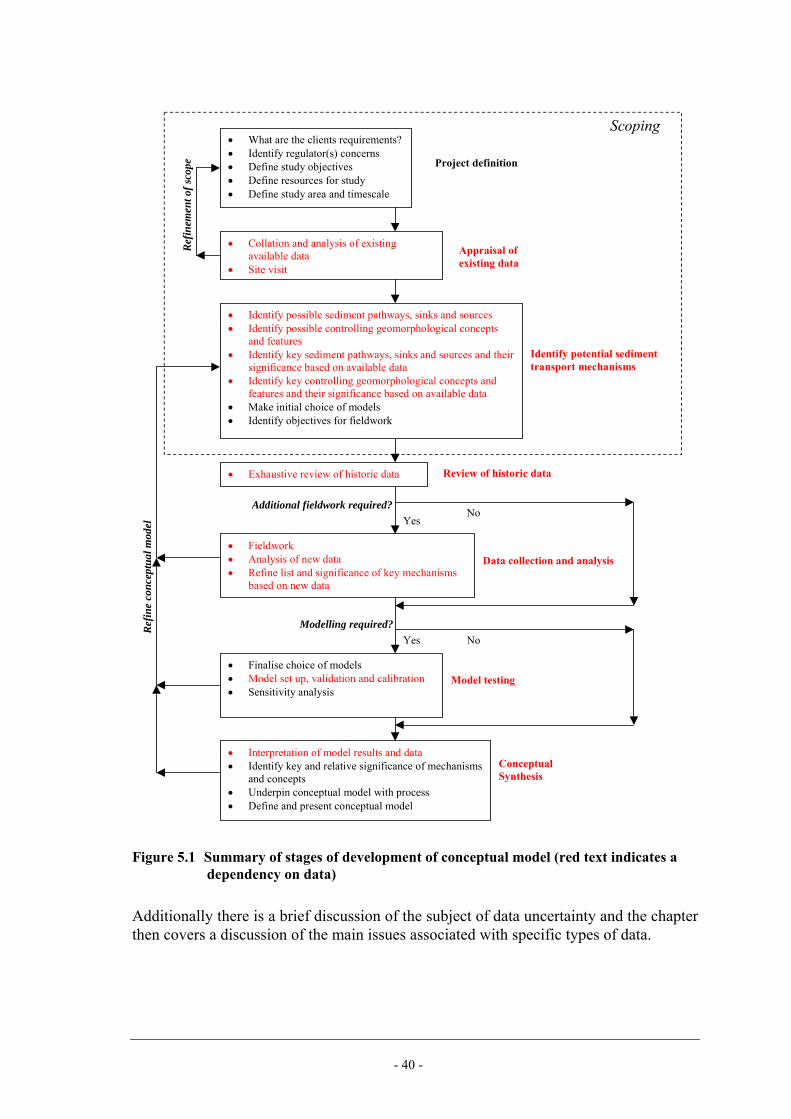
- 40 -

• Collation and analysis of existingavailable data

• Site visit

• Identify possible sediment pathways, sinks and sources• Identify possible controlling geomorphological concepts

and features• Identify key sediment pathways, sinks and sources and their

significance based on available data• Identify key controlling geomorphological concepts and

features and their significance based on available data• Make initial choice of models• Identify objectives for fieldwork

Project definition

Identify potential sedimenttransport mechanisms

Scoping

Appraisal ofexisting data

• Fieldwork• Analysis of new data• Refine list and significance of key mechanisms

based on new data

Data collection and analysis

• Finalise choice of models• Model set up, validation and calibration• Sensitivity analysis

ConceptualSynthesis

• Interpretation of model results and data• Identify key and relative significance of mechanisms

and concepts• Underpin conceptual model with process• Define and present conceptual model

Model testing

• Exhaustive review of historic data Review of historic data

Additional fieldwork required?Yes

Modelling required?Yes

No

No

• What are the clients requirements?• Identify regulator(s) concerns• Define study objectives• Define resources for study• Define study area and timescale

Ref

ine

conc

eptu

al m

odel

Ref

inem

ent o

f sco

pe l

Figure 5.1 Summary of stages of development of conceptual model (red text indicates a

dependency on data)

Additionally there is a brief discussion of the subject of data uncertainty and the chapter then covers a discussion of the main issues associated with specific types of data.

- 41 -

5.3 Appraisal of existing data At the start of a project it is important to make best use of the data already available. A thorough investigation of existing data should lead to a better understanding of the key processes involved and forms the basis for a sound conceptual model. The types of data that can be utilised are summarised in Box 5.2.

Box 5.2 What data might be available?

• Bathymetry/coastline/topography • Dredging/disposal records • Tidal levels, waves, currents, salinity, water quality • Seabed sediments, suspended sediments, bedforms • Sediment and sedimentary characteristics • Biota, vegetation • Geological

With existing data the issue of data quality is even more important than for new field data because there is no control and often no appropriate description over how the existing data was collected. This is particularly true of historical data. It is therefore important to check the quality of data, datums and projections. Often data is available from a previous study. However, it should be noted that the presence of data in a report does not ensure its reliability. For instance, suspended sediment measurements made using a sensor rather than water samples are often prone to unreliability unless a thorough calibration is demonstrated. Moreover, some data can be considered to just be unreliable by its very nature, e.g.: • Measurements of current speed/direction of below 0.1m/s; • Settling velocity measurements using gravimetric analysis; • Sediment parameters (erosion stress, etc) on the basis of laboratory measurements. The recommended approach to existing data can be summarised as,

TRUST NOTHING WITHOUT CHECKING Where possible the consistency of different data should be established using “back of the envelope” calculations. This practice will aid the identification of problem data sets. 5.4 Further field data requirements After the collation of any available existing data and the analysis of this data to develop an initial idea of the key sediment transport mechanisms within the study area, the next step within the approach presented is to assess the need (if any) to collect further data. The requirement for further data should come from the identification of gaps in the understanding of the key sediment transport processes within the conceptual model, the required accuracy of the assessment and the budget/time constraints for the study. In particular there are three common situations where further data may be required:

- 42 -

Where there is no existing data - Further data is most obviously required if no baseline information on the existing situation exists, although, if only an initial desk assessment is to be undertaken, experience of sites nearby may be sufficient. To understand key mechanisms - Key mechanisms identified or postulated by the conceptual model may require closer evaluation. For calibration and validation of models - Any applied models used will need to be suitably robust in their representation of the exiting conditions and new data may be required to provide validation data. The definition of further data requirements should be informed by the choice of applied model and the time/spatial scale that will be simulated by the model. Collection of further field data – The definition of further field data collection campaigns will depend on the level of knowledge regarding the key processes identified within the initial conceptual model, the time and spatial scale of the key processes and the overall budget/time scale of the study. Any new field data collection should keep in mind the purpose to which any collected data will be used and should complement existing data. The complexity of collecting the required data and its likely quality should also be taken into account, being aware of any errors inherent in the method used. For large or sensitive studies the collection of further data may be both comprehensive and should be expected. For such studies the collection of field data needs to be planned in advance at the first opportunity, particularly as the field experiments may need to take place at set times of the year, or indeed over the course of a year, to obtain the relevant data. Field campaigns are expensive and a failed campaign will be doubly expensive due to the waste of project time involved. Many problems encountered can be mitigated by appropriate design and planning. In particular the following considerations are important: • Ensure the quality of data is adequate. • Build in flexibility to respond to some data failure. • Be aware of errors inherent in the method used – are these errors acceptable? • Ensure that any new data collected complements the existing data. • Consult before collection of data. Make sure the surveyor knows what the data is

being used for otherwise the data collected may be compromised. • Collection requires permission (for instance FEPA5 or a Notice To Mariners). In spite of the best preparation significant errors can occur in the collected data. However, it is common that errors do not become apparent until the data is used in earnest. It is therefore important that those providing the data have allotted time and resources to provide follow-up support, potentially involving considerable analysis and re-analysis of the data. It should be expected that after provision of data there will be a period of discussion between survey team and the user of the data.

5 FEPA – Food and Environment Protection Act 1985

- 43 -

5.5 Data for modelling It is beyond the scope of this chapter to consider the specific data requirements of modelling-based studies in detail but as geomorphological studies often utilise the results of previous modelling studies or form part of larger studies where modelling forms an important component, here we briefly outline some main points regarding the use of data for flow and sediment transport modelling. The inputs needed for modelling include data for: • Defining the model coastline and bathymetry; • Defining the model boundary conditions; • Establishing key sediment transport parameters ; and, • Establishing calibration data. Calibration of models should be objective and transparent, i.e. understandable to non-modellers. The key aim is to enhance confidence in the assessment. It is worthwhile defining the calibration target (i.e. defining what properties are most important to predict with error below a certain threshold) before calibration commences. This exercise will clarify the calibration process to other interested parties and gives an objective context for the calibration process given that it is not possible to reproduce the observations exactly. Calibration is often a “black art” and can be made more so by subjective and qualitative judgements by the modeller regarding whether the model has successfully achieved its performance target. For this reason, where possible, it is advisable to use an objective assessment of model performance. Examples of this are: • A simple calculation of mean error between model prediction and observation (e.g.

water level, current speed, bathymetric change, etc); • Tabulation of the percentage of model results within various levels of tolerance; • The use of statistical measures of model fit such as the Brier Skill Score (Sutherland

et al, 2004; Haigh et al, 2005). Where EGA is undertaken and makes use of the results of previous modelling studies it is prudent to check the calibration of the model used in previous studies. Although stated as “good” or “reasonable” in the report an independent assessment may reveal a less acceptable result. Lastly, it should be stated that calibration data, like all data, can be prone to error and discrepancy between model and observations may not always be the fault of the model! 5.6 Data uncertainty Data is prone to uncertainty, both from the inherent spatial and temporal variation of a given property but also from the measurement device used to characterise the property. Since data is paramount to a study it is important to allow adequate time to review data, prior to analysis and use, to ensure that serious errors are identified and the overall level of error is minimised.

- 44 -

It is good practice to make a best estimate of the likely error in the data and an assessment of the uncertainty that this error will have on the geomorphological assessment. Some examples of how this can be done at the level of geomorphological assessment are presented in Boxes 5.3 to 5.5.

Box 5.3 Example of effect of maintenance dredging and disposal on upstream intertidal areas

Most maintenance dredging usually entails offshore disposal of sediment. In muddy estuaries especially the artificially deepened channel and/or berth will trap sediment that would otherwise remain in suspension if the channel/berth was not there. The trap effectively reduces suspended sediment concentrations in general in the estuary and hence the flux of sediment onto intertidal areas. The calculation of the resulting impact (if any) on the intertidal areas arising from this process can be undertaken at varying levels of complexity. For this example, though, we will assume (as in the case with the Stour/Orwell – Section 8.7) that the natural deposition on the intertidal areas is proportional to the average concentration occurring over the intertidal, which itself is roughly proportional to the annual flux of sediment, S, into the estuary from offshore. If the annual offshore disposal of maintenance dredged material from the channel/berth is D then the concentrations in the estuary, and hence the deposition on the intertidal area is proportional to (S-D)/S. In this example the proportional reduction in the rate of deposition (dep) and hence the morphological impact on the intertidal is given by dep.D/S. Now if the data relating to the maintenance dredging and disposal is not accurate there could be an error of for example 50% in the value D, and hence the error in the assessment of impact is +/- dep.D/2S.

Box 5.4 Example of effect of error in current data on estimate of future morphological change

In this example a morphological prediction has been undertaken (unspecified in this example) using standard sand transport formulae and data derived from a calibrated flow model. The flow model is well calibrated with peak current speeds in the region of 1m/s and errors in the prediction of peak flood and ebb speed are of the order of 10%. For the purpose of this example we will assume that the sediment transport formulae is of the form, S=a.Vn where S is the sand flux, V is the current speed and a and n are constants and n has a value of between 3 and 4. The proportional error in the sand transport flux (which is proportional to any resulting morphological change) then is roughly 30-40%. Further error will come from the uncertainty in the sediment transport formula itself.

- 45 -

Box 5.5 Effect of survey error on estimate of future morphological change

In this example a morphological prediction has been undertaken (unspecified in this example) but the initial rate of morphological change (and the final extent of the change) is a function of the observed volume change between two bathymetric surveys taken five years apart. It is important to know the likely error in the volume comparison between surveys in order to know the error in the estimate of the rate and magnitude of resulting morphological change. Suppose the two original bathymetric surveys were roughly composed of 100 data points and both on average 50m apart. Suppose also that the surveys were undertaken by the same surveying team of good reputation, and undertaken at the same time of year, using the same methodology. The discussion of HTA given in Chapter 6 and the S44 standards for hydrography indicate that the standard error in each measurement of depth would be around 0.15m and that the random measurement error in a volume based on 2x100 data points is then V.V. 010

200150

≈ where V is the calculated volume

change between the two surveys. The error caused by random measurement error is therefore around 1% and insignificant. However there are other sources of error and in this example we consider the error from coarse data resolution. To evaluate the magnitude of this error the volume calculation is repeated but this time taking every 2nd measurement from both surveys. Suppose then that the difference in the original and reduced data calculations of volume was 20%. This is then representative of the error from coarse data resolution in the surveys and has a significant effect on the uncertainty in the prediction of morphological change.

5.7 Bathymetric data Bathymetric data is used for: • Establishing the history and rate of change of morphology; • In running baseline model simulations; and, • For providing calibration data (bed level/volume change) for sediment transport

models. Sources of Bathymetric data include: • Surveys (usually navigation channels but sometimes intertidal); • Admiralty Charts (usually based on navigation surveys - intertidal data is sparse); • LiDAR (when ground-truthed can be highly detailed intertidal data); • Dredging surveys (quality can vary, will be confined to a navigation area of high

accretion rate); • Aerial photographs and satellite images (can be useful but often not available for the

period required unless specifically taken for a purpose);

- 46 -

• Ordnance Survey maps (limited to giving information on MHW6 and 7MLW); and, • Beach profile surveys (quality can vary). It should be noted that bathymetric data needs to be detailed and consistently measured or its use becomes limited. Bathymetric data can contain errors. A more complete discussion is presented in Chapter 7 on Historical Trend Analysis but the key sources of error are listed below: • Systematic errors: e.g. resulting from an inherent error in the survey methodology.

This error tends to cancel out if two surveys using are compared which used the same methodology;

• Measurement bias e.g. lead line measurements; • Random measurement errors:

– For current standards of hydrography see S44 (4th edition) (IHO, 1998); – Vertical errors usually more important than horizontal errors; – Horizontal errors usually only significant when measuring bathymetry on steep

slopes or as a result of the changes in positioning that resulted from the WGS84 protocol;

• Navigation charts generally highlight the shallowest bathymetric measurements and therefore are biased to some extent;

• Rounding Errors: depths are usually rounded down (van der Wal and Pye, 2003, ABPmer, 2002);

• Metrification: This conversion may result in the introduction of errors. (ABPmer, 2002);

• Chart/Survey Dates: Modern charts (e.g. Admiralty Charts) are often composites of a number of surveys over different years; and,

• Datum errors and/or changes: – Errors in old datums e.g. pre 1921 Liverpool datum (for more information see

Doodson and Warburg, 1941); and, – Changes in datums over time as a response to changes in water level (e.g. the

Port of London Authority changed their chart datums around 1970). 5.8 Flow data 5.8.1 Water level data The principle source of water level data is from tidal gauges although in many cases the tidal predictions available from Admiralty Tide Tables (themselves based on harmonics derived from analysis of tide gauges) is sufficient. Water level data experiences all the datum problems discussed under bathymetric data (Section 5.7). Additionally water level measurements can be affected by meteorological effects such as storm surges and waves and there is a need for accompanying measurement of meteorological data to identify these additional effects.

6 MHW Mean High Water, 7 MLW Mean Low Water

- 47 -

5.8.2 Current data Current data is one of the most important resources for understanding how an estuary system functions and for developing a conceptual model. Sources of current data: • ADCP8 (strictly speaking the current term is ADP since ADCP is a trade name): The

best if available since ADCP gives measurements of current speed and direction throughout the water column. However this device has blind spots. If vessel mounted, cannot measure around 1m from sensor and bottom 16% of the water column, if bed mounted the reverse is true;

• Current meter: usually reliable but limited to point measurements; • Admiralty Tidal Diamonds: Often historical and therefore may be false if large local

morphological change has occurred. Date of origin can be pinned down by investigating historical admiralty charts; and,

• Float tracking: a rough method for establishing current magnitudes but useful for establishing residual trends in currents. Susceptible to error from wind effects.

Current data can give misleading readings if: • The current magnitudes are below 0.1m/s; • If the internal compass reading is unreliable (not uncommon); • If historical (due to morphological change); • If placed at a fixed level on an intertidal area – since the sensor is experiencing a

change in water depth as well as changes in depth-averaged current speed; and, • If vessel mounted in large waves and low current speeds – wave induced orbital

velocities will produce considerable scatter on the tidal or wind driven current signal.

5.8.3 Salinity measurements Salinity measurement is included in this section on flow measurement because gradients in salinity cause residual density currents and affect the tidal current flow. Any assessment of current flow in an estuary is therefore incomplete without some assessment of salinity gradients. Even a well-mixed estuary will have horizontal salinity gradients producing a residual landward current near the bed. Salinity measurements are normally made using a rapid drop profiler deployed from a vessel. Measurement errors are not normally significant except if the sampling frequency of the profiler is low compared to the speed at which the profiler is dropped/raised through the water column. If the frequency is low, each salinity measurement will be an average salinity over a significant depth of water and near-bed readings may be erroneous.

8 ADCP Acoustic Doppler Current Profiler

- 48 -

5.9 Wave data Wave data can be measured using a number of methods, for instance: • Pressure gauge; • ADCP; • Accelerometer mounted on a wave buoy; • High Frequency radar; and, • Voluntary Ship Observations. All of these devices have their good and bad points and will respond to different sorts of errors. More complete surveys will include measurements of waves from more than one device. The most common errors in wave measurements tend to come from the following sources: • Lack of inclusion of the effect of attenuation of the recorded pressure signal with

water depth; and, • Failing to sample at a sufficiently high frequency to capture high frequency waves. Wave measurements differ from other typical estuary phenomena measurements in that it is less common to calibrate predicted wave action against field data. Wave measurements are generally undertaken in order to calculate design conditions for engineering structures. However, although it is common not to calibrate wave model predictions it does not mean that this is good practice. Waves are in essence non-deterministic and occur as a result of both local wind activity and as a result of ocean swell. Both components can be important in estuaries and each component is essentially derived from different sources. The swell component has a longer period and results from the inshore transformation (due to refraction, shoaling, friction etc) of a wave generated offshore. The local wave is generated from wind blowing over a certain fetch (again transformed by refraction, shoaling, friction etc). For any assessment of wave action within an estuary it is therefore important to have offshore and inshore wave climate information. 5.10 Sediment transport data The collection of sediment transport data is expensive and often technically difficult. Additionally, since sediment transport is greatest during storms (which are by definition hard to monitor) and the largest spring tides there are considerations of whether data collected is representative. The most common measurements of sediment transport are as follows: • Concentrations:

- Water samples; - Optical device measurements; - Laser diffraction measurements;

- 49 -

- ADCP back scatter; • Morphological change (see Section 5.7); and, • Dredging records (see Section 5.11). The principle problem with measurements of suspended sediment concentration is that water sampling is time consuming and costly but is the only independent method of establishing concentration. The other methods, whilst quicker and, in the case of ADCP backscatter, allowing through depth measurements, require calibration against water samples. Hence measurements using one of these non-direct measurement methods is associated with some (considerable) uncertainty unless the calibration of sensor reading against water sample observations is presented. An additional problem which affects the non-direct methods of measurement is that instrument response is a function of particle size and even if well calibrated against total solids content there will be uncertainty in the sensor readings resulting from natural variation in the particle size distribution over time. It is also possible that the readings can be contaminated by bio-fouling of the sensor element. Less commonly measurements of the following are undertaken: • Bed density; • Settling velocity; and, • Identification of bedforms and of material type using multi-beam sonar and side-

scan sonar imaging or acoustic sediment discrimination systems, with ground truthing provided with sea bed grab samples.

Bed density can be important in sediment budget analysis and assessment of morphological change because it relates mass of sediment, as predicted using sediment transport formulae, to volume change. However, bed density varies both spatially and with depth. Establishing representative values for use in morphological assessment is not a trivial task. Although the settling velocity of sand particles is fairly well established (e.g. Soulsby, 1997) and a range of methods exist for mud (e.g. Whitehouse et al, 2000) the measurement of settling velocity of mud flocs is a technically complex subject. Best practice at present is to undertake insitu measurements using sophisticated measurement devices which do not disturb the sediment floc structure and enable video footage of floc settling to be taken (e.g. the INSSEV device, Fennessy et al 1994). Estimates of settling velocity made without this type of approach will have shortcomings, although laser diffraction devices (such as LISST) claim (as yet without formal evaluation) to be able to measure floc settling velocity while retaining the benefit of a device that can be easily deployed. In particular the traditional method of gravimetric analysis (the use of water sampling from settling columns) should not be used because the sampling process causes re-circulation of settling flocs and underestimates settling velocity by up to an order of magnitude (Dearnaley, 1996).

- 50 -

5.11 Dredging data Dredging data can often be the only way of establishing the tendency for deposition in an estuary system and can be especially important for establishing key sediment parameters in sediment transport model studies. Comprehensive dredging records (where, when and how much) are an extremely valuable resource but they need to be kept over a decent period to be reliable. Types of dredging data: • (Repeat) bathymetric surveys following a dredge; • Pre and post dredge bathymetric surveys; • Data based on number of hopper loads taken to disposal site; • Data from local Harbour Authority on:

– Harbour operations (lock operations, turning areas, ferry traffic, pilotage); – Past and present dredging (capital and maintenance); – Locations and history of use of disposal sites;

• Information held in Regulator’s data bases (e.g. MAFF/Defra disposal database); and,

• Data from dredging Contractors who have worked at the site. The best dredging data is derived from pre and post dredge bathymetric surveys since these tell you exactly what was removed from the dredged area. Data based on hopper loads only tells you what was taken from the site – not what was additionally disturbed from/released at the site during operations. A starting point is the MAFF (now Defra) database of disposal although this database is by no means complete and only as good as the data supplied to it. The database only includes information on disposal rather than the amount dredged (i.e. there is no information about sediment “spilled” during dredging or used for beneficial use). 5.12 History of management and natural changes Any geomorphological assessment is incomplete without taking into account anthropogenic effects resulting from: • Archaeology; • Embanking/reclamation; • Training walls; • Bridge building/removal; • Dredging/disposal; • Foreshore/dune management; and, • Industries such as brick-making. and additionally the effect of large-scale natural changes such as, • Salt-marsh loss (e.g. Poole Harbour); and, • Eel-grass loss (e.g. Stour Estuary, Essex)

- 51 -

This information is derived from the journals of the local Port or engineer, anecdotal sources, old records and history books. When taking into account the long-term evolution (for instance since the start of the Holocene period) it is also necessary to take into account the roman, medieval and pre-industrial land reclamation that may be more responsible for recent morphological trends in the estuary system. Table 5.1 gives an indication of the importance of this phenomenon. Table 5.1 Habitat loss in English estuaries (Healy and Hickey, 2002, adapted

from Davidson et al., 1991) Estuary Name Area lost (ha) Reclamation Period The Wash 47,000 Since Roman Times Severn Estuary c. 8,000 Since Roman Times Dee Estuary 6,000 Since 1730 Humber Estuary 4,600 1600-1850 Greater Thames Estuary 4,340 Mostly pre-1800 Tees Estuary 3,300 Since 1720 Ribble Estuary 2,320 Since 1800 Morecambe Bay 1,320 1200-1900 Ore/Alde/Butley Estuary 3,640 Since 1200 Deben Estuary 2,240 Since 1200 Stour Estuary 1,600 Since 1200 Blyth Estuary 1,280 Since 1200 Orwell Estuary 980 Since 1200 Southampton Water 690 Since 1830 Poole Harbour 530 Since 1807 Portsmouth Harbour 490 Since 1540 Mersey Estuary 490 1800-1900 5.13 Estuary geometry data In this section we briefly discuss issues surrounding the use of estuarine geometric parameters often used in the context of EGA and used in many of the tools described in Chapters 7 to 15. The parameters discussed here are as follows: • Tidal prism/tidal volume; • Cross-section area; • Depth; • Length; and, • Width. It is important to note that most of these parameters can vary seasonally (high/low fluvial flow) and over the spring/neap cycle. When evaluating these parameters it is important to make it clear under which conditions these parameters were derived. Which conditions most characterise an estuary is not an easy question to answer conclusively but in general spring tide conditions are considered to be more representative than mean or neap tide conditions. It is therefore suggested that these parameters be evaluated for spring tide conditions except where there is a good reason for evaluating under other or all types of conditions.

- 52 -

5.13.1 Tidal prism/tidal volume Tidal prism and tidal volume are terms which are used interchangeably and both relate to the volume of water flowing into the estuary from the sea on the flood tide. However there is strictly speaking a subtle distinction between these two properties. Tidal volume is the volume of water that flows into an estuary from the sea on a flood tide (and out again on the ebb). To evaluate this volume a numerical flow model will be required. Tidal prism is the volume within the estuary bounded by the LW and HW9 levels (note that there is a spectrum of tidal volumes, depending on whether a spring, mean or neap tide is the subject of interest, although it is the spring tide that is usually referred to). Tidal prism can thus be derived from bathymetric data. Tidal volume and tidal prism should be very similar and they differ primarily because HW and LW are not experienced synchronously along an estuary length. Often tidal prism is estimated using a fixed elevation for HW and LW along an estuary. This can enable a more rapid assessment of tidal prism from bathymetry but in reality HW and LW vary along the estuary and for a more accurate assessment of tidal prism the volume calculated must reflect this. In the upper estuary approximation using fixed level may become too inaccurate for the resulting estimate to be useful. It should be stated which option has been used when generating estuary tidal prisms/volumes. 5.13.2 Cross-section area The calculation of cross-section area consists of the integration of a profile of bathymetric data across a transect in an estuary. The calculation itself is straightforward – use of the trapezoidal rule will generally suffice – but the selection of a transect can sometimes be problematic. In some estuaries the LW channel can diverge considerably from the general alignment of the MSL10 and HW level. At such locations the direction of the water flow may be significantly different at different times in the tide (Figure 5.1). If so it is not clear how to evaluate the discharge through the channel as a simple, obvious cross-section does not exist. The best way of dealing with this problem is to avoid it by locating the cross-sections in places where this problem does not arise. For geomorphological assessment there are two cross-section area parameters that are most relevant:

• Cross-section area at MSL – used in regime theory with O’Brien type prism-area relationships; and,

• Cross-section area at peak discharge – this is closely related and also used in regime theory peak discharge-area relationships (where the benefits of a numerical flow model can be utilised) but may significantly differ from the width at MSL in the upper estuary.

9 LW Low Water, HW High Water 10 MSL Mean Sea Level

- 53 -

The calculation of cross-section area may also be important for deducing average estuary depth at HW and LW. Usually the water levels of relevance are around mean spring LW and mean spring HW. 5.14 Depth When considering cross-section depth invariably the parameter of interest that should be used is the average channel depth, equal to the LW cross-section area plus the tidal amplitude. However, in some instances an “average estuary depth” is required. When considering average estuary depth it is important to note that there are a number of ways to average depths (which vary significantly along an estuary) and it is possible to result in a large variation values. For instance, average depth can be calculated as an arithmetic average, (Σhi)/N) or a geometric average, (Πhi

1/N) and this will give smaller and larger results respectively. Friedrichs and Aubrey (1994) overcame this problem by stating average depths as a range of values to account for the uncertainty (e.g. Thames, 8.5+/-0.7m, Tamar, 2.9+/-0.2m, Delaware (US) 5.8+/-0.3m). 5.14.1 Cross-section averaged current speed Cross-section averaged current speed features directly or indirectly in many of the tools described in Chapters 7 to 15. In particular cross-section averaged current speed may be used as a means of deriving the tidal prism or peak discharge through a section. The easiest way to derive this variable is to generate the estuary flows using a numerical model. The software associated with the model will then provide the cross-section averaged current speed either as a direct output or provide a means for integrating cross-section area and discharge so that the cross-section averaged current speed can be deduced. It is important to note that single point measurements of current speed in an estuary do not represent a good estimate of cross-section averaged current speed. This is because there is significant variation in current speed across a cross-section especially as current speeds will reduce in the shallower waters on either side of the channel. Where the only basis for deriving cross-section averaged current speed is a single point measurement the estimate can be improved to some extent using the following procedure, assuming that the point measurement represents the largest current speeds in the centre of the channel. We assume Chezy’s law is valid (equivalently Manning’s law can be used with a slightly different outcome but the same qualitative result),

rsCv = (5.1) where v is the current speed;

r is the hydraulic depth (equal to the cross-section area divided by the wetted perimeter and roughly equal to average depth); C is the Chezy constant.

Longitudinal water slope is assumed to be the same at all points along a cross-section transect, and the current speed is assumed to vary gradually in the longitudinal direction.

- 54 -

Equation 5.1 then gives,

maxmax rr

vv

= (5.2)

where vmax and rmax is the maximum current speed and depth in the middle of the

channel; v and r are the current speed and depth anywhere along the transect.

Equation 5.2 gives a method of estimating the variation in current speed along the transect. Once this variation is known each velocity estimate can be multiplied by the depth at that point to produce an overall discharge and cross-section area and hence a cross-section averaged current speed. 5.14.2 Cross-section Width Cross-section width suffers from the same problems of identification as cross-section area but, subject to uncertainty in identifying alignment of a representative cross-section, is a fairly straightforward a parameter to evaluate. For geomorphological assessment there are four widths that are relevant: • Width at MSL – used in regime theory with O’Brien type prism-area relationships.

Closely related is width at peak discharge which is also used in regime theory peak discharge-area relationships (where the benefits of a numerical flow model can be utilised) but may significantly differ from the width at MSL in the upper estuary;

• Width at LW – a measure of the extent of the LW channel and used in the context of evaluating tidal asymmetry. Usually the LW level of relevance is around mean spring LW; and,

• Width at HW – a measure of the extent of the LW channel and used in the context of evaluating tidal asymmetry. Usually the LW level of relevance is around mean spring HW.

5.14.3 Estuary Length Estuary length is commonly a loosely specified parameter and some care should be taken in the derivation of this parameter and in the use of values derived by other parties. The estuary length is the length from the seaward limit of the estuary, which is sometimes obvious and sometimes not, to the normal upstream tidal limit, which for almost all cases can be taken as that stated on OS maps. It should be noted that estuary length defined in this way is commonly a function of the presence of weirs at the upstream end of an estuary and therefore may differ from the natural, or at least pre-industrial, length of the estuary. Some authors have suggested a means of calculating estuary length on the basis of other parameters (e.g. Pethick, 1994, Prandle, 2003) and a distinction has to be made between the estuary length used by these authors (which is not a function of man-made influence) and the observed man-influenced values. Figure 5.2 shows the problems that can arise when defining the seaward limit of an estuary. Two schematic examples are shown – one that can be said to typify, for

- 55 -

example, the Thames and Severn Estuaries where in effect an arbitrary downstream limit is often chosen, and one that can be said to typify estuaries where a definite headland exists, for instance in the Fal, the Stour/Orwell, and the Mersey Estuaries. The potential for different decisions to be made by different researchers/consultants regarding the seaward limit means that it is very important to state the seaward limit chosen so that others know what has been done. It is best to maintain consistency with the definition of the seaward limit used in previous studies unless there is a very good reason for change. There are further considerations regarding the seaward limit even when an obvious headland limit is present. Whether an estuary delta or bar is part of the estuary length is a question often posed. Additionally considerations of whether part(s) of a particular estuary function as an estuary can sometimes arise. The Humber Estuary for instance has a reasonably defined mouth between Spurn Head and the coastline to the south (Figure 5.3). However, it can be argued that the size of the Skeffling Mudflats Bay enclosed by Spurn Head and the fact that the water between Grimsby and Spurn Head is fully saline means that this body of water is sea rather than estuary. Defining the seaward limit then becomes one of defining the seaward point where a landward salinity gradient is induced. This argument would contrast with the opposing view that regardless of gradients in salinity the body of water seaward of Grimsby cannot be separated from the estuary further landward in a functional sense – i.e. water and sediment flows up and down the estuary seaward and landward of Grimsby. It would be fair to say that the authors of this report had mixed opinions on this argument. However, where uncertainty of this kind arises it is best to err on the side of simplicity:

…if it looks like an estuary, it probably is an estuary. 5.15 Data for long term prediction For long-term assessments of morphological change there are additional data requirements to the data outlined above: • Climate change data:

– sea level change; – history of the wind and wave climate;

• Synoptic historical data sets; • Bedrock and surface geology; and, • Feedback between biology/vegetation and morphological change. Over long periods of time the extent of sea level rise becomes significant and needs to be incorporated into any hindcasting or forecasting of change, as do changes in the wind and wave climate. Hindcasting of morphological change is aided considerably by synoptic historical data sets of hydrodynamics and bathymetry, which, though rare, do exist for some estuary systems. For future predictions of morphological change it is essential to know how the evolution of the estuary may be constrained by geology. As important, is the role of biology and vegetation in controlling morphological change. At present there is very little scientific knowledge regarding the morphological feedback from biology and vegetation but the

- 56 -

point is made here that the absence of this feedback in a morphological prediction results in additional uncertainty. 5.16 Conclusions 1. Data is paramount to EGA studies and the use of data should be carefully managed

in such studies to enhance confidence in the assessment; 2. The assumption that there is enough data in all cases to inform EGA studies needs to

be verified at the outset of any study; 3. Data is (generally) site-specific and collection of data is time-consuming and

expensive; 4. Collection of data is not the end of the problem - each type of data has sources of

error associated with its collection and processing which need to be understood; 5. Understanding of the technical aspects of collection and the use for which the data is

being collected will reduce the level of uncertainty in the data; 6. Review and analysis of data are essential and this can be a time-consuming and

hence an expensive part of the process; 7. There is a requirement in every study to allow some flexibility in the project scope

and budget if at the end of the data review it is clear that the previously anticipated activities need to be modified or new tasks are identified to achieve the goals of the study; and,

8. There is a requirement to understand how uncertainty associated with the data used in a study feeds through to the conclusions of that study.

5.17 References ABPmer, (2002). Humber SMP. Historical Analysis: Review of Potential Lead Line Variations in the Period 1930 – 1040. Internal Technical Note. ABPmer, Southampton. Davidson, N.C., Laffoley, D d'A., Doody, J.P., Way, L.S., Gordon, J., Key, R., Drake, C.M., Pienkowski, M.W., Mitchell, R., and Duff, K.L. (1991). Nature Conservation and Estuaries in Great Britain. Peterborough, UK: Nature Conservancy Council, 422p. Dearnaley, M.P. (1996). Direct measurement of settling velocities in the Owen Tube: A comparison with gravimetric analysis, Netherlands Journal of Sea Research, volume 36, pp41-47. Dodson, A. and Warburg, H.D. (1941). Admiralty Manual of Tides. Dearnaley, M.P., Baugh, J.V. and Spearman, J.R. (2004). Modelling sediment transport and sedimentation. Proceedings of the Maintenance II Conference, Institute of Civil Engineers, 2004. EMPHASYS. (2000). A guide to prediction of morphological change within estuarine systems, Report TR 114 produced by the EMPHASYS consortium for MAFF project FD1401, Estuaries Research Programme, Phase 1, December 2000.

- 57 -

Haigh, I., Norton, P. and Townend, I. (2005). Understanding and predicting morophological change in the inner Humber Estuary. Proceedings of the 29th International Conference on Coastal Engineering, ed. J. McKee Smith, 2493 – 2505. Healy, M.G. and Hickey, K.R. (2002). Historic land reclamation in the intertidal wetlands of the Shannon estuary, western Ireland, Journal of Coastal Research, Volume 36, pp365-373, 2002. IHO. (1998). IHO standards for Hydrographic Surveys, International Hydrographic Organisation, Special Publication Number 44, 4th edition, 23pp. Pethick, J. (1994). Estuarines and wetlands: Function and form. In: Falconer, R.A. and Goodwin, P. (eds.), Wetland Management, Proceedings of the International Conference, Institution of Civil Engineers, London, pp 75-87. Prandle, D. (2003). Relationships between tidal dynamics and bathymetry in strongly convergent estuaries. Journal of Physical Oceanography, Volume 33, pp2738-2750. Soulsby, R.L. (1997). Dynamics of Marine Sands. A manual for practical applications. Thomas Telford Publications. Sutherland, J., Peet, A.H. and Soulsby, R.L. (2004). Evaluating the performance of morphological models. Coastal Engineering, 51, 917 – 939. Van der Wal, D. and Pye, K. (2003). The use of historical bathymetric charts in a GIS to assess morphological change in estuaries. The Geographical Journal, 169 (1), 21-31. Whitehouse, R., Soulsby, R., Roberts, W. and Mitchener, H. (2000). Dynamics of Estuarine Muds. Thomas Telford, London.

- 58 -

currents

LW

HW

OK

Currentsnear LW

LW

HW

Not OKCurrentsnear HW

Transect 1

Transect 2

Figure 5.1 Considerations when choosing a cross-section

- 59 -

Estuary limit

Estuary limit?

Figure 5.2 Problems associated with identifying estuary seaward limits

- 60 -

Figure 5.3 The Humber Estuary

- 61 -

PART 3 – GEOMORPHOLOGICAL TOOLS AND METHODS

The Camel Estuary, Cornwall (Photograph copyright Richard Whitehouse, HR Wallingford)

- 62 -

- 63 -

6. INTRODUCTION TO GEOMORPHOLOGICAL ASSESSMENT TOOLS

Chapters 7 to 15 provide a critical examination of the best use and reliability for a range of predictive tools that are available to the geomorphologist for estuary studies. Among the tools that will be investigated are the following (which were described and applied in the Estuaries Phase 1B project): Data methods • Historical Trends Analysis (Chapter 7); • Sediment budget modelling (Chapter 8); Long time-scale methods • Rollover model (Chapter 9); • Geological methods for estuarine studies (Chapter 10); • Regime theory (Chapter 11); Medium time-scale methods • Entropy based relationships (Chapter 12); • Asymmetry relationships (Chapter 13); • Analytical solutions (Chapter 14); and, • Intertidal form (Chapter 15). Some of the tools examined in this report – Regime Theory, Entropy based relationships, Asymmetry relationships, Analytical tools and Intertidal form – require in-depth examination of the underlying theory as well as presentation and discussion of best practice. For these chapters the sections are separated into those dealing with theory and those dealing with best practice. The other tools – Historical Trends Analysis and Sediment Budget Analysis, Rollover and Geological Methods – are less theory-based and merit a more discursive style of examination where all the relevant issues are highlighted. For these tools theory and best practice are intertwined and they are presented as such. For each Chapter the type of tool is classified using an easy to follow classification that links back to Table 4.2; for example for Historical Trends Analysis the header table looks like the following:

Method Indicator Bottom-Up Hybrid Top-Down

YES Where relevant examples and case studies are included in the text to illustrate key points. A full index of examples and case studies of estuaries included in this report is presented after Chapter 17. As discussed in Chapter 2, there are other tools available such as the bottom-up process-based methods. These are not directly the subject of the present report. Additionally in recent times a group of models, which shall be termed “behavourial” models (e.g. Cowell et al, 2003), has been developed. This group of models is best described as hybrid predictive numerical models which seek to represent the various key processes in an estuary system in a simplified manner in order to study the longer term evolution of

- 64 -

the system. Examples of these models are the ASMITA model (Stive et al, 1998), the ESTMORF model (Wang et al, 1998) and the lagoon models developed by Di Silvio (Di Silvio, 1989, Di Silvio and Gambolati, 1990, Di Silvio, 1998). Discussion of ASMITA is included in the Chapter 9 on Rollover. 6.1 References Cowell P J, Stive M J F, Niedoroda A W, de Vriend H J, Swift D J P, Kaminsky G M, and Capobianco M (2003) The Coastal-Tract (Part1): A conceptual approach to aggregated modelling of low-order coastal change, Journal of Coastal Research, Volume 19, number 4, pp812-827. Di Silvio, G. (1989.) Modelling the morphological evolution of tidal lagoons and their equilibrium configurations, XXIII Congress of the IAHR, Ottawa, August 1989. Di Silvio, G. (1998). Interactions between marshes, channels and shoals in a tidal lagoon investigated by a 2-D morphological model, Interaction 3rd International Conference on Hydro-Science and -Engineering Brandenburg University of Technology at Cottbus Cottbus/Berlin, Germany, August 31 - September 3, 1998. Di Silvio, G. and Gambolati, G. (1990). Two-dimensional model of the long-term morphological evolution of tidal lagoons, VIII International Conference on Computational Methods in Water Resources, Venice, Italy, June 11-15, 1990. Stive, M.J.F. Capobianco, M., Wang, Z.B., Ruol, P. and Buijsman, M.C. (1998). Morphodynamics of a tidal lagoon and the adjacent coast. In: Dronkers J and Scheffers M (Editors), Physics of Estuaries and Coastal Seas, pp397-407, Balkema, Rotterdam. Wang, Z. B., Karssen, B., Fokkink, R. J. and Langerak, A. (1998). A dynamic-empirical model for estuarine morphology, Physics of estuarine and coastal seas, Dronkers and Cheffers (eds), Balkema, Rotterdam, 1998, ISBN 905410965 3.

- 65 -

7. HISTORICAL TREND ANALYSIS

Method Indicator Bottom-Up Hybrid Top-Down

YES 7.1 Background This section provides a critique of the application of Historical Trends Analysis (HTA) to estuarine environments. HTA is a geomorphological tool that involves the analysis of data relating to a particular physical process or morphological feature from different periods of time in order to identify directional trends and, if quantifiable, rates of changes in that process or feature. This critique provides the following:

• an overview of the technique of HTA (Section 7.2); • discussion of the data requirements (Section 7.3); • a procedure for the application of the technique (Section 7.4); • identification of relevant data issues (Section 7.5); • examples of its application to a number of UK estuaries (Section 7.6); and, • summary of information and recommended ‘best practice’ advice regarding its use,

as drawn from the experience and lessons learned from previous application (Section 7.7).

7.2 Overview of Technique HTA can be defined as the analysis of available data from different periods of time in order to identify historical trends and, if quantifiable, rates of change in estuarine processes or morphology. Typically this will cover ‘recent historical’ time periods, ranging from decades to a few centuries. Whilst the approach can relate specifically to physical processes, such as long-term sea level trends, it more frequently relates to many different aspects of historical and ongoing estuarine morphological behaviour, such as erosion or progradation of inter-tidal saltmarshes, changes in the position or shape of estuarine channels and banks, or changes in the location of spits across estuary mouths. Due to the focus of the FD2116 study on estuarine morphology, it is these aspects that are considered more fully in this critique. In addition to identifying the historical changes that have occurred, it is also important that these are attributed, in so far as is possible, to likely causes of morphological change in terms of the historical and ongoing forcing or constraints imposed on the system. This could take the form of trends or changes in natural forcing (such as sea level rise, changes in rainfall, wind or wave patterns, changes in current speed and direction, natural changes in rates of sediment supply as stocks become extinguished, etc.) or perturbations to the estuary system caused by anthropogenic activities (such as estuary-scale responses to major engineering works like training walls, reclamation, dredging, water abstraction, flood defences, re-alignment, barrages, etc.). If the causes of historical and ongoing morphological change can be identified, then a good understanding can be developed of the cause–consequence or process-response relationships in the estuary and this can provide a useful indicator of possible directions

- 66 -

and rates of future morphological responses. If such causes cannot be identified then the data can be misleading and caution needs to be applied in interpreting it. One also needs to be aware that the responses associated with some changes take long timescales to become fully manifest. Many estuaries are today believed to be still responding to historical, large-scale, reclamation activities. Forms of HTA have been applied, with varying degrees of sophistication, to estuarine environments for many years for the purposes of both research and management. Within the UK Estuaries Research Programme Phase 1 (ERP1), HTA was applied to a number of UK estuaries leading to a degree of formalisation of the approach (EMPHASYS Consortium, 2000a; 2000b; 2000c). The technique is now widely regarded by researchers and consultants investigating estuarine morphology as a particularly useful tool for determining locations and rates of historical change, as a precursor to anticipating, either qualitatively or quantitatively, future likely changes in estuarine behaviour over different epochs. A summary of some key issues relating to HTA is presented in Table 7.1. Table 7.1 Historical Trend Analysis: Summary of Key Issue

Issue Historical Trend Analysis Description Assessment of data from different periods in time in order to identify

directional trends and possibly rates of change of morphological features or physical processes within an estuary

Temporal Applicability

Past 1-200 years, depending on data availability

Spatial Applicability

Whole estuary or specific geomorphological features/geographical locations within an estuary, depending on data availability

Links with Other Tools

• Complements longer-term geological analysis approaches. • Can provide useful data to inform ‘regime analyses’. • Provides key input to establishing a conceptual understanding of the

longer-term estuary behaviour during ‘synthesis of results’ (or Expert Geomorphological Assessment (EGA)).

Data Sources Newspaper articles, published papers, parliamentary records, land registry archives, anecdotal evidence, maps and charts, aerial photography, topographic and bathymetric surveys, remote sensing imagery

Necessary Software Tools / Skills

• Identifying, collating and reviewing relevant data/information sources

• GIS11/image processing software/photogrammetry • Cartography/digital ground modelling • Geomorphological interpretation of output

Typical Analyses

• Changes in shoreline position (e.g. MHW, MLW12) • Changes in channel/bank morphology or position • Changes in sediment volumes above certain datums • Identification of areas of ‘cut’ and ‘fill’ or erosion/recession and

deposition/progradation over time

11 GIS Geographical Information System 12 MHW Mean High Water, MLW Mean Low Water

- 67 -

Table 7.1 Historical Trend Analysis: Summary of Key Issue (continued)

Issue Historical Trend Analysis Limitations • Availability of historical data can be limited in some areas

• Accuracy of some historical datasets can be questionable • Different measurement techniques, specifications, datums, units,

density of data points in successive datasets • Identifies net change between successive datasets, but not the scale

of variability over shorter timescales • Need information on anthropogenic intervention which is often not

well documented • Many estuaries can exhibit long relaxation (lag) times before

changes are manifest, making cause-consequence assessments difficult

• Past trends are not always a good indicator of future behaviour Example Applications

• Humber Estuary • Ribble Estuary • Mersey Estuary • Stour Estuary • Southampton Water • Chichester Harbour

When applying HTA, it is important to be fully aware of the limitations of the approach, which primarily relate to data issues and the way in which the data is interpreted. These issues are discussed further in the following sections. 7.3 Data Requirements Clearly, due to the nature of the technique, HTA is a highly data-dependent geomorphological tool and the key limitation to its application is the availability of historical data covering the relevant estuary under consideration. The quality and quantity of data will determine more precisely how the technique is applied, the extent to which the assessment can be quantified, and the degree of confidence that can be placed in the results. Often it will be necessary to undertake a scoping review of existing data sources and apply concerted efforts to make best-use of the available data. Commonly, data coverage for a particular estuary would not be available at regular time intervals and its spatial coverage may be incomplete in nature. Nonetheless, there will be at least some historical data for most estuaries in the UK that can be used for purposes of HTA. If nothing else, this could involve qualitative assessment of the first and most recent edition Ordnance Survey maps to identify broad changes (or otherwise) in features: an simple approach that can yield very useful results. The primary data that is required to apply the technique is a historical time series. In terms of estuary morphology, navigational charts are the main source of such data although, as described later, there are some limitations associated with these data sets. In many cases, charts will be available spanning a long period of time providing suitable records for assessing and quantifying morphological change. Charts may be available

- 68 -

from the Admiralty and the local Port or Harbour Authority. It may be possible to supplement navigational charts with other data sources, such as aerial photographs, LiDAR or CASI data, Environment Agency or local authority surveys, and so on. To correlate recorded morphological change with potential causes of change, data is also required defining both processes and anthropogenic change. Process data of relevance includes time series data relating to water levels, waves, flows (tidal and freshwater), sediment types, etc. Records of anthropogenic influence may include: land reclamation records, maintenance and capital dredging records, records of flood defence/coast protection, aggregate dredging records, dredged spoil disposal records, training wall construction records and anecdotal evidence. Further supporting information (e.g. significant changes such as channels switching, sealing or opening, bank crests altering, key erosion or flooding events, abstraction, construction of major engineering works, etc.) can be derived from newspaper articles, published papers, parliamentary records, land registry records, local and county archives, archaeological records, studies by local historians and local anecdotal evidence. Although primarily relating to the coastal zone rather than estuaries, the Dorset Coast Digital Archive13 represents an exemplary collation of extremely useful photographs, maps, images, written documents, videos and other information in this regard. Output from the ERP1 Uptake Project (FD2110) provides some historical data for a selected sample of UK estuaries (Defra, 2003). The reliance of the technique on an adequate historical data coverage (most essentially covering bathymetry and anthropogenic intervention) acts to restrict the extent to which HTA can be applied in certain estuaries. Bathymetric data primarily are derived from navigational charts, meaning estuaries with large, long-established ports are likely to be well served. Smaller estuaries with no port or harbour are less likely to yield sufficient data or are likely to provide data for a more restricted analytical approach. 7.4 Application Procedure The following section provides details of a generalised procedure for applying HTA, with specific examples of its application to assess changes in estuary bathymetry presented in Box 7.1. 7.4.1 Data Collation Prior to commencement of HTA, a scoping review should be undertaken to identify relevant data sources for the particular estuary under consideration. Many organisations provide historical maps or photographs, whilst literature searches can reveal relevant published papers and organisations such as the UK Hydrographic Office, Ordnance Survey, British Geological Survey, local Port/Harbour Authority, Environment Agency and Local Authorities are likely to hold certain historical data or records. Information about such data holdings should be gained, where possible considering issues such as data accuracy, format, costs, etc. Following a scoping review of the

13 www.dcda.org.uk

- 69 -

available data, those most likely to address the requirements of a particular study can be identified and obtained. 7.4.2 Data Processing Most historical datasets are unlikely to be available in a digital format and consequently a degree of digitisation is to be anticipated if the data is to be used for anything other than visual comparative assessments. This stage may require key skills in cartography and/or GIS and, if required, is likely to be one of the most time-consuming elements of the procedure. 7.4.3 Data Analysis Historical data can be analysed in a number of ways. These can include visual comparisons of successive datasets to identify broad changes in morphology, such as the location of channels and banks, the extent of inter-tidal area, changes in shoreline alignment (e.g. due to reclamation). Further information can be yielded from historical datasets by digitally overlaying successive surveys and computing changes, for example in saltmarsh area or in bed levels. These digitised data sets can also be used to determine additional parameters to support other assessment tools. For example, a digital ground model of a historical estuary bathymetry can be used to extract planimetric values or estuary cross-sectional areas to inform various types of regime analyses. Quantitative means of assessing estuarine morphological changes include: • ‘standard’ statistical methods (e.g. mean and variance in a particular parameter over

time); • direct observation of changes (e.g. volumetric analysis, changes in plan form

position, etc.); and, • advanced statistical methods (e.g. Empirical Orthogonal Function (EOF) analysis

based on eigenfuctions). Each analytical approach has its own advantages and limitations and often a more complete picture of historical change can be determined by using a number of these HTA approaches in combination. 7.4.4 Data Interpretation Output from HTA needs to be interpreted with due care and with full awareness of the limitations of the supporting data and associated processing/analytical approaches. These issues are described in more detail in Section 7.5. When interpreting the output, it is also important to attempt to relate the observed trends or rates of change to causative effects, such as altered forcing conditions (e.g. due to long-term sea level changes) or constraints to the estuary system (e.g. anthropogenic intervention). It is important that output from HTA, with its associated limitations and scales of error explicitly noted, are incorporated within the synthesis of results (known here as Expert Geomorphological Assessment).

- 70 -

Box 7.1 Example application procedure for HTA using bathymetric data

• Data Collation: Available charts and complementary survey data or other evidence should be collated along with ‘metadata’ (details regarding these data). Useful metadata includes: the survey date(s); the survey method; the spatial coverage of the survey; the density of data coverage; the datum to which the level data is reduced; the grid system to which the data is geographically referenced (if any); the scale of the chart; the owner and status of the data (i.e. public/confidential).

• Data Processing: It is preferable to use original survey data within a historical

analysis. However, this is unlikely to be possible, particularly for older datasets, and the data presented on charts is likely to be the only option. This means that such chart data (spot depths, contours and boundaries) should be digitised within a relevant GIS package to produce a raw ‘x,y,z’ dataset for each interval. It is likely that the datums and projections to which the surveys and charts are referred may vary over time and as such a correction to reduce all the data to a common datum and projection may be required.

Interpolation routines can then be applied, again within a relevant GIS or digital ground modelling package, to create a continuous elevation surface for each time interval. This process allows each dataset to be placed on a grid of similar dimensions and projection to allow direct comparison and analysis of sequential charts.

At this point the data can be interrogated in an attempt to investigate any discrepancies or anomalies present in the various digital ground models. A number of potential data issues are discussed in Section 7.5.

• Data Analysis: There are a variety of ways in which the data can be assessed to

compute changes over time. The selection of an approach to the change analysis will be dictated to a large extent by the quality and quantity of the data and the particular focus of the investigation. The types of change analysis can be broadly grouped into horizontal changes and vertical changes.

• Identifying horizontal changes allows migrations and trends in the location of key

features in an estuary to be quantified. The parameters that can be assessed include: – The position of the high and low water mark (and hence the width of inter-tidal

and sub-tidal). – Channel positions, for example via analysis of movements in the channel

margins over time. – Migration and changes in surface area of individual morphological features,

such as sandbanks, saltmarshes and mudflats.

Identifying vertical changes allows sedimentation and erosion patterns and trend to be quantified. Forms of vertical change analysis include: – Difference plots, thereby allowing areas of erosion, accretion, infilling and scour

to be identified on sequential charts and over specific periods.

- 71 -

Box 7.1 Example application procedure for HTA using bathymetric data (continued)

– Sediment volume changes, allowing behavioural trends to be quantified. Sediment volumes can be calculated: above specified planes; for inter-tidal and sub-tidal volumes; for specific features such as sand banks or mudflats; according to reaches along the estuary or specific locations.

– Cross-sectional areas at various locations throughout the estuary. – Depth of the channel thalweg (deepest part of the estuary’s main channel).

• Data Interpretation: This stage involves using the results from the above element of

the analysis in an attempt to explain the observed morphological changes in terms of causes of change. The interpretation of change should be made with knowledge of the constraints to the estuary system, either natural (geological) or anthropogenic (such as flood embankments). Depending on the quality and quantity of the data and the complexity of processes and responses, this may be undertaken in a quantitative manner examining correlations and statistical methods to relate process datasets and observed changes. Alternatively, morphological responses can be discussed in a more qualitative fashion based on anticipated process-response relationships. It may be possible using knowledge of trends and the causes of trends to extrapolate data to predict likely future behaviour in the short to medium term although it should be recognised that (a) any trends identified are by their very nature historical (and so may be out of date if a function of anthropogenic activity) and (b) the estuary response to its forcing may change over time.

7.5 Data Issues There are a number of data issues that arise when using historical data to assess historical change. These issues have the potential to introduce errors when using sequential datasets to quantify change over time and can arise due to a number of factors, for example: • changing survey techniques; • variations in sampling density over time and across different areas of an estuary;

and, • the use of different datums in surveys. A number of relevant data issues are discussed below in terms of the source of the potential error and the manner with which it impacts on the assessment of historical trends. There are a number of possible ways in which each data issue can be accounted for when applying the HTA technique. These fall into three generic categories: • Qualitative Assessment: making a qualitative assessment of the likely importance of

a particular data issue on a study-specific basis; • Error Assessment: quantifying the likely magnitude of the error introduced by the

issue; and, • Data Corrections: correcting the data to remove any error introduced by a particular

data issue.

- 72 -

The degree to which any data issue will require addressing using any one of the three above approaches will vary between studies and issues. In general terms, the level to which a data issue requires assessing will depend on: • The nature and purpose of the study; • The nature of the data; • The perceived sensitivity of recorded morphological change to each issue; and, • The nature of the particular data issue. It is not possible to provide a standard correction of level or error for each of the data issues that can simply be applied to each dataset being utilised. Each issue requires consideration on an individual and site-specific basis. 7.5.1 Survey Techniques As technology has advanced, various survey techniques have improved dramatically in the period covered by historical datasets in terms of their accuracy. In the case of bathymetric surveying, for example, this has implications for variations over time in both the vertical and horizontal accuracy of the resulting charts. In addition, the resolution and coverage of data points provided by surveys has changed with advances in survey techniques. Error in the Method of Vertical Measurement Systematic Errors: Data on early hydrographic charts was collected using a lead line, with a correction to the depths obtained to account for the effects of flows. This technique had the potential to introduce errors in a number of ways: (i) in areas of fine sediments, with a poorly defined bed, the lead line could settle below the bed level; and (ii) the lead line may not settle to record an accurate depth on a slope. The lead line may therefore have a tendency to overestimate depths. Lead lining was replaced in approximately the 1930’s by single beam echo-sounders. This change represented an increase in the accuracy of measurements, relative to the lead line. However, errors were still introduced into the data. The subsonic frequency of early echo-sounders led to some penetration through soft muddy sea beds prior to signal reflection (van der Wal and Pye, 2003). A later change to ultra-sonic echo-sounders meant reflection occurred at the top of fluid mud overlying the actual solid bed (Wilkinson et al., 1973). Modern multi-frequency equipment is now capable of overcoming this problem. These changes in the vertical accuracy of the data used to compile navigational charts over time could potentially introduce errors into the analysis of changes between successive charts, as the errors will be transferred through to the volume calculations. Firstly the volume changes calculated through lead lining will be slightly larger than their true value and secondly a comparison of a lead lined survey with an acoustic survey could potentially produce a significant error of a few percent of the volume of water in the survey area. It is not possible to provide a universally applicable correction and instead a dataset-specific assessment is required to determine if and how the issue should be addressed. A

- 73 -

qualitative assessment can first be carried out to assess the need for a correction to be applied. To do this requires knowledge of the survey techniques that were used to compile each chart, i.e. at what time a change in technique occurred. This knowledge can be used to assess if the historical analysis demonstrates a marked change or step that coincides with a change in survey technique. If this change cannot be explained with reference to known events in the estuary or attributed to a known cause and the magnitude of the change is beyond what would be expected then it might be necessary to investigate determining a correction. An example of such an assessment and resulting correction can be provided by the historical analysis of the Humber (ABP Research, 1999). Within this study a correction to bed levels was produced to account for the difference between data collected via a lead line and that from echo-sounders. A 10% correction was initially applied to all of the pre-1930 data, following advice from surveying sources. To assess how the correction had performed in removing the difference introduced by the different survey techniques, the datasets immediately either side of the correction (1925 – 1936) were compared both with and without the 10% adjustment, in terms of inter-tidal and sub-tidal sediment volumes. A marked ‘step’ in sediment volumes (especially in the sub-tidal data) was observed between the two dates both with and without the correction, but each in opposite directions. This provides an important illustration of the sensitivity of the results produced by a historical analysis to such corrections. It was concluded that some form of correction was required, but 10% was too large. In this example the correction was refined by using a time series from 1920 – 1986 to assess the natural variability in the data and provide an upper and lower band of change over the period of transition in survey technique. A change of 3.5% was derived and the application of a 3.5% correction to the data provided more consistency in terms of sub-tidal sediment volumes. At other locations using different survey regimes other corrections are appropriate. A comparison of lead lining measurements with echo sounder measurements in a 1946 survey of the Mersey Estuary (Thomas, 2002) suggests that errors from lead lining measurements are normally distributed but with a non-zero mean. In the case of the Mersey the mean error was 0.9% of the average depth (with an absolute value of approximately 0.1m). The non-zero mean is a result of the line not being fully vertical when the measurement is taken, increasing the depth relative to the true measurement. The random error is a function of wave effects, errors in correction to tidal datum, etc. It should be noted that, as illustrated above, determining the magnitude of a correction to account for a change in survey technique is a complex task. In some cases the preferable course of action may not necessarily be to apply a correction but instead to make explicit consideration of the issue when interpreting the data. Byrne et al (2002) state that in modern surveys (1950’s onwards) the magnitude of bias error is generally insignificant, although this conclusion does not discount the possibility of human error. Random Errors: Ignoring error introduced by instrument bias, any method of depth measurement can be thought of as having a random, normally distributed, error such that repeated (and averaged) measurements of the depth at the same point should converge upon the true depth. This random error has a fixed component and a depth-dependent component but

- 74 -

the latter is generally negligible in the sort of depths occurring around the coast and in estuaries. Standards for the allowable magnitude of depth measurement error have been published since the late 1800’s and are now defined internationally by S44 (4th edition) (IHO, 1998). When considering the effect of random measurement error on the estimation volume changes, e.g. for estimating changes in estuary morphology, it is important to note that volume changes are calculated from a large number of measurements with random error and that the average expected error associated with each measurement is reduced. In fact (assuming the data points are evenly distributed), the standard deviation of the error, ε, will generally reduce as ε/n1/2 where n is the total number of survey points (i.e. from both surveys). It is clear that sufficient survey data resolution in surveys can reduce the volumetric error associated with comparison of two surveys to acceptable limits. Error in the Method of Horizontal Measurement: The accuracy of the position fix at the time a depth sample is taken is another source of potential error that requires accounting for when applying HTA. As with vertical accuracy, the accuracy of positional data has changed over time. The early lead line surveys were positioned using triangulation. This was later replaced by transponders that could fix positions to within accuracy of ±3m (ABP Research, 2001). Modern GPS utilises a number of satellites to provide fixes with an accuracy of ±0.5-1m. Positional errors could potentially introduce errors into sequential assessments when two depth values over different years are assumed to be located in the same position, when in fact they may not be. In line with this, positional errors will have the most pronounced influence on the historical analysis process in areas of an estuary with marked slopes. This issue is less likely to have a significant effect on the results of a historical analysis than the vertical issues. However, an error assessment can be made to quantify the error introduced into any volume calculations due to positional errors during data collection. A constant offset can be applied to the raw co-ordinate data equal to the accuracy of that data, in a random direction (e.g. 0.5m for GPS positioned data). Calculation of sediment volumes both with and without this offset can be compared to provide an error estimate. Data Resolution: As surveying techniques have improved over time, so the density of sample points has increased (for example more sample points would have been acquired by echo-sounder relative to lead line surveys and so on). HQUASCE (2002) describes the primary factors that impact accuracy of volume computations: terrain irregularity, data density, depth measurement bias errors and deviations in depth observations. Of these the terrain irregularity and data density have the greatest influence on overall accuracy of volume change (Byrnes et al, 2002). In general the error introduced into a survey volume through coarse data resolution is proportional to 1/n where n is the number of survey data points (HR Wallingford, 2001). An estimate of the volume error associated with a volumetric comparison can be made by computing the volume change twice: once as normal and a second time with half as

- 75 -

many data points (chosen by selecting every other point in both surveys). The error in the volumetric comparison will then be approximately equal to the difference between the ‘data-rich’ and ‘data-sparse’ estimates. In particular lower resolution raw data may prevent the digital ground model fully representing bathymetric features of a certain scale (e.g. sand waves, swashways, etc.), which higher resolution raw data is likely to resolve. If datasets are comprised of different densities of survey points the error in the volumetric comparison will be at least equal to the error associated with the lowest resolution data set. In addition to changes in data resolution over time, it is also important to recognise spatial variations in resolution within each survey. Bathymetric charts are produced for the primary purpose of aiding navigation. The primary focus of the survey is therefore likely to be the sub-tidal navigable channels and surrounding areas. Coverage of inter-tidal areas is likely to be far less comprehensive, particularly on older surveys. This issue has increased relevance when viewed alongside the fact that one of the focuses of many historical studies in estuaries is the response of the estuary to sea level rise, within which a consideration of inter-tidal changes is vital. In more recent years, complementary data from a number of sources may be available to provide improved resolution of the inter-tidal. This may include cross-sectional estuary surveys or LiDAR data, which provides a means of obtaining higher resolution coverage of inter-tidal if it is reliably ‘ground truthed’ against topographic survey data. However, such data is unlikely to extend back further than the most recent decade. The spatial coverage of the raw data must be taken into consideration when interpreting the changes illustrated on charts, in particular the resolution of inter-tidal raw data coverage must be accounted for. This will principally consist of a qualitative assessment, relating any recorded changes between charts to the raw data coverage. This will allow an understanding to be developed of where actual changes are recorded and where data resolution is too poor to permit an interpretation of change. In some cases this may mean the data only permits a longer time period assessment of sub-tidal changes. Poor data resolution across the inter-tidal has implications in terms of errors translating into the historical analysis. Firstly, due to the lack of generally available data there will be a tendency for studies to utilise inter-tidal bathymetric data derived from charts created for nautical purposes (such as Admiralty Charts, Port Authority charts, etc). These charts are deliberately biased towards recording high spots on the sea bed and so the data they present does not represent the sea bed accurately. This can have significant consequences for comparison of variable inter-tidal areas such as those with saltmarsh. In addition, assuming raw (rather than navigation-biased) data is available, there are two particular features of the upper inter-tidal that may not be resolved if raw data on inter-tidal elevations are sparse: (i) a step at the seaward edge of saltmarsh; and/or (ii) the crest and toe of the line of sea defence at the upper margin of the inter-tidal. Both these features have the potential to propagate significant error into the historical analysis, particularly if they are represented in one (more recent) dataset but not in other (older) datasets. If data resolution over the inter-tidal is poor, then any interpolation to create the digital ground model may not resolve the step or cliffing that occurs at the boundary

- 76 -

between mudflat and saltmarsh. In this situation an overestimate of sediment volume is likely and consequently when comparing volumes with later data sets (based on more accurate representation of the inter-tidal) large amounts of erosion may be indicated. Improving the representation of these areas in the raw data may reduce the error associated with these two issues. To achieve this may involve making a number of assumptions and generalising data between datasets. It is likely that the features can be resolved only with the most recent datasets, as discussed, through the use of cross-sections and/or LiDAR. It may then be necessary to apply this data to each dataset to allow more realistic comparisons. This procedure involves the unrealistic assumption that these features are static over time and also assumes that the error caused by the introduction of the data into the sparse data set is less than the reduction in error achieved by better defining the saltmarsh cliff or seawall. However, this method may provide the best available basis for comparison. 7.5.2 Chart Production Techniques A number of data issues arise that can be categorised under the general heading of chart production techniques. Four main issues can be identified: Chart-biasing for navigation: Most Admiralty and Port Authority charts are produced specifically for purposes of preparing navigation charts and consequently there tends to be a focus of coverage within the main estuary channels. This often means that such charts have relatively poor coverage across inter-tidal areas and any data interpolation techniques used within a GIS or digital ground modelling package may be influenced by such bias in data coverage. Rounding Errors: Due to the fact that bathymetric surveys are undertaken for the primary purpose of navigational safety, depths are usually rounded down and the least depth will be illustrated on a chart (ABPmer, 2002, van der Wal and Pye, 2003). Metrification: As a result of metrification, the recording of depths changed from feet to metres. This conversion may result in the introduction of errors. Work on the Humber showed the conversion caused an average increase in depths of 0.1m. The date of this change may vary, on the Humber this occurred between 1973 and 1974 (ABPmer, 2002). Chart/Survey Dates: Early bathymetric charts are often based on a single survey of a known, quoted, date. However, modern charts are often composites of a number of surveys over different years. Again due to the primary intention of the surveys being navigational safety, areas of less concern to navigation may be re-surveyed less frequently (e.g. inter-tidal or deep water areas) relative to more dynamic areas that pose a greater risk to navigation (van der Wal and Pye, 2003). Investigation of the details of the survey and the resulting chart may allow the above data issues to be accounted for or noted during the interpretation of changes.

- 77 -

7.5.3 Data Processing Errors The issues discussed in Sections 7.5.1 and 7.5.2 relate largely to the data collection (i.e. bathymetric surveying) or product production aspects (i.e. chart production). Some errors can also be introduced during data processing activities, such as digitisation, datum or projections corrections and grid interpolation in digital ground models. These issues are discussed below. Digitisation: Many historical charts are available in paper copy format and the survey data that they contain requires digitisation if detailed quantitative comparisons between successive surveys is to be facilitated. Similarly, many aerial photographs exist to enable assessment of saltmarsh changes in a particular estuary over time. These too often require digitisation. When undertaking such activities it is important that the techniques used are precise and also that they are well documented so that future studies can update the results using consistent methodologies as more information becomes available. This is exemplified through HTA studies investigating saltmarsh change in the Essex estuaries. An original study was undertaken by Burd (1992) using aerial photographs and a GIS to quantify areas of saltmarsh erosion and accretion in the Essex estuaries between 1973 and 1988. Since the digitisation methods, which were very precise, were so well documented, a repeat study could be undertaken, updating the analysis with aerial photographs from 1998 (University of Newcastle, 2000). However, where inconsistent digitisation methods and/or levels of accuracy and detail are used, errors can be introduced to the historical datasets through the digitisation process. Datum or Projection Corrections: The depths (‘z-values’) on charts can be referred to a number of different datums, for example Ordnance Datum Newlyn, Chart Datum or a local datum. A simple correction is required to ensure each successive dataset is referred to a consistent datum, commonly Ordnance Datum Newlyn (ODN). The precise level of each datum may vary along the length of an estuary due to tidal variations. The level at each tide gauge along an estuary can be related to ODN via a known correction specific to that tide gauge as long as the land levels have not changed over the period of the record. In the absence of actual data, it may be necessary to employ a linear interpolation to obtain points between tide gauges, although this can be a problem in some estuaries that possess relatively few stations. The datum that levels are referred to are often related to tide levels (for example chart datum is relative, approximately, to lowest astronomical tide at a particular location). These tide levels will obviously vary over time, according to a number of timescales (such as long term relative sea level rise, the nodal tidal cycle). Relative sea level rise will mean that any volumes calculated within the historical analysis may indicate a trend of erosion; although this will depend on how often the reference datum is corrected. It should also be noted that historically principal chart datums have changed: prior to 1921 the ‘standard’ datum was derived from measurements taken at Liverpool in 1840-1860. In subsequent years large errors were found in the levelling for different parts of the country. At Harwich the error was as much as 0.55m or 1.8ft (Doodson and Warburg, 1941).

- 78 -

The data can also be presented in a number of different geographical projections (‘x- and y-values’) and similarly these data need to be translated to a common projection prior to analysis. Interpolation: As previously discussed, for purposes of quantitative comparisons of historical chart data, it is necessary to convert the individual data points from each survey, onto a regular grid. This grid effectively provides a continuous surface, or digital ground model with which to undertake analysis of horizontal and vertical changes on each sequential dataset. An interpolation routine is required to transform the discrete data onto the grid. A number of mathematical algorithms are available for use within various software packages to achieve this. Each algorithm operates in a slightly different manner and hence produces differing results. Due to this the choice of interpolation algorithm has potential implications in terms of the error introduced into the digital ground model and therefore any subsequent quantification of changes over time. To address this issue, it is possible to undertake an error assessment. Within the Historical analysis undertaken for Southampton Water (ABP Research, 2001) a number of sensitivity tests were undertaken to determine the impact of the choice of algorithm. Eight algorithms were utilised to create a digital ground model for the same two datasets. The digital ground models were then used to calculate sediment volumes and the differences assessed to provide an error estimate. In this specific case, the errors in the inter-tidal volumes produced by the different routines ranged from 2% for one of the datasets to 3% for the other dataset. A similar comparison was undertaken by HR Wallingford for the EIA studies associated with proposed development at Bathside Bay, Harwich (HR Wallingford 2001). A comparison of the computed changes in the Stour Estuary between 1994 and 1999 was made for a variety of different interpolation resolutions and methods. The changes resulting from the various applied resolutions and methods were less than 2% for an interpolation resolution of 50m and a survey point resolution of 5-20m with 20-80m lines. The successful application of different interpolation methods is affected by the resolution of the interpolation. Sparse data can result in odd results when the more complex routines such as kriging are applied – particularly around low water where the steep side slope of the low water channel meets the shallower slope of the intertidal. For this reason, except where the user has some expertise in the theory of geostatistics and use of more complicated approaches, it is advised that linear interpolation be used at all times. On occasion linear interpolation will result in strikingly linear, rather than smooth, bathymetric contours and in this case more complicated routines can be used for aesthetic purposes (such as figure production) as long as they do not show significant departure from the linear-generated figure. Further discussion of the advantages and disadvantages of different interpolation routines can be found in Burrough and McDonnell (1998).

- 79 -

7.5.4 The Need for Supporting Historical Information and Linkage with other Analytical Tools within an EGA

As described in Section 7.2, it is important when applying HTA to not only identify and quantify the historical morphological changes that have occurred, but also to associate these observed changes with specific anthropogenic activities or changes in forcing factors. For example, HTA analysis undertaken to determine morphological changes in the Stour Estuary (HR Wallingford, 2001) showed unexpected morphological change in the upper reaches around Stutton Mill which could not be explained by normal estuary evolution. After consultation with Harwich Haven Authority it was discovered that extensive gravel dredging had been undertaken over a twenty-year period, removing millions of tonnes of material from the estuary. Consequently, it is important that information regarding such anthropogenic intervention is collated near the outset of the study (See Section 3.8). When interpreting results from HTA it is also important to have metadata about the data sets that have been used. For example, changes identified between an historical map and a contemporary survey may simply be due to different survey accuracies or different densities of survey points on each survey. Similarly, mapping of saltmarsh change from aerial photographs may reveal misleading results if one set of photographs was captured in summer and the other in winter, since vegetation coverage will be different. It is also vital to recognise that estuarine systems (and different internal components of estuarine systems) respond to different pressures over different timescales. For example, some changes observed through HTA might be cyclical, whilst others will be occurring only once; some might be short-term and others long-term. Additionally, estuarine systems can have long relaxation times: that is they may take decades or centuries to fully readjust morphologically to large-scale anthropogenic intervention (i.e. cause and effect is not necessarily synchronous). The nature of the morphological response may also need to be considered when interpreting results from HTA since the long-term morphological readjustment may not be linear or monotonic. Consequently, in order to fully understand the causes of changes observed from HTA, it is necessary to interpret the results alongside the results from other analytical tools within the context of an EGA. 7.5.5 Summary It is important to be aware of each of the data issues described above when interpreting the results from a historical trend analysis. A qualitative assessment of each issue will often determine its relevance and importance and hence the need to take further action to address the issue. This can be achieved either through deriving and applying a correction or undertaking an error assessment. The existence and recognition of data issues does not preclude the application of historical trend analysis. However, it does affect the manner in which the data is interpreted and the degree of quantification and confidence that can be placed on the interpretation.

- 80 -

It is important that results from HTA are interpreted within the context of an Expert Geomorphological Assessment (EGA) so that observed historical morphological changes can be associated with changes in forcing factors or anthropogenic activities. In doing so, it is vital to acknowledge that estuaries will respond to different events over different timescales and the EGA should attempt to understand this by using HTA results in parallel with other available historical information (e.g. dates, locations and volumes of dredging or reclamation) and analytical tools (e.g. geological methods to provide the longer-term context). 7.6 Examples of Previous Experience Various examples of previous application of HTA have been referred to throughout Section 7.5. Some more specific example applications are presented below relating to: (i) estuary bathymetry changes; (ii) saltmarsh area changes; and (iii) spit evolution at an inlet mouth. 7.6.1 Estuary Bathymetry Changes Pye and van der Wal (2000) report on the application of HTA to four estuaries, the Ribble, Mersey, Southampton Water and Humber, as part of the ERP1 R&D programme. In all cases, sequential analysis of hydrographic surveys was undertaken, with these data supplemented by ground survey data and CASI or LiDAR data where available. The available Admiralty and Port Authority charts were digitised and converted to x,y,z (National Grid) and reduced in level to Ordnance Datum, Newlyn to enable subsequent comparison of consistent datasets. The resulting data were interpolated to a grid and subject to both qualitative visual comparison and quantitative analysis using digital ground modelling software to assess: • sediment volumes and areas of erosion or deposition; • estuary tidal prism; • planimetric areas; • coastline positions; • foreshore gradients; and • the estuary thalweg. Though the application of HTA to the Mersey and Southampton Water were less successful owing to lack of temporal resolution (for the Mersey resulting from selection of too few data sets) and poor inter-tidal survey coverage (Southampton Water) application of the method to the Humber and the Ribble were more successful. In the Ribble Estuary, HTA using bathymetric data from 1847, 1904, 1951 and 1994 enabled historical patterns of channel bifurcation, opening, closure, infilling and migration to be documented, the effect of the training walls on this pattern to be identified, and the effect of both sediment infilling and historical reclamation on the estuary tidal prism to be calculated. In the Humber Estuary, data from 1851, 1900, 1956 and 1998 were used to characterise historical changes in the channels and shoals, and identify areas where saltmarsh has developed. The HTA identified large spatial and temporal differences in the rate of

- 81 -

sediment infilling within the estuary and revealed that whilst there had been recent historical net loss of inter-tidal area in the outer estuary, there had also been an increase in inter-tidal area in the inner estuary. Long-term morphological behaviour in the Humber Estuary has also been investigated using advanced statistical methods as part of the Environment Agency-led Humber Estuary Geomorphological Studies. Reeve and Horrillo (2003) applied Empirical Orthogonal Function (EOF) analysis to a series of 14 historical bathymetric surveys of the Humber to investigate temporal and spatial patterns of variability. EOF provides a means of representing the estuary bed morphology as a function of horizontal position and time and determines eigenfunctions of variations in bed level over time. The temporal eigenfunctions were interpolated onto evenly-spaced intervals over time and the spectrum of the temporal eigenfunctions was calculated to gauge the strength of any cyclic behaviour in morphology. The eigenfunctions were then extrapolated to predict a future morphological state of the estuary. This advanced statistical approach revealed the existence of oscillatory morphological behaviours over time periods ranging from 20 to 50 years. The application of HTA to investigate the causes of change in the Mersey Estuary has been undertaken over the last 50 years (Cashin, 1949; Price and Kendrick, 1963; HR Wallingford 1983; Thomas, 2000; Thomas, 2002). This has been made possible by the unique practice of five-yearly surveys carried out at the same cross-sections (160 of them) over the last 130 years. As a consequence data of the variation in volume capacity (i.e. the whole estuary volume to a nominal high water level) exists for the whole of the 130 year period. This data set has been used by many authors over the years as a basis for investigating the evolution of the Mersey over the last century. Recently the availability of GIS methods has allowed a more in-depth analysis of historical bathymetric changes in the Mersey (Thomas 2000, 2002) allowing hind-casting of flow, waves and sediment transport and a re-evaluation of earlier work by Price and Kendrick (1963). The conclusions of this detailed re-evaluation essentially confirmed the previous study that changes in flow patterns in Liverpool Bay caused by the construction of training works resulted in a supply of sediment to the Mersey entrance that could be transported landwards by tidal pumping. This sediment transport resulted in deposition in the inner estuary until the changes in morphology enhanced ebb tide currents sufficiently as to reduce the landward transport. Between 1997 and 2001 HR Wallingford undertook a series of HTA studies on the Stour Estuary to develop an understanding of the how the estuary had changed with successive port development over the period 1965-1999. The studies are summarised in HR Wallingford (2001). The assessments of morphological change were based on four vessel-based surveys of varying coverage and survey density. The surveys were converted to a digital grid using GIS software and were processed to give: • visual representations of changes in inter-tidal bed level; • volumes of change; • average bed level change; • rate of loss of inter-tidal area.

- 82 -

The results of the analysis from the earlier surveys were patchy due to incomplete coverage but results for the later surveys (1982, 1994, 1999) indicated that the average rate of inter-tidal erosion in the estuary was fairly constant over the period 1982-1999 at around 13mm/yr and the present (1994-1999) rate of loss of inter-tidal area was calculated to be around 13ha/yr.

-5.50

-3.00

-1.00

-0.50

-0.20

-0.10

0.10

0.20

0.50

1.00

m

accretion

erosion

Change in bed level 1965 to 1982 Stutton Mill to Wrabness

613000.00 613500.00 614000.00 614500.00 615000.00 615500.00 616000.00 616500.00 617000.00

231500.00

232000.00

232500.00

233000.00

233500.00

234000.00

+1.0

+1.0

+0.0

+0.0 +0.0

+1.0

Stutton Mill

Nether Hall

Stutton Ness

Holbrook Bay

Wrabness Point

Figure 7.1 Change in bed level over the period 1965-82 in the Stour Estuary between Stutton Mill and Wrabness An example of the change in bed levels occurring over the period 1965-1982 in the upper part of the estuary between Stutton Mill and Wrabness is shown in Figure 7.1. This figure is interesting because it highlights the morphological effects of gravel dredging that occurred over this period. Between 1967 and 1989 around 4.4Mm3 of material was dredged from the Stour, around a half of this from the upper reaches. The evidence of significant deepening can be seen in Figure 7.1 but the figure also shows evidence of accretion in creeks and at the sides of the low water channel. This accretion (which coring has shown to be of the right material type) is considered to be from the settling of overflowed material from the aggregate dredger. Since dredging stopped in 1989 some of this settled material has undergone subsequent erosion. The morphological changes resulting from the dredging are significantly larger than any discernible changes arising from port development. The analysis of bed level changes included an in-depth evaluation of the likely error sources arising from random measurement error, coarse survey data, systematic error and incomplete data coverage. 7.6.2 Historical Saltmarsh Area Changes To quantify changes in saltmarsh coverage at Calshot in Southampton Water, aerial photograph analysis was used by ABP Research (2000a) to obtain the spatial

- 83 -

distribution of saltmarsh boundaries. These were captured between 1946 and 1999 at approximately decadal intervals (Figure 7.2). A complete coverage of the estuary was limited by data availability. A number of areas had poor contrast and/or were not available in stereo cover (especially areas of the River Hamble). The physical condition of the photos was generally very good, although some of the older photographs had considerable physical and optical distortion. Due to the land reclamation in the area, the changes in saltmarsh coverage are confined to the area seaward of the present day sea defences and walls in Southampton Water. Aerial photographs were analysed to provide digital datasets using analytical stereoplotting instruments. Furthermore, specialist training was provided for the intertidal zone feature identification. Ground controls were established from a number of reference points collected from the most recent 1:10,000 OS maps. The sequence of analysis started with the most recent coverage and worked backwards to the 1940s cover. The purpose of this sequence was to take advantage of the recent colour photographs, which were both of high quality and where marsh features were clear, before commencing analysis of older and less distinct black and white prints. In addition to the marsh front, water line and notional shoreline, two other vector datasets, were digitised; cheniers (crescentic accumulations of shell material on the front of the marsh) and areas of indistinct marsh (areas which potentially represented areas of previous die-back of saltmarsh plants). The delimitation of the cheniers was limited to the morphological ridge which appears on the front of some marsh areas. Four broad categories characterised the potential error or difficulty, in interpreting change in marsh coverage. Most of the problems related to the quality of early photographic coverage and the determination of the extent of the marsh due to varied marsh frontage morphology and different levels of algal cover: • the misinterpretation of the consistent marsh frontage, either due to poor quality

coverage or poor contrast; • the omission of areas that are marsh; • the inclusion of marsh that is reclaimed - where the marsh structure appears intact

but the marsh is at least partially reclaimed and behind a sea wall; and • areas where there is lateral shift demarked in the data, but where such apparent

movement of marsh creeks is thought to be very unlikely, since creeks are usually very stable morphological features.

- 84 -

Figure 7.2 Changes in saltmarsh coverage at Calshot between 1946 and 1999, ABP Research (2000a)

- 85 -

7.6.3 Spit Evolution at an Inlet Mouth ABP Research (2000b) assessed historical spit evolution at the mouth of Chichester Harbour between 1842 and 2000. The plan shape evolution of the spit, named East Head, was determined by observing the changes that have occurred to its outline through time. The outline position was derived from historical OS maps and aerial photographs, supported by more recent topographic surveys. Differences in the position of the coast between successive maps allowed retreat rates to be calculated. Tracings of the outline of the spit and selected common features were taken from the various data sources. The tracings were then digitised and common points used to allow transformation of the data to the National Grid and to enable individual years to be mapped and compared. The coastal outlines were then entered into a GIS (as shown in Figure 7.3). The GIS was used to locate the positions of the coastline in successive surveys and derive a rate of change at key locations. The work identified that the spit has progressively rotated clockwise around a hinge point, which is now fixed by temporary defences, and has experienced substantial sediment accretion at its distal end, due primarily to aeolian dune growth.

300 0 300 600 Meters NHistorical changes at the mouth of Chichester Harbour, 1842 - 2000

ABP Res earchPath finder HouseMaritime WaySout hamptonHamps hire, SO14 3AE

tel +44 (023) 8033 8100fax . +44 (023) 8033 8400email ABP@researc h.abpor ts.c o.uk

2000

1999

1997

1977

1946

1940

1933

1926

1911

1898

1887

1842

Land outlines

Figure 7.3 East Head spit development at Chichester Harbour 7.7 Conclusions Historical Trend Analysis (HTA) is an extremely useful tool to incorporate in any study of estuary morphology or processes. In the context of the present study, focus has been on medium- to long-term changes in estuarine morphology and, in this context HTA, can yield valuable information regarding, amongst other properties: • the presence and persistence of morphological features;

- 86 -

• the opening, closing, switching, migration, infilling or deepening of sub-tidal channels;

• the evolution of spits at an estuary mouth; • changes in saltmarsh area; • changes in planimetric properties; • changes in volumetric properties; • changes in channel cross-section; • changes in shoreline position (e.g. Mean High Water); • changes in foreshore gradient; and, • areas of sea bed erosion or deposition. HTA can be used in both a qualitative sense and quantitatively. In recent approaches, modern GIS and digital ground modelling software can output very precise calculations of sediment or water volume, planimetric area or bed level changes. However, the precision of these outputs, particularly if applied to older historical data, can potentially lead the user into a false sense of reliability and the data input and processing limitations should always be borne in mind. It is recommended that any issues that may affect the quality of the data, such as data coverage, survey technique, data quality, data processing, etc, be fully documented in any HTA study. This will ensure that such limitations are explicitly incorporated in any interpretation of the results. In addition, where uncertainty is known to exist due to data issues, sensitivity tests can be adopted to determine the significance of certain assumptions or estimated data errors. It is also recommended that historical trends should not necessarily always be extrapolated in a linear fashion to yield future anticipated morphological behaviour. This is because of two key reasons. Firstly, many morphological changes, such as channel switching, exhibit a cyclic behaviour pattern and often the available historical data is not of sufficient temporal resolution to fully establish the precise timescales of, or controls on, such behaviour. Secondly, estuaries can have long response times to changes in forcing or controls. This means it is not always possible to correlate changes with specific causes and hence it is difficult to predict future behaviour when the causes of past or ongoing behaviour remain speculative. Instead, HTA should be used as one of a number of available tools to provide information that will be of some use in developing an understanding of estuary behaviour within an EGA. 7.8 References ABP Research, 1999. Historical Analysis of Humber Morphology. Report No. R.839. Report to Binnie, Black and Veatch for the Environment Agency. ABP Research, 2000a. A Summary of Changes in the Physical Environment of Southampton Water. Report to Associated British Ports. Report No. R.770. ABP Research, 2000b. Geomorphological Analysis of East Head and Chichester Harbour. ABP Research & Consultancy Ltd. Report No. R.893. ABP Research, 2001. Dibden Terminal: Marine Environment. Changes in the Physical Environment of Southampton Water: Review of Change Analysis.

- 87 -

ABPmer, 2002. Humber SMP. Historical Analysis: Review of Potential Lead Line Variations in the Period 1930 – 1040. Internal Technical Note. ABPmer, Southampton. Burd F, 1992. Erosion and vegetation change on the saltmarshes of Essex and north Kent between 1973 and 1988. Nature Conservancy Council, Research and survey in nature conservation, Report No. 42. Burrough, P.A. and McDonnell, R.A. 1998. Principles of geographical information systems. Oxford University Press. Cashin J A 1949. Engineering Works for the Improvement of the Mersey. Maritime and Waterways Paper No.13, Journal of the Institution of Civil Engineers, Number 7, May 1949, pp296-367 Defra, 2003. Estuaries Research Programme Phase 1 Uptake Project (FD2110): Estuaries Database 2003. A spatio-temporal GIS database of environmental data for 6 UK estuaries produced by ABPmer. Doodson A.T. and Warburg H.D. 1941. Admiralty Manual of Tides, HMSO. EMPHASYS Consortium, 2000a. Modelling Estuary Morphology and Process: Final Report. TR111. EMPHASYS Consortium for MAFF Project FD1401. EMPHASYS Consortium, 2000b. Recommendations for Phase 2 of the Estuaries Research Programme: Final Report. TR113. EMPHASYS Consortium for MAFF Project FD 1401. EMPHASYS Consortium, 2000c. A Guide to Prediction of Morphological Change within Estuarine Systems. Final Report. TR114. EMPHASYS Consortium for MAFF Project FD 1401. HR Wallingford (2001) Harwich Harbour Strategic Studies Analysis of the Bathymetric Surveys of the Stour and Orwell Estuaries, Report EX 4424, October 2001, In: Bathside Bay, Tidal Works and Approach Channel Deepening, Environmental Statement, October 2001, Report prepared for Hutchison Ports and Harwich Haven Authority by Posford Haskoning Ltd. and HR Wallingford. HQUSACE, (2002). To follow IHO(1998) IHO standards for Hydrographic Surveys, International Hydrographic Organisation, Special Publication Number 44, 4th edition, 23pp Price W A and Kendrick M P (1963) Field and model investigation into the reasons for siltation in the Mersey Estuary, Proceedings of the Institution of Civil Engineers, Volume 24, pp473-517 Pye, K. and van der Wal, D., 2000. Historical Trend Analysis as a tool for long-term morphological prediction in estuaries. In: EMPHASYS Consortium. Modelling Estuary

- 88 -

Morphology and Process. Estuaries Research Programme, Phase 1. Final Report. Report TR 111, MAFF, pp. 89-96 Reeve D E and Horrillo-Caraballo J M (2003). Analysis and prediction of complex estuary morphology. Proceedings of COPEDEC VI, Sri Lanka, Paper 117, Ch 17, 14pp. Reeve D E, Horrillo J M and Young R (2003). Quantitative analysis of morphological changes in the Humber Estuary over a 150-year epoch, Singapore Maritime & Port Journal, p137-150, 2003. Thomas C (2000) 1D modelling of the hydrodynamic response to morphological change in the Mersey Estuary, In: Modelling Estuary Morphology and Process, Report prepared for MAFF by the EMPHASYS Consortium, December 2000. Thomas C (2002) The application of historical data and computational method for investigating causes of long-term morphological change in estuaries: A case study of the Mersey Estuary, UK, PhD for Oxford Brookes University, 2002. Townend, I. 2004. Understanding and Managing Morphological Change in Estuaries. ABP Marine Environmental Research Ltd. Available from: www.estuary-guide.net University of Newcastle, 2000. Erosion of the saltmarshes of Essex between 1988 and 1998. Report No. STCG/1998/28 to Environment Agency, January 2000. van der Wal , D and Pye, K. 2003. The use of historical bathymetric charts in a GIS to assess morphological change in estuaries. The Geographical Journal, 169 (1), 21-31. Wilkinson, H. R., de Boer, G. and Thunder, A. 1973. A cartographic analysis of the changing bed of the Humber. Report to the Humber Estuary Research Committee. Department of Geography, University of Hull.

- 89 -

8. SEDIMENT BUDGET MODELLING

Method Indicator Bottom-Up Hybrid Top-Down

YES 8.1 Background Sediment budget analysis consists of the evaluation of sediment fluxes, sources and sinks from different mechanisms within a control volume (e.g. a section of coast or an estuary) in order to gain a better understanding of the estuary system. This chapter includes the following sections: • Overview of technique (Section 8.2) • Discussion of the method (Section 8.3) • Data commonly used in sediment budget analysis (Section 8.4) • A sediment budget for the Humber system Section (Section 8.5 ) • Sediment budget analysis to aid identification of the causes of impact (Section 8.6) • Use of a sediment budget model to aid impact assessment (Section 8.7) • Best practice (Section 8.8) 8.2 Overview of technique Table 8.1 Sediment Budget Analysis: Summary of Key Issues

Issue Sediment Budget Analysis Description Concept of overall sediment mass continuity within estuary system

Temporal Applicability

Any

Spatial Applicability

Any

Links with Other Tools

Always useful as an aid to conceptual understanding alongside any tool.

Data Sources • Bathymetric data sets (as HTA) • Suspended sediment concentration measurements • Sea bed density • Fluvial discharge • Discharge measurements at the mouth of the estuary • Estimates of littoral drift made on the basis of standard equations or

numerical models and wave data • Estimates of sediment transport made by numerical models

Necessary Software Tools / Skills

• The skills of HTA • Understanding of sediment transport in estuaries • Geomorphological interpretation of output

- 90 -

Table 8.1 Sediment Budget Analysis: Summary of Key Issues (continued)

Issue Sediment Budget Analysis Typical Analyses

• As a conceptual aid to understanding how the system functions • As a method of quantifying a bulk flux or mass of sediment which

cannot be identified by modelling or field measurement – e.g. residual net transport over long periods.

Limitations It can be necessary to consider the mathematics of the method in detail to understand whether a particular analytical method can reliably be applied to a given estuary system.

Example Applications

• Humber Estuary (Section 8.5) • Mersey Estuary (Section 8.6) • Stour/Orwell System (Section 8.7)

8.3 Discussion Intrinsic to the method is the idea of a balancing budget, i.e. that, [total sediment inputs] – [total sediment outputs] = [increase in total sediment within the system] This is to say that a net flux of sediment into the system must be accompanied by accretion or by an increase in suspended sediment concentrations while a net efflux from the system must be accompanied by a reduction in suspended sediment concentrations and/or erosion. In particular the technique is used to identify the most important sediment transport processes or, by using the concept of a balancing budget, to find the value (erosion or deposition or flux) of a process for which there is no information. Table 8.2 presents a list of the main sediment budget contributions that might be considered for a typical estuary under the headings of “inputs” and “outputs” of sediment to the system and “within-system” transfers of sediment such as between sub-tidal and inter-tidal areas or between inter-tidal areas and saltmarsh. Table 8.2 Main sediment budget contributions Inputs Within-system transfers Outputs Main contributions Marine influx (sand/mud)

Saltmarsh erosion/accretion (sand/mud) Efflux to sea (sand/mud)

Fluvial influx (sand/mud)

Intertidal erosion/accretion (sand/mud)

Littoral drift Subtidal erosion/accretion (sand/mud) Total mass of suspended sediment in

system

Other man-made contributions Dispersion/disturbance from dredging Offshore placement Vessel-induced erosion of intertidal/subtidal

Other contributions Cliff erosion

- 91 -

Note that the main contributions can be greatly influenced by both the strength of wave activity and fluvial flow. Thus an overall picture of the sediment budget may require data from calm and stormy periods and from the periods of low (e.g. summer) and high (e.g. winter) river flow. The drawback to the sediment budget approach is that (by definition) it requires a considerable amount of data, from observations and/or input from numerical flow and sediment transport models. An additional problem, often encountered, is when the focus of interest is the net difference between large and opposing contributions, such as whether there is net erosion or accretion of intertidal areas as a whole as a result of the net contributions of wave erosion and deposition under calm periods. The uncertainty in the large and opposing contributions can produce very large uncertainty indeed in the residual value. For this reason it is always a good idea to test (even as a rough calculation) the sensitivity of the sediment budget analysis to errors in the data. To illustrate use of the method three recent examples of sediment budget analysis from estuaries in the UK are presented. The first example, from the Humber Estuary, illustrates how the method can be used to identify the key components of an estuary as an aid to understanding the system. The second and third examples from the Mersey Estuary demonstrates how the method can be used to identify the cause of impact. A third example, from the Stour/Orwell system shows how a simple sediment budget model can be used to aid predictive assessment. At the end of this chapter guidance in best practice of this sediment budget tool is presented drawing on conclusions from these illustrative and other studies. 8.4 Data commonly used in sediment budget analysis Although sediment budgets are developed from all sources of information available regarding an estuary system the more common sources of data providing input to the method are as follows: • Bathymetric data sets • Suspended sediment concentration measurements • Sea bed density • Fluvial discharge • Discharge measurements at the mouth of the estuary • Estimates of littoral drift made on the basis of standard equations or numerical

models and wave data • Estimates of sediment transport made by numerical models. The present morphological trends within an estuary the method are usually derived from the careful analysis and comparison of bathymetric data sets. Comparison of bathymetric data should follow the guidance presented in the section on HTA. Suspended sediment concentration measurements together with the corresponding discharges of water, if available in sufficient quantity to represent calm and stormy conditions under conditions of high and low fluvial flow, may enable an assessment of the net sediment fluxes to/from fluvial and marine sources. However it is often the case

- 92 -

that the variable nature of these fluxes over a variety of scales is not well described by the data. In this case estimates of net sediment fluxes must be inferred from other data such as bathymetric data. The best situation is where both good suspended sediment data and morphological data is available. Fluvial data is normally available from the Environment Agency who monitor gauging stations to the main fluvial sources to estuary systems. Discharge data within an estuary system is best provided by well-calibrated numerical models. Littoral drift is normally estimated on the basis of standard equations e.g. the CERC method (Soulsby, 1997) or from numerical models for nearshore profile hydrodynamics and sediment transport (e.g. COSMOS, Nairn and Southgate, 1993). Estimating littoral drift is a very imprecise science and that should be remembered when constructing the sediment budget, Well-calibrated sediment transport models can greatly aid the development of a sediment budget as especially as the integrated and net nature of the data required by the sediment budget method is easily obtainable from such models. When using any data source in a sediment budget calculation it is good practice to recognise that it may be erroneous (e.g. because of field measurement error or outmoded measurement techniques, incorrect analysis, the failure of the data to cover all the relevant estuary conditions, the data being taken during an unrepresentative event, etc.). Therefore, where possible, all data used in the sediment budget should be corroborated by any means possible. This corroboration can take many forms: back of the envelope calculations, comparison with other “similar” estuaries, anecdotal evidence, previous studies and data collection campaigns, etc. Furthermore, where ever possible it is good practice to quantify the uncertainty in any data used in the sediment budget. This is particularly relevant as sediment budgets often feature a small net input or output resulting from much larger gross input/outputs. A small error in these gross fluxes can cause large changes in the predicted net change in an estuary or even reverse its direction. 8.5 A sediment budget for the Humber system (Townend and Whitehead, 2003) In January 1998 the Environment Agency appointed a consortium (composed of Binnie Black & Veatch, ABP Research and Consultancy, the University of Newcastle, HR Wallingford and the British Geological Society) to undertake Phase 2 of a three-phase programme of Strategic Geomorphological Studies for the Humber Estuary (Environment Agency, 2000). As part of these studies a sediment budget for the Humber Estuary was proposed. The Humber Estuary (Figure 8.1) is located on the east coast of England and interposes between the Ouse, Don, Aire and Trent rivers and the North Sea. The estuary is 147km long to the tidal limit on the River Trent and 62km long between Trent Falls (the confluence of the rivers) and the sea. Intertidal area takes up around a third of the plan area of the estuary. The estuary is macrotidal with a mean spring tidal range at the estuary mouth of 5.8m.

- 93 -

The Humber Estuary sediment budget was defined on the basis of exchanges in suspended sediment mass contained within the confines of the Estuary. The sediment budget concentrated on the net movement of sediment into the estuary from river and marine sources (and from cliff erosion) within the estuary system) and the net deposition from suspension to subtidal, intertidal and saltmarsh (Figure 8.2 and Townend and Whitehead, 2003). The individual components of the sediment budget were calculated on the following bases: • The fluvial input of sediment was derived from the average fluvial discharge and

“typical” fluvial suspended sediment concentration. • The gross tidal flux at the mouth in and out of the estuary was derived from

measurements from the LOIS study • Net contribution from/to Marine Sources:

– Considerable analysis was undertaken regarding this aspect. – Net transport was found to be a combination of storm wave activity,

gravitational circulation and tidal asymmetry – Geological evidence was examined which showed (historical) sediment import

of fine sediments (Rees et al, 2000) – Mineralogical tracer studies (Cox, 2002) were undertaken which also indicated

net import of sediment into the Estuary from offshore sources – The net contribution shown in Figure 8.2 of import 100tonnes/tide was derived

from balancing sediment budget assuming no overall loss of suspended sediment from Humber. However, the uncertainty in this figure (Townend and Whitehead, 2003) is of the order of 50-1500tonnes/tide.

• Deposition on intertidal (non-saltmarsh) and subtidal areas was calculated from bathymetric analysis and assuming representative bulk densities of 1350kg/m3 (roughly 500kg/m3 dry density) for intertidal sediment and of 1550kg/m3 (roughly 850kg/m3 dry density) for subtidal sediment based density probe measurements and “densities encountered during dredging operations (sic) ”.

• Deposition/erosion of sediment on saltmarsh areas was calculated on the basis of: – Changes in saltmarsh area (derived from photogrammetric analysis) multiplied

by an assumed saltmarsh cliff height of 0.3m. – An assumption that the saltmarsh was keeping its position in the tidal frame with

respect to sea level rise (1.1mm/yr on the best available evidence, Woodrolfe et al, 1999)

• Cliff erosion was calculated on the basis of the length and height of cliff identified as a source (2.6km and 5m, respectively), the estimate of recession rate (0.3m/yr) and an in situ density of cliff material of 1800kg/m3.

• Dredging does take place inside the estuary but the corresponding disposal also takes place within the estuary so there is no net change in terms of sediment balance.

The net fluxes from and to different parts of the Humber Estuary System are presented in Figure 8.2. It can be seen immediately that the amount of sediment transported in and out of the estuary on every tide is over two orders of magnitude greater than the net flux into the estuary and that the total volume of suspended sediment is an order of magnitude greater than this tidal flux.

- 94 -

Because the net flux in or out of the estuary is small compared to the gross flux the estimate of net flux contains a fair amount of uncertainty. The initial estimate of net flux (BBV, 2000) suggested net export from estuary owing to the ebb-dominated tidal asymmetry. However, further geological, mineralogical and numerical modelling studies led to the conclusion of net import from marine sources and a revised sediment budget (See Figure 1, Townend and Whitehead, 2003). This example illustrates the iterative nature of sediment budget analysis – the sediment budget will be revised as more information and better data becomes available. 8.6 Sediment budget analysis to aid identification of the causes of impact in the

Mersey (Thomas, 2000) Thomas (2000), as part of doctoral research at Oxford Brookes University with HR Wallingford, contributing to the Estuary Research Project Phase 1B funded by Defra and the Environment Agency, investigated the causes of the decline in estuary volume in the Mersey Estuary over the 20th century. The Mersey Estuary (Figure 8.3) has bathymetric data measured consistently at exactly the same cross-sections every 5 years from about 1850 onwards (with gaps from time to time because of WWII, etc). The Mersey Estuary also experienced considerable morphological change in the 20th century which makes the Mersey data set an invaluable description of detailed long term morphological change. Previous to 1911 the Mersey Estuary (as measured by estuary volume to a temporally constant datum which varies along the estuary) was in a state of quasi-equilibrium albeit with significant year to year variation (Figure 8.4). From around 1911, the Mersey experienced significant accretion of sand (Water Pollution Research, 1938, Cashin, 1949, O’Connor, 1987) which reduced the overall volume of the estuary, over a period of around 50 years, from 745Mm3 to 680Mm3. Analysis of bathymetric change appear to indicate that the estuary attained a new equilibrium during the period 1961-1977 (HR Wallingford, 1999). Previous to the studies by Thomas the causes of the morphological change have been examined by WPRB (1938), Cashin (1949) and notably by Price and Kendrick (1963) in their prize winning paper. It is noted that all of these previous studies were undertaken without the benefit of 2D/3D numerical flow, wave and sediment transport models and since their time many advances in the understanding of physical processes and estuary morphology have been made. However, these previous studies are rich sources of data that were utilised by Thomas in his investigation. The most likely potential causes for morphological change in the Mersey that have been identified by previous authors are: • The construction of training walls to maintain the navigation channel in Liverpool

Bay between 1909 and 1933 (further extended over the period 1945-1960). • Dredging activity in the sea channels (Cashin, 1949, Price and Kendrick, 1963) • Sewage disposal (WPRB, 1938) • Other engineering activity (HR Wallingford, 1999, Thomas, 2000) • Littoral drift along the Sefton and Wirral coastlines (Pye and Neal, 1994)

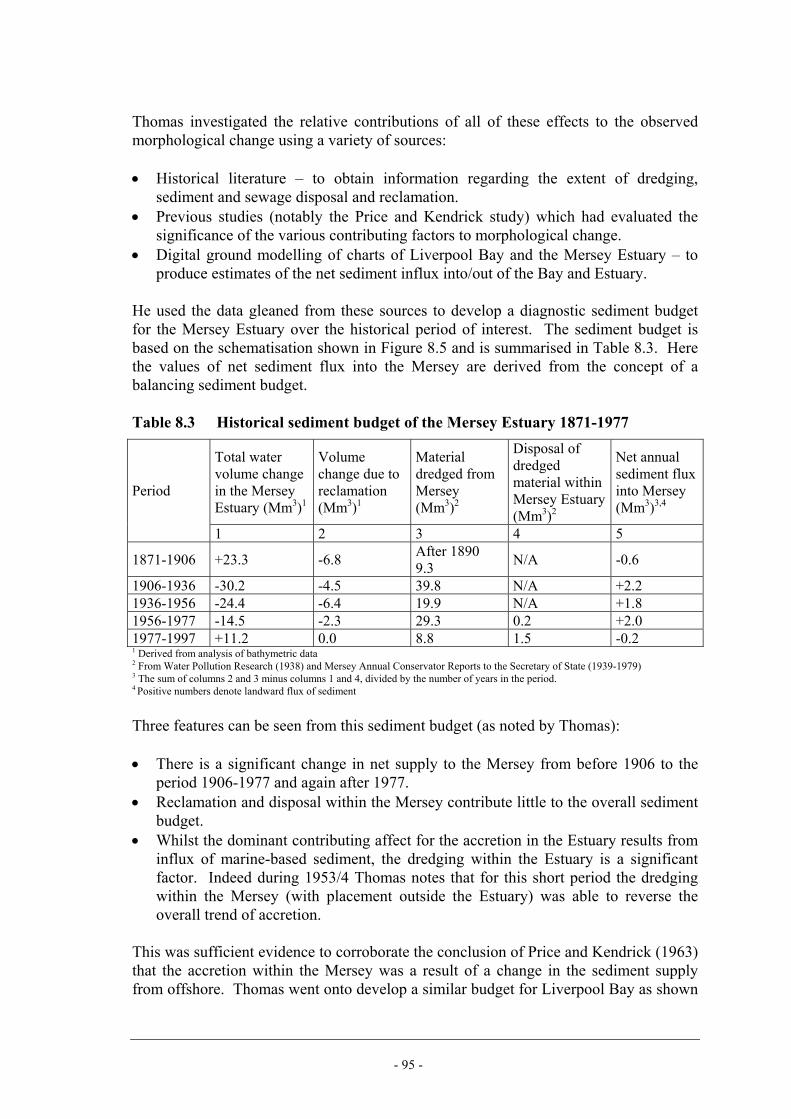
- 95 -

Thomas investigated the relative contributions of all of these effects to the observed morphological change using a variety of sources: • Historical literature – to obtain information regarding the extent of dredging,

sediment and sewage disposal and reclamation. • Previous studies (notably the Price and Kendrick study) which had evaluated the

significance of the various contributing factors to morphological change. • Digital ground modelling of charts of Liverpool Bay and the Mersey Estuary – to

produce estimates of the net sediment influx into/out of the Bay and Estuary. He used the data gleaned from these sources to develop a diagnostic sediment budget for the Mersey Estuary over the historical period of interest. The sediment budget is based on the schematisation shown in Figure 8.5 and is summarised in Table 8.3. Here the values of net sediment flux into the Mersey are derived from the concept of a balancing sediment budget. Table 8.3 Historical sediment budget of the Mersey Estuary 1871-1977

Total water volume change in the Mersey Estuary (Mm3)1

Volume change due to reclamation (Mm3)1

Material dredged from Mersey (Mm3)2

Disposal of dredged material within Mersey Estuary (Mm3)2

Net annual sediment flux into Mersey (Mm3)3,4

Period

1 2 3 4 5

1871-1906 +23.3 -6.8 After 1890 9.3 N/A -0.6

1906-1936 -30.2 -4.5 39.8 N/A +2.2 1936-1956 -24.4 -6.4 19.9 N/A +1.8 1956-1977 -14.5 -2.3 29.3 0.2 +2.0 1977-1997 +11.2 0.0 8.8 1.5 -0.2 1 Derived from analysis of bathymetric data 2 From Water Pollution Research (1938) and Mersey Annual Conservator Reports to the Secretary of State (1939-1979) 3 The sum of columns 2 and 3 minus columns 1 and 4, divided by the number of years in the period. 4 Positive numbers denote landward flux of sediment Three features can be seen from this sediment budget (as noted by Thomas): • There is a significant change in net supply to the Mersey from before 1906 to the

period 1906-1977 and again after 1977. • Reclamation and disposal within the Mersey contribute little to the overall sediment

budget. • Whilst the dominant contributing affect for the accretion in the Estuary results from

influx of marine-based sediment, the dredging within the Estuary is a significant factor. Indeed during 1953/4 Thomas notes that for this short period the dredging within the Mersey (with placement outside the Estuary) was able to reverse the overall trend of accretion.

This was sufficient evidence to corroborate the conclusion of Price and Kendrick (1963) that the accretion within the Mersey was a result of a change in the sediment supply from offshore. Thomas went onto develop a similar budget for Liverpool Bay as shown

- 96 -

in Table 8.4. Here the values of net sediment flux into Liverpool Bay are derived from the concept of a balancing sediment budget. Table 8.4 Historical sediment budget of Liverpool Bay 1904-1977

Total water volume change in Liverpool Bay (Mm3)1

Dredging in sea channels (Mm3)2

Disposal of dredged material within Liverpool Bay (Mm3)2

Sediment transported into Mersey Estuary (Mm3)1

Net annual sediment flux into Bay from offshore (Mm3)3,4

Period

1 2 3 4 5 1904-1933 +163 110 140 65.4 +6.6

1933-1977 -203 90 131 76.4 -2.25 1 Derived from analysis of bathymetric data 2 From Water Pollution Research (1938) and Mersey Annual Conservator Reports to the Secretary of State (1939-1979) 3 The sum of columns 1, 2 and 4 minus column 3, divided by the number of years in the period. 4 Positive numbers denote landward flux of sediment 5 Thomas’s thesis features a typo here – this is the correct value.

The sediment budget for Liverpool Bay was far more imprecise owing to less bathymetric data and uncertainty regarding whether all of the material dredged from the Mersey was placed back within the Liverpool Bay system or whether a proportion of it was placed outside of the system (as reflected in Table 8.3). However the Table indicates that the main difference between the 1906-33 and 1933-1977 periods as regards the overall budget is the supply of sediment to Liverpool Bay from offshore. A more detailed examination of changes in Liverpool Bay showed significant erosion of Great Burbo Bank (to the west of the navigation channel) suggesting that this was the specific source of much of the sediment entering the Mersey. Thomas then used 2D and 3D modelling to hind-cast the annual flux of sediment into the Mersey as a result of the spectra of wave and tidal conditions for different historical times – before, during and after the morphological evolution, and found in broad terms that the modelling reflected the changes in sediment transport obtained from the sediment budget. On the basis of these results Thomas found that the changes to ebb and flood tide hydrodynamics In Liverpool Bay caused by the training walls increased the supply of sediment to the mouth of the estuary. This increased sediment supply was then transported landward by the near bed residual current in the Mersey (caused by gravitational circulation). This result concurs with the conclusion of Price and Kendrick (1963) based on physical modelling. Additionally Thomas’ results showed that as the estuary attained approached its new equilibrium the changes in estuary morphology resulted in reduced landward transport. 8.7 Use of a sediment budget model to aid impact assessment in the

Stour/Orwell (HR Wallingford, 2001) As part of the investigative studies for the Environmental Impact Assessment associated with the proposed 1998-2000 deepening of the approaches to Felixstowe Port (HR Wallingford, 1998) HR Wallingford developed a sediment budget for the Stour/Orwell Estuary system. This sediment budget was slightly revised and updated for a subsequent study for the Environmental Impact Assessment associated with the proposed container terminal development at Bathside Bay, Harwich (HR Wallingford, 2001).

- 97 -

Figure 8.6 shows the Stour/Orwell system and Figure 8.7 shows the schematisation of the system used in the sediment budget analysis. Both estuaries are relatively short in length (around 20km including the Harbour) with a 3.6m mean spring tidal range and very little freshwater flow (both of the order of 1m3/s with a negligible sediment input). The principle source of sediment is from offshore, in particular the near shore coast to the east of the Harbour mouth. The intertidal areas within the Stour Estuary and the lower Orwell Estuary are experiencing net erosion which has been continuing for some time, arguably throughout most of the 20th century. The sediment budget was developed using an approach based on the concept of two types of behaviour – deposition during calm periods and erosion during wavy periods. During calm periods sediment enters the estuary from marine sources and settles on intertidal areas. During erosion periods, waves and currents cause erosion of intertidal areas resulting in the seaward advection of eroded sediment. Most of this sediment is lost from the estuary system on the ebb-tide but a proportion of this sediment returns to the estuary and resettles on intertidal areas. This behaviour can be expressed by the following equation,

( ) DWCE −−= 1 where E is the net erosion of intertidal areas, D is the (gross) deposition on inter-tidal areas from marine import of material; W is the mass of material eroded from inter-tidal areas in the estuary system; C is the proportion of inter-tidal sediment resuspended by waves and re-depositing on intertidal areas; E, the net erosion, was derived from analysis of detailed bathymetric data sets. C, the proportion of wave-eroded material resettling onto intertidal areas, was derived from calibrated numerical sediment transport modelling. D, the gross deposition, is dependent on the overall supply of sediment to the system, Msys , and on the amount of sediment that is removed from the system by dredging, Mdredge . D was calculated from calibrated sediment transport modelling but adjusted to account for options in the management of dredging and disposal by assuming D is proportional to Msys-Mdredge. In particular this allowed the effect of disposal of water column recharge in the estuary (instead of offshore placement) to be examined. W, the amount of wave erosion from intertidal areas was derived using the observed estimate for E and values for C and D gained from numerical modelling. Once derived this value was assumed to be constant except where intertidal was reclaimed, whereupon W was adjusted proportionally with the intertidal area. The results of the sediment budget analysis are summarised in Table 8.5. The table shows a historical increase in the erosion rate in the Stour and a reduction in the rate of accretion in the Orwell. The proposed Bathside Bay development was predicted to enhance this historical trend. An additional result of the sediment budget analysis was the sensitivity of the system response to changes in the management of dredging and disposal.

- 98 -

Table 8.5 Summary of predicted changes to intertidal sediment budget Calculated net erosion, E (tonnes, from bathymetric analysis)

Deposition on intertidal areas, D (tonnes)

Wave erosion W (tonnes)

Proportion of wave-eroded material re-depositing on intertidal areas, C

Predicted net erosion, E (tonnes)

Period

Stour Orwell Stour Orwell Stour Orwell Stour Orwell Stour Orwell 1976 573,000 204,000 750,000 177,000 0.046 0.081 143,000 -41,000 1986

540,000 192,000 750,000 177,000 0.030 0.057 187,000 -25,000

1997 180,000 -24,000 529,000 188,000 750,000 177,000 0.054 0.070 Post Approach Channel Deepening

533,000 189,000 750,000 177,000 0.057 0.064 174,000 -24,000

Post Bathside Bay Development

492,000 181,000 720,000 177,000 0.053 0.068 189,000 -17,000

Note that sea level rise was not taken account of in the sediment budget. This is because sea level rise (of the order of 1-2mm/yr) is small compared to the ongoing rate of intertidal erosion (in the region of 13mm/yr). 8.8 Best practice in sediment budget analysis 8.8.1 Introduction The creation of a sediment budget is an approximate balance that can be carried out on a number of scales - local, within an obvious control volume such as a length of coast or estuary, or on a wider regional basis. The relative importance of the dominant sediment transport mechanisms can be assessed at any or all of these scales depending on the characteristics of the study area. It is clear from the examples shown above that the method is a data rich approach but this should not prevent the method being used at all stages of a study to: • aid the synthesis of all the different data available about an estuary; • identify the main sediment transport mechanisms: • identify (through the concept of a balancing budget) the relative contribution of a

mechanism or source or sink that there is no information for. As better and more plentiful information becomes available the quality and reliability of the sediment budget increases. In this sense the creation of a sediment budget is an iterative process. All of the three example sediment budgets presented above were improved from previous estimates constructed in earlier studies. The sediment budget studies presented above highlight the requirement for exhaustive review of historical literature, detailing the extent of any morphological change, engineering works, reclamation, dredging and disposal. Without this exhaustive review any sediment budget developed for an estuary is likely to be flawed.

- 99 -

The examples shown above of the Humber, Mersey and Stour/Orwell indicate that sediment budget analysis falls into two different types: • The first type is associated with estuaries undergoing significant morphological

change (e.g. the Stour/ Orwell and Mersey throughout the 20th century). In these estuaries sediment budget analysis is less about the trend in an estuary and more about establishing the mechanisms by which change is occurring. In such estuaries the influence of sea level rise may be “swamped” by greater natural/or man-made influences over the short to medium term and the use of geological methods to evaluate future trends may not be relevant.

• The second type is associated with estuaries where the trends of morphological change are not obvious (e.g. the Humber) and the morphological trends imposed by sea level rise are thus significant. In such estuaries the techniques of accommodation space and geological assessment of sediment are assessment tools which are likely to be required to build up the overall picture of the sediment budget. By definition, because the trends are less obvious the uncertainty in the assessment of trends will usually be greater than in the type 1 estuaries above.

As noted by Townend and Whitehead there are two ways in which a sediment budget can be constructed, either, • by defining the changes in volume bounded by surfaces within a control volume to

give a volume balance. This works well for non-cohesive shores where the amount held in the water column is low and the material types throughout the control volume are similar; or,

• by defining the exchanges in mass to and from the water column to give a mass balance. This approach makes more sense where large amounts of sediment are resident within the water column.

Typically, however, data are available as a mix of volume changes and mass exchanges. Hence it is necessary to convert from volume changes to mass exchange (or vice versa) which requires data or an expert estimate of the likely density of the sediment on the sea bed. The density of the bed will vary spatially according to the environmental characteristics – e.g. energetic or calm, intertidal or subtidal. While a combination of expert assessment and data is normally sufficient for providing a reasonable estimate of sea bed density it should be recognised that there will be significant uncertainty in the choice of density used. 8.9 Steps in building a sediment budget 1. Is there enough reliable information to build a sediment budget? (e.g. observations

and well-calibrated numerical model results). 2. Schematise the estuary system into a simple flow chart. Try to devise a

schematisation which crystallises the focus of the analysis most simply and succinctly.

3. Choose the units of the sediment budget – tonnes/year is usually a good option. 4. Choose whether the budget is to be in terms of sand and/or mud. In practice the

mud sediment budget and the sand sediment budget can be developed independently though it may not be necessary to complete both for the sediment budget.

- 100 -

5. Evaluate the most straightforward inputs to the sediment budget first. These are often, • the volume of sediment in the system (which can be derived from suspended

sediment concentration measurements and the volume of the estuary from charts);

• the fluvial input to the system (which can be derived from fluvial discharge and concentration). In some situations it may be appropriate to take a reasonable first estimate for the fluvial sediment input as zero.

• The morphological trend (derived from comparison of bathymetric data). 6. Some sediment budget inputs can be very difficult to derive from observations - e.g.

net flux from/to the sea in wide estuaries and the extent of erosion of intertidals resulting from wave action – and so it may be best to derive these values by balancing the budget and providing data for all the other budget contributions. If this is not possible then the derivation of these contributions may require in-depth analysis, numerical modelling of sediment transport and/or further data collection to determine the sediment contributions.

7. With the possible exception of the contributions discussed in Step 6, try and quantify all of the sediment budget contributions presented in Table 8.2. Do not neglect the effects of dredging and disposal and treat all information regarding dredging and disposal as being estimates with considerable inherent uncertainty.

8. Build iteratively – start on the basis of the available data and gradually improve the sediment budget as knowledge of the system and better data becomes available. Try and independently examine the veracity (or at least plausibility) of each of the sediment budget components using back of the envelope calculations, comparison with other similar estuaries, anecdotal information, etc.

9. Undertake a thorough search for historical data (including geological data if relevant) – old studies, anecdotal information, history of development, geology, etc. Use this historical data to improve the data in the sediment budget and to aid the understanding of the sediment budget result.

10. Once numbers are available to complete the sediment budget, assess the uncertainty in the all the contributions to the sediment budget. Is the uncertainty in the sediment budget too great to make it a meaningful budget?

8.10 Conclusions The creation of a sediment budget is an approximate balance that can be carried out on a number of scales - local, within an obvious control volume such as a length of coast or estuary, or on a wider regional basis. The relative importance of the dominant sediment transport mechanisms can be assessed at any or all of these scales depending on the characteristics of the study area. The method is highly dependent on data (derived from the field and/or modeling) and highly dependent on a thorough understanding of the historical changes in estuary morphology and anthropogenic intervention. It is very important to understand the uncertainty inherent in the development of a sediment budget as the conclusions may sometimes depend on relatively minor changes in sediment inputs to a system relative to sediment outputs from the system. In particular it is difficult to independently estimate the net input of sediment through estuary mouths with any accuracy, although sediment budget analysis is a good means of deriving this figure if all the other sediment inputs and outputs to a system are

- 101 -

known. The paper by Rosati and Kraus (1999) discusses many similar issues to those referred to in this Chapter with respect to establishing a sediment budget for coastal inlets. 8.11 References BBV, (2000) Humber Estuary Geomorphological Studies. Phase 2, Volume 1. Final Report. March 2000. Report prepared by Binnie, Black & Veatch for the Environment Agency. Cashin, J.A. (1949) Engineering Works for the Improvement of the Estuary of the Mersey, Journal of the Institution of Civil Engineers, Number 7, 1948-49, May. Cox, J. M. (2002) Southern North Sea Sediment Transport Study, Phase 2, Sediment Transport Report, Appendix 9, Report on Mineralogical Tracers, July 2002. Download from: www.sns2.org Environment Agency (2000) Humber Estuary Tidal Defences, Humber Estuary Geomorphological Studies, Phase 2, Volume 1, Report prepared for the Environment Agency by Binnie Black and Veatch, March 2000. HR Wallingford (1998) Harwich Haven Approach Channel Deepening, Impact of channel deepening on mud transport, HR Wallingford Report EX 3748, February 1998. HR Wallingford (1999) Mersey Survey 1997, Changes capacity since 1977, HR Wallingford Report IT 474, December 1999. HR Wallingford (2001) Bathside Bay Development Studies, Impact of proposed scheme on sediment transport and morphology, HR Wallingford Report EX4426, In: Supporting Document 1, Harwich Harbour Strategic Studies, Bathside Bay Tidal Works Environmental Statement, Report prepared by HR Wallingford and Posford Haskoning Ltd. for Hutchison Ports (UK) Ltd. and Harwich Haven Authority, October 2001. Nairn, R.B. and Southgate, H.N. (1993) Deterministic profile modeling of nearshore processes. Part 2. Sediment transport and beach profile development. Coastal Eng., 19, 57 - 96. O’Connor, B. A. (1987) Short and long term changes in estuary capacity, Journal of the Geological Society, London, 144, pp187-195. Price, W. A. and Kendrick, M. P. (1963) Field and model investigations into the reasons for siltation in the Mersey Estuary, Proceedings of the Institute of Civil Engineers, pp473-517. Pye, K. and Neal, A. (1994) Coastal dune erosion at Formby Point, north Merseyside, England: Causes and mechanisms. Mar. Geol., 119, 39-56. Rees, J. G., Ridgway, J., Ellis, S., Knox, R. W. O., Newsham, R. and Parkes, A. (2000) Holocene Storage in the Humber Estuary, In: I Shennan, J E Andrews (eds), Holocene

- 102 -

land-ocean interaction and environmental change around the North Sea, Special Publication 166, London: Geological Society, 2000, pp119-143. Rosati, J. D. and Kraus, N. C. (1999) Advances in coastal sediment budget methodology – with emphasis on inlets. Shore and Beach, 67 (2 & 3), 56-65. Thomas, C. (2002) The application of historical data and computational methods for investigating causes of long term morphological change in estuaries: A case study of the Mersey Estuary, UK, PhD Thesis, Oxford Brookes University, February 2002. Townend, I. and Whitehead, P. (2003) A preliminary net sediment budget for the Humber Estuary, The Science of the Environment, 314-316, pp755-767. Woodrolfe, P. L., Tsimplis, N., Flather, R. A., Shennan, I., (1999) A review of the trends observed in British Isles mean sea level data measured by tidal gauges, Geophysics Journal International, 136(3):651-670. Water Pollution Research Board (1938) Effect of discharge of crude sewage into the estuary of the River Mersey on the amount and hardness of the deposit in the estuary, Water Pollution Research Technical Paper Number 7, Department of Scientific and Industrial Research, HMSO.

Figure 8.1 Humber Estuary

- 103 -

Estuary

Intertidal

Subtidal

Saltmarsh

Cliff erosion

Sea

River

Suspended load

Total (average) mass insuspension = 1.2x106 tonnes

Net marine input= 100 tonnes/tide

Deposition= 230 tonnes/tide

Deposition= 200 tonnes/tide

Deposition= 11 tonnes/tide

Deposition= 7 tonnes/tide Net fluvial input

= 335 tonnes/tide

AverageTidal flux= 1.2x105

tonnes/tide

Figure 8.2 Sediment budget for the Humber Estuary

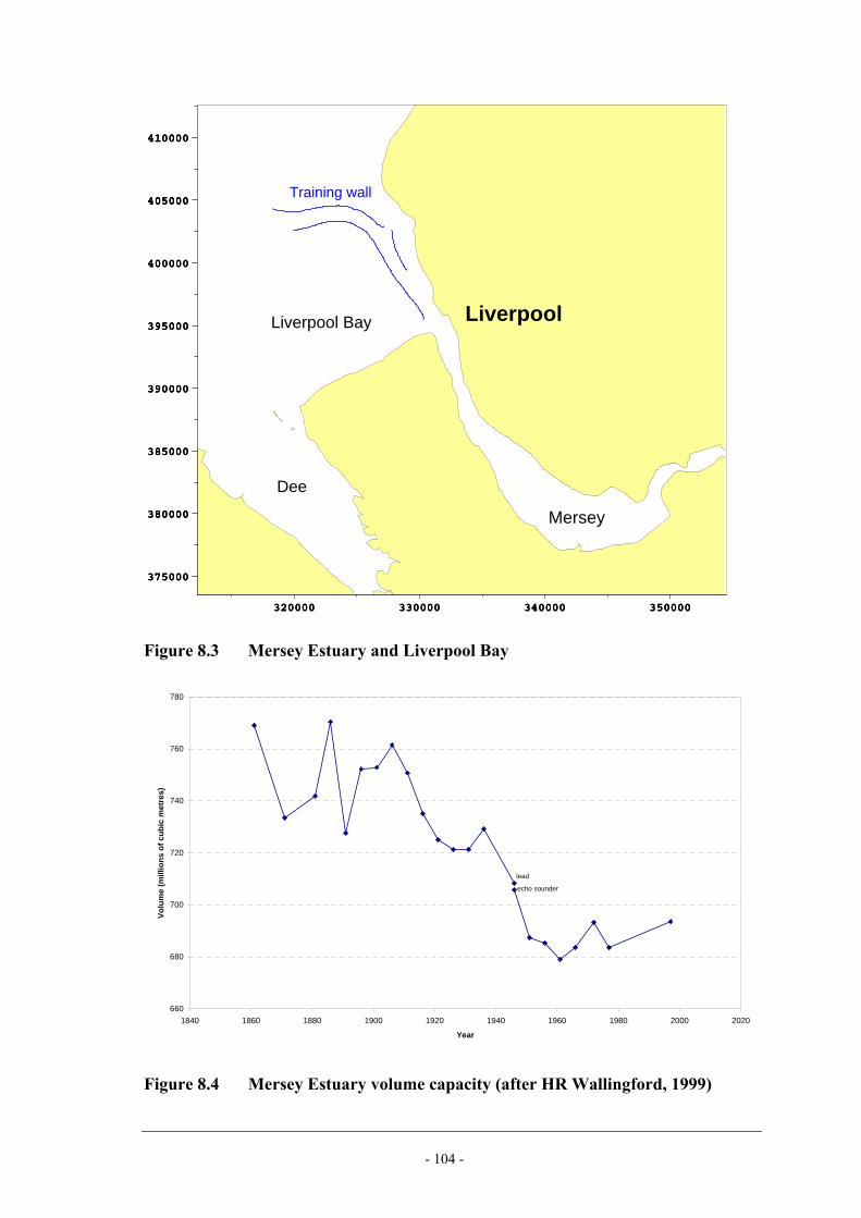
- 104 -

375000

380000

385000

390000

395000

400000

405000

410000

320000 330000 340000 350000

375000

380000

385000

390000

395000

400000

405000

410000

320000 330000 340000 350000

375000

380000

385000

390000

395000

400000

405000

410000

320000 330000 340000 350000

Training wall

Liverpool

Mersey

Dee

Liverpool Bay

Figure 8.3 Mersey Estuary and Liverpool Bay

660

680

700

720

740

760

780

1840 1860 1880 1900 1920 1940 1960 1980 2000 2020

Year

Volu

me

(mill

ions

of c

ubic

met

res)

lead

echo sounder

Figure 8.4 Mersey Estuary volume capacity (after HR Wallingford, 1999)

- 105 -

Liverpool Bay

Mersey Estuary

Irish Sea

Dredging

Disposal

Disposal

DisposalReclamation

Change involume

Liverpool BaySediment budget

Mersey EstuarySediment budget

Figure 8.5 Schematised systems for Mersey Estuary and Liverpool Bay sediment budgets

- 106 -

Figure 8.6 Stour and Orwell Estuary System

- 107 -

Sea

Intertidal

Stour channel

Harbour

Orwell channel

Intertidal

Offshoreplacement

Waveerosion

Waveerosion

Depositionduring calmperiods

Depositionduring calmperiods

Import Export

Deposition indredged areas

Figure 8.7 Schematisation of the Stour/Orwell Estuary System

- 108 -

- 109 -

9. ROLLOVER MODEL

Method Indicator Bottom-Up Hybrid Top-Down

YES 9.1 Background The Rollover model is a concept regarding a general tendency of estuary response to sea level rise which can be then quantified using application of other top-down approaches such as regime theory. Its basis can be attributed in part to Allen (1990) but has since been developed by Pethick (2000). The basic concept is that as sea level rise occurs an estuary will transgress longitudinally landwards and vertical upwards thus keeping its position in the tidal frame. 9.2 Overview of technique Table 9.1 Summary Table

Issue Summary

Description Stratigraphic roll-over describes one possible outcome of the morphological and sedimentological response of an estuary to sea level rise. The Roll-over “model” is the tendency for erosion of the upper inter-tidal in the outer estuary and transport of derived sediment to the estuary head where its inter-tidal deposition results in headward transgression.

Temporal Applicability Long-term

Spatial Applicability Whole estuary

Links with Other Tools This method is more of an observation of a natural tendency in some estuaries and the Rollover method therefore requires other tools to evaluate how the process of Rollover might occur.

Data sources As a general concept no data is required. To find evidence of this process for a specific estuary requires considerable bathymetric and archaeological evidence.

Necessary Software Tools / Skills

None except those normally associated with EGA

Typical Analyses Prediction of the long term effects of sea level rise

Limitations The tool is a general concept that does not apply to every estuary and the tool does not provide a means of evaluating how this might occur in practice.

Key Issues Estuarine response to sea level rise may take the form of: • Drowning; or • Vertical sedimentation in pace with sea level rise; or • Vertical sedimentation and horizontal translation of the estuarine morphology

(roll-over). The type of morphological response depends on sediment availability and rate of sea level rise. Inter-tidal drowning results when sediment availability is low or sea level rise rates are high. Availability of marine-sourced sediment may allow inter-tidal warping with no increase in tidal prism and no spatial translation. Restricted external sediment sources results in internal redistribution of sediment. Increased wave propagation in outer estuary results in inter-tidal erosion. Increased water depths increases flood dominance and thus landward sediment transport resulting in headward transgression.

- 110 -

9.3 The Roll-over hypothesis The vertical morphological response of an estuary to sea level rise is primarily governed by the rate of rise and the availability of sediment. Rapid sea level rise coupled with low sediment availability is likely to result in progressive drowning of the estuary, while slower rates of sea level rise coupled with abundant sediment may allow the estuary to ‘warp up’ so keeping pace with sea level changes. A key question however is whether these morphological changes are accompanied by horizontal movement of the estuary relative to the coast. Three possibilities may be envisaged: • Drown in-situ; • Warp up to maintain levels relative to sea level but without moving in space; and, • Warp up and horizontal translation landwards. It is this latter scenario, that of an upwards and landwards translation of the estuary in response to sea level rise, that has been referred to as the roll-over hypothesis (Pethick 2000). Although evidence from some UK estuaries appears to support the hypothesis, its general applicability is difficult to gauge, perhaps due to the variations in sediment supply between estuaries on the UK coast. The roll-over hypothesis was initially developed by Allen (1987-1990) who, in a series of papers, described the morphology of the inter-tidal sediments of the Severn, including that of the reclaimed marshes. The most important characteristic is the stepped nature of the marsh surface morphology. Allen notes that the mean surface elevation of the older, reclaimed marshes, dating from pre-medieval period, becomes progressively higher as their age decreases; while the more recent un-reclaimed salt marshes exhibit the opposite tendency, that is their surface elevation is reduced on the younger marshes so that they exhibit a series of downward steps towards the estuary. Allen considers this complex sequence to be a result of the combined effects of sea level rise and the landward transgression of the estuary. Marsh surface elevations are controlled by the tidal maxima which rise in elevation along the longitudinal axis of the estuary (Figure 9.1). The transgression of the estuary caused by sea level rise involves both an upward and a landward movement of this inclined plane and, under certain combinations of these two rates, the tidal maximum will fall at any given location. Although in the pre-medieval period the resultant movement of tidal maxima was upwards leading to a temporal increase in salt marsh elevations, more recently the outcome has apparently been a fall in high water levels at any given point as the landward transgression has increased relative to sea level rise. This has led to the progressive reduction in marsh surfaces forming the characteristic stepped marsh surfaces reported by Allen (1990). The importance of this model lies not only in the impact of sea level on salt marsh morphology, but also in the fact that the entire estuary is shown to be transgressing landwards as a response to sea level rise. Allen suggested that this transgression was brought about by erosion of salt marsh sediment at the mouth of the Severn and their subsequent transport landwards where they are deposited in the inner estuary. He called this process ‘stratigraphic roll-over’.

- 111 -

Mouth

Head

High Water Levels

Form of tidal wave translates landwardswith estuary

Water levels reduceWater levels increase

Sealevelrise

Figure 9.1 Schematic diagram to show transgression of tidal wave in an estuary due to sea level rise Most estuaries in England and Wales have experienced continuous sea level rise over the Holocene period. Over the past 2000 years the rate of rise has been in the order of 1mm to 2mm per year (Shennan & Horton 2002). As a result, estuarine morphology has been adjusting continuously to these imposed changes so that observed estuarine behaviour represents a continuous adaptation to sea level rise. Observed behaviour is difficult to summarise but includes erosion of upper inter-tidal areas at estuarine mouths resulting in salt marsh recession (see for example Burd 1992; Cooper et al 2000) and extensive salt marsh deposition at estuarine heads forming narrow meandering channels. It must also include the stepped-down sequence of salt marsh observed by Allen (1990) in the Severn estuary, although these have not been reported elsewhere. 9.4 Analysis of system response to sea level rise A large amount of research has been undertaken into the impact of sea level rise on coastal environments, especially with reference to the Dutch tidal inlets. It has been of particular interest to explore how different rates of sea level rise might result in the different system responses of rollover, keeping pace or drowning as discussed in Section 9.3 and whether simplified models of coastal and inlet systems might provide the basis for exploring the answers to these questions. A conceptual approach to sea level rise in coastal environments has been developed which considers the interaction between different parts of the coastal system at the macro level (Cowell et al, 2003). In order to remove the shortcomings of bottom-up models from studying long term system response these authors concentrated on the response of large-scale or aggregated coastal features. This resulted in a framework for developing a conceptual model of interaction between inlet, delta and the surrounding coast based on representation of simple box elements and simple descriptions of interaction between these elements. The approach was developed into the ASMITA model (Stive et al, 1998). The ASMITA type model, as discussed in Chapter 6, is outside the scope of this report but in this section we discuss the basis for the ASMITA model in its simplest form and show how a relatively simple analysis can reveal valuable insights in future long term macro-scale evolution.

- 112 -

The ASMITA model approach considers the interaction between inlet, delta and the surrounding coast (Figure 9.2). For simplicity we will consider only the interaction between a channel and the surrounding coast (essentially lumping the delta and tidal flats into the channel element). The erosion/deposition in the channel is given by the simplified sediment transport equation (Galapatti and Vreugdenhil, 1985),

Figure 9.2 Schematisation of coastal system used by ASMITA model

( )ccAwtV

ebs −=∂∂ (9.1)

Where V is the volume of water in the channel; ws is the exchange of sediment between the bed and the overlying water; Ab is the surface area of the channel; c is the sediment concentration in the channel (in this case a volumetric concentration) and ce is the equilibrium sediment concentration. The exchange of water between the channel and the outside coast is given by δ and therefore by continuity,

( )ccAwc ebs −=δ (9.2) The equilibrium sediment concentration is the sediment concentration that would result in no overall morphological change. The ASMITA approach assumes that a long-term equilibrium concentration exists, which we will term cE , and that the equilibrium concentration in the channel is a function both of cE and of changes in velocity in the channel. It is assumed that the proportional change in the average velocity in the channel can be characterised by (VE/V)r where VE is the original equilibrium volume and r is an empirical constant in the region of 2. This results in,

rE

Ee VV

cc ⎟⎠⎞

⎜⎝⎛= (9.3)

This assumption has the effect of increasingly making the channel a sink as the channel volume increases and increasingly making the channel an exporter of sediment as the channel reduces in volume. The mechanisms by which this process could occur in practice are discussed below in Sections 9.5 to 9.11. With the addition of sea level rise at a constant rate of dt

dζ the Equation (9.1) becomes (Stive and Wang, 2003),

flat

channel

delta coast coast

- 113 -

dtdA

VV

AwCAw

tV

b

rE

bs

Ebs ζδ

δ+⎟

⎟⎠

⎞⎜⎜⎝

⎛−⎟

⎠⎞

⎜⎝⎛

+=

∂∂ 1 (9.4)

When sea level rise is constant it can be shown that a dynamic equilibrium can be established (whereby V tends to a constant but the channel is changing in its elevation with respect to a fixed datum at the rate of sea level rise) and that,

r

Es

bs

ESL

CwAw

dtd

VV 1

.1 ⎟⎟⎠

⎞⎜⎜⎝

⎛ +−

=

δδζ

(9.5)

where VSL is the equilibrium volume in response to sea level rise and VE is the equilibrium volume without sea level rise. This result shows that a channel system experiencing sea level rise can in general keep pace with sea level rise because, as the volume of the channel increases with the rise in water level the channel increasingly will become a sink for local sediment and the rate of vertical infill will approach that of the rise in water level. Note that this methodology establishes the equilibrium is based on the size of the system, the sediment supply, the sediment type and the rate of sea level rise (see Section 9.9.3). However, the channel can only keep pace with sea level rise if the rate of sea level rise is below the critical value given by,

bs

Es

AwCw

dtd

+=

δδζ (9.6)

This analysis suggests that rollover will occur in some form for rates of sea level rise less than that given by Equation (9.6) and drowning will occur for rates of sea level rise higher than this. Estimates made by Van Goor et al (2002) for the critical rate of sea level rise for tidal inlets in the Netherlands were of the order of 10-20mm/yr. 9.5 Tidal prism changes In a rectangular channel cross-section, a rise in sea level accompanied by an equivalent rise in the tidal frame would not result in any change in tidal prism. In a trapezoidal channel, however, sea level rise will be accompanied by an increase in water depth at the channel margins. In general, but with details related to the actual cross-section shape, this may result in an increase in tidal prism that will be approximated by the product of inter-tidal area and the amount of sea level rise. The resultant increase in tidal power within the estuary will lead to an increase in the downstream ‘flare’ in estuary width, which might be increased by erosion of salt marsh edges and upper inter-tidal surfaces. This erosion may release sufficient sediment to allow deposition at the head of an estuary, thus satisfying the stratigraphic roll-over condition. However, any increase in tidal prism may only be an initial and temporary response to sea level rise. If sufficient sediment is available from external sources, then inter-tidal areas could warp-up (i.e. accrete with sediment) to keep pace with sea level rise. If this is the case then

- 114 -

the estuary would merely move upwards and/or landwards without morphological modification. 9.6 Headward transgression Landward transgression of an estuary cannot be unambiguously derived from either tidal energetics or simple geometrical considerations. Assuming that the tidal range remains constant, an increase in mean sea level would result in a landward transgression of the high water extremity at the estuary head but this will be constrained by the valley slope as shown in Figure 9.1. Providing sufficient sediment is available, such a headwater transgression may be accompanied by sedimentation on the inter-tidal flats, forcing landwards the inner margin of salt marshes. The rate of transgression of salt marsh will again depend upon the valley (accommodation) slope as well as the rate of sea level rise and the deposition rate. 9.7 Mouth transgression Defining the mouth of an estuary is in itself problematic (see Section 5.14.3). In many cases the hydrodynamic mouth cannot be simply defined by extrapolating the line of the adjacent coast, even where this is well delineated, since tidal delta morphology may extend for considerable distance seaward and landward of this. Long term movement of the highly volatile tidal delta morphology is difficult to observe and measure and no data are available to show if landward transgression of this feature does take place. Another possibility is that the mouth of the estuary can be defined by a break in slope of the high water surface, such as that shown by the Humber estuary (Figure 9.3). However, in many cases the high water surface within the estuary merges with that of the open sea without any break in slope (e.g. the Blackwater Figure 9.4 and Severn Figure 9.5). 9.8 Longitudinal transgression If the problem of definition of the estuary mouth is ignored then some trial experiments demonstrate the difficulty of generalising as to the outcome of sea level rise on estuary morphology. Figures 9.3 to 9.5 show the observed high water surface along the axis of three estuaries, Humber, Blackwater and Severn. Superimposed on this surface is a post-sea level rise surface that has been moved 0.1m upwards and 10km landward in all three cases, thus simulating approximately 100 years of sea level rise at 1mm per year and assuming a transgression rate of 10m per year. This movement assumes that sea level rise merely results in the landward and upward transgression of these surfaces, without any modification in their longitudinal shape.

- 115 -

Humber HWM

2.5

3

3.5

4

4.5

5

0 20000 40000 60000 80000 100000 120000 140000

Distance (m)

HW

M E

leva

tion

(mO

D)

Pre-SLRPost SLR

Figure 9.3 High water surface for the Humber estuary pre- and post sea level rise of 0.1m

Blackwater HWM

1.5

1.7

1.9

2.1

2.3

0 10 20 30 40

Distance (km)

HW

M E

leva

tion

(mO

D)

Pre SLRPost SLR

Figure 9.4 High water surface for the Blackwater estuary pre- and post sea level rise of 0.1m

Severn HWM

4

4.5

5

5.5

6

0 20 40 60 80 100

Distance (km)

HW

M E

leva

tion

(MO

D)

Pre SLRPost SLR

Figure 9.5 High water surface for the Severn estuary pre- and post sea level rise of 0.1m Comparison of the pre-and post sea level rise high water surfaces show a wide range of adjustments even for these three cases. The Humber experiences a substantial fall in tidal maxima in the outer estuary but a rise in the inner channel; the Blackwater exhibits a slight decrease in high water in the outer estuary but a rise elsewhere while the Severn shows a fall in high water elevations along its entire length. These differences are, of course, produced by the contrasting shapes of the high-water long profiles, since convex

- 116 -

profiles are more likely to result in falling water levels in the outer estuary after sea level rise as shown in Figure 9.1. The form of the tidal surface is itself largely a product of estuarine morphology and therefore will change as the transgression takes place. Nevertheless it is clear that under certain circumstances high water maxima may fall as sea levels rise and that this is especially so in the Severn Estuary lending some support to Allen’s ‘step-down’ hypothesis. It is not apparent however from these examples why a rise in water level in itself should result in erosion in the outer estuary and deposition in the inner estuary. It may be concluded that if sea level rise does result in stratigraphic roll-over, then some additional processes must be present other than changes in water level, a possibility that is further discussed in Section 9.9. 9.9 Waves and tidal asymmetry 9.9.1 Waves and water depth Increased mean sea level at the mouth of an estuary allows waves generated at sea to propagate further into the estuary. This results in accelerated erosion of the upper inter-tidal areas of the outer estuary and release of sediment. Further into the estuary, waves are fetch limited but here too increased water depths reduce energy dissipation on upper inter-tidal areas so allowing wave action to erode the upper inter-tidal and salt marsh edge, again releasing sediment. The morphological response to such a change in wave energy levels is to widen the entire estuary channel and, in general, relatively more so in the outer estuary channel. As the elevation of the upper inter-tidal surfaces is reduced so wave energy dissipation is also reduced and a positive feedback is generated which is further exacerbated by the increase in tidal prisms that develops as the inter-tidal area widens. This increased tidal prism will generally result in higher tidal velocities and bed stress increases with resultant increased sediment movement. The development of positive feedback connecting inter-tidal erosion with increased energy levels is clearly untenable in the long term. Since both inter-tidal mudflats and salt marshes exist in estuaries despite 6000 years of Holocene sea level rise, it is demonstrable that some further process must intervene. This process may be that of tidal asymmetry. 9.9.2 Tidal asymmetry and roll-over Increased water depth in the estuary resulting from sea level rise, together with the erosion of upper inter-tidal tidal areas and the recession of salt marsh edges, leads to modification in estuarine cross section morphology and therefore to tidal asymmetry. Dronkers (1998) showed that flood dominant tides developed where wide cross sections with low inter-tidal areas and shallow sub-tidal channels were present in an estuary. In such cross sections the mean water depth at high tide exceeds that at low tide so that the celerity of the tidal wave crest at high water overtakes the trough at low water and tidal stage, discharge and velocity all become flood dominant. Sediment derived from erosion of the upper inter-tidal areas in the outer estuary is moved landward by these flood dominant processes. Increased water depths in an estuary therefore lead to erosion of the upper inter-tidal surfaces and a change in cross section morphology, leading to enhanced flood dominance and transfer of released sediment to the inner estuary. The inner estuary

- 117 -

adjusts to the imposed rise in mean water levels by increasing the elevation of inter-tidal marshes. This reduces flood asymmetry so that net sediment movement into these inner estuary areas is also reduced and the centre of deposition moves seawards gradually restoring inter-tidal elevations and reducing the positive feedback effect of wave and tidal erosion. Thus the estuary as a whole responds to the impact of the positive feedback by stratigraphic roll-over that eventually modifies the entire estuary morphology and results in a dynamic equilibrium with sea level rise. Based on these arguments, it is suggested that the process of sediment release and transfer that results in stratigraphic roll-over in estuaries may be a response to the changes in wave energy distribution and tidal asymmetry that themselves are brought about by an increase in water levels within the estuary. These processes will be modified by both the rate of sea level rise and the availability of sediment from external sources to the estuary so that considerable spatial variation in estuarine response may be expected. However, over long time periods, perhaps that of the Holocene, it may be that these spatial differences are gradually reduced and that the overall stratigraphic roll-over response to Holocene sea level rise is a generic one: a proposition discussed in section 3.3. 9.9.3 Tidal asymmetry in the Holocene The initial flooding of valleys in the early Holocene would have resulted in flood asymmetry in which low inter-tidal areas were interspersed by shallow sub-tidal channels (Pethick, 1994). The net landward movement of sediment, derived mainly from marine sources that followed this initial stage would have resulted in higher inter-tidal areas and deeper sub-tidal channels leading to ebb dominance as in the estuaries on the south-east coast of the UK. Additionally an early stage in this process may be seen in some of the estuaries of the south west coast such as the Fal. Here Stapleton & Pethick (1996) showed that although low sedimentation rates in the outer estuary have failed to keep pace with sea level rise, historical records show that in the inner estuary there had been a gradual seaward progression of inter-tidal deposition starting at the headwaters and moving slowly seaward. This may be equivalent to the roll-over response outlined above for “morphologically mature” estuaries, in which the slow but steady increase in sea level over the past 2000 years or so has led to a constant re-adjustment by roll-over so that, superimposed upon the oscillations around the steady state in response to the initial massive sea level rise in the early Holocene, lies a long term trend of adjustment to the ongoing sea level rise.

- 118 -

Flood dominance

Ebb dominance-0.3-0.2-0.1

00.10.20.30.40.5

0 0.5 1 1.5 2

Time (10,000 years)

Sym

met

ry ra

tio Flood dominance

Ebb dominance

Figure 9.6 Oscillatory adjustment of tidal asymmetry following an initial rise in sea level As discussed, the superimposition of a continuous re-adjustment to sea level rise on the damped oscillation shown in Figure 9.6 may be expected to shift the balance of estuarine asymmetry towards the flood dominant so that most estuaries may be predicted to exhibit flood dominance. The rate at which morphological maturity (i.e. the target equilibrium form) is attained in an estuary depends largely upon sediment availability. In east coast estuaries where sediment availability has been high over the Holocene, morphological adjustments to the initial Holocene sea level rise, between 10,000 BP and 6,000BP, have been relatively rapid and estuaries may, after 6,000 years, be expected to approach, if not finally to have attained, tidal symmetry. In such estuaries the small, but continuous rise in sea level over the past 2,000 years may have been expected to have had only a minor impact. In these estuaries the availability of large stores of inter-tidal sediment in the outer reaches would enable rapid roll-over adjustments to be made. The suggestion is that they are in effect, held in a steady state, perhaps adjusting to sea level rise and seasonally (e.g. McCave & Frostick, 1972; O’Brien et al, 2000). In contrast, south west coast estuaries have experienced a slow adjustment to the early Holocene sea level rise and thus are relatively immature with minimal inter-tidal deposits in the outer estuaries. As a result morphological adjustments to the slow, continuous sea level rise over the past 2000 years has not resulted in stratigraphic roll-over and the estuaries are still in a flood dominant, dis-equilibrium stage. 9.9.4 Tidal prism and tidal asymmetry The distinction in response to sea level rise between mature estuaries with large sediment resources and immature estuaries with minimal inter-tidal deposits is further strengthened by the contrast in tidal prism variations. Assuming, as discussed above, that the tidal frame rises in step with sea level rise, then any increase in tidal prism in an estuary due to sea level rise is related to the increased water depths over the inter-tidal area only. In estuaries with flood dominant tidal asymmetry the ratio of inter-area to total channel surface area is small, thus tidal prism increases in these estuaries will be relatively unimportant compared to estuaries with symmetrical or ebb-dominant tides. This may result in immature estuaries such as those on the south west coast responding

- 119 -

less markedly to sea level rise than the more mature estuaries on the east coast whose morphology approaches that needed for tidal symmetry. These gross differences between estuaries in contrasted coastal environments may be paralleled by more subtle distinctions between estuaries in similar sediment environments. Asymmetry relationships are discussed in Chapter 13. 9.9.5 Future changes The predicted increase in the rate of sea level rise over the next century, coupled with a decrease in the available sediment from marine sources, will have a major impact on the extent of the roll-over process in any given estuary. On the east coast the result of increased rates of sea level rise may already be discernable, there is some evidence from the Blackwater for example which appears to be experiencing accelerated roll-over resulting in a demand for net imports of marine sediment (see Section 9.11.1). 9.10 Sea level rise and roll over prediction 9.10.1 Roll over and sediment balance The process of roll-over as a response to sea level rise is suggested as being linked to the development of tidal symmetry in estuaries. The attainment of tidal symmetry is thought to be equivalent to morphological steady state since no net movement of sediment takes place (e.g. Dronkers, 1998). In theory it is possible for a mature estuary to maintain its morphological steady state, despite increases in sea level, by internal redistribution of sediment without the need for imports from external sources. The transfer of sediment from outer estuary erosional sites to inner estuary depositional sites can result in a transgression of the entire estuarine morphology landward and upwards so that the estuary remains in equilibrium with its environment controls. It is uncertain whether this internal adjustment can be achieved during long periods of continuous sea level rise, or whether it is a theoretical model based upon a single isolated movement of sea level. The ability to maintain morphological equilibrium depends principally upon the magnitude of the change in sea level and the size of the sediment resource within the estuary, but the distance that the estuary moves in response to a given sea level change depends also upon a number of other factors such as the accommodation space (see Chapter 10 of this report) and the tidal propagation within the estuary. Two approaches to the theoretical calculation of the transgression distance are examined here: • A form modelling method (Wells & Townend, In prep) • Regime modelling (Pethick, 2000) Both approaches described here use the Humber

as a type example. Although this is one of the largest estuarine systems in England and Wales, the Humber does have the advantage of an excellent data base.

Neither approach directly predicts morphological transgression in estuaries, the first calculates the sediment balance under a number of transgression scenarios; the second calculates changes in channel width that may be expected to be related to longitudinal movement. Despite the use of these surrogates, the two methods do provide further insight into the relationship between the rates of sea level rise and morphological adjustments in the estuary.

- 120 -

Form modelling Wells & Townend (In prep) were concerned to estimate under what conditions an estuary such as the Humber might achieve steady state without any net sediment imports form external sources: the original concept of stratigraphic roll-over in which the estuary is self-sustaining. They devised an approach based on the Bruun Rule for beaches but converted to the estuarine case resulting in an expression for landward transgression, R:

⎟⎟⎠

⎞⎜⎜⎝

⎛+=

hw

sm

m bmb

dLSR

.21.. (9.7)

Where S is sea level rise, L is estuary length; dm is depth at estuary mouth; bsm is salt marsh width at mouth and bm hw is estuary channel mouth width at high water. Applying this expression to an idealised morphology of the Humber they calculated the volume of sediment that would be contained between successive surfaces as sea level rose. They found that for short transgression distances involving considerable warping (deposition) but little erosion, the estuary was in net sediment deficit so that sediment import was required. Longer transgression distances for the same vertical rise in sea level provided more extensive erosion lengths so that a net export of sediment was eventually attained. A sediment balance for the Humber was attained when transgression distances were in the region of 5m per 1mm rise in sea level. Regime modelling In contrast to the Wells & Townend approach that concentrated on roll-over sediment volumes, Pethick (2000) was concerned to estimate the transgression distance that was associated with any given rise in sea level. He used a regime approach based on the O’Brien model (e.g. Pethick & Lowe, 2000) that relates estuarine tidal prism with cross sectional area in a power function of the form:

nm aTPCA =

Where CAm is cross sectional area at the mouth, a and n are constants derived from empirical data sets, TP is tidal prism. Calibrating this equation using regression analysis of a sample of estuaries from the UK (Townend, 2005) was assumed to define the ‘ideal’ steady state form for a single estuary. For a steady state estuary and averaged over a geomorphologically significant period, it was postulated that sediment transport can be defined by a representative critical stress and that the mean depth needed to produce this critical stress could be calculated from sediment characteristics and that channel width could be derived from the steady state channel cross sectional area. Mapping the pre- and post-channel widths resulted in identification of the long-axis separation distance between similar widths and which was assumed to be analogous to the transgression distance, that is the horizontal displacement of the estuary, even though mouth and headwater were not free to move within the model.

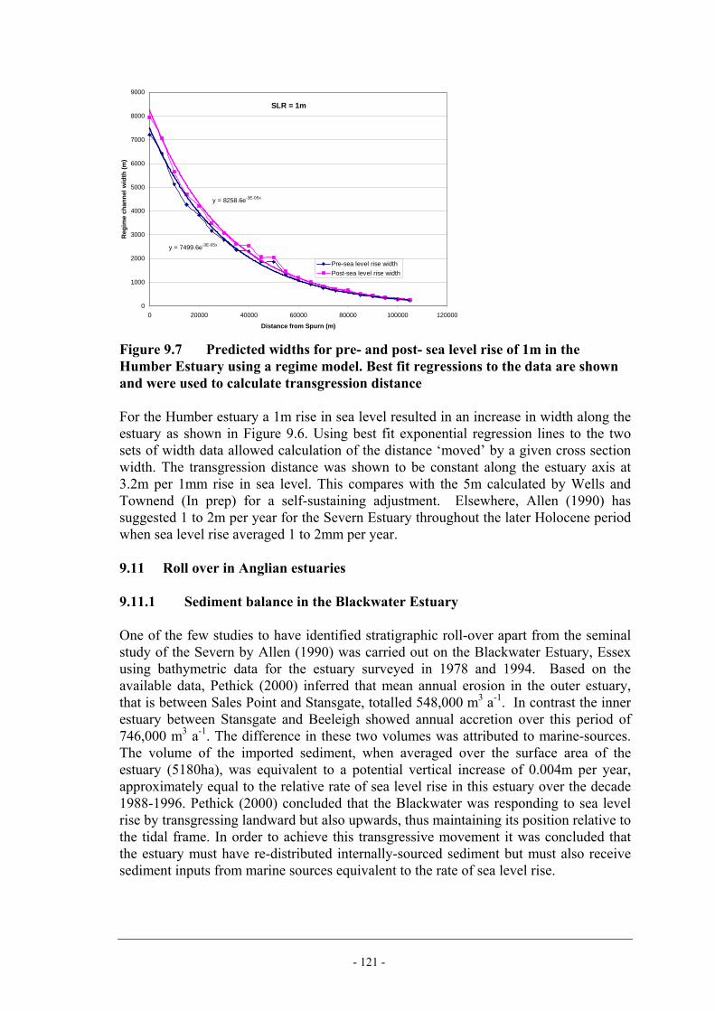
- 121 -

SLR = 1m

y = 8258.6e-3E-05x

y = 7499.6e-3E-05x

0

1000

2000

3000

4000

5000

6000

7000

8000

9000

0 20000 40000 60000 80000 100000 120000

Distance from Spurn (m)

Reg

ime

chan

nel w

idth

(m)

Pre-sea level rise widthPost-sea level rise width

Figure 9.7 Predicted widths for pre- and post- sea level rise of 1m in the Humber Estuary using a regime model. Best fit regressions to the data are shown and were used to calculate transgression distance For the Humber estuary a 1m rise in sea level resulted in an increase in width along the estuary as shown in Figure 9.6. Using best fit exponential regression lines to the two sets of width data allowed calculation of the distance ‘moved’ by a given cross section width. The transgression distance was shown to be constant along the estuary axis at 3.2m per 1mm rise in sea level. This compares with the 5m calculated by Wells and Townend (In prep) for a self-sustaining adjustment. Elsewhere, Allen (1990) has suggested 1 to 2m per year for the Severn Estuary throughout the later Holocene period when sea level rise averaged 1 to 2mm per year. 9.11 Roll over in Anglian estuaries 9.11.1 Sediment balance in the Blackwater Estuary One of the few studies to have identified stratigraphic roll-over apart from the seminal study of the Severn by Allen (1990) was carried out on the Blackwater Estuary, Essex using bathymetric data for the estuary surveyed in 1978 and 1994. Based on the available data, Pethick (2000) inferred that mean annual erosion in the outer estuary, that is between Sales Point and Stansgate, totalled 548,000 m3 a-1. In contrast the inner estuary between Stansgate and Beeleigh showed annual accretion over this period of 746,000 m3 a-1. The difference in these two volumes was attributed to marine-sources. The volume of the imported sediment, when averaged over the surface area of the estuary (5180ha), was equivalent to a potential vertical increase of 0.004m per year, approximately equal to the relative rate of sea level rise in this estuary over the decade 1988-1996. Pethick (2000) concluded that the Blackwater was responding to sea level rise by transgressing landward but also upwards, thus maintaining its position relative to the tidal frame. In order to achieve this transgressive movement it was concluded that the estuary must have re-distributed internally-sourced sediment but must also receive sediment inputs from marine sources equivalent to the rate of sea level rise.

- 122 -

9.11.2 Transgression distance in the Blackwater A later study attempted to define transgression distances in the Blackwater using sedimentary evidence (Pethick, 2002). The landward transgression of the estuary is difficult to measure in the field since the rates of movement involved are low and no fixed markers can be used. The presence of a sediment null-point at the landward end of the saline intrusion was identified in the Blackwater with reasonable precision. This null point was marked by an abrupt transition from fine-grained sediment, carried landward by residual and tidal currents, and coarse grained, sediments, mainly gravels, carried seaward by fluvial fresh water flows. In the Blackwater this transition was, in 1998, located at the Maldon Town Bridge. In 1972, however, the null point was located at Heybridge, some 300 m seaward of its 1998 location. This movement of 300m in 26 years or 11.6m a-1, may be taken as analogous to the estuarine morphological transgression rate, although there is no necessary relationship between the null point and other morphology parameters. Assuming that the rate of relative sea level rise in the Blackwater was 4mm per year over the decade prior to the study, this rate is 2.9m per 1mm sea level rise. Since the Blackwater at Maldon is a drying channel at low water, it is possible to calculate the impact of bed slope as a constraint on high water transgression distances. The high water surface gradient along the Blackwater axis is 1:109,000 (West et al, 1988). Without topographic constraint this would give a transgression distance of 109m per 1mm rise in sea level, two orders of magnitude greater than the observed distance. The low-water bed slope at Maldon is 1:3000, which would result in a landward transgression of 3m per 1mm sea level rise, compared to the observed rate of 2.9m. The observed rate of transgression of the sediment null point at Maldon agrees closely with results of predictive modelling of the rate of transgression in the Blackwater, using the regime approach described above and reported by Pethick (2002). This predicted a rate of 2.55m a-1 compared to the observed 2.9m a-1. 9.12 Conclusions The vertical morphological response of an estuary to sea level rise is primarily governed by the rate of rise and the availability of sediment. Analysis of the impact of sea level at the macro-system scale indicates that the size of the estuary and the type of sediment are also important. Rapid sea level rise coupled with low sediment availability is likely to result in progressive drowning of the estuary, while slower rates of sea level rise coupled with abundant sediment may allow the estuary to ‘warp up’ so keeping pace with sea level changes. Estuaries that are able to keep pace with sea level rise may experience an upwards and landwards translation of the estuary in response to sea level rise, known as “roll-over”. The evidence to support the roll-over hypothesis is as yet incomplete. There are some grounds for assuming that sea level rise does result in a transgression involving transfers of sediment from outer to inner estuary areas, but the discussion given above suggests that the regional variation in the response may be extremely large. Nevertheless, sufficient evidence is available to indicate that a precautionary approach should be taken by estuarine managers to the issue of roll-over since the practical implications of the process are potentially serious.

- 123 -

Loss of outer estuary salt marsh due to increased wave erosion following sea level rise is one of the outcomes of the roll-over hypothesis. In many estuaries these salt marsh habitats are designated under European legislation and their progressive loss is a matter of some concern. The loss has been exacerbated by the process of coastal squeeze in which lateral transgression of the salt marsh is prevented by flood embankments. The roll-over hypothesis predicts that sediment released from these salt marshes will be moved landward to form ‘new’ inter-tidal habitat suggesting that no overall loss will occur. However, the replacement of saline salt marsh at the mouth of an estuary is not compensated by the development of brackish or fresh water marshes at the head of the estuary. In addition many inner estuaries channels have been embanked so that very little inter-tidal areas are available for the development of new habitat. This is in effect longitudinal coastal squeeze and is perhaps one of the most significant aspects of the roll-over process. Estuary management schemes designed for medium to long-term time scales should take account of the implications of sea level rise, and in particular the roll-over process. Managed realignment programmes are an obvious example. In outer estuaries, managed realignment (after an initial transient phase) may be expected to experience erosion. In inner estuary areas, managed realignment may be expected to experience deposition of sediment transferred from sources to seaward. When considered on this basis (though in practice managed realignment is planned on the basis of a whole host of criteria) it would seem that upstream (rather than downstream) locations would be more likely over the longer term to increase habitat and reduce sedimentation in tidal channels with consequent amelioration of the fresh water drainage issues described above. The drivers and design issues in undertaking estuarine as well as coastal managed realignment are discussed in Leggett et al (2004). 9.13 References Allen, J.R.L. and Rae, J.E., 1987. Late Flandrian shoreline oscillations in the Severn Estuary: a geomorphological and stratigraphical reconnaissance. Phil. Trans. Roy. Soc., B315: 185-230. Allen, J.R.L. and Rae, J.E., 1988. Vertical Salt-marsh accretion since the Roman period in the Severn Estuary, Southwest Britain. Allen, J.R.L. 1990. The Severn Estuary in southwest Britain: its retreat under marine transgression, and fine-sediment regime. Sedimentary Geology, 66, pp13-28. Bruun, P. 1962. Sea level rise as a cause of shore erosion, Journal of Waterways and Harbours Division, ASCE, 88, 117-130. Bruun, P. 1980. The "Bruun Rule", discussion on boundary conditions, In: Proceedings of the Per Bruun Symposium, International Geographical Union Commission on the Coastal Environment, pp. 79-83. Burd, F. 1992. Erosion and vegetation change on the saltmarshes of Essex and north Kent between 1973 and 1988. Nature Conservancy Council, Research & Survey in Nature Conservation Series, 42. Peterborough, Nature Conservancy Council.

- 124 -

Cooper, N.J., Skrzypczak, T. and Burd F. 2000. Erosion of the saltmarshes of Essex between 1988 and 1998. University of Newcastle, Coastal Geomorphology Partnership. Report to Environment Agency. Cowell, P. J., Stive, M. J. F., Niedoroda, A. W., de Vriend, H. J., Swift, D. J. P., Kaminsky, G. M. and Capobianco, M. (2003). The Coastal-Tract (Part1): A conceptual approach to aggregated modelling of low-order coastal change, Journal of Coastal Research, Volume 19, number 4, pp812-827. Dronkers, J. 1998. Morphodynamics of the Dutch Delta, In: Dronkers J, Scheffers MBAM (Eds.), Physics of Estuaries and Coastal Seas, Balkema, Rotterdam, pp. 297-304. Friedrichs, C.T., 1993. Hydrodynamics and morphodynamics of shallow tidal channels and intertidal flats, Woods Hole Oceanographic Institution, 1-214. Friedrichs, C.T. and Aubrey, D.G., 1988. Non-linear tidal distortion in shallow well-mixed estuaries: a synthesis, Estuarine Coastal and Shelf Science, 27(5), 521-546. Frostick, L.E. and McCave, I.N. 1972. Seasonal shifts of sediment within an estuary. Estuary Coastal Marine Science 9, 569-576. Gallappatti, R. and Vreugdenhil, C. B. (1985). A depth-integrated model for suspended transport, Journal of Hydraulic Research, 23 (4), pp359-377. Leggett, D., Cooper, N. & Harvey, R. 2004. Coastal and Estuarine Managed Realignment – Design Issues. Report C628, CIRIA, London. O’Brien, D.J., Whitehouse, R.J.S. and Cramp, A., 2000. The cyclic development of a macrotidal mudflat on varying timescales. Continental Shelf Research, 20, 1593-1619. Pethick, J.S. 1994. Estuaries and wetlands: function and form., In: Wetland Management, Thomas Telford, London, pp. 75-87. Pethick, J. S. 1996. Mudflat geomorphology. In Nordstrom, K and Roman, C. (Eds): Estuarine shorelines, geomorphological and ecological interactions. Wiley. Pethick, J.S. 2000. Coastal sensitivity to sea level rise: calibrating the rate of spatial change. Catena 42, 307-322 Elsevier. Pethick, J. and Lowe, J. 2000. Regime models in estuarine research. In EMPHASYS Consortium, A Guide to Prediction of Morphological Change within Estuarine Systems, HR Wallingford, TR114. Pethick, J. 2002. Coastal Habitat Management Plan: Essex. English Nature/Environment Agency Living with the Sea. Shennan, I. and Horton, B. 2002. Holocene land and sea level changes in Great Britain. Journal of Quaternary Research, 17. (5-6), 511-526.

- 125 -

Spearman, J.R., Dearnaley, M.P. and Dennis, J.M. 1998. A simulation of estuary response to training wall construction using a regime approach. Coastal Engineering, 33, 2-3 71-89. Stapleton, C. and Pethick, J. 1996. The Fal Estuary: Coastal Processes and Conservation. Report by the Institute of Estuarine and Coastal Studies, University of Hull for English Nature. Stive, M.J.F. Capobianco, M., Wang, Z.B., Ruol, P. and Buijsman, M.C. (1998). Morphodynamics of a tidal lagoon and the adjacent coast. In: Dronkers J and Scheffers M (Editors), Physics of Estuaries and Coastal Seas, pp397-407, Balkema, Rotterdam. Townend, I.H.T. (2005). An examination of empirical stability relationships for UK estuaries. Journal of Coastal Research, 21, 1042-1053. Van Goor, M. A., Stive, M. J. F., Wang, Z.B. and Zitman, T. J. (2002). Influence of relative sea level rise on coastal inlets and tidal basins. Proceedings, Coastal Dynamics ’01, ASCE, Lund, Sweden, pp 242-252. Wells, T.J. & Townend, I.H. In prep, A morphometric model to study creek and estuary forms, In preparation. West, J.R., Horsington, R.W., Calverly, M.J. & Blackmore, J.P. 1988. Blackwater Estuary water quality survey, June 1988. Birmingham University Dept Civil Engineering Unpubl. Report.

- 126 -

- 127 -

10. GEOLOGICAL METHODS FOR ESTUARINE STUDIES

Method Indicator Bottom-Up Hybrid Top-Down

YES 10.1 Background It is important to understand the geological context of an estuary within when undertaking an Expert Geomorphological Assessment as this provides additional evidence on the past and current behaviour of the estuary system. The geological context relates to the suite of inherited materials in which the estuary resides, and strengthens the basis on which the conceptual model for that system is developed. Estuary management decisions often relate to the medium time scale of, for example, 50 years and predictions of morphological change are often needed as input to the decision making process. At this scale the geological context of time development and the influence on estuary form is often relevant. However, for longer-term issues the underlying geology may have a significant impact. Additionally, even for shorter time scales when attempting to understand the historical evolution of the estuary the influence of geology on this historical change needs to be taken into account. 10.2 Overview of technique Estuarine morphology is a response to energy inputs from tides, waves and river flow acting on a suite of materials embracing inherited geology and ongoing sediment inputs to the coastal system. The geological component of this interaction embraces the topography as well as the lithology14 and structure of the rock that encompasses the estuary. Estuaries are basically depositional landforms, their channels are formed by deposition of sediment within an inherited coastal lowland, derived from previous fluvial, glacial or tectonic activity and which connects the open sea to the fluvial systems of the hinterland. In general, estuarine processes do not include erosion of this inherited topography. For this reason, the lithology of its geological substrate is, in almost all cases of limited importance in any assessment of the morphology of an estuary. The exceptions to this are those estuaries whose substrate consists in whole or in part of unconsolidated sedimentary rocks such as glacial or fluvio-glacial materials which may be eroded by waves and tidal flows. Even here the morphological adjustments made in an estuary by direct erosion to the inherited topography are relatively minor compared to the depositional modifications that occur. Thus, estuaries may be said to accommodate themselves by depositional processes to their geological framework and as a result, the topography of the inherited geological substrate acts as a major constraint on the development of an estuary. Although all estuaries share a common set of dynamic driving forces, the morphology of each estuary will display a unique set of adjustments to its inherited geology and

14 Lithology is the source rock type

- 128 -

topography. This inherited topography is here referred to as the ‘accommodation space’15 of an estuary. The rate at which the estuary inhabits and modifies this accommodation space to produce a stable, dynamic form, depends on a number of factors such as the size of the accommodation space itself, the available sediment and the hydrodynamics within the estuary. Variation in these factors between, and within estuaries, means that each estuary may be at a different stage in a continuous development towards a stable dynamic form. This chapter discusses the importance of the geological and topographical site of an estuary and the rates of development of the estuary over a geological time frame and includes a definition of accommodation space and discussion of the role of accommodation space in dictating estuarine evolution (Section 10.2) Table 10.1 Summary table

Description Review of geological controls and constraints on estuaries that may affect top-down modelling predictions.

Temporal Applicability

Long term - centuries and longer

Spatial Applicability

Estuary wide

Links with Other Tools

Forms part of the conceptual understanding of a system

Data Sources On the most general level can be used on the basis of a chart or a site visit. However, for a depth assessment of the constraints of the accommodation space an extensive network of boreholes is required that can be analysed by expert geologists.

Key Issues Geology described as limiting or constraining since estuarine tidal flows rarely capable of eroding solid geological substrate. The geological substrate resulting from interaction of pre-Holocene geomorphological processes and lithology, defines the estuary accommodation space. Accommodation space constraints to steady state estuarine development principally involve estuarine length and width. Accommodation space depths are in most cases greater than necessary and have been infilled by tidal sediment.

Necessary Software Tools / Skills

Background knowledge of geomorphology

Typical Analyses

• In its most general form a broad brush and long-term assessment of the trends and constraints on the estuary system.

• Specialist study of the geology/sediments of the estuary to reveal how the estuary has changed since the Holocene providing a valuable contribution to the conceptual understanding of the estuary.

15 It is noted that the term ‘accommodation space’ has also been used to define “the volume between the estuary bed and the level of high water, therefore being the maximum volume available for the deposition of sediments within the estuary at any given point in time” (Balson, 2000, p. 67).

- 129 -

Table 10.1 Summary table (continued)

Description Review of geological controls and constraints on estuaries that may affect top-down modelling predictions.

Limitations • In its most general form the method relies upon the experience of the geomorphologist in relating his/her experience of other systems to a specific estuary.

• In-depth analysis of accommodation space requires specialist study of the geology/sediments of the estuary.

Example Applications

• Humber Holocene Chronology (Section 10.9)

The Chapter discusses the relationship between accommodation space and estuary morphology, issues related to estuary length/width/depth and geological timescales. The Chapter finishes with a case study from the Humber Estuary. 10.3 Estuarine morphology and accommodation space The topographical controls of an estuary have been described as its ‘accommodation space’ - that is the volume of the coastal valley or lowland into which tidal water propagates and therefore in which the estuary must develop. One definition of accommodation space is therefore the volume between the estuary bed and the water surface at high water. As both the bed and water surface change over time, so the volume and hence the accommodation space changes (ABPmer, 2004a). The rate of change is therefore influenced by the initial or ‘antecedent’ topography of the river valley, sea level change and the sediment supply (Rees et al., 2000). In order to carry out a formal analysis of accommodation space it is necessary to be able to define the basal topography of the estuarine sediments, as well as the high water surface and long-term sea level within the estuary. In particular, borehole data over the entire estuary domain (including the full extent of the floodplain) is needed to establish the base of the Holocene sediments and provide some indication of maximum water levels over time. Inevitably this tends to limit the application of this method to those estuaries with sufficient data, although an indicative assessment may be possible in situations with only limited data, using modern topographic maps and some knowledge of the solid geology (ABPmer, 2004a). This accommodation space is determined by both geology and geomorphic history and may be characterised by its three basic dimensions of length, width and depth. Each dimension provides a different type of constraint on the development of the estuary. In order to define these constraints however, it is essential to understand the stable, or equilibrium, average form (variously defined as dynamic equilibrium; quasi-equilibrium; grade; regime and steady state, Richards 1982) towards which the estuary morphology is evolving. Although the details of such a morphology cannot be predicted at the outset, the basic geomorphological principles involved do provide sufficient information to allow the geological constraints on estuary development to be considered. These come in at a practical level when assessing estuary morphology evolution which may be limited by exposures of harder more resistant material, such as chalk and glacial till clays in the Humber Estuary.

- 130 -

The nature of the dynamic equilibrium will be affected by two major influences. The first is that, unlike fluvial channels, discharge (or tidal prism) in an estuary is dependent on the volume of the channel itself. This means that discharge increases more rapidly towards the mouth of the channel than in fluvial systems. The second influence on the equilibrium morphology is provided by the interaction between the estuary and the processes of the open coast at its mouth. In order to flow into the sea the estuary channel must cut through the sediment transport pathways of the open coast. The equilibrium morphology that must evolve in order to conform to these basic principles can be described in a general manner, if not in detail, for a given estuary. Individual estuaries will differ as a result of the unique constraints imposed upon them by their geological inheritance: the accommodation space. Examining how the accommodation space has changed historically can therefore give some indication of the degree to which the estuary environment may have changed and thus provide information on the relative stability of the system. By examining the space available above the present high water level and considering future sea level scenarios it is then possible to compare future projections of available accommodation space against the Holocene values and hence infer the likely estuary environment (ABPmer, 2004a). Where an estuary is constrained by human developments, as well as the antecedent geological constraints, it can be informative to compare the situation with and without defences. Clearly the defences are limiting the available accommodation space. 10.4 Current velocity and length In order to examine the manner in which geological constraints may act to modify the theoretical steady state morphology of an estuary, it is necessary to provide some account of such a theoretical state using a broad brush characterisation of an estuary system. Using data for a sample of 40 UK estuaries, as provided in Davidson (1991), it can be shown that channel width at the mouth is, broadly speaking, an exponential function of estuary length (Figure 10.1) such that: W = aenx (10.1)

As is to be expected, the relationship shows some considerable scatter, some of which may be due to artificial constraints on estuarine length imposed by weirs or other barriers, some by variation in conditions at the mouth imposed by natural longshore transport or artificial barriers.

- 131 -

y = 402.18e0.0373x

0

5000

10000

15000

20000

25000

0 20 40 60 80 100 120

Length (km)

Cha

nnel

wid

th (m

)

Figure 10.1 Channel width related to estuary length for a sample of 40 UK Estuaries If this relationship is assumed to apply to a single estuarine channel as well as to a spatial diverse sample as in Figure 10.1 then the impact on downstream velocity variations can be determined. Figure 10.2 shows a theoretical example of exponential width increases along a single channel using a range of values for the exponent n. Assuming constant depth along the channel, integrating for each of these curves yields values of the variation in tidal prism with length as shown in Figure 10.3. The mean velocity for each cross section along the estuarine axis can then be calculated, for a symmetrical tide and constant depth downstream, as shown in Figure 10.4. Figure 10.4 shows that when n = 0.035, as in the case of the relationship shown in Figure 10.1, downstream velocity variations are minimised. Although larger values of n would reduce velocity variation still further, any increase of n > 0.035 results in a mouth width that would exceed the physical constraints of most accommodation spaces. For the example shown in Figure 10.4, when n = 0.035 a 100km long estuary would require a mouth width of 13km. This is approximately the width and length of the Humber estuary. Increasing the exponent to n=0.06, for example, would demand accommodation space dimensions capable of containing an estuary with a mouth width of 59km and a length of 100km.

Estuary width: exponential increase with distance seaward (w=aenx)

02000400060008000

100001200014000

0 20 40 60 80 100 120

Distance (km)

Wid

th (m

)

n=0.01n=0.02n=0.025n=0.03n=0.035

Figure 10.2 Theoretical variations in the exponential increase in channel width with distance downstream

- 132 -

Tidal prism variations for exponential width increase (w=aenx)

0

100000

200000

300000

400000

0 20 40 60 80 100 120

Distance (km)

Tida

l pris

m (m

3/10

00)

n=0.01n=0.02n=0.025n=0.03n=0.035

Figure 10.3 Tidal prisms calculated for the channel widths shown in Figure 10.1

Velocity variation for exponential increase in width (w=aenx)

00.5

11.5

22.5

3

0 20 40 60 80 100 120

Distance (km)

Vel

ocity

(m/s

) n=0.01n=0.02n=0.025n=0.03n=0.035

Figure 10.4 Velocity variations downstream calculated for the channel widths shown in Figure 10.1 The analytical methods described in Chapter 14 show that for funnel shaped estuaries the (peak) current velocity will tend to be roughly constant along the estuary. In practice (and as Equation 10.1 would tend to imply) there tends (in general but not always) to be a slight increase in current speed with distance seaward along the estuary. Owing to the interaction with fluvial flow, and the effects of friction and tidal amplitude variation, current velocity tends to vary more rapidly with distance in the headwater reaches of an estuary and thus, by implication, in shorter estuaries. This effect may be reduced if the assumption of constant depth is removed, since shallower depths at the estuary head would result in increased velocity here. Nevertheless, in general, current speed or “tidal power” is dependent on estuary length. In the example shown, a short estuary is defined as <20km. The power remains approximately constant for estuaries longer than 20km, assuming that sufficient accommodation space is available to allow full exponential width development. This type of approach provides an indication of whether an estuary might be experiencing constraints on its development. 10.5 Accommodation space: Length The length of an estuary is defined as the distance between the mouth and the upstream or landward tidal limit. Most definitions of mouth and tidal limit are based upon salinity

- 133 -

variations and have little morphological significance. In morphological terms the estuary mouth could be defined as the outer edge of the ebb-tide delta and the estuary head as the point at which tidal range is zero. In practice neither of these definitions are easily determined and as a result approximations using topographic features such as headlands for the mouth and tidal weirs for the head are commonly used. The tidal length of an estuary is determined by the tidal range, the frictional modification of the tidal range imposed by inter-tidal flats, and the valley slope imposed by the accommodation space. Assuming similar tidal ranges, estuaries in low relief areas will be longer than those in high relief areas. In England and Wales, west coast estuaries might be expected to be shorter than those on the east coast for similar tidal ranges. The discussion in Section 10.4 suggested that where estuary length is limited by accommodation space, tidal prism and thus tidal energy will also be limited. The theoretical example used in the analysis indicated that this limit to tidal power may affect estuaries with tidal lengths <30km. The morphological implications of this relationship between power and length are discussed below under three headings: • Short estuaries: less than 20km • Medium length estuaries: 20 to 40km • Long estuaries : more than 40km 10.5.1 Short estuaries The development of dynamic equilibrium in an estuary is most complex at the mouth where the estuarine flows interact with the tidal and waves forces of the open coast. Here the shore-normal movement of estuarine water and associated sediment must cross the shore parallel movement of the open coast water and sediments. For convenience we will use the terms “estuarine power” and “coastal longshore power” to mean the collective physical processes contributing to sediment transport at out of the estuary mouth and along the shoreline respectively. The ratio between estuarine power and coastal longshore power must be sufficiently high to maintain a channel across this coastal zone. In the case of short estuaries on high relief coasts where lengths and thus tidal prisms are small, or those with low tidal range, estuarine power will be limited. River mouths In the extreme case, a steep river valley entering a coastal zone with low tidal range will have a restricted tidal length and tidal prism. Where coastal longshore sediment movements are low, this may result in the river entering the sea directly with little or no estuarine development. Such is the case for example, at Staithes in N Yorkshire. Coastal barriers Where longshore sediment movements are high, a low estuarine to coastal power ratio can lead to the closure of the estuary mouth by a coastal barrier beach. If this closure were to be permanent then of course no estuary would exist, since tidal water would not enter the coastal lowland, although fluvial discharge may continue to flow to the sea by percolation through the coastal barrier. Major examples are the Slapton Lea, south Devon and Horner Water, Porlock in Somerset, although numerous small scale examples are present around the coastline. In some cases, however, closure is not permanent and fluvial water can periodically breach the barrier allowing tidal flow to

- 134 -

resume temporarily. A spectacular non-UK example is the Russian River in California where fluvial breaching occurs on a 10 year cycle, but Loe Bar, Cornwall may have previously acted in this way prior to the construction of an artificial conduit for fluvial discharge to alleviate flooding in Helston. Morphological Features arising from accommodation space constraint In many estuaries with lengths <20km, the constraint on estuarine length provided by accommodation length may have been overcome by one or more morphological adaptation features. These include: • Meandering: where accommodation widths permit and where the channel is

confined within high inter-tidal banks, the estuarine channel can increase its tidal length and prism by meandering thus increasing power at the coastal entrance. The classic case is of the Cuckmere estuary in Sussex a 5km long estuary which increased its length to 7km by meandering in its seaward reach. However, the tidal meander was cut-off in 1849 and replaced by shorter straight channel section. The intention was to increase flushing through the shingle bar at the mouth but the reduction in length produced the opposite effect and has necessitated shingle re-profiling and revetments. Meandering is, of course, not confined to short estuaries and in the more general case is a feature which minimises energy dissipation (and maximises transport, White et al, 1982) providing an additional degree of freedom over and above the valley slope.

• Tidal inlets: where accommodation space acts to constrain both estuarine width and

length, an increase in the tidal prism may be achieved by the formation of a tidal lagoon at the coast immediately inshore of the coastal barrier. The effect of this additional tidal volume is to increase discharge and thus velocity through the estuary mouth, where longshore drift forces a restricted cross section, and thus to maintain an open channel to the sea. The classic case is of the bar-built estuaries in southern USA where low tidal range results in large surface areas to the lagoons in order to achieve the necessary tidal prism increase, but examples in England and Wales include the complex estuary of the Irt, Esk and Mite in Cumbria where the three estuaries coalesce to form a tidal lagoon inshore of the barriers formed by the Esk Meals and Drigg dunes. Other examples include Christchurch, Langstone and Pagham Harbours and Hamford Water in Essex.

• Coastal extensions: again where accommodation space is a constraint in the inner

estuary, equilibrium can occur on the basis of the estuary channel flowing along the coast inshore of the barrier beach. This is typified by the Ord/Alde estuary in Suffolk where an additional 12km of channel is produced inshore of Orford Ness. Blakeney Point, Norfolk is another example of a barrier leading to estuarine length extensions along the coast. In such cases the longshore drift creates a barrier beach blocking the estuary mouth and forcing it to flow shore-parallel until the extended length provides sufficient tidal prism and discharge to break through the barrier.

10.5.2 Medium length estuaries An increase in the estuarine power/coast power ratio as a result of increased length and tidal range can allow a permanent channel to be maintained through the coastal zone via

- 135 -

a tidal delta without the morphological features described above. In these estuaries, partial closure of the estuary mouth by the longshore sediment movement results in shallower depths and higher velocities the development of flood and ebb delta lobes. Longshore sediment passes across the estuary mouth as an intermittent series of sand waves driven by storm waves. The classic example of this morphology are shown in the tidal entrances between the Frisian Islands, but UK examples are numerous including Exe Estuary, Devon; Blakeney, Norfolk; Dovey, Wales. 10.5.3 Long estuaries Long estuaries are defined here as >40km. and include the Thames, Severn and Humber where macro-tidal range combines with length to give a high ratio of estuarine to coastal power. In these cases sediment movement along the coast is either dislocated so that the estuary acts as a sediment parting (e.g. Severn) or coastal sediment pathways are diverted into and out of the estuary along mutually exclusive routes (e.g. Humber). 10.5.4 Reduction in length Since tidal current magnitude in most estuaries in the UK can be thought of as broadly constant over the seawards reaches of a long estuary, minor reduction in length due to artificial interference in the system such as reclamation or tidal barriers at the head of an estuary, will have a relatively little impact. If such length reductions result in a channel which is less than say 30km in length however, the analysis presented suggests that a major loss in tidal power will result. Such is the case of the Cheshire Dee, whose length was reduced from 45km to 20km by reclamation in the 19th century. The resultant loss in power has led to major accretion of salt marsh and reduction in channel width. Similarly, reduction of the length of the former estuaries of the Fenland, principally the Great Ouse led to loss of tidal power and salt marsh accretion that proceeds to the present day. 10.6 Accommodation space: width It was proposed in section 10.3 that the width of an estuary channel is a function of length resulting in an equilibrium morphology in which velocity tends to be roughly constant. Although the velocity is dependent on the rate at which the width ‘flare’ increases, there is a physical limit to this flare imposed by the accommodation space. Thus accommodation width, unlike length, can act as a limit to, rather than a determinant of, estuarine morphology. Such a limit is more likely to develop on high relief coasts where accommodation space is deeply incised into the hinterland. Where constraints to equilibrium width development are present, estuarine channels may exhibit truncated cross sections with their upper inter-tidal areas terminating in rock rather than in sedimentary deposits such as salt marsh. Examples of such constraints on equilibrium width are found in the Fowey Estuary Cornwall, Medina, IoW, and the Severn Estuary whose mouth, defined as a line drawn between Lavernock and Brean Down, is formed between rock cliffs. In contrast, in many estuaries the initial accommodation space width available to the evolving estuary was much larger than necessary for the attainment of an equilibrium form given the length of the channel. In these cases, as sea level rose in the mid-

- 136 -

Holocene, the power per unit area was low leading to inter-tidal deposition and the formation of extensive salt marshes along the borders of the estuarine channel. The marshes then defined a channel in which equilibrium width was attained. Examples of such infill of accommodation space by salt marsh in England and Wales have almost all been modified by reclamation, thus, for example the Crouch/Roach system in Essex has a channel area of 2764ha but the area of reclaimed salt marsh, representing infilled accommodation space, extends to 11600ha, four times the area of the existing estuary. 10.7 Accommodation space: Depth The depth of the accommodation space available for estuarine development, in England and Wales, was determined by the base level of fluvial, glacial or periglacial activity during the last ice age. Since sea levels dropped to -100m the base levels of these valleys are normally at or around -20m to -30m below present day sea level depending on the location. This means that the depth of the accommodation space, rather than acting as a constraint to estuary development, is excessive, and has led to depositional infill during the Holocene (Balson, 2000). The conversion of deep accommodation space to a dynamic estuarine morphology proceeds at a rate governed mainly by the availability of suspended sediment. Most of this sediment is derived from marine sources, although some may be produced by reworking of in situ periglacial or glacial deposits. In east coast UK estuaries abundant sediment derived from glacial deposits on the shallow North Sea bed or from coastal deposits allowed estuaries to develop rapidly, infilling their inherited accommodation space and forming smooth dynamic tidal forms. In contrast, estuaries on the south west coast derived very low levels of suspended sediment from the Atlantic/Celtic Seas and outer English Channel and here the rate of estuarine morphology proceeded much more slowly. Estuaries such as the Fal and Tamar, for example, have so far failed to infill their accommodation space, at least in their seaward reaches, and the estuaries are irregular in outline and relatively deep. This has caused some authors to refer erroneously to these estuaries as having a different origin from those of the east coast and has resulted in the emergence of a separate term, rias, defined as a drowned river valley. However, most estuaries in England and Wales have inherited former river valleys incised to similar base levels and the only difference between the south-west estuaries and others is in the relative rates of adjustment to such accommodation space. In Scotland and other intensely glaciated regions, former glaciers have incised channels far below river base levels. Here even with high levels of suspended sediment the over-deepened channels have not yet infilled with sediment during the post-glacial so that these are referred to as fjords rather than estuaries. Despite the terminology, the difference between fjords and estuaries once again is one of temporal stage rather than any inherent geomorphological division. Work undertaken for the strategy studies associated with the Humber suggests that where the available accommodation space is limited, then channel migration with more extensive sand or mudflats is likely to be a characteristic of the estuary (ABPmer 2004b). In contrast, where the accommodation space is increasing with time, the conditions are more conducive to a stable channel alignment with the potential for intertidal areas to develop marsh vegetation.

- 137 -

10.8 Geological time scales Estuaries are relatively young landforms. Since their morphology is formed almost entirely of depositional, unconsolidated sediment estuaries, during the last ice advance (80,000 to 14,000BP) when sea levels fell by over 100m these unconsolidated sediments were exposed to erosion by fluvial, glacial and periglacial processes. In some case, for example those within the glacial zone, all the pre-glacial estuarine sediments were removed by this process. In others, in southern England, for example, the pre-glacial estuarine morphology was profoundly altered. In England and Wales, sea levels did not re-occupy former estuarine lowland areas until around 6000 years ago and most estuarine morphology dates from this time. This means that, for all practical purposes, consideration of geological time frames for estuarine management is restricted to the Holocene period. The evolution of estuarine morphology over this comparatively short period means that in many cases where sedimentation rates have been low or accommodation space large, insufficient time has elapsed to allow steady state morphology to develop. In order to understand the present day morphology of any individual estuary it is therefore necessary to consider its Holocene history and, in particular, recent morphological trends that may provide clues as to its stage of development. 10.9 Case Study – Humber Holocene Chronology As part of the Humber Estuary Geomorphology Study undertaken for the Environment Agency (Environment Agency, 2000, Rees et al, 2000, Balson, 2000 and ABPmer, 2004b). Using borehole records, seismic reflection profiles and evidence from the distribution of floodplain sediments the time series of changes in accommodation space from periods before the Holocene to the present day was deduced. This enabled the summary of estuary evolution presented in Table 10.2 and Figure 10.5.

- 138 -

Table 10.2 Holocene chronology of the Humber (from ABPmer, 2004b) Time BP Chronology of Events pre 18000 Ice cover

18000-16000 Outer channel scoured out by ice melt waters out to -25mODN contour post 16000 Outer channel continues to be scoured by fluvial waters

14000-10000

End of last glacial period Sea levels below -45mODN Lake Humber infills with fresh water sediments from land runoff Sill at Hull creates either a complete barrier or more likely a waterfall to a lower level river which flows on to the North Sea

10000 Sea level somewhere between -16m and -30mODN Possible that fluvial incision is formed in sill at Hull Lake remains fresh water

8500 Garthorpe suite begins to develop in outer estuary (see Figure 6 for details of how suites relate to take up of accommodation space)

8000

Sea level somewhere between -12 and -14mODN Lower crest of sill overtopped by tidal waters (sill now at -12mODN but it may have been subject to further erosion since initial tidal breakthrough) Lake begins to exhibit brackish influence

7400 Deposition of Newland and Butterwick suites within the lake upstream of the sill. This is overlain by the Garthorpe suite from about 6600, reflecting the progressive marine influence Extensive saltmarsh

6500

Sea level about -8mODN Peats at the end of Spurn (at -7mODN ) suggest a period of marine regression and narrowing of the estuary; possibly linked with the marked slowing in the rate of sea level rise.

6000-3600

Full channel flow established Lake becomes part of the tidal headwaters and marine influence begins to dominate flora, fauna and sediments Plenty of accommodation space for sediment infilling, which probably meant that the channel maintained a stable alignment. Upstream of Trent Falls the channel may not have followed its present day alignment but there are insufficient data to properly map any change.

4000-1600(?) Sea level rises from -4 to -2mODN (a rate of 1mm/year) Extensive sandflats and mudflats as the Saltend suite is laid down in an environment with pronounced channel switching

1600(?)-600

Return to a more stable channel alignment and saltmarsh habitat. The Sunk Island suite begins to be laid down in this period (from at least 800BP – see Figure 6) Climatic optimum occurs from 900-700BP (1100-1300AD)

600-200

Deposits are once again largely channel sediments (sand and mudflats) with channel incision and migration Anthropogenic reclamation and sea walls may have removed some of the available accommodation space. Little Ice Age occurs from 450-250BP (1550-1750AD)

150-50 Sediment continues to infill the channel but sea walls limit take up of accommodation space

50-present Sea level in estuary rising at between 1 and 2mm/year Erosion of channel in outer and middle Humber

- 139 -

Figure 10.5 Holocene infilling of the Humber basin (from ABPmer, 2004b)

- 140 -

10.10 Conclusions Top-down model predictions may need to recognise estuarine temporal development over the long term: • Estuaries are geologically young (i.e. <6000 years) and many have not yet adjusted

to mid-Holocene sea level changes; • Temporal development towards steady state may include oscillations between flood

and ebb dominant morphology; • In addition, many estuaries are still adjusting to more recent historical reclamation; Time scales for estuarine development depend on sediment availability and size of accommodation space Accommodation space length is the critical constraint on estuary development and is defined by the valley slope and tidal range within the estuary. Estuary length defines its tidal discharge. Estuaries are classified as short (<20km) medium (20-40km) or long (>40km). As a result of accommodation space constraints on length: Short estuaries with low tidal discharge may have their mouths partially or wholly closed by longshore sediment transport unless the following mechanisms can occur: • Tidal lagoons (e.g. Hamford Water, Essex) • Meandering (e.g. Cuckmere, Sussex) • Coastal extensions (e.g. Glaven/ Blakeney Point, Norfolk) Medium length estuaries may develop: • Tidal deltas allowing sediment bypassing (e.g.Exe, Devon) • Spits: reducing mouth cross section area and increasing tidal flow velocities (e.g.

Drigg/Eskmeals, Cumbria) Long estuaries with high ratios of estuarine to coastal power may act as coastal sediment divides (e.g. Thames) 10.11 References ABPmer (2004a). Accommodation Space, ABPmer web site, http://www.estuary-guide.net/toolbox/pages/accomodation%20space.htm. ABPmer (2004b). Humber Holocene Evolution, ABPmer web site, http://www.estuary-guide.net/pdfs/humber%20holocene%20chronology.pdf. Balson, P. (2000). Accommodation space and estuarine evolution. Paper 11 in EMPHASYS (2000). Modelling Estuary Morphology and Process, produced by the EMPHASYS consortium for MAFF project FD1401, Estuaries Research Programme, Phase 1, December 2000. Report TR 111, HR Wallingford. Download from http://www.hrwallingford.co.uk/projects/ERP/index.html

- 141 -

Davidson, N.C., et al., (1991). Nature conservation and estuaries in Great Britain, 422 pages. ISBN 0 86139 708 8. Dronkers, J. (1998). Morphodynamics of the Dutch Delta, In: Dronkers J, Scheffers MBAM (Eds.), Physics of Estuaries and Coastal Seas, Balkema, Rotterdam, pp. 297-304. Environment Agency. (2000). Humber Estuary Geomorphology Study, Phase 2, Final Report. Friedrichs, C.T. and Aubrey, D,G, (1988). Non-linear tidal distortion in shallow well-mixed estuaries: a synthesis. Estuarine Coastal and Shelf Science, 27(5), 521-546. Leopold, L.B., Wolman, M.G. and Miller, J.P. (1966). Fluvial processes in geomorphology. W.H. Freeman & Co, San Francisco. Leopold, L.B. and Langbein, W.B. (1962). The concept of entropy in landscape evolution, US Geological Survey, United States Government Printing Office, Washington, Report No: Professional Paper 500-A, A1-A20. Metcalfe, S. Ellis, S., Horton, B., Innes, J., MacArthur, J., Mitlehner, I., Parkes, A., Pethick, J., Rees, J., Ridgeway, G., Rutherford, L., Shennan, I., and Tooley, M. (2000). Holocene evolution of the Humber Estuary. Geol Soc London Spec. Publ.. 166, 97-118. Richards, K.S. (1982). Rivers: form and process in alluvial channels. 358pp. Methuen. Townend, I.H.T. (2005). An examination of empirical stability relationships for UK estuaries. J. Coastal Research, 21, 1042 – 1053. White, R.W., Bettess, R. and Paris, E. (1982). Analytical Approach to River Regime. Journal of the Hydraulics Division, Proceedings of the ASCE, volume 108, HY10, October, 1982.

- 142 -

- 143 -

11. REGIME THEORY

Method Indicator Bottom-Up Hybrid Top-Down

YES YES 11.1 Background This chapter provides a critique of the application of Regime Theory to estuarine environments. Regime Theory involves the characterisation of the link between hydrodynamics and estuary morphology in terms of a simple empirical formula (or formulae) which can be used to describe both the estuary equilibrium (or quasi-equilibrium) and its subsequent evolution following disturbance to the system. The theory is applied in two distinct forms – application to estuary and tidal inlet entrances and application throughout estuary systems. Both forms of regime theory are addressed. As discussed in Chapter 6 this report does not set out to discuss the use of “behavioural” morphological models. However, there are similarities between the use of regime theory for morphological prediction and these behavioural models and many of the behavioural models currently used implement regime relationships as part of their model structure. This section will therefore discuss these aspects as and where relevant. This critique comprises the following sections: • an overview of the technique of Regime Theory (Section 11.2); • a brief introduction to the data requirements associated with the method (Section

11.3); • a brief introduction to the origins of the theory (Section 11.4); • a brief description of how the theory has hitherto been applied in the related subject

area of River Regime Theory (Section 11.5); • an introduction to the use of regime theory in estuaries (Section 11.6); • an in-depth discussion of the theory as it is applied to estuary entrances (Section

11.7); • a description of best practice in applying the theory to estuary entrances (Section

11.8); • an in-depth discussion of the theory as it is applied to throughout estuary systems

(Section 11.9); • a description of best practice in applying the theory throughout estuary systems

(Section 11.10); and, • examples of the application of the approach to a number of UK estuaries (Section

11.11); e.g. Lune, Tollesbury, and Mersey. 11.2 Overview of Technique A summary of some key issues relating to regime theory is presented in Table 11.1.

- 144 -

Table 11.1 Regime theory: Summary of Key Issues

Issue Regime Theory Description Characterisation of the link between hydrodynamics and estuary

morphology in terms of a simple empirical formula (or formulae) which can be used to describe both the estuary equilibrium (or quasi-equilibrium) and its subsequent evolution following disturbance to the system

Temporal Applicability

Years to a century

Spatial Applicability

Whole estuary or estuary entrance

Links with Other Tools

• Often utilises HTA bathymetric analysis as a basis for the method; • Can be used on a number of levels ranging from top-down approach

to hybrid model • Can provide input to deciphering historical behaviour during

conceptual model development. Data Sources Bathymetry: maps and charts, aerial photography, topographic and

bathymetric surveys, remote sensing imagery Discharge/Tidal prism: As bathymetry and/or the results of flow modelling Littoral drift: Wave models and/or observed wave data and littoral drift models Suspended sediment concentration: field measurements at several places within the estuary Sediment type: analysed grab samples, water samples, Admiralty Chart sediment information

Necessary Software Tools / Skills

Regime theory covers a range of skills depending on the complexity of the application. At its simplest level the skills required are similar to those of HTA, i.e.: • Identifying, collating and reviewing relevant data/information

sources • GIS/image processing software/photogrammetry • Cartography/digital ground modelling • Basic understanding of estuarine process and sediment transport • Geomorphological interpretation of output At its most complex level Regime Theory becomes a hybrid method with the following necessary skills/tools: • Flow model (1D is usually satisfactory but 2D can be used) • Programming/IT skills to link flow model results with regime

relationships • Thorough understanding of estuarine process and sediment transport • Experience of predictive modelling in estuarine environments • Geomorphological interpretation of output

Typical Analyses

• Prediction of estuary evolution or estuary/inlet entrance evolution following disturbance

• Assessment of stability of estuary/inlet entrances (using Escoffier theory)

- 145 -

Table 11.1 Regime theory: Summary of Key Issues (continued)

Issue Regime Theory Limitations Estuary/Inlet Entrance Regime Theory

• No underlying analytical basis except (potentially) for inlet or estuary entrances which can be characterised by a balance between littoral drift and ebb-tide transport.

• The empiricism of this method results in considerable uncertainty which can limit the applicability of the method.

• As applied in a predictive sense the method is best suited to tidal inlets. This is because it is often possible to approximate the tidal flows in the inlet by an analytical model, unlike estuary entrances where a flow model will be necessary, and moreover the evolution of estuary entrances will be affected by changes within the estuary as a whole.

Estuary-wide regime theory • Not all estuaries can be described by the type of empirical

relationships that this method uses • The form of regime theory commonly implemented does not

necessarily represent estuary evolution adequately • Validation data is scarce • Method works best where impacts of a disturbance are 1-

dimensional in their effect. Where impacts are 2-Dimensional method works less well.

• To be used effectively in a predictive sense the technique usually requires the use of a flow model and data relating to sediment and/or sediment transport.

11.3 Introduction to data requirements The form(s) of regime theory commonly practiced today require only bathymetric information to be implemented. However, the analysis undertaken in this chapter shows that in many cases these applications are flawed because the form of the regime relationship used does not take into account all of the important mechanisms of estuary evolution. Depending on the nature of the application data regarding any or all of the following potentially important mechanisms could be important: • sediment type, in particular sand or mud (and if sand then sediment grain diameter) • littoral drift • suspended sediment concentration • external sediment supply • geology • fluvial flow • wave action • tidal asymmetry. In addition it is possible that the Regime method is to be implemented using a flow model. This combination enables more detailed flow input to the regime algorithm and

- 146 -

can be used as a hybrid model. Either way the flow model will require validation of tidal currents and water levels in the normal way. The data requirements for regime theory are considered in more detail in Sections 11.8.5 and Section 11.10.2. 11.4 Origins of regime theory Regime theory has its origins in work by Kennedy for the design of canals in India at the end of the 19th century (Ackers, 1992). The original concept was that an equation for a stable channel could describe the cross-section mean flow velocity, in terms of average depth, H, U = a.Hb where a and b are empirical constants. (11.1) This work was notably expanded by Lindley (1919) and Lacey (1930) who established the concept that an equation for a stable channel could describe the cross-section mean flow velocity, U, in terms of the design width, B, and depth, H, and slope, S, of a channel could be expressed as functions of the design discharge, Q. Lacey established a set of equations from which the following commonly used equations could be derived (Ackers, 1992), H α Q1/3 B α Q1/2 S α Q-1/6 U α Q1/6 (11.2) Other authors tried to develop the work of Lacey by extending the data set upon which these empirical relationships were based (e.g. Bose, 1936, and Simons and Albertson, 1963). 11.5 Application of regime theory to rivers Following the development of empirical regime theory, an attempt was made to provide an analytic foundation for regime theory in uni-directional channels. A river channel can be described in terms of seven variables, width, depth, slope, discharge, velocity sediment concentration and sediment size. Importantly for river channels (but not so for estuaries) the discharge may be regarded as being an independent variable of the system. In addition the sediment concentration and the sediment size may also be considered to be independent variables. This means there are four dependent variables. These variables are related by a sediment transport equation (e.g. Ackers and White Sediment transport theory), a friction law (e.g. Chezy’s law) and the continuity equation (Q=VBH). The result is that only one more constraint is required to define the system. The approach of White et al (1982), amongst others (e.g. Chang, 1980) was to attempt to “close” the system by assuming an additional relationship based on the system maximising or minimising a particular function of the system such as sediment transport, slope, or stream power (a function of discharge and slope). The hypothesis that some quality of the system is maximised or minimised are sometimes referred to as an extreme hypothesis or variational principle. White et al went on to show that the

- 147 -

principle of minimisation of slope is equivalent to the maximisation of sediment transport. Use of extremal hypotheses is not without criticism by some researchers, e.g. Lamberti (1988). His assertion that the detail of the forcing processes is at least as important as the consideration of variational principles. These criticisms are not without some merit as the results of application of the method still showed considerable scatter (e.g. White et al, 1982) and moreover the results of the method vary considerably with the application of different sediment transport equations (Bettess and White, 1987). 11.6 Introduction to estuary regime theory Estuarine systems are more complex than riverine systems because they include many more processes than rivers such as tides, waves, and density differences. Moreover, unlike in riverine systems, discharge is not an independent variable but dependent on the morphology of the entire estuary. As a result the application of regime theory is at a less mature stage than its riverine counterpart. Having said this estuary regime theory has followed similar stages of evolution – at first development of a theory as a result of empirical evidence and then the attempt to provide an analytical basis to underpin the theory. In the remainder of this chapter the various theoretical approaches to estuary regime will be described and examined and the requirements and best practice associated with this theory will be summarised. There are two distinct branches of theory which are commonly termed estuary regime theory: • regime theory for the entrances of estuaries and tidal inlets; and • regime theory for estuaries. These two branches of theory are dealt with separately in Section 11.7/11.8 and Section 11.9/11.10, respectively. 11.7 The use of regime theory for the entrances of estuaries and tidal inlets –

Part 1 - Theory 11.7.1 O’Brien relationships Regime theory for the entrances of estuaries and tidal inlets was developed because of a need to understand whether entrances of tidal inlets (very common in the US but less so in the UK) were exhibiting stable equilibria or evolution. Such matters clearly have important design consequences for navigation and waterside development. Although other engineers had considered the relationship between tidal volume and inlet cross-section area before him, it is O’Brien who is usually credited with deriving the now familiar relationship A=f(Ω) where A is cross-section area (in this case to mean sea level, MSL) and Ω is tidal prism. O’Brien (1931) originally proposed the simple relationship, A= 1000.Ω0.85, to describe the relationship between cross-section area and

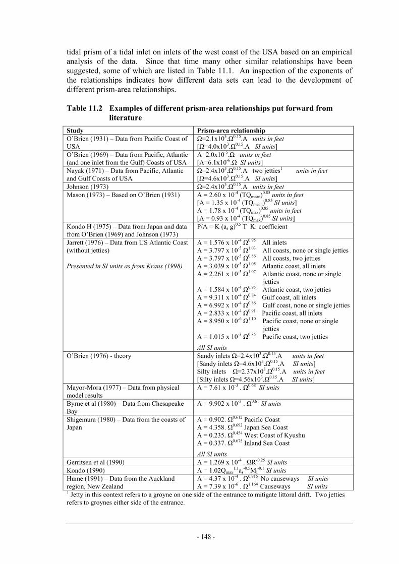
- 148 -

tidal prism of a tidal inlet on inlets of the west coast of the USA based on an empirical analysis of the data. Since that time many other similar relationships have been suggested, some of which are listed in Table 11.1. An inspection of the exponents of the relationships indicates how different data sets can lead to the development of different prism-area relationships. Table 11.2 Examples of different prism-area relationships put forward from

literature Study Prism-area relationship O’Brien (1931) – Data from Pacific Coast of USA

Ω=2.1x103.Ω0.15.A units in feet [Ω=4.0x103.Ω0.15.A SI units]

O’Brien (1969) – Data from Pacific, Atlantic (and one inlet from the Gulf) Coasts of USA

A=2.0x10-5.Ω units in feet [A=6.1x10-6.Ω SI units]

Nayak (1971) – Data from Pacific, Atlantic and Gulf Coasts of USA

Ω=2.4x103.Ω0.15.A two jetties1 units in feet [Ω=4.6x103.Ω0.15.A SI units]

Johnson (1973) Ω=2.4x103.Ω0.15.A units in feet Mason (1973) – Based on O’Brien (1931) A = 2.60 x 10-4 (TQmean)0.85 units in feet

[A = 1.35 x 10-4 (TQmean)0.85 SI units] A = 1.78 x 10-4 (TQmax)0.85 units in feet [A = 0.93 x 10-4 (TQmax)0.85 SI units]

Kondo H (1975) – Data from Japan and data from O’Brien (1969) and Johnson (1973)

P/A = K (as g)0.5 T K: coefficient

Jarrett (1976) – Data from US Atlantic Coast (without jetties) Presented in SI units as from Kraus (1998)

A = 1.576 x 10-4 Ω0.95 All inlets A = 3.797 x 10-5 Ω1.03 All coasts, none or single jetties A = 3.797 x 10-5 Ω0.86 All coasts, two jetties A = 3.039 x 10-5 Ω1.05 Atlantic coast, all inlets A = 2.261 x 10-5 Ω1.07 Atlantic coast, none or single jetties A = 1.584 x 10-4 Ω0.95 Atlantic coast, two jetties A = 9.311 x 10-4 Ω0.84 Gulf coast, all inlets A = 6.992 x 10-4 Ω0.86 Gulf coast, none or single jetties A = 2.833 x 10-4 Ω0.91 Pacific coast, all inlets A = 8.950 x 10-6 Ω1.10 Pacific coast, none or single jetties A = 1.015 x 10-3 Ω0.85 Pacific coast, two jetties

All SI units O’Brien (1976) - theory Sandy inlets Ω=2.4x103.Ω0.15.A units in feet

[Sandy inlets Ω=4.6x103.Ω0.15.A SI units] Silty inlets Ω=2.37x103.Ω0.15.A units in feet [Silty inlets Ω=4.56x103.Ω0.15.A SI units]

Mayor-Mora (1977) – Data from physical model results

A = 7.61 x 10-3 . Ω0.68 SI units

Byrne et al (1980) – Data from Chesapeake Bay

A = 9.902 x 10-3 . Ω0.61 SI units

Shigemura (1980) – Data from the coasts of Japan

A = 0.902. Ω0.612 Pacific Coast A = 4.358. Ω0.692 Japan Sea Coast A = 0.235. Ω0.454 West Coast of Kyushu A = 0.337. Ω0.675 Inland Sea Coast

All SI units Gerritsen et al (1990) A = 1.269 x 10-4 . ΩR-0.25 SI units Kondo (1990) A = 1.02Qmax

1.1as-0.5Ml

-0.1 SI units Hume (1991) – Data from the Auckland region, New Zealand

A = 4.37 x 10-4 . Ω0.915 No causeways SI units A = 7.39 x 10-6 . Ω1.164 Causeways SI units

1 Jetty in this context refers to a groyne on one side of the entrance to mitigate littoral drift. Two jetties refers to groynes either side of the entrance.

- 149 -

Where T is the tidal period in seconds, Qmean is given by Qmean = 2Ω/T, Qmax is given by Qmax = Ωπ/T , R is the hydraulic radius (m), as is the semi amplitude of tide (m), T is the tidal period, Ml is the littoral drift (in m3) 11.7.2 Controlling factors in prism-area relationships Figure 11.1 shows the scatter of (prism/area) data from a large number of tidal inlets in Japan, China, UK and the USA (Gao and Collins, 1994). The figure shows a scatter of over two orders of magnitude for any given area or prism value. This scatter more or less proves that there are important additional controlling factors which govern an inlet entrance which must be considered and that the O’Brien rule or its contemporaries does not describe estuary entrances sufficiently by itself. These controlling factors can be identified by considering the physical processes occurring at estuary entrances. The entrances to estuaries experience the effect of tidal currents waves bringing sediment into the entrance from offshore, the effect of littoral drift bringing sediment into the entrance area as well as the effect of ebb currents which tend to sweep the entrance channel free of sediment. In some estuary and tidal inlet entrances the processes at the entrance are further complicated by the geology of the entrance which constrains the channel from widening (e.g. Humber, Lune, Mersey). It is clear, therefore, that any regime theory which seeks to predict the size of entrances of estuaries must include the effects of offshore sediment supply, littoral drift, wave activity and geological constraints. This was acknowledged by O’Brien in his 1976 paper. Some authors have attempted with varying success to incorporate one or more of these factors: • Sediment supply, including littoral drift (Bruun and Geritsen, 1960, Bruun, 1978,

Moore, 1972, Kondo, 1990, Kraus, 1998) • Wave action (de Jong and Gerritsen, 1984, Eysink 1991, Spearman 1995). The following sections discuss three approaches to the use of O’Brien relationships which attempt to incorporate these factors in a holistic manner. The approaches considered are those of Hume and Herdendorf (Section 11.7.3), Kraus (Section 11.7.4) and Hughes (Section 11.7.5). 11.7.3 The approach of Hume and Herdendorf One of the most successful attempts to include these factors has come from the classification approach of Hume and Herdendorf (1988, 1992, 1993). Their approach was to classify estuaries into the following different geomorphological types: • Funnel-shaped estuaries (Simple branched drowned-river valley systems with

funnel-shaped inlets) • Headland enclosed estuaries (Inlets constrained by rock headlands) • Barrier-enclosed estuaries (Drowned river valleys and embayments whose inlet is

formed by either a double-spit, single spit, tombolo, island or beach landforms, each forming a single estuary type)

- 150 -

• River-mouth estuaries (large fluvial input and river-dominated hydrology. The lower reaches of the river are stratified or there is a tidal backwater effect on flows. This type of estuary is split into four sub-types: straight-banked river mouths, split lagoon river mouths with some tidal prism, split lagoon river mouths with virtually no tidal prism and deltaic river mouths).

• Coastal embayments • Fault embayments • Diastrophic embayments (created as a result of tectonic plate movement) • Volcanic embayments (drowned craters that have been breached by the sea) • Glacial eroded embayments (fjords). The idea was that by classifying New Zealand estuaries/inlets into the sixteen types listed above the inlets would be grouped into classes with similar wave, flow and sedimentological regimes. Figure 11.2 (from Hume and Herdendorf, 1988) summarises the results of the exercise. By producing O’Brien type relationships for each separate inlet/estuary class the large range of scatter exemplified by Figure 11.1 was greatly reduced. The figure shows that the prism-area relationship is very consistent for Barrier Enclosed estuaries, but less consistent for the funnel-shaped and river mouth. Interestingly the headland enclosed estuaries also gave a reasonably consistent prism-area relationship even though from common sense point of view the inlet throat is a function of geology. Comparison with barrier enclosed estuaries from Japan appear to show that there is some consistency between data sets for New Zealand and Japan but a comparison of the correlations derived by Hume and Herdendorf (1988) with those of Shigemura (1980) for apparently the same group of estuaries show very different results. Without inferring error on the part of any of these researchers it would be prudent to clear up this uncertainty through a detailed examination of the data before relying on this particular result. Townend (2005) analysed bathymetric data sets (from the C-Map database, ABP Research 2000, but originally from a variety of sources) of 65 Estuaries in the UK. Townend applied a similar but modified classification process (based on the work of Hume and Herdendorf, above) classifying estuaries as following: • Group “B” – estuaries which were muddy with rocky shores and beds or with

“softer geology, and infilling with muddy sediments in conditions where supplied is limited”. These estuaries were thought to be analogous with Hume and Herdendorf’s funnel shaped, tectonic fault and volcanic embayment entrances.

• “Group C” – all other estuaries. This group was taken to be analogous with Hume and Herdendorf’s barrier enclosed and river mouth entrance groups.

Using this classification the scatter for the UK estuary data sets was much reduced and followed distinct prism area relationship (Figure 11.3). Moreover the prism-area relationships of the UK B and C groups appeared to be very similar to those of the corresponding New Zealand B and C groups from the Hume and Herdendorf data. However, the error (the root mean square error) in the UK dataset about these best fit prism area relationships is still in the region of 75% (based on an analysis of Figure 11.3).

- 151 -

The classification approach of Hume and Herdendorf (with or without the modifications suggested by Townend) reduces the scatter in the data sets but even within classes it will still be true that wave action and littoral drift will vary leading to inevitable scatter. 11.7.4 The approach of Kraus A different approach was undertaken by Kraus (1998) who derived a prism area relationship on the basis of physical processes,

903

34233

.

g

k

TQWnC

A Ω⎥⎥⎦

⎤

⎢⎢⎣

⎡=

απ (11.3)

where α is an empirical coefficient ≈ 1.0, Ck is a tide factor that takes into account the non-sinusoidal nature of the tide (0.81 ≤ Ck ≤ 1.0), n is the Manning coefficient, W is the channel width, Qg is the longshore sediment transport rate and T is the tidal period. Kraus derived this relationship by balancing the transport capability of the tidal flow against the longshore transport which deposits in the channel. The equation was applied to data from Bruun (1978) with some success but Townend (2005) did not find the equations produced by Kraus successfully reproduced the observations from the UK estuary data set. It is likely that lack of data for littoral drift may be partially responsible since the predicted cross-section area is very sensitive to this parameter. Moreover, as noted by Hughes (2002), the cross sectional area given by Equation 11.3 depends inversely on this parameter, producing unrealistic values when littoral drift is small. This problem is introduced by lack of consideration by Kraus of other sediment transport processes occurring at the entrance. Kraus’ formulation may apply to the simple littoral drift-ebb tide scour sediment balance that occurs in tidal inlets but in estuaries other processes occur such as transport into the inlet or estuary from offshore and out of the inlet/estuary to the bay, which are both driven not only by tidal currents but also by wave action. Thus in its present form the Kraus methodology is not applicable to estuary entrances. 11.7.5 Hughes approach Hughes (2002) also attempted to find a physical basis for regime relationships at inlet entrances by assuming that the inlet equilibrium was characterised by current velocities at the level of the threshold of motion. His analysis resulted in the following formula,

( ) 98

650 Ω= la Ck.A where ( )[ ] Tdgs

WCe

l8

32

1

81

1−= (11.4)

- 152 -

and s is the specific density of sediment ≈ 2.65, de is a representative sediment diameter and ka is an empirical coefficient. Townend (2005) applied the Hughes equation to the same UK data set mentioned above. Analysing his results (based on Figure 7 of the paper) the error between the predicted cross-section area as given by the Hughes equation was on average of the order of 75%, a similar result to the error resulting from the use of the Hume and Herdendorf approach. Townend states clearly that crude figures for particle size, de, were utilised (0.5mm for sandy estuaries and 0.005mm for muddy estuaries) and it would be an interesting task to see if the data improved with better sediment data. However, the practical difficulties of selecting a representative grain diameter for an estuary entrance from a spectrum of spatially varying fractions means that an improvement to the fit of this relationship is by no means certain. Moreover, Townend points out that the Hughes formulation is based on an evaluation of critical shear stress only applicable to non-cohesive sediment. In this light the application of Equation 11.4 to muddy estuaries cannot be advised. The use of threshold of motion as a criteria for equilibrium (as here) has more merit in an inlet entrance, where deposition in the channel from littoral drift is balanced against the ability of the tidal currents to remove it, than for the situation for estuaries in general (as discussed in Section 11.4.3). Note, however, that the use of this criteria is biased towards identification of the upper limit of the range of variation of the cross-section area (Friedrichs, 1995). Hughes tested Equation 11.4 on data from work by Jarrett (1976), Byrne et al (1980) Mayor-Mora (1977) and Seaburgh et al (2001), with ka the empirical coefficient set to 1.0. The data indicated that Equation 11.4 under-predicted the observed cross-sectional areas by an average of 34% and, as a consequence, the value of ka was set to 1.34. The use of this value improved the fit of the equation developed by Hughes but inevitably reduces Hughes equation to an empirically fitted relationship since it is very likely the value of 1.34 he found for US data would be different in other parts of the world. 11.7.6 Escoffier’s approach Though not directly a regime theory approach, Escoffier’s analysis is so inter-twined with the application of regime theory to entrances of tidal inlets and estuaries that it merits inclusion here. Escoffier characterised tidal inlets as being a balance between the transport of sediment into the entrance channel by littoral drift and the capacity of the ebb-tide currents at the inlet entrance to transport the sediment out of the entrance. He constructed a theory based on a concept of an equilibrium current velocity “just” able to remove the littoral drift. When Escoffier used this concept together with an understanding of the hydraulic response in tidal inlets with changes in entrance cross-section area, he was able to derive a key concept in tidal inlet stability. The general response of tidal currents at an inlet entrance to changes in entrance area is shown in Figure 11.4. Super-imposed on this picture is the line corresponding to u=ueq. It is clear that in general there are two possible values of cross-section area corresponding to the equilibrium current velocity and we will label the less of these

- 153 -

values A1 and the greater A2. Escoffier pointed out that only one of the two cross-section areas A1 and A2 represents a stable equilibrium. Consider first the value of cross-section area A2. Any increase in cross-section size from this equilibrium will result in a reduction in current velocity – leading to a reduction in cross-section as the channel fills with sediment and a return to the equilibrium at A2. Similarly a reduction in cross-section size will result in an increase in velocity and a corresponding return to the equilibrium at A2. Consider now the value of cross-section A1. In contrast to the equilibrium at A2, an increase in cross-section at A1 will result in an increase in current velocity and a larger cross-section. A reduction in cross-section at A1 will cause a reduction in current velocity and a reduction in cross-section area. Thus A1 represents an unstable state. This analysis results in the following conclusions: • There is a cross-section area, A*, (equal to the maximum in cross-section area in

Figure 11.5) which marks the limit of inlet stability. If the entrance cross-section area is above this value then a viable equilibrium exists and the inlet entrance is likely to converge to this equilibrium.

• If cross-section areas reduce below A*, the inlet entrance will continue to reduce until it closes.

11.7.7 An application of regime theory at a tidal inlet entrance (van de Kreeke,

2004) The use of O’Brien-type relationships in a predictive assessment is illustrated well in a paper by Van de Kreeke (2004). Van de Kreeke used these relationships in an assessment of the impact of basin reduction in the Frisian Inlet, part of the Dutch Wadden Sea. In 1969, through the closure of the Lauwers Sea, the basin surface area of the Frisian Inlet was reduced by approximately 30%. The purpose of Van de Kreeke’s study was to identify the impact of the closure on the new equilibrium area of the Frisian Inlet. Van de Kreeke characterised the Frisian inlet as a balance between littoral drift, M, being transported into an entrance channel (of width W and equilibrium cross-sectional area AE) of the tidal inlet and ebb tide transport which removes this imported material. He further assumed that that the equilibrium cross-section of the tidal inlet could be described by annually-averaged conditions so that the value of littoral drift, M2 used corresponded to annually-averaged total and the relevant ebb tide conditions were those for a mean tide. The prism-area relationship used was of the form,

qeq CA Ω= (11.5)

where Ω is the mean tide prism and C and q were derived from a best fit to observed values of cross-sectional area and prism at five other nearby inlets in the Dutch Wadden Sea (including the Frisian inlet prior to basin reduction). These observations gave

- 154 -

values for C and q of 6.8x10-5 and 1.0 (SI units), respectively with the tidal prism used being based on mean tide conditions. It is noted here that Van de Kreeke was fortunate to have a series of nearby tidal inlets with similar characteristics and environmental conditions from which to derive this relationship. More generally the data available to derive this relationship will be more sparse and may result in considerable uncertainty. Van de Kreeke assumed that the shape of the cross-section would remain constant in time (so that the width of the channel is proportional to √AE) and made use of the equation,

TAu Ω

=π (11.6)

where u is the cross-section averaged and tidally-averaged current velocity at equilibrium and T is the tidal period, and,

mnWukTR = (11.7) where TR is a generalised formulae for the sediment transport rate on the ebb tide, W is the width of the channel, and k, n and m are empirical constants. Equations 11.5, 11.6 and 11.7 suggest that the ebb tide transport can be written as,

2mAukTR nmα= (11.8)

Van de Kreeke composed an equation describing the sediment balance in the channel:

( )MAuk

dtAAd

W mnmE −=−

2α (11.9)

Since the RHS of equation 11.9 is zero at equilibrium, Equation 11.9 can be adapted to give,

( )WM

AA

uu

WM

dtAAd

m

E

n

E

E −=⎟⎟⎠

⎞⎜⎜⎝

⎛⎟⎟⎠

⎞⎜⎜⎝

⎛−

− 2

(11.10)

It is necessary here to provide a means of estimating the relationship )A(fu = . One way of doing this in general is to apply a flow model. However the simpler form of tidal inlets can often be characterised by an analytical hydraulic model. Van de Kreeke chose the following formula by Mehta and Oszoy (1978),

( ) ( )

4

2224

422

0 4411

1882212

1

K.

KK.K

ˆAAu

b

−−⎥⎦⎤

⎢⎣⎡ +−

=ησ

(11.11)

- 155 -

where FLˆg

AAK

b 0

45

ηα

σ= and

bLAgA

K σ=2

Ab is the basin area of the tidal inlet, σ is the tidal frequency (=2π/T), L is the length of the inlet channel, F is a friction factor (to be empirically estimated, Van de Kreeke found this value to be 0.0033) and

0η is the ocean tide amplitude. Equation 11.10 was solved in the following manner: • Eu is given by the use of Equations 11.5 and 11.6. • The resulting value of Eu (which, unless q is equal to zero, as in the Van de Kreeke

study, will be in terms of AE) is used in Equation 11.11 to derive the equilibrium value of AE to which the tidal inlet will evolve.

• A is the time-varying cross-section area and u at any time t is given by Equation 11.11 using the value of A(t).

The results of the application of this methodology to the Frisian inlet are summarised in Figure 11.5. Owing to the historical nature (1969) of the closure of the Lauwer Sea data was available to compare Van de Kreeke’s prediction with the initial evolution of the inlet. The result shows a good reproduction of this initial evolution although there is significant observed year-on-year variation about the predicted trend. This application of prism-area relationships for tidal inlets benefits from both a reliable formulation of the prism-area relationship and an analytical relationship which can approximate the tidal flow. In a typical estuarine situation the uncertainty in the prism-area relationship will be greater and it will be necessary to compute the current velocity through the entrance using a flow model. 11.8 The use of regime theory for the entrances of estuaries and tidal inlets –

Part II – Best practice 11.8.1 Introduction to best practice The use of O’Brien relationships for estuary/tidal inlet entrances differs from the use of the O’Brien relationships within estuaries in that the use of these relationships within estuaries (See Section 11.9) requires a site specific approach and the empirical selection of a relationship based on an individual estuary, while use of the approach at entrances seeks to make a more objective assessment of the state of the estuary/inlet based on more general relationships that relate to all estuaries or all estuaries from a certain group. The use of the “entrances” O’Brien rule (and similar) for predictive studies is hampered by problems surrounding the uncertainty (error) in applying these sorts of relationships more widely. The problem is that although a prism-area data set may show a relatively high correlation coefficient over a significant range of scales, an examination of the

- 156 -

actual error in the relationship may be actually large – i.e. of the order of 100%. The scientific community differs in attitudes to the goodness of fit displayed by these relationships. Some point to the clustering of points in prism-area plots as evidence of a definitive relationship between prism and area, others query this conclusion, pointing to the amount of scatter in such plots as evidence that any apparent relationship is fortuitous. As the discussion of theory above implies, the answer lies somewhere between these two points of view. Whilst it would be churlish to ignore the similarities between inlets and estuaries of a similar geomorphological type (e.g. Section 11.7.3) it is also important to note that just because a log-log plot of prism and area gives rise to a correlation coefficient (r2) of more than 0.9 through a variety of scales, it is not evidence of a fundamental close link between these two parameters – in general these two parameters will show a relationship just because larger estuaries in general will have larger entrance areas while smaller estuaries will have smaller entrance areas. The important question is therefore not, “does an O’Brien relationship give a good correlation?” but,

“does the error inherent in the relationship introduce too much error when I use it in my predictive study?”.

When the emphasis is put on the extent of error/uncertainty, rather than the usual consideration of goodness of fit, it is often the case that the error/uncertainty inherent in O’Brien applications render them of limited predictive use. This is because there are a number of factors affecting the relationship between tidal prism and area, for instance wave action, littoral drift, geology and sediment type and these vary from estuary to estuary or inlet to inlet. 11.8.2 The effect of uncertainty on the use of O’Brien relationships The chosen or derived O’Brien relationship will inevitably have some degree of uncertainty or error associated with it as applied to any given estuary or tidal inlet. The main questions arising from this uncertainty are: • What effect does the uncertainty/error in the O’Brien relationship have on the

assessment of stability of the inlet (in its existing state or following evolution)? • What effect does the uncertainty/error in the O’Brien relationship have on

predictions of evolution of the entrance resulting from changes in tidal prism? • What effect does the uncertainty/error in the O’Brien relationship have on the

assessment of impact on the entrance (in terms of environmental impact, navigation, etc)?

To discuss these questions we use Figure 11.6 as an illustration of the problem. Consider an estuary or tidal inlet entrance (A) which has values of tidal prism and area which (for example) are significantly (for example) larger (by dA) than the best fit regime equation (derived from theory or empirically). Assume further that some impact occurs within the estuary/tidal inlet to reduce the tidal prism, causing evolution of the entrance to a new geometry (B) which is still larger than the equilibrium value given by the regime equation (by a difference, dA').

- 157 -

The difference (dA) between the equilibrium condition at A (as given by the regime equation) and the actual value of cross-section area initially creates some uncertainty regarding whether the condition at A denotes an equilibrium condition or not. This uncertainty affects the critical value of the cross-section area (see Section 11.7.6) and therefore gives a potentially false idea of the stability of the entrance. Confirmation of the initial entrance conditions may be required using measurements of the cross-section over time. Consideration of the theory outlined above in Section 11.7 indicates that, as long as there is evidence that the entrance is stable and that the exponent of the chosen O’Brien relationship (i.e. the value of q in Equation 11.5) approximates to the real underlying trend of evolution, the effect of uncertainty in the O’Brien relationship will not significantly affect the estimate of relative change arising from a change in tidal prism. However, there will still be a difference (dA') between the equilibrium condition at B (as given by the regime equation) and the actual value of cross-section area. If the pre-evolution state (A) was stable then it may be reasonably concluded that A was a better indicator of the equilibrium state than the regime equation and consequently that the post evolution state (B) is more likely to be a better indicator of the equilibrium state following evolution. However if the stability of A is not known, or A is shown to be a transition state then the equilibrium cross-section area corresponding to the pre-evolution state could be anywhere between the observed value and the regime equation value. Similarly the equilibrium cross-section area corresponding to the post-evolution state (B) could be anywhere between the predicted value and the regime equation value. This creates uncertainty both in the stability of the post-evolution scenario (B) and in its impact on issues such as navigation and the environment. 11.8.3 Reducing Uncertainty in O’Brien relationships Two main approaches to reducing the error/uncertainty (equivalent to taking account of the influential factors mentioned above) in O’Brien relationships have been put forward: the first is to find a process-based underlying explanation of the observed affinity between prism and area and the second is to base the prism-area relationships on estuaries/inlets of a certain geomorphological type, reducing uncertainty through the similarities of the estuaries/inlets in question. The section on theory describes two process-based approaches to developing an O’Brien relationship. • The formula put forward by Kraus is based on a balance between littoral drift

depositing in an inlet channel and the action of the ebb tide currents in transporting the deposited sediment out of the channel. The relationship has some limited validation in the context of tidal inlets but, since estuaries experience the additional effects of flood tide transport and wave-enhanced transport the method of Kraus will not work for estuaries in general. This has been demonstrated to some extent by Townend (2005) who applied the relationship to a large number of UK estuaries (albeit without appropriate littoral drift data). The approach merits further investigation in the context of tidal inlets, however, which can be characterised by the simple littoral drift/ebb tide current balance.

• The formula by Hughes is again based on the idea of a balance between the influx of littoral drift into a tidal and the ebb tide currents being “just” able to remove the

- 158 -

deposit but this time the balance is expressed in terms of sediment particles being in a state of equilibrium stress and on the point of mobilisation. This approach will tend to predict the upper limit of potential variation of the entrance area. Validation from US estuaries found that the method on average under-estimated the cross-section area by 34%. Application to UK estuaries by Townend (2005), with limited particle size data, found a reasonable fit with errors in prediction of entrance area in the region of 75%. This approach is likely to result in large amounts of uncertainty where the particle size distribution in the study area is vary varied because of the reliance on a representative particle size to ascertain the threshold of motion. Similarly since the basis for the Hughes formula is based (as for the Kraus formula) on a balance between ebb tide transport and wave-induced littoral drift the uncertainty resulting from the application of this approach may be large in estuarine situations.

As yet no underlying basis for the prism-area relationships in estuaries has been devised (Dyer, 2004) and in its absence the most successful approach to date is that of Hume and Herdendorf who developed O’Brien type relationships for geomorphically and geographically similar entrances where the data shows greater empirical adherence resulting from similar tides, waves, and sediment transport. This idea is not new – to some extent the whole history of the application of O’Brien relationships to entrances has been to develop relationships for specific geomorphically and geographically similar entrances – but Hume and Herdendorf are the first to approach the problem in a formal manner using geomorphological classification. Using this approach Hume and Herdendorf (1993) derived prism-area relationships for New Zealand estuaries with average errors of the order of 30%. An application of their methodology to UK estuaries (Townend, 2005) resulted in larger average errors in the region of 75%. If this is acceptable to the user for their purposes then the procedures outlined by these authors can be applied. For UK estuaries the results of Townend will be applicable. Where the likely errors from the empirical analysis of Hume and Herdendorf and/or Townend are too large for the purposes of the project, the only recourse is to consider the processes occurring at the entrance. For the present state of the entrance historical survey data must be used to ascertain the current trend (is it increasing or reducing in size?). For predicting the future state of the entrance as a result of proposed works (or sea level rise) the qualitative impact on the inlet entrance can be deduced from predicted trends in wave action, littoral drift and tidal currents. 11.8.4 How can these relationships be used? Entrance prism-area relationships (as opposed to relationships valid throughout estuaries discussed in Section 11.9) are most commonly used to assess the evolution of entrances to tidal inlets where the entrance is commonly the morphological feature of most interest to stake-holders (navigation, ecology, etc). In estuaries, except those where entrance closure from littoral drift is a risk, the focus is usually less centred upon the entrance. Moreover, in estuaries the flow conditions at the entrance are much more sensitive to morphological change further landward and it is usually necessary to include the morphology of the wider estuary in any predictive assessment.

- 159 -

• Predicting changes to tidal inlet entrances Where sufficiently reliable prism-areas relationships can be derived (using empiricism or the process-based relationships presented in Section 11.8) the evolution of tidal inlet entrances can be derived using the methodology exhibited by van de Kreeke (2004) in Section 11.7.7. This approach consists of the following parts:

– Derivation of representative values of tidal prism, cross-sectional area and littoral drift

– Derivation of the O’Brien relationship – Development of a tidal flow model or analytical relationship such as the Mehta-

Oszoy type – Implementation of a sediment balance between littoral drift and ebb-tide

transport, such as that exhibited in Equation 11.10. Where the derived prism-area relationships are less reliable an estimate of the evolution of the tidal inlet can still be used by assuming that the prism-area relationship is correct in relative terms (See Figure 11.6). However, without some additional information regarding the initial stability of the entrance before evolution there will be considerable uncertainty regarding its post evolution state and stability. It is possible that in some cases the level of uncertainty introduced would be so large as to prevent meaningful assessment of the post-evolution state of the estuary. In considering the morphological evolution and stability of a tidal inlet entrance the analysis of Escoffier should be utilised where relevant. • Predicting changes in estuary entrances

In estuarine situations where the essential sediment balance is one between littoral drift and ebb-tide transport the methodology of van de Kreeke (2004) can be implemented, though this situation is not common to UK estuaries. Where the sediment balance is more complex, use of a method which only considers morphological change at the entrance is not likely to result in the correct description of the evolution of the estuary. Instead the implementation of other tools is advised such as the use of estuary-wide regime relationships (see Section 11.9).

• Use of O’Brien’s relationships as an aid to conceptual understanding

O’Brien relationships, along with other top-down, and bottom-up approaches can be an aid to developing a conceptual model of the system. A comparison of the tidal prism and cross-sectional area of a system with more geographically/geomorphically generic relationships may identify some of the evolutional trend of the entrance. As discussed elsewhere in Section 11.8, however, care must be taken to ensure that the system is being compared with other systems of a similar type. One example of this type of application was undertaken by ABP Research (2000, now referred to as ABPmer) in studies associated with East Head and Chichester Harbour.

• Use of O’Brien’s relationships in geomorphological classification

The work of Hume and Herdendorf (1993) and Townend (2005) shows that O’Brien relationships are a function of geomorphology. This result can be used to reduce the uncertainty in these relationships but can also be used in reverse – that is to say

- 160 -

something about the geomorphology of an estuary based on the O’Brien relationship. Townend found that UK estuaries, based on the data from the C-MAP data set formed two distinct prism-area groupings. Townend interpreted these two groups as:

– Group “B” – estuaries which were muddy with rocky shores and beds or with “softer geology, and infilling with muddy sediments in conditions where supplied is limited”.

– Group “C” – all other estuaries. The estuaries belonging to Group B have cross-section entrances on average an order of magnitude larger than those of Group C. Townend refers to the former as “immature” – a term relating to the lack of sediment infill of these estuaries since the Holocene and describing their state on a geological time scale. Examples of estuaries in Group B (i.e. “immature”) are the areas of Cornwall such as the Fal. 11.8.5 Data needs The main parameters associated with use of this method are listed below. However it should be noted that these parameters will vary throughout the year: seasonally due to more intense wave activity causing a higher rate of littoral drift, and potentially, though to a much smaller extent, over the spring- neap tidal cycle due to variations in ebb-tide currents. Inevitably O’Brien type relationships characterise the cross-section at the entrance of an estuary in terms of specific tidal and seasonal (minimum cross-section or maximum cross-section) or annually-averaged conditions. Usually (but not always, e.g. van de Kreeke, 2004) the tidal conditions chosen are mean spring tide conditions. The main data requirements for using O’Brien relationships at estuary/inlet entrances are as follows: • Channel cross section area and channel width

These parameters are discussed in the section on data and are derived from bathymetric surveys. It is usual for all cross-section parameters (area, width, etc) to correspond to mean sea level.

• Tidal prism This parameter is discussed in the section on data. This parameter can be derived from flow modelling or from bathymetry surveys. As stated above tidal prisms will normally correspond to mean spring tide conditions.

• Littoral drift In practice this will be derived from wave data and a littoral drift model or algorithm. An annual total or annually-averaged total are normally required.

For a more thorough in-depth investigation of evolution at entrances, seasonal surveys are desirable as well as year on year surveys (to set any evolution in the context of natural changes). Entrance data for other nearby or similar estuaries/inlets entrances may be required to help derive the O’Brien relationship.

- 161 -

Note that if implementing the method of Hughes (2002) then particle size data (D50) for the inlet will be required. 11.9 The use of regime theory within estuaries – Part 1 - Theory 11.9.1 The underlying basis of estuary regime theory There are three main views of the basis for regime theory in estuaries. The first is that regime theory predicts the most probable state of an estuary on the basis of entropy-based considerations. The second view is that the basis for regime theory is a dynamic equilibrium dependent on the threshold of sediment movement. The third view is that regime theory is essentially a simplified calculation of sediment transport within an estuary. None of these views has as yet been definitively demonstrated as being valid. Although some proponents of the theory consider that the basis of regime theory may not matter, there are significant consequences for the application and meaning of the results. Each of the regime theories set out in detail below. The regime theory that we consider here is basically of the form, H α Qp, B α Qq, U α Qr. (11.12) where p q and r are constants to be derived and where Q is the peak discharge which can be replaced by tidal prism, Ω. 11.9.2 Regime theory based on entropy considerations This section does not address entropy theory as a whole (which is dealt with in Chapter 9) or entropy theory as a basis for river regime theory (which is also touched on in Chapter 9) but rather the present state of entropy theory as a basis for estuary regime theory. The application of entropy as a basis for regime theory can be attributed to Langbein (1963). Langbein found a basis for characterising estuaries in the form given by Equation 11.12. H α Qp, B α Qq, U α Qr. The exponents of these relationships were derived as a result of attempting to close the system of variables (in an analogous manner to that of White et al (1982), etc, for river regime) by considering extremal hypotheses involving energy considerations. The approach of the latter is superficially attractive because it suggests that an estuary will tend to a specific form, H α Q0.23, B α Q0.72, U α Q0.05 (11.13) The proof presented by Langbein is repeated in Appendix 1. Langbein argues, based on considerations of entropy in closed systems, that the most probable state of an estuary is one that (a) minimises the total done in the estuary work (where here “work” refers to energy expended or the integral of force over distance) and that (b) distributes the work done as uniformly as possible. However, as discussed in Appendix 1, Langbein’s analysis is flawed. Essentially the premise upon which Langbein derives the (most

- 162 -

probable) value of p is incorrect. Following this incorrect derivation the values calculated for q and r are also then incorrect. On this basis it is necessary to rule out Langbein’s analysis as a basis for regime theory. Langbein himself described the power law relationships he (incorrectly) derived as being “…central values about which there is considerable variance”. Anyone who has tried to apply the discharge-area (or prism-area) relationships to a few estuaries will realise that there is a considerable variation in the regime exponents (p, q, and r) from estuary to estuary, and even along an estuary, which again indicates how real estuaries will vary from the Langbein estimate of the “most probable” regime relationships. Conclusion Entropy and extremal energy considerations may have a useful role in considering the long term trends in estuarine systems (see Chapter 12) but they have not yet been demonstrated as a basis for underpinning estuary regime theory. 11.9.3 Regime theory based on the threshold of motion The idea of estuary cross-sectional geometry based on the threshold of motion originally stems from the origins of regime theory for uni-directional flow (canals and rivers). The concept in this case is simple – in order to design for zero scour the limiting design condition for a canal cross-section is that the current velocity must be less than the velocity corresponding to the critical shear stress of the bed material. Whilst superficially attractive because it provides a physical basis for regime theory this idea of channel equilibrium based on the threshold of motion cannot be straightforwardly applied to estuaries. This conclusion arises because the threshold of motion concept implies that at equilibrium there must be no sediment transport in the channel. Moreover, the threshold of motion concept implies that a reduction in discharge or current velocity can have no impact whatsoever on the channel geometry – since there is no sediment transport, there is no deposition. If this were true of estuaries then their geometries would be static over time and defined by the most extreme conditions experienced in the estuary. These hypothetical conditions contrast with those of real estuaries where sediment is transported back and forth on the flood and ebb tides. It is clear that the dynamic nature of estuaries cannot be characterised satisfactorily using a concept of no sediment transport. The one possible exception to this rule is where, as in tidal inlets, the estuary is characterised by littoral drift into the estuary entrance and the removal of this sediment by ebb tide transport. Such cases correspond more closely to the uni-directional ideal from which the threshold of motion concept was developed. This topic is discussed in more detail in Section 11.7. Friedrichs (1995) examined the possible use of the threshold of motion concept in regime theory and suggested that the threshold of motion can be thought of as a lower bound of the equilibrium shear stress and the resulting estimates of geometry for cross sections then becomes an upper bound. Using Manning’s roughness equation he derived a regime relationship,

- 163 -

21

61

⎟⎟⎠

⎞⎜⎜⎝

⎛=

E

gQnAhτρ (11.14)

where n is Manning’s coefficient and τE is the equilibrium shear stress, approximated for sand by the threshold of motion. In the case of muddy estuaries he also asserted that the equilibrium shear stress describing the equilibrium was not the critical shear stress for motion, which is of the order of 0.06-0.1N/m2 (Whitehouse et al, 2000), but a shear stress corresponding to significant or bulk erosion. This assertion no longer precludes the existence of sediment transport and goes someway to addressing the inherent conceptual problems with regime theory based on the threshold of motion. However, Friedrich’s assertion introduces another problem of identifying the erosion threshold of significant erosion. For muddy systems it is not practically possible to derive values for such a threshold with any real certainty and Friedrichs cites a number of different studies resulting in hugely different estimates of the threshold of significant erosion. Conclusion The threshold of motion concept does not describe the regime state of estuaries well though it may give an order of magnitude prediction of stable estuary cross-section geometry if good information is known about the bed sediment type. 11.9.4 Regime theory based on sediment transport In this case regime theory starts with the following assumptions: • An estuary in equilibrium (net sediment movement, over a long period of time at

any place is negligible, disregarding seasonal variation); • The equilibrium estuary width and depth can be characterised by a (“regime”)

relationship with peak discharge (specifically peak discharge or tidal prism). These two assumptions lead, using standard equations of sediment transport to the following conclusion, • An estuary perturbated from the equilibrium will respond by moving back towards

its equilibrium “regime” state. The proof of the latter conclusion is presented in Appendices 2 and 3 for sandy and muddy estuaries, respectively. The proof is based on the assumption that the estuary in its stable state obeys the regime equations BαQp and HαQq, and rewriting standard equations of sediment transport in terms of the peak discharge, Q. By considering the change in cross-section area for a small perturbation and comparing this to the equilibrium case an algorithm for estimating the evolution of the estuary over time can be derived and the stability of this algorithm can be examined. The analysis in Appendices 2 and 3 builds and improves upon the analysis present by Spearman (1995) and Spearman et al (1998) which lacked robustness in a number of places.

- 164 -

Note, however, there is no firm proof that the basic principles of sediment transport and fluid flow will automatically lead to a regime relationship of the form BαQp and HαQq. On the basis of this analysis the following conclusions are made: • The traditional form of regime theory, which is described in algorithm form as,

( )qp

iqp

iii QQ.AA ++++ −=− 131 λ (11.13)

where A=λ3.Qp+q is the characteristic regime equation, Ai is the cross-section area at the ith iteration

Equation 11.13 is not a correct assessment of estuary evolution and can significantly over-estimate the extent of morphological evolution in an estuary. • Starting from first principles it is possible to derive new regime algorithms (see

Appendices 2 and 3),

sandy estuaries

( ) ( )⎥⎦⎤

⎢⎣⎡ −+−′−=− −−

+nnK

iii kdxdknQtKAA γγµδ 2

11 (11.14)

where K1 = λ1 λ4

n dtwtn

tide.sin∫β , λ1 and λ2 are given by pQB 1λ= , qQH 2λ= ,

and β is given by the general transport equation S=βVn , µ is the exponential growth/decay of the velocity with distance along the estuary given by VE=V0e-µx , K2 = p+(1-p-q)n , k is a parameter of order O(1), γ is a parameter of O(1) describing the tidal asymmetry, and , δt' is the number of tides represented by one iteration of the algorithm. muddy estuaries

⎥⎥⎦

⎤

⎢⎢⎣

⎡⎟⎟⎠

⎞⎜⎜⎝

⎛−⎟⎟

⎠

⎞⎜⎜⎝

⎛′=− +

+

++

221

1

111

Ki

m

i

i,EKi

m

i

i,Eii Q

CC

QC

CKtAA δ (11.15)

where Ci and Ci, E are the “representative” actual and equilibrium concentrations at a cross-section at time step i of the evolution, K1 =1/2 λ1TMeρCDλ4

2(1-p-q) , λ1 is given by, pQB 1λ= , λ4 is given by qpQV −−= 1

4λ , T is the tidal period, Me is an erosion rate parameter, ρ is the water density, CD is the drag coefficient, K2=2-p-2q , Qi is the peak discharge on the ith iteration, and, δt' is the number of tides represented by an iteration of the algorithm.

- 165 -

In the short term any changes to concentrations in the water column arising from erosion/deposition will be limited to the area local to the disturbance but rapidly any such changes will be distributed through the estuary owing to the relatively long tidal excursion of muddy sediment. In many cases the change in concentration will be distributed such that the existing concentrations decrease proportionally by the ratio of the new total sediment in the estuary system (following morphological change), Mi to the old total (before the change), M0. This means that Equation 11.15 can be simplified to the form,

⎥⎥⎦

⎤

⎢⎢⎣

⎡⎟⎟⎠

⎞⎜⎜⎝

⎛−⎟⎟

⎠

⎞⎜⎜⎝

⎛′=− +

++

22 01

1

011

Ki

m

i

Ki

m

iii Q

MM

QMM

KtAA δ (11.16)

• These are different algorithms from the one commonly used (Equation 11.13), more

representative of estuary evolution and because they are based on sediment transport theory they allow an estimate of the time-scale of evolution to be derived (unlike Equation 11.13 which does not). Equations 11.14 and 11.15 can be thought of as developments of 11.13 (rather than a replacement) – in particular deconstructing the value of the (Equation 11.13) λ3 rate constant and describing how this varies throughout evolution.

• It is clear from the analysis in Appendices 2 and 3 that the commonly used regime

equation (11.13) does not describe the underlying drivers of estuarine evolution appropriately except in limited circumstances.

• For sandy conditions the analysis of Appendix 2 has highlighted that morphological

response (Equation 11.14) is principally a function of tidal asymmetry and spatial gradients in discharge (whereas Equation 11.13 relates morphological response to change sin current magnitude) . This result is supported by the changes that have occurred in the classic case study of the evolution of the Mersey over the 20th century (Thomas, 2000, Price and Kendrick, 1963). In essence the Mersey Estuary is considered to have responded to a change in the boundary conditions at the estuary mouth. As the estuary accreted the greater expanse of tidal flats caused by the evolution resulted in the growing enhancement of ebb-dominance (tidal asymmetry) and this reduced the (net) input of sediment into the estuary until a new equilibrium was achieved (see Section 11.11.3). This contrasts with Equation 11.13 which assumes estuaries only respond only to changes in the magnitude of discharge which (initially at least) did not change significantly within the Mersey and is thus not a principal cause of the change. In terms of more local change at specific cross-sections the new algorithm is also a better descriptor of local evolution. The previous method produces evolution due to more localised change which is independent of the need for mass continuity of sediment. The new method essentially represents evolution due to more localised change as diffusion of the initial impact and therefore ensures some idea of overall continuity of sediment (see Appendix 2).

For muddy conditions the analysis of Appendix 3 has shown that the total sediment mass involved in morphological change is significant to the evolution of an estuary and

- 166 -

that an estuary will respond to the reduction/increase in sediment concentrations and evolution will be attenuated and attained much more rapidly. It is important to note that the analysis presented in Appendices 2 and 3 has been primarily undertaken to highlight deficiencies in the current understanding of regime theory. This analysis has resulted in new algorithms (Equations 11.14 and 11.15) which are likely to result in better estimates of morphological evolution, but which have not been subjected to an extensive period of use by experts in the field. Some of the problems that might arise from use of these algorithms are discussed below. However the inevitable lack of collective experience of practical implementation of these algorithms may result in other unforeseen practical problems. The algorithm for evolution in sandy estuaries contains three important terms: • γ: this is the parameter governing the tidal asymmetry; • k: this is the parameter accounting for the difference between transport from

sinusoidal 1D currents and the real 3D current structure;

• ( )nkdxd −− γ this term governs the local gradient in sediment flux.

The dependence of the sandy regime algorithm on tidal asymmetry and gradients in discharge (or velocity) results in Equation 11.14 being unwieldy and less useful as an algorithm for characterising estuary evolution. In fact the equation is not much reduced from the 1D sand transport equation on which it was based. Under some circumstances it may be more practical to predict the ensuing estuary evolution using a 1D sand transport model. For an estuary in equilibrium k=γ-n where n is an empirical (sediment transport) constant in the region of 3-5. This means that at any location in a sandy estuary in equilibrium the potential net transport due to tidal asymmetry is balanced by sediment availability. However an increase or decrease in either of these terms will result in morphological change. The value of γ is calculated either using a flow model by comparing the model predictions of ebb and flood current speed. If a flow model is not available it may be possible to use Dronkers’ theory (Equation 10.5). The values of k are calculated for each cross-section using the result k=γ-n for the pre-evolution estuary. Unless there is evidence for a change in the value of k it is then fixed for the estuary evolution, while γ may still vary. The algorithm for evolution in muddy estuaries contains an additional important

term,1

1

+

+

i

i,E

CC

, the ratio of the equilibrium and actual (time-averaged) suspended sediment

concentrations at a given cross-section. It is therefore necessary to characterise the value of CE along the estuary. Initially this task is straightforward as CE can be derived on the basis of measured data, assuming this is available. However, as evolution occurs the equilibrium concentration corresponding to any given cross-section may change. In

many cases the ratio 1

1

+

+

i

i,E

CC

can be estimated as the ratio of the initial mass of sediment

- 167 -

in suspension in the system to that at time step i, iM

M 0 . Note that this ratio indirectly

takes into account the secondary effects of changes in tidal asymmetry, sediment supply and export and even dredging and disposal. The analysis of regime theory for sandy and muddy estuaries, though an improvement on the present understanding of estuary regime theory, creates an additional problem: in may estuaries the lower estuary is sandy while the upper estuary is muddy – how can the different natures of evolution in these two areas be seamlessly represented? Unfortunately this problem is outside the scope of this study but it is noted that this is an ongoing topic of research in sediment transport. 11.9.5 The choice of peak discharge or tidal prism as controlling parameter There has been continued discussion regarding the best discharge-area relationship to use in the context of estuary regime theory (e.g. De Jong and Gerritsen 1984, Spearman, 1995). Different authors have concluded differently based on different data sets. Based on the literature the best fits to observed estuary data tend to be the Ω-areaMW and the Qmax-AQmax relationships. Of these the latter is heuristically superior since it is most closely linked to the peak values of velocity which are responsible for sediment transport but to use it usually requires a flow model of the system. The Ω-areaMW relationship has the benefit that it can be used on the basis of bathymetric data alone. Spearman (1995) also found that for a number of estuaries a discharge-area relationship based on the discharge at peak velocity (QVmax-AVmax) gave a good fit to data. This is not surprising because peak velocity is even more closely linked with sediment transport than peak discharge. In his 1995 study this form of discharge-area relationship was discarded because, for the estuaries examined, peak velocity sometimes coincided with ebb tide flows near Low Water which affected only a small proportion of the cross-section. However, in a later study Spearman (2001) examined the effects of managed realignment in a small creek tributary of the Blackwater Estuary which was dominated by saltmarsh storage, about which (at the time) there was considerable uncertainty. The peak discharge occurred at a time corresponding to water levels which interacted with this salt-marsh and thus the peak discharge was associated with considerable uncertainty. The Qmax-Amax relationship was used instead with reasonable success. Conclusion It is concluded that (in general) neither parameter (peak discharge or tidal prism) is clearly more advantageous except that when using the method on the basis of bathymetric data use of tidal prism is required and when using a flow model (in a hybrid combination) use of peak discharge will be more convenient. 11.9.6 The importance of sediment supply Unlike the related topic of estuary entrance regime relationships the role of sediment transport on estuary regime relationships as applied throughout estuaries has been largely ignored by researchers in this discipline.

- 168 -

More recently, however, it has been recognised that the regime relationship itself is a function of the sediment transport supply into an estuary (Spearman, 1995, Wang et al, 1998). Spearman (1995) showed that estuary evolution will cause concentrations to change throughout an estuary in the case of limited sediment supply and that consequently in this case evolution was a function of the mass balance of the system. Spearman also suggested that the representative or equilibrium concentration throughout he estuary could be characterised by a relationship of the form C=f(Qmax). Both these ideas were independently derived and implemented by Wang et al (1998) for their hybrid morphological model. The role of sediment supply is made clear by a simple thought experiment. Consider an ebb-dominant estuary with input of (muddy) marine sediment that is in an equilibrium state characterised by a set of regime equations such as Equation 11.12.

The estuary equilibrium is basically described by a balance between the diffusion of the marine sediment into the estuary and the ebb dominance of the estuary. However if the sediment supply into the estuary is cut off suddenly there is no longer a balance between sediment input and output. As a result the estuary will erode until the ebb-dominance is reduced (this mechanism is discussed in Chapter 10 on Asymmetry Relationships). Note that in this estuary system immediately after the sediment supply is cut off, the estuary can still evolve to satisfy the regime equations but will have to change its morphology to do so. In addition to estuary evolution being a function of external sediment supply, the evolution of the estuary itself will affect the supply of sediment. If a section erodes the sediment eroded will not automatically be lost to the estuary and needs to be considered as part of the mass balance of the system. Similarly if a section accretes, the amount of sediment that was previously transported to and fro in the estuary will be reduced. The relationship between morphological evolution and sediment supply is shown in the derivation of the sediment transport basis for regime theory in Appendix 3 for muddy estuaries. The proof presented in Appendix 3 shows that the evolution of a muddy estuary, if it can be characterised by a regime relationship, is dependent on the suspended sediment concentration (C), and the regime algorithm becomes,

⎥⎥⎦

⎤

⎢⎢⎣

⎡⎟⎟⎠

⎞⎜⎜⎝

⎛−⎟⎟

⎠

⎞⎜⎜⎝

⎛′=− +

+

+++

m

E,i

iKi

m

E,i

iKiii C

CQ

CC

QKtAA 1

1

1111

22δ (11.17)

which can be simplified to,

Marine import

Ebb dominance sea

river

- 169 -

⎥⎥⎦

⎤

⎢⎢⎣

⎡⎟⎟⎠

⎞⎜⎜⎝

⎛−⎟⎟

⎠

⎞⎜⎜⎝

⎛′=− +

++

22 01

1

011

Ki

m

i

Ki

m

iii Q

MM

QMM

KtAA δ (11.18)

where Ci and Ci, E are the “representative” actual and equilibrium concentrations at a cross-section at time step i of the evolution, M0 and Mi is the initial mass of sediment contained in suspension within the estuary and the mass at time step i , respectively, K1 =1/2 λ1TMeρCDλ4

2(1-p-q) , λ1 is given by, pQB 1λ= , T is the tidal period, Me is an erosion rate parameter, ρ is the water density, CD is the drag coefficient, λ4 is given by

qpQV −−= 14λ , K2=2-p-2q and Qi is the peak discharge on the ith iteration and δt' is the

number of tides represented by one iteration of the algorithm. Stive at al (1998) suggested an alternative method for estimating CE,I when investigating the long term evolution of an estuary system simplified into delta, channel and flats. They assumed that the equilibrium concentration CE,i is related to velocity and the ratio of the equilibrium velocity in the estuary to the actual velocity is roughly equal to the ratio of the equilibrium volume of the estuary channel to the actual volume of the estuary channel. Under this assumption CE,i can be approximated by

n

i

iE

VV

C ⎟⎟⎠

⎞⎜⎜⎝

⎛′ , where C′

is the long-term averaged concentration of the system which is assumed to be a constant, where Vi is the volume of the channel, VE,i is the equilibrium volume of the channel and n is a constant of order 2. Using this idea but adapting it for implementation in a cross-sectional estuary schematisation (as suggested by Wang et al, 1998) one arrives at an approximation of CE,i by

m

i

iEi A

AC ⎟⎟

⎠

⎞⎜⎜⎝

⎛′ , where C′ is the long-term

averaged concentration of cross-section i which is assumed to be a constant and equal to the initial concentration at this section, and where Ai is the cross-section area, AE,i is the equilibrium cross-section area and m is an empirical constant. Equation 11.18 then becomes,

⎥⎥⎦

⎤

⎢⎢⎣

⎡⎟⎟⎠

⎞⎜⎜⎝

⎛′−⎟⎟

⎠

⎞⎜⎜⎝

⎛′′=− +

+

+

++

22 ,1

1

1,

111

Ki

m

i

iE

i

Ki

m

i

iE

iii Q

AA

CCQ

AA

CCKtAA δ (11.19)

With sandy sediment the sediment availability is much less of an issue because the nature of sand transport is much more localised than sand transport. The exception to this is for sandy areas immediately “downstream” of areas where sand is absent. In such circumstances the simple rule (in order to maintain mass continuity) is that the mass deposition/erosion at any section for a given iteration should be limited by the sum of the flux from the “upstream” section minus the flux to the “downstream” section. Conclusions • Estuary regime is a function of sediment supply and regime theory algorithms used

to predict estuary evolution need to reflect this. 11.9.7 Other issues for regime theory

- 170 -

The use of regime theory to characterise estuary systems suffers from the same problems as the use of regime theory to characterise estuarine entrances: the discharge-area relationships (or prism-area relationships) are affected by waves, littoral drift and sediment transport, geological considerations but also because the whole of the estuary is being considered, other factors: • Fluvial flow • Gravitational circulation • Changes in sediment type, in particular sand or mud • Increasing tidal asymmetry with landward distance along estuary. Because of all these complications, attempts to provide an underlying analytical basis for (estuary) regime theory have failed to date (Dyer, 2005). For this reason the only sensible manner in which to apply regime theory in the characterisation of estuarine systems is to empirically derive the discharge area (or prism-area) relationship for a specific estuary. However, even in this case the factors outlined must be incorporated somehow into the regime relationship. Importantly it should be noted that the contribution of all of the factors listed above varies along the length of the estuary. Therefore the nature of these factors (waves, littoral drift, tidal amplitude, sediment type and supply, etc) at the estuary mouth will differ to those further upstream in the estuary. For this reason the regime equations corresponding to entrance regime theory should not be used to represent estuary regime throughout an estuary. Fluvial flow The impact of fluvial flow can have two effects: that of increasing discharge through a cross-section but also, near the head of an estuary, fluvial flow may become the dominant regime and the exponents of the regime relationship should therefore become more similar to those of river regime exponents. The first effect can be incorporated by increasing discharge by the fluvial flow or tidal prism by (slightly over) six hours of fluvial flow (Bruun and Gerritsen, 1960). The second effect may be incorporated by allowing a further degree of freedom in the empirical regime relationship to allow for the transition between pure tidal and pure riverine systems (Spearman, 1995, 1998). One way of doing this, suggested by Spearman (1995) was to modify the discharge-area relationship to,

( ) cQlog.bQlog.aQlog maxmaxmax ++= 2 (11.20) where a, b and c are constants to be derived. This relationship has the benefit that the extra degree of freedom can also be used to represent changes in sediment type along an estuary, the increasing effect of tidal asymmetry and other along estuary variation. However, by including the extra degree of freedom in this form (in particular the square of the logarithm) the relationship becomes more esoteric and removed from physical considerations. This relationship is one example of how the transition of estuary characteristics along the length of an

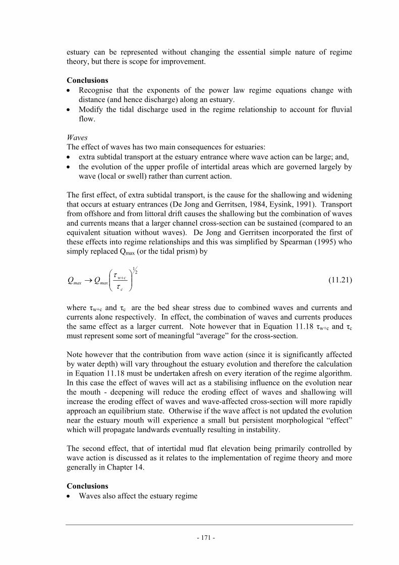
- 171 -

estuary can be represented without changing the essential simple nature of regime theory, but there is scope for improvement. Conclusions • Recognise that the exponents of the power law regime equations change with

distance (and hence discharge) along an estuary. • Modify the tidal discharge used in the regime relationship to account for fluvial

flow. Waves The effect of waves has two main consequences for estuaries: • extra subtidal transport at the estuary entrance where wave action can be large; and, • the evolution of the upper profile of intertidal areas which are governed largely by

wave (local or swell) rather than current action. The first effect, of extra subtidal transport, is the cause for the shallowing and widening that occurs at estuary entrances (De Jong and Gerritsen, 1984, Eysink, 1991). Transport from offshore and from littoral drift causes the shallowing but the combination of waves and currents means that a larger channel cross-section can be sustained (compared to an equivalent situation without waves). De Jong and Gerritsen incorporated the first of these effects into regime relationships and this was simplified by Spearman (1995) who simply replaced Qmax (or the tidal prism) by

21

⎟⎟⎠

⎞⎜⎜⎝

⎛→ +

c

cwmaxmax QQ

ττ

(11.21)

where τw+c and τc are the bed shear stress due to combined waves and currents and currents alone respectively. In effect, the combination of waves and currents produces the same effect as a larger current. Note however that in Equation 11.18 τw+c and τc must represent some sort of meaningful “average” for the cross-section. Note however that the contribution from wave action (since it is significantly affected by water depth) will vary throughout the estuary evolution and therefore the calculation in Equation 11.18 must be undertaken afresh on every iteration of the regime algorithm. In this case the effect of waves will act as a stabilising influence on the evolution near the mouth - deepening will reduce the eroding effect of waves and shallowing will increase the eroding effect of waves and wave-affected cross-section will more rapidly approach an equilibrium state. Otherwise if the wave affect is not updated the evolution near the estuary mouth will experience a small but persistent morphological “effect” which will propagate landwards eventually resulting in instability. The second effect, that of intertidal mud flat elevation being primarily controlled by wave action is discussed as it relates to the implementation of regime theory and more generally in Chapter 14. Conclusions • Waves also affect the estuary regime

- 172 -

• The discharge used in the estuary regime relationship should be altered as in Equation 11.18.

Geological considerations Regime theory relates tidal discharge (Qmax or Ω) to cross-section or to width and depth. Where an estuary cross-section has an inerodible bed, the relationship between discharge and cross-section variables will not conform to the regime relationship as the width and/or depth will be constrained. Many estuaries display this characteristic, the Mersey, Lune, Conwy, to name a few. However, the fact that they are geologically constrained for some reaches does not preclude them from exhibiting some sort of characteristic relationship of the regime type for their unconstrained reaches. Spearman (1995) showed that a regime theory can be applied to such estuaries by assuming that a geologically constrained cross-section will remain constant until (and if) discharges through such a cross-section fall below the “regime discharge” whereupon accretion may occur. There are two important points to make about geological considerations: • The first is that (as discussed in Chapter 13) the morphological evolution of all

estuaries takes place within a certain imposed geological constraint or “space”. The long-term evolution of the estuary is significantly affected by the geological constraint and even over medium and short time-scales estuary evolution will also be affected if any part of this geological constraint is “exposed”. In circumstances where estuary evolution is likely to include significant erosion at locations within the estuary it is therefore necessary to know, in order to assess the resulting estuary evolution, the whether such erosion would be unconstrained or whether it would be reduced by the underlying geology.

• The second important point, which is actually very similar to the first point, is that estuary evolution is affected not just by the underlying geological variation but also by the underlying sedimentological variation. This is not just a reference to a change from sand to mud but a reference to the variation in sediment characteristics that occurs with depth in typical bed sediment. In an eroding patch of sea bed or foreshore the rate of erosion is often attenuated by experiencing the more consolidated and less erosive sediment that was hitherto buried by less resistant sediment. Similarly in an accreting area freshly deposited sediment will be much more susceptible to erosion that any underlying sediment that has remained in place for some time. While the effect of geological constraints on estuary evolution may not be relevant to many studies, the nature of how sediment characteristics will vary with erosion or deposition is likely to be relevant to most studies where estuary evolution could occur. This situation is complex because the nature of sediment in situ could change on exposure due to weathering or biology and this represents a significant source of uncertainty in the model results (Spearman, 2001).

Conclusion • Estuaries with geological constraints can be represented by regime theory as long as

there are enough unconstrained cross-sections to derive the characteristic regime equation and if there is sufficient knowledge about the estuary-wide geological

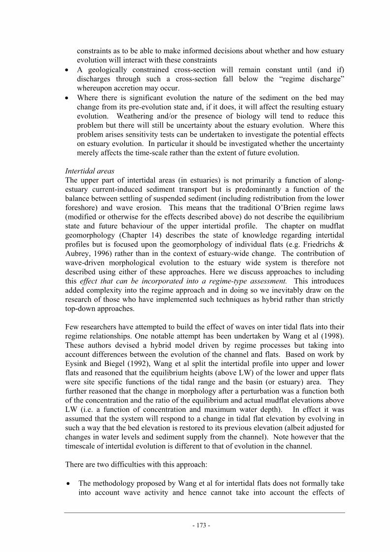
- 173 -

constraints as to be able to make informed decisions about whether and how estuary evolution will interact with these constraints

• A geologically constrained cross-section will remain constant until (and if) discharges through such a cross-section fall below the “regime discharge” whereupon accretion may occur.

• Where there is significant evolution the nature of the sediment on the bed may change from its pre-evolution state and, if it does, it will affect the resulting estuary evolution. Weathering and/or the presence of biology will tend to reduce this problem but there will still be uncertainty about the estuary evolution. Where this problem arises sensitivity tests can be undertaken to investigate the potential effects on estuary evolution. In particular it should be investigated whether the uncertainty merely affects the time-scale rather than the extent of future evolution.

Intertidal areas The upper part of intertidal areas (in estuaries) is not primarily a function of along-estuary current-induced sediment transport but is predominantly a function of the balance between settling of suspended sediment (including redistribution from the lower foreshore) and wave erosion. This means that the traditional O’Brien regime laws (modified or otherwise for the effects described above) do not describe the equilibrium state and future behaviour of the upper intertidal profile. The chapter on mudflat geomorphology (Chapter 14) describes the state of knowledge regarding intertidal profiles but is focused upon the geomorphology of individual flats (e.g. Friedrichs & Aubrey, 1996) rather than in the context of estuary-wide change. The contribution of wave-driven morphological evolution to the estuary wide system is therefore not described using either of these approaches. Here we discuss approaches to including this effect that can be incorporated into a regime-type assessment. This introduces added complexity into the regime approach and in doing so we inevitably draw on the research of those who have implemented such techniques as hybrid rather than strictly top-down approaches. Few researchers have attempted to build the effect of waves on inter tidal flats into their regime relationships. One notable attempt has been undertaken by Wang et al (1998). These authors devised a hybrid model driven by regime processes but taking into account differences between the evolution of the channel and flats. Based on work by Eysink and Biegel (1992), Wang et al split the intertidal profile into upper and lower flats and reasoned that the equilibrium heights (above LW) of the lower and upper flats were site specific functions of the tidal range and the basin (or estuary) area. They further reasoned that the change in morphology after a perturbation was a function both of the concentration and the ratio of the equilibrium and actual mudflat elevations above LW (i.e. a function of concentration and maximum water depth). In effect it was assumed that the system will respond to a change in tidal flat elevation by evolving in such a way that the bed elevation is restored to its previous elevation (albeit adjusted for changes in water levels and sediment supply from the channel). Note however that the timescale of intertidal evolution is different to that of evolution in the channel. There are two difficulties with this approach: • The methodology proposed by Wang et al for intertidal flats does not formally take

into account wave activity and hence cannot take into account the effects of

- 174 -

changes in wave action (e.g. arising from development or climate change or mudflat evolution itself) upon morphology.

• Notwithstanding the bullet point above, a substantial amount of data may be required to find the site-specific equilibrium relationships for the equilibrium, if one can be found at all - the scientific basis for this method is restricted to data from the Wadden Sea which may not universally applicable.

Di Silvio also applied a similar approach to top-down and hybrid models of the Venice Lagoon (Di Silvio, 1989, Di Silvio and Gambolati, 1990, Di Silvio, 1998). He first assumed a simplification of sediment transport (also adopted by Wang et al above) where the net erosion/deposition is given by the formula,

)CC(wE E −= (11.22) and E is the net erosion (or deposition), w is a settling parameter, and C and CE are the actual equilibrium concentrations. Di Silvio reasoned that on intertidal flats (in his paper he refers to them as “shoals”) the equilibrium concentration is given by,

HWE H

fC = (11.23)

where f is a local parameter relating to wave energy and the local bottom resistance and HHW is the maximum water depth. Thus, as in the model of Wang et al, the change in morphology after a perturbation was a function both of the concentration and maximum water depth and the system is assumed to respond to a change in tidal flat elevation by evolving in such a way that the bed elevation is restored to its previous elevation (albeit adjusted for changes in water level and sediment supply). Di Silvio’s method has a slight advantage over that of Wang et al because the effect of changes in waves is straightforwardly implemented by changing the parameter f, albeit crudely. However the second criticism applied to Wang et al’s approach – that of a substantial amount of data being required to find the site-specific equilibrium relationships for the inter-tidal equilibrium (or equilibria - different intertidal areas will have different wave conditions) remains true. It should be noted with both these approaches that the equilibrium states of intertidal areas are indirectly a function of sediment supply as well as water depth and wave action since if the sediment supply increases/reduces there will be deposition/erosion of the intertidal area and the water depth will reduce/increase until the equilibrium concentration matches the supplied concentration (e.g. Equations 11.22 and 11.23). Conclusions • The only representation of intertidal flat mechanisms in estuary-wide regime theory

known to the authors are: – Wang et al (1998) implementing the results of morphological studies of the

Wadden Sea by Eysink in 1992. – Di Silvio (1989, 1998)/Di Silvio and Gambolati (1990), implementing a

conceptual framework for sediment transport in tidal lagoons.

- 175 -

• The Wang study did not proposed specific relationships but suggested that, given a steady wave regime and some impulse to the system a tidal flat will essentially evolve to maintain the same elevation above LW subject to changes in water level and sediment supply. No methodology for considering the estuary wide evolution resulting from changes in wave action on intertidal areas is presently available using this approach.

• The Di Silvio studies assumed some simplified relationships governing intertidal evolution and his methodology is able to characterise in a simple way the impacts of changes in wave activity on intertidals. Essentially intertidal evolution becomes a function of water depth, wave action and sediment supply.

• Both the Wang et al and Di Silvio approaches involve some representation of sediment supply from channel areas to intertidal flats. The inclusion of this process increases the complexity of the regime approach and moves it towards hybrid modelling rather than top-down assessment.

11.9.8 Empirical derivation of the regime relationship One of the biggest problems with regime theory is that in most cases, the estuary system, on the basis of the field or model data available, does not conform to a smooth relationship of the type A=Ωn or A=f(C) Ωn but instead presents considerable scatter around a best fit relationship of that form. Adopting the best fit relationship and implementing the regime algorithm to derive the morphological evolution of the estuary, will, unless the perturbation of interest is very significant, result in false evolution of the estuary driven entirely by the scatter in the data and the uncertainty inherent in the method (Spearman, 1995, 2001). There is no perfect method for overcoming this problem. Spearman (1995) suggested initially iterating the estuary until the fit of the characteristic regime equation is sufficiently good (Spearman used the criterion of a maximum error against observations being less than 5%) whereupon the effect of a further perturbation can be much more readily assessed. This overcomes the practical problems but introduces a different uncertainty in that the estuary used to investigate the effect of some perturbation is “not quite the same” as that observed. This method also has the flaw that where the regime relationship used does not describe the estuary system well initially the use of this method can result in large changes in cross-sections (Townend, pers.comm., 2005). Spearman (2001) also suggested an alternative method. For this alternative the discrepancies between the real estuary and the equilibrium values given by the regime equation are initially evaluated and held to be constant throughout the evolution. In other words (Townend, pers.comm., 2005),

“it is assumed that the channel section is in regime (for reasons we do not fully understand) and existing channel is adjusted in proportion to the relative change between the pre- and post-scenario regime channels.”

Whilst this method can over-come the problems of large discrepancies of an estuary from the chosen regime relationship (Townend, pers.comm., 2005), Spearman (2001) reports that this alternative method did not completely remove spurious evolution caused by the initial state of the model. The problem is, as discussed in Section 11.8.2,

- 176 -

that it is not known whether the differences between the initial estuary bathymetry and the equilibrium bathymetry given by the regime equation will vary as the estuary evolves or whether they will remain constant. It is evident that the level of uncertainty in the regime relationship is very important for understanding the level of uncertainty in the corresponding morphological predictions arising from its use. This important information (and any steps taken to overcome it) is often not included in a study description. Conclusion • Except when considering large perturbations in estuaries, the error in the ability of

the regime equation to characterise an estuary will significantly affect the predicted evolution of the estuary using estuary regime theory, possibly compromising the whole prediction.

• It is important therefore to reduce this problem where possible by careful selection and consideration of the regime algorithm to be used.

• There will still be residual error and there are two methods to overcome the problem of error affecting the predicted evolution: (a) initially iterate the estuary system until the fit of the regime equation improves sufficiently that the error can be ignored (albeit the “baseline” estuary is then different to reality) or (b) assume that the channel section is in regime (for reasons we do not fully understand) and adjust the existing channel in proportion to the relative change between the pre- and post-scenario regime channels.”

Part 2 - Best Practice 11.10 Best practice for using regime theory in estuaries 11.10.1 Introduction to best practice As noted in Section 11.8.1 the use of O’Brien relationships within estuaries differs from the use of the O’Brien relationships for estuary/tidal inlet entrances in that the use of these relationships within estuaries requires a site specific approach and the empirical selection of a relationship based on an individual estuary, while use of the approach at entrances seeks to make a more objective assessment of the state of the estuary/inlet based on more general relationships that relate to all estuaries or all estuaries from a certain group (See Section 11.7). As for the use of regime theory at estuary entrances the use of regime theory throughout estuaries is hampered by problems surrounding uncertainty (error) inherent in this empirical method. As discussed in Section 11.9.7 this uncertainty will affect the predicted estuary evolution and although steps can be taken to reduce the impact of this uncertainty it cannot be removed completely and in some cases may still compromise the validity of the predicted evolution. Again the important question is therefore not, “does a regime relationship give a good correlation?” but,

“what is the effect of the error inherent in the relationship on my prediction of estuary evolution?”.

- 177 -

This study has found that the form of the (estuary-wide) regime relationships commonly used for predictive studies is actually flawed because it doesn’t take into consideration all of the factors that may affect estuary evolution. This adds to the uncertainty in the method. Modifications to the regime approach outlined in Appendices 2 and 3 and in Section 11.9 will reduce this source of uncertainty - it that associated with use of the method itself. In practice the method can be applied on a spectrum of levels of complexity ranging from a very top-down application depending predominantly on bathymetric data to a hybrid modelling combination of flow model and regime algorithm. Although deployment of the latter is outside the scope of this report the key issues of use of the method do not alter significantly. 11.10.2 Data needs The main parameters associated with use of this method are listed below. However it should be noted that these parameters will vary throughout the year: seasonally due to more intense wave activity and higher fluvial flows, and potentially, though to a much smaller extent, over the spring- neap tidal cycle due to variations in tidal currents. Usually the tidal conditions chosen are mean spring tide conditions. In practice the representative morphological conditions will vary from estuary to estuary but can be derived using the data-filtering techniques proposed by for instance Chesher and Miles (1992) and de Vriend et al (1993). Where this level of in-depth analysis is beyond the scope of Expert Geomorphological Analysis it is suggested that mean spring tide conditions be used with mean wave heights and mean annual fluvial flow. The main data requirements for using Regime Theory throughout estuaries are spit into discharge and area parameters, which are always required, parameters needed for the application of the theory in sandy and muddy estuaries, other potentially important parameters and finally the data required should the method be applied using a flow model. • Channel cross section area, channel width and channel depth

These parameters are discussed in the section on data and are derived from bathymetric surveys. It is usual for all cross-section parameters (area, width, etc) to correspond to mean sea level.

• Tidal prism/peak discharge

This parameter is discussed in the section on data. This parameter can be derived from flow modelling or from bathymetry surveys. As stated above tidal prisms will normally correspond to mean spring tide conditions.

For Sandy estuaries • Sediment grain size

As shown in Appendix 2, the evolution of the estuary is dependent on the sediment transport equation used, which is itself dependent on sediment grain size. This is derived from laboratory analysis of in situ samples of the sea bed.

- 178 -

• Velocity at peak discharge This is required to evaluate the parameter µ in Equation 11.14 which represents the exponential rate of decay in velocity with distance. In practice this can be derived from the parameters of discharge and cross-section area.

For muddy estuaries • Suspended sediment concentration

As shown in Appendix 3 and Section 11.9.4 the method requires data on the initial suspended sediment concentrations throughout the estuary. This data is obtained from in situ measurements or, less commonly, well-calibrated sediment transport models.

• Erosion threshold

If the erosion threshold is not small then the evolution of the estuary will additionally be influenced by this parameter. However in practice this parameter is very difficult to measure and/or estimate in muddy environments.

Other potentially important parameters • Fluvial flow

This parameter is used to adjust the tidal prism to represent the total discharge through a cross-section, or alternatively (see below) to inform the boundary conditions for a flow model if such a model is being used to provide data on peak discharge. For most estuaries in the UK the main tributaries are gauged and the key statistics for each gauge are made available by the Environment Agency.

• Wave height and period

These parameters are used to adjust the peak discharge used on the regime relationship to include the additional effects of wave erosion. The data used for this can be derived from wave measurements or suitably reliable wave models.

• Geological constraints

For most estuary studies the presence and distribution of geological constraints will be sufficiently obvious from an examination of the bathymetry. However for more detailed studies of long-term evolution the underlying geological constraints of the basin will be important. This sort of data requires expert geological input.

Calibration of flow model The data necessary for flow model calibration are listed below and discussed in the data chapter. • Water level data • Tidal current measurements • Fluvial data Additionally there is a requirement for data with which to calibrate the predictive approach before undertaking a prediction of impact. Ideally some morphological

- 179 -

evolution prior to the existing state of an estuary would have been detailed by bathymetric surveys. Unfortunately such data sets are few and far between. 11.10.3 Implementation of the method 1. Make an initial evaluation of whether use of regime theory is viable. • Is there a robustly calibrated flow model which can be used? – this will give data on

depth, width, cross-section area and discharge. • If not is there enough data available to either develop a model (boundary data,

calibration data) or to produce estimates of discharge and cross-section area? • Is there data on sediment type? • If the estuary is muddy then sediment supply will become important:

– Is there data on supply of sediment to the system? – Is there data on suspended sediment concentration?

• If there is significant fluvial flow or wave action at the entrance – is there data for this?

2. Make a secondary evaluation of whether use of regime theory is viable. • Ascertain on the basis or model results whether the system in question exhibits a

characteristic regime relationship between peak discharge/tidal prism and cross-section are.

• In the case where data (not a flow model) is being used, only one iteration of the regime algorithm (following some estuary change) can be achieved. The time frame corresponding to this iteration can be derived but further evolution will probably occur – is this satisfactory?

3. Develop regime relationship • On the basis of the data develop regime relationship with modifications for:

– Waves 2

1

⎟⎟⎠

⎞⎜⎜⎝

⎛→ +

c

cwmaxmax QQ

ττ

– Fluvial flow fmaxmax QQQ +→ – Geological constraint iiii QQAA >=− ++ 11 0

iiKi

Kiii QQQQAA <−=− +++ 111

22

• Use a regime relationship that allows variation in the regime along the estuary e.g. ( ) cQlog.bQlog.aQlog maxmaxmax ++= 2

• If sandy conditions then the regime algorithm becomes

( ) ( )⎥⎦⎤

⎢⎣⎡ −+−′−=− −−

+nnK

iii kdxdknQtKAA γγµδ 2

11

where K1 = λ1 λ4

n dtwtn

tide.sin∫β , λ1 and λ2 are given by pQB 1λ= , qQH 2λ= ,

and β is given by the general transport equation S=βVn , µ is the exponential growth/decay of the velocity with distance along the estuary given by VE=V0e-µx ,

- 180 -

K2 = p+(1-p-q)n , k is a parameter of order O(1), γ is a parameter of O(1) describing the tidal asymmetry, and, δt' is the number of tides represented by one iteration of the algorithm. The equation is useful as an aid to understanding and under some circumstances represents a valuable top-down tool (see Section 11.11.3). However, in practice this equation is equivalent to a 1D sand transport model (see Appendix 2) and for predictive purposes it is likely that calculating the change in morphology using 1D sand transport will be more practical than applying the regime equation. In either case the 1D model or regime algorithm would be used iteratively with a flow model to derive the evolution of the estuary system. Whether the regime algorithm is applied or the equivalent 1D sand transport model it is important to recognize that the estuary system is initially assumed to be in equilibrium and therefore flood and ebb tide transport for the representative conditions used must be equal. In practice this means choosing values of k in the equation above for each cross-section to ensure a balance between ebb and flood transport. These values of k are then held constant for the evolution following some disturbance.

• If muddy conditions use the regime algorithm

⎥⎥⎦

⎤

⎢⎢⎣

⎡⎟⎟⎠

⎞⎜⎜⎝

⎛−⎟⎟

⎠

⎞⎜⎜⎝

⎛=− +

+

++

221

1

111

Ki

m

i

i,EKi

m

i

i,Eii Q

CC

QC

CK.tAA δ

where Ci and Ci, E are the “representative” actual and equilibrium concentrations at a

cross-section at time step i of the evolution. and ⎟⎟⎠

⎞⎜⎜⎝

⎛

+

+

1

1

i

i,E

CC

is approximately equal to

⎟⎟⎠

⎞⎜⎜⎝

⎛

iMM 0 where M0 and Mi are the total mass of sediment in the system before estuary

evolution starts and on the ith iteration of the regime algorithm, K1 =1/2 λ1TMeρCDλ4

2(1-p-q) , λ1 is given by, pQB 1λ= , λ4 is given by qpQV −−= 1

4λ , T is the tidal period, M is an erosion rate parameter, ρ is the water density, CD is the drag coefficient, K2=2-p-2q Qi is the peak discharge on the ith iteration, and, δt' is the number of tides represented by one iteration of the algorithm.

4. Consider how to deal with uncertainty in regime relationship In the case of muddy estuaries either • (If using a flow model) Use best fit relationship to iterate estuary bathymetry, then

derive the new best fit relationship. Repeat until difference between actual and

- 181 -

regime discharge is below 5% (or some more stringent criterion). (See Section 11.9.7)

Or • Decide to use changes in width and depth given by regime relationship in a

proportional way. Record level of uncertainty in regime equation in terms of standard deviation in % terms between observed data and regime predictions. This is an estimate of the level of uncertainty in the prediction of impact. In the case of sandy estuaries • Select the values of k in Equation 11.14 such that ebb and flood tide transport is

initially equal throughout the estuary system. 5. Implement change to estuary • Remodel estuary with change represented or, if not using a model, calculate changes

to discharge and estuary cross-sections on the basis of changes in bathymetry. • If muddy, consider effect on concentrations. Derive the %age change in total

sediment in the estuary, considering, the following influences: – Morphological change – Sediment supply – Dredging and disposal – Fluvial input of sediment

• Assume ratio of increase above baseline by this %age amount. • Keep implementing iterations until the predicted change on each iteration is less

than set criterion (% of initial perturbation or below fixed limit). • If instability occurs (the estuary continues to fill or to erode without slowing) then

reduce the time step represented by each iteration of the algorithm. 6. Sensitivity analysis • Repeat step 4 using different key assumptions/parameters to check believability of

results. 11.11 Case studies To illustrate the uses of regime theory three case studies are included below. All of the case studies are associated with long-term prediction of the evolution following estuary management schemes. Two of the case studies (the Lune and Tollesbury Creek examples) utilise regime theory in a hybrid format. These studies utilise the “traditional” form of the regime algorithm – i.e. without the improvements discussed above and examined in Appendices 2 and 3. The third example (Mersey) utilises the “improved sandy” version of the regime algorithm to describe the evolution in the Mersey Estuary as a response to training wall construction. 11.11.1 Simulation of response to training wall construction in the Lune Estuary Spearman et al (1998) used a regime algorithm and a 1D flow model as a hybrid tool to predict the evolution of the Lune Estuary following training wall construction in 1847-1851.

- 182 -

Prior to the training wall construction the estuary displayed considerable instability (meandering) in its lower water course and the consulting company recommended training wall construction (see Figure 11.7) to improve navigation depths and fix the location of the main channel. A complete survey of the estuary was undertaken before construction in 1844 and the estuary was re-surveyed in 1956. The second survey showed that the total volume of the estuary under mean spring tide conditions had reduced from 57.5Mm3 to 30.3 Mm3, a reduction of almost 50% (Inglis and Kestner, 1958). Furthermore analysis reported by Inglis and Kestner showed that the peak discharge at the estuary mouth had reduced by 47%. The 1D model was calibrated to available water level and discharge data presented in Inglis and Kestner (1958). The regime relationship chosen was as follows (See section 11.9.6),

( ) 599168810780 2 .Alog.Alog.Qlog maxQmaxQE ++−= (11.24) where QE is the equilibrium peak discharge and AQmax is the cross-section area at peak discharge. Equation 11.24 was combined with the following equations describing the variation in equilibrium width and depth at every cross-section,

630

1

.

Enn Q

QBB ⎟⎟⎠

⎞⎜⎜⎝

⎛=+

430

1

.

Enn Q

QHH ⎟⎟⎠

⎞⎜⎜⎝

⎛=+ model elements 1-17 (11.25)

nn HH =+1 model elements 18 and 19 where Bi and Hi are the width and depth, respectively, on the ith iteration, and Q is the peak discharge. These regime relationships were derived by iterating the method for the pre-evolution equilibrium state. The flow model for the initial pre-evolution state did not show a smooth relationship between discharge and cross-sectional area, even allowing for those cross-sections which were geologically constrained. To identify the regime relationship the estuary geometry was progressively adjusted using Equations of the form of 11.24 and 11.25 except that instead of using fixed regime relationships (as used to predict subsequent evolution) the regime relationship itself was allowed to change, being derived on a best fit basis on each iteration. Thus over time the bathymetry “smoothed” and the regime relationship converged. The regime method is ideally suited to situations where the changes to the system can be adequately represented as 1-Dimensional. In this case the initial effect of the training walls was to cause accretion behind the walls and deepening of the low water channel – effects which are 2-Dimensional and therefore not well described by the method. For this reason no attempt was made to reproduce this initial estuary evolution

- 183 -

using the method. A basic characterisation of what these initial changes would have been (partially based on data observed by the consultants during this initial period) was undertaken (amounting to 10% of the total observed accretion in the estuary resulting from the training wall) and used as the initial conditions for the long-term evolution of the estuary. The long term evolution of the estuary was modelled using Equations 11.24 and 11.25 in an interactive fashion using the procedure summarised in Figure 11.8. The hybrid approach predicted that the peak discharge would reduce by 28% (around 3/5 of the observed decrease) and that the tidal volume of the estuary would reduce by 31% (around 2/3 of the observed reduction). 11.11.2 A simulation of tidal creek response to managed retreat As part of the EMPHASYS project a regime relationship and a 1D flow model were combined together as a hybrid morphological modelling tool to simulate the morphological evolution of a tidal creek in response to managed retreat. The tidal creek investigated was part of Tollesbury Fleet, a tributary of the River Blackwater in Essex, UK. This creek is currently part of an ongoing Defra (previously MAFF) study into the effects of coastal realignment and a farmer’s field, located at the head of the creek was deliberately breached in 1995 to create setback. Tollesbury Creek itself is just over 1km in length (Figure 11.9). Mean spring tidal range within the estuary is of the order of 4m. The intertidal area of the creek is composed of a complex network of saltmarsh cliffs and small-scale creeks and most of the creek dries out at low water. Peak currents are of the order of 0.3-0.5m/s and wave heights are small, the annual wave height being of the order of 0.3m (Hs). Tollesbury Creek exhibits some significant 2D flow characteristics which reduce the ability of a 1D model to describe the hydrodynamic behaviour of the creek in an accurate manner. The results of the 2D modelling undertaken as part of the MAFF study (Chesher et al, 1995) identified the following features: • The level and flow through the salt marsh level is poorly defined. • The catchment boundary of Tollesbury Creek is poorly defined. • The creek system experiences two distinct phases of flow with the direction of flow

changing significantly near HW. • There are significant differences in the directions of the flow before and after the

breach in the vicinity of the breach itself. This feature is most prevalent near HW, when the water level has risen above the level of the salt marsh.

These features affect the prediction of cross-section area and discharge by the 1D flow model and therefore the regime relationships and predicted creek evolution of the hybrid morphological model. While the 1D model would have to represent the salt marsh surface and cliff as a constant solid boundary, in reality there is considerable flow through the salt marsh creeks. The scenario of managed setback therefore presents a difficult test for the hybrid approach used and this type of approach is open to criticism for this reason. However,

- 184 -

the purpose of the study was to highlight the various practical problems involved with predicting morphological change resulting from setback schemes and to provide an indication of the degree of accuracy which can be expected to be achieved with good practice. The breach occurred in 1995, allowing the inundation of a 21 hectare area. The ongoing study into the impact of the breach includes regular bathymetric and biological field surveys. As part of the study 2D flow modelling of the scenarios before and after the breach and a series of bathymetric surveys from before the breach in 1994 and annual surveys after the breach in 1996, 1997, 1998 and 1999. A calibrated 1D model of the tidal creek was developed based on field measurements, bathymetric survey data and 2D modelling work. This 1D model was used to develop regime relationships for cross-sectional area, width and depth based on a power law dependence on discharge. After deriving the regime relationships the 1D model was re-run with the breach in place and the corresponding pattern of discharge and cross-sectional area was used as input to the regime relationships to establish a new bathymetry corresponding to a time in the future. The 1D model was re-run with this new bathymetry to gain the next set of discharge/area data, and so on, iteratively, simulating the evolution of the morphology over time. The model used for the 1D flow modelling was the HR Wallingford/Halcrow ISIS model. The bathymetric data from the 1994 pre breach survey was processed augmented using data from the TELEMAC-2D model bathymetry used in Chesher et al (1995) and from further field surveys and aerial photograph analysis presented in the same study and in Spearman and Chesher (1997). The downstream tidal boundary condition was taken from field measurements undertaken near the mouth of the creek (Chesher et al, 1995) and the upstream discharge boundary conditions imposed were all of zero flux. Further field measurements given in Chesher et al (1995), consisting of water level measurements and fixed point measurements of current speed were used as calibration data. However, no measurements of water level or current speed were available from the setback field itself. It was considered that any deficiencies in the 1D model were either a result of processes also not reproduced in the 2D modelling, and therefore beyond the scope of this study to consider further, or possibly a result of uncertainty arising from field measurements. As a first step towards simulating the evolution of the creek over time, the calibrated 1D model discussed above was used to derive the regime relationship. A large number of different discharge/area parameters have been used in literature, of which relationships between peak discharge and area at peak discharge, and tidal prism and area at mean water level, are the most common. However, for this study these relationships were rejected for the following reasons: • A relationship based on tidal prism would have been too susceptible to uncertainty

in the representation of flow over and through the saltmarsh and the poorly defined water shed of the creek.

• The relationship based on peak discharge was found to be too responsive to effects other than the effect of the breach. This may be due to sudden large changes in the cross-section area at peak discharge as the water level at which peak discharge occurred crept above or below the defined salt marsh storage level.

- 185 -

• Previous morphological studies reproducing evolution of the Lune Estuary as a response to training wall construction (Spearman et al, 1998) found that relationships based on peak discharge cause changes in the estuary at higher water levels thus causing large changes at the channel margins which were not observed to occur.

For these reasons a relationship between discharge at peak velocity and area at peak velocity was chosen. This relationship was best able to describe changes in the LW channel and was found to respond well to the forcing effect of the breach. As described above the spurious evolution caused by uncertainty (scatter) in the regime relationship was removed through “smoothing” the estuary bathymetry by evolving the estuary to a steady state (subject to some sensible tolerance), rederiving the regime relationship on each iteration. The smoothing process undertaken consisted of 5 half-steps, being terminated when the average discrepancy of cross-sectional discharge at peak velocity, QVmax, from the regime value was less than 1% and the maximum discrepancy was less than 5%. The resultant regime relationships took the form, QVmax = 0.4194 AVmax

0.952 (11.26) W α Q0.4749 and H α Q0.6271 (11.27) where AVmax is the cross-sectional area at the time of peak velocity and W and H are channel width and depth respectively at the time of peak velocity. The procedure of finding the regime relationship for the estuary highlighted the fact that the section of the channel leading to the breach – cross sections 29, 30 and 30a (See Figure 11.9) -was not “in regime” with the rest of the estuary. The pre-breach current speeds through this section were much reduced, (for both the 1D and 2D models) even though the sea wall protecting the farmers’ field had been in place for approximately 30 years. This result suggest that this part of the creek is sediment supply limited or at least that the time scale for encroachment by saltmarsh is very long. It is also apparent from anecdotal observations that there has been no noticeable erosion of the salt marsh cliffs. For this reason the evolution of the channel in the simulations described below was constrained to below the level considered to be a reasonable estimate of the level at which saltmarsh cliffing would occur (1.5mOD). The flow model was used to derive the value of QVmax and AVmax and the regime relationship (Equation 11.26) was used to derive the regime value of discharge, QE for the given cross-section area. The width and depth were then changed as follows:

4749.0

max

⎟⎟⎠

⎞⎜⎜⎝

⎛→

reg

V

QQ

WW 6271.0

max

⎟⎟⎠

⎞⎜⎜⎝

⎛→

reg

V

QQ

HH (11.28)

The time scale corresponding to each iteration was estimated by running a simple calculation of the total net erosion occurring for a single (spring) tide and comparing this total with the total net erosion predicted by the regime model. The ratio between these totals represented the number of spring tides simulated by each iteration of the regime model. The sediment transport calculation used constant but representative values for settling velocity, and suspended sediment concentration and deposition

- 186 -

threshold. However, the net erosion within the creek was dominated by the parameters of erosion threshold and erosion rate constant. In some ways this manner of calculating the time-scale of the corresponding evolution is unsatisfactory since the range of erosion rates produced by the possible range of all the relevant parameters is at least an order of magnitude and thus the time scale can be “legitimately” adjusted to almost any value required. The results of the simulation were compared to the surveyed bathymetry for the end of 1999, some 4 years after the breach. The model predicted significantly more erosion downstream (seaward) of the breach as a result of the breach than was been observed although the model did reproduce the observation that the change upstream (landward) of the breach would be small. The results also predicted that the time scale of evolution was approximately 20 years. Sensitivity tests were carried out to observe the sensitivity of the results to the representation of flow in the setback field and the sensitivity of the results to allowing the breach itself to evolve. The results showed that the evolution of the creek was relatively insensitive to both these changes. The 2D features of the creek did not appear to cause too many problems for the method in this particular case because the 2D features were manifest near HW and the peak velocities driving the evolution of the creek occurred sufficiently below this level as to be reasonably approximated by the 1D model. This would not be the case had a regime relationship based on tidal prism or peak discharge been used. The study indicated that a reasonable assessment of future evolution can be achieved although the accuracy of predictions can be best described as qualitative rather than quantitative. However a considerable number of trial runs were undertaken together with extensive examination of results to achieve these results. Furthermore, this study benefited from hindsight in being able to make judgements about the manner in which evolution occurred, and in being able to use bathymetric data from just after the breach to eliminate further error that would result from trying to reproduce the rapid evolution occurring for the period immediately after breaching. Essentially the predictive model was “calibrated” to reproduce the observed evolution of the creek. Without the benefit of hindsight, and this “calibration” process the inaccuracy of predictions would have been considerably greater. 11.11.3 Application of regime theory to evolution observed in the Mersey

Estuary This case study demonstrates how the application of regime theory (in the revised form based on the analysis of Appendix 2) can be utilised in a top-down format to diagnose historical estuary evolution and additionally demonstrates how the typical results of studies aimed at predicting the future evolution resulting from a proposed scheme or from possible natural change could be used to make a longer term assessment of the estuary evolution. The case study uses the example of the Mersey Estuary which experienced considerable morphological change in the 20th century arising from training wall construction in Liverpool Bay. This example is described in detail in Section 12.6 where the example

- 187 -

is also used as an illustration of sediment budget analysis. The Mersey Estuary and Liverpool Bay are shown in Figure 12.3. Previous to 1911 the Mersey Estuary was in a state of quasi-equilibrium albeit with significant year to year variation (Figure 12.4). From around 1911, the Mersey experienced significant accretion of sand which reduced the overall volume of the estuary and increased the intertidal area. Analysis of bathymetric change appear to indicate that the estuary attained a new equilibrium around 1977 (HR Wallingford, 1999). Thomas (2000) undertook 2D and 3D modelling of the impact of the training wall construction on the net sand flux into the Mersey Estuary. He calculated the (potential) annual net flux of sand into the Mersey in 1906 before the training walls were in place, in 1936 roughly when the training wall construction was completed and in 1977 when the a new equilibrium had apparently been attained. Table 11.3 summarises his calculations (which roughly concur with the sediment budget calculations presented in Table 12.2). Table 11.3 Residual sediment transport fluxes to estuary mouth

Simulation conditions Net sediment flux to estuary mouth (Mm3)

1906 Mean spring tide 0.15 1936 Mean spring tide 2.63 1977 Mean spring tide -2.53

The table indicates that the net flux of sediment to the mouth of the Mersey was small in 1906 and that it increased significantly in 1936. In 1977 when the new equilibrium was attained the net flux was reversed. On the basis of Thomas’s data (including unpublished work) it is estimated that in 1936 the gross flux into the Mersey on the flood tide was 50-100% greater than the gross flux on the ebb tide. We will use this figure to estimate the long-term morphological change resulting from the training wall construction. In this case study it is apparent that the main change in the estuary is that of sediment supply and that there are no significant local variations in discharge and that the impact on hydrodynamics within the Mersey arising from the training wall construction are minor in comparison. Equation 11.28 and Appendix 2 then suggest that the initial increase in net sediment flux into the estuary will result in accretion and an increase in intertidal area but that this net sediment flux will reduce as the intertidal area reduces, the ratio of estuary area at LW to estuary area at HW (SLW/SHW) increases and the flood dominance of the system is reduced (Equations 10.3 to 10.5). Equation 11.28 states that equilibrium will be attained when the ratio of the flood flux to the ebb flux is equal to the relative increase in Dronkers parameter γ to the power n (where 3 < n < 5), i.e.,

- 188 -

n

tLW

equilibiumLw

n

tHW

LW

LW

HW

mEquilibriuHW

LW

LW

HW

tebb

fld

S

S

SS

HH

SS

HH

SS

⎪⎭

⎪⎬⎫

⎪⎩

⎪⎨⎧

≈

⎪⎪⎪

⎭

⎪⎪⎪

⎬

⎫

⎪⎪⎪

⎩

⎪⎪⎪

⎨

⎧

⎥⎥⎦

⎤

⎢⎢⎣

⎡⎟⎟⎠

⎞⎜⎜⎝

⎛

⎥⎥⎦

⎤

⎢⎢⎣

⎡⎟⎟⎠

⎞⎜⎜⎝

⎛

==

=

=0

0

2

2

0 (11.29)

(Note that the Mersey, because it is constricted at the mouth is not a strongly converging estuary and therefore Dronkers parameter is used in its original form rather than the modifications discussed in Chapter 10). Since the ratio of depth at HW to depth at LW are not likely to change greatly (and calculations by Thomas, 2000, shows this to be the case) the ratio of the pre-construction and equilibrium Dronkers parameters is roughly equal to the ratio of the LW areas before construction and at equilibrium to the power n (see Equation 11.26). Using this result, and arbitrarily using n=3.4 (which corresponds to the depth-averaged parameterisation of sediment transport proposed by van Rijn), we calculate that the Mersey following training wall construction will evolve so that the subtidal area will decrease by 15-30%. On the basis of simple geometry it was calculated that such a reduction in subtidal area (with a corresponding increase in intertidal area) in the Mersey would correspond to a volume reduction of around 5-10%. In fact history shows that the Mersey reduced its volume from 745Mm3 to 680Mm3 over the 50-60 year period – a reduction of around 9% (HR Wallingford, 1999, Thomas, 2000). 11.12 Conclusions Regime theory is a potentially useful tool for predicting the estuary evolution following disturbance because it can enable the characterisation of long periods of evolution relatively simply. However, the method has clear limitations and associated uncertainty and the understanding of these limitations and the uncertainty is as much important as knowing how to implement the tool itself. Regime theory comes in two forms – that applied to estuary and tidal inlet entrances and that applied in an estuary wide sense. The conclusions relevant to each form of the theory are presented below: Regime theory as applied to estuary and tidal inlet entrances • Entrance prism-area relationships are most commonly used to assess the evolution

of entrances to tidal inlets where the entrance is commonly the morphological feature of most interest to stake-holders (navigation, ecology, etc). In estuaries, except those where entrance closure from littoral drift is a risk, the focus is usually less centred upon the entrance. Moreover, in estuaries the flow conditions at the entrance are much more sensitive to morphological change further landward and it is usually necessary to include the morphology of the wider estuary in any predictive assessment.

- 189 -

• In this form regime theory can be implemented to predict changes to tidal inlet (and some estuary) entrances, to investigate their stability and as an aid to geomorphological classification.

• The method is based on relationships involving tidal prism (or peak discharge) and cross-section area – relationships often referred to as O’Brien relationships. Such relationships have been shown to exhibit relatively high correlations when compared against with data from inlets/estuaries from the same geographical area. However a more general comparison of this data shows the scatter or uncertainty in the O’Brien relationship to be significant.

• The uncertainty in the O’Brien relationships is due to variations in the underlying physical processes – e.g. variation in tidal range, estuary/inlet size, wave action, littoral drift, sediment type and supply, geology and geomorphology.

• Attempts to reduce uncertainty by developing an underlying theoretical basis for this method have had some limited success but in general have been restricted to tidal inlets which can be conceptually described as a balance between the flux of littoral drift into the entrance channel and the ebb tide transport which transports it away.

• The most practically useful method of reducing uncertainty in O’Brien relationships (Hume and Herdendorf, 1988) is to classify estuaries on a geomorphological basis and to produce regime relationships for each separate class. This ensures estuary entrances are compared with those that experience similar conditions.

• It is possible to use O’Brien type relationships to predict the changes in estuary/inlet entrances and a good example of this type of study is presented in Van de Kreeke (2004).

Regime theory as applied in an estuary-wide form • In this form regime theory can be implemented to predict the evolution of estuaries

following disturbance. As well as evaluating potential impacts arising from development the approach can be used to aid the diagnosis of historical morphological change as part of the development of the conceptual model.

• The method is based on relationships involving tidal prism (or peak discharge) and cross-section area but in this case these relationships have to be developed on an estuary by estuary basis. This means that estuary entrance relationships cannot be used for estuary-wide regime theory.

• At present no underlying theoretical basis has been established for establishing the parameters governing these relationships.

• As for the entrance regime relationships, estuary-wide regime relationships exhibit scatter and uncertainty. Some of this uncertainty is due to the underlying physical processes – e.g. variation in tidal range, estuary/inlet size, wave action, littoral drift, sediment type and supply, erosion threshold, fluvial flow, and the constraint of geology. This uncertainty can be reduced by including the effects of these physical processes in the regime relationships.

• In particular analysis of the estuary equilibrium and how evolution occurs following perturbation has identified that the common prism-area power law form of the regime algorithm does not model estuary evolution correctly and other terms, which are different for sandy and muddy estuaries, need to be included.

- 190 -

• The regime method can be used on a number of levels ranging from top-down to hybrid. However to be used as a predictive tool Regime Theory is best implemented in a hybrid form.

• Since the regime approach is essentially a cross-section averaged or 1-Dimensional approach, its use for 2-Dimensional impacts can be clumsy.

11.13 References ABP Research. (2000) An investigation of the gross properties of UK estuaries, ABP Research and Consultancy, Southampton, R.900, 39p. ABP Research. (2000) Geomorphological Analysis of East Head and Chichester Harbour, ABP Research and Consultancy Ltd., Report Number R893. Ackers, P. (1992) Canal and River Regime in Theory and Practice, 1929-1992, Gerald Lacey Memorial Lecture, Proceedings of the Institution of Civil Engineers, Water, Maritime and Energy, Paper 1019, Volume 96, p167-178. Bettess, R. and White, W. R. (1987) Extremal hypotheses applied to river regime, In: Sediment transport in gravel-bed rivers, C R Thorne, J C Bathurst and R D Hey (Eds), John Wiley and Sons Ltd., 1987 Bose, N. K. (1936) Silt movement and design of channels, Punjab Engineering Congress, Paper 192. Bruun, P. and Geritsen, F. (1960) Stability of coastal inlets, North Holland Publishing Company, Amsterdam, 1960. Bruun, P. (1978) Stability of tidal inlets – Theory and engineering, Amsterdam: Elsevier Scientific Publishing, Developments in Geotechnical Engineering, Volume 23. Byrne, R. J., Gammisch, R. A. and Thomas, G. R. (1980) Tidal prism-inlet area relations for small tidal inlets, Proceedings of the17th Coastal Engineering Conference, Sydney, Australia, March 1980, pp2517-2533. Chang, H. H. (1980) Stable Alluvial Canal Design, Journal of the Hydraulics Division, ASCE, Volume 106, Number HY5, May 1980, pp873-891. Chesher, T. J. and Miles, G. V. (1992) The concept of a single representative wave for use in numerical models of long term sediment transport predictions, Proceedings of the Second International Conference on Hydraulic and Environmental Modelling of Coastal, Estuarine and River Waters, 1992, Bradford, UK. Chesher, T.J., Price, D.M. and Southgate, H.N. (1995) MAFF Set Back Experiment, Tollesbury Creek, Report on model investigation of breaching scenarios, HR Wallingford Report SR 413, January 1995. de Jong, H. and Gerritsen, F. (1984) Stability parameters of Western Scheldt Estuary, Proceedings of the 19th Coastal Engineering Conference, Houston, USA, 1984, pp 3078-3093.

- 191 -

De Vriend, H. J., Capobianco, M., Chesher, T., de Swart, H. E., Latteux, B. and Stive, M. J. F. (1993) Approaches to Long Term Modelling of Coastal Morphology: A Review, Coastal Engineering, Volume 21, pp225-269. Di Silvio, G. (1989) Modelling the morphological evolution of tidal lagoons and their equilibrium configurations, XXIII Congress of the IAHR, Ottawa, August 1989. Di Silvio, G. (1998) Interactions between marshes, channels and shoals in a tidal lagoon investigated by a 2-D morphological model, Interaction 3rd International Conference on Hydro-Science and -Engineering Brandenburg University of Technology at Cottbus Cottbus/Berlin, Germany, August 31 - September 3, 1998. Di Silvio, G. and Gambolati, G. (1990) Two-dimensional model of the long-term morphological evolution of tidal lagoons, VIII International Conference on Computational Methods in Water Resources, Venice, Italy, June 11-15, 1990. Dyer, K. (2006) The Dimensional Relationships of Estuaries, submitted as part of the Estuaries Research Project Phase 2, see Section 2.4.3 of EstProc Consortium (2006). EstProc Consortium. (2006) Integrated Research Results on Hydrobiosedimentary Processes in Estuaries. Final Report of the Estuary Process Research Project (EstProc). R&D Technical Report prepared by the Estuary Process Consortium for the Defra and Environment Agency Joint Flood and Coastal Processes Theme. Report No FD1905/TR3 – Algorithms and Scientific Information. Download from: www.estproc.net Eysink, W. D. (1991) Simple relationships for estuaries and tidal channels- handy tools for engineering, Proceedings of the International Conference on Coastal and Port Engineering in Developing Countries, Volume II, Kenya, pp1003-1013. Eysink, W. D. and Biegel, E. J. (1992) Impact of sea level rise on the morphology of the Wadden Sea in the scope of its ecological function, Investigations on empirical morphological relations, Delft Hydraulics Report H1300, Phase 3. Friedrichs, C. (1995) Stability Shear Stress and Equilibrium Cross-sectional geometry of sheltered tidal channels, Journal of Coastal Research, volume 11, number 4, pp1062-1074, Fall, 1995. Gao, S. and Collins, M. (1994) Tidal inlet equilibrium, in relation to cross-sectional area and sediment transport patterns, Estuarine Coastal and Shelf Science, 38, pp157-172. Gerritsen, F., de Jong, H. and Langerak, A. (1990) Cross-sectional stability of estuary channels in the Netherlands, Proceedings of 22nd Conference on Coastal Engineering, Delft, 1990, pp2922-2935. Hughes, S. (2002) Equilibrium Cross-sectional Area at Tidal Inlets, Journal of Coastal Research, Volume 18, Number 1, pp160-174, Winter 2002.

- 192 -

Hume, T. M. (1991) Empirical Stability Equations for Estuarine Waterways and Equations for Stable Channel Design, Journal of Coastal Research, Volume 7, part 4, 1991, pp1097-1111. Hume, T. M. and Herdendorf, C. E. (1988) A geomorphic classification of estuaries and its application to coastal resource management – a New Zealand example, Ocean and Shoreline Management, 11, pp249-274, Hume, T. M. and Herdendorf, C. E. (1992) Factors controlling tidal inlet characteristics on low drift coasts, Journal of Coastal Research 8(2), pp355-375. Hume, T. M. and Herdendorf, C. E. (1993) On the use of empirical stability relationships for characterising estuaries, Journal of Coastal Research, 9(2), pp413-422. Lamberti, A. (1988) About extremal hypotheses and river regime, In: International Conference on river regime, Paper C4, 18-20 May 1988, pp121-134. Jarrett, I. T. (1976) Tidal prism –Inlet area relationships, GITI Report 3, US Army Corps of Engineers, Coastal Engineering Research Centre, Fort Belvoir and the US Army Engineer Waterways Experiment Station, Vicksburg, USA. Price, W. A. and Kendrick, M. P. (1963) Field and model investigation into the reasons for siltation in the Mersey Estuary, Proceedings of the Institution of Civil Engineers, April, pp473-517. Kondo, H. (1990) Flow area prediction of tidal inlets after sea level rise Proceedings of 22nd Conference on Coastal Engineering, Delft, 1990, pp3062-3072. Kraus, N. C. (1998) Inlet cross-sectional area calculated by process-based model, Proceedings of the 26th International Conference on Coastal Engineering22 - 26 June 1998 Copenhagen, Denmark, pp3265-3278. Lacey, G. (1930) Stable channels in Alluvium, Minutes of Proceedings of the Institution of Civil Engineers. Langbein, W. R. (1963) The Hydraulic Geometry of a small estuary, Bulletin of International Association for Scientific Hydrology, Volume 8, 1963, pp84-94. Lindley, E.S. (1919) Regime Channels, Proceedings of the Punjab Engineering Congress, Number 7 pp63-74 Mason, C. (1973) Regime Equations and tidal inlets, Journal of the Waterways, Harbors and Coastal Engineering Division, Proceedings of the American Society of Civil Engineers, Volume 99, Number WW3, August 1973. Mayor-Mora, R. E. (1977) Laboratory investigation of tidal inlets on sandy coasts, GITI Report 11, US Army Corps of Engineers, Coastal Engineering Research Centre, Fort Belvoir and the US Army Engineer Waterways Experiment Station, Vicksburg, USA.

- 193 -

Mehta, A. J. and Oszoy, E. (1978) Inlet hydraulics, In: Bruun P (Ed), Stability of tidal inlets, Elsevier, Amsterdam, pp510. Moore, J. T. (1972) The influence of bed material size on the tidal prism-area relationship in a tidal inlet, University of California Hydraulic Engineering Laboratory Technical Report HEL-24-13, Berkeley California, February 1972. Myrick, R. M. and Leopold, L. B. (1963) Hydraulic geometry of a small estuary, Physiographic and Hydraulic Studies of Rivers, Geological Survey Professional Paper 422-B, United States Government Printing Office, Washington, 1963. Nayak, I. V. (1971), Tidal Prism-Area relationship in a model inlet, Hydraulic Engineering Laboratory, Technical Report Number HEL-24-1, University of California, February 1971. O’Brien, M. P. (1931) Estuary tidal prism related to entrance areas, Civil Engineering, Volume 1, Number 8, 1931, p738. O’Brien, M. P. (1969) Note on tidal inlets on sandy shores, GITI Report 5, prepared for the US Army Coastal Engineering Research Centre by the University of California Berkeley, February 1976. O’Brien, M. P. (1976) Note on tidal inlets on sandy shores, GITI Report 5, prepared for the US Army Coastal Engineering Research Centre by the University of California Berkeley, February 1976. Seaburgh, W. C., King, D. B. and Stephens, B. E. (2001) Tidal equilibrium area experiments, inlet laboratory investigation, ERDC/CHL, TR-01-02, US Army Engineer Research and Development Center, Vicksburg, Mississippi. Shigemura, T. (1980) Tidal prism-Throat Area Relationships of the Bays of Japan, Shore and Beach, July 1990, pp31-35. Simons, D. B. and Albertson, M. L. (1963) Uniform Water Conveyance Channels in Alluvium Channels in Alluvial Material, Transactions of the ACSE, volume 128, Part I, paper 3399, pp65-107. Spearman, J. R. (1995) Estuary Regimes and methods for prediction of long-term changes, PhD Thesis for Oxford Brookes University, March 1995. Spearman, J. R., Dearnaley, M. P. and Dennis, J. M. (1998) A simulation of estuary response to training wall construction using a regime approach, Coastal Engineering, 33, pp71-89. Spearman, J. R. (2001) A simulation of tidal creek response to managed retreat using a hybrid regime model, HR Wallingford Report TR 118, January 2001. Spearman, J. R. and Chesher, T. J. (1997) Tollesbury Creek Managed Set Back Experiment, Comparison of model results with field observations, HR Wallingford Report TR 35.

- 194 -

Stive, M. J. F., Capobianco, M., Wang, Z. B., Roul, P. and Buijsman, M. C. (1998) Morphodynamics of a tidal lagoon and the adjacent coast, Proceedings of the 8th International Biennial Conference on Physics of Estuaries and Coastal Seas, The Hague, 1996, pp397-407. Thomas, C. (2002) The application of historical data and computational methods for investigating causes of long term morphological change in estuaries: A case study of the Mersey Estuary UK, PhD Thesis for Oxford Brookes University, February 2002. Townend, I. (2005) An examination of empirical stability relationships for UK estuaries, Journal of Coastal Research, 21, 1042-1053. Van de Kreeke, J. (1992) Stability of tidal inlets; Escoffiers Analysis, Shore and Beach, Volume 60, number 1, January, 1992, pp9-12. Van de Kreeke, J. (2004) Equilibrium and cross-sectional stability of tidal inlets: application to the Frisian Inlet before and after basin reduction, Coastal Engineering, number 51, pp337-350. Wang, Z. B., Karssen, B., Fokkink, R. J. and Langerak, A. (1998) A dynamic-empirical model for estuarine morphology, Physics of estuarine and coastal seas, Dronkers and Cheffers (eds), Balkema, Rotterdam, 1998, ISBN 905410965 3. White, R. W., Bettess, R. and Paris, E. (1982) Analytical Approach to River Regime, Journal of the Hydraulics Division, Proceedings of the ASCE, volume 108, HY10, October, 1982. Whitehouse, R., Soulsby, R., Roberts, W. and Mitchener, H. (2000) Dynamics of estuarine muds, Thomas Telford, London.

- 195 -

Figure 11.1 Inlet cross-sectional area related to tidal prism, for tidal inlets in the UK, USA, Japan and China Reprinted from Gao and Collins (1994) Estuarine Coastal and Shelf Science, Vol 38, 1994, pp 157-172, Copyright (1994), with permission from Elsevier.

- 196 -

Figure 11.2 Relationships between inlet cross-secitonal area at mid-tide and mean spring tidal prism for eight groups of estuary inlets on the New Zealand coast Reprinted from Hume and Herdendorf (1988) Journal of Ocean and Shoreline Management, Vol 11, pp 249-274, Copyright (1988), with permission from Elsevier.

- 197 -

1.E+01

1.E+02

1.E+03

1.E+04

1.E+05

1.E+06

1.E+07

1.E+04 1.E+05 1.E+06 1.E+07 1.E+08 1.E+09 1.E+10

Prism (m3)

CSA

(m2 )

B

C

HH-A

HH-B

HH-C

Figure 11.3 Prism-area data for UK estuaries by estuary type, from Townend (2005)

Figure 11.4 Observed and predicted evolution of the Frisian inlet following basin closure, after van de Kreeke (1992)

1

1.2

1.4

1.6

1.8

2

2.2

2.4

2.6

1970 1980 1990 2000 2010 2020Year

Cro

ss-s

ectio

n ar

ea (s

q.m

)

Eq.(7.10) with M/Le=300 and n=4 observed

Final Equlibrium, AE

- 198 -

ueq

u

AA1 A2

Figure 11.5 Escoffier’s diagram, after van de Kreeke (1992)

Figure 11.6 Uncertainty in the Regime relationship

0

1

2

3

4

5

6

0 2000 4000 6000 8000 10000Cross section area at entrance (sq.m)

Tida

l pris

m (M

illio

ns c

ubic

met

res

Best f it line(regime equation) r2=0.95

Example changein tidal volume

dA'

dA

Evolution

A

B

- 199 -

Figure 11.7 The Lune training walls (after Inglis and Kestner, 1958)

Figure 11.8 Summary of method used for long-term prediction

- 200 -

Figure 11.9 Tollesbury Creek and flow model cross-sections

- 201 -

12. ENTROPY BASED RELATIONSHIPS

Method Indicator Bottom-Up Hybrid Top-Down

YES 12.1 Background Entropy-based relationships are a method of characterising the most probable hydraulic state. Their use within Phase 1 of the Estuaries Research Programme has been developed previously by Dun and Townend (1998) and Gill (2000). Whilst new work as part of this project has clarified the potential for this approach, it has also highlighted the fact that much more needs to be done before this can be presented as a useful tool. For the purposes of this report, attention is therefore confined to the more established concepts and their use. 12.2 Overview of technique The concepts of entropy and energy dissipation have been reviewed as applied to a range of hydro-geomorphological systems, notably river basins, rivers, estuaries and beaches. As the concept of entropy is often considered obscure, the rest of this introduction provides some background to the concept and some important definitions. Section 12.3 discusses a range of previous applications of the concepts. The review focuses on the steady non-equilibrium (in a thermodynamic sense) condition that is often referred to as dynamic equilibrium. However, some important behavioral understanding can be derived by considering perturbations about the equilibrium state and this is discussed, qualitatively, in Section 12.4. The existing basis for applying entropy to estuaries is confined to considering how the energy flux varies along the length of the estuary. In Section 12.5 this is explored in some detail, to illustrate how the method can be used as a diagnostic tool and highlight some of the current limitations. Some conclusions are made in Section 12.6. Table 12.1 provides a summary of the key issues for the use of entropy methods.

- 202 -

Table 12.1 Entropy: Summary of Key Issues

Issue Entropy Analysis Description The technique explores the conditions that are likely to prevail close to dynamic

equilibrium for open systems with flows of matter and energy. It also has the potential to be used to examine the behavior of the system when it is perturbed but this is, as yet, a relatively new area of development and has only been presented here in a qualitative form.

Temporal Applicability

Long-term. Seeks to establish the most probable state. Necessarily this has different time-scales for different aspects of the landscape. So, whilst the river basin as a whole will be reducing over a very long time scale, river meanders will be evolving over decadal time scales and channel sections change to reflect prevailing flows and episodic events. Providing the constraints and boundary conditions are appropriately specified the technique can be applied across this spectrum of scales.

Spatial Applicability

In principle over any scale for which inputs and outputs of energy can be specified. However, this is closely linked to the chosen temporal scale and so reflects the scales noted above.

Links with Other Tools

The concept provides one way of deriving regime relationships (Langbein, 1963) and can be used with historical trends analysis to assess the evolution of the system towards a more probable state (Townend & Dun, 2000; Gill, 2000).

Data Sources Level 1 - bathymetry, water levels, fresh water flows Level 2 - sediment, temperature and salinity gradients

Necessary Software Tools / Skills

Level 1 - Hydrodynamic model in 1, 2 or 3-D plus suitable post-processing routines Level 2 – Hydrodynamic and sediment transport model in 1, 2 or 3-D plus suitable post-processing routines

Typical Analyses To look for perturbations from the most probable state, both in the existing regime and with any imposed changes (developments, sea level rise, etc).

Limitations Main use is as a diagnostic tool. The method has not yet been developed in a way that allows it to be used as a predictive tool.

12.2.1 General concepts and definitions There are many definitions, interpretations and uses of the term “entropy” (from the Greek word εντρπη meaning “evolution” (Prigogine, 1955), although Jaynes (1980) notes that according to Clausius it comes from τρπη meaning “to turn”, to which he added the prefix εν to make the word look and sound like “energy”). Although predominantly used in thermodynamics, statistical mechanics and information theory, there are many interpretations, as expressed by Williams (1997), who presented the information in Table 12.2 to illustrate what constitutes high and low entropy. Even within the confines of thermodynamics, there is often a perceived difficulty because of the close inter-relationship with other thermodynamic properties and the confusion arising from the interpretation of different forms of energy, notably internal energy. A very clear explanation is provided in the two books by Atkins (1984; 2003). Indeed, Atkins (1984, p30) has argued that in some senses entropy is an easier concept to grasp than energy, it is simply that the everyday use of the word ‘energy’ gives it a familiarity that belies its complexity. Energy can be any form of organisation of matter that is capable of doing work and can take the form of kinetic (motion), or potential (elevation in a gravitational field) energy. By way of an introduction, we consider a simple example, Box 12.1. This illustrates the process of doing work, where energy is transferred from one location to another. This is achieved by converting between potential energy (PE) and kinetic energy (KE). Along the way, some energy is lost to the environment in coherent forms such as noise and through the transfer of heat.

- 203 -

Table 12.2 Extreme or opposite states of entropy (after Williams, 1997)

High entropy Low entropy Proportion of energy available to do work Low High Degree of order, sorting or separation Low High Probability of a selected event Low High Probability of events Equally probable Preordained outcomes Type of distribution Uniform Highly uneven Degree of certainty Low High Predictability Low, random & unpredictable High leading to accurate forecasts Range of outcomes Wide variety Constrained Amount of diversity Large Small Degree of surprise Lots Little or none Amount of information High Low Information needed to specify system state Large Small Accuracy of data High Low

Box 12.1 Example of energy transfer between states

A brick on top of a wall is in a stable static equilibrium state and has potential energy. The energy of the system is well structured and organised with high ability to do work. If the brick is pushed off the wall it will fall under gravity, converting the potential energy to kinetic energy. Some energy will be lost to the atmosphere through friction, causing a small rise in temperature of the surrounding environment. It will eventually hit the ground and possibly break apart, converting the kinetic energy into heat and noise on impact. At this stage the organised structure of the energy is lost, as the well-channelled kinetic energy has been converted into noise and a further rise in temperature, which disperse away and is irretrievable. If the brick smashes on impact there is a further loss of organised structure and an input of energy would be required to reform the brick. At each stage of the above example the total energy of the system (the brick and its environment) is constant, it is simply converted into different forms, either by doing work or as heat (see Box 12.2).

The energy of a system is the sum of the kinetic and potential energies of all the particles. However for many particle bodies (i.e. matter) the energy can have the additional property of structure or order, which is referred to as coherence. Thus incoherent motion is the random thermal motion of particles. Work stimulates coherent motion on the system or its surroundings. For this kinetic and potential energy are the main stores of coherent particle motion and the act of doing work causes a reduction in

Before During After

All PE

PE converted to KE

All KE converted to heat and noise

- 204 -

coherence and a transfer of heat, which stimulates incoherent thermal motion. Where some structure resides, such that there is a temperature gradient, the system retains a more limited capacity to do work. The order in solids is based on a global structure. For fluids this is limited to a local structure and gases are almost devoid of structure. The degree of structure is synonymous with coherence and points to the fact that coherence can be some form of organisation in space or time. Every system is associated with an energy and an entropy. When matter undergoes a transformation from one state to another, the total energy remains the same but the total entropy can only increase. Energy stored at a high temperature has a low entropy and a high quality (where quality is a measure of the energies potential to do work). Conversely energy stored at a low temperature has a high entropy and a low quality. In effect entropy describes the way energy is stored. The natural direction of change is one that causes the quality of the energy to decline (i.e. its availability to do useful work reduces). Systems always evolve in time in such a way that the total entropy of the system and the environment increases. This is expressed by Atkins (1984) as follows:-

“Natural processes are those that accompany the dispersal of energy. In these terms it is easy to understand why a hot object cools to the temperature of its surroundings, why coherent motion gives way to incoherent and why uniform motion decays by friction to thermal motion.”

Entropy is a macroscopic variable, in that it is associated with the overall state of a system and calculable from macroscopic quantities associated with that state. It is related to the microscopic quantity, which is the relative probability of the different ways of sorting out the molecules of that system. For example, consider a gas held in one corner of a box and then allowed to expand into the rest of the box. From the macroscopic viewpoint this is an irreversible process with an associated increase in entropy. At a microscopic level, the arrangement of molecules in just one corner is of very low probability as there are a limited number of ways that the molecules can be distributed in the one place. It is much more likely that the molecules will distribute themselves throughout the box, as there are many more possible arrangements of this state and so it is more probable. The more ways a state can be achieved the higher its probability. Hence a uniform distribution is the most probable state because it can be achieved in the most ways. If a system starts in a highly organised and, therefore, highly improbable state (with a high degree of coherence), the spontaneous motion of the particles causes the system to reach other states and hence find more probable states. As it does so, it is unlikely to return to the less probable state because the random particle motions have only a remote possibility of taking it there by chance. Within the universe, energy can be dispersed in many ways and consequently it progresses towards equilibrium almost irreversibly. It is possible to consider three types of system: • Isolated systems do not exchange energy or matter with the exterior • Closed systems exchange energy with the exterior but not matter • Open systems exchange both energy and matter with the exterior

- 205 -

Jørgensen & Svirezhev (2004) also define the Supersystem to describe the system and its environment.

Box 12.2 Some useful definitions

Anergy components of energy that cannot do work (energy = exergy + anergy) – see exergy Dynamical changing with time Entropy Thermodynamics – a measure of unavailable energy

Probability – degree of disorder or disorganisation Information – a measure of the amount of information in a message

Energy capacity to do work. There are just two forms of energy: kinetic and potential. Other forms such as electrical energy, chemical energy and nuclear energy are special combinations of kinetic and potential energy. The only exception to this is the energy of electromagnetic radiation, such as the energy of light from the Sun. (Units of Joules)

Energy head is the sum of the potential and kinetic energy of the stream per unit mass of flow (= z+d+v2/2g).

Equilibrium is the state the system is attracted towards (a state of balance). Thermal equilibrium corresponds to the most probable state and is the condition of maximum entropy. There are no gradients, the average motion is zero, and all that remains is the random motion of the constituent particles. It is an example of dynamic equilibrium because although from the outside the system gives the appearance of being stationary, the underlying random motion of the particles continues. For open systems with a flow of matter and/or energy, the state is invariably a non-equilibrium state, in thermodynamic terms, and may be near or far-from- equilibrium (i.e. thermodynamic equilibrium). None-the-less, a steady state is still possible, often referred to as a dynamic equilibrium, but this can take many forms.

Exergy components of energy that can do work (energy = exergy + anergy) – used in ecology Force external agency capable of altering state of rest or motion in a body; e.g. the action on a

body generated by a field gradient (= mass x acceleration, with units of Newtons). Heat transfer of thermal energy. There is no such thing as heat, i.e. it is not a form of energy but

rather a way of transferring energy from one location to another as a result of a temperature difference.

Kinetic energy is the energy due to the motion of a body. Where a force, F, acts on a mass, m, originally at rest and accelerates it to a velocity, v, over a distance, d, the work done = ½ mv2 = kinetic energy

Newton’s laws of motion

(1) A body continues in its state of uniform motion in a straight line unless it is subjected to a force.

(2) The acceleration of the body is proportional to the force applied. (3) To every action there is always opposed an equal reaction.

Principles of thermodynamics

(0) establishes that two systems are in thermal equilibrium if they have the same temperature.

(1) determines what states are accessible with the energy available. States that energy is conserved.

(2) indicates whether the state is spontaneously accessible (i.e. without intervention) and is measured by the entropy of the system. States that natural processes are accompanied by an increase in the entropy of the universe.

(3) deals with the behaviour of matter as the temperature approaches absolute zero and states that entropy is zero at absolute zero, so that disorder cannot exist.

(4) among the many ways for (eco)systems to move away from thermodynamic equilibrium, the one maximising the rate of change of exergy, under the given constraints, will be selected. This additional principle has recently been proposed by Jørgensen and Svirezhev (2004, p307).

Potential energy is energy due to the position of a body. The work done in raising a mass, m, a distance, h, above datum is given by m*g*h Joules and is stored as potential energy in the mass.

Power measure of the rate at which work is being done. Power = work/time = force x velocity, units of Watts = Joules/second.

Stream power is power per unit of channel length (=ρgSQ) Work work is done whenever an object is moved against an opposing force. As with heat, there is

no such thing as work it is simply a way to transferring energy from one location to another, e.g. from potential to kinetic or vice versa. Work = force x distance (units of Joules = Newton x metre)

Unit stream power is the power of the flow per unit mass of water (=Sv)

- 206 -

For an isolated system, thermodynamic equilibrium is a time-invariant state in which there are no further physical or chemical changes in the system. The system evolves towards this state because of irreversible processes. It therefore follows that when these processes cease to operate, the system has reached a state of equilibrium. For two or more systems which exchange energy or matter, it follows that equilibrium exists when all the systems have reached a uniform temperature. For a system with constant volume and temperature, the rate of entropy production is equal to the rate of change of free energy (Helmholtz energy), which is in turn equivalent to the rate of energy dissipation (for the system) and these quantities will all tend to a minimum. For an open system, this will also depend on the exchanges of free energy and entropy between the system and the environment. Some further definitions that are used later in this Chapter are provided in Box 12.2. 12.2.2 Hydro-geomorphological context In the case of hydrodynamic systems, the useful energy is in the relative elevation and movement of water and sediment due to run-off, tides and density flows. These movements are relatively ordered and the flow of energy can be well defined. However there are many processes that act to break down this structure and increase the entropy of the system.

‘Larger scales have lesser scales that feed on their vorticity, And lesser scales have smaller still and so on to viscosity.’

Richardson, (1920)

This neatly describes the energy cascade of fluid motion. A strong current with ordered kinetic and gravitational potential energy may have eddies that form when it passes a change in bathymetry or opposes another current. These eddies will break off from the main flow and get broken down into smaller turbulent flows until the energy is eventually dissipated through viscosity (friction). The useful energy of the current (coherent motion) has broken down to random thermal motion of the water particles (incoherent motion). Other dissipating processes include friction with the seabed, wave breaking, sediment transport and processes associated with gradients in temperature, density, etc. The energy of a river or estuary comprises primarily kinetic and potential energy, although heat and chemical exchanges will also result in energy flows. This kinetic and potential energy represents coherent motion, because the energy can be used to do work. By contrast, heat stimulates incoherent motion, which is random, chaotic and uncorrelated. The first law of thermodynamics requires that energy is neither created nor destroyed. This gives rise to the conservation of energy such that the energy supplied to a system by heating, doing work (where heat and work are forms of transfer and not forms of energy) or mass fluxes must equal the increase in energy of the system (comprising internal, kinetic and potential energies). The second law of thermodynamics then describes the way in which energy disperses, such that natural processes are accompanied by an increase in the entropy of the universe. Entropy represents the degree of coherence to the particle motion and the natural direction is one

- 207 -

that causes this coherence to decline. Low entropy therefore reflects highly coherent energy, whereas high entropy relatively incoherent thermal motion. In an open system, such as a river or estuary, we are concerned with the flow of matter through the system, in addition to the dispersion of energy. Such flows have, at least local structure, which exists for as long as there is a flow of matter, or energy is being dispersed. This structure may be regarded as synonymous with coherence and clearly can occur in both space and time. Given that this form of structure serves to disperse energy, it is sometimes referred to as a dissipative structure. The Second Law tells us that such structures cannot emerge spontaneously out of disorder. We can however generate local structure or order, providing there is a greater increase in disorder elsewhere. Again quoting Atkins (1984): "Energy everywhere disperses: the world is a globe of corruption. But the dispersion is so channelled and geared together that instead of a single, swift, violent collapse immediately after the world was formed, there is a slow unwinding, structures emerge locally, and although all are transient, some can last a billion years." We can therefore view the river/estuary system as a dissipative structure, in which coherent forms of energy are dispersed to more incoherent forms, leading ultimately to a transfer of kinetic and potential energy to the thermal motion of the sea. This simple structure is of course complicated by the action of the tides within both the sea and estuary, and other flows, such as those induced by temperature and salinity gradients. 12.3 Previous Applications One area that has received particular attention is the derivation of the hydraulic geometry of fluvial channels. The various approaches that have been used are summarised in a recent paper by Singh et al (2003a; 2003b). This paper draws together much of the previous literature and groups the various papers as empirical, or minimum/maximum extremal: Empirical Regression (Leopold & Maddock, 1953) Regime (Blench, 1969) Tractive force (Lane, 1955) Threshold channel (Li, 1974) Stability (Stebbings, 1963) Hydrodynamic (Smith, 1974) Thermodynamic entropy (Yalin & Ferreira da Silva, 1999; 2001) Minimum extremal Minimum channel mobility (Dou, 1964) Minimum unit stream power (Yang & Song, 1986) (~minimum rate of energy dissipation) Minimum stream power (Chang, 1980; 1988; Yang et al. 1981) Minimum energy dissipation (Rodríguez-Iturbe et al. 1992) Minimum energy degradation (Brebner & Wilson, 1967) Minimum entropy production (Leopold & Langbein, 1962) Principle of least action (Huang & Nanson, 2000)

- 208 -

Minimum variance (Langbein, 1964) Maximum extremal Maximum friction (Davies & Sutherland, 1983) Maximum sediment discharge (White et al. 1982) Maximum sediment discharge (Ramette, 1980) and Froude number Maximum entropy theory (Deng & Zhang, 1994) As far as estuaries are concerned the principle application of this approach is by Dunn and Townend (1998, 1999) , Townend and Dunn (2000), following the approach proposed by Leopold and Langbein (1962) almost 40 years earlier for rivers. However, in addition to the hydraulic geometry studies cited above, there is an extensive body of literature covering a wide range of applications to different aspects of river basin (Scheidegger, 1961; Rodríguez-Iturbe & Rinaldo, 1997), rivers (Brebner & Wilson, 1967; Yang, 1971c; Yalin & Ferreira da Silva, 2001), and beach morphology (Dean, 1977; Bodge, 1992; Lee & Mehta, 1997). These papers have all adopted an approach that has a thermodynamic basis. There is a further, extensive literature covering a wide range of applications that use a statistical approach based on the Principle of Maximum Entropy, or POME, some of which are cited above for hydraulic geometry. Both methods are briefly reviewed below. The concepts of minimum entropy production, unit stream power and more generally the extremal hypothesis have been subject to extensive criticism over the last 30 years (Davy & Davies, 1979; Griffiths, 1984; Lamberti, 1988 and the various discussions of Yang's papers in the ASCE, J of Hydraulics). Much of this comes about either because of a lack of appreciation of the underlying assumptions in the thermodynamic derivation, particularly with regard to the work on minimum entropy production by Prigogine, or because extremal methods are being applied without a broader physically based context. To overcome this and establish a valid critique of the approach, a broader context is required. A qualitative assessment is provided in the review that follows but, in order to develop the method further, this will need to be supported by a more comprehensive derivation of the governing equations making use of established hydrodynamic and thermodynamic principles. This work is underway but is not yet at a stage where it can be usefully reported. 12.3.1 Thermodynamic approach Landscape The general concepts and applications to hillside and landscape are provided in the text on theoretical geomorphology by Scheidegger (1961). In particular this covers the application of various forms of diffusion model (see Scheidegger & Langbein, 1966). This is considerably expanded upon in the more recent book on fractal river basins by Rodríguez-Iturbe and Rinaldo (1997). They address a wide range of previous models and relate them to concepts in thermodynamics, optimal channel networks, fractals and self-organisation. From a thermodynamic perspective, they postulate three principles of energy expenditure to explain the three-dimensional structure of the drainage network:

- 209 -

• “the principle of minimum energy expenditure in any link of the network for the transportation of a given discharge

• the principle of equal energy expenditure per unit area of channel anywhere in the network

• the principle of minimum energy expenditure in the network as a whole.” The first principle is a local condition. The second is an optimal condition throughout the network and suggests that energy expenditure is the same everywhere when normalised by the area of the channel. The final principle addresses the efficiency of the overall topological structure of the network. They suggest that the combination of these principles is sufficient to explain the tree like structure of the drainage network and that they generally explain the observed internal organisation of the network and how this links with the flow characteristics (Rodríguez-Iturbe & Rinaldo, 1997, p253). Rivers One of the earliest applications of thermodynamic principles was to both describe the longitudinal profile of rivers and derive a set of parameters to describe the hydraulic geometry of the channel. This was proposed by Leopold and Langbein (1962) who drew an analogy between heat transfer at a given temperature and mass transfer at a given elevation in a landscape to formulate a basis for the spatial variation in levels. They identify the end constraints as the head of the river and the open sea. The equations of conservation of mass and energy are noted to be necessary but not sufficient to explain the surface form or how it changes with time. Their thesis is that the distribution of energy tends towards the most probable. The important point being that they consider the distribution of energy rather than simply the total available energy and this provides the analogy with thermodynamics and in particular entropy. For the general case of an open system the statement of continuity of entropy is given by (Denbigh, 1951) as:

Rate of increase of entropy in system + rate of outflow of entropy = rate of internal generation of entropy For an open system in dynamic equilibrium the rate of increase in entropy in the system should be zero and continuity gives: Rate of outflow of entropy = rate of internal generation of entropy In a river system in dynamic equilibrium, the rate of outflow of entropy is represented by the dissipation of energy as heat. This equals the rate of internal generation of entropy represented by the energy gradient towards base level. They then use the analogy of the heat engine to derive the rate of entropy production per unit of flow and give a corresponding statement for a river system:

hdxdh

QdtdS //

= (12.1)

where S is the entropy, t is time, Q is the river discharge, h is the elevation or total energy content above base level (which, in this simplified case, only considers potential

- 210 -

energy) and x distance (note also that dh/dx is the gradient of energy and is often taken to be equivalent to the river slope). This equation is written in terms of the rate of entropy change per unit of flow rate and so readily accommodates inputs such as tributaries, run-off, etc. It is only necessary to assume that there are no losses in transit (i.e. water and sediment are conserved within the transport system). Given that the evolution of the stationary state (dynamic equilibrium) of an open system depends on achieving the minimum rate of entropy production per unit volume compatible with the conditions imposed on the system, the authors explore the role of a selection of constraints in some detail. In particular they examine the effect of constraining the length and base level of the system. The conclusions relating to the constraints examined are: • the absence of constraints leads to no solution; • a profile only constrained by base level is exponential with respect to elevation; • a profile only constrained by length is exponential with respect to stream length (a

logarithmic function with respect to elevation); • if both length and base level are constrained, the concavity of the profile decreases

and the influence of the base level is reduced; • introducing a constraint of partial base level, above that of the sea, adds a measure

of convexity to the profile. They then use the above principles to derive a set of hydraulic geometry coefficients in terms of the discharge Q (exponents are m for velocity, f for depth, b for width, z for slope and y for the friction factor). The basis of the analogy between landscape elevation and thermodynamic temperature was subsequently explored in more detail by Scheidegger (1964; 1967), who developed a number of analogues for work, entropy, internal energy, etc. Brebner and Wilson (1967) used the principle of minimum rate of energy degradation, the isothermal form of the thermodynamic principle of minimum entropy production rate, to link the seemingly disparate regime and excess-energy approaches that have been adopted for the study of two phase flows. Following a similar line of argument, there is an extensive literature by Yang and co-workers that derives and uses the concepts of uniform stream order fall16 and minimum rate of potential energy expenditure (e.g. Yang, 1971a; 1971b; 1971c; Yang & Song, 1979; 1986). In developing his potential energy theory for stream morphology, Yang notes that the only useful energy that nature provides to a unit mass of raindrops falling on the slope of a watershed is its potential energy above a datum, say, sea level. The derivation is based on a network that changes from lower order to higher order as streams combine in a downstream direction. As a unit mass of water flows downstream it converts its potential energy into kinetic energy and friction loss or heat. The 16 Stream order is a simple method of classifying stream segments based on the number of tributaries upstream. A stream with no tributaries (headwater stream) is considered a first order stream. A segment downstream of the confluence of two first order streams is a second order stream.

- 211 -

resulting kinetic energy is the useful energy with which the flow carves its own channel. The variation of kinetic energy and friction loss is complex, however, the sum of the two must be equal to the total potential energy loss in the same reach. He derives the equation of least time rate of energy expenditure and shows that the time rate of energy expenditure should be minimised, subject to the external constraints. The total rate of energy dissipation is given by:

minimum ⇒=Φ eQLSγ or if sediment transport is included:

minimum )( ⇒+=Φ ess LSQQ γγ

where γ is the specific weight of water, Q the discharge, L the channel length, Se the energy slope and subscript s refers to sediment transport. More recently, the concept of minimum rate of energy dissipation has been applied in conjunction with the Principle of Maximum Entropy, to look at hydraulic geometry (Yang et al. 1981; Deng & Singh, 1999b) leading to the paper by Singh et al (2003a). They conclude that: (1) “The application of the principles of minimum energy dissipation rate, or its

simplified minimum stream power and maximum entropy, lead to a family of hydraulic geometry relations. These relations correspond to four different possibilities, depending on the way the spatial change in stream power is distributed among variables.

(2) The exponent values are not fixed; rather they have ranges dictated by the value of the associated weighting factors. The exponent values vary continuously.

(3) The exponent values derived here encompass the reported range in the literature. (4) The scale factors are not fixed but vary with hydraulic variables and their relation

may be helpful with regionalization.” The four different possibilities referred to in (1) are in effect limiting cases where one of the variables is constrained. This is equivalent to some form of physical constraint on the system. Similarly the weighting coefficients used to vary the relative contribution of individual variables is equivalent to a partial constraint on the system. Given the resultant variability in the equations, this highlights the importance of being able to adequately define the constraints. As the authors note, all four possibilities can occur in the same river, in different reaches, or in the same reach at different times, which further emphasises the need to fully define the constraints, if a detailed prescription of the hydraulic geometry is to be made. Finally, it is worth noting the derivation proposed by Yalin and Ferreira da Silva (2001). Considering a river meander of defined slope, they make use of the conservation of energy, defining the internal energy using entropy, with a series of physical arguments to reason that the average velocity must tend to uniformity and that the entropy increment is provided by the flow’s kinetic energy, by altering the channel configuration (channel geometry and effective roughness) so as to minimise the velocity

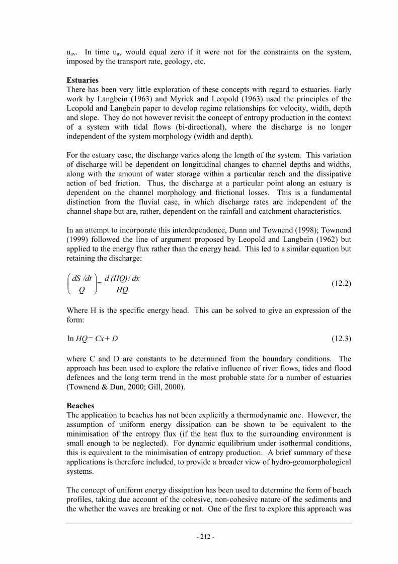
- 212 -

uav. In time uav would equal zero if it were not for the constraints on the system, imposed by the transport rate, geology, etc. Estuaries There has been very little exploration of these concepts with regard to estuaries. Early work by Langbein (1963) and Myrick and Leopold (1963) used the principles of the Leopold and Langbein paper to develop regime relationships for velocity, width, depth and slope. They do not however revisit the concept of entropy production in the context of a system with tidal flows (bi-directional), where the discharge is no longer independent of the system morphology (width and depth). For the estuary case, the discharge varies along the length of the system. This variation of discharge will be dependent on longitudinal changes to channel depths and widths, along with the amount of water storage within a particular reach and the dissipative action of bed friction. Thus, the discharge at a particular point along an estuary is dependent on the channel morphology and frictional losses. This is a fundamental distinction from the fluvial case, in which discharge rates are independent of the channel shape but are, rather, dependent on the rainfall and catchment characteristics. In an attempt to incorporate this interdependence, Dunn and Townend (1998); Townend (1999) followed the line of argument proposed by Leopold and Langbein (1962) but applied to the energy flux rather than the energy head. This led to a similar equation but retaining the discharge:

HQ

dx(HQ) d = Q/dt dS /

⎟⎟⎠

⎞⎜⎜⎝

⎛ (12.2)

Where H is the specific energy head. This can be solved to give an expression of the form:

D + Cx = HQ ln (12.3)

where C and D are constants to be determined from the boundary conditions. The approach has been used to explore the relative influence of river flows, tides and flood defences and the long term trend in the most probable state for a number of estuaries (Townend & Dun, 2000; Gill, 2000). Beaches The application to beaches has not been explicitly a thermodynamic one. However, the assumption of uniform energy dissipation can be shown to be equivalent to the minimisation of the entropy flux (if the heat flux to the surrounding environment is small enough to be neglected). For dynamic equilibrium under isothermal conditions, this is equivalent to the minimisation of entropy production. A brief summary of these applications is therefore included, to provide a broader view of hydro-geomorphological systems. The concept of uniform energy dissipation has been used to determine the form of beach profiles, taking due account of the cohesive, non-cohesive nature of the sediments and the whether the waves are breaking or not. One of the first to explore this approach was

- 213 -

Dean (1977). He considered the cases of uniform energy dissipation per unit area and per unit volume, i.e. for unit area we have:

5/22Ad depth,for water expressionan toleads which )( yEC

y dg =−=∂∂ ε

where E is the wave energy per unit area averaged over a wave period, Cg is the wave group celerity and εd is the rate of energy dissipation and d is the depth17. Whereas for unit volume we have:

3/23Ad depth,for water expressionan toleads which )(1 yEC

yd dg =−=∂∂ ε

The latter was shown to be a better representation of measured profiles. Following a similar line of argument, Lee and Mehta (1997) start with the equation for wave-mean energy dissipation per unit area, as given above. For a gentle slope giving rise to the progressive decay of a progressive sinusoidal wave (i.e. no breaking) an exponential form for the wave height attenuation is adopted

))(exp( oo yyHH −−= κ Here H denotes wave height and H0 the deep water wave height, and, noting that the group celerity in shallow water is given by (gd)1/2, they derive an expression for the depth variation of the form:

2

0

))(4exp( ⎟⎟⎠

⎞⎜⎜⎝

⎛−=

yyyydd oo κ

where d is the depth, subscript 0 denoting the offshore value, y the distance from the shore, and κ is the wave attenuation coefficient. They then introduce a further corrective term to take account of the slope, soil properties and influence of waves at the shoreline. 12.3.2 Statistical Approach The concepts of information entropy developed by (Shannon, 1948) and the principle that an equilibrium system under steady constraints tends to maximise the entropy, proposed by (Jaynes, 1957), have been extensively used to suggest most probable distributions18 of a range of parameters studied in open channel flow. These include: Velocity (Chiu, 1988; 1989; 1991)

17 In the coastal literature the depth is denoted, h. However, in rivers h relates to the hydraulic depth and d the actual depth. Given that the profiles derived here define actual rather than hydraulic depths, the river convention has been adopted to avoid possible confusion when the various components are combined. 18 In this context, the most probable distribution refers to the system state that is most likely

- 214 -

Shear stress and sediment concentration (Chiu, 1987) Transverse slope (Cao & Knight, 1996) Energy gradient/valley slope (Cao & Chang, 1988) Channel curvature (Deng & Singh, 1999b) Unit stream power (vS) (Deng & Zhang, 1994) The general approach is to define a probability density function for the chosen parameter, which can be used to define the entropy in terms of probability (Shannon, 1948). Jaynes (1957) has shown that an equilibrium system under steady constraints tends to maximise its entropy. This is commonly known as the Principle of Maximum Entropy (POME). In some cases this principle is used directly to examine the basis of equal probability (e.g. Singh et al. 2003a) and in others the method is used in conjunction with the calculus of variations to derive a solution (e.g. Cao and Knight, 1996). The difficulty seems to be that in taking a broader view one needs a basis for determining which parameters probabilities can be maximised based on the constraints imposed on the system. It would therefore seem that a complete solution of the regime problem is more likely to be arrived at through the application of thermodynamic entropy, based on physical processes, rather than statistical entropy. This is not to deny the valuable role of the statistical method for analysing and interpreting measured data. The issue however is that a rational framework is needed, so that the choice of which parameters to maximise is a function of the physics and the boundary conditions, rather than some arbitrary choice. 12.3.3 Summary of applications The early applications of entropy concepts considered either maximising the entropy or minimising the entropy production (although the determination of entropy production should often more accurately be termed entropy flux). This made use of an analogy between thermodynamic temperature and land surface elevation. A number of workers subsequently sidestepped the need to make use of this analogy and developed the concept of minimum rate of energy dissipation. A special case, when other forms of energy dissipation are ignored (e.g. any dissipation due to the sediment load) and only the water discharge is considered, leads to the minimisation of the stream power (QSe). Further, by ignoring any slope or velocity variations across the channel leads to the minimisation of the unit stream power (vSe). Taking a different approach by assuming that the energy slope, Se, is constant locally in a reach or meander, and using thermodynamic arguments relating to the earth and its sub-compartments down to the scale of river basins, it has been shown that rivers should minimise the average channel velocity. This is entirely consistent with the more general finding that for thermodynamic systems operating in the linear or quasi-linear region, close to equilibrium, the forces and fluxes will adjust so that all unconstrained forces disappear and those that are constrained adjust to minimise the flux and hence the entropy production (or equivalently at dynamic equilibrium the entropy flux). A third approach has been a statistical one, making use of the principle of maximum entropy (POME). This seeks to identify the most probable distribution of a variable by maximising the system entropy. This is done in terms of a probability density function

- 215 -

for the chosen parameter, which can be used to define the entropy in terms of probability. The concept has been applied to a single variable such as slope, velocity, stream power, etc to determine its distribution. The principle has also been used to examine the relationship between the various hydraulic geometry parameters by identifying the proportion of adjustment attributable to each parameter and then using POME arguments to equate these under chosen constraints. Given that landscapes are open systems subject to flows of matter and energy, there is a reasonable basis for expecting the equations of hydrodynamics and thermodynamics to provide a description of their behaviour. It might be expected that the physical arguments this presents will have greater explanatory power than simply adopting probabilistic arguments. That is not to say that such methods are excluded. Techniques such as the Principle of Maximum Entropy (POME) may well play a supporting role but the foundation should be defined using physical arguments and the various balance equations. Approaches using such arguments can be derived from the basic entropy balance equation, and have been used in various guises in a wide range of applications, covering landscapes, rivers, estuaries and beaches. Reviewing the applications across a range of geomorphological units has revealed a number of inconsistencies that need to be addressed. In particular: • The methods used should have a clear relationship with the fundamental equations

of hydraulics and thermodynamics, so that simplifying assumptions can be clearly identified and their consequences understood.

• There needs to be a more careful handling of constraints and in particular accommodation of vertical and horizontal constraints.

• The specification of the minimum condition needs to be developed in a way that can be applied in a consistent manner across the different applications.

12.4 Perturbations about dynamic equilibrium Although much of the focus so far has been on the equilibrium condition, there is a considerable literature on the study of perturbations about the equilibrium. Most texts on system dynamics cover this topic (Nicolis & Prigogine, 1977; Nicolis, 1995) as do texts on thermodynamics (Kondepudi & Prigogine, 1999). For the purposes of this review, only a brief qualitative discussion of perturbations is provided. This is based on the theoretical arguments set out by Gu et al (1986), which show how the rate of energy dissipation is a maximum when energy is being stored in the system, albeit to the minimum extent necessary to maintain continuity. Conversely, the rate of energy dissipation is a minimum when energy is being exported from the system, again to the minimum extent necessary. 12.4.1 Interpretation for hydro-geomorphological systems 12.4.1.1 Landscape For a time scale shorter than the Quaternary and assuming no tectonic changes in the regional landform, the river basin is eroding and the land levels are lowering. If we take the energy storage as equivalent to the potential energy due to the land elevation, then

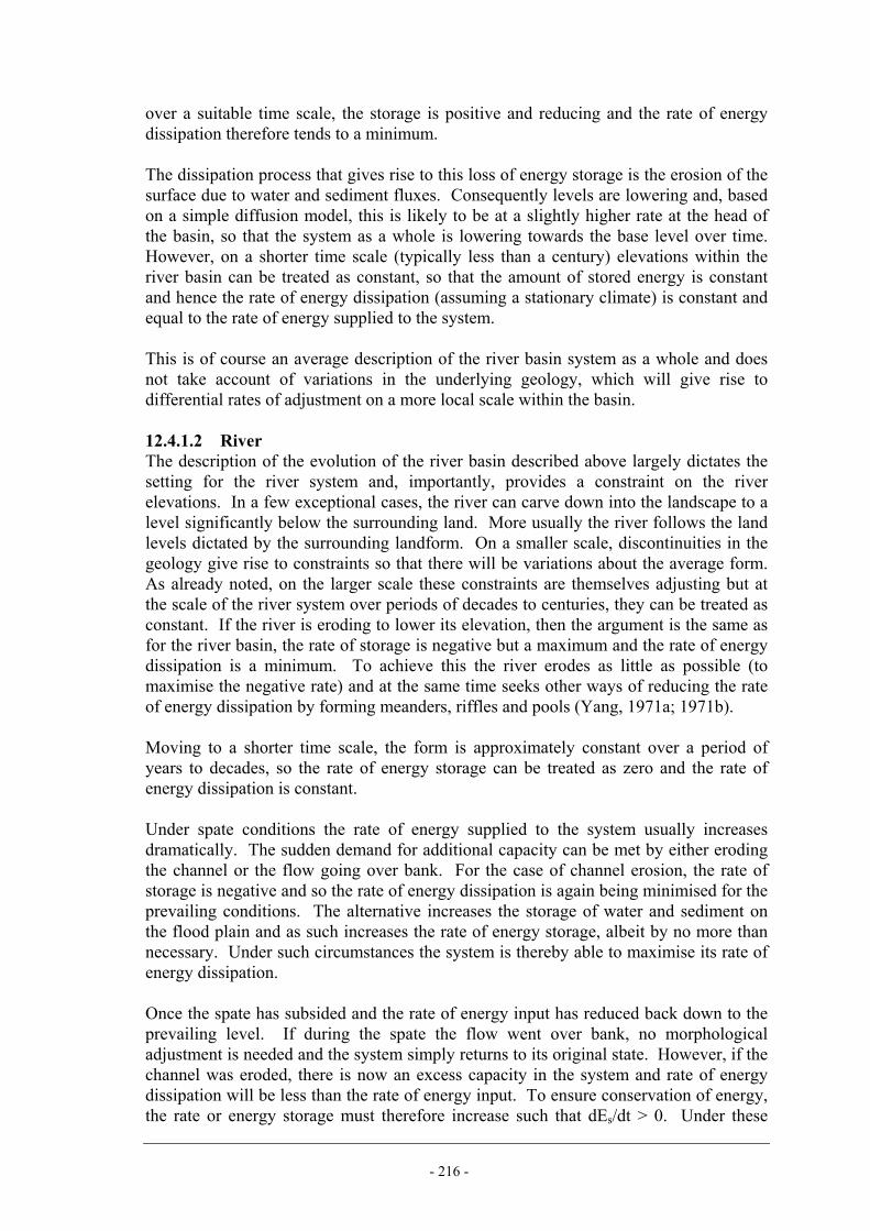
- 216 -

over a suitable time scale, the storage is positive and reducing and the rate of energy dissipation therefore tends to a minimum. The dissipation process that gives rise to this loss of energy storage is the erosion of the surface due to water and sediment fluxes. Consequently levels are lowering and, based on a simple diffusion model, this is likely to be at a slightly higher rate at the head of the basin, so that the system as a whole is lowering towards the base level over time. However, on a shorter time scale (typically less than a century) elevations within the river basin can be treated as constant, so that the amount of stored energy is constant and hence the rate of energy dissipation (assuming a stationary climate) is constant and equal to the rate of energy supplied to the system. This is of course an average description of the river basin system as a whole and does not take account of variations in the underlying geology, which will give rise to differential rates of adjustment on a more local scale within the basin. 12.4.1.2 River The description of the evolution of the river basin described above largely dictates the setting for the river system and, importantly, provides a constraint on the river elevations. In a few exceptional cases, the river can carve down into the landscape to a level significantly below the surrounding land. More usually the river follows the land levels dictated by the surrounding landform. On a smaller scale, discontinuities in the geology give rise to constraints so that there will be variations about the average form. As already noted, on the larger scale these constraints are themselves adjusting but at the scale of the river system over periods of decades to centuries, they can be treated as constant. If the river is eroding to lower its elevation, then the argument is the same as for the river basin, the rate of storage is negative but a maximum and the rate of energy dissipation is a minimum. To achieve this the river erodes as little as possible (to maximise the negative rate) and at the same time seeks other ways of reducing the rate of energy dissipation by forming meanders, riffles and pools (Yang, 1971a; 1971b). Moving to a shorter time scale, the form is approximately constant over a period of years to decades, so the rate of energy storage can be treated as zero and the rate of energy dissipation is constant. Under spate conditions the rate of energy supplied to the system usually increases dramatically. The sudden demand for additional capacity can be met by either eroding the channel or the flow going over bank. For the case of channel erosion, the rate of storage is negative and so the rate of energy dissipation is again being minimised for the prevailing conditions. The alternative increases the storage of water and sediment on the flood plain and as such increases the rate of energy storage, albeit by no more than necessary. Under such circumstances the system is thereby able to maximise its rate of energy dissipation. Once the spate has subsided and the rate of energy input has reduced back down to the prevailing level. If during the spate the flow went over bank, no morphological adjustment is needed and the system simply returns to its original state. However, if the channel was eroded, there is now an excess capacity in the system and rate of energy dissipation will be less than the rate of energy input. To ensure conservation of energy, the rate or energy storage must therefore increase such that dEs/dt > 0. Under these

- 217 -

circumstances, deposition is likely as a means of storing energy in the system, although the amount of storage will be the minimum required to return the system to a condition where the rate of dissipation equals the rate of energy input. Following a similar line of argument, when flow rates increase dramatically, the system can increase capacity by switching from a meander to a braided form. This has the effect of increasing the rate of energy dissipation. This is still a minimum for the new conditions and further contributes to ensuring that the amount of erosion is no more than needed to accommodate the new rate of energy input. Once the event has passed the return to a meander form will be dictated by the arguments already outlined. 12.4.1.3 Estuary The channels, meanders and storage areas in an estuary serve a similar purpose, as a means of adjusting the rates of energy storage and dissipation, as in the rivers case. In addition the intertidal functions both as a storage area to accommodate the discharge variations that occur on every tide and also to act as a means of adjusting the margins of the estuary to varying levels of wind-wave energy. This is typically much less than the energy inputs on the open coast but the mechanisms are similar. In the case of an estuary or less exposed open coast areas, this can be supplemented by saltmarshes, which further enhance the dissipative capacity of the system and serve to store a greater volume of sediment. 12.4.1.4 Beach A similar line of reasoning can be applied to beaches. Under normal conditions, the rate of energy dissipation across the beach and in time is a constant. When the system is perturbed by for instance a storm event, the rate of energy input increases over and above the existing dissipative capacity. To cope with this, the rate of energy storage in the beach becomes negative and the system erodes. This means the elevations are lowered (potentially energy reduced) as material from the upper part of the beach is moved down the beach to form bars on the lower shore. Following the storm the dissipative capacity is now much greater than the prevailing rate of energy input, such that rate of energy dissipation is now too small. As a consequence the excess energy (the difference between input and dissipation rates) is used to store energy in the beach, by transporting material from the lower shore to build the upper beach and so raising the levels back up. 12.5 Application to estuaries As summarised above, Leopold and Langbein (1962) applied the concept of minimum entropy production to the problem of river hydraulics and morphology. A subsequent paper by Langbein (1963) considered the application of the same approach to shallow estuaries. This however deals with an 'ideal' estuary (Pillsbury, 1956) and therefore is constrained by the assumption that the amplitude of the tidal elevation and velocity are constant throughout the system19. The influence of the frictional terms (Lamb, 1932; Dronkers, 1986) and the interaction of M2 and M4 tidal constituents, referred to as the

19 Although the paper includes a derivation for varying depth, an approximate integration is used. This leads to the erroneous result as explained more fully in Appendix 1 of the present report.

- 218 -

overtide, (Friedrichs & Aubrey, 1988) further limit the validity of Langbein's application of this approach to the case of an estuary. In order to develop a more rigorous approach, the derivation of minimum entropy production in a river system was re-examined. This was found to be a special case of the more general case of a reach with bi-directional and variable discharge. The generalised formulation applies to the estuary case and can be used to investigate the relationship between morphology and tidal energy distribution. For the evolution to a probable state in a system near to equilibrium, it has been suggested that the entropy production per unit volume will tend to evolve to a minimum compatible with the conditions imposed on the system (Prigogine, 1955). Relating this to an estuary suggests that, in the long-term, a natural system will tend to evolve in an attempt to achieve the most probable distribution of tidal energy. However, the time taken to evolve to this state will be dependant on constraints imposed upon the system (such as geological constraints and supply of sediments). Such constraints may be significant enough to prevent the evolution to the most probable state in which entropy is maximised, or may induce a switch to some other steady state. Another complication is that the energy available to the system varies temporally over the evolutionary timescale, due to climatic changes, sea level rise, etc. The concept of minimum entropy production per unit discharge has been derived for the more general case of a bi-directional variable discharge along a channel reach (Townend, 1999). Following a similar line of argument to that of Leopold and Langbein (1962), the longitudinal energy distribution along an estuary may be represented as:

tCdxHQd

HQ=

)(1 (12.4)

where; Ct is a constant at time t, H is the specific energy head and Q is the discharge. This describes the energy distribution at any given stage in the tidal cycle. Considering the complete tidal cycle we can write:

e = dt HQ D + x C 11∫ (12.5) where dt HQ∫ is the sum of the energy flux through a section at a distance x from the mouth of the estuary over a complete tide, or power, P(x). C1 and D1 are constants. This suggests that, for the most probable distribution of energy throughout an estuary (and thus a constant production of entropy per unit discharge), the energy transferred due to the tidal wave will decay exponentially in the upstream direction. This general model of variable discharge along a reach can incorporate energy introduced at the up-stream limits of the estuary as a result of river inputs. In order to generate a solution for Equation (12.5), boundary conditions have to be defined in a similar manner to the fluvial case. Although it is possible to generate a tidal curve at the mouth of an estuary, it is not possible to generate a discharge curve, as this is dependent on the morphology of the estuarine channel. However, given an initial

- 219 -

bathymetry, an appropriate analytical or numerical model can be used to generate the discharge curve via the solution of the equations of continuity and momentum. The most probable distribution of energy can then be obtained using Equation (12.5), by noting that: • At x = 0, C = P(0)

• At x = L, ⎟⎟⎠

⎞⎜⎜⎝

⎛=

)0()(ln1

PLP

LD

Using the values of P(0) and P(L) taken at the inner and outer boundaries, where L denotes the total length of the system, the theoretical distribution can be compared to the actual (numerical model or measured) energy flux distribution along the length of the estuary. By comparing the most probable with the modelled results, areas that are likely to experience a loss of conveyance, can be identified. Depth and width changes may then be introduced into the model and the results compared with the updated most probable state solution. Examining the differences from the most probable provides a basis for assessing the relative direction of change from the most probable state (i.e. whether the system is getting closer to, or moving further away from, the preferred state). This is illustrated in Figure 12.1. The top plot shows the variation of the energy flux along the length of the estuary and is compared with the most probable distribution obtained using Equation (12.5). In the middle plot this is shown as the difference between the two curves in the upper plot. Finally, the lower plot shows the difference of a percentage of the actual value at any given distance along the estuary. Whilst the middle plot shows the absolute difference, the lower plot shows the difference relative to the magnitude at a given point in the estuary. Given the very large gradient in energy flux, along the length of the estuary, this provides a better indication of the deviation from the most probable state.

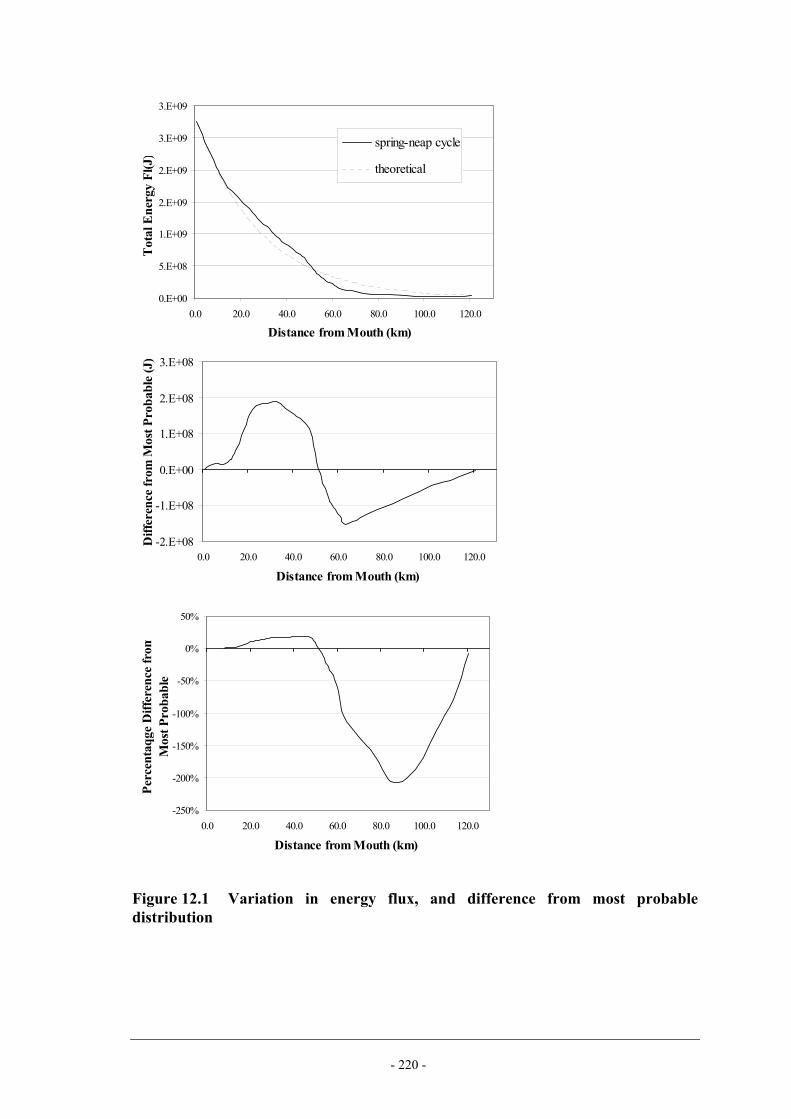
- 220 -

0.E+00

5.E+08

1.E+09

2.E+09

2.E+09

3.E+09

3.E+09

0.0 20.0 40.0 60.0 80.0 100.0 120.0

Distance from Mouth (km)

Tot

al E

nerg

y Fl

(J)

spring-neap cycle

theoretical

-2.E+08

-1.E+08

0.E+00

1.E+08

2.E+08

3.E+08

0.0 20.0 40.0 60.0 80.0 100.0 120.0

Distance from Mouth (km)

Diff

eren

ce fr

om M

ost P

roba

ble

(J)

-250%

-200%

-150%

-100%

-50%

0%

50%

0.0 20.0 40.0 60.0 80.0 100.0 120.0

Distance from Mouth (km)

Perc

enta

qge

Diff

eren

ce fr

omM

ost P

roba

ble

Figure 12.1 Variation in energy flux, and difference from most probable distribution

- 221 -

12.5.1 Influence of boundary conditions In an open system, such as an estuary, defining just where to position the boundaries is not always obvious. Where the estuary rapidly opens to the sea it is usually possible to define a mouth. However, it must be recognised that this may not be the boundary of the “system”, which may extend to include the ebb tidal delta, or may now be located within an embayment. Similarly, at the upstream end, the tidal limit is an obvious choice but other constraints may dictate other intermediate boundaries.

0.0E+00

5.0E+08

1.0E+09

1.5E+09

2.0E+09

2.5E+09

0.0 20.0 40.0 60.0 80.0 100.0 120.0

Distance from Mouth (km)

Tot

al E

nerg

y Fl

ux (J

) 1920

MP to tidal limit

MP to ~90km

MP to ~60km

-250%

-200%

-150%

-100%

-50%

0%

50%

100%

0.0 20.0 40.0 60.0 80.0 100.0 120.0

Distance from Mouth (km)

Perc

enta

ge D

iffer

ence

from

Mos

t Pro

babl

e

To tidal limit

To 90km

To 60km

-2.0E+08

-1.0E+08

0.0E+00

1.0E+08

2.0E+08

3.0E+08

4.0E+08

0.0 20.0 40.0 60.0 80.0 100.0 120.0

Distance from Mouth (km)

Diff

eren

ce fr

om M

ost P

roba

ble

(J)

To tidal limit

To ~90km

To ~60km

Figure 12.2 Influence of boundaries on most probable distribution

- 222 -

The effect of moving the boundary can be quite significant because, in the approach presented above; this is the basis for calculating the values of the constants C and D. This is illustrated in Figure 12.2, which shows the case presented in Figure 12.1, with inner boundaries for the definition of C and D at the 60, 90 and 120km (the tidal limit). In the upper plot of total energy flux, the actual data are seen to accord well with the tidal limit boundary values, at least in the outer estuary. In contrast, the other limits, which only cover the outer estuary, exhibit a greater discrepancy. This is highlighted in the middle plot, which shows the absolute difference from the most probable values. When this is considered as a relative difference (lower plot) this, in effect, rotates the curve about the zero chainage point. The minimum entropy production concept is applicable within any given reach, as well as for the system as a whole. Thus it is important to note the context of the length being examined, as some part of the system as a whole, but it remains valid to consider the relative change and, in particular, the direction of change, within any given length. 12.5.2 Intermediate constraints Internal constraints can also influence the form of the most probable state. This is an essential aspect of the derivation (Prigogine, 1955) and has recently been shown to have a determining influence in the resultant form of river regime equations (Singh et al. 2003a). The point is nicely illustrated using data from the Bristol Channel (Dun, pers comm.). Using constraints based on the inner and outer boundaries the resultant theoretical curve is shown in Figure (labelled “Boundary fit”). A simple exponential curve has also been fitted to the data (labelled “Best fit”). The difference of the data from the Best fit can be interpreted as the excess entropy production in the existing system.

0.E+00

1.E+16

2.E+16

3.E+16

4.E+16

5.E+16

6.E+16

7.E+16

0 20 40 60 80 100 120 140

Chainage from Milford Haven (km)

Ene

rgy

Actual

Best fit

Boundary fitNash Point

Milford Haven

Penarth Point

Avonmouth

Figure 12.3 Variation in energy flux in the Bristol Channel

- 223 -

It is clear that the Boundary fit does not represent the data very well. The geology for the area and in particular the cliffs and extensive areas of exposed rock bed suggest that the section from Nash Point to Minehead may act as a constraint on the system. The section between Penarth Point and Avonmouth may also be a constraint. For further discussion on the nature of the constraints see Townend and Dun (2000). To illustrate the influence of internal constraints, an internal boundary was introduced at the Nash Point section. The data upstream and downstream of this section were treated as separate data sets and both boundary and best fitting techniques were applied, Figure 12.4. Both of the fitted curves now show good agreement downstream of Nash Point. Upstream the Boundary fit continues to suggest a lower energy transmission and the Best fit overshoots beyond Penarth Point. It is likely that this can be resolved by introducing a further internal boundary at Penarth Point, which is again justified on the basis of an identifiable constraint – in this case the hard rock geology.

0.E+00

1.E+16

2.E+16

3.E+16

4.E+16

5.E+16

6.E+16

7.E+16

0 20 40 60 80 100 120 140

Chainage from Milford Haven (km)

Ene

rgy

Actual

Best fit

Boundary fit Nash Point

Penarth Point

Milford Haven Avonmouth

Figure 12.4 Variation in energy flux taking account of internal constraint The significance of constraints cannot be over emphasised. For this reason the use of the entropy method needs to be done in conjunction with geological and geomorphological mapping and interpretation (Chapters 4, 5 and 10), in order that potential constraints can be identified and assessed for their degree of influence on the system. 12.5.3 Multiple fluxes In the derivation presented here, interest is confined to the variation in energy flux and hence the energy head and associated mass discharge. These describe the variation in kinetic and potential energy in the system. A simple extension of the method is to include the variation in water–sediment mixture density in the energy head description. There are, however, a number of other sources of entropy flux related to other density gradients e.g. due to sediment, salinity and temperature. These give rise to a degree of

- 224 -

order in the system, which can be dissipated by diffusion, or reinforced and/or dissipated by convection processes. Such processes alter the order in the system and the rate of change of the irreversible processes, such as diffusion, contributes to entropy production. A more formal and complete derivation of the entropy equation will necessarily provide for these additional processes. For now these are neglected and we focus on the energy flux and hence the rate of energy dissipation, which, for many systems, is probably the most significant contribution to entropy production. With the method presented above, it is possible to consider the contribution of different sources of energy. For instance the river and tidal contributions can be considered individually to gain an appreciation of their relative contribution. This is illustrated in Figure 12.5, which shows plots of energy flux for the Humber Estuary with tidal flow, river flow and the two combined.

- 225 -

Figure 12.5 Variation in energy flux for tide only, river only and river & tide on the Humber

0.0e+0

1.0e+7

2.0e+7

3.0e+7

4.0e+7

5.0e+7

6.0e+7

7.0e+7

8.0e+7

0 50000 100000 150000

Chainage from tidal limit of R. Trent (m)

Ener

gy

Theoretical No river

0.0e+0

1.0e+5

2.0e+5

3.0e+5

4.0e+5

5.0e+5

6.0e+5

7.0e+5

0 50000 100000 150000Chainage from tidal limit of R. Trent (m)

Ener

gy

Theoretical No tide

0.0e+0

1.0e+7

2.0e+7

3.0e+7

4.0e+7

5.0e+7

6.0e+7

7.0e+7

8.0e+7

0 50000 100000 150000Chainage from tidal limit of R. Trent (m)

Ener

gy

Theoretical River & tide

Tide only

River only

Tide and river combined

- 226 -

For the case of a river only, the energy flux decays from the head to an approximately constant level at a chainage of about 60km from the tidal limit. As can be seen, the curve compares well with the theoretical most probable state for the river on its own. The small deviations are thought to be a consequence of the way in which the energy from the different tributaries has been summed together. The case with a tide only decays in the opposite direction and only deviates from the river and tide case for the inner reaches of the estuary (above the 60km chainage). It should be noted that in this case the river fluxes are two orders of magnitude smaller than those due to the tide. Consequently there is only a small difference between the upper and lower plots. However the notable deviation in the outer estuary that can be clearly seen in the upper plot suggests that there are other constraints that need to be taken account of, following the approach outlined above. In this case the narrows, upstream of Hull is associated with a geological sill across the estuary and may well provide a further constraint on the system. Considering the two cases together, there would appear a transition from fluvial to tidal dominance at about the 60km chainage. This is supported by examination of the energy head and discharge parameters, which also indicate a transition at around this location. Upstream the energy head dominates the energy term, whereas downstream the discharge makes the major contribution. This in turn is reflected in the morphology. As one would expect river bed elevation governs energy for the fluvial section. In contrast, in the tidal reach there is an almost constant energy head and discharge decays exponentially. Given velocities throughout are of approximately the same magnitude (roughly 1-2m/s), this can only be achieved by the cross-sectional area varying exponentially. This only approximately translates into an exponential decay in width. An examination of width and hydraulic depth variations along the length of the estuary reveals a strong negative correlation, particularly in the vicinity of the major bends in the system. This appears to reflect a degree of redundancy in the system which allows the width and depth to adjust to accommodate local asymmetries but maintain the longitudinal variation in cross-sectional area. More generally, the river and tidal flows can be seen as competing systems. In the outer estuary the tide dominates and in the fluvial rivers clearly the river dominates. There is however a transition zone downstream of the tidal limit where there is a progressive switch from fluvial dominance at the tidal limit over to tidal dominance. As river and tidal energy fluxes decay in opposite directions there will be an energy flux minimum in this transition zone. Changes in river flow rate, tidal range, sea level will act to move the location of this transition and system can be described as two competing components using an allometric relationship (von Bertalanffy, 1968). This approach imposes further constraints on the system and so helps reduce the uncertainty in just how the boundaries should be prescribed. This can be illustrated by examining different forcing conditions. In Figure 12.6 the results for a number of different tidal and fluvial conditions are shown in terms of energy flux and percentage difference from the most probable. The tidal condition clearly has a large effect on the magnitude of the energy flux in the outer estuary but results in only small variations from the most probable (indeed the neap tide exhibits all

- 227 -

most no difference). In contrast, the seemingly small differences in the rivers (>60km) give rise to substantial variations from the most probable. Here the surge seems to be the condition closest to the most probable state and the fluvial flood event gives rise to the largest deviation.

Figure 12.6 Energy flux as a result of different forcing conditions This begs the question: which is the most appropriate condition to indicate the state of the estuary? The proof of minimum entropy production requires the boundary conditions to be stationary (Prigogine, 1955). The spatial and temporal scales considered therefore need to be compatible with this requirement. For an estuary as a whole one might expect the form to adjust, on average, to the mean spring-neap cycle. Variations about this, due to extreme events such as surges and fluvial floods, may then be considered as perturbations and the system response will be as discussed in Section

0.0E+00

1.0E+09

2.0E+09

3.0E+09

4.0E+09

5.0E+09

6.0E+09

7.0E+09

8.0E+09

0 20 40 60 80 100 120

Distance from Mouth (km)

Tot

al E

nerg

y Fl

ux (J

)

spring-neap cycle

spring

neap

surge

flood + sp-np

-450%

-400%

-350%

-300%

-250%

-200%

-150%

-100%

-50%

0%

50%

100%

0 20 40 60 80 100 120

Distance from Mouth (km)

Perc

enta

qge

Diff

eren

ce fr

om M

ost P

roba

ble

spring-neap cycle

spring

neap

surge

flood + sp-np

- 228 -

12.3. However, in real systems we may be observing a system that has been perturbed by an extreme event and is in the process of recovering on a timescale of years or decades. For the Humber, it has already been noted that in the rivers (>60km) the system is better adjusted to surge events than fluvial floods, Figure 12.6. This might be explained by the fact that surges have their greatest influence towards high water, whereas fluvial floods have a greater effect on morphology in the tidal reaches, towards low water. A perturbation due to a flood therefore moves the system away from its most probable state. However, all subsequent events (predominantly tidal) seek to restore the original state. In contrast, morphological changes due to a surge are less likely to be altered by subsequent events and the system therefore retains the capacity to accommodate these events. This is however an area that needs further investigation. This should focus on

• the “instantaneous state” throughout the tidal cycle and how this relates to the long-term steady state and

• the effect of perturbations and how these relate to the long-term steady state, so providing a better means of assessing the existing condition of an estuary.

12.5.4 Examination of change One particular use of the entropy technique is to consider the long-term trend of the system. Using historical data of bathymetry, sea level and tidal range, the temporal variation in the estuary relative to the most probable state can be assessed. In doing this, it is important to note that the definition of the most probable state is not constant but varies as the boundary conditions vary. Hence it is most useful to examine the variation in terms of the difference from the most probable or the percentage difference.

-300%

-250%

-200%

-150%

-100%

-50%

0%

50%

0.0 20.0 40.0 60.0 80.0 100.0 120.0

Distance from Mouth (km)

Perc

enta

ge D

iffer

ence

from

Mos

t Pro

babl

e

1993

1946

1920

1851

Figure 12.7 Historical variation for the Humber Estuary

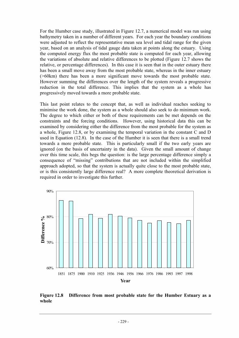
- 229 -

For the Humber case study, illustrated in Figure 12.7, a numerical model was run using bathymetry taken in a number of different years. For each year the boundary conditions were adjusted to reflect the representative mean sea level and tidal range for the given year, based on an analysis of tidal gauge data taken at points along the estuary. Using the computed energy flux the most probable state is computed for each year, allowing the variations of absolute and relative differences to be plotted (Figure 12.7 shows the relative, or percentage differences). In this case it is seen that in the outer estuary there has been a small move away from the most probable state, whereas in the inner estuary (>60km) there has been a more significant move towards the most probable state. However summing the differences over the length of the system reveals a progressive reduction in the total difference. This implies that the system as a whole has progressively moved towards a more probable state. This last point relates to the concept that, as well as individual reaches seeking to minimise the work done, the system as a whole should also seek to do minimum work. The degree to which either or both of these requirements can be met depends on the constraints and the forcing conditions. However, using historical data this can be examined by considering either the difference from the most probable for the system as a whole, Figure 12.8, or by examining the temporal variation in the constant C and D used in Equation (12.8). In the case of the Humber it is seen that there is a small trend towards a more probable state. This is particularly small if the two early years are ignored (on the basis of uncertainty in the data). Given the small amount of change over this time scale, this begs the question: is the large percentage difference simply a consequence of “missing” contributions that are not included within the simplified approach adopted, so that the system is actually quite close to the most probable state, or is this consistently large difference real? A more complete theoretical derivation is required in order to investigate this further.

60%

70%

80%

90%

1851 1875 1900 1910 1925 1936 1946 1956 1966 1976 1986 1993 1997 1998

Year

Diff

eren

ce %

Figure 12.8 Difference from most probable state for the Humber Estuary as a whole

- 230 -

A similar approach can be used to examine the potential impact of other changes such as sea level rise or human interventions. For example, in trying to understand the likely system response to re-introducing intertidal areas within the Humber, a number of large-scale re-alignments were modelled (Townend & Pethick, 2002). This entailed the removal of the flood defences over large parts of the system (e.g. the whole of the inner estuary). The resultant percentage differences for a number of hypothetical scenarios are shown in Figure 12.9. At this large scale, the results suggest that the system is not particularly sensitive to the removal of defences in the outer estuary but becomes progressively more sensitive to the removal of defences further upstream.

-500%

-400%

-300%

-200%

-100%

0%

100%

0 20 40 60 80 100 120

Distance from Mouth (km)

Perc

enta

ge D

iffer

ence

from

Mos

t Pro

babl

e

Existing

No defences outer

No defences inner

No defences river

Remove all defences

Figure 12.9 Influence of various large-scale interventions on the Humber Estuary In this particular study (part of the Humber SMP studies for the Environment Agency) a number of smaller scale schemes were also assessed to determine the practicality and likely impact of managed realignment schemes around the estuary (Townend & Pethick, 2002). In order to provide a direct comparison of the potential sensitivity of the system to different schemes, the percentage difference from the most probable state for the system as a whole was calculated for each scenario, Figure 12.10. This figure shows both the sensitivity to different forcing conditions (on the left hand side) and then a range of scenarios, which were all modelled using a surge tide (this being the case of most interest to the Environment Agency in this study). This again reveals the greater sensitivity to schemes in the rivers (>60km) than in the outer or middle estuary (for further details, see Townend & Pethick, 2002).

- 231 -

77

54

118

148

29

103

29

50

96

27 21 28 29 29 30

55 57

29 28

52

0

20

40

60

80

100

120

140

160

Sp-np c

ycle

Spring

NeapFloo

dSurg

eAll

Outer

Inner

Rivers

0.1m slr

0.5m slr

Sunk I

sland

Skitter

ness

Alkboro

ugh,

surge,

toe a

t +2.6

Alkboro

ugh,

surge,

toe a

t -0.6

Alkboro

ugh,

spring

, toe a

t +2.6

Alkboro

ugh,

spring

, toe a

t -0.6

Goole s

mall

Scuntho

rpe

Goole l

arge

Diff

eren

ce (%

)

Figure 12.10 Difference in the total work done (for whole estuary) from theoretical most probable (%) for a range of cases (Townend & Pethick, 2002) 12.5.5 Summary of application For the present, entropy based relationships cannot be used in a predictive mode. However they can be used as a diagnostic tool, along with other techniques to develop a better understanding of system behaviour and to assess the potential sensitivity to change. Further discussion of a range of applications, making use of historical and geological data can be found in Dun and Townend (1999), Gill (2000), Townend and Pethick (2002). When applying the method outlined in this section, it is important to recognise that: • the boundaries need to be chosen with care to reflect the controlling inputs and

constraints on the system; • the sensitivity to different sources of energy input should be examined; • in order to assess patterns of change consider both the internal changes and those for

the system as a whole, recognising that in a steady state both should approach the most probable state; and

• given the limitations of the current derivation and the uncertainties associated with the system dynamics, make use of relative changes rather than putting too much weight on the absolute values.

12.6 Conclusions There is still a considerable amount of further research required to complete the theoretical derivation of the concepts that follow from the combined application of hydrodynamic and thermodynamic principles. This review has sought to identify how entropy concepts have been applied to landscapes, in order to provide a more rigorous basis for the development of appropriate applications. It is hoped that this will, in time, allow a more complete determination of the goal functions and the state of a system relative to the most probable state. For now, the technique remains essentially a

- 232 -

diagnostic tool, allowing the user to assess the condition of a system relative to some theoretical most probable state, considering just the kinetic and potential energy flux contributions. As indicated, the definition of this condition, itself requires further development. However, where sufficient historical data are available, or there are well-defined changes, such as reclamation or realignment, the technique can usefully be applied to look at the direction of change in the system as a whole. 12.7 References Atkins, P.W., 1984, The 2nd Law, American Scientific.

Atkins, P.W., 2003, Galileo's Finger: The ten great ideas of science, Oxford University Press, Oxford.

Blench, T., 1969, Coordination in mobile-bed hydraulics, Journal of the Hydraulics Division, Proceedings of the American Society of Civil Engineers, 95(HY6), 1871-1988.

Bodge, K.R., 1992, Representing equilibrium beach profiles with an exponential expression, Journal of Coastal Research, 8(1), 47-55.

Brebner, A., Wilson, K.C., 1967, Derivation of the regime equations from relationships for pressurised flow by use of the principle of energy-degradation rate, Proceedings of the Institution of Civil Engineers, 36, 47-62.

Cao, S., Chang, H.H., 1988, Entropy as a probability concept in energy-gradient distribution, In: Proc.Nat.Con.Hyd.Engr., ASCE, New York, pp. 1013-1018.

Cao, S., Knight, D., 1996, Regime theory of alluvial channels based upon concepts of stream power and probability, Water, Maritime & Energy, 118(Sept), 160-167.

Chang, H.H., 1980, Geometry of gravel streams, Journal of the Hydraulics Division, Proceedings of the American Society of Civil Engineers, 106(HY9), 1443-1456.

Chang, H.H., 1988, Fluvial processes in river engineering, John Wiley, Hoboken, NJ.

Chiu, C.L., 1987, Entropy and probability concepts in hydraulics, Journal of Hydraulic Engineering, 113(5), 583-600.

Chiu, C.L., 1988, Entropy and 2-D velocity distribution in open channels, Journal of Hydraulic Engineering, 114(7), 738-755.

Chiu, C.L., 1989, Velocity distribution in open channel flow, Journal of Hydraulic Engineering, 115(5), 576-594.

Chiu, C.L., 1991, Application of entropy concept in open-channel flow study, Journal of Hydraulic Engineering, 117(5), 615-628.

Davies, T.R.H., Sutherland, A.J., 1983, Extremal hypothesis for river behaviour, Water Resources Research, 19, 141-148.

- 233 -

Davy, B.W., Davies, T.R.H., 1979, Entropy concepts in fluvial geomorphology - a re-evaluation, Water Resources Research, 15(1), 103-106.

Dean, R.G., 1977, Equilibrium beach profiles: US Atlantic and Gulf coasts, University of Delaware, Newark, Delaware, Report No: Ocean Engineering Report No 12.

Dean, R.G., 1987, Coastal sediment processes: toward engineering solutions, In: Proc. Special Conference on Coastal Sediments, ASCE, New York, pp. 1-24.

Denbigh, K.G., 1951, The thermodynamics of the steady state, Methuen & Co, London.

Deng, Z-Q. Singh, V.P., 1999a, Mechanism and conditions for change in channel pattern, Journal of Hydraulic Research, 37(4), 465-478.

Deng, Z-Q., Singh, V.P., 1999b, Mechanism and conditions for change in channel pattern, Journal of Hydraulic Research, 37(4), 465-478.

Deng, Z-Q. Zhang, K., 1994, Morphological equations based on the principle of maximum entropy, Int.J.Sediment Res., 9(1), 31-46.

Dou, G.R., 1964, Hydraulic geometry of plain alluvial rivers and tidal river mouth (in Chinese), Journal of Hydraulic Engineering, 2, 1-13.

Dronkers, J., 1986, Tidal asymmetry and estuarine morphology, Netherlands Journal of Sea Research, 20(2/3), 117-131.

Dun, R., Townend, I.H., 1998, Contemporary estuary morphology and long-term change, In: Littoral '98, Suport Serveis, SA, Barcelona, pp. 281-293.

Friedrichs, C.T., Aubrey, D.G., 1988, Non-linear tidal distortion in shallow well-mixed estuaries: a synthesis, Estuarine Coastal and Shelf Science, 27(5), 521-546.

Gill, J., 2000, An evaluation of 'EstEnt' on six selected estuaries, Working paper submitted as part of MSc in Coastal Zone Management, University of Bournemouth, School of Conservation Sciences, Bournemouth, 1-30.

Griffiths, G.A., 1984, Extremal hypotheses for river regimes: an illusion of progress, Water Resources Research, 20(1), 113-188.

Gu, H., Chen, S., Qian, X., Ai, N., Zan, T., 1986, River-geomorphologic processes and dissipative structure, In: Gardiner V (Ed.), International Geomorphology, John Wiley & Sons, London, pp. 211-224.

Huang, H.W., Nanson, G.C., 2000, Hydraulic geometry and maximum flow efficiency as products of the principle of least action, Earth Surface Processes and Landforms, 25, 1-16.

Jaynes, E.T., 1957, Information theory and statistical mechanics, Physics Review, 106, 620-630.

Jaynes, E.T., 1980, The minimum entropy production principle, In: Rabinovitch S (Ed.), Annual Reviews Inc, Palo Alto, California.

- 234 -

Jørgensen, S., Svirezhev, Y.M., 2004, Towards a thermodynamic theory for ecological systems, Elsevier, Amsterdam.

Kondepudi, D., Prigogine, I., 1999, Modern thermodynamics: From heat engines to dissipative structures, John Wiley & Sons Ltd, Chichester, England.

Lamb, H., 1932, Hydrodynamics, Cambridge University Press.

Lamberti, A., 1988, About extremal hypotheses and river regime, In: Proceedings of the International Conference of River Regime, Paper C4, pp. 121-134.

Lane, E.W., 1955, Design of stable channels, Trans.Am.Soc.Civ.Eng., 120, 1234-1260.

Langbein, W.B., 1963, The hydraulic geometry of a shallow estuary, Bulletin of Int Assoc Sci Hydrology, 8, 84-94.

Langbein, W.B., 1964, Geometry of river channels, Journal of the Hydraulics Division, Proceedings of the American Society of Civil Engineers, 90(HY2), 301-311.

Lee, S-C., Mehta, A.J., 1997, Problems in characterizing dynamics of mud shore profiles, Journal of Hydraulic Engineering, ASCE, 123(4), 351-361.

Leopold, L.B., Langbein, W.B., 1962, The concept of entropy in landscape evolution, US Geological Survey, United States Government Printing Office, Washington, Report No: Professional Paper 500-A, A1-A20.

Leopold, L.B., Maddock, T., 1953, Hydraulic geometry of stream channels and some physiographic implications, US Geological Survey, Report No: Professional Paper 252, 1-57.

Li, R.M., 1974, Mathematical modelling of response from small watersheds, Colorado State University, Fort Collins, 1-212.

Myrick, R.M., Leopold, L.B., 1963, Hydraulic geometry of a small tidal estuary, Geological Survey Professional Papers, United States Government Printing Office, Washington, Report No: 422-B, 1-18.

Nicolis, G., 1995, Introduction to nonlinear science, Cambridge University Press, Cambridge.

Nicolis, G., Prigogine, I., 1977, Self-organization in nonequilibrium systems: from dissipative structures to order through fluctuations, John Wiley & Sons, New York.

Pillsbury, G.B., 1956, Tidal Hydraulics, Corps of Engineers, U S Army, Vicksburg, Mississippi.

Prigogine, I., 1955, Introduction to thermodynamics of irreversible processes, John Wiley & Sons, London.

Ramette, M., 1980, A theoretical approach on fluvial processes, In: International Symposium on River Sedimentation, Chinese Academy of Hydraulic Engineering, Beijing.

- 235 -

Rodríguez-Iturbe, I., Rinaldo, A., 1997, Fractal river basins: chance and self-organisation, Cambridge University Press, Cambridge.

Rodríguez-Iturbe, I., Rinaldo, A., Rigon, R., Bras, R.L., Marani, A., Ijjasz-Vasquez, E., 1992, Energy dissipation, runoff production and the three dimensional structure of river basins, Water Resources Research, 28(1095), 1103.

Scheidegger, A.E., 1961, Theoretical Geomorphology, Springer-Verlag, Berlin.

Scheidegger, A.E., 1964, Some implications of statistical mechanics in geomorphology, Int.Ass.Sci.Hydrol.Bul., 9(1), 12-16.

Scheidegger, A.E., 1967, A complete thermodynamic analogy for landscape evolution, Int.Ass.Sci.Hydrol.Bul., 12(4), 56-62.

Scheidegger, A.E., Langbein, W.B., 1966, Probability concepts in geomorphology, Geological Survey Professional Paper, 500-C, C1-C14.

Shannon, C.E., 1948, A mathematical theory of communication, The Bell System Technical Journal, 27, 623-656.

Singh, V.P., Yang, C.T., Deng, Z-Q., 2003a, Downstream hydraulic geometry relations: 1. Theoretical development, Water Resources Research, 39(12), SWC21-SWC215.

Singh, V.P., Yang, C.T., Deng, Z-Q., 2003b, Downstream hydraulic geometry relations: 2. Calibration and testing, Water Resources Research, 39(12), SWC31-SWC310.

Smith, T.R., 1974, A derivation of the hydraulic geometry of steady-state channels from conservation principles and sediment transport laws, J.Geol, 82, 98-104.

Stebbings, J., 1963, The shape of self formed model alluvial channels, Proceedings of the Institution of Civil Engineers, 25, 485-510.

Townend, I.H., 1999, Long-term changes in estuary morphology using the entropy method, In: IAHR Symposium on River, Coastal and Estuarine Morphodynamics, University of Genova, Department of Environmental Engineering, II, pp. 339-348.

Townend, I.H., Dun, R.W., 2000, A diagnostic tool to study long-term changes in estuary morphology, In: Pye K, Allen JRL (Eds.), Coastal and Estuarine Environments, sedimentology, geomorphology and geoarchaeology, Geological Society, London, pp. 75-86.

Townend, I.H., Pethick, J., 2002, Estuarine flooding and managed retreat, Phil.Trans.R.Soc.Lond.A, 360, 1477-1495.

von Bertalanffy, L., 1968, General system theory, George Braziller, New York.

White, W.R., Bettess, R., Paris, E., 1982, Analytical approach to river regime, Journal of the Hydraulics Division, Proceedings of the American Society of Civil Engineers, 108(HY10), 1179-1193.

Williams, G.P., 1997, Chaos theory tamed, Taylor & Francis Ltd, London.

- 236 -

Yalin, M.S., Ferreira da Silva, A.M., 1999, Regime channels in cohesionless alluvium, Journal of Hydraulic Research, 37(Special Issue), 725-742.

Yalin, M.S., Ferreira da Silva, A.M., 2001, Fluvial processes, IAHR International Association of Hydraulic Engineering and Research, Delft, Netherlands.

Yang, C.T., 1971a, Formation of riffles and pools, Water Resources Research, 7(6), 1567-1574.

Yang, C.T., 1971b, On river meanders, Journal of Hydrology, 13, 231-253.

Yang, C.T., 1971c, Potential energy and stream morphology, Water Resources Research, 7(2), 311-322.

Yang, C.T., Song, C.C.S., 1979, Theory of minimum rate of energy dissipation, Journal of the Hydraulics Division, Proceedings of the American Society of Civil Engineers, 105(HY7), 769-784.

Yang, C.T., Song, C.C.S., 1986, Theory of minimum energy and energy dissipation rate, In: Encyclopedia of Fluid Mechanics, Gulf, Houston, Texas.

Yang, C.T., Song, C.C.S., Woldenberg, M.J., 1981, Hydraulic geometry and minimum rate of energy dissipation, Water Resources Research, 17, 1014-1018.

- 237 -

13. ASYMMETRY RELATIONSHIPS

Method Indicator Bottom-Up Hybrid Top-Down

YES 13.1 Background This chapter provides a critique of the application of Asymmetry relationships to estuarine environments. Asymmetry relationships can be used as a means of evaluating historical changes in estuary functioning and to evaluate physical impact arising from development. To some extent these relationships could be described as analytical relationships (which are discussed more generally in Chapter 14) but as they are directly relevant to EGA20 studies they merit their own section. Asymmetry relationships focus on the effect of estuary morphology on tidal propagation in order to identify trends in net sediment transport and thus to identify future morphological changes. This critique provides the following: • an overview of asymmetry relationships (Section 13.2); • discussion of the data requirements for this method (Section 13.3); • a discussion of the theory behind asymmetry relationships (Section 13.4); • a description of best practice in applying the theory throughout estuary systems

(Section 13.5); and, • examples of the application of the approach to a number of UK estuaries (Section

13.6). 13.2 Overview of Technique The development of asymmetry relationships has in general followed from observation of estuary behaviour, which over time has been characterised into a qualitative description, and then captured in analytical terms. In this respect the ideas discussed in this chapter have been around for many years and have been applied in a non-quantitative form for the purposes of both research and estuary management. A summary of some key issues relating to Asymmetry relationships is presented in Table 13.1.

20 EGA Expert Geomorphological Assessment

- 238 -

Table 13.1 Asymmetry relationships: Summary of Key Issues

Issue Asymmetry relationships Description Assessment of data from different periods in time in order to identify

directional trends and possibly rates of change of morphological features or physical processes within an estuary

Temporal Applicability

Short term (several tides) to long term (100 years)

Spatial Applicability

Whole estuary or upstream areas of the estuary

Links with Other Tools

• Complements longer-term geological analysis approaches. • Can provide useful data to inform ‘regime analyses’. • Provides key input to establishing a conceptual understanding of the

longer-term estuary behaviour during ‘synthesis of results’ (or Expert Geomorphological Assessment).

Data Sources Bathymetry: maps and charts, aerial photography, topographic and bathymetric surveys, remote sensing imagery Tidal information: Admiralty tables, tidal gauge measurements, flow models Tidal current information: Current measurements, flow models

Necessary Software Tools / Skills

• Identifying, collating and reviewing relevant data/information sources

• GIS/image processing software/photogrammetry • Cartography/digital ground modelling • Geomorphological interpretation of output

Typical Analyses

• Changes in ebb/flood tide duration as a proxy for changes in net sediment transport

• Identifying equilibrium morphology on the basis of tidal symmetry Limitations • There is always uncertainty regarding the nature of equilibria.

Because of this the method works best in a relative sense or qualitatively rather than as a quantitative assessment.

Example Applications

• Mersey Estuary (see Section 7.11) • Stour/Orwell

13.3 Data requirements The approaches of Friedrichs and Aubrey and Dronkers (1998) described below require the following data: • Basin area (at LW and HW21) – this can be derived from maps and charts, aerial

photography, topographic and bathymetric surveys and/or remote sensing imagery. • Mean depth (averaged within area of estuary being considered) - this can be derived

from maps and charts, aerial photography, topographic and bathymetric surveys and/or remote sensing imagery.

• Average tidal amplitude (approximately half of tidal range) within area(s) of estuary being considered - this can be derived from Admiralty tables, tidal gauge measurements and/or flow models.

21 LW Low Water, HW High Water

- 239 -

The approach of Dronkers (1986) requires data on the duration of slack water (i.e. duration when current velocities below some threshold) – this information can be found from current measurements but in practice is much more likely to be derived from flow model output. More information on data requirements was given in Chapter 5 of the present report. 13.4 Theory 13.4.1 Introduction to theory Estuaries or inlets, unlike rivers, experience a feed-back relationship between their morphology and the current velocities generated inside them. In some situations it is useful to be able to characterise the nature of this feed back so that the implication of a change in the estuary – sea level rise, development etc – can be deduced in a broad overall sense. Of particular interest is how changes to estuary morphology change the asymmetry of current velocities through a given cross-section. In basic terms cross-sections with peak ebb and peak flood velocities of the same magnitude will not induce net transport while asymmetric tides produce higher ebb or higher flood velocities, leading to net sediment transport in one direction or the other. Thus changes to an estuary could cause erosion or deposition in a previously morphologically stable estuary or enhance or reverse the trend completely. In this chapter two three of the best and most applicable approaches to describing the relationship between morphology and tidal asymmetry are described and examined and best practice presented regarding their use. 13.4.2 Dronkers’ (1998) theory Dronkers (1998), used the following one-dimensional tidal equations (with the advection term neglected and the friction term linearized) as a starting point,

( ) 0=∂∂

+∂∂

tbHub

x cη (13.1)

0=+∂∂

+∂∂

+∂∂

huu

Cx

gtuu

tu

Dη (13.2)

where bc is the channel stream width (i.e. the width of the channel that is not defined as “storage”. Can for most purposes be taken as the width of Low Water channel, but in practice will vary throughout the tide); b is the storage width; h is the depth; u is the current velocity; η is the tidal elevation; and CD is the friction drag coefficient.

- 240 -

Dronkers (1998) paper contains minor errors though the proof is also presented in corrected and slightly expanded form in Duijts (2002). By solving the equations analytically Dronkers showed that the ratio of ebb and flood tide durations was dependent on the factor,

HW

LW

SS

ahah 2

⎟⎠⎞

⎜⎝⎛

−+

≈γ (13.3)

where the difference between the flood period and exactly half of a semi-diurnal cycle (a semi-diurnal cycle is 12 hours and 24 minutes) is proportional to (1-γ); h is the average depth of the channel (=VLW/SLW); a is the tidal amplitude (half the tidal range), and, S is the surface area with the subscripts LW and HW indicating surface area at Low and High Water. Note that in Equation 13.3, the parameters of h, a, SLW and SHW are average estuary-wide values (or area-wide values if the relationship is applied to part of an estuary). Thus if flood tides reduce in duration with respect to ebb tides, γ is increased and vice versa. When γ ≈1 the ebb and flood tides are of equal duration, which in simple terms can be thought of as a descriptor of equilibrium. In fact, because of the phenomenon of Stokes Drift which tends to increase ebb dominance in estuaries the equilibrium value of γ ought in general to be bigger than 1. Dronkers suggests the value 1.1, based on data from the Netherlands. Dronkers used Equation 13.3 in the context of the whole of an estuary (or tidal inlet), the tidal asymmetry that he was interested in being that of the mouth of the estuary/inlet. There is nothing intrinsic to his analysis that prevents the relationship being used for areas of the estuary landward of the mouth except that Equations 13.3, 13.4 and 13.5 are all derived on the basis that the tide at the estuary mouth is roughly sinusoidal with periods of equal flood and ebb tide. If this is not true then these equations are not strictly valid. In most estuaries the tide will tend to become less sinusoidal with distance upstream. Dronkers (1998) paper contains minor errors though the proof is also presented in corrected and slightly expanded form in Duijts (2002). A close examination of the proof in the appendix of Dronkers’ paper reveals that Dronkers includes a term relating to the ratio of the (horizontal, non-storage) channel area at HW and LW which in Equation 13.3 he assumes to be close to 1. For shallow tidal basins with extensive flats this ratio will be significantly bigger than 1. Including this extra term in Equation 13.3 gives,

LWC

HWC

HW

LW

SS

SS

ahah

,

,2

⎟⎠⎞

⎜⎝⎛

−+

=γ (13.4)

where SC,HW and SC,LW are the (horizontal) channel areas at HW and LW, respectively.

- 241 -

There is a further point to make about Dronkers analysis. Dronkers analysis was based on characterising the estuary or inlet as a prismatic channel (i.e. no change in depth and width with distance) and thus his derived solution to Equations 13.1 and 13.2, as discussed in Chapter 11, is not correct for “strongly convergent” or funnel-shaped channels which are typical of UK estuaries. Dronkers notes this, however, and although he does not present the analysis in detail he notes that the effect of friction in strongly convergent channels results in the ebb/tide duration being dependent upon the square root of the parameters in Equation 13.4. This effectively means that the asymmetry in the flood and ebb tidal current varies as,

LWC

HWC

HW

LW

SS

SS

ahah

,

,2

⎟⎠⎞

⎜⎝⎛

−+

=γ (13.5)

Note that the relationship (Equations 13.3 and 13.4) proposed by Dronkers apply equally to spring and neap tides (although the values of SLW , and possibly, SHW , will vary depending on the tidal amplitude, a). 13.4.3 The work of Speer, Aubrey and Friedrichs Speer, Aubrey and Friedrichs produced a series of three papers: Aubrey and Speer (1985), Spear and Aubrey (1985), and Friedrichs and Aubrey (1988). The papers considered real observations, analytical theory and numerical modelling and identified the two parameters, h

a and c

sv

v , as being key indicators of ebb/flood dominance in a system, where a is the amplitude of the tidal range, h is the mean depth, vs is the volume of intertidal storage (i.e. the volume between LW and HW over intertidal areas) and vc is the volume of channels (i.e. the volume in the channel to mean sea level). The synthesis paper (Friedrichs and Aubrey, 1988) found that the parameter h

a is mostly responsible for asymmetric tides in flood dominant systems while the parameter

cs

vv is mostly responsible for asymmetric tides in ebb dominant systems. Based on US observations, values of h

a of less than 0.2 were seen to be ebb-dominant, values of ha of

between 0.2 and 0.3 were seen to be flood or ebb-dominant dependent on the value of c

sv

v , while values of ha of greater than 0.3 were seen to be flood-dominant.

These results need to be seen in the context of their derivation. The results were principally derived from application of a 1D model to reproduce flows from estuaries and inlets along the Atlantic coast of the US. The data set was based on an offshore tidal range of 0.75m (constant for all simulations, which was meant to represent an average M2 tide for the data set) and a mean channel depth of 2.8m, which for instance differ greatly from typical UK estuaries which on the whole would be deeper and have a larger tidal range. The US estuaries were also modelled schematically so that the shape of the channel was proportionally the same for all estuaries and constant along their length. For this reason, while the general trends in flood and ebb dominance with variation in h

a and c

sv

v remain valid, the Friedrichs and Aubrey absolute values at which flood and ebb dominance is considered to occur cannot be relied upon in a

- 242 -

general sense. This lack of general applicability of absolute values for ha and

cs

vv is the

main reason for the apparent disparity between the predictions of Dronkers and of Friedrichs and Aubrey highlighted by Townend (2005) when considering UK data. Townend’s analysis of data from UK estuaries (presented in Townend et al, 2000) using Dronkers theory had suggested that most UK estuaries were ebb dominant while an assessment of the h

a parameter suggested that it exceeded 0.3 in most estuaries supposedly indicating flood dominance (Townend et al, 2000). It is clear however that the behaviour of say the Severn and Avon Estuaries with tidal ranges over 10m that nearly dry out at LW cannot be compared to the Atlantic Coast of the US so that the value of 0.3 suggested by Friedrichs and Aubrey is not universally valid. However, application of some mathematics shows that in a qualitative sense the two approaches are formally equivalent where tidal amplitude, a, is small compared to mean channel depth, h.

⎟⎟⎠

⎞⎜⎜⎝

⎛++=⎥⎦

⎤⎢⎣⎡

−+

2

22

21haO

ha

ahah (13.6)

hv

S cLW = (13.7)

(this assumes that the estuary has constant depth. Assuming a variation in depth along the estuary complicates the proof but doesn’t change the result.)

( )av

hah

hv

av

SS scsLWHW +

−=+≈ (assuming a triangular cross-section shape) (13.8)

⎟⎟⎠

⎞⎜⎜⎝

⎛+

⎟⎠⎞

⎜⎝⎛ +

=⎟⎠⎞

⎜⎝⎛+

⎟⎟⎟⎟

⎠

⎞

⎜⎜⎜⎜

⎝

⎛

+

⎭⎬⎫

⎩⎨⎧ −

⎟⎠⎞

⎜⎝⎛ +≈⎥⎦

⎤⎢⎣⎡

−+

∝⇒

ha

vv

sc

c

HW

LW

cs

ha

haO

av

hv

ha

hv

ha

SS

ahah

1

1121

22

γ (13.9)

or for strongly convergent estuaries (see Section 13.4.2),

⎟⎟⎠

⎞⎜⎜⎝

⎛+

⎟⎠⎞

⎜⎝⎛ +

=⎟⎠⎞

⎜⎝⎛+

⎟⎟⎟⎟

⎠

⎞

⎜⎜⎜⎜

⎝

⎛

+

⎭⎬⎫

⎩⎨⎧ −

⎟⎠⎞

⎜⎝⎛ +≈⎥⎦

⎤⎢⎣⎡

−+

∝⇒

ha

vv

sc

c

HW

LW

cs

ha

haO

av

hv

ha

hv

ha

SS

ahah

1

1121

222γ

where h is the average depth of the channel to mean sea level; a is the tidal amplitude (half the tidal range), and, S is the surface area with the subscripts LW and HW indicating surface area at Low and High Water; υs is the intertidal storage volume; υs is the channel volume at mean sea level.

- 243 -

Thus as the value of ha increases (flood dominance) the value of γ increases (flood

dominance) and as the value of c

sv

v increases (ebb dominance) the value of γ decreases (ebb dominance). 13.4.4 Dronkers (1986) Theory As well as the theory regarding changes in ebb/flood tide duration, Dronkers (1986) also developed ideas first put forward by Postma (1961) relating to the effect of differences in the nature of the periods of HW and LW slack on net sediment transport. Dronkers deduced that the net sediment transport flux arising from differences in HW and LW slack through a cross-section is,

−−++ −= λµλµS (13.10) where µ+ (respectively, µ-) is the amount of sediment settled on the bed during the period of HW slack (respectively LW slack) and λ+ (respectively, λ-) is the distance travelled by fluid parcels during the period of HW slack (respectively LW slack) during which the deposited material remains settled. Dronker explained this in physical terms as follows: “The amount of sediment µ+, which is settled per unit length at HW slack, will not follow the tidal motion before the ebb current reaches the critical speed for erosion. In this lapse of time the settled sediment is displaced with respect to the suspended sediment in a landward direction over a distance which on average equals λ+. Around LW slack a similar displacement will occur of sediment mass, µ- , in a seaward direction over an average distance, λ- .” Equation 13.10 leads to the conclusion that, Landward (respectively, seaward) transport is favoured if the duration of HW (respectively LW) slack is greater than that corresponding to LW (respectively HW) slack. Dronkers went on to illustrate this result using examples of tidal inlets from the Wadden Sea and Eastern Scheldt. Equation 13.10 also implies (Dronkers, 1986) that the effects of wave action will also enhance seaward transport because wave action will cause a much greater reduction in deposition during HW slack than during LW slack. 13.5 Best practice in the application of asymmetry relationships to EGA 13.5.1 Careful use of the term “flood/ebb dominance” The term ebb/flood dominance can refer to asymmetry in tidal water levels (e.g. shorter flood tide than ebb tide), asymmetry in ebb and flood current speeds or to net landward or seaward transport. Although these different types of flood/ebb dominance often

- 244 -

occur together they are not necessarily equivalent. Asymmetry relationships such as those considered above relate the differences in ebb and flood velocities to the estuary morphology. However, there is no capacity in these relationships to consider sediment transport supply. Many estuaries combine some degree of ebb dominance with a marine sediment source so that a balance in sediment transport exists between a seaward residual and landward diffusion from the marine source. A similar balance can occur in flood dominant systems with a turbidity maximum. In these cases (as in many estuaries) the supply of material is integral to the estuary balance and any potential changes to this supply need to be considered alongside potential changes in tidal currents. For this reason it is necessary to explicitly state what is meant by ebb/flood dominance. 13.5.2 Careful specification of the data used In order that other parties can have confidence in the assessment it is important that the source of the data used, the locations at which γ, h

a and c

sv

v are calculated, and the exact methods (and levels) used to calculate the channel and storage volumes, and surface areas. 13.5.3 Use of the asymmetry approaches to determine trends in ebb/flood

dominance The discussion above has underlined the fact that the use of the Dronkers and Friedrichs and Aubrey approaches can be used to determine trends in ebb/flood dominance but that the use of absolute numbers is unwise. Roberts et al (1998) used the Dronkers and Friedrichs and Aubrey approaches to observe historical trends in the Stour and Orwell Estuaries (See Section 13.7). The research calculated the relevant parameters γ (in the form of Equation 13.3), h

a and c

sv

v to establish trends rather than absolute values, (which is recommended) and found a significant increase in ebb dominance over the 20th century. The research is notable because the γ parameter was calculated in a slightly different form from that proposed by Dronkers. Dronkers suggested that the parameters HLW and HHW should be calculated as follows:

aHH LWHW += where LW

LWLW S

VH = (13.11)

where HLW (respectively HHW) is the water depth at Low Water (respectively High Water), VLW (respectively VHW) is the estuary volume at Low Water (respectively High Water) and SLW (respectively SHW) is the estuary area at Low Water (respectively High Water). Roberts et al (1998) instead used,

HW

HWHW S

VH = where

LW

LWLW S

VH = (13.12)

- 245 -

Equation 13.12 gives a different (and smaller) evaluation of HHW than Equation 13.11 essentially because the depth of water over intertidal areas is always less than the tidal range (except of course in channels with near-rectangular cross-sections). This difference should be viewed in the context of Dronkers’ analysis which is based on 1D flow model formulations (Equations 13.1 and 13.2) which are themselves a simplification of the system. Dronkers characterises the estuary system as a channel where there is (along estuary) flow and intertidal storage where there is no (along estuary) flow. Conceptually this schematisation sits slightly better with Equation 13.11 but in the grand scheme of things there is no overt reason why Equation 13.11 is strictly “more accurate” than Equation 13.12. Townend (pers.comm., 2005) reports that Equation 13.12 is less prone to large variations and thus in practice may be a more useful estimate than Equation 13.11. It is important, however, to recognise the distinction. Equation 13.12 will result in assessments of tidal asymmetry that are more ebb-dominant than those of Equation 13.11. There is a question over which tide (spring, mean or neap?) should be used in any analysis of tidal asymmetry. Ideally the choice should be made on the basis of a discussion of which tide is most representative of “average” sediment transport. On a simpler level it is suggested that a good starting point is to undertake the analysis for a mean spring tide. 13.5.4 Procedure for using Asymmetry relationships 1. Establish bathymetric and tidal data 2. Derive values of γ, h

a and c

sv

v for the existing estuary at required locations. 3. (If velocity data or a flow model is available) Calculate the periods or HW and LW

slack according to a reasonable velocity threshold (0.25m/s is suggested). 4. Define metadata (sources of data, locations of calculations, assumptions made, etc)

Implement proposed change to the estuary bathymetry and/or tide. 5. Define assumptions made in characterising the proposed change in the estuary. 6. Recalculate γ, h

a and c

sv

v for the new estuary following change. 7. (If flow model output for the new estuary is available) Calculate the periods or HW

and LW slack for the new estuary following change. 8. Compare the parameter values of γ, h

a and c

sv

v and slackwater duration for the new and existing estuary scenarios.

13.6 Case study- Tidal propagation analysis of the Stour and Orwell (Roberts et

al, 1998) Roberts et al (1998) investigated the changing geometry of the Stour and Orwell Estuaries, and the tidal propagation within them over the 20th century. The Stour and Orwell join at an area of water referred to as Harwich Harbour where the historical Port of Harwich and the Port of Felixstowe (the largest container port in the UK) are situated (Figure 13.1). The navigational importance of these Ports over the years has meant that there has been extensive surveying and this information made it possible to set up flow models were for the years 1900, 1960, 1974, 1986 and 1996. The flow and bathymetric information were interrogated to examine how a variety of tidal propagation parameters had varied throughout the 1900-1996 period.

- 246 -

Table 13.2 shows the variation in peak ebb and flood current speeds at the mouth of the Stour at Shotley and the ratio of peak ebb to peak flood speeds, together with the corresponding Dronker’s parameter, γ , calculated from Equation 13.3. Table 13.2 Peak currents, ratios and tidal asymmetry in the Stour 1900-1996

Year Stour peak ebb current (m/s)

Stour peak flood current (m/s)

Ratio of peak ebb to peak flood current

Dronkers parameter, γ

1900 0.69 0.63 1.10 1.21 1960 0.62 0.58 1.07 1.36 1974 0.78 0.67 1.16 0.69 1986 0.72 0.56 1.29 0.76 1996 0.77 0.57 1.35 0.73 The results showed a reasonable correlation between the degree of ebb-dominance as measured by the ratio of peak flood and peak ebb current magnitudes and as measured by the Dronkers parameter, γ. It can be seen that there had been a significant increase in the ebb-dominance of the system over the period with the evidence from Table 13.1 pointing to an increase in flood dominance between 1900 and 1960 and a significant increase in ebb-dominance after 1960. Examination of the historical events (see Table 13.3) that have taken place in the Stour over the 20th century resulted in a clear understanding of the causes to the tidal propagation changes summarised in Table 13.2. Table 13.3 Historical Events in the Stour Estuary over 20th Century

Period Event 1900-1960 - Die-off of large quantities of eel grass (Zostera) from intertidal areas

due to disease - Increase of 12% of intertidal volume during this period

1960-1974 - Sub-tidal channel of Stour dredged by 1.5-3m in depth - 25% increase in sub-tidal volume of estuary - Deepening of the Harbour - Removal of bar at Harbour entrance - Aggregate Dredging throughout the Stour 22

1974-1986 - Approach channel to Harbour deepened from –7.3mCD to –11mCD - Container terminal (Trinity I) constructed in Harbour - Further dredging of lower Stour - Aggregate Dredging throughout the Stour13

1986-1996 - Trinity II Container Terminal constructed in Harbour - Approach channel to Harbour deepened from –11mCD to –13mCD - Trinity III Container Terminal constructed in Harbour

Table 13.2 shows that the historical events prior to 1960 consisted of events that increased intertidal volume – which would enhance flood-dominance (Equation

22 Aggregate dredging took place during the period 1967-1989 removing a total of 4.4Mm3 of material from locations throughout the Estuary. This was not known to Roberts et al at the time.

- 247 -

13.3/13.4). Historical events after 1960 consisted of events that deepened the subtidal area of the estuary – which would enhance ebb-dominance (Equation 13.3/13.4, Section 13.4.3). 13.7 Case study- Mersey Estuary The use of asymmetry relationships in the context of regime theory has been described in Section 11.11.3. 13.8 Conclusions Asymmetry relationships provide a means for the assessment of data from different periods in time in order to identify directional trends and possibly rates of change of morphological features or physical processes within an estuary. These relationships can provide key input to establishing a conceptual understanding of the longer-term estuary behaviour in EGA studies. The relationships generally work on the basis that ebb and flood tide sediment transport can be characterised by ebb/flood tide duration. However, there is always uncertainty regarding the nature of the balance between ebb and flood transport. Because of this the method works best in a relative sense or qualitatively rather than as a quantitative assessment. 13.9 References Aubrey, D. G. and Speer, P. E. (1985) A study of non-linear tidal propagation in shallow inlet/estuarine systems, Part 1: Observations, Estuarine Coastal and Shelf Science, 21, 1985, pp185-205. Duijts, R. (2002) Tidal Asymmetry in the Dutch Wadden Sea, A model study of morphodynamic equilibrium of tidal basins, MSc Thesis for Delft University of Technology, February 2002. Dronkers, J. (1986) Tidal asymmetry and estuarine morphology. Netherlands Journal of Sea Research, 20(2/3), 117 – 131. EstProc Consortium. (2006) Integrated Research Results on Hydrobiosedimentary Processes in Estuaries. Final Report of the Estuary Process Research Project (EstProc). R&D Technical Report prepared by the Estuary Process Consortium for the Defra and Environment Agency Joint Flood and Coastal Processes Theme. Report No FD1905/TR3 – Algorithms and Scientific Information. Download from www.estproc.net Friedrichs, C. T. and Aubrey, D. G. (1988) Non-linear tidal distortion in shallow well-mixed estuaries: a synthesis, Estuarine Coastal and Shelf Science, 27, 1988, pp521-545. Roberts, W., Dearnaley, M. P., Baugh, J. V., Spearman, J. R. and Allen, R. S. (1998) The sediment regime of the Stour and Orwell Estuaries, Physics of Estuaries and Coastal Seas, Dronkers and Scheffers (eds), Balkema, Rotterdam, 1998.

- 248 -

Speer, P. E. and Aubrey, D. G. (1985) A study of non-linear tidal propagation in shallow inlet/estuarine systems, Part 1: Observations, Estuarine Coastal and Shelf Science, 21, 1985, pp207-224. Townend, I., Wright, A., and Price, D. (2000) An investigation of the gross properties of UK estuaries, In: Modelling Estuary Morphology and Process, Report Prepared by the EMPHASYS consortium for the Estuaries Research Programme Phase 1, MAFF Project FD1401, December 2000. Townend, I. (2005) An examination of empirical stability relationships for UK estuaries, Journal of Coastal Research, 21, 1042 – 1053.

Figure 13.1 The Stour and Orwell Estuaries

- 249 -

14. ANALYTICAL SOLUTIONS

Method Indicator Bottom-Up Hybrid Top-Down

YES 14.1 Background Analytical solutions are a group of mathematical expressions, often derived from basic physical principles but usually resulting from a simplification of estuary systems that can be utilised to gain insight into the functioning and potential changes within an estuary system. 14.2 Overview of technique Analytical solutions exist for a diverse range of physical processes and mechanisms encountered within estuarine environments, for example: tidal propagation and current flow, residual circulation, saline intrusion, wind-wave generation, wave propagation and evolution, sediment transport, flocculation and contaminant mixing. These analytical solutions are continuously published, peer-reviewed and revised in journals throughout the world. The role of analytical solutions is to simplify the estuary system or the physical process in question into something more tangible and useable. By this means the complex, layered and often random nature of natural systems, which obscures the underlying process, can be removed to reveal the first order relationships associated with the system or physical process. These relationships then allow a straightforward evaluation of the impact of changes to the underlying drivers in the system or physical process to be evaluated. Usually this simplification enables changes to estuary systems to be evaluated in a qualitative manner but in appropriate circumstances analytical solutions can provide quantitative estimates. In such circumstances the simplified nature of analytical solutions typically results in tools which are quick to use and require only a calculator or spreadsheet to implement. In order to derive the analytical solutions, it is normally the case that a number of simplifying assumptions have to be made regarding the estuary system or physical process. The determination of these assumptions requires judgement and experience to assess whether the analytical solution can be applied because the assumptions upon which is based are appropriate for a given situation. The scope of analytical methods that could be considered in this chapter is wide and therefore it is has been necessary to limit those considered. In practice those analytical methods that featured in the Estuaries Research Programme Phase 1 study (EMPHASYS, 2000) and the Phase 2 EstProc study (EstProc Consortium, 2006) have been covered. This chapter will therefore consider analytical solutions under the following topics:

• Tidal flow • Residual current profiles and saline intrusion • Residual sediment transport

- 250 -

• Suspended sediment concentration profiles Tidal flow, in particular how tidal currents vary along an estuary with a given geometry, is a very relevant application of analytical solutions for EGA23 studies. The 1D characterisation of an estuary system is ideal for a basic conceptualisation of how geometric changes might affect the velocities (and therefore sediment transport) in an estuary system. The interaction of saltwater and freshwater in an estuary system results in mixing and residual currents the nature of which depends on the estuary geometry and density gradient along the estuary. The residual currents and mixing arising from this interaction can have an impact both on sediment transport (for instance in maintaining the turbidity maximum) and saltwater intrusion. Also considered here are a number of analytical solutions dealing with the direction of the residual sediment transport and the nature of suspended sediment concentrations in a system which is in balance between erosion and deposition. 14.3 Chapter content This chapter is split into six further sections as follows:

• Over-view of method (Section 14.3) • Analytical methods for tidal flows (Section 14.4) • Analytical methods for residual current profiles and saline intrusion (Section 14.5) • Analytical methods for residual sediment transport (Section 14.6) • Analytical methods for suspended sediment concentration profiles (Section 14.7) • Best practice in the use of analytical methods (Section 14.8) Sections 14.4 to 14.7 concentrate on the theory behind the methods and best practice is summarised in Section 14.8. 14.4 Overview Table 14.1 Analytical methods: Summary of Key Issues

Issue Analytical methods Description Characterisation of the estuary system or estuary processes into

manageable stand alone mathematical equations. Temporal Applicability

Short term (several tides) to long term (100 years)

Spatial Applicability

Whole estuary or large areas of the estuary

Links with Other Tools

• Asymmetry relationships form a subset of analytical methods • Always useful as an aid to conceptual understanding alongside any

tool. Data Sources Sources vary enormously depending on the type of analytical equation

23 Expert Geomorphological Assessment

- 251 -

Table 14.1 Analytical methods: Summary of Key Issues (continued)

Issue Analytical methods Necessary Software Tools / Skills

• An understanding of physical process • (Preferable) A familiarity with mathematical argument • Geomorphological interpretation of output

Typical Analyses

• As a conceptual aid to understanding how the system will evolve following some change

• As a back-of-the envelope quantitative assessment Limitations It can be necessary to consider the mathematics of the method in detail

to understand whether a particular analytical method can reliably be applied to a given estuary system.

14.5 Application to tidal flow -theory 14.5.1 Introduction Friedrichs and Aubrey (1994) in their paper on tidal propagation in strongly convergent channels summarise the basis for evaluating the important processes occurring in estuarine hydrodynamics and this section draws heavily on their introductory sections. The classical representation of estuaries is that of a one-dimensional linearized governing equation for water level variation, η , in a prismatic frictionless channel, which reduces to the familiar second-order wave equation,

2

2202

2

xc

t ∂∂

=∂∂ ηη where c0 = (gH)1/2 and H is the (mean) water depth. (14.1)

For a sinusoidally forced channel closed at one end Equation (14.1) produces a standing wave solution characterised by incident and reflected waves causing tidal amplitude to vary through nodes and anti-nodes and producing a relative phase of 90º between velocity and water level (i.e. LW slack occurs roughly at LW, HW slack occurs roughly at HW and peak tides occur roughly at mean water level). If the channel has a length of exactly one quarter (tidal) wave-length then the incident and reflected waves cancel entirely at the mouth and resonance occurs within the channel. In a channel of infinite length Equation (14.1) produces a progressive wave with a relative phase of 0º (since there is no reflected wave) and the phase speed becomes equal to c0. In most real estuaries in the UK the tidal phase speed has been observed to be close to c0 and the relative phase is observed to be close to 90º. Hunt (1964) showed that this behaviour (he based his studies on the Thames Estuary) was inconsistent with Equation (14.1) and more consistent with the effect of friction in “strongly convergent” channels (i.e. channels where the proportional change in cross-section area with distance along the estuary is much larger than the proportional change in peak current speed). He de-emphasized the importance of incident and reflected waves and instead expressed his solutions as propagating wave forms modified by geometry and friction. Since this ground breaking work of Hunt various approaches have been tried which have included different mathematical terms, and to different order, in the form of the

- 252 -

momentum and continuity equations. Friedrichs and Aubrey (1994) tried to bring some rigour to this problem by formally evaluating which terms were important and at which orders of accuracy. Their solution to the problem is summarised below. It should be noted however, that the form of the solution given by Equation 14.1 (i.e. frictionless channel with constant width and depth) is still often used and discussed by authors but in most cases (at least in the UK) will be a poor representation of estuary tidal propagation. 14.5.2 Pillsbury’s approach From now on the focus will be on the form of the 1D hydrodynamic equations in Equations (14.2) and (14.3).

0=∂

∂+

∂∂

xAu

tB η (continuity) (14.2)

0=−∂∂

−=∂∂

+∂∂

Hufu

xg

xuu

tu η (momentum) (14.3)

where u is the cross-section averaged current speed; B is the channel width; A is the cross-section area; η is the water level above mean sea level; H is the water depth; f is the friction coefficient. Possibly the most simple form of this is the “ideal” estuary solution developed by Pillsbury (1956). Pillsbury assumed the following: • Rectangular cross-section; • Width reduces exponentially with distance upstream,; • Depth is constant; • Tidal range is constant,

• The xuu

∂∂ term (the 2nd term on the LHS of Equation 14.3) is ignored.

( )kxta −= ση sin. (14.4)

( )φσφ −−= kxtc

agu sinsin (14.5)

where the exponential variation in B is given by,

φcotkxexpBB −= 0 (14.6)

and gHk

c ==σ

(14.7)

where η is the water level above mean sea level;

- 253 -

a is the amplitude of the water level variation; σ is the tidal frequency; u is the cross-section averaged current speed; φ is the phase lag of u relative to η; x is the distance upstream from the estuary mouth; B is the width of the cross-section; B0 is the width of the estuary mouth; k is the wave number; H is the mean water depth; g is the acceleration due to gravity. 14.5.3 Friedrichs and Aubrey’s approach Friedrichs and Aubrey give the 1D estuary solution in a more generalised form for the slightly different configuration of an estuary cross-section. They assumed that an estuary cross-section is made up of storage and channel components (See Figure 14.1) and computed the 1st and 2nd order solutions for an estuary with exponentially decaying storage width and channel cross-section area.

Figure 14.1 Friedrichs and Aubreys schematisation Friedrichs and Aubrey assumed the following: • Width and depth reduce exponentially with distance upstream; • Tidal range is constant (for 1st order solution), i.e. A.dA/dx >> η.dη/dx:

The xuu

∂∂ (the 2nd term on the LHS of Equation 14.3) can be ignored. This was shown

explicitly to be true where (a) the variation in cross-section area along the estuary is much larger than that of tidal amplitude and (b) the phase speed is of the same order as the frictionless wave speed. The first order continuity and momentum equations were presented as follows:

ALuA

tB =

∂∂η (continuity) (14.8)

HHW H

w

B(x,t)

B(x,t)

η (x,t)

HLW

- 254 -

Fux

g −∂∂

−=η0 (momentum) (14.9)

where F is given by H

ucF d

π38

= , LA is given by ALx

eAA−

= 0 , Cd is the friction

coefficient, u is the peak current speed and overbars indicate time-averaged quantities. The first order solution is given by,

( )kxtcosa −= ση where AFL

ck

c20==

σ (14.10)

( )kxtsinuu −= σ where ( )BAaLu Aσ= (14.11)

The 2nd order solution is presented in Appendix 4. Equations 14.4 and 14.5 or 14.10 and 14.11 can be used to give an indication of the manner in which the hydrodynamics in an estuary will initially change following a change in bathymetry. For example an increase in depth will give rise to a reduction in current speed and a change in the growth or reduction of the tidal range and current speed (see Appendix 4). Over the longer term there will be a morphological response to the change in hydrodynamics. In particular sediment will tend to diffuse away from current maxima to areas where currents are smaller (Friedrichs and Aubrey, 1994). 14.5.4 Prandle’s approach Prandle composed a solution to the 1D estuary problem (2003a, 2003b, 2004b). In his solution he assumed a constant estuary depth to width ratio and a triangular cross-section shape and (as for the methods of Pillsbury and of Friedrichs and Aubrey) that the acceleration terms can be ignored. In this case Prandle derived the following form of Equations 14.2 and 14.3,

02

=∂∂

+∂∂

+∂∂

xuD

xDu

tη (14.12)

0=+∂∂

+∂∂ Fu

xg

tu η where ( )

Duf.

DufeF 4611

38

=−=π

(14.13)

and f is a constant of order O(2.5x10-3). This gave rise to the solutions,

( )kxtcos.a −= ση (14.14)

( )θσ +−= kxtcosuu (14.15)

- 255 -

where ( ) 2122 /Fagku+

=σ

(14.16)

21

2

/Dgk

⎟⎠⎞

⎜⎝⎛

=σ

(14.17)

DkSFtan 2

=−=σ

θ (14.18)

and where u is the current amplitude, and xDS

∂∂

= .

Using Equations (14.16) to (14.18) Prandle solved for S (∂D/∂x) and, by integrating S, deduced the values of depth (and therefore width) along the estuary. For the case where F>>σ the solution for depth D (and therefore width) can be solved analytically to give,

( )( )

54

54

41

21

2461

45 /

/

/

/L x

gf.aD ′⎥

⎦

⎤⎢⎣

⎡=

σ (14.19)

where x' = L –x and L is the length of the estuary (which Prandle defines as the point where depth becomes zero). On the basis of Equation 14.19 the width and depth in an estuary vary as (or close to) D=D0[(L-x)/L]4/5 , W=W0[(L-x)/L]4/5. The definition of F (Equation 14.13) and Equations (14.16) and (14.17) then infer that u is proportional to [(L-x)/L]1/5. 14.5.5 Discussion The solutions of Pillsbury relate to constant tidal amplitude and depth and exponentially varying width which results in a constant peak velocity with distance landward; those of Friedrichs and Aubrey relate to constant tidal amplitude and exponentially varying width and depth which result in an exponentially varying velocity with distance landward, while Prandle composes a solution with a constant width/depth ratio and a constant tidal amplitude and a velocity, depth and (since width varies linearly with depth) width, that are interrelated via Equations (14.16-14.18). Prandle therefore solves the “inverse” problem – namely what longitudinal variation in depth (and width) gives a solution with constant tidal amplitude and velocity. When computing the hydrodynamics it is usual to assume some simple characterisation of the bed (such as depth is constant or varying exponentially, etc.) from which the landward variation in velocity is then computed as a result. However, Prandle chooses to calculate the variation in depth (and therefore width) directly from Equations (14.16) to (14.18). As a result Prandle is calculating a property, D, that is normally considered as a boundary condition of the problem. If the variation in cross-section area along the estuary is correct then the prediction of along estuary (cross-section-averaged) current velocity will also be approximately correct, i.e. correct to first order (Friedrichs and Aubrey, 1994).

- 256 -

Equation (14.19) suggests that all estuaries, whose longitudinal variation in currents and tidal amplitude can be said to be roughly constant, will take a specific bathymetric/hydrodynamic form where depth and width are inversely proportional to the four-fifths power of distance from the mouth and peak current speed is inversely proportional to the fifth power of distance from the mouth. Many estuaries vary in the rate of convergence of the bathymetry towards the head and also in their longitudinal changes in current velocity, and hence the analytical methods can only be considered approximate in these situations. The analytical solutions of Pillsbury and Friedrichs/Aubrey can be used to deduce the effects of changes in estuary bathymetry on tidal flows. In basic terms, assuming tidal amplitude remains unaffected an increase in the rate of decrease of width with distance along the estuary will result in a reduction in current speed while an increase in the rate of decrease of depth with distance along the estuary will result in an increase in current speed. Conclusions Based on certain assumptions which have been stated above:

• Analytical formulations such as those of Friedrichs and Aubrey can serve to illustrate the basic functioning of a estuary,

• The analytical solution of Prandle generates information on the idealised form of the estuary.

14.6 Residual current profiles and saline intrusion - theory The non-time-varying version of the 1D momentum equation can be expressed as,

( ) 2

2

2

2

YuE

ZuESZg

xg yzx ∂

∂+

∂∂

=−+∂∂ ηη (14.23)

Where g is the acceleration due to gravity; η is the free surface elevation above mean sea level; Z is the vertical position; Y is the horizontal distance from the estuary axis lateral to the direction of flow; Sx is the density gradient (ρ-1∂ρ/∂x) u is the residual current speed at height z and lateral distance y; Ez and Ey are the vertical and transverse eddy viscosities.

The terms on the right hand side of Equation 14.23, 2

2

ZuEz ∂

∂ and 2

2

YuEy ∂

∂ represent the

effects of vertical and lateral mixing, respectively. The scientific literature contains information on which of these terms dominates longitudinal mixing in estuaries. Hansen and Rattray (1965, 1966) and Ippen and Harleman (1961) devised systems of estuary classification on the basis that vertical mixing predominates in estuary systems. Others such as Officer (1976) and Prandle (1985) have used the same assumption to derive solutions for the saline-induced residual circulation and intrusion (see below). In the 1970’s however Fischer (e.g. Fischer et al, 1979), showed that, as in riverine systems, lateral or transverse mixing dominates in well-mixed estuaries with variable depth

- 257 -

across their cross-section. Since the work of Fischer increased attention has focused upon the dependence of the transverse mixing structure on bathymetry (Friedrichs, 2004). e.g. Nunes and Simpson (1986), Li and Valle-Levinson (1999), Friedrichs and de Velasco (1998), Geyer et al (2000), Mied et al (2002) and Winant and de Velasco (2002). The work of all these authors as a whole appears to suggest that stratified or narrow partially mixed estuaries vertical mixing predominates while in well-mixed estuaries or partially mixed estuaries with variable depth across the cross-section transverse mixing will predominate. This conclusion is supported by measurements from real estuaries (for instance those of Murray et al, 1975, and Dyer, 1974 discussed in Fischer et al, 1979). For a well-mixed estuary with a longitudinal density gradient and a depth that was homogeneous over the width of the channel Prandle (1985, 2004b) expressed the non-time varying residual current in terms of Equation 14.23 but assumed the effect of

lateral mixing, 2

2

YuEy ∂

∂ , was negligible. By assuming a density gradient, Sx, constant

in time and space and a constant eddy viscosity equal to HukEz = (with k=0.0025, u equal to the tidal amplitude and H, depth) Prandle derived the results,

⎭⎬⎫

⎩⎨⎧

−−+−≈

⎭⎬⎫

⎩⎨⎧

−−+−=

0293003730268706

0293003730268706

232

233

.z.z.zuk

HgS

.z.z.zEHgSu

x

Zxs

(14.24)

where us is the “average” residual near bed current speed along the length of the saline intrusion due to gravitational circulation; H is the “average” water depth along the length of the saline intrusion; z is the position above the bed, Sx is the longitudinal saline gradient. This leads to a residual current at the bed given by,

ukHgS.u xs

2

0290= (14.25)

Equations 14.24 and 14.25 are valid for well-mixed estuaries with homogenous depth over the cross-section. For partially-mixed or stratified estuaries the freshwater input is confined to a surface layer and there exists a saline layer near the bed. Prandle (1985) developed the corresponding solution for residual current at the bed for partially-mixed or stratified estuaries as follows,

du.us −

=10180 (14.26)

where ū (= Qf/A) is the river discharge divided by the cross-section area (the depth-averaged residual velocity) and d (=D/H) is the thickness of the saline bottom layer divided by the water depth.

- 258 -

The validation of Equations 14.24 to 14.26 was undertaken in flume experiments and using data from the Rotterdam Waterway (Prandle, 1985). The validation was therefore undertaken in an estuary situation where there was no lateral bathymetric variation. Prandle then developed a simple parameterisation for the length of saline intrusion. He proposed a conceptual two layer model with a residual discharge equal to the freshwater flow input flowing in the top layer and zero net residual discharge in the lower layer. Based on Equation (14.20) and an assumption of a linearly varying saline wedge profile he developed the equation,

ρρ∆

=0

20050uufH.Li (14.27)

where Li is the intrusion length,

f is the friction coefficient encountered in Section 14.2.4, u is the “average” peak current speed along the length of the saline intrusion, u0 is the velocity resulting from the river discharge divided by H, ρ and ∆ρ are the density of sea water and the difference in density between the freshwater river flow and the seawater of the marine boundary.

In a channel of varying cross-section depth the mixing is dominated by transverse mixing (Fischer et al, 1979, etc). Fischer et al give a rough estimate for the ratio, R, of the mixing caused by the transverse gradient to that of the vertical gradient,

v

t

HW

Rεε

2

2

≈ (14.28)

where W is the channel width and εt and εv are the transverse and vertical mixing coefficients. Fischer et al asserted that in all but the most strongly stratified estuaries this ratio can be large. For an estuary of triangular cross-section (of width W and depth H), it can be shown that the value of us in Equation 14.25 becomes,

⎟⎟⎠

⎞⎜⎜⎝

⎛=

v

z

Zxbeds EW

EHEHgSu 2

23

0293.0 (14.29)

The corollary of this result is that, where such lateral variation in the cross-section exists, the residual longitudinal current will be significantly lower than the result for a narrow partially mixed estuary. Conclusions From this assessment of analytical approaches to residual current profiles and saline mixing the following conclusions have been made: • The longitudinal dispersion of salinity in stratified or narrow partially mixed

estuaries is principally a function of vertical mixing, while in well-mixed estuaries or partially mixed estuaries with variable depth across the cross-section transverse mixing will predominate.

- 259 -

• Analytical solutions such as those presented above help to evaluate the residual current velocity caused by a longitudinal salinity gradient, but care must be taken to choose an appropriate solution for specific estuarine condition.

14.7 Residual sediment transport - theory Abbott (1960) wrote two papers regarding the residual mean near bed current (and hence sediment transport) resulting from gradients in current velocity and in salinity. In the first paper Abbott considered a 2DV schematisation of an estuary that is homogenous through the channel width and that varies only gradually in width with distance along the estuary (i.e. not strongly convergent). The tidal variation of the estuary was assumed to be sinusoidal and the eddy viscosity was assumed to be constant through depth. The constituent equations are solved by a method of successive approximation. The second approximation to the longitudinal velocity component takes account of the non-linear convective acceleration terms and contributes a non-periodic term which is in general non-zero. Thus, superimposed on the periodic motion of the water, there is a residual net motion of water near the bed which is indicative of the residual direction of motion. Abbott found that, if the surface velocity in a well-mixed estuary can be described by,

( ) ( ) ( ) xwtcosxUt,xU ψ−= 0 (14.28) then a criterion for landward or seaward transport in the estuary is that,

( ) ⇒> 00ψeU

dxd landward transport

( ) ⇒< 00ψeU

dxd seaward transport

Abbott tried this conclusion on the example of the Thames and found that the criterion above could identify the rough location of the turbidity maximum located in the area of the estuary known as the Mud Reaches. However, to some extent this may be a fortunate result since the Thames Estuary is “strongly convergent” and Abbott’s analysis is based on estuaries which are constant (or “prismatic”) in width and depth. It is concluded here that for strongly convergent estuaries like the Thames that Abbott’s analysis may still have some use but cannot be relied upon with confidence. For estuary channels which vary more gradually the analysis will be more reliable but it is then also likely that other mechanisms such as salinity-induced density gradients will be important. In Abbott’s second paper he considered the magnitude of the various terms in the 2DV longitudinal momentum equation and ignoring these, including the convective term, Abbott derived the criterion,

- 260 -

⇒>⎟⎠⎞

⎜⎝⎛

∂∂

−dxdS

xh ρρ

21 landward transport

⇐>⎟⎠⎞

⎜⎝⎛

∂∂

−dxdS

xh ρρ

21 seaward transport

This conclusion was tested on the Thames, but the criterion above did not successively identify the turbidity maximum since the density gradient in the Thames (based on measurements from Inglis and Allen, 1957) is (apparently) not able to sustain a landward gradient near the bed. A further test using the example of the Mersey Estuary, which has a stronger longitudinal density gradient, was able to locate the node of zero residual current identified through physical modelling. Abbott noted that in estuaries such as the Thames where the balance of forces is not simply between the pressure and density gradients, that the convective term becomes important and the criterion above becomes,

⇒⎟⎟⎠

⎞⎜⎜⎝

⎛∂

∂+>⎟

⎠⎞

⎜⎝⎛

∂∂

−x

Ug

UdxdS

xh 00

21 ρρ landward transport

⇒⎟⎟⎠

⎞⎜⎜⎝

⎛∂

∂+<⎟

⎠⎞

⎜⎝⎛

∂∂

−x

Ug

UdxdS

xh 00

21 ρρ seaward transport

Friedrichs and Aubrey (1994) comment on the residual net transport suggesting that the direction of residual transport is, in strongly convergent channels, dominated by gradients in the current velocity alone. Areas of higher velocity, it was argued, will disperse sediment away from the area and areas of low velocity will represent a sink for sediment dispersing from areas of higher velocity. This idea produces the following criterion,

⇒<∂∂ 0

xu landward transport

⇒>∂∂ 0

xu seaward transport

Note that there are similarities between this criterion and the Abbott criterion relating to salinity effects if the density and saline gradients are set to zero. In the literature there are more complex analytical formulae which consider the net residual transport resulting from fluvial flow, gravitational circulation and tidal asymmetry. However, the characterisation of estuaries as analytical or semi-analytical models is still in its infancy and the models thus far developed are not tried and tested in the wider scientific community or even, commonly, against observations. The assumptions made in the development of these models are often opaque to the reader but are very important to the validity of the resulting analytical model. It is unwise therefore to use any of these more complex analytical models in a predictive sense

- 261 -

without further validation or alternatively a thorough background in the numerical analysis and physical understanding needed to understand and critique these models. The dedicated reader is invited to compare and contrast the findings of a number of relevant papers including those by Prandle referenced in this report and Schuttelaars et al (2002) and Scully and Friedrichs (2002). It is also noted that once the complex processes of residual transport and tidal mixing are the focus of interest the investigation has essentially moved from being geomorphological to one of expert modelling and data analysis and thus becomes outside of the focus of the EGA study. Conclusion From this assessment of the analytical approach to residual sediment transport: • It is considered that the Abbott criterion for the direction of net residual transport in

estuaries with no density gradient should not be used for strongly convergent estuaries such as those commonly experienced in the UK and instead the simpler Friedrichs and Aubrey criterion regarding the gradient of current velocity should be used.

• In estuaries where the density gradient is significant Abbott’s density gradient criterion can be used.

• It is suggested that other analytical formulations for residual sediment flux are used for predictive assessment are based on experience of hydrodynamic and sediment processes, and data where possible. Also it is recommended that the relative importance of the various contributions of the respective terms in the momentum and transport equations is assessed.

14.8 Application to suspended sediment concentration profiles - theory For estuary studies it is often the case that two main approaches to characterising suspended sediment transport are useful. The first is an initial assessment based on limited data where a “back of the envelope” type approach is required. The second is a more comprehensive study based on numerical modelling and observations to validate the numerical model. Discussion of numerical modelling studies is outside the scope of this report and instead the more limited desk study approach is considered. When using this type of approach the objectives are often to either derive the net transport through a cross-section or location or by assuming that the estuary is in balance to deduce something about the nature of the sediment transport in the estuary system. In both cases the use of sediment transport formulae is required. The reader is referred to Chapter 17 for literature dealing with the basis and use of such formulae. One example of an approach which uses the concept of a balance between erosion and deposition is given by Soulsby (2004). Traditionally mud transport is described for modelling purposes by only four parameters: the threshold shear-stresses for erosion and deposition and the erosion-rate constant for the mud bed, and the settling velocity of the suspended mud just above the Soulsby examined how these four parameters interact with the flow-generated bed shear-stresses in the simplest possible representation of a tidal estuary to determine the concentrations of mud in suspension and the masses of mud eroded and deposited per unit area.

- 262 -

It was assumed that the estuary was of uniform depth in both horizontal directions, and that the mud properties were horizontally uniform. The tidal depth variation is ignored, and the flow was represented by a repeating rectilinear tidal velocity such that the bed shear-stress varies sinusoidally as τ(t) = τ . sin (ωt). The settling velocity of the suspended mud was treated as constant, and the concentration profile was schematised as a linear variation from bed to surface C(z) = Cb.(1-α.z/h). Giving a bottom concentration of C =βCb, where β = 1 – α/2. Soulsby used the idea of equilibrium to balance the pattern of erosion and deposition through the tide to derive algebraic expressions for the bottom concentration at slack water, and the maximum and minimum bottom concentrations in the tidal cycle. The maximum concentration occurs at the end of the erosion phase, and is given by: Cmax = Co exp (A) (14.32) The minimum concentration occurs at the end of the deposition phase, and is given by: Cmin = Co exp (–A) (14.33) where,

⎪⎭

⎪⎬⎫

⎪⎩

⎪⎨⎧

⎟⎠⎞

⎜⎝⎛ φ−

π⎟⎠

⎞⎜⎝

⎛ττ

−⎥⎥⎦

⎤

⎢⎢⎣

⎡⎟⎠

⎞⎜⎝

⎛ττ

−= Ee

2es

o 2ˆˆ1

)Asinh(C

C2

1

(14.34)

Where τσβ

τˆH

wA ds

2= ,

HˆmC e

s σβτ

= and ⎟⎠

⎞⎜⎝

⎛ττ

=φ −

ˆsin e1

E

The bottom concentrations Co, Cmax, Cmin can be converted to depth-averaged concentrations by multiplying them by the factor β. The parameters used in Equations (14.32) to (14.34) are listed below. Tidal radian frequency (s-1)

σ

Amplitude of tidal bed shear-stress (N.m-2) τ Threshold shear-stress for erosion (N.m-2) τe Threshold shear-stress for deposition (N.m-2) τd Mud erosion-rate constant (kg.N-1. s-1) me Settling velocity of flocs (m.s-1) ws Ratio of depth-averaged concentration to bottom concentration β Bottom concentration at slack water (kg.m-3) Co Maximum bottom concentration through tidal cycle (kg.m-3) Cmax Minimum bottom concentration through tidal cycle (kg.m-3) Cmin Mass of mud eroded per half-cycle (kg.m-2) ME Mass of mud deposited per half-cycle (kg.m-2) MD

- 263 -

Soulsby was careful to list a number of limitations on this formulation, including: • The flow and bed properties are assumed to be horizontally uniform, and the

advection of suspended sediment is neglected, which, as noted above, is an important and often dominant effect in many estuaries.

• The concentration profile is assumed to be linear, and to change at all levels instantaneously when the bottom concentration changes.

14.8.1 General comments regarding sediment parameters Although sediment parameters for non-cohesive sediments are can be fairly reliably estimated, the corresponding parameters for cohesive sediment, particularly settling velocity (ws), the erosion threshold (τe) and the erosion rate constant (me) are notoriously difficult to measure and are very site specific. The use of these parameters without proper calibration against detailed data can result in very significant error and therefore should be accompanied by an appropriate sensitivity analysis. For non-cohesive particles (usually of diameter greater than 60 microns) the settling velocity is principally a function of the particle’s size. There are many adequate equations to describe this relationship, many of which are described in Soulsby (1997). Cohesive sediment particles (usually of diameter less than 60 microns) in estuaries tend to aggregate together to form larger “flocs” which have higher settling velocities. For cohesive sediment settling velocity is a parameter dependent on the extent of flocculation which in turn is dependent on both the suspended sediment concentration, which affects the frequency with which sediment particles collide, and turbulence, which affects both the frequency and strength of collision, and thus can enhance flocculation (low turbulence) or reduce flocculation (high turbulence). The erosion threshold and the rate of erosion are fairly well described for non-cohesive (sandy) sediment and formulae for the threshold of movement and the resulting transport are can be derived from many well known manuals or text books (e.g. Soulsby, 1997). However, the erosion threshold and the rate of erosion for cohesive sediments is dependent on the biology and on the physico-chemical properties of the sediment in question which may vary spatially and temporally throughout an estuary or even throughout a particular mud bed. Thus any attempt to estimate these parameters carries with it a significant amount of uncertainty. Conclusions Based on this review of analytical approaches to estuarine sediment transport the following conclusions have been drawn: • The equations provide good indications of the key features of the sediment transport

profile. Once validated with data they might be applicable for quantitative assessments.

• For studies where a “ball-park” indication of the sediment concentration is required, and or a reasonable idea of how changes to the estuary might affect concentrations along the estuary, the Soulsby formulation can be applied. Cohesive sediment parameters, particularly settling velocity (ws), the erosion threshold (τe) and the erosion rate constant (me) are difficult to measure and are very site specific.

• Calibrations and sensitivity tests should be carried out where possible.

- 264 -

14.9 Best practice in the use of analytical methods 14.9.1 Introduction This Chapter has described some of the analytical methods which could be of use during geomorphological studies. It has discussed analytical formulations for 1D flow models, formulations for deriving the residual current velocity near the bed and/or its direction and some recent algorithms developed for characterising the suspended sediment concentrations likely to be found in an estuary. This section summarises the best practice in the use of these analytical methods. 14.9.2 1D estuary flow equations The most straightforward and well-described analytical formulations for 1D flow equations are those proposed by Friedrichs and Aubrey. These equations are based on a thorough evaluation of the first and second order terms and allow for the solution of cross-section averaged velocity for different estuary geometry. However these equations are for tidally dominated estuaries and do not apply to estuaries dominated by fluvial flow. The first order continuity and momentum equations were presented in Section 14.3.3. The equations outline the hydrodynamic changes that will occur in response to changes in the estuary bathymetry and tidal range. In practice all estuaries diverge from their ideal counterparts and these analytical equations are best employed in a qualitative sense to explain how changes to a particular estuary geometry would contribute changes in tidal flows. 14.9.3 Residual current profiles and saline intrusion The processes leading to residual current profiles and saline intrusion are complex and may not be clearly defined in any particular estuary. Additionally, the formulations involve “average” estuarine values for depth and current speed which, since these parameters can vary considerably along an estuary, will cause a significant source of error depending on the amount of data available and the method of calculation. Detailed assessment of residual current profiles and saline intrusion may be best undertaken as a numerical modelling study using a “bottom-up” process model (Chapter 2) and detailed observational data for validation (Chapter 5). However, notwithstanding these comments it is possible to gain some qualitative insights into changes in mixing and saline intrusion by using the following relationships: For a well-mixed estuary with homogeneous lateral depth variation (Prandle, 1985),

ukHgS~u xs

2

- 265 -

For a well-mixed or partially mixed estuary with significant heterogeneous lateral depth variation (Fischer et al 1979),

⎟⎟⎠

⎞⎜⎜⎝

⎛

v

zxs EW

EHuk

HgSu 2

22

ˆ~

For a partially mixed with homogeneous lateral depth variation or stratified estuary (Prandle, 1985)

du.us −

=10180 and

ρρ∆

0

2

uufH~Li

where us is the “average” residual near bed current speed along the length of the saline intrusion due to gravitational circulation; Sx is the density gradient (ρ-1∂ρ/∂x); H is the “average” water depth along the length of the saline intrusion; Li is the length of saline intrusion; f and k are coefficients with values in the region of 0.0025; u is the “average” peak current speed along the length of the saline intrusion; u0 is the velocity resulting from the river discharge divided by depth (Qf / H); ρ and ∆ρ are the density of sea water and the difference in density between the freshwater river flow and the seawater of the marine boundary; d (=D/H) is the thickness of the saline lower layer as a proportion of the water depth. Thus the following general rules can be generated: • The residual near bed velocity caused by gravitational circulation increases with

depth but reduces with width • The longitudinal salinity gradient but reduces with current speed. • The length of salinity intrusion increases with depth and the salinity difference

between the fresh and salt water but reduces with tidal current speed and the current speed induced by the river discharge, and friction.

14.9.4 Net residual sediment transport For well-mixed strongly convergent estuaries the direction of residual transport can be is as follows (Friedrichs and Aubrey, 1994):

⇒<∂∂ 0

xu landward transport

⇒>∂∂ 0

xu seaward transport

- 266 -

For partially mixed estuaries the direction of residual transport is as follows (Abbott, 1960):

⇒⎟⎟⎠

⎞⎜⎜⎝

⎛∂

∂+>⎟

⎠⎞

⎜⎝⎛

∂∂

−x

Ug

UdxdS

xh 00

21 ρρ landward transport

⇒⎟⎟⎠

⎞⎜⎜⎝

⎛∂

∂+<⎟

⎠⎞

⎜⎝⎛

∂∂

−x

Ug

UdxdS

xh 00

21 ρρ seaward transport

A stated above it is not suggested that any analytical formulations for residual sediment flux are used for predictive assessment without considerable experience of hydrodynamic and sediment processes and the relative importance of the various contributions of the respective terms in the momentum and transport equations. The dedicated reader is invited to compare and contrast the findings of a number of relevant papers including those by Prandle referenced in this report and Schuttelaars et al (2002) and Scully and Friedrichs (2002). 14.9.5 Suspended sediment concentration profiles Suspended sediment transport is a complex field of study and for accurate quantitative assessment requires the application of new modelling and a considerable amount of observational data to verify the model results. However, for studies where a rough idea of the sediment concentration is required, and or a reasonable idea of how changes to the current estuary might affect concentrations along the estuary, the most straightforward approach is to balance the erosion occurring through a tide against the deposition occurring through a tide (which generally occurs at slack water). This approach is encapsulated neatly by the formulation of Soulsby (2004) outlined in Section 14.6.2. Soulsby was careful to list a number of limitations on this formulation, which should always be considered in the context of sediment transport: • The flow and bed properties are assumed to be horizontally uniform, and the

advection of suspended sediment is neglected, which, as noted above, is an important and often dominant effect in many estuaries.

• The concentration profile is assumed to be linear, and to change at all levels instantaneously when the bottom concentration changes.

It is important to note that cohesive sediment parameters, particularly settling velocity (ws), the erosion threshold (τe) and the erosion rate constant (me) which appear in Soulsby’s formulation (and indeed any formulation of cohesive suspended sediment transport) are notoriously difficult to measure and are very site specific. The use of these parameters without proper calibration against detailed data can result in very significant error and therefore should be accompanied by an appropriate sensitivity analysis.

- 267 -

14.10 Conclusions Analytical solutions are a group of mathematical expressions, often derived from basic physical principles but usually resulting from a simplification of estuary systems, that can be utilised to gain insight into the functioning and potential changes within an estuary system. Analytical solutions exist for a diverse range of physical processes and mechanisms encountered within estuarine environments, a sub-set of which have been discussed above. The role of analytical solutions is to simplify the estuary system or the physical process in question into something more tangible and useable. They are particularly useful as a conceptual aid to understanding how the system will evolve following some change or as a back-of-the envelope quantitative assessment. However, in order to derive these analytical solutions, it is normally the case that a number of simplifying assumptions have to be made regarding the estuary system or physical process. The application of these relationships requires judgement and experience to assess whether the analytical solution is justified for the given situation. 14.11 References Abbott, M. R. (1960) Boundary Layer Effects in Estuaries, Journal of Marine Research, volume 18, pp83-100. Abbott, M. R. (1960) Salinity Effects in Estuaries, Journal of Marine Research, volume 18, pp101-111. Dyer, K. R. (1974) The salt balance in stratified estuaries, Estuarine Coastal and Marine Science, Volume 2, pp273-281. EMPHASYS. (2000) Modelling Estuary Morphology and Process, produced by the EMPHASYS consortium for MAFF project FD1401, Estuaries Research Programme, Phase 1, December 2000. Report TR 111, HR Wallingford. Download from http://www.hrwallingford.co.uk/projects/ERP/index.html EstProc Consortium. (2006) Integrated Research Results on Hydrobiosedimentary Processes in Estuaries. Final Report of the Estuary Process Research Project (EstProc). R&D Technical Report prepared by the Estuary Process Consortium for the Defra and Environment Agency Joint Flood and Coastal Processes Theme. Report No FD1905/TR3 – Algorithms and Scientific Information. Download from www.estproc.net

Fischer, H. B., List, E. J., Koh, R. C. Y., Imberger, J. and Brocks, N. K. (1979) Mixing in inland and coastal waters, Academic Press, In. , New York. Friedrichs, C. T. (2004) Across-channel tidal velocity in straight, weakly stratified estuaries. Physics of Estuaries and Coastal Seas 12th International Biennial Conference, Merida, Mexico, 18-22 October.

- 268 -

Friedrichs, C. T. and Aubrey, D. G. (1994) Tidal propagation in strongly convergent channels, Journal of Geophysical Research, Volume 99, Number C2. Pp3321-3336, February, 1994. Friedrichs, C. T. and Valle-Levinson, A. (1998) Transverse circulation associated with lateral shear in tidal estuaries, Proceedings of the Physics of Estuaries and Coastal Seas, 9th International Biennial Conference, Matsuyama, Japan, 24-26 September, pp15-17. Geyer, W. R., Trowbridge, J. H. and Bowen, M. M. (2000) The dynamics of a partially mixed estuary, Journal of Physical Oceanography, Volume 30, pp2035-2048. Hansen, D. V. and Rattray, M. J. (1965) Gravitational circulation in straits and estuaries, Journal of Marine Research, Volume 23, 104-122. Hansen, D. V. and Rattray, M. J. (1966) New dimensions in estuary classification, Limnology Oceanography 11, pp319-326. Hunt, J. (1964) Tidal Oscillations in Estuaries, Geophysical Journal of the Royal Astonomical Society, Volume 8, pp440-455. Ippen A T and Harleman D R F (1961) One dimensional analysis of salinity intrusion in estuaries, US Army Corps of Engineers, Waterways Experiment Station, Vicksburg, Mississippi Technical Bulletin Number 5. Li, C. and Valle-Levinson, A. (1999) A two-dimensional analytical model for a narrow estuary or arbitrary lateral depth variation: the intra-tidal motion, Journal of Geophysical Research, Volume 104: 23, 525-23, 543. Manning, A. and Dyer, K. R. (2002) A comparison of floc properties observed during neap and spring tidal conditions, IN: Fine sediment dynamics in the marine environment, J C Winterwerp and C Kranenburg (eds), Elsevier Science, 2002, pp233-250. Manning, A.J. (2004) The observed effects of turbulence on estuarine flocculation. In: P. Ciavola, M. B. Collins and C. Corbau (eds), Sediment Transport in European Estuaries, Journal of Coastal Research Special Issue, SI 41, (in press). Mied, R. P., Handler, R. A. and Donato, T. F. (2002) Regions of estuarine convergence at high Rossby number: a solution in estuaries with elliptical cross-sections, Journal of Geophysical Research, 107 (C11): 27-1 to 27-9. Murray, S., Conlon, D., Siripong, A. and Santoro, J. (1975) Circulation and salinity distribution in the Rio Guayas Estuary, Ecuador, In: “Estuarine Research”, L E Cronin (Ed), Volume 2, pp345-363, Academic Press, New York. Nunes, R. A. and Simpson, J. H. (1986) Axial convergence in a well-mixed estuary, Estuarine Coastal and Shelf Science, Volume 20: 637-649. Officer, C. B. (1976) Physical Oceanography of Estuaries, John Wiley, New York.

- 269 -

Pillsbury, G. B. (1956) Tidal Hydraulics (revised edition), Corps of Engineers, US Army, May, 247pp. Prandle, D. (1997) Tidal characteristics of suspended sediment concentrations, Journal of Hydraulic Engineering, Volume 124, number 4, April, 1997. Prandle, D. and Lane, A. (2003a) Equilibria between estuarine bathymetries and tides, river flow and sediment supply, Proceedings of the 39th Defra Flood and Coastal Management Conference, July 2004. Prandle, D. (2003b) Relationships between tidal dynamics and bathymetry in strongly convergent estuaries, Journal of Physical Oceanography, Volume 33, pp2738-2750. Prandle D (2004a) Saline intrusion in partially mixed estuaries, Estuarine Coastal and Shelf Science, 59 pp385-397. Prandle, D. (2004b) How tides and river flows determine estuarine bathymetries, Progress in Oceanography, 61, pp1-26. Prandle, D. (2004c) Sediment trapping, turbidity maxima and bathymetric stability in macrotidal estuaries, Journal of Geophysical Research, Volume 109, CO80001, doi:10.1029/2004JC002271. Schuttelaars, H.M., Friedrichs, C.T. and de Swart, H.E. (2004) Formation of Estuarine Turbidity Maxima in partially mixed estuaries. Submitted to: Proceedings of the Physics in Estuaries and Coastal Sea (PECS) Conference 2002, Hamburg, http://www.phys.uu.nl/~deswart/ems_web/publications_loicz.htm (In press). Scully, M. and Friedrichs, C. (2002) The Influence of Asymmetries in Stratification on Sediment Transport in a Partially Mixed Estuary, Abstract submitted to: Proceedings of the Physics in Estuaries and Coastal Sea (PECS) Conference 2002, Hamburg, http://www.vims.edu/physical/projects/CHSD/publications/proceedings/SF2002_PECS.pdf Soulsby, R. L. (1997) Dynamics of Marine Sands, Thomas Telford Publications, London. Soulsby, R. L. (2004) Methods for predicting suspensions of mud, HR Wallingford Report TR 104. Winant, C. D. and de Velasco, G. G. (2003) Tidal dynamics and residual circulation in a well-mixed inverse estuary, Journal of Physical Oceanography, Volume 33, No. 7, pp. 1365–1379.

- 270 -

- 271 -

15. INTERTIDAL FORM

Method Indicator Bottom-Up Hybrid Top-Down

YES 15.1 Introduction The intertidal form, or intertidal geomorphology, is an important feature within the larger estuarine morphological system. This zone provides the transition between the subtidal channel of the estuary and the shoreline with its natural features or man-made coast protection or flood defence works. The overall aim of this Chapter is to review a number of the available approaches to predicting the evolution of the intertidal profile formed in muddy sediments; hence much of the work relates to intertidal mudflats and the term “mudflat” will be used. 15.2 Overview of technique The aim of this class of methods is to determine the equilibrium shape of the intertidal profile (mudflat) given the prevailing environmental conditions. The inputs that are required are: • Initial intertidal profile from subtidal (e.g. Lowest Astronomical Tide LAT) to at

least Highest Astronomical Tide (HAT); • Tidal range and shape of tidal curve; • Wave parameters offshore of the intertidal – height, period and direction; • Bed sediment properties – erosion threshold; and, • Boundary sediment concentration – this controls the potential supply of sediment to

the mudflat. The methodology for application of the various modelling approaches is presented to enable assessments of: • The natural behaviour of mudflats under wave and current forcing; • The response of mudflats to sea-level rise; and, • The response to engineering works or encroachment. Early work on the form of the intertidal under currents and under waves was done by Friedrichs (1993) and Friedrichs and Aubrey (1996), Whitehouse and Roberts (1999) extended the work to include sediment properties and a sediment concentration term. This method for currents and waves allowed investigation of a wider range of parameters. Pethick (2002) derived a method to predict the profile evolution under waves and examined the role of Sea Level Rise.

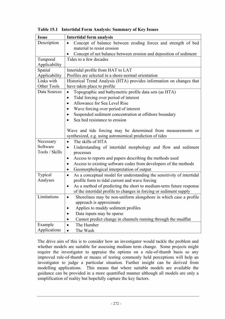
- 272 -

Table 15.1 Intertidal Form Analysis: Summary of Key Issues

Issue Intertidal form analysis Description • Concept of balance between eroding forces and strength of bed

material to resist erosion • Concept of net balance between erosion and deposition of sediment

Temporal Applicability

Tides to a few decades

Spatial Applicability

Intertidal profile from HAT to LAT Profiles are selected in a shore-normal orientation

Links with Other Tools

Historical Trend Analysis (HTA) provides information on changes that have taken place to profile

Data Sources • Topographic and bathymetric profile data sets (as HTA) • Tidal forcing over period of interest • Allowance for Sea Level Rise • Wave forcing over period of interest • Suspended sediment concentration at offshore boundary • Sea bed resistance to erosion Wave and tide forcing may be determined from measurements or synthesized, e.g. using astronomical prediction of tides

Necessary Software Tools / Skills

• The skills of HTA • Understanding of intertidal morphology and flow and sediment

processes • Access to reports and papers describing the methods used • Access to existing software codes from developers of the methods • Geomorphological interpretation of output

Typical Analyses

• As a conceptual model for understanding the sensitivity of intertidal profile form to tidal current and wave forcing

• As a method of predicting the short to medium-term future response of the intertidal profile to changes in forcing or sediment supply

Limitations • Shorelines may be non-uniform alongshore in which case a profile approach is approximate

• Applies to muddy sediment profiles • Data inputs may be sparse • Cannot predict change in channels running through the mudflat

Example Applications

• The Humber • The Wash

The drive aim of this is to consider how an investigator would tackle the problem and whether models are suitable for assessing medium term change. Some projects might require the investigator to appraise the options on a rule-of-thumb basis so any improved rule-of-thumb or means of testing commonly held perceptions will help an investigator to judge a particular situation. Further insight can be derived from modelling applications. This means that where suitable models are available the guidance can be provided in a more quantified manner although all models are only a simplification of reality but hopefully capture the key factors.

- 273 -

15.3 Mudflat typology and classification Mudflats are a subset of the estuarine system and the EC project INTRMUD led by Professor Keith Dyer between 1996 and 1999 produced a descriptive typology and a classification of these features. An initial assessment of a particular site can be made based on simple information collected by visiting a particular site. The typology also provides a way of seeking analogues between sites. The typology (Dyer, 1998) was based on: • Tidal range - controlling the overall morphological profile; • Atmospheric exposure; • Waves; • Sediment;

Bedforms; • Biology. The approach taken was to start from the basis of the geographical situation, and the external driving parameters which are imposed on the mudflat and to which it has to respond. The typology was aimed at tide dominated North-west European mudflats. The next step was to develop the typology including the following factors: 1. Tide range – macro-, meso-, micro-tidal; 2. Wave energy – high, low (qualitative); 3. Sediment supply – surplus, deficit – depending on whether the profile is

depositional or erosional; 4. Steepness (slope) – flat, steep – threshold at 1:750; 5. Zones – assign upper, middle, lower depending on lunar tidal range and mudflat

profile 6. Sediment density – soft, intermediate, hard; qualitative indication from walking on

mud – soft to intermediate boundary taken as sinking 30cm and intermediate to hard boundary taken as sinking 10cm; equating to mean bulk densities of about 1200 kg/m3 and 1300 kg/m3 respectively;

7. Bedforms – indicating presence or not of: • Channels; • Gullies; • Slumps; • Planar; • Cliffs.

8. Organic content – high taken as organic matter content exceeding 5% determined by loss on ignition;

9. Biology - indicating presence or not of: • Worms; • Bivalves; • Macrophytobenthos; • Microphytobenthos.

A typology of 12 mudflat types based on these parameters was devised. The listed parameters were presented in a matrix moving from left to right as you move down the

- 274 -

above list. Parameters 1 through 6 and 7 are a semi-quantitative measure of the environment, parameters 7 and 8 are yes/no indicators of the features listed. The next stage of the work was to produce a classification (Dyer et al, 2000). In summary, the classification proposed was based on the readily observable field measurements that formed the basis of the typology. They found that the most important external driving variables were: • tidal range, followed by; • exposure to waves and mudflat slope. The next level for the meso- and macrotidal mudflats examined yielded a separation into three groups based on the bed sediment dry density. They also analysed floral and faunal assemblages and showed that the relationships between sites on the upper mudflat were caused by differences in grain sizes. The relationships for the middle and lower mudflats were not well defined. These findings have significance for monitoring of hydrogeomorphological parameters. Overall Dyer et al concluded that “the main attributes of mudflats appear to be the result of physical rather than biological processes”. Also that there was “excellent agreement” with the conceptual typology proposed by Dyer (1998). Further developments were proposed to build on the classification using the typology, e.g. to indicate the presence or otherwise of bedforms and biological assemblages. In a future development the scheme might be used as a predictive tool for examining the response of mudflats to natural and man-made changes to the driving variables. The scheme has merits for UK mudflats although the generality of the scheme remains to be tested using a wider range of mudflats from around the UK, and ultimately the world. If the information is collected in the framework of the empirical mudflat typology (Dyer, 1998) then an initial assessment of the state of the mudflat can be made. More detailed assessments of the historical behaviour can be made by the analysis of historical charts (See Chapter 7) and the future behaviour then needs to be assessed. The future behaviour will be a function of the current state of the system, the history of the system and the most likely changes in external conditions whether natural or man made. For the future prediction, analysis can be done based on an interpretation of the knowledge that has been collected or one of the modelling approaches can be applied – discussed in Section 15.7. The results obtained by comparing the outcome of different “what if” scenarios in model runs provide useful information for assessing the outcome from changes in hydraulic conditions or in sediment properties/sediment supply.

- 275 -

15.4 The importance of hydraulics and sediment properties To make an assessment of mudflat response requires the investigator to combine knowledge of the physical principles governing mudflat behaviour with an examination of the local conditions which determine how these physical principles manifest themselves. The aspects which should be considered are presented below, subdivided into hydraulic influences, sediments and morphology and historical context. Information about the features of the mudflat itself can give some clues as to its behaviour (O’Brien et al, 2000; Whitehouse et al, 2000a). Although the typology discussed in Section 15.3 is a generalization it provides a very useful starting point for an assessment. By considering the information under the heading “Hydraulic influences” (Section 15.5), together with gross easily identifiable features of the morphology, such as the mudflat width (ratio of tidal range to mudflat slope), the typology gives an indication of what types of smaller scale features are to be expected, such as sediment density, bed forms and biological activity. If any direct observations of these other features are available there is a further opportunity to see if the mudflat in question falls into a well-defined type. Not every mudflat will fit all of the listed features in the typology, but for those which fit reasonably well, an idea of behaviour can be gained by comparison with other mudflats of the same type. This classification approach can be also used in a predictive way, albeit at a quite general level. If, for example, an engineering scheme is envisaged which will shelter a mudflat from waves, changing it from a high wave energy mudflat to a low wave energy mudflat, then the typology can be used to identify what features of the mudflat are expected to change. The gross features of the mudflat morphology can be used in combination with the hydraulic influences to understand the dominant forcing on the mudflat. 15.5 Hydraulic influences This covers the sources of energy which are available to move sediment and hence modify the shape of the mudflat. These can come from any or all of: 1. tides:

• tidal range; • magnitude of tidal currents in the estuary, particularly near the mudflat – these

may manifest as cross-shore or shore-parallel currents; and, • tidal asymmetry, i.e. is there a difference in the duration of flood and ebb phases

of the tide?; is there a difference in the peak value of tidal current speeds on the flood and ebb? The sediment transport balance in flood and ebb dominated systems appears to influence the mudflat shape and position in the tidal frame (Pethick, 1992).

2. river flow:

• consider mean river flows and annual maximum river flow; • how does the fresh water discharge compare with the tidal discharge in the

estuary and at the mudflat site? (compare river flow over a six hour period with the tidal prism, for example); and,

- 276 -

• what is the salinity at the mudflat site? 3. waves:

• is the site exposed to waves from the open sea, or is all wave activity locally generated ?

• examine the wind climate, if known, to identify the frequency and direction of strong wind events;

• how long are the fetches in different directions from the mudflat?; and, • consider the wet area of the estuary at high and low water, to identify if there is

a big difference in fetch length at different water levels. The potential variation in wave conditions can be estimated from e.g. Yarde et al (1995).

The dominant form of energy acting on the mudflat is one (or a combination) of the following: • Cross-shore currents; • Shore-parallel currents; • Waves. Examples of the conditions at three sites in the UK including suspended sediment concentrations are summarized in Box 15.1 (from Whitehouse and Roberts, 1999) and the different types of forcing are discussed further below.

Box 15.1 Summary of conditions experienced by mudflats in three UK estuaries

• Stour: low energy, low suspended sediment concentration (SSC), relatively coarse sediments, dominated by long-shore currents, with waves being more important than cross-shore currents.

• Humber: medium energy, medium SSC, fine sediments, dominated by cross-shore currents, with waves being more important than long-shore currents.

• Severn: high energy, high SSC, fine sediments, dominated by long-shore currents, although waves are also larger than at the other sites.

Cross-shore currents: proportional to the width of the mudflat and hence are significant on wide intertidal areas. They tend to be negligible on narrow mudflats. The magnitude of the cross-shore tidal current on the intertidal, below mean sea level, can be approximated for a semi-diurnal sinusoidal tide curve by:

tideTWu π

=max (15.1)

where umax is maximum value of current speed, W the mudflat width, and Ttide the tidal period (Friedrichs and Aubrey, 1996; Le Hir et al, 2000; Roberts et al, 2000) – see Box 15.2 below. Above mean sea level the on the upper flat the maximum current occurs at the tidal front and can be predicted by a modified form of Equation (15.1) (Friedrichs and Aubrey, 1996; Le Hir et al, 2000).

- 277 -

Shore-parallel currents: these depend on tidal range and tidal volume; for example, a large tidal volume is associated with a large cross-sectional area, as described by Regime Theory (Chapter 11). If measurements are available of current speeds in the estuary channel, an approximate guide for extrapolating those to flows over the mudflat is that the current speed is roughly proportional to the square root of the water depth. If we assume a constant shear stress over the intertidal profile, in balance with the water surface slope (Whitehouse et al, 2000a) we arrive at the following expression for the variation of flow speed with position on the intertidal:

zz C

huρ

= (15.2)

2

0ln

⎥⎥⎥⎥

⎦

⎤

⎢⎢⎢⎢

⎣

⎡

⎟⎠⎞⎜

⎝⎛

=

zz

Czκ (15.3)

This means that the cross-shore profile of current speed u at height z above the bed can be prescribed based on the local water depth h and the drag coefficient Cz with κ the Von Karman constant (0.4) and z0 the bed roughness length related to the configuration of the sediment boundary – see Box 15.2 below. If the water depth at a point on the mudflat is four times smaller than in the estuary channel at a given time, the long-shore current speed on the mudflat will be about half that in the estuary channel. A more accurate assessment can be made from current measurements on the mudflat or from the results of a computational model of the estuary hydrodynamics. For example, Uncles et al (2000) ran their TRANSVERSE model to determine the tidal currents perpendicular to the cross-shore profile.

Box 15.2 Example estimations of current speeds

The methods for estimating current speeds can be used to assess the prevailing importance of cross-shore and shore-parallel currents at a particular site. It is required to calculate the maximum value of cross-shore current speed on the intertidal using Equation (15.1). The inputs are: Constant π = 3.1416 Mudflat width W = 4200m Ttide = 44640 seconds (equating to 12.4 hours) The resulting value for umax is 0.29 m/s The value of W can be approximated by the ratio of tidal range R in metres to mudflat slope β; for example, with R = 6m and β = 1/700 this equates to W = 4200m.

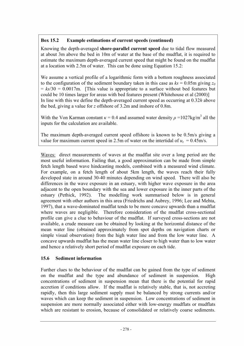
- 278 -

Box 15.2 Example estimations of current speeds (continued)

Knowing the depth-averaged shore-parallel current speed due to tidal flow measured at about 3m above the bed in 10m of water at the base of the mudflat, it is required to estimate the maximum depth-averaged current speed that might be found on the mudflat at a location with 2.5m of water. This can be done using Equation 15.2: We assume a vertical profile of a logarithmic form with a bottom roughness associated to the configuration of the sediment boundary taken in this case as ks = 0.05m giving z0 = ks/30 = 0.0017m. [This value is appropriate to a surface without bed features but could be 10 times larger for areas with bed features present (Whitehouse et al (2000)] In line with this we define the depth-averaged current speed as occurring at 0.32h above the bed, giving a value for z offshore of 3.2m and inshore of 0.8m. With the Von Karman constant κ = 0.4 and assumed water density ρ =1027kg/m3 all the inputs for the calculation are available. The maximum depth-averaged current speed offshore is known to be 0.5m/s giving a value for maximum current speed in 2.5m of water on the intertidal of uz = 0.45m/s.

Waves: direct measurements of waves at the mudflat site over a long period are the most useful information. Failing that, a good approximation can be made from simple fetch length based wave hindcasting models, combined with a measured wind climate. For example, on a fetch length of about 5km length, the waves reach their fully developed state in around 30-40 minutes depending on wind speed. There will also be differences in the wave exposure in an estuary, with higher wave exposure in the area adjacent to the open boundary with the sea and lower exposure in the inner parts of the estuary (Pethick, 1992). The modelling work summarised below is in general agreement with other authors in this area (Friedrichs and Aubrey, 1996; Lee and Mehta, 1997), that a wave-dominated mudflat tends to be more concave upwards than a mudflat where waves are negligible. Therefore consideration of the mudflat cross-sectional profile can give a clue to behaviour of the mudflat. If surveyed cross-sections are not available, a crude measure can be obtained by looking at the horizontal distance of the mean water line (obtained approximately from spot depths on navigation charts or simple visual observation) from the high water line and from the low water line. A concave upwards mudflat has the mean water line closer to high water than to low water and hence a relatively short period of mudflat exposure on each tide. 15.6 Sediment information Further clues to the behaviour of the mudflat can be gained from the type of sediment on the mudflat and the type and abundance of sediment in suspension. High concentrations of sediment in suspension mean that there is the potential for rapid accretion if conditions allow. If the mudflat is relatively stable, that is, not accreting rapidly, then this large sediment supply must be balanced by strong currents and/or waves which can keep the sediment in suspension. Low concentrations of sediment in suspension are more normally associated either with low-energy mudflats or mudflats which are resistant to erosion, because of consolidated or relatively coarse sediments.

- 279 -

Future behaviour of a mudflat following a change in forcing will depend on the supply of sediment. Coarse mudflat sediments indicate low sediment supply and/or strong forcing from waves or currents. Underlying sediments can exert an influence on the profile response. Seasonal deposition of sediment can build up to protect the underlying clay profile from erosion and in turn this means the underlying sediment can only erode when it is exposed. As an example, vertical erosion of the underlying stiff clay forming the Wentlooge Formation has been measured along the north shore of the Severn Estuary by Kirby (1994) and by O'Brien et al (2000): Kirby deduced a mean annual erosion rate of 43mm yr-1 since the 1920's with respect to the level of the Rumney Valley Sewer pipeline. During the 12 month period September 1996 to 1997 O'Brien et al measured 59, 105 and 67mm of erosion at three locations on the intertidal, denoted as stations E, F and G. Stations E, F and G were 600m, 700m and 800m offshore from the seawall behind the saltmarsh at this location and stations E and G equated to elevations at mean tidal level, about 0m ODN, and at just below Mean Low Water Neap tide level with F lying in between. These rates appeared to be higher than the average measured at a different location along the coastline by Kirby but this probably reflects interannual variation. Mitchener and O'Brien (2001) found that when the clay substrate was exposed by erosion of the seasonal (underconsolidated) sediments it was considerably more consolidated than the modern layer but it had an erosion threshold similar to the underconsolidated sediments. This evidence led them to conclude that the surface of the sediment had been weakened since becoming uncovered and hence the surface layer was more susceptible to erosion than might have been expected from its bulk strength. 15.7 Modelling approaches Previous approaches to modelling intertidal form in estuaries due to currents and due to waves are reviewed below. It is essential to treat the mudflat response in context of the whole estuary except for certain special cases such as the influence of cross-shore currents and of waves on the profile where long-shore currents are locally less important. These modelling techniques are required to provide details of the intertidal areas that are only treated in a general way by presently available whole estuary morphological approaches. 15.7.1 Friedrichs Friedrichs (1993) and Friedrichs and Aubrey (1996) predicted the equilibrium profile (hypsometric profile) under tidal dominated conditions. He found that the tidal current induced shear stress led to an upward convexity in the bed profile, more particularly a linear lower portion to the profile with convexity becoming strong above the mean water line. He adopted the approach where the equilibrium was defined by uniformity of peak bed shear stress over the whole tidal flat with the bed shear stress arising from the rise and fall of the tide on and off the flat. For wave dominated conditions Friedrichs adopted an approach in which the equilibrium profile was defined by the situation where the rate of energy dissipation was uniform over the mudflat; also akin to uniformity of maximum shear stress. He found

- 280 -

that the solution led to a concave upwards profile with a 2/3rds power dependence of elevation h(x) on distance x across the intertidal flat:

( ) 32

0

1 Lx

hhx −= (15.4)

In which x = 0 at the offshore limit with depth h0 and x = L at the onshore limit. This is similar to the Dean rule for sandy beach profiles (Dean, 1991):

nAyyh =)( (15.5) Where h(y) is the water depth at an offshore distance y from the shoreline with n an empirical constant with a value centred on 2/3 or 0.67 from fit to a beach profile dataset. This was consistent with uniform energy dissipation per unit volume within the wave breaking zone. As Equation (15.5) is dimensional the coefficient A, a profile scaling parameter related to the settling velocity of the particles forming the beach, has dimensions of length to the power (1-n). Lee and Mehta (1997a and b) extended this type of analysis to include a dataset of fine-grained, clayey foreshore profiles. They found n lay in the range 0.5 to 0.6, with a mean of 0.51 and developed a modeling approach where the effect of the soft sediment on wave energy dissipation was included (Lee and Mehta, 1997b). Yamada and Kobayashi (2004) fitted quadratic equations to measured profiles of estuarine mudflats backed by seawalls in an estuary in Japan. They found the profiles to have a convex upwards form that moved up and down seasonally. 15.7.2 Whitehouse and Roberts Whitehouse and Roberts (1999), Roberts et al (2000) and Roberts and Whitehouse (2001) extended the modelling approach for cross-shore current dominated environments. The equilibrium profile, or target profile (Lee and Mehta, 1997b), was defined from the concept that at each point on the profile there is net zero sediment transport integrated over a chosen period of time; tide, spring-neap cycle or longer. The balance is determined when the deposition flux integrated in time and space balances the integrated erosion flux in time and space. The mudflat profile is assumed longshore uniform so that the profiles are similar to the hypsometric diagrams for such situations. Solving for the long term equilibrium profile – cross-shore currents This section follows the approach presented in Roberts and Whitehouse (2001). The idea of equilibrium of a mudflat, or other sediment-water system, is that given sufficient time and constant forcing the morphology will adjust to a stable form, which does not change when viewed over a suitable time scale. This can be defined as

dttxerosion = dttxdepositiont

t

t

t

+

-

+

-

),(),( ∫∫ (15.6)

for all points x on the mudflat, where (t-, t+) is the relevant time interval.

- 281 -

Intuitively this is a straightforward idea, but to obtain a precise definition, in a situation where the forcing on the mudflat is varying on various time scales, becomes much more complicated. As a simple first case, Roberts and Whitehouse addressed the situation of a uniform tidal range, i.e. a system where every tide is the same. In this case the time interval in Equation (15.6) is the tidal period and the definition of equilibrium allows variation of mudflat level during the tide, but no net change over a tidal cycle. Thus periods of erosion must be matched by periods of deposition. The magnitude of these intertidal fluctuations (e.g. Whitehouse and Mitchener, 1998) would be expected to vary according to sediment properties and sediment supply. To evaluate the expressions in Equation (15.6) requires knowledge of hydrodynamics and sediment transport rates. The approach taken was to use simple formulations of the water and sediment behavior, to see which aspects of mudflat form could be shown to arise from the basic elements of the water and sediment dynamics. The hydrodynamics of the flow of tidal currents across the mudflat were represented by solving an equation for the conservation of water volume, with a sinusoidally varying water level imposed at the seaward boundary of the modelled area. As the water level rises and falls, water flows onto the mudflat during the rising tide and off the mudflat during the falling tide. The conservation of momentum equation is ignored, which means that the water surface is always horizontal. Therefore, any shallow water, inertia and frictional effects and thus any effects of tidal asymmetry on residual sediment transport are not represented by this approach. This is a reasonable approximation as long as the width of the mudflat is small compared with the tidal wavelength, or equivalently, that the Froude number, Fr = u/√(gh), of flow across the mudflat is small, where u is the depth-averaged velocity, g the acceleration due to gravity and h is the water depth. It should be noted that his approximation may break down when the slope of parts of the mudflat becomes very small (i.e. very flat); this can be examined using Equation (15.1) to derive u. The current speeds are calculated from the volume flux per unit width divided by the local water depth. A sinusoidally varying water level has been applied. The main influences on the current speed are the rate of change of water level, fastest at mid-tide, and the slope of the bed. Shallow bed slopes mean that the water’s edge must move quickly as the water level changes and this leads to rapid cross-shore currents. The conservation of water volume is represented by:

0)(=

∂∂

+∂∂

xuh

th (15.7)

where h is the water depth, u is the depth-averaged velocity and x is the cross-shore distance, in this case defined at the landwards end of the profile. Equation (15.7) is solved with a boundary condition for water depth hbnd at the offshore boundary of the model domain, i.e.:

)/2(cos5.0 TtRhbnd π= (15.8) where R is the tidal range and T is the tidal period, and:

- 282 -

0)(

=∂+∂x

zh b (15.9)

where zb is the local elevation of the sea bed, i.e. the water surface is forced to be horizontal. To calculate the sediment transport, a simple approach was taken. The conservation of sediment was expressed as a depth-averaged equation for the advection of suspended sediment, with source and sink terms representing the exchange of sediment between suspension and the bed. The equation was solved with a boundary condition for suspended sediment concentration (SSC) on inflow, representing the external supply of sediment to the mudflat:

de QQx

ucht

ch−=

∂∂

+∂

∂ )()( (15.10)

where c is the depth-averaged concentration, Qe is the flux of material from the bed into suspension by erosion and Qd is the flux of suspended material depositing on the bed. Qe and Qd were calculated using the following characteristic formulations (referenced in Dyer, 1986):

⎟⎟⎠

⎞⎜⎜⎝

⎛−= 1

eee mQ

ττ (15.11)

⎟⎟⎠

⎞⎜⎜⎝

⎛−=

dsd cwQ

ττ1 (15.12)

where me is the erosion rate, τe is the critical bed shear stress for erosion, ws is the settling velocity (assumed constant) and τd is the critical bed shear stress for deposition. [Note: The use of a threshold for τd is convenient as a tuning parameter but its physical meaning has been questioned recently (EstProc Consortium, 2006)]. The usual longitudinal diffusion term was not explicitly included in Equation (15.10), but the numerical method used to solve the advection equation introduces a certain amount of numerical diffusion. Large concentration gradients can occur in the shallow water, but the numerical method for advection makes use of the unidirectional currents to maintain conservation and non-negativity, with an acceptably small amount of numerical diffusion. The boundary condition are expressed as:

0,0

0,0

>=∂∂

<=

uxc

ucc

bnd

bnd

(15.13)

where u is positive in the offshore direction. In real estuarine situations, the suspended sediment concentration will normally vary throughout the tidal cycle. However, rather than represent the full complexity of the natural variations, the above schematic approach was taken, to investigate the gross effect of high or low sediment supply.

- 283 -

The bed shear stress was calculated from the depth-averaged velocity, as follows:

2ucDρτ = (15.14) where cD is a drag coefficient, assigned a constant value in the Roberts and Whitehouse simulations of 0.002. The profile optimisation was attempted using two approaches, simulated annealing which searches for a global minimum of a function (following the method in Roberts and Whitehouse, 2001), and a morphodynamic approach, in which the variation of current speed with time is calculated from the equation for conservation of water volume. The morphodynamic approach has been selected here following Roberts and Whitehouse (2001). The underlying assumptions are that the tidal variation is sinusoidal, forced at the offshore boundary and that the profile remains monotonic. The morphodynamic approach starts from an initial profile, this could be linear or some measured profile, and solves Equations (15.7) and (15.10) over a tidal cycle. With a small number of grid points and the simple equations used it was found quite practical to simulate 100 years of 700 tides per year. A grid of 40 points was used for the simulations, with a grid spacing of 250-300m. The morphodynamic approach can indicate how fast the profile is moving towards equilibrium, whereas the simulated annealing approach does not, and the number of iterations required to reach equilibrium depended on how close the initial profile was to the equilibrium profile. In general the model generated a realistic profile which was convex upwards and linear in the lower portion. The profile model was applied to the Humber Bight Skeffling mudflat (Figure 15.1) and a reasonable agreement in profile shape was found (Figure 15.2) by adjusting the input coefficients to take reasonable physical values (Roberts et al, 2000). Boundary suspended sediment concentration: 0.180g/l Critical shear stress for erosion: 0.1Pa Critical shear stress for deposition: 0.06Pa Settling velocity: 2mm/s Erosion rate: 4.0x10-5 kg/m2/s

- 284 -

Plate 15.1 The mudflats at Skeffling on the Spurn Bight, Humber Estuary (Photograph copyright Richard Whitehouse, HR Wallingford)

Figure 15.1 The Skeffling intertidal profile. Reproduced from Black and Paterson (1998) in Geological Society Special Publication 139, with permission

- 285 -

Figure 15.2 Comparison between measured and modelled mudflat profile at Skeffling (from Roberts et al, 2000, Continental Shelf Research, Pergamon) Also Whitehouse and Roberts (1999) and Roberts et al (2001) explored the mudflat response to tidal range (Figure 15.3) and sediment concentration at the boundary (Figure 15.4). The following inputs were used to obtain these results: Boundary suspended sediment concentration: 0.1g/l or

0.025 to 0.4g/l, Figure (15.4) Critical shear stress for erosion: 0.2Pa Critical shear stress for deposition: 0.1Pa Settling velocity: 1mm/s Erosion rate: 5.0x10-5 kg/m2/s Typically the model results were extracted after 40,000 tidal cycles (i.e. approximately 57 years), as this was found to be similar to that achieved after 80,000 tidal cycles (Roberts et al, 2000). The equilibrium shape of the mudflat was found to be independent of the initial mudflat profile.

- 286 -

Figure 15.3 Variation in modelled intertidal profile with tidal range (Whitehouse and Roberts, 1999)

Figure 15.4 Variation in modelled intertidal profile with sediment concentration at boundary (Whitehouse and Roberts, 1999) Including the effect of waves Whitehouse and Roberts (1999) developed the morphodynamic approach to include wave action on the profile, i.e. the situation of waves combined with cross-shore tidal currents, with the assumption that the wave height is small compared with tidal range. The tidal currents contribute to the bed shear stress and act as the mechanism for sediment transport. The model of sediment transport in suspension is the same as for the tidal currents only case, with erosion and deposition rates as a function of bed shear stress (Equations 15.11 and 15.12), thus neglecting the more complex aspects of wave-mud interaction. A simple representation of wave behaviour was adopted, as follows. Linear wave theory for small amplitude shallow water waves indicates that the orbital velocity amplitude, uw is given by:

2/1

2⎟⎠⎞

⎜⎝⎛=

hgHuw (15.15)

- 287 -

where H is the wave height, h is the water depth and g is the acceleration due to gravity. Thus the bed shear stress due to such a wave is then given by:

hgHf ww 42

1 2

ρτ = (15.16)

where ρ is the density of water and fw is the wave friction factor. In the schematic model tests Whitehouse and Roberts used a value of 2x10-3 for fw. This approximation is used in the numerical model, and is extended somewhat beyond its limits of applicability by using it in intermediate water depths as well as in shallow water (as defined by the ratio of water depth to wave length). In addition, it was assumed that the wave will break when the wave height is approximately 50% of the water depth. Shoreward of this point, the wave height decay is depth limited to a height of less than or equal to 50% of the depth. Application of the above formula for bed shear stress means that the largest stress occurs at the location of wave breaking. Inshore of the breaking point, as the maximum value of wave height is equal to half of the depth the shear stress becomes linearly dependent on the depth and thus decreases towards the shore. The combined effect of waves and currents was treated by linear superposition of the wave and current shear stresses. This is a reasonable approximation to take for the schematic approach adopted but if a more complex approach is needed new methods are available (Soulsby and Clarke, 2004). These have been produced and trialled as part of the project (EstProc Consortium, 2006). The same morphodynamic approach described for the cross-shore current model was used. The action of waves reduced the convexity of the profile (Figure 15.5) and with increasing wave height the profile became concave. The highest waves tested produced (unrealistically) large cliffing at the top of the intertidal.

Figure 15.5 Effect of wave action on the modelled profile (Whitehouse and Roberts, 1999)

- 288 -

One solution to this problem, which introduced a more realistic representation of the occurrence of waves, was proposed by Roberts et al (2000). They examined the comparative response of continuous wave action, wave action varying with tidal level, and intermittent wave action, i.e. waves not occurring on every tide. Extensions by Roberts et al (2000), Roberts and Whitehouse (2001), and Pritchard et al (2002) included applications with an asymmetric tide and a spring-neap tide. Including biology effects on sediment properties As the modeling approaches include representations of the physical processes of sediment transport they are amenable to inclusion of the effects of biology on those processes. For example, Wood (2000) ran her model Biosed – similar in basis to Whitehouse and Roberts approach – to determine erosion and deposition on a cross-shore current dominated profile including the parameterised effects of biological action on the bed sediments. It is noted that the influence of biological processes on sediments has been further explored and parameterized in recent research (EstProc Consortium, 2006), leading to algorithms that can be implemented directly in morphological models. 15.7.3 MUDPACK model Pethick’s (2002) MUDPACK model was applied to coastal data analysis and the prediction of long-term inter-tidal profile evolution modelling in the Wash. This model does not use the concept of sediment transport balance but the balance of the forces acting on the mudflat surface; namely the balance between the stresses applied by waves and tidal flows and the resistance to this shear arising from the inherent strength of the sediment at the mudflat surface. The modelling approach is similar to Roberts et al (2000) but the profile was gridded at intervals of 0.05 times the tidal width and the elevation at each grid point adjusted at every time step for the balance between the applied wave-induced bed shear stress and the sediment shear strength. The applied bed shear stress was calculated using Equation (15.16). The model is driven with inputs of the initial profile (usually obtained from an intertidal survey along a line normal to the shore), waves, tides, sediment characteristics (shear strength), annual rate of Sea Level Rise (SLR). From wave conditions recorded in deep water over the period of one year, the Weibull statistics of this annual record were used to derive appropriate duration time series of waves. The wave height decay over the profile was determined from measurements of waves and water levels at three locations on the intertidal. From three locations in the Wash measurements of waves showed wave heights to decay approximately linearly to the shore from locations where the wave height equalled 0.6 to 0.8 the water depth; thus wave breaking was assumed to start further offshore than in the modeling approach of Whitehouse and Roberts (1999) described in Section 15.7.2 The erosion is derived from an erosion formula including applied shear stress, threshold shear stress and erosion constant (same as Equation 15.11). The deposition is derived from a function including applied shear stress, threshold shear stress for deposition, suspended concentration and fall velocity (same as Equation 15.12). The sediment strength was defined in the top 100mm of the bed – 5 layers each of 20mm thickness. Shear strength increased with depth in these layers. The model calculates the erosion or

- 289 -

deposition every 3 hours at the pre-defined spatial intervals on the model grid, and the profile was adjusted accordingly. Allowance for SLR is made by adding a linear function of the annual rate at every time step. Model validation The model predictions were hindcast over the period 1992 to 1999 and the comparison of the observed and predicted changes are shown for one of the site locations in Figure 15.6. It is noted that the predicted profile has similar features to the observed profile but that neither profiles are monotonic – which was an assumption in the Roberts/Whitehouse approach. The MUDPACK model was optimised for a specific value of boundary suspended sediment concentration. Model predictions in the long term The model was then applied in forecast mode over a 50 year prediction horizon to assess intertidal profile change and change to the position of the saltmarsh boundary. Results from one of the sites are shown in Figure (15.7). The model shows a lowering of the intertidal, as shown in the expanded section in Figure (15.7), with the effect of SLR resulting in higher elevations after 50 years than those achieved with a static mean sea level. It is noted that the 50 year model results produce “cliffing” at the inshore and offshore ends of the profile. Mean Sea Level will be near to, or somewhat above, 0m ODN and hence erosion by wave action may be concentrated near to the high (c. 1.8m to 4.5m) and low (c. -0.8m to -2.9m) water stands. Examining the 50 year predictions in more detail, it appears the elevations seawards of 200m are higher with allowance for SLR, whereas landwards of 200m they are lower – presumably as slightly higher waves are able to propagate into this shallow water area through the influence of a rising sea level. At the offshore end of the profile, 2250m, the lowest eroded profile is for the static sea level and SLR reduces the degree of net erosion at this location

- 290 -

Figure 15.6 Hindcast prediction of intertidal response using Mudpack model (from Pethick, 2002, produced for the Environment Agency)

- 291 -

Mudpack predictions Wrangle Flats (Wash)

-2

-1

0

1

2

3

4

0 500 1000 1500 2000 2500 3000

Distance (m)

Elev

atio

n (m

OD

N)

Initial profileSLR 0m/yrSLR 0.0018m/yrSLR 0.006m/yr

Mudpack predictions Wrangle Flats (Wash)

1.5

1.7

1.9

2.1

2.3

2.5

500 600 700 800 900 1000

Distance (m)

Elev

atio

n (m

OD

N)

Figure 15.7 Predictions of 50 year evolution of the intertidal at Wrangle Flats in the Wash, showing the influence of sea level rise on future morphological response (data from Pethick, 2002) 15.8 Practical relevance of the modelling results The results of these modelling approaches have been shown to have some relevance for determining realistic mudflat profiles. How do the results reflect on the suggestion that accretionary mudflats are convex in shape and that erosional mudflats are concave? Kirby and Dyer suggest a basic premise that convex-upwards mudflat profiles are associated with depositional environments and concave-upwards profiles with erosional environments. Accretionary mudflats are those where there is a net increase in sediment mass on the mudflat over a specified length of time and erosional is where the net mass is reduced over time. This appears to be a reasonably good rule of thumb but there are other factors that need to be considered, one of the most important being the choice of length of time over which any changes are being considered. However, the mudflat level and gradient changes seasonally (O’Brien et al, 2000; Yamada and Kobayashi, 2004) and can vary on longer timescales as the flood-ebb dominance of the

- 292 -

estuarine system in which it sits varies. This can be over tens of years and might be associated with, for example, the 18.6 year lunar-nodal change in tidal elevations or changes in sediment supply to the estuary or within the estuary. In terms of the mechanism, Pritchard et al (2002) have demonstrated the potential for ebb dominated conditions to lead to an export of sediment from the flat resulting in a lower position in the tidal frame. In reality the mudflat sits within the estuarine system and it will be necessary to determine the sediment budget balance between saltmarsh – intertidal flat – subtidal channel to provide a clear assessment of the sediment supply that is available to the intertidal. The schematic modelling results described in this Chapter and the work by Friedrichs (1993) and Friedrichs and Aubrey (1996, p.423) tend to suggest that the profile shape is related to the prevailing hydrodynamic conditions. The results of this work lead to the suggestion that the equilibrium profile for current dominated mudflats is convex and for wave dominated mudflats it is concave. Under moderate wave height and small tidal range the shear stress due to waves dominates and the equilibrium profile will be concave. Where the tidal range is large and waves are moderate then the wave shear stresses probably no longer dominate and the equilibrium profile may be more convex. It can be concluded for certain that a linear profile is not in equilibrium whilst the generally concave upwards profile associated with waves appears to have something in common with the "graded" or "Dean" power law profile produced by waves on sandy coastlines – as discussed in Section 15.7.1. The influence of shore planshape is an important factor determining the equilibrium profile shape under both wave and current dominated conditions. A protruding lobate shoreline only slightly increases the concavity of the profile whereas an embayed shoreline greatly decreases the concavity of the shoreline, to the extent that the cross shore profile becomes essentially convex (Friedrichs and Aubrey, 1996, p. 424). The Peterstone mudflat near Cardiff on the Severn Estuary, in common with much of the Severn (Kirby, 1994), is erosional in the long-term (O'Brien, 1998, p. 94) with a convex upwards profile above MWL which apparently contradicts the traditional view about convex and concave profiles. Having said this, the profile is linear to slightly concave upwards below MWL where the erosion is greatest. It could be that the combined influence of a modern deposit overlying a clay substrate means that the profile shape is different. The work of Friedrichs and Aubrey (1996, p.415) demonstrates the convex upwards profile form for the straight shoreline with cross-shore current action, but they point out that much of this convexity is confined to the upper part of the tidal range. They also suggested, without quoting a mechanism, that the degree of convexity will be reduced by the presence of a saltmarsh above the mudflat. It is possible that the saltmarsh constrains the upper extent of the mudflat or that it retains sediment when tidal levels inundate the marsh, thus reducing the amount of sediment that can be deposited on the mudflat. Pethick (1996) noted that the wave exposure at the mouth of the Humber produced long and flat profiles, e.g. 1:500 slope, which were at 0m with respect mid tide level. In the inner estuary the mudflats were narrower, 100-300m wide, and steep (1:50) as well as being higher in the tidal frame.

- 293 -

Kirby (1992) has examined the stability of mudflats and suggested that mudflats can switch from being accretionary to erosional, and vice-versa. The timescales for this kind of change were of the order 90 years (Cardiff Bay) and 300 years (Medway). The causes of change in regime will be presumably linked to changes in the whole estuary. 15.9 Best practice methodology It is essential to treat the mudflat response in context of the whole estuary except for certain special cases such as the influence of cross-shore currents and of waves on the profile where long-shore currents are locally less important. These modelling techniques provide details of the intertidal areas that are only treated in a general way by presently available whole estuary morphological approaches, for example the Regime approach (Chapter 11 of this report) or the hybrid model Estmorf (Wang et al, 1998). The following approach to assessing the response of intertidal mudflats to changes in environmental conditions is proposed: 1. Determine the key features present on the intertidal area (Section 15.3). If the

mudflats examined in Sections 15.7.2 and 15.7.3 are analogues of the mudflat to be examined then the results of the model results presented may provide indications as to the response of the mudflat to changes in mean water level, currents, waves, or suspended sediment concentration.

2. Determine how the mudflat is situated within the estuarine system and the prevailing processes relating to sediments, tides, currents, waves (Section 15.5);

3. The mudflat constraints may be determined by Historical Trend Analysis (Chapter 7), Regime analysis (Chapter 11), Rollover (Chapter 9), Asymmetry relationships (Chapter 13), Sediment budget analysis (Chapter 8), and a review of Geological features (Chapter 10);

4. If new model results are required and cross-shore currents dominate, then use the modeling approach in Section 15.7.2; prescribe the initial profile and sediment characteristics and determine the input forcing time series. Sediment behaviour can be prescribed using the methods in Whitehouse et al (2000b);

5. If waves dominate then drive the model with waves (Section 15.7.2 and 15.7.3); prescribe the offshore wave conditions and transfer them into shallow water across the mudflat using a theoretical approach (Equation 15.15) or measured information on wave propagation at the site;

6. Wherever possible compare the results of model predictions in hindcast mode with historical data before making forecast predictions; and,

7. Analyse, interpret and present the results within an Expert Geomorphological Framework (Chapter 4).

15.10 Conclusions A range of methods are available with which to predict the cross-sectional form of the intertidal mudflats in estuaries. The methods enable the form of the mudflat exposed to wave and current forcing to be evaluated over a period of tides to a few decades.

- 294 -

Much insight can be gained from examination of geomorphological features and the profile shape. An element of quantification can be obtained on how sensitive the profile shape will be in the medium to long term to factors such as wave height, current speed, sea level rise and sediment supply. 15.11 References Dean, R.G. (1991). Equilibrium beach profiles: characteristics and applications. Journal of Coastal Research, 7 (1), 53-84. Dyer, K.R. (1986). Coastal and Estuarine Sediment Dynamics. Wiley. Dyer, K.R. (1998). The typology of intertidal mudflats. In: Black, K S, Paterson D M and Cramp A (eds) Sedimentary Processes in the Intertidal Zone. Geological Society, London, Special Publications, 139, 11-24. Dyer, K.R., Christie, M.C. and Wright, E.W. (2000). The classification of intertidal mudflats. Continental Shelf Research, Volume 20, Numbers 10-11, 1039-1060. EMPHASYS Consortium (2000). Modelling Estuary Morphology and Process, produced by the EMPHASYS consortium for MAFF project FD1401, Estuaries Research Programme, Phase 1, December 2000. Report TR 111, HR Wallingford. Download from http://www.hrwallingford.co.uk/projects/ERP/index.html EstProc Consortium (2006). Integrated Research Results on Hydrobiosedimentary Processes in Estuaries. Final Report of the Estuary Process Research Project (EstProc). R&D Technical Report prepared by the Estuary Process Consortium for the Defra and Environment Agency Joint Flood and Coastal Processes Theme. Report No FD1905/TR3 – Algorithms and Scientific Information. Download from: www.estproc.net Friedrichs, C.T. (1993). Hydrodynamics and morphodynamics of shallow tidal channels and intertidal flats . PhD thesis, Woods Hole Oceanographic Institution. Friedrichs, C.T. and Aubrey, D.G. (1996). Uniform bottom shear stress and equilibrium hysometry of intertidal flats. In (C. Pattiarachi, ed.) Mixing in Estuaries and Coastal Seas. Coastal and Estuarine Studies Volume 50, 405-429. American Geophysical Union, Washington, D.C. Kirby, R. (1992). Effects of sea level rise on muddy coastal margins. In: Prandle, D (ed) Dynamics and Exchanges in Estuaries and the Coastal Zone. Coastal and Estuarine Studies, Volume 40, American Geophysical Union, Washington DC, 313-334. Kirby, R. (1994). The evolution of the fine sediment regime of the Severn Estuary and Bristol Channel. Biological Journal of the Linnean Society, 51, 37-44. Le Hir, P., Roberts, W., Cazaillet, O., Christie, M., Bassoullet, P. and Bacher, C. (2000). Characterization of intertidal flat hydrodynamics. Continental Shelf Research, 20, 1433-1459.

- 295 -

Lee, S-C. and Mehta, A.J. (1997a). Equilibrium hypsometry of fine-grained shore profiles. In: Cohesive Sediments, N. Burt, R. Parker and J. Watts (eds.), 429-437. John Wiley & Sons Ltd. Lee, S-C. and Mehta, A.J. (1997b). Problems in Characterizing Dynamics of Mud Shore Profiles. ASCE Journal of Hydraulic Engineering, Volume 123 (4), 351-361. Mitchener, H.J. and O’Brien, D.M. (2001). Seasonal variability of sediment erodability and properties on a macrotidal mudflat, Peterstone Wentlooge, Severn Estuary, U.K. In: Coastal and Estuarine Fine Sediment Processes, W.H. McAnally and A.J. Mehta, eds., 301-322. Elsevier. O’Brien, D.M. (1998). The sediment dynamics of a macrotidal mudflat on varying timescales. Unpublished PhD thesis, Department of Earth Sciences, University of Wales, Cardiff, September 1998. O’Brien, D.J., Whitehouse, R..J.S. and Cramp, A. (2000). The cyclic development of a macrotidal mudflat on varying timescales. Continental Shelf Research, 20, 1593-1619. Pethick, J.S. (1996). The geomorphology of mudflats. Chapter Eight in Estuarine Shores: Evolution, Environment and Human Alterations. Eds. K.F. Nordstrom and C.T. Roman. John Wiley & Sons Ltd, 185-211. Pethick, J. (2001). Coastal management and sea-level rise. Catena, 42 (2-4), 307-322. Pethick, J. (2002). Coastal data analysis: The Wash. Report on Study 3: Long-term inter-tidal profile evolution modelling. Report prepared for Environment Agency, University of Newcastle, July 2002. Pritchard, D. and Hogg, A.J. (2003). Cross-shore sediment transport and the equilibrium morphology of mudflats under tidal currents. J. Geophys. Res., 108 (C10), 3313-3329. Pritchard, D., Hogg, A.J. and Roberts, W. (2002). Morphological modelling of intertidal mudflats: the role of cross-shore tidal currents. Continental Shelf Research, 22, 1887-1895. Roberts W., Le Hir P., and Whitehouse R.J.S. (2000). Investigation using simple mathematical models of the effect of tidal currents and waves on the profile shape of intertidal mudflats. Continental Shelf Research, 20, 1074-1097. Roberts W. and Whitehouse R.J.S. (2001). Predicting the profile of intertidal mudflats formed by cross-shore tidal currents. In: Coastal and Estuarine Fine Sediment Processes, W.H. McAnally and A.J. Mehta, eds., 263-285 Elsevier. Soulsby, R. L. and Clarke, S. (2004). Bed Shear-stresses Under Combined Waves and Currents on Smooth and Rough Beds. HR Wallingford Report TR 137. Uncles, R., Stephens, J and Harris, C. (2000). Modelled currents over estuarine cross-sections in the Tamar system. Paper 10 in EMPHASYS Consortium (2000).

- 296 -

Wang, Z.B., Karssen, B., Fokkink, R.J. and Langerak, A. (1998). A dynamic/empirical model for estuarine morphology. Physics of Estuaries and Coastal Seas, Dronkers and Scheffers (eds), 279-286, Balkema. Whitehouse R.J.S., Bassoullet P., Dyer K.R., Mitchener H. J. and Roberts W. (2000a). The influence of bedforms on flow and sediment transport over intertidal mudflats. Continental Shelf Research, 20, 1099-1124. Whitehouse, R.J.S. and Mitchener, H.J. (1998). Observations of the morphodynamic behaviour of an intertidal mudflat at different time scales. In: Black K S, Paterson D and Cramp A (eds) Sedimentary Processes in the Intertidal Zone. Geological Society, London, Special Publications, 139, 255-271. Whitehouse, R.J.S. and Roberts, W. (1999). Predicting the morphological evolution of intertidal mudflats. HR Wallingford Report SR538, October 1999. Whitehouse, R. Soulsby, R., Roberts, W. and Mitchener, H. (2000b). Dynamics of Estuarine Muds. Thomas Telford. London. Wood, R. (2000). A model of biotically-influenced sediment transport over an intertidal transect. Paper 8 in EMPHASYS Consortium (2000). Yamada, F. and Kobayashi, N. (2004). Annual variations of tide level and mudflat profile. Journal of Waterway, Port, Coastal and Ocean Engineering, ASCE, May/June, 119-126. Yarde A J, Banyard L S and Allsop N W H (1995). Reservoir Dams: wave conditions, wave overtopping and slab protection. HR Wallingford Report SR 459.

- 297 -

16. RECOMMENDATIONS FOR FURTHER RESEARCH A range of immediate as well as longer term actions are required to obtain maximum benefit from the completed research: 1. The research completed in this report needs to be used to inform the update of the

Estuary Impact Assessment System developed by EMPHASYS (Chapter 1) and feed into the future development of an Estuary Management System.

2. The predictive methods in Part 3 need to be applied to practical projects and their performance documented. The approach to achieving this should be discussed as part of the project FD2119 “Development and dissemination of the Estuary Research Programme”.

3. The new results on estuary regime (Chapter 11) need to be implemented in the framework (“shell”) for estuary simulation being developed in Defra project FD2107 on development and demonstration of system based estuary simulators.

4. The requirements for data of the predictive methods described in Part 3 and the general assessment of data needs will need to be evaluated within Defra project FD2107 on development of estuary morphological model. That project is undertaking a further evaluation and synthesis of the datasets available to support prediction of estuary morphology. The datasets will include information on geological constraints to estuarine development.

5. The formalized methods in Part 3, including those on regime, can be used in the development and implementation of behavioural models as part of project FD2107. This will build on the Asmita and Estmorf type of models using the new research findings of this project leading to an enhanced predictive capability.

6. The framework for Expert Geomorphological Assessment described in Chapter 4 needs formal evaluation and application within a “live” estuary management project, including application of a range of the methods in Part 3.

7. Rework and evaluate the application of the Friedrichs and Aubrey 1988 (Chapter 13) modelling of tidal asymmetry using a representative cross-section of UK estuaries. This would build on work completed in the Defra Futurecoast project. This work needs to be undertaken for estuaries with higher tidal ranges than considered in the original paper. This makes them more susceptible to hydraulic friction and potential for flood dominance.

- 298 -

- 299 -

17. BIBLIOGRAPHY AND OTHER SOURCES 17.1 Reference sources The following published reference books are listed in chronological order: McDowell, D.M. and O'Connor, B.A. (1977). Hydraulic Behaviour of Estuaries. The Macmillan Press. Pethick, J. (1984). An Introduction to Coastal Geomorphology. Edward Arnold. Dyer, K.R. (1986). Coastal and Estuarine Sediment Dynamics. Wiley. Van Rijn, L.C. (1993). Principles of Coastal Morphology. Aqua Publications. Dyer, K.R. (1997). Estuaries. A Physical Introduction. 2nd Edition. Wiley. Soulsby, R.L. (1997). Dynamics of Marine Sands. Thomas Telford, London. Whitehouse, R., Soulsby, R., Roberts, W. and Mitchener, H. (2000). Dynamics of Estuarine Muds. Thomas Telford, London. Masselink, G. and Hughes, M.G. (2003). Introduction to Coastal Processes and Geomorphology. Arnold. 17.2 Research outputs EstProc Consortium (2006). Integrated Research Results on Hydrobiosedimentary Processes in Estuaries. Final Report of the Estuary Process Research Project (EstProc). R&D Technical Report prepared by the Estuary Process Consortium for the Defra and Environment Agency Joint Flood and Coastal Processes Theme. Report No FD1905/TR3 – Algorithms and Scientific Information. Download from: www.estproc.net EMPHASYS (2000). A guide to prediction of morphological change within estuarine systems, Version 1B, produced by the EMPHASYS consortium for MAFF project FD1401, Estuaries Research Programme, Phase 1, December 2000. Report TR 114, HR Wallingford. Download from http://www.hrwallingford.co.uk/projects/ERP/index.html

EMPHASYS (2000). Modelling Estuary Morphology and Process, produced by the EMPHASYS consortium for MAFF project FD1401, Estuaries Research Programme, Phase 1, December 2000. Report TR 111, HR Wallingford. Download from http://www.hrwallingford.co.uk/projects/ERP/index.html

Futurecoast: estuary methodology and estuary assessments (Defra project). For more information see: www.defra.gov.uk

- 300 -

Leggett, D., Cooper, N. & Harvey, R. 2004. Coastal and Estuarine Managed Realignment – Design Issues. Report C628, CIRIA, London. 17.3 Web resources EMPHASYS reports http://www.hrwallingford.co.uk/projects/ERP/index.html Estuary assessment www.estuary-guide.net FD2110 web tool (may not be functioning as at Dec 2006) www.erp1software.net Saltmarsh management manual http://www.saltmarshmanagementmanual.co.uk/

- 301 -

INDEX Blythe, 29 Chichester Harbour, 67, 85, 86, 159,

190 Dee, 51, 135 Fowey, 135 Humber, 51, 55, 60, 67, 73, 76, 80, 81,

86, 87, 88, 89, 90, 91, 92, 93, 99, 101, 102, 103, 114, 115, 119, 120, 121, 129, 131, 135, 136, 137, 138, 139, 140, 141, 149, 224, 225, 228, 229, 230, 272, 276, 283, 284, 292

Medina, 135 Morecambe Bay, 51 Poole Harbour, 30, 31, 37, 50, 51 Ribble, 51, 67, 80 Severn, 51, 55, 110, 111, 114, 115, 121,

123, 135, 242, 276, 279, 292, 294, 295

Stour/Orwell, 44, 55, 90, 91, 96, 97, 99, 107, 238

Tees, 11, 51

- 302 -

- 303 -

APPENDICES

- 304 -

- 305 -

Appendix 1 Langbein’s proof of estuary regime theory on the basis of entropy Langbein bases his analysis on the 1D solution of an ideal estuary with the following characteristics: • exponentially reducing width; • constant depth; • rectangular cross-section. The solution he used for the estuary tidal motion was originally presented by Pillsbury (1956) and has the form,

( )kxta −= ση sin. (A1.1)

( )φσφ −−= kxtc

agu sinsin (A1.2)

Where η is water level above mean sea level, a amplitude of the water level variation, σ the tidal frequency, t time, k is the wave number (2π/L) with L the tidal wavelength, x the distance upstream from the estuary mouth, g acceleration due to gravity, φ the phase lag of current speed u relative to η and,

gHk

c ==σ . (A1.3)

Where H is the mean water depth. The exponential variation in estuary width B with respect to a reference value B0 at the estuary mouth is given by,

xcotkexpBB φ−= 0 (A1.4) Langbein was looking for solutions of the form BαQp, HαQq , VαQr where V is cross-section averaged velocity and p, q and r are constants to be derived. His idea was to extend Pillsburys solution (where p=1 and q=r=0) to the case where depth and velocity also change exponentially with distance landwards. Langbein reasoned that the latter estuary, as well as converging in depth, would converge more strongly in width when compared to the constant depth estuary and that the increase in rate of narrowing with distance along the estuary would be equal to the rate of shallowing of the depth,

( ) xqcotkexpBB +−= φ0 where q is positive, (A1.5) This reasoning was in fact incorrect as is shown below. However for completeness Langbein’s derivation is presented in full. Langbein then reasoned that the value p is given by, (A1.6)

- 306 -

( )( ) rqcotk

qcotkxrqcotk

xqcotkQlogBlogp

+++

=++−

+−=

22 φφ

φφα

Langein used a further result by Pillsbury that at peak discharge V α H1/5 which implies that r=0.2q. Langbein then derived,

1221

22 −−

=⇒+

+=

p.pcotkq

q.cotkqcotkp φ

φφ (A1.7)

Langbein assumed that the minimisation of entropy demanded both minimisation and uniformity of work done. He reasoned that the first of these was satisfied by p=1 (which corresponds to uniform distribution of work) and the latter was satisfied by p=0.45 (which corresponds to minimisation of work), whereupon the denominator of the definition of q in Equation (A1.7) goes to zero and j qp becomes infinite. He then deduced that the most probable estuary state which was achieved by a value of p=0.72 mid-way between these two values. Having derived the most probable value of b p, continuity gives p+q+r=1. Langbein used the additional result given by Pillsbury, derived from physical modelling of tidal channels that VαH1/5. These two additional equations give the following solution, p=0.72, q=0.23, r=0.05. In fact Equation (A1.7) is wrong. It is wrong for two reasons: • Langbein assumes that an estuary with reducing depth will result in a reducing

width when compared to a Pillsbury type estuary with the same tidal range and entrance geometry. However Langbein doesn’t explain how this result is obtained. Moreover, Langbein is looking for solutions of the form, BαQp, HαQq , VαQr where p is less than 1 and the sum of q and r are equal to 1-p . In this case, since p < 1 (and assuming the tidal range is similar), by definition the rate of narrowing of the estuary width must be less than that of the Pillsbury estuary. In which case Equations (A1.6) and (A1.7) become invalid.

• Even if Langbein’s assertion that the width of the estuary will narrow more rapidly

compared to a similar estuary with constant depth is correct, it is still incorrect to assume that the increase in the rate of narrowing is equal to the rate of decrease of depth. There is no reason why this should be so. If we denote the increase in the narrowing of the estuary by ( ) xccotkexpBB +−= φ0 for some constant c, then Equation (A1.7) becomes,

( )p.pccotkq

cq.cotkccotkp

211

21−

+=⇒++

+= φ

φφ

(A1.8)

It can be seen that there is now no basis for identifying the value of p other than the upper limit for p is 1. Thus it is not possible to solve for p, q and r. What we have shown above is that Langbein’s proof of estuary regime theory on the basis of entropy is flawed. This does not mean that entropy is not a basis for evaluating

- 307 -

estuary geomorphology – rather that its use as a basis for regime theory is not yet proven. References Friedrichs, C.T. and Aubrey, D.G. (1994). Tidal propagation in strongly convergent channels, Journal of Geophysical Research, 99 (C2), 3321-3336, February 15, 1994. Pillsbury, G.B. (1956). Tidal hydraulics (revised edition): Corps of Engineers, US Army, 247 pp, May 1956.

- 308 -

- 309 -

Appendix 2 Regime Theory as sediment transport (Sandy estuary) 1 Introduction and assumptions used in the proof For this proof we assume that the estuary can be characterised by regime relationships for width (B) and depth (H), ie,

pQB 1λ= (A2.1)

qQH 2λ= (A2.2) where Q is the maximum discharge associated with a characteristic tidal condition. This implies that cross-section area (at peak discharge), AQmax, is given by

qpQ QA

max

+= 3λ (A2.3) and cross-section averaged velocity (at peak discharge), VQmax, is given by

qpQV −−= 14λ (A2.4)

The proof uses the assumptions above to re-write the sand transport equation in terms of peak discharge for an equilibrium case (where there is no net transport). The corresponding rate of change of morphology for the case where there has been a small perturbation to the estuary system is established and compared to the equilibrium case. This comparison leads to a first order evaluation of the rate of change of estuary morphology which is used to gain insight into the convergence of the estuary to a new equilibrium. As noted above, for this proof we assume the normal regime algorithm, that a particular characteristic tidal condition represents an average sediment transport condition (sometimes referred to as a “morphological tide”) and that analysis on the basis of this single tide can be used as a synthesis of the range of tidal conditions normally encountered. To make the mathematics simpler we choose a sand transport formula of the form, S=βVn , where S is the sand flux, V is the current velocity magnitude, β is a parameter which varies only slightly with depth (and thus can be ignored for the purposes of this proof) and is principally a function of sediment size, and n is a parameter where 3 ≤ n ≤ 5. Into this category of sand transport formulae one may include the commonly use van Rijn (1984) formula and the Engelund and Hansen (1972) formula. Note that other formulae (e.g. Ackers and White, 1973) are expressed as a concentration rather than a flux and therefore this proof requires a small modification with regard to these formulae. The modification does not, however, alter the basic form or conclusions of this analysis.

- 310 -

2 Derivation of the equilibrium condition The net flux through any cross-section is given by,

dtVdtVSSSebb

nebbfld

nfldebbfldtide ∫∫ −=−= ββ (A2.5)

where Stide is the net flux of sediment over a tide; Sfld and Sebb are the total sediment fluxes for the flood and ebb tides respectively; Vfld and Vebb are the current velocity magnitudes for the flood and ebb tides respectively. We assume that the tidal variation in the velocity, V, is roughly sinusoidal but with different amplitudes Vfld and Vebb , on the flood and ebb tides, respectively. It is also assumed for this study that the time of peak velocity is the time of peak discharge. The net flux (per unit width) over a tide, Stide , is given by,

( )nn

fldn

ebbnfld

nnebbtide

nnfldtidetide

VVV

dtwtVdtwtVS−−=−=

−= ∫∫γβββ

ββ

1

.sin.sin

222

(A2.6)

where β2 is a constant depending on the tidal period, n and β (for n=3, β2 = 2βT/3) ; Vfld and Vebb are the peak velocities at peak flood and peak ebb. It can be seen from Equation A2.6 that Stide is zero only if γ=1. However, in real estuaries tidal currents are not purely sinusoidal or one-dimensional and thus we introduce the parameter k of order O(1) to account for a more generalised system.

( )nnfldtide kVS −−= γβ 2 (A2.7)

At equilibrium, therefore, γ-n=k . Henceforth we refer to n

fldV as nV and we express nebbV in terms of nV and the tidal

asymmetry, γ. The change in cross-section area in a tide, δAtide , is then given by,

( ) ( ) ( )⎥⎦⎤

⎢⎣⎡ −+−=−= −−−− nnnnnn

tide kdxdV

dxdVVknBkV

dxdBA γγβγβδ 1

22 .. (A2.8)

For the purposes of this study we assume that the variation of the equilibrium velocity broadly varies exponentially along the estuary. In this case the derivative of the velocity with respect to x is proportional to the velocity itself. Friedrichs and Aubrey (1994 and chapter 11) that in cross-sectionally converging estuaries the velocity will tend to vary in an exponential manner (to second order) along the estuary. In practice the derivative can be calculated directly and this assumption need not be relied upon but it is used here to illustrate the convergence of the method and to enable a straightforward comparison of the form of the modified regime equation with that used traditionally. Using this assumption we can express dV/dx as –µV where µ is given by VE=V0e-µx .

- 311 -

Equation A2.8 can then be re-written as,

( ) ( )⎥⎦⎤

⎢⎣⎡ −+−−= −− nnn

tide kdxdknV.BA γγµβδ 2 (A2.9)

We now describe V in terms of Q using the equilibrium relationships A2.1 to A2.4. Furthermore we introduce a time-scale, t', which relates to the longer term changes in the system (rather than small-scale intra-tidal changes) and that has units of the number of tides. In this case Equation A2.9 becomes,

( ) ( )⎥⎦⎤

⎢⎣⎡ −+−−=

′−−−−+ nnn)qp(p k

dxdknQ

tddA γγµβ 1

3 (A2.10)

where β3 = λ1 λ4

nβ2 (from Equations A2.1 and A2.4). In an estuary in equilibrium, dA/dt , when averaged over a sufficiently long period, is equal to zero. This means that, ( ) 0=− −nk γ (A2.11) 3 The effect of a perturbation to the estuary Now we consider the case where the estuary is perturbated by some development or natural effect. The nature of the perturbation is not specified except for the following assumptions: • It is assumed that the size of the perturbation is small enough that the proportional

change in tidal range along the estuary is small; • It is assumed that the size of the perturbation is small enough that any

morphological change at the estuary mouth is small. These assumptions ensure that any changes in the boundary conditions of the estuary are small. We assume that there are perturbations in the parameter k and flood/ebb dominance γ, i.e., ( ) ( ) ( ) ( ) 011 2121 ≠−=+−+→− − εεεγεγ nknkk n . We additionally assume that the peak discharge, Q , attains a new value ,Q' , where Q' = (1+∆)QE and QE is the equilibrium discharge before the perturbation. Assuming that the peak velocity occurs at the time of peak discharge, it follows that, V→V' =(1+∆)VE where VE is the equilibrium velocity before the perturbation. Note that here VE refers to the equilibrium velocity before perturbation for reasons which are explained below. dV/dx is therefore no longer given simply by –µV but by,

( ) ( ) ( )dxdVV

dxdVV

dxdV

dxdV

dxdV

dxdV

EEEEEE ∆

+−=∆

+∆+−=∆

+∆+=∆+

= µµ 111

( )2

11

∆+⎟⎠⎞

⎜⎝⎛ ∆

−−=⎟⎟⎠

⎞⎜⎜⎝

⎛ ∆∆+

+−=⎟⎠⎞

⎜⎝⎛ ∆

+−= OdxdV

dxdV

dxd

VVV E µµµ (A2.12)

- 312 -

Re-writing Equation 2.10 with perturbations in ( )nk −− γ and V results in,

( ) ⎥⎦

⎤⎢⎣

⎡+−⎟⎟

⎠

⎞⎜⎜⎝

⎛ ∆−−=

′−−+

dxdnk

dxdnQ

tddA nqpp εεε

µµβ 21

)1(3

11

( ) ( ) ( )εεε

εεµβ ∆+⎥⎦⎤

⎢⎣⎡ −

+−−= −−+ Odx

ndnknQ nqpp 21

21)1(

3 (A2.13)

4 Evolution of the estuary to a new equilibrium 4.1 Introduction Equation A2.13 summarises the evolution of the estuary towards a new equilibrium state. In this section different types of perturbation to the system are assumed and A2.13 is used to illustrate how convergence occurs in each case. It is apparent from Equation A2.13 that, unlike the traditional regime algorithm, convergence towards a new equilibrium state does not result from changes in discharge; instead the convergence occurs because of the term (k-γ-n ). There are three main scenarios whereupon the estuary may be perturbed: • A change in the sediment supply as represented by the parameter, k; • A change in the ebb/flood dominance as represented by the parameter, γ; • Creation of a local maxima or minima in the value of ∆ = (A-AE)/AE 4.2 Effect of change in the parameter k Firstly we consider a perturbation whereby γ initially remains constant and k increases, k→k(1+ε1). The increase in supply causes the cross-section to reduce, and the reduction in width causes an enhancement of ebb-dominance (Equation A2.7) and a reduction in γ (i.e. ε1 becomes negative). As γ reduces the rate of decrease in cross-section area reduces until Equation A2.11 is again satisfied, i.e. when ε1 = ε2/n . It can be seen that the convergence of the estuary for a perturbation in k is equivalent to the scenario whereupon the parameter, k, remains fixed but there is an initial perturbation in ebb/flood dominance, γ. We will consider this second scenario in more detail. 4.3 Effect of change in ebb-flood dominance Suppose there is an initial perturbation which changes the ebb flood dominance but where the sediment supply remains constant and there are no local minima or maxima in k . In this scenario, Equation A2.19 becomes,

212 εKQK

tddA

−=′

(A2.14)

where dtwtknknnK

tide

nnn .sin241

23

231 ∫=≈= − µλβλµβγµβ

In order to investigate the evolution of Equation A2.14 we assume that the ratio Vfld/Vebb is proportional to Dronkers’ γ parameter (see Chapter 10), where,

- 313 -

HW

LW

SS

ahah 2

2 ⎟⎠⎞

⎜⎝⎛

−+

=γ (A2.15)

where h is the mean water depth, a is the semi-amplitude of the tidal variation, SLW and SHW are the surface areas of the estuary landward of the cross-section at Low Water and High Water respectively. Note that Equation A2.6 differs from the normal version of this formula as the LHS is expressed in terms of γ2 instead of the normal γ. However, the form included here is more correct for an estuary dominated by friction such as in a strongly convergent estuary – i.e. where the (proportional) rate of change of peak current velocity is small compared with the (proportional) rate of change of cross-sectional area (see Dronkers, 1998 and Chapter 10). Equation A2.15 is equivalent to,

⎟⎟⎠

⎞⎜⎜⎝

⎛+⎥⎦

⎤⎢⎣⎡ +=

∫2

22 21

haO

S

dxB

ha

HW

LWγ (A2.16)

where a is the semi-amplitude of the tide, and BLW , B and B0 are the estuary width at LW, mean sea level at a location x metres from the estuary mouth, and B0 is the initial width of the estuary at mean sea level. Equation A2.16 shows that flood-ebb dominance varies linearly with width and weakly with depth. The assumed regime equations imply that B/BE = (A/AE)p/p+q and H/HE = (A/AE)q/p+q . For the sake of illustrating the convergence of Equation A2.14 we will crudely approximate (1+a/H)/(1+a/HE) by (A/AE)z/p+q where z is small. We now let Λ be the proportional change in A, i.e. A=(1+Λ)AE and dA≈ΛA where AE is the equilibrium cross-section area given by Equation A2.3. To illustrate the convergence of Equation A2.20, it is useful to assume that the value of Λ is similar for all cross-sections landward of an arbitrary cross-section i. In this case Equation A2.16 gives ε2 = p-z/p+q Λ . Rewriting Equation A2.14 in terms of Λ we get,

Λ+−

−=′

Λ +− )qp(KQKqpzp

tdd

21 (A2.17)

which has the solution (assuming K2≈p+q) ,

⎭⎬⎫

⎩⎨⎧ ′

+−

−Λ=Λ +− tQKqpzpexp )qp(K2

10 (A2.18)

where Λ0 = A0 = (1+Λ0)AE and A0 is the cross-section immediately after the initial perturbation. The convergence of this equation is immediately obvious. It is worthwhile examining the convergence of Equations A2.14 and A2.17 a little more closely. Although Equation A2.18 is the general solution of the convergence to

- 314 -

j+1 j

j-1 j-2 seaward landward

equilibrium, the actual form in which Equations A2.14 and A2.17 will be applied is the discretised form,

[ ]nKiii kQAA −

+ −−=− γβ 221 (A2.19)

which, if put in terms of Λ is equivalent to (from Equation A2.17),

⎭⎬⎫

⎩⎨⎧ ′

+−

−Λ=Λ′+−

−Λ=Λ +−+−+

)qp(Kii

)qp(Kii Q.tK

qpzpQ.tK

qpzp

22111 1 δδ (A2.20)

This difference equation does not converge exponentially but at the slightly slower rate of,

i)qp(KQK

qpzp

⎭⎬⎫

⎩⎨⎧

+−

−Λ=Λ +−210 1 . (A2.21)

4.4 Effect of local maxima/minima in the value of ε2=k-γ-n

Lastly, we consider the case where k remains constant in time (ε1=0) and there is a maxima or minima in γ (and hence ε2 ) with respect to x at cross-section j. In this case only the d/dx term is important. ε2 is effectively the difference between the rate of change (with respect to x) of peak velocity on the flood tide and the rate of change of peak velocity on the ebb tide. Let dεf/dx be the rate of change of velocity on the flood tide (defined by the cross-section and the section immediately seaward) and let dε/dx be the rate of change of velocity on the ebb tide (defined by the cross-section and the section immediately landward). dεf/dx and dεe/dx are given by,

xdxd jj

f

δε 1−∆−∆

= and xdx

d jje

δε ∆−∆

=+1

(A2.22)

where ∆j denotes the local perturbation or proportional increase in peak velocity value at the jth cross-section and the j-1th and j+1th cross-sections are seaward and landward of j, respectively. Equation A2.13 can be re-written as,

2

2

3

11

33222 .2

dxdQx

xQ

dxd

dxd

Qtd

dA jK

jjjKefK ∆

−≈⎟⎟⎠

⎞⎜⎜⎝

⎛ ∆+∆−∆−=⎟⎟

⎠

⎞⎜⎜⎝

⎛−=

′

+−

βδδ

βεε

β (A2.23)

It is pertinent here to examine in detail what Equation A2.26 means in terms of physical change on the estuary as driven by sand transport. We examine the transport and morphological change associated with a local deepening at cross-section j. Firstly we consider the changes occurring at j. At j sediment will move from j-1 to j on the flood tide but the sediment flux from j to j-1 on the ebb tide will be less because the current flows at j will be reduced. Similarly sediment will move from j to j+1 on the ebb tide but the sediment flux from j to j+1 on

- 315 -

the flood tide will be less because the current flows at j will be reduced. Thus there is net flux from both j-1 and j+1 to j and j will accrete. This agrees with Equation A2.23

since j is a local minima in ∆ and therefore 2

2

dxd j∆ will be positive and

tddA

′ will be

negative. Now we consider changes occurring at j-1. Sediment will move from j-2 to j-1 on the flood tide and the (initially at least) there will be a similar sediment flux from j-1 to j on the ebb tide. However, sediment will move from j-1 to j on the flood tide but the sediment flux from j to j-1 on the ebb tide will be less because the current flows at j will be reduced. Thus there is no net flux from j-1 to j-2 but there is a next flux from j-1 to j . j-1 will therefore erode. This agrees with Equation A2.23 since (initially)

0≈dx

d fε and 0<

dxd eε

and therefore 2

2

dxd j∆ will be negative and

tddA

′ will be positive.

To examine the convergence of Equation A2.23 we change the equation so that it is in terms of the proportional difference between the equilibrium and actual cross-section area, Λ , using the results that dA/dt' = 1/AdΛ/dt' and (1+∆) p+q = (1-Λ) . Equation A2.23 then becomes,

( )[ ] 2

2)(

32.

dxdQqpx

dtd qpK Λ

+≈Λ +−βδ (A2.24)

Note that A2.24 is equivalent to the classic diffusion equation and will converge to a state where the initial local perturbation is “smoothed” along the estuary. The solution to A2.24 for a point at x=xj (assuming K2≈p+q and changes in tidal volume can be ignored) is,

( )⎥⎥⎦

⎤

⎢⎢⎣

⎡ −−

′=Λ

Dtxx

exptD

M)t,x( j

44

2

π (A2.25)

where D=δx. (p+q)β3 and M=(xj+1-xj)Λj

0 and Λj0 is the initial disturbance at the jth

cross-section. It is important to note that the tendency of an estuary to “smooth out” local maxima/minima in ∆ and Λ will keep the estuary close its initial regime state given by Equations A2.1 to A2.4, even though the evolution of the estuary is not directly dependent on ∆. It is considered that if the estuary mouth remains little changed then the regime relationships after the evolution must be pretty identical to those before the evolution (Equations A2.1 to A2.4). 5 New regime equation in algorithm form It is possible to write Equation A2.13 in the form of an algorithm,

( ) ( )⎥⎦⎤

⎢⎣⎡ −+−′−=− −−

+nnK

iii kdxdknQtKAA γγµδ 2

11 (A2.26)

where K1=β3 , i denotes the ith time step , j denotes the jth cross-section, and xj is the distance to the jth cross-section from the estuary mouth.

- 316 -

6 Comparison of derived algorithm with traditional algorithm The difference Equation A2.26 differs from the normally used regime algorithm which is equivalent to,

qpi

qpiii QQAA ++++ −=− 3131 λλ (A2.27)

where qpQA += 3λ is the regime Equation A2.3. Expressed in this way it becomes clear that the normally used regime algorithm, will cause the estuary to evolve very differently from the sediment transport in the system resulting in an incorrect prediction. In particular the evolution of Equation 2.26 depends solely on the size of the discharge whereas the new regime relationship given by Equation A.2.18 is a function of the ebb-flood asymmetry, the sediment supply and the local maxima/minima of the imposed disturbance. The stability of the new regime algorithm Equation A2.26 has been discussed. It is useful to consider the convergence of the old or standard regime algorithm. Equation A2.26 is equivalent to,

⎭⎬⎫

⎩⎨⎧

+−Λ=

+Λ

−Λ=Λ−Λ=Λ +

++

+ qpqpQQ

AQ

ii

qpi

qpi

iii

qPi

ii3

331 1λ

λλ (A2.28)

where Λi is the proportional difference between the actual area and the equilibrium area on the ith iteration and is given by A=(1+Λ)AE ; ∆ is the proportional difference between the actual and equilibrium discharge at the ith iteration. However, Equation A2.28 does not take into account the morphological “positive feed-back” – i.e. the change in tidal volume that the morphological change, Λi , will cause. This feed-back has the effect of slowing down the rate of convergence of the estuary to an equilibrium state. In fact the proportional increase in tidal volume, from a proportional change in cross-section area (at all sections landward of an arbitrary cross-section) of (1+Λ) is (1+Λi) (1-q)/(p+q) which approximates to (1+ 1-q/p+q Λi). When this result is included in Equation A2.31 this equation becomes,

⎭⎬⎫

⎩⎨⎧

+−Λ=

⎭⎬⎫

⎩⎨⎧

⎥⎦

⎤⎢⎣

⎡+−

−+

−Λ=Λ + qpq

qpq

qp iii 331 1111 λλ (A2.29)

If 11 3 <+

−qp

qλ then the difference Equation 2.29 converges. Note that this

criterion requires that ⎟⎟⎠

⎞⎜⎜⎝

⎛ +<

qqp23λ .

The convergence of Equation A2.29 is slightly slower than exponential which was observed in practical use of the algorithm by Spearman (1995). The result that

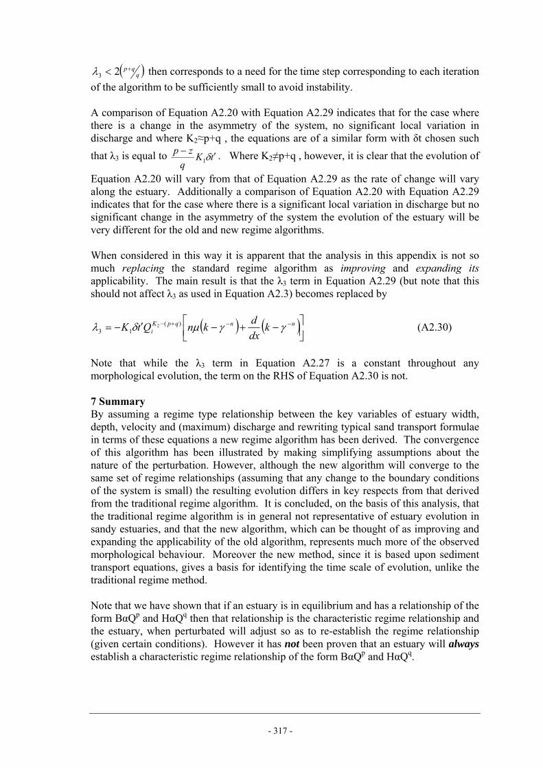
- 317 -

( )qqp+< 23λ then corresponds to a need for the time step corresponding to each iteration

of the algorithm to be sufficiently small to avoid instability. A comparison of Equation A2.20 with Equation A2.29 indicates that for the case where there is a change in the asymmetry of the system, no significant local variation in discharge and where K2≈p+q , the equations are of a similar form with δt chosen such that λ3 is equal to tK

qzp ′− δ1 . Where K2≠p+q , however, it is clear that the evolution of

Equation A2.20 will vary from that of Equation A2.29 as the rate of change will vary along the estuary. Additionally a comparison of Equation A2.20 with Equation A2.29 indicates that for the case where there is a significant local variation in discharge but no significant change in the asymmetry of the system the evolution of the estuary will be very different for the old and new regime algorithms. When considered in this way it is apparent that the analysis in this appendix is not so much replacing the standard regime algorithm as improving and expanding its applicability. The main result is that the λ3 term in Equation A2.29 (but note that this should not affect λ3 as used in Equation A2.3) becomes replaced by

( ) ( )⎥⎦⎤

⎢⎣⎡ −+−′−= −−+− nnqpK

i kdxdknQtK γγµδλ )(

132 (A2.30)

Note that while the λ3 term in Equation A2.27 is a constant throughout any morphological evolution, the term on the RHS of Equation A2.30 is not. 7 Summary By assuming a regime type relationship between the key variables of estuary width, depth, velocity and (maximum) discharge and rewriting typical sand transport formulae in terms of these equations a new regime algorithm has been derived. The convergence of this algorithm has been illustrated by making simplifying assumptions about the nature of the perturbation. However, although the new algorithm will converge to the same set of regime relationships (assuming that any change to the boundary conditions of the system is small) the resulting evolution differs in key respects from that derived from the traditional regime algorithm. It is concluded, on the basis of this analysis, that the traditional regime algorithm is in general not representative of estuary evolution in sandy estuaries, and that the new algorithm, which can be thought of as improving and expanding the applicability of the old algorithm, represents much more of the observed morphological behaviour. Moreover the new method, since it is based upon sediment transport equations, gives a basis for identifying the time scale of evolution, unlike the traditional regime method. Note that we have shown that if an estuary is in equilibrium and has a relationship of the form BαQp and HαQq then that relationship is the characteristic regime relationship and the estuary, when perturbated will adjust so as to re-establish the regime relationship (given certain conditions). However it has not been proven that an estuary will always establish a characteristic regime relationship of the form BαQp and HαQq.

- 318 -

8 References Abbott, M. R. (1960). Boundary Layer Effects, Journal of Marine Research, volume 18, part 2,October 1960, pp83-100. Ackers, P. and White, W. R. (1973). Sediment transport: a new approach and analysis, Proceedings of the ASCE, vol 99, HY11, pp2041-2060. Engelund, F. and Hansen, E. (1972). A monograph on sediment transport of alluvial streams, 3rd edition, Technical Press, Copenhagen. Friedrichs, C. T. and Aubrey, D. G. (1994). Tidal propagation in strongly convergent channels, Journal of Geophysical Research, Volume 99, Number C2, pp3321-3336, February 15, 1994. Spearman, J. R. (1995). Estuary Regimes and methods for prediction of long-term changes, PhD Thesis for Oxford Brookes University, March 1995. van Rijn, L. C. (1984). Sediment transport: part I: bed load transport; part II: suspended load transport; part III: bed forms and alluvial roughness, Proceedings of the ASCE Journal of Hydraulics Division, vol 110, HY10, pp1431-1456; HY11, pp1613-1641; HY12, pp1733-1754.

- 319 -

Appendix 3 Regime Theory as sediment transport (Muddy estuary) 1 Introduction and assumptions used in the proof For this proof we assume that the estuary can be characterised by regime relationships for width (B) and depth (H), i.e.,

pQB 1λ= (A3.1)

qQH 2λ= (A3.2) where Q is the maximum discharge associated with a characteristic tidal condition. This implies that cross-section area (at peak discharge), AQmax, is given by

qpQ QA

max

+= 3λ (A3.3) and cross-section averaged velocity (at peak discharge), VQmax, is given by

qpQV −−= 14λ (A3.4)

As for the sandy estuary we assume the normal regime algorithm, that a particular characteristic tidal condition represents an average sediment transport condition (sometimes referred to as a “morphological tide”) and that analysis on the basis of this single tide can be used as a synthesis of the range of tidal conditions normally encountered. The nature of mud transport is different to that of sand because of the scale of horizontal movement and settling. The nature of mud erosion/deposition is primarily a balance between vertical erosion and deposition while the nature of sand erosion/deposition is primarily a result of the rate of change of flux. For this reason the commonly used sediment transport equations for mud and sand are quite different which leads to very different forms for the regime algorithms derived for the mud and sandy estuary scenarios. It is assumed that velocity is sinusoidal and it is further assumed (on the basis of recent research by Winterwerp, 2007) that there is no critical shear stress for deposition, which simplifies Equation A3.6. It should be noted, however, that including a deposition threshold doesn’t change the essential result of the analysis, just some of the detail in the analysis and, moreover, any resultant regime algorithm will contain the deposition threshold term. 2 Derivation of the equilibrium condition As for Appendix 3 we introduce the time scale t which relates to the small-scale intro-tidal temporal variation and the time scale t' which relates to the long term time scale in units of the number of tides.

- 320 -

The change in cross-section area over a single tide is given by,

( ) ( ) dtCwVCM.BdtCwM.Btd

dAseDetideseetide

−−=−−=′ ∫∫ τρττ 2 (A3.5)

where B is the width of the estuary cross-section, Me is the erosion rate constant, τ and τe are the bed shear stress and critical shear stress for erosion, ρ is the water density, CD is the drag coefficient, C is the suspended sediment concentration, and ws is the settling velocity. If V is assumed to be sinusoidal and it is further assumed that eDVC τρ >>2

0 , then,

( ) dtCw)t(sinVCM.Btd

dAseDetide

−−=′ ∫ τθρ 22

0

( )seDe CwVCMBT −−≈ τρ 202

1 (A3.6) where θ=T/2π , T is the period of the tidal cycle and where sCw is the tidally averaged settling flux. Note that it is assumed that τe is small here compared to 2

0VCDρ but it could be same order in which case the regime becomes also a function of τe. At equilibrium,

( ) ( ) 0202

1202

1 =−≈−−=′

sDeseDe CwVCMBTCwVCMBTtd

dA ρτρ (A3.7)

Now since B=λ1Qp and V=λ4Q1-p-q (Equations A3.1 and A3.4)

( ) 012242

11 =−=

′−−

s)qp(

Dep CwQCMT.Q

tddA λρλ (A3.8)

In an estuary in equilibrium, dA/dt , when averaged over a sufficiently long period, is equal to zero. This means that,

s)qp(

De CwQCM =⇒ −−12242

1 λρ (A3.9) 3 The effect of a perturbation to the estuary 3.1 Introduction Now we consider the case where the estuary is perturbated by some development or natural effect. The nature of the perturbation is not specified except for the following assumptions: • It is assumed that the size of the perturbation is small enough that the proportional

change in tidal range along the estuary is small; • It is assumed that the size of the perturbation is small enough that any

morphological change at the estuary mouth is small. These assumptions ensure that any change in the boundary conditions of the estuary are limited. In this case the peak discharge, Q = QE , attains a new value Q' , where Q' =

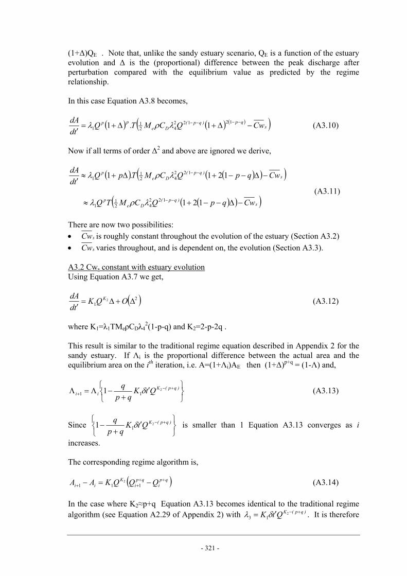
- 321 -

(1+∆)QE . Note that, unlike the sandy estuary scenario, QE is a function of the estuary evolution and ∆ is the (proportional) difference between the peak discharge after perturbation compared with the equilibrium value as predicted by the regime relationship. In this case Equation A3.8 becomes,

( ) ( ) ( )( )sqp)qp(

Depp CwQCMT.Q

tddA

−∆+∆+=′

−−−− 1212242

11 11 λρλ (A3.10)

Now if all terms of order ∆2 and above are ignored we derive,

( ) ( )( )( )s)qp(

Dep CwqpQCMT.pQ

tddA

−∆−−+∆+≈′

−− 1211 12242

11 λρλ

(A3.11) ( )( )( )s

)qp(De

p CwqpQCMTQ −∆−−+≈ −− 12112242

11 λρλ

There are now two possibilities: • sCw is roughly constant throughout the evolution of the estuary (Section A3.2) • sCw varies throughout, and is dependent on, the evolution (Section A3.3). A3.2 Cws constant with estuary evolution Using Equation A3.7 we get,

( )21

2 ∆+∆=′

OQKtd

dA K (A3.12)

where K1=λ1TMeρCDλ4

2(1-p-q) and K2=2-p-2q . This result is similar to the traditional regime equation described in Appendix 2 for the sandy estuary. If Λi is the proportional difference between the actual area and the equilibrium area on the ith iteration, i.e. A=(1+Λi)AE then (1+∆)p+q = (1-Λ) and,

⎭⎬⎫

⎩⎨⎧ ′

+−Λ=Λ +−

+)qp(K

ii QtKqp

q2

11 1 δ (A3.13)

Since ⎭⎬⎫

⎩⎨⎧ ′

+− +− )qp(KQtK

qpq

211 δ is smaller than 1 Equation A3.13 converges as i

increases. The corresponding regime algorithm is,

( )qpi

qpi

Kii QQQKAA ++

++ −=− 1112 (A3.14)

In the case where K2≈p+q Equation A3.13 becomes identical to the traditional regime algorithm (see Equation A2.29 of Appendix 2) with )qp(KQtK +−′= 2

13 δλ . It is therefore

- 322 -

true that the traditional regime equation is solving Equation A3.12 assuming that suspended sediment concentration is unaffected by the morphological evolution of the estuary. 3.3 Cws varies with estuary evolution Thus far we have considered the case where concentration is unaffected by morphological change. However, as Q1→ Q2 , and A1→A2 the change in volume of the estuary will supply or reduce the availability of sediment and therefore will increase or reduce concentrations. This scenario is a more realistic scenario than the case above (where evolution is unaffected by changes in concentrations). In general sCw will vary as,

sCw α Cm =[CE(1+ε)]m (A3.15) where m is in the region of 2 (e.g. Whitehouse et al, 2000). In this case Equation A3.11 becomes, to first order,

( ) ( )21 )1(22 ∆+−∆−−=

′OmqpQK

tddA K ε (A3.16)

where K1=1/2 λ1TMeρCDλ4

2(1-p-q) and K2=2-p-2q . This leads to the following algorithm,

⎥⎥⎦

⎤

⎢⎢⎣

⎡⎟⎟⎠

⎞⎜⎜⎝

⎛−⎟⎟

⎠

⎞⎜⎜⎝

⎛′=− +

+

++

221

1

111

Ki

m

i

i,EKi

m

i

i,Eii Q

CC

QC

CKtAA δ (A3.17)

where Qi is the peak discharge on the ith iteration, CE,i is the equilibrium suspended sediment concentration on the ith iteration, Ci is the actual suspended sediment concentration on the ith iteration First of all we consider how sediment eroded from the bed during morphological evolution and/or how sediment the sediment depletion in the water column resulting from during morphological evolution will be distributed. In the short term any changes to concentrations in the water column arising from erosion/deposition will be limited to the area local to the disturbance but rapidly any such changes will be distributed through the estuary owing to the relatively long tidal excursion of muddy sediment. For the purposes of this study it is assumed that any such sediment (or absence of sediment) is distributed such that the existing concentrations decrease proportionally by the ratio of the new total sediment in the estuary system (following morphological change), Mi to the old total (before the change), M0. This means that Equation A3.18 can be re-written as,

⎥⎥⎦

⎤

⎢⎢⎣

⎡⎟⎟⎠

⎞⎜⎜⎝

⎛−⎟⎟

⎠

⎞⎜⎜⎝

⎛′=− +

++

22 01

1

011

Ki

m

i

Ki

m

iii Q

MMQ

MMKtAA δ (A3.18)

- 323 -

We can investigate the stability of this equation. This means that the proportional change in suspended sediment concentration, ε , is given by the proportional change in total mass in the system. Equation A3.16 to A3.18 imply that,

⎟⎠⎞

⎜⎝⎛ ∆−−+−′+Λ=Λ +−

+ ii,vol,vold)qp(K

iii )qp(VVM

mQKt 120112

ρδ (A3.19)

where M is the total mass of sediment in the system under characteristic conditions before morphological evolution commenced; ρd is the dry density of the sediment on the channel bed; Vvol,0 and Vvol,i are the volumes of the system before the perturbation and at the ith time step. However, as in Appendix 2, the change in tidal volume arising from the change in bathymetry will reduce the convergence towards equilibrium, and Equation A3.19 becomes more correctly,

⎟⎠⎞

⎜⎝⎛ ∆−−+−′+Λ=Λ +−

+ ii,vol,vold)qp(K

iii )qp(qVVM

mQKt 120112

ρδ (A3.20)

Note that in this case equilibrium is not based on the discharge approaching an equilibrium value but rather the increase/decrease in sediment supply caused by morphological change itself. This result is rather different from the case where suspended sediment concentrations are constant throughout the evolution. Moreover Since ρd is much larger than Vvol/M it is clear that the change in estuary volume required for Equation 3.20 to converge small compared with the magnitude of ∆i and thus convergence is more rapid and the resulting total change in bathymetry is small compared with the evolution described in Equation A3.13. 4 Summary By assuming a regime type relationship between the key variables of estuary width, depth, velocity and (maximum) discharge and rewriting typical mud transport formulae in terms of these equations a new regime algorithm has been derived. The convergence of this algorithm has been illustrated. The resulting evolution differs in from that derived from the traditional regime algorithm in the inclusion of an additional concentration term. This term ensures that convergence to a new equilibrium is more rapid than for the old regime method but also means that the algorithm will not necessarily converge to the same discharge-area (or prism-area) relationships observed prior to evolution. As in the case of sandy estuaries (Appendix 2) it is apparent that the analysis in this appendix is not so much replacing the standard regime algorithm as improving and expanding its applicability. Moreover the new method gives a basis for identifying the time scale of evolution, unlike the traditional regime method. However, it is also concluded that the traditional regime algorithm is not representative of estuary evolution in muddy estuaries, and that the new algorithm represents much more of the observed morphological behaviour.

- 324 -

Note that we have shown that if an estuary is in equilibrium and has a relationship of the form BαQp and HαQq then that relationship is the characteristic regime relationship and the estuary, when perturbated will adjust so as to re-establish the regime relationship (given certain conditions). However it has not been proven that an estuary will always establish a characteristic regime relationship of the form BαQp and HαQq. 5 References Winterwerp, J. C. (2007). On the sedimentation rate of cohesive sediment. In: Estuarine and Coastal Fine Sediment Dynamics, (eds.) J. P.-Y. Maa, L. P. Sandford and D. H. Schoellhamer. pp 209-226 Elsevier. Whitehouse, R., Soulsby, R., Roberts, W. and Mitchener, H. (2000). Dynamics of estuarine muds, Thomas Telford, London.

- 325 -

Appendix 4 Second order solution to the strongly convergent 1D equations The second order solution to the strongly convergent 1D equations as given by Friedrichs and Aubrey (1994) is as follows:

( )kxtcosae kx −= ση µ1 (12)

( ) ( )222 22222

θσσγη −−+−= kxtcosakxtsinkxa (13)

where η1 and η2 are the dominant and harmonic tidal components; a2 and θ2 are the amplitude and phase of the η2 component;

µ is the amplitude growth factor given by, ⎪⎭

⎪⎬⎫

⎪⎩

⎪⎨⎧

−⎟⎟⎠

⎞⎜⎜⎝

⎛= 1

2

0cc

Aεµ

and c=σ/k and c0 = (gH)1/2 and εA=kLA and LA is given by A(x) = A0 exp-x/LA; γ is the tidal asymmetry factor given by, ( ) bh εεδγ −+= 1 , where εh is a/H and εb is (B-w)/B and w is the width of the LW channel.

( )Akx kxtsineuu εσµ −−−=1 (14)

( ) ( ) ( )22

2 222222222

θσσσγ−−−−−−= kxtsinu

aakxtcoskxkxtsinuu (15)

where u1 and u2 are the dominant and harmonic velocity components. References Friedrichs, C. T. and Aubrey, D. G. (1994). Tidal propagation in strongly convergent channels. Journal of Geophysical Research, 99 (C2), 3321-3336.

- 326 -

PB 12527 / 12

Nobel House17 Smith SquareLondon SW1P 3JR

www.defra.gov.uk

PB11207-CVR.qxd 1/9/05 11:42 AM Page 2