reverse convection potential saturation in the polar
TRANSCRIPT
REVERSE CONVECTION POTENTIAL
SATURATION IN THE POLAR
IONOSPHERE
Frederick D. Wilder
Thesis submitted to the faculty of the Virginia Polytechnic Institute and StateUniversity in partial fulfillment of the requirements for the degree of
Master of Sciencein
Electrical Engineering
Dr. C. Robert Clauer, ChairDr. Wayne A. ScalesDr. Scott M. Bailey
April 17, 2008Blacksburg, VA
Keywords: Ionosphere, Magnetosphere, Electromagnetics, HF Radar, PlasmaPhysics
Copyright: 2008

ABSTRACT
Reverse Convection Potential Saturation in the Polar Ionosphere
byFrederick D. Wilder
Chair: Dr. C. R. Clauer
The results of an investigation of the reverse convection potentials in the day side
high latitude ionosphere during periods of steady northward interplanetary magnetic
field (IMF) are reported. While it has been shown that the polar cap potential in the
ionosphere exhibits non-linear saturation behavior when the IMF becomes increas-
ingly southward, it has yet to be shown whether the high latitude reverse convection
cells in response to increasingly northward IMF exhibit similar behavior. Solar wind
data from the ACE satellite from 1998 to 2005 was used to search for events in the
solar wind when the IMF is northward and the interplanetary electric field is stable
for more than 40 minutes. Bin-averaged SuperDARN convection data was used with
a spherical harmonic fit applied to calculate the average potential pattern for each
northward IMF bin. Results show that the reverse convection cells do, in fact, ex-
hibit non-linear saturation behavior. The saturation potential is approximately 20
kV and is achieved when the electric coupling function reaches between 18 and 30
kV/RE.
ACKNOWLEDGEMENTS
I foremost would like to express my most sincere gratitude to my advisor, Profes-
sor C. Robert Clauer, who has supported me during the research and also assisted me
immensely with his expertise in the field of space science. I’d also like to thank him
for all the opportunities to travel and see the world, meeting many exciting people
in the process. I would also like to thank Professor Wayne A. Scales for assisting me
in my decision to pursue space science as well as introducing me to the field. Thanks
also go to Professor Scott M. Bailey for serving on my committee and being a great
teacher in aeronomy and atmospheric science.
I would also like to thank Dr. Joseph Baker, for helping to provide me with some
of the software to perform this research as well as many helpful discussions on the
best way to pursue this phenomenon. I would also like to thank Dr. Valeriy Petrov
and Dr. Vladimir (Volodya) Papitashvili for access to the Flat File Software, as well
as the MIST virtual global magnetic observatory. Special thanks to Robin Barnes
for providing and assisting me with the SuperDARN toolkit.
Finally, I would like to thank my Parents and family who have been very sup-
portive throughout my life and academic career as a whole.
This research is supported by the National Science Foundation through grant
ATM-0728538 to the Virginia Polytechnic Institute and State University. Operation
of the northern hemisphere SuperDARN radars is supported by the national funding
agencies of Canada, France, Japan, the United Kingdom and the United States.
iii

TABLE OF CONTENTS
ACKNOWLEDGEMENTS . . . . . . . . . . . . . . . . . . . . . . . . . . iii
LIST OF FIGURES . . . . . . . . . . . . . . . . . . . . . . . . . . . . . . . v
LIST OF TABLES . . . . . . . . . . . . . . . . . . . . . . . . . . . . . . . . x
LIST OF APPENDICES . . . . . . . . . . . . . . . . . . . . . . . . . . . . xi
CHAPTER
I. INTRODUCTION . . . . . . . . . . . . . . . . . . . . . . . . . . . 1
1.1 The Interplanetary Magnetic Field . . . . . . . . . . . . . . . 21.2 The Earth’s Magnetosphere . . . . . . . . . . . . . . . . . . . 41.3 Solar Wind - Magnetosphere - Ionosphere Coupling . . . . . . 101.4 Motivation . . . . . . . . . . . . . . . . . . . . . . . . . . . . 15
II. FIELD ALIGNED CURRENTS UNDER VARIOUS IMFCONFIGURATIONS . . . . . . . . . . . . . . . . . . . . . . . . . 17
2.1 Ionospheric Electrodynamics . . . . . . . . . . . . . . . . . . 172.2 Field Aligned Currents and Associated Convection Patterns . 192.3 Transpolar Potential Saturation and Existing Models . . . . . 24
III. METHODOLOGY . . . . . . . . . . . . . . . . . . . . . . . . . . 26
3.1 Solar Wind Data Analysis . . . . . . . . . . . . . . . . . . . . 263.2 Ionospheric Electric Potential Mapping . . . . . . . . . . . . 313.3 Event Selection Criteria and Convection Map Averaging . . . 36
IV. RESULTS AND DISCUSSION . . . . . . . . . . . . . . . . . . . 39
4.1 Results and Discussion . . . . . . . . . . . . . . . . . . . . . . 39
APPENDICES . . . . . . . . . . . . . . . . . . . . . . . . . . . . . . . . . . 43
BIBLIOGRAPHY . . . . . . . . . . . . . . . . . . . . . . . . . . . . . . . . 58
iv

LIST OF FIGURES
Figure
1.1 Archimedes spiral representation of solar wind propagating at velocity,Vsw (Hundhausen, 1995). . . . . . . . . . . . . . . . . . . . . . . . . 2
1.2 The GSM Coordinate System . . . . . . . . . . . . . . . . . . . . . . 3
1.3 An illustration of the solar wind encountering the earth’s magnetosphere.Courtesy of NASA Marshal Space Flight Center’s Space Plasma PhysicsBranch. Available at http://science.nasa.gov/ssl/pad/sppb/edu/magnetosphere/images/mag+sun.gif . . . . . . . . . . . . . . . . . . . . . . . . . . . 5
1.4 Magnetic reconnection and its driving of magnetospheric convection. TheIMF (lines 1,2) encounters the earth’s magnetic field (line 3) and merges.The two merged field lines split at the reconnection point, forming anx-shaped geometry called the “x-line.” The broken field lines are highlybent and thus will feel tension and straighten. This straightening pullsthe field lines towards the magnetotail (line 4) and eventually, the lineswill reconnect again to close the tail (line 5). The new field line (line 7)attached to the magnetosphere will then flow towards the earth and swingaround to the dayside (line 8) where the reconnection process can repeat.The re-formed IMF (line 6) will continue traveling through interplanetaryspace, adapted from Dungey (1961) . . . . . . . . . . . . . . . . . . . 6
1.5 The Sweet-Parker model of reconnection (Gurnett and Bhattacharjee, 2005). 7
1.6 Reconnection at high latitudes for Northward IMF. N1 and N2 are thepoints where the diffusion regions exist, the red field lines are the IMF,and the blue and green lines are the earth’s magnetic field. From Dorelliet al. (2007) . . . . . . . . . . . . . . . . . . . . . . . . . . . . . . . 8
v

1.7 The Structure of the Low Latitude Boundary Layer. Region 4 is the solarwind flow, region 3 is the higher density “boundary layer proper” (Sckopkeet al., 1981), and region 2 is the halo region where the boundary layerdensity profile approaches that of the magnetosphere. Kelvin-Helmholtzinstabilities determine the shape of region 3 (Sckopke et al., 1981; Kivel-son, 1995) . . . . . . . . . . . . . . . . . . . . . . . . . . . . . . . . 9
1.8 Plasma convection in the magnetosphere driven by viscous-like interac-tions (Axford and Hines, 1961) . . . . . . . . . . . . . . . . . . . . . . 10
1.9 The streamlines of ionospheric convection as a result of magnetic recon-nection (Dungey , 1961). The picture is viewed from above the northmagnetic pole looking down. The top of the figure is local noon. . . . . 11
1.10 An illustration of Region 1 and 2 FACs, as well as the resulting ionosphericelectric field (E), plasma convection(V) and electric currents (Jp ad Jh). 13
1.11 A demonstration of ΦPC saturation as a function of EKL, a non-physicalcoupling metric which represents the electric field of the solar wind beforemagnetic reconnection. APL FIT is the technique used by the datasetknown as the SuperDARN radar to determine the potential across thepolar cap (explained in detail in Chapter 3). Count’s demonstrates theamount of coverage the SuperDARN radars had for each value of EKL.From Shepherd et al. (2002). . . . . . . . . . . . . . . . . . . . . . . 14
1.12 An illustration of the convection pattern under northward IMF. Thelarger cells are the background convection pattern due to viscous-likeinteractions, and the smaller high latitude cells are due to reconnectionnear the cusp. . . . . . . . . . . . . . . . . . . . . . . . . . . . . . . 15
2.1 An illustration of the field aligned currents and resulting convection dur-ing periods of Northward IMF. . . . . . . . . . . . . . . . . . . . . . . 22
2.2 Field aligned current maps in the polar ionosphere based on eight differ-ent IMF orientations in the Y-Z plane. “The magnitude of the IMF inthe GSM Y-Z plane BT is fixed at 5nT, the solar wind velocity VSW is400kms−1, the solar wind proton number density nSW ... contours aroundnegative currents are drawn with dashed lines, and solid lines are usedfor positive currents, with the convention that positive currents are intothe ionosphere. The magnitude of the current is also indicated with theintensity of the grey scale shading”(Weimer , 2001). . . . . . . . . . . . 23
3.1 A picture of the ACE orbit with respect to the magnetopause and theparker spiral. . . . . . . . . . . . . . . . . . . . . . . . . . . . . . . . 28
vi
3.2 ERC versus the IMF y and z component for solar wind with a bulk velocityof 500 km/s and n = 2 . . . . . . . . . . . . . . . . . . . . . . . . . . 30
3.3 ERC versus the IMF y and z component for solar wind with a bulk velocityof 500 km/s and n = 4 . . . . . . . . . . . . . . . . . . . . . . . . . . 30
3.4 Coverage of the SuperDARN radars in the northern hemisphere. FromRuohoniemi and Baker (1998). . . . . . . . . . . . . . . . . . . . . . . 31
3.5 An example of the grid used for averaging the line of sight velocity vectors.The velocity data is taken from the Goose Bay Radar on December 14,1994, from 2003-2004:43 UT. From Ruohoniemi and Baker (1998). . . . 33
3.6 Averaged line of site velocities from SuperDARN radars in Saskatoon,Kupaskasing, Goose Bay and Stokkseyri on December 14, 1994, 2006-2012 UT. Taken from Ruohoniemi and Baker (1998) . . . . . . . . . . . 33
3.7 The velocity vectors resolved from the LOS vectors in Figure 3.6. FromRuohoniemi and Baker (1998) . . . . . . . . . . . . . . . . . . . . . . 34
3.8 The convection and potential pattern fit to the LOS vectors in Figure 3.6.The order of the expansion is 7. From Ruohoniemi and Baker (1998) . . 36
4.1 Calculated four cell convection pattern for four ERC bins: a) 2 to 4kV/Re, b) 10 to 13 kV/Re, c) 19 to 23 kV/Re and d) 32 to 39 kV/Re.The dayside convection cells are circled in red. . . . . . . . . . . . . . . 40
4.2 The reverse convection potential, ΦRC , as a function of ERC . The marksrepresent the center of the bins, and the horizontal lines represent thewidth of each bin in kV/Re . . . . . . . . . . . . . . . . . . . . . . . . 41
A.1 Potential pattern for the bin with ERC stability criteria within 2 to 4kV/RE . . . . . . . . . . . . . . . . . . . . . . . . . . . . . . . . . . 44
A.2 Potential pattern for the bin with ERC stability criteria within 4 to 6kV/RE . . . . . . . . . . . . . . . . . . . . . . . . . . . . . . . . . . 45
A.3 Potential pattern for the bin with ERC stability criteria within 10 to 13kV/RE . . . . . . . . . . . . . . . . . . . . . . . . . . . . . . . . . . 45
A.4 Potential pattern for the bin with ERC stability criteria within 12 to 15kV/RE . . . . . . . . . . . . . . . . . . . . . . . . . . . . . . . . . . 46
vii

A.5 Potential pattern for the bin with ERC stability criteria within 13 to 16kV/RE . . . . . . . . . . . . . . . . . . . . . . . . . . . . . . . . . . 46
A.6 Potential pattern for the bin with ERC stability criteria within 14 to 18kV/RE . . . . . . . . . . . . . . . . . . . . . . . . . . . . . . . . . . 47
A.7 Potential pattern for the bin with ERC stability criteria within 16 to 19kV/RE . . . . . . . . . . . . . . . . . . . . . . . . . . . . . . . . . . 47
A.8 Potential pattern for the bin with ERC stability criteria within 16 to 21kV/RE . . . . . . . . . . . . . . . . . . . . . . . . . . . . . . . . . . 48
A.9 Potential pattern for the bin with ERC stability criteria within 18 to 22kV/RE . . . . . . . . . . . . . . . . . . . . . . . . . . . . . . . . . . 48
A.10 Potential pattern for the bin with ERC stability criteria within 19 to 23kV/RE . . . . . . . . . . . . . . . . . . . . . . . . . . . . . . . . . . 49
A.11 Potential pattern for the bin with ERC stability criteria within 20 to 24kV/RE . . . . . . . . . . . . . . . . . . . . . . . . . . . . . . . . . . 49
A.12 Potential pattern for the bin with ERC stability criteria within 21 to 25kV/RE . . . . . . . . . . . . . . . . . . . . . . . . . . . . . . . . . . 50
A.13 Potential pattern for the bin with ERC stability criteria within 22 to 26kV/RE . . . . . . . . . . . . . . . . . . . . . . . . . . . . . . . . . . 50
A.14 Potential pattern for the bin with ERC stability criteria within 23 to 27kV/RE . . . . . . . . . . . . . . . . . . . . . . . . . . . . . . . . . . 51
A.15 Potential pattern for the bin with ERC stability criteria within 24 to 28kV/RE . . . . . . . . . . . . . . . . . . . . . . . . . . . . . . . . . . 51
A.16 Potential pattern for the bin with ERC stability criteria within 25 to 30kV/RE . . . . . . . . . . . . . . . . . . . . . . . . . . . . . . . . . . 52
A.17 Potential pattern for the bin with ERC stability criteria within 27 to 32kV/RE . . . . . . . . . . . . . . . . . . . . . . . . . . . . . . . . . . 52
A.18 Potential pattern for the bin with ERC stability criteria within 28 to 36kV/RE . . . . . . . . . . . . . . . . . . . . . . . . . . . . . . . . . . 53
A.19 Potential pattern for the bin with ERC stability criteria within 30 to 36kV/RE . . . . . . . . . . . . . . . . . . . . . . . . . . . . . . . . . . 53
viii

A.20 Potential pattern for the bin with ERC stability criteria within 31 to 38kV/RE . . . . . . . . . . . . . . . . . . . . . . . . . . . . . . . . . . 54
A.21 Potential pattern for the bin with ERC stability criteria within 31 to 40kV/RE . . . . . . . . . . . . . . . . . . . . . . . . . . . . . . . . . . 54
A.22 Potential pattern for the bin with ERC stability criteria within 32 to 36kV/RE . . . . . . . . . . . . . . . . . . . . . . . . . . . . . . . . . . 55
A.23 Potential pattern for the bin with ERC stability criteria within 32 to 39kV/RE . . . . . . . . . . . . . . . . . . . . . . . . . . . . . . . . . . 55
A.24 Potential pattern for the bin with ERC stability criteria within 37 to 47kV/RE . . . . . . . . . . . . . . . . . . . . . . . . . . . . . . . . . . 56
A.25 Potential pattern for the bin with ERC stability criteria within 40 to 50kV/RE . . . . . . . . . . . . . . . . . . . . . . . . . . . . . . . . . . 56
A.26 Potential pattern for the bin with ERC stability criteria within 43 to 53kV/RE . . . . . . . . . . . . . . . . . . . . . . . . . . . . . . . . . . 57
A.27 Potential pattern for the bin with ERC stability criteria within 46 to 56kV/RE . . . . . . . . . . . . . . . . . . . . . . . . . . . . . . . . . . 57
ix

LIST OF TABLES
Table
3.1 Bins of ERC Used To Generate Figure 4.2 . . . . . . . . . . . . . . . 37
x

LIST OF APPENDICES
Appendix
A. SuperDARN Plots Used to Generate Saturation Curve . . . . . . . . . 44
xi

CHAPTER I
INTRODUCTION
The interactions between the sun and the earth have been a subject of fascination
since the dawn of human history. As a blackbody radiator, the sun’s irradiance is a
crucial driving factor in the regulation of earth’s temperature. With the invention
of the telescope, scientists such as Galileo Galilei observed the sun’s surface and
sunspots (Russell , 1995). As modern technology and observational capabilities de-
veloped, a scientific discipline known as “solar-terrestrial physics” or “space physics”
emerged.
Central to solar-terrestrial physics is the interaction between plasma ejected from
the sun and the earth’s magnetic field. The corona is the outermost layer of the sun’s
atmosphere. It is an extremely hot gas consisting of ionized hydrogen, free electrons,
and helium. Due to a large pressure difference between the corona and interplanetary
space, this plasma expands outward into interplanetary space at supersonic speeds
and is called the “solar wind” (Hundhausen, 1995). Since the sun is constantly
rotating, the plasma will also be ejected in a spiral shape, similar to a lawn sprinkler
known as the “Parker spiral” (Hundhausen, 1995). The Parker spiral is shown in
Figure 1.1.
1

2
Figure 1.1: Archimedes spiral representation of solar wind propagating at velocity, Vsw(Hundhausen, 1995).
1.1 The Interplanetary Magnetic Field
Because of its high conductivity, the solar wind is often assumed to be an ideal
Magnetohydrodynamic (MHD) fluid. When describing the time rate of change of
the magnetic field, it can be shown that the magnetic induction equation becomes:
∂B
∂t= ∇× (u×B) (1.1)
Where B is the magnetic field contained in the solar wind, and u is the velocity of
the solar wind (Gurnett and Bhattacharjee, 2005). Since the (1.1) assumes very large
conductivity in the solar wind plasma, there is no term included for the diffusion of
the magnetic field. It is thus assumed that the magnetic field is “frozen in” the
solar wind and that field lines are carried by the solar wind bulk velocity (Gurnett
and Bhattacharjee, 2005). This frozen in field is called the “interplanetary magnetic
field” (IMF).

3
For this research, the IMF will be measured in geocentric solar magnetospheric
(GSM) coordinates. In this, the origin is at the center of the earth, the z axis contains
the projection of the earth’s dipole axis, the positive y axis from the origin to local
dusk, and the positive x axis points towards the sun, as shown in Figure 1.2(Kivelson
and Russell , 1995). The Y,Z plane rocks on the x axis as the earth rotates.
Figure 1.2: The GSM Coordinate System
In MHD, ohm’s law is usually given by (1.2).
J = σ(E + u×B) (1.2)
Where J is the electric current density in the plasma, σ is the electrical con-
ductivity of the plasma, and E is the associated electric field. Due to the frozen in
condition, however, the [E + u × B] term must be negligible to maintain a finite
current density (Hundhausen, 1995). The associated electric field in the frame of

4
reference of the solar wind plasma is then given by (1.3).
E ≈ −(u×B) (1.3)
1.2 The Earth’s Magnetosphere
As the solar wind flows through interplanetary space, it interacts with plane-
tary magnetic fields in a variety of ways. The Earth’s magnetic field, for example,
presents an obstacle to the solar wind plasma causing a shock to form upstream.
The earth’s magnetic field is confined to a cavity in the solar wind flow called the
magnetosphere. Due to the dynamic pressure of the solar wind, the magnetosphere
is compressed on the day side and drawn into a long comet-like tail behind the earth
on the night side (Walker and Russell , 1995). The shocked solar wind flows around
the magnetosphere in a region called the magnetosheath. The area where the solar
wind dynamic pressure is at a standoff with the earth’s magnetic pressure is called
the “magnetopause” and the subsolar magnetopause distance is typically located at
about 10 earth radii (RE) away from the center of the earth on the dayside (Walker
and Russell , 1995). Figure 1.3 shows an illustration of a typical interaction between
the solar wind and the magnetosphere.

5
Figure 1.3: An illustration of the solar wind encountering the earth’s magneto-sphere. Courtesy of NASA Marshal Space Flight Center’s Space PlasmaPhysics Branch. Available at http://science.nasa.gov/ssl/pad/sppb/edu/magnetosphere/images/mag+sun.gif
Large scale convection of plasma within the magnetosphere is tied to various
parameters within the solar wind. This convection maps along magnetic field lines
into the earth’s polar ionosphere, where it can have a direct impact on ionospheric
electric fields and thus modern technology. It is therefore important to understand
the mechanisms by which magnetospheric convection is driven.
1.2.1 Magnetic Reconnection
The primary mechanism whereby energy and momentum are coupled to the mag-
netosphere from the solar wind is the process of magnetic reconnection on the day
side of the Earth (Dungey , 1961). Magnetic reconnection is a process in plasma
physics where two anti-parallel magnetic field lines collide at very high pressure, and

6
the field lines literally shear and merge (Dungey , 1961). For example, if the IMF
is oriented southward when the solar wind encounters the earth’s magnetic field,
reconnection will occur as in Figure 1.4 (Dungey , 1961).
Figure 1.4: Magnetic reconnection and its driving of magnetospheric convection. TheIMF (lines 1,2) encounters the earth’s magnetic field (line 3) and merges. Thetwo merged field lines split at the reconnection point, forming an x-shapedgeometry called the “x-line.” The broken field lines are highly bent and thuswill feel tension and straighten. This straightening pulls the field lines towardsthe magnetotail (line 4) and eventually, the lines will reconnect again to closethe tail (line 5). The new field line (line 7) attached to the magnetosphere willthen flow towards the earth and swing around to the dayside (line 8) wherethe reconnection process can repeat. The re-formed IMF (line 6) will continuetraveling through interplanetary space, adapted from Dungey (1961)
Reconnection occurs when the frozen in flux condition breaks down (Hughes ,
1995). The most common model of reconnection is the Sweet-Parker model, which
is illustrated by Figure 1.5.

7
Figure 1.5: The Sweet-Parker model of reconnection (Gurnett and Bhattacharjee, 2005).
In the Sweet-Parker model of magnetic reconnection, there is a region in the
center of the X-line where the frozen field condition breaks down, called the diffusion
region (Hughes , 1995). The outflow velocity Uout is twice the phase velocity of an
MHD wave in the inflowing plasma called the Alfven speed (Hughes , 1995).
Magnetic reconnection can also occur when the IMF has other orientations. When
the IMF is oriented in an east-west direction, reconnection occurs on the flanks of
the earth’s magnetosphere, which will skew the resulting magnetospheric convection
patterns either in the east or the west (Friis-Christensen and Wilhjelm, 1975). When
the IMF is oriented northward, the IMF and the magnetic field are anti-parallel at
the poleward side of the cusp of the magnetosphere, where the magnetic fields enter
and exit the poles (Dorelli et al., 2007). This reconnection orientation is shown by
Figure 1.6.

8
Figure 1.6: Reconnection at high latitudes for Northward IMF. N1 and N2 are the pointswhere the diffusion regions exist, the red field lines are the IMF, and the blueand green lines are the earth’s magnetic field. From Dorelli et al. (2007)
1.2.2 Viscous Interactions
Another mechanism thought to influence magnetospheric plasma convection is a
viscous-like interaction between the solar wind and the earth’s magnetic field (Axford
and Hines , 1961). When a viscous fluid flows over a solid boundary, the viscous effects
are confined to a thin layer close to the solid body surface called the “boundary layer”
(Karemcheti , 1966). Since the velocity at the surface must have a limiting value of
zero, but the fluid has non-zero velocity, the boundary layer is an unstable region
where the velocity increases rapidly (Karemcheti , 1966).
In the magnetosphere, shocked solar wind flows over the surface in a region called
the magnetosheath as in Figure 1.3. The magnetosheath plasma has a viscous-like
interaction with the magnetosphere, in which a boundary layer is formed (Sckopke
et al., 1981). See Figure 1.7 for a representation of the boundary layer at low lat-
itudes. Unlike a fluid flowing over a solid body, the boundary layer of the magne-
9
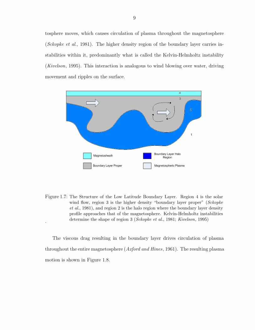
tosphere moves, which causes circulation of plasma throughout the magnetosphere
(Sckopke et al., 1981). The higher density region of the boundary layer carries in-
stabilities within it, predominantly what is called the Kelvin-Helmholtz instability
(Kivelson, 1995). This interaction is analogous to wind blowing over water, driving
movement and ripples on the surface.
Figure 1.7: The Structure of the Low Latitude Boundary Layer. Region 4 is the solarwind flow, region 3 is the higher density “boundary layer proper” (Sckopkeet al., 1981), and region 2 is the halo region where the boundary layer densityprofile approaches that of the magnetosphere. Kelvin-Helmholtz instabilitiesdetermine the shape of region 3 (Sckopke et al., 1981; Kivelson, 1995).
The viscous drag resulting in the boundary layer drives circulation of plasma
throughout the entire magnetosphere (Axford and Hines , 1961). The resulting plasma
motion is shown in Figure 1.8.

10
Figure 1.8: Plasma convection in the magnetosphere driven by viscous-like interactions(Axford and Hines, 1961)
1.3 Solar Wind - Magnetosphere - Ionosphere Coupling
In the upper regions of earth’s atmosphere, solar radiation and particle precipi-
tation can lead to the ionization of various molecules, including O2, N2, O and NO

11
(Rees , 1989). Because the ionosphere thus consists of plasma and partially ionized
gas, it can have electrodynamic interactions with the earth’s magnetosphere. The
electric field in the ionosphere can thus be used as a metric of how much energy is
transfered in the Solar Wind-Magnetosphere-Ionosphere system.
The earth’s magnetic field lines point out of the south pole and point into the
north pole. When a large scale effect such as magnetic reconnection with the solar
wind occurs, the movement of the magnetic field lines and the resulting plasma
convection will be mapped to the high latitude ionosphere (Dungey , 1961). This is
shown in Figure 1.9, where the high latitude trace lines correspond to magnetic field
lines being pulled over the polar cusp, and the low latitude lines correspond to the
magnetic field lines being pulled along the center of the magnetosphere back to the
earth on the night side (Dungey , 1961). A similar convection pattern arises in the
absence of reconnection due to viscous-like interactions (Axford and Hines , 1961).
Figure 1.9: The streamlines of ionospheric convection as a result of magnetic reconnection(Dungey , 1961). The picture is viewed from above the north magnetic polelooking down. The top of the figure is local noon.

12
The convection shown in Figure 1.9 is associated with a phenomenon called
“Field-aligned Currents” (FACs). Since magnetic fields can be approximated as
good conductors (Chen, 1974), electric currents move along magnetic field lines into
and out of the polar ionosphere called “region 1 currents”, leading to a net electric
field oriented across the polar cap. When plasma is in the presence of an electric
field and a magnetic field, it will have a bulk drift velocity called the E × B drift,
given by Equation (1.4) (Chen, 1974).
vE×B =E×B
B2(1.4)
Where vE×B is the drift velocity of the plasma particles and B is the magnitude
of the magnetic field. In the northern hemisphere, the magnetic field points into the
poles, and so the E×B drift of the Ionospheric plasma at high latitudes will point
anti-sunward, or from local noon to local midnight. Applying this analysis to lower
latitude field aligned currents that close the system called “region 2 currents”, one
gets the opposite motion, resulting in the plasma flow vortices shown in Figure 1.10.
Applying the same principles, there will be plasma flow vortices in the magneto-
sphere where the currents close as well. Magnetic reconnection is also thought to
generate field aligned currents, as well as compression of plasma (Friis-Christensen
and Wilhjelm, 1975; Song and Lysak , 1995). Field-aligned current systems and cur-
rent closure in the ionosphere-magnetosphere system will be described in greater
detail in Chapter 2.

13
Figure 1.10: An illustration of Region 1 and 2 FACs, as well as the resulting ionosphericelectric field (E), plasma convection(V) and electric currents (Jp ad Jh).
Because convecting plasma in a magnetic field has an associated electric field,
and because the earth’s magnetic field is often assumed to be static, an ionospheric
electric potential pattern [E = −∇Φ] is generated. The equipotential lines of the pat-
tern are the streamlines of the plasma convection (Wolf , 1995; Reiff and Luhmann,
1986). The potential drop across the two convection cells is called the cross polar
cap potential, ΦPC , and is an important metric in the Solar Wind-Magnetosphere-
Ionosphere system. As the IMF becomes increasingly southward, ΦPC has been
14
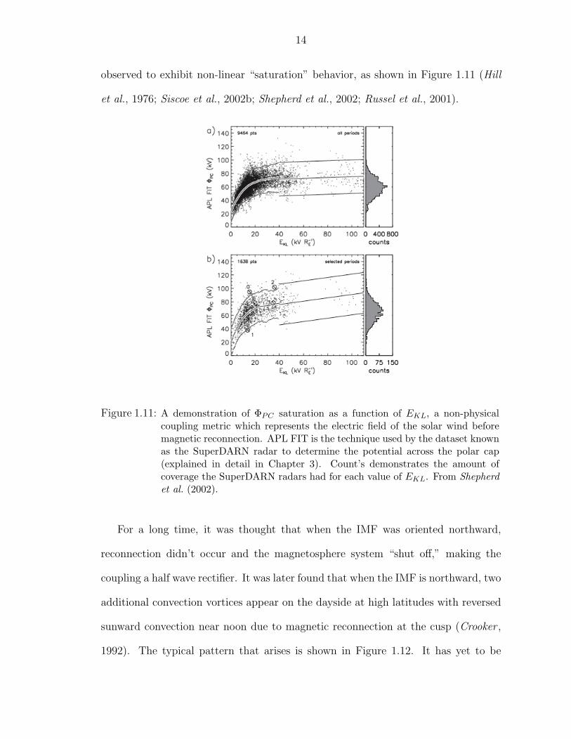
observed to exhibit non-linear “saturation” behavior, as shown in Figure 1.11 (Hill
et al., 1976; Siscoe et al., 2002b; Shepherd et al., 2002; Russel et al., 2001).
Figure 1.11: A demonstration of ΦPC saturation as a function of EKL, a non-physicalcoupling metric which represents the electric field of the solar wind beforemagnetic reconnection. APL FIT is the technique used by the dataset knownas the SuperDARN radar to determine the potential across the polar cap(explained in detail in Chapter 3). Count’s demonstrates the amount ofcoverage the SuperDARN radars had for each value of EKL. From Shepherdet al. (2002).
For a long time, it was thought that when the IMF was oriented northward,
reconnection didn’t occur and the magnetosphere system “shut off,” making the
coupling a half wave rectifier. It was later found that when the IMF is northward, two
additional convection vortices appear on the dayside at high latitudes with reversed
sunward convection near noon due to magnetic reconnection at the cusp (Crooker ,
1992). The typical pattern that arises is shown in Figure 1.12. It has yet to be

15
determined if the potential difference across the reverse convection vortices, hereafter
referred to as ΦRC , also exhibits non-linear saturation behavior.
Figure 1.12: An illustration of the convection pattern under northward IMF. The largercells are the background convection pattern due to viscous-like interactions,and the smaller high latitude cells are due to reconnection near the cusp.
1.4 Motivation
The best possible picture of ionospheric electric field behavior is a crucial aspect
of theoretical models and simulations of the Solar Wind-Magnetosphere-Ionosphere
system. As field aligned currents close in the ionosphere, the behavior of plasma
convection and electrodynamics in the magnetosphere is intricately coupled with the
polar ionosphere.
While it has been shown that ΦPC saturates (Shepherd et al., 2002; Hairston

16
et al., 2003; Russel et al., 2001), the behavior of ΦRC as a function of increasingly
northward IMF has not yet been studied in detail. For the above reasons, it is the
purpose of the present study to determine whether the reverse convection cells also
exhibits saturation behavior.

CHAPTER II
FIELD ALIGNED CURRENTS UNDER
VARIOUS IMF CONFIGURATIONS
2.1 Ionospheric Electrodynamics
2.1.1 Formation of the Ionosphere
The main mechanisms for ionization in the earth’s upper atmosphere are pho-
toionization and particle precipitation. With photoionization, high energy UV pho-
tons collide with molecules to separate electrons from the nucleus. The three primary
photoionization reactions are given by Equations (2.1) through (2.3) (Rees , 1989).
N2 + hν(< 796A) −→ N+2 + e− (2.1)
O2 + hν(< 1026A) −→ O+2 + e− (2.2)
O + hν(< 911A) −→ O+ + e− (2.3)
Where the photon wavelength corresponds to the ionization threshold from the
molecule’s ground state (Rees , 1989). These ions can also collide to form other
ions, such as NO+ (Carlson and Egeland , 1995). Another method is the impact of
“energetic” electrons, usually with energy greater than 1 keV, precipitating along
magnetic field lines from the magnetosphere (Luhmann, 1995). Ions can also be lost
due to various forms of recombination (Luhmann, 1995).
17

18
The ionosphere is often categorized in three layers, based on the density of ions
and electrons in the gas. These are the D (altitude below 90km), E (altitude between
90 and 130 km) and F (altitude above 130 km) regions (Luhmann, 1995). These
regions are listed in order of increasing charged particle density.
2.1.2 Ionospheric Conductivity
Due to collisions between ions and neutrals limiting the speed of ions, electric
currents can be induced in the ionosphere. It is well known that the ionosphere has
anisotropic conductivity, which can be seen in the ionospheric Ohm’s law, given by
(2.4) (Richmond and Thayer , 2000).
J = σPE⊥ + σHb× E⊥ + σ‖E‖b (2.4)
Where E is the ionospheric electric field, and b is a unit vector in the direction
of the earth’s geomagnetic field. The subscripts ⊥ and ‖ indicate components per-
pendicular to and parallel to the geomagnetic field, respectively. σP , σH , and σ‖ are
called the Pederson, Hall and parallel conductivities respectively. As can be seen in
Figure 1.10, the Pederson current, JP , is in the direction of the polar cap electric
field and the Hall Current, JH , is in the opposite direction of the twin cell convection
vortices. The expression for the conductivity components are given by Equations
(2.5) through (2.7) (Richmond and Thayer , 2000).
σ‖ =Nee
2
me
(νen‖ + νei‖
) (2.5)
σP =Nee
B
(νinΩi
ν2in + Ω2
i
+νen⊥Ωe
ν2en⊥ + Ω2
e
)(2.6)
σH =Nee
B
(Ω2
e
ν2en⊥ + Ω2
e
− Ω2i
ν2in + Ω2
i
)(2.7)
Where Ne is the ionospheric electron density; e is the electron charge; B is the
magnetic field magnitude; Ωj is the frequency a which a charged particle of species

19
j gyrates around a magnetic field line and is called the cyclotron frequency; νjk
is the collision frequency between particle species j and k; the subscripts ⊥ and
‖ correspond to directions perpendicular to and parallel to the geomagnetic field
respectively; and the subscripts i, e, and n correspond to the ions, electrons and
neutral molecules respectively. A full derivation of Equations (2.5) through (2.7) can
be found in Richmond and Thayer (2000).
As can be seen from Equations (2.6) and (2.7), if the collision frequency between
charged particles and neutrals is much smaller than their cyclotron frequency, the
Hall conductivity becomes zero. Therefore, at higher altitudes such as the F-region
where the charged particle density is high, the Pederson conductivity will dominate.
Often, Ohm’s law is written using a conductivity tensor given by Equations (2.8)
and (2.9) (Gurnett and Bhattacharjee, 2005).
J =←→σ (E + v ×B) (2.8)
←→σ =
σP σH 0
−σH σP 0
0 0 σ‖
(2.9)
Understanding how currents are directed through the ionosphere is crucial to
understanding how field-aligned currents close in the coupling between the Solar
Wind, Magnetosphere and Ionosphere.
2.2 Field Aligned Currents and Associated Convection Pat-terns
Although there are debates on small scale generation of field aligned currents,
large-scale FACs are thought to be associated with changes in field aligned vorticity in
20
magnetospheric convection cells generated by viscous-like interactions and magnetic
reconnection (Song and Lysak , 1995). As discussed in Chapter 1.2.1 and 1.3, different
orientations of the IMF will generate different convection patterns and therefore
different associated field aligned currents.
Friis-Christensen and Wilhjelm (1975) demonstrated that there are different cur-
rent and convection patterns in the polar cap ionosphere depending on the orientation
of the IMF in the Y-Z plane. When the IMF Z component is negative (southward
IMF), the two cell pattern shown in Figure 1.9 occurs. When the IMF Z compo-
nent is zero, and there is a non-zero IMF Y component, then the convection pattern
is skewed in either an east or west direction. These skewed patterns are associated
with what Friis-Christensen and Wilhjelm (1975) termed the “DPY” currents. When
the IMF Z component is positive, a four cell convection pattern appears similar to
Figure 1.12. The field aligned currents associated with the high latitude reverse
convection cells on the dayside in this pattern were termed “NBZ” by Iijima et al.
(1984).
In the case of reconnection with Southward IMF as well as viscous-like interac-
tions, the electrodynamic coupling between the magnetosphere and ionosphere can
be seen in Figure 1.10. At high altitudes, Pederson currents close the current in
the ionosphere, related by Ohm’s law to the electric field. If the geomagnetic field
is assumed to be static, then ∇ × E = 0 and the electric field can be expressed as
the negative gradient of a potential, Φ (Jackson, 1975). The drift velocity of the
ionospheric plasma can then be expressed by Equation (2.10).
v = −∇Φ×B
B(2.10)
It can be seen from Equation (2.10) that Φ is a stream-function of v. It follows

21
that equipotential lines given by Φ = constant represent streamlines of ionospheric
plasma flow. A more detailed discussion of streamlines and stream-functions can be
found in Karemcheti (1966).
When the IMF is oriented northward and the NBZ currents are generated, the
current system is more complicated and is shown in Figure 2.1. Region 1 and 2
currents still feed into the ionosphere due to viscous-like interactions, but they are
further coupled with the NBZ currents to generate the four cell convection pattern,
as well as the potential contours implied by Equation (2.10).

22
Figure 2.1: An illustration of the field aligned currents and resulting convection duringperiods of Northward IMF.
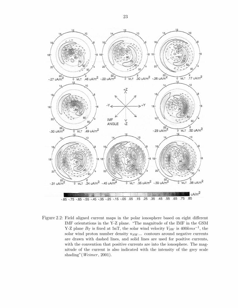
In summary, the field-aligned currents associated with various IMF orientations
are shown in Figure 2.2, taken from Weimer (2001). For northward IMF, the NBZ
currents as well as the Region 1 and 2 currents due to viscous-like interactions can
be seen, with skewing in the east or west direction when the IMF-Y component is
non-zero.
23
Figure 2.2: Field aligned current maps in the polar ionosphere based on eight differentIMF orientations in the Y-Z plane. “The magnitude of the IMF in the GSMY-Z plane BT is fixed at 5nT, the solar wind velocity VSW is 400kms−1, thesolar wind proton number density nSW ... contours around negative currentsare drawn with dashed lines, and solid lines are used for positive currents,with the convention that positive currents are into the ionosphere. The mag-nitude of the current is also indicated with the intensity of the grey scaleshading”(Weimer , 2001).

24
2.3 Transpolar Potential Saturation and Existing Models
The electric potential existing across the two cells shown in Figure 1.9 is usually
called the “Cross Polar Cap Potential,” and shall be denoted ΦPC . It was originally
thought that as the IMF turned increasingly southward, ΦPC would increase linearly
with the interplanetary electric field (IEF). The idea was that a fraction of the
solar wind electric field would be impressed upon the magnetosphere, generating a
magnetospheric convection potential, Φm. This large scale potential would then map
along magnetic field lines into the polar ionosphere, with ΦPC being approximately
equal to Φm (Hill et al., 1976; Reiff and Luhmann, 1986; Siscoe et al., 2002b).
An alternative to the linear model was that by some undefined mechanism, ΦPC
would eventually become non-linear, and reach a saturation value similar to that seen
in Figure 1.11 (Hill et al., 1976; Siscoe et al., 2002b). This saturation model was
called the Hill Model of Saturation, and is given by Equation (2.11) (Siscoe et al.,
2002b).
ΦPC =ΦmΦS
Φm + ΦS
(2.11)
Where ΦS is called the “Saturation Potential.” In the Hill Model, when Φm <<
ΦS, then the polar cap potential is approximately equal to the magnetospheric po-
tential. When Φm >> ΦS, the polar cap potential will be approximately equal to
the saturation potential. Empirical studies have demonstrated the Saturation Model
to be more accurate than the linear model, with ΦS found to be between 100 and
200 kV (Siscoe et al., 2002b; Shepherd et al., 2002; Russel et al., 2001).
Several models have been proposed based on MHD simulations that attempt to
explain the saturation phenomenon. One model suggests that Region 1 FACs weaken

25
the earth’s magnetic field in at the magnetopause, limiting reconnection. A similar
model states that a dimple in the magnetic field forms at the stagnation point in
solar wind flow, which also limits reconnection (Siscoe et al., 2004). Another model,
given by (Siscoe et al., 2002a), is that Region 1 FACs saturate when they become
strong enough that their J × B force can balance out the dynamic pressure of the
solar wind. A fourth model involves the magnetopause becoming blunt, which widens
the magnetosheath. The solar wind then has more room in the magnetosheath to
flow past the magnetosphere, limiting reconnection (Siscoe et al., 2004). Nagatsuma
(2004) also observed that the saturation phenomenon is partially determined by the
conductivity of the ionosphere. As the solar zenith angle decreases and the Pederson
conductivity of the ionosphere increases, the saturation phenomenon becomes more
pronounced (Nagatsuma, 2004).
While it has been demonstrated that convection cells associated Region 1 and 2
FACs saturate, there have been no observations of the trend in the reverse convection
cells associated with the NBZ Currents. Comparing the geometry of reconnection in
the case of southward and northward IMF (Figures 1.4 and 1.6 respectively), one can
see the impact on the current models for ΦPC saturation. Since during northward
IMF, reconnection occurs at the high latitude edge of the cusp, a strengthening of
the NBZ currents could not have the same effect that the Region 1 currents have at
the equatorial magnetopause. Therefore, it is crucial to determine whether the NBZ
currents saturate.

CHAPTER III
METHODOLOGY
In order to determine if the reverse convection potential associated with the NBZ
current system saturates, several steps were taken. First, a large amount of events
where the IMF is steadily northward were found. These events were then sorted and
binned based on the strength of the solar wind electric field. Ionospheric convection
data from the Super Dual Auroral Radar Network (SuperDARN) (Chisham et al.,
2007) was then be compiled to generate convection patterns for each bin to get a
convection map, from which the potential pattern was inferred. Once a convection
potential is obtained, the potential across the high latitude dayside reverse convection
cells, ΦRC can be measured for each bin.
3.1 Solar Wind Data Analysis
3.1.1 The ACE Satellite
All solar wind and IMF data was taken from the Advanced Composition Ex-
plorer (ACE) satellite. This satellite orbits around the L1 point, which is one of
the Lagrange points where the gravitational fields of the earth and the sun cancel.
The L1 point is upstream in the solar wind between the earth and the sun between
the earth’s day side and the sun. For this reason, it is a prime location to measure
26

27
solar wind parameters before they reach the earth. There are two instruments on
ACE. MAG measures the components of the magnetic field vector and SWEPAM
measures plasma parameters such as composition, density, velocity and temperature
(Stone et al., 1998).
A complication in using ACE satellite data is the delay between a measurement
the satellite makes and the time it takes for that measurement to reach the earth’s
magnetopause. As can be seen from Figure 3.1, depending on where the ACE satellite
is in its orbit around the L1 point, it will see a different point on the Parker Spiral.
Thus, the earth’s magnetopause might see the measurement earlier or later than
the expected time of travel between the L1 point and the magnetopause (Ridley ,
2000). There are several methods to calculate when a measured parameter will hit
the magnetopause, but the data used in this study was pre-propagated UCLA data
which used the minimum variance technique outlined by Weimer et al. (2003). The
error of propagation time estimates can be on the order of a few minutes, and thus
will effect time selection criteria when the effects of Northward IMF are measured
(Ridley , 2000).

28
Figure 3.1: A picture of the ACE orbit with respect to the magnetopause and the parkerspiral.
3.1.2 The Energy Coupling Function
In order to determine the response of the reverse convection potential to the
solar wind, there must be a metric which represents how much of the interplanetary
electric field (IEF) is coupled into the ionosphere from the solar wind. Kan and Lee
29
(1979) developed a metric which was used by Shepherd et al. (2002) in their study
of the polar cap potential saturation response to southward IMF conditions, called
the “energy coupling function.” The energy coupling function for southward IMF is
given in equation (3.1).
Ekl = VxBT sin2 θ
2(3.1)
Where Vx is the x component of the solar wind velocity, BT =√
B2y + B2
z is the
component of the IMF transverse to the solar wind bulk velocity, and θ = cos−1 Bz
BT
is called the IMF clock angle, which represents the orientation of the IMF in the
Y-Z (GSM) plane. Equation 3.1 is loosely based on the frozen field theory given by
Equation 1.3 and is measured in kilovolts per earth radii (kV/RE). The equation is
derived assuming that the solar wind bulk velocity only travels in the x direction,
which is reasonable (Kan and Lee, 1979).
When the IMF is purely northward, there will be a clock angle of zero degrees,
and the sine term in equation (3.1) will be zero. Thus, in order to study the behavior
of reverse convection cells, another metric must be used. Since the sine term is a
non-physical geometric scaling factor, it can be altered to look for events where high
latitude reverse convection cells would form. If one assumes that a pure y IMF would
not generate reverse convection and that the y-component of the IMF only affects
the skew of the reverse cells, the energy coupling function can be modified as shown
in Equation (3.2).
ERC = −VxBT cosnθ (3.2)
This will always be positive as long as the value of n is an even integer and the
clock angle is between −90o and 90o. The value of the exponent will directly effect

30
how much the y component of the IMF impacts the value of ERC . The larger n is,
the more the y component will reduce the coupling function’s magnitude. Plots of
these functions for n = 2 and n = 4 can be seen in Figures 3.2 and 3.3.
Figure 3.2: ERC versus the IMF y and z component for solar wind with a bulk velocityof 500 km/s and n = 2
Figure 3.3: ERC versus the IMF y and z component for solar wind with a bulk velocityof 500 km/s and n = 4
In this study, n = 4 will be used. As seen in Figure 3.3, an exponent of four limits
the influence of the IMF-y component. Also, n > 4 was not used because Super-

31
DARN would not have enough doppler measurements to produce enough accurate
maps to cover the range of Figure 4.2.
3.2 Ionospheric Electric Potential Mapping
3.2.1 The Super Dual Auroral Radar Network
The Super Dual Auroral Radar Network (SuperDARN) is a network of high
latitude coherent scatter radars which work in conjunction to produce large scale
convection patterns in the polar ionosphere. As of 2007 there were 11 radars in the
northern hemisphere and 7 radars in the southern hemisphere, with a diagram of
the locations and overlap given in Figure 3.4. A detailed list of all radars and their
geographic and geomagnetic location Additional radars have been constructed since
2007, but their doppler measurements have not been used in the present study.
Figure 3.4: Coverage of the SuperDARN radars in the northern hemisphere. From Ruo-honiemi and Baker (1998).
A SuperDARN radar operates at the high frequency (HF) band of the radio
spectrum, and is typically capable of transmitting at center frequencies between
8 and 20 MHz (Chisham et al., 2007). The major mechanism by which the radar
calculates line of sight plasma drift velocities is by backscatter from ionization density

32
irregularities aligned with the geomagnetic field. At 10.8 MHz, the signal is sensitive
to irregularities with a wavelength of 13.9 m and studies have shown that in the F
region the irregularities which produce backscatter convect with the E ×B drift of
the plasma (Ruohoniemi et al., 1987). They have also been demonstrated to be a
common occurrence in the high-latitude regions of the ionosphere (Ruohoniemi et al.,
1987). The signal incident on the irregularities must be approximately orthogonal to
the geomagnetic field lines, and thus the scatter is actually assisted by the refraction
of the signal in the ionosphere (Ruohoniemi et al., 1987; Ruohoniemi and Greenwald ,
1996; Chisham et al., 2007).
In order to obtain the large scale convection pattern, several steps must be taken.
First, the line of sight velocities calculated by the each radar are placed into spatial
bins with a width of 1 degree of latitude and 10 degree increments of magnetic
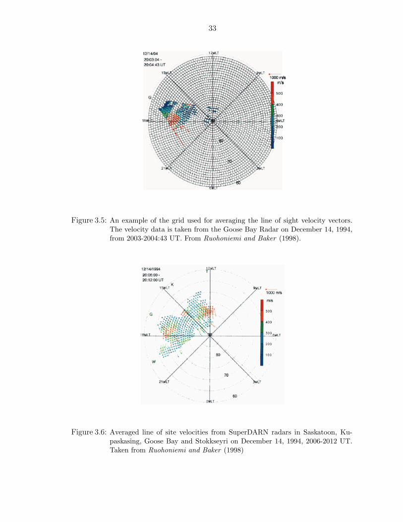
azimuth, and the values are averaged within each bin (Ruohoniemi and Baker , 1998).
An example of these bins and the resulting average line of site velocities for a specific
event are given by Figures 3.5 and 3.6.
33
Figure 3.5: An example of the grid used for averaging the line of sight velocity vectors.The velocity data is taken from the Goose Bay Radar on December 14, 1994,from 2003-2004:43 UT. From Ruohoniemi and Baker (1998).
Figure 3.6: Averaged line of site velocities from SuperDARN radars in Saskatoon, Ku-paskasing, Goose Bay and Stokkseyri on December 14, 1994, 2006-2012 UT.Taken from Ruohoniemi and Baker (1998)

34
Once the spatially averaged line of site velocities are calculated, line of site ve-
locities in areas where the fields of view of two or more radars can be resolved into
convection velocity vectors. If more than two radars overlap, a least square error
fit is used (Ruohoniemi and Baker , 1998). Figure 3.7 shows the result when the
LOS velocity vectors given in Figure 3.6 are resolved. Areas with no overlap are not
included (Ruohoniemi and Baker , 1998).
Figure 3.7: The velocity vectors resolved from the LOS vectors in Figure 3.6. From Ruo-honiemi and Baker (1998)
3.2.2 Spherical Harmonic Mapping of the Ionospheric Electric Potential
Once ionospheric velocity vectors have been calculated by SuperDARN, one can
proceed to calculate the ionospheric potential pattern, Φ. This is done by assum-
ing that the geomagnetic field is stationary and that the net charge density in the
ionosphere is zero. In this case, the ionospheric electric potential can be found using
Laplace’s Equation (3.3) (Jackson, 1975).

35
∇2Φ = 0 (3.3)
If the potential is assumed to exist on the surface of a spherical earth, then the
solution of Laplace’s equation is a spherical harmonic expansion given by Equation
(3.4) (Weimer , 1995; Jackson, 1975).
Φ(θ, φ) =∞∑l=0
+l∑m=−l
Alm
√2l + 1
4π
(l −m)!
(l + m)!Pm
l (cos θ)eimφ (3.4)
Where θ is the co-latitude and φ is the azimuthal angle on the surface of an
arbitrary sphere, and Pml is the Legendre polynomial. For the ionospheric potential,
θ and Φ can be explained in terms of geomagnetic coordinates by Equations (3.5)
and (3.6) (Weimer , 1995).
θ = (90−MLAT )pi
45(3.5)
φ = MLTpi
12(3.6)
Where MLAT is the magnetic latitude and MLT is the magnetic local time.
MLAT is the latitude based on the location of the magnetic north pole, not the
geographic one. MLT is the location where it is at a certain time. For example,
MLT noon would be the magnetic longitude line which directly faces the sun and
MLT midnight would be the magnetic longitude line facing opposite the sun.
Since it was shown by Equation (2.10) that the plasma convection velocity in the
ionosphere flows on equipotential lines, an electric potential pattern can be fit to
convection data (Weimer , 1995; Ruohoniemi and Baker , 1998).

36
SuperDARN uses a routine called APLFIT to fit velocity vectors to a spherical
harmonic expansion. Coefficients are calculated to minimize the χ2 value for the
LOS component of the velocity vectors (Ruohoniemi and Baker , 1998). Because χ2
is defined for the LOS component, even vectors where there is no overlap may be
used in the spherical harmonic fit. Also, to fill in spaces with no coverage, statistical
patterns based on IMF orientation are used (Ruohoniemi and Greenwald , 1996). The
result of APLFIT applied to the velocity LOS vectors given in Figure 3.6 is shown
in Figure 3.8.
Figure 3.8: The convection and potential pattern fit to the LOS vectors in Figure 3.6.The order of the expansion is 7. From Ruohoniemi and Baker (1998)
3.3 Event Selection Criteria and Convection Map Averaging
3.3.1 Solar Wind and IMF Stability Criteria
Using ERC , events were found using ACE MAG and SWEPAM data from 1998 to
2005. Events of quasi-stable ERC were then placed into bins containing a minimum
and maximum ERC value. The criteria for quasi-stability was that the event stayed

37
within the bin’s maximum and minimum ERC value for a minimum of 40 minutes.
The minimum event duration was chosen to account for solar wind propagation
estimation delays, as well as the time it takes for the reverse convection cells to form
after a northward turning of the IMF (Clauer and Friis-Christensen, 1988). The
ERC range for each bin was selected to maximise the spatial coverage of Doppler
measurements by SuperDARN in each bin, but at the same time provide enough
discretization for the curve in Figure 4.2 to see the saturation effect. Table 3.1 shows
the range of each bin, as well as the number of quasi-stable events.
Table 3.1: Bins of ERC Used To Generate Figure 4.2
Range (kV/RE) Events Range (kV/RE) Events Range (kV/RE) Events
0-2 4,286 19-23 33 31-38 10
2-4 175 20-24 38 31-40 25
4-6 79 21-25 31 32-36 11
10-16 65 22-26 26 32-39 15
12-15 54 23-27 20 37-47 13
13-16 45 24-28 15 40-50 15
14-18 27 25-30 23 43-53 10
16-19 22 27-32 21 46-56 8
16-21 26 28-36 26
18-22 33 30-36 11
3.3.2 Convection Map Averaging
For a given bin of ERC , velocity vectors from 20 minutes into each quasi-stable
event were further divided into spatial bins on a grid of 100km and 10-degree incre-
ments of magnetic azimuth. The median value in each spatial bin was then calculated.
This pre-processing reduces the amount of data which goes into the spherical har-

38
monic fitter. It is also beneficial because it smoothes out large positive and negative
values which cancel in the fitter at convection reversal boundaries. The APLFIT
technique was then applied, deriving the electric potential pattern. Velocity vec-
tors from the SuperDARN statistical model were not used to generate the potential
patterns so as not to bias the results. Figure 4.1 shows the results of the spherical
harmonic fit for several bins of ERC . Once an ERC bin’s potential pattern is calcu-
lated, ΦRC can be found by measuring the potential between the reverse convection
cells, circled in red in Figure 4.1.

CHAPTER IV
RESULTS AND DISCUSSION
Figure 4.1 shows four convection patterns as the IMF turns increasingly north-
ward. Each pattern is presented in AACGM MLAT-MLT format with the magnetic
pole at the center and magnetic noon directed up the page. The lowest latitude
shown is 60 degrees and the contour spacing is 1kV. Color-coding shows the number
of gridded SuperDARN measurements that contributed to the calculation of each
pattern. The four convection patterns in Figure 4.1 correspond to the following bins
of ERC : (a) 2-4, (b) 10-13, (c) 19-23, and (d) 32-39 kV/RE. The values of the re-
versed convection potential, ΦRC , are 2.85, 10.66, 17.44, and 19.36 kV respectively.
The reader is invited to count the potential contours across the dayside reverse con-
vection cells to demonstrate these potential values. Appendix A contains average
convection maps for all of the ERC bins used in the present study.
4.1 Results and Discussion
As seen in Figure 4.1, as the value of ERC increases, the reversed convection cells
first become more pronounced but then the reversed convection potential eventually
saturates. Also note that as the value of ERC is allowed to increase the number of
SuperDARN measurements available to calculate the pattern also decreases. Beyond
39

40
a. b.
c. d.
Figure 4.1: Calculated four cell convection pattern for four ERC bins: a) 2 to 4 kV/Re,b) 10 to 13 kV/Re, c) 19 to 23 kV/Re and d) 32 to 39 kV/Re. The daysideconvection cells are circled in red.
60 kV/RE there were too few Doppler measurements available to calculate a potential
pattern.
Figure 4.2 shows a plot of the reverse convection potential for ERC values up to
70 kV/RE. The horizontal bars show the range of values used in each ERC bin used
to calculate each convection pattern. For low values of ERC (i.e. 0-18 kV/RE) the
reverse convection potential exhibits linear characteristics but as ERC increases the
reverse potential starts to saturate, similar to what has been identified previously for

41
southward IMF (Shepherd et al., 2002). The rapid decrease in the slope of ΦRC can
clearly be seen in the ERC range 20 to 26 kv/RE.
Figure 4.2: The reverse convection potential, ΦRC , as a function of ERC . The marksrepresent the center of the bins, and the horizontal lines represent the widthof each bin in kV/Re
It is still unclear at this time why the NBZ currents and the potential across
the vortices they generate should saturate. In the case of southward IMF, there are
several models that account for saturation of ΦPC . Three common models are: the
strengthening of Region 1 field aligned currents to the point where their J×B force
replaces the currents at the magnetopause as the main counter to solar wind ram
pressure; the erosion of the magnetopause magnetic field which limits reconnection;
and the magnetopause becoming blunt, giving the solar wind more room to flow
around the magnetosphere (Siscoe et al., 2004). All of these models are related to
the strength of the Region 1 field-aligned currents. Since the NBZ currents are driven
by reconnection at the cusp, it is unlikely that these models could also be applied to
saturation of the reverse convection cells. One thing that hasn’t been investigated is
whether or not there is a limit to the amount of current the ionosphere can carry. If

42
it is the case that the ionospheric conductivity plays a role, then it could help explain
the saturation phenomenon for both the southward and northward IMF cases.
For further study, case studies of events with even stronger ERC will be done
combining high latitude radar and satellite data. Analysis of the reverse convection
cell response time will also be done, as well as further analysis of the transition from
linear to non-linear behavior. The Canadian high latitude PolarDARN radars, as
well as the Resolute Bay incoherent scatter radar when it begins operation, will also
give more coverage to the regions where reverse cells form, and at the next solar
maximum, a better picture of the reverse convection potential during strong IMF
will be developed. This will assist in determining as well as possible the maximum
potential the reverse convection phenomena can generate. Also, comparing electric
fields with the Southward IMF case and looking for seasonal asymmetries would help
to determine how much current can pass through the ionosphere at a given time, as
well as the effects of conductivity.

APPENDICES
43

44
APPENDIX A
SuperDARN Plots Used to Generate Saturation
Curve
Figure A.1: Potential pattern for the bin with ERC stability criteria within 2 to 4 kV/RE
45
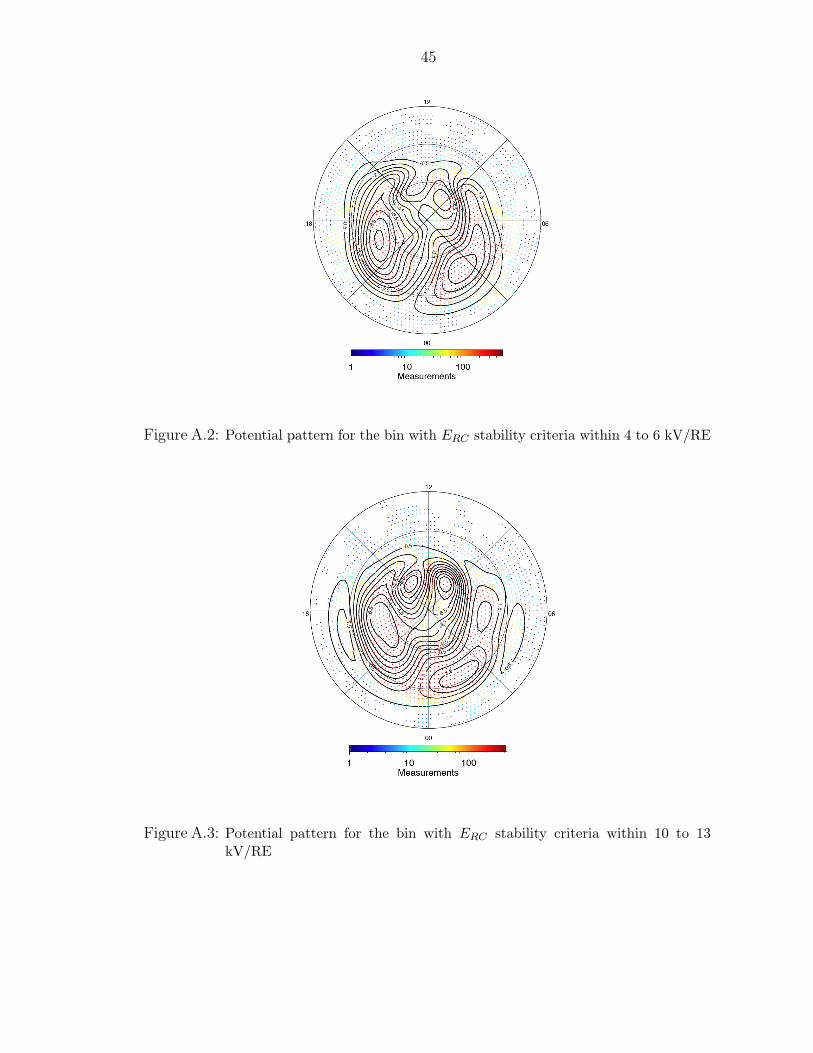
Figure A.2: Potential pattern for the bin with ERC stability criteria within 4 to 6 kV/RE
Figure A.3: Potential pattern for the bin with ERC stability criteria within 10 to 13kV/RE

46
Figure A.4: Potential pattern for the bin with ERC stability criteria within 12 to 15kV/RE
Figure A.5: Potential pattern for the bin with ERC stability criteria within 13 to 16kV/RE

47
Figure A.6: Potential pattern for the bin with ERC stability criteria within 14 to 18kV/RE
Figure A.7: Potential pattern for the bin with ERC stability criteria within 16 to 19kV/RE

48
Figure A.8: Potential pattern for the bin with ERC stability criteria within 16 to 21kV/RE
Figure A.9: Potential pattern for the bin with ERC stability criteria within 18 to 22kV/RE

49
Figure A.10: Potential pattern for the bin with ERC stability criteria within 19 to 23kV/RE
Figure A.11: Potential pattern for the bin with ERC stability criteria within 20 to 24kV/RE

50
Figure A.12: Potential pattern for the bin with ERC stability criteria within 21 to 25kV/RE
Figure A.13: Potential pattern for the bin with ERC stability criteria within 22 to 26kV/RE

51
Figure A.14: Potential pattern for the bin with ERC stability criteria within 23 to 27kV/RE
Figure A.15: Potential pattern for the bin with ERC stability criteria within 24 to 28kV/RE

52
Figure A.16: Potential pattern for the bin with ERC stability criteria within 25 to 30kV/RE
Figure A.17: Potential pattern for the bin with ERC stability criteria within 27 to 32kV/RE

53
Figure A.18: Potential pattern for the bin with ERC stability criteria within 28 to 36kV/RE
Figure A.19: Potential pattern for the bin with ERC stability criteria within 30 to 36kV/RE

54
Figure A.20: Potential pattern for the bin with ERC stability criteria within 31 to 38kV/RE
Figure A.21: Potential pattern for the bin with ERC stability criteria within 31 to 40kV/RE
55
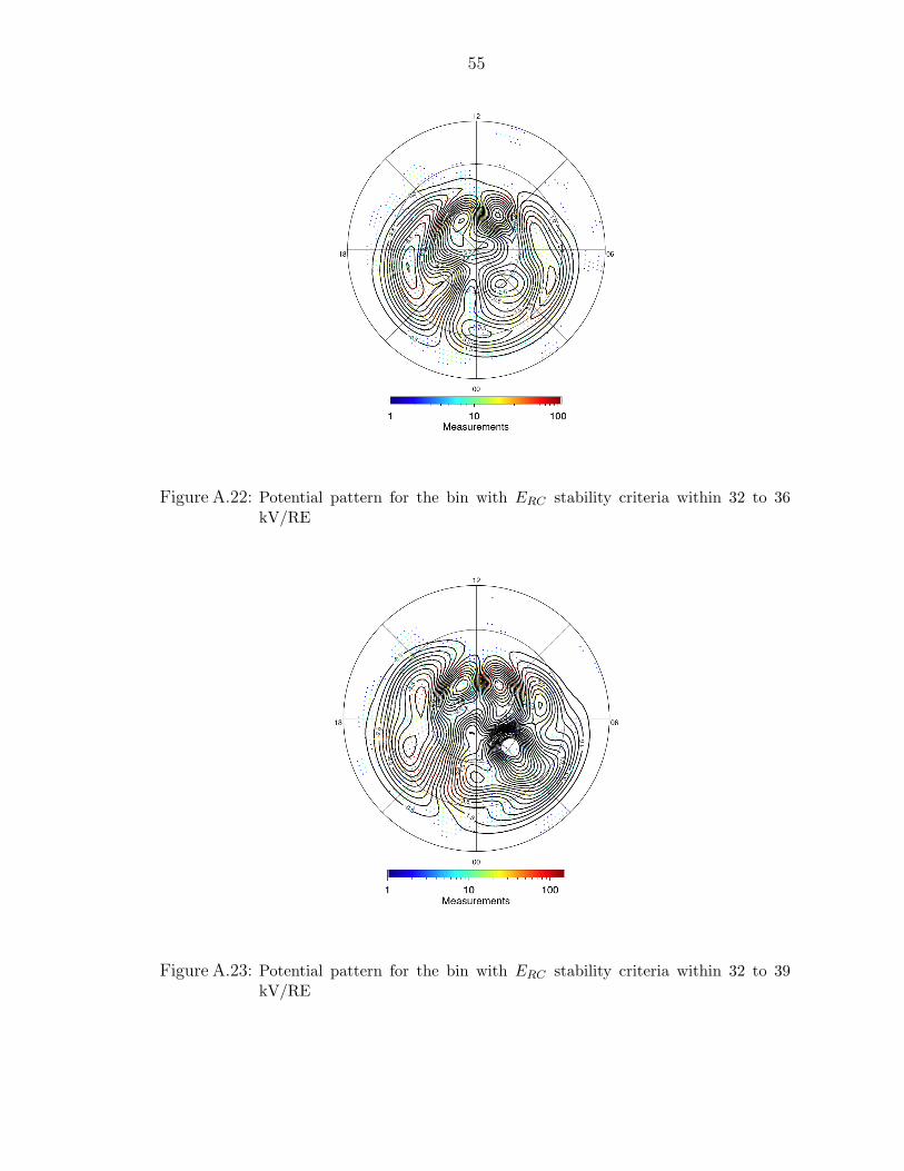
Figure A.22: Potential pattern for the bin with ERC stability criteria within 32 to 36kV/RE
Figure A.23: Potential pattern for the bin with ERC stability criteria within 32 to 39kV/RE

56
Figure A.24: Potential pattern for the bin with ERC stability criteria within 37 to 47kV/RE
Figure A.25: Potential pattern for the bin with ERC stability criteria within 40 to 50kV/RE

57
Figure A.26: Potential pattern for the bin with ERC stability criteria within 43 to 53kV/RE
Figure A.27: Potential pattern for the bin with ERC stability criteria within 46 to 56kV/RE

BIBLIOGRAPHY
58

59
BIBLIOGRAPHY
Axford, W., and C. Hines, A unifying theory of high-latitude geophysical phe-nomena and geomagnetic storms, Can. J. Phys., 39 , 1433, 1961.
Carlson, H., and A. Egeland, “The aurora and auroral ionosphere,” in Intro-duction to Space Physics,edited by M.G. Kivelson and C.T. Russell, p. 459 ,Cambridge University Press, Cambridge, 1995.
Chen, F. F., Introduction To Plasma Physics and Controlled Fusion Volume 1:Plasma Physics, Second Edition, Springer, New York, 1974.
Chisham, G., et al., A decade of the super dual auroral radar network (super-darn): scientific achievements, new techniques and future directions, Surveys inGeophysics , 28 (1), 33–109, 2007.
Clauer, C. R., and E. Friis-Christensen, High latitude dayside electric fields andcurrents during strong northward imf: Observations and model simulation, J.Geophys. Res., 93 , 2749, 1988.
Crooker, N. U., Reverse convection, J. Geophys. Res., 97 , 19363, 1992.
Dorelli, J., A. Bhattacharjee, and J. Raeder, Separator reconnection at earth’sdayside magnetopause under northward interplanetary magnetic field condi-tions, J. Geophys. Res., 112 (A02202), doi:10.1029/2006JA011877, 2007.
Dungey, J. W., Interplanetary magnetic field and the auroral zones, Phys. Rev.Lett., 6 , 47, 1961.
Friis-Christensen, E., and J. Wilhjelm, Polar cap currents for different directionsof the interplanetary magnetic field in the Y − Z plane, J. Geophys. Res., 80 ,1248, 1975.
Gurnett, D., and A. Bhattacharjee, Introduction to Plasma Physics With Spaceand Laboratory Applications , Cambridge University Press, Cambridge, 2005.
Hairston, M., T. Hill, and R. Heelis, Observed saturation of the ionosphericpolar cap during the 31 march 2001 storm, Geophys. Res. Lett., 30 (6),doi:10.1029/2002GL015894, 2003.

60
Hill, T., A. J. Dessler, and R. A. Wolf, Mercury and Mars: The role of iono-spheric conductivity in the acceleration of magnetospheric particles, Geophys.Res. Lett., 3 , 429 – 432, 1976.
Hughes, W., “The magnetopause, magnetotail and magnetic reconnection,” inIntroduction to Space Physics,edited by M.G. Kivelson and C.T. Russell, p. 227 ,Cambridge University Press, Cambridge, 1995.
Hundhausen, A., “The solar wind,” in Introduction to Space Physics,edited byM.G. Kivelson and C.T. Russell, p. 91 , Cambridge University Press, Cambridge,1995.
Iijima, T., T. A. Potemra, L. J. Zanetti, and P. F. Bythrow, Large-scale Birke-land currents in the dayside polar region during strongly northward IMF: A newBirkeland current system, J. Geophys. Res., 89 , 7441, 1984.
Jackson, J. D., Classical Eelectrodynamics , John Wiley and Sons, New York,1975.
Kan, J. R., and L. C. Lee, Energy coupling function and solar wind magneto-sphere dynamo, Geophys. Res. Lett., 6 , 577, 1979.
Karemcheti, K., Principles of Ideal Fluid Aerodynamics , Krieger, Malabar, 1966.
Kivelson, M., “Pulsations and magnetohydrodynamic waves,” in Introductionto Space Physics,edited by M.G. Kivelson and C.T. Russell, p. 330 , CambridgeUniversity Press, Cambridge, 1995.
Kivelson, M. G., and C. T. Russell, Geophysical coordinate transformations, inIntroduction to Space Physics , edited by M. G. Kivelson, and C. T. Russell, pp.531–543, Cambridge University Press, Cambridge, UK, 1995.
Luhmann, J., “Ionospheres,” in Introduction to Space Physics,edited by M.G.Kivelson and C.T. Russell, p. 183 , Cambridge University Press, Cambridge,1995.
Nagatsuma, T., Conductivity dependance of cross-polar potential saturation, J.Geophys. Res., 109 , 2004.
Rees, M., Physics and Chemistry of the Upper Atmosphere, Cambridge Univer-sity Press, Cambridge, 1989.
Reiff, P. H., and J. G. Luhmann, Solar wind control of the polar cap voltage, inSolar Wind - Magnetosphere Coupling, edited by Y. Kamide and J.A. Slavin,p. 507 , Terra Scientific Publishing, Tokyo, Japan, 1986.
Richmond, A., and J. Thayer, “Ionospheric electrodynamics: A Tutorial”, inMagnetospheric Current Systems, AGU Geophys. Monogr. Ser., Vol. 118, editedby S. Ohtani, R. Fujii, M. Hesse, and R. L. Lysak, p. 131 , AGU, Washington,D.C., 2000.
61
Ridley, A. J., Estimations of the uncertainty in timing the relationship betweenmagnetospheric and solar wind processes, J. Atmos. Sol. Terr. Phys., 62 , 757,2000.
Ruohoniemi, J., and S. K. Baker, Large-scale imaging of high-latitude convectionwith super dual auroral radar network hf radar observations, J. Geophys. Res.,103 (A9), 20797–20811, 1998.
Ruohoniemi, J. M., and R. A. Greenwald, Statistical patterns of the high-latitude convection obtained from Goose Bay HF radar observations, J. Geo-phys. Res., 101 , 21,743, 1996.
Ruohoniemi, J. M., R. Greenwald, K. Baker, J. Villain, and M. McCready, Driftmotions of small-scale irregularities in the high-latitude f region: an experimen-tal comparison with plasma drift motions, J. Geophys. Res., 92 (A5), 4553–4564,1987.
Russel, C. T., J. Luhmann, and G. Lu, Nonlinear response of the polar iono-sphere to large values of the interplanetary electric field, J. Geophys. Res.,106 (A9), 21083–21094, 2001.
Russell, C. T., “A brief history of solar-terrestrial physics,” in Introduction toSpace Physics,edited by M.G. Kivelson and C.T. Russell, p. 227 , CambridgeUniversity Press, Cambridge, 1995.
Sckopke, N., G. Paschmann, G. Haerendel, B. U. O. Sonnerup, S. J. Bame,T. G. Forbes, J. E. W. Hones, and C. T. Russell, Structure of the low-latitudeboundary layer, J. Geophys. Res., 86 , 2099–2110, 1981.
Shepherd, S., R. Greenwald, and J. Ruohoniemi, Cross polar cap potentialsmeasured with super dual auroral radar network during quasi-steadi solarwind and interplanetary magnetic field conditions, J. Geophys. Res., 107 (A7),doi:10.1029/2001JA000152, 2002.
Siscoe, G., J. Raeder, and A. Ridley, Transpolar potential saturation modelscompared, J. Geophys. Res., 109 (A09203), doi:10.1029/2003JA010318, 2004.
Siscoe, G. L., N. U. Crooker, and K. D. Siebert, Transpolar potential saturation:Roles of region 1 current system and solar wind ram pressure, J. Geophys. Res.,107 (A10), 2002a.
Siscoe, G. L., G. M. Erickson, B. U. O. Sonnerup, N. C. Maynard, J. A. Schoen-dorf, K. D. Siebert, D. R. Weimer, W. W. White, and G. R. Wilson, Hill modelof transpolar potential saturation: Comparisons with MHD simulations, J. Geo-phys. Res., 107 (A6), 2002b.
Song, Y., and R. Lysak, “Paradigm Transition in Cosmic Plasma Physics, Mag-netic Reconnection and the Generation of Field-Aligned Current,” in Magneto-spheric Current Systems, AGU Geophysical Monograph 118,edited by S. Ohtani,

62
R. Fujii, M. Hesse and R.L. Lysak, p. 11 , Cambridge University Press, Cam-bridge, 1995.
Stone, E., A. Frandsen, R. Mewaldt, E. Christian, D. Margolies, J. Ormes, andF. Snow, The advanced composition explorer, Space Science Reviews , 86 , 1–22,1998.
Walker, R., and C. Russell, “Solar-wind interactions with magnetized planets,”in Introduction to Space Physics,edited by M.G. Kivelson and C.T. Russell, p.164 , Cambridge University Press, Cambridge, 1995.
Weimer, D., Models of high-latitude electric potentials derived with a least errorfit of spherical harmonic coefficients, J. Geophys. Res., 100 , 19,595, 1995.
Weimer, D., Maps of field-aligned currents as a function of the interplanetarymagnetic field derived from Dynamic Explorer 2 data, J. Geophys. Res., 106 ,12,889, 2001.
Weimer, D., D. Ober, N. Maynard, M. Collier, D. McComas, N. Ness, C. Smith,and J. Watermann, Predicting interplanetary magnetic field (imf) propagationdelay times using the minimum variance technique, J. Geophys. Res., 108 (A1),doi:10.1029/2002JA009405, 2003.
Wolf, R., “Magnetospheric Configuration,” in Introduction to SpacePhysics,edited by M.G. Kivelson and C.T. Russell, p. 288 , Cambridge Uni-versity Press, Cambridge, 1995.