rev ersibilit y and pro duct-f orm net w orks i{ 1 art rev ...rev ersibilit y and pro duct-f orm net...
TRANSCRIPT
Reversibility and Product-Form Networks I { 1
Spring 1999Professor Costis Maglaras
B9801-33 Stochastic Processing Networks409 Uris Hall
Part I: Reversibility and Product-Form Networks
Summary. The �rst part of the course is a brief tour d'horizon of the descriptive theory of product
form networks. This is the class of queueing networks for which exact solutions and performance
characterizations exist. In this section we introduce some of the basic de�nitions, network models,
and key concepts to be used later on. In detail, section I.1 contains some background material
on Markov Processes, and section I.2 inroduces the concept of reversibility, which is central in the
development of the theory of product form networks. Section I.3 covers Burke's \Output Theorem,"
and gives a �rst glimse to simple product form results. From that point onwards, we turn to
product form networks. Section I.4 describes and analyzes open queueing networks of reversible
queues. Section I.5 generalizes these results to the class of \Kelly networks" of quasi-reversible
queues. Section I.6 describes networks with symmetric queues that allow for general service time
dsirtibutions. Finally, section I.7 introduces the corresponding class of closed queueing networks.
The primary reference is the book by Kelly [Kel79]. Important results will be refered to using the
labels found in [Kel79]. Much of the material we cover is based on lecture notes originally developed
by Professor Michael Harrison.
I.1 Preliminaries: Markov Processes
1. Let X(t) be a stochastic process taking values on a discrete (countable) state space S. The time
parameter t takes values on a set T . For a discrete time process T is the set of integers Z, that
is t = 0; 1; 2; : : :, while for a continuous time process T will be the real line R.
2. If (X(t1);X(t2); : : : ;X(tn)) and (X(t1+ �);X(t2 + �); : : : ;X(tn+ �)) have the same probability
distribution for all t1; t2; : : : ; tn; � 2 T then the process X(t) is said to be stationary.
3. The stochastic process X(t) is a Markov process (MP) if for any t1 < t2 < � � � < tn < tn+1
P (X(tn+1) = xn+1jX(t1) = x1;X(t2) = x2; : : : ;X(tn) = xn) = P (X(tn+1) = xn+1jX(tn) = xn);
(I.1)
i.e., the future is independent of the past given the present or else, all information contained in
the past evolution of the process that is useful in predicting its future behavior is contained in
the current state of the process.
Fact I.1.1 The stochastic process X(t) is Markov, if for any t1 < t2 < � � � < tm < � � � <tn conditional on X(tm) (the present), (X(t1);X(t2); : : : ;X(tm�1) (the past) is independent of
(X(tm+1); : : : ;X(tn)) (the future).
Reversibility and Product-Form Networks I { 2
4. A MP is time homogeneous if P (X(t+ �) = kjX(t) = j) does not depend on t.
5. A MP X(t) irreducible if every pair of states (k; j) communicates (k; j 2 S).
6. Hereafter, when we say X = fX(t); t � 0g is a MP, it is understood that
(a) the state space S is discrete (countable),
(b) the process is time homogeneous,
(c) irreducible (i.e., all pairs of states in S communicate)
(d) X stays in each state a positive length of time, and
(e) only �nitely many transitions occur in a �nite amount of time.
The last two conditions are additional assumptions imposed in order to exlude some continuous
time Markov processes that exhibit very erratic behavior.
7. De�ne the transition rate from state j to state k by
q(j; k) = limh!0
1
hP (X(t+ h) = kjX(t) = j); (I.2)
for k 6= j, with q(j; j) = 0. Let q(j) =P
k2S q(j; k).
Fact I.1.2 Under the assumptions imposed on X, starting from any state j, X stays there an
exponentially distributed length of time with mean 1=q(j); the probability that the next state
visited is k is p(j; k) � q(j; k)=q(j). We call p(j; k) and fp(j; k)g the transition probabilities and
transition matrix for the embedded jump chain respectively. Note thatP
k2S p(j; k) = 1.
8. An equilibrium distribution for X is de�ned as a set of positve numbers f�(j); j 2 Sg that sumto 1 (
Pj2S �(j) = 1) and satisfy the equilibrium equations
�(j)Xk2S
q(j; k) =Xk2S
�(k)q(k; j); j 2 S: (I.3)
The LHS of (I.3) is equal to �(j)q(j) which is the \probability ux" out of state j. The RHS
(I.3) is equal to the \probability ux" into state j. In equilibrium, the ux out of any state j
should be equal to the ux into state j; this is precisely (I.3) which is also refered to as the global
balance equations.
Fact I.1.3 If an equilibrium distribution exists, then it is unique, and it is moreover
(a) the unique stationary distribution of X,
(b) the limit distribution of X for every starting state j, that is
limt!1
P (X(t) = kjX(0) = j) = �(k); j 2 S;

Reversibility and Product-Form Networks I { 3
(c) the long-run occupancy distribution of X, almost surely for every starting state; that is
limT!1
1
T
Z T
01k(t)dt = �(k) a:s:;
where 1k(t) is the indicator function (1k(t) = 1 if X(t) = 1, and zero otherwise).
Fact I.1.4 If there exists a set of numbers f�(j)g that satisfy (I.3) that sum up to 1, then there
is no equilibrium distribution, and X has no stationary distribution. In this case, P (X(t) =
kjX(0) = j) ! 0 as t!1 for all j; k 2 S, and the limiting fraction of time spent in any state
k is also zero (almost surely, for any starting state j).
9. As an example try analyzing the simplest example possible of the M=M=1 queue: start from the
MP description for the queue, verify all assumptions described in (6), derive the stationary distri-
bution, the expected waiting time and the expected (total) delay per arriving job, the expected
backlog in the system. How do these measures vary with the load (or traÆc intensity � = �=�,
where � and � are the arrival and service rates respectively)? This is the simplest example of a
birth-death (B&D) process with birth rate � (arrivals) and death rate � (departures).
I.2 Reversibility
1. The property of reversibility plays an important role in the descriptive theory of queueing net-
works. Intuitively speaking, if we take a trace of a reversible process and run it backwards in
time the resulting process is statistically indistinguishable from the original process. That is,
the behavior of a reversible process remains the same when the direction of time is reversed.
De�nition I.2.1 X is said to be reversible if (X(t1); : : : ;X(tn)) has the same distribution with
(X(� � t1); : : : ;X(� � tn)).
Proposition I.2.1 A reversible process is stationary.
Proof.
(X(t1); : : : ; X(tn)) � (X(� � t1); : : : ; X(� � tn))
� (X(�t1); : : : ; X(�tn))
� (X(� + t1); : : : ; X(� + tn));
the �rst step follows from the de�nition of reversibility, the second by setting � = 0, and the third
by the reversibility of the \time reversed" process X(�t). �
2. Theorem 1 (Thm. 1.3 [Kel79]) A stationary MP X is reversible if and only if there exists a
probability distribution f�(j); j 2 Sg satisfying the detailed balance equations
�(j)q(j; k) = �(k)q(k; j) for all j; k 2 S: (I.4)
Reversibility and Product-Form Networks I { 4
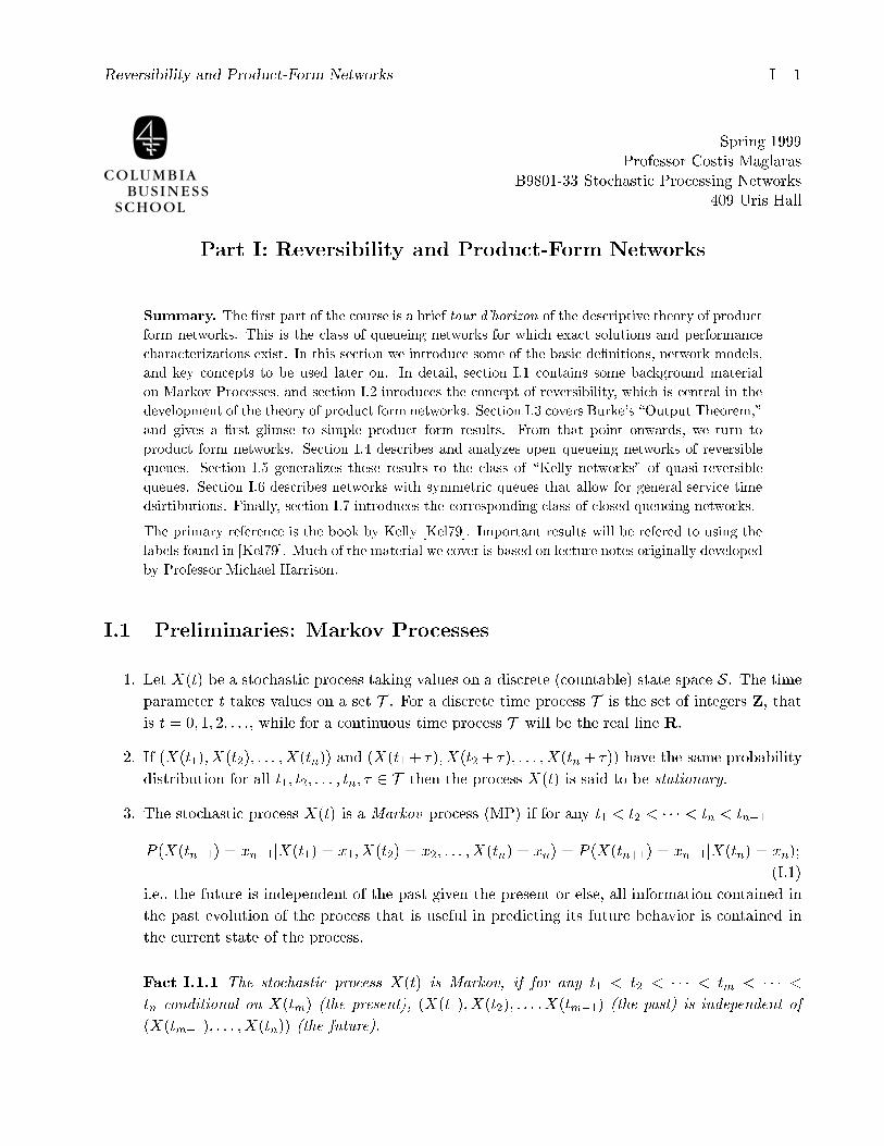
(a) (b)
j k
T S � T
Forward chain Reversed chain
Figure 1: Examples: (a) reversible chain { simple network with tree structure; (b) non-reversible chain { the forward chain has clockwise transitions whereas the reversed chainhas anticlockwise transitions; from [BG92].
Remark. Any such collection f�(j)g must be the equilibrium distribution of X ; sum (I.4) over
k 2 S to obtain the equilibrium equations (I.3).
3. Examples of reversible processes.
De�nition I.2.2 The graph G associated with the MP X has a vertex for each state j 2 Sand an edge between j and k if either q(j; k) or q(k; j) is positive. (Irreducibility ) graph is
connected.) A cut is a division of S into complementary sets T and S � T .
Proposition I.2.2 If G is a tree, then X is reversible. (Thus the standard B&D process is
reversible.)
Proof. Introduce a cut along the edge (j; k) that divides S into T and S �T . In equilibrium, the
ow balance equations along this cut areXi2T ; l2S�T
�(i)q(i; l) =X
i2T ; l2S�T
�(l)q(l; i): (I.5)
Since G is a tree, it follows that q(i; l) = 0 for all i 6= j, l 6= k, and thus (I.5) reduces to (I.4). �
Corollary I.2.1 The queue length process associated with an M=M=1 queue is reversible.
Proof. The queue length process of an M=M=1 queue is a B&D process. �
Proposition I.2.3 If the transition rates of a reversible MP with state space S and equilibrium
distribution f�(j)g are altered by changing q(j; k) to cq(j; k) for j 2 T and k 2 S � T , then the
new MP is reversible in equilibrium and has equilibrium distribution
�0(j) =
(B�(j) 8j 2 TBc�(j) 8j 2 S � T ;
where B is some normalization constant.
Reversibility and Product-Form Networks I { 5
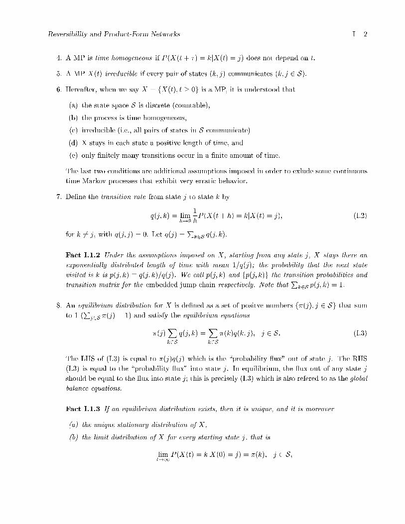
�1 �2
�1 �2
�1 �2
�1 �2
Common bu�erfor 3 jobs
Figure 2: Two M=M=1 queues in parallel operating with common waiting room of size 4.
Proof. f�0(j)g and fq0(j; k)g satisfy the detailed balance equations (I.4). (This is also true for
c = 0.) �
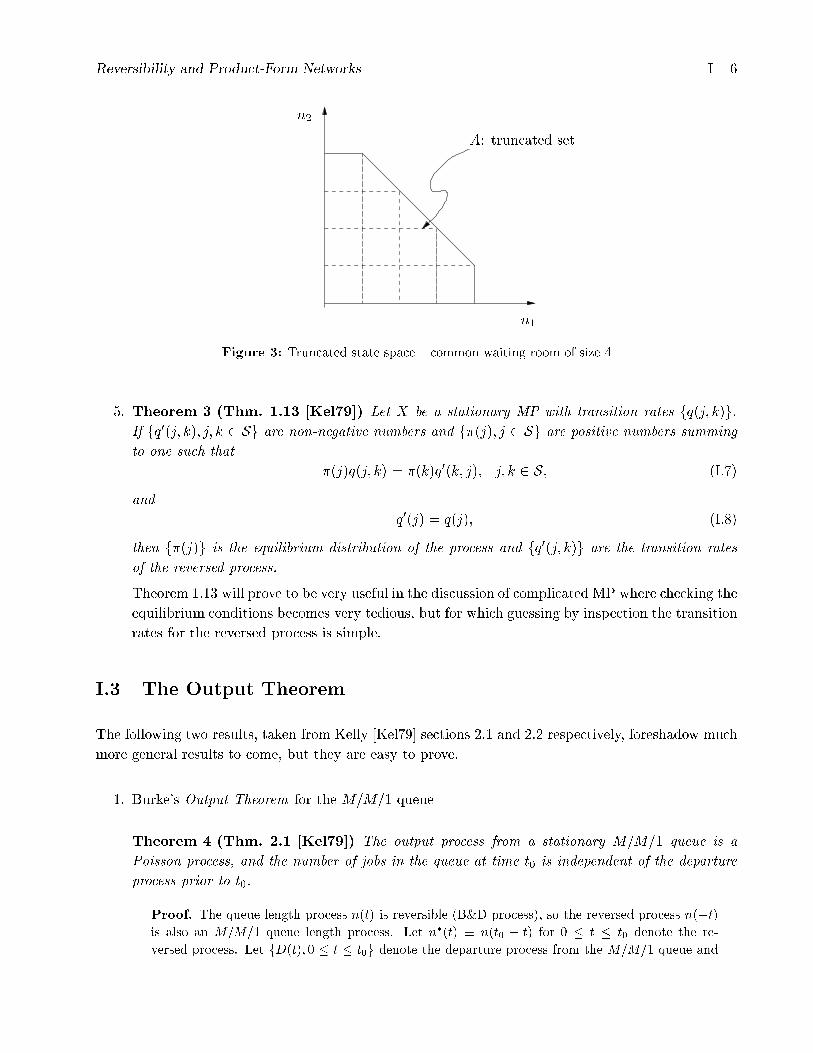
Corollary I.2.2 If the state space of X is simply truncated (or restricted) to stay in T (this is
the case c = 0), then the new equilibrium distribution is
�0(j) =�(j)Pk2T �(k)
; j 2 T :
Example: Two independent M=M=1 queues are operating in parallel with in�nite waiting
rooms. Now impose a common waiting room of size 4. (That is, at any time there can be at
most 3 jobs waiting for service and each server can be processing at most one job.)
Let n1 and n2 denote the # of jobs in queues one and two respectively. First we need to show
that the two-dimensional queue length process (n1(t); n2(t)) is reversible. From independence of
the two queues we have that
�(n1; n2) = �1(n1) � �(n2); where �(ni) = (1� �i)�ni
i :
It is now easy to verify conditions (I.4) to show that (n1(t); n2(t)) is reversible. Imposing the
common waiting room, the truncated state space is shown in Figure 3. Using the last corollary
we get that �0(n1; n2) = B�(n1; n2) for (n1; n2) 2 A.
4. Theorem 2 (Thm. 1.12 [Kel79]) If X(t) is a stationary MP with transition rates fq(j; kgand equilibrium distribution f�(j)g, then the reversed process X(� � t) is a stationary MP with
the same equilibrium distribution and transition rates
q0(j; k) =�(k)
�(j)q(k; j); j; k 2 S: (I.6)
That is, the probability ux from k to j for the original process is equal to the ux from j to k for
the time reversed process. This is intuitive since every forward transition from j to k corresponds
to a backwards transition from k to j. In equilibrium, the number of forward transitions from
j to k is equal to �(j)q(j; k) and the number of backward transitions from k to j are equal to
�(k)q(k; j). Finally, for the process to be reversible we further require that q0(j; k) = q(j; k). In
this case, (I.6) reduces to (I.4).
Reversibility and Product-Form Networks I { 6
n1
n2
A: truncated set
Figure 3: Truncated state space { common waiting room of size 4
5. Theorem 3 (Thm. 1.13 [Kel79]) Let X be a stationary MP with transition rates fq(j; k)g.If fq0(j; k); j; k 2 Sg are non-negative numbers and f�(j); j 2 Sg are positive numbers summing
to one such that
�(j)q(j; k) = �(k)q0(k; j); j; k 2 S; (I.7)
and
q0(j) = q(j); (I.8)
then f�(j)g is the equilibrium distribution of the process and fq0(j; k)g are the transition rates
of the reversed process.
Theorem 1.13 will prove to be very useful in the discussion of complicated MP where checking the
equilibrium conditions becomes very tedious, but for which guessing by inspection the transition
rates for the reversed process is simple.
I.3 The Output Theorem
The following two results, taken from Kelly [Kel79] sections 2.1 and 2.2 respectively, foreshadow much
more general results to come, but they are easy to prove.
1. Burke's Output Theorem for the M=M=1 queue
Theorem 4 (Thm. 2.1 [Kel79]) The output process from a stationary M=M=1 queue is a
Poisson process, and the number of jobs in the queue at time t0 is independent of the departure
process prior to t0.
Proof. The queue length process n(t) is reversible (B&D process), so the reversed process n(�t)
is also an M=M=1 queue length process. Let n�(t) � n(t0 � t) for 0 � t � t0 denote the re-
versed process. Let fD(t); 0 � t � t0g denote the departure process from the M=M=1 queue and
Reversibility and Product-Form Networks I { 7
�
�1 �2
1 2
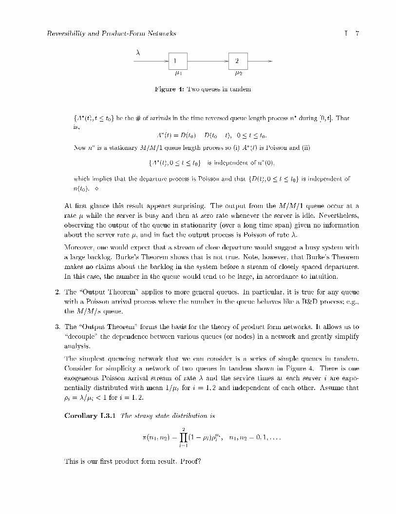
Figure 4: Two queues in tandem
fA�(t); t � t0g be the # of arrivals in the time reversed queue length process n� during [0; t]. That
is,
A�(t) = D(t0)�D(t0 � t); 0 � t � t0:
Now n� is a stationary M=M=1 queue length process so (i) A�(t) is Poisson and (ii)
fA�(t); 0 � t � t0g is independent of n�(0);
which implies that the departure process is Poisson and that fD(t); 0 � t � t0g is independent of
n(t0). �
At �rst glance this result appears surprising. The output from the M=M=1 queue occur at a
rate � while the server is busy and then at zero rate whenever the server is idle. Nevertheless,
observing the output of the queue in stationarity (over a long time span) given no information
about the server rate �, and in fact the output process is Poisson of rate �.
Moreover, one would expect that a stream of close departure would suggest a busy system with
a large backlog. Burke's Theorem shows that is not true. Note, however, that Burke's Theorem
makes no claims about the backlog in the system before a stream of closely spaced departures.
In this case, the number in the queue would tend to be large, in accordance to intuition.
2. The \Output Theorem" applies to more general queues. In particular, it is true for any queue
with a Poisson arrival process where the number in the queue behaves like a B&D process; e.g.,
the M=M=s queue.
3. The \Output Theorem" forms the basis for the theory of product form networks. It allows us to
\decouple" the dependence between various queues (or nodes) in a network and greatly simplify
analysis.
The simplest queueing network that we can consider is a series of simple queues in tandem.
Consider for simplicity a network of two queues in tandem shown in Figure 4. There is one
exogeneous Poisson arrival stream of rate � and the service times at each server i are expo-
nentially distributed with mean 1=�i for i = 1; 2 and independent of each other. Assume that
�i = �=�i < 1 for i = 1; 2.
Corollary I.3.1 The steasy state distribution is
�(n1; n2) =2Yi=1
(1� �i)�ni
i ; n1; n2 = 0; 1; : : : :
This is our �rst product form result. Proof?
Reversibility and Product-Form Networks I { 8
Resource allocation: Let's assume that the service discipline at each station is First-In-First-Out
(FIFO). Consider the problem of allocating resources in this two station tandem network in
order to minimize the expected throughput time seen by any arriving job (this is the total time
the job will spend in the system). Let Wi be the waiting time encountered at each queue and
W =W1 +W2. Our problem is to choose the processing rates �1 and �2 to
min E[W ]
s:t: c1�1 + c2�2 � C:
The last constraint is a \total budget constraint."
First, observe that W1 is independent of W2, and thus the waiting time encountered at each
of the queues is that corresponding to an M=M=1 queue in equilibrium (why?). (Note however
that D1 is not independent of D2!) That is,
E[Wi] =1
�i � �; for �i > �; i = 1; 2:
So the resource allocation problem is
min 1�1��
+ 1�2��
s:t: c1�1 + c2�2 � C:
The Lagrangian for this problem is
L(�1; �2; �) = 1
�1 � �+
1
�2 � �+ �(C � c1�1 � c2�2);
and the �rst order optimality conditions are
1
(�1 � �)2� �c1 = 0 ) �1 = �+
1p�c1
1
(�2 � �)2� �c2 = 0 ) �2 = �+
1p�c2
:
Observing that the budget contraint will be binding (why?), we solve for the multiplier � to get
p� =
P2i=1
pci
C � (c1 + c2)�:
The optimal resource allocations �i can now be determined. This is the so called \square root"
capacity assignment, �rst derived by Kleinrock. Roughly speaking, the optimal assignment
�rst allocates just enough capacity at each station in order to satisfy its arrival rate, and then
allocates the excess capacity among stations in proportion to the square root of their weighted
arrival rates. This result can be extended to more general networks that admit product form
solutions.
4. The \Output Theorem" (that is the Poisson nature and independence of the departure processes
from each queue) can be extended to the case of acyclic (or feedforward) networks. Roughly
speaking, in these networks jobs are owing in a downstream direction, hence the name feedfor-
ward. The results of this section can be extended to acyclic networks using a similar induction
argument as one traverses further downstream in the network.

Reversibility and Product-Form Networks I { 9
I.4 Open Networks of Reversible nodes
Our discussion is based on section 3.1 of Kelly [Kel79].
1. The model. We have a network of J service stations and K job classes (K � J). Each class
k = 1; : : : ;K is served at a unique station s(k) 2 f1; : : : ; Jg. De�ne C(j) = fk : s(k) = jg to
be the set of job classes that are served at station j; we call this set the constituency of station
j. In general the mapping from classes to stations is many-to-one; that is, many classes may be
served at the same station.
External arrivals into classes 1; : : : ;K occur according to independent Poisson processes at av-
erage rates �1; : : : ; �K . After completing service at station s(k), a class k job will become
(instantaneously) a class l job with probability P (k; l), where P = [P (k; l)] is a K �K transient
switching or routing matrix of the queueing network; note that routing is Markovian, i.e., de-
pends only on current job class designation and is independent of all past. (Transience of the
switching matrix implies that any job that enters the network will eventually leave the system.
A matrix P with this property is called sub-stochastic. Its spectral radius is less than one.)
2. E�ective arrival rates. Since P is transient there exists a unique solution �(1); : : : ; �(k) to the
following linear system of traÆc equations
�(l) = �(l) +KXk=1
�(k)P (k; l); for l = 1; : : : ;K; (I.9)
or in matrix form
� = � + P 0� ) � = (I � P 0)�1�: (I.10)
Interpret �(k) as the total arrival rate into class k, including both external arrivals and internal
transitions.
3. Jackson and Kelly networks. An important special case of this class of networks are the so called
Jackson networks, that have a one-to-one relation between job classes and stations. In this case,
J = K and each station serves jobs in FIFO. In Jackson networks, jobs that transition to a
certain station \loose" their identity with respect to their future routes. Consider the example
of Figure 5.
1 2
3
�
�
Figure 5: Example of a non-Jackson network

Reversibility and Product-Form Networks I { 10
Clealry, the routing is not Markovian since the future route of a job completing service at
station 2 depends on its previous history. To approximate it with a Jackson network we set:
P (1; 2) = 1; P (1; 3) = 1, and P (2; 3) = 1=2. We use P (2; 3) = 1=2 to approximate the original
network because on the average half the jobs through station 2 will go to station 3. It turns out
that this setup gives the correct product form solution (unlike what we would expect so far.)
Within the class of networks considered here, one can incorporate Markovian switching among
classes with a many-to-one relationship between classes and stations, provided that all classes
served at any given station have identical service requirements. In the previous example one
would need to introduce di�erent class designations for jobs arriving to station 2 after a visit at
station 1 to the jobs that will next visit station 3 as shown below:
1 2
3
c1
c2
c3 c4
�
�
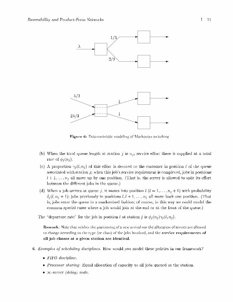
4. Deterministic vs. Markovian routing. In contrast the setup that allows for Markovian switching,
Kelly assumes that jobs of I di�erent types arrive according to independent Poisson processes,
and jobs of each type follow a determnistic route (sequence of stations visited) through the
network. The two formulations are (essentially) equivalent. Here is an example of how one
would model within Kelly's deterministic routing an example with Markovian switching:
First note that random splitting of a Poisson stream give independent Poisson streams. The
derived network (after the input has been split) is equivalent to the original one if we do not
use information about the splitted input stream in the station's service rate and scheduling
discipline.
In general, the general Kelly network with Markovian switching among classes can be reduced to
one with multiple types and deterministic routes as follows: just de�ne one type for each possible
route through the network (lots of them!!). If the original switching matrix P had feedback then
we would get countably in�nite types. Even in this case we can get good �nite approximations.
Therefore, the restriction to Markovian switching among classes is really no restriction at all,
because the number of \classes" or \types" can be arbitrarily large.
Of course, the assumption of independent Poisson inputs is restrictive, as are the following
assumptions about the \servive mechanisms" at the various stations.
5. Service mechanism.
(a) The \service requirement" of each job at each stage of its route is exponentially distributed
with unit mean, independent of type and all previous history; that is, all classes served at
a given station have identical service requirements.
Reversibility and Product-Form Networks I { 11
�
1=3
2=3
�=3
2�=3
1
1
Figure 6: Detereministic modeling of Markovian switching
(b) When the total queue length at station j is nj, service e�ort there is supplied at a total
rate of �j(nj).
(c) A proportion j(l; nj) of this e�ort is devoted to the customer in position l of the queue
associated with station j; when this job's service requirement is completed, jobs in positions
l + 1; : : : ; nj all move up by one position. (That is, the server is allowed to split its e�ort
between the di�erent jobs in the queue.)
(d) When a job arrives at queue j, it moves into position l (l = 1; : : : ; nj + 1) with probability
Æj(l; nj + 1); jobs previously in positions l; l + 1; : : : ; nj all move back one position. (That
is, jobs enter the queue in a randomized fashion; of course, in this way we could model the
common special cases where a job would join at the end or at the front of the queue.)
The \departure rate" for the job in position l at station j is �j(nj) j(l; nj).
Remark. Note that neither the positioning of a new arrival nor the allocation of service are allowed
to change according to the type (or class) of the jobs involved, and the service requirements of
all job classes at a given station are identical.
6. Examples of scheduling disciplines. How would you model these policies in our framework?
� FIFO discipline.
� Processor sharing: Equal allocation of capacity to all jobs queued at the station.
� 1-server (delay) node.
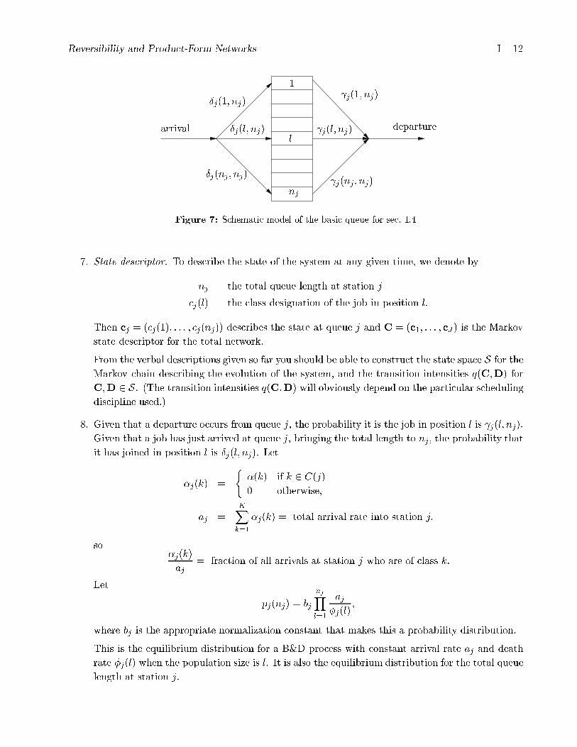
Reversibility and Product-Form Networks I { 12
arrival departure
Æj(1; nj)
Æj(l; nj)
Æj(nj; nj)
j(1; nj)
j(l; nj)
j(nj; nj)nj
1
l
Figure 7: Schematic model of the basic queue for sec. I.4
7. State descriptor. To describe the state of the system at any given time, we denote by
nj the total queue length at station j
cj(l) the class designation of the job in position l:
Then cj = (cj(1); : : : ; cj(nj)) describes the state at queue j and C = (c1; : : : ; cJ) is the Markov
state descriptor for the total network.
From the verbal descriptions given so far you should be able to construct the state space S for the
Markov chain describing the evolution of the system, and the transition intensities q(C;D) for
C;D 2 S. (The transition intensities q(C;D) will obviously depend on the particular scheduling
discipline used.)
8. Given that a departure occurs from queue j, the probability it is the job in position l is j(l; nj).
Given that a job has just arrived at queue j, bringing the total length to nj, the probability that
it has joined in position l is Æj(l; nj). Let
�j(k) =
(�(k) if k 2 C(j)
0 otherwise;
aj =KXk=1
�j(k) = total arrival rate into station j;
so�j(k)
aj= fraction of all arrivals at station j who are of class k:
Let
pj(nj) = bj
njYl=1
aj�j(l)
;
where bj is the appropriate normalization constant that makes this a probability distribution.
This is the equilibrium distribution for a B&D process with constant arrival rate aj and death
rate �j(l) when the population size is l. It is also the equilibrium distribution for the total queue
length at station j.

Reversibility and Product-Form Networks I { 13
Let
�j(cj) = pj(nj)
njYl=1
�j(cj(l))
aj;
the last term describes the particular job con�guration in the queue.
9. Theorem 5 (Thm. 3.1 [Kel79]) The equilibrium distribution of the open queueing network
described above is
�(C) =JYj=1
�j(cj); C 2 S:
Remark. Thus, in equilibrium, (i) the states of the di�erent queues are independent, (ii) the total
queue length at station j has distribution fpj(�)g, and (iii) the probability that the job in position
l in queue j is of class k is �j(k)=aj , independent of everything else.
Proof. (Sketch) Let's de�ne the reversed network. First, let
�0(k) = �(k)
1�
KXl=1
P (k; l)
!for k = 1; : : : ;K
and
P 0(k; l) =�(l)
�(k)P (l; k) for k; l = 1; : : : ;K;
�(l)P (l; k) is the number of k arrivals due to l transitions, and thus P 0(k; l) will be the fraction of
k arrivals that is due ot l transitions, or in terms of the reversed process P 0(k; l) is the fraction of
class k jobs that will transition to class l jobs upon completion of their service.
Now cosnider a related open network in which the external arrival rate to class k is �0(k), the
switching matrix is P 0 = [P 0(k; l)], the level of service at station j is �j(nj) as before, and the
rates j(l; nj) and Æj(l; nj) are reversed. Let fq0(C;D)g be the transition intensity function for
this related network. It can be veri�ed that the hypothesized equilibrium dstribution �(�) satis�es
�(C)q(C;D) = �(D)q0(D;C); 8 C;D 2 S;
and moreover
q(C) = q0(C) =
JXj=1
�j(nj) +
KXk=1
�(k) 8 C 2 S:
The desired result now follows from Theorem 1.13 of Kelly, and in addition we have that the
time-reversed transition intensity function for our original network is q(�). �
Remark. The proof of this theorem {as for some of the results to follow{ is algrebraic and hinges
on the veri�cation fo the conditions of Theorem 1.13. It is not apparent how the probabilistic
assumptions made so far are used in obtaining this result. In fact, the essential feature that results
in this product form behavior is that the individual queues (nodes) as decribed so far are reversible
and satisfy the \Output Theorem" (exercize). A probabilistic argument that exploits this reversible
structure and the concequences of the \Output Theorem" can be found in Walrand [Wal83].
10. Following our previous remark, this theorem contains as a special case \Jackson's Theorem"
that established the product form nature for the family of Jackson networks.
Reversibility and Product-Form Networks I { 14
11. The main assumptions (and limitations) of these models are:
(a) Multiple classes owing through the network and Markovian switching; this allows for
feedback (i.e., not acyclic structure any more).
(b) The assumption of Poisson arrivals and exponential service times.
(c) The scheduling disciplines allowed that cannot di�erentiate between di�erent classes served
at each station.
(d) All classes served at any give station have identical service requirements.
The basic topology of this network will dominate most of this course, but the restrictive assump-
tions (b)-(d) will be relaxed very soon.
I.5 Open Networks of Quasi-Reversible Nodes
Our discussion is based on section 3.2 of Kelly [Kel79]. The routing structure described in section I.4
is quite general for most purposes (i.e., adequate in modelling realistic applications) but the structure
of each individual queue was quite restrictive. In this section we will describe a more general class of
queues (or nodes{ this is the term I will use hereafter) that still achieve the same behavior described
by the product form distribution. This class of nodes will be referred to as quasi-reversible (Q-R).
1. The node. We start by describing the basic structure of a node. Later nodes of a network will
be indexed by j = 1; : : : ; J . In that setting, the notation used below to describe a node will
be augmented by hanging a j as a subscript or a functional argument in order to specify which
node we are talking about.
There is a �nite set C of classes that are served at the node, and its state at any given time
is decsribed by some x 2 S (a countable set). (That state descriptor may contain information
about the number of jobs in the queue, the class of each job in the queue their position etc..)
Associated with each state x is a non-negative vector n(x) = fnc(x); c 2 Cg whose cth component
tells how many jobs of class c are currently present at the node. Let S(c; x) be the set of statesx0 2 S with n(x0) = n(x) + ec (where ec is a unit vector with a 1 in the cth position and zeros
elsewhere); i.e., the set of x0's that di�er from x by one class c arrival.
A node is characterized by (or de�ned as) a transition intensity function q(x; x0j�) that has
property (I.11) below. Here � = f�(c); c 2 Cg is a non-negative vector that parametrizes what
really is a family of transition intensity functions; think of � as the vector of intensity parameters
for a collection of independent Poisson arrival processes.
q(x; x0j�) = 0 except in the following cases (I.11)
a) n(x0) = n(x) [\internal transition"]
b) x 2 S(c; x0) for some c [\departure transition"]
c) x0 2 S(c; x) for some c [\arrival transition"]
Reversibility and Product-Form Networks I { 15
In cases a) and b), q(x; x0j�) is actually independent of �, and we will just write q(x; x0) hereafter.In case c) we have
q(x; x0j�) = �(c)pc(x; x0) whereX
x02S(c;x)
pc(x; x0) = 1;
and pc(x; x0) is the probability that a class c arrival will steer the state from x to x0. An example
of internal transitions is in the case where the service requirement for some job class follows an
Erlang distribution (this is a sum of -say k- IID exponentials). In this case the state descriptor
needs to keep track of the stage information. When the stage changes without service completion,
we have an internal transition.
To repeat, (I.11) de�nes a node (not necessarily Q-R). Note that for a given � the node has a
stationary distribution f�(xj�); x 2 Sg and if we denote by X(t) the associated MP, then the
reversed process X(�t) describes the equilibrium behavior of another node (one must check that
(I.11) is satis�ed) with transition function
q0(x; x0j�) = �(x0j�)�(xj�) q(x
0; xj�) (I.12)
and the same stationary distribution f�(xj�)g. In each n(x(t)) can change only by a departure
or an arrival.
2. Quasi-reversibility.
De�nition I.5.1 A node is said to be Q-R if, for each � such that the stationary distribution
exists, Xx02S(c;x)
q0(x; x0j�) = �(c) 8 x 2 S; c 2 C: (I.13)
Condition (I.13) gives a precise mathematical articulation of what we mean by quasi-reversibility,
but the following interpretation will certainly help your intuition. First, (I.13) really just says
that Xx02S(c;x)
q0(x; x0j�) is independent of x 8 c 2 C; (I.14)
because (I.14) says that the class c arrival intensity is constant for the reversed process, and
the only constant consistent with equilibrium is �(c), the arrival rate for class c in the original
process and hence the departure rate for class c when time is reversed.
Now (I.14) is equivalent to saying that arrivals after time t in the reversed system are independent
of X(t) which is equivalent to saying that departures up to time t in the original system are
independent of the state X(t).
To summarize, quasi-reversibility is an input-output property: if you drive the node with
a vector Poisson input process and initialize with the stationary distribution, then the vector
output is statistically idenstical to the input process, and moreover departures up to time t are
independent of the state X(t). That is, a node is Q-R if the Output Theorem holds.

Reversibility and Product-Form Networks I { 16
3. \Partial balance" and quasi-reversibility. Substitute the de�nition (I.11) of q0(�; �) into (I.13) andyou see that (I.13) is equivalent to
�(x)X
x02S(c;x)
q(x; x0j�) =X
x02S(c;x)
�(x0)q(x0; xj�); (I.15)
which are the so called partial balance equations. The intuition is the following: starting at state
x, a class c arrival can steer the state to x0, where x0 2 S(c; l). Condition (I.15) requires that theprobability ux from state x to the set S(c; x) is equal to the probability ux from S(c; x) backto x; i.e., ux into x due to class c arrivals is equal to the ux out of x0 due to class c departures.
A similar argument explains the case of transitions due to class c departures.
It remains to consider what happens during \internal transitions" from x to x0 for which x0 6= x
but n(x0) = n(x). First recall that the state transitioning from x can either stay in the set of
interest (i.e., x0 6= x and n(x0) = n(x)) or it will end up in some set S(c; x) considered above.
Since the total probability ux out of x is equal to the total probability ux into x (this follows
from the equilibrium conditions), using the partial balance equations we can conclude that also
the probability ux out of x to this set (i.e., X 0 6= x and n(x0) = n(x)) will equal the total
probability ux from this set into x.
Note that any node that satis�es the detailed balance equations also satis�es the partial balance
equations (just add (I.4) over x0 2 S(c; x)), and thus reversibility implies quasi-reversibility.
4. The network. Nodes are indexed by j = 1; : : : ; J . Input and routing are exactly as in section I.4:
external arrivals to classes k = 1; : : : ;K via independent Poisson processes at rates �(1); : : : ; �(k);
upon completing service at station s(k), a class k job switches class according to the transient
matrix [P (k; l)]. De�ne total arrival rates �(k) and time reversed routing matrix P 0 = [P 0(k; l)]
as in the previous section. Let �j(x) = �j(xj�) be tha stationary distribution of node j when it
is driven by Poisson inputs at rates f�(c); c 2 Cjg.The \network" is a MP with generic state x = (x1; : : : ; xJ), where xj 2 Sj for all j. Its transitionintensities are de�ned as follows
(a) Suppose that c 2 Cj , xj 2 Sj(c; x0), and xi = x0i for all other nodes i. Then, letting
P (c; 0) � 1 � PKl=1 P (c; l), we have that q(x; x0) = qj(xj ; x
0j)P (c; 0). (These transitions
correspond to class c service completions where the job then leaves the network.)
(b) Suppose that c 2 Cj, x0j 2 Sj(c; xj), and xi = x0i for all other nodes i. Then q(x; x0) =
�(c)pcj(xj ; x0j). (These transitions correspond to external arrivals into class c.)
(c) Suppose nj(xj) = nj(x0j) and xi = x0i for all other nodes i. Then q(x; x0) = qj(xj ; x
0j).
(These transitions correspond to \internal state changes" at node i.)
(d) Suppose that xi 2 Si(c; x0i) and x0j 2 Sj(c0; xj), where c 2 Ci and c0 2 Cj and xk = x0k for all
other nodes k. Then
q(x; x0) = qi(xi; x0i)P (c; c
0)pcj(xj ; x0j):
(These transitions correspond to service completions of class c jobs at node i where the job
next witches to class c0. Note that one can have i = j here, meaning that classes c and c0
are served at the same node i. This last formula is similar to that of case (b) only with a
Reversibility and Product-Form Networks I { 17
di�erent e�ective arrival rate for class c0 arrivals due to class c completions starting at state
xi and transitioning into state x0i.
(e) Otherwise, q(x; x0) = 0.
5. Kelly's Theorem.
Theorem 6 (Thm. 3.7 [Kel79]) If the vector of total arrival rates is such that the station-
ary distribution �j(�; �) exists for every node j, then the unique stationary distribution for the
network is
�(x) = �1(x1j�) � � � �J(xJ j�):
In order to prove this theorem one would proceed as follows. First, guess the time-reversed
transition intensity function q0(x; x0) for the network to be as follows in cases (a)-(e) above:
(a) q0(x0; x) = q0j(x0j ; xj j�)
(b) q0(x0; x) = qj(x0j ; xj j�)
�1�PK
l=1 P0(c; l)
�(c) q0(x0; x) = q0j(x
0j ; xj j�)
(d) q0(x0; x) = q0j(x0j ; xj j�)P 0(c0; c)
q0i(x0i; xij�)P
y2Si(c;x0
i) q0i(x
0i; yj�)
(e) q0(x0; x) = 0 otherwise.
Now try to verify the conditions of Theorem 1.13; i.e., �rst show that �(x)q(x; x0) = �(x0)q0(x0; x)
for all x; x0 2 S (this requires a separate argument for each of the cases (a)-(d) above), and second,
verify that Xx02S
q(x; x0) =Xx02S
q0(x; x0):
One would expect that the statement of this theorem is true for acyclic (or feedforward) network,
but how about networks with feedback that are allowed in this model? In fact, the ows in the
feedback paths are no longer Poisson. For a detailed probabilistic argument of this result see
Walrand [Wal83].
6. Stability. This is our �rst look at a stability result. The existence of a stationary distribution
(and consequently of the product form solution) is guaranteed provided that the traÆc intensity
at each station is less than 1. That is,
�i �P
c2Ci�(c)
�i< 1 for i = 1; : : : ; J:
That is, each node in isolation should have enough processing capacity in order to satisfy all of
its e�ective arriving traÆc (of rateP
c2Ci�(c)).
7. Examples of Q-R nodes. Kelly's Theorem says that a network of quasi-reversible nodes admits
a product form solution. So far, however, we have not speci�ed an example of a Q-R node.
The setup of section I.4 requires essentially that all job classes served at a node have the same
exponential service distribution. With that restriction, the service discipline is quite general. It
turns out (in homework?) that this node is indeed Q-R. The next section shows another example
of a Q-R node.

Reversibility and Product-Form Networks I { 18
I.6 Symmetric Queues
In this section we describe another example of a Q-R node, where the service time requirements are
essentially arbitrary but the scheduling discipline is very speci�c (e.g., FIFO is rulled out).
1. Independent Poisson inputs with rates f�(c); c 2 Cg. Jobs of class c require w(c) independent
stages of service; the duration of each is exponential with mean d(c). Each class has its own
Erlang service time distribution, and we will generalize that to mixtures of Erlang distributions,
which are in fact dense in the set of all distributions.
2. Let c(l) be the class of the job in position l, and u(l) the stage of service this job has reached,
1 � u(l) � w(c(l)). Set c(l) = (c(l); u(l)). The state of the node is c = (c(1); : : : ; c(n)), where n
is the number of jobs present. The queue discipline for a symmetric node is as follows:
(a) Total service e�ort is supplied at rate �(n)
(b) Fraction (l; n) of that e�ort goes to job in position l; (1; n) + � � � + (n; n) = 1. When a
job in position l completes his �nal stage and departs, jobs in positions l + 1; : : : ; n move
to positions l; : : : ; n� 1 respectively.
(c) When a new job arrives, bringing the total population to n + 1, he moves into position l
with probability (l; n+ 1); jobs previously in positions l; : : : ; n move to l + 1; : : : ; n+ 1.
This specializes the discipline of section I.4 by requiring that = Æ (hence the name symmetric).
Again emphasize that the positioning of new arrivals and division of e�ort cannot depend on
class.
departuresarrival
j(1; nj) j(1; nj)
j(l; nj)
j(nj; nj)
j(nj; nj)
j(nj; nj)nj
1
l
Figure 8: Symmetric queue
3. Examples. Think of total service requirement of a job as S = S1+� � �+Sw(c) (a random variable).
The job departs when the cumulative service e�ort provided reaches S. Examples of disciplines
that can be modeled in this framework are:
(a) Stack (LIFO, preemptive-resume)
(b) Server-sharing
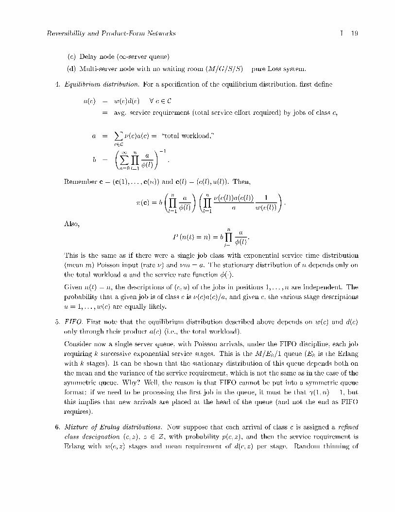
Reversibility and Product-Form Networks I { 19
(c) Delay node (1-server queue)
(d) Multi-server node with no waiting room (M=G=S=S) { pure Loss system.
4. Equilibrium distribution. For a speci�cation of the equilibrium distribution, �rst de�ne
a(c) = w(c)d(c) 8 c 2 C= avg. service requirement (total service e�ort required) by jobs of class c;
a =Xc2C
�(c)a(c) = \total workload,"
b =
1Xn=0
nYl=1
a
�(l)
!�1:
Remember c = (c(1); : : : ; c(n)) and c(l) = (c(l); u(l)). Then,
�(c) = b
nYl=1
a
�(l)
! nYl=1
�(c(l))a(c(l))
a
1
w(c(l))
!:
Also,
P (n(t) = n) = bnYl=1
a
�(l):
This is the same as if there were a single job class with exponential service time distribution
(mean m) Poisson input (rate �) and �m = a. The stationary distribution of n depends only on
the total workload a and the service rate function �(�).Given n(t) = n, the descriptions of (c; u) of the jobs in positions 1; : : : ; n are independent. The
probability that a given job is of class c is �(c)a(c)=a, and given c, the various stage descriptions
u = 1; : : : ; w(c) are equally likely.
5. FIFO. First note that the equilibrium distribution described above depends on w(c) and d(c)
only through their product a(c) (i.e., the total workload).
Consider now a single server queue, with Poisson arrivals, under the FIFO discipline, each job
requiring k successive exponential service stages. This is the M=Ek=1 queue (Ek is the Erlang
with k stages). It can be shown that the stationary distribution of this queue depends both on
the mean and the variance of the service requirement, which is not the same as in the case of the
symmetric queue. Why? Well, the reason is that FIFO cannot be put into a symmetric queue
format: if we need to be processing the �rst job in the queue, it must be that (1; n) = 1, but
this implies that new arrivals are placed at the head of the queue (and not the end as FIFO
requires).
6. Mixture of Eralng distributions. Now suppose that each arrival of class c is assigned a re�ned
class descignation (c; z), z 2 Z, with probability p(c; z), and then the service requirement is
Erlang with w(c; z) stages and mean requirement of d(c; z) per stage. Random thinning of

Reversibility and Product-Form Networks I { 20
Poisson streams gives independent Poisson streams, so this situation maps into that already
described. Let
a(c) =Xz2Z
p(c; z)w(c; z)d(c; z);
a =Xc2C
�(c)a(c):
Summing up the equilibrium distributions of the re�ned state descriptions, we �nd that
� Marginal distribution of n is as before
� Given n, gross class designations c(1); : : : ; c(n)are independent, and the probability that
any given job is of (gross) class c is �(c)a(c)=a, as before.
� Given the (gross) class designation c of a job in any position, the conditional distribution
of total service e�ort received thus far by that job is
F �c (x) =1
a(c)
Z x
0[1� Fc(y)]dy;
where Fc is the the distribution of total service requirement for jobs of (gross) class c (a
mixture of Erlang distributions), and F �c is the residual lifetime distribution { familiar from
renewal theory.
� Method of stages to approximate arbitrary distributions; i.e., general distributions are ap-
proximated as mixtures of Erlang distributions that in turn are just sums of exponentials.
7. Kelly proves that � is the equilibrium distribution by guessing the structure of the reversed
process (the obvious one) and verifying as usual, using Theorem 1.13. Since the time-reversed
system has Poisson input streams, independent of current state, the node is Q�R.
Now we see that very general networks of Q � R nodes can be built up. Poisson inputs and
nodes of various types, including
� FIFO, multi-server, and all classes served at node have ientical exponential service time
distribution.
� Processor sharing node where each class has its own arbitrary service distribution.
� A delay node where each class has its own arbitrary delay distribution (jobs of a given type
may visit many times with di�erent distributions).
I.7 Closed Networks
1. Closed network description. Now there are no external arrivals, and we assume that the switching
matrix P = [P (k; l)] is stochastic (row sums equal to one). There is an initial population of size
N , and these jobs circulate endlessly through the class designations k = 1; : : : ;K. As before
we have J service stations and each class k is served at a unique station s(k). Each station is
assumed to be quasi-reversible in equilibrium, and all the notation of sections I.4-I.6 remains in

Reversibility and Product-Form Networks I { 21
force. In particular, �j(�; �) denotes the stationary distribution for station j when it is driven
by independent Poisson inputs with arrival rates f�(k); k 2 C(j)g.To avoid trivialities, we assume that the switching matrix P to be such that no job class k
is transient. Thus the job classes can be partitioned into \communicating classes" -or \cells"-
and renumbered so that P has block-diagonal structure (each block representing an irreducible
communicating class or cell). That is, jobs whose initial class designation belongs to a particular
cell can never visit any class outside that cell, and all classes within a cell communicate. We
denote by M(r) the initial population of cell r, so M(1) + � � �M(R) = N , where R is the # of
cells.
2. Stationary distribution. To describe the stationary distribution of the closed network we need a
positive vector � = (�(1); : : : ; �(k)) satisfying the traÆc equations
�(l) =KXk=1
�(k)P (k; l) for l = 1; : : : ;K: (I.16)
The solution of (I.16) is de�ned only up to a set of R positive constant (one for each cell); the
�'s for any given cell can be thought of as an arbitrary positive rescaling of the equilibrium
distribution for that cell. We assume there exists a choice of the scaling constants such that
the stationary distribution �j(�; j�) exists for each station j of the network. That choice of � is
considered �xed hereafter.
Let us denote by S the set of all state descriptions x = (x1; : : : ; xJ) for the network. Then,
JXj=1
Xc2Cr
nj(c; xj) =M(r) for all r = 1; : : : ; R; (I.17)
where Cr is the set of job classes belonging to cell r. This is the state space for our multi-cell
closed queueing network.
3. Main result.
Theorem 7 The unique equilibrium distribution for the closed network is
�(x) = B(�;M(1); : : : ;M(R))JYj=1
�j(xj j�); x 2 S;
where B(�) is the normalization constant that makes �(�) a probability distribution on S.
This theorem is proves as usual by \guessing" the time-reversed transition intensity function
q0(x0; x) and the using Theorem 1.13.
� The stationary distribution is that of an open network model restricted to the hyperplanes
of (I.17).
� A remarkable (that is, not at all obvious) \corollary" of this theorem is that the equilibrium
distribution �(�) ultimately obtained is una�ected by the R arbitrary scaling constants in
our choice of �; the e�ect of those scaling constants is cancelled out by the normalization
constant B(�).
Reversibility and Product-Form Networks I { 22
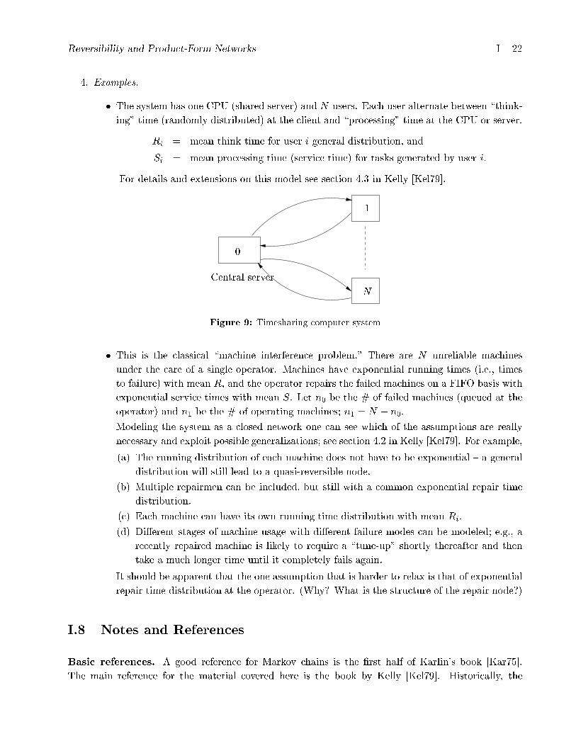
4. Examples.
� The system has one CPU (shared server) and N users. Each user alternate between \think-
ing" time (randomly distributed) at the client and \processing" time at the CPU or server.
Ri = mean think time for user i general distribution, and
Si = mean processing time (service time) for tasks generated by user i:
For details and extensions on this model see section 4.3 in Kelly [Kel79].
Central server
0
1
N
Figure 9: Timesharing computer system
� This is the classical \machine interference problem." There are N unreliable machines
under the care of a single operator. Machines have exponential running times (i.e., times
to failure) with mean R, and the operator repairs the failed machines on a FIFO basis with
exponential service times with mean S. Let n0 be the # of failed machines (queued at the
operator) and n1 be the # of operating machines; n1 = N � n0.
Modeling the system as a closed network one can see which of the assumptions are really
necessary and exploit possible generalizations; see section 4.2 in Kelly [Kel79]. For example,
(a) The running distribution of each machine does not have to be exponential { a general
distribution will still lead to a quasi-reversible node.
(b) Multiple repairmen can be included, but still with a common exponential repair time
distribution.
(c) Each machine can have its own running time distribution with mean Ri.
(d) Di�erent stages of machine usage with di�erent failure modes can be modeled; e.g., a
recently repaired machine is likely to require a \tune-up" shortly thereafter and then
take a much longer time until it completely fails again.
It should be apparent that the one assumption that is harder to relax is that of exponential
repair time distribution at the operator. (Why? What is the structure of the repair node?)
I.8 Notes and References
Basic references. A good reference for Markov chains is the �rst half of Karlin's book [Kar75].
The main reference for the material covered here is the book by Kelly [Kel79]. Historically, the

Reversibility and Product-Form Networks I { 23
Single
repairman
N
identical
machines
Figure 10: Single repairman
�rst important results in the area of product form networks are due to Jackson [Jac57, Jac63]; the
motivation there was in manufacturing systems. Later on, important references can be found in the
work of Kleinrock [Kle64, Kle75, Kle76], where the motivation was �rst in communication networks
and later, in computer systems. Another major reference on this material, motivated by computer
system applications, is the paper by Baskett, Chandy, Muntz, and Palacios [BCMP75]. Around the
same time Kelly introduced the concept of quasi-reversibility. A probabilistic argument explaining the
nature of product form results can be found in Walrand [Wal83]. A good exposition of the material
can be found in the book by Walrand [Wal88].
Appliations. The paper by Solberg [Sol77] describes the applications of closed queueing network
models in manufacturing systems. The \BCMP" paper [BCMP75] describes applications in computer
systems. An extensive overview of applications of queueing network models to manufacturing systems
can be found in the review article by Buzacott and Shanthikumar [BS92] and in the book by Gershwin
[Ger94].
Current status. The network models considered here have been generalized in several directions, but
some of the restrictive probabilistic and structural assumptions are still in place. An updated reference
on this area is the forthcoming book by Chao, Miyazawa, and Pinedo [CMP99] that describes several
extensions to the class of models discussed here that still fall in the category of \product form"
networks.
References
[BCMP75] F. Baskett, M. Chandy, R. Muntz, and F. Palacios. Open, closed and mixed networks of queues
of di�erent classes of customers. Journal of the Association for Computing Machinery, 22:248{260,
April 1975.
[BG92] D. Bertsekas and R. Gallager. Data Networks. Prentice-Hall, Englewood Cli�s, N.J., 1992.
[BS92] J. A. Buzacott and J. G. Shanthikumar. Design of manufacturing models using queueing models.
Queueing Systems, 12:135{214, 1992.

Reversibility and Product-Form Networks I { 24
[CMP99] X. Chao, M. Miyazawa, and M. Pinedo. Queueing networks: Customers, Signals, and Product Form
Solutions. John Wiley & Sons, 1999. Forthcoming.
[Ger94] S. B. Gershwin. Manufacturing Systems Engineering. Prentice Hall, 1994.
[Jac57] J. R. Jackson. Networks of waiting lines. Math. Oper. Res., 5:518{521, 1957.
[Jac63] J. R. Jackson. Jobshop-like queueing systems. Management Science, 10:131{142, 1963.
[Kar75] S. Karlin. A �rst course in stochastic processes. Academic Press, New York, N.Y., 1975.
[Kel79] F. P. Kelly. Reversibility and Stochastic Networks. John Wiley & Sons, New York, N.Y., 1979.
[Kle64] L. Kleinrock. Communication Nets: Stochastic Message Flow and Delay. McGraw-Hill, New York,
N.Y., 1964.
[Kle75] L. Kleinrock. Queueing Systems, volume 1. Wiley, New York, N.Y., 1975.
[Kle76] L. Kleinrock. Queueing Systems, volume 2. Wiley, New York, N.Y., 1976.
[Sol77] J. J. Solberg. A mathematical model of computerized manufacturing systems. In 4th International
Conference on Production Research, Tokyo, 1977.
[Wal83] J. Walrand. A probabilistic look at networks of quasi-reversible queues. IEEE Trans. Information
Theory, 29(6):825{831, November 1983.
[Wal88] J. Walrand. An introduction to Queueing Networks. Prentice-Hall, Englewood Cli�s, N.J., 1988.
Reversibility and Product-Form Networks I { 25
I.9 Exercises { Homework #1
1. Consider an open Jackson network (one-to-one correspondence between job classes and service
stations) with J stations, exponential service time distribution at each station, FIFO queue
discipline at each station, and possibly multiple servers at each station. We say that the routing
chain is reversible if the matrix P 0(i; j), de�ned in the lecture notes in section I.4 is identical to
P (i; j).
(a) Show that if the routing chain is reversible in equilibrium, then the vector queue length
process is reversible in equilibrium.
(b) Suppose that the routing matrix satis�es P (i; 1) = 1 for i > 1 and all external arrivals are
into station 1. (This is common in modelling exible manufacturing systems, where node
1 ia an in�nite-server station representing a recirculating conveyor that carries workpieces
on carts from one operation to another.) Show that the routing chain is reversible in
equilibrium.
(c) Suppose that the rouitng chain has the property described in (b). Now consider a modi�ed
system where each station i = 2; : : : ; J has �nite capacity b(i). In terms of the queue length
process, this is interpreted to mean simply that movement of jobs from station 1 to station
i is eliminated when the total queue length at station i is b(i). What is the equilibrium
distribution for this modi�ed system?
2. Consider an M=M=1 queue with arrival rate �, mean service time 1=m and last-in-�rst-out
preemptive-resume discipline: if a new job arrives while you are being served, that job imme-
diately displaces you, and your service must begin all over when you next gain access to the
server. Think of the service time of a job as a random variable S associated with the job rather
than the server: once the job has occupied the server for S uninterrupted minutes it departs the
system. How would you describe the state of the system in order to make it a Markov process?
How would your answer di�er if service time variability were associated entirely with the server
rather than the job? (In the latter case, the time required to complete service of any given job
is exponentially distributed with parameter m, independent of any previous experience of that
job.)
3. Consider the open queueing network model described in section I.4. Specialize to the case where
every station has a single server and FIFO service discipline, but then generalize by allowing jobs
of class k to have an arbitrary service time distribution Fk(x). Networks having this structure
are called standard shops.
Now consider the apparently more general case of a standard shop with server breakdown. To be
speci�c, suppose that server j breaks down after providing an exponentially distributed amount
of service: the failure rate (reciprocal of the mean time to failure) is bj when server j is working.
Server breakdown during a period of idleness is impossible.
A job who is being served at the time of a breakdown at station j is not harmed; repair takes
a random length of time with distribution Gj(y), and then the service resumes where it left o�.
The service may be interrupted repeatedly by breakdowns.

Reversibility and Product-Form Networks I { 26
(a) Under what conditions will the system have an equilibrium distribution? Assuming these
conditions are met, what is the long-run fraction of time that server j spends working,
being repaired, and simply idle? (You need not justify your answers.)
(b) Explain how a standard shop with server breakdown can be reduced to one without break-
downs. What are the data of the equivalent system?
4. Consider a service node of the type described in section I.4. Show that such a node is quasi-
reversible.
5. In Figure 11, there are 4 stations A,B,C,D and two types of jobs 1 and 2. Type 1 jobs visit
station A, then B, then C, then leave the system with probability p and with probability 1 � p
visit station D and then exit. Type 2 jobs visit A, then B, then D and exit. All stations use
FIFO. The arrivals of type i jobs are Poisson with rate �i; i = 1; 2. Each station is a single
server queue with exponential service times. The service rates are respectively �A; �B and �C .
Station D's rate dependes on the type: it is �D;1 for type 1 and �D;2 for type 2.
A B
C
D
p
1� p�1
type 1
�2type 2
Figure 11: Four station network of ex.5
(a) Is the joint distribution of the number of jobs in stations A,B,C of product form? If so �nd
it.
(b) Is the joint distribution of the number of jobs in stations A;B;C;D of product form? If so
�nd it.
(c) Find the distribution of jobs in station D.
(d) Find the total expected time type 1 jobs spent in the system