retracted article: stability analysis of dynamic collaboration model under two-lane case
TRANSCRIPT

Nonlinear DynDOI 10.1007/s11071-014-1339-8
ORIGINAL PAPER
Stability analysis of dynamic collaboration model undertwo-lane case
Zhipeng Li · Run Zhang · Shangzhi Xu ·Yeqing Qian
Received: 8 October 2013 / Accepted: 1 March 2014© Springer Science+Business Media Dordrecht 2014
Abstract In this paper, we propose a dynamic col-laboration model for two-lane situation and study theinfluence of the dynamic collaboration on the two-lane traffic flow stability with lane- changing behav-iors. We derive the stability conditions for our two-lane dynamic collaboration model by theoretical sta-bility analysis and conclude that the stability of trafficflow is affected greatly by the new considerations in theproposed models. It indicates that the new dynamic col-laboration model can make the traffic flow more stablewith increasing its dynamic factors. Besides, we con-clude that the two dynamic factors of the two nearestpreceding vehicles on two lanes play an important rolefor stabilizing the traffic flow, while the two dynamicfactors of the two nearest following vehicles on twolanes are not helpful to make the traffic flow stable. Inaddition, direct simulations are conducted to verify the-oretical results, and a variety of conditions are studiedto analyze the effect of dynamic factors on the trafficstability.
Keywords Stability analysis · Dynamic collabo-ration model · Lane-changing behaviors · Dynamicfactors
Z. Li · R. Zhang (B) · S. Xu · Y. QianThe Key Laboratory of Embedded System and ServiceComputing Supported by Ministry of Education, TongjiUniversity, Shanghai 201804, Chinae-mail: [email protected]
Z. Lie-mail: [email protected]
1 Introduction
With the rapid development of global economic, somesocial problems are becoming more and more promi-nent, such as the expanding population, the urban traf-fic congestion, environmental pollution, excessive con-sumption of energy, and other issues. What is more, theloss caused by urban traffic congestion has been par-ticularly significant [1–11]. In order to understand anddescribe the complex phenomena of traffic flow, vari-ous vehicular traffic models have been put forward inthe past decades [12–26]. According to the details ofthe different descriptions of traffic flow, there are threedifferent conceptual frameworks for modeling traffic:microscopic model, mesoscopic model, and macro-scopic model. Kinematic model and fluid dynamicsmodel are typical macroscopic models, in which theoverall transport actors are regarded as a continuousmedia. However, the microscopic model focuses onindividual vehicles each of which is represented bya particle and the nature of the interactions amongthese particles. The optimal velocity model (OVM) issuch one of microscopic models, proposed by Bandoet al. [2], which can simulate some traffic phenomena,for instance, traffic stability, congestion, stop and gotraffic. Since then, many researchers extended the OVmodel from different aspects and utilized them to ana-lyze various traffic density waves so as to obtain thestability conditions at different situations, for exam-ple, two-car following model (TCFM) advised by Penget al. [27], Peng and Cheng [28], and Peng and Sun [29];
123

Z. Li et al.
two velocity difference models (TVDM) proposed byGe et al. [12–14]; and generalized OVM (GOVM) putforward by Sawada [30]; and so on. All of the abovemodels have been extended with the consideration ofvehicle distance or speed difference.
Innovatively, we proposed a new traffic flow modelby considering the dynamic collaboration with the near-est preceding vehicle (the front vehicle) and the nearestfollowing vehicle (the rear vehicle) in our latest arti-cle [31]. In our dynamic collaboration model, vehicle’sdynamical equation is determined not only by its ownmotion information, but also by the motion informa-tion of its nearest preceding and following vehicles.Dynamic collaboration introduces the other vehicle’smotion information into microscopic modeling of eachvehicle, which will finally convert to the power fine-tuning of a single vehicle in traffic system. Actually,the result obtained in our latest article shows that powerfine-tuning of individual vehicle can suppress the traf-fic congestion of traffic flow. In Fig. 1, we will sim-ply show the acceleration smoothing effect of dynamiccollaboration. It is assumed that the acceleration ofthe 4th vehicle increases suddenly. For the accelera-tion smoothing effect, all these vehicles maintained thesame acceleration eventually after an enough long time.Therefore, dynamic collaboration can stabilize the traf-fic flow through the acceleration smoothing effect.
In order to analyze the stability of two-lane trafficflow, Tang et al. [20,21] first presented an extendedcar-following model on two lanes by incorporating thelateral effect in traffic flow. Although two-lane car-following models are evolved from single-lane mod-els, there are some different characteristics in two-
lane models. Under the circumstance of two-lane traf-fic, apart from the effects in front, the lateral effectsshould also be taken into account. Besides, Zheng et al.[32] proposed a two-lane optimal velocity (OV) modelfocusing mainly on the stability analysis of two-lanetraffic flow with lateral friction and had obtained its sta-bility condition from the viewpoint of control theory. Inorder to suppress the traffic jam in a discrete-time OVmodel, Konishi et al. [33] proposed a dynamic versionof the decentralized delayed feedback control (DDFC)method firstly by investigating the traffic jams phenom-ena under periodic boundary condition in 2000.
The most significant difference between the two-lane traffic flow system and the single-lane traffic sys-tem is that there are lane-changing behaviors in thetwo-lane traffic system. Undoubtedly, lane-changingbehaviors have great influence on the stability of trafficflow. Then we wonder whether the dynamic collab-oration can suppress the traffic congestion or not bysmoothing vehicles’ acceleration under two-lane case.In this paper, we extend the single-lane dynamic collab-oration model to two-lane case with the considerationof the lateral effects and utilize the new model withdifferent dynamic factors to analyze traffic character-istics and stability under the two-lane case. Namely,the vehicle’s motion is influenced by both the front andrear vehicles’ motion in the same lane and the vehicles’motion in another lane. Clearly, the stability analysis oftraffic flow gets more complicated. We derive the stabil-ity conditions for the two-lane dynamic collaborationmodel by theoretical stability analysis, and direct sim-ulations are conducted to confirm the above theoreticalresults.
Fig. 1 Schematic trafficflow mutation
123

Stability analysis of dynamic collaboration model
This paper is organized as follows: In Sect. 2, thedynamic collaboration model is explained with lane-changing behaviors for two-lane traffic flow and thestability conditions are analyzed. In Sect. 3, numeri-cal simulations are presented to confirm the theoreticalresults. Finally, the conclusions are drawn in Sect. 4.
2 Model
2.1 Description of model
In the paper, for the sake of describing the dynamicbehaviors of two vehicle groups in a circular two-laneroad, we can extend the single-lane dynamic collabo-ration model to two-lane case. Furthermore, it is eas-ily known that the vehicle’s movements are not onlyinfluenced by the block interference from the front andbehind vehicles in the same lane but also affected by thefriction interference from vehicles in the neighbor lane,which should not be neglected when two-lane or multi-lane traffic flow are modeled. Now, let us consider thebelow two-lane case (see Fig. 2).
Before extending the three-car dynamic collabora-tion model to two- lane case, we rewrite two-lane OVmodel as follows:
⎧⎪⎪⎪⎪⎪⎪⎨
⎪⎪⎪⎪⎪⎪⎩
dvl,nl(t)
dt = al{Vl(yl,nl(t),
ql,nl(t)) − vl,nl
(t)},dyl,nl
(t)
dt = vl,nl −1(t) − vl,nl(t),
dql,nl(t)
dt = v fl,nl
(t) − vl,nl(t)
(nl = 1 · · · Nl),
(1)
where vl,nl(t) is the velocity of vehicle nl at time t
in lane l, Vl(yl,nl(t), ql,nl
(t)) is the OV function in lanel, yl,nl
(t) is the headway between two vehicles (nl −1)
and nl in the same lane l at time t, ql,nl (t) is the lateraldistance (i.e., the distance between the vehicle nl in lanel and the closest vehicle in neighbor lane in front of thisvehicle at time t). v f
l,nl(t) is the velocity of the closest
vehicle in the neighbor lane in front of vehicle nl at timet, al > 0 is the driver’s sensitivity with respect to thedifference between the optimal and current velocitiesin lane l.
Moreover, the OV function has been given by Eq.(2)
Vl(yl,nl(t), ql,nl
(t))
= Vl(_yl(t)) = tanh(
_yl(t) − hd
l ) + tanh(hdl ),
(2)
where_yl(t) = α
yl yl,nl
(t) + αql ql,nl (t) is a comprehen-
sive distance reflecting both block and friction interfer-ences. αy
l and αql are the weights of yl,nl
(t) and ql,nl (t)
in lane l, αyl +α
ql = 1, and α
yl ≥ α
ql , hd
l is the desiredcomprehensive distance in lane l.
The dynamical equation of the three-car dynamiccollaboration model in single-lane case is rewritten asbelow:dv j (t)
dt= a j−1
[V (�x j−1(t)) − v j−1(t)
]
+ a j[V (�x j (t)) − v j (t)
]
+ a j+1[V (�x j+1(t)) − v j+1(t)
], (3)
where v j (t) is the velocity of vehicle j at timet, v j−1(t) is the velocity of front vehicle, v j+1(t) isthe velocity of the behind vehicle; V (�x j (t)) is the OV
Fig. 2 Location of vehicles
123

Z. Li et al.
function of vehicle j, V (�x j−1(t)) is the OV functionof the front vehicle, V (�x j+1(t)) is the OV function ofthe behind vehicle, �x j (t) is the headway between twovehicles j −1 and j at time t ,�x j−1(t) is the headwaybetween two vehicles j−2 and j−1 at time t ,�x j+1(t)is the headway between two vehicles j and j +1 at timet; al > 0 is the driver’s sensitivity with respect to thedifference between the optimal and current velocitiesin lane l, al−1 is the front vehicle’s sensitivity, and al+1
is the front vehicle’s sensitivity.Moreover, the OV functions about the single-lane
dynamic collaboration are given as below:V (�x j (t)) = tanh(�x j (t) − h) + tanh(h),
V (�x j−1(t)) = tanh(�x j−1(t) − h) + tanh(h),
V (�x j+1(t)) = tanh(�x j+1(t) − h) + tanh(h).
Considering the form of the two-lane OV model, weextend the three-car dynamic collaboration model tothe two-lane case. Then the two-lane dynamic collab-oration model is given as below:⎧⎪⎪⎪⎪⎪⎪⎪⎪⎪⎪⎪⎪⎪⎪⎪⎪⎪⎪⎪⎪⎪⎪⎪⎪⎪⎪⎨
⎪⎪⎪⎪⎪⎪⎪⎪⎪⎪⎪⎪⎪⎪⎪⎪⎪⎪⎪⎪⎪⎪⎪⎪⎪⎪⎩
dvl,nl(t)
dt = al{Vl(yl,nl(t),
ql,nl(t)) − vl,nl
(t)}+ al−1{Vl(yl,nl −1(t),ql,nl −1(t)) − vl,nl −1(t)}+ al+1{Vl(yl ,nl+1(t),ql ,nl+1(t)) − vl ,nl+1(t)},
dyl,nl(t)
dt = vl,nl −1(t) − vl,nl(t),
dql,nl(t)
dt = v fl,nl
(t) − vl,nl(t)
dyl,nl −1 (t)
dt = vl,nl−2(t) − vl,nl −1(t)dql,nl −1 (t)
dt = v fl,nl −1
(t) − vl,nl −1(t)dyl,nl +1(t)
dt = vl,nl(t) − vl,nl +1(t)
dql,nl +1 (t)
dt = v fl,nl +1
(t) − vl,nl +1(t)
(nl = 1 · · · Nl),
(4)
where vl,nl(t) is the velocity of vehicle nl at time
t in lane l, Vl(yl,nl(t), ql,nl
(t)) is the OV function ofthe vehicle in lane l, Vl(yl,nl −1(t), ql,nl −1(t)) is the OVfunction of the front vehicle, Vl(yl,nl+1(t), ql,nl+1(t))is the OV function of the behind vehicle, yl,nl
(t) is theheadway between vehicles (nl − 1) and nl in the samelane l at time t, yl,nl −1(t) is the headway between vehi-cles (nl − 2), and (nl − 1), yl,nl+1(t) is the headwaybetween vehicles (nl) and (nl + 1), ql,nl
(t) is the lat-eral distance between the vehicle nl in lane l and theclosest vehicle in neighbor lane in front of this vehi-cle at time t, ql,nl −1(t) is the lateral distance between
the vehicle nl − 1 and the closest vehicle in neighborlane in front of this vehicle, ql,nl +1(t) is the lateral dis-tance between the vehicle nl +1 and the closest vehiclein neighbor lane in front of this vehicle, v f
l,nl(t) is the
velocity of the closest vehicle in the neighbor lane infront of vehicle nl at time t, v f
l,nl −1(t) is the velocity
of the closest vehicle in the neighbor lane in front ofvehicle nl − 1, v f
l,nl +1(t) is the velocity of the closest
vehicle in the neighbor lane in front of vehicle nl + 1,al > 0 is the driver’s sensitivity with respect to the dif-ference between the optimal and current velocities inlane l, al−1 is the front vehicle’s sensitivity, and al+1
is the front vehicle’s sensitivity. Besides, al−1 and al+1
are called dynamic factors.Moreover, the OV functions about the two-lane
dynamic collaboration have been given as below:Vl(yl,nl
(t), ql,nl(t))
= Vl(_yl(t)) = tanh(
_yl(t) − hd
l ) + tanh(hdl )
Vl(yl,nl −1(t), ql,nl −1(t))
= Vl(_yl,nl−1(t)) = tanh(
_yl,nl−1(t) − hd
l )
+ tanh(hdl )
Vl(yl ,nl+1(t), ql,nl +1(t))
= Vl(_yl,nl+1(t)) = tanh(
_yl,nl+1(t) − hd
l )
+ tanh(hdl ),
where_yl,nl (t) = αl,nl x
y yl,nl(t) + α
ql,nl
ql,nl(t)
αyl,nl
+ αql,nl
= 1_yl,nl−1(t) = α
yl,nl−1 yl ,nl−1(t) + α
ql,nl−1ql,nl −1(t)
αyl,nl−1 + α
ql,nl−1 = 1
_yl,nl+1(t) = α
yl,nl+1 yl ,nl+1(t) + α
ql,nl+1ql,nl +1(t)
αyl,nl+1 + α
ql,nl+1 = 1,
where_yl(t) = α
yl yl,nl
(t) + αql ql,nl
(t) is a comprehen-sive distance reflecting both block and friction interfer-ences. α
yl and α
ql are the weights of yl,nl
(t) and ql,nl(t)
in lane l, αyl + α
ql = 1, and α
yl ≥ α
ql , hd
l is the desiredcomprehensive distance in lane l.
Besides, if the desired velocity of vehicles in lanel is v∗
l , the desired comprehensive distance is y∗l =
F−1l (v∗
l ); once weight coefficients αyl , α
ql and desired
headway y∗l are determined, the desired lateral distance
q∗l would be confirmed. Therefore, the final steady
state of the whole vehicular system can be expressed asfollows:
(v∗l , y∗
l , q∗l )T . (5)
123
Stability analysis of dynamic collaboration model
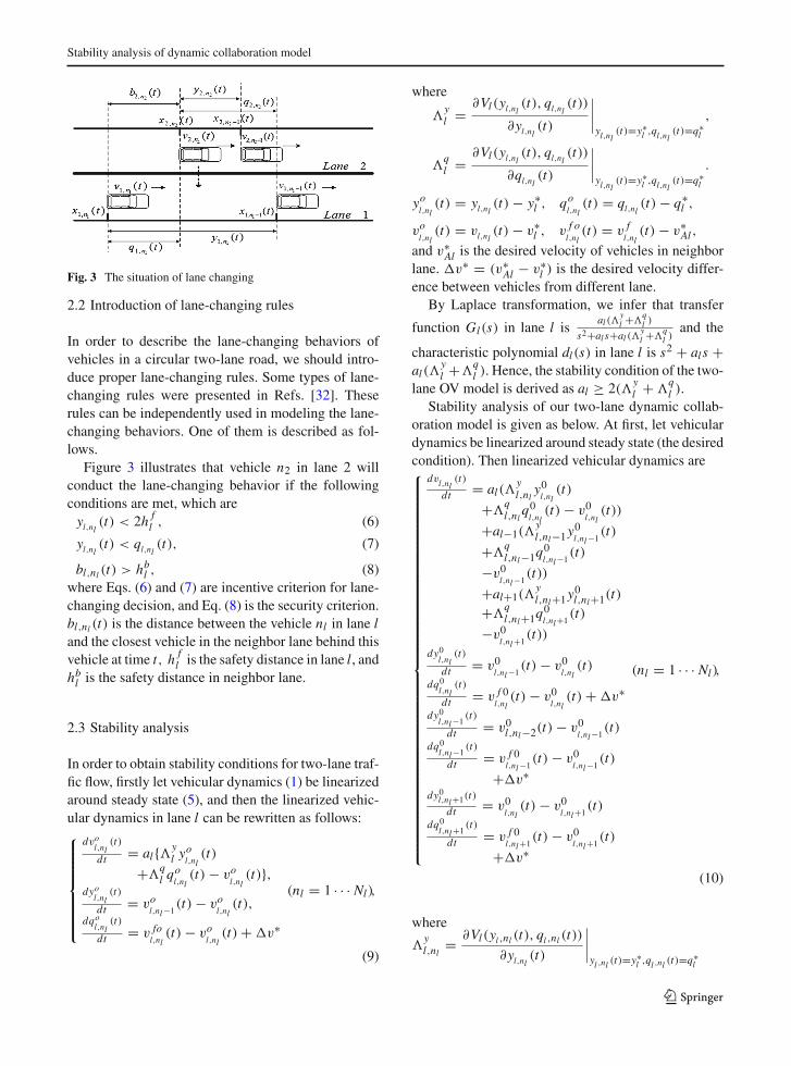
Fig. 3 The situation of lane changing
2.2 Introduction of lane-changing rules
In order to describe the lane-changing behaviors ofvehicles in a circular two-lane road, we should intro-duce proper lane-changing rules. Some types of lane-changing rules were presented in Refs. [32]. Theserules can be independently used in modeling the lane-changing behaviors. One of them is described as fol-lows.
Figure 3 illustrates that vehicle n2 in lane 2 willconduct the lane-changing behavior if the followingconditions are met, which are
yl,nl(t) < 2h f
l , (6)
yl,nl(t) < ql,nl
(t), (7)
bl,nl (t) > hbl , (8)
where Eqs. (6) and (7) are incentive criterion for lane-changing decision, and Eq. (8) is the security criterion.bl,nl (t) is the distance between the vehicle nl in lane land the closest vehicle in the neighbor lane behind thisvehicle at time t, h f
l is the safety distance in lane l, andhb
l is the safety distance in neighbor lane.
2.3 Stability analysis
In order to obtain stability conditions for two-lane traf-fic flow, firstly let vehicular dynamics (1) be linearizedaround steady state (5), and then the linearized vehic-ular dynamics in lane l can be rewritten as follows:⎧⎪⎪⎪⎪⎪⎪⎨
⎪⎪⎪⎪⎪⎪⎩
dvol,nl
(t)
dt = al{�yl yo
l,nl(t)
+�ql qo
l,nl(t) − vo
l,nl(t)},
dyol,nl
(t)
dt = vol,nl −1
(t) − vol,nl
(t),dqo
l,nl(t)
dt = v fol,nl
(t) − vol,nl
(t) + �v∗
(nl = 1 · · · Nl),
(9)
where
�yl = ∂Vl(yl,nl
(t), ql,nl(t))
∂yl,nl(t)
∣∣∣∣yl,nl
(t)=y∗l ,ql,nl
(t)=q∗l
,
�ql = ∂Vl(yl,nl
(t), ql,nl(t))
∂ql,nl(t)
∣∣∣∣yl,nl
(t)=y∗l ,ql,nl
(t)=q∗l
.
yol,nl
(t) = yl,nl(t) − y∗
l , qol,nl
(t) = ql,nl(t) − q∗
l ,
vol,nl
(t) = vl,nl(t) − v∗
l , v f ol,nl
(t) = v fl,nl
(t) − v∗Al ,
and v∗Al is the desired velocity of vehicles in neighbor
lane. �v∗ = (v∗Al − v∗
l ) is the desired velocity differ-ence between vehicles from different lane.
By Laplace transformation, we infer that transfer
function Gl(s) in lane l isal (�
yl +�
ql )
s2+al s+al (�yl +�
ql )
and the
characteristic polynomial dl(s) in lane l is s2 + als +al(�
yl +�
ql ). Hence, the stability condition of the two-
lane OV model is derived as al ≥ 2(�yl + �
ql ).
Stability analysis of our two-lane dynamic collab-oration model is given as below. At first, let vehiculardynamics be linearized around steady state (the desiredcondition). Then linearized vehicular dynamics are⎧⎪⎪⎪⎪⎪⎪⎪⎪⎪⎪⎪⎪⎪⎪⎪⎪⎪⎪⎪⎪⎪⎪⎪⎪⎪⎪⎪⎪⎪⎪⎪⎪⎪⎪⎪⎪⎪⎪⎪⎨
⎪⎪⎪⎪⎪⎪⎪⎪⎪⎪⎪⎪⎪⎪⎪⎪⎪⎪⎪⎪⎪⎪⎪⎪⎪⎪⎪⎪⎪⎪⎪⎪⎪⎪⎪⎪⎪⎪⎪⎩
dvl,nl(t)
dt = al(�yl,nl
y0l,nl
(t)
+�ql,nl
q0l,nl
(t) − v0l,nl
(t))
+al−1(�yl,nl−1 y0
l,nl −1(t)
+�ql,nl−1q0
l,nl −1(t)
−v0l,nl −1
(t))
+al+1(�yl,nl+1 y0
l,nl+1(t)+�
ql,nl+1q0
l,nl +1(t)
−v0l,nl +1
(t))dy0
l,nl(t)
dt = v0l,nl −1
(t) − v0l,nl
(t)dq0
l,nl(t)
dt = v f 0l,nl
(t) − v0l,nl
(t) + �v∗dy0
l,nl −1(t)
dt = v0l,nl−2(t) − v0
l,nl −1(t)
dq0l,nl −1
(t)
dt = v f 0l,nl −1
(t) − v0l,nl −1
(t)
+�v∗dy0
l,nl +1(t)
dt = v0l,nl
(t) − v0l,nl +1
(t)dq0
l,nl +1(t)
dt = v f 0l,nl +1
(t) − v0l,nl +1
(t)
+�v∗
(nl = 1 · · · Nl),
(10)
where
�yl,nl
= ∂Vl(yl ,nl (t), ql ,nl (t))
∂yl,nl(t)
∣∣∣∣yl ,nl (t)=y∗
l ,ql ,nl (t)=q∗l
123

Z. Li et al.
�ql,nl
= ∂Vl(yl ,nl (t), ql ,nl (t))
∂ql ,nl (t)
∣∣∣∣yl ,nl (t)=y∗
l ,ql ,nl (t)=q∗l
�yl,nl−1 = ∂Vl(yl,nl −1(t), ql ,nl−1(t))
∂yl,nl −1(t)
∣∣∣∣ yl ,nl−1(t) = y∗
l ,
ql,nl −1(t) = q∗l
�ql,nl−1 = ∂Vl(yl,nl −1(t), ql ,nl−1(t))
∂ql,nl −1(t)
∣∣∣∣ yl ,nl−1(t) = y∗
l ,
ql ,nl−1(t) = q∗l
�yl,nl+1 = ∂Vl(yl ,nl+1(t), ql ,nl+1(t))
∂yl ,nl+1(t)
∣∣∣∣ yl ,nl+1(t) = y∗
l ,
ql ,nl+1(t) = q∗l
�ql,nl+1 = ∂Vl(yl ,nl+1(t), ql ,nl+1(t))
∂yl ,nl+1(t)
∣∣∣∣ yl ,nl+1(t) = y∗
l ,
ql ,nl+1(t) = q∗l
yol,nl
(t) = yl,nl(t) − y∗
l qol,nl
(t) = ql ,nl (t) − q∗l vo
l,nl(t)
= vl,nl(t) − v∗
l v f ol,nl
(t) = v fl,nl
(t) − v∗Al
yol ,nl−1(t) = yl ,nl−1(t) − y∗
l qol ,nl−1(t)
= ql ,nl−1(t) − q∗l vo
l,nl −1(t)
= vl ,nl−1(t) − v∗l v f o
l,nl −1(t)
= v fl,nl −1
(t) − v∗Al yo
l,nl+1(t)
= yl ,nl+1(t) − y∗l qo
l,nl +1(t)
= ql ,nl+1(t) − q∗l vo
l,nl +1(t)
= vl ,nl+1(t) − v∗l v f o
l,nl −1(t)
= vf
l ,nl−1(t) − v∗Al .
From the viewpoints of control theory, the above vehic-ular dynamics can be rewritten as a linear time-invariantsystems, that is
⎡
⎢⎢⎢⎢⎢⎢⎢⎢⎢⎢⎢⎢⎢⎢⎢⎢⎢⎢⎣
dvol,nl
(t)
dtdyo
l,nl(t)
dtdqo
l,nl(t)
dtdyo
l,nl −1(t)
dtdqo
l,nl −1(t)
dtdyo
l,nl +1(t)
dtdqo
l,nl +1(t)
dt
⎤
⎥⎥⎥⎥⎥⎥⎥⎥⎥⎥⎥⎥⎥⎥⎥⎥⎥⎥⎦
=
⎡
⎢⎢⎢⎢⎢⎢⎢⎢⎣
−al al�yl,nl
al�ql,nl
al−1�yl,nl−1 al−1�
ql,nl−1 al+1�
yl,nl+1 al+1�
ql,nl+1
−1 0 0 0 0 0 0−1 0 0 0 0 0 00 0 0 0 0 0 00 0 0 0 0 0 01 0 0 0 0 0 00 0 0 0 0 0 0
⎤
⎥⎥⎥⎥⎥⎥⎥⎥⎦
.
⎡
⎢⎢⎢⎢⎢⎢⎢⎢⎢⎢⎣
vol,nl
(t)
yol,nl
(t)
qol,nl
(t)
yol,nl −1
(t)
qol,nl −1
(t)
yol,nl+1(t)
qol,nl +1
(t)
⎤
⎥⎥⎥⎥⎥⎥⎥⎥⎥⎥⎦
+
⎡
⎢⎢⎢⎢⎢⎢⎢⎢⎣
010−1−100
⎤
⎥⎥⎥⎥⎥⎥⎥⎥⎦
.vol,nl −1
(t) +
⎡
⎢⎢⎢⎢⎢⎢⎢⎢⎣
0010000
⎤
⎥⎥⎥⎥⎥⎥⎥⎥⎦
.v f ol,nl
(t) +
⎡
⎢⎢⎢⎢⎢⎢⎢⎢⎣
0001000
⎤
⎥⎥⎥⎥⎥⎥⎥⎥⎦
.v0l,nl −1
(t) +
⎡
⎢⎢⎢⎢⎢⎢⎢⎢⎣
0001000
⎤
⎥⎥⎥⎥⎥⎥⎥⎥⎦
.v f 0l,nl −1
(t) +
⎡
⎢⎢⎢⎢⎢⎢⎢⎢⎣
00000−1−1
⎤
⎥⎥⎥⎥⎥⎥⎥⎥⎦
.v0l,nl +1
(t)
+
⎡
⎢⎢⎢⎢⎢⎢⎢⎢⎣
0000001
⎤
⎥⎥⎥⎥⎥⎥⎥⎥⎦
.v f 0l,nl +1
(t) +
⎡
⎢⎢⎢⎢⎢⎢⎢⎢⎣
0010101
⎤
⎥⎥⎥⎥⎥⎥⎥⎥⎦
.�v∗.
(11)
123

Stability analysis of dynamic collaboration model
After Laplace transformation, we have
s
⎡
⎢⎢⎢⎢⎢⎢⎢⎢⎢⎢⎣
vol,nl
(s)
yol,nl
(s)
qol,nl
(s)
yol,nl −1
(s)
qol,nl −1
(s)
Y ol,nl+1(s)
qol,nl +1
(s)
⎤
⎥⎥⎥⎥⎥⎥⎥⎥⎥⎥⎦
=
⎡
⎢⎢⎢⎢⎢⎢⎢⎢⎣
−al al�yl,nl
al�ql,nl
al−1�yl,nl−1 al−1�
ql,nl−1 al+1�
yl,nl+1 al+1�
ql,nl+1
−1 0 0 0 0 0 0−1 0 0 0 0 0 00 0 0 0 0 0 00 0 0 0 0 0 01 0 0 0 0 0 00 0 0 0 0 0 0
⎤
⎥⎥⎥⎥⎥⎥⎥⎥⎦
.
⎡
⎢⎢⎢⎢⎢⎢⎢⎢⎢⎢⎣
vol,nl
(s)
yol,nl
(s)
qol,nl
(s)
yol,nl −1
(s)
qol,nl −1
(s)
Y ol,nl+1(s)
qol,nl +1
(s)
⎤
⎥⎥⎥⎥⎥⎥⎥⎥⎥⎥⎦
+
⎡
⎢⎢⎢⎢⎢⎢⎢⎢⎣
010−1−100
⎤
⎥⎥⎥⎥⎥⎥⎥⎥⎦
.vol,nl −1
(s) +
⎡
⎢⎢⎢⎢⎢⎢⎢⎢⎣
0010000
⎤
⎥⎥⎥⎥⎥⎥⎥⎥⎦
.v f ol,nl
(s) +
⎡
⎢⎢⎢⎢⎢⎢⎢⎢⎣
0001000
⎤
⎥⎥⎥⎥⎥⎥⎥⎥⎦
.V 0l,nl−2(s) +
⎡
⎢⎢⎢⎢⎢⎢⎢⎢⎣
0001000
⎤
⎥⎥⎥⎥⎥⎥⎥⎥⎦
.v f 0l,nl −1
(s)
+
⎡
⎢⎢⎢⎢⎢⎢⎢⎢⎣
00000−1−1
⎤
⎥⎥⎥⎥⎥⎥⎥⎥⎦
.v0l,nl +1
(s) +
⎡
⎢⎢⎢⎢⎢⎢⎢⎢⎣
0000001
⎤
⎥⎥⎥⎥⎥⎥⎥⎥⎦
.v f 0l,nl +1
(s) +
⎡
⎢⎢⎢⎢⎢⎢⎢⎢⎣
0010101
⎤
⎥⎥⎥⎥⎥⎥⎥⎥⎦
.�V ∗.
vol,nl
(s) = L(vol,nl
(t))yol,nl
(s) = L(yol,nl
(t))qol,nl
(s) = L(qol,nl
(t))yol,nl −1
(s) = L(yol,nl −1
(t))
qol,nl −1
(s) = L(qol,nl −1
(t))Y ol,nl+1(s) = L(yo
l,nl+1(t))qol,nl +1
(s) = L(qol,nl +1
(t))
vol,nl −1
(s) = L(vol,nl −1
(t))vfol,nl
(s) = L(vfol,nl
(t))V ol,nl−2(s) = L(vo
l,nl−2(t))vfol,nl −1
(s) = L(vfol,nl −1
(t))
vol,nl +1
(s) = L(vol,nl +1
(t))vfol,nl +1
(s) = L(vfol,nl +1
(t))�V ∗ = L(�v∗);
where L(·) denotes the Laplace transform.After derivation, we have the following transfer rela-
tionship:
vol,nl
(s) = al�yl − al−1�
yl,nl
− al�ql,nl
s(s + al) + al�yl,nl
+ al�ql,nl
− al+1�ql,nl+1
.V ol,nl−1(s)
− al+1�yl + al+1�
ql,nl+1
s(s + al) + al�yl,nl
+ al�ql,nl
− al+1�ql,nl+1
.vol,nl +1
(s)
+ al−1�yl,nl−1
s(s + al) + al�yl,nl
+ al�ql,nl
− al+1�ql,nl+1
.V ol,nl−2(s)
+ al�ql,nl
s(s + al) + al�yl,nl
+ al�ql,nl
− al+1�ql,nl+1
.v f ol,nl
(s)
+al−1�
ql,nl−1
s(s + al ) + al�yl,nl
+ al�ql,nl
− al+1�ql,nl+1
.v f ol,nl −1
(s)
+al+1�
ql,nl+1
s(s + al ) + al�yl,nl
+ al�ql,nl
− al+1�ql,nl+1
.v f ol,nl +1
(s)
+al�
ql,nl
+ al−1�ql,nl−1 + al+1�
ql,nl+1
s(s + al ) + al�yl,nl
+ al�ql,nl
− al+1�ql,nl+1
.�V ∗ (12)
vol,nl
(s) = Gl (s).vol,nl −1
(s) (13)
Gl (s) =al�
yl,nl
+ al�ql,nl
− al+1�ql,nl+1
s(s + al ) + al�yl,nl
+ al�ql,nl
− al+1�ql,nl+1
(14)
dl (s) = s2+sal + al�yl,nl
+al�ql,nl
− al+1�ql,nl+1. (15)
123

Z. Li et al.
According to our analysis, the traffic jams will neveroccur if the characteristic polynomial dl(s) is stableand ‖Gl(s)‖∞ ≤ 1. What deserves our attention isthat H∞ norm of transfer functions should be equalto or less than 1 so as to guarantee that the velocityfluctuation would not be amplified when propagatedbackward. Therefore, after derivation we can get thestability condition: al�
yl,nl
+ al�ql,nl
> al+1�ql,nl+1.
3 Numerical simulations
In the paper, the periodic boundary condition isadopted. The desired velocities of vehicles in both lanesare v∗
1 = 0.9354 and v∗2 = 0.9468, respectively; and
the desired comprehensive distances are hd1 = 1.7 and
hd2 = 1.8, respectively. Meanwhile, we can set that
αy1 = 0.7, α
q1 = 0.3, y∗
1 = 2, q∗1 = 1 in lane 1 and
αy2 = 0.8, α
q2 = 0.2, y∗
2 = 2, q∗2 = 1 in lane 2.
hb1 = h f
2 = 0.5. Besides, the length of the circulartwo-lane highway is 200. Let Nl vehicles be distrib-uted along lane l homogeneously, where Nl is an evennumber (i.e., N1 = N2 = 100). The initial positions ofthese vehicles in both lanes are
x1,1(0) = 199, x1,n1(0) = 199 − 2(n1 − 1); x2,1(0)
= 200, x2,n2(0) = 200 − 2(n2 − 1).
Obviously, we know that yl,nl(0) = 2 and ql,nl
(0) = 1for l = 1 and 2. However, because of the unsteadinessof traffic flow, the headway of the 50th vehicle reducessuddenly for a small period of time as follows:
i f (20 ≤ t ≤ 30), y1,50(t) = y1,50(t)/3, y1,51(t)
= y1,51(t) + 2y1,50(t)/3.
Besides, when a vehicle carries out lane changing, itsheadway is set as 5 so as to record its lane-changingbehavior. Considering the lane-changing behaviors, wewill perform some numerical simulations for the caseswith different dynamic factors.
3.1 The numerical experiments with OV model
(1) The sensitivities of drivers in both lanes are a1 = 1.0and a2 = 1.5, respectively. a1 and a2 represent thesensitivities of current vehicles on lane 1 and lane 2,respectively.
Figure 4 shows the diagrams of headway and veloc-ity fluctuations without lane-changing behaviors andFig. 5 shows the diagrams of headway and velocity fluc-
Fig. 4 The diagrams of headway and velocity fluctuations for the case without lane-changing behaviors. a Headway fluctuation in thefirst 2.5 s, b headway fluctuation in the last 2.5 s, and c velocity fluctuation in different time points
Fig. 5 The diagrams of headway and velocity fluctuations with lane-changing behaviors. a Headway fluctuation in the first 2.5 s, bheadway fluctuation in the last 2.5 s, and c velocity fluctuation in different time points
123
Stability analysis of dynamic collaboration model
tuations with lane-changing behaviors, respectively.Figs. 4 and 5 illustrate that the headway and velocityfluctuations of vehicles on lane 1 have been amplified asthe headway reduction of 50th vehicle has propagatedbackward when the stability conditions are not met.Namely, the traffic flow is not stable with these sen-sitivities. Besides, Fig. 5a indicates that four vehicleshave carried out lane changing. By comparing Figs. 4and 5, it is known that lane-changing behaviors have lit-tle effect on the running state of the vehicles on lane 1,except that the velocity fluctuations of individual vehi-cles at time 75s in Fig. 5c is bigger than that in Fig. 4c.
3.2 The numericalexperiments with dynamic collaboration model
(2) The sensitivities of drivers in both lanes are a1 =1.0, (a1 − 1) = 0.1, (a1 + 1) = 0.1 and a2 = 1.5,(a2 − 1) = 0.1, (a2 + 1) = 0.1, respectively. (a1 − 1)
and (a1 + 1) represent the dynamic factors of the near-est preceding and following vehicles on lane 1, respec-tively. (a2 − 1) and (a2 + 1) represent the dynamic
factors of the nearest preceding and following vehicleson lane 2, respectively.
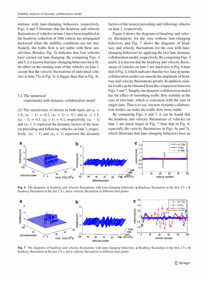
Figure 6 shows the diagrams of headway and veloc-ity fluctuations for the case without lane-changingbehaviors and Fig. 7 shows the diagrams of head-way and velocity fluctuations for the case with lane-changing behaviors by applying the two-lane dynamiccollaboration model, respectively. By comparing Figs. 4and 6, it is known that the headway and velocity fluctu-ations of vehicles on lane 1 are much less in Fig. 6 thanthat in Fig. 4, which indicates that the two-lane dynamiccollaboration model can smooth the amplitude of head-way and velocity fluctuations greatly. In addition, simi-lar result can be obtained from the comparison betweenFigs. 5 and 7. Simply, our dynamic collaboration modelhas the effect of smoothing traffic flow stability in thecase of two-lane, which is consistent with the case ofsingle-lane. That is to say, our new dynamic collabora-tion model can make the traffic flow more stable.
By comparing Figs. 6 and 7, it can be found thatthe headway and velocity fluctuations of vehicles onlane 1 are much larger in Fig. 7 than that in Fig. 6,especially the velocity fluctuations in Figs. 6c and 7c,which illustrates that lane-changing behaviors have an
Fig. 6 The diagrams of headway and velocity fluctuations with lane-changing behaviors. a Headway fluctuation in the first 2.5 s, bheadway fluctuation in the last 2.5 s, and c velocity fluctuation in different time points
Fig. 7 The diagrams of headway and velocity fluctuations with lane-changing behaviors. a Headway fluctuation in the first 2.5 s, bheadway fluctuation in the last 2.5 s, and c velocity fluctuation in different time points
123

Z. Li et al.
important influence on the traffic stability. Obviously,lane-changing behaviors have greater influence on thetraffic stability with two-lane dynamic collaborationmodel. Moreover, the effect of dynamic collaborationon traffic flow stability in the case of two-lane will bediscussed with different dynamic factors below.
(3) The sensitivities of drivers in both lanes are a1 =1.0, (a1 − 1) = 0.15, (a1 + 1) = 0.15 and a2 = 1.5,(a2 − 1) = 0.15, (a2 + 1) = 0.15, respectively.
(4) The sensitivities of drivers in both lanes area1 = 1.0, (a1 −1) = 0.3, (a1 +1) = 0.3 and a2 = 1.5,(a2 − 1) = 0.3, (a2 + 1) = 0.3, respectively.
Figures 8 and 9 show the diagrams of headwayand velocity fluctuations for the case of lane-changingbehaviors with different dynamic collaboration factors.By comparing Figs. 5, 7, 8, and 9, it can be found that theheadway fluctuations in the last 2.5 s decrease greatly,and velocity fluctuations in different time points reduceas well, except individual vehicles’ velocity fluctua-tions in Fig. 9c. Generally, the two-lane dynamic col-laboration model can suppress the traffic congestionwith increasing the dynamic factors. Namely, the two-
lane dynamic collaboration model can stabilize the traf-fic flow.
We have just discussed the stability of the trafficflow by changing the four dynamic factors. What ismore, we get the conclusion that dynamic collabora-tion model can make the traffic flow more steady withincreasing the dynamic factors. Next, we discuss theinfluences of the four dynamic factors on the trafficstability, respectively. Firstly, the two dynamic factorsof vehicles in the fast lane are researched with the otherfactors unchanged.
(5) The sensitivities of drivers in both lanes area1 = 1.0, (a1 −1) = 0.1, (a1 +1) = 0.1 and a2 = 1.5,(a2 − 1) = 0.15, (a2 + 1) = 0.15, respectively.
(6) The sensitivities of drivers in both lanes area1 = 1.0, (a1 −1) = 0.1, (a1 +1) = 0.1 and a2 = 1.5,(a2 − 1) = 0.3, (a2 + 1) = 0.3, respectively.
(7) The sensitivities of drivers in both lanes area1 = 1.0, (a1 −1) = 0.1, (a1 +1) = 0.1 and a2 = 1.5,(a2 − 1) = 0.45, (a2 + 1) = 0.45, respectively.
Figures 10, 11, and 12 show the diagrams ofheadway and velocity fluctuations for the case oflane-changing behaviors for the case of different
Fig. 8 The diagrams of headway and velocity fluctuations with lane-changing behaviors. a Headway fluctuation in the first 2.5 s, bheadway fluctuation in the last 2.5 s, and c velocity fluctuation in different time points
Fig. 9 The diagrams of headway and velocity fluctuations with lane-changing behaviors. a Headway fluctuation in the first 2.5 s, bheadway fluctuation in the last 2.5 s, and c velocity fluctuation in different time points
123

Stability analysis of dynamic collaboration model
Fig. 10 The diagrams of headway and velocity fluctuations with lane-changing behaviors. a Headway fluctuation in the first 2.5 s, bheadway fluctuation in the last 2.5 s, and c velocity fluctuation in different time points
Fig. 11 The diagrams of headway and velocity fluctuations with lane-changing behaviors. a Headway fluctuation in the first 2.5 s, bheadway fluctuation in the last 2.5 s, and c velocity fluctuation in different time points
Fig. 12 The diagrams of headway and velocity fluctuations with lane-changing behaviors. a Headway fluctuation in the first 2.5 s, bheadway fluctuation in the last 2.5 s, and c velocity fluctuation in different time points
dynamic factors of vehicles on lane 2. By compar-ing Figs. 5, 10, 11, and 12, it can be found that theheadway fluctuations in the last 2.5 s decrease greatly,and velocity fluctuations in different time points reduceas well. Apparently, the two dynamic factors of vehi-cles in the fast lane are helpful to stabilize the trafficflow.
Secondly, the two dynamic factors of vehicles inthe slow lane are researched with the other factorsunchanged.
(8) The sensitivities of drivers in both lanes area1 = 1.0, (a1 − 1) = 0.15, (a1 + 1) = 0.15 anda2 = 1.5, (a2 − 1) = 0.1, (a2 + 1) = 0.1, respectively.
(9) The sensitivities of drivers in both lanes area1 = 1.0, (a1 −1) = 0.3, (a1 +1) = 0.3 and a2 = 1.5,(a2 − 1) = 0.1, (a2 + 1) = 0.1, respectively.
(10) The sensitivities of drivers in both lanes area1 = 1.0, (a1 − 1) = 0.45, (a1 + 1) = 0.45and a2 = 1.5, (a2 − 1) = 0.1, (a2 + 1) = 0.1,respectively.
123

Z. Li et al.
Fig. 13 The diagrams of headway and velocity fluctuations with lane-changing behaviors. a Headway fluctuation in the first 2.5 s. bheadway fluctuation in the last 2.5 s, and c velocity fluctuation in different time points
Fig. 14 The diagrams of headway and velocity fluctuations with lane-changing behaviors. a Headway fluctuation in the first 2.5 s, bheadway fluctuation in the last 2.5 s, and c velocity fluctuation in different time points
Fig. 15 The diagrams of headway and velocity fluctuations with lane-changing behaviors. a Headway fluctuation in the first 2.5 s, bheadway fluctuation in the last 2.5 s, and c velocity fluctuation in different time points
Figures 13, 14, and 15 show the diagrams of head-way and velocity fluctuations for the case of lane-changing behaviors with different dynamic factors ofvehicles on lane 1. Obviously, it is known that head-way fluctuation decreases gradually in the last 2.5 s, asthe velocity fluctuation in different time points by com-paring Figs. 5, 13, 14, and 15. In other words, the twodynamic factors of vehicles in the slow lane contributeto the stability of traffic flow.
Thirdly, the two dynamic factors of the two near-est following vehicles on two lanes (following fac-
tors, for short) are researched with the other factorsunchanged.
(11) The sensitivities of drivers in both lanes area1 = 1.0, (a1−1) = 0.1, (a1+1) = 0.15 and a2 = 1.5,(a2 − 1) = 0.1, (a2 + 1) = 0.15, respectively.
(12) The sensitivities of drivers in both lanes area1 = 1.0, (a1 −1) = 0.1, (a1 +1) = 0.3 and a2 = 1.5,(a2 − 1) = 0.1, (a2 + 1) = 0.3, respectively.
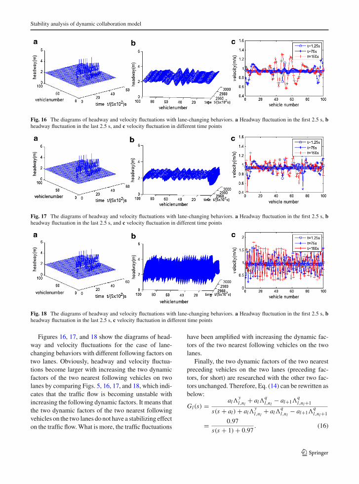
(13) The sensitivities of drivers in both lanes area1 = 1.0, (a1−1) = 0.1, (a1+1) = 0.45 and a2 = 1.5,(a2 − 1) = 0.1, (a2 + 1) = 0.45, respectively.
123
Stability analysis of dynamic collaboration model
Fig. 16 The diagrams of headway and velocity fluctuations with lane-changing behaviors. a Headway fluctuation in the first 2.5 s, bheadway fluctuation in the last 2.5 s, and c velocity fluctuation in different time points
Fig. 17 The diagrams of headway and velocity fluctuations with lane-changing behaviors. a Headway fluctuation in the first 2.5 s, bheadway fluctuation in the last 2.5 s, and c velocity fluctuation in different time points
Fig. 18 The diagrams of headway and velocity fluctuations with lane-changing behaviors. a Headway fluctuation in the first 2.5 s, bheadway fluctuation in the last 2.5 s, c velocity fluctuation in different time points
Figures 16, 17, and 18 show the diagrams of head-way and velocity fluctuations for the case of lane-changing behaviors with different following factors ontwo lanes. Obviously, headway and velocity fluctua-tions become larger with increasing the two dynamicfactors of the two nearest following vehicles on twolanes by comparing Figs. 5, 16, 17, and 18, which indi-cates that the traffic flow is becoming unstable withincreasing the following dynamic factors. It means thatthe two dynamic factors of the two nearest followingvehicles on the two lanes do not have a stabilizing effecton the traffic flow. What is more, the traffic fluctuations
have been amplified with increasing the dynamic fac-tors of the two nearest following vehicles on the twolanes.
Finally, the two dynamic factors of the two nearestpreceding vehicles on the two lanes (preceding fac-tors, for short) are researched with the other two fac-tors unchanged. Therefore, Eq. (14) can be rewritten asbelow:
Gl(s) = al�yl,nl
+ al�ql,nl
− al+1�ql,nl+1
s(s + al) + al�yl,nl
+ al�ql,nl
− al+1�ql,nl+1
= 0.97
s(s + 1) + 0.97. (16)
123
Z. Li et al.
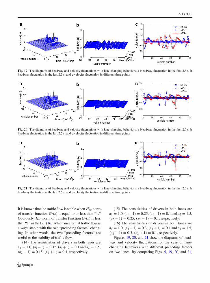
Fig. 19 The diagrams of headway and velocity fluctuations with lane-changing behaviors. a Headway fluctuation in the first 2.5 s, bheadway fluctuation in the last 2.5 s, and c velocity fluctuation in different time points
Fig. 20 The diagrams of headway and velocity fluctuations with lane-changing behaviors. a Headway fluctuation in the first 2.5 s, bheadway fluctuation in the last 2.5 s, and c velocity fluctuation in different time points
Fig. 21 The diagrams of headway and velocity fluctuations with lane-changing behaviors. a Headway fluctuation in the first 2.5 s, bheadway fluctuation in the last 2.5 s, and c velocity fluctuation in different time points
It is known that the traffic flow is stable when H∞ normof transfer function Gl(s) is equal to or less than “1.”Obviously, H∞ norm of transfer function Gl(s) is lessthan “1” in the Eq. (16), which means that traffic flow isalways stable with the two “preceding factors” chang-ing. In other words, the two “preceding factors” areuseful to the stability of traffic flow.
(14) The sensitivities of drivers in both lanes area1 = 1.0, (a1−1) = 0.15, (a1+1) = 0.1 and a2 = 1.5,(a2 − 1) = 0.15, (a2 + 1) = 0.1, respectively.
(15) The sensitivities of drivers in both lanes area1 = 1.0, (a1−1) = 0.25, (a1+1) = 0.1 and a2 = 1.5,(a2 − 1) = 0.25, (a2 + 1) = 0.1, respectively.
(16) The sensitivities of drivers in both lanes area1 = 1.0, (a1 −1) = 0.3, (a1 +1) = 0.1 and a2 = 1.5,(a2 − 1) = 0.3, (a2 + 1) = 0.1, respectively.
Figures 19, 20, and 21 show the diagrams of head-way and velocity fluctuations for the case of lane-changing behaviors with different preceding factorson two lanes. By comparing Figs. 5, 19, 20, and 21,
123
Stability analysis of dynamic collaboration model
it can be found that the headway fluctuations in thelast 2.5 s decrease greatly, and velocity fluctuations indifferent time points reduce as well, except individ-ual vehicle’s velocity fluctuations in Fig. 21c. Gener-ally, the traffic congestion can be suppressed by thetwo-lane dynamic collaboration model with increasingthe preceding dynamic factors. In other words, the twodynamic factors of the nearest preceding vehicles havea stabilizing effect on the traffic flow.
All in all, the two-lane dynamic collaboration modelcan suppress the traffic congestion and stabilize the traf-fic flow. Furthermore, the two dynamic factors of thetwo nearest preceding vehicles on two lanes play a piv-otal role of stabilizing the traffic flow. However, the twodynamic factors of the two nearest following vehicleson two lanes cannot promote the traffic flow steadily.The results concluded are consistent with both the the-oretical derivation and the numerical simulations.
4 Conclusions
The paper mainly studies the influence of dynamic fac-tors for the case of lane-changing behaviors on the traf-fic flow stability by the two-lane dynamic collaborationmodel. Theoretical stability analysis about the two-lanedynamic collaboration has been accomplished and thestability conditions for both lanes are derived. We con-clude that the two-lane dynamic collaboration modelcan make the traffic flow more stable with increasingits dynamic factors. It means that our new dynamiccollaboration model is helpful for the stability of traf-fic flow. Furthermore, the two dynamic factors of thetwo nearest preceding vehicles on the two lanes play animportant role for steadying the traffic flow. But the twodynamic factors of the two nearest following vehicleson the two lanes have a different effect.
Acknowledgments This work is supported by the NaturalScience Foundation of China under Grant Nos. 60904068,10902076, 11072117, and 61004113; and the FundamentalResearch Funds for the Central Universities under Grant No.0800219198
References
1. Pipes, L.A.: An operational analysis of traffic dynamics. J.Appl. Phys. 41, 274–281 (1953)
2. Bando, M., Hasebe, K., Nakayama, A.: Dynamical modelof traffic congestion and numerical simulation. Phys. Rev.E 51, 1035–1042 (1995)
3. Helbing, D., Tilch, B.: Generalized force model of trafficdynamics. Phys. Rev. E 58, 133–38 (1998)
4. Jiang, R., Wu, Q.S., Zhu, Z.J.: Full velocity difference modelfor a car-following theory. Phys. Rev. E 64, 017101 (2001)
5. Newell, G.F.: Nonlinear effects in the dynamics of carfollowing. Oper. Res. 9, 209–229 (1961)
6. Nagatani, T.: Modified KdV equation for jamming tran-sition in the continuum models of traffic. Phys. A 261,599–607 (1998)
7. Nagatani, T.: Jamming transitions and the modifiedKorteweg-de Vries equation in a two-lane traffic flow. Phys.A 265, 297–310 (1999)
8. Nagatani, T.: Stabilization and enhancement of traffic flowby the next-nearest-neighbor interaction. Phys. Rev. E 60,6395–6401 (1999)
9. Hasebe, K., Nakayama, A., Sugiyama, Y.: Equivalence oflinear response among extended optimal velocity models.Phys. Rev. E 69, 017103 (2004)
10. Hasebe, K., Nakayama, A., Sugiyama, Y.: Dynamicalmodel of a cooperative driving system for freeway traffic.Phys. Rev. E 68, 026102 (2003)
11. Li, Z.P., Liu, Y.C., Liu, F.Q.: A dynamical model withnext-nearest-neighbor interaction in relative velocity. Int. J.Mod. Phys. C 18, 819–832 (2007)
12. Ge, H.X., Dai, S.Q., Dong, L.Y., Xue, Y.: Stabilizationeffect of traffic flow in an extended car-following modelbased on an intelligent transportation system application.Phys. Rev. E 70, 066134 (2004)
13. Ge, H.X., Dai, S.Q., Xue, Y., Dong, L.Y.: Stabilizationanalysis and modified Korteweg-de Vries equation in acooperative driving system. Phys. Rev. E 71, 066119 (2005)
14. Ge, H.X., Cheng, R.J., Li, Z.P.: Two velocity differencemodel for a car following theory. Phys. A 387, 5239–5245(2008)
15. Jin, S., Wang, D.H., Tao, P.F.: Non-lane-based full velocitydifference car following model. Phys. A 389, 4654–466(2010)
16. Komada, K., Masukura, S., Nagatani, T.: Effect of gravita-tional force upon traffic flow with gradients. Phys. A 388,2880–2894 (2009)
17. Treibe, M.: Congested traffic states in empirical obser-vations and microscopic simulation. Phys. Rev. E 62,1805–1824 (2000)
18. Zhu, W.X.: Motion energy dissipation in traffic flow on acurved road. Int. J. Mod. Phys. C 24, 1350046 (2013)
19. Zhu, W.X., Zhang, C.H.: Analysis of energy dissipation intraffic flow with a variable slope. Phys. A 392, 3301–3307(2013)
20. Tang, T.Q., Li, C.Y., Huang, H.J., Shang, H.Y.: A newfundamental diagram theory with the individual differenceof the driver’s perception ability. Nonlinear Dyn. 67,2255–2265 (2012)
21. Tang, T.Q., Li, C.Y., Huang, H.J., Shang, H.Y.: An extendedoptimal velocity model with consideration of Honk effect.Commun. Theor. Phys. 54, 1151–1155 (2010)
22. Kerner, B.S., Konhäuser, P.: Cluster effect in initiallyhomogeneous traffic flow. Phys. Rev. E 48, R23355 (1993)
23. Chowdhury, D., Pasupathy, A., Sinha, S.: Distributions oftime- and distance-headways in the Nagel–Schreckenbergmodel of vehicular traffic: effects of hindrances. Eur. Phys.J. B 5, 781–786 (1998)
123

Z. Li et al.
24. Schadschneider, A.: The nagel-schreckenberg modelrevisited. Eur. Phys. J. B 10, 573–582 (1999)
25. Nakayama, A., Sugiyama, Y., Hasebe, K.: Effect of lookingat the car that follows in an optimal velocity model of trafficflow. Phys. Rev. E 65, 016112 (2001)
26. Zhao, X.M., Gao, Z.Y.: The stability analysis of the fullvelocity and acceleration velocity model. Phys. A 375,679–686 (2007)
27. Peng, G.H., Cai, X.H., Liu, C.Q., Cao, B.F., Tuo, M.X.:Optimal velocity difference model for a car-followingtheory. Phys. Lett. A 375, 3973–3977 (2011)
28. Peng, G.H., Cheng, R.J.: A new car-following model withthe consideration of anticipation optimal velocity. Phys. A392, 3563–3569 (2013)
29. Peng, G.H., Sun, D.H.: Multiple car-following model oftraffic flow and numerical simulation. Chin. Phys. B 18,5420–5430 (2009)
30. Sawada, S.: Nonlinear analysis of a differential-differenceequation with next-nearest-neighbour interaction for trafficflow. J. Phys. A 34, 11253–11259 (2001)
31. Li, Z.P., Zhang, R.: An Extended Non-Lane-Based OptimalVelocity Model with Dynamic Collaboration. MPE. http://dx.doi.org/10.1155/2013/124908 (2013)
32. Zheng, L., Ma, S.F., Zhong, S.Q.: Influence of lane changeon stability analysis for two-lane traffic flow. Chin. Phys.B. 20, 088701 (2012)
33. Konishi, K., Kokame, H., Hirata, K.: Decentralized delayed-feedback control of an optimal velocity traffic model. Eur.Phys. J. B 15, 715–722 (2000)
123