IZA DP No. 2986

Retirement and Consumption in a Life Cycle Model

David M. Blau

DI

SC

US

SI

ON

PA

PE

R S

ER

IE

S

Forschungsinstitutzur Zukunft der ArbeitInstitute for the Studyof Labor

August 2007

Retirement and Consumption in a

Life Cycle Model

David M. Blau Ohio State University

and IZA

Discussion Paper No. 2986 August 2007

IZA

P.O. Box 7240 53072 Bonn

Germany

Phone: +49-228-3894-0 Fax: +49-228-3894-180

E-mail: iza@iza.org

Any opinions expressed here are those of the author(s) and not those of the institute. Research disseminated by IZA may include views on policy, but the institute itself takes no institutional policy positions. The Institute for the Study of Labor (IZA) in Bonn is a local and virtual international research center and a place of communication between science, politics and business. IZA is an independent nonprofit company supported by Deutsche Post World Net. The center is associated with the University of Bonn and offers a stimulating research environment through its research networks, research support, and visitors and doctoral programs. IZA engages in (i) original and internationally competitive research in all fields of labor economics, (ii) development of policy concepts, and (iii) dissemination of research results and concepts to the interested public. IZA Discussion Papers often represent preliminary work and are circulated to encourage discussion. Citation of such a paper should account for its provisional character. A revised version may be available directly from the author.

IZA Discussion Paper No. 2986 August 2007

ABSTRACT

Retirement and Consumption in a Life Cycle Model* Consumption expenditure declines sharply at the time of retirement for many households, but the majority maintain a smooth consumption path. A simple life cycle model with uncertainty about the time of retirement can account for this pattern. A richer version of the model is calibrated to data from the Health and Retirement Study. The median change in consumption expenditure at retirement generated by the model is zero, while the mean is negative, matching the HRS data. However, the magnitude of the drop in consumption among households that experience a decline is too small in the model compared to the data. JEL Classification: J26, H55 Keywords: retirement, consumption, saving, life cycle model Corresponding author: David M. Blau Department of Economics The Ohio State University Arps Hall, 1945 N. High St. Columbus, OH 43210-1172 USA E-mail: Blau.12@osu.edu

* I am grateful to the National Institute on Aging (grant no. R01 AG021990) and INSEE for financial support and to CREST-INSEE and DEEE-INSEE for hospitality during the work on this paper. I thank Eric French, and Jon Skinner, for very detailed and helpful comments. I am also grateful to Rob Alessie, John Bailey Jones, Moshe Buchinski, Pierre-Olivier Gourinchas, Steven Haider, Mike Hurd, Winfried Koeniger, Francis Kramarz, Anne Laferrere, Guy Laroque, Jacques Mairesse, Pierre-Carl Michaud, Luigi Pistaferri, Gerard van den Berg, and seminar participants at the University of Basel, CREST-INSEE, IZA, the Finnish Doctoral Program in Economics, the Tinbergen Institute, William and Mary, RAND, UCLA, Tilburg University, Ohio State University, and the SOLE/EALE 2005 meeting in San Francisco for helpful comments. I thank Alan Gustman and Tom Steinmeier for helpful advice on pension data. None of the above are in any way responsible for the content.

1

1. Introduction

Consumption expenditure declines sharply at the time of retirement for many U.S.

households (Bernheim, Skinner, and Weinberg, 2001; Hurd and Rohwedder, 2006). Some

analysts argue that this poses a puzzle for the life cycle framework, because it is inconsistent

with the consumption smoothing motive implied by the framework. Alternative “behavioral”

models of saving, in which consumers have limited ability or willingness to plan for the future or

to carry out their plans, have been suggested as an explanation. These alternative models imply

that a laissez-faire approach to saving policy is likely to be inefficient (Ameriks, Caplin, and

Leahy, 2003; Bernheim 1994; Laibson et al., 1998; Poterba, Venti, and Wise, 1996; Thaler and

Benartzi, 2004). Others argue that the evidence is consistent with adequate retirement savings,

and that policies intended to encourage greater savings are likely to be ineffective and costly

(Lazear, 1994; Engen, Gale, and Uccello, 1999; Engen, Gale, and Scholz, 1996; Scholz,

Seshadri, and Khitatrakun, 2006). This is clearly a major public policy issue in view of the rapid

aging of the population.

The “retirement-consumption puzzle” has attracted considerable attention from

economists. One approach to explaining the apparent puzzle emphasizes substitution of time for

purchased goods in the home production of final consumption commodities, as a result a decline

in the relative price of time used in home production after retirement (Aguiar and Hurst, 2005;

Hurd and Rohwedder, 2003). In this view, a drop in consumption expenditure at retirement is

consistent with life cycle theory because it does not imply a drop in consumption, and it is the

latter that is the object of attention in economic theory. A second approach emphasizes non-

separability of consumption and leisure in preferences. In this approach, the magnitude of the

1See Lundberg, Startz, and Stillman (2003), Miniaci, Monfardini, and Weber (2003), andSmith (2006) for other approaches and additional evidence.

2

drop in consumption at retirement is used to infer the quantitative importance of non-separability

in preferences, taking the life cycle framework as a maintained assumption (French, 2005;

Laitner and Silverman, 2005).

A third approach focuses on testing whether the drop in consumption at retirement can be

reconciled with the implications of the life cycle framework (Bernheim, Skinner, and Weinberg,

2001; Banks, Blundell, and Tanner, 1998; Haider and Stephens, forthcoming).1 These studies

specify a consumption function in which retirement or employment status is an independent

variable. Retirement is endogenous to consumption if unexpected shocks cause earlier-than-

anticipated retirement. The consumption function is estimated by Instrumental Variables (IV),

using instruments that predict retirement but that are plausibly uncorrelated with shocks. A test

of the implications of the life cycle framework is equivalent to a test of the null hypothesis that

the coefficient on retirement is equal to zero after instrumenting: consumption should be

smoothed around predictable events such as “planned retirement.” The studies that have

followed this approach have all rejected the null.

Three main questions remain unanswered by these approaches. First, what exactly are the

implications of the life cycle framework for consumption behavior at retirement in a world with

uncertainty and discrete employment choices? Intuitively, it seems plausible that consumption

would drop abruptly at retirement if retirement is caused by an unexpected shock, while life

cycle consumers would smooth consumption over the “planned” retirement date. But this

intuition has not been formalized, and the conditions under which the intuition is correct are

3

unknown. Second, can a life cycle model quantitatively explain retirement and consumption

behavior without relying on non-separable preferences? It is tautological that non-separable

preferences can account for a drop in consumption at retirement, but an important unanswered

question is whether there are fundamental features of the life cycle framework that can explain

consumption behavior at retirement without simply attributing it to preferences. Third, are the IV

approaches that have been used to test the implications of the life cycle framework valid? That

is, suppose consumption behavior is determined by some version of the life cycle model with

uncertainty about the timing of retirement. Would the IV approaches proposed in the literature

be successful in eliminating the part of the variation in retirement timing that is endogenous to

retirement?

This study addresses these three issues. A simple theoretical analysis is developed in

order to demonstrate the conditions under which a drop in consumption at retirement is predicted

by the life cycle framework. The analysis shows that when there is uncertainty about the timing

of retirement and retirement is a discrete event, then a drop in consumption is implied by the life

cycle framework if retirement is caused by an unexpected shock. If retirement occurs at the

planned date, there is no drop in consumption at retirement. These predictions are consistent with

the patterns found in consumption expenditure data from the Health and Retirement Study

(HRS), and they do not require any assumptions about preferences.

The second main contribution of this study is to calibrate, solve, and simulate a more

realistic version of the life cycle model in order to determine whether such a model can explain

the observed drop in consumption at retirement quantitatively, without relying on non-separable

preferences. The model incorporates key constraints facing older households: Social Security

4

retirement and disability programs, employer pensions, a consumption floor provided by

government welfare programs, stochastic processes for earnings and asset returns, layoff risk,

job offer risk, health risk, and mortality risk. The model is calibrated to data from the Health and

Retirement Study (HRS), and its implications for consumption behavior are analyzed. The main

finding of the quantitative analysis is that the model generates consumption and retirement

patterns that are qualitatively consistent with the data: the mean change in consumption at

retirement is negative, while the median is zero. However, the drop in consumption among the

subset of households that do experience a decline is much smaller in the model than in the data.

This implies that other factors such as non-separable preferences, substitution of time for

purchased goods, and bounded rationality must be responsible for the bulk of the observed drop

in consumption expenditure at retirement.

Third, as a byproduct of solving and simulating the life cycle model, I can replicate the

IV approaches discussed above on simulated data from the model. If the IV approaches proposed

in these studies are successful, they should eliminate the drop in consumption at retirement in the

simulated data, since the simulated data are by construction consistent with the life cycle

framework. I find that the drop in consumption at retirement in the simulated data is in fact

eliminated by instrumenting. Hence I conclude that the IV approach based on a linear

consumption model is successful at controlling for the endogeneity of retirement.

Section 2 of the paper describes the drop in consumption at retirement, and section 3

develops a simple life cycle model to explain it. Section 4 describes the quantitative model and

solution approach. Section 5 describes the data, calibrated parameters, and model fit. The results

of simulations based on the model are discussed in section 6, and section 7 summarizes the

5

results of an extensive robustness analysis. The final section offers conclusions.

2. Consumption Behavior at Retirement

Until recently, there were no panel data available with information on total consumption

expenditure. Analysts relied on pseudo-panels formed from time series of cross sections (e.g. the

Consumer Expenditure Survey in the U.S. and the Family Expenditure Survey in the UK), or

panel data with incomplete measures of consumption (e.g., the Panel Study of Income

Dynamics). Recently, panel data on consumption expenditure have been developed as part of the

Health and Retirement Study (HRS). The HRS began in 1992 with baseline in-person interviews

with a sample of households containing individuals aged 51-61 and their spouses. Telephone

interviews have been conducted every other year since 1994, and new cohorts have been added

periodically. A random sample of 5000 of the HRS households interviewed in the 2000 wave

was asked to participate in a longitudinal Consumption and Activities Mail Survey (CAMS) in

the off-survey years beginning in 2001. The CAMS contains expenditure questions on an array

of items that, when summed, are intended to provide a comprehensive measure of consumption

expenditure. It also contains direct questions about how consumption expenditure changed at the

time of retirement for individuals who were retired at the time of the CAMS, and questions about

how non-retired individuals expect their spending to change when they retire. The key advantage

of these data is that changes in consumption expenditure can be measured at the household level,

so the entire distribution of expenditure changes can be identified. Pseudo panels can identify

changes in the expenditure distribution, but cannot identify the distribution of expenditure

changes.

6

In this section, I rely on the very informative analysis of the 2001 and 2003 CAMS data

by Hurd and Rohwedder (2006), which documents the following key facts about changes in

consumption expenditure at retirement. First, consumption declines at retirement for a large

minority of households, but the median change in consumption expenditure at retirement is zero

(Hurd and Rohwedder, 2006, Table 1). Second, a decline in consumption at retirement is

anticipated by the majority of households prior to retirement; the mean and median anticipated

declines are both 20% (Hurd and Rohwedder, 2006, Table 2).

In addition to the key facts about consumption expenditure, there are two features of

retirement behavior that are important to account for in a model of consumption and retirement.

First, in some cases retirement is precipitated by negative shocks such as health problems or job

loss, but the majority of individuals do not appear to retire in response to shocks. One example

that illustrates this clearly is the well-documented large spike in retirement at age 62 in the U.S.

In the HRS sample used in this paper, the exit rate from employment is more than twice as large

at age 62 than at age 61 (see Figure 1 below). There is no reason to expect a spike in negative

shocks at age 62. The much more plausible explanation is that retirement at age 62 is a planned

response to Social Security incentives. Furthermore, when asked directly about their reasons for

retirement, the majority of people do not mention health or other shocks as an important reason

(Hurd and Rohwedder, 2006; Maestas, 2004). The second key feature of retirement behavior is

that retirement is usually a discrete event, not a gradual decline in hours worked (Blau, 1994;

Hurd, 1996; Rust and Phelan, 1997).

These facts suggest a simple story about the decline in consumption at retirement that is

consistent with the life cycle framework. The majority of people anticipate the possibility of a

7

decline in consumption at retirement, because they are aware that there is a risk of experiencing

a negative shock before the “planned” retirement date. That is, the expected value of the change

in consumption at retirement is negative. But the majority of people do not actually experience a

shock before their planned retirement date. They retire without a change in plans, so their

consumption does not change at retirement. A testable implication of this line of reasoning is that

people who experienced a decline in consumption at retirement were more likely than other

people to have retired as a result of a shock, and people who did not experience a decline in

consumption at retirement were more likely than other people to have retired as planned rather

than as the result of a shock.

There is evidence to support this implication in Hurd and Rohwedder (2006), Table 8.

They classify retired CAMS respondents according to whether they reported that health was an

important reason for retirement. Among those who said yes (29% of their sample), both the mean

and median recollected change in consumption at retirement are -20%. Among those who said

that health was not important, the mean change was -11% and the median change was zero. This

suggests that a simple life cycle model in which individuals choose when to retire but are subject

to shocks that may cause earlier-than-planned retirement can account qualitatively for the

stylized facts.

3. A Simple Model

I now present a very simple example of such a model. Suppose that an individual plans to

retire at age T. He lives through age T* $ T with certainty and then dies. Imagine that T is the

optimal retirement age given the information available to the individual at some age less than T,

8

and there is no chance of receiving any new information that affects the optimal retirement date.

However, at the beginning of each period t < T a shock may occur that forces the individual to

retire immediately. If a shock occurs in period t, the individual must retire in period t, and

retirement is irreversible. The probability that a shock occurs in a given period is π, constant

across periods for simplicity. There are no other sources of uncertainty. There is a perfect capital

market with interest rate r, and for simplicity the rate of time preference is also equal to r. The

only constraint on borrowing is that debt must be zero at death. Interest income on assets carried

forward from t to t+1 is credited at the beginning of t+1. The individual receives earnings W if he

works in a given period, and Social Security benefit B if he is retired in the period. Both W and B

are constant for simplicity. The period utility function is U(Ct), where Ct is consumption in

period t, and the marginal utility of consumption (UN / MU(C)/MC) is continuous and

monotonically decreasing in C. The individual chooses consumption in each period to maximize

the expected present discounted value of remaining lifetime utility, conditional on T. The goal of

the analysis is to demonstrate that (1) consumption drops at retirement if retirement is caused by

a shock, and (2) consumption does not drop at retirement if retirement occurs as planned at age

T.

It is trivial to demonstrate the second claim. If the individual has not received a shock

before period T-1 and no shock occurs at the beginning of period T-1, then there is no remaining

uncertainty: he works in T-1 and retires as planned in T. Given that the interest rate equals the

rate of time preference, the Euler equation characterizing optimal consumption in period T-1 is

easily shown to be UN(CET-1) = UN(CRT) => CET-1 = CRT, where CET-1 is consumption conditional on

employment (E) in T-1, and CRT is consumption conditional on retiring (R) in T. Thus

9

consumption does not drop at retirement if the individual retires as planned. And because the

interest rate equals the rate of time preference and there is no further uncertainty after T-1,

consumption is constant at CRT in all periods after retirement.

The first claim can be demonstrated as follows. It is easily shown that the no-debt-at-

death constraint, together with the assumption that the interest rate equals the rate of time

preference imply that if the individual retires in period t, then his consumption during retirement T*

is given by CRt = At/Dt + B, where At is wealth at the beginning of period t, Dt = 3Ds-t, and D = s=t

1/(1+r). This equation holds both for earlier-than-expected retirement (t < T) and for retirement

at the optimal age (t = T). Suppose the individual arrives at period T -2 without experiencing a

shock. The Euler equation characterizing optimal consumption in T-2 is

UN(CET-2) = πUN(CRT-1) + (1-π)UN(CET-1).

The marginal utility of consumption in the current period equals the expected value of the

marginal utility of consumption in the next period. With probability π a shock will arrive in T-1,

forcing the individual to retire in T-1, with consumption in T-1 and all subsequent periods given

by CRT-1 = AT-1/DT-1 + B. With probability 1-π no shock will occur in T-1, and as shown above the

individual works in T-1 and consumes CET-1 = CRT = AT/DT + B. It is clear from the Euler equation

that CET-2 is a convex combination of CRT-1 and CET-1. If we can show that CRT-1 < CET-1, then this

will establish that CRT-1 < CET-2 < CET-1. This would yield the claimed result, that consumption

drops at retirement if retirement is due to a shock: consumption upon retirement in T-1, CRT-1, is

less than consumption while employed in T-2, CET-2. Since CET-1 = CRT, it is sufficient to show

that CRT-1 < CRT.

To demonstrate the conditions under which CRT-1 < CRT, use the expressions for CRT-1 and

10

CRT together with the law of motion for assets conditional on employment in period t, At+1 = (At +

W - Ct)/D, to show that CRT-1 and CRT can be written as follows:

CRT-1 = (AT-2 + W - CET-2 + BDDT-1)/DDT-1

CRT = ((AT-2 + W - CET-2)/D + W + BDDT)/(1 + DDT)

Then some algebra shows that CRT > CRT-1 if

(AT-2 + W - CET-2)(DT-1 - 1 - DDT) + (W - B)DDT-1 > 0

From the definitions of DT and DT-1, it is straightforward to show that the term in the second set

of parentheses, DT-1 - 1 - DDT, is zero . It is clear that DDT-1 > 0, and it is reasonable to assume W

> B (i.e., the Social Security replacement rate is less than one). This demonstrates that CRT > CRT-

1, and therefore consumption drops at retirement in period T-1 if retirement is caused by a shock

in period T-1. The same logic applies in previous periods as well. This confirms the intuition that

earlier-than-expected retirement causes a drop in consumption at retirement in a life cycle model.

4. A Quantitative Model

In this section, a richer model of consumption and retirement is developed, with the aim

of quantitatively explaining observed retirement and consumption patterns. Here, employment

and consumption are both choice variables. Allowing employment to be a choice is not critical

for generating a drop in consumption at retirement, but it is necessary in order to account for

employment patterns such as the spike in retirement at age 62.

The agent in the model is assumed to be married, but behavior of the spouse is not

modeled. Time is discrete and is indexed by t. Period t shocks are realized at the beginning of the

period, before period t choices are made. There is a finite horizon, T, and death is certain at T+1.

2In this specification, all wage variation is transitory. I repeated the analysis with aspecification that includes a permanent wage shock in addition to the transitory shock (as inGourinchas and Parker, 2002), and found similar results. I do not report those results here,because the solution was less stable than in the case with only a transitory shock.

11

t = 1 corresponds to age 51, so age in period t is at = 50 + t. A period is one year.

Health and mortality. The probability of health changing from h to hN at the beginning of

period t is πhhNt, h = 0,1; hN = 0,1,2; where 0=good, 1=bad, and 2=dead. Health transition rates

depend only on age.

Employment and earnings. The employment choice variable is jt, which takes on the

value 1 if the agent chooses to be employed in period t and 0 if he chooses non-employment.

There is a layoff probability of λ each period. If the agent was employed in period t-1 and not

laid off at the beginning of t, then his choice set includes employment. If he was not employed in

t-1 or was laid off at the beginning of t, then he receives a job offer at the beginning of t with

probability φt. With probability 1- φt, there is no job offer and the only option available is non-

employment. The log hourly wage offer in period t is lnwt = β + ηt, where ηt ~ iid N(0, ση2).2

Wages are constant with respect to age and experience because this is what the data show at

older ages. Employment is assumed to be full time and hours of work are not modeled, so annual

earnings are specified as Wt = 2000wt. There are no differences among jobs except that the job

held entering period 1 may provide a pension, the details of which are described below. If the

period 1 job offers a pension, then in any period in which the agent remains employed at the

pension job and has not yet reached the mandatory pension-entitlement age, there is a probability

χ that he receives an offer from another employer that does not provide a pension. If he receives

such an offer, then in addition to choosing between employment and non-employment, he

12

chooses whether to remain on the pension job or take the new offer. Leaving the pension job is

irreversible, although re-entry to employment at another job is possible. The job choice variable

is kt, where kt = 0 if the individual chooses to remain on the pension job, and kt = 1 if he leaves

the pension job and either accepts an offer from a new employer or leaves employment. Once he

has left the pension job, there are no differences among jobs and job choice is no longer

modeled. The log wage offer received from the alternative job in periods in which alternative

jobs are relevant is lnwta = β + ξt, where ξt ~ iid N(0, σξ2).

Social Security. The Social Security retirement (Old-Age and Survivors Insurance, or

OASI) benefit is determined by the formula Bt = B(AIMEt, fe, jtWt, at), where AIMEt is average

indexed monthly earnings, and fe is the age at which the individual first entitles to OASI.

Earnings (jW) matter because there is an earnings test at some ages. Age (at) matters because

there is a minimum age of eligibility, and because the earnings test is age-specific. Details of the

formula are described in the Appendix. Initial claiming of the benefit is assumed to take place in

the first period on or after the minimum age of eligibility (62) in which the individual chooses

non-employment. Thus the age at which the benefit is claimed is not a choice variable except as

it is affected by the employment choice. Initial entitlement is a one-time irreversible choice,

although the benefit can vary over time as a result of the earnings test and subsequent adjustment

for benefits lost as a result of the earnings test. Entitlement is assumed to take place no later than

age 70, since beginning at age 70 there is no gain to postponing entitlement and no earnings test.

The Social Security Disability Insurance (SSDI) benefit for an individual who is enrolled

in SSDI is determined by the formula Bt = D(AIMEt, t), for at < min{fe, nra}, where nra is the

Social Security “normal retirement age” (here, taken to be 65). Eligibility for SSDI benefits is

3In reality, a small amount of earnings is allowed per month before an individual isconsidered to be engaged in “substantial gainful activity” and therefore becomes ineligible forSSDI. The monthly limit on earnings in the 1990s was $500. This is ignored here.

13

assumed to be determined as follows. An agent can become entitled to SSDI benefits only after

one year spent in non-employment (the waiting period, which in reality is 5 months) and in bad

health. Application is assumed to be costless, so everyone who is in bad health and chooses non-

employment at age t (and has not yet entitled to the OASI benefit or reached the normal

retirement age) applies. At the beginning of t+1, an individual who applied for SSDI in period t

is accepted to the program with probability ψ. I assume that an individual cannot be on SSDI if

he is employed, so he is automatically terminated in any period in which he chooses to be

employed.3 Otherwise, he remains in the program until he reaches the normal retirement age,

since being enrolled is assumed to be costless conditional on non-employment, even if health

subsequently improves. This is a reasonable approximation, because the exit rate from SSDI due

to improvement in health is extremely low. The SSDI benefit formula is similar to the retirement

benefit formula except that there is no reduction for early entitlement. An individual who is

enrolled in SSDI upon reaching the normal retirement age has his SSDI benefit converted to a

retirement (OASI) benefit, following Social Security rules. This specification is an

approximation to the complicated application, appeal, and eligibility process that characterizes

the actual SSDI program.

If the individual has not yet reached the age of eligibility for early retirement and is not

on SSDI, then average earnings (AIME) evolve according to the rule

AIMEt = (AIMEt-1(t*-1) + jt[min{Wt, Wm}/12])/t*

where Wm is maximum taxable Social Security earnings, t* = 25 + t, and the agent is assumed to

14

have worked for 25 years prior to the first period of the model. If he is between the early and

normal retirement ages, then AIME follows this rule or the rule AIMEt = AIMEt-1 depending on

which yields the higher value. Beginning at the normal retirement age, AIMEt = AIMEt-1.

Employer-Provided Pension. The job held at t=1 may provide a defined benefit (DB)

pension plan with a benefit formula that is representative of such plans in the U.S. DB pension

plans typically strongly penalize exit before the early retirement age, while providing little

incentive to remain on the job after the early retirement age, and strong incentives to exit by the

age of normal retirement. The pension benefit Pt is based on average pension-job earnings during

the last few years on the job. However, in order to make solution of the model simpler and faster,

I assume that the benefit is determined by the Social Security AIME at the time of pension

entitlement, as in French (2005). The age of early retirement in the pension plan is assumed to be

55, and the age of normal retirement 65. These are the most common ages for early and normal

retirement in such plans. If the agent remains on the pension job at age 65, I assume that he

nevertheless becomes entitled to his pension since there is no further increase in the benefit from

further delay, and he can receive the benefit while remaining employed at the pension job. See

the Appendix for further details. In calibration of the model, the fraction of jobs with a DB

pension is determined by the HRS data. This is the only source of permanent heterogeneity in the

model.

Assets and returns. The law of motion for assets is At+1 = At*Rt+1, where At

* is the stock of

assets at the end of t, At+1 is the stock of assets at the beginning of t+1, Rt+1 = 1+rt+1, and rt+1 is

the rate of return on assets held at the end of period t. Rt+1, the return factor, is determined by

lnRt+1 = ln + θt+1, where θt ~ iid N(0, σθ2). Thus, the model allows for uncertainty in the rate of

15

return, with a stationary process. Returns are defined to include capital gains, so Rt<1

corresponds to a capital loss. I assume there is a liquidity constraint, > 0, and a consumption

floor, > 0. The liquidity constraint prevents agents from borrowing against uncertain future

income ( is a small positive number rather than zero for analytic convenience). The

consumption floor is a convenient way of accounting for government welfare programs such as

Supplemental Security Income (SSI), Food Stamps, and Medicaid that allow individuals with no

other sources of income to survive (Hubbard, Skinner, and Zeldes, 1995). If cash on hand

(income plus assets) for given employment and job choices is less than , then the government

provides the individual with consumption of and confiscates all cash on hand.

Other income and medical expenditure. To account for income other than earnings and

Social Security and pension benefits, I specify a simple stationary exogenous process for the

logarithm of other income: lnOt = o0 + o1t + ςt, where ςt ~ iid N(0, σς2). In the data, most other

income is from the spouse, and here this income is assumed to be taken as given by the agent.

The logarithm of out-of-pocket medical expenditure is modeled as a stationary exogenous

stochastic process conditional on age and health, lnMt = m0 + m1t + m2ht + υt, where υt ~ iid N(0,

συ2). There is no utility from medical expenditure, and health insurance is not explicitly modeled.

Income, taxes, and consumption. Non-asset income net of out-of-pocket medical

expenditure is It = jtWt + Bt + Pt + Ot - Mt - τt, where τt includes federal income and payroll

taxes, calculated using the rules in effect for 1992. Cash on hand at the beginning of period t net

of out-of-pocket medical expenditure and taxes is At + It, and assets carried forward to the next

period are At* = At + It - Ct, where Ct is non-medical consumption expenditure.

Utility function. Utility in period t for employment choice j, job choice k, consumption

16

choice C, and health status h is given by

Ut = (Ct1-α)/(1-α) + (γh1 + γh2t)jt + γh3(1-jt-1)jt + εhjkt,

where α is the coefficient of relative risk aversion, the γhi are health-specific determinants of the

disutility of employment, and εhjkt is an iid (across periods) shock to utility: εhjkt ~ N(0, σε2). Note

that leisure and consumption are additively separable within periods. The coefficient γh3 allows

for a psychic cost of returning to work, which is a simple way of preventing excessive

“churning” in employment behavior. Leisure preferences are allowed to change linearly with

age.

Bequests. The agent is assumed to be a married man, and the typical married man can

expect his wife to outlive him. Thus I allow the agent to derive utility from leaving assets to his

wife in the event of his death. I refer to this as a bequest motive for brevity, although transfer of

assets to a surviving spouse is not usually considered a bequest. The utility received in period t

in the event of death in t+1 is specified as κtln(max{At* , }), where κt = κ0 - κ1t, and κ0, κ1 $0.

The strength of the bequest motive declines with age because the longer one lives, the more

likely it is that one’s spouse has already died, in which case the bequest motive would

presumably become weaker. This approach allows me to avoid incorporating the wife’s presence

as an explicit state variable.

The agent’s goal is to choose jt, kt, and Ct, t=1,...T, to maximize the expected present

discounted value of lifetime utility, with discount factor δ. The model is solved by backward

recursion starting at period T, using a variant of the monte carlo simulation and regression

approximation approach developed by Keane and Wolpin (1994). The solution method is

4Employment patterns for ten-year birth cohorts (1921-30, 1931-40, 1941-50) within thissample are very similar, but employment patterns for different education groups within ten-yearbirth cohorts are quite different. Hence, I use a narrowly defined education group to preservehomogeneity, and a relatively wide set birth cohorts in order increase sample size. I repeated theanalysis using only the original HRS cohort (born 1931 to 1941) and found very similar results.

17

described in an unpublished Appendix available on the author’s web page.

5. Data and Calibration

Data from the HRS are used to characterize labor force behavior, income, pension and

Social Security entitlement, health, and mortality. The model is calibrated to generate behavior

that resembles the mean or median by age of key variables in the HRS. I use data from the

RAND HRS files for 1992-2004 (www.rand.org/labor/aging). The model is calibrated to data for

white non-Hispanic men born between 1921 and 1950 who graduated from high school but did

not attend college, and are married. I chose a relatively homogeneous group because the model

does not allow for heterogeneity (except in pension coverage).4 The sample size is 2,054, with

9,304 person-year observations. Employment is defined here as working full-time (35+ hours per

week) year round (36+ weeks per year). The average hourly earnings of individuals who were

employed by this definition is the wage measure, excluding cases with hourly earnings less than

$2 or greater than $500. Health is defined as bad if the answer to the question on self-reported

health status is “fair” or “poor” and as good if the answer is “good,” “very good,” or “excellent.”

Information on the date of death is available from relatives and the National Death Index. Assets

are measured by the total net worth of the household. The ages at which the respondent first

claimed his OASI and pension benefits are recorded, and an indicator for whether the respondent

is receiving SSDI benefits is available as well. The amounts of each of these benefits are also

5A more formal approach to calibration is desirable, but is beyond the scope of this paper.In ongoing work I am attempting to estimate a version of the model.

18

recorded. All dollar amounts are inflated by the Consumer Price Index to 2003 dollars.

The model was calibrated as follows. Logit health transition equations were estimated as

a function of age to characterize the health transition and mortality risk parameters. The wage

data were used to estimate the parameters of the log wage distribution. The layoff, other income,

and medical expenditure process parameters were estimated from HRS data. The mean rate of

return on assets was estimated from aggregate data covering the 1992-2003 period, with weights

on the different components of assets determined by observed shares in the HRS sample. The

pension parameters were chosen to be representative of defined benefit plans in the U.S. See the

Appendix for details on asset returns and pensions.

Alternative arbitrary combinations of the coefficient of relative risk aversion (α), time

preference (δ), the job offer rate (φt), and the variance of the asset return process (σθ2) were

specified. The utility function parameters (γ’s and σε’s), bequest parameters (κt = κ0 + κ1t), and

SSDI acceptance rate (ψ) were then chosen so as to match the observed age profiles of

employment, employment transitions, OASI entitlement, SSDI enrollment, and assets. This was

done visually, so this process should be treated as nothing more than an “existence proof;” there

is no presumption that the parameters used here are the only ones consistent with the patterns

observed in the data or that they maximize the value of some objective criterion function.5 Table

1 shows the parameter values for a baseline case with a risk aversion coefficient of 2, a rate of

time preference of 3 percent, variance of log asset returns of .0016, and an initially high but

6The annual job offer rate when not employed implied by the parameters in Table 1 isabout 0.80 at age 51, 0.50 at age 60, 0.20 at age 70, and 0.04 at age 80.

19

steeply declining job offer rate profile.6

The model solution was used to simulate life cycle trajectories for 10,000 artificial

agents. Each agent begins at age 51 with given values of assets ($100,000) and AIME (an

annualized value of $32,600), chosen to match initial median assets and mean AIME in the data.

Agents are randomly assigned an initial health status, employment status, pension coverage, and

SSDI status to match the proportions observed in the data. They are randomly assigned a draw

from the distribution of the disturbances, and make optimal employment, job, and consumption

choices for t=1 (age=51). The realizations of the stochastic processes together with the choices

they make determine the values of the state variables at the end of the period, which are passed

forward to the next period. The process repeats until period T or death.

Figures 1-8 illustrate the fit of the model to the age profiles of key variables in the HRS

data. Figure 1 shows that the model fits the employment profile well, capturing the acceleration

in the rate of non-employment around age 62 and the much slower rate of change after age 65.

These changes in the slope of the age-employment relationship are mostly due to Social Security

and pension incentives in the model, since health status changes smoothly with age and the

disutility of employment is constant with respect to age (i.e. γh2 = 0) . In Figure 2, the model

reproduces the general pattern of the two-year entry rate to employment: high at younger ages

and then rapidly declining. Figure 3 shows that the model is able to mimic the two year transition

rate from employment to non-employment reasonably well, although the spike in the data at age

62 is spread over ages 62 and 63 in the simulation. Figure 4 shows that the model over-predicts

7In the model, SSDI receipt is zero by assumption beginning at age 65, since SSDI isconverted to OASI at age 65 as required by law. In the data, SSDI and Supplemental SecurityIncome (SSI) receipt are included in the same variable, so the 6 percent rate of receipt at age 65in the data is presumably due to SSI or to misreporting.

20

the rate of entitlement to OASI benefits at age 62, but captures the general pattern of entitlement

occurring predominantly at ages 62-65. In the model, anyone who is not employed at age 62 is

assumed to entitle, which is clearly not the case in the data. Figure 5 shows that the model

predicts the level and age pattern of receipt of SSDI benefits reasonably well.7

Figure 6 shows the cumulative distribution of the age of pension entitlement in the data

and simulation. In the simulation, entitlement can occur beginning at age 55 and must occur by

age 65, by assumption. The data show that few people entitle before age 55 and the entitlement

rate increases gradually to about 55 percent by age 65. The simulation shows an entitlement rate

of about 15 percent at age 55 and almost linear growth to 50 percent at age 65.

Figure 7 shows that median assets in the HRS data rise from $100,000 at 51 to around

$250,000 at 65 and are roughly constant or slightly declining thereafter. The model mimics this

pattern closely. The sharp increase in median assets observed in the data is partly a result of a

high saving rate in the 50s. The HRS asset data also show considerable appreciation of home

values and other assets. Figure 8 shows that median annual total household income is under-

predicted by about $10,000 at younger ages, but is well-captured beginning in the early 60s . The

pattern of income declining with age in the data is mimicked by the model.

Figure 9 compares the average consumption trajectory generated by the model with the

trajectory derived from the CAMS data for the same cohort of men. The CAMS sample size for

the cohort of men used here is small, so the data profile is quite noisy. The model predicts a

8In previous versions of the paper I used data from the Consumer Expenditure Survey(CEX) to characterize consumption patterns, because the CAMS data were not yet available. TheCEX data show a pronounced negative consumption-age profile, similar to the pattern in the UKFamily Expenditure Survey (Banks, Blundell, and Tanner, 1998). The inconsistency between theconsumption-age profile in the CEX and the CAMS for the same population suggests thatdisentangling cohort and age effects from a time series of cross sections may be difficult.

21

gently rising profile, and the CAMS data are consistent with this, although they do not rule out a

flat or gently declining profile. The model predicts the observed level of consumption quite well.

The consumption data were not used in calibration of the model, so comparing the fit of the

model to the data for consumption can be viewed as an external validity test of the model.8 The

model passes this test, although it is admittedly not a strong test, given the noisiness of the

observed consumption profile.

6. Implications of the Model for the Retirement-Consumption Puzzle

A. Simulated Distribution of the Change in Consumption at Retirement

Figure 10 shows the mean and median change in the logarithm of consumption at the age

of exit from the labor force. The mean change in log consumption associated with exit from

employment is negative at almost all ages, and is between zero and -.03 at the typical ages of

retirement in the early 60s. The median change is approximately zero at all ages. This pattern is

qualitatively similar to the pattern revealed by the CAMS data, based on direct questions about

how consumption expenditure changed at retirement. Thus the model is able to successfully

capture the key distributional pattern of consumption change at retirement: the majority of

households do not experience a drop in consumption at retirement, but a substantial minority do.

The first column of Table 2 summarizes the distribution of consumption changes at the time of

22

labor force exit, averaged over all ages. The mean change is about -2 percentage points and the

median change is zero. The 25th percentile change is also close to zero. The 10th percentile

change is -.155 log points. Thus there is a sizeable drop in consumption only for a relatively

small proportion of the simulated population. 37 percent of cases experience a drop in

consumption at labor force exit, and the mean change among those cases is -.094 log points. But

the median change in consumption is only -1.2 percentage points even among the cases with a

negative change. Consumption increases at the time of labor force exit for some agents.

The simulated distribution of consumption changes at the time of labor force exit can be

compared with the distribution of self-reported change in the CAMS data, shown in the last

column of Table 2. The CAMS consumption change data are from the following questions: “Are

you retired?” If yes, “How did your TOTAL spending change with retirement? Stayed the same.

Increased. Decreased.” If it changed, “By how much: _____%.” Note that respondents can define

retirement however they wish: there is no guidance provided by the survey. The mean reported

change in consumption at retirement is -12% and the median is zero. The model matches the

median but yields a much smaller mean than observed in the data. The 25th and 10th percentiles of

the distribution of spending change are also much larger in absolute value in the data than in the

model. The model predicts that 37% of households experience a drop in consumption at labor

force exit, compared to 45% in the data.

Some exits from the labor force are temporary, especially at young ages. In order to focus

exclusively on the change in consumption associated with retirement, as opposed to temporary

withdrawal from employment, Figure 11 plots mean consumption profiles for selected

employment sequences in which there is a clear date of retirement. In all of the cases shown,

9To eliminate uncertainty, all variances were set equal to zero, and the risk of healthtransitions, death, and layoffs were also set to zero. Another way to eliminate or substantiallyreduce the magnitude of the drop in consumption at retirement is to make retirement easilyreversible. Setting the utility cost of moving from non-employment to employment (γh3) to zero,and setting the job offer rate when not employed (φt) to one, results in a smooth meanconsumption profile. This is sensible: if employment decisions are reversible at low cost, thenshocks that result in labor force exit do not have persistent consequences for lifetime resources.

23

several consecutive periods of employment are followed by several consecutive periods of non-

employment. In most cases, there is a small but clear drop in mean consumption at retirement,

ranging from about $500 to $2,000. Mean consumption rises before retirement and declines

following retirement. Figure 12 shows the median consumption profiles for the same

employment sequences. There is no drop in median consumption at retirement in any of the

profiles. The second column of Table 2 shows summary statistics for the change in consumption

at “retirement.” The mean and median changes are smaller than for all cases of labor force exit,

and there are fewer declines. The overall message is the same as for the larger sample of all labor

force exits: the model accurately predicts the zero median change in consumption at retirement

and also reproduces the fact that consumption declines for only a minority of households. But the

model predicts a much smaller drop in consumption at retirement for the households that do

experience a decline, compared to the data.

The theory presented in Section 3 suggested two key requirements for a drop in

consumption at retirement in a model with separable preferences: uncertainty and discrete

retirement. The fact that uncertainty is necessary is supported by Figure 13, which shows the

consumption profile for the case of no uncertainty. In this specification, the optimal retirement

age was 62, and there is clearly no abrupt change in consumption at this (or any other) age in the

certainty case9. Laitner and Silverman (2005) demonstrate that a drop in consumption at

However, this specification fits the employment transition data poorly: it generates a muchhigher rate of movement from non-employment to employment in the simulations than isobserved in the data.

24

retirement is consistent with a model with no uncertainty, if retirement is a discrete choice and

preferences are non-separable. The importance of the discreteness of retirement is demonstrated

by the results of French (2005). He analyzes consumption and hours of work jointly, and finds

that the only way to explain the drop in consumption at retirement in a model with a continuous

hours of work choice and uncertainty is with a utility function that is non-separable in

consumption and leisure within periods.

Another specification of interest is one in which retirement is a not a choice but is

stochastic. In this specification, individuals work until they are “forced” to retire, as in the

simple model described in section 3. I calibrated a shock process so as to reproduce the general

pattern of declining employment, although such a process inevitably generates a much smoother

employment path than the one observed in the data. Figure 14 shows the mean and median

change in consumption at the age of labor force exit in the stochastic retirement model. The

patterns in Figure 14 are very similar to those shown in Figure 10 for the specification in which

retirement is a choice: the mean change in consumption at labor force exit is negative but small

at the most common retirement ages, and the median change is close to zero at all ages. This

similarity indicates that allowing retirement to be a choice variable is not crucial in order to

generate a drop in consumption at retirement. The key requirements for a drop in consumption at

retirement in a model with separable utility are uncertainty and discrete employment choice.

B. The Effect of Unexpected Retirement

This discussion suggests that “unexpected” or “unplanned” retirement should be

25

associated with a larger drop in consumption than “expected” or “planned” retirement. This idea

has been discussed in the literature, but without reference to a specific model the concept of

“unexpected” retirement is difficult to precisely define and measure. In the model developed

here, there is a natural definition and a straightforward way to measure this concept. Let Vt

represent the value function and St the vector of state variables. Define

Etmax(work) = EtmaxVt+1(St+1, jt+1=1 | jt, Ct, kt, St) Ct+1, kt+1

as the expected present discounted value (EPDV) of working in period t+1 given period t choices

and states; and

Etmax(nowork) = EtmaxVt+1(St+1, jt+1=0 | jt,Ct,kt, St) Ct+1, kt+1

as the EPDV of not working in t+1. Note that in both cases the optimal choices of Ct+1 and kt+1

(leaving the pension job) are assumed to be made, given the employment decision. Define EGt /

Etmax(work) - Etmax(nowork) as the expected gain in lifetime utility from working in t+1

relative to not working. A natural interpretation is that the larger the value of EGt, the more

likely it is that the agent “plans” in period t to work in t+1, and the more “unexpected” it is if he

actually does not work in t+1 given the realizations of the t+1 shocks. Thus a higher value of EGt

should be associated with a bigger drop in consumption at retirement.

I used the simulated data to estimate a regression explaining the change in log

consumption at the time of labor force exit as a function of age, assets, health change, work

experience (consecutive periods of employment), lagged consumption (a useful summary

statistic for past decisions), the change in net income at the time of labor force exit, and EGt. To

provide a flexible characterization of the effects of assets and expectations, the regression uses a

series of dummy variables for intervals of these two variables. Cells in the tails of the

26

distribution of each variable with small numbers of observations were merged. Cases in which

employment was not an option as a result of a layoff and lack of a job offer are excluded.

Figure 15 shows the estimated relationship between EGt and the change in consumption

at retirement, holding the other variables constant at their means. The graph shows that the drop

in consumption at retirement is larger when retirement is more unexpected, as measured by this

particular metric. The difference in the consumption decline at retirement between EG=0 and

EG=10% by this metric is about three log points. This demonstrates that “unexpected retirement”

can explain part of the drop in consumption at retirement, but not the bulk of the decline.

Figure 16 shows the estimated relationship between assets at the time of retirement and

the drop in consumption at retirement, again holding other variables constant. The predicted

change in log consumption at the time of labor force exit is highly nonlinear in assets, with a

steep rise in the predicted change from the lowest asset category to the next highest, no effect of

assets over the range from about $120,000 to $280,000, another steep rise in the predicted

consumption change from $280,000 to $330,000, and another flat part at the high end of the

distribution. The pattern shown in Figure 16 is quite robust to alternative parameterizations,

although the specific magnitudes are not. Thus for low enough assets, the model always predicts

a large drop in consumption at retirement. Most agents avoid a large drop in consumption, since

they are endowed with $100,000 in assets in the first period and typically accumulate assets

steadily. But some agents experience a sequence of adverse shocks, leaving them with relatively

low assets. If they retire at a typical age such as 62, they must cut consumption in order to avoid

depleting assets quickly. Many choose instead to work past the typical retirement ages and

accumulate enough assets to avoid a substantial drop in consumption at retirement, but this is not

27

always the optimal strategy: 5% of simulated households in the sample used in Figure 16 retired

with assets of $120,000 or less. The explanation for the non-linearity at the upper end of the

wealth distribution is less clear. It may reflect precautionary wealth holding in anticipation of the

possibility of a shock that could cause earlier-then-planned retirement. If retirement occurs as

planned, there is no longer any need for precautionary wealth holding against this particular

source of uncertainty, thus releasing the assets for consumption.

C. The IV Approach to Testing the Life Cycle Model

As discussed previously, several studies have tested the implication of the life cycle

framework that households should smooth consumption around the predictable component of the

timing of retirement. They specify a panel (or pseudo-panel) data consumption equation with

employment or retirement status as an independent variable and estimate it by IV, using

instruments for retirement that households could plausibly use themselves to predict when they

will retire. This is intended to eliminate the part of the variation in retirement timing caused by

unforeseen events that, as shown in section 3, will also directly cause a drop in consumption at

retirement. Bernheim, Skinner, and Weinberg (2001; henceforth, BSW) use as instruments

education, family size, gender of the household head, and marital status, all interacted with

single-year-of-age dummies. Banks, Blundell, and Tanner (1998; henceforth BBT) use age,

lagged retirement, consumption growth, and income growth. Haider and Stephens (forthcoming)

use subjective retirement expectations. By construction, any drop in consumption in the

simulated data is consistent with the life cycle model, since the data are generated by such a

model. Thus, if the IV approaches used in previous studies are successful, they should

completely eliminate the drop in consumption at retirement in the simulated data.

28

I attempted to replicate the empirical approaches of BSW and BBT. I cannot replicate the

approach of Haider and Stephens because it is not clear how to construct a measure of subjective

retirement expectations with simulated data. Details of the replication are provided in the

Appendix. BSW report in their Table 7 an estimate of -.685 (t-statistic 4.3) for the effect of the

predicted probability of being retired on the logarithm of consumption for households in the

lowest wealth and income quartiles of their sample. My corresponding estimate is -.015 (std. err.

.042) using predicted retirement, compared to -.097 (std. err. .003) using actual retirement. The

IV estimate using simulated data is insignificantly different from zero, indicating that the BSW

approach is successful in eliminating the unpredictable part of the timing of retirement. BBT

(page 779) report an IV estimate of the effect on log consumption of being out of the labor force

of -.258 (std. err. .067). My corresponding estimate is .091 (.004), compared to an OLS estimate

of -.034 (.001). The IV estimate is positive and significantly different from zero in this case,

which is somewhat difficult to interpret. Nevertheless, the IV approach used by BBT does

eliminate the drop in consumption at the time of predicted retirement.

These results imply that uncertainty alone cannot account for the drop in consumption at

retirement, since the IV approaches eliminate the effect of uncertainty but still find a drop in

consumption at the time of predicted retirement in real data. This is consistent with the relatively

minor quantitative role of “unexpected” retirement in the model analyzed here, and with the

failure of the model to predict the magnitude of the drop in consumption at retirement observed

in the data. Bounded rationality is emphasized by BSW as an explanation consistent with their

findings, and BBT suggest failure of households to anticipate the magnitude of the decline in

their income following retirement. However, non-separable preferences and substitution of time

10BSW also account for an additive fixed effect, which should deal with heterogeneity inpreferences. This approach is also used by Lundberg, Startz, and Stillman (2003), but not byBBT or Haider and Stephens (forthcoming).

29

for purchased goods in home production are also consistent with their findings, as emphasized

by Aguiar and Hurst (2005), French (2005), and Hurd and Rohwedder (2003).10

7. Robustness

An extensive analysis of the robustness of the magnitude of the drop in consumption at

retirement to alternative parameter values and model specifications is summarized here. Results

are presented for two samples: all simulated cases of transition from employment to non-

employment, and simulated individuals who worked for at least three consecutive periods, left

employment, and remained non-employed for at least three consecutive periods as of age 67.

Cases in the latter sample have a well-defined date of retirement, although the specific criterion

is somewhat arbitrary. In each case, the employment preference and bequest parameters and the

SSDI acceptance rate (γ’s, σε, κ’s, ψ) were calibrated so that the simulated employment, asset,

OASI, SSDI, and pension patterns matched the HRS data by age as closely as possible. The

baseline specification is the one shown in Table 1, and the results of the robustness analysis are

shown in Table 3.

The first row of Table 3 repeats results from Table 2 showing that the baseline

specification generates a mean change in consumption of -.019 for all labor force exits and -.010

for retirement, with a median change of essentially zero in both samples. There has been

considerable discussion in the literature about whether home equity is treated by households as a

30

source of wealth for consumption smoothing purposes, and several studies have examined results

under alternative assumptions about how households view home equity for consumption

purposes (e.g. Engen et al., 1999; Scholz et al., 2006). The average share of home equity in net

worth is 57 percent in the HRS sample in 1992, so non-home wealth is much smaller than total

wealth. I re-calibrated the model to fit the trajectory of median non-home wealth rather than total

net worth. In this specification, the mean drop in consumption at labor force exit is 2.7 log

points, compared to 1.9 log points in the baseline specification. In the same vein, I re-calibrated

the model to fit the trajectory of median financial wealth, excluding other real estate, vehicles,

and personal belongings in addition to home equity. Table 3 shows a mean drop of 5.2 log points

in this case, but the median change remains small. A final re-specification along these lines

eliminates the bequest motive and does not attempt to fit the asset distribution. Asset

accumulation is much lower in the absence of a bequest motive (not shown). The mean change in

consumption at labor force exit is -10 log points, and the median change is -4. The mean change

is 7.6 log points at retirement, but the median remains close to zero. As noted above, low-wealth

agents who experience a shock that induces a strong desire for early retirement have little choice

but to cut consumption sharply at retirement.

I noted above that the discreteness or “lumpiness” of the employment decision in the

model is one of the probable causes of the drop in consumption at retirement. To test this, I

extended the model to allow both full time and part time employment. This makes the

employment choice less lumpy and provides agents with another mechanism for adjusting to

shocks. I calibrated this version of the model to the HRS data on full time and part time

employment. The drop in consumption at retirement in this case is in fact smaller than in the

31

baseline case. This confirms the intuition that lumpiness of the employment choice is a factor in

the drop in consumption at retirement. But in quantitative terms, the effect is small.

Table 3 shows that the magnitude of the drop in consumption at retirement is robust to

alternative values of the risk aversion parameter except for the case of risk neutrality. Risk-

neutral agents are indifferent to consumption fluctuations, so a large drop in consumption at

retirement in this case is not a surprise. The results are also quite robust to alternative values of

the rate of time preference, the variance of asset returns and earnings, the job offer probability,

and the consumption floor.

8. Conclusions

The results in this paper show that a drop in consumption at retirement is not in principle

a puzzle for the life cycle framework, even with preferences that are separable between

consumption and leisure. Retirement is typically a discrete event, the timing of which is

inherently uncertain. And retirement may not be easily reversible, for a variety of reasons. If

retirement occurs as a result of an unanticipated negative shock to health or an unanticipated

layoff, there is an abrupt drop in expected lifetime resources as well. Thus it should not be

surprising that consumption behavior is discontinuous at retirement for some households. The

model proposed in this paper can explain why the median drop in consumption at retirement is

zero while the mean is negative. However, it is clear from the results that unexpected retirement

alone cannot account for much of the drop in consumption at retirement observed in the data for

the subset of households that do experience a drop. The calibrated model predicts a mean decline

of 1-2 percentage points, while the data show a mean decline of about 12 percentage points.

32

Other proposed explanations for the decline in consumption at retirement, such as non-separable

preferences, substitution of time for goods in home production, and bounded rationality, should

continue to be explored in future research based on the life cycle framework.

33

Appendix

Social Security Retirement (OASI)

The formula for computing the Primary Insurance Amount (PIA) from Average Indexed

Monthly Earnings (AIME, measured in dollars per month) in 1992 was:

PIA = .9*AIME if AIME # $387

PIA = .9*387 + .32(AIME - 387) if $387 < AIME # $2,333

PIA = .9*387 + .32(2,333 - 387) + .15(AIME - 2,333) if $2,333 < AIME

The OASI monthly benefit equals: PIA for first entitlement at age 65; PIA reduced by 6.67% per

year of first entitlement prior to 65 (a maximum reduction of 20% for the earliest age of

entitlement, 62); PIA increased by 5% per year of first entitlement past 65, up to a maximum of

25% for entitlement at age 70. See Blau and Gilleskie (2006) for a description of how benefits

are approximated for re-entitlement following return to employment after initial entitlement. In

1992, the Social Security Earnings Test for ages 62-64 reduced benefits by 50 cents per dollar of

earnings above an annual exempt amount of $7,440. For ages 65-70, the reduction was 33 cents

per dollar of earnings above an exempt amount of $10,200, and there was no earnings test for

ages 70 and above. The maximum taxable earnings amount in 1992 was $55,500.

Employer-Provided Pension

The formula for the pension benefit is:

Pt = 0 if t < te, Pt = exτpAIMEtp if te # tp # t < tn

Pt = yxτpAIMEtp if tp < te # t Pt = xτnAIMEtp if tn # tp # t,

where t is age, te is the age of early retirement in the pension plan; y is a reduction factor for exit

from the pension job before the age of early retirement; x is the fraction that converts earnings

34

and tenure into the normal retirement benefit; τp is job tenure on the pension job at the date of

exit from the pension job; AIMEtp is AIME on the date at which the agent entitled to the pension

benefit; tp is the age at which the individual leaves the pension job; tn is the age of normal

retirement in the pension plan; τn is job tenure on the pension job at the age of normal retirement;

and e is a reduction factor for exit from the pension job on or after the age of early retirement

and before the normal age. Here, y = .77, e = .88, x = .03, te = 5 (age 55), and tn = 15 (age 65). I

assume that tenure on the pension job at the beginning of the first period is 10 years. The

probability of receiving a job offer from another employer (χ) is 0.30.

Rate of return

The chart below lists the data used to measure the rate of return: the Standard and Poor

500 stock price return, the six month Certificate of Deposit (CD) return, the Moody AAA

corporate bond return, and a house price index based on Fannie Mae and Freddie Mac data

(www.ofheo.gov/HPI.asp). In order to construct weights for returns on the various items, I used

the portfolio composition of the HRS subsample in 1992. The mean percentage shares of home

equity, stocks, bonds, CDs, checking and saving accounts, IRAs, vehicles, and other assets in

total net wealth were 56.8, 4.1, 0.4, 2.8, 7.5, 8.6, 10.1, and 9.5, respectively. I assumed that IRA

assets were allocated equally between stocks and bonds; returns on checking and saving

accounts and vehicles were zero; and returns on other assets were equal to CD returns. The chart

shows the resulting nominal return, along with the CPI and the real return. The average real

return during the period shown was 2.0 percent.

35

Stock CD Bond House Nominal RealYear return return return return return CPI return1992 4.46 3.76 8.14 1.86 2.29 2.90 -0.611993 8.00 3.28 7.22 1.67 2.37 2.75 -0.381994 -1.13 4.96 7.97 0.79 1.35 2.67 -1.321995 34.11 5.98 7.59 4.50 6.53 2.54 3.99 1996 20.27 5.47 7.37 2.58 4.20 3.32 0.88 1997 31.01 5.73 7.27 4.59 6.27 1.70 4.571998 26.67 5.44 6.53 4.96 6.05 1.61 4.431999 19.53 5.46 7.05 5.33 5.68 2.68 3.00 2000 -9.19 6.59 7.62 7.63 4.74 3.39 1.35 2001 -13.04 3.66 7.08 7.54 3.98 1.55 2.43 2002 -23.37 1.81 6.49 7.72 2.96 2.38 0.58 2003 26.38 1.17 5.66 7.97 7.16 1.88 5.28

Replication analysis

Bernheim, Skinner, and Weinberg (2001) use cases with a well-defined retirement date,

so in replicating their approach I also use simulated cases with a well-defined date of retirement:

between ages 57 and 67 they worked at least three years in a row, left employment and remained

non-employed for at least three years in a row as of age 67. I use simulated data from ages 60-69.

I measure the ratio of (after-tax) post-retirement to pre-retirement income following the method

described in Bernheim et al., and similarly for the ratio of wealth to pre-retirement income.

Following their suggestion, I use the wealth ratio at age 59 as a measure of wealth “at some

standardized age that is sufficiently advanced for individuals to have accumulated a significant

fraction of their retirement resources, but early enough to precede retirement...” (pages 842-3). I

estimate a model with the same specification as in column A of their Table 7, except that family

size, marital status, female head, and household fixed effects are not relevant. The dependent

variable is log consumption, and the regressors are age, age squared, and a retirement dummy (1

if retired, 0 if not) interacted with dummies for wealth ratio quartile and income ratio quartile.

All of the regressors except age and age squared are instrumented using single year of age

dummies in the first stage equation. Bernheim et al. also used education interacted with age

36

dummies as an instrument, but this is not relevant here. The model is estimated by Two Stage

Least Squares, instead of the two-step probit-OLS approach used by Bernheim et al. The F-

statistic for the age dummies in the first stage equation is over 20,000.

Banks, Blundell, and Tanner (1998) use all observations, including cases in which non-

employment may be transitory, so in replicating their approach I use all available simulated

observations. Their data were not longitudinal, so they created a pseudo-panel by taking means

within cells defined by birth year and time period. I use the individual simulated data since it is a

panel. I replicate the model reported on page 779 of their paper. The dependent variable is ΔlnCt,

the change in log consumption from one period to the next. The regressors are age and Δ(Head

out of labor market), the difference in employment status across periods. Their other regressors -

multiple adults, the interest rate, and mortality risk - are not relevant here. Δ(Head out of labor

market) is instrumented with a full set of age dummies, twice-lagged consumption growth and

income growth, and two-and-three period lags of retirement.

37

References

Aguiar, Mark, and Eric Hurst. 2005. Consumption versus expenditure, Journal of PoliticalEconomy 113 (October): 919-948.

Ameriks, John, Andrew Caplin, and John Leahy. 2003. Wealth accumulation and the propensityto plan, Quarterly Journal of Economics vol (August): 1007-47.

Banks, James, Richard Blundell, and Sarah Tanner. 1998. Is there a retirement savings puzzle?American Economic Review, 88 (September): 769-788.

Bernheim, B. Douglas. 1994. Comment on ‘Some thoughts on savings.’ in Studies in theeconomics of aging, ed. David Wise. Chicago: University of Chicago Press.

Bernheim, B. Douglas, Jonathan Skinner, and Steven Weinberg. 2001. What accounts for thevariation in retirement wealth among U.S. households? American Economic Review, 91(September): 832-857.

Blau, David M. 1994. Labor force dynamics of older men. Econometrica 62 (January): 117-156.

Blau, David M., and Donna B. Gilleskie. 2006. Health insurance and retirement of marriedcouples. Journal of Applied Econometrics 21 (November): 935–953.

Engen, Eric M., William G. Gale, and John Karl Scholz. 1996. The illusory effect of savingsincentives on saving, Journal of Economic Perspectives 10, no. 4: 113-38.

Engen, Eric. M, William G. Gale, and Cori E. Uccello. 1999. The adequacy of household saving,Brookings Papers on Economic Activity, no. 2, 65-187.

French, Eric. 2005. The effects of health, wealth, and wages on labour supply and retirementbehavior, Review of Economic Studies 72 (April): 395-427.

Gourinchas, Pierre-Olivier, and Jonathan Parker. 2002. Consumption over the life cycle,Econometrica 70 (January): 47-90.

Haider, Steven J., and Melvin Stephens Jr. forthcoming. Is there a retirement-consumptionpuzzle? Evidence Using Subjective Retirement Expectations, Review of Economics andStatistics.

Hubbard, R. Glenn, Jonathan Skinner, and Stephen P. Zeldes. 1995. Precautionary saving andsocial insurance, Journal of Political Economy 103 (April): 360-399.

Hurd, Michael D. 1996. The effect of labor market rigidities on the labor force behavior of olderworkers. in Advances in the economics of aging, ed. David Wise. Chicago: University ofChicago Press.

Hurd, Michael, and Susan Rohwedder. 2003. The retirement-consumption puzzle: anticipatedand actual declines in spending at retirement, Working Paper 9586, National Bureau of

38

Economic Research, Cambridge, MA.

Hurd, Michael, and Susan Rohwedder. 2006. Some answers to the retirement-consumptionpuzzle, Working Paper 12057, National Bureau of Economic Research, Cambridge, MA.

Keane, Michael and Kenneth Wolpin. 1994. The solution and estimation of discrete choicedynamic programming models by simulation and interpolation: monte carlo evidence, Review ofEconomics and Statistics 76 (November): 648-672.

Laibson, David I., Andrea Repetto, and Jeremy Tobacman. 1998. Self-control and saving forretirement, Brookings Papers on Economic Activity, no. 1, 91-196.

Laitner, John, and Dan Silverman. 2005. Estimating life-cycle parameters from consumptionbehavior at retirement, Working paper 11163, National Bureau of Economic Research,Cambridge, MA.

Lazear, Edward. 1994. Some thoughts on savings. in Studies in the economics of aging, ed.David Wise. Chicago: University of Chicago Press.

Lundberg, Shelly, Richard Startz, and Steven Stillman. 2003. The retirement-consumptionpuzzle: A marital bargaining approach, Journal of Public Economics 87: 1199-1218.

Maestas, Nicole. 2004. Back to work: expectations and realizations of work after retirement,Working Paper 196, RAND, Santa Monica, CA.

Miniaci, R., C. Monfardini, and G. Weber. 2003. Is there a retirement consumption puzzle inItaly? Working Paper no. 03143, Institute for Fiscal Studies, London, UK.

Poterba, James M., Steven F. Venti, and David A. Wise. 1996. How retirement savings programsincrease saving, Journal of Economic Perspectives 10, no. 4: 91-112.

Rust, John and Christopher Phelan. 1997. "How Social Security and Medicare affect retirementbehavior in a world of incomplete markets," Econometrica 65(July): 781-832.

Smith, Sarah. 2006. The retirement-consumption puzzle and involuntary early retirement:evidence from the British Panel Household Survey. Economic Journal 116 (March): C130-C148.

Scholz, John Karl, Ananth Seshadri, and Surachai Khitatrakun. 2006. Are Americans saving‘optimally’ for retirement? Journal of Political Economy 114, no. 2: 607-643.

Thaler, Richard H., and Shlomo Benartzi. 2004. Save more tomorrow: Using behavioraleconomics to increase employee saving. Journal of Political Economy 112 (1), pt. 2: S164-S187.

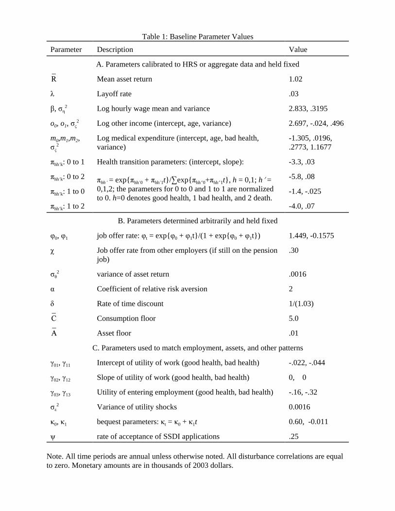
Table 1: Baseline Parameter Values

Parameter Description Value

A. Parameters calibrated to HRS or aggregate data and held fixed

Mean asset return 1.02

λ Layoff rate .03

β, ση2 Log hourly wage mean and variance 2.833, .3195

o0, o1, σς2 Log other income (intercept, age, variance) 2.697, -.024, .496

m0,m1,m2,σς2

Log medical expenditure (intercept, age, bad health,variance)

-1.305, .0196,.2773, 1.1677

πhhNk: 0 to 1 Health transition parameters: (intercept, slope):

πhhN = exp{πhhN0 + πhhN1t}/3exp{πhhO0+πhhO1t}, h = 0,1; hN =0,1,2; the parameters for 0 to 0 and 1 to 1 are normalizedto 0. h=0 denotes good health, 1 bad health, and 2 death.

-3.3, .03

πhhNk: 0 to 2 -5.8, .08

πhhNk: 1 to 0 -1.4, -.025

πhhNk: 1 to 2 -4.0, .07

B. Parameters determined arbitrarily and held fixed

φ0, φ1 job offer rate: φt = exp{φ0 + φ1t}/(1 + exp{φ0 + φ1t}) 1.449, -0.1575

χ Job offer rate from other employers (if still on the pensionjob)

.30

σθ2 variance of asset return .0016

α Coefficient of relative risk aversion 2

δ Rate of time discount 1/(1.03)

Consumption floor 5.0

Asset floor .01

C. Parameters used to match employment, assets, and other patterns

γ01, γ11 Intercept of utility of work (good health, bad health) -.022, -.044

γ02, γ12 Slope of utility of work (good health, bad health) 0, 0

γ03, γ13 Utility of entering employment (good health, bad health) -.16, -.32

σε2 Variance of utility shocks 0.0016

κ0, κ1 bequest parameters: κt = κ0 + κ1t 0.60, -0.011

ψ rate of acceptance of SSDI applications .25

Note. All time periods are annual unless otherwise noted. All disturbance correlations are equalto zero. Monetary amounts are in thousands of 2003 dollars.

Table 2: The Distribution of the change in the logarithm of consumption at the time of labor force exit

SimulationCAMS Data:RetirementAll exits Retirement

mean -.019 -.011 -.120

90th percentile .018 .018 0

75th percentile .008 .008 0

median .002 .003 0

25th percentile -.006 0 -.250

10th percentile -.155 -.150 -.400

Percent < 0 37 22 45

mean if < 0 -.094 -.157 -.304

median if < 0 -.012 -.124 -.300

sample size 10,441 4,011 790

Note. The sample in the second column contains simulated individuals who worked for at leastthree consecutive periods, left employment, and remained non-employed for at least threeconsecutive periods as of age 67. The CAMS sample in the third column includes non-Hispanicwhite married men with a high school diploma and no college attendance, born from 1921-1950.

Table 3: Robustness analysis of the change in consumption at the time of labor force exit

Specification All Retirement

mean median mean median

Baseline -.019 .002 -.011 .003

Nonhousing assets -.027 -.003 -.016 0

financial assets -.052 -.011 -.033 -.007

no bequest motive -.099 -.041 -.076 .001

Full time and part time -.014 .0 -.007 .004

CRRA (α) = 0 -.769 -.685 -.599 -.555

CRRA = 1 -.016 .005 -.007 .006

CRRA = 3 -.008 .002 -.006 .002

CRRA = 4 -.006 0 -.002 .002

Time preference = .00 -.010 .006 -.005 .006

Time preference = .06 -.022 -.003 -.013 -.002

Time preference = .09 -.029 -.003 -.020 -.004

Variance of return shock σθ2 = 0 -.022 .003 -.017 .006

σθ2 = .0032 -.016 0 -.010 .001

Variance of wage shock ση2 = 0 -.007 .0 .007 .003

ση2 = .639 -.025 .002 -.021 .004

Job offer rate φt = 1 -.021 .003 -.008 .004

φt = 0 -.016 .003 -.013 .003

Consumption floor = 1 -.018 .002 -.010 .003

Consumption floor = 10 -.019 .002 -.011 .003Note. The baseline specification is the one shown in Table 1: CRRA (α) = 2; rate of timepreference = .03; variance of the return shock (σθ2) = .0016; variance of the log wage shockση2=.3195; job offer parameters φ0=1.449, φ1=-.1575, with φt = exp{φ0 + φ1t}/(1 + exp{φ0 +φ1t}), and =5. The sample in the last two columns contains simulated individuals who workedfor at least three consecutive periods, left employment, and remained non-employed for at leastthree consecutive periods as of age 67. In the specification with full time and part timeemployment, the cases shown are for movement from full time to not employed. See Table 1 forthe parameters used in the simulation.

Figure Titles

Figure 1: Employment rate by age

Figure 2: Two year entry rate to employment by age

Figure 3: Two year exit rate from employment by age

Figure 4: Cumulative distribution of age of OASI entitlement

Figure 5: Enrollment rate in SSDI by age

Figure 6: Cumulative distribution of age of pension entitlement

Figure 7: Median assets by age

Figure 8: Median total household income by age

Figure 9: Median consumption by age

Figure 10: Change in log consumption at labor force exit

Figure 11: Mean consumption path by employment sequence

Figure 12: Median consumption path by employment sequence

Figure 13: Mean consumption path with no uncertainty

Figure 14: Change in log consumption at labor force exit in stochastic retirement model

Figure 15: Change in log consumption at retirement by expected gain from retirement (EG)

Figure 16: Change in log consumption at retirement by wealth

0.2

.4.6

.8pr

obab

ility

50 60 70 80age

data simulation

0.2

.4.6

prob

abilit

y

50 60 70 80age

data simulation

0.2

.4.6

prob

abilit

y

50 55 60 65 70 75age

data simulation

.2.4

.6.8

1pr

obab

ility

60 65 70 75age

data simulation

0.2

.4.6

prob

abilit

y

50 55 60 65age

data simulation

0.0

2.0

4.0

6.0

8.1

prob

abilit

y

50 55 60 65age

data simulation

010

020

030

0

50 60 70 80 90 100age

data simulation

2030

4050

6070

50 60 70 80 90 100age

data simulation

2530

3540

$000

50 60 70 80age

data simulation

-.06

-.04

-.02

0.0

2

50 60 70 80age

mean median

2530

3540

$000

50 55 60 65 70 75age

2530

3540

$000

50 55 60 65 70 75age

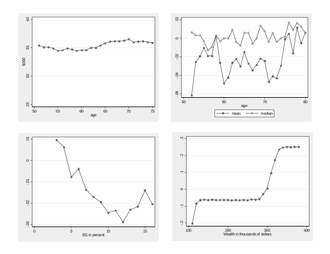
2530

3540

$000

50 55 60 65 70 75age

-.06

-.04

-.02

0.0

2

50 60 70 80age

mean median

-.03

-.02

-.01

0.0

1

0 5 10 15EG in percent

-.2-.1

0.1

.2.3

100 200 300 400Wealth in thousands of dollars