Rethinking Space-Time Networkswith Improved Memory Coverage forEfficient Video Object Segmentation

Ho Kei Cheng†University of IllinoisUrbana-Champaign

hokeikc2@illinois.edu

Yu-Wing TaiKuaishou

Technologyyuwing@gmail.com

Chi-Keung TangThe Hong Kong University of

Science and Technologycktang@cs.ust.hk

Abstract

This paper presents a simple yet effective approach to modeling space-time cor-respondences in the context of video object segmentation. Unlike most existingapproaches, we establish correspondences directly between frames without re-encoding the mask features for every object, leading to a highly efficient and robustframework. With the correspondences, every node in the current query frame isinferred by aggregating features from the past in an associative fashion. We castthe aggregation process as a voting problem and find that the existing inner-productaffinity leads to poor use of memory with a small (fixed) subset of memory nodesdominating the votes, regardless of the query. In light of this phenomenon, wepropose using the negative squared Euclidean distance instead to compute theaffinities. We validate that every memory node now has a chance to contribute,and experimentally show that such diversified voting is beneficial to both memoryefficiency and inference accuracy. The synergy of correspondence networks anddiversified voting works exceedingly well, achieves new state-of-the-art results onboth DAVIS and YouTubeVOS datasets while running significantly faster at 20+FPS for multiple objects without bells and whistles.

1 Introduction

Video object segmentation (VOS) aims to identify and segment target instances in a video sequence.This work focuses on the semi-supervised setting where the first-frame segmentation is given andthe algorithm needs to infer the segmentation for the remaining frames. This task is an extensionof video object tracking [1, 2], requiring detailed object masks instead of simple bounding boxes.A high-performing algorithm should be able to delineate an object from the background or otherdistractors (e.g., similar instances) under partial or complete occlusion, appearance changes, andobject deformation [3].

Most current methods either fit a model using the initial segmentation [4, 5, 6, 7, 8, 9] or leveragetemporal propagation [10, 11, 12, 13, 14, 15, 16], particularly with spatio-temporal matching [17,18, 19, 20, 21, 22, 23, 24, 25, 26, 27]. Space-Time Memory networks [18] are especially popularrecently due to its high performance and simplicity – many variants [16, 21, 22, 23, 24, 28, 29, 30],including competitions’ winners [31, 32], have been developed to improve the speed, reduce memoryusage, or to regularize the memory readout process of STM.

In this work, we aim to subtract from STM to arrive at a minimalistic form of matching networks,dubbed Space-Time Correspondence Network (STCN) 1. Specifically, we start from the basic premise

†This work was done in The Hong Kong University of Science and Technology.1Training/inference code and pretrained models: https://github.com/hkchengrex/STCN

35th Conference on Neural Information Processing Systems (NeurIPS 2021).

arX

iv:2

106.

0521

0v2

[cs

.CV

] 8

Oct

202

1

that correspondences are target-agnostic. Instead of building a specific memory bank and thereforeaffinity for every object in the video as in STM, we build a single affinity matrix using only RGBrelations. For querying, each target object passes through the same affinity matrix for feature transfer.This is not only more efficient but also more robust – the model is forced to learn all object relationsbeyond just the labeled ones. With the learned affinity, the algorithm can propagate features from thefirst frame to the rest of the video sequence, with intermediate features stored as memory.

While STCN already reaches state-of-the-art performance and speed in this simple form, we furtherprobe into the inner workings of the construction of affinities. Traditionally, affinities are constructedfrom dot products followed by a softmax as in attention mechanisms [18, 33]. This however implicitlyencoded “confidence” (magnitude) with high-confidence points dominating the affinities all the time,regardless of query features. Some memory nodes will therefore be always suppressed, and the (large)memory bank will be underutilized, reducing effective diversity and robustness. We find this to beharmful, and propose using the negative squared Euclidean distance as a similarity measure with anefficient implementation instead. Though simple, this small change ensures that every memory nodehas a chance to contribute significantly (given the right query), leading to better performance, higherrobustness, and more efficient use of memory.

Our contribution is three-fold:

• We propose STCN with direct image-to-image correspondence that is simpler, more efficient,and more effective than STM.

• We examine the affinity in detail, and propose using L2 similarity in place of dot product fora better memory coverage, where every memory node contributes instead of just a few.

• The synergy of the above two results in a simple and strong method, which suppressesprevious state-of-the-art performance without additional complications while running fast at20+ FPS.

2 Related Works

Correspondence Learning Finding correspondences is one of the most fundamental problems incomputer vision. Local correspondences have been used heavily in optical flow [34, 35, 36] and objecttracking [37, 38, 39] with fast running time and high performance. More explicit correspondencelearning has also been achieved with deep learning [40, 41, 42].

Few-shots learning can be considered as a matching problem where the query is compared with everyelement in the support set [43, 44, 45, 46]. Typical approaches use a Siamese network [47] and com-pare the embedded query/support features using a similarity measure such as cosine similarity [43],squared Euclidean distance [48], or even a learned function [49]. Our task can also be formulated as afew-shots problem, where our memory bank acts as the support set. This connection helps us with thechoice of similarity function, albeit we are dealing with a million times more pointwise comparisons.

Video Object Segmentation Early VOS methods [4, 5, 50] employ online first-frame finetuningwhich is very slow in inference and have been gradually phased out. Faster approaches have been pro-posed such as a more efficient online learning algorithm [6, 7, 8], MRF graph inference [51], temporalCNN [52], capsule routing [53], tracking [11, 13, 15, 54, 55, 56, 57], embedding learning [10, 58, 59]and space-time matching [17, 18, 19, 20]. Embedding learning bears a high similarity to space-timematching, both attempting to learn a deep feature representation of an object that remains consistentacross a video. Usually embedding learning methods are more constrained [10, 58], adopting localsearch window and hard one-to-one matching.

We are particularly interested in the class of Space-Time Memory networks (STM) [18] which arethe backbone for many follow-up state-of-the-art VOS methods. STM constructs a memory bank foreach object in the video, and matches every query frame to the memory bank to perform “memoryreadout”. Newly inferred frames can be added to the memory, and then the algorithm propagatesforward in time. Derivatives either apply STM at other tasks [21, 60], improve the training data oraugmentation policy [21, 22], augment the memory readout process [16, 21, 22, 24, 28], use opticalflow [29], or reduce the size of the memory bank by limiting its growth [23, 30]. MAST [61] isan adjacent research that focused on unsupervised learning with a photometric reconstruction loss.Without the input mask, they use Siamese networks on RGB images to build the correspondenceout of necessity. In this work, we deliberately build such connections and establish that building

2

correspondences between images is a better choice, even when input masks are available, rather thana concession.

We propose to overhaul STM into STCN where the construction of affinity is redefined to be betweenframes only. We also take a close look at the similarity function, which has always been the dotproduct in all STM variants, make changes and comparisons according to our findings. The resultantframework is both faster and better while still principled. STCN is even fundamentally simpler thanSTM, and we hope that STCN can be adopted as the new and efficient backbone for future works.

3 Space-Time Correspondence Networks (STCN)

Given a video sequence and the first-frame annotation, we process the frames sequentially andmaintain a memory bank of features. For each query frame, we extract a key feature which iscompared with the keys in the memory bank, and retrieve corresponding value features from memoryusing key affinities as in STM [18].

Memory Encoder

Query Encoder

Memory Encoder

Memory Encoder

𝑘1𝑀 𝑘2

𝑀 𝑘3𝑀𝑘𝑄

AffinityAffinity

Affinity

Decoder

𝑣1𝑀 𝑣2

𝑀 𝑣3𝑀

Decoder DecoderSkip-Connection

Query Memory

Affinity path

Decoding path

Key Encoder

Key Encoder

𝑘𝑀𝑘𝑄

Affinity

DecoderSkip-Connection

Light Value Encoder

Light Value Encoder

Light Value Encoder

Decoder Decoder

Featurereuse

Query Memory

𝑣1𝑀 𝑣2

𝑀 𝑣3𝑀

(a) STM and variants (b) STCN (Ours)[18, 21, 22, 23, 24, 28, 29, 30]

Figure 1: Left: The general framework of the popularly used Space-Time Memory (STM) networks,ignoring fine-level variations. Objects are encoded separately, and affinities are specific to each object.Right: Our proposed Space-Time Correspondence Networks (STCN). We use Siamese key encodersto compute affinity directly from RGB images, making it more robust and efficient. Note that thequery key can be cached and reused later as a memory key (unlike in STM) as it is independent of themask.

3.1 Feature Extraction

Figure 1 illustrates the overall flow of STCN. While STM [18] parameterizes a Query Encoder (imageas input) and a Memory Encoder (image and mask as input) with two ResNet50 [62], we insteadconstruct a Key Encoder (image as input) and a Value Encoder (image and mask as input) with aResNet50 and a ResNet18 respectively. Thus, unlike in STM [18], the key features (and thus theresultant affinity) can be extracted independently without the mask, computed only once for eachframe, and symmetric between memory and query.2 The rationales are 1) Correspondences (keyfeatures) are more difficult to extract than value, hence a deeper network, and 2) Correspondencesshould exist between frames in a video, and there is little reason to introduce the mask as a distraction.From another perspective, we are using a Siamese structure [47] which is widely adopted in few-shotslearning [49, 63] for computing the key features, as if our memory bank is the few-shots support set.As the key features are independent of the mask, we can reuse the “query key” later as a “memorykey” if we decide to turn the query frame into a memory frame during propagation (strategy to bediscussed in Section 3.3). This means the key encoder is used exactly once per image in the entireprocess, despite the two appearances in Figure 1 (which is for brevity).

2That is, matching between two points does not depend on whether they are query or memory points (nottrue in STM [18] as they are from different encoders).

3

Architecture. Following the STM practice [18], we take res4 features with stride 16 from the baseResNets as our backbone features and discard res5. A 3×3 convolutional layer without non-linearityis used as a projection head from the backbone feature to either the key space (Ck dimensional) orthe value space (Cv dimensional). We set Cv to be 512 following STM and discuss the choice of Ck

in Section 4.1.

Feature reuse. As seen from Figure 1, both the key encoder and the value encoder are processingthe same frame, albeit with different inputs. It is natural to reuse features from the key encoder (withfewer inputs and a deeper network) at the value encoder. To avoid bloating the feature dimensionsand for simplicity, we concatenate the last layer features from both encoders (before the projectionhead) and process them with two ResBlocks [62] and a CBAM block3 [64] as the final value output.

3.2 Memory Reading and Decoding

Given T memory frames and a query frame, the feature extraction step would generate the followings:memory key kM ∈ RCk×THW , memory value vM ∈ RCv×THW , and query key kQ ∈ RCk×HW ,whereH andW are (stride 16) spatial dimensions. Then, for any similarity measure c : RCk×RCk →R, we can compute the pairwise affinity matrix S and the softmax-normalized affinity matrix W,where S,W ∈ RTHW×HW with:

Sij = c(kMi ,k

Qj ) Wij =

exp (Sij)∑n (exp (Snj))

, (1)

where ki denotes the feature vector at the i-th position. The similarities are normalized by√Ck as in

standard practice [18, 33] and is not shown for brevity. In STM [18], the dot product is used as c.Memory reading regularization like KMN [22] or top-k filtering [21] can be applied at this step.

With the normalized affinity matrix W, the aggregated readout feature vQ ∈ RCv×HW for thequery frame can be computed as a weighted sum of the memory features with an efficient matrixmultiplication:

vQ = vMW, (2)which is then passed to the decoder for mask generation.

In the case of multi-object segmentation, only Equation 2 has to be repeated as W is defined betweenimage features only, and thus is the same for different objects. In the case of STM [18], W must berecomputed instead. Detailed running time analysis can be found in Section 6.2.

Decoder. Our decoder structure stays close to that of the STM [18] as it is not the focus of this paper.Features are processed and upsampled at a scale of two gradually with higher-resolution featuresfrom the key encoder incorporated using skip-connections. The final layer of the decoder produces astride 4 mask which is bilinearly upsampled to the original resolution. In the case of multiple objects,soft aggregation [18] of the output masks is used.

3.3 Memory Management

So far we have assumed the existence of a memory bank of size T . Here, we will describe theconstruction of the memory bank. For each memory frame, we store two items: memory key andmemory value. Note that all memory frames (except the first one) are once query frames. The memorykey is simply reused from the query key, as described in Section 3.1 without extra computation. Thememory value is computed after mask generation of that frame, independently for each object as thevalue encoder takes both the image and the object mask as inputs.

STM [18] consider every fifth query frame as a memory frame, and the immediately previous frameas a temporary memory frame to ensure accurate matching. In the case of STCN, we find that it isunnecessary, and in fact harmful, to include the last frame as temporary memory. This is a directconsequence of using shared key encoders – 1) key features are sufficiently robust to match wellwithout the need for close-range (temporal) propagation, and 2) the temporary memory key wouldotherwise be too similar to that of the query, as the image context usually changes smoothly and we donot have the encoding noises resultant from distinct encoders, leading to drifting.4 This modificationalso reduces the number of calls to the value encoder, contributing a significant speedup.

3We find this block to be non-essential in a later experiment but it is kept for consistency.4This effect is amplified by the use of L2 similarity. See the supplementary material for a full comparison.

4

Table 1: Performance comparison between STM and STCN under different memory configurationson the DAVIS 2017 validation set [65].

STM STCN

Every 5th + Last Every 5th only Every 5th + Last Every 5th only

J&F 82.7 81.0 83.1 85.4FPS 12.3 16.7 15.4 20.2

Table 1 tabulates the performance comparisons between STM and STCN. For a video of length Lwith m ≥ 1 objects, and a final memory bank of size T < L, STM [18] would need to invoke thememory encoder and compute the affinity mL times. Our proposed STCN, on the other hand, onlyinvokes the value encoder mT times and computes the affinity L times. It is therefore evident thatSTCN is significantly faster. Section 6.2 provides a breakdown of running time.

4 Computing Affinity

The similarity function c : RCk × RCk → R plays a crucial role in both STM and STCN, as itsupports the construction of affinity that is central to both correspondences and memory reading. Italso has to be fast and memory-efficient as there can be up to 50M pairwise relations (THW ×HW )to compute for just one query frame.

To recap, we need to compute the similarity between a memory key kM ∈ RCk×HW and a querykey kQ ∈ RCk×HW . The resultant pairwise affinity matrix is denoted as S ∈ RTHW×HW , withSij = c(kM

i ,kQj ) denoting the similarity between kM

i (the memory feature vector at the i-th position)and kQ

j (the query feature vector at the j-th position).

In the case of dot product, it can be implemented very efficiently with a matrix multiplication:

Sdotij = kM

i · kQj ⇒ Sdot =

(kM)T

kQ (3)

In the following, we will also discuss the use of cosine similarity and negative squared Euclideandistance as similarity functions. They are defined as (with efficient implementation discussed later):

Scosij =

kMi · k

Qj∥∥kM

i

∥∥2×∥∥kQ

j

∥∥2

SL2ij = −

∥∥∥kMi − kQ

j

∥∥∥22

(4)

For brevity, we will use the shorthand “L2” or “L2 similarity” to denote the negative squaredEuclidean distance in the rest of the paper. The ranges for dot product, cosine similarity and L2similarity are (−∞,∞), [−1, 1], and (−∞, 0] respectively. Note that cosine similarity has a limitedrange. Non-related points are encouraged to have a low similarity score through back-propagationsuch that they have a close-to-zero affinity (Eq. 1), and thus no value is propagated (Eq. 2).

4.1 A Closer Look at the Affinity

The affinity matrix is core to STCN and deserves close attention. Previous works [18, 21, 22, 23, 24],almost by default, use the dot product as the similarity function – but is this a good choice?

Cosine similarity computes the angle between two vectors and is often regarded as the normalizeddot product. Reversely, we can consider dot product as a scaled version of cosine similarity, with thescale equals to the product of vectors’ norms. Note that this is query-agnostic, meaning that everysimilarity with a memory key kM

i will be scaled by its norm. If we cast the aggregation process(Eq. 2) as voting with similarity representing the weights, memory keys with large magnitudes willpredominately suppress any representation from other memory nodes.

5

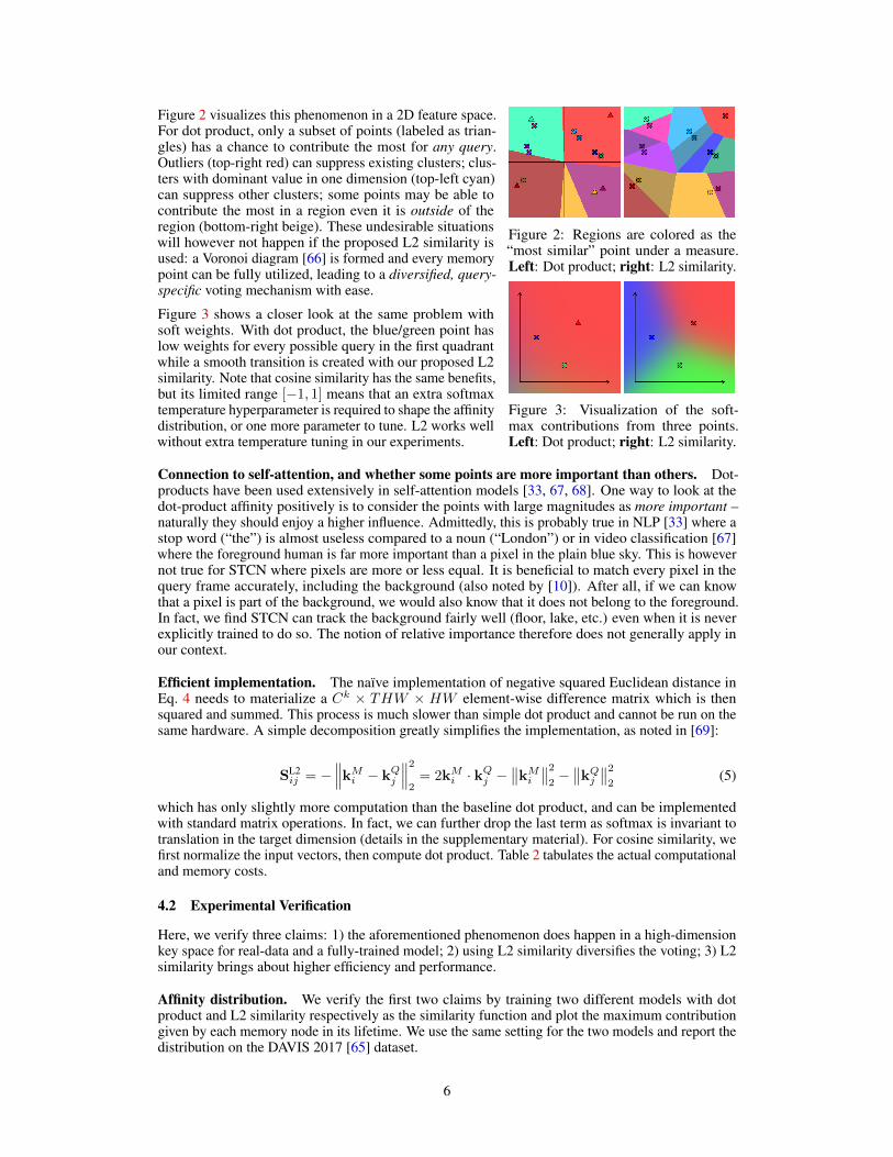
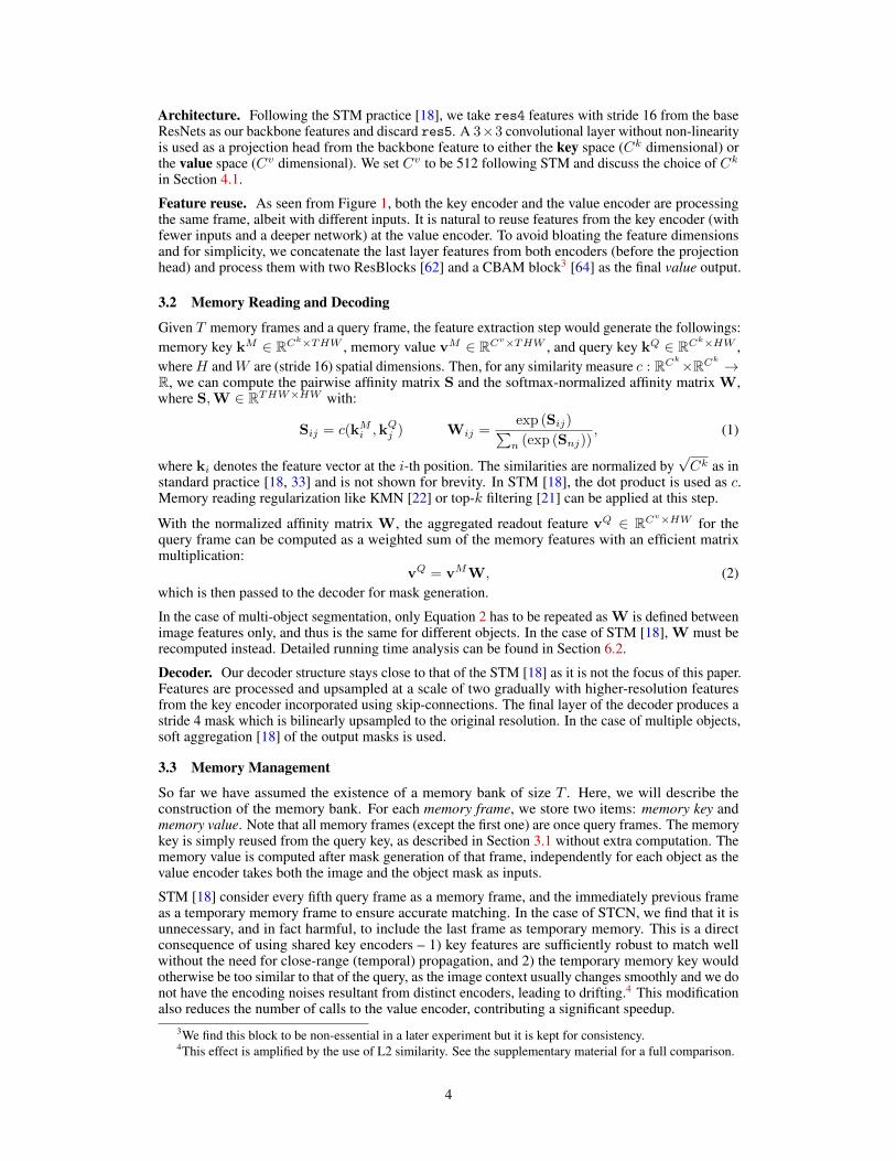
Figure 2: Regions are colored as the“most similar” point under a measure.Left: Dot product; right: L2 similarity.

Figure 2 visualizes this phenomenon in a 2D feature space.For dot product, only a subset of points (labeled as trian-gles) has a chance to contribute the most for any query.Outliers (top-right red) can suppress existing clusters; clus-ters with dominant value in one dimension (top-left cyan)can suppress other clusters; some points may be able tocontribute the most in a region even it is outside of theregion (bottom-right beige). These undesirable situationswill however not happen if the proposed L2 similarity isused: a Voronoi diagram [66] is formed and every memorypoint can be fully utilized, leading to a diversified, query-specific voting mechanism with ease.

Figure 3: Visualization of the soft-max contributions from three points.Left: Dot product; right: L2 similarity.

Figure 3 shows a closer look at the same problem withsoft weights. With dot product, the blue/green point haslow weights for every possible query in the first quadrantwhile a smooth transition is created with our proposed L2similarity. Note that cosine similarity has the same benefits,but its limited range [−1, 1] means that an extra softmaxtemperature hyperparameter is required to shape the affinitydistribution, or one more parameter to tune. L2 works wellwithout extra temperature tuning in our experiments.

Connection to self-attention, and whether some points are more important than others. Dot-products have been used extensively in self-attention models [33, 67, 68]. One way to look at thedot-product affinity positively is to consider the points with large magnitudes as more important –naturally they should enjoy a higher influence. Admittedly, this is probably true in NLP [33] where astop word (“the”) is almost useless compared to a noun (“London”) or in video classification [67]where the foreground human is far more important than a pixel in the plain blue sky. This is howevernot true for STCN where pixels are more or less equal. It is beneficial to match every pixel in thequery frame accurately, including the background (also noted by [10]). After all, if we can knowthat a pixel is part of the background, we would also know that it does not belong to the foreground.In fact, we find STCN can track the background fairly well (floor, lake, etc.) even when it is neverexplicitly trained to do so. The notion of relative importance therefore does not generally apply inour context.

Efficient implementation. The naïve implementation of negative squared Euclidean distance inEq. 4 needs to materialize a Ck × THW × HW element-wise difference matrix which is thensquared and summed. This process is much slower than simple dot product and cannot be run on thesame hardware. A simple decomposition greatly simplifies the implementation, as noted in [69]:

SL2ij = −

∥∥∥kMi − kQ

j

∥∥∥22= 2kM

i · kQj −

∥∥kMi

∥∥22−∥∥kQ

j

∥∥22

(5)

which has only slightly more computation than the baseline dot product, and can be implementedwith standard matrix operations. In fact, we can further drop the last term as softmax is invariant totranslation in the target dimension (details in the supplementary material). For cosine similarity, wefirst normalize the input vectors, then compute dot product. Table 2 tabulates the actual computationaland memory costs.

4.2 Experimental Verification

Here, we verify three claims: 1) the aforementioned phenomenon does happen in a high-dimensionkey space for real-data and a fully-trained model; 2) using L2 similarity diversifies the voting; 3) L2similarity brings about higher efficiency and performance.

Affinity distribution. We verify the first two claims by training two different models with dotproduct and L2 similarity respectively as the similarity function and plot the maximum contributiongiven by each memory node in its lifetime. We use the same setting for the two models and report thedistribution on the DAVIS 2017 [65] dataset.

6

0.0 0.2 0.4 0.6 0.8 1.0Have contribution weights more than

0

100

200

300

400

500

600

No. o

f mem

ory

node

s (K)

Dot productL2 similarity

Figure 4: The curves show the numberof memory nodes that have contributedabove a certain threshold at least once.

Figure 4 shows the pertinent distributions. Under the L2similarity measure, a lot more memory nodes contribute afair share. Specifically, around 3% memory nodes nevercontribute more than 1% weight under dot product whileonly 0.06% suffer the same fate with L2. Under dot product,31% memory nodes contribute less than 10% weight at bestwhile the same only happen for 7% of the memory withL2 similarity. To measure the distribution inequality, weadditionally compute the Gini coefficient [70] (the higher itis, the more unequal the distribution). The Gini coefficientfor dot product is 44.0, while the Gini coefficient for L2similarity is much lower at 31.8.

Performance and efficiency. Next, we show that using L2 similarity does improve performancewith negligible overhead. We compare three similarity measures: dot product, cosine similarity, andL2 similarity. For cosine similarity, we use a softmax temperature of 0.01 while a default temperatureof 1 is used for both dot product and L2 similarity. This scaling is crucial for cosine similarity onlysince it is the only one with a limited output range [−1, 1]. Searching for an extra hyperparameter iscomputationally demanding – we simply picked one that converges fairly quickly without collapsing.Table 2 tabulates the main results.

Interestingly, we find that reducing the key space dimension (Ck) is beneficial to both cosine similarityand L2 similarity but not dot product. This can be explained in the context of Section 4.1 – thenetwork needs more dimensions so that it can spread the memory key features out to save themfrom being suppressed by high-magnitude points. Cosine similarity and L2 similarity do not sufferfrom this problem and can utilize the full key space. The reduced key space in turn benefits memoryefficiency and improves running time.

Table 2: Performance comparison between different similarity functions and key space dimensionality(Ck) in STCN on the DAVIS 2017 validation set [65]. The number of floating-point operations(FLOPs) are computed for Eq. 3 and Eq. 4 only with T = 10. L2 works the best with a reduced keyspace and a small computational overhead.

Similarity function Ck J&F # FLOPs (G) Size of keys (MB)

Dot product 128 84.1 6.26 8.70Cosine similarity 128 82.6 6.26 8.70L2 similarity 128 85.0 6.33 8.70

Dot product 64 83.2 3.13 4.35Cosine similarity 64 83.4 3.13 4.35L2 similarity 64 85.4 3.20 4.35

5 Implementation Details

Models are trained with two 11GB 2080Ti GPUs with the Adam optimizer [71] using PyTorch [72].Following previous practices [18, 21], we first pretrain the model on static image datasets [73,74, 75, 76, 77] with synthetic deformation then perform main training on YouTubeVOS [78] andDAVIS [3, 65]. We also experimented with the synthetic dataset BL30K [79, 80] proposed in [21]which is not used unless otherwise specified. We use a batch size of 16 during pretraining and a batchsize of 8 during main training. Pre-training takes about 36 hours and main training takes around16 hours with batchnorm layers frozen during training following [18]. Bootstrapped cross entropy isused following [21]. The full set of hyperparameters can be found in the open-sourced code.

In each iteration, we pick three temporally ordered frames (with the ground-truth mask for the firstframe) from a video to form a training sample [18]. First, we predict the second frame using the firstframe as memory. The prediction will be saved as the second memory frame, and then the third framewill be predicted using the union of the first and the second frame. The temporal distance betweenthe frames will first gradually increase from 5 to 25 as a curriculum learning schedule and annealback to 5 towards the end of training. This process follows the implementation of MiVOS [21].

7

For memory-read augmentation, we experimented with kernelized memory reading [22] and top-kfiltering [21]. We find that top-k works well universally and improves running time while kernelizedmemory reading is slower and does not always help. We find that k = 20 always works better forSTCN (original paper uses k = 50) and we adopt top-k filtering in all our experiments with k = 20.For fairness, we also re-run all experiments in MiVOS [21] with k = 20, and pick the best result intheir favor. We use L2 similarity with Ck = 64 in all experiments unless otherwise specified.

For inference, a 2080Ti GPU is used with full floating point precision for a fair running timecomparison. We memorize every 5th frame and no temporary frame is used as discussed in Section 3.3.

6 ExperimentsWe mainly conduct experiments in the DAVIS 2017 validation [65] set and theYouTubeVOS 2018 [78] validation set. For completeness, we also include results in the singleobject DAVIS 2016 validation [3] set and the expanded YouTubeVOS 2019 [78] validation set.Results for the DAVIS 2017 test-dev [65] set are included in the supplementary material. We firstconduct quantitative comparisons with previous methods, and then analyze the running time for eachcomponent in STCN. For reference, we also present results without pretraining on stataic images.Ablation studies have been included in previous sections (Table 1 and Table 2).

6.1 EvaluationsTable 3 tabulates the comparisons of STCN with previous methods in semi-supervised video objectsegmentation benchmarks. For DAVIS 2017 [65], we compare the standard metrics: region similarityJ , contour accuracy F , and their average J&F . For YouTubeVOS [78], we report J and F for bothseen and unseen categories, and the averaged overall score G. For comparing the speed, we computethe multi-object FPS that is the total number of output frames divided by the total processing timefor the entire DAVIS 2017 [65] validation set. We either copy the FPS directly from papers/projectwebsites, or estimate based on their single object inference FPS (simply labeled as <5). We use 480presolution videos for both DAVIS and YouTubeVOS. Table 4, 5, 6, and 7 tabulate additional results.For the interactive setting, we replace the propagation module of MiVOS [21] with STCN.

Visualizations. Figure 6 visualizes the learned correspondences. Note that our correspondencesare general and mask-free, naturally associating every pixel (including background bystanders)even when it is only trained with foreground masks. Figure 7 visualizes our semi-supervised maskpropagation results with the last row being a failure case (Section 7).

Leaderboard results. Our method is also very competitive on the public VOS challengeleaderboard [78]. Methods on the leaderboard are typically cutting-edge, with engineering ex-tensions like deeper network, multi-scale inference, and model ensemble. They usually repre-sent the highest achievable performance at the time. On the latest YouTubeVOS 2019 validation

STM STCN0

10

20

30

40

50

60

70

80

Tim

e (m

s)

Memory/Value EncoderAffinity MatchingQuery/Key EncoderDecoder

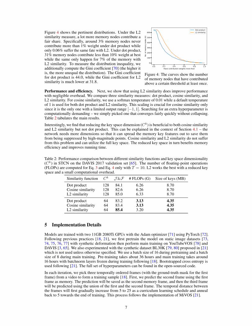
Figure 5: Average running timeof each component in STM andSTCN.

split [78], our base model (84.2 G) outperforms the previous chal-lenge winner [32] (based on STM [18], 82.0 G) by a large margin.With ensemble and multi-scale testing (details in the supplemen-tary material), our method is ranked first place (86.7 G) at the timeof submission on the still active leaderboard.

6.2 Running Time AnalysisHere, we analyze the running time of each component in STMand STCN on DAVIS 2017 [65]. For a fair comparison, we useour own implementation of STM, enabled top-k filtering [21], andset Ck = 64 for both methods such that all the speed improve-ments come from the fundamental differences between STM andSTCN. Our affinity matching time is lower because we computea single affinity between raw images while STM [18] computeone for every object. Our value encoder takes much less time thanthe memory encoder in STM [18] because of our light network,feature reuse, and robust memory bank/management as discussedin Section 3.3.

5A linear extrapolation would severally underestimate the performance of many previous methods.

8

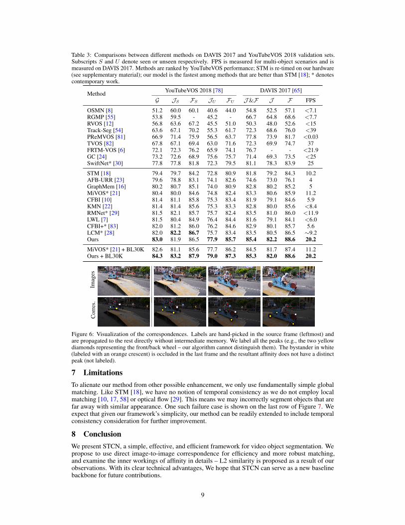
Table 3: Comparisons between different methods on DAVIS 2017 and YouTubeVOS 2018 validation sets.Subscripts S and U denote seen or unseen respectively. FPS is measured for multi-object scenarios and ismeasured on DAVIS 2017. Methods are ranked by YouTubeVOS performance; STM is re-timed on our hardware(see supplementary material); our model is the fastest among methods that are better than STM [18]; * denotescontemporary work.

Method YouTubeVOS 2018 [78] DAVIS 2017 [65]

G JS FS JU FU J&F J F FPS

OSMN [8] 51.2 60.0 60.1 40.6 44.0 54.8 52.5 57.1 <7.1RGMP [55] 53.8 59.5 - 45.2 - 66.7 64.8 68.6 <7.7RVOS [12] 56.8 63.6 67.2 45.5 51.0 50.3 48.0 52.6 <15Track-Seg [54] 63.6 67.1 70.2 55.3 61.7 72.3 68.6 76.0 <39PReMVOS [81] 66.9 71.4 75.9 56.5 63.7 77.8 73.9 81.7 <0.03TVOS [82] 67.8 67.1 69.4 63.0 71.6 72.3 69.9 74.7 37FRTM-VOS [6] 72.1 72.3 76.2 65.9 74.1 76.7 - - <21.9GC [24] 73.2 72.6 68.9 75.6 75.7 71.4 69.3 73.5 <25SwiftNet* [30] 77.8 77.8 81.8 72.3 79.5 81.1 78.3 83.9 25

STM [18] 79.4 79.7 84.2 72.8 80.9 81.8 79.2 84.3 10.2AFB-URR [23] 79.6 78.8 83.1 74.1 82.6 74.6 73.0 76.1 4GraphMem [16] 80.2 80.7 85.1 74.0 80.9 82.8 80.2 85.2 5MiVOS* [21] 80.4 80.0 84.6 74.8 82.4 83.3 80.6 85.9 11.2CFBI [10] 81.4 81.1 85.8 75.3 83.4 81.9 79.1 84.6 5.9KMN [22] 81.4 81.4 85.6 75.3 83.3 82.8 80.0 85.6 <8.4RMNet* [29] 81.5 82.1 85.7 75.7 82.4 83.5 81.0 86.0 <11.9LWL [7] 81.5 80.4 84.9 76.4 84.4 81.6 79.1 84.1 <6.0CFBI+* [83] 82.0 81.2 86.0 76.2 84.6 82.9 80.1 85.7 5.6LCM* [28] 82.0 82.2 86.7 75.7 83.4 83.5 80.5 86.5 ∼9.2Ours 83.0 81.9 86.5 77.9 85.7 85.4 82.2 88.6 20.2

MiVOS* [21] + BL30K 82.6 81.1 85.6 77.7 86.2 84.5 81.7 87.4 11.2Ours + BL30K 84.3 83.2 87.9 79.0 87.3 85.3 82.0 88.6 20.2

Imag

esC

orre

s.

Figure 6: Visualization of the correspondences. Labels are hand-picked in the source frame (leftmost) andare propagated to the rest directly without intermediate memory. We label all the peaks (e.g., the two yellowdiamonds representing the front/back wheel – our algorithm cannot distinguish them). The bystander in white(labeled with an orange crescent) is occluded in the last frame and the resultant affinity does not have a distinctpeak (not labeled).

7 LimitationsTo alienate our method from other possible enhancement, we only use fundamentally simple globalmatching. Like STM [18], we have no notion of temporal consistency as we do not employ localmatching [10, 17, 58] or optical flow [29]. This means we may incorrectly segment objects that arefar away with similar appearance. One such failure case is shown on the last row of Figure 7. Weexpect that given our framework’s simplicity, our method can be readily extended to include temporalconsistency consideration for further improvement.

8 ConclusionWe present STCN, a simple, effective, and efficient framework for video object segmentation. Wepropose to use direct image-to-image correspondence for efficiency and more robust matching,and examine the inner workings of affinity in details – L2 similarity is proposed as a result of ourobservations. With its clear technical advantages, We hope that STCN can serve as a new baselinebackbone for future contributions.

9

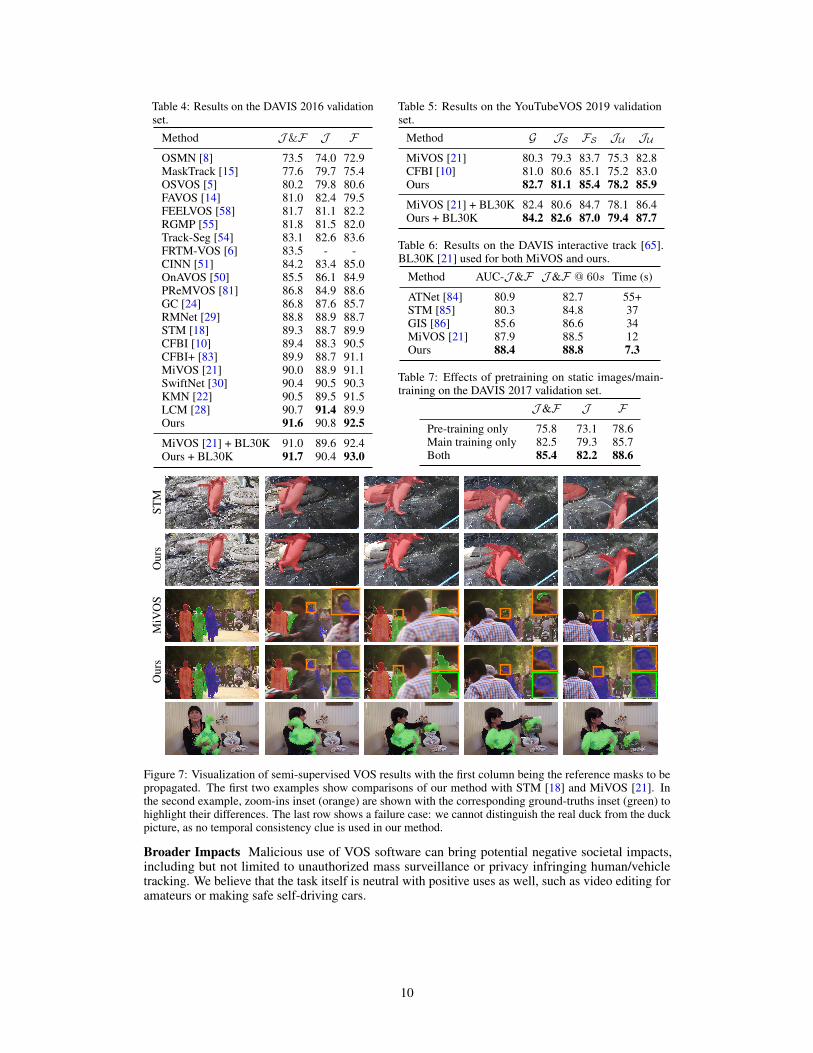
Table 4: Results on the DAVIS 2016 validationset.

Method J&F J FOSMN [8] 73.5 74.0 72.9MaskTrack [15] 77.6 79.7 75.4OSVOS [5] 80.2 79.8 80.6FAVOS [14] 81.0 82.4 79.5FEELVOS [58] 81.7 81.1 82.2RGMP [55] 81.8 81.5 82.0Track-Seg [54] 83.1 82.6 83.6FRTM-VOS [6] 83.5 - -CINN [51] 84.2 83.4 85.0OnAVOS [50] 85.5 86.1 84.9PReMVOS [81] 86.8 84.9 88.6GC [24] 86.8 87.6 85.7RMNet [29] 88.8 88.9 88.7STM [18] 89.3 88.7 89.9CFBI [10] 89.4 88.3 90.5CFBI+ [83] 89.9 88.7 91.1MiVOS [21] 90.0 88.9 91.1SwiftNet [30] 90.4 90.5 90.3KMN [22] 90.5 89.5 91.5LCM [28] 90.7 91.4 89.9Ours 91.6 90.8 92.5

MiVOS [21] + BL30K 91.0 89.6 92.4Ours + BL30K 91.7 90.4 93.0

Table 5: Results on the YouTubeVOS 2019 validationset.

Method G JS FS JU JU

MiVOS [21] 80.3 79.3 83.7 75.3 82.8CFBI [10] 81.0 80.6 85.1 75.2 83.0Ours 82.7 81.1 85.4 78.2 85.9

MiVOS [21] + BL30K 82.4 80.6 84.7 78.1 86.4Ours + BL30K 84.2 82.6 87.0 79.4 87.7

Table 6: Results on the DAVIS interactive track [65].BL30K [21] used for both MiVOS and ours.

Method AUC-J&F J&F @ 60s Time (s)

ATNet [84] 80.9 82.7 55+STM [85] 80.3 84.8 37GIS [86] 85.6 86.6 34MiVOS [21] 87.9 88.5 12Ours 88.4 88.8 7.3

Table 7: Effects of pretraining on static images/main-training on the DAVIS 2017 validation set.

J&F J FPre-training only 75.8 73.1 78.6Main training only 82.5 79.3 85.7Both 85.4 82.2 88.6

STM

Our

sM

iVO

SO

urs

Figure 7: Visualization of semi-supervised VOS results with the first column being the reference masks to bepropagated. The first two examples show comparisons of our method with STM [18] and MiVOS [21]. Inthe second example, zoom-ins inset (orange) are shown with the corresponding ground-truths inset (green) tohighlight their differences. The last row shows a failure case: we cannot distinguish the real duck from the duckpicture, as no temporal consistency clue is used in our method.

Broader Impacts Malicious use of VOS software can bring potential negative societal impacts,including but not limited to unauthorized mass surveillance or privacy infringing human/vehicletracking. We believe that the task itself is neutral with positive uses as well, such as video editing foramateurs or making safe self-driving cars.

10

Acknowledgment

This research is supported in part by Kuaishou Technology and the Research Grant Council of theHong Kong SAR under grant no. 16201818.

References[1] Anton Milan, Laura Leal-Taixé, Ian Reid, Stefan Roth, and Konrad Schindler. MOT16: A benchmark for

multi-object tracking. In arXiv preprint arXiv:1603.00831, 2016.

[2] Achal Dave, Tarasha Khurana, Pavel Tokmakov, Cordelia Schmid, and Deva Ramanan. Tao: A large-scalebenchmark for tracking any object. In European Conference on Computer Vision, 2020.

[3] Federico Perazzi, Jordi Pont-Tuset, Brian McWilliams, Luc Van Gool, Markus Gross, and AlexanderSorkine-Hornung. A benchmark dataset and evaluation methodology for video object segmentation. InCVPR, 2016.

[4] K-K Maninis, Sergi Caelles, Yuhua Chen, Jordi Pont-Tuset, Laura Leal-Taixé, Daniel Cremers, and LucVan Gool. Video object segmentation without temporal information. In PAMI, 2018.

[5] Sergi Caelles, Kevis-Kokitsi Maninis, Jordi Pont-Tuset, Laura Leal-Taixé, Daniel Cremers, and LucVan Gool. One-shot video object segmentation. In CVPR, 2017.

[6] Andreas Robinson, Felix Jaremo Lawin, Martin Danelljan, Fahad Shahbaz Khan, and Michael Felsberg.Learning fast and robust target models for video object segmentation. In CVPR, 2020.

[7] Goutam Bhat, Felix Järemo Lawin, Martin Danelljan, Andreas Robinson, Michael Felsberg, Luc Van Gool,and Radu Timofte. Learning what to learn for video object segmentation. In ECCV, 2020.

[8] Linjie Yang, Yanran Wang, Xuehan Xiong, Jianchao Yang, and Aggelos K Katsaggelos. Efficient videoobject segmentation via network modulation. In CVPR, 2018.

[9] Tim Meinhardt and Laura Leal-Taixé. Make one-shot video object segmentation efficient again. 2020.

[10] Zongxin Yang, Yunchao Wei, and Yi Yang. Collaborative video object segmentation by foreground-background integration. In ECCV, 2020.

[11] Won-Dong Jang and Chang-Su Kim. Online video object segmentation via convolutional trident network.In CVPR, 2017.

[12] Carles Ventura, Miriam Bellver, Andreu Girbau, Amaia Salvador, Ferran Marques, and Xavier Giro-i Nieto.Rvos: End-to-end recurrent network for video object segmentation. In CVPR, 2019.

[13] Qiang Wang, Li Zhang, Luca Bertinetto, Weiming Hu, and Philip HS Torr. Fast online object tracking andsegmentation: A unifying approach. In CVPR, 2019.

[14] Jingchun Cheng, Yi-Hsuan Tsai, Wei-Chih Hung, Shengjin Wang, and Ming-Hsuan Yang. Fast andaccurate online video object segmentation via tracking parts. In CVPR, 2018.

[15] Federico Perazzi, Anna Khoreva, Rodrigo Benenson, Bernt Schiele, and Alexander Sorkine-Hornung.Learning video object segmentation from static images. In CVPR, 2017.

[16] Xiankai Lu, Wenguan Wang, Danelljan Martin, Tianfei Zhou, Jianbing Shen, and Van Gool Luc. Videoobject segmentation with episodic graph memory networks. In ECCV, 2020.

[17] Yuan-Ting Hu, Jia-Bin Huang, and Alexander G Schwing. Videomatch: Matching based video objectsegmentation. In ECCV, 2018.

[18] Seoung Wug Oh, Joon-Young Lee, Ning Xu, and Seon Joo Kim. Video object segmentation usingspace-time memory networks. In ICCV, 2019.

[19] Xuhua Huang, Jiarui Xu, Yu-Wing Tai, and Chi-Keung Tang. Fast video object segmentation with temporalaggregation network and dynamic template matching. In CVPR, 2020.

[20] Ziqin Wang, Jun Xu, Li Liu, Fan Zhu, and Ling Shao. Ranet: Ranking attention network for fast videoobject segmentation. In ICCV, 2019.

[21] Ho Kei Cheng, Yu-Wing Tai, and Chi-Keung Tang. Modular interactive video object segmentation:Interaction-to-mask, propagation and difference-aware fusion. In CVPR, 2021.

11

[22] Hongje Seong, Junhyuk Hyun, and Euntai Kim. Kernelized memory network for video object segmentation.In ECCV, 2020.

[23] Yongqing Liang, Xin Li, Navid Jafari, and Jim Chen. Video object segmentation with adaptive featurebank and uncertain-region refinement. In NeurIPS, 2020.

[24] Yu Li, Zhuoran Shen, and Ying Shan. Fast video object segmentation using the global context module. InECCV, 2020.

[25] Yuan-Ting Hu, Jia-Bin Huang, and Alexander Schwing. Maskrnn: Instance level video object segmentation.In NIPS, 2017.

[26] Joakim Johnander, Martin Danelljan, Emil Brissman, Fahad Shahbaz Khan, and Michael Felsberg. Agenerative appearance model for end-to-end video object segmentation. In Proceedings of the IEEE/CVFConference on Computer Vision and Pattern Recognition, pages 8953–8962, 2019.

[27] Xiaoxiao Li and Chen Change Loy. Video object segmentation with joint re-identification and attention-aware mask propagation. In ECCV, 2018.

[28] Li Hu, Peng Zhang, Bang Zhang, Pan Pan, Yinghui Xu, and Rong Jin. Learning position and targetconsistency for memory-based video object segmentation. In CVPR, 2021.

[29] Haozhe Xie, Hongxun Yao, Shangchen Zhou, Shengping Zhang, and Wenxiu Sun. Efficient regionalmemory network for video object segmentation. 2021.

[30] Haochen Wang, Xiaolong Jiang, Haibing Ren, Yao Hu, and Song Bai. Swiftnet: Real-time video objectsegmentation. In CVPR, 2021.

[31] Peng Zhang, Li Hu, Bang Zhang, and Pan Pan. Spatial constrained memory network for semi-supervisedvideo object segmentation. CVPR Workshops, 2020.

[32] Zhishan Zhou, Lejian Ren, Pengfei Xiong, Yifei Ji, Peisen Wang, Haoqiang Fan, and Si Liu. Enhancedmemory network for video segmentation. In ICCV Workshops, 2019.

[33] Ashish Vaswani, Noam Shazeer, Niki Parmar, Jakob Uszkoreit, Llion Jones, Aidan N Gomez, LukaszKaiser, and Illia Polosukhin. Attention is all you need. In NIPS, 2017.

[34] Simon Baker and Iain Matthews. Lucas-kanade 20 years on: A unifying framework. 2004.

[35] Alexey Dosovitskiy, Philipp Fischer, Eddy Ilg, Philip Hausser, Caner Hazirbas, Vladimir Golkov, PatrickVan Der Smagt, Daniel Cremers, and Thomas Brox. Flownet: Learning optical flow with convolutionalnetworks. In ICCV, 2015.

[36] Deqing Sun, Xiaodong Yang, Ming-Yu Liu, and Jan Kautz. PWC-Net: CNNs for optical flow usingpyramid, warping, and cost volume. In CVPR, 2018.

[37] João F Henriques, Rui Caseiro, Pedro Martins, and Jorge Batista. High-speed tracking with kernelizedcorrelation filters. In PAMI, 2014.

[38] Luca Bertinetto, Jack Valmadre, Joao F Henriques, Andrea Vedaldi, and Philip HS Torr. Fully-convolutionalsiamese networks for object tracking. In ECCV, 2016.

[39] Bo Li, Junjie Yan, Wei Wu, Zheng Zhu, and Xiaolin Hu. High performance visual tracking with siameseregion proposal network. In CVPR, 2018.

[40] Jonathan Long, Ning Zhang, and Trevor Darrell. Do convnets learn correspondence? In NIPS, 2014.

[41] Kai Han, Rafael S Rezende, Bumsub Ham, Kwan-Yee K Wong, Minsu Cho, Cordelia Schmid, and JeanPonce. Scnet: Learning semantic correspondence. In ICCV, 2017.

[42] Ignacio Rocco, Relja Arandjelovic, and Josef Sivic. End-to-end weakly-supervised semantic alignment. InCVPR, 2018.

[43] Oriol Vinyals, Charles Blundell, Timothy Lillicrap, Koray Kavukcuoglu, and Daan Wierstra. Matchingnetworks for one shot learning. In NIPS, 2016.

[44] Qi Fan, Wei Zhuo, Chi-Keung Tang, and Yu-Wing Tai. Few-shot object detection with attention-rpn andmulti-relation detector. In CVPR, 2020.

12

[45] Christian Simon, Piotr Koniusz, Richard Nock, and Mehrtash Harandi. Adaptive subspaces for few-shotlearning. In CVPR, 2020.

[46] Kaixin Wang, Jun Hao Liew, Yingtian Zou, Daquan Zhou, and Jiashi Feng. Panet: Few-shot imagesemantic segmentation with prototype alignment. In ICCV, 2019.

[47] Jane Bromley, Isabelle Guyon, Yann LeCun, Eduard Säckinger, and Roopak Shah. Signature verificationusing a "siamese" time delay neural network. In NIPS, 1993.

[48] Jake Snell, Kevin Swersky, and Richard S Zemel. Prototypical networks for few-shot learning. In NIPS,2017.

[49] Flood Sung, Yongxin Yang, Li Zhang, Tao Xiang, Philip HS Torr, and Timothy M Hospedales. Learning tocompare: Relation network for few-shot learning. In CVPR, 2018.

[50] Paul Voigtlaender and Bastian Leibe. Online adaptation of convolutional neural networks for video objectsegmentation. In BMVC, 2017.

[51] Linchao Bao, Baoyuan Wu, and Wei Liu. Cnn in mrf: Video object segmentation via inference in acnn-based higher-order spatio-temporal mrf. In CVPR, 2018.

[52] Kai Xu, Longyin Wen, Guorong Li, Liefeng Bo, and Qingming Huang. Spatiotemporal cnn for videoobject segmentation. In CVPR, 2019.

[53] Kevin Duarte, Yogesh S. Rawat, and Mubarak Shah. Capsulevos: Semi-supervised video object segmenta-tion using capsule routing. In ICCV, 2019.

[54] Xi Chen, Zuoxin Li, Ye Yuan, Gang Yu, Jianxin Shen, and Donglian Qi. State-aware tracker for real-timevideo object segmentation. In CVPR, 2020.

[55] Seoung Wug Oh, Joon-Young Lee, Kalyan Sunkavalli, and Seon Joo Kim. Fast video object segmentationby reference-guided mask propagation. In CVPR, 2018.

[56] Lu Zhang, Zhe Lin, Jianming Zhang, Huchuan Lu, and You He. Fast video object segmentation viadynamic targeting network. In ICCV, 2019.

[57] Ping Hu, Gang Wang, Xiangfei Kong, Jason Kuen, and Yap-Peng Tan. Motion-guided cascaded refinementnetwork for video object segmentation. In CVPR, 2018.

[58] Paul Voigtlaender, Yuning Chai, Florian Schroff, Hartwig Adam, Bastian Leibe, and Liang-Chieh Chen.Feelvos: Fast end-to-end embedding learning for video object segmentation. In CVPR, 2019.

[59] Yuhua Chen, Jordi Pont-Tuset, Alberto Montes, and Luc Van Gool. Blazingly fast video object segmentationwith pixel-wise metric learning. In CVPR, 2018.

[60] Seoung Wug Oh, Joon-Young Lee, Ning Xu, and Seon Joo Kim. Space-time memory networks for videoobject segmentation with user guidance. 2020.

[61] Zihang Lai, Erika Lu, and Weidi Xie. Mast: A memory-augmented self-supervised tracker. In Proceedingsof the IEEE/CVF Conference on Computer Vision and Pattern Recognition, pages 6479–6488, 2020.

[62] Kaiming He, Xiangyu Zhang, Shaoqing Ren, and Jian Sun. Deep residual learning for image recognition.In CVPR, 2016.

[63] Gregory Koch, Richard Zemel, and Ruslan Salakhutdinov. Siamese neural networks for one-shot imagerecognition. In ICML deep learning workshop, 2015.

[64] Sanghyun Woo, Jongchan Park, Joon-Young Lee, and In So Kweon. Cbam: Convolutional block attentionmodule. In ECCV, 2018.

[65] Jordi Pont-Tuset, Federico Perazzi, Sergi Caelles, Pablo Arbeláez, Alexander Sorkine-Hornung, and LucVan Gool. The 2017 davis challenge on video object segmentation. In arXiv:1704.00675, 2017.

[66] Mark De Berg, Marc Van Kreveld, Mark Overmars, and Otfried Schwarzkopf. Computational geometry.In Computational geometry. Springer, 1997.

[67] Xiaolong Wang, Ross Girshick, Abhinav Gupta, and Kaiming He. Non-local neural networks. In CVPR,2018.

13

[68] Prajit Ramachandran, Niki Parmar, Ashish Vaswani, Irwan Bello, Anselm Levskaya, and Jonathon Shlens.Stand-alone self-attention in vision models. In NIPS, 2019.

[69] Hyunjik Kim, George Papamakarios, and Andriy Mnih. The lipschitz constant of self-attention. In arXivpreprint arXiv:2006.04710, 2020.

[70] Robert I Lerman and Shlomo Yitzhaki. A note on the calculation and interpretation of the gini index.Economics Letters, 15(3-4):363–368, 1984.

[71] Diederik P Kingma and Jimmy Ba. Adam: A method for stochastic optimization. In ICLR, 2015.

[72] Adam Paszke, Sam Gross, Francisco Massa, Adam Lerer, James Bradbury, Gregory Chanan, TrevorKilleen, Zeming Lin, Natalia Gimelshein, Luca Antiga, Alban Desmaison, Andreas Kopf, Edward Yang,Zachary DeVito, Martin Raison, Alykhan Tejani, Sasank Chilamkurthy, Benoit Steiner, Lu Fang, JunjieBai, and Soumith Chintala. Pytorch: An imperative style, high-performance deep learning library. In NIPS,2019.

[73] Lijun Wang, Huchuan Lu, Yifan Wang, Mengyang Feng, Dong Wang, Baocai Yin, and Xiang Ruan.Learning to detect salient objects with image-level supervision. In CVPR, 2017.

[74] Jianping Shi, Qiong Yan, Li Xu, and Jiaya Jia. Hierarchical image saliency detection on extended cssd. InTPAMI, 2015.

[75] Yi Zeng, Pingping Zhang, Jianming Zhang, Zhe Lin, and Huchuan Lu. Towards high-resolution salientobject detection. In ICCV, 2019.

[76] Ho Kei Cheng, Jihoon Chung, Yu-Wing Tai, and Chi-Keung Tang. Cascadepsp: Toward class-agnostic andvery high-resolution segmentation via global and local refinement. In CVPR, 2020.

[77] Xiang Li, Tianhan Wei, Yau Pun Chen, Yu-Wing Tai, and Chi-Keung Tang. Fss-1000: A 1000-class datasetfor few-shot segmentation. In CVPR, 2020.

[78] Ning Xu, Linjie Yang, Yuchen Fan, Dingcheng Yue, Yuchen Liang, Jianchao Yang, and Thomas Huang.Youtube-vos: A large-scale video object segmentation benchmark. In ECCV, 2018.

[79] Angel Xuan Chang, Thomas Funkhouser, Leonidas Guibas, Pat Hanrahan, Qixing Huang, Zimo Li, SilvioSavarese, Manolis Savva, Shuran Song, Hao Su, Jianxiong Xiao, Li Yi, and Fisher Yu. ShapeNet: AnInformation-Rich 3D Model Repository. In arXiv:1512.03012, 2015.

[80] Maximilian Denninger, Martin Sundermeyer, Dominik Winkelbauer, Youssef Zidan, Dmitry Olefir, Mo-hamad Elbadrawy, Ahsan Lodhi, and Harinandan Katam. Blenderproc. In arXiv:1911.01911, 2019.

[81] Jonathon Luiten, Paul Voigtlaender, and Bastian Leibe. Premvos: Proposal-generation, refinement andmerging for video object segmentation. In ACCV, 2018.

[82] Yizhuo Zhang, Zhirong Wu, Houwen Peng, and Stephen Lin. A transductive approach for video objectsegmentation. In CVPR, 2020.

[83] Zongxin Yang, Yunchao Wei, and Yi Yang. Collaborative video object segmentation by multi-scaleforeground-background integration. In PAMI, 2021.

[84] Yuk Heo, Yeong Jun Koh, and Chang-Su Kim. Interactive video object segmentation using global andlocal transfer modules. In ECCV, 2020.

[85] Seoung Wug Oh, Joon-Young Lee, Ning Xu, and Seon Joo Kim. Space-time memory networks for videoobject segmentation with user guidance. In TPAMI, 2020.

[86] Yuk Heo, Yeong Jun Koh, and Chang-Su Kim. Guided interactive video object segmentation usingreliability-based attention maps. In CVPR, 2021.

[87] Sergey Zagoruyko and Nikos Komodakis. Wide residual networks. BMVC, 2016.

[88] Liang-Chieh Chen, George Papandreou, Florian Schroff, and Hartwig Adam. Rethinking atrous convolutionfor semantic image segmentation. arXiv preprint arXiv:1706.05587, 2017.

[89] Fred L. Bookstein. Principal warps: Thin-plate splines and the decomposition of deformations. PAMI,1989.

14

A PyTorch-style Pseudocode

We first prove that the∥∥kQ

j

∥∥22

term will be canceled out in the subsequent softmax operation:

Wij =exp

(SL2

ij

)∑n exp

(SL2nj

)=

exp(2kM

i · kQj −

∥∥kMi

∥∥22−∥∥kQ

j

∥∥22

)∑

n exp(2kM

n · kQj − ‖kM

n ‖22 −

∥∥kQj

∥∥22

)=

exp(2kM

i · kQj −

∥∥kMi

∥∥22

)/ exp

(∥∥kQj

∥∥22

)∑

n exp(2kM

n · kQj − ‖kM

n ‖22

)/ exp

(∥∥kQj

∥∥22

)=

exp(2kM

i · kQj −

∥∥kMi

∥∥22

)∑

n exp(2kM

n · kQj − ‖kM

n ‖22

)Then, we show our efficient PyTorch [72] style implementation of Eq. 5.

Algorithm 1: L2 Similarity Computation// Input:// kM : Ck × THW// kQ : Ck ×HW// Returns:// S : THW ×HW

1 function GetSimilarity(kM, kQ)// Decomposing L2 distance into two parts: ab, a_sq// b_sq is canceled out as shown above.

2 ab← kM.transpose().matmul(kQ) // ab : THW ×HW3 a_sq← kM.pow(2).sum(dim=0).unsqueeze(dim=1) // a_sq : THW × 1

// This step utilizes broadcasting: dimensions of size 1 will beimplicitly expanded to match other tensors without extra memorycost

4 S← 2 ∗ ab− a_sq // S : THW ×HW5 return S

B Additional results on memory scheduling

Table 8 tabulates additional quantitative results of STM/STCN with dot product/L2 similarity underdifferent memory scheduling strategies.

1. With STM, there is a significant performance drop when the temporary frame is not usedregardless of the similarity function. This supports our claim that STM requires close-rangerelations for robust matching.

2. With STCN+dot product, the performance drop is slight. Note that by dropping the tempo-rary frame, we also enjoy a 31% increase in FPS as shown in the main paper. This supportsthat the STCN architecture provides more robust key features.

3. With STCN+L2 similarity, it performs the best when the temporary frame is not used (whilealso enjoying the 31% speed improvement). This suggests L2 similarity is more susceptibleto drifting when the memory scheduling is not carefully designed. Overall, L2 similarity isstill beneficial.

15

Table 8: Performance (J&F) of networks under different memory configurations on the DAVIS2017 validation set [65].

Every 5th + Last Every 5th only

STM + Dot product 83.3 81.3STM + L2 similarity 82.7 81.0STCN + Dot product 84.3 84.1STCN + L2 similarity 83.1 85.4

C DAVIS test-dev

The test-dev split of DAVIS 2017 is notably more difficult than the training or validation setwith rapid illumination changes and highly similar objects. As a result, methods with strong spatialconstraints like KMN [22] or CFBI [10] typically perform better (while still suffering a drop inperformance from validation to test-dev). Some would use additional engineering, such as using600p videos instead of the standard 480p [18, 22, 83].

Our baseline is severally punished for lacking spatial cues. BL30K helps a lot in this case but is stillnot enough to reach SOTA performance. We find that simply encoding memory more frequently, i.e.,every third frame instead of every fifth frame, can boost the performance of the model with extendedtraining to be above state-of-the-art on DAVIS test-dev. Admittedly, this comes with additionalcomputational and memory costs. Thanks to our efficient base model, STCN with increased memoryfrequency is still runnable on the same 11GB GPU and is the fastest among competitors. Table 9tabulates the comparison with other methods. FPS for methods that use 600p evaluation is estimatedfrom that of 480p (assuming linear scaling) unless given in their original paper.

Table 9: Comparisons between competitive methods on DAVIS 2017 test-dev [65]. M3 denotesincreased memory frequency. ∗ denotes 600p evaluation and † denotes the use of spatial cues – ourbaseline is severally punished for lacking it which is crucial in this particular data split. Subscriptarrow denotes changes from baseline. Some results are modified from the table in [83]. 6

Method DAVIS 2017 test-dev [65]

J&F J F FPS

OSMN [8] 41.3 37.3 44.9 <2.38OnAVOS [50] 56.5 53.4 59.6 <0.03RGMP [55] 52.9 51.3 54.4 <2.38FEELVOS [58] 57.8 55.2 60.5 <1.85PReMVOS [81] 71.6 67.5 75.7 <0.02STM ∗ [18] 72.2 69.3 75.2 6.5RMNet † [29] 75.0 71.9 78.1 <11.9CFBI ∗† [10] 76.6 73.0 80.1 2.9KMN ∗† [22] 77.2 74.1 80.3 <5.4CFBI+ ∗† [83] 78.0 74.4 81.6 3.4LCM † [28] 78.1 74.4 81.8 9.2MiVOS† [21] + BL30K 78.6 74.9 82.2 10.7

Ours 76.1 72.7 79.6 20.2Ours, M3 76.5↑0.4 73.1↑0.4 80.0↑0.4 14.6↓5.6Ours + BL30K 77.8↑1.7 74.3↑1.6 81.3↑1.7 20.2Ours + BL30K, M3 79.9↑3.8 76.3↑3.6 83.5↑3.9 14.6↓5.6

D Re-timing on Our Hardware

The inference speed of networks (even with the same architecture) can be influenced by implemen-tations, software package versions, or simply hardware. As we are mainly evolving STM [18] intoSTCN, we believe that it is just to re-time our re-implemented STM with our software and hardware

16

for a fair comparison. While the original paper reported 6.25 single-object FPS (which will onlybe slower for multi-object), we obtain 10.2 multi-object FPS which is reported in our Table 3. Webelieve this gives the proper acknowledgment that STM deserves.

E Multi-scale Testing and Ensemble

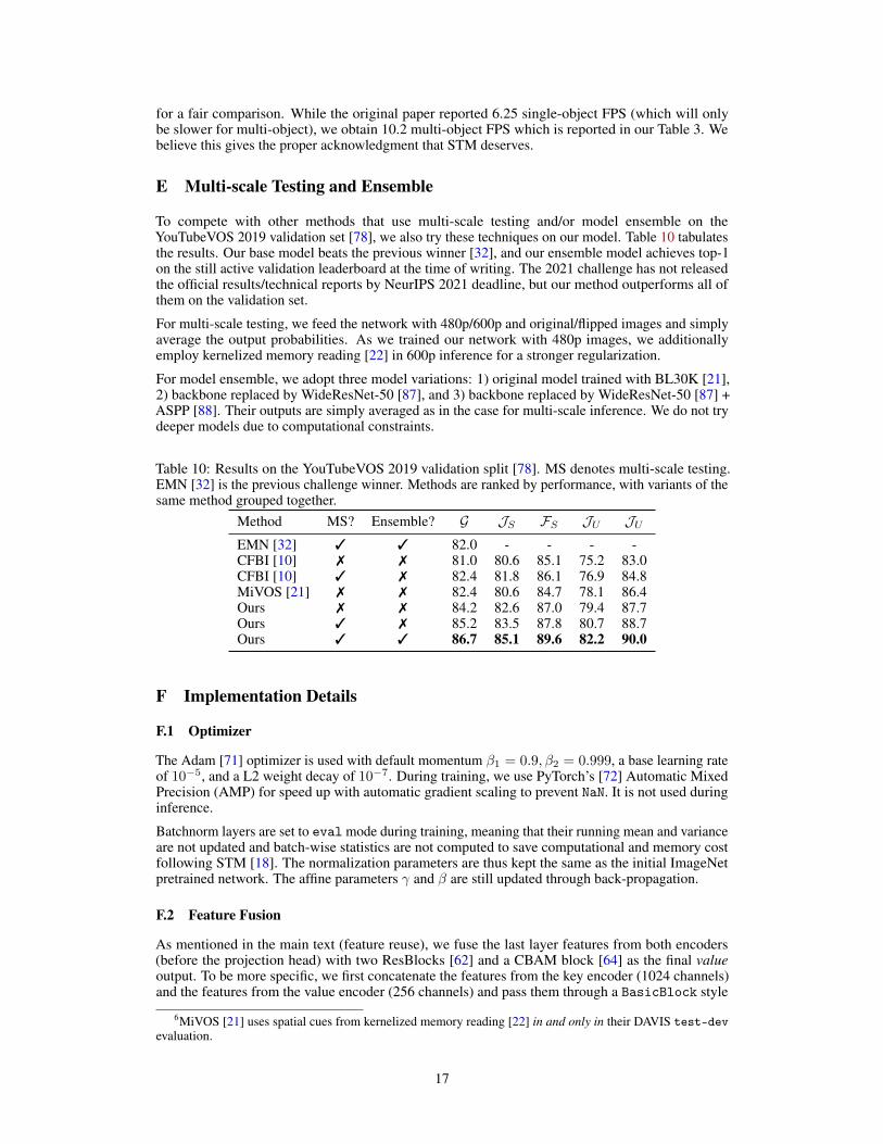
To compete with other methods that use multi-scale testing and/or model ensemble on theYouTubeVOS 2019 validation set [78], we also try these techniques on our model. Table 10 tabulatesthe results. Our base model beats the previous winner [32], and our ensemble model achieves top-1on the still active validation leaderboard at the time of writing. The 2021 challenge has not releasedthe official results/technical reports by NeurIPS 2021 deadline, but our method outperforms all ofthem on the validation set.

For multi-scale testing, we feed the network with 480p/600p and original/flipped images and simplyaverage the output probabilities. As we trained our network with 480p images, we additionallyemploy kernelized memory reading [22] in 600p inference for a stronger regularization.

For model ensemble, we adopt three model variations: 1) original model trained with BL30K [21],2) backbone replaced by WideResNet-50 [87], and 3) backbone replaced by WideResNet-50 [87] +ASPP [88]. Their outputs are simply averaged as in the case for multi-scale inference. We do not trydeeper models due to computational constraints.

Table 10: Results on the YouTubeVOS 2019 validation split [78]. MS denotes multi-scale testing.EMN [32] is the previous challenge winner. Methods are ranked by performance, with variants of thesame method grouped together.

Method MS? Ensemble? G JS FS JU JUEMN [32] 3 3 82.0 - - - -CFBI [10] 7 7 81.0 80.6 85.1 75.2 83.0CFBI [10] 3 7 82.4 81.8 86.1 76.9 84.8MiVOS [21] 7 7 82.4 80.6 84.7 78.1 86.4Ours 7 7 84.2 82.6 87.0 79.4 87.7Ours 3 7 85.2 83.5 87.8 80.7 88.7Ours 3 3 86.7 85.1 89.6 82.2 90.0

F Implementation Details

F.1 Optimizer

The Adam [71] optimizer is used with default momentum β1 = 0.9, β2 = 0.999, a base learning rateof 10−5, and a L2 weight decay of 10−7. During training, we use PyTorch’s [72] Automatic MixedPrecision (AMP) for speed up with automatic gradient scaling to prevent NaN. It is not used duringinference.

Batchnorm layers are set to eval mode during training, meaning that their running mean and varianceare not updated and batch-wise statistics are not computed to save computational and memory costfollowing STM [18]. The normalization parameters are thus kept the same as the initial ImageNetpretrained network. The affine parameters γ and β are still updated through back-propagation.

F.2 Feature Fusion

As mentioned in the main text (feature reuse), we fuse the last layer features from both encoders(before the projection head) with two ResBlocks [62] and a CBAM block [64] as the final valueoutput. To be more specific, we first concatenate the features from the key encoder (1024 channels)and the features from the value encoder (256 channels) and pass them through a BasicBlock style

6MiVOS [21] uses spatial cues from kernelized memory reading [22] in and only in their DAVIS test-devevaluation.

17

ResBlock with two 3× 3 convolutions which output a tensor with 512 channels. Batchnorm is notused. We maintain the channel size in the rest of the fusion block, and pass the tensor through aCBAM block [64] under the default setting and another BasicBlock style ResBlock.

F.3 Dataset

All the data augmentation strategies follow exactly from the open-sourced training code ofMiVOS [21] to avoid engineering distractions. They are mentioned here for completeness, butreaders are encouraged to look at the implementation directly.

F.3.1 Pre-training

We used ECSSD [74], FSS1000 [77], HRSOD [75], BIG [76], and both the training and testing set ofDUTS [73]. We downsized BIG and HRSOD images such that the longer edge has 512 pixels. Theannotations in BIG and HRSOD are of higher quality and thus they appear five times more often thanimages in other datasets. We use a batch size of 16 during the static image pretraining stage witheach data sample containing three synthetic frames augmented from the same image.

For augmentation, we first perform PyTorch’s random scaling of [0.8, 1.5], random horizontal flip,random color jitter of (brightness=0.1, contrast=0.05, saturation=0.05, hue=0.05),and random grayscale with a probability of 0.05 on the base image. Then, for each synthetic frame,we perform PyTorch’s random affine transform with rotation between [−20, 20] degrees, scalingbetween [0.9, 1.1], shearing between [−10, 10] degrees, and another color jitter of (brightness=0.1,contrast=0.05, saturation=0.05). The output image is resized such that the shorter side has alength of 384 pixels, and then a random crop of 384 pixels is taken. With a probability of 33%, theframe undergoes an additional thin-plate spline transform [89] with 12 randomly selected controlpoints whose displacements are drawn from a normal distribution with scale equals 0.02 times theimage dimension (384).

F.3.2 Main training

We use the training set of YouTubeVOS [78] and DAVIS [65] 480p in main training. All the imagesin YouTubeVOS are downsized such that shorter edge has 480 pixels, like those in the DAVIS 480pset. Annotations in DAVIS has a higher quality and they appear 5 times more often than videos inYouTubeVOS, following STM [18]. We use a batch size of 8 during main training with each datasample containing three temporally ordered frames from the same video.

For augmentation, we first perform PyTorch’s random horizontal flip, random resizedcrop with (crop_size=384, scale=(0.36, 1), ratio=(0.75, 1.25)), color jitter of(brightness=0.1, contrast=0.03, saturation=0.03), and random grayscale with a proba-bility of 0.05 for every image in the sequence with the same random seed such that every imageundergoes the same initial transformation. Then, for every image (with different random seed), we ap-ply another PyTorch’s color jitter of (brightness=0.01, contrast=0.01, saturation=0.01),random affine transformation with rotation between [−15, 15] degrees and shearing between [−10, 10]degrees. Finally, we pick at most two objects that appear on the first frame as target objects to besegmented.

F.3.3 BL30K training

BL30K [21] is a synthetic VOS dataset that can be used after static image pretraining and before maintraining. It allows the model to learn complex occlusion patterns that do not exist in static images(and the main training datasets are not large enough). The sampling and augmentation strategy isthe same as the ones in main training, except 1) cropping scale in the first random resized crop is(0.25, 1.0) instead of (0.36, 1.0) – this is because BL30K images are slightly larger and 2) we discardobjects that are tiny in the first frame (<100 pixels) as they are very difficult to learn and unavoidablein these synthetic data.

F.4 Training iteration and scheduling

By default, we first train on static images for 300K iterations then perform main training for 150Kiterations. When we use BL30K [21], we train for 500K iterations on it after static image pretraining

18

and before main training. Main training would be extended to 300K iterations to combat the domainshift caused by BL30K. Regular training without BL30K takes around 30 hours and extended trainingwith BL30K takes around 4 days in total.

With a base learning rate of 10−5, we apply step learning rate decay with a decay ratio of γ = 0.1.In static image pretraining, we perform decay once after 150K iterations. In standard (150K) maintraining, once after 125K iterations; in BL30K training, once after 450K iterations; in extended(300K) main training, once after 250K iterations. The learning rate scheduling is independent ofthe training stages, i.e., all training stages start with the base learning rate of 10−5 regardless of anypretraining.

As for curriculum learning mentioned in Section 5, we apply the same schedule as MiVOS [21]. Themaximum temporal distance between frames is set to be [5, 10, 15, 20, 25, 5] at the correspondingiterations of [0%, 10%, 20%, 30%, 40%, 90%] or [0%, 10%, 20%, 30%, 40%, 80%] of the total train-ing iterations for main training and BL30K respectively. A longer annealing time is used for BL30Kbecause it is relatively harder.

F.5 Loss function

We use bootstrapped cross entropy (or hard pixel-mining) as in MiVOS [21]. Again, the parametersare the same as in MiVOS [21] as we do not aim to over-engineer and are included for completeness.

For the first 20K iterations, we use standard cross entropy loss. After that, we pick the top-p% pixelsthat have the highest loss and only compute gradients for these pixels. p is linearly decreased from100 to 15 over 50K iterations and is fixed at 15 afterward.

19