retail facility layout design a dissertation ahmet reha
TRANSCRIPT

RETAIL FACILITY LAYOUT DESIGN
A Dissertation
by
AHMET REHA BOTSALI
Submitted to the Office of Graduate Studies ofTexas A&M University
in partial fulfillment of the requirements for the degree of
DOCTOR OF PHILOSOPHY
May 2007
Major Subject: Industrial Engineering
RETAIL FACILITY LAYOUT DESIGN
A Dissertation
by
AHMET REHA BOTSALI
Submitted to the Office of Graduate Studies ofTexas A&M University
in partial fulfillment of the requirements for the degree of
DOCTOR OF PHILOSOPHY
Approved by:
Co-Chairs of Committee, Georgia-Ann KlutkeBrett A. Peters
Committee Members, Illya V. HicksE. Powell Robinson
Head of Department, Brett A. Peters
May 2007
Major Subject: Industrial Engineering
iii
ABSTRACT
Retail Facility Layout Design. (May 2007)
Ahmet Reha Botsalı, B.S., Bilkent University Turkey;
M.S., Bilkent University, Turkey
Co–Chairs of Advisory Committee: Dr. Georgia-Ann KlutkeDr. Brett A. Peters
Layout design problems have a long and rich past in the literature of Industrial
Engineering and Operations Research (IE/OR). Traditionally, this problem is ana-
lyzed in the context of manufacturing and distribution facilities, and many effective
solution techniques have been developed. This dissertation focuses on the layout de-
sign of a retail facility, which differs from traditional manufacturing and warehouse
layout design in many ways, including its revenue-based performance measures, highly
variable customer profiles and shopping behavior, and customer service considera-
tions, such as expected travel distance to complete a shopping tour. Surprisingly,
despite the economic impact of the retail industry and the ubiquitousness of retail
facilities, the layout design of a retail facility has received almost no attention in the
IE/OR literature.
Although some guidelines are set by the retailing community for layout design
of the retail facility, they do not provide an analytical approach for this problem.
Having this motivation, we analyze the applicability of three distinct types of layouts,
namely, grid, serpentine and hub-and-spoke layouts in retail facilities. We evaluate the
performance of these layouts with respect to impulse purchase (unplanned purchase)
revenue and customer travel distance.
The results show that impulse purchase revenue and customer travel distance
iv
depend on many factors, such as the type of layout used in the retail facility, length
of the shopping list of the customers, product demand rates and product location
strategies. As the length of the shopping list increases, travel distance and impulse
purchase revenue increase. Furthermore, if shortcuts are allowed and the product
categories have different impulse purchase rates, then it is possible to increase im-
pulse purchase revenue and decrease customer travel distance simultaneously in the
serpentine layout. In addition, for the serpentine layout, as the variability in the
average purchase revenues of product categories increases, it is possible to increase
impulse purchase revenue without increasing travel distance. Another key finding is
the negative effect of the uncertainty in the shopping tour of the customer on im-
pulse purchase revenue. The grid layout model shows that when there are multiple
shopping route alternatives that the customers can use, impulse purchase revenue
decreases.

v
ACKNOWLEDGMENTS
I am grateful to my advisors Dr. Georgia-Ann Klutke and Dr. Brett Peters
for their support and guidance throughout my research and the development of this
dissertation. I would like to thank my committee members Dr. Illya Hicks and Dr.
Powell Robinson for their critical comments and suggestions. In addition, I would like
to thank my friends Fatih Cakıroglu and Bahadır Aral for their help in computational
runs and coding, respectively.
Finally, I am grateful to my family for their constant support and love throughout
my educational life.

vi
TABLE OF CONTENTS
CHAPTER Page
I INTRODUCTION . . . . . . . . . . . . . . . . . . . . . . . . . . 1
II RELATED LITERATURE . . . . . . . . . . . . . . . . . . . . . 5
1. Product Assortment and Shelf Space Allocation . . . . . . 5
2. Impulse Purchases . . . . . . . . . . . . . . . . . . . . . . 8
3. Store Environment and Atmosphere . . . . . . . . . . . . . 10
4. Layout Design and Consumer Behavior . . . . . . . . . . . 11
5. Store Format . . . . . . . . . . . . . . . . . . . . . . . . . 12
III MODELING ISSUES IN RETAIL FACILITY LAYOUT DESIGN 14
1. Retail Facility Layout Design versus Traditional Facil-
ity Layout Design . . . . . . . . . . . . . . . . . . . . . . 14
2. Current Practice in Retail Facility Layout Design . . . . . 17
3. Modeling Framework . . . . . . . . . . . . . . . . . . . . . 19
3.1.Model Sets, Parameters and Functions . . . . . . . . . 20
3.2.Variables . . . . . . . . . . . . . . . . . . . . . . . . . 21
3.3.Network Based Model . . . . . . . . . . . . . . . . . . 21
IV NETWORK MODELS FOR STORE LAYOUT . . . . . . . . . 24
1. Expected Shortest Distance between Two Random Locations 26
2. Expected Number of Paths between Two Random Locations 31
3. Expected Shopping Tour Length . . . . . . . . . . . . . . . 33
4. Conclusion . . . . . . . . . . . . . . . . . . . . . . . . . . . 44
V GRID LAYOUT DESIGN . . . . . . . . . . . . . . . . . . . . . 46
1. Grid Layout Design Model . . . . . . . . . . . . . . . . . 46
2. Layout Generation and Evaluation . . . . . . . . . . . . . 51
3. Solution Methodology . . . . . . . . . . . . . . . . . . . . 53
4. Computational Results and Discussion . . . . . . . . . . . 56
5. User Interface . . . . . . . . . . . . . . . . . . . . . . . . . 64
6. Conclusion . . . . . . . . . . . . . . . . . . . . . . . . . . 66
VI SERPENTINE LAYOUT DESIGN . . . . . . . . . . . . . . . . 67

vii
CHAPTER Page
1. Serpentine Layout Design . . . . . . . . . . . . . . . . . . 67
2. Layout Design Model . . . . . . . . . . . . . . . . . . . . 70
3. Solution Methodology . . . . . . . . . . . . . . . . . . . . 73
4. Computational Results and Discussion . . . . . . . . . . . 75
5. Conclusion . . . . . . . . . . . . . . . . . . . . . . . . . . 81
VII RETAIL STORE LAYOUT WITH STOCHASTIC PROD-
UCT DEMAND . . . . . . . . . . . . . . . . . . . . . . . . . . . 84
1. Analytical Travel Distance Models for Aisle-Based and
Serpentine Layouts . . . . . . . . . . . . . . . . . . . . . . 84
1.1.Expected Travel Distance Derivation for the Grid
Layout Design . . . . . . . . . . . . . . . . . . . . . . 86
1.2.Expected Travel Distance Derivation for the Ser-
pentine Layout Design . . . . . . . . . . . . . . . . . 88
1.3.Comparison of Grid and Serpentine Layouts . . . . . . 90
1.4.Multiple Customer Profiles . . . . . . . . . . . . . . . 92
2. Expected Impulse Purchase Revenue and Travel Dis-
tance Formulations for Serpentine Layout . . . . . . . . . . 92
3. Product Location Strategies for the Serpentine Layout Design 95
3.1.Analysis of Product Location Strategies for Deter-
ministic Shopping List . . . . . . . . . . . . . . . . . . 96
3.2.Analysis of Product Location Strategies for Non-
Deterministic Shopping List . . . . . . . . . . . . . . . 101
4. Discussion . . . . . . . . . . . . . . . . . . . . . . . . . . . 103
5. Conclusion . . . . . . . . . . . . . . . . . . . . . . . . . . . 106
VIII SUMMARY AND CONCLUSIONS . . . . . . . . . . . . . . . . 113
REFERENCES . . . . . . . . . . . . . . . . . . . . . . . . . . . . . . . . . . . 118
APPENDIX A . . . . . . . . . . . . . . . . . . . . . . . . . . . . . . . . . . . 123
APPENDIX B . . . . . . . . . . . . . . . . . . . . . . . . . . . . . . . . . . . 127
APPENDIX C . . . . . . . . . . . . . . . . . . . . . . . . . . . . . . . . . . . 130
APPENDIX D . . . . . . . . . . . . . . . . . . . . . . . . . . . . . . . . . . . 146
APPENDIX E . . . . . . . . . . . . . . . . . . . . . . . . . . . . . . . . . . . 148
viii
Page
VITA . . . . . . . . . . . . . . . . . . . . . . . . . . . . . . . . . . . . . . . . 155
ix
LIST OF TABLES
TABLE Page
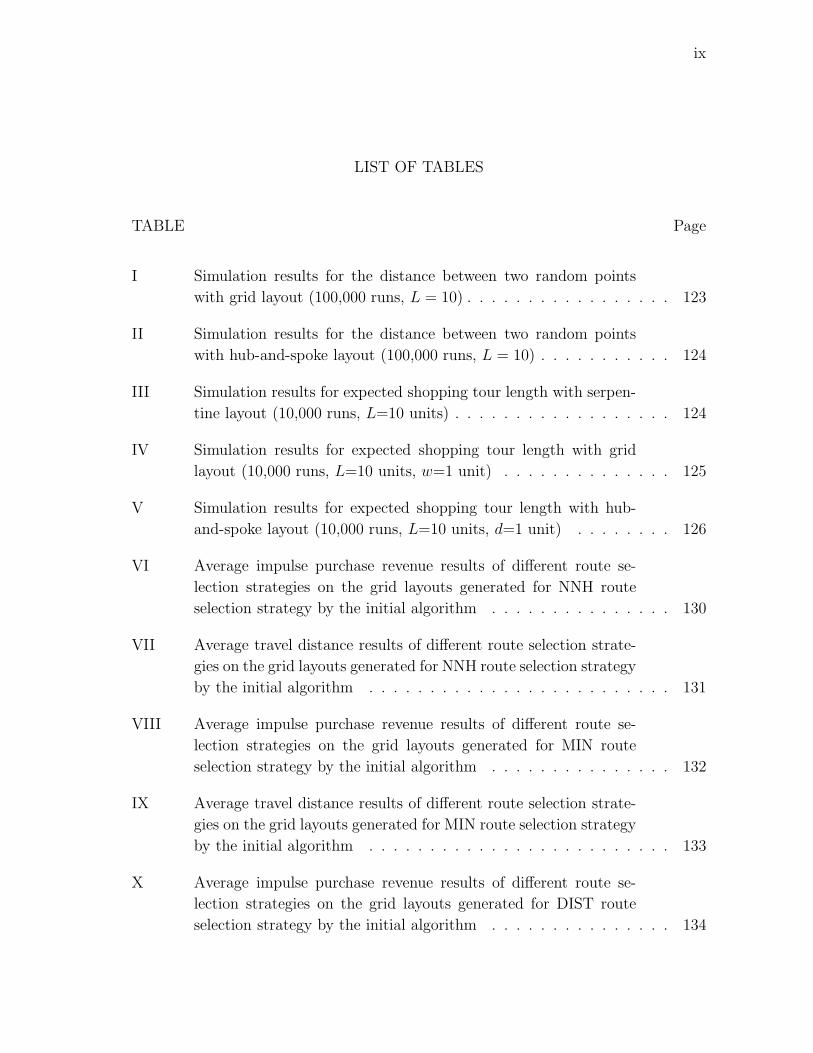
I Simulation results for the distance between two random points
with grid layout (100,000 runs, L = 10) . . . . . . . . . . . . . . . . . 123
II Simulation results for the distance between two random points
with hub-and-spoke layout (100,000 runs, L = 10) . . . . . . . . . . . 124
III Simulation results for expected shopping tour length with serpen-
tine layout (10,000 runs, L=10 units) . . . . . . . . . . . . . . . . . . 124
IV Simulation results for expected shopping tour length with grid
layout (10,000 runs, L=10 units, w=1 unit) . . . . . . . . . . . . . . 125
V Simulation results for expected shopping tour length with hub-
and-spoke layout (10,000 runs, L=10 units, d=1 unit) . . . . . . . . 126
VI Average impulse purchase revenue results of different route se-
lection strategies on the grid layouts generated for NNH route
selection strategy by the initial algorithm . . . . . . . . . . . . . . . 130
VII Average travel distance results of different route selection strate-
gies on the grid layouts generated for NNH route selection strategy
by the initial algorithm . . . . . . . . . . . . . . . . . . . . . . . . . 131
VIII Average impulse purchase revenue results of different route se-
lection strategies on the grid layouts generated for MIN route
selection strategy by the initial algorithm . . . . . . . . . . . . . . . 132
IX Average travel distance results of different route selection strate-
gies on the grid layouts generated for MIN route selection strategy
by the initial algorithm . . . . . . . . . . . . . . . . . . . . . . . . . 133
X Average impulse purchase revenue results of different route se-
lection strategies on the grid layouts generated for DIST route
selection strategy by the initial algorithm . . . . . . . . . . . . . . . 134
x
TABLE Page
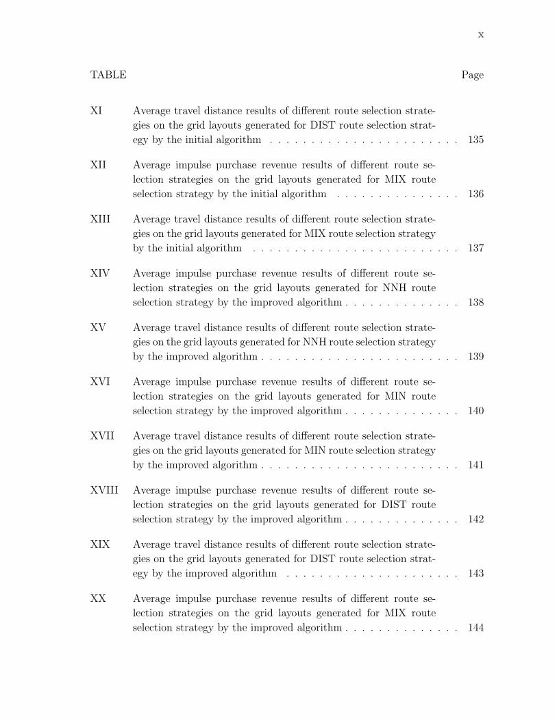
XI Average travel distance results of different route selection strate-
gies on the grid layouts generated for DIST route selection strat-
egy by the initial algorithm . . . . . . . . . . . . . . . . . . . . . . . 135
XII Average impulse purchase revenue results of different route se-
lection strategies on the grid layouts generated for MIX route
selection strategy by the initial algorithm . . . . . . . . . . . . . . . 136
XIII Average travel distance results of different route selection strate-
gies on the grid layouts generated for MIX route selection strategy
by the initial algorithm . . . . . . . . . . . . . . . . . . . . . . . . . 137
XIV Average impulse purchase revenue results of different route se-
lection strategies on the grid layouts generated for NNH route
selection strategy by the improved algorithm . . . . . . . . . . . . . . 138
XV Average travel distance results of different route selection strate-
gies on the grid layouts generated for NNH route selection strategy
by the improved algorithm . . . . . . . . . . . . . . . . . . . . . . . . 139
XVI Average impulse purchase revenue results of different route se-
lection strategies on the grid layouts generated for MIN route
selection strategy by the improved algorithm . . . . . . . . . . . . . . 140
XVII Average travel distance results of different route selection strate-
gies on the grid layouts generated for MIN route selection strategy
by the improved algorithm . . . . . . . . . . . . . . . . . . . . . . . . 141
XVIII Average impulse purchase revenue results of different route se-
lection strategies on the grid layouts generated for DIST route
selection strategy by the improved algorithm . . . . . . . . . . . . . . 142
XIX Average travel distance results of different route selection strate-
gies on the grid layouts generated for DIST route selection strat-
egy by the improved algorithm . . . . . . . . . . . . . . . . . . . . . 143
XX Average impulse purchase revenue results of different route se-
lection strategies on the grid layouts generated for MIX route
selection strategy by the improved algorithm . . . . . . . . . . . . . . 144
xi
TABLE Page
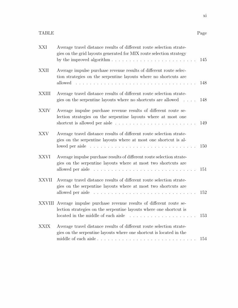
XXI Average travel distance results of different route selection strate-
gies on the grid layouts generated for MIX route selection strategy
by the improved algorithm . . . . . . . . . . . . . . . . . . . . . . . . 145
XXII Average impulse purchase revenue results of different route selec-
tion strategies on the serpentine layouts where no shortcuts are
allowed . . . . . . . . . . . . . . . . . . . . . . . . . . . . . . . . . . 148
XXIII Average travel distance results of different route selection strate-
gies on the serpentine layouts where no shortcuts are allowed . . . . 148
XXIV Average impulse purchase revenue results of different route se-
lection strategies on the serpentine layouts where at most one
shortcut is allowed per aisle . . . . . . . . . . . . . . . . . . . . . . . 149
XXV Average travel distance results of different route selection strate-
gies on the serpentine layouts where at most one shortcut is al-
lowed per aisle . . . . . . . . . . . . . . . . . . . . . . . . . . . . . . 150
XXVI Average impulse purchase results of different route selection strate-
gies on the serpentine layouts where at most two shortcuts are
allowed per aisle . . . . . . . . . . . . . . . . . . . . . . . . . . . . . 151
XXVII Average travel distance results of different route selection strate-
gies on the serpentine layouts where at most two shortcuts are
allowed per aisle . . . . . . . . . . . . . . . . . . . . . . . . . . . . . 152
XXVIII Average impulse purchase revenue results of different route se-
lection strategies on the serpentine layouts where one shortcut is
located in the middle of each aisle . . . . . . . . . . . . . . . . . . . 153
XXIX Average travel distance results of different route selection strate-
gies on the serpentine layouts where one shortcut is located in the
middle of each aisle . . . . . . . . . . . . . . . . . . . . . . . . . . . . 154

xii
LIST OF FIGURES
FIGURE Page
1 Schematics for different layout types . . . . . . . . . . . . . . . . . . 24
2 Walkway skeletons for different layout types . . . . . . . . . . . . . . 25
3 Representation of the products on the network . . . . . . . . . . . . 25
4 Aisle combinations in a grid layout having four aisles . . . . . . . . . 29
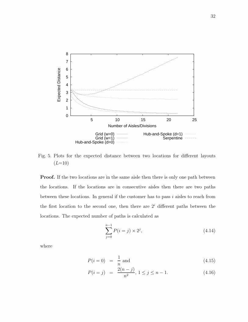
5 Plots for the expected distance between two locations for different
layouts (L=10) . . . . . . . . . . . . . . . . . . . . . . . . . . . . . . 32
6 Expected shopping tour length for the serpentine layout (L=30) . . . 39
7 Expected shopping tour length for the serpentine layout . . . . . . . 40
8 Expected shopping tour length with grid layout (w=0,L=30) . . . . 41
9 Expected shopping tour length with grid layout (w=1,L=30) . . . . 42
10 Expected shopping tour length with hub-and-spoke layout (d=0,L=30) 43
11 Expected shopping tour length with hub-and-spoke layout (d=1,L=30) 44
12 Different grid layout realizations . . . . . . . . . . . . . . . . . . . . 47
13 A grid unit with two shelf rows . . . . . . . . . . . . . . . . . . . . . 48
14 Grid unit based layout design and walkway network . . . . . . . . . . 49
15 Grid layout parameters . . . . . . . . . . . . . . . . . . . . . . . . . 50
16 Visibility factor calculations . . . . . . . . . . . . . . . . . . . . . . . 52
17 Search algorithm for the layout design . . . . . . . . . . . . . . . . . 54
18 Average impulse purchase revenue and travel distance vs. shop-
ping list length plots of the shopping route selection strategies . . . . 57
xiii
FIGURE Page
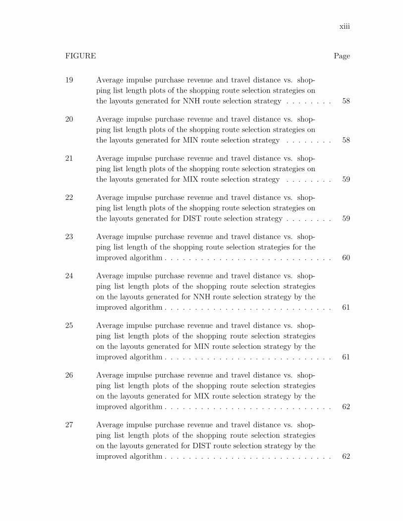
19 Average impulse purchase revenue and travel distance vs. shop-
ping list length plots of the shopping route selection strategies on
the layouts generated for NNH route selection strategy . . . . . . . . 58
20 Average impulse purchase revenue and travel distance vs. shop-
ping list length plots of the shopping route selection strategies on
the layouts generated for MIN route selection strategy . . . . . . . . 58
21 Average impulse purchase revenue and travel distance vs. shop-
ping list length plots of the shopping route selection strategies on
the layouts generated for MIX route selection strategy . . . . . . . . 59
22 Average impulse purchase revenue and travel distance vs. shop-
ping list length plots of the shopping route selection strategies on
the layouts generated for DIST route selection strategy . . . . . . . . 59
23 Average impulse purchase revenue and travel distance vs. shop-
ping list length of the shopping route selection strategies for the
improved algorithm . . . . . . . . . . . . . . . . . . . . . . . . . . . . 60
24 Average impulse purchase revenue and travel distance vs. shop-
ping list length plots of the shopping route selection strategies
on the layouts generated for NNH route selection strategy by the
improved algorithm . . . . . . . . . . . . . . . . . . . . . . . . . . . . 61
25 Average impulse purchase revenue and travel distance vs. shop-
ping list length plots of the shopping route selection strategies
on the layouts generated for MIN route selection strategy by the
improved algorithm . . . . . . . . . . . . . . . . . . . . . . . . . . . . 61
26 Average impulse purchase revenue and travel distance vs. shop-
ping list length plots of the shopping route selection strategies
on the layouts generated for MIX route selection strategy by the
improved algorithm . . . . . . . . . . . . . . . . . . . . . . . . . . . . 62
27 Average impulse purchase revenue and travel distance vs. shop-
ping list length plots of the shopping route selection strategies
on the layouts generated for DIST route selection strategy by the
improved algorithm . . . . . . . . . . . . . . . . . . . . . . . . . . . . 62
xiv
FIGURE Page
28 Interaction between system elements . . . . . . . . . . . . . . . . . . 64
29 The user interface for the grid layout analysis . . . . . . . . . . . . . 65
30 Different serpentine layout realizations . . . . . . . . . . . . . . . . . 68
31 Network generation from layout design model and shortcut addi-
tion . . . . . . . . . . . . . . . . . . . . . . . . . . . . . . . . . . . . 71
32 Product category assignments to edges and end caps . . . . . . . . . 72
33 Search algorithm for layout design . . . . . . . . . . . . . . . . . . . 73
34 Layout generation from product sequence and shelf rows . . . . . . . 74
35 The user interface for the serpentine layout analysis . . . . . . . . . . 77
36 Average impulse purchase revenue and travel distance vs. shop-
ping list length plots for NNH route selection strategy . . . . . . . . 77
37 Average impulse purchase revenue and travel distance vs. shop-
ping list length plots for CO route selection strategy . . . . . . . . . 78
38 Average impulse purchase revenue and travel distance vs. shop-
ping list length plots for MIN route selection strategy . . . . . . . . . 78
39 Average impulse purchase revenue and travel distance vs. shop-
ping list length plots for at most one shortcut per aisle . . . . . . . . 79
40 Average impulse purchase revenue and travel distance vs. shop-
ping list length plots for at most two shortcuts per aisle . . . . . . . 79
41 Average impulse purchase revenue and travel distance vs. shop-
ping list length plots for fixed shortcut in the middle of each aisle . . 82
42 Line representation of walkways and product projection . . . . . . . 85
43 Network representation of grid and serpentine layout designs, and
basic network units . . . . . . . . . . . . . . . . . . . . . . . . . . . . 85
44 Possible customer travel patterns in an aisle . . . . . . . . . . . . . 87

xv
FIGURE Page
45 Possible customer travel patterns in a bypass area . . . . . . . . . . . 89
46 Expected travel distance vs. shopping list length plots for grid
(G) and serpentine layouts with i ∈ {1 . . . 4} shortcuts (S-i) . . . . . 91
47 Incomplete travel in an aisle . . . . . . . . . . . . . . . . . . . . . . . 94
48 Regions in a bypass area . . . . . . . . . . . . . . . . . . . . . . . . . 94
49 Network representation of a serpentine layout with three bypass areas 95
50 Impulse purchase revenue and travel distance vs. shopping list
length plots for deterministic demand and low variability in im-
pulse purchase revenue parameters . . . . . . . . . . . . . . . . . . . 107
51 Impulse purchase revenue and travel distance vs. shopping list
length plots for deterministic demand and medium variability in
impulse purchase revenue parameters . . . . . . . . . . . . . . . . . . 108
52 Impulse purchase revenue and travel distance vs. shopping list
length plots for deterministic demand and high variability in im-
pulse purchase revenue parameters . . . . . . . . . . . . . . . . . . . 109
53 Impulse purchase revenue and travel distance vs. shopping list
length plots for stochastic demand and low variability in impulse
purchase revenue parameters . . . . . . . . . . . . . . . . . . . . . . 110
54 Impulse purchase revenue and travel distance vs. shopping list
length plots for stochastic demand and medium variability in im-
pulse purchase revenue parameters . . . . . . . . . . . . . . . . . . . 111
55 Impulse purchase revenue and travel distance vs. shopping list
length plots for stochastic demand and high variability in impulse
purchase revenue parameters . . . . . . . . . . . . . . . . . . . . . . 112

1
CHAPTER I
INTRODUCTION
The retail industry in the U.S. constitutes more than 23 million employees (roughly
one in five American workers) across more than 1.6 million establishments, with
annual sales totaling $4.4 trillion in 2005 (National Retail Federation). Given the
large number of retail facilities and the huge economic impact of retail industry, it is
interesting that there has not been much work done related to the layout design of
retail facilities in Operations Research (OR) literature. Although OR techniques are
used in certain fields of retailing literature such as shelf space allocation and category
management, these studies only focus on subproblems of retail facility layout design.
Retail facility layout design is a relatively unexplored research area, and it provides
an attractive research direction to follow.
Layout design problems have been studied for a long time and there is a very rich
literature for the application of (OR) techniques to layout design problems (c.f., Meller
and Gau, 1996; Kusiak and Heragu, 1987). However, generally the scope of the layout
design problems analyzed so far is limited to manufacturing or distribution facilities
with the main objective of minimizing material handling cost. Relatively few studies
have analyzed the layout design problem in the context of the service sector such as
airports (Braaksma, 1977) or hospitals (Hahn and Krarup, 2001). When compared
to manufacturing plants or distribution centers, the operations in service facilities
vary greatly depending on the type of the service offered to customers. In addition,
the active involvement of customers in service facilities creates extra diversity in
operations. As a consequence, the constraints and the objective of layout design
This dissertation follows the style of IIE Transactions.
2
problems can differ in two different service facilities, and the variety in the design
characteristics of service facilities provides a fruitful research area.
A retail facility layout design is a good example for how a service facility layout
design problem may differ in terms of the constraints and the objective function
compared to a manufacturing facility. The traditional layout performance measures
such as material handling cost are not applicable in a retail facility layout. Generally
in retailing, the performance measures such as total store sales or profit per unit
square area are more common for evaluating the layout design effectiveness. These
different performance measures provide a unique layout design perspective and require
us to use different approaches than the ones used for manufacturing facilities.
In this study, we use impulse purchase revenue and customer travel distance
as the two main performance measures to evaluate layout design effectiveness. As
explained in Chapter II, impulse purchases are the unplanned purchases made by the
customers without prior intention before entering the store, and they are important
for retailers due to their potential impact on sales revenue. It has been reported that
for some product categories, more than 50% of the purchases are done impulsively
(POPAI/duPont Studies, 1978), and this cannot be neglected by retailers.
Although retailers are interested in increasing the time spent by the customers in
the store, the negative impact of requiring customers to spend more time in the store
out of their will cannot be overlooked. Recent studies (Messinger and Narasimhan,
1997; Seiders, Berry and Gresham, 2000) show that the value customers place on their
time has increased over the years. Thus, we also consider customer travel distance as
another performance measure, which highly influences customers’ shopping time.
Our research objective is to analyze the applicability of a set of existing lay-
out types in retail settings and compare these layout types with respect to different
performance measures. In addition to this, we believe this study to be the first in

3
the literature that introduces a quantitative model for retail facility layout design
problem in the context of retail stores. In our analysis, we search for the answers of
several questions such as:
• Is it possible to increase impulse purchase revenue and decrease customer travel
distance simultaneously in a store layout?
• How does customer’s shopping behavior in the store affect impulse purchase
revenue?
• Where should the products be located in the store based on their price and
demand information?
During our search for the ideal store layout, we focus on the variations of three
different layout design patterns in retail store settings, which are grid, serpentine and
hub-and-spoke layouts. Grid layout consists of perpendicular and parallel aisles, and
it is the most popular layout design pattern observed in retail facilities such as grocery
stores, discount stores and hardware stores. Serpentine layout basically consists of a
single walkway that traverses the whole facility. Although serpentine layout is not
as common as grid layout design, there are successful examples of its application in
practice (e.g., IKEA stores, HEB Central Market). Finally, hub-and-spoke layout
consists of several departments located around a central area. Although this layout
design is not commonly applied in retail facilities, we think that it has some potential
since the customer can quickly browse several departments at once from the central
area.
There are several factors that need to be taken into account in layout design such
as customer traffic in the store, average impulse purchase revenue generated from
each product category, customers’ shopping list contents and product demand rates.
4
These factors are closely related to each other. As an example, customer traffic in
the store determines the visibility of the products depending on their location, which
consequently affects impulse purchase revenue. On the other hand, customer traffic is
affected by layout design and also the location of the products that are in customers’
shopping lists. In addition to these interactions between different factors, each factor
has its own characteristics. For example, different product categories have different
impulse purchase and demand rates. We address these issues in our models with
respect to different assumptions.
The outline of the dissertation is as follows. In Chapter II, a brief overview of
different study areas related to retail facility layout design is given. In Chapter III
the retail facility layout design problem is compared with traditional facility layout
design problems studied in OR literature, and modeling issues are discussed. In
Chapter IV, network representation of layout design concept is introduced. Different
layout designs are represented as simple networks and their performance is compared
with respect to customer travel distance in the store. In Chapter V, a grid layout
design model is introduced. Later, this model is embedded in a simulated annealing
(SA) algorithm to generate layouts with respect to different customer shopping list
scenarios. In Chapter VI, a serpentine layout design model is introduced and similar
to Chapter V, this model is used in a SA algorithm to generate serpentine layouts.
In Chapter VII, network representations of serpentine and grid layouts provided in
Chapter IV are extended. Also the effect of stochastic product demand on the per-
formance of serpentine layout design is analyzed. Finally in Chapter VIII, a brief
summary of the dissertation is given and future research directions are discussed.
5
CHAPTER II
RELATED LITERATURE
The retail facility layout design problem is a complex decision making process influ-
enced by a number of variables, and consequently the studies on retail facility design
show great variety depending on the issues that are analyzed. In conjunction with
the high variety of issues, the methodology used in these studies extends from appli-
cation of purely analytical models to analysis of empirical data such as survey results.
In this chapter, a brief overview of different issues related to retail facility design is
given.
1. Product Assortment and Shelf Space Allocation
Product assortment and shelf space allocation problems are closely related to each
other. Since each product in the assortment requires a minimum amount of shelf-
space, the assortment size is directly proportional to the shelf-space requirement.
On the other hand, retailers generally have fixed amount of shelf-space to allocate
different products. These two facts make the literature focus on the integration
of product assortment and shelf-space allocation models into one single model. This
single model should find the optimal product assortment and the shelf-space allocated
for each product in the assortment. The objective can be either optimizing the profit
or minimizing the operating cost. In addition, product category management plays
an important role in product assortment and shelf space allocation decisions due to
substitution and complementary effects. The interaction between product category
demands, which is related to demand elasticity, is also considered in some models.
Although the main idea is to build-up a single integrated model that includes
all aspects of the shelf space allocation and product assortment problem, the as-

6
sumptions and the considered details of the problem characteristics result in several
different models. In one of the pioneering studies in this field, Corstjens and Doyle
(1981) use geometric programming to optimize shelf space allocations across differ-
ent product categories to maximize total profit. An important contribution of this
study is a demand function formulation for the products, which is expressed as the
multiplicative, power function of the displayed areas allocated to the product groups.
By this concept, it is possible to define demand functions that take cross product
space elasticity into account. Their demand function concept is used frequently in
the literature.
Bultez and Naert (1988) present another model named SH.A.R.P. Their study
is an extension of Corstjens and Doyle (1981). They propose a model for the inte-
grated product assortment and shelf-space allocation problem. Using this model, they
conclude that the space allocated for a product in an optimal design is a weighted
function of the product’s relative contribution to the assortment profitability and the
product’s contribution to the assortment’s total sales volume. They give an iterative
heuristic to find a solution for the problem, which was a generalized reduced gradi-
ent method to solve sub-problems in the iterations. The suggested methodology is
applied in a case study on a product category in an European pet food shop, and an
increase of 11% in the sales profit is observed.
A very detailed model for the same problem is provided by Borin, Farris and
Freeland (1994). They try to include all factors that affect the demand of a product
such as the effect of stock-out products on the demand of available products, the effect
of products that are not in the product assortment on the demand of products that
are offered, and the cross space elasticity of products. They formulate this problem
as a complex non-linear programming model and use a simulated annealing (SA)
algorithm to find solutions for sample problems. They also compare their algorithm
7
with a basic technique that retailers use for shelf-space allocation, which allocates
space to a product in proportion to the product’s historical share of sales. Their
algorithm outperforms this traditional management approach.
Borin and Farris (1995) extend the work of Borin et al. (1994). They analyze the
quality of solutions obtained by incorrect parameter values. By using two different
algorithms (SA algorithm given in Borin et al. (1994) and a greedy heuristic), they
show that even if the absolute value of the parameter error is high, the decrease
in objective function value is within 5% of the optimal solution. However, when a
traditional management approach as explained in Borin et al. (1994) is used, the
deviation of the solution obtained by incorrect parameter values can be larger.
Another integrated model is proposed by Urban (1998). In this model, inventory
is included in the model. Inventory is divided into two sets: 1) the displayed inventory
(items on the shelves), and 2) the backroom inventory (items in the warehouse of the
retailer). The demand function for an item is dependent on the displayed inventory
level of the item. After giving an inventory model, the author integrates the inventory
model with a shelf space allocation model. Genetic algorithm (GA) is used to solve
the resulting non-linear problem.
The models and suggested solution methods in the mentioned studies show that
the integrated product assortment and shelf-space allocation problem can effectively
utilize OR techniques. On the other hand, there are management papers (e.g., Chiang
and Wilcox, 1997; Desmet and Renaudin, 1998) that analyze the shelf-space alloca-
tion and product assortment decisions in terms of empirical data. Regardless of the
methodology used in the papers, product assortment and shelf space allocation prob-
lems are closely related to store layout design since products are the main layout
components in a store. In this dissertation, we consider shelf space requirement of
product categories during layout design. We assume that for each product category,
8
the product assortment and allocated shelf space are known in advance, which can
be estimated by shelf space allocation and product assortment models.
2. Impulse Purchases
Impulse purchases are generally considered to be purchases that are made by the
customers without prior intention, yet there are several specific definitions. For ex-
ample, Kollat and Willet (1967) define impulse purchase as the difference between
the products purchased and the products planned to be purchased before entering
the store. This seems to be the most general definition of impulse purchase. It is
possible to find other definitions of impulse purchase in retailing literature as given
by Kollat and Willet (1969).
In addition to the variety of definitions for impulse purchase, different theories
have been proposed to explain why impulse purchases occur. Two main theories given
in Kollat and Willet (1967) are the so-called exposure to in-store stimuli hypothesis
and the customer commitment hypothesis.
The exposure to in-store stimuli hypothesis assumes that impulse purchases are
caused by in-store stimuli. Different stimuli (e.g., promotional advertising, product
displays etc.) that the customers are subject to remind them of some of their existing
needs or make them realize some of their new needs. Consequently, becoming aware
of the needs causes impulse purchases.
On the other hand, customer commitment hypothesis states that the difference
between the intended purchase and the actual purchase occurs because of the inad-
equate measure of actual intentions of the customers before going to shopping. The
customers may give incomplete information about their shopping plan because they
may not want to devote the time and thought to itemize the shopping during the in-

9
terview. According to this hypothesis, the techniques (e.g., interviews, surveys) used
in evaluating impulse purchase behavior of customers may overestimate the number
of unplanned purchases due to the difficulty of measuring actual purchase intentions
of the customers.
Despite the different views about its origin and measurement, impulse purchases
are an important issue for retailers to increase potential sales. As Bellenger, Robertson
and Hirschman (1978) suggest, impulse purchases should be analyzed depending on
the purpose for which the collected information is used. Since retailers are concerned
with increasing sales, they are most likely to be interested in additional purchase
decisions made by the customers in the store. So a simple approach to define impulse
purchase depends on the answer whether the customer makes the purchase decision
before entering the store or in the store. This idea is also consistent with the first
definition of impulse purchase (Kollat and Willet, 1967) which is given previously.
In this study, one of the objectives is maximizing the total impulse purchase revenue
and for this reason, impulse purchase rates of the products are important. Studies
(e.g., Bellenger et al., 1978; McGoldrick, 1982) show that different product categories
have different impulse purchase rates. As an example, according to POPAI/duPont
Studies (1978), 51% of pharmaceuticals and 61% of healthcare and beauty aids are
purchased without prior intention. Thus, retailers should locate products with high
impulse purchase rates on high customer traffic areas in the store in order to increase
impulse purchase revenue. In other words, impulse purchase revenue depends on the
layout configuration of the store.
10
3. Store Environment and Atmosphere
Customer satisfaction is one of the key elements of a successful retail environment.
Being aware of this, retailers should take some service measures such as travel dis-
tance, aisle width, cashier line length, etc. into consideration during layout design.
These service measures affect the retail store layout. For example, a store layout
requiring customers spend so much time for shopping can result in frustrated and
annoyed customers who may never visit that store again. Consequently, response
of customers to different shopping experiences becomes an attractive research area
for retailers. In retailing and consumer psychology literature, there are interesting
studies that analyze the relationship between consumer behavior and retail store en-
vironment. Donovan and Rossiter (1982) use Mehrabian-Russell (M-R) (Mehrabian
and Russell, 1974) model to analyze the customer behavior in retail settings. M-R
model classifies the behaviors in an environment as either approach (such as move
towards, stay in, explore) or avoidance behavior (feeling dissatisfaction, boredom,
desire to leave). According to this model, such behaviors are the results of two emo-
tional states. These emotional states can be measured by two dimensions, which are
pleasure and arousal, and to some extent measured by a third dimension dominance.
These dimensions are hypothesized in a way that arousal amplifies approach behavior
in pleasant environments and avoidance behavior in unpleasant environments. They
conclude that arousal, or store-induced feelings of alertness and excitement, can in-
crease time spent in the store and also willingness to interact with sales personnel.
Later Donovan, Rossiter, Marcoolyn and Nesdale (1994) extend Donovan and Rossiter
(1982). They observe that pleasure is a significant predictor of both extra time spent
in store and unplanned spending. They also conclude that emotional factors appear
to be more important for extra time spent in store, whereas the cognitive factors
11
appear to be slightly more important than emotional factors for unplanned spending.
There is a wide range of factors such as background music (Dube and Morin,
2001; Mattila and Wirtz, 2001), illumination (Summers and Hebert, 2001), scent
(Mattila and Wirtz, 2001) that can affect customers’ behavior in a store. In addition,
the coherence between these factors and the shopping environment is also important.
As an example, Mattila and Wirtz (2001) show that customers’ shopping experience
is enhanced when the ambient scent is matched with an appropriate background
music. For increasing impulse purchase revenue, they suggest to use appropriate
scent and background music combination that matches the characteristics of the retail
environment. An extensive review on the effect of store environment on customer
behavior can be found in Lam (2001) and Turley and Milliman (2000). Since our
research focuses on layout design, we are more interested in the effect of layout design
on consumer behavior, which is discussed in the next section.
4. Layout Design and Consumer Behavior
The influence of store layout design on customer behavior is another issue in which
retailers are interested. In retailing literature, there are several studies analyzing this
relationship through consumer surveys and empirical data analysis. These studies
show a high variety with respect to the context in which they analyze this issue.
As an example, Iyer (1989) analyzes the joint effect of time pressure and store lay-
out knowledge on customer’s purchase behavior. His empirical analysis over data
collected from 68 participants shows that lower store knowledge and lower time pres-
sure increase the amount of unplanned purchases. In another study, Park, Iyer and
Smith (1989) find similar results related to store knowledge and time pressure. Floch
(1988) studies the layout design problem from a consumer psychology perspective.

12
She divides the customers into four groups as convenience, utopian, diversionary and
critical, and she suggests that the store layout should be a combination of different
layout patterns that fit the preferences of different customer groups. Zacharias (1997)
studies the effect of layout and visual stimuli on customers in an open market area.
The results show that pedestrian movement within the public market environment
is guided chiefly by aesthetic and especially, visual experience, but still the exact
role of visual stimuli and then visual schemata on preference and behavior remain as
an important issue in understanding human spatial behavior. Sommer and Aitkens
(1982) analyze the store layout design from a customer cognition perspective and
show that customers are more likely to remember the product locations that are on
the peripheral aisles. In this dissertation, we analyze the effect of customer’s route
choice behavior on impulse purchase revenue and customer travel distance in our
layout design models.
5. Store Format
With the increasing popularity of one-stop shopping centers, researchers have ex-
amined the relationship between customer behavior and store format. The increase
in store size due to store format directly affects the layout design. Messinger and
Narasimhan (1997) demonstrate that the increase in customer evaluation of time has
positive impact on one-stop shopping centers. Supporting this conclusion, according
to a survey result, 52% of the consumers intend to spend less time for shopping to
increase time for other uses (Seiders et al., 2000). Despite the increase in number
of one-stop shopping centers, Merrilees and Miller (1997) analyze the superstore for-
mat in Australia and they conclude that there are some retail categories for which
superstore format does not fit well. Leszczyc and Timmermans (2001) analyze the
13
preference of the customers with respect to specialty stores and one-stop shopping
centers. According to their results, customers’ shopping strategies are shaped by
a number of factors such as travel time, check-out line length, assortment size and
price. In this dissertation, we focus on the layout design of the store area where
customers browse the products and make purchases. Thus our layout design models
are applicable in both specialty stores and one-stop shopping centers.
Despite the variety of store layout design related issues studied in retailing liter-
ature, there are basic layout design principles used by retailers. A discussion of these
principles and a detailed comparison of retail facility layout design with manufactur-
ing facility layout design are given in the next chapter.
14
CHAPTER III
MODELING ISSUES IN RETAIL FACILITY LAYOUT DESIGN
Retail facility layout design issues given in Chapter II show that retail facility layout
design problems have different characteristics compared to manufacturing facility or
distribution center layout design problems. However, the richness of layout design
methodologies developed for manufacturing and distribution facilities requires us to
compare retail facility layout design problem with these traditional layout design
problems in detail. In this way, we can analyze adapting existing layout design
techniques to retail facility layout design. In the next section, a detailed comparison
of retail facility layout design and traditional layout design problems are given. Later
in this chapter, we discuss the current practice in retail facility layout design and
introduce a generic model for layout design of retail facilities.
1. Retail Facility Layout Design versus Traditional Facility Layout Design
The layout type used in a manufacturing facility partly depends on the designer’s
objective during the layout design stage. The most commonly used objective in
layout design of a manufacturing facility is minimization of the material handling cost.
Based on the distribution of the material flow amounts between the departments (e.g.,
machines, cells, etc.), minimization of the material handling cost objective results
in different layout types. This approach distinguishes manufacturing facility layout
design from retail facility layout design, since material flow between the departments
is used to shape the manufacturing facility layout. On the other hand, if an analogy
is established between the customer flow and the material flow, then it is seen that
the layout design is used to shape the customer flow.
Design of material flow paths is important for manufacturing facilities because

15
of material handling cost. Traditionally, layouts are first designed as block plans
where only department locations and their boundaries are determined. The material
flow path and exact department shapes are given in the detailed layout which are
generated from block plans (Meller and Gau, 1996). This two step layout design
process may not provide optimal layout. To overcome this, recent studies focus on
the integration of layout and material handling system design at the same time (e.g.,
Ho and Moodie, 2000; Castillo and Peters, 2002; Banerjee, Zhou and Montreuil, 1997;
Welgama and Gibson, 1996). Because of the complexity of the integrated problem,
these studies give heuristic solution methods to find a good layout.
The integration of customer flow path and store layout designs is inevitable for
having an effective store layout. The walkways inside the store direct the customer
traffic. Consequently, if the customers visit the location of the products with high
impulse purchase rates, then the retailer is expected to receive more impulse purchase
revenue. At this point, a retailer may be interested in having a single walkway which
travels all along the store. Locating entrance and exit gates at the two ends of this
walkway requires customers to visit all the product locations in the store. Such an
approach may seem to maximize the expected impulse purchase revenue, but it should
not be forgotten that the store layout design should take into account customer needs.
No retailer wants to lose its customers, especially if maintaining an existing customer
is less costly than gaining a new customer. Considering the importance of customer
service, the retailer has to satisfy certain service levels and the distance traveled
by the customers in the store is one of them. Compared to past, time has more
value for the customers and this leads to the popularity of large one-stop shopping
centers where customers can do most of their shopping without going somewhere else
(Messinger and Narasimhan, 1997). Under these conditions, one of the objectives
(or constraints) of retail store layout designer is not to require customers travel long
16
distances and spend more time in the store. A retail layout design model should
handle the delicate issue of balancing the trade-off between the time value of the
customer and the impulse purchase revenue obtained during the time the customer
spends inside the store.
Two popular layouts in manufacturing, job-shop and flow-shop, differ from each
other by the grouping of machines. In the job-shop layout, machines with similar pro-
cessing capabilities are grouped together in one department whereas in the flow-shop
layout various machines with different processing capabilities, but in the same prod-
uct line, are grouped in the same department. In retailing context, there exist several
grouping of products. Bellenger and Goldstucker (1983) divide grouping of products
into two as generic grouping and customer preference grouping. In generic group-
ing, products with common end characteristics are placed in the same department
(e.g., shoe department). In customer preference grouping, products with different
characteristics are placed in the same department based on customer needs (e.g.,
gift department). Morgenstein and Strongin (1983) give a more detailed classifica-
tion of product grouping which are functional, purchase-motivation, market-segment
and storability product groupings. Functional and market-segment product group-
ings are similar to generic and customer preference product groupings respectively.
Purchase-motivation product grouping is described as grouping of products based on
their impulse purchase rates whereas storability product grouping refers to grouping
of products based on their storage requirements such as refrigeration needs.
If the products in a retail store are considered as machines in a manufacturing
facility, then generic product grouping resembles to job-shop production system. In
the same way, customer-preference product grouping is close to flow-shop production
system. A job-shop production system is preferable when the demand is low and
product variability is high. On the other hand, a flow-shop system is more preferable
17
when the demand levels are high and the variety of products is low. With a similar
reasoning we can conclude that retail stores can use generic or customer-preference
product grouping based on the shopping patterns of the customers. However, it
should be noticed that flow-shop and job-shop production systems aim to minimize
the material handling cost and increase machine utilization, respectively. For the
retailer’s case, if the objective is to maximize the impulse purchase revenue, it may
be more preferable to increase the customer flow in the store as much as possible
opposite to the minimization of material handling concept in manufacturing. This
requires us to have a different approach in retail facility layout design.
How to represent product groups on the layout is another critical decision for the
retailers. Usually in layout studies, the components to be located on the floor plan
are assumed to be departments, cells or machines. For the retail store layout case, the
layout components can be between the departmental level (e.g., produce department)
and brand level (e.g., brand X cookies). As the component size gets smaller, both
the accuracy and the complexity increase from modeling perspective. The size of the
layout component should allow the retailer to estimate the visibility of the products
inside the component for a given layout. At the same time, the products inside
the layout component should not be diverse so that the parameters such as average
expected revenue or average impulse purchase rate of the component’s products is
close to the actual values for each product.
2. Current Practice in Retail Facility Layout Design
Today, depending on the traffic flow pattern inside the store, the retail management
literature classifies the store layouts into three main groups as grid pattern, free-flow
pattern and boutique pattern.

18
Grid layout routes the traffic in straight, rectangular fashion. This layout pattern
is mostly used by food retailers, discount stores, hardware stores and other conve-
nience oriented stores. The advantages of grid pattern layout can be summarized as
the creation of an efficient, austere store atmosphere where the customers can shop
more quickly (Berman and Evans, 1989). It provides a high floor space utilization,
and ease in inventory and security control. On the other hand a grid pattern layout
may trigger a rushed shopping behavior, create an impersonal store atmosphere and
limit the browsing of the products.
Free-flow layout is mostly used in department stores, clothing stores and other
shopping oriented stores. In contrast to the aisle structure of grid pattern, free-flow
pattern allows customers to be able to move in several directions. This provides a
friendly atmosphere and customers do not feel rushed. As a result they browse the
store more and make more impulse purchases. The associated disadvantages with
this layout design are difficulty in inventory and security control, potential customer
confusion and inefficient utilization of the floor space (Berman and Evans, 1989).
Finally, boutique layout is similar to free-flow and it is described in Morgenstein
and Strongin (1983) as:
The boutique pattern creates a small specialty show within an area
of the selling floor. This arrangement utilizes the free-flow pattern in a
“little shop” setting such as a “Bed and Bath” corner. The boutique
pattern makes it easy for the consumer with a particular interest to see
complete offerings in one area.
Besides grouping of layout patterns, there are some standard guidelines that are
used by retailers in store layout design. As an example, it is preferred to locate high
demand products (also referred as staples or power items such as milk, bread in a
19
grocery store) in the corners of the store, so the customers browse the store more. In
product location decisions, complementary relationship (e.g., coffee and sugar, corn
flake and milk) is another point retailers take into account in terms of closeness of
products. Despite such intuitive guidelines for store layout design, there is not an
analytical layout design model for retail stores in retailing literature.
In fact, it is not possible to restrict store layouts to the above layout patterns.
There may be stores with unique layout designs (e.g., IKEA stores with serpentine
layouts), as well as several layout design patterns can be observed in the same store
within different departments. Furthermore, the retail facility layout design problem
is not limited to the store level. On the micro level, shelf space allocation problems
can be considered as a subproblem of retail facility layout design. On the other
hand, at the highest level, the location of shops in a shopping mall (Aickelin and
Dowsland, 2002) can also be considered as a retail facility layout design problem. In
this dissertation, the focus is on the store layout aspect of retail facility layout design.
3. Modeling Framework
A retail store layout design model should aid the retailer to estimate the customer
traffic and the potential impulse purchase revenue for a given layout. In addition,
the model should take the customer service measures such as walking distance into
account. Also the uncertainty of human behavior such as route selection or making
an impulse purchase should be represented accurately by the model. At this point, a
network based model can meet most of the requirements the retail store layout model
should have. The skeleton of the customer walkways in the store can be represented
as a network. The location of layout components (such as product categories) and
intersection points of walkways can be shown by nodes. The resulting network allows

20
us to analyze the measures like the route choice of the customers, locations in the
store that are most likely to be visited and the distance traveled by the customers.
A generic model to find the optimal product location on the representative net-
work of the store layout is given in the next subsections.
3.1. Model Sets, Parameters and Functions
P Set of product groups (layout components) to be located on the network.
S Shopping list of the customer. S contains the product groups from which the
customer certainly buys an item (S ⊆ P )
L Set of all locations where the product groups can be located.
Vp Set of locations where product group p can be located (p ∈ P , Vp ⊆ L).
Gl Set of product groups that can be located on location l (l ∈ L, Gl ⊆ P ).
mp The average impulse purchase rate of an item in product group p when it is seen
by a customer. If p ∈ S then mp is 1. (mp ∈ [0, 1], p ∈ P ).
rp The average revenue obtained by a purchase from product group p (rp ≥ 0, p ∈ P ).
g(p, f, S) Function showing the probability the customer notices product group p
with respect to its location in the feasible layout f for a given shopping list S.
This function takes value 1, if p ∈ S. (p ∈ P , f ∈ F , g(, ) : (P, F, S) → [0, 1])
B Set of service requirements such as customer shopping time, customer travel dis-
tance, etc.
bi Minimum service level requirement for service i (i ∈ B)

21
hi(f, S) Function for the service level amount achieved for service i in feasible layout
f for given shopping list S. (i ∈ B, f ∈ F , hi() : (F, S) → ℜ)
3.2. Variables
xpl Binary variable, takes value 1 if product group p is located at location l, 0 other-
wise (p ∈ P , l ∈ L, p ∈ Gl, l ∈ Vp )
F Set of binary variable xpl assignment matrices representing feasible layouts (p ∈ Gl,
l ∈ Vp).
3.3. Network Based Model
Objective Function :
maximize∑
p∈P
mp rp g(f, p, S) (3.1)
Subject To:
∑
p∈Gl
xpl ≤ 1 ∀ l ∈ L (3.2)
∑
l∈Vp
xpl = 1 ∀ p ∈ P (3.3)
hi(f, S) ≥ bi ∀ i ∈ B (3.4)
xpl ∈ {0, 1} ∀ p ∈ P, ∀ l ∈ L, p ∈ Gl, l ∈ Vp (3.5)
In the above formulation, the objective function (3.1) maximizes the expected
impulse purchase revenue. The probability noticing an item from product group p
and making an impulse purchase is given by g(p, f, S)×mp for a feasible layout f and
shopping list S. By multiplying this probability with the average revenue parameter
rp, the expected impulse purchase revenue is obtained. The constraint sets (3.2) and
22
(3.3) ensure that no more than one product group is assigned to each location and
that each product group is assigned to exactly one location, respectively. The final
set of constraints (3.4) assure that the layout determined by the product group –
location assignment variables satisfies the service level requirements.
There are two questions that have to be answered related to this model. The
first one is “How can we construct the initial store layout network on which the prod-
uct location assignments are done?”. The second question is “How can we define
the visibility function g and the service level function hi on this network ?” There
are graph representations for layouts that can be used in the design stage (Francis,
McGinnis and White, 1992), but such graph representations are not close to the net-
work concept we described. The functions g and hi depend on the network structure,
relative location of the product groups on the network and also the location of shop-
ping list items. It should be noticed that the above formulation considers a single
customer profile represented by the shopping list S. However, this formulation can
be expanded to the case where there are several customer profiles. After defining
visibility and service level functions, and impulse purchase rate parameters for each
customer profile, the objective function can be taken as a weighted sum of the ex-
pected impulse purchase revenues obtained from each customer profile. If C denotes
the set of customer profiles and customer profile c has shopping list Sc, then the new
objective function is given by:
maximize∑
c∈C
∑
p∈P
mpc rp g(f, p, Sc) (3.6)
Each customer profile may have different impulse purchase rates for different
product groups. Hence, in the new objective function, mpc denotes the impulse pur-
chase rate of product group p (p ∈ P ) by a customer belonging to customer profile c.
If customer profile c’s minimum service level requirement for ith service is shown by
23
bic, then constraint set (3.4) is redefined as:
hi(f, Sc) ≥ bic ∀ i ∈ B, c ∈ {1 . . . C} (3.7)
Throughout the following chapters we address these issues which are being re-
ferred to in different layout design models. We first start with simple network repre-
sentations of different store layout types, which are given in the next chapter.
24
CHAPTER IV
NETWORK MODELS FOR STORE LAYOUT
In Chapter III, the necessity of using networks in layout design to control customer
traffic was discussed. Since we are interested in the shopping routes of the customers
in the store, a reasonable approach would be to construct the layout network using
walkways of the store. The walkways of the store form a skeleton, which can be con-
verted to a network. Consequently, each layout type has a specific network structure.
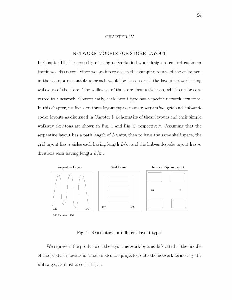
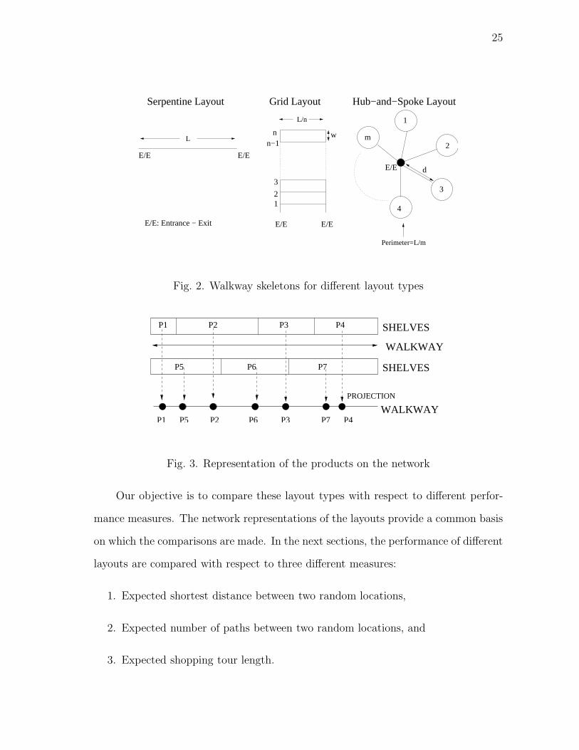
In this chapter, we focus on three layout types, namely serpentine, grid and hub-and-
spoke layouts as discussed in Chapter I. Schematics of these layouts and their simple
walkway skeletons are shown in Fig. 1 and Fig. 2, respectively. Assuming that the
serpentine layout has a path length of L units, then to have the same shelf space, the
grid layout has n aisles each having length L/n, and the hub-and-spoke layout has m
divisions each having length L/m.
Grid LayoutSerpentine Layout Hub−and−Spoke Layout
E/EE/E E/E
E/E E/E
E/E
E/E: Entrance − Exit
Fig. 1. Schematics for different layout types
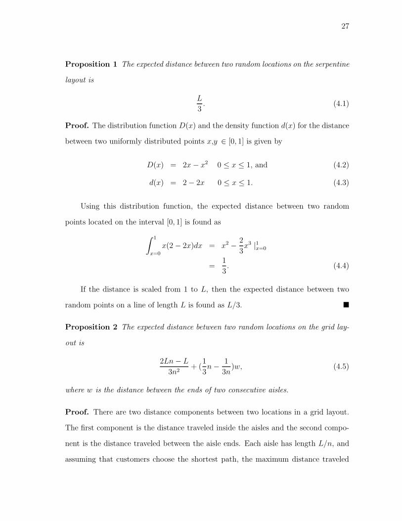
We represent the products on the layout network by a node located in the middle
of the product’s location. These nodes are projected onto the network formed by the
walkways, as illustrated in Fig. 3.
25
E/E
E/E E/E
E/E
Perimeter=L/m
L/n
L
E/E
E/E: Entrance − Exit
Serpentine Layout Grid Layout Hub−and−Spoke Layout
n
3
2
m
1
2
3
41
n−1w
d
Fig. 2. Walkway skeletons for different layout types
P1 P5 P6 P3 P7 P4P2
P1 P2 P3 P4
P5 P6 P7 SHELVES
WALKWAY
SHELVES
PROJECTION
WALKWAY
Fig. 3. Representation of the products on the network
Our objective is to compare these layout types with respect to different perfor-
mance measures. The network representations of the layouts provide a common basis
on which the comparisons are made. In the next sections, the performance of different
layouts are compared with respect to three different measures:
1. Expected shortest distance between two random locations,
2. Expected number of paths between two random locations, and
3. Expected shopping tour length.

26
For each of these performance measures, the expected value formulas are derived
based on the following assumptions:
1. All products are uniformly distributed on the layout and, consequently on the
layout network.
2. The serpentine layout network is composed of a single direct path with length
L. The customers may enter the network from each end of this path. Once
a customer starts walking along the path, the customer moves in the same
direction until he finishes purchasing all the items in the shopping list. When
the customer purchases the last item in the shopping list, he chooses the closest
end of the path to exit the store. If we assumed that the customer enters the
path from one end and leaves the path from the other hand, then the expected
shopping tour length would simply be the total path length.
3. The grid layout network is composed of n parallel lines with length L/n con-
nected to each other by their end points. Customers enter and exit the store
from the points adjacent to the first aisle, as shown in Fig. 2.
4. The hub-and-spoke layout network is composed of m divisions that are con-
nected to the center point by direct paths, as shown in Fig. 2. Each division
has a circular structure and the perimeter of this circle has length L/m.
1. Expected Shortest Distance between Two Random Locations
In this section, the expected distance formula between two random locations is derived
for each layout type. Our derivations are based on the assumption that the points
are uniformly located on the layout network. A simulation analysis of these expected
values is given in Appendix A.
27
Proposition 1 The expected distance between two random locations on the serpentine
layout is
L
3. (4.1)
Proof. The distribution function D(x) and the density function d(x) for the distance
between two uniformly distributed points x,y ∈ [0, 1] is given by
D(x) = 2x − x2 0 ≤ x ≤ 1, and (4.2)
d(x) = 2 − 2x 0 ≤ x ≤ 1. (4.3)
Using this distribution function, the expected distance between two random
points located on the interval [0, 1] is found as
∫ 1
x=0
x(2 − 2x)dx = x2 −2
3x3 |1x=0
=1
3. (4.4)
If the distance is scaled from 1 to L, then the expected distance between two
random points on a line of length L is found as L/3. �
Proposition 2 The expected distance between two random locations on the grid lay-
out is
2Ln − L
3n2+ (
1
3n −
1
3n)w, (4.5)
where w is the distance between the ends of two consecutive aisles.
Proof. There are two distance components between two locations in a grid layout.
The first component is the distance traveled inside the aisles and the second compo-
nent is the distance traveled between the aisle ends. Each aisle has length L/n, and
assuming that customers choose the shortest path, the maximum distance traveled
28
inside the aisles is always less than L/n. If the locations are in separate aisles, the
distance traveled in the aisles has two components: The distance traveled in the aisle
of the first location, and the distance traveled in the aisle of the second location. If
X and Y show uniform (0, L/n) variables for the locations of the first and the second
locations in their aisles, respectively, then for the case of having locations at different
aisles, the total aisle distance traveled is a random variable that is expressed by (4.6):
min(X + Y, 1 − (X + Y )); (4.6)
.
Since both X and Y are uniform variables, X + Y has a triangular distribution,
and the expected value of the total distance traveled in the aisles given that the
locations are in different aisles is equal to:
2L
3n(4.7)
.
If the locations are in the same aisle, then using (4.4), the expected distance
between the locations is found as L/(3n). The probability of having both locations in
the same aisle is equal to 1/n, and the probability of having them in different aisles
is equal to 1− (1/n). So the expected total distance traveled in the aisles is equal to:
1
n×
L
3n+
n − 1
n×
2L
3n=
2Ln − L
3n(4.8)
.
29
1
2
3
4
1−2, 2−1, 2−3, 3−2, 3−4, 4−3
1−1, 2−2, 3−3, 4−4
1−3, 3−1, 2−4, 4−2
1−4, 4−1
=1
=0
=2
=3
i
i
i
i
w Aisle pairs having iw distance between aisle ends
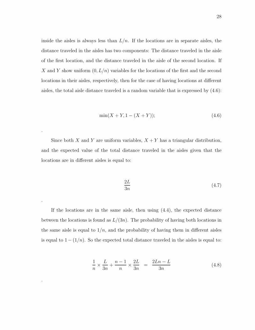
Fig. 4. Aisle combinations in a grid layout having four aisles
There are n2 different ways to choose two aisles out of n aisles. In 2(n − 1) of
these ways, the distance between the two aisle ends is (n − 1)w. Similarly, there are
2(n − 2) different combinations in which the distance between the two aisle ends is
(n−2)w. So we can make the generalization that among all the possible combinations,
in 2(n − i) of them, the distance between the two aisle ends is (n − i)w. This is also
illustrated in Fig. 4 for a grid layout having four aisles. Using this generalization, the
expected distance traveled between the ends of the aisles is found as:
1
n2
n−1∑
i=1
2wi(n − i) =1
3wn −
1
3nw (4.9)
Combining (4.8) and (4.9) gives us (4.5). �
Proposition 3 The expected distance between two random locations on the hub-and-
spoke layout is
−L
4m2+
L − 4d
2m+ 2d, (4.10)
where d is the distance between a division and the center.
Proof. There are two cases when two locations are randomly chosen on the layout
network: either the locations are in the same division or they are not. The probability
of having the locations in the same division is equal to 1/m and the probability of
30
having them in separate divisions is equal to 1 − 1/m = (m − 1)/m.
If two locations are in the same division, then we can fix one of the locations.
With probability 0.5 the other location is closer to the left side of the fixed location
with distance random between 0 and L/2m. Since the distance between the two
locations is uniformly distributed between 0 and L/2m, the expected distance between
the locations is equal to L/4m. The same argument applies when the other location
is closer to the right side of the fixed location. So the expected distance between two
locations when they are in the same division is given by
1
2×
L
4m+
1
2×
L
4m=
L
4m. (4.11)
In the second case, with probability (m− 1)/m, the locations can be in separate
divisions. This time the expected distance includes the distance between the locations
and the entrances of the divisions they are in, and also the distance between the
division entrances. The distance between the entrances of two separate divisions is
equal to 2d. The expected distance between a location and its division entrance is
equal to L/4m. So the expected distance between two locations in separate divisions
is given by
2d +L
2m. (4.12)
The expected distance between two random locations on the hub-and-spoke lay-
out (4.10) is given by the sum of the first case conditional expected value (4.11)
multiplied by its probability 1/m and the second case conditional expected value
(4.12) multiplied by its probability (m − 1)/m. Simulation results given in Table II
in Appendix A verify the correctness of equation (4.10). �
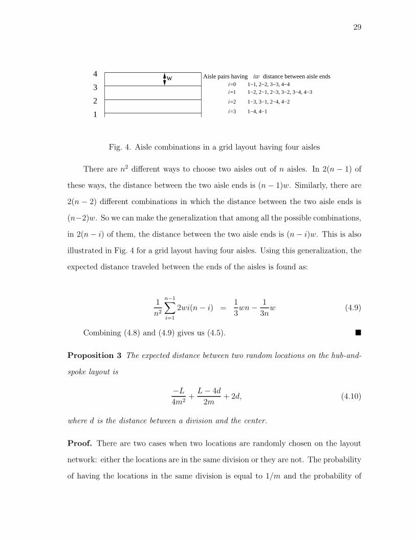
In Fig. 5, plots for the expected distance between two random locations are shown
for different layouts. Note that, for the serpentine layout, the expected distance

31
is constant since there is one path of length 10 units. However, for the grid and
hub-and-spoke layouts, the expected distance changes depending on the number of
aisles/divisions and the w/d parameter values. As the number of aisles/divisions
increases, the travel distance of the customer in an aisle or division decreases, which
in turn decreases the total distance if w or d is 0. On the other hand, if there is a
positive distance between two consecutive aisle ends (w) then as the number of aisles
increases, the customer tends to travel more due to the increase in the probability
of having product locations on two separate aisles that are far from each other. For
the hub-and-spoke layout, if there is a positive distance (d) between the divisions
and the central area, then the customer has to travel a distance of 2d to go from
one division to another. As the number of divisions increases, the travel distance
inside the divisions decreases and the customer’s travel distance converges to 2d on
the hub-and-spoke layout. In conclusion, we can say that the hub-and-spoke layout
is more advantageous for the customer in terms of travel distance if he wants to go
from one random product location to another one.
2. Expected Number of Paths between Two Random Locations
In this section, the expected number of paths between two random locations are
derived for grid and hub-and-spoke layouts. For the serpentine layout, the number of
paths is just one, since there is only one path between two points on a line.
Proposition 4 For the grid layout,if we assume that the customer never visits the
same aisle more than once during shopping, then the expected number of paths between
two locations is equal to
2n+2 − 4
n2−
3
n. (4.13)
32
0
1
2
3
4
5
6
7
8
5 10 15 20 25
Exp
ecte
d D
ista
nce
Number of Aisles/Divisions
Grid (w=0)Grid (w=1)
Hub-and-Spoke (d=0)
Hub-and-Spoke (d=1)Serpentine
Fig. 5. Plots for the expected distance between two locations for different layouts
(L=10)
Proof. If the two locations are in the same aisle then there is only one path between
the locations. If the locations are in consecutive aisles then there are two paths
between these locations. In general if the customer has to pass i aisles to reach from
the first location to the second one, then there are 2i different paths between the
locations. The expected number of paths is calculated as
n−1∑
j=0
P (i = j) × 2j , (4.14)
where
P (i = 0) =1
nand (4.15)
P (i = j) =2(n − j)
n2, 1 ≤ j ≤ n − 1. (4.16)
33
Placing (4.15) and (4.16) in (4.14) gives (4.13). �
Proposition 5 For the hub-and-spoke layout, the expected number of paths between
two locations is equal to
1
m× 2 +
m − 1
m× 4 = 4 −
2
m. (4.17)
Proof. For the hub-and-spoke layout, there are two different paths between the two
locations in the same division. If the locations are not in the same division, then there
are four different paths between the locations. The probability of having the locations
in the same division is 1/m and having them in different divisions is (m − 1)/m. So
the expected number of paths between two locations for the hub-and-spoke layout is
given by
1
m× 2 +
m − 1
m× 4 = 4 −
2
m. (4.18)
�
In Chapter III, the importance of controlling customer flow is stressed. The
expected number of paths between two locations is maximum for the grid layout and
minimum for the serpentine layout, which implies that on the grid layout it is difficult
to control customer travel compared to the hub-and-spoke and the serpentine layouts.
On the serpentine layout the customer flow can be easily controlled.
3. Expected Shopping Tour Length
Expected shopping tour length refers to the expected distance a customer travels to
complete the purchase of all the items in the shopping list. It is assumed that there
are K items in the shopping list and they are randomly located on the layout. In this
section, the expected shopping tour lengths for the serpentine, grid, and hub-and-
34
spoke layouts are given. A simulation analysis of expected shopping tour lengths is
given in Appendix A.
Proposition 6 The expected shopping tour length for the serpentine layout is equal
to
(1
2)K(
K
K + 1L − L) + L. (4.19)
Proof. In the serpentine layout, after entering the store the customer moves along
the path until all the items from the shopping list are purchased. When the last
item from the shopping list is purchased, the customer checks his closeness to the
entrance/exit points and chooses the closest one to leave the store. Then there are
two cases for the customer’s shopping route which are:
1. All the items in the shopping list are closer to the point where the customer
enters the store.
2. At least one of the items in the shopping list is closer to the opposite en-
trance/exit point to the one through which the customer enters the store.
In the first case, the customer enters the store, continues to move along one
direction until all the shopping list items are purchased. Then he returns back and
exits the store from the same entrance/exit point he entered through. This case can
occur only if all the shopping list items are located closer to the entrance point of
the customer. If there are K items in the shopping list and the total serpentine path
has length one unit, then with probability 0.5K , all the items in the shopping list are
closer to the customer’s entrance point. Given that all the shopping list items are
located in the same half of the path where the entrance point exists, then the one
way travel distance of the customer has the distribution function F (x) and density
35
function f(x):
F (x) = (2x
L)K 0 ≤ x ≤
L
2(4.20)
f(x) =K
LK2KxK−1 0 ≤ x ≤
L
2(4.21)
The conditional expected travel distance for the first case is given by:
2
∫ L2
x=0
x(K
LK2KxK−1)dx =
K
LK(K + 1)2K+1xK+1 |
L2
x=0
=K
K + 1L (4.22)
In the second case, the shopping list items are located in both halves of the
path. This time, the customer has to travel all the path to complete his shopping.
The expected travel distance for this case is L and the probability of occurrence of
this case is 1 − (0.5)K. The expected travel distance is calculated as sum of the
multiplications of the probabilities with the conditional expected values over all the
cases and it is found as
(1
2)K K
K + 1L + (1 − (
1
2)K)L (4.23)
= (1
2)K(
K
K + 1L − L) + L. (4.24)
�
Proposition 7 The expected shopping tour length for the grid layout is equal to
K∑
i=0
(n − 1)K−i
nK−1
(
K
i
)
[(1
2)i(
i
i + 1(L
n) −
L
n) +
L
n] + 2w(n −
1
2−
n−1∑
i=1
iK
nK). (4.25)
Proof. There are two distance components for the grid layout
1. The distance traveled in the aisles, and
2. The distance traveled between different aisle ends.
36
The expected distance traveled in a particular aisle is given by
K∑
i=0
P (i items in the aisle)×E[Distance traveled in an aisle having i items]. (4.26)
The probability of having i items in a particular aisle is given by
1
nK
(
K
i
)
(n − 1)K−i. (4.27)
The expected distance traveled in an aisle given that i shopping list items are located
in the aisle can be calculated using the equation (4.24) where the aisle is assumed to
be a serpentine layout of length L/n. Then the conditional expected travel distance
in a particular aisle is given by
K∑
i=0
(n − 1)K−i
nK
(
K
i
)
[(1
2)i(
i
i + 1(L
n) −
L
n) +
L
n]. (4.28)
Since there are n aisles and the products are randomly located along the aisles,
the expected travel distance within the aisles considering all aisles in the store is given
by multiplying (4.28) with n, which is equal to
K∑
i=0
(n − 1)K−i
nK−1
(
K
i
)
[(1
2)i(
i
i + 1(L
n) −
L
n) +
L
n]. (4.29)
If the aisles are numbered from 1 to n, starting from the entrance point, the
customer does not visit aisles with number greater than i, if aisle i is the last aisle
that contains item(s) from the shopping list. The probability that aisle i is the farthest
aisle the customer visits is defined as
P (aisles greater than i are not visited) =iK
nK. (4.30)
The expected number of the farthest aisle visited is given by
n∑
i=0
P (aisles greater than i are not visited), (4.31)
37
which is equal to
n∑
i=0
(1 −iK
nK) = n −
n−1∑
i=1
iK
nK. (4.32)
Since the distance between two consecutive aisle ends is w and the customer
needs to come back from the farthest aisle to exit through entrance/exit point, the
expected distance traveled between aisle ends is equal to
2w(n −1
2−
n−1∑
i=1
iK
nK). (4.33)
While inserting (4.32) into (4.33), we subtract 1/2 from (4.32) since the first aisle
is only w/2 distance units away from the entrance/exit point.
The expected shopping tour length of the customer is given by the sum of (4.29)
and (4.33), which is
K∑
i=0
(n − 1)K−i
nK−1
(
K
i
)
[(1
2)i(
i
i + 1(L
n) −
L
n) +
L
n] + 2w(n −
1
2−
n−1∑
i=1
iK
nK). (4.34)
�
Proposition 8 For the hub-and-spoke layout, the expected shopping tour length is
equal to
2d(m −(m − 1)K
mK−1) +
K∑
i=0
(m − 1)K−i
mK−1
(
K
i
)
[(1
2)i(
i
i + 1(L
m) −
L
m) +
L
m]. (4.35)
Proof. The expected shopping tour length in the hub-and-spoke layout depends on:
1. The number of divisions that contain item(s) from the shopping list,
2. The expected travel distance in a division.

38
The probability of having at least one item from the shopping list in a particular
division is equal to
mK − (m − 1)K
MK= 1 −
(m − 1)K
mK. (4.36)
Using (4.36), the expected number of divisions containing a shopping list item is
given by
m × (1 −(m − 1)K
mK) = m −
(m − 1)K
mK−1. (4.37)
The expected travel distance between the divisions is found by multiplying (4.37)
with the total round trip distance between the central area and a division, which is
equal to
2d(m −(m − 1)K
mK−1). (4.38)
The travel distance in a particular division depends on the number of items from
the shopping list located in that division. Probability of having i shopping list items
in a division is given by
(m − 1)K−i
mK
(
K
i
)
. (4.39)
If we assume that the customer’s visit in a division of length (L/m) is similar to
the customer’s travel in a serpentine layout of path length (L/m), then the expected
travel distance in that division is calculated by using equation (4.24). So the expected
shopping tour length in a particular division is equal to
P (i Shopping list items present in the division)×E[Travel distance for i items]
=K
∑
i=0
(m − 1)K−i
mK
(
K
i
)
[(1
2)i(
i
i + 1(L
m) −
L
m) +
L
m]. (4.40)
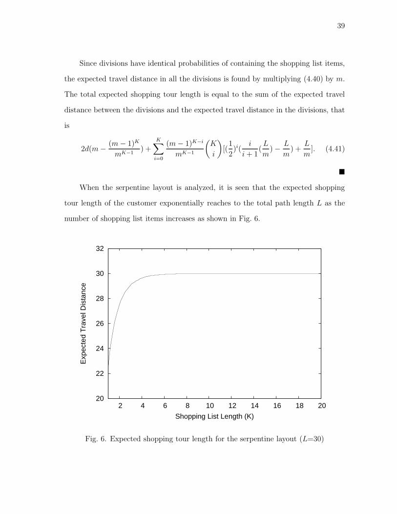
39
Since divisions have identical probabilities of containing the shopping list items,
the expected travel distance in all the divisions is found by multiplying (4.40) by m.
The total expected shopping tour length is equal to the sum of the expected travel
distance between the divisions and the expected travel distance in the divisions, that
is
2d(m −(m − 1)K
mK−1) +
K∑
i=0
(m − 1)K−i
mK−1
(
K
i
)
[(1
2)i(
i
i + 1(L
m) −
L
m) +
L
m]. (4.41)
�
When the serpentine layout is analyzed, it is seen that the expected shopping
tour length of the customer exponentially reaches to the total path length L as the
number of shopping list items increases as shown in Fig. 6.
20
22
24
26
28
30
32
2 4 6 8 10 12 14 16 18 20
Exp
ecte
d T
rave
l Dis
tanc
e
Shopping List Length (K)
Fig. 6. Expected shopping tour length for the serpentine layout (L=30)

40
Also, the expected shopping tour length linearly increases with path length L for
the serpentine layout. A 3D plot of expected shopping tour length for different K and
L values is shown in Fig. 7. For a fixed K value, the expected shopping tour length
increases linearly as L increases. Also, for a fixed L value, the expected shopping
tour length increases exponentially and converges to the value of L as K increases.
1 2 3 4 5 6 7 8 9 10 0 5
10 15
20 25
30
0 5
10 15 20 25 30
Expected Travel Distance
Shopping List Length (K)
Path Length (L)
Expected Travel Distance
Fig. 7. Expected shopping tour length for the serpentine layout
For the grid layout, if L is fixed, then there are three important parameters that
affect the shopping tour length, which are the number of shopping list items (K),
the distance between two consecutive aisle ends (w), and the number of aisles (n).
Intuitively, as K increases then the shopping tour length should increase. This is
clearly seen in Figs. 8 and 9. In Fig. 8, since w is equal to 0 (no distance between
aisle ends), the shopping tour length always decreases as n increases for a fixed K

41
value. When n is fixed to a specific value, the shopping tour length increases as K
increases. However the rate of increase due to K depends on the value of n, because
as n gets smaller, then the shopping tour length converges faster to L. In Fig. 9, w is
set to 1. Since w > 0, for a fixed K value there is a critical n value after which any
increase in n increases the shopping tour length. Consequently, we can conclude that
for a fixed shopping list size, there is a critical value for the number of aisles that
minimizes the expected shopping tour length of the customer.
0 5
10 15
20 25
30
0 10
20 30
40 50
60
0
5
10
15
20
25
30
Expected Travel Distance
Number of Aisles (n)
Shopping List Length (K)
Expected Travel Distance
Fig. 8. Expected shopping tour length with grid layout (w=0,L=30)
For the hub-and-spoke layout, as shown in Fig. 10, when the distance between
the divisions (2d) is zero, then the expected shopping tour length always decreases as
the number of divisions m increases. Similarly, as the number of items in the shopping
list (K) increases, the expected shopping tour length always increases. For the case
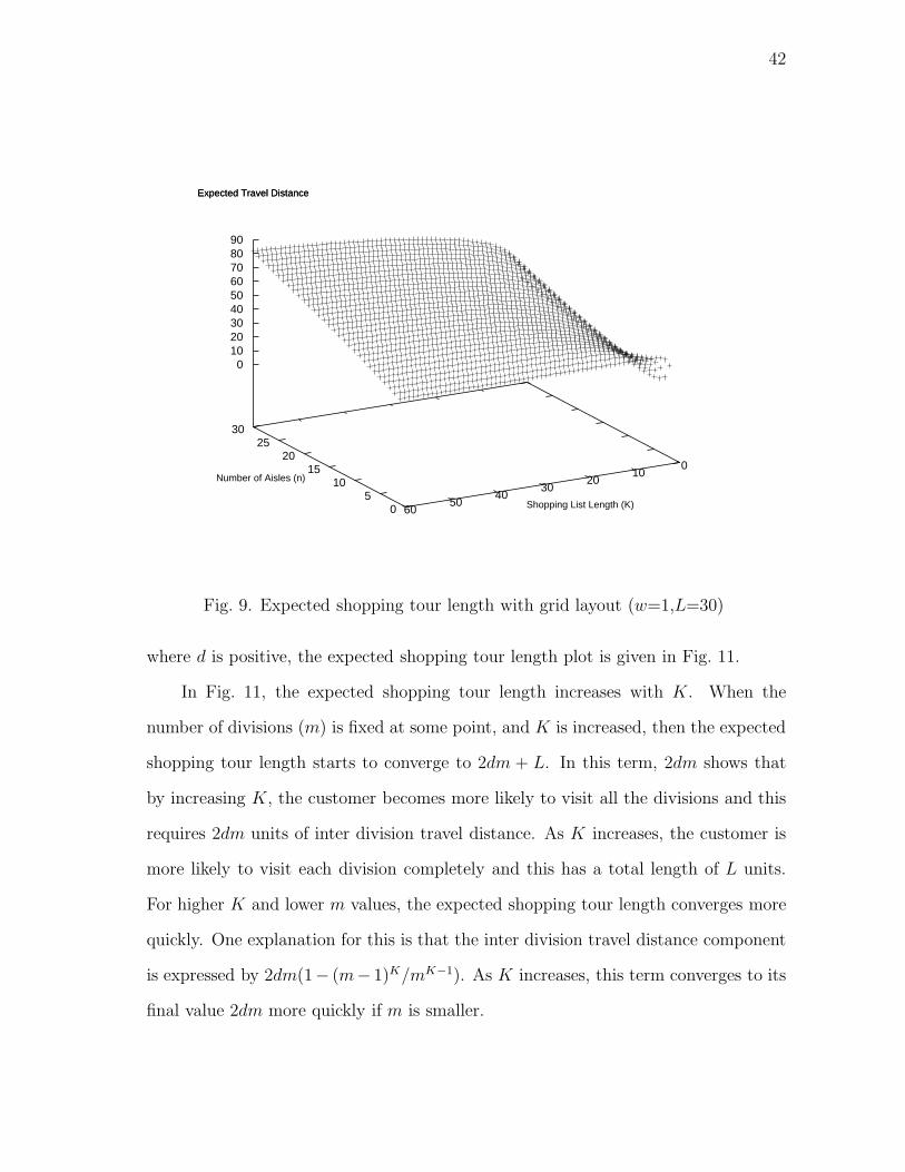
42
0 5
10 15
20 25
30
0 10
20 30
40 50
60
0 10 20 30 40 50 60 70 80 90
Expected Travel Distance
Number of Aisles (n)
Shopping List Length (K)
Expected Travel Distance
Fig. 9. Expected shopping tour length with grid layout (w=1,L=30)
where d is positive, the expected shopping tour length plot is given in Fig. 11.
In Fig. 11, the expected shopping tour length increases with K. When the
number of divisions (m) is fixed at some point, and K is increased, then the expected
shopping tour length starts to converge to 2dm + L. In this term, 2dm shows that
by increasing K, the customer becomes more likely to visit all the divisions and this
requires 2dm units of inter division travel distance. As K increases, the customer is
more likely to visit each division completely and this has a total length of L units.
For higher K and lower m values, the expected shopping tour length converges more
quickly. One explanation for this is that the inter division travel distance component
is expressed by 2dm(1− (m− 1)K/mK−1). As K increases, this term converges to its
final value 2dm more quickly if m is smaller.
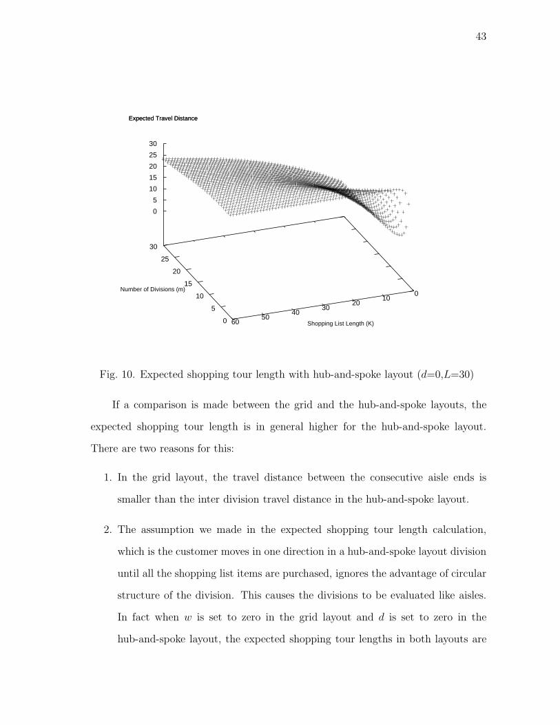
43
0
5
10
15
20
25
30
0 10
20 30
40 50
60
0
5
10
15
20
25
30
Expected Travel Distance
Number of Divisions (m)
Shopping List Length (K)
Expected Travel Distance
Fig. 10. Expected shopping tour length with hub-and-spoke layout (d=0,L=30)
If a comparison is made between the grid and the hub-and-spoke layouts, the
expected shopping tour length is in general higher for the hub-and-spoke layout.
There are two reasons for this:
1. In the grid layout, the travel distance between the consecutive aisle ends is
smaller than the inter division travel distance in the hub-and-spoke layout.
2. The assumption we made in the expected shopping tour length calculation,
which is the customer moves in one direction in a hub-and-spoke layout division
until all the shopping list items are purchased, ignores the advantage of circular
structure of the division. This causes the divisions to be evaluated like aisles.
In fact when w is set to zero in the grid layout and d is set to zero in the
hub-and-spoke layout, the expected shopping tour lengths in both layouts are
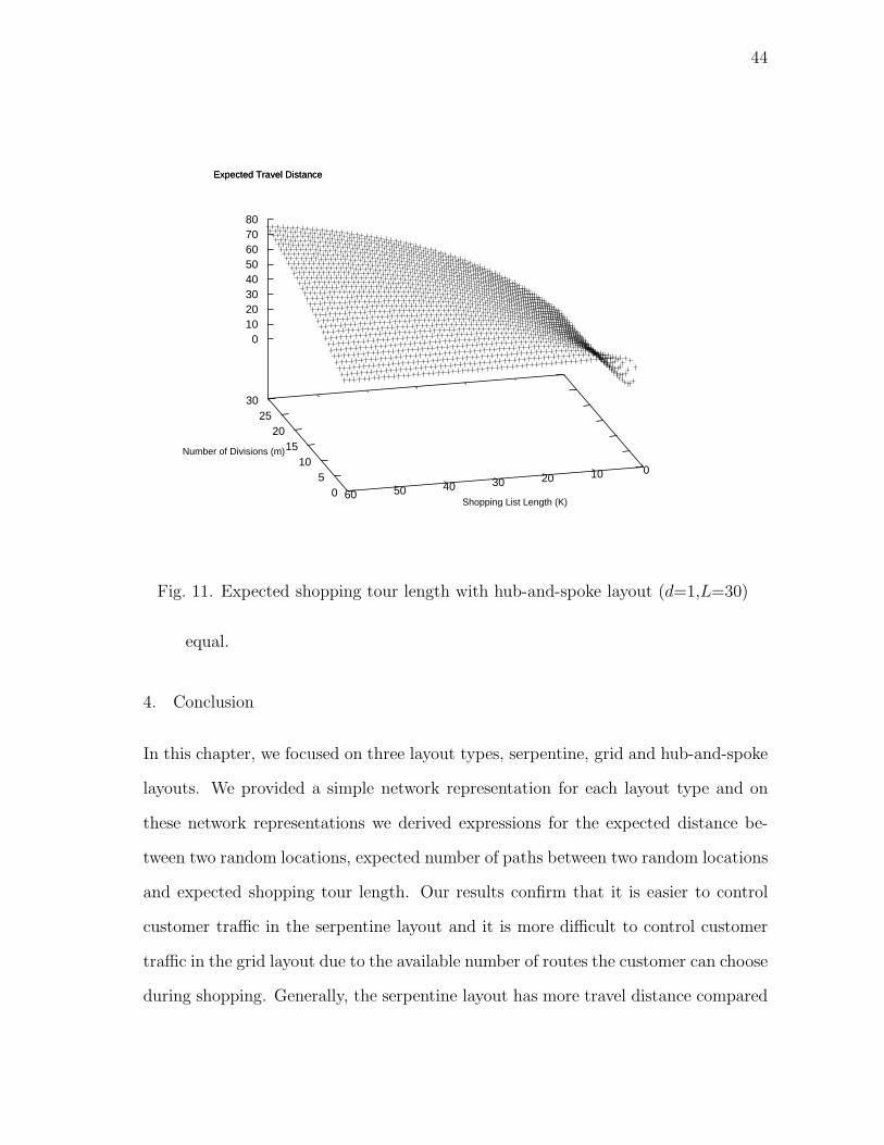
44
0 5
10 15
20 25
30
0 10 20 30 40 50 60
0 10 20 30 40 50 60 70 80
Expected Travel Distance
Number of Divisions (m)
Shopping List Length (K)
Expected Travel Distance
Fig. 11. Expected shopping tour length with hub-and-spoke layout (d=1,L=30)
equal.
4. Conclusion
In this chapter, we focused on three layout types, serpentine, grid and hub-and-spoke
layouts. We provided a simple network representation for each layout type and on
these network representations we derived expressions for the expected distance be-
tween two random locations, expected number of paths between two random locations
and expected shopping tour length. Our results confirm that it is easier to control
customer traffic in the serpentine layout and it is more difficult to control customer
traffic in the grid layout due to the available number of routes the customer can choose
during shopping. Generally, the serpentine layout has more travel distance compared
45
to other layout types. However, the expected shopping tour lengths in the grid and
hub-and-spoke layouts depend on the distance between consecutive aisles (w) and the
distance between divisions (2d), respectively. If w and d values are set to reasonable
values with respect to aisle and division lengths, then the grid and hub-and-spoke
layouts provide significant travel distance advantage for the customer compared to
the serpentine layout.
From a managerial perspective, serpentine layout appears to be the best option
to increase impulse purchase revenue unless there is a negative effect of higher travel
distances on customers’ loyalty. However, if the value customers place on time is high,
then the retailer may prefer to use other layout design alternatives, grid and hub-and-
spoke layouts, to maintain customer loyalty. On the other hand, the analysis based
on travel distance does not necessarily reflect the performance of layouts in terms of
impulse purchase revenue. In the next two chapters, we analyze the serpentine and
the grid layouts further with respect to both impulse purchase revenue and travel
distance. Considering the popularity of grid layout, and also the similarity between
grid and hub-and-spoke layouts in terms of aisle-division correspondence, we limit our
analysis for the hub-and-spoke layout to this chapter,and instead we focus on grid
layout in the next chapter. In Chapter VII, we return back to network representations
of the serpentine and grid layouts and extend them further.
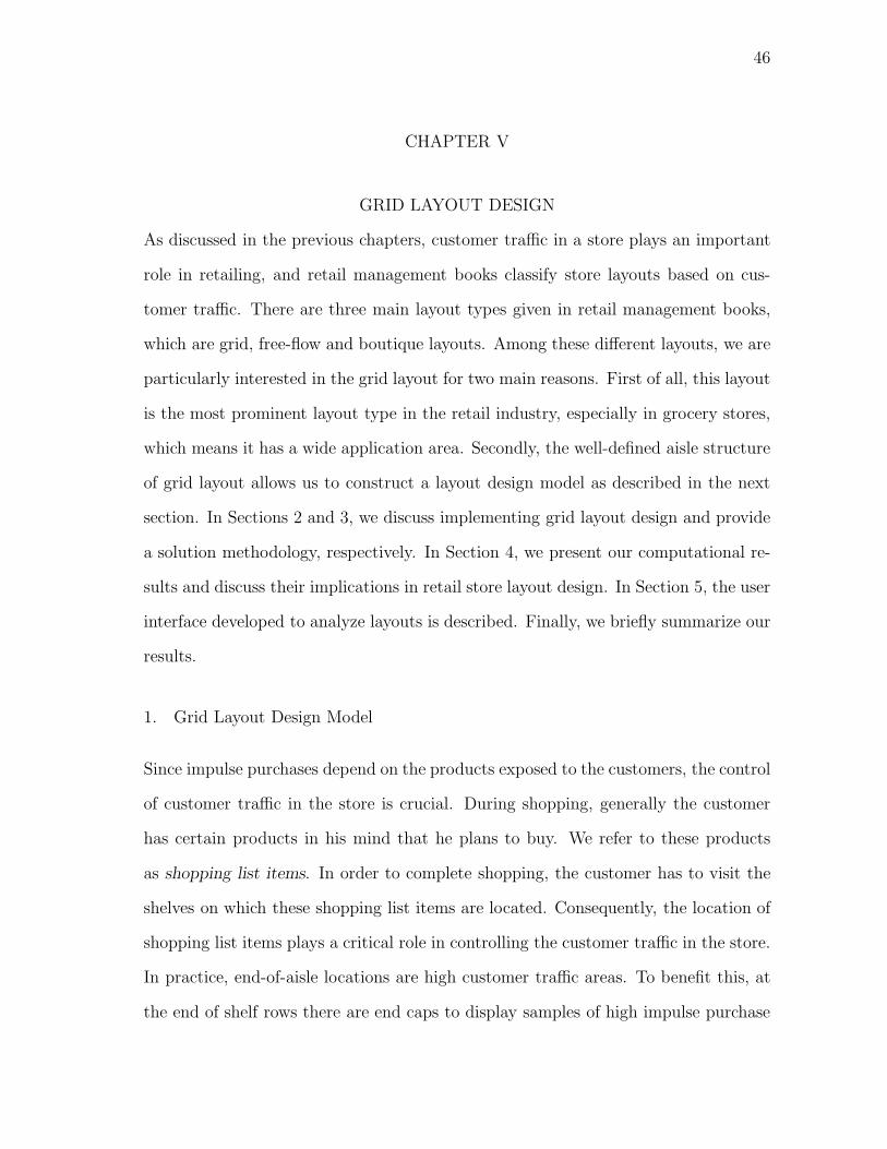
46
CHAPTER V
GRID LAYOUT DESIGN
As discussed in the previous chapters, customer traffic in a store plays an important
role in retailing, and retail management books classify store layouts based on cus-
tomer traffic. There are three main layout types given in retail management books,
which are grid, free-flow and boutique layouts. Among these different layouts, we are
particularly interested in the grid layout for two main reasons. First of all, this layout
is the most prominent layout type in the retail industry, especially in grocery stores,
which means it has a wide application area. Secondly, the well-defined aisle structure
of grid layout allows us to construct a layout design model as described in the next
section. In Sections 2 and 3, we discuss implementing grid layout design and provide
a solution methodology, respectively. In Section 4, we present our computational re-
sults and discuss their implications in retail store layout design. In Section 5, the user
interface developed to analyze layouts is described. Finally, we briefly summarize our
results.
1. Grid Layout Design Model
Since impulse purchases depend on the products exposed to the customers, the control
of customer traffic in the store is crucial. During shopping, generally the customer
has certain products in his mind that he plans to buy. We refer to these products
as shopping list items. In order to complete shopping, the customer has to visit the
shelves on which these shopping list items are located. Consequently, the location of
shopping list items plays a critical role in controlling the customer traffic in the store.
In practice, end-of-aisle locations are high customer traffic areas. To benefit this, at
the end of shelf rows there are end caps to display samples of high impulse purchase

47
revenue or promotion items. This is another point that should be taken into account
during layout design.
Other than the locations of shopping list items, the layout design model should
clearly identify the walkways that the customer can use in the store. These walkways
define the possible set of routes the customer may follow. By locating products with
high impulse purchase revenue along the walkways the customer follows, it is possible
to increase the visibility of these products, and consequently the potential impulse
purchase revenue. In grid layout, the walkways are defined by the aisles between the
shelf rows. Depending on the length and orientation of aisles, we may have different
grid layout realizations as shown in Fig. 12.
Fig. 12. Different grid layout realizations
In order to capture these aspects of grid layout, we define a basic layout compo-
nent, which we refer to as grid unit. A grid unit contains a number of parallel shelf
rows and aisle clearances between these shelf rows. At the end of shelf rows, there
are end caps to display products having high impulse purchase rates. In Fig. 13, a
grid unit having two shelf rows is presented. The grid unit has a square shape and its
dimensions are proportional to the number of shelf rows it contains. The final layout
consists of a set of connected grid units and perimeter shelves along the boundaries
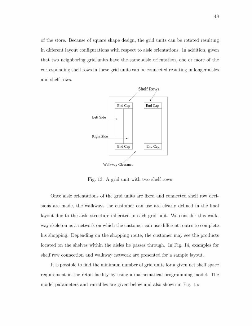
48
of the store. Because of square shape design, the grid units can be rotated resulting
in different layout configurations with respect to aisle orientations. In addition, given
that two neighboring grid units have the same aisle orientation, one or more of the
corresponding shelf rows in these grid units can be connected resulting in longer aisles
and shelf rows.
End CapEnd Cap
End CapEnd Cap
Walkway Clearance
Right Side
Left Side
Shelf Rows
Fig. 13. A grid unit with two shelf rows
Once aisle orientations of the grid units are fixed and connected shelf row deci-
sions are made, the walkways the customer can use are clearly defined in the final
layout due to the aisle structure inherited in each grid unit. We consider this walk-
way skeleton as a network on which the customer can use different routes to complete
his shopping. Depending on the shopping route, the customer may see the products
located on the shelves within the aisles he passes through. In Fig. 14, examples for
shelf row connection and walkway network are presented for a sample layout.
It is possible to find the minimum number of grid units for a given net shelf space
requirement in the retail facility by using a mathematical programming model. The
model parameters and variables are given below and also shown in Fig. 15:
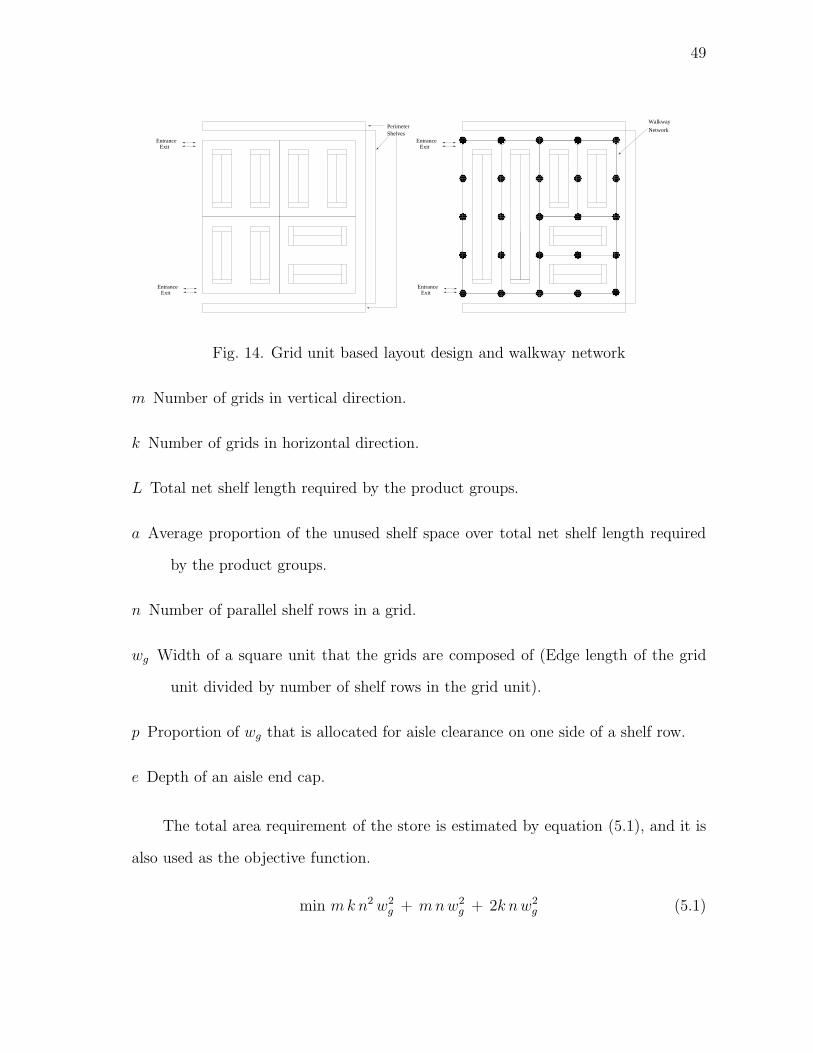
49
Shelves
EntranceExit
EntranceExit
PerimeterNetwork
EntranceExit
EntranceExit ���
���������������
������������������
������������������
������������������
������������������
������������������
������������������
������������������
������������������
������������������
������������������
������������������
������������������
������������������
������������������
������������������
������������������
������������������
������������������
������������������
���������������
���������������
���������������
���������������
���������������
���������������
������������������
������������������
���������������
���������������
������������������
������������������
������������������
������������������
������������������
������������������
���������������
���������������
���������������
���������������
���������������
���������������
������������������
������������������
���������������
���������������
���������������
���������������
������������������
������������������
������������������
������������������
������������
������������
Walkway
Fig. 14. Grid unit based layout design and walkway network
m Number of grids in vertical direction.
k Number of grids in horizontal direction.
L Total net shelf length required by the product groups.
a Average proportion of the unused shelf space over total net shelf length required
by the product groups.
n Number of parallel shelf rows in a grid.
wg Width of a square unit that the grids are composed of (Edge length of the grid
unit divided by number of shelf rows in the grid unit).
p Proportion of wg that is allocated for aisle clearance on one side of a shelf row.
e Depth of an aisle end cap.
The total area requirement of the store is estimated by equation (5.1), and it is
also used as the objective function.
min m k n2 w2g + m n w2
g + 2k n w2g (5.1)
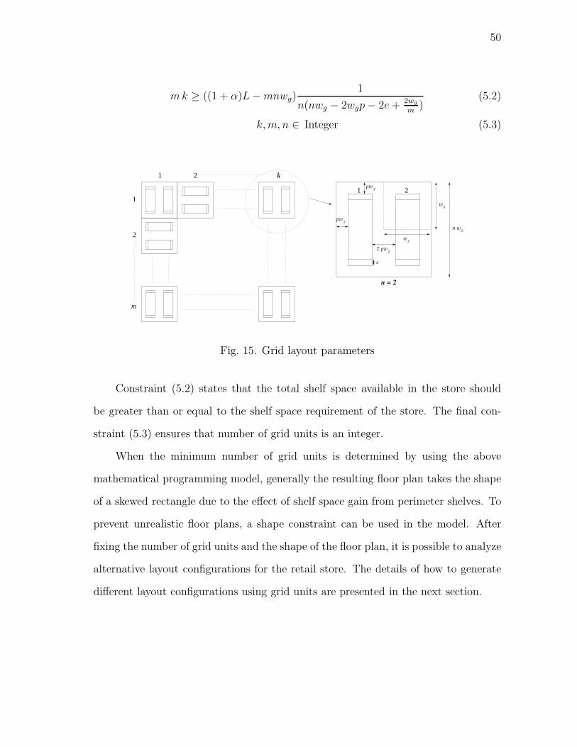
50
m k ≥ ((1 + α)L − mnwg)1
n(nwg − 2wgp − 2e + 2wg
m)
(5.2)
k, m, n ∈ Integer (5.3)
k
pw g
pw g
pw g
21
1 2
1
2
e
w
w
g
g
2
n w g
n = 2
m
Fig. 15. Grid layout parameters
Constraint (5.2) states that the total shelf space available in the store should
be greater than or equal to the shelf space requirement of the store. The final con-
straint (5.3) ensures that number of grid units is an integer.
When the minimum number of grid units is determined by using the above
mathematical programming model, generally the resulting floor plan takes the shape
of a skewed rectangle due to the effect of shelf space gain from perimeter shelves. To
prevent unrealistic floor plans, a shape constraint can be used in the model. After
fixing the number of grid units and the shape of the floor plan, it is possible to analyze
alternative layout configurations for the retail store. The details of how to generate
different layout configurations using grid units are presented in the next section.
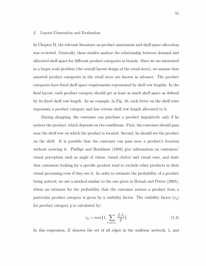
51
2. Layout Generation and Evaluation
In Chapter II, the relevant literature on product assortment and shelf space allocation
was reviewed. Generally, these studies analyze the relationship between demand and
allocated shelf space for different product categories or brands. Since we are interested
in a larger scale problem (the overall layout design of the retail store), we assume that
assorted product categories in the retail store are known in advance. The product
categories have fixed shelf space requirements represented by shelf row lengths. In the
final layout, each product category should get at least as much shelf space as defined
by its fixed shelf row length. As an example, in Fig. 16, each letter on the shelf rows
represents a product category and has certain shelf row length allocated to it.
During shopping, the customer can purchase a product impulsively only if he
notices the product, which depends on two conditions. First, the customer should pass
near the shelf row on which the product is located. Second, he should see the product
on the shelf. It is possible that the customer can pass near a product’s location
without noticing it. Phillips and Bradshaw (1993) give information on customers’
visual perception such as angle of vision, visual clutter and visual cues, and state
that customers looking for a specific product tend to exclude other products in their
visual processing even if they see it. In order to estimate the probability of a product
being noticed, we use a method similar to the one given in Botsalı and Peters (2005),
where an estimate for the probability that the customer notices a product from a
particular product category is given by a visibility factor. The visibility factor (vp)
for product category p is calculated by:
vp = min{1,∑
e: p∈Ce
fe leT
} (5.4)
In this expression, E denotes the set of all edges in the walkway network; le and
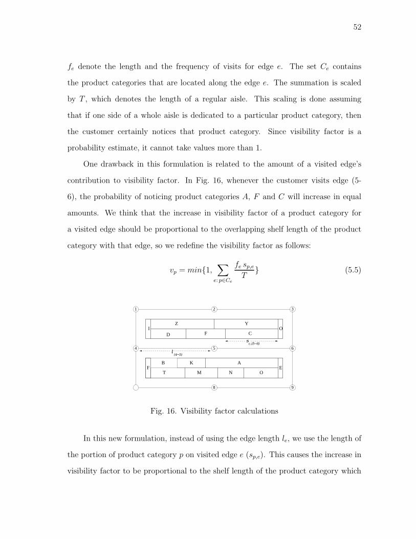
52
fe denote the length and the frequency of visits for edge e. The set Ce contains
the product categories that are located along the edge e. The summation is scaled
by T , which denotes the length of a regular aisle. This scaling is done assuming
that if one side of a whole aisle is dedicated to a particular product category, then
the customer certainly notices that product category. Since visibility factor is a
probability estimate, it cannot take values more than 1.
One drawback in this formulation is related to the amount of a visited edge’s
contribution to visibility factor. In Fig. 16, whenever the customer visits edge (5-
6), the probability of noticing product categories A, F and C will increase in equal
amounts. We think that the increase in visibility factor of a product category for
a visited edge should be proportional to the overlapping shelf length of the product
category with that edge, so we redefine the visibility factor as follows:
vp = min{1,∑
e: p∈Ce
fe sp,e
T} (5.5)
l
C
T NEF
2 3
654
9
Z
D F
YOI
B K A
M O
87
1
sc,(5−6)
(4−5)
Fig. 16. Visibility factor calculations
In this new formulation, instead of using the edge length le, we use the length of
the portion of product category p on visited edge e (sp,e). This causes the increase in
visibility factor to be proportional to the shelf length of the product category which
53
is more realistic.
Once the visibility factor values of the product categories are calculated for a
given shopping route, by using the average impulse purchase rate (ip) and average
revenue per purchase (rp) parameter values for each product category p, the total
average impulse purchase revenue obtained from the customer is given by the sum-
mation over the set of all product categories (P ):
∑
p∈P
vp ip rp (5.6)
In the above summation, the average impulse purchase revenue contribution of prod-
uct category p is assumed to be equal to the multiplication of its visibility probability
(vp), the average rate a customer makes a purchase from product category p im-
pulsively after noticing it (ip) and the average revenue per purchase from product
category p (rp). ip and rp parameter values can be estimated by analyzing stud-
ies related to impulse purchases (e.g., Bellenger et al., 1978; McGoldrick, 1982) and
marketing sales data, respectively.
Equation (5.6) can be used to evaluate a layout configuration in terms of average
impulse purchase revenue for a given shopping route scenario. If the customer makes
purchases based on a shopping list, it is possible to generate alternative shopping
routes for the customer. In the next section, we provide our solution methodology to
find a layout that maximizes average impulse purchase revenue when the customer’s
shopping list information is available.
3. Solution Methodology
Due to the characteristics of the problem, it is difficult to formulate a mathematical
programming model that considers all aspects of grid layout design. On the other
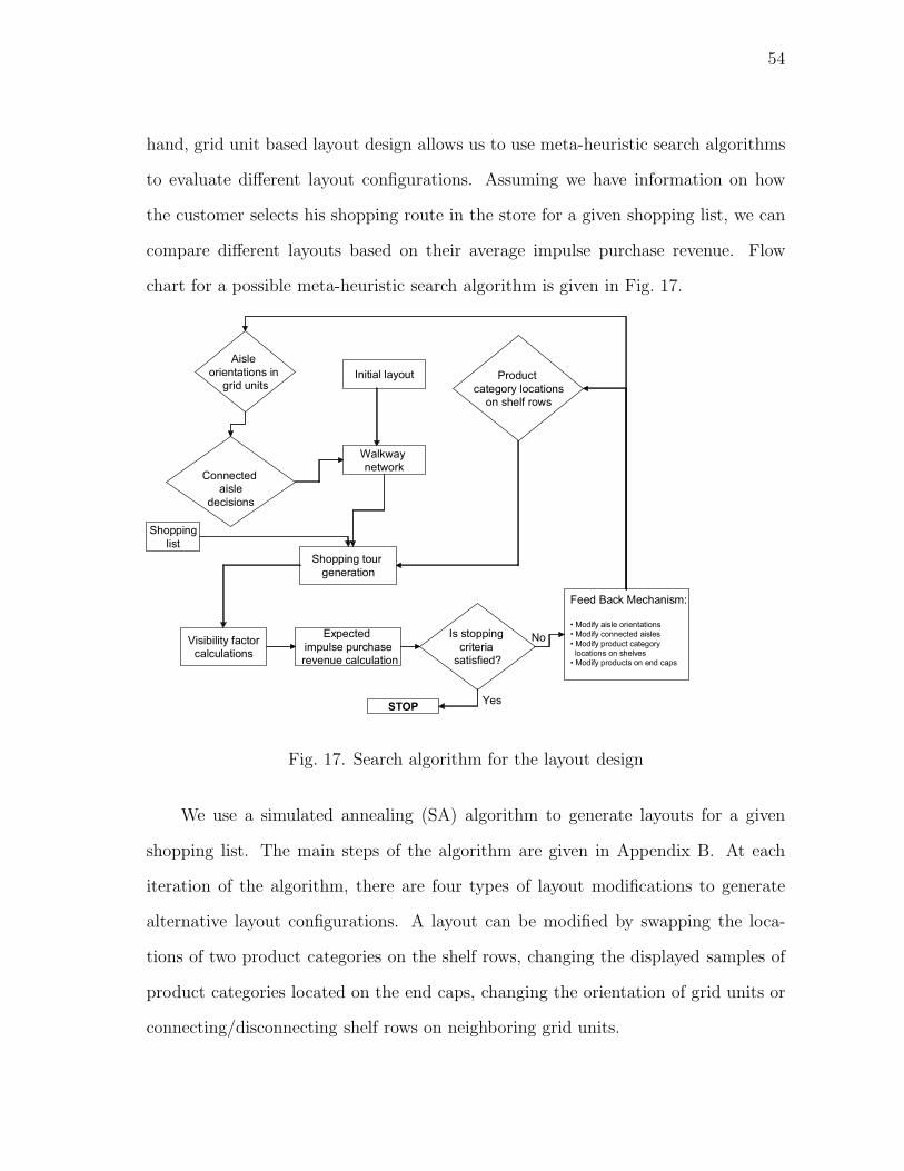
54
hand, grid unit based layout design allows us to use meta-heuristic search algorithms
to evaluate different layout configurations. Assuming we have information on how
the customer selects his shopping route in the store for a given shopping list, we can
compare different layouts based on their average impulse purchase revenue. Flow
chart for a possible meta-heuristic search algorithm is given in Fig. 17.
Fig. 17. Search algorithm for the layout design
We use a simulated annealing (SA) algorithm to generate layouts for a given
shopping list. The main steps of the algorithm are given in Appendix B. At each
iteration of the algorithm, there are four types of layout modifications to generate
alternative layout configurations. A layout can be modified by swapping the loca-
tions of two product categories on the shelf rows, changing the displayed samples of
product categories located on the end caps, changing the orientation of grid units or
connecting/disconnecting shelf rows on neighboring grid units.
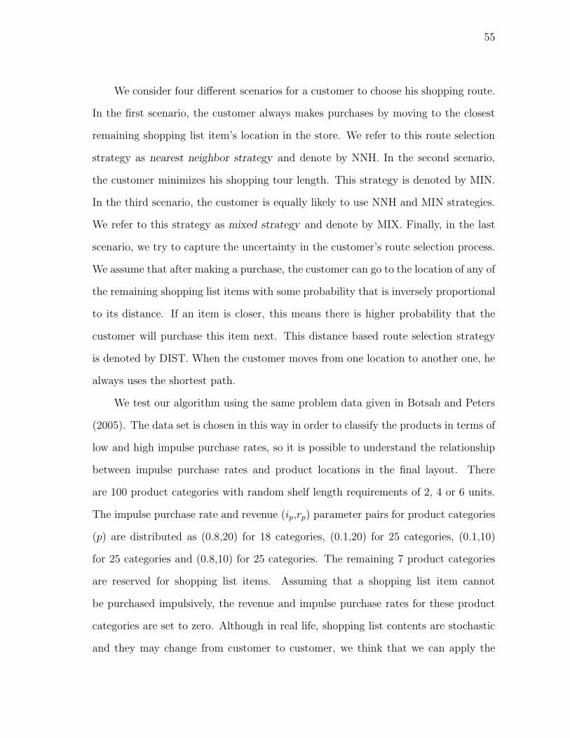
55
We consider four different scenarios for a customer to choose his shopping route.
In the first scenario, the customer always makes purchases by moving to the closest
remaining shopping list item’s location in the store. We refer to this route selection
strategy as nearest neighbor strategy and denote by NNH. In the second scenario,
the customer minimizes his shopping tour length. This strategy is denoted by MIN.
In the third scenario, the customer is equally likely to use NNH and MIN strategies.
We refer to this strategy as mixed strategy and denote by MIX. Finally, in the last
scenario, we try to capture the uncertainty in the customer’s route selection process.
We assume that after making a purchase, the customer can go to the location of any of
the remaining shopping list items with some probability that is inversely proportional
to its distance. If an item is closer, this means there is higher probability that the
customer will purchase this item next. This distance based route selection strategy
is denoted by DIST. When the customer moves from one location to another one, he
always uses the shortest path.
We test our algorithm using the same problem data given in Botsalı and Peters
(2005). The data set is chosen in this way in order to classify the products in terms of
low and high impulse purchase rates, so it is possible to understand the relationship
between impulse purchase rates and product locations in the final layout. There
are 100 product categories with random shelf length requirements of 2, 4 or 6 units.
The impulse purchase rate and revenue (ip,rp) parameter pairs for product categories
(p) are distributed as (0.8,20) for 18 categories, (0.1,20) for 25 categories, (0.1,10)
for 25 categories and (0.8,10) for 25 categories. The remaining 7 product categories
are reserved for shopping list items. Assuming that a shopping list item cannot
be purchased impulsively, the revenue and impulse purchase rates for these product
categories are set to zero. Although in real life, shopping list contents are stochastic
and they may change from customer to customer, we think that we can apply the

56
deterministic shopping list approach by defining a set of product categories with high
demands. For example, in retailing literature such high demand product categories
are referred as power products (e.g., bread, milk, etc.), and they are used to control
the customer traffic in the store.
The store layout consists of 21 grid units (3×7). Each grid unit is a 10×10 units
square and contains two shelf rows. The width and length of a shelf row is 3 and 8
units respectively. The depth of an end cap is 1 unit. In visibility factor calculations,
we use the same parameter T value as in Botsalı and Peters (2005) which is 26 units.
The customer can enter the store using any of the two doors located on the same side
with equal probability and after completing all the purchases, leaves the store using
the closest exit. Our computational results are presented in the next section.
4. Computational Results and Discussion
In the simulated annealing algorithm initial and final temperatures are set to 10 and
10−3, respectively based on our preliminary experimentation. The cooling rate is
taken as 0.7 and at each temperature, 20 iterations are made. One iteration con-
sists of 100 pair wise product category exchanges on the shelf rows, 20 product
category changes on the end caps, one grid unit orientation change and one con-
nected/disconnected shelf row modification. There are seven different shopping list
scenarios based on the number of items in the shopping list. For each shopping list
scenario, we consider four different shopping route selection strategies, which are dis-
cussed in the previous section. For a fixed shopping list length and route selection
strategy, the average result at the end of five computer runs is taken for the analysis.
For NNH, MIN and MIX shopping route selection strategies, an average computer
run takes between 3-5 hours on a Pentium IV 3.2 Ghz computer with 512 MB RAM.
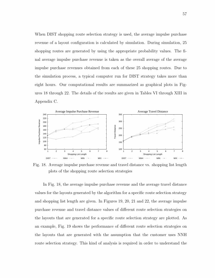
57
When DIST shopping route selection strategy is used, the average impulse purchase
revenue of a layout configuration is calculated by simulation. During simulation, 25
shopping routes are generated by using the appropriate probability values. The fi-
nal average impulse purchase revenue is taken as the overall average of the average
impulse purchase revenues obtained from each of these 25 shopping routes. Due to
the simulation process, a typical computer run for DIST strategy takes more than
eight hours. Our computational results are summarized as graphical plots in Fig-
ures 18 through 22. The details of the results are given in Tables VI through XIII in
Appendix C.
60
80
100
120
140
160
180
200
220
240
1 2 3 4 5 6 7 8
Impu
lse
Pur
chas
e R
even
ue
Shopping List Length
Average Impulse Purchase Revenue
DIST NNH MIN MIX
100
150
200
250
300
350
1 2 3 4 5 6 7 8
Tra
vel D
ista
nce
Shopping List Length
Average Travel Distance
DIST NNH MIN MIX
Fig. 18. Average impulse purchase revenue and travel distance vs. shopping list length
plots of the shopping route selection strategies
In Fig. 18, the average impulse purchase revenue and the average travel distance
values for the layouts generated by the algorithm for a specific route selection strategy
and shopping list length are given. In Figures 19, 20, 21 and 22, the average impulse
purchase revenue and travel distance values of different route selection strategies on
the layouts that are generated for a specific route selection strategy are plotted. As
an example, Fig. 19 shows the performance of different route selection strategies on
the layouts that are generated with the assumption that the customer uses NNH
route selection strategy. This kind of analysis is required in order to understand the

58
60
80
100
120
140
160
180
200
220
240
1 2 3 4 5 6 7 8
Impu
lse
Pur
chas
e R
even
ue
Shopping List Length
Average Impulse Purchase Revenue (NNH)
DIST NNH MIN MIX
100
150
200
250
300
350
1 2 3 4 5 6 7 8
Tra
vel D
ista
nce
Shopping List Length
Average Travel Distance (NNH)
DIST NNH MIN MIX
Fig. 19. Average impulse purchase revenue and travel distance vs. shopping list length
plots of the shopping route selection strategies on the layouts generated for
NNH route selection strategy
60
80
100
120
140
160
180
200
220
240
1 2 3 4 5 6 7 8
Impu
lse
Pur
chas
e R
even
ue
Shopping List Length
Average Impulse Purchase Revenue (MIN)
DIST NNH MIN MIX
100
150
200
250
300
350
1 2 3 4 5 6 7 8
Tra
vel D
ista
nce
Shopping List Length
Average Travel Distance (MIN)
DIST NNH MIN MIX
Fig. 20. Average impulse purchase revenue and travel distance vs. shopping list length
plots of the shopping route selection strategies on the layouts generated for
MIN route selection strategy
performance of a specific layout with respect to different customer profiles.
From Fig. 18, we can conclude that as the shopping list length increases, the
average travel distance of the customer and also the average impulse purchase revenue
increase in general. On the other hand, it is observed that there are some fluctuations
in the increase trend of the average impulse purchase revenue results. As an example,
in Fig. 20, for the layouts generated with the assumption that customer uses MIN
route selection strategy, the average impulse purchase revenue decreases although the

59
60
80
100
120
140
160
180
200
220
240
1 2 3 4 5 6 7 8
Impu
lse
Pur
chas
e R
even
ue
Shopping List Length
Average Impulse Purchase Revenue (MIX)
DIST NNH MIN MIX
100
150
200
250
300
350
1 2 3 4 5 6 7 8
Tra
vel D
ista
nce
Shopping List Length
Average Travel Distance (MIX)
DIST NNH MIN MIX
Fig. 21. Average impulse purchase revenue and travel distance vs. shopping list length
plots of the shopping route selection strategies on the layouts generated for
MIX route selection strategy
60
80
100
120
140
160
180
200
220
240
1 2 3 4 5 6 7 8
Impu
lse
Pur
chas
e R
even
ue
Shopping List Length
Average Impulse Purchase Revenue (DIST)
DIST NNH MIN MIX
100
150
200
250
300
350
1 2 3 4 5 6 7 8
Tra
vel D
ista
nce
Shopping List Length
Average Travel Distance (DIST)
DIST NNH MIN MIX
Fig. 22. Average impulse purchase revenue and travel distance vs. shopping list length
plots of the shopping route selection strategies on the layouts generated for
DIST route selection strategy
shopping list length is increased from six to seven for almost all the strategies. We
thought that this sharp decrease in the average impulse purchase revenue was caused
by some inefficiency in our SA algorithm and we decided to improve the algorithm
further.
In the initial algorithm, one of the layout modification methods was to swap the
locations of the products on the layout. However, if an existing layout is modified by
changing the locations of two products which are not visited by the customer, then this
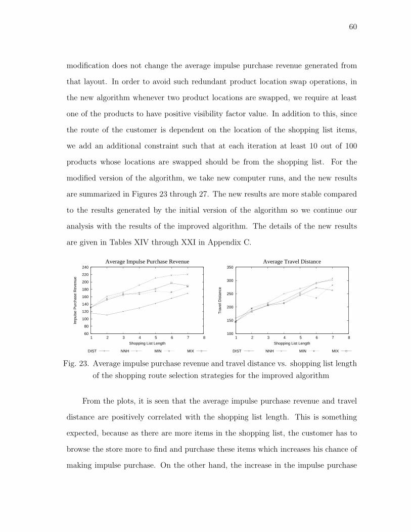
60
modification does not change the average impulse purchase revenue generated from
that layout. In order to avoid such redundant product location swap operations, in
the new algorithm whenever two product locations are swapped, we require at least
one of the products to have positive visibility factor value. In addition to this, since
the route of the customer is dependent on the location of the shopping list items,
we add an additional constraint such that at each iteration at least 10 out of 100
products whose locations are swapped should be from the shopping list. For the
modified version of the algorithm, we take new computer runs, and the new results
are summarized in Figures 23 through 27. The new results are more stable compared
to the results generated by the initial version of the algorithm so we continue our
analysis with the results of the improved algorithm. The details of the new results
are given in Tables XIV through XXI in Appendix C.
60
80
100
120
140
160
180
200
220
240
1 2 3 4 5 6 7 8
Impu
lse
Pur
chas
e R
even
ue
Shopping List Length
Average Impulse Purchase Revenue
DIST NNH MIN MIX
100
150
200
250
300
350
1 2 3 4 5 6 7 8
Tra
vel D
ista
nce
Shopping List Length
Average Travel Distance
DIST NNH MIN MIX
Fig. 23. Average impulse purchase revenue and travel distance vs. shopping list length
of the shopping route selection strategies for the improved algorithm
From the plots, it is seen that the average impulse purchase revenue and travel
distance are positively correlated with the shopping list length. This is something
expected, because as there are more items in the shopping list, the customer has to
browse the store more to find and purchase these items which increases his chance of
making impulse purchase. On the other hand, the increase in the impulse purchase
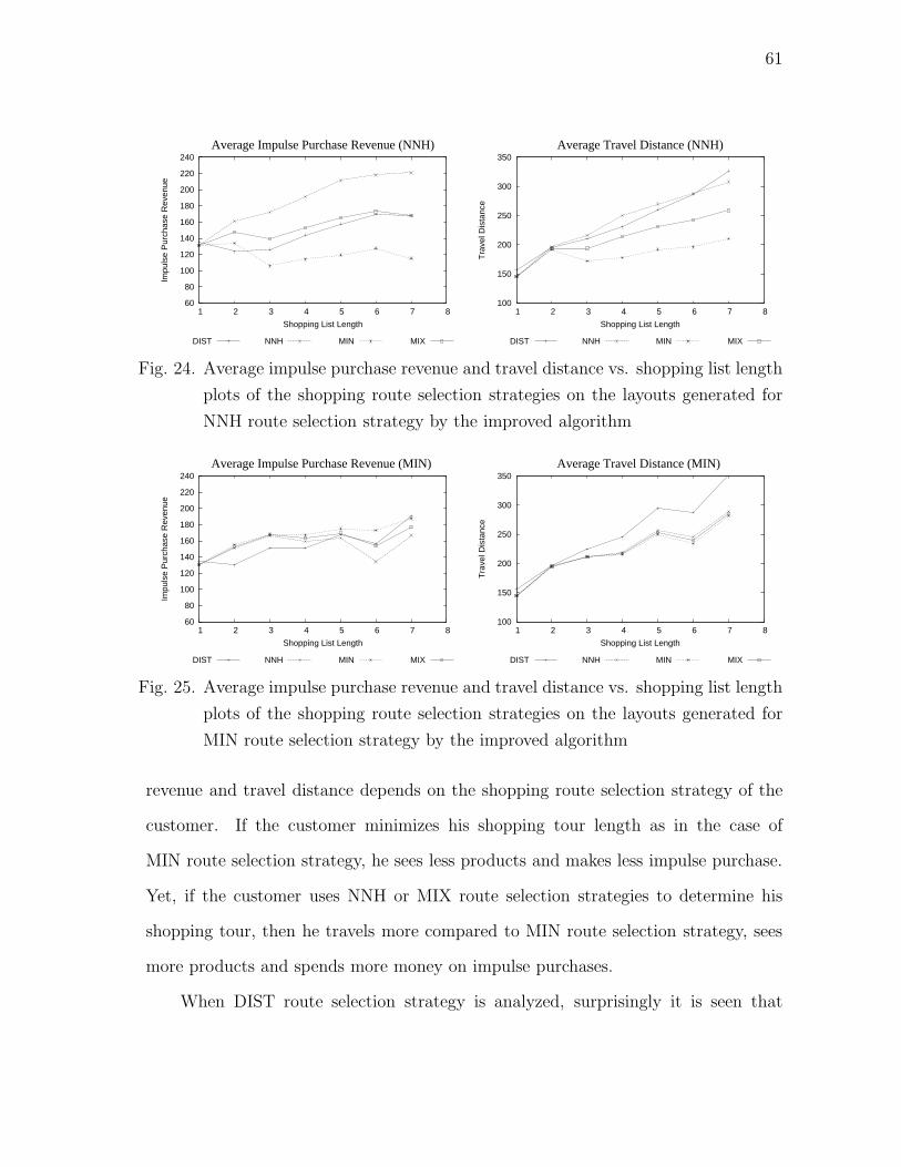
61
60
80
100
120
140
160
180
200
220
240
1 2 3 4 5 6 7 8
Impu
lse
Pur
chas
e R
even
ue
Shopping List Length
Average Impulse Purchase Revenue (NNH)
DIST NNH MIN MIX
100
150
200
250
300
350
1 2 3 4 5 6 7 8
Tra
vel D
ista
nce
Shopping List Length
Average Travel Distance (NNH)
DIST NNH MIN MIX
Fig. 24. Average impulse purchase revenue and travel distance vs. shopping list length
plots of the shopping route selection strategies on the layouts generated for
NNH route selection strategy by the improved algorithm
60
80
100
120
140
160
180
200
220
240
1 2 3 4 5 6 7 8
Impu
lse
Pur
chas
e R
even
ue
Shopping List Length
Average Impulse Purchase Revenue (MIN)
DIST NNH MIN MIX
100
150
200
250
300
350
1 2 3 4 5 6 7 8
Tra
vel D
ista
nce
Shopping List Length
Average Travel Distance (MIN)
DIST NNH MIN MIX
Fig. 25. Average impulse purchase revenue and travel distance vs. shopping list length
plots of the shopping route selection strategies on the layouts generated for
MIN route selection strategy by the improved algorithm
revenue and travel distance depends on the shopping route selection strategy of the
customer. If the customer minimizes his shopping tour length as in the case of
MIN route selection strategy, he sees less products and makes less impulse purchase.
Yet, if the customer uses NNH or MIX route selection strategies to determine his
shopping tour, then he travels more compared to MIN route selection strategy, sees
more products and spends more money on impulse purchases.
When DIST route selection strategy is analyzed, surprisingly it is seen that
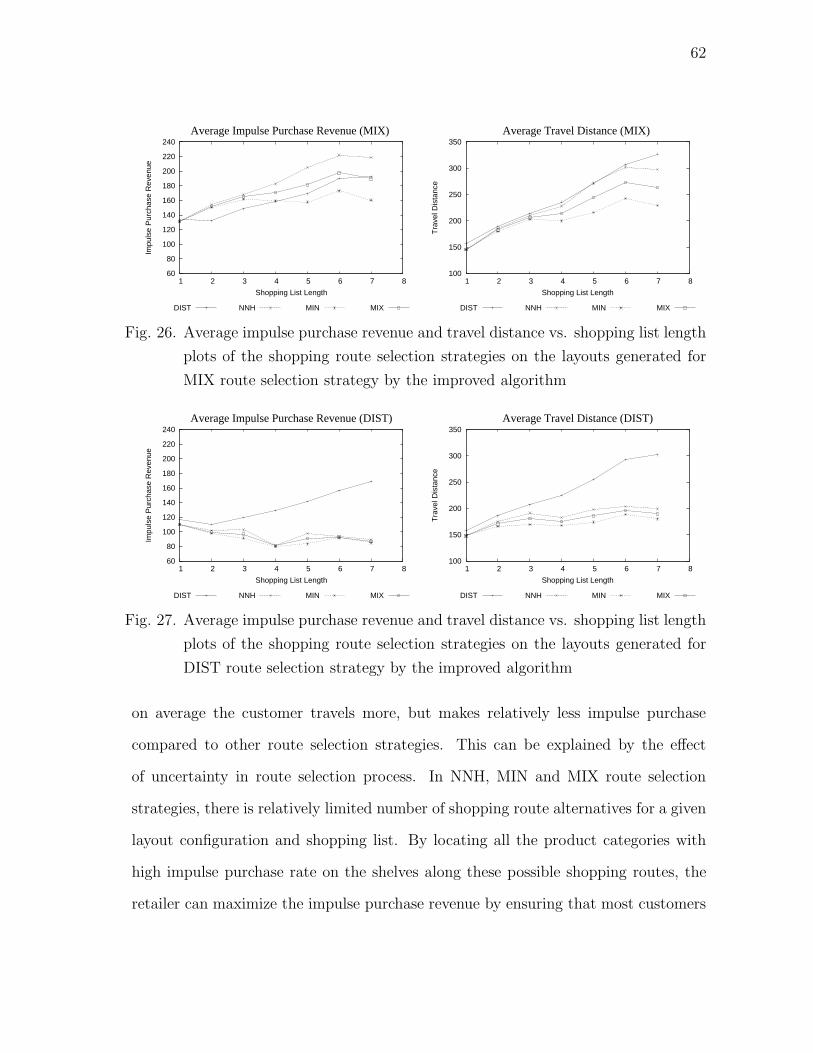
62
60
80
100
120
140
160
180
200
220
240
1 2 3 4 5 6 7 8
Impu
lse
Pur
chas
e R
even
ue
Shopping List Length
Average Impulse Purchase Revenue (MIX)
DIST NNH MIN MIX
100
150
200
250
300
350
1 2 3 4 5 6 7 8
Tra
vel D
ista
nce
Shopping List Length
Average Travel Distance (MIX)
DIST NNH MIN MIX
Fig. 26. Average impulse purchase revenue and travel distance vs. shopping list length
plots of the shopping route selection strategies on the layouts generated for
MIX route selection strategy by the improved algorithm
60
80
100
120
140
160
180
200
220
240
1 2 3 4 5 6 7 8
Impu
lse
Pur
chas
e R
even
ue
Shopping List Length
Average Impulse Purchase Revenue (DIST)
DIST NNH MIN MIX
100
150
200
250
300
350
1 2 3 4 5 6 7 8
Tra
vel D
ista
nce
Shopping List Length
Average Travel Distance (DIST)
DIST NNH MIN MIX
Fig. 27. Average impulse purchase revenue and travel distance vs. shopping list length
plots of the shopping route selection strategies on the layouts generated for
DIST route selection strategy by the improved algorithm
on average the customer travels more, but makes relatively less impulse purchase
compared to other route selection strategies. This can be explained by the effect
of uncertainty in route selection process. In NNH, MIN and MIX route selection
strategies, there is relatively limited number of shopping route alternatives for a given
layout configuration and shopping list. By locating all the product categories with
high impulse purchase rate on the shelves along these possible shopping routes, the
retailer can maximize the impulse purchase revenue by ensuring that most customers
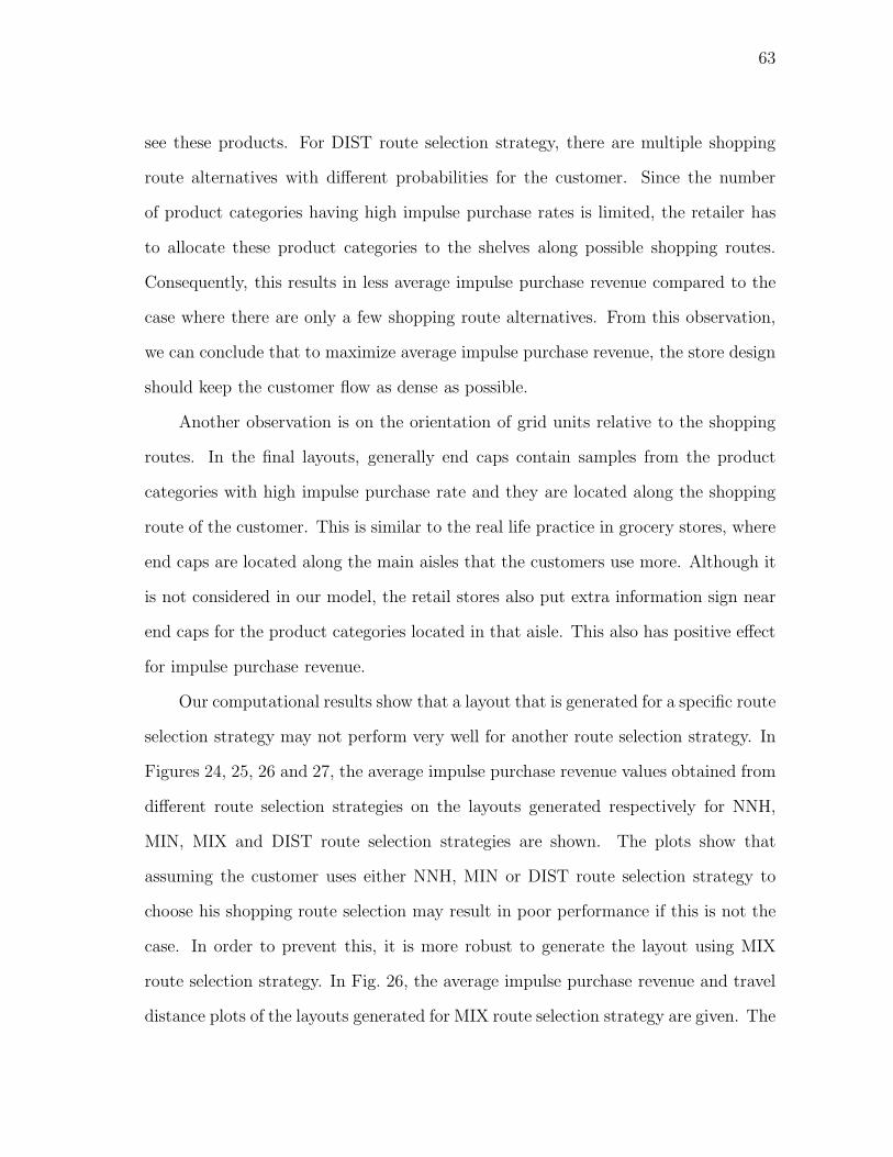
63
see these products. For DIST route selection strategy, there are multiple shopping
route alternatives with different probabilities for the customer. Since the number
of product categories having high impulse purchase rates is limited, the retailer has
to allocate these product categories to the shelves along possible shopping routes.
Consequently, this results in less average impulse purchase revenue compared to the
case where there are only a few shopping route alternatives. From this observation,
we can conclude that to maximize average impulse purchase revenue, the store design
should keep the customer flow as dense as possible.
Another observation is on the orientation of grid units relative to the shopping
routes. In the final layouts, generally end caps contain samples from the product
categories with high impulse purchase rate and they are located along the shopping
route of the customer. This is similar to the real life practice in grocery stores, where
end caps are located along the main aisles that the customers use more. Although it
is not considered in our model, the retail stores also put extra information sign near
end caps for the product categories located in that aisle. This also has positive effect
for impulse purchase revenue.
Our computational results show that a layout that is generated for a specific route
selection strategy may not perform very well for another route selection strategy. In
Figures 24, 25, 26 and 27, the average impulse purchase revenue values obtained from
different route selection strategies on the layouts generated respectively for NNH,
MIN, MIX and DIST route selection strategies are shown. The plots show that
assuming the customer uses either NNH, MIN or DIST route selection strategy to
choose his shopping route selection may result in poor performance if this is not the
case. In order to prevent this, it is more robust to generate the layout using MIX
route selection strategy. In Fig. 26, the average impulse purchase revenue and travel
distance plots of the layouts generated for MIX route selection strategy are given. The

64
results show that the layouts generated for MIX route selection strategy maximize
the average impulse purchase revenue of all route selection strategies in general. This
result is expected since MIX route selection strategy takes into consideration the
possibility of other route selection strategies (NNH and MIN) during layout generation
process, and this also has positive influence on the average impulse purchase revenue
of DIST route selection strategy.
5. User Interface
C++
1
2 6JAVA
5
4
MySQL
3
Fig. 28. Interaction between system elements
A computer based system is developed to analyze the layouts generated by SA
algorithm. The system uses C++, JAVA programming languages and a MySQL
database for information flow. SA algorithm is coded using C++ programming lan-
guage. Product and layout information is stored in the MySQL database. A JAVA
based user interface is used to analyze the layout data that is stored in the database.
The interaction between different system elements is shown in Fig. 28. System oper-
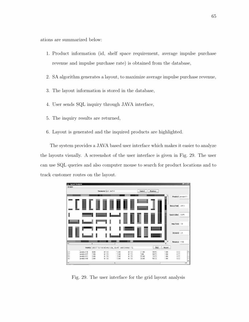
65
ations are summarized below:
1. Product information (id, shelf space requirement, average impulse purchase
revenue and impulse purchase rate) is obtained from the database,
2. SA algorithm generates a layout, to maximize average impulse purchase revenue,
3. The layout information is stored in the database,
4. User sends SQL inquiry through JAVA interface,
5. The inquiry results are returned,
6. Layout is generated and the inquired products are highlighted.
The system provides a JAVA based user interface which makes it easier to analyze
the layouts visually. A screenshot of the user interface is given in Fig. 29. The user
can use SQL queries and also computer mouse to search for product locations and to
track customer routes on the layout.
Fig. 29. The user interface for the grid layout analysis
66
6. Conclusion
In this chapter, we further analyze the grid layout for retail stores. Our computa-
tional results show that there is a correlation between planned purchase decisions and
impulse purchases. The longer the customer’s shopping list, the longer he browses
the store, and the more impulse purchases he makes. Moreover, impulse purchases
depend on how the customer selects his shopping route in the store. If the shopping
route is longer, there is more chance the customer can make an impulse purchase.
Uncertainty in customer behavior is not good for the retailer. If the retailer
does not have full information about how the customer selects his shopping route
in the store, the retailer cannot maximize the store’s impulse purchase revenue. We
conclude that it is to the retailer’s benefit to minimize the number of alternative
shopping routes for the customers. At this point, different layout designs that have
more control on customer traffic, such as serpentine layout studied in Botsalı and
Peters (2005), provide an attractive research direction and we further explore the
serpentine layout in Chapter VI. Related to uncertainty, although we assume that we
have the shopping list information of the customer, this may not be always available.
In this case, our solution algorithm can be applied assuming that the shopping list
consists of high demand items (power items or stables) such as bread, milk, eggs, etc.
As in common practice, end-of-aisle locations provide a good opportunity to
increase impulse purchase revenue of the store. The end caps at the end of shelf rows
are used to display samples from products categories having high impulse purchase
rates. This increases the visibility of these product categories and, consequently, the
impulse purchase revenue.

67
CHAPTER VI
SERPENTINE LAYOUT DESIGN
In Chapter V, we have shown that it is to the retailer’s benefit to minimize the
number of possible shopping routes for the customer during shopping. By this way,
the retailer can place high impulse purchase rate products on the shelves along the
walkways the customer follows and increase impulse purchase revenue. Based on this
idea, we analyze an alternate approach to store layout design. We assume that the
store is designed as a serpentine layout in which a single walkway extends through
store. Since there is only one walkway with exit and entrance doors at the ends, it is
easy to control customer flow, which in turn affects impulse purchase decisions. This
chapter studies application of serpentine layout in retail store settings. In the next
section, we discuss serpentine layout design. In Section 2 we extend the serpentine
layout design model given in Botsalı and Peters (2005). In Section 3, we describe our
solution methodology. In Section 4, we present our computational results and discuss
their implications for retail store layout design. Finally, we briefly summarize our
results and provide future extensions.
1. Serpentine Layout Design
The serpentine layout consists of a single walking path that traverses all the floor
space. Since there is only one path to follow for the customers, the retailer can easily
control the customer traffic and the product exposure, which in turn affect impulse
purchase revenue. In addition to this, it is possible to see serpentine layout design
used in retail stores in practice where certain departments of the stores or even the
whole store (e.g., IKEA stores) are designed based on a serpentine layout scheme.
Consequently, performance analysis of serpentine layout in retail store settings be-
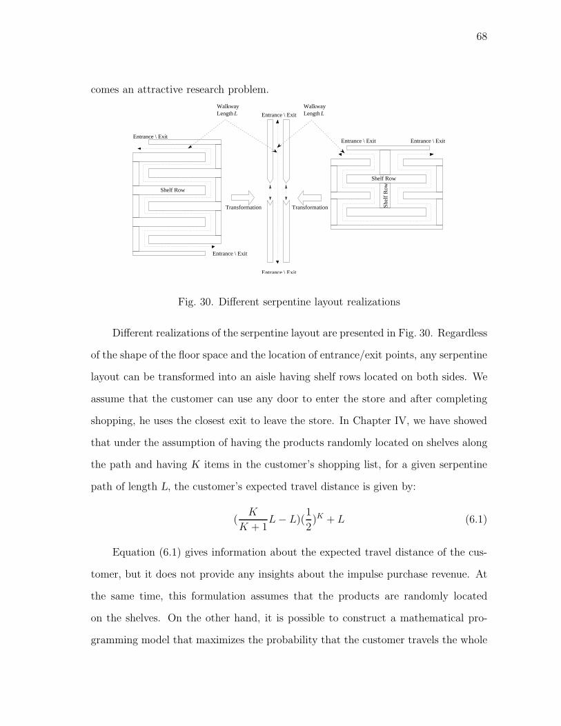
68
comes an attractive research problem.
Transformation
LengthLWalkwayLengthL
Entrance \ ExitEntrance \ Exit
Shelf Row
She
lf R
ow
Entrance \ Exit
Entrance \ Exit
Shelf Row
Entrance \ Exit
Entrance \ Exit
Transformation
Walkway
Fig. 30. Different serpentine layout realizations
Different realizations of the serpentine layout are presented in Fig. 30. Regardless
of the shape of the floor space and the location of entrance/exit points, any serpentine
layout can be transformed into an aisle having shelf rows located on both sides. We
assume that the customer can use any door to enter the store and after completing
shopping, he uses the closest exit to leave the store. In Chapter IV, we have showed
that under the assumption of having the products randomly located on shelves along
the path and having K items in the customer’s shopping list, for a given serpentine
path of length L, the customer’s expected travel distance is given by:
(K
K + 1L − L)(
1
2)K + L (6.1)
Equation (6.1) gives information about the expected travel distance of the cus-
tomer, but it does not provide any insights about the impulse purchase revenue. At
the same time, this formulation assumes that the products are randomly located
on the shelves. On the other hand, it is possible to construct a mathematical pro-
gramming model that maximizes the probability that the customer travels the whole
69
serpentine path in the store. By this way, the retailer can increase the number of the
product categories exposed as well as the potential impulse purchase revenue. The
set of all product categories is denoted by P and for each product category p, dp
gives the probability that an item from that product category will be in the shop-
ping list. Assuming that the product demands are independent, the mathematical
programming model below maximizes the probability that the customer travels along
the entire walking path in the serpentine layout.
max (1 − Πp∈P y1p)((1 − Πp∈P y2p)) (6.2)
Subject to:
x1p + x2p = 1 ∀p ∈ P (6.3)
∑
p∈P
lp × xip = L i ∈ {1, 2} (6.4)
y1p ≥ x1p(1 − dp) + x2p ∀p ∈ P (6.5)
y2p ≥ x2p(1 − dp) + x1p ∀p ∈ P (6.6)
xip ∈ {0, 1} ∀p ∈ P, i ∈ {1, 2} (6.7)
(1 − dp) ≤ yip ≤ 1 ∀p ∈ P, i ∈ {1, 2} (6.8)
In this model, the entire walking path of length L is divided into two equal halves
based on the closeness to the entrance points. The objective function maximizes the
probability that there is at least one shopping list item in each half of the walking
path. The binary variable xip takes value one or zero depending on whether product
category p is located on the ith half. lp denotes the shelf space requirement of product
category p in terms of shelf length. Since shelves are located on both sides of the
walking path, each half has shelf capacity of length L as stated by constraint 6.4 .
Constraints 6.5 and 6.6 ensure that the variable yip gets value one, if product category
70
p is not located on the ith. half. Otherwise, yip gets the value of the probability that
no item from product category p is in the shopping list. The high number of variables
and the non-linear objective function makes this model difficult to solve. In addition,
this model assumes that the travel distance of the customer and the impulse purchase
revenue are positively correlated. On the other hand, as shown in Botsalı and Peters
(2005), it is possible to obtain more impulse purchase revenue without requiring the
customer to travel entire walking path of the serpentine layout. In this study, we
redefine some of the terminology given in Botsalı and Peters (2005), and extend the
model for different cases. In the next section, the details of the model are presented.
2. Layout Design Model
The customer cannot make an impulse purchase from a product category unless he
visits that product category’s location during shopping. Since there is only one path
to follow in the serpentine layout, it is ensured that the customer visits all the product
category locations once he travels the entire walking path of the store. However, most
stores augment the pure serpentine layouts with shortcuts at certain locations. This
creates alternative shopping routes for the customer, which consequently affect the
impulse purchase revenue. The retailer has to keep track of the customer’s shopping
route in the store in order to estimate which products are exposed to the customer.
One way to control customer travel in the layout design model is to embed the store’s
walkway skeleton as a network in the model. At the same time, the layout design
model should be flexible enough to add and remove shortcuts on the serpentine path
to capture alternative layout scenarios. In Botsalı and Peters (2005), a layout model
that integrates the layout design and the walkway skeleton in the store is given. In
this model, the shelf rows are divided into segments of length w, which is also equal to

71
the width of an aisle. Similarly, the edges of the network representing the walkways
in parallel aisles of the store are set to have length w. Whenever, a shortcut is added
between the parallel aisles at a particular location in this model, the corresponding
shelf row segment on that location is cancelled out and an edge representing the
shortcut is added on the network. The layout model and the network generation
process are illustrated in Fig. 31.
W
W W
Fig. 31. Network generation from layout design model and shortcut addition
On the network, edges correspond to the portions of the walkway in the store,
and the product categories the customer can see at a specific location on the walkway
are limited. For this reason, each edge e on the network has a set of product categories
(Ce) that can be noticed by the customer whenever he uses the corresponding walkway.
As an example, in Fig. 32, when the customer passes through the location represented
by edge (3-4), he can see product categories B, E and F . Other than this, at the
end of shelf rows there are extra end caps that are designed to locate samples from
promotion or high impulse purchase rate product categories. Whenever the customer
moves between two parallel aisles, he sees the products located on the corresponding
end caps.
For a given shopping route, we can identify which product categories are exposed
to the customer during his shopping tour. However, it is possible for the customer
to pass nearby the location of a product category without noticing it. To estimate
the probability that the customer notices a particular product category p, we use the
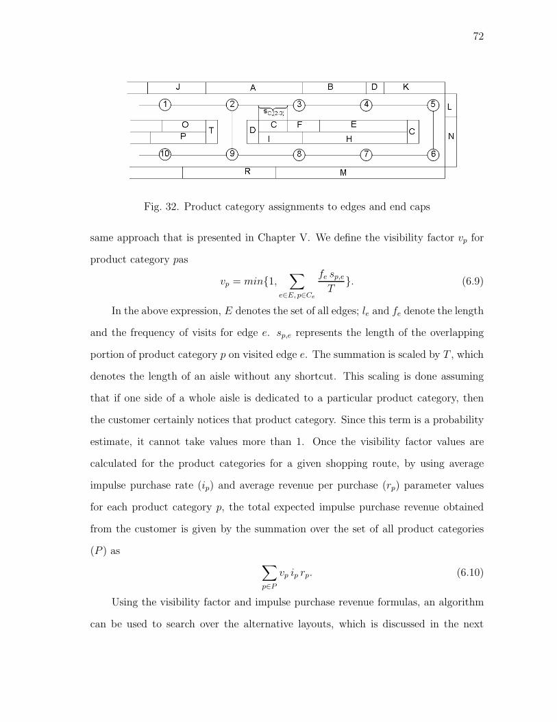
72
Fig. 32. Product category assignments to edges and end caps
same approach that is presented in Chapter V. We define the visibility factor vp for
product category pas
vp = min{1,∑
e∈E,p∈Ce
fe sp,e
T}. (6.9)
In the above expression, E denotes the set of all edges; le and fe denote the length
and the frequency of visits for edge e. sp,e represents the length of the overlapping
portion of product category p on visited edge e. The summation is scaled by T , which
denotes the length of an aisle without any shortcut. This scaling is done assuming
that if one side of a whole aisle is dedicated to a particular product category, then
the customer certainly notices that product category. Since this term is a probability
estimate, it cannot take values more than 1. Once the visibility factor values are
calculated for the product categories for a given shopping route, by using average
impulse purchase rate (ip) and average revenue per purchase (rp) parameter values
for each product category p, the total expected impulse purchase revenue obtained
from the customer is given by the summation over the set of all product categories
(P ) as∑
p∈P
vp ip rp. (6.10)
Using the visibility factor and impulse purchase revenue formulas, an algorithm
can be used to search over the alternative layouts, which is discussed in the next
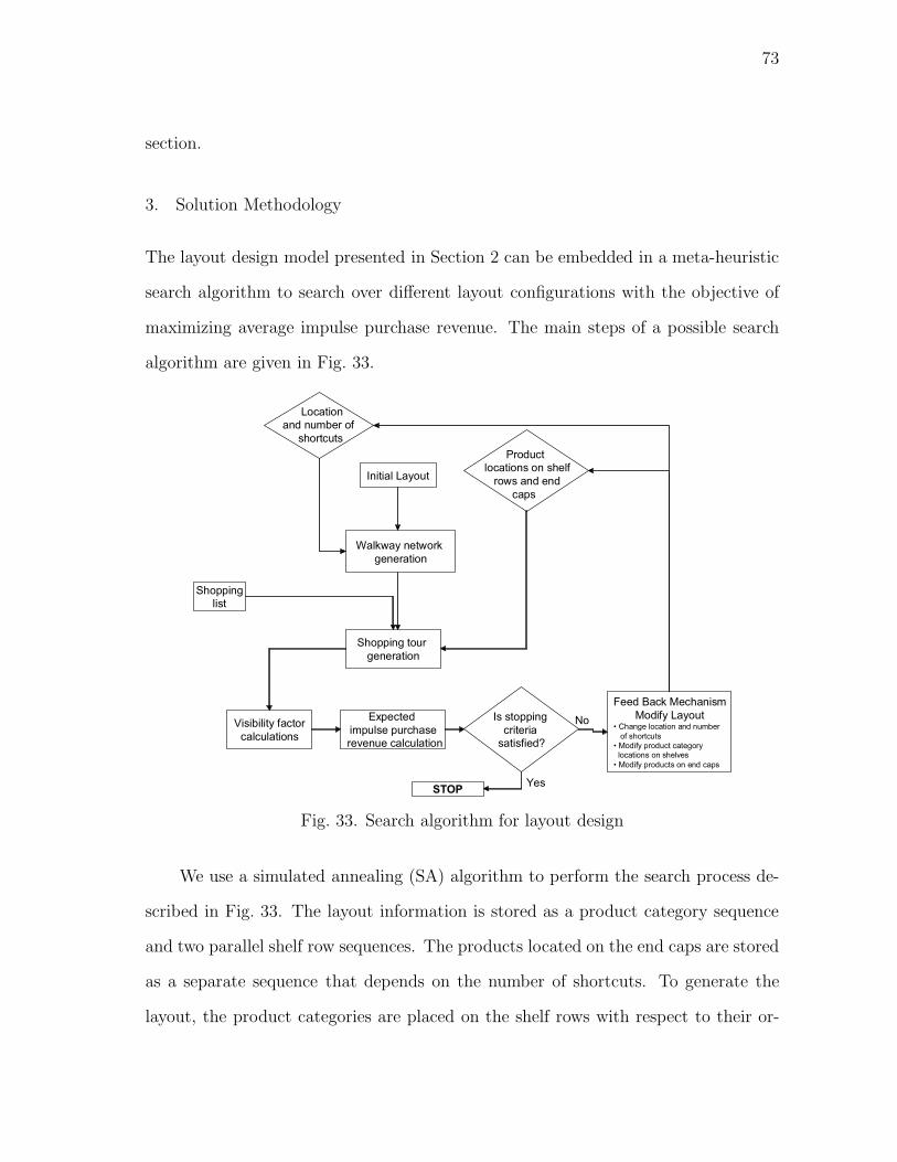
73
section.
3. Solution Methodology
The layout design model presented in Section 2 can be embedded in a meta-heuristic
search algorithm to search over different layout configurations with the objective of
maximizing average impulse purchase revenue. The main steps of a possible search
algorithm are given in Fig. 33.
Fig. 33. Search algorithm for layout design
We use a simulated annealing (SA) algorithm to perform the search process de-
scribed in Fig. 33. The layout information is stored as a product category sequence
and two parallel shelf row sequences. The products located on the end caps are stored
as a separate sequence that depends on the number of shortcuts. To generate the
layout, the product categories are placed on the shelf rows with respect to their or-
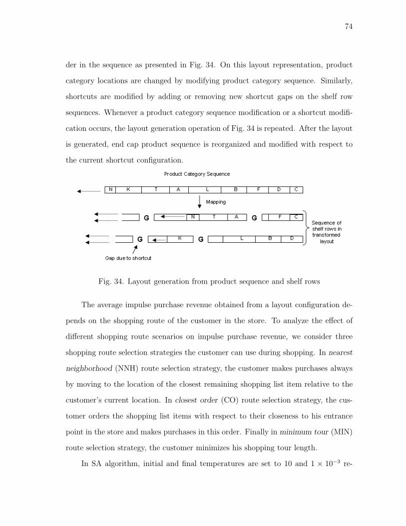
74
der in the sequence as presented in Fig. 34. On this layout representation, product
category locations are changed by modifying product category sequence. Similarly,
shortcuts are modified by adding or removing new shortcut gaps on the shelf row
sequences. Whenever a product category sequence modification or a shortcut modifi-
cation occurs, the layout generation operation of Fig. 34 is repeated. After the layout
is generated, end cap product sequence is reorganized and modified with respect to
the current shortcut configuration.
Fig. 34. Layout generation from product sequence and shelf rows
The average impulse purchase revenue obtained from a layout configuration de-
pends on the shopping route of the customer in the store. To analyze the effect of
different shopping route scenarios on impulse purchase revenue, we consider three
shopping route selection strategies the customer can use during shopping. In nearest
neighborhood (NNH) route selection strategy, the customer makes purchases always
by moving to the location of the closest remaining shopping list item relative to the
customer’s current location. In closest order (CO) route selection strategy, the cus-
tomer orders the shopping list items with respect to their closeness to his entrance
point in the store and makes purchases in this order. Finally in minimum tour (MIN)
route selection strategy, the customer minimizes his shopping tour length.
In SA algorithm, initial and final temperatures are set to 10 and 1 × 10⁻³ re-
75
spectively. The cooling rate is taken as 0.7. At each temperature 15 iterations are
made. At each iteration the layout is modified in three ways. First, 100 pair wise
product category location exchanges are made on the product category sequence. In
the second step, if shortcuts are allowed in the layout, then one shortcut modifi-
cation (addition or cancellation of a shortcut) is made on each aisle. In the third
step, the products on the end caps are changed or replaced. During search, a new
layout is always accepted as the best layout if its objective value (OVnew) calculated
by the equation (6.10) is greater than the objective value (OVold) of the current best
layout. Otherwise, the new layout is taken to be the best layout with probability
e(OVnew−OVold)/CT where CT is the current temperature. Steps of the algorithm are
given in Appendix D.
4. Computational Results and Discussion
The computational experiments are done using the same product data given in Chap-
ter V. There are 100 product categories with random shelf length requirements of
2, 4 or 6 units. The impulse purchase rate and revenue (ip,rp) parameter pairs for
product categories (p) are distributed as (0.8,20) for 18 categories, (0.1,20) for 25
categories, (0.1,10) for 25 categories and (0.8,10) for 25 categories. The remaining
7 product categories are reserved for shopping list. Assuming a shopping list item
cannot be purchased impulsively, the revenue and impulse purchase rate for these
product categories are set to zero. The data set is chosen in this way in order to
classify the products in terms of low and high impulse purchase rates, so it is possible
to understand the relationship between impulse purchase rates and product locations
in the final layout. It is assumed that the customer’s shopping list information is
available in advance. In other words, we know from which product categories the
76
customer will certainly make a purchase. The customer can enter the store using any
of the two doors with equal probability and after completing all the purchases, leaves
the store using the closest exit.
The store layout consists of 11 aisles where each aisle has a length of 26 units.
The aisle width w is set to 2 units. The length of a shortcut between two parallel
aisles is 7 units. Since we do not know the number of shortcuts in the layout in
advance, the total shelf space available in the store is greater than the net shelf space
requirement of the product categories. If there is insufficient shelf space to satisfy
the shelf space requirement in a layout due to the number of shortcuts, that layout
is considered to be infeasible.
During computational runs, three different shortcut scenarios, which are no short-
cut, at most one shortcut per aisle, and at most two shortcuts per aisle, are considered.
For a fixed shopping list length, shopping tour selection strategy and shortcut sce-
nario, five runs are taken and their average is used in the analysis. Depending on the
problem size, each run takes between four to six hours on a Pentium IV 3.2 Ghz com-
puter with 512 MB memory. The results are summarized as plots in Figs. 36 through
40. We use the same computer based system described in Chapter V to analyze the
final layouts. A screenshot of the user interface is given in Fig. 35.
When we have a pure serpentine layout with no shortcut, then the average im-
pulse purchase revenue and travel distance are almost same for different shopping
list length scenarios. As explained in Botsalı and Peters (2005), if there are not any
shortcuts in the layout, then all the shopping list items are located on a particular
half of the layout where at least one of the shopping list items is located as far as
possible from the entrance/exit point in that half. Since the customer uses both doors
to enter the store with equal probability, the half of the store containing shopping
list items are visited 1.5 times in average for any shopping route selection strategy.
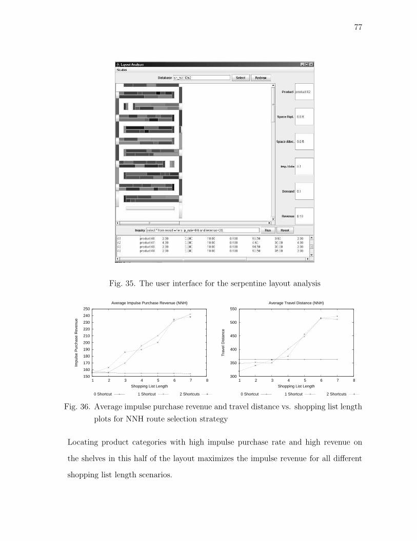
77
Fig. 35. The user interface for the serpentine layout analysis
150
160
170
180
190
200
210
220
230
240
250
1 2 3 4 5 6 7 8
Impu
lse
Pur
chas
e R
even
ue
Shopping List Length
Average Impulse Purchase Revenue (NNH)
0 Shortcut 1 Shortcut 2 Shortcuts
300
350
400
450
500
550
1 2 3 4 5 6 7 8
Tra
vel D
ista
nce
Shopping List Length
Average Travel Distance (NNH)
0 Shortcut 1 Shortcut 2 Shortcuts
Fig. 36. Average impulse purchase revenue and travel distance vs. shopping list length
plots for NNH route selection strategy
Locating product categories with high impulse purchase rate and high revenue on
the shelves in this half of the layout maximizes the impulse revenue for all different
shopping list length scenarios.
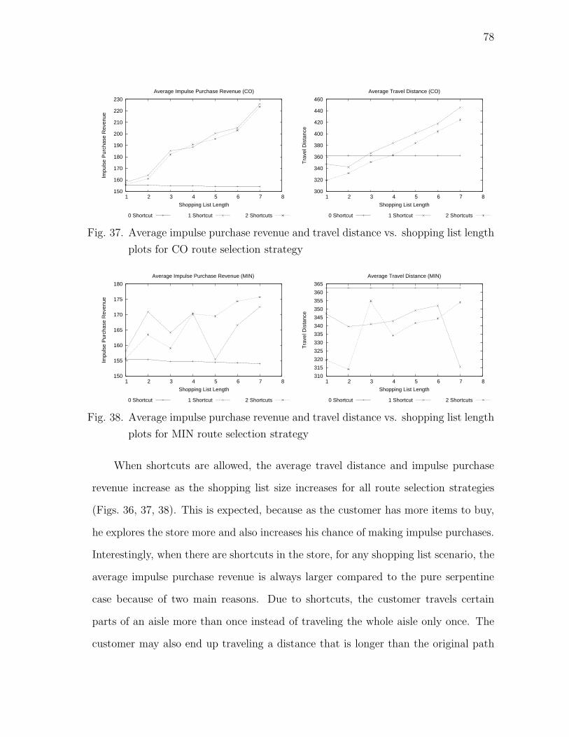
78
150
160
170
180
190
200
210
220
230
1 2 3 4 5 6 7 8
Impu
lse
Pur
chas
e R
even
ue
Shopping List Length
Average Impulse Purchase Revenue (CO)
0 Shortcut 1 Shortcut 2 Shortcuts
300
320
340
360
380
400
420
440
460
1 2 3 4 5 6 7 8
Tra
vel D
ista
nce
Shopping List Length
Average Travel Distance (CO)
0 Shortcut 1 Shortcut 2 Shortcuts
Fig. 37. Average impulse purchase revenue and travel distance vs. shopping list length
plots for CO route selection strategy
150
155
160
165
170
175
180
1 2 3 4 5 6 7 8
Impu
lse
Pur
chas
e R
even
ue
Shopping List Length
Average Impulse Purchase Revenue (MIN)
0 Shortcut 1 Shortcut 2 Shortcuts
310
315
320
325
330
335
340
345
350
355
360
365
1 2 3 4 5 6 7 8
Tra
vel D
ista
nce
Shopping List Length
Average Travel Distance (MIN)
0 Shortcut 1 Shortcut 2 Shortcuts
Fig. 38. Average impulse purchase revenue and travel distance vs. shopping list length
plots for MIN route selection strategy
When shortcuts are allowed, the average travel distance and impulse purchase
revenue increase as the shopping list size increases for all route selection strategies
(Figs. 36, 37, 38). This is expected, because as the customer has more items to buy,
he explores the store more and also increases his chance of making impulse purchases.
Interestingly, when there are shortcuts in the store, for any shopping list scenario, the
average impulse purchase revenue is always larger compared to the pure serpentine
case because of two main reasons. Due to shortcuts, the customer travels certain
parts of an aisle more than once instead of traveling the whole aisle only once. The
customer may also end up traveling a distance that is longer than the original path
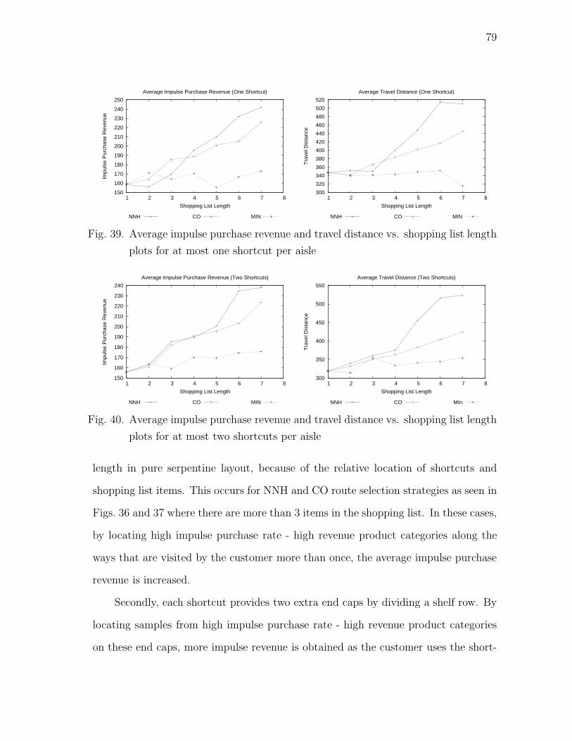
79
150
160
170
180
190
200
210
220
230
240
250
1 2 3 4 5 6 7 8
Impu
lse
Pur
chas
e R
even
ue
Shopping List Length
Average Impulse Purchase Revenue (One Shortcut)
NNH CO MIN
300
320
340
360
380
400
420
440
460
480
500
520
1 2 3 4 5 6 7 8
Tra
vel D
ista
nce
Shopping List Length
Average Travel Distance (One Shortcut)
NNH CO MIN
Fig. 39. Average impulse purchase revenue and travel distance vs. shopping list length
plots for at most one shortcut per aisle
150
160
170
180
190
200
210
220
230
240
1 2 3 4 5 6 7 8
Impu
lse
Pur
chas
e R
even
ue
Shopping List Length
Average Impulse Purchase Revenue (Two Shortcuts)
NNH CO MIN
300
350
400
450
500
550
1 2 3 4 5 6 7 8
Tra
vel D
ista
nce
Shopping List Length
Average Travel Distance (Two Shortcuts)
NNH CO MIn
Fig. 40. Average impulse purchase revenue and travel distance vs. shopping list length
plots for at most two shortcuts per aisle
length in pure serpentine layout, because of the relative location of shortcuts and
shopping list items. This occurs for NNH and CO route selection strategies as seen in
Figs. 36 and 37 where there are more than 3 items in the shopping list. In these cases,
by locating high impulse purchase rate - high revenue product categories along the
ways that are visited by the customer more than once, the average impulse purchase
revenue is increased.
Secondly, each shortcut provides two extra end caps by dividing a shelf row. By
locating samples from high impulse purchase rate - high revenue product categories
on these end caps, more impulse revenue is obtained as the customer uses the short-
80
cut. This effect is evident for all route selection strategies; however it is especially
prominent in MIN route selection strategy (Fig. 38). The plots show that the average
travel distance is shorter, but the average impulse purchase revenue is higher for MIN
route selection strategy in a layout with shortcuts compared to the pure serpentine
layout case.
Among different route selection strategies (Figures 39 and 40), MIN route se-
lection strategy has the minimum average travel distance and impulse purchase rev-
enue, which is expected. As the customer minimizes the shopping tour length, he
decreases his chance of making impulse purchase compared to the other two route
selection strategies. For any shortcut scenario, NNH route selection strategy gives
longer shopping tours than CO route selection strategy as the shopping list length
increases, and the difference in travel distance is reflected in slightly higher average
impulse purchase revenue for long shopping lists. This difference is caused by the
single path structure inherent in the serpentine layout. The customer is less likely to
make repeated visits to certain locations under CO route selection strategy compared
to NNH route selection strategy, which saves travel distance.
When two shortcuts are allowed instead of one, the travel distance decreases for
all route selection strategies. At the same time, except MIN route selection strategy,
allowing two shortcuts results in slightly lower impulse purchase revenues. In fact, the
feasible set of layouts for one shortcut case is already a subset of the feasible layouts
for two shortcuts case. We think that the increase in the size of solution space by
allowing two shortcuts per aisle (which results in more than 1×10¹³ extra possibilities
for additional shortcuts) makes it more difficult for SA algorithm to explore the whole
solution space using the same computational time as used for one shortcut case. Yet,
regardless of the number of shortcuts allowed, the results show that retailers can
obtain additional benefits by having shortcuts.

81
During our analysis, we observe that there is not a specific pattern for the location
of shortcuts. Generally, the algorithm tends to locate the shortcuts closer to the
end of aisles, so that the number of product categories bypassed by the shortcuts
is not so high. The experimentation shows that extreme use of shortcuts can have
negative impact on the average impulse purchase revenue. As an example, under the
assumption that each aisle has exactly one shortcut located in the middle, the impulse
purchase revenue and travel distance greatly decreases as presented in Fig. 41. In this
case, any route selection strategy almost gives the same average impulse purchase
revenue, and the average travel distance increases as the shopping list size increases.
In this study, we used fixed product assortment size (100 product categories)
and fixed layout space (11 aisles). Since each shortcut causes some shelf space loss,
the shelf space utilization ratio in the store layout changes depending on the shortcut
scenario. In this regard, the unused shelf space in pure serpentine layout can be much
larger than the unused shelf space when shortcuts are allowed in the store. During our
analysis, we did not include the opportunity cost of allocating space for the shortcuts
in the store. The interaction between the cost of shelf space reserved for the shortcuts
and the increase in the average impulse purchase revenue due to the shortcuts can be
an interesting future research problem.
5. Conclusion
The retail store layout design problem has unique characteristics, such as profit max-
imization objective, which make it different from the traditionally studied layout
design problems. In this chapter, we extend the model given in Botsalı and Peters
(2005), and analyze the serpentine layout in retail store settings. We use a simulated
annealing algorithm to generate layouts for different cases.
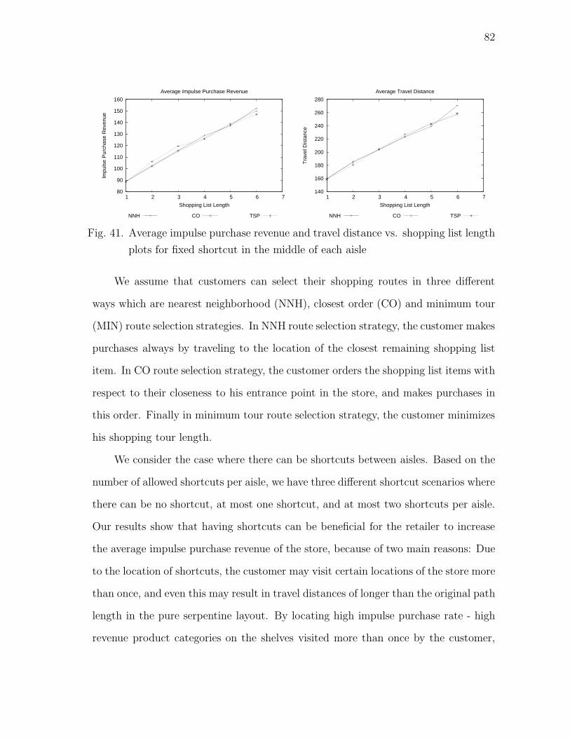
82
80
90
100
110
120
130
140
150
160
1 2 3 4 5 6 7
Impu
lse
Pur
chas
e R
even
ue
Shopping List Length
Average Impulse Purchase Revenue
NNH CO TSP
140
160
180
200
220
240
260
280
1 2 3 4 5 6 7
Tra
vel D
ista
nce
Shopping List Length
Average Travel Distance
NNH CO TSP
Fig. 41. Average impulse purchase revenue and travel distance vs. shopping list length
plots for fixed shortcut in the middle of each aisle
We assume that customers can select their shopping routes in three different
ways which are nearest neighborhood (NNH), closest order (CO) and minimum tour
(MIN) route selection strategies. In NNH route selection strategy, the customer makes
purchases always by traveling to the location of the closest remaining shopping list
item. In CO route selection strategy, the customer orders the shopping list items with
respect to their closeness to his entrance point in the store, and makes purchases in
this order. Finally in minimum tour route selection strategy, the customer minimizes
his shopping tour length.
We consider the case where there can be shortcuts between aisles. Based on the
number of allowed shortcuts per aisle, we have three different shortcut scenarios where
there can be no shortcut, at most one shortcut, and at most two shortcuts per aisle.
Our results show that having shortcuts can be beneficial for the retailer to increase
the average impulse purchase revenue of the store, because of two main reasons: Due
to the location of shortcuts, the customer may visit certain locations of the store more
than once, and even this may result in travel distances of longer than the original path
length in the pure serpentine layout. By locating high impulse purchase rate - high
revenue product categories on the shelves visited more than once by the customer,
83
the retailer may increase the chance for the customer to notice product categories and
make impulse purchases. Secondly, the shortcuts provide end caps. Since shortcuts
carry high customer traffic, locating products from high impulse purchase rate - high
revenue product categories on these end caps increases the potential impulse purchase
revenue from these product categories.
During our experimentation, we used a fixed product assortment size and a
fixed store size for all different shortcut scenarios. We did not consider the effect of
opportunity cost of allocating store space for shortcuts. Also we did not consider
the expected profit that could be obtained by increasing product assortment size and
utilizing the unused shelf space in the layout. Inclusion of these factors in the layout
design process can provide good extensions for this study.
Another limitation of this study is the assumption of having deterministic shop-
ping lists. In practice, the shopping list contents are stochastic and they may change
from customer to customer. Yet, we believe that we can apply the deterministic shop-
ping list approach by defining a set of product categories with high demands. For
example, in the retailing literature such high demand product categories are referred
as power products (e.g., bread, milk, etc.), and they are used to control the customer
traffic in the store. As with the stochastic nature of customer decisions, stochastic
shopping route selection strategies and stochastic product demand rates seem to be
an interesting research direction and we further analyze these issues for the serpentine
layout in the next chapter.
84
CHAPTER VII
RETAIL STORE LAYOUT WITH STOCHASTIC PRODUCT DEMAND
In Chapter IV, we focused on network based layout design models. In the first part
of this chapter, we analyze the network based models for grid and serpentine layouts
in more detail. For the grid layout, we assume that there exists shelves at the end-
of-aisles and also on the sides of the store. For the serpentine layout, we include
the possibility of having shortcuts in the network model. In the second part of the
chapter, we focus on the serpentine layout and incorporate demand uncertainty, travel
distance and impulse purchase revenue in a network based model.
In the next section, we present models for determining travel distance character-
istics for both grid and serpentine layout classes when customers have fixed shopping
lists. In Section 2, we study the trade-off between impulse purchase revenue and travel
distance for serpentine layouts. In Section 3, we compare different product location
strategies for serpentine layouts with both fixed and random demands. Sections 4
and 5 present our discussion and conclusions.
1. Analytical Travel Distance Models for Aisle-Based and Serpentine Layouts
In order to track the travel of customers and to analyze customer traffic in the store,
it is more appropriate to represent customer walkways of the store as a network. We
assume that each walkway in the store has shelves on both sides and whenever the
customer uses a particular walkway, he notices the products located on the shelves
along the walkway with some probability. Based on this assumption, each walkway
can be represented as a line and the products that the customers can see along a
walkway are projected onto the corresponding walkway as shown in Fig. 42.
Using this projection mechanism, the store layout can be represented as a net-

85
2 3 4
5 6 7
1
1 5 2 6 3 7 4
Shelves
Shelves
Walkway
Fig. 42. Line representation of walkways and product projection
EXIT
ENTRANCE
Network for an Aisle Unit
(a) Grid layout
SH
OR
TC
UT
ENTRANCE
EXIT
Network for a Bypass Area
Potential Shortcut
(b) Serpentine layout
Fig. 43. Network representation of grid and serpentine layout designs, and basic net-
work units
work. In Fig. 43, examples for the network representations of grid and serpentine
layout designs are given. Due to the complexity of tracking all possible customer
travel patterns on the full layout network, we divide layout networks into simpler
network units and study the customer travel pattern separately in each unit. For the
86
grid layout, a basic network unit is taken as an aisle. For the serpentine layout, a
basic network unit is defined as bypass area where the customer can use a shortcut to
bypass the corresponding region of the store without visiting the product locations.
The network units for grid and serpentine layouts are also displayed in Fig. 43.
In Sections 1.1 and 1.2, expected travel distance formulations are derived for
grid and serpentine layout networks, respectively, in a manner similar to Chapter IV.
However, in this chapter we have side shelves and end-of-aisle shelves in the grid
layout design, and we also allow shortcuts in the serpentine layout design. This
analysis assumes that the customer visits the aisles where the shopping list items are
located and will use the closest end of an aisle when leaving after purchasing all the
items in that aisle.
1.1. Expected Travel Distance Derivation for the Grid Layout Design
If products are randomly located along the shelves, which implies that the products
are randomly distributed along the aisle network, then there is an equal probability
that the customer may enter an aisle from either end. Depending on the location of
the products that the customer plans to select from an aisle, we analyze the customer’s
travel in an aisle under four different cases as shown in Fig. 44. When we identify these
cases, we assume that after the customer completes shopping in an aisle, the customer
chooses the closest end to leave the aisle. Since the customer may enter the aisle from
either end with equal probability and the products are randomly distributed, we can
pick either aisle end for the customer’s entrance point in our analysis. In Fig. 44,
the four possible cases for the customer to complete the shopping in an aisle are
demonstrated assuming that the customer enters the aisle from the left end.
For a particular case to occur, the regions that contain a shopping list item are
circled in Fig. 44. If the aisle does not contain any shopping list items or all the

87
shopping list items are located on the left end-of-aisle location, the customer does
not enter the aisle as in Case I. If all the shopping list items are located on the left
half of the aisle, then the customer partially visits the aisle as in Case II. If there are
some shopping list items located on the right half of the aisle, but no shopping list
items on the right end-of-aisle region, then the customer moves as shown by Case III.
Finally, if there is a shopping list item on the right end-of-aisle region, the customer
moves as shown by case IV. The process of expected travel distance derivation for
the grid layout (ETDGL) is summarized by equation (7.1) for n aisles, each having a
length and width of A and w units, respectively. The shopping list length is taken as
K items.
A/2 A/2Aw
CASE I CASE II CASE III CASE IV
Enter
Leave
Fig. 44. Possible customer travel patterns in an aisle
ETDGL = (# aisles) ×
K∑
i=0
{ P ( i items in an aisle)
×∑
Case1...4
E[Travel distance | i items in an aisle]} (7.1)
If the customer enters an aisle of length A and selects n randomly located items,
and leaves the aisle using the same end he entered as shown by Case II in Fig. 44, his
expected travel distance in the aisle (ETDAn) is found by using uniform distribution
as given by equation 4.22 in Chapter IV:
ETDAn=
2n
n + 1A (7.2)
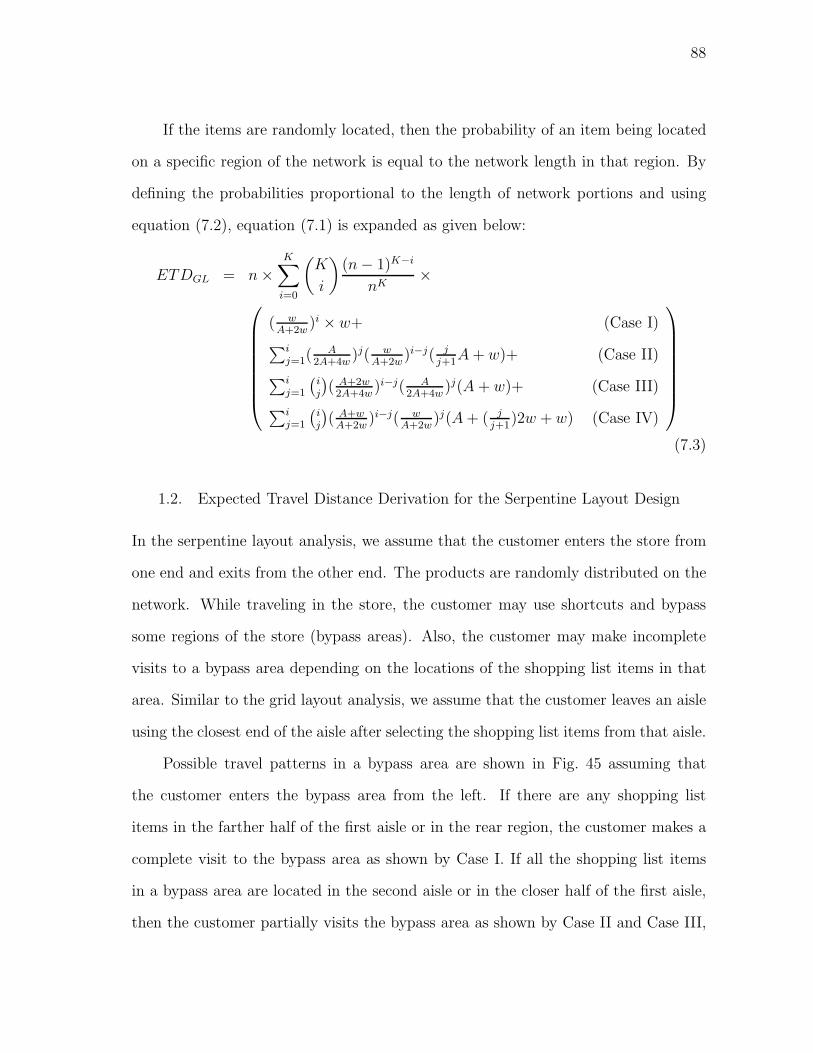
88
If the items are randomly located, then the probability of an item being located
on a specific region of the network is equal to the network length in that region. By
defining the probabilities proportional to the length of network portions and using
equation (7.2), equation (7.1) is expanded as given below:
ETDGL = n ×K
∑
i=0
(
K
i
)
(n − 1)K−i
nK×
( wA+2w
)i × w+ (Case I)
∑ij=1(
A2A+4w
)j( wA+2w
)i−j( jj+1
A + w)+ (Case II)∑i
j=1
(
ij
)
( A+2w2A+4w
)i−j( A2A+4w
)j(A + w)+ (Case III)∑i
j=1
(
ij
)
( A+wA+2w
)i−j( wA+2w
)j(A + ( jj+1
)2w + w) (Case IV)
(7.3)
1.2. Expected Travel Distance Derivation for the Serpentine Layout Design
In the serpentine layout analysis, we assume that the customer enters the store from
one end and exits from the other end. The products are randomly distributed on the
network. While traveling in the store, the customer may use shortcuts and bypass
some regions of the store (bypass areas). Also, the customer may make incomplete
visits to a bypass area depending on the locations of the shopping list items in that
area. Similar to the grid layout analysis, we assume that the customer leaves an aisle
using the closest end of the aisle after selecting the shopping list items from that aisle.
Possible travel patterns in a bypass area are shown in Fig. 45 assuming that
the customer enters the bypass area from the left. If there are any shopping list
items in the farther half of the first aisle or in the rear region, the customer makes a
complete visit to the bypass area as shown by Case I. If all the shopping list items
in a bypass area are located in the second aisle or in the closer half of the first aisle,
then the customer partially visits the bypass area as shown by Case II and Case III,
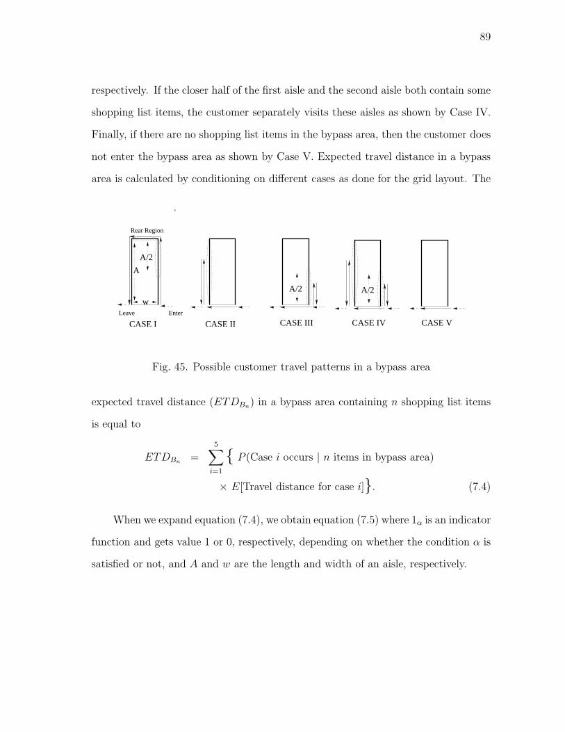
89
respectively. If the closer half of the first aisle and the second aisle both contain some
shopping list items, the customer separately visits these aisles as shown by Case IV.
Finally, if there are no shopping list items in the bypass area, then the customer does
not enter the bypass area as shown by Case V. Expected travel distance in a bypass
area is calculated by conditioning on different cases as done for the grid layout. The
A/2 A/2
A/2
A
w
CASE I CASE II CASE III CASE IV CASE VEnterLeave
Rear Region
Fig. 45. Possible customer travel patterns in a bypass area
expected travel distance (ETDBn) in a bypass area containing n shopping list items
is equal to
ETDBn=
5∑
i=1
{ P (Case i occurs | n items in bypass area)
× E[Travel distance for case i]}. (7.4)
When we expand equation (7.4), we obtain equation (7.5) where 1α is an indicator
function and gets value 1 or 0, respectively, depending on whether the condition α is
satisfied or not, and A and w are the length and width of an aisle, respectively.
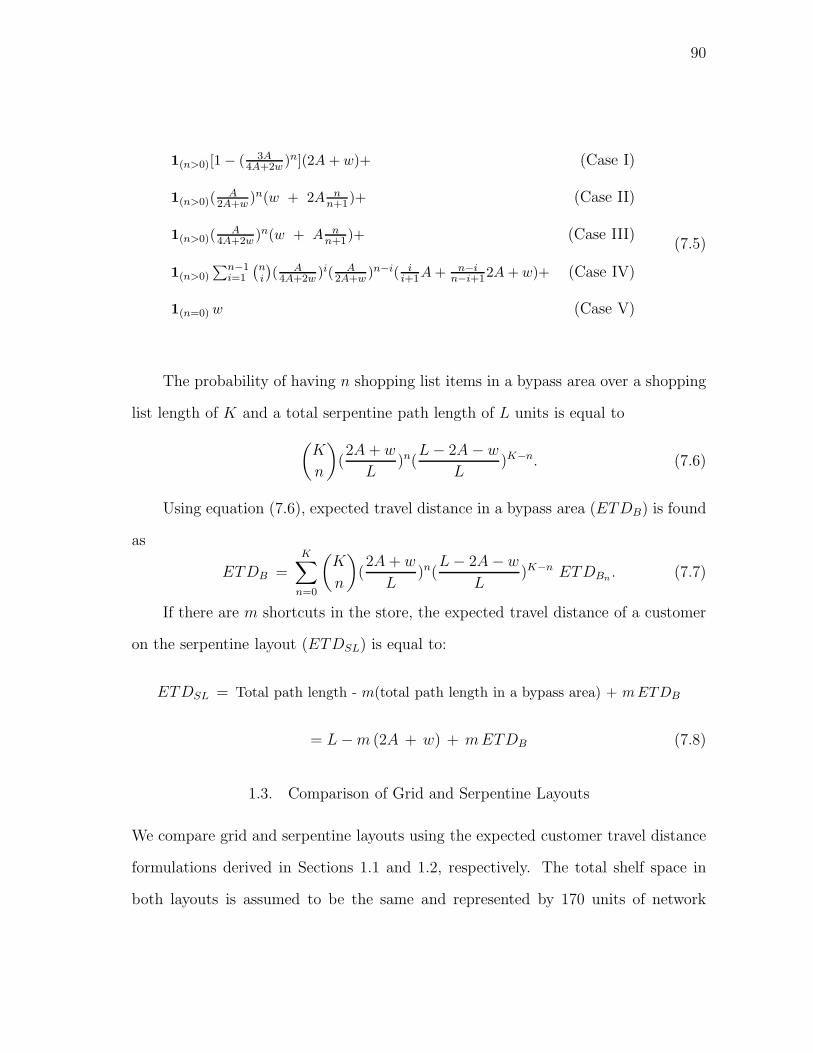
90
1(n>0)[1 − ( 3A4A+2w )n](2A + w)+ (Case I)
1(n>0)(A
2A+w )n(w + 2A nn+1)+ (Case II)
1(n>0)(A
4A+2w )n(w + An
n+1)+ (Case III)
1(n>0)
∑n−1i=1
(ni
)
( A4A+2w )i( A
2A+w )n−i( ii+1A + n−i
n−i+12A + w)+ (Case IV)
1(n=0) w (Case V)
(7.5)
The probability of having n shopping list items in a bypass area over a shopping
list length of K and a total serpentine path length of L units is equal to
(
K
n
)
(2A + w
L)n(
L − 2A − w
L)K−n. (7.6)
Using equation (7.6), expected travel distance in a bypass area (ETDB) is found
as
ETDB =K
∑
n=0
(
K
n
)
(2A + w
L)n(
L − 2A − w
L)K−n ETDBn
. (7.7)
If there are m shortcuts in the store, the expected travel distance of a customer
on the serpentine layout (ETDSL) is equal to:
ETDSL = Total path length - m(total path length in a bypass area) + m ETDB
= L − m (2A + w) + m ETDB (7.8)
1.3. Comparison of Grid and Serpentine Layouts
We compare grid and serpentine layouts using the expected customer travel distance
formulations derived in Sections 1.1 and 1.2, respectively. The total shelf space in
both layouts is assumed to be the same and represented by 170 units of network

91
0.2
0.3
0.4
0.5
0.6
0.7
0.8
0.9
1
5 10 15 20 25 30 35
Tra
vel D
ista
nce
/ Max
imum
Dis
tanc
e
Shopping List Length (K)
Grid vs. Serpentine Layout
GS-1S-2S-3S-4
Fig. 46. Expected travel distance vs. shopping list length plots for grid (G) and ser-
pentine layouts with i ∈ {1 . . . 4} shortcuts (S-i)
length. In the grid layout, there are eight aisle units each having length and width of
11.25 and 5 units, respectively. For the serpentine layout, again there are eight aisles
(four bypass areas) each having length and width of 16.875 and 5 units, respectively.
As Fig. 46 shows, the grid layout has significant advantage over the serpentine
layout in terms of travel distance. If the products displayed in the store have high
demand and low impulse purchase rates, then the retailer may prefer a grid layout
design to a serpentine layout design in order to minimize the time customers spend
in the store. On the other hand, if there are some products with low demand and
high impulse purchase rates, then it may be beneficial for the retailer to use a ser-
pentine layout design to maximize the revenue from impulse purchases. In fact, if
the products are not identical in terms of demand and impulse purchase rates, then
different strategies that are used to locate products on the shelves may result in dif-
ferent impulse purchase revenue and customer travel distance scenarios. In sections 2
and 3, the serpentine layout and the effect of different product location strategies are
analyzed for products with non-identical demand and impulse purchase rates.
92
1.4. Multiple Customer Profiles
From Fig. 46, it is seen that the expected travel distance functions of the customers
on serpentine and grid layouts are concave functions of shopping list length K.
In general, shopping list length is a random variable that depends on different
customer profiles. If K is defined as the average of the expected shopping list lengths
of different customer profiles, then Jensen’s inequality explains the effect of aggregat-
ing all customer profiles into one customer profile on the expected travel distance:
Jensen’s Inequality If f() is a convex function and X is a random variable then
E[f(X)] ≥ f(E[X]) (Ross, 1996). If f() is a concave function, then inequality
becomes as E[f(X)] ≤ f(E[X]).
If expected travel distance with respect to shopping list length K is denoted by
function g(K), and if we apply Jensen’s inequality, then we have
E[g(K)] ≤ g(E[K]), (7.9)
which means the expected travel distance of one aggregated customer profile is an up-
per bound for the expected travel distance when there are multiple customer profiles.
Consequently, equations (7.3) and (7.8) provide an upper bound for the expected
customer travel distance in grid and serpentine layouts, respectively, when there are
more than one customer profile.
2. Expected Impulse Purchase Revenue and Travel Distance Formulations for Ser-
pentine Layout
In this section, we analyze the serpentine layout in detail in order to exploit its unique
characteristics. To capture the effect of product demand and impulse purchase rates
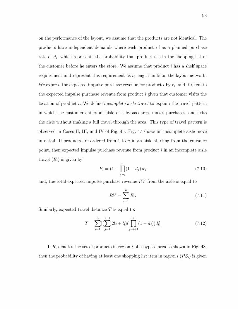
93
on the performance of the layout, we assume that the products are not identical. The
products have independent demands where each product i has a planned purchase
rate of di, which represents the probability that product i is in the shopping list of
the customer before he enters the store. We assume that product i has a shelf space
requirement and represent this requirement as li length units on the layout network.
We express the expected impulse purchase revenue for product i by ri, and it refers to
the expected impulse purchase revenue from product i given that customer visits the
location of product i. We define incomplete aisle travel to explain the travel pattern
in which the customer enters an aisle of a bypass area, makes purchases, and exits
the aisle without making a full travel through the area. This type of travel pattern is
observed in Cases II, III, and IV of Fig. 45. Fig. 47 shows an incomplete aisle move
in detail. If products are ordered from 1 to n in an aisle starting from the entrance
point, then expected impulse purchase revenue from product i in an incomplete aisle
travel (Ei) is given by:
Ei = (1 −n
∏
j=i
(1 − dj))ri (7.10)
and, the total expected impulse purchase revenue RV from the aisle is equal to
RV =
n∑
i=1
Ei. (7.11)
Similarly, expected travel distance T is equal to:
T =
n∑
i=1
[(
i−1∑
j=1
2lj + li)(
n∏
j=i+1
(1 − dj))di] (7.12)
If Ri denotes the set of products in region i of a bypass area as shown in Fig. 48,
then the probability of having at least one shopping list item in region i (PSi) is given

94
Product 1 Product 3 Product k Product n−1 Product n
Customer’s move in the aisle Buy the last producton the shopping list
Enter aisle
Return back
Product 2
Fig. 47. Incomplete travel in an aisle
A
A/2
w
Region 3
Region 1
Region 2
Shortcut
Fig. 48. Regions in a bypass area
by:
PSi = 1 −∏
p∈Ri
(1 − dp) i ∈ {1 . . . 3} (7.13)
For each bypass area, by using equations (7.11), (7.12), and (7.13), we can find the
expected impulse purchase revenue and the travel distance for a customer if the cus-
tomer has the same travel pattern shown in Fig. 45. The summation of expected
values for each bypass area together with the expected values calculated for the prod-
ucts located in between bypass areas give the expected value for the total store. Since
the expected travel distance and impulse purchase revenue depend on the location of
the products, we analyze the effect of different product location strategies on expected
travel distance and impulse purchase revenue in the next section.
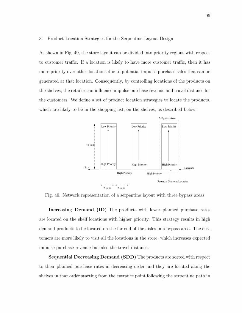
95
3. Product Location Strategies for the Serpentine Layout Design
As shown in Fig. 49, the store layout can be divided into priority regions with respect
to customer traffic. If a location is likely to have more customer traffic, then it has
more priority over other locations due to potential impulse purchase sales that can be
generated at that location. Consequently, by controlling locations of the products on
the shelves, the retailer can influence impulse purchase revenue and travel distance for
the customers. We define a set of product location strategies to locate the products,
which are likely to be in the shopping list, on the shelves, as described below:
2 units
10 units
High Priority High Priority
High Priority High Priority High Priority
Low Priority Low Priority Low Priority
A Bypass Area
Exit Entrance
Potential Shortcut Location
2 units
Fig. 49. Network representation of a serpentine layout with three bypass areas
Increasing Demand (ID) The products with lower planned purchase rates
are located on the shelf locations with higher priority. This strategy results in high
demand products to be located on the far end of the aisles in a bypass area. The cus-
tomers are more likely to visit all the locations in the store, which increases expected
impulse purchase revenue but also the travel distance.
Sequential Decreasing Demand (SDD) The products are sorted with respect
to their planned purchase rates in decreasing order and they are located along the
shelves in that order starting from the entrance point following the serpentine path in

96
the store. As a result of this strategy, each bypass area is likely to contain products
that have similar planned purchase rates.
Decreasing Demand (DD) As opposed to increasing demand strategy, this
product location strategy locates the products with higher planned purchase rates on
higher priority regions. A store layout design using this location strategy is likely to
have smaller customer travel distance, but also less impulse purchase revenue.
Shifted Decreasing Demand (SHD) In this product location strategy, shelves
along the highest priority locations are dedicated for the products with high impulse
purchase revenue. For the remaining shelves, the products are located using a decreas-
ing demand strategy. This strategy tries to find a compromise between decreasing
demand and increasing demand strategies.
Spread Demand (SD) Products with high planned purchase rates are divided
into three groups based on their planned purchase rates in decreasing order and then
located on high, moderate and low priority regions, respectively. The logic behind
this strategy is to shorten the travel distance of the customers with shorter shopping
list lengths.
These product location strategies are tested for two different scenarios based on
the planned purchase rates of the products. In the first scenario, the products that
can be in the shopping list are predetermined and their planned purchase rate is set
to 1. In the second scenario, all the products are assumed to have planned purchase
rates between 0 and 1.
3.1. Analysis of Product Location Strategies for Deterministic Shopping List
To analyze the performance of different product location strategies, a serpentine lay-
out having three bypass areas is considered as shown in Fig. 49. The aisle lengths (A)
and width (w) parameters are set to 10 and 2 units, respectively. The product assort-

97
ment size of the store is set to 70, and each product is assumed to have 1 unit length
of shelf space requirement. The customer’s shopping list length can vary between 1
to 18. The first 18 of the 70 products are assumed to be in the shopping list. In
order to analyze the effect of variability in product revenue, three different scenarios
are considered, which are low variability, medium variability, and high variability in
product revenue parameters.
1. If there is low variability in revenue parameters (ri), the distribution of revenue
parameters are as follows: 5 units for 18 products (high demand products), 30
units for the rest of the 52 products,
2. If there is medium variability in revenue parameters, the distribution of revenue
parameters are as follows: 5 units for 18 products (high demand products), 15
units for 13 products, 25 units for 13 products, 35 units for 13 products, 45
units for 13 products,
3. If there is high variability in revenue parameters, the distribution of revenue
parameters are as follows: 5 units for 18 products (high demand products), 10
units for 26 products, 20 units for 16 products, 98 units for 10 products.
In any revenue parameter settings, the maximum revenue can be 1650 units (in
case all the product locations are visited), and the average revenue for non-shopping
list products is 30 units. It is assumed that if a customer has n items in his shopping
list, then the first 1 . . . n products are in the list and their planned purchase rates are
equal to 1 (The rest of the products have 0 planned purchase rate). According to this
assumption, product 1 appears in every shopping list and product 18 only appears in
a shopping list of length 18. The first 18 products are located on the shelves using
the product location strategies. The remaining products are located on the shelves
98
to maximize the expected impulse purchase revenue of the store assuming that there
are three shortcuts in the store.
Since there are three bypass areas, the number of shortcuts can vary from 0 to
3. For any given shortcut scenario, bypass areas that contain shortcuts are selected
in a way to maximize expected impulse purchase revenue obtained from the prod-
ucts located on the shelves. Expected impulse purchase revenue and travel distance
plots for 1, 2, and 3 shortcut scenarios for each revenue parameter setting are given
in Figures 50 through 52 for different product location strategies. In these figures,
the expected impulse revenue and travel distance are plotted as the percentage ratio
of expected impulse purchase revenue and travel distance over the maximum possi-
ble impulse purchase revenue and travel distance, respectively. This representation
helps us to compare different scenarios independent of the nominal values of expected
impulse purchase revenue and travel distance.
As expected, the plots show that both expected impulse purchase revenue and
travel distance increase as shopping list length increases. Increasing the number
of shortcuts also decreases expected impulse purchase revenue and travel distance
for each strategy. Among all the strategies, generally decreasing demand (DD) and
increasing demand (ID) strategies give the lowest and highest expected impulse pur-
chase revenue and travel distance, respectively. In ID strategy, since the shopping
list items are located at the far end of aisles in bypass areas, the customer tends to
visit all the locations in the store. This increases the expected impulse purchase rev-
enue, but also the travel distance. On the other hand, in DD strategy, the shopping
list items are located closer to shortcut locations and, consequently, after selecting
shopping list items from the shelves, the customer uses the shortcuts (if they exist)
and bypasses the bypass areas. This results in smaller travel distance, but also lower
expected impulse purchase revenue.

99
The effect of shortcuts is the least for ID strategy. For other strategies, since
the customer is inclined to use shortcuts, having an extra shortcut in the store has
some effect in expected impulse purchase revenue and travel distance depending on
the strategy. As an example, in sequential decreasing demand (SDD) strategy, since
all the shopping list items are located in one bypass area, having a shortcut in one
of the other bypass areas results in that bypass area to be totally ignored by the
customer. This cuts down the expected travel distance but also the expected impulse
purchase revenue in that bypass area. If the bypass area that is ignored by the
customer contains impulse purchase products having high revenue parameters, the
expected revenue loss can be quite high for SDD strategy as observed in Fig. 52 when
the number of shortcuts is increased from two to three.
Shifted decreasing demand (SHD) strategy pulls the customer flow into the aisles
by locating high planned purchase rate products inside the aisles. Starting from some
distance (shift amount) away from the aisle start, the high demand products are
located towards the end of the aisle in decreasing demand rate order. In this strategy
for a particular bypass area, the customers with short shopping lists are more likely
to make incomplete travels, where as the customers with long shopping lists end up
traveling the entire bypass area. In any case, to reach the high demand items, certain
portions of the aisles are visited. By locating high impulse purchase revenue products
on these commonly visited portions, expected impulse purchase revenue is increased
in expense of an increase in expected travel distance.
On the other hand, SHD strategy can be disadvantageous compared to marginal
increase in expected impulse purchase revenue with respect to travel distance. This
may occur when the customer uses the shortcut and visits the aisles of the bypass area
separately without making a full travel in the entire bypass area. The customer may
end up traveling a distance that is equal to or more than a full travel distance of the

100
bypass area without visiting all the product locations in that bypass area. If multiple
visits to product locations do not have an effect on impulse purchase decisions, then
this creates some disadvantage for SHD strategy. In order to minimize such disad-
vantages, the percentage of different customer profiles having different shopping list
lengths should be considered, and the shift distance should be chosen accordingly.
As another observation, in spread demand (SD) strategy, the customers with
short shopping lists (≤ 4) have the minimum travel distance since the products they
purchase are located on high priority locations that are visited by each customer. For
the customers with longer shopping lists, as the products are spread towards the back
of the aisles, both the travel distance and the impulse purchase revenue increase.
The effect of shortcuts is more significant for the customers with short shopping
list lengths. Except DD and SDD strategies, as the shopping list length increases,
the customer tends to visit all the locations in the store regardless of the number of
shortcuts. As another point, the decrease in the expected impulse purchase revenue
due to shortcuts is less when there is high variability in revenue parameters. When
two different revenue parameter settings are compared, in general the expected im-
pulse purchase revenue generated from a given layout configuration is higher when
the revenue parameters have high variability, even if the expected travel distance
remains the same. The positive effect of high revenue parameter variability on ex-
pected impulse purchase revenue is more significant for SD, SDD, and SHD strategies,
especially when the customer has a short shopping list length.
The assumption of having a deterministic shopping list gives us insights about
the relative performance of different product location strategies with respect to each
other. However, in practice two customers having the same shopping list length may
have different items in their shopping lists. It is critical to analyze the effect of
layout design on different customer profiles. In the next subsection, the uncertainty
101
in shopping list content is considered.
3.2. Analysis of Product Location Strategies for Non-Deterministic Shopping List
The same serpentine layout displayed in Fig. 49 is used to analyze the effect of un-
certainty in product demands. In this case, the first 18 products (i ∈ {1 . . . 18}) have
planned purchase rates of (0.95-i×0.025),and the rest of the products have planned
purchase rates of 0.1. If the planned purchase rate for each product is considered as
the probability of being in the shopping list for that product, then for this demand
rate distribution, the expected shopping list length, which is equal to the sum of
planned purchase rates of all the products, is approximately 18 items. To analyze the
layout for a shopping list length of n items, the above demand rates are multiplied by
n/18, and then expected impulse purchase revenue and travel distance are calculated.
Again the three sets of revenue parameter settings given in Section 3.1 are used to
analyze the effect of variability in revenue parameters.
The same product location strategies explained in the previous section are used
to compare different layout designs. Since we incorporate uncertainty in demand
rates, this time each product can be in the shopping list with probability of its
assigned planned purchase rate for a given shopping list length scenario. Analogous
to deterministic shopping list case, product i has a higher probability of being in the
shopping list than product j if i < j for the first 18 products. Expected impulse
purchase revenue and travel distance plots for 1, 2, and 3 shortcut scenarios for each
revenue parameter setting are given in Figures 53 through 55 for different product
location strategies.
Again, results show that expected impulse purchase revenue and travel distance
increase as shopping list length increases. Conversely, as the number of shortcuts
increases, both the expected impulse purchase revenue and travel distance decrease.
102
Decreasing demand (DD) strategy gives minimum expected impulse purchase revenue
and travel distance for all scenarios. On the other hand, maximum expected impulse
purchase revenue and travel distance are either obtained by sequential decreasing
demand (SDD) or increasing demand (ID) strategy depending on the number of
shortcuts. When the number of shortcuts is less than or equal to the number of
bypass areas that contain high demand products, SDD strategy results in maximum
expected impulse purchase revenue and maximum expected travel distance among
other strategies. The reason behind this is the fact that if the shortcuts are located
on bypass areas containing high demand items, then the customers are more likely
to make full travel in these bypass areas. Consequently, expected travel distance and
impulse purchase revenue are close to the case where there are no shortcuts. When
the number of shortcuts becomes more than the number of bypass areas that contain
high demand products, expected impulse purchase revenue and travel distance start
to decrease sharply for SDD strategy. This sharp change is due to the shortcuts that
are located on bypass areas containing low demand – high impulse purchase revenue
products.
As the number of shortcuts increases, ID strategy becomes dominant over other
product location strategies in terms of expected impulse purchase revenue and travel
distance. Expected impulse purchase revenue and travel distance obtained by shifted
demand (SHD) and spread demand (SD) strategies are always between expected
impulse purchase revenue and travel distance of decreasing demand (DD) and ID
strategies. However, SHD strategy results in higher expected travel distance and
impulse purchase revenue than SD strategy.
Similar to deterministic shopping list case, the effect of shortcuts is more sig-
nificant for the customers with short shopping list lengths. Except DD and SDD
strategies, as the shopping list length increases, the customer tends to visit all the
103
locations in the store regardless of the number of shortcuts.
The effect of diversity in product revenues is also present. As the variability
in product revenue parameters increases, the decrease in expected impulse purchase
revenue due to shortcuts becomes less significant. This can be explained as follows:
Assume that we know the customer traffic density at each location in the store. We
have a set of high impulse purchase rate products each having the same revenue pa-
rameter, and the sum of these revenue parameters is equal to R. Regardless of how
we locate these high impulse purchase rate products, the expected impulse purchase
revenue from these products is same, since there is no differentiation between the
products. For the same store with the same customer traffic density, we can have
another set of high impulse purchase rate products with different revenue parame-
ters, but the same total revenue of R units. In the second product set, by assigning
the products with higher impulse purchase revenue parameters to the locations with
higher customer traffic density, it is possible to obtain higher expected impulse pur-
chase revenue compared to the first set of products. For our test data, we can see
this for both the deterministic and stochastic demand cases when we compare Fig. 50
with Fig. 52 and Fig. 53 with Fig. 55, respectively. Especially, when there are three
shortcuts in the store, it is possible to increase expected impulse purchase revenue by
adding variability in product revenues without increasing the customer travel distance
for certain product location strategies.
4. Discussion
The analysis given in Section 3 shows that for the same product assortment, it is pos-
sible to have store layout designs with different expected impulse purchase revenue
and customer travel distance depending on the product and shortcut location deci-
104
sions. This variation in revenue and travel distance makes the layout design decisions
critical for the retailer.
If we assume that the basic objective of the retailer is to maximize the store
revenue, then one might think that the best layout design for the store will be a pure
serpentine layout without shortcuts. However, considering the competition between
retailers to attract new customers and to build customer loyalty, the retailer has to
design the store layout to provide a good shopping experience for the customers, as
this will ultimately affect the long-term revenue generated by the store.
In practice, the products differentiate from each other based on their demand
rates and impulse purchase revenues. It is more likely that products with higher
planned purchase rates have less impulse purchase revenues and vice versa. Conse-
quently, it is for the retailer’s benefit to have a layout design in which the location of
the products with higher impulse purchase revenues are visited with higher probabil-
ity. One way to achieve this result is to locate all the high impulse purchase revenue
products in the same bypass areas. If no shortcuts are located on these bypass areas,
then the customers have to visit each product location on these bypass areas, which
maximizes impulse purchase revenue. In fact, it is possible to observe this character-
istic in practice in some grocery stores where certain departments of the store have
serpentine layout design. Another alternative to this approach will be again locating
all high impulse purchase revenue products in the same bypass areas, but this time
these bypass areas contain shortcuts. In order to reduce the probability that the
customers do not enter the bypass areas, a set of products with very high planned
purchase rates can be located at the back of the aisles away from the shortcuts. In
this way, although it is possible for the customers not to visit this section of the store,
the customers are more likely to visit all the product locations in these bypass areas.
In addition, the existing shortcuts give the customers a perceived ease of shopping in
105
the store, which is good for the store image.
As the layout design requires the customers to visit more product locations,
the travel distance of the customers increases. Assuming that the products have
diversity in terms of impulse purchase revenues, if the products with highest impulse
purchase revenues are located in the same bypass areas as described above, then for
the remaining products the marginal increase in impulse purchase revenue per unit
increase in travel distance is not very high. At this point, a compromise between
customer travel distance and impulse purchase revenue has to be achieved. The
layout design should still locate the products with higher impulse purchase revenues
on locations with higher visit probabilities, however requiring the customers to visit
all the product locations is not very realistic. The trade-off between revenue and
travel distance can be balanced by using a spread demand or shifted demand product
location strategy.
Finally, if there exists a set of products with relatively high planned purchase
rates and low impulse purchase revenues, then using grid layout design may be more
appropriate, as discussed earlier. In this case, since the shelves on the aisle ends
and perimeters have more customer traffic, products with higher impulse purchase
revenue can be located on these locations.
As a final note, the product location strategy and shortcut location decisions
should match the characteristics of the products that are displayed. Since the prod-
ucts in a retail store have different characteristics, it is the retailers responsibility
to classify the products into departments and use the appropriate layout design for
each department. While grouping products and forming the departments, the retailer
can use common methods such as generic grouping and customer preference group-
ing (Bellenger and Goldstucker, 1983), or functional, purchase-motivation, market-
segment and storability product groupings (Morgenstein and Strongin, 1983), which

106
are discussed in Chapter III. Once the product and department assignments are
done, the ideal store layout design should contain departments having different lay-
out design patterns that match the characteristics of the products the department
contains.
5. Conclusion
In this chapter, we compare two different layouts, grid and serpentine layouts, in retail
store settings. If we assume that products are identical and randomly located in the
store, our analysis show that grid layout provides significant savings in customer’s
travel distance. Since retailers are interested in controlling customer traffic in the store
in order to increase impulse purchase revenue, we further analyzed the performance of
serpentine layout in terms of expected impulse purchase revenue and customer travel
distance. When the products are not identical, the locations of the products in the
store become more important as well as the number of shortcuts for the serpentine
layout. We tested the performance of the serpentine layout with respect to various
product location strategies. Although our analysis uses a limited data set, the results
show that it is possible to control impulse purchase revenue and customer travel
distance by controlling the location of the products in the store.

107
0.6
0.7
0.8
0.9
1
1.1
2 4 6 8 10 12 14 16 18 20
Rev
enue
/ (M
ax. R
even
ue A
vaila
ble)
Shopping List Length
Impulse Purchase Revenue vs. Shopping List Length (1 Shortcut)
ID SDD SHD SD DD
0.7
0.8
0.9
1
1.1
2 4 6 8 10 12 14 16 18 20
Tra
vel D
ista
nce
/ (T
otal
Pat
h Le
ngth
)
Shopping List Length
Travel Distance vs. Shopping List Length (1 Shortcut)
ID SDD SHD SD DD
0.3
0.4
0.5
0.6
0.7
0.8
0.9
1
1.1
2 4 6 8 10 12 14 16 18 20
Rev
enue
/ (M
ax. R
even
ue A
vaila
ble)
Shopping List Length
Impulse Purchase Revenue vs. Shopping List Length (2 Shortcuts)
ID SDD SHD SD DD
0.4
0.5
0.6
0.7
0.8
0.9
1
1.1
2 4 6 8 10 12 14 16 18 20
Tra
vel D
ista
nce
/ (T
otal
Pat
h Le
ngth
)
Shopping List Length
Travel Distance vs. Shopping List Length (2 Shortcuts)
ID SDD SHD SD DD
0
0.1
0.2
0.3
0.4
0.5
0.6
0.7
0.8
0.9
1
1.1
2 4 6 8 10 12 14 16 18 20
Rev
enue
/ (M
ax. R
even
ue A
vaila
ble)
Shopping List Length
Impulse Purchase Revenue vs. Shopping List Length (3 Shortcuts)
ID SDD SHD SD DD
0.1
0.2
0.3
0.4
0.5
0.6
0.7
0.8
0.9
1
1.1
2 4 6 8 10 12 14 16 18 20
Tra
vel D
ista
nce
/ (T
otal
Pat
h Le
ngth
)
Shopping List Length
Travel Distance vs. Shopping List Length (3 Shortcuts)
ID SDD SHD SD DD
Fig. 50. Impulse purchase revenue and travel distance vs. shopping list length plots
for deterministic demand and low variability in impulse purchase revenue
parameters
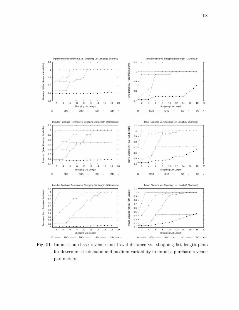
108
0.6
0.7
0.8
0.9
1
1.1
2 4 6 8 10 12 14 16 18 20
Rev
enue
/ (M
ax. R
even
ue A
vaila
ble)
Shopping List Length
Impulse Purchase Revenue vs. Shopping List Length (1 Shortcut)
ID SDD SHD SD DD
0.7
0.8
0.9
1
1.1
2 4 6 8 10 12 14 16 18 20
Tra
vel D
ista
nce
/ (T
otal
Pat
h Le
ngth
)
Shopping List Length
Travel Distance vs. Shopping List Length (1 Shortcut)
ID SDD SHD SD DD
0.3
0.4
0.5
0.6
0.7
0.8
0.9
1
1.1
2 4 6 8 10 12 14 16 18 20
Rev
enue
/ (M
ax. R
even
ue A
vaila
ble)
Shopping List Length
Impulse Purchase Revenue vs. Shopping List Length (2 Shortcuts)
ID SDD SHD SD DD
0.4
0.5
0.6
0.7
0.8
0.9
1
1.1
2 4 6 8 10 12 14 16 18 20
Tra
vel D
ista
nce
/ (T
otal
Pat
h Le
ngth
)
Shopping List Length
Travel Distance vs. Shopping List Length (2 Shortcuts)
ID SDD SHD SD DD
0
0.1
0.2
0.3
0.4
0.5
0.6
0.7
0.8
0.9
1
1.1
2 4 6 8 10 12 14 16 18 20
Rev
enue
/ (M
ax. R
even
ue A
vaila
ble)
Shopping List Length
Impulse Purchase Revenue vs. Shopping List Length (3 Shortcuts)
ID SDD SHD SD DD
0.1
0.2
0.3
0.4
0.5
0.6
0.7
0.8
0.9
1
1.1
2 4 6 8 10 12 14 16 18 20
Tra
vel D
ista
nce
/ (T
otal
Pat
h Le
ngth
)
Shopping List Length
Travel Distance vs. Shopping List Length (3 Shortcuts)
ID SDD SHD SD DD
Fig. 51. Impulse purchase revenue and travel distance vs. shopping list length plots
for deterministic demand and medium variability in impulse purchase revenue
parameters
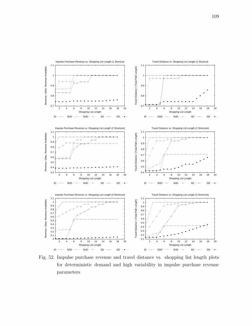
109
0.7
0.8
0.9
1
1.1
2 4 6 8 10 12 14 16 18 20
Rev
enue
/ (M
ax. R
even
ue A
vaila
ble)
Shopping List Length
Impulse Purchase Revenue vs. Shopping List Length (1 Shortcut)
ID SDD SHD SD DD
0.7
0.8
0.9
1
1.1
2 4 6 8 10 12 14 16 18 20
Tra
vel D
ista
nce
/ (T
otal
Pat
h Le
ngth
)
Shopping List Length
Travel Distance vs. Shopping List Length (1 Shortcut)
ID SDD SHD SD DD
0.3
0.4
0.5
0.6
0.7
0.8
0.9
1
1.1
2 4 6 8 10 12 14 16 18 20
Rev
enue
/ (M
ax. R
even
ue A
vaila
ble)
Shopping List Length
Impulse Purchase Revenue vs. Shopping List Length (2 Shortcuts)
ID SDD SHD SD DD
0.4
0.5
0.6
0.7
0.8
0.9
1
1.1
2 4 6 8 10 12 14 16 18 20
Tra
vel D
ista
nce
/ (T
otal
Pat
h Le
ngth
)
Shopping List Length
Travel Distance vs. Shopping List Length (2 Shortcuts)
ID SDD SHD SD DD
0
0.1
0.2
0.3
0.4
0.5
0.6
0.7
0.8
0.9
1
1.1
2 4 6 8 10 12 14 16 18 20
Rev
enue
/ (M
ax. R
even
ue A
vaila
ble)
Shopping List Length
Impulse Purchase Revenue vs. Shopping List Length (3 Shortcuts)
ID SDD SHD SD DD
0.1
0.2
0.3
0.4
0.5
0.6
0.7
0.8
0.9
1
1.1
2 4 6 8 10 12 14 16 18 20
Tra
vel D
ista
nce
/ (T
otal
Pat
h Le
ngth
)
Shopping List Length
Travel Distance vs. Shopping List Length (3 Shortcuts)
ID SDD SHD SD DD
Fig. 52. Impulse purchase revenue and travel distance vs. shopping list length plots
for deterministic demand and high variability in impulse purchase revenue
parameters
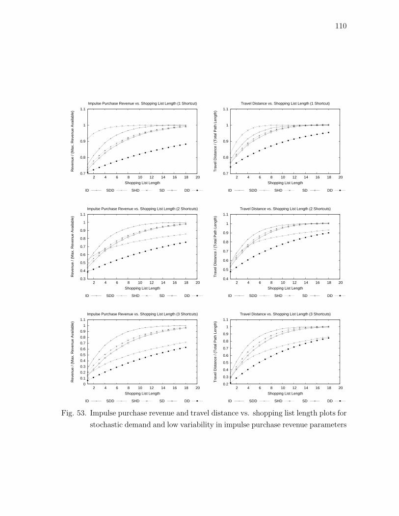
110
0.7
0.8
0.9
1
1.1
2 4 6 8 10 12 14 16 18 20
Rev
enue
/ (M
ax. R
even
ue A
vaila
ble)
Shopping List Length
Impulse Purchase Revenue vs. Shopping List Length (1 Shortcut)
ID SDD SHD SD DD
0.7
0.8
0.9
1
1.1
2 4 6 8 10 12 14 16 18 20
Tra
vel D
ista
nce
/ (T
otal
Pat
h Le
ngth
)
Shopping List Length
Travel Distance vs. Shopping List Length (1 Shortcut)
ID SDD SHD SD DD
0.3
0.4
0.5
0.6
0.7
0.8
0.9
1
1.1
2 4 6 8 10 12 14 16 18 20
Rev
enue
/ (M
ax. R
even
ue A
vaila
ble)
Shopping List Length
Impulse Purchase Revenue vs. Shopping List Length (2 Shortcuts)
ID SDD SHD SD DD
0.4
0.5
0.6
0.7
0.8
0.9
1
1.1
2 4 6 8 10 12 14 16 18 20
Tra
vel D
ista
nce
/ (T
otal
Pat
h Le
ngth
)
Shopping List Length
Travel Distance vs. Shopping List Length (2 Shortcuts)
ID SDD SHD SD DD
0
0.1
0.2
0.3
0.4
0.5
0.6
0.7
0.8
0.9
1
1.1
2 4 6 8 10 12 14 16 18 20
Rev
enue
/ (M
ax. R
even
ue A
vaila
ble)
Shopping List Length
Impulse Purchase Revenue vs. Shopping List Length (3 Shortcuts)
ID SDD SHD SD DD
0.2
0.3
0.4
0.5
0.6
0.7
0.8
0.9
1
1.1
2 4 6 8 10 12 14 16 18 20
Tra
vel D
ista
nce
/ (T
otal
Pat
h Le
ngth
)
Shopping List Length
Travel Distance vs. Shopping List Length (3 Shortcuts)
ID SDD SHD SD DD
Fig. 53. Impulse purchase revenue and travel distance vs. shopping list length plots for
stochastic demand and low variability in impulse purchase revenue parameters

111
0.7
0.8
0.9
1
1.1
2 4 6 8 10 12 14 16 18 20
Rev
enue
/ (M
ax. R
even
ue A
vaila
ble)
Shopping List Length
Impulse Purchase Revenue vs. Shopping List Length (1 Shortcut)
ID SDD SHD SD DD
0.7
0.8
0.9
1
1.1
2 4 6 8 10 12 14 16 18 20
Tra
vel D
ista
nce
/ (T
otal
Pat
h Le
ngth
)
Shopping List Length
Travel Distance vs. Shopping List Length (1 Shortcut)
ID SDD SHD SD DD
0.3
0.4
0.5
0.6
0.7
0.8
0.9
1
1.1
2 4 6 8 10 12 14 16 18 20
Rev
enue
/ (M
ax. R
even
ue A
vaila
ble)
Shopping List Length
Impulse Purchase Revenue vs. Shopping List Length (2 Shortcuts)
ID SDD SHD SD DD
0.4
0.5
0.6
0.7
0.8
0.9
1
1.1
2 4 6 8 10 12 14 16 18 20
Tra
vel D
ista
nce
/ (T
otal
Pat
h Le
ngth
)
Shopping List Length
Travel Distance vs. Shopping List Length (2 Shortcuts)
ID SDD SHD SD DD
0
0.1
0.2
0.3
0.4
0.5
0.6
0.7
0.8
0.9
1
1.1
2 4 6 8 10 12 14 16 18 20
Rev
enue
/ (M
ax. R
even
ue A
vaila
ble)
Shopping List Length
Impulse Purchase Revenue vs. Shopping List Length (3 Shortcuts)
ID SDD SHD SD DD
0.2
0.3
0.4
0.5
0.6
0.7
0.8
0.9
1
1.1
2 4 6 8 10 12 14 16 18 20
Tra
vel D
ista
nce
/ (T
otal
Pat
h Le
ngth
)
Shopping List Length
Travel Distance vs. Shopping List Length (3 Shortcuts)
ID SDD SHD SD DD
Fig. 54. Impulse purchase revenue and travel distance vs. shopping list length plots
for stochastic demand and medium variability in impulse purchase revenue
parameters
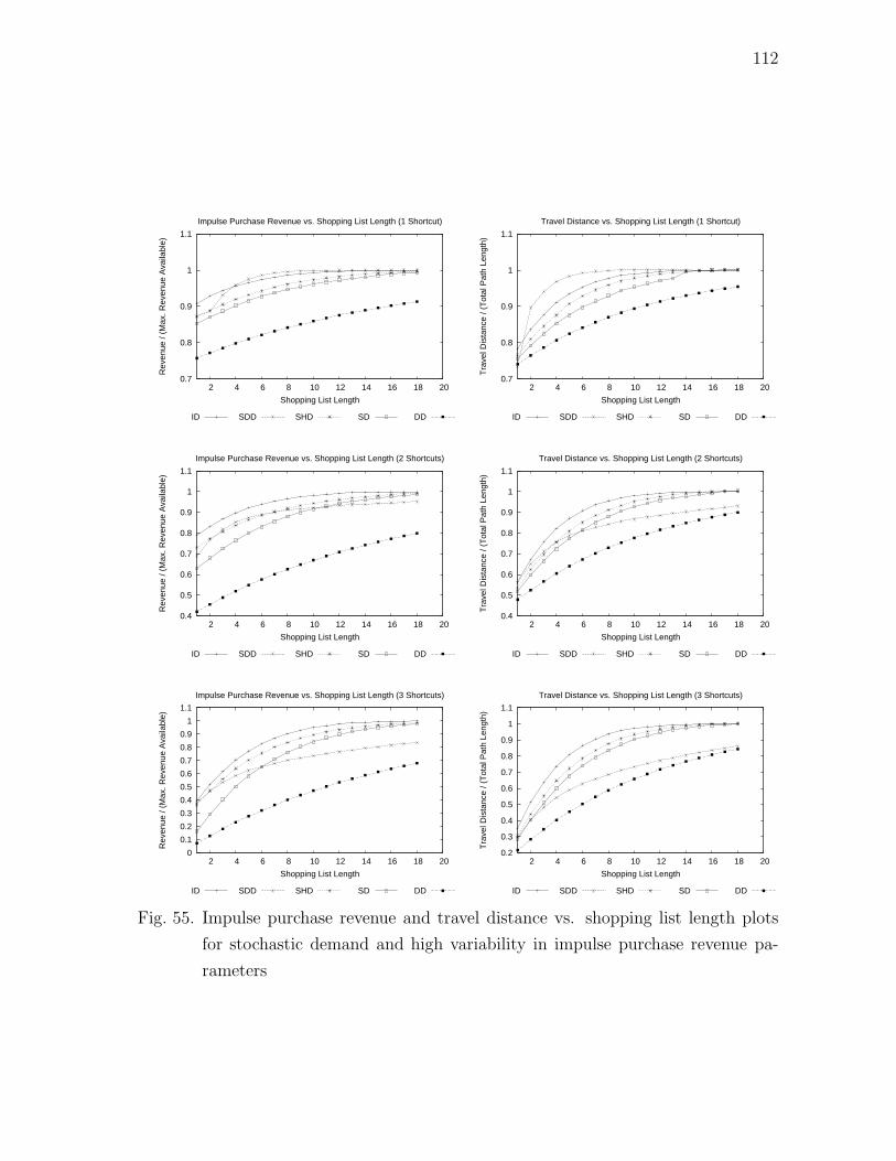
112
0.7
0.8
0.9
1
1.1
2 4 6 8 10 12 14 16 18 20
Rev
enue
/ (M
ax. R
even
ue A
vaila
ble)
Shopping List Length
Impulse Purchase Revenue vs. Shopping List Length (1 Shortcut)
ID SDD SHD SD DD
0.7
0.8
0.9
1
1.1
2 4 6 8 10 12 14 16 18 20
Tra
vel D
ista
nce
/ (T
otal
Pat
h Le
ngth
)
Shopping List Length
Travel Distance vs. Shopping List Length (1 Shortcut)
ID SDD SHD SD DD
0.4
0.5
0.6
0.7
0.8
0.9
1
1.1
2 4 6 8 10 12 14 16 18 20
Rev
enue
/ (M
ax. R
even
ue A
vaila
ble)
Shopping List Length
Impulse Purchase Revenue vs. Shopping List Length (2 Shortcuts)
ID SDD SHD SD DD
0.4
0.5
0.6
0.7
0.8
0.9
1
1.1
2 4 6 8 10 12 14 16 18 20
Tra
vel D
ista
nce
/ (T
otal
Pat
h Le
ngth
)
Shopping List Length
Travel Distance vs. Shopping List Length (2 Shortcuts)
ID SDD SHD SD DD
0
0.1
0.2
0.3
0.4
0.5
0.6
0.7
0.8
0.9
1
1.1
2 4 6 8 10 12 14 16 18 20
Rev
enue
/ (M
ax. R
even
ue A
vaila
ble)
Shopping List Length
Impulse Purchase Revenue vs. Shopping List Length (3 Shortcuts)
ID SDD SHD SD DD
0.2
0.3
0.4
0.5
0.6
0.7
0.8
0.9
1
1.1
2 4 6 8 10 12 14 16 18 20
Tra
vel D
ista
nce
/ (T
otal
Pat
h Le
ngth
)
Shopping List Length
Travel Distance vs. Shopping List Length (3 Shortcuts)
ID SDD SHD SD DD
Fig. 55. Impulse purchase revenue and travel distance vs. shopping list length plots
for stochastic demand and high variability in impulse purchase revenue pa-
rameters
113
CHAPTER VIII
SUMMARY AND CONCLUSIONS
In this dissertation we address the retail facility layout design problem, which dif-
fers dramatically from the traditional layout design problems studied in the IE/OR
literature. In general, the main objective of layout design problems is to minimize
the material handling cost. On the other hand, since retailers are interested in sales
revenue, a revenue based performance measure is more appropriate to evaluate the
effectiveness of retail facility layout design. Considering the effect of impulse pur-
chases in sales revenue, we use impulse purchase revenue as the primary performance
measure to evaluate the retail facility layout effectiveness. In addition, we evaluate
the performance of retail facility layouts from customer’s perspective. Due to the
increase in the value the customers place on time, we use customer travel distance
as another performance measure, which reflects the time the customers spend during
shopping.
A large number of studies in the retailing literature analyze the retail facility
layout design problem. In Chapter II, a brief overview of different study areas related
to retail facility layout design is given. The studies on retail facility layout design
show great variety with respect to the different aspects of the retail facility layout
design that they analyze such as the effect of the environment on customer behavior
and the interaction between different product categories. In this dissertation we focus
on the store layout design aspect of the retail facility layout design problem. To the
best of our knowledge, there is no analytical model for the retail store layout design
problem in either the IE/OR or retailing literature.
In Chapter III, we give brief information on how the retail management textbooks
classify store layout designs. We compare the retail facility layout design problem with
114
traditional facility layout design problems and point out differences and similarities.
Since purchase decisions of customers are shaped by the products they see during
shopping, it is important to incorporate the customer flow in the store into a layout
design model. We suggest using network models to keep track of customer travel and
give a generic network based layout design model to maximize the impulse purchase
revenue of stores.
In Chapter IV, we introduce network representations for three different layout
patterns, which are serpentine, grid, and hub-and-spoke layouts. For the network
representations, we derive expected value expressions for the travel distance between
two random product locations, the number of alternative routes between two random
product locations, and the expected shopping tour length. Our analysis shows that
the serpentine layout has higher travel distances for the customer, but it is easier for
the retailer to control customer traffic on the serpentine layout since there are fewer
alternative shopping routes. For grid and hub-and-spoke layouts, customer travel
distances depend on the distance between different aisles and divisions, respectively.
If inter-aisle and division distances are not very high, then travel distances of the cus-
tomer in grid and hub-and-spoke layouts is relatively less compared to the serpentine
layout. On the other hand, due to the number of alternative shopping routes, it is
not easy to control customer traffic in the grid or hub-and-spoke layouts.
In Chapter V, we introduce a grid layout model for retail stores. This model
allows us to have variable aisle lengths and orientations in the store. We embed our
model in a simulated annealing algorithm to generate layouts maximizing impulse
purchase revenue. The results of our analysis show that the impulse purchase revenue
and the travel distance of the customer are positively correlated with the shopping
list length and also depends on how the customer selects his shopping route in the
store. Uncertainty in the customer’s route selection behavior has a negative effect on
115
impulse purchase revenue.
In Chapter VI, we analyze the serpentine layout and provide a network based
model, which allows us to have shortcuts in the serpentine layout. We use this
model in a simulated annealing algorithm and generate layouts for different shopping
list lengths, number of shortcuts, and customer route selection strategy scenarios.
We show that when shortcuts are allowed, it is possible to decrease customer travel
distance and increase impulse purchase revenue simultaneously. This is achieved by
increasing the exposure of high impulse purchase revenue products by using shortcuts.
In Chapter VII, we extend the network models for grid and serpentine layouts
given in Chapter IV. For the grid layout, we add end-of-aisle and side shelves, and
for the serpentine layout we include the possibility of having shortcuts. It is shown
that for a fixed store shelf space, the customer has significantly less travel distance
in the grid layout compared to the serpentine layout. This result shows that if the
products have high demand and low impulse purchase rates, then it may be more
appropriate to use a grid layout in order to save customers’ time and also to eliminate
congestion in customer traffic. On the other hand, if the products have low demand
and high impulse purchase rates, then it may be better to use a serpentine layout
to better control customer flow and increase impulse purchase revenue. In order to
analyze the trade-off between customer travel distance and impulse purchase revenue
in the serpentine layout, we analyze the effect of different product location strategies
on impulse purchase revenue and customer travel distance. Our results show that
as the variability in product revenues increases, it is possible to increase impulse
purchase revenue without increasing the expected customer travel distance by using
an appropriate product location strategy.
Retail facility layout design is a very broad topic and in this dissertation we only
focus on a small portion of it. Yet, this study has an important role in introducing

116
the retail facility layout design problem into the IE/OR literature. We introduce
analytical layout design models for retail stores. Our study sheds light on several
possible future research directions for the retail facility layout design.
Retail facilities consist of a store side and also a back storage area where product
inventory is kept and warehousing operations are done. Although we analyze the
store side, it is possible to integrate the warehouse side of retail facilities in the
store layout design process. In this way, the shelf space allocation decisions for the
products in the store and also the inventory level decisions in the warehouse can be
made concurrently, which can create savings in shelf space and product replenishment
cost.
As another extension, product assortment decisions can be incorporated in lay-
out design models as has been done in shelf space allocation studies. Although in
this study we work with fixed product assortment, it is possible to make product
assortment decisions based on the available shelf space of the store, impulse purchase
rates of the products, and product demand rates before constructing store layout.
A higher level of integration in retail facility layout design problem is the consid-
eration of required store size with respect to product assortment size decisions. Store
size is determined by the floor area allocated for the front and back sides of the store.
In addition, depending on the products in the assortment and the product demand
levels, the shelf space allocated for each product category and the inventory kept for
each product directly affect store floor area requirements. An optimal solution to this
integrated problem can provide considerable amount of savings to retailers.
Also, the uncertainty in customer behavior and product demand rates provide
several research directions to extend layout design models. The customers’ route
selection process and also the negative effect of travel distance on customers’ purchase
decisions can be analyzed further and the layout design models can be extended
117
accordingly. In addition, the interaction between different product categories, such
as substitution and complementary relationships, can be taken into account in layout
design models.
118
REFERENCES
Aickelin, U. and Dowsland, K. (2002). Enhanced direct and indirect genetic algorithm
approaches for a mall layout and tenant selection problem, Journal of Heuristics
8(5): 503–514.
Banerjee, P., Zhou, Y. and Montreuil, B. (1997). Genetically assisted optimization
of cell layout and material flow path skeleton, IIE Transactions 29: 277–291.
Bellenger, D. N. and Goldstucker, J. I. (1983). Retailing Basics, Richard D. Irwin,
Inc., Homewood, IL.
Bellenger, D., Robertson, D. and Hirschman, E. (1978). Impulse buying varies by
product, Journal of Advertising Research 18(6): 15–18.
Berman, B. and Evans, J. R. (1989). Retail Management– A Strategic Approach, 4th
edn., Macmillan Publishing Company, New York, NY.
Borin, N. and Farris, P. (1995). A sensitivity analysis of retailer shelf management
models, Journal of Retailing 71(2): 153–171.
Borin, N., Farris, P. and Freeland, J. (1994). A model for determining retail product
category assortment and shelf space allocation, Decision Sciences 25(3): 359–
384.
Botsalı, A. and Peters, B. (2005). A network based layout design model for retail
stores, Proceedings of the IERC, Atlanta, GA.
Braaksma, H. (1977). Optimum airport terminal layout planning, Engineering Opti-
mization 3: 1–15.
119
Bultez, A. and Naert, P. (1988). SH.A.R.P: Shelf allocation for retailers’ profit,
Marketing Science 7(3): 211–231.
Castillo, I. and Peters, B. A. (2002). Unit load and material-handling consider-
ations in facility layout design, International Journal of Production Research
40(13): 2955–2989.
Chiang, J. and Wilcox, R. (1997). A cross-category analysis of shelf space allocation,
product variety, and retail margins, Marketing Letters 8(2): 183–191.
Corstjens, M. and Doyle, P. (1981). A model for optimizing retail space allocations,
Management Science 27(7): 822–833.
Desmet, P. and Renaudin, V. (1998). Estimation of product category sales respon-
siveness to allocated shelf space, International Journal of Research in Marketing
15(5): 443–457.
Donovan, R. and Rossiter, J. (1982). Store atmosphere: An environmental psychology
approach, Journal of Retailing 58: 34–57.
Donovan, R., Rossiter, J., Marcoolyn, G. and Nesdale, A. (1994). Store atmosphere
and purchasing behavior, Journal of Retailing 70(3): 283–294.
Dube, L. and Morin, S. (2001). Background music pleasure and store evaluation -
Intensity effects and psychological mechanisms, Journal of Business Research
54: 107–113.
Floch, J. (1988). The contribution of a structural semiotics to the design of a hyper-
market, International Journal of Research in Marketing 4: 233–252.
Francis, R., McGinnis, L. and White, J. (1992). Facility layout and location : An
analytical approach, 2nd edn., Prentice Hall, Englewood Cliffs, NJ.
120
Hahn, P. and Krarup, J. (2001). A hospital facility layout problem finally solved,
Journal of Intelligent Manufacturing 12: 487–496.
Ho, Y.-C. and Moodie, C. L. (2000). A hybrid approach for concurrent layout design
of cells and their flow paths in a tree configuration, International Journal of
Production Research 38(4): 895–928.
Iyer, E. (1989). Unplanned purchasing: Knowledge of shopping environment and
time pressure, Journal of Retailing 65(1): 41–57.
Kollat, D. and Willet, R. (1967). Customer impulse purchasing behavior, Journal of
Marketing Research 4: 21–31.
Kollat, D. and Willet, R. (1969). Is impulse purchasing really a useful concept for
marketing decisions?, Journal of Retailing 33: 79–83.
Kusiak, A. and Heragu, S. (1987). The facility layout problem, European Journal of
Operational Research 29: 229–251.
Lam, S. (2001). The effects of store environment on shopping behaviors: A critical
review, Advances in Consumer Research 28: 190–196.
Leszczyc, P. T. P. and Timmermans, H. (2001). Experimental choice analysis of
shopping strategies, Journal of Retailing 77: 493–509.
Mattila, A. and Wirtz, J. (2001). Congruency of scent and music as a driver of
in-store evaluations and behavior, Journal of Retailing 77(2): 273–289.
McGoldrick, P. (1982). How unplanned are impulse purchases?, Retail & Distribution
Management pp. 27–31.

121
Mehrabian, A. and Russell, J. (1974). An Approach to Environmental Psychology,
Massachusetts Institute of Technology, Cambridge, MA.
Meller, R. and Gau, K. Y. (1996). The facility layout problem: Recent and emerging
trends and perspectives, Journal of Manufacturing Systems 15(5): 351–366.
Merrilees, B. and Miller, D. (1997). The superstore format in australia: Opportunities
and limitations, Long Range Planning 30(6): 889–905.
Messinger, P. and Narasimhan, C. (1997). A model of retail formats based on con-
sumers’ economizing on shopping time, Marketing Science 16(1): 1–23.
Morgenstein, M. and Strongin, H. (1983). Modern Retailing, John Wiley & Sons,
New York, NY.
Park, C., Iyer, E. and Smith, D. (1989). The effects of situational factors on in store
grocery shopping behavior: The role of store environment and time availability
for shopping, Journal of Consumer Research 15: 422–433.
Phillips, H. and Bradshaw, R. (1993). How customers actually shop: Customer inter-
action with the point of sale, Journal of the Market Research Society 35(1): 51–
62.
POPAI/duPont Studies (1978). Marketing emphasis, Product Marketing pp. 61–64.
Ross, S. (1996). Stochastic Processes, 2nd edn., John Wiley & Sons, Inc., New York,
NY.
Seiders, K., Berry, L. and Gresham, L. (2000). Attention, retailers! How convenient
is your convenience strategy?, Sloan Management Review 41(3): 79–89.
122
Sommer, R. and Aitkens, S. (1982). Mental mapping of two supermarkets, Journal
of Consumer Research 9: 211–215.
Summers, T. and Hebert, P. (2001). Shedding some light on store atmospherics
influence of illumination on consumer behavior, Journal of Business Research
54: 145–150.
Turley, L. and Milliman, R. (2000). Atmospheric effects on shopping behavior: A
review of the experimental evidence, Journal of Business Research 49: 193–211.
Urban, T. (1998). An inventory-theoretic approach to product assortment and shelf-
space allocation, Journal of Retailing 74(1): 15–35.
Welgama, P. S. and Gibson, P. R. (1996). An integrated methodology for automating
the determination of layout and materials handling system, International Journal
of Production Research 34(8): 2247–2264.
Zacharias, J. (1997). The impact of layout and visual stimuli on the itineraries and
perceptions of pedestrians in a public market, Environment and Planning B:
Planning and Design 23: 23–35.
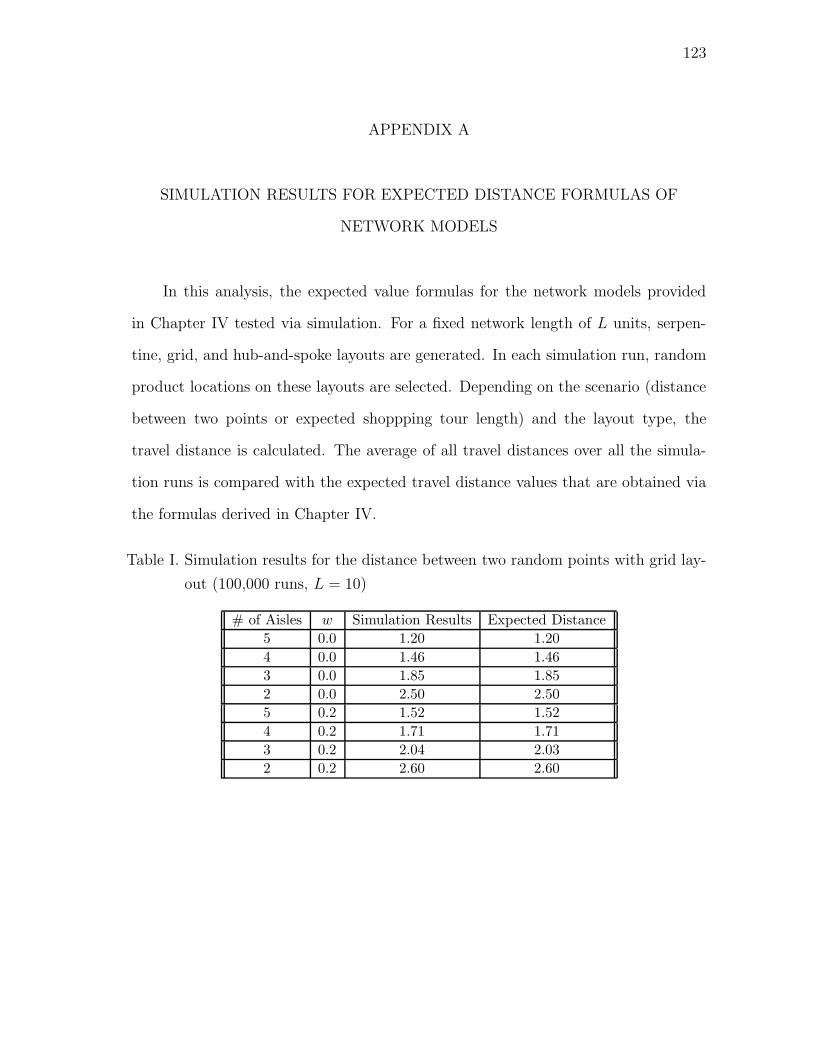
123
APPENDIX A
SIMULATION RESULTS FOR EXPECTED DISTANCE FORMULAS OF
NETWORK MODELS
In this analysis, the expected value formulas for the network models provided
in Chapter IV tested via simulation. For a fixed network length of L units, serpen-
tine, grid, and hub-and-spoke layouts are generated. In each simulation run, random
product locations on these layouts are selected. Depending on the scenario (distance
between two points or expected shoppping tour length) and the layout type, the
travel distance is calculated. The average of all travel distances over all the simula-
tion runs is compared with the expected travel distance values that are obtained via
the formulas derived in Chapter IV.
Table I. Simulation results for the distance between two random points with grid lay-
out (100,000 runs, L = 10)
# of Aisles w Simulation Results Expected Distance
5 0.0 1.20 1.20
4 0.0 1.46 1.46
3 0.0 1.85 1.85
2 0.0 2.50 2.50
5 0.2 1.52 1.52
4 0.2 1.71 1.71
3 0.2 2.04 2.03
2 0.2 2.60 2.60

124
Table II. Simulation results for the distance between two random points with
hub-and-spoke layout (100,000 runs, L = 10)
# of Divisions d Simulation Results Expected Distance
5 0 0.90 0.90
4 0 1.09 1.09
3 0 1.39 1.39
2 0 1.87 1.88
5 0.2 1.22 1.22
4 0.2 1.39 1.39
3 0.2 1.66 1.66
2 0.2 2.07 2.08
Table III. Simulation results for expected shopping tour length with serpentine layout
(10,000 runs, L=10 units)
Shopping List Length Expected Tour Length Simulation Results
1.00 7.50 7.49
2.00 9.17 9.15
3.00 9.69 9.66
4.00 9.88 9.88
5.00 9.95 9.94
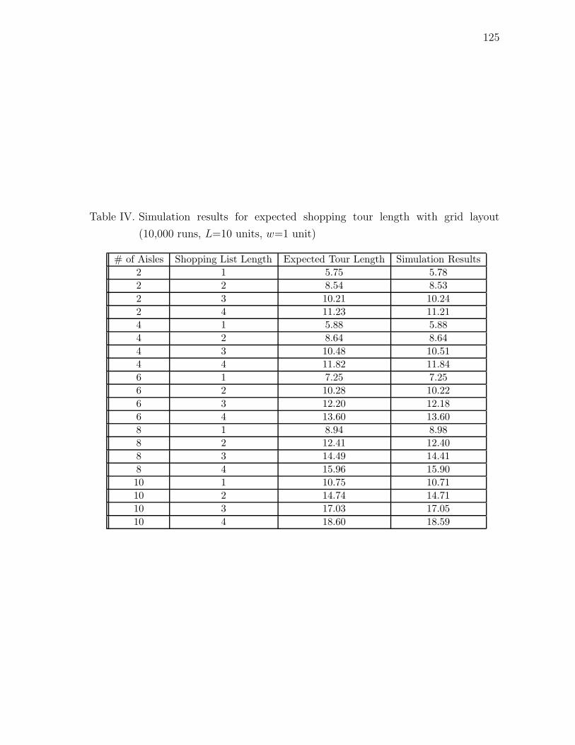
125
Table IV. Simulation results for expected shopping tour length with grid layout
(10,000 runs, L=10 units, w=1 unit)
# of Aisles Shopping List Length Expected Tour Length Simulation Results
2 1 5.75 5.78
2 2 8.54 8.53
2 3 10.21 10.24
2 4 11.23 11.21
4 1 5.88 5.88
4 2 8.64 8.64
4 3 10.48 10.51
4 4 11.82 11.84
6 1 7.25 7.25
6 2 10.28 10.22
6 3 12.20 12.18
6 4 13.60 13.60
8 1 8.94 8.98
8 2 12.41 12.40
8 3 14.49 14.41
8 4 15.96 15.90
10 1 10.75 10.71
10 2 14.74 14.71
10 3 17.03 17.05
10 4 18.60 18.59
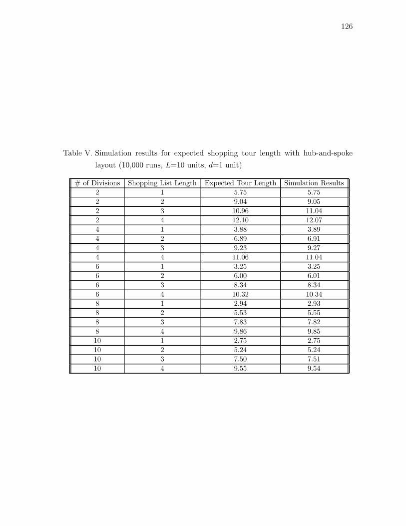
126
Table V. Simulation results for expected shopping tour length with hub-and-spoke
layout (10,000 runs, L=10 units, d=1 unit)
# of Divisions Shopping List Length Expected Tour Length Simulation Results
2 1 5.75 5.75
2 2 9.04 9.05
2 3 10.96 11.04
2 4 12.10 12.07
4 1 3.88 3.89
4 2 6.89 6.91
4 3 9.23 9.27
4 4 11.06 11.04
6 1 3.25 3.25
6 2 6.00 6.01
6 3 8.34 8.34
6 4 10.32 10.34
8 1 2.94 2.93
8 2 5.53 5.55
8 3 7.83 7.82
8 4 9.86 9.85
10 1 2.75 2.75
10 2 5.24 5.24
10 3 7.50 7.51
10 4 9.55 9.54

127
APPENDIX B
SIMULATED ANNEALING ALGORITHM FOR GRID LAYOUT
1 Set initial temperature (IT=10), final temperature (FT=0.001),
cooling rate (c=0.7), number of iterations at each temperature
(n=20)
2 Generate initial feasible solution and set it to best solution
3 Current Temperature (CT) = IT
4 While CT > FT
4.1 For i =1 to n do
4.1.1 For j = 1 to (number of product categories)/2
4.1.1.1 Select randomly two product categories a and b
4.1.1.2 If (feasible), then swap shelf locations of a and b
4.1.1.3 If new layout has larger impulse purchase revenue (NR)
than best solution’s impulse purchase revenue (BR),
then best solution = new layout
4.1.1.4 Else if new layout has smaller impulse purchase
revenue, then best solution = new layout with
probability (exp{(BR-NR)/CT})
4.1.2 Select a grid randomly and modify its orientation
4.1.3 If new layout has larger impulse purchase revenue (NR)
than best solution’s impulse purchase revenue (BR),
then best solution = new layout
4.1.4 Else if new layout has smaller impulse purchase revenue,

128
then best solution = new layout with probability
(exp{(BR-NR)/CT})
4.1.5 For j = 1 to (number of product categories)/2
4.1.5.1 Select randomly two product categories a and b
4.1.5.2 If (feasible), then swap shelf locations of a and b
4.1.5.3 If new layout has larger impulse purchase revenue (NR)
than best solution’s impulse purchase revenue (BR),
then best solution = new layout
4.1.5.4 Else if new layout has smaller impulse purchase
revenue, then best solution = new layout with
probability (exp{(BR-NR)/CT})
4.1.6 Separate or connect two randomly selected neighboring
shelf rows
4.1.7 If new layout has larger impulse purchase revenue (NR)
than best solution’s impulse purchase revenue (BR),
then best solution = new layout
4.1.8 Else if new layout has smaller impulse purchase
revenue, then best solution = new layout with
probability (exp{(BR-NR)/CT})
4.1.9 For j = 1 to 20
4.1.9.1 Select randomly two product categories a and b
4.1.9.2 Swap or replace end caps for a and b
4.1.9.3 If new layout has larger impulse purchase revenue (NR)
than best solutions impulse purchase revenue (BR),
then best solution = new layout
4.1.9.4 Else if new layout has smaller impulse purchase

129
revenue, then best solution = new layout with
probability (exp{(BR-NR)/CT})
5 Return best solution
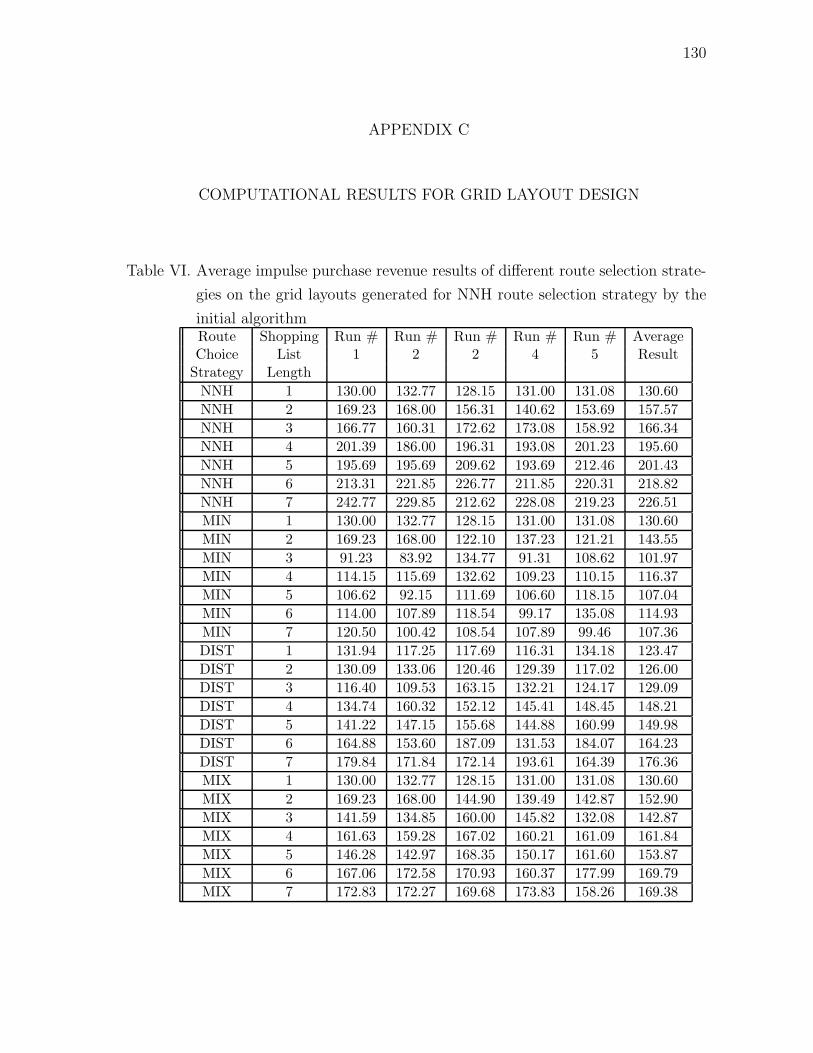
130
APPENDIX C
COMPUTATIONAL RESULTS FOR GRID LAYOUT DESIGN
Table VI. Average impulse purchase revenue results of different route selection strate-
gies on the grid layouts generated for NNH route selection strategy by the
initial algorithmRoute Shopping Run # Run # Run # Run # Run # AverageChoice List 1 2 2 4 5 Result
Strategy Length
NNH 1 130.00 132.77 128.15 131.00 131.08 130.60
NNH 2 169.23 168.00 156.31 140.62 153.69 157.57
NNH 3 166.77 160.31 172.62 173.08 158.92 166.34
NNH 4 201.39 186.00 196.31 193.08 201.23 195.60
NNH 5 195.69 195.69 209.62 193.69 212.46 201.43
NNH 6 213.31 221.85 226.77 211.85 220.31 218.82
NNH 7 242.77 229.85 212.62 228.08 219.23 226.51
MIN 1 130.00 132.77 128.15 131.00 131.08 130.60
MIN 2 169.23 168.00 122.10 137.23 121.21 143.55
MIN 3 91.23 83.92 134.77 91.31 108.62 101.97
MIN 4 114.15 115.69 132.62 109.23 110.15 116.37
MIN 5 106.62 92.15 111.69 106.60 118.15 107.04
MIN 6 114.00 107.89 118.54 99.17 135.08 114.93
MIN 7 120.50 100.42 108.54 107.89 99.46 107.36
DIST 1 131.94 117.25 117.69 116.31 134.18 123.47
DIST 2 130.09 133.06 120.46 129.39 117.02 126.00
DIST 3 116.40 109.53 163.15 132.21 124.17 129.09
DIST 4 134.74 160.32 152.12 145.41 148.45 148.21
DIST 5 141.22 147.15 155.68 144.88 160.99 149.98
DIST 6 164.88 153.60 187.09 131.53 184.07 164.23
DIST 7 179.84 171.84 172.14 193.61 164.39 176.36
MIX 1 130.00 132.77 128.15 131.00 131.08 130.60
MIX 2 169.23 168.00 144.90 139.49 142.87 152.90
MIX 3 141.59 134.85 160.00 145.82 132.08 142.87
MIX 4 161.63 159.28 167.02 160.21 161.09 161.84
MIX 5 146.28 142.97 168.35 150.17 161.60 153.87
MIX 6 167.06 172.58 170.93 160.37 177.99 169.79
MIX 7 172.83 172.27 169.68 173.83 158.26 169.38

131
Table VII. Average travel distance results of different route selection strategies on
the grid layouts generated for NNH route selection strategy by the initial
algorithmRoute Shopping Run # Run # Run # Run # Run # AverageChoice List 1 2 2 4 5 Result
Strategy Length
NNH 1 145.00 170.00 160.00 170.00 145.00 158.00
NNH 2 200.00 200.00 190.00 170.00 190.00 190.00
NNH 3 215.00 215.00 210.00 215.00 220.00 215.00
NNH 4 265.00 235.00 240.00 250.00 265.00 251.00
NNH 5 265.00 255.00 285.00 275.00 295.00 275.00
NNH 6 300.00 275.00 300.00 275.00 275.00 285.00
NNH 7 325.00 305.00 275.00 310.00 295.00 302.00
MIN 1 145.00 170.00 160.00 170.00 145.00 158.00
MIN 2 200.00 200.00 180.00 160.00 180.00 184.00
MIN 3 170.00 170.00 170.00 170.00 170.00 170.00
MIN 4 180.00 170.00 170.00 170.00 180.00 174.00
MIN 5 170.00 160.00 190.00 200.00 190.00 182.00
MIN 6 180.00 200.00 200.00 200.00 180.00 192.00
MIN 7 220.00 200.00 180.00 190.00 200.00 198.00
DIST 1 154.00 170.00 170.80 170.00 157.60 164.48
DIST 2 200.00 200.00 188.80 174.40 188.00 190.24
DIST 3 204.20 207.00 215.00 217.40 211.40 211.00
DIST 4 238.40 223.40 235.00 226.20 243.40 233.28
DIST 5 251.60 252.20 276.40 267.00 282.40 265.92
DIST 6 292.00 271.00 305.60 276.40 299.60 288.92
DIST 7 355.00 318.40 293.20 321.00 304.20 318.36
MIX 1 145.00 170.00 160.00 170.00 145.00 158.00
MIX 2 200.00 200.00 186.67 166.67 186.67 188.00
MIX 3 200.00 200.00 196.67 200.00 201.67 199.67
MIX 4 230.00 210.00 213.33 218.33 230.00 220.33
MIX 5 231.67 216.67 253.33 248.33 256.67 241.33
MIX 6 263.33 251.67 263.33 251.67 250.00 256.00
MIX 7 291.67 271.67 243.33 273.33 265.00 269.00
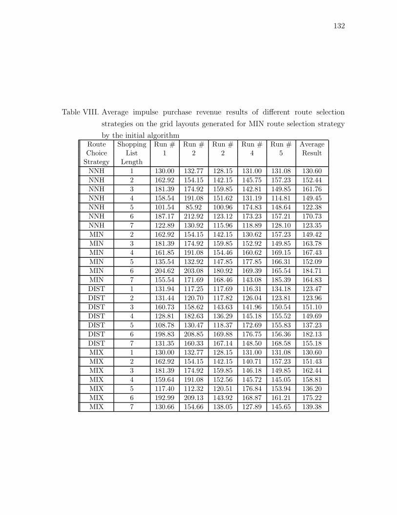
132
Table VIII. Average impulse purchase revenue results of different route selection
strategies on the grid layouts generated for MIN route selection strategy
by the initial algorithmRoute Shopping Run # Run # Run # Run # Run # AverageChoice List 1 2 2 4 5 Result
Strategy Length
NNH 1 130.00 132.77 128.15 131.00 131.08 130.60
NNH 2 162.92 154.15 142.15 145.75 157.23 152.44
NNH 3 181.39 174.92 159.85 142.81 149.85 161.76
NNH 4 158.54 191.08 151.62 131.19 114.81 149.45
NNH 5 101.54 85.92 100.96 174.83 148.64 122.38
NNH 6 187.17 212.92 123.12 173.23 157.21 170.73
NNH 7 122.89 130.92 115.96 118.89 128.10 123.35
MIN 2 162.92 154.15 142.15 130.62 157.23 149.42
MIN 3 181.39 174.92 159.85 152.92 149.85 163.78
MIN 4 161.85 191.08 154.46 160.62 169.15 167.43
MIN 5 135.54 132.92 147.85 177.85 166.31 152.09
MIN 6 204.62 203.08 180.92 169.39 165.54 184.71
MIN 7 155.54 171.69 168.46 143.08 185.39 164.83
DIST 1 131.94 117.25 117.69 116.31 134.18 123.47
DIST 2 131.44 120.70 117.82 126.04 123.81 123.96
DIST 3 160.73 158.62 143.63 141.96 150.54 151.10
DIST 4 128.81 182.63 136.29 145.18 155.52 149.69
DIST 5 108.78 130.47 118.37 172.69 155.83 137.23
DIST 6 198.83 208.85 169.88 176.75 156.36 182.13
DIST 7 131.35 160.33 167.14 148.50 168.58 155.18
MIX 1 130.00 132.77 128.15 131.00 131.08 130.60
MIX 2 162.92 154.15 142.15 140.71 157.23 151.43
MIX 3 181.39 174.92 159.85 146.18 149.85 162.44
MIX 4 159.64 191.08 152.56 145.72 145.05 158.81
MIX 5 117.40 112.32 120.51 176.84 153.94 136.20
MIX 6 192.99 209.13 143.92 168.87 161.21 175.22
MIX 7 130.66 154.66 138.05 127.89 145.65 139.38
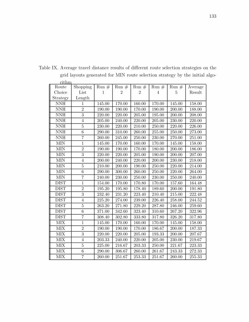
133
Table IX. Average travel distance results of different route selection strategies on the
grid layouts generated for MIN route selection strategy by the initial algo-
rithmRoute Shopping Run # Run # Run # Run # Run # AverageChoice List 1 2 2 4 5 Result
Strategy Length
NNH 1 145.00 170.00 160.00 170.00 145.00 158.00
NNH 2 190.00 190.00 170.00 190.00 200.00 188.00
NNH 3 220.00 220.00 205.00 195.00 200.00 208.00
NNH 4 205.00 240.00 220.00 205.00 230.00 220.00
NNH 5 230.00 220.00 210.00 250.00 220.00 226.00
NNH 6 290.00 310.00 260.00 255.00 250.00 273.00
NNH 7 260.00 245.00 250.00 230.00 270.00 251.00
MIN 1 145.00 170.00 160.00 170.00 145.00 158.00
MIN 2 190.00 190.00 170.00 180.00 200.00 186.00
MIN 3 220.00 220.00 205.00 190.00 200.00 207.00
MIN 4 200.00 240.00 220.00 200.00 230.00 218.00
MIN 5 210.00 200.00 190.00 250.00 220.00 214.00
MIN 6 290.00 300.00 260.00 250.00 220.00 264.00
MIN 7 240.00 230.00 250.00 230.00 250.00 240.00
DIST 1 154.00 170.00 170.80 170.00 157.60 164.48
DIST 2 195.20 195.80 178.40 189.60 200.00 191.80
DIST 3 232.40 231.20 223.40 210.40 215.00 222.48
DIST 4 225.20 274.00 239.00 226.40 258.00 244.52
DIST 5 263.20 271.80 229.20 287.80 246.00 259.60
DIST 6 371.00 342.60 323.40 310.60 267.20 322.96
DIST 7 308.40 302.80 333.80 317.80 326.20 317.80
MIX 1 145.00 170.00 160.00 170.00 145.00 158.00
MIX 2 190.00 190.00 170.00 186.67 200.00 187.33
MIX 3 220.00 220.00 205.00 193.33 200.00 207.67
MIX 4 203.33 240.00 220.00 205.00 230.00 219.67
MIX 5 225.00 216.67 203.33 250.00 221.67 223.33
MIX 6 290.00 306.67 260.00 261.67 243.33 272.33
MIX 7 260.00 251.67 253.33 251.67 260.00 255.33
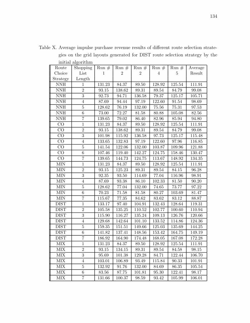
134
Table X. Average impulse purchase revenue results of different route selection strate-
gies on the grid layouts generated for DIST route selection strategy by the
initial algorithmRoute Shopping Run # Run # Run # Run # Run # AverageChoice List 1 2 2 4 5 Result
Strategy Length
NNH 1 131.23 84.37 89.50 128.92 125.54 111.91
NNH 2 93.15 138.62 89.31 89.54 84.79 99.08
NNH 3 92.73 94.71 136.58 79.37 125.17 105.71
NNH 4 87.69 94.44 97.19 122.60 91.54 98.69
NNH 5 128.62 76.19 132.00 75.56 75.31 97.53
NNH 6 73.00 72.27 81.58 80.88 105.08 82.56
NNH 7 139.65 79.02 86.40 82.96 85.94 94.80
CO 1 131.23 84.37 89.50 128.92 125.54 111.91
CO 2 93.15 138.62 89.31 89.54 84.79 99.08
CO 3 101.98 115.92 136.58 97.73 125.17 115.48
CO 4 133.65 132.83 97.19 122.60 97.96 116.85
CO 5 141.54 122.06 132.00 103.87 109.96 121.88
CO 6 107.46 119.40 142.27 124.75 158.46 130.47
CO 7 139.65 144.73 124.75 113.67 148.92 134.35
MIN 1 131.23 84.37 89.50 128.92 125.54 111.91
MIN 2 93.15 125.23 89.31 89.54 84.15 96.28
MIN 3 92.35 93.50 114.69 77.04 116.96 98.91
MIN 4 87.69 93.38 86.10 102.33 81.50 90.20
MIN 5 128.62 77.04 132.00 74.65 73.77 97.22
MIN 6 70.23 71.58 81.58 80.27 103.69 81.47
MIN 7 115.67 77.35 84.62 83.62 83.12 88.87
DIST 1 133.17 97.40 104.91 132.43 128.64 119.31
DIST 2 105.58 135.25 110.52 102.77 100.60 110.94
DIST 3 115.90 116.27 135.24 109.13 126.76 120.66
DIST 4 129.68 142.64 101.10 133.52 114.86 124.36
DIST 5 159.35 151.51 149.66 125.03 135.69 144.25
DIST 6 141.82 137.41 148.56 153.42 164.75 149.19
DIST 7 186.92 164.90 174.48 168.05 167.08 172.28
MIX 1 131.23 84.37 89.50 128.92 125.54 111.91
MIX 2 93.15 134.15 89.31 89.54 84.58 98.15
MIX 3 95.69 101.38 129.28 84.71 122.44 106.70
MIX 4 103.01 106.89 93.49 115.84 90.33 101.91
MIX 5 132.92 91.76 132.00 84.69 86.35 105.54
MIX 6 83.56 87.75 101.81 95.30 122.41 98.17
MIX 7 131.66 100.37 98.59 93.42 105.99 106.01

135
Table XI. Average travel distance results of different route selection strategies on the
grid layouts generated for DIST route selection strategy by the initial algo-
rithmRoute Shopping Run # Run # Run # Run # Run # AverageChoice List 1 2 2 4 5 Result
Strategy Length
NNH 1 145.00 160.00 160.00 145.00 145.00 151.00
NNH 2 170.00 175.00 170.00 170.00 185.00 174.00
NNH 3 175.00 185.00 195.00 185.00 180.00 184.00
NNH 4 170.00 175.00 185.00 215.00 185.00 186.00
NNH 5 230.00 200.00 200.00 190.00 185.00 201.00
NNH 6 185.00 205.00 170.00 185.00 190.00 187.00
NNH 7 235.00 185.00 220.00 220.00 195.00 211.00
CO 1 145.00 160.00 160.00 145.00 145.00 151.00
CO 2 170.00 175.00 170.00 170.00 185.00 174.00
CO 3 190.00 200.00 195.00 190.00 180.00 191.00
CO 4 250.00 210.00 185.00 215.00 190.00 210.00
CO 5 245.00 230.00 200.00 230.00 215.00 224.00
CO 6 220.00 265.00 270.00 235.00 265.00 251.00
CO 7 235.00 290.00 255.00 255.00 285.00 264.00
MIN 1 145.00 160.00 160.00 145.00 145.00 151.00
MIN 2 170.00 160.00 170.00 170.00 170.00 168.00
MIN 3 160.00 170.00 170.00 170.00 170.00 168.00
MIN 4 170.00 160.00 180.00 210.00 160.00 176.00
MIN 5 230.00 190.00 200.00 170.00 170.00 192.00
MIN 6 170.00 190.00 170.00 170.00 180.00 176.00
MIN 7 230.00 170.00 210.00 210.00 180.00 200.00
DIST 1 154.00 168.40 170.80 156.40 157.60 161.44
DIST 2 189.20 182.80 194.40 186.40 186.60 187.88
DIST 3 208.80 201.20 205.20 203.00 193.60 202.36
DIST 4 245.80 229.00 217.20 252.00 216.60 232.12
DIST 5 293.60 266.00 247.20 258.20 242.80 261.56
DIST 6 269.20 284.20 272.00 282.20 286.80 278.88
DIST 7 330.40 308.00 321.40 322.40 311.20 318.68
MIX 1 145.00 160.00 160.00 145.00 145.00 151.00
MIX 2 170.00 170.00 170.00 170.00 180.00 172.00
MIX 3 175.00 185.00 186.67 181.67 176.67 181.00
MIX 4 196.67 181.67 183.33 213.33 178.33 190.67
MIX 5 235.00 206.67 200.00 196.67 190.00 205.67
MIX 6 191.67 220.00 203.33 196.67 211.67 204.67
MIX 7 233.33 215.00 228.33 228.33 220.00 225.00

136
Table XII. Average impulse purchase revenue results of different route selection strate-
gies on the grid layouts generated for MIX route selection strategy by the
initial algorithmRoute Shopping Run # Run # Run # Run # Run # AverageChoice List 1 2 2 4 5 Result
Strategy Length
NNH 1 130.00 132.77 128.15 131.00 131.08 130.60
NNH 2 140.92 158.31 154.15 165.69 160.46 155.91
NNH 3 168.92 158.31 176.62 158.46 177.23 167.91
NNH 4 179.69 161.69 177.54 174.92 152.92 169.35
NNH 5 168.46 215.23 161.85 176.62 174.15 179.26
NNH 6 206.77 205.39 212.31 206.15 205.39 207.20
NNH 7 206.92 186.62 197.54 209.23 222.77 204.62
MIN 1 130.00 132.77 128.15 131.00 131.08 130.60
MIN 2 140.92 133.54 154.15 165.69 160.46 150.95
MIN 3 159.08 158.31 131.69 148.62 177.23 154.98
MIN 4 134.15 146.77 156.92 114.77 146.62 139.85
MIN 5 168.62 185.69 142.77 134.77 152.00 156.77
MIN 6 136.62 178.15 137.23 154.46 125.39 146.37
MIN 7 147.69 144.77 129.85 140.31 146.46 141.82
DIST 1 131.94 117.25 117.69 116.31 134.18 123.47
DIST 2 118.09 129.96 121.42 123.63 124.20 123.46
DIST 3 134.18 134.16 167.73 135.81 157.34 145.84
DIST 4 171.95 152.27 156.76 159.81 158.70 159.90
DIST 5 179.57 191.77 172.48 177.11 178.63 179.91
DIST 6 197.22 179.62 188.13 178.47 181.78 185.04
DIST 7 196.67 192.86 202.59 192.73 194.33 195.83
MIX 1 130.00 132.77 128.15 131.00 131.08 130.60
MIX 2 140.92 150.05 154.15 165.69 160.46 154.26
MIX 3 165.64 158.31 161.64 155.18 177.23 163.60
MIX 4 169.44 156.05 170.67 151.85 162.67 162.13
MIX 5 175.23 198.82 170.26 169.69 180.51 178.90
MIX 6 183.18 202.15 185.03 186.54 175.49 186.48
MIX 7 189.85 189.69 191.64 185.49 197.74 190.88
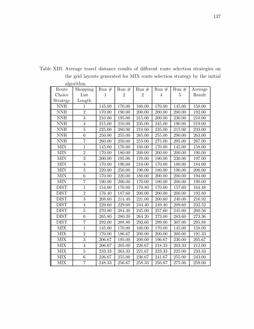
137
Table XIII. Average travel distance results of different route selection strategies on
the grid layouts generated for MIX route selection strategy by the initial
algorithmRoute Shopping Run # Run # Run # Run # Run # AverageChoice List 1 2 2 4 5 Result
Strategy Length
NNH 1 145.00 170.00 160.00 170.00 145.00 158.00
NNH 2 170.00 190.00 200.00 200.00 200.00 192.00
NNH 3 210.00 195.00 215.00 200.00 230.00 210.00
NNH 4 215.00 210.00 235.00 245.00 190.00 219.00
NNH 5 225.00 280.00 210.00 235.00 215.00 233.00
NNH 6 250.00 255.00 265.00 255.00 290.00 263.00
NNH 7 260.00 250.00 255.00 275.00 295.00 267.00
MIN 1 145.00 170.00 160.00 170.00 145.00 158.00
MIN 2 170.00 180.00 200.00 200.00 200.00 190.00
MIN 3 200.00 195.00 170.00 190.00 230.00 197.00
MIN 4 170.00 190.00 210.00 170.00 180.00 184.00
MIN 5 220.00 250.00 190.00 180.00 190.00 206.00
MIN 6 170.00 220.00 180.00 200.00 200.00 194.00
MIN 7 190.00 200.00 170.00 190.00 200.00 190.00
DIST 1 154.00 170.00 170.80 170.00 157.60 164.48
DIST 2 176.40 187.60 200.00 200.00 200.00 192.80
DIST 3 208.60 214.40 221.00 200.60 240.00 216.92
DIST 4 229.60 229.60 244.40 249.40 209.60 232.52
DIST 5 270.80 284.40 245.00 257.60 245.00 260.56
DIST 6 265.80 280.20 264.20 273.00 283.60 273.36
DIST 7 292.00 288.80 292.60 299.00 307.00 295.88
MIX 1 145.00 170.00 160.00 170.00 145.00 158.00
MIX 2 170.00 186.67 200.00 200.00 200.00 191.33
MIX 3 206.67 195.00 200.00 196.67 230.00 205.67
MIX 4 206.67 205.00 226.67 218.33 203.33 212.00
MIX 5 233.33 263.33 221.67 223.33 225.00 233.33
MIX 6 226.67 255.00 236.67 241.67 255.00 243.00
MIX 7 248.33 256.67 258.33 256.67 275.00 259.00
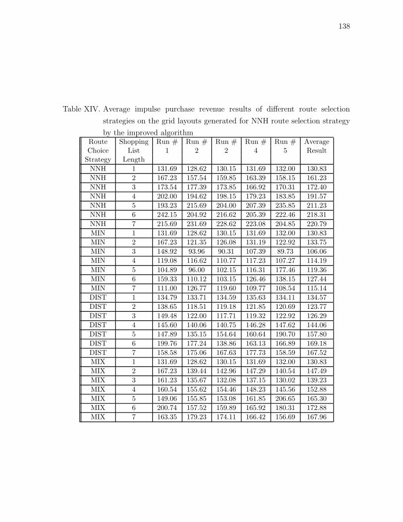
138
Table XIV. Average impulse purchase revenue results of different route selection
strategies on the grid layouts generated for NNH route selection strategy
by the improved algorithmRoute Shopping Run # Run # Run # Run # Run # AverageChoice List 1 2 2 4 5 Result
Strategy Length
NNH 1 131.69 128.62 130.15 131.69 132.00 130.83
NNH 2 167.23 157.54 159.85 163.39 158.15 161.23
NNH 3 173.54 177.39 173.85 166.92 170.31 172.40
NNH 4 202.00 194.62 198.15 179.23 183.85 191.57
NNH 5 193.23 215.69 204.00 207.39 235.85 211.23
NNH 6 242.15 204.92 216.62 205.39 222.46 218.31
NNH 7 215.69 231.69 228.62 223.08 204.85 220.79
MIN 1 131.69 128.62 130.15 131.69 132.00 130.83
MIN 2 167.23 121.35 126.08 131.19 122.92 133.75
MIN 3 148.92 93.96 90.31 107.39 89.73 106.06
MIN 4 119.08 116.62 110.77 117.23 107.27 114.19
MIN 5 104.89 96.00 102.15 116.31 177.46 119.36
MIN 6 159.33 110.12 103.15 126.46 138.15 127.44
MIN 7 111.00 126.77 119.60 109.77 108.54 115.14
DIST 1 134.79 133.71 134.59 135.63 134.11 134.57
DIST 2 138.65 118.51 119.18 121.85 120.69 123.77
DIST 3 149.48 122.00 117.71 119.32 122.92 126.29
DIST 4 145.60 140.06 140.75 146.28 147.62 144.06
DIST 5 147.89 135.15 154.64 160.64 190.70 157.80
DIST 6 199.76 177.24 138.86 163.13 166.89 169.18
DIST 7 158.58 175.06 167.63 177.73 158.59 167.52
MIX 1 131.69 128.62 130.15 131.69 132.00 130.83
MIX 2 167.23 139.44 142.96 147.29 140.54 147.49
MIX 3 161.23 135.67 132.08 137.15 130.02 139.23
MIX 4 160.54 155.62 154.46 148.23 145.56 152.88
MIX 5 149.06 155.85 153.08 161.85 206.65 165.30
MIX 6 200.74 157.52 159.89 165.92 180.31 172.88
MIX 7 163.35 179.23 174.11 166.42 156.69 167.96
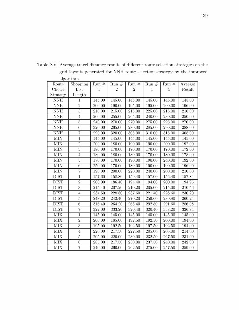
139
Table XV. Average travel distance results of different route selection strategies on the
grid layouts generated for NNH route selection strategy by the improved
algorithmRoute Shopping Run # Run # Run # Run # Run # AverageChoice List 1 2 2 4 5 Result
Strategy Length
NNH 1 145.00 145.00 145.00 145.00 145.00 145.00
NNH 2 200.00 190.00 195.00 195.00 200.00 196.00
NNH 3 210.00 215.00 215.00 225.00 215.00 216.00
NNH 4 260.00 255.00 265.00 240.00 230.00 250.00
NNH 5 240.00 270.00 270.00 275.00 295.00 270.00
NNH 6 320.00 265.00 280.00 285.00 290.00 288.00
NNH 7 290.00 320.00 305.00 310.00 315.00 308.00
MIN 1 145.00 145.00 145.00 145.00 145.00 145.00
MIN 2 200.00 180.00 190.00 190.00 200.00 192.00
MIN 3 180.00 170.00 170.00 170.00 170.00 172.00
MIN 4 180.00 180.00 180.00 170.00 180.00 178.00
MIN 5 170.00 170.00 190.00 190.00 240.00 192.00
MIN 6 250.00 170.00 180.00 190.00 190.00 196.00
MIN 7 190.00 200.00 220.00 240.00 200.00 210.00
DIST 1 157.60 158.80 159.40 157.00 156.40 157.84
DIST 2 200.00 186.40 194.40 194.00 200.00 194.96
DIST 3 215.40 207.20 210.20 205.00 215.00 210.56
DIST 4 234.60 228.80 237.60 221.40 228.60 230.20
DIST 5 248.20 242.40 270.20 259.60 280.80 260.24
DIST 6 316.40 264.20 265.40 292.80 291.60 286.08
DIST 7 322.00 333.20 320.40 320.40 338.20 326.84
MIX 1 145.00 145.00 145.00 145.00 145.00 145.00
MIX 2 200.00 185.00 192.50 192.50 200.00 194.00
MIX 3 195.00 192.50 192.50 197.50 192.50 194.00
MIX 4 220.00 217.50 222.50 205.00 205.00 214.00
MIX 5 205.00 220.00 230.00 232.50 267.50 231.00
MIX 6 285.00 217.50 230.00 237.50 240.00 242.00
MIX 7 240.00 260.00 262.50 275.00 257.50 259.00

140
Table XVI. Average impulse purchase revenue results of different route selection
strategies on the grid layouts generated for MIN route selection strategy
by the improved algorithmRoute Shopping Run # Run # Run # Run # Run # AverageChoice List 1 2 2 4 5 Result
Strategy Length
NNH 1 131.69 128.62 130.15 131.69 132.00 130.83
NNH 2 115.19 159.69 148.62 163.39 166.77 150.73
NNH 3 184.62 171.85 163.39 164.31 146.85 166.20
NNH 4 146.98 190.15 146.27 130.46 182.31 159.24
NNH 5 159.69 181.23 171.50 101.83 204.15 163.68
NNH 6 145.77 126.39 120.40 159.67 118.89 134.22
NNH 7 154.39 211.31 155.79 118.00 193.69 166.64
MIN 1 131.69 128.62 130.15 131.69 132.00 130.83
MIN 2 135.69 159.69 150.77 163.39 166.77 155.26
MIN 3 184.62 171.85 164.77 164.31 155.08 168.12
MIN 4 161.23 190.15 154.46 146.15 182.31 166.86
MIN 5 168.31 181.23 174.46 146.85 204.15 175.00
MIN 6 172.31 189.85 158.62 166.77 176.62 172.83
MIN 7 192.69 211.31 173.54 166.00 193.69 187.45
DIST 1 134.65 133.27 133.66 135.04 134.33 134.19
DIST 2 133.10 126.93 127.33 132.46 130.28 130.02
DIST 3 167.20 151.33 146.85 145.59 144.68 151.13
DIST 4 124.53 182.39 151.68 137.11 160.81 151.31
DIST 5 151.62 201.84 172.81 106.57 205.78 167.72
DIST 6 169.93 169.24 136.70 158.74 145.03 155.93
DIST 7 183.52 246.73 167.60 137.00 220.42 191.05
MIX 1 131.69 128.62 130.15 131.69 132.00 130.83
MIX 2 125.44 159.69 149.69 163.39 166.77 153.00
MIX 3 184.62 171.85 164.08 164.31 150.96 167.16
MIX 4 154.11 190.15 150.37 138.31 182.31 163.05
MIX 5 164.00 181.23 172.98 124.34 204.15 169.34
MIX 6 159.04 158.12 139.51 163.22 147.75 153.53
MIX 7 173.54 211.31 164.66 142.00 193.69 177.04
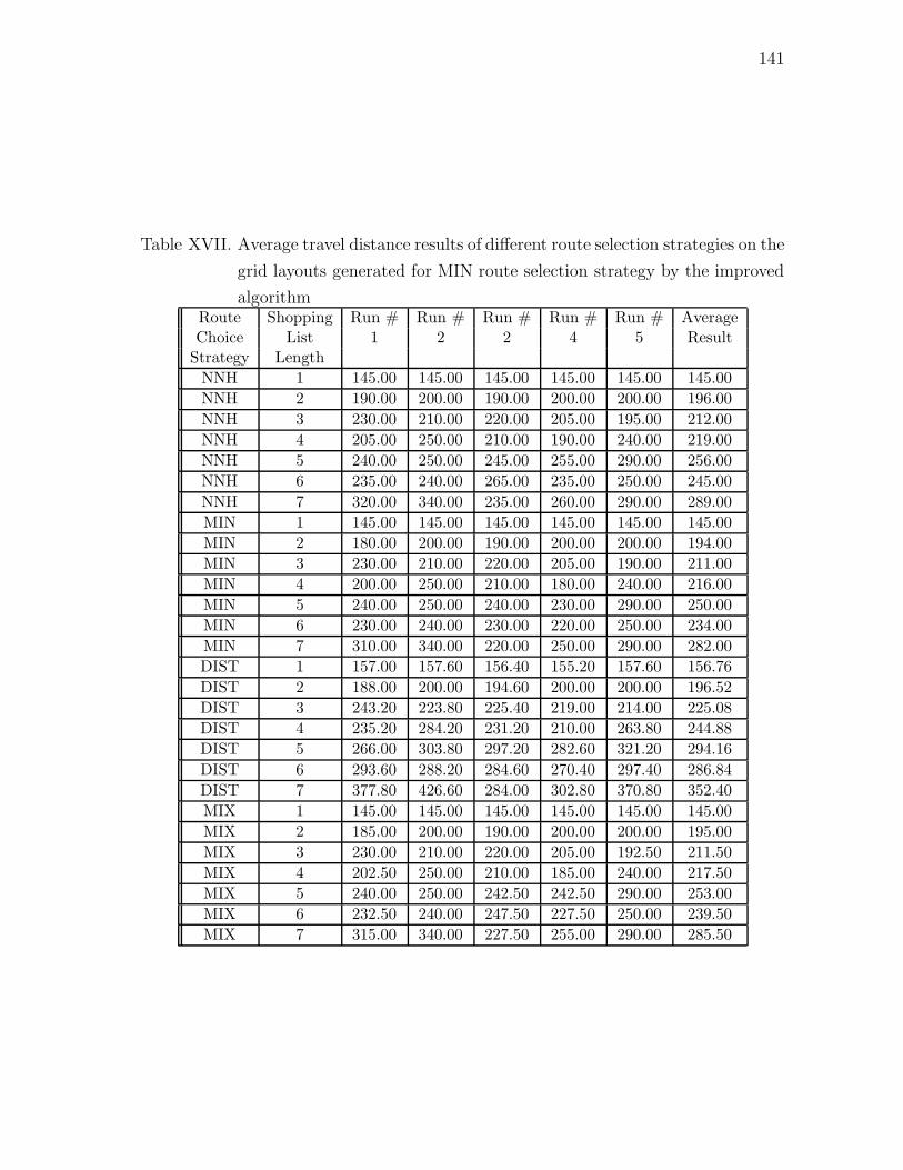
141
Table XVII. Average travel distance results of different route selection strategies on the
grid layouts generated for MIN route selection strategy by the improved
algorithmRoute Shopping Run # Run # Run # Run # Run # AverageChoice List 1 2 2 4 5 Result
Strategy Length
NNH 1 145.00 145.00 145.00 145.00 145.00 145.00
NNH 2 190.00 200.00 190.00 200.00 200.00 196.00
NNH 3 230.00 210.00 220.00 205.00 195.00 212.00
NNH 4 205.00 250.00 210.00 190.00 240.00 219.00
NNH 5 240.00 250.00 245.00 255.00 290.00 256.00
NNH 6 235.00 240.00 265.00 235.00 250.00 245.00
NNH 7 320.00 340.00 235.00 260.00 290.00 289.00
MIN 1 145.00 145.00 145.00 145.00 145.00 145.00
MIN 2 180.00 200.00 190.00 200.00 200.00 194.00
MIN 3 230.00 210.00 220.00 205.00 190.00 211.00
MIN 4 200.00 250.00 210.00 180.00 240.00 216.00
MIN 5 240.00 250.00 240.00 230.00 290.00 250.00
MIN 6 230.00 240.00 230.00 220.00 250.00 234.00
MIN 7 310.00 340.00 220.00 250.00 290.00 282.00
DIST 1 157.00 157.60 156.40 155.20 157.60 156.76
DIST 2 188.00 200.00 194.60 200.00 200.00 196.52
DIST 3 243.20 223.80 225.40 219.00 214.00 225.08
DIST 4 235.20 284.20 231.20 210.00 263.80 244.88
DIST 5 266.00 303.80 297.20 282.60 321.20 294.16
DIST 6 293.60 288.20 284.60 270.40 297.40 286.84
DIST 7 377.80 426.60 284.00 302.80 370.80 352.40
MIX 1 145.00 145.00 145.00 145.00 145.00 145.00
MIX 2 185.00 200.00 190.00 200.00 200.00 195.00
MIX 3 230.00 210.00 220.00 205.00 192.50 211.50
MIX 4 202.50 250.00 210.00 185.00 240.00 217.50
MIX 5 240.00 250.00 242.50 242.50 290.00 253.00
MIX 6 232.50 240.00 247.50 227.50 250.00 239.50
MIX 7 315.00 340.00 227.50 255.00 290.00 285.50
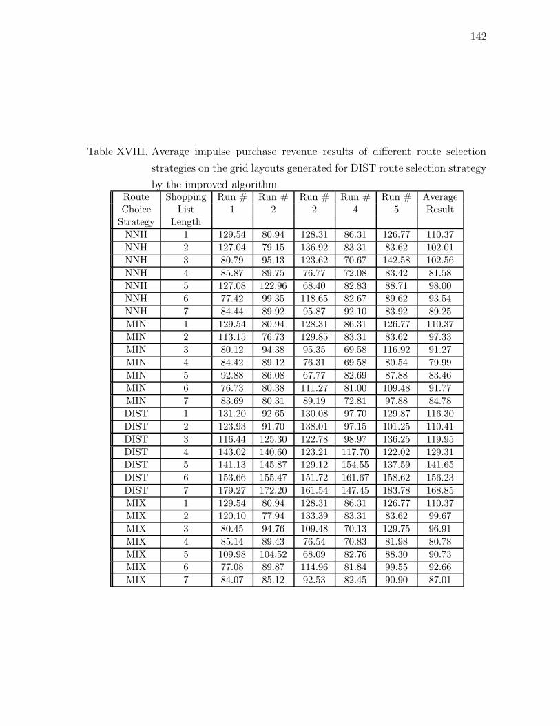
142
Table XVIII. Average impulse purchase revenue results of different route selection
strategies on the grid layouts generated for DIST route selection strategy
by the improved algorithmRoute Shopping Run # Run # Run # Run # Run # AverageChoice List 1 2 2 4 5 Result
Strategy Length
NNH 1 129.54 80.94 128.31 86.31 126.77 110.37
NNH 2 127.04 79.15 136.92 83.31 83.62 102.01
NNH 3 80.79 95.13 123.62 70.67 142.58 102.56
NNH 4 85.87 89.75 76.77 72.08 83.42 81.58
NNH 5 127.08 122.96 68.40 82.83 88.71 98.00
NNH 6 77.42 99.35 118.65 82.67 89.62 93.54
NNH 7 84.44 89.92 95.87 92.10 83.92 89.25
MIN 1 129.54 80.94 128.31 86.31 126.77 110.37
MIN 2 113.15 76.73 129.85 83.31 83.62 97.33
MIN 3 80.12 94.38 95.35 69.58 116.92 91.27
MIN 4 84.42 89.12 76.31 69.58 80.54 79.99
MIN 5 92.88 86.08 67.77 82.69 87.88 83.46
MIN 6 76.73 80.38 111.27 81.00 109.48 91.77
MIN 7 83.69 80.31 89.19 72.81 97.88 84.78
DIST 1 131.20 92.65 130.08 97.70 129.87 116.30
DIST 2 123.93 91.70 138.01 97.15 101.25 110.41
DIST 3 116.44 125.30 122.78 98.97 136.25 119.95
DIST 4 143.02 140.60 123.21 117.70 122.02 129.31
DIST 5 141.13 145.87 129.12 154.55 137.59 141.65
DIST 6 153.66 155.47 151.72 161.67 158.62 156.23
DIST 7 179.27 172.20 161.54 147.45 183.78 168.85
MIX 1 129.54 80.94 128.31 86.31 126.77 110.37
MIX 2 120.10 77.94 133.39 83.31 83.62 99.67
MIX 3 80.45 94.76 109.48 70.13 129.75 96.91
MIX 4 85.14 89.43 76.54 70.83 81.98 80.78
MIX 5 109.98 104.52 68.09 82.76 88.30 90.73
MIX 6 77.08 89.87 114.96 81.84 99.55 92.66
MIX 7 84.07 85.12 92.53 82.45 90.90 87.01
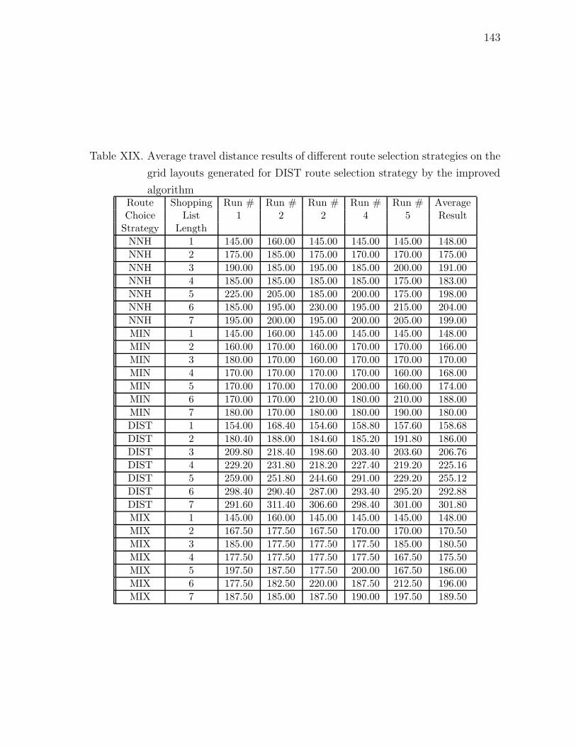
143
Table XIX. Average travel distance results of different route selection strategies on the
grid layouts generated for DIST route selection strategy by the improved
algorithmRoute Shopping Run # Run # Run # Run # Run # AverageChoice List 1 2 2 4 5 Result
Strategy Length
NNH 1 145.00 160.00 145.00 145.00 145.00 148.00
NNH 2 175.00 185.00 175.00 170.00 170.00 175.00
NNH 3 190.00 185.00 195.00 185.00 200.00 191.00
NNH 4 185.00 185.00 185.00 185.00 175.00 183.00
NNH 5 225.00 205.00 185.00 200.00 175.00 198.00
NNH 6 185.00 195.00 230.00 195.00 215.00 204.00
NNH 7 195.00 200.00 195.00 200.00 205.00 199.00
MIN 1 145.00 160.00 145.00 145.00 145.00 148.00
MIN 2 160.00 170.00 160.00 170.00 170.00 166.00
MIN 3 180.00 170.00 160.00 170.00 170.00 170.00
MIN 4 170.00 170.00 170.00 170.00 160.00 168.00
MIN 5 170.00 170.00 170.00 200.00 160.00 174.00
MIN 6 170.00 170.00 210.00 180.00 210.00 188.00
MIN 7 180.00 170.00 180.00 180.00 190.00 180.00
DIST 1 154.00 168.40 154.60 158.80 157.60 158.68
DIST 2 180.40 188.00 184.60 185.20 191.80 186.00
DIST 3 209.80 218.40 198.60 203.40 203.60 206.76
DIST 4 229.20 231.80 218.20 227.40 219.20 225.16
DIST 5 259.00 251.80 244.60 291.00 229.20 255.12
DIST 6 298.40 290.40 287.00 293.40 295.20 292.88
DIST 7 291.60 311.40 306.60 298.40 301.00 301.80
MIX 1 145.00 160.00 145.00 145.00 145.00 148.00
MIX 2 167.50 177.50 167.50 170.00 170.00 170.50
MIX 3 185.00 177.50 177.50 177.50 185.00 180.50
MIX 4 177.50 177.50 177.50 177.50 167.50 175.50
MIX 5 197.50 187.50 177.50 200.00 167.50 186.00
MIX 6 177.50 182.50 220.00 187.50 212.50 196.00
MIX 7 187.50 185.00 187.50 190.00 197.50 189.50
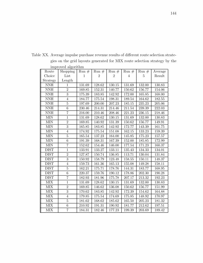
144
Table XX. Average impulse purchase revenue results of different route selection strate-
gies on the grid layouts generated for MIX route selection strategy by the
improved algorithmRoute Shopping Run # Run # Run # Run # Run # AverageChoice List 1 2 2 4 5 Result
Strategy Length
NNH 1 131.69 128.62 130.15 131.69 132.00 130.83
NNH 2 169.85 152.31 140.77 150.62 156.77 154.06
NNH 3 175.39 183.85 142.92 172.00 165.85 168.00
NNH 4 184.77 175.54 198.31 189.54 164.62 182.55
NNH 5 197.69 200.00 207.23 185.15 235.23 205.06
NNH 6 230.46 214.31 214.46 211.54 239.39 222.03
NNH 7 216.00 210.46 208.46 221.23 236.15 218.46
MIN 1 131.69 128.62 130.15 131.69 132.00 130.83
MIN 2 169.85 140.92 131.39 150.62 156.77 149.91
MIN 3 165.85 183.85 142.92 172.77 143.39 161.75
MIN 4 174.92 175.54 151.08 162.15 133.23 159.39
MIN 5 165.54 137.23 164.00 145.85 175.23 157.57
MIN 6 191.39 168.31 167.39 152.00 185.85 172.99
MIN 7 152.62 154.46 146.00 177.54 171.23 160.37
DIST 1 133.91 133.27 133.11 135.43 134.33 134.01
DIST 2 127.87 150.74 136.85 113.71 130.04 131.84
DIST 3 150.92 158.79 123.48 158.55 150.11 148.37
DIST 4 159.73 161.36 165.13 155.08 149.28 158.11
DIST 5 162.21 175.71 178.76 144.31 183.77 168.95
DIST 6 220.37 159.76 190.12 178.86 202.30 190.28
DIST 7 182.93 181.96 175.78 207.17 213.32 192.23
MIX 1 131.69 128.62 130.15 131.69 132.00 130.83
MIX 2 169.85 146.62 136.08 150.62 156.77 151.99
MIX 3 170.62 183.85 142.92 172.39 154.62 164.88
MIX 4 179.85 175.54 174.69 175.85 148.92 170.97
MIX 5 181.62 168.62 185.62 165.50 205.23 181.32
MIX 6 210.92 191.31 190.92 181.77 212.62 197.51
MIX 7 184.31 182.46 177.23 199.39 203.69 189.42
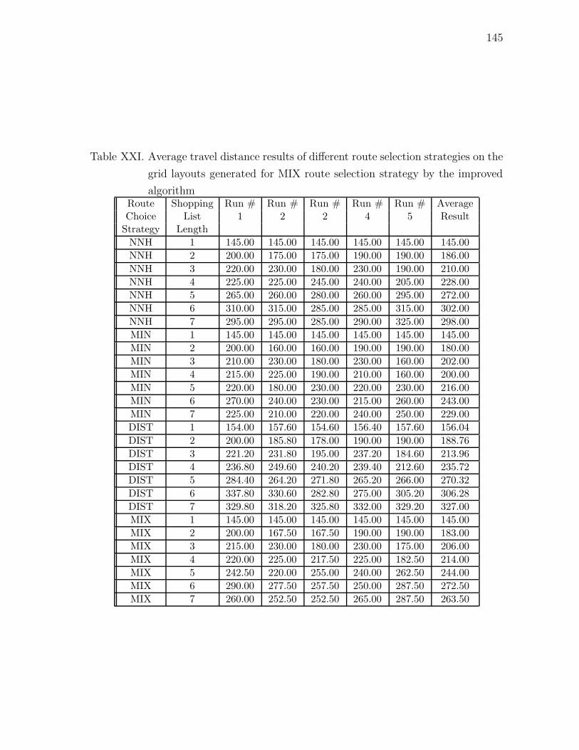
145
Table XXI. Average travel distance results of different route selection strategies on the
grid layouts generated for MIX route selection strategy by the improved
algorithmRoute Shopping Run # Run # Run # Run # Run # AverageChoice List 1 2 2 4 5 Result
Strategy Length
NNH 1 145.00 145.00 145.00 145.00 145.00 145.00
NNH 2 200.00 175.00 175.00 190.00 190.00 186.00
NNH 3 220.00 230.00 180.00 230.00 190.00 210.00
NNH 4 225.00 225.00 245.00 240.00 205.00 228.00
NNH 5 265.00 260.00 280.00 260.00 295.00 272.00
NNH 6 310.00 315.00 285.00 285.00 315.00 302.00
NNH 7 295.00 295.00 285.00 290.00 325.00 298.00
MIN 1 145.00 145.00 145.00 145.00 145.00 145.00
MIN 2 200.00 160.00 160.00 190.00 190.00 180.00
MIN 3 210.00 230.00 180.00 230.00 160.00 202.00
MIN 4 215.00 225.00 190.00 210.00 160.00 200.00
MIN 5 220.00 180.00 230.00 220.00 230.00 216.00
MIN 6 270.00 240.00 230.00 215.00 260.00 243.00
MIN 7 225.00 210.00 220.00 240.00 250.00 229.00
DIST 1 154.00 157.60 154.60 156.40 157.60 156.04
DIST 2 200.00 185.80 178.00 190.00 190.00 188.76
DIST 3 221.20 231.80 195.00 237.20 184.60 213.96
DIST 4 236.80 249.60 240.20 239.40 212.60 235.72
DIST 5 284.40 264.20 271.80 265.20 266.00 270.32
DIST 6 337.80 330.60 282.80 275.00 305.20 306.28
DIST 7 329.80 318.20 325.80 332.00 329.20 327.00
MIX 1 145.00 145.00 145.00 145.00 145.00 145.00
MIX 2 200.00 167.50 167.50 190.00 190.00 183.00
MIX 3 215.00 230.00 180.00 230.00 175.00 206.00
MIX 4 220.00 225.00 217.50 225.00 182.50 214.00
MIX 5 242.50 220.00 255.00 240.00 262.50 244.00
MIX 6 290.00 277.50 257.50 250.00 287.50 272.50
MIX 7 260.00 252.50 252.50 265.00 287.50 263.50
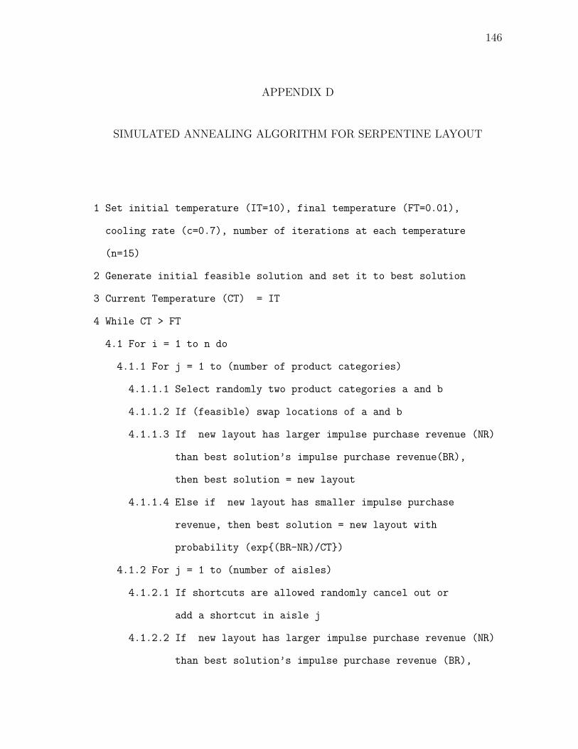
146
APPENDIX D
SIMULATED ANNEALING ALGORITHM FOR SERPENTINE LAYOUT
1 Set initial temperature (IT=10), final temperature (FT=0.01),
cooling rate (c=0.7), number of iterations at each temperature
(n=15)
2 Generate initial feasible solution and set it to best solution
3 Current Temperature (CT) = IT
4 While CT > FT
4.1 For i = 1 to n do
4.1.1 For j = 1 to (number of product categories)
4.1.1.1 Select randomly two product categories a and b
4.1.1.2 If (feasible) swap locations of a and b
4.1.1.3 If new layout has larger impulse purchase revenue (NR)
than best solution’s impulse purchase revenue(BR),
then best solution = new layout
4.1.1.4 Else if new layout has smaller impulse purchase
revenue, then best solution = new layout with
probability (exp{(BR-NR)/CT})
4.1.2 For j = 1 to (number of aisles)
4.1.2.1 If shortcuts are allowed randomly cancel out or
add a shortcut in aisle j
4.1.2.2 If new layout has larger impulse purchase revenue (NR)
than best solution’s impulse purchase revenue (BR),
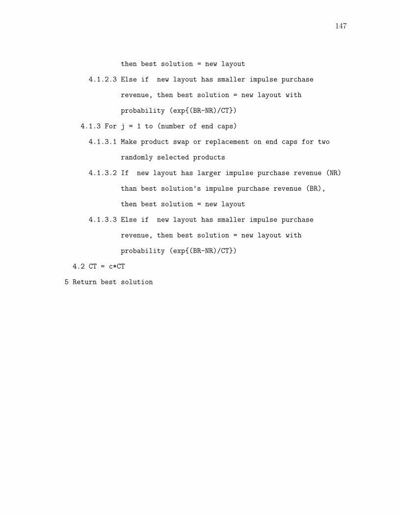
147
then best solution = new layout
4.1.2.3 Else if new layout has smaller impulse purchase
revenue, then best solution = new layout with
probability (exp{(BR-NR)/CT})
4.1.3 For j = 1 to (number of end caps)
4.1.3.1 Make product swap or replacement on end caps for two
randomly selected products
4.1.3.2 If new layout has larger impulse purchase revenue (NR)
than best solution’s impulse purchase revenue (BR),
then best solution = new layout
4.1.3.3 Else if new layout has smaller impulse purchase
revenue, then best solution = new layout with
probability (exp{(BR-NR)/CT})
4.2 CT = c*CT
5 Return best solution

148
APPENDIX E
COMPUTATIONAL RESULTS FOR SERPENTINE LAYOUT DESIGN
Table XXII. Average impulse purchase revenue results of different route selection
strategies on the serpentine layouts where no shortcuts are allowedShopping List Run # Run # Run # Run # Run # Average
Length 1 2 3 4 5
1 155.23 155.85 155.69 155.39 155.39 155.51
2 155.31 155.39 155.46 154.92 155.69 155.35
3 153.31 155.15 155.08 154.92 155.08 154.71
4 155.08 154.77 154.77 154.77 154.69 154.82
5 154.00 154.46 154.46 154.77 154.46 154.43
6 154.39 154.46 154.54 154.08 154.46 154.38
7 153.69 154.15 154.00 153.92 154.15 153.98
Table XXIII. Average travel distance results of different route selection strategies on
the serpentine layouts where no shortcuts are allowedShopping List Run # Run # Run # Run # Run # Average
Length 1 2 3 4 5
1 362.50 362.50 362.50 362.50 362.50 362.50
2 362.50 362.50 362.50 362.50 362.50 362.50
3 362.50 362.50 362.50 362.50 362.50 362.50
4 362.50 362.50 362.50 362.50 362.50 362.50
5 362.50 362.50 362.50 362.50 362.50 362.50
6 362.50 362.50 362.50 362.50 362.50 362.50
7 362.50 362.50 362.50 362.50 362.50 362.50
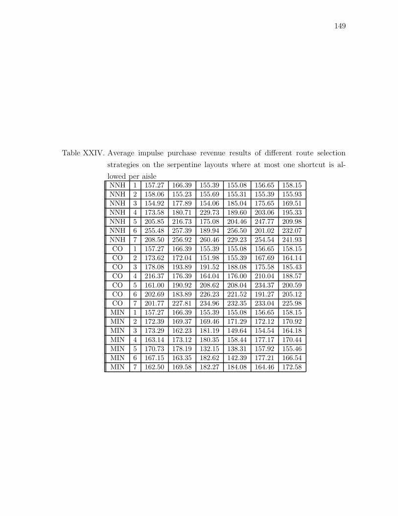
149
Table XXIV. Average impulse purchase revenue results of different route selection
strategies on the serpentine layouts where at most one shortcut is al-
lowed per aisleNNH 1 157.27 166.39 155.39 155.08 156.65 158.15
NNH 2 158.06 155.23 155.69 155.31 155.39 155.93
NNH 3 154.92 177.89 154.06 185.04 175.65 169.51
NNH 4 173.58 180.71 229.73 189.60 203.06 195.33
NNH 5 205.85 216.73 175.08 204.46 247.77 209.98
NNH 6 255.48 257.39 189.94 256.50 201.02 232.07
NNH 7 208.50 256.92 260.46 229.23 254.54 241.93
CO 1 157.27 166.39 155.39 155.08 156.65 158.15
CO 2 173.62 172.04 151.98 155.39 167.69 164.14
CO 3 178.08 193.89 191.52 188.08 175.58 185.43
CO 4 216.37 176.39 164.04 176.00 210.04 188.57
CO 5 161.00 190.92 208.62 208.04 234.37 200.59
CO 6 202.69 183.89 226.23 221.52 191.27 205.12
CO 7 201.77 227.81 234.96 232.35 233.04 225.98
MIN 1 157.27 166.39 155.39 155.08 156.65 158.15
MIN 2 172.39 169.37 169.46 171.29 172.12 170.92
MIN 3 173.29 162.23 181.19 149.64 154.54 164.18
MIN 4 163.14 173.12 180.35 158.44 177.17 170.44
MIN 5 170.73 178.19 132.15 138.31 157.92 155.46
MIN 6 167.15 163.35 182.62 142.39 177.21 166.54
MIN 7 162.50 169.58 182.27 184.08 164.46 172.58
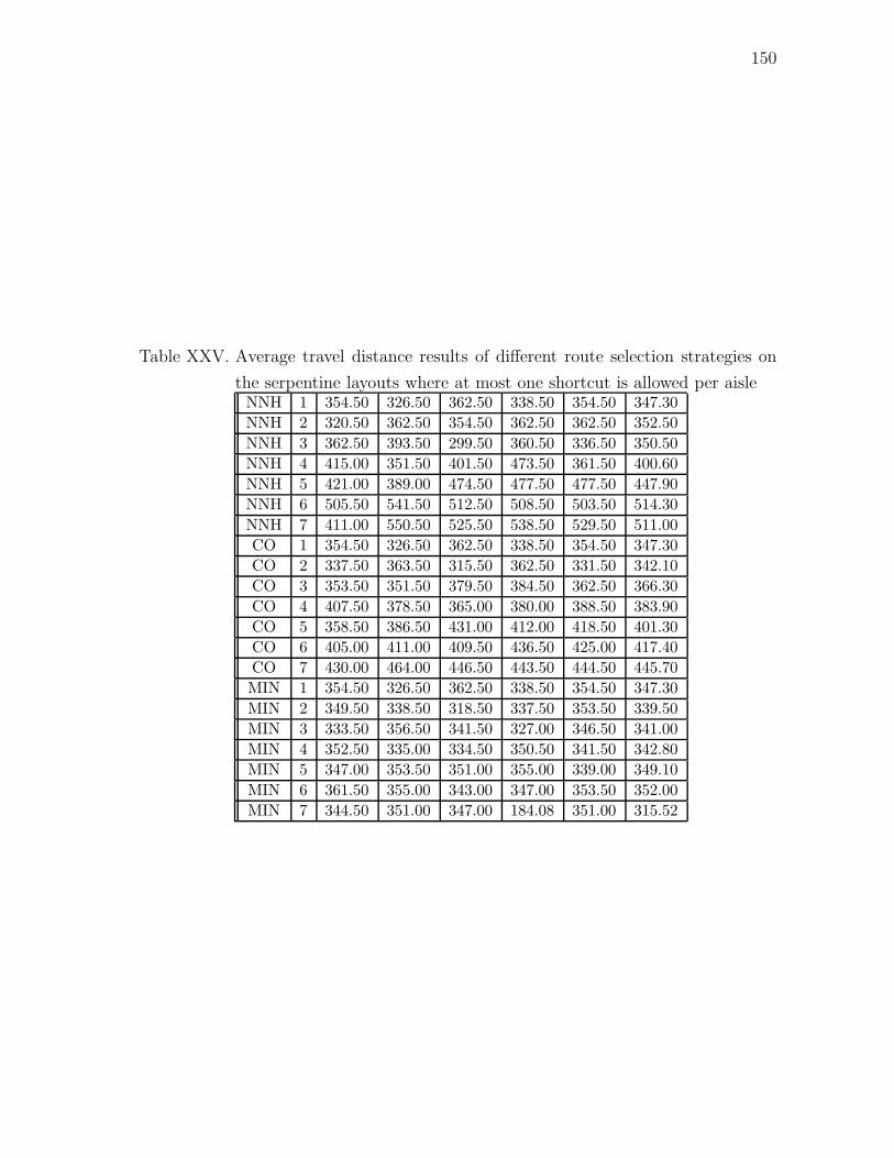
150
Table XXV. Average travel distance results of different route selection strategies on
the serpentine layouts where at most one shortcut is allowed per aisleNNH 1 354.50 326.50 362.50 338.50 354.50 347.30
NNH 2 320.50 362.50 354.50 362.50 362.50 352.50
NNH 3 362.50 393.50 299.50 360.50 336.50 350.50
NNH 4 415.00 351.50 401.50 473.50 361.50 400.60
NNH 5 421.00 389.00 474.50 477.50 477.50 447.90
NNH 6 505.50 541.50 512.50 508.50 503.50 514.30
NNH 7 411.00 550.50 525.50 538.50 529.50 511.00
CO 1 354.50 326.50 362.50 338.50 354.50 347.30
CO 2 337.50 363.50 315.50 362.50 331.50 342.10
CO 3 353.50 351.50 379.50 384.50 362.50 366.30
CO 4 407.50 378.50 365.00 380.00 388.50 383.90
CO 5 358.50 386.50 431.00 412.00 418.50 401.30
CO 6 405.00 411.00 409.50 436.50 425.00 417.40
CO 7 430.00 464.00 446.50 443.50 444.50 445.70
MIN 1 354.50 326.50 362.50 338.50 354.50 347.30
MIN 2 349.50 338.50 318.50 337.50 353.50 339.50
MIN 3 333.50 356.50 341.50 327.00 346.50 341.00
MIN 4 352.50 335.00 334.50 350.50 341.50 342.80
MIN 5 347.00 353.50 351.00 355.00 339.00 349.10
MIN 6 361.50 355.00 343.00 347.00 353.50 352.00
MIN 7 344.50 351.00 347.00 184.08 351.00 315.52

151
Table XXVI. Average impulse purchase results of different route selection strategies
on the serpentine layouts where at most two shortcuts are allowed per
aisleNNH 1 160.21 155.69 156.77 147.64 158.50 155.76
NNH 2 154.52 168.10 155.23 171.27 165.17 162.86
NNH 3 202.98 171.87 174.69 169.15 209.42 185.62
NNH 4 198.56 190.94 177.58 193.98 186.69 189.55
NNH 5 200.14 193.39 188.58 230.31 189.65 200.41
NNH 6 224.58 209.67 275.27 223.39 239.96 234.57
NNH 7 262.73 228.12 240.15 216.04 242.92 237.99
CO 1 160.21 155.69 156.77 147.64 158.50 155.76
CO 2 160.02 173.98 159.27 156.75 154.89 160.98
CO 3 167.96 173.89 188.94 186.62 192.52 181.98
CO 4 172.46 190.12 179.54 199.12 212.48 190.74
CO 5 175.39 204.89 206.54 194.37 196.19 195.47
CO 6 210.15 200.96 215.10 188.69 200.69 203.12
CO 7 230.90 241.02 215.54 236.39 194.92 223.75
MIN 1 160.21 155.69 156.77 147.64 158.50 155.76
MIN 2 172.29 166.85 140.19 163.92 174.33 163.52
MIN 3 155.08 158.62 169.04 165.23 147.62 159.12
MIN 4 168.40 174.83 169.73 171.73 166.04 170.15
MIN 5 168.96 180.85 161.67 181.23 154.60 169.46
MIN 6 173.19 158.73 186.42 177.27 176.04 174.33
MIN 7 181.58 174.19 187.19 167.12 168.81 175.78
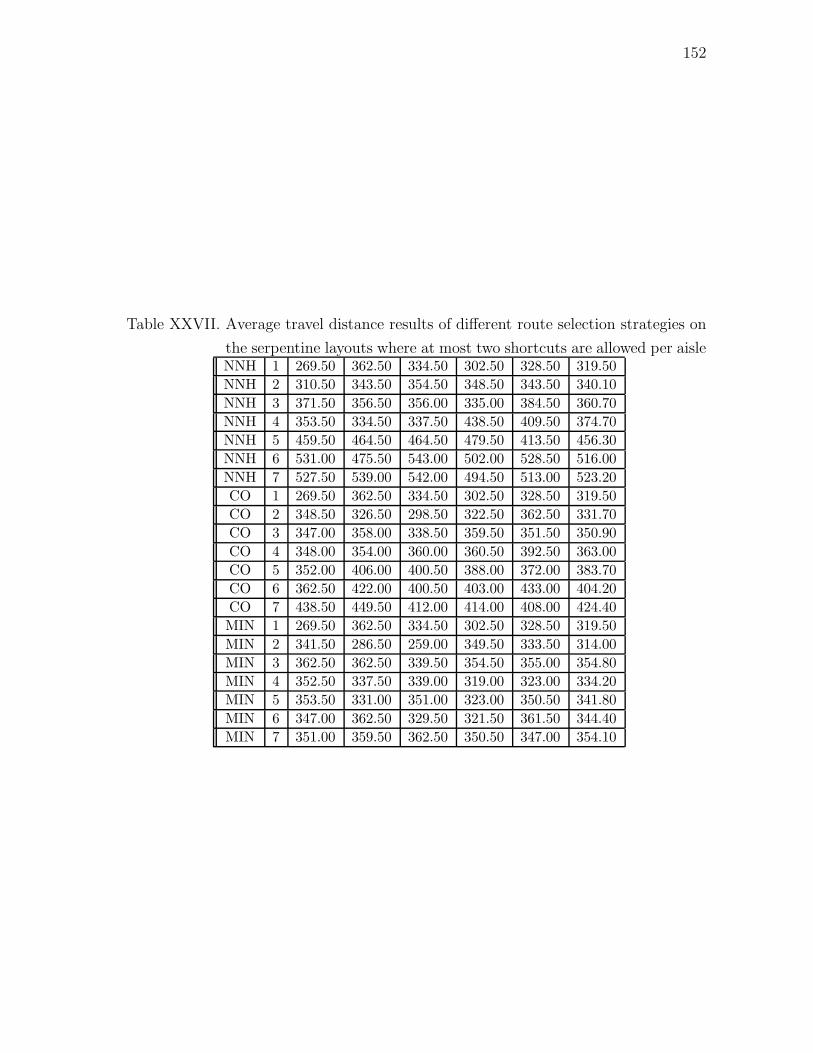
152
Table XXVII. Average travel distance results of different route selection strategies on
the serpentine layouts where at most two shortcuts are allowed per aisleNNH 1 269.50 362.50 334.50 302.50 328.50 319.50
NNH 2 310.50 343.50 354.50 348.50 343.50 340.10
NNH 3 371.50 356.50 356.00 335.00 384.50 360.70
NNH 4 353.50 334.50 337.50 438.50 409.50 374.70
NNH 5 459.50 464.50 464.50 479.50 413.50 456.30
NNH 6 531.00 475.50 543.00 502.00 528.50 516.00
NNH 7 527.50 539.00 542.00 494.50 513.00 523.20
CO 1 269.50 362.50 334.50 302.50 328.50 319.50
CO 2 348.50 326.50 298.50 322.50 362.50 331.70
CO 3 347.00 358.00 338.50 359.50 351.50 350.90
CO 4 348.00 354.00 360.00 360.50 392.50 363.00
CO 5 352.00 406.00 400.50 388.00 372.00 383.70
CO 6 362.50 422.00 400.50 403.00 433.00 404.20
CO 7 438.50 449.50 412.00 414.00 408.00 424.40
MIN 1 269.50 362.50 334.50 302.50 328.50 319.50
MIN 2 341.50 286.50 259.00 349.50 333.50 314.00
MIN 3 362.50 362.50 339.50 354.50 355.00 354.80
MIN 4 352.50 337.50 339.00 319.00 323.00 334.20
MIN 5 353.50 331.00 351.00 323.00 350.50 341.80
MIN 6 347.00 362.50 329.50 321.50 361.50 344.40
MIN 7 351.00 359.50 362.50 350.50 347.00 354.10

153
Table XXVIII. Average impulse purchase revenue results of different route selection
strategies on the serpentine layouts where one shortcut is located in
the middle of each aisleShopping Route Run # Run # Run # Run # Run # Average
List Choice 1 2 3 4 5 ResultLength Strategy
1 NNH 88.77 88.15 89.38 88.77 89.08 88.83
2 NNH 104.62 102.46 102.00 99.85 102.46 102.28
3 NNH 119.39 117.54 114.31 115.08 112.15 115.69
4 NNH 129.54 134.92 123.39 122.77 133.69 128.86
5 NNH 133.08 134.31 142.77 132.31 144.69 137.43
6 NNH 150.77 160.00 151.54 145.85 153.08 152.25
1 CO 89.38 89.08 86.00 89.38 88.77 88.52
2 CO 104.31 102.15 101.85 98.31 103.08 101.94
3 CO 110.00 115.54 117.31 115.08 118.77 115.34
4 CO 132.00 127.23 118.92 124.92 127.39 126.09
5 CO 139.69 141.08 133.23 141.08 140.31 139.08
6 CO 152.62 149.69 147.54 153.23 146.46 149.91
1 MIN 89.38 89.08 86.00 89.38 88.77 88.52
2 MIN 109.08 105.69 103.85 108.46 104.46 106.31
3 MIN 119.39 113.08 116.92 122.62 124.77 119.35
4 MIN 122.77 127.69 126.31 126.15 125.54 125.69
5 MIN 136.62 136.46 135.08 137.85 144.77 138.15
6 MIN 148.62 146.77 147.39 147.69 145.39 147.17

154
Table XXIX. Average travel distance results of different route selection strategies on
the serpentine layouts where one shortcut is located in the middle of
each aisleShopping Route Run # Run # Run # Run # Run # Average
List Choice 1 2 3 4 5 ResultLength Strategy
1 NNH 160.50 160.50 160.50 160.50 160.50 160.50
2 NNH 184.50 184.50 189.00 189.00 174.50 184.30
3 NNH 204.50 209.00 196.50 204.50 207.00 204.30
4 NNH 214.50 218.50 229.00 233.00 222.50 223.50
5 NNH 245.00 239.00 239.00 225.00 249.00 239.40
6 NNH 261.00 278.50 294.00 251.00 269.50 270.80
1 CO 160.50 160.50 151.50 160.50 160.50 158.70
2 CO 184.50 189.00 189.00 181.00 184.50 185.60
3 CO 207.00 194.50 204.50 209.00 204.50 203.90
4 CO 216.50 227.00 221.00 225.00 229.00 223.70
5 CO 245.00 243.00 247.00 243.00 237.00 243.00
6 CO 265.00 257.00 253.00 265.00 247.00 257.40
1 MIN 160.50 160.50 151.50 160.50 160.50 158.70
2 MIN 184.50 184.50 175.50 184.50 175.50 180.90
3 MIN 200.50 205.00 200.50 208.50 208.50 204.60
4 MIN 229.00 229.00 229.00 225.00 225.00 227.40
5 MIN 245.00 237.00 241.00 249.00 240.50 242.50
6 MIN 269.00 261.00 257.00 261.00 249.00 259.40
155
VITA
Ahmet Reha Botsalı received his B.S and M.S degrees from the Industrial Engi-
neering Department of Bilkent University in 1998 and 2000, and his Ph.D degree from
the Department of Industrial and Systems Engineering of Texas A&M University in
2007, respectively. His research interests include facilities planning and layout design,
heuristic optimization and scheduling. His permanent address is Dr. Hulusi Baybal
Cd. Nisantası Sitesi 10/45 Selcuklu Konya, Turkey.