resume - École de technologie supérieure · learns the process behavior and uses a fuzzy...

THE BIAS TEMPERATURE DEPENDENCE ESTIMATION AND COMPENSATIONFOR AN ACCELEROMETER BY USE OF THE NEURO-FUZZY TECHNIQUES

Lucian Teodor GrigorieDepartment ofAvionics, 107 Decebal Blvd.

Faculty of Electrical Engineering, University ofCraiova, Craiova, Dolj 200440, RomaniaContact: [email protected]

Ruxandra Mihaela BotezDepartment ofAutomated Manufacturing Engineering, 1100 Notre Dame West

Ecole de technologie superieure, Montreal, Quebec, Canada, H3C IK3Contact: [email protected]

Received October 2007, Accepted October 2008No. 07-CSME-46, E.lC. Accession 3015

ABSTRACTIn this paper, we describe a new method for improved performance of inertial sensors, with

applications in strap-down inertial systems. A new empirical model is proposed for the biastemperature dependence compensation of accelerometers using their input and output data.Experimental testing of the accelerometer is first realized, as data for 2 inputs and 1 output arecollected. Based on this data, an empirical model is built using a neuro-fuzzy network, whichlearns the process behavior and uses a Fuzzy Inference System (FIS) for model realization. Theimprovement in the reproduction quality of the experimental surface by the neuro-fuzzy model isachieved through the FIS training using a Sugeno learning algorithm with two inputs and oneoutput. Generation and training of the FIS are performed with Matlab functions, the training ofwhich is realized on a high number of epochs, for example, on a number of 105 training epochs.It is noticed that the proposed algorithm leads to a 35.5 times reduction in the error due totemperature dependence of the bias.

L'ESTIMATION ET LA COMPENSATION DE LA DEPENDANCE AVEC LATEMPERATURE DU BlAIS D'UN ACCELEROMETRE EN UTILISANT DES

TECHNIQUES NEURO-FLOUES

RESUMEDans cet article, nous decrivons une nouvelle methode pour I'amelioration des performances

des capteurs inertiels, avec des applications dans les systemes inertiels a composantes lies. Unnouvel modele empirique est propose pour la compensation de la dependance avec latemperature du biais des accelerometres en utilisant leurs donnees d'entrees et de sorties. L'essaiexperimental de l'accelerometre est realise, car les donnees pour deux entrees et une sortie sontrassembles. Base sur ces donnees, un modele empirique est conyu avec un reseau neuro-flou, quiapprend Ie comportement du processus, et utilise un systeme flou d'inference (FIS) pour larealisation du modele. L'amelioration de la qualite de reproduction de la surface experimentalepar Ie modele neuro-flou est realisee par l'entrainement du FIS en utilisant un algorithme d'etudede type Sugeno avec deux entrees et une sortie. La generation du FIS et son entrainement sontexecutees avec des fonctions en Matlab. La generation du FIS est realisee sur un nombre eleved'epoques, par exemple, sur un nombre de 105 epoques, et il est note que l'algorithme proposemene aune reduction de 35.5 fois de l'erreur due ala dependance avec la temperature du biais.

Transactions ofthe CSME Ide la SCGM Vol. 32, No. 3-4, 2008 383

1. INTRODUCTION

High precision accelerometers and gyros have biased reduced values, due to the inclusion ofcompensation devices in their architecture whose laws are dependent on the sensor's workingtemperature. In fact, the bias is strongly influenced by the temperature of the sensor's category, and forthis reason, each sensor contains an auxiliary temperature transducer which allows for the estimation andcompensation of this dependency ([1], [2], [3], [4]). In order to estimate the bias variation withtemperature, the sensor's producer should conduct a series of tests under various conditions, and shoulddetermine the mathematical model characterizing this variation ([5], [6]). This operation is lesscomplicated as it requires the use of a high precision temperature-controlled testing room. Practically, thesensor is tested on a rotating platform at a constant acceleration or angular speed at a constant temperaturefor which a high number of sensor output readings is acquired. By averaging these values the influence ofnoise and parasite vibrations induced by the rotating platform on the measurements is eliminated. Aparametric investigation is conducted following this procedure for a set of accelerations, or angularspeeds, at various temperatures. For temperatures and inputs modified between certain limits, results ameasured data set that characterizes the sensor from the point of view of the dependency of its outputs onthe temperature.

According to our bibliographical research ([7], [8]), the determination of the error model reduces to anidentification problem for a double input - single output system, and further, by use of the Vandermondematrix method, is reduced to the identification of a double input - single output system using a leastsquares method. As an example, the measurement errors of a RD21 00 gyro, produced by KVH [2], can berepresented by an error model of the following form [7]:

lC"CO,1 CO,2 C.)]

ol0/

s(tV,T) = [T 2 T 1] Cl,o C1,1 C1,2 C1,3 (1)

C2,o C2 ,1 C2,2 C2,3

tV

1

where s is the bias temperature dependence error, tV is the gyro indicated angular speed, T is thetemperature and Cij are the identified system coefficients.

The paper presents a new method to estimate and compensate the temperature dependence of the biasfor accelerometers and gyros based on the numerical values resulting from the sensors experimentaltesting. In this respect, the fuzzy logic offers remarkable facilities; it allows signal processing by puttingup empirical models, which avoid complex mathematic calculus used at present. In addition, the fuzzymodels have excellent results on non - linear, multidimensional systems, where there are problemsconcerning parameters variations or where the signals provided by the sensors are not very accurate ([9]and [10]).

To put up such a model we need a fuzzy set and the original theory of fuzzy logic conceived by LotfiA. Zadeh. The most serious problem it has to deal with comes from the determination of a complete set ofrules and the establishing of the membership functions corresponding to each input. The many attemptsto reduce errors and optimize the model are time - consuming and, very often, the results are far from theones intended in the beginning. A modem design method allows, though, to build up competitive fuzzymodels, in a relatively short interval. In short, ANFIS (Adaptiv Neuro-Fuzzy Inference System), thedesigning technique allows to generate and optimize the set of rules and the parameters of themembership functions by means of using the neural networks ([10]). Moreover, already implemented inMatlab Neuro-Fuzzy software tools, it is relatively easy to use.

Transactions a/the CSME Ide la SCGM Vol. 32, No. 3-4, 2008 384

2. THE NEW APPROACH

To solve the problem we will try to build a neuro-fuzzy controller for bias modeling. Considering theexperimental data, it is possible to arrange an empirical model based on a neuro-fuzzy network. Themodel can learn the process behavior based on the input-output process data by using a fuzzy inferencesystem (FrS) which should model the data set with two inputs and one output. Following the training, themodel may be used for the error value generation corresponding to the sensor's measured parameters (aor m) and to the temperature transducer parameter (1) followed by its compensation ([9] and [10]).

It is also possible to create a Fuzzy Inference System (FIS) using the Matlab "genfis2" function. Thisfunction generates an initial FIS of Sugeno type by decomposition of the operation domain into differentregions using the fuzzy subtractive clustering method. For each region, a low order linear model candescribe the process local parameters. Thus, the non-linear process is locally linearized around afunctioning point by using the Least Squares method. Then, the obtained model is considered valid in theentire region around this point. To limit the operating regions implies the existence of overlapping amongthese different regions. Their definition is given in a fuzzy manner. Thus, for each model input, severalfuzzy sets are associated with their corresponding definitions of their membership functions (mf). Bycombination of these fuzzy inputs, the input space is divided into fuzzy regions. For each such region, alocal linear model is used, while the global model is obtained by defuzzification with the gravity centremethod (Sugeno), by which the interpolation of the local models' outputs is done ([9] and [10]).

The Sugeno fuzzy model was proposed by Takagi, Sugeno and Kang to generate the fuzzy rules froma given input-output data set ([11]). For our system (two inputs and one output) a first-order model isconsidered, and for Nrules is given by ([11] and [12]):

(2)

where xq (q =1,2) are individual input variables, A; (i =1,N) are associated individual antecedent fuzzy

sets of each input variable, and / (i =1, N) is the first-order polynomial function in the consequent.

a~ (k =1,2, i =1, N) are parameters of the linear function and b~ (i =1, N) denotes a scalar offset. The

parameters a~, b~ (k = 1,2, i = I,N) are optimized by Least Squares method.

For any input vector, x = [x" x2 f, if the singleton fuzzifier, the product fuzzy inference and the centre

average defuzzifier are applied, the output of the fuzzy model y is infered as follows (weighted average):

(3)

where

Transactions a/the CSME Ide fa SCGM Vol. 32, No. 3-4, 2008

(4)

385

wi(x) represents the degree of fulfillment of the antecedent, that is, the level of firing of the ith rule.

The Matlab "genfis2" function generates the membership functions of the Gaussian type, defined asfollows ([10] and [12]):

{ ( .J2}. x-c'A~(x)=exp-0.5 (J;q , (5)

where <is the cluster center, and (J; is the dispersion of the cluster.

3. NUMERICAL SIMULAnONS RESULTS

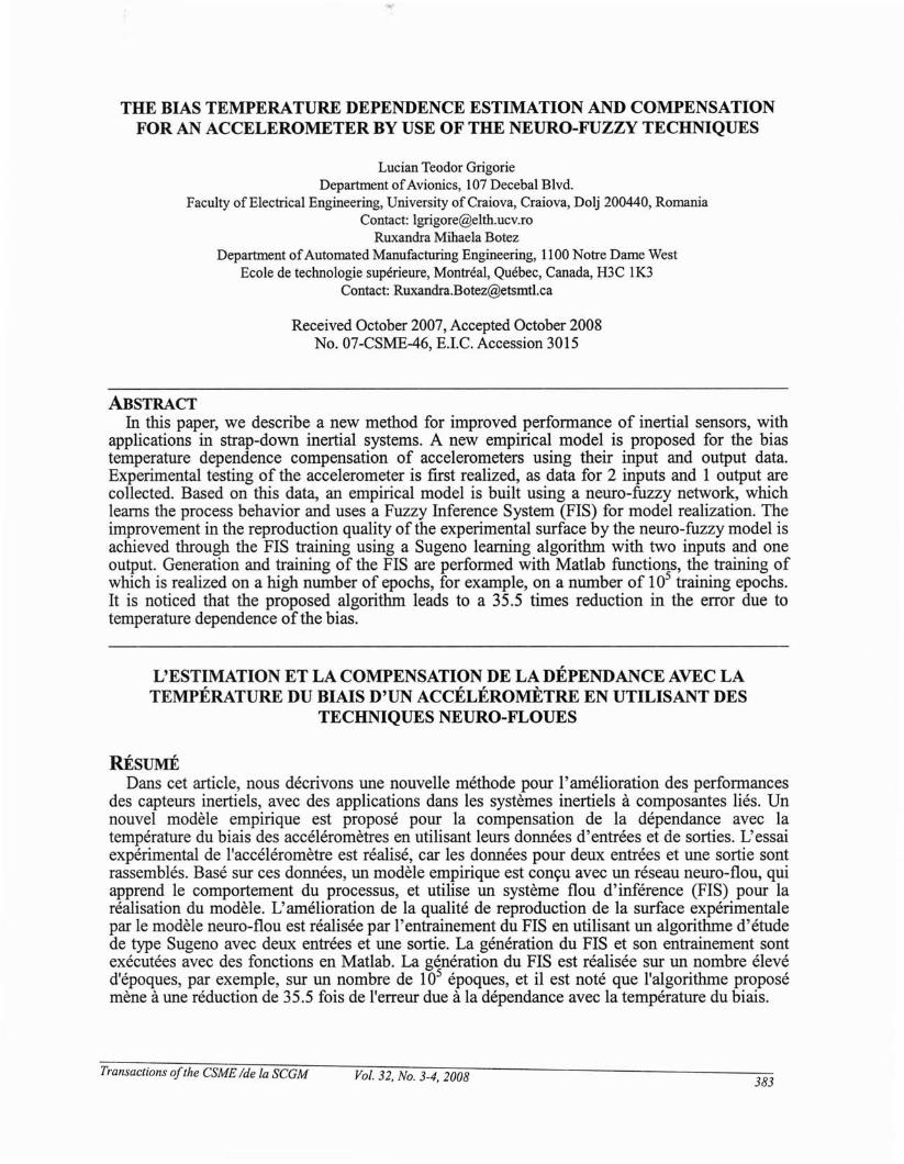
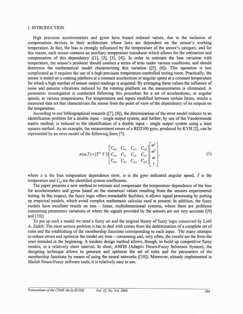
In order to validate the method presented herein, a MEMS accelerometer is used. Its measurementdomain is located in the range -lOg to 109. The measurements were performed at acceleration valuesranging from -8g to 8g and at temperatures ranging from -20°C to 80°C. The accelerometer'smeasurement errors e influenced by the temperature T variations for different acceleration a values arepresented in Figure 1 (e = f{T»), Figure 2 ((e = f{a))) and Figure 3 (e= fiT, a)), which is a combination ofFigures 1 and 2.

------~------------:---.-.----

0.02 .

0.06 -+ j""

-0.04

-0.06

e[g)

0.1 r-~-~-~~-~-~--c-~-~--,

0.08 -+... ..L : .'.

20 30 40 50 60 70 80T["C]

. , , . , , , , .

-0.08 ·········r········+···········,· ········;···········j············;···········r········"T""""'1""""""

-0.1 '----'-_----'-_-'----'-_-'-_-'-----'-_-'-_-'----.--J

-20 -10 0 10

Figure 1 Error variation with the temperature

From the analysis of these three figures, it can be noticed that the bias error eranges within the intervallimits from -0.08g to 0.08g for temperature variations of -20°C to 80°C, and for acceleration variations of-8g to 8g. Moreover, the error increases as the absolute value of the acceleration is augmented at aconstant temperature. From the numerical and experimental data, the highest error value obtained fornegative accelerations is e = -0.0724g and is reached for a = -8g and T = 60°C, while the highest errorvalue for positive accelerations is e= 0.0759g, and is reached for a = 8g and for T= 70°C.

The PIS training is obtained with the Matlab "ANFIS" function, which uses a learning algorithm forthe identification of the membership functions' parameters of the fuzzy inference system of a Sugeno type


with two outputs and one input. We further consider as a starting point the input-output data and the FISmodel generated with "genfis2", then the "ANFIS" optimizes the membership functions' parameters for anumber of training epochs; this number is set by the user. The optimization is realized for a better processapproximation performed by the neuro-fuzzy model by means of a quality parameter present in thetraining algorithm ([10]).

s [g]

0.1 ,---~-~-~-.,--~-~-~--,---------,---,

10a[g]

8642

··r······· --r" ----.-.~-.... ...--:------------

-··-·-~··--···-·-·t··········-j············~··········.

o-2

--~.- + + ~ ~ + .

-4-6

·-1············~···········~···········+··········+···_.. __ .._~-----------~-----------~-----------

-8

o

-0.08 . ----.---1----------T -------., --.---,

-0.1 '-------'------'-------'---'----'------'-------'----'-----'----'-10

-0.02 ·-·········i··

-0.04 .-..- .

-0.06 - .

0.08 .-- ------,-----------j-------..-.+---.-.....-, ...-.- ..-.-t- +---.------;--------.-.+.-----.----~ ~ j

0.06 ·········--!-··········i···········+···········!·········.+ , + .: :

0.02 ... -

0.04 .----.----+-.-.----+

Figure 2 Error variation with the acceleration

-20

o20

40 T ["C]60

10 80

o /

-0.1 -..,-10

_ - r····:··::l:.:.:...:.•~[....,..:_·.•.•.••..::I!.-'.- :1 '.. ,0.1 ...., ! -..( '"

)_ ,.,i·· .""'W'_-"-'_,.""...-0.05 -...,- i )/ ···----·1

-0.05 ..../(

s[g]

Figure 3 Accelerometer's errors in 3D space

The input-output data corresponding to the accelerometer's tests, shown in Figures 1 to 3, are arrangedin a three-column matrix, in which the first two columns contain input data related to the temperature Tand the accelerometer's output acceleration a, while the third column contains the output data related tothe error e. Using the Matlab "genfis2" function for the data set, the "BiasFis" Fuzzy Inference System isobtained.

To visualize the "BiasFis" FIS features, use is made of the Matlab "anfisedit" command followed by

Transactions ofthe CSME Ide fa SCGM Vol. 32, No. 3-4, 2008 387

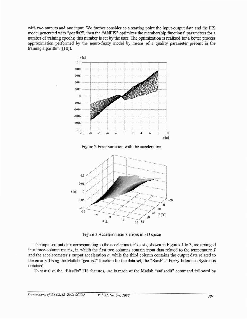
the FIS importation on the interface level. Visualization of the following characteristics of the untrainedFIS is achieved through the use of the interface: Structure (Figure 4), Membership functions mf for thefirst input (temperature T) (Figure 5), Membership functions mf for the second input (acceleration a)(Figure 6), Defuzzification rules (Figure 7), and Surfaces generated for the model with the two inputs(Figure 8 - The 3D error presentation, Figure 9 - Error dependent on the temperature, Figure 10 - Errordependent on the acceleration).

Figure 4 The "BiasFis" FIS structure

Figure 6 The mf of input 2


Figure 7 The deffuzification rules

The generated FIS is of Sugeno type, with two inputs and one output; for each of the two inputs, 8Gaussian type membership functions mf are automatically generated. The output membership functions(mt) result from the use of the Sugeno inference engine based on the following logic: "if (the input 1 is mfk) and (the input 2 is mf k), then (the output is mf k)", where "mf k" is the k's membership function foreach of the inputs, and respectively for the output. Before the training of the "ErrorFis" FIS, the

Transactions a/the CSME Ide fa SCGM Va!. 32, No. 3-4, 2008 388

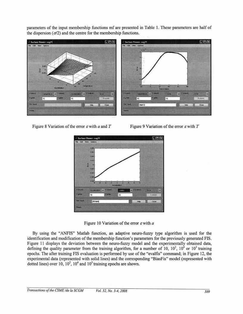
parameters of the input membership functions mf are presented in Table 1. These parameters are half ofthe dispersion (al2) and the centre for the membership functions.

Figure 8 Variation of the error ewith a and T Figure 9 Variation of the error ewith T

Surfcu:e VIl;!wcr sue]l ~I.Q iX]

Figure 10 Variation of the error ewith a

By using the "ANFIS" Matlab function, an adaptive neuro-fuzzy type algorithm is used for theidentification and modification ofthe membership function's parameters for the previously generated FIS.Figure 11 displays the deviation between the neuro-fuzzy model and the experimentally obtained data,defming the quality parameter from the training algorithm, for a number of 10, 102

, 104 or 105 trainingepochs. The after training FIS evaluation is performed by use of the "evalfis" command; in Figure 12, theexperimental data (represented with solid lines) and the corresponding "BiasFis" model (represented withdotted lines) over 10, 102

, 104 and 105 training epochs are shown.


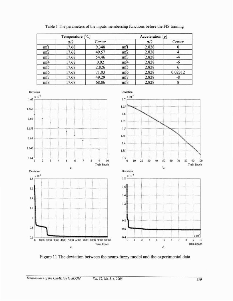
Table 1 The parameters of the inputs membership functions before the FIS training

Temperature [0C] Acceleration [g]

cr/2 Center cr/2 Centermf1 17.68 9.348 mf1 2.828 0mf2 17.68 49.57 mf2 2.828 4mf3 17.68 54.46 mf3 2.828 -4mf4 17.68 0.92 mf4 2.828 -6mf5 17.68 2.826 mf5 2.828 6mf6 17.68 71.03 mf6 2.828 0.02312mD 17.68 49.29 mD 2.828 -8mfS 17.68 68.86 mfS 2.828 8

Deviation

x 10.31.67r---~-~-~-~-~-~-~~--,

Deviationx 10,3

1.7 ,--~-~-~~-~-~~-~-~__,

a.

80 90 100

Train Epoch7060

b.

5040302010

, , , "

, , , "

, " +, + ,

11:~L •••••·LLLr1.55 ------:------~------~------~ .--- ------;..-----~------~------~------

[ ~ j ~.', ~ ! ~ ~

1.5 " .. , ':""" t",·j".', 't" --":"',. :':'.-":-- .. ,":---" '1"""1.45 ------.------ .. ------ .. ------ ----.. ----- - --- .. ------.------

:: i l: j :~:

II~: """:"""1"""1"""i"""i"""j""'1"""l'.~'""',j,""'(',·(···[······f·'··":""",j,"",j,""'j"::.:

1.3 '---~'-~'-~'-~'-~'-~'-~'-~'~~' ------'o

---"'''\------

._----,'-----

-- -- --~. ------

______ J. _

------t-------

8 9 10

Train Epoch6 7

, , ,···---t-----.·,-------,------, , ,· , ,, , ,, , ,· , ,· . ,· . ,, , ,------r-------,------;------· . ,, . ,, . ,, , ,, , ,, , ,, , ,

______ L '•• J _, , ,I ' ,.. ' ,, , ,, , ,: .. :, , ,

___ ._.L. .L •• }. _

: : +, , ,, , ,, , ,, , ,, , ,_ L L. .J __ • _

, , ,, , ,, , ,

421.64 '---~-~-~-~-~-~-~~--'

I

1.66 ,.. ,"t""" ,.... ,

• .J •• _ •••• A.

1.65 .J. •• ----

_____ .J. _

1.645

1.655

1.665

Deviation

x 10.31.8 ,--~-~-r----..-~-~~-~-~_,

, I , ,

, " ,

1,6 "'-·':-',·,":"""1"""-',·,-·,"',·,!"""""'",""","""1.4 ""':'.""~.""':"',.':""":",.":",.":""":"",.;'--'"

! : : : : : :1.2 .--"r""':"""1"""["""[""":"""-:-""'1'""';"""

1 ", ":'" ",~""" ~"""i"",,~"".':'"",~"""~"",,i"""• • , , , , I , ,

• • , • I , I , ,, , , • I , I , I, , , , , , I , I

, , , I I , I , ,

• • • , I , I • ,, , I I I I 1 ,

0.8 -~- ---_. ~. -----~ _. ----~. -----:- -_ .. --:- _.. --~ .. ---- ~------

: : : : : : : :, • , • , , 1 •

I , • , I , I •

0.6 L~~~~~·~~'!!!!!!!!i!!!!!''!!!!!!!!i!'!!!!!!!!!!!!!!'!!!'!!!!'!!i!'!!'~o 1000 2000 3000 4000 5000 6000 7000 8000 9000 10000

Train Epochc.

Deviationx 10,3

1.8 ,--~--~-~~-~-~~-~-~__,

1.6' """:"""r""'1"""["""~""'T--·'·>""'·r'·"j"--"

1.4 "", ':""" ~""" ~""";""";'""';"',.~"" "~""":'" , ", + , , , , , , ,

, , , , , , , , ,, , , , , , , , ,, . , , , , , , ,, . , , , , , , ,

1.2 ""'r""r"'1"""'t"""r""'-r""'~"""r""1""", , , . , , , . .

1."'" ':.... ,':' ..... :•••• " i'" --':', ..--(..1-·"" :'" --.:"', ..

::r~·1:···..:x 10 4

0.4 '---~-~-~~-~-~~-~--"-''-''-'o 2 4 5 6 7 8 9 10

Train Epochd.

Figure 11 The deviation between the neufO-fuzzy model and the experimental data

Transactions a/the CSME Ide la SCGM Vol. 32, No. 3-4, 2008 390

144 6 8 10 12

Number of input data points x 10-2

b.

2

0.08

0.06

0.04

0.02:§g 0~

-0.02 --

-0.04 --

-0.06

-0.0814 04 6 8 10 12


a.

2-0.08 '--_--'-__--'-__-'--_-'-_---'__--'-_---i

o

-0.06

-0.04

0.02

0.04

0.06 1'---,---1

~ 0

-0.02

0.08 rr====:;:--:-----:--:-:------;l

0.08 rr====:;:-~----;---;-----;-___:J--data I I ! I i

0.06 - - - - FIS model ~---------~--------t--------~---------:--- - --

:§ :::.LT'"t'I"I..•.•••-0.02 --

-0.04 --

144 6 8 10 12


2

0.08

0.06

0.04

0.02:§g 0

~

-0.02 --

-0.04 --

-0.06

-0.080144 6 8 10 12


2-0.08

o

-0.06

c. d.

Figure 12 The after training FrS evaluation for different training epochs

Figure 11 shows a rapid decrease in the deviation between the experimental data and the neuro-fuzzymodel for the quality parameter within the training algorithm over the first 200 training epochs. Thisdecrease is followed by a slower decrease over the next 1400 epochs, by a quick decrease between the1600 to 1800 epochs and finally by a very slow decrease from 1800 to 25000 training epochs. FromFigure 11, it can also be observed that the Frs model may be trained on 105 epochs due to the fact that thedeviation has an approximately constant value of 5.8· 10-4

•

Figure 12 reiterates the same observations as those obtained from Figure 11. Note the overlapping ofthe Frs model (evaluated for the input data) with the experimental data. This superposition is dependenton the training epochs' number, and is better as the number of training epochs is larger. The modeltraining over more than 105 epochs produces a very small deviation below 5.8·10-4. An improvedapproximation of the real model is achieved with the neuro-fuzzy methods in the case when a highernumber of experimental data is used for the error evolution description.

Through visualization of the trained model characteristics, using an "anfisedit" interface, the followingfigures are obtained: ANFrS model structure (Figure 13), Membership functions of the first input(temperature 1) (Figure 14), Membership functions of the second input (acceleration a) (Figure 15),


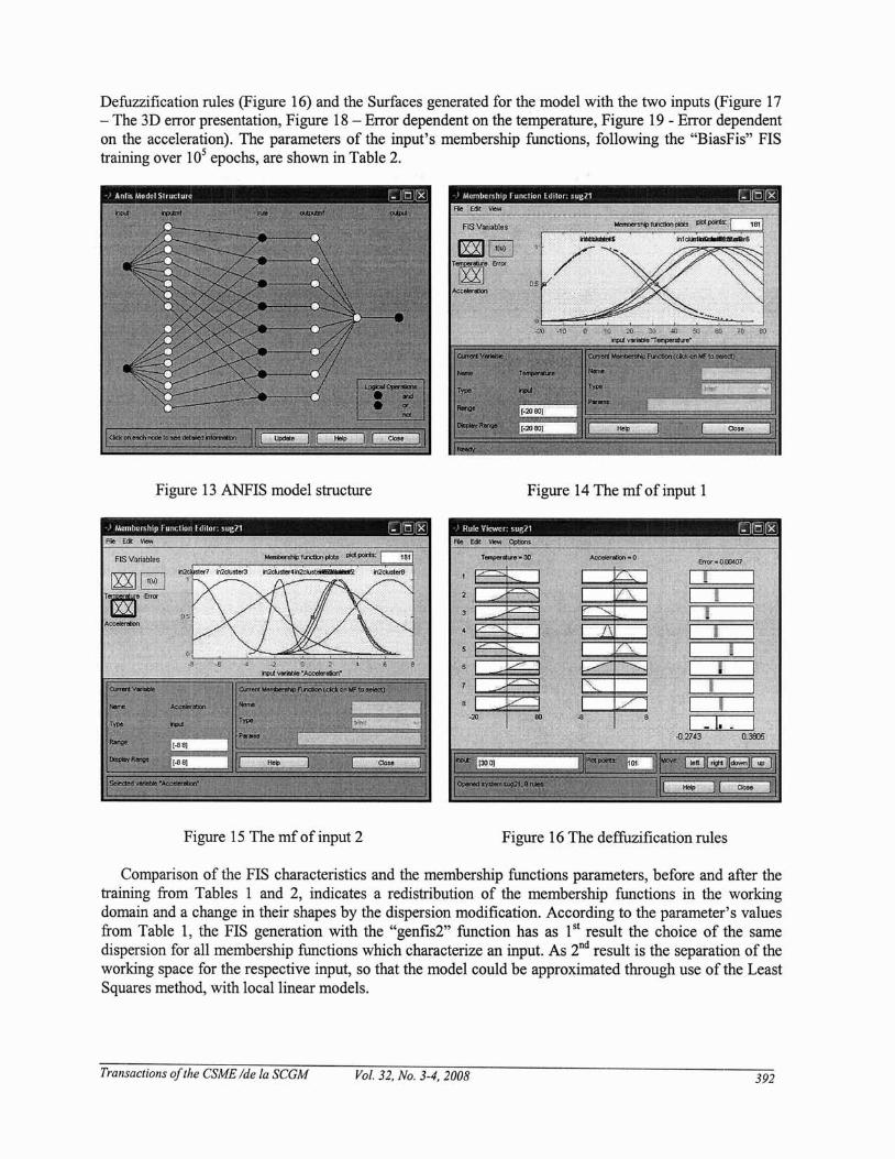
Defuzzification rules (Figure 16) and the Surfaces generated for the model with the two inputs (Figure 17- The 3D error presentation, Figure 18 - Error dependent on the temperature, Figure 19 - Error dependenton the acceleration). The parameters of the input's membership functions, following the "BiasFis" FIStraining over 105 epochs, are shown in Table 2.

Figure 13 ANFIS model structure



Figure 16 The deffuzification rules

Comparison of the FIS characteristics and the membership functions parameters, before and after thetraining from Tables 1 and 2, indicates a redistribution of the membership functions in the workingdomain and a change in their shapes by the dispersion modification. According to the parameter's valuesfrom Table 1, the FIS generation with the "genfis2" function has as 1sl result the choice of the samedispersion for all membership functions which characterize an input. As 2nd result is the separation of theworking space for the respective input, so that the model could be approximated through use of the LeastSquares method, with local linear models.


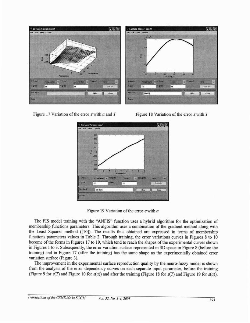
Figure 17 Variation of the error cwith a and T Figure 18 Variation of the error cwith T

Figure 19 Variation of the error c with a

The FIS model training with the "ANFIS" function uses a hybrid algorithm for the optimization ofmembership functions parameters. This algorithm uses a combination of the gradient method along withthe Least Squares method ([10]). The results thus obtained are expressed in terms of membershipfunctions parameters values in Table 2. Through training, the error variations curves in Figures 8 to 10become of the forms in Figures 17 to 19, which tend to reach the shapes of the experimental curves shownin Figures 1 to 3. Subsequently, the error variation surface represented in 3D space in Figure 8 (before thetraining) and in Figure 17 (after the training) has the same shape as the experimentally obtained errorvariation surface (Figure 3).

The improvement in the experimental surface reproduction quality by the neuro-fuzzy model is shownfrom the analysis of the error dependency curves on each separate input parameter, before the training(Figure 9 for &{1) and Figure 10 for &{a» and after the training (Figure 18 for &{1) and Figure 19 for &{a».


Thus, the greater similitude of c(T) and c(a) shapes to the experimental shapes (Figures 1 and 2) isemphasized following the FrS model training during 105 epochs.

Table 2 The parameters of the input's membership functions following the FIS training

Temperature [0C] Acceleration [g]cr/2 Center cr/2 Center

mfl 21.37 6.771 mfl 1.444 2.415mf2 18.77 48.41 mf2 1.231 2.636mD 25.14 58.46 mD 3.114 -5.09mf4 19.45 4.8 mf4 0.6759 -1.675mf5 21.27 6.497 mf5 1.402 2.604mf6 25.8 67.1 mf6 4.123 0.873mD 21.16 54.82 mD 1.825 -7.798mf8 22.8 63.5 mf8 2.654 6.284

Evaluating the FIS for the experimental values of temperature and acceleration used in the modelling,and realizing the error correction, results in the 3D characteristics shown in Figure 20.a, at the same scaleas the one in Figure 3. For a better visualization of the error variation domain after the correction, Figure20.b shows the previous characteristics for a smaller domain on the error axis. The error 8 dependence onthe temperature and acceleration, after the correction, is shown in Figures 21 and 22. The curves shown inFigures 21 a. and 22 a. are drawn at the same scale as the ones shown in Figures 1 and 2. It is possible tovisualize the error variation domain for the two characteristics (c(T) and c(a» , obtained after thecompensation, by decreasing the interval on which the error 8 is represented (Figure 21.b for c(T) andFigure 22.b for c(a».

E [g]

-0.05

-0.1-10

-5o

a [g]

-20 -20

L ~

Figure 20 The accelerometer's errors in 3D after the compensation with the neuro-fuzzy model

From the numerical and graphical results obtained with the proposed neuro-fuzzy model simulation(Figures 20 to 22), a considerable decrease in the absolute error value due to the bias dependency with thetemperature may be noted. At first glance, the error variation surface resulting from the compensationwith the neuro-fuzzy model varies within the limits -2.2·1O-3g to 2.1·l0-3g. By means of evaluation ofthe obtained numerical values, we note that after compensation, the maximum error value on the positiveaxis is &= 0.00204277g and is reached for a = -7g and T= -20°C, while the maximum error value on the


negative axis is E = - O.00214114g and is reached for a = 7g and T= 80°C. The proposed algorithm bringsabout a decrease in the absolute value of the error, due to the bias depending on the temperature, ofapproximately 35.5 times (from O.0759g to O.00214114g).

, " "+ " ". , , , , , , , ,

------,------,------,------ ... _--_ ... -_ ......------.- .. _-- .. ------ .. ------

E[g]0.1 r---,---,-- --,-- --,-- ---,

. . , , , . , , ,•• '. J. ! '-. '- "" ! L , _

I , , • I , , I I

I • , , I , , I •, . . , , , . , ., • , , I • • , ,

, , , I I , , I I------,-------;------1---··-1"------,·_-----,------1------t--_···,-------, . , , , , . , ,, , ., ".: : : : : : : : :--_. --,- -- -_. ~ _. -_. -.. -_. --..... ---.... _. --..,- -- - -- -- - -- - -. - -- -- -.- - -- --

60 70 80

T["C]b.

10 20 30 40 50o

E [g)

1.5

-2.5 '--~-~-~~-~-~~-~-~--'-20 -10

0.5

o-0.5

-1

-1.5

-2

70 80

T["C]

605040

a.

302010

, , , , I I ,...... __ __ _---- .. _----_._----- .. __ ._--, , , , I , 1

I I , I , , ,

, , , " ,, 't I ,

o

, ., .I I, '" I I- - _...'. - - - - _ .. - - - - -_. -- - - _.'- - _. -_.... --_. _ .... --- - ~ .. - -_.. ~ - - _. - -'- - - -- --, , , , , , , , ,, , , , , I , , ,

----.-:------;------i------f------i------·i------i------f-----+------, , , , ,

, , , , , , , , ,- - - - ••,••••• ~,. - •• _. T • - _. _ .... - ••• -I" - - - - -.,- - _ •• -, _. _. - • r - - • - _.1". _. ---

, , , , , , , , ,, "", ""

-0.1 '--~-~-'~~-~-.~~. -~'--'~--'

-20 -10

0.08

0.06

0.04

0.02

Oi--.......-------......---,.;---~-0.02

-0.04

-0.06

-0.08

Figure 21 The dependence of the neuro-fuzzy corrected error on the temperature

E [g]

0.1 .-------.-----.-------.--.,---...------.--.-----.--------.---,

6 8

a [g]

42o

b.

-2-4

0.5

E[g]

-1.5

o

-0.5

-2.5 '--~-~-~-~-~-~-~----'-8 -6

a.

, , , , , , , , ,••••••' •••••• J •••••• L ••••••'•••••• ~. __ ••• L __ ••• _'_ •••• __ ' J ••• _

, , I , I , I , I

, , I , I

, '" ,I " I I

, , I , I , , , I•• - •••,' •••• - 1 - _. - • - r· - _.. ',- _.... ',' _•.. - T - - - _. -,- - _. - •• ,- - _ •• -, ••• - ~-

, " I , I • I

, ""'"I " I " I

--- ---~- ---- - j ------ ~ ----. -i-·· ---~------t------~ ------i- -----~ ------, ",., I I, ",., I ,

-0.1 '--~-~~-~-~~-~-~~--'-10 -8 -6 -4 -2 0 2 4 6 10

a [g]

0.08 --. ---;- -----: --- ---: ------;- ----- ~- --- --: _.- --.: --- ---;--- --- ~ -- ----. . . . , , , , ,, , , , , , . , ,0.06 --- --~-- --- -: ------: ----- -: ---- -~-- ----: ----- -: -- -- --;--- ---: ---- --

, . . , , , , . ., , , , , , , , ,, . . , , , , , ,

:::: ::::T::::r::::r::::::::::T::::i::::::~::::::::::::T::::, , , , , . . , ,. , " ""o __hh~! " ,., ,

, , , , ,

, , , , .-0.02 ------:- -----: -_. --.: -----_:- -... -~. -. --.: --- ---~ --.- -.:- .... -~ ..... -

-0.04

-0.06

-0.08

Figure 22 The dependence of the neuro-fuzzy corrected error on the acceleration

If the classical method ([7]) is used and the measurement errors are represented by the next model:

(2)


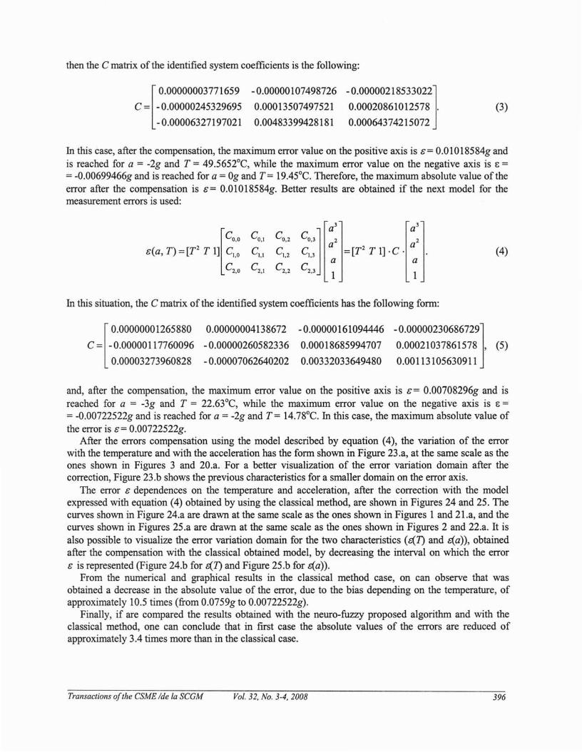
then the C matrix of the identified system coefficients is the following:

r

0.00000003771659 -0.00000107498726 -0.00000218533022]

C = -0.00000245329695 0.00013507497521 0.00020861012578.

- 0.00006327197021 0.00483399428181 0.00064374215072

(3)

In this case, after the compensation, the maximum error value on the positive axis is &= 0.01018584g andis reached for a = -2g and T = 49.5652°C, while the maximum error value on the negative axis is c =

=-0.00699466g and is reached for a = Og and T= 19.45°C. Therefore, the maximum absolute value oftheerror after the compensation is &= 0.01018584g. Better results are obtained if the next model for themeasurement errors is used:

a

a3

CO,I CO,2 CO'31 2a 2 a2

CI,I CI,2 CI,3 =[T T 1] .C .C C C a

2,1 2,2 2,3 1

In this situation, the C matrix of the identified system coefficients has the following form:

(4)

[

0.00000001265880 0.00000004138672 -0.00000161094446 -0.00000230686729]

C = -0.00000117760096 - 0.00000260582336 0.00018685994707 0.00021037861578, (5)

0.00003273960828 - 0.00007062640202 0.00332033649480 0.00113105630911

and, after the compensation, the maximum error value on the positive axis is &= 0.00708296g and isreached for a = -3g and T = 22.63°C, while the maximum error value on the negative axis is c =

= -0.00722522g and is reached for a = -2g and T= 14.78°C. In this case, the maximum absolute value ofthe error is &= 0.00722522g.

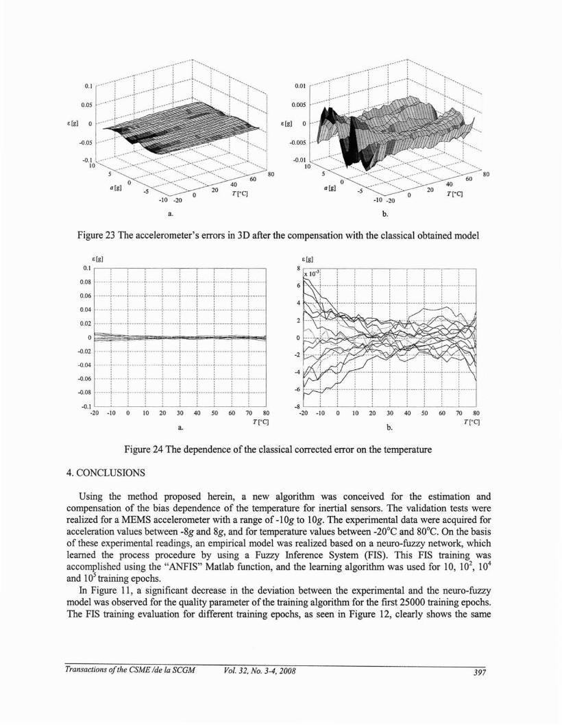
After the errors compensation using the model described by equation (4), the variation of the errorwith the temperature and with the acceleration has the form shown in Figure 23.a, at the same scale as theones shown in Figures 3 and 20.a. For a better visualization of the error variation domain after thecorrection, Figure 23.b shows the previous characteristics for a smaller domain on the error axis.

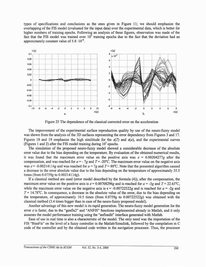
The error & dependences on the temperature and acceleration, after the correction with the modelexpressed with equation (4) obtained by using the classical method, are shown in Figures 24 and 25. Thecurves shown in Figure 24.a are drawn at the same scale as the ones shown in Figures 1 and 21.a, and thecurves shown in Figures 25.a are drawn at the same scale as the ones shown in Figures 2 and 22.a. It isalso possible to visualize the error variation domain for the two characteristics (&(1) and &(a)), obtainedafter the compensation with the classical obtained model, by decreasing the interval on which the error& is represented (Figure 24.b for &(1) and Figure 25.b for &(a)).

From the numerical and graphical results in the classical method case, on can observe that wasobtained a decrease in the absolute value of the error, due to the bias depending on the temperature, ofapproximately 10.5 times (from 0.0759g to 0.00722522g).

Finally, if are compared the results obtained with the neuro-fuzzy proposed algorithm and with theclassical method, one can conclude that in first case the absolute values of the errors are reduced ofapproximately 3.4 times more than in the classical case.


80

-10 -20

----5

oa[g]

-om10

0.005

-0.005 -'

E[g] 0

80

-10 -20

-5o

a[g]

Ji[i}lFrJ~'~j

0.1

0.05

E[g] 0

-0.05

-0.110

a. b.

Figure 23 The accelerometer's errors in 3D after the compensation with the classical obtained model

o

60 70 80

T[°C]b.

10 20 30 40 50o

4

-8 '--~_~~_~~~~_~~_~--.J-20 -10

a.

E[g]

0.1 ,--.--.---,--.---,----,--,.-------,--,..---,

:::,:r-TI:1i:r:r:.:: ::::::r::::::l::::::r::::::t::::::r::::::l::::::1::::::r::::r::::::

:' .. : :" : :

i~!i'Ifj:jI:r-0.1 '--~-~~-~~----'----~~-~----'

-20 -10 0 10 20 30 40 50 60 70 80

T[°C]

Figure 24 The dependence of the classical corrected error on the temperature

4. CONCLUSIONS

Using the method proposed herein, a new algorithm was conceived for the estimation andcompensation of the bias dependence of the temperature for inertial sensors. The validation tests wererealized for a MEMS accelerometer with a range of -lOg to 109. The experimental data were acquired foracceleration values between -8g and 8g, and for temperature values between -20°C and 80°C. On the basisof these experimental readings, an empirical model was realized based on a neuro-fuzzy network, whichlearned the process procedure by using a Fuzzy Inference System (FIS). This FIS training wasaccomplished using the "ANFIS" Matlab function, and the learning algorithm was used for 10, 102

, 104

and 105 training epochs.In Figure 11, a significant decrease in the deviation between the experimental and the neuro-fuzzy

model was observed for the quality parameter of the training algorithm for the first 25000 training epochs.The FIS training evaluation for different training epochs, as seen in Figure 12, clearly shows the same


types of specifications and conclusions as the ones given in Figure 11; we should emphasize theoverlapping of the FIS model (evaluated for the input data) over the experimental data, which is better forhigher numbers of training epochs. Following an analysis of these figures, observation was made of thefact that the FIS model was trained over 105 training epochs due to the fact that the deviation had anapproximately constant value of 5.8· 10-4.

6 8a[g]

42o

b.

·2-4-6

t[g]

8 3'

, , ,-- .. -------- .. -------- .. --------, , ., , ,, , ,, , ,, , ,, , ,------~--- --- - -~ -- ----- --.-- ------, , ,, , ,, , ,, , ,, , ,

, . ,.8 '--_~_~_~_~_~_..L__..L_____'-8

·4

a.

E[g]0.1 ,----.-,-----,----.--,----,---,---.--,----,

::llrrrilrr:::: ::::::r:::::r::::r:::::r::::::r:::::r::::r::::r::::r::::

o .--mr· :.;_. fA i» i ~7?YM1···--·

::: ::::::!:::::1::::J:::t::::!:::::1::::1:::[::::::::·0.08 ······r······i······r·····T······r······i······!······T······!······

·0.1 '--~-~~-~-~--'----'----'-~---'·10 ·8 ·6 -4 ·2 0 2 4 6 10

a[g]

Figure 25 The dependence of the classical corrected error on the acceleration

The improvement of the experimental surface reproduction quality by use of the neuro-fuzzy modelwas shown from the analysis of the 3D surfaces representing the error dependency from Figures 3 and 17.Figures 18 and 19 emphasize the high similitude for the d..1) and d..a), and the experimental curves(Figures 1 and 2) after the FrS model training during 105 epochs.

The simulation of the proposed neuro-fuzzy model showed a considerable decrease of the absoluteerror value due to the bias depending on the temperature. By evaluation of the obtained numerical results,it was found that the maximum error value on the positive axis was & = 0.00204277g after thecompensation, and was reached for a = -7g and T= -20oe. The maximum error value on the negative axiswas &= -0.00214114g and was reached for a = 7g and T= 80oe. Note that the presented algorithm causeda decrease in the error absolute value due to the bias depending on the temperature of approximately 35.5times (from 0.0759g to 0.00214114g).

If a classical method are used (error model described by the formula (4», after the compensation, themaximum error value on the positive axis is &= 0.00708296g and is reached for a = -3g and T= 22.63°e,while the maximum error value on the negative axis is E = -0.00722522g and is reached for a = -2g andT = 14.78°e. In consequence, a decrease in the absolute value of the error, due to the bias depending onthe temperature, of approximately 10.5 times (from 0.0759g to 0.00722522g) was obtained with theclassical method (3.4 times bigger than in case of the neuro-fuzzy proposed model).

Another advantage of this new model is its rapid generation. The neuro-fuzzy model generation for theerror & is faster, due to the "genfis2" and "ANFIS" functions implemented already in Matlab, and it onlyassumes the model performance training using the "anfisedit" interface generated with Matlab.

Ease of use in real time is also a characteristic of the model. The only need was the importation of theFIS "BiasFis" on the level of a fuzzy controller in the Matlab/Simulink, followed by the compilation in ecode of the controller and by the obtained code written in the navigation processor. Thus, the processor


receives the acceleration and temperature data from the accelerometer, and based on the model, thecorrected acceleration is generated.

5. REFERENCES

1. Honeywell Avionics webpage <http://www.honeywell.com/sites/aero/technology/avionics.htm>.2. KVH Industries webpage <http://www.kvh.com>.3. Northrop Grumman weppage <http://www.northropgrumman.com>.4. SAAB Technologies webpage <http://products.saab.se>.5. IEEE Std. 1293-1998 "IEEE Standard Specification Format Guide and Test Procedure for Linear,

Single-Axis, Nongyroscopic Accelerometers ", Published by IEEE, New York, USA, 16 April, 1999.6. IEEE Std. 836-1991 "IEEE Recommended Practice for Precision Centrifuge Testing of Linear

Accelerometers ", Published by IEEE, New York, USA, June 15, 1992.7. Borenstein, J. "Experimental evaluation of a fiber optics gyroscope for improving dead-reckoning

Accuracy in Mobile Robots ", 1998 IEEE International Conference on Robotics and Automation,Leuven, Belgium, May 16-21, pp. 3456-3461, 1998.

8. Ojeda, L., Chung, H., Borenstein, J. "Precision-calibration of Fiber-optics Gyroscopes for MobileRobot Navigation ", Proceedings of the 2000 IEEE International Conference on Robotics andAutomation, San Francisco, CA, April 24-28 ,pp. 2064-2069, 2000.

9. Kosko, B. "Neural networks and fuzzy systems - A dynamical systems approach to machineintelligence", Prentice Hall, New Jersey, 1992.

10.*** Matlab Fuzzy Logic and Neural Network Toolboxes - Help.11. Mahfouf, M., Linkens, D. A., Kandiah, S. "Fuzzy Takagi-Sugeno Kang model predictive control for

process engineering", The Institution of Electrical Engineers. Printed and published by the IEE, Savoyplace, London WCPR OBL. UK, 1999.

12.Kung, c.c., Su, J.Y. "Affine Takagi-Sugeno fuzzy modelling algorithm by fuzzy c-regression modelsclustering with a novel cluster validity criterion ", IET Control Theory Appl., 1, (5), pp. 1255-1265,2007

NOMENCLATURE

A; associated individual antecedent fuzzy sets of each input variable (i = 1, N)

C matrix of the identified system coefficientsCiJ identified system coefficientsN number of the fuzzy rulesT temperaturea acceleration of the MEMS sensor

a~ parameters of the linear function in the rules set ( k = 1,2, i = 1, N )

b~ scalar offset in the rules set (i = 1, N)

ci cluster centerq

g gravitational accelerationx input vectory output of the fuzzy model

xq individual input variables (q = 1,2)

/ first-order polynomial function in the consequent (i = 1, N)


Wi degree of fulfillment of the antecedent, that is, the level of firing of the ith

rule& error due to the bias temperature dependenceOJ angular speed indicated by the gyroa dispersion of the Gaussian membership function

a~ dispersion of the cluster

FIS fuzzy inference systemmf membership functionsmf k the k's membership function

Transactions ofthe CSME Ide la SCGM Vol. 32, No. 3-4,2008 400

resume - École de technologie supérieure · learns the process behavior and uses a fuzzy...

Documents