Restoring Water Levels on Lake Michigan-HuronA Cost-Benefit Analysis

CLAude desjARLAis, Economic Consultant, Ouranos

BoB dunCAnson, Executive Director, Georgian Bay Association

dReW GRoneWoLd, Hydrologist and Physical Scientist, National Oceanic and Atmospheric Administration

MARC Hudon, Chair, Water Commission, Nature Québec

deBRA jensen, Planning Services Supervisor, Milwaukee Metropolitan Sewerage District

dAvid KLiBeR, Business Development Manager, Eurofins S-F Analytical Laboratories

GAiL KRAntzBeRG, Professor and Lead, Engineering and Public Policy Program, Booth School Of Engineering Practice, McMaster University

AcknowledgementsThe authors would like to thank members of our steering committee; Paul Allen and David Fay of the International Joint Commission; and James Radner of the University of Toronto for their feedback on previous drafts. We would also like to thank our colleagues at the Mowat Centre and especially Richard Carlson, Sara Ditta, William Forward, Sunil Johal, Mike Moffat, Matthew Mendelsohn, Scott Perchall, Reuven Shlozberg, Paul Sommerville, Peter Spiro, Elaine Stam and Emma Tarswell for their assistance, comments and design work. Finally, we thank Mark Fisher, President and Chief Executive Officer of the Council of the Great Lakes Region, for his leadership and guidance and Syed Afaq Moin for his feedback and data support.

The opinions expressed are those of the authors and do not necessarily reflect the opinions of the steering committee or Natural Resources Canada.

AuthorsRob Dorling was an economist at the Mowat Centre from 2013 to 2015. He is now an economist at the British Columbia Ministry of the Environment. His research interests include environmental and natural resource economics.

Kyle Hanniman was a policy associate at the Mowat Centre from 2014 to 2015. He is now an Assistant Professor of Political Studies

at Queen’s University. His research interests include fiscal federalism, political economy and public debt.

MAsoud AsAdzAdeH, Assistant Professor, Department of Civil Engineering (Water Resources), University of Manitoba

eLizABetH AtKinson, Senior Policy Manager, Climate Change Impacts and Adaptation Division, Natural Resources Canada

joHn BAKeR, General Organizer, International Longshoremen’s Association AFL-CIO

dALe BeRGeRon, Associate Professor, Minnesota Sea Grant, University of Minnesota Duluth, Maritime Transportation Education and Extension.

jennifeR Keyes, Manager, Water Resources Section, Ontario Ministry of Natural Resources and Forestry

MuRRAy CLAMen, Former Secretary, International Joint Commission, Canadian Section; Affiliate Professor, Department of Bioresource Engineering, McGill University

steering CommitteeRoBeRt LeWis-MAnninG, President, Canadian Shipowners Association

LARRy MACdonALd, Mayor, City of Bayfield, WI

BiLL MCKinLAy, Director, Corporate Relations, Ontario Power Generation

dAvid sWeetnAM, Executive Director and Georgian Baykeeper, Georgian Bay Forever

jAMes zoRn, Executive Administrator, Great Lakes Indian Fish and Wildlife Commission

With support from Natural Resources Canada (NRCan). Produced through the Adaptation Platform.

RestoRinG WAteR LeveLs on LAKe MiCHiGAn-HuRon: A Cost-Benefit AnALysis©2016 isBn 978-1-77259-014-2 ApRiL 2016 CounCiLGReAtLAKesReGion.oRG

Contentsexecutive summary 1

Résumé 5

Part 1: introduction 9

Part 2: General Methodology 17 2.1 overview of quantitative analysis 18 2.1.1 seCtoRs AnALyzed 18 2.1.2 inteRventions And tHeiR Costs And Benefits 18 2.1.3 poLiCy sCenARios 19 2.1.4 tiMe HoRizons And WAteR LeveL AssuMptions 19 2.1.5 disCountinG 20 2.1.6 CuRRenCy 20 2.1.7 study LiMitAtions 21

2.2 overview of qualitative analysis: pareto optimality and political feasibility 21 2.3 A note on data sources 22

Part 3: economic sectors and impacts 25 3.1 Commercial shipping and harbours 27

3.2 tourism and recreational water activities (marinas) 28

3.3 Hydroelectric generation 28

3.4 Waterfront properties 30

3.5 What we do not quantify 31

Part 4: Restoration 33 4.1 Quantitative analysis 35 4.1.1 siLLs 36

4.1.2 fixed RoCK-fiLLed diKes in tHe eAsteRn CHAnneLs of stAG isLAnd And fAWn isLAnd 39

4.1.3 pARALLeL diKes And WeiRs in LAKe HuRon 40

4.1.4 infLAtABLe fLAp GAtes At stAG isLAnd And fAWn isLAnd 41

4.1.5 HydRoKinetiC tuRBines 42

4.1.6 suMMARy of QuAntitAtive findinGs 43

4.2 political feasibility 43

Part 5: Multi-Lake Regulation 47 5.1 Background and findings of the international upper great lakes study 48 5.2 political feasibility 51

Part 6: Adaptive Management 53 6.1 Adaptive management - key characteristics and the ijC’s am strategy 54 6.2 Benefits and political feasibility 55

Part 7: summary, Lessons and Recommendations 57

Appendices 60 1: Canadian dollar conversions 60 2: data and methodology on economic impacts 63 3: detailed CBA tables and results 67 4: our hydraulic scenario in context 69 5: sensitivity analysis results 72

Works Cited 73

exeC

uti

ve s

uM

MA

Ry

CG

LR | R

estoR

inG

WAteR

LeveLs on

LAK

e MiC

HiG

An

-Hu

Ro

n | 1

» Raising or lowering water levels, as conditions

dictate, on the entire GLSLS using new and

existing dam-like structures, channel excavations

and region-wide regulation plans, a process

known as multi-lake regulation.

» Creating a structured, iterative and bi-national

process of improving responses to changing

water levels through long-term monitoring,

modelling and assessment of hydrological trends

and their impacts, a process known as adaptive

management (AM).

Data and methodological constraints preclude

a cost-benefit analysis (CBA) of all of these

approaches. Instead, we attempt to provide the

first comprehensive economic CBA of existing

proposals to restore water levels on Lake Michigan-

Huron using previously-studied structural options.

We also provide qualitative analyses of the two

remaining approaches — multi-lake regulation and

AM — and assess the political viability of all three

approaches.

We assess mitigation strategies with a focus on

water levels in Lake Michigan-Huron. Our focus

on Lake Michigan-Huron is not arbitrary; it was

the hardest hit of the Great Lakes during the low-

water spell of 1999 to 2013, and remains highly

vulnerable to extreme lows, which is critical

given the region’s massive shipping, tourism,

hydroelectric and cottage industries.

We identify a number of previously-studied

structures that are capable of generating positive

economic net benefits under our worst-case low

water level scenario. The most promising of these

interventions, according to our analysis, is a series

of sills in the upper St. Clair River. But we stop

short of recommending specific interventions for

three reasons.

Water levels in the Great Lakes are in a constant

state of flux. This is good; natural fluctuations are

essential to a healthy ecosystem. But sustained

periods of extreme water levels are potentially

costly, both for the economy and the environment.

In June 2014’s Low Water Blues, we estimated the

direct economic costs of an extreme low water

level scenario on selected sectors in the Great

Lakes and St. Lawrence River System (GLSLS). The

results were revealing and, given missing data on

a wide range of sectors and impacts, may prove

conservative.

This report builds on this research by assessing

previously identified mitigation strategies under a

similar extreme low water level scenario. We assess

the costs and benefits of these approaches under

this water level scenario for four key Great Lakes

sectors:

» Commercial shipping and harbours

» Tourism and recreational water activities

» Waterfront properties

» Hydroelectric generation

Although the International Joint Commission

(IJC) has noted the capacity of key GLSLS interest

to adapt to water levels within historical upper

and lower ranges, it warns that levels outside of

these ranges would require certain interests to

adopt more systematic responses than they have

undertaken to date. In this regard, experts have

advanced three broad approaches:

» Raising water levels in Lake Michigan-Huron by

installing fixed structures in and around the St.

Clair River, a process known as restoration.

executive summary

2 |

exe

Cu

tive

su

MM

AR

y

that harm major interests. This does not preclude

intervention if policymakers can find ways of

resolving redistributive conflicts. But as we will

argue, these solutions may be difficult to find.

These challenges have raised interest in multi-

lake regulation — raising or lowering water levels,

as conditions dictate, on the entire GLSLS using

dam-like structures, channel excavations and

region-wide regulation plans. This approach

would allow the region to better cope with sudden

and dramatic changes in water supplies and

could ease tensions between stakeholders in

flood- and non-flood prone regions. It could also

present opportunities for habitat enhancement

and restoration. But multi-lake regulation is

no panacea. It is ecologically risky; would not

eliminate the risks of extreme water levels; and

would involve billions of dollars in excavation,

construction and operation and maintenance

costs.

This brings us to our third approach: adaptive

management (AM). AM does not involve

managing or raising water levels (though it can

be combined with these approaches). Rather it

is a structured, iterative process of improving

responses to changing water levels through long-

term monitoring, modelling and assessment of

hydrological trends and impacts. It was recently

endorsed by the International Upper Great Lakes

Study as the most economical and politically

practical means of adapting to the uncertainties

and costs surrounding water levels, which explains

the IJC’s recent efforts to strengthen bi-national

cooperation in this area.

We draw two conclusions from our analysis. First,

the economic viability of restoration requires

further research. Future CBAs ought to build on our

work by including ecological impacts; additional

economic impacts; more sophisticated modelling

of economic outcomes; a wider range of hydraulic

scenarios; better cost estimates of engineering

structures; and, if existing proposals are incapable

First, our estimates are modest. In our best-case

scenario, restoration could yield almost $250

million USD in benefits from now to 2064. It is

possible these estimates are conservative: they

apply a four per cent discount rate, incorporate

conservative estimates of several impacts and

exclude costs that our structures would mitigate.

However, it is also possible that our estimates

are liberal: they exclude costs associated with

restoration and assume a worst-case low water

level scenario. This is of course problematic: if

restorative structures, which are only capable of

raising water levels, are not viable under our low

water level scenario, then they are not viable at all.

Second, our estimates are limited by the same

uncertainties associated with any analysis of this

nature: uncertainty about fluctuations in water

levels; uncertainty about the impacts of water

levels on ecological and economic outcomes;

and uncertainty about the costs and benefits of

interventions.

Finally, restoring water levels — no matter what

the net regional benefit may be — faces formidable

political obstacles. Virtually any effort to raise or

lower water levels is likely to benefit some groups

at the expense of others. This is a major constraint,

as policymakers are reluctant to adopt structures

The politics of adapting to and mitigating the impacts of climate change in the Great Lakes and St. Lawrence Region means identifying policies and structures capable of eliminating or limiting redistributive conflicts and environmental risks.

CG

LR | R

estoR

inG

WAteR

LeveLs on

LAK

e MiC

HiG

An

-Hu

Ro

n | 3

of redressing political and environmental

hurdles, promising proposals for new engineering

structures (indeed, most of the proposals we

analyze were developed several decades ago).

Second, future research needs to grapple with

the politics of adapting to and mitigating the

impacts of climate change in the Great Lakes and

St. Lawrence Region. Decisions over boundary

and transboundary water levels today are taken

by unofficial consensus, where virtually any group

can veto measures expected to significantly

harm their interests. Researchers ought to admit

this constraint and find ways of redressing it.

Ultimately, this means identifying policies and

structures capable of eliminating or limiting

redistributive conflicts and environmental risks.

The shortcomings of our study limit the

recommendations we can make. However, one

key recommendation emerges from our research

which, if implemented, would help all interests

adapt to changing water conditions and improve

the quality of future research. We advise the

Canadian and US governments to approve the

IJC’s proposals to strengthen AM on a bi-national

basis. Specifically, we advise them to establish a

Levels Advisory Board (LAB) capable of facilitating

monitoring and modelling of hydrological trends

and their impacts. This approach is not without

political and administrative costs. But it is the

most politically practical means of addressing

fluctuating water levels: it is not as controversial

as restoration or multi-lake regulation, and would

help all actors, regardless of their preferences over

water levels, by providing them with more, and

better, information on hydrological conditions.

AM is also a necessary, albeit insufficient, condition

for structural interventions. Neither restoration nor

multi-lake regulation has any chance of approval

unless uncertainty over their impacts is reduced.

Systematic monitoring and modelling would not

eliminate this uncertainty, but it would mitigate

it, perhaps opening the door to a more reliable

analysis of engineering options.

4 |

Rés

uM

é

CG

LR | R

estoR

inG

WAteR

LeveLs on

LAK

e MiC

HiG

An

-Hu

Ro

n | 5

CG

LR | R

estoR

inG

WAteR

LeveLs on

LAK

e MiC

HiG

An

-Hu

Ro

n | 5

Les niveaux d’eau dans les Grands Lacs sont

dans un état d’évolution constante. Et c’est une

bonne chose. Les fluctuations naturelles sont

essentielles à la santé des écosystèmes. Mais des

périodes continues de variations extrêmes de

niveaux d’eau sont potentiellement coûteuses,

tant pour l’économie que pour l’environnement.

En juin 2014, nous avons estimé les coûts

économiques directs d’un scénario de niveaux

d’eau particulièrement bas dans certains secteurs

du réseau des Grands Lacs et de la Voie maritime

du Saint-Laurent (GLVMSL). Les conclusions en

sont révélatrices étant donné les contraintes de

données et la nature prudente de cette estimation.

Le présent rapport fait fond sur ces recherches en

évaluant les stratégies d’atténuation des coûts

d’un pareil scénario dans quatre secteurs :

» Navigation commerciale et ports

» Tourisme et activités nautiques récréatives

» Propriétés riveraines

» Production hydroélectrique

Les experts ont proposé trois moyens de limiter les

coûts associés aux variations extrêmes des niveaux

d’eau :

» La hausse des niveaux d’eau des lacs Michigan

et Huron en installant des structures fixes dans

la rivière Sainte-Claire et dans les environs; ce

processus est connu sous le nom de restauration.

» La hausse ou l’abaissement des niveaux d’eau,

selon les conditions, dans l’ensemble du

réseau des GLVMSL en utilisant des structures

comme des digues et l’excavation de canaux, un

processus appelé régularisation multilac.

» L’adaptation, plutôt que la gestion, des niveaux

d’eau et l’amélioration des niveaux d’eau et

améliorer les mesures adaptatives par le biais

d’une surveillance, d’une modélisation et d’une

évaluation des conditions hydrologiques du

système complet à long terme, un processus

dénommé la gestion adaptative (GA).

Les contraintes méthodologiques et de données

excluent l’analyse coût/bénéfice (ACB) de chacune

de ces approches. Cependant, nous proposons

la première ACB complète des propositions de

restauration des niveaux d’eau des lacs Michigan

et Huron. Ce choix n’est pas arbitraire. Les lacs

Michigan et Huron ont été les plus touchés parmi

les Grands Lacs par la période de bas niveau d’eau

de 1999 à 2013 et ont, par conséquent, le plus

besoin de restauration.

En plus de notre analyse quantitative de la

restauration, nous avons proposé des analyses

des deux autres approches — la régularisation

multilac et la gestion adaptative — nous évaluons

la viabilité politique des trois solutions.

Nous avons défini un certain nombre de structures

aptes à produire d’importants avantages nets

dans le cadre de notre scénario de niveaux d’eau

bas le plus défavorable. D’après notre analyse,

l’intervention la plus prometteuse est une série de

socles en amont de la rivière Sainte-Claire. Mais

nous ne sommes pas en mesure de recommander

les interventions pour trois raisons.

D’abord, nos estimations sont modestes.

Même dans le meilleur des cas, la restauration

rapporterait moins de 250 millions de dollars

américains d’ici 2064. Il se peut que nos

estimations soient prudentes. Toutefois, il est

aussi possible qu’elles soient généreuses. Cela

pose problème. Si les structures de restauration

qui sont uniquement susceptibles de faire

augmenter les niveaux d’eau et ne sont pas viables

Résumé

6 |

Rés

uM

é

dans nos scénarios de bas niveaux d’eau, elles ne

sont pas viables du tout.

Par ailleurs, nos estimations souffrent de

nombreuses incertitudes à l’égard de :

l’orientation des fluctuations du niveau d’eau; des

conséquences des niveaux d’eau sur les résultats

écologiques et économiques; et des coûts et des

avantages des interventions.

Enfin, la restauration des niveaux d’eau — peu

importe les avantages régionaux nets — est

confrontée à de redoutables obstacles politiques.

Pratiquement toute initiative visant à hausser

ou abaisser les niveaux d’eau aura pour effet

d’avantager certains groupes au détriment

d’autres. Cela constitue un obstacle de taille.

Comme nous l’expliquerons, la Commission mixte

internationale (CMI) (l’organisme quasi judiciaire

chargé de la résolution et de la prévention des

différends sur la gestion du niveau des eaux

limitrophes et transfrontalières), ainsi que les

gouvernements canadien et américain, sont peu

susceptibles de faire monter les niveaux d’eau sans

l’approbation d’une grande majorité des intérêts

concernés. En conséquence, les décideurs auraient

probablement besoin de trouver des moyens

de protéger ou d’indemniser les perdants avant

l’approbation des projets. Ces solutions pourraient

être difficiles à trouver.

Ces défis ont suscité de l’intérêt pour des solutions

plus souples en mesure de relever et d’abaisser

les niveaux d’eau de tous les Grands Lacs par le

biais de digues et des plans de régularisation.

Cette approche permettrait à la région de mieux

composer avec les changements soudains et

dramatiques dans l’approvisionnement en

eau et pourrait atténuer les tensions entre les

intervenants dans les zones inondables ou non.

Mais la régularisation multilac n’est pas une

panacée. Elle présente des risques écologiques,

n’éliminerait plus les risques de variations

extrêmes des niveaux d’eau et mettrait en jeu

des milliards de dollars en coûts d’excavation, de

construction et de fonctionnement et d’entretien.

Ce qui nous amène à la troisième voie

envisageable : la gestion adaptative. Celle-ci

ne consiste pas à gérer les niveaux d’eau, mais

à trouver de nouveaux et meilleurs moyens

de s’adapter leurs fluctuations. L’adaptation

associée à cette approche n’est pas accidentelle,

mais éclairée par la surveillance, la modélisation

et l’évaluation binationales des tendances

hydrologiques et leurs conséquences.

Nous avons tiré deux conclusions. D’abord, la

viabilité de la restauration exige des recherches

plus approfondies. Les futures ACB devraient

faire fond sur nos travaux et comprendre

l’incidence écologique; les effets économiques

supplémentaires; une modélisation plus

sophistiquée des résultats économiques; une

plus grande gamme de scénarios hydrauliques;

de meilleures estimations des coûts des ouvrages

de génie; et si les propositions existantes ne

permettent pas de franchir les obstacles politiques

et environnementaux, des propositions de

nouvelles structures de génie.

Les décisions concernant les eaux limitrophes et transfrontalières sur les niveaux d’eau sont prises officieusement au consensus et pratiquement n’importe quel groupe possède un droit de veto sur les mesures susceptibles de nuire sensiblement à leurs intérêts.

CG

LR | R

estoR

inG

WAteR

LeveLs on

LAK

e MiC

HiG

An

-Hu

Ro

n | 7

Deuxièmement, les recherches doivent se pencher

sur les aspects politiques de restauration. Les

décisions concernant les eaux limitrophes et

transfrontalières sur les niveaux d’eau sont prises

officieusement au consensus et pratiquement

n’importe quel groupe possède un droit de veto sur

les mesures susceptibles de nuire sensiblement à

leurs intérêts. Les chercheurs devraient admettre

l’existence de ces restrictions et trouver des

moyens de les assouplir. En fin de compte, il s’agit

de définir des politiques et des structures aptes à

éliminer ou à réduire les conflits de redistribution

et les risques environnementaux.

Les lacunes de notre étude limitent les

recommandations que nous sommes en mesure

de formuler. Néanmoins, nous estimons qu’une

recommandation aiderait tous les intéressés à

s’adapter à l’évolution des conditions de l’eau

et à améliorer la qualité des recherches futures.

Nous conseillons aux gouvernements canadien

et américain d’approuver les propositions du

CMI visant à renforcer la gestation adaptative

sur une base binationale. En particulier, nous les

invitons à mettre sur pied un Comité consultatif

sur les niveaux d’eau (CCN) en mesure de faciliter

la surveillance et la modélisation des tendances

hydrologiques et de leurs impacts. La gestion

adaptative est la manière la plus pratique de

s’occuper de la fluctuation des niveaux d’eau :

elle n’exige pas explicitement de redistribution,

aiderait tous les acteurs, peu importe leurs

préférences sur les niveaux d’eau, en leur donnant

plus de renseignements détaillés sur les conditions

hydrologiques.

La gestion adaptative est également une condition

nécessaire, bien qu’insuffisante, des interventions

structurelles. Ni la restauration ni la régularisation

multilac ne risquent d’être approuvées à moins

de dissiper l’incertitude entourant leur incidence.

La surveillance et la modélisation systématique

n’élimineraient pas cette incertitude, mais

l’atténueraient et ouvriraient éventuellement la

voie à une analyse plus fiable des options de génie.

8 |

pA

Rt

1: in

tRo

du

Cti

on

part 1: introduction

CG

LR | R

estoR

inG

WAteR

LeveLs on

LAK

e MiC

HiG

An

-Hu

Ro

n | 9

In January 2013, water levels on Lake Michigan-

Huron1 hit their lowest level since consistent

measurement began in 1918. The record was part of a

streak of 186 months in which lake levels were below

the lake’s long-term monthly averages. Although

Michigan-Huron was hit particularly hard, levels were

also low, at times, on Lake Superior, where, in 2007,

they were at their lowest level since 1926.2

By 2014, the situation had changed dramatically.

Water levels on Lake Michigan-Huron and Superior

surged and, at the time of writing, all lakes

exceeded their long-term monthly averages. From

January 2013 to December 2014, Lake Superior

jumped roughly two feet, a record increase for that

24-month span. Lake Michigan-Huron rose by nearly

three feet, just shy of the record for that period.3

Water levels are in a constant state of flux. This is

good. Natural fluctuations are essential to a healthy

ecosystem. But sustained periods of extreme water

levels are potentially costly, both for the economy and

the environment. Extreme highs can cause flooding,

collapsed buildings, and loss of beaches, recreational

areas and wetlands. Extreme lows can impede

navigation, limit hydroelectric generation, strand

wetlands and undermine tourism and property values.4

In our June 2014 report,5 we estimated the direct

economic costs of an extreme low water level

scenario on the Great Lakes and St. Lawrence River

System (GLSLS). Our estimates included selected

outcomes in five sectors:

1 The reference to Lake Michigan-Huron will confuse readers who know lakes Michigan and Huron as separate entities. But the lakes actually share the same surface water elevation (because of their connection at the Straits of Mackinac), which makes them a single lake from a hydrau-lic and hydrological perspective. 2 For a discussion of water losses during this period, see Gronewold and Stow, 2014. Water levels on Lake Ontario also fell below their long-term averages at various points during this time, but not as often or by as much. Unlike lakes Michigan-Huron and Erie, Ontario is regulated by the Moses-Saunders Dam at Cornwall and Massena on the St. Lawrence River. Lake Superior is also regulated (by dams on the St. Marys River), but this did not prevent it from experiencing record lows, caused by increased evaporation and decreased precipitation, during this period.3 Gronewold et al., 2015b.4 IUGLS, 2012: 8.5 Shlozberg et al., 2014.

» Commercial shipping and harbours

» Tourism and recreational water activities

» Waterfront properties

» Hydroelectric generation

» Municipal, industrial and rural water users

The estimates were non-trivial and, given missing

data on a wide range of sectors and impacts, may

prove conservative.

This report assesses strategies for mitigating the costs

of low water levels on the first four of these sectors.6

In general, experts have proposed three broad

approaches, all of which are thoroughly described in

the International Upper Great Lakes Study (IUGLS):7

» Raising water levels in Lake Michigan-Huron by installing fixed structures in and around the St. Clair River to “compensate for past natural and human-induced changes,”8 a process known as restoration.

» Using region-wide regulation plans to raise or lower water levels, as conditions dictate, on the entire GLSLS using existing and more flexible dam-like structures and channel excavations, a process known as multi-lake regulation.

» Improving responses through long-term, system-wide monitoring, modelling and assessment of hydrological trends and their impacts, a process known as adaptive management (AM).

Data and methodological constraints preclude

a cost-benefit analysis (CBA) of each of these

approaches. However, we provide the first

comprehensive economic CBA of proposals to

restore water levels on Lake Michigan-Huron. The

focus on Michigan-Huron is not arbitrary. It was

the hardest hit of the Great Lakes during the recent

low-water spell and is, therefore, arguably in the

greatest need of restoration. It has also inspired a

number of proposals to raise water levels. These

proposals provide most of the data for our analysis.

6 We were not, for methodological reasons, able to assess the impacts of low water levels on municipal, industrial and rural water users.7 IUGLS, 2012.8 IUGLS, 2012: 113.

10 |

pA

Rt

1: in

tRo

du

Cti

on

CG

LR | R

estoR

inG

WAteR

LeveLs on

LAK

e MiC

HiG

An

-Hu

Ro

n | 11

In addition to our quantitative analysis of restoration,

we provide qualitative analyses of the two remaining

approaches — multi-lake regulation and AM — and

assess the political viability of all three. Our political

analysis is crucial. The merits of restoration are highly

contested, particularly between those who stand to

benefit from higher water levels (including property

owners and defenders of wetlands in Georgian Bay)

and those who stand to lose (including interests along

the heavily populated and flood- and erosion-prone

shores of southern Lake Michigan).

We identify a number of previously-studied

structures that are capable of generating positive

economic net benefits under our worst-case low

water level scenario. The most promising of these

interventions, according to our analysis, is a series

of sills in the upper St. Clair River. These structures

would raise water levels on Lake Michigan-Huron

by restricting outflows from the outlet of Lake

Michigan-Huron. If construction were started

immediately and completed in stages, net economic

benefits could reach $234 million USD over 50

years. If construction were delayed 20 years (a more

realistic scenario), these benefits would fall to $122

million USD from 2015 to 2084.

Despite these benefits, we stop short of

recommending interventions for three reasons. First,

our estimates are modest. In our best-case scenario,

restoration would yield less than $250 million USD

from now to 2064. It is possible these estimates are

conservative: they apply a four per cent discount

rate, incorporate conservative estimates of several

impacts and exclude costs that our structures

would mitigate. However, it is also possible that our

estimates are liberal: they exclude costs associated

with restoration, including the costs of temporarily

lowering water levels on the St. Lawrence River, and

assume a worst-case low water level scenario.

Second, our estimates suffer from uncertainty:

uncertainty about the direction of water level

fluctuations; uncertainty about the impacts of

water levels on ecological and economic outcomes;

and uncertainty about the costs and benefits of

interventions. This report is the first to systematically

quantify the latter. But significant uncertainty remains:

data constraints prevent us from quantifying ecological

impacts and the full range of economic benefits and we

only consider a single hydraulic scenario.9

Third, restoration — no matter what the net regional

benefits may be — faces formidable political obstacles.

Virtually any effort to raise or lower water levels is likely

to benefit some groups at the expense of others. This is

a major constraint. History shows that the International

Joint Commission (IJC), the quasi-judicial body

charged with helping resolve and prevent disputes over

boundary and transboundary waters,10 along with the

Canadian and US governments, are unlikely to raise water

levels without the approval of the vast majority of affected

groups. This does not preclude intervention if policymakers

find ways of resolving redistributive conflicts. But as we will

argue, these solutions may be difficult to find.

These challenges have raised interest in more

flexible solutions capable of raising and lowering

water levels, on all of the Great Lakes, through dams

and regulation plans. This approach — already in

place on lakes Ontario and Superior — would allow

the region to better cope with sudden and dramatic

changes in water supplies and could ease tensions

between stakeholders in flood- and non-flood prone

regions. But multi-lake regulation is no panacea. As

the IUGLS explains,11 it is ecologically risky; would

not eliminate the risks of extreme water levels;

and would involve billions of dollars in excavation,

construction and operation and maintenance costs.

All that said, multi-lake regulation might be viable

if extreme water levels were to become the norm.

However, the frequency and magnitude of extremes

is difficult to forecast.

9 Nonetheless, this scenario provides a useful boundary case. If restor-ative structures, which are only capable of raising water levels, are not eco-nomically viable under a low-water scenario, then they are not viable at all.10 IJC, 2012: 211 IUGLS, 2012: viii.

Water levels in the GLsLs system depend on several factors. this box describes three: climate change, glacial isostatic adjustment and the increased conveyance capacity of the st. Clair River. We highlight these factors because of their technical and political importance.12

Climate Change

Climate affects water levels by influencing the lakes’ net basin supplies (nBs). nBs values account for water entering each lake basin through precipitation (and runoff) and leaving each lake basin through evapotranspiration.13

Historically, changes in precipitation have accounted for most of the long-run variation in water supplies and levels.14 However, persistent lows on superior and Michigan-Huron from 1999 to 2013 were primarily the result of increased evaporation — not decreased rain and snowfall. it is believed that higher evaporation rates were caused, in turn, by warmer surface water temperatures and decreased ice coverage (note, however, that this relationship is not entirely clear15). in the winter of 2013-2014, climatic conditions changed abruptly. surface temperatures cooled, evaporation decreased and rain and snowfall increased. Water supplies and levels on superior and Michigan-Huron rose as a result.

the causes of these abrupt transitions are unclear, but a recent paper by Gronewold and his colleagues16 suggestively and partially links them to regional climate perturbations. they note that the warm, low-water period from 1999 to 2013 was preceded by an unusually strong el niño in 1997-98, whereas a cool, high-water period may have taken root with the Arctic polar vortex anomaly in 2013-14.17

future water levels remain far from certain and will remain so until our ability to predict precipitation and evaporation is significantly improved. But the growing frequency of extreme climate events suggests that recent and abrupt shifts in the system’s thermal and hydrological regime may become more common.18

12 Most of the water withdrawn from the basin for human uses, including hydroelectric generation, irrigation and industrial uses, is returned (IUGLS, 2012: 25).13 Lenters et al., 2013. Water also enters the lakes through runoff from the surrounding drainage basin (IUGLS, 2012: 4, footnote 1).14 Gronewold and Stow, 2014. Changes in net basin supplies also reflect short-term and seasonal variations. Short-term fluctuations, which can last anywhere from minutes to days, come from sustained high winds and shifts in barometric pressure (IUGLS, 2012: 3). Seasonal variations are more predictable. Water supplies are generally higher in the spring and early summer because of snowmelt and spring rainfall and lower in the fall and early winter because of higher evaporation, a consequence of the “cool, dry air [passing] over the relatively warm water of the lakes” (IUGLS, 2012: 4). There are, however, occasional deviations from these trends. In 2014, for example, water levels on Lake Michigan-Huron actually rose from September to October (Gronewold et al., 2015b).15 Ice cover lowers evaporation rates by acting as a cap, essentially preventing water vapor from escaping into the air. But recent research shows that high evaporation rates lead to higher ice cover (Lenters et al., 2013). Thus, the relationship between evaporation and ice coverage is complex.16 Gronewold et al., 2015a.17 Note, however, that the recent surge began in the spring of 2013.18 According to a report by the International Great Lakes-St. Lawrence River Adaptive Management Task Team, “in the future, we will likely experience more extreme water levels – both high and low – that are outside the historical range experienced over the past century.” (2013: i).

Causes of water level fluctuations

12 |

pA

Rt

1: in

tRo

du

Cti

on

Glacial Isostatic Adjustment (GIA) GiA refers to the gradual tilting of the earth’s crust in response to the retreat of glaciers from the last ice age. the weight of the ice sheets depressed the earth and caused it to bulge beyond the glaciers’ edge. As the glacier retreated and the weight decreased, the earth began to rebound and the bulge began to subside. this process is causing shorelines in the northern and eastern sections of the Great Lakes basin to slowly rise and shorelines in the southern and western sections to slowly fall. the upshots are perceived decreases in water levels in rising areas, which include Georgian Bay, and perceived increases in water levels in falling areas, which include Chicago and Milwaukee.19

Increased Conveyance Capacity of the St. Clair River the st. Clair River connects lakes Huron and st. Clair. in 2009, the ijC concluded that the river’s conveyance (or water-carrying) capacity had increased since the last dredging of the river in 1962 and that the increase was responsible for a permanent, 7 to 14 centimeter (2.8 to 5.5 inch) drop in water levels on Lake Michigan-Huron (though dredging was not the only factor that affected the river’s conveyance capacity during this period).20 the Canadian and us governments approved works to stem dredging-induced water losses in the 1960s, but water levels surged shortly after. Compensating structures, which would have raised water levels ever further, were never built as a result.21

the relative weight of these causes has important policy implications. if large swings in supplies and lake levels are primarily caused by fluctuations in climate, which they are, then a flexible policy response — one capable of managing or adapting to unpredictable shifts in water levels — may be appropriate (though see our reservations about multi-lake regulation in section 5). if, however, the increased conveyance capacity of the st. Clair River plays a major role, then structures leading to a permanent increase are easier to justify.

Another issue is the role of human activity. Residents of Georgian Bay, who saw their property values and wetlands suffer from the recent low-water spell, can understandably claim that water losses caused by dredging ought to be reversed. But their case is complicated by the fact that permanently raising water levels could exacerbate coastal flooding and property damage downstream when water levels are high, which they were in the mid-1980s.

GiA complicates matters even further. GiA strengthens demand for restoration in Georgian Bay, where shorelines are rising at 17 centimeters to 27 centimeters per century (the precise rise depends on the precise area). But it would increase flood risk along the southern and western sections of Lake Michigan (and to a lesser degree Lake Huron), where shorelines are falling and flooding has occurred in the past.22

19 IUGLS, 2012: 6.20 IUGLS, 2009.21 See, among others, Georgian Bay Forever, 2012.22 IUGLS, 2012: 124.

CG

LR | R

estoR

inG

WAteR

LeveLs on

LAK

e MiC

HiG

An

-Hu

Ro

n | 13

This brings us to our third approach: AM. AM

does not involve managing or raising water

levels (though it can be combined with these

approaches). Rather it is a structured, iterative

process of improving responses to changing water

levels through long-term monitoring, modelling

and assessment of hydrological trends and

impacts. It was endorsed by the IUGLS as the most

economical and politically practical means of

adapting to uncertainties and costs surrounding

water levels, which explains the IJC’s recent

efforts to strengthen and formalize bi-national

cooperation in this area.23

We draw two conclusions and lessons. First, the

economic viability of restorative structures requires

further research. Future CBAs ought to build on

our work by incorporating ecological impacts;

additional economic impacts; more sophisticated

modelling of economic outcomes; a wider range

of hydraulic scenarios; better cost estimates of

engineering structures; and, if existing proposals are

incapable of redressing political and environmental

hurdles, promising proposals for new engineering

options. In the absence of considerable capacity

and resources, this research should start small,

23 IUGLS, 2012.

focusing on specific lakes, sectors or even impacts

within them. This would allow researchers to collect

more fine-grained data and develop better models

of individual impacts. Eventually, it would provide

a stronger foundation for a broader and deeper

analysis of regional impacts.

Second, future research needs to grapple with the

politics of restoration. Decisions over transboundary

water levels are taken by unofficial consensus, where

virtually any group can veto measures expected

to significantly harm their interests. Researchers

ought to admit this constraint and identify ways of

redressing it. This probably means identifying policies

and structures capable of eliminating or limiting

redistributive conflicts and environmental risks.

The modesty and uncertainty of our estimates limit

the policy recommendations we can make. However,

we do make one, which, we believe, will improve the

capacity of actors to adapt to fluctuating water levels

and provide the foundation for future research. We

advise the Canadian and US governments to approve

the International Joint Commission’s proposals to

strengthen AM on a bi-national basis. Specifically,

we advise them to establish a Levels Advisory Board

(LAB) capable of facilitating monitoring and modelling

of hydrological trends and their impacts. AM is

the most politically practical means of addressing

fluctuating water levels: it is not as controversial as

restoration or multi-lake regulation; and it would

help all actors, regardless of their preferences over

water levels, adapt by providing them with more and

better information on hydrological conditions. AM

is also a necessary, albeit insufficient, condition for

structural interventions. Neither restoration nor multi-

lake regulation has any chance of approval unless

uncertainty over their impacts is reduced. Systematic

monitoring and modelling would not eliminate this

uncertainty, but it would mitigate it, perhaps opening

the door to a more reliable analysis of engineering

options.

14 |

pA

Rt

1: in

tRo

du

Cti

on

The economic viability of restorative structures requiresfurther research to collectmore fine-grained data and develop better modelsof individual impacts. Eventually, it would providea stronger foundation for a broader and deeperanalysis of regional impacts.

CG

LR | R

estoR

inG

WAteR

LeveLs on

LAK

e MiC

HiG

An

-Hu

Ro

n | 15

The remainder of the report proceeds as follows:

» Part 2 develops our general methodology.

» Part 3 identifies the economic sectors under analysis.

» Part 4 analyzes the costs and benefits of restorative options.

» Part 5 discusses the pros and cons of multi-lake regulation.

» Part 6 discusses the pros and cons of AM.

» Part 7 summarizes our results, their limitations

and their research and policy implications.

16 |

pA

Rt

2: G

eneR

AL

Met

Ho

do

LGy

CG

LR | R

estoR

inG

WAteR

LeveLs on

LAK

e MiC

HiG

An

-Hu

Ro

n | 17

part 2:General Methodology

2.1 overview of quantitative analysis

2.1.1 sectors analyzed

The first step is to determine which interests to

include in our CBA; in other words, which groups

have standing. We analyze four:

» Commercial shipping and harbours.

» Tourism and recreational water activities.

» Waterfront properties.

» Hydroelectric generation.

Sectors were chosen on the basis of three criteria:

their importance to their local economies and

the GLSLS as a whole (the IJC recognizes each as

critical);24 their sensitivity to water levels; and the

availability of economic impact data.

These sectors are not homogeneous. They consist

of sub-sectors and distinct geographic interests.

What is good for property owners in Georgian Bay,

for example, is not necessarily good for property

owners on Lake Erie. Thus, we disaggregate impacts

by lake or region.

There are several sectors or interests — including

ecosystem services, First Nations and Native

Americans and municipal and industrial users —

that our quantitative analysis does not include. We

consider these sectors important and omit them

only because of methodological or data constraints.

We also discuss their importance, at various points,

throughout the report.

24 IUGLS, 2012: 23.

2.1.2 interventions and their costs and benefitsThree broad categories of structures are available

to manage water levels: (1) restorative options, such

as sills, dikes and weirs, which would raise upstream

water levels; (2) regulative options, such as dams

and enlarged outlet channels, which would raise and

lower water levels as conditions dictate; and (3) semi-

restorative options, such as inflatable flap gates and

hydrokinetic turbines, which would combine regulative

and restorative features. Our quantitative analysis

focuses on three restorative and two semi-restorative

structures. All five would be located in or around the

St. Clair River and all five would raise water levels on

Lake Michigan-Huron by restricting the conveyance

capacity of the St. Clair River.

As the term suggests, restoration could refer to any

effort to raise or lower water levels to what they would

have otherwise been in the absence of some natural

or human-induced cause. With respect to the GLSLS,

it often refers to measures to compensate for dredging

of the St. Clair River (see pg. 13). We do not engage

in these definitional debates. We merely assess the

economic and political feasibility of raising Michigan-

Huron levels by fixed amounts.

For each option, we generally consider four costs:

» Materials, labour and other construction costs.

» Engineering and design, real estate purchases, planning and program management and other non-construction costs.

» Operation and maintenance.25

» The costs of temporarily lower water levels downstream.

The last item — downstream costs — requires

25 We do not include operation and maintenance costs for all options. They are negligible for one (sills) and unavailable for two others (hydroki-netic turbines and parallel dikes and weirs in Lake Huron).

18 |

pA

Rt

2: G

eneR

AL

Met

Ho

do

LGy

This section outlines the major elements and limitations of our CBA. It also describes our analysis of the

political feasibility of engineering structures.

CG

LR | R

estoR

inG

WAteR

LeveLs on

LAK

e MiC

HiG

An

-Hu

Ro

n | 19

elaboration. Each of the structures would lower

water levels on downstream bodies, including Lake

Erie, Lake St. Clair and the St. Lawrence River, by

slowing flows through the St. Clair River. The effect

would be temporary, however, as the increasing head

differential (or difference between upstream and

downstream water levels) would eventually increase

flows to what they would have been prior to the

intervention.26 We estimate these costs on Lake Erie

and the Niagara River, but lack cost data for Lake St.

Clair and simulated river flow data (needed to estimate

costs) for Lake Ontario and the St. Lawrence River. We

exclude these bodies as a result.

2.1.3 policy scenarios

We also consider the moderating effects of policy

scenarios. The impacts of interventions depend on

two key decisions. The first is whether construction

is staged. Staging reduces benefits on Lake Michigan-

Huron by reducing and delaying cumulative increases

in water levels, but it lowers costs on Lake Erie

by reducing and delaying cumulative decreases

downstream. Accordingly, for each option, we

analyze two construction outcomes: one in which

construction is completed in one stage and another

in which it is completed in five, with each stage taking

five years to complete and the first stage beginning

immediately.

The second policy decision concerns the approval

process. The IUGLS27 estimates that it could take 20

years or more before the necessary environmental,

regulatory and other approvals for restorative

structures are in place.28 We consider two regulatory

scenarios: one that takes 20 years to obtain approvals

26 IUGLS, 2012: 116-117.27 IUGLS, 2012: 127.28 The IUGLS provides a long list of procedures and requirements that would need to precede construction. They include “an assessment of the need for a bi-national study and the scope and nature of the study; required authorizing legislation; the requirement for new IJC Orders of Approval; other required regulatory and environmental approvals; the specific role of the IJC compared to other jurisdictions and how the decision process could function; possible funding mechanisms; an assessment of whether the benefits justify the costs; and a review of past approvals for dredging in the St. Clair River system and related commit-ments to mitigate” (2012: 127).

and another that takes zero. The immediate

construction scenario, while unrealistic, allows us to

estimate the structures’ maximum potential.

This yields four policy scenarios per structure:

» Construction begins immediately and is completed in one step.

» Construction begins immediately and is completed in five steps.

» Construction begins in 20 years and is completed in one step.

» Construction begins in 20 years and is completed

in five steps.

2.1.4 time horizons and water level assumptions

We employ two time horizons: one from 2015 to 2064

and another from 2015 to 2084. The first is used for

scenarios in which construction begins immediately;

the second for scenarios in which construction

is delayed 20 years. The difference ensures a fair

comparison of immediate and delayed construction

scenarios. Had we used the same horizon, we would

have compared the effects of 50 years of interventions

under the immediate scenarios with the impacts

of 30 years of interventions under the delayed

scenarios. We, and several reviewers, considered

this comparison unfair.

We assume a worst-case low water level scenario

over these horizons. This decision is data-driven:

sufficient economic impact data for high-water

conditions are not yet available. To calculate water

levels, we use the projected average water level

from 2041 to 2060 from the Canadian Centre for

Climate Analysis and Modelling’s 2050 scenario

(CCCma 2050).29 We then assume this average level

is the 2064 level and linearly interpolate values for

the remaining years using 2014 and 2064 as our

start and end dates. For the delayed construction

scenarios, we hold levels constant, at their 2064

level, from 2064 to 2084.

29 Millerd, 2005.

Our hydraulic scenario is similar to the one used in

our Low Water Blues report.30 However, we make

small adjustments to increase consistency with

the methodological guidelines developed for a

series of regional studies on the economics of

climate change. The studies, including this one, are

supported by Natural Resources Canada (NRCan)

as part of the program of the Economics Working

Group of Canada’s Adaptation Platform.31

Our projected 2064 water levels are roughly one

meter (3.2 feet) below the annual average from

1918 to 2014 for Lake Michigan-Huron and roughly

0.8 meters (2.6 feet) below the annual average

from 1918 to 2014 for Lake Erie. Projected water

levels for lakes Ontario and Superior, which are

regulated, are similar to their historical averages

(see Table 2.1 for details).

Our approach differs from most forecasts of water

levels, which simulate monthly levels based on

assumptions about climate variables. Climate

assumptions affect water levels by affecting

NBS — where NBS refers to the “net amount of

water entering each Great Lake resulting from

precipitation falling directly on the lake surface,

runoff to the lake from the surrounding drainage

basin and evaporation from the lake.”32 Together

with the inflow received from an upper great

30 Shlozberg et al., 2014.31 The guidelines were developed by the Cross-Region Integration Group. The group was convened by NRCan and consisted of the regional study leads and members of the Economics Working Group. The region-al studies include this study and three others: one on the St Lawrence region, one on the coastal region of Quebec and another on the coastal zones of the Atlantic Provinces. For further information on the Adapta-tion Platform and Economics Working Group, see: http://www.nrcan.gc.ca/environment/impacts-adaptation/adaptation-platform/10027.32 IUGLS, 2012: 4, footnote 1.

lake, NBS drives water levels and lake outflows.

Increases in NBS correspond to wetter climate

scenarios and higher water levels, while decreases

in NBS correspond to drier climate scenarios

and lower water levels. Although we do not

simulate water levels, our scenario most closely

corresponds to the two driest sequences simulated

in the IUGLS33 and the International Lake Ontario-

St. Lawrence River Study.34 See Appendix 4 for

details.

2.1.5 discountingMost cost-benefit analyses discount future costs

and benefits. Discounting is generally advised for

two reasons. First, people value current over future

outcomes and second, the future is less certain

than the present. Our discount rate is four per cent.

We also conduct sensitivity analyses using two

per cent and six per cent rates. As with our time

horizon, these values were used for consistency

among the series of regional studies supported by

NRCan.

2.1.6 CurrencyAll values in our analysis have been converted

to 2012 US dollars and factor out the effects of

general inflation. Thus, our discount rate is a real

rate of four per cent.

33 IUGLS, 2012.34 ILOSLRSB, 2006. The study labels these sequences as T1 and T2. In both, the effects of climate change become more pronounced over time.

20 |

pA

Rt

2: G

eneR

AL

Met

Ho

do

LGy

tABLe 2.1 Water levels in the Great Lakes

Lake 2014 (in meters)

Historical average (1918-2014 in meters)

2064 projection (in meters)

Superior 183.51 183.4 183.03

Michigan-Huron 176.3 176.42 175.43

Erie 174.21 174.14 173.35

Ontario 74.77 74.75 74.31

CG

LR | R

estoR

inG

WAteR

LeveLs on

LAK

e MiC

HiG

An

-Hu

Ro

n | 21

2.1.7 study limitations

Our analysis has several limitations. First, we focus

on direct economic costs and ignore effects on

secondary markets.

Second, we do not quantify the full range of direct

economic costs and benefits. We do not, for

example, estimate the impacts of interventions on

recreational boaters and fishers or municipal and

industrial water users. We also omit impacts on

lakes St. Clair and Ontario and the St. Lawrence

River. Section 3 explains these omissions in detail.

Third, we exclude environmental impacts. These

impacts, while vitally important, are difficult to

quantify. We do, however, discuss their importance

throughout the report.

Fourth, our cost data are arguably dated. We rely

on estimates from the secondary literature, but a

number of proposals were developed several years

or even decades ago.

Fifth, our cost estimates have been adjusted for

general inflation, but not to possible changes in

the relative prices of labour, construction materials

and other inputs.

Finally, our expectations about future water

levels are contested. We assume a worst-case low

water level scenario and model water levels as a

decreasing linear trend over time. However, we

appreciate that a range of scenarios are plausible

and that outcomes are stochastic and unlikely,

therefore, to follow a linear trend. We would have

preferred to simulate economic impacts under a

variety of scenarios (the key policy challenge is not,

after all, to plan for persistently low water levels,

but to cope with variability and uncertainty). But

this would have generated estimates of extremely

high levels, an outcome for which credible

economic impact data are lacking.35

35 For a discussion of data constraints, see Shlozberg et al., 2014: 14.

Despite these weaknesses, our low water scenario

provides a useful boundary case. Restorative

structures are designed to increase water levels

by a fixed amount. If these structures (which

are not capable of lowering water levels) are not

economically viable under our low water level

scenario, then they are not viable under higher

water level scenarios either. In fact, restoration

could create serious costs under such a scenario,

particularly to the densely populated southern

shores of Lake Michigan and the southeastern

shores of Lake Huron.36

2.2 overview of qualitative analysis: pareto optimality and political feasibilityThe conceptual foundation of CBA is Pareto

efficiency. A Pareto efficient outcome is one in

which it is impossible to find another policy that

makes everyone better off without making at least

one person worse off. As attractive as this principle

is, it is generally impossible (in the absence of

transfers) to identify Pareto-improving outcomes

when dealing with policies affecting large numbers

of diverse interests. Managing water levels falls

under this category. Great Lakes water levels affect

a wide range of interests, including domestic,

municipal and industrial water users; hydroelectric

producers; recreational boaters and tourists;

commercial shippers and harbours; and property

owners. To complicate matters, these interests

are spread across two countries; two Canadian

provinces and eight US states; thousands of units

of local government; and more than 100 Native

American tribes and First Nations.

Does the inability to please all groups inevitably

wed cost-benefit analysts to the status quo?

Not necessarily. If projects generate positive

net benefits, the winners can, in theory at least,

transfer a portion of their gains to the losers, such

that everyone is better off — or at least no worse

off — under the new policy.

36 IUGLS, 2012: 125.

22 |

pA

Rt

2: G

eneR

AL

Met

Ho

do

LGy

plan 2014: A new proposal to regulate water levels on Lake ontario

new efforts to restore or regulate water levels face a number of political obstacles, as do measures to alter existing regulation plans. Consider recent efforts to revise the regulation of Lake ontario. the existing plan, which was designed to meet objectives set in 1956, narrows the range of likely Lake ontario water levels by releasing or withholding water at the Moses saunders dam near Cornwall. this has reduced the variability of water levels significantly, benefiting shoreline homeowners, shippers, recreational boaters and other interests as a result. But it has also caused significant environmental harm. the ijC blames the current plan for damaging 26,000 hectares (64,000 acres) of coastal wetlands.37

the ijC recently proposed plan 2014, which would continue to compress Lake ontario water levels, but within a wider range. the plan is the product of 14 years of analysis and public consultation and is expected to have neutral or minor impacts on most groups, but to provide major benefits to wetlands38 and animal habitats. it has been sent to the Canadian and us governments for concurrence and while it is generally popular in Canada and with some us groups, it is opposed by lakeshore property owner communities in new york state. the latter worry that the plan will increase flooding and erosion. that may be true, but its most likely effect, argues the ijC, is to increase the costs of maintaining sea walls, revetments and other shoreline protections.39

37 IJC, 2014.38 In the words of the IJC (2014), wetlands “act as the kidneys of the Great Lakes by filtering pollutants, and by providing critical habitat to many species of amphibians, birds, mammals and fish.” 39 This is less of a concern in Canada, where the gov-ernment prohibited construction on flood plains after Hurricane Hazel in 1954.

Unfortunately, a net surplus does not

mean that all or even a lot of that surplus

is available for redistribution. A number of

tricky political and technical issues can get in

the way. How, for example, do the beneficiaries

of higher water levels compensate the losers

from increased flood risk?

The problem is not merely normative. It is a

political constraint as well. Barring a special

agreement between the Canadian and U.S.

governments, any application for a new

obstruction, use or diversion of shared waters

requires IJC approval. And if the obstruction

is expected to raise waters beyond natural

levels, the IJC must, pursuant to the

Boundary Waters Treaty, ensure “suitable

and adequate protection” of any interests

potentially harmed across the border.40

This does not mean that the IJC cannot

approve projects harmful to certain groups.41

But the IJC and the Canadian and US

governments are clearly reluctant, in their

dealings with water levels and flows, to create

significant losers.42 Recent efforts to revise

the regulation of Lake Ontario provide a case

in point (see sidebar). Indeed, it would appear

decisions over GLSLS water levels are taken

by unofficial consensus, where virtually every

major group exercises a de facto veto over

measures expected to significantly harm their

interests. In other words, it would seem that

Pareto optimality is a quasi-political — and

not merely a normative — constraint.43

40 IJC 2012.41 IJC 2012.42 A good example of this is the “balancing principle” under-lying the regulation of Lake Superior: the IJC tries to provide benefits and relief to groups affected by water levels without causing undue harm to other groups (IUGLS, 2012: 23).43 We emphasize the quasi-political nature of this constraint, because the IJC and both governments are not, from a strictly legal perspective, prohibited from approving projects that inflict harm. We simply believe they are extremely reluctant to do so.

Granted, these constraints have not prevented the

IJC or either government from undertaking socially

and environmentally disruptive projects. The St.

Lawrence Seaway and Power Project, for example,

flooded 38,000 acres of land and forced seven

villages, three hamlets and 225 farms to relocate.44

Importantly, affected parties were compensated in

this instance. But public acceptance for disruptions

of this scale has clearly declined. No engineering

project faces an easy road. They all require

extensive public consultation and economic,

regulatory and environmental review.

2.3 A note on data sourcesWe rely on a range of data sources, including

published data, publicly available datasets and

data from academic researchers, government and

industry. Data on water levels and their benefits

come, by and large, from our Low Water Blues

report.

44 For a detailed history of this project, see Macfarlane (2014).

CG

LR | R

estoR

inG

WAteR

LeveLs on

LAK

e MiC

HiG

An

-Hu

Ro

n | 23

The IJC and the Canadian and US governments are clearly reluctant, in their dealings with water levels and flows, to create significant losers. Virtually every major group exercises a de facto veto overmeasures expected to significantly harm theirinterests.

24 |

pA

Rt

3: e

Co

no

MiC

seC

toR

s A

nd

iMpA

Cts

CG

LR | R

estoR

inG

WAteR

LeveLs on

LAK

e MiC

HiG

An

-Hu

Ro

n | 25

part 3: economic sectors and impacts

Our study examines the effects of low water levels

and mitigating structures on four sectors:

» Commercial shipping and harbours

» Tourism and recreational water activities

» Waterfront properties

» Hydroelectric generation

This section briefly describes these sectors (see

our Low Water Blues report for more details45). It

also estimates the costs that these sectors would

bear in the event our low water level scenario is

realized.

Our estimates are mostly limited to lakes Michigan-

Huron and Erie. An exception is hydroelectric

generation. Here, we focus on plants located on

the Niagara River, the facilities most likely to be

affected by a temporary decrease in Lake Erie

levels.46

We focus on these bodies for three reasons. First,

Michigan-Huron and Erie are the only Great Lakes

not subject to regulation of their outlet flows (lake

Michigan-Huron levels are moderated in an indirect

and limited way by dams on the St. Marys River,47

while Lake Erie is not regulated at all). Second, our

data comes from public cost estimates and these

estimates are limited to structures targeting Lake

Michigan-Huron. Third, restoration on Michigan-

Huron would temporarily lower water levels

downstream, creating costs on several bodies,

including Lake Erie and the Niagara River.

45 Shlozberg et al., 2014.46 Plants on the St. Lawrence River would also be affected, but we lack the data necessary to study these effects.47 Since 1979, plans to regulate Lake Superior have incorporated in-terests both upstream and downstream from key regulatory structures (these structures are located on the St. Marys River, the channel con-necting lakes Superior and Michigan-Huron). Before making a decision to release water from Lake Superior, regulators observe, at the start of each month, water levels on Superior and Michigan-Huron. If levels on Superior are slightly above their long-term average and levels on Michigan-Huron are slightly below, then regulators release more water from Lake Superior than they otherwise would to bring levels on both lakes closer to their long-term averages. Michigan-Huron flows are not, however, regulated downstream at the St. Clair River, which explains why it is more vulnerable to extreme lows than lakes regulated both upstream and downstream (i.e., Superior and Ontario).

We should, in theory, extend our analysis to other

lakes and rivers downstream, including the St.

Lawrence River, as restoration would affect these

bodies as well. However, we lack the economic

impact and simulated river flow data to do so.

Note that while our sectoral analysis largely follows

Low Water Blues, sectoral impact values in the

present report differ from those in that earlier

report for two reasons. One, sectoral impact

values in Low Water Blues were calculated at a

region-wide level in part by using region-level

data that cannot be separated at the lake-by-lake

level. Since we need this separation to capture

the differential effects of restoration on lakes

Michigan-Huron and Erie, the present report

calculates only those adaptation costs that can be

separated at the lake-by-lake level.

Two, the necessary methodological adjustments

described in section 2.1.4 also affected impact

values in the present report. These adjustments

increased the total impacts in sectors for which

impact calculations were estimated on a yearly

basis (e.g. for hydroelectric producers) as each

additional year of low water levels increases the

total impact to the sector. However, it decreased

total impacts in sectors for which impact

calculations were estimated over the entire time

horizon based on the final year’s water level (e.g.

residential property owners.48

48 By keeping the same water level projection and adding 12 years to the time horizon, the average annual impacts decline for sectors that calculate impacts for the entire timeframe, which leads to a significant-ly lower NPV. When the impact calculations are estimated yearly, this simply means 12 more years of additional impacts.

26 |

pA

Rt

3: e

Co

no

MiC

seC

toR

s A

nd

iMpA

Cts

CG

LR | R

estoR

inG

WAteR

LeveLs on

LAK

e MiC

HiG

An

-Hu

Ro

n | 27

3.1 Commercial shipping and harbours

Valued at $5.8 trillion USD in 2014, the Great

Lakes and St. Lawrence Region would, if it were a

country, constitute the third largest economy in

the world behind the United States and China.49 It

is hard to imagine this level of economic activity if

not for the 2,300 miles (3,700 kilometers) of marine

highway stretching from the Atlantic Ocean to

the far shores of Lake Superior. According to the St.

Lawrence Seaway Corporation, the seaway sustains

annually 227,000 jobs in the US and Canada and saves

$3.6 billion in transportation costs compared to the

next least expensive mode of transportation.50

In general, lower water levels harm shipping

interests. Most ships in the region are designed to

carry as much cargo as possible at existing depths.

A sharp decline in water levels would increase the

risk of vessels running aground. Shippers would

have to take measures — including reducing

speeds and cargo loads — to keep under-keel

clearances (or the distance between the lowest

part of the hull and the bottom of the river or lake)

above legal minimums. In the short term, this

would mean more and longer trips to ship a given

amount of cargo. In the long term, it could require

modifications and expansions of existing fleets.51

49 Kavcic, 2015.50 Saint Lawrence Seaway Development Corporation, 2011.51 IUGLS, 2012: 27.

Data constraints prevent us from estimating the

full range of costs of low water levels for this

sector. Accordingly, we focus on two outcomes: (1)

the costs of lost carrying capacity, which are borne

by shippers and (2) infrastructure and maintenance

costs, which are borne by ports, taxpayers and the

maritime industry.52

In keeping with our focus on direct impacts, we

do not consider the potential benefits of higher

shipping costs for the rail and trucking industries.

We do not see this as a problem, however, as it

is still cheaper to transport bulk commodities by

water, even under our low water level scenario.

Ports and harbours would also suffer. Shallow

waters expose wooden dock supports to air and

cause dry rot, increasing maintenance costs.

They also slow or obstruct traffic in and out of

harbours, necessitating maintenance and, in some

cases, capital dredging. Busier ports could cause

additional delays for shippers, though they could

also boost short-term revenues for ports.53

Assuming a 50-year time horizon, the total

estimated cost of our low water level scenario for

shipping and harbours is roughly $2 billion. That

estimate comes from an estimated $42.9 million

in harbour maintenance costs on Lake Michigan-

Huron; $48 million in harbour maintenance costs

on Lake Erie; $1 billion to replace lost carrying

capacity on Lake Michigan-Huron; and $839 million

to replace lost carrying capacity on Lake Erie.

52 In Canada, 19 ports are managed and maintained by federal author-ities. The remaining facilities are managed by private companies and provincial and municipal governments. The maritime industry pays for maintenance and dredging on the St. Lawrence River. Governments cover, through general revenues, the remaining costs along the GLSL Seaway. In the US, private companies manage some commercial ports, but most are managed by public port authorities established by state and local governments. Maintenance and dredging is the responsibility of the United States Army Corps of Engineers. Funding for maintenance dredging is supposed to come from a nationwide harbour mainte-nance tax, though in practice a significant portion of those revenues is transferred to general revenues. Legislation that would dedicate these revenues first and foremost to harbour maintenance was signed into law in 2014 (Marine Delivers, n.d.; Shlozberg et al., 2014). 53 Shlozberg et al., 2014. Extremely high water levels are also costly (they can disable loading facilities and make it harder to safely operate navigation locks) but low levels are – generally speaking – costlier.

3.2 tourism and recreational water activities (marinas)Coastal tourism is a major component of the GLSLS

economy. According to the IUGLS, in the areas

bordering the Upper Great Lakes alone, visitor

tourism in 2007 was responsible for $55 billion to

$60 billion USD in direct spending and supported

over 650,000 jobs.54

In Low Water Blues, we estimated the impacts of

low water levels on three outcomes: (1) spending

on sport fishing; (2) lost revenues to marinas from

lost slips; and (3) boating days, which affects

spending on trips, equipment, boats and boat

maintenance.

We are unable to estimate the costs of lost boating

and fishing days in this report. The first report

used aggregated data for the GLSLS and calculated

the costs of lost days as a linear function of water

levels (we assumed each lake would experience

the same decline in levels at any given point). This

approach is not viable in this report, however,

because we want to capture the variable impacts

of restorative structures on two lakes: Michigan-

Huron and Erie.

As a result, our calculations here are restricted to

those adaptation costs that can be separated on

a lake-by-lake level, namely additional harbour

dredging and lost rental income from stranded

slips. Notably, this represents a small segment of

the region-wide impact values reported for this

sector in Low Water Blues, the bulk of which came

from lost boating and fishing days.55

We do not think the effect of these changes alters

our general conclusions regarding the viability

of restoration options. In Low Water Blues we

estimated the cost of low water levels on GLSLS

recreational boating trips and spending at roughly

54 IUGLS, 2012: 34.55 In addition, we refined our Low Water Blues methodology to enable us to estimate the potential benefits of different restoration options, as explained in Appendix 2 section A2.2. This change further lowered the adaptation costs and impact values calculated in the present report from those calculated in Low Water Blues.

$11 billion 2012 USD (Shlozberg et al., 2014).

This is not a trivial value, but it is not a massive

value either given our 38-year, 2012 to 2050, time

horizon. Also note that restoration would mitigate

some — but not all — of these costs under our

worst-case low water level scenario.

Assuming a 50-year time horizon, the total

estimated cost of additional dredging and lost

rental income from stranded slips under our low

water level scenario is roughly $5.5 million ($4.1

million for Lake Michigan-Huron and $1.4 million

for Lake Erie).

3.3 Hydroelectric generation

The GLSLS is a major producer of hydroelectric

power. Hydroelectricity accounts for about a

seventh of the region’s net generation, but it is a

more prominent source of power in Ontario (25 per

cent), New York State (19 per cent) and Quebec (98

per cent) (though most of Quebec’s hydroelectric

generation comes from Northern Quebec and

Labrador, not the St. Lawrence River).56 It is also an

important source of power for northern Michigan

and northeastern Wisconsin.

Although hydroelectric dams can have negative

ecological and social impacts, those impacts are

usually subject to environmental assessment and

screening by regulators. Hydroelectric generation

also has a number of advantages over other

energy sources. Hydroelectric stations do not emit

carbon dioxide, generally last much longer than

other generation sources57 and do not require any

fuel inputs other than water. They can also be

dispatched in periods of high electricity demand

and backed off in periods of low demand.

56 These figures are averages for 2008 to 2014. American data come from the US Energy Information Administration and the authors’ calcu-lations. The Canadian data come from Statistics Canada (Cansim Table 127-0002) and the authors’ calculations. The data were downloaded on March 16, 2015. 57 A hydroelectric dam can last as long as a century (IEA, 2010).

28 |

pA

Rt

3: e

Co

no

MiC

seC

toR

s A

nd

iMpA

Cts

CG

LR | R

estoR

inG

WAteR

LeveLs on

LAK

e MiC

HiG

An

-Hu

Ro

n | 29

Future demand for hydroelectricity, and for that

matter electricity, is uncertain. Population growth

and public opposition to greenhouse gas emissions

may increase demand for renewable non-emitting

sources.58 However, more efficient energy

consumption may reduce the overall demand for

electricity and hydroelectricity along with it.

Low river flows and water levels impose potentially

serious costs on hydroelectric producers and

customers. Production depends on the amount

of water available for reservoirs and rivers and

the head — or difference between upstream

and downstream water levels — at hydro dams.

Generally, lower water levels mean less head,

which results in less hydroelectric generation.

According to the IUGLS, “drought, or any event that

threatens the long-term, reliable supply of water,

is the greatest risk to hydroelectric generation

interests.”59

Extremely high water levels are also costly, though

not nearly as costly as low water levels.60 They can

cause flooding by forcing producers to spill excess

water from rivers and reservoirs;61 increasing

the need to open and close gates; threatening

the structural integrity of dams (though dams

are generally designed to withstand floods); and

increasing the risk of erosion of power canals and

the channels that carry water away from turbines.62

We calculate — for every foot drop in water levels

— the cost of replacing hydroelectric production

with natural gas, the most commonly used source

of comparably dispatchable electricity. Our

analysis is limited to facilities on the Niagara River.

We use water levels on Lake Erie as a proxy. We use

data from Buttle and his colleagues63 to estimate

58 IUGLS, 2012: 28.59 IUGLS, 2012: 29. 60 IUGLS, 2012: 29.61 High water levels only increase production up to a certain threshold determined, among other things, by the size of reservoirs (in conven-tional facilities) and demand for energy. Beyond that threshold, the facility must spill surplus water from the reservoir (IUGLS, 2012: 29). 62 These channels are known as tailraces.63 Buttle et al., 2004.

the replacement costs per foot loss in water levels

for the three Adam Beck facilities (Adam Beck

1 and 2 and the Adam Beck Pump Generation

Station) and extrapolate this estimate to the US

facilities on the Niagara River, namely the Robert

Moses and Lewiston plants.

Assuming a 50-year time horizon, the total

estimated cost of replacing lost hydroelectric

generation on the Niagara River under our low

water level scenario is $6.2 billion.

3.4 Waterfront propertiesIn the spring of 2013, The Globe and Mail published a series of

then-and-now photos of shoreline properties in the Georgian

Bay area.65 The photos revealed sharp declines in water

levels from the 1970s, 1980s and 1990s and the rock, mud

and stranded docks and shorelines left in their wake. The

effects on property values were unmistakable: these were

clearly less desirable places to vacation and live (though their

desirability may have increased with the recent rise in water

levels).

But the threat of low water levels to Great Lake properties is

uneven. It is highest for property with relatively flat foreshore

slopes on Georgian Bay, where water levels have — on account

of isostatic rebound and the increased conveyance capacity of

the St. Clair River — seen the sharpest declines.66 It is lowest

along the southern shores of lakes Michigan and Ontario where

high — not low — levels are the biggest threat.67 Indeed, it is

possible that property values on the sandy, erodible shore of

Lake Michigan benefited from low levels from 1999 to 2013.

We estimate the impact of water levels on property values

using data on residential waterfront properties in Ontario

municipalities located on Great Lake shores (Section A2.4 in

Appendix 2 describes our regression analysis). It is possible

our estimates are conservative. Our regression sample

does not include negatively affected properties outside of

Ontario.68 Nor do we include future waterfront developments,

which, according to the IUGLS, are likely to be extensive.69

But it is also possible that our estimates are liberal. Our

regression does not include property values along the

southern shores of Lake Michigan, which may actually benefit

from low water levels.

Assuming a 50-year time horizon, the total estimated cost of

our low water level scenario for property values is $535 million:

roughly $412 million for Lake Michigan-Huron and roughly $123

million for Lake Erie.

65 Baic and Whetstone, 2013.66 A report commissioned by municipalities in the Georgian Bay area estimates that property values dropped 25 per cent during the recent low-water period (Case Brook, 2013: 44).67 Shlozberg et al. 2014.68 Of the roughly 90,000 properties along the shores of the upper great lakes, only 29,700 are located in Canada (IUGLS, 2012: 31). 69 The IUGLS expects private and public-sector interests to develop the entire shoreline of Lake Michigan-Huron, with the exception of Georgian Bay, over the next 50 years (2012: 31).

30 |

pA

Rt

3: e

Co

no

MiC

seC

toR

s A

nd

iMpA

Cts

Low water levels undermine property values in several ways: they limit access to piers, boat launches and beaches; diminish properties’ aesthetic appeal; expose piers and boat launches to dry rot; and undermine tourist and other economic activities in surrounding areas.64 High water levels also cost property owners: they erode shorelines; damage shoreline structures; limit access to boat launches, piers and beaches; flood homes and cottages; and increase the costs of flood insurance.

64 Georgian Bay Forever estimates that the 10,000 cottages along the eastern and northern shores of Georgian Bay contrib-ute over $100 million CAD to the region’s local economies (these estimates were provided to us by Georgian Bay Forever).

CG

LR | R

estoR

inG

WAteR

LeveLs on

LAK

e MiC

HiG

An

-Hu

Ro

n | 31

3.5 What we do not quantifyOur analysis does not capture the full range

of actors or sectors affected by water levels.

Omissions reflect data and methodological

constraints, not a lack of concern for these

outcomes. Notably, our analysis neglects:

» Municipal and industrial water users

» Recreational boaters and fishers

» Native Americans and First Nations

» Ecological services

» Hydroelectric generation on the St. Lawrence River

Note that the first two groups — municipal and

industrial water users and recreational boaters and

fishers — were included in our first report. They are

excluded here because we were unable to separate

their adaptation costs on a lake-by-lake basis, as

explained earlier. For the reasons noted in section

3.2, we do not think the effect of these changes

alters our general conclusions regarding the viability

of restoration options.

Ideally, we would also include First Nations

and Native American Tribes, but we lack data

on revenues from wild rice harvests, tourism,

commercial and subsistence fishing and other

sectors of indigenous economies.70 We also

recognize that indigenous concerns transcend

simple economic analysis and cannot, therefore, be

fully captured by our quantitative approach.71

The GLSLS also provides a number of ecological

services. Many of these — including fish for commercial

and recreational sport fisheries, waterfowl and

ecotourism — serve vital economic functions. Others —

including clean drinking water, biodiversity and air and

70 The impacts of low water levels on deep-water fishing are unknown. They would, however, have costs for groups reliant on wet-land-spawning and shallow-water species (Shlozberg et al., 2014).71 First nations and tribal groups use the region’s natural resources to meet a variety of economic, cultural and spiritual needs. They also view the earth, including its water resources, “as an interconnected ecosys-tem, where human life is part of and not separate from that ecosystem, and where people have strong intergenerational connections both to the past and the future” (IUGLS, 2012: 36). This relationship belies quantification.

water filtration — are not strictly economic. Ideally, we

would assign dollar values to these impacts, but we

cannot do so for two reasons. First, the relationship

between water levels and ecological services is

more complicated than the linear relationship we

assume for other sectors. Sustained highs and lows

have negative consequences,72 but so do narrow

fluctuations (recall the consequences of Lake Ontario’s

aggressive regulation plan). This makes our standard

approach — estimating a constant cost per foot drop in

water levels — absurd. A more complex cost function

— one capable of capturing the benefits of cyclical

fluctuations — is needed.

Second, many, if not most, ecological services are

not bought and sold in markets, leaving us without

prices to measure their effects. Granted, methods

of valuating nonmarket effects are available. We

could, for example, have asked people how much

they are willing to pay to protect various services

under various conditions. But this approach,

known as a contingent valuation surveying, was

beyond the scope of our analysis.73

72 Extreme lows, for example, increase green algae growth in shallow waters (Cattaneo et al., 2013); threaten wetland vegetation and the fish species that feed on it (Mortsch, 1998); and make GLSLS waterways more susceptible to invasive species, such as phragmites (Kling et al., 2003).73 It is clear that residents of the GLSLS value ecological services. It is evident in the advocacy of ecological groups, including The National Wildlife Federation, Ducks Unlimited, Great Lakes United, the Nature Conservancy and the Nature Conservancy of Canada. It is also evident in environmental laws and regulation.

Assuming a 50-year time horizon, the total estimated cost of our low water level scenario for shipping and harbours is roughly $2 billion.

32 |

pA

Rt

4: R

esto

RAt

ion

CG

LR | R

estoR

inG

WAteR

LeveLs on

LAK

e MiC

HiG

An

-Hu

Ro

n | 33

part 4: Restoration

Low water levels impose a number of costs. It is

possible to alleviate these costs by adjusting water

levels with engineering structures. These options

fall under three categories: restorative options

designed to permanently increase water levels;

regulative structures designed to raise and lower

water levels, within limits, according to regulation

plans; and hybrid or semi-restorative structures

that combine restorative and regulative features.

Our quantitative analysis focuses on restorative

and hybrid options.

In theory, restoration could refer to any effort to

raise or lower water levels to what they would

have been in the absence of human intervention

or natural events.74 But among GLSLS observers, it

typically refers to proposals to raise Lake Michigan-

Huron levels.

As section 2.1.2 explains, the focus on Lake

Michigan-Huron is partly technical. It was the

hardest hit of the Great Lakes during the latest

low-water spell and arguably in the greatest need,

74 IUGLS, 2012: 8.

therefore, of restoration. But the focus is also

political. Water levels would not have fallen as low

as they had if not for dredging of the St. Clair River

in the 1930s and 1960s.75 This increased the river’s

navigability, but at the expense of property owners

and ecological interests in Georgian Bay. Not

surprisingly, residents in this area have been vocal

proponents of restoration, though some groups,

including Georgian Bay Forever, prefer multi-lake

regulation. Restoration also has its fair share of

critics, however, including residents of the flood-

prone shores of southern Lake Michigan.

Figures 4.1 and 4.2 visualize the location and

effects of the interventions. Figure 4.1 is a cross-

section of the GLSLS, showing water flowing

downstream from Lake Superior to the Atlantic

Ocean. Although unique, each option would affect

water levels in the same basic way: they would

raise levels in Michigan-Huron by impeding water

as it flows downstream from Lake Huron and

through the St. Clair River. The structures would

also temporarily restrict flows into lakes Erie, St.

75 IUGLS, 2009.

fiGuRe 4.1 Cross-section of Great Lakes-st. Lawrence River system

Note: Diagram adapted from Michigan Sea Grant

Lake SuperiorLake

Huron

Lake Michigan

Lake Erie

Lake Ontario

St. Marys River

St. Clair River:

Detroit River Niagara Falls

St. Lawrence River

Sea Level

Elevation601.1ft

Elevation577.5ft

Elevation572.3ft

Lake St. Clair

Elevation569.2ft

Elevation243.3ft

Depth1,330ft

Depth923ft Depth

802ft

Depth210ft

379 60 223 89 236 35 150 77 1,249

Total

Miles

Distance

Niagara RiverDepth750ft

Location of proposed structures to raise water levels on Lake Michigan-Huron.

34 |

pA

Rt

4: R

esto

RAt

ion

CG

LR | R

estoR

inG

WAteR

LeveLs on

LAK

e MiC

HiG

An

-Hu

Ro

n | 35

Clair and Ontario and the Niagara and St. Lawrence

rivers. This would temporarily low water levels,

creating costs on these bodies. Figure 4.2 shows

where four of the five structures would be located.

We discuss each in more detail below.

The goal of this section is twofold: to assess

whether these options are economically and

politically viable. The economic analysis is largely

quantitative. It compares the benefits of raising

water levels on Michigan-Huron against two sets

of costs: the costs of temporarily lowering water

levels on Lake Erie and the Niagara River and

the costs of building, maintaining and operating

engineering structures. The political analysis

is qualitative. It identifies the redistributive

tensions surrounding these options and whether

these tensions, which decrease the likelihood of

intervention, can be eased.

4.1 Quantitative analysisWe estimate the impacts of five sets of options: (1)

sills, (2) fixed rock-filled dikes, (3) parallel dikes and

weirs, (4) inflatable flap gates and (5) hydrokinetic

turbines. All five would be located in or near the

St. Clair River — the channel connecting lakes

Huron and St. Clair — and all five would raise water

levels on Lake Michigan-Huron by restricting the

conveyance capacity of the St. Clair River (see

Figure 4.2). These options are not new: all have

been studied in the IUGLS76 and elsewhere. But our

study is the first to quantify their direct economic

impacts across a wide range of sectors.

76 IUGLS, 2012.

fiGuRe 4.2 Location of restoration options

Note: Diagram adapted from Bruxer (2011)

Before proceeding, a caveat: readers ought to pay

particular attention to our analysis of sills. It is

more extensive than our analysis of other options

for two reasons. First, sills are, according to our

estimates, the most viable option. Second, their

impacts do not differ significantly from those of

other structures (most options have similar effects

across lakes, sectors and policy scenarios).

4.1.1 sills77

Sills are simple stone or stone and concrete

structures that operate as “speed bumps” on the

bottom of the connecting channel. Sills would raise

water levels in Michigan-Huron by obstructing

flows as they head downstream.78

The ideal location for sills is the upper St. Clair

River. This is the narrowest and fastest portion of

the river and is, therefore, where sills would exert

77 The sections on sills and other options draw heavily on Bruxer (2011) and Froste and Merte (2011).78 More technically, they would raise water levels by “restricting channel conveyance and raising upstream water levels by reducing the channel cross-sectional area and increasing the river bed roughness” (Bruxer, 2011: 5).

their maximum effect. It is also the deepest portion

of the channel, ensuring they would not interfere

with shipping and other forms of navigation.

The level of restoration depends on the size,

number and location of sills. Any number of

combinations could be analyzed. We analyze

four of eleven promising combinations studied

by Franco and Glover.79 Their simulation is still

considered the most comprehensive80 and Frost

and Merte81 recently estimated the costs of

building their proposals.

The combinations and their estimated costs and

restoration levels appear in Table 4.1. The full or

eventual impacts on Michigan-Huron water levels

range from 6 centimeters for combination A to 23

centimeters for combination D. Option A would

cost $10.7 million to build. Option D would cost

$182.8 million.82

79 Franco and Glover, 1972.80 Bruxer, 2011.81 Frost and Merte, 2011.82 CAD values for tables 4.1, 4.2, 4.3, 4.4, 4.5, 4.6, 4.7, 4.8 and 4.10 are provided in Appendix 1.

tABLe 4.1 estimated costs and restoration levels for sills (figures expressed in millions of 2012 usd)

Cost/Benefits Option A Option B Option C Option D

Restoration level 6 cm 21 cm 8 cm 23 cm

Construction 10.74 57.90 34.30 182.80

Non-construction 1.57 7.43 3.94 20.03

Construction time 18 months (our assumption) 18 months 18 months (our assumption) 31 months

Note: Options A and B use type 4 sills, whereas options C and D use type 11 sills. See Bruxer (2011) for descriptions of these types.

tABLe 4.2 estimated net present value for sills (figures expressed in millions of 2012 usd)

Adaptation option

No policy delay, non-staged construction

No policy delay, staged construction

20-year policy delay, non-staged construction

20-year policy delay, staged construction

6cm 3.46 70.85 -5.21 31.84

21cm 190.94 233.51 50.82 121.83

8cm -16.39 80.54 -31.86 38.36

23cm 85.00 173.51 -61.71 96.54

Note: 4 per cent discount rate.

36 |

pA

Rt

4: R

esto

RAt

ion

CG

LR | R

estoR

inG

WAteR

LeveLs on

LAK

e MiC

HiG

An

-Hu

Ro

n | 37

The literature83 estimates construction times

for options B and D, but not options A and C. We

assume options A and C, like option B, would take

18 months to build.

As with all of our restoration scenarios, we

consider four policy scenarios (immediate

construction in stages; delayed construction in

stages; immediate construction in one stage; and

delayed construction in one stage).

The structures involve a mix of costs and benefits.

They would raise water levels on Michigan-

Huron, thus benefiting interests on this lake. But

they would temporarily lower water levels on

downstream bodies, including Lake Erie, thus

costing interests on these bodies.

83 Frost and Merte, 2011.

The plots in Figure 4.3 display the impacts of

sill combination B on both lakes. In each plot,

construction begins immediately. However, in the plots

on the left, it occurs in a single stage. In the plots on

the right, it occurs in five. In both cases, effects take

time to ramp up. In the staged scenario, this ramping-

up process begins immediately and proceeds, in

a linear fashion, over five years for each of the five

stages. In the non-staged-scenario, it is delayed and

proceeds, in a linear fashion, over 10 years.84 Non-

staged effects take longer to begin and ramp up,

because of the additional time required to build,

and realize the effects of, a larger numbers of sills.

84 We assume small stages take no time to build. We could have as-sumed a small number of months for construction, but this would have had virtually no impact on our overall results.

fiGuRe 4.3 impact of sill combination B on Michigan-Huron and erie water levels

Note: The blue line refers to water levels under our base-case low-water level scenario.

IMMEDIATE AND STAGED CONSTRUCTION

IMMEDIATE AND STAGED CONSTRUCTION

IMMEDIATE AND NON-STAGED CONSTRUCTION

IMMEDIATE AND NON-STAGED CONSTRUCTION

LAKE ERIE

Without Sills With Sills

-3.0

-2.5

-2.0

-1.5

-1.0

-0.5

0.0

0.5

-3.0

-2.5

-2.0

-1.5

-1.0

-0.5

0.0

0.5

2060205520502045204020352030202520202015

LAKE MICHIGAN-HURON

-3.0

-2.5

-2.0

-1.5

-1.0

-0.5

0.0

0.5

-3.0

-2.5

-2.0

-1.5

-1.0

-0.5

0.0

0.5

20602055205020452040203520302025202020152060205520502045204020352030202520202015

2060205520502045204020352030202520202015

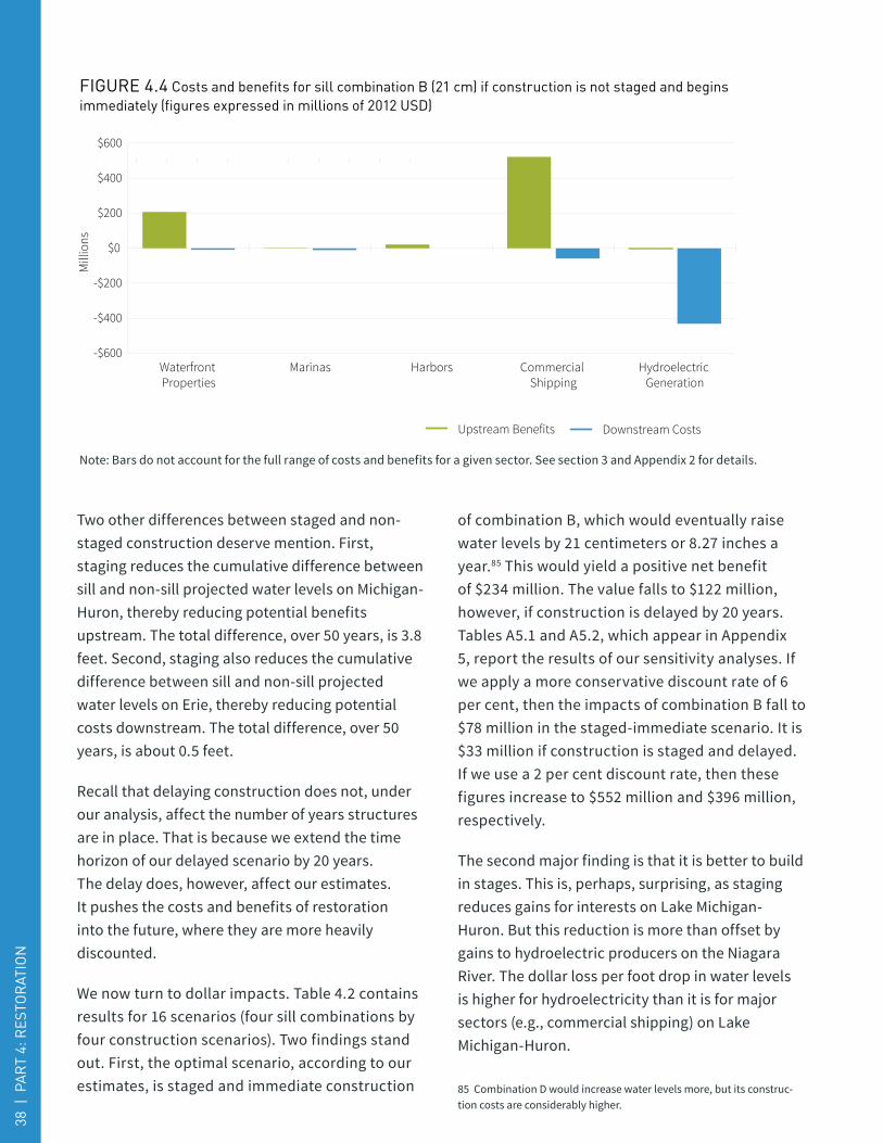
Two other differences between staged and non-

staged construction deserve mention. First,

staging reduces the cumulative difference between

sill and non-sill projected water levels on Michigan-

Huron, thereby reducing potential benefits

upstream. The total difference, over 50 years, is 3.8

feet. Second, staging also reduces the cumulative

difference between sill and non-sill projected

water levels on Erie, thereby reducing potential

costs downstream. The total difference, over 50

years, is about 0.5 feet.

Recall that delaying construction does not, under

our analysis, affect the number of years structures

are in place. That is because we extend the time

horizon of our delayed scenario by 20 years.

The delay does, however, affect our estimates.

It pushes the costs and benefits of restoration

into the future, where they are more heavily

discounted.

We now turn to dollar impacts. Table 4.2 contains

results for 16 scenarios (four sill combinations by

four construction scenarios). Two findings stand

out. First, the optimal scenario, according to our

estimates, is staged and immediate construction

of combination B, which would eventually raise

water levels by 21 centimeters or 8.27 inches a

year.85 This would yield a positive net benefit

of $234 million. The value falls to $122 million,

however, if construction is delayed by 20 years.

Tables A5.1 and A5.2, which appear in Appendix

5, report the results of our sensitivity analyses. If

we apply a more conservative discount rate of 6

per cent, then the impacts of combination B fall to

$78 million in the staged-immediate scenario. It is

$33 million if construction is staged and delayed.

If we use a 2 per cent discount rate, then these

figures increase to $552 million and $396 million,

respectively.

The second major finding is that it is better to build

in stages. This is, perhaps, surprising, as staging

reduces gains for interests on Lake Michigan-

Huron. But this reduction is more than offset by

gains to hydroelectric producers on the Niagara

River. The dollar loss per foot drop in water levels

is higher for hydroelectricity than it is for major

sectors (e.g., commercial shipping) on Lake

Michigan-Huron.

85 Combination D would increase water levels more, but its construc-tion costs are considerably higher.

fiGuRe 4.4 Costs and benefits for sill combination B (21 cm) if construction is not staged and begins immediately (figures expressed in millions of 2012 usd)

Note: Bars do not account for the full range of costs and benefits for a given sector. See section 3 and Appendix 2 for details.

Upstream Benefits Downstream Costs

-$600

-$400

-$200

$0

$200

$400

$600

Hydroelectric Generation

Commercial Shipping

HarborsMarinasWaterfront Properties

Mill

ions

38 |

pA

Rt

4: R

esto

RAt

ion

CG

LR | R

estoR

inG

WAteR

LeveLs on

LAK

e MiC

HiG

An

-Hu

Ro

n | 39

Figure 4.4 provides a breakdown of impacts by

lake and sector for the immediate, non-staged

construction scenario. Benefits (or the green

bars) refer exclusively to Michigan-Huron. Costs

(or the blue bars) refer exclusively to Lake Erie

and the Niagara River (the channel connecting

lakes Erie and Ontario). As Figure 4.4 reveals, the

cost-benefit equation is dominated by benefits

to shippers ($522 million) and property owners

($208 million) on Michigan-Huron and costs to

hydroelectric producers ($431 million) on the

Niagara River.

4.1.2 fixed rock-filled dikes in the eastern channels of stag island and fawn island

Our second restoration option is laying fixed

rock-filled dikes across the eastern channels of

two islands — Stag and Fawn — in the St. Clair

River. These structures would raise water levels by

limiting downstream flows to the islands’ western

channels.

Table 4.3 displays the estimated costs and

restoration levels of the Stag and Fawn

structures. We analyze the structures individually.

The Stag Island structure would cost $105.2

million to build, with an additional $13.3 million in

non-construction costs. The Fawn Island structure

would cost $71.8 million to build, with an additional

$9.2 million in non-construction costs.

The Stag option is expected to take 34 months to

complete. The Fawn option is expected to take 23

months.

In contrast to sills, dikes involve operation and

maintenance costs. These costs are estimated at

$0.8 million per year for both structures.

The weirs would increase the velocity of flows

along the islands’ western channels. As Bruxer

notes, this may result in erosion and expansion

of the channels, which would necessitate sills

or other structures to mitigate these effects.

Thus, following Bruxer, we include costs and

tABLe 4.3 estimated costs and restoration levels for fixed rock-filled dikes (figures expressed in millions of 2012 usd)

Cost/Benefits Option A: Stag Island

Option B: Fawn Island

Restoration level 16cm 5cm

Construction 105.20 71.78

Non-construction 13.33 9.19

Construction time 34 months 23 months

Operation and maintenance 0.80 0.80

Sill costs 52.52 52.52

Sill construction time 16 months 16 months

Source: Bruxer, 2011.

tABLe 4.4 estimated net present value for fixed rock-filled dikes (figures expressed in millions of 2012 usd)

Adaptation option

No policy delay, non-staged construction

No policy delay, staged construction

20-year policy delay, non-staged construction

20-year policy delay, staged construction

16cm 99.99 224.52 40.31 109.14

5cm -113.39 -13.59 -56.75 -6.28

Note: 4 per cent discount rate.

construction times for 150 rock sills.86 These sills

are expected to cost $52.5 million and to take 16

months to install.

The Stag Island structure is expected to raise water

levels the most: 16 centimeters or 6.23 inches

compared to five centimeters or 1.97 inches for the

Fawn Island structure. As with sills, weirs are also

expected to have negative downstream effects on

Lake Erie.

The main results appear in Table 4.4. Additional

details appear in Table A3.2 of Appendix 3. All of

the Stag structures generate positive net benefits.

As with sills, the highest estimated benefits come

from staged construction beginning immediately,

which yields an estimated $225 million, just $9

million shy of the estimate for sills. If staged

construction is delayed 20 years, this figure falls to

$109 million. None of the Fawn Island structures

are viable.

The distribution of impacts across groups and

lakes does not differ significantly from the

distributions for sills (or any other intervention):

property owners and shippers on Lake Michigan-

86 Bruxer, 2011: 18, 20.

Huron would benefit most; hydroelectric generators

on the Niagara River would lose the most.

4.1.3 parallel dikes and weirs in Lake Huron

A third restorative option is dikes and weirs in Lake

Huron. These structures would raise water levels

by narrowing the lake’s outlet at the St. Clair River

and extending this narrowed passage into the lake

(see Figure 4.2).87 The proposed structures would

be approximately a mile (1,500 meters) in length

and would be made of cement. Moore’s proposal,

described by Bruxer, calls for weirs to connect the

dikes to the land surrounding the St. Clair outlet.

As Bruxer notes, Moore’s proposals, which were

developed in the 1930s, were not designed to deal

with a number of changes in the channel, including

the increased probability of structures increasing

flow velocities.88 Unfortunately, we do not have cost

estimates of structures to mitigate these effects.

Table 4.5 reports estimated restoration levels

and construction costs. There is no simulated

estimate of the structure’s effect on water levels.

87 Bruxer, 2011: 11.88 Bruxer, 2011: 11.

tABLe 4.5 estimated costs and restoration levels for dikes and weirs (figures expressed in millions of 2012 usd)

Cost/Benefits

Restoration level 16cm

Construction 138.70

Non-construction 17.55

Operation and maintenance NA

Construction time 30 months

Sources: Bruxer, 2011; Frost and Merte, 2011.

tABLe 4.6 estimated net present values for parallel dikes and weirs (figures expressed in millions of 2012 usd)

Adaptation option

No policy delay, non-staged

construction

No policy delay, staged construction

20-year policy delay, non-staged construction

20-year policy delay, staged construction

16cm 32.44 177.29 9.75 87.53

Note: 4 per cent discount rate.

40 |

pA

Rt

4: R

esto

RAt

ion

CG

LR | R

estoR

inG

WAteR

LeveLs on

LAK

e MiC

HiG

An

-Hu

Ro

n | 41

Moore assumed, however, it would be roughly

16 centimeters or about 6 inches. Like Bruxer,

we use this assumption. The United States Army

Corps of Engineers Detroit District89 estimated

total construction and non-construction costs at

approximately $156 million USD. It also estimated

that the structures would take 30 months to build.

The results appear in Table 4.6 and, in more

detailed form, in Table A3.3 in Appendix 3. When

we apply a four per cent discount rate, positive net

benefits range from $10 million in the non-staged

and delayed construction scenario to $177 million

in the immediate and staged scenario.

4.1.4 inflatable flap gates at stag island and fawn islandWe now turn to hybrid options. But before we do,

a caveat: it is possible our low water level scenario

underestimates the benefits of these interventions.

The main advantage of these options over strictly

restorative structures is the ability to reverse

restoration in the event of high water levels. But

this benefit is potentially offset by two factors: the

89 Frost and Merte, 2011.

effects of hybrids are not immediately reversible

(they take time to fully dissipate) and the very

necessity of reversals — while beneficial to flood-

prone areas — negates much of their positive impact.

The first hybrid structures are inflatable flap

gates in the eastern channels of Stag Island

and Fawn Island. The proposed gates would

consist of metal and would rest on concrete

foundations until raised by compressed air. The

raised structures would increase water levels

by obstructing water as it flows downstream.

Regulators could deflate the gates to reverse their

effects. It would take several years, however,

for inflated gates to realize their full impact, just

as it would take several years for the effects to

dissipate once gates are deflated.

Table 4.7 contains costs and restoration estimates

under low- and high-cost scenarios. Estimated

construction times are unavailable.

The scenarios are expected to exert identical

restorative effects: 16 centimeters or roughly

6 inches. However, option B involves higher

construction, non-construction and operation and

maintenance costs.

tABLe 4.7 estimated costs and restoration levels for inflatable flap gates (figures expressed in millions of 2012 usd)

Cost/Benefits Low estimate High estimate

Restoration level 16cm 16cm

Construction 119.27 151.99

Non-construction 15.08 19.14

Operation and maintenance 0.80 1.00

Construction time Unknown Unknown

Sill costs Not necessary 52.52

Sill construction time Not necessary 16 months

Source: Bruxer, 2011.

tABLe 4.8 estimated net present values for inflatable flap gates (figures expressed in millions of 2012 usd)

Adaptation optionNo policy delay,

non-staged construction

No policy delay, staged construction

20-year policy delay, non-staged

construction

20-year policy delay, staged construction

16cm high cost

52.82 189.74 9.85 87.64

5cm -30.30 134.33 4.65 75.15

Note: 4 per cent discount rate.

Like certain fixed structures, flap gates could

also increase velocities in the islands’ western

channels. This is only likely true of option B,

however. Accordingly, we only include costs for

mitigating sills for this option.

As with all interventions, we consider staged

and non-staged and delayed and non-delayed

scenarios, giving us a total of four construction

scenarios.

The scenarios and their estimated costs appear

in Table 4.8. Full results are reported in Table A3.4

in Appendix 3. Each of the low-cost scenarios

generates positive net benefits. They range from

$10 million for non-staged construction with a 20-

year policy delay to $190 million for immediate and

staged construction.

4.1.5 Hydrokinetic turbinesThe second hybrid option is hydrokinetic turbines. In addition to raising water levels, turbines have

the added benefit of generating hydroelectric

power. Hydrokinetic turbines are similar to large

freestanding windmills, but harness the current of

the river, rather than wind, to generate electricity.

It is possible to halt the turbines if water levels rise,

but as with flag gates, it would take time for their

effects to dissipate.

The ideal location for turbines is the upper St. Clair

River, where they can take advantage of strong

currents to raise water levels and generate power.

We measure the value of electricity by multiplying

the number of megawatt-hours (MWh) the turbines

produce by the replacement cost of producing

the energy. We use a natural gas plant producing

power at levelized costs of $67 per MWh, the same

figure we use to calculate the replacement cost

of lost hydroelectric production in the Niagara

region.90

90 This figure, which comes from the United States Energy Information Administration (2014), is the cost of replacing hydroelectric generation with natural gas generation over a 30-year period. It includes both the market price of producing natural gas and the costs of building new natural gas facilities.

tABLe 4.9 estimated costs and restoration levels for hydrokinetic turbines (figures expressed in millions of 2012 usd)

Costs/Benefits 56 Turbines 151 Turbines

Restoration level 9cm 19cm

Construction 179.60 345.4

Non-construction

Operation and maintenance Unknown Unknown

Construction time Unknown Unknown

Power Production 1.3MW 2.5MW

Note: Option A refers to the 56-turbine scenario. Option B refers to the 151-turbine scenario. Construction values were estimated from Kumar and Saini and are based on projects comparable to the Verdant RITE project, which uses turbines similar to those proposed in the IUGLS. No currency or year were given for construction cost estimates. The authors assumed they were priced in 2012 USD.

Source: IUGLS, 2012; Kumar and Saini, 2014; authors’ calculations.

tABLe 4.10 estimated net present values for hydrokinetic turbines (figures expressed in millions of 2012 usd)

Adaptation option

No policy delay, non-staged

construction

No policy delay, staged construction

20-year policy delay, non-staged construction

20-year policy delay, staged construction

19cm -54.30 125.16 -27.59 68.57

9cm -124.79 9.73 -58.41 12.43

Source: IUGLS, 2012; Kumar and Saini, 2014; authors’ calculations.

42 |

pA

Rt

4: R

esto

RAt

ion

CG

LR | R

estoR

inG

WAteR

LeveLs on

LAK

e MiC

HiG

An

-Hu

Ro

n | 43

Table 4.9 contains restoration estimates for two

combinations of turbines in the upper St. Clair

River. Unfortunately, we lack data on operation and

maintenance costs, but we were able to estimate

construction costs using figures for comparable

projects from Kumar and Saini.91 Note, however,

that these estimates come from a demonstration

project and may, therefore, be inflated.

We assume the structures would take five years to

build. This estimate is based on construction times

for Verdant Power’s Roosevelt Island Tidal Energy

(RITE) Project in New York State.

The results are summarized in Table 4.10

and, in more detailed form, in Table A3.5 in

Appendix 3. If construction is staged and started

immediately, combination A would yield $125

million in positive net benefits. Combination

B performs significantly worse. It appears

hydrokinetic turbines are the least viable of our

five interventions.

4.1.6 summary of quantitative findings

We identify a number of previously-studied

structures that are capable of generating

positive economic net benefits under our

model assumptions. The most promising of

these interventions, from a simple net benefits

perspective, is a series of sills in the upper St.

Clair River. If construction is staged and begun

immediately, net benefits could reach $234

million over our 50-year time horizon. If, however,

construction is staged and delayed 20 years (a

more likely scenario), then net benefits would fall

to $122 million from 2015 to 2084.

The least viable option appears to be hydrokinetic

turbines. At a four per cent discount rate, they

would generate $125 million if construction were

staged and started immediately. This figure falls to

$69 million if construction is delayed.

91 Kumar and Saini, 2014.

In general, benefits are maximized when

construction is staged. As we have noted, staging

reduces the cumulative annual water level

increases on Michigan-Huron, limiting benefits to

property owners, commercial shippers and other

interest on this lake. However, it also reduces

cumulative annual decreases in water losses on

Lake Erie, supporting hydroelectric production

on the Niagara River. Hydroelectricity is more

sensitive to water level decreases than property

values and shipping costs, which explains why

staging is preferable.

4.2 political feasibilityOur analysis suggests that certain restorative

options would generate positive net benefits. The

next question is whether cost-beneficial projects

are politically viable. We think there is good reason

to be skeptical. Barring a special international

agreement between Canada and the United States,

any application to affect water levels or flows

requires the approval of the IJC, but the IJC and

both governments are unlikely — for legal and

political reasons — to approve projects that inflict

significant harm on key interests, even if they

would benefit the region as a whole.

This is a serious constraint. Water levels in the

GLSLS affect countless groups. Any solution

is bound to leave at least one geographic or

economic interest worse off. This does not,

however, mean we are stuck with the status quo, at

least not in theory. If projects generate sufficient

net gains, the winners can transfer a portion of

their gains to losers, such that everyone is no

worse off.

These payments work well in certain policy areas,

including international trade negotiations. But

they are not an effective means of facilitating

agreements over water levels. Consider, for

example, threats to flood-prone areas: all of our

restorative options would permanently increase

water levels on Michigan-Huron. Property owners

and defenders of wetlands in Georgian Bay would

welcome this outcome, but residents on the

southwestern shores of Lake Michigan — who

were victims of flooding in the 1980s — would

not. Theoretically, interests in Georgian Bay could

compensate losers for assuming added flood risk.

But what would these transfers look like? And

would potential losers accept such a deal?

This is why hybrid options are appealing. Flap gates

and hydrokinetic turbines would increase water

levels — thus mitigating risks for low-water areas. But

their effects are partially or fully reversible — thus

mitigating risks to flood-prone areas. It would seem,

therefore, that redistributive conflict is avoided.

But three problems arise. First, hybrids are

partially regulative and would require regulation

plans. This would involve additional planning and

delays, factors that would quickly eat into the

modest benefits these structures are expected

to provide. Second, although their effects are

reversible, they are slow to dissipate, meaning

they may not provide regulators with the flexibility

needed to cope with climate change.

Finally, hybrids, like strictly restorative options,

pose ecological risks. They would potentially

disrupt sediment transport and disturb and re-

suspend contaminated sediments along the St.

Clair River. What is more, the upper St. Clair River

— the ideal location for sills and hydrokinetic

turbines — is a spawning ground for lake sturgeon,

an endangered species. The eastern channels of

Stag Island and Fawn Island, the proposed sites of

our remaining options, have also been identified as

potential sturgeon spawning grounds.92

Ecological risks are even harder to manage than

economic ones, because it is impossible, even in

theory, to design compensating measures. Fish

cannot negotiate transfers and environmental

laws prevent both countries from endangering fish

habitats. Proponents would likely need, therefore,

to convince governments that structures pose little

or no environmental risk.93

This is major source of frustration among residents

of Georgian Bay, where wetlands and property

values have suffered as a result of dredging-

induced water losses. The US Army Corps of

92 For a more detailed discussion of ecological threats, see IUGLS, 2012: 126-127.93 This is why the Sierra Club proposes building sills on stilts, which, it argues, would allow sturgeon to safely travel underneath. See, for exam-ple, Bialkowski, 2012. But this and other proposals to mitigate ecologi-cal risks have not been widely studied or discussed. Other groups, such as Georgian Bay Forever, note that lake Sturgeon are not considered endangered in Ontario (they are considered species of special concern) and that there is no “ecological justification for sacrificing the habitat of numerous [endangered or threatened species in Georgian Bay] in order to protect a species of special concern” (Georgian Bay Forever, 2012: 22).

44 |

pA

Rt

4: R

esto

RAt

ion

We identify a number of previously-studied structures that are capable of generating positive economic net benefits under our model assumptions. The most promising of these interventions, from a simple net benefits perspective, is a series of sills in the upper St.Clair River. If construction is staged and begun immediately, net benefits could reach $234 million over our 50-year time horizon.

CG

LR | R

estoR

inG

WAteR

LeveLs on

LAK

e MiC

HiG

An

-Hu

Ro

n | 45

Engineers designed structures to offset dredging

in the 1960s, but high water supplies caused lake

levels to surge shortly after and the structures

were never built. This raises the question of

whether the pre-dredged conditions of the St.

Clair — rather than today’s water levels — ought

to be the baseline for policy decisions. Both

governments approved dredging, after all, albeit

without IJC involvement.

It is a difficult moral question, but it appears,

for practical purposes, to be moot. The decision

to install compensating structures preceded

environmental review and today’s status quo — not

pre-dredged conditions — clearly anchors current

policymaking.

46 |

pA

Rt

5: M

uLt

i-LA

Ke

ReG

uLA

tio

n

CG

LR | R

estoR

inG

WAteR

LeveLs on

LAK

e MiC

HiG

An

-Hu

Ro

n | 47

part 5: Multi-Lake Regulation

Restoration has a number of drawbacks, the most

notable of which may be higher risk of flooding

on Lake Michigan. Hybrid options mitigate these

risks, but not fully. They still increase the risk of

flooding and are incapable of lowering water levels

in the event of extreme highs. The inadequacies

of restoration are only likely to grow. Water levels

are dominated by climate factors and these factors

are becoming increasingly variable and difficult to

forecast. Water levels are apt, therefore, to mirror

these volatile and unpredictable trends.

This reality has strengthened calls for regulatory

structures capable of raising and lowering water

levels, within certain limits, as conditions dictate.94

Two Great Lakes — Superior and Ontario — are

already regulated by dams and regulation plans

subject to IJC Orders of Approval. The question is

whether to extend this approach to the GLSLS as

a whole. This would require new regulation plans

and, in all likelihood, new regulatory structures

and further channel excavation.

Our discussion of multi-lake regulation is

qualitative and draws heavily on the findings of

other reports, including the IUGLS and Tolson

and colleagues.95 A quantitative analysis was

not possible given data constraints and our

deterministic hydraulic scenario. The goal of

regulation is not to achieve a permanent increase

in water levels, but to limit the frequency with

which extreme highs and lows occur. Not only is

this process error-prone (there is always some

probability of regulation plans missing their mark),

but it is not designed to maintain a fixed water

level (regulation plans would permit a degree

of fluctuation). Thus, we cannot assume a fixed

increase in water levels in the event of intervention,

as we do with our restoration scenarios. We would

94 Specifically, according to the IUGLS, it would involve “operating regulation structures to benefit the Great Lakes-St. Lawrence River system as a whole to keep the entire system within observed historical extremes on all lakes under more extreme climate conditions in the future” (IUGLS, 2012: 212).95 Tolson, Razavi and Asadzadeh, 2011.

need to simulate large numbers of future monthly

water levels; use these simulations to construct

monthly probability distributions; calculate the

economic impacts across these distributions;

and use this information to generate expected

economic impacts in the presence and absence of

intervention. This analysis is beyond the scope of

our study and may not even be possible given data

constraints. A major reason why we focus on low

water levels is the lack of economic impact data

for high-water conditions. There is always some

probability — even under dry climate scenarios —

of realizing the latter. A stochastic model would,

therefore, force us to estimate costs for outcomes

for which data do not exist.

5.1 Background and findings of the international upper Great Lakes study (iuGLs)Multi-lake regulation would regulate water levels

throughout the GLSLS by opening and closing

dam-like structures on the system’s connecting

channels. Decisions to release water at regulation

points would not be ad hoc. They would be

governed by the mathematical rules defining

regulation plans.96

The IUGLS explored the costs and benefits of

multi-lake regulation, but without conducting a

formal CBA.97 The study had two components. In

the first, researchers simulated water levels under

a series of multi-lake regulation plans, including

current plans for regulating lakes Superior and

Ontario, which they used as their base case. The

study assessed the efficiency or ability of the plans

to limit the occurrence of extreme water levels,

relative to the base case, under eight climate

scenarios.

96 These mathematical rules are known as rule curves (IUGLS 2012, 134).97 The following summary comes from chapter 8 of the IUGLS report. See IUGLS, 2012.

48 |

pA

Rt

5: M

uLt

i-LA

Ke

ReG

uLA

tio

n

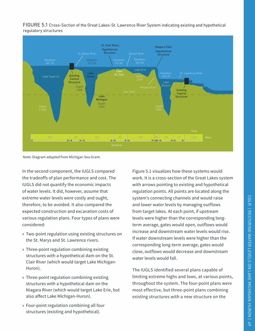
CG

LR | R

estoR

inG

WAteR

LeveLs on

LAK

e MiC

HiG

An

-Hu

Ro

n | 49

fiGuRe 5.1 Cross-section of the Great Lakes-st. Lawrence River system indicating existing and hypothetical regulatory structures

Note: Diagram adapted from Michigan Sea Grant.

Lake SuperiorLake

Huron

Lake Michigan

Lake Erie

Lake Ontario

St. Marys River

St. Clair River:

Detroit River

Niagara Falls

St. Lawrence River

Sea Level

Elevation601.1ft

Elevation577.5ft

Elevation572.3ft

Lake St. Clair

Elevation569.2ft

Elevation243.3ft

Depth1,330ft

Depth923ft Depth

802ft

Depth210ft

379 60 223 89 236 35 150 77 1,249

Total

Miles

Distance

Niagara RiverDepth750ft

Existing Control

Structure

Existing Control

Structure

Hypothetical Structure Hypothetical

Structure

In the second component, the IUGLS compared

the tradeoffs of plan performance and cost. The

IUGLS did not quantify the economic impacts

of water levels. It did, however, assume that

extreme water levels were costly and ought,

therefore, to be avoided. It also compared the

expected construction and excavation costs of

various regulation plans. Four types of plans were

considered:

» Two-point regulation using existing structures on the St. Marys and St. Lawrence rivers.

» Three-point regulation combining existing structures with a hypothetical dam on the St. Clair River (which would target Lake Michigan-Huron).

» Three-point regulation combining existing structures with a hypothetical dam on the Niagara River (which would target Lake Erie, but also affect Lake Michigan-Huron).

» Four-point regulation combining all four structures (existing and hypothetical).

Figure 5.1 visualizes how these systems would

work. It is a cross-section of the Great Lakes system

with arrows pointing to existing and hypothetical

regulation points. All points are located along the

system’s connecting channels and would raise

and lower water levels by managing outflows

from target lakes. At each point, if upstream

levels were higher than the corresponding long-

term average, gates would open, outflows would

increase and downstream water levels would rise.

If water downstream levels were higher than the

corresponding long-term average, gates would

close, outflows would decrease and downstream

water levels would fall.

The IUGLS identified several plans capable of

limiting extreme highs and lows, at various points,

throughout the system. The four-point plans were

most effective, but three-point plans combining

existing structures with a new structure on the

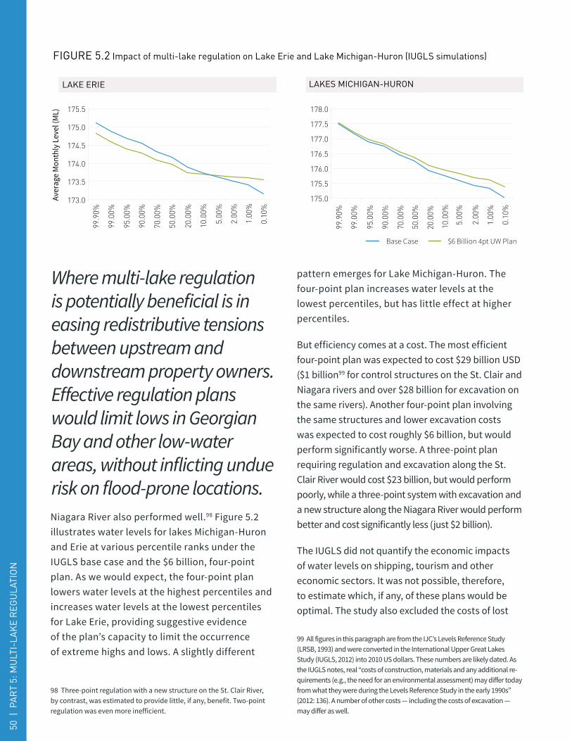
Niagara River also performed well.98 Figure 5.2

illustrates water levels for lakes Michigan-Huron

and Erie at various percentile ranks under the

IUGLS base case and the $6 billion, four-point

plan. As we would expect, the four-point plan

lowers water levels at the highest percentiles and

increases water levels at the lowest percentiles

for Lake Erie, providing suggestive evidence

of the plan’s capacity to limit the occurrence

of extreme highs and lows. A slightly different

98 Three-point regulation with a new structure on the St. Clair River, by contrast, was estimated to provide little, if any, benefit. Two-point regulation was even more inefficient.

pattern emerges for Lake Michigan-Huron. The

four-point plan increases water levels at the

lowest percentiles, but has little effect at higher

percentiles.

But efficiency comes at a cost. The most efficient

four-point plan was expected to cost $29 billion USD

($1 billion99 for control structures on the St. Clair and

Niagara rivers and over $28 billion for excavation on

the same rivers). Another four-point plan involving

the same structures and lower excavation costs

was expected to cost roughly $6 billion, but would

perform significantly worse. A three-point plan

requiring regulation and excavation along the St.

Clair River would cost $23 billion, but would perform

poorly, while a three-point system with excavation and

a new structure along the Niagara River would perform

better and cost significantly less (just $2 billion).

The IUGLS did not quantify the economic impacts

of water levels on shipping, tourism and other

economic sectors. It was not possible, therefore,

to estimate which, if any, of these plans would be

optimal. The study also excluded the costs of lost

99 All figures in this paragraph are from the IJC’s Levels Reference Study (LRSB, 1993) and were converted in the International Upper Great Lakes Study (IUGLS, 2012) into 2010 US dollars. These numbers are likely dated. As the IUGLS notes, real “costs of construction, materials and any additional re-quirements (e.g., the need for an environmental assessment) may differ today from what they were during the Levels Reference Study in the early 1990s” (2012: 136). A number of other costs — including the costs of excavation — may differ as well.

50 |

pA

Rt

5: M

uLt

i-LA

Ke

ReG

uLA

tio

n

fiGuRe 5.2 impact of multi-lake regulation on Lake erie and Lake Michigan-Huron (iuGLs simulations)

LAKES MICHIGAN-HURON

Aver

age

Mon

thly

Lev

el (M

L)

LAKE ERIE

Base Case $6 Billion 4pt UW Plan

173.0

173.5

174.0

174.5

175.0

175.5

0.10

%

1.00

%

2.00

%

5.00

%

10.0

0%

20.0

0%

50.0

0%

70.0

0%

90.0

0%

95.0

0%

99.0

0%

99.9

0%

175.0

175.5

176.0

176.5

177.0

177.5

178.0

0.10

%

1.00

%

2.00

%

5.00

%

10.0

0%

20.0

0%

50.0

0%

70.0

0%

90.0

0%

95.0

0%

99.0

0%

99.9

0%

Where multi-lake regulation is potentially beneficial is in easing redistributive tensions between upstream and downstream property owners. Effective regulation plans would limit lows in Georgian Bay and other low-water areas, without inflicting undue risk on flood-prone locations.

CG

LR | R

estoR

inG

WAteR

LeveLs on

LAK

e MiC

HiG

An

-Hu

Ro

n | 51

efficiency on the lower St. Lawrence River, where

the simulations revealed that multi-lake regulation

would increase the occurrence of extreme water

levels. Any multi-lake regulation plan would need

to mitigate these effects.100 This would not be

cheap, as it would require additional structures and

excavation costs.101

5.2 political feasibilityMulti-lake regulation and restoration face similar

political obstacles. All four-point and certain

three-point plans call for dams on the St. Clair

River. The optimal location for these structures is

the upper reaches of the river, where dams would

take advantage of the narrow channel and — if

hydroelectric generation were a priority — the

steep slope of the water surface. But dams in this

location would disturb contaminated sediment,

interfere with sturgeon spawning grounds and

possibly have other negative environmental impacts.

Where multi-lake regulation is potentially

beneficial is in easing redistributive tensions

between upstream and downstream property

owners. Effective regulation plans would limit lows

in Georgian Bay and other low-water areas, without

inflicting undue risk on flood-prone locations. The

question is whether the benefits outweigh the

100 According to the IJC, any approvals to change regulation upstream would require “suitable and adequate provision” to protect interests on the lower St. Lawrence River (IUGLS 2012, 133).101 In addition to examining the costs and benefits of multi-lake regula-tion, a number of studies have also looked at the potential for improving the existing regulation of lakes Ontario and Superior. The IJC, for exam-ple, recently proposed an alternative plan for Lake Ontario, which would continue to compress water levels but within in a wider range (see box on page 22). Asadzadeh and his colleagues (2014) designed a new reg-ulation policy for Lake Superior in the form of a parametric rule-curve and optimized the parameters using a multi-scenario simulation-optimi-zation framework. Their plan outperformed the previous Lake Superior plan (Plan 1977A) under the historical water level scenario (see Table A4.1) by increasing operational benefits and limiting extremely high and low water levels across the Upper Great Lakes. The optimized plan also demonstrated significant benefits under the other future climate scenarios described in Table A4.1. The most significant benefit was the plan’s ability to limit extremely low water levels under an extremely dry future climate scenario (a scenario that caused Plan 1977A to stop releasing water from Lake Superior). Costs and benefits were estimated using IJC-approved software. The estimates focused on commercial navigation, hydroelectric generation and shoreline protection.

costs. The answer is unknown. Economic outcomes

depend on water levels and climate in turn, but

these outcomes are fraught with uncertainty.

And any attempt to extend regulation would also

have to take downstream impacts — including

costs on the St. Lawrence River — into account. The

IUGLS did not systematically study these costs, but

it did say that the lower St. Lawrence levels would

require billions of dollars of mitigating measures,

including excavation and control structures.102

Indeed, the study recommended no further

analysis of multi-lake regulation unless these costs

are assessed.103

Inevitably, these uncertainties — along with

the magnitude and geographic coverage of the

projects — would delay construction. The IUGLS

estimates that it would take 20 years or more to

complete “the necessary planning, environmental

reviews, regulatory approvals and design steps.”104

Ultimately, the IUGLS advised against further

analysis of multi-lake regulation at this time. It

argued that multi-lake regulation had the potential

to limit extreme water levels, but that this potential

was more than offset by high costs, environmental

concerns, institutional requirements and

uncertainty over “climate and its impact on Great

Lakes hydrology.”105

It would seem, therefore, that the first step in

adopting any engineering solution — whether

restorative or regulative — is establishing better

monitoring, modelling and assessment of water

levels and their economic impacts.106 It is to these

issues that we now turn.

102 IUGLS, 2012: 187.103 IUGLS, 2012: 151.104 IUGLS, 2012: 147.105 IUGLS, 2012: 187.106 IUGLS, 2012: 148.

52 |

pA

Rt

6: A

dA

pti

ve M

An

AGeM

ent

CG

LR | R

estoR

inG

WAteR

LeveLs on

LAK

e MiC

HiG

An

-Hu

Ro

n | 53

part 6: Adaptive Management

Restoration and regulation would respond to

shifting water levels by altering water flows.

This section considers a third strategy, adaptive

management (AM). AM does not involve

managing or raising water levels (though it can

be combined with these approaches). Rather it

is a structured, iterative process of improving

responses to changing water levels through long-

term monitoring, modelling and assessment of

hydrological trends and impacts.107 We are not in a

position to quantify the costs and benefits of this

approach, but we assess its merits qualitatively.

6.1 Adaptive management – key characteristics and the ijC’s AM strategyOver the past half century, the IJC has conducted

a number of detailed studies of Great Lakes water

levels.108 These studies shed considerable light on Great

Lakes hydrology, but they occur sporadically — usually

in response to sustained periods of extreme water levels

— with limited research in between. This has led to gaps

in data and knowledge and an inability to track and

verify hydrological trends and their impacts.109

The IUGLS has recognized this problem and

called for more sustained collaboration, data

collection and analysis among stakeholders

and public officials. In May 2012, the IJC called

on the International Great Lakes-St. Lawrence

River Adaptive Management (GLAM) Task Team

to develop an AM plan for the Great Lakes and

St. Lawrence River System. The proposed plan

has two parts. The first is an ongoing review and

107 IUGLS, 2012108 These studies include: Regulation of Great Lakes Water Levels Reference Study (under 1964 reference) (International Great Lakes Levels Board, 1973); Great Lakes Diversions and Consumptive Uses Reference Study (under 1977 reference) (IGLDCUSB, 1981); Limited Regulation of Lake Erie Study (under 1977 reference) (ILERSB, 1981); Water Levels Reference Study (under 1986 reference) (LRSB, 1993); Report on the Protection of the Waters of the Great Lakes (under 1999 reference) (IJC, 2000); Lake Ontario-St Lawrence River Study (under 2000 IJC directive) (ILOSLRSB, 2006); International Upper Great Lakes Study (under 2007 IJC directive) (IUGLS, 2012).109 The International Great Lakes-St. Lawrence River Adaptive Management Task Team, 2013: 5.

evaluation of the effectiveness of the regulation of

Lake Superior and the Niagara and St. Lawrence

rivers. The second, which is more relevant to our

analysis, is the collaborative development and

evaluation of solutions to problems associated

with extreme water levels that cannot be solved

through regulation alone.

The IJC has yet to establish a clear leadership

role in this area. It has, however, proposed the

establishment of the Great Lakes and St. Lawrence

River Levels Advisory Board (LAB), which would

initiate a series of AM pilots and “engage agencies,

organizations and institutions from across the

[GLSLS]” to develop five system-wide networks

responsible for:

» Hydroclimate Monitoring and Modelling to improve knowledge on water balance and water supply, the forecasting of net basin supply, lake levels and climate modelling.

» Performance Indicators and Risk Assessment to assess risks of extreme water levels to shoreline property, commercial navigation, municipal and industrial water uses, recreational boating, ecosystems, hydropower and other interests.

» Evaluation and Decision Tools to maintain, update and improve the tools needed for the evaluation of regulation plans over time and to develop new tools to support decision-making on potential responses to extreme water levels.

» Information Management and Distribution to facilitate the sharing of water level-related data and information among the Great Lakes and St. Lawrence River System community.

» Outreach and Engagement to educate and establish two-way communication on water level-related issues through the Great Lakes and St. Lawrence River System community.

— From The International Great Lakes-St. Lawrence

River Adaptive Management Task Team, 2013: iii.

54 |

pA

Rt

6: A

dA

pti

ve M

An

AGeM

ent

CG

LR | R

estoR

inG

WAteR

LeveLs on

LAK

e MiC

HiG

An

-Hu

Ro

n | 55

While each of these activities is vital, the second

— assessing the risks of extreme water levels to

economic and ecological interests — is particularly

relevant to our report. Better data and modelling of

outcomes would go a long way in broadening and

deepening the analysis of engineering options.

6.2 Benefits and political feasibilityAM is more viable, currently, than regulation or

restoration for three reasons. First, it provides

clear benefits for all sectors. Property owners,

hydroelectric producers, municipal users and

others groups all stand to benefit from more

and better information about the direction and

risks associated with water levels. Second, AM is

not as controversial as restoration or multi-lake

regulation. It does not put lake sturgeon at risk nor

does it risk flooding flood-prone areas. It is unlikely,

therefore, to face significant political resistance.

Finally, AM is not merely useful in its own right. It is

also a necessary, albeit insufficient, condition for

structural interventions. Neither restoration nor

multi-lake regulation has any chance of approval

unless uncertainty over their impacts is reduced.

AM would not eliminate this uncertainty, but it

would mitigate it, perhaps opening the door to a

reliable analysis of engineering options.

But we also acknowledge the technical limits of this

approach. Experimenting with new technologies

is a key part of AM, but it excludes, by definition,

raising or lowering water levels. This confines the

analysis of engineering structures to lab settings,

where ecological risks, such as threats to lake

sturgeon, are difficult to assess.

A potential workaround, suggested by members

of our steering committee, would be to combine

AM with smaller scale interventions or pilot

projects, such as a limited number of sills in the

upper St. Clair River. Theoretically, this would

allow researchers to assess the costs and benefits

of structures while limiting their risks. But no

mitigating structure, regardless of its scale,

faces an easy path. They all involve the same

redistributive struggles and institutional hurdles,

including authorizing legislation, IJC orders or

approval, environmental and regulatory approvals,

and public consultation.110

110 Presumably, for example, pilot sills would be located in the upper St. Clair River. This is where they would have the biggest impact, but it is also where sturgeon spawn.

56 |

pA

Rt

7: s

uM

MA

Ry,

Les

son

s &

ReC

oM

Men

dAt

ion

s

CG

LR | R

estoR

inG

WAteR

LeveLs on

LAK

e MiC

HiG

An

-Hu

Ro

n | 57

part 7: summary, lessons and recommendations

This study has assessed the economic impacts of

raising water levels on Lake Michigan-Huron. It has

also examined, in a largely qualitative fashion, the

economic implications of multi-lake regulation and

adaptive management and the political feasibility

of each approach.

Our quantitative analysis reveals several options

capable of generating positive net benefits.

However, we refrain from recommending specific

options for three reasons: (1) our estimated

impacts are modest; (2) they are subject to

considerable uncertainty; (3) and they face

significant political obstacles.

This is not to suggest that restoration is impossible

or ill advised or that we cannot recommend

options until uncertainty is eliminated; merely that

the political obstacles are daunting and that our

knowledge is insufficient to recommend options at

present.

With these thoughts in mind, we draw three

conclusions.

First, the economic viability of restoration

structures requires further research.

This research ought to include ecological

impacts;111 more economic impacts;112 better data

on the economic impacts we do include;113 a wider

range of hydraulic scenarios;114 more sophisticated

modelling of economic outcomes; updated

cost estimates of existing proposals;115 and, if

existing proposals are incapable of redressing

redistributive conflicts, promising proposals

for new structures. In the absence of significant

capacity and resources, this research ought to start

small, focusing on specific lakes, sectors or even

impacts within them. This would allow researchers

to collect more fine-grained data and develop

better models of individual impacts. Eventually,

it would provide the foundations of a deeper and

broader CBA.

Second, future research needs to grapple with the

politics of restoration.

As this paper has argued, decisions over GLSLS

water levels are taken by unofficial consensus,

where virtually any group can veto measures

expected to cause significant harm. The problem,

111 Not all ecological outcomes are possible or appropriate to quantify. But dollar estimates of some outcomes could, in theory, be collected through contingent valuation surveys (i.e., surveys that ask citizens how much they would be willing to pay to protect particular ecological services under partic-ular circumstances).112 Although our analysis is strictly economic, there are a number of impacts our study does not quantify. Some of these omissions are sec-toral (for example, the impacts on the recreational boating and tourism industries). Others concern specific rivers and lakes (for example, the impact of temporarily lower water levels on the St. Lawrence River).113 Measures of several impacts are less than ideal, forcing us to push our data in some cases. An example is hydroelectric revenues. We estimated the impact of lower water levels on the revenues of plants in the Niagara region. But we only had data for one plant and extrapolated these estimates to other facilities in the region. Ideally, we would rely on plant-specific estimates.114 Ideally, we would have estimated the costs of restoration under a high-wa-ter level scenario. Unfortunately, we lacked the economic impact data to do so.115 Our study only analyzes proposals with adequate cost data. Unfortunate-ly, a number of these options were engineered prior to 1977. Recent techno-logical advances could improve the cost effectiveness of these structures.

58 |

pA

Rt

7: s

uM

MA

Ry,

Les

son

s &

ReC

oM

Men

dAt

ion

s

We encourage the Canadian and US governments to approve the IJC’s proposals to strengthen AM on a bi-national basis. Specifically, we support the creation of a Levels Advisory Board (LAB) capable of facilitating monitoring and modelling of hydrological trends and their impacts.

CG

LR | R

estoR

inG

WAteR

LeveLs on

LAK

e MiC

HiG

An

-Hu

Ro

n | 59

of course, is that any structure is likely to benefit

some groups at the expense of others. Researchers

ought to admit this constraint and identify ways

of redressing it. Ultimately, this means identifying

policies and structures capable of eliminating or

limiting redistributive conflicts and environmental

risks. This is no easy task.

The study’s shortcomings limit the policy

recommendations we can make. However, we do

make one recommendation, which, we believe, will

improve the capacity of actors to adapt to water

levels and pave the way for future research.

We encourage the Canadian and US governments

to approve the IJC’s proposals to strengthen AM

on a bi-national basis. Specifically, we support

the creation of a Levels Advisory Board (LAB)

capable of facilitating monitoring and modelling of

hydrological trends and their impacts.

AM is the most politically practical means of

addressing fluctuating water levels: it is not

as controversial as restoration or multi-lake

regulation, and would help all actors, regardless

of their preferences over water levels, by providing

them with more and better information on

hydrological conditions. But AM is not merely

useful in its own right. It is also a necessary, albeit

insufficient, condition for structural interventions.

Neither restoration nor multi-lake regulation has

any chance of approval unless uncertainty over

hydrological trends and their impacts is reduced.

AM would not eliminate this uncertainty, but it

would mitigate it, opening the door to a more

reliable analysis of engineering options.

60 |

Ap

pen

dix

1: C

An

Ad

iAn

do

LLA

R C

on

veR

sio

ns

Appendix 1:Canadian dollar conversionsThe tables below represent CAD values for tables 4.1, 4.2, 4.3, 4.4, 4.5, 4.6, 4.7, 4.8 and 4.10.

tABLe A1.1 estimated costs and restoration levels for sills (figures expressed in millions of 2012 CAd)

Cost/Benefits Option A Option B Option C Option D

Restoration level 6 cm 21 cm 8 cm 23 cm

Construction 11.31 60.64 36.12 192.49

Non-construction 1.65 7.82 4.15 21.09

Construction time 18 months (our assumption) 18 months 18 months (our assumption) 31 months

Note: Options A and B use type 4 sills, whereas, options C and D use type 11 sills. See Bruxer (2011) for descriptions of these types.

tABLe A1.2 estimated net present value for sills (figures expressed in millions of 2012 CAd)

Adaptation option

No policy delay, non-staged construction

No policy delay, staged construction

20-year policy delay, non-staged

construction

20-year policy delay, staged construction

6cm 3.85 78.72 -5.79 35.38

21cm 212.15 259.46 56.47 135.37

8cm -18.21 89.49 -35.40 42.63

23cm 94.45 192.79 -68.57 107.27

Note: 4 per cent discount rate.

tABLe A1.3 estimated costs and restoration levels for weirs (figures expressed in millions of 2012 CAd)

Cost/Benefits Option A: Stag Island

Option B: Fawn Island

Restoration level 16cm 5cm

Construction 110.78 75.58

Non-construction 14.04 9.68

Construction time 34 months 23 months

Operation and maintenance 0.84 0.84

Sill costs 55.30 55.30

Sill construction time 16 months 16 months

Source: Bruxer, 2011.

CG

LR | R

estoR

inG

WAteR

LeveLs on

LAK

e MiC

HiG

An

-Hu

Ro

n | 61

tABLe A1.4 estimated net present value for fixed rock-filled dikes (figures expressed in millions of 2012 CAd)

Adaptation option

No policy delay, non-staged

construction

No policy delay, staged construction

20-year policy delay, non-staged

construction

20-year policy delay, staged construction

16cm 111.10 249.46 44.79 121.27

5cm -125.99 -15.10 -63.05 -6.97

Note: 4 per cent discount rate.

tABLe A1.5 estimated costs and restoration levels for dikes and weirs (figures expressed in millions of 2012 CAd)

Cost/Benefits

Restoration level 16cm

Construction 146.23

Non-construction 18.44

Operation and maintenance NA

Construction time 30 months

Sources: Bruxer, 2011; Frost and Merte, 2011.

tABLe A1.6 estimated net present values for parallel dikes and weirs (figures expressed in millions of 2012 CAd)

Adaptation option

No policy delay, non-staged construction

No policy delay, staged construction

20-year policy delay, non-staged construction

20-year policy delay, staged construction

16cm 36.05 196.99 10.83 97.26

Note: 4 per cent discount rate.

tABLe A1.7 estimated costs and restoration levels for inflatable flap gates (figures expressed in millions of 2012 CAd)

Cost/Benefits Low estimate High estimate

Restoration level 16cm 16cm

Construction 125.59 160.05

Non-construction 15.88 20.15

Operation and maintenance 0.84 1.05

Construction time Unknown Unknown

Sill costs Not necessary 55.30

Sill construction time Not necessary 16 months

Source: Bruxer, 2011.

tABLe A1.8 estimated net present values for inflatable flap gates (figures expressed in millions of 2012 CAd)

Adaptation option

No policy delay, non-staged construction

No policy delay, staged construction

20-year policy delay, non-staged construction

20-year policy delay, staged construction

16cm high cost

58.69 210.82 10.95 97.38

5cm -33.67 149.25 5.17 83.50 Note: 4 per cent discount rate.

tABLe A1.9 estimated net present values for hydrokinetic turbines (figures expressed in millions of 2012 CAd)

Adaptation option

No policy delay, non-staged construction

No policy delay, staged construction

20-year policy delay, non-staged construction

20-year policy delay, staged construction

19cm -60.33 139.07 -30.65 76.18

9cm -138.65 10.81 -64.90 13.81

Note: Construction values were estimated from Kumar and Saini and are based on projects comparable to the Verdant RITE project, which uses turbines similar to those proposed in the IUGLS.

Sources: IUGLS, 2012; Kumar and Saini, 2014; authors’ calculations.

62 |

Ap

pen

dix

1: C

An

Ad

iAn

do

LLA

R C

on

veR

sio

ns

CG

LR | R

estoR

inG

WAteR

LeveLs on

LAK

e MiC

HiG

An

-Hu

Ro

n | 63

Appendix 2: data and methodology on economic impactsThis appendix describes our methodologies for calculating the economic impacts of low water levels. More

detailed descriptions of calculations are available from appendices two through six of our Low Water Blues

report.116 Note that we apply two time horizons: 2015 to 2064 and 2015 to 2084. For the latter, we assume

that water levels remain constant from 2064 to 2084. That means that, in the absence of discounting, losses

would be constant across that period.

A2.1 Commercial shipping and harboursCarrying capacity: In general, lower water levels harm shipping interests. Most vessels in the region are

designed to carry as much cargo as possible at existing depths. A sharp decline in water levels would

increase the risk of vessels running aground. Shippers would have to take measures – including reducing

speeds and cargo loads – to keep under-keel clearances (or the distance between the lowest part of the hull

and the bottom of the river or lake) above legal minimums.117

We estimate the costs of replacing lost carrying capacity — measured in ton miles — in the event of low water

levels. Replacement could, in theory, involve increased trucking and rail transit. However, these methods

are significantly more expensive than marine navigation. Thus, we assume replacement will occur through

reduction of cargo loads and the expansion of existing fleets. We calculate these costs in four steps.

First, we estimate the lost carrying capacity for bulk cargo for the median-length ship in both the Canadian

and the US shipping fleets. Data on median-length ships comes from Greenwood’s.118 Quinn119 provides

figures for the estimated tonnage loss per inch decline in water levels for vessels of various sizes. We use

Quinn’s data to identify the lost load per inch of the median Canadian and US ships.

Second, we multiply tons lost per foot by the projected water level loss in the year 2064, using 2014 as our

base water-level year.

Third, we calculate the reduction in ton capacity by dividing tonnage losses for 2064 by the tonnage

capacity of the median ship for both fleets. We multiply this figure by 100 to give us the percentage

reduction in ton capacity. We assume that the reduction for the median ship is the same for all vessels in

the national fleet.

This allows us to take our fourth step, which is to multiply the reduction in ton capacity of the median

vessel by the total ton miles travelled in the Canadian and US fleets in 2013.120 This gives us the reduction in

ton miles for each fleet for 2064.

116 Shlozberg et al., 2014.117 IUGLS, 2012: 27.118 Greenwood’s, 2013.119 Quinn, 2002.120 Canadian data comes from English and Hackston, 2013. US data come from the United States Department of Maritime Administration (2013).

Next, we estimate ton miles lost for the remaining years by linearly interpolating annual values between

2014 and 2064.

Finally, we calculate dollar value losses per year by multiplying ton miles lost by the cost of replacement.

Anonymous industry sources estimate replacement costs at 10 cents per ton mile, which is the levelized

cost of purchasing, maintaining and operating new vessels for the fleet over an extended period of time.

Harbour infrastructure: Lower water levels increase the costs of maintaining harbour infrastructure. We

focus on the costs of maintaining harbour docks. Low water levels increase these costs by exposing docks

to dry rot. We could also analyze the costs of slip and harbour dredging. However, we assume shippers will

adapt to lower water levels by reducing cargo loads (see above), thereby negating or at least reducing the

need for dredging. We estimate the costs of harbour maintenance in four steps.

First, we identify the costs of replacing and repairing individual docks. Bergeron and Clark121 estimate the

cost of replacement at $5,000 per dock foot and the cost of repair at $3,000 per dock foot.

Second, we identify the dock footage and dock-face depths of each dock on each lake. Dock footage tells

us how much infrastructure needs maintenance. Dock-face depth tells us whether maintenance requires

repair or replacement. This information, which we have for 544 docks, comes from Greenwood’s.122

Third, we assume that after 20 years of persistently low water levels, docks are going to require

maintenance.

Fourth, we determine whether maintenance would involve repair or replacement. Bergeron and Clark123

assume it is optimal to replace docks when dock-face water level depths exceed 30 feet. Otherwise it is

optimal to repair.

Finally, we sum the costs of repairing and replacing docks and spread the costs equally over the 2014 to

2064 period. When we extend our time horizon to 2084, we assume water levels and costs are constant

from 2064 onward.

A2.2 tourism and recreational water activities (marinas)

Low water levels create a number of costs for marinas. We estimate two: the costs of lost rental income from

stranded slips and the costs of additional dredging to ensure water is deep enough to allow boats to enter and

leave. Our cost estimates come from a survey of marina owners on lakes Erie and Michigan-Huron. The true

populations of marinas for each lake is unknown, making it difficult to reliably extrapolate the results to the

population at large. Nonetheless, they provide the most representative cost estimates available.124

121 Bergeron and Clark, 2011.122 Greenwood’s, 2013.123 Bergeron and Clark, 2011.124 Ontario Centre for Climate Impacts and Adaptation Resources, 2010.

64 |

Ap

pen

dix

1: d

AtA

An

d M

etH

od

oLo

Gy

on

eC

on

oM

iC iM

pAC

ts

CG

LR | R

estoR

inG

WAteR

LeveLs on

LAK

e MiC

HiG

An

-Hu

Ro

n | 65

The study reports average estimates of minimum and maximum costs for owners on lakes Erie and Michigan-

Huron. We use the average minimum values to ensure conservative estimates and extrapolate these to all

marinas on each lake. Estimates of the number of marinas come from Boating Ontario125 and the US Army

Corps of Engineers.126

The study provides cost estimates for one-, two- and three-foot drops. Unfortunately, we do not have

estimates for drops between one and two and two and three feet. Thus, we linearly interpolate losses over

a three-foot range, assuming zero losses at 2014 water levels.127 The projected water level losses for 2064

are 3.2 feet for Lake Michigan-Huron and 2.6 feet for Lake Erie.

A2.3 Hydroelectric generationResearch on the economic impacts of water levels on hydroelectric revenues in the GLSLS is scarce. Our

study draws heavily on work by Buttle and his colleagues,128 which quantifies the dollar losses of replacing

hydroelectric production with natural gas powered plants, the next cheapest source of electricity.

Buttle et al. provide estimates of dollar losses of low water levels for three sets of facilities: the Adam Beck

facilities on the Niagara River; the Saunders facility on the St. Lawrence River; and the Clergue facility on the

St. Marys River. All three are located in Ontario and all three are operated by Ontario Power Generation. We

want to analyze the costs of low water levels in the Niagara region, but only have data for the facilities studied

by Buttle et al. Rather than collecting data for additional facilities, we assume the relationship between

revenues and water levels is the same for all facilities in the region and use this assumption to extrapolate

losses at the Adam Beck facilities129 to Robert Moses and Lewiston, both of which are located in the US.

Our calculations consist of four steps. First, we estimate the lost hydroelectric revenues per foot. Buttle et al. estimate

the losses per year under the CCCma2050 climate model for the Adam Beck facilities. We divide this estimate by the

difference between the projected average annual water levels for Lake Erie under CCCma2050 and Lake Erie’s historic

annual average. This gives us the estimated revenue loss per foot loss of water levels, which is needed to calculate the

yearly losses estimated for each year (and subsequently each water level) over our time horizon.

Second, we take the average yearly revenue losses per foot of water levels for the Adam Beck facilities from

Buttle and his colleagues and estimate the potential losses to other facilities on the Niagara River. We do

this by adjusting the revenue losses to different plant capacities,130 assuming the same load factor used in

Buttle et al. To accommodate the study of additional facilities, we also assume that all production loss will

have to be made up by additional sources, in this case combined cycle gas turbine plants. We update the

generation costs used in Buttle to $67 MW/h131 and apply this value to Buttle et al.’s calculations to find the

total cost of the replacement power for each facility.

Third, we sum the losses for each facility for 2064.

125 Boating Ontario, n.d.126 USACE, 2008. 127 This refines our Low Water Blues methodology, where we used one- and two- foot drops as proxies for our two water level drops scenarios. This change enables us to estimate the potential benefits of different restoration options, impossible under the Low Water Blues methodology. This change also results in more conservative impact estimates. 128 Buttle et al., 2004.129 Buttle and his colleagues generate a single estimate for Adam Beck 1 and 2 and the Adam Beck Pump Generation Station.130 Data on plant capacities comes from utility and company websites and Wikipedia-compiled lists. For details, see Shlozberg et al., 2014: 102.131 The values come from the United States Energy Information Administration, 2014. We use combined cycle gas turbines, which are commonly used for energy replacement in the north east of North America.

Fourth, we linearly interpolate costs from 2014 to 2064.

Note an important difference between our approach and Buttle et al.’s. Buttle et al. assume a positive and

convex relationship between revenue losses and water level declines. Unfortunately, we do not have access

to their cost function. In its place, we linearly approximate their function (1) by matching our 2064 water level

projection to their projected revenue loss for that water level and (2) assuming zero revenue losses for 2014.

This latter approach is slightly problematic, as Buttle et al. use Lake Erie’s average historic level as their base

case, whereas we use the 2014 level. Fortunately, the difference between these figures is only four centimeters

or 0.13 standard deviations of the annual historic average. If Buttle et al.’s convex function is correct, our linear

approximation overestimates the potential costs of lower water levels in all but the final year of our forecast.

A2.4 Waterfront properties

In Low Water Blues, we estimated the impact of changes in water levels on percentage changes in property

values. Our data, which came from Ontario’s Municipal Property Assessment Corporation (MPAC), were

not disaggregated to the level of individual properties. We did, however, have access to average property

values for 105 Ontario municipalities located next to lakes Huron, Superior, Erie and Ontario. Data were

available for three years: 2003, 2008 and 2012, which allowed us to look at changes in property values over

two periods: 2003 to 2008 and 2008 to 2012.

We estimated impacts by regressing the percentage change in average municipal property values on the

change in water levels in adjacent lakes. We restricted our sample to municipalities identified by MPAC as

containing at least one seasonal recreational property.132 This reduced our sample to 84 municipalities.

According to our estimates, average municipal property values decline, on average, by 14 per cent for

every one foot decline in water levels. We were concerned, however, that this estimate was too large: while

our model controlled for changes in average non-waterfront properties, it omitted a number of possible

causes of lower values. Accordingly, we took a conservative approach, adjusting our estimate downwards

by subtracting two standard errors. This yielded an impact of six per cent, which we used in our impact

analysis.133

132 We do not expect water levels to affect the property values of non-seasonal recreational properties, such as properties in downtown Toronto.133 In other words, we used the lower bound of our 95 per cent confidence interval.

66 |

Ap

pen

dix

2: d

AtA

An

d M

etH

od

oLo

Gy

on

eC

on

oM

iC iM

pAC

ts

CG

LR | R

estoR

inG

WAteR

LeveLs on

LAK

e MiC

HiG

An

-Hu

Ro

n | 67

Appendix 3: detailed CBA tables and results This appendix provides a detailed breakdown of the costs and benefits of each of our restoration options.

The tables identify (1) construction, non-construction and operation and maintenance costs; (2) the

upstream benefits of higher water levels on Lake Michigan-Huron; and (3) the downstream costs of

temporarily lower water levels on Lake Erie. Additional power production is also included in upstream

benefits for hydrokinetic turbines. tABLe A3.1 estimated net present values for sills (figures expressed in millions of 2012 usd)

Adaptation option Impact

No policy delay, non-staged

construction

No policy delay, staged construction

20-year policy delay, non-staged

construction

20-year policy delay, staged construction

6cm

Cost -11.29 -7.48 -11.95 -10.21

Benefit 215.37 171.57 98.29 78.30

Downstream -200.62 -93.24 -91.56 -36.25

Net 3.46 70.85 -5.21 31.84

21cm

Cost -61.32 -40.63 -64.30 -25.34

Benefit 753.81 600.48 344.03 274.05

Downstream -501.56 -326.34 -228.90 -126.88

Net 190.94 233.51 50.82 121.83

8cm

Cost -191.28 -126.75 -187.81 -64.64

Benefit 825.60 657.67 376.79 300.15

Downstream -549.32 -357.41 -250.70 -138.97

Net 85.00 173.51 -61.71 96.54

23cm

Cost -191.28 -126.75 -187.81 -64.64

Benefit 825.60 657.67 376.79 300.15

Downstream -549.32 -357.41 -250.70 -138.97

Net 85.00 173.51 -61.71 96.54

Note: 4 per cent discount rate.

tABLe A3.2 estimated net present values for rock-filled dikes (figures expressed in millions of 2012 usd)

Adaptation option Impact

No policy delay, non-staged

construction

No policy delay, staged construction

20-year policy delay, non-staged

construction

20-year policy delay, staged construction

16cm

Cost -92.21 -55.39 -47.41 -30.60

Benefit 574.33 457.51 262.12 208.80

Downstream -382.14 -177.60 -174.40 -69.05

Net 99.99 224.52 40.31 109.14

5cm

Cost -125.68 -78.86 -62.36 -41.32

Benefit 179.48 142.97 81.91 65.25

Downstream -167.19 -77.70 -76.30 -30.21

Net -113.39 -13.59 -56.75 -6.28

Note: 4 per cent discount rate.

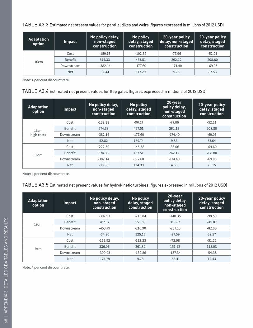
tABLe A3.3 estimated net present values for parallel dikes and weirs (figures expressed in millions of 2012 usd)

Adaptation option Impact

No policy delay, non-staged

construction

No policy delay, staged construction

20-year policy delay, non-staged

construction

20-year policy delay, staged construction

16cm

Cost -159.75 -102.62 -77.96 -52.21

Benefit 574.33 457.51 262.12 208.80

Downstream -382.14 -177.60 -174.40 -69.05

Net 32.44 177.29 9.75 87.53

Note: 4 per cent discount rate.

tABLe A3.4 estimated net present values for flap gates (figures expressed in millions of 2012 usd)

Adaptation option Impact

No policy delay, non-staged

construction

No policy delay, staged construction

20-year policy delay, non-staged

construction

20-year policy delay, staged construction

16cm high costs

Cost -139.38 -90.17 -77.86 -52.11

Benefit 574.33 457.51 262.12 208.80

Downstream -382.14 -177.60 -174.40 -69.05

Net 52.82 189.74 9.85 87.64

16cm

Cost -222.50 -145.58 -83.06 -64.60

Benefit 574.33 457.51 262.12 208.80

Downstream -382.14 -177.60 -174.40 -69.05

Net -30.30 134.33 4.65 75.15

Note: 4 per cent discount rate.

tABLe A3.5 estimated net present values for hydrokinetic turbines (figures expressed in millions of 2012 usd)

Adaptation option Impact

No policy delay, non-staged

construction

No policy delay, staged construction

20-year policy delay, non-staged

construction

20-year policy delay, staged construction

19cm

Cost -307.53 -215.84 -140.35 -98.50

Benefit 707.02 551.89 319.87 249.07

Downstream -453.79 -210.90 -207.10 -82.00

Net -54.30 125.16 -27.59 68.57

9cm

Cost -159.92 -112.23 -72.98 -51.22

Benefit 336.06 261.82 151.92 118.03

Downstream -300.93 -139.86 -137.34 -54.38

Net -124.79 9.73 -58.41 12.43

Note: 4 per cent discount rate.

68 |

Ap

pen

dix

3: d

etA

iLed

CB

A t

AB

Les

An

d R

esu

Lts

CG

LR | R

estoR

inG

WAteR

LeveLs on

LAK

e MiC

HiG

An

-Hu

Ro

n | 69

Appendix 4: our hydraulic scenario in contextThis section provides a rough sense of the comparability of our hydraulic scenario with the climate

sequences simulated in the IUGLS and the Lake Ontario-St. Lawrence Study Board (LOSLSB) report. To

reiterate from section 2.1.4, we use projected average water levels from 2041 to 2060 from the CCCma 2050

scenario. We then assume these levels for 2064 (the last year of our immediate construction time horizon)

and linearly interpolate values for missing years using 2014 as our start point.

We want to get a sense of the likelihood of observing our 2064 or low water level point under the climate

sequences simulated in the IUGLS and LOSLSB studies. Table A4.1 provides descriptions of selected

scenarios used to generate the sequences in these reports. Table A4.2 reports the percentile rank of our low

water level point relative to the monthly observations simulated under these 109-year sequences.

The assumptions of our dry, low water level scenario most closely approximate the assumptions of the

reports’ T1 scenario. According to Table A4.2, 20 per cent of the simulated monthly levels for Lake Michigan-

Huron in T1 fall below our 2064 level (these simulations assume the current regulation plan for Lake

Superior remains in place), whereas none of the simulated monthly levels for Lake Erie in T1 fall below our

2064 level. 10 per cent of simulated monthly levels for Erie do, however, fall below our 2064 level in the

studies’ TR or trend scenario.

Figures A4.1 through A4.4 plot the maximum, average and minimum water levels under the HI and T2

scenarios for each of the Great Lakes. The dashed lines refer to monthly values for the HI scenario. The

solid lines refer to monthly values for the T2 scenario. Scenarios for lakes Superior, Michigan-Huron and

Erie apply the 2014 Lake Superior regulation plan. The scenarios for Lake Ontario apply Plan 2014 and

regulation Plan 58DD for Lake Ontario.

As figures A4.1 through A4.4 indicate, our 2064 estimate is roughly comparable to the projected average for

Lake Superior under T2. It is slightly below average for lakes Michigan-Huron and Erie.

tABLe A4.1 description of iuGLs sequences

Classification Name

Ranking from least severe scenarios to

most severe scenarios for low water levels

Climate scenario Scenario description

HI 6 Historical Average Recorded NBS for 1900 to 2008

AT 5 Uncertain change One of the sequences produced by the Canadian regional climate models (RCM) that produces higher highs and lower lows.

AV 4 Change to drier A Canadian RCM sequence that produces lower levels.

T1 3 Change to drier One of hundreds of climate change sequences in which the climate change effect becomes more pronounced over time.

T2 2 Change to drier Another sequence in which climate change effect becomes more pronounced over time, but more severe than T1.

TR 1 Change to drier This sequence did not use climate models, but just extended historical NBS trends assuming the means would continue to change as they have in the last four decades.

tABLe A4.2 percentiles comparable by year

Classification Name

Regulation plan NatOpt3 (Current regulation plan for Lake Superior)

Superior Michigan-Huron ErieHI 0.02 0.00 0.00

AT 0.05 0.00 0.00

AB 0.05 0.01 0.00

T1 0.20 0.20 0.00

T2 0.50 0.10 0.00

TR 0.50 0.20 0.10

tABLe A4.3 Water levels past, present, and future

Lake 2014 water levels (in meters)

Historical average water levels (1918-2014 in meters)

CCCma2050 projection (in meters)

Superior 183.51 183.40 183.03

Michigan-Huron 176.30 176.42 175.43

Erie 174.20 174.14 173.35

Ontario 74.77 74.75 74.31

70 |

Ap

pen

dix

4: o

uR

Hyd

RA

uLi

C s

Cen

AR

io in

Co

nte

xt

CG

LR | R

estoR

inG

WAteR

LeveLs on

LAK

e MiC

HiG

An

-Hu

Ro

n | 71

fiGuRe A4.1 Monthly and yearly averages of different climate scenarios for the Great Lakes

LAKES MICHIGAN-HURON

LAKE ONTARIO

LAKE SUPERIOR

LAKE ERIE

P2014 Hi Max

P2014 Hi Avg

P2014 Hi Min

CCCma2050

P2014 TR Max

P2014 TR Avg

P2014 TR Min

173.0173.5174.0174.5175.0175.5176.0176.5177.0177.5178.0

DecNovOctSeptAugJulyJuneMayAprMarFebJan

72.0

72.5

73.0

73.5

74.0

74.5

75.0

75.5

76.0

DecNovOctSeptAugJulyJuneMayAprMarFebJan172.0

172.5

173.0

173.5

174.0

174.5

175.0

175.5

176.0

DecNovOctSeptAugJulyJuneMayAprilMarFebJan

181.0

181.5

182.0

182.5

183.0

183.5

184.0

DecNovOctSeptAugJulyJuneMayAprMarFebJan

See page 69 for a description of these figures.

Appendix 5: sensitivity analysis resultsOur analysis applies a four per cent discount rate. However, we also conduct sensitivity analyses using two

per cent and six per cent rates. Tables A5.1 and A5.2 report the net present values of the impacts of our four

sill options on lakes Michigan-Huron and Erie using these discount factors.

tABLe A5.1 estimated net present values for sills (figures expressed in millions of usd, 2 per cent discount rate)

Option ImpactNo policy delay, non-staged construction

No policy delay, staged construction

20-year policy delay, non-staged construction

20-year policy delay, staged construction

6cm

Cost -11.62 -9.35 -16.00 -14.47

Benefit 343.10 286.43 230.90 192.76

Downstream -224.66 -114.35 -151.19 -67.48

Net 106.82 162.73 63.71 110.81

21cm

Cost -63.12 -50.78 -68.94 -42.35

Benefit 1,200.84 1,002.51 808.13 674.66

Downstream -561.64 -400.22 -377.97 -236.18

Net 576.08 551.51 361.23 396.13

8cm

Cost -196.90 -158.40 -198.72 -114.77

Benefit 1,315.21 1,097.98 885.10 738.91

Downstream -615.13 -438.34 -413.96 -258.67

Net 503.18 501.25 272.41 365.46

23cm

Cost -196.90 -158.40 -198.72 -114.77

Benefit 1,315.21 1,097.98 885.10 738.91

Downstream -615.13 -438.34 -413.96 -258.67

Net 503.18 501.25 272.41 365.46

tABLe A5.2 estimated net present values for sills (figures expressed in millions of usd, 6 per cent discount rate)

Option ImpactNo policy delay, non-staged construction

No policy delay, staged construction

20-year policy delay, non-staged construction

20-year policy delay, staged construction

6cm

Cost -10.97 -6.12 -9.16 -7.64

Benefit 143.78 109.56 44.83 34.16

Downstream -179.92 -77.69 -56.10 -20.00

Net -47.11 25.75 -20.42 6.52

21cm

Cost -59.60 -33.25 -60.65 -16.10

Benefit 503.23 383.46 156.91 119.57

Downstream -449.80 -271.92 -140.25 -70.00

Net -6.17 78.30 -43.99 33.46

8cm

Cost -185.93 -103.71 -179.03 -38.07

Benefit 551.16 419.98 171.85 130.95

Downstream -492.63 -297.81 -153.61 -76.67

Net -127.41 18.46 -160.78 16.21

23cm

Cost -185.93 -103.71 -179.03 -38.07

Benefit 551.16 419.98 171.85 130.95

Downstream -492.63 -297.81 -153.61 -76.67

Net -127.41 18.46 -160.78 16.21

72 |

Ap

pen

dix

5: s

ensi

tivi

ty A

nA

Lysi

s R

esu

Lts

CG

LR | R

estoR

inG

WAteR

LeveLs on

LAK

e MiC

HiG

An

-Hu

Ro

n | 73

Works citedAsadzadeh, M., S. Razavi, B.A. Tolson, and D. Fay. 2014. “Pre-emption strategies for efficient multi-objective optimiziation: Application to the development of Lake Superior regulation plan.” Environmental Modelling & Software, 54, 128-141.

Baic, D. and M. Whetstone. 2013. “That was then, this is now. How water levels have fallen on Georgian Bay”. The Globe and Mail. http://www.theglobeandmail.com/news/national/water-levels/article13365158/. Last accessed 16 May 2015.

Bergeron, D., and G. Clark. 2011. “Economic Implications of Climate Change Impacts to Great Lakes Ports, Harbors, and Marinas.” Webinar available at http://changingclimate.osu.edu/webinars/ archives/2011-03-01/. Last accessed 10 June 2014.

Bialkowski, B. 2012. “Restoring Lake Michigan Huron Water Levels Responsibly.” http://www.sierraclub.ca/sites/sierraclub.ca/files/bialkowski_2012-11-10-kelk-presentation-final_shortened.pdf. Last accessed 27 November 2015.

Boating Ontario, n.d. Interactive map of marinas. http://www.boatingontario.ca/Find/Interactivemapofmarinas.aspx. Last accessed 13 November 2015.

Bruxer, J. 2011. Potential St. Clair River restoration structures. Report to the International Upper Great Lakes Study. http://www.iugls.org/DocStore/ProjectArchive/AMG_AdaptiveManagement/AMG05_Bruxer_LiteratureReviewReview RegulationCompensation/Reports/AMG05-R2_Bruxer.pdf. Last accessed 18 November 2015.

Buttle, J., T. Muir, and J. Frain. 2004. “Economic Impacts of Climate Change on the Canadian Great Lakes Hydro–Electric Power Producers: A Supply Analysis.” Canadian Water Resources Journal, 29, 89-110.

Case Book: The Harms Caused by Low Water Levels in Georgian Bay 2012-2013. 2013.http://www.thebluemountains.ca/public_docs/documents/GB%20Final%20Casebook%20Re%20Low%20Water%20Levels.pdf. Last accessed 18 November 2015.

Cattaneo, A., C. Hudon, C. Vis, and P. Gagnon. 2013. “Hydrological Control of Filamentous Green Algae in a Large Fluvial Lake (Lake Saint-Pierre, St. Lawrence River, Canada).” Journal of Great Lakes Research, 39, 409–419.

English, G., and D. C. Hackston. 2013. Environmental and Social Impacts of Marine Transport. Research and Traffic Group.

Franco, J. J. and J.E. Glover, 1972. Effects of Submerged Sills in the St. Clair River; Hydraulic Model Investigation. Technical Report H-72-4. U.S. Army Engineer Waterways Experiment Station, Vicksburg, Mississippi. http://acwc.sdp.sirsi.net/client/search/asset/1034201. Last accessed 18 November 2015.

Frost, J. and W. Merte. 2011. Cost Engineering Report and Resource Requirements for the Potential St. Clair River Restoration and Regulation Structures. Report to the International Upper Great Lakes Study. http://iugls.org/DocStore/ProjectArchive/RST_RestorationOfMichiganHuronLevels/RST01_MerteFrost_CostEstimatesPotentialStClair RestorationStructures/Reports/RST01-R1_FrostMerte_StClairCostEstimateSummary.pdf. Last accessed 18 November 2015.

Georgian Bay Forever. 2012. Comments to the International Joint Commission on the recommendations of the International Upper Great Lakes Study. Caledon, ON: Georgian Bay Forever.

Greenwood’s. 2013. Greenwoods’s Guide to Great Lakes Shipping 2013. Boyne City, MI: Harbour House Publishers.

Gronewold, A.D., E. J. Anderson, B. Lofgren, P. D. Blanken, J. Wang, J. Smith, T. Hunter, G. Lang, C. A. Stow, D. Beletsky, J. Bratton. 2015a. “Impacts of extreme 2013-2014 winter conditions on Lake Michigan’s fall heat content, surface temperature, and evaporation.” Geophysical Research Letters, 42, 3364-3370.

Gronewold, A.D., A. H. Clites, J. Bruxer, K. W. Kompoltowicz, J, P. Smith, T. S. Hunter, and C. Wong. 2015b. “Water Levels Surge on Great Lakes.” Eos, 17 March 2015.

Gronewold, A.D., and C.A. Stow. 2014. “Water Loss from the Great Lakes.” Science, 343, 1084-1085.

International Energy Agency (IEA). 2010. “Renewable Energy Essentials: Hydropower.”http://www.iea.org/publications/freepublications/publication/hydropower_essentials.pdf. Last accessed 18 November 2015.

International Great Lakes Diversions and Consumptive Uses Study Board (IGLDCUSB). 1981. Great Lakes Diversions and Consumptive Uses. Report to the International Joint Commission.

International Great Lakes Levels Board. 1973. Regulation of Great Lakes Water Levels. Report to the International Joint Commission.

The International Great Lakes – St. Lawrence River Adaptive Management Task Team. 2013. “Building Collaboration Across the Great Lakes St. Lawrence River System: An Adaptive Management Plan for Addressing Extreme Water Levels, Breakdown of Roles, Responsibilities, and Proposed Tasks.” Report to the International Joint Commission. http://www.ijc.org/files/publications/FinalReport_AdaptiveManagementPlan_20130530.pdf. Last accessed 18 November 2015.

International Joint Commission (IJC). 2000. Protection of the Waters of the Great Lakes. Final Report to the Governments of Canada and the United States.

International Joint Commission (IJC). 2012. Guidance in Seeking Approval for Uses, Obstructions, or Diversions of Waters Under the Boundary Waters Treaty of 1909.

International Joint Commission (IJC). 2014. “IJC reaffirms Plan 2014 for Lake Ontario and St. Lawrence River.” http://www.ijc.org/en_/news?news_id=445. Last accessed 18 November 2015.

International Lake Erie Regulation Study Board. 1981. Lake Erie Water Level Study. Report to the International Joint Commission.

International Lake Ontario-St. Lawrence River Study Board (ILOSLRSB). 2006. Options for Managing Lake Ontario and St. Lawrence River Water Levels and Flows. Report to the International Joint Commission. http://www.ijc.org/loslr/en/library/LOSLR%20Study%20Reports/report-main-e-6KB.pdf. Last accessed 18 November 2015.

International Upper Great Lakes Study (IUGLS). 2009. Impacts on Upper Great Lakes Water Levels: St. Clair River – Summary Report. Report to the International Joint Commission. http://www.ijc.org/files/publications/IUGLS%20St%20Clair%20Report%20Summary.pdf. Last accessed 18 November 2015.

International Upper Great Lakes Study (IUGLS). 2012. Lake Superior Regulation: Addressing Uncertainty in Upper Great Lakes Water Levels. Report to the International Joint Commission. http://www.ijc.org/files/tinymce/uploaded/IUGLS_Summary_Report.pdf. Last accessed 18 November 2015.

74 |

Wo

RK

s C

ited

Kavcic, R. 2015. “Great Lakes-St. Lawrence Region: North America’s Economic Engine.” Bank of Montreal Special Report. April 2015. http://www.bmonesbittburns.com/economics/reports/20150427/sr150427.pdf. Last accessed 18 November 2015.

Kling, G. W., Katharine H., L. B. Johnson, J. J. Magnuson, S. Polasky, S. K. Robinson, B. J. Shuter, M. M. Wander, D. J. Wuebblesband D. R. Zak. 2003. Confronting Climate Change in the Great Lakes Region: Impacts on Our Communities and Ecosystems. Cambridge, MA: Union of Concerned Scientists, and Washington, DC: The Ecological Society of America.

Kumar, A., R.P. Saini. 2014. “Development of Hydrokinetic Power Generation System: A Review.” 2014. International Journal of Engineering Science and Advanced Technology, 4, 464-477.

Lenters, J.D., J.B. Anderton, P.D. Blanken, C. Spence, A.E. Suyker. 2013. “Assessing the Impacts of Climate Variability and Change on Great Lakes Evaporation: Implications for water levels and the need for a coordinated observation network.” In 2011 Project Reports. D. Brown, D. Bidwell, and L. Briley, eds. Great Lakes Integrated Sciences and Assessments (GLISA) Center. http://glisa.umich.edu/media/files/projectreports/GLISA_ProjRep_Lake_Evaporation.pdf. Last accessed 18 November 2015.

Levels Reference Study Board (LRSB). 1993. Levels Reference Study – Great Lakes-St. Lawrence Basin. Report to the International Joint Commission. March 1993. http://graham.umich.edu/media/files/water-levels-ijc-reference-study-1993.pdf. Last accessed 18 November 2015.

Macfarlane, D. 2014. Negotiating a River: Canada, the US and the Creation of the St. Lawrence Seaway. UBC Press.

Marine Delivers. n.d. “Great Lakes Commercial Ports.” http://www.marinedelivers.com/great-lakes-commercial-ports. Last accessed 18 November 2015.

Millerd, F. 2005. “The Economic Impact of Climate Change on Canadian Commercial Navigation on the Great Lakes.” Canadian Water Resources Journal, 30, 269–280. http:// www.tandfonline.com/doi/pdf/10.4296/ cwrj3004269. Last accessed June 10, 2014.

Mortsch, L. D. 1998. “Assessing the Impact of Climate Change on the Great Lakes Shoreline Wetlands.” Climatic Change, 40, 391-416.

Ontario Centre for Climate Impacts and Adaptation Resources. 2010. International Upper Great Lakes Study: Recreational Boating Final Report. Sudbury, ON: Mining Innovation, Rehabilitation and Applied Research Corporation (MIRARCO).

Quinn, F. H. 2002. “The Potential Impacts of Climate Change on Great Lakes Transportation.” In The Potential Impacts of Climate Change on Transportation: A Federal Research Partnership Workshop, 115-124. US Department of Transportation Centre for Climate Change and Environmental Forecasting.

Saint Lawrence Seaway Development Corporation. 2014. “Why You Should Care About the Seaway!” Seaway Compass, Winter 2014. http://www.greatlakes-seaway.com/en/pdf/slsdc_newsletter_winter_2014.pdf. Last accessed 18 November 2015.

Shlozberg, R., R. Dorling and P. Spiro. 2014. Low Water Blues: An Economic Impact Assessment of Future Low Water Levels in the Great Lakes and St. Lawrence River. The Mowat Centre, June 2014. http://www.mowatcentre.ca/wp-content/uploads/publications/89_low_water_blues.pdf. Last accessed 18 November 2015.

Tolson, B., S. Razavi and M. Asadzadeh. 2011. Formulation and Evaluation of New Control Structures in the Great Lakes System. Report to the International Upper Great Lakes Study. http://www.iugls.org/files/tinymce/uploaded/PeerReview_pdfs/MultiLake%20Regulation%20Final%20Report%20-%20Initial%20Draft.pdf. Last accessed 18 November 2015.

United States Army Corps of Engineers (USACE). 2008. “Great Lakes Recreational Boating.” In Response to Public Law 106-53, Water Resources Development Act of 1999, Section 455(c), John Glenn Great Lakes Basin Program, Great Lakes Recreational Boating: Main Report. Washington, DC: United States Army Corps of Engineers.

United States Department of Transportation Maritime Administration, 2013. Status of the U.S.-Flag Great Lakes Water Transportation Industry. Washington, DC: United States Department of Transportation Maritime Administration.

United States Energy Information Administration, 2014. Levelized Cost of New Generation Resources in the Annual Energy Outlook 2014. http://www.eia.gov/forecasts/ aeo/er/pdf/electricity_generation.pdf.

CG

LR | R

estoR

inG

WAteR

LeveLs on

LAK

e MiC

HiG

An

-Hu

Ro

n | 75

the Council of the Great Lakes Region (CGLR) is a member-based organization with a mandate to collaborate with the many successful organizations already working in the region to high-light, enhance and support their projects. the Council also looks to inform state, provincial and federal decision makers in both countries about the region’s long-term economic, social, and environmental goals. finally, the Council is also working to play a leadership role in connecting private, public, and not-for-profit actors across the region, cultivating a strong regional voice to promote shared interests and solutions to our common challenges.

the Mowat Centre is an independent public policy think tank located at the school of public policy & Governance at the university of toronto. the Mowat Centre is ontario’s non-partisan, evidence-based voice on public policy. it undertakes collaborative applied policy research, proposes innovative research-driven recommendations, and engages in public dialogue on Canada’s most important national issues.

COUNCIL OF THE GREAT LAKES REGION

subscribe to our mailing list, become a sponsor member and learn more about CGLR at: councilgreatlakesregion.org613.668.2044 | councilgreatlakesregion.org | info@councilgreatlakesregion.org439 university Avenue, suite 2200 · toronto, on · Canada · M5G 1y811075 east Blvd, #245A · Cleveland, ohio · 44106

@MowatCentre the Mowat Centre

@CGLRGreatLakes Council of the Great Lakes Region