responsiveness of residential electricity demand in oecd
TRANSCRIPT

FCN Working Paper No. 8/2011
Responsiveness of Residential Electricity Demand
in OECD Countries: A Panel Cointegation and
Causality Analysis
Ronald Bernstein and Reinhard Madlener
April 2011
Institute for Future Energy Consumer Needs and Behavior (FCN)
School of Business and Economics / E.ON ERC

FCN Working Paper No. 8/2011
Responsiveness of Residential Electricity Demand in OECD Countries: A Panel
Cointegation and Causality Analysis
April 2011
Authors’ addresses: Ronald Bernstein, Reinhard Madlener Institute for Future Energy Consumer Needs and Behavior (FCN) School of Business and Economics / E.ON Energy Research Center
RWTH Aachen University Mathieustrasse 6
52074 Aachen, Germany E-mail: [email protected], [email protected]
Publisher: Prof. Dr. Reinhard Madlener Chair of Energy Economics and Management Director, Institute for Future Energy Consumer Needs and Behavior (FCN) E.ON Energy Research Center (E.ON ERC) RWTH Aachen University Mathieustrasse 6, 52074 Aachen, Germany
Phone: +49 (0) 241-80 49820 Fax: +49 (0) 241-80 49829 Web: www.eonerc.rwth-aachen.de/fcn E-mail: [email protected]

1
Responsiveness of Residential Electricity Demand in OECD Countries: A Panel Cointegration and Causality Analysis
Ronald Bernstein* and Reinhard Madlener
Institute for Future Energy Consumer Needs and Behavior (FCN), School of Business and Economics / E.ON Energy Research Center, RWTH Aachen University,
Mathieustrasse 6, 52074 Aachen, Germany
April 2011
Abstract
In this paper we estimate residential electricity demand elasticities and conduct an analysis of the causal relationship between electricity demand, disposable income and electricity price for a group of several OECD members. We apply panel cointegration and Granger causality testing to a data set consisting of eighteen countries in the cross-sectional dimension and the years 1981–2008 in the time domain. Our results for the whole panel indicate a near unity income elasticity and an inelastic price elasticity of approximately –0.4 in the long run. These results are robust with regard to the estimation methods employed (group-means panel FMOLS and DOLS). In the short run, our estimates from an ECM indicate an income elasticity of 0.2 and a price elasticity of approximately –0.1. Moreover, our tests on Granger causality provide an indication for a bidirectional causal relationship between electricity consumption and economic growth. Hence, our findings are in favor of the feedback hypothesis.
JEL classification: Q41; Q43
Keywords: Residential electricity demand; Elasticities; Panel cointegration; Granger-causality; OECD countries
__________________________________
* Tel.: +49 241 80 49 832; fax: +49 241 80 49 829; e-mail: [email protected] (R. Bernstein);
[email protected] (R. Madlener)

2
1. Introduction
Insights concerning the responsiveness of energy demand to other economic factors have a
crucial relevance for policy advice with regard to objectives such as the security of energy
supply and GHG abatement. Especially in the light of the current debate and concern
regarding anthropological causes of global warming and its effects on the environment, these
topics have risen again on the agenda of policy-makers and researchers alike.
A possible policy instrument for the purpose of energy conservation is a Pigouvian energy
tax. Therefore, knowledge about the response of energy consumption to changes in energy
prices is of paramount importance for optimal policy design.
Furthermore, the assessment of the causal relationship between energy use and economic
activity is valuable for an appraisal of potentially conflicting policy objectives, such as the
trade-off between energy conservation and economic growth. There are four opposing
economic hypotheses regarding the causal mechanisms underlying the energy consumption –
economic growth nexus, which are currently heavily under debate in the energy economics
literature (for a useful survey see Payne, 2010): the conservation hypothesis, the growth
hypothesis, the feedback hypothesis and the neutrality hypothesis. While the conservation
hypothesis implies causality running from economic growth to energy consumption, the
growth hypothesis implies the opposite causal relationship. The feedback hypothesis
combines the latter hypotheses, by claiming an interdependent causal relationship between
both variables. Finally, the neutrality hypothesis states that both variables are only of little
importance in determining each other.
Most previous studies on estimating residential electricity demand elasticities are based on
time series data. One major problem of economic time series is the likely existence of
stochastic trends in the variables. This requires applying econometric approaches, i.e. unit
root and cointegration methods, which take the nonstationarity of the data-generating process
(DGP) underlying the considered variables explicitly into account. However, traditional unit
root and cointegration tests in a pure time series context are known to suffer from the problem
of very low power and size. Hence, increasing the number of observations by including a
cross-sectional dimension helps to reduce this problem. The added cross-sections can be
interpreted as repeated draws from the same distribution, that increase power and hence
permit more reliable statistical inference.

3
The aim of this paper is twofold. First, we estimate residential electricity demand elasticities
with regard to income and own price for a group of OECD countries, thereby differentiating
between the short and the long run in an error correction framework. The long-run
relationship is estimated by applying the fully modified ordinary least squares (FMOLS) and
dynamic OLS (DOLS) group-means panel estimators (Pedroni, 2000 and 2001) to a panel of
eighteen countries in the cross-sectional dimension and the period 1981–2008 in the time
domain. The countries considered are: Austria, Denmark, Finland, France, Germany, Greece,
Ireland, Italy, Japan, Mexico, the Netherlands, Norway, Portugal, South Korea, Spain,
Switzerland, the UK and the US.
Second, we investigate the causal relationship between residential electricity demand,
disposable income and electricity price by utilizing the concept of Granger causality (Granger,
1969). For this purpose we employ the pooled mean group estimator (PMGE) proposed by
Pesaran et al. (1999) for estimating a trivariate panel vector error correction model (PVECM).
A set of tests on short-run, long-run and joint causality are conducted, in order to assess the
direction of causality between the variables at hand.
Following the arguments in Bernstein and Madlener (2010), we choose a disaggregate
approach in the sense that, firstly, we restrict our analysis to one energy carrier (electricity).
Secondly, we only examine one economic sector (households), aiming at capturing the
behavior of a relatively homogeneous group of economic agents.
The econometric estimation of energy demand elasticities has a long tradition, going back as
far as the early 1950’s. Among the first studies are Houthakker (1951), Fisher and Kaysen
(1962), Halvorsen (1975) and Pindyck (1979). Similarly, the related literature strand aimed at
determining the causal relationship in the energy-growth nexus was sparked by the early work
of Kraft and Kraft (1978), and has received considerable interest in the last ten to fifteen
years. However, it was only with the introduction of cointegration analysis, which was
triggered by the seminal paper of Engle and Granger (1987), that the problem of spurious
regressions was starting to be adequately dealt with in econometric applications.
Table 1 gives an overview of selected recent studies on residential electricity demand
elasticities, most of which employ pure time series methods for single countries:1 Athukorala 1 We only consider studies here that employ time-series or panel estimation techniques, that account for non-
stationarity in the DGP, and that were published after the year 2000.

4
and Wilson (2010) for Sri Lanka; Dergiadis and Tsoulfidis (2008) for the US; Halicioglu
(2007) for Turkey; Holtedahl and Joutz (2004) for Taiwan; Hondroyiannis (2004) for Greece;
Nakajima (2010) for Japan; Nakajima and Hamori (2010) for the US; Narayan and Smyth
(2005) for Australia; Narayan et al. (2007) for the G7 countries; Zachariadis and Pashourtidou
(2007) for Cyprus and Ziramba (2008) for South Africa. The long-run demand elasticities
from these studies range between 0.25 and 1.57 with regard to income and between –0.14 and
–1.56 with regard to own price. For the short run, the elasticity estimates range between 0.10
and 0.44 with regard to income and between –0.11 and –0.46 with regard to own price.
Unlike the majority of the studies reported, Nakajima and Hamori (2010), Nakajima (2010)
and Narayan et al. (2007), use cointegration techniques that are based on panel data in their
analyses. In order to attain a cross-sectional dimension, the former two studies make use of
available data on geographical regions within Japan and the US, respectively. The latter study
is closest to ours with regard to the countries2 analyzed and the econometric approach used,
but interestingly comes to different conclusions. Specifically, Narayan et al. (2007) analyze a
panel consisting of the G7 countries as the cross-sectional dimension for the time period
1978–2003. They employ both the OLS and the DOLS method (Stock and Watson, 1993; Kao
and Chiang, 2000) to estimate the cointegration relationship between electricity demand,
income, electricity price, and natural gas price. For the whole panel they estimate an inelastic
income elasticity of 0.25 (0.31) and an elastic price elasticity of –1.56 (–1.45) using DOLS
(OLS). Consequently, they come to the conclusion that pricing policies aimed at reducing
residential electricity consumption and hence GHG emissions are bound to be successful.
Table 2 displays the three studies from the set of studies mentioned above that conduct
Granger causality analyses for residential electricity consumption, income and electricity
price. Dergiades and Tsoulfidis (2008) and Halicioglu (2007) both find unidirectional long-
run causality from income and price to electricity consumption. For the short run, the former
find causality from electricity price to income, while the latter finds causality from income
and price to electricity consumption.3 Zachariadis and Pashourtidou (2007) find evidence for a
2 Our set of countries also includes the G7 countries, except for Canada, for which recent data on the residential
electricity price were lacking. 3 Dergiades and Tsoulfidis (2008) also consider other variables such as oil price and cooling and heating degree
days, for which we do not report the results.

5
Table 1 Recent residential electricity demand studies and elasticity estimates
Study Country Method Data Elasticity estimates Income Price
Athukorala & Wilson (2010)
Sri Lanka Johansen / VECM
Time series, 1960–2007 (annual)
L: 0.78 S: 0.32
L: –0.62 S: –0.16
Dergiades & Tsoulfidis (2008)
US Bounds testing / ARDL
Time series, 1965–2006 (annual)
L: 0.27 S: 0.10
L: –1.07 S: –0.39
Halicioglu (2007)
Turkey Bounds testing / ARDL
Time series, 1968–2005 (annual)
L: 0.49 to 0.70 S: 0.37 to 0.44
L: –0.52 to –0.63 S: –0.33 to –0.46
Holtedahl & Joutz (2004)
Taiwan Johansen / VECM
Time series, 1955–1995 (annual)
L: 1.04 to 1.57 S: 0.22
L: –0.15 S: –0.15
Hondroyiannis (2004)
Greece Johansen / VECM
Time series, 1986–1999 (monthly)
L: 1.56 S: 0.20
L: –0.41
Nakajima (2010)
Japan Panel cointegration, DOLS
Panel data, 1975–2005 (annual), T × N: 31 × 46 = 1426
L: 0.60 to 0.65 L: –1.13 to –1.20
Nakajima & Hamori (2010)
US Panel cointegration, DOLS
Panel data, 1993–2008 (quarterly), T × N: 32 × 49 = 1568
L: 0.38 to 0.85 L: –0.14 to –0.33
Narayan & Smyth (2005)
Australia Bounds testing / ARDL
Time series, 1969–2000 (annual)
L: 0.32 to 0.41 S: 0.01 to 0.04
L: –0.47 to –0.54 S: –0.26 to –0.27
Narayan et al. (2007)
G7 Panel Cointegration, OLS & DOLS
Panel data, 1978–2003 (annual), T × N: 26 × 7 = 182
L: 0.25 to 0.31 S: –0.19
L: –1.45 to –1.56 S: –0.11
Zachariadis & Pashourtidou (2007)
Cyprus Johansen / VECM
Time series, 1960–2004 (annual)
L: 1.18 L: –0.43
Ziramba (2008)
South Africa
Bounds testing / ARDL
Time series, 1978–2005 (annual)
L: 0.31 to 0.87 S: 0.30
L: –0.01 to –0.04 S: –0.02
Notes: S and L denote estimates for the short and the long run, respectively. Elasticity estimates which are not statistically significantly different from zero on conventional levels are printed in italics. T: Number of time series observations; N: Number of cross-sections. DOLS: Dynamic OLS; ARDL: Autoregressive Distributed Lag.
long-run causal relationship, running from income and price to electricity consumption, and
from electricity consumption and price to income. For the short run, they only find causality
running from electricity consumption to income. Hence, so far there is empirical evidence for

6
the conservation as well as the feedback hypothesis concerning the causal relationship
between residential electricity demand and real income.
Table 2 Results from causality analyses on residential electricity demand
Study Country Data Direction of causality Long-run Short-run
Dergiades & Tsoulfidis (2008)
US Time series, 1965–2006 (annual)
Y, P → E P → Y
Halicioglu (2007) Turkey Time series, 1968–2005 (annual)
Y, P → E Y, P → E
Zachariadis & Pashourtidou (2007)
Cyprus Time series, 1960–2004 (annual)
Y, P → E E, P → Y
E → Y
Notes: Y: Income; P: Electricity price; E: Electricity consumption; → denotes the direction of causality.
Our paper proceeds as follows. In Section 2, we provide the analytical framework for the
econometric analysis undertaken. Section 3 gives a methodological overview of the applied
estimation and testing procedures applied, while Section 4 discusses the data, the application
of the model and the results from the analysis. Section 5 concludes.
2. Analytical framework
The long-run relationship between residential electricity demand and its determinants can be
characterized by the general function
, , , ,, , ,i t i t i t i tE f Y P X (1)
with the subscripts i (i = 1,…, N) and t (t = 1,…, T), denoting the cross-sectional and time
dimension, respectively. Eq. (1) states that residential electricity consumption per capita (Ei,t)
is a function of real (disposable) income per capita (Yi,t) and real residential electricity price
(Pi,t).4 Previous studies on residential electricity demand have included further control
variables (Xt), as for example the real price of an electricity substitute (e.g., Narayan et al.,
2007), heating and cooling degree days (e.g., Zachariadis and Pashourtidou, 2007), 4 In the following, real disposable income per capita and real residential electricity price will be referred to as
“income” and “electricity price” for brevity.

7
urbanization (e.g., Holtedahl and Joutz, 2004), and capital variables (e.g., Silk and Joutz,
1997).
Following the principle of Occam’s razor, we choose a parsimonious specification, which
only includes real disposable income per capita and real residential electricity price as
determinants of electricity demand. Furthermore, as the following analysis comprises a panel
of various countries, problems with the availability of data on additional variables would have
brought further restrictions to the data set with regard to the cross-sections and/or the time
period studied.5 Finally, having less parameters to estimate has the advantage of attaining
more degrees of freedom in the estimation of the core explanatory variables’ coefficients.
More specifically, the demand model on which our econometric analysis is based takes the
following standard constant elasticity functional form:
, , ,
, , , ,y i p i i t
i t i i t i tE C Y P e (2)
where the subscripts i (i = 1, …, N) and t (t = 1, …, T) represent the cross-sectional dimension
(the eighteen countries considered) and the time dimension (the years 1981–2008 considered),
respectively. Ci are country-specific drift terms, e is Euler’s number, εi,t are random error
terms, and βy,i and βp,i are the long-run elasticities to be estimated with regard to income and
electricity price, respectively. A higher income is expected to increase electricity demand on
account of higher economic activity, whereas a higher electricity price is naturally expected to
decrease electricity demand. Moreover, the price elasticity is expected to be inelastic, as in
general electricity is characterized by a lack of substitutability.
3. Methodology
3.1. Panel unit root tests
As a preliminary analysis, we check for the order of integration of the single series by
employing a number of panel unit root tests. In detail, these are: the LLC (Levin et al., 2002),
5 Also, not all variables, such as cooling degree days or the price of natural gas, are likely to have the same
relevance or, more specifically, similar explanatory power for all the considered countries.
8
the UB (Breitung, 2000), the IPS (Im et al., 2003), the ADF-Fisher (Maddala and Wu, 1999),
and the PP-Fisher (Maddala and Wu, 1999).
All the mentioned tests are based on the following AR(1) panel regression model:
, , 1 , , ,i t i i t i i t i tx x X u i = 1, 2, …, N; t = 1, 2, …, T, (3)
where δi are the autoregressive parameters, Xi,t represents exogenous variables and/or fixed
effects and cross-section-specific time trends and ui,t are stationary error terms. In the case
that |δi| < 1, xi is referred to be weakly trend-stationary. In contrast, if |δi| = 1, xi is considered
to be a unit root process.
The five aforementioned tests can be divided into two different groups with respect to the
assumptions about the δi. The LLC test and the UB test assume that all cross-sections have a
common unit root, i.e. δi = δ for all i. On the other hand, the IPS test, the ADF-Fisher test and
the PP-Fisher test all assume that the δi can be heterogeneous across the cross-sections. In
order to save space we refer the reader to the original articles for further details on these tests.
In the case where the test results for a variable in levels indicate a rejection of the null
hypothesis, whereas the test results for the same variable in first differences does not reject
the null at conventional significance levels, this variable is assumed to be integrated of order
one, denoted I(1).
3.2. Panel cointegration tests
Given that the variables electricity consumption, income and electricity price are all integrated
of order one, i.e. ei,t, yi,t, pi,t ~ I(1), we can include them in the cointegration analysis, in order
to be able to estimate the long-run relationship described by Eq. (2). Taking natural
logarithms of Eq. (2) yields the econometric specification of our long-run residential
electricity demand function:
, , , , , , ,i t i y i i t p i i t i te c y p i = 1, 2, …, N; t = 1, 2, …, T, (4)
where ei,t = ln(Ei,t), yi,t = ln(Yi,t), pi,t = ln(Pi,t), ci are country-specific fixed effects and εi,t are the
error terms, which are interpreted as deviations from long-run equilibria. The country-specific
slope coefficients βy,i and βp,i are the long-run elasticities to be estimated with regard to

9
income and electricity price, respectively. Hence, this specification allows for the
cointegrating vectors to vary across the single countries of our panel.
Pedroni (1999, 2004) extends the cointegration testing approach of Engle and Granger (1987),
which is based on examining the stationarity properties of the residuals from a regression
using I(1) variables, to a panel data setting. Following this approach, Eq. (4) is estimated by
OLS, and the residuals obtained, ,i t , are used for the following auxiliary autoregression for
every i:
, , 1 , , ,1
ˆ ˆ ˆ ,in
i t i i t i t i t j i tj
w
(5)
Where the ρi are autoregressive parameters, ni are the lag lengths in the augmented case, and
wi are stationary error terms.
Under the null hypothesis of no cointegration, the ,i t should be found to be I(1). This is the
case if
0 : 1, 1,...,iH i N
is not rejected. For each of the seven statistics provided by Pedroni (1999, 2004) this is the
null hypothesis. Concerning the alternative hypothesis, the tests can be divided into two
classes. For the so-called (within-dimension) panel statistics tests (i.e. the Panel-v, the Panel-
PP-ρ, the Panel-PP-t and the Panel-ADF-t test) the alternative hypothesis is
1 : 1, 1,..., ,iH i N
whereas for the so-called (between-dimension) group statistics tests (i.e. the Group-PP-ρ, the
Group-PP-t and the Group-ADF-t test) the alternative hypothesis is
1 : 1, 1,..., .iH i N
Hence, the group statistics tests are less restrictive in the sense that they allow for
heterogeneity across countries.

10
3.3. Estimation of long- and short-run elasticities
Given that the panel cointegration tests indicate a significant cointegration relationship, we
apply the fully modified OLS (FMOLS) and the dynamic OLS (DOLS) group-means panel
estimators proposed by Pedroni (2000, 2001) for estimating the long-run demand relationship
characterized by Eq. (4). Both estimators allow for standard normal inference through
incorporating corrections for endogeneity bias and serial correlation.6 While the FMOLS
estimator employs a semi-parametric correction using Δyi,t, Δpi,t and ,i t , the DOLS estimator
employs a parametric approach by augmenting Eq. (4) with lead and lag dynamics of Δyi,t and
Δpi,t as follows:
, , , , , , , , , , , ,
i i
i i
l l
i t i y i i t p i i t y i l i t l p i l i t l i tl l l l
e y p y p
(6)
where li is the lead and lag length, μi is the country-specific fixed effect and υi,t is the error
term.
The group-means FMOLS and DOLS panel estimates for the slope coefficients, ˆ FMOLSG and
ˆ DOLSG , and their corresponding t-statistics, ˆ FMOLS
Gt and ˆ DOLSGt , are calculated as follows:
, ,1
1ˆ ˆN
m mG y y i
iN
(7)
, ,1
1ˆ ˆN
m mG y y i
i
t tN
(8)
, ,1
1ˆ ˆN
m mG p p i
iN
(9)
, ,1
1ˆ ˆN
m mG p p i
i
t tN
(10)
where the superscript m is a place holder denoting either the FMOLS or the DOLS estimation
method; ,
ˆy i and
,ˆ
p i are the country-specific estimates of income and price elasticity,
respectively.
6 Harris and Sollis (2003) provide an excellent exposition on this topic.
11
Considering both the FMOLS and the DOLS panel approach has the advantage of being able
to provide some evidence on the robustness of our results with regard to the estimation
method.
In order to estimate the short-run elasticities and the speed of adjustment to long-run
equilibrium, the residuals from the cointegrating regressions, which resemble the deviation
from long-run equilibrium in any given period t, are used as error correction terms (ECT) in
country-specific and panel error correction models (ECM). The latter takes on the following
form
, 0, , 1 , , , , , ,m m m m m mi t i i i t y i i t p i i t i te ECT y p (11)
where m denotes the estimation method (FMOLS or DOLS), γ0,i is a country-specific
constant, αi is the speed of adjustment coefficient, ECTi is the aforementioned error correction
term lagged by one period, γy,i and γp,i are the short-run income and price elasticities,
respectively, and νi,t are the error terms. To ensure an error correction mechanism via
adjustments of electricity consumption, αi has to be negative.
3.4. Panel Granger causality
A cointegration relationship between a set of variables necessarily implies Granger causality
in at least one direction. For the residential electricity demand relationship in Eq. (2), the
direction of Granger causality between the single variables is tested by the two-step Engle-
Granger procedure (Engle and Granger, 1987) on the basis of the following PVECM:
, 1, 1, , 1 11, , , 12, , , 13, , , 1, ,1 1 1
k k km m m m m m m
i t i i i t i j i t j i j i t j i j i t j i tj j j
e ECT e y p
(12a)
, 2, 2, , 1 21, , , 22, , , 23, , , 2, ,1 1 1
k k km m m m m m m
i t i i i t i j i t j i j i t j i j i t j i tj j j
y ECT e y p
(12b)
, 3, 3, , 1 31, , , 32, , , 33, , , 3, ,1 1 1
k k km m m m m m m
i t i i i t i j i t j i j i t j i j i t j i tj j j
p ECT e y p
(12c)
where m again denotes the estimation method, ECTi is the error correction term (obtained
from estimation of Eq. (4)), k is the lag length, the ϕi are the speed of adjustment coefficients,

12
the γi are country-specific constants, the θi are short-run coefficients and the φi,t are serially
uncorrelated error terms. The equation system (12a-c) is estimated by the PMGE method
proposed by Pesaran et al. (1999).
For the long run, the direction of Granger causality can be checked for by testing whether the
adjustment coefficient of the respective equation is significantly different from zero. Besides
long-run Granger causality, short-run Granger causality can occur through the lagged first
differences of the independent variables in each equation of the system. Hence we check for
short-run Granger causality from income and electricity price to electricity consumption by
testing H0 : θ12,i,j = 0, i,j and H0 : θ13,i,j = 0, i,j in Eq. (12a). For short-run Granger causality
from electricity consumption and electricity price to income in Eq. (12b), we test H0 : θ21,i,j =
0, i,j and H0 : θ23,i,j = 0, i,j, respectively. In Eq. (12c) we test H0 : θ31,i,j = 0, i,j and
H0 : θ32,i,j = 0, i,j for short-run Granger causality running from electricity consumption and
income to electricity price, respectively. Finally, we test on the joint significance between the
lagged ECT and the lagged differences of the independent variables in the respective
equations in order to check for strong causality in each equation.
4. Empirical analysis
4.1. Data
We make use of annual data on residential electricity consumption, net disposable income and
residential electricity price, which are all available for a reasonable length of time (1978–
2008) for eighteen OECD countries already mentioned in the introduction.
The time series are transformed as follows: In order to obtain real values, disposable income
and residential electricity price are deflated to the 2000 levels using the consumer price index
(CPI) of the respective country. After that, the 2000 exchange rate conversion factors are used
to standardize both the series for every non-Euro country to €. Electricity consumption and
disposable income are divided by total population in order to get per capita values for each
country. Finally, all the series are log-transformed.7
7 Note, that the German unification in October 1990 is treated by imposing trends for West-Germany to the
series of unified Germany in 1991.

13
Data on residential electricity consumption and residential electricity price are taken from the
International Energy Agency (IEA) database (http://www.iea.org/stats) ‘Energy Balances of
OECD Countries’ and ‘Energy Prices & Taxes’, respectively, while the currency exchange
rates are from the European Central Bank (ECB, http://www.ecb.int/stats). All other variables,
i.e. national net disposable income, total population and CPIs, are adopted from the OECD
database (http://stats.oecd.org).
The second oil price shock in 1979/1980 will most likely have introduced exogenous
structural breaks to the DGP of the time series at hand. In order to circumvent this problem,
we truncate the initially available period (1978–2008) accordingly, which leaves us with a
sample ranging from 1981 to 2008 for every country. This yields a panel with the dimensions
N = 18 and T = 28. Hence, our analysis is based on 504 observations in total.
Fig. 1, plots (a) – (c) displays the individual time series of electricity consumption (measured
in tons of oil equivalent, toe) per capita, real disposable income (measured in constant 1000 €,
base year 2000 = 100) per capita, and real electricity price (measured in constant 1000 €/toe,
base year 2000 = 100), respectively.
Both, electricity consumption and real income show an overall upward trend in all countries
considered. The decreasing effect of the latest financial crisis in 2008 on the level of these
variables can be seen in nearly all of the income series. One anomaly worth mentioning is the
Norwegian electricity consumption, which features very high per capita values and reveals a
very high volatility compared to other countries. Both characteristics presumably are due to
the fact that Norwegian households predominantly (approximately 70%) use electricity for
heating purposes, which of course is highly subject to the weather conditions in a given year.
For the price of electricity it is difficult to identify an overall trend for all countries. One price
series that stands out is the one for Japan, which compared internationally, starts on a very
high level in the beginning of the 1980’s and then shows a sharp decline throughout the time
period under consideration. One of the reasons for this high initial level is a very high
proportion of oil in the power generation mix at that time and the all-time peak in oil prices
following the oil crises. The subsequent decline of electricity prices can, amongst other
possible reasons, be attributed to the following decrease of oil prices. Moreover, since the
early 1990’s, the Japanese government has undertaken several efforts with regard to power

14
0
0,1
0,2
0,3
0,4
0,5
0,6
0,7
1981
1986
1991
1996
2001
2006
Austria
1981
1986
1991
1996
2001
2006
Denmark
1981
1986
1991
1996
2001
2006
Finland
1981
1986
1991
1996
2001
2006
France
1981
1986
1991
1996
2001
2006
Germany
1981
1986
1991
1996
2001
2006
Greece
1981
1986
1991
1996
2001
2006
Ireland
1981
1986
1991
1996
2001
2006
Italy
1981
1986
1991
1996
2001
2006
Japan
1981
1986
1991
1996
2001
2006
Mexico
1981
1986
1991
1996
2001
2006
Netherlands
1981
1986
1991
1996
2001
2006
Norway
1981
1986
1991
1996
2001
2006
Portugal
1981
1986
1991
1996
2001
2006
South Korea
1981
1986
1991
1996
2001
2006
Spain
1981
1986
1991
1996
2001
2006
Switzerland
1981
1986
1991
1996
2001
2006
UK
1981
1986
1991
1996
2001
2006
US
(a) Residential electricity consumption
2
7
12
17
22
27
32
37
42
47
1981
1986
1991
1996
2001
2006
Austria
1981
1986
1991
1996
2001
2006
Denmark
1981
1986
1991
1996
2001
2006
Finland
1981
1986
1991
1996
2001
2006
France
1981
1986
1991
1996
2001
2006
Germany
1981
1986
1991
1996
2001
2006
Greece
1981
1986
1991
1996
2001
2006
Ireland
1981
1986
1991
1996
2001
2006
Italy
1981
1986
1991
1996
2001
2006
Japan
1981
1986
1991
1996
2001
2006
Mexico
1981
1986
1991
1996
2001
2006
Netherlands
1981
1986
1991
1996
2001
2006
Norway
1981
1986
1991
1996
2001
2006
Portugal
1981
1986
1991
1996
2001
2006
South Korea
1981
1986
1991
1996
2001
2006
Spain
1981
1986
1991
1996
2001
2006
Switzerland
1981
1986
1991
1996
2001
2006
UK
1981
1986
1991
1996
2001
2006
US
(b) Real net disposable income
0,6
1,1
1,6
2,1
2,6
3,1
3,6
4,1
1981
1986
1991
1996
2001
2006
Austria
1981
1986
1991
1996
2001
2006
Denmark
1981
1986
1991
1996
2001
2006
Finland
1981
1986
1991
1996
2001
2006
France
1981
1986
1991
1996
2001
2006
Germany
1981
1986
1991
1996
2001
2006
Greece
1981
1986
1991
1996
2001
2006
Ireland1981
1986
1991
1996
2001
2006
Italy
1981
1986
1991
1996
2001
2006
Japan
1981
1986
1991
1996
2001
2006
Mexico
1981
1986
1991
1996
2001
2006
Netherlands
1981
1986
1991
1996
2001
2006
Norway
1981
1986
1991
1996
2001
2006
Portugal
1981
1986
1991
1996
2001
2006
South Korea
1981
1986
1991
1996
2001
2006
Spain
1981
1986
1991
1996
2001
2006
Switzerland
1981
1986
1991
1996
2001
2006
UK
1981
1986
1991
1996
2001
2006
US
(c) Real residential electricity prices
Fig. 1: Visual inspection of data by country, 1981–2008; Notes: (a) Residential electricity consumption (toe) per capita. (b) Real net disposable income (1000 €) per capita, 2000 = 100. (c) Real residential electricity prices (1000 €/toe), 2000 = 100. Data sources: IEA, ECB, OECD, own calculations and illustration.

15
market liberalization in order to lower electricity price to an internationally more competitive
level (see IEA, 2008).
4.2. Panel unit root tests
To check for the properties of the time series, we apply the panel unit root tests outlined in
Section 3.1.8 The test statistics and the corresponding p-values are reported in Table 3. While
the test regressions for the variables in levels (e, y, p) contain an intercept and a time trend,
the test regressions for the variables in first differences (∆e, ∆y, ∆p) only contain an intercept.
For the first four tests, the lag lengths are selected according to the usual information criteria.
Table 3 Panel unit root tests Method e Δe y Δy p Δp
LLC –0.67 [0.25]
–15.09*** [0.00]
0.29 [0.61]
–3.45*** [0.00]
0.12 [0.55]
–9.77*** [0.00]
UB 1.07 [0.86]
–6.09*** [0.00]
5.37 [1.00]
1.15 [0.87]
3.65 [1.00]
–1.53* [0.06]
IPS 0.23 [0.59]
–15.02*** [0.00]
–0.33 [0.37]
–7.25*** [0.00]
–0.26 [0.40]
–10.76*** [0.00]
ADF-Fisher 31.47 [0.68]
179.25*** [0.00]
46.62 [0.11]
123.87*** [0.00]
39.29 [0.32]
95.69*** [0.00]
PP-Fisher 43.88 [0.17]
282.98*** [0.00]
19.63 [0.99]
132.09*** [0.00]
44.41 [0.16]
218.85*** [0.00]
Notes: *** and * denote significance at the 1% and 10% level, respectively. p-values are reported in squared brackets. LLC: Levin et al. (2002); UB: Breitung (2000); IPS: Im et al. (2003); ADF-Fisher and PP-Fisher: Maddala & Wu (1999).
The results of the first five tests on the variables in levels do not allow for a rejection of the
panel unit root hypothesis at the conventional significance levels and hence indicate an order
of integration of at least one for all three variables. However, the tests on the first differences
of the variables reject the null hypothesis at least at the 10% level. An exception is the UB test
statistic, which indicates a second panel unit root for real income. As this order of integration
is very unlikely for variables such as income, and the other tests clearly reject the panel unit
8 We also considered the test of Hadri (2000), but the results, which we do not report here, indicate the existence
of a second unit root for all three variables. In a simulation study, Hlouskova and Wagner (2006) find that the
Hadri test tends to overreject the null hypothesis of stationarity, which is consistent with the findings of most
empirical applications.

16
root hypothesis for the first differences of the income variable, we conclude for all three
variables that they are indeed integrated of order one, I(1).
4.3. Panel cointegration tests
Having established a non-stationary behavior for all the series, we proceed to testing for a
long-run cointegrating relationship by applying Pedroni’s panel cointegration tests described
in Section 3.2. The results for both the within- and the between-dimension tests are
summarized in Table 4. Except for the Panel PP-ρ and the Group PP-ρ tests, the null
hypothesis of no cointegration is rejected at the 1% level. Using Monte Carlo simulations,
Pedroni (2004) investigates the small-sample properties of the Panel v, the Panel PP-ρ, the
Panel PP-t, the Group PP-ρ and the Group PP-t statistics for different dimensions of the panel.
In the case where N = 20, which is fairly close to our case, the Panel PP-t and Group PP-t
perform best regarding size and power when T < 130 and T < 40, respectively. Hence, we
have some evidence for a stationary behavior of the residuals from Eq. (4) and conclude that
there exists a panel-cointegrating relationship between residential electricity consumption,
real disposable income and real residential electricity price.
Table 4 Pedroni’s panel cointegration test
Method Unweighted Weighted
Inference Statistic [Prob.] Statistic [Prob.]
Alternative hypothesis: common AR coefficients (within-dimension) Panel v
Panel PP-ρ
Panel PP-t
Panel ADF-t
8.78***
–0.51
–3.10***
–4.39***
[0.00]
[0.30]
[0.00]
[0.00]
4.52***
–0.67
–3.59***
–4.46***
[0.00]
[0.25]
[0.00]
[0.00]
,ˆ 0i t I
,ˆ 1i t I
,ˆ 0i t I
,ˆ 0i t I
Alternative hypothesis: individual AR coefficients (between-dimension) Group PP-ρ
Group PP-t
Group ADF-t
0.44
–3.11***
–4.14***
[0.67]
[0.00]
[0.00]
,ˆ 1i t I
,ˆ 0i t I
,ˆ 0i t I
Notes: Normalization: ei,t = ci + βy,i yi,t + βp,i pi,t + εi,t. Null hypothesis: no cointegration. Tests assume individual intercepts. Lag lengths selected by Schwarz Information Criterion (SIC). *** denotes significance at the 1% level. p-values are reported in squared brackets.
17
4.4. Long-run and short-run elasticities
Long-run elasticities
As a next step we employ Pedronis’ group-means FMOLS and DOLS panel estimators
described in Section 3.3 for estimating the long-run demand relationship characterized by
Eq. (4). The coefficient estimates and the corresponding t-statistics from both the individual
tests and the panel tests are summarized in Table 5. Comparing the FMOLS and DOLS
estimates of the slope coefficients with each other, we find that most of them are in agreement
concerning sign and magnitude, rendering our results robust with regard to the estimation
method. Furthermore, the plausibility of the cointegrating vector estimates in terms of sign
and magnitude, as well as the statistical significance, indicate that we have indeed attained a
reasonable approximation of the true equilibrium relationship. In the following, we
summarize the results in more detail.
For the whole panel the estimate of the income elasticity is 0.96 (0.91) from the FMOLS
(DOLS) estimator. This implies that a 1% rise in income is associated with a 0.9%–1.0%
increase in electricity demand. The estimate of the price elasticity is –0.39 (–0.38) from the
FMOLS (DOLS) estimator, implying a change in the magnitude of –0.39% (–0.38%) in
electricity demand in response to a 1% increase in electricity price.
In the country-specific regressions, the coefficients on real disposable income from both
FMOLS and DOLS have a positive sign and are significant at the 1% level in sixteen out of
the eighteen countries considered. The magnitudes of the significant coefficients vary between
0.38 (0.35) in the UK and a high 2.04 (1.92) in Austria from the FMOLS (DOLS) estimator.
The price elasticities have a negative sign and are significant at the 10% level in ten out of
eighteen countries for both the FMOLS and DOLS estimations. The magnitudes of the
significant coefficients vary between –0.12 (–0.14) in the UK and –1.36 (–1.37) in Japan from
the FMOLS (DOLS) estimator.
The only country which exhibits neither a significant income nor a significant price elasticity
is Norway. A possible explanation can be found in the observations from the graphical
inspection of Fig. 1, plot (a), in Section 4.1. Accordingly, in contrast to other countries,
weather conditions presumably have a much higher explanatory power for the variation in
electricity consumption in Norway, as compared to, say, income or the price of electricity.

18
Table 5 Long-run elasticities by (group-means panel) FMOLS and DOLS estimation
Countries Fully modified OLS (FMOLS)
Dynamic OLS (DOLS)
y p y p
Group 0.96*** (38.33)
–0.39*** (–9.76)
0.91*** (27.96)
–0.38*** (–13.19)
Austria 2.04*** (6.53)
0.37 (1.24)
1.92*** (5.81)
0.27 (0.81)
Denmark 0.82*** (9.15)
–0.87*** (–7.63)
0.79*** (7.25)
–0.80*** (–5.37)
Finland 0.87*** (5.70)
–1.03** (–2.32)
0.99*** (4.95)
–0.85 (–1.51)
France 1.59*** (3.10)
0.08 (0.23)
1.64*** (3.23)
0.03 (0.10)
Germany 0.48*** (8.80)
–0.04 (–0.65)
0.42*** (6.01)
–0.16** (–2.25)
Greece 1.14*** (7.89)
–0.58*** (–6.60)
0.98*** (4.82)
–0.56*** (–6.04)
Ireland 0.53*** (15.46)
0.03 (0.31)
0.53*** (10.93)
0.06 (0.42)
Italy 0.99*** (34.75)
0.04 (0.57)
0.90*** (25.09)
0.10 (0.97)
Japan –0.09 (–0.43)
–1.36*** (–11.32)
–0.05 (–0.55)
–1.37*** (–27.51)
Mexico 1.61*** (5.92)
–1.28*** (–2.88)
1.57*** (5.00)
–1.16** (–2.21)
Netherlands 0.74*** (20.55)
0.00 (0.09)
0.56*** (6.13)
–0.01 (–0.13)
Norway 0.10 (0.95)
–0.13 (–0.63)
0.14 (0.87)
–0.25 (–0.97)
Portugal 1.42*** (7.68)
–0.80*** (–2.88)
1.60*** (4.91)
–0.67* (–1.88)
South Korea 0.97*** (6.78)
–0.58** (–2.23)
0.86*** (6.63)
–0.66** (–2.83)
Spain 1.21*** (9.79)
–0.34** (–2.35)
1.24*** (9.61)
–0.30** (–2.30)
Switzerland 1.72*** (4.38)
–0.09 (–0.33)
1.34*** (3.11)
–0.23 (–0.70)
UK 0.38*** (10.12)
–0.12* (–1.93)
0.35*** (9.17)
–0.14** (–2.13)
US 0.72*** (5.50)
–0.23** (–2.08)
0.66*** (5.64)
–0.21** (–2.41)
Notes: Dependent variable: Electricity consumption (e). t-statistics appear in parentheses below the respective coefficients. ***, ** and * denote significance at the 1%, 5% and 10% level, respectively. Coefficient estimates significant at the 10% level are highlighted in boldface.
Table 6 compares country-specific estimates of long-run elasticities from our analysis to
estimates from previous studies:

19
For France, our estimate of the income elasticity is fairly high (1.64) and of similar
magnitude as the one obtained in Narayan et al. (2007) of 1.49. However, our estimate of
the price elasticity is not significant, while their estimate is, and amounts to –0.50.
For Germany, our income elasticity is 0.42 compared to 0.54 (not significant) from
Narayan et al. (2007). Concerning the price elasticity we find a considerable difference:
While we estimate an elasticity of –0.16, their estimate takes on a value of –4.20, which
seems implausibly high in magnitude, as electricity price elasticities in general are
expected to be fairly inelastic due to limited substitution possibilities for electricity.
For Greece, we have very similar results with regard to the price elasticity as
Hondroyiannis (2004), i.e. –0.56 versus –0.41, respectively. However, while we estimate
a near unity income elasticity, his estimate is somewhat higher (1.56).
For Italy, our estimate of the income elasticity amounts to 0.90, while the estimate of the
price elasticity is statistically not significant. In Narayan et al. (2007) both estimates are
not significant.
For Japan, our estimate for the price elasticity, which appears to be fairly high in
magnitude (–1.37), is supported by both Nakajima (2010) and Narayan et al. (2007),
whose estimates are –1.20 and –1.49, respectively.
For the UK, our estimate of the income elasticity amounts to 0.35, while the estimate of
the price elasticity amounts to –0.14. The estimates from Narayan et al. (2007) are both
not significant.
For the US, our results are much closer to Nakajima and Hamori (2010) than to
Dergiades and Tsoulfidis (2008). While our estimate for the income elasticity (price
elasticity) is 0.66 (–0.21), which is fairly close to the 0.85 (–0.33) from Nakajima and
Hamori, Dergiades and Tsoulfidis find an income elasticity (price elasticity) of 0.27
(–1.07). In Narayan et al. (2007) both estimates are not significant.
Comparing our group estimates of electricity demand elasticities to the ones from Narayan et
al. (2007) we find a striking difference in magnitudes, despite the similarity with regard to the
time span analyzed and the estimation method used. While we find a near unity income
elasticity (0.9 to 1) and an inelastic price elasticity (–0.4) for the whole panel, their estimates
reveal an inelastic income elasticity (0.2 to 0.3) and an elastic price elasticity (–1.6 to –1.5).

20
We suspect that their group estimate for price elasticity is most likely biased to a considerable
extent by the unreasonably high estimate for Germany (–4.20), especially bearing in mind that
the sample only consists of seven countries in the cross-sectional dimension.
Table 6 Comparison of long-run country-specific demand elasticities
Countries BM NSP H DS N NH
Y P Y P Y P Y P Y P Y P
France 1.64 0.03 1.49 –0.50 __ __ __ __ __ __ __ __
Germany 0.42 –0.16 0.54 –4.20 __ __ __ __ __ __ __ __
Greece 0.98 –0.56 __ __ 1.56 –0.41 __ __ __ __ __ __
Italy 0.90 0.10 –0.49 0.08 __ __ __ __ __ __ __ __
Japan –0.05 –1.37 –0.89 –1.49 __ __ __ __ 0.65 –1.20 __ __
UK 0.35 –0.14 0.66 0.60 __ __ __ __ __ __ __ __
US 0.66 –0.21 0.40 0.33 __ __ 0.27 –1.07 __ __ 0.85 –0.33
Notes: Y and P denote income and price elasticities, respectively. Elasticity estimates statistically significantly different from zero at conventional levels are highlighted in boldface. BM: our estimations; NSP: Narayan et al. (2007); H: Hondroyiannis (2004); DS: Dergiades & Tsoulfidis (2008); N: Nakajima (2010); NH: Nakajima & Hamori (2010). For simplicity of illustration we only report the DOLS estimates from BM and only the most recent estimates from NH.
Hence, quite contrary to the findings of Narayan et al. (2007), the implications from our
results indicate that in general the potential effectiveness of pricing policies aimed at reducing
residential electricity consumption are very limited.
Short-run elasticities
Using the residuals from the FMOLS and DOLS cointegrating regressions, we estimate two
ECMs for each country and the whole panel according to Eq. (11). The coefficients and the
corresponding t-statistics are reported in Table 7. As expected, electricity consumption adjusts
negatively to deviations from the long-run equilibrium both in the panel and in the country-
specific models.
For the panel, the adjustment coefficients have the expected negative sign to ensure error
correction to the long-run equilibrium. The short-run income elasticity estimate is 0.23 and
0.17, while the short-run price elasticity is estimated at –0.06 and –0.05, depending on
whether the ECTs are estimated by FMOLS or DOLS. Hence, the elasticities are lower in

21
magnitude than their long-run counterparts, which complies with intuition and the results
from previous studies.
Table 7 Short-run elasticities
Countries ECTs from FMOLS estimation ECTs from DOLS estimation
Constant Δy Δp ECTt–1 Constant Δy Δp ECTt–1
Group 0.02*** (8.04)
0.23*** (4.99)
–0.06*** (–2.68)
–0.17*** (–6.40)
0.02*** (8.38)
0.17*** (4.28)
–0.05** (–2.40)
–0.27*** (–6.81)
Austria 0.02 (1.57)
0.79 (1.22)
–0.04 (–0.18)
–0.36** (–2.21)
0.02 (1.10)
0.73 (1.14)
–0.10 (–0.49)
–0.35** (–2.22)
Denmark 0.00 (0.62)
0.45* (1.84)
–0.21** (–2.14)
–0.45*** (–3.74)
0.00 (0.62)
0.40 (1.66)
–0.19* (–1.99)
–0.43*** (–3.61)
Finland 0.03*** (3.54)
0.03 (0.19)
0.15 (0.91)
–0.23*** (–3.57)
0.03*** (3.68)
–0.03 (–0.17)
0.10 (0.58)
–0.19*** (–2.99)
France 0.03*** (2.88)
–0.40 (–0.98)
–0.22 (–0.80)
–0.36*** (–2.92)
0.03*** (3.05)
–0.45 (–1.06)
–0.24 (–1.05)
–0.29** (–2.36)
Germany 0.01 (1.19)
0.24 (0.85)
0.04 (0.36)
–0.33 (–1.63)
0.01* (1.70)
–0.05 (–0.23)
–0.05 (–0.50)
–0.49* (–1.75)
Greece 0.03*** (4.42)
0.19 (0.86)
–0.17 (–1.52)
–0.24* (–1.90)
0.03*** (4.72)
0.13 (0.67)
–0.07 (–0.74)
–0.52*** (–3.06)
Ireland 0.02** (2.43)
0.10 (0.86)
–0.19* (–1.93)
–0.49*** (–3.09)
0.02*** (3.29)
–0.01 (–0.08)
–0.14 (–1.30)
–0.56** (–2.41)
Italy 0.01*** (3.91)
0.34** (2.43)
–0.02 (–0.45)
–0.29** (–2.25)
0.01*** (4.02)
0.28** (2.20)
–0.04 (–0.74)
–0.55*** (–2.78)
Japan 0.02*** (3.69)
0.16 (0.78)
–0.30 (–1.02)
–0.26** (–2.15)
0.02** (3.69)
0.16 (0.78)
–0.30 (–1.02)
–0.26** (–2.15)
Mexico 0.04*** (5.13)
0.23* (1.74)
0.08 (0.90)
–0.05 (–1.08)
0.04*** (4.88)
0.22 (1.65)
0.09 (1.03)
–0.16* (–1.89)
Netherlands 0.01* (1.88)
0.18 (0.77)
0.02 (0.33)
–0.27 (–1.61)
0.01* (1.85)
0.03 (0.11)
0.02 (0.37)
–0.60 (–1.63)
Norway 0.01 (1.14)
0.07 (0.49)
–0.12** (–2.10)
–0.29*** (–3.00)
0.01 (0.75)
0.06 (0.42)
–0.11* (–1.85)
–0.40*** (–2.96)
Portugal 0.04*** (4.73)
0.27 (1.37)
0.02 (0.09)
–0.12 (–1.37)
0.05*** (6.67)
0.05 (0.32)
0.16 (0.83)
–0.33*** (–3.01)
South Korea
0.03*** (3.76)
0.53*** (4.53)
–0.27 (–1.57)
–0.23** (–2.10)
0.04*** (4.51)
0.45*** (4.43)
–0.29* (–1.91)
–0.46*** (–3.09)
Spain 0.03*** (3.02)
0.30 (0.89)
0.01 (0.06)
–0.27* (–1.72)
0.03*** (3.53)
0.14 (0.48)
–0.14 (–0.64)
–0.52*** (–2.81)
Switzerland 0.02*** (4.54)
0.31** (2.76)
0.61*** (3.84)
–0.27*** (–4.53)
0.02*** (4.07)
0.28** (2.16)
0.45** (2.64)
–0.21*** (–3.29)
UK 0.02** (2.03)
–0.21 (–0.86)
–0.16* (–2.00)
–0.31* (–1.76)
0.01* (1.78)
–0.16 (–0.66)
–0.15* (–1.94)
–0.33* (–1.95)
US 0.01 (1.13)
0.29* (1.80)
–0.21 (–1.52)
–0.47** (–2.72)
0.01 (1.58)
0.29* (2.01)
–0.23* (–1.85)
–0.85*** (–4.03)
Notes: Dependent variable: First difference of electricity consumption (∆e). t-statistics appear in parentheses below the respective coefficients. ***, ** and * denote significance at the 1%, 5% and 10% level, respectively. Slope coefficient estimates which are significant at the 10% level are highlighted in boldface.

22
In the country-specific ECMs the adjustment coefficients are all negative and mostly
significant in both the FMOLS-based ECMs and the DOLS-based ECMs. In both models for
the Netherlands, significance is only found at a level of approximately 12%. For the most
part, the country-specific short-run elasticities are not significantly different from zero. Where
they are, the signs and magnitudes are reasonable, and, in magnitude well below the
corresponding long-run elasticities. The only exception is the short-run price elasticity of
Switzerland, which takes on a significant positive value.
4.5. Panel Granger causality testing
As the last step in our analysis of residential electricity demand in OECD countries, we
conduct tests on Granger causality between electricity consumption, disposable income and
electricity price. As described in Section 3.4, we estimate two PVECMs according to Eq.
(12a-c), both of which are based on the residuals of the FMOLS and DOLS regressions,
respectively, using the PMGE method proposed by Pesaran et al. (1999). The lag length is
chosen such that serially uncorrelated residuals are ensured. The Schwarz Information
Criterion points at an optimal lag length of one, k = 1. The results are reported in Table 8.
First of all, in the short run we find evidence for causality running from disposable income to
electricity consumption in both, the FMOLS- and DOLS-based models. Vice versa, the null
hypothesis of no short-run causality from electricity consumption to disposable income is
only rejected in the FMOLS-based PVECM. In both models, the ECTs in the electricity
consumption and disposable income equations are significant and have the right sign in order
to ensure error correction to long-run equilibrium after a shock occurs. This bidirectional
long-run Granger causality between electricity consumption and disposable income is also
supported by the results of the F-tests on joint significance. The magnitudes of the adjustment
coefficients (not reported in Table 8) are –0.13 (–0.25) and 0.17 (0.12) for the electricity
consumption and disposable income equation in the FMOLS-based (DOLS-based) model.
Thus, near-complete adjustments (of at least 95%) to long-run equilibrium induced by
changes in electricity consumption and disposable income take approximately seven to nine
years.
For the electricity price equation there is only evidence for an adjustment to equilibrium, and
hence long-run causality, in the FMOLS-based model and only at the 10% level of
23
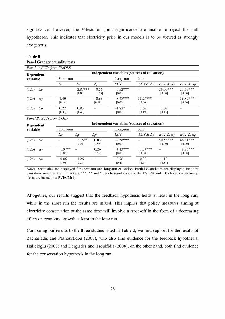
significance. However, the F-tests on joint significance are unable to reject the null
hypotheses. This indicates that electricity price in our models is to be viewed as strongly
exogenous.
Table 8 Panel Granger causality tests Panel A: ECTs from FMOLS
Dependent variable
Independent variables (sources of causation)
Short-run Long-run Joint
Δe Δy Δp ECT ECT & Δe ECT & Δy ECT & Δp
(12a) Δe – 2.87*** [0.00]
0.56 [0.58]
–6.52*** [0.00]
– 26.00*** [0.00]
21.65*** [0.00]
(12b) Δy 1.40 [0.16]
– –0.68 [0.49]
8.48*** [0.00]
38.24*** [0.00]
– 36.89*** [0.00]
(12c) Δp 0.22 [0.83]
0.83 [0.40]
– –1.82* [0.07]
1.67 [0.19]
2.07 [0.13]
–
Panel B: ECTs from DOLS
Dependent variable
Independent variables (sources of causation)
Short-run Long-run Joint
Δe Δy Δp ECT ECT & Δe ECT & Δy ECT & Δp
(12a) Δe – 2.15** [0.03]
0.03 [0.98]
–9.58*** [0.00]
– 50.53*** [0.00]
46.31*** [0.00]
(12b) Δy 1.97** [0.05]
– 0.26 [0.79]
4.13*** [0.00]
11.34*** [0.00]
– 8.73*** [0.00]
(12c) Δp –0.06 [0.95]
1.26 [0.21]
– –0.76 [0.45]
0.30 [0.74]
1.18 [0.31]
–
Notes: t-statistics are displayed for short-run and long-run causation. Partial F-statistics are displayed for joint causation. p-values are in brackets. ***, ** and * denote significance at the 1%, 5% and 10% level, respectively. Tests are based on a PVECM(1).
Altogether, our results suggest that the feedback hypothesis holds at least in the long run,
while in the short run the results are mixed. This implies that policy measures aiming at
electricity conservation at the same time will involve a trade-off in the form of a decreasing
effect on economic growth at least in the long run.
Comparing our results to the three studies listed in Table 2, we find support for the results of
Zachariadis and Pashourtidou (2007), who also find evidence for the feedback hypothesis.
Halicioglu (2007) and Dergiades and Tsoulfidis (2008), on the other hand, both find evidence
for the conservation hypothesis in the long run.
24
5. Conclusions
In this paper we have conducted an analysis on the responsiveness of residential electricity
demand for a set of OECD countries. We estimate electricity demand elasticities with regard
to disposable income and own price, thereby differentiating between the short and the long
run in an error correction framework. Furthermore, we conduct tests on Granger causality
between the variables. In order to circumvent the problem of low power and size of more
traditional unit root and cointegration tests based on time series data, we make use of
available panel data for eighteen countries in the cross-sectional dimension and the years
1981–2008 in the time domain. The methods employed for estimating the cointegrating
vectors are Pedroni’s group-means fully modified OLS (FMOLS) and dynamic OLS (DOLS)
panel estimators. The Granger causality tests are based on a panel vector error correction
model estimated using the pooled mean group estimator (Pesaran et al., 1999).
Our findings for the whole panel indicate a near unity income elasticity and an inelastic price
elasticity of approximately –0.4 in the long run. These results are robust to the two estimation
methods employed. In the short run, our estimates from error correction models indicate an
income elasticity of 0.2 and a price elasticity of approximately –0.1. When compared with the
results of previous studies on residential electricity demand, our elasticity estimates bear some
resemblance to other estimates on the individual country level.
Overall, our results imply that the steering effect of tax-induced price increases on residential
electricity demand has a very limited potential for energy conservation, and hence a reduction
of GHG emissions. These policy implications are in stark contrast, e.g., to the ones of
Narayan et al. (2007).
Furthermore, our tests on Granger causality indicate that both electricity consumption and
income adjust toward the long-run equilibrium after a shock hits the system. Thus, a
bidirectional causal relationship between electricity consumption and economic growth exists
in the long run. Our findings are, therefore, in favor of the feedback hypothesis. Hence, a
reduction of electricity consumption will be associated with a trade-off with regard to per
capita income.

25
References
Athukorala, P.P.A.W, Wilson C. (2010). Estimating short and long-term residential demand
for electricity: New evidence from Sri Lanka. Energy Economics 32(S1): S34–S40. Bernstein, R., Madlener, R. (2010). Short- and Long-Run Electricity Demand Elasticities at
the Subsectoral Level: A Cointegration Analysis for German Manufacturing Industries. FCN Working Paper No. 19/2010, Institute for Future Energy Consumer Needs and Behavior, RWTH Aachen University, November.
Breitung, J. (2000). The local power of some unit root tests for panel data. In: Baltagi, B.H.,
Formby, T.B., Hill, R.C. (Eds.), Advances in Econometrics: Nonstationary Panels, Panel Cointegration and Dynamic Panels, JAI Press, Amsterdam, Vol. 15: 161–178.
Dergiades, T., Tsoulfidis, L. (2008). Estimating residential demand for electricity in the
United States, 1965–2006. Energy Economics 30(5): 2722–2730. Engle, R.F., Granger, C.W.J. (1987). Co-integration and error correction: representation,
estimation and testing. Econometrica 55(2): 251–276. Fisher, F.M., Kaysen, C. (1962). A Study in Econometrics: The demand for electricity in the
United States. North-Holland Publishing Company, Amsterdam. Granger, C.W.J. (1969). Investigating causal relations by econometric models and cross-
spectral methods. Econometrica 37(3): 424–438. Hadri, K. (2000). Testing for stationarity in heterogeneous panel data. Econometrics Journal
3(2): 148–161. Halicioglu, F. (2007). Residential electricity demand dynamics in Turkey. Energy Economics
29(2): 199–210. Halvorsen, R. (1975). Residential demand for electric energy. The Review of Economics and
Statistics 75(1): 12–18. Harris, R., Sollis, R. (2003). Applied Time Series Modelling and Forecasting. John Wiley &
Sons, Chichester. Hlouskova, J., Wagner, M. (2006). The performance of panel unit root and stationarity tests:
results from a large scale simulation study. Econometric Reviews 25(1): 85–116. Holtedahl, P., Joutz, F.L. (2004). Residential electricity demand in Taiwan. Energy
Economics 26(2): 201–224. Hondroyiannis, G. (2004). Estimating residential demand for electricity in Greece. Energy
Economics 26(3): 319–334.

26
Houthakker, H.S. (1951). Some calculations on electricity consumption in Great Britain. Journal of the Royal Statistical Society, Series A (General), CXIV, part III: 359–371.
IEA (2008). Energy policies of IEA countries – Japan, 2008 Review. [Online] URL:
http://www.iea.org/textbase/nppdf/free/2008/japan2008.pdf. Im, K.S., Pesaran, M.H., Shin, Y. (2003). Testing for unit roots in heterogeneous panels.
Journal of Econometrics 115(1): 53–74. Kao, C., Chiang, M-H. (2000). On the estimation and inference of a cointegrated regression in
panel data. In: Baltagi, B.H., Formby, T.B., Hill, R.C, (Eds.), Advances in Econometrics: Nonstationary Panels, Panel Cointegration and Dynamic Panels, JAI Press, Amsterdam, Vol. 15: 179–222.
Kraft J., Kraft, A. (1978). On the relationship between energy and GNP. Journal of Energy
and Development 3(2): 401–403. Levin, A., Lin, C.F., Chu, C.S. (2002). Unit root tests in panel data: asymptotic and finite-
sample properties. Journal of Econometrics 108(1): 1–24. Maddala, G.S., Wu, S.A. (1999). A comparative study of unit root tests with panel data and a
new simple test. Oxford Bulletin of Economics and Statistics 61(S1): 631–652. Nakajima, T. (2010). The residential demand for electricity in Japan: An examination using
empirical panel analysis techniques. Journal of Asian Economics 21(4): 412–420. Nakajima, T., Hamori, S. (2010). Change in consumer sensitivity to electricity prices in
response to retail deregulation: a panel empirical analysis of the residential demand for electricity in the United States. Energy Policy 38(5): 2470–2476.
Narayan, P.K., Smyth, R. (2005). The residential demand for electricity in Australia: an
application of the bounds testing approach to cointegration. Energy Policy 33(4): 467–474.
Narayan, P.K., Smyth, R., Prasad, A. (2007). Electricity consumption in G7 countries: A
panel cointegration analysis of residential demand elasticities. Energy Policy 35(9): 4485–4494.
Payne, J.E. (2010). Survey of the international evidence on the causal relationship between
energy consumption and growth. Journal of Economic Studies 37(1): 53–95. Pedroni, P. (1999). Critical values for cointegration tests in heterogeneous panels with
multiple regressors. Oxford Bulletin of Economics and Statistics 61(1): 653–670. Pedroni, P. (2000). Fully modified OLS for heterogeneous cointegrated panels. In: Baltagi,
B.H., Formby, T.B. and Hill, R.C. (Eds.), Advances in Econometrics: Nonstationary Panels, Panel Cointegration and Dynamic Panels, JAI Press, Amsterdam, Vol. 15: 93–130.

27
Pedroni, P. (2001). Purchasing power parity tests in cointegrated panels. The Review of Economics and Statistics 83(4): 727–731.
Pedroni, P. (2004). Panel cointegration: asymptotic and finite sample properties of pooled
time series tests with an application to the PPP hypothesis. Econometric Theory 20(3): 597–625.
Pesaran, H.M., Shin, Y., Smith, R.P. (1999). Pooled mean group estimation of dynamic
heterogeneous panels. Journal of the American Statistical Association 94(446): 621–634.
Pindyck, R.S. (1979). Interfuel substitution and the industrial demand for energy: an
international comparison. The Review of Economics and Statistics 61(2): 169–179. Silk, J.I., Joutz, F.L. (1997). Short and long-run elasticities in US residential electricity
demand: a co-integration approach. Energy Economics 19(4): 493–513. Stock, J.H., Watson, M.W. (1993). A simple estimator of cointegrating vectors in higher order
integrated systems. Econometrica 61(4): 783–820. Zachariadis, T., Pashourtidou, N. (2007). An empirical analysis of electricity consumption in
Cyprus. Energy Economics 29(2): 183–198. Ziramba, E. (2008). The demand for residential electricity in South Africa. Energy Policy
36(9): 3460–3466.

List of FCN Working Papers
2011 Sorda G., Sunak Y., Madlener R. (2011). A Spatial MAS Simulation to Evaluate the Promotion of Electricity from
Agricultural Biogas Plants in Germany, FCN Working Paper No. 1/2011, Institute for Future Energy Consumer Needs and Behavior, RWTH Aachen University, January.
Madlener R., Hauertmann M. (2011). Rebound Effects in German Residential Heating: Do Ownership and Income
Matter?, FCN Working Paper No. 2/2011, Institute for Future Energy Consumer Needs and Behavior, RWTH Aachen University, February.
Garbuzova M., Madlener R. (2011). Towards an Efficient and Low-Carbon Economy Post-2012: Opportunities
and Barriers for Foreign Companies in the Russian Market, FCN Working Paper No. 3/2011, Institute for Future Energy Consumer Needs and Behavior, RWTH Aachen University, February.
Westner G., Madlener R. (2011). The Impact of Modified EU ETS Allocation Principles on the Economics of CHP-
Based District Heating Networks. FCN Working Paper No. 4/2011, Institute for Future Energy Consumer Needs and Behavior, RWTH Aachen University, February.
Madlener R., Ruschhaupt J. (2011). Modeling the Influence of Network Externalities and Quality on Market
Shares of Plug-in Hybrid Vehicles, FCN Working Paper No. 5/2011, Institute for Future Energy Consumer Needs and Behavior, RWTH Aachen University, March.
Juckenack S., Madlener R. (2011). Optimal Time to Start Serial Production: The Case of the Direct Drive Wind
Turbine of Siemens Wind Power A/S, FCN Working Paper No. 6/2011, Institute for Future Energy Consumer Needs and Behavior, RWTH Aachen University, March.
Madlener R., Sicking S. (2011). Assessing the Economic Potential of Microdrilling in Geothermal Exploration,
FCN Working Paper No. 7/2011, Institute for Future Energy Consumer Needs and Behavior, RWTH Aachen University, April.
Bernstein R., Madlener R. (2011). Responsiveness of Residential Electricity Demand in OECD Countries: A Panel
Cointegation and Causality Analysis , FCN Working Paper No. 8/2011, Institute for Future Energy Consumer Needs and Behavior, RWTH Aachen University, April.
2010 Lang J., Madlener R. (2010). Relevance of Risk Capital and Margining for the Valuation of Power Plants: Cash
Requirements for Credit Risk Mitigation, FCN Working Paper No. 1/2010, Institute for Future Energy Consumer Needs and Behavior, RWTH Aachen University, February.
Michelsen C., Madlener R. (2010). Integrated Theoretical Framework for a Homeowner’s Decision in Favor of an
Innovative Residential Heating System, FCN Working Paper No. 2/2010, Institute for Future Energy Consumer Needs and Behavior, RWTH Aachen University, February.
Harmsen - van Hout M.J.W., Herings P.J.-J., Dellaert B.G.C. (2010). The Structure of Online Consumer
Communication Networks, FCN Working Paper No. 3/2010, Institute for Future Energy Consumer Needs and Behavior, RWTH Aachen University, March.
Madlener R., Neustadt I. (2010). Renewable Energy Policy in the Presence of Innovation: Does Government Pre-
Commitment Matter?, FCN Working Paper No. 4/2010, Institute for Future Energy Consumer Needs and Behavior, RWTH Aachen University, April (revised June 2010).
Harmsen-van Hout M.J.W., Dellaert B.G.C., Herings, P.J.-J. (2010). Behavioral Effects in Individual Decisions of
Network Formation: Complexity Reduces Payoff Orientation and Social Preferences, FCN Working Paper No. 5/2010, Institute for Future Energy Consumer Needs and Behavior, RWTH Aachen University, May.

Lohwasser R., Madlener R. (2010). Relating R&D and Investment Policies to CCS Market Diffusion Through Two-Factor Learning, FCN Working Paper No. 6/2010, Institute for Future Energy Consumer Needs and Behavior, RWTH Aachen University, June.
Rohlfs W., Madlener R. (2010). Valuation of CCS-Ready Coal-Fired Power Plants: A Multi-Dimensional Real
Options Approach, FCN Working Paper No. 7/2010, Institute for Future Energy Consumer Needs and Behavior, RWTH Aachen University, July.
Rohlfs W., Madlener R. (2010). Cost Effectiveness of Carbon Capture-Ready Coal Power Plants with Delayed
Retrofit, FCN Working Paper No. 8/2010, Institute for Future Energy Consumer Needs and Behavior, RWTH Aachen University, August.
Gampert M., Madlener R. (2010). Pan-European Management of Electricity Portfolios: Risks and Opportunities of
Contract Bundling, FCN Working Paper No. 9/2010, Institute for Future Energy Consumer Needs and Behavior, RWTH Aachen University, August.
Glensk B., Madlener R. (2010). Fuzzy Portfolio Optimization for Power Generation Assets, FCN Working Paper
No. 10/2010, Institute for Future Energy Consumer Needs and Behavior, RWTH Aachen University, August. Lang J., Madlener R. (2010). Portfolio Optimization for Power Plants: The Impact of Credit Risk Mitigation and
Margining, FCN Working Paper No. 11/2010, Institute for Future Energy Consumer Needs and Behavior, RWTH Aachen University, September.
Westner G., Madlener R. (2010). Investment in New Power Generation Under Uncertainty: Benefits of CHP vs.
Condensing Plants in a Copula-Based Analysis, FCN Working Paper No. 12/2010, Institute for Future Energy Consumer Needs and Behavior, RWTH Aachen University, September.
Bellmann E., Lang J., Madlener R. (2010). Cost Evaluation of Credit Risk Securitization in the Electricity Industry:
Credit Default Acceptance vs. Margining Costs, FCN Working Paper No. 13/2010, Institute for Future Energy Consumer Needs and Behavior, RWTH Aachen University, September.
Ernst C.-S., Lunz B., Hackbarth A., Madlener R., Sauer D.-U., Eckstein L. (2010). Optimal Battery Size for Serial
Plug-in Hybrid Vehicles: A Model-Based Economic Analysis for Germany, FCN Working Paper No. 14/2010, Institute for Future Energy Consumer Needs and Behavior, RWTH Aachen University, October.
Harmsen - van Hout M.J.W., Herings P.J.-J., Dellaert B.G.C. (2010). Communication Network Formation with Link
Specificity and Value Transferability, FCN Working Paper No. 15/2010, Institute for Future Energy Consumer Needs and Behavior, RWTH Aachen University, November.
Paulun T., Feess E., Madlener R. (2010). Why Higher Price Sensitivity of Consumers May Increase Average
Prices: An Analysis of the European Electricity Market, FCN Working Paper No. 16/2010, Institute for Future Energy Consumer Needs and Behavior, RWTH Aachen University, November.
Madlener R., Glensk B. (2010). Portfolio Impact of New Power Generation Investments of E.ON in Germany,
Sweden and the UK, FCN Working Paper No. 17/2010, Institute for Future Energy Consumer Needs and Behavior, RWTH Aachen University, November.
Ghosh G., Kwasnica A., Shortle J. (2010). A Laboratory Experiment to Compare Two Market Institutions for
Emissions Trading, FCN Working Paper No. 18/2010, Institute for Future Energy Consumer Needs and Behavior, RWTH Aachen University, November.
Bernstein R., Madlener R. (2010). Short- and Long-Run Electricity Demand Elasticities at the Subsectoral Level:
A Cointegration Analysis for German Manufacturing Industries, FCN Working Paper No. 19/2010, Institute for Future Energy Consumer Needs and Behavior, RWTH Aachen University, November.
Mazur C., Madlener R. (2010). Impact of Plug-in Hybrid Electric Vehicles and Charging Regimes on Power
Generation Costs and Emissions in Germany, FCN Working Paper No. 20/2010, Institute for Future Energy Consumer Needs and Behavior, RWTH Aachen University, November.
Madlener R., Stoverink S. (2010). Power Plant Investments in the Turkish Electricity Sector: A Real Options
Approach Taking into Account Market Liberalization, FCN Working Paper No. 21/2010, Institute for Future Energy Consumer Needs and Behavior, RWTH Aachen University, December.
Melchior T., Madlener R. (2010). Economic Evaluation of IGCC Plants with Hot Gas Cleaning, FCN Working
Paper No. 22/2010, Institute for Future Energy Consumer Needs and Behavior, RWTH Aachen University, December.

Lüschen A., Madlener R. (2010). Economics of Biomass Co-Firing in New Hard Coal Power Plants in Germany, FCN Working Paper No. 23/2010, Institute for Future Energy Consumer Needs and Behavior, RWTH Aachen University, December.
Madlener R., Tomm V. (2010). Electricity Consumption of an Ageing Society: Empirical Evidence from a Swiss
Household Survey, FCN Working Paper No. 24/2010, Institute for Future Energy Consumer Needs and Behavior, RWTH Aachen University, December.
Tomm V., Madlener R. (2010). Appliance Endowment and User Behaviour by Age Group: Insights from a Swiss
Micro-Survey on Residential Electricity Demand, FCN Working Paper No. 25/2010, Institute for Future Energy Consumer Needs and Behavior, RWTH Aachen University, December.
Hinrichs H., Madlener R., Pearson P. (2010). Liberalisation of Germany’s Electricity System and the Ways
Forward of the Unbundling Process: A Historical Perspective and an Outlook, FCN Working Paper No. 26/2010, Institute for Future Energy Consumer Needs and Behavior, RWTH Aachen University, December.
Achtnicht M. (2010). Do Environmental Benefits Matter? A Choice Experiment Among House Owners in
Germany, FCN Working Paper No. 27/2010, Institute for Future Energy Consumer Needs and Behavior, RWTH Aachen University, December.
2009 Madlener R., Mathar T. (2009). Development Trends and Economics of Concentrating Solar Power Generation
Technologies: A Comparative Analysis, FCN Working Paper No. 1/2009, Institute for Future Energy Consumer Needs and Behavior, RWTH Aachen University, November.
Madlener R., Latz J. (2009). Centralized and Integrated Decentralized Compressed Air Energy Storage for
Enhanced Grid Integration of Wind Power, FCN Working Paper No. 2/2009, Institute for Future Energy Consumer Needs and Behavior, RWTH Aachen University, November (revised September 2010).
Kraemer C., Madlener R. (2009). Using Fuzzy Real Options Valuation for Assessing Investments in NGCC and
CCS Energy Conversion Technology, FCN Working Paper No. 3/2009, Institute for Future Energy Consumer Needs and Behavior, RWTH Aachen University, November.
Westner G., Madlener R. (2009). Development of Cogeneration in Germany: A Dynamic Portfolio Analysis Based
on the New Regulatory Framework, FCN Working Paper No. 4/2009, Institute for Future Energy Consumer Needs and Behavior, RWTH Aachen University, November (revised March 2010).
Westner G., Madlener R. (2009). The Benefit of Regional Diversification of Cogeneration Investments in Europe:
A Mean-Variance Portfolio Analysis, FCN Working Paper No. 5/2009, Institute for Future Energy Consumer Needs and Behavior, RWTH Aachen University, November (revised March 2010).
Lohwasser R., Madlener R. (2009). Simulation of the European Electricity Market and CCS Development with the
HECTOR Model, FCN Working Paper No. 6/2009, Institute for Future Energy Consumer Needs and Behavior, RWTH Aachen University, November.
Lohwasser R., Madlener R. (2009). Impact of CCS on the Economics of Coal-Fired Power Plants – Why
Investment Costs Do and Efficiency Doesn’t Matter, FCN Working Paper No. 7/2009, Institute for Future Energy Consumer Needs and Behavior, RWTH Aachen University, November.
Holtermann T., Madlener R. (2009). Assessment of the Technological Development and Economic Potential of
Photobioreactors, FCN Working Paper No. 8/2009, Institute for Future Energy Consumer Needs and Behavior, RWTH Aachen University, November.
Ghosh G., Carriazo F. (2009). A Comparison of Three Methods of Estimation in the Context of Spatial Modeling,
FCN Working Paper No. 9/2009, Institute for Future Energy Consumer Needs and Behavior, RWTH Aachen University, November.
Ghosh G., Shortle J. (2009). Water Quality Trading when Nonpoint Pollution Loads are Stochastic, FCN Working
Paper No. 10/2009, Institute for Future Energy Consumer Needs and Behavior, RWTH Aachen University, November.
Ghosh G., Ribaudo M., Shortle J. (2009). Do Baseline Requirements hinder Trades in Water Quality Trading
Programs?, FCN Working Paper No. 11/2009, Institute for Future Energy Consumer Needs and Behavior, RWTH Aachen University, November.

Madlener R., Glensk B., Raymond P. (2009). Investigation of E.ON’s Power Generation Assets by Using Mean-Variance Portfolio Analysis, FCN Working Paper No. 12/2009, Institute for Future Energy Consumer Needs and Behavior, RWTH Aachen University, November.
2008 Madlener R., Gao W., Neustadt I., Zweifel P. (2008). Promoting Renewable Electricity Generation in Imperfect
Markets: Price vs. Quantity Policies, FCN Working Paper No. 1/2008, Institute for Future Energy Consumer Needs and Behavior, RWTH Aachen University, July (revised May 2009).
Madlener R., Wenk C. (2008). Efficient Investment Portfolios for the Swiss Electricity Supply Sector, FCN Working
Paper No. 2/2008, Institute for Future Energy Consumer Needs and Behavior, RWTH Aachen University, August.
Omann I., Kowalski K., Bohunovsky L., Madlener R., Stagl S. (2008). The Influence of Social Preferences on
Multi-Criteria Evaluation of Energy Scenarios, FCN Working Paper No. 3/2008, Institute for Future Energy Consumer Needs and Behavior, RWTH Aachen University, August.
Bernstein R., Madlener R. (2008). The Impact of Disaggregated ICT Capital on Electricity Intensity of Production:
Econometric Analysis of Major European Industries, FCN Working Paper No. 4/2008, Institute for Future Energy Consumer Needs and Behavior, RWTH Aachen University, September.
Erber G., Madlener R. (2008). Impact of ICT and Human Skills on the European Financial Intermediation Sector,
FCN Working Paper No. 5/2008, Institute for Future Energy Consumer Needs and Behavior, RWTH Aachen University, September.
FCN Working Papers are free of charge. They can mostly be downloaded in pdf format from the FCN / E.ON ERC Website (www.eonerc.rwth-aachen.de/fcn) and the SSRN Website (www.ssrn.com), respectively. Alternatively, they may also be ordered as hardcopies from Ms Sabine Schill (Phone: +49 (0) 241-80 49820, E-mail: [email protected]), RWTH Aachen University, Institute for Future Energy Consumer Needs and Behavior (FCN), Chair of Energy Economics and Management (Prof. Dr. Reinhard Madlener), Mathieustrasse 6, 52074 Aachen, Germany.