response of near-inertial energy to a supercritical
TRANSCRIPT

1
Response of near-inertial energy to a supercritical tropical cyclone and jet in the
South China Sea: modeling study
Hiu Suet Kung, Jianping Gan*
Department of Ocean Science and Department of Mathematics, Center for Ocean Research in
Hong Kong and Macau, Hong Kong University of Science and Technology, Hong Kong
Corresponding author: [email protected]

2
ABSTRACT 1
We used a well-validated three-dimensional ocean model to investigate the process of energetic 2
response of near-inertial oscillations (NIOs) to a tropical cyclone (TC) and strong background jet 3
in the South China Sea (SCS). We found that the NIO and near-inertial kinetic energy (KEni) 4
varied distinctly during different stages of the TC forcing, and the horizontal and vertical transport 5
of KEni was largely modulated by the velocity and vorticity of the jet. The KEni reached its peak 6
value within ~one-half the inertial period after the initial TC forcing stage in the upper layer, 7
decayed quickly by one-half in the next two days, and further decreased in a slower rate during the 8
relaxation stage of the TC forcing. Analyses of the KEni balance indicate that the weakened KEni 9
in the upper layer during the forcing stage was mainly attributed to the downward KEni transport 10
due to pressure work through the vertical displacement of isopycnal surfaces, while upward KEni 11
advection from depths also contributed to the weakening in the TC-induced upwelling region. In 12
contrast, during the relaxation stage as TC moved away, the effect of vertical advection on KEni 13
reduction was negligible and the KEni was chiefly removed by the outward propagation of inertial-14
gravity waves, horizontal advection and viscous dissipation. Both the outward wave propagation 15
and horizontal advection by the jet provided the KEni source in the far-field. During both stages, 16
the negative geostrophic vorticity south of the jet facilitated the vertical propagation of inertial-17
gravity waves. 18
19
3
1 Introduction 20
Near-inertial oscillations (NIOs), whose frequencies are close to the local inertial frequency, 21
contain around half of the observed internal wave kinetic energy in the ocean (Simmons and 22
Alford, 2012). NIOs also greatly affect the kinetic energy budget in the deeper ocean as they 23
propagate downward from the surface and enhance the mixing by increasing vertical shear (Gill, 24
1984; Gregg et al., 1986; Ferrari and Wunsch, 2009; Alford et al., 2016). 25
Tropical cyclones (TCs), with the rapid change of wind stress, provide an important 26
generation mechanism for the NIOs. Observational studies related to a single storm or tropical 27
cyclone (Price, 1981; Shay and Elsberry, 1987; D'Asaro et al., 1995) showed that the NIOs related 28
to TCs can be a factor 2-3 larger than the background NIOs and last for more than 5 inertial periods 29
(IPs). Using a hurricane-ocean coupled model, Liu et al. (2008) estimated that the energy input of 30
tropical cyclones into the near-inertial currents was about 0.03 TW, about 10% of the total wind-31
induced near-inertial energy (Watanabe and Hibiya, 2002; Alford, 2003). The input of wind energy 32
to the near-inertial band is also controlled by the translation speed of the TC (Uh) (Geisler, 1970; 33
Price, 1981). In fact, the NIOs are largely variable during the forcing and relaxation stage of the 34
TC forcing related to the intensity and translation speed of the TC. The variation is determined not 35
only by the different magnitude of input of wind energy, but also by the different dynamic 36
conditions that regulate the near-inertial kinetic energy (KEni) transport during these stages. The 37
variable response of NIOs during different stage of TC forcing is critical for understanding the 38
process and physics of NIOs. 39
Once generated, the characteristics of NIOs, in terms of the decay time scale, propagation 40
direction, and propagation speed are influenced by various mechanisms. In linear wave theory, the 41
β-effect leads to equatorward propagation of the NIOs and their decay time scale is reduced 42

4
because of the vertical propagation into deeper ocean (Gill, 1984; D'Asaro, 1989; Garrett, 2001). 43
Background flow fields also impose large influence on the evolution of NIOs. The influence of 44
background vorticity on NIOs has been observed by Weller (1982) and Kunze and Sanford (1984), 45
and proven analytically by Kunze (1985), Young and Ben Jelloul (1997), and Danioux et al. 46
(2015). Numerical study using a primitive equation model with a turbulent mesoscale eddy field 47
and uniform wind forcing gave a similar conclusion (Danioux et al., 2008). Non-linear interactions 48
also provide a mechanism for increasing the vertical wave number, thus for larger vertical shear 49
and dissipation and reduced decay time (Davies and Xing, 2002; Zedler, 2009). In addition to 50
modifying the characteristics of the inertial-gravity waves, nonlinear advection related to a front 51
can transport NIOs away from the storm track and to higher latitudes (Zhai et al., 2004). Recent 52
observations and numerical studies in Gulf Stream, Kuroshio, and Japan Sea revealed the role of 53
vertical circulation on the generation and radiation of near inertial energy (Whitt and Thomas, 54
2013; Nagai et al., 2015; Rocha et al., 2018; Thomas, 2019). 55
The South China Sea (SCS) is a region with frequent tropical cyclone occurrence, ~10 each 56
year (Wang et al., 2007). Observations (Sun et al., 2011a, b; Xu et al., 2013) and numerical studies 57
(Chu et al., 2000) indicated that these TC events are sources for near-inertial energy bursts. 58
Additionally, the SCS circulation contains abundant energetic flow (e.g. Qu, 2000; Gan et al., 59
2006; Gan et al., 2016a) and mesoscale features, such as a strong coastal jet off the Vietnamese 60
coast (e.g. Gan and Qu, 2008) and eddies (e.g. Chen et al., 2012). The distribution and evolution 61
of the TC-induced NIOs are susceptible to the influence of these background currents. (Sun et al., 62
2011a; Sun et al., 2011b). However, the estimate of the total contribution of a TC to the KEni in 63
the SCS is difficult to obtain from observations or linear wave theory due to sparse spatial 64
observations and the non-homogenous nature of SCS circulation. 65

5
In this study, we apply a well-validated numerical model with specific China Sea 66
configurations to examine the response of KEni to a large TC and background jet over the sloping 67
topography in the SCS. A description of Typhoon Neoguri and the details of the numerical model 68
implementation are given in Section 2. In Section 3, the general characteristic response of the near-69
inertial current and the energy fluxes during the TC forced stage and their later relaxation stage as 70
TC moved away from the concerned region are presented. Following Section 3, the KEni equation 71
is used to identify the dynamic processes of the vertical viscous dissipation, pressure work, and 72
nonlinearity during different phases of the NIOs. 73
2 Typhoon Neoguri (2008) and the Ocean Model 74
2.1 Typhoon Neoguri (2008) 75
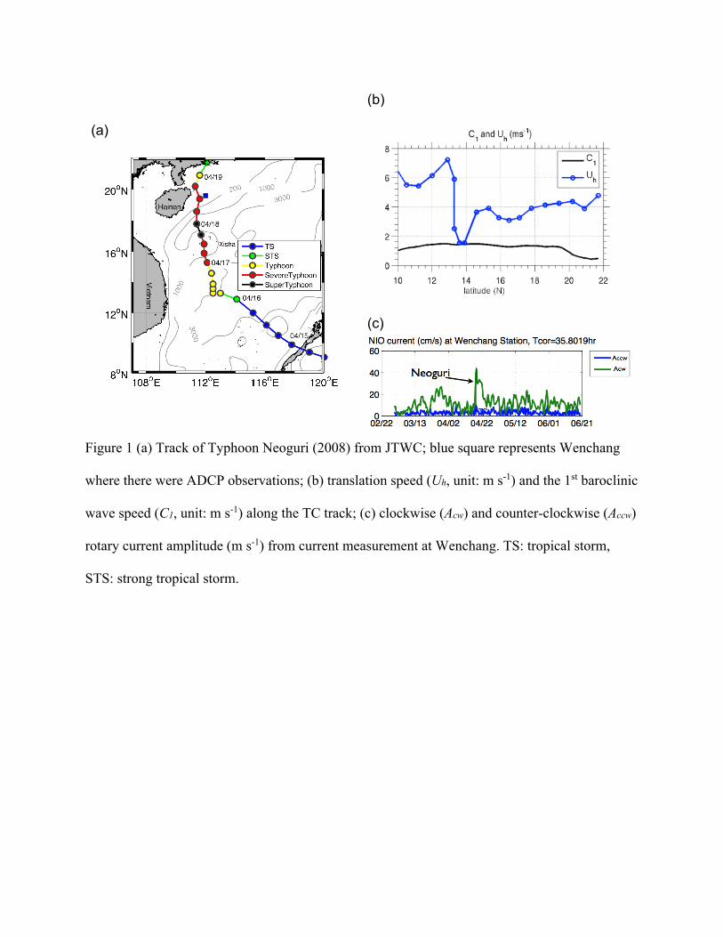
Typhoon Neoguri formed east of the Philippines and entered the SCS on April 15. It first moved 76
west-northwest with an average translation speed of 5.8 m s-1 before it slowed down to 1.6 m s-1 77
on April 16, based on the Joint Typhoon Warning Center (JTWC) best track data, (Fig. 1). On 78
April 17, Neoguri sped up to 3.8 m s-1, turned more northward, and developed into a typhoon with 79
a maximum wind speed 51 m s-1 and a MSLP (minimum sea level pressure) 948 hPa, at 1800 UTC 80
on April 17 near the Xisha Islands. The Neoguri was a supercritical typhoon travelling with a 81
translation speed greater than the first baroclinic wave speed. After skirting Hainan Island on April 82
18, Neoguri moved northward, weakened to a tropical storm, and further dissipated as it moved 83
farther inland. The NIO burst induced by Neoguri was shown by the clockwise (Acw) and counter-84
clockwise (Accw) rotary current amplitudes (m s-1), from a current meter mooring at Wenchang 85
station, to the east off Hainan Island (Fig. 1c). 86

6
2.2 Ocean Model 87
We use the China Sea Multi-scale Ocean Modeling System (CMOMS) (Gan et al., 2016a; Gan et 88
al., 2016b) in this study. CMOMS is based on the Regional Ocean Modeling System (ROMS) 89
(Shchepetkin and McWilliams,2005), and the model domain covers the northwest Pacific Ocean 90
(NPO) and the entire China Seas (Bohai, Yellow Sea, East China Sea, and SCS) from 91
approximately 0.95oN, 99oE in the southwest corner to the northeast corner of the Sea of Japan. 92
The horizontal size of this grid array decreased gradually from ~10 km in the southern part to~7 93
km in the northern part of the domain. Vertically, we adopted a 30-level stretched generalized 94
terrain-following coordinate (s). 95
The model was forced with 6-hourly actual wind speeds of typhoon Neoguri obtained from 96
the Cross-Calibrated Multi-Platform (CCMP) dataset, with a horizontal resolution of 0.25° (Atlas 97
et al. (2011), ftp://podaac-ftp.jpl.nasa.gov/allData/ccmp/L3.0/flk). Wind stress is calculated based 98
on the bulk formulation by Fairall et al. (2003). The daily mean air temperature, atmospheric 99
pressure, rainfall/evaporation, radiation, and other meteorological variables from April 15 to April 100
18, 2008 from the NCEP/NCAR Reanalysis 1 were used to derive the atmospheric heat and fresh 101
water fluxes. External forcing of depth-integrated velocities (U, V), depth-dependent velocities (u, 102
v), temperature, T, and salinity, S, at the lateral boundaries were obtained from the Ocean General 103
Circulation Model for the Earth Simulator (OFES) (Sasaki et al., 2008). Open boundary conditions 104
from Gan and Allen (2005) were applied at the open boundaries. 105
The model was spun up from January 1, 2005 with winter initial fields (temperature and 106
salinity) obtained from the last three-year mean fields of a 25-year run that is initialized with the 107
World Ocean Atlas 2005 (WOA05, Locarnini et al., 2006, Antonov et al., 2006) data, and forced 108
by wind stress derived from climatological (averaged from 1988 to 2013) monthly Reanalysis of 109

7
10 m Blended Sea Winds released by the National Oceanic and Atmospheric Administration 110
(https://www.ncdc.noaa.gov/oa/rsad/air-sea/seawinds.htm). The dynamic configuration and 111
numerical implementation of the CMOMS system are described in detail in Gan et al. (2016a, 112
2016b). 113
We have thoroughly validated the CMOMS by comparing simulated results with those 114
obtained from various measurements and findings in previous studies. In particular, we have 115
validated the extrinsic forcing of time-dependent, three-dimensional current system in the tropical 116
NPO, transports through the straits around the periphery of the SCS, and corresponding intrinsic 117
responses of circulation, hydrography and water masses in the SCS (Gan et al., 2016a). We have 118
also validated the circulation of CMOMS by providing a consistent physics between the intrinsic 119
responses of the circulation and extrinsic forcing of flow exchange with adjacent oceans (Gan et 120
al., 2016b). The model is also validated with available ARGO temperature profiles (not shown), 121
observed sea surface temperature (SST) and currents from a time-series current meter mooring 122
during Neoguri, as described below. 123
Three-dimensional, hourly-mean dynamic, and thermodynamic variables from April 10 to 124
May 10, 2008 were used to examine the near-inertial oscillations in this study. Because the inertial 125
period (IP) in the SCS is larger than 32 hours (near 22°N), the error induced by the hourly model 126
output is <3%. 127
3 Model result 128
3.1 Characteristic response to the TC 129
The evolution of the response to the TC in the ocean with existence of a coastal jet in the 130
SCS is presented according to different stages of the TC forcing. During the pre-storm stage (PS), 131
before Neoguri entered the SCS on April 14, the wind stress was relatively weak (<0.1 Pa). A 132

8
prominent jet current separated from the Vietnamese coast flowing northeastward near 16°N (Fig. 133
2a), and characterized the circulation in the western part of the SCS. The jet was resulting from 134
the (summer) monsoon-driven strong coastal current over narrow shelf topography off Vietnam 135
and it persisted as a distinct circulation feature in the SCS during summer. The northward flowing 136
coastal current separated from the coast and overshoots northeastward into the SCS basin as it 137
encountered the coastal promontory in the central Vietnam (Gan and Qu, 2008). 138
The jet formed negative (positive) geostrophic vorticity (ζg) to the south (north), with the 139
minimum (maximum) Rossby number (ζg/f) <-0.2 (>0.2) near 15.8°N (16.8°N). During the forced 140
stage (FS, Fig. 2b) between April 15 and April 19, the SCS was under the direct influence of 141
Neoguri, the wind forcing became significantly stronger (>0.1 Pa), the KE near the surface (10 m) 142
intensified significantly (>500 J m-3) to the east of the TC, and the coastal jet was suppressed by 143
southward flow. Meanwhile, a strong local divergence and upwelling formed in the surface and 144
generated a strong cooling (~1.5°C) belt along the TC path that lasted for more than a week. The 145
cooling zone radiated hundreds of kilometer away from the core of the TC. These features were 146
well captured by the TC-induced temperature difference between April 19 and 14 from both 147
simulated (Fig. 3a) and observed SST (Fig. 3b) (http://podaac.jpl.nasa.gov/dataset/JPL-L4UHfnd-148
GLOB-MUR). After the end of the FS on April 20 (Fig. 2c), the jet returned to its pre-storm 149
intensity and shifted slightly northward (Fig. 2c) when the TC center approached the coast (Fig. 150
1a). Afterwards, during the relaxation stage (RS) after April 20 (Fig. 2d), the wind forcing from 151
the TC decreased to <0.05 Pa. 152
Rotary spectrum shows that the near-inertial response of surface currents to the TC 153
occurred near the local inertial frequency (f = 0.028 cph) at station Wenchang (112°E, 19.6°N) 154

9
during the model simulation period (April 10 – May 5) (Fig. 4). The clockwise rotary spectra is 155
calculated by: 156
Scw = 1/8(Puu + Pvv - 2Quv), (1) 157
where Puu, Pvv and Quv are auto- and quadrature-spectra, respectively (Gonella, 1972). This 158
simulated result is highly consistent with the observations in the lower frequency band. We found 159
that the correlation coefficients of near-inertial band-passed velocity between ADCP and model 160
simulation at Wenchang station were 0.62 and 0.57 for east-west (u) and north-south (v) 161
component, respectively, which indicated that the model captured reasonably well the NIOs under 162
the influence of the background circulation of the SCS. There existed inevitably model-observation 163
discrepancies, such as differences of velocity magnitude (~0.06 m s-1 ) at near-inertial band and 164
rotary spectra at the higher frequency (Fig. 4). The discrepancies could have been caused by many 165
reasons, such as the lack of mesoscale and sub-mesoscale processes in the atmospheric forcing 166
field, the linear interpolation process of the atmospheric forcing (Jing et al., 2015), and not 167
resolving the oceanic subscale processes by the current model resolution. However, these 168
discrepancies will not undermine the discussion about the process and mechanism of near-inertial 169
energy response to the TC and jet in this study. 170
3.2. Near-inertial response in the upper ocean 171
We adopted the complex demodulation method successfully used in previous NIO studies 172
(Gonella, 1972; Brink, 1989; Qi et al., 1995) to extract the inertial current signal. The simulated 173
horizontal currents (𝑢 were analyzed for inertial currents (𝑢 . The inertial currents contain 174
clockwise (cw) and counter-clockwise (ccw) rotating components: 175
𝑢 𝑖𝑣 𝐴 𝑒 𝐴 𝑒 , (2) 176
10
where ui and vi are the eastward and northward inertial currents at 10 m in the mixed layer, A and 177
ϕ are the amplitude and phase of the rotary currents, respectively. Subscripts represent the 178
clockwise (cw) and counter-clockwise (ccw) rotating direction, and f is the local Coriolis 179
coefficient. To obtain the amplitude and phase, we performed harmonic analysis daily with each 180
segment over one inertial period (IP). Then the rotary amplitude and phase were calculated 181
following previous studies (Mooers, 1973, Qi et al., 1995, Jordi and Wang, 2008). 182
The time evolution of the daily rotary currents during the FS and RS in the surface layer 183
varied spatially and was related to the intensity and translation speed of the TC. On April 15 during 184
PS, Neoguri affected mainly the region south of 13°N, with a relatively fast translation speed (Uh 185
> 3C1, Fig. 1b) and weaker intensity (Vmax~35 m s-1). In most areas, cw rotary currents were strong 186
(Acw >0.1 m s-1) yet decayed quickly after 3 days (<2 IP) (Fig. 5a), while the magnitudes of ccw 187
currents were very small (Fig. 5b). After April 18, Neoguri moved into the region between 14°N 188
and 18°N, where it intensified more than 40% but moved slower with Uh~2C1. Both the cw and 189
ccw currents possessed larger intensities than in the southern region. The induced cw currents 190
displayed an obvious rightward bias, where the enhanced inertial currents extended to ~350 km to 191
the right of the track and to ~<150 km to the left of the track. This extension of horizontal scale 192
was related to the region with wind stress |τ|>0.25 Pa in Neoguri. 193
The maxima of the ccw component were located to the left of the TC’s path where the wind 194
vector (Fig. 6) rotated in the same direction as the ocean currents presented in Fig. 5. The 195
connection between the right (left) bias of the cw (ccw) currents with the rotation direction of the 196
wind vector is in agreement with the explanation of Price (1981). 2-3 IPs (>6 days) after the direct 197
forcing, the cw currents remained significant (>0.2 m s-1) in an area extending from 110°E to 198
116°E. In contrast, the ccw components dissipated quickly, within ~1 day after the wind forcing 199

11
stopped. This short duration of the forced inertial motion is in agreement with previous studies 200
(Jordi and Wang, 2008). 201
Besides the intensity and duration, we also looked at the frequency shift (δω=ω-f) and the 202
horizontal scale of the NIOs. The frequency shift from the local inertial frequency was estimated 203
from the temporal evolution of the phase of the rotary current: δω=-∂ϕ/∂t. In the FS, the maximum 204
frequency shift occurred near the jet (112°E to 115°E, 15°N to 16°N), where δω≈0.08f 205
(∆ϕ≈π/4,∆t=3 days, f=4×10⁻⁵ s-1 at 16°N). The horizontal scale was estimated from the spatial 206
variation of the rotary current by calculating the horizontal wave number in the meridional 207
direction as ky=∂ϕ/∂y. The largest wave number 𝑘 3.1 10 rad m-1 was also found near the 208
jet. 209
3.3 Characteristic near-inertial energy 210
Response in the upper layer 211
We focused on the area between 110-115°E and 13-19°N (box in Fig. 5a), defined as the 212
forced region, where the strongest NIO was produced during FS of Neoguri. We calculated the 213
wind-induced near-inertial energy flux (or the wind work) using 𝜏 ∙ 𝑢 , where 𝜏 is the band-passed 214
near-inertial wind stress and 𝑢 is the near-inertial current at the surface (Silverthorne and Toole, 215
2009). A 4th order elliptic band-pass filter (Morozov and Velarde, 2008) was applied to obtain 216
near-inertial motion with a band ranging from 0.8f to 1.2f, where f is the local Coriolis coefficient. 217
The time series of domain-averaged 𝜏 ∙ 𝑢 over the forced region reveals that significant energy 218
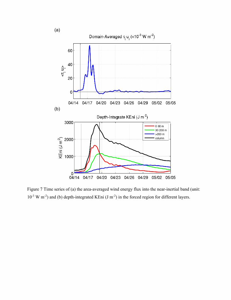
input took place during the FS, with the peak value about 68×10-3 W m-2 on April 17 (Fig. 7). 219
Under this large wind energy input, the area-averaged depth-integrated KEni (or AKEni hereafter) 220
in the upper layer (0-30 m) increased significantly from its pre-storm value to a maximum ~1500 221
J m-2 during the FS, with an increase rate of about 16×10-3 W m-2 (Fig. 7a). We set 0-30 m as upper 222
12
layer based on domain mean stratification and current (vorticity) vertical structure. Despite the 223
continuous positive wind energy flux, the AKEni in the upper layer plateaued, indicating that a 224
large amount of the wind energy was either propagating out of the forced region or was lost to the 225
lower layers due to entrainment. The detailed mechanisms are discussed in the following sections. 226
After the peak of FS, the wind work decreased significantly with small negative value around the 227
end of the FS. The AKEni decreased to one half of its peak value within 2 days (decrease rate was 228
about 7×10⁻³ W m-2). After that, the wind work was almost negligible, and the decrease rate of 229
AKEni became smaller (~0.8×10⁻³ W m-2). 230
Response at depths 231
During the FS, the AKEni in the upper 200 m constituted ~90% of the total AKEni in the 232
whole water column, while the AKEni between 30-200 m alone accounted for ~30-50% (Fig. 7b). 233
The KENI in this mid-layer had a temporal evolution different from that in the near surface layer. 234
It reached its maximum on April 20, around one and a half days later, and was more than 70% of 235
the peak value of the AKEni in the upper layer (~1700 J m-2). Compared to the upper layer AKEni, 236
the the mid-layer AKEni during FS increased slightly more slowly (~ 4×10⁻³ W m-2) while from 237
April 20 to May 5 during RS it decreased much more slowly (~0.61×10⁻³ W m-2), and the AKEni 238
became greater than that in the upper layer at the end of FS. The AKEni below 200 m was much 239
smaller, but increased continuously from April 17 to 29, with a rate of about 0.62×10⁻³ W m-2, 240
which was comparable to the AKEni rate of decrease in the 30-200 m layer. The AKEni in this 241
deep layer became greater than that in the upper layer after April 25 and that in the layer 30-200 242
m after April 29; the deep layer reached its maximum value ~10 days after the ending of the FS. 243
Spatially, two relatively large KEni patches below upper layer were located to north and 244
south of ~16°N (Fig. 8a). Their horizontal scales, influenced by near-inertial waves, were much 245

13
smaller compared with those in the upper layer. The region with relatively large KEni in the layer 246
between 30-200 m located near the jet currents, with stronger value during FS than during RS (Fig. 247
8 a,b). These results suggest that the KEni in this layer might have been determined by both vertical 248
propagation of the near-inertial gravity wave and horizontal advection of KEni of the background 249
current. Similar horizontal distribution also occurred below 200 m (Fig. 8 c,d). In contrast to the 250
layer above, the relatively large value during RS on April 30 indicated a downward propagation 251
of KEni into the deeper layer. Around the saddle zone west of the Xisha Islands, a relatively large 252
KEni below 200 m aligned with the 1000 m isobath, and might reflect a topographic effect on the 253
near-inertial wave. 254
3.4 Vertical propagation of near-inertial energy 255
It is clear that the distribution of the KEni was mainly controlled by the propagation of 256
near-inertial wave energy both horizontally and vertically as well as by the background jet. In order 257
to understand the KEni distribution in the deeper water inside the forced region and in the far field, 258
we selected four different locations, marked as A1, A2, C1, and C2 in Fig. 8 (a-d), for the analysis 259
of the KEni evolution during the FS and RS. Among them, A1 (113°E, 15.7°N) and A2 (112.5°E, 260
16.9°N) are on the right side of the TC track, inside the forced region, and situated about 200 km 261
apart from each other at the northern (A2) and southern (A1) sides of the jet, respectively. C1 262
(114.9°E, 16.9°N) and C2 (114.9°E, 18°N) are the corresponding stations in the far field where 263
relatively strong KEni intensification occurred. 264
Forced region (stations A1 and A2) 265
South of the jet at station A1 266
The time series of the band-passed inertial velocity ui as a function of depth shows that there was 267
an upward phase propagation, in which ui, in the layers below 100 m was leading the upper 50 m 268

14
(Fig. 9a). Accompanying this phase propagation was a downward propagation of surface KEni, 269
which was represented by the lowering of the ui maxima as a typical Poincaré wave (Kundu and 270
Cohen, 2008). There were two phases of vertical energy propagation: 1) during FS, there was a 271
rapid extension of the large ui maxima to below 100 m from April 17 to 20, and 2) during RS, the 272
center of the large ui value descended from ~100 m to 280 m from April 25 to May 5. The vertical 273
propagation velocity, Cgz, estimated from this downward transport, was ~17 m day-1. 274
During the first phase, the KEni in the top 30 m and in the 30-200 m layer shared a similar 275
rate of increase on April 17, indicating that the enhancement of KEni at 30-200 m was related to 276
the entrainment between the upper and deep layer (Fig. 9c). While the KEni in the upper 30 m 277
decreased quickly from April 18, it kept increasing at depths from 30-200 m, suggesting that other 278
contributing mechanisms existed besides the entrainment. The KEni below 200 m also experienced 279
notable intensification, with a smaller rate of increase than that found in the 30-200 m layer (Fig. 280
9c). Because the viscous effect is small in the deeper water, this enhancement of the KEni was 281
most likely associated with the propagation of an inertial-gravity wave. 282
During the second phase, the KEni in the 30-200 m layer decreased significantly at station 283
A1, indicating the existence of either downward or horizontal energy transport. From the linearized 284
inertial-gravity wave equation under the influence of background vorticity, Cgz can be obtained by 285
(Morozov and Velarde, 2008), 286
Cgz 2 feff
2
m, (3) 287
where ω≈1.08f is the frequency with maximum Scw at 200 m (Fig. 9e); feff=f+ζg/2 is the effective 288
Coriolis coefficient; and ζg/f=-0.1 at A1. m is the vertical wave number that we chose to be the first 289
baroclinic mode under a two-layer approximation based on the stratification (blue line in Fig. 10a). 290
From Eq. (3), Cgz was about 19.1 m day-1, which was in the same range as the modeled Cgz. 291

15
Consistent with the case of (ω0-feff)/feff <0.1 in Kunze (1985), the background vorticity in our case 292
accounted for more than 90% of the modification of the magnitude of the wave dispersion property. 293
Meanwhile, the KEni in the layer below 200 m did not increase notably, suggesting that other 294
mechanisms besides vertical propagation of the near-inertial gravity wave might have been 295
important in the evolution of KEni in water deeper than 200 m. 296
North of the jet at station A2 297
At location A2, strong ui was mainly trapped in the water above 100 m, and below 100 m 298
ui <10 cm s-1. It returned to its pre-storm magnitude after 5 IPs (Fig. 9b). This constraining of 299
vertical propagation is likely associated with the vertical scale of the strong positive background 300
vorticity (Fig. 10b). The KEni was generally smaller than that at A1, and relatively large energy 301
was found only in the ML (Fig. 9d). Cgz at A2, estimated from Eq. (3), was 2.1 m day-1 (feff =1.08f, 302
ω≈1.1f , f=4.2×10⁻⁵s-1, and m=2π/30 m), which was about one tenth of that at A1. This is consistent 303
with the lack of a distinct pattern of vertical propagation of NIOs at this station, as shown in the 304
band-passed ui (Fig. 9b), and the presence (absence) of a near-inertial peak of Scw at 10 m (200 m) 305
(Fig. 9f). 306
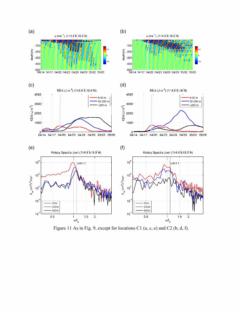
Far field region (stations C1 and C2) 307
C1 and C2 are located ~400 km to the right of the forced region. During the FS, ui (Fig. 11a,b) and 308
KEni (Fig. 11c,d) in the upper layer were smaller than those at those stations in the forced region 309
due to the weaker TC influence. Only a small downward propagation was discerned during the FS 310
(Fig. 11a,b). However, notable intensification of the KEni occurred in the layers below the upper 311
layer after April 23. At C1, the Scw at 10 m had a small red shift, while the Scw at 200 and 500 m 312
displayed blue shifts with peaks near 1.07f (Fig. 11e). The difference between Scw in the upper 313

16
layer and in the layers below implies another source of KEni other than local inertial-gravity wave 314
vertical propagation. 315
At C2, downward energy propagation appeared after April 23, reaching 100 m from the 316
surface within 7 days, giving Cgz =14.3 m day-1 (Fig. 11b). Unlike C1, the intensification was 317
mainly in the 30-200 m layer. The Scw at both 10 m and 200 m had a broad energy band near the 318
local f (Fig. 11f). Because ζg/f = -0.11 and feff = 1.06f, Cgz estimated from Eq. (3) had an upward 319
propagation (Cgz =-5.4 m day-1), which cannot explain the downward propagation here. The 320
linearized wave theory, with the consideration of Doppler drift due to background currents, does 321
not seem to be valid in this location. We will discuss this issue in the next section. 322
4 KEni Budget 323
We utilized the KEni equation to provide a further analysis of the source of KEni in the water 324
column. Because the horizontal component of near-inertial kinetic energy is significantly larger 325
than the vertical component (Hebert and Moum, 1994), we used the horizontal component to 326
represent the KEni. The KEni budget can be obtained from the horizontal momentum equation: 327
(4) 328
where KEni is the near-inertial energy; 𝑢 and 𝑢 are the near inertial velocity vector and horizontal 329
velocity, respectively; p is pressure; ρ0 is the reference density; ∇ is the horizontal gradient 330
operator; w is the vertical velocity; 𝜐 is the viscosity coefficient; and the angle bracket represents 331
band-passed filtering on the near-inertial band. The PRES term on the right side of equation 332
represents the pressure work on the KEni, which is associated with the inertial-gravity wave 333
propagation. NLh and NLv represent the horizontal and vertical divergence of energy flux that 334
include the effects of 1) the advection of KEni due to background currents and 2) the straining of 335

17
the wave field due to the background shear currents. Zhai et al. (2004) found that the geostrophic 336
advection of KEni contributed most of the NLh and was the main mechanism for transporting the 337
NIOs in the absence of baroclinic dispersion of inertial-gravity waves. It was also found to be more 338
important than the dispersive processes along the Gulf Stream or shelf-break jet. VVISC is the 339
vertical viscous effect. As before, we integrate this equation vertically in three layers: the upper 340
layer (0-30 m), the subsurface layer (30-200 m), and the deep layer (>200 m). In the following 341
sections, the AKEni budget is considered in entire forced region (Fig. 5) as well as at the specific 342
stations along the jet. 343
4.1. Mean balance 344
Figure 12 shows the time series of the AKEni budget over the entire forced region defined in Fig. 345
5. The time-averaged horizontal distributions of each term are presented in Fig. 13. During the FS, 346
the increase of AKEni in the upper layer was mainly attributed to the wind energy input because 347
the VVISC term was one order larger than the other terms, with a maximum of 30×10-3 W m-2 on 348
April 17 (Fig. 12a). The time-integrated VVISC during the FS was 2.15×10³ J m-2 (Table 1). 349
Stronger VVISC in the upper 30 m occurred in the region between 14°N and18°N (Fig. 13a) along 350
the TC track with a rightward bias, similar to the distribution of current intensity (Fig. 5c). Like 351
the wind work during the FS (Fig. 7a), VVISC became negative after April 19, indicating the AKEni 352
removal by negative wind work. The influence of VVISC extended to the 30-200 m layer, and 353
provided a positive energy flux (~1×10³ J m-2) in this layer (Figs. 12b, 13b). The effect of VVISC 354
in the deep layer was negligible (Fig. 12c). 355
Shortly (~1 day) after the large injection of KEni into the upper layer during the FS, the 356
PRES became significant (Fig. 12a, Table 1) and its horizontal distribution resembled that of 357
VVISC (Fig. 13a, d), suggesting that PRES radiated the KEni out of the forced region. It provided 358

18
a negative KEni flux in the upper layer (-0.65×10³ J m-2), which was largely compensated by the 359
positive flux in deeper layers (Table 1). This suggests that, during the FS, the main role of the 360
pressure work was to transport the KEni from the upper layer to the deep layers, and <15% of the 361
KEni was horizontally propagated outside the forced region. 362
During the RS, the VVISC was relatively small in the upper layer and it accounted for one 363
third of the AKEni removal in the layers below (Table 1). The PRES became a major sink for 364
AKEni in the ML (-0.85×10³ J m-2) and subsurface layer (-0.16×10³ J m-2), but was the major 365
source in the water below 200 m. The AKEni loss due to the horizontal wave propagation outside 366
the forced region was ~-0.42×10³ J m-2, accounting for about 40% of the total loss in the whole 367
water column. 368
Nonlinear advection terms had an important influence in the top 200 m but made little 369
contribution to the AKEni budget in the water below 200 m (Fig. 12, Table 1). The horizontal 370
effects of NLh and NLv in these layers were mainly limited to a smaller region, as compared to the 371
VVISC and the PRES; and their relatively large values occurred near the slope and the jet (Figs. 372
13). 373
In the upper layer, NLh advected the KEni from the source region; NLh had positive and 374
negative values on the eastern and western sides of the TC track, respectively (Fig. 13g). Similar 375
features, but with much weaker amplitude, were found in the layers below (Fig. 13h,i). During the 376
FS, in the 30-200 m layer, the domain-averaged NLh was positive (0.21×10³ J m-2), indicating a 377
possible extraction of the KEni from background flows. NLv was a strong energy sink in the upper 378
200 m (~0.64×10³ J m-2). The TC wind field generated a strong surface horizontal divergence and 379
upwelling around 16-17°N (Fig. 4b). As a result, the smaller KEni in the lower layer was advected 380
to the surface east of the Xiasha Islands. This lower KEni generated a negative gradient with 381

19
ambient water and resulted in the strong eastwards transport of KEni in the eastward jet current. 382
As a result, a positive NLh center located around the area with the strongest negative NLv, and a 383
negative NLh center lay to the west of the positive maximum of NLh. During the RS, NLh became 384
negative for all layers and provided ~1/3 of the total KEni loss in the water column (-0.35×10³ J 385
m-2), while NLv over the whole water column was significantly reduced. 386
4.2 Role of the jet 387
We further show the distinct AKEni balance in the southern and northern sides of the jet. During 388
the FS, VVISC at A1 on the southern side of the jet was the dominant AKEni source in both the 389
upper layer and the 30-200 m layer (Fig. 14a,b), consistent with the large vertical scale on the 390
southern side of the jet due to local negative vorticity. The enhancement of near-inertial currents 391
in the upper layer and the concurrent current divergence resulted in the vertical oscillation of 392
isopycnals (pressure) below the upper layer at this station. During this pumping process, the AKEni 393
in the upper layer was partly transported downward by the PRES and partly by the NLv. During the 394
RS, the PRES became the main factor in the AKEni budget. It changed from source to sink in the 395
30-200 m layer, because of less downward KEni flux from the upper layer. In the deeper layer, the 396
negative PRES indicated that there was a near-inertial wave propagating away from this location. 397
The positive AKEni flux provided by NLh weakened the effect of the negative PRES. 398
During the FS at A2 on the northern side of the jet, VVISC in the upper layer (Fig. 14d) had 399
slightly larger magnitude than that at A1. However, it greatly decreased to 3×10⁻³ W m-2 below the 400
ML (Fig. 14e), which suggested that the smaller vertical scale on the northern side of the jet limited 401
the deep penetration of the wind energy in this location. Compared to A1, the NLv was much 402
stronger in the upper layer, and about one half of the lost energy was compensated for by the NLh. 403
The PRES was negligible compared to that at A1 (Fig. 14d-f). During the RS, the PRES in the ML 404

20
became a notable sink after April 21 and was accompanied by a positive NLh (Fig. 14d). This 405
suggests that the strong jet increased the AKEni through either advection or wave propagation due 406
to PRES as a result of jet-NIO interaction at this station. In the deeper layer, the PRES provided a 407
positive AKEni flux. From the spectral analysis, the wave at 500 m had a large blue shift of >0.15f 408
(Fig. 9f) that cannot be explained by the background vorticity alone. The wave likely originated 409
from the northern latitude. 410
In the far field at stations C1 and C2, where there was no direct wind forcing from the TC, 411
surface forcing (VVISC) was relatively small during the FS (Fig. 14g,j). Therefore, horizontal 412
transport of energy is needed to sustain the KEni intensification at these two locations (Fig. 11c,d). 413
At C1, which was on the southern side of the jet (Fig. 8) and had a negative background vorticity, 414
the PRES was the main source of AKEni in both subsurface and deep layers (Fig. 14h,i). The 415
existences of the blue shift near the local inertial frequency (Fig. 11e) and of the negative 416
background vorticity suggest the presence of a southward propagating near-inertial wave towards 417
C1 from northern region. Because C2 lies near the northeastward turning point of the jet (Fig. 8), 418
the nonlinear effect became significant in the 30-200 m layer where the jet was strongest (Fig. 419
14k). After the enhancement of AKEni in the subsurface layer, the PRES further transported the 420
KEni downwards and became the major source for the increase of AKEni in the deep layer after 421
April 27 (Fig. 14l). The northeast current advected the lower frequency NIO from the lower 422
latitude towards the higher latitude, C2, which explains the red shift of the NIO at this location 423
(Fig. 11f). 424
5 Summary 425
TCs force the ocean to form NIOs. The response of NIOs is largely associated with the 426
different forcing stages of the TCs and background flow. Due to spatiotemporally limited 427
21
measurements, our understanding of the process and mechanism that govern the NIO response is 428
mainly based on theories that are constrained by idealized assumptions. In this study, we utilize a 429
well-validated circulation model to investigate the characteristic response of KEni to a moderately 430
strong TC (Neoguri) with observed strong KEni and to a unique background circulation. 431
The near-inertial currents in the upper layer strengthened significantly during the TC forced 432
stage and displayed a clear rightward bias due to stronger wind forcing and the resonance between 433
the wind and the near-inertial currents. The distribution of near-inertial currents and the associated 434
rotary spectra showed that the propagation patterns of NIOs varied greatly from location to 435
location and were closely linked to the influences of the background jet. 436
We calculated the KEni balance to diagnose spatiotemporally varying responses and 437
processes of the near-inertial signals in terms of different forcing stages of the TC. Results show 438
that during the forcing period, the vertical viscous term, which represents the wind work and 439
entrainment at the base of the upper layer, was the KEni source in the upper layer. Around 0.5 IP 440
after the maximum TC forcing, the pressure work became the main KEni sink in the upper layer, 441
transporting KEni in the ML into the deeper layers through inertial pumping. In the meantime 442
upwelling, caused by the TC-enhanced divergence, advected smaller KEni from deeper layers to 443
weaken the KEni in the upper layer. 444
During the TC relaxation stage, the loss of KEni in the forced region of the whole water 445
column were caused by the vertical viscous term, the pressure work, and horizontal advection 446
effects (Table 1). However, these effects acted differently in different layers. The viscous effect 447
mainly occurred inside the water column, but decreased to near zero in the upper layer after the 448
direct impact of Neoguri. The pressure work mainly transported the KEni out of the forced region 449
horizontally and out of the upper layer vertically. It was strongest on the southern side of the jet, 450

22
where the negative background vorticity located. The horizontal nonlinear effect also contributed 451
greatly to the KEni balance near the jet region. It acted as a major sink of KEni by horizontally 452
advecting the NIO away from the forced region. For locations away from forced region, both near-453
inertial wave propagation and horizontal advection contributed to the intensification of the KEni. 454
We examined the NIOs processes and underlying dynamics in response to different stage 455
of the TC in the semi-enclosed SCS under influence of unique and strong basin-wide circulation. 456
Unlike similar study in the SCS, this study enriches our understanding of the spatiotemporal 457
variability of TC-induced NIOs and provides a useful physical guidance for future process-458
oriented field experiment in the SCS as well as in other subtropical marginal seas that are 459
frequently affected by the TC. 460
461 Acknowledgments. 462
This research was funded by the Key Research Project of the National Science Foundation of 463
China (41930539), the General Research Fund of Hong Kong Research Grant Council 464
(GRF16204915) and the Center for Ocean Research (CORE), a joint research center between 465
QNLM and HKUST. The buoy data was provided by Qi He from CNOOC Energy Technology & 466
Services Limited, China. We appreciate editor’s review and suggestion. We are also grateful for 467
the support of The National Supercomputing Center of Tianjin and Guangzhou. 468
469

23
References 470 471 Alford, M. H., 2003: Improved global maps and 54-year history of wind-work on ocean inertial 472
motions. Geophys. Res. Lett., 30 (8), 1424, doi:10.1029/2002GL016614. 473
Alford, M. H., M. F. Cronin, and J. M. Klymak, 2012: Annual cycle and depth penetration of wind-474
generated near-inertial internal waves at ocean station papa in the northeast pacific. J. Phys. 475
Oceanogr., 42, 889-908. 476
Alford, M.H., MacKinnon, J.A., Simmons, H.L. and Nash, J.D., 2016: Near-inertial internal 477
gravity waves in the ocean. Annu. Rev. Mar. Sci., 8(1), 95-123. 478
Antonov, J. I., R. A. Locarnini, T. P. Boyer, A. V. Mishonov, and H. E. Garcia, 2006. World Ocean 479
Atlas 2005, Volume 2: Salinity. S. Levitus, Ed. NOAA Atlas NESDIS 62, U.S. Government 480
Printing Office, Washington, D.C., 182 pp. 481
Atlas, R., R. N. Homan, J. Ardizzone, S. M. Leidner, J. C. Jusem, D. K. Smith, and D. Gombos, 482
2011: A cross-calibrated, multiplatform ocean surface wind velocity product for meteorological 483
and oceanographic applications. Bull. Amer. Meteor. Soc., 92, 157-174, 484
doi:10.1175/2010BAMS2946.1. 485
Brink, K. H., 1989: Observations of the response of thermocline currents to a hurricane. J. Phys. 486
Oceanogr., 19, 1017-1022. 487
Chen, G., J. Gan, Q. Xie, X. Chu, D. Wang, and Y. Hou, 2012. Eddy heat and salt transports in the 488
South China Sea and their seasonal modulations, J. Geophys. Res., 117, C05021, 489
doi:10.1029/2011JC007724. 490
Chu, P. C., J. M. Veneziano, C. Fan, M. J. Carron, and W. T. Liu, 2000: Response of the south 491
china sea to tropical cyclone ernie 1996. J. Geophys. Res., 105 (C6), 13 991-14 009. 492

24
D'Asaro, E. A., 1989: The decay of wind-forced mixed layer inertial oscillations due to the β-493
effect. J. Geophys. Res., 94 (C2), 2045-2056. 494
D'Asaro, E. A., C. C. Eriksen, M. D. Levine, P. Niiler, C. A. Paulson, and P. V. Meurs, 1995: 495
Upper-ocean inertial currents forced by a strong storm. part I: Data and comparisons with linear 496
theory. J. Phys. Oceanogr., 25, 2909-2937. 497
Danioux, E., P. Klein, and P. Riviere, 2008: Propagation of Wind Energy into the Deep Ocean 498
through Mesoscale Eddy Field. J. Phys. Oceanogr., 38, 2224-2241. 499
Danioux, E., Vanneste, J. and Bühler, O., 2015: On the concentration of near-inertial waves in 500
anticyclones. Journal of Fluid Mechanics, 773. 501
Davies, A. M. and J. Xing, 2002: Influence of coastal fronts on near-inertial internal waves. 502
Geophys. Res. Lett., 29 (23), 2114, doi:10.1029/2002GL015904. 503
Fairall, C. W., E. F. Bradley, J. E. Hare, A. A. Grachev, and J. B. Edson, 2003: Bulk 504
parameterization of air-sea fluxes: Updates and verification for the COARE algorithm, J. Clim.,16 505
(4), 571–591. 506
Ferrari, R., and C. Wunsch, 2009: Ocean circulation kinetic energy: Reservoirs, sources, and sinks. 507
Annual Review of Fluid Mechanics, 41, 253-282. 508
Gan J., Z. Liu and L. Liang, 2016a: Numerical modeling of intrinsically and extrinsically forced 509
seasonal circulation in the China Seas: A kinematic study, J. Geophys. Res. (Oceans), 121 (7), 510
4697-4715, doi: 10.1002/2016JC011800. 511
Gan, J., Z. Liu and C. Hui, 2016b: A three-layer alternating spinning circulation in the South China 512
Sea, J. Phys. Oceanogr. doi:10.1175/JPO-D-16-0044. 513
Gan, J. and J. S. Allen, 2005: On open boundary conditions for a limited-area coastal model off 514
Oregon. part 1: Response to idealized wind forcing. Ocean Modelling, 8, 115-133. 515

25
Gan, J., H. Li, E. N. Curchister, and D. B. Haidvogel, 2006: Modeling South China Sea circulation: 516
Response to seasonal forcing regimes. J. Geophys. Res., 111 (C06034), 517
doi:10.1029/2005JC003298. 518
Gan, J., and T. Qu, 2008: Coastal jet separation and associated flow variability in the southwest 519
South China Sea. Deep-Sea Res. I, doi:10.1016/j.dsr. 2007.09.008. 520
Garrett, C., 2001: What is the “near-inertial” band and why is it different from the rest of the 521
internal wave spectrum? J. Phys. Oceanogr., 31, 962-971. 522
Geisler, J.E., 1970: Linear theory of the response of a two layer ocean to a moving hurricane. 523
Geophysical and Astrophysical Fluid Dynamics, 1, 249-272. 524
Gill, A. E., 1984: On the behavior of internal waves in the wakes of storms. J. Phys. Oceanogr., 525
14, 1129-1151. 526
Gonella, J., 1972: A rotary-component method for analysing meteorological and oceanographic 527
vector time series. Deep-Sea Research, 19, 833-846. 528
Gregg, M. C., E. A. D'Asaro, T. J. Shay, and N. Larson, 1986: Observations of persistent mixing 529
and near-inertial internal waves. J. Phys. Oceanogr., 16, 856-885, 21. 530
Hebert, D. and J. N. Moum, 1994: Decay of a near-inertial wave. J. Phys. Oceanogr., 24, 2334-531
2351. 532
Jing, Z., Wu, L. and Ma, X. 2015: Improve the simulations of near-inertial internal waves in the 533
ocean general circulation models. J. Atmos. Ocean. Technol., 32(10), 1960-1970. 534
Jordi, A. and D.-P. Wang, 2008: Near-inertial motions in and around the Palamos submarine 535
canyon (NW Mediterranean) generated by a severe storm. Continental Shelf Research, 28, 2523-536
2534. 537
Kundu, P. K. and I. M. Cohen, 2008: Fluid Mechanics, 872 pp. Academic, San Diego. 538

26
Kunze, E., 1985: Nearinertial wave propagation in geostrophic shear. J. Phys. Oceanogr., 15, 544-539
565. 540
Liu, L. L., W. Wang, and R. X. Huang, 2008: The mechanical energy input to the ocean induced 541
by tropical cyclones. J. Phys. Oceanogr., 38, 1253-1266. 542
Locarnini, R. A., A. V. Mishonov, J. I. Antonov, T. P. Boyer, and H. E. Garcia, 2006. World Ocean 543
Atlas 2005, Volume 1: Temperature. S. Levitus, Ed. NOAA Atlas NESDIS 61, U.S. Government 544
Printing Office, Washington, D.C., 182 pp. 545
Mooers, C. N. K., 1973: A technique for the cross spectrum analysis of pairs of complex- valued 546
time series, with emphasis on properties of polarized components and rotational invariants. Deep-547
Sea Research, 20, 1129-1141. 548
Morozov, E. G. and M. G. Velarde, 2008: Inertial oscillations as deep ocean response to hurricanes. 549
Journal of Oceanography, 64(4), 495-509, doi:10.1007/s10872-008-0042-0. 550
Nagai, T., Tandon, A., Kunze, E. and Mahadevan, A., 2015: Spontaneous generation of near-551
inertial waves by the Kuroshio Front. J. Phys. Oceanogr., 45, 2381-2406. 552
Price, J., 1981: Upper ocean response to a hurricane. J. Phys. Oceanogr., 11(2), 153-175. 553
Qi, H., R. A. de Szoeke, and C. A. Paulson, 1995: The structure of near-inertial waves during 554
ocean storms. J. Phys. Oceanogr., 25, 2853-2871. 22. 555
Rocha, C.B., Wagner, G.L. and Young, W.R., 2018: Stimulated generation: extraction of energy 556
from balanced flow by near-inertial waves. Journal of Fluid Mechanics, 847, 417-451. 557
Sasaki, H., M. Nonaka, Y. Masumoto, Y. Sasai, H. Uehara, and H. Sakuma, 2008: An eddy-558
resolving hindcast simulation of the quasiglobal ocean from 1950 to 2003 on the Earth Simulator. 559
In High Resolution Numerical Modelling of the Atmosphere and Ocean, K. Hamilton and 560
W. Ohfuchi (eds.), chapter 10, pp. 157–185, Springer, New York. 561
27
Shay, L. K. and R. L. Elsberry, 1987: Near-inertial ocean current responses to hurricane Frederic. 562
J. Phys. Oceanogr., 17, 1249-1269. 563
Shchepetkin, A. F. and J. C. McWilliams, 2005: The regional ocean modeling system: A split-564
explicit, free-surface, topography following coordinates ocean model. Ocean Modelling, 9, 347-565
404. 566
Silverthorne, K. E. and J. M. Toole, 2009: Seasonal kinetic energy variability of near-inertial 567
motions. J. Phys. Oceanogr., 39, 1035-1049. 568
Simmons, H. L. and M. H. Alford, 2012: Simulating the long-range swell of internal waves 569
generated by ocean storms. Oceanography, 25 (2), 30-41, doi:http://dx.doi.org/10.5670/ 570
oceanog.2012.39. 571
Sun, L., Q. Zheng, D. Wang, J. Hu, C.-K. Tai, and Z. Sun, 2011a: A case study of near-inertial 572
oscillation in the south china sea using mooring observations and satellite altimeter data. Journal 573
of Oceanography, 67, 677-687, doi:10.1007/s10872-011-0081-9. 574
Sun, Z., J. Hu, Q. Zheng, and C. Li, 2011b: Strong near-inertial oscillations in geostrophic shear 575
in the northern south china sea. Journal of Oceanography, 67, 377-384, doi:10.1007/ s10872-011-576
0038-z. 577
Thomas, L. N., 2019: Enhanced radiation of near-inertial energy by frontal vertical circulations. 578
J. Phys. Oceanogr., 49, 2407-2421. 579
Wang, G., J. Su, Y. Ding, and D. Chen, 2007: Tropical cyclone genesis over the South China Sea. 580
Journal of Marine Systems, 68, 318–326. 581
Watanabe, M. and T. Hibiya, 2002: Global estimate of the wind-induced energy flux to the inertial 582
motion in the surface mixed layer. Geophys. Res. Lett., 29, 1239, doi:10.1029/2001GL04422. 23. 583
28
Whitt, D.B. and Thomas, L.N., 2013. Near-inertial waves in strongly baroclinic currents. J. Phys. 584
Oceanogr., 43, 706-725. 585
Xu, Z., B. Yin, Y. Hou, and Y. Xu, 2013: Variability of internal tides and near-inertial waves on 586
the continental slope of the northwestern South China Sea. J. Geophys. Res., 118, 1-15, 587
doi:10.1029/2012JC008212. 588
Young, W. R. and M. B. Jelloul, 1997: Propagation of near-inertial oscillations through a 589
geostrophic flow. Journal of Marine Research, 55, 735-766. 590
Zedler, S. E., 2009: Simulations of the ocean response to a hurricane: Nonlinear processes. J. Phys. 591
Oceanogr., 39, 2618-2634. 592
Zhai, X., R. J. Greatbatch, and J. Sheng, 2004: Advective spreading of storm-induced inertial 593
oscillations in a model of the northwest Atlantic Ocean. Geophys. Res. Lett., 31 (L14315), 594
doi:10.1029/2004GL020084. 595

List of Table
Table 1. Time integrated KEni budget (unit: ×103 J m-2) during the FS and RS.

List of Figures
Figure 1 (a) Track of Typhoon Neoguri (2008) from JTWC; blue square represents Wenchang
where there were ADCP observations; (b) translation speed (Uh, unit: m s-1) and the 1st baroclinic
wave speed (C1, unit: m s-1) along the TC track; (c) clockwise (Acw) and counter-clockwise (Accw)
rotary current amplitude (m s-1) from current measurement at Wenchang. TS: tropical storm, STS:
strong tropical storm.
Figure 2 Daily mean KE (J m-3, color contour) and current vectors (arrows) at 10 m (a) on April
14 of the pre-storm stage (PS), (b) on April 18 during the strongest wind forcing of the forced stage
(FS), (c) on April 20 after the end of the FS, and (d) on April 30 during the relaxation stage (RS).
The grey contours are the 200 m, 500 m, and 1000 m isobaths. The magenta line represents TC
track. Yellow triangle on April 18 represents the TC location. The TC was located beyond the
plotting domain during the other three days, as shown in Figure 1a. The velocity magnitudes<0.2
ms-1 are not shown in the vectors.
Figure 3: ΔSST (SSTApril 19-SSTApril14) from (a) model results and (b) GHRSST JPL MUR
satellite products. The pink curve refers to the trajectory of the TC Neoguri.
Figure 4 Rotary spectra of clockwise component (upper 10 m) at Wenchang (112°E, 19.6°N) from
model simulations (red) and observations (blue).
Figure 5 Time series, represented by color bar, of daily (a) clockwise and (b) counter-clockwise
rotary current vectors from April 14 to 30 during different stages of the TC forcing, signifying the
response of the current to the local wind rotation. For the clockwise (counter-clockwise)
component, only currents with magnitude larger than 0.2 (0.05) m s-1 are shown. The black box
represents the forced region.

Figure 6 Time series of 6-hourly wind stress vectors during the forced-stage (FS) from April 15-
20.
Figure 7 Time series of (a) the area-averaged wind energy flux into the near-inertial band (unit:
10-3 W m-2) and (b) depth-integrated KEni (J m-2) in the forced region for different layers.
Figure 8 Daily averaged KEni (KJ m-2) of layers (a, b) 30-200 m and (c,d) <200m on (a, c) April
20 during FS, and (b,d) April 30 during RS. The thick red arrows show the location of the jet
(Fig. 2), while the blue curve arrows indicate regions with relative vorticity 0 , and the
orange curve arrows indicate regions with 0 . Stations A1 and A2 are on the right side of the
TC track at the northern (A2) and southern (A1) sides of the jet, respectively. Stations C1 and C2
are corresponding stations in the far field. Station B is located in the upstream of the jet.
Figure 9 Time series of (a, b) ui (m s-1), (c, d) KEni (J m-2), and (e, f) rotary spectra (cw
component) at locations A1 (a,c,e) and A2 (b,d,f).
Figure 10 Time-averaged (a) N2 (s-2) and (b) low-passed (3 day) vorticity from April 15 to May 5
at locations A1 (red) and A2 (blue).
Figure 11 As in Fig. 9, except for locations C1 (a, c, e) and C2 (b, d, f).
Figure 12 Time series of area-averaged, depth-integrated KEni budget for (a) 0-30 m, (b) 30-200
m, and (c) >200 m in the forced region. Terms represent (unit: ×10-3 W m-2): divergence of
energy flux (PRES), vertical viscous effect (VVISC), horizontal non-linear interaction (NLh),
vertical non-linear interaction (NLv), and changing rate of KEni (RATE). The vertical lines
separate the pre-storm stage, FS and RS during the TC forcing.
Figure 13 Horizontal distribution of time-averaged (April 15-May 5) depth-integrated KEni budget
in different layers: 0-30 m (left column), 30-200 m (middle), and >200 m (right). The terms
represented are (unit: ×10-3 W m-2): (a-c) VVISC, (d-f) PRES, (g-i) NLh, and (j-l) NLv.

Figure 14 Time series of KEni budget at locations: A1 (a-c), A2 (d-f), C1 (g-i), and C2 (j-l) in
layers: 0-30 m (left column), 30-200 m (middle column), and >200 m (right column).
presented are (unit: ×10-3 W m-2): (a-c) VVISC, (d-f) PRES, (g-i) NLh, and (j-l) NLv.

TERM RATE VVISC PRES NLh NLv
Phase FS RS FS RS FS RS FS RS FS RS
0-30 m 1.15 -0.97 2.15 0.00 -0.65 -0.85 -0.05 -0.10 -0.29 -0.01
30-200m 1.11 -0.44 0.96 -0.19 0.30 -0.16 0.21 -0.18 -0.35 0.10
>200 m 0.23 0.36 -0.02 -0.09 0.26 0.59 0.00 -0.07 -0.01 -0.07
Column 2.51 -1.02 3.10 -0.27 -0.09 -0.42 0.16 -0.35 -0.66 0.02
Table 1. Time integrated KEni budget (unit: ×103 J m-2) during the FS and RS.
(a)
(b)
(c)
Figure 1 (a) Track of Typhoon Neoguri (2008) from JTWC; blue square represents Wenchang
where there were ADCP observations; (b) translation speed (Uh, unit: m s-1) and the 1st baroclinic
wave speed (C1, unit: m s-1) along the TC track; (c) clockwise (Acw) and counter-clockwise (Accw)
rotary current amplitude (m s-1) from current measurement at Wenchang. TS: tropical storm,
STS: strong tropical storm.

Figure 2 Daily mean KE (J m-3, color contour) and current vectors (arrows) at 10 m (a) on April
14 of the pre-storm stage (PS), (b) on April 18 during the strongest wind forcing of the forced
stage (FS), (c) on April 20 after the end of the FS, and (d) on April 30 during the relaxation stage
(RS). The grey contours are the 200 m, 500 m, and 1000 m isobaths. The magenta line represents
TC track. Yellow triangle on April 18 represents the TC location. The TC was located beyond
the plotting domain during the other three days, as shown in Figure 1a. The velocity
magnitudes<0.2 ms-1 are not shown in the vectors.
(b)
(c) (d)
(a)

(a)
(b)
Figure 3 ΔSST (SSTApril 19-SSTApril14) from (a) model results and (b) GHRSST JPL MUR satellite
products. The pink curve refers to the trajectory of the TC Neoguri.

Figure 4 Rotary spectra of clockwise component (upper 10 m) at Wenchang (112°E, 19.6°N)
from model simulations (red) and observations (blue).

Figure 5 Time series, represented by color bar, of daily (a) clockwise and (b) counter-clockwise
rotary current vectors from April 14 to 30 during different stages of the TC forcing, signifying
the response of the current to the local wind rotation. For the clockwise (counter-clockwise)
component, only currents with magnitude larger than 0.2 (0.05) m s-1 are shown. The black box
represents the forced region.

Figure 6 Time series of 6-hourly wind stress vectors during the forced-stage (FS) from April 15-
20.
(a)
(b)
Figure 7 Time series of (a) the area-averaged wind energy flux into the near-inertial band (unit:
10-3 W m-2) and (b) depth-integrated KEni (J m-2) in the forced region for different layers.

Figure 8 Daily averaged KEni (KJ m-2) of layers (a, b) 30-200 m and (c,d) <200m on (a, c) April
20 during FS, and (b,d) April 30 during RS. The thick red arrows show the location of the jet
(Fig. 2), while the blue curve arrows indicate regions with relative vorticity 0 , and the
orange curve arrows indicate regions with 0 . Stations A1 and A2 are on the right side of the
TC track at the northern (A2) and southern (A1) sides of the jet, respectively. Stations C1 and C2
are corresponding stations in the far field. Station B is located in the upstream of the jet.
(a) (b)
(c) (d)
A2
A1
C1
C2
C1
C2
A1
C1
C2
A1
C1
C2
A2
A1
A2 A2

(a)
(b)
(c) (d)
(e) (f)
Figure 9 Time series of (a, b) ui (m s-1), (c, d) KEni (J m-2), and (e, f) rotary spectra (cw
component) at locations A1 (a,c,e) and A2 (b,d,f).
Station A1 Station A2

Figure 10 Time-averaged (a) N2 (s-2) and (b) low-passed (3 day) vorticity from April 15 to May 5
at locations A1 (red) and A2 (blue).
(a) (b)
(a)
(b)
(c) (d)
(e) (f)
Figure 11 As in Fig. 9, except for locations C1 (a, c, e) and C2 (b, d, f).

Figure 12 Time series of area-averaged, depth-integrated KEni budget for (a) 0-30 m, (b) 30-200
m, and (c) >200 m in the forced region. Terms represent (unit: ×10-3 W m-2): divergence of
energy flux (PRES), vertical viscous effect (VVISC), horizontal non-linear interaction (NLh),
vertical non-linear interaction (NLv), and changing rate of KEni (RATE). The vertical lines
separate the pre-storm stage, FS and RS during the TC forcing.
Depth-Integrated KEni budget ( 10-3 W m-2), 0-30 m
Depth-Integrated KEni budget ( 10-3 W m-2), 30-200 m
Depth-Integrated KEni budget ( 10-3 W m-2), >200 m

Figure 13 Horizontal distribution of time-averaged (April 15-May 5) depth-integrated KEni
budget in different layers: 0-30 m (left column), 30-200 m (middle), and >200 m (right). The
terms represented are (unit: ×10-3 W m-2): (a-c) VVISC, (d-f) PRES, (g-i) NLh, and (j-l) NLv.
(a) (b) (c)
(d) (e) (f)
(g) (h) (i)
(j) (k) (l)
0-30 m 30-200 m >200 m
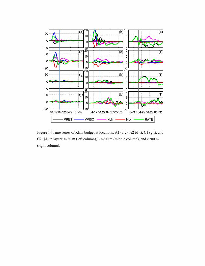
Figure 14 Time series of KEni budget at locations: A1 (a-c), A2 (d-f), C1 (g-i), and
C2 (j-l) in layers: 0-30 m (left column), 30-200 m (middle column), and >200 m
(right column).
(a) (b) (c)
(d) (e) (f)
(g) (h) (i)
(j) (k) (l)