resources in arizona and the - open...
TRANSCRIPT

Hydrology and Water Resources in Arizonaand the Southwest, Volume 17 (1987)
Item Type text; Proceedings
Publisher Arizona-Nevada Academy of Science
Journal Hydrology and Water Resources in Arizona and the Southwest
Rights Copyright ©, where appropriate, is held by the author.
Download date 21/06/2018 00:22:07
Link to Item http://hdl.handle.net/10150/296402

pd,,, J
Volume 17
HYDROLOGYand WATERRESOURCESin ARIZONAand theSOUTHWEST
PROCEEDINGS OF THE 1987 MEETINGSOF THEARIZONA SECTION -AMERICAN WATER RESOURCES ASSOCIATION,HYDROLOGY SECTION -ARIZONA-NEVADA ACADEMY OF SCIENCEAND THEARIZONA HYDROLOGICAL SOCIETY
APRIL 18, 1987, NORTHERN ARIZONA UNIVERSITYFLAGSTAFF, ARIZONA

Volume 17
Hydrology and Water Resources in Arizona and the Southwest
Proceedings of the 1987 Meetingof theArizona Section --American Water Resources Association,Hydrology Section --Arizona- Nevada Academy of Scienceand theArizona Hydrological Society
April 18, 1987Northern Arizona UniversityFlagstaff, Arizona

TABLE OF CONTENTS
PAGE
introduction v
Ordering information for AWRA Publications vii
Distribution of Summer Rainfall Deficits on a Southwest RangelandWatershedHerbert B. Osborn and J. Roger Simanton 1
Adaptability of a Daily Rainfall Dlsaggregation Model to theMidwestern United StatesThomas W. Econopouly, D.R. Davis and D.A. Woolhiser 11
Simulating the impacts of Fire: a Hydrologic ComponentPeter F. Ffolliott, William O. Rasmussen and D. Phillip Guertin 23
Predicting Solar Radiation From Cloud Cover for Snowmelt ModelingDouglas P. McAda and Peter Ffolliott 29
Apparent Abstraction Rates in Ephemeral Stream ChannelsCarl Unkrich and Herbert B. Osborn 35
Analysis of Natural Ground -water Level Variations forAquifer ConceptualizationR. Nevulis, D. Davis, S. Sorooshian and R. Wolford 43
Seasonal Analysis of Colorado River Flows through the Grand Canyonfrom 1914 -1985Charles C. Avery, Stanley S. Beus and Steven W. Carothers 55
A Limnological investigation of an Urban Lake System in CentralArizonaFrederick A. Amalfi and Milton R. Sommerfeld 67
Water Quality of the Upper San Pedro Basin, Cochise County, ArizonaOralynn T. Self 79
Environmental Hazard EvaluationsEdward D. Ricci 91
Minimizing the Effects of Cement Slurry Bleed -Water on Water QualitySamplesLauren G. Evans 101
A Risk Analysis Approach to Groundwater Quality Management In theUpper Santa Cruz BasinThomas C. Richardson and Donald R. Davis 107

INTRODUCTION
The Arizona Section of the American Water Resources Association, theHydrology Section of the Arizona- Nevada Academy of Science and the ArizonaHydrological Society met at Northern Arizona University on April 18, 1987.The annual meeting provides a forum to discuss water issues and presentcurrent research results. This document is made up of the proceedings ofthat meeting.
Papers presented at the meeting were submitted camera -ready by theirauthors for this publication.
These proceedings were produced by the editorial and graphics sectionof the Office of Arid Lands Studies, University of Arizona.
v

ORDERING INFORMATION FOR AWRA PUBLICATIONS
Copies of the following documents can be ordered from ArizonaSection, American Water Resources Association, 845 North Park Avenue,Tucson, Arizona 85719, c/o Dale Wright.
Hydrology and Water Resources in Arizona and the Southwest. Volumes 7through 10 (proceedings of the 1977 -1980 meetings) $12 per copy. Volumes11 through 17 (proceedings of the 1981 -1987 meetings) $14 per copy.
Urban Water Management: Augmentation and Conservation (October 21, 1983,symposium) $10 per copy.
Water Quality and Environmental Health (November 9, 1984, symposium) $10per copy.
Conjunctive Management of Water Resources (October 18, 1985, symposium)$10 per copy.
Water Markets and Transfers: Arizona issues and Challenges (November 7,1986, symposium) $12 per copy.
vii

DISTRIBUTION OF SUMMER RAINFALL DEFICITS ON ASOUTHWEST RANGELAND WATERSHED
_ Herbert B. Osborn and J. Roger SimantonUSDA -ARS, Aridland Watershed Management Research Unit,
2000 E. Allen Rd., Tucson, Arizona 85719
In southeastern Arizona, summer precipitation is the principal andmost reliable source of rangeland moisture (Osborn, 1968). Summerstorms are convective, short -lived events of limited areal extent.Within a watershed, rainfall varies both seasonally and annually, aswell as spatially. Warm season range vegetation must take advantage ofsummer rainfall following a hot, dry spring. The amount of summer rain-fall that is critical to the survival of range vegetation is consider-ably below the long -term average. Local rainfall deficits can occurwithin a season which is designated as average or above average over theregion. Identifying the probability of local rainfall deficits is par-ticularly important in evaluating range management and renovation ef-forts such as grazing rotation and revegetation. In this paper, a pro-posed non -parametric method (Robinson and Fesperman, 1986) was used toinvestigate the pattern of summer rainfall deficits within a 58 -sq -mirangeland watershed in southeastern Arizona.
WATERSHED DESCRIPTION
The 58 -sq -mi Walnut Gulch Experimental Rangeland Watershed insoutheastern Arizona (Figure 1) is representative of millions of acresof brush and warm- season rangeland found throughout the semiarid south-west and is considered a transition zone between the Chihuahuan andSonoran Deserts (Hastings and Turner, 1965). The Pacific Ocean is themajor source of summer rainfall in southeastern Arizona, with the Gulfof Mexico a secondary source (Hales, 1973; Osborn and Davis, 1977).Major thunderstorms occur when substantial moist tropical air flows intoArizona from the south and southwest. Average annual precipitation onthe watershed is about 11.5 inches and is bimodally distributed with 70%occurring during the summer thunderstorm season from late June to midSeptember and the remaining 30% occurring as frontal winter storms.There are no significant positive or negative correlations between seasonal or annual precipitation totals (Osborn, 1983).
METHODS
Robinson and Fesperman (1986) used a method of conditional prob-abilities for adjacent raingage stations to look for patterns ofseasonal and annual precipitation deficits in North Carolina. Theyfound this simple non -parametric test useful for identifying areas with-in the State prone to drought. They considered North Carolina as asmall, or mesoscale, area. The dominance of convective storms in theSouthwest suggested that such a procedure might apply to much smallerareas such as the Walnut Gulch Watershed, at least for summer rainfall.
The study was based on records from 38 weighing -type recordingraingages for the summers of 1956 through 1977 (Fig. 1). Although thepresent network consists of 90 recording raingages, only 38 were in
1

® M
INIM
UM
PO
INT
RA
INF
ALL
® M
AX
IMU
M P
OIN
T R
AIN
FA
LL
AV
ER
AG
E W
AT
ER
SH
ED
RA
INF
ALL
12\ --
--\\
ON
NM
OA
OE
LO
CA
TIO
N A
N. N
uwN
.10
w'0
INT
01N
5 IN
TU
T A
BO
VE
N.S
.I.. W 2 O 2 J
6J z 4
Fig
ure
1.W
alnu
t Gul
ch r
elie
fim
pan
d ra
inga
ge n
etw
ork.
1.0
ú0.
82 W O t 0
.6W
0.4
J R ú0.
2 002
46
e10
SU
MM
ER
RA
INF
ALL
(IN
CH
ES
)12
Fig
ure
2.D
istr
ibut
ion
of s
umm
er r
ainf
all o
n W
alnu
t Gul
ch.
14
\, \
\\ \
%\
6570
75Y
EA
R
Fig
ure
3.W
alnu
t Gul
ch s
imm
er r
ainf
all.

continuous operation from 1956 through 1977. For this study, summermonths were considered as June, July, and August, since this is themaximum period of growth for many range species. Major vegetation ofthe watershed includes: creosote bush (Larrea tridentia), white -thorn(Acaci= constricta), tarbush (Flourensia cernua), snakeweed (GutierreziaSarothrae), burroweed (Aplopappus tenuisectus), black grama (Boutelouaeriopoda), blue grama (1. gracilis), sideoats grama (A. curtíoendula),and bush muhly (Muhlenbergia Dorteri).
The non -parametric technique developed by Robinson and Fespermanessentially uses the quantile values of precipitation amount at eachstation to identify times of low precipitation. In this way, differ-ences in annual and seasonal means within the region, due to such fac-tors as elevation and aspect, are eliminated. We also adapted themethod to the case in which we assume that the distribution function ofsummer rainfall is the same for all gages on Walnut Gulch.
RESULTS
In the first case, assuming long -term differences because of gagelocation and elevation, the annual summer rainfall amounts were rankedin order for each gage, the largest to the smallest, and the years withrainfall below the 20th percentile were considered deficit. The fouryears which were considered deficit at each gage are marked with an"x" (Table 1). In the second case, where summer rainfall was consideredcompletely random, all summer point (raingage) amounts were ranked toge-ther, and those below the 20th percentile were considered deficit.There were as many as eight deficit years at some gages and a minimum ofone year at two gages (Table 2, Fig. 2).
Yearly average, maximum and minimum summer rainfall amounts for the38 -gage network are shown in Fig. 3. Average summer rainfall for the22 -yr record was 6.44 inches and ranged from 2.92 inches (1960) to 9.46inches (1966), with point values ranging from 1.57 inches (1960) to13.24 inches (1966). Average point summer rainfall varied from 5.63inches to 7.17 inches (Fig.4). In the "driest" summer (1960), the water-shed average was 2.92 inches, with a point range of 1.57 to 5.02 inches(Fig. 5), and well below average rainfall was recorded over the entirewatershed. In contrast, in 1966, the "wettest" summer, the averagerainfall was 9.46 inches, with a range of 7.47 to 13.24 inches, and theentire watershed had above average rainfall (Fig. 6). Average annualprecipitation for the 22 -yr record was 11.46 inches, and summer rainfallamounted to 56% of annual precipitation. Fall (Sep.- Nov.), winter(Dec.- Feb.), and spring (Mar. -May) precipitation were 23%, 14%, and 7%,respectively, of annual precipitation.
Based on the assumption that differences in average summer rainfall(Fig. 4) represented real long -term differences associated with gagesite and elevation, there were deficits on significant portions of thewatershed in six of the 22 years of record (Fig. 7 -11). However, therewas below average rainfall over the entire watershed only in 1960.In 1962, 1970, 1973, 1975, and 1976, summer deficits occurred onsignificant portions of the watershed, but other parts of the watershedreceived above average rainfall (Fig. 7 -11). Deficit summer rainfall
3

TABLE 1.
Year
Deficit Summer Rainfall On Walnut Gulch, 1956 -1977.
Raingage Number
0 0 0 0 0 0 0 1 1 1 1 1 1 2 2 2 2 2 2 3 3 3 3 3 4 4 4 4 4 4 4 5 5 6 6 6 6 72 3 4 5 7 8 9 1 3 4 5 6 8 1 3 4 6 7 9 0 1 3 6 9 1 2 3 4 5 7 8 4 6 0 5 6 8 0
1956 X X X X X X X X X X X
1957
1958 X X X X X
1959
1960XXXXXXXXXXXXX XXXXXX XXXXXXXXXXXXXXXXX1961
1962 X X X X X X X X X' X X X X X X X X X X X X
1963
1964 X X
1965 X X X X X X X
1966
1967 X X X X X X X
1968
1969 X X X
1970 X XXXXX X
1971
1972
1973 X X XX XX XX XXX XXXXX
1974 X X
1975 X X X X X X X X X X X X X X X X X X X X
1976 XX XXXX XX XX XX X
1977 X X X X X
4

Table 2. Gages Recording Deficit summer rainfall on Walnut Gulch, 1956 -1977,based on random distribution of summer rainfall.
Tsar Raingage Number
0 0 0 0 0 0 0 1 1 1 1 1 1 2 2 2 2 2 2 3 3 3 3 3 4 4 4 4 4 4 4 5 5 6 6 6 6 72 3 4 5 7 8 9 1 3 4 5 6 8 1 3 4 6 7 9 0 1 3 6 9 1 2 3 4 5 7 8 4 6 0 5 6 8 0
1956 0 0 0 0 0 0 0 0 0 0
1957 0
1958 0 0 0 0
1959
1960 0 0 0 0 0 0 0 0 0 0 0 0 0 0 0 0 0 0 0 0 0 0 0 0 0 0 0 0 0 0 0 0 0 0 0
1961
1962 0 0 0 0 0 0 0 0 0 0 0 0 0 0 0 0 0 0 0
1963 0 0
1964 0
19650000 0 0 0 00
1966
1967 0 0 0 0 0 0
1968
1969 0 0
1970 0 0 0 0 0 0
1971
1972
19730 0 00 00000 000 000001974 0 0
1975 0 0 0 0 0 0 0 0 0 0 0 0 0 0 0 0 0 0 0 0
1976 0 0 0 00 00 00 00 0 0
1977 0 0 0 0
5

6
nEO
W

'4309 3nuLeM uo Lle;ule.a aams 9L61 21311a0 'lt a.1n611
--.`
^.
`'
..
.-_-
93N311192
fin
-¡`,
i¡
is, `
°£3/13tl1%
3 iCY
-,11rlN
1r1/ 1171930ti11'£
471n9 3nuLeM uo Lle;ule.l aauuns EL61 31314a0
'6
'--¡llrlN
lYN
117143041'f
-_-ë
--6'L
Ii
`¡-
`-,.,
-e
_
oti
e'-'-
!o
Or,
e!Z
Z
!*Z°
_a_o.._.s
ZIf,
°°
°e___!_-
r'-.o
----__.!£l'f.
..-
arn6lj
£'tte_9
---
'431n9 3nuLeM uo lle;ule.a
.aaulrnsSL6L 3131da0 '01 a11613
ttiws
io
i
w
r .
----o,
- _
áYZ
'L
i -
.-.
I
LE
2;
SY£
-..a
4309 rum uo Lle;ule.a Jauelns OL61 31311a0
8 a.an6lj
--
`.
11110.tlw
os
oe
es
'-'i-
i-.. .
O
! ..41......'-
.!*C
Z,
:'-- -6'!s----9'-"-
r.._:
ro
'`so__
was recorded at over half of the raingages in 1962, although severalraingages recórded above average rainfall (Fig. 7). The minimum andmaximum in 1962 were 2.83 and 7.11 inches. A portion of the lower endof the watershed received deficit rainfall in 1970, whereas most of thewatershed received average or above average rainfall. Summer deficitswere recorded on about half of the watershed in 1973 and 1975 (Fig. 9and 10). The minimums and maximums were 3.12 and 7.59 inches in 1973,and 2.37 and 7.86 inches in 1975. A deficit was recorded on about 33%of the watershed in 1976, with a minimum and maximum of 2.84 and 9.83inches (Fig. 11).
In other words, while a portion of the watershed may be extremelydry, other portions may receive well above average rainfall. The great-est recorded difference between maximum and minimum summer rainfall,7.90 inches, occurred in 1969, when the minimum and maximum were 3.50and 11.40 inches. In most summers, the minimum point rainfall was lessthan 50% of the maximum. In 1960, 1969, 1975, and 1976, the minimum wasabout 30% of the maximum. In only two summers, both relatively wet, wasthe minimum more than 50% of the maximum. In eight of the 22 years,none of the 38 gages recorded deficit summer rainfall.
We also analyzed the 22 years of data assuming that long -term sum-mer rainfall is randomly distributed on Walnut Gulch. When all summerrainfall data were lumped together, deficit gage /years (below the 20thpercentile) were those with less than 4.60 inches of rainfall (Fig.2).Based on this assumption, the lower end of the watershed was consider-ably drier than most of the watershed, and the south central portion wasmuch wetter than most of the watershed (Fig. 4 and 12).
DISCUSSION
There was no indication, at least for the 22 years of record, of apersistence in deficit summer rainfall from year to year on any portionof the watershed. There were differences in mean summer rainfall betweenraingages (Fig. 4), which could be meaningful in terms of range condi-tions. Furthermore, a suggestion of possible nonrandom distribution ofdeficit summer rainfall (Fig. 12) needs to be explained. Further analyses are in order when more years of data are available.
SUMMARY
A simple non -parametric technique (Robinson and Fesperman, 1986)was used to investigate the possible persistence of summer rainfalldeficits on the Walnut Gulch experimental watershed in southeasternArizona. By ranking summer rainfall at each raingage from the largestto the smallest amount and looking at the lowest 20th percentile, wereaffirmed the extreme variability of summer rainfall on a 58 -sq -mirangeland watershed, but found no evidence of persistence in deficitrainfall on any particular portion of the watershed. However, the datadid suggest a possible non - random pattern of summer rainfall that couldnot be readily explained, and suggested that when more data are avail-able further evaluation would be appropriate.
8

REFERENCES
Hales, J. E. 1973. Southwestern United States summer monsoon source- -
Gulf of Mexico or Pacific Ocean. NOAA Tech. Memo. NW- SWR -84, 26p.
Hastings, J. R. and R. M. Turner. 1965. The Changing Mile. Universityof Arizona Press, Tucson, Arizona, 317p.
Osborn, H. B. 1968. Persistence of summer rainy and drought periods ona semiarid rangeland watershed. Bull. LASH, 13(1):14 -19.
Osborn, H. B. 1983. Precipitation characteristics affecting hydrologicresponse of southwestern rangelands. USDA -ARS Agricultural Reviewsand Manuals, ARM -W -34, 55p.
Osborn, H. B., and D. R. Davis. 1977. Simulation of summer rainfalloccurrence in Arizona and New Mexico. Hydrology of Water Resourcesin Arizona and the Southwest. Office of Aridland Studies.University of Arizona, 7:153 -162.
Robinson, P. J. and J. N. Fesperman. 1987. On the mesoscaledistribution of precipitation deficits. Archives for Meteorology,Geophysics, and Bioclimatology, Ser. B, University of NorthCarolina, In Press.
4 4 lE,-., i4 4 5 .-s- 4 ... _- r ,^_^.- _ / DRYr- a
o,36. 5, ? 3 ,- . -> g' DRY. .
il''..._ WfT,°" ' : 4-:r3' , ' c6 r¡ 5T- 4 - " ;,
fr.6Rl:ET 70 \ ,, ,°, ET ,; 4
. _.. - ,', J3- , .\ _ -I
. \ xti
- - -nRV ¡ .'ir) , °3 .r
. -_ ,,-WETTfST ` .. . .I WET", ;i 1 q .` 2 , g5
e , i\
% . --_-,
4
Figure 12. Distribution of deficit summer rainfall ( <4.60 ") on Walnut Gulch.
9

ADAPTABILITY OF A DAILY RAINFALL DISAGGEGATION MODEL TO THE
MIDWESTERN UNITED STAPES
Thomas Y. Econopouly, D. R. Davis, and D. A. Woolhiser
INTRODUCTION
Daily disaggregation of rainfall is a technique used to separate adaily rainfall depth into smaller showers. The showers can then befurther disaggregated into intensity patterns, which may be used asinput for time varying infiltration models (Woolhiser and Osborn,1985). A stochastic model for the disaggregation of daily summer rain-fall in southeastern Arizona was developed by Hershenhorn (1984).Hershenhorn used data collected at a gage on the Walnut GulchWatershed. Hershenhorn and Woolhiser (1987) found that this model wasapplicable for locations up to 75 miles away from the original gage.In this paper, we discuss the applicability of the model to two midwes-tern locations.
DATA SET
The data used in the study were collected on the AgriculturalResearch Service's Experimental Watersheds at Hastings, Nebraska andMcCredie (now Kingdom City) Missouri, and were obtained on magnetictape from the U.S.D.A.'s Water Data Laboratory. The period of recordfor Hastings was 1938 through 1967, and for McCredie was 1941 through1974. Two periods of the year were investigated - May and June, andJuly and August.
The climate for both of these locations is considered continental,with an annual precipitation cycle that exhibits a winter minimum and asummer maximum. The maximum amount precipitation occurs during June,and over half of the total annual precipitation occurs during themonths of May through September. The early summer maximum is a resultof the continental influence resulting in increasing temperatures andadvection of moisture from the Gulf of Mexico, coupled with stillfairly active spring storms (Trewartha, 1981). Approximately 80 per-cent of the summer precipitation in the region has been classified asfrontal in nature (Rudd, 1961).
DAILY DISAGGREGATION MODEL
The mathematical description of the disaggregation model isdescribed in detail by Hershenhorn (1984) and Hershenhorn and Woolhiser(1987). The model's structure requires a daily precipitation amount asan input. Given daily amounts the model can be used to describe thenumber of showers within a day, the starting time, the depth and theduration for each shower.
11

Complete vs. Prartial Showers
Two types of showers are defined - a complete shower is one thatbegins and ends within the same day, and a partial shower is one thatbegins on one day and ends on another. Table 1 lists the number of twoconsecutive days with precipitation and the percentage of those con-taining a partial event. The rank sum test (Hoel, 1971) was used todetermine if the sums or products of the daily depth amounts for con-secutive wet days with partials and those without partials weredifferent. At the five percent level, there were no significant dif-ferences between the consecutive wet days with partials and thosewithout partials.
Table 1. Number of Two Consecutive Wet Days
No. of Two Consecutive Percentage 1/Location Period Wet Days with Partials
Hastings May and June 188 34Hastings July and August 107 34
McCredie May and June 272 24McCredie July and August 164 21
Walnut Gulch July and August 217 17
1/ Number of consecutive wet days when the shower continued throughmidnight divided by the total number of consecutive wet days.
Partial showers were separated into two smaller showers which wereassigned to the day on which each occurred. For the remainder of thispaper a partial shower will be considered as either parts of the showerthat crossed midnight. A log likelihood ratio test was performed onthe distributions of partial and complete showers depths at WalnutGulch (Hershenhorn, 1984), it found that the complete and partialdepths could be described by the same distribution. The log likelihoodratio test was also performed using the Hastings and McCredie data andit was found that only the McCredie - July and August, complete andpartial depths could be described by one distribution. However, thetwo sample Kolmogorov- Smirnov (KS) test could not distinguish betweenany of the midwestern complete or partial shower depth distributions.Thus, to make the description of the rainfall process more tractable,the partial and complete depths were assumed to be samples from thesame distribution. This assumption was necessary in order to distributedaily depths into multiple shower depths.
Distribution of Number of Showers Given Daily Precipitation
A joint distribution was required to describe the number ofshowers in a day, given a daily precipitation amount. The joint
12

distribution of the number of showers per day, and the daily amount canbe written as the product of the conditional and marginal distribu-tions:
where:
HN,Z,(n,z) - GNIZ,(nIz)FZ,(z) (1)
N - the number of showers.
Z'- the daily precipitation depth minus a threshold.
Because the lower limit of the daily observation was 0.01 inch,the threshold was set at 0.009 inch. The threshold was set at thisvalue so all small depth values would remain in the data set.
In this study, the marginal distribution of daily rainfall wasdeveloped so that the goodness of fit of the conditional distributioncould be tested. When the overall model is used, the daily depth willbe obtained from historical data or perhaps a climate generating model.The marginal distribution chosen for test purposes was the MixedExponential distribution (Smith and Schreiber, 1974) which density hasthe form:
where:
fZ,(z) - á exp (-z/01) + é exp (-Z/82) (2)1 2
a- is a weighting parameter (0 5 a 5 1)
8 and 82 are parameters
Hershenhorn (1984) found that the Shifted Negative Binomial (SNB)distribution provided a good fit for the conditional distribution ofthe number of showers given daily rainfall. The probability mass func-tion of the SNB is written as:
P(N -n) - (n +r-2)pr(1- p)n -1;
n- 1,2,... (3)
Variables p and r were allowed to vary with daily depth. TheWalnut Gulch data indicated that the number of showers given Z,asymptotically approached a limiting value. However, the McCredie datasuggested that the expected number of showers asymptotically approacheda straight line with a positive slope (figure 1), and thus a new func-tional form was developed for p and r. This new functional formaccounts for this factor and includes the Walnut Gulch function as aspecial case. The functional form for p and r is now:
p - exp(-Al x Z) (4)
r - (E - 1.0) x p/(1.0 - p) (5)
E - A2 + A3 x Z + (1.0 - A2) x exp(-A4 x Z) (6)
13

5.0
4.5EXP 4.0ECT 3.5ED3.0
N0. 2.5
0F 2.0
SH 1.50wE 1.0RS
.50
.00
r I 1
EXPECTED NUMBER OF SHOWERS VS. DAILY PflECIPITATION
WALNUT GULCH (JULY AND AUGUST)- - W*iSTINGS (MAY AND JUNE)
. ----- NOCREDIE (MAY AND JUNE) MIN
00
5e
1
PfiECIPITATION ( INCHES)
2 2
Figure 1. Expected Number of Showers vs. Daily Precipitation.
14
3

where:
E - is the expected amount of showers given a daily precipita-tion amount.
Z - is daily precipitation depth.
Al, A2, A3 and A4 are fitted parameters.
Parameter values were obtained for the midwestern data by numeri-cal maximum likelihood techniques. The null hypothesis that the sampledata were taken from the identified bivariate distribution could not berejected for the McCredie data sets, according to a Chi - Squared good-ness of fit test, at the 1 percent level.
Individual Shower Depths
Given a daily rainfall depth, Z, and the number of showers perday, N, individual shower amounts, Y1 Y2,...YN need to be determined.The summation of all the individual depths which occur within a daymust equal that day's rainfall depth. The ratio technique developedfor the Walnut Gulch data (Hershenhorn, 1984), also represented themidwestern locations. The technique used ratios developed from showeramounts and daily depth. The ratios were then fitted to either a BetaFourier distribution or a Uniform distribution. The ratio techniquewas used to describe up to 6 showers within a day at Walnut Gulch. TheMcCredie data had up to 13 showers per day.
Shower Starting Times
A partial shower was defined as one that ends or begins at mid-night, so once the durations had been determined, the time of the startof a shower was determined. Hershenhorn (1984) used the Mixed Betadistribution to describe normalized starting times for the completeshowers. The starting times were normalized by defining the startingtimes as time (in hours) from midnight and dividing by 24. The MixedBeta distribution can written as:
where:
w'(a1+ ß1)
tal-1ß1-1
fTc(t) r(al)r(ß1)(1-t) +
r(.22 + ß2) a2-1 02-1(1-w) t (1-t)
r(a2) r(ß2)
r - is the gamma function
w - is a weighting parameter (0 5 w 5 1)
al, ß2, a2, and ß2 are parameters
15
(7)

The Mixed Beta distribution has some undesirable features. The
distribution is not necessarily periodic. However, the process that wewish to describe is periodic. The distribution can not be explicitlyintegrated. If numerically integrated, care must be taken at the tailswhere the Mixed Beta distribution may take on infinite values. To
overcome the problems with the Mixed Beta, a Fourier distribution witha mean of one and two harmonics was tested to determine if it couldreplace the Mixed Beta. The Fourier distribution is periodic and canbe explicitly integrated. The Fourier distribution can be written as:
where:
fTc(t) - 1.0 + a cos (2rt + ß) + 8 cos (4at + p)
a - the first amplitude.
ß - the first phase angle.
8 - the second amplitude
p - the second phase angle.
(8)
Parameter values for the Mixed Beta distribution and the Fourierdistribution were obtained by using numerical maximum likelihood tech-niques for the individual data sets . The data sets were divided intosubclasses, which were grouped according to the number of showers perday, up to 6 showers per day. All days with 6 or more showers weregrouped together. One- sample KS tests were performed to determinewhether the historical cumulative distribution functions (CDF's) weresignificantly different from the CDF's calculated from the parametervalues optimized over the entire data set. At the one percent level,all the historical CDF's for each subclass were not significantly dif-ferent from the Fourier CDF's. The Hastings, July and August - 1
shower per day data was the only subclass that was significantly dif-ferent, at the one percent level, from the Mixed Beta CDF's.
The hypothesis of the independence of multiple starting times on aday with more than one shower, and whether they can be described byorder statistics was tested for both the Mixed Beta and the Fourierdistr l utions. Let FT (t) represent the CDF of the starting time ofthe r shower on a relay in which n showers occur (Kendall and Stuart,1977). The general form is:
n!
FTr(t) - (r -1)! (n-r)!
n -̂r
)
(nir+-1)i
(FTc)i+ri-0
where Fm is the CDF of all shower starting times as given by the CDFof the Piríxed Beta or Fourier distribution.
The empirical distribution functions were compared with the theo-retical distributions given the assumption of independence. The one -
sample KS test was used to test the hypothesis that the shower starting
16

times were independent. When the order statistics were calculated fromthe Mixed Betá distribution, there were 5 instances out of 36 when thedistributions were considered significantly different at the one per-cent level. Tests with the Fourier distribution revealed 3 instancesout of 36 where the distributions were significantly different.
The Mixed Beta and the Fourier distribution appear to fit the dataequally well. Therefore, because of its favorable properties pre-viously mentioned, the Fourier distribution was chosen as thedistribution to use to describe the starting times of complete showers.
Starting time for one shower per day. To reflect the relationbetween depth and starting time, the shower starting times were condi-tioned upon depth. However, we will describe only one shower per dayin this manner because the statistical description of more than oneshower per day becomes intractable. The joint distribution of showerdepth and time of day may be written as:
fX,Tc(x't) fX/Tc(x/t) gTc(t)
where:
fX /Tc(x /t) is the conditional distribution of depth giventime of day.
gTc(t) the marginal distribution of starting timesthe Fourier distribution.
(10)
The following marginal distribution for depth was obtained by integrat-ing the joint distribution over time:
gX(x) JTc(u) fX/Tc(x/u)du (11)
From Bayes' theorem the conditional distribution of time given depth:
fTc/X(t,x) - (g. (t) fX /Tc(X /Tc)] / gX(x) (12)
The cumulative probability of the conditional time given depth is:
P(T<t / x) -JTc,x(u/c) du (13)
Preliminary investigations revealed that the Exponential distribu-tion may be used to describe the distribution of shower depths withintwo hour intervals. Therefore, an Exponential distribution with a timevarying parameter was chosen for the conditional distribution of depthof a shower given time of day. The conditional distribution may bewritten as:
fX /Tc(x /t) - 1.0 /1(t) [exp(t/l(t))] (14)
where the mean 1(t), is represented by a fourier series with two terms:
1(t) - A + B cos(2xx + C) + D cos(4xx + E) (15)
17

The parameters A, B, C, D and E are obtained by numerical optimizationusing maximum likelihood techniques. To improve the fit of this dis-tribution to the data set and to reduce the number of showers to besimulated, only showers greater than 0.10 of an inch were included.
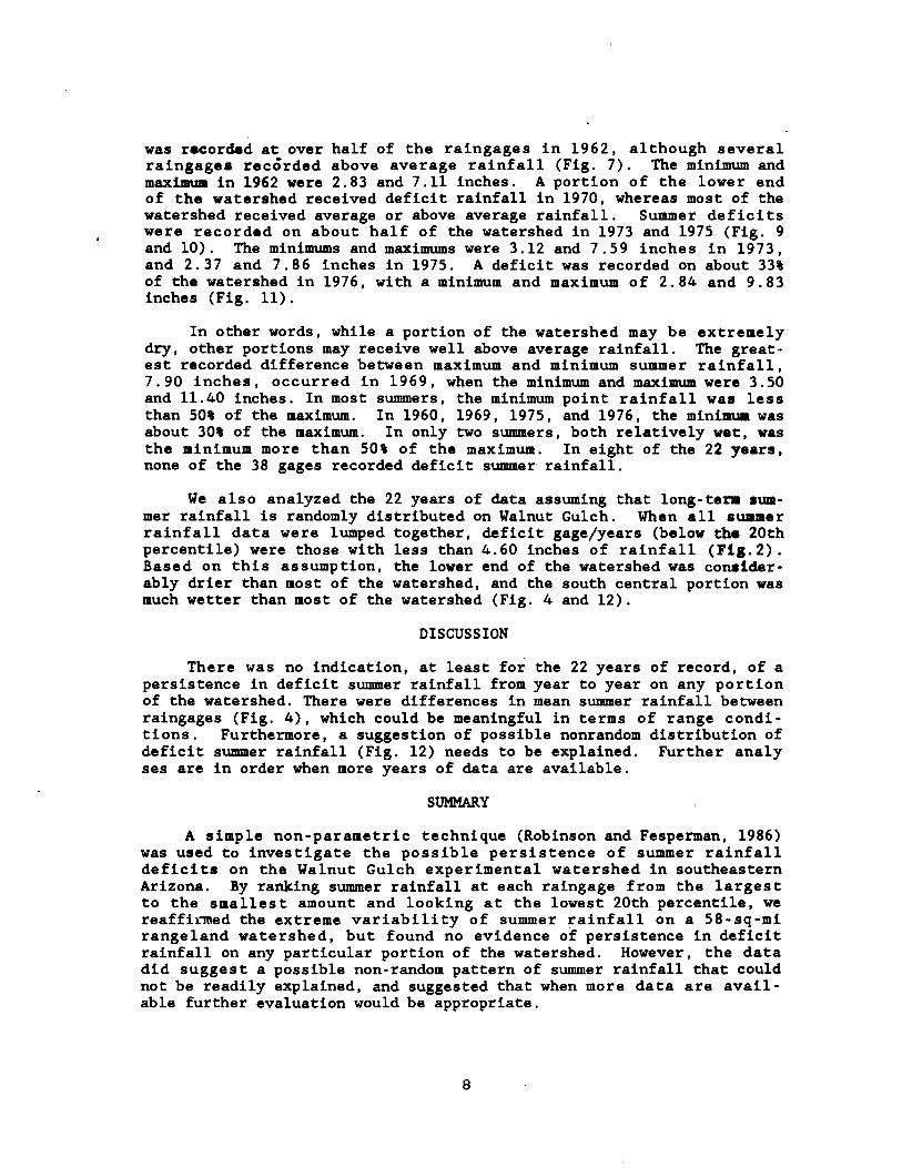
The Chi - Square goodness of fit test was used to determine whetherthe theoretical joint distribution was significantly different from thehistorical distribution of shower depths and starting times. At theone percent significance level, the only data set that was consideredsignificantly different is the July and August data set from Hastings.Inspection of the cumulative plot of starting times (figure 2) for theone per day showers reveals a high frequency of points at 6:00 am. Theoccurrence of this many points at one time probably is an artifact dueto the techniques used to convert analog rainfall data into a digitalform. The number of points at 6:00 am made it difficult to fit a curvethrough these data.
Joint Distribution of Shower Duration and Amount
Shower durations were determined from the corresponding showerdepth. The joint distribution of shower duration and amount may bewritten as:
hy, D(y,d) - gD/y,(d /y) fy.(y)
Where d is the shower duration and y is the shower depth minus a thres-hold amount. The shower depth is obtained from the storm ratio tech-nique.
(16)
Hershenhorn (1984) used a bivariate log -normal distribution forD(y,d). Different functional relationships between depth and dura-
tioh were tested for linear dependency for the complete and partialshowers, individually. The best linear relationship obtained for thecomplete showers, with a threshold equal to 0.009, for three of thefour midwestern data sets, was when the duration was transformed to itsnatural log and the depth was raised to the one -third power. However,the hypothesis that the residuals came from a normal distribution witha mean equal to zero and a standard deviation equal to the standarderror of estimate could not be accepted by the Chi- Squared test at theone percent significance level, for half of the data sets.
The threshold for the complete showers was increased to 0.099inches, to reduce the number of data points, and to facilitate the fitof a regression line. In future simulations, showers of less than 0.10inch will be treated in a simpler fashion than showers greater than orequal to 0.10 inch. The highest coefficient of determination for twoof the midwestern data sets resulted when the durations were trans-formed to their natural logs and the depths were not transformed. The
remaining data sets highest coefficient of determination resulted when
the duration was transformed to its natural log and the depth wastransformed to its square root.
The hypothesis of linearity of regression was tested by using acorrelation ratio test (Kendall and Stuart, 1977). When all the four
18
1.8
.9e
C .MUM
u .?eLAT .68I
VE .90
R .49E0U .30ENC .aeY
. 18
. e0
8 i 2 3 4 5 6e e e e e e e e
DEPTH FäiTIO
19e e
Figure 2. Starting Time of Showers for Hastings (July and August).
19

data sets' durations were transformed to their natural logs and thedepths were allowed to remain the same, all four transformed data setspassed the linearity test at the five percent level. When the datasets' durations were transformed to their natural logs and the depthswere transformed to their square, three of the data sets passed thetest at the five percent level, and the Hastings, May and June datapassed at the one percent level.
Testing was also performed to determine if the residuals from theregression were from a normal distribution with a mean of zero and astandard deviation equal to the standard error of estimate. To deter-mine if the standard deviation of the residuals was constant the Chi -Square test was performed on four subclasses of each data set. Thesubclasses were set up so each subclass had the same sample size. Fourof the total of sixteen subclasses' residuals could not be consideredfrom a normal distribution, at the one percent level, for the log dura-tion vs. depth relationship. At the one percent level, four of thesixteen subclasses' residuals could not be considered from a normaldistribution for the log duration vs square root of depth relationship.
The residuals for all of the four midwestern data were also testedfor normality without breaking up the data sets into subclasses. Atthe one percent level, just the McCredie July and August data set'sresiduals could not be considered as from a normal distribution for thelog duration vs depth relationship. Only the Hastings, May and Juneresiduals did not pass the significance testing when the log durationvs square root of depth relationship was examined.
The log duration vs. depth relationship used for the complete datasets was tested for linearity and normality, with the partial datasets. The threshold was set to 0.009 inch. At the five percent level,the data sets transformed in this manner passed all the tests.
CONCLUSIONS
The daily disaggregation technique developed by Hershenhorn (1984)from summer precipitation data collected in southeastern, Arizona re-quired slight modification to be used to describe spring and summerprecipitation for two midwestern stations.
Two of the modifications which were needed improved the tractabil-ity of the model. The Fourier distribution was used to replace theMixed Beta distribution for the description of the starting times ofthe showers. The replacement made the description of the startingtimes more theoretically correct because the Fourier distribution isperiodic where the Mixed Beta is not. The Fourier density distributionis also much easier to integrate for its use in simulations. Thisreplacement may be suitable for the Arizona data as well. A change wasmade in the functional forms of the p and r values of the ShiftedNegative Binomial distribution, which improved the old functional formby allowing the parameters to take additional functional forms.
The duration vs. depth relationship which resulted in the greatestlinear dependency was different at the midwestern locations from that
20

in Arizona. The residuals of the complete shower depths minus thethreshold of 0.009 inch were not normally distributed about the regres-sion line of the greatest linear dependency, thus the threshold for thecomplete showers had to be increased to 0.099 inch. This change ofthreshold should not reduce the applicability of the model sinceprecipitation intensities from showers of less than 0.10 inch arerarely needed in models which use time varying infiltration techniques.
The disaggregation technique was improved by conditioning thestarting times of the one shower per day on the depth of the shower.This allows the daily disaggregation to partially describe the diurnalfluctuation of depth. This addition may also be used to describethediurnal fluctuation of depth in southeastern Arizona.
REFERENCES CITED
Hershenhorn, J.S. 1984. Stochastic Modeling ofSequences. M.S. Thesis, University of Arizona.
Hershenhorn, J.S. and D.A. Woolhiser, 1987 (In Press).of Daily Rainfall. Journal of Hydrology.
Daily Rainfall
Disaggregation
Hoel, P.G. 1971. Introduction to Mathematical Statistics. John Wileyand Sons, Inc., New York.
Kendall, M., and Stuart, A., 1977. The Advanced Theory of Statistics,Vol. 2. Charles Griffin and Company, Ltd., London.
Rudd, R.D. 1961. Summer Frontal Precipitation in the United StatesArea of Daf Climate. J. Geophys. Res., 66: 125 -130.
Smith, R.E., and Schreiber, H.A. 1974. Point Processes of SeasonalThunderstorm Rainfall. 2. Rainfall Depth Probabilities. WaterResources Research, Vol. 10, No. 3, pp. 418 -428.
Trewartha, G.T. 1981. The Earth's Problem Climates, 2nd Edition. TheUniversity of Wisconsin Press, Madison, 1981.
Woolhiser, D.A. and Osborn, H.B. 1985. A Stochastic Model ofDimensionless Thunderstorm Rainfall, Water Resour. Res. 21:511-522.
21

SIIMPal2C TIE IIIPlilL'1S CF FIRE: A HYDROLOGIC COMPOIDERr
Peter F. Ffolliott, William O. Rasmussen, and D. Phillip GuertinSchool of Renewable Natural Resources, University of Arizona
Tucson, Arizona 85721
Introduction
To estimate the impacts of fire on various components of southwesternponderosa pine forest ecosystems, BURN, a computer simulation model whichestimates benefits or losses after a fire occurrence, has been developed.BURN considers vegetative components, including mortality of forestoverstories, regeneration of tree species, and production of herbaceousunderstories; wildlife components, including changes in population structuresand effects on habitat qualities; and hydrologic components, including changesin annual streamflow and water quality parameters. The formulation,application, and future developmental work of the hydrologic component aredescribed in this paper.
Foravlaticn of Model
The general approach employed in the formulation of BURN was to assumethat changes in an ecosystem after a fire can be viewed as flows of benefitsor losses through time. Then, by contrasting the flows of benefits or lossesagainst a control (an unburned area), so- called "time -trend responsefunctions" can be developed (Lowe et al. 1978). These functions, which aregraphical representations of benefits or losses that occur after a fire, formthe basis for the formulation of BURN.
Tine- ?rend Response Functions
For each "ecosystem component" in BURN, a set of index values has beenderived to characterize the resource. To present the source data in aconsistent manner, the index values for post -fire conditions, derived bysampling for an attribute (1) at different points in time after a fire hasoccurred or (2) from sampling an attribute on a series of study areasrepresenting different fire histories, are divided by index values obtained ona control area. The result is a unitless value, with the value of the controlalways LO. Assuming that the ecosystem component in question would respondin the same manner to fluctuations in weather conditions, time of year, andcyclic alterations, the ratios can be considered indicators of changes due tofire only.
Graphs are structured for each attribute investigated in the formulationof BURN, with the ratios plotted on the Y -axis and time after a fire on the X-axis. The control is represented by a horizontal line with a value of 1.0.Schematic curves represent the flows of benefits or losses for an arbitrarily
23

selected time period of 20 -years after the occurrence of a fire. If a curveis *meths control line, it is assumed to measure a benefit, while a curvebelow the control line is a measure of a loss. If a ratio is not differentfrom the control value, no change in benefit or loss is assumed. Again, thesecurves are the time - trend response functions, by definition.
lides of Benefits of Loases
The time -trend response functions are converted to an index of benefitsor losses by initially determining strew of annual ratio values (Love et ai.1978). Then, the streams of annual ratios are converted to annuities,representing equal annual returns from a resource. While annuities normallyare thought of in terms of dollars, the concept is applicable to nal- monetaryflows. The annuities are calculated from:
a is Vo
where a =
Vb =
i =
n =
(1+i) n-1
the annuity
the total of all annual values from a time -trend responsefunction, discounted to time zero
the discount rate
the number of years in the analysis (1 to 20)
In the above calculation, Vro is determined from
2_0 VhViz)
= nil(1+i)n
where Vh the value of the ratio taken from a time -trend response functionfor the individual years in the analysis (1 to 20)
The annuities allow a condensation of annual ratio values into a singleannual index value. Theoretically, the annuity value of 1.0 is "indifferent"to the actual stream of annual ratios each year; since the ratio for thecontrol is LO for each year, the annuity also is 1.0. Annuity values thatare higher or lower than 1.0 indicate benefits or losses, respectively.
Annuities calculated for 20 -year periods are highly responsive to thediscount rate selected. In essence, the discount rate determines how such'weight" is given to the different annual ratios. The greater the discountrate, the more heavily future yields are discounted. For example, if a 5percent discount rate is selected, ratios for i year after a fire has occurredare weighed 2.5 times as heavily as ratios for 20 years after the fire.However, if a 10 percent discount rate is used, ratios for 1 year after a fire
24

are weighted more than 6 times as heavily as ratios for 20 years after thefire.
Attributes Measured
In the hydrologic component of BURN, two attributes are consideredcurrently, annual streamflow and water quality. Measurements of theseattributes were obtained from secondary data sources, as described below.
Annual streamflow amounts were measured by water -stage recorders atcontrol sections located at the cutlets of study watersheds, near Flagstaff,Arizona (Campbell et al. 1977). These study watersheds had been burn3 -over bya wildfire of different intensities. Unfortunately, due to the limitedstreamflow records available, extensions of annual streamflow response to thefire through a 20 -year evaluation period were judgemental. However, therelative orders of magnitude for the annual ratio values employed incalculating the annuities are thought to be appropriate.
Water samples collected before and after a series of prescribed fires inthe Santa Catalina Mountains, near Tucson, Arizona, were analyzed by theDepartment of Soils and Water at the University of Arizona (Sims et al. 1982).These baseline data sets provided the source information on water qualityparameters. Specific chemical constituents analyzed included calcium,magnesium, sodium, chloride, sulfate, bicarbonate, fluoride, nitrate, pH,total soluble salts, and electrical conductivity. Supplementary informationon water quality was obtained from Campbell et al. (1977).
Flowchart
The flow of activities followed in executing BURN to obtain estimates ofbenefits or losses after a fire has occurred is illustrated in figure 1.Through inputs of forest type, evaluation component, fire intensity, post -burning evaluation period, and a discount rate, an annuity value, termed a"fire impact index," is calculated. If desired, the simulation exercise canbe recycled to analyze a series of discount rates, evaluation periods, fireintensities, and evaluation components.
A summary display is presented at the end of the simulation exercise,showing the estimates of benefits or losses, in terms of annuities, after theoccurrence of a fire.
Application of Model
Perhaps, the best way to illustrate the application of the hydrologiccomponent of BURN is through an example. In this example, we will examine theeffects of a hypothetical fire on annual streamflow amounts from a watershedstocked with southwestern ponderosa pine forests.
Arbitrarily, a fire intensity of less than 5,000 Btu /second /foot has been
selected to represent the intensity of the hypothetical fire. It is assumedthat this fire has burned uniformly over the watershed. The length of thepost- burning evaluation period will be 10 years. A discount rate of 5 percent
25

START
`FOREST TYPE
E VALUATION COMPONENT
FIRE INTENSITY IiEVALUATION PERIOD
0\ DISCOUNT R
SUMMARY DISPLAY
Figure 1. - Flowchart of BURN.
26

is used in this example. From this information, the fire impact index forannual streamflow is calculated to be 1.73.
As mentioned above, a fire impact index of greater than 1.0 represents abenefit. Therefore, one effect of the hypothetical fire is an increase inannual streamflow amounts. Specifically, the simulated fire impact indexindicates that the amount of annual streamflow (measured before the fireoccurred) will be increased 1.73 times (173 percent) through the 10-yearevaluation, within the framework of the illustrated inputs.
If desired, the user can "re- cycle" the simulation exercise toinvestigate other combinations of post -burning evaluation periods and discountrates in studying the effects of the hypothetical fire on annual streamflowamounts.
Future Developments
BURN is considered to be a "prototypical" computer simulation model.Regarding the hydrologic component, all appropriate data sets available havebeen utilized in the initial structuring of the model and, to date,independent source data have not been collected to adequately evaluate thecomponent of the model in terms of known conditions. It is anticipated that,once the required information becomes available, a "verification" of BORN willbe undertaken.
Hydrologic attributes in addition to annual streamflow and water qualitywill be incorporated into the hydrologic component of BURN. Changes in thedistribution of streamflow amounts, including time to peak and characteristicsof recession flows, are examples of attributes that will be considered infuture developmental work.
As currently formulated, only three arbitrarily -defined fire intensityoptions can be considered in BURN, namely: less than 5,000 Btu/second /foot,5,000 to 10,000 Btu /second /foot, and over 10,000 Btu /second /foot. Also, afire is assumed to burn uniformly over the entire area in question and doesnot account for partial burns. In the future, "refined" fire intensityoptions and options for non -uniform burning patterns should be offered tousers for "more sensitive" analyses of the impacts of fire. Future work inthe development of BURN must consider post -burning evaluation periods that arelonger than 20 years. Sensivity analyses are needed to measure the effects ofalternative discount rates on "fire index" values.
Once testing has been completed and the necessary modifications have beenmade to satisfy the appropriateness of BURN in southwestern ponderosa pineforest ecosystems, it is hoped that the basic structure of BURN, which isgeneral in nature, can be extended to other forest and woodland types, in thesouthwestern United States.
References Cited
Campbell, R. E., M. B. Baker, Jr., P. F. Ffolliott, F. R. Larson, and C. C.Avery. 1977. Wildfire effects on a ponderosa pine ecosystem: An Arizonacase study. USDA Forest Service, Research Paper RM -191, 12 p.
27

Lowe, Philip O., Peter F. Ffolliott, John H. Dieterich, and David R. Patton.
1978. Determining potential wildlife benefits from wildfire in Arizonaponderosa pine forests. USDA Forest Service, General Technical ReportRM -52, 12 p.
Sims, Bruce D., Gordon S. Lehman, and Peter F. Ffolliott. 1982. Some effectsof controlled burning on surface water quality. Hydrology and WaterResources in Arizona and the Southwest. 11:87 -90.
28

Pii'BDIC'FING SOLAR RADIATION F101 QCUD COVER FOR MUMS NCDELIIG
Douglas P. McAda and Peter F. FfolliottSchool of renewable Natural Resources, University of Arizona
Tucson, Arizona 85721
Introduction
In Arizona, efficient use of water is of concern because of its shortsupply. Much of this water originates as snowmelt runoff. Improvement oftechniques to predict the amount and timing of snoomelt runoff may increasethe efficiency by which this water can be used.
To improve prediction techniques, efforts have been made to modelsnowmelt processes through computer simulation (Leaf and Brink 1973, Solomonet al. 1976, Leavesley and Striffler 1979). Most snowmelt models requiremeasurements of solar radiation, a primary source of energy for snowmelt.Unfortunately, direct measurements of solar radiation are not obtainedroutinely. Therefore, a means of estimating this parameter from readilyavailable information would be useful.
Solomon et al. (1976) used average daily proportion of cloud -to -clear skyto estimate solar radiation in program SNOWMELT, a modified version of thesnowmelt model MELZMCD (Leaf and Brink 1973), when solar radiationmeasurements were not available. Lacis and Hansen (1974) and Twomey (1976)have shown that cloud types vary in transmission and diffusioncharacteristics. Therefore, a better prediction of solar radiation may beachieved by relating solar radiation to clouds with similar diffusioncharacteristics.
As part of a study to relate solar radiation to cloud cover in ponderosapine forests (McAda 1978), empirical equations relating solar radiation toopaque and transparent clouds were developed for incorporation into a computersubroutine for predicting solar radiation in program SNOWIER. Development ofthese equations is described here.
Study Areas
Two study areas, Schnebley Hill and Alpine, were chosen to sample therange of spatial variability of ponderosa pine forests in Arizona, were chosento monitor solar radiation and cloud cover. Schnebley Hill, 32 km south ofFlagstaff, is at a latitude of 34 degrees 55 minutes North and a longitude of111 degrees 40 minutes West, with an elevation of 2,100 m. Alpine, located ineast -central Arizona, is at a latitude of 33 degrees 51 minutes North and alongitude of 109 degrees 8 minutes West, with an elevation of 2,400 m.
29

Methods
Global solar radiation was divided into its two components: direct anddiffuse solar radiation. Therefore, two radiometers were utilized at eachstudy area, one to measure global solar radiation and the other, fitted with ashadow band of the design used by Horowitz (1969), to obtain diffuse solarradiation. Direct solar radiation was calculated by subtraction.
At Schnebley Hill, global solar radiation was measured with a Kipp andZonen solarimeter and diffuse solar radiation was measured with an Eppley (180degree pyrheliometer) pyranometer under a shadow bard. Two Lintronic domesolarimeters were used at Alpine, one to measure global solar radiation andthe other to measure diffuse solar radiation under a shadow band. Differencesin instrumentation, due to availability, were reconciled through calibrationagainst each other.
Measurements of cloud cover used in this study were proportions of skycover by opaque and transparent clouds. A cloud was defined as opaque if itobscured the portion of the sky it covered or transparent if it did not. Themeasurements of cloud cover were obtained from interpretations of 8-mm time -lapse imagery taken with cameras designed by Patton et al. (1972). Thecameras, vertically oriented to photograph approximately 10 percent of thehemisphere, exposed a frame every 3 minutes during the daylight hours.Although only 10 percent of the hemisphere was sampled, it was assumed thatthe average cloud cover of that portion of the sky would adequately representthe average daily cloud cover of the entire sky. Interpretation of cloudcover was made by projecting each image onto a screen.
Emphasis in this study was placed on developing empirical equations to beused during the snowmelt season. Therefore, source data were collected overtwo snowmelt seasons, 1976 -77 and 1977 -78.
Results and Discussion
A preliminary analysis indicated no differences (at the 5 percent levelof significance) in the coefficients of equations representing the two studyareas. Therefore, the source data were combined for subsequent analysis.
Ripirical Equations
Equations developed to predict direct and diffuse solar radiationutilized potential daily solar radiation (Frank and Lee 1966), solar elevationat solar noon (Sellers 1965), and opaque and transparent cloud cover asindependent variables. Time of year and latitude were reflected in the solarelevation variable. Solar elevation at solar noon was calculated fromknowledge of latitude and solar declination (Sellers 1965).
Given proportions of sky covered by opaque and transparent clouds,equations to predict daily direct and diffuse solar radiation are presentedbelow.
30

adir s Rd (-0.274 + 0.00546(S) - 0.971(0) + 0.516(0)2 - 0.340(T)) (1)
r = 0.79
n = 124
Rdif = Rd (-0.00422 + 0.00132(S) + 0.489(0) - 0.277(0)2 + 0.259(T)) (2)
r = 0.76
n = 147
where:
adir = daily direct solar radiation in langleys
ddif = daily diffuse solar radiation in langleys
Rd = potential daily solar radiation in langleys
S = solar elevation at solar noon in degrees
0 = average daily proportion of sky covered by opaque clouds
T = average daily proportion of sky covered by transparent clouds
r = correlation coefficient
n = sample size
To provide information about the conditions under which the aboveequations were developed, the means and standard deviations of all variables,both dependent and independent, are shown in table 1.
Subroutine Description
Subroutine RADAY, structured from the above empirical equations, can beused as an alternative to subroutines SOLAR and CLOUD in program SNOWMELT(Solomon et al. 1976). RADAY calculates times of sunrise and sunset on ahorizontal and, if required, sloping surface. From these times, potentialdaily solar radiation at the top of the atmosphere is calculated forhorizontal and sloping surfaces. As in SOLAR, the values of potential dailysolar radiation are calculated for every fifth day, due to their relativelysmall change over that time period. Finally, daily direct and diffuse solarradiation is predicted from the empirical equations. The direct and diffusesolar radiation values are added to obtain the daily global solar radiation(figure 1).
If a user desired to use RADAY in program SNOWMELT, the only modificationneeded in the existing program is to call RADAY instead of SOLAR in subroutineRADBAL. A listing of subroutine RADAY can be obtained from the authors.
31

Table 1. - Means and Standard Deviations of Variables
Variable Unit of Measure Mean Standard Deviation
Equation No. 1
Dependent variable
langleys 323 190
Independent variables
R langleys 749 140
S degrees
average daily
56.3 11.9
0 proportion of skycovered
average daily
0.168 0.253
T proportion of skycovered
0.137 0.219
Equation Nb. 2
Dependent variable
Rdif langleys 129 101
Independent variables
Rd langleys 731 140
S degrees
average daily
55.0 11.6
0 proportion of skycovered
average daily
0.218 0.321
T proportion of skycovered
0.137 0.237
32

INITIALIZE VARIARLES
CALCULATE SOLAR DECLINATION
i
CALCULATE SOLAR ELEVATION
iCALCULATE TIMES OF SUNRISE E, SUNSETON A NOSIZONTAL I SLOPING SURFACE
ESTIMATE SQUARED 11Á110 OF EARTH'S DISTANCEFROM SUN TO ITS MEAN DISTANCE
CALCULATE POTENTIAL SOLAR RADIATION ON A HORIZONTAL ILSLOPING SURFACE AT TOP OF ATMOSPHERE
iINPUT CLOUD
COVER
i
COMPUTE DIFFUSE SOLAR RADIATIONI (HORIZONTAL POTENTIAL RADIATION.
SOLAR ELEVATION. OPAQUE ITRANSPARENT CLOUDS)
iCOMPUTE DIRECT SOLAR RADIATIONf (POTENTIAL RADIATION ON SLOPE.
SOLAR ELEVATION, OPAQUE ITRANSPARENT CLOUDS)
I
COMPUTE GLOBAL SOLAR RADIATIONDIRECT DIFFUSE
Figure 1. - Flowchart of Subroutine RADAY.
33

Conclusions
Through use of solar radiation -cloud cover equations such as thosedeveloped in this study and utilized in subroutine RADAY, a watershed managercan apply snowmelt simulation models to areas without direct measurements ofsolar radiation by using average daily cloud cover information obtainedthrough on -site observations. The number of on -site observations required foran acceptable estimate of average cloud cover depends upon the accuracydesired and observer availability.
Importantly, extrapolation of solutions of the empirical equationspresented beyond the range of latitudes sampled must be undertaken withcaution.
References Cited
Frank, E. C., and R. Lee. 1966. Potential solar beam irradiation on slopes:Tables for 30 to 50 degrees latitude. USDA Forest Service, ResearchPaper RM -18, 116 p.
Horowitz, J. L. 1969. An easily constructed shadow -band for separatingdirect and diffuse solar radiation. Solar Energy 12:543 -545.
Lacis, A. A., and J. E. Hansen. 1974. A parameterization for the absorptionof solar radiation in the earth's atmosphere. Journal of AtmosphericSciences 31:118 -133.
Leaf, C. F., and G. E. Brink. 1973. Computer simulation of snowmelt within aColorado subalpine watershed. USDA Forest Service, Research Paper RM -99,16 p.
Leavesley, G. H., and W. D. Striffler. 1979. A mountain watershed simulationmodel. In: Proceedings, Modeling of Snow Cover Runoff. U.S. Army Corps
of Engineers, Cold Regions Research and Engineering Laboratory, Hanover,New Hampshire, pp. 379 -386.
McAda, D. P. 1978. Indexing solar radiation by clouds for snowmelt modeling.Unpublished Master's Thesis, University of Arizona, Tucson, Arizona, 54
PPatton, D. R., V. E. Scott, and E. L. Boeker. 1972. Construction of an 8 -mm
time -lapse camera for biological research. USDA Forest Service, Research
Paper RM -88, 8 p.
Sellers, W. D. 1965. Physical Climatology. University of Chicago Press,Chicago, Illinois, 272 p.
Solomon, R. M., P. F. Ffolliott, M. B. Baker, Jr., and J. R. Thompson. 1976.
Computer simulation of snowmelt. USDA Forest Service, Research Paper RM-
174, 8 p.
Twomey, S. 1976. Computations of the absorption of solar radiation byclouds. Journal of Atmospheric Sciences 33:1087 -1091.
34

APPARENT ABSTRACTION RATES IN KPMEMERAL STREAM CHANNELS
Carl Unkrich and Herbert B. Osborn
USDA -ARS Aridland Watershed Management Research Unit, 2000 E.Allen Rd., Tucson, Arizona 85719.
INTRODUCTION
Modeling flow in a broad, sandy ephemeral stream channel iscomplicated by the presence of transient, meandering subchannels.These erosive features affect the hydraulic properties of thechannel as well as the area available for infiltration into thebed. Models which simulate erodable channels are complex, requireextensive data, and are not well verified (Dawdy and Vanoni,1986, Chang, 1984). Models which simulate stable channels,however, are widely used by scientists and engineers. The purposeof this study was to evaluate the performance of a well- tested,stable channel model when used to simulate flow in an erodablechannel.
STUDY REAM
The study area is located within the Walnut GulchExperimental Watershed near Tombstone, Arizona, and is operatedby the Agricultural Research Service of the USDA. The mainchannel is 2.6 miles long and from 40 to 100 feet wide, with adeep sand bed and stable banks. There are four main tributaries,all equipped with flumes to measure flow into the main channel.
PREVIOUS STUDIES
There have been several studies of runoff in the ephemeralstream channels on Walnut Gulch. Keppel and Renard (1962)reported that transmission losses are influenced by antecedentmoisture conditions within the channel alluvium, peak dischargeat the upstream gaging station, duration of flow, channel width,and quantity and texture of the channel alluvium. They foundabstraction rates ranging from 0.2 to 9 ac -ft /mi/hr in the lowerreaches of Walnut Gulch. Renard and Keppel (1966) then reportedon the influence of translation waves and transmission losses onthe shape of the runoff hydrograph. Renard and Laursen (1975)explained the cancellation of greater downstream transmissionlosses by tributary inflow. Freyburg (1983) stated that, forephemeral streams, the infiltration along the channel is acomplex function of bed material, channel geometry, andhydrograph shape. Smith (1972) described the kinematic modelingof shock -type flood waves and recognized its potential as a toolfor studying transmission losses in ephemeral streams.
35

MODEL DESCRIPTION
The model employed a four point implicit finite differencemethod for estimating the solution of the combined continuity anduniform flow equations ( "kinematic wave ") for flow area inchannel segments with uniform slopes and trapezoidal crosssections (Rovey, Woolhiser and Smith, 1977). The routingequations included a transmission loss component, which for thisstudy was approximated by a constant abstraction rate.
PROCEDURE
(1) The study reach was discretized into segments; each segmentwas assigned uniform properties (Fig. 1, Table 1).
(2) Seven flood events, for which intermediate inflow along thestudy reach could be neglected, were identified. They includedtwo events originating from flume 8; two from flumes 9 and 15combined; one from flumes 8,9,10 and 15; one from flumes 8,9 and10; and one from flumes 9 and 10.
(3) Simulated hydrographs were adjusted to match the observedhydrographs by selecting an optimal bed abstraction rate for eachevent.
RESULTS
The optimal simulations required a range of abstractionrates from 1.0 to 6.5 iph, or 0.67 to 4.36 ac- ft /mi/hr, a subsetof the range found by Keppel and Renard. The resulting simulatedpeak flows and flow volumes were mostly very close to theobserved values (Figs. 4 -9). Bed abstraction rates were plottedagainst corresponding values of both peak discharge and inflowvolume (Figs. 2 and 3). The plots suggest a relationship betweenabstraction rate and the magnitude of the event.
COACIITSIOFS
There is no theoretical justification for assigning adifferent abstraction rate to each event, unless the range ofabstraction rates can be explained by antecedent moistureconditions alone; inspection of flow records indicated this wasnot the case. Therefore, most of the difference must beattributed to the initial configuration of the channel and itsevolution during the event, i.e., the formation of subchannels.Although our model cannot simulate these subchannels directly, itmay be possible to model their effect by abandoning the explicitgeometrical representation and making the area- discharge curve afunction of some aspect of the flow. By constructing differentarea -discharge curves, the kinematic model could be used toquickly test assumptions about the relationship between channelflow, morphology, and abstraction. Until this is done, the use of
36

a stable channel model to route flow in broad, sandy ephemeralstream channels cannot be recommended.
References Cited
Chang, H. H. 1984. Modeling of River Channel Changes. Journal ofHydraulic Engineering, ASCE, 110(2):157 -172.
Dawdy, D. R. and V. A. Vanoni. 1986. Modeling Alluvial Channels.Water Resources Research, AGU, 22(9):71 -81.
Freyburg, D. L. 1983. Modeling the Effects of a Time - DependentWetted Perimeter on Infiltration From Ephemeral Channels.Water Resources Research, AGU, 19(2):559 -566.
Keppel, R. V. and K. G. Renard. 1962. Transmission Losses inEphemeral Stream Beds. Journal of the Hydraulics Division,ASCE, 88(HY3):59 -68.
Renard, K. G. and R. V. Keppel. 1966. Hydrographs of EphemeralStreams in the Southwest. Journal of the HydraulicsDivision, ASCE, 92(HY2):33 -52.
Renard, K. G. and E. M. Laursen. 1975. A Dynamic Behavior Modelof an Ephemeral Stream. Journal of the Hydraulics Division,ASCE, 101(HY5):511 -528.
Rovey, E. W., Woolhiser, D. A. and R. E. Smith. 1977. ADistributed Kinematic Model of Upland Watersheds. HydrologyPaper No. 93, Colorado Stàte University, 52 p.
Smith, R. E. 1972. Border Irrigation Advance and Ephemeral FloodWaves. Journal of the Irrigation and Drainage Division,ASCE, 98(IR2):289 -307.
37

J
Flume 8
G F D C
Flume 6 ) I
Flume 15
Figure 1. Schematic of Model Representation.
Table 1. Properties of Channel Segments.
Segment Length (ft) Width (ft) Slope
A 524 30 .0113
B 271 20 .0113
C 4617 40 .0113
D 1707 65 .0099
E 339 20 .0090
F 2527 65 .0151
G 1988 40 .0105
H 1331 100 .0117
I 2722 45 .0136
J 1675 100 .0112
38
Flume 10
Flume 9

.,
6
5
4
5 3
V
2
1
e
e
MMI
8 2 4 '6 8 18 12
Peak Discharge (100 cfs)
Figure 2. Abstraction versus peak discharge.
7
6
5
4
3
2
i
8
14
o
o
o
co
omod
- _
I I I I I I I I I I ì
5 10 15 20 25 30 35 40 45 50 55
Inflow Volume (180000 cu.ft)
Figure 3. Abstraction versus inflow volume.
39

I
4JO2
1
tn sMOO .0
.. Nos 0
Nss
..n6
..66 .00
6000!6 i3
m1 I 1 1
s ss0 i A il
1..1 02 Vlrn
i
40
I
fas 0
MOO
MOO s
Nn
NOS
..n
.. .(11
ns 6
sX

o0 .
- mine s
moo s
NN. .
1 I I
s s sI Ri ibJ02 - 4J 1r111
1
s
NIDO .
+ps
*SS s
1110 ..
sss.
.. .t
MOO .
P100 s
Nin. .
1 l 1
t i ßJO2 ua
41
..Ns .+.. 0
N s ..s...

c..
O Joa.. 1 i iVIr Y1
I
nI
NVIS
N.4n .
.MSS
01
J. NOS
t I ts
I 1 i 1 S6..102 vlrU
42
N
*

ANALYSIS OF NATURAL LEVEL VARIATIONSFOR AQUIFER CONCEPTUALIZATION
R. Nevulis, D. Davis, S. Sorooshian, R. Wolford (All at Univ. ofArizona, Dept. of Hydrology and Water Resources, Tucson, AZ 85721)
Abstract
Statistical evaluations of time -series ground -water level data canbe used to infer ground-water flow concepts. Advantages of suchpassive methods of analysis may include relative simplicity, low oast,and avoidance of disturbances typically associated with stress testingof aquifers. In this analysis, selected statistical methods were usedto draw inferences on the characteristics of an aquifer within theCblumbia River basalts in the Pasco Basin of southcentral Waelíington.This information will be used in developing a conceptual nadel ofground water flow and in the planning of future hydrologic fieldinvestigations.
Introduction
Analysis of natural and incidental temporal variations of ground-water levels may provide additional information about the charac-teristics of an aquifer. It is not always possible to perform large-scale tests by stressing the aquifer to determine its properties. Aninexpensive alternative or additional source of information are theground -water time - series that may be available at various wells in anarea.
In this study, an attempt is made to gain conceptual informationabout the hydrogeology of an area within the Pasco Basin before theoommencement of large -scale aquifer pumping tests. A lengthy period oftime without disturbances to the system is needed to establish the pre-test grcuand- water baseline. Without affecting this process, analysisof natural ground-water variations within the study area'may lead to abetter understanding of the flow in the region. This information canthen be used to plan for the aquifer test and possibly give an estimateof aquifer properties and boundaries locations.
Description of Study Area
Geology
The study area is located within the Pasco Basin in southoentralWashington (Figure 1). The stratigraphy within the basin consists
43

ColumbiStation mbi
a River
Umtan um RidgeAnticline
O'BriantGround- % Ford
iefWaterilrrationDB-11
Enyeert
Borehole Location
I i I
0 1 2
miles
DB-12
DC -23
Hydrologic Barrier
DC-20DC-22
ColdSyn1r
DB-14
DC-19
Washington
PascoBasin
Figure 1. Map of the study area within the Pasco Basin, Washington.
44

primarily of Miocene Columbia River basalts with intermittent sedi-mentary irrterbeds. The primary focus will be on trie Priest Rapids andSentinel Gap interflaws and the overlying Mabton interbed. Trie basaltflaws have relatively high -permeable interflow zones and low- per -meability flow interiors. The Mabbon interbed is a moderately topoorly lithified fluvial clay, silt unit.
The dbminant geologic structures (Figure 1) in the Pasco Basin areeast - west treading anticlines and synclines. Two such structureswithin the study area are the Lhrtarun Ridge anticline and the CbldCreek syncline. Most of the attention will be given to the UntarumRidge anticline, which is an asymmetric fold plu ging to the east. Theanticline's north limb has a significantly greater dip than the southlimb.
Geophysical studies have identified a significant geologicstructure which has resulted in a 400 -foot diapiao®aent of some beds inthe area. This structure, the Cbld creek barrier, is thought to be afault or monocline. It has a north-south orientation with an unknownareal extent.
Groundwater
The Priest Rapids and Sentinel Gap interflows and Mabton interbedare confined units within the study area. The majority of ground -waterflow is believed to occur within the basalt interflaws. The flowinteriors are thought to have very low permeabilities, the onlysignificant flow being through the columnar joints. The Mabtoninterned, consisting primarily of clays, generally has a lower perme-ability than the basalt interfiows.
Horizontal, ground -water gradients in the study area are rela-tively small between the axes of the Untarun Ridge anticline and CbldCreek syncline. The gradient appears to be greater north of theanticline and west of the Cbld Creek barrier. In addition the ground-water levels west of the barrier are approximately 400 feet higher thanlevels to the east.
There are two possible sources which could be significantlyaffecting the ground -water levels in tige area. First, there is theCblunbia River which traverses the northern section of the study area.The changes in river stage may cause fluctuations in certain wells.Secondly, on the western edge of the study area, there is ground -waterpumping for crap and pasture irrigation. There may be variations inground-water levels due to this stress.
45

Data Preparati
Identification and re moval of extraneous effects on the ground-water levels are needed to gain a better understanding of the hydro-geology. The one obvious effect on ground-water levels when measuredin a well are the baranetric effects. Depax isng an the properties ofthe aquifer, the ground -water levels will fluctuate together inresponse to the changes in the atmospheric pressure. If both time -series include barometric fluctuations, results will show spuricusly-high correlations. The atmospheric effects were removed when thebaranetric data were available.
Deterministic trends in the time -series were identified andremoved for a few of the wells in the study area. Piezometers DC -19,DC -20, and DC -22 all show recovery trends. A Theis recovery model wasused to remove that trend and obtain the residual ground-water levelsfor further analysis. If not removed, there will be spuriously -highcorrelations between wells with a similar trend and spiri m y -lowoorrelations between wells that do not exhibit a common trend.
Miming averages and interpolations were two additional statisticaltools used to analyze the time -series more productively. Fbr certaincorrelations, the Columbia River stage data were smoothed using movingaverages to eliminate the daily fluctuations due to the Priest RapidsDam releases upstream. In some cases, tine-series were interpolated toprovide matching data pairs.
Effects of the Columbia River on.Grcund -water Levels
The effects of the Columbia River stage fluctuations on ground-water levels have been shown in the upper, unconfined units (Newcomb,1972) and is suspected in the upper confined units near the river. Thenatural variations in ground -water levels in certain wells wereanalyzed to determine the strength and areal extent of the river'seffect. Methods to identify this stress in the tine-series includedcorrelations between the river stage and ground -water levels, and ananalytical solution (Ferris, 1951) which models pressure waves througha confined aquifer.
DB-12 is the nearest well to the Columbia River in the study area.The well is open to the Priest Rapids interflow and weekly ground-water level readings are taken at the site. Gammon observation datesfor the river and DB -12 were matched, then a lagged cross- correlationanalysis was performed. The river stage data were smoothed using a 49-day moving average to remove the higher frequency fluctuations that thedata exhibit due to discharges from the reservoir upstream. The cross -
correlations between the fluctuations in the river and at DB -12 arepresented in Table i. Figure 2 provides a visual indication of therelationship between the river and the well.
46

be
'1111111Lc).-NI-
1 11 1 1 1 1 1 1 1 1 1, 1 I! 1 1 1 1 1 I 1 I i I I I
o in o'- o 0d- d- d-
(1j) jaAaZ .zalv.m.
47

Ferris' (Ferris, 1951) model was employed to determine whether therelationship indicated by the correlation analysis can be physicallyexplained with the given hydrogeologic information. Figure 3 shows twopossible processes which may be causing the fluctuations at Dß-12.
DB -12 DB -11 O'Brian
Columbia RiverStage .95(16) .56(56`) .52(42*)
Table 1. Goss- coorrelations and the corresponding lag, in days,behind the river stage for DB -12, DB-11, and O'Brian wells(* - ahead of river).
Fbr the given documented range of values of T /S, the contact model(Figure 3a) explains the observed fluctuations and time lag. Theloading model (Figure 3b), however, does not predict the fluctuationand time lag observed at DB-12.
With the relationship between the Columbia River and DB-12established, the time- series of wells farther away were exandnad. TheO'Brian and DB -11 wells were correlated with the river stage. Thecorrelations in Table 1 indicate that O'Brian and DB -11 are notaffected by the Columbia River. The annual fluctuations at these wellsare ahead of the river and the correlation coefficients are not largeenough to assume a relaticaship. The correlation that is seen betweenthe river and these wells is possibly the result of similar seasonaleffects on water levels due to an independent source. The river stageis dependent on variations in seasonal runoff; the grain -water levelsat O'Brian and DB -11 are probably the result of irrigation pumping inthe Cbld (leek Valley.
The time -series of the DC -20 and DC -22 piezometers were cross-correlated with the river stage data. The Mabton interbed, PriestRapids and Sentinel Gap interflows were examined at each piezcmeter.Table 2 shows that the Mabton interbed (M.i.) shows a strcr er correla-tion with the river than either the Priest Rapids (P.R.) or SentinelGap (S.G.) interflows. The time lags for the Mabton interbed at eachpiezometer, however, are significantly different. The lack of a highcorrelation between the river and DC -20 and DC -22, combined with thefact that the time lags are not clear or explainable, indicates thatthere may be a very weak or rnn- existent relationship between theColumbia River and these piezometers.
The seasonal fluctuations predicted by Ferris' model (Ferris,1951) at DC -20 and DC -22 due to the annual river stage fluctuationsshould be greater than one foot. The observed fluctuations, however,are approximately 0.20 feet. The model, therefore, does not predictthe lack of response seen at these piezaneters. This indicates that
48

Cold Creek 8er,rier
It is well known that grand -water levels in wells in the westernsection were significantly higher than the remainder of the study area.The wells O'Brian, Ford, Enyeaxt, and DB-11 have gromd-water levelswithin the Priest Rapids interflow which are approximately 400 feethigher than wells to the east. Subsequent geophysical studies andaddìticnal drillholes have identified a 400 -foot displacement of basaltflows. The geologic strudhae, which has a north-south arientaticn, isthought to be either a fault or steep max cline. The areal extent andeffectiveness of the barrier are undetermined.
Lagged cross- cozrelaticr s were calculated using O'Brian and DB-11on the west side of the barrier with DC -20 and DC -22 on the oppositeside. Gt d -water levels within the Priest Rapids (P.R.) interfiowand Mabton interbed (M.i.) were examined at DC -20 and DC -22. Table 3shows that the results are similar to otite correlaticns with DC -20 andDC -22. The Mabbon interbed has the highest correlation with O'Brianand DB-11, but the results for each of the two stratigraphie units werenot conclusive. In addition, the correlograms did not show anydefinite peak in correlation for a certain lag.
DC-20 DC-20 DC-22 DC-22M.i. P.R. M.i. P.R.
DB-11 .62(14') .41(91) .75(77) .55(51)
O'Brian .70(0) .44(103) .73(98) .59(95)
Table 3. cross- correlations and the oorrespondirtg lag, in days,behind DB -11 and O'Brian for the Mabbon interbed andPriest Rapids interflow (* - lag ahead of DB -11).
Another tactic for studying the effectiveness of the barrier is toestimate the irrigation pumping in the Cold Creek Valley and determineif the expected drawdowns are observed in wells on the opposite side.A formula for consumptive c rcp use (James, 1982) was employed toestimate the nudu,ly irrigation ruts. The estimated dischargewas used in the Theis ground- water flaw equation to obtain an expecteddrawdown at DC -22.
The expected draawdown at DC -22 was calculated by two methods.First, a range of documented values for the hydraulic diffusivity (T /S)was used in the Theis transient flow equation. The results show thatthe range for the calculated drawdown at DC -22 is:
2.9 ft. < calculated &awdown < 12.0 ft.
observed drawdown = 0.20 ft.
51

Secarrl, a method was used. The observed drawdowns atthe O'Brian and D9-11 wells were plotted against the log of thedistances from the irrigation pumping. The expected drawdo nz for thismethod (4 ft.) is 20 times the observed dre down. These calculationsindicate that the barrier is acting as a ground-water ,impediment.
Drilling disturbances in the basin may also aid the study of theCold Creek Barrier. Development of well DC -23 resulted in a ground-water level disturbance at DC -20 and DC -22. The disturbance does notappear in the weekly readings at DB--ii on the opposite side of thebarrier. Closer analysis of the continuous tape recordings willdetermine if the disturbance propogated across the barrier.
Additional Cross- Correlation Analyses
Relationships between the hydrostratigraphic units within certainareas were discovered. Figure 4 shows the correlations for a few ofthese wells. The results from DC -19, DC-20, and DC-22 indicate thatthe Priest Rapids and Sentinel Gap inberflcws are acting as a singlehydrogeologic unit in this area of the basin. The flow interiorbetween the two units may have a significant vertical permeability dueto fractures or joints, causing an increased connection. The PriestRapids and Sentinel Gaap interflows also correlate well in space betweenpiezcmeters DC -20 and DC -22. Correlations between these two piezam-eters and DC -19 are not as high, possibly a result of distance and /orunknown geologic structures.
DC-20DC-22
'
,47
.98
69 ui111IIIIIIIIIÌÌ+--....uii111
.1111I11IIIIIiI
DC-19
interbedMabton
.36
8911111111111IIIIIiilIIIIIIIiii111111I
59
' 4611iii111111
.59
interflowPriest Rapids
.98
88II11111111IÍuiII1111111111us,"
.57
36 11111mu ...........--.98
Sentinel Gap interflow49
Figure 4. Cross -correlations for three hydrostratigraphic unitsat DC -19, DC -20, and DC -22.
52

Another conclusive finding came from the analyses of wellsO'Brian, Fbrd, and DB -11. The correlation matrix shown in Table 4indicates that the water levels are closely related in time and space.The estimate of the lag is zero to seven days, which was the bestresoluticn the data would allow. This indicates that the Priest Rapidsinterflow is ccntinuous thronngh the area, and that the effects from theirrigation pu ing are evident in each well.
O'Brian Fbrd DB-11
O'Brian * .96(0) .98(0)
Ford .96(0) * .98(0)
D8-11 .98(0) .98(0) *
Table 4. Goes- correlatians and the corresponding lag, in days,for wells within the Cbld creek valley.
The results of the cross -correlation analyses for wells in areaswithout significant geologic structures are more conclusive thanprevious correlations across geologic structures. The basalt flowsappear to be continuous within these areas. The Priest Rapids andSentinel Gap interflaas were also found to act as a single hydro -geologic unit in this area of the basin.
Smeary of Kilts and Cboclusians
Results and conclusions from the analyses of ground -water leveltime -series in the study area include the following:
(1) Useful information can be gathered form a statistical analysisof ground -water level time -series. Identification of extraneousstresses an groundwater and the effectiveness of hydrogeologicbarriers may be made with a detailed study of available ground-water level data.
(2) Data preparation was necessary to properly analyze theground -water time-series. Removal of atmospheric effects andrecovery trends is an essential process in ground -water time -series analysis. High frequency fluctuations also needed tobe smoothed when analyzing low - frequency changes.
(3) Annual fluctuations in the Columbia River stage affectground -water levels as far south as well DB -12. Fluctuationswere expected at other wells but did not propogate aspredicted south of the Umtanum Ridge anticline.
53

(4) The ünta un Ridge anticline seams to act as a barrierbased on the results stated above and the fact that dis-tuabermee are not found in time -series on the opposite sideof the anticlinal axis.
(5) The postulated fault or m isocline in the Cold CreekValley acts as an effective barrier to periodic ground-waterlevel fluctuations. The areal extent of the barrier was notable to be determined.
(6) The Priest Rapids interflow appears to be a continuoushydroetratigraphic unit in areas of the study area where noMural barriers are ]mown.
(7) The Priest Rapids and Sentinel Gap interflows act as asingle hydrostratigraphic unit.
Acknowledgment. This research was supported by the Northwest Collegeand University Association for Science (NORC S) under contractDE- ÁM06- 76- RL02225 with the U.S. Department of Energy.
References Cited
Ferris, J.G., Cyclic Fluctuations of Water Level as a Basis forDetermining Aquifer Transmissibility, Int. Assoc. Sci. Hydrology,Publ. 33, pp 148 -155, 1951.
James, L.G., Erpenbeck, J.M., Bassett, D:L., Middleton, J.E., Irriga-tion Requirements for Washington-Estimates and Methodology,Agricultural Research Center, Wash. St. Univ., Research Bull.,XB 0925, 1982.
Newcomb, R.C. , Strand, J.R. , Frank, F.J. , Geology and Ground -waterCharacteristics of the Hanford Reservation of the U.S. AtomicEnergy Commission, Washington, U.S.G.S. Prof. Paper, no. 717,1972.
54

SEASONAL ANALYSIS OF COLORADO RIVERFLOWS THROUGH THE GRAND CANYON
FROM 1914 -1985
CHARLES C. AVERY1 STANLEY S. BEUS2 and STEVEN W. CAROTHERS3
1School of ForestryNorthern Arizona University
Flagstaff, Arizona
2Department of GeologyNorthern Arizona University
Flagstaff, Arizona
3Flagstaff, Arizona
Abstract
The building of the Colorado River Storage Project dams duringthe 1956 -1976 period obviously altered the natural flow regime ofthe Colorado River through the Grand Canyon. As desired, the springsnow -melt generated flows were retarded and the annual fluctuationswere considerably dampened. This paper presents an analysis of theseasonal flow changes caused by the CRSP structures and highlightssome of the characteristics of historic Colorado River flows.
It also suggests that a strategy for recreating the pre -damecosystem would be to emulate some significant characteristics ofthe pre -dam flows.
Background
The unanticipated and drastic weather events of May 1983 wereresponsible for the unusually large releases through Glen Canyon Damlater that year and also for the subsequent costly structuraldamage. Yet one positive result of this activity seems to hava beenthe rebuilding of a number of beaches along the Colorado Riverthrough the Grand Canyon (Beus, Avery and Carothers, 1986). It was
because of observations made of these beaches that an analysis wasmade of the annual peak flow records of the Colorado River at LeesFerry, in order to see what might have been the flow regime In pastyears. Rough estimates based on a Gumbai plot, however, disclosedthat the abnormally high release of 93,000 cfs in July 1983 shouldnot be construed as having been unusual for the pre -dam period assuch an event would have had a return period of about 3 years. The
(pre -dam) 2.33 year event was determined to be 86,000 cfs + 5%.
55

Comparison of the timing of the 1983 release with the timing ofthe unregulated ( "pre -dam ") peak flows of the river demonstratedthat the 1983 peak flow event was likewise also not an unusualoccurence. In essence, the 1983 flow was somewhat "normal" for theriver, If an anthrocentric viewpoint can be allowed.
Historical Overview
The Colorado River has an attraction for many that Is out ofproportion to Its size: perhaps that is due to both itsgeographical setting and Its history. Its wide fluctuations Indischarge have also created for it a certain fascination, andproposals to regulate its flow ultimately resulted in the BoulderCanyon Project of the Bureau of Reclamation, a massivedepression -era undertaking. Because the river rises in both theWind River Range of Wyoming and in the Colorado Rockies and fallsabout 7000 feet in its journey to Lees Ferry, It gathers over 90% ofits total flow volume from these upland areas while draining onlyabout 47% of its entire basin in the process . The river's pre -damlate -Spring runoff volumes which resulted from the melting ofaccumultated mountain snowpacks, and its long season of very lowflows, was not shared by tributary rivers.
Although Its tributaries demonstrated fairly quick responses tolocalized storms, the Colorado River mainstem, however featured onlyminimal departures from a seasonal decline. Thus the Boulder CanyonProject was politically justified on the basis of demonstrable needfor dependable water supplies. It was made possible because, in1922, the Lower Basin States of California, Arizona and Nevada andthe Upper Basin States (Colorado, Utah, New Mexico, and Wyoming) hadsigned the Colorado River Compact which neatly divided the (assumed)long -term dependable flow of the river and specified that a total of75 million acre -feet must be made available for Lower Basinwithdrawals every 10 years. (Parenthetically, the "over -allocation"of the river did not become apparent until after the Upper ColoradoStorage Project had begun - and the Boulder Canyon Projectcompleted.) To meet this "compact" obligation and at the same timeto have available an equal amount of water, for their collectiveconsumptive use,the Upper Basin States required a means to store"surplus" flows.
In 1956, work began on the first two units of the UpperColorado Storage Project, the Glen Canyon and the Flaming GorgeUnits. Glen Canyon Dam was closed in 1963. The gaging station atLees Ferry, 16 miles downstream from the Glen Canyon Dam, has servedto record the effect of careful reservoir management as Compactobligations were met and the reservoir was filled. By 1980 the lakehad "topped out" at 3700 feet with about 24 million AF in storage."Post -dam" releases since 1963 were understandably consistent whilethe lake was filling. When full, Lake Powell could be looked uponto provide stability for the Upper Basin States' development
56

projects, which would otherwise have had an intermittent effect onriver flows, or have not be feasible at all given the Institutionalconstraints Imposed by the 1922 Compact.
Lees Ferry, the site of the "Compact Point" gaging station, wasestablished as a river crossing shortly after the Civil War. It has
had a colorful and sometimes poignant history. Today the area isunder National Park Service Management and it is known to many asthe place to begin downstream rafting adventures through Marble andthe Grand Canyon and upstream fishing trips through Glen Canyon.Lees Ferry (also known as Lee's Ferry or Lee Ferry) records arecollected at a station one mile downstream from the mouth of theParla River, and have been obtained continuously since June 1921.Yearly river discharges were estimated from intermittent records forthe period 1895 -1910 and monthly estimates of river flows exist forthe period 1911 -1921.
Monthly River Flows
The pre -dam period has a pronounced consistency of low -flowevents In the December -February period and a rather high variance Inthe peak flow period of May to June (Table One).
Although a peak flow of record Is documented as having occurredin July 1884 (300,000 cfs est), other notable discharges apparentlyoccurred both later (10 June 1921: 220,000 cfs) and earlier (June1886: 400,000 cfs est) (Dickenson, 1944). The pre -dam plot (Figure1) Illustrates very well the uncontrolled river's seasonal patternand variability.
By contrast, the post -dam (1963 -1982) mean monthly flows werehighly constrained with peak flows hardly ever exceeding 28,000 cfsuntil 1980 as discharges through the dam are generally revenue -generating, and 28,000 cfs Is the nominal combined rating of theturbines. However, discharges up to 43,000 cfs can be accommodatedby using the dam's by -pass tubes In conjunction with the generators:the by -pass tubes have a rated capacity of 17,000 cfs. They wereconstructed to Insure that the Upper Basin States' obligations couldbe met,
Super -Imposing the two regimes (Figure 3), the regulatedriver's history looks rather uninteresting; however it has provenhighly attractive and relatively safe for rafters and the amount ofuse it Is currently controlled at 15,000 passengers by the NationalPark Service.
The 1983 record monthly mean (Figure 4) displays someinteresting departures as "regulation" was forced to conform toreality because of as the late Spring snowmelt In the ColoradoRockies which generated Inflows Into Lake Powell of about 120,000
cfs. By the end of June 1983 the two spillways were opened and
57
flows above 90,000 cfs were recorded until the rising of the lakelevel finally ceased 8 feet above the design capacity. In 1984record high inflows Into Lake Powell (184,000 cfs) again occurredbut this time only the bypass tubes were needed to control thelake's rise as 27 feet of storage space existed. Again, In 1985,
several days of non -Income generating releases were permitted.
Interpretation
A composite of the 1983 (and later) mean monthly dischargeswith the pre -dam and post -dam flows is difficult to interpret. The1983 monthly maximums and minimums are perhaps more enlightening.In either case the message is the same: the pre -dam conditions werenot exactly emulated by the 1984 or 1985 releases, but the 1983release might be Judged as a mimic of the past (Figure 5). From anecological viewpoint, periodic high releases early in the calendaryear may have some value to the fishery as well as to the vegetationsince both systems probably evolved in concert with the pre -damphysical setting. Some Investigators surmise that chub reproductionmay be linked to warm residual ponds; others question whethermesquite reproduction is dependant on soil moisture availability ata season that does not Inflict high evaporative demands. If "high"releases (about 40,000 cfs) could be effected periodically perhapsthe benefits of both terrace deposition and of increased biologicalproductivity could be realized.
References
Beus, Stanley S., Carothers, S.W. and Avery, C.C. 1985. Topographicchanges in terrace deposits used in campsite beaches along theColorado River in Grand Canyon. Journal of the Arizona- NevadaAcademy of Science 20:111 -120.
Dickinson, W. E. 1944. Summary of records of surface waters at basestations in the Colorado River Basin, 1891 -1938. U.S.
Geological Survey Water Supply Paper 918.
58
List of Figures
Figure 1. Monthly means with standard deviations for the ColoradoRiver at Lees Ferry, 1914 -1983.
Figure 2. Monthly means with standard deviations for the ColoradoRiver at Lees Ferry, 1963 -1983.
Figure 3. Monthly means with standard deviations for both the1914 -1963 period and the 1963 -1983 period. ColoradoRiver at Lees Ferry.
Figure 4. 1983, 1984, and 1985 monthly mean discharge of theColorado River at Lees Ferry.
Figure 5. A composite of the monthly mean discharge of the ColoradoRiver at Lees Ferry showing the relation between thepre -dam, post -dam and 1983 discharges.
List of Tables
Table 1. Monthly mean discharge values and standard deviation,1914 -1963. Compiled from various sources.
Table 2. Monthly mean discharge values and standard deviation,1963 -1983. Compiled from various sources.
59

Table 1.
Month
COLORADO RIVER AT LEES FERRY
Pre -Dam (1914 -1963)
Monthly Means (cis) Std. Dev.
October 14,830 12,990November 11,880 11,630December 7,560 1,670January 7,000 1,820February 9,660 5,040March 14,860 7,090AprIl 34,630 17,110May 61,670 30,040June 75,280 34,510July 39,680 22,710August 19,610 15,120September 17,460 17,780
(cfs)

Table 2.
Month
COLORADO RIVER AT LEES FERRY
Posf -Dam (1963 -1982)
Monthly Means (cts) Std. Dev.
October 13,580 4,770November 14,510 4,680December 16,230 5,180January 17,480 5,120February 15,390 4,330March 15,830 5,720AprIl 17,490 8,130May 19,280 10,050June 18,880 11,180July 17,410 6,830August 17,910 6,180September 18,030 5,340
61
(cts)

w:, ...:. .. ::. : .;....y;;i:;:;;: r;;;:. 'r. x.. '::i:v::;}. r :.{},:t: ;},Q;:?:;.{,'vY:::.:_ ::.'.: :.,h1M%rAJIW,l:'.4:::ÌX%Ì.ÁV1{.JrµWHÏ. %iM
-......:1!...._ v.I:WÄ'_ _ _
{ÿir¡
.A.-L
:ti\h:
yM :'.tiY...::ti:...:. .::.
'' Ï1_._rr.l:M :..rvM
- - - r_::r_itC'
tiVY.W.NA.M.};'.{:
K:
0 0co
Sd 3 0001.62
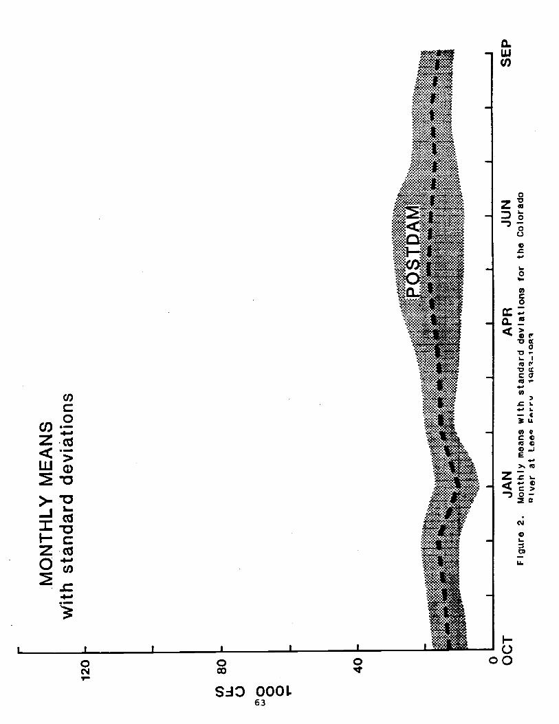
t i
Ñ
t t t t
o
SAO 0001.63
a.40;.:::..
: 1,iwv.;:v:i :}:' i ::::!,:.'..._ .
..w.::á1
t Ú00

Ñ
f: t Ï :;.{Vÿÿÿÿÿÿÿ.Vp::ti:
:¡:ti:': Ï ..XfJ :V/I1K::.:X::.
aW
HItÄ;ÄtitiV W.W V11\\1Ñ:Á
. . !:llÄL : {¿;fÏfl.A
. i :t':{W:t:f ÌÌM:Vt%%f.....iV ..................
r
1
SAO 0001.64
.. .:7y
U00

120
40 0
nmIl H
OC
Tl
1l
JAN
AP
RJU
NFigure 4.
1983, 1984, and 1985 monthlymean discharge of the
Colorado River at Lees
Ferry.
SE
R

Ñ
i
74,10050.:.;: {sÌ0AMÌXi/ÄMÁhÁtiV.V1IÏi :YV
N
I::::}Ï,tiif:{tli Ïi Ä'1..f.i¡ : :: ::1Iy..::Wf
:'i:}:...:::1:
I
co
SAO 0001.66
.,.
{I::tiï
'{::ï
w%
MEP
INN
MIN
r
W
00

A LIMNOLOGICAL INVESTIGATION OF AN URBAN LAKESYSTEM IN CENTRAL ARIZONA
Frederick A. Amalfi and Milton R. SommerfeldDepartment of Botany and Microbiology
Arizona State University, Tempe, Arizona 85287
BACKGROUND
Reports of limnological Investigations of natural and large -sizedman -made impoundments are abundant in the scientific literature.However, information regarding physical, chemical and biologicalcharacteristics of small urban lakes associated with residentialsubdivisions and master -planned communities are suprisingly absentfrom the literature. In Arizona, no data on these water bodies havebeen collected or compiled by State regulatory agencies (personalcommunication, Arizona Department of Health Services).
Urban lakes provide communities with recreational facilities- forfishing and boating, and their oasis -like beauty serves as anattraction for tourists, new residents, and prospective businesses.In addition, many of the lakes have been designed to be flood controlbasins, receiving runoff from residential streets and undevelopedland.
The need for comprehensive examinations of urban lake systems istwofold. Currently, the water quality of urban lakes in Arizona isnot regulated by the State. Based on the rampant development ofmaster -planned communities incorporating urban lakes as recreationalfacilities, and pressure placed on the State Legslature by waterconservation groups to restrict future development of urban lakes, it
is likely that State involvement in urban lake management will occur.Additionally the Clean Water Act reauthorization bill dictates thatstates must develop plans for controlling nonpoint pollution sources,including municipal stormwater runoff (Rhein 1987). Because manyurban lakes are designed to retain stormwater runoff, State regulatoryagencies will become interested in the accumulation and discharge ofwater from these impoundments. Secondly, historical and operationalcontrol data are required by the owner /operators of these impoundmentsso that proper and cost -effective management decisions can be maderelative to maintaining the aesthetic and recreational beauty of thelakes, preventing the interception, accumulation, and production ofcompounds which are potentially toxic or noxious to the communityresidents and lake inhabitants, protecting and enhancing thefisheries, avoiding uncontrolled silting of the lake bottoms, and
retarding eutrophication.The purpose of this report is to bring attention to the need of
further studies on urban lake systems. Salient features and resultsof a comprehensive limnological investigation of an urban lake system
67

are presented. Attention Is drawn to those parameters which arecritical to the management of the lake system, especially in regard toreception, formation, distribution, and accumulation of substances inthe waters and sediments and their potential impact on aquaticinhabitants, aesthetic quality, and fisheries.
THE STUDY SITE
Approximately thirteen years ago, a 65 -acre (0.26 km2) system ofman -made lakes was created as an integral component of the DobsonRanch residential community in Mesa, Arizona. The lakes receive theirprimary source of water via the Salt River Project, Tempe Canal. Theeight lakes of the system (Figure 1) are connected by a series ofgates which allow water to flow from one impoundment to the next(north to south). An outlet is provided at the terminus of the chainof lakes, thus providing for a flow- through system. However, due tohigh evaporative losses and irrigation uses, only in times of excessrunoff (flooding of adjacent land) is water d i schargp, from the lastlake. The lakes have a total volume of 0.58 x 10 , with a meandepth of 2.2 meters. Water residence time is 0.59 years, based oninfluent flow.
METHOD$
Water samples were collected with a Van Dorn bottle at the 1 -meterdepth in the deepest area of each lake. Sediment samples werecollected using an Eckman dredge directly below the water samplingpoint. When necessary, samples were preserved in accordance with therecommendations of the USEPA (1983). The sampling was initiated inOctober, 1985 and terminated in October, 1986.
Analyses were performed in accordance with standard methodologies(APHA et al. 1985, USEPA 1983). Light penetration was measured with aLicor Quantum Radiometer. Sediment samples were dried at 60 °C priorto analysis, where applicable, to obtain concentrations on a dry
weight basis. Water samples analyzed for dissolved metals wereprefiltered using 0.45 um membrane filters. Water and sedimentsamples analyzed for total metals were prepared according to EPAmethods 3020 and 3050 respectively. Samples analyzed for thecharacteristic of EP toxicity were prepared and analyzed as specifiedin the Federal Register (1980) and by the USEPA (1982). Stormwaterrunoff was collected prior to its entrance into Lakes 1 and 3 duringthe storm events of 15 February 1986 and 29 August 1986.
68
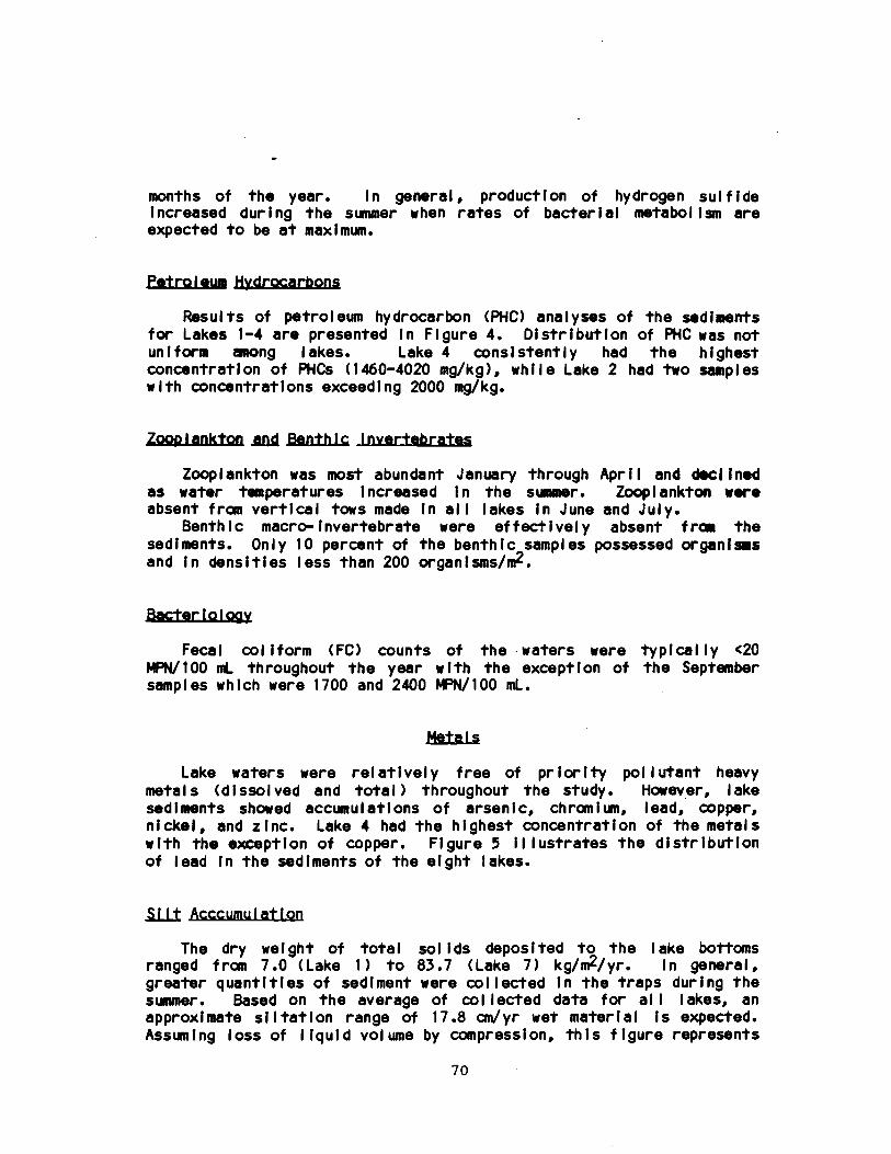
months of the year. In general, production of hydrogen sulfideincreased during the summer when rates of bacterial metabolism areexpected to be at maximum.
Petroleum Hydrocarbons
Results of petroleum hydrocarbon (PHC) analyses of the sedimentsfor Lakes 1 -4 are presented in Figure 4. Distribution of PHC was notuniform among lakes. Lake 4 consistently had the highestconcentration of PHCs (1460 -4020 mg /kg), while Lake 2 had two sampleswith concentrations exceeding 2000 mg /kg.
Zooplanktort jag Benthiç Invertebrates
Zooplankton was most abundant January through April and declinedas water temperatures increased in the summer. Zooplankton wereabsent from vertical tows made in all lakes in June and July.
Benthic macro-invertebrate were effectively absent from thesediments. Only 10 percent of the benthic samples possessed organismsand in densities less than 200 organisms /m2.
Bacteriology
Fecal coliform (FC) counts of the - waters were typically <20MPN/100 mL throughout the year with the exception of the Septembersamples which were 1700 and 2400 MPN /100 mL.
Metals
Lake waters were relatively free of priority pollutant heavymetals (dissolved and total) throughout the study. However, lake
sediments showed accumulations of arsenic, chromium, lead, copper,
nickel, and zinc. Lake 4 had the highest concentration of the metalswith the exception of copper. Figure 5 illustrates the distributionof lead in the sediments of the eight lakes.
Si It Accc umu Lot i ort
The dry weight of total solids deposited to the lake bottomsranged from 7.0 (Lake 1) to 83.7 (Lake 7) kg /m2 /yr. In general,greater quantities of sediment were collected in the traps during thesummer. Based on the average of collected data for all lakes, anapproximate siltation range of 17.8 cm/yr wet material is expected.Assuming loss of liquid volume by compression, this figure represents
70

a deposition of approximately 3.1 cm of material per year. Themajority of the deposited material (mean of 84.3 %) is inorganic.
Stormwater Runoff
Table 1 presents the physical, chemical, and bacteriologicalcomposition of the collected urban runoff. Flow rates ranged from 6.8to 55.4 m3 /hr. The stormwater runoff which entered the Dobson Ranchlakes was highly variable in composition seasonally and from storm tostorm. The total solids load of the runoff ranged from 111 to678 mg/L of which most was suspended material making the water highlyturbid. Appreciable quantities of nutrients and metals, primarily inthe particulate form, were carried in the storm flow.
DISCUSSION
Temperature Just Mineral Redistribution
Although a distinct thermocline was not evident in the lakesduring the summer, the 2 °C temperature difference between surface andbottom layers of water created a large density difference equivalentto a 10 °C temperature between water layers at 4 and 16° (Cole 1983).Therefore mixing between adjacent layers would occur due to thegradual decline (differences) in temperature with depth, but a
physical barrier to complete circulation (i.e., density) of the entirewater column would exist. During late fall deterioration of thethermal stratification occurred.
Such a variation in temperature stratification is characteristicof warm monomictic lakes which circulate during the winter months andare stratified during the summer (Cole 1968). Intense solar radiationin most seasons brings about pronounced diurnal density differences.During summer nights, cooling of the surface waters (primarily byevaporation) creates downwelling convection currents which destroy thestratification. Nocturnal circulation continues until terminated bysolar input the following day. Therefore, the lakes are expected tobe mixing throughout the year and would be more properly classified aspolymictic.
The result of polymixis is the absence of distinct chemicallydifferent layers of water in the lakes. Distribution of dissolved andsuspended chemical species occurs each evening so that stratificationis only temporary. This feature permits adequate oxygen and nutrientsto be available to organisms throughout the water column. During theday, sufficient solar radiation results in an orthograde oxygen curve.Lower concentrations of dissolved oxygen near the bottom of the lakesduring the summer are associated with increased biological
decomposition, chemical oxidation of organic matter at the
71

sediment -water interface and lower oxygen solubility with increasingtemperatures. Seasonal variations in chemical composition of thewater caused by redistribution from the sediments upon changes in
redox potential would be minimal. The absence of significant wind andwave action further limits redistribution of materials from thesediments via upwelling. The lakes have become sinks for precipitatednitrogen (2200 -3200 mg /kg) and phosphorus (680 -1000 mg /kg) due tomaintenance of a permanent oxidized microzone over the sediments.
Light Extinction
The abrupt change in optical characteristics of the lake waters inSeptember is attributed to relatively high suspended solidsconcentrations and color in runoff entering the lakes 3 days prior tosampling. The suspended solids range of the lakes was typically3 -14 mg /L, but increased to a range of 4 -125 mg /L after the lateAugust precipitation. Rainfall also occurred during other timeperiods, but sampling of the lakes occurred 6 to 14 days after theprecipitation. With the longer interval, sufficient time had elapsedfor solids, transported into the lake by runoff, to settle to the lakebottoms. Thus, the adverse affects of urban runoff on the aestheticquality of lakes is short term.
Algal Production
Low chlorophyll concentrations are rather surprising because ofthe amounts of total nitrogen and phosphorus which enter the lakes viathe influent (4.17 -4.83 mg /L N and 0.12 -0.15 mg /L P) and stormwaterrunoff (Table 1). It appears that either copper sulfate ( algicide)
treatments to the lakes, intermittent depletions of ortho-phosphate,some other limiting factor not identified during the study, or acombination of these factors suppressed development of dense
phytoplankton populations. Zooplankton grazing may also be anothernatural control since several of the maximum standing crops occurredduring June and July, which correspond to the absence of grazing
zooplankters. No historical data on algal concentrations are
available from periods when algicide treatments were not made.
Hydrogen Sulfide Production
The apparent absence of hydrogen sulfide in the water, as comparedto its presence in many sediment samples, is attributed to rapidoxidation of sediment -released sulfides to sulfate in the highlyaerobic water column or the general inability of the hydrogen sulfideto escape from deep anaerobic sediments through an overlying oxidizedmicrozone at the water -sediment interface.
72
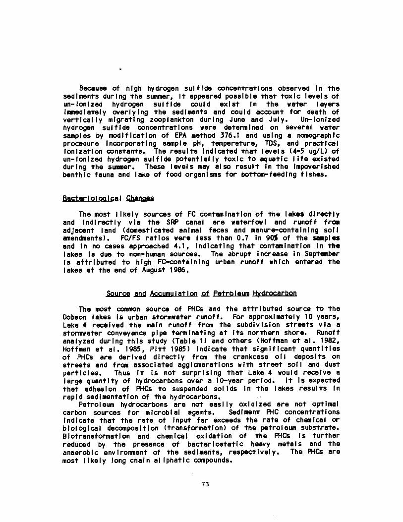
Because of high hydrogen sulfide concentrations observed in thesediments during the summer, it appeared possible that toxic levels ofun- ionized hydrogen sulfide could exist in the water layersimmediately overlying the sediments and could account for death ofvertically migrating zooplankton during June and July. Un- ionized
hydrogen sulfide concentrations were determined on several watersamples by modification of EPA method 376.1 and using a Homographicprocedure incorporating sample pH, temperature, TDS, and practicalionization constants. The results indicated that levels (4 -5 ug /L) ofun- ionized hydrogen sulfide potentially toxic to aquatic life existedduring the summer. These levels may also result in the impoverishedbenthic fauna and lake of food organisms for bottom- feeding fishes.
Bacteriological Changes
The most likely sources of FC contamination of the lakes directlyand indirectly via the SRP canal are waterfowl and runoff from
adjacent land (domesticated animal feces and manure -containing sollamendments). FC /FS ratios were less than 0.7 in 90% of the samplesand in no cases approached 4.1, indicating that contamination in thelakes is due to non -human sources. The abrupt increase in Septemberis attributed to high FC- containing urban runoff which entered thelakes at the end of August 1986.
Source mid Accumulation ,Q{ Petroleum Hydrocarbon
The most common source of PHCs and the attributed source to theDobson lakes is urban stormwater runoff. For approximately 10 years,Lake 4 received the main runoff from the subdivision streets via astormwater conveyance pipe terminating at its northern shore. Runoff
analyzed during this study (Table 1) and others (Hoffman et al. 1982,Hoffman et al. 1985, Pitt 1985) indicate that significant quantitiesof PHCs are derived directly from the crankcase oil deposits onstreets and from associated agglomerations with street soil and dust
particles. Thus it is not surprising that Lake 4 would receive alarge quantity of hydrocarbons over a 10 -year period. It is expected
that adhesion of PHCs to suspended solids in the lakes results in
rapid sedimentation of the hydrocarbons.Petroleum hydrocarbons are not easily oxidized are not optimal
carbon sources for microbial agents. Sediment PHC concentrationsindicate that the rate of input far exceeds the rate of chemical orbiological decomposition (transformation) of the petroleum substrate.Biotransformation and chemical oxidation of the FHCs is further
reduced by the presence of bacteriostatic heavy metals and theanaerobic environment of the sediments, respectively. The PHCs aremost likely long chain aliphatic compounds.
73

Source mg Accumulation Id metal
As with PHCs, metals entering the lake are primarily associatedwith particulates and thereby have little effect on water quality dueto rapid sedimentation. Urban runoff also appears to be a majorcontributor to the accumulation of metals in the sediments. Metals inthe runoff most likely originate from weathering products of soils andengine wear metals associated with lubricants and emission exhaustsdeposited on pavements. The high concentration of lead in the Lake 4sediments is attributed to the long -term reception of the bulk ofsubdivision street runoff described previously. The accumulation ofheavy metals in the sediments Is a contributing factor in the generalabsence of benthic fauna and flora.
To ascertain the ability of the metals to be leached from thesediment, the Lake 4 sediment sample collected in August was analyzedfor the characteristic of EP toxicity. Based on the results of the EPtoxicity -metals analysis, no metallic species concentration exceededthe maximum contaminant level (MCL). Therefore, it is unlikely thatthe lake sediments are a potential source of groundwater or parentmaterial contamination. The metals appear to be tightly bound toorganic matter (organometallic complexes).
Lake Silting
Higher amounts of sediment were collected in the summer than thewinter due partially to slightly higher algal biomass and sinking ofdead cells, but more importantly to the differences In precipitationpatterns in the watershed. Short, intense, late summer thunderstormscharacteristic of the desert monsoon season, dislodge greater
quantities of debris from the watershed as compared to long duration,winter rain showers. This results in import of 2 to 4 times the' mass
of settleable material to the lakes via interception of stormwaterrunoff.
SUMMARY
The results of the comprehensive Ilmnological investigation of theDobson Ranch lakes demonstrated that several physical and biochemicalcharacteristics of the lakes play an important role in the
distribution and accumulation of materials in the lake system.
Diurnal temperature patterns in the lake permit daily distribution ofdissolved gases and minerals in the lakes, and the complete
oxygenation of the water column reduces redistribution of materialfrom the sediments. Although the lake waters are relatively free ofmetals, sulfides, and petroleum hydrocarbons, the sediments accumulatethese substances. The reception of urban stormwater runoff is a major
factor in the accumulation of the materials in the sediments,
74

short -term reductions in aesthetic quality (clarity), and abundance oforganisms in the lakes.
REFERENCES CITED
APHA, AWWA, WPCF. 1985. Standard Methods for the Examination ofWater and Wastewaters. 16th ed.
Cole, G.A. 1968. Desert Limnology. In G.W. Brown (ed.) DesertBiology, Vol. 1, Ch. IX. Academic Press, New York.
Cole, G.A. 1983. Textbook of Limnology. C.V. Mosby Co., St. Louis.Federal Register, 1980. FR79318, November 28, 1980.Hoffman, E.J., J.S Latimer, G.L. Mills, and J.G. Quinn. 1982.
Petroleum hydrocarbons in urban runoff from a commercial land usearea. Journ. Water Poll. Control Fed. 54(11):1517.
Hoffman, E.J., J.S. Latimer, C.D Hunt, G.L. Mills, and J.G. Quinn.1985. Stormwater runoff from highways. Water, Air and SollPollution. 25:349.
Pitt, R. 1985. Characterizing and controlling urban runoff throughstreet cleaning. EPA Project Summary. EPA/600 /52- 85/038. WERL,
Cincinnati.Rhein, R. 1987. Large majorities pass Clean Water Act again.
McGraw -Hill Construction Weekly. January, 29.U.S. Environmental Protection Agency. 1982. Test Methods for
Evaluation of Solid Waste -Physical and Chemical Methods. SW846.
Office of Solid Waste, Washington D.C.U.S. Environmental Protection Agency. 1983. Methods for Chemical
Analysis of Water and Wastes. EPA 600/4 -79 -020. EnvironmentalMonitoring and Support Laboratory, Cincinnati.
75

Table 1.
Composition of urban stormwater runoff entering the Dobson
Ranch lakes.
Parameter
2 -15 -86
8 -29-86
Lake 1
Ramp
Lake 3
Storm drain
Lake 3
Walk
Lake 1
Lake 3
Ramp
Storm drain
Total dissolved
solids, mg/L
67.
64.
73.
103.
384.
Suspended solids,
mg/L
56.
175.
38.
592.
294.
Total phosphorus,
mg/L
0.402
0.121
0.890
0.396
0.721
Total nitrogen,
mg/L
3.76
1.75
4.50
6.65
4.10
Fecal collforms,
MPN/100 mL
>1600
>1600
>1600
>16000
>16000
Metals, total
Copper, mg /L
0.017
0.05
Nickel, mg /L
0.09
<0.02
Zinc, mg/L
0.32
0.06
Arsenic, mg /L
0.0027
0.0026
Chromium, mg/L
0.04
0.02
Lead, mg/L
0.07
0.03
OBaseline Rd. Scale
Guadalupe Rd.
1/4 Mile
Figure 1.
Dobson Ranch lakes and location of sampling sites.

SE
AS
ON
AL
LAK
E T
EM
PE
RA
TU
RE
OX
YG
EN
CO
MP
AR
ISO
NLAKE 8
LAKE 2
0.0
0.5
1.0
1.5
2.0
ON
TE
MP
ER
AT
UR
E. C
DIS
SO
LVE
D O
XY
GE
N. M
G /L
Né
1.1
.a
óí
áó
íai
l1
1.1
11
1
oD
EC
+M
AR
sJU
Ne
SE
P
N a
0.0
0.5
1.5
2.0
J aD
EC
+FEB
MA
Y
AP
R
xA
UG
.1S
EP
Figure 2.
Seasonal vertical temperature profiles of Lake 8.
Figure 3.
Seasonal vertical oxygen profiles of Lake 2.

PETROLEUM HYDROCARBONS -SEDIMENTSLAKES 1 THROUGH 4
4.5
4-
3.3 -
1 -
0.3
NOV FES MAY
MONTH® LAKE 1 ® LAKE 2 ® LAKE 3Figure 4. Total petroleum hydrocarbon concentrations in Lakes 1
through 4.
AUG SEP
® LAKE 4
LEAD CONCENTRATION IN SEDIMENTS200190 -180 -170 -1 60 -150 -140 -130 -
O 120 -110 -100 -9080 -
p 70F- 60
50 -40 130 -/2010
o
Mean Value for Each Lake
2 3 4 5
LAKE NUMBER
Figure 5. Total lead concentration of the sediments of Lakes 1
through 8.
a
78

WATER QUALITY OF THE UPPER SAN PEDRO BASIN,COCHISE COUNTY, ARIZONA
Oralynn T. SelfCivil Engineering, Arizona State University, Tempe, AZ 85281
Introduction
The San Pedro Basin lies in south- eastern Arizona. The San Pedro River flowsthrough the middle of the basin, originating in Mexico, and continuing northward toempty into the Gila River at Winkleman. The upper basin is divided from the lowerbasin at "the Narrows" located approximately 11 miles north of Benson, Arizona.
Residents of the upper basin rely soley on groundwater and a few springs for theirpotable water supply. Waters of the emphermeral San Pedro River are used forirrigation in the St. David and Benson area. There are about 66,000 residents of thebasin at present. By the year 2000, the population is expected to increase to 90,000.Along the river, a unique riparian habitat exists of a diverse population of plant andwildlife communities. Many fear that the rise in population will overtax thegroundwater supplies, effecting residents of the valley and the riparian habitat which isdependent upon the high water table in the inner valley. As water resources becomemore limited, the quality of the remaining water supply becomes increasinglyimportant.
Most of the water withdrawn from the basin is derived from aquifers locatedbelow 100 feet or more of alluvium. This water is. of excellent quality. However, theshallower groundwaters of the basin near the San Pedro River are of a poorer qualitythan the regional aquifer, and in places have been contaminated by man's activities to thepoint of being undrinkable.
The following report is a summary of the ambient water quality of the surface andsubsurface waters of the Upper San Pedro Basin, followed by specific water qualityissues affecting or potentially affecting the basin.
Ambient Surface Water Quality
The waters of the ephemeral San Pedro River are predominatelycalcium -bicarbonate type. Generally, the water quality is good, but its often turbidnature and occasional fecal coliform contamination makes it expensive to bring up todrinking water standards. The low sodium absorption ratio of the river water allows itto be used for crop irrigation.
Various studies of the San Pedro River water quality include the USGS (Roeske andWerrel, 1973) study of river water at three locations in 1941, the University ofArizona (1961) analysis of 295 samples from the San Pedro River at Charlestonbetween 1945 and 1960, and the URS Company and the W.R. Booth and Associates
79

(1976) survey of -the river water quality in 1973 for the ADHS. The University ofArizona (DeCook et al., 1977) performed the first comprehensive water qualityanalysis of the San Pedro River. They found barium, lead, and copper concentrationsoften exceeded water quality standards. 62% of their water samples taken in the UpperSan Pedro Basin exceeded state standards for fecal coliform.
More recent work by Arizona Department of Health Services (ADHS),SouthEastern Arizona Governments Organization (SEAGO), Arizona Game and FishDepartment (AGFD), and the Anaconda Company have found an improvement in surfacewater quality probably due to the many improvements of muncipal wastewatertreatment facilities and the reduction in mine effluent releases from Cananea, Mexico.Surface water quality data collected at Palominas near the United States - MexicoInternational Border and at St. David in 1980 is presented in Table 1.
In 1986 the AGFD sampled fish tissue, water, and sediment from the San PedroRiver which was analyzed by the U.S. Environmental Protection Agency. Resultsindicated zinc contamination averaging greater than 50 mg /kg. Certain chemicalcompounds have been found above detection limits including benzoic acid, diethylphthalate, freon, bis(2ethylhexyl)plthal, naphthalene, benzo(k)fluoranthene, and 4 4DDT.
Ambient Groundwater Quality
Groundwater in the Upper San Pedro Basin is generally of excellent quality withrelatively low values of total dissolved solids (TDS). The regional aquifer ispredominately calcium -bicarbonate type with a TDS quantity between 200 to 400 mg/I,composed primarily of calcium, sodium, and bicarbonate (USGS, 1952). BetweenPalominas and Hereford and between St. David and Benson this is artesian flow ofprimarily sodium- bicarbonate and sodium -sulfate types with high TDS values, in mostcases over 1000 mg/I (Putnam, 1985).
SEAGO (1981) found that shallow water wells are poorest in water quality. Theirdata indicates a correlation between surface and groundwater less than 80 feet deep.Shallower waters tend to have higher TDS values than the regional aquifer (Heindl,1952). The USGS (Roeskel and Werrel,1973) found sulfate levels three times greaterthan the state's standard in the shallow waters of the Benson (850 mg /I) and Pomereneareas. The highest sulfate concentration found by the USGS was 2,360 mg/I in a watersample taken from a depth of 130 feet in a well at the Tres Alamos Ranch. When thewell was deepened to 875 feet, the level dropped to 1000 mg /I. High sulfateconcentrations add a bitter taste to water and act as a laxative to humans.
The USGS also measured a nitrate concentration of 53 mg/I in a well in the St.David area in 1952. Arizona state's safe drinking water standard for nitrate is 45mg /I. Possibly this excessive amount was an early sign of the nitrate contaminationproblem that exists there.
Konieczki (1978) found high levels of flouride in groundwater taken from wellsin Tombstone (2.2 mg /I), south of Benson (4.4 mg/I), and the St. David area (5.9mg/I). Optimum amounts of flouride in the San Pedro area are between 0.7 and 0.8
80

TABLE 1- SEAGO 1980 Upper San Pedro Basin Water QualityAnalysis
Parameters
San Pedro RiverWater Quality
Palominas St. David
GroundwaterQuality
Palominas St. DavidNo. of sampieg 6 7 10 10Water Temp. (°ç,), 19.25 23.6 18 19$ample Resist. OHMS( 1793 787 965 731pH (units). 8.3 8.0 7.5 7.5Calcium 74 133 134.0 111.0Magnesium 8.5 22.0 15.7 24.0Sodium 47.0 89.0 76.3 202.0Jtsa 0.91(5) 0.49(4) 1.71(2) 1.36(8)Copper <0.05 <0.05 <0.05 <0.05MaLlganatie 0.12(5) 0.08(3) <0.05 0.07(5)Zinc <0.05 <0.05 0.08 0.33Agc P (CaCO3) 0.3 0 0 0AIk Mp 190.0 236.0 284.4 522.0Chloride 6.8 19.3 16.5 31.0Nitrate 13.3(1) 231.0(6) 33.4(2) 17.0Sulfate 91.0 171 229.5 178.0Total PO4 0.06 0.03 0.05 0.09Flouride 0.41 1.5 0.26 2.10Nitrite 0.02 0.35 <0.01 0.02Residua 365.0 651 637.2 810.0Hardness (CaCO3) 220.0 404.0 403.6 366.0Total S.S, 87.0 27.6 5.3 86.0Kjeldahl Nitr% 0.6 1.2 0.3 0.3Arsenic 0.005 <0.005 0.005 0.007Silver <0.01 0.01 <0.01 <0.01Chromium <0.01 0.01 <0.01 <0.01Cadmium <0.005 <0.005 <0.005 <0.005Lead <0.02 <0.02 <0.02 <0.02Selenium <0.005 <0.005 <0.005 <0.005Mercury <0.0005 <0.0005 <0.0005 <0.0005Turbidity 48.6 21.0 2.2 30.4Est. Flow in cfs. 3.2 2.9F. Coli/100 mL, 134 147F. Strep/100 ml. 5708 232Static Water Lave( 20' 22'Well Depth 117' 105'
Note: Chemical parameters are in mg/I.Number in parentheses is number of times the State of Arizona municipaldrinking water standards were violated.For data given as less than some quantity, that quantity was used to determine theaverage.
Source: SEAGO, 1981.
81

mg /I. Excessive amounts of flouride in drinking water causes mottling of childrens'teeth enamel. Konieczki (1978) also measured TDS of 960 to 1030 mg/I in thevicinity of the Narrows, 2650 to 4400 mg/I just north of Benson, and as high as 1020mg/I in the St. David area.
Following the major Cananea mining spills of the late 1970's, the ADHS (1981)and SEAGO analyzed the water quality of 7 wells and found them all within state'sstandards, except one well situated 10 yards from the river. This well was found tohave excessive amounts of iron, lead, and manganese possible due to contamination fromthe polluted San Pedro River. As no data had been collected before the spills, positivecorrelation could not be made. Arizona state monitors iron and manganeseconcentrations for aesthetic reasons. Lead is a toxin which can affect human'shematopoietic system, central and perpheral nervous system, and kidneys. A followupstudy was done by SEAGO monitored the water quality of 6 wells throughout most of1980. Two out of ten analyzes from a well in Palominas yielded iron and nitrateconcentrations exceeding state standards, possible due to the fertilizer use in thisagricultural community. A well at St. David was found to often have excessively highiron and manganese concentrations, as did a well in Pomerene. The Pomerene well wasalso found to have an average content of sulfate three times the state standard, and on oneoccassion out of 10 test, was found to exceeded state standards for copper content.Averages of the SEAGO monitoring results of groundwater quality at Palominas and St.David are also presented in Table 1.
Specific Water Quality Issues
Overall the Upper San Pedro Basin water quality is excellent, but there are someproblems and site specific contaminations. Several of the water quality issues effectingthe basin are not site specific and can affect any basin; these are potential problemsassociated with wastewater treatment plants, landfills, pesticides and fertilizers use,accidental spills, livestock grazing, and air pollutant problems
Cananea Mine Spills
During the harsh winter rains of 1977 -78 and 1978 -79, earthern dam failuresat the Cananea Copper Mine in Sonora, Mexico released polluted acidic water into the SanPedro River. Aquatic life over a 60 mile stretch north of the border perished in thepolluted river. Water samples contained high concentrations of heavy metals and yieldedpH measurements as low as 3.1, as compared to an average pre -spill pH of 8.1 (ADHS,1981). Although mine modifications, completed in August, 1981, were meant toprevent future mining spills, as late as the 85 -86 winter, polluted mining wastewaterhas flowed into the United States. The new influxes of polluted water could not beattributed to the flushing of bank contaminations deposited by earlier spills (Pringle,1986).
ADHS, SEAGO, AGFD and Anacoda Copper Company Environmental EngineeringDivision have monitored the effects of the mine spills. ADHS reported that state surfacewater quality standards for pH, copper, dissolved oxygen, zinc, and turbidity were
82

repeated violated during the period of mine spills. Water quality recovery wasapparently rapid as no surface water quality violations were found during monitoring inJuly 1979, four months after the spills had stopped. Interestingly enough, ADHS foundlower copper and manganese concentrations during the July, 1979 sampling then thosereported by the Water Resources Research Center, WRRC, monitoring in 1977. In1977, the WRRC reported surface water quality violations for barium, lead, and copper(Decook et ai, 1977). A possible explanation for the high metal concentrations in1977 is that minor spills may have been occurring for many years prior to theremedial action taken after the larger failures in 1978 and 1979. This would agreewith reports by local citizens that the river had occasionally ran red -orange in colorfor a few days at a time.
SEAGO and ADHS monitored water quality at 10 surface water and 6 well sitesduring the drier than normal period from 2/80 to 12/80. The groundwater showed noinfluence of the polluted mine waters and there was a striking improvement in surfacewater quality from the 1978 -79 data. As the flow from the winter storms subsided, theheavy minerals settled out and were deposited on the banks and floor of the river. Thecontinued high reading of some heavy minerals may be the results of continued flushingof these bank deposits.
Nitrate Contamination in the St. David Area
After the Cananea Mine spills of 1978 -1979, the ADHS and SEAGO undertook ajoint study of the San Pedro River water quality. The river was found relatively free ofnitrates, except for an area just upstream from the Highway 80 bridge near the town ofSt. David. There, nitrate -nitrogen concentrations exceeded values 7 times the state'ssafe drinking water levels of 10 mg/liter (or 45 mg/I as NOS) (SEAGO, 1981). Asurvey of private wells in the area found 11 contaminated wells, the worst of whichcontained 47 times the safe level of nitrate. High nitrate levels in drinking water hasbeen linked to infantile methomoglobinemia, a condition afflicting some infants whichimpairs the transport of oxygen in the blood stream.
A 1980 ADHS survey of surface water quality delineated that the upstreamboundary of the nitrate problem lies adjacent to the Apache Powder Company. Thecompany, an explosives and chemicals manufacturing firm, "has produced nitroglycerinsince 1922, ammonium nitrate since the 1940's, detonating fuses since 1968, andnitric acid. Three hundred thousand gallons per day of waste water were generated,primarily during washdown and blowdown operations" (EPA, 1980). The company'spractice of dumping effluent into a dry wash and later of using unlined retention pondsmay be a contributing factor to the adjacent nitrate contamination.
The extent of the contaminated plume is not well defined. Drilling records showthe depth to the water table is generally 40 to 50 feet below the surface. The aquifer'slower boundary is a clay aquiclude at a depth of 100 to 110 feet. A lower aquifer liesbelow this aquiciude at a depth of 250 to 300 feet. Natural flow is from the loweraquifer to the upper one in the local area, and the lower aquifer appears to beuncontaminated (Tersey, 1984). An ADHS official estimates groundwater velocities tobe 100 to 544 feet per year based on data from a Fort Huachuca groundwater study, andthat the plume could extend 1.1 to 6.2 miles north considering only subsurface flow.
83

The river probably serves as an axis of the hydraulic gradient with flow from each sideof the river flowing toward the axis. A further study of groundwater flow in the area isnecessary to better delineate the plume extent. The Apache Powder site was nominated tothe Federal Superfund's National Priority List for toxic waste cleanup in June 1986.
Cyanide Contamination near Tombstone
In 1983, a silver mine retention leaching pond dam failed and released thousandsof gallons of cyanide leaching solution into Walnut Gulch near Tombstone. Remedialaction was overseen by the EPA and ADHS. Much of the contaminated soil was removedfrom the gulch and placed without treatment in the mine tailings area. While thecyanide is not known to have contaminated Tombstone's or any private wells' drinkingsupply, the leaching process produces many metaliocompiexes with unknown toxicitythat may persist in the environment.
Sufficient doses of cyanide induced by inhaling, ingesting, or absorption throughthe skin can impair the metabolism and transport of oxygen to the body, causing thevictim to suffocate. The body is able to metabolize sublethal doses. The U.S. PublicHealth Service set a cyanide ion standard in 1962 for drinking water at a maximum of0.2 mg /I.
In June 1984, water from one of the Tombstone mine's industrial wells was foundto be contaminated with cyanide at a concentration of 100 ppm. Two possible sourceswere reported by mine officials. The caliche lining material of a holding pondcontaining cyanide -rich leaching solutions may have separated from a drain allowing thesolution to seep into the underlying fractured metamorphic rock (Kennett, 1985). Apregnant pond containing cyanide rich solution and leached silver forming compoundsand metals in solution was also found to be leaking (Kennett, 1986). The syntheticplastic liner which had just been installed in May 1984 was punctured duringemplacement. The liner was less than 10 mil thick, well below the ADHS newlyrecommended standard of 30 mil; no liner standards existed at the time of emplacement.It is believed that the cyanide solution had been leaking for only a short period of time,possibly a month before being discovered. It migrated quickly through the fracturedbedrock, possibly along old mine workings, or down the well bore which is gravelpacked to the surface, and contaminated the groundwater which lies 500 feet below thesite. Water was pumped from the contaminated well in an effort to contain the cyanideplume. The water was treated with hypochlorite and placed on a bermed landing strip toevaporate. A new company, Cochise Silver Mines Inc., plans to reopen the mine. Theyare being held responsible for the clean up and closure of the old facility as part ofrequirements for a Groundwater Quality Protection Permit.
In February of 1987, four cattle were found poisoned from drinking water from amake -shift silver leaching pond. The illegal leaching operation was found to be in "totalnon -compliance with statutory and public -safety laws" (Arizona Republic, 1987). Theoperation was cleaned up soon after discovery and contaminated soil removed.
84

Accidental Spills of Hazardous Material
On April 18, 1984, a 15 car train derailment on the Southern Pacific Railway, 3miles east of Benson, spilled 15,000 gallons of 1, 3 Dichloropropene onto the desertfloor. 1, 3 Dichloropropene (DCP) is a soil fumigant used on field crops and citrusplants to prevent worms, disease, and weeds. It is highly toxic to human beings wheningested or inhaled.
No overland flow had occurred; the DCP seeped directly into the ground and wasisolated to a small area 80 feet by 100 feet by 30 -40 feet deep. No wells in the areahave shown any contamination (IT Corporation, 1984). In -situ aeration process wasimplemented which operates on the premise that if air is forced to flow through the soil,contaminants can be removed through venting and released to the atmosphere throughbore holes. By early 1985, all soils in the contaminated area were reported to have DCPconcentrations less than 10 ppm.
The transportation of hazardous material has become a great concern because ofincreasing incidents and the potential for major castrophies. Hazardous materials (HM)as defined by the Secretary of Transportation are materials that have a "quantity andform that may pose an unreasonable risk to health and safety or property whentransported in commerce ".
A survey that monitored incoming shipments at the five major ports In Arizonafound 1 out of every 13 trucks transported HM, or an estimated 120,000 truckloadsenter the state a year (Pijawka, et al., 1986). Estimated annual truckloads of HM onInterstate 10 crossing the Upper San Pedro Basin is 10,000 to 60,000 a year. Further,many interstate shipments of HM go uncounted. An estimated 824 truckloads or7,004,000 gallons of gasoline were shipped to Sierra Vista in 1984 alone.
Effects of Grazing
Heavy grazing reduces vegetation and compacts soil, producing an increase insurface water runoff carrying top soil and bacteriological organisms. The relativelylow amount of precipitation in the basin helps to prevent severe soil erosion. A SEAGO(1981) study concluded that the effects of grazing in the valley were less thananticipated and there was no need for rangeland related best management practices tomitigate water quality problems. Leased state and federal lands are monitored toprevent overgrazing, but the majority of the basin is unregulated, privately owned land.State surface water quality standards of the San Pedro River from the Mexican border toRedington set maximum allowable limits for suspended solids (turbidity) at 50 NTU(nephelometric turbidity units) and fecal streptococci at a geometric mean of 1000bacteria per 100 milliliters.
The turbidity of the San Pedro River is governed by many factors, the mostimporant of which are the amount and duration of precipation, the topography, and theamount of vegetative cover. SEAGO monitored the turbidity of the river during arelatively dry period extending from 2/80 to 12/80. They found a great amount ofvariation along the river course with the highest measurement of 180 NTU occurring
85

near Benson. Typically the river averaged less than 20 NTU ( SEAGO, 1981).
Fecal streptococci have been monitored by SEAGO (1981) and Kenneth Hanks(1978). Kenneth Hanks found in the Walnut Gulch watershed of the San Pedro Basinthat a large number of bacteria are carried by runoff in high intensity storms. Highestcounts are present initially in water flow events, but a washing effect was observed andall bacteria groups decrease in numbers as the rainfall continues (Hanks, 1978).Therefore, fecal streptococci measurements will vary greatly depending on when themeasurements are taken in relation to rainfall events. SEAGO's surface water studyrevealed several high fecal streptococci readings; no wells studied showed any bacterialcontamination. Their monitoring between 8/19/80 to 12/18/80 did not note whethermeasurements were taking during rainfall events, or dry periods. Still slightly highervalues were measured, during the late summer "rainy season" (SEAGO, 1981). Fecalstretococci were measured as high as 15,000, but typically averaged less than 200 per100 ml. ( SEAGO, 1981).
Bacterial Contamination
In the San Pedro River, the most commonly violated state water quality standardis fecal coliform. In 1977, 62% of surface water samples taken in the river by theWater Resource Research Center (WRRC) exceeded state health standards for fecalcoliform (DeCook et al., 1977). Since then, many upgrades in municipal sewage plantsystems within the basin has resulted in fewer violations. SEAGO found no fecalcoliform violations during the monitoring period from February 1980 to December1980 (Francaviglia, 1981). The WRRC study found that fecal coliform counts appearedto increase with higher flow; in fact, 100% of the readings taken August 3, 1977during the "rainy season" exceeded state health standards. Possibly the lack ofviolations noted during SEAGO monitoring period is a result of the low precipitation thatyear. Much higher values may be more typical.
Fecal coliform bacteria presence is an indicator of the possible existence of otherdangerous microorganisms found in human waste that cause such illnesses as hepatitis,cholera, and typhoid. Dr. Charles Sterling of the Veternary Sciences Department at theUniversity of Arizona has monitored surface water throughout the state for bacterialorganisms. Thus far, only one sample taken from the San Pedro River at Palominas hasbeen analyzed. The sample taken 7/24/86 contained 210 oosysts /gal ofCryptosporidium. Cryptosporidium is a protozoan parasite transmitted through waterwhich causes severe diaherria lasting for about a week. At this concentration, the wateris unsafe to drink and full body contact is not recommended owing to the potential ofgulping water. No giardiasis was found (Marshall, 1986).
The practice of dumping waste into Tombstone's abandoned mine shafts ceased in1980 with the completion of a municipal sewage treatment plant. No bacterialcontamination has been found recently in the Tombstone drinking water supply(Bulanowski, 1987).
In Naco, Sonora, Mexico, wastewater treatment facilities have often failedresulting in the release of raw sewage into Greenbush Draw which drains into the SanPedro River. The Naco sewage treatment ponds on the east side of town are earthern
86

ponds, suspectable to failures during heavy rain events. Sewage line breaks resulting insewage streaming from manholes have been reported (Rand, 1986). The Mexicangovernment plans to build new, properly designed, sewage treatment ponds on the westside of town and replace old sewer pipes.
A potential problem exists in the adjacent American town of Naco where a newwaste water treatment plant (in operation since 1982) overlies the city of Bisbee'sdrinking water well field. The wastewater treatment ponds are unlined and thegroundwater lies about 80 feet below them; pumping level is 105 -115 feet deep.Cochise County health officials found that water from the treatment ponds does infiltrateinto the ground (Harold Dispatch and Bisbee Review, 1983). The well field is alsooverlain by the occasionally sewage polluted Green Bush Draw. Regular monitoring thusfar has shown no contamination of the well field's water supply (Rand, 1986). It isimportant to determine whether the Bisbee drinking water aquifer is isolated from thepolluted surface waters.
Wastewater Treatment Facilities
Municipal and privately owned wastewater treatment facilities are notoriousenvironmental polluters. Problems stem from the pollution potential of the effluent.The larger facilites of the Upper San Pedro Basin all produce an effluent treated tosecondary standards, which if not disinfected, as is typically the case, containsnumerous microorganisms including fecal coliform and possibly disease -causingbacteria and viruses.
In the Upper San Pedro Basin, only one municipality, Tombstone, discharges itseffluent into San Pedro River or its tributaries. The new facility in Tombstone willultimately use its effluent to irrigate a city park and golf course, but for now effluentdischarges into Walnut Gulch. All other municipalities presently use their effluent toirrigate crops, grazing land, and parks or utilize holding tanks for evaporation andpercolation. Of the seven privately owned wastewater treatment plants in the San PedroBasin, only one rather small plant discharges into a tributary of the San Pedro River.
The Arizona Department of Health Services annually inspects all wastewatertreatment facilities. There are no known contamination problems with any of thesetreatment facilities. The Benson wastewater treatment plant is running at 30% aboveits design capacity. Levels above design capacity result in too short of a retention timefor proper treatment of the wastewater. The effluent is used for irrigation of crop landand to date water quality parameters have been met for their effluent reuse permit(Rendes, 1987).
Landfills
The primary potential water quality problem associated with landfills comes fromthe release of leachate, or polluted landfill drainage. Water from landfills can carrydissolved toxic chemicals, heavy metals, and disease -causing microorganismsdetrimental to water quality and the environment through which the water flows.
87

There are three active and four closed landfills located within the basin. TheHuachuca City landfill's drainage structure has recently been improved due to pastproblems during heavy monsoon rains when refuge and soil was strewn upon nearbyprivate property. Active for the last 20 years, the Benson landfill lies near the SanPedro River; the landfill in places is as close as 200 yards. Refuge is dumped into35 -40' deep pits carved out of the permeable soil. No liner is used. The groundwatertable in the region is about 50 feet below the ground surface. This landfill therefore hasthe potential for a leachate problem.
The location of most old landfill sites is unknown. The legacy of these lost dumpsmay someday haunt the residents of the valley. Typically, leachate problems associatedwith landfills go undetected for many years. State and federal law now holds ownersresponsible for sanitary landfill conditions for all time, or from "cradle to grave ".Water quality is not monitored around the landfills at Benson and Tombstone and a closedfacility at St. David. The potential for castrophic degradation of aquifers demandsregular monitoring for groundwater degradation, careful facility design, andresponsible management of all landfill sites during and after use.
Pesticides
Pesticides applied to crops can be leached from the soil and enter the groundwateror be carried away with runoff to pollute surface waters. Pesticide is a general termencompassing various plant, disease, fungus, rodent, insect, and other bug eradicators.
Estimated irrigated acreage in the Upper San Pedro Basin is 9,858 acres(Putman, 1985). A list of priority pesticides used on crops in Cochise county was madepublic by the ADHS in 1982. Only a minor portion of agriculture in Cochise county islocated in the San Pedro basin and there is no available data of pesticide use in the basinitself. No known problems exist.
Effects of Air Pollutants on Water Quality
Air pollutants settling out of the air or brought down by precipitation representan indirect source of water pollution. Air quality throughout the San Pedro basin isgenerally good. State and federal standards for air quality were never exceeded duringthe 1985 monitoring period for the parameters monitored (ADHS, 1986).
Sulfuric acid forms from the interaction of rain water with sulfur dioxide, and toa minor extent sulfur monoxide. Sulfur dioxide (802) is a byproduct of copper smeltingoperations involving the separation of copper from the host ore. Acid rain producedpredominantly from the three large copper smelters in the area is believed to have littleeffect on the water quality of the basin because the alkaline soils readily neutralize acidrain.
88

Conclusions
In general the water quality of the Upper San Pedro Basin is excellent. The riverappears to have rejuvenated since the polluted flows in the late 1970's associated withthe Cananea mine spills. Occasionally there are reports of polluted flow, but theseappear associated with relatively minor spills. However, the ephemeral surface watersare turbid and often polluted with fecal coliform.
The regional aquifer is of excellent quality with a low TDS concentration. Highfloride concentrations at Benson, Tombstone, and St. David are believed to be associatedwith natural deposits. The shallow waters have higher TDS values than the regionalaquifer as does the artesian waters of the St. David - Benson, and Hereford - Palominasareas which typically have TDS values greater than 1000 mg/I.
References Cited
Arizona Department of Health Services. 1981. San Pedro River Basin water qualitystatus report for period 1973 -1979. January.
Arizona Department of Health Services. 1986. 1985 Air quality control for Arizona,annual report. June.
Arizona Republic The. 1987. "Cyanide spill found near Tombstone ", Phoenix, Arizona.pg. B1. February 17.
Bulanowski, J. 1987. Personal communication. ADHS- Drinking Water ComplianceUnit. January 7.
DeCook, K. J., et al.. 1977. Surface water quality monitoring San Pedro River Basin,Arizona. Water Resources Research Center, University of Arizona. Submitted tothe ADHS. October.
Environmental Protection Agency. 1980. Apache Powder site investigation, narrativeappendix. June 19.
Francaviglia, R. V. 1981. San Pedro River Valley water quality monitoring1979 -1980: An analysis of the data. SouthEastern Arizona GovernmentsOrganization. Bisbee, Arizona. June.
Hanks, K. S. 1978. "Bacteriological groundwater quality characteristics of the WalnutGulch experimental watershed ". Unpublished MS Thesis, Watershed Management,University of Arizona, Tucson.
Heindl, L. A. 1952. Upper San Pedro Basin, Cochise County. In: Groundwater in theGila River Basin and adjacent areas, Arizona - A summary. Halpenny, L.D.(Ed.).U.S.G.S. Open File Report No. 29.
Herald -Dispatch and Bisbee Review. 1983. "Bisbee's vulnerable water". By R.V.Francaviglia. pg. 5. Bisbee, Arizona. November 6.
IT Corporation. 1984. Letter to Mr. Harry Seraydarian of the EPA, subject: SouthernPacific Benson, Arizona, Train Derailment. Job No. 3524. November 27.
Kennett, R. W. 1985. Cyanide heap leaching potential for and protection fromcontamination. ADHS. May 7.
Kennett, R. W. 1986. Personal communication. ADHS Environmental Health Services.December 22.
Konieczki, A. D. 1978. Maps showing groundwater conditions in the Upper San Pedroarea, Pima, Cochise, and Santa Cruz counties, Arizona. U.S.G.S. Open File Report78 -1 192.
89

Marshall, M. 1996. Personal communication. Member of Dr. C. Sterling researchteam, Vetemary Sciences Department, University of Arizona. December 19.
Pijawka, D. A., et al. 1986. Transportation of hazardous material in Arizona.Prepared for the Arizona Department of Transportation. #FHWA/AZ 86/233 -3.3 volumes. January.
Pringle, T. 1986. Personal communication. Arizona Game and Fish Department.December 23.
Putman, F., et al. 1986. Draft: Water resources of the Upper San Pedro Basin,Arizona. Arizona Department of Water Resources. November.
Rand, A. 1986. Personal communication. Division Manager of Arizona Water Companyin Bisbee. November 4.
Rendes, A. 1987. Personal communication. ADHS -Tucson. May 1.Roeskel, R. H., and W. L. Werrel. 1973. Hydrologic conditions in the San Pedro Valley,
Arizona, 1971. Arizona Water Commission, Bull. 4, Phoenix, Arizona. Preparedby the United States Geological Survey. March.
SouthEastem Arizona Governments Organization. 1981. San Pedro River Valley waterquality monitoring 1979 -1980: Analysis of the data ", June.
Tersey, D. M. 1984. Preliminary analysis of San Pedro nitrates data. Arizona StateLand Department. December 18.
United States Geological Survey. 1952. Ground water in the Gila River Basin andadjacent area, Arizona - A summary. U.S.G.S. Open File Report.
URS Company & W. R. Booth & Associates. 1976. Water quality management plan forthe Upper Gila and San Pedro River Basins. Denver. January.
90

ENVIRONMENTAL HAZARD EVALUATIONS
Edward D. RicciWater Resources Associates, Inc.
3033 North 44th StreetSuite 228
Phoenix, Arizona 85018
INTRODUCTION
Due to the legal and financial liabilitiesassociated with potentially contaminated property,environmental hazard evaluations are typicallyconducted as a condition of purchase in real estatetransactions. Environmental hazards are structural,operational, or chemical aspects of a historical orpresently operating facility that may present somefuture liability for a potential buyer of property.In response to stringent environmental regulations,particularly those that have been issued to satisfythe mandates of the Resource Conservation and RecoveryAct (RCRA), industrial and commercial facilitiesroutinely conduct environmental hazard evaluations.These evaluations are usually specifically oriented torequirements of the law and activities of the subjectfacilities.
This paper will focus on the components of anenvironmental hazard evaluation of a typicalindustrial or commercial property to satisfy conditionof purchase requirements. Specific tasks that arecompleted in the investigation of an industrialfacility to satisfy RCRA requirements will begenerally discussed in the final section of thispaper. Many of the items that will be discussed underthe condition of purchase evaluation are components ofRCRA investigations.
91

CONDITION OF PURCHASE EVALUATION
The potential property buyer typically has beenprovided little information concerning theenvironmental hazards of the parcel subject topurchase. For this reason, the hazards evaluationmust include not only a historical review of pastbusiness practices and filed reports but also a
thorough site investigation.
A particular concern related to past businesspractices includes chemical usage and handling. Thereare a number of other concerns which will also beaddressed herein.
Historical Review
The historical review of a property is often themost critical yet most sensitive component of theenvironmental hazards evaluation. Information relatedto site history is gathered from two sources -from thequestion business(es) itself and from public records.
In typical condition of purchase contracts thequestion businesses (if leases are in effect) arerequired by the present property owners to makeavailable most non -proprietary information relating tobusiness practices. Therefore interviews may beconducted with appropriate individuals. Theseinterviews should be scheduled and organized. A
prepared question format that is oriented towards theinterviewee should be prepared. Key individuals whomay be interviewed include the plant superintendent,shift manager, and chemical handler (technician).
Due to the nature of environmental problems, notonly present facility operations but previousbusinesses located on the subject premises should be
evaluated. It is possible that some past tenant couldhave illegally disposed of chemicals in the on -sitearea, thereby presenting a future liability for the
92

potential buyer. The documentation of past business,especially in cases when they are dissolved, is oftena very difficult task requiring extensive recordsearches.
Documentation of chemical usage and disposalshould be requested. This documentation includesinventory records that relate to volumes of chemicalsthat are:
received;stored;used;reprocessed;disposed of.
Usage of chemicals should be documented with a
Materials Safety Data Sheet. Disposal of chemicalsshould be documented with a Manifest Form.
An effective way to survey historical operationsat a question facility is to obtain aerialphotographs. Aerial photographs of the Phoenixmetropolitan area are available from the 1940's. In
many locations, photographs have been taken in atleast five -year intervals. Aerial photographs areindicative of chemical storage and disposal practices,additions to building structures, transportationroutes, and topography.
In conjunction with obtaining facility recordsand reports, county, state, and federal recordsrelating to the question facility operations should beobtained. These records or reports may include thefollowing:
permits for operation /disposal;citations;soil reports;construction drawings;flood plain designation;water table and ground -water gradientmaps.
93

Permits are allowances by regulatory authoritiesfor a facility to operate within a prescribed set ofguidelines. Permit applications for wastewaterdisposal are processed by the Arizona Department ofHealth Services (beginning July 1, 1987, Department ofEnvironmental Quality). Citations are issued when a
permit is violated. Permits and citations arereviewed in order to evaluate facility operations thatmay be in violation of existing regulations andtherefore pose a future environmental liability forthe prospective buyer.
Soils reports, construction drawings, and floodplain designation mostly relate to concerns about thestructural integrity of the building and adequateinsurance coverage. Water table and ground -watergradient maps are available from the ArizonaDepartment of Water Resources. These maps may becritical pieces of information, especially in floodplain areas where the water table is relativelyshallow compared to the land surface. In these areas,overland disposal of waste products and the distanceto the saturated zone is a primary concern.
On -Site Property Inspection
After records from all available sources arecollected and reviewed, an on -site inspection shouldbe conducted. The on -site inspection includes, athorough investigation of structures and practicesemployed inside of the question buildings as well as
about outside areas subject to purchase.
Items located inside of buildings that should beinvestigated include:
walls, piping, floors, ceilings, roof;ventilation system;drains;stockpiled materials;evidence of leaks or spills.
94

It is imperative that environmental hazardsposing future liability for the property buyer areidentified. These relate to situations where capitalcosts will be incurred or where remedial efforts arerequired. For example, if an improper ventilationsystem is installed at a dry -cleaning operation, thepotential buyer may inherit a needed capitalimprovement.
One of the most costly and publicly- sensitiveitems related to building structures is the detectionand removal of asbestos. Asbestos typically occurs inolder buildings as insulation in walls, ceilings,floors and around piping. The detection of asbestosin a question property may cause a sales transactionto be modified or halted.
Procedures that are followed in the handling andstorage of chemicals inside the facility may indicatepotential -environmental hazards. Chemical storageareas should be identified and inventories recorded.Areas of obvious leakage or spills should bedocumented. These areas are particularly important inrelation to floor drains. Whether the drainsdischarge into a septic system, public sewer, oroutside area should be investigated. The nature andextent of stockpiled materials should be noted.
Items located outside of the facility building(s)that should be investigated include:
drains;dry wells;water wells;stained soil;excavations;stockpiled materials;transformers.
Potential conduits for ground -water contaminationmust be closely scrutinized during environmentalhazard evaluations. These conduits may occur asdrains or wells. Almost all Superfund investigations
95

have been initiated due to the occurrence of ground-water contamination. In many cases, the principalresponsible party for the contamination has not beenidentified. In some cases, the present propertyowners are liable, at least partially, for remediationof a contamination problem they did not cause.Therefore, emphasis of conducting the environmentalhazards evaluation is to identify any potentialproblems and remove this liability from theprospective buyer or at least make him aware of theproblem.
Present site conditions may be indicative ofhistorical disposal practices. Stained areas maypoint out potential soils or ground -watercontamination. Excavated areas or locations that havebeen covered with new fill may indicate disposalsites. The nature and extent of stockpiled materialsincluding the containment conditions should bescrutinized.
One possible liability is the location andcondition of electrical transformers. Many existingtransformer oils have PCBs as a component because ofits stable chemical properties. The currentregulations (under the Toxic Substances Control _Act -TSCA) provide that PCB concentrations in excess of 50ppm are considered hazardous. Transformer oilsexceeding the PCB concentration of 50 ppm are requiredto be disposed of at an appropriate hazardous wastesfacility. This regulation is currently being modifiedand the 50 ppm level will become more stringent. Mostpublic utilities that own transformers have programsto test for and report on PCB levels.
Soil and Water Testing
Depending on the results of the historicalrecords review and the site inspection, soil and watertests may be required. The general strategy for soiland water testing is to assume a conservative phasedapproach. Constituents selected for chemical analysisare based on information related to the nature of thebusiness and chemical inventory records.
96

The technique of soil sampling employed dependson the objectives of the study. If a general sitereconnaissance is desired at a site that hasunidentified solid debris, backhoe excavations in a
random sampling grid may be preferred. If specificlocations of soils contamination have been identifiedand the objective is to document contaminant movementin the vadose zone, hand augering or drill -rig boringsmight be employed.
Soils are typically composite sampled at severaldepth intervals. Depending on the specific chemicalgroups being investigated, a soil sampling programmight require that samples are collected andcomposited from 0 to 2 feet and from 2 to 4 feet.Depending on the physical dynamics of the chemicalsbeing analyzed, if no contamination occurs in the 0 to2 foot interval, the deeper interval may not beanalyzed.
Ground water is tested if the vertical extent ofsoil contamination has not been delimited or there isevidence of direct discharge into an aquifer. Thereare well- documented techniques for collecting groundwater with various sampling apparatuses from differentsized wells. Costs for monitor well installationsvary but they may represent an investment that makes aproperty purchase prohibitive. An average cost for a
150 foot monitor well installed in alluvium mightapproach $10,000. Ground -water contamination beneatha subject operation may not be the result of on -siteactivities but due to the conduct of up- gradientfacilities.
RCRA FACILITY INSPECTION
Investigation of RCRA facilities are usually inresponse to application for permit, verification ofpermit requirements, or closure /post -closure actions.The RCRA requirements are related to "cradle to grave"maintenance of facility operations and chemical usage.Permits are required for the storage and handling,transport, and disposal of hazardous chemicals. Theoperations and chemical uses of the facility must be
97

fully documented and presented in technical format tosatisfy the requirements of the RCRA regulations.
Regulations established by the EnvironmentalProtection Agency to satisfy the legal requirements ofRCRA are found in Title 40 (Protection of Environment)of the Code of Federal Regulations (40 CFR). Majorchapters under 40 CFR include regulations that applyto the following:
40 CFR 263 -40 CFR 264 -
40 CFR 265
40 CFR 26640 CFR 26840 CFR 280
-
-
-
-
TransportersTreatment, Storage, and DisposalFacilities - Permitted or NewFacilitiesTreatment, Storage, and DisposalFacilities - Interim StatusFacilitiesRecyclersLand DisposalTanks
Any RCRA inspection or investigation should closelyfollow the referenced guidelines. It is recommendedthat the appropriate State regulatory contact isapprised of the study and allowed to comment on the
study approach.
Inspection and collection of data at RCRAfacilities in order to permit their activities areoften lengthy and tedious exercises. The following isa skeleton list of items that must be addressed (if
applicable) in order to permit existing treatment,storage, or disposal facilities:
descriptive analysis of process wastestreams;personnel training;preparation of contingency plans;ground -water monitoring;closure plans;post- closure plans;financial assurance;techincal description of containers;technical description of tank systems;
98

technical description of surfaceimpoundments;technical description of waste piles;technical description of land treatment;technical description of landfills;technical description of incinerators.
Some of the most stringent requirements in theapplication for RCRA permits relate to the descriptionof ground -water dynamics beneath a subject facility.The direction and rate of ground -water flow must beaddressed. This information is obtained from themonitoring of piezometers for water level measurementsand testing of a pumping well. The aquifer testing ofa pumping well with response drawdown water levelmeasurements at observation wells will provideinformation that is used to formulate a ground -waterflow equation.
The simplest and most often used ground -waterequation is the Darcy equation. The Darcy equation isused to arrive at time of travel estimates forpotentially discharged contaminants. If the groundwater occurs at a relatively deep level, time oftravel estimations may be calculated for both thevadose zone and the saturated zone.
Soils investigations are typically conducted whena facility or facility process is to be "closed ". Theprocedures required to close a facility are delineatedin the 40CFR Parts 264 and 265. Before a facility isproperly closed, the subject operation must show thathandling and disposal practices did not result inenvironmental contamination. If remediation isrequired due to closure investigations, monitoring ofsubject environmental matrices may be required under apost- closure plan.
99

MINIMIZING THE EFFECTS OF CEMENT SLURRY BLEED -WATER' ON WATER QUALITY SAMPLES
Lauren G. Evans (Arizona Department of Health Services, Phoenix, Arizona)
Abstract
Some groundwater monitor wells produce water quality samples with anoma-lously high pH measurements. In some of these wells it is obvious that thesewater quality samples are affected by the bleed -water from the cement used toseal the annuli. To gain an understanding as to why cement bleed -water occursand how it can be controlled, literature from both the cement and petroleumindustries are reviewed.
Cement is a very alkaline material. When too much water is used to preparethe slurry, alkaline bleed -water can drain through or along the cement sheathsurrounding the casing. This results in an increase in the pH measurements ofgroundwater samples. This bleed -water can separate from the cement in-threeways: it can move into the formation during cementing, it can accumulate withinthe cement forming pockets and channels behind the casing, and it can remainwithin the interconnected capillaries that exist throughout the cementsheath.
The drainage of alkaline bleed -water from the cement can be greatly re-duced by controlling the amount of water used in the preparation of the slurry.The amount of water added can be monitored during well construction by measur-ing the slurry density. By implementing this quality control procedure duringwell construction along with specifying the correct amount of mix -water for theslurry, the elevated pH levels in groundwater samples should be greatly reduced
if not completely eliminated.
Introduction
Groundwater monitor wells are being installed in response to the many new
federal and state groundwater quality protection programs. These wells providethe water samples required to evaluate the impacts of our society's past andcurrent waste disposal practices on the underlying aquifers. The water samplescollected from these wells are required to be representative of the aquifers'water quality and should not be affected by well construction materials.
In a well were the borehole diameter is larger than the casing's, cementcan be used to seal the annular space above the gravel pack. Unfortunately,some of these wells produce water samples with anomalously high pH measurements(above 10.0) that can be attributed to the alkaline bleed -water from the cement.This effect can be particularly striking when it occurs in an area where ground-water has a pH range that is approximately 7.5. In some cases these alkalinewells can not be used for the collection of water quality samples. This can bevery costly especially with deep monitor wells. For example, the cost of re-placing a rotary drilled well in the Southwest where depth to water can easilybe 350 feet would be between $20,000.00 to $25,000.00 (Cady, 1987).
Groundwater professionals have noted that cement "grouts" can cause inter-ference with water quality samples (Barcelona et al., 1983 and Nukamoto,.19800).But, a description of the fundamental processes of how a cement slurry can in-crease the pH of water quality samples in monitor wells does not appear to be
well documented in the groundwater industry literature. In an attempt to under-stand the fundamental processes occurring downhole after the slurry has beenpumped into place, both the cement and the petroleum industries literature are
reviewed. 101

Chemical Composition of Cement
The cement used in well construction is a chemically complex material com-posed of various oxides. These oxides can be divided into major and minor com-ponents. The major components consist of tricalcium silicate (3CaO.Si02), di-calcium silicate (2CaO.Si02), tricalcium aluminate (3CaO.A1203) and tetracalciumaluminoferrite (4CaO.A1203.Fe203). The minor components, which represent lessthan six percent of the total weight of the cement, consist of MgO, Ti02, Mn203,K20 and Na20. In addition, a small amount of unreacted free lime is present asa residue from the cement's manufacturing process.
This cement is referred to as a hydraulic cement since it must be mixedwith water to produce a slurry that will develop strength and harden. Sincecontact with water is required for this reaction to occur, a slurry can hydrateand set while under water (Neville, 1981).
Physical Structure of a Cement Slurry
The size of an individual cement particle is not measured directly. Cementis so finely ground during the manufacturing process that the degree of finenessis measured by the Wagner turbidity meter. The greater the measured turbidity,
than the finer the grind. A finer ground cement provides more surface area forthe water to react with. This turbidity measurement relates the amount of sur-
face area to the weight of he sample. The unit of measurement is in centi-meters squared per gram (cm /g). For a typical cement used in well construc-tion, the Wagner fineness measurement is 1,800 cm2 /g.
When water is mixed with cement,a slurry, or paste, is formed. A simpli-fied cement -paste model was described by Powers in 1958 that illustrates thephysical structure on a colloidal level. This model is presented in Figure 1.There are three features in the model of interest. They are: gel particles
which are represented by the solid dots, gel pores which are the interstitial
spaces between the gel particles, and the capillary pores which are labeled
with a "c".A gel particle is formed as a cement particle begins to hydrate with the
free water. A gel is formed on the particle surface. As the particle continues
to hydrate with the water, the surface area begins to increase greatly. These
gel particles will begin to interlock as the chemical reactions proceed and crys-tal growth begins.
Small spaces exist between thegel particles. As the gel particleshydrate and grow, free water mole-
s c cules can get trapped within these
c c spaces permanently. These spaces,referred to as gel pores, may be as
- small as 15 X in diameter. Since
c this is only one order of magnitude
c clarger than a water molecule, anywater trapped within these spacescannot drain out and is consideredas part of the solid cement mass.
The last feature, and the mostFigure 1. Simplified Model of Paste
significant to well construction,Structure (Modified after Powers, 1958)
are the capillary pores. A majorityof the water exists here prior to
102

reacting with the cement. As the cement continues to hydrate and age, these
capillaries began to segment as they are blocked by expanding gel particles.But these capillaries will not be blocked off if too much water has been addedto the slurry. This highly alkaline free water can remain in the cement thathas been used to seal a monitor well annulus since there is no opportunity forit to evaporate. This free water, commonly referred to as bleed -water, canaffect water quality samples if it can drain downward and enter the filter pack.
The potential for increases in the pH measurements of water quality samplesshould increase as the amount of mix water in the slurry increases past theamount required by the cement to properly hydrate. There are two reasons forthis. First, as the amount of excess bleed -water is increased, the source ofalkaline water that could impact water quality samples by draining down thecement column is increased. Secondly, this increase in excess mix water producesa final set cement with a higher permeability. Therefore, any unreacted waterwithin the cement could more easily drain down through the cement and enter thefilter pack.
Studies have been conducted which define the ratio of water to cement byweight at which capillaries become segmented (Powers, et al., 1959). This datais presented in Table 1.
Problems Identified bythe Petroleum Industry with
Excess Water to Cement Ratios
As early as 1940, Colman andCorrigan conducted bench tests todetermine the effects of variouswater to cement ratios. The re-sults provide insight for thosedesigning slurries for monitorwells. They found that the water"that does not adhere to or reactwith the cement particles tend tomove upward in the cement,... ".They cited invesitgations that showed that when molds as high as 6 to 12 feetwere used, the excess water did not always migrate to the top of the cementcolumn. It was concluded that "there would be no large quantity of water abovethe top of the set cement (within the well) and that most of the excess waterwould be trapped in pockets or channels at various points in the column of theset cement."
Colman and Corrigan determined that "there is a range of water to cementratios for any cement so that the cement will set without producing water pock-ets or channels." It was also determined that this ratio is directly relatedto the fineness of the grind of the cement if the chemical composition remainedconstant. The finer the grind, the higher the acceptable range of water tocement ratios.
The range of acceptable water to cement ratios has been defined. They are
referred to as the maximum and minimum water ratios for a particular cement.The maximum amount is defined as the amount of mix water that can be added tothe slurry which would not exceed the amount required to keep the cement parti-cles in suspension, thus preventing the formation of water pockets and channels.The minimum amount would be defined as the least amount of mix water requiredto provide an easily pumpable slurry (Saunders and Nussbaumer, 1952).
Water /Cement Ratioby Weight
0.400.450.500.600.70
over 0.70
TimeRequired
3 days7 days14 days6 months1 year
impossible
Table 1. Approximate Age Required toProduce Maturity at which CapillariesBecome Segmented (Powers, et al., 1959)
103
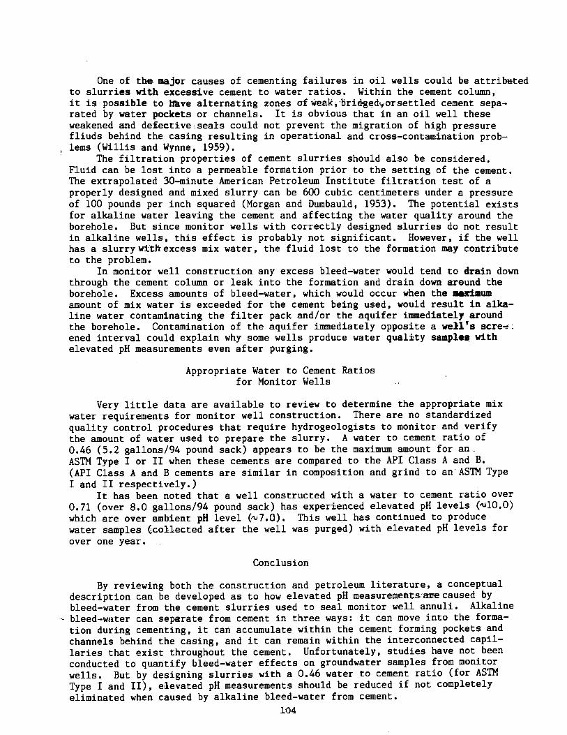
One of the major causes of cementing failures in oil wells could be attributedto slurries with excessive cement to water ratios. Within the cement column,it is possible to hive alternating zones of weak,-bridgedvarsettled cement sepa-rated by water pockets or channels. It is obvious that in an oil well theseweakened and defective: seals could not prevent the migration of high pressurefliuds behind the casing resulting in operational and cross -contamination prob-lems (Willis and Wynne, 1959).
The filtration properties of cement slurries should also be considered.Fluid can be lost into a permeable formation prior to the setting of the cement.The extrapolated 30- minute American Petroleum Institute filtration test of aproperly designed and mixed slurry can be 600 cubic centimeters under a pressureof 100 pounds per inch squared (Morgan and Dumbauld, 1953). The potential existsfor alkaline water leaving the cement and affecting the water quality around theborehole. But since monitor wells with correctly designed slurries do not resultin alkaline wells, this effect is probably not significant. However, if the wellhas a slurrywithexcess mix water, the fluid lost to the formation may contributeto the problem.
In monitor well construction any excess bleed -water would tend to drain downthrough the cement column or leak into the formation and drain down around theborehole. Excess amounts of bleed- water, which would occur when the maximumamount of mix water is exceeded for the cement being used, would result in alka-line water contaminating the filter pack and /or the aquifer immediately aroundthe borehole. Contamination of the aquifer immediately opposite a well's scream::ened interval could explain why some wells produce water quality samples withelevated pH measurements even after purging.
Appropriate Water to Cement Ratiosfor Monitor Wells
Very little data are available to review to determine the appropriate mixwater requirements for monitor well construction. There are no standardizedquality control procedures that require hydrogeologists to monitor and verifythe amount of water used to prepare the slurry. A water to cement ratio of0.46 (5.2 gallons /94 pound sack) appears to be the maximum amount for anASTM Type I or II when these cements are compared to the API Class A and B.(API Class A and B cements are similar in composition and grind to an ASTM TypeI and II respectively.)
It has been noted that a well constructed with a water to cement ratio over0.71 (over 8.0 gallons /94 pound sack) has experienced elevated pH levels 0110.0)which are over ambient pH level (4+7.0). This well has continued to producewater samples (collected after the well was purged) with elevated pH levels for
over one year.
Conclusion
By reviewing both the construction and petroleum literature, a conceptualdescription can be developed as to how elevated pH measurementsime caused bybleed -water from the cement slurries used to seal monitor well annuli. Alkaline
- bleed -water can separate from cement in three ways: it can move into the forma-
tion during cementing, it can accumulate within the cement forming pockets andchannels behind the casing, and it can remain within the interconnected capil-laries that exist throughout the cement. Unfortunately, studies have not been
conducted to quantify bleed -water effects on groundwater samples from monitor
wells. But by designing slurries with a 0.46 water to cement ratio (for ASTM
Type I and II), elevated pH measurements should be reduced if not completelyeliminated when caused by alkaline bleed -water from cement.
104

Disclaimer
The views expressed in this paper are those of the author and do not neces-sarily reflect those of the Arizona Department of Health Services.
References
Barcelona, M.J., Gibb, J.P., and Miller, R.A., 1983. A Guide to the Selection ofMaterials for Monitoring Well Construction and Ground -Water Sampling. IllinoisState Water Survey. Champaign, Illinois. 78 pp.
Cady, C.V., 1987. Oral communication, February, 1987. Arizona Department ofWater Resources. Phoenix, Arizona.
Coleman, R.J., and Corrigan, G.L., 1941. Fineness and Water -to- Cement Ratio inRelation to Volume and Permeability of Cement. Petroleum Technology. Tech.Pub. No. 1266. pp. 1 -11.
Morgan, B.E., and Dumbauld, G.K., 1953. Recent Developments in the Use of Ben-tonite Cement. API Drilling and Production Practice. pp. 163 -176.
Nakamoto, D.B., McLaren F.R., and Phillips, P.J., 1986. Multiple CompletionMonitor Wells. Ground Water Monitoring Review, Vol. VI. No. II. pp. 50-55.
Neville, A.M., 1981. Properties of Concrete. Longman Group Limited. Essex,England. 779 pp.
Powers, T.C., 1958. The Physical Structure and Engineering Properties of Con-crete. Portland Cement Assoc. Res. Dept. Bul. 90, Chicago, Illinois. 39 pp.
Powers, T.C., Copeland, L.E., and Mann, H.M., 1959. Capillary Continuity orDiscontinuity in Cement Pastes, Journal Portland Cement Assoc. Research andDevelopment Laboratories, 1, No..2. pp. 38 -48.
Saunders, C.D., and Nussbaumer, F.W., 1952. Trend in Use of Low- Weight Cement
Slurries. API Drilling and Production Practices. pp. 189 -200.
Willis, A.J., and Wynne, R.A., 1959. Combating Lost Circulation while Cementingin the Mid -Continent. API Drilling and Production Practice. pp. 190 -201.
Biographical Sketch
Lauren Evans received her B.S. in Geology from Northern Arizona Universityin 1979. From 1980 through 1983, she worked for the Arizona Department of WaterResources as a hydrologist participating in hydrogeologic investigations ofalluvial basins in the Southwest. Since 1984, she has been with the Arizona
Department of Health Services (2005 N. Central Ave., Phoenix, Arizona 85004).Currently, she manages a hydrology unit which provides the hydrogeologic sup-port to the Department's hazardous waste and underground stroage tank programs.
105

A RISK ANALYSIS APPROACH TO GROUNDWATERQUALITY MANAGEMENT IN THE UPPER SANTA CRUZ BASIN
Thomas C. Richardson and Donald R. Davis
Research Assistant and Professor of Hydrology respectively,Department of Hydrology and Water Resources, University ofArizona, Tucson, Arizona 85721
Abstract
Potential groundwater contaminant sources in the upperSanta Cruz basin include copper mines, irrigatedagriculture, and urban wastewater. Risks to human healthare posed by groundwater contaminants. Analysis of theserisks provides useful information to decision makers forcomparing groundwater quality management alternatives.Alternatives include preventing the input of contaminantsat their sources, preventing migration of contaminants ingroundwater to withdrawal points, removal of contaminantsat the points of groundwater withdrawal, relocation ofwithdrawal points, importation of water, and compensationfor those who suffer damages. The framework for riskanalysis is composed of hazard identification, hazardestimation, risk estimation, and identification andevaluation of risk response alternatives. Potentialcontaminants identified range from inorganic ions tocomplex organic molecules. Hazards have been estimated interms of fate of potential contaminants in the environmentand their toxicity. Risks to groundwater quality and humanhealth in time and space are described with the use of agroundwater contaminant transport model. Becauseinformation for the analysis is incomplete, the estimationof risks is not without uncertainties. Major uncertaintiesremain in data on contaminant concentrations and toxicologyof contaminants. The results of the risk estimation,including the uncertainties, may be used to evaluate thegroundwater management alternatives.
107
Introduction
Area Of Study
The upper Santa Cruz basin is located in thesouthern portion of Arizona, beginning near Lochiel,Arizona and running south into northern Sonora, Mexicobefore turning north near Nogales, Sonora. The upper basincontinues north to Tucson, Arizona between the Santa Ritamountains to the east and the Sierrita mountains to thewest. The limits of the study area are the southernboundary of Pima county to the south, the the foothills ofthe Sierrita mountains to the west, the southern outskirtsof Tucson to the north, and the foothills of the Santa Ritamountains to the east.
The upper Santa Cruz basin is oriented as a
northwest sloping valley. The physiographic regime istypical of basin and range geology. The geology of thebasin consists generally of horizontal sedimentary units.Groundwater is encountered at depths ranging fromapproximately 100 feet near the Santa Cruz river to morethan 400 feet in the mountain regions. The flow ofgroundwater in the basin is generally north of northwest.A complete description of the geohydrology of the basin isgiven by Davidson (1973).
Groundwater Quality Concerns
The major source of water in the basin is
groundwater. Currently, water uses include public drinkingwater supply, irrigation water for agriculture, andindustrial uses (mainly copper ore processing). Thequality of groundwater in the area is acceptable for mostpurposes. Impurities are largely composed of totaldissolved salts, of which calcium sulfate is the mostimportant. Historical groundwater quality is described indetail by Laney (1972). More recent investigations ofgroundwater quality have been performed by the PimaAssociation of Governments in the Upper Santa Cruz BasinMines Task Force reports (Pima Association of Governments;1979, 1983a, 1983b, 1983c, 1986).
Concerns exist about potential groundwater qualitydegradation in the basin. The three major areas of concern
108

are agricultural areas, mining areas, and urban wastewaterdisposal areas. Some groundwater quality changes have beendocumented in the vicinities of these areas (PimaAssociation of Governments; 1983a,1983b,1983c,1986).
Future changes in land use and groundwater use inthe basin are likely. Plans for further urban developmentand the retirement of agricultural lands exist. The futureof mining operations is uncertain, although currently indecline. Substantial population growth is expected, bothcreating an increased need for suitable drinking water andincreasing urban wastewater flows. The changes in wateruses and increasing demands for drinking water require thatgroundwater quality management options be considered tomeet these demands.
Method Of Study
Alternatives for management of groundwater qualityin the upper Santa Cruz basin are being examined within aframework of risk analysis. Because groundwater for thepurpose of drinking water supplies is the main concern forthe future, risks to human health from consumingcontaminated groundwater are considered. Risk has manydifferent definitions. For the purpose of this study, theworks of several authors have been drawn upon to definerisk in simple workable terms (Kaplan and Garrick, 1981;Rowe, 1977; Hiessl and Waterstone, 1986).
Risk Analysis
Risk is a function of uncertainty, hazard, exposure,damage, and safeguards. Risk is directly related touncertainty, hazard, exposure, and damage. Risk isinversely related to safeguards. Uncertainty may be due tolack of data, incorrectness of data, natural variation ofdata, and misapplication of data. A hazard is a source ofdanger, in this case, potential groundwater contaminantswhich exist within the basin. Exposure is the pathway forcontact between the hazards and human activities. Damageis the harm caused by the hazards, in this case, adverseeffects upon human health. Safeguards are actions whichreduce damage. In this case, safeguards are groundwaterquality management options which prevent contaminatedgroundwater from being consumed by humans, which provide
109

alternative water sources, or which relocate water -usingactivities. -
A framework has been chosen to analyze risks posedby potential goundwater contamination in the basin.Deisler (1982) has proposed a system for risk evaluationand risk response determination. This system has beenadopted to form the framework for this study. Theframework consists of the following four steps : (1) hazardidentification, (2) hazard estimation, (3) risk estimation,and (4) identification and evaluation of risk responsealternatives.
Hazard Identification
Hazard identification entails the collection anddocumentation of all available information regarding theexistence of hazards in the study area ( Deisler, 1982). Inour case, all potential groundwater contaminants in thebasin were identified and inventoried. Further, for eachidentified contaminant, literature on toxicology anddrinking water quality standards was reviewed to determinethe potential for adverse effects.
A wide range of contaminants have been identified inthe basin. Contaminants which may occur, and which areclassified as hazards include sulfate, nitrate, chloride,increased total dissolved solids, heavy metals, arsenic,radionuclides, selenium, hydrocarbons, ore processingchemicals, pesticides, and microbiological contaminants.Potential adverse effects range from undesirable taste andmild intestinal problems to cancer and death. For thesesubstances identified as hazards, the analysis hasproceeded to hazard estimation.
Hazard Estimation
The transition to hazard estimation represents animportant decision (Deisler, 1982). For each contaminantidentified in the previous step as a hazard, furtherresearch must be conducted regarding its behaviour in thespecific environmental setting of the study area. In thisstudy, the fate of each contaminant in the unsaturated zonehas been assessed. The assessment of environmental fate
110

determines the potential for actual migration ofcontaminants from the source into the aquifer.
In hazard estimation, potential exposure routes forcontaminants are identified. An exposure route is apathway from a specific contaminant source into the aquiferand to a point at which the contaminated groundwater may beextracted for human consumption. We are only consideringexposure through the consumption of contaminatedgroundwater. If, in the assessment of environmental fate,a contaminant is expected to be attenuated before enteringthe groundwater, no exposure route should exist.
Risk Estimation
Risk estimation focuses on the expected effects ofhazards in the real world situation (Deisler, 1982). Thisstep uses information generated in hazard estimationcombined with information regarding the likelihood ofexposure (Dreith, 1982). Because in our case riskestimation is for future condtions; projections of land andwater use, population, and possible future contaminantinputs must be made as well.
We are using the following three parameters toestimate risk: (1) number of people affected, (2)distribution of contaminants in time and space, and (3)health effects. Past, present, and future human activitiesin the basin may produce contaminants in groundwater. Thedistributions of these contaminants in time and space mayadversely affect humans. Adverse effects manifestthemselves as health effects caused by consumingcontaminated drinking water. The likelihood of theseevents occuring is predicted in risk estimation.
Scenarios are being developed for urbanization,groundwater pumpage, contaminant inputs, and recharge intothe aquifer. These scenarios are based on existingdevelopment plans and population projections. Healtheffects have been assessed using available literature. Thedistribution of contaminants in time and space is thephenomenon which may be simulated using a computer model.Inputs for the computer model include variables forgroundwater pumpage, recharge, and contaminant inputsgenerated in the projected scenarios.
A groundwater flow and solute transport modeldeveloped for the United States Geological Survey (Konikow
111
and Bredehoeft, 1978) is being used to predict thedistribution of of groundwater contamination in time andspace in the study area. The entire basin is being modeledto predict large scale groundwater quality changes overtime, from 1985 to 2035. The model has been calibrated andverified using known data on groundwater elevations andsolute concentrations over previous years. Geostatisticaltechniques were used to aid in calibration of the model(Williams, 1987).
Risk Response Alternatives
Identification and evaluation of options to reducerisks from groundwater contamination is the final step inthe risk analysis process (Deisler, 1982). In this step,comparisons of the effects of risk response actions may bemade. Comparisons are made regarding the costs andbenefits of such actions as well as risks. Alternativesinclude no action, preventing inputs of contaminants attheir sources, preventing migration of contaminants throughthe aquifer to withdrawal points, removal of contaminantsfrom groundwater at withdrawal points, relocation ofwithdrawal points, importation of water, and compensationfor those who suffer damages.
Uncertainties
Uncertainties are involved in all risk analyses.Data may be uncertain in quality, completeness, andapplicability. There are uncertainties in the groundwatermodel due to implicit assumptions and input variables. Themodel is two -dimensional only and provides no mechanism forchemical changes in groundwater. Small scale point sourcesof contaminantion are not known and are not considered.Uncertainties also exist in the assessment of potentialhealth effects. Future conditions must be projected usingavailable data and judgement, therefore scenarios developedfor risk estimation include uncertainties.
112

Results
The assessment of environmental fate of contaminantsin the hazard estimation has provided interesting resultsas shown by Scovill (1987). Physical, chemical, andbiological attenuation processes have been identified whichmay affect contaminants in the unsaturated zone of thebasin. It is expected that most organic chemicals andmicrobes should be attenuated in the unsaturated zone andshould not migrate to the groundwater table. Heavy metalsand radionuclides are expected to adsorb onto particlesurfaces and not reach groundwater. Cyanide is expected tobe attenuated as well. Arsenic has a greater probabilityof contaminating groundwater. However, groundwater samplesfrom the study area which have been analyzed for arsenichave shown concentrations well below water qualitystandards (Pima Association of Governments, 1983a).Sulfate and total dissolved inorganic salts are expected tobe highly mobile and may contaminate groundwater at highconcentrations. Nitrate is mobile in groundwater, butresidence times in the unsaturated zone may be very long.
Contaminants which may be expected to entergroundwater in the study area will be considered further.Sulfate, total dissolved salts, nitrate, and arsenic arethe main inorganic constituents of concern. The effects ofincreased wastewater discharges will be assessed as well.For these contaminants, the likelihood of exposure will beexamined.
While there are no final results from the riskestimation at this time, two options for groundwaterquality management at the copper mines have beeninvestigated. Interceptor,wells have been used to controlthe spread of groundwater contaminated with high sulfateand total dissolved solids near one mine's tailings pondsince 1979 (Pima Association of Governments, 1983a).Continued pumpage of interceptor wells at rates equal tothose reported for the mid- 1980's has been examined asoption A. Sealing tailings ponds to prevent furtherrecharge of contaminated water has also been studied asoption B. The effects of these options were predictedusing the groundwater model developed for the study area.For these predictions, pumpage and recharge throughout thebasin were held constant through time at rates reported forthe mid- 1980's. The predictions of the model for thesescenarios are based on otherwise unchanging conditionswithin the basin; not a likely future condition. However,these preliminary results may be considered a firstapproximation.
113
The concentrations of sulfate in the basin for 1985are shown in figure 1. These concentrations, generated bythe groundwater model, have been verified by comparisonwith known data. In scenario 1, recharge of water high insulfate through tailings ponds is continuous through timeat rates reported for the mid- 1980's. Option A is appliedin scenario 1, and the effect on the sulfate plumespredicted for 2035 is shown in figure 2.
In scenario 2, both options A and B are used. Theeffect of both options used together is evident in figure3. The two southernmost plumes are predicted to be moreattenuated in scenario 2 using options A and B togetherthan in scenario 1 using option A only.
Scenario 3 includes option B alone; interceptor wellpumpage is discontinued. Figure 4 shows the effect on thepredicted plumes for scenario 3. Comparing figures 2 and 4reveals no difference in predicted plume growth when usingoption A alone (scenario 1) or using option B alone(scenario 3).
Neither option A nor B is applied in scenario 4.Figure 5 displays the predicted sulfate plumes for 2035using no mitigative options. A comparison of figures 2, 4,and 5 reveals that the use of option A alone (scenario 1)or option B alone (scenario 3) has the same effect on thesulfate plumes predicted for 2035 as using no options(scenario 4).
These preliminary results make it clear that thesetwo options must be used together to have any noticeableeffect on the sulfate plumes predicted for 2035 at thescale of the model. Preventing recharge at the tailingsponds alone does not mitigate the spread of the existingsulfate plumes. Pumping of interceptor wells at presentrates alone also has no noticeable effect. Higher pumpagerates may be considered as another option, as well asconstructing and pumping additional interceptor wells.
Further options for groundwater quality managementat all known sources of contamination will be studied.Comparisons of these options will be performed includingthe costs, benefits, and risks that result. Areas ofcontaminant plumes and rates of growth of plumes over timeresulting from different options will be used to comparerisks due to groundwater contamination. Future urbandevelopment, including areas that may be used for theextraction of drinking water from the aquifer, will beconsidered when comparing predicted contaminant plumes.
114
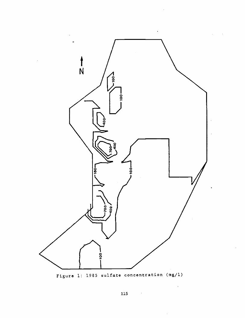
Figure 1: 1985 sulfate concentration (mg /1)
115

Figure 2: Scenario 1, 2035 sulfate conc. (mg /1)
116

Figure 3: Scenario 2, 2035 sulfate conc. (mg /1)
117
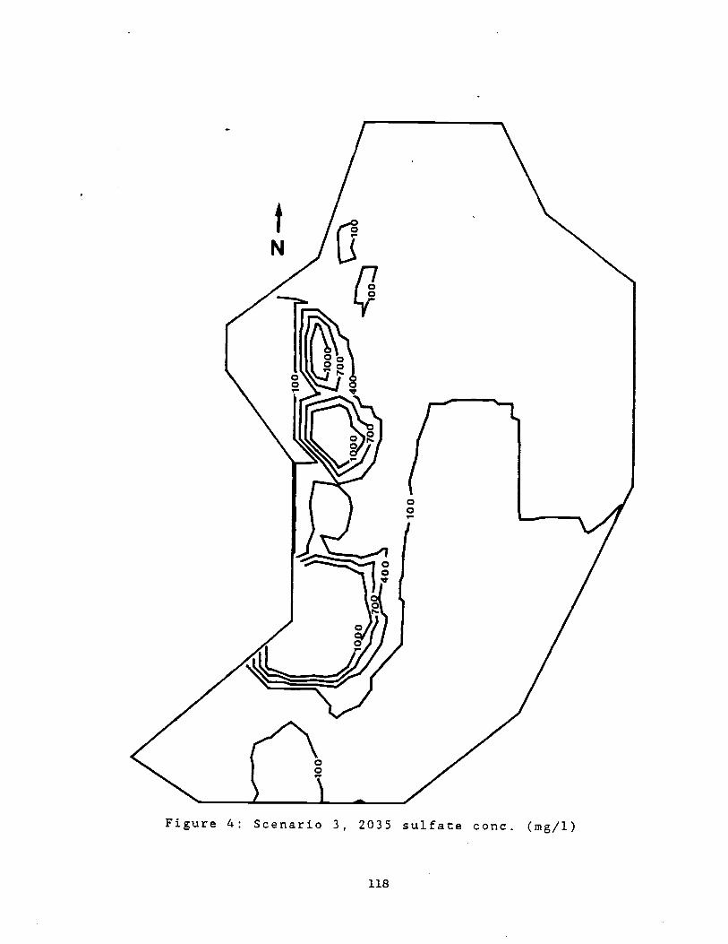
Figure 4: Scenario 3, 2035 sulfate conc. (mg /1)
118

Figure 5: Scenario 4, 2035 sulfate conc. (mg /1)
119

The information generated by risk analysis should proveuseful for decision makers when considering future land andwater use in the basin.
Acknowledgements: The work upon which this paper is basedwas supported by funds provided by the United StatesDepartment of the Interior, Office of Water Research andTechnology, as authorized under the Water ResourcesResearch Act of 1978.
Contents of this publication do not necessarily reflect theviews and policies of the Office of Water Research andTechnology, U.S. Department of the Interior.
Essential guidance was provided by the following principalinvestigators of the Upper Santa Cruz Basin Project team:Dr. W. B. Lord, Dr. M. M. Minnich, and Dr. S. P. Neuman.Invaluable research contributions were provided by thefollowing graduate assistants: Andy Lieuwen, Dennis Rule,Georgia Scovill, Derrik Williams, and project manager CraigTinney.
120

References Cited
Davidson, E. S. 1973. Geohydrology and water resources ofthe Tucson basin, Arizona. United States GeologicalSurvey water supply paper 1939 -E. Washington, D. C.:United States Government Printing Office.
Deisler, P. F. 1982. A goal oriented approach toindustrially related carcinogenic risks. DrugMetabolism Reviews,13(5):875 -911.
Dreith, R. H. 1982. An industry's guidelines for riskassessment at hazardous waste sites. F. A. Long andG. E. Schweitzer (Eds.). Washington, D. C.: AmericanChemical Society symposium series 204 :45 -53.
Hiessl, H. and M. Waterstone. 1986. Issues with risk.Tucson, Arizona: Arizona Water Resources ResearchCenter.
Kaplan, S. and B. J. Garrick. 1981. On the quantitativedefinition of risk. Risk Analysis, 1(1):11 -27.
Konikow, L. F. and J. D. Bredehoeft. 1978. Computer modelof two -dimensional solute transport and dispersion inground water. In: Techniques of water- resourcesinvestigations of the United States GeologicalSurvey, book 7, chapter C2. -Washington, D. C.:United States Government Printing Office.
Laney, R. L. 1972. Chemical quality of the water in theTucson basin, Arizona. United States GeologicalSurvey water supply paper 1939 -D. Washington, D. C.:United States Government Printing Office.
Pima Association of Governments Upper Santa Cruz BasinMines Task Force. 1979. Upper Santa Cruz groundwaterquality baseline report. Tucson, Arizona: PimaAssociation of Governments.
Pima Association of Governments Upper Santa Cruz BasinMines Task Force. 1983a. Ground -water monitoring inthe Tucson copper mining district. Tucson, Arizona:Pima Association of Governments.
121

Pima Association of Governments Upper Santa Cruz BasinMines Task Force. 1983b. Assessment of nitrate ingroundwater of the upper Santa Cruz basin and detailedupper Santa Cruz basin mines task force arearecommendations. Tucson, Arizona: Pima Associationof Governments.
Pima Association of Governments Upper Santa Cruz BasinMines Task Force. 1983c. Region wide ground waterquality in the upper Santa Cruz basin mines task forcestudy area and detailed upper Santa Cruz basin minestask force recommendations. Tucson, Arizona: PimaAssociation of Governments.
Pima Association of Governments. 1986. Impacts of theGreen Valley wastewater treatment facility upongroundwater quality. Tucson, Arizona: PimaAssociation of Governments.
Rowe, W. D. 1977. An anatomy of risk. New York: JohnWiley and Sons.
Scovill, G. L. 1987. Environmental fate of potentialground water contaminants in the unsaturated zone ofthe upper Santa Cruz basin area. Draft Report.Tucson,Arizona: Arizona Water Resources ResearchCenter.
Williams, D. 1987. Geostatistical analysis and inversemodeling of the upper Santa Cruz basin. Mastersthesis, University of Arizona, Tucson. In press.
122