resource loading under uncertainty with his practical experience were a source of inspiration. i...

Resource Loading Under

Uncertainty

Gerhard Wullink

This thesis is number D-72 of the thesis series of the Beta Research School for

Operations Management and Logistics. The Beta Research School is a joint

effort of the departments of Technology Management, and Mathematics and

Computing Science at the Eindhoven University of Technology and the Centre

for Production, Logistics, and Operations Management at the University of

Twente. Beta is the largest research centre in the Netherlands in the field of

operations management in technology-intensive environments. The mission of

Beta is to carry out fundamental and applied research on the analysis, design,

and control of operational processes.

Dissertation committee

Chairman Prof.dr.ir. J.J. Krabbendam (University of Twente)

Secretary Prof.dr. B.E. van Vucht-Tijssen (University of Twente)

Promotor Prof.dr. A. van Harten (University of Twente)

Assistant Promotor Dr.ir. E.W. Hans (University of Twente)

Expert Dr.ir. A.J.R.M Gademann (ORTEC B.V.)

Members Prof.dr.ir. F.J.A.M. van Houten (University of Twente)

Prof.dr. W.H.M. Zijm (University of Twente)

Prof.dr. W.S. Herroelen (Katholic University of Leuven)

Prof.dr.ir. J.W.M. Bertrand (Eindhoven University of

Technology)

Prof.dr. J. Telgen (University of Twente)

ISBN 90-365-2157-2

c© G. Wullink, Enschede, 2005

Printed by Febodruk B.V., Enschede, The Netherlands

RESOURCE LOADING UNDER

UNCERTAINTY

PROEFSCHRIFT

ter verkrijging van

de graad van doctor aan de Universiteit Twente,

op gezag van de rector magnificus,

prof.dr. W.H.M. Zijm,

volgens besluit van het College voor Promoties

in het openbaar te verdedigen

op vrijdag 4 maart 2005 om 13.15 uur

door

Gerhard Wullink

geboren op 16 maart 1976

te Zwolle

Dit proefschrift is goedgekeurd door de promotor:

Prof.dr. A. van Harten

en de assistent-promotor:

Dr.ir. E.W. Hans

v

Acknowledgements

This Ph.D. project is about planning projects that involve uncertainty. In

retrospect I can say that taking into account uncertainty might have been

helpful in doing this Ph.D. project. While the possibility to negotiate the

deadline is very limited, after all, four years is four years, I could have assessed

the consequences of doing a Ph.D. on my personal life better. A person has

only limited regular and nonregular working time, of which the latter is the

most expensive in terms of “work-life-balance”. Nevertheless, I can say now

that it was more than worth it.

I obviously couldn’t have done this Ph.D. project on my own, so I owe my

gratitude to several people who were involved in the realization of this thesis.

The people below, I thank in particular.

First of all, I express my gratitude to Aart van Harten, who offered me the

position and who had the confidence that putting me on the project would re-

sult in a thesis. He was always prepared to give useful comments and directions,

and he stimulated me to broaden my horizon, for instance, when he suggested

me to visit a foreign university for a few months. I thank Noud Gademann,

who was involved in the early stages of the project. His critical remarks, com-

bined with his practical experience were a source of inspiration. I also thank

Marco Schutten for, besides being a great colleague, reading Chapter 3 of my

thesis. Furthermore, I express my gratitude to Willy Herroelen and Roel Leus

for having me in Leuven for two months. This opportunity to temporarily join

another scientific community was a very valuable experience for me. I enor-

mously appreciate the way we worked together. I am also grateful to Geert

Schouten who reviewed the example in Chapter 1. His practical experience in

the maritime industry made the example more realistic. Finally, I thank the

person who was mostly involved in my Ph.D. project: Erwin Hans. As my daily

vi

supervisor he was always there to coach me through the world of programming

and mathematical modeling, and to patiently correct my, sometimes repetitive,

mistakes. Besides that, he was, and still is, more than just a daily supervisor.

Besides the people that were directly involved in the realization of my thesis,

several people had a more indirect contribution. I thank all my colleagues for

creating an excellent working atmosphere. I will miss the, sometimes long,

coffee breaks, lunches, or the sunny rides in Elke’s convertible for a delicious

Van der Poel ice cream. Such things make doing a Ph.D. even more enjoyable.

I am also very grateful that Annemiek and Eduard have their share in the

realization of this thesis. Annemiek for helping me creating the cover of my

thesis and Eduard for supporting me on the day of the defense as one of my

paranimfs. I also thank Imre for being my second paranimf and a very special

friend. Last but one, I thank my parents for all of the love, support, and

encouragement they have provided me throughout my life.

Finally, I thank Babette, whose love, support, and dedication throughout

the last four years have helped get me through it all. You were always pre-

pared to patiently listen to my disappointments or moments of euphoria. Our

weekends in Amsterdam and wonderful holidays were welcome interruptions

to working on this thesis. Babette, your unconditional support and love have

been, and still are, very precious to me.

Gerhard Wullink

Enschede, March 2005

vii

Contents

Acknowlegdements v

1 Introduction 1

1.1 Introductory example . . . . . . . . . . . . . . . . . . . . . . . 1

1.2 Motivation of this research . . . . . . . . . . . . . . . . . . . . . 5

1.3 Engineer-To-Order production . . . . . . . . . . . . . . . . . . . 7

1.4 Uncertainties in ETO manufacturing planning and control . . . 9

1.5 Resource loading . . . . . . . . . . . . . . . . . . . . . . . . . . 11

1.6 Literature and related work . . . . . . . . . . . . . . . . . . . . 12

1.6.1 Strategic planning . . . . . . . . . . . . . . . . . . . . . 13

1.6.2 Tactical planning . . . . . . . . . . . . . . . . . . . . . . 13

1.6.3 Operational planning . . . . . . . . . . . . . . . . . . . . 17

1.7 Overview of the thesis . . . . . . . . . . . . . . . . . . . . . . . 18

2 Hierarchical production planning and control 21

2.1 Project Management . . . . . . . . . . . . . . . . . . . . . . . . 22

2.2 Multi-project management . . . . . . . . . . . . . . . . . . . . . 24

2.2.1 Multi-project management . . . . . . . . . . . . . . . . 25

2.2.2 Organizational aspects of multi-project management . . 26

2.2.3 A classification matrix for multi-project organizations . 27

2.3 Hierarchical frameworks for planning and control . . . . . . . . 31

2.3.1 Hierarchical planning and control for project organizations 31

2.3.2 Hierarchical planning and control for manufacturing or-

ganizations . . . . . . . . . . . . . . . . . . . . . . . . . 34

2.3.3 Hierarchical planning and control for multi-project orga-

nizations . . . . . . . . . . . . . . . . . . . . . . . . . . 36

viii Contents

2.4 Rough Cut Capacity Planning . . . . . . . . . . . . . . . . . . . 37

2.5 Resource constrained project scheduling . . . . . . . . . . . . . 39

2.6 Interaction . . . . . . . . . . . . . . . . . . . . . . . . . . . . . 42

2.7 Conclusions . . . . . . . . . . . . . . . . . . . . . . . . . . . . . 44

3 Deterministic resource loading 45

3.1 Formal problem description . . . . . . . . . . . . . . . . . . . . 46

3.2 Models for deterministic resource loading . . . . . . . . . . . . 47

3.2.1 Complexity . . . . . . . . . . . . . . . . . . . . . . . . . 47

3.2.2 Base model without precedence constraints . . . . . . . 48

3.2.3 Implicitly modeled precedence relations . . . . . . . . . 49

3.2.4 Explicit precedence constraints . . . . . . . . . . . . . . 51

3.3 Solution approaches . . . . . . . . . . . . . . . . . . . . . . . . 54

3.3.1 Straightforward constructive heuristics (Class 1) . . . . 55

3.3.2 LP based heuristics (Class 2) . . . . . . . . . . . . . . . 63

3.3.3 Exact algorithms (Class 3) . . . . . . . . . . . . . . . . 67

3.3.4 Overview of all deterministic resource loading methods . 70

3.4 Computational results . . . . . . . . . . . . . . . . . . . . . . . 70

3.4.1 Instance generation . . . . . . . . . . . . . . . . . . . . . 70

3.4.2 Lower bounds . . . . . . . . . . . . . . . . . . . . . . . . 73

3.4.3 Straightforward constructive heuristics (Class 1) . . . . 74

3.4.4 LP based heuristics (Class 2) . . . . . . . . . . . . . . . 76

3.4.5 Exact approaches (Class 3) . . . . . . . . . . . . . . . . 76

3.5 Conclusions . . . . . . . . . . . . . . . . . . . . . . . . . . . . . 78

4 Scenario based approach 81

4.1 Problem description . . . . . . . . . . . . . . . . . . . . . . . . 82

4.2 Scenario based model . . . . . . . . . . . . . . . . . . . . . . . 86

4.2.1 Model . . . . . . . . . . . . . . . . . . . . . . . . . . . . 86

4.3 Solution approaches . . . . . . . . . . . . . . . . . . . . . . . . 87

4.3.1 Sampling or selecting . . . . . . . . . . . . . . . . . . . 88

4.4 Computational experiments . . . . . . . . . . . . . . . . . . . . 89

4.4.1 Instance generation . . . . . . . . . . . . . . . . . . . . . 90

4.4.2 Preliminary results . . . . . . . . . . . . . . . . . . . . . 91

4.4.3 Sensitivity analyses . . . . . . . . . . . . . . . . . . . . . 93

ix

4.5 Final remarks and conclusions . . . . . . . . . . . . . . . . . . . 95

5 Robustness optimization based approach 97

5.1 Problem description . . . . . . . . . . . . . . . . . . . . . . . . 99

5.2 Robustness in resource loading . . . . . . . . . . . . . . . . . . 100

5.2.1 Resource plan robustness . . . . . . . . . . . . . . . . . 101

5.2.2 Activity plan robustness . . . . . . . . . . . . . . . . . 102

5.3 Implicitly modeled precedence relations . . . . . . . . . . . . . 104

5.4 RRL with explicit precedence constraints . . . . . . . . . . . . 106

5.5 Computational experiments . . . . . . . . . . . . . . . . . . . . 109

5.5.1 Test approach . . . . . . . . . . . . . . . . . . . . . . . . 109

5.5.2 Instance generation . . . . . . . . . . . . . . . . . . . . 110

5.5.3 Results . . . . . . . . . . . . . . . . . . . . . . . . . . . 111

5.5.4 Sensitivity analyses . . . . . . . . . . . . . . . . . . . . . 113

5.6 Conclusions and further research . . . . . . . . . . . . . . . . . 115

6 Conclusions 119

6.1 Summary . . . . . . . . . . . . . . . . . . . . . . . . . . . . . . 120

6.2 Future research . . . . . . . . . . . . . . . . . . . . . . . . . . . 122

Bibliography 125

Samenvatting 137

Curriculum Vitae 141

x Contents

1

Chapter 1

Introduction

The competitiveness of an Engineer-To-Order (ETO) company highly depends

on its ability to manage its resource capacity and order portfolio in an environ-

ment characterized by uncertainty. These uncertainties can have a particularly

devastating effect on the performance of a company in terms of efficient resource

utilization and service level. In this thesis we develop and test models and al-

gorithms for tactical capacity planning under uncertainty in ETO production

environments.

An example in Section 1.1 illustrates the impact of uncertainty on the

capacity planning and order acceptance of an ETO company. The example

introduces a key issue for the tactical planning process that we address in this

thesis: resource loading. The remainder of the chapter is structured as follows.

Section 1.2 summarizes our research motivation, Section 1.3 discusses system

and control characteristics of the ETO production environment, Section 1.4

elaborates uncertainties typical for the tactical planning level, and Section 1.5

discusses the resource loading problem. Section 1.6 contains a short review of

the relevant literature and Section 1.7 outlines the remainder of this thesis.

1.1 Introductory example

During its journey from the Middle East to the harbor of Rotterdam, the oil

tanker “Jonah” collides with a large object, which the crew suspects to be

a whale. It is difficult to establish the precise location(s) and extent of the

2 Chapter 1. Introduction

damage at sea in the Channel; an inspection is impossible without dry-docking

the ship. Therefore, the ship owner immediately negotiates with the repair

yard Rotterdam Ship Yards (RSY) to come to an agreement about repairing

the ship in po-dock. Since the ship owner loses income every day the ship is

in dry-dock, he wants the job to be done as quickly as possible and will claim

huge delivery penalties from the repair yard if the job is not done on time.

To quote a reliable due date, RSY and the ship owner negotiate the re-

pair activities. Since negotiation takes place prior to inspection (the ship is

still at sea), rough estimates have to be made on the work content and the

duration of the activities. The following eight activities are established: (1)

dry-docking, (2) cleaning, (3) inspection, (4) removal of damaged parts, (5)

prefabrication, (6) welding, (7) painting, and (8) un-docking. The resources

RSY uses to execute the repair are divided into three groups: fitters, welders,

and dockworkers. In this example, the dockworkers perform all activities in-

volved with dry-docking, cleaning, painting and un-docking the ship. Table 1.1

shows the estimated data for the eight activities. These estimates are generally

based on experience and historical data of both the ship owner and the repair

yard. Because the exact extent of the damage cannot be established, the work

contents of several activities are uncertain. The “removal of damaged parts”,

“prefabrication”, and “welding”, are activities of which the work content can

increase up to seven hours per activity. This uncertainty poses a serious risk

to the resource costs and the reliability of the due date. Uncertain activities

are indicated by an asterisk.

Table 1.1: Project data

Activity↓ Nr. Minimum Estimated work content (hrs)

duration (days) Welders Fitters Dockworkers

Dry-docking 1 1 - - 4

Cleaning 2 1 - - 8

Inspection 3 1 3 4 -

Removal∗ 4 1 8 8 -

Prefabrication∗ 5 1 9 12 -

Welding∗ 6 1 7 10 -

Painting 7 1 - - 4

Un-docking 8 1 - - 4

1.1. Introductory example 3

Several repair activities require more than one resource group during exe-

cution. Prefabrication, for instance, requires welders and fitters simultaneously.

In this example, all activities have a minimum duration of one day. The mini-

mum activity duration is a result of technical restrictions: the duration cannot

be shortened even when more resource capacity is deployed. This may be a

result of limited working space, such as activities in the engine compartment.

The activities of the repair project are related according to the precedence

network displayed in Figure 1.1.

1

2

4 7 8

53

6

1

2

4 7 8

53

6

Figure 1.1: Network of the repair of the Jonah

RSY has one source of nonregular capacity for the three resource groups:

working in overtime. Working in overtime means additional costs and a resource

group cannot work more than three hours per day in overtime. Table 1.2 shows

the resource data of RSY.

Table 1.2: Resource capacity data

Regular capacity per day (hrs)

↓Resource group 1 2 3 4 5 6 7 8

Welders 0 0 2 8 8 8 6 0

Fitters 0 8 10 10 10 10 8 0

Dockworkers 4 4 4 0 0 0 4 4

To negotiate a reliable due date, to assess the status of the production

system, to plan working in overtime, and to order materials, RSY draws up a

rough capacity plan to know when activities will be executed. This capacity

plan is then optimized with respect to resource utilization (see Figure 1.1). In

this thesis, we refer to such a capacity plan as a resource loading plan. Note


that this resource loading plan does not require overtime for any of the resource

groups. All work can be completed within the regular capacity (indicated by

the dotted line) and before the due date.

Although the resource loading plan in Figure 1.2 is optimized with respect to

Fitters

0

2

4

6

8

10

12

1 2 3 4 5 6 7 8Periods

Cap

acit

y (h

ou

rs)

Welders

0

2

4

6

8

10

1 2 3 4 5 6 7 8Periods

Cap

acit

y (h

ou

rs)

Dockworkers

0

1

2

3

4

5

1 2 3 4 5 6 7 8Periods

Cap

acit

y (h

ou

rs)

Dry-docking

Cleaning

Inspection

Removal

Welding

Prefabrication

Painting

Un-docking

Figure 1.2: Cost optimal resource loading plan

resource utilization (i.e., no additional capacity is needed), the managers of

RSY are worried that materialization of the uncertainty will disturb the plan,

and induce delivery penalty costs or costs for working in overtime. Activities

(4) removal of damaged parts, (5) prefabrication, and (6) welding are espe-

cially vulnerable because they have no free regular capacity to use if disturbed.

The plan raises the following questions: what is the performance in terms of

resource utilization and penalty costs of this plan in case uncertainties ma-

terialize? Is there a plan with a better performance with respect to dealing

with uncertainty? Answering these questions can mean the difference between

the Jonah repair project being profitable or not. The remainder of this thesis

develops methods that can help to answer these questions.

1.2. Motivation of this research 5

1.2 Motivation of this research

The example described provides a typical situation faced by every ETO com-

pany on a regular basis: making decisions in uncertain circumstances that are

of vital importance for the primary company objective of profitability. Prof-

itability can be the company objective to satisfy the shareholders, guarantee

continuity, a combination of these, or other criteria. Profitability in general,

however, is not directly used as an optimization criterion in most manufac-

turing planning and control (MPC) models. Typically, related objectives are

used, such as minimization of risk and costs, and maximization of revenues,

profitability, flexibility , and service level. Furthermore, many of today’s man-

agers and planners have the tendency to focus on urgent short term operational

problems caused by disturbances. Problems such as dissatisfied customers, pro-

duction disturbances, or capacity problems distract managers from the overall

company objective of profitability. An MPC approach should provide meth-

ods that incorporate costs, risk, revenues, flexibility, and service level at all

planning levels.

ETO companies like the repair yard from the example in Section 1.4, face

numerous internal and external uncertainties on a daily basis. These uncer-

tainties can vary from resource breakdowns to uncertain order characteristics.

Such ambiguity imposes great risk on the profitability of a single order or on the

performance of the entire production system. Since production managers are

typically risk averse, uncertainties should be dealt with in any MPC approach.

At the tactical planning level, order acceptance deals with accepting, re-

jecting, and negotiating orders. Resource loading is another tactical planning

function that deals with loading a set of orders to resource groups in the pro-

duction system. If necessary, resource loading can temporarily expand resource

capacity, by assigning nonregular capacity, such as overtime or subcontracting,

against additional costs. As we argue in Section 1.5, resource loading is an

indispensable tool for order acceptance to quote reliable delivery dates and de-

termine the capacity impact of new customer orders. Since the turnover of a

company is eventually determined by the composition of the order portfolio,

order acceptance and resource loading play a crucial role in optimizing revenues

and profitability. In practice, however, order acceptance and resource loading

are often functionally dispersed. Consequently, driven by turnover maximiza-


tion, a sales department often tries to acquire as many orders as it can without

considering the status of the production system. Since order characteristics are

often not fully known in ETO environments, it is difficult to assess the capacity

impact of new orders. Moreover, it requires an aggregate, less detailed, rep-

resentation of the entire production system, and a higher level of abstraction

than for scheduling, where more information on activities is available after the

engineering and design stage. The inability to assess the status of the pro-

duction system may result in an overloaded production system, excess work in

process levels, and increased lead times. This can eventually have a negative

effect on the overall company performance in terms of service levels and costs.

We refer to the tendency of managers to focus first on operational prob-

lems as the “real time hype”. The operational planning level, however, lacks

the flexibility to deal satisfactorily with these problems. After all, the workload

has already been determined, and additional production capacity is difficult to

arrange on short notice and is often very expensive on the short term. This

flexibility is available at the tactical level: less orders can be accepted or ad-

ditional capacity can be arranged, such as subcontracting, hiring additional

personnel, or working overtime.

A solution for the potentially devastating effects of ETO inherent un-

certainties and the production system overload is an approach that uses the

flexibility available at the tactical planning level. In this thesis, we propose

that such tactical planning methods should use the flexibility of the medium

planning term on the one hand and on the other deal with the uncertainties

inherent to ETO production. The literature, as we shall argue in Section 1.6,

focuses mainly on the operational planning level. We focus particularly on the

tactical planning level, and aim to develop planning techniques that contribute

to optimizing the aforementioned objectives. Although we do not explicitly

focus on order acceptance, we believe that our resource loading methods con-

tribute significantly to more effective order acceptance. The idea is that for a

given set of orders that is considered for acceptance, the effects of uncertainty

on the resource loading can be analyzed in terms of robustness.

1.3. Engineer-To-Order production 7

1.3 Engineer-To-Order production

Since ETO companies play a central role in this thesis, we give a more detailed

description of ETO manufacturing in this section. Typically, an ETO company

has a job shop production layout with multiple resource, tool, or personnel

groups. These resource groups may consist of machines of the same resource

type, or can be manufacturing cells (see Burbidge, 1979). Consider the resource

group welding from the example in Section 1.1, which consists of several types

of welders: from specialized sheet metal arc welders for the thick plates of the

ship hull, to regular welders for standard operations. The resource groups have

a limited regular capacity. Nonregular capacity is also limited but can often

be arranged on the medium term. This temporary capacity flexibility can

consist of hiring additional personnel, subcontracting activities, extra shifts,

or overtime. Using nonregular capacity induces additional costs; labor laws

often demand that personnel who work in overtime get additional free time in

subsequent periods.

Orders in ETO companies typically go through five stages, some of which

can be executed partly simultaneously.

Order negotiation & resource loading In the order acceptance stage, or-

ders consist of work packages or main activities with a routing. The data in this

stage are estimates based on experience and historical data. Activities require

one or more resource groups, for example, welders, ironworkers, or painters,

through which they have to be processed for a given, often uncertain, amount

of time. The earliest moment on which the first activity can begin is the release

date of the order. The moment on which the customer wants its product to be

delivered is the due date. Based on this information a resource loading plan

should be drawn up to assess the capacity consequences of customer orders

and to negotiate reliable due dates. Since ETO companies produce nonstan-

dard products based on customer requirements, order acceptance is typically

done in close cooperation with the customer. During this process, rough order

specifications can only be based on experience or historical data. Consequently,

order acceptance decisions are often made based on uncertain and incomplete

information. Decisions about the use of nonregular capacity should usually be

made in this stage.


Engineering & micro process planning If an order is not a repeat order,

engineering and design deal with establishing the exact order specifications.

After engineering, preparations for the actual production process take place

in micro process planning. Typical results of micro process planning are a

routing through the shop floor, a bill of materials, tool selection, and code for

automated manufacturing.

Detailed scheduling & resource allocation At this stage, virtually all

production specifications and instructions have been generated. Operations

are now scheduled and allocated to resources using this precise information.

While some ETO companies use formal scheduling algorithms to support this

stage, others let the planners schedule the operations on the shop floor. In

general, the objectives of scheduling and resource allocation methods are time

related (e.g., minimization of the makespan or tardiness), with the amount of

regular and nonregular capacity as a restriction.

Manufacturing During manufacturing, orders are processed on the resources

of the production system. A shop floor control system can be used to monitor

production and detect disruptions. Information on the status of the shop floor

control can be fed back to the MPC system, which may result in rescheduling

or replanning actions to keep up to date.

Quality control & service Generally during and after the manufacturing

process quality control inspects the final product. Orders, or parts of orders,

may require rework. In some industries, on site installation, service and main-

tenance are part of the service mix offered by a company.

Traditionally, there has been a sharp distinction in the literature between

(multi-) project organizations and ETO organizations. In practice this is not

the case, as they are essentially the same. In this thesis, we also do not dis-

tinguish between these two forms. We consider a (multi-) project organization

as a special case of ETO production and present our methods for an ETO

production environment, which comprises ETO and project organizations. On

the other hand, we use the terminology of multi-project management, if this

is more convenient (see Chapter 2). In the remainder of this thesis we use the

1.4. Uncertainties in ETO manufacturing planning and control 9

terms order, activity, and operation for the order breakdown structure. We

use the term resource groups for capacity groups, operators, departments, or

machine groups.

1.4 Uncertainties in ETO manufacturing plan-

ning and control

Uncertainties play a role on various levels of ETO manufacturing planning

and control. At the strategic level, economic developments or the political

climate force decision makers to deal with uncertainties. At the operational

level there are many sources of uncertainties, such as inaccurate processing

times or resource breakdowns. For an extensive taxonomy of uncertainties on

the operational planning level we refer to Aytug et al. (2005). At the tactical

level, particularly ETO production environments have additional sources of

uncertainty which, as illustrated in Section 1.2, can have a negative impact on

the overall company objectives. The following uncertainties are most common

in ETO manufacturing planning and control.

Work content of activities The work content of an activity is generally

an estimation based on historical data or the experience of the planner or the

customer. The accuracy may vary considerably depending on the nature of the

activity or the required resource group. For instance, consider the under water

damage of the Jonah. The damage cannot be inspected before dry-docking,

so it is hard to make a reliable estimation of the work content of the repair

activities. Furthermore, the disaggregation of activities into operations for op-

erational planning is a considerable source of uncertainty because of precedence

relations, setups, or multi-resource requirements. We refer to this uncertainty

as disaggregation uncertainty.

Occurrence of an activity The occurrence of some activities may also be

uncertain. A test or inspection activity may, for instance, result in additional

work that was not expected. In the Jonah example, dry-docking and inspecting

a ship may reveal additional repair work. For example, once the ship is dry-

docked, manholes can be opened, revealing the condition of the ballast tanks.


With respect to the occurrence of an activity, weather conditions may play a

role, or the ship owner may decide to postpone less critical repair activities.

Resource requirements of an activity At the tactical level engineering

has often not been completed. As a result, resource requirements of some

activities may be uncertain.

Capacity availability If a resource is expected to be unavailable for a long

time, it should also be accounted for on the tactical planning level. Consider,

for instance, the risk of personnel being on long sick leaves. The availability of

nonregular capacity can also be a major source of uncertainty.

Precedence relations Precedence relations may also be a source of uncer-

tainty. Suppose the damage of the Jonah is located closer to the engine com-

partment than expected. Activities that were initially planned in parallel, for

instance, burning out a damaged section of the ship and working in the engine

compartment, may then have additional precedence relations.

Release dates Release dates can depend on special material requirements or

special activities upstream in the supply chain, which can result in uncertainty

in the delivery date.

Rush orders Rush orders are a typical source of uncertainty for ETO pro-

duction. At any moment a rush order can arrive, which may have such high

strategic priority that other orders have to be replanned to give precedence to

the rush order. In the situation of the ship repair business, rush orders are

common practice.

In this thesis, we develop resource loading methods that deal with un-

certainty of the work content, occurrence and the resource requirements of an

activity, as well as the capacity availability of resource groups. We leave un-

certain precedence relations, uncertain release dates, and rush orders out of

consideration in this thesis.

1.5. Resource loading 11

1.5 Resource loading

In the previous two sections, we discussed the characteristics of ETO produc-

tion. As we argued in Section 1.2, vital decisions are made at the tactical level

for the profitability of ETO companies. Furthermore, we argued that tacti-

cal planning offers opportunities to exploit available flexibility to optimize the

performance of the production system in terms of resource utilization, service

level, and dealing with uncertainty. In this section, we discuss a tactical plan-

ning function that addresses the aforementioned aspects. It is the central topic

of this thesis: resource loading.

Resource loading deals with loading orders on the resource groups of a

production system. These are orders that are already accepted or considered for

acceptance. The orders have a due date considered externally determined, for

example, after negotiation with the customer. The orders consist of activities

related according to precedence relations. Activities have a work content that

must be processed on one or more resource groups. Activities may have a

minimum duration. This minimum duration is the result of the maximum

amount of resource capacity that can be allocated to the activity in each period.

The planning horizon of the resource loading problem typically varies from a few

weeks to several months. Resource groups have limited regular and nonregular

capacity. Using nonregular capacity invokes additional costs. As argued in

Section 1.4, several problem parameters of the resource loading problem can

be uncertain.

On the one hand, resource loading considers an aggregation level appro-

priate to support planning decisions based on the rough order details available

at the tactical stage. On the other hand, it comprises enough detail to give an

accurate representation of the actual status of the production system.

The objective of resource loading is to load the orders into the production

system, in such a way that resource utilization and service level are optimized,

and uncertainties are dealt with by using the time and capacity flexibility avail-

able at the tactical planning level. It supports a company in making a trade-off

between delivery performance and capacity utilization, and takes into account

the robustness of plans.

In general, three types of resource loading problems are distinguished:

resource driven resource loading, time driven resource loading, and hybrid re-


source loading. Resource driven resource loading considers all capacity levels

as fixed (i.e., no nonregular capacity can be used). An objective of the resource

driven resource loading problem can, for instance, be to minimize the tardiness

costs of orders. This type of resource loading is typically applicable in settings

where capacity flexibility is minimal. The time driven resource loading con-

siders the due dates as deadlines. The objective of the time driven problem

is to minimize the cost of using nonregular capacity. Typically, time driven

resource loading is useful for settings where a due date is given by a customer.

The planning of the Jonah repair project in Section 1.1 is an example of time

driven resource loading. In hybrid resource loading a trade-off can be made be-

tween delivery performance, the costs for using nonregular capacity, or another

criterion, for instance, the robustness of a plan.

The deterministic resource loading problem is a Combinatorial Optimiza-

tion (CO) problem, which, as we will show in Section 3.2.1, is NP-hard in the

strong sense. In this thesis, we study resource loading under uncertainty. This

problem contains the deterministic resource loading problem as a special case,

and is therefore also NP-hard in the strong sense. Being able to solve the re-

source loading problem under uncertainty is a challenge, both from a practical

and a scientific point of view.

1.6 Literature and related work

To position our research and discuss related work about planning under uncer-

tainty and tactical planning in manufacturing, we use a hierarchical planning

decomposition with three planning levels generally distinguished in the litera-

ture as (see, e.g., Bitran and Tirupati, 1993a and Zijm, 2000):

• Strategic planning

• Tactical planning

• Operational planning

We discuss various methods for strategic and operational planning under

uncertainty and several approaches for tactical planning in general.

1.6. Literature and related work 13

1.6.1 Strategic planning

Strategic planning involves long term decisions at the company management

level. It addresses problems like facility location planning, workforce planning,

and product mix planning. Strategic planning problems are often solved with

LP techniques (see, e.g., Hopp and Spearman, 1996, and Nam and Logendran,

1992). Aggregate planning typical deals with capacity flexibility, but not with

technological restrictions such as precedence relations. It typically uses demand

forecasts as input data. These forecasts are a considerable source of uncertainty.

An example of a strategic planning technique that accounts for these uncertain-

ties is the multi-stage LP technique proposed by Eppen, Martin and Schrage

(1989). Escudero et al. (1993) propose a scenario based LP model for produc-

tion planning problems with unknown product demands. Rosenhead, Elton

and Gupta (1972) discuss robustness and optimality as criteria for strategic

decisions, and argue that for many strategic decisions sheer, optimality is not

a sufficient decision criterion. They introduce the concept of robustness as a

measure of the useful flexibility of a solution. They claim that robustness deals

with uncertainty, not by imposing a probabilistic structure, but by stressing

the importance of the flexibility of a decision. They also discuss the concept of

stability and claim that an initial decision is stable if the long run performance

of the decision is satisfactory and no corrective decisions have to be made. They

apply their ideas to a plant location problem. As a robustness measure they

use the number of possible future decisions that can be taken given a certain

set of decision sequences (see also Rosenhead, 1978 and Rosenhead, 1980). An

important characteristic of strategic planning is that it does not assume any

information about specific customer orders, but instead uses demand forecasts

that yield aggregate data about the future demands. This makes it unsuit-

able for tactical planning in ETO environments, where customer order data is

required for order acceptance and resource capacity management.

1.6.2 Tactical planning

Most research on tactical planning in ETO production environments concerns

lead time estimations, order acceptance, workload control, MRP systems, and

resource loading. We briefly discuss several of these approaches.

Buzacott and Shanthikumar (1993) estimate lead times in a job shop by


modeling a manufacturing system as a closed queuing network. Buitenhek

(1998) also studies lead times in a job shop environment. He uses semi open

queuing networks to analyze various complex manufacturing systems. Zijm

(2000) argues that focusing on stable internal lead times has its merits, but

does not deal with the discrepancy between meeting customer order due dates

and optimizing resource utilization. He argues for integrating workload control

and resource availability on a higher level, or even supporting order acceptance

by sophisticated load based procedures.

Other authors propose approaches that use the schedule of the produc-

tion system to support order acceptance. Kapuscinski and Tayur (2000) study

dynamic capacity reservation to support lead time estimation and order ac-

ceptance in MTO environments. They argue that for lead time estimation

also future orders should be taken into account. Çakanyildirim et al. (1999)

propose an approach for capacity driven order acceptance for batch manufac-

turing. They argue that order acceptance decisions should be based on the

available capacity in a schedule. While in MTO manufacturing order data is

more predictable, such scheduling based approaches are suitable for MTO. For

ETO an approach that uses more aggregate order data is required.

Wester, Wijngaard and Zijm (1992) propose three approaches for order

acceptance in production-to-order environments. The first approach uses the

detailed information of the production schedule for order acceptance, the second

approach uses global capacity load profiles, and the third approach uses a so-

called myopic schedule, which only schedules an order when a machine becomes

idle. They test the approaches in a strictly deterministic one stage production

setting, without routing constraints which make them unsuitable for an ETO

production environment. Bertrand (1983) proposes to estimate due dates by

using: (a) the arrival time of the order, (b) the number of operations of the

order, (c) the total workload of the order, and (d) the flow time. The latter is

derived from the congestion resulting from the time phase-dependent workload

in the shop floor. He argues that taking into account the workload results

in more reliable due dates. Other researchers use statistical estimates of the

required capacity to support order acceptance in batch process production (see,

e.g., Ivanescu, Fransoo and Bertrand, 2002 and Raaymakers, 1999). The latter

techniques assume a flow shop layout typical for batch process industries, but

unsuitable for ETO manufacturing.


Bertrand and Wortmann (1981), Land and Gaalman (1996), and Wiendahl

(1987) propose a workload control approach to control the workload in the job

shop. The principle of workload control is that jobs are kept in a pool of

unreleased jobs and are only released to the shop floor if they do not cause the

planned queues to exceed a predetermined norm. Workload control contributes

to a more accurate prediction of internal lead times because no work is allowed

in the shop if the workload is too high. The problem, however, is shifted to

the buffers before the job shop. Therefore, the total lead time of an order in

and before the system is not dealt with and has the tendency to increase (see

Hendry, Kingsman and Cheung, 1998).

One of the most critical assumptions of MRP is that the lead time of an

activity is an input parameter for planning. This automatically implies that

the lead time is independent of the actual workload and the free capacity in

the production system. The consequence of this assumption is that lead times

of orders are increased in the case of frequent due date violations. This results

in higher work in process levels, which results in more congestion, and hence

an increasing lead time through the production system (see Hopp and Spear-

man, 1996). This effect is often referred to as the “planning loop” (see, e.g.,

Zäpfel and Missbauer, 1993). Furthermore, MRP assumes infinite production

capacity, which is an unrealistic assumption since every production system has

limited resource capacity. In MPRII, a later version of MRP, this flaw is over-

come by a capacity requirements check performed a posteriori, and unable to

anticipate capacity problems. Moreover, this approach can result in infeasi-

ble plans (see Negenman, 2000). It is generally recognized that MRP based

systems are suitable to support the materials planning of large make-to-stock

companies (see Orlicky, 1975 and Vollmann, Berry and Whybarck, 1997). For

ETO manufacturing they are not suitable, all the more because of the ETO

inherent uncertainties that can even amplify the flaws of MRP systems. While

techniques that protect MRP systems against uncertainty have been proposed,

these merely aim at dampening and buffering, for instance, by applying safety

stocks (see, e.g., Whybark and Williams, 1976). A safety stock strategy is not

suitable for ETO manufacturing since it is not known what orders will arrive;

safety stocks increase work in process (WIP) levels, which can have a negative

effect on the lead times. For an extensive review on other approaches on deal-

ing with uncertainty in MRP systems we refer to Koh, Saad and Jones (2002)


or Tang and Grubbström (2002).

During exploratory research at several Dutch companies (see Snoep, 1995,

Van Assen, 1996, De Boer, 1998, and De Boer and Schutten, 1999), new in-

sights were gained with respect to using mathematical programming (MP)

approaches for the resource loading problem. The authors propose to formu-

late the problem as a bucket loading problem in which buckets are periods to

which activities or parts of activities are assigned. De Boer (1998) proposes

several heuristics for deterministic resource loading. Hans (2001) proposes an

exact approach and Gademann and Schutten (2004) develop several LP based

heuristics for the resource loading problem. Kis (2004) proposes another exact

approach for the deterministic resource loading problem, which he refers to as

project scheduling with variable intensity activities. In Chapter 3 we give an

overview of approaches for deterministic resource loading. While the authors

of the previous resource loading approaches agree that uncertainty is a critical

factor for the tactical planning decisions, they do not deal with this explicitly

in their models. They argue that choosing the proper data aggregation level is

an appropriate way to deal with uncertainty. We propose that the flexibility of

the tactical planning level offers much more possibilities to deal with the uncer-

tainties typical for ETO production. Moreover, the current status of operations

research (OR), and the computational power of commercial solvers and per-

sonal computers offer new opportunities to explicitly incorporate uncertainty

in complex planning models.


1.6.3 Operational planning

Operational planning concerns the short term scheduling or sequencing of oper-

ations on resources. Operational planning objectives are generally time related.

For a comprehensive reference on operations scheduling we refer to Pinedo, 2001

and Demeulemeester and Herroelen, 2002. At the operational planning stage

resource capacity is generally considered fixed, which means that there is hardly

any flexibility to absorb disruptions. Consequently, uncertainties may result in

nervousness of the schedules created with deterministic input data. Dealing

with uncertainty in scheduling has gained the interest of researchers in the

past decades. Herroelen and Leus (2002) distinguish five main approaches of

scheduling under uncertainty: reactive scheduling, stochastic project scheduling,

stochastic project networks, fuzzy project scheduling, and proactive or robust

scheduling.

Reactive scheduling and stochastic project scheduling are online scheduling

techniques that respectively reoptimize the schedule after a disturbance, or

develop an optimal policy (see, e.g., Möhring, 2000a and Möhring, 2000b) to

deal with disturbances when they occur. Another reactive planning approach

is proposed by Dvir and Lechler, 2004, who state: “plans are nothing, changing

plans is everything”.

Stochastic project networks deal with projects with a stochastic evolution

structure of the activity network. This means that it is unknown in advance

which activities are going to be executed, and for how long. Because of the high

computational requirements of these methods, analysis of stochastic project

networks is often performed by simulation. For more details about stochastic

project scheduling we refer to Neumann and Zimmermann (1979), Stork (2001),

or Golenko-Ginzburg and Gonik (1997).

Fuzzy project scheduling is based on the assumption that activity durations

rely on human estimations. Hapke and Slowinski (1996) propose a priority

based scheduling heuristic using fuzzy number theory. Fuzzy project scheduling

results in fuzzy plans, which may be infeasible. For another approach for fuzzy

scheduling see Wang (2004).

Herroelen and Leus (2002) distinguish proactive or robust scheduling ap-

proaches for scheduling under uncertainty. The main goal of proactive or robust

scheduling approaches is to generate a robust baseline schedule. They propose


a pairwise float model, which is a mathematical programming technique to de-

velop stable (robust) baseline schedules. This approach aims to minimize the

difference between the start times of the realization and the initial schedule.

Furthermore, Leus (2003) proposes an approach to generate stable resource al-

location plans given a certain (stable) baseline schedule (see also Herroelen and

Leus, 2003 and Herroelen and Leus, 2004). For more approaches to schedul-

ing uncertainty we refer to, for example, Brandimarte (1999), Byeon, Wu and

Storer (1998), Cai and Zhou (1999), Honkomp, Mockus and Reklaitis (1999),

Lawrence and Sewell (1997), Valls et al. (1999), or Ke and Liu (2004). Finally, a

more practical example of proactive scheduling is proposed by Goldratt (1997).

This approach is based on insertion of buffers to deal with disturbances. For ex-

tensive reviews on scheduling under uncertainty we refer to Aytug et al. (2005)

or Davenport and Beck (2002).

We discussed several planning approaches for the planning levels in manu-

facturing planning. Some approaches do not deal with uncertainty, while others

do. In the latter category, approaches either deal with uncertainty by using ag-

gregate data, or by explicitly modeling uncertainty. Approaches that explicitly

incorporate uncertainty, either use a proactive approach or a reactive approach.

For the tactical level, however, we found no method that on the one hand deals

with the aggregation level of data that is required for tactical planning in ETO

manufacturing, and on the other hand explicitly incorporates uncertainty.

1.7 Overview of the thesis

This thesis is structured as follows. In Chapter 2, we propose a generic frame-

work for manufacturing planning and control for project and manufacturing

environments. Chapter 3 surveys existing techniques to solve the determinis-

tic resource loading problem. We also introduce a new exact approach and a

new heuristic for the deterministic resource loading problem. Chapter 4 pro-

poses a scenario based approach for resource loading under uncertainty. In

this approach, we use scenarios to model uncertainty. Solving the resulting

scenario based MILP yields a solution with minimum expected costs over all

scenarios. Chapter 5 proposes an approach for robust resource loading based

on the idea of incorporating robustness measures in an MILP formulation for

1.7. Overview of the thesis 19

resource loading. This results in a multi-objective optimization approach for

resource loading under uncertainty. Finally, in Chapter 6, we draw conclusions

and make several recommendations for future research.

21

Chapter 2

Hierarchical production planning and

control

Whereas adequate tactical planning can boost profitability of a company, it is

part of a larger MPC approach. Hence, for the success of a planning method,

it should be able to interact with other methods that are part of the manufac-

turing planning and control model.

The original paper1 is written with multi-project organizations in mind,

but as we argued before, these do not essentially differ from ETO organizations.

So the proposed hierarchical framework is also applicable to ETO environments.

We aim at providing an integrated approach to manufacturing planning

and control in ETO environments. Such an approach should both deal with

the complexity and the uncertainty of the production environment. Our goal is

to provide a general guide for using advanced production planning techniques

in practice. We propose a classification matrix to distinguish between different

types of ETO production organizations. This classification matrix uses the

dimensions of variability and complexity of an ETO or project organization.

The classification framework enables the selection of appropriate manufacturing

planning methods as a function of the organizational characteristics. We also

propose a hierarchical framework for manufacturing planning and control in

1This chapter is based on the paper: R. Leus, G.Wullink, E.W. Hans, and W.S. Herroelen,A hierarchical approach to multi-project planning under uncertainty, Beta working paper

WP-121, Leus et al. (2003).

22 Chapter 2. Hierarchical production planning and control

ETO organizations. This framework distinguishes three hierarchical levels.

Each level contains MPC functions that are geared to the planning horizon

and the measure of detail appropriate for that level. We discuss each level of

the hierarchy with its associated functions in detail. In this discussion we focus

especially on the two dimensions of the classification matrix, i.e., complexity

and variability.

This chapter is organized as follows. Section 2.1 discusses project manage-

ment in general and Section 2.2 surveys the existing approaches to practical

multi-project planning. Section 2.3 discusses hierarchical planning and control

frameworks that can be found in the literature, and proposes a hierarchical

framework for MPC. Sections 2.4 and 2.5 treat the tactical and operational as-

pects of planning in more detail. It mainly focusses on methods for the tactical

Rough Cut Capacity Planning (RCCP) problem and the operational Resource

Constrained Project Scheduling Problem (RCPSP). Note that RCCP in project

environments is the equivalent to resource loading in ETO environments. Sec-

tion 2.6 sets out a number of requirements such that these two levels can be

integrated, and we discuss in which situations each of the hierarchical levels

deserves the most attention. We end this chapter with some conclusions in

Section 2.7.

2.1 Project Management

Project management is a management discipline that is receiving a continu-

ously growing amount of attention (see, e.g., Kerzner, 1998 and Meridith and

Mantel, 2003). Both in production and in service sectors, ever more organi-

zations and companies adhere to project based organization and work, within

a wide variety of applications: research and development, software develop-

ment, construction, public infrastructure, process reengineering, maintenance

operations, or complex machinery. A project can be informally defined as a

unique undertaking, consisting of a complex set of precedence related activities

that have to be executed using diverse and mostly limited company resources.

Project management deals with the selection and initiation of projects, as well

as with their operation, planning and control.

A significant number of international high profile projects fail to be de-

2.1. Project Management 23

livered on time and on budget (see, e.g., Winch, 1996). One example that

immediately springs to mind is the construction of the Channel Tunnel, but

undoubtedly, most readers can also recall smaller scale projects closer to their

work environment, which did not work out as anticipated. A number of un-

desirable characteristics are associated with failing projects: budget overruns,

compromised project specifications, and missed milestones. In other words,

the three basic dimensions of project success, namely time, cost and quality,

are often in jeopardy. To avoid these problems, proper project planning is in

order: a description of the objectives and general approach of the project, its

resources and personnel, evaluation methods, and also a project schedule as

well as a description of potential problems that may be encountered.

Traditionally, research has focused on planning for so-called single-project

organizations. An increasing amount of companies, however, tend towards

an organizational structure in which multiple projects are run simultaneously.

Several authors (e.g., Levy and Globerson, 1997, Lova, Maroto and Tormos,

2000, and Payne, 1995), explicitly point out that companies mostly run a num-

ber of projects, which share the same scarce resources, in parallel. This results

in frequent conflicts of interest when multiple projects require the same scarce

resource at the same time. In this chapter we refer to the overall coordination

of such multi-project organizations as multi-project management.

A high degree of complexity and uncertainty about the activities and opera-

tions of the projects characterizes these environments. As coherently described

in Silver, Pyke and Peterson (1998), Anthony (1965) proposes that managerial

activities fall into three broad categories, whose names have been somewhat

changed over the years to become strategic planning, tactical planning and op-

erational control. These categories are concerned with different types of deci-

sions and objectives, managerial levels, time horizons and planning frequencies,

and also with different modeling assumptions and levels of detail. To deal with

the planning complexity in multi-project organizations, the planning process is

broken down into more manageable parts using a model for hierarchical plan-

ning and control based on the three managerial decision levels discerned in the

foregoing. Uncertainties in the multi-project driven organization are mainly

caused by two sources. On the one hand, detailed information about the re-

quired activities often becomes available only gradually, and on the other hand

numerous operational uncertainties can occur on the shop floor. Since all real


life projects are faced with uncertainty, this chapter pays particular attention

to planning models that account for variability and uncertain events.

We can distinguish between two distinct approaches for dealing with uncer-

tainty, namely the proactive and the reactive approach. The proactive method

tries to alleviate the consequences of uncertainties prior to the start of the

project, for example, by allocating the slack or flexibility in a plan to the pe-

riods where there are uncertainties. The reactive approach aims at generating

the best possible reaction given disturbances that cannot be dealt with by the

existing plan without changing it. This can be done by, for example, a re-

planning approach, which reoptimizes or repairs the complete plan after an

unexpected event occurs. Reactive approaches are particularly useful if distur-

bances cannot be completely foreseen or when they have too much impact to

be absorbed by the slack or the available capacity in a plan.

De Boer (1998) points out that in many organizations, part of the work is

made up by projects, while the rest is performed in “traditional manners”. A

software house, for instance, may sell standard software applications, for which

it has dedicated product development lines. At the same time, it can provide

custom made software applications, for which project managers are responsible.

De Boer (1998) uses the term “semi project driven” to describe such organi-

zations. Although this is certainly a pertinent remark, we do not specifically

distinguish between project driven and semi project driven organizations. The

techniques we study are applicable to the project based part of organizations,

whether this constitutes all, or only part of those organizations.

2.2 Multi-project management

This section is devoted to multi-project management, the broader management

discipline that encompasses the planning function that is the main target of

this chapter — we use the two terms “multi-project management” and “multi-

project planning” interchangeably in the remainder of this chapter. The focus

of Section 2.2.1 is on the planning aspect of multi-project management. In Sec-

tion 2.2.2 we discuss organizational aspects of multi-project management. We

present a classification matrix for multi-project management in Section 2.2.3.

2.2. Multi-project management 25

2.2.1 Multi-project management

Adler et al. (1995) suggest adopting a process viewpoint to multi-project man-

agement. They remark that most managers think of multi-project manage-

ment simply as the management of a list of individual projects, rather than

as a complex operation with a given capacity and workload. Their suggestion

is compatible with the introduction of a “Management By Projects” (MBP)

orientation at enterprise level, which takes the benefits of project management

with its focus on specific project goals and deliverables as a starting point,

but builds it into the needs of the overall organization. As such, MBP is the

integration, prioritization and continuous control of multiple projects and oper-

ational schedules in an enterprise wide operating environment (Boznak, 1996).

Various approaches for “multi-project management and planning” have been

proposed in the literature. Real multi-project approaches that are compatible

with an MBP focus, however, are scarce.

Dye and Pennypacker (2002) point out that there still exists a difference

between multi-project management (with the same content as what we defined

as “MBP”) and project portfolio management. The former is geared towards

operational and tactical decisions on capacity allocation and scheduling, and

is the job of project or resource managers; the latter is concerned with project

selection and prioritization by executive and senior management, with a focus

on strategic medium and long term decisions.

Finally, multi-project management should also not be confused with pro-

gram management, which is a separate concept altogether: program manage-

ment is a special case of multi-project management that has a single goal or

purpose (for instance, putting a man on the moon), whereas multi-project man-

agement generally treats the case of multiple independent goals (Wysokci, Beck

and Crane, 2002). A program can be seen as a family of related projects.

In the multi-project based part of an organization, projects compete for

the same scarce resources. Unfortunately, many multi-project approaches do

not recognize this and thus treat the multi-project planning problem as a set

of independent single-project planning problems. In this way, the typical “re-

source conflict” that emerges when managing multiple concurrent projects is

overlooked. Moreover, many so-called advanced planning systems lack a multi-

project planning function at the aggregate capacity level. Often this lack is


filled with an “aggregate scheduling” module, which is not capable of utilizing

the capacity flexibility at the tactical level.

An aggregate, combined project plan is a good help for management to

ensure that the organization does not take on more projects than it can com-

plete (Wheelright and Clark, 1992); it also facilitates cross-project analysis and

reporting (Kerzner, 1998). Maintaining integrated plans is difficult, however,

because of the uncertainty inherent to each individual project, the size of the

projects, the dynamic nature of the project portfolio, and the fact that dif-

ferent projects usually have different project managers with differing, or even

conflicting objectives. Reiss (2002) also discerns a number of problems that

can arise with the (IT aspects of) consolidation of individual project plans.

To adequately perform multi-project planning, projects must be considered

simultaneously at all planning levels, while taking into account that different

planning levels have different objectives, planning constraints and degrees of

aggregation. These objectives are, for instance, the optimal timing of opera-

tions for the operational level, optimal resource management for the tactical

level, and, in the case of an organization with much variability, robustness or

stability of plans for all levels. Multi-project management approaches must deal

with these objectives hierarchically. The techniques we study are applicable to

the project based part of organizations and can handle the varying objectives

of complex multi-project organizations.

2.2.2 Organizational aspects of multi-project management

From Meridith and Mantel (2003) it can be remarked that any time a project is

initiated, whether the organization is only conducting a few occasional projects

or is rather fully project oriented and carrying on scores of projects, it must be

decided how to tie the project to the parent firm, especially to its resources.

Meredith and Mantel distinguish three main organizational forms commonly

used to house projects within an enterprise. We briefly discuss these three

methods.

A first alternative for situating the project within the parent organization

is to make it entirely part of one of the functional divisions of the firm. It

is clear that this option is only possible when the activities particular to the

project are all strongly tied to the function performed by the functional division


it is embraced by. At the other end of the organizational spectrum, we find a

pure project organization. The project is separated from the rest of the par-

ent system and becomes a self contained unit with its own dedicated staff and

other resources. Single-project management techniques at the operational level

normally suffice for these cases. This structure has the obvious disadvantage

of duplication of effort in multiple functional areas and may induce subopti-

mization of project goals rather than overall organization objectives. On the

other hand, the project can function autonomously with clear focus, without

conflicts with other projects or functional departments.

The matrix structure is an intermediate solution between the two extreme

organizational models discussed above, attempting to combine the advantages

of both and to avoid some of the disadvantages of each form. Resources are asso-

ciated to functional departments but are assigned to different ongoing projects

throughout time. The strength of the link of resources between their func-

tional department and their current project(s) allows a wide range of different

organizational choices. Assuming a “balanced” matrix structure (not yielding

towards any of the extremes), the multi-project organization can be modeled

from a process viewpoint as a job shop or assembly shop: work is done by

functional departments that operate as workstations and projects are jobs that

flow between the workstations.

2.2.3 A classification matrix for multi-project organiza-

tions

To distinguish between various types of multi-project organizations, we pro-

pose a classification matrix that will allow us to categorize the various forms

of multi-project environments based on their characteristics. Earlier in this

chapter, we cited variability and complexity as two key concepts that are often

used in the hierarchical project management literature. Shenhar (2001), for in-

stance, argues that not all projects have the same characteristics with respect

to technological uncertainty and system complexity, and uses these two con-

cepts to define a matrix in which he positions several practical projects. This

matrix is the starting point for a discussion of managerial styles that are best

suitable for particular project environments. Shenhar (2001) does not consider

environments in which multiple projects are executed simultaneously. Dietrich


(1991) describes a taxonomy of discrete manufacturing systems. In our opinion,

however, an MPC approach for ETO manufacturing or project organizations

should put more emphasis on the presence of uncertainty.

Leus (2003) and Herroelen and Leus (2003) describe a methodological

framework to position project planning methods, in which they distinguish two

key determinants: the degree of general variability in the work environment

and the degree of dependency of the project. The “variability” is an aggregated

measure for the uncertainty because of, on the one hand, the lack of informa-

tion in the tactical stage and, on the other hand, operational uncertainties on

the shop floor, or both. The “dependency” measures to what extent a par-

ticular project is dependent on influences external to the individual project.

These influences can be actors from outside the company (e.g., subcontrac-

tors or material coordination), but also dependencies from inside, for instance,

shared resources with other projects. Dependency is part of the complexity of

the planning of a project based organization and is the key complexity com-

ponent we distinguish. It will strongly determine the organizational structure

(see Section 2.2.2), although this choice is not always exclusively based on the

characteristics of the company. Other factors may also play a role, such as

unwillingness to change: choices that have been determined historically are

sometimes hard to undo, even though better alternatives might be available

under new circumstances.

These two dimensions result in the classification matrix that is depicted

in Figure 2.1. The scale of the dimensions is continuous. For simplicity we

discuss the four extreme cases of and variability and and

dependency. To name the four extreme cases we draw a parallel with the

preparation of food. We call the case where dependency and variability are

coffee, and we call the case where dependency is and variability is

home dinner. We call the case where dependency is and variability

is fast food, and the case where dependency and variability are both

à la carte. We provide the matrix with a case-by-case comment.


LOW

HIG

H

LOW HIGH

Var

iabi

lity

Dependency

coffee

home dinner

fast food

à la carte

LOW

HIG

H

LOW HIGH

Var

iabi

lity

Dependency

coffee

home dinner

fast food

à la carte

Figure 2.1: Classification matrix

coffee: Low variability and a low dependency can typically be found in

a dedicated single-project organization. In such organizations, resources are

completely dedicated to one particular project and activities have a low degree

of uncertainty. An example is an on site maintenance project, which is per-

formed on a preventive basis. Activities of these projects are often specified

in advance and executed routinely. Therefore the degree of uncertainty is rel-

atively low. Moreover, such maintenance projects often have little interaction

with other projects, so the degree of dependency is also low.

fast food : In this project environment many project activities are depen-

dent on external or internal actors. One can think of, for instance, a small

furniture manufacturer that produces wooden furniture on a Make-To-Order

(MTO) basis (e.g., chairs, beds, etc.). Most operations in such a company

will be executed on universal woodworking machines like drills, saws, or lathes.

Hence, the manufacturing process will be relatively basic, which results in a

low degree of operational variability. Moreover, variability resulting from un-

certainties in the order negotiation stage is relatively low, because of the low

degree of complexity of the products and the production processes. In contrast

to the low variability in this setting, dependency of projects in this environment

can be high because of many projects that may claim the same woodworking

machines simultaneously. This fast food setting is most related to the classical


job shop.

home dinner : An environment with high variability combined with a low

degree of dependency can be found in, for instance, large construction projects.

These construction projects are typically subject to large environmental uncer-

tainties such as weather conditions, or uncertain or constantly changing project

specifications. The degree of dependency on other projects is typically low, be-

cause in view of the size of general construction projects, the deployed resources

are often dedicated.

à la carte: A high degree of uncertainty in combination with highly depen-

dent projects can typically be found in Engineer-To-Order (ETO) environments

with several complex projects in parallel. These projects are typically com-

pletely new to the company, which results in a long engineering trajectory and

many disruptions and adaptations because of changes imposed by, for instance,

the customer. As an example, we mention the ship repair yard in the example

of Section 1.1. Every repair project concerns a specific (new) customer, and

most projects require engineering or inspection. Moreover, a customer may fre-

quently require modifications during the repair project. Combining this with

the complexity of the product results in a project environment that has an ex-

tremely high degree of variability. Furthermore, ship repair yards often execute

multiple repair projects simultaneously, which also results in a high degree of

dependency between the projects.

A project that is situated in the à la carte category requires planning

and control approaches that can deal with both the organizational complexity

and the variability as well as with the complexity of the planning problem.

Clearly, the lower right quadrant of the classification matrix is most difficult

to manage. This chapter provides an MPC framework and discusses several

planning techniques that can deal with high variability and a high degree of

dependency at the same time. Moreover, we discuss the interaction between

the proposed planning approaches on the different hierarchical levels.

2.3. Hierarchical frameworks for planning and control 31

2.3 Hierarchical frameworks for planning and

control

Various hierarchical MPC frameworks for manufacturing and project environ-

ments have been proposed. In Section 2.3.1, we survey the existing literature on

hierarchical MPC frameworks for multi-project planning. Section 2.3.2 investi-

gates the related subject of hierarchical MPC for manufacturing environments.

Finally, in Section 2.3.3, we present a generic hierarchical MPC framework for

project driven organizations.

2.3.1 Hierarchical planning and control for project orga-

nizations

Fendly (1968) is an early reference; he discusses the development of procedures

for the formulation of a complete multi-project scheduling system that uses:

(1) a method for assigning due dates to incoming projects, and (2) a priority

rule for sequencing individual jobs such that total costs are minimized (heuris-

tically). Fendley points out that, because of the uncertainty of performance

times, it is almost impossible to maintain an advance schedule in a multi-project

organization. What can and should be determined in advance, the author says,

is a delivery date or due date for each project. He remarks that since the per-

formance times of the activities are uncertain, the sequencing of the individual

activities must be handled on a dynamic basis.

Leachman and Boysen (1985) and Hackman and Leachman (1989) describe

a two-phase hierarchical approach. In the first phase, due dates are selected for

new projects and resources are allocated among projects based on an aggregate

analysis. An aggregate model of each project is developed by aggregating

detailed activities with similar mixes of resource requirements into aggregate

activities. Given actual due dates for committed projects and trial due dates

for proposed projects, the aggregate project models are then combined in a

multi-project resource allocation model that is formulated as a linear program.

The linear program minimizes the discounted cost of unused resources, i.e., the

present value of cost overruns associated with charging ongoing projects for

unused resources. The authors suggest to iteratively solve linear programs and

revise trial due dates until a desirable resource loading plan has been developed.


Both the selected due dates and the computed resource allocations define the

single-project scheduling problems to be addressed in the second phase.

Kim and Leachman (1993) describe another hierarchical methodology to

schedule multi-project environments under the objective of minimizing total

project lateness costs. In the first stage, target resource profiles are com-

puted for each project as convex combinations of the early and late cumula-

tive resource curves associated with the earliest- and latest-start CPM sched-

ules. These target resource levels then serve as decision aids for regulating

the progress speeds of the projects during detailed activity scheduling using a

heuristic procedure based on the variable intensity model proposed by Leach-

man, Dincerler and Kim (1990).

Speranza and Vercellis (1993) remark that little effort has been devoted

to a structured quantitative approach that addresses the issue of integration

between the tactical and the operational stages of the project planning process.

They propose to distinguish between a tactical and an operational level with

different planning objectives at each level. On the tactical level due dates are

set and resources are allocated. On the operational (service) level the activity

modes are set and the timing of the activities is determined. Their approach

is based on the assumption that a set of aggregated activities forms a macro

activity on the tactical level. If these macro activities are interrelated by means

of precedence relations, they form a program. It should be mentioned that

Hartmann and Sprecher (1996) have provided counterexamples to show that

the algorithm may fail to determine the optimum.

Yang and Sum (1993) and Yang and Sum (1997) propose to use a dual

level structure for managing the use of resources in a multi-project environment.

A central authority, which can be a resource group manager or a director of

projects, negotiates the project due dates with the customer (Payne, 1995),

determines the allocation of resources among projects such that resources are

allocated to the critical projects, and decides on the project release dates.

The lower level decisions of scheduling the activities within each project are

managed by an independent project manager who schedules the activities of his

project using only the resources assigned to him. Yang and Sum (1993) examine

the performance of heuristic resource allocation and activity scheduling rules.

Yang and Sum (1997) investigate the performance of rules for due date setting,

resource allocation, project release, and activity scheduling in a multi-project


environment, where significant resource transfer times are incurred for moving

resources from one project to another.

Franck, Neumann and Schwindt (1997) propose a capacity oriented hi-

erarchical approach for hierarchical project planning with project scheduling

methods. They distinguish several planning problems as, for instance, lot siz-

ing, capacity planning, and shop floor scheduling. They formulate optimization

models that resembles the deterministic resource constrained project scheduling

problem. Nevertheless, they do not explicitly distinguish between the different

planning objectives of the various planning levels.

Dey and Tabucanon (1996) propose a hierarchical integrated approach

for project planning. They discuss different planning objectives at different

planning levels and use goal programming techniques to solve the corresponding

planning problems. They, however, approach the problem from a purely single-

project view point.

De Boer (1998) proposes a hierarchical planning framework for project

driven organizations. He argues that a hierarchical decomposition is needed

to come to a more manageable planning process. He also mentions that, es-

pecially in project environments, uncertainties play an important role. In ac-

cordance with Galbraith (1973), De Boer argues that if uncertainties are too

large, channels in hierarchical structures become overloaded with information.

He proposes four strategies to prevent this: (a) the creation of slack by lower-

ing output targets; (b) the creation of self contained activities, i.e., large tasks

that can be executed by multi-disciplinary teams; (c) the creation of lateral

linkages using, for example, a matrix organization or special teams; and (d)

investment in vertical information systems. He argues that these strategies are

an effective way to deal with uncertainty in project driven organizations, how-

ever, like many other authors, he proposes deterministic planning techniques at

the separate planning levels, which do not explicitly account for uncertainties.

Neumann, Schwindt and Zimmermann (2003) (see also Neumann and

Schwindt, 1998) present and illustrate a three level hierarchical multi-project

planning process under the assumption that a portfolio of long term projects is

to be performed within a planning horizon of two to four years. Each project

has a given release date, deadline, and work breakdown structure, i.e., it con-

sists of subprojects, which include different work packages, each of which can

be decomposed into individual activities. At the first level (long term), all the


projects are grouped into a single multi-project network that contains all the

subprojects as aggregate activities. The release date and deadlines are mod-

eled using generalized precedence relations. The aggregate activities are to be

scheduled subject to scarce key resources (e.g., experts, research equipment,

special purpose facilities). The estimated duration of an aggregate activity

equals the critical path length of the corresponding subproject, plus a time

buffer that anticipates the time extension of the aggregate activity that will

occur due to the scheduling of the disaggregated projects at the third planning

level. Neumann, Schwindt and Zimmermann (2003) suggest to estimate the

size of the time buffers using queuing theory. The key resource requirement

of an aggregate activity is computed as the ratio of the total workload of the

corresponding subproject, and its pre-estimated duration. The capacity of the

key resources is fixed by the general business strategy. The financial objective

function is the maximization of the net present value of the project portfolio.

The resulting schedule provides a maximum duration for every project, and the

resulting resource profiles provide the time dependent resource capacities for

the key resources at the second planning level. At the second level (medium

term), each project is condensed by choosing the aggregate activities to be the

work packages. The durations, time lags and resource requirements are deter-

mined analogously to what happened at the first level. At the second level,

Neumann, Schwindt and Zimmermann (2003) also consider primary resources

(technical and administrative staff or machinery) with unlimited availability.

The objective is to level the use of these resources over the project duration. At

the third planning level (short term) the condensed projects are disaggregated

into detailed projects with individual activities. Resource constraints are given

for the key and primary resources as well as for low cost secondary resources

(tools, auxiliary resources). The objective is to minimize the project duration.

2.3.2 Hierarchical planning and control for manufactur-

ing organizations

The majority of the work on hierarchical MPC focuses on manufacturing en-

vironments rather than project environments. Some authors argue that shop

floor planning is a specialization of multi-project planning. We adhere to this

point of view for the discussion of hierarchical MPC frameworks. Therefore, we


also discuss work on hierarchical planning and control frameworks for manufac-

turing environments. A fundamental study on hierarchical production planning

is that of Hax and Meal (1975). After this, several articles on hierarchical inte-

gration of different planning levels of production planning and control followed,

for instance, Bitran and Hax (1977), Bitran, Haas and Hax (1982), Hax and

Candea (1984), and Bitran and Tirupati (1993b). Basically, they all propose

hierarchical approaches for planning and scheduling at various levels in an orga-

nization. Harhalakis, Nagi and Proth (1992) propose an hierarchical modeling

approach for production planning. They discuss various issues like complex-

ity, disaggregation, and random events. Kolisch (2001) proposes a hierarchical

framework to distinguish between the managerial processes in MTO manufac-

turing. He distinguishes three levels or processes, namely, the order selection

level, the manufacturing planning level, and operations scheduling level. He

also proposes deterministic models for the various levels. Other comprehen-

sive references on hierarchical production planning and control are Bertrand,

Wortmann and Wijngaard (1990), and Vollmann, Berry and Whybarck (1997).

In a review on intelligent manufacturing and control systems, Zijm (2000)

remarks that in practice, the existing hierarchical planning approaches have

proven to be inadequate for several reasons. The main reason is that the ex-

isting planning frameworks are either material oriented (e.g., MRP/MRP II

systems) or capacity oriented (HPP systems). Zijm proposes a hierarchical

framework that focuses on the integration of technological planning and lo-

gistics and capacity planning, and the integration of capacity planning and

material coordination. Zijm also mentions that there is a lack of appropriate

aggregate capacity planning methods at the order acceptance level. To fill this

gap, Hans (2001) proposed several deterministic models and techniques to solve

the resource loading problem. With these deterministic techniques a planner

can quote reliable due dates and estimate the capacity requirements over a time

horizon of several weeks to several months. These methods can also be used

for multi-project capacity planning in project environments.

It must be noted that some authors propose other approaches like holonic

MPC for complex manufacturing environments where uncertainty and complex-

ity play a crucial role (see, e.g., Wullink, Giebels and Kals, 2002 and Giebels,

2000). In this thesis, however, we adopt the hierarchical approach.

From this short review of hierarchical MPC frameworks we can conclude


that several frameworks have been proposed for manufacturing environments

and for project driven organizations. Only few, however, actually deal with dif-

ferent objectives of planning problems at different levels. Moreover, little effort

has been devoted to the aspect of uncertainty in the hierarchical multi-project

planning approach, the integration of technological planning and logistics plan-

ning, and the integration of material coordination and capacity planning.

2.3.3 Hierarchical planning and control for multi-project

organizations

We propose a hierarchical project planning and control framework that is

partly based on the framework that was proposed by De Boer (1998). We

have adapted the framework to also discern the various MPC functions with

respect to material coordination and technological planning. As shown in Fig-

ure 2.2, we distinguish three hierarchical levels: the strategic level, the tactical

level, and the operational level. We distinguish three functional planning areas:

technological planning, capacity planning, and material coordination.

Strategic

Operational

Tactical

Strategic resource planning

Order acceptance and resource loading

Scheduling, sequencing, and resource allocation

Supply chain design and warehouse design

Procurement and purchasing

Order picking, routing, and order batching

Resource capacity planning

Material coordination

Technological planning

Macro process planning

Micro process planning and engineering

R&D and marketingStrategic

Operational

Tactical

Strategic resource planning

Order acceptance and resource loading

Scheduling, sequencing, and resource allocation

Supply chain design and warehouse design

Procurement and purchasing

Order picking, routing, and order batching

Resource capacity planning

Material coordination

Technological planning

Macro process planning

Micro process planning and engineering

R&D and marketing

Figure 2.2: Generic framework for hierarchical manufacturing planning andcontrol

In this hierarchy we define three capacity planning functions: strategic

resource planning; tactical resource planning (order acceptance and Rough

Cut Capacity Planning (RCCP)), and operational resource planning (the Re-

source Constrained Project Scheduling Problem (RCPSP) or resource alloca-

tion). Contrary to De Boer, we position both the RCPSP and resource alloca-

2.4. Rough Cut Capacity Planning 37

tion problem at the operational level. In Sections 2.4 and 2.5, we elaborate on

the tactical (RCCP) and operational (RCPSP) planning level.

Note that at each level of the hierarchy, classification matrix of Figure 2.1

can be applied. Some organizations are characterized by a high degree of vari-

ability on the operational level whilst on the tactical level the uncertainties

are much more controllable. On the other hand the dependency of projects

in some companies may be considerable on the tactical level while projects

are completely independent on the operational level. These differences play

an important role in modeling the interactions between the hierarchical plan-

ning levels; we will elaborate on this issue of interaction between the levels in

Section 2.6.

2.4 Rough Cut Capacity Planning

In the early project stages, projects may vary significantly with respect to

routings, material, tool requirements, or the work content of activities. In spite

of the uncertain project characteristics, project accept or reject decisions must

be made, and important milestones (such as the due date) must be set. It is

common practice that companies accept as many projects as they can possibly

acquire, although the impact of a decision on the operational performance of

the production system is extremely hard to estimate. Moreover, to acquire

projects, companies tend to promise a delivery date that is as early as possible.

This is generally done without sufficiently assessing the impact of these projects

on the resource capacity. This may lead to a serious overload of resources, which

has a devastating effect on the delivery performance and the profitability of the

production system as a whole.

Customers require reliable project due dates as part of the service mix of-

fered by the company during order negotiation. Being able to quote tight and

reliable due dates is a major competitive advantage. Therefore, at the negoti-

ation and acceptance stage, adequate Rough Cut Capacity Planning (RCCP)

methods that assess the consequences of decisions for the production system

are essential. Contrary to the operational planning level, the tactical planning

stage is characterized by a high degree of capacity flexibility (e.g., by working

in nonregular time or by subcontracting). Tactical planning therefore requires


methods that use more aggregate data, and that can exploit this capacity flex-

ibility. Ideally, RCCP methods should use this flexibility to support a planner

in making a trade-off between the expected delivery performance and the ex-

pected costs of exploiting flexibility by using nonregular capacity.

De Boer (1998), Hans (2001), and Gademann and Schutten (2004) propose

several deterministic planning approaches for RCCP. These tactical planning

approaches all use an objective function that minimizes the cost of using (e.g.,

subcontracting) nonregular capacity. De Boer (1998), Hans (2001) and Gade-

mann and Schutten (2004) implicitly claim that for project environments that

are in the coffee and home diner categories of the classification matrix it suffices

to choose a proper data aggregation level to cope with the disturbances that

might occur. Although this assumption may be justified for environments that

are in the area of coffee and home diner, it should be noted that for project

environments in the fast food and à la carte area of our classification matrix,

restriction of attention to the choice of a proper data aggregation level and

deterministic planning approaches is not sufficient.

We believe that all planning methods should be able to deal with the

uncertainties that are typical for the particular planning level they work on.

These uncertainties may range from unexpected operational events (e.g., ma-

chine breakdowns or operator unavailability) to uncertainties that typically

result from the lack of information at the concerned project stage. The former

category of uncertainties is typically dealt with at the operational planning

level. The latter category typically arises in the earlier project stages, and is

handled at the tactical (RCCP) level. Elmaghraby (2002) affirms that the work

content of an activity is one of the most important sources of uncertainty. He

claims that resource capacity management methods that can deal with these

uncertainties have a decisive impact on the overall performance of a project

driven organization. Uncertainties that can be considered in RCCP models

are, for instance, the work content of an activity, activity occurrence, resource

availability, or release and due dates. In general, the deterministic models for

RCCP have been developed under the assumption that the aforementioned

uncertainties are dealt with by using a proper level of aggregation and by re-

serving additional resource capacity. Few planning approaches explicitly take

into account uncertainty at the RCCP stage.

Wullink et al. (2004) propose a proactive approach to deal with the RCCP

2.5. Resource constrained project scheduling 39

problem under uncertainty (see also Chapter 4). They use a scenario approach

to model uncertain work content of activities. With a scenario based MILP

model they minimize the expected costs of using nonregular capacity. The

scenario based approach results in considerable improvements with respect to

the expected costs over all scenarios of a plan compared to the previously

proposed deterministic approaches.

Deterministic approaches for RCCP as proposed by De Boer (1998), Hans

(2001) and Gademann and Schutten (2004) optimize a cost objective. This

suffices to solve the deterministic problem. Nevertheless, taking into account

uncertainties may require other objectives. For instance, the robustness of a

plan may be incorporated in the objective. An example of such a robustness

criterion estimates the ability of a plan to absorb disturbances. Using this

robustness indicator results in a second approach for RCCP under uncertainty,

which minimizes the weighed sum of the costs of using nonregular capacity and

a robustness criterion. This approach allows making a trade-off between the

robustness and the use of nonregular capacity (see Chapter 6).

In general, mathematical optimization techniques focus on optimality of

a solution. If an optimum is reached the problem is generally considered as

solved satisfactorily. Usually, alternative solutions with equivalent or almost

equivalent values for the objective functions are discarded. Nevertheless, these

solutions might provide an improvement with respect to other criteria than the

initial objective, such as, for instance, robustness.

The approaches to deal with uncertainty on the tactical level we have

discussed so far are all proactive approaches. These approaches aim at antici-

pating uncertain events. Reactive methods for tactical planning can use one or

more replanning rules that are applied when a disturbance occurs, to generate

a new plan. Most companies already apply reactive planning by updating their

plans with a certain frequency, or when existing plans have become infeasible.

2.5 Resource constrained project scheduling

Our focus in this section is on the simultaneous scheduling of multiple projects.

Apart from the hierarchical multi-project planning schemes discussed in Sec-

tion 2.2.1, existing research efforts in multi-project scheduling have mainly


assumed a single-level structure where a single manager oversees all projects

and where the resource transfer times for moving resources from one project

to another are negligible. In a first approach, projects are artificially bound

together into a single project by the addition of two dummy activities represent-

ing the start and end of the single “aggregate” project, possibly with different

ready (arrival) times and individual due dates. In such a case, existing exact

and suboptimal procedures for single-project scheduling may be used to plan

the aggregate project.

In a second approach, the projects are considered to be independent and

specific multi-project scheduling techniques — mostly heuristic in nature — are

used. Kurtulus and Davis (1982) report on computational experience obtained

with six priority rules under the objective of minimizing total project delay.

Kurtulus (1985) and Kurtulus and Davis (1985) analyze the performance of

several priority rules for resource constrained multi-project scheduling under

equal and unequal project delay penalties. Lova, Maroto and Tormos (2000)

have developed a multi-criteria heuristic for multi-project scheduling for both

time related and time unrelated criteria. Lova and Tormos (2002) have de-

veloped combined random sampling and backward forward heuristics for the

objectives of mean project delay and multi-project duration increase.

Several authors have studied the problem of project due date assignment

in a multi-project environment. Dumond and Mabert (1988) evaluated the

relative performance of four project due date heuristics and seven resource al-

location heuristics; related research can be found in Dumond (1992). Bock and

Patterson (1990) investigate several of the resource assignment and due date

setting rules of Dumond and Mabert (1988) to determine the extent to which

their results are generalizable to different project data sets under conditions of

activity preemption. Lawrence and Morton (1993) study the due date setting

problem and performed large scale testing of various heuristic procedures for

scheduling multiple projects with weighted tardiness objective. Several model

extensions are discussed in Morton and Pentico (1993).

As we mentioned earlier in Section 2.3.1, in a hierarchical project manage-

ment system, due dates are usually set on the tactical level. Yang and Sum

(1997) determine due dates on the first level of their suggested dual level struc-

ture. Their conclusions are consistent with the ones reported in the references

listed in this section. The use of information that goes beyond critical path

2.5. Resource constrained project scheduling 41

length and number of activities and takes into account the work content of the

projects provides better due dates. They also conclude that the relative perfor-

mance ranking of the due date rules is unaffected by the presence of customers’

control over the due dates nor by the choice of the other decision rules for

resource allocation, project release and activity scheduling. In our hierarchical

framework shown in Figure 2.2, we assume that due dates are set by RCCP.

All the methods described so far in this section schedule the project ac-

tivities for efficiency in a deterministic environment and under the assumption

of complete information. During execution, however, the project is subject to

considerable uncertainty, which may lead to numerous schedule disruptions —

we refer the reader to the variability dimension of Figure 2.1. This variability

factor in the matrix involves a joint impression of the uncertainty and vari-

ability associated with the size of the various project parameters (time, cost,

quality), uncertainty about the basis of the estimates (activity durations, work

content), uncertainty about the objectives, priorities and available trade-offs,

and uncertainty about fundamental relationships between the various project

parties involved. It should be clear that reliable and effective rough cut ca-

pacity planning will also have a strong beneficial impact on variability at the

operational level.

When dependency and variability are both low (the coffee case), determin-

istic single-project scheduling methods can be used to schedule each individual

project in a multi-project environment: the project can be planned and exe-

cuted with dedicated resources and without outside restrictions. For the case

home diner, with high variability and low dependency, a detailed determin-

istic schedule covering the entire project will be subject to a high degree of

uncertainty. Dispatching of individual activities according to some decision

rule (without prior overall schedule) is possible, since the resources are avail-

able almost 100% to the project. Alternatively, a reactive approach can be

followed: reactive scheduling revises or reoptimizes the baseline schedule when

unexpected events occur. Proactive schedules are schedules that are as well

as possible protected against anticipated schedule disruptions that may occur

during project execution. Proactive scheduling techniques can be applied to

enhance the quality of objective function projections in reactive scheduling.

In high dependency cases (fast food or à la carte), a large number of re-

sources are shared, a large number of activities have constrained time windows,


or both. A stable plan should be set up for these activities, such that small

disruptions do not propagate throughout the overall plan. Stability is a par-

ticular kind of robustness that attempts to guarantee an acceptable degree of

insensitivity of the activity starting times of the bulk of the project to local

disruptions; for more details on stability in scheduling we refer to Leus (2003).

Satisficing may be required to obtain a feasible plan with a minimal number of

(e.g., resource) conflicts. Case à la carte is best seen from a process manage-

ment viewpoint: the resources are workstations that are visited by (or visit)

work packages and pass these on to the appropriate successor resources after

completion. A rough ballpark plan can be constructed to come up with inter-

mediate milestones, which can be used for setting priorities for the resources

in choosing the next work package to consider.

Intermediate cases with moderate dependency may benefit from an iden-

tification of what we refer to as the drum activities: these are the activities

that induce the dependency. Either they are performed by shared internal or

external resources, or their start or completion time is constrained. It may

make sense to adopt a two level scheduling pass, planning the drum activities

first and the remaining activities afterwards. The drum can be scheduled ei-

ther efficiently or in a stable manner; the remainder activities can either be

scheduled from the start or rather dispatched in function of the progress on the

drum.

2.6 Interaction

Planning approaches on the various hierarchical levels cannot operate indepen-

dently from each other. Information that is generated by other (planning) func-

tions in the framework should be exploited to the best possible extent. More

specifically, it should be clear which information is passed down from high to

low levels and vice versa. Several authors have discussed the interaction be-

tween the various hierarchical planning levels with a focus on manufacturing

organizations. Krajewski and Ritzman (1977) give a survey of a disaggregation

approach in manufacturing and service organizations. For a multi-stage sys-

tem with multiple products and nonlinear assembly trees they state that this

problem is hard to solve because of its computational complexity. Therefore,

2.6. Interaction 43

they propose to use MRP for this problem. It should be noted, though, that

in general, MRP is not suitable for MTO and ETO environments.

Kolisch (2001) remarks that assemblies and subassemblies should be bro-

ken down into individual operations with detailed resource requirements, and

that resources should be differentiated with respect to their specific qualifica-

tions. Most authors, however, do not describe the actual interaction and the

information that is exchanged between the planning levels.

We will discuss this interaction between the various hierarchical levels ac-

cording to the classification matrix proposed in Section 2.2.3. For our analysis,

we distinguish between project driven organizations with low and high depen-

dency.

Project organizations with high dependency (fast food and à la carte) gen-

erally adopt a matrix organizational structure. For this type of multi-project

organizations, we propose to exchange information between the tactical and

operational planning levels in the following way. In the early stages of the

project when only rough information about the project content is available,

the most important output of RCCP methods are activity time windows, mile-

stones, and required capacity levels. This information will serve as the basis

for acquiring additional resources if necessary, ordering raw materials and final

fixing of due dates. In a later stadium, more information becomes available

gradually as more preparatory work is performed. This data is combined with

information generated by process planning and design and passed on as input

for the operational planning phase. Operational planning itself consists of a

multi-project RCPSP, as discussed in Section 2.5.

The other two cases in our matrix (coffee and home diner) correspond

to the other end of the organizational spectrum, i.e., the dedicated or pure

project organization. For this kind of organizations we propose a different

way of interaction. Here, resources are dedicated to a specific project, and

so the assignment of resources to projects can already be done in the tactical

stage. Therefore, besides the information that was exchanged between the

hierarchical levels in the fast food and à la carte cases (i.e., due date, milestones

and capacity levels), resource allocation decisions are also passed down to the

operational level in cases coffee and home diner. Consequently, and as already

pointed out in Section 2.5, the subsequent operational planning problem is

single-project oriented: multiple separate single-project plans are developed at


the operational level.

For clarity of exposition, the foregoing paragraphs have described two ex-

treme forms of interaction, but in practice, intermediate solutions may of course

be required. We have also focused solely on the capacity planning aspects of the

interaction. Obviously, there is an exchange of a lot of additional information

between the hierarchical levels that we have left unmentioned, for instance, in

the domain of technological planning and material coordination.

2.7 Conclusions

In this chapter, we have proposed a classification matrix for multi-project plan-

ning environments, and we have pointed out that different levels of hierarchical

decision making (strategic, tactical, and operational) require different methods

and should not always be combined into one “monolithic” model. The models

should allow practitioners to better manage and control complex multi-project

environments with uncertainty. We have also discussed the current state of the

art in the research on hierarchical planning approaches, both for “traditional”

manufacturing organizations and for project environments.

45

Chapter 3

Deterministic resource loading

Despite the relative immaturity of the research field of resource loading, a

considerable variety of approaches to the problem can be found in the lit-

erature. They vary from straightforward constructive heuristics to advanced

algorithms that use LP-techniques or column generation. In this chapter, we

give an overview of existing heuristics for deterministic resource loading and

we propose several new straightforward heuristics, and LP based heuristics.

Furthermore, we discuss several existing exact approaches for the determin-

istic resource loading problem and we propose a new exact approach. The

approaches for deterministic resource loading that are discussed in this chapter

are used in the remainder of this thesis as a basis for incorporating uncertainty

in the resource loading problem.

The outline of this chapter is as follows. Section 3.1 gives a formal problem

description of the deterministic resource loading problem. Section 3.2 discusses

several mathematical programming approaches for the resource loading prob-

lem. Section 3.3 discusses some existing and new algorithms to solve the deter-

ministic resource loading problem and Section 3.4 compares the computational

results of the discussed algorithms. Finally, Section 3.5 discusses the results

and draws conclusions.

46 Chapter 3. Deterministic resource loading

3.1 Formal problem description

Consider a planning horizon that is discretized into T periods of equal size (e.g.,

days or weeks). A set of n orders (index j), each consisting of nj activities (work

packages) have to be processed on a subset of K independent resource groups.

The nj activities (index b) have generic precedence relations (i.e., network

structures). By definition, the set Ωbj consists of all successors of activity

(b, j), and the set Φbj consists of all predecessors of (b, j). Activity (b, j) has a

work content of pbj time units (e.g., hours). The parameter ωbj is the minimum

duration for activity (b, j), measured in periods. The minimum duration is the

result of technical limitations that have to be accounted for during execution

of the activity. An activity has a release date (rbj) and a due date (dbj). These

release and due dates are feasible with respect to the precedence relations

and the minimum durations, but the time window specified by activity release

and due dates can be smaller than the time window that is specified by the

precedence relations. An activity may require more than one resource group

simultaneously. The fraction of the work content of activity (b, j) that must be

performed on resource group i is vbji. We refer to vbji as the resource fraction

of the activity. Hence the work content of activity (b, j) on resource group i

is pbjvbji time units. In period t resource group i has a regular capacity of cit

and a nonregular capacity sit. Consider the following definitions regarding the

representation of the solution of the deterministic resource loading problem:

Definition 3.1 A loading schedule for order j is a vector Yj with elements

Ybjt that specify the fraction of activity (b, j) executed in period t. The start

time Sbj of activity (b, j) in a loading schedule is the earliest period t for which

Ybjt > 0. The completion time Cbj of activity (b, j) in a loading schedule is

the last period t in which Ybjt > 0. The time window for activity (b, j) is the

interval [Sbj , Cbj ]. An order plan for order j is a set of time windows for all

activities (b, j).

The loading schedule and order plan concepts were introduced by Hans

(2001). Regarding feasibility of a resource loading solution, consider the fol-

lowing definitions:

Definition 3.2 A feasible order plan respects all technological restrictions (pre-

cedence relations, minimum durations, and release and due dates). A feasible

3.2. Models for deterministic resource loading 47

loading schedule is a loading schedule for which the corresponding order plan

is feasible, and for which Ybjt ≤1

ωbj(∀b, j, t).

Definition 3.3 A feasible resource loading solution contains one feasible load-

ing schedule for each order. Together these feasible loading schedules are feasible

with respect to the resource capacity constraints.

The objective of the deterministic resource loading problem is to find a

feasible resource loading solution that minimizes the total costs for using non-

regular capacity or tardiness, or a linear combination of these criteria.

3.2 Models for deterministic resource loading

Particularly precedence relations make resource loading a complex combinato-

rial optimization problem. As we discuss in Section 3.2.1 the resource loading

problem is NP-hard in the strong sense. De Boer (1998) developed several

heuristic algorithms to solve the problem (he refers to resource loading as Rough

Cut Capacity Planning). For several of his heuristics, he uses a resource loading

model without precedence relations. This relaxation can be used to compute

lower bounds or to generate a starting solution for a precedence relation repair

heuristic. In Section 3.2.2 we discuss the relaxed base model, which is based on

the model proposed by De Boer (1998). This model is the basis, and therefore

part of all LP based approaches for resource loading that we discuss in this

chapter. Section 3.2.3 discusses the approach proposed by Hans (2001) to en-

force precedence relations implicitly. This approach uses binary columns that

indicate in which period an activity is allowed to be executed. Section 3.2.4

discusses two models in which precedence relations are modeled explicitly. It

first proposes a new approach of modeling precedence relations explicitly. The

second explicit approach, which is developed independently and in parallel, was

proposed by Kis (2004).

3.2.1 Complexity

The resource loading problem is proven to be NP-hard in the strong sense by

Kis (2004). His proof is based on the fact that the resource loading problem

contains the preemptive flow shop scheduling problem (PFSP) as a special


case. The PFSP was proven to be NP-hard in the strong sense by Gonzales

and Sahni (1978). Hence, the resource loading problem is NP-hard in the

strong sense as well.

The complexity proof assumes deterministic input data. The deterministic

resource loading problem is a special case of resource loading with uncertain

input data, so the latter problem, which we discuss in Chapters 4 and 5, is

NP-hard in the strong sense as well. So unless P = NP, it is unlikely that the

resource loading with uncertainty can be solved within polynomial time.

3.2.2 Base model without precedence constraints

We define the base model as a model for the hybrid resource loading problem

without precedence relations (see also De Boer, 1998). We use the base model

for the algorithms that use mathematical programming techniques. Let us

introduce the decision variable Oit, which is the work content that is planned in

nonregular capacity on resource group i in period t. Using nonregular capacity

on resource group i is penalized with a cost parameter ζi. Ybjt is the fraction

of activity (b, j) that is executed in period t. The model accounts for activity

tardiness by penalizing tardiness of activity (b, j) by a costs parameter θbj .

Let ∂bj be the tardiness of activity (b, j). We define ∂bj as follows: ∂bj =

max Cbj − dbj , 0. The base model for the hybrid resource loading problem is

then:

minT∑

t=0

ζi

K∑i=1

Oit +n∑

j=1

nj∑b=1

θbj∂bj (3.1)

Subject to:T∑

t=rbj

Ybjt = 1 (∀b, j) (3.2)

Ybjt 1

ωbj

(∀b, j, t) (3.3)

n∑j=1

nj∑b=1

pbjvbjiYbjt cit +Oit (∀i, t) (3.4)

Oit sit (∀i, t) (3.5)


all variables ≥ 0 (3.6)

The objective (3.1) is to minimize the use of nonregular capacity (Oit) over

all resource groups i over all periods t, and the tardiness for activity (b, j).

Constraints (3.2) ensure that all work is done. In case of time driven resource

loading we set θbj = 0 for all activities and ζi = 1 for all resources. Con-

straints (3.3) ensure that all activities are executed respecting the minimum

duration restriction. Constraints (3.4) ensure that all work that is not done

in regular capacity (cit) is done in nonregular capacity. Constraints (3.5) en-

sure that the use of nonregular capacity cannot exceed the capacity limits for

nonregular capacity (sit). Constraints (3.6) ensure that all decision variables

in the model are nonnegative.

In the remainder of this thesis we consider the resource loading models

and solution approaches for the time driven resource loading problem, so we

do not incorporate tardiness in the objective function.

3.2.3 Implicitly modeled precedence relations

Hans (2001) proposes an MILP based resource loading approach, in which the

MILP is solved using a combination of column generation and branch-and-

bound. The columns that are generated are binary columns that represent

feasible order plans. By letting the model select precisely one binary column

for each order and generating a consistent feasible loading schedule, the prece-

dence relations are implicitly enforced. Hans argues that modeling precedence

relations implicitly has enormous advantages regarding the size of the model

and the number of integer variables.

In Hans’ model, an order plan is represented by a binary column aπj , where

π is the order plan index. Activity (b, j) is allowed to be executed in period t,

if and only if element aπbjt in column π is 1. The model only considers feasible

order plans, and the model uses binary variables Xπj to select a feasible binary

column (order plan) for order j. Accordingly, it generates a consistent feasible

loading schedule, which is represented by the variable Ybjt. The objective is

formulated as follows:

minT∑

t=0

ζi

K∑i=1

Oit (3.7)


To model the precedence relations, the following constraints are added to the

base model from Section 3.2.2:

∑π∈Πj

Xπj = 1 (∀j) (3.8)

Ybjt

∑π∈Πj

aπbjtXπj

ωbj

(∀b, j, t ∈ rbj , ..., dbj) (3.9)

Xπj ∈ 0, 1 (∀j, π ∈ Πj ⊂ Π) (3.10)

Constraints (3.8) and (3.10) ensure that exactly one binary column aπj is se-

lected for each order j. Constraints (3.9) ensure that for each order j, the

loading schedule Y πbjt is consistent with the selected binary column aπj . They

also ensure that if activity (b, j) has a minimum duration of ωbj periods, no

more than 1ωbj

pbj of activity (b, j) can be done per period. Constraints (3.9)

replace Constraints (3.3) of the base model.

We have formulated this model for the time driven problem. Hans (2001)

formulates the model with implicitly modeled precedence relations with order

tardiness. He defines the completion time of order j as the last period in which

order j is allowed to be processed in order plan π, i.e., Cπbj = max

t|aπbjt = 1

.

Accordingly, the lateness of an order is the difference between the completion

time Cπj and the due date dj of order j, measured in periods. The tardiness

∂πj = 1 of an activity is zero if the lateness is non-positive, and equal to the

lateness if it is positive, or formally: ∂πj = max

0, Cπ

j − dj. The tardiness for

order j is penalized in the objective function with a cost parameter θj . Observe

that the allowed tardiness as defined by the order plans is penalized, instead

of the actual tardiness as defined by the loading schedules. The exact solution

procedure (see Section 3.3.3) that Hans uses to solve the hybrid resource loading

problem, however, always leads to a solution where only the actual tardiness

is penalized. Note that formulating the model with tardiness requires that

Constraints (3.9) apply for the entire planning horizon.


3.2.4 Explicit precedence constraints

This section discusses two approaches to model precedence relations explicitly.

We refer to the first explicit approach as Ex, and the second approach, which

was proposed by Kis (2004), as ExK . By adding valid inequalities to the model,

the search space of the problem can be reduced, which can speed up solving the

problem. Therefore we propose several valid inequalities for Ex. For clarity

of exposure, we give a schematic overview of the discussed constraints for the

time driven resource loading problem. Finally, we discuss how tardiness can be

incorporated in the models with explicitly modeled precedence relations.

Explicit approach Ex

To model precedence relations explicitly we introduce a binary decision variable

Zbjt. This indicator Zbjt is 0 in the periods before the first period where activity

(b, j) is executed, otherwise Zbjt = 1. Again we use the variable Ybjt to indicate

the loading schedule. The objective is formulated as follows:

minT∑

t=0

ζi

K∑i=1

Oit (3.11)

To model the precedence relations, we add the following constraints to the base

model of Section 3.2.2:

t−1∑τ=rbk

Ybjτ Zkjt (∀(k, j) ∈ Ωbj , t ∈ rkj , ...,min dbj , dkj − ωkj) (3.12)

t∑τ=rbj

Ybjτ Zbjt (∀b, j, t ∈ rbj , ..., dbj − ωbj) (3.13)

Zbjt ∈ 0, 1 (∀b, j, t ∈ rbj, ..., dbj − ωbj) (3.14)

Constraints (3.12) ensure that activity (b, j) must be completed before any

successor of (b, j) can start. Constraints (3.13) allow Ybjt to be nonzero only if

Zbjt = 1. Constraints (3.14) define binary variables Zbjt. Figure 3.1 gives an

overview of the period domains for Constraints (3.12) and (3.13).


Explicit approach ExK

Weglarz (1981) proposes an approach for project scheduling with variable in-

tensity activities. To model variable execution intensities of activities he uses a

continuous function. Based on this idea of scheduling with variable intensity ac-

tivities, Kis (2004) proposes an approach for project scheduling with variable

intensity activities. He refers to this problem as RCPSVP. Discretizing the

continuous intensity function proposed by Weglarz (1981) yields the resource

loading problem as formulated in Section 3.1. In our opinion, the qualification

of this problem as a scheduling problem is questionable, because scheduling

generally lacks capacity flexibility. This capacity flexibility is one of the most

important characteristics that distinguishes the resource loading problem from

a scheduling problem. To model the precedence relations, Kis uses a binary

decision variable (Zbjt) that indicates whether activity (b, j) is allowed to be

performed in periods t ∈ rbj , . . . , dbj − ωbj that overlap with a predecessor

of activity (b, j). The precedence relations are formulated as follows:

Ybjt Zbjt − Zkjt

ωbj

(∀(k, j) ∈ Ωbj , t ∈ rkj , . . . , dbj − ωbj) (3.15)

Ybjt Zbjt

ωbj

(∀b, j, t ∈ rbj , . . . ,min rkj − 1, ..., dbj − ωbj) (3.16)

Ybjt 1− Zkjt

ωbj

∀(k, j) ∈ Ωbj ,

t ∈ max dbj − ωbj + 1, rk , . . . ,min dkj − ωkj , dbj (3.17)

Zbjt Zbj,t+1 (∀b, j, t ∈ rbj , ..., dbj − ωbj − 1) (3.18)

Constraints (3.15) ensure that on the domain t ∈ rkj , . . . , dbj − ωbj the frac-

tion that is executed of activity (b, j) must be smaller than 1ωbj

if successors

(k, j) ∈ Ωbj are not started yet, and 0 otherwise. Constraints (3.16) ensure

that on the domain t ∈ rbj , . . . ,min rkj − 1, ..., dbj − ωbj, the fraction of

activity (b, j) is smaller than 1ωbj

, if (b, j) is allowed to be executed. Con-

straints (3.17) ensure that, on the domain t ∈ max dbj − ωbj + 1, rk , . . . ,


min dkj − ωkj , dbj, the fraction of activity (b, j) can only be larger than 0

if an activity (k, j) ∈ Ωbj is not executed. Constraints (3.18) ensure that the

integer variable Zbjt must always be smaller or equal than Zkjt in the next

period. To clarify the difference between Ex and ExK , we give an overview of

the constraint domains in Figure 3.1.

Valid inequalities ExV

We formulate the following valid inequalities:

Zbjt = 1 (∀t ∈ max∀(l,j)∈Φbj

dlj + 1, rbj, ..., dbj − ωbj (3.19)

Zbjt Zbj,t+1 (∀b, j, t ∈ rbj , ..., dbj − ωbj − 1) (3.20)

Zbjt Zkjt (∀(k, j) ∈ Ωbj , t ∈ rkj , ..., dbj − ωbj) (3.21)

Constraints (3.19) ensure that Zbjt = 1 from the maximum of the release date of

(b, j) and the maximum due date of all predecessors of (b, j), to the due date of

activity (b, j), minus the minimum duration of activity (b, j). Constraints (3.20)

ensure that the value of the binary variable Zbjt is equal or smaller than Zbjt

for each successive period. Constraints (3.21) ensure that Zbjt is larger or equal

than Zkjt for the successors of activity (b, j).

Note that the valid inequalities formulated in Constraints (3.20) are also

part of the ExK approach of modeling precedence relations. We refer to the

set of valid inequalities as ExV .

Schematic overview of the constraint domains

Figure 3.1 gives an overview of the constraint domains, i.e., the periods for

which the constraints for explicitly modeling the precedence relations are valid.

The figure assumes an example activity b and an example successor k.


Ex

ExV

ExK

rb db

rk dk

wk

wb

(3.13)(3.14)

(3.22)(3.23)

(3.17)

(3.18)(3.19)

(3.20)

Activity b

Successor k

Ex

ExV

ExK

rb db

rk dk

wk

wb

(3.13)(3.14)

(3.22)(3.23)

(3.17)

(3.18)(3.19)

(3.20)

Activity b

Successor k

Figure 3.1: Overview of the constraint domains (periods)

Activity tardiness

To extend the explicit models for activity tardiness, we define the completion

time of activity (b, j) as the last period in which activity (b, j) is processed,

i.e., Cbj = max t|Ybjt > 0. Consequently, the activity tardiness is defined as:

∂bj = max 0, Cbj − dbj. We can penalize the tardiness by a factor θbj in the

objective function. For the model with activity tardiness Constraints (3.12)-

(3.14), (3.15)-(3.18), and (3.19)-(3.21) must be defined for the entire planning

horizon T .

3.3 Solution approaches

We distinguish three classes of solution approaches for the deterministic re-

source loading problem:

1. Straightforward constructive heuristics

2. LP based heuristics

3. Exact approaches

3.3. Solution approaches 55

Class 1 comprises approximation algorithms that construct a feasible solu-

tion. They typically use a priority rule to plan activities or parts of activities.

Algorithms in Class 1 do not use mathematical programming techniques (LP

or MILP). Class 2 comprises LP based heuristics. We discuss techniques that

improve a feasible solution that was generated by heuristics from Class 1, or

that generate a (possibly infeasible) starting solution by LP that is made fea-

sible with a repair procedure. Class 3 consists of exact approaches, which vary

from a branch-and-price approach to solve the implicit model, to solving the

MILP’s proposed in Section 3.2.4. Sections 3.3.1-3.3.3 successively discuss the

three classes for the time driven resource loading problem.

3.3.1 Straightforward constructive heuristics (Class 1)

We distinguish two subclasses of straightforward constructive heuristics: single-

pass heuristics (Class 1.1) and multi-pass heuristics (Class 1.2). Class 1.1

heuristics construct a feasible order plan or a feasible loading schedule in a single

pass. Class 1.2 algorithms improve the performance of the aforementioned

heuristics by executing multiple passes of the Class 1.1 heuristics. By using a

randomization scheme, each pass may yield a different solution. A well known

randomization scheme is the adaptive search procedure, which was proposed

by Kolisch and Drexl (1996) for the resource constrained project scheduling

problem.

This section discusses several Class 1.1 and 1.2 algorithms that were pro-

posed in the literature. It also proposes a new Class 1.1 heuristic. Based

on this heuristic, we develop a multi-pass heuristic using the adaptive search

randomization procedure (Class 1.2).

Class 1.1

First, we discuss two basic heuristics that generate feasible order plans without

considering the capacity restrictions. Next, we discuss the Incremental Capac-

ity Planning Algorithm (ICPA) as proposed by De Boer (1998). Finally, we

propose a new single-pass heuristic, which we refer to as the Largest Activity

Part (LAP ) heuristic.


Basic heuristics Gademann and Schutten (2004) propose two basic resource

loading heuristics Hbasic and HCPM . These are straightforward constructive

heuristics, which are used to generate feasible order plans for more advanced

heuristics. Hbasic and HCPM do not consider the capacity restrictions of the

resource loading problem. Hbasic generates a set of feasible order plans by

setting Sbj to rbj and Cbj = mindbj ,minkj∈Ωbj

rkj. HCPM generates

feasible order plans by first determining the critical path of the resource loading

instance. Subsequently, HCPM proportionally divides the slack of the activities

over the activities on the critical path. For more details about these heuristics

we refer to Gademann and Schutten (2004).

Incremental Capacity Planning Algorithm (ICPA) The Incremental

Capacity Planning Algorithm (ICPA) is proposed by De Boer (1998) in two

versions. The first version is based on the EDD priority rule (ICPAEDD).

The second version uses the slack of an activity to determine its priority

(ICPAMSlk). Both versions of the algorithm use the same mechanism; we

describe the ICPAEDD version.

After sorting the activities in order of nondecreasing due dates, the heuris-

tic plans each activity in two phases. In Phase 1, the algorithm plans an ac-

tivity, taking into account the regular capacity availability, the release and due

dates (rbj , dbj), and the precedence relations. The earliest start time of an activ-

ity (ESTbj) is calculated as follows: ESTbj = maxrbj ,maxl∈Φbj

Clj + 1,

where Clj is the completion time of activity (l, j). ICPA determines the frac-

tion Ybjt of activity (b, j) that can be planned in period t as follows:

Ybjt = max

⎧⎪⎪⎪⎪⎪⎪⎪⎨⎪⎪⎪⎪⎪⎪⎪⎩

min∀i∈1,...,K

⎧⎨⎩

cit+sit−∑

(b′,j′)pb′j′νb′j′iYb′j′t

pbj

⎫⎬⎭ ,

1ωbj

,

1−t−1∑

τ=ESTbj

Ybjτ

⎫⎪⎪⎪⎪⎪⎪⎪⎬⎪⎪⎪⎪⎪⎪⎪⎭

. (3.22)

An activity (b, j) is planned with a fraction Ybjt in period t, without using

nonregular capacity.

In Phase 2, all remaining work content of activity (b, j) that was not yet

planned, is planned in nonregular capacity. For this purpose, De Boer de-


fines ξbj = 1dbj−ESTbj+1 as the fraction of activity (b, j) if it would be evenly

planned in t ∈ ESTbj, ..., dbj. Furthermore, he defines λbj as the frac-

tion of the work content of activity (b, j) that is not planned yet: λbj =

1 −∑dbj

τ=ESTbjYbjτ . Subsequently, the algorithm replaces the fraction Ybjt

that was already planned by a new fraction Y′

bjt of activity (b, j) in period

t: Y′

bjt = maxYbjt,min

ξbj , λbj + Ybjt

. We do this over the interval t ∈

ESTbj , ..., dbj for which we update t until λ = 0.

If the activity is completely planned, the algorithm returns to Phase 1

and plans the next activity in the EDD sequence. This is repeated until all

activities have been planned.

De Boer (1998) shows that the ICPA algorithm costs O(N2+NKT ) time,

where N =∑n

j=1 nj .

Largest Activity Part (LAP) LAP plans the activities in four phases. In

Phase 1, LAP plans all “trivial” activities. These are activities that have a

minimum duration that is equal to the size of the time window. In Phase 2,

LAP plans activities using only regular capacity. In Phase 3, LAP also uses

nonregular capacity to plan activities. The activity, however, must be at least

partly planned in regular capacity. In Phase 4, the remaining work content is

planned in nonregular capacity.

Phase 1 [trivial activities] LAP plans all “trivial” activities. These

are all activities with a minimum duration (ωbj) that is equal to the maximum

time window size, i.e., ωbj = dbj − rbj + 1. The part that must be planned in

each period is 1ωbj

pbj for each trivial activity in any feasible resource loading

solution.

Phase 2 [only regular capacity] LAP prioritizes each activity based

on the work content that can be planned in regular capacity. This work content

depends on the free capacity on the involved resource groups, the maximum

fraction that can be planned due to the minimum duration, and the unplanned

part of activity (b, j).

The activity priority bj is determined as follows. The time windows for

the activities are initialized on [rbj , dbj ]. LAP calculates Wbjit, which is the


work content of activity (b, j) that can be planned in regular capacity in period

t, i.e., the total work content on all required resource groups, assuming that

resource group i is the most restrictive resource group in that period:

Wbjit = min

⎧⎪⎪⎪⎨⎪⎪⎪⎩

ubj︸︷︷︸1

,pbjωbj︸︷︷︸2

, max

1

vbji

(cit −

∑(b′,j′)

pb′j′vb′j′iYb′j′t

), 0

︸︷︷︸

3

⎫⎪⎪⎪⎬⎪⎪⎪⎭

(3.23)

where (b′, j′) are the activities that are already partially planned. Term 1 is the

remaining unplanned work content of activity (b, j). Term 2 is the maximum

work content that can be planned in period t because of the minimum duration

restriction. Term 3 is the available regular capacity on resource group i in

period t, divided by the resource fraction of the activity.

Let t∗ be the period for which: bj = maxt∈rbj ,...,dbj

mini|vbji>0

Wbjit.

If Wbjit = 0 for all resource groups and all periods, bj = 0 for that activity.

By taking the minimum of Wbjit over all resource groups, LAP ensures that

no nonregular capacity is used in Phase 2. LAP plans the activity (b, j) with

max(b,j) bj in the corresponding period t∗. If necessary, LAP recursively

updates the time windows after each iteration. After that, the priorities are

recalculated and LAP goes to the next iteration in Phase 2. If there are mul-

tiple periods t∗ with equal bj , we discern two variants of LAP . LAP1 selects

the first period, or LAP2 selects a random period. If max(b,j) bj = 0, no

activities can be planned in regular capacity, so LAP goes to Phase 3.

Phase 3 [partly nonregular capacity] In Phase 3 there are no ac-

tivities for which additional work content can be planned entirely in regular

capacity. LAP now prioritizes the activities using a ratio κbj to plan the re-

maining work content of activities that partly require nonregular capacity. To

calculateWbjit we replace term 2 of Equation (3.23) bypbj

ωbj−pbjYbjt, since work

already has been planned. The part of Wbjit that can be planned in regular


capacity is:

Rbjit =K∑

i′=1

min

⎧⎪⎪⎨⎪⎪⎩Wbjit · vbji′︸︷︷︸

1

,max

ci′t −

∑(b′,j′)

pb′j′vb′j′i′Yb′j′t, 0

︸︷︷︸

2

⎫⎪⎪⎬⎪⎪⎭ ,

where term 1 is the work content of activity (b, j) that is planned if there is

enough resource capacity on resource group i′

, and term 2 is the work content

that is planned on resource i′

if there is limited capacity on resource group i.

The part ofWbjit that must planned in nonregular capacity is thusWbjit−Rbjit.

The priority κbj is determined as follows: κbj = maxi,t∈rbj ,...,dbj

Rbjit

Wbjit−Rbjit

.

Just as in Phase 2, LAP successively plans the partsWbjit of activity (b, j) with

the highest κbj until all priorities are 0. Also in Phase 3 we have the two vari-

ants LAP1 and LAP2.

Phase 4 [remaining work content] LAP starts when Wbjit = 0

for all activities for all resource groups, all periods, and there exist activi-

ties with unplanned work content (i.e., ubj > 0). The remaining work con-

tent in this phase is completely planned in nonregular capacity. We plan

Kbjit = minubjvbji,pbj

ωbjvbji, sit + mcit −

∑(b,j) pbjvbjiYbjt in each period t

on each resource i from the start time of activity (b, j) to the completion time

of activity (b, j). If this is not possible (i.e., if this leads to an infeasible solu-

tion), LAP aborts, and starts with a new pass.

Planning all trivial activities in Phase 1 costs at most O(NKT ) time.

Computing all bj ’s in an iteration in Phase 2 costs O(N2KT ) since we must

review all resource groups, activities, periods, and all planned activities. In

Phase 2 at most NT iterations are executed. Hence, Phase 2 costs O(N3KT 2)

time. Computing all Rbjit’s in Phase 3 in each iteration costs N2KT . Phase 3

can cost at most NKT iterations, hence Phase 3 costs O(N3K2T 2) time. Fi-

nally, planning the remaining work content in Phase 4 costs O(NKT ) time.

Therefore, LAP runs in O(N3K2T 2) time.

We have discussed LAP for the time driven resource loading problem. An

extension to the algorithm for the resource driven resource loading problem, or

for the hybrid problem, can be obtained by allowing the algorithm to plan after


the due dates of activities. During calculation of the priorities the violation

of due dates should then be penalized. We illustrate LAP for a time driven

problem instance of the resource loading problem in the following example.

Example of LAP Consider an instance with 2 resource groups, 1 activity and

3 periods. The regular capacity of resource group 1 (c11, c12, c13) is (8, 10, 4),

the regular capacity of resource group 2 (c2t) is (3, 4, 5). Both resource groups

have infinite nonregular capacity. The activity must be planned for (vbj1 =) 23

on resource group 1 and for (vbj2 =) 13 on resource group 2. The work content

of the activity (pbj) is 33 time units and the minimum duration (ωbj) of the

activity is 2. Because of the minimum duration the maximum work content

that can be planned in each period is (pbj

ωbj=) 161

2 .

Phase 1 [trivial activities]: The problem instance does not contain

any trivial activities, so LAP skips Phase 1.

Phase 2 [only regular capacity], Iteration 1: Wbj11 = min3312 , 16

12 ,

8 · 32 = 12, Wbj12 = 15, Wbj13 = 6, and Wbj21 = 9, Wbj22 = 12, Wbj23 = 15.

Hence, bj = max min 12, 9 ,min 15, 12 ,min 6, 15 = 12, and LAP

plans a part of Wbj22 = 12 in period 2. After this iteration ubj = 21. Fig-

ure 3.2 shows the resource loading plan after the first iteration.

2468

10

t=1 t=2 t=3

246

108

t=1 t=2 t=3

2468

10

t=1 t=2 t=3

246

108

t=1 t=2 t=3

Figure 3.2: First iteration of LAP

Phase 2 [only regular capacity], Iteration 2: Wbj11 = 12 , Wbj12 =

3, Wbj13 = 6 and Wbj21 = 9, Wbj22 = 0, Wbj23 = 15. Hence, bj =

max min 12, 9 ,min 15, 0 ,min 6, 15 = 9. Hence, LAP plans a part of

Wbj22 = 9 in period 1. After this iteration ubj = 12. Figure 3.3 shows the

resource loading plan after this iteration.


2468

10

246

108

t=1 t=2 t=3 t=1 t=2 t=3

2468

10

246

108

t=1 t=2 t=3 t=1 t=2 t=3

Figure 3.3: Second iteration of LAP

Phase 2 [only regular capacity], Iteration 3: Wbj11 = 3 , Wbj12 =

3, Wbj13 = 6 and Wbj21 = 0, Wbj22 = 0, Wbj23 = 15. Hence, bj =

max min 12, 0 ,min 15, 0 ,min 6, 15 = 6. Hence, LAP plans a part

Wbj22 = 6 in period 3. After this iteration ubj = 6. Figure 3.4 shows the

resource loading plan after this iteration.

2468

10

246

108

t=1 t=2 t=3 t=1 t=2 t=3

2468

10

246

108

t=1 t=2 t=3 t=1 t=2 t=3

Figure 3.4: Third iteration of LAP

Since no additional work content can be planned in regular capacity with-

out using nonregular capacity on one of the resource groups, LAP goes to

Phase 3.

Phase 3 [partly nonregular capacity], Iteration 1: Wbj11 = 3 ,

Wbj12 = 3, Wbj13 = 0 and Wbj21 = 0, Wbj22 = 0, Wbj23 = 6. Hence, κbj =

max21 ,

21 , 0, 0, 0,

24

= 2. Hence, LAP plans a part of Wbj22 = 3 in period 1.

Note that since ubj = 3, Wbjit 3. Figure 3.5 shows the resource loading plan

after this iteration.


2468

10

246

108

t=1 t=2 t=3 t=1 t=2 t=3

2468

10

246

108

t=1 t=2 t=3 t=1 t=2 t=3

Figure 3.5: Fourth iteration of LAP

Phase 3 [partly nonregular capacity], Iteration 2: Wbj11 = 0 ,

Wbj12 = 3, Wbj13 = 0 and Wbj21 = 0, Wbj22 = 0, Wbj23 = 3. Hence, κbj =

max0, 21 , 0, 0, 0,

12

= 2. Hence, LAP plans Wbj22 = 3 in period 2. Figure 3.6

shows the resource loading plan after this iteration.

2468

10

246

108

t=1 t=2 t=3 t=1 t=2 t=3

2468

10

246

108

t=1 t=2 t=3 t=1 t=2 t=3

Figure 3.6: Fifth iteration for LAP

Phase 4 [remaining work content]: All work content has been planned,

so Phase 4 is discarded.

Note that the problem instance does not contain any precedence relations

so it can be solved to optimality with the base model from Section 3.2.2. This

also results in an objective value of 2. Hence, for this simple problem instance

LAP finds an optimal solution.

Class 1.2

In this section, we extend LAP to an algorithm that conducts multiple passes

that each yield a different solution value using a randomization scheme. We

use the randomization scheme that is based on the adaptive search sampling

procedure proposed by Kolisch and Drexl (1996).

Adaptive search LAP(ALAP) We use adaptive search in combination with

LAP to obtain an adaptive search heuristic for resource loading: Adaptive


search Largest Activity Part (ALAP ). This heuristic uses the priorities bj

(in Phase 2) and κbj (Phase 3) in a randomization scheme to generate different

solutions in each sample. The best solution that is encountered during the

execution of a predetermined number of samples is stored.

Each sample of ALAP starts with Phase 1 of LAP . In Phase 2 the activity

prioritiesbj are calculated. ALAP then uniformly draws an activity using the

following biased probability, which is used in adaptive search procedures: Pbj =(1+ρbj)

α

∑bj(1+ρbj)

, where ρbj is a regret factor: ρbj = bj −min(b′,j′) bj |bj > 0

and α is a bias factor (α 0). Using these probabilities, we uniformly draw

an activity for which we plan bj . After that, we recalculate the activity

priorities, regret factors, and probabilities, and we uniformly draw the next

activity. Phase 2 completes when bj = 0 for all activities. In Phase 3 we use

κbj as priorities. Phase 4 is executed as in LAP . A sample is completed when

all activities are completely planned. Note that if α approaches infinity, ALAP

becomes a deterministic sampling procedure. For α = 0, all activity parts have

equal probability.

For ALAP we also can use both period selection approaches (LAP1 and

LAP2). We refer to the methods as ALAP1 and ALAP2. We test the perfor-

mance of ALAP1 and ALAP2 with various values of α.

3.3.2 LP based heuristics (Class 2)

Corresponding to Gademann and Schutten (2004) we distinguish three sub-

classes of linear programming based heuristics for resource loading. Class 2.1

consists of heuristics that use a constructive heuristic from Class 1 to generate

a feasible loading schedule. With the corresponding feasible order plans we

solve the base model of Section 3.2.2 to obtain the optimal loading schedules.

Class 2.2 consists of heuristics that solve the base model without considering

the precedence relations or a feasible order plan and repair the resulting, gen-

erally infeasible, solution. Class 2.3 consists of local search heuristics. These

heuristics start with an initial feasible solution (generated by a straightforward

constructive heuristic from Class 1). The resulting feasible order plan is used to

solve the base model. Next, the heuristic uses shadow prices, generated by solv-

ing the base model, to iteratively steer improvement by adjusting the activity

time windows. We discuss the three subclasses in the following subsections.


Class 2.1

In this section, we discuss several existing LP based heuristics from Class 2.1

that were proposed by Van Krieken (2001). Furthermore, we propose several

new heuristics that use the base model in combination with feasible order plans

generated by a heuristic from LAP and ALAP .

Van Krieken LP based heuristics (MRULP ) Van Krieken (2001) pro-

poses to use adaptive search in combination with linear programming. For

the adaptive search heuristic, Van Krieken tests three different priority rules:

EDD, Minimum Slack (MS), and Minimum Resource Usage (MRU). The

EDD rule uses the due dates to calculate the priorities for the adaptive search

algorithm. The MS rule uses the slack of an activity (i.e., dbj − rbj −wbj +1)

as the priority. Finally, the MRU rule uses a resource usage priority, which is

calculated as follows: bj =pbj∑

Tt=0

∑Ki=1

(cit+Oit)−pbj.

For the three rules, Van Krieken calculates the priorities of all activities.

Then the activities are sorted in order of nondecreasing priority. Like ALAP ,

Van Krieken calculates a biased probability, using a regret factor, which she

uses to select an activity. The selected activity is then planned in exactly the

same way as in ICPA. If all activities are planned, the algorithm stops.

Van Krieken proposes two ways of incorporating the base model in the

algorithms. The first approach is to solve the base model to find an optimal

solution for the constructed feasible order plans in each adaptive search pass.

The second approach is to stop building a loading schedule, when the costs

up to that point are higher than total costs of the incumbent solution. These

costs are calculated by summing up all nonregular capacity that is used to that

point. Only the order plans of completed loading schedules are used to find the

optimal loading schedules.

Combining the three priority rules with the two ways of incorporating the

base model, yields six LP based heuristics for resource loading. Computational

experiments show that MRU in combination with LP in each pass yields the

best results. Therefore, we will use this approach for comparison with other

approaches in this section. We refer to this approach as MRULP .


LAP and ALAP with LP In this section we extend LAP and ALAP with

linear programming. Computational experiments in Section 3.4 show that

LAP2 and ALAP2 are the best variants of the LAP heuristics. Therefore,

we select these two variants to be extended with LP.

We use LAP2 to generate a feasible order plan, which we then use in the

base model to find the optimal loading schedule. We refer to this approach as

LAPLP .

We extend ALAP2 with LP in two ways. The first is to generate one

feasible order plan with ALAP2. For this order plan, an optimal solution is

generated by the base model. We refer to this approach as ALAPLPend. The

second approach is to use the base model to find an optimal solution that is

found in each pass of ALAP2. We refer to this approach as ALAPLPit.

Class 2.2

Heuristics from Class 2.2 solve the base model without feasible order plans.

Instead, they use the initial activity release and due dates as time windows to

solve the base model. The resulting, generally infeasible, loading schedules are

subsequently made feasible by a repair procedure. We discuss the repair proce-

dures proposed by De Boer and Schutten (1999) and Gademann and Schutten

(2004).

DBwc repair heuristics De Boer and Schutten (1999) proposes a repair

heuristic that tries to find a Tbk ∈ [rkj , dbj ] for each activity pair (b, j) , (k, j)

with (k, j) ∈ Ωbj and with a violated precedence relation. Tbk is the pe-

riod before which activity (b, j) must be completed, and activity (k, j) can

start in. They discuss several approaches to find such a Tbk. The best ap-

proach is to determine Tbk using the ratio of the work content of activity

(b, j) and (k, j). For this purpose, they define ηbk =pbj

pbj+pkj. Subsequently,

Tbk = min rbj +max ωbj , round (ηbk (dbj − rbj + 1))− 1, dkj − ωkj, where

round(x) is the nearest integer number to x. We refer to this repair heuristic as

DBwc. For more details about DBwc we refer to De Boer and Schutten (1999).

GSenum repair heuristics Gademann and Schutten (2004) also suggest an

approach to repair an infeasible order plan by finding a Tbk ∈ [dkj , rbj ] for

each activity pair with a violated precedence relation. For each activity pair


(b, j) , (k, j) with (k, j) ∈ Ωbj and for which the precedence relation is violated,

they determine the number of possible Tbk’s. Again Tbk is the period before

which activity (b, j) must be completed, and in which (k, j) can start. For the

activity with the fewest Tbk’s (i.e., the lowest number of possible repairs), they

solve the base model for each possible Tbk. They fix Tbk for the lowest found

objective value of the base model. This procedure is repeated until there are

no more violated precedence relations. We refer to this approach as GSenum.

Class 2.3

Class 2.3 consists of heuristics that use shadow prices of the LP to iteratively

steer improvement of the solution. We discuss the approach that was proposed

by Gademann and Schutten (2004).

Shadow price heuristic (SPH) SPH needs a feasible order plan to start

with. Gademann and Schutten (2004) test SPH with Hbasic and with HCPM

to generate a feasible order plan. We use the results for SPH in combination

with HCPM

Given a feasible order plan, SPH proceeds as follows: in every iteration,

after solving the base model, the heuristic retrieves the shadow prices, which

are used as an estimate for the expected yield of all possible changes to the

time window of each activity. SPH considers changes that are obtained by

modifying (increasing or decreasing) the start or completion times of activities

by one period. Hence, there are four possible types of changes for each activity.

SPH then starts to evaluate the yields of the possible changes. Starting with

the highest yield, it accepts the first yield that results in an improvement. SPH

then reoptimizes the base model to obtain a new solution and new shadow

prices. The heuristic terminates if none of the changes lead to an expected

improvement. Figure 3.7 gives an overview of SPH.

Gademann and Schutten (2004) propose a combination of heuristics, which

we refer to as SPH+. The best performing variant of SPH+ works as follows:

first, SPH+ generates a feasible order plan using GSenum. Then it generates

29 neighbors of this order plan, by randomly disturbing the initial order plan.

For each of these 30 order plans they use the local search procedure SPH to


Start: Generate a feasible order plan

Solve the base model and determine

shadow prices

Calculate the shadow prices of all possible

time window adjustments

Accept the adjustment with the highest

expected yield with a positive improvement

no Stop Expected yield exists?

yes

Figure 3.7: Overview of SPH

improve the 30 solutions. Subsequently, they generate 4 neighbors for each of

these 30 solutions, by again randomly disturbing the time windows. The best

solution out of these 150 possible solutions is the eventual result of SPH+.

3.3.3 Exact algorithms (Class 3)

Hans (2001) proposes an exact solution approach for the resource loading prob-

lem. This approach is a combination of branch-and-bound and column gener-

ation, also called branch-and-price. We discuss this approach in the following

section. In the last part of this section, we discuss solving the explicit models.

Branch-and-price approach (B&P)

The number of feasible order plans required to formulate the MILP model de-

scribed in Section 3.2.3 will increase dramatically with the size of the problem

instance. Therefore, the MILP with all feasible order plans will result in a

computationally intractable model. Hans (2001) opts for a branch-and-price

approach, which is a combination of branch-and-bound and column generation.

This has the advantage that only order plans that yield an expected improve-


ment are generated. This technique has been applied in other areas (see, e.g.,

Barnhart et al., 1998 and Vance et al., 1994). The algorithm roughly proceeds

as follows.

In each node (thus the root node also), the algorithm optimizes the LP-

relaxation of the MILP formulation in that node by column generation. To

this end, Hans formulates a restricted LP-relaxation of the MILP (RLP ) in

which a subset Πj of all feasible order plans Πj is considered. To start the

column generation on RLP , this subset Πj must be sufficient to solve the

initial RLP . This subset Πj is expanded in each column generation iteration

thereafter. To obtain an initial feasible RLP , at least one feasible order plan

ajπ is generated by a constructive heuristic based on the Earliest Due Date

(EDD) priority rule. If this heuristic does not succeed, Hans (2001) proposes

to use a procedure which is based on phase I of the two-phase simplex method,

to either find a feasible solution, or to prove that no solution exists. In this

chapter, we also test the B&P approach using an initial solution generated by

the LAP heuristic (B&P+). The branching strategy determines which order

plans are allowed for Πj in each node. We discuss this strategy briefly. In

each column generation iteration the algorithm solves a pricing problem to

determine if order plans exist with negative reduced costs, which may improve

the RLP solution. The pricing problem is formulated as an ILP that appeared

to be solvable in little time. Small pricing problems are solved by dynamic

programming. For each order j, the order plan with the lowest reduced costs

(if such an order plan exists) is added to Πj in RLP . After that, RLP is

reoptimized.

The solution of RLP (in each node of the branching tree) is generally

not a feasible MILP solution, since RLP allows more than one order plan to

be fractionally selected. As a result, the combined order plans are generally

precedence infeasible. B&P then proceeds by branching on these violated

precedence constraints. In each node, it selects an arbitrary activity pair with

a violated precedence relation. Each child node corresponds with a possible

repair of this precedence relation, which the algorithm obtains by modifying

the internal activity release and due dates, such that these activities cannot

overlap. B&P then discards the order plans in Πj of RLP that do not satisfy

the renewed activity release and due dates. Next, RLP is reoptimized in this

node of the branching tree by column generation. If necessary, we apply phase


Generate new nodes by branching

Select an unexplored node (depth first)

All nodes explored?

Optimize LP in this node by column generation on RLP

LP solution better than incumbent solution?

ILP solution found

Fathom node

Stop

yes

LP solution ILP feasible?yes

no

no

yes

no

Generate RLP for the current node

Feasible RLP exists?

yes

no

Start

Generate new nodes by branching

Select an unexplored node (depth first)

All nodes explored?

Optimize LP in this node by column generation on RLP

LP solution better than incumbent solution?

ILP solution found

Fathom node

Stop

yes

LP solution ILP feasible?yes

no

no

yes

no

Generate RLP for the current node

Feasible RLP exists?

yes

no

Start

Figure 3.8: Scheme of the branch-and-price procedure (Hans 2001)

I of the two phase simplex method to obtain a feasible RLP . If no precedence

constraint in an RLP solution is violated, a feasible RLP solution has been

found. By branching through all nodes, optimality of the incumbent solution

can be proven. We truncate the algorithm after 10 minutes and select the best

solution that has been found until then. Figure 3.8 schematically depicts the

procedure.

Solving the models with explicitly modeled precedence relations

We solve the explicit formulations and several combinations of the explicit for-

mulations using the commercial solver CPLEX. The first model we solve is the

Ex model as formulated in the first part of Section 3.2.4. Second, we solve

the model with the explicit precedence constraints as formulated by Kis (2004)

(ExK). Third, we solve the Ex formulation extended with the valid inequali-


ties. We refer to this model as Ex+ExV . The fourth model we solve is the Ex

model extended with the constraints for the precedence relations as formulated

by Kis (2004) (Ex+ExK). The fifth model is the Ex model extended with the

valid inequalities and the ExK precedence constraints (Ex+ExV +ExK). The

sixth approach is a polyhedral approach applied to the ExK model. This poly-

hedral approach proposed by Kis (2004) gives an efficient polyhedral description

of the overlapping parts of each activity pair with a precedence relation. Using

this polyhedral description he defines a separation algorithm and valid inequal-

ities. For a more detailed description of the approach and its results, we refer

to Kis (2004). We refer to the ExK model with the polyhedral approach as

ExK+ .

3.3.4 Overview of all deterministic resource loading meth-

ods

Table 3.1 gives an overview of all deterministic resource loading methods dis-

cussed or presented in this chapter.

3.4 Computational results

Section 3.4.1 describes the instance generation procedure of the benchmark

set, Section 3.4.2 discusses the computation of lower bounds, Section 3.4.3

discusses the performance of the Class 1 heuristics, and Section 3.4.4 discusses

the performance of the Class 2 heuristics. Finally, Section 3.4.5 discusses the

performance of the Class 3 algorithms.

3.4.1 Instance generation

We use the set of benchmark instances proposed by De Boer (1998). The

instances are generated with the following procedure. An instance is charac-

terized by n (the number of orders), K (the number of resource groups), φ

(internal slack), and T (the planning horizon). The activity release and due

dates, and the generic activity precedence relations are generated using the fol-

lowing network generation procedure (based on Kolisch, Sprecher and Drexl,

1995). Step 1 determines the start activities (activities without predecessors)

3.4. Computational results 71

Table 3.1: Overview of all deterministic resource loading methods

Name Class Description

ICPAEDD 1.1 Incremental Capacity Planning Algorithm (EDD priority)

ICPAmslk 1.1 Incremental Capacity Planning Algorithm

(minimum slack priority)

LAP 1 1.1 Largest Activity Part (first period)

LAP 2 1.1 Largest Activity Part (random period)

ALAP 1 1.2 Adaptive search Largest Activity Part (first period)

ALAP 2 1.2 Adaptive search Largest Activity Part (random period)

LAP 1LP 2.1 Largest Activity Part (first period and LP)

LAP 2LP 2.1 Largest Activity Part (random period and LP)

ALAPLPend 2.1 Adaptive search Largest Activity Part

(random period and LP after the last iteration)

MRULP 2.1 Minimum Resource Usage (LP at the end)

MRULPit 2.1 Minimum Resource Usage (LP in each iteration)

ALAPLPit 2.1 Adaptive search Largest Activity Part

(random period and LP in each iteration)

DBwc 2.2 De Boer precedence repair based on work content

GSenum 2.2 Gademann and Schutten enumeration heuristic

SPH 2.3 Shadow Price Heuristic

SPH+ 2.3 Shadow Price Heuristic with randomization

B&P 3 Branch-and-Price

B&P+ 3 Branch-and-Price with order plans from LAP2

Ex 3 Explicitly modeled precedence relations

ExK 3 Explicitly modeled precedence relations according to Kis

ExV 3 Valid inequalities for explicitly modeled

precedence relations

ExK+ 3 Explicitly modeled precedence relations according to Kis

with polyhedral results

and the finish activities (activities without successors). All activities (b, j) for

which Φbj ∈ ∅ have release date rbj = 0. Step 2 randomly assigns one pre-

decessor to each non-start activity (Φbj /∈ ∅). Step 3 randomly assigns one

successor to each non-finish activity. A precedence arc is added in Steps 2 and

3 only if it is not redundant, i.e., if the concerned activities are unconnected

by a directed path. Step 4 adds non-redundant arcs until the desired average

number of predecessors per node (i.e., the network complexity) is reached. For

our test set the desired average of predecessors per node is 2. The slack of an


instance is defined as:

φ =

∑nj=1

∑nj

b=1 (dbj − ωbj − rbj + 1)∑nj=1 nj

, (3.24)

where (dbj − ωbj − rbj + 1) is the slack of activity (b, j), and where internal

activity release and due dates rbj and dbj are calculated based on the precedence

relations and minimum durations of activity (b, j). The minimum duration ωbj

of activity (b, j) is an integer number uniformly drawn from the set 1, ..., 5.

Next, the due dates of the activities with Ωbj ∈ ∅ are increased until the desired

value of slack is attained. This results in a length of the planning horizon T that

varies from 12 to 72. For more details about the network generation procedure

we refer to De Boer and Schutten (1999).

Although this procedure is designed to generate instances with n orders,

it generates instances with one order. To benchmark our methods, we can use

instances with one order without loss of generality, since the order networks

contain parallel multi-resource activities.

For all instances, the number of resource groups K is 3, 10, or 20. The

regular capacity for each resource group cit in each period t is uniformly drawn

from [0, 20]. This results in a capacity profile that may be unrealistic from

a practical point of view, but it leads to instances that comprise sufficient

computational complexity to test the efficiency of our resource loading ap-

proaches. We do not limit the subcontracting capacity, i.e., sit = ∞. Each

activity (b, j) requires a number of resource groups, which are uniformly drawn

from 1, ...,min(K, 5). The work content of activity (b, j) on resource group i

(vbjipbj) is now uniformly drawn from the interval:[1, 2 · u ·

∑Ki=1

∑Tt=0 cit

njminK,5+1

2

− 1

], (3.25)

where∑K

i=1

∑Tt=0 cit is the total capacity of all resource groups, and minK,5+1

2

is the average number of resource groups per activity. If this interval is empty,

a new interval is generated by drawing a new value for cit. In Equation (3.25),

u is the expected utilization over all K resource groups. In the test instances

u = 0.8, which yields an expected utilization rate of 80%. Table 3.2 shows the

parameter values of our benchmark instances. For each parameter combination


10 instances are generated, which gives a total of 450 instances.

Table 3.2: Parameter values for the test instances

Number of activities∑

nj∈ 10, 20, 50Number of resource groups K ∈ 3, 10, 20The total slack φ ∈ 2, 5, 10, 15, 20

For the time driven case we set θbj = 0 for all activities (b, j) and ζi = 1

for all resources i.

3.4.2 Lower bounds

We compare the results of the discussed heuristics, with lower bounds for the

problem instances proposed by Gademann and Schutten (2004). The first lower

bound is obtained by solving the base model (see Section 3.2.2) with the activity

release and due dates of the instance. We refer to this lower bound as LB1.

A second lower bound can be obtained by be fixing all precedence relations of

each activity pair (b, j), (k, j) as follows: for each activity pair (b, j), (k, j) with

(k, j) ∈ Ωbj and with a violated precedence relation in the solution of the base

model, we select a period Tbk from the interval [rkj , dbj ]. Let z (Tbk) be an

optimal solution of the base model with [rbj , Tbk − 1] as the time window for

activity (b, j), and [Tbk, dkj ] as the time window for activity (k, j). Note that

these time windows are precedence feasible in any solution for activity pair

(b, j) , (k, j). Suppose LBbk = min z (Tbk) |Tbk ∈ rkj , ..., dbj. The second

lower bound is then: LB2 = maxLBbk. We obtain a third lower bound LB3

by relaxing the integrality Constraints (3.14) in the Ex model. Note that

LB2 LB1 and LB3 LB1.

Computing these lower bounds yields an average over all benchmark in-

stances of: LB1 = 939.75, LB2 = 984.12, and LB3 = 948.54. Since LB2 is

the highest lower bound we will use LB2 for comparison of the heuristics. In

accordance with De Boer (1998) we use:

dev =

∑Ki=1

∑Tt=0 Oit − LB2

LB2 +∑K

i=1

∑Tt=0 cit

· 100 (3.26)

to calculate the relative deviation (dev) of the heuristic from the lower bound


LB2.

3.4.3 Straightforward constructive heuristics (Class 1)

We implement LAP and ALAP in the programming language Borland Del-

phi 7.0. We run the experiments on a Pentium V 2.5 GHz personal computer.

Note that the experiments ICPAEDD and ICPAmslk are run on a Pentium III

with a 233 MHz processor. Therefore, the computation times of these three

heuristics cannot be directly compared to LAP1 and LAP2.

First, we first investigate the effect of the bias parameter (α) and the

number of passes (S) on the performance of ALAP1. For this purpose we

uniformly draw 40 instances from the benchmark set. We run ALAP1 for

various combinations of α and S. Table 3.3 shows the values of the average of

the objective over the 40 instances that determined the sampling scheme.

Table 3.3: Average objective value of ALAP1 in relation to α and the numberof samples

α↓S→

1 2 5 10 50 1000 5000

0.1 1647.32 1632.58 1619.20 1612.22 1596.20 1583.28∗ 1578.53∗

0.5 1626.12 1619.13 1607.58∗ 1605.68∗ 1594.73∗ 1587.33 1583.47

2 1631.53 1619.10∗ 1615.00 1606.29 1600.68 1595.79 1593.62

∞ 1629.31∗ 1629.31 1629.31 1629.31 1629.31 1629.31 1629.31

Based on Table 3.3 we choose the following sampling scheme (α,S) for

ALAP1: first we execute one sample with an α = ∞, then we execute two

samples with α = 2, then we execute 50 samples with α = 0.5, finally we

execute 5000 samples with α = 0.1. We denote this sampling scheme as fol-

lows: (∞, 1) , (2, 2) , (0.5, 50) , (0.1, 5000). We conduct the same experiment for

ALAP2. The resulting sampling scheme for ALAP2 is (∞, 1) , (5, 2) , (2, 10) ,

(0.5, 1000) (0.1, 5000).

We define two additional stopping criteria. The first criterion is the total

computation time, which we set to 180 seconds. The second criterion is the

time t∆ during which the heuristic found no improvement. Suppose ALAP

found the incumbent solution at time t∗. We define t∆ = t∗ − t, where t is the

current time. We set t∆ to 60 seconds.


Table 3.4 shows the overall results for the Class 1.1 and 1.2. heuristics.

“dev” is the average value over all instances as defined in Equation (3.26).

“Obj” is the average objective value over all instances and “CPU(sec)” is the

average computation time in seconds.

Table 3.4: Results for the Class 1 heuristics

Class 1.1 Class 1.2

ICPAEDD ICPAmslk LAP 1 LAP 2 ALAP 1 ALAP 2

dev 12.0 12.3 8.7 8.7 6.5 6.0

Obj 1596.9 1590.7 1446.5 1445.8 1361.2 1339.2

CPU(sec) 1 1 0.1 0.1 77 81

Observe that both LAP variants perform considerably better than ICPA.

Also, the LAP2 variant performs better than the LAP1 variant. However, the

randomization procedure requires a little more computation time because of

the administration of multiple activity parts with equal Wbjit. For a detailed

analysis of ICPAEDD and ICPAmslk we refer to De Boer (1998). Observe also

that applying the adaptive search randomization approach yields a considerable

improvement with respect to the solution quality. We conducted sensitivity

analyses for LAP2 with respect to the instance parameters. Table 3.5 shows

the average values for dev for LAP2 in relation to the slack (φ), the number of

activities (N), and the number of resource groups (K).

Table 3.5: Values of dev for LAP2 in relation to φ, N , and K

N → 10 20 50

φ ↓ K → 3 10 20 3 10 20 3 10 20

1 1.3 2.5 2.1 3.9 2.6 2.4 2.3 2.3 3.1

2 4.7 4.6 5.0 5.9 6.0 5.6 4.6 5.2 6.5

4 8.8 9.0 7.5 7.5 9.7 8.7 8.1 9.5 10.1

10 9.3 12.5 8.5 9.1 10.2 13.7 7.5 10.9 12.3

20 10.8 14.6 9.1 9.1 13.6 14.0 9.0 12.3 15.7

As expected, LAP2 performs worse for instances with more activities, more

resource groups, and more slack. The average slack appears to have the most

influence on the solution quality. Although we do not show these results for

ALAP in this section, the same behavior can be observed for that heuristic.


3.4.4 LP based heuristics (Class 2)

The LP based implementations of LAP and ALAP interface with the ILOG

CPLEX 8.1 callable library. The experiments for DBwc were run on a Pen-

tium III with a 233 MHz processor. The Linear programs were solved using

the CPLEX 4.0.9 linear optimizer. The experiments with GSenum, SPH, and

SPH+ are run on a Pentium II with a 500 MHz processor. Therefore, the

computation times of these three heuristics cannot be directly compared to the

results of the LP based versions of LAP and ALAP .

Table 3.6 shows the results of the LP based heuristics. The row “dev” gives

the values for dev as defined in Equation 3.26. “Obj” is the average objective

value over all instances, and “CPU(sec)” is the average computation time over

all instances.

Table 3.6: Results for the LP based heuristics

Class 2.1

LAP 1LP LAP 2LP ALAPLPend MRULP ALAPLPit

dev 7.8 7.7 5.4 9.2 5.3

Obj 1410.9 1409.8 1316.4 1499.9 1315.3

CPU(sec) 0.1 0.1 83 222 90

Class 2.2 Class 2.3

DBwc GSenum SPH SPH+

dev 8.8 5.2 5.8 4.7

Obj 1470.4 1307.3 1324.2 1280.1

CPU(sec) 20 13 200 480

For a detailed analyses of the results of MRULP we refer to Van Krieken

(2001), for a detailed analysis of DBwc we refer to De Boer (1998), and for an

analysis of GSenum, SPH, and SPH+ we refer to Gademann and Schutten

(2004). ALAPLPit shows the same behavior as LAP with respect to instances

with more activities, more resource groups, and more slack.

3.4.5 Exact approaches (Class 3)

We implement B&P , B&P+, Ex, ExK , ExV , Ex+ExK , and Ex+ExV +ExK

in the Borland Delphi 7.0 programming language. The applications interface

with the ILOG CPLEX 8.1 callable library. The experiments are run on a

Pentium V 2.5 GHz personal computer. We truncate the solver after 600


seconds. For the ExK+ we use the detailed results obtained by Kis (2004).

Note that these results were obtained on a Pentium IV 1.6 GHz with the

ILOG CPLEX 7.5 solver, and that the solver was truncated after 675 seconds.

The row “#optimal” represents the number of instances that are solved

to optimality.

Table 3.7: Results for the exact approaches

B&P B&P+ Ex ExK Ex+ Ex+ Ex+ ExK+

ExV ExK ExV +ExK

dev 5.8 5.0 4.7 4.6 4.7 4.6 4.6 4.7

Obj 1326.4 1294.2 1284.1 1280.0 1285.4 1280.0 1279.0 1286.7

CPU(sec) 440 439 178 154 176 153 153 167

#optimal 133 133 330 352 331 351 352 357

From Table 3.7 we see that ExB+V+K performs the best regarding the

average objective criterion. Table 3.8 shows the number of instances that are

solved to optimality in relation to the internal slack (φ). It appears that,

especially for instances with a high internal slack, the polyhedral approach of

Kis solves more instances to optimality than the other exact approaches.

Table 3.8: Number of instances that were solved to optimality in relation to φ

φ ↓ B&P B&P+ Ex ExK Ex+ Ex+ Ex+ ExK+

ExV ExK ExV +ExK

1 72 70 90 90 90 90 90 90

2 37 37 82 89 83 90 90 90

5 18 18 68 70 68 72 71 72

10 4 6 48 56 49 55 57 59

20 2 2 42 47 41 44 44 46

There are 90 instances for each of the values of slack. Observe that all exact

methods have difficulty solving an instance with more average slack. Table 3.9

shows the number of instances that were solved to optimality by the exact

approaches in relation to the number of activities.


Table 3.9: Number of instances that were solved to optimality in relation to N

N ↓ B&P B&P+ Ex ExK Ex+ Ex+ Ex+ ExK+

ExV ExK ExV +ExK

10 85 84 150 150 150 150 150 150

20 37 37 119 132 118 128 130 133

50 11 12 61 70 63 73 72 74

There are 150 instances for each value of the number of activities. Observe

again that the exact methods also have difficulties in solving instances with a

higher number of activities. Table 3.10 shows the number of instances that

are solved to optimality by the exact approaches in relation to the number of

resource groups.

Table 3.10: Number of instances that were solved to optimality in relation toK

K ↓ B&P B&P+ Ex ExK Ex+ Ex+ Ex+ ExK+

ExV ExK ExV +ExK

3 53 54 128 129 128 130 130 131

10 40 40 106 114 107 114 113 113

20 40 39 96 109 96 107 109 113

Also the number of resource groups in an instance has a negative effect on

the number of instances that can be solved to optimality.

3.5 Conclusions

This chapter provides an overview of deterministic resource loading techniques.

We also propose a new dynamic priority rule for resource loading. Based on

this priority rule, we develop an adaptive search algorithm, which we extended

with LP techniques. Computational experiments show that in Class 1 (the

straightforward constructive heuristics) LAP and ALAP outperform the other

Class 1 heuristics. Both on solution quality and computation time they perform

considerably better than the other heuristics in Class 1.

In Class 2, the GS+enum yield the best results. GS+

enum is a combination

of several heuristics with intermediate randomization steps to get out of local

3.5. Conclusions 79

optima. Therefore, it needs a considerable amount of computation time.

The approaches with explicitly modeled precedence relations yield a con-

siderable improvement compared to the B&P approach regarding the compu-

tation time and objective value.

A cross-class analysis reveals that there is still a considerable gap between

the solution quality of the Class 1 heuristics and the algorithms of Class 2 and

3. This gap can be explained by the absence of LP techniques in Class 1. After

all, given an order plan, the base model always yields an optimal solution for

that order plan. Furthermore, SPH+ performs almost as good as the best

exact approaches with respect to solution quality. Note, however, that SPH+

requires a considerable amount of computation time.

In the remainder of this thesis, we will extend the model with implicitly

modeled precedence relations, the model with explicit precedence relations, and

SPH to deal with the resource loading problem with ETO inherent uncertain-

ties.

81

Chapter 4

Scenario based approach

We propose1 a model for Robust Resource Loading (RRL) problems that can

deal with the uncertainties that ETO companies are faced with during order

negotiation. We propose an MILP model that minimizes expected costs of the

resource loading problem with multiple scenarios. This model is a generaliza-

tion of the deterministic resource loading with implicitly modeled precedence

relations (see Section 3.2.3). We use scenarios to model uncertainties that are

typical for the tactical planning level. We propose an exact and a heuristic

algorithm to solve this scenario based resource loading model, for all scenarios

or over a selection of all scenarios.

This chapter is outlined as follows. Section 4.1 discusses the main assump-

tions and modeling issues for the scenario approach and discusses how scenarios

are constructed as well as how this construction approach is related to reality.

Section 4.2 proposes additional notations to make the model suitable for mul-

tiple scenarios and presents the scenario based model. Section 4.3 discusses

three solution approaches for the scenario based model. Finally, Section 4.5

draws some conclusions about the scenario based model.

1This chapter is based on the paper: G. Wullink, E.W. Hans, A.J.R.M. Gademann and A.,van Harten, (2004) Scenario based approach for Flexible Resource Loading under Uncertainty,International Journal of Production Research 42 (24), 5079-5098, Wullink et al. (2004).

82 Chapter 4. Scenario based approach

4.1 Problem description

In resource loading many order and resource characteristics can be uncertain.

As an extension to deterministic resource loading we propose an approach to

model various kinds of uncertainty, like uncertain work contents, uncertain

capacity availability, uncertain resource requirements and uncertain activity

occurrence. We present the approach using uncertain work contents as an ex-

ample. For a problem description of the deterministic resource loading problem

we refer to Section 3.1. This section describes the extension of this problem

with respect to modeling uncertainty.

We assume that a planner identifies the uncertain activities. For such

an uncertain activity a limited number of work contents per uncertain activ-

ity may actually occur, which we call modes. The actual number of modes

and the values of the corresponding work contents are based on historical data

and experience of the planner. The modes can be seen as a discretization of

a continuous probability distribution, which may be based on historical data.

For example, the planner takes into account that with some probability re-

work has to be done after a quality test. Such rework can be modeled as an

extra processing mode with a probability. As another example, consider that

the availability of a required operator is uncertain. An experienced operator

is available with a small probability. He performs the activity with a given

processing mode. With a larger complementary probability a less experienced

operator is available, who executes the work in 40% more time. Hence we have

two processing modes that can occur with a given probability.

We define a scenario as a case in which each uncertain activity occurs in

a specific mode. The modes for different activities are considered to be inde-

pendent. Hence, a scenario refers to a realization of the independent stochastic

variables that model the uncertain work content of the uncertain activities.

Furthermore, we assume that we have no a priori information about the mode

of an activity, until we start the activity. Only at the start of the activity we

know the realized mode of that activity. Of course, a plan must be causal, i.e.,

it can only use statistical information about which scenarios may occur, but

beforehand it is unknown which scenario will materialize. This condition is also

referred to as the non-anticipativity constraint (see, e.g., Fernandez, Armacost

and Pet-Edwards, 1996).

4.1. Problem description 83

Based on this limited knowledge, we want to construct a non-anticipative

plan that has minimum expected costs for nonregular capacity over all sce-

narios. We regard this measure as an estimate for robustness (see, e.g., Leus,

2003). We define such a non-anticipative plan as follows: for each activity we

determine the fraction of that activity that has to be processed in each period.

Note that this fraction is deterministic. This fraction of the activity is exe-

cuted no matter which scenario materializes. Since the work content is known

at the start of the activity, we can execute such a plan in any scenario. To find

such a plan we present an approach to solve the scenario based RRL problem

by minimizing the expected costs over all scenarios. Basically, the idea of this

approach is that uncertain activities will be planned in buckets with the largest

amount of excess capacity. We illustrate this by the following example.

Example Consider the following small problem instance with one resource

group and two orders. Each order has one activity with a given minimum

duration. Activity (1, 1) is certain, and thus only occurs in one processing

mode. Activity (2, 1) is uncertain, and has three processing modes with an

equal probability of 13 . This results in three scenarios, each with a probability

of 13 . The resource groups have regular and nonregular capacity. Table 4.1 and

Table 4.2 show the order and resource data.

Table 4.1: Order data

Order Activity Resource group Min dur. Proc. modes Probabilities

1 1 1 2 − 60 − − 1 −2 1 1 1 5 10 15 1

313

13

Table 4.2: Resource group data

Resource group Regular capacity Nonregular capacity

t = 1 t = 2 t = 1 t = 21 40 40 10 10

Solving the problem as if there is only one expected scenario with work

content 10 for activity (2, 1) may yield a cost optimal solution for that scenario

as displayed in Figure 4.1. This feasible loading schedule uses the following


fractions: 12 of activity (1, 1) is executed in period 1 and 1

2 is executed in period

2. Activity (2, 1) is executed entirely in period 2 (observe that alternative

optimal solutions exist).

t=2 t=1

40

Act. (1.1) Act. (1,1)

Act. (2,1) 30

50 Nonregular Cap.

Regular Cap.

Figure 4.1: A solution for the expected scenario

Let us now take into account the uncertainty of activity (2, 1). If, for

instance, this activity occurs with work content 15 (the worst case scenario),

in this plan this would require(1 ∗ 15 + 1

2 ∗ 60− 40 =)5 hours of nonregular

capacity in period 2. The expected costs over all three scenarios of this loading

schedule are: (13 ∗ 0) + (13 ∗ 0) + (13 ∗ 5) = 123 .

If we take into account all scenarios beforehand we could have generated

a better loading schedule that executes 40 hours of activity (1, 1) in period 1

and 20 hours of activity (1, 1) in period 2 (see Figure 4.2).

t=2 t=1

40

20

Act. (1,1) Act. (1,1)

Act. (2,1) 30

50 Nonregular Cap.

Regular Cap.

Figure 4.2: Preferred robust solution

This solution does not require nonregular capacity if activity (2, 1) occurs

in the worst case scenario (i.e., with work content 15). Hence, the expected

costs of this better (or more robust) loading schedule over all 3 scenarios are

(13 ∗ 0) + (13 ∗ 0) + (13 ∗ 0) = 0.


We introduce the following notation to specify scenario dependent data.

We start with the identification of the uncertain activities. For each uncertain

activity we define a finite number of processing modes by drawing the work

content from a uniform distribution. We construct scenarios assuming that

various processing modes can occur independently. We use pmbj to indicate the

work content of activity (b, j) in mode m. The probability for a mode m is

qmbj . The case where order j has uj uncertain activities with three processing

modes results in a total of l = Πj (3)uj scenarios. The mode in which an

uncertain activity (b, j) occurs in scenario σ is indicated by zσbj . The scenario

probability qσ is then given by: Πb,j,m|m=zσbjqmbj . In the remainder of this

chapter we indicate the work content of activity (b, j) in scenario σ by pσbj . For

uncertain resource capacity, nonregular capacity and resource requirements we

respectively use the scenario dependent parameters cσit, sσit, and vσbji. If, for

instance, the activity occurrence is uncertain, pσbj can be set to 0 in one scenario.

Using scenario independent loading schedules automatically results in satisfying

the causality or non-anticipativity condition.


4.2 Scenario based model

For the scenario based model we use the deterministic resource loading model

with implicitly modeled precedence relations (see Section 3.2.3) as a basis. We

extend this model to make it suitable to deal with scenarios. Therefore, we

introduce the following additional notation:

Indices

σ scenarios (σ = 1, ..., l)

Scenario dependent parameters

pσbj the work content of activity (b, j) in scenario σ

pmbj the work content of activity (b, j) in mode m

qσ probability of scenario σ

qmbj probability that activity (b, j) occurs in mode m

zσbj the mode in which activity (b, j) occurs in scenario σ

υσbji fraction of activity (b, j) that is performed on resource group i in scenario σ

cσit total regular capacity of resource group i in period t in scenario σ

sσit nonregular capacity on resource group i in period t in scenario σ

Scenario dependent decision variables

Oσit nonregular capacity on resource group i in period t in scenario σ

4.2.1 Model

The objective of the model is to minimize the expected costs over all scenarios:

z∗ILP = minl∑

σ=1

qσ

(K∑i=1

ζi

T∑t=0

Oσit

)(4.1)

Subject to: ∑π∈Πj

Xπj = 1 (∀j) (4.2)

Ybjt

∑π∈Πj

aπbjtXπj

ωbj

(∀b, j, t) (4.3)


T∑t=rj

Ybjt = 1 (∀b, j) (4.4)

n∑j=1

nj∑b=1

pσbjυσbjiYbjt cσit +Oσ

it (∀i, t, σ) (4.5)

K∑i=1

Oσit sσt (∀t, σ) (4.6)

Xπj ∈ 0, 1 (∀j, π ∈ Πj ⊂ Π) (4.7)

all variables ≥ 0 (4.8)

Constraints (4.2) and (4.7) ensure that exactly one order plan is selected for

each order j. Constraints (4.3) ensure that for each order j, the loading schedule

Y πbjt is consistent with the selected order plan aπj . They also ensure that if

activity (b, j) has a minimum duration of wbj periods, no more thanpbj

ωbjof

the activity can be done per period. Constraints (4.4) ensure that all work is

done. Constraints (4.5) and (4.6) are the resource capacity and subcontracting

capacity constraints for each scenario σ. An LP relaxation of this model, which

we shall use later on, is obtained by relaxing Constraints (4.7) to Xπj 1

(∀j, π ∈ Πj ⊂ Π) .

4.3 Solution approaches

The deterministic resource loading problem for the expected scenario is NP-

hard in the strong sense (see Section 3.2.1). Incorporating scenarios obviously

increases the complexity of the model, so besides using an exact branch-and-

price approach (see Section 3.3.3) we also use an LP based improvement heuris-

tic and a sampling or selection approach (see Section 3.3.2). We adapt the

branch-and-price approach proposed in Section 3.3.3 so that it can solve the

scenario based model. We also adapt the LP based improvement heuristic

proposed in Section 3.3.2. In Section 4.3.1, we discuss how to let the aforemen-

tioned methods use a sample or selection of all scenarios.


4.3.1 Sampling or selecting

Introducing only one additional scenario in the MILP model described in Sec-

tion 4.2, already considerably increases the size of the model. Moreover, the

number of scenarios increases exponentially with the number of uncertain ac-

tivities. For example an instance with 4 uncertain activities with 3 modes

implies 81 scenarios. A model with all scenarios may be too large to solve

within reasonable computation time. A way to reduce the model size and thus

the computation time is to use a sample or a selection of all scenarios. To

determine the size of the selection or the sample we must make a trade-off. A

larger sample may require more computation time but may lead to a better

solution.

We propose approaches. The first is to uniformly draw a number of sce-

narios. We refer to this as the “rand” sampling approach. For this approach

we draw samples from all scenarios with the known probability of the scenarios.

In our experiments the uniformly drawn samples have size 2, 3, 5, 10, or 20.

The second method is to select specific scenarios to construct a selection.

Such a selection can, for instance, contain the worst case scenario, the best case

scenario, and the expected scenario. We refer to this as the “sel” approach. If

there are 4 uncertain activities and each activity has 3 processing modes (amin,

exp, and max mode), we construct this selection as follows. For the selection

of size 2 we use the expected scenario and the scenario with the maximum work

content (i.e., all activities are in the max mode). For the selection of size 3 we

use the scenarios with the minimum (i.e., all activities are in the min mode)

and the maximum work content and the expected scenario (i.e., all activities are

in the exp mode). For larger selections, the scenario with the maximum work

content, the scenario with the minimum work content, the expected scenario

and 7 scenarios spread evenly in between are selected.

For both approaches (i.e., rand and sel) the probabilities of the scenarios in

the sample or the selection are proportional to the probabilities of the scenarios

in the complete set of all scenarios. We test the two approaches combined with

the exact approach and the improvement heuristic.

4.4. Computational experiments 89

4.4 Computational experiments

Section 4.4.1 describes the test instance generation procedure and Section 4.4.2

discusses the preliminary experiments. We perform the preliminary experi-

ments to select the best solution approach(es). Finally, we test the approach(es)

that yields the best results in the preliminary experiments on a larger set of

test instances to investigate the sensitivity to various parameter settings (Sec-

tion 4.4.3).

The idea of our test approach is as follows. We use the set of instances for

the deterministic resource loading problem generated by De Boer, 1998, which

we extend to instances with uncertainty. The instances are for the time driven

case, i.e., tardiness is not allowed, and therefore we assume tardiness penalty

θ is set to 0. We describe this instance generation procedure in Section 4.4.1.

We perform experiments on each instance as follows. As a basic refer-

ence for our results we first consider the deterministic problem, corresponding

with the expected scenario. We solve this problem by branch-and-price, and

evaluate the robustness of the solution by computing the expected costs over

all scenarios, as defined in the Objective (4.1) of the MILP. We refer to this

reference result as Deterministic Branch-and-Price (DBP ). This serves as a

benchmark solution for the other methods. Then we solve the problem with

the solution approaches that do account for scenarios. We use the difference in

expected costs as a performance measure for the scenario based approaches.

We test both the branch-and-price procedure and the LP based improve-

ment heuristic (SPH in Section 3.3.2) in combination with the selection and

the sampling approach. Further, we test the sampling and the selection ap-

proach with various sizes (for more details about theses approaches see 4.4.2).

To limit computation time we truncate all methods after 10 minutes. Table 4.3

shows all procedures that we use for preliminary testing.


Table 4.3: Overview of the used methods

DBP Deterministic branch-and-priceSBP Scenario based branch-and-price (all scenarios)SBP (rand) Scenario based branch-and-price with a random sampleSBP (sel) Scenario based branch-and-price with a selectionSIH Scenario based improvement heuristic (all scenarios)SIH(rand) Scenario based improvement heuristic with a random sampleSIH(sel) Scenario based improvement heuristic with a selection

We implement and test all methods in the Borland Delphi 7.0 program-

ming language on a Pentium III 1.6 Ghz personal computer. The application

interfaces with the ILOG CPLEX 8.1 callable library, which we use to optimize

the linear programming models.


We extend the instance generation procedure discussed in Section 3.4.1, such

that it generates instances with uncertainty. We set the number of uncertain

activities to 4 (∑

uj = 4). We draw these uncertain activities randomly from

all∑

nj activities. The processing modes are determined as follows: pminbj =

α ∗ pbj , pmaxbj = β ∗ pbj , and pexpbj = α+β

2 ∗ pbj , where α is uniformly drawn from

[0.5, 1] and β is uniformly drawn from [1, 2]. For our experiments we choose the

probabilities qmbj equal to13 for each modem. Note that since in general pexpbj <>

pbj , the expected utilization of the instances with uncertainty is unequal to the

expected utilization of the deterministic instance. The expected utilization for

the instances with uncertainty becomes:

u

(∑nj − 4∑nj

+0.75 + 1.5

2

4∑nj

)= u

(1 +

1

2∑

nj

)For instance, with

∑nj = 20, the increase in expected utilization is 2.5%. We

have formulated the model for the resource loading problem with scenario de-

pendent work content, resource requirements, resource capacity and outsourc-

ing capacity (see Section 4.2). For the computational experiments we generate

instances with scenario dependent work content (pσbj). Hence, vσbji, cσit and sσit

are independent of the scenario in our experiments.

The test set contains 10 instances for each combination of the parameter


values in Table 4.4, which results in a total of 810 instances.



nj ∈ 10, 20, 50Number of resource groups K ∈ 3, 10, 20The average slack φ ∈ 2, 5, 10Utilization parameter u ∈ 0.5, 0.7, 0.9

4.4.2 Preliminary results

For the preliminary experiments we use 2 instances of all parameter combina-

tions from Table 4.4. This yields 162 instances. 15 of these 162 instances were

solved to optimality by SBP . Table 4.5 shows the expected costs for the plans

that were obtained by the tested approaches. The results are averaged over all

instances.

Table 4.5: Results of the 15 instance that could be solved to optimality bySBP

Size

Method 1 2 3 5 10 20 81(all)

DBP 534.4 - - - - - -

SBP - - - - - - 531.9

SBP (rand) - - 533.3 532.2 532.2 533.1 -

SBP (sel) - 534.3 531.9 531.9 532.0 531.9 -

SIH - - - - - - 531.9

SIH(rand) - - 533.3 532.2 532.2 532.0 -

SIH(sel) - 534.4 531.9 531.9 532.0 531.9 -

As it should, SBP outperforms all other approaches if it is not truncated.

Table 4.6 shows the results of the preliminary experiments for all 162 instances.

It turns out that the effects of truncating the algorithms are dramatic.

Table 4.6 shows that the LP based improvement heuristic with a selection

size of 3 (SIH(sel)) yields the best results over all 162 instances. For all SBP

approaches, a sample larger than 2 yields even worse results than just using

DBP with the expected scenario in the truncated cases. Basically, according to

our expectation, the quality of the solutions depends on the trade-off between

the size of the sample or the selection, and the computation time. As Table 4.7


Table 4.6: Results of all 162 instances

Size

Method 1 2 3 5 10 20 81(all)

DBP 1240.1 - - - - - -

SBP - - - - - - 1315.7

SBP (rand) - - 1244.2 1250.4 1251.6 1264.4 -

SBP (sel) - 1238.5 1247.8 1243.9 1257.6 1267.5 -

SIH - - - - - 1300.0 -

SIH(rand) - - 1184.4 1183.4 1193.4 1215.8 -

SIH(sel) - 1180.8 1180.5 1187.4 1196.0 1216.2 -

shows, the computation times for the approaches that use the improvement

heuristic are much lower than for the approaches that use branch-and-price.

This explains the good results of the SIH methods in Table 4.6.

Table 4.7: Computation times (sec) for the various methods

Size

Method 1 2 3 5 10 20 81(all)

DBP 285.0 - - - - - -

SBP - - - - - - 567.3

SBP (rand) - - 344.3 335.7 408.4 457.2 -

SBP (sel) - 304.1 318.0 370.7 404.5 553.9 -

SIH - - - - - - 519.1

SIH(rand) - - 105.8 122.3 174.1 270.4 -

SIH(sel) - 73.2 90.1 139.0 175.0 321.5 -

Based on the preliminary experiments we conclude that a sampling or se-

lection approach with a relatively small number of scenarios yields the best

results. Taking into account all 81 scenarios did not prove to be beneficial

for the instances that we used for testing. The main reason is the frequency

that instances are truncated if all scenarios are incorporated. The preliminary

experiments also showed that selecting scenarios yields better results than ran-

dom sampling. For more detailed analyses we only take a small selection of

scenarios.


4.4.3 Sensitivity analyses

To test the proposed methods more extensively we perform experiments with

all 810 instances for the methods that proved to yield good results in the

preliminary experiments. For that purpose we use SBP (sel) with 2, 3, and

5 scenarios to test more extensively. For the SIH(sel) variants we also do

tests with sample size 10 and 20. In the preliminary experiments it appeared

that using more than 10, or 20 scenarios cannot be preferred over using 2 or

3 scenarios. Nevertheless, we want to test this more extensively. We perform

sensitivity analyses with respect to the average slack, the number of activities,

the number of resource groups, and the expected utilization.

Besides evaluating the expected costs of a plan we also want to investigate

whether other characteristics also are an estimate for the quality of a plan.

Therefore, we calculate two other measures: the standard deviation over all

scenarios (√var) and the scenario that yields the highest costs for that plan

(worst case scenario). Table 4.8 shows the results for all 810 instances. The

results are again averaged over all 810 instances.

Table 4.8: Results averaged over all 810 instances

Method Size Expected costs√var Worst case scenario

DBP 1 1148.4 46.9 [1251.2]

SBP (sel) 2 1150.5 45.8 [1249.1]

3 1148.6 47.3 [1250.2]

5 1152.1 47.1 [1252.7]

SIH(sel) 2 1086.3 44.2 [1182.0]

3 1085.7 46.3 [1185.4]

5 1090.4 46.1 [1189.4]

10 1099.6 45.9 [1199.1]

20 1127.8 46.2 [1227.3]

Table 4.8 shows that the plans generated by the truncated SBP approaches

do not show improvement with respect to the expected costs of DBP . Further-

more, the standard deviations and the costs in case of the maximum scenario

did not significantly improve. The improvement heuristics (SIH) perform bet-

ter. Averaged over all instances we see that SIH(sel) with 3 scenarios has

5.5% lower expected costs than SBP . Also the worst case scenario perfor-

mance of SIH(sel) with 2 scenarios improves by 5.5%. Note that also some


small improvement in the standard deviation can be observed for all the SIH

approaches.

Table 4.9 shows the sensitivity of the methods with respect to the average

slack (φ). In this table the change in expected costs compared with DBP is

given in percentages. We see this percentage as the robustness improvement.

Table 4.9: Improvement of the expected costs with respect to the internal slack(in percentages)

Average slack (φ)Method Size φ =2 φ =5 φ =10

DBP 1 - - -

SBP (sel) 2 -0.05 -0.11 -0.35

3 0.17 0.14 -0.32

5 0.00 -1.16 0.04

SIH(sel) 2 0.55 6.02 8.97

3 0.66 6.25 8.84

5 0.71 4.59 9.03

10 0.71 3.77 7.57

20 0.54 1.71 2.88

As may be expected, Table 4.9 shows that the instances with less aver-

age slack leave less room for improving the robustness. Table 4.10 shows the

sensitivity of the methods to the instance size, which is measured here by the

number of activities (∑

nj) and the number of resource groups (K).

Table 4.10: Average improvement of expected costs (in percentages)∑nj → 10 10 10 20 20 20 50 50 50

K → 3 10 20 3 10 20 3 10 20

Method↓ Size↓DBP 1 - - - - - - - - -

SBP (sel) 2 -0.1 -0.1 -0.2 3.1 0.7 -0.5 1.0 -1.0 -0.1

3 0.4 0.2 0.2 2.5 0.2 0.2 -0.6 -1.1 -0.3

5 0.9 1.5 0.8 2.5 0.9 -0.3 -0.6 -3.0 -1.0

SIH(sel) 2 4.2 4.3 1.2 11.6 9.5 5.2 11.1 10.3 6.0

3 4.8 4.7 1.4 12.5 9.8 5.4 9.8 9.9 5.8

5 5.1 5.0 2.1 12.3 9.7 5.3 8.6 8.7 4.6

10 4.3 4.8 2.1 12.8 9.8 5.3 7.8 5.3 2.6

20 5.1 4.9 2.1 12.5 8.4 3.7 6.5 -1.8 -2.6

4.5. Final remarks and conclusions 95

From Table 4.10 we can conclude that for both SBP (sel) and SIH(sel),

particularly a high number of resource groups (K) has negative impact on the

improvement.

Table 4.11 shows the sensitivity of the methods with respect to the uti-

lization parameter (u).

Table 4.11: Average improvement of expected costs (in percentages)

Utilization parameter (u)Method Size 0.5 0.7 0.9

DBP 1 - - -

SBP (sel) 2 0.17 -0.18 -0.41

3 0.20 0.38 0.38

5 -0.18 0.18 -0.92

SIH(sel) 2 7.84 5.69 3.53

3 8.00 5.75 3.52

5 7.28 5.18 3.38

10 7.24 4.38 2.07

20 2.90 1.97 0.85

Table 4.11 shows that less robustness improvement can be attained for the

instances with a high expected utilization. The main reason for this behavior

is that instances with a higher utilization parameter (u) offer less room for

improvement because of reduced capacity flexibility.

4.5 Final remarks and conclusions

We have presented a scenario based model for robust resource loading. The

model contains many aspects that are typical for the resource loading problem,

like uncertainty, capacity flexibility, release and due dates, and generic prece-

dence constraints. The scenario based robust resource loading model accounts

for uncertainties by incorporating scenarios. It minimizes the expected costs

over these scenarios as a robustness indicator.

We discussed several exact and approximation algorithms to solve the sce-

nario based model. Computational experiments showed that significant im-

provement of the expected costs can be achieved by using the scenario based

model, as opposed to using a deterministic approach. We have shown that the


exact approaches often cannot solve instances to optimality within reasonable

time, even when only a number of scenarios is considered.

An LP based improvement heuristic in combination with scenario sampling

or selection appears to be the most promising approach. Moreover, a small

number of scenarios, for instance, 2 or 3, appears to be sufficient to achieve a

considerable improvement with respect to the expected costs.

At the moment of publication of this paper on which this chapter is based,

we had not yet developed the resource loading model with explicitly modeled

precedence relations (Section 3.2.4). Since this approach appears to be more

powerful than the branch-and-price approach, it may also be more powerful for

the scenario based model in this chapter. This is subject of further research.

97

Chapter 5

Robustness optimization based

approach

In this chapter1 , we focus on developing resource loading methods that account

for ETO inherent uncertainties by incorporating the robustness as a quality

measure of a plan in the model objective. Existing measures for the robustness

of a plan or schedule are often designed for the operational planning (i.e.,

scheduling) problem. They are not suitable for the resource loading problem

because they do not account for the higher capacity and planning flexibility at

the tactical level. Often, these indicators focus on the time dimension of the

planning problem or aim at minimizing the need for change of a schedule in

case of disturbances. To use a robustness concept in resource loading we define

new robustness indicators.

In the last decades robustness or stability in operational planning has

gained the interest of several researchers. Leus (2003), uses the idea of sta-

bility to measure the quality of a plan. He uses the concept to indicate the

amount of slack available for an activity or the stability in the resource allo-

cation. He remarks that stability, or by many authors referred to as quality

robustness, is the insensitivity of the start times of activity to changes in the

input data. Having mentioned quality robustness, solution robustness is a term

1This chapter is based on the working paper: G. Wullink, E.W. Hans, and A. van Harten,(2004) Robust Resource Loading for Engineer-To-Order manufacturing, Beta working paper

WP-123, Wullink, Hans and Van Harten (2004)

98 Chapter 5. Robustness optimization based approach

that is also frequently used in literature on planning under uncertainty. It is

often defined as the insensitivity of the objective value of a solution to changes

in the input data. Jenssen (2001) defines a robust schedule as a schedule that

is still acceptable if a small delay occurs during schedule execution. He ar-

gues that disturbances have less impact on the quality of a robust schedule

than on the quality of a brittle schedule. Leon, Wu and Storer (1994) define

a robust schedule as a schedule of which the performance remains high in the

presence of disruptions. They define three robustness indicators. All share the

same assumption that the deviation of the makespan is the basic performance

measure of a schedule. Recently, Tereso, Madalena and Elmaghraby (2004)

proposed an approach for adaptive resource allocation for multi-modal activ-

ity networks. They argue that - while previous work on operational planning

under uncertainty was primarily focused on uncertain duration - uncertainty

mainly resides in uncertain work content of activities. Basic to their approach

is the idea that manipulating resource allocations allows the planner to deal

with uncertainties of the activity work content. In other literature on robust

optimization, robustness is generally referred to as the ability of a solution

to deal with multiple scenarios or to deal with the worst case scenario (see

e.g., Bai, Carpenter and Mulvey, 1997 or Kouvelis and Yu, 1997). In their

book about robust optimization Kouvelis and Yu (1997) pose that robustness

indicators are specific to particular planning situation. They give several ex-

amples of strategic and other planning problems to show applications of robust

optimization techniques.

For a planning problem such as resource loading, however, where uncer-

tainty plays an important role, there are, besides the scenario based approach

proposed by Wullink et al. (2004), to our knowledge, no approaches that deal

with robustness in the resource loading problem explicitly. As argued, exist-

ing concepts for robustness do not account for the capacity flexibility. In this

paper we propose an approach to solve the resource loading problem under

uncertainty by introducing robustness indicators in the objective of an opti-

mization model that account for both resource capacity flexibility and activity

planning flexibility. We incorporate these indicators in the objective function

of a multi-objective optimization model.

In this chapter we incorporate these robustness indicators in the objective

functions of two multi-objective optimization approaches for the RRL problem:


an approach with implicitly modeled precedence relations and an approach with

explicitly modeled precedence relations. With these approaches we facilitate a

trade-off between the costs for using nonregular capacity and the robustness of

a plan. We do not incorporate tardiness in the models in this chapter, however,

the models can be extended to account for tardiness.

Our goal with these two RRL models is threefold. First we want to com-

pare plans of an RRL approach with those from a deterministic resource loading

approach. Second, we want to investigate the consequences of RRL for the cost

objective (i.e., what are the costs of robustness). Third, since the resource load-

ing problem is NP-hard in the strong sense (see Section 3.2.1), we investigate

the computational issues of both models.

5.1 Problem description

We extend the deterministic resource loading problem of Section 3.1 to account

for uncertain work content of activities. The approach that is discussed in this

chapter particularly deals with the possibility of the work content of an activity

being larger than expected, since this may result in capacity problems. We

do this as follows: pbj is the a priori, non-disturbed work content of activity

(b, j). If an activity is uncertain we define pbj (pbj > pbj) to indicate the work

content if this uncertainty materializes. One might relate pbj to the cumulative

probability distribution Fbj for the work content of activity (b, j). The value of

pbj is then such that Fbj(pbj) = x, where x is a given probability. This approach

of modeling uncertainty is less information intensive compared to the scenario

approach proposed by Wullink et al. (2004). The solution to the deterministic

resource loading problem is a loading schedule Y with minimal costs for using

nonregular capacity, tardiness, or both. The objective of RRL is to generate a

feasible loading schedule Y that uses minimum nonregular capacity and that is

as robust as possible (i.e., is robust enough to cope with the increase in work

content (pbj − pbj) of uncertain activities).


5.2 Robustness in resource loading

Flexibility at the tactical planning level is much higher than at the operational

planning level. This flexibility has two main sources. First there is, just as at

the operational level, the flexibility of shifting activities over various periods.

We call this the planning flexibility. Second, there is the possibility of using

more regular or nonregular capacity (i.e., working in overtime, hiring additional

personal, or subcontracting) in the same period, if available. We call this

capacity flexibility. Planning flexibility and capacity flexibility can be used

to deal with uncertain activities. Possibilities to assign uncertain activities

such that there is capacity slack for compensation, to plan uncertain activities

as early as possible so that response to uncertainty is facilitated. These two

aspects, therefore, must both be accounted for in any robustness measure for

resource loading.

A robust resource loading plan is in the interest of two stakeholders: the

customer and the company. On the one hand the customer wants its order

delivered in time and on the other hand the resource manager (i.e., the com-

pany) wants to optimize resource utilization, often given planning constraints.

From a portfolio management point of view we can identify the same stake-

holders (see De Boer, 1998): the resource manager on behalf of the company,

and the project (activity) manager on behalf of the customer. Hence, as a

matter of customer relation management, a robustness indicator should be a

time-oriented activity planning flexibility indicator. One the other hand, from

a resource management viewpoint, a robustness indicator should be a capac-

ity flexibility oriented resource planning robustness indicator. Accordingly, we

define two robustness indicators: Activity Plan Robustness (APR), which cap-

tures the activity planning flexibility of robust resource loading and Resource

Plan Robustness (RPR), which captures the aspect of the resource capacity

flexibility.

This section introduces two robustness indicators to measure robustness

of a loading schedule. To avoid scaling problems we develop indicators that

have a range of 0 to 1. Generally, an MP with a linear objective function

is less difficult to optimize than an MP with a nonlinear objective function.

Therefore, we prefer linear robustness indicators. Incorporating a robustness

indicator in the objective allows us to make a trade-off between robustness

5.2. Robustness in resource loading 101

and the cost for using nonregular capacity. In Section 5.2.1 we present the

indicator for Resource Plan Robustness (RPR) and in Section 5.2.2 we present

an indicator for Activity Plan Robustness (APR).

5.2.1 Resource plan robustness

The Resource Plan Robustness (RPR) is based on the availability of free ca-

pacity on all resource groups in all relevant periods. This free capacity can

be used to deal with uncertainty in activities. RPR uses the initial load-

ing schedule Y as a basis. Consequently, only free capacity in periods in

which Ybjt > 0 contributes to RPR. In other words, if the work content of

an activity increases, it is assumed to increase proportional to the fraction

Ybjt performed in period t. Let us introduce some definitions. We define

the Total Uncertain demand (TUi) on resource group i. TUi is the maxi-

mum additional work content that can occur on resource group i. We de-

fine TUi as follows: TUi =∑n

j=1

∑nj

b=1(pbj − pbj)νbji. The Free Capacity

(FCit) in period t on resource group i. FCit is the capacity (regular and

nonregular) not used by activities in period t on resource group i if all ac-

tivities are executed with their a priori, non-disturbed work content (pbj):

FCit = cit + Oit −∑n

j=1

∑nj

b=1 pbjνbjiYbjt. We define the Uncertain Demand

in period t on resource group i (UDit). UDit is the total increase in work

content that occurs in period t on resource group i for loading schedule (Ybjt)

if the uncertain work content pbj materializes for all uncertain activities in

the worst case. Hence: UDit =∑n

j=1

∑nj

b=1(pbj − pbj)νbjiYbjt). Note that

TUi =∑T

t=0 UDit.

We define the Resource Robustness (RRi) on resource group i as:

RRi =

∑Tt=0 min(FCit, UDit)

TUi

(∀i) (5.1)

The denominator Rit = min(FCit, UDit) represents the extent in which the

increase of the work content of uncertain activities can be dealt with by the

available free capacity. We multiply this measure with a weight factor TUi∑i TUi

to get an overall robustness indicator. This yields the following definition for


the Resource Plan Robustness (RPR):

RPR =1∑i TUi

∑it

min(FCit, UDit) (5.2)

If the value of RPR is close to 1, a plan is “resource robust”, since then∑T

t=0min(FCit, UDit) = TUi. If RPR is close to 0, a plan is not “resource

robust”.

The robustness indicator RPRmeasures to what extent the total uncertain

work content in each period in a worst case scenario can be dealt with. Hence

we add up all uncertain work content in period t in UDit. We could have taken

a less pessimistic approach, in which, for example, we redefine TUi and UDit as

follows: TUi = max(b,j)(pbj − pbj)νbji and UDit = max(b,j)(pbj − pbj)νbjiYbjt.

This approach would stimulate to cluster uncertain activities. We do not use

this variant in this thesis.

Time can play an important role in the RRL problem. Generally, a planner

would like to postpone repair of an infeasible plan as long as possible. Therefore,

he prefers a loading schedule that is robust (i.e., does not need repair) in

the first periods of the planning horizon and that remains robust as long as

possible. Hence, robustness in early periods is of more value than robustness in

later periods. To achieve this, we reward “early” robustness more than “late”

robustness. We formulate this time related, or discounted, RPR as follows:

DRPR =1∑i TUi

∑it

min(FCit, UDit)e−αt∑T

t=0 e−αt(5.3)

5.2.2 Activity plan robustness

Activity Plan Robustness (APR) focuses on flexibility by shifting parts of ac-

tivities to other periods if uncertainty materializes. Note that RPR focuses on

instantaneous capacity (i.e., in a period in which activity (b, j) is executed).

APR is a measure for the amount of capacity slack available for all uncertain

activities in the periods where they are allowed to be executed. This robust-

ness measure may also comprise capacity slack located in periods in which an

uncertain activity is not (yet) planned (i.e., where Ybjt = 0), but where it can

be executed if necessary when the activity is disturbed. As mentioned in the

previous section, RPR takes the pessimistic scenario in which all activities are

5.2. Robustness in resource loading 103

disturbed. For APR we take the optimistic scenario in which only one activity

is disturbed in period t. This is reflected in the difference between the definition

of the uncertain demand in Section 5.2.1 and the way we define the maximum

uncertain work content for APR.

For the definition of RPR (Section 5.2.1) we adhere to the initial loading

schedule). For APR we allow an uncertain activity to use all periods between

the earliest allowed start time in the loading schedule (ESTbj) and latest al-

lowed completion time in the loading schedule (LCTbj) of activity (b, j). We

define ESTbj as the latest completion time of all predecessors of activity (b, j)

and LCTbj as the earliest start time of all successors of activity (b, j).

Before we define APR, consider the following definitions. We use FCit

as defined in Section 5.2.1. The Maximum Uncertain (MUbji) demand is the

demand for free regular capacity on resource group i if an uncertain work

content pbj of only one activity (b, j) materializes: MUbji = (pbj−pbj)νbji. We

thus use a more optimistic approach than for RPR, for which we assumed the

worst case scenario where all uncertainty materializes simultaneously. Observe

also that, contrary to UDit for RPR (see Section 5.2.1), MUbji is independent

on the loading schedule.

Next, we define the Maximum additional Work (MWbjit) content. The

minimum duration restriction makes that at mostpbj

ωbjwork content may be

executed in a period. Therefore, we define the maximum additional work con-

tent (MWbjit) for activity (b, j) in period t ∈ ESTbj , ..., LCTbj on resource

group i: MWbjit = (pbj

ωbj− pbjYbjt)νbji. Note that MUbji

∑LCTbj

t=ESTbjMWbjit.

Also, minFCit,MWbjit is the maximum useful capacity on resource group i

to cope with uncertainty of activity (b, j) in period t. In the robustness mea-

sure that we define here, we aim to use the activity planning flexibility during

periods [ESTbj , LCTbj ]. This total useful planning flexibility for activity (b, j)

on resource group i is min∑LCTbj

t=ESTbjminFCit,MWbjit,MUbji. As a con-

sequence, we define Activity Robustness (ARbji) as:

ARbji =min∑LCTbj

t=ESTbjminFCit,MWbjit,MUbji

MUbji

(5.4)

Note that ARbji has a value in [0, 1]. We obtain APR by multiplying ARbji

with a weight factor: wbji =MUbji∑

nj=1

∑nj

b=1

∑Ki=1

MUbji

. This yields the weighted


average of ARbji over all activities and all resource groups:

APR =n∑

j=1

nj∑b=1

K∑i=1

wbji ·ARbji (5.5)

Again we may discount APR by e−αt∑Tt=0

e−αtto incorporate the time aspect in

the robustness indicator.

If the value of APR is close to 1, a plan is “activity robust”. If APR is

close to 0, a plan is not “activity robust”. In the remainder of this chapter we

use the variable Abjit to indicate the available capacity on resource group i to

be used in period t to cope with the uncertainty of activity (b, j). Note that

Abjit minFCit,MWbjit and∑T

t=0Abjit MUbji.

5.3 Implicitly modeled precedence relations

In this section we propose a model for RRL, which is based in the model

discussed in Section 3.2.4, which implicitly models precedence relations. We

extend this model to incorporate the robustness criteria RPR and APR. The

objective of the RRL model is to make a trade-off between the costs of us-

ing nonregular capacity, RPR, APR, or a linear combination of these three

criteria. Note that we can work with∑T

t=0

∑K

i=1 Rit in the objective to rep-

resent RPR, apart from a proportionality constant. Also, we can work with∑T

t=0

∑n

j=1

∑nj

b=1

∑K

i=1Abjit to represent APR in the objective, apart from a

proportionality constant, because optimization will ensure that:∑T

t=0Abjit =

min∑LCTbj

t=ESTbjminFCit,MWbjit,MUbji. The objective thus becomes:

z∗ILP = minK∑i=1

ζi

T∑t=0

Oit − βT∑

t=0

K∑i=1

Rit − αT∑

t=0

n∑j=1

nj∑b=1

K∑i=1

Abjit (5.6)

Subject to:

∑π∈Πj

Xπj = 1 (∀j) (5.7)

5.3. Implicitly modeled precedence relations 105

Ybjt

∑π∈Πj

aπbjtXπj

ωbj

(∀b, j, t) (5.8)

dbj∑t=rbj

Ybjt = 1 (∀b, j) (5.9)

n∑j=1

nj∑b=1

pbjυbjiYbjt cit +Oit (∀i, t) (5.10)

K∑i=1

Oit st (∀t) (5.11)

Rit cit +Oit −n∑

j=1

nj∑b=1

pbjvbjiYbjt(∀i, t) (5.12)

Rit

n∑j=1

nj∑b=1

(pbj − pbj)vbjiYbjt (∀i, t) (5.13)

Abjit cit +Oit −n∑

j′=1

nj′∑b′=1

pb′j′vb′j′iYb′j′t (∀b, j, i, t) (5.14)

T∑t=0

Abjit (pbj − pbj)vbji (∀b, j, i) (5.15)

Abjit µ∑

π∈Πj

aπbjtXπj (∀b, j, i, t) (5.16)

Abjit (pbjωbj

− pbjYbjt)νbji (∀b, j, i, t) (5.17)

Xπj ∈ 0, 1 (∀j, π ∈ Πj ⊂ Π) (5.18)

all variables 0 (5.19)

Constraints (5.7)-(5.11), and 5.18 and 5.19 are the same as in the model in

Section 3.2.3. Below we discuss the constraints regarding APR and RPR.


Resource plan robustness To incorporate resource plan robustness in the

objective function we introduce an auxiliary variable Rit. Rit is derived from

Equation (5.1) and is defined as follows: Rit = min(FCit, UDit). This is

achieved by Constraints (5.12) and (5.13). Constraints (5.12) ensure that Rit

is smaller than the free capacity on resource group i in period t (FCit). Con-

straints (5.13) ensure that Rit is smaller than the uncertain demand (UDit)

over all uncertain activities (b, j) in period t. In the objective function we

multiply∑K

i=1

∑Tt=0 Rit by a factor −β (β > 0).

Activity plan robustness For APR we also introduce an auxiliary variable

Abjit, where Abjit = minFRit,MWbjit and∑T

t=0Abjit MUbjt. Abjit can

only be positive for t ∈ ESTbj , ..., LCTbj (see Section 5.2.2). Abjit represents

the capacity on resource group i in period t that can be used for disturbances

of activity (b, j). Constraints (5.14) ensure that Abjit summed over all periods

is smaller than the free capacity available for activity (b, j) on resource group

i in period t (FRbjit in Section 5.2.2). Constraints (5.15) ensure that Abjit

for activity (b, j) is smaller than the maximum uncertain demand (MUbji) for

activity (b, j) on resource group i. Constraints (5.16) ensure that Abjit > 0

only if aπbjt = 1, where µ = max(pbj − pbj) (∀b, j). Finally, Constraints (5.17)

ensure that Abjit cannot be larger than allowed by the minimum duration

(i.e., Abjit MWbjit). In the objective we multiply the total activity plan

robustness (∑n

j=1

∑nj

b=1

∑K

i=1

∑T

t=0Abjit) by a factor −α (α > 0).

Note that, because of incorporating the nonregular capacity (Oit) in Con-

straints (5.12) and (5.14), RPR and APR can be increased by increasing the

availability of nonregular capacity. We refer to this mechanism as “buying”

robustness.

5.4 RRL with explicit precedence constraints

In this section we propose another model for RRL. This model is based on the

model deterministic resource loading discussed in Section 3.2.4. As opposed

to the model in the previous section, this model has explicit constraints to

formulate precedence relations. Note that we can use∑T

t=0

∑K

i=1Rit to repre-

sent RPR and∑T

t=0

∑n

j=1

∑nj

b=1

∑K

i=1Abjit to represent APR in the objective,

5.4. RRL with explicit precedence constraints 107

apart from a proportionality constant. We formulate the model as follows:

z∗ILP = minK∑i=1

ζi

T∑t=0

Oit − βT∑

t=0

K∑i=1

Rit − αT∑

t=0

n∑j=1

nj∑b=1

K∑i=1

Abjit (5.20)

Subject to:

t−1∑τ=rbk

Ybjτ Zkjt (∀b, j, k ∈ Ωbj , t ∈ rkj , ...,min dbj , dkj − ωkj) (5.21)

t∑τ=rbj

Ybjτ Zbjt (∀b, j, t ∈ rbj , ..., dbj − ωbj) (5.22)

Ybjt 1

ωbj

(∀b, j, t ∈ rbj , ..., dbj) (5.23)

dbj∑t=rbj

Ybjt = 1 (∀b, j) (5.24)

n∑j=1

nj∑b=1

pbjυbjiYbjt cit +Oit (∀i, t) (5.25)

K∑i=1

Oit st (∀t) (5.26)

Rit cit +Oit −n∑

j=1

nj∑b=1

pbjvbjiYbjt(∀i, t) (5.27)

Rit

n∑j=1

nj∑b=1

(pbj − pbj)vbjiYbjt (∀i, t) (5.28)

Abjit cit +Oit −n∑

j′=1

nj∑b′=1

pb′j′vb′j′iYb′j′t (∀b, j, i, t ∈ rbj , ..., dbj) (5.29)

Zbjt Zbjt − Zkjt (∀b, j, k ∈ Ωbj , t ∈ rbj , ..., dbj) (5.30)


Zbjt Zbjt (∀b, j | Ωbj = ∅, t ∈ rbj , ..., dbj) (5.31)

dbj∑t=rbj

Abjit (pbj − pbj)νbji(∀b, j, i) (5.32)

K∑i=1

Abjit Zbjtµ (∀b, j, t) (5.33)

Abjit (pbjωbj

− pbjYbjt)νbji(∀b, j, i, t) (5.34)

Zbjt ∈ 0, 1 (5.35)

Zbjt =

∈ 0, 1 (∀b, j, t ∈ rbj , .., dbj)0 otherwise

all variables 0 (5.36)

For Constraints (5.21)-(5.26), and (5.35) and (5.36) we refer to Section 3.2.4

Resource Plan Robustness The resource plan robustness is incorporated

in the explicit model in the same way as in the implicit model.

Activity plan robustness Again we use the auxiliary variable Abjit. Recall

that Abjit can only be positive for t ∈ ESTbj , ..., LCTbj (see Section 5.2.2).

Constraints (5.29) ensure that Abjit is smaller than the useful capacity to cope

with uncertainty of activity (b, j) on resource group i in period t. (i.e., FCbjit

in Section 5.2.2).

To calculate ESTbj and the LCTbj in the explicit model we introduced

use the auxiliary variable Zbjt. Constraints (5.30) serve to ensure that Zbjt can

only be 1 in periods where no successor of activity (b, j) is executed. Hence,

the first period for which Zbjt = 1 is ESTbj and the last period for which

Zbjt = 1 is LCTbj . Constraints (5.31) ensure that all activities without suc-

cessor (i.e., Ωbj ∈ ∅) have Zbjt = 1 only if Zbjt = 1. We thus can use Zbjt

in a similar way as the order plans of the implicit model. Constraints (5.32)


ensure that Abjit summed over all periods for activity (b, j) is smaller than

the Maximum Uncertain demand (i.e., MUbji in Section 5.2.2) for activity

(b, j) on resource group i. Constraints (5.33) ensure that Abjit has a value

larger than zero only if Zbjt = 1, where µ is max(pbj − pbj) (∀b, j). Finally,

Constraints (5.34) ensure that Abjit cannot be larger than allowed by the min-

imum duration ωbj . In the objective we multiply the term for activity plan

robustness (∑n

j=1

∑nj

b=1

∑Ki=1

∑Tt=0Abjit) by a factor −α (α > 0).

5.5 Computational experiments

We set up the computational experiments as follows. Section 5.5.1 describes

the test approach and the selected parameter settings. Section 5.5.2 describes

the test instance generation procedure and Section 5.5.3 presents the overall

results of the experiments. Finally, Section 5.5.4 performs sensitivity analyses

to investigate the impact of various instance parameters on the performance of

the models.

5.5.1 Test approach

The following acronyms represent the two RRL models:

• RRLI: Robust Resource Loading with Implicitly modeled precedence

relations

• RRLE: Robust Resource Loading with Explicitly modeled precedence

relations

We test both RRL models with various parameter settings for ζ, α, and

β. We use the annotation of RRLI(ζ, α, β) and RRLE(ζ, α, β) to indicate

the parameter settings of both models. Table 5.1 shows the various parameter

settings we test.

The parameter setting (1, 0, 0) corresponds to deterministic resource load-

ing (i.e., no uncertainty and robustness is accounted for). We evaluate the

performance of the models by comparing the values APR and the RPR of the

solutions of the RRL models with various parameter settings. We also evaluate

the various RRL approaches by calculating∑

Abijt,∑

Rit, and∑

Oit for each

method. With these values we can also compare ζ∑

Oit −α∑

Abijt−β∑

Rit


Table 5.1: Parameter configurations for the RRL models

ζ α β1 0 012

12 0

12 0 1

213

13

13

of the (1, 0, 0) parameter setting (i.e., deterministic approach) with other para-

meter settings. We call this value the objective of the deterministic plan. This

gives an impression of the improvement in robustness realized by the various

RRL models with positive weighting factor for APR, RPR, or both.

After comparing the average results over all instances we perform sensi-

tivity analyses in Section 5.5.4. We investigate the influence of the number

of activities (nj), the number of machines (K), and the internal slack of an

instance (φ) on the performance of the models.

We truncate all algorithms after 10 minutes of computation time. We im-

plement and test all methods in the Borland Delphi 7.0 programming language

on a Pentium V 2.5 GHz personal computer. The application interfaces with

the ILOG CPLEX 8.1 callable library to optimize the linear and mixed integer

programming models.


We use the benchmark set discussed in Section 3.4.1. We randomly assign

20% of the activities as uncertain activities. These activities have a regular

work content pbj and an uncertain work content pbj . We draw the value of pbj

uniformly from the interval [pbj , 112 ·pbj ]. Table 5.2 shows the parameter values

of our instances.



j nj ∈ 10, 20, 50Number of resource groups K ∈ 3, 10, 20The total slack φ ∈ 2, 5, 10, 15

For each parameter combination we generate 10 instances, which gives a


total of 360 instances.

5.5.3 Results

Table 5.3 shows the results for the RRLE and the RRLI model, for the same

test instances, with the parameter values from Table 5.1. Column “Obj. val.”

shows the objective values of the methods. Column “Obj. val. det. plan” shows

the average value of the objective of the deterministic plan (see Section 5.5.1).

The columns APR and RPR show the values of the robustness indicators. The

columns∑

Abjit,∑

Rit, and∑

Oit show the terms of the objective function.

Table 5.3: Averages of the objectives, the robustness indicators, the term ofthe objective function

Obj. Obj. val.

Method(ζ, α, β) val. det. plan APR RPR∑

Abjit

∑Rit

∑Oit

RRLI(1, 0, 0) 1365.7 1365.7 0.243 0.169 48.8 31.2 1365.7RRLI( 12 , 0,

12 ) 660.0 667.2 0.368 0.497 72.8 99.1 1419.0

RRLI( 12 ,12 , 0) 651.5 658.4 0.611 0.205 135.2 37.6 1438.2

RRLI( 13 ,13 ,

13 ) 372.4 428.6 0.845 0.774 209.7 191.6 1518.2

RRLE(1, 0, 0) 1230.2 1230.2 0.222 0.166 43.6 31.1 1230.2RRLE( 12 , 0,

12 ) 590.8 599.5 0.353 0.398 72.7 85.5 1267.1

RRLE( 12 ,12 , 0) 579.8 593.3 0.646 0.222 159.7 41.4 1319.2

RRLE( 13 ,13 ,

13 ) 324.3 385.2 0.882 0.799 228.0 204.8 1405.6

From Table 5.3 we conclude that the objective value is significantly im-

proved by both methods compared to the deterministic approach (i.e., RRLI

(1, 0, 0) and RRLE(1, 0, 0)). We can see that robustness can be bought at the

cost of using nonregular capacity (∑

Oit). Also the values for the robustness

indicators are considerably improved (i.e., from approximately 0.2 to 0.9). For

both methods the improvements are larger for the parameter setting ( 12 ,12 , 0)

than for ( 12 , 0,12 ). This is because APR can be increased more than RPR be-

cause APR also considers periods in which the activity is not yet executed, but

is allowed to be executed. Observe that, for example, with parameter setting

RRLI(12 , 0,12 ) the value of APR still improves slightly. The reason is that

rewarding RPR in the objective also has the side effect of improving APR,

because RPR and APR have a positive correlation.

Observe also that parameter setting ( 13 ,13 ,

13 ) yields high improvements


for all performance criteria. This is because this parameter setting gives the

highest reward for robustness (i.e., 23 in total). In addition, observe that the

RRLE models perform considerably better than the RRLI methods. This is

because the explicit approach finds an optimal solution for more instances than

the implicit model. RRLI finds an optimal solution for 86 instances, whereas

RRLE finds an optimal solution for all four parameter configurations for 260

instances. Table 5.4 shows the results for the 86 instances solved to optimality

for all parameter settings and approaches.

Table 5.4: Results for the instances that were solved to optimality for bothmethods

Obj. Obj. val.

Method(ζ, α, β) val. det. plan APR RPR∑

Abjit

∑Rit

∑Oit

RRLI(1, 0, 0) 910.9 910.9 0.211 0.171 19.1 14.6 910.9RRLI( 12 , 0,

12 ) 445.5 448.2 0.299 0.494 28.4 51.2 942.2

RRLI( 12 ,12 , 0) 442.0 445.9 0.604 0.196 71.5 15.9 955.5

RRLI( 13 ,13 ,

13 ) 259.7 292.4 0.825 0.766 116.7 108.9 1004.5

RRLE(1, 0, 0) 910.9 910.9 0.202 0.172 18.6 14.7 910.9RRLE( 12 , 0,

12 ) 445.5 448.1 0.270 0.311 26.4 33.0 924.0

RRLE( 12 ,12 , 0) 442.0 446.2 0.512 0.201 62.2 16.1 946.2

RRLE( 13 ,13 ,

13 ) 259.7 292.5 0.820 0.761 115.6 107.8 1004.5

Since all objective values in Table 5.4 are objective values of optimal solu-

tions, they are the same for each parameter setting. The results in Table 5.4 give

an impression of the improvement of the robustness that can be achieved for

all instances that are solved to optimality. We see that the values of APR and

RPR sometimes slightly differ. This is caused by different values for∑

Abjit,∑Rit, and

∑Oit that can yield the same objective value. Table 5.5 shows

the average computation times for all methods for the 86 instances that were

solved to optimality by all approaches.

Observe that the explicit method needs considerably less computation time

and thus solves more instances to optimality.

Earlier we argued that RRL allows a trade-off between costs of nonregular

capacity and robustness. To illustrate this trade-off we conduct experiments

with various values of α and β in 0, 0.05, 0.1, ..., 0.9, 0.95. We conduct these

experiments with the RRLE(·) model for 18 instances randomly drawn from

the complete set of instances. These experiments yield the results displayed in


Table 5.5: Average computation times (sec)

Average over instances

solved to optimality (#)

RRLI(1, 0, 0) 59.1(92)RRLI( 12 , 0,

12 ) 58.6(92)

RRLI( 12 ,12 , 0) 66.8(89)

RRLI( 13 ,13 ,

13 ) 62.5(88)

RRLE(1, 0, 0) 0.3(282)RRLE( 12 , 0,

12 ) 0.4(280)

RRLE( 12 ,12 , 0) 0.8(263)

RRLE( 13 ,13 ,

13 ) 0.7(274)

Figure 5.1.

Figure 5.1 shows that with a relative small investment the RPR can be

increased from 0.18 to 0.32. The dashed trend line indicates the global trend of

the costs of RPR. If the RPR is more than 0.4 the costs increase significantly.

The trade-off between costs of using nonregular capacity and robustness is thus

obvious.

Figure 5.2 shows that APR behaves equally to RPR with respect to the

costs for robustness. With a relative small investment robustness can be in-

creased to around 0.48. If APR is more than 0.5, significantly more investment

in nonregular capacity is needed.

5.5.4 Sensitivity analyses

To investigate the impact of instance parameters (φ, n and K) on the perfor-

mance of the methods we conduct sensitivity analyses.

Internal slack

Table 5.6 shows the effect of the internal slack on the improvement of RPR

and APR for various parameter settings.

Observe that in general more internal slack offers more potential for im-

provement for RPR and APR. Nevertheless, more slack also makes the in-

stance harder to solve given a limited computation time, so particularly for the

RRLI(·) model a lot of slack has a negative effect on the improvement of the

robustness.


0

0.1

0.2

0.3

0.4

0.5

0.6

0.7

0.8

0.9

0 50 100 150 200 250Costs for robustness (RPR)

RP

R

β=0.5

0.5<β<1

0<β<0.5

Figure 5.1: Costs for Resource Plan Robustness

Table 5.6: Relation between the internal slack and the improvement of RPRand APR (RPR/APR) given a limited computation time

Method(ζ, α, β) φ = 2 φ = 5 φ = 10 φ = 15RRLI(12 , 0,

12 ) 0.23/0.08 0.37/0.13 0.36/0.13 0.35/0.16

RRLI(12 ,12 , 0) 0.03/0.35 0.04/0.42 0.03/0.36 0.04/0.35

RRLI(13 ,13 ,

13 ) 0.58/0.61 0.63/0.62 0.60/0.58 0.61/0.60

RRLE(12 , 0,12 ) 0.15/0.07 0.20/0.12 0.29/0.17 0.29/0.16

RRLE(12 ,12 , 0) 0.03/0.32 0.05/0.38 0.07/0.48 0.07/0.51

RRLE(13 ,13 ,

13 ) 0.58/0.61 0.65/0.66 0.64/0.66 0.67/0.70

Number of activities and number of resource groups

Table 5.7 shows the improvement of the robustness compared to the (1, 0, 0)

parameter setting with respect to the number of resource groups (K) and the

number of activities (n).

Contrary to the internal slack both the number of activities and the number

of resource groups appear to have a considerable impact on the complexity of

the instances. Especially the implicitly model suffers from this effect. Table 5.8

shows the number of instances solved to optimality for each combination of n

and K. Observe that for each combination there are 30 instances.

Again, we see that the implicit model has difficulties solving the instances

5.6. Conclusions and further research 115

0

0.1

0.2

0.3

0.4

0.5

0.6

0.7

0.8

0.9

1

0 50 100 150 200 250Cost for robustness (APR)

AP

R0.5<α<1

α=0.5

α<=0.3

0.3<α<0.5

Figure 5.2: Costs for Activity Plan Robustness

with a large number of activities to optimality. Also the explicit model has

problems solving instances with a large number of activities and resource groups.

Nevertheless, it performs considerably better than the implicit model.

5.6 Conclusions and further research

We proposed two approaches for robust resource loading for ETO manufac-

turing. The first approach is based on an existing deterministic approach for

resource loading. This approach models precedence relations implicitly using

binary columns. The second approach models the precedence relations ex-

plicitly. By incorporating robustness indicators in the objective function of

the aforementioned models we obtain multi-objective optimization models that

facilitate a trade-off between the costs of using nonregular capacity and ro-

bustness. To model robustness we define two robustness indicators that use

the flexibility that is typical for the tactical planning level. The first indicator

uses the resource capacity flexibility and the second indicator uses the activity

planning flexibility. Both RRL models can be generalized to allow tardiness.

This can be done by penalizing the execution of activities after their due date

(see Section 3.2). This results in a model that facilitates a trade-off between


Table 5.7: Relation between the number of resource groups and the number ofactivities, and the improvement of RPR and APR given a limited computationtime of 10 minutes

K → 3 3 3 10 10 10 20 10 10Method(ζ, α, β) n → 10 20 50 10 10 10 10 20 50RRLI( 12 , 0,

12 ) RPR 0.49 0.47 0.35 0.41 0.32 0.27 0.25 0.20 0.19

APR 0.31 0.31 0.31 0.15 0.18 0.22 0.09 0.10 0.13RRLI( 12 ,

12 , 0) RPR 0.05 0.06 0.07 0.02 0.02 0.03 0.01 0.01 0.02

APR 0.58 0.54 0.47 0.49 0.46 0.44 0.37 0.29 0.35RRLI( 13 ,

13 ,

13 ) RPR 0.60 0.61 0.53 0.68 0.67 0.59 0.62 0.55 0.60

APR 0.69 0.68 0.64 0.74 0.73 0.69 0.65 0.59 0.68RRLE( 12 , 0,

12 ) RPR 0.26 0.32 0.38 0.19 0.20 0.30 0.10 0.14 0.21

APR 0.23 0.28 0.34 0.14 0.16 0.24 0.07 0.08 0.15RRLE( 12 ,

12 , 0) RPR 0.07 0.09 0.14 0.03 0.03 0.08 0.01 0.02 0.03

APR 0.48 0.53 0.59 0.42 0.51 0.56 0.32 0.38 0.53RRLE( 13 ,

13 ,

13 ) RPR 0.61 0.63 0.57 0.66 0.67 0.61 0.64 0.63 0.67

APR 0.69 0.72 0.68 0.73 0.75 0.73 0.67 0.69 0.78

costs for using nonregular capacity, tardiness costs, and robustness.

The first goal of our research was to investigate if plans can be made more

robust and at what expense. From our computational experiments it appears

that a considerable amount of robustness can be gained by using multi-objective

models with a robustness indicator in the objective function, especially if this

robustness is rewarded high enough in the objective function. Obviously, this

induces higher costs for using nonregular capacity. Nevertheless, the robustness

can be improved considerably with relative little investment.

A second goal of our research was to investigate which modeling approach

performs better, the approach with implicitly modeled precedence relations or

the approach with explicitly modeled precedence relations. We can conclude

that the explicit approach outperforms the implicit approach by far. It requires

much less computation time and thus solves approximately three times more

instances to optimality than the model with implicitly modeled precedence

relations. It also appeared that the explicit approach also performs better

than the implicit approach in a deterministic setting. In future research we will

do more research with the explicit model to exploit its advantages to their full

extent. We will also investigate whether the robustness indicators we developed

can be used in combination with straightforward heuristics, or that can generate

5.6. Conclusions and further research 117

Table 5.8: Relation between the number of resource groups and the number ofactivities, and the number of instances that were solved to optimality

K → 3 3 3 10 10 10 20 20 20Method(ζ, α, β) n → 10 20 50 10 20 50 10 20 50 Tot.RRLI(1, 0, 0) 26 11 1 20 10 0 17 7 0 92RRLI(12 , 0,

12 ) 26 10 2 20 10 0 17 7 0 92

RRLI(12 ,12 , 0) 25 10 2 20 10 0 16 6 0 89

RRLI(13 ,13 ,

13 ) 25 10 1 20 10 0 16 6 0 88

RRLE(1, 0, 0) 40 40 26 40 35 18 40 29 14 282RRLE(12 , 0,

12 ) 40 40 25 40 34 18 40 28 15 280

RRLE(12 ,12 , 0) 40 39 21 40 28 17 39 27 12 263

RRLE(13 ,13 ,

13 ) 40 38 21 40 35 17 39 29 15 274

multiple alternative robust plans. The latter approach allows a planner to

choose between various robust plans.

119

Chapter 6

Conclusions

Section 1.1 discusses a ship repair company that was confronted with a situation

of an order that is considered for acceptation. This situation is typical for

ETO manufacturing environments. The resource loading plan that is drawn up

raises the following questions: What is the performance in terms of resource

utilization and penalty costs of this plan in case some of the uncertainties

materialize? Is there a plan with a better performance with respect to dealing

with uncertainty?

Figure 6.1 shows the resource loading plan for the problem of Section

1.1, if we use the robust resource loading approach from Chapter 5 for the

time driven case. We set the weighting parameters for the trade-off between

robustness and use of nonregular capacity as follows: α = 0.5, β = 0, and

ζi(∀i). For this resource loading plan, RSY must hire one hour of welding,

one hour of fitting, and one hour of dock working in period two. Hiring these

three hours of temporary workers, however, results in 21 hours of free capacity

for the uncertain activities in the periods three, four, five, and six. In this

plan, uncertain activities have sufficient free capacity for the case in which

the uncertainty materializes; robustness has been bought at the cost of using

some nonregular capacity. This thesis proposes several methods to make such

a trade-off in a rational way.

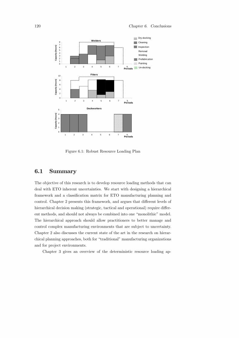
120 Chapter 6. Conclusions

Welders

01234

5678

1 2 3 4 5 6 7 8Periods

Cap

acit

y (h

ou

rs)

Fitters

0

2

4

6

8

10

1 2 3 4 5 6 7 8Periods

Cap

acit

y (h

ou

rs)

Dockworkers

0

1

2

3

4

5

1 2 3 4 5 6 7 8Periods

Cap

acit

y (h

ou

rs)

Dry-docking

Cleaning

Inspection

Removal

Welding

Prefabrication

Painting

Un-docking

Figure 6.1: Robust Resource Loading Plan

6.1 Summary

The objective of this research is to develop resource loading methods that can

deal with ETO inherent uncertainties. We start with designing a hierarchical

framework and a classification matrix for ETO manufacturing planning and

control. Chapter 2 presents this framework, and argues that different levels of

hierarchical decision making (strategic, tactical and operational) require differ-

ent methods, and should not always be combined into one “monolithic” model.

The hierarchical approach should allow practitioners to better manage and

control complex manufacturing environments that are subject to uncertainty.

Chapter 2 also discusses the current state of the art in the research on hierar-

chical planning approaches, both for “traditional” manufacturing organizations

and for project environments.

Chapter 3 gives an overview of the deterministic resource loading ap-

6.1. Summary 121

proaches known from the literature. It discusses various modeling approaches

for deterministic resource loading and proposes an approach to model prece-

dence relations explicitly in an MILP for resource loading. To solve the de-

terministic resource loading problem we distinguish three classes of solution

approaches: straightforward constructive heuristics (Class 1), LP based heuris-

tics (Class 2), and exact approaches (Class 3). We propose an additional Class 1

heuristic and Class 2 heuristic.

The new Class 1 heuristic performs considerably better than existing heuris-

tics with regard to solution quality or computation time. With respect to the

performance of the exact approaches we can conclude that the exact approach

with explicitly modeled precedence relations performs considerably better than

the column generation approach for the set of benchmark instances. We do

note that the performance of the exact approach will suffer more from larger

instances with many orders and activity precedence relations than the column

generation approach. We use several of the deterministic resource loading ap-

proaches as a basis for the generalized models that can deal with uncertainty.

Chapter 4 presents a scenario based model for resource loading under un-

certainty. The scenario based model is based on the resource loading model

with implicitly modeled precedence relations in Section 3.2.3. The model ac-

counts for uncertainties by incorporating multiple scenarios. Its objective is to

minimize the expected costs over these scenarios. To solve the model we use the

branch-and-price approach (see Section 3.3.3) and the shadow price heuristic

(see Section 3.3.2). Computational experiments show that significant improve-

ment of the expected costs can be achieved by using the scenario based model,

as opposed to using a deterministic approach. We have also shown that the

exact approaches often cannot solve instances to optimality within reasonable

time, even when only a sample or selection of the scenarios is considered. An

LP based improvement heuristic in combination with scenario selection appears

to be the most promising approach. Moreover, a small selection (for instance, 2

or 3 scenarios) appears to be sufficient to achieve a considerable improvement

with respect to the expected costs. At the moment of publication of the paper

on which Chapter 4 is based, we had not yet developed the resource loading

model with explicitly modeled precedence relations (see Section 3.2.4). Since

the latter approach appears to be more powerful than the branch-and-price

approach, we expect that it is also more powerful for the scenario based model


in this chapter. This is subject of further research.

Chapter 5 proposes two approaches for robust resource loading for ETO

manufacturing. The first approach is based on the model with implicitly mod-

eled precedence relations (Section 3.2.3). The second robust resource load-

ing approach is based on the model with explicitly modeled precedence rela-

tions (Section 3.2.4). By incorporating robustness indicators in the objective

functions of the aforementioned models we obtain multi-objective optimization

models that facilitate making a trade-off between the costs of using nonregular

capacity and robustness. To model robustness we define two robustness indi-

cators that use the flexibility that is typical for the tactical planning level. The

first indicator uses the resource capacity flexibility and the second indicator

uses the activity planning flexibility. Computational experiments show that

a considerable amount of robustness can be gained by using multi-objective

models with a robustness indicator in the objective function, especially if this

robustness is rewarded high enough in the objective function. Although this

can induce higher costs for using nonregular capacity, the robustness of resource

loading plan can be improved considerably with relative little investment.

Again, at the moment that Chapter 5 was written, we had not yet devel-

oped the model with explicitly modeled precedence relations. Only during the

development of the robust resource loading model, we developed the explicit

approach of modeling precedence relations. Therefore, we incorporated both

approaches in this chapter.

6.2 Future research

Our research on resource loading under uncertainty has yields several topics

for future research. An interesting topic of research would be to deal with

other inherent ETO uncertainties, like uncertain release dates or rush orders.

Another interesting topic of future research is to investigate how heuristics for

resource loading can be extended to deal with uncertainty or hybrid resource

loading problems. Particularly, Class 1 and 2 heuristics offer a lot of flexibility

to incorporate several kinds of ETO inherent uncertainties.

We show that a scenario based model for resource loading suffers from

computational issues due to the size of the model as a result of the scenar-

6.2. Future research 123

ios. Chapter 3 shows that a resource loading approach with explicitly modeled

precedence relations outperforms the approach with implicitly modeled prece-

dence relations with respect to computation times. Therefore, in future research

it would be interesting to investigate whether the model with explicitly modeled

precedence relations performs better for a scenario based approach. It should

be noted, however, that the model with explicitly modeled precedence relations

is likely to become very large for instances with many orders and many activity

precedence relations. In future research we recommend to investigate whether

the model with implicitly modeled precedence relations still performs better

than the approach with implicitly modeled precedence relations for instances

that contain more precedence relations than the instances in our benchmark

set.

We propose several robustness indicators for our robust resource load-

ing approach. These indicators are relative straightforward measures for the

robustness of a resource loading plan. Therefore, they might be suitable to

incorporate in other resource loading approaches, like Class 1 and 2 heuristics.

An interesting approach would be to generate order plans with a deterministic

resource loading approach. These order plans can subsequently be optimized

with the base model with robustness indictors in the objective function.

Finally, the proposed resource loading methods are off-line planning meth-

ods, with a finite planning horizon. In practice however, manufacturing is an

ongoing process that is continuously subject to changes and disturbances. An

ideal way to test the planning methods proposed in this thesis in an on-line

setting would be to use a simulation approach. With such a simulation model

various research topics can be addressed, for instance:

• the relation between system and control characteristics and the per-

formance of various order acceptance, resource loading, and scheduling

methods,

• coordination of the interaction between the tactical level and the opera-

tional planning level,

• the relation between system and control characteristics and the utilization

rates of the resource groups.

Development of such a simulation model for ETO manufacturing and


test resource loading methods in rolling horizon setting is also subject of

ongoing and future research (see, e.g., Heideveld, 2004, Hendriksen, 2004,

and Ebben, Hans and Olde Weghuis, 2005).

125

Bibliography

Adler, S., A. Mandelbaum, V. Nguyen, and E. Schwerer (1995). From project

management to process management: An emperically-based framework

for analysing product development time. Management Science 41(3),

458—484.

Anthony, R.N. (1965). Planning and Control Systems: A Framework for

Analysis. Graduate School of Business Administration, Harvard Univer-

sity.

Aytug, H., M.A. Lawley, K. McKay, S. Mohan, and R. Uzsoy (2005). Ex-

ecuting production schedules in the face of uncertainties: A review and

future directions. European Journal of Production Research 161, 86—110.

Bai, D., T. Carpenter, and J. Mulvey (1997). Making a case for robust

optimization. Management Science 43, 895—907.

Barnhart, C., E.L. Johnson, G.L. Nemhauser, M.W.P. Savelsbergh, and

P. Vance (1998). Branch-and-price: Column generation for solving huge

integer programs. Operations Research 46, 316—329.

Bertrand, J.W.M. (1983). The effect of workload dependent due-date on job

shop performance. Management Science 29 (7), 799—816.

Bertrand, J.W.M. and J.C. Wortmann (1981). Production Control and In-

formation Systems for Component Manufacturing Shops. Elsevier, Ams-

terdam.

Bertrand, J.W.M., J.C. Wortmann, and J.C. Wijngaard (1990). Production

Planning and Control: A Structured and Design Oriented Approach. El-

sevier, Amsterdam.

126 Bibliography

Bitran, G.R., E.A. Haas, and A.C. Hax (1982). Hierarchical production plan-

ning: A two stage system. Operations Research 30, 232—251.

Bitran, G.R. and A.C. Hax (1977). On the design of hierarchical production

planning systems. Decision Sciences 8, 28—52.

Bitran, G.R. and D. Tirupati (1993a). Hierarchical Production Planning, Vol-

ume 4 of Logistics of Production and Inventory, Handbooks in Operations

Research and Management Science. North-Holland, Amsterdam.

Bitran, G.R. and D. Tirupati (1993b). Hierarchical production planning.

Chapter 10 in Graves et al. (1993).

Bock, D.B. and J.H. Patterson (1990). A comparison of due date setting,

resource assignment, and job preemption heuristics for the multi-project

scheduling problem. Decision Sciences 21, 387—402.

Boznak, R.G. (1996). Management of projects: A giant step beyond project

management. PM network 10, 27—30.

Brandimarte, P. (1999). Exploiting process plan flexibility in production

scheduling: A multi-objective approach. European Journal of Operational

Research 114, 59—71.

Buitenhek, R. (1998). Performance Evaluation of Dual Resource Manufac-

turing Systems. Ph. D. thesis, Unversity of Twente, The Netherlands.

Burbidge, J.L. (1979). Group Technology in the Engineering Industry. Me-

chanical Engineering Publications LTD.

Buzacott, J.A. and J.G. Shanthikumar (1993). Stochastic Models of Manu-

facturing Systems. Prentice-Hall, Englewood Cliffs.

Byeon, E., S.D. Wu, and R.H. Storer (1998). Decomposition heuristics for

robust job-shop scheduling. IEEE Transactions on Robotics and Automa-

tion 14 (2), 303—313.

Cai, X. and S. Zhou (1999). Stochastic scheduling on parallel machines sub-

ject to random breakdowns to minimize the expected costs for earliness

and tardy jobs. Operations Research 47 (3), 422—437.

Çakanyildirim, M., D. Chen, P. Chen, M.B. Freimer, P.L. Jackson,

V. Melkonian, and R. Roundy (1999). Capacity driven acceptance of

127

customer orders for a multi-stage batch manufacturing system: Models

and algorithms. Technical Report No. 1233.

Davenport, A.J. and J.C. Beck (2002). A survey of

scheduling techniques with uncertainty. Available at:

http://www.eil.utoronto.ca/profiles/chris/chris.papers.html .

De Boer, R. (1998). Resource-Constrained Multi-Project Management - A Hi-

erarchical Decision Support System. Ph. D. thesis, University Of Twente,

The Netherlands.

De Boer, R. and J.M.J. Schutten (1999). Multi-project rough-cut capacity

planning. In Flexible Automation and Intelligent Manufacturing: Pro-

ceedings of the Ninth International FAIM Conference, New York, pp.

631—644. Center for Economic Research (CentER): Begell House Inc.

Demeulemeester, E.L. and W.S. Herroelen (2002). Project Scheduling; A

Research Handbook. Kluwer Academic Publishers, Boston.

Dey, P.K. and M.T. Tabucanon (1996). Hierarchical approach to project

planning: The case of a petroleum pipeline construction. Applied Math-

ematical Modelling 20, 683—698.

Dietrich, B.L. (1991). A taxonomy of discrete manufacturing systems. Oper-

ations Research 39 (6), 886—902.

Dumond, J. (1992). In a multi-resource environment, how much is enough?

International Journal of Production Research 30 (2), 395—410.

Dumond, J. and V.A. Mabert (1988). Evaluating project scheduling and

due date assignment procedures: and experimental analysis.Management

Science 34, 101—118.

Dvir, D. and T. Lechler (2004). Plans are nothing, changing plans is every-

thing: The impact of changes on project success. Research Policy 33,

1—15.

Dye, L.D. and J.S. (Eds.) Pennypacker (2002). Managing Multiple Projects:

Planning, Scheduling, and Allocating Resources for Competitive Advan-

tage. Dekker/CRC Press.

Ebben, M.J.R., E.W. Hans, and F.M. Olde Weghuis (2005). Workload based

order acceptance in job shop environments. OR Spectrum 27 (1), 107—122.

128 Bibliography

Elmaghraby, S.E. (2002, April 3-5). Contribution to the round table discus-

sion on new challenges in project scheduling. PMS Conference, Valencia,

Spain.

Eppen, G.D., R.K. Martin, and L. Schrage (1989). A scenario approach to

capacity planning. Operations Research 37, 517—527.

Escudero, L.F., P.V. Kamesam, A.J. King, and R.J-B. Wes (1993). Produc-

tion planning via scenario modelling. Annals of Operations Research 43,

311—335.

Fendly, L.G. (1968). Towards the development of a complete multi-project

scheduling system. The Journal of Industrial Engineering 19 (10), 505—

515.

Fernandez, A.A., R.L. Armacost, and J.J.A. Pet-Edwards (1996). The role

of the nonanticipativity constraint in commercial software for stochastic

project scheduling. In Proceedings of the 19th International Conference

on Computers and Industrial Engineering.

Franck, B., K. Neumann, and C. Schwindt (1997). A capacity-oriented hi-

erarchical approach to single-item and small batch production planning

using project-scheduling methods. OR Spektrum 19, 77—85.

Gademann, A.J.R.M. and J.M.J. Schutten (2004). Linear programming

based heuristics for project capacity planning. IIE Transactions 36, 1—13.

Galbraith, J.R. (1973). Designing Complex Organizations. Addison-Wesley,

London.

Giebels, M.M.T. (2000). EtoPlan: A Concept for Concurrent Manufacturing

Planning and Control. Ph. D. thesis, University of Twente, The Nether-

lands.

Goldratt, E.M. (1997). Critical Chain. The North River Press Publishing

Corporation, Great Barrington.

Golenko-Ginzburg, D. and A. Gonik (1997). Stochastic network project

scheduling with non-consumable limited resources. International Jour-

nal of Production Economics 48, 29—37.

Gonzales, T. and S. Sahni (1978). Flowshop and jobshop schedules: Com-

plexity and approximation. Operations Research 26 (1), 35—52.

129

Hackman, S.T. and R.C. Leachman (1989). An aggregate model of project-

oriented production. IEEE Transactions on Systems, Man, and Cyber-

netics 19 (2), 220—231.

Hans, E.W. (2001). Resource Loading by Branch-and-Price Techniques. Ph.

D. thesis, University of Twente, The Netherlands.

Hapke, M. and R. Slowinski (1996). Fuzzy priority rules for project schedul-

ing. Fuzzy Sets and Systems 83, 291—299.

Harhalakis, G., R. Nagi, and J.M. Proth (1992). Hier-

archical modeling approach for production planning.

http://techreports.isr.umd.edu/reports/1992/TR_92-14.pdf.

Hartmann, S. and A. Sprecher (1996). A note on "hierarchical models for

multi-project planning and scheduling". European Journal of Production

Research 94, 377—383.

Hax, A.C. and D. Candea (1984). Production and Inventory Management.

Englewood Cliffs: Prentice-Hall, Englewood Cliffs.

Hax, A.C. and H.C. Meal (1975). Hierarchical Integration of Production

Planning and Scheduling. Studies in Management Sciences, Vol. 1, Lo-

gistics. North Holland TIMS.

Heideveld, S.A. (2004). Scheduling in een rollende horizon omgeving; sim-

ulatie van een Engineer-To-Order fabriek. Master’s thesis, Unversity of

Twente, The Netherlands.

Hendriksen, C.J.H. (2004). Simulation of online capacity planning in an

Engineer-To-Order environment. Master’s thesis, University of Twente,

The Netherlands.

Hendry, L.C., B.G. Kingsman, and P. Cheung (1998). The effect of workload

control (WLC) on performance in make-to-order companies. Journal of

Operations Management 16, 63—75.

Herroelen, W.S. and R. Leus (2002). Project scheduling under uncertainty;

survey and research potentials. Technical report, Department of Applied

Economics, Katholieke Universiteit Leuven, Belgium.

Herroelen, W.S. and R. Leus (2003). Solution and quality robust project

130 Bibliography

scheduling - a methodological framework. Technical Report 0315, Depart-

ment of Applied Economics, Katholieke Universiteit Leuven, Belgium.

Herroelen, W.S. and R. Leus (2004, August). The construction of sta-

ble project baseline schedules. European Journal of Operational Re-

search 156 (156), 550—556.

Honkomp, S.J., L. Mockus, and G.V. Reklaitis (1999). A framework for

schedule evaluation with processing time uncertainty. Computers &

Chemical Engineering 23, 595—609.

Hopp, W.J. and M.L. Spearman (1996). Factory Physics - Foundations of

Manufacturing Management. IRWIN, Boston.

Ivanescu, C.V., J.C. Fransoo, and J.W.M. Bertrand (2002). Makespan esti-

mation and order acceptance in batch process industries when processing

times are uncertain. OR Spectrum 24 (4), 467—495.

Jenssen, M.T. (2001). Improving robustness and flexibility of tardiness

and total flowtime job shops using robustness measures. Technical re-

port, Department of Computer Science, University of Aarhus, Danmark.

http://www.daimi.au.dk/ mjensen/ (Mikkel T. Jensen).

Kapuscinski, R. and S. Tayur (2000). Dynamic ca-

pacity reservation in a make-to-order environment.

http://citeseer.ist.psu.edu/kapuscinski00dynamic.html.

Ke, H. and B. Liu (2004). Project scheduling problem with stochastic activity

duration times. To appear in: Applied Mathematics and Computation.

Kerzner, H. (1998). Project Management, A Systems Approach to Planning,

Scheduling and Controlling. John Wiley & Sons Inc., New York.

Kim, S.Y. and R.C. Leachman (1993). Multi-project scheduling with explicit

lateness costs. IIE Transactions 25 (2), 34—44.

Kis, T. (2004). A branch-and-cut algorithm for scheduling of projects with

variable-intensity activities. To appear in: Mathematical Programming .

Koh, S.C.L., S.D. Saad, and M.H. Jones (2002). Uncertainty under MRP -

planned manufacture: Review and categorization. International Journal

of Production Research 40 (10), 2399—2421.

131

Kolisch, R. (2001). Make-To-Order Assembly Management. Springer-Verlag,

Berlin.

Kolisch, R. and A. Drexl (1996). Adaptive search for solving hard project

scheduling problems. Naval Research Logistics 43, 23—40.

Kolisch, R., A. Sprecher, and A. Drexl (1995). Characterization and gener-

ation of a general class of resource constrained project scheduling prob-

lems. Management Science 10, 1693—1703.

Kouvelis, S.P. and G. Yu (1997). Robust Discrete Optimization and its Ap-

plications, Volume 14 of Nonconvex Optimization and its Applications.

Kluwer Academic Publishers.

Krajewski, L.J. and L.P. Ritzman (1977). Disaggregation in manufacturing

and service organisations: Survey of problems and research. Decision

Sciences 8, 1—18.

Kurtulus, I. (1985). Multi-project scheduling: Analysis of scheduling strate-

gies under unequal delay penalties. Journal of Operations Manage-

ment 5 (3), 291—303.

Kurtulus, I.S. and E.W. Davis (1982). Multi-project scheduling: Categoriza-

tion of heuristic rules performance. Management Science 28 (2), 161—172.

Kurtulus, I.S. and E.W. Davis (1985). Multi-project scheduling: Analysis of

project performance. IIE Transactions 17 (1), 58—66.

Land, M.J. and G.J.C. Gaalman (1996). Workload control concepts in job

shops; a critical assessment. International Journal of Production Eco-

nomics 46, 535—548.

Lawrence, S.R. and T.E. Morton (1993). Resource-constrained multi-project

scheduling costs with tardy costs: Comparing myopic bottleneck and

resource pricing heuristics. European Journal of Operational Research 64,

168—187.

Lawrence, S.R. and E.C. Sewell (1997). Heuristic, optimal, static, and dy-

namic schedules when processing times are uncertain. Journal of Opera-

tions Management 15, 71—82.

Leachman, R.C. and J. Boysen (1985). An Aggregate Model for Multi-Project

Resource Allocation (Project Management: Methods and Studies ed.).,

132 Bibliography

pp. 43—64. Amsterdam, North Holland: In Dean B.V. (ed.).

Leachman, R.C., A. Dincerler, and S. Kim (1990). Resource-constrained

scheduling of projects with variable-intensity activities. IIE Transac-

tions 22 (1), 31—40.

Leon, J.V., D.S. Wu, and R.H. Storer (1994). Robustness measures and

robust scheduling for job shops. IIE Transactions 26 (5), 32—43.

Leus, R. (2003). The Generation of Stable Project Plans, Complexity and

Exact Algorithms. Ph. D. thesis, Katholic University Leuven, Belgium.

Leus, R., G. Wullink, E.W. Hans, and W.S. Herroelen (2003). A hierarchi-

cal approach to multi-project planning under uncertainty. Beta working

paper WP 121.

Levy, N. and S. Globerson (1997). Improving multi-project management by

using a queueing theory approach. Project Management Journal Decem-

ber Issue, 40—46.

Lova, A., C. Maroto, and P. Tormos (2000). A multicriteria heuristic method

to improve resource allocation in multi-project scheduling. European

Journal of Operational Research 127, 408—424.

Lova, A. and P. Tormos (2002, April 3-5). Combining random sampling

and backward-forward heuristics for resource-constrained multi-project

scheduling. In Proceedings of Eight International Workshop of Manage-

ment and Scheduling, Valencia, pp. 244—248.

Meridith, J.R. and J.S. Jr. Mantel (2003). Project Management. A Manage-

rial Approach (fifth ed.). John Wiley & Sons Inc., New York.

Möhring, R.H. (2000a). Scheduling under uncertainty: Bounding the

makespan distribution. Technical Report 700/2000, Technical University

Berlin, Germany.

Möhring, R.H. (2000b). Scheduling under uncertainty: Optimizing against

a random adversary. Technical Report 681/2000, Technical University

Berlin, Germany.

Morton, T.E. and D.W. Pentico (1993). Heuristic Scheduling Systems: With

Applications to Production Systems and Project Management. JohnWiley

& Sons Inc., New York.

133

Nam, S. and R. Logendran (1992). Aggregate production planning - a sur-

vey of models and methodologies. European Journal of Operational Re-

search 61, 255—272.

Negenman, E. (2000). Material Coordination Under Capacity Constraints.

Ph. D. thesis, Eindhoven University of Technology, The Netherlands.

Neumann, K. and C. Schwindt (1998). A capacitated hierarchical approach

to make-to-order production. European Journal Automation 32, 397—413.

Neumann, K., C. Schwindt, and J. Zimmermann (2003). Project Schedul-

ing with Time Windows and Scarce Resources - Temporal Resource-

Constrained Project Scheduling with Regular and Nonregular Objective

Functions (2 ed.). Springer-Verlag, Berlin.

Neumann, K. and J. Zimmermann (1979). GERT-Networks and the Time-

Oriented Evaluation of Projects, Volume 172. Springer-Verlag, Berlin.

Orlicky, J. (1975). Material Requirements Planning. McGraw-Hill, London.

Payne, J.H. (1995). Managing of multiple simultaneous projects: A state-

of-the-art review. International Journal of Project Management 13 (3),

163—168.

Pinedo, M. (2001). Scheduling: Theory, Algorithms, and Systems (2nd ed.).

Prentice-Hall, Englewood Cliffs.

Raaymakers, W.H.M. (1999). Order Acceptance and Capacity Loading in

Batch Process Industries. Ph. D. thesis, Eindhoven University of Tech-

nology, The Netherlands.

Reiss, G. (2002). Multi-Project Scheduling and Management, Chapter 9

in: Pennypacker and Dye (2002a). Also available at: http://www.e-

programme.com/articles_site.htm.

Rosenhead, J. (1978). An education in robustness. The Journal of the Oper-

ational Research Society 29 (2), 105—216.

Rosenhead, J. (1980). Planning under uncertainty: II. a methodology for ro-

bustness analysis. The Journal of the Operational Research Society 31 (4),

331—341.

Rosenhead, J., M. Elton, and S.K. Gupta (1972). Robustness and optimality

as criteria for strategic decisions. Operational Research Quarterly 23 (4),

134 Bibliography

413—431.

Shenhar, A.J. (2001). One size does not fit all projects: Exploring classical

contingency domains. Management Science 47 (3), 394—414.

Silver, E.A., D.F. Pyke, and R. Peterson (1998). Inventory Management and

Production Planning and Scheduling. John Wiley & Sons Inc., New York.

Snoep, M.W.M. (1995). Produktiebesturing en -beheersing in Machinefab-

riek Noord-Oost Nederland. Master’s thesis, University of Twente, The

Netherlands.

Speranza, M.G. and C. Vercellis (1993). Hierarchical models for multi-project

planning and scheduling. European Journal of Operational Research 64,

312—325.

Stork, F. (2001). Stochastic Resource-Constrained Project Scheduling. Ph. D.

thesis, School of Mathematics and Natural Sciences, Technical University

of Berlin, Germany.

Tang, O. and R.W. Grubbström (2002). Planning and replanning the master

production schedule under demand uncertainty. International Journal of

Production Economics 78, 323—334.

Tereso, A.P., T.A. Madalena, and S.E. Elmaghraby (2004). Adaptive re-

source allocation in multi-modal activity networks. International Journal

of Production Economics 92, 1—10.

Valls, V., M. Laguna, P. Lino, A. Perez, and S. Quintilla (1999). Project

Scheduling with Stochastic Activity Interruptions, Chapter 15. Kluwer

Academic Publishers.

Van Assen, M.F. (1996). Produktiebesturing van semi-autonome produktie-

teams bij Urenco Nederland B.V. Master’s thesis, University of Twente,

The Netherlands.

Van Krieken, M. (2001). Medium-term capacity planning in resource-

constrained multi-project environments - a cost driven approach. Mas-

ter’s thesis, Tilburg University, Tilburg.

Vance, P.H., C. Barnhard, E.L. Johnson, and G.L. Nemhauser (1994). Solv-

ing binary cutting stock problems by column generation and branch-and-

bound. Computational Optimization and Applications 3, 111—130.

135

Vollmann, T.E., W.L. Berry, and D.C. Whybarck (1997). Manufacturing

Planning and Control Systems (4th ed.). New York: Irwin/Mc-GrawHill.

Wang, J. (2004). A fuzzy robust scheduling approach for product develop-

ment processes. European Journal of Production Research 152, 180—194.

Weglarz, J. (1981). Project scheduling with continuously-divisible, double

constrained resources. Management Science 27 (9), 1040—1053.

Wester, F.A.W., J. Wijngaard, and W.H.M. Zijm (1992). Order acceptance

strategies in a production-to-order environment with setup times and due

dates. International Journal of Production Research 30 (6), 1313—1326.

Wheelright, S.C. and K.B. Clark (1992). Creating project plans to focus

product development. Harvard Busines Review March-April Issue, 70—

82.

Whybark, D.C. and J.G. Williams (1976). Material requirements planning

under uncertainty. Decision Sciences 7 (4), 595—606.

Wiendahl, H.-P. (1987). Belastungsorientierte Fertigungssteuerung. Carl

Hanser.

Winch, G. (1996). Thirty years of project management what have we

learned? Published at: http://bprc.warwick.ac.uk/repwinch.html.

Wullink, G., M.M.T. Giebels, and H.J.J. Kals (2002). A system architecture

for holonic manufacturing planning and control (ETOplan). Robotics and

Computer Integrated Manufacturing 18, 313—318.

Wullink, G., E.W. Hans, A.J.R.M. Gademann, and A. Van Harten (2004).

Scenario based approach for flexible resource loading under uncertainty.

International Journal of Production Research 42 (24), 5079—5098.

Wullink, G., E.W. Hans, and A. Van Harten (2004). Robust resource loading

for engineer-to-order manufacturing. Beta Working Paper WP-123.

Wysokci, R.K., J. Jr. Beck, and D.B. Crane (2002). Extensions to Multiple

Projects, Chapter 12, in: Pennypacker and Bye (2002a).

Yang, K.K. and C.C. Sum (1993). A comparison of resource allocation and

activity scheduling rules in a dynamic multi-project environment. Journal

of Operations Management 11, 207—218.

136 Bibliography

Yang, K.K. and C.C. Sum (1997). An evaluation of due date, resource al-

location, project release, and activity scheduling rules in a multi-project

environment. European Journal of Operational Research 103, 139—154.

Zäpfel, G. and H. Missbauer (1993). New concepts for production planning

and control. European Journal of Operations Research 67, 297—320.

Zijm, W.H.M. (2000). Towards intelligent manufacturing planning and con-

trol systems. OR Spektrum 22, 313—345.

137

Samenvatting

Winstgevendheid van een klantordergestuurd productiebedrijf wordt in grote

mate bepaald door de leverbetrouwbaarheid, de bezettingsgraad, flexibiliteit

en het kunnen omgaan met onzekerheden. Vooral in klantordergestuurde pro-

ductieomgevingen worden veel zaken omtrent de order vastgelegd in het order-

onderhandelingsproces die van grote invloed zijn op deze factoren. De ruwe

orderspecificaties worden bepaald, een levertijd wordt afgesproken en de ca-

paciteitsconsequenties en risico’s van een eventuele orderacceptatie worden ge-

ëvalueerd.

Veel van de huidige planningsmethoden zijn niet in staat om op al deze

facetten tegelijkertijd te focussen. Operationele planningsmethoden richten

zich over het algemeen op een te laag aggregatieniveau en eisen te veel de-

tail om deze beslissingen in dit stadium te ondersteunen. Strategische plan-

ningsmethoden zijn vaak niet in staat om specifieke klantorders mee te ne-

men in het beslissingsondersteuningsproces. Resource loading is een tactische

planningsmethode die wél geschikt is voor het bovengenoemde probleem. Het

houdt rekening met specifieke orderspecificaties zoals bijvoorbeeld volgordere-

laties tussen activiteiten, de werkinhoud van activiteiten, de minimale duur van

een activiteit en de levertijd van een order. Verder vereist het minder detail

dan een operationele planningsmethode en is daarom bij uitstek geschikt voor

gebruik gedurende het orderonderhandelingsproces waar details vaak nog niet

bekend zijn. Het ontwikkelen van resource loading methoden en modellen die

rekening houden met onzekerheid is de centrale probleemstelling in dit proef-

schrift.

De bestaande resource loading methoden gaan uit van orderdata zonder

onzekerheid, echter klantordergestuurde productie is onderhevig aan een grote

mate van onzekerheid. De uniciteit van de orders maakt het voor het bedrijf

138 Samenvatting

en een klant vaak moeilijk om in te schatten hoe de daadwerkelijke order er

precies uit zal zien. Verder kunnen bepaalde resources een onzekere capaciteits-

beschikbaarheid hebben. Toch zullen er beslissingen moeten worden genomen

over acceptatie, levertijd of het inhuren van extra capaciteit. Een resource load-

ing methode zal dus rekening moeten houden met onzekerheden in de orderdata

en beschikbare machinecapaciteit.

Voor adequate productiebesturing en -beheersing moet een resource load-

ing methode goed aansluiten op de omliggende planningsmethoden. Om re-

source loading te positioneren in een breder kader van productiebesturing en

-beheersing voor klantordergestuurde productieomgevingen gebruiken we een

hiërarchisch besturingsraamwerk. In dit raamwerk (Hoofdstuk 2) onderschei-

den we drie planningslagen: strategische planning, tactische planning en op-

erationele planning. Deze lagen zijn onderverdeeld in drie verticale kolomen:

technologische planning, resource capaciteitsplanning en materiaalcoördinatie.

Deze onderverdeling resulteert in negen functies voor productiebesturing en -

beheersing. Voor een goed functioneren van al deze functies afzonderlijk en het

productiesysteem als geheel is het van groot belang dat een adequate interactie

tot stand kan worden gebracht.

Verder moet voor iedere functie in het hiërarchisch raamwerk een meth-

ode worden toegepast die rekening houdt met de mate van onzekerheid en de

complexiteit van het productieproces. Hiertoe stellen we een classificatiematrix

voor met de dimensies variabiliteit en afhankelijkheid op. De variabiliteitsdi-

mensie staat voor de mate van onzekerheid en variabiliteit van de orderportfolio.

De afhankelijkheid staat voor de onderlinge afhankelijkheid van projecten door

enerzijds resource conflicten en anderzijds de afhankelijkheid van externe par-

tijen. Deze classificatiematrix is een hulpmiddel om voor iedere planningslaag

in het hiërarchische raamwerk een planningsmethode te kiezen die aansluit bij

de systeemkarakteristieken.

Resource loading is een relatief nieuw onderzoeksgebied. Om een beeld te

geven van de status van het onderzoek naar deterministische resource loading

technieken geven we een beschrijving van verschillende bestaande en nieuwe

modelleermethoden voor het resource loading probleem in Hoofdstuk 3. We

behandelen een model zonder volgorderelaties, een model met impliciet gefor-

muleerde volgorderelaties en een model met expliciet geformuleerde volgorde-

relaties. Vervolgens bespreken we een aantal oplosmethoden voor het deter-

139

mistische resource loading probleem. We maken een onderverdeling in klassen.

Klasse 1 zijn de constructieve heuristieken. Deze heuristieken gebruiken relatief

eenvoudig prioriteitsregels en construeren een oplossing in één zogenaamde

"pass". De Klasse 1 heuristieken worden uitgebreid met een zogenaamde ran-

domisatie aanpak waardoor de prestaties kunnen worden verbeterd. Klasse 2

bevat heuristieken die gebruiken maken van lineaire programmeringstechnieken.

Een belangrijke eigenschap van Klasse 2 heuristieken is dat de LP modellen geen

volgorderelaties bevatten. Klasse 3 bevat de exacte oplosmethoden.

De eerste methode die expliciet rekening houdt met onzekerheid is de

scenario-gebaseerde aanpak die wordt beschreven in Hoofdstuk 4 van dit proef-

schrift. De basis voor deze aanpak is een deterministisch resource loading model

met impliciet geformuleerde volgorderelaties. Dit model passen we aan zodat

het om kan gaan met meerdere scenario’s. Een scenario wordt bepaald door

de verschillende modi waarin een probleem parameter kan voorkomen. Een

combinatie van alle modi vormt een scenario. De doelstelling van de scenario-

gebaseerde aanpak is het minimaliseren van de verwachte kosten voor gebruik

van niet reguliere capaciteit over alle scenario’s. Een nadeel van de scenario-

gebaseerde aanpak is dat ieder extra scenario dat wordt opgenomen in het

model in een groot aantal extra voorwaarden en beslissingsvariabelen resul-

teert. Het meenemen van meer informatie over onzekerheid heeft daardoor een

sterk nadelig effect op de rekenefficiëntie van het model. Om met dit probleem

om te gaan, bespreken we een aantal methoden. De eerste methode is om in

plaats van alle "bekende" scenario’s maar een deel van de scenario’s op te ne-

men in het model. We bespreken verschillende varianten van het construeren

van dit zogenaamde "sample" van scenario’s. Een andere manier is om in

plaats van een exacte oplosmethode een heuristiek te gebruiken. We laten zien

dat de combinatie van een heuristiek en het gebruik van de samplingsmethode

leidt tot de laagste verwachte kosten over alle scenario’s over alle testinstanties

gemiddeld bij een beperkte rekentijd.

In Hoofdstuk 5 beschrijven we een resource loading methode die gebruik

maakt van indicatoren voor de robuustheid van een plan. Deze indicatoren zijn

gebaseerd op de vrije capaciteit die een onzekere activiteit tot zijn beschikking

heeft. Hierin wordt rekening gehouden met de hoeveelheid uitloop die de

onzekere activiteit waarschijnlijk zal hebben. Deze robuustheidsindicatoren

worden opgenomen in de doelfunctie van een resource loading model. We testen

140 Samenvatting

twee varianten van zo’n robuust resource loading model. De eerste variant is

het resource loading model met impliciet geformuleerde volgorderelaties met

robuustheidsindicatoren in de doelfunctie. De tweede variant gebruikt expli-

ciet geformuleerde volgorderelaties. Tests van beide modellen tonen aan dat

gebruik van robuustheidsindicatoren in de doelfunctie een positief effect heeft

op de robuustheid van een plan. Met een relatief kleine investering kan de

robuustheid aanzienlijk worden verbeterd. Verder laten de tests zien dat het

model met expliciet geformuleerde volgorderelaties vaker een optimale oplossing

oplevert dan het model met impliciet geformuleerde volgorderelaties.

141

Curriculum Vitae

Gerhard Wullink was born on the 16th of March 1976 in Zwolle, the Nether-

lands. He obtained his Atheneum diploma at the secondary school De Noord-

gouw in Heerde in 1994. From 1994 to 2000 he studied mechanical engineering

at the University of Twente with the specialization Production and Operations

Management.

In December 2000 he started as a Ph.D. student under supervision of

prof. dr. A. Van Harten in the group Operational Methods for Production

and Logistics at the School of Business, Public and Administration at the

University of Twente. The project entitled "Capacity planning and flexibility

in Manufacture-To-Order environments" resulted in this thesis.

142 Curriculum Vitae

resource loading under uncertainty with his practical experience were a source of inspiration. i...

Documents