resource assessment service maryland … assessment service maryland geological survey ... this...

RESOURCE ASSESSMENT SERVICE

MARYLAND GEOLOGICAL SURVEY Emery T. Cleaves, Director

COASTAL AND ESTUARINE GEOLOGY

FILE REPORT NO. 02-05

Shoreline Erosion as a Source of Sediments and Nutrients

Northern Coastal Bays, Maryland

by

Darlene V. Wells, E. Lamere Hennessee and James M. Hill

This study was funded by the Maryland Coastal Zone Management Program of the

Maryland Department of Natural Resources pursuant to National Oceanic and Atmospheric Administration

Award No. NA07OZ0118

December 2002

ii

For information or additional copies, please contact:

Maryland Department of Natural Resources Maryland Geological Survey

2300 St. Paul Street Baltimore, MD 21218

(410) 554-5500 Website: www.mgs.md.gov

The facilities and services of the Maryland Department of Natural Resources are available to all without regard to race, color, religion, sex, sexual

orientation, age, national origin or physical or mental disability.

This document is available in alternative format upon request from a qualified individual with a disability.

iii

TABLE OF CONTENTS Page Executive Summary .......................................................................................................1 1. Introduction....................................................................................................................3 Objectives ................................................................................................................3 Acknowledgements..................................................................................................3 2. Previous Studies.............................................................................................................4 Shoreline Change and Coastal Land Loss Studies...................................................4 Nutrient Budget and Pollutant Loading Studies ......................................................5 3. Study Area .....................................................................................................................7 Geomorphology .......................................................................................................7 Geology..................................................................................................................10 Bay Bottom Sediments ....................................................................................12 4. Methods ....................................................................................................................15

Selection of Sampling Sites ...................................................................................15 Field Methods ........................................................................................................17

Laboratory Methods...............................................................................................19 Quantifying Land Loss ....................................................................................19

Bank Height ...............................................................................................23 Sediments.........................................................................................................24

Core Processing .........................................................................................24 Bulk Density and Water Content ...............................................................24 Grain Size Analysis....................................................................................26 Chemical Analysis .....................................................................................27

Data Reduction.......................................................................................................28 5. Results and Discussion ................................................................................................29 Field and Lab Observations ...................................................................................29

Land Loss (Area and Volume)...............................................................................30 Sediments...............................................................................................................32

Bulk Density ....................................................................................................32 Water Content ..................................................................................................33 Texture (Grain size composition) ....................................................................34 Nutrients...........................................................................................................34 Metals...............................................................................................................36 Regression Analysis.........................................................................................37

Sediments and Nutrient Loadings..........................................................................39 Comparison with existing models and previous studies ..................................41 6. Conclusions..................................................................................................................45 Recommendations..................................................................................................45 7. References ....................................................................................................................47 Appendix A - Site descriptions and core logs....................................................................53 Appendix B - Quality Assurance/Quality Control...........................................................103 Appendix C - Data Tables................................................................................................111 Appendix D - Land loss and loading calculations ...........................................................137

iv

Figures Page Figure 3-1. The Delmarva Peninsula, showing the location of the

study area .....................................................................................................8 Figure 3-2. Study area.....................................................................................................9 Figure 3-3. Geology of the study area ..........................................................................11 Figure 3-4. Distribution of bottom sediments, based on Shepard’s

(1954) classification...................................................................................13 Figure 4-1. Locations of sampling sites and land loss polygons. .................................18 Figure 4-2. Shepard’s (1954) classification of sediment types.....................................27 Figure 5-1. Bluff at Site 5 .............................................................................................29 Figure 5-2. The main features developed along a marsh shoreline due

to wave erosion ..........................................................................................29 Figure 5-3. Pocket beach ..............................................................................................30 Figure 5-4. Mussels armoring scarp face at Site 1........................................................30 Figure 5-5. Comparison of linear erosion rate and volumetric loss for

each land loss polygon...............................................................................32 Figure 5-6. Measured wet bulk density as a function of water content. .......................33 Figure 5-7. Difference (%) between measured wet bulk density and

B&L bulk density, plotted against the plant content of the sediment .....................................................................................................33

Figure 5-8. Total carbon content vs. organic content of the sediments........................34 Figure 5-9. Loadings of sand, silt, and clay for each land loss polygon ......................41 Figure 5-10. Annual total nitrogen and total phosphorus loads entering

the northern coastal bays, revised to include contributions from shoreline erosion ...............................................................................44

Figure B-1. Relative standard deviation (%) vs. concentration of total nitrogen for the suite of replicate and triplicate analyses ........................106

Figure B-2. Relative standard deviation (%) vs. concentration of total carbon for the suite of replicate and triplicate analyses...........................106

Figure B-3. Relative standard deviation (%) vs. concentration of total phosphorus for the suite of replicate and triplicate analyses. ..................107

v

Tables Page Table ES-1. Annual loadings (kg/yr) of nutrients and sediments,

northern coastal bays....................................................................................2 Table 2-1. Average rates of recession (ft/yr) for reaches of shoreline in

the study area, from Volonté and Leatherman (1992) .................................5 Table 3-1 Morphometric data for Isle of Wight and Assawoman Bays

and the St. Martin River...............................................................................7 Table 4-1 Sampling sites ............................................................................................15 Table 4-2 Land loss polygons and associated sampling sites ....................................20 Table 4-3 Mean bank heights (m) calculated for land loss polygons

P15, P16, and P18 ......................................................................................23 Table 5-1 Volume (m3) and rate of land lost during the 47-year period

between 1942 and 1989 and linear rates (m/yr) of shoreline erosion, by basin. .......................................................................................31

Table 5-2. Summary statistics for each of the elements measured in the samples.................................................................................................35

Table 5-3. Comparison of mass ratios of C, N, and P observed in different samples (sources). .......................................................................36

Table 5-4. Comparison of average enrichment factors of certain metals measured in the different groups of sediments from the northern coastal bays..................................................................................37

Table 5-5. Coefficients of multiple-stepwise regression of nutrient and metal data. ..................................................................................................39

Table 5-6 Summary of annual loadings of sediments and nutrients contributed by shoreline erosion in the northern coastal bays. ...........................................................................................................40

Table 5-7 Annual total nitrogen (TN) and total phosphorus (TN) loadings (kg/yr) to the northern coastal bays, based on the UM and CESI (1993) report. .....................................................................42

Table 5-8 Annual total nitrogen (TN) and total phosphorus (TP) loadings (kg/yr) to the northern coastal bays, based on TMDL study for the same study area (MDE, 2001)..................................43

Table 5-9 Comparison of the UM and CESI (1993) loadings and MGS estimates from shoreline erosion for total suspended solids (TSS), Pb and Zn. All loads in kg/yr. .............................................44

Table B-1. Mean and range of water content and calculated weight loss after cleaning for each sediment type (Shepard’s (1`954) classification), based on sediments collected in Isle of Wight and Assawoman Bays (Wells and others, 1994)...........................104

Table B-2. Mean and range of water content and calculated weight loss after cleaning for each sediment type (Shepard’s (1954) classification), based on sediments collected for this study. ...................104

Table B-3. Comparison of results of replicate textural analyses of selected core samples. ..............................................................................105

vi

Page Table B-4. Results of nitrogen, carbon and sulfur analyses of NIST

SRM 1646 (Estuarine Sediment) and National Research Council of Canada SRM PACS-1 (Marine Sediment) compared to the certified or known values ..............................................105

Table B-5. Comparison of certified values to the analytical results from Actlabs for the SRMs. .....................................................................108

Table B-6. Comparison of certified values to Actlab’s analytical results for U.S. Geological Survey standards. .........................................109

Table C-1. Sample data: physical properties. ............................................................113 Table C-2. Sample data: chemical analyses...............................................................121 Table D-1. Area (m2) and volume (m3) of land lost during the 47-year

period between 1942 and 1989 and linear rates (m/yr) of shoreline erosion, by shoreline reach (land loss polygon). ......................138

Table D-2. Mean textural and nutrient concentrations calculated for each site using equations D-2 and D-3. ...................................................140

Table D-3. Annual component loadings (Kg/yr) for each land-loss polygon. ...................................................................................................142

Equations Equation 4-1. Determination of water content as percent wet weight........................24 Equation 4-2. Volume calculation for bluff samples..................................................25 Equation 4-3. Wet bulk density calculation based on Bennett and

Lambert (1971) ....................................................................................25 Equation 4-4. Correction factor calculation for core compaction ..............................26 Equation 5-1. Enrichment factor.................................................................................37 Equation 5-2. Estimate of element concentration based on sediment

components ..........................................................................................38 Equation D-1. Determination of annual rate of shoreline retreat ..............................137 E quation D-2. Calculation of mean nutrient concentrations for each

site ......................................................................................................139 Equation D-3. Calculation of mean bulk concentrations of sand, silt,

clay components for each site ............................................................139 Equation D-4. Calculation of nutrient and sediment loadings for each

land loss polygons..............................................................................141

1

EXECUTIVE SUMMARY The Maryland Geological Survey (MGS) began a multi-year study to determine the flux of

sediments and nutrients eroding from unprotected shorelines bordering Maryland’s coastal bays. The first year of study focused on the northern-most bays: Assawoman and Isle of Wight Bays and the St. Martin River.

Sampling locations were selected on the basis of linear rates of shoreline change, as well as

geology and geomorphology (marsh, bluff, or beach). At each of the 16 sites, bank heights were measured. Sediment samples were collected from marshes and beaches and from distinct geologic horizons within banks. Samples were analyzed for grain size composition, bulk density, total organics, total carbon (TC), nitrogen (TN), phosphorus (TP), and a suite of trace metals. The analytical results were then used in conjunction with coastal land loss estimates to determine sediment and nutrient loadings to the bays. Annual land lost was based on a digital comparison of two historical shorelines dating from 1942 and 1989.

Based on geomorphologic variability and differing rates of shoreline erosion, the study area shoreline was divided into 23 reaches, ranging in length from about 600 m to 45,000 m; most were less than 9,000 m long. A template of irregular polygons was constructed to demarcate the reaches, and total land loss (m2) during the 47-year period was determined for each polygon. These “land loss” polygons provided a structure for organizing the results of the physical and chemical analyses. Each sampling site was associated with one or more of the land loss polygon. Mean bank heights and concentrations of the measured constituents (i.e., TN, TP, TSS, etc. in kg/m3), averaged for each of the sampling sites, were used to calculate annual loadings (kg/yr) for each polygon.

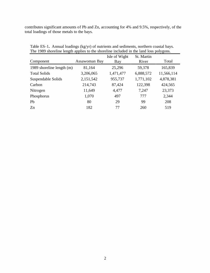
During the 47-year period, shoreline erosion contributed an estimated 11.6 x 106 kg/yr of total sediments into the three-bay system (Table ES-1). Of the total sediment load, approximately 42%, or 4.9 x 106 kg/yr, were total suspendable solids (TSS). That amounts to about one-third of the TSS load from upland (surface) run-off. Annual total sediment loadings were greatest in the St. Martin River (6.9 x 106 kg/yr), due in part to high bank elevations and relatively dense bluff material. Bulk densities of sediments collected from bluffs averaged 1.4 g/cm3. Total sediment loading from shore erosion in Assawoman Bay was about half that of the St. Martin River (3.2 x 106 kg/yr). Sediment loadings from Isle of Wight Bay shorelines were even lower (1.5 x 106 kg/yr). Much of the shoreline bordering Assawoman and Isle of Wight Bays is low-lying marsh, composed of sediments with average bulk densities of 0.4 g/cm3.

Sand-sized sediments account for approximately 57% of the total sediments contributed

from shoreline erosion. The sand contributed from erosion about half of the sand coming into the bays. More than one-third of the sand is eroded from the St. Martin River shoreline.

Shoreline erosion is a significant source of nutrients, contributing up to 8.5% of the total

nitrogen and total phosphorus delivered to the system. Nutrient contributions from shoreline erosion slightly exceed input from point sources. In addition to nutrients, erosion also

2

contributes significant amounts of Pb and Zn, accounting for 4% and 9.5%, respectively, of the total loadings of those metals to the bays.

Table ES-1. Annual loadings (kg/yr) of nutrients and sediments, northern coastal bays. The 1989 shoreline length applies to the shoreline included in the land loss polygons.

Component Assawoman Bay Isle of Wight

Bay St. Martin

River Total

1989 shoreline length (m) 81,164 25,296 59,378 165,839 Total Solids 3,206,065 1,471,477 6,888,572 11,566,114 Suspendable Solids 2,151,542 955,737 1,771,102 4,878,381 Carbon 214,743 87,424 122,398 424,565 Nitrogen 11,649 4,477 7,247 23,373 Phosphorus 1,070 497 777 2,344 Pb 80 29 99 208 Zn 182 77 260 519

3

1. INTRODUCTION

The Maryland Coastal Bays Program has developed a four-pronged action plan to restore and protect the natural resources of the State’s coastal bays (MCBP, 1999). The plan addresses (1) water quality, (2) fish and wildlife, (3) recreation and navigation, and (4) community and economic development. Meeting the goals associated with the first three of these depends in part on understanding the sediment and nutrient input contributed by shoreline erosion to the coastal bays. Shoreline erosion releases sediments to the water column. Finer-grained sediments tend to remain suspended in the water, reducing water clarity and affecting underwater habitat (e.g., reducing light penetration for submerged aquatic vegetation). The eventual deposition of eroded sediments contributes to the in-filling of navigational channels. Shoreline erosion also acts as a non-point source of nutrients (nitrogen and phosphorus), which affect the water quality of the coastal bays.

Although shoreline erosion has been identified as a source of sediments and nutrients to

nearby waters, there has been little effort to quantify that input and to compare it to other sources. To provide this information, the Maryland Geological Survey (MGS) began a multi-year study to determine the flux of sediments and nutrients eroding from unprotected shorelines bordering the coastal bays. The first year of study focused on the northernmost coastal bays: Assawoman Bay, Isle of Wight Bay, and the St. Martin River. The results of that study are presented in this report. OBJECTIVES To estimate the nutrient and sediment loads contributed by shoreline erosion to the northern coastal bays of Maryland, MGS set the following objectives:

1. Identify unprotected reaches of shoreline at greatest risk of erosion, based on historical linear rates of change;

2. Measure certain physical, chemical, and biological properties of eroding sediments; and 3. Determine the volume of eroding sediments and the flux of sediments and nutrients into

the northern coastal bays. Examine the flux of material from shoreline erosion in the context of existing nutrient budgets for the study area.

ACKNOWLEDGMENTS This study was funded by the Coastal Zone Management Program of the Maryland Department of Natural Resources pursuant to National Oceanic and Atmospheric Administration Award #NA07OZ0118. The authors extend their gratitude to the many landowners who allowed access to their property, so that MGS might collect samples and measure bank heights. They also wish to thank Neil Dunnemyer, Richard Ortt, Dan Sailsbury, and Geoff Wikel, who assisted with sample collection and laboratory analyses. Special thanks are due to Al Wesche and Jim Casey for their assistance in collecting cores and the use of Fisheries’ boat.

4

2. PREVIOUS STUDIES

SHORELINE CHANGE AND COASTAL LAND LOSS STUDIES

The earliest, comprehensive shoreline change information available for the coastal bays,

excluding the upstream portions of some of the tributaries, comes from a 1949 study of tidewater Maryland by Singewald and Slaughter. The authors calculated rates of erosion by comparing two sets of shorelines, dating from ca. 1850 and ca. 1940. Conkwright (1975) updated their work, producing a series of maps that depict the 1850 and 1940 shorelines on 7.5-minute U.S. Geological Survey (USGS) topographic quadrangles. The most recent shorelines shown on the topographic base maps range between 1942 and 1972.

Using the shoreline change data reported by Singwald and Slaughter, Bartberger (1973,

1976) estimated the volume of sediment contributed to Chincoteague Bay from shore erosion, as part of his study of the origin, distribution and rates of accumulation of sediments in the bay. Based on Bartberger’s estimates, shore erosion contributes approximately 40 x 103 m3/yr of sediment to Chincoteague Bay, approximately eight times the amount delivered by streams. Almost all of the eroded sediment comes from the mainland shore and bay islands, which consist largely of marsh. Bartberger assumed that shore-derived sediments consisted primarily of mud (silt plus clay fraction). Because the sand:mud ratio of sediments deposited on the bay floor was 1:1, he reasoned that an equal amount of sand was introduced into the bay from other sources, mainly from Assateague Island through overwash processes and wind deposits. Transport of sand through the active inlets, Ocean City Inlet and Chincoteague Inlet, is important only as a local source.

Later studies of coastal erosion in the region, including those by the National Oceanic and

Atmospheric Administration (NOAA, 1988) and Leatherman (1983), were more limited in area, for example, to the vicinity of the Ocean City Inlet or the Atlantic shoreline of Maryland. Volonté and Leatherman (1992) predicted future wetlands and upland losses for the mainland (western) shores of Assawoman and Isle of Wight Bays and their main tributaries, including the St. Martin River. As part of that study, they measured linear rates of shoreline change along 41 miles of shoreline (at 215 sites located approximately 1000 ft apart) for the period 1850-1989. Their findings for several reaches of shoreline are relevant to this study (Table 2-1). Average rates of recession in the study area, by water body, range from -0.2 to -1.1 ft/yr (-0.6 to -0.34 cm/yr). Based on that study, Volonté and Leatherman concluded that marshy shorelines undergo the highest rates of erosion.

Recently, MGS remapped and assessed shoreline change in Maryland’s coastal bays

(Hennessee and Stott, 1999; Hennessee and others, 2002; Stott and others, 1999, 2000). The project involved digitizing historical and recent shoreline positions for the 450 mi (724 km) of shoreline defining the coastal bays. Using a geographic information system (GIS), MGS digitally updated nine 7.5-minute quadrangles covering the coastal bays and produced a corresponding series of Shoreline Changes maps. MGS also determined the area of land lost within the coastal bays since the mid-1800s. Between 1850 and 1989, Assawoman Bay lost a net of 948 acres (3.84 km2) to shoreline erosion, at an annual rate per mile of shoreline of 0.09

5

acres/mi/yr (226.3 m2 /km/yr). Comparable figures for Isle of Wight Bay and the St. Martin River, respectively, are 159 acres (0.64 km2) at a rate of 0.03 acres/mi/yr (75.4 m2/km/yr) and 254 acres (1.03 km2) at a rate of 0.10 acres/mi/yr (251.5 m2/km/yr).

Table 2-1: Average rates of recession (ft/yr) for reaches of shoreline in the study area, from Volonté and Leatherman (1992).

Zone Area Linear rate of recession (ft/yr)

1 Isle of Wight Bay -1.0 5 St. Martin River -1.1 6 Shingle Landing Prong -0.2 7 Bishopville Prong -0.3 8 Isle of Wight -1.1 9 Assawoman Bay -0.5

NUTRIENT BUDGET AND POLLUTANT LOADING STUDIES In 1993, the Maryland Department of the Environment (MDE) conducted an assessment of Maryland's coastal bay aquatic ecosystem (UM and CESI, 1993). The authors reviewed existing data for trends in the overall quality of the bays’ ecosystem. One objective was to assess terrestrial pollutant loadings. The study identified contributing sources and estimated pollutant loadings from point source discharges, surface runoff, and direct discharge of groundwater into the bays. Loadings from shoreline erosion were not considered. The pollutants included nitrogen, phosphorus, total suspended solids (TSS), metals (zinc and lead) and biochemical oxygen demand (BOD). Estimates of pollutant loadings from surface runoff were based on land use and land cover. The study identified the upper bays (Assawoman and Isle of Wight Bays) and, in particular, the St. Martin River as areas exhibiting serious water quality problems due, in part, to poor flushing, waterfront development, and high nutrient loadings. Estimated loading rates for all of the pollutants included in the assessment were very high for Turville and Herring Creeks and the St. Martin River, compared to those observed for the other coastal bays and selected portions of the Chesapeake Bay. Impaired by nutrients (nitrogen and phosphorus), the St. Martin River was placed on Maryland’s list of water-quality-limited segments in 1994. Two years later, Assawoman and Isle of Wight Bays were added to the list. As a result, the State was required, under Section 303(d) of the Federal Clean Water Act, to develop a total maximum daily load (TMDL) for these two bays. A TMDL reflects the total pollutant loading of an impairing substance that a water body can receive and still meet water quality standards. In the process of developing the TMDLs, MDE revised the nutrient loadings reported in the UM and CESI report (MDE, 2001). MDE recalculated nutrient loadings based on 1997 land use information and updated groundwater inputs based on data from a recent groundwater study (Dillow and others, 2002). Again, in developing a nutrient budget for the northern coastal bays, MDE omitted contributions from shoreline erosion. In general, few published nutrient budgets have included input from shoreline erosion. One exception was a study conducted by Ibison and others (1990), who measured sediment and

6

nutrient contributions from eroding banks along tidal shorelines of the Virginia portion of the Chesapeake Bay and several of its major tributaries. The researchers selected 14 non-marsh sites that were undergoing high rates and volumes of erosion and that were located near living marine resources. For fastland bank samples, nitrogen concentrations ranged from 0.01 to 3.34 mg/g (0.001 to 0.334%); phosphorus concentrations ranged from 0.01 to 1.28 mg/g (0.001 to 0.128%). The authors compared their results with nutrient loadings from controllable non-point sources. Shoreline erosion contributed 5.2% of the nitrogen load and 23.6% of the phosphorus load. Differences in nutrient loadings among the sites were due to differences in bank heights and erosion rates; differences in nitrogen and phosphorus concentrations were not a significant factor. Two years later, Ibison and others (1992) expanded their initial research to include an additional 44 eroding banks. They examined the relationship between nutrient concentrations and land use for four land use categories: active farms, fallow farms, wooded, and rural residential. And, they resolved a question that arose following the publication of their earlier report. Was the mineral apatite in fossiliferous soil horizons a possible source of error in their phosphorus measurements? The researchers confirmed that nutrient concentrations and loading rates varied greatly from site to site. Nutrient loading rates from shoreline erosion exceeded those from agricultural runoff because of the large volumes of soil lost to shoreline erosion. Nutrient loading concentrations and land use were related. The highest mean total nitrogen and total phosphorus loading concentrations were associated with the cultivated croplands of active farms. Surprisingly, though, average total nitrogen loading concentrations were equally high for wooded land. For fossiliferous horizons, mean total phosphorus loading concentrations were about twice the mean for unfossiliferous banks. However, mean inorganic phosphorous loading concentrations were the same for both.

7

3. STUDY AREA

GEOMORPHOLOGY The study area is located on the Atlantic coast of the Delmarva Peninsula (Fig. 3-1). Isle of Wight and Assawoman Bays are the two northernmost coastal bays in Maryland. Fenwick Island, part of the barrier island/southern spit unit of the Delmarva coastal compartment (Fisher, 1967), separates the two coastal bays from the Atlantic Ocean. The Town of Ocean City is located on Fenwick Island.

Assawoman Bay and Isle of Wight Bay, microtidal (<2 m tidal range) coastal lagoons, are contiguous with each other. For this discussion, the boundary between Assawoman Bay and Isle of Wight Bay is the Rt. 90 Bridge, which spans Fenwick Island (Ocean City at 60th Street) and Isle of Wight (Fig. 3-2). St. Martin River, which drains into Isle of Wight Bay, is the major tributary, accounting for 62 % of the total drainage area for the two bays (Bartberger and Biggs, 1970; UM and CESI, 1993). In addition to the St. Martin River, several smaller streams drain into the two bays. Roy Creek and Greys Creek drain into Assawoman Bay. Manklin Creek, Turville Creek, and Herring Creek drain into Isle of Wight Bay. Table 3-1 lists basic morphometric data for both bays and the St. Martin River.

The two bays are connected to the Atlantic Ocean through a single outlet, Ocean City Inlet, located at the southern end of Isle of Wight Bay. Ocean City Inlet formed during a hurricane in 1933 and was immediately stabilized by jetties to keep it open. A canal, known as "The Ditch," connects Assawoman Bay to Little Assawoman Bay, in Delaware.

Historically, several other inlets have been documented along Fenwick Island (Truitt, 1968).

These inlets, like Ocean City Inlet, also formed during storms. Eventually, they filled in as a result of natural processes. During the Ash Wednesday storm in March 1962, Fenwick Island was breached in the vicinity of 71st Street, and a 50-ft-wide channel was cut through to the bay

Table 3-1. Morphometric data for Isle of Wight and Assawoman Bays and the St. Martin River; area data compiled from UM and CESI (1993) and this study. Total shoreline includes islands and reaches of major tributaries: Grey, Herring, Manklin and Turville Creeks, as shown in Figure 3-2.

Assawoman Bay

Isle of Wight Bay

St. Martin River

Northern Bay System

Surface area 20.9 km2 19 km2 7 km2 46.9 km2 Maximum

length 7.9 km 6.7 km 5.9 km 14.5 km

Drainage area 24.7 km2 146.4 km2 * 106 km2 171.1 km2 Total shoreline

(1989) 152.5 km 125.2 km 84.8 km 401.7 km **

* Drainage area for Isle of Wight Bay includes that of the St. Martin River ** Northern Bay system shoreline includes Delaware portion of Assawoman Bay (39.2 km).

8

20 30 40 50 Kilometers

30 Miles2010

76 75

MARYLAND

VIRGINIA

NEW JERSEY

VIRGINIA

KentIsland

Lewes

Rehoboth Beach

Bethany BeachCambridge

Dover

Cape May

Bridgeton

Salisbury Ocean City

Public

DELAWARE

SinepuxentNeck

Landing

0 10

0

PENI

NSUL

A

CAPE

CHAR

LES

StudyArea

39

38

Figure 3-1. The Delmarva Peninsula, showing the location of the study area.

9

556000 560000 564000 568000

76000

78000

80000

82000

84000

86000

88000

90000

LittleAssawomanBay

Roy

Creek

Greys Creek

Manklin Creek

Turville Creek

Her

ring

Cre

ek

St. Martin River

Ocean City Inlet

Atla

ntic

Oce

an

Isleof

Wight Rt. 90 BridgeRt. 90

Rt. 50

AssawomanBay

Isle of Wight

Bay

N

N

N

N

N

N

N

N

E E E E

North American Datum of 1983Projection and 2,000-meter grid tics:Maryland State Plane Coordinate System

Study Area

Bishopville Prong

Shingle Landing Prong

DelawareMaryland

BayshoreEstates

Figure 3-2. Study area.

10

(U.S. Army Corps of Engineers, 1962). The Army Corps of Engineers immediately filled in the inlet with sand dredged from Assawoman Bay.

Circulation patterns and tidal ranges in the two bays depend on proximity to the Ocean City

Inlet and wind conditions. Near the inlet, currents are affected primarily by tidal cycles. Current velocities near the inlet and within the federal navigation channel commonly exceed 200 cm/sec. The maximum tide range is approximately 0.6 meters (2 ft.) at the inlet and diminishes with distance from the inlet. Most of the tide attenuation occurs around 27th Street (Bayshore Estates), at which point Isle of Wight Bay widens dramatically. North of the Rt. 90 bridges (St. Martin River and Assawoman Bay), the mean tide range is relatively constant at 0.3 meters (1 ft) (Wells and Ortt, 2001). In St. Martin River and along the western and northern margins of Assawoman Bay, wind conditions can have a greater effect than tides on water levels and current velocities.

The shoreline bordering the bays is dominantly wetlands and marshes. Much of the bay side

of Fenwick Island (Town of Ocean City, proper) has been developed at the expense of wetlands (Dolan and others, 1980). Large areas have been in-filled and built up, and more than 75% of the natural shoreline has been armored by bulkheads or rip-rap. GEOLOGY Unconsolidated Coastal Plain sediments, the upper 60 m of which are Cenozoic in age, underlie the study area. Sediments of the Sinepuxent Formation (Qs) are exposed along much of Maryland's coastal area from Bethany Beach, Delaware, southward to the Maryland-Virginia border (Fig. 3-3). The formation directly underlies Assawoman and Isle of Wight Bays and is exposed in several non-marsh areas along the mainland shore of both bays. However, Owens and Denny (1978) classified most of the shoreline marshes as Holocene (modern) deposits (Qtm). It is unclear why the marshes bordering southern Isle of Wight Bay were not distinguished from the underlying Sinepuxent Formation. The Sinepuxent Formation is composed of dark colored, poorly sorted, silty fine-to-medium sand with thin beds of peaty sand and black clay. Heavy minerals are abundant and consist of both amphibole and pyroxene minerals. All of the major clay mineral groups – kaolinite, montmorillonite, illite, and chlorite – are represented. The sand consists of quartz, feldspar and an abundance of mica – muscovite, biotite, and chlorite. The preponderance of mica makes the Sinepuxent Formation lithologically distinct from underlying older units (Owens and Denny, 1979). The Sinepuxent Formation, interpreted to be a marginal marine deposit, has been correlated with offshore Q2 deposits dating from 80,000 to 120,000 years before the present (Toscano, 1992; Toscano and others, 1989; Toscano and York, 1992).

The western edge of the Sinepuxent Formation abuts the Ironshire Formation (Qi). Consisting of pale yellow to white sand and gravelly sand, the Ironshire Formation is thought to be a barrier-back barrier sequence (Owens and Denny, 1978). Although the Ironshire Formation

11

76000

78000

80000

82000

84000

86000

88000

90000N

N

N

N

N

N

N

N

554000E 558000E 562000E 566000E 570000E

LittleAssawomanBay

St. Martin River

Ocean City Inlet

Atla

ntic

Oce

an

AssawomanBay

Isle of Wight

Bay


Geology of the Study Area

Qal

Qal

Qi

Qi

Qi

Qi

Qi

Qi

Qi

Qo

Qo

Qo

Qo

Qo

Qp

Qp

Qp

QpQp

Qp

Qp

Qp

Qp

Qp

Tp

TpTp

Tp

Tp

Tp

Tp

Tp

Qs

Qs

Qs

Qs

Qs

Qs

Qs

Qs

Qs

Qs

Qi

Qtm

Qtm

Qtm

Qtm

Qtm

QtmQtm

Qtm

Qtm

Qtm

Qtm

Qtm

Qtm

Qtm

Qtm

Qtm

Qtm

Qtm

Qtm

fill

fill

fill

Qbs

Qbs

Qbs

Qbs

Qbs

OMAR

IRONSHIRE

SINEPUXENT

"YORKTOWN(?) and COHANSEY(?)"

Assateague Island,Maryland

So-called

??

?

PARSONSBURG

METERS

SEA

30

20

10

10

20

30

LEVEL

BEAVERDAM

Figure 3-3. Geology of the study area. The cross-section illustrates the general relationship of geologic formations (modified from Owens and Denny, 1978 1979).

PLEI

STO

CEN

E

TER

TIA

RY

(not shown on map)

"Yorktown and Cohansey(?)"

(not shown on map)

MIO

CEN

E

(not shown)

Beaverdam

YorktownFormation

Tb Sand

PLIO

CEN

E

Formation

WalstonTw Silt

OmarQo

Correlation of map units

SinepuxentFormation

IronshireFormationQi

Qs

QU

ATE

RN

AR

Y

Qp Parsonsburg Sand

Barrier Sand

QtmQalTidal MarshAlluvium

Qbs

HO

LOC

ENE

12

sits unconformably above the Beaverdam Sand, at no point does it underlie the Sinepuxent Formation (Owens and Denny, 1979). Within the study area, the Ironshire Formation is exposed along the upstream area of Greys Creek.

The Sinepuxent is underlain by the Beaverdam Sand (Tb), which is Pliocene in age. The

exposed portion of the Beaverdam Formation is characterized by extensively cross-stratified sand, interbedded with clay-silt laminae. Unweathered Beaverdam Sand sediments may be pale blue-green or white; weathered sediments are orange or reddish brown. Due to the abundance of silt, the Beaverdam Sand is more cohesive than the Ironshire Formation. Locally, the Beaverdam Sand is exposed along the upstream area of the St. Martin River (Fig. 3-3).

The Omar Formation (Qo), thought to be early Pleistocene in age, is exposed west of the

Ironshire Formation and lies directly above the Beaverdam. Within the study area, the Omar Formation consists of interstratified light colored sand and dark colored sand-silt-clay or silty clay. It is exposed along the banks of the Bishopville Prong, one of the two main branches of the St. Martin River.

Bay Bottom Sediments

The average grain size distribution of bottom sediments in Assawoman and Isle of Wight Bays is 54% sand, 28% silt, and 18% clay (Wells and others, 1996; Wells and Conkwright, 1999). The sand to mud ratio is nearly 1:1, similar to Bartberger’s (1976) findings for Chincoteague Bay. Bottom sediments include seven of Shepard’s (1954) ten categories (see Fig. 4-2), although most of the samples are classified as Sand, Clayey-Silt, or Silty-Sand.

Bottom sediments tend to become coarser, that is, increase in grain size, from west to east (Fig.

3-4). Sandy sediments (i.e., sand > 75%) are found primarily along the eastern side of the bays. Clayey-Silts are found in the tributaries and in isolated pockets associated with marshy shorelines. Silty-Clays are restricted to upstream areas of tributaries. Silty-Sands, Sandy-Silts, and Sand-Silt-Clays are found in isolated pockets along marshy shorelines and along the boundaries between Sand and Clayey-Silts. The boundary areas represent zones of mixing between the coarser- and finer-grained end members of the sediment distribution. However, the transition between mud-dominated and sand-dominated areas is quite abrupt for most of the bays.

Sediment distributions reflect the energy of the environments, as well as proximity to sediment source. Sand found along the western side of the bays represents material carried across the barrier island, Fenwick Island, as washover or eolian deposits, or carried through the inlet. These areas are shallower and exposed to a relatively large fetch. The bottom in these areas is subject to higher energies from wind-generated waves. Fine-grained sediments are either not deposited or are actively winnowed from these higher energy areas. At the southern end of Isle of Wight Bay, large sand shoals have been deposited as part of the flood tidal delta associated with Ocean City Inlet. Based on vibracores collected from these shoals, Wells and Kerhin (1982) determined that the central flood tidal delta is about 4.2 m (14 ft) thick and contains medium-to-fine sand.

13


Clay

Sand Silt

556000 560000 564000 568000

76000

78000

80000

82000

84000

86000

88000

90000N

N

N

N

N

N

N

N

E E E E

Cl

SiClClSi

Si

SaSiCl

SaCl

ClSa

Sa SiSa SaSi

Sediment Distribution(from Wells and Conkwright, 1999)

LittleAssawomanBay

Ocean City Inlet

Atla

ntic

Oce

an

Figure 3-4. Distribution of bottom sediments, based on Shepard’s (1954) classification.

14

The sand-dominated area around Isle of Wight is interpreted to be reworked sand from the exposed pre-transgression surface, which seismic data show outcropping in this area. This exposed surface is interpreted to represent the former footprint of a larger Isle of Wight. Silty-Clays and Clayey-Silts are confined primarily to marsh areas and tributaries. Clayey-Silts are found in the lower reaches of tributaries and in lobes extending from the tributaries into the main bays (Fig. 3-4). Silty-Clays are found in the upper reaches of tributaries. The source of the fine-grained deposits is sediments transported by surface runoff or eroded directly from the shoreline. The finer-grained material eroded from shorelines is selectively removed, suspended, and deposited in areas where wave action is minimal – areas of limited fetch (e.g., protected marshy areas) and areas below wave base (e.g., deeper mid-channel areas).

15

4. METHODS SELECTION OF SAMPLING SITES

Sampling locations were selected primarily on the basis of historical shoreline retreat, geology, geomorphology, and marsh type. First, possible candidates were chosen by identifying unprotected reaches of shoreline that had experienced relatively high rates of erosion, as shown on Shoreline Changes maps of the area. Within those reaches, researchers selected 22 sites that represented:

1 the main water bodies in the study area, 2 the diverse geomorphology, namely marsh, bluff, and beach, 3 the various geological formations exposed along area shorelines, and 4 the different types of vegetation in marshes bordering the rivers and bays.

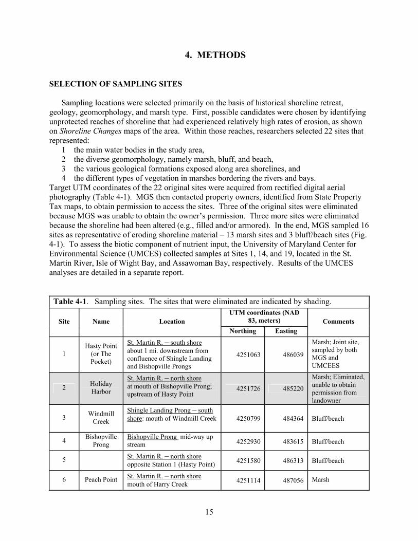
Target UTM coordinates of the 22 original sites were acquired from rectified digital aerial photography (Table 4-1). MGS then contacted property owners, identified from State Property Tax maps, to obtain permission to access the sites. Three of the original sites were eliminated because MGS was unable to obtain the owner’s permission. Three more sites were eliminated because the shoreline had been altered (e.g., filled and/or armored). In the end, MGS sampled 16 sites as representative of eroding shoreline material – 13 marsh sites and 3 bluff/beach sites (Fig. 4-1). To assess the biotic component of nutrient input, the University of Maryland Center for Environmental Science (UMCES) collected samples at Sites 1, 14, and 19, located in the St. Martin River, Isle of Wight Bay, and Assawoman Bay, respectively. Results of the UMCES analyses are detailed in a separate report.

Table 4-1. Sampling sites. The sites that were eliminated are indicated by shading.

UTM coordinates (NAD 83, meters) Site Name Location

Northing Easting Comments

1 Hasty Point

(or The Pocket)

St. Martin R. – south shore about 1 mi. downstream from confluence of Shingle Landing and Bishopville Prongs

4251063 486039

Marsh; Joint site, sampled by both MGS and UMCEES

2 Holiday Harbor

St. Martin R. – north shore at mouth of Bishopville Prong; upstream of Hasty Point

4251726 485220

Marsh; Eliminated, unable to obtain permission from landowner

3 Windmill Creek

Shingle Landing Prong – south shore: mouth of Windmill Creek

4250799 484364 Bluff/beach

4 Bishopville Prong

Bishopville Prong mid-way up stream 4252930 483615 Bluff/beach

5 St. Martin R. – north shore opposite Station 1 (Hasty Point) 4251580 486313 Bluff/beach

6 Peach Point St. Martin R. – north shore mouth of Harry Creek 4251114 487056 Marsh

16

Table 4-1. Sampling sites. The sites that were eliminated are indicated by shading. UTM coordinates (NAD

83, meters) Site Name Location Northing Easting

Comments

7 Salt Grass

Point

St. Martin R. – north shore vicinity of Buck Island Pond and Buck Island Creek

4250713 488658 Marsh

8 Smokehouse Cove

St. Martin R. – north shore NW of Isle of Wight 4249726 489906 Marsh

9 Drum Point Assawoman Bay – west shore easternmost extent of St. Martin Neck

4250598 491619 Marsh

10 Tulls Island

Assawoman Bay – west shore unnamed point between Drum Point and Hills Island, immediately west of former Tulls Island

4251941 491252 Marsh

11 Goose Pond Assawoman Bay – west shore 4252708 491080 Marsh

12 Peeks Creek

Assawoman Bay – west shore or Greys Creek – south shore shoreline between Peeks Creek and Back Creek; SE of confluence of Greys Creek and Back Creek

4253294 490442 Marsh

4253246 492193 Core 13

13* South Hammocks

Assawoman Bay – west shore SE side of South Hammocks; ~ due north of Drum Point ~1.75 mi.

4253251 492200

Core 13B (second core taken)

Marsh

4255752 492582 Core 14

14* Lone Cedar Point

Assawoman Bay – west shore northern extent of study area in MD

4255727 492780

Core 14B (second core taken)

Marsh; Joint site, sampled by both MGS and UMCES

15 Caine Keys Assawoman Bay – east shore ~ opposite South Hammocks 4253790 494430

Marsh; Eliminated, not natural shoreline

16 Swan Point Assawoman Bay – east shore ~1 mi. N of Rt. 90 Bridge; ~ opposite Drum Point

4250065 493830


17 Bay Shore Acres

Isle of Wight Bay – west shore immediately nw of Horn Island; ~0.5 mi. N of Rt. 50 bridge

4244389 491773


17

Table 4-1. Sampling sites. The sites that were eliminated are indicated by shading. UTM coordinates (NAD

83, meters) Site Name Location Northing Easting

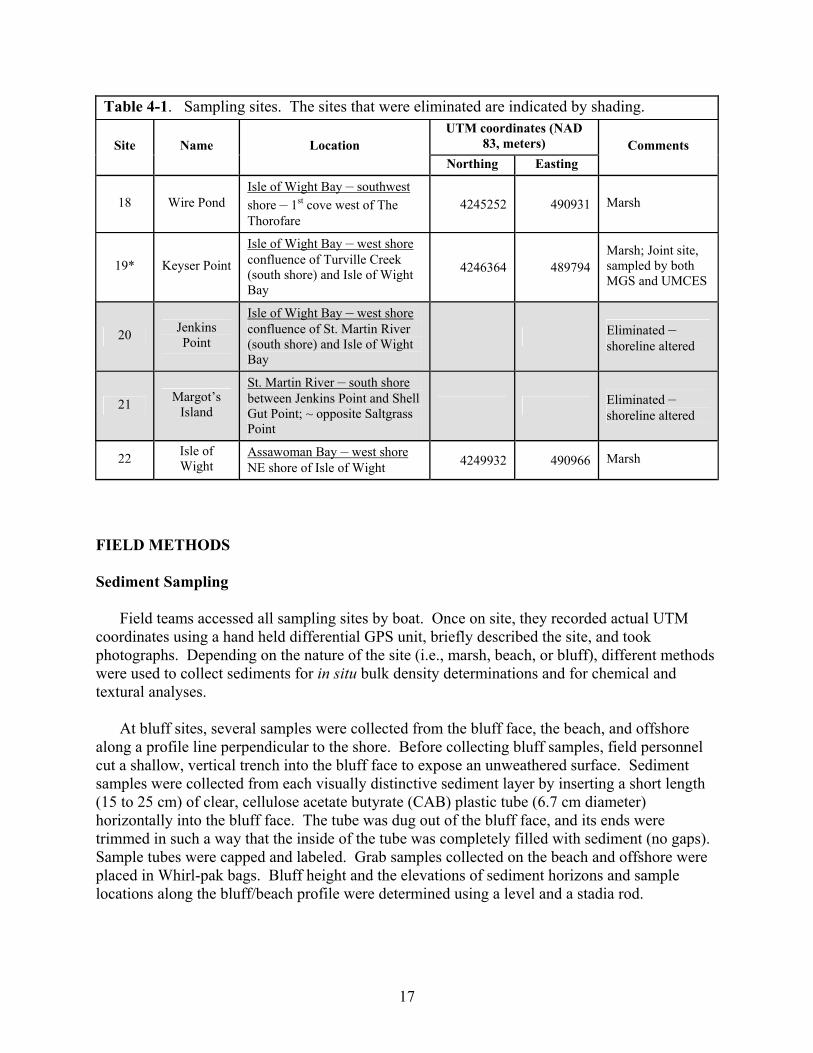
Comments

18 Wire Pond Isle of Wight Bay – southwest shore – 1st cove west of The Thorofare

4245252 490931 Marsh

19* Keyser Point

Isle of Wight Bay – west shore confluence of Turville Creek (south shore) and Isle of Wight Bay

4246364 489794 Marsh; Joint site, sampled by both MGS and UMCES

20 Jenkins Point

Isle of Wight Bay – west shore confluence of St. Martin River (south shore) and Isle of Wight Bay

Eliminated –shoreline altered

21 Margot’s Island

St. Martin River – south shore between Jenkins Point and Shell Gut Point; ~ opposite Saltgrass Point

Eliminated –shoreline altered

22 Isle of Wight

Assawoman Bay – west shore NE shore of Isle of Wight 4249932 490966 Marsh

FIELD METHODS Sediment Sampling

Field teams accessed all sampling sites by boat. Once on site, they recorded actual UTM coordinates using a hand held differential GPS unit, briefly described the site, and took photographs. Depending on the nature of the site (i.e., marsh, beach, or bluff), different methods were used to collect sediments for in situ bulk density determinations and for chemical and textural analyses.

At bluff sites, several samples were collected from the bluff face, the beach, and offshore along a profile line perpendicular to the shore. Before collecting bluff samples, field personnel cut a shallow, vertical trench into the bluff face to expose an unweathered surface. Sediment samples were collected from each visually distinctive sediment layer by inserting a short length (15 to 25 cm) of clear, cellulose acetate butyrate (CAB) plastic tube (6.7 cm diameter) horizontally into the bluff face. The tube was dug out of the bluff face, and its ends were trimmed in such a way that the inside of the tube was completely filled with sediment (no gaps). Sample tubes were capped and labeled. Grab samples collected on the beach and offshore were placed in Whirl-pak bags. Bluff height and the elevations of sediment horizons and sample locations along the bluff/beach profile were determined using a level and a stadia rod.

18

556000 560000 564000 568000

76000

78000

80000

82000

84000

86000

88000

90000

LittleAssawomanBay

Ocean City Inlet

Atla

ntic

Oce

an

1

24

6

7

8

9

10

1213

141516

17

1819

2021 26 27

28 29

30

13

4

5

6 7

8 22

9

10

11

1213

14

19

18

N

N

N

N

N

N

N

N

E E E E


DelawareMaryland

2

15

16

17

20

21

27

19 - Sampling Sites

- Land-loss polygon

Figure 4-1. Locations of sampling sites (in red) and land loss polygons (in blue). The sampling sites with light blue numbers were eliminated from the study because the shoreline at the site was altered or researchers could not obtain the owner’s permission to access the site.

19

At marsh sites, a continuous sediment core was collected on a prominent neck or point of the

marsh, approximately 1 m from the water’s edge. The length of core needed at each site was determined by averaging several bank height measurements. Bank height was defined as the distance between the top of the marsh and the base of the erosional scarp at the marsh edge. The base of the scarp was usually underwater. Marsh cores were collected by vibrating or pounding 7.62 cm-diameter aluminum tubing into the marsh surface down to the desired depth. Sediment compaction was measured and recorded before the core was extracted. Following extraction, the liner was trimmed to the top of the sediment and sealed at both ends for transportation back to the lab. There, it was kept refrigerated until it was processed. A grab sample was collected approximately 0.3 m offshore adjacent to the core location. LABORATORY METHODS Quantifying Land Loss

The amount of land lost annually in the study area is based on a digital comparison of two historical shorelines, one dating from 1942 and the other from 1989. The 1942 shoreline was previously digitized from 1:20,000-scale National Oceanic and Atmospheric Administration (NOAA) coastal survey maps, also known as topographic (T-) sheets. The 1989 shoreline was previously interpreted from 1:12,000-scale orthophotography. At the time it was delineated, the 1989 shoreline was also classified by shoreline type (i.e., beach, structure, vegetated, or water’s edge) (Hennessee, 2001). MGS used a geographic information system (GIS), MicroImages’ TNTmips, to compare shoreline positions and quantify losses due to erosion.

Different stretches of shoreline erode at different rates. To account for this variability, MGS divided the study area shoreline into 23 segments. Shoreline reaches ranged in length from about 600 m to 45,000 m; most were less than 9,000 m long. To demarcate the reaches, MGS constructed a template of irregular, mostly contiguous, “land loss” polygons. The polygons were drawn in such a way that:

• They contained all unprotected shoreline in the study area, except for the following, unsampled tributaries: the head of Greys Creek; Back Creek; the upstream reaches of Manklin Creek; and Turville and Herring Creeks above their confluence.

• They excluded protected shoreline: the western side of Fenwick Island (eastern Assawoman and Isle of Wight Bays); the southern end of Isle of Wight; the south shore of the St. Martin River bordering the community of Ocean Pines; the north shore of Manklin Creek; and a short stretch of shoreline in the vicinity of Octopus Pond.

• With the exceptions listed above, as well as a short reach of shoreline in the vicinity of Saltgrass Pt., they initially included the 1942 and 1989 shorelines in their entirety. (Only one shoreline was available for Saltgrass Pt.)

• Based on researchers’ field experience and an inspection of 1989 digital orthophotography, each contained, as far as practicable, similar types of shoreline (i.e., marsh or upland).

20

• In areas of changing geology, their boundaries coincided with the contacts between geologic formations. For instance, the cross-shore boundaries of polygon P16 at the mouth of Bishopville Prong coincided with an outcrop of the Beaverdam Sand.

• In the vicinity of a bay or tributary mouth, polygon boundaries coincided with the mouth (e.g., polygons P8 and P12), to allow researchers to report their results by water body.

• In the absence of any of the above criteria, polygon boundaries were drawn equidistant between sample locations (e.g., polygons P6 through P10). No polygon included more than one sampling site.

Each land loss polygon in the template was assigned a number, P#. The polygons are shown

in Figure 4-1, and a description of their locations is presented in Table 4-2. Table 4-2. Land loss polygons and associated sampling sites

Land loss

polygon Location Geology*

Associated sampling

site

P1 Assawoman Bay Lone Cedar Pt.

(P & S) – Holocene Tidal Marsh Deposits (Qtm) 14B

P2

Assawoman Bay Marsh south of Lone Cedar Pt., along western shore of Assawoman Bay and northern shore of Greys Cr., including Corn Hammocks, South Hammocks, and Swan Gut

(P) – Mostly Qtm, except Middle-Wisconsin Sinepuxent Fm. (Qs) upstream of Swan Gut; polygon boundary drawn at contact between Qs and Upper Sangamon Ironshire Fm. (Qi) (S) – Qtm

13B

P4

Greys Creek Southern shore of Grays Cr. upstream of Back Cr.

(P) – Mostly Qtm, except some Qs; polygon boundary drawn at contact between Qs and Qi (S) – No sample in polygon

12

P6

Assawoman Bay Western shore of Assawoman Bay (or southern shore of Greys Cr.) from Back Cr. to Peeks Cr.

(P & S) – Qtm

12

P7 Assawoman Bay Northern Goose Pond

(P) – Mostly Qtm, except some Qs (S) – Qtm

11

P8 Assawoman Bay Southern Goose Pond; Tulls Island to Drum Pt.

(P & S) – Qtm 10

P9 Assawoman Bay Drum Pt.

(P) – Equally Qs and Qtm (S) – Qtm 9

21

Table 4-2. Land loss polygons and associated sampling sites Land loss


Associated sampling

site

P10 Assawoman Bay Drum Pt. to Wight Pt.

(P & S) – Qtm 22

P12

St. Martin River West side of Isle of Wight, north of Rt. 90 bridge, and Smokehouse Cove

(P) – Qtm, except for some Qs on southwest side of Isle of Wight (S) – Qtm

8

P13

St. Martin River Northern shore of St. Martin R. from Smokehouse Cove west past Saltgrass Pt. to vicinity of mouth of Buck Island Cr.; includes Buck Island Pond and Buck Island Cr.

(P & S) – Qtm

7

P14

St. Martin River Northern shore of St. Martin R. in vicinity of Peach Pt. and mouth of Harry Cr.

(P & S) – Qtm

6

P15

St. Martin River Northern shore of St. Martin R. in vicinity of Woods Pt. at mouth of Zippy Cr.

(P & S) – Pliocene Beaverdam Fm. (Tb)

5

P16

Bishopville Prong Both shores of Bishopville Prong from mouth of prong north to contact between Beaverdam Sand and Ironshire Fm.

(P) – Tb (S) – No sample in polygon

5

P17

Bishopville Prong Both shores of Bishopville Prong bordered by Ironshire Fm.

(P & S) – Lower Sangamon Omar Fm. (Qo) 4

P18

Shingle Landing Prong Both shores of Shingle Landing Prong, from mouth upstream past confluence of Birch Br., Middle Br., and Church Br.

(P & S) – Tb

3

22

Table 4-2. Land loss polygons and associated sampling sites Land loss


Associated sampling

site

P19

St. Martin River Southern shore of St. Martin R. from mouth of Shingle Landing Prong east past Hasty Pt. to first canal

(P) – Mostly Qtm, except some Tb (S) – Qtm 1

P20

Manklin Creek Southern shore of Manklin Cr. immediately upstream of mouth

(P) – Mostly Qs, except some Qtm (S) – No sample in polygon 8

P21

Turville Creek Northern shore of Turville Cr. from mouth of Herring Cr. to Mocassin Pond

(P) – Equally Qs and Qtm (S) – No sample in polygon 8

P26

Turville Creek Southern shore of Turville Cr. from mouth of Herring Cr. to Keyser Pt.

(P) – Mostly Qs, except some Qtm (S) – No sample in polygon 19

P27 Isle of Wight Bay Keyser Pt. to Octopus Pond

(P & S) – Qs 19

P28

Isle of Wight Bay Wire Pond and undeveloped (eastern) section of Octopus Pond

(P & S) – Qs

18

P29

Isle of Wight Bay The Thorofare, from Drum Island to the start of the marsh bordering Wire Pond

(P) – Qs (S) – No sample in polygon 18

P30 Isle of Wight Bay Rt. 50 bridge to Drum Island

(P) – Qs (S) – No sample in polygon

18

* within polygon (P) and at sampling site (S)

Once it was constructed, the polygon template was merged first with the 1942 shoreline and then with the 1989 shoreline. Both shoreline/template files were edited:

• Long stretches of developed shorelines were erased. • Small gaps in the remaining shoreline were closed, usually by drawing short, straight

lines between the dangling shoreline segments. • Man-made features, usually canals, present in one year but not the other, were deleted.

(In some cases, the headward reach of a small tributary extended further upstream in one

23

year than in another. Likewise, some ponds and coves, particularly in or along marshes, were evident in only one coverage. These features were left unaltered.)

• Within each of the land loss polygons, interior polygons were assigned one of the following attributes: “fastland,” “island,” or “water.”

For each land loss polygon, the areas (m2) covered by fastland, island and water were

recorded, by year, in an Excel spreadsheet. Likewise, the total length (m) of the 1989 shoreline, as well as the length of each type of shoreline (beach, structure, vegetated, water’s edge) was recorded. For each polygon, land loss over the 47-year period was determined by subtracting water area in 1989 from water area in 1942. The difference in water area is equivalent to the area of land lost by erosion. A summary of area and shoreline changes for each polygon is presented in Table D-1 (Appendix D).

The land loss polygons provided a structure for organizing the results of the sediment, pore water, and plant tissue analyses. Each sample location was associated with one or more of the land loss polygons (Table 4-2). In the simplest case, where polygons and samples were co-located, the association is direct. For instance, the results for Site 13, located within polygon P12, are associated with polygon P12. For unsampled polygons, the association was based either on similarity in geology or shoreline type (marsh or upland), or on proximity.

Bank Height

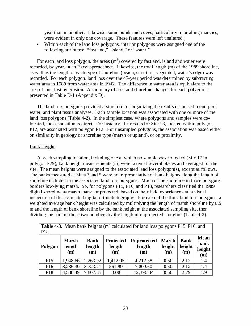
At each sampling location, including one at which no sample was collected (Site 17 in polygon P29), bank height measurements (m) were taken at several places and averaged for the site. The mean heights were assigned to the associated land loss polygon(s), except as follows. The banks measured at Sites 3 and 5 were not representative of bank heights along the length of shoreline included in the associated land loss polygons. Much of the shoreline in those polygons borders low-lying marsh. So, for polygons P15, P16, and P18, researchers classified the 1989 digital shoreline as marsh, bank, or protected, based on their field experience and a visual inspection of the associated digital orthophotography. For each of the three land loss polygons, a weighted average bank height was calculated by multiplying the length of marsh shoreline by 0.5 m and the length of bank shoreline by the bank height at the associated sampling site, then dividing the sum of those two numbers by the length of unprotected shoreline (Table 4-3).

Table 4-3. Mean bank heights (m) calculated for land loss polygons P15, P16, and P18.

Polygon Marsh length

(m)

Bank length

(m)

Protected length

(m)

Unprotected length

(m)

Marsh height

(m)

Bank height

(m)

Mean bank height

(m) P15 1,948.66 2,263.92 1,412.05 4,212.58 0.50 2.12 1.4 P16 3,286.39 3,723.21 561.99 7,009.60 0.50 2.12 1.4 P18 4,588.49 7,807.85 0.00 12,396.34 0.50 2.79 1.9

24

Sediments Core Processing

Before opening the cores, MGS x-rayed them in their liners using a TORR-MED medical X-ray unit. The exposure settings were 84 to 90 kilovolts for 6 to 8 seconds at 5 milliAmps. Radiographic images were developed using a Xerox 125 xeroradiograph processor.

After x-raying was completed, each core was cut in half lengthwise. First, the aluminum liner was cut using a circular saw. The sediment core within the liner was then cut in half with a very sharp, stainless steel knife. The knife produced a clean cut through the plant roots and peat material, minimizing deformation of the core structure or shape. Lab personnel photographed and described the split core, noting changes in sediment and structure with depth. Xeroradiographs (x-rays), photographs and core logs are presented in Appendix A. The core was divided into sections 10 to 25 cm long. The exact length depended on lithological changes observed in the split core and in the radiographs. Each section was split lengthwise into three or four subsamples, which were designated for specific analyses (i.e., bulk density, grain size, or chemical analyses). The sub-samples were placed in Whirl-Pak bags. Bulk density splits were processed first, before other splits were made (see next section).

Bulk Density and Water Content

For both bluff samples and cored marsh sediments, MGS used similar methods to determine bulk density and water content. Grab samples collected from the beach and nearshore were processed for water content only. Bluff Samples

The entire sediment sample was removed from the plastic core tube and weighed. The length of the tube was recorded. The sample was then mixed to homogenize it. Exactly ¼ of the sample, by weight, was placed in a drying vessel, dried at 60°C, and then reweighed. The dried sample was saved for chemical analyses. The remaining ¾ of the sample was saved for grain size analysis.

Water content was calculated as the percentage of water weight to the total weight of wet sediment, as follows:

where: Ww is the weight (g) of water, and Wt is the weight (g) of wet sediment.

Wet and dry bulk densities (referred to in this study as “measured” bulk density, in g/cm3 or Kg/m3) were calculated as the wet weight or dried weight (g), respectively, of the subsample

100 )WW( = OH %

t

w *2 Eq. 4-1

25

divided by ¼ of the volume of the entire bluff sample. Volume was calculated using the volume formula for a cylinder:

V = π r 2 l Eq. 4-2

where: V is the volume (cm3) of the subsample,

π is 3.14159, r is the radius of the circumference of the CAB tube liner, or ½ the

diameter (6.7 cm), and l is the length (cm) of the core tube.

A second method was used to calculate bulk density (wet) using the water content of the

sediment (Bennett and Lambert, 1971). This method assumes that average sediment grain density is 2.72 g/cm3 and that the sample is fully saturated with water.

wd

tLB

WWW

+=

72.2

)&(ρ Eq. 4-3

where: )&( LBρ is the calculated bulk density, based on Bennett and Lambert,

Wt is the weight (g) of wet sediment, Wd is the weight (g) of dry sediment, and Ww is the weight (g) of water.

Cored Marsh Samples

Each section of core was weighed to determine the total weight of the section. Exactly ½ of the section, by weight, was place in a drying vessel, dried at 60°C, and then reweighed. The dried sample was archived.

Water content and calculated wet bulk density, based on Bennett and Lambert, were calculated using Equations 4-1 and 4-3, respectively. Measured bulk densities were calculated as the wet and dried weights (g) of the subsample divided by ½ of the volume of the core section. The volume of the core section was calculated using Equation 4-2, where r = ½ the diameter of the aluminum tubing (7.62 cm diameter) and l = section length.

26

Dry bulk density of the core section was adjusted to account for any core compaction. For most of the cores, there was some compaction (compression) of the sediments during the insertion of the core liner. The amount of compaction was measured as the difference between the top of the marsh and the top of the sediment in the core liner once the liner was emplaced. The degree of compaction along the length of the core varied depending on sediment texture. However, for this study, MGS assumed that compaction was evenly distributed over the length of the core. Bulk densities were multiplied by a compaction correction calculated as:

−−=)(

)()()( 1

s

tsc l

llc Eq. 4-4

where, c(c) is the compaction correction,

l(s) is the length or depth (cm) of the sediment column cored or sampled, and

l(t) is the length (cm) of the sediment core collected.

Grain Size Analysis

In preparation for grain size analysis, sediment samples underwent a cleaning process to remove soluble salts, carbonates, and organic matter. These constituents may interfere with the dispersal of individual sediment particles and, thereby, affect the subsequent separation of the sand and mud fractions. All sediment samples were treated first with a 10% solution of hydrochloric acid (HCl) to remove carbonate material, such as shells, and then with a 6% or 15% solution of hydrogen peroxide (H2O2) to remove organic material. A 0.26% solution of the dispersant sodium hexametaphosphate ((NaPO3)6) was then added to ensure that individual grains did not clump, or flocculate, during pipette analysis.

Marsh samples, which contained significant amounts of plant material, were wet-sieved through a 14-mesh (~1.4 mm) nylon screen to remove large plant roots and debris. The plant material was dried and weighed. Usually, plant matter was separated from sediments after the HCl treatment. However, for cores collected at sites sampled jointly by MGS and UMCES, samples were sieved prior to HCl treatment, and the plant fractions (> 1.4 mm) were saved for chemical analysis.

For each sample, the sand fraction was separated from the mud fraction by wet-sieving through a 4-phi mesh sieve (0.0625 mm, U.S. Standard Sieve #230). The sand fraction (i.e., particles > 0.0625 mm) was dried and weighed. The mud fraction (i.e., sediment passing through the #230 sieve) was analyzed using a pipette technique to determine the proportions of silt and clay (Krumbein and Pettijohn, 1938). The mud fraction was suspended in a 1000-ml cylinder in a solution of 0.26% sodium hexametaphosphate. The suspension was agitated and, at specified times thereafter, 20 ml pipette withdrawals were made. The rationale behind this process is that larger particles settle faster than smaller ones. By calculating the settling velocities of different sized particles, withdrawal times can be determined. At the time of withdrawal, all particles larger than a specified size have settled past the point of withdrawal. Sampling times were

27

calculated to permit the determination of the total amount of silt and clay (4 phi) and clay-sized (8 phi) particles in the suspension. Withdrawn samples were dried at 60°C and weighed. From these dry weights, the percentages of sand, silt, and clay were calculated for each sample and classified according to Shepard's (1954) nomenclature (Fig. 4-2). Figure 4-2. Shepard’s (1954) classification of sediment types. Chemical Analysis Sample Preparation

Before marsh samples were dried and ground, they were processed using a commercially available food blender and plastic (styrene copolymer) processor containers. Between 50 to 100 g of wet core sample, roots and all, were mixed with 50 to 100 ml of ultra-pure water. The slurry was processed at hi/liquefy for 1 minute or until no visible pieces of plant material remained. The processed slurry was then transferred to an evaporating dish and dried at 60oC.

The dried marsh samples and the bluff samples dried for bulk density/water content determinations were ground in tungsten-carbide vials using a ball mill, placed in Whirl-Pak bags, and stored in a desiccator. Total Carbon and Nitrogen Analysis Untreated, ground sediments were analyzed for total nitrogen, carbon, and sulfur (NCS) using a Carlo Erba NA1500 analyzer. Approximately 10 to 15 mg of dried sediment were weighed into a tin capsule. The exact weight of the sample, to the nearest µg, was recorded. To ensure complete combustion during analysis, 15 to 20 mg of vanadium pentoxide (V2O5) were added to the tin capsule and mixed with the sediment. The capsule was then crimped to seal and stored until analysis.

28

The encapsulated sediment sample was dropped into a combustion chamber, where the sample was oxidized in pure oxygen. The resulting combustion gases (N, C, H, and S), along with pure helium, the carrier gas, were passed through a reduction furnace to remove free oxygen and then through a sorption trap to remove water. Separation of the gas components was achieved by passing the gas mixture through a chromatographic column. A thermal conductivity detector was used to measure the relative concentrations of the gases. The NA1500 Analyzer was configured for NCS analysis using the manufacturer's recommended settings. As a primary standard, 5-chloro- 4-hydroxy- 3-methoxy- benzylisothiourea phosphate was used. Blanks (tin capsules containing only vanadium pentoxide) were run every 12 samples. Replicates of every fifth sample were run. As secondary standards, at least one standard reference material (SRM) (NIST SRM #1646 – Estuarine Sediment; NIST SRM #2704 – Buffalo River Sediment, or the National Research Council of Canada PACS-1 – Marine Sediment) was run every six or seven samples. Comparisons of the results of the SRMs to the certified values are presented in the discussion of quality assurance and quality control (Appendix C). Total Phosphorus and Metals Activation Laboratories, Ltd. (Actlabs) of Tucson, Ariz., analyzed bluff and marsh sediments for 22 elements including total phosphorus. The lab used a four-acid, “near total” digestion process, followed by analysis of the digestate by inductively coupled plasma emission spectroscopy (ICP-OES). The four-acid digestion employed perchloric (HClO4), hydrochloric (HCl), nitric (HNO3), and hydrofluoric (HF) acids. Quality assurance was checked using the method of bracketing standards (Van Loon, 1980). The SRMs, similar to the sediments being analyzed, included the same standards used in the total nitrogen, carbon, and sulfur analyses. Actlabs’ results of the analyses of the SRMs are listed in Appendix B. Analytical results for the bluff and marsh core samples are listed in Appendix C. DATA REDUCTION

Average concentrations of nutrients (total carbon, nitrogen, and phosphorus), specific metals

(Pb and Zn), and textural components (total solids, sand, silt, clay) were calculated for each core or bank/bluff site by averaging the concentrations of the individual core samples or bluff samples, normalized to bank height. Mean site concentrations were then assigned to specific land loss polygons (see Table 4-2) to calculate the component loadings for the polygons. Equations for the data reductions, along with detailed explanations and calculation tables, are presented in Appendix D.

29

5. RESULTS AND DISCUSSION

FIELD AND LAB OBSERVATIONS

Within the study area, sediment samples were collected from three basic types of shorelines: marsh, bluff and beach. Sites 3, 4, and 5, in the upstream area of the St. Martin River, are located along shorelines dominated by low bluffs, 2 to 3 m high, fronted by a narrow (6 to 9 m wide), sandy beach (Fig. 5-1). Both the Omar Formation (Site 5) and the Beaverdam Formation (Sites 3 and 5) are exposed along this portion of the river (Fig. 3.3). The bluff sediments consist of predominately grayish yellow to brownish gray sands with some mud. The lower half of the bluff at Site 3 consists of greenish blue sandy mud, which is more resistant to erosion. As a result, the bluff at Site 3 has a 40% slope. The bluffs at Sites 4 and 5 are steeper, with slopes greater than 60%.

Figure 5-1. Bluff at Site 5.

Figure 5-2. The main features developed along a marsh shoreline due to wave erosion (from Schwimmer, 2001).

The remaining sites are located on prominent points along marshy shorelines composed of

either Holocene tidal marsh deposits or Sinepuxent deposits (Fig. 3-3). Most marsh shorelines are highly convoluted and edged by a 0.3 to 0.7 m erosional scarp, which is often undercut beneath the root mat layer. Features observed along the marsh shoreline include neck and cleft, pinched necks, stacks and isolated islands (Fig. 5-2), all of which are indicative of wave attack, a significant erosional process operating in the coastal bays (Schwimmer, 2001).

Pocket beaches (Fig. 5-3), the lengths of which range from 10 m to more than 50 m, are common along the marsh shoreline, particularly on the mainland side of Assawoman Bay. Pocket beaches may reflect a localized sand source (e.g., sandy facies in the underlying Sinepuxent Formation), nearshore sediment transport processes, or a combination of both. Most marsh sites characterized by sandy sediments are located near eroding headlands, a potential source of sand. In Rehoboth Bay, Delaware, Schwimmer (2001) observed that sandy beaches occur where eroding shoreline intersects upland areas. Subtle variations in lithologies at marsh sites may be related to antecedent topography, as well as to local sediment transport processes.

30

The dominant marsh vegetation is Spartina alterniflora. At many sites, the marsh surface and scarp are armored with live mussels (Modiolus sp) (Fig. 5-4). Based on an examination of the marsh cores, sediment characteristics vary not only from site to site, but both vertically and laterally across a given site. Marsh sediments are predominately fine-grained muds with abundant plant material and organic matter (peat). Bulk organic content ranges from less than 5% (dry weight) to 71%. Sand content decreases with depth at most sites. Active (live) root zones range from depths of 20 cm (Site 13) to 50 cm (Site 10) below the marsh surface. In many cores, a redox boundary is evident just below the active root zone. Also, a 10 to 20 cm thick layer containing very high peat or plant material content with little sediment occurs at or below the active root zone. This “spongy” layer accounts for most of the compaction that occurs during the collection of cores and the “quaking” of the marsh surface felt when large waves hit the shoreline or when walking.

Figure 5-3. Pocket beach. This sandy beach is one of several found at Site 14 (Lone Cedar Point). A short core collected from this beach revealed a layer of sand overlying marsh mud.

Figure 5-4. Mussels armoring scarp face at Site 1.

LAND LOSS (AREA AND VOLUME) For the 47-year period between 1942 and 1989, Table 5-1 shows land lost and rates of erosion for the northern coastal bays. Overall, the 166 km of shoreline lost about -1.2 x 106 m2 of land to erosion. On average, the shoreline retreated a total of -7.3 m, at an annual rate of -16 cm/yr. Rates of loss varied widely (Fig. 5-5). The protected shorelines of Bishopville Prong (P17) and Shingle Landing Prong (P18), tributaries of the St. Martin River, experienced minimal erosion, -4 cm/yr. Rates reached a maximum of -39 cm/yr along the exposed western shore of Isle of Wight Bay (P27). These annual erosion rates are similar to those measured along marsh shorelines in Rehoboth Bay, Delaware, where, over a three year period, rates averaged between -14 to -43 cm/yr (Schwimmer, 2001).

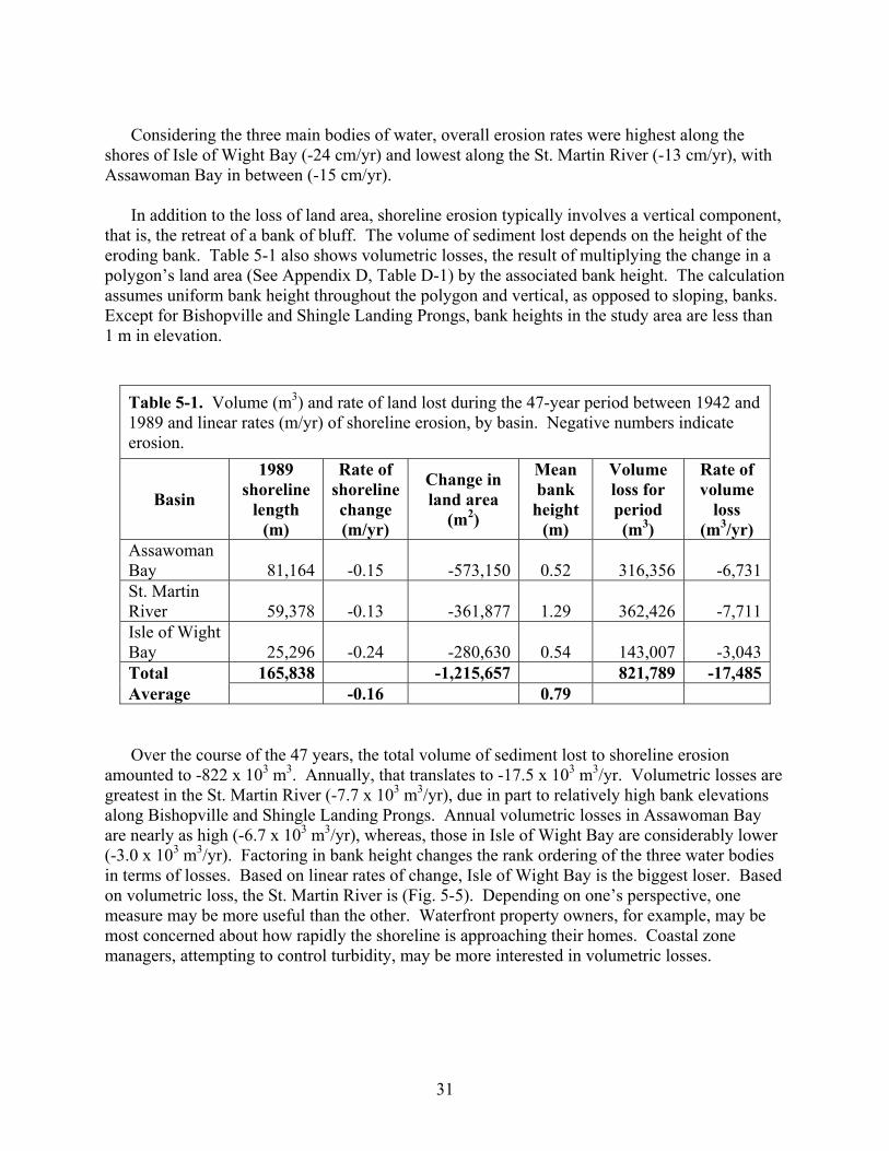
31

Considering the three main bodies of water, overall erosion rates were highest along the shores of Isle of Wight Bay (-24 cm/yr) and lowest along the St. Martin River (-13 cm/yr), with Assawoman Bay in between (-15 cm/yr).

In addition to the loss of land area, shoreline erosion typically involves a vertical component, that is, the retreat of a bank of bluff. The volume of sediment lost depends on the height of the eroding bank. Table 5-1 also shows volumetric losses, the result of multiplying the change in a polygon’s land area (See Appendix D, Table D-1) by the associated bank height. The calculation assumes uniform bank height throughout the polygon and vertical, as opposed to sloping, banks. Except for Bishopville and Shingle Landing Prongs, bank heights in the study area are less than 1 m in elevation.

Table 5-1. Volume (m3) and rate of land lost during the 47-year period between 1942 and 1989 and linear rates (m/yr) of shoreline erosion, by basin. Negative numbers indicate erosion.

Basin

1989 shoreline

length (m)

Rate of shoreline change (m/yr)

Change in land area

(m2)

Mean bank height

(m)

Volume loss for period (m3)

Rate of volume

loss (m3/yr)

Assawoman Bay 81,164 -0.15 -573,150 0.52 316,356 -6,731St. Martin River 59,378 -0.13 -361,877 1.29 362,426 -7,711Isle of Wight Bay

25,296

-0.24

-280,630 0.54 143,007 -3,043

Total 165,838 -1,215,657 821,789 -17,485Average -0.16 0.79

Over the course of the 47 years, the total volume of sediment lost to shoreline erosion amounted to -822 x 103 m3. Annually, that translates to -17.5 x 103 m3/yr. Volumetric losses are greatest in the St. Martin River (-7.7 x 103 m3/yr), due in part to relatively high bank elevations along Bishopville and Shingle Landing Prongs. Annual volumetric losses in Assawoman Bay are nearly as high (-6.7 x 103 m3/yr), whereas, those in Isle of Wight Bay are considerably lower (-3.0 x 103 m3/yr). Factoring in bank height changes the rank ordering of the three water bodies in terms of losses. Based on linear rates of change, Isle of Wight Bay is the biggest loser. Based on volumetric loss, the St. Martin River is (Fig. 5-5). Depending on one’s perspective, one measure may be more useful than the other. Waterfront property owners, for example, may be most concerned about how rapidly the shoreline is approaching their homes. Coastal zone managers, attempting to control turbidity, may be more interested in volumetric losses.

32

Figure 5-5. Comparison of linear erosion rate and volumetric loss for each land loss polygon. To normalize differences in polygon area, volume loss for each polygon is divided by shoreline length within the polygon; losses are given as volume (m3) per year per linear meter of shoreline.

SEDIMENTS Bulk Density

One of the most important parameters measured in this study is bulk density, a determination of the total solids in a volume of sediment. Bulk density is used to convert the volume of land lost to mass loadings. Bulk density is calculated by two different methods. First, it is measured directly. A known volume of sediment is weighed and assumed to reflect the in situ density of shoreline sediments, accounting for all air pockets, clastics, plant material, etc. Second, bulk density is calculated as a function of water content (Bennett and Lambert, 1971). Results of both methods, reported in Appendix C, are discussed below. The emphasis is on measured dry bulk density, the number used in the mass loading calculations.

The measured dry bulk density of sediments ranges from 0.12 to 1.54 g/cm3. Higher bulk

densities (i.e., >1.25 g/cm3) are associated with sediments sampled from bluff sites (Sites 3, 4, and 5). These sediments consist almost entirely of sand and contain little plant material or organic matter. The average dry bulk density of bluff sediments is 1.39 ± 0.13 g/cm3, which is slightly lower than the average bulk density of 1.5 g/cm3 used by Ibison and others (1990, 1992).

The measured dry bulk density of marsh sediments ranges from 0.12 to 1.03 g/cm3,

averaging 0.43 ± 0.28 g/cm3. This range is within the range of values observed in marsh sediments in the Chesapeake Bay (Anderson and others, 1997; Stevenson and others, 1985). Higher bulk densities correspond to the sandy sediments found at the tops of cores. At most core

33

sites, densities decrease with depth below the marsh surface. The lowest bulk densities correspond to a “spongy” layer, which consists of abundant plant material and organic matter, and very little sand or mud. Water Content Water content of marsh samples ranges from 28 to 86%, averaging 65 ±17%. Bluff sediments contain very little water, less than 10% for all samples except the clay unit at the base of Site 3. For sediments that are saturated with water, particularly marsh samples, water content is inversely related to bulk density (Figs. 5-6 and 5-7). Water content, which reflects the volume of pore space between solid particles, is a function of grain size, grain shape, and the packing of grains. Measured wet bulk density is typically 5% less than the calculated Bennett and Lambert values (B&L bulk density). The difference is attributable to incomplete saturation with water, as with the bluff samples, and to the deviation of the average specific gravity (i.e., density) of the solids in the sediment from the constant, 2.72 g/cm3, used by Bennett and Lambert (Eq. 4-3). Figure 5-6. Measured wet bulk density as a function of water content. Superimposed on the plot is a (blue) curve representing bulk density calculated using Bennett and Lambert’s equation. Measured wet bulk density values agree very well with Bennett and Lambert values (R2 = 0.95). The outlying cluster of four data points (water content < 20%) corresponds to bluff samples.

Marsh sediments contain varying amounts of plant material, which reduces the overall (average) density. Figure 5-7 is a graph of the difference (% variation) between measured bulk density and B&L bulk density, plotted against plant content (i.e., plant > 14 mesh). Plant content accounts for much of the variation from the calculated bulk density.

Figure 5-7. Difference (%) between measured wet bulk density and B&L bulk density, plotted against the plant content of the sediment. Superimposed on the plot are the 99% (red) and 95% (purple) confidence level limits and trend line (blue; R2 = 0.158). The red Xs represent bluff samples and are treated as outliers.

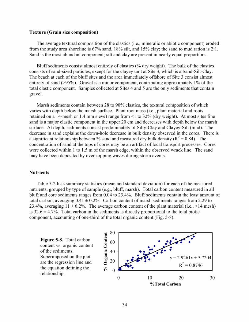
34

Texture (Grain size composition)

The average textural composition of the clastics (i.e., mineralic or abiotic component) eroded from the study area shoreline is 67% sand, 18% silt, and 15% clay; the sand to mud ration is 2:1. Sand is the most abundant component; silt and clay are present in nearly equal proportions.

Bluff sediments consist almost entirely of clastics (% dry weight). The bulk of the clastics

consists of sand-sized particles, except for the clayey unit at Site 3, which is a Sand-Silt-Clay. The beach at each of the bluff sites and the area immediately offshore of Site 3 consist almost entirely of sand (>95%). Gravel is a minor component, contributing approximately 1% of the total clastic component. Samples collected at Sites 4 and 5 are the only sediments that contain gravel.

Marsh sediments contain between 28 to 90% clastics, the textural composition of which

varies with depth below the marsh surface. Plant root mass (i.e., plant material and roots retained on a 14-mesh or 1.4 mm sieve) range from <1 to 32% (dry weight). At most sites fine sand is a major clastic component in the upper 20 cm and decreases with depth below the marsh surface. At depth, sediments consist predominately of Silty-Clay and Clayey-Silt (mud). The decrease in sand explains the down-hole decrease in bulk density observed in the cores. There is a significant relationship between % sand and measured dry bulk density (R2 = 0.84). The concentration of sand at the tops of cores may be an artifact of local transport processes. Cores were collected within 1 to 1.5 m of the marsh edge, within the observed wrack line. The sand may have been deposited by over-topping waves during storm events.

Nutrients

Table 5-2 lists summary statistics (mean and standard deviation) for each of the measured

nutrients, grouped by type of sample (e.g., bluff, marsh). Total carbon content measured in all bluff and core sediments ranges from 0.04 to 23.4%. Bluff sediments contain the least amount of total carbon, averaging 0.41 ± 0.2%. Carbon content of marsh sediments ranges from 2.29 to 23.4%, averaging 11 ± 6.2%. The average carbon content of the plant material (i.e., >14 mesh) is 32.6 ± 4.7%. Total carbon in the sediments is directly proportional to the total biotic component, accounting of one-third of the total organic content (Fig. 5-8).

Figure 5-8. Total carbon content vs. organic content of the sediments. Superimposed on the plot are the regression line and the equation defining the relationship.

y = 2.9261x + 5.7204R2 = 0.8746

0

20

40

60

80

0 10 20 30%Total Carbon

% O

rgan

ic C

onte

nt

35

Total nitrogen content measured in bluff and marsh sediments ranges from 0.004 to 1.28%. As with carbon, bluff samples contain the least amount of total nitrogen, averaging less than 0.05%. Marsh sediments yield nitrogen values between 0.13 to 1.28%, averaging 0.58 ± 0.31%. Total nitrogen content of the plant fraction averages 1.02 ± 0.18%.

Table 5-2. Summary statistics for each of the elements measured in the samples. BDL indicates below detection limit for the analytical method.

Marsh sediments Bluff sediments Plant fraction

(>14 mesh) Ave. Std. Ave. Std. Ave. Std. Nutrients (%) Carbon (C) 11 6.2 0.41 0.2 32.6 4.7 Nitrogen (N) 0.58 0.31 0.036 0.014 1.02 0.18 Phosphorus (P) 0.042 0.017 0.007 0.005 0.052 0.02 Sulfur (S) 1.61 0.77 0.008 0.015 2.57 2.05 Metals (ppm) Silver (Ag) 0.47 0.11 BDL 0.67 0.15 Aluminum (Al, %) 3.65 0.82 2.54 1.47 1.95 0.33 Beryllium (Be) 1.11 0.31 BDL BDL Bismuth (Bi) 2.42 0.79 BDL BDL Cobalt (Co) 8.48 2.04 8 4.2 14.4 7.7 Copper (Cu) 16.4 8.9 17 4.2 23.4 12 Iron (Fe, %) 1.84 0.57 1.51 0.99 2.18 2.14 Manganese (Mn) 161 68 89 32 88 37 Molybdenum (Mo) 5.73 2.44 BDL 9.78 Nickel (Ni) 25.4 7.5 5.8 4.2 15.7 10.6 Lead (Pb) 24.9 10.6 10.8 3.6 45.9 55.7 Strontium (Sr) 146 39 82 22 88 38 Titanium (Ti, %) 0.278 0.063 0.19 0.13 0.13 0.03 Vanadium (V) 63.9 18.4 37 33.6 57.5 14.3 Yttrium (Y) 11.8 3.3 4.8 1.3 14 3 Zinc (Zn) 61 20 37 12 63 23

Generally, for all of the sediments measured, nitrogen content correlates well with carbon content (R2 = 0.78). Depending on the nature of the organic source, nitrogen is expected to maintain a fairly constant proportionality with carbon content, as shown in Table 5-3, which lists the C:N ratios for the different samples. The mean C:N ratio for marsh samples is higher than both the mean ratio of 7.04, obtained from bottom samples collected in the northern coastal bays (Wells and others, 1994), and the Redfield’s ratio of 5.7 for planktonic organisms (Redfield and others, 1963). The intermediate C:N ratio found in the marsh sediment reflects a combination of organic material types.

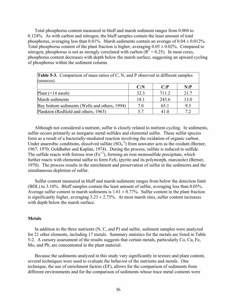
36

Total phosphorus content measured in bluff and marsh sediment ranges from 0.004 to 0.124%. As with carbon and nitrogen, the bluff samples contain the least amount of total phosphorus, averaging less than 0.01%. Marsh sediments contain an average of 0.04 ± 0.012%. Total phosphorus content of the plant fraction is higher, averaging 0.05 ± 0.02%. Compared to nitrogen, phosphorus is not as strongly correlated with carbon (R2 = 0.25). In most cores, phosphorus content decreases with depth below the marsh surface, suggesting an upward cycling of phosphorus within the sediment column.

Although not considered a nutrient, sulfur is closely related to nutrient cycling. In sediments, sulfur occurs primarily as inorganic metal sulfides and elemental sulfur. These sulfur species form as a result of a bacterially-mediated reaction involving the oxidation of organic carbon. Under anaerobic conditions, dissolved sulfate (SO4

-2) from seawater acts as the oxidant (Berner, 1967, 1970; Goldhaber and Kaplan, 1974). During the process, sulfate is reduced to sulfide. The sulfide reacts with ferrous iron (Fe+2), forming an iron monosulfide precipitate, which further reacts with elemental sulfur to form FeS2 (pyrite and its polymorph, marcasite) (Berner, 1970). The process results in the enrichment and preservation of sulfur in the sediments and the simultaneous depletion of sulfur.

Sulfur content measured in bluff and marsh sediments ranges from below the detection limit

(BDL) to 3.10%. Bluff samples contain the least amount of sulfur, averaging less than 0.05%. Average sulfur content in marsh sediments is 1.61 ± 0.77%. Sulfur content in the plant fraction is significantly higher, averaging 3.23 ± 2.73%. At most marsh sites, sulfur content increases with depth below the marsh surface. Metals

In addition to the three nutrients (N, C, and P) and sulfur, sediment samples were analyzed

for 21 other elements, including 17 metals. Summary statistics for the metals are listed in Table 5-2. A cursory assessment of the results suggests that certain metals, particularly Co, Cu, Fe, Mo, and Pb, are concentrated in the plant material.

Because the sediments analyzed in this study vary significantly in texture and plant content,

several techniques were used to evaluate the behavior of the nutrients and metals. One technique, the use of enrichment factors (EF), allows for the comparison of sediments from different environments and for the comparison of sediments whose trace metal contents were

Table 5-3. Comparison of mass ratios of C, N, and P observed in different samples (sources).

C:N C:P N:P Plant (>14 mesh) 32.3 711.2 21.7 Marsh sediments 18.1 243.6 13.0 Bay bottom sediments (Wells and others, 1994) 7.0 65.1 9.3 Plankton (Redfield and others, 1963) 5.7 41.0 7.2

37

obtained by different analytical techniques (Sinex and Helz, 1981; Wells and others, 1994). An enrichment factor is defined as:

reference

samplex

FeXFeXEF

)/()/(

)( = Eq. 5-1

where: EF(x) is the enrichment factor for the metal X,

X/Fe sample is the ratio of the concentrations of the metal X to Fe in the samples, and

X/Fe reference is the ratio of the concentrations of the metal X to Fe in the reference material, such as an average crustal rock.

Fe is used for normalizing because anthropogenic sources of Fe are small compared to

natural sources (Sinex and Helz, 1981). Taylor’s (1964) average continental crust is used as the reference material.

Table 5-4 presents mean EF values, referenced to Taylor’s average crustal material, for six

metals: Co, Cu, Mn, Ni, Pb, and Zn, for which there are comparable data from other estuaries and coastal bays (Sinex and Helz, 1981). Mean EF values for marsh and bluff sediments lie within the range of values obtained for other coastal bays not affected by industry. When the mean EF values of the various sediment sources within the bay system (i.e., marsh vs. bottom sediments) are compared, several trends become apparent. For example, Zn enrichment is about the same for marsh, bluff and bottom sediments. Marsh sediments are enriched in Cu, Ni and Pb. Curiously, EF values for Co and Cu are highest for bluff sediments.

Table 5-4. Comparison of average enrichment factors of certain metals measured in the different groups of sediments from the northern coastal bays. Enrichment factors are referenced to the average earth’s crust (Taylor, 1964) and calculated using Equation 5-1.

Co Cu Mn Ni Pb Zn

Marsh sediments (this study)

1.18 ±0.63

0.98 ±0.68

0.56 ±0.21

1.22 ±0.51

6.41 ±2.91

2.79 ±0.90

Bluff sediments (this study)

2.23 ±1.89

1.90 ±0.89

0.61 ±0.35

0.49 ±0.25

5.53 ±2.53

2.93 ±0.98

Bay bottom sediments (Wells and others, 1994)

–

0.52 ±0.29

0.98 ±0.85

0.61 ±0.37

2.98 ±1.40

2.54 ±0.63

Regression Analysis Another approach used to evaluate the geochemical behavior of nutrients and metals, regression analysis is a technique that MGS has employed routinely for evaluating sediments in the Chesapeake Bay and the coastal bays (Hill and others, 1990; Wells and others, 1994, 1996, 1999). Hill and others (1990) initially devised the method for monitoring bottom sediments in the vicinity of the Hart-Miller Island Dredged Material Containment Facility in northern Chesapeake Bay. This technique is a sensitive indicator that can be used to measure (1)

38

anthropogenic loading, (2) differences in source material, or (3) changes in geochemical environment. The analysis is based on the association of an element, in this case, a nutrient or metal, with different physical components of the soils or sediments. In this study, the behavior of an element is determined by correlating its concentration with the associated grain size (adjusted by the clastic content) and plant content of the sediment, as shown in Equation 5-2.

X = a(Sand) + b(Silt) + c(Clay) + d(Plant) Eq. 5-2

where: X is the element (nutrient or metal) of interest,

a, b, c, and d is the determined coefficients (see Table 5.5), Sand, Silt, and Clay is the grain size fractions of the sample multiplied by the clastic

fraction, and Plant is the plant (>14 mesh) fraction

A least-squares fit of the data is obtained using a multiple stepwise regression analysis. The

results of this analysis are presented in Table 5-5. Equation 5-2 states that the elemental composition of a sediment is a linear combination of end member components (i.e., Sand, Silt, Clay, and Plant). For any given component, the associated coefficient is the concentration of the element in the pure end member.

The results of this analysis indicate the following: • The association of the elements with the different grain size fractions is relatively

uniform throughout the study area. If there were a significant variation among the samples, the correlation of the regression fit would be poor. Samples that did not follow the general trend would be outliers to the regression fit. However, this is not the case. This provides a higher confidence level in extrapolating the data across the region calculating input values. It also provides a potential tool to do a more detailed study using more samples and fewer chemical analyses. Such a study would rely more heavily on grain size analyses and the elemental associations reported here.

• Plant matter is frequently the component with the highest concentration of a given

element and is a significant factor in all of the elements analyzed. This is shown in the Rank column in Table 5-5. The rank, ranging from 1 to 4, is the order of the plant material coefficient, 1 being the most concentrated and 4, the least. In nine of the 15 elements included in the regression analysis, plant matter is the most concentrated component. Analytical results of the isolated plant material (Table 5-2) are directly comparable to the determined plant coefficient. Consequently, the plant component must be taken into account when determining nutrient input due to shoreline erosion, especially in soils or sediments with high organic matter content, such as those found in marshes.

• The agreement between the measured metals and nutrients in the plant matter and the

determined contribution from the plant end member (regression coefficient) is excellent. Eight of the fifteen elements are within one standard deviation. Where there are differences between the measured plant material and the regression coefficients, the measured values are lower. This is expected, due to the loss of finer plant material in the

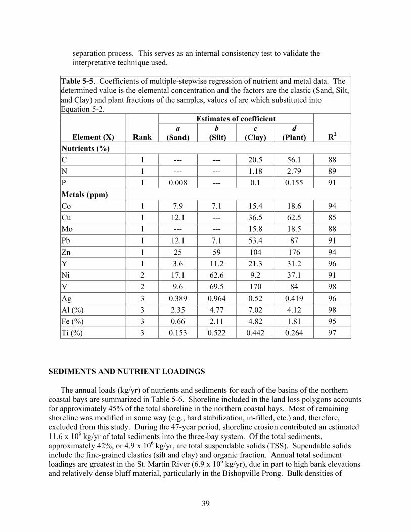
39

separation process. This serves as an internal consistency test to validate the interpretative technique used.

Table 5-5. Coefficients of multiple-stepwise regression of nutrient and metal data. The determined value is the elemental concentration and the factors are the clastic (Sand, Silt, and Clay) and plant fractions of the samples, values of are which substituted into Equation 5-2.

Estimates of coefficient

Element (X)

Rank a

(Sand) b

(Silt) c

(Clay) d

(Plant)

R2 Nutrients (%) C 1 --- --- 20.5 56.1 88 N 1 --- --- 1.18 2.79 89 P 1 0.008 --- 0.1 0.155 91 Metals (ppm) Co 1 7.9 7.1 15.4 18.6 94 Cu 1 12.1 --- 36.5 62.5 85 Mo 1 --- --- 15.8 18.5 88 Pb 1 12.1 7.1 53.4 87 91 Zn 1 25 59 104 176 94 Y 1 3.6 11.2 21.3 31.2 96 Ni 2 17.1 62.6 9.2 37.1 91 V 2 9.6 69.5 170 84 98 Ag 3 0.389 0.964 0.52 0.419 96 Al (%) 3 2.35 4.77 7.02 4.12 98 Fe (%) 3 0.66 2.11 4.82 1.81 95 Ti (%) 3 0.153 0.522 0.442 0.264 97

SEDIMENTS AND NUTRIENT LOADINGS

The annual loads (kg/yr) of nutrients and sediments for each of the basins of the northern coastal bays are summarized in Table 5-6. Shoreline included in the land loss polygons accounts for approximately 45% of the total shoreline in the northern coastal bays. Most of remaining shoreline was modified in some way (e.g., hard stabilization, in-filled, etc.) and, therefore, excluded from this study. During the 47-year period, shoreline erosion contributed an estimated 11.6 x 106 kg/yr of total sediments into the three-bay system. Of the total sediments, approximately 42%, or 4.9 x 106 kg/yr, are total suspendable solids (TSS). Supendable solids include the fine-grained clastics (silt and clay) and organic fraction. Annual total sediment loadings are greatest in the St. Martin River (6.9 x 106 kg/yr), due in part to high bank elevations and relatively dense bluff material, particularly in the Bishopville Prong. Bulk densities of

40

sediments collected from bluffs averaged 1.4 g/cm3. Total sediment loadings from shore erosion in Assawoman Bay are about half those of St. Martin River (3.2 x 106 kg/yr), and those in Isle of Wight Bay are even lower (1.5 x 106 kg/yr). Much of the shoreline bordering Assawoman and Isle of Wight is low-lying marsh composed of sediments with average bulk densities of 0.4 g/cm3.

Sand-sized sediments account for approximately 57% of the total sediments contributed from

shoreline erosion. More than one-third of the sand is eroded from the St. Martin River shoreline (Fig. 5-9). Sand is probably deposited locally, as indicated by the sand that has collected immediately offshore of the bluff sites. Eroded sand tends to remain in the vicinity of its source. Except under extremely high flow conditions, sand is generally not considered suspendable. Given the volume of sand eroding into the St. Martin River, one would expect to find a mixture of sandy sediments on the river bottom. Wells and others (1994) mapped fine sediments in the St. Martin River (refer to Fig. 3-4), based on sampling sites located some distance from shore. They probably missed areas covered with sand-sized sediments.

Table 5-6. Summary of annual loadings of sediments and nutrients contributed by shoreline erosion in the northern coastal bays. The length of the 1989 shoreline applies only to the shoreline included in the land loss polygons (Fig. 4-1).

Basin

Component Assawoman Bay

Bishopville Prong

Shingle Landing

Prong

St. Martin River

Isle of Wight Bay Total

1989 shoreline length (m) 81,164 16,269 12,403 30,706 25,296 165,839

Annual volume of erosion (m3/yr) 6,731 2,178 1,002 4,531 3,043 17,485

Total sediments (kg/yr) 3,206,065 3,037,005 1,271,018 2,580,549 1,471,477 11,566,114

Total organics (kg/yr) 804,329 63,831 39,031 435,512 345,508 1,688,212

Carbon (kg/yr) 214,743 4,979 7,329 110,090 87,424 424,565

Nitrogen (kg/yr) 11,649 603 603 6,041 4,477 23,373

Phosphorus (kg/yr) 1,070 161 96 520 497 2,344Pb (kg/yr) 80 33 13 53 29 208Zn (kg/yr) 182 91 43 126 77 519

Total clastics (kg/yr) 2,401,736 2,973,173 1,231,987 2,145,036 1,125,969 9,877,902

Sand (kg/yr) 1,054,523 2,462,059 1,027,552 1,513,751 515,740 6,573,625

Silt (kg/yr) 768,639 188,739 120,419 290,110 381,012 1,748,918

Clay (kg/yr) 578,574 230,862 84,016 318,582 229,217 1,441,251

Gravel (kg/yr) 114,108 114,108

41

Figure 5-9. Loadings of sand, silt, and clay for each land loss polygon. Gravel, which accounts for less than 1% of the total sediment load, is not shown. Only samples collected in Polygons 16, 17, and 18 contained gravel.

Comparison with existing models and previous studies

Tables 5-7 and 5-8 summarize total nitrogen (TN) and total phosphorus (TP) loads from

various sources for the northern coastal bays. Loading figures are taken from two reports: UM and CESI (1993) and MDE (2001). For comparison, the loading estimates for TN and TP from this study are included in the tables. The estimates from the UM and CESI and the MDE reports are presented in this discussion as the range of values for nitrogen and phosphorus loadings into the northern coastal bays. The UM and CESI estimates are about twice those reported by MDE. UM and CESI attributed a large proportion of the runoff loading to feedlot operations, the discharge from which was assumed to enter streams directly. MDE considered the UM and CESI feedlot calculations to be too high (Sajan Pokharel, pers. comm.). Instead, MDE treated feedlot operations as confined and used urban land use loading rates to calculate their loadings. Although MDE used the UM and CESI loading coefficients to calculate runoff based on land use, they updated the land use acreage, using 1997 data. The loading estimates reported by MDE are more conservative, representing an annual baseline loading for the study area. MDE loading estimates were used in developing TMDLs for the northern bays. Neither report considered contributions from shore erosion. Shoreline erosion represents a significant source of TN and TP loadings to the bays. Depending on the nutrient budget used for comparison (Fig. 5-10), shore erosion contributes between 4.1% to 8.5% of the total nitrogen and 4.7% to 8.5% of the total phosphorus delivered to Maryland’s northern coastal bays. Nutrient contributions from shoreline erosion slightly exceed input from known point sources.

42

Table 5-7. Annual total nitrogen (TN) and total phosphorus (TP) loadings (kg/yr) to the northern coastal bays, based on the UM and CESI (1993) report. Total loadings contributed from shoreline erosion are included for comparison.

Basin 1 Point sources1

Non-point sources 2

Atmospheric sources 3

Shore erosion

(this study)

Total loading

Nitrogen loading (kg/yr) Assawoman Bay 0 52,091 39,800 11,649 103,540Isle of Wight Bay 0 91,218 32,902 4,477 128,597St. Martin River 18,290 302,867 12,382 7,247 340,786 Total 18,290 446,179 85,084 23,373 572,923

Phosphorus loading (kg/yr) Assawoman Bay 0 4,776 1,602 1,070 7,448Isle of Wight Bay 0 8,944 1,324 497 10,765St. Martin River 1,569 28,897 498 777 31,741 Total 1,569 42,617 3,424 2,344 49,954

1 Point source data for nitrogen and phosphorus were developed by Coastal Environmental Services, Inc., based on information from the Maryland Dept. of the Environment. Data are for 1990-91. 2 Non point sources include surface water inputs (runoff), groundwater inputs and inputs from chicken rendering operations. Loading from direct groundwater discharge into the northern coastal bays (from Snug Harbor to Maryland/Delaware line) were estimated using Ritter (1986) coefficients: TN= 123,804 kg/yr and TP=9,420 kg/yr. 3 Atmospheric inputs represent total nitrogen and phosphorus deposition in wet-fall directly to the surface of bay waters, based on an average annual rainfall of 43.8 inches/yr reported for 1990. Concentrations of TN and TP are from Smullen and others (1982).

The N:P (mass ratio) loading ratio for material eroded from the shoreline is about 10:1. This

ratio is consistent with loading ratios based on both UM and CESI data (N:P = 12:1) and MDE data (N:P = 10:1), both of which are higher than the Redfield ratio (N:P = 7.2:1). The differences are related to the types of nutrient sources (Table 5-3).

In Table 5-9, annual TSS, Pb, and Zn loadings from the UM and CESI report are compared

with estimates from this study (MGS). (MDE did not report loading components other than TN and TP.) The annual TSS loadings reported by UM and CESI represent suspended solids delivered by overland runoff. That amount is about three times the TSS contributed by shoreline erosion for the entire study area. However, in Assawoman Bay, the annual contribution of TSS from shoreline erosion is slightly more than input from runoff. Conversely, in the St. Martin River, the annual TSS load from overland runoff is five times that contributed from shoreline erosion.

The sand:mud ratio of sediments contributed from shoreline erosion is 2:1. In the St. Martin River, the ratio is much larger, 4:1. However, the sand:mud ratio of 1:1 reported for the bottom sediments (Wells and others, 1994) in the northern coastal bays does not reflect this large influx of sand. The difference in sand proportions may be accounted for by the contribution of fine-grained material from upland runoff, which has the effect of “diluting” the sand being eroded from the shoreline, explaining the preponderance of fine-grained sediments mapped in the river.

43

Assuming that the 15.1 x 106 kg/yr of TSS from runoff reported by UM and CESI has approximately the same percentage of organics as the sediment contributed from shoreline erosion (i.e. 34.6% organics), then the mud portion of the TSS contributed from upland runoff is 9.81 x 106 kg/yr. The total mud contribution from shoreline erosion and upland runoff would be 13.00 x 106 kg/yr. When compared to the sand contribution of 6.57 x 106 kg/yr from shoreline erosion (assuming that no sand is being contributed from upland runoff), the sand:mud ratio of sediment entering the northern bays is 1:2. To bring the ratio to 1:1, other sources of sand may be assumed, contributions on the order of 6.43 x 106 kg/yr of sand from wind deposits and overwash across Fenwick Island and loads transported through the Inlet.

Shoreline erosion contributes significant amounts of Pb and Zn, accounting for 4% and 9.5%, respectively, of the total loadings of these metals from runoff into the bays. However, these percentages may be high. UM and CESI calculated annual loading values for Pb and Zn based on runoff from urban land only, coefficient factors for the two metals being equal. Runoff coefficients for other non-urban land were unavailable at the time. Table 5-8. Annual total nitrogen (TN) and total phosphorus (TP) loadings (kg/yr) to the northern coastal bays, based on TMDL study for the same study area (MDE, 2001). Total loadings contributed from shoreline erosion are included for comparison.

Basin Point sources

Overland runoff

Ground-water

discharge1

Atmospheric deposition

Shore erosion

(this study)

Total loadings

Nitrogen loading (kg/yr) Assawoman Bay 0 35,086 4,386 23,182 11,649 74,302Isle of Wight Bay* 0 33,472 4,385 24,377 4,477 66,710St. Martin River 16,621 117,001 1,258 7,599 7,247 149,726 TOTAL 16,621 185,559 10,028 55,157 23,373 290,738

Phosphorus loading (kg/yr) Assawoman Bay 0 4,293 N/R 1,431 1,070 6,795Isle of Wight Bay* 0 3,732 N/R 1,533 497 5,762St. Martin River 1,051 13,941 N/R 431 777 16,200 TOTAL 1,051 21,967 3,395 2,344 28,7571 The direct groundwater loads for TN were estimated based on methods described in Dillow and Greene (1999). Direct discharge to the northern coastal bays was separated out from the total reported by John Dillow. MDE did not report groundwater loads for TP.

44

Table 5-9. Comparison of the UM and CESI (1993) loadings and MGS estimates from shoreline erosion for total suspended solids (TSS), Pb and Zn. All loads in kg/yr.

UM and CESI (1993) MGS (This study)

Basin TSS Pb Zn TSS Pb Zn Assawoman Bay 1,918,741 832 832 2,151,542 80 182 Isle of Wight 4,184,314 2,642 2,642 955,737 29 77 St. Martin River 8,992,063 1,493 1,493 1,771,102 99 260 Total 15,095,118 4,967 4,967 4,878,381 208 519

Figure 5-10. Annual total nitrogen and total phosphorus loads entering the northern coastal bays, revised to include contributions from shoreline erosion. Top pie charts depict annual loads based on loading report by UM and CESI (1993). The bottom pie charts depict annual loads based on loadings reported by MDE (2001).

45

6. CONCLUSIONS

Anthropogenic loading of nutrients, metals, and sediment and shoreline armoring alter the natural cycles that operate in the evolution of the coastal bays. These alterations affect the ecosystem of the coastal bays, changing biological communities and the physical structure of the system. Stewardship of these resources requires balancing human impacts to minimize the effects on these natural cycles, while allowing the watersheds to be used for a variety of commercial and residential purposes. Understanding the relative contribution and effects of each of the inputs to the system allows for effective management of the ecosystem. The contribution of shoreline erosion as a component of the natural cycles in the coastal bays was unknown prior to this study. This study has found:

§ Rather than relying on general sediment density estimates, this study directly measured sediments for bulk density, improving the accuracy of nutrient load estimates. § While shoreline erosion contributes a considerable load of suspendable solids, the contribution is about 1/3 that from overland runoff. In Assawoman Bay, TSS loads from shoreline erosion exceed those contributed from upland runoff. On the other hand, runoff is the dominant source of TSS in Isle of Wight Bay and the St. Martin River, where the bulk of the TSS is delivered from the major tributaries (Bishopville and Shingle Landing Prongs, Turville and Manklin Creeks). § Shoreline erosion is a dominant source of sand into the northern bay system, contributing approximately 6.57 x 106 kg/yr or about half of the sand coming into the bays. Other sources include sand transported through the Inlet and carried across Fenwick Island by wind and overwash. Presumably, upland runoff contributes an insignificant amount of sand. Sand is important in maintaining a healthy balance of bottom habitats in the bays. § Shoreline erosion is a significant source of nutrients, contributing between 4.1% to 8.5% of the total nitrogen and 4.7% to 8.5% of the total phosphorus delivered to Maryland’s northern coastal bays. Nutrient contributions from shoreline erosion slightly exceed input from point sources, and are comparable to, but lower than, atmospheric sources. However, the total nitrogen and total phosphorus measurements do not distinguish among the different forms of the nutrients (i.e., nitrates, ammonia, orthophosphate, etc.) and do not reflect how much of the total may be available for biological uptake. § In addition to nutrients, shoreline erosion contributes 208 kg/yr of Pb and 519 kg/yr of Zn, accounting for 4% and 9.5 % of the total loadings of those metals, respectively, to the bays. RECOMMENDATIONS § This report provides initial estimates of the sediment and nutrient loads contributed by shoreline erosion. The load calculations are based on two assumptions: 1) the component concentrations, averaged for each site, reflect the average lithology along the shoreline within a given polygon and 2) bank heights are uniform throughout any given land loss polygon, and the

46

banks themselves are vertical, rather than sloping. To refine these estimates, additional field work and analyses are required.

§ Loadings reflect the average annual input over a 47-year period (between 1942 and 1989). The assumption is that contribution rates also apply for the period between 1989 and the present and will continue for some time in the future. Additional study should look at contributions from erosion in the future based on projected rates of sea level rise and resulting changes in shoreline configuration (refer to Volonté and Leatherman, 1992).

47

7. REFERENCES Anderson, I.C., Miller, W. D., and Neubauer, S. C., 1997, The effects of wrack

deposition and increased inundation frequency on production and respiration in Spartina patens/Distichlis spicata salt marsh: Virginia Coast Reserve Long Term Ecological Research (VCR_LTER) All Scientists Meeting, June 1997, VIMS, College of William and Mary, Gloucester Pt., Va.

Bartberger, C.E., 1973, Origin, Distribution, and Rates of Accumulation of Sediments in

Chincoteague Bay, Maryland and Virginia (Master’s Thesis, Syracuse University), 167 p.

Bartberger, C.E., 1976, Sediment sources and sedimentation rates, Chincoteague Bay,

Maryland and Virginia: Jour. Sed. Pet., vol. 46, p. 326-336. Bartberger, C.E., and Biggs, R.B., 1970, Sedimentation in Chincoteague Bay, in Natural

Resources Institute, University of Maryland, Oct. 1970, Assateague ecological studies, Part II: Environmental threats, Contribution #446, Chesapeake Biological Lab, Solomons, Md., p. 70-90.

Bennett, R.H., and Lambert, D.V., 1971, Rapid and reliable technique for determining

unit weight and porosity of deep-sea sediments: Marine Geology, vol. 11, p. 201-207. Berner, R.A., 1967, Diagenesis of iron sulfide in recent marine sediments, in Lauff, G.,

ed., Estuaries: Washington, D.C., American Association for the Advancement of Science Special Pub. 83, p. 268-272.

Berner, R.A., 1970, Sedimentary pyrite formation: American Journal of Science, v. 268,

p. 1-23. Conkwright, R.D., 1975, Historical Shorelines and Erosion Rates Atlases: Maryland

Geological Survey, Baltimore, Md., 4 volumes. Dillow, J.J.A., and Green, E.A., 1999, Ground-water discharge loadings to the coastal

bays of Maryland: U.S. Geological Survey Water-Resources Investigations Report 99-4167, 8 p.

Dolan, R., Lins, H., and Stewart, J., 1980, Geographical analysis of Fenwick Island,

Maryland, a Middle Atlantic coast barrier island: U.S. Geological Survey Professional Paper 1177-A, 24 p.

Fisher, J.J., 1967, Origin of barrier island chain shoreline, Middle Atlantic states: Geol.

Soc. Amer. Special Paper 115, p. 66-67. GSA, 1991, Rock-Color Chart, Geological Society of America, Boulder CO.

48

Goldhaber, M.B., and Kaplan, I.R., 1974, The sulfur cycle, in Goldberg, E.D. (ed.), The Sea, Volume 5, Marine Chemistry: New York, Wiley-Interscience, p. 569-655.

Hennessee, L., 2001, Acquiring a modern digital shoreline for Maryland from recent

(1988-1995) orthophotography (Coastal and Estuarine Geology File Report No. 00-7): Maryland Geological Survey, Baltimore, Md., 18 p.

Hennessee, L., and Stott, J., 1999, Shoreline changes and erosion rates for the northern

coastal bays of Maryland (Coastal and Estuarine Geology File Report No. 99-7): Maryland Geological Survey, Baltimore, Md., 30 p.

Hennessee, L., Stott, J., and Bethke. T., 2002a, Shoreline changes and erosion rates for

the southern coastal bays of Maryland (Coastal and Estuarine Geology File Report No. 00-1): Maryland Geological Survey, Baltimore, Md., 41 p.

Hennessee, E.L., Valentino, M., Lesh, A.M., and Myers, L., 2002b, Determining shoreline erosion rates for the coastal regions of Maryland (Part 1) (Coastal and Estuarine Geology File Report No. 02-04): Maryland Geological Survey, Baltimore, Md., 32 p.

Hill, J.M., Hennessee, E.L., Park, M.J., and Wells, D.V., 1990, Interpretive techniques

for assessing temporal variability of trace metal levels in estuarine sediments (Abst): Goldschmidt Conference, Hunt Valley, Md.

Ibison, N.A., Frye, C.W., Frye, J.E., Hill, C.L., and Burger, N.H., 1990, Sediment and

nutrient contributions of selected eroding banks of the Chesapeake Bay estuarine system (Technical Report to Council on the Environment for Coastal Zone Management Grant #NA88AA-D-CZ092): Department of Conservation and Recreation, Division of Soil and Water Conservation, Shoreline Programs Bureau, Gloucester Point, Va., 71 p.

Ibison, N.A., Baumer, J.C., Hill, C.L., Burger, N.H., and Frye, J.E., 1992, Eroding bank

nutrient verification study for the lower Chesapeake Bay: Department of Conservation and Recreation, Division of Soil and Water Conservation, Shoreline Programs Bureau, Gloucester Point, Va., 80 p.

Krumbein, W.C., and Pettijohn, F.J., 1938, Manual of sedimentary petrography: New

York, Appleton-Century-Crofts, 549 pp. Leatherman, S.P., 1983, Historical and projected shoreline changes, Ocean City and

northern Assateague Island, Maryland: Technical Report No. 79, Maryland Water Resources Research Center, University of Maryland, College Park, Md., 39 p.

Maryland Coastal Bays Program (MCBP), 1999, Today’s treasures for tomorrow:

towards a brighter future: a comprehensive conservation and management plan for Maryland’s Coastal Bays, Berlin, Md., 181 p.

49

Maryland Department of the Environment (MDE), 2001, Total maximum daily loads of nitrogen and phosphorus for five tidal tributaries in the northern coastal bays system, Worcester County, Maryland, Final Report submitted to Watershed Protection Division, USEPA, Region III, Dec. 2001.

NOAA, 1988, NOAA/NOS-CERC cooperative shoreline movement study: Part II- Cape

Henlopen, DE - Cape Charles, VA, 16 maps, 1:24,000 scale, National Ocean Service, Washington, D.C.

Owens, J.P., and Denny, C.S., 1978, Geologic Map of Worcester County, scale 1:62,500:

Maryland Geological Survey, Baltimore, Md. Owens, J.P., and Denny, C.S., 1979, Upper Cenozoic deposits of the central Delmarva

Peninsula, Maryland and Delaware: U.S. Geol. Survey. Prof. Paper 1067-A, 28 p. Pokharel, Sajan, personal communication, email dated July 31, 2002, from Mr. Pokharel

of the Computer Modeling Program, Technical and Regulatory Services Administration (TARSA), Maryland Dept. of the Environment, re: comparison of MDE TMDL loading calculations for total nitrogen and total phosphorus with those of UM and CESI report (1993).

Redfield, A.C., Ketchum, B.H., and Richards, F.A., 1963, The influence of organisms on

the composition of sea-water, in Hill, M.N. (ed.), The Sea, Volume 2, The Composition of Sea-water, Comparative and Descriptive Oceanography: London, Interscience, p. 26-77.

Ritter, W.F., 1986, Nutrient budgets for the inland bays, Document # FPR-86-001,

Agriculture Engineering Dept., Delaware Agricultural Experiment Station, Univ. of Delaware, Newark, Del.

Schwimmer, R.A., 2001, Rates and processes of marsh shoreline erosion in Rehoboth

Bay, Delaware, U.S.A.: Jour. Coastal Research, vol. 17, p. 672-683. Shepard, F.P., 1954, Nomenclature based on sand-silt-clay ratios: Jour. Sed. Petrology,

vol. 24, p. 151-158. Sinex, S.A., and Helz, G.R., 1981, Regional geochemistry of trace elements in

Chesapeake Bay sediments: Environ. Geol., vol. 3, p. 315-323. Singewald, J.T., and Slaughter, T.H., 1949, Shore Erosion in Tidewater Maryland:

Maryland Department of Geology, Mines, and Mineral Resources, Baltimore, Md., Bulletin 6, 141 p.

Smullen, J. T., Taft, J. L., and Macknis, J., 1982, Nutrient and sediment loads to the tidal

Chesapeake Bay system in Chesapeake Bay Program technical studies: a synthesis: U.S. Environmental Protection Agency, Annapolis, Md., p. 150-251.

50

Stevenson, J.C., Ward, L.G., Kearney, M.S., and Jordan, T.E., 1985, Sedimentary

processes and sea level rise in tidal marsh systems of Chesapeake Bay: Proceedings of the Conference on Wetlands of the Chesapeake – Protecting the future of the Bay, April 1985, Easton, Md., Environmental Law Institute Publication, p. 37-62.

Stott, J.A., Hennessee, E.L., and Kerhin, R.T., 1999, 2000, Shoreline Changes: Maryland

Geological Survey, Baltimore, Md., 9 maps. Taylor, S.R., 1964, The abundance of chemical elements in the continental crusts – a new

table: Geochim. Cosmochim. Acta, vol. 28, p. 283-294. Toscano, M.A., 1992, Record of Oxygen Isotope Stage 5 on the Maryland inner shelf

Atlantic Coastal Plain – A post-transgressive-highstand regime in Wehmiller, J.F. and Fletcher, C.H. (eds.), Quaternary Coasts of the United States: Lacustrine and Marine Systems: Society of Economic Paleontologists and Mineralogists (SEPM) Special Publication No. 48, p. 89-99.

Toscano, M.A., Kerhin, R.T., York, L. L., Cronin, T. M., and Williams, S. J., 1989,

Quaternary stratigraphy of the inner continental shelf of Maryland: Maryland Geological Survey Report of Investigations No. 50, Baltimore, Md., 117 pp.

Toscano, M.A. and York, L. L., 1992, Quaternary stratigraphy and sea- level history of

the U.S. middle Atlantic Coastal Plain: Quaternary Sci. Rev., vol. 11, p. 301-328. Truitt, R.V., 1968, High winds – high tides: a chronicle of Maryland's coastal hurricanes:

Univ. of Maryland, Nat. Res. Inst., Ed. Ser. No. 77, 35 pp. University of Md. (UM), and Coastal Environmental Services, Inc. (CESI), 1993,

Maryland's coastal bays: An assessment of aquatic ecosystems, pollutant loadings, and management options: submitted to Maryland Dept. of the Environment, Chesapeake Bay and Special Projects Branch, Baltimore, Md.

U.S. Army Corps of Engineers, 1962, The March 1962 storm along the coast of

Maryland: Report of District activities during and immediately following the storm, Baltimore District, Baltimore, Md., 21 p.

Van Loon, J.C., 1980, Analytical Atomic Absorption Spectroscopy: Selected Methods:

Academic Press, New York, 337 p. Volonté, C.R., and Leatherman, S.P., 1992, Future sea level rise impacts: Maryland’s

Atlantic coastal bays (Report prepared for the Maryland Department of Natural Resources through a grant from the Coastal and Watershed Resources Division (No. NA17OZ0497-01): University of Maryland Geography Department, College Park, Md., 97 p.

51

Wells, D.V., and Kerhin, R.T., 1982, Geological analysis and re-evaluation of Isle of Wight shoals as a potential borrow site: report submitted to Tidewater Administration, 33 p.

Wells, D.V., Conkwright, R.D., Hill, J.M., and Park, M.J., 1994, The surficial sediments

of Assawoman Bay and Isle of Wight Bay in Maryland: Physical and chemical characteristics (Coastal and Estuarine Geology File Report No. 94-2): Maryland Geological Survey, Baltimore, Md., 99 p.

Wells, D.V., Conkwright, R.D., Gast, R., Hill, J.M., and Park, J., 1996, The surficial

sediments of Newport Bay and Sinepuxent Bay in Maryland: Physical and chemical characteristics (Coastal and Estuarine Geology File Report No. 96-2): Maryland Geological Survey, Baltimore, Md., 116 p.

Wells, D.V., and Conkwright, R.D., 1999, Maryland coastal bays sediment mapping

project: Physical and chemical characteristics of the sediments – Atlas and Synthesis Report (Coastal and Estuarine Geology File Report No. 99-5) in HTML format: Maryland Geological Survey, Baltimore, Md., on Compact Disk (CD-ROM).

Wells, D.V., and Ortt, R.A., Jr., 2001, Bathymetric survey of Assawoman Bay, St. Martin

River, Sinepuxent Bay and Newport Bay (Coastal and Estuarine Geology File Report No. 01-2): Maryland Geological Survey, Baltimore, Md., on Compact Disk (CD-ROM).

53

APPENDIX A

Site descriptions (field notes, photos, cross sections, profiles)

Core logs (core descriptions, lithology, radiographs, photos)

Note: In the radiographs, sediment layers with more plant material, which is nearly transparent to x-rays, appear as darker areas in the image. Layers with higher percentages of clastics (i.e., sand-, silt-, and clay-sized minerals) are denser or more opaque to x-rays and appear as lighter areas. White layers represent denser lenses of sediment, not necessarily composed of sand, but containing a higher percentage of clastics (non-plant material).

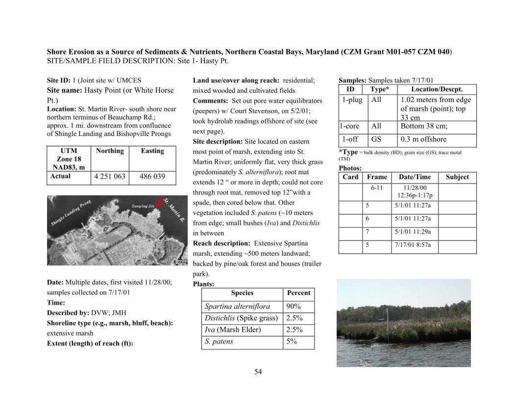
Shore Erosion as a Source of Sediments & Nutrients, Northern Coastal Bays, Maryland (CZM Grant M01-057 CZM 040) SITE/SAMPLE FIELD DESCRIPTION: Site 1- Hasty Pt.

54

Site ID: 1 (Joint site w/ UMCES Site name: Hasty Point (or White Horse Pt.) Location: St. Martin River- south shore near northern terminus of Beauchamp Rd.; approx. 1 mi. downstream from confluence of Shingle Landing and Bishopville Prongs

UTM Zone 18

NAD83, m

Northing Easting

Actual 4 251 063 486 039

Date: Multiple dates, first visited 11/28/00; samples collected on 7/17/01 Time: Described by: DVW; JMH Shoreline type (e.g., marsh, bluff, beach): extensive marsh Extent (length) of reach (ft):

Land use/cover along reach: residential; mixed wooded and cultivated fields Comments: Set out pore water equilibrators (peepers) w/ Court Stevenson, on 5/2/01; took hydrolab readings offshore of site (see next page). Site description: Site located on eastern most point of marsh, extending into St. Martin River; uniformly flat, very thick grass (predominately S. alterniflora); root mat extends 12 “ or more in depth; could not core through root mat, removed top 12”with a spade, then cored below that. Other vegetation included S. patens (~10 meters from edge; small bushes (Iva) and Distichlis in between Reach description: Extensive Spartina marsh, extending ~500 meters landward; backed by pine/oak forest and houses (trailer park). Plants:

Species Percent

Spartina alterniflora 90% Distichlis (Spike grass) 2.5% Iva (Marsh Elder) 2.5% S. patens 5%

Samples: Samples taken 7/17/01 ID Type* Location/Descpt.

1-plug All 1.02 meters from edge of marsh (point); top 33 cm

1-core All Bottom 38 cm;

1-off GS 0.3 m offshore *Type = bulk density (BD); grain size (GS); trace metal (TM) Photos:

Card Frame Date/Time Subject 6-11 11/28/00

12:36p-1:17p

5 5/1/01 11:27a

6 5/1/01 11:27a

7 5/1/01 11:29a

5 7/17/01 8:57a

Shore Erosion as a Source of Sediments & Nutrients, Northern Coastal Bays, Maryland (CZM Grant M01-057 CZM 040) SITE/SAMPLE FIELD DESCRIPTION: Site 1- Hasty Pt.

55

Plan view (sample locs; site features, reach & beach extents)

Stratigraphic section

Stadia readings (see fig to right for locations) Pt. Top Mid Bot Dist

(from level)(ft)

Bank Hgt (ft)

Comments

Level Λ 4.62 0 1 4.84 4.77 4.70 14 2 5.19 5.04 4.89 30 1.83 By Court’s post 3 7.025 6.87 6.715 31 Base of marsh 4 7.71 7.51 7.31 40 Off shore 5 4.905 4.80 4.69 43 1.615 Top of marsh 6 6.52 6.415 6.30 22 Base of marsh 7 4.78 4.64 4.50 28 1.8 Top of marsh 8 6.59 6.44 6.29 30 Base of marsh 9 4.78 4.525 4.25 53 10 4.79 4.515 4.24 55 Hydrolab readings taken 5/2/01 1:35 pm EDT Temp. (degrees C) 21.7 Salinity (ppt) 24.25 DO (mg/l) 8.89 113% SaturationpH 5.88 Turb. (ntu) 9.8 Depth (m) 1.5

Shore Erosion as a Source of Sediments & Nutrients, Northern Coastal Bays, Maryland (CZM Grant M01-057 CZM 040) SITE/SAMPLE DESCRIPTION: Site 3- Windmill Creek

56

Site ID: 3 Site name: Windmill Creek Location: Shingle Landing Prong- south shore, north side of the mouth of Windmill Creek

UTM Zone 18

NAD83, m

Northing Easting

Actual 4 250 799 484 364

Date: 5/01/01 Time: 12:33 pm EDT Described by: Jim Hill Shoreline type (e.g., marsh, bluff, beach): bluff fronted by narrow beach

Bank elevation (ft): Above water: see stadia data Below water Land use/cover along reach: forest behind bluffs Site description: Fine sand beach with ~12 ft bluff backing beach; top of bluffs moderately to highly vegetated; mix pine/oak with shrubs, low trees under-story (pred. Maples, bayberry and holly). Off shore bottom sediments very red, clayey. Reach description: Bluffs along eroding headland, extending ~300 meters, southeast end truncated by a spit at mouth of Windmill Ck., north end truncated by shallow cove. Plants:

Species Percent

Pine 35

Oak 35

Maple 10

Bayberry 10

holly 10

Samples: ID Type* Location**

3-T All Top layer of bluff

3-B All Bottom of bluff; clay layer

3-beach GS Grab from beach

3-Off GS Grab offshore *Type = bulk density (BD); grain size (GS); trace metal (TM) **Location = show on stratigraphic section Stratigraphic section: Top 7.8 ft sandy loam, weathering to reddish color; sharp contact, below it greenish clayey sand, very hard, dry; part of bluff face is vegetated

Shore Erosion as a Source of Sediments & Nutrients, Northern Coastal Bays, Maryland (CZM Grant M01-057 CZM 040) SITE/SAMPLE DESCRIPTION: Site 3- Windmill Creek

57

Site 3- Windmill Creek Stadia Readings Stadia rod intercept (Feet) Feet Meters

Pt. top middle bottom Dist Elev Dist Elev 1 15.69 15.48 15.25 44 0 13.41 0.00 WL 2 14.52 14.37 14.22 30 1.11 9.14 0.34 Beach, Beach grab sample 3 13.99 13.87 13.74 25 1.61 7.62 0.49 Base of bluff 4 13.35 13.23 13.11 24 2.25 7.32 0.69 Clay, bluff sample 5 11.94 11.86 11.78 16 3.62 4.88 1.10 Sand/clay interface 6 8.26 8.24 8.2 6 7.24 1.83 2.21 Sand, Bluff sample

Tripod 4.04 0 11.44 0.00 3.49 Top of bluff

Site 3- Windmill Creek

0.00

1.00

2.00

3.00

4.00

0 2 4 6 8 10 12 14 16

Meters

Meters

Shore Erosion as a Source of Sediments & Nutrients, Northern Coastal Bays, Maryland (CZM Grant M01-057 CZM 040) SITE/SAMPLE DESCRIPTION: Site 4 - Bishopville Prong

58

Site ID: 4 Site name: Bishopville Prong Location: East bank of Bishopville Prong, just north of public boat ramp (Shell Mill Landing)

UTM Zone 18

NAD83, m

Northing Easting

Actual 4 252 930 483 615

Date: 4/30/01 Time: 12:28 EDT Described by: DVW/JMH Shoreline type (e.g., marsh, bluff, beach): bluff Extent (length) of reach (ft): Bank elevation (ft): 2.7 m Land use/cover along reach: forested; south end of bluff backed by parking lot

Site description: Fine sand muddy beach with ~8 ft bluff backing beach; top of bluffs moderately vegetated; mix pine/oak with shrubs. Some grass along beach. Reach description: Low bluffs along east bank of Bishopville Prong, just upstream of boat ramp, extending north ~250 ft (~80 m), to small stream, salt marsh. Bluffs continue upstream. Both sides of river characterized by vegetated bluffs, heights varying from 6 to 10 ft. North end: N 4 252 977 E 483 630 UTM South end: N 4 252 900 E 483 608 Plants:

Species Percent

Pine 40

Oak 25

maple 20

other 15


4-T All Top of bluff

4-B All Bottom of bluff

4-beach GS Grab on beach *Type = bulk density (BD); grain size (GS); trace metal (TM) **Location = show on stratigraphic section Photos:

Card Frame Time Subject

2 1 1:18 Dan sampling

2 2 1:19 Dan sampling

2 3 1:19 Bluff from water

2 4 1:20 Bluff close-up

Shore Erosion as a Source of Sediments & Nutrients, Northern Coastal Bays, Maryland (CZM Grant M01-057 CZM 040) SITE/SAMPLE DESCRIPTION: Site 4 - Bishopville Prong

59

Stratigraphic section Bluff appeared to be homogenous in material, yellowish gray sand with some clay, clay content slightly higher toward the top of the bluff; sampled top and bottom. Site 4- Bishopville Prong Stadia Readings Feet Feet Meters

Pt. top middle bottom Dist Elev Dist Elev 5 15.43 15.26 15.09 34 0 10.36 0.00 Water 4 13.62 13.52 13.42 20 1.74 6.10 0.53 Sample Base of bluff 3 10.29 10.21 10.13 16 5.05 4.88 1.54 2 6.52 6.46 6.4 12 8.8 3.66 2.68 Sample 1 5.03 5 4.97 6 10.26 1.83 3.13


Site 4- Bishopville Prong

0.00

1.00

2.00

3.00

4.00

0 2 4 6 8 10 12

Meters

Meters

Shore Erosion as a Source of Sediments & Nutrients, Northern Coastal Bays, Maryland (CZM Grant M01-057 CZM 040) SITE/SAMPLE DESCRIPTION: Site 5 – Photographed bluff

60

Site ID: 5 Site name: Photographed bluff Location: St. Martin River- north shore; opposite Station 1 (Hasty Pt.)

UTM Zone 18

NAD83, m

Northing Easting

Actual 4 251 580 486 313

Date: 5/1/01 Time: 1:54 pm EDT Described by: DVW/JMH Shoreline type (e.g., marsh, bluff, beach): bluff Extent (length) of reach (ft): ~200 meters Bank elevation (ft): 2 m Land use/cover along reach: agriculture/field

Site description: Narrow beach backed by acute bluff stabilized by tree roots; vegetated buffer backed by large field. Bluff composed of laminated deposits w/ pebble lenses. Reach description: Bluffs along eroding headland, extending ~200 meters, truncated on the north end by small stream/marsh and on south end by small cove/marsh. North end: N 4 251 607 E 486 262 UTM South end: N 4 251 476 E 486 398 Plants:

Species Percent

Pine 45

Oak 45

Maple 10


5 All Mid bluff

5-beach

GS Grab on beach

5-off GS Grab offshore *Type = bulk density (BD); grain size (GS); trace metal (TM) **Location = show on stratigraphic section Photos:

Card Frame

Time Subject

1 2:09p Field behind bluff

2 2:09p Beach from top

3 2:09p Level

4 2:23p Close up of bluff face

5 2:24p

6 2:27p Bluff face w/Dan

Shore Erosion as a Source of Sediments & Nutrients, Northern Coastal Bays, Maryland (CZM Grant M01-057 CZM 040) SITE/SAMPLE DESCRIPTION: Site 5 – Photographed bluff

61

Stratigraphic section Lamination evenly distributed along height of bluff, yellowish gray sand with gravel lenses and trace of clay. Photo to the right: Bluff face with Dan Sailsbury holding stadia rod. Bluff is approximately 2 meters high. Profile of bluff is shown below. Site 5- St. Martin River, opposite of Hasting Pt. (Site #1) Stadia Readings Feet Feet Meters

Pt. top middle bottom Dist Elev Dist Elev 1 13.685 13.49 13.295 39 0 11.89 0.00 2 13.27 13.12 12.97 30 0.37 9.14 0.11 Water line 3 12.42 12.31 12.2 22 1.18 6.71 0.36 4 11.32 11.265 11.21 11 2.225 3.35 0.68 5 10.77 10.725 10.68 9 2.765 2.74 0.84 Base of bluff


Site 5- St. Martin River, opposite of Hasting Pt. (Site #1)

0.00

1.00

2.00

3.00

0 2 4 6 8 10 12 14

Meters

Meters

Shore Erosion as a Source of Sediments & Nutrients, Northern Coastal Bays, Maryland (CZM Grant M01-057 CZM 040) SITE/SAMPLE DESCRIPTION: Site 6 – Peach Pt.

62

Site ID: 6 Site name: Peach Point Location: St. Martin River, north shore at mouth of Harry Creek

UTM Zone 18

NAD83, m

Northing Easting

Actual 4 251 114 487 056

Date: 5/1/01 Time: 13:13 EDT Described by: JMH Shoreline type (e.g., marsh, bluff, beach): marsh Extent (length) of reach (ft): 500 m

Bank elevation (ft): 0.7 m (2.2 ft) Land use/cover along reach: Marsh Site description: Sampling site is on small point (Peach Pt.) of marsh on north side of Harry Creek, small tributary flowing into St. Martin River Reach description: Extensive marsh on north side of Harry Creek. Marsh is flat, uniform, Spartina sp. dominating, shoreline irregular. Small stream to the north and Harry Creek to the south truncate reach. Marsh is backed by forest.

Plants: Species Percent

S. alterniflora 90

Iva 5

Limonium 2

Samples:

ID Type* Location

Core 1 All 43 “ from edge of water

Plug 1 All Top 9.5 “ of sediment column

1- off GS Offshore grab *Type = bulk density (BD); grain size (GS); trace metal (TM) Photos:

Date Time Subject

5/1/01 15:29 Marsh toward tree line

5/1/01 15:29 On site w/ JimH and DanS

7/17/01 10:23 DanS and NeilD

Shore Erosion as a Source of Sediments & Nutrients, Northern Coastal Bays, Maryland (CZM Grant M01-057 CZM 040) SITE/SAMPLE DESCRIPTION: Site 6 – Peach Pt.

63

Plan view

Site 6 - Peach Point Stadia data Stadia Readings Ft. Feet Meters

Pt. top middle bottom Dist Elev* Dist Elev Bank Height tripod 4.3 0

1 7.35 7.08 6.81 54 -2.78 16.5 -0.85 2.69 2 4.67 4.39 4.13 54 -0.09 16.5 -0.03 3 4.72 4.48 4.24 48 -0.18 14.6 -0.05 4 4.66 4.48 4.3 36 -0.18 11.0 -0.05 5 4.58 4.49 4.4 18 -0.19 5.5 -0.06 6 6.86 6.71 6.56 30 -2.41 9.1 -0.73 2.245 7 4.61 4.465 4.32 29 -0.165 8.8 -0.05 8 6.35 6.095 5.84 51 -1.795 15.5 -0.55 1.725 9 4.62 4.37 4.12 50 -0.07 15.2 -0.02

*assumed elevation for tripod (level) pt.

Shore Erosion as a Source of Sediments & Nutrients, Northern Coastal Bays, Maryland (CZM Grant M01-057 CZM 040) SITE/SAMPLE DESCRIPTION: Site 7 – Saltgrass Pt.

64

Site ID: 7 Site name: Saltgrass Point Location: On north shore of St. Martin River, in vicinity of Buck Island Pond and Buck Island Creek

UTM Zone 18

NAD83, m

Northing Easting

Actual 4 250 713 488 658

Date: 5/1/01; 7/16/01 Time: 15:45; 16:30 EDT Described by: JMH Shoreline type (e.g., marsh, bluff, beach): marsh Land use/cover along reach: natural

Extent (length) of reach (ft): Bank elevation (ft): 0.7 m (2.4 ft) Site description: Site is on a ‘pinched point” that is almost an island. Mosquito ditching is east of point. Shoreline convoluted. Marsh is flat, uniform, Spartina alternaflora dominating. Abundant mussels covering on top marsh and in sediment. Entire site is very ‘spongy,’ quaking when walking. Reach description: Extensive marsh characterized by very convoluted shoreline, and network of ditching. Several creeks meander through marsh area. Marsh is backed by forest buffer, then agriculture fields. Plants:

Species Percent

Spartina alterniflora 95

Samples: ID Type* Location

Core 7 All 110 “ from edge

Plug 7 All Top 8” of sediment

7-Off GS Grab offshore *Type = bulk density (BD); grain size (GS); trace metal (TM) Photos:

Date Time EDT

Subject

5/1/01 15:56 Level & tripod

5/1/01 16:03 Ditching

7/16/01 16:40 Core site

Shore Erosion as a Source of Sediments & Nutrients, Northern Coastal Bays, Maryland (CZM Grant M01-057 CZM 040) SITE/SAMPLE DESCRIPTION: Site 7 – Saltgrass Pt.

65

Photo: Dan Sailsbury on site with stadia rod. Red flag marks location of core.

Photo: Mosquito ditching east of sampling site.

Plan view

Site 7 - Salt Grass Point Stadia Readings Feet Feet Meters

Pt. top middle bottom Dist Elev* Dist Elev Bank Height 1 8.2 7.88 7.57 63 -3.54 19.2 -1.08 3.23 2 4.96 4.65 4.34 62 -0.31 18.9 -0.09 3 4.66 4.39 4.12 54 -0.05 16.5 -0.02 4 4.55 4.42 4.29 26 -0.08 7.9 -0.02

tripod 4.34 0 0.00 5 6.95 6.78 6.6 35 -2.44 10.7 -0.74 2.20 6 4.75 4.58 4.41 34 -0.24 10.4 -0.07 7 7 6.69 6.38 62 -2.35 18.9 -0.72 1.66 8 5.34 5.03 4.72 62 -0.69 18.9 -0.21


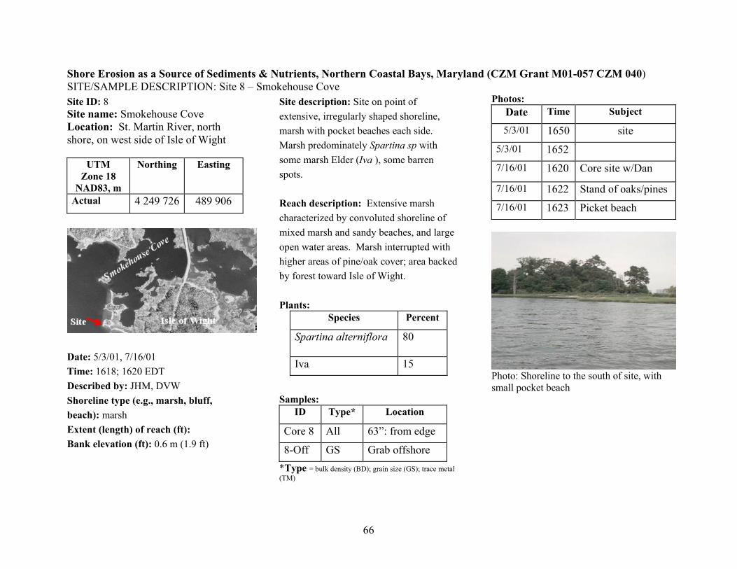
Shore Erosion as a Source of Sediments & Nutrients, Northern Coastal Bays, Maryland (CZM Grant M01-057 CZM 040) SITE/SAMPLE DESCRIPTION: Site 8 – Smokehouse Cove

66

Site ID: 8 Site name: Smokehouse Cove Location: St. Martin River, north shore, on west side of Isle of Wight

UTM Zone 18

NAD83, m

Northing Easting

Actual 4 249 726 489 906

Date: 5/3/01, 7/16/01 Time: 1618; 1620 EDT Described by: JHM, DVW Shoreline type (e.g., marsh, bluff, beach): marsh Extent (length) of reach (ft): Bank elevation (ft): 0.6 m (1.9 ft)

Site description: Site on point of extensive, irregularly shaped shoreline, marsh with pocket beaches each side. Marsh predominately Spartina sp with some marsh Elder (Iva ), some barren spots. Reach description: Extensive marsh characterized by convoluted shoreline of mixed marsh and sandy beaches, and large open water areas. Marsh interrupted with higher areas of pine/oak cover; area backed by forest toward Isle of Wight. Plants:

Species Percent

Spartina alterniflora 80

Iva 15

Samples:

ID Type* Location

Core 8 All 63”: from edge

8-Off GS Grab offshore *Type = bulk density (BD); grain size (GS); trace metal (TM)

Photos: Date Time Subject

5/3/01 1650 site 5/3/01 1652 7/16/01 1620 Core site w/Dan

7/16/01 1622 Stand of oaks/pines 7/16/01 1623 Picket beach

Photo: Shoreline to the south of site, with small pocket beach

Shore Erosion as a Source of Sediments & Nutrients, Northern Coastal Bays, Maryland (CZM Grant M01-057 CZM 040) SITE/SAMPLE DESCRIPTION: Site 8 – Smokehouse Cove Page 67 of 2

67

Plan view

Photo: Site showing pocket beach to the north.

Site 8 - Smokehouse Cove

Stadia Readings Feet Feet Meters Pt. # top middle bottom Dist Elev* Dist Elev Bank Height

1 6.8 6.48 6.16 64 -2.00 19.5 -0.61 2.15 2 4.75 4.33 4.11 64 0.15 19.5 0.05 3 4.48 4.15 3.9 58 0.33 17.7 0.10 core site 4 4.41 4.28 4.15 26 0.20 7.9 0.06

tripod 4.48 0 0.00 0.00 5 6.92 6.65 6.38 54 -2.17 16.5 -0.66 1.72 6 5.18 4.93 4.66 52 -0.45 15.8 -0.14 7 6.48 6.06 5.64 84 -1.58 25.6 -0.48 1.74 8 4.73 4.325 3.91 82 0.16 25.0 0.05


Shore Erosion as a Source of Sediments & Nutrients, Northern Coastal Bays, Maryland (CZM Grant M01-057 CZM 040) SITE/SAMPLE DESCRIPTION: Site 9 – Drum Point

68

Site ID: 9 Site name: Drum Point Location: Assawoman Bay, west shore, first point north of Isle of Wight UTM Zone 18 NAD83, m

Northing Easting

Actual 4 250 598 491 619

Date: 5/1/01; 7/17/01 Time: 1730 EDT Described by: JMH; DVW Shoreline type (e.g., marsh, bluff, beach): marsh Extent (length) of reach (ft): Bank elevation (ft): 0.6 m (2.0 ft) Land use/cover along reach: Golf course

Site description:. Site on end of small ‘pinched’ point, tipped with small island. Fairly flat marsh, backed (~100 yds) by Lighthouse SoundGolf Course. Very little natural vegetation as buffer between Golf Course and marsh areas. Reach description: Reach highly irregular shoreline, with islands, and pocket beaches. In some areas, shoreline protection has been emplaced, particularly where golf greens are near the shoreline (see photo to right with Darlene and Dan surveying: in background two golfer are putting on green located on point north of site. Plants:

Species Percent

Spartina sp. 100


Core 9 All 31” from edge

Plug 9 All Top 7.25” of sediment

9-OFf GS Grab offshore *Type = bulk density (BD); grain size (GS); trace metal (TM) Photos:

Date Time EDT

Subject

5/1/01 1725 Drum Pt.

5/1/01 1730 Golf course

Photo: Level site, looking northwest; golf green in background

Shore Erosion as a Source of Sediments & Nutrients, Northern Coastal Bays, Maryland (CZM Grant M01-057 CZM 040) SITE/SAMPLE DESCRIPTION: Site 9 – Drum Point

69

Photo: Level, looking east toward core site.

Site map: stadia data next page

Site 9 - Drum Point

Stadia Readings Feet Feet Meters Pt. # top middle bottom Dist Elev* Dist Elev Bank Height (ft.)

1 7.62 7.305 6.99 63 -3.02 19.2 -0.92 2.69 2 4.93 4.62 4.31 62 -0.33 18.9 -0.10 3 4.86 4.58 4.3 56 -0.29 17.1 -0.09 core site 4 4.62 4.47 4.32 30 -0.18 9.1 -0.05

tripod 4.29 0 0.00 0.0 0.00 5 6.76 6.63 6.49 27 -2.34 8.2 -0.71 2.06 6 4.7 4.57 4.44 26 -0.28 7.9 -0.09 7 5.99 5.83 5.67 32 -1.54 9.8 -0.47 1.33 8 4.66 4.5 4.34 32 -0.21 9.8 -0.06 *assumed elevation for tripod (level) pt. Ave.-2.03

Shore Erosion as a Source of Sediments & Nutrients, Northern Coastal Bays, Maryland (CZM Grant M01-057 CZM 040) SITE/SAMPLE DESCRIPTION: Site 10 – Tulls Island

70

Site ID: 10 Site name: Tulls Island Location: Assawoman Bay, west shore, unnamed point between Drum Point and Hills Island, immediately west of former Tulls Island.

UTM Zone 18

NAD83, m Northing Easting

Actual 4 251 937 491 272

Date: 5/1/01; 7/17/01 Time: 1740 EDT Described by: JMH; DVW Shoreline type (e.g., marsh, bluff, beach): marsh

Extent (length) of reach (ft): Bank elevation (ft): 0.4 m (1.3 ft) Land use/cover along reach: Golf course; Lighthouse Sound Development (residential) Site description:. Site on end of large island. Fairly flat marsh, irregularly shaped; abundant mussels, some bald (no vegetation) spots. Photo: Behind level, look east toward core site.

Reach description: Reach highly irregular shoreline, with islands, and some pocket beaches. Site on island which recently (within last 25 years) separated from end of extensive peninsula.



Plug 10 All Top 8.5” of

sediment

10-Off GS Grab offshore *Type = bulk density (BD); grain size (GS); trace metal (TM)


Spartina sp. 90 Broad leaf shrub (Iva?)

<10

Photos:

Date Time EDT

Subject

5/1/01 1755 Site with boat, looking due east

5/1/01 1730 Site looking northwest

Shore Erosion as a Source of Sediments & Nutrients, Northern Coastal Bays, Maryland (CZM Grant M01-057 CZM 040) SITE/SAMPLE DESCRIPTION: Site 10 – Tulls Island

71

Photo: Level, looking southeast toward core site (behind boat).

Plan view

Site 10 - Tulls Island


1 5.82 5.49 5.16 66 -1.32 20.1 -0.40 1.35 2 4.46 4.14 3.82 64 0.03 19.5 0.01 3 4.49 4.22 3.95 54 -0.05 16.5 -0.02 4 4.27 4.17 4.07 20 0.00 6.1 0.00

tripod 4.17 0 0.00 0.0 0.00 5 5.97 5.89 5.83 14 -1.72 4.3 -0.52 1.46 6 4.49 4.43 4.37 12 -0.26 3.7 -0.08 7 5.42 5.33 5.24 18 -1.16 5.5 -0.35 1.08 8 4.34 4.25 4.16 18 -0.08 5.5 -0.02 *assumed elevation for tripod (level) pt. Average-1.30

Shore Erosion as a Source of Sediments & Nutrients, Northern Coastal Bays, Maryland (CZM Grant M01-057 CZM 040) SITE/SAMPLE DESCRIPTION: Site 11 – Hills Island

72

Site ID: 11 Site name: Hills Island Location: Assawoman Bay, west shore, on island north of Tulls Point in Goose Pond area

UTM Zone 18


Actual 4 252 708 491 080

Date: 7/17/01 Time: 1623 EDT Described by: DVW Shoreline type (e.g., marsh, bluff, beach): marsh Extent (length) of reach (ft): `1000 m Bank elevation (ft): 0.5 m (1.6 ft)

Land use/cover along reach: Duck blind on island; Golf course; Lighthouse Sound Development (residential) on mainland Site description: Site on north side of small island marsh east of Goose Pond area. Island ~ 75 x 100 meters. Marsh predominately Spartina, some beach lavender; edge of marsh armored with live mussels (photo to the right). Reach description: Reach highly irregular shoreline, with islands, and some pocket beaches. Plants:

Species Percent

Spartina alterniflora 90 Limonium >5

Photos:

Date Time EDT

Subject

7/17/01 1655 Site showing mussel shells

7/17/01 1655 Core site

7/17/01 1655 Island looking west

Photo: Core site with areas of exposed mud, and live mussels

Photo: Looking east toward duck blind on point.

Shore Erosion as a Source of Sediments & Nutrients, Northern Coastal Bays, Maryland (CZM Grant M01-057 CZM 040) SITE/SAMPLE DESCRIPTION: Site 11 – Hills Island

73

Samples:

ID Type* Location

Plug 11 All Top 7.5” of sediment column


11-Off GS Grab offshore

*Type = bulk density (BD); grain size (GS); trace metal (TM)

Photo: At level, looking west.

Plan view stadia data below

Site 11 - Hills Island


1 4.51 4.425 4.34 17 -0.13 5.2 -0.04 2 4.96 4.81 4.66 30 -0.51 9.1 -0.16 core site 3 4.57 4.41 4.23 34 -0.11 10.4 -0.03 -1.74 4 6.32 6.15 5.98 34 -1.85 10.4 -0.56

tripod 4.3 0 0.00 0.0 0.00 5 4.97 4.75 4.53 44 -0.45 13.4 -0.14 -0.91 6 5.89 5.66 5.43 46 -1.36 14.0 -0.41 7 4.54 4.32 4.1 44 -0.02 13.4 -0.01 -2.27 8 6.81 6.585 6.36 45 -2.29 13.7 -0.70 *assumed elevation for tripod (level) pt. Average -1.64

Shore Erosion as a Source of Sediments & Nutrients, Northern Coastal Bays, Maryland (CZM Grant M01-057 CZM 040) SITE/SAMPLE DESCRIPTION: Site 12 – Peeks Creek

74

Site ID: 12 Site name: Peeks Creek Location: Assawoman Bay, west shore, shoreline between Peeks Creek and Back Creek, SE of confluence of Greys Creek and Back Creek

UTM Zone 18


Actual 4 253 294 490 442

Date: 5/3/01; 7/17/01 Time: 1255 EDT; 1500 EDT Described by: DVW Shoreline type (e.g., marsh, bluff, beach): marsh Extent (length) of reach (ft): ~700 m (length of peninsula) Bank elevation (ft): 0.4 m (1.4 ft) Land use/cover along reach: Undeveloped, mixed marsh, woods

Site description: .Site on marsh point protruding NW into Greys Creek. Sandy beach to the north of site. Marsh is predominately S. alterniflora, with some Limonium (sea lavender) and D. spicata (spike grass). Some mussels on surface, near edge. Marsh backed by stands of shrubs (Iva), cedars, and various hardwoods, some of which were dead or dying. Reach description: Reach is northeast shore of small peninsula or neck separating Peeks Creek from Greys Creek. Shoreline is irregular and consists of alternating marsh points and pocket beaches. Neck is ~150 m wide, with large expanse of water and channeling behind it. Photos:

Date Time EDT

Subject

5/3/01 1255 Reach to south

5/3/01 1256 Reach to north

5/3/01 1257 Core site

7/17/01 1508 Close up of marsh eroding




12-Off GS Grab offshore *Type = bulk density (BD); grain size (GS); trace metal (TM) Plants:

Species Percent

Spartina alterniflora 85 Limonium <5 Distlichlis spicata <5

Photo : Reach looking north; note small cove and pocket beach in background

Shore Erosion as a Source of Sediments & Nutrients, Northern Coastal Bays, Maryland (CZM Grant M01-057 CZM 040) SITE/SAMPLE DESCRIPTION: Site 12 – Peeks Creek

75

Photos: Above: Reach looking southeast; Below: looking northwest toward back pond

Plan view

Site 12 - Peeks Creek Stadia Readings Feet Feet Meters Pt. # top middle bottom Dist Elev* Dist Elev Bank Height

1 7.41 6.83 6.25 116 -2.58 35.4 -0.79 1.44 2 5.97 5.39 4.81 116 -1.14 35.4 -0.35 3 5.68 5.26 4.84 84 -1.01 25.6 -0.31 4 5.12 4.89 4.66 46 -0.64 14.0 -0.20

tripod 4.25 0.00 0.0 0.00 5 6.88 6.69 6.5 38 -2.44 11.6 -0.74 1.75 6 5.13 4.945 4.76 37 -0.70 11.3 -0.21 7 6.61 5.965 5.31 130 -1.72 39.6 -0.52 0.89 8 5.71 5.08 4.43 128 -0.83 39.0 -0.25 *assumed elevation for tripod (level) pt. Average -1.36

Shore Erosion as a Source of Sediments & Nutrients, Northern Coastal Bays, Maryland (CZM Grant M01-057 CZM 040) SITE/SAMPLE DESCRIPTION: Site 13 - South Hammocks

76

Site ID: 13 Site name: South Hammocks Location: Assawoman Bay – west shore, SE south tip of southern-most island

UTM Zone 18


Site 13 4 253 246 492 193

Site 13B 4 253 251 492 200

Date: 5/3/01; 7/17/01; 12/11/01 Time: 1320 EDT; 1400 EDT; 1528 EST Described by: DVW Shoreline type (e.g., marsh, bluff, beach): marsh Extent (length) of reach (ft): ~500 m (length of island) Bank elevation (ft): 0.7 m (2.2 ft)

Land use/cover along reach: Undeveloped, marsh with some forest cover Site description: Site on southern most point of South Hammocks Island, eroding marsh between two pocket beaches; vegetation predominately S. alterniflora, with some scrubs backing marsh; pines and hardwoods in interior of island.

Reach description: Southern shoreline of South Hammocks Island; irregular shoreline of alternating marsh and sandy beaches. The southern half of island now separated from northern half. Plants:

Species Percent

Spartina alterniflora >95 Limonium <5

Samples: Note two cores collected at this site.

ID Type* Location

Plug 13 All Top 7” of di tCore 13 All 166” from edge

13 Off GS Grab offshore

Core 13B All 36” from edge; no top plug taken

*Type = bulk density (BD); grain size (GS); trace metal (TM) Photos:

Date Time EDT

Subject

5/3/01 1323 Close-up of bank showing slumping

5/3/01 1324 Site look W, from offshore

7/17/01 1413 Site looking WNW, from offshore

7/17/01 1413 Site looking N, from offshore

7/17/01 1414 Close-up of bank showing shelf and slumping

12/11/01 1422 Coring site

12/11/01 1422 Close-up of bank

12/11/01 1423 Site looking NE, from offshore

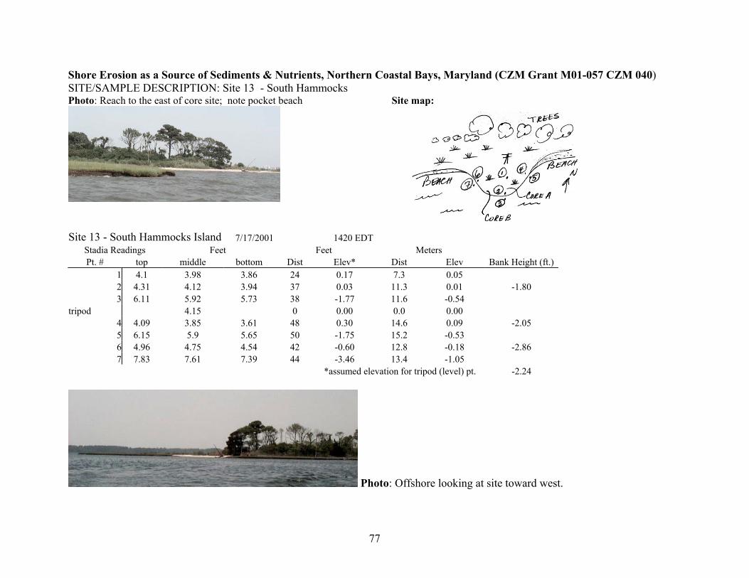
Shore Erosion as a Source of Sediments & Nutrients, Northern Coastal Bays, Maryland (CZM Grant M01-057 CZM 040) SITE/SAMPLE DESCRIPTION: Site 13 - South Hammocks

77

Photo: Reach to the east of core site; note pocket beach

Site map:

Site 13 - South Hammocks Island 7/17/2001 1420 EDT Stadia Readings Feet Feet Meters Pt. # top middle bottom Dist Elev* Dist Elev Bank Height (ft.)

1 4.1 3.98 3.86 24 0.17 7.3 0.05 2 4.31 4.12 3.94 37 0.03 11.3 0.01 -1.80 3 6.11 5.92 5.73 38 -1.77 11.6 -0.54

tripod 4.15 0 0.00 0.0 0.00 4 4.09 3.85 3.61 48 0.30 14.6 0.09 -2.05 5 6.15 5.9 5.65 50 -1.75 15.2 -0.53 6 4.96 4.75 4.54 42 -0.60 12.8 -0.18 -2.86 7 7.83 7.61 7.39 44 -3.46 13.4 -1.05

*assumed elevation for tripod (level) pt. -2.24

Photo: Offshore looking at site toward west.

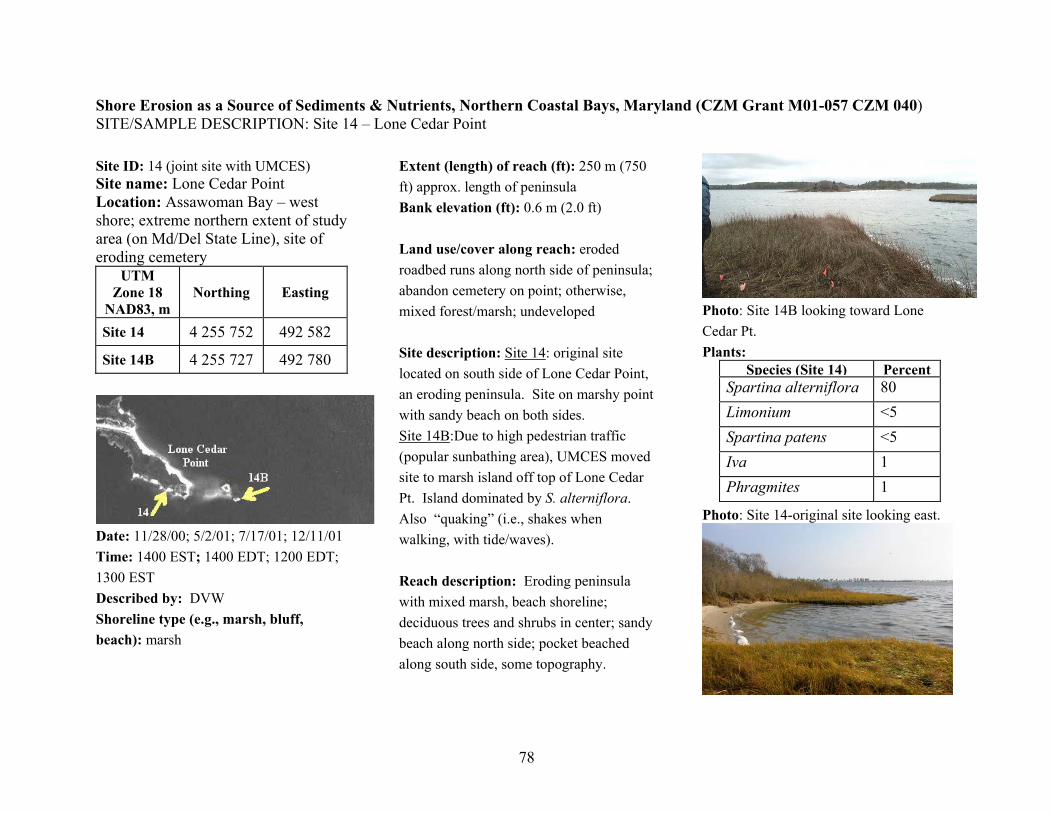
Shore Erosion as a Source of Sediments & Nutrients, Northern Coastal Bays, Maryland (CZM Grant M01-057 CZM 040) SITE/SAMPLE DESCRIPTION: Site 14 – Lone Cedar Point

78

Site ID: 14 (joint site with UMCES) Site name: Lone Cedar Point Location: Assawoman Bay – west shore; extreme northern extent of study area (on Md/Del State Line), site of eroding cemetery

UTM Zone 18


Site 14 4 255 752 492 582

Site 14B 4 255 727 492 780

Date: 11/28/00; 5/2/01; 7/17/01; 12/11/01 Time: 1400 EST; 1400 EDT; 1200 EDT; 1300 EST Described by: DVW Shoreline type (e.g., marsh, bluff, beach): marsh

Extent (length) of reach (ft): 250 m (750 ft) approx. length of peninsula Bank elevation (ft): 0.6 m (2.0 ft) Land use/cover along reach: eroded roadbed runs along north side of peninsula; abandon cemetery on point; otherwise, mixed forest/marsh; undeveloped Site description: Site 14: original site located on south side of Lone Cedar Point, an eroding peninsula. Site on marshy point with sandy beach on both sides. Site 14B:Due to high pedestrian traffic (popular sunbathing area), UMCES moved site to marsh island off top of Lone Cedar Pt. Island dominated by S. alterniflora. Also “quaking” (i.e., shakes when walking, with tide/waves). Reach description: Eroding peninsula with mixed marsh, beach shoreline; deciduous trees and shrubs in center; sandy beach along north side; pocket beached along south side, some topography.

Photo: Site 14B looking toward Lone Cedar Pt. Plants:

Species (Site 14) PercentSpartina alterniflora 80 Limonium <5 Spartina patens <5 Iva 1 Phragmites 1

Photo: Site 14-original site looking east.

Shore Erosion as a Source of Sediments & Nutrients, Northern Coastal Bays, Maryland (CZM Grant M01-057 CZM 040) SITE/SAMPLE DESCRIPTION: Site 14 – Lone Cedar Point

79

Samples: ID Type

*Location

Plug-14 All Top 7” of sediment column

Core-14 All 43” from edge

Core 14 beach

GS Back side of beach to the east

14- Off GS Grab offshore Core 14B All Island, 3.3 ft from

waters edge *Type = bulk density (BD); grain size (GS); trace metal (TM)

Photos:

Date TimeEDT Subject

11/28/00 1404CourtS, setting out peerpers, collecting

plant tissue

11/28/00 1405 “

11/28/00 1414 Beach east

12/11/01 1337 Site 14B-Dan&Rich collecting core

12/11/01 1338 Site 14B-Dan&Rich

12/11/01 1350 Site 14B looking to Lone Cedar Pt.

Hydrolab readings 5/2/2001 12:52 EDT Temp 21.32 degrees CSalinity 23.6 pptDO 7.37Sat 91 %pH 5.54Turb 8.1 NTUDepth 0.93 ftNote: We had trouble collecting a core at site 14 due to significant compression when inserting liner and suction when extracting core. Collected second core on adjacent beach to see if sand overlies muddy marsh sediment.

Site 14 - Lone Cedar Point Stadia

Readings Feet Feet Meters

Pt. # top middle bottom Dist Elev* Dist Elev Bank Hht

(ft.) 1 7.2 6.93 6.65 55 -2.31 16.8 -0.70 2.21 2 5 4.72 4.44 56 -0.10 17.1 -0.03 3 4.73 4.595 4.46 27 0.03 8.2 0.01 4 6.88 6.62 6.36 52 -2.00 15.8 -0.61 1.83 5 5.05 4.79 4.53 52 -0.17 15.8 -0.05

tripod 4.62 0 0.00 0.0 0.00 6 4.61 4.08 3.55 106 0.54 32.3 0.16

*assumed elevation for tripod (level) pt. Average

2.02

Plane view:

Shore Erosion as a Source of Sediments & Nutrients, Northern Coastal Bays, Maryland (CZM Grant M01-057 CZM 040) SITE/SAMPLE DESCRIPTION: Site 18 – Wire Pond

80

Site ID: 18 Site name: Wire Pond Location: Isle of Wight Bay – southwest shore; first cove west of the Thorofare

UTM Zone 18

NAD83, m

Northing Easting

Actual 4 245 252 490 931

Date: 11/28/00; 5/2/01 Time: 1500 EST; 0853 EDT Described by: JMH Shoreline type (e.g., marsh, bluff, beach): marsh Extent (length) of reach (ft): Bank elevation (ft): m ( ft) Land use/cover along reach:

Site description:.On first marsh point east of mouth to Wire Pond; extensive flat marsh; shallow shelf surrounding point. Photo: Site looking SW toward Wire Pond

Reach description: Site is on island marsh at mouth of Wire Pond, south Isle of Wight Bay; deep channel (The Thorofare)cuts along north side of island Plants:

Species Percent

Spartina alterniflora 70 Distichlis (Spike grass) <10 Limonium (Sea Lavander) <10


Plug 18 All Top 9.5” of sed column


18 Off GS Grab offshore *Type = bulk density (BD); grain size (GS); trace metal (TM) Photos:

Date Time EDT

Subject

11/28/00 1512 Site from distance

11/28/00 1513 Site looking SW

11/28/00 1514 Site looking SE 5/2/01 0905 Site 5/2/01 0905 Site

Shore Erosion as a Source of Sediments & Nutrients, Northern Coastal Bays, Maryland (CZM Grant M01-057 CZM 040) SITE/SAMPLE DESCRIPTION: Site 18 – Wire Pond

81

Photo: Looking to SW at sampling site on point

Site map: stadia data below

Site 18 - Wire Pond

Stadia Readings Feet Feet Meters Pt. # top middle bottom Dist Elev* Dist Elev Bank Height (ft.)

1 13.14 12.52 11.9 124 -7.89 37.8 -2.40 2 8.36 7.74 7.12 124 -3.11 37.8 -0.95 3 6.35 5.84 5.32 103 -1.21 31.4 -0.37 1.02 4 5.33 4.82 4.31 102 -0.19 31.1 -0.06 5 5.31 4.805 4.3 101 -0.18 30.8 -0.05 6 4.8 4.61 4.43 37 0.02 11.3 0.01

tripod 4.63 0 0.00 0.0 0.00 7 6.03 5.585 5.14 89 -0.96 27.1 -0.29 0.85 8 5.18 4.74 4.3 88 -0.11 26.8 -0.03 9 7.35 6.81 6.27 108 -2.18 32.9 -0.66 1.77

10 5.58 5.04 4.5 108 -0.41 32.9 -0.12 *assumed elevation for tripod (level) pt. Average 1.21

Shore Erosion as a Source of Sediments & Nutrients, Northern Coastal Bays, Maryland (CZM Grant M01-057 CZM 040) SITE/SAMPLE DESCRIPTION: Site 19 – Keyser Point

82

Site ID: 19 (joint with UMCES) Site name: Keyser Point Location: Isle of Wight, west shore; south side of mouth into Isle of Wight Bay

UTM Zone 18

NAD83, m

Northing Easting

Actual 4 246 364 489 794

Date: 11/28/00; 5/2/01; 5/3/01 Time: 12:00 EDT; Described by: DVW Shoreline type (e.g., marsh, bluff, beach): marsh Extent (length) of reach (ft): ~450 m (length of island

Bank elevation (ft): 0.28 m (0.925 ft) Land use/cover along reach: undeveloped marsh; forest and large homes on mainland next to island. NOTE: visited the site several times; the first and second times with Dr. Stevenson to set out pore water equilibrators (peepers) and to take hydrolab data offshore (see next page) Site description:. Site on eastern shore of island marsh; site almost entirely vegetated with S. alterniflora and some small shrubs (Iva). Reach description: Site located on rregularly shaped extensive island marsh, approx. 450 m by 300 m; marsh punctuated with internal ponds/channels; Plants:

Species Percent

Spartina alterniflora 70 Distichlis (Spike grass) 20 Limonium (Sea Lavander) >5

Samples:

ID Type* Location



10 Off GS Grab offshore *Type = bulk density (BD); grain size (GS); trace metal (TM) Photos:

Date Time EDT

Subject

11/28/00 1158 Setting out grid for grass tissue sampling

11/28/00 1159 Clipping grasses (for biomas)

11/28/00 1207 Site from offshore

Photo: Site from offshore.

Shore Erosion as a Source of Sediments & Nutrients, Northern Coastal Bays, Maryland (CZM Grant M01-057 CZM 040) SITE/SAMPLE DESCRIPTION: Site 19 – Keyser Point

83

Photo: Court Stevenson and Al Wesche setting out grids to collect plant tissue samples. Isle of Wight is in background

Plan view

Hydrolab readings 5/2/2001 Offshore at site 19

12:00 EDT

At OC Inlet

14:15 EDT

Temp 18.5 degrees C 11.75 degrees CSalinity 28.9 ppt 32.25 ppt DO 7.49 mg/l 8.72 mg/l Sat 93 % 95 % pH 5.64 5.6 Turb 3.8 NTU 3.7 NTU Depth 1.5 m 1.25 m

Site 19 - Keyser Point Stadia Readings Feet Feet Meters

Pt. # top middle bottom Dist Elev* Dist Elev Bank Height (ft.) 1 6.33 5.97 5.61 72 -1.41 21.9 -0.43 0.94 2 5.39 5.025 4.66 73 -0.47 22.3 -0.14 3 5.09 4.76 4.43 66 -0.20 20.1 -0.06 4 4.69 4.52 4.36 33 0.04 10.1 0.01

tripod 4.56 0 0.00 0.0 0.00 5 5.82 5.59 5.36 46 -1.03 14.0 -0.31 0.67 6 5.15 4.92 4.69 46 -0.36 14.0 -0.11 7 6.39 5.93 5.47 92 -1.37 28.0 -0.42 1.16 8 5.23 4.77 4.31 92 -0.21 28.0 -0.06

*assumed elevation for tripod (level) pt. Average 0.93

Shore Erosion as a Source of Sediments & Nutrients, Northern Coastal Bays, Maryland (CZM Grant M01-057 CZM 040) SITE/SAMPLE DESCRIPTION: Site 22 – Isle of Wight

84

Site ID: 22 Site name: Isle of Wight Location: Assawoman Bay – west shore; NE shore of Isle of Wight, directly across from site 8 on NW shore of Isle.

UTM Zone 18

NAD83, m

Northing Easting

Actual 4 249 932 490 966

Date: 7/17/01 Time: 1845 EDT Described by: DVW Shoreline type (e.g., marsh, bluff, beach): marsh Extent (length) of reach (ft): ~1000 m

Bank elevation (ft): 0.49 m ( 1.6 ft) Land use/cover along reach: Undeveloped marsh; backed by forest Site description:. Site on small island on point of extensive marsh; thickly vegetated with almost all Spartina alterniflora, some beach lavender. Reach description: Site on small island off very extensive marsh area characterized by convoluted shoreline with islands and ditching Photo: Dan and Neal collecting core at site; looking SE


Spartina alterniflora >90 Limonium 5

Samples:

ID Type* Location



22 Off GS Offshore grab *Type = bulk density (BD); grain size (GS); trace metal (TM) Photos:

Date Time EDT

Subject

7/17/01 1845 Dan and Neal w/core

7/17/01 1845 Site

7/17/01 1848 Neal w/core

7/17/01 1907 Site from distance

7/17/01 1908 OC sunset

Shore Erosion as a Source of Sediments & Nutrients, Northern Coastal Bays, Maryland (CZM Grant M01-057 CZM 040) SITE/SAMPLE DESCRIPTION: Site 22 – Isle of Wight

85

Photo: Main marsh, looking SW from site.

Plan view

Site 22 - Isle of Wight Stadia Readings Feet Feet Meters Pt. # top middle bottom Dist Elev* Dist Elev Bank Height (ft.)

1 4.12 4.03 3.94 18 0.00 5.5 0.00 2 4.35 4.13 3.92 43 -0.10 13.1 -0.03 1.61 3 5.97 5.74 5.51 46 -1.71 14.0 -0.52

tripod 4.03 0 0.00 0.0 0.00 4 4.2 4.12 4.04 16 -0.09 4.9 -0.03 1.26 5 5.48 5.375 5.27 21 -1.35 6.4 -0.41 6 4.22 3.99 3.76 46 0.04 14.0 0.01 1.93 7 6.16 5.92 5.68 48 -1.89 14.6 -0.58 *assumed elevation for tripod (level) pt. Average = 1.60

86

Site #1- White Horse Point, St. Martin River Total length - 53.3 cm Date collected - 7/17/01 Date processes - 7/31/01

Radiograph

Photograph Interval

(cm) Color

(Munsell Color Standard, GSA, 1991)

Description

0-13

5YR 2/2 to 10 YR 3/2

Active root zone; dark gray brown silty mud; lots of large (2-4 cm diameter) rhizomes; some mussels shells in life position at top

13-19

10 YR 3/2 Active root zone; gray brown mud with rhizomes, root material

19-27

10 R 3/2 Gray brown, more compact mud w/ large fibrous root remnants

27-32

5 YR 3/2 Gray brown spongy peat w/ voids; very little sediment (clastics)

32-38

5 YR 2/2 Dark gray brown mud w/ root remnants

38-42 5 YR 2/1 Dark gray black mud, watery, w/ peat and root remnants

42-46.5 5 YR 2/2 mottled w/ 10 R 3 /4

Dark gray brown silty mud mottled with peat and root remnants

46.5-47.5 10 R 3 /4 Reddish brown peat

47.5-53.3 5 YR 2/2 Dark gray brown silty mud with abundant peat and root remnants

87

Site #6 Peach Point, St. Martin River, Core 6 Total length- 61 cm Date collected- Date processed-

Radiograph

Photograph Interval

(cm) Color

(Munsell Color Standard, GSA,

1991)

Description

0-11 5 YR 2/2, mottled with N2

Active root zone, live mussels in very top, live small crab; dark brown to black silty mud, lots of active roots

11-24 10 YR 2/2 Active root zone; section lighter in color, dark brown to ducky yellowish brown silty mud

24-38 10 YR 3/2 Active root zone; long fibrous roots, moderate dusky grown mud

38-45 5 YR 2/2 Very dark dusky brown mud, root material, short peat-like

45-48.5 5 YR 2/1 Very dark gray brown mud, less plant material

48.5-61 10 YR 2/2 Dark brown dusky yellow mud with pockets of reddish brown peat, lots of root material, spongy layer

88

Site #7 – Salt Grass Point, St. Martin River Total length-95 cm Date collected- Date processed- Note: Overall appearance is banding alternating dark and light layers; clastics generally brown to olive gray, and plant material more yellow to reddish in color.

Radiograph

Photograph

Interval (cm)

Color (Munsell Color Standard,

GSA, 1991)

Description

0-11 5 YR 3/2 11-14 5 YR 2/2 14-17 5 YR 3/2

Active root zone; layered brownish gray to moderate brown, very compact silty mud; some sand with lots of large roots

17-30.5 5 YR 4/4 Active root zone; moderate brown mud, spongy, less dense, root material smaller in size and oriented more horizontal than vertical

30.5-40 10 R 2/2 Very dusky red, less dense mud with peat like root material, some larger plant pieces, layered horizontally

40-46 5 YR 2/2 Dusky brown, less dense spongy peat layer

46-56.5 10 R 2/4 Moderate yellow brown mud, abundant plant material, lots of voids

56.5-59 5 YR 4/2 59-63.5 5 YR 3/2 63.5-66 5 YR 2/1 66-73.5 5 YR 3/2

73.5-77.5 5 YR 2/2 77.5-82 10 YR 3/2 82-85 5 Y 2/1 85-90.5 5 YR 2/1

90.5-95.5 10 YR 2/2

Alternating brown to brownish gray mud and yellow brown to reddish brown peat layers

89

Site #8 Smokehouse Cove, St. Martin River Total length- 63.5 cm Date collected- 7/16/01 Date processed- 8/9/01

Radiograph

Photograph Interval

(cm) Color


Description

0-14.5 Banded 10 YR 2/2 to 5 Y 5/2

Active root zone; banded olive gray to dusky yellow brown mud and sand layers, layers ranging 1 to 3 cm thick, abundant roots

14.5-26.5 5 YR 2/2 Active root zone; uniform dark brown silty mud, sand decreasing with depth, roots

26.5-29 10 YR 2/2 Active root zone; darker dusky brown mud, root material, peat like clumps

29-51 5 YR 2/2 Uniform dusky brown mud with peat and roots

51-57 10 Y 2.5/1 Dark brown peaty mud

57-59 5 Y 4/4 Olive brown silty mud with some roots and peat

59-63.5 N2 Very dark almost black, mud with abundant peat material

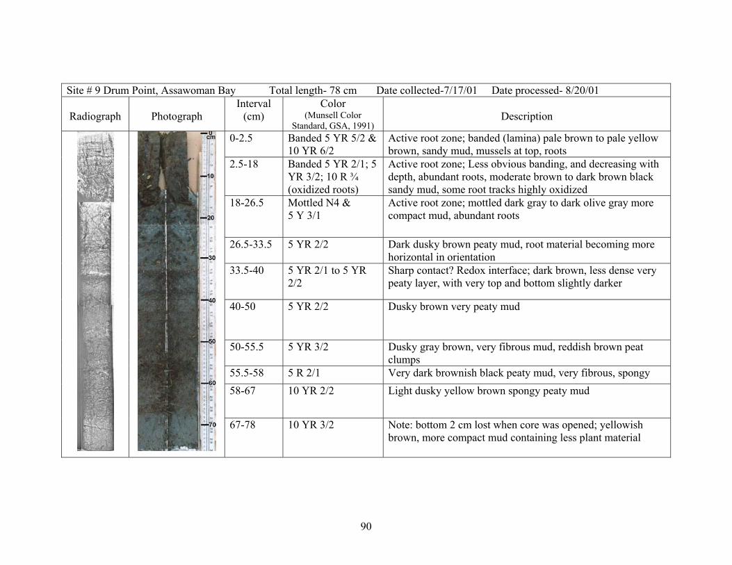
90

Site # 9 Drum Point, Assawoman Bay Total length- 78 cm Date collected-7/17/01 Date processed- 8/20/01

Radiograph

Photograph Interval

(cm) Color


Description

0-2.5 Banded 5 YR 5/2 & 10 YR 6/2

Active root zone; banded (lamina) pale brown to pale yellow brown, sandy mud, mussels at top, roots

2.5-18 Banded 5 YR 2/1; 5 YR 3/2; 10 R ¾ (oxidized roots)

Active root zone; Less obvious banding, and decreasing with depth, abundant roots, moderate brown to dark brown black sandy mud, some root tracks highly oxidized

18-26.5 Mottled N4 & 5 Y 3/1

Active root zone; mottled dark gray to dark olive gray more compact mud, abundant roots

26.5-33.5 5 YR 2/2 Dark dusky brown peaty mud, root material becoming more horizontal in orientation

33.5-40 5 YR 2/1 to 5 YR 2/2

Sharp contact? Redox interface; dark brown, less dense very peaty layer, with very top and bottom slightly darker

40-50 5 YR 2/2 Dusky brown very peaty mud

50-55.5 5 YR 3/2 Dusky gray brown, very fibrous mud, reddish brown peat clumps

55.5-58 5 R 2/1 Very dark brownish black peaty mud, very fibrous, spongy 58-67 10 YR 2/2 Light dusky yellow brown spongy peaty mud

67-78 10 YR 3/2 Note: bottom 2 cm lost when core was opened; yellowish brown, more compact mud containing less plant material

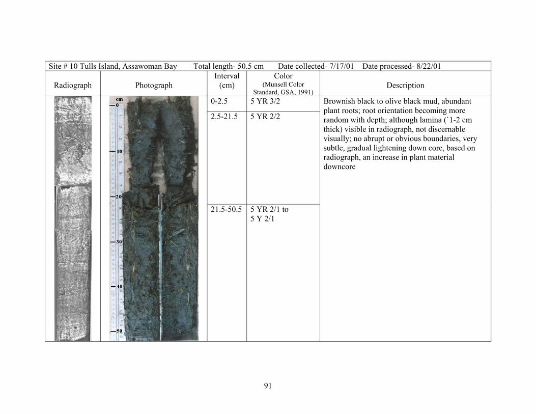
91

Site # 10 Tulls Island, Assawoman Bay Total length- 50.5 cm Date collected- 7/17/01 Date processed- 8/22/01

Radiograph

Photograph Interval

(cm) Color


Description

0-2.5 5 YR 3/2

2.5-21.5 5 YR 2/2

21.5-50.5 5 YR 2/1 to 5 Y 2/1

Brownish black to olive black mud, abundant plant roots; root orientation becoming more random with depth; although lamina (`1-2 cm thick) visible in radiograph, not discernable visually; no abrupt or obvious boundaries, very subtle, gradual lightening down core, based on radiograph, an increase in plant material downcore

92

Site # 11 Goose Pone, Assawoman Bay Total length- 60 cm Date collected- 7/17/01 Date processed- 8/23/01

Radiograph

Photograph Interval

(cm) Color


Description

0-6 5 Y 4/1

6-8.5 5 G 3/1

Active root zone: olive gray sandy silty mud with very large roots; thick layer of mussels on surface; subtle color banding, gradual darkening down core.

8.5-19 5 GY 3/1 Active root zone: dark greenish gray mud with large, thick stems; root abundance decrease with depth

19-34 5 Y 3/1 Active root zone: dark olive gray mud with root material, several very large woody (non root) stems; shift from predominately vertical orientation of plant material to horizontal orientation

34-41 5 Y 2/1 Very dark olive gray mud; abundant peat material

41-47 N 1 to 5 GY 1/1 Redox boundary at 41 cm; dark greenish black to black peaty mud

47-60 5 G 2/1 Slightly lighter greenish black, watery muddy peat, very “loose” packing (with voids), some discernable root stems

93

Site # 12 Peeks Creek, Assawoman Bay Total length- 67.5 cm Date collected- 7/17/01 Date processed- 8/24/01

Radiograph

Photograph

Interval (cm)

Color (Munsell Color Standard, GSA,

1991)

Description

0-20.5 5 y 2/1 Active root zone: dark olive black sandy silty mud with mussels on top; large roots; radiograph incite thin lamina (sandier?) but not visible to the eye

20.5-32.5 5 GY 2/1 Active root zone: dark greenish black slightly less dense silty mud with abundant roots

32.5-38 5 YR 2/1 Brownish black muddy peat; some larger root stems, appears to be more oxidized than surrounding layers

38-43 5 Y 2/1 Dark olive black peaty mud

43-58.5 10 YR 2/2 to 10 YR 3/2

Dusky yellow brown, highly peaty, gradually lightens to yellowish brown; plant material decrease with depth

58.5-64 5 G 2/1 to N 1

Redox boundary at 58.5 cm; greenish black to black peaty mud

64-67.5 5 GY 4/1 Dark greenish gray mud, lighter in color than rest of core; also less plant material

94

Site # 13 – South Hammocks, Assawoman Bay Total length- 35.5 cm Date collected- 7/17/01 Date processed- 8/27/01

Radiograph

Photograph Interval

(cm) Color


1991)

Description

0-1 5 Y 8/1 Active root zone; yellowish gray sand 1-3 5 Y 2/1 Active root zone; dark olive black to brown muddy sand 3-7 5 Y 8/1 Active root zone; yellowish gray very fine sand

7-19 Banded; 5 Y 8/1 10 YR 4/2 N 3

Active root zone; alternating lamina of yellowish gray sand, dark yellow brown sandy mud, and dark gray very compact sandy mud; sand increased down core, bottom of section is dark brown gray sand ; plant material present but not abundant except in very bottom of section

19-29.5 Mottled; 5 YR 4/1 N 2

Active root zone; mottled brownish gray to gray black silty mud; plant material throughout section; redox boundary at 27 cm

29.5-35.5 5 GY 2/1 Greenish black mud with abundant plant material (roots and peat)

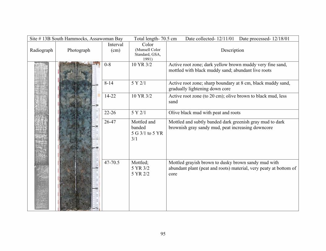
95

Site # 13B South Hammocks, Assawoman Bay Total length- 70.5 cm Date collected- 12/11/01 Date processed- 12/18/01

Radiograph

Photograph Interval

(cm) Color


1991)

Description

0-8 10 YR 3/2 Active root zone; dark yellow brown muddy very fine sand, mottled with black muddy sand; abundant live roots

8-14 5 Y 2/1 Active root zone; sharp boundary at 8 cm, black muddy sand, gradually lightening down core

14-22 10 YR 3/2 Active root zone (to 20 cm); olive brown to black mud, less sand

22-26 5 Y 2/1 Olive black mud with peat and roots

26-47 Mottled and banded 5 G 3/1 to 5 YR 3/1

Mottled and subtly banded dark greenish gray mud to dark brownish gray sandy mud, peat increasing downcore

47-70.5 Mottled; 5 YR 3/2 5 YR 2/2

Mottled grayish brown to dusky brown sandy mud with abundant plant (peat and roots) material, very peaty at bottom of core

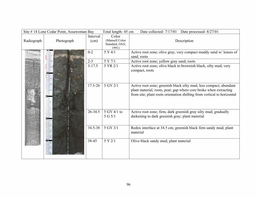
96

Site # 14 Lone Cedar Point, Assawoman Bay Total length- 45 cm Date collected- 7/17/01 Date processed- 8/27/01

Radiograph

Photograph Interval

(cm) Color


1991)

Description

0-2 5 Y 4/1 Active root zone; olive gray, very compact muddy sand w/ lenses of sand, roots

2-3 5 Y 7/1 Active root zone; yellow gray sand, roots 3-17.5 5 YR 2/1 Active root zone; olive black to brownish black, silty mud, very

compact, roots

17.5-26 5 GY 2/1 Active root zone; greenish black silty mud, less compact; abundant plant material, roots, peat; gap where core broke when extracting from site; plant roots orientation shifting from vertical to horizontal

26-34.5 5 GY 4/1 to 5 G 5/1

Active root zone; firm, dark greenish gray silty mud; gradually darkening to dark greenish gray; plant material

34.5-38 5 GY 3/1 Redox interface at 34.5 cm; greenish black firm sandy mud; plant material

38-45 5 Y 2/1 Olive black sandy mud; plant material

97

Site #14B Lone Cedar Key, Assawoman Bay, Total Length- 86.5 cm Date collected- 12/11/01 Date processes- 12/18/1

Radiograph

Photograph Interval

(cm) Color (Munsell Color Standard,

GSA, 1991)

Description

0-13 5 YR 4/1 to 5 YR 2/1

Active root zone; mottled medium to dark gray brown mud, with abundant rhizomes; very muddy at top, sand gradually increasing w/depth

13-15 5 Y 5/1 Active root zone; dark gray brown sandy mud with rhizomes 15-23.5

5 YR 2/1 to N2 Active root zone to 19 cm; dark gray brown mud with roots

23.5-32.5

5 YR 2/1

32.5-46.5

5 YR 3/1

Gray brown peat, slight banding

46.5-64.5

5YR 2/1, 5 YR 4/1, 5 Y 4/1

Banded peaty mud with sand lenses

64.5-75.5

N6 to 5 B 7/1 Sharp contact; steel gray, very clayey compact, dry mud

75.5-80 5 YR 2/1 Very dark olive black peaty mud, less compact 80-85 N6 to 5 B 7/1 Sand lenses at 81-82 cm, interbedded w/ peaty mud layers

Note: bottom 10 cm not in radiograph 85-86.5 N2 Very dark gray, peaty mud

98

Site # 18, Top section; Wire Pond, Isle of Wight Bay Total length- 143 cm Date collected- 5/2/01 Date processed- 5/14/01 Comments: H2S odor; distinct banding

Radiograph 0-70 cm

Photograph

Interval (cm)

Color (Munsell Color

Standard, GSA, 1991)

Description

0-24.5 (color not true; turned anoxic in bag

Active root zone; grayish brown silty mud with abundant roots

24.5-63 5 YR 3 /4 5 Y 4/1

Active root zone; mottled moderate brown to olive gray silty mud with abundant roots

63-68 5 YR 2/1 Brownish black muddy peat

99

Site # 18, Bottom section; Wire Pond, Isle of Wight Bay Total length- 143 cm Date collected- 5/2/01 Date processed- 5/14/01 Comments: H2S odor; distinct banding

Radiograph 70-143 cm

Photograph

Interval (cm)

Color (Munsell Color

Standard, GSA, 1991)

Description

68-96 5 Y 3/2 5 G 4/1

Subtlety banded olive gray to greenish gray clayey mud, roots and peat; very clayey at bottom of section

96-103 5 YR 2/2

103-107 10 YR 2/2 107-118 5 YR 2/2

118-122 5 Y 3/2

Alternate layers of dusky brown peaty mud, dusky yellow brown mud with some plant material, and olive gray mud with little plant/peat

122-137 5 YR 2/1 Brownish black muddy peat

137-143 5 Y 3/2 Olive gray mud with some peat pockets

100

Site #19 Keyser Pt., Isle of Wight Bay, Total Length- 59 cm Date collected- 5/3/01 Date processes- 9/10/01

Radiograph

Photograph Interval

(cm) Color (Munsell Color Standard,

GSA, 1991)

Description

0-15 5 Y 4/1; 5 YR 4/1; 10 R 3 /4

Active root zone; mottled olive gray mud, very sandy with inclusion’s of large (>5 cm) sand pockets, light brown, gritty, lots of mica, highly oxidized around some root paths (dark reddish brown); abundant roots, plant material

15-19.5 5 GY 41 Active root zone; very compact, greenish gray mud, micacous, faint laminations, abundant roots and root material

19.5-21.5 5 Y 3/1 21.5-23.5 5 Y 6/1

?Active root zone; olive gray mud, laminated, roots

23.5-46.5 5 G 4/1; 5 YR 4/1; 5 B 4/1

Alternating dark olive gray to light olive gray mud; highly laminated, compact, silty mud, micaceous layers range from 1 cm to 3 cm, sand lenses, root material

46.5-51.5 5 Y 2/1 Very sharp change to olive black peaty mud

51.5-59 5 YR 2/1 Sharp change to very dark brownish black peat, with some clastics

101

Site # 22 Isle of Wight, Assawoman Bay Total length- 58.5 cm Date collected- 7/17/01 Date processed- 9/13/01

Radiograph

Photograph Interval

(cm) Color


1991)

Description

0-2 5 G 2/1; 5 Y 3/1

Active root zone; top 2 cm mottled greenish black and dark olive gray mud with abundant plant and root material

2-22 5 Y 4/1 Active root zone; dark olive gray mud with abundant plant and root material

22-42 5 GY 3/1 Active root zone; dark greenish gray silty mud with abundant plant material; radiograph indicates slightly denser layer at 36 cm which is not visible w/eye

42-48.5 5 YR 3/1 Brownish gray peat with mud, spongy

48.5-58.5 5 Y 3/1 Olive gray peaty mud, not as peaty as overlying section

103

APPENDIX B Quality Assurance/Quality Control

Textural Analyses

The techniques used to determine grain size composition are based on traditional analytical methods developed for the sedimentology lab. Still, some analytical error is inherent in the methodology. For example, results can be affected by the technician’s level of skill and/or changes in laboratory conditions, such as sudden temperature changes. Furthermore, no standard reference material includes the broad range of particle sizes and shapes contained in natural sediment. To maximize the consistency of textural analyses, several checks are used to monitor results. Calculated gravel, sand, silt, and clay percentages are checked against (1) field descriptions of the samples, (2) calculated water content, and (3) calculated weight loss of the sample during processing. These comparisons are made to determine if the grain size composition matches the visual description of the sample and/or falls within an expected Shepard’s (1954) class with respect to water content and weight loss. Any discrepancy is flagged, and the results are reviewed to determine if reanalysis is warranted.

Specifically, the criteria for each of the internal checks are as follows: (1) Calculated gravel, sand, silt, and clay percentages and Shepard’s classification

are compared with the field description of the sediment. If the results seem to indicate a very different sample from the one described, then the sample is reanalyzed.

(2) Gravel, sand, silt, and clay percentages are compared to calculated water content. For each of the sediment types, Table B-1 lists the typical mean and range of values for water content, based on bottom sediments collected in Isle of Wight and Assawoman Bays. The mean and range of values for marsh sediments collected as part of this study fall within expected values for water content (Table B-2).

(3) Sample loss (% dry weight) during cleaning is calculated for each sample. The calculated water content, which is usually measured shortly after the sample is collected, is used to determine weight loss. If the sediment dries out, even slightly, before it is sub-sampled for textural analysis, then weight loss is underestimated and, in some instances, negative. The weight lost during the cleaning process is related to sediment type, that is, grain size composition, as well as to the organic and/or carbonate content of the sediment. Organic-rich, fine-grained bay bottom sediments (i.e., silty clay and clayey silt) may lose up to 30% dry weight during cleaning (Table B-1). Sand, which is fairly clean, usually losses the least weight and often shows a negative weight loss, due to errors inherent in water content determinations. In this study, many of the core sediments lost over 50% dry weight during the cleaning process due to the very high amount of plant material (Table B-2).

104

Table B-1. Mean and range of water content and calculated weight loss after cleaning for each sediment type (Shepard’s (1954) classification), based on sediments collected in Isle of Wight and Assawoman Bays (Wells and others, 1994). Means are rounded to the nearest whole percentage.

Water content (% wet weight)

Weight loss (% dry weight)

Sediment type Mean

Range

Mean

Range

Sand

22

17 - 27

1

-4 - 6

Silty-Sand

39

31 - 47

7

2 - 12

Clayey-Sand

47

41 - 53

3

0 -6

Sandy-Silt

48

42 - 54

13

5 - 21

Clayey-Silt

60

53 - 67

20

13 - 27

Silty-Clay

70

67 - 73

28

23 - 33

Sand-Silt-Clay

56

49 - 63

13

2 - 24

Table B-2. Mean and range of water content and calculated weight loss after cleaning for each sediment type (Shepard’s (1954) classification), based on sediments collected for this study. Means and ranges are rounded to the nearest whole percentage. Blank range values indicate that only a single sample represented the sediment class.

Water content (% wet weight) Weight loss (% dry weight) Sediment type Mean Range Mean Range

Sand 21 4 - 37 4 -3 - 10 Silty-Sand 42 38 - 51 17 6 - 27 Clayey-Sand 51 26 Sandy-Silt 46 11 Clayey-Silt 70 52 - 86 39 19 - 66 Silty-Clay 78 69 - 86 55 23 - 72 Sand-Silt-Clay 62 23 - 87 36 5 - 69

For this study, less than 5% of the sediment samples were flagged for repeated

textural analyses. Table B-3 lists the results of the replicated analyses. Results of all duplicate analyses yielded sand, silt, and clay percentages that fell within 5% of their first analyses.

105

Table B-3. Comparison of results of replicate textural analyses of selected core samples Sample

ID

%

Water

%

Sand

% Silt

%

Clay

Shepard’s

classification

∆

Sand

∆

Silt

∆

Clay

Comments

13-20 53.14 19.64 51.05 29.31 Clayey-Silt 13-2 R 53.14 20.06 51.82 28.13 Sand-Silt-Clay

0.32 0.77

1.18

Change in classification as a result of slight change in % sand

13-3 49.31 34.35 40.77 24.88 Sand-Silt-Clay 13-3 R 49.31 34.94 41.13 23.93 Sand-Silt-Clay

0.59 0.36

0.95

No change in classification

13-4 62.45 17.21 45.13 37.67 Clayey-Silt

13-4 R 62.45 17.66 45.69 36.65 Clayey-Silt 0.45 0.56

0.02

No change in classification

Nitrogen, Carbon and Sulfur Analyses

As part of MGS’s QA/QC protocol, several standard reference materials (SRMs) are used as secondary standards and run every 6 to 7 samples (unknowns). Table B-4 compares MGS results with certified SRM values for total carbon, nitrogen, and sulfur. The detection limit for this method is 0.001% for all three elements. There is excellent agreement between SRM values and MGS's results.

In addition to SRMs, replicate analyses were done on every seventh sediment sample.

The relative standard deviation for the replicate analyses may be used to determine analytical variability of the method with respect to concentration. The relative standard deviation plots for total nitrogen and carbon show that variability decreases with increasing concentrations (Figs. B-1 and B-2).

Table B-4. Results of nitrogen, carbon, and sulfur analyses of NIST SRM 1646 (Estuarine Sediment) and National Research Council of Canada SRM PACS-1 (Marine Sediment) compared to the certified or known values. MGS values were obtained by averaging the results of all SRM analyses run during this study. All samples were analyzed over a two-week period.

NIST SRM 1646 – Estuarine Mud PACS-1 – Marine Sediment Certified values* MGS results Certified

values MGS results Component

Value ±Std Dev

Mean value ±Std Dev % Recovery Value

±Std Dev Mean value

±Std Dev % Recovery

Nitrogen 0.180 0.17± 0.00 96.96 0.260

0.276 ± 0.011 106.14

Carbon 1.720 1.64± 0.05 95.21 3.690

3.578 ± 0.097 96.96

Sulfur 0.960 1.02 ± 0.08 106.25 1.320

1.252 ± 0.046 94.85

* The value for carbon is certified by NIST. The sulfur value is the non-certified value reported by NIST. The NIST did not report nitrogen for the SRM. The value for nitrogen was obtained from repeated analyses in-house and by other laboratories (Haake Buchler Labs and the U.S. Dept. of Agriculture).

106

Figure B-1. Relative standard deviation (%) vs. concentration of total nitrogen for the suite of replicate and triplicate analyses.

Figure B-2. Relative standard deviation (%) vs. concentration of total carbon for the suite of replicate and triplicate analyses. Metal Analyses

For elemental analyses completed by Activation Laboratories, Ltd. (Actlabs), quality assurance was confirmed in the following manner. The set of sediment samples sent to Actlabs contained a series of SRMs and replicate samples, the identities of which were not revealed to Actlabs. MGS also requested that Actlabs run a reagent blank every 20 samples. The three SRMs used were (1) NIST-SRM #1646a – Estuarine Sediment, (2) NIST-SRM #2704 – Buffalo River Sediment, and (3) National Research Council of Canada PACS-2 – Marine Sediment. These SRMs closely resembled the types of sediments being analyzed (i.e., fine-grained marine sediment). Results of the analyses of the three standard reference materials are compared to the certified values in Table B-5.

Carbon

0123456

0.000 10.000 20.000 30.000 40.000

Concentration (% dry weight)

RSD

Nitrogen

0

1

2

3

4

5

0.000 0.500 1.000 1.500 2.000


RSD

107

As part of their internal QA/QC protocol, Actlabs analyzed a suite of standards used by the U.S. Geological Survey. Those results are presented in Table B-6. Actlabs also ran a replicate of every tenth sample; independent of the blind replicates that MGS included. As a result, some samples were analyzed three times. The relative standard deviation for the replicate and triplicate analyses were calculated and used to determine analytical variability with respect to concentration. A plot of the relative standard deviation (RSD) vs. the concentration of total phosphorus shows that variability decreases with increasing concentration (Fig. B-3).

Figure B-3. Relative standard deviation (%) vs. concentration of total phosphorus for the suite of replicate and triplicate analyses.

Phosphorus

012345678

0.000 0.020 0.040 0.060 0.080 0.100 0.120 0.140


RSD

108

Table B-5. Comparison of certified values to the analytical results from Actlabs for the SRMs. Values in parentheses are non-certified values. “NA” indicates that no value was reported for the element.

NIST 1646a – Estuarine Mud NIST 2704 – Buffalo River Mud PACS-2 – Marine Mud

Certified values Actlabs Results Certified values Actlabs Results Certified values Actlabs Results Element

Value ±Std dev Value ±Std dev % Recovery Value ±Std dev Value ±Std dev %

Recovery Value ±Std dev % Recovery

Ag (ppm) (<0.3) 0.4 ± 0.1 119.9 NA 1.00 ± 0.08 --- 1.22 ± 0.14 1.27 ± 0.11 103.7 Al (%) 2.297 ± 0.018 2.162 ± 0.063 94.1 6.11 ± 0.16 5.34 ± 0.29 87.4 6.62 ± 0.32 10.02 ± 1.72 151.4 Be (ppm) (<1) -1 --- NA 1.87 ± 0.06 --- 1 ± 0.2 1.19 ± 0.03 118.9 Bi (ppm) NA -2 --- NA -2.00 --- NA -2 ± 0 --- Ca (%) 0.519 ± 0.020 0.541 ± 0.01 104.2 2.6 ± 0.03 2.72 ± 0.10 104.6 1.965 ± 0.18 2.15 ± 0.05 109.3 Cd (ppm) 0.148 ± 0.007 -0.30 --- 3.45 ± 0.22 1.98 ± 0.75 57.5 2.11 ± 0.15 1.11 ± 0.16 52.6 Co (ppm) (5) 4.67 ± 0.48 93.4 14 ± 0.6 13 ± 0.44 93.6 11.5 ± 0.3 10.96 ± 0.52 95.3 Cu (ppm) 10.01 ± 0.34 15.94 ± 6.66 159.3 98.6 ± 5 97.79 ± 5 99.2 310 ± 12 305 ± 12 98.5 Fe (%) 2.008 ± 0.039 1.955 ± 0.055 97.4 4.11 ± 0.1 4.09 ± 0.16 99.5 4.09 ± 0.06 4.14 ± 0.13 101.2 K (%) 0.864 ± 0.016 0.809 ± 0.022 93.6 2 ± 0.04 1.88 ± 0.09 94.2 1.23 ± 0.05 1.53 ± 0.14 124.3 Mg (%) 0.388 ± 0.009 0.441 ± 0.012 113.7 1.2 ± 0.02 1.30 ± 0.05 108.3 1.472 ± 0.133 1.98 ± 0.19 134.6 Mn (ppm) 234 ± 2.8 233 ± 3.49 99.5 555 ± 19 580 ± 25 104.5 440 ± 19 430 ± 15 97.6 Mo (ppm) (1.8) 2.28 ± 0.53 126.7 NA 5.01 ± 1 --- 5.43 ± 0.28 6.35 ± 0.92 116.9 Na (%) 0.741 ± 0.017 0.766 ± 0.027 103.4 0.547 ± 0.014 0.626 ± 0.039 114.5 3.71 ± 0.185 3.62 ± 0.19 97.7 Ni (ppm) (23) 23 ± 1.06 99.3 44.1 ± 3 43.89 ± 2 99.5 39.5 ± 2.3 40.8 ± 1.5 103.2 P (ppm) 270 ± 10 250 ± 7.7 92.5 998 ± 28 884 ± 31 88.5 960 ± 44 945 ± 40 98.5 Pb (ppm) 11.7 ± 1.2 12.54 ± 1.04 107.2 161 ± 17 168.59 ± 7 104.7 183 ± 8 185 ± 5 100.9 S (%) (0.352) 0.39 ± 0.01 109.9 0.397 ± 0.004 0.419 ± 0.018 105.6 1.29 ± 0.13 1.41 ± 0.03 109.6 Sr (ppm) (68) 69 ± 1.78 100.8 (130) 133 ± 6 102.4 276 ± 30 289 ± 10 104.6 Ti (%) 0.456 ± 0.021 0.395 ± 0.015 86.6 0.457 ± 0.018 0.398 ± 0.028 87.1 0.443 ± 0.032 0.42 ± 0.01 95.9 V (ppm) 44.84 ± 0.76 40.40 ± 3.08 90.1 95 ± 4 99 ± 3 104.7 133 ± 5 139 ± 5 104.3 Y (ppm) NA 9.91 ± 0.33 --- (2.8) 23.49 ± 1.18 838.8 NA 25.23 ± 4.52 --- Zn (ppm) 48.9 ± 4.6 59.61 ± 14.20 121.9 438 ± 12 405 ± 9 92.4 364 ± 23 349 ± 12 95.9

109

Table B-6. Comparison of certified values to Actlab’s analytical results for U.S. Geological Survey standards. Certificate data underlined are recommended values; other values are proposed except those preceded by a "(", which are information values.

G-2 (granite)

SDC-1 (mica schist)

DNC-1 (dolerite)

SCO-1 (cody shale)

GXR-6 (soil)

GXR-2 (soil)

GXR-1 (jasperoid)

GXR-4 (copper mill

head) Element Certified

values Actlab results

Certified value

Actlab results

Certified value

Actlab results

Certified value

Actlab results

Certified value

Actlab results

Certified value

Actlab results

Certified value

Actlab results

Certified value

Actlab results

Ag (ppm) 0.04 -0.3 0.041 -0.3 (.027 -0.3 0.134 0.5 1.3 0.7 17 16.3 31 30.6 4 3.6 Al (%) 8.147 5.82 8.338 6.02 9.687 9.72 7.24 5.69 17.68 9.03 16.46 6.90 3.52 1.80 7.20 6.09 Be (ppm) 2.5 2 3.0 3 1 -1 1.84 2 1.4 1 1.7 2 1.22 1 1.9 2 Bi (ppm) 0.037 -2 0.26 -2 (.02 -2 0.37 -2 (.29 -2 (.69 -2 1380 1518 19 35 Ca (%) 1.401 1.17 1.001 0.94 8.055 8.08 1.87 1.80 0.179 0.15 0.929 0.70 0.958 0.94 1.01 1.05 Cd (ppm) 0.016 -0.3 (.08 -0.3 (.182 -0.3 0.14 -0.3 (1 -0.3 4.1 2.0 3.3 1.8 (.86 -0.3 Co (ppm) 4.6 3 17.9 18 54.7 58 10.5 11 13.8 12 8.6 8 8.2 7 14.6 15 Cu (ppm) 11 11 30 29 96 124 28.7 39 66 66 76 76 1110 1210 6520 6464 Fe (%) 1.86 1.75 4.825 4.82 6.94 7.23 3.59 3.48 5.58 5.09 1.86 1.82 23.64 25.74 3.09 3.15 K (%) 3.718 3.45 2.722 2.53 0.19 0.25 2.30 2.11 1.87 1.43 1.37 1.13 0.05 0.05 4.01 3.97 Mg (%) 0.452 0.42 1.019 1.03 6.06 6.99 1.64 1.70 0.61 0.47 0.85 0.74 0.22 0.22 1.66 1.88 Mn (ppm) 232 246 883 866 1154 1122 410 385 1008 920 1008 791 853 979 155 147 Mo (ppm) (1.1 1 (.25 3 (.7 1 1.37 1 2.4 3 (2.1 3 18 21 310 308 Ni (ppm) (5 3 38 34 247 251 27 26 27 24 21 19 41 42 42 39 Na (%) 3.027 2.98 1.521 1.57 1.39 1.61 0.67 0.69 0.1 0.10 0.56 0.54 0.05 0.05 0.56 0.55 P (%) 0.061 0.050 0.069 0.056 0.037 0.025 0.090 0.077 0.035 0.057 0.105 0.057 0.065 0.060 0.120 0.124 Pb (ppm) 30 31 25 22 6.3 10 31 32 101 97 690 699 730 802 52 53 S (%) (0.01 0.016 0.065 0.065 (0.039 0.067 0.063 0.067 0.016 0.011 0.031 0.027 0.257 0.281 1.770 1.995 Sr (ppm) 478 430 183 173 145 147 174 161 35 35 160 136 275 324 221 232 Ti (%) 0.288 0.29 0.606 0.58 0.287 0.29 0.38 0.34 0.498 0.48 0.3 0.29 0.036 0.02 0.29 0.26 V (ppm) 36 38 102 103 148 159 131 141 186 198 52 55 80 91 87 96 Y (ppm) 11 6 40 24 18 19 26 17 14 5 17 9 32 35 14 13 Zn (ppm) 86 86 103 103 66 66 103 99 118 125 530 509 760 739 73 79

111

APPENDIX C Data Tables

113

Table C-1. Sample data: physical properties. Off denotes offshore grab sample. Sites 3, 4, and 5 are bluff sites: T and B denoting top and bottom of bluff. All other sites are coring sites (marsh). Core compaction factor used to correct bulk density for sediment compaction. Adjusted dry bulk density is assumed to represent total solids in the sediment. Percent reactive organics and carbonates was calculated from sample weight loss due to cleaning. Kg/m3 = g/cm3 * 1000.

Sediment interval: Core samples - depth below

marsh surface (cm) Bluff sample - height above

shoreline (m)

Bulk density (measured) Bulk composition

Sample ID

Upper interval

Lower interval

Wet (g/cm3)

Dry (g/cm3)

Plant (% >14 mesh)

Clastic (%)

Reactive organics/

carbonates (%)

Total organics

Core compaction

factor

Total solids (Kg/m3 )

1-1 0.0 12.7 0.92 0.24 20.96 50.15 28.89 49.85 1 239.90 1-2 12.7 27.0 0.95 0.22 27.01 31.49 41.50 68.51 0.89 192.18 1-3 27.0 38.0 0.85 0.12 26.74 28.52 44.73 71.48 0.89 105.09 1-4 38.0 53.3 0.85 0.18 25.43 40.03 34.53 59.97 0.89 162.44 6-1 0.0 27.5 1.03 0.27 20.37 37.82 41.81 62.18 1 273.07 6-2 27.5 44.0 1.03 0.21 26.56 40.90 32.54 59.10 0.85 175.84 6-3 44.0 61.0 1.07 0.22 26.56 34.08 39.35 65.92 0.85 190.95 8-1 0.0 14.5 1.52 0.95 10.50 79.51 9.99 20.49 0.94 890.25 8-2 14.5 29.0 1.29 0.55 5.02 74.86 20.12 25.14 0.94 520.90 8-3 29.0 45.0 1.10 0.31 8.63 55.17 36.19 44.83 0.94 286.97 8-4 45.0 63.5 1.09 0.27 3.78 57.71 38.51 42.29 0.94 250.18 7-1 0.0 20.0 1.02 0.26 27.62 44.19 28.19 55.81 1 257.92 7-2 20.0 40.0 0.98 0.16 32.33 28.15 39.52 71.85 0.88 137.04 7-3 40.0 60.0 0.97 0.18 7.67 41.86 50.47 58.14 0.88 158.93 7-4 60.0 78.0 1.02 0.17 3.38 41.26 55.36 58.74 0.88 148.02 7-5 78.0 95.0 1.01 0.15 8.53 33.03 58.43 66.97 0.88 134.46

9-1 #1 0.0 19.0 1.49 0.88 3.26 93.88 2.86 6.12 1 878.89 9-2 19.0 39.0 1.22 0.48 9.81 70.87 19.33 29.13 0.94 452.03 9-3 39.0 59.0 1.02 0.23 20.25 38.91 40.84 61.09 0.94 217.02

114




shoreline (m)


Sample ID

Upper interval

Lower interval

Wet (g/cm3)

Dry (g/cm3)

Plant (% >14 mesh)

Clastic (%)

Reactive organics/

carbonates (%)

Total organics

Core compaction

factor


9-4 59.0 76.0 1.13 0.35 1.17 72.66 26.17 27.34 0.94 330.57 10-1 0.0 23.5 1.27 0.51 11.51 65.88 22.62 34.12 1 505.40 10-2 23.5 35.5 1.19 0.39 4.15 74.77 21.08 25.23 0.96 376.82 10-3 35.5 48.5 1.14 0.33 4.66 68.86 26.49 31.14 0.96 316.14 11-1 0.0 19.0 1.36 0.67 10.94 72.99 16.07 27.01 1 668.60 11-2 19.0 36.0 1.10 0.40 12.70 60.94 26.36 39.06 0.86 341.12 11-3 36.0 47.0 1.00 0.17 24.28 34.08 41.64 65.92 0.86 146.00 11-4 47.0 60.0 0.97 0.17 6.26 55.83 37.90 44.17 0.86 146.08

12-1 #1 0.0 21.0 1.18 0.46 9.94 67.95 22.12 32.05 1 464.93 12-2 21.0 38.0 1.05 0.22 24.77 38.22 37.02 61.78 1 221.98 12-3 38.0 52.0 0.93 0.13 13.88 36.30 49.82 63.70 1 131.68 12-4 52.0 67.5 1.02 0.21 6.14 62.96 30.90 37.04 1 210.75 13-1 0.0 21.0 1.29 0.92 2.84 89.94 7.22 10.06 1 920.29 13-2 21.0 35.5 1.34 0.63 12.11 59.63 28.27 40.37 0.87 544.64

13B-1 0.0 8.0 1.54 1.03 3.84 90.54 5.63 9.46 0.95 981.41 13B-2 8.0 20.0 1.48 0.95 2.88 91.54 5.58 8.46 0.95 899.48 13B-3 20.0 35.0 1.36 0.69 5.95 77.21 16.84 22.79 0.95 654.88 13B-4 35.0 46.5 1.20 0.45 10.26 78.77 10.97 21.23 0.95 429.13 13B-5 46.5 70.5 1.03 0.23 16.46 44.13 39.41 55.87 0.95 220.30 14-1 0.0 17.5 1.24 0.58 13.30 60.55 26.14 39.45 1 577.33 14-2 17.5 26.0 1.02 0.28 16.91 50.91 32.18 49.09 1 278.28

115




shoreline (m)


Sample ID

Upper interval

Lower interval

Wet (g/cm3)

Dry (g/cm3)

Plant (% >14 mesh)

Clastic (%)

Reactive organics/

carbonates (%)

Total organics

Core compaction

factor


14-3 26.0 45.5 1.19 0.43 14.20 56.43 29.37 43.57 1 430.21 14B-1 0.0 16.0 1.30 0.61 11.75 76.02 12.23 23.98 0.85 516.60 14B-2 16.0 28.5 1.31 0.58 4.76 80.26 14.99 19.74 0.85 491.31 14B-3 28.5 46.5 1.12 0.29 17.55 61.98 20.46 38.02 0.85 249.66 14B-4 46.5 64.5 1.20 0.37 5.57 77.04 17.39 22.96 0.85 314.85 14B-5 64.5 75.5 1.39 0.67 2.11 78.24 19.65 21.76 0.85 570.05 14B-6 75.5 86.5 1.19 0.42 4.19 80.88 14.93 19.12 0.85 354.33 18-0 0.0 24.5 1.00 0.43 11.34 68.07 20.59 31.93 1 434.80 18-1 24.5 37.0 0.70 0.17 13.88 57.92 28.19 42.08 0.97 163.79 18-2 37.0 62.0 0.99 0.31 4.98 67.39 27.62 32.61 0.97 299.15 18-3 62.0 87.0 1.14 0.41 2.09 79.93 17.98 20.07 0.97 395.29 18-4 87.0 112.0 1.05 0.26 2.68 48.18 49.14 51.82 0.97 247.93 18-5 112.0 143.0 1.24 0.51 1.65 73.90 24.45 26.10 0.97 494.57 19-1 0.0 17.0 1.58 1.01 2.73 89.91 7.37 10.09 1 1010.00 19-2 17.0 30.0 1.52 0.93 2.27 85.93 11.80 14.07 1 927.95 19-3 30.0 46.5 1.46 0.79 2.22 89.39 8.39 10.61 1 785.65 19-4 46.5 57.5 1.11 0.28 22.63 51.60 25.77 48.40 1 284.80 22-1 0.0 23.0 1.22 0.37 18.14 63.03 18.83 36.97 1 369.33 22-2 23.0 42.0 1.12 0.31 7.82 71.55 20.63 28.45 0.85 260.96 22-3 42.0 58.0 0.98 0.17 15.83 41.89 42.27 58.11 0.85 142.39

Site 3-T 2.8 0.4 1.29 1.24 0.00 97.34 2.66 2.66 1 1238.92

116




shoreline (m)


Sample ID

Upper interval

Lower interval

Wet (g/cm3)

Dry (g/cm3)

Plant (% >14 mesh)

Clastic (%)

Reactive organics/

carbonates (%)

Total organics

Core compaction

factor


Site 3-B 0.4 0.0 1.84 1.43 0.00 94.91 5.09 5.09 1 1434.43 Site 4-T 2.6 1.3 1.43 1.35 0.00 97.58 2.42 2.42 1 1346.65 Site 4-B 1.3 0.0 1.65 1.54 0.00 97.92 2.08 2.08 1 1538.04 Site 5 2.1 0.0 1.44 1.34 0.00 98.07 1.93 1.93 1 1336.30 1-Off 0.00 56.10 43.90 43.90

3-Beach 0.00 98.99 1.01 1.01 3-Off 0.00 96.03 3.97 3.97

4-Beach 0.00 96.52 3.48 3.48 5-Beach 0.00 97.04 2.96 2.96

6-Off 0.00 39.98 60.02 60.02 7-Off 0.00 32.60 67.40 67.40 8-Off 0.00 73.60 26.40 26.40 9-Off 0.00 61.83 38.17 38.17 10-Off 0.00 51.98 48.02 48.02 11-Off 0.00 64.86 35.14 35.14 12-Off 0.00 30.99 69.01 69.01 13-Off 0.00 100.00 0.00 0.00

14A-Off 0.00 96.21 3.79 3.79 22-Off 0.00 50.14 49.86 49.86

117

Table C-1. Sample data: physical properties (cont.). Off denotes offshore grab sample. Sites 3, 4, and 5 are bluff sites: T and B denoting top and bottom of bluff. All other sites are coring sites (marsh). Bulk density calculated using Bennett and Lambert (1971) method.

Sample ID Upper

interval (cm)

Lower interval

(cm)

H20 (% wet weight)

Bulk density (Bennett & Lambert) (g/cm3)

Gravel (%)

Sand (%)

Silt (%)

Clay (%)

Shepard’s (1954) classification

1-1 0.00 12.70 73.99 1.20 0.00 24.44 26.17 49.39 Sand-Silt-Clay 1-2 12.70 27.00 77.24 1.17 0.00 9.24 39.45 51.30 Silty-Clay 1-3 27.00 38.00 86.15 1.10 0.00 0.98 29.10 69.92 Silty-Clay 1-4 38.00 53.30 78.48 1.16 0.00 2.31 44.98 52.71 Silty-Clay 6-1 0.00 27.50 73.48 1.20 0.00 8.70 37.36 53.94 Silty-Clay 6-2 27.50 44.00 79.90 1.15 0.00 10.39 46.93 42.68 Clayey-Silt 6-3 44.00 61.00 78.93 1.15 0.00 2.27 49.16 48.57 Clayey-Silt 8-1 0.00 14.50 37.85 1.65 0.00 74.56 16.52 8.92 Silty-Sand 8-2 14.50 29.00 57.08 1.37 0.00 29.10 40.27 30.62 Sand-Silt-Clay 8-3 29.00 45.00 72.29 1.21 0.00 1.03 52.82 46.15 Clayey-Silt 8-4 45.00 63.50 75.60 1.18 0.00 8.12 40.95 50.93 Silty-Clay 7-1 0.00 20.00 74.70 1.19 0.00 7.24 42.95 49.81 Silty-Clay 7-2 20.00 40.00 84.07 1.11 0.00 1.97 44.90 53.13 Silty-Clay 7-3 40.00 60.00 81.36 1.13 0.00 4.02 50.21 45.77 Clayey-Silt 7-4 60.00 78.00 83.49 1.12 0.00 4.10 54.74 41.17 Clayey-Silt 7-5 78.00 95.00 84.93 1.11 0.00 0.15 44.01 55.84 Silty-Clay

9-1 #1 0.00 19.00 41.18 1.59 0.00 73.06 15.95 11.00 Silty-Sand 9-2 19.00 39.00 60.54 1.33 0.00 10.31 51.25 38.44 Clayey-Silt 9-3 39.00 59.00 77.38 1.17 0.00 5.55 48.53 45.92 Clayey-Silt 9-4 59.00 76.00 68.83 1.25 0.00 10.18 44.19 45.62 Silty-Clay 10-1 0.00 23.50 60.10 1.34 0.00 16.45 49.25 34.31 Clayey-Silt 10-2 23.50 35.50 67.02 1.26 0.00 0.78 54.02 45.20 Clayey-Silt 10-3 35.50 48.50 71.13 1.22 0.00 0.28 50.53 49.19 Clayey-Silt 11-1 0.00 19.00 50.88 1.45 0.00 61.93 22.02 16.06 Silty-Sand 11-2 19.00 36.00 63.87 1.30 0.00 3.91 54.69 41.40 Clayey-Silt

118


Sample ID Upper

interval (cm)

Lower interval

(cm)

H20 (% wet weight)


Gravel (%)

Sand (%)

Silt (%)

Clay (%)


11-3 36.00 47.00 83.00 1.12 0.00 0.58 45.53 53.89 Silty-Clay 11-4 47.00 60.00 82.53 1.12 0.00 4.23 47.14 48.63 Silty-Clay

12-1 #1 0.00 21.00 60.70 1.33 0.00 12.52 44.97 42.51 Clayey-Silt 12-2 21.00 38.00 78.95 1.15 0.00 0.82 42.93 56.25 Silty-Clay 12-3 38.00 52.00 85.79 1.10 0.00 4.37 50.91 44.73 Clayey-Silt 12-4 52.00 67.50 79.33 1.15 0.00 6.55 50.72 42.72 Clayey-Silt 13-1 0.00 21.00 28.85 1.82 0.00 75.06 17.24 7.71 Sand 13-2 21.00 35.50 53.14 1.42 0.00 19.64 51.05 29.31 Clayey-Silt

13B-1 0.00 8.00 33.13 1.73 0.00 80.39 13.54 6.07 Sand 13B-2 8.00 20.00 36.13 1.68 0.00 76.82 14.96 8.22 Sand 13B-3 20.00 35.00 49.31 1.47 0.00 34.35 40.77 24.88 Sand-Silt-Clay 13B-4 35.00 46.50 62.45 1.31 0.00 17.21 45.13 37.67 Clayey-Silt 13B-5 46.50 70.50 77.48 1.17 0.00 4.91 46.35 48.74 Silty-Clay 14-1 0.00 17.50 53.42 1.42 0.00 43.75 29.33 26.92 Sand-Silt-Clay 14-2 17.50 26.00 72.80 1.21 0.00 8.15 44.72 47.13 Silty-Clay 14-3 26.00 45.50 63.80 1.30 0.00 47.68 27.00 25.32 Sand-Silt-Clay

14B-1 0.00 16.00 53.23 1.42 0.00 48.69 28.14 23.17 Sand-Silt-Clay 14B-2 16.00 28.50 55.90 1.39 0.00 30.42 34.43 35.15 Sand-Silt-Clay 14B-3 28.50 46.50 73.75 1.20 0.00 8.39 40.64 50.97 Silty-Clay 14B-4 46.50 64.50 69.14 1.24 0.00 11.96 42.21 45.82 Silty-Clay 14B-5 64.50 75.50 51.81 1.44 0.00 2.01 55.67 42.32 Clayey-Silt 14B-6 75.50 86.50 64.88 1.29 0.00 2.97 61.72 35.31 Clayey-Silt 18-0 0.00 24.50 56.69 1.38 0.00 16.48 52.25 31.26 Clayey-Silt 18-1 24.50 37.00 75.79 1.18 0.00 15.63 50.44 33.93 Clayey-Silt 18-2 37.00 62.00 68.98 1.24 0.00 13.08 50.75 36.17 Clayey-Silt 18-3 62.00 87.00 64.36 1.29 0.00 1.25 61.39 37.35 Clayey-Silt

119


Sample ID Upper

interval (cm)

Lower interval

(cm)

H20 (% wet weight)


Gravel (%)

Sand (%)

Silt (%)

Clay (%)


18-4 87.00 112.00 75.55 1.18 0.00 1.07 50.62 48.31 Clayey-Silt 18-5 112.00 143.00 58.75 1.35 0.00 44.90 25.65 29.45 Sand-Silt-Clay 19-1 0.00 17.00 35.91 1.68 0.00 75.25 17.40 7.35 Sand 19-2 17.00 30.00 38.89 1.63 0.00 60.43 27.19 12.38 Silty-Sand 19-3 30.00 46.50 46.25 1.51 0.00 39.61 45.37 15.03 Sandy-Silt 19-4 46.50 57.50 74.36 1.19 0.00 24.59 55.02 20.40 Sand-Silt-Clay 22-1 0.00 23.00 69.74 1.24 0.00 0.99 54.90 44.11 Clayey-Silt 22-2 23.00 42.00 72.50 1.21 0.00 0.61 51.26 48.13 Clayey-Silt 22-3 42.00 58.00 82.84 1.12 0.00 2.33 46.56 51.12 Silty-Clay

Site 3-T 2.79 0.42 4.06 2.54 0.00 90.60 7.22 2.18 Sand Site 3-B 0.42 0.00 22.71 1.96 0.00 47.46 22.53 30.02 Sand-Silt-Clay Site 4-T 2.60 1.30 5.03 2.50 3.62 77.78 11.31 7.29 Sand Site 4-B 1.30 0.00 6.44 2.45 4.98 86.35 2.54 6.13 Sand

Site 5 2.12 0.00 6.75 2.44 1.45 83.39 5.99 9.18 Sand 1-Off 77.87 1.16 0.00 41.83 35.92 22.25 Sand-Silt-Clay

3-Beach 17.24 2.10 0.00 98.82 1.18 0.00 Sand 3-Off 21.48 1.99 0.00 96.45 2.15 1.40 Sand

4-Beach 20.88 2.00 0.71 95.69 2.77 0.84 Sand 5-Beach 15.33 2.15 0.90 98.30 0.80 0.00 Sand

6-Off 81.55 1.13 0.00 10.53 40.21 49.26 Silty-Clay 7-Off 81.07 1.14 0.00 13.20 39.33 47.47 Silty-Clay 8-Off 51.42 1.44 0.13 64.89 14.62 20.36 Clayey-Sand 9-Off 71.21 1.22 0.00 15.84 48.36 35.81 Clayey-Silt 10-Off 80.77 1.14 0.00 31.46 41.04 27.50 Sand-Silt-Clay 11-Off 62.18 1.31 0.00 30.95 42.89 26.16 Sand-Silt-Clay 12-Off 87.35 1.09 0.00 21.00 37.53 41.48 Sand-Silt-Clay

120


Sample ID Upper

interval (cm)

Lower interval

(cm)

H20 (% wet weight)


Gravel (%)

Sand (%)

Silt (%)

Clay (%)


13-Off 37.38 1.66 0.00 93.60 3.51 2.89 Sand 14A-Off 23.02 1.95 0.04 95.04 3.32 1.60 Sand 22-Off 83.26 1.12 0.00 4.14 46.56 49.29 Silty-Clay

121

Table C-2. Sample data: chemical analyses. Sample ID: P = Plant tissue samples; R = Replicate sample (QA/QC); T = triplicate sample (QA/QC). Off denotes offshore grab sample. Sites 3, 4, and 5 are bluff sites: T and B denoting top and bottom of bluff. All other sites are coring sites (marsh). BDL denotes “below detection limit.”

Nutrients Elements Sample ID

Upper interval

(cm)

Lower interval

(cm) N

(%) C

(%) P

(%) S

(%) Ag

(ppm) Al

(%) Be

(ppm) Bi

(ppm) 1-1 0.00 12.70 0.935 13.750 0.125 0.829 0.4 3.70 1.560 BDL

1-1 R 0.00 12.70 0.908 13.795 0.124 0.783 BDL 3.17 1.528 BDL 1-2 12.70 27.00 0.955 16.775 0.069 1.334 BDL 3.12 1.341 BDL 1-3 27.00 38.00 1.255 23.083 0.066 1.673 BDL 2.35 1.072 2.388 1-4 38.00 53.30 1.122 21.737 0.048 2.444 BDL 2.45 BDL 3.264

1-1 P 0.00 12.70 1.433 27.842 0.102 0.725 BDL 2.11 BDL BDL 1-1 P R 1.445 29.943 1.110 1-2 P 12.70 27.00 1.159 31.493 0.064 1.081 BDL 2.04 BDL BDL 1-3 P 27.00 38.00 1.222 38.817 0.048 1.145 BDL 1.50 BDL BDL 1-4 P 38.00 53.30 0.927 34.554 0.039 1.375 BDL 1.73 BDL BDL 6-1 0.00 27.50 0.786 13.007 0.077 1.121 0.4 4.03 1.330 BDL

6-1 R 0.00 27.50 0.077 0.3 4.49 1.309 BDL 6-2 27.50 44.00 0.882 20.012 0.062 2.603 0.4 3.42 1.187 BDL 6-3 44.00 61.00 0.975 21.003 0.045 2.669 0.3 3.11 1.153 BDL 7-1 0.00 20.00 0.880 15.176 0.066 1.224 0.5 3.91 1.257 2.006 7-2 20.00 40.00 1.044 22.280 0.055 2.858 BDL 2.58 BDL 2.036 7-3 40.00 60.00 0.981 18.500 0.044 2.193 0.3 2.98 1.128 BDL 7-4 60.00 78.00 1.011 18.780 0.043 2.281 BDL 3.16 1.128 BDL

7-4 R 60.00 78.00 0.996 18.715 0.044 2.314 BDL 3.48 1.146 BDL 7-5 78.00 95.00 1.281 23.432 0.065 2.923 0.5 8.34 2.437 2.324 8-1 0.00 14.50 0.158 2.895 0.019 0.438 0.4 3.07 BDL BDL

8-1 R 0.00 14.50 0.153 2.986 0.019 0.445 0.5 3.00 BDL BDL 8-1 T 0.00 14.50 0.018 0.5 2.83 BDL BDL 8-2 14.50 29.00 0.380 7.293 0.036 1.131 0.5 2.80 1.230 BDL 8-3 29.00 45.00 0.606 10.715 0.043 1.671 0.5 3.63 1.377 BDL

122



Upper interval

(cm)

Lower interval

(cm) N

(%) C

(%) P

(%) S

(%) Ag

(ppm) Al

(%) Be

(ppm) Bi

(ppm) 8-4 45.00 63.50 0.713 13.958 0.051 1.554 0.3 3.78 1.455 BDL

9-1 #1 0.00 19.00 0.250 4.506 0.039 0.592 0.5 3.29 BDL BDL 9-1 #1 R 0.00 19.00 0.038 0.4 2.96 BDL BDL

9-1 #2 0.00 19.00 0.247 3.745 0.038 0.504 0.5 2.90 BDL BDL 9-2 19.00 39.00 0.456 8.331 0.038 0.973 0.6 3.98 1.333 BDL 9-3 39.00 59.00 0.808 15.651 0.047 2.974 0.4 3.46 1.187 BDL 9-4 59.00 76.00 0.489 8.635 0.026 2.129 0.5 3.99 1.350 BDL 10-1 0.00 23.50 0.439 8.239 0.046 1.243 0.6 4.50 1.448 BDL

10-1 R 0.00 23.50 0.428 8.036 0.045 1.242 0.6 4.35 1.459 BDL 10-2 23.50 35.50 0.478 8.596 0.039 2.187 0.7 4.19 1.613 BDL 10-3 35.50 48.50 0.535 11.444 0.038 3.095 0.5 3.93 1.487 BDL

10-3 R 35.50 48.50 0.037 0.5 3.66 1.441 BDL 11-1 0.00 19.00 0.267 4.547 0.030 0.605 0.6 3.83 1.025 BDL

11-1 R 0.00 19.00 0.030 0.5 3.54 1.033 BDL 11-2 19.00 36.00 0.394 7.093 0.040 1.453 0.6 4.49 1.620 BDL 11-3 36.00 47.00 0.944 18.397 0.053 2.889 BDL 3.48 1.073 BDL 11-4 47.00 60.00 0.770 16.660 0.047 2.263 0.4 3.24 BDL BDL

12-1 #1 0.00 21.00 0.472 8.620 0.040 1.294 0.4 4.31 1.497 BDL 12-1 #1 R 0.00 21.00 0.479 8.687 1.277 12-1 #2 0.00 21.00 0.472 8.695 0.039 1.292 0.4 4.22 1.477 BDL

12-2 21.00 38.00 0.885 16.746 0.042 2.951 0.3 3.34 1.286 BDL 12-3 38.00 52.00 0.928 20.151 0.037 2.396 0.3 2.86 BDL 2.258 12-4 52.00 67.50 0.632 12.405 0.040 1.454 BDL 3.70 1.222 BDL 13-1 0.00 21.00 0.149 2.294 0.026 0.200 0.3 3.00 BDL BDL 13-2 21.00 35.50 0.396 6.898 0.043 1.242 0.6 4.02 1.322 BDL

13B-1 0.00 8.00 0.157 3.051 0.022 0.273 0.5 2.74 BDL BDL

123



Upper interval

(cm)

Lower interval

(cm) N

(%) C

(%) P

(%) S

(%) Ag

(ppm) Al

(%) Be

(ppm) Bi

(ppm) 13B-2 8.00 20.00 0.154 2.957 0.020 0.275 0.5 2.60 BDL BDL

13B-2 R 8.00 20.00 0.165 3.204 0.020 0.476 0.4 2.44 BDL BDL 13B-3 20.00 35.00 0.279 4.543 0.036 0.997 BDL 3.94 1.139 BDL 13B-4 35.00 46.50 0.400 6.592 0.040 1.536 0.4 3.84 1.426 BDL 13B-5 46.50 70.50 0.792 15.252 0.044 2.548 0.3 3.38 1.092 BDL 14-1 0.00 17.50 0.493 8.204 0.042 0.772 0.4 3.06 BDL BDL 14-2 17.50 26.00 0.493 9.572 0.038 1.151 0.5 3.92 1.203 BDL 14-3 26.00 45.50 0.554 9.993 0.037 1.232 BDL 2.83 BDL BDL

14-3 R 26.00 45.50 0.555 10.154 1.263 14B-1 0.00 16.00 0.299 6.017 0.030 0.863 0.4 3.25 BDL BDL 14B-2 16.00 28.50 0.351 6.224 0.035 1.446 0.6 4.11 1.346 BDL

14B-2 R 16.00 28.50 0.036 0.5 4.44 1.393 BDL 14B-3 28.50 46.50 0.801 13.833 0.051 2.397 0.5 3.55 1.272 BDL 14B-4 46.50 64.50 0.564 9.876 0.041 1.429 0.5 4.04 1.367 BDL 14B-5 64.50 75.50 0.244 4.208 0.033 1.859 0.6 5.01 1.660 BDL 14B-6 75.50 86.50 0.403 8.606 0.028 1.881 0.5 4.23 1.383 BDL

14B-6 R 75.50 86.50 0.027 0.6 4.03 1.348 BDL 14B-1 P 0.00 16.00 0.898 25.112 0.036 1.909 0.8 1.86 BDL BDL 14B-2 P 16.00 28.50 1.081 31.556 0.044 5.005 0.4 1.94 1.005 BDL 14B-3 P 28.50 46.50 1.044 29.903 0.049 2.911 BDL 2.41 BDL BDL 14B-4 P 46.50 64.50 0.989 32.706 0.044 2.411 BDL 2.47 1.006 BDL 14B-5 P 64.50 75.50 0.790 30.799 0.029 7.875 BDL 2.19 BDL BDL 14B-6 P 75.50 86.50 0.970 37.499 0.032 5.004 BDL 1.67 BDL BDL

18-0 0.00 24.50 0.302 6.138 0.038 1.110 0.7 4.06 1.429 BDL 18-0 R 0.304 6.378 1.113

18-1 24.50 37.00 0.717 14.877 0.038 1.898 0.5 3.56 1.027 BDL

124



Upper interval

(cm)

Lower interval

(cm) N

(%) C

(%) P

(%) S

(%) Ag

(ppm) Al

(%) Be

(ppm) Bi

(ppm) 18-2 37.00 62.00 0.500 9.107 0.037 1.466 0.5 3.83 1.351 BDL 18-3 62.00 87.00 0.348 5.927 0.034 1.007 0.6 3.84 1.474 BDL 18-4 87.00 112.00 0.571 11.574 0.028 2.705 0.5 4.21 1.390 BDL 18-5 112.00 143.00 0.327 6.430 0.027 1.400 0.5 3.71 1.109 3.706

18-5 R 112.00 143.00 0.027 0.3 3.44 1.196 BDL 18-5 R 112.00 143.00 0.027 0.3 3.20 1.143 BDL 18-5 T 112.00 143.00 0.028 BDL 3.83 1.146 BDL 19-1 0.00 17.00 0.167 3.858 0.035 1.066 0.3 3.78 1.014 BDL

19-1 R 0.00 17.00 0.036 0.4 3.67 1.024 BDL 19-1 T 0.00 17.00 0.036 0.3 3.56 1.002 BDL 19-2 17.00 30.00 0.132 2.392 0.023 0.572 0.5 4.01 1.048 BDL

19-2 R 17.00 30.00 0.136 2.477 0.527 19-3 30.00 46.50 0.159 2.745 0.031 0.809 0.8 4.17 1.302 BDL 19-4 46.50 57.50 0.673 16.597 0.041 2.173 0.3 2.85 BDL BDL

19-1 P 0.00 17.00 0.748 25.756 0.081 0.756 0.7 2.16 BDL BDL 19-2 P 17.00 30.00 0.949 29.787 0.057 1.285 0.8 2.01 BDL 2.202

19-2 P R 17.00 30.00 0.942 29.702 1.200 19-3 P 30.00 46.50 0.910 32.688 0.048 1.856 0.5 1.99 BDL BDL 19-4 P 46.50 57.50 0.977 40.018 0.049 2.522 BDL 1.25 BDL BDL 22-1 0.00 23.00 0.466 9.895 0.041 1.154 0.6 3.62 1.360 BDL 22-2 23.00 42.00 0.476 9.268 0.036 1.368 0.4 3.67 1.477 BDL 22-3 42.00 58.00 0.966 16.478 0.040 2.129 0.4 3.45 1.121 BDL

Site 3-T Bluff top 0.019 0.405 0.006 BDL BDL 1.56 BDL BDL Site 3-B Bluff bottom 0.031 0.537 0.014 0.044 0.6 4.73 1.280 BDL

Site 3-B R Bluff bottom 0.030 0.534 0.016 0.023 0.6 4.52 1.229 BDL Site 4-T Bluff top 0.013 0.259 0.005 BDL BDL 2.08 BDL BDL

125



Upper interval

(cm)

Lower interval

(cm) N

(%) C

(%) P

(%) S

(%) Ag

(ppm) Al

(%) Be

(ppm) Bi

(ppm) Site 4-B Bluff bottom 0.010 0.167 0.004 BDL BDL 1.80 BDL BDL Site 5 Bluff 0.004 0.041 0.006 0.007 BDL 3.60 BDL BDL 1-Off 0.801 16.977 1.649

3-Beach 3-Off 0.032 0.273 0.053

4-Beach 5-Beach

6-Off 0.932 18.151 2.216 7-Off 0.823 14.673 1.928 8-Off 0.181 3.468 0.369 9-Off 0.533 10.245 1.185 10-Off 0.594 14.041 1.713 11-Off 0.317 5.753 0.785 12-Off 0.833 19.449 2.781 13-Off 0.127 2.468 0.443

14A-Off 0.029 0.446 0.058 14B-Off 0.026 0.377 0.045 22-Off 0.781 16.023 2.603

126

Table C-2. Sample data: chemical analyses (cont.). Sample ID: P = Plant tissue samples; R = Replicate sample (QA/QC); T = triplicate sample (QA/QC). Off denotes offshore grab sample. Sites 3, 4, and 5 are bluff sites: T and B denoting top and bottom of bluff. All other sites are coring sites (marsh). BDL denotes “below detection limit.”

Elements (Cont.) Sample ID

Upper interval

(cm)

Lower interval

(cm) Ca

(%) Cd

(ppm) Co

(ppm) Cu

(ppm) Fe

(%) K

(%) Mg (%)

Mn (ppm)

1-1 0.00 12.70 1.74 BDL 10 49 1.83 1.25 0.94 176 1-1 R 0.00 12.70 1.72 BDL 10 38 1.69 1.17 0.89 170 1-2 12.70 27.00 0.49 BDL 9 32 1.29 0.93 0.71 161 1-3 27.00 38.00 0.52 BDL 12 39 0.88 0.71 0.93 54 1-4 38.00 53.30 0.48 BDL 10 20 1.66 0.74 0.70 67

1-1 P 0.00 12.70 1.18 BDL 14 32 0.86 0.63 0.56 95 1-1 P R 0.00 12.70 1-2 P 12.70 27.00 0.30 BDL 10 23 0.93 0.51 0.47 46 1-3 P 27.00 38.00 0.32 BDL 8 26 0.42 0.20 0.42 65 1-4 P 38.00 53.30 0.26 BDL 10 13 1.44 0.41 0.33 40 6-1 0.00 27.50 4.54 BDL 8 30 1.98 1.36 0.93 170

6-1 R 0.00 27.50 4.54 BDL 8 30 1.94 1.34 0.93 168 6-2 27.50 44.00 0.62 BDL 11 25 2.00 1.02 0.79 103 6-3 44.00 61.00 0.63 BDL 8 21 2.00 0.94 0.88 105 7-1 0.00 20.00 0.60 BDL 7 32 1.43 1.28 0.96 158 7-2 20.00 40.00 0.51 BDL 9 27 1.48 0.78 0.90 76 7-3 40.00 60.00 0.62 BDL 6 19 1.26 1.05 0.94 90 7-4 60.00 78.00 0.73 BDL 7 15 1.04 1.13 1.07 88

7-4 R 60.00 78.00 0.74 BDL 7 12 1.05 1.16 1.09 78 7-5 78.00 95.00 1.30 BDL 5 21 1.78 4.26 1.32 540 8-1 0.00 14.50 0.39 BDL 13 15 0.91 1.36 0.34 113

8-1 R 0.00 14.50 0.39 BDL 13 17 0.86 1.31 0.33 105 8-1 T 0.00 14.50 0.38 BDL 12 13 0.86 1.29 0.34 110 8-2 14.50 29.00 0.49 BDL 6 17 1.68 1.38 0.70 145

127



Upper interval

(cm)

Lower interval

(cm) Ca

(%) Cd

(ppm) Co

(ppm) Cu

(ppm) Fe

(%) K

(%) Mg (%)

Mn (ppm)

8-3 29.00 45.00 0.56 BDL 7 17 1.99 1.33 0.95 148 8-4 45.00 63.50 0.65 BDL 7 15 1.60 1.32 1.14 127

9-1 #1 0.00 19.00 0.48 BDL 6 12 1.46 1.37 0.51 164 9-1 #1 R 0.00 19.00 0.46 BDL 7 12 1.40 1.33 0.48 158 9-1 #2 0.00 19.00 0.45 BDL 6 12 1.41 1.28 0.48 157

9-2 19.00 39.00 0.67 BDL 8 15 1.83 1.64 0.84 194 9-3 39.00 59.00 0.60 BDL 11 9 2.53 1.20 0.99 114 9-4 59.00 76.00 0.69 BDL 8 10 2.51 1.60 0.96 166 10-1 0.00 23.50 0.68 BDL 8 16 2.21 1.63 0.86 215

10-1 R 0.00 23.50 0.68 BDL 9 20 2.24 1.62 0.85 218 10-2 23.50 35.50 0.69 BDL 12 21 3.04 1.58 0.99 215 10-3 35.50 48.50 0.61 BDL 12 16 3.37 1.38 1.07 198

10-3 R 35.50 48.50 0.59 BDL 11 16 3.23 1.28 0.99 191 11-1 0.00 19.00 0.84 BDL 6 12 1.33 1.46 0.59 170

11-1 R 0.00 19.00 0.83 BDL 6 12 1.37 1.43 0.59 173 11-2 19.00 36.00 0.67 BDL 10 15 2.53 1.65 0.90 215 11-3 36.00 47.00 0.60 BDL 9 9 2.27 1.10 1.02 90 11-4 47.00 60.00 0.71 BDL 9 9 1.40 1.15 1.07 99

12-1 #1 0.00 21.00 0.63 BDL 9 15 2.31 1.60 0.91 206 12-1 #1 R 0.00 21.00 12-1 #2 0.00 21.00 0.61 BDL 8 15 2.22 1.58 0.89 201

12-2 21.00 38.00 0.54 BDL 9 15 2.50 1.13 1.02 127 12-3 38.00 52.00 0.68 BDL 5 8 1.09 1.02 0.98 75 12-4 52.00 67.50 0.74 BDL 8 7 1.48 1.44 0.98 150 13-1 0.00 21.00 0.44 BDL 5 7 1.20 1.39 0.43 173

128



Upper interval

(cm)

Lower interval

(cm) Ca

(%) Cd

(ppm) Co

(ppm) Cu

(ppm) Fe

(%) K

(%) Mg (%)

Mn (ppm)

13-2 21.00 35.50 0.65 BDL 9 16 2.32 1.52 0.94 212 13B-1 0.00 8.00 0.48 BDL 15 11 0.81 1.30 0.31 135 13B-2 8.00 20.00 0.41 BDL 7 8 1.07 1.31 0.35 157

13B-2 R 8.00 20.00 0.40 BDL 7 11 1.06 1.30 0.34 154 13B-3 20.00 35.00 0.62 BDL 7 12 2.06 1.52 0.68 243 13B-4 35.00 46.50 0.63 BDL 9 15 2.55 1.54 0.87 265 13B-5 46.50 70.50 0.59 BDL 8 10 2.38 1.17 1.11 181 14-1 0.00 17.50 0.47 BDL 6 13 1.71 1.16 0.74 165 14-2 17.50 26.00 0.53 BDL 9 29 2.07 1.42 0.81 178 14-3 26.00 45.50 0.50 BDL 7 12 1.45 1.07 0.69 129

14-3 R 26.00 45.50 14B-1 0.00 16.00 0.45 BDL 10 14 1.35 1.19 0.53 149 14B-2 16.00 28.50 0.60 BDL 10 22 2.23 1.50 0.78 204

14B-2 R 16.00 28.50 0.63 BDL 10 14 2.31 1.56 0.83 209 14B-3 28.50 46.50 0.65 BDL 9 15 2.12 1.20 0.93 135 14B-4 46.50 64.50 0.75 BDL 8 10 1.88 1.54 0.94 188 14B-5 64.50 75.50 0.78 BDL 10 12 3.33 1.86 0.94 242 14B-6 75.50 86.50 0.80 BDL 7 11 2.20 1.58 0.87 176

14B-6 R 75.50 86.50 0.77 BDL 7 11 2.12 1.53 0.85 167 14B-1 P 0.00 16.00 0.56 BDL 11 52 1.14 0.65 0.45 95 14B-2 P 16.00 28.50 0.43 0.4 15 33 5.01 0.52 0.57 164 14B-3 P 28.50 46.50 0.52 BDL 10 9 1.67 0.66 0.72 89 14B-4 P 46.50 64.50 0.60 BDL 8 13 1.58 0.67 0.81 98 14B-5 P 64.50 75.50 0.44 BDL 36 31 8.60 0.50 0.60 153 14B-6 P 75.50 86.50 0.58 BDL 16 21 2.72 0.43 0.76 73

129



Upper interval

(cm)

Lower interval

(cm) Ca

(%) Cd

(ppm) Co

(ppm) Cu

(ppm) Fe

(%) K

(%) Mg (%)

Mn (ppm)

18-0 0.00 24.50 0.79 BDL 9 15 2.31 1.60 0.81 231 18-0 R 0.00 24.50 18-1 24.50 37.00 0.63 BDL 7 17 1.62 1.20 0.90 134 18-2 37.00 62.00 0.73 BDL 9 8 1.89 1.46 0.82 164 18-3 62.00 87.00 0.75 BDL 8 8 2.10 1.65 0.83 209 18-4 87.00 112.00 0.65 BDL 12 7 2.67 1.47 0.94 116 18-5 112.00 143.00 0.65 BDL 7 32 1.58 1.37 0.63 137

18-5 R 112.00 143.00 0.64 BDL 8 5 1.60 1.37 0.65 144 18-5 R 112.00 143.00 0.61 BDL 7 4 1.55 1.34 0.62 137 18-5 T 112.00 143.00 0.67 BDL 8 4 1.63 1.40 0.66 147 19-1 0.00 17.00 0.77 BDL 6 7 1.34 1.42 0.51 163

19-1 R 0.00 17.00 0.76 BDL 6 8 1.36 1.48 0.52 162 19-1 T 0.00 17.00 0.75 BDL 6 6 1.34 1.46 0.50 161 19-2 17.00 30.00 0.84 BDL 8 8 1.20 1.50 0.52 167

19-2 R 17.00 30.00 19-3 30.00 46.50 0.86 BDL 9 9 1.75 1.63 0.65 215 19-4 46.50 57.50 0.66 BDL 8 8 1.44 1.03 0.87 119

19-1 P 0.00 17.00 0.46 0.3 24 19 1.59 0.71 0.47 113 19-2 P 17.00 30.00 0.28 BDL 19 28 1.56 0.59 0.37 79

19-2 P R 17.00 30.00 19-3 P 30.00 46.50 0.30 0.4 18 23 2.28 0.58 0.38 73 19-4 P 46.50 57.50 0.25 BDL 7 5 1.15 0.32 0.35 44 22-1 0.00 23.00 0.54 BDL 9 37 1.97 1.47 0.97 183 22-2 23.00 42.00 0.56 BDL 10 13 2.03 1.41 0.95 174 22-3 42.00 58.00 0.49 BDL 6 9 1.73 1.22 0.91 89

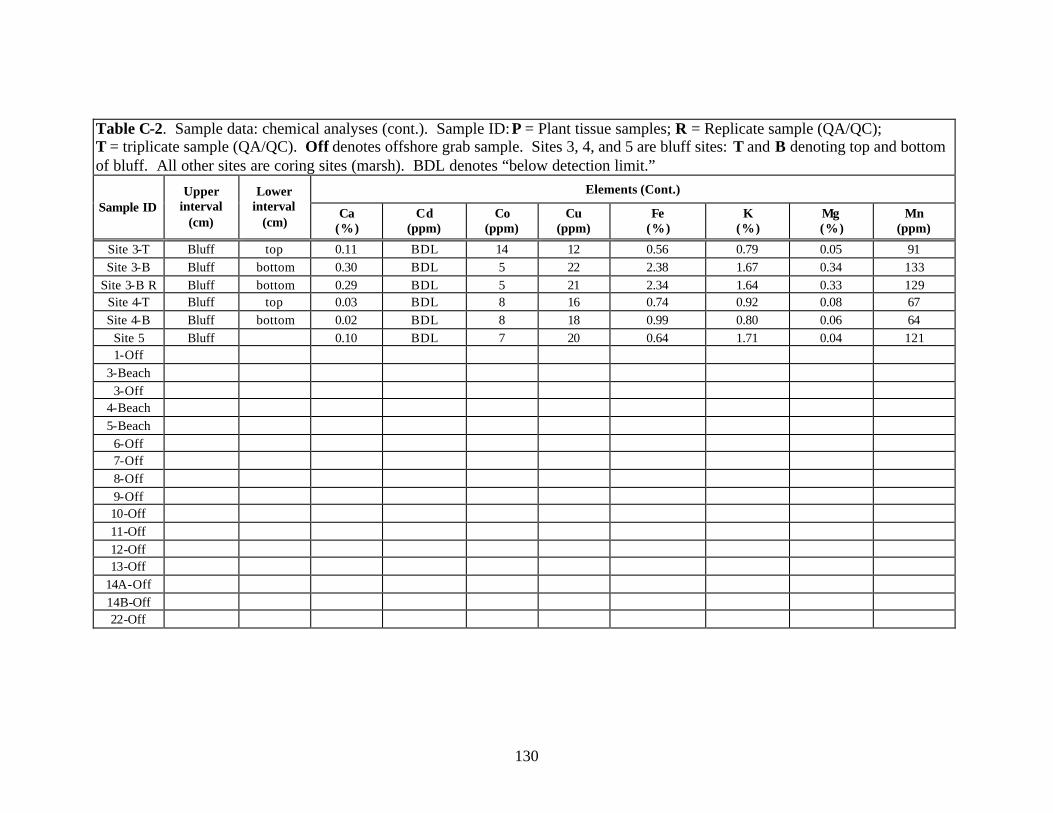
130



Upper interval

(cm)

Lower interval

(cm) Ca

(%) Cd

(ppm) Co

(ppm) Cu

(ppm) Fe

(%) K

(%) Mg (%)

Mn (ppm)

Site 3-T Bluff top 0.11 BDL 14 12 0.56 0.79 0.05 91 Site 3-B Bluff bottom 0.30 BDL 5 22 2.38 1.67 0.34 133

Site 3-B R Bluff bottom 0.29 BDL 5 21 2.34 1.64 0.33 129 Site 4-T Bluff top 0.03 BDL 8 16 0.74 0.92 0.08 67 Site 4-B Bluff bottom 0.02 BDL 8 18 0.99 0.80 0.06 64

Site 5 Bluff 0.10 BDL 7 20 0.64 1.71 0.04 121 1-Off

3-Beach 3-Off

4-Beach 5-Beach

6-Off 7-Off 8-Off 9-Off 10-Off 11-Off 12-Off 13-Off

14A-Off 14B-Off 22-Off

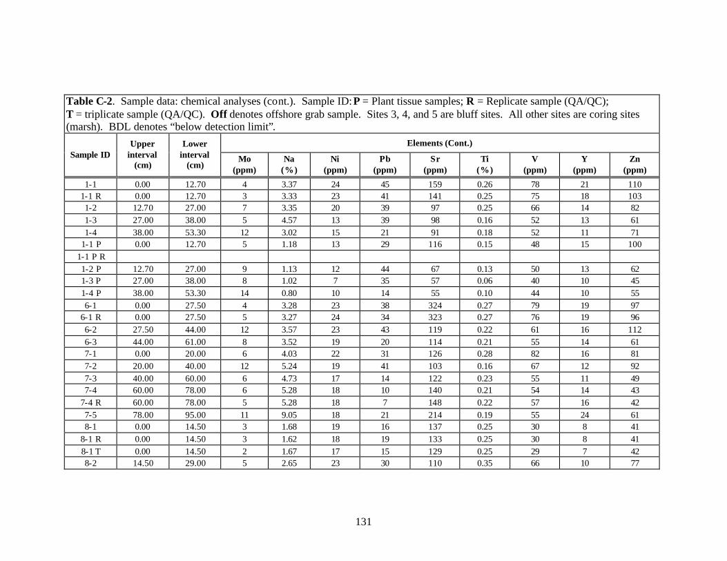
131

Table C-2. Sample data: chemical analyses (cont.). Sample ID: P = Plant tissue samples; R = Replicate sample (QA/QC); T = triplicate sample (QA/QC). Off denotes offshore grab sample. Sites 3, 4, and 5 are bluff sites. All other sites are coring sites (marsh). BDL denotes “below detection limit”.


Upper interval

(cm)

Lower interval

(cm) Mo

(ppm) Na

(%) Ni

(ppm) Pb

(ppm) Sr

(ppm) Ti

(%) V

(ppm) Y

(ppm) Zn

(ppm)

1-1 0.00 12.70 4 3.37 24 45 159 0.26 78 21 110 1-1 R 0.00 12.70 3 3.33 23 41 141 0.25 75 18 103 1-2 12.70 27.00 7 3.35 20 39 97 0.25 66 14 82 1-3 27.00 38.00 5 4.57 13 39 98 0.16 52 13 61 1-4 38.00 53.30 12 3.02 15 21 91 0.18 52 11 71

1-1 P 0.00 12.70 5 1.18 13 29 116 0.15 48 15 100 1-1 P R 1-2 P 12.70 27.00 9 1.13 12 44 67 0.13 50 13 62 1-3 P 27.00 38.00 8 1.02 7 35 57 0.06 40 10 45 1-4 P 38.00 53.30 14 0.80 10 14 55 0.10 44 10 55 6-1 0.00 27.50 4 3.28 23 38 324 0.27 79 19 97

6-1 R 0.00 27.50 5 3.27 24 34 323 0.27 76 19 96 6-2 27.50 44.00 12 3.57 23 43 119 0.22 61 16 112 6-3 44.00 61.00 8 3.52 19 20 114 0.21 55 14 61 7-1 0.00 20.00 6 4.03 22 31 126 0.28 82 16 81 7-2 20.00 40.00 12 5.24 19 41 103 0.16 67 12 92 7-3 40.00 60.00 6 4.73 17 14 122 0.23 55 11 49 7-4 60.00 78.00 6 5.28 18 10 140 0.21 54 14 43

7-4 R 60.00 78.00 5 5.28 18 7 148 0.22 57 16 42 7-5 78.00 95.00 11 9.05 18 21 214 0.19 55 24 61 8-1 0.00 14.50 3 1.68 19 16 137 0.25 30 8 41

8-1 R 0.00 14.50 3 1.62 18 19 133 0.25 30 8 41 8-1 T 0.00 14.50 2 1.67 17 15 129 0.25 29 7 42 8-2 14.50 29.00 5 2.65 23 30 110 0.35 66 10 77

132



Upper interval

(cm)

Lower interval

(cm) Mo

(ppm) Na

(%) Ni

(ppm) Pb

(ppm) Sr

(ppm) Ti

(%) V

(ppm) Y

(ppm) Zn

(ppm)

8-3 29.00 45.00 5 3.71 20 25 116 0.32 74 11 65 8-4 45.00 63.50 6 4.59 20 14 135 0.28 75 14 46

9-1 #1 0.00 19.00 3 1.90 40 24 135 0.27 46 10 52 9-1 #1 R 0.00 19.00 4 1.84 39 21 131 0.27 45 9 48 9-1 #2 0.00 19.00 3 1.82 39 25 127 0.25 44 9 48

9-2 19.00 39.00 5 3.12 25 28 156 0.35 78 12 60 9-3 39.00 59.00 7 4.78 24 20 126 0.26 66 14 79 9-4 59.00 76.00 6 3.92 25 13 157 0.33 80 11 53 10-1 0.00 23.50 3 2.82 26 32 159 0.35 77 15 69

10-1 R 0.00 23.50 5 2.84 26 32 160 0.35 78 15 72 10-2 23.50 35.50 5 3.10 27 38 146 0.37 94 14 93 10-3 35.50 48.50 5 3.67 27 33 119 0.30 79 12 110

10-3 R 35.50 48.50 5 3.49 25 33 114 0.29 77 13 109 11-1 0.00 19.00 4 1.82 33 25 148 0.30 59 11 50

11-1 R 0.00 19.00 5 1.81 35 21 146 0.30 60 10 48 11-2 19.00 36.00 6 2.67 27 39 150 0.38 92 14 88 11-3 36.00 47.00 7 4.82 17 19 126 0.23 57 14 50 11-4 47.00 60.00 6 5.45 16 14 139 0.25 58 11 34

12-1 #1 0.00 21.00 5 2.74 26 35 145 0.35 91 14 68 12-1 #1 R 0.00 21.00 12-1 #2 0.00 21.00 6 2.64 25 36 144 0.29 87 13 69

12-2 21.00 38.00 9 3.98 23 32 115 0.23 69 12 77 12-3 38.00 52.00 8 5.38 15 11 134 0.21 46 8 28 12-4 52.00 67.50 5 4.03 21 11 162 0.25 68 10 41 13-1 0.00 21.00 2 1.99 25 16 143 0.25 29 7 33

133



Upper interval

(cm)

Lower interval

(cm) Mo

(ppm) Na

(%) Ni

(ppm) Pb

(ppm) Sr

(ppm) Ti

(%) V

(ppm) Y

(ppm) Zn

(ppm)

13-2 21.00 35.50 4 3.42 44 33 152 0.32 73 12 79 13B-1 0.00 8.00 3 1.35 33 15 134 0.25 27 6 31 13B-2 8.00 20.00 2 1.46 22 16 131 0.29 30 7 40

13B-2 R 8.00 20.00 2 1.44 23 17 132 0.28 30 6 42 13B-3 20.00 35.00 4 2.14 32 27 156 0.26 60 11 66 13B-4 35.00 46.50 4 2.68 27 32 149 0.32 79 12 73 13B-5 46.50 70.50 7 4.50 21 23 121 0.25 65 11 55 14-1 0.00 17.50 4 2.51 33 27 108 0.33 62 9 52 14-2 17.50 26.00 7 3.06 23 38 117 0.33 82 9 70 14-3 26.00 45.50 3 2.50 30 20 110 0.28 47 9 44

14-3 R 26.00 45.50 14B-1 0.00 16.00 3 1.59 31 25 115 0.28 51 11 54 14B-2 16.00 28.50 5 2.12 38 34 149 0.36 71 13 74

14B-2 R 16.00 28.50 4 2.19 36 36 149 0.35 73 14 76 14B-3 28.50 46.50 6 3.29 26 61 127 0.29 70 14 54 14B-4 46.50 64.50 5 3.14 26 17 158 0.35 79 11 43 14B-5 64.50 75.50 6 2.34 35 17 175 0.40 96 14 64 14B-6 75.50 86.50 7 3.05 22 12 173 0.33 75 13 43

14B-6 R 75.50 86.50 8 2.98 23 11 167 0.31 73 13 42 14B-1 P 0.00 16.00 6 1.16 10 33 84 0.14 43 9 62 14B-2 P 16.00 28.50 14 0.64 22 81 85 0.15 77 16 103 14B-3 P 28.50 46.50 5 0.97 18 230 99 0.18 53 15 53 14B-4 P 46.50 64.50 5 0.73 14 13 109 0.19 60 17 38 14B-5 P 64.50 75.50 26 0.53 50 28 83 0.14 82 17 68 14B-6 P 75.50 86.50 19 0.66 18 12 101 0.13 69 20 37

134



Upper interval

(cm)

Lower interval

(cm) Mo

(ppm) Na

(%) Ni

(ppm) Pb

(ppm) Sr

(ppm) Ti

(%) V

(ppm) Y

(ppm) Zn

(ppm)

18-0 0.00 24.50 6 2.78 39 31 177 0.33 74 12 87 18-0 R 18-1 24.50 37.00 7 4.23 21 28 127 0.28 68 11 51 18-2 37.00 62.00 6 3.21 27 15 163 0.31 69 11 51 18-3 62.00 87.00 6 2.90 27 15 164 0.36 84 10 52 18-4 87.00 112.00 12 3.85 27 11 137 0.29 78 12 54 18-5 112.00 143.00 5 2.71 48 12 175 0.26 47 9 34

18-5 R 112.00 143.00 6 2.81 49 12 154 0.27 48 9 30 18-5 R 112.00 143.00 5 2.75 46 10 142 0.26 47 7 28 18-5 T 112.00 143.00 6 2.77 49 11 181 0.24 48 9 29 19-1 0.00 17.00 3 2.15 33 20 196 0.21 37 9 45

19-1 R 0.00 17.00 3 2.18 33 19 196 0.20 38 9 47 19-1 T 0.00 17.00 3 2.14 32 17 193 0.19 37 8 44 19-2 17.00 30.00 3 2.29 30 18 212 0.22 39 8 46

19-2 R 17.00 30.00 19-3 30.00 46.50 3 2.41 35 23 204 0.33 54 11 68 19-4 46.50 57.50 4 4.54 23 21 137 0.21 40 13 55

19-1 P 0.00 17.00 6 1.46 11 36 107 0.17 42 15 72 19-2 P 17.00 30.00 6 0.79 12 27 65 0.15 54 14 46

19-2 P R 17.00 30.00 19-3 P 30.00 46.50 8 0.75 14 40 65 0.17 66 18 95 19-4 P 46.50 57.50 6 1.03 9 21 53 0.09 26 12 41 22-1 0.00 23.00 6 3.19 32 29 110 0.36 90 11 65 22-2 23.00 42.00 6 3.20 27 31 114 0.34 84 13 67 22-3 42.00 58.00 9 3.87 20 17 106 0.28 69 12 44

135



Upper interval

(cm)

Lower interval

(cm) Mo

(ppm) Na

(%) Ni

(ppm) Pb

(ppm) Sr

(ppm) Ti

(%) V

(ppm) Y

(ppm) Zn

(ppm)

Site 3-T Bluff top BDL 0.28 3 9 66 0.11 6 3 29 Site 3-B Bluff bottom 2 0.90 12 16 131 0.29 64 5 54

Site 3-B R Bluff bottom 2 0.89 14 20 126 0.32 68 5 56 Site 4-T Bluff top BDL 0.14 5 10 52 0.05 10 6 32 Site 4-B Bluff bottom BDL 0.11 3 8 47 0.07 10 2 31

Site 5 Bluff BDL 0.31 8 14 109 0.21 16 3 28 1-Off

3-Beach 3-Off

4-Beach 5-Beach

6-Off 7-Off 8-Off 9-Off 10-Off 11-Off 12-Off 13-Off

14A-Off 14B-Off 22-Off

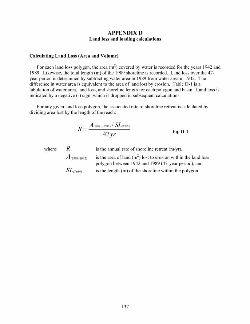
137

APPENDIX D Land loss and loading calculations

Calculating Land Loss (Area and Volume)

For each land loss polygon, the area (m2) covered by water is recorded for the years 1942 and 1989. Likewise, the total length (m) of the 1989 shoreline is recorded. Land loss over the 47-year period is determined by subtracting water area in 1989 from water area in 1942. The difference in water area is equivalent to the area of land lost by erosion. Table D-1 is a tabulation of water area, land loss, and shoreline length for each polygon and basin. Land loss is indicated by a negative (-) sign, which is dropped in subsequent calculations.

For any given land loss polygon, the associated rate of shoreline retreat is calculated by dividing area lost by the length of the reach:

yrSLAR

47/ )1989()19421989( −

= Eq. D-1

where: R is the annual rate of shoreline retreat (m/yr),

A(1989-1942) is the area of land (m2) lost to erosion within the land loss polygon between 1942 and 1989 (47-year period), and

SL(1989) is the length (m) of the shoreline within the polygon.

138

Table D-1. Area (m2) and volume (m3) of land lost during the 47-year period between 1942 and 1989 and linear rates (m/yr) of shoreline erosion, by shoreline reach (land loss polygon).

Polygon

1942

water area (m2)

1989

water area (m2)

SL

1989 shoreline

length (m)

A(1989-1942)

Change in land area

(m2)

Change per meter

of shoreline

R Annual

shoreline change (m/yr)

H

Bank height

(m)

Volume

(m3)

Annual volume (m3/yr)

P1 47,950.94 50,805.64 583.18 -2,854.70 -4.90 -0.10 0.6 -1,712.82 -36.44

P2 3,526,880.74 3,778,632.75 44,410.90 -251,752.01 -5.67 -0.12 0.68 -171,191.37 -3,642.37 P4 298,803.57 331,356.66 4,444.16 -32,553.09 -7.32 -0.16 0.4 -13,021.24 -277.05 P6 628,573.16 697,538.96 7,531.84 -68,965.80 -9.16 -0.19 0.4 -27,586.32 -586.94 P7 888,199.10 953,787.44 6,962.69 -65,588.34 -9.42 -0.20 0.5 -32,794.17 -697.75 P8 670,821.01 741,784.40 6,301.49 -70,963.39 -11.26 -0.24 0.4 -28,385.36 -603.94 P9 154,799.59 168,758.89 1,135.80 -13,959.30 -12.29 -0.26 0.65 -9,073.55 -193.05 P10 566,711.81 633,225.41 9,793.89 -66,513.60 -6.79 -0.14 0.49 -32,591.66 -693.44 P12 472,959.59 572,462.32 11,258.65 -99,502.73 -8.84 -0.19 0.57 -56,716.56 -1,206.74 P13 1,116,239.83 1,219,653.87 8,740.04 -103,414.04 -11.83 -0.25 0.72 -74,458.11 -1,584.22 P14 264,016.06 283,567.41 2,892.47 -19,551.35 -6.76 -0.14 0.68 -13,294.92 -282.87 P15 643,466.91 683,503.74 5,637.03 -40,036.83 -7.10 -0.15 1.4 -56,051.56 -1,192.59 P16 430,363.14 463,622.89 7,582.11 -33,259.75 -4.39 -0.09 1.4 -46,563.65 -990.72 P17 246,228.81 264,120.82 8,687.06 -17,892.01 -2.06 -0.04 3.12 -55,823.07 -1,187.72 P18 916,842.02 941,630.89 12,403.39 -24,788.87 -2.00 -0.04 1.9 -47,098.85 -1,002.10 P19 430,330.55 453,762.39 2,177.43 -23,431.84 -10.76 -0.23 0.53 -12,418.88 -264.23 P20 114,667.58 132,586.22 1,533.47 -17,918.64 -11.69 -0.25 0.42 -7,525.83 -160.12 P21 578,696.59 610,993.02 5,135.51 -32,296.43 -6.29 -0.13 0.42 -13,564.50 -288.61 P26 446,165.72 498,731.88 4,816.07 -52,566.16 -10.91 -0.23 0.28 -14,718.52 -313.16 P27 762,215.56 814,221.01 2,821.89 -52,005.45 -18.43 -0.39 0.28 -14,561.53 -309.82 P28 418,131.38 476,037.20 5,325.49 -57,905.82 -10.87 -0.23 0.45 -26,057.62 -554.42 P29 301,883.44 322,794.91 1,181.26 -20,911.47 -17.70 -0.38 0.98 -20,493.24 -436.03 P30 454,263.04 501,288.98 4,482.79 -47,025.94 -10.49 -0.22 0.98 -46,085.42 -980.54

Totals 14,379,210.14 15,594,867.70 165,838.61 1,215,657.56 Mean = -7.33

Mean = -0.16 --- 821,788.75 17,484.87

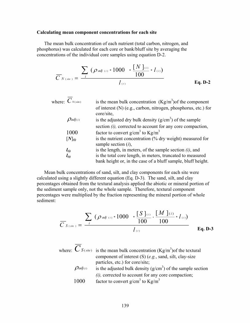
139

Calculating mean component concentrations for each site

The mean bulk concentration of each nutrient (total carbon, nitrogen, and phosphorus) was calculated for each core or bank/bluff site by averaging the concentrations of the individual core samples using equation D-2.

)(

)()(

)(

)(

)100

][1000( ***

t

ii

i

site

l

lN

C iadj

N

∑=

ρ

Eq. D-2

where: )( siteNC is the mean bulk concentration (Kg/m3)of the component of interest (N) (e.g., carbon, nitrogen, phosphorus, etc.) for core/site,

)( iadjρ is the adjusted dry bulk density (g/cm3) of the sample section (i), corrected to account for any core compaction,

1000 factor to convert g/cm3 to Kg/m3 [N](i) is the nutrient concentration (% dry weight) measured for

sample section (i), l(i) is the length, in meters, of the sample section (i), and

l(t) is the total core length, in meters, truncated to measured bank height or, in the case of a bluff sample, bluff height.

Mean bulk concentrations of sand, silt, and clay components for each site were calculated using a slightly different equation (Eq. D-3). The sand, silt, and clay percentages obtained from the textural analysis applied the abiotic or mineral portion of the sediment sample only, not the whole sample. Therefore, textural component percentages were multiplied by the fraction representing the mineral portion of whole sediment:

)(

)(*)(

)(

)(

)100

][100

][1000( *)(

**

t

ii

i

site

l

lMS

C i

iadj

S

∑=

ρ

Eq. D-3

where: )( siteSC is the mean bulk concentration (Kg/m3)of the textural component of interest (S) (e.g., sand, silt, clay-size particles, etc.) for core/site;

)( iadjρ is the adjusted bulk density (g/cm3) of the sample section (i), corrected to account for any core compaction;

1000 factor to convert g/cm3 to Kg/m3

140

[S](i) is the textural component (% dry weight sand, silt, or clay) measured for sample section (i);

[M](i) is the abiotic or mineral portion ( %dry weight) of the sample section;

l(i) is the length, in meters, of the sample section (i); l(t) is the total core length, in meters, truncated to measured

bank height; or, in the case of a bluff sample, height of the bluff.

Table D-2. Mean textural and nutrient concentrations calculated for each site using equations D-2 and D-3. All values listed are Kg/m3. These site values are assigned to specific land loss polygons (see Table 4-2) to calculate the sediment and nutrient contribution rates for the polygon using equation D-4.

Nutrients Textural component Site Total solids

Total organics (biotic

component) Nitrogen Carbon Phosphorus Sand Silt Clay

1 177.04 107.28 1.84 33.07 0.143 9.00 24.10 36.65 3 1268.35 38.95 0.60 7.31 0.096 1025.39 120.17 83.84 4 1442.34 32.27 0.35 3.45 0.064 1161.32 93.46 94.05 5 1336.30 25.74 0.20 0.89 0.086 1092.87 78.47 120.27 6 223.88 139.73 1.91 36.71 0.149 6.48 35.44 42.23 7 178.53 107.49 1.71 32.15 0.098 3.66 33.26 34.11 8 492.20 138.09 1.72 32.30 0.151 166.06 105.61 82.43 9 493.28 99.51 1.97 36.25 0.191 190.06 111.38 92.33

10 445.54 140.92 2.02 37.95 0.193 32.89 154.37 117.36 11 410.93 138.98 1.51 27.15 0.143 117.87 86.77 67.31 12 339.81 139.33 2.04 37.96 0.137 20.70 89.65 90.13 13 766.86 144.58 1.69 27.83 0.236 393.56 152.12 76.60

13B 560.88 111.60 1.69 30.53 0.169 245.32 121.40 82.56 14 458.42 193.45 2.43 41.90 0.181 110.60 79.36 75.01

14B 384.69 97.57 1.85 32.05 0.145 85.45 99.71 101.96 18 325.46 108.08 1.36 26.65 0.123 32.90 112.02 72.46 19 977.77 113.18 1.64 32.75 0.300 604.17 181.11 79.31 22 294.89 104.70 1.49 29.90 0.115 1.72 101.06 87.40

141

Calculating component loadings (Kg/yr) The mean site concentration values were then assigned to specific polygons to calculate the nutrient loading for the polygon using the following equation:

Eq. D-4

where: L(N),(S) is the annual loading (Kg/yr) of the component of interest (

N: e.g., carbon, nitrogen or phosphorus; or S: e.g., sand, silt, clay) for the land loss polygon;

)(, siteSNC is the mean loading concentration (Kg/m3)of the component of interest (N) (e.g., carbon, nitrogen, phosphorus, etc.) for core/site assigned to the land loss polygon;

A(1989-1942) is the area of land (m2) lost to erosion within the land loss polygon between 1942 and 1989 (47 year period);

H is the mean bank height assigned to the land loss polygon.

=

−

yrHACL siteSNSN

47** )19421989(

)(,)(),(

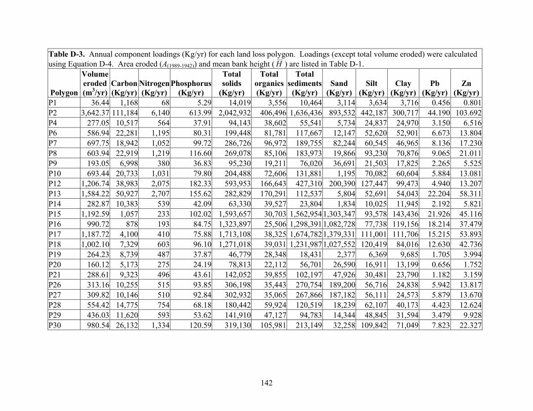
142

Table D-3. Annual component loadings (Kg/yr) for each land loss polygon. Loadings (except total volume eroded) were calculated using Equation D-4. Area eroded (A(1989-1942)) and mean bank height ( H ) are listed in Table D-1.

Polygon

Volume eroded (m3/yr)

Carbon (Kg/yr)

Nitrogen(Kg/yr)

Phosphorus(Kg/yr)

Total solids

(Kg/yr)

Total organics(Kg/yr)

Total sediments

(Kg/yr) Sand

(Kg/yr)Silt

(Kg/yr)Clay

(Kg/yr)Pb

(Kg/yr)Zn

(Kg/yr)P1 36.44 1,168 68 5.29 14,019 3,556 10,464 3,114 3,634 3,716 0.456 0.801P2 3,642.37 111,184 6,140 613.99 2,042,932 406,496 1,636,436 893,532 442,187 300,717 44.190 103.692P4 277.05 10,517 564 37.91 94,143 38,602 55,541 5,734 24,837 24,970 3.150 6.516P6 586.94 22,281 1,195 80.31 199,448 81,781 117,667 12,147 52,620 52,901 6.673 13.804P7 697.75 18,942 1,052 99.72 286,726 96,972 189,755 82,244 60,545 46,965 8.136 17.230P8 603.94 22,919 1,219 116.60 269,078 85,106 183,973 19,866 93,230 70,876 9.065 21.011P9 193.05 6,998 380 36.83 95,230 19,211 76,020 36,691 21,503 17,825 2.265 5.525P10 693.44 20,733 1,031 79.80 204,488 72,606 131,881 1,195 70,082 60,604 5.884 13.081P12 1,206.74 38,983 2,075 182.33 593,953 166,643 427,310 200,390 127,447 99,473 4.940 13.207P13 1,584.22 50,927 2,707 155.62 282,829 170,291 112,537 5,804 52,691 54,043 22.204 58.311P14 282.87 10,383 539 42.09 63,330 39,527 23,804 1,834 10,025 11,945 2.192 5.821P15 1,192.59 1,057 233 102.02 1,593,657 30,703 1,562,954 1,303,347 93,578 143,436 21.926 45.116P16 990.72 878 193 84.75 1,323,897 25,506 1,298,391 1,082,728 77,738 119,156 18.214 37.479P17 1,187.72 4,100 410 75.88 1,713,108 38,325 1,674,782 1,379,331 111,001 111,706 15.215 53.893P18 1,002.10 7,329 603 96.10 1,271,018 39,031 1,231,987 1,027,552 120,419 84,016 12.630 42.736P19 264.23 8,739 487 37.87 46,779 28,348 18,431 2,377 6,369 9,685 1.705 3.994P20 160.12 5,173 275 24.19 78,813 22,112 56,701 26,590 16,911 13,199 0.656 1.752P21 288.61 9,323 496 43.61 142,052 39,855 102,197 47,926 30,481 23,790 1.182 3.159P26 313.16 10,255 515 93.85 306,198 35,443 270,754 189,200 56,716 24,838 5.942 13.817P27 309.82 10,146 510 92.84 302,932 35,065 267,866 187,182 56,111 24,573 5.879 13.670P28 554.42 14,775 754 68.18 180,442 59,924 120,519 18,239 62,107 40,173 4.423 12.624P29 436.03 11,620 593 53.62 141,910 47,127 94,783 14,344 48,845 31,594 3.479 9.928P30 980.54 26,132 1,334 120.59 319,130 105,981 213,149 32,258 109,842 71,049 7.823 22.327

resource assessment service maryland … assessment service maryland geological survey ... this...

Documents