resource abundance, fisheries management, and fishing

Resource Abundance, FisheriesManagement, and Fishing Ports: TheU.S. Atlantic Sea Scallop Fishery

Min-Yang Lee, Sharon Benjamin, Andrew Carr-Harris,Deborah Hart, and Cameron Speir

The Atlantic Sea Scallop fishery has grown tremendously over the past twentyyears. The location and magnitude of harvestable biomass fluctuates dramaticallydue to both natural variation and the explicitly spatial management systemdesigned to allow small individuals to grow larger and more valuable. Thesefluctuations in natural advantages can have profound effects on fishing ports. Weuse methods from economic growth literature to show that ports with lowerinitial scallop landings have grown the fastest. Furthermore, good access tobiomass influences long-run changes in landings, although this effect exhibitsconsiderable variability across ports. We also find evidence of returns to scope,suggesting that ports with other fishing activities could be well positioned toattract new scalloping activity when stock conditions are favorable. Furtherinvestigation of the largest ports using time-series methods also shows a highdegree of variability; there are long-run relationships between scallop fishingand harvestable scallop stock in some ports, short-run relationships in someports, and no relationship between the two in others. We interpret this asevidence that heterogeneity in the natural productivity of the ocean combinedwith explicitly spatial fisheries management has induced a spatial component tothe port-level response to changes in biomass availability.

Key Words: economic geography, fisheries management, fishing ports, naturalresource economics

The Atlantic Sea Scallop fishery has experienced dramatic increases in biomass,landings, and prices over a twenty-year time period (Hart and Rago 2006,Northeast Fisheries Science Center 2014). We use a set of econometricmethods and models to understand how port-level landings have respondedto changes in proximity to biomass. Access to biomass, a particular type ofnatural advantage, fluctuates from year-to-year in this fishery and may cause

Min-Yang Lee, National Oceanic and Atmospheric Administration, National Marine FisheriesService, Northeast Fisheries Science Center, 166 Water St, Woods Hole, MA 02543 SharonBenjamin, NOAA, NMFS, NEFSC, and Integrated Statistics Andrew Carr-Harris, NOAA, NMFS,NEFSC and Department of Environmental and Natural Resource Economics, University of RhodeIsland Deborah Hart, NOAA, NMFS, NEFSC Cameron Speir, NOAA, NMFS, Southwest FisheriesScience Center Correspondence: Min-Yang Lee, National Oceanic and Atmospheric Administration,National Marine Fisheries Service, Northeast Fisheries Science Center, 166 Water St, Woods Hole,MA 02543, ph: (508) 495-4704, Email: [email protected]

Agricultural and Resource Economics Review 48/1 (April 2019) 71–99© The Author(s) 2019. This is an Open Access article, distributed under the terms of the CreativeCommons Attribution licence (http://creativecommons.org/licenses/by/4.0/), which permits

unrestricted re-use, distribution, and reproduction in any medium, provided the original work isproperly cited.

http

s://

doi.o

rg/1

0.10

17/a

ge.2

018.

23D

ownl

oade

d fr

om h

ttps

://w

ww

.cam

brid

ge.o

rg/c

ore.

IP a

ddre

ss: 6

5.21

.228

.167

, on

10 D

ec 2

021

at 0

2:07

:47,

sub

ject

to th

e Ca

mbr

idge

Cor

e te

rms

of u

se, a

vaila

ble

at h

ttps

://w

ww

.cam

brid

ge.o

rg/c

ore/

term

s.

mailto:[email protected]

https://doi.org/10.1017/age.2018.23

https://www.cambridge.org/core

https://www.cambridge.org/core/terms

long-lasting changes in the geographic distribution of fishing as agents respondto changing environmental and regulatory conditions by investing in capital orrelocating existing capital (Portman, Jin, and Thunberg 2009, 2011). In addition,within- and across-fishery agglomerative forces (separate from any naturaladvantages conferred by access to biomass) may influence where scallops arelanded as participants in the industry respond to economies of scale andscope. We examine these effects by estimating long-run economic growthmodels that relate growth of scallop fishing over fifteen years to initialconditions and exposure to biomass. Fluctuations in natural and regulatoryconditions may also have effects that vary across ports or occur at a fastertime scale. We test for the existence and relative magnitude of these effectsusing time-series methods.Fisheries management in the United States has many goals; these include

mandates to prevent overfishing, provide the greatest overall benefit to thenation, and take into account the importance of fishery resources to fishingcommunities (Magnuson-Stevens Fishery Conservation and Management Act2007). The effects of natural advantages relative to endogenously determinedcapital has implications for resource managers concerned with fishingcommunities. If port-level landings are very sensitive to biomass, then portswill quickly expand or contract after experiencing temporary biomass shocks.However, if landings are not sensitive to biomass, then it may be necessary toidentify ports that are declining, and understand why they are doing so, priorto formulating an appropriate policy response designed to address fishingcommunities.Furthermore, economic studies of cities illustrate that changes in economic

activity in one industry could have secondary effects on other parts of thelocal economy through spillovers (Quigley 1998, Puga 2010, Behrens,Duranton, and Robert-Nicoud 2014). The commercial fishing industry islinked to upstream and downstream industries, including seafood processors,wholesalers, gear suppliers, settlement houses, and repair operations (Kaplan1999, Hall-Arber et al. 2001, National Marine Fisheries Service 2016). Thepotential for spillover effects on other fisheries and related industries hasinduced local governments to develop port management plans (Georgiannaet al. 2014) or directly lobby the executive and legislative branches of the U.S.government to preserve local fishing capacity (Bonner 2017, Valencia 2017).Marshall (1920) posited natural advantages, economies of scale, input

sharing technology adoption, and labor market matching as possible driversfor clustering and agglomeration of economic activity. Re-energized byKrugman (1991), a substantial burst of research has been directed atcharacterizing the agglomeration of economic activity at fine scales andunderstanding which of these Marshallian forces is most important1. Kim

1 Duranton and Puga (2004), Rosenthal and Strange (2004), Redding (2009) provide recentoverviews of these efforts.

Agricultural and Resource Economics Review72 April 2019

http

s://

doi.o

rg/1

0.10

17/a

ge.2

018.

23D

ownl

oade

d fr

om h

ttps

://w

ww

.cam

brid

ge.o

rg/c

ore.

IP a

ddre

ss: 6

5.21

.228

.167

, on

10 D

ec 2

021

at 0

2:07

:47,

sub

ject

to th

e Ca

mbr

idge

Cor

e te

rms

of u

se, a

vaila

ble

at h

ttps

://w

ww

.cam

brid

ge.o

rg/c

ore/

term

s.




(1999), Ellison and Glaeser (1999), Midelfart-Knarvik et al. (2001), Bleakleyand Lin (2012) find support for the importance of factor endowments in U.S.manufacturing location, U.S. manufacturing agglomeration, EU industriallocation, and U.S. economic activity respectively2.Extensive research has demonstrated the importance of natural advantages,

as measured by high catch rates or low costs, in determining where fishingactivity takes place (Girardin et al. 2017). Quite a bit less is known aboutports. Portman, Jin, and Thunberg (2009, 2011) show that healthy biomasssignals high future profits and encourage development of land to support thefishing industry. Watson and Johnson (2012) finds evidence that nonspatialpolicies can have heterogeneous effects across the coast as well. Watson andJohnson (2012) examine changes in landings on the West Coast of the UnitedStates after a fishery buyback in 2003 using static panel methods, findingthat small ports had higher variability in landings after a buyback than largeports. Speir, Pomeroy, and Sutinen (2014) and Lee et al. (2017) characterizebut do not explain spatial distribution of fishing for fisheries on the East andWest Coast of the United States. Agnarsson, Matthiasson, and Giry (2016)examine distribution of quota across ports in Iceland, which is likely to beclosely related to landing locations.Both first-nature (natural advantages) and second-nature (caused by

humans) geography are likely to be important. For example, ports that arelocated near productive fishing locations will have first-nature geographicadvantages relative to ports that are farther from good fishing grounds.Similarly, endowments of social (Kaplan 1999, Hall-Arber et al. 2001, Holland,Pinto da Silva, and Kitts 2015, Clay, Colburn, and Seara 2016) and physicalcapital can confer second-nature advantages to established ports tonontraditional fishing ports. The Atlantic Sea Scallop fishery provides aunique opportunity to study the importance of natural advantages relative to“second-nature” geography. Unlike finfish, scallops are relatively immobileafter settling on the ocean floor (Hart and Rago 2006). There is extensivefishery-independent survey data that provides information about the locationand scale of biomass. The geographic distribution of fishable scallop biomasshas also changed frequently due to both natural variability and area-basedfishing regulations (Hart and Rago 2006). The management system, whichopens and closes areas of the ocean to solve the growth overfishingproblem3, can dramatically change a port’s access to biomass from one yearto the next.

2 At larger geographic scales, the effects of natural resources on economic performance are notsettled, see Bloom et al. (1998), Gallup, Sachs, and Mellinger (1999), Sachs and Warner (1999),Acemoglu, Johnson, and Robinson (2002), Rodrik, Subramanian, and Trebbi (2004), Papyrakisand Gerlagh (2007), Michaels (2011), Van Der Ploeg (2011), Havranek, Horvath, and Zeynalov(2016).3 See, for example, Hart (2003), Diekert et al. (2010), Diekert (2012).

Lee et al. Resource Abundance, Fisheries Management, and Fishing Ports 73

http

s://

doi.o

rg/1

0.10

17/a

ge.2

018.

23D

ownl

oade

d fr

om h

ttps

://w

ww

.cam

brid

ge.o

rg/c

ore.

IP a

ddre

ss: 6

5.21

.228

.167

, on

10 D

ec 2

021

at 0

2:07

:47,

sub

ject

to th

e Ca

mbr

idge

Cor

e te

rms

of u

se, a

vaila

ble

at h

ttps

://w

ww

.cam

brid

ge.o

rg/c

ore/

term

s.




We use two sets of methods to examine the effects of changes in naturaladvantages on ports and fishing activity. We first estimate a long-run growthmodel to examine how natural advantages (access to biomass and variabilityof access over time) and returns to both scale and scope influence scalloplandings at the port level. We also estimate time series models that explorethe relationship between natural advantages and landings at a finer temporalstep for the twenty-five largest scallop ports in the region.

Scallops, the Fishery, and Regulations

The Atlantic sea scallop is found on the continental shelf of the Northeast UnitedStates, from North Carolina through Maine. Important fishing grounds are onGeorges Bank (GB), Southern New England (SNE), and the Mid-Atlantic Bight(MAB), at depths up to about 350 feet (Hart and Chute 2004, Hart and Rago2006). Scallops reproduce by producing large amounts of eggs; larvaesubsequently drift with water currents before settling to the bottom of theocean (Hart and Chute 2004). Under favorable conditions, this can result inextremely high abundances of juvenile scallops in localized areas. Thebiological characteristics of sea scallops make them particularly well suited tospatial management: scallops grow relatively quickly, adults typically havelow natural mortality, and scallops are relatively immobile after settling onthe ocean floor (Hart and Rago 2006). The biomass of scallops is currentlyhigh (Northeast Fisheries Science Center 2014). Scallops in GB and MABwaters grow similarly until they are about 8 cm shell height, but scallops onGB grow to a larger asymptotic size (Hart and Chute 2009). In both areas,scallops grow to a smaller asymptotic size in deeper depths; this effect ismore pronounced in the MAB (Hart and Chute 2009).4

The National Marine Fisheries Service (NMFS) is responsible for assessing thesea scallop population and fishery in federal waters off the coast of the US; thishas historically been accomplished using a dredge survey and commercial data.Beginning in the mid-2000s, this was supplemented by a pair of optical surveysthat increased the intensity and geographic breadth of scientific information. Asa result of the high intensity of survey efforts, the biomass and location ofscallops are quite well understood.The New England Fishery Management Council, composed of industry

stakeholders, non-industry stakeholders, state officials, and federal officials, isresponsible for recommending scallop fishery policy in federal waters (3–200nautical miles from shore). NMFS translates these policies into regulationsand enforces those regulations. Fisheries policies are guided primarily by theMagnuson-Stevens Fishery Conservation and Management Act, whichdescribes ten standards for fisheries management. The charge to prevent

4 See Serchuk et al. (1979), Hart and Chute (2004), Hart and Rago (2006), Northeast FisheriesScience Center (2014), Cooley et al. (2015) for biology, ecology, and stock dynamics.


http

s://

doi.o

rg/1

0.10

17/a

ge.2

018.

23D

ownl

oade

d fr

om h

ttps

://w

ww

.cam

brid

ge.o

rg/c

ore.

IP a

ddre

ss: 6

5.21

.228

.167

, on

10 D

ec 2

021

at 0

2:07

:47,

sub

ject

to th

e Ca

mbr

idge

Cor

e te

rms

of u

se, a

vaila

ble

at h

ttps

://w

ww

.cam

brid

ge.o

rg/c

ore/

term

s.




overfishing and achieve “optimum yield” (Magnuson-Stevens FisheryConservation and Management Act 2007) is frequently the most difficult toachieve; however, the MSFCMA also requires understanding how regulationsaffect fishing communities and accounting for those effects when settingpolicy. Fishing vessels in the Atlantic sea scallop fishery typically use dredgegear to harvest scallops from the ocean bottom Northeast Fisheries ScienceCenter (2014). Processing of scallops, in which the adductor muscle isretained and sorted by size, has occurred on-board the vessel since the mid1930s (Georgianna, Lee, and Walden 2017). As part of the fisherymanagement process, NMFS requires both fishing vessels and fish buyers toobtain permits. Fishing vessels are required to file trip reports, and buyersare required to report purchases of scallop from those fishing vessels.Because the primary objective of these data collection efforts are todetermine the amount of fish and shellfish that are harvested, there are noreporting requirements for subsequent sales further up the supply chain.In the scallop fishery, fishing regulations primarily include limits on days at

sea (DAS), gear restrictions, crew restrictions, and temporary closures ofparts of the ocean, so that the annual catch limits (ACLs) are not exceeded5.Since 1994, scallop vessels were allocated a number of DAS which they coulduse in “open” areas. Spatial management has featured prominently in scallopmanagement since early 1994, when two large areas on Georges Bank(Closed Area I and II) and another in Southern New England (NantucketLightship) were closed to bottom-tending gear, including dredges and bottomtrawls, to rebuild depleted stocks of groundfish (59 Federal Register 26; 59Federal Register 9872). Two areas in the Mid-Atlantic were closed in 1998 toallow juvenile scallops to mature. The scallop fleet was allowed to fish in aportion of Closed Area II in 1999 and the access program was expanded toparts of Closed Area I and Nantucket Lightship in 2000. The Mid-Atlanticareas were reopened as rotational access areas in 2001. Vessels fishing inthese areas were required to use DAS and were subject to a possession limit(typically a trip “cost” 10 DAS).In 2004 the current management system, consisting of access, open, and

closed areas was adopted (69 Federal Register 35194–224). One of thesouthern access areas (Virginia Beach) was reconfigured as an open areabecause it was not successful at encouraging growth of scallops. Additionalareas have been added to the rotational program; the boundaries of theseareas experienced minimal changes until 2015, when the Mid-Atlantic regionswere reconfigured into a single large access area and a small closed area. Inthe current system, an area can be closed to scallop fishing when it containshigh abundances of juvenile scallops. This allows scallops to grow larger,addressing the growth overfishing problem. When opened, fishing vessels are

5 Until 2018, the fishing year ran from March to February; unless otherwise noted all years arefishing years.


http

s://

doi.o

rg/1

0.10

17/a

ge.2

018.

23D

ownl

oade

d fr

om h

ttps

://w

ww

.cam

brid

ge.o

rg/c

ore.

IP a

ddre

ss: 6

5.21

.228

.167

, on

10 D

ec 2

021

at 0

2:07

:47,

sub

ject

to th

e Ca

mbr

idge

Cor

e te

rms

of u

se, a

vaila

ble

at h

ttps

://w

ww

.cam

brid

ge.o

rg/c

ore/

term

s.




allocated trips, with a possession limit, into the access areas. These trips nolonger require using open-area DAS.6

As access areas are opened and closed, and biomass in all parts of the oceanfluctuate, the relative advantages of fishing from a particular port are likely tochange. Increases in travel time to the rotational areas leads to increasedexpenditures on fuel. Increases in travel time to open areas are even costlierbecause fishing vessels also must use scarce DAS to steam instead of activelyfish. Fishing vessels are quite mobile and can respond to spatial variations incosts by changing locations. It seems natural, then, to examine the effects ofchanging resource advantages on ports.

Data

The subsequent analysis primarily relies on two datasets containing data from1996–2015. Exploitable biomass in each of the twelve discrete areas wasconstructed using fishery independent data collected through dredge andoptical surveys. These estimates were aggregated to construct an availablebiomass index using the schedule of openings and closing taken from thefishery regulations published in the Federal Register. The second datasetcontains information on landings and value, by species, aggregated to theport level. The major ports and biomass regions are illustrated in Figure 1.We constructed an inverse-distance weighted biomass availability index to

measure natural advantages in each port. We used estimates of exploitablebiomass density (kilograms per standardized tow, only individuals largerthan 90 mm) in each of twelve discrete areas where scallops are harvested(Figure 2)7. Each of the twelve biomass regions was decomposed into small

(14km2) cells. We index ports, fishing region, and cells with i, r, and k

subscripts respectively and suppress the time subscript for compactness.Each fishing region has Kr cells. Ordering the regions so that the regionsindexed r¼ 1, …R1 are open and the rest are closed, the available biomassindex (Availablei) is:

Availablei ¼XR1

r¼1

XKr

k¼1

Exploitable Biomass DensityrDistanceik

,(1)

where Distanceik is the over-water travel distance (kilometers) from port i to cellk. This formulation allows the available biomass index to vary both across portswithin a year due to different distances, and across years within a port as stock

6 See Doeringer, Moss, and Terkla (1986), Edwards (2001), Repetto (2001), Baskaran andAnderson (2005), Ardini and Lee (2018) for further detail about economics and management ofthis fishery.7 We did not include the Gulf of Maine, because, until very recently, there was minimal scallopfishing in this region and no survey efforts directed at scallops.


http

s://

doi.o

rg/1

0.10

17/a

ge.2

018.

23D

ownl

oade

d fr

om h

ttps

://w

ww

.cam

brid

ge.o

rg/c

ore.

IP a

ddre

ss: 6

5.21

.228

.167

, on

10 D

ec 2

021

at 0

2:07

:47,

sub

ject

to th

e Ca

mbr

idge

Cor

e te

rms

of u

se, a

vaila

ble

at h

ttps

://w

ww

.cam

brid

ge.o

rg/c

ore/

term

s.




levels fluctuate and areas of the ocean are opened and closed. It also is constructedso that differently sized regions contribute in proportion to their size.The available biomass index is plotted for four ports to illustrate the

variability in this index: New Bedford, MA (north); East Hampton, NY

Figure 1. Study Area with Biomass Regions and Largest Twenty-Five Ports


http

s://

doi.o

rg/1

0.10

17/a

ge.2

018.

23D

ownl

oade

d fr

om h

ttps

://w

ww

.cam

brid

ge.o

rg/c

ore.

IP a

ddre

ss: 6

5.21

.228

.167

, on

10 D

ec 2

021

at 0

2:07

:47,

sub

ject

to th

e Ca

mbr

idge

Cor

e te

rms

of u

se, a

vaila

ble

at h

ttps

://w

ww

.cam

brid

ge.o

rg/c

ore/

term

s.




(central); Cape May, NJ (south); and Newport News, VA (far south) in the upperpanel of Figure 3. New Bedford, MA is located at approximately the samelatitude as the northernmost scalloping area in Georges Bank, while NewportNews, VA is slightly south of the southernmost scalloping area in the MAB.There is variability both within- and between ports. The lower panel ofFigure 3 illustrates the rank order of the biomass index for these four ports.There is a substantial variability in this measure of resource advantage. Thisvariability is driven by both large, localized recruitment events and byopenings and closings of areas by managers. However, most of the ports thatare persistently ranked lowest are in Virginia, which is the southernmostportion of the scallop habitat.Landings and value are constructed using vessel trip report and dealer report

data. The vessel trip report data have been mandatory for federally permittedfishing vessels since 1994; however, the first two years of data have manydata errors, only data from 1996–2015 were used. The vessel trip reportdata are used as the source for landings (quantities) and port landed8. The

Figure 2. Exploitable Biomass Density in the Twelve Areas. Years in Which aRegion was Closed to Scallop Fishing are Shaded in Gray

8 In this article, landings are expressed in meat weights and were converted from in-shellweights when necessary.


http

s://

doi.o

rg/1

0.10

17/a

ge.2

018.

23D

ownl

oade

d fr

om h

ttps

://w

ww

.cam

brid

ge.o

rg/c

ore.

IP a

ddre

ss: 6

5.21

.228

.167

, on

10 D

ec 2

021

at 0

2:07

:47,

sub

ject

to th

e Ca

mbr

idge

Cor

e te

rms

of u

se, a

vaila

ble

at h

ttps

://w

ww

.cam

brid

ge.o

rg/c

ore/

term

s.




dealer data are used to construct prices needed to compute value. We aggregateto the 2013 version of the U.S. Census county subdivision to construct a datasetof annual landings, based on the scallop fishing year, and value for each species.While vessel captains report the port of landing, the precision of this particulardata field seems to have varied across captains and over time. The countysubdivision strikes a reasonable balance between high spatial resolution and

Figure 3. The Available Biomass Indices (Left) and Rank (Right) for FourSelected Ports in the Northeast United States


http

s://

doi.o

rg/1

0.10

17/a

ge.2

018.

23D

ownl

oade

d fr

om h

ttps

://w

ww

.cam

brid

ge.o

rg/c

ore.

IP a

ddre

ss: 6

5.21

.228

.167

, on

10 D

ec 2

021

at 0

2:07

:47,

sub

ject

to th

e Ca

mbr

idge

Cor

e te

rms

of u

se, a

vaila

ble

at h

ttps

://w

ww

.cam

brid

ge.o

rg/c

ore/

term

s.




potential error in classification. Fishing vessels have landed scallops in 177distinct ports in the northeast U.S. over the past 20 years. However, thelargest 25 ports account for 98.6 percent of the fishery value over the 20-year time period. Among the top three to four ports, there has been minimalfluctuation in the rank order of scallop landings; however, there has morevariation for the medium and small scallop ports (Figure 4). While we wouldideally include controls for the location and scale of scallop processing firmsin our econometric analysis; the data collection protocol for NMFS’s annualprocessor survey changed recently to exclude firms that only freeze orwholesale seafood products. This has the effect of removing many scallopprocessors from the survey.

A Long-Run Growth Perspective

Scallop biomass and landings have increased substantially in the past twodecades; we first examine the relative importance of natural advantages andreturns-to-scale on long-run growth of scallop landings in ports in theNortheast US. In standard empirical growth models, growth rates in outputare inversely related to initial values (Barro and Sala-I-Martin 1992, Mankiw,Romer, and Weil 1992); that is, in the long run, economies with relativelysmall initial capital stocks will grow more quickly than large economicsbecause the marginal productivity for additional capital in these economies isgreater. Applied to a model of scallop landings at the port level, the standardeconomic growth model regresses the natural log of growth rate (gi,annualized over N years) on initial conditions (Landingsi0) and otherexplanatory variables (Z 0

i):

gi ¼ 1N( ln LandingsiT � ln Landingsi0) ¼ α þ β1 ln Landingsi0 þ βkZ

0i þ εi:(2)

Adding1Nln Landingsi0 to both sides of equation 2 and collecting terms

produces the equivalent specification:

1Nln LandingsiT ¼ α þ (β1 þ

1N) ln Landingsi0 þ βkZ

0i þ εi:(3)

In extensions of the standard growth model, Z 0i typically includes variables

that control for stocks of human capital, physical capital, natural capital,institutions, and geography. After controlling for these common steady-statedeterminants across regions, the β1 coefficient is expected to be negative, andlarge (or small) absolute values indicate fast (or slow) economic convergence.We aggregate our core dataset into three time periods: initial (t¼ 0:1996�

1999), intermediate (t¼M:2000� 2011), and terminal (t¼ T:2012� 2015).Initial and terminal conditions are constructed as averages during t ¼ 0 and


http

s://

doi.o

rg/1

0.10

17/a

ge.2

018.

23D

ownl

oade

d fr

om h

ttps

://w

ww

.cam

brid

ge.o

rg/c

ore.

IP a

ddre

ss: 6

5.21

.228

.167

, on

10 D

ec 2

021

at 0

2:07

:47,

sub

ject

to th

e Ca

mbr

idge

Cor

e te

rms

of u

se, a

vaila

ble

at h

ttps

://w

ww

.cam

brid

ge.o

rg/c

ore/

term

s.




t ¼ T periods, respectively. This aggregation smooths out year-to-yearfluctuations, providing a more general representation of long-run fisheryconditions and outcomes during these periods. We focus on the 105 portsthat had landings during the four-year period from 2012–2015. Landings inthese 105 ports represent just over 99 percent of total landings over theentire study period. An additional 28 ports had landings in the initial period(1996–1999), but not the terminal period.

Figure 4. Time Series of Landing Ranks for the 25 Large Ports Used in thePanel and Cross-Sectional Models. While the Largest Ports are RelativelyStable, the Rank of the Smaller Ports Display a Good Amount of Variability


http

s://

doi.o

rg/1

0.10

17/a

ge.2

018.

23D

ownl

oade

d fr

om h

ttps

://w

ww

.cam

brid

ge.o

rg/c

ore.

IP a

ddre

ss: 6

5.21

.228

.167

, on

10 D

ec 2

021

at 0

2:07

:47,

sub

ject

to th

e Ca

mbr

idge

Cor

e te

rms

of u

se, a

vaila

ble

at h

ttps

://w

ww

.cam

brid

ge.o

rg/c

ore/

term

s.




Two initial conditions, initial scallop landings (Landingsi0) and initialnonscallop landings value (Otheri0), are constructed that proxy for returns toscale and returns to scope respectively9. We also construct two long-runnatural advantage proxies derived from the available biomass index duringthe intermediate time period:

AVGi ¼ 1N

Xt∈M

lnAvailableit(4)

SDi ¼

ffiffiffiffiffiffiffiffiffiffiffiffiffiffiffiffiffiffiffiffiffiffiffiffiffiffiffiffiffiffiffiffiffiffiffiffiffiffiffiffiffiffiffiffiffiffiffiffiffiffiffiffiffiffiffiffiffiffiffiffiffiffiffiffiffiffiffiffiffiffiffiXt∈M

( lnAvailableit � InAvailableit)2

(N � 1)

vuuut(5)

The average (AVGi) and standard deviation (SDi) of the Availability Index areboth included in our long-run growth models to control for port accessibility tonatural capital. It is reasonable to think that increases in Availability would leadto increases in landings; over time, good (poor) access to biomass could inducefirms to relocate into (out) of a port. We suspect that variability (SDi) leads to alower growth rate. We also include controls for activity in other fisheries toexplain differences in landings growth across ports. These may work throughagglomeration economies if, for example, larger ports are able to attractlandings from smaller ports by exploiting economies of scale and thick inputmarkets to offer services at lower costs. Similarly, decreases in fishing activitycould result in fewer full-service ports and encourage consolidation of afishery into a small set of core ports as mobile fishing firms (or fishingrights) migrate away from the periphery.Equation 2 is typically estimated on large cross-sectional units (countries)

using aggregate measure of economic activity for which zeros for initial orterminal conditions do not occur. Because we are estimating a model onsmall cross-sectional units (ports) on a disaggregate measure of economicactivity (scallop fishing), we occasionally observe zeros for either initial orterminal conditions. The methodology outlined in Battese (1997) allows us toinclude observations that have values of zero for the initial conditionvariables in our sample and obtain unbiased parameter estimates. Weconstruct the variable Landings⋆i0 ¼ max(Landingsi0, 1� DLi0), where DLi0¼ 1if Landingsi0> 0 and zero otherwise10. This process is repeated for Otheri0

9 We used value for nonscallop landings instead of weight because the prices of fish varytremendously by species. We chose to use pounds for scallops, instead of value, so our findingswould reflect changes in output and not be potentially confounded by the large increases inoutput prices.10 An alternative approach would be to estimate a model in levels instead of logs. The model inlevels fit extremely poorly.


http

s://

doi.o

rg/1

0.10

17/a

ge.2

018.

23D

ownl

oade

d fr

om h

ttps

://w

ww

.cam

brid

ge.o

rg/c

ore.

IP a

ddre

ss: 6

5.21

.228

.167

, on

10 D

ec 2

021

at 0

2:07

:47,

sub

ject

to th

e Ca

mbr

idge

Cor

e te

rms

of u

se, a

vaila

ble

at h

ttps

://w

ww

.cam

brid

ge.o

rg/c

ore/

term

s.




and our estimating equation is:

1Nln (LandingsiT) ¼ α þ (β1 þ

1N) ln (Landings⋆i0)

þ β2 ln (Other⋆i0)þ β3AVGi þ β4SDi þ β5DLi0 þ β6DOi0 þ ε

(6)

This specification allows us to construct an estimation sample (EstimationSample 1) that includes ports that had no scallop or other landings in theinitial period; however, the 28 ports with no landings in the terminal periodstill drop out of the sample11.To examine the robustness of results obtained from specifications that omit

these ports, we estimate our growth equations on a second, aggregateestimation sample that aggregates the 28 ports that did not have landings inthe terminal period with their nearest neighbors (Estimation Sample 2);summary statistics for both samples are contained in Table 1. Biomass datais recalculated as the annual average across ports for each multiportobservation in this aggregated data set.We extend the specifications defined by equation 6 by interacting the natural

advantage variables (AVGi and SDi) with the initial conditions to allow for theeffects of natural advantages to vary with initial sizes. For the specificationswith interactions, we also de-mean the interaction terms by subtracting themean values of AVG, SD, Landings, and Other prior to interacting. Thisfacilitate comparisons to the non-interacted model. As part of ourspecification search, we initially included a market access variable; this didnot improve model fit, and we therefore omit these results12. We alsoprovide estimates based on equation 2 in the appendix using both theaggregate and non-aggregate samples, but note that these estimation samplesdo not include ports that have values of zero for Landings0 or Other0.Table 2 display the results of our long-run growth regressions. Columns (1)

and (3) show estimates based on the nonaggregated sample of ports;equivalent specifications that use the aggregated sample are shown incolumns (2) and (4), respectively. Model fit is reasonably good—R2 rangesfrom 0.50 to 0.60 across the four models and when significant, coefficientestimates remain fairly robust. Information criteria approaches for modelselection prefers models (1) and (3). However, a joint F-test of the interactioncoefficients suggested that the interaction terms belong in the model.Because omitting the explanatory variables can lead to biased estimatedcoefficients if they truly belong, we focus our interpretation on the results in

11 Approximately 887,000 pounds (1.3 percent of total landings) of scallops were landed inthese ports during the initial period.12 We used an inverse distance weighted measure of market access based on county-levelpopulations and median income estimates from the US Census. Results available from authorson request.


http

s://

doi.o

rg/1

0.10

17/a

ge.2

018.

23D

ownl

oade

d fr

om h

ttps

://w

ww

.cam

brid

ge.o

rg/c

ore.

IP a

ddre

ss: 6

5.21

.228

.167

, on

10 D

ec 2

021

at 0

2:07

:47,

sub

ject

to th

e Ca

mbr

idge

Cor

e te

rms

of u

se, a

vaila

ble

at h

ttps

://w

ww

.cam

brid

ge.o

rg/c

ore/

term

s.




column (3) of Table 213. The Landings0 coefficient estimated from equation 6 isdifficult to interpret: we therefore report the original structural β1 coefficient14.The conditional (implied) main effect of initial scallop landings on growth isnegative. We interpret this as evidence that, at average levels of the twovariables characterizing biomass, ports less engaged in the scallop fishery grewat a faster rate than the larger ones (convergence). This finding is broadlyconsistent with the finding of increase geographic dispersion by Lee et al.(2017). We also interpret the positive coefficient on non-scallop values asevidence of aggregation economies and returns to scope: ports that wereinitially active in other fisheries may have been poised to attract scalloping activity.The positive and statistically significant coefficient on AVG is evidence that

better access to biomass leads to higher scallop landings for average-sizedports. However, given the interaction between AVG and the two initialconditions variables, we can examine how this effect varies across the fullrange of initial port sizes by computing the derivative of growth with respectto AVG at observed values of Landings0 and Other0. The top panels ofFigure 5 provide a graphical illustration of these results based on theestimated coefficients from our preferred specification. Values of Landings0

Table 1. Summary statistics of the variables used in the growth model.Averages with standard deviations below in parenthesis

Variable name Abbreviation Estimation Sample 1EstimationSample 2

Dependent Variable

0.632 (0.248) 0.632 (0.248)

Initial Conditions

Initial Scallop Landings Landingsi0 151,952 (830,851) 154,063(830,589)

Initial Other Otheri0 2,662,988 (6,499,805) 2,737,475(6,486,621)

Natural Advantages(Constructed from1999–2012 data)

Average AvailableBiomass

AVGi 1,539,990 (600,333) 1,536,289(593,675)

Standard Deviation of ln(Available Biomass)

SDi 0.390 (0.052) 0.390 (0.052)

13 We check the robustness of our results by estimating equation 2 using a sample ofobservations having average scallop landings of at least 400 pounds during initial period years.This corresponds a single trip from a General Category scallop vessel per year. Theserobustness checks are reported in the appendix.14 Standard errors for the transformed coefficient are not affected by this transformation.


http

s://

doi.o

rg/1

0.10

17/a

ge.2

018.

23D

ownl

oade

d fr

om h

ttps

://w

ww

.cam

brid

ge.o

rg/c

ore.

IP a

ddre

ss: 6

5.21

.228

.167

, on

10 D

ec 2

021

at 0

2:07

:47,

sub

ject

to th

e Ca

mbr

idge

Cor

e te

rms

of u

se, a

vaila

ble

at h

ttps

://w

ww

.cam

brid

ge.o

rg/c

ore/

term

s.




Table 2. Long-run cross-sectional landings growth models, OLS estimates of Equation 6

Coefficient (1) (2) (3) (4)

Landings*0 (β1) �0.030*** (0.009) �0.030*** (0.008) �0.033*** (0.008) �0.031*** (0.008)

Other⋆0 0.020** (0.008) 0.019* (0.008) 0.021*** (0.006) 0.017** (0.006)

AVG 0.162*** (0.043) 0.185*** (0.043) 0.156** (0.046) 0.183*** (0.044)

SD 0.320 (0.350) 0.443 (0.378) 0.035 (0.356) 0.116 (0.380)

Landings⋆0 × AVG �0.010 (0.011) �0.011 (0.012)

Landings⋆0 × SD �0.310*** (0.088) �0.392*** (0.097)

Other⋆0 × AVG 0.026 (0.015) 0.027 (0.015)

Other⋆0 × SD 0.229* (0.104) 0.260* (0.107)

DL �0.242** (0.078) �0.245** (0.080) �0.247** (0.073) 0.287*** (0.072)

DO �0.228* (0.089) �0.232* (0.099) �0.179 (0.092) 0.140 (0.104)

R2 0.574 0.531 0.637 0.612

Adj. R2 0.548 0.502 0.598 0.571

BIC �52.74 �42.75 �51.0 �44.1

Observations 105 105 105 105

The Re-transformed landings coefficient (β1) is reported. All models include a constant term. Nonaggregated port sample used in columns (1) and (3);aggregated port sample used in columns (2) and (4) (see text for details). Robust standard errors in parenthesis. *, **, *** represent significance at the 10percent, 5 percent, and 1 percent level, respectively.

Leeet

al.Resource

Abundance,Fisheries

Managem

ent,andFishing

Ports

85

https://doi.org/10.1017/age.2018.23Downloaded from https://www.cambridge.org/core. IP address: 65.21.228.167, on 10 Dec 2021 at 02:07:47, subject to the Cambridge Core terms of use, available at https://www.cambridge.org/core/terms.




and Other0 are sorted along the horizontal axis in the top left and right panels,respectively. At each specified covariate value of Landings0 and Other0, weestimate the variance of the derivative of growth with respect to AVG usingthe Delta method; implied derivatives of growth that are statisticallysignificant at the 10 percent level are plotted in black.The top left panel of Figure 5 shows that the effect of AVG is positive and

relatively stable across a range of values for initial scallop landings. The slopeof the line fit to these derivatives shows that returns to growth from AVG areslightly amplified for larger scallop ports, which suggests that larger scallopports are more capable of attracting landings when biomass conditions arefavorable than smaller scallop ports. The top right panel of Figure 5 alsoreveals a positive growth effect from AVG for a majority of ports across therange of initial no-scallop landed revenue. This plot shows a clearly definedrelationship between returns to growth from AVG and initial port size, andgrowth effects that increase in magnitude with initial non-scallop landedrevenues. Comparing the results of both plots in the top panel of Figure 5leads to a somewhat counterintuitive conclusion: the effect of AVG onlandings growth is more sensitive to ports’ initial engagement in otherfisheries than it is to ports’ initial engagement in the scallop fishery, butboth plots highlight the fact that large ports (those highly engaged in thescallop fishery or other fisheries) are better able to capitalize on long-runbiomass conditions. This result can be viewed as evidence in favor of anagglomerative theory of landings activity. However, further research is neededto disentangle the underlying mechanisms that may be driving these results.The bottom panels of Figure 5 provide equivalent illustrations of the implied

growth effect from biomass variability as measured by SD. The bottom left panelshows that among ports with few or no scallop landings during the initialperiod, this effect is positive and statistically significant. This result suggeststhat variability in the availability of biomass induces landings growth in portsthat might otherwise remain disengaged from the fishery. At values of initialscallop landings around the sample mean, the effect of biomass variability ongrowth is ambiguous. However, the value of initial scallop landings just abovethe sample mean is a threshold at which the implied growth effect from SD(when significant) turns negative. Although these above average-sized scallopports are shown to be most adversely affected by variability in biomass, it islikely that these negative effects are partially offset by gains stemming fromreturns to scale in other fisheries. The bottom right panel of Figure 5 showsthat the implied growth effects from SD are mixed across the range of valuesof non-scallop landed revenue. For some ports that have values of Other0above the sample average, these effects are insignificantly or negativelyrelated to landings growth. For others, the implied growth effects from SDare positive and of substantial magnitude. The positive and statisticallysignificant coefficient on the interaction between SD and Other0 seems drivenonly by a handful of these above-average sized ports for which SD is revealedto be a positive determinant of growth.


http

s://

doi.o

rg/1

0.10

17/a

ge.2

018.

23D

ownl

oade

d fr

om h

ttps

://w

ww

.cam

brid

ge.o

rg/c

ore.

IP a

ddre

ss: 6

5.21

.228

.167

, on

10 D

ec 2

021

at 0

2:07

:47,

sub

ject

to th

e Ca

mbr

idge

Cor

e te

rms

of u

se, a

vaila

ble

at h

ttps

://w

ww

.cam

brid

ge.o

rg/c

ore/

term

s.




Exploring Heterogeneity in Port-level Dynamics

The growth regressions examined long-run links between environmentalconditions and the location of scalloping activity. This section furtherexplores the relationship between port level scallop landings and biomass forthe twenty-five largest ports. We hypothesize that, in equilibrium, landings ina port at time t are a function of available biomass:

landingst ¼ cþ b Availablet þ et(7)

Directly estimating equation 7 by least squares is complicated by the fact thatboth biomass availability and landings may be nonstationary, causing aspurious relationship between the two. It is also reasonable to think that theequilibrium relationship between landings and biomass never holds, becauseother factors of production adjust slowly. Therefore, we model this as anautoregressive distributed lag model (ARDL) of order (p,n):

landingst ¼ cþXpi¼1

ai landingst�i þXni¼0

bi Availablet�i þ et ,(8)

Figure 5. Growth Effects Implied by Cross-Section Estimation


http

s://

doi.o

rg/1

0.10

17/a

ge.2

018.

23D

ownl

oade

d fr

om h

ttps

://w

ww

.cam

brid

ge.o

rg/c

ore.

IP a

ddre

ss: 6

5.21

.228

.167

, on

10 D

ec 2

021

at 0

2:07

:47,

sub

ject

to th

e Ca

mbr

idge

Cor

e te

rms

of u

se, a

vaila

ble

at h

ttps

://w

ww

.cam

brid

ge.o

rg/c

ore/

term

s.




which can be written as an error correction model (ECM):

Δlandingst ¼γ þ α1landingst�1 þXpi¼1

θiΔlandingst�i

þXni¼0

βiΔAvailablet�i þ et ,

(9)

where Δ is the first-differences operator (Pesaran, Shin, and Smith 2000). The γparameter must also be restricted (γ¼ c/α1) for these equations 8 and 9 to beequivalent. The available biomass index will be zero if there is no fishablebiomass in the water. Since biomass is essential to producing landings, itseems reasonable to specify a model in which c¼ γ¼ 0. However, we alsospecify a model that contains a (restricted) constant as a robustness check.We further assume that biomass availability can affect landings, but thatlagged values of biomass availability do not directly affect landings. Thisseems reasonable: fishermen use current – not past – values and locations ofbiomass, to catch fish. The ARDL and ECM formulations therefore simplify to:

landingst ¼ cþXpi¼1

ailandingst�i þ b0Availablet þ et(10)

Δlandingst ¼ γþ α1 landingst�1 þXpi¼1

θiΔlandingst�i

þ β0ΔAvailablet þ et

(11)

The adjustment speed isPp

i¼1 ai � 1 in equation (10) and equivalently α1 inequation (11). Values near 0 imply slow convergence to the long runequilibrium while values near �1 imply very fast convergence. θi capturesshort-run effects while β0 is the instantaneous marginal effect of availablebiomass on landings. The long-run marginal effect of available biomass onlandings can be computed by dividing β0 by (1� α1).Our estimation strategy has three parts. First, we employ the bounds testing

procedure developed by Pesaran, Shin, and Smith (2001) to test for theexistence of a long-run relationship between landings and biomass. Toconstruct the Pesaran, Shin, and Smith (2001) test, we estimate equation 11.We used the Bayesian Information Criteria (BIC) for model selection,estimating models where p ¼ 1 or 2. The bounds test involves forming an F-statistic for the null hypothesis that α1, γ, and β0 are jointly zero. High valuesof the F-statistic are evidence of a long-run relationship and low values areevidence of no long-run relationship, regardless of whether landings orbiomass are integrated of order zero or one. However, there is aninconclusive zone; if the test statistic falls within this zone, then knowledge


http

s://

doi.o

rg/1

0.10

17/a

ge.2

018.

23D

ownl

oade

d fr

om h

ttps

://w

ww

.cam

brid

ge.o

rg/c

ore.

IP a

ddre

ss: 6

5.21

.228

.167

, on

10 D

ec 2

021

at 0

2:07

:47,

sub

ject

to th

e Ca

mbr

idge

Cor

e te

rms

of u

se, a

vaila

ble

at h

ttps

://w

ww

.cam

brid

ge.o

rg/c

ore/

term

s.




of the order of integration is required for inference. The critical values are alsobased on the number of independent variables in equation 11 and the way theconstant or time-trends are modeled; we use the critical values reported inNarayan (2005) and Pesaran, Shin, and Smith (2001).15 As part of this stage,we check that the residuals from equation 11 are not autocorrelated. We willalso examine stationarity of landings and biomass using an augmentedDickey-Fuller test (Dickey and Fuller 1979).Second, for ports that have a long-run relationship, we estimate model 10

using OLS and calculate an elasticity of landings with respect to biomass forboth models based on port-level averages. Third, for ports that do not have along-run relationship, we difference equation 7 to produce:

Δlandingst ¼ bΔAvailablet þ et(12)

and estimate a short-run model, using OLS. The b terms are the short-run effectsof changes in available biomass.The two versions of the bounds test find that five ports have a long-run

relationship between biomass availability and landings: Gloucester, MA, PointPleasant, NJ, Barnegat, NJ, Wildwood, NJ, and Cape May, NJ (Table 3). There isalso some weaker evidence that Harwich, MA and Southampton, NY also havea long-run relationship; however, this relies on the “no constant” specificationbeing correct. Chatham, MA, New London, CT, Chincoteague, VA, andSouthampton, NY all have test statistics that fall in the inconclusive regionthat requires knowledge of the integration order of the landings and biomass.With the exception of landings in Southampton, NY, the augmented Dickey-Fuller stationarity tests fail to reject the null of nonstationarity at the 5percent confidence level for any port’s landings or biomass index16. Becausethe Dickey-Fuller tests indicate nonstationary landings and available biomassfor these ports, we interpret the F-statistics for these ports as evidence of nolong-run relationship. The bounds test implies no long-run relationship forthe other ports, a somewhat surprising finding, given the results of thegrowth models.We estimate equation 11 without a constant for the five ports with a long-run

relationship, plus the two ports for which the evidence is mixed (Table 4)17.Model fit is reasonable: R2 range from 0.42 to 0.58. The BIC values are usedfor model selection within ports but are not directly comparable across ports.

15 Pesaran, Shin, and Smith (2001) present the bounds testing procedure with two alternativespecifications, which they refer to as Case I and Case II. Case I has neither a trend nor a constantterm. Case II has a restricted constant. Visual inspection of landings data indicates that there is nolinear time trend, so we do not include a trend in either of our ECM specifications.16 However, we might reject the null of nonstationarity for a few ports’s landings (Gloucester,MA; Provincetown, MA) and biomass index (Gloucester, Provincetown, Harwich, Chatham,Barnstable, New Bedford, and Fairhaven) at the 10 percent confidence level.17 Results from a restricted constant model are similar and are reported in the Appendix.


http

s://

doi.o

rg/1

0.10

17/a

ge.2

018.

23D

ownl

oade

d fr

om h

ttps

://w

ww

.cam

brid

ge.o

rg/c

ore.

IP a

ddre

ss: 6

5.21

.228

.167

, on

10 D

ec 2

021

at 0

2:07

:47,

sub

ject

to th

e Ca

mbr

idge

Cor

e te

rms

of u

se, a

vaila

ble

at h

ttps

://w

ww

.cam

brid

ge.o

rg/c

ore/

term

s.




Table 3. Bounds Tests for a long-run relationship between biomass andlandings based on an Error Correction Model with up to two lags; laglength selected using BIC and a Breusch-Godfrey test for no serialcorrelation of residuals

Bounds Test Statistic Dickey-Fuller Z-statistic

Case I Case II Landings Biomass

Gloucester, MA 10.22a 6.4a �2.72 �2.69

Provincetown, MA 2.60 2.60 �2.75 �2.69

Harwich, MA 5.82a 3.87 �1.83 �2.79

Chatham, MA 3.55 2.26 �1.48 �2.72

Barnstable, MA 3.1 2.83 �2.00 �2.82

New Bedford, MA 2.45 3.78 �1.81 �2.72

Fairhaven, MA 2.51 1.81 �1.74 �2.74

North Kingstown, RI 2.09 1.31 �1.72 �2.57

Newport, RI 2.62 1.68 �2.35 �2.57

Narragansett, RI 0.87 1.14 �1.60 �2.53

Stonington, CT 0.78 0.76 �1.48 �2.39

New London, CT 3.46 2.28 �1.60 �2.36

East Hampton, NY 2.37 1.56 �1.26 �2.27

Southampton, NY 6.55a 4.22 �3.25b �2.16

Hempstead, NY 3.28 3.72 �2.21 �2.08

Point Pleasant, NJ 6.27a 4.90a �1.78 �2.07

Barnegat, NJ 5.9a 5.69a �1.75 �2.15

Atlantic City, NJ 2.96 1.84 �1.39 �2.23

Wildwood, NJ 9.70a 6.17a �1.84 �2.23

Cape May, NJ 10.54a 7.03a �1.85 �2.23

Ocean City, MD 0.89 0.99 �1.70 �2.16

Chincoteague, VA 3.23 2.18 �1.63 �2.08

Seaford, VA 1.96 2.06 �1.43 �2.14

Newport News, VA 2.82 2.5 �1.29 �2.15

Hampton, VA X 2 �1.30 �2.13

Critical Values

10% (2.44, 3.28) (3.303,3.797) �2.63 �2.63

5% (3.15, 4.11) (4.09, 4.663) �3 �3

Tests for stationarity of landings and available biomass at the port level. Ports arranged north to south.The Case I model for Hampton was mis-specified using one or two lags of the dependent variable.aEvidence of a long-run relationship between biomass and landings at the 5 percent confidence level.bEvidence of stationarity at a 5 percent confidence level.


http

s://

doi.o

rg/1

0.10

17/a

ge.2

018.

23D

ownl

oade

d fr

om h

ttps

://w

ww

.cam

brid

ge.o

rg/c

ore.

IP a

ddre

ss: 6

5.21

.228

.167

, on

10 D

ec 2

021

at 0

2:07

:47,

sub

ject

to th

e Ca

mbr

idge

Cor

e te

rms

of u

se, a

vaila

ble

at h

ttps

://w

ww

.cam

brid

ge.o

rg/c

ore/

term

s.




Table 4. Model results, diagnostics, and derived long-run effects of available biomass on scallop landings for anARDL with at most 2 lags of the dependent variable and no constant term

Gloucester Harwich Southampton Point Pleasant Barnegat Wildwood Cape May

Landingst�1 �0.840***(0.190)

�0.422***(0.139)

�0.810***(0.225)

�0.452***(0.137)

�0.287***(0.0858)

�0.416***(0.111)

�0.385***(0.0934)

Available Index 0.0749***(0.0209)

0.0174***(0.00537)

0.0384**(0.0134)

0.268***(0.0758)

0.273***(0.0799)

0.0576***(0.0132)

1.184***(0.261)

ΔLandingst�1 0.417**(0.189)

�0.176 (0.191) 0.548**(0.175)

Model Diagnostics

R2 0.577 0.421 0.450 0.492 0.563 0.548 0.569

BIC �27.36 �62.41 �29.95 3.32 5.85 �37.0 67.3

Derived Long-runEffects

Available 0.041***(0.01)

0.0012***(0.003)

0.021***(0.006)

0.185*** (0.04) 0.212***(0.05)

0.041***(0.01)

0.855***(0.15)

Elasticity 0.413***(0.09)

0.352***(0.09)

0.436***(0.12)

0.314*** (0.06) 0.212***(0.05)

0.32***(0.06)

0.276***(0.05)

Standard errors for the long-run effects are computed using the delta method; elasticities are computed at average values. Ports are arranged north to south.

Leeet

al.Resource

Abundance,Fisheries

Managem

ent,andFishing

Ports

91





Ports without a ΔLandingst�1 coefficient in Table 4 correspond to an AR(1)model. The coefficient on landingst�1 is the speed of adjustment: this variesnearly threefold from the port that adjusts fastest (Gloucester) to the portthat adjusts the slowest (Barnegat). For all seven ports, increases in availablebiomass result in higher landings, as expected.The fit of the short-run models ranges from nil to reasonable; R2 range from

less than 0.01 to 0.49 (Table 5). One of the more interesting findings is that thesimple short-run model explains little variability in landings for the NewEngland ports, but performs reasonably well for the Mid-Atlantic ports. Thestatistically significant coefficients on the available biomass index are positive.Chincoteague, VA is the exception; this port had relatively high scallop

landings in the early 2000s, 2010, and 2014–2015 (Figure 4) when thebiomass index was relatively low (Figure 3a). Conversely, scallop landingswere relatively low from the mid 2000s through 2012 (except 2010), whenbiomass was high. This strong inverse relationship is quite surprising. Oneexplanation could be that fishing vessels that use this port have a particularlystrong preference to continue operating from that port while vessels usingthe other ports are more footloose.

Discussion and Conclusions

In this research, we have characterized some aspects of the economic geographyof the sea scallop fishery along the northeast coast of the United States. Ourresults indicate that factors related to economic geography and port sizeaffect the long-run dynamics of landings patterns. Exploratory analysisindicated that smaller ports have more variable rank orders than larger ports(Figure 4) a finding consistent with Watson and Johnson (2012). Our modelsof long run growth in port-level landings in Section 4 provide evidence thatports with lower initial scallop landings have grown the fastest, a resultconsistent with theories of dispersion from regional science and results inLee et al. (2017). Furthermore, like Portman, Jin, and Thunberg (2009, 2011),we also find evidence that port-level natural advantages influence long-runchanges in landings, although this effect exhibits considerable heterogeneityacross ports. Access to high average biomass values is correlated with higherrates of landings growth in larger ports. Higher variability in availablebiomass tends to result in lower rates of long run growth in scallop landingsfor larger ports.While our long run growth models in Section 4 suggest that access to biomass

is an important determinant of landings in ports our port-level time seriesmodels in Section 5 show a high degree of heterogeneity in the response ofscallop landings to biomass. The time-series models show relationshipsbetween landings and biomass in both large and small ports; we find long-run, positive relationships between biomass and landings for the 2, 5, 7, 14,20, 21, and 24 ranked ports. Short-run models have reasonable explanatorypower for the 2nd-8th ranked ports. Like the long-run models, the magnitudes


http

s://

doi.o

rg/1

0.10

17/a

ge.2

018.

23D

ownl

oade

d fr

om h

ttps

://w

ww

.cam

brid

ge.o

rg/c

ore.

IP a

ddre

ss: 6

5.21

.228

.167

, on

10 D

ec 2

021

at 0

2:07

:47,

sub

ject

to th

e Ca

mbr

idge

Cor

e te

rms

of u

se, a

vaila

ble

at h

ttps

://w

ww

.cam

brid

ge.o

rg/c

ore/

term

s.




Table 5. Model results and diagnostics for a short-run model (Equation 12)

PortAvailableIndex Std. Err. Elasticity Std. Err.

Breusch-Godfrey R2

RegressionF-Statistic Rank

Gloucester 0.0790* (0.0407) 0.801 0.413 0.001 0.173 3.768 20

Provincetown �0.0289 (0.0260) 0.136 0.064 1.236 18

Harwich 0.0105 (0.00844) 0.005 0.079 1.546 24

Chatham 0.00640 (0.0204) 1.256 0.00547 0.0990 15

Barnstable Town �0.00627 (0.0176) 1.354 0.007 0.128 22

New Bedford 1.669 (1.044) 0.076 0.124 2.557 1

Fairhaven �0.0412 (0.0685) 0.092 0.0197 0.363 9

North Kingstown �0.00832 (0.0139) 0.024 0.0196 0.360 25

Newport �0.150 (0.148) 0.059 0.0543 1.034 10

Narragansett �0.0518 (0.0506) 0.007 0.0549 1.046 11

Stonington 0.197** (0.0813) 0.391 0.161 0.232 0.246 5.870 8

New London 0.0399 (0.0439) 1.506 0.0438 0.825 12

East Hampton 0.0132 (0.0209) 1.681 0.022 0.400 19

Southampton �0.00411 (0.0355) 1.415 0.000745 0.0134 21

Hempstead 0.0508 (0.0540) 0.003 0.0468 0.884 23

Point Pleasant 0.205** (0.0841) 0.348 0.143 0.759 0.248 5.923 7

Barnegat 0.179* (0.0957) 0.179 0.0960 5.187a 0.188 3.490 5

Atlantic City 0.0461** (0.0209) 0.465 0.211 2.99a 0.201 4.861 17

Wildwood 0.0436** (0.0196) 0.343 0.155 0.156 0.215 4.919 14

Cape May 0.940** (0.358) 0.303 0.115 0.837 0.277 6.906 2

Ocean City �0.0415 (0.0404) 1.2 0.0555 1.058 16

Continued

Leeet

al.Resource

Abundance,Fisheries

Managem

ent,andFishing

Ports

93





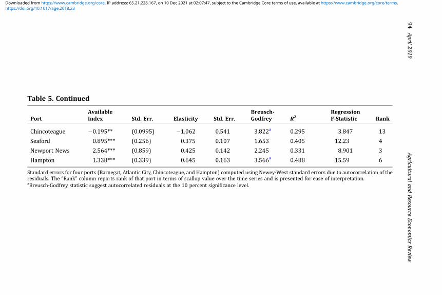
Table 5. Continued

PortAvailableIndex Std. Err. Elasticity Std. Err.

Breusch-Godfrey R2

RegressionF-Statistic Rank

Chincoteague �0.195** (0.0995) �1.062 0.541 3.822a 0.295 3.847 13

Seaford 0.895*** (0.256) 0.375 0.107 1.653 0.405 12.23 4

Newport News 2.564*** (0.859) 0.425 0.142 2.245 0.331 8.901 3

Hampton 1.338*** (0.339) 0.645 0.163 3.566a 0.488 15.59 6

Standard errors for four ports (Barnegat, Atlantic City, Chincoteague, and Hampton) computed using Newey-West standard errors due to autocorrelation of theresiduals. The “Rank” column reports rank of that port in terms of scallop value over the time series and is presented for ease of interpretation.aBreusch-Godfrey statistic suggest autocorrelated residuals at the 10 percent significance level.

Agricultural

andResource

Econom

icsReview

94

April

2019





of marginal effects of biomass on landings vary widely across the ports. Thetime-series models do not have explanatory power for the moderate-sizedports located in New York, Connecticut, and Massachusetts, nor the largestport (New Bedford).We suspect that heterogeneity in the natural productivity of parts of the ocean

and the distances from ports to those areas (natural advantages) combinedwithfisheries management to induce a spatial component to the port-level responseto changes in biomass availability. Ports in the southern portion of our studyarea (say, Point Pleasant, NJ and further south) tended to have positive short-term relationships between biomass and landings. The biomass areas in theMid-Atlantic Bight (from LI south, see Figure 1) are characterized bygenerally lower abundance with spikes in abundance in some years (seeFigure 2). These southern areas may be characterized by temporary high andlow levels of scalloping activity when the nearby fishing grounds are notgood alternatives or are closed to fishing entirely. In contrast, ports furthernorth, adjacent to biomass areas off the coast of New England, tend to haveaccess to better fishing grounds that are characterized by both higherabundances and less intrayear variation. When a port’s closest option isunavailable, it may still be viable to land scallops even if the fishing groundsare more distant. Fishery managers, concerned with the short-run effects ofregulations on these southern communities, might consider regulations thatsmooth the interyear variability in access to biomass or regulations thatlower the cost of access for these southern ports. For example, managersmight open a southern area to fishing before scallops are optimally sized orconstruct a no-cost transit corridor (New England Fishery ManagementCouncil 2015). These policies would have consequences for economic efficiency.Returns to scope (from the growth equations) suggest that ports with other

fishing activities could be well-positioned to attract new fishing activity whenstock conditions are favorable. While we have only characterized onedirection by which spillovers might operate, it is possible that scallop fishingcould crowd out or attract other fishing activity. While beyond the scope ofthis study, examining the extent to which these effects spill out to thebroader marine economy would provide tremendous insight into the wayfisheries management can affect regional economies. For example, if dock orother space is at a premium, then fisheries that are highly profitable maycrowd out the less profitable ones. Alternatively, traditional spillovermechanisms, like thick inputs markets may counteract this effect. Localgovernments and other stakeholders have been concerned about thepreservation of shoreside infrastructure, working waterfronts, and socialcapital in the fishing industry (Breen and Rigby 1985, Georgianna et al. 2014,Ounanian 2015). There are theoretical reasons to believe the locations of atleast some fishery support infrastructure (including seafood processors,repair facilities, and supply shops) both affects and is affected by landingslocation (and therefore biomass availability). For example, processors maychoose to locate in locations with high levels of landings to take advantage of


http

s://

doi.o

rg/1

0.10

17/a

ge.2

018.

23D

ownl

oade

d fr

om h

ttps

://w

ww

.cam

brid

ge.o

rg/c

ore.

IP a

ddre

ss: 6

5.21

.228

.167

, on

10 D

ec 2

021

at 0

2:07

:47,

sub

ject

to th

e Ca

mbr

idge

Cor

e te

rms

of u

se, a

vaila

ble

at h

ttps

://w

ww

.cam

brid

ge.o

rg/c

ore/

term

s.




economies of scale and reduce the transport costs of raw materials.Alternatively, they may locate in closer to final demand if transport costs ofraw materials are low. Further research characterizing the mechanisms bywhich fishing activities affect associated industries and communities isessential for fisheries managers to fully understand the effects ofmanagement on fishing communities.

Supplementary material

The supplementary material for this article can be found at https://doi.org/10.1017/age.2018.23

Acknowledgements

The authors are grateful for comments from participants at the 2016 IIFET andNAREA conferences and from the anonymous reviewers. The findings andconclusions in the manuscript are those of the authors and do not reflect theposition of the Department of Commerce or the National Oceanographic andAtmospheric Administration. As usual, all remaining errors are our own.

References

Acemoglu, D., S. Johnson, and J.A. Robinson. 2002. “Reversal of Fortune: Geography andInstitutions in the Making of the Modern World Income Distribution.” The QuarterlyJournal of Economics 117(4): 1231–1294.

Agnarsson, S., T. Matthiasson, and F. Giry. 2016. “Consolidation and Distribution of QuotaHoldings in the Icelandic Fisheries.” Marine Policy 72: 263–270.

Ardini, G., and M.Y. Lee. 2018. “Do IFQs in the US Atlantic Sea Scallop Fishery Impact Price andSize?” Marine Resource Economics 33(3): 263–288.

Barro, R.J., and X. Sala-I-Martin. 1992. “Convergence.” Journal of Political Economy 100(2):223–251.

Baskaran, R., and J.L. Anderson. 2005. “Atlantic Sea Scallop Management: An Alter-NativeRights-Based Cooperative Approach to Resource Sustainability.” Marine Policy 29(4):357–369.

Battese, G.E. 1997. “A Note on the Estimation of Cobb-Douglas Production Functions WhenSome Explanatory Variables Have Zero Values.” Journal of Agricultural Economics 48(1–3): 250–252.

Behrens, K., G. Duranton, and F. Robert-Nicoud. 2014. “Productive Cities: Sorting, Selection,and Agglomeration.” Journal of Political Economy 122(3): 507–553.

Bleakley, H., and J. Lin. 2012. “Portage and Path Dependence.” Quarterly Journal of Economics127(2): 587–644.

Bloom, D.E., J.D. Sachs, P. Collier, and C. Udry. 1998. “Geography, Demography, and EconomicGrowth in Africa.” Source: Brookings Papers on Economic Activity 1998(2): 207–295.

Bonner, M. 2017. “Jockeying to Control Rafael’s Fishing Rights Ramps Up.” South Coast Today,June 24.

Breen, A., and D. Rigby. 1985. “SOS for the Working Waterfront.” Planning 51(6): 6–12.Clay, P.M., L.L. Colburn, and T. Seara. 2016. “Social Bonds and Recovery: An Analysis of

Hurricane Sandy in the First Year after Landfall.” Marine Policy 74: 334–340.


http

s://

doi.o

rg/1

0.10

17/a

ge.2

018.

23D

ownl

oade

d fr

om h

ttps

://w

ww

.cam

brid

ge.o

rg/c

ore.

IP a

ddre

ss: 6

5.21

.228

.167

, on

10 D

ec 2

021

at 0

2:07

:47,

sub

ject

to th

e Ca

mbr

idge

Cor

e te

rms

of u

se, a

vaila

ble

at h

ttps

://w

ww

.cam

brid

ge.o

rg/c

ore/

term

s.







Cooley, S.R., J.E. Rheuban, D.R. Hart, V. Luu, D.M. Glover, J.A. Hare, and S.C. Doney. 2015. “AnIntegrated Assessment Model for Helping the United States Sea Scallop (Placopectenmagellanicus) Fishery Plan Ahead for Ocean Acidification and Warming.” PLoS ONE 10(5): 1–27.

Dickey, D.A., and W.A. Fuller. 1979. “Distribution of the Estimators for AutoregressiveTime Series with a Unit Root.” Journal of the American Statistical Association 74(366a):427–431.

Diekert, F.K. 2012. “Growth Overfishing: The Race to Fish Extends to the Dimension of Size.”Environmental and Resource Economics 52(4): 549–572.

Diekert, F.K., D. Hjermann, E. Nævdal, and N.C. Stenseth. 2010. “Spare the Young Fish: OptimalHarvesting Policies for North-East Arctic Cod.” Environmental and Resource Economics47(4): 455–475.

Doeringer, P.B., P.I. Moss, and D.G. Terkla. 1986. “Capitalism and Kinship: Do InstitutionsMatter in the Labor Market?” Industrial and Labor Relations Review 40(1):48–60.

Duranton, G., and D. Puga. 2004. “Micro-foundations of Urban Agglomeration Economies.” InJ.V. Henderson and J.F. Thisse, eds., The Handbook of Urban And Regional EconomicsVolume 4: Cities and Geography. 48: 2063–2117. Amsterdam: Elsevier.

Edwards, S.F. 2001. “Rent-Seeking and Property Rights Formation in the U.S. Atlantic SeaScallop Fishery.” Marine Resource Economics 16(4): 263–275.

Ellison, G., and E.L. Glaeser. 1999. “The Geographic Concentration of Industry: Does NaturalAdvantage Explain Agglomeration?” American Economic Review 89(2): 311–316.

Gallup, J.L., J. Sachs, and A.D. Mellinger. 1999. “Geography and Economic Development”International Regional Science Review 22(2): 179–232.

Georgianna, D., R. Avila, D. Bethoney, A. Cass, S. Challingsworth, and W. Hogan. 2014.“Groundfish Port Recovery and Revitalization Plan for the Port of New Bedford/Fairhaven.” Technical report, University of Massachusetts - Dartmouth, Fairhaven, MA.

Georgianna, D., M.Y. Lee, and J. Walden. 2017. “Contrasting Trends in the Northeast UnitedStates Groundfish and Scallop Processing Industries.” Marine Policy 85: 100–106.

Girardin, R., K.G. Hamon, J. Pinnegar, J.J. Poos, O. Thebaud, A. Tidd, Y. Vermard, and P. Marchal.2017. “Thirty Years of Fleet Dynamics Modelling Using Discrete-Choice Models: WhatHave We Learned?” Fish and Fisheries 18: 638–655.

Hall-Arber, M., C. Dyer, J. Poggie, J. Mcnally, and R. Gagne. 2001. “New England’s FishingCommunities.” Technical report, MIT Sea Grant Program, Cambridge, MA.

Hart, D.R. 2003. “Yield-and Biomass-per-Recruit Analysis for Rotational Fisheries, with anApplication to the Atlantic Sea Scallop (Placopecten magellanicus).” Fishery Bulletin101(1): 44–57.

Hart, D.R., and A.S. Chute. 2004. “Essential Fish Habitat Source Document: Sea Scallop,Placopecten magellanicus, Life History and Habitat Characteristics 2nd edition.”Technical report, National Marine Fisheries Service, Woods Hole.

———. 2009. “Estimating von Bertalanffy Growth Parameters From Growth Increment DataUsing a Linear Mixed-Effects Model, with an Application to the Sea Scallop Placopectenmagellanicus.” ICES Journal of Marine Science 66(10): 2165–2175.

Hart, D.R., and P.J. Rago. 2006. “Long-Term Dynamics of US Atlantic Sea Scallop Placopectenmagellanicus Populations.” North American Journal of Fisheries Management 26(2):490–501.

Havranek, T., R. Horvath, and A. Zeynalov. 2016. “Natural Resources and Economic Growth: AMeta-Analysis.” World Development 88: 134–151.

Holland, D.S., P. Pinto da Silva, and A.W. Kitts. 2015. “Evolution of Social Capital and EconomicPerformance in New England Harvest Cooperatives.” Marine Resource Economics 30(4):371–392.

Kaplan, I.M. 1999. “Suspicion, Growth and Co-Management in the Commercial FishingIndustry: The Financial Settlers of New Bedford.” Marine Policy 23(3): 227–241.


http

s://

doi.o

rg/1

0.10

17/a

ge.2

018.

23D

ownl

oade

d fr

om h

ttps

://w

ww

.cam

brid

ge.o

rg/c

ore.

IP a

ddre

ss: 6

5.21

.228

.167

, on

10 D

ec 2

021

at 0

2:07

:47,

sub

ject

to th

e Ca

mbr

idge

Cor

e te

rms

of u

se, a

vaila

ble

at h

ttps

://w

ww

.cam

brid

ge.o

rg/c

ore/

term

s.




Kim, S. 1999. “Regions, Resources, and Economic Geography: Sources of U.S. RegionalComparative Advantage, 18801987.” Regional Science and Urban Economics 29(1): 1–32.

Krugman, P.R. 1991. Geography and Trade. Cambridge: MIT Press.Lee, M.Y., C. Speir, A. Carr-Harris, and S. Benjamin. 2017. “Geographic Concentration of the

Atlantic Sea Scallop Fishery.” The Review of Regional Studies 47: 25–46.Magnuson-Stevens Fishery Conservation and Management Act. 2007. “Public Law 109-479,

109th Congress.”Mankiw, N.G., D. Romer, and D.N. Weil. 1992. “A Contribution to the Empirics of Economic

Growth.” The Quarterly Journal of Economics 107(2): 407–437.Marshall, A. 1920. Principles of Economics (8th edition). London: McMillan.Michaels, G. 2011. “The Long-Term Consequences of Resource Based Specialization.” The

Economic Journal 121(551): 31–57.Midelfart-Knarvik, K.H., H.G. Overman, A. Venables, and K. Helene. 2001. “Comparative

Advantage and Economic Geography: Estimating the Determinants of IndustrialLocation in the EU.”

Narayan, P.K. 2005. “The Saving and Investment Nexus for China: Evidence fromCointegration Tests.” Applied Economics 37(17): 1979–1990.

National Marine Fisheries Service. 2016. “Fisheries Economics of The United States: 2015.”Technical report, National Marine Fisheries Service, Silver Spring, MD.

New England Fishery Management Council. 2015. “Framework 26 to the Scallop FMP.”Technical report, New England Fishery Management Council, Newburyport, MA.

Northeast Fisheries Science Center. 2014. “59th Northeast Regional Stock AssessmentWorkshop (59th SAW) Assessment Report.” Technical report, Northeast FisheriesScience Center, Woods Hole, MA.

Ounanian, K. 2015. “Wither the Waterfront: Does the United States Need Federal Legislationto Preserve Working Waterfronts?” Coastal Management 43(6): 668–684.

Papyrakis, E., and R. Gerlagh. 2007. “Resource Abundance and Economic Growth in theUnited States.” European Economic Review 51(4): 1011–1039.

Pesaran, M.H., Y. Shin, and R.J. Smith. 2000. “Structural Analysis of Vector Error CorrectionModels with Exogenous I(1) Variables.” Journal of Econometrics 97(2): 293–343.

———. 2001. “Bounds Testing Approaches to the Analysis of Level Relationships.” Journal ofApplied Econometrics 16(3): 289–326.

Portman, M.E., D. Jin, and E. Thunberg. 2009. “Waterfront Land Use Change and MarineResource Conditions: The Case of New Bedford and Fairhaven, Massachusetts.”Ecological Economics 68(8): 2354–2362.

———. 2011. “The Connection Between Fisheries Resources and Spatial Land Use Change: TheCase of Two New England Fish Ports.” Land Use Policy 28(3): 523–533.

Puga, D. 2010. “The Magnitude and Causes of Agglomeration Economies.” Journal of RegionalScience 50(1): 203–219.

Quigley, J.M. 1998. “Urban Diversity and Economic Growth.” Journal of Economic Perspectives12(2): 127–138.

Redding, S.J. 2009. “Economic Geography: A Review of the Theoretical and EmpiricalLiterature.” In D. Bernhofen, R. Falvey D. Greenaway and U. Kreickemeier, eds.,“Palgrave Handbook of International Trade,” pp. 497–531. London: Palgrave Macmillan.

Repetto, R. 2001. “A Natural Experiment in Fisheries Management.” Marine Policy 25:251–264.

Rodrik, D., A. Subramanian, and F. Trebbi. 2004. “Institutions Rule: The Primacy ofInstitutions over Geography and Integration in Economic Development.” Journal ofEconomic Growth 9(2): 131–165.

Rosenthal, S.S., and W.C. Strange. 2004. “Evidence on the Nature and Sources ofAgglomeration Economies.” In J.V. Henderson and J. Thisse, eds., The Handbook ofUrban And Regional Economics Volume 4: Cities and Geography. 49: 2119–2171.Amsterdam: Elsevier.


http

s://

doi.o

rg/1

0.10

17/a

ge.2

018.

23D

ownl

oade

d fr

om h

ttps

://w

ww

.cam

brid

ge.o

rg/c

ore.

IP a

ddre

ss: 6

5.21

.228

.167

, on

10 D

ec 2

021

at 0

2:07

:47,

sub

ject

to th

e Ca

mbr

idge

Cor

e te

rms

of u

se, a

vaila

ble

at h

ttps

://w

ww

.cam

brid

ge.o

rg/c

ore/

term

s.




Sachs, J., andWarner, A. 1999. “Natural Resource Intensity and Economic Growth.” In J. Mayer,B. Chambers and A. Farooq, eds., Development Policies in Natural Resource Economics.2:13-38. Edward Elgar. Northampton, MA

Serchuk, F.M., P.W. Wood, J.A. Posgay, and B.E. Brown. 1979. “Assessment and status of seaScallop Populations off the Northeast Coast of the United States.” Proceedings of theNational Shellfisheries Association 69: 161–191.

Speir, C., C. Pomeroy, and J.G. Sutinen. 2014. “Port Level Fishing Dynamics: Assessing Changesin the Distribution of Fishing Activity Over Time.” Marine Policy 46: 171–191.

Valencia, M.J. 2017. “Loss of ‘Codfather’ Permits Could Hurt New Bedford.” The Boston Globe,April 21.

Van Der Ploeg, F. 2011. “Natural Resources: Curse or Blessing?” Journal of EconomicLiterature 49(2): 366–420.

Watson, P., and T. Johnson. 2012. “Federal Fishery Policy and the Geographic Distribution ofCommercial U.S. West Coast Fish Landings: Insights from the 2003 Federal GroundfishPermit Buyback.” Marine Resource Economics 27(4): 289–301.


http

s://

doi.o

rg/1

0.10

17/a

ge.2

018.

23D

ownl

oade

d fr

om h

ttps

://w

ww

.cam

brid

ge.o

rg/c

ore.

IP a

ddre

ss: 6

5.21

.228

.167

, on

10 D

ec 2

021

at 0

2:07

:47,

sub

ject

to th

e Ca

mbr

idge

Cor

e te

rms

of u

se, a

vaila

ble

at h

ttps

://w

ww

.cam

brid

ge.o

rg/c

ore/

term

s.




resource abundance, fisheries management, and fishing

Documents