resonant effects of the violin tailpiece - schulich … effects of the violin tailpiece jason leung...
TRANSCRIPT
Resonant Effects of the Violin Tailpiece
Jason Leung
Music Technology Area, Department of Music ResearchSchulich School of Music
McGill UniversityMontreal, Quebec, Canada
December 2015
A thesis submitted to McGill University in partial fulfillment of the requirements forthe degree of Master of Arts in Music Technology.
c© 2015 Jason Leung

i
Abstract
This thesis explores the dynamical relationship between the violin body and tailpiece,with a focus on the effect of tailpiece resonances on the violin’s acoustic performance.These resonances are controlled by attaching a series of small masses to several pointson the tailpiece, which changes its mass distribution and moment of inertia. To observethe changes in the dynamic behaviour, input admittance measurements were taken atthe bridge and several points along the length of the tailpiece. The resulting frequencyresponse functions, when analyzed using a mode-fitting algorithm, demonstrate thata body–tailpiece coupling can occur when the most prominent vibration modes of thebody and tailpiece are aligned. This coupling decreases the frequency, quality factor,and magnitude of that body resonance. Informal playing tests reveal that a small mass(around 5 g) is sufficient to audibly temper the brightness of the instrument as well asits wolf note. A similar effect is achieved when a full set of fine tuners is deployed.
ii
Résumé
Cette thèse explore la relation dynamique entre le corps et le cordier d’un violon, enmettant l’accent sur l’effet des résonances du cordier sur la performance acoustique duviolon. Ces résonances sont contrôlées par la fixation d’une série de petites masses surplusieurs points sur le cordier, changeant ainsi sa distribution de masse et son momentd’inertie. Afin d’observer les changements de comportement dynamique, des mesuresd’admittance d’entrée ont été prises sur le pont et sur plusieurs points sur la longueurdu cordier. Les fonctions de réponse en fréquence obtenues, lorsqu’elles sont analyséesen utilisant un algorithme pour le calcul des modes propres de vibration, démontrentqu’un couplage corps–cordier peut se produire lorsque les modes de vibration les pluséminents du corps et du cordier sont alignés. Ce couplage diminue la fréquence, lefacteur de qualité, et l’amplitude de la résonance du corps. Les tests informels en situ-ation de jeu révèlent qu’une petite masse (environ 5 g) est suffisante pour tempérer defaçon audible la brillance de l’instrument ainsi que sa note de loup. Un effet similaireest atteint lorsqu’un ensemble complet de tendeurs est monté.
iii
Acknowledgments
This work would not have been possible without the support, guidance, and patienceof my advisor, Dr. Gary Scavone. His expertise on the subject enabled many new ideasto take root and grow, while his devotion to his students ensured that this project couldcome to fruition.
I am extremely grateful to my colleagues at the Music Technology Area, and espe-cially to the members of the Computational Acoustics Modeling Laboratory (CAML),who brought many insightful discussions: Connor Kemp, Esteban Maestre, HosseinMansour, Mark Rau, Charalampos “Harry” Saitis, and Shi Yong. I extend the most sin-cere thanks to Darryl Cameron and Yves Méthot for their technical assistance duringthe experiment sessions. And of course, I should never forget my friends (from McGilland beyond) Christopher Antila, Andrew Fogarty, Andrew Hankinson, Andrew Hor-witz, Catherine Massie, Alex McLeod, Jordan Miller, Lillio Mok, Lauren Tyros, GabrielVigliensoni, Ling-Xiao Yang, and Rosalind Zhang, who provided an abundance of de-lightful conversations, fond memories, and beer.
This research was funded by the Natural Sciences and Engineering Research Councilof Canada (NSERC) through the Alexander Graham Bell Canada Graduate Scholarshipprogram.

iv
v
Contents
1 Introduction 11.1 Motivation . . . . . . . . . . . . . . . . . . . . . . . . . . . . . . . . . . . . . 11.2 Outline . . . . . . . . . . . . . . . . . . . . . . . . . . . . . . . . . . . . . . . 2
2 Background 32.1 The Violin Family . . . . . . . . . . . . . . . . . . . . . . . . . . . . . . . . . 32.2 Violin Acoustics . . . . . . . . . . . . . . . . . . . . . . . . . . . . . . . . . . 4
2.2.1 The Strings . . . . . . . . . . . . . . . . . . . . . . . . . . . . . . . . 52.2.2 The Violin Body . . . . . . . . . . . . . . . . . . . . . . . . . . . . . . 82.2.3 The Bridge . . . . . . . . . . . . . . . . . . . . . . . . . . . . . . . . . 92.2.4 The “Wolf Note” . . . . . . . . . . . . . . . . . . . . . . . . . . . . . 92.2.5 The Tailpiece . . . . . . . . . . . . . . . . . . . . . . . . . . . . . . . 10
2.3 Measurements . . . . . . . . . . . . . . . . . . . . . . . . . . . . . . . . . . . 122.3.1 Modal Analysis . . . . . . . . . . . . . . . . . . . . . . . . . . . . . . 122.3.2 Admittance Measurements . . . . . . . . . . . . . . . . . . . . . . . 132.3.3 Microphone Measurements . . . . . . . . . . . . . . . . . . . . . . . 15
2.4 Perception: What makes a “good” violin? . . . . . . . . . . . . . . . . . . . 16
3 Experiment Procedure 173.1 Equipment . . . . . . . . . . . . . . . . . . . . . . . . . . . . . . . . . . . . . 173.2 Experiment Setup . . . . . . . . . . . . . . . . . . . . . . . . . . . . . . . . . 183.3 Data Acquisition . . . . . . . . . . . . . . . . . . . . . . . . . . . . . . . . . 193.4 Data Analysis . . . . . . . . . . . . . . . . . . . . . . . . . . . . . . . . . . . 22
3.4.1 Mode Fitting . . . . . . . . . . . . . . . . . . . . . . . . . . . . . . . 233.5 Repeatability of Measurements . . . . . . . . . . . . . . . . . . . . . . . . . 24
vi Contents
4 Results 254.1 Reference Measurements (unmodified violin) . . . . . . . . . . . . . . . . . 26
4.1.1 Frequency Response: Bridge . . . . . . . . . . . . . . . . . . . . . . 264.1.2 Frequency Response: Tailpiece . . . . . . . . . . . . . . . . . . . . . 27
4.2 Mass-loaded Tailpiece . . . . . . . . . . . . . . . . . . . . . . . . . . . . . . 324.2.1 2.5-gram mass . . . . . . . . . . . . . . . . . . . . . . . . . . . . . . . 334.2.2 5.5-gram mass . . . . . . . . . . . . . . . . . . . . . . . . . . . . . . . 374.2.3 16.0-gram mass . . . . . . . . . . . . . . . . . . . . . . . . . . . . . . 40
4.3 Fine Tuners . . . . . . . . . . . . . . . . . . . . . . . . . . . . . . . . . . . . . 434.4 Summary . . . . . . . . . . . . . . . . . . . . . . . . . . . . . . . . . . . . . . 47
5 Conclusions and Future Work 495.1 Conclusions . . . . . . . . . . . . . . . . . . . . . . . . . . . . . . . . . . . . 495.2 Future Work . . . . . . . . . . . . . . . . . . . . . . . . . . . . . . . . . . . . 50
vii
List of Figures
2.1 The violin family . . . . . . . . . . . . . . . . . . . . . . . . . . . . . . . . . 42.2 Parts of the violin . . . . . . . . . . . . . . . . . . . . . . . . . . . . . . . . . 62.3 Helmholtz motion . . . . . . . . . . . . . . . . . . . . . . . . . . . . . . . . . 72.4 Tailpiece modes, from Stough (1996) . . . . . . . . . . . . . . . . . . . . . . 11
3.1 Experiment setup . . . . . . . . . . . . . . . . . . . . . . . . . . . . . . . . . 203.2 Measurement points . . . . . . . . . . . . . . . . . . . . . . . . . . . . . . . 21
4.1 Measurement directions . . . . . . . . . . . . . . . . . . . . . . . . . . . . . 254.2 Bridge FRFs (100–1000 Hz) . . . . . . . . . . . . . . . . . . . . . . . . . . . . 284.3 Bridge FRFs (up to 6 kHz) . . . . . . . . . . . . . . . . . . . . . . . . . . . . 294.4 Tailpiece FRFs (100–1000 Hz) . . . . . . . . . . . . . . . . . . . . . . . . . . 304.5 Tailpiece FRFs (up to 6 kHz) . . . . . . . . . . . . . . . . . . . . . . . . . . . 314.6 2.5 g mass: Bridge FRFs . . . . . . . . . . . . . . . . . . . . . . . . . . . . . 344.7 2.5 g mass: Tailpiece FRFs . . . . . . . . . . . . . . . . . . . . . . . . . . . . 354.8 2.5 g mass: Bridge/tailpiece FRFs . . . . . . . . . . . . . . . . . . . . . . . . 364.9 5.5 g mass: Bridge FRFs . . . . . . . . . . . . . . . . . . . . . . . . . . . . . 384.10 5.5 g mass: Tailpiece FRFs . . . . . . . . . . . . . . . . . . . . . . . . . . . . 394.11 5.5 g mass: Bridge/tailpiece FRFs . . . . . . . . . . . . . . . . . . . . . . . . 404.12 16.0 g mass: Bridge FRFs . . . . . . . . . . . . . . . . . . . . . . . . . . . . . 414.13 16.0 g mass: Tailpiece FRFs . . . . . . . . . . . . . . . . . . . . . . . . . . . . 424.14 16.0 g mass: Bridge/tailpiece FRFs . . . . . . . . . . . . . . . . . . . . . . . 434.15 Fine tuners: Bridge FRFs . . . . . . . . . . . . . . . . . . . . . . . . . . . . . 454.16 Fine tuners: Tailpiece FRFs . . . . . . . . . . . . . . . . . . . . . . . . . . . . 464.17 Fine tuners: Bridge/tailpiece FRFs . . . . . . . . . . . . . . . . . . . . . . . 47

viii

ix
List of Tables
3.1 String properties . . . . . . . . . . . . . . . . . . . . . . . . . . . . . . . . . . 183.2 Tailpiece measurement locations . . . . . . . . . . . . . . . . . . . . . . . . 22
4.1 Signature modes of the violin . . . . . . . . . . . . . . . . . . . . . . . . . . 264.2 Tailpiece resonances from Stough (1996) . . . . . . . . . . . . . . . . . . . . 274.3 Tailpiece resonances (measured) . . . . . . . . . . . . . . . . . . . . . . . . 324.4 2.5 g mass: Signature modes . . . . . . . . . . . . . . . . . . . . . . . . . . . 334.5 5.5 g mass: Signature modes . . . . . . . . . . . . . . . . . . . . . . . . . . . 374.6 16.0 g mass: Signature modes . . . . . . . . . . . . . . . . . . . . . . . . . . 434.7 Fine tuners: Signature modes . . . . . . . . . . . . . . . . . . . . . . . . . . 444.8 Relative changes to the B1+ mode . . . . . . . . . . . . . . . . . . . . . . . 48

x
1
Chapter 1
Introduction
1.1 Motivation
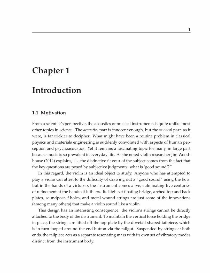
From a scientist’s perspective, the acoustics of musical instruments is quite unlike mostother topics in science. The acoustics part is innocent enough, but the musical part, as itwere, is far trickier to decipher. What might have been a routine problem in classicalphysics and materials engineering is suddenly convoluted with aspects of human per-ception and psychoacoustics. Yet it remains a fascinating topic for many, in large partbecause music is so prevalent in everyday life. As the noted violin researcher Jim Wood-house (2014) explains, “. . . the distinctive flavour of the subject comes from the fact thatthe key questions are posed by subjective judgments: what is ‘good sound’?”
In this regard, the violin is an ideal object to study. Anyone who has attempted toplay a violin can attest to the difficulty of drawing out a “good sound” using the bow.But in the hands of a virtuoso, the instrument comes alive, culminating five centuriesof refinement at the hands of luthiers. Its high-set floating bridge, arched top and backplates, soundpost, f-holes, and metal-wound strings are just some of the innovations(among many others) that make a violin sound like a violin.
This design has an interesting consequence: the violin’s strings cannot be directlyattached to the body of the instrument. To maintain the vertical force holding the bridgein place, the strings are lifted off the top plate by the dovetail-shaped tailpiece, whichis in turn looped around the end button via the tailgut. Suspended by strings at bothends, the tailpiece acts as a separate resonating mass with its own set of vibratory modesdistinct from the instrument body.
2 Introduction
The tailpiece inevitably has an influence on the sound of the instrument, but sucheffects are poorly understood. Even though the majority of scientific investigations ofthe violin have taken place over the last 50 years, most of those efforts have been directedtoward investigating the more prominent components of the instrument: the body, thestrings, and the bridge (e.g., Bissinger, 2008). By comparison, the tailpiece has receivedalmost no attention.
At the same time, luthiers are well aware that the tailpiece has some influence on aviolin’s sound. But as the existing corpus of violin acoustics literature does not addressthese effects in a systematic way, tailpiece adjustments are typically guided solely by theluthier’s experience and intuition, and the optimum solution may be overlooked. Thepresent study will address this dearth of information and provide a scientific perspectiveon the issues.
1.2 Outline
This work will be presented in the following fashion: First, Chapter 2 will introducethe realm of violin acoustics. Past research on the topic will be presented to form thebasis for this work. Chapter 3 will describe the experimental procedure and the dataacquisition and analysis tools used. Their advantages and disadvantages will be com-pared with other techniques commonly used in similar studies. Chapter 4 will presentthe data collected and propose physical interpretations of the observations. Changes intone effected by the tailpiece modifications will also be recounted. Finally, Chapter 5will summarize the conclusions that can be drawn from the results of this study. Impli-cations for luthiers and potential goals for future research will be assessed.
3
Chapter 2
Background
2.1 The Violin Family
The musical instruments of the violin family are the most popular and recognizablebowed string instruments today. From the immense string choirs of the great sym-phonies to the intimate settings of small chamber works, the violin, viola, cello (com-mon abbreviation of violoncello), and double bass (also contrabass or string bass) occupya central role within Western musical traditions. In spite of this, these instruments haveremarkably plebeian roots, having been gradually refined by unknown artisans in theremote towns of northern Italy during the early Renaissance. Even though the basicdesign of the violin and its larger cousins had largely been finalized by the early 16th
century, their construction continued to evolve, spurred on by shifting artistic tastes andnew innovations and advances in technology (Curtin and Rossing, 2010). By the late20th century, electric violins have also gained prominence in the popular music scene,even as traditional acoustic violins continue to pervade the popular mindset.
Being bowed string instruments, their primary mechanism for sound production iswith a bow, even though players can – and often will – create other musical soundsthrough other means such as plucking the strings (pizzicato), slapping the strings andbody, or various other forms of extended techniques. Because of this common trait,many basic facets of the violin also apply to the entire violin family (Curtin and Ross-ing, 2010). Nonetheless, there are a number of differences in design tailored to the viola,cello, and double bass, usually for ergonomic reasons – in order to be playable, theymust be made proportionately smaller compared to the wavelength of the notes within
4 Background
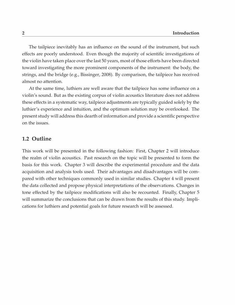
Figure 2.1: The modern violin family compared with the wavelength of the fundamen-tal for their lowest notes. The black bars correspond to one-quarter of the respectivewavelengths. “Alto” is an alternative name for the viola. From Askenfelt (2010).
their playing range (see Figure 2.1). In other words, they are not merely scaled-up ver-sions of the violin; each member has its own acoustical signature imparted by its uniquestructural design (Bynum and Rossing, 2010; Askenfelt, 2010).
2.2 Violin Acoustics
The modern violin is a true marvel of engineering. Each of its components has beenmeticulously refined by generations of luthiers for a single purpose: the production ofmusic. At first glance, this seems like a regular physics problem, yet this deceptivelysimple statement has baffled researchers for centuries; how, exactly, does one producemusic? Only within the past 50 years have researchers truly begun to understand thefiner nuances of violin acoustics: Cremer’s (1981) monograph Physik der Geige (trans-lated into English as The Physics of the Violin) is a landmark work in this genre, while ex-tensive surveys of the topic have also been penned by McIntyre and Woodhouse (1978),

2.2 Violin Acoustics 5
Hutchins (1983), and Gough (2000). Most recently, Woodhouse (2014) has contextual-ized the instrument as only one part of a larger physiological–psychoacoustical systemcentred on the player – after all, it is the violinist who decides the quality of a violin.
Due to its complexity, the violin is typically broken down into its constituent partsfor individual study. An exploded view of the violin is shown in Figure 2.2.
2.2.1 The Strings
Vibrating strings have been used for music throughout all of recorded human history,and, very likely, long before that. Plucked strings, such as harps and lyres, were alreadyknown to the ancient Mesopotamians and Greeks, who were masters of elaborate mu-sical systems. In particular, Pythagoras of Samos’ work in the 6th century BC relatingmusical intervals with numerical ratios was monumental in the history of Western mu-sic; divisions of the monochord continued to define musical intervals as late as 1722, inJean-Philippe Rameau’s Traité de l’harmonie (Nolan, 2002).
By comparison, the bowed string is a much more recent invention. The late develop-ment of scraping fibres to against strings for musical purposes likely stems from the factthat it is far easier to make a horrendous noise in this manner than a pleasing sound. Un-like a plucked string, whose vibrations are very well approximated by a linear sum of itsnatural frequencies, a bowed string is a continuously-driven, self-sustaining nonlinearsystem characterized by a parameter space largely hostile to “musical” sounds. Whereasa misplayed note on a guitar is still recognizably “musical”, a beginning violinist (andthose unfortunate enough to be close by) does not have this luxury (Woodhouse, 2014).
At first glance, a bowed string appears to vibrate sinusoidally, much like a standingwave on a freely vibrating string. Over 150 years ago, Helmholtz (1863) demonstratedthat a bowed string more closely resembles a triangular shape – two straight portionsjoined at a sharp bend. This bend races back and forth down the length of the string,reversing its orientation at each end and triggering a transition between the “stick” and“slip” phases of the cycle each time it passes the bow: The string sticks to the bow whilethe bend travels to the player’s finger and back, and slips rapidly across the bow-hairduring the shorter trip to the bridge and back (Woodhouse, 2014). Because this happenstoo quickly for the human eye (hundreds of cycles per second), all that is seen is thecurved path outlining the motion of the string. This stick–slip cycle, or “Helmholtzmotion”, is illustrated in Figure 2.3.

6 Background
Figure 2.2: An exploded view of the violin. From Johannsson (2015).

2.2 Violin Acoustics 7
Figure 2.3: A time-lapse representation of Helmholtz motion. (Left) The bend in thestring (the “Helmholtz corner”) traces out a curved path as it travels along the string;(right) the associated velocities of the string. From Rossing et al. (2002).
As a mechanical waveguide, the string has a characteristic wave impedance, a prop-erty that determines its resistance to wave motion along its length or to changes in thewave pattern (Guettler, 2010). Formally, impedance Z(ω) is defined in the frequencydomain as the ratio between force F (ω) to velocity V (ω),
Z(ω) =F (ω)
V (ω), (2.1)
and is measured in g/s, or mass (displaced) per unit time. On a bowed string, thegoverning force is the string’s tension, T , while the propagating speed is the productof frequency and twice the playing length (one wavelength), v = 2f�. Alternatively,the wave equation also prescribes a propagating speed of v =
√T/μ on an ideal string,
where μ is the density of the string. Combining these observations, the characteristic
8 Background
wave impedance may be expressed as
Z =T
2f�=
√Tμ . (2.2)
In general, the impedance of the string dictates, in the parlance of violinists, its respon-siveness. When designing strings, manufacturers must carefully balance their physicalparameters against musical considerations, a task made more difficult by the lack ofknown materials with the required tensile strength. Typical values of string density,transverse impedance, tension, and wave propagation speed are provided in Guettler(2010).
2.2.2 The Violin Body
Despite being the defining attribute of the violin family of instruments, the strings, ontheir own, do not produce or radiate very much sound due to the small amount of airdisplaced. Instead, their vibrational energy must be transferred to a radiation-efficientwooden (or synthetic) body that can move a much larger volume of air (Gough, 2007;Guettler, 2010). Thus, the body may be characterized as a mechanical amplifier.
However, its frequency response is far from flat. Instead, the body’s resonances actas an important filter, adding a distinctive colour that makes a violin sound like a violin(Woodhouse, 2014). Variations in their frequencies, bandwidths, qualities (Q factors),and peak magnitudes govern each instrument’s individual character.
For this reason, great emphasis has been placed into uncovering an optimal combina-tion of the resonances. Historically, this has been achieved through centuries of trial anderror at the hands of luthiers, but in recent times, technology has greatly aided the taskof understanding the violin’s structure and design. In particular, the Strad3D project(Zygmuntowicz et al., 2009) used CT scans and laser vibrometry to document the ge-ometries and main body resonances of three prized Italian violins: the Titian Stradivari(1715), the Willemotte Stradivari (1734), and the Plowden Guarneri (1735).
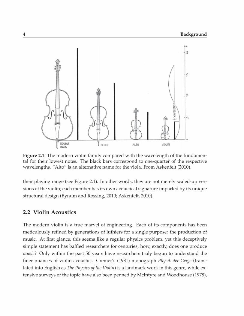
Individual components of the instrument have also been isolated and studied to de-termine their roles in driving the resonances. For example, the bass bar and sound post,besides increasing the overall stiffness of the body, were found to provide an asymmetryvital to exciting several strongly radiating body resonances (Gough, 2013). Meanwhile,the f-holes introduce a monopolar Helmholtz resonance by allowing air to flow in and
2.2 Violin Acoustics 9
out of the instrument (Curtin and Rossing, 2010; Woodhouse, 2014). The f-holes’ distinctshape and central placement are thought to have evolved over the centuries to boost theacoustic power efficiency of this mode (Nia et al., 2015).
Nonetheless, caution must be exercised in a strictly reductionist approach. Schleske(1996), for instance, performed experimental modal testing on a violin through eachstage of its construction, and found that the boundary conditions changed so drasticallythat there is no correlation between tuning of the individual plates (Hutchins’ (1981)“tap tones”) and the resulting frequency spectrum of the violin (up to 1 000 Hz) once ithas been assembled.
2.2.3 The Bridge
Unlike the low-set solid bridges found on most string instruments (whether plucked,bowed, or struck), the bridges of the violin family are intricately carved, rest on twofeet, lift the strings extremely high off the top plate, and are held in place solely bythe tension of the strings (Gough, 2007). This highly unusual design is necessary fortranslating the mainly lateral vibrations of the string into mainly vertical vibrations ofthe top plate (Curtin and Rossing, 2010).
The side effects of this innovation are profound. A complicated coupling betweenthe lowest bridge resonance and the “island” – the area on the top plate between the f-holes (Cremer, 1981) – results in a broad peak around 2–3 kHz in the violin’s frequencyresponse profile. Named the “bridge hill” by Jansson (1997), this feature is an importantingredient of violin sound, much like a formant in a human vocal tract (Woodhouse,2014). Further studies on the bridge hill were conducted by Jansson and Niewczyk(1997, 1999), Beldie (2003), and Woodhouse (2005).
2.2.4 The “Wolf Note”
A phenomenon familiar to and yet dreaded by all violinists is the “wolf note”, so namedbecause of its characteristic warbling howl-like sound. It occurs at a point where thebridge impedance falls too close to the string impedance, usually due to a strong bodyresonance; the impedances are said to be matched. When that happens, too much energyis transferred from the string, causing a buildup of vibrational energy at the bridge thatinterferes catastrophically with Helmholtz motion (Curtin and Rossing, 2010; Guettler,

10 Background
2010) – the string slips too early in the stick–slip cycle and Helmholtz motion gives wayto double slipping motion. Because such motion produces far less energy at the funda-mental frequency, the original body vibration is allowed to dissipate. Helmholtz motionis re-established and the cycle repeats, resulting in the distinctive warble (Woodhouse,2014).
The wolf note most commonly plagues violas and cellos, whose under-sized propor-tions exacerbate the string–bridge impedance match. On the violin, this effect is mostpronounced on the lower strings, which are heavier and thus have a higher impedance.One solution commonly employed by cellists is to attach a metallic mass, called a wolfeliminator, to the string afterlength to dissipate energy from the wolf note resonance. Butbecause wolf eliminators tend to be too bulky for use on a violin or viola, the player’sonly recourse is to increase the bow force to prevent the double slip from initiating.Unfortunately, doing so also reduces the tonal palette available to the player.
2.2.5 The Tailpiece
The tailpiece is the fixture used to hold the strings. Like all aspects of the violin, itsdesign has evolved over the centuries, but as a highly visible element, it is particularlysusceptible to the whims of artistic tastes. Houssay (2014) examined the history of thisornate wooden piece, starting with the cello iconography of the 17th–18th centuries, andthrough the violin-making treatises of the 19th–20th centuries.
Although luthiers have long been aware of the acoustic influences of the tailpiece,there has been a general lack of interest on this topic. Indeed, Riechers (1895, p.22) re-marked that “this part of the instrument exercises a great influence on the tone, althoughthe fact is doubted by a great many performers” – a sentiment that continues to this day.Even as players bicker endlessly over the setup of the strings, bridge, sound post, bassbar, and even the neck and fingerboard, they will routinely settle for an industriallymade tailpiece (White, 2012). This was not always so; tool marks on pre-19th-centurytailpieces suggest that luthiers had crafted and tuned them to match the instrument towhich it was attached. Lamentably, this art has become a casualty of the mass mecha-nization during the Industrial Revolution (Houssay, 2014).
As a result, no empirical research has been performed on the tailpiece until veryrecently. Hutchins (1993) first reported enhancements in tone after tuning the tailpieceto the frequency of other violin modes, but it was Stough (1996) who first described
2.2 Violin Acoustics 11
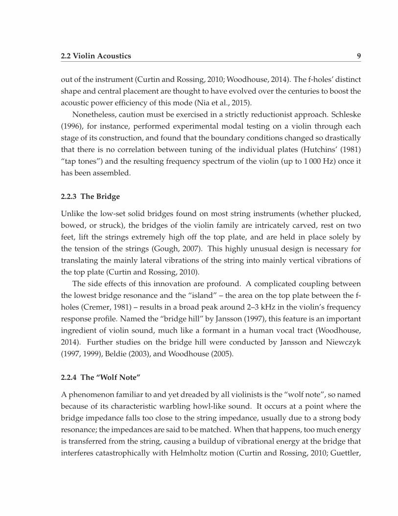
Figure 2.4: Tailpiece modes as depicted by Stough (1996), demonstrating the three“swing” modes (top) and the two rotation modes (bottom).
the vibrational behaviour of the tailpiece itself. He found five of its vibrating modesbelow 1 500 Hz, where the tailpiece behaved as a rigid body. These modes fell into twoclasses: three “swing” modes and two rotation modes, as illustrated in Figure 2.4. Healso noted that their frequencies depended on the tailpiece mass and tailgut length, andthat the two rotation modes could be tuned to modify the main resonance of the violinbody. Similarly, Fouilhé et al. (2011) conducted modal analysis on a cello tailpiece andidentified nine fundamental modes, seven of which lay well within the natural playingrange of the instrument. Experiments in altering the tailpiece mass, as well as its centreof mass, showed significantly different frequency response profiles.
This idea was pursued by White (2012), who recognized the tailpiece’s temperingeffect on string–bridge vibrations. Collaborating with Pirquet (2011), they developed anadjustable tailpiece with the aim of damping out undesirable resonances. By modifying

12 Background
the mass distribution of the tailpiece and the length of the tailgut (the looping cord usedto attach the tailpiece to the end button), they found that a major tailpiece resonance canbe made to couple with the body’s wolf resonance, thereby “taming the wolf”.
Beyond this, very little is known about the resonant effects of the tailpiece. Whitesuggested that the flexural (torsional) modes may be exploited to alter the timbre of theinstrument, as they tend to vary the vertical force applied by the four strings (Fouilhéet al., 2011). However, the method by which this could be done remains unknown.
2.3 Measurements
From a scientific point of view, the primary purpose of a violin is to radiate as muchenergy as musically tolerable. In this regard, it performs exceptionally well, a feat madeeven more impressive considering scientific methods were not available throughoutmost of its illustrious history.
Making observations in a pre-electronic age was extraordinarily troublesome. Forinstance, the physicist Félix Savart (1791–1841) required constant assistance from theluthier Jean-Baptiste Vuillaume (1798–1875) in assessing various experimental geome-tries for the violin (Savart, 1819), while Hermann von Helmholtz (1821–1894) had to becontent with a vibrating microscope for his bowed string experiments (Helmholtz, 1863).Technology has made great strides in the interim, and the ubiquity of the personal com-puter has made accurate measurements and complex modal analyses possible even in aluthier’s workshop. Because of this, luthiers are now increasingly embracing scientificmethods in advancing their craft (Woodhouse, 2014).
2.3.1 Modal Analysis
Modal analysis is a common technique used in structural engineering to study the dy-namic response of a structure during excitation, typically by extracting and analyzingmodal parameters such as natural frequency, damping factor, modal mass, and modeshape. The structure can either be tested experimentally or modeled on a computerusing finite element modeling (FEM) or boundary element modeling (BEM) methods(Curtin and Rossing, 2010). Over the years, every technique developed for structuralvibration has been enthusiastically applied to the violin, often as soon as the technologybecame available (Woodhouse, 2014).

2.3 Measurements 13
The earliest and simplest electroacoustic measurements involved driving the instru-ment body with a sinusoidal input, creating operating deflection shapes (ODSs) (Wood-house, 2014). If the modes are sufficiently far apart, ODSs can reasonably approximatethe mode shape, which can be discerned using Chladni patterns. Otherwise, the shapewill be the superposition of the overlapped modes and more advanced techniques willbe required to separate them. Landmark studies from this era include Backhaus (1930)and Eggers (1959).
The introduction of holographic interferometry in the late 1960s allowed researchersto observe, for the first time, the dynamic behaviour of the violin of the violin body inreal time. Ågren and Stetson (1969), Reinicke and Cremer (1970), Jansson et al. (1970),and Jansson (1973) were the earliest adopters of this revolutionary technique.
Since then, holographic methods have largely given way to experimental modal test-ing, led by advances in computational power and signal processing techniques – espe-cially of the fast Fourier transform (FFT) algorithm. Detailed multidimensional infor-mation is first extracted by a set of roving input and output sensors surveying the entirestructure. Using Fourier analysis, true mode shapes (rather than ODSs) can be conjuredfrom the resulting transfer functions, as well as their characteristic mass, frequency, anddamping parameters. Specialized software can combine these results with finite elementmethods to build accurate three-dimensional models simulating the dynamic behaviourof the violin (e.g., see Stoppani et al., 2009).
2.3.2 Admittance Measurements
While modal analysis is the most exhaustive method of studying structural dynamics,it requires significant care and time in measuring FRFs at many precisely defined loca-tions on an object, and so it is also the most exhausting method. In practice, the violinis only excited at the string (excluding extended techniques). The resulting vibrationsare regulated by the bridge, whose function is twofold: it is both the primary conduittransmitting energy between the string and the body, and the gate reflecting energy backinto the string to sustain Helmholtz motion. This observation leads to the notion thatthe most useful single measure of the acoustical performance of an instrument may bethe driving-point impedance at the single point of contact between the string and thebridge (Woodhouse and Langley, 2012).
14 Background
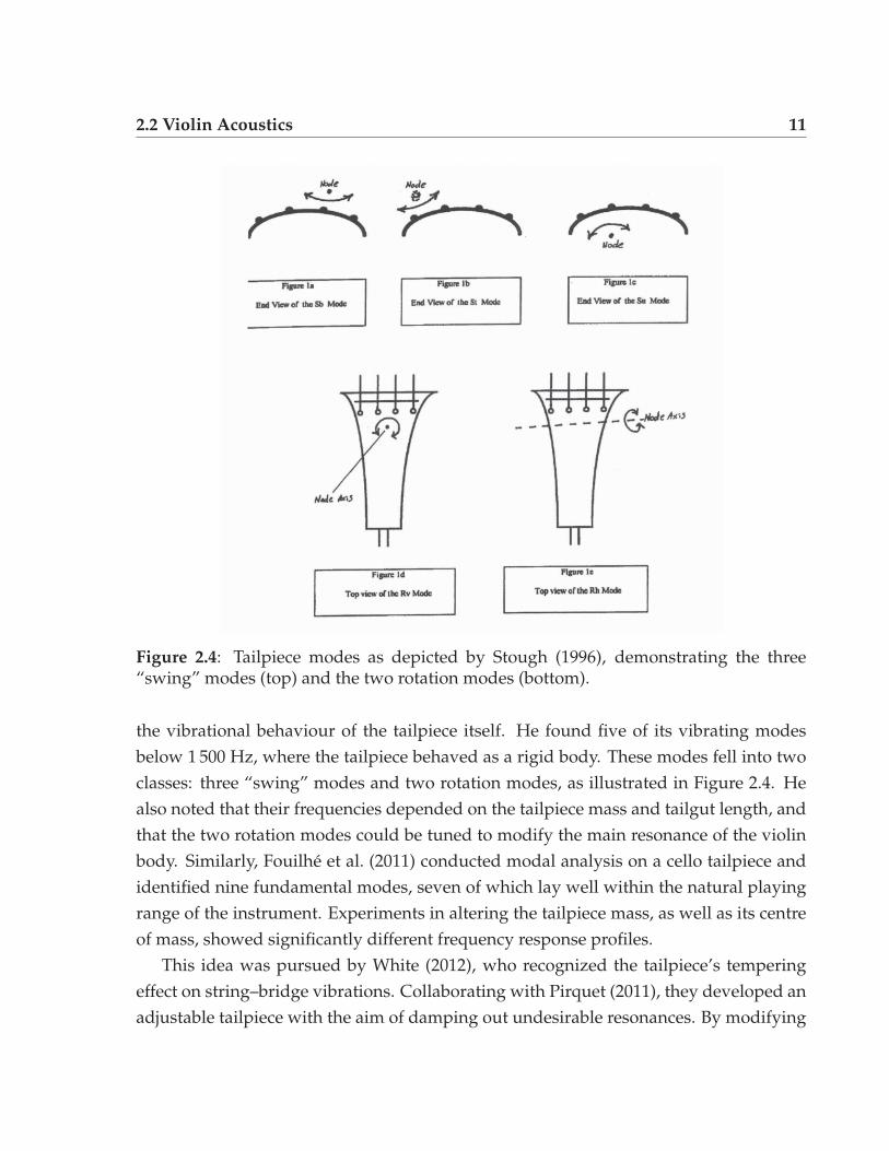
The driving-point impedance is an important characterization of a structure’s dy-namic behaviour, as it governs the flow of energy entering and feeding back from thesystem. Unlike wave impedances, which are properties of individual traveling wavesand difficult to isolate in reality, driving-point impedances simply measure the responseof a structure to an excitation force and are easily obtained using standard equipment.Ideally, the input and output should correspond to the same spatial point, but since thisis physically impossible to measure, careful design is required to obtain accurate results.Finally, Fourier analysis is used to generate frequency response functions (FRFs) of thestructure.
The first experiments of this type were independently conducted by the researchgroups of Cremer and Jansson in the 1970s (Zhang and Woodhouse, 2014). In imitationof a bowing force, the bridge is driven in the bowing direction using an impedancehead and strong magnets. Jansson and Niewczyk (1999) later replaced the impedancehead with a magnet–accelerometer system attached to the bridge, increasing the range ofmeasurement up to 10 kHz. Since this setup measures the response velocity (convertedfrom the accelerometer) resulting from a driving force, calculations are usually donein terms of the admittance at the bridge rather than the impedance. Admittance Y (ω)
is simply the inverse of impedance (Equation 2.1), relating the driving force F (ω) toresponse velocity V (ω) via the expression
Y (ω) ≡ 1
Z(ω)=
V (ω)
F (ω). (2.3)
Jansson et al. (1986) experimented with using an instrumented impact hammer ratherthan a constant magnetic driving force. This lessened the mass-loading effect on thebridge. The process was further refined when Gren et al. (2006) replaced the accelerom-eter with a laser Doppler vibrometer measurement system. Because impulse hammermeasurements are highly portable and easily replicated (they are not dependent on ex-ternal factors such as room acoustics), they are the most preferred vibration measure-ment for the study of musical instruments today (Zhang and Woodhouse, 2014).
Hammer measurements are usually conducted only in one direction: To imitate theexcitation from a violinist’s bow, the hammer strikes against one corner of the bridge inthe (idealized) bowing direction of the nearest string, while the accelerometer or vibrom-eter measures from the opposite corner. In reality, transverse vibrations of the string

2.3 Measurements 15
occur in two orthogonal polarizations coupled together at the bridge (Woodhouse, 2014),and a player’s bowing direction will vary throughout the course of a performance, im-posing forces in both directions. Consequently, Lambourg and Chaigne (1993), Boutil-lon et al. (1988), and Woodhouse and Courtney (2003) acquired multidimensional mea-surements to depict more completely the vibrational behaviour of the violin. A two-dimensional measurement, for instance, would generate the admittance matrix
Y =
[Y11 Y12
Y21 Y22
], (2.4)
where the two subscripts respectively denote the directions of input and output. Byconvention, the two directions are in the plane of the bridge – the principal plane ofvibration caused by the string’s transverse vibrations. Measurements are then takenwith the hammer and accelerometer (or vibrometer) oriented along each direction. Bythe principle of reciprocity, admittance matrices are always symmetric (i.e., Y12 = Y21).
Despite this, a number of luthiers have raised concerns regarding the practice of sub-stituting real bowing gestures with a hammer impact. Zhang and Woodhouse (2014) in-vestigated the reliability and accuracy of the hammer method by carrying out extensiveexperiments on a cello, comparing three different driving conditions and three differentboundary conditions. Their results showed conclusively that “there is nothing funda-mentally different about the hammer method, compared to other kinds of excitation.”
2.3.3 Microphone Measurements
A study of a musical instrument’s acoustic performance cannot be deemed completewithout considering the instrument as it is heard by an audience. Supplementing modalanalysis and input admittance, microphone measurements can be used to examine theradiation field of a violin. Such experiments can provide answers to the aspects mostpertinent to a performance, such as a violin’s carrying power, or projection. As before,researchers can excite the violin using a myriad of techniques depending on the experi-ment: it could be bowed, struck with an impact hammer, driven with magnetic coils, etc.
The greatest challenge of this kind of experiment, however, comes from the place-ment of the microphones. Because the violin’s radiation pattern is highly dependent onfrequency (Meyer, 1972), a single microphone cannot fully capture the entire sound field

16 Background
of the instrument without being physically moved to different spatial locations. Thus,to obtain the most out of each measurement, researchers usually use multiple micro-phones. As Curtin and Rossing (2010) recounted, Langhoff (1994) placed five in front ofthe violin and three behind; Schleske (2002) spaced 36 evenly around the instrument inthe plane of the bridge; while Bissinger (2008) arranged 266 in a spherical grid.
2.4 Perception: What makes a “good” violin?
Ultimately, the goal of these measurements is to find relationships between the measur-able vibrational properties of instruments and their perceived qualities. This has provedto be a formidable task on both fronts – all attempts to find a scientific criterion describ-ing a “good” violin thus far have been inconclusive.
Even though massive improvements in measurement technologies and analysis tech-niques have greatly enhanced our understanding of the acoustic behaviour of the violin,Bissinger (2008) found only one “robust” quality differentiator distinguishing the “ex-cellent” violins from the “bad” violins: the Helmholtz resonance was observed to besignificantly higher in the excellent violins. All other measures tested revealed no obvi-ous quality-related trends.
Meanwhile, numerous psychoacoustic challenges remain. For example, two violin-ists will not listen to or judge an instrument in the exact same way, nor would theynecessarily use the same verbal descriptions for the same phenomenon. Indeed, inves-tigations by Willgoss and Walker (2007), Fritz et al. (2007, 2010), Saitis et al. (2012), andWollman (2013) have all found little agreement between listeners – regardless of thedemographics of the group – when rating subjective parameters (e.g., liveliness, bright-ness, responsiveness, etc.). Wollman’s study, in particular, stands out since two of theinstruments in the experimental pool were actually the same instrument. By outfittingit with an adjustable tailpiece made by White, its centre of mass was shifted betweentwo positions to give the impression of having two different instruments. But despitehaving similar admittance profiles between the two configurations, listeners assignedratings that were, on average, as diverse as those between two physically distinct in-struments. This suggests that violinists are extremely sensitive to slight differences inthe admittance curve, but precisely how these differences might affect their perceptualjudgments of the instrument is not currently known.
17
Chapter 3
Experiment Procedure
The main purpose of this study is to explore the effect of tailpiece resonances on the vi-olin’s acoustic performance. Stough (1996) and White (2012) showed that a small massplaced strategically on the tailpiece can be used to dampen the violin’s main body reso-nance, but beyond this, little is known about the dynamical relationship between the vi-olin body and the tailpiece. This study will build upon their work in a systematic way, aswell as attempt to address the physical mechanism behind the body–tailpiece coupling.
3.1 Equipment
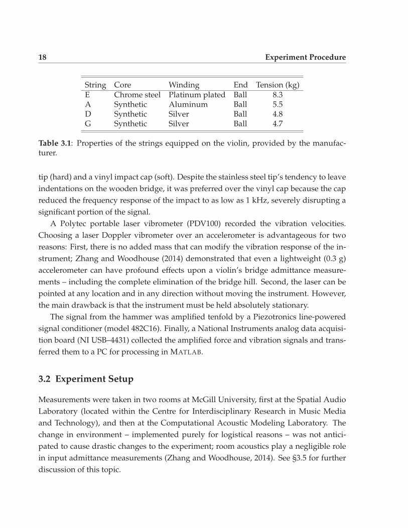
The violin used in this experiment was made in 2005 by H. Armenious, a luthier oper-ating in Toronto, Canada. It was chosen because of its expert craftsmanship, ensuringthat its properties can be readily compared with other violins. The violin was equippedwith a set of Thomastik–Infeld Peter Infeld strings held under standard tension (Table3.1), aurally tuned in just intonation with the A4 set to 440 Hz. A Hill model fine tunerfastens the E-string onto a Hill model tailpiece, which is 113 mm long and constructedof rosewood. After tuning, the afterlength measures 52 mm from the bridge to the “fret”on the tailpiece, while the tailgut extends 39 mm from the tailpiece (78 mm around thewhole loop). All non-essential accessories, including the chin rest, were removed so thatthe body could vibrate as freely as possible.
The input force was generated by a Piezotronics miniature instrumented impacthammer (model 086E80), whose 2.5 mm-diameter conical tip can precisely strike thethin edges of the bridge. Two tips were supplied by the manufacturer, a stainless steel
18 Experiment Procedure
String Core Winding End Tension (kg)E Chrome steel Platinum plated Ball 8.3A Synthetic Aluminum Ball 5.5D Synthetic Silver Ball 4.8G Synthetic Silver Ball 4.7
Table 3.1: Properties of the strings equipped on the violin, provided by the manufac-turer.
tip (hard) and a vinyl impact cap (soft). Despite the stainless steel tip’s tendency to leaveindentations on the wooden bridge, it was preferred over the vinyl cap because the capreduced the frequency response of the impact to as low as 1 kHz, severely disrupting asignificant portion of the signal.
A Polytec portable laser vibrometer (PDV100) recorded the vibration velocities.Choosing a laser Doppler vibrometer over an accelerometer is advantageous for tworeasons: First, there is no added mass that can modify the vibration response of the in-strument; Zhang and Woodhouse (2014) demonstrated that even a lightweight (0.3 g)accelerometer can have profound effects upon a violin’s bridge admittance measure-ments – including the complete elimination of the bridge hill. Second, the laser can bepointed at any location and in any direction without moving the instrument. However,the main drawback is that the instrument must be held absolutely stationary.
The signal from the hammer was amplified tenfold by a Piezotronics line-poweredsignal conditioner (model 482C16). Finally, a National Instruments analog data acquisi-tion board (NI USB–4431) collected the amplified force and vibration signals and trans-ferred them to a PC for processing in MATLAB.
3.2 Experiment Setup
Measurements were taken in two rooms at McGill University, first at the Spatial AudioLaboratory (located within the Centre for Interdisciplinary Research in Music Mediaand Technology), and then at the Computational Acoustic Modeling Laboratory. Thechange in environment – implemented purely for logistical reasons – was not antici-pated to cause drastic changes to the experiment; room acoustics play a negligible rolein input admittance measurements (Zhang and Woodhouse, 2014). See §3.5 for furtherdiscussion of this topic.
3.3 Data Acquisition 19
In order to approximate “free–free” boundary conditions, the violin was verticallysuspended from a rigid fixture on the ceiling (in both rooms) using a string loopedaround the scroll. Soft foam was placed lightly under the end button, partly to supportthe instrument, and partly to subdue the induced low-frequency “swinging” caused bythe hammer’s impact. Sufficient manœuvrability around the point of contact was main-tained to ensure that only this low-frequency contamination (which lies below the rangeof interest for these measurements) is damped. Other than these boundary conditions,no other point on the instrument body was in contact with an external object. A pieceof cardboard and two small pieces of foam were strategically placed along the playinglength of the strings to prevent their resonances from interfering with those of the body,but these dampeners were not in contact with the violin body. Figure 3.1 shows thesetup in the Spatial Audio Laboratory, which was replicated as closely as possible whenthe experiment moved to the Computational Acoustic Modeling Laboratory.
The impact hammer was secured onto a vertically adjustable altitude–azimuth mount.Like a pendulum, it swings freely along the altitude axis to ensure that impacts wouldconsistently land at the same position with roughly the same force. Nonetheless, fill-ing in the two-dimensional admittance matrix (Equation 2.4) required the instrument tobe struck and measured along both directions. And with only one laser available, the(symmetric) cross-terms must be measured separately from the on-axis terms. Thus, thehammer and laser had to be moved manually to obtain the three measurements (twoon-axis terms and one cross-axis term). The hammer and laser each had its own standso that their movements would not affect the free-swinging violin.
3.3 Data Acquisition
As in previous studies of this kind (e.g., Bissinger, 2008), the impact hammer was po-sitioned to strike on the bass (G-string) side of the instrument. Ideally, the point ofmeasurement should coincide with the strike. But since this is physically impossible,the laser beam is aimed at the closest possible point instead. The need to take two-dimensional measurements further restricted the selection of impact points to areas ly-ing along edges where perpendicular surfaces met – the laser cannot be pointed at alocation within the interior of the wood. Consequently, the upper bass-side corner wasdesignated as the impact point on the bridge (Figure 3.2a), while four points were se-lected along the same side on the tailpiece (Figure 3.2b and Table 3.2).

20 Experiment Procedure
Figure 3.1: The experiment setup in the Spatial Audio Laboratory. From left to right are:the laser vibrometer, the hammer and pendulum secured on an altazimuth mount, andthe violin suspended from the ceiling and gently supported by foam.

3.3 Data Acquisition 21
G D A
E Impact/ Measurement Point
(a) Bridge
110 mm (IP 1)
65 mm (IP 2)
35 mm (IP 3)
10 mm (IP 4)
Impact/Measurement Points
40 mm (Pos. 1)
10 mm (Pos. 2)
Mass Positions
Tailpiece length: 113 mm
Head
Tail
(b) Tailpiece
Figure 3.2: Selected points for measurement (red circles) and placement of masses onthe tailpiece (blue circles).
22 Experiment Procedure
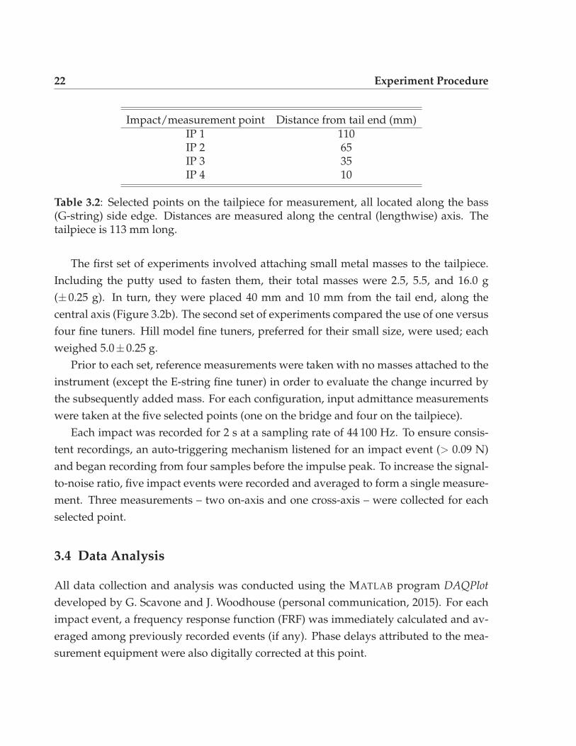
Impact/measurement point Distance from tail end (mm)IP 1 110IP 2 65IP 3 35IP 4 10
Table 3.2: Selected points on the tailpiece for measurement, all located along the bass(G-string) side edge. Distances are measured along the central (lengthwise) axis. Thetailpiece is 113 mm long.
The first set of experiments involved attaching small metal masses to the tailpiece.Including the putty used to fasten them, their total masses were 2.5, 5.5, and 16.0 g(±0.25 g). In turn, they were placed 40 mm and 10 mm from the tail end, along thecentral axis (Figure 3.2b). The second set of experiments compared the use of one versusfour fine tuners. Hill model fine tuners, preferred for their small size, were used; eachweighed 5.0±0.25 g.
Prior to each set, reference measurements were taken with no masses attached to theinstrument (except the E-string fine tuner) in order to evaluate the change incurred bythe subsequently added mass. For each configuration, input admittance measurementswere taken at the five selected points (one on the bridge and four on the tailpiece).
Each impact was recorded for 2 s at a sampling rate of 44 100 Hz. To ensure consis-tent recordings, an auto-triggering mechanism listened for an impact event (> 0.09 N)and began recording from four samples before the impulse peak. To increase the signal-to-noise ratio, five impact events were recorded and averaged to form a single measure-ment. Three measurements – two on-axis and one cross-axis – were collected for eachselected point.
3.4 Data Analysis
All data collection and analysis was conducted using the MATLAB program DAQPlotdeveloped by G. Scavone and J. Woodhouse (personal communication, 2015). For eachimpact event, a frequency response function (FRF) was immediately calculated and av-eraged among previously recorded events (if any). Phase delays attributed to the mea-surement equipment were also digitally corrected at this point.
3.4 Data Analysis 23
During the averaging, a coherence function was also calculated as a measure of thelinearity of the measurement – a coherence of unity throughout the frequency spectrumis considered ideal. Thus, the coherence could be used to evaluate an impact event’squality, as faulty strikes occasionally occur, resulting in drastically different FRFs. With-out having to inspect the FRFs from the other impact events (which may be difficult),the coherence function provided the information at a glance. Such faulty impact eventswere unceremoniously discarded.
3.4.1 Mode Fitting
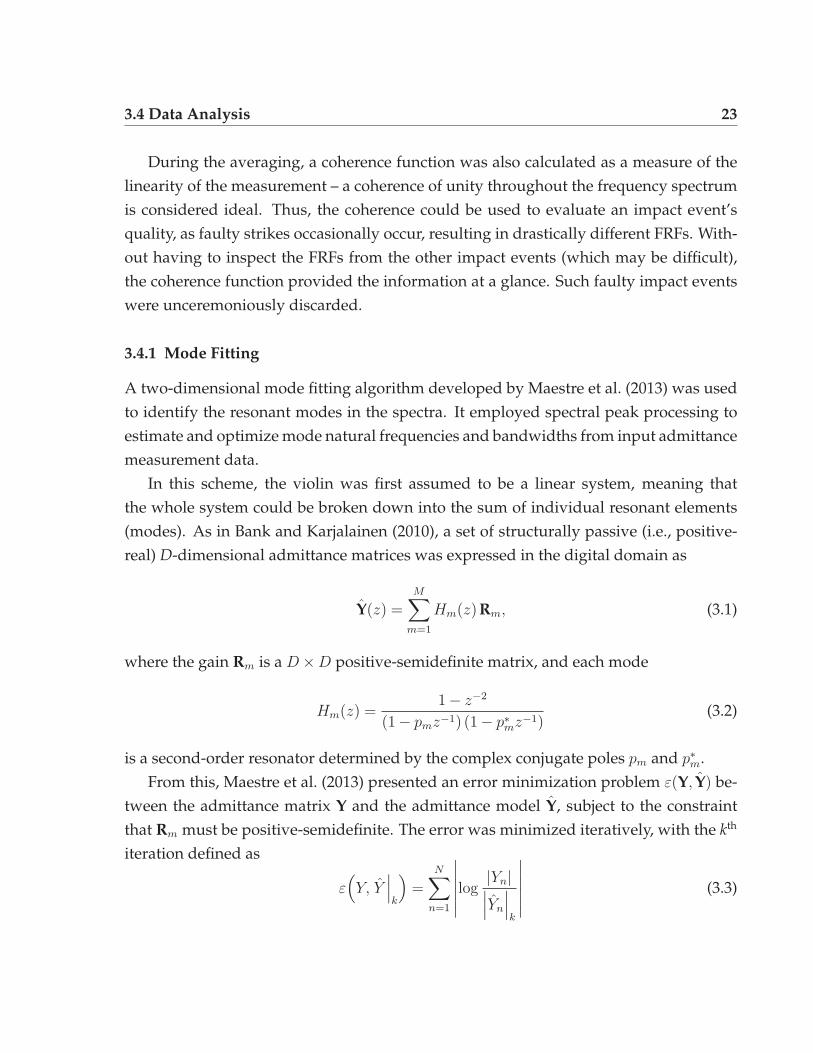
A two-dimensional mode fitting algorithm developed by Maestre et al. (2013) was usedto identify the resonant modes in the spectra. It employed spectral peak processing toestimate and optimize mode natural frequencies and bandwidths from input admittancemeasurement data.
In this scheme, the violin was first assumed to be a linear system, meaning thatthe whole system could be broken down into the sum of individual resonant elements(modes). As in Bank and Karjalainen (2010), a set of structurally passive (i.e., positive-real) D-dimensional admittance matrices was expressed in the digital domain as
Y(z) =M∑
m=1
Hm(z)Rm, (3.1)
where the gain Rm is a D×D positive-semidefinite matrix, and each mode
Hm(z) =1− z−2
(1− pmz−1) (1− p∗mz−1)(3.2)
is a second-order resonator determined by the complex conjugate poles pm and p∗m.From this, Maestre et al. (2013) presented an error minimization problem ε(Y, Y) be-
tween the admittance matrix Y and the admittance model Y, subject to the constraintthat Rm must be positive-semidefinite. The error was minimized iteratively, with the kth
iteration defined as
ε(Y, Y
∣∣∣k
)=
N∑n=1
∣∣∣∣∣∣log|Yn|∣∣∣Yn
∣∣∣k
∣∣∣∣∣∣ (3.3)
24 Experiment Procedure
for N-sample long vectors Y (ω) and Y (ω) taken in 0 ≤ ω < π. When expressed in alogarithmic scale, Equation 3.3 reduces to a difference of magnitudes.
Finally, the MATLAB software package CVX (Grant and Boyd, 2008, 2014) conductedconvex minimization to find a set of parameters H and R such that ε(Y, Y) was min-imized within a selected frequency range. In this study, optimization was performedbetween 100 and 6 000 Hz, where measurement coherence was closest to unity.
3.5 Repeatability of Measurements
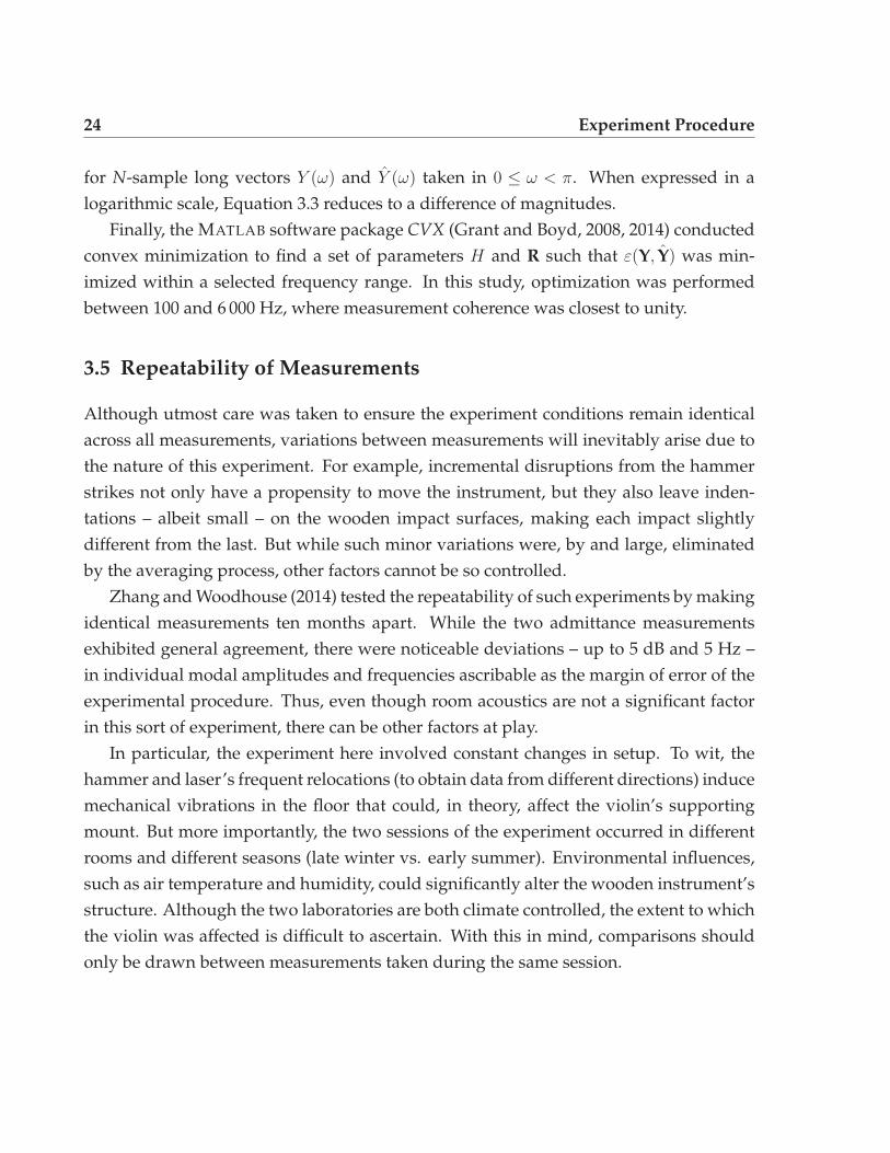
Although utmost care was taken to ensure the experiment conditions remain identicalacross all measurements, variations between measurements will inevitably arise due tothe nature of this experiment. For example, incremental disruptions from the hammerstrikes not only have a propensity to move the instrument, but they also leave inden-tations – albeit small – on the wooden impact surfaces, making each impact slightlydifferent from the last. But while such minor variations were, by and large, eliminatedby the averaging process, other factors cannot be so controlled.
Zhang and Woodhouse (2014) tested the repeatability of such experiments by makingidentical measurements ten months apart. While the two admittance measurementsexhibited general agreement, there were noticeable deviations – up to 5 dB and 5 Hz –in individual modal amplitudes and frequencies ascribable as the margin of error of theexperimental procedure. Thus, even though room acoustics are not a significant factorin this sort of experiment, there can be other factors at play.
In particular, the experiment here involved constant changes in setup. To wit, thehammer and laser’s frequent relocations (to obtain data from different directions) inducemechanical vibrations in the floor that could, in theory, affect the violin’s supportingmount. But more importantly, the two sessions of the experiment occurred in differentrooms and different seasons (late winter vs. early summer). Environmental influences,such as air temperature and humidity, could significantly alter the wooden instrument’sstructure. Although the two laboratories are both climate controlled, the extent to whichthe violin was affected is difficult to ascertain. With this in mind, comparisons shouldonly be drawn between measurements taken during the same session.
25
Chapter 4
Results
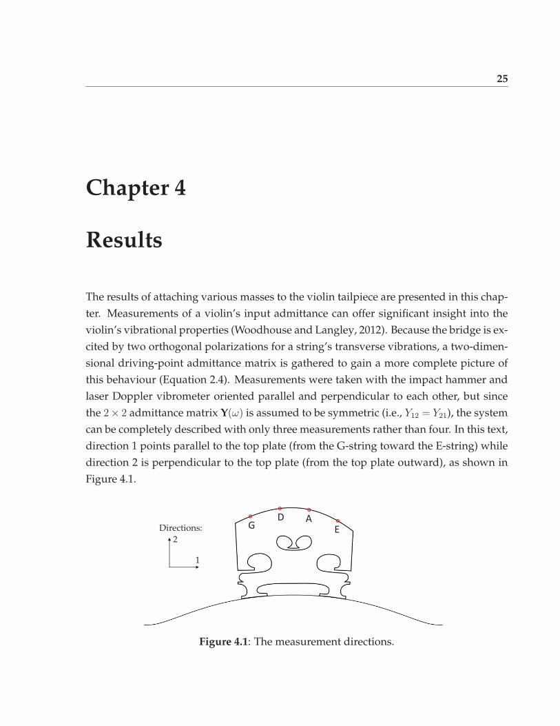
The results of attaching various masses to the violin tailpiece are presented in this chap-ter. Measurements of a violin’s input admittance can offer significant insight into theviolin’s vibrational properties (Woodhouse and Langley, 2012). Because the bridge is ex-cited by two orthogonal polarizations for a string’s transverse vibrations, a two-dimen-sional driving-point admittance matrix is gathered to gain a more complete picture ofthis behaviour (Equation 2.4). Measurements were taken with the impact hammer andlaser Doppler vibrometer oriented parallel and perpendicular to each other, but sincethe 2× 2 admittance matrix Y(ω) is assumed to be symmetric (i.e., Y12 = Y21), the systemcan be completely described with only three measurements rather than four. In this text,direction 1 points parallel to the top plate (from the G-string toward the E-string) whiledirection 2 is perpendicular to the top plate (from the top plate outward), as shown inFigure 4.1.
G D A
E Directions: 2
1
Figure 4.1: The measurement directions.
26 Results
4.1 Reference Measurements (unmodified violin)
Reference measurements were taken with the violin unmodified (i.e., with no mass at-tached) prior to every data collecting session. As discussed in Section 3.5, variationsinevitably arise regardless of the steps taken to ensure consistency. This was furtherexacerbated by the fact that the data was collected over multiple sessions, where thesetup was torn down and rebuilt each time. Establishing a ground truth for each set istherefore crucial to making comparisons across data sets: Even though absolute changesacross data sets cannot be directly compared, relative changes – i.e., deviations from therespective reference measurements – can be.
4.1.1 Frequency Response: Bridge
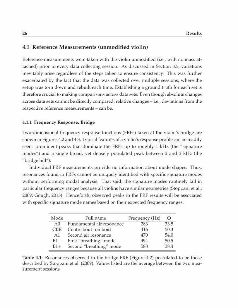
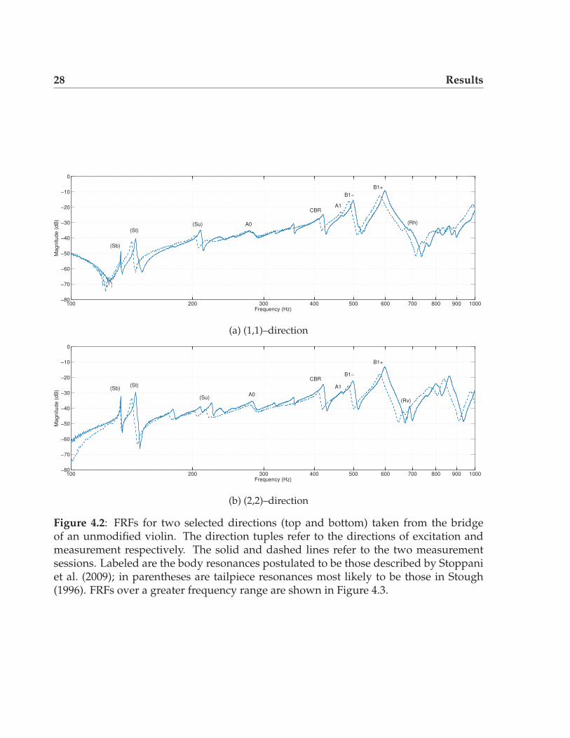
Two-dimensional frequency response functions (FRFs) taken at the violin’s bridge areshown in Figures 4.2 and 4.3. Typical features of a violin’s response profile can be readilyseen: prominent peaks that dominate the FRFs up to roughly 1 kHz (the “signaturemodes”) and a single broad, yet densely populated peak between 2 and 3 kHz (the“bridge hill”).
Individual FRF measurements provide no information about mode shapes. Thus,resonances found in FRFs cannot be uniquely identified with specific signature modeswithout performing modal analysis. That said, the signature modes routinely fall inparticular frequency ranges because all violins have similar geometries (Stoppani et al.,2009; Gough, 2013). Henceforth, observed peaks in the FRF results will be associatedwith specific signature mode names based on their expected frequency ranges.
Mode Full name Frequency (Hz) QA0 Fundamental air resonance 283 33.5
CBR Centre bout romboid 416 50.3A1 Second air resonance 470 54.0
B1− First “breathing” mode 494 50.5B1+ Second “breathing” mode 588 38.4
Table 4.1: Resonances observed in the bridge FRF (Figure 4.2) postulated to be thosedescribed by Stoppani et al. (2009). Values listed are the average between the two mea-surement sessions.

4.1 Reference Measurements (unmodified violin) 27
Mode Full name Frequency (Hz) QSb Swing mode, bass side 100–140 50–80St Swing mode, treble side 120–160 60–90Su Swing mode, under 180–230 35–70Rh Rotation, horizontal axis 300–800 34–110Rv Rotation, vertical axis 300–800 38–110
Table 4.2: Tailpiece resonances identified by Stough (1996). The frequencies and Qs aregiven by ranges since their precise values depend on the tailpiece’s setup.
Several resonances are also spotted in the spectrum around 135, 210, and 650 Hz.As it turns out, these are tailpiece resonances, a direct consequence of leaving the after-length undamped. These modes will be discussed in the next section (§4.1.2).
Besides the signature modes, bridge hill, and tailpiece resonances, there are no othersignificant features to be discerned. Below 100 Hz, the violin does not have any sig-nificant resonances, and the spectrum is instead dominated by the resonances of thesupport rig. Above 10 kHz, the signal becomes concealed by noise due to insufficientimpact (input) energy.
4.1.2 Frequency Response: Tailpiece
Hammer measurements taken on the tailpiece reveal the vibrational behaviour of thesystem from the tailpiece’s point of view. Unlike the bridge, measurements were taken atmultiple points on the tailpiece (Figure 3.2b); the collected FRFs are presented in Figures4.4 and 4.5.
The observed tailpiece resonances can be matched with those in Stough (1996). Ascan be seen by comparing Tables 4.2 and 4.3, there is very good agreement between thevalues found by Stough and by this experiment. But as with the signature modes of theviolin body, modal analysis is required to verify their identities, and the matching of theobserved modes to those identified by Stough is purely conjectural.
All of the modes identified in Table 4.3 are rigid-body modes; this is attested by not-ing that their values are uniform along the length of the tailpiece. Also, all of these rigid-body modes quite conveniently lie in the region of interest between 100 and 1 000 Hz. IfFouilhé et al.’s (2011) work on the cello tailpiece carries over to the violin tailpiece, thenthese are the only rigid-body modes of the tailpiece – all higher-frequency resonancesare torsional.
28 Results
100 200 300 400 500 600 700 800 900 1000−80
−70
−60
−50
−40
−30
−20
−10
0
Frequency (Hz)
Mag
nitu
de (
dB)
(Sb)
(St)(Su)
CBR
A0
A1
B1−B1+
(Rh)
(a) (1,1)–direction
100 200 300 400 500 600 700 800 900 1000−80
−70
−60
−50
−40
−30
−20
−10
0
Frequency (Hz)
Mag
nitu
de (
dB) (Sb) (St)
(Su)
CBR
(Rv)A0
A1
B1−
B1+
(b) (2,2)–direction
Figure 4.2: FRFs for two selected directions (top and bottom) taken from the bridgeof an unmodified violin. The direction tuples refer to the directions of excitation andmeasurement respectively. The solid and dashed lines refer to the two measurementsessions. Labeled are the body resonances postulated to be those described by Stoppaniet al. (2009); in parentheses are tailpiece resonances most likely to be those in Stough(1996). FRFs over a greater frequency range are shown in Figure 4.3.

4.1 Reference Measurements (unmodified violin) 29
100
101
102
103
−80
−70
−60
−50
−40
−30
−20
−10
0
Frequency (Hz)
Mag
nitu
de (
dB)
(Su)
CBR
A0
B1−
B1+
(a) (1,1)–direction
100
101
102
103
−80
−70
−60
−50
−40
−30
−20
−10
0
Frequency (Hz)
Mag
nitu
de (
dB)
(b) (1,2)–direction
100
101
102
103
−80
−70
−60
−50
−40
−30
−20
−10
0
Frequency (Hz)
Mag
nitu
de (
dB)
(Sb)
(St)
(c) (2,2)–direction
Figure 4.3: Bridge FRFs of an unmodified violin. The direction tuples refer to the di-rections of excitation and measurement respectively. The solid and dashed lines refer tothe two measurement sessions. Labeled are the body resonances postulated to be thosedescribed by Stoppani et al. (2009); in parentheses are tailpiece resonances most likelyto be those in Stough (1996).
30 Results
100 200 300 400 500 600 700 800 900 1000−70
−60
−50
−40
−30
−20
−10
0
10
20
30
Frequency (Hz)
Mag
nitu
de (
dB)
Sb
St
Su
(CBR)
Rv
(a) (1,1)–direction
100 200 300 400 500 600 700 800 900 1000−70
−60
−50
−40
−30
−20
−10
0
10
20
30
Frequency (Hz)
Mag
nitu
de (
dB)
(A0)
(B1−) (B1+)
Rh
(b) (2,2)–direction
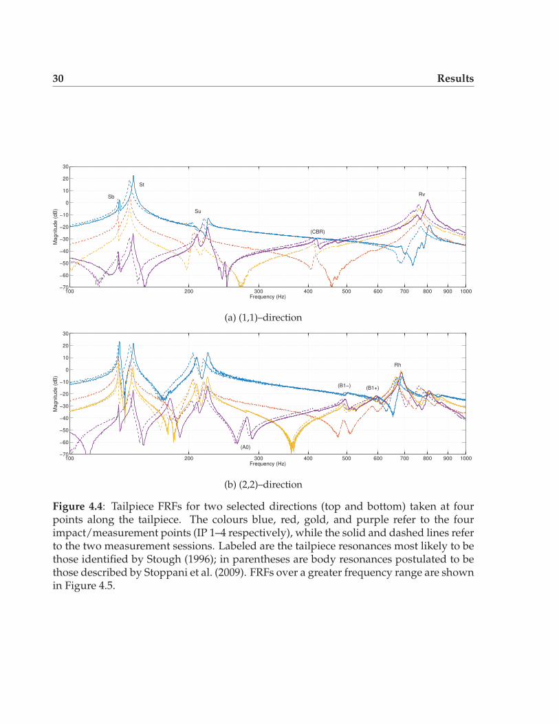
Figure 4.4: Tailpiece FRFs for two selected directions (top and bottom) taken at fourpoints along the tailpiece. The colours blue, red, gold, and purple refer to the fourimpact/measurement points (IP 1–4 respectively), while the solid and dashed lines referto the two measurement sessions. Labeled are the tailpiece resonances most likely to bethose identified by Stough (1996); in parentheses are body resonances postulated to bethose described by Stoppani et al. (2009). FRFs over a greater frequency range are shownin Figure 4.5.
4.1 Reference Measurements (unmodified violin) 31
100
101
102
103
−80
−70
−60
−50
−40
−30
−20
−10
0
10
20
30
Frequency (Hz)
Mag
nitu
de (
dB)
Sb
St
Su
(CBR)
Rv
(a) (1,1)–direction
100
101
102
103
−80
−70
−60
−50
−40
−30
−20
−10
0
10
20
30
Frequency (Hz)
Mag
nitu
de (
dB)
(b) (1,2)–direction
100
101
102
103
−80
−70
−60
−50
−40
−30
−20
−10
0
10
20
30
Frequency (Hz)
Mag
nitu
de (
dB)
(A0)
(B1−)(B1+)
Rh
(c) (2,2)–direction
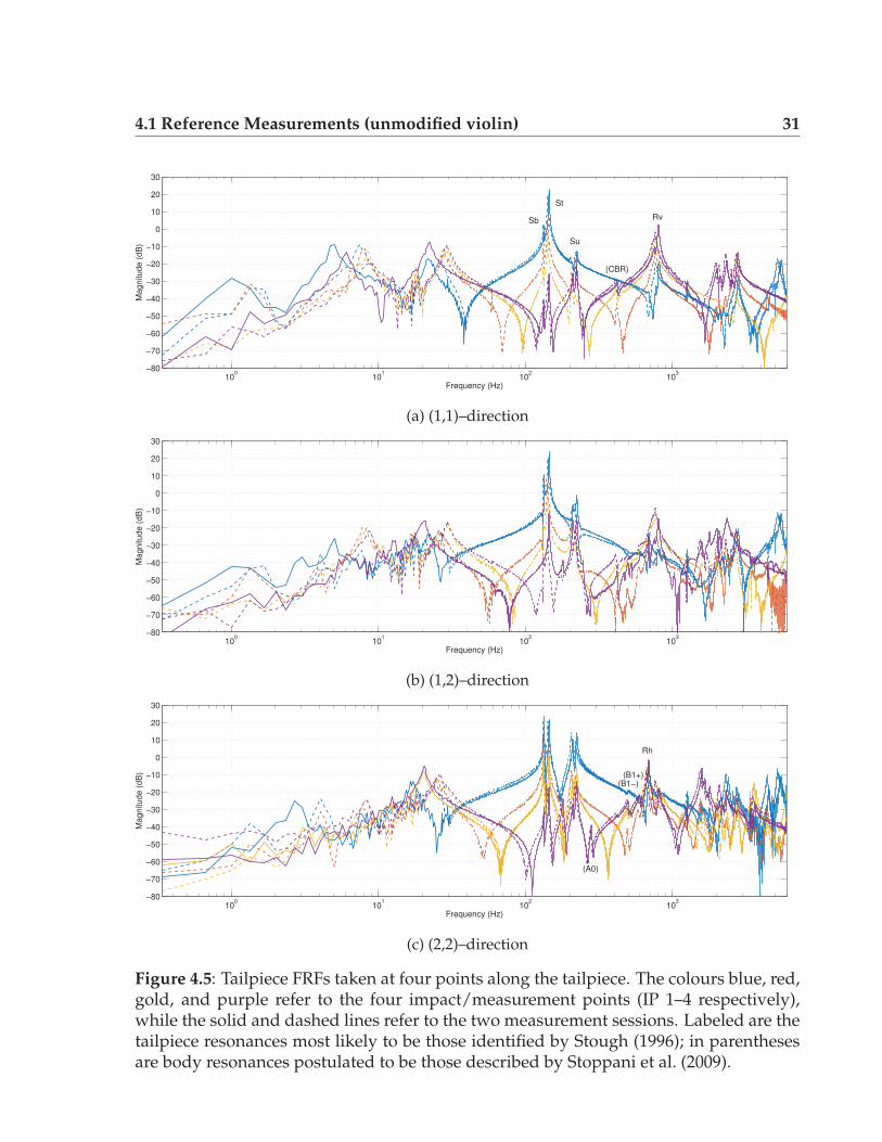
Figure 4.5: Tailpiece FRFs taken at four points along the tailpiece. The colours blue, red,gold, and purple refer to the four impact/measurement points (IP 1–4 respectively),while the solid and dashed lines refer to the two measurement sessions. Labeled are thetailpiece resonances most likely to be those identified by Stough (1996); in parenthesesare body resonances postulated to be those described by Stoppani et al. (2009).

32 Results
Mode Frequency (Hz) QSb 133 133 133 133 73.6 69.6 73.3 94.8St 142 142 143 142 59.1 64.7 59.5 52.0
*Su 205 205 205 205218 218 218 217
50.0 58.6 56.9 81.272.5 48.5 49.5 79.7
Rh 667 668 666 666 38.7 38.7 38.9 38.1Rv 761 763 759 758 26.0 30.9 26.6 32.6
Table 4.3: Tailpiece resonances identified from Figure 4.4. In each category, the fourcolumns represent the four impact/measurement points (IP 1–4 respectively). Valueslisted are the average between the two measurement sessions. *Su is a split peak.
In the portrait gathered in Figures 4.4 and 4.5, the swing modes and rotation modesare seen to influence the tailpiece non-uniformly: Near the head of the tailpiece (closestto the bridge), the swing modes dominate; whereas near the tail end, the rotation modesprevail. However, Stough has observed that the three swing modes have little effect onthe violin’s tonal output. This is perhaps unsurprising, as they all lie well below thesignature modes of the violin. The rotation modes, by contrast, lie just above them.
But surveying the tailpiece plots reveals a peculiar feature: the presence of the bodymodes within the tailpiece signal, especially near the tail end (compare the blue (IP 1)and purple (IP 4) curves of Figure 4.4). In itself, this is not particularly surprising sincethe tailpiece is fixed to the top plate via the tailgut. Tautly stretched, the tailgut couplesthe two components together quite effectively, allowing them to vibrate in tandem. Nearthe saddle (where the tailgut bends around the top plate), the CBR mode is torsionalroughly about the central (lengthwise) axis, yet moving chiefly in direction 1, while thetwo breathing modes pulsate in direction 2 (Stoppani et al., 2009; Gough, 2013).
Thus, the path forward is clear: attempt to couple the rotation modes with the vio-lin’s breathing modes. The simplest method to lower the frequency of a resonance is toadd mass to the region of greatest amplitude (an antinode). In this case, that would betoward the tail end of the tailpiece.
4.2 Mass-loaded Tailpiece
There are two independent variables in this experiment: the mass and its position. Insuccession, three small masses (2.5, 5.5, and 16.0 g) are placed at two positions on the

4.2 Mass-loaded Tailpiece 33
Direction 1 Direction 2Mode Frequency (Hz) Q magnitude (dB) magnitude (dB)
A0 284 283 283 43.0 27.0 40.4 −40.7 − 46.7 − 40.4 −39.4 − 43.8 − 43.3CBR 421 420 420 56.9 57.5 57.5 −25.0 − 28.1 − 24.1 −24.1 − 28.4 − 29.0A1 471 471 471 55.4 45.7 38.6 −45.4 − 48.3 − 37.3 −45.3 − 47.7 − 48.1
B1− 500 498 495 50.0 45.7 40.1 −15.3 − 19.5 − 19.0 −20.1 − 29.6 − 33.5B1+ 596 590 588 43.2 31.4 25.2 −12.7 − 15.6 − 15.9 −15.8 − 21.0 − 25.0
Table 4.4: Effect of a 2.5 g mass on the signature modes. In each category, the threecolumns represent the measured values (from left to right) with the mass off, and withit attached at positions 1 and 2.
tailpiece (40 mm and 10 mm from the tail end; Figure 3.2b) to study the effects on thebridge and tailpiece FRFs.
4.2.1 2.5-gram mass
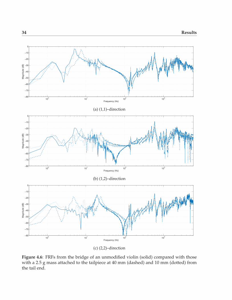
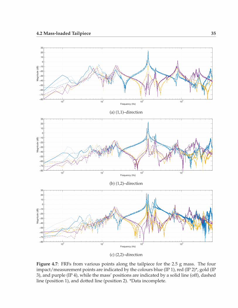
The lightest mass attached was 2.5±0.25 g. The resulting bridge FRFs are shown inFigure 4.6, while the values of the signature modes are given in Table 4.4. Notably, theproperties of the two breathing (B1− and B1+) modes display a clear correlation withthe position of the mass – placing the mass closer to the tail end is accompanied by areduction in both frequency and amplitude, as well as a broadening, of the peaks. Thissuggests that the tailpiece plays a non-negligible role in shaping the bridge FRF and,consequently, the vibrational characteristics of the violin. To explore the mechanismbehind this coupling, the tailpiece FRF, as measured at four locations, is presented inFigure 4.7.
All of the tailpiece modes identified in Table 4.3 were noticeably affected. But with alack of prominent body resonances near the three swing modes, the following analysiswill focus exclusively on the two rotation modes.
Like the signature modes, the rotation modes responded to the added mass with areduction in frequency and magnitude, only much more dramatically – the Rv mode (asmeasured at IP 1) shifted from 806 to 721 Hz and dropped from −22.0 to −37.5 dB, whilethe Rh mode shifted from 692 to 635 Hz and fell from −10.0 to −17.5 dB. Given that thetailpiece is much less massive than the violin body, this was not unexpected.
What is most fascinating though, is that lowering the Rh mode’s frequency causessome of its energy to be transferred to the B1-induced modes on the tailpiece (compare
34 Results
100
101
102
103
−80
−70
−60
−50
−40
−30
−20
−10
0
Frequency (Hz)
Mag
nitu
de (
dB)
(a) (1,1)–direction
100
101
102
103
−80
−70
−60
−50
−40
−30
−20
−10
0
Frequency (Hz)
Mag
nitu
de (
dB)
(b) (1,2)–direction
100
101
102
103
−80
−70
−60
−50
−40
−30
−20
−10
0
Frequency (Hz)
Mag
nitu
de (
dB)
(c) (2,2)–direction
Figure 4.6: FRFs from the bridge of an unmodified violin (solid) compared with thosewith a 2.5 g mass attached to the tailpiece at 40 mm (dashed) and 10 mm (dotted) fromthe tail end.
4.2 Mass-loaded Tailpiece 35
100
101
102
103
−80
−70
−60
−50
−40
−30
−20
−10
0
10
20
30
Frequency (Hz)
Mag
nitu
de (
dB)
(a) (1,1)–direction
100
101
102
103
−80
−70
−60
−50
−40
−30
−20
−10
0
10
20
30
Frequency (Hz)
Mag
nitu
de (
dB)
(b) (1,2)–direction
100
101
102
103
−80
−70
−60
−50
−40
−30
−20
−10
0
10
20
30
Frequency (Hz)
Mag
nitu
de (
dB)
(c) (2,2)–direction
Figure 4.7: FRFs from various points along the tailpiece for the 2.5 g mass. The fourimpact/measurement points are indicated by the colours blue (IP 1), red (IP 2)*, gold (IP3), and purple (IP 4), while the mass’ positions are indicated by a solid line (off), dashedline (position 1), and dotted line (position 2). *Data incomplete.

36 Results
100 200 300 400 500 600 700 800 900 1000−80
−70
−60
−50
−40
−30
−20
−10
0
Frequency (Hz)
Mag
nitu
de (
dB)
B1+← Rh
Figure 4.8: FRFs from the bridge (blue) overlaid onto those from IP 2 of the tailpiece(gold) demonstrate the coupling between the B1+ and Rh modes after a 2.5 g mass wasattached at position 1 (dashed line) and position 2 (dotted line), compared to having themass off (solid line). The arrow indicates the downward shift of the Rh mode.
the solid and dashed gold lines of Figure 4.8), allowing it to absorb vibrational energyfrom the body much more effectively. As shown in Figure 4.8, the body’s B1+ modeis much influenced by this modal interaction, and is reminiscent of the notch filteringeffect observed by Stough (1996). In that study, a small 3.95 g mass attached to thetailgut end of the tailpiece (presumably near position 2) was used to lower the Rh mode’sfrequency, and the B1+ mode (referred to as the W resonance) fell by about 10 dB aftertheir frequencies were matched. It remains to be seen whether lowering the rotationmodes further will incite more dramatic effects; to be determined is whether the Rh andB1+ modes can become locked, or whether the as yet inconspicuous Rv mode may cometo play a role.
In his custom tailpieces, White (2012) also uses a small mass of 2.5 g. The work re-ported here, conducted on a violin outfitted with only a “normal” tailpiece, corroboratesthe results reported by Pirquet (2011) and White (2012): Placing a small mass near thetail end of the tailpiece is sufficient to noticeably alter the main body modes of the vi-olin, resulting in the lowering in frequency and amplitude of the B1+ mode. However,Pirquet and White also observed a splitting of the B1+ peak, which was not replicatedto the same degree in this work. The nascent peak (in the body), induced by the Rhmode, is the result of the aforementioned body–tailpiece coupling, and can also be seenin Figure 4.8 (at around 630 Hz).
4.2 Mass-loaded Tailpiece 37
Direction 1 Direction 2Mode Frequency (Hz) Q magnitude (dB) magnitude (dB)
A0 281 281 280 24.0 20.4 24.3 −42.9 − 43.4 − 39.7 −42.7 − 46.2 − 48.7CBR 411 412 411 43.7 43.4 39.2 −30.2 − 32.8 − 32.9 −30.6 − 34.4 − 39.2A1 468 467 468 52.6 53.1 52.6 −33.1 − 36.3 − 32.0 −38.4 − 43.3 − 46.3
B1− 488 488 485 50.9 46.4 48.0 −16.0 − 18.6 − 20.0 −25.4 − 33.1 − 40.4B1+ 579 568 566 33.5 21.3 14.6 −12.2 − 18.7 − 21.7 −17.5 − 26.0 − 31.3
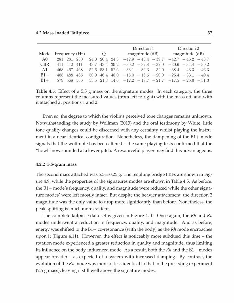
Table 4.5: Effect of a 5.5 g mass on the signature modes. In each category, the threecolumns represent the measured values (from left to right) with the mass off, and withit attached at positions 1 and 2.
Even so, the degree to which the violin’s perceived tone changes remains unknown.Notwithstanding the study by Wollman (2013) and the oral testimony by White, littletone quality changes could be discerned with any certainty whilst playing the instru-ment in a near-identical configuration. Nonetheless, the dampening of the B1+ modesignals that the wolf note has been altered – the same playing tests confirmed that the“howl” now sounded at a lower pitch. A resourceful player may find this advantageous.
4.2.2 5.5-gram mass
The second mass attached was 5.5±0.25 g. The resulting bridge FRFs are shown in Fig-ure 4.9, while the properties of the signatures modes are shown in Table 4.5. As before,the B1+ mode’s frequency, quality, and magnitude were reduced while the other signa-ture modes’ were left mostly intact. But despite the heavier attachment, the direction 2magnitude was the only value to drop more significantly than before. Nonetheless, thepeak splitting is much more evident.
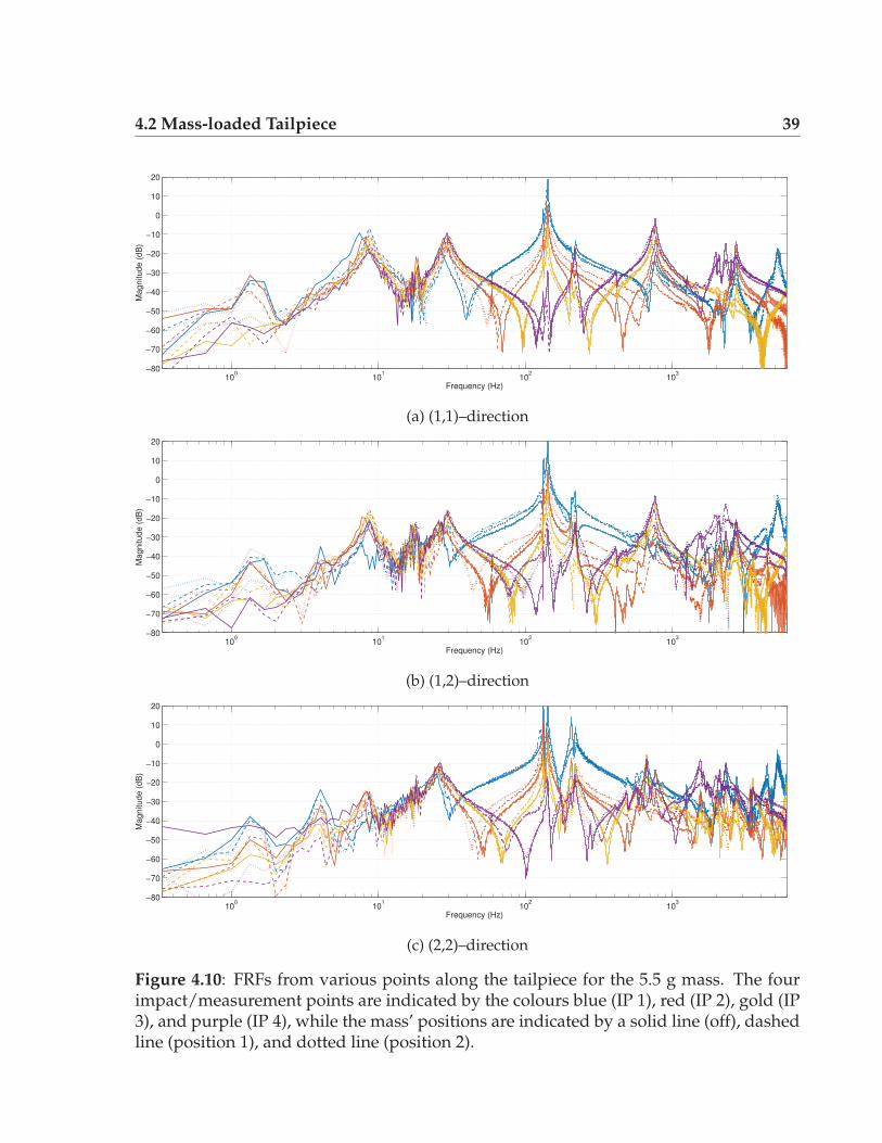
The complete tailpiece data set is given in Figure 4.10. Once again, the Rh and Rvmodes underwent a reduction in frequency, quality, and magnitude. And as before,energy was shifted to the B1+ co-resonance (with the body) as the Rh mode encroachesupon it (Figure 4.11). However, the effect is noticeably more subdued this time – therotation mode experienced a greater reduction in quality and magnitude, thus limitingits influence on the body-influenced mode. As a result, both the Rh and the B1+ modesappear broader – as expected of a system with increased damping. By contrast, theevolution of the Rv mode was more or less identical to that in the preceding experiment(2.5 g mass), leaving it still well above the signature modes.

38 Results
100
101
102
103
−80
−70
−60
−50
−40
−30
−20
−10
0
Frequency (Hz)
Mag
nitu
de (
dB)
(a) (1,1)–direction
100
101
102
103
−80
−70
−60
−50
−40
−30
−20
−10
0
Frequency (Hz)
Mag
nitu
de (
dB)
(b) (1,2)–direction
100
101
102
103
−80
−70
−60
−50
−40
−30
−20
−10
0
Frequency (Hz)
Mag
nitu
de (
dB)
(c) (2,2)–direction
Figure 4.9: FRFs from the bridge of an unmodified violin (solid) compared with thosewith a 5.5 g mass attached to the tailpiece at 40 mm (dashed) and 10 mm (dotted) fromthe tail end.
4.2 Mass-loaded Tailpiece 39
100
101
102
103
−80
−70
−60
−50
−40
−30
−20
−10
0
10
20
Frequency (Hz)
Mag
nitu
de (
dB)
(a) (1,1)–direction
100
101
102
103
−80
−70
−60
−50
−40
−30
−20
−10
0
10
20
Frequency (Hz)
Mag
nitu
de (
dB)
(b) (1,2)–direction
100
101
102
103
−80
−70
−60
−50
−40
−30
−20
−10
0
10
20
Frequency (Hz)
Mag
nitu
de (
dB)
(c) (2,2)–direction
Figure 4.10: FRFs from various points along the tailpiece for the 5.5 g mass. The fourimpact/measurement points are indicated by the colours blue (IP 1), red (IP 2), gold (IP3), and purple (IP 4), while the mass’ positions are indicated by a solid line (off), dashedline (position 1), and dotted line (position 2).
40 Results
100 200 300 400 500 600 700 800 900 1000−80
−70
−60
−50
−40
−30
−20
−10
0
Frequency (Hz)
Mag
nitu
de (
dB)
B1+
← Rh
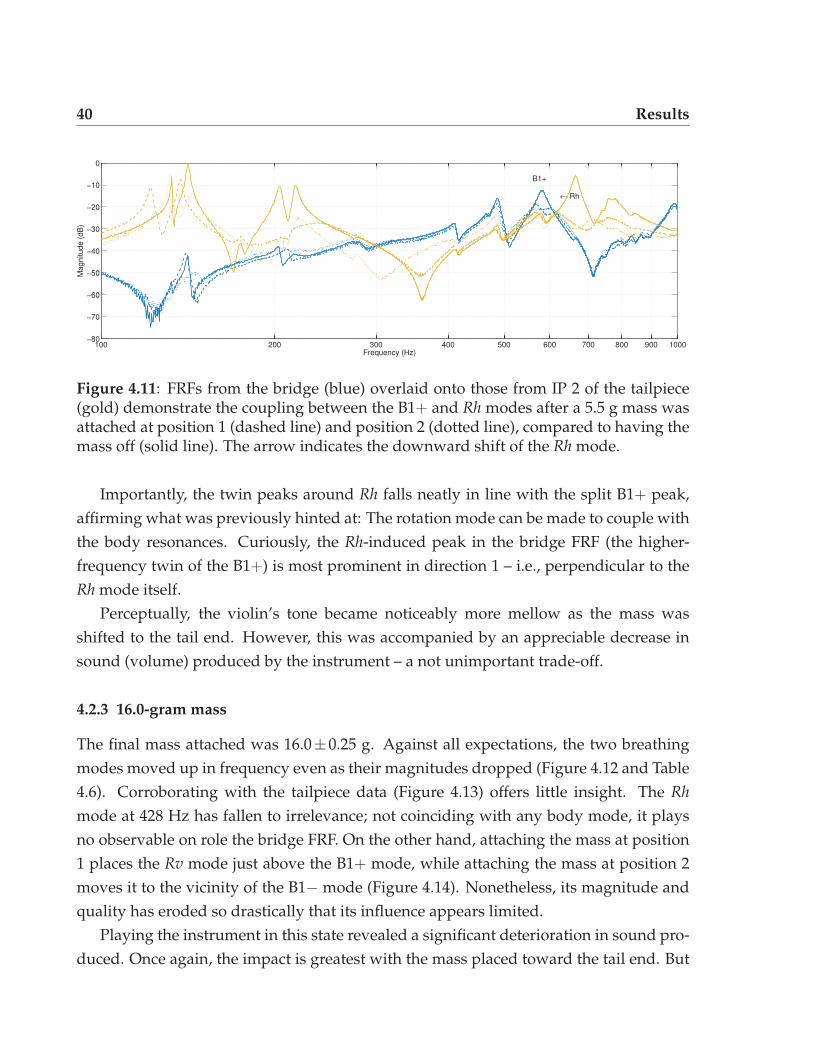
Figure 4.11: FRFs from the bridge (blue) overlaid onto those from IP 2 of the tailpiece(gold) demonstrate the coupling between the B1+ and Rh modes after a 5.5 g mass wasattached at position 1 (dashed line) and position 2 (dotted line), compared to having themass off (solid line). The arrow indicates the downward shift of the Rh mode.
Importantly, the twin peaks around Rh falls neatly in line with the split B1+ peak,affirming what was previously hinted at: The rotation mode can be made to couple withthe body resonances. Curiously, the Rh-induced peak in the bridge FRF (the higher-frequency twin of the B1+) is most prominent in direction 1 – i.e., perpendicular to theRh mode itself.
Perceptually, the violin’s tone became noticeably more mellow as the mass wasshifted to the tail end. However, this was accompanied by an appreciable decrease insound (volume) produced by the instrument – a not unimportant trade-off.
4.2.3 16.0-gram mass
The final mass attached was 16.0±0.25 g. Against all expectations, the two breathingmodes moved up in frequency even as their magnitudes dropped (Figure 4.12 and Table4.6). Corroborating with the tailpiece data (Figure 4.13) offers little insight. The Rhmode at 428 Hz has fallen to irrelevance; not coinciding with any body mode, it playsno observable on role the bridge FRF. On the other hand, attaching the mass at position1 places the Rv mode just above the B1+ mode, while attaching the mass at position 2moves it to the vicinity of the B1− mode (Figure 4.14). Nonetheless, its magnitude andquality has eroded so drastically that its influence appears limited.
Playing the instrument in this state revealed a significant deterioration in sound pro-duced. Once again, the impact is greatest with the mass placed toward the tail end. But

4.2 Mass-loaded Tailpiece 41
100
101
102
103
−80
−70
−60
−50
−40
−30
−20
−10
0
Frequency (Hz)
Mag
nitu
de (
dB)
(a) (1,1)–direction
100
101
102
103
−80
−70
−60
−50
−40
−30
−20
−10
0
Frequency (Hz)
Mag
nitu
de (
dB)
(b) (1,2)–direction
100
101
102
103
−80
−70
−60
−50
−40
−30
−20
−10
0
Frequency (Hz)
Mag
nitu
de (
dB)
(c) (2,2)–direction
Figure 4.12: FRFs from the bridge of an unmodified violin (solid) compared with thosewith a 16.0 g mass attached to the tailpiece at 40 mm (dashed) and 10 mm (dotted) fromthe tail end.

42 Results
100
101
102
103
−80
−70
−60
−50
−40
−30
−20
−10
0
10
20
Frequency (Hz)
Mag
nitu
de (
dB)
(a) (1,1)–direction
100
101
102
103
−80
−70
−60
−50
−40
−30
−20
−10
0
10
20
Frequency (Hz)
Mag
nitu
de (
dB)
(b) (1,2)–direction
100
101
102
103
−80
−70
−60
−50
−40
−30
−20
−10
0
10
20
Frequency (Hz)
Mag
nitu
de (
dB)
(c) (2,2)–direction
Figure 4.13: FRFs from various points along the tailpiece for the 16.0 g mass. The fourimpact/measurement points are indicated by the colours blue (IP 1), red (IP 2), gold (IP3), and purple (IP 4), while the mass’ positions are indicated by a solid line (off), dashedline (position 1), and dotted line (position 2).
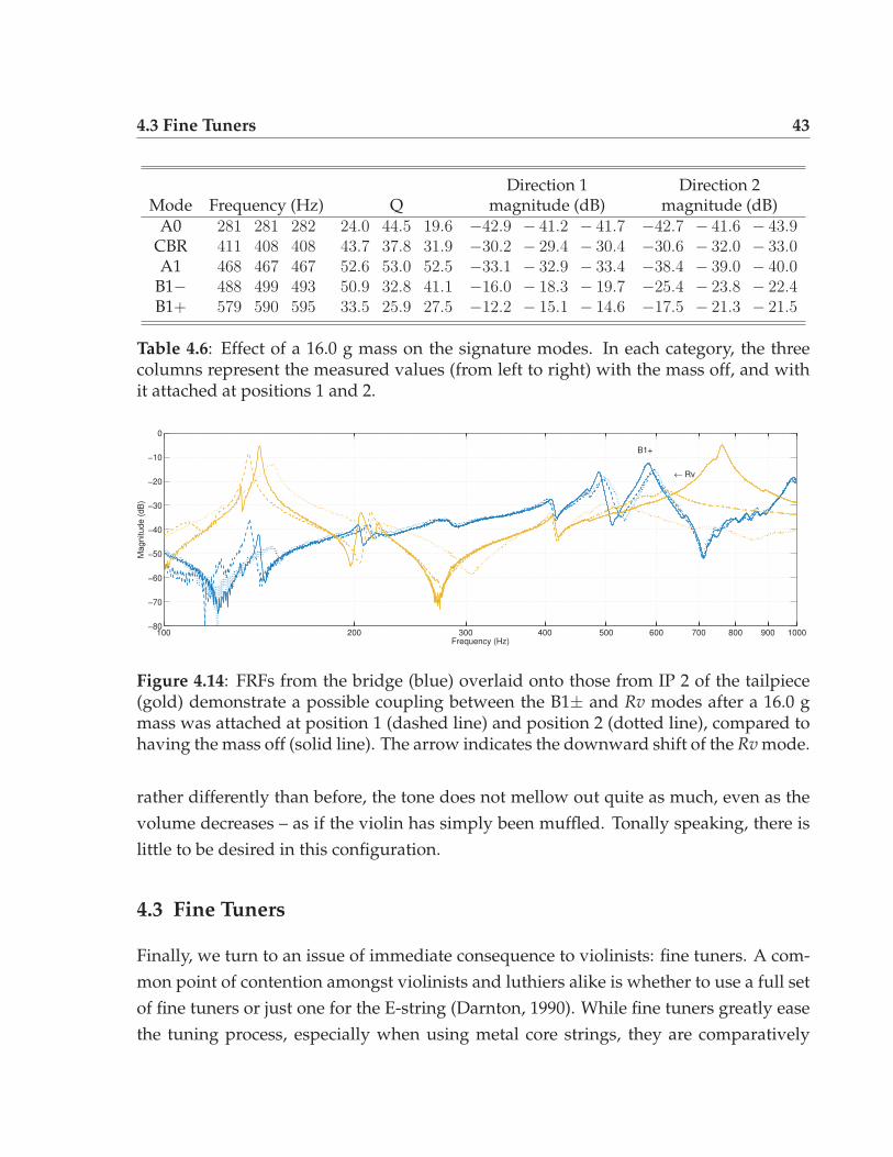
4.3 Fine Tuners 43
Direction 1 Direction 2Mode Frequency (Hz) Q magnitude (dB) magnitude (dB)
A0 281 281 282 24.0 44.5 19.6 −42.9 − 41.2 − 41.7 −42.7 − 41.6 − 43.9CBR 411 408 408 43.7 37.8 31.9 −30.2 − 29.4 − 30.4 −30.6 − 32.0 − 33.0A1 468 467 467 52.6 53.0 52.5 −33.1 − 32.9 − 33.4 −38.4 − 39.0 − 40.0
B1− 488 499 493 50.9 32.8 41.1 −16.0 − 18.3 − 19.7 −25.4 − 23.8 − 22.4B1+ 579 590 595 33.5 25.9 27.5 −12.2 − 15.1 − 14.6 −17.5 − 21.3 − 21.5
Table 4.6: Effect of a 16.0 g mass on the signature modes. In each category, the threecolumns represent the measured values (from left to right) with the mass off, and withit attached at positions 1 and 2.
100 200 300 400 500 600 700 800 900 1000−80
−70
−60
−50
−40
−30
−20
−10
0
Frequency (Hz)
Mag
nitu
de (
dB)
← Rv
B1+
Figure 4.14: FRFs from the bridge (blue) overlaid onto those from IP 2 of the tailpiece(gold) demonstrate a possible coupling between the B1± and Rv modes after a 16.0 gmass was attached at position 1 (dashed line) and position 2 (dotted line), compared tohaving the mass off (solid line). The arrow indicates the downward shift of the Rv mode.
rather differently than before, the tone does not mellow out quite as much, even as thevolume decreases – as if the violin has simply been muffled. Tonally speaking, there islittle to be desired in this configuration.
4.3 Fine Tuners
Finally, we turn to an issue of immediate consequence to violinists: fine tuners. A com-mon point of contention amongst violinists and luthiers alike is whether to use a full setof fine tuners or just one for the E-string (Darnton, 1990). While fine tuners greatly easethe tuning process, especially when using metal core strings, they are comparatively
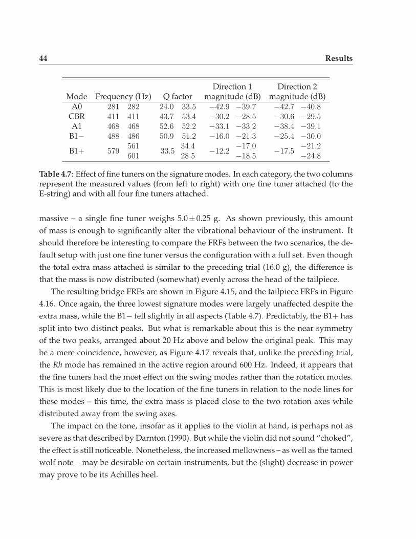
44 Results
Direction 1 Direction 2Mode Frequency (Hz) Q factor magnitude (dB) magnitude (dB)
A0 281 282 24.0 33.5 −42.9 −39.7 −42.7 −40.8CBR 411 411 43.7 53.4 −30.2 −28.5 −30.6 −29.5A1 468 468 52.6 52.2 −33.1 −33.2 −38.4 −39.1
B1− 488 486 50.9 51.2 −16.0 −21.3 −25.4 −30.0
B1+ 579561601
33.534.428.5
−12.2−17.0−18.5
−17.5−21.2−24.8
Table 4.7: Effect of fine tuners on the signature modes. In each category, the two columnsrepresent the measured values (from left to right) with one fine tuner attached (to theE-string) and with all four fine tuners attached.
massive – a single fine tuner weighs 5.0±0.25 g. As shown previously, this amountof mass is enough to significantly alter the vibrational behaviour of the instrument. Itshould therefore be interesting to compare the FRFs between the two scenarios, the de-fault setup with just one fine tuner versus the configuration with a full set. Even thoughthe total extra mass attached is similar to the preceding trial (16.0 g), the difference isthat the mass is now distributed (somewhat) evenly across the head of the tailpiece.
The resulting bridge FRFs are shown in Figure 4.15, and the tailpiece FRFs in Figure4.16. Once again, the three lowest signature modes were largely unaffected despite theextra mass, while the B1− fell slightly in all aspects (Table 4.7). Predictably, the B1+ hassplit into two distinct peaks. But what is remarkable about this is the near symmetryof the two peaks, arranged about 20 Hz above and below the original peak. This maybe a mere coincidence, however, as Figure 4.17 reveals that, unlike the preceding trial,the Rh mode has remained in the active region around 600 Hz. Indeed, it appears thatthe fine tuners had the most effect on the swing modes rather than the rotation modes.This is most likely due to the location of the fine tuners in relation to the node lines forthese modes – this time, the extra mass is placed close to the two rotation axes whiledistributed away from the swing axes.
The impact on the tone, insofar as it applies to the violin at hand, is perhaps not assevere as that described by Darnton (1990). But while the violin did not sound “choked”,the effect is still noticeable. Nonetheless, the increased mellowness – as well as the tamedwolf note – may be desirable on certain instruments, but the (slight) decrease in powermay prove to be its Achilles heel.
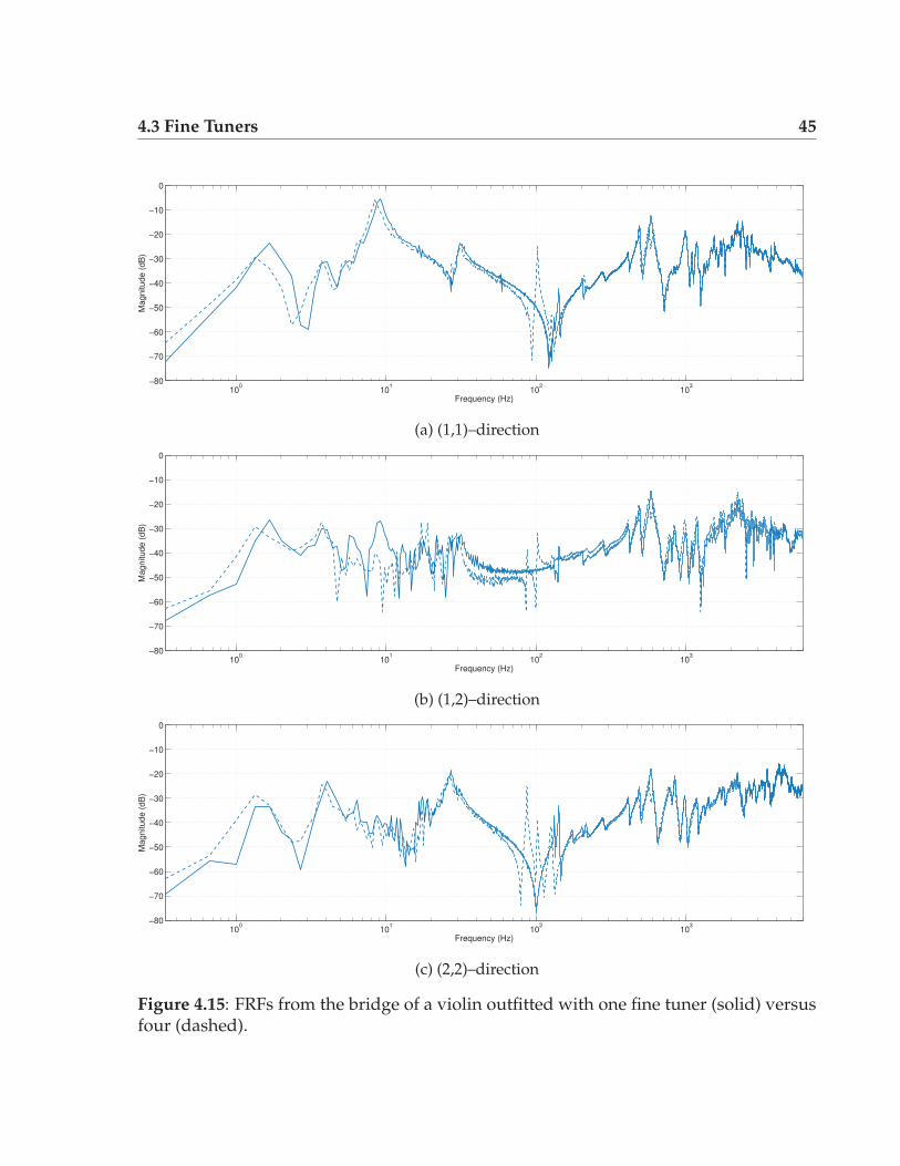
4.3 Fine Tuners 45
100
101
102
103
−80
−70
−60
−50
−40
−30
−20
−10
0
Frequency (Hz)
Mag
nitu
de (
dB)
(a) (1,1)–direction
100
101
102
103
−80
−70
−60
−50
−40
−30
−20
−10
0
Frequency (Hz)
Mag
nitu
de (
dB)
(b) (1,2)–direction
100
101
102
103
−80
−70
−60
−50
−40
−30
−20
−10
0
Frequency (Hz)
Mag
nitu
de (
dB)
(c) (2,2)–direction
Figure 4.15: FRFs from the bridge of a violin outfitted with one fine tuner (solid) versusfour (dashed).

46 Results
100
101
102
103
−80
−70
−60
−50
−40
−30
−20
−10
0
10
20
Frequency (Hz)
Mag
nitu
de (
dB)
(a) (1,1)–direction
100
101
102
103
−80
−70
−60
−50
−40
−30
−20
−10
0
10
20
Frequency (Hz)
Mag
nitu
de (
dB)
(b) (1,2)–direction
100
101
102
103
−80
−70
−60
−50
−40
−30
−20
−10
0
10
20
Frequency (Hz)
Mag
nitu
de (
dB)
(c) (2,2)–direction
Figure 4.16: FRFs from various points along the tailpiece outfitted with fine tuners. Thefour impact/measurement points are indicated by the colours blue (IP 1), red (IP 2), gold(IP 3), and purple (IP 4), while the number of fine tuners deployed is indicated by a solidline (one) and a dashed line (four – a full set).
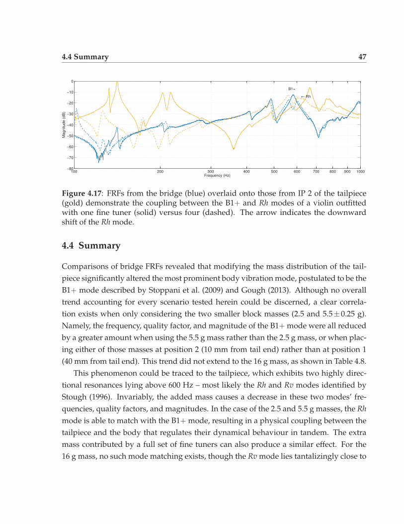
4.4 Summary 47
100 200 300 400 500 600 700 800 900 1000−80
−70
−60
−50
−40
−30
−20
−10
0
Frequency (Hz)
Mag
nitu
de (
dB)
B1+
← Rh
Figure 4.17: FRFs from the bridge (blue) overlaid onto those from IP 2 of the tailpiece(gold) demonstrate the coupling between the B1+ and Rh modes of a violin outfittedwith one fine tuner (solid) versus four (dashed). The arrow indicates the downwardshift of the Rh mode.
4.4 Summary
Comparisons of bridge FRFs revealed that modifying the mass distribution of the tail-piece significantly altered the most prominent body vibration mode, postulated to be theB1+ mode described by Stoppani et al. (2009) and Gough (2013). Although no overalltrend accounting for every scenario tested herein could be discerned, a clear correla-tion exists when only considering the two smaller block masses (2.5 and 5.5±0.25 g).Namely, the frequency, quality factor, and magnitude of the B1+ mode were all reducedby a greater amount when using the 5.5 g mass rather than the 2.5 g mass, or when plac-ing either of those masses at position 2 (10 mm from tail end) rather than at position 1(40 mm from tail end). This trend did not extend to the 16 g mass, as shown in Table 4.8.
This phenomenon could be traced to the tailpiece, which exhibits two highly direc-tional resonances lying above 600 Hz – most likely the Rh and Rv modes identified byStough (1996). Invariably, the added mass causes a decrease in these two modes’ fre-quencies, quality factors, and magnitudes. In the case of the 2.5 and 5.5 g masses, the Rhmode is able to match with the B1+ mode, resulting in a physical coupling between thetailpiece and the body that regulates their dynamical behaviour in tandem. The extramass contributed by a full set of fine tuners can also produce a similar effect. For the16 g mass, no such mode matching exists, though the Rv mode lies tantalizingly close to
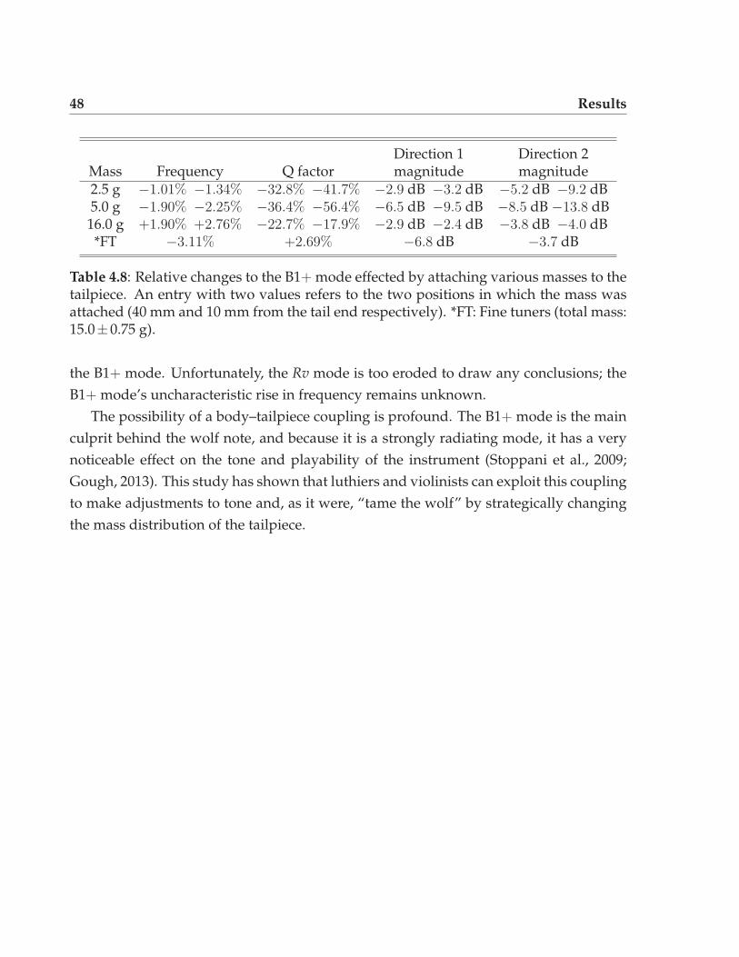
48 Results
Direction 1 Direction 2Mass Frequency Q factor magnitude magnitude2.5 g −1.01% −1.34% −32.8% −41.7% −2.9 dB −3.2 dB −5.2 dB −9.2 dB5.0 g −1.90% −2.25% −36.4% −56.4% −6.5 dB −9.5 dB −8.5 dB −13.8 dB
16.0 g +1.90% +2.76% −22.7% −17.9% −2.9 dB −2.4 dB −3.8 dB −4.0 dB*FT −3.11% +2.69% −6.8 dB −3.7 dB
Table 4.8: Relative changes to the B1+ mode effected by attaching various masses to thetailpiece. An entry with two values refers to the two positions in which the mass wasattached (40 mm and 10 mm from the tail end respectively). *FT: Fine tuners (total mass:15.0±0.75 g).
the B1+ mode. Unfortunately, the Rv mode is too eroded to draw any conclusions; theB1+ mode’s uncharacteristic rise in frequency remains unknown.
The possibility of a body–tailpiece coupling is profound. The B1+ mode is the mainculprit behind the wolf note, and because it is a strongly radiating mode, it has a verynoticeable effect on the tone and playability of the instrument (Stoppani et al., 2009;Gough, 2013). This study has shown that luthiers and violinists can exploit this couplingto make adjustments to tone and, as it were, “tame the wolf” by strategically changingthe mass distribution of the tailpiece.
49
Chapter 5
Conclusions and Future Work
5.1 Conclusions
All things considered, the tailpiece appears to be a non-negligible part of the violin. In-deed, its mass distribution is a significant parameter regulating the dynamic behaviour– and hence, the tone – of the violin.
This study aims to provide a systematic account of this process and search for mu-sically desirable configurations. To alter its moment of inertia, a series of small masses(2.5, 5.5, and 16.0±0.25 g) were placed at two positions on the tailpiece (40 and 10 mmfrom the tail end) in succession. For each setup, two-dimensional admittance measure-ments at the bridge and four points along the tailpiece were acquired using a miniatureimpact hammer and laser Doppler vibrometer. Comparison of their FRFs revealed thatthe most prominent body vibration mode could be coupled with a tailpiece resonanceusing the two lighter masses, resulting in a lowering of its frequency, quality factor, andmagnitude correlating to the weight and position of the mass. For the violinist, informalplaying tests showed that this translates to a reduction of the dreaded wolf note, butalso a decrease in the perceived brightness and power (loudness) of the instrument.
The experimental procedure was also repeated with the extra mass contributed by afull set of fine tuners instead of a single block mass. After extra fine tuners (5.0±0.25 geach) were attached to the G-, D-, and A-string sockets, admittance measurements pro-duced FRFs similar to the results of the 2.5 and 5.5 g masses – in spite of the fact that thetotal mass of the extra fine tuners (15 g) is on the order of the heaviest mass used in theprevious trials (16 g).
50 Conclusions and Future Work
The current work indicates that the tailpiece can be used by luthiers and violinists asan additional parameter for tone adjustment. By strategically changing its mass distri-bution (e.g., by attaching small masses), the tailpiece can couple with and shift the mostprominent body mode, granting it the ability to change the tone colour of the instrumentand to mitigate the wolf note.
5.2 Future Work
Nonetheless, it would be beneficial to determine how these results apply to differentviolins, which may have different setups, and to the other instruments of the violin fam-ily. During these tests, more information could be gathered about the whole tailpiecesystem, from bridge to tailgut. Past research has indicated that the tailgut length plays asignificant role in the tailpiece’s rotational modes (e.g., Stough, 1996; Fouilhé and Hous-say, 2013). Unfortunately, this study was unable to address this important parameterdue to physical constraints: The modern tailpiece anchors the tailgut to its reverse side,rendering it inaccessible without detaching all the strings and hence, altering the phys-ical state of the violin. This prevents us from manipulating the mass distribution (moreprecisely, the rotation axes) without altering the total mass of the tailpiece, or from iso-lating the effects of either parameter on the vibrating modes. That said, violinists areusually unable to access the tailgut for the same reason, making mass-loading the onlypractical approach to exploiting the body–tailpiece coupling.
Even so, modal analysis may shed further light on the dynamic behaviour of thiscoupling. Presently, all characterizations of the vibrational modes are tentatively basedon admittance measurements. Even though they can be good indicators of the acousticperformance of the instrument, multidimensional modal analysis – perhaps aided bynumerical modeling – would provide a more definitive understanding of the body–tailpiece interactions and resolve the lingering questions from this study.

51
References
Ågren, C.-H., and K. A. Stetson. 1969. Measuring the wood resonances of treble violplates by hologram interferometry. Journal of the Acoustical Society of America 46: 120.
Askenfelt, A. 2010. Double bass. In T. D. Rossing (Ed.), The Science of String Instruments,Chapter 15, 259–77. New York: Springer.
Backhaus, H. 1930. Über die Schwingungsformen von Geigenkörpern. Zeitschrift fürPhysik 62 (3–4): 143–66.
Bank, B., and M. Karjalainen. 2010. Passive admittance matrix modeling for guitar syn-thesis. In Proceedings of the 13th International Conference on Digital Audio Effects (DAFx–10), Graz, Austria, 1–7.
Beldie, I. P. 2003. About the bridge hill mystery. Catgut Acoustical Society Journal 4 (8):9–13.
Bissinger, G. 2008. Structural acoustics of good and bad violins. Journal of the AcousticalSociety of America 124 (3): 1764–73.
Boutillon, X., G. Weinreich, and N. R. Michael. 1988. Experimental developments for themeasurement of violin bridge admittance. Journal of the Acoustical Society of America 84:S179.
Bynum, E., and T. D. Rossing. 2010. Cello. In T. D. Rossing (Ed.), The Science of StringInstruments, Chapter 14, 245–57. New York: Springer.
Cremer, L. 1981. Physik der Geige. Stuttgart: S. Hirzel Verlag. Translated by John S. Allenas The Physics of the Violin. (Cambridge, MA: MIT Press, 1984).
52 References
Curtin, J., and T. D. Rossing. 2010. Violin. In T. D. Rossing (Ed.), The Science of StringInstruments, Chapter 13, 209–44. New York: Springer.
Darnton, M. 1990. Violin Setups. In T. Olsen (Ed.), The Big Red Book of American Lutherie,Volume 3, 352–67. Guild of American Luthiers.
Eggers, F. 1959. Untersuchung von Corpus-schwingungen am Violoncello. Acustica 9(6): 463–5.
Fouilhé, E., G. Goli, A. Houssay, and G. Stoppani. 2011. Vibration modes of the cellotailpiece. Archives of Acoustics 36 (4): 713–26.
Fouilhé, E., and A. Houssay. 2013. String “after-length” and the cello tailpiece: Acous-tics and perception. In Proceedings of the Stockholm Music Acoustics Conference, RoyalSwedish Academy of Music, Stockholm, 60–5.
Fritz, C., I. Cross, B. C. J. Moore, and J. Woodhouse. 2007. Perceptual thresholds fordetecting modifications applied to the acoustical properties of a violin. Journal of theAcoustical Society of America 122: 3640–50.
Fritz, C., J. Woodhouse, F. P.-H. Cheng, I. Cross, A. F. Blackwell, and B. C. J. Moore. 2010.Perceptual studies of violin body damping and vibrato. Journal of the Acoustical Societyof America 127: 513–24.
Gough, C. 2000. Science and the Stradivarius. Physics World 13: 27–33.
Gough, C. 2007. Musical acoustics. In T. D. Rossing (Ed.), Springer Handbook of Acoustics,Chapter 15, 533–667. New York: Springer.
Gough, C. 2013. Vibrational modes of the violin family. In Proceedings of the StockholmMusic Acoustics Conference, Royal Swedish Academy of Music, Stockholm, 66–74.
Grant, M., and S. Boyd. 2008. Graph implementations for nonsmooth convex programs.In V. Blondel, S. Boyd, and H. Kimura (Eds.), Recent Advances in Learning and Control,Lecture Notes in Control and Information Sciences, 95–110. Springer-Verlag Limited.http://stanford.edu/~boyd/graph_dcp.html.
Grant, M., and S. Boyd. 2014. CVX: Matlab software for disciplined convex program-ming, version 2.1. http://cvxr.com/cvx. Accessed: 2015–07–20.

References 53
Gren, P., K. Tatar, J. Granström, N.-E. Molin, and E. V. Jansson. 2006. Laser vibrometrymeasurements of vibration and sound fields of a bowed violin. Measurement Scienceand Technology 17 (4): 635–44.
Guettler, K. 2010. Bows, strings, and bowing. In T. D. Rossing (Ed.), The Science of StringInstruments, Chapter 15, 279–99. New York: Springer.
Helmholtz, H. v. 1863. Die Lehre von Tonemfindungen. Braunschweg: Friedrich Vieweg.Translated by Alexander Ellis as On the Sensations of Tone. (New York: Dover Publica-tions, Inc., 1954).
Houssay, A. 2014. The string “after-length” of the cello tailpiece: History, acousticsand performance techniques. In Proceedings of the International Symposium on MusicalAcoustics, Le Mans, France, 207–13.
Hutchins, C. M. 1981. The acoustics of violin plates. Scientific American 245 (4): 170–86.
Hutchins, C. M. 1983. A history of violin research. Journal of the Acoustical Society ofAmerica 73 (5): 1421–40.
Hutchins, C. M. 1993. The effect of relating the tailpiece frequency to that of other violinmodes. Catgut Acoustical Society Journal 2 (3): 5–8.
Jansson, E. V. 1973. Investigation of a violin by laser speckle interferometry and acous-tical measurements. Acustica 29 (1): 21–8.
Jansson, E. V. 1997. Admittance measurements of 25 high quality violins. Acustica 83:337–41.
Jansson, E. V., I. Bork, and J. Meyer. 1986. Investigations into the acoustical properties ofthe violin. Acustica 62: 1–15.
Jansson, E. V., N.-E. Molin, and H. Sundin. 1970. Resonances of a violin studied byhologram interferometry and acoustical methods. Physica Scripta 2: 243–56.
Jansson, E. V., and B. K. Niewczyk. 1997. Admittance measurements of violins with higharching. Acustica 83: 571–4.
54 References
Jansson, E. V., and B. K. Niewczyk. 1999. On the acoustics of the violin: Bridge hill orbody hill? Catgut Acoustical Society Journal 3 (7): 23–7.
Johannsson, H. 2015. Hans Johannsson Violins: Making. http://hansjohannsson.com/page25/page18/making.html. Accessed: 2015–08–01.
Lambourg, C., and A. Chaigne. 1993. Measurements and modeling of the admittancematrix at the bridge in guitars. In Proceedings of the Stockholm Music Acoustics Confer-ence, Royal Swedish Academy of Music, Stockholm, 448–53.
Langhoff, A. 1994. Measurement of acoustic violin spectra and their interpretation usinga 3d representation. Acustica 80: 505–15.
Maestre, E., G. P. Scavone, and J. O. Smith. 2013. Digital modeling of bridge driving-point admittances from measurements on violin-family instruments. In Proceedingsof the Stockholm Music Acoustics Conference, Royal Swedish Academy of Music, Stock-holm, 101–8.
McIntyre, M. E., and J. Woodhouse. 1978. The acoustics of stringed musical instruments.Interdisciplinary Science Reviews 3 (2): 157–73.
Meyer, J. 1972. Directivity of the bowed strings instruments and its effect on orchestralsound in concert halls. Journal of the Acoustical Society of America 51 (6): 1994–2009.
Nia, H. T., A. D. Jain, Y. Liu, M.-R. Alam, R. Barnas, and N. C. Makris. 2015. The evolu-tion of air resonance power efficiency in the violin and its ancestors. Proceedings of theRoyal Society of London A 471 (2175): 20140905.
Nolan, C. 2002. Music theory and mathematics. In T. Christensen (Ed.), The CambridgeHistory of Western Music History, Chapter 10, 272–304. Cambridge, UK: CambridgeUniversity Press.
Pirquet, O. 2011. Violin tailpiece dynamics: Design and function. Undergraduate thesis,University of Victoria, Victoria, Canada.
Reinicke, W., and L. Cremer. 1970. Application of holographic interferometry to vibra-tions of the bodies of string instruments. Journal of the Acoustical Society of America 47:131.
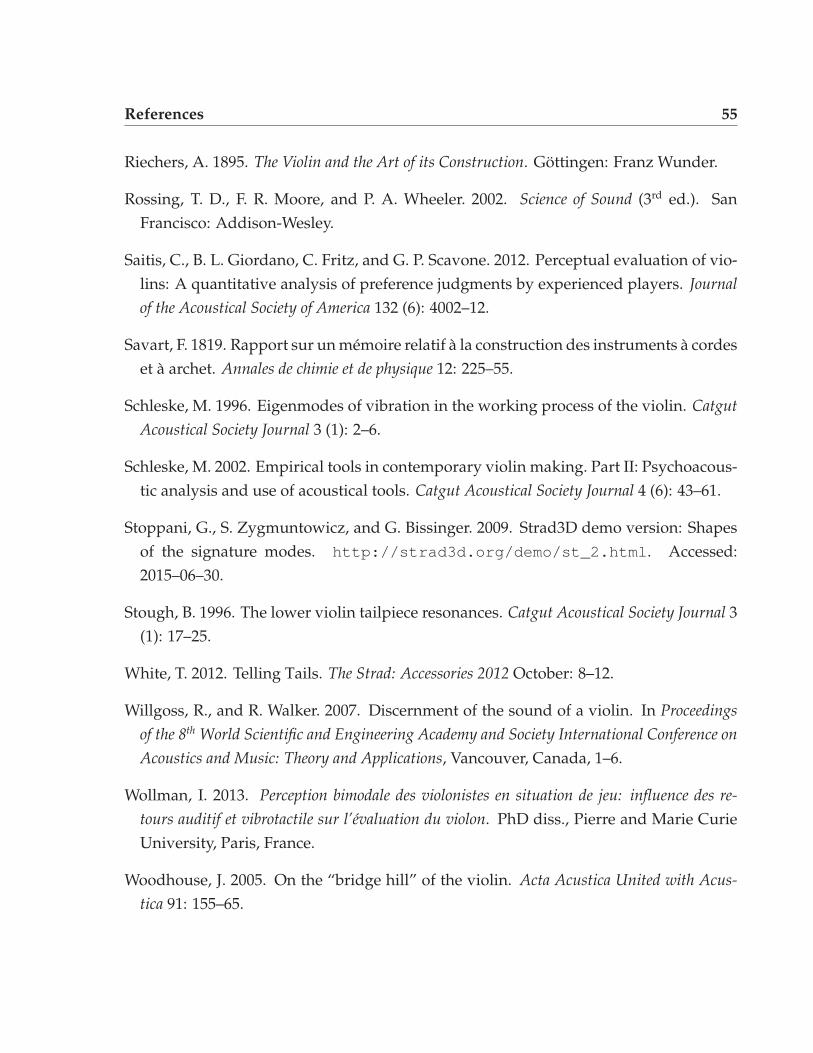
References 55
Riechers, A. 1895. The Violin and the Art of its Construction. Göttingen: Franz Wunder.
Rossing, T. D., F. R. Moore, and P. A. Wheeler. 2002. Science of Sound (3rd ed.). SanFrancisco: Addison-Wesley.
Saitis, C., B. L. Giordano, C. Fritz, and G. P. Scavone. 2012. Perceptual evaluation of vio-lins: A quantitative analysis of preference judgments by experienced players. Journalof the Acoustical Society of America 132 (6): 4002–12.
Savart, F. 1819. Rapport sur un mémoire relatif à la construction des instruments à cordeset à archet. Annales de chimie et de physique 12: 225–55.
Schleske, M. 1996. Eigenmodes of vibration in the working process of the violin. CatgutAcoustical Society Journal 3 (1): 2–6.
Schleske, M. 2002. Empirical tools in contemporary violin making. Part II: Psychoacous-tic analysis and use of acoustical tools. Catgut Acoustical Society Journal 4 (6): 43–61.
Stoppani, G., S. Zygmuntowicz, and G. Bissinger. 2009. Strad3D demo version: Shapesof the signature modes. http://strad3d.org/demo/st_2.html. Accessed:2015–06–30.
Stough, B. 1996. The lower violin tailpiece resonances. Catgut Acoustical Society Journal 3(1): 17–25.
White, T. 2012. Telling Tails. The Strad: Accessories 2012 October: 8–12.
Willgoss, R., and R. Walker. 2007. Discernment of the sound of a violin. In Proceedingsof the 8th World Scientific and Engineering Academy and Society International Conference onAcoustics and Music: Theory and Applications, Vancouver, Canada, 1–6.
Wollman, I. 2013. Perception bimodale des violonistes en situation de jeu: influence des re-tours auditif et vibrotactile sur l’évaluation du violon. PhD diss., Pierre and Marie CurieUniversity, Paris, France.
Woodhouse, J. 2005. On the “bridge hill” of the violin. Acta Acustica United with Acus-tica 91: 155–65.
56 References
Woodhouse, J. 2014. The acoustics of the violin: A review. Reports on Progress inPhysics 77 (11): 115901.
Woodhouse, J., and P. E. Courtney. 2003. The admittance matrix of a cello. In Proceed-ings of the Stockholm Music Acoustics Conference, Royal Swedish Academy of Music,Stockholm, 107–10.
Woodhouse, J., and R. S. Langley. 2012. Interpreting the input admittance of violins andguitars. Acta Acustica United with Acustica 98: 611–28.
Zhang, A., and J. Woodhouse. 2014. Reliability of the input admittance of bowed-stringinstruments measured by the hammer method. Journal of the Acoustical Society of Amer-ica 136 (6): 3371–81.
Zygmuntowicz, S., G. Bissinger, and G. Stoppani. 2009. Strad3D demo version. http://strad3d.org/demo/. Accessed: 2015–06–30.