Institutionen för medicin och vård Avdelningen för radiofysik

Hälsouniversitetet

Resolution, unsharpness and MTF

Bengt Nielsen

Department of Medicine and Care Radio Physics

Faculty of Health Sciences

Series: Report / Institutionen för radiologi, Universitetet i Linköping; 39 ISSN: 0348-7679 ISRN: LIU-RAD-R-039 Publishing year: 1980 © The Author(s)

ISSN 0348-7679

Resolution, unsharpness and MTF

Bengt Nielsen

Department of Radiation PhysicsFaculty of Health SciencesLinköping universitySWEDEN

REPORTLiU-RAD-R-039

1

TABLE OF CONTENTS

I. Resolution and unsharpness .......3

II. Fundamental concepts to describe the performance of an imaging system .......9

III. Modulation transfer function, MTF ......15

IV.References ......20

2

Resolution, unsharpness and MTF

I. RESOLUTION AND UNSHARPNESS

Definitions

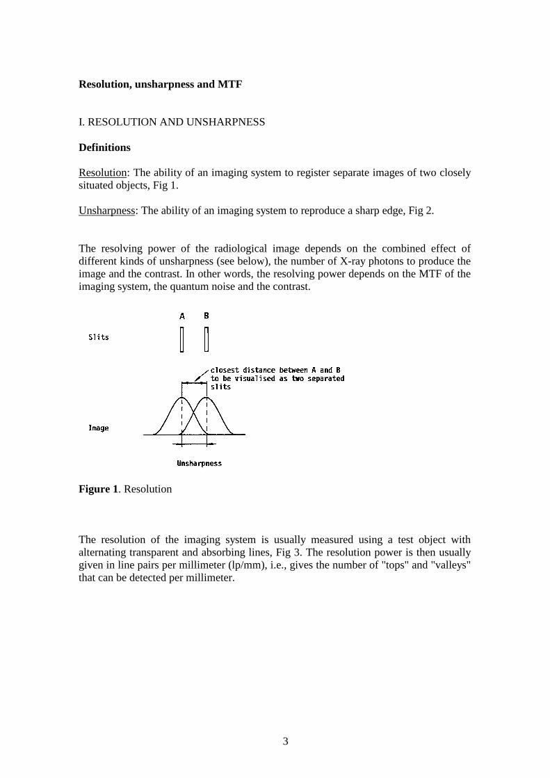
Resolution: The ability of an imaging system to register separate images of two closelysituated objects, Fig 1.

Unsharpness: The ability of an imaging system to reproduce a sharp edge, Fig 2.

The resolving power of the radiological image depends on the combined effect ofdifferent kinds of unsharpness (see below), the number of X-ray photons to produce theimage and the contrast. In other words, the resolving power depends on the MTF of theimaging system, the quantum noise and the contrast.

Figure 1. Resolution

The resolution of the imaging system is usually measured using a test object withalternating transparent and absorbing lines, Fig 3. The resolution power is then usuallygiven in line pairs per millimeter (lp/mm), i.e., gives the number of "tops" and "valleys"that can be detected per millimeter.

3

Figure 2. Unsharpness

Figure 3. Line test pattern for determining the resolution of the imaging system

Sources of unsharpness

The total unsharpness can be didvided into contributionas from different sources.

a. Focal spotb. Movementc. Receptor

a. Focal spot

The unsharpness caused by the focus is due to the finite size of the focal spot.

Because of the focal spot size, an edge in the object is reproduced by a density gradientUF, i.e., a region where the optical density gradually decreases from maximum tominimum, Fig 4.

4

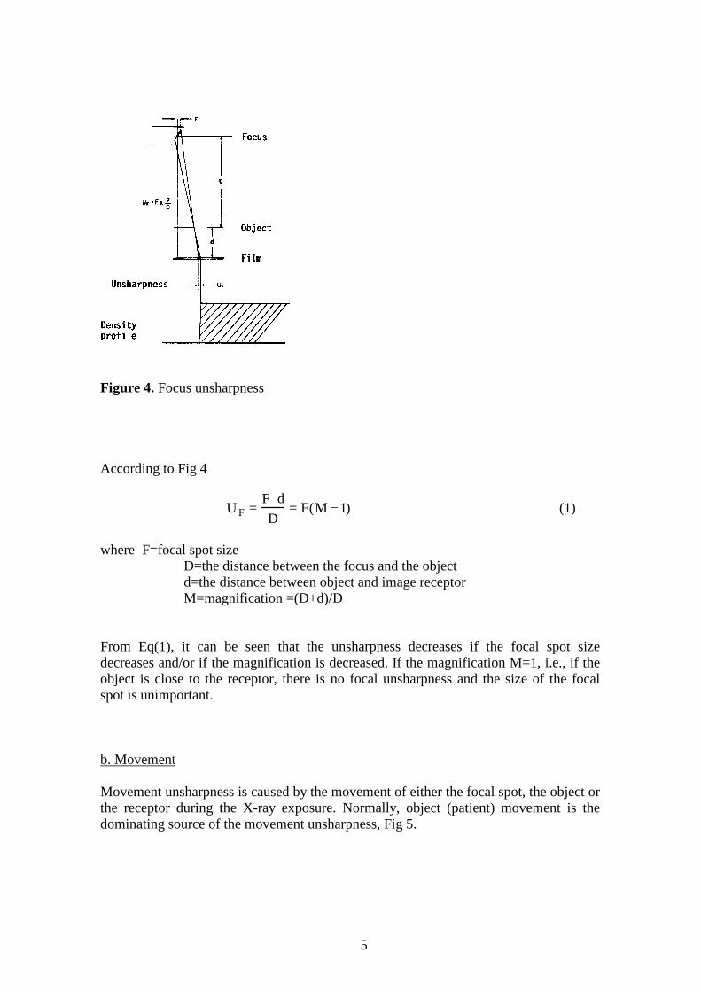
Figure 4. Focus unsharpness

According to Fig 4

U F = F⋅dD

= F(M − 1) (1)

where F=focal spot sizeD=the distance between the focus and the objectd=the distance between object and image receptorM=magnification =(D+d)/D

From Eq(1), it can be seen that the unsharpness decreases if the focal spot sizedecreases and/or if the magnification is decreased. If the magnification M=1, i.e., if theobject is close to the receptor, there is no focal unsharpness and the size of the focalspot is unimportant.

b. Movement

Movement unsharpness is caused by the movement of either the focal spot, the object orthe receptor during the X-ray exposure. Normally, object (patient) movement is thedominating source of the movement unsharpness, Fig 5.

5

Figure 5. Unsharpness due to moving object

According to Fig 5, the width of the density gradient U m0 caused by the moving object

can be derived from

U m0= ∆m 0

⋅D + dD

= ∆m0⋅M = M ⋅v ⋅t (2)

where ∆ m0 = the distance the object has moved m[ ]

D = the distance between the focus and the receptor m[ ]d = the distance between the object and the receptor m[ ]M = the magnification = (D+d)/Dv= the velocity of the movement m / s[ ]t = time of exposure s[]

From Eq(2), it can be seen that movement unsharpness can be reduced by decreasingexposure time (t) and magnification (M).

c. Receptor unsharpness

To illustrate receptor unsharpness, a conventional screen-film combination is chosen.The dominating cause of unsharpness is in this case the diffusion of light in the screen,Fig 6.

6

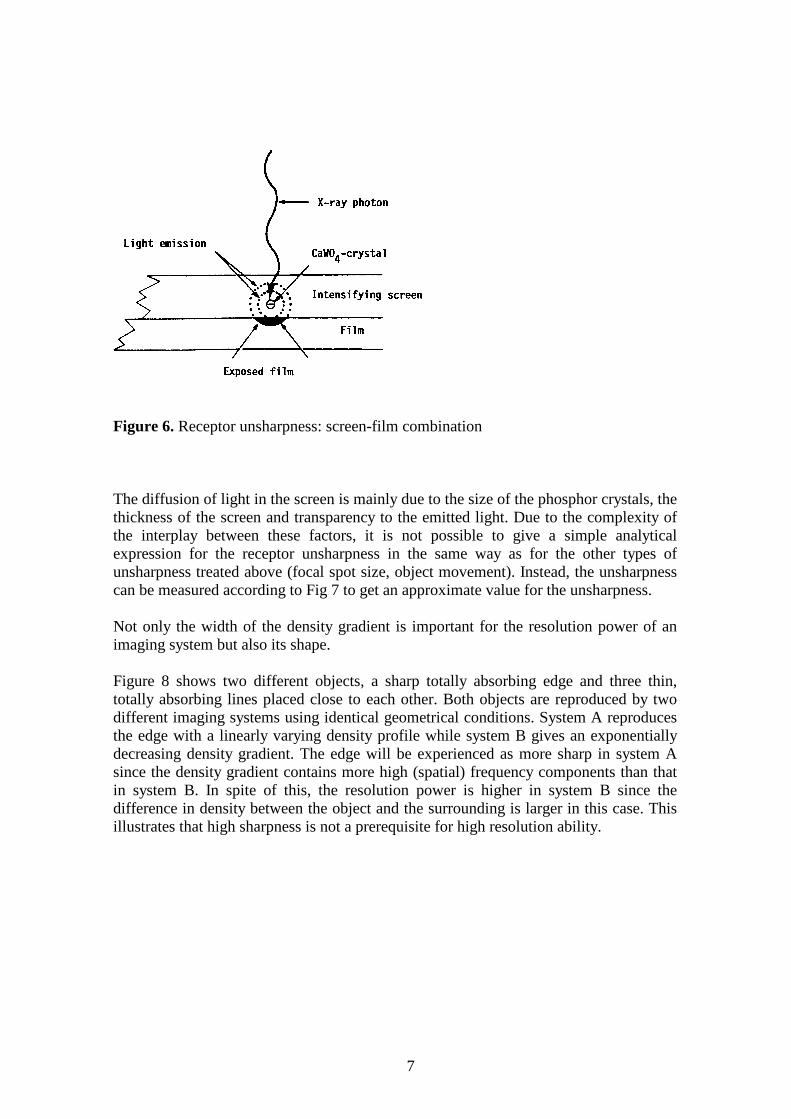
Figure 6. Receptor unsharpness: screen-film combination

The diffusion of light in the screen is mainly due to the size of the phosphor crystals, thethickness of the screen and transparency to the emitted light. Due to the complexity ofthe interplay between these factors, it is not possible to give a simple analyticalexpression for the receptor unsharpness in the same way as for the other types ofunsharpness treated above (focal spot size, object movement). Instead, the unsharpnesscan be measured according to Fig 7 to get an approximate value for the unsharpness.

Not only the width of the density gradient is important for the resolution power of animaging system but also its shape.

Figure 8 shows two different objects, a sharp totally absorbing edge and three thin,totally absorbing lines placed close to each other. Both objects are reproduced by twodifferent imaging systems using identical geometrical conditions. System A reproducesthe edge with a linearly varying density profile while system B gives an exponentiallydecreasing density gradient. The edge will be experienced as more sharp in system Asince the density gradient contains more high (spatial) frequency components than thatin system B. In spite of this, the resolution power is higher in system B since thedifference in density between the object and the surrounding is larger in this case. Thisillustrates that high sharpness is not a prerequisite for high resolution ability.

7

Figure 7. Determination of receptor unsharpness

Figure 8. Resolving power and unsharpness for two shapes of the density gradientA serious limitation of the concept of unsharpness is that the total unsharpness of thesystem cannot easily be deduced from knowledge of its components. This is due to, asillustrated in Fig 8, that besides the width of the density gradient (the unsharpness), theshape of the gradient is important. Also, comparing unsharpness of different imagingsystems does not give a complete description of the imaging properties of the systems.A more fundamental approach to describing the imaging abilities of different systems isneeded.

Attenuation unsharpness. In connection with unsharpness, attenaution unsharpness issometimes mentioned. Attenuation unsharpness is present in an image, even if the othertypes of unsharpness are not. Attenuation unsharpness depends on the shape of theobject and is due to the gradual transition of the attenuation of the X-rays at the edge ofan object. The longer the relative path of tangential rays through the object, the smalleris the attenuation unsharpness.

8

Figure 9. Attenuation unsharpness

II. FUNDAMENTAL CONCEPTS TO DESCRIBE THE PERFORMANCE OF ANIMAGING SYSTEM

Point spread function PSF

The image quality depends fundamentally on the ability of the imaging system toreproduce each single point in the object.

Consider the following simple experiment: a lead plate with a very small hole is imagedin contact with a screen-film combination, Fig 10. The image (output signal) is anunsharp point.

In the following analysis, we consider linear imaging systems for which the point spreadfunction is independent of the size of the input signal. The screen-film system illustratedin Fig 10 is non-linear since the optical density does not increase linearly with theabsorbed energy in the screen. However, the system can be "linearised" by translatingthe density units into energy units by means of the characteristic (H&D) curve.

Figure 10. Determination of the point spread function for a screen-film combination

9

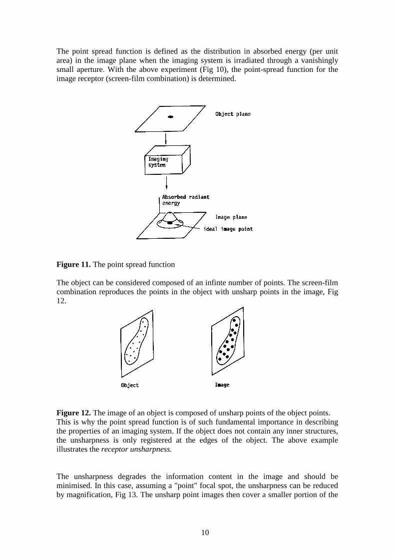
The point spread function is defined as the distribution in absorbed energy (per unitarea) in the image plane when the imaging system is irradiated through a vanishinglysmall aperture. With the above experiment (Fig 10), the point-spread function for theimage receptor (screen-film combination) is determined.

Figure 11. The point spread function

The object can be considered composed of an infinte number of points. The screen-filmcombination reproduces the points in the object with unsharp points in the image, Fig12.

Figure 12. The image of an object is composed of unsharp points of the object points.This is why the point spread function is of such fundamental importance in describingthe properties of an imaging system. If the object does not contain any inner structures,the unsharpness is only registered at the edges of the object. The above exampleillustrates the receptor unsharpness.

The unsharpness degrades the information content in the image and should beminimised. In this case, assuming a "point" focal spot, the unsharpness can be reducedby magnification, Fig 13. The unsharp point images then cover a smaller portion of the

10

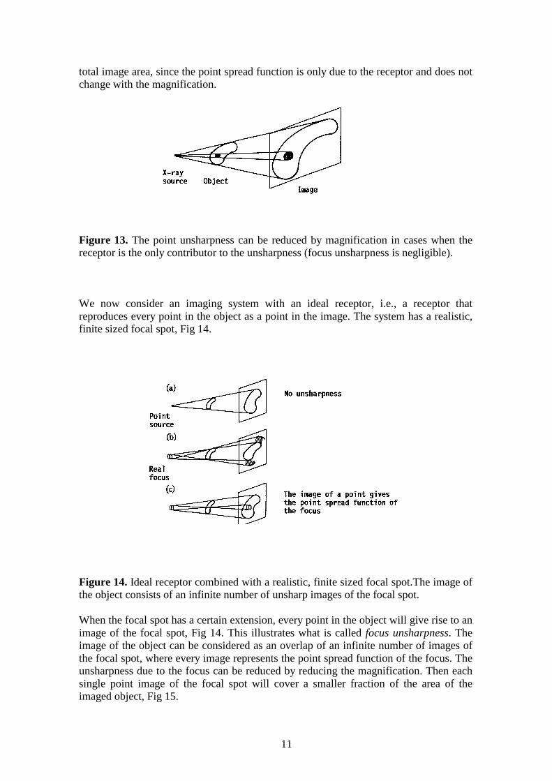
total image area, since the point spread function is only due to the receptor and does notchange with the magnification.

Figure 13. The point unsharpness can be reduced by magnification in cases when thereceptor is the only contributor to the unsharpness (focus unsharpness is negligible).

We now consider an imaging system with an ideal receptor, i.e., a receptor thatreproduces every point in the object as a point in the image. The system has a realistic,finite sized focal spot, Fig 14.

Figure 14. Ideal receptor combined with a realistic, finite sized focal spot.The image ofthe object consists of an infinite number of unsharp images of the focal spot.

When the focal spot has a certain extension, every point in the object will give rise to animage of the focal spot, Fig 14. This illustrates what is called focus unsharpness. Theimage of the object can be considered as an overlap of an infinite number of images ofthe focal spot, where every image represents the point spread function of the focus. Theunsharpness due to the focus can be reduced by reducing the magnification. Then eachsingle point image of the focal spot will cover a smaller fraction of the area of theimaged object, Fig 15.

11

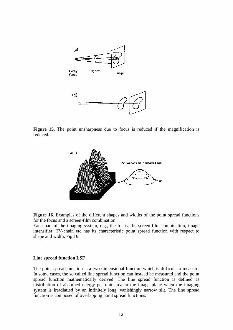
Figure 15. The point unsharpness due to focus is reduced if the magnification isreduced.

Figure 16. Examples of the different shapes and widths of the point spread functionsfor the focus and a screen-film combination.Each part of the imaging system, e.g., the focus, the screen-film combination, imageintensifier, TV-chain etc has its characteristic point spread function with respect toshape and width, Fig 16.

Line spread function LSF

The point spread function is a two dimensional function which is difficult to measure.In some cases, the so called line spread function can instead be measured and the pointspread function mathematically derived. The line spread function is defined asdistribution of absorbed energy per unit area in the image plane when the imagingsystem is irradiatied by an infinitely long, vanishingly narrow slit. The line spreadfunction is composed of overlapping point spread functions.

12

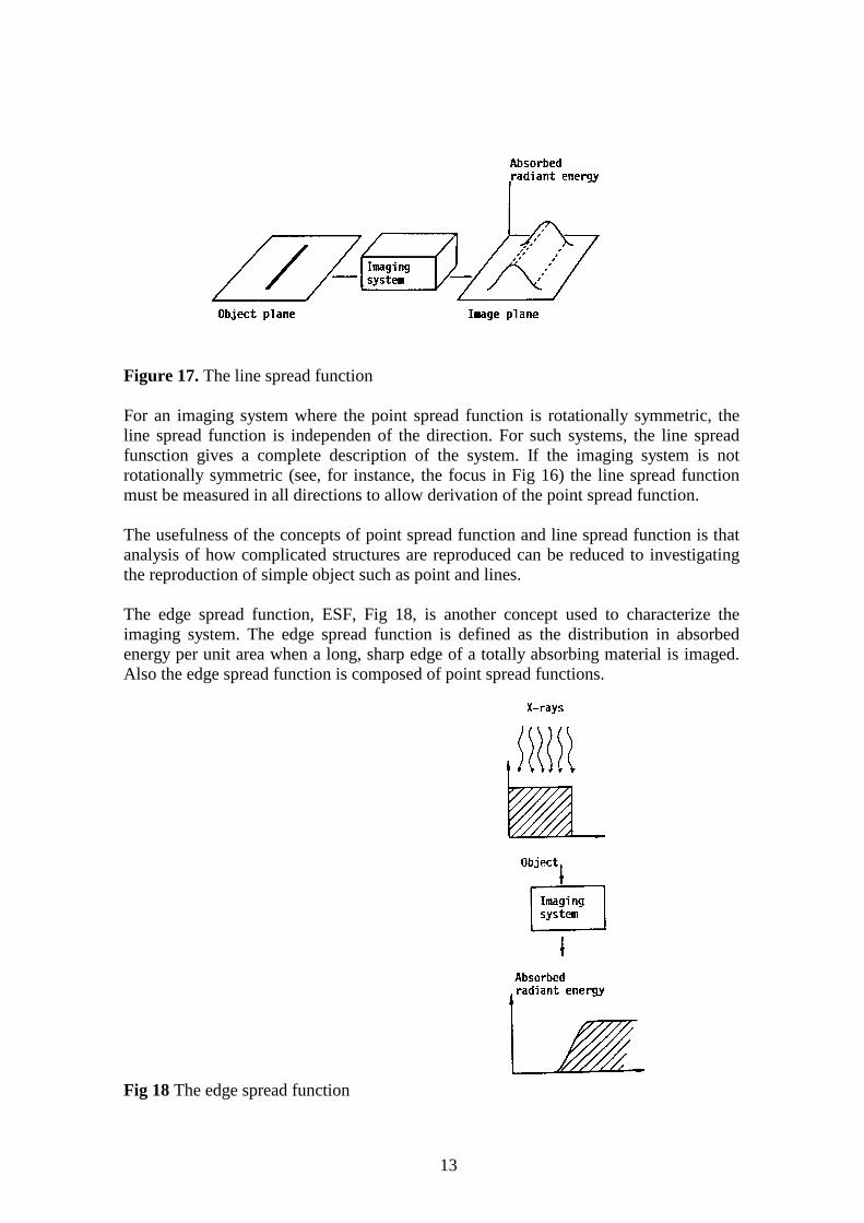
Figure 17. The line spread function

For an imaging system where the point spread function is rotationally symmetric, theline spread function is independen of the direction. For such systems, the line spreadfunsction gives a complete description of the system. If the imaging system is notrotationally symmetric (see, for instance, the focus in Fig 16) the line spread functionmust be measured in all directions to allow derivation of the point spread function.

The usefulness of the concepts of point spread function and line spread function is thatanalysis of how complicated structures are reproduced can be reduced to investigatingthe reproduction of simple object such as point and lines.

The edge spread function, ESF, Fig 18, is another concept used to characterize theimaging system. The edge spread function is defined as the distribution in absorbedenergy per unit area when a long, sharp edge of a totally absorbing material is imaged.Also the edge spread function is composed of point spread functions.

Fig 18 The edge spread function

13

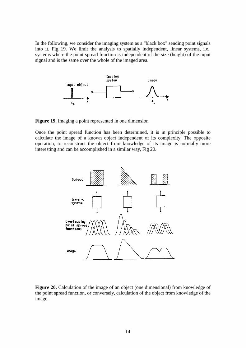
In the following, we consider the imaging system as a "black box" sending point signalsinto it, Fig 19. We limit the analysis to spatially independent, linear systems, i.e.,systems where the point spread function is independent of the size (height) of the inputsignal and is the same over the whole of the imaged area.

Figure 19. Imaging a point represented in one dimension

Once the point spread function has been determined, it is in principle possible tocalculate the image of a known object independent of its complexity. The oppositeoperation, to reconstruct the object from knowledge of its image is normally moreinteresting and can be accomplished in a similar way, Fig 20.

Figure 20. Calculation of the image of an object (one dimensional) from knowledge ofthe point spread function, or conversely, calculation of the object from knowledge of theimage.

14

III. MODULATION TRANSFER FUNCTION, MTF

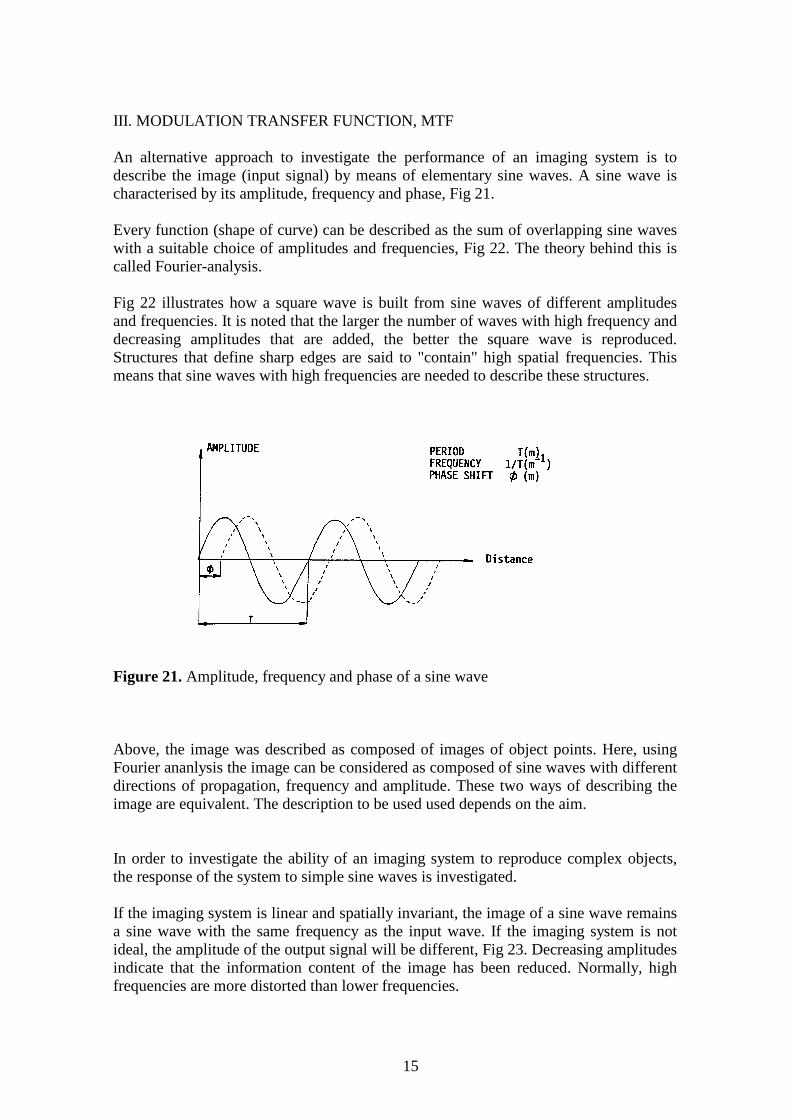
An alternative approach to investigate the performance of an imaging system is todescribe the image (input signal) by means of elementary sine waves. A sine wave ischaracterised by its amplitude, frequency and phase, Fig 21.

Every function (shape of curve) can be described as the sum of overlapping sine waveswith a suitable choice of amplitudes and frequencies, Fig 22. The theory behind this iscalled Fourier-analysis.

Fig 22 illustrates how a square wave is built from sine waves of different amplitudesand frequencies. It is noted that the larger the number of waves with high frequency anddecreasing amplitudes that are added, the better the square wave is reproduced.Structures that define sharp edges are said to "contain" high spatial frequencies. Thismeans that sine waves with high frequencies are needed to describe these structures.

Figure 21. Amplitude, frequency and phase of a sine wave

Above, the image was described as composed of images of object points. Here, usingFourier ananlysis the image can be considered as composed of sine waves with differentdirections of propagation, frequency and amplitude. These two ways of describing theimage are equivalent. The description to be used used depends on the aim.

In order to investigate the ability of an imaging system to reproduce complex objects,the response of the system to simple sine waves is investigated.

If the imaging system is linear and spatially invariant, the image of a sine wave remainsa sine wave with the same frequency as the input wave. If the imaging system is notideal, the amplitude of the output signal will be different, Fig 23. Decreasing amplitudesindicate that the information content of the image has been reduced. Normally, highfrequencies are more distorted than lower frequencies.

15

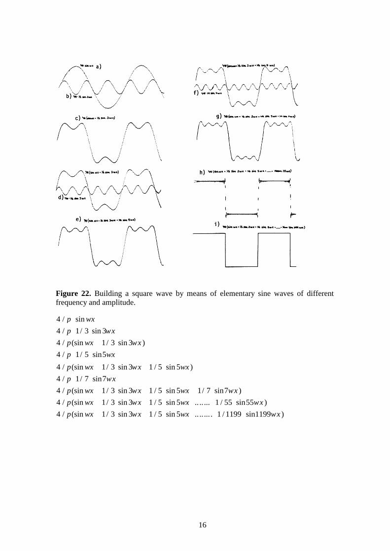
Figure 22. Building a square wave by means of elementary sine waves of differentfrequency and amplitude.

4 / π⋅sin ωx4 / π⋅1/ 3⋅sin 3ω x4 / π(sin ωx + 1/ 3⋅sin 3ω x )4 / π⋅1/ 5⋅sin5ωx

4 / π(sin ωx + 1/ 3⋅sin 3ω x + 1 / 5 ⋅sin 5ωx )4 / π⋅1/ 7⋅sin7ω x4 / π(sin ωx + 1/ 3⋅sin 3ω x + 1 / 5 ⋅sin 5ωx + 1/ 7⋅sin7ω x )4 / π(sin ωx + 1/ 3⋅sin 3ω x + 1 / 5 ⋅sin 5ωx + .. .. ...+ 1 / 55⋅sin55ω x )4 / π(sin ωx + 1/ 3⋅sin 3ω x + 1 / 5 ⋅sin 5ωx + .. .. ... . + 1 / 1199 ⋅sin1199ω x )

16

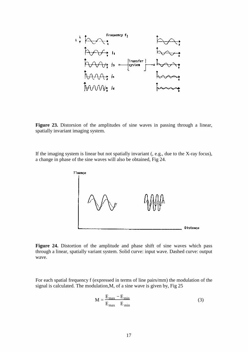
Figure 23. Distorsion of the amplitudes of sine waves in passing through a linear,spatially invariant imaging system.

If the imaging system is linear but not spatially invariant (, e.g., due to the X-ray focus),a change in phase of the sine waves will also be obtained, Fig 24.

Figure 24. Distortion of the amplitude and phase shift of sine waves which passthrough a linear, spatially variant system. Solid curve: input wave. Dashed curve: outputwave.

For each spatial frequency f (expressed in terms of line pairs/mm) the modulation of thesignal is calculated. The modulation,M, of a sine wave is given by, Fig 25

M = Emax − EminEmax + E min

(3)

17

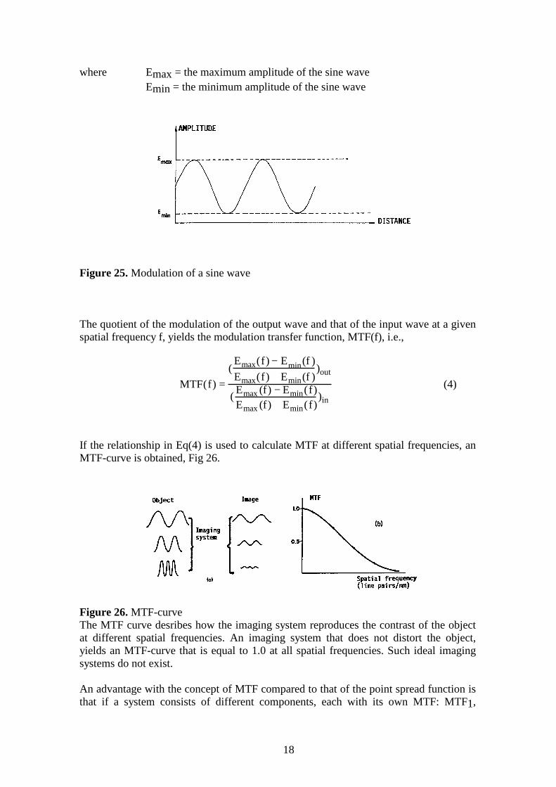
where Emax = the maximum amplitude of the sine waveEmin = the minimum amplitude of the sine wave

Figure 25. Modulation of a sine wave

The quotient of the modulation of the output wave and that of the input wave at a givenspatial frequency f, yields the modulation transfer function, MTF(f), i.e.,

MTF(f) =(

Emax(f) − Emin(f )Emax(f) + Emin(f )

)out

( Emax (f) − Emin(f)Emax (f) + Emin(f)

)in

(4)

If the relationship in Eq(4) is used to calculate MTF at different spatial frequencies, anMTF-curve is obtained, Fig 26.

Figure 26. MTF-curveThe MTF curve desribes how the imaging system reproduces the contrast of the objectat different spatial frequencies. An imaging system that does not distort the object,yields an MTF-curve that is equal to 1.0 at all spatial frequencies. Such ideal imagingsystems do not exist.

An advantage with the concept of MTF compared to that of the point spread function isthat if a system consists of different components, each with its own MTF: MTF1,

18

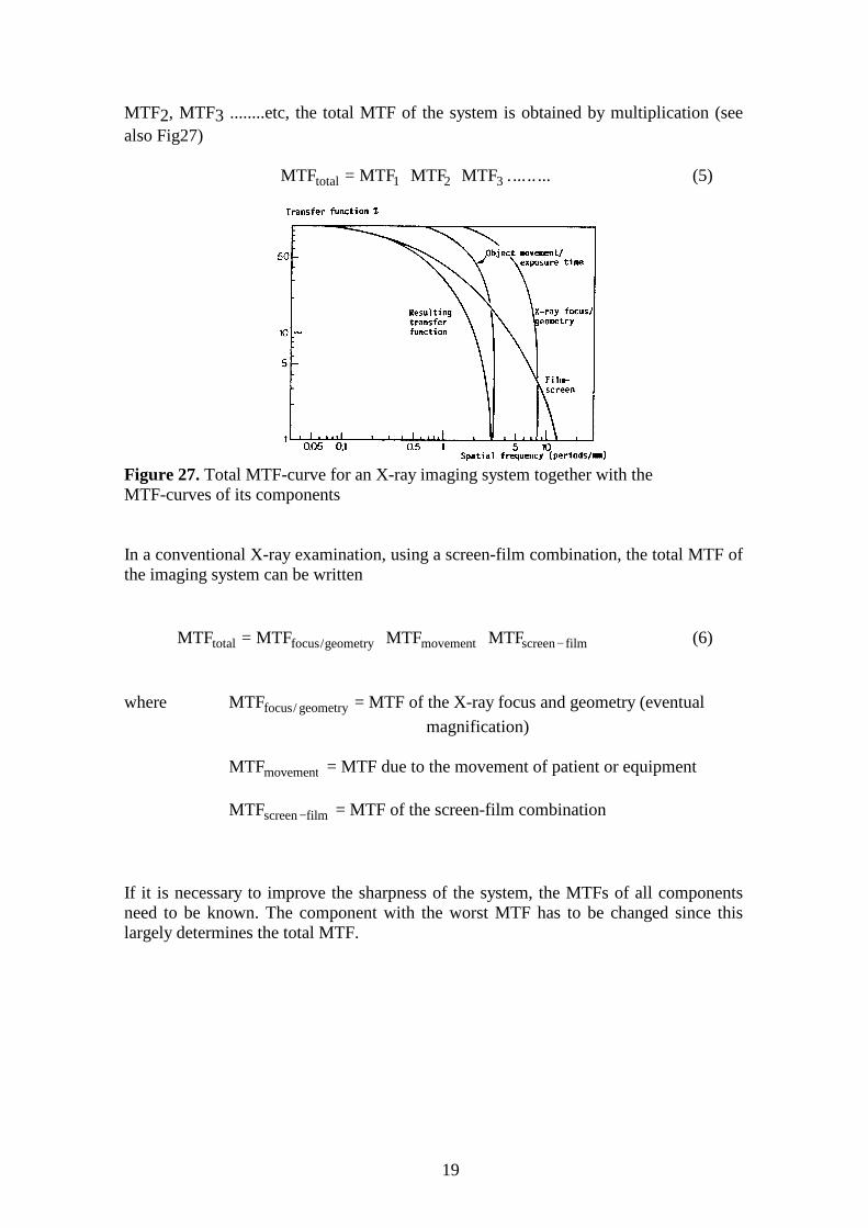
MTF2, MTF3 ........etc, the total MTF of the system is obtained by multiplication (seealso Fig27)

MTFtotal = MTF1 ⋅MTF2 ⋅MTF3⋅. ... .. ... (5)

Figure 27. Total MTF-curve for an X-ray imaging system together with theMTF-curves of its components

In a conventional X-ray examination, using a screen-film combination, the total MTF ofthe imaging system can be written

MTFtotal = MTFfocus/geometry ⋅MTFmovement ⋅MTFscreen − film (6)

where MTFfocus/ geometry = MTF of the X-ray focus and geometry (eventual magnification)

MTFmovement = MTF due to the movement of patient or equipment

MTFscreen − film = MTF of the screen-film combination

If it is necessary to improve the sharpness of the system, the MTFs of all componentsneed to be known. The component with the worst MTF has to be changed since thislargely determines the total MTF.

19

IV. REFERENCES

Dainty JC and Shaw R (1974). "Image science" Chapters 6 and 7. Academic Press, NewYork

Rossman K (1969). Point-spread function, line spread function and modulation transferfunction.Radiology93,257-272

20