resilience of biota in wetlands of intermediate...
TRANSCRIPT

Resilience of Biota in wetlands of intermediate salinity
by
Sarah Bradbury B. App. Sci (Envir Mgt), B. Env. Sci. (Hons)
Submitted in fulfilment of the requirements for the degree of
Doctor of Philosophy
Deakin University
November, 2013


Abstract Wetlands of intermediate salinity (10 g/L to 45 g/L) are known to have lower biodiversity
than their fresher counterparts but are also known to be highly productive providing
habitat for resilient plant, invertebrate and fish species. However, many of these species
are unable to tolerate hypersaline conditions (> 45 g/L) and if these wetlands become
hypersaline their ecological and conservation value rapidly decreases. This study
investigated the changes in salinity and watering regimes of wetlands of the northwestern
Victoria overtime, the salinity thresholds and sub lethal effects of increased salinity for
the loss of aquatic marcophyte and invertebrate communities, the effect of drying periods
on the propagule banks of wetlands of intermediate salinity. Historical and current distributions of wetlands of intermediate salinity in the Kerang,
Lake Charm and Lake Boga regions were examined. Results indicated that the abundance
of these wetlands and their biota has decreased since European settlement, in response to
increased salinity and changes to watering regimes. The remaining permanent wetlands of
intermediate salinity in the region were surveyed and results showed that the diversity of
aquatic macrophyte and fish species was low. However three wetlands supported
populations of the threatened fish species Craterocephalus fluviatilis McCulloch 1912
(Murray hardyhead). Propagule bank experiments were conducted on the sediments of an ephemeral wetland of
an intermediate salinity in the region to investigate the effect of increasing salinity on the
emergence of aquatic macrophyte and invertebrate species. Results showed that species
present in the propagule bank were resilient to short term salinity increases and were able
to re-establish at lower salinities. The majority of aquatic macrophyte and invertebrate
species present were tolerant of salinity treatments up to and including 37.7 g/L. Studies were conducted on Ruppia megacarpa seeds to investigate the effect of salinity,
photoperiod, temperature, seed source and drying periods on their germination. While
germination rates were low (< 35%), the presence of substrate, increased temperature and
lower salinities (< 45 g/L) had a significant positive effect on germination of
R. megacarpa. The information gained from these studies will assist managers in
designing improved watering regimes and management plans for these remaining
wetlands of intermediate salinity to ensure maximum biodiversity is maintained in the
region.

Acknowledgements Firstly I would like to thank my supervisors, Kimberley James and Anneke Veenstra for
not only their wealth of knowledge and assistance in developing my research, but more
importantly for their encouragement, enthusiasm, patience and support throughout my
candidature.
To my field assistants, Kathryn Sheffield, Christine Ashton and Andrew Armstrong who
travelled with me to Kerang, Swan Hill and Mildura, thank you not only for your hard
work, but also your patience, and companionship. You helped to make those long
journeys very enjoyable and it is much appreciated.
To the “salt” research team at Arthur Rylah Institute for Environmental Research,
(Michael Smith, Keely Ough, Sabine Schrebier, Michelle Kohout, Ruth Lennie,
Changhao Jin and Derek Turnbull), thank you for all your assistance throughout the
propagule bank experiments. The experience of being able to work collaboratively with
you with these experiments from their design through to completion proved invaluable.
I would thank Michelle Casanova for her assistance not only in identifying the
charophytes collected throughout my research but in helping me further develop my
understanding of charophytes and how salt effects their growth. I also would like to thank
Jarrod Lyon and Bill Dixon from Arthur Rylah Institute for Environmental Research, who
taught me the field techniques involved in surveying Murray Hardyhead populations.
Also, I would like to acknowledge the grants I received from the Holsworth Trust and the
River Basin Management Societies, as this research would not have been possible without
their assistance and is much appreciated.
My fellow colleagues at MIBT and the students and staff in the School of Life and
Environmental Sciences at Deakin University have also been a source of support,
motivation and friendship over the years. In particular I would like to thank Megan Short,
Bernadette Sinclair, Cuong Huynh, Jenny Gordon, Megan Underwood, Keely Ough, Luke
Shelly, Hugh Robertson, and Pathum Dhanapala. I also wish to thank to my colleages at
basketball (my “extended” family) and my close family friends; you may not have always
understood what I was doing, but you were always supportive and showed interest in my

project. In particular I wish to thank Kevin and Faye Winter, Sally Wall, Ben Dall, Lynne
and Neil Radford, Sally Radford, Alfie Jones, Grace Ramsden, Benn Keillor, Ryann
Sullivan, Catherine Odgers, Clare McIntosh, Louise Ma and Theresa Ting.
To my family who have always supported me throughout my life, thank you for all you
have done for me. I would like to especially thank my parents (Neil and Anne Bradbury),
my brother Marcus and my Nan (Shirley Reeves). There have also been three very special
people in my life that have helped me along the journey, to Kathryn Sheffield, Beth Parle
and Megan Underwood thank you so much for your support, encouragement and the
numerous cups of coffee in both the good, and the more challenging times. And finally to
Andrew (Goldie), you may have only been on the journey for a short time at the end, but
your love and encouragement has ensured the completion of this project.

Table of contents
Chapter 1.0 Salinity and its effects on biodiversity ................................................. 1 1.1 Introduction ........................................................................................................ 1
1.2 Models for predicting the effects of increased salinity on biodiversity ................. 5
1.3 Resilience .........................................................................................................11
1.4 Biota of wetlands of intermediate salinity ...........................................................14
1.4.1 Aquatic macrophytes .................................................................................14
1.4.2 Macroinvertebrates ....................................................................................16
1.4.3 Fish ...........................................................................................................17
1.4.4 Waterfowl ..................................................................................................20
1.4.5 Benthic microbial mats...............................................................................20
1.5.6 Phytoplankton ............................................................................................21
1.6 Hypotheses .......................................................................................................21
Chapter 2.0 The distribution of intermediate saline wetlands in northwest Victoria and their associated biota including the threatened fish Craterocephaulus fluviatilis (Murray Hardyhead) .......... 22
2.1 Introduction .......................................................................................................22
2.1.1 Case Study – Changes in salinity and distribution of key biota of selected wetlands in the Kerang to Swan Hill region of northwest Victoria ...............22
2.1.2 Aims of the investigation ............................................................................33
2.2 Methods ............................................................................................................34
2.2.1 Site descriptions ........................................................................................34
2.2.2 Water quality .............................................................................................39
2.2.3 Aquatic macrophytes – belt transects ........................................................40
2.2.4 Aquatic macrophytes – boat survey ...........................................................42
2.2.5 Murray Hardyhead survey .........................................................................42
2.2.6 Data Analysis ............................................................................................43
2.3 Results ..............................................................................................................44
2.3.1 Water quality .............................................................................................44
2.3.2 Aquatic macrophytes .................................................................................45
2.3.3 Fish survey ................................................................................................54
2.4 Discussion ........................................................................................................57
2.4.1 Water quality .............................................................................................57
2.4.2 Aquatic macrophyte composition and abundance ......................................58
2.4.3 Fish community composition and abundance ............................................60
Loss of Craterocephalus fluviatilis populations from Lake Elizabeth ..........60
2.4.4 Management implications for saline wetlands in northwest Victoria ...........63

Chapter 3.0 Effect of salinity on the egg and propagule bank of Lake Cullen, an ephemeral saline wetland of northwestern Victoria ............................... 65
3.1 Introduction .......................................................................................................65
3.1.1 Lake Cullen ...............................................................................................66
3.1.2 Hypotheses ...............................................................................................67
3.2 Methods ............................................................................................................69
3.2.1 Air temperature and water quality monitoring .............................................70
3.2.2 Monitoring of aquatic macrophyte and invertebrate emergence form the propagule bank, plus algal blooms ............................................................71
3.2.3 Invertebrate emergence and identification .................................................71
3.2.4 Harvesting of aquatic macrophytes ............................................................72
3.2.5 Results of sugar flotation method for invertebrate sorting ..........................73
3.2.6 Data analysis .............................................................................................73
3.3 Results ..............................................................................................................75
3.3.1 Air temperature and water quality monitoring .............................................75
3.3.2 Emergence of aquatic macrophyte and invertebrate taxa ..........................75
3.3.3 Ruppia megacarpa germination .................................................................79
3.3.4 Ruppia megacarpa - reproductive success ................................................81
3.3.5 Lamprothamnium macropogon germination ..............................................82
3.3.6 Lamprothamnium macropogon – reproductive success .............................85
3.3.7 Comparison of macrophyte species ...........................................................87
3.3.8 Phytoplankton blooms ...............................................................................89
3.3.9 Invertebrate results ....................................................................................89
3.3.10 Multivariate analysis ................................................................................92
3.4 Discussion ........................................................................................................94
3.4.1 Effect of salinity on the germination of aquatic macrophytes ......................94
3.4.2 Effects of salinity on macrophyte growth ....................................................96
3.4.3 Effects of salinity on aquatic macrophyte reproductive success .................97
3.4.4 Comparison of macrophyte species ...........................................................98
3.4.5 Effect of salinity on the number of invertebrates in populations developing from the seed bank ....................................................................................98 3.4.6 Salinity thresholds for submerged aquatic macrophyte and invertebrate
communities ..............................................................................................99
Chapter 4.0 An investigation of the effect of high salinity disturbances on the propagule bank of Lake Cullen ........................................ 101
4.1 Introduction ..................................................................................................... 101
4.1.1 Models for predicting the effect of salinity on the loss of macrophytes from wetlands .................................................................................................. 101
4.1.2 Hypotheses ............................................................................................. 105
4.2 Methods .......................................................................................................... 107
4.2.1 Air temperature and water quality monitoring ........................................... 109
4.2.2 Monitoring of aquatic macrophyte germination (seeds and asexual propagules) and invertebrate hatching from the propagule bank ............. 110
4.2.3 Invertebrate sampling .............................................................................. 110
4.2.4 Harvesting aquatic macrophytes .............................................................. 110
4.2.5 Data analysis ........................................................................................... 111
4.3 Results ............................................................................................................ 112
4.3.1 Air temperature and water quality monitoring ........................................... 112
4.3.2 Emergence of aquatic macrophyte and invertebrate taxa ........................ 112
4.3.3 Aquatic macrophyte germination – Ruppia megacarpa ............................ 116
4.3.4 Aquatic macrophyte germination – Lamprothamnium macropogon ......... 119
4.3.5 Phytoplankton blooms ............................................................................. 123
4.3.6 Invertebrate emergence – Mytilocypris henricae ...................................... 125
4.3.7 Invertebrate emergence – Australocypris spp. ......................................... 126
4.4 Discussion ...................................................................................................... 128
4.4.1 Evidence for models predicting the effect of increased salinity levels on community change in the propagule bank biota ....................................... 128
4.4.2 Effect of disturbance and recovery salinities on germination and growth of individual aquatic macrophyte species ................................................... 130
4.4.3 Effect of disturbance and recovery salinities on aquatic macrophyte reproductive structures ............................................................................ 132
4.4.4 Effect of disturbance and recovery salinities on invertebrate emergence from the propagule bank .................................................................................. 133
Chapter 5.0 The effects of environmental conditions on the germination of
Ruppia megacarpa seeds ....................................................... 135 5.1 Introduction ..................................................................................................... 135
5.1.1 Aims of the investigation .......................................................................... 137
5.2 Methods .......................................................................................................... 138
5.2.1 The effect of environmental variables on the germination of Ruppia megacarpa seeds .................................................................................... 138
5.2.2 The effect of photoperiod on the germination of Ruppia megacarpa seeds ...................................................................................................... 139

5.2.3 The affect of temperature on the germination of Ruppia megacarpa seeds ...................................................................................................... 140
5.2.4 Data Analysis .......................................................................................... 141
5.3 Results ................................................................................................................ 142
5.3.1 The effect of environmental variables on the germination of Ruppia megacarpa seeds .................................................................................... 142
5.3.2 The effect of photoperiod on Ruppia megacarpa seed germination ......... 147
5.3.3 The effect of temperature on Ruppia megacarpa seed germination ......... 147
5.4 Discussion ...................................................................................................... 149
Chapter 6.0 The effects of salinity and desiccation disturbances on germination success of Ruppia megacarpa ......................... 151
6.1 Introduction ..................................................................................................... 151
6.1.1 Hypotheses ............................................................................................. 153
6.2 Methods .......................................................................................................... 154
6.2.1 Data analysis ........................................................................................... 156
6.3 Results ............................................................................................................ 157
6.4 Discussion ...................................................................................................... 160
Chapter 7.0 Implications for management of wetlands of intermediate salinity in northwest Victoria ....................................................... 164
7.1 The distribution and biota of wetlands of intermediate salinity in northwestern Victoria ........................................................................................................... 165
7.1.1 The distribution of Craterocephalus fluviatilis (Murray Hardyhead) in northwestern Victoria ............................................................................... 166 7.2 The effect of salinity on clear water, aquatic macrophyte dominated communities ................................................................................................... 170
7.3 The existence of alternative stable states and the response of the Lake Cullen propagule bank to high salinity disturbance ............................................. 172
7.4 Effect of environmental factors of Ruppia megacarpa seeds ........................... 174
7.5 Further research ............................................................................................. 175
7.5.1 Further investigations into the effect of salinity on, and the management of Craterocephalus fluviatilis populations ..................................................... 175
7.5.2 Further investigations into the effect of salinity on propagule banks of wetlands of intermediate salinity .............................................................. 176
References .................................................................................................... 178

Appendices Appendix 1 Table of random numbers to indicate sites for water quality monitoring
.......................................................................................................... 193
Appendix 2 Selection of quadrat size for belt transects ........................................ 194
Appendix 3 Belt transect results (depth, percentage vegetation cover, dry weight biomass and biovolume) ................................................................... 198
Appendix 4 Results of fish survey in wetlands of intermediate salinity in northwest Victoria - detailed results ................................................................... 222
Appendix 5 Random location of replicates for experiment investigating the effect of salinity on the egg and propagule bank of Lake Cullen ..................... 225
Appendix 6 QA/QC checks for the effectiveness of sugar floatation methods for separating invertebrates from organic materials (Chapter 3 experiments) ..................................................................................... 225
Appendix 7 Air temperature and water quality monitoring for experiment investigating the effect of salinity on the egg and propagule bank of Lake Cullen .. 227
Appendix 8 Detailed regression analysis and ANOVA results for experiment investigating the effect of salinity on the egg and propagule bank of Lake Cullen ............................................................................................... 230
Appendix 9 Random location of replicates for experiment investigating the effect of high salinity disturbances on the propagule bank of Lake Cullen ...... 234
Appendix 10 QA/QC checks for the effectiveness of sugar floatation methods for separating invertebrates from organic materials (Chapter 4 experiments) .................................................................................. 235
Appendix 11 Air temperature and water quality monitoring for experiment investigating the effects of high salinity disturbance on the propagule bank of Lake Cullen ....................................................................... 236
Appendix 12 The abundance of minor invertebrate species for the experiment investigating the effect of high salinity disturbances on the propagule bank of Lake Cullen ....................................................................... 249
Appendix 13 Detailed Regression analysis and ANOVA results for experiment investigating the effect of high salinity disturbances on the egg and propagule bank of Lake Cullen ....................................................... 250
Appendix 14 Random location of replicates in germination cabinet for the experiment investigating the effect of location of seed source and presence of substrate on the germination of Ruppia megacarpa seeds at two differing salinities ............................................................................ 256
Appendix 15 Table of random numbers to determine order of experiments testing the effect of photoperiod and temperature on the germination of Ruppia megacarpa seeds ........................................................................... 257

Appendix 16 Random location of replicates in the germination cabinet for the experiment investigating the effect of photoperiod on the germination of Ruppia megacarpa seeds .............................................................. 258
Appendix 17 Random location of replicates in germination cabinet form the experiment investigating the effect of temperature on the germination of Ruppia megacarpa seeds .............................................................. 259
Appendix 18 Random location of replicates in germination cabinet for the experiment investigating the effect of salinity and desiccation on the germination of Ruppia megacarpa seeds .............................................................. 260
Appendix 19 The effect of various drying periods and salinity treatments on the germination of Ruppia megacarpa seeds - Day to day results ........ 261
List of Figures Chapter 1 Figure 1.1 Differing models to show ways in which ecosystems can respond to
external stressors such as salinity – modified from Gordon et al.(2008) and Davis et al. (2010) A and B refer to different ecological regimes ................. 7
Figure 1.2 Resilience in ecosystems and the shift between stable states. Adapted from Scheffer et al. (2001) and Levin (2009). ....................................................11
Chapter 2 Figure 2.1 Case Study – Locations of the northwest Kerang, Lake Charm and Lake
Boga regions and selected associated wetlands not to scale. Modified from Department of Sustainability and Environment (2010) ...............................23
Figure 2.2 Northwest Kerang region – changes in salinity and distribution of Craterocephalus fluviatilis (Murray Hardyhead) in selected wetlands between 1975 to 2003 .............................................................................................25
Figure 2.3 Case study - Lake Charm region – changes in salinity and distribution of Craterocephalus fluviatilis (Murray Hardyhead) in selected wetlands between 1975 to 2003 .............................................................................................29
Figure 2.4 Case study - Lake Boga region - changes in salinity and distribution of Craterocephalus fluviatilis (Murray Hardyhead) in selected wetlands between 1975 to 2003 .............................................................................................32
Figure 2.5 Location of Lake Elizabeth. Round Lake, Woorinen North Lake and Lake Hawthorn in northwestern Victoria (not to scale) modified from Department of Sustainability and Environment (2010) ......................................................35
Figure 2.6 Lake Elizabeth A. Aerial photo showing surrounding farmland (Google, 2012) B. Photo (looking northwest across the lake) showing Juncus acutus (Spiny Rush) in foreground and Cyprus atratus (Black Swans) on the lake ..........36
Figure 2.7 Round Lake A. Aerial photo showing surrounding farmland (Google, 2012) B. Photo (looking southwest across the lake) showing Juncus acutus (Spiny Rush) in foreground and numerous Cyprus atratus (Black Swans) on the lake ...........................................................................................................37
Figure 2.8 Woorinen North Lake A. Aerial photo showing surrounding farmland (Google, 2012) B. Photo (looking southwest across the lake) showing two Pelicanus conspicillatus Temminick 1824 (Australian Pelican) and very little riparian vegetation surrounding the lake. ................................................................38
Figure 2.9 Lake Hawthorn A. Aerial photo showing surrounding farmland (Google, 2012) B. Photo (looking southwest across the lake) showing Juncus acutus (Spiny Rush) in foreground ...................................................................................39
Figure 2.10 Random selection of sites for water quality measurements using a table of random numbers and clock face method ...................................................40
Figure 2.11 Selection of belt transect sites A. Photo showing the patch like distribution of macrophyte growth in Round Lake; near Lake Boga. B. Diagram showing selection of perpendicular and parallel belt transects ................................41
Figure 2.12 Diagram showing measurements methods used in fish survey for forked tailed fish (left) and those without forked tail (right) ....................................43
Figure 2.13 Mean aquatic macrophyte % cover as observed from boat at the four wetlands – Lake Elizabeth, Round Lake, Lake Woorinen North and Lake Hawthorn (n=100) .....................................................................................53
Figure 2.14 A. Size of Craterocephalus fluviatilis individuals caught from Round Lake B. Size of Craterocephalus fluviatilis individuals caught from Lake Hawthorn ..................................................................................................................56
Chapter 3 Figure 3.1 Location of Lake Cullen within the Kerang Lakes Area, Victoria (not to
scale) ........................................................................................................67
Figure 3.2 A. Glasshouse set up showing random allocation of tubs. B. Close up of one of the tubs showing plant growth in the two plastic trays............................70
Figure 3.3 Regressions showing the effect of salinity on the a) germination, b) biovolume, c) dry weight biomass of Ruppia megacarpa (n=5, square root transformation), lines only shown where regressions were significant (p <0.05) ........................................................................................................80
Figure 3.4 Number of weeks until Ruppia megacarpa reproductive structures a) flowers and b) fruits were first observed in replicates (n=5) ...................................82
Figure 3.5 Regressions showing the effect of salinity on the a) germination, b) biovolume, c) dry weight biomass of Lamprothamnium macropogon (n=5), trend lines only shown where regressions were significant (p <0.05) .........84
Figure 3.6 The percentage of Lamprothamnium macropogon individuals containing each type of reproductive structures (n=5, square root transformation), regression trend lines only shown where regressions were significant (p < 0.05) ........86
Figure 3.7 Number of weeks until Lamprothamnium macropogon antheridia were first observed in replicates exposed to varying salinity levels (n=5) ..................87
Figure 3.8 Comparison of Ruppia megacarpa and Lamprothamnium macropogon a) germination success, b) biovolume and c) dry weight biomass in varying salinity concentrations ...............................................................................88
Figure 3.9 Three different replicates from various treatments showing A. macrophyte growth (23.3 g/L treatment), B. no macrophyte growth (98.7 g/L treatment), C. phytoplankton bloom (136 g/L) ..............................................................89
Figure 3.10 The number of Mytilocypris henricae individuals (n=5, square root transformed), trend line represents a significant regression (p <0.05) .......90
Figure 3.11 The total number of Australocypris spp. individuals (n=5, square root transformed), trend line represents a significant regression (p <0.05) .......91

Figure 3.12 Effect of salinity on the time until invertebrates were first observed to have emerged in each replicate of substrate subjected to varying salinity levels (n=5) .........................................................................................................92
Figure 3.13 Multivariate analysis of number of plant and invertebrate individuals emerged from the propagule bank for all treatments ≤ 61 g/L. a. Cluster dendrogram generated from Bray-Curtis similarity index. Slice represents 65% similarity level. b. MDS ordination, contours represent 65% similarity level. Stress = 0.07 ....................................................................................93
Chapter 4 Figure 4.1 Differing models to show ways in which ecosystems can respond to external
stressors such as salinity – modified from Gordon et al. (2008) and Davis et al. (2010). Regime A represents wetlands dominated by submerged aquatic macrophytes; regime B represents wetlands with alternative regime (either microbial mat or phytoplankton dominated wetlands) .............................. 102
Figure 4.2 The proposed interactions between hydrological regime, salinisation, eutrophication, on the state of shallow freshwater systems in southwestern Australia modified from Davis et al. (2010) .............................................. 104
Figure 4.3 The design of the propagule bank study showing the disturbance and recovery salinity treatments tested .......................................................... 108
Figure 4.4 The effect of high Disturbance Phase and Recovery Phase salinity levels on the time until macrophyte germination ..................................................... 113
Figure 4.5 The effect of Disturbance Phase and Recovery Phase salinity levels on the time until emergence of ostracod species, Mytilocypris henricae and Australocypris spp. .................................................................................. 115
Figure 4.6 The effect of Recovery Phase salinity on the number of Ruppia megacarpa stems produced for each Disturbance Phase salinity treatment (n=5 square root transformed). Lines represents regressions where regressions were found to be significant (p <0.05) .............................................................. 117
Figure 4.7 The effect of Recovery Phase salinity on the amount of Ruppia megacarpa dry weight biomass produced for each Disturbance Phase salinity treatment (n=5 square root transformed). Lines represents where regressions were significant (p <0.05) ................................................................................. 119
Figure 4.8 The effect of Recovery Phase salinity on the number of Lamprothamnium macropogon germinants for each Disturbance Phase salinity treatment (n=5 square root transformed). Lines represents where regressions were significant (p <0.05) ................................................................................. 121
Figure 4.9 The effect of Recovery Phase salinity on the amount of Lamprothamnium macropogon dry weight biomass in each Disturbance Phase salinity treatment (n=5 square root transformed). Lines represents regressions where significant (p <0.05) ................................................................................. 122
Figure 4.10 The effect of Recovery Phase salinity on the number of Mytilocypris henricae individuals emerged from the sediments in each Disturbance Phase salinity treatment (n=5 square root transformed). Lines represent where regressions were significant (p <0.05) ..................................................... 125
Figure 4.11 The effect of Recovery Phase salinity on the number of Australocypris spp. individuals that emerged from the sediments in each Disturbance Phase salinity treatment (n=5 square root transformed). Lines indicate where regressions were significant (p <0.05) ..................................................... 127
Chapter 5 Figure 5.1 Set up of sample jars in pilot germination experiments ............................ 139
Figure 5.2 The effect of different seed sources on the germination rate for Ruppia megacarpa seeds in a) no substrate, 1.4 g/L, b) no substrate, 3.4 g/l, c) substrate, 1.4 g/L, d) substrate, 3.4 g/L (n=5, square root transformed) .. 142
Figure 5.3 Effects of the presence of lake substrate and salinity on the germination of Ruppia megacarpa seeds from a. Lake Cullen, b. Lake Golf Course and c. Lake Wandella (n=5, square root transformed) .................................... 145
List of Tables
Chapter 1 Table 1.1 Known effects of salinity on the major biotic taxa of freshwater systems in Australia, in taxonomic order ........................................................................... 3
Table 1.2 Classification of wetlands on the basis of salinity levels (Davis et al., 2003; Sim et al., 2003) ......................................................................................................... 6
Table 1.3 Criteria defining the four ecological regimes found by Strehlow et al. (2005) for saline lakes in southwest Australia ..................................................................... 10
Table 1.4 Native and introduced fish of Victorian inland waters in the Murray Darling Basin that are tolerant of salinities above 10 g/L .......................................................... 18
Chapter 2 Table 2.1 Water quality results for four lakes of intermediate salinity in northwest Victoria,
figures are shown as means (± standard error) .................................................. 44
Table 2.2 Lake Elizabeth belt transects – presence/absence of Ruppia megacarpa in the lake .................................................................................................................... 46
Table 2.3 Lake Elizabeth belt transects – presence/absence of Lamprothamnium macropogon in the lake ...................................................................................... 47
Table 2.4 Summary of macrophyte biovolume and dry weight biomass results from belt transects surveyed at Lake Elizabeth ................................................................. 48
Table 2.5 Round Lake belt transects – presence/absence of Ruppia megacarpa in the lake ................................................................................................................... 48
Table 2.6 Round Lake belt transects – presence/absence of Lamprothamnium macropogon in the lake ...................................................................................... 48
Table 2.7 Round Lake belt transects – presence/absence of Typha domingensis in the lake .................................................................................................................... 48
Table 2.8 Round Lake belt transects – presence/absence of Jucus acutus in the lake ...... 47
Table 2.9 Summary of macrophyte biovolume and dry weight biomass results from belt transects surveyed at Round Lake ..................................................................... 49
Table 2.10 Lake Woorinen North belt transects – presence/absence of Ruppia Megacarpa in the lake ........................................................................................ 50
Table 2.11 Summary of macrophyte biovolume and dry weight biomass results from belt transects surveyed at Lake Woorinen North ....................................................... 51
Table 2.12 Lake Hawthorn belt transects – presence/absence of Ruppia megacarpa in the lake .................................................................................................................... 52
Table 2.13 Lake Hawthorn belt transects – presence/absence of Lamprothamnium macropogon in the lake ..................................................................................... 52

Table 2.14 Lake Hawthorn belt transects – presence/absence of Typha domingensis in the lake .................................................................................................................... 52
Table 2.15 Summary of macrophyte biovolume and dry weight biomass results from belt transects surveyed at Lake Hawthorn ................................................................ 53
Table 2.16 Results of post hoc Tukey’s test for % cover of aquatic macrophytes at the four lakes .................................................................................................................. 54
Table 2.17 Total number of individuals caught for each species and catch per unit effort for each species, found in the four lakes ................................................................. 55
Chapter 3
Table 3.1 Salinity treatments tested in this study, using Lake Cullen substrate samples .... 69
Table 3.2 Presence/absence of each species of macrophyte and invertebrate, for each replicate (A, B, C, D and E) in this propagule bank study based on Lake Cullen substrate ............................................................................................................ 76
Table 3.3 The week species of macrophyte and invertebrate species were first observed for each replicate (A, B, C, D and E) in this propagule bank study based on Lake Cullen substrate, invertebrate species could not be identified at this early stage .................................................................................................................. 78
Table 3.4 Presence of algal blooms in replicates in the 136 g/L treatment for the duration of this experiment ............................................................................................... 89
Chapter 4
Table 4.1 Presence of algal blooms in replicates in the 136.0 g/L Disturbance Phase sainity treatment for the duration of the experiment. Numbers (up to 5) indicate the number of replicates where algal blooms were present .............................. 124
Chapter 5
Table 5.1 Treatments testing the effect of locality substrate presence and salinity on germination rates in Ruppia megacarpa ........................................................... 138
Table 5.2 Results of one-way ANOVA on the effect of seed source on the germination rate of Ruppia megacarpa seeds * indicates significance to p <0.05 level ............... 143
Table 5.3 Results of post hoc Tukey’s test for the substrate 3.4 g/L salinity treatment, * indicates significance to p <0.05 level ............................................................ 143
Table 5.4 t-test results for Lake Cullen comparing a. the effect of substrate and b. effect of salinity on the rate of germination on Ruppia megacarpa seeds * indicates significance to p < 0.10 level ............................................................................ 146
Table 5.5 t-test results for Lake Golf Course comparing a. the effect of substrate and b. effect of salinity on the rate of germination on Ruppia megacarpa seeds * indicates significance to p < 0.10 level, ** indicates significance to p <0.05 level ......................................................................................................................... 146
Table 5.6 t-test results for Lake Wandella comparing a. the effect of substrate and b. effect of salinity on the rate of germination on Ruppia megacarpa seeds * indicates significance to p < 0.10 level, ** indicates significance to p <0.05 level ......... 146
Table 5.7 The total number and percentage of Ruppia megacarpa seeds germinated for each photoperiod treatment ............................................................................. 147
Table 5.8 The total number and percentage of germinated Ruppia megacarpa seeds at two different temperatures ................................................................................ 147
Chapter 6
Table 6.1 Description of treatments used to test germination success of Ruppia megacarpa seeds collected from Lake Wandella ............................................. 154
Table 6.2 Overall germination rates of Ruppia megacarpa seeds collected from Lake Wandella in each treatment at completion of the experiment, highlighted (bold) treatments represent the highest and lowest germination rates ........................ 158
Table 6.3 Results of between subjects factor in a mixed four-way ANOVA testing the effect of Phase 1 salinity, Phase 2 salinity and the presence of desiccation period on the number of Ruppia megacarpa germinants .................................................. 159
Table 6.4 Results of post hoc Tukey’s test comparing Phase 2 salinity treatments on the number of Ruppia megacarpa germinants ....................................................... 159
Chapter 7
Table 7.1 Australian and Victorian Acts and the agencies and organisations responsible for the management of wetlands in northwest Victoria ..................................... 165
1
1.0 Salinity and its effects on biodiversity 1.1 Introduction There are two types of saline wetland systems found within Australia. Those wetland
systems that are naturally saline (primary salinisation), and those that are affected
from rising water tables caused by anthroprogenic changes to the landscape
(secondary salinisation) (Davis et al., 2003; Strehlow et al., 2005). Wetlands that are
naturally saline (primary salinisation) are often very productive and can be areas of
high ecological and conservation value, whereas secondary salnised wetlands are
often degraded (Timms, 1993; Williams, 1993b; Williams, 1993a; Timms, 1997;
Timms, 1998b; Timms, 1998a; Strehlow et al., 2005; Timms, 2005; Bailey et al.,
2006). Secondary salinity has been recognised as an increasing problem throughout
Australia and it has been reported that currently around 252 700 hectares in Victoria
are effected by dyland salinity and that by 2050, almost 14% of the total area of
Victoria will be affected by increased salinity (Morgan, 2001; Blinn et al., 2004).
Salinity has been shown to have adverse effects on aquatic biodiversity in many
regions across Australia including Victoria, and the southwest of Western Australia
(Brock and Lane, 1983; Brock and Sheil, 1983; Hart et al., 1990; Hart et al., 1991;
James et al., 2003; Nielsen et al., 2003b; Nielsen and Brock, 2009; Beatty et al.,
2011).
There are two forms of secondary salinity that can affect landscapes: dryland salinity
and irrigation salinity. Dryland salinity is caused by the loss of deep rooted
vegetation, often as a result of landclearing. Widespread clearing of deep rooted trees
and vegetation in agricultural areas of Australia has occurred and native vegetation
has been replaced with shallow rooted grasses. These shallow rooted pastures do not
absorb as much water as the deep rooted native vegetation therefore excess water
enters the water table and causes the water table to rise towards the surface. Water
tables of much of the interior regions of Australia are naturally salty, and as such can
cause widespread salinity issues as the water table rises (Aplin, 1998). Irrigation
salinity is caused by the build of up salts at or near the surface of the soil in irrigated
areas and is often caused by the application of large volumes of water to areas
without adequate drainage. This again can cause a rise in the water table and an
accumulation of salts near the surface. Run off from irrigated areas can also contain

2
high salt loads, thus increasing the salinity concentrations of streams and other
waterways (Aplin, 1998).
Salinity can have differnt types of adverse effects on aquatic biota, the first being
direct toxic effects through physiological changes, particularly changes caused by the
stress placed on osmoregulation. The second being indirect effects, caused by the
modification of ecosystem’s species composition and the loss of species that the
community relies on for food as well as habitat (ANZECC and ARMCANZ, 2000;
Nielsen et al., 2003b). Changes to the environment caused by salinity can also
impact biota (Bailey et al., 2006; Boon, 2006). For example with increased salinity,
suspended clays tend to fall out of suspension in the water column causing increased
water clarity. Salinity is also known to reduce dissolved oxygen concentations in
water and is also known to be associated with lower pH. Secondary salinity is often
associated with higher loads of sulphates and can lead to the production of acid
sulphate sediments (Bailey et al., 2006; Boon, 2006).
The impact of the effects of salinity on freshwater biota has been extensively
reviewed (Hart et al., 1990; Hart et al., 1991; Metzeling et al., 1995; James et al.,
2003; Nielsen et al., 2003b; Nielsen and Brock, 2009). However our knowledge of
the ecological consequences of increased salinisation in Australian freshwater
systems and the sublethal effects of salinity is limited to some knowledge on few
species and few studies have been completed investigating the effects of salinity on
ecosystem functioning (Nielsen et al., 2003b) (Table 1.1).

3
Table 1.1 Known effects of salinity on the major biotic taxa of freshwater
systems in Australia, in taxonomic order Taxa Salinity Tolerance References
Algae Majority of algae do not appear to be tolerant of salt concentrations > 10 g/L, although there are exceptions e.g. Dunaliella salina and many diatom species
Blinn et al., (2004), Neilsen et al., (2003b), James et al., (2013)
Benthic microbial mats
Tend to dominate at salinities > 50 g/L and be can be found in wetlands with lower salinities (approximately 12 g/L).
Herst and Blinn (1998) Sim et al., (2006b), Sim et al., (2006c)
Macrophytes Many submerged freshwater macrophyte species experience lethal or sublethal effects at salt concentrations of 1 to 2 g/L and most freshwater species disappear from aquatic systems at salinities > 4 g/L. Exceptions to this include Lepilaena spp. and Ruppia spp. suggesting that halophyte species have an upper tolerance around 45 g/L
Bailey (1998), Bailey and James (2000), James et al., (2013) Hart et al., (1991), Metzeling et al., (1995), Neilsen et al., (2003b), Sim et al., (2006a)
Riparian Vegetation
Affected at salinities > 3 g/L Increased salinity will affect non-halophytic plants. Increased salinity decreases riparian plant diversity
Hart et al., (1991), Lymbery et al., (2003)
Macro-invertebrates
The effect of salinity on this group is well researched using both field observations and toxicity tests. Reductions in the abundance of many animals within this group becomes apparent once salinity is > 1 g/L. Each phyla of invertebrates contain species that are highly sensitive to increases in salinity. However substantial changes in the diversity of wetland macroinvertebates only occurs in salinities ≥ 10 g/L.
Bailey (1998), Bailey and James (2000), Halse et al., (1998), Hart et al., (1991), Kefford et al., (2007) Metzeling et al., (1995)
Fish Tolerant between 7 and 13 g/L. Adults of most fish associated with lowland rivers appear to be tolerant of high salinities, but juveniles and eggs of some species are known to be susceptible to concentrations > 10 g/L
Beatty et al., (2011) Hart et al., (1991), James et al., (2003), Metzeling et al., (1995)
Amphibians Little information on the impact of salinity on amphibians, however one study on tadpoles reports that no tadpoles were found in waters > 3.84 g/L.
Hart et al., (1991), Smith et al., (2007)
Waterbirds May not be directly affected. Indirectly, the loss of riparian vegetation, macrophytes and invertebrates may change the distribution of many birds. Many species are able to feed in saline wetlands but need freshwater nearby to drink. Salinities > 3 g/L may affect breeding success.
Hart et al., (1991), Kingsford et al., (1994), Timms (2009)
Given the nature of salinity in Australia there have been many studies on the effects
salinity has on freshwater biota focusing on the impact of toxicity on plants and
macroinvertebates (Hart et al., 1990). Studies have observed that with increased
salinity there is a decrease in biodiversity (Brock and Lane, 1983; Hart et al., 1990;

4
Williams et al., 1990; Hart et al., 1991; Williams, 1998a; Brendonck and Williams,
2000; Williams, 2001; Williams, 2002). While an increase in salinity may reduce
overall biodiversity, the effects of salinity on particular taxa can be very different.
Hart et al., (1990) found that micro-algae, plants, and macroinvertebrates were the
taxa most sensitive to salinity changes. There are however some species within these
taxa, that are a very salt tolerant, Hart et al., (1991) and James et al., (2003), reported
that the aquatic macrophytes Ruppia (Widgeon grass), Lepilaena (Watermat) and the
charophyte Lamprothamnium (Stonewort) genera can tolerate concentrations of
salinity in excess of 10 g/L. Fish and birds are also less affected by salinity increases
because of their mobility; thus enabling them to swim or fly away from areas of high
salinity. In the case of waterbirds they have a distinct advantage over other genera in
that they are able to move easily from one water body to the next. It is generally
accepted that fish, for example Bidyanus bidyanus Mitchell 1838 (Silver perch),
Hypseleotris klunzingeri Ogilby 1898 (Western carp gudgeon) Maccullochella
macquariensis Cuvier 1829 (Trout cod), Macquaria australasica Cuvier 1830
(Macquarie perch) and Macquaria ambigua Richardson 1845 (Goldern perch) can
tolerate salinity concentrations up to 10 g/L (Hart et al., 1991; Metzeling et al., 1995;
Clunie et al., 2002; Nielsen et al., 2003b).
But these salinity tolerance values need to be treated with caution, as there has been
little research on the sublethal effects of salinity on both plants and animals and
further research is required in this area (Hart et al., 1991; James et al., 2003). The
majority of studies have only focused on salinity thresholds and tolerance levels of
adult life stages and have not considered juvenile life stages, seeds or the effects of
salinity on plant growth and vigour (Hart et al., 1991; James et al., 2003). O’Brian
and Ryan (1997), found that the early stages of development in M. australasica were
more susceptible to increases in salinity than adult life stages. Adult fish have a
salinity tolerance of more than 30 g/L, but egg survivorship was reduced by 100% at
a salinity of only 4 g/L. Therefore while some biota may appear to be tolerant of
salinity above 10 g/L, early life forms are potentially at risk at lower salinity
concentrations (O'Brian and Ryan, 1999). Sublethal effects have also been reported
in plant species, for example Hart et al., (1991), found that increases in salinity
effected the germination and growth of Phragmites australis (Cav.) Trin ex Steud
(Common reed). While James and Hart (1993), reported different sublethal effects on
four macrophyte species: Myriophyllum crispaturn Orchard (Upright water milfoil),
5
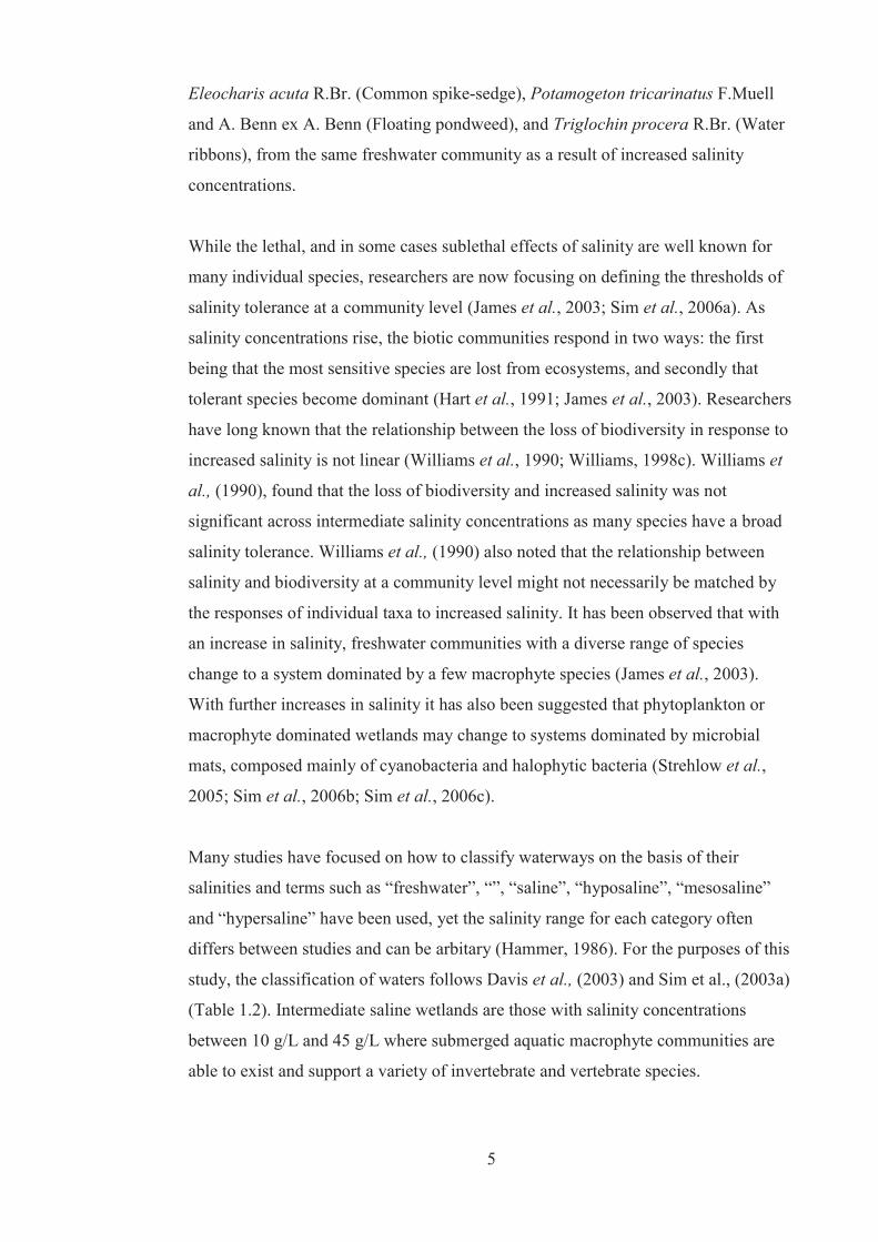
Eleocharis acuta R.Br. (Common spike-sedge), Potamogeton tricarinatus F.Muell
and A. Benn ex A. Benn (Floating pondweed), and Triglochin procera R.Br. (Water
ribbons), from the same freshwater community as a result of increased salinity
concentrations.
While the lethal, and in some cases sublethal effects of salinity are well known for
many individual species, researchers are now focusing on defining the thresholds of
salinity tolerance at a community level (James et al., 2003; Sim et al., 2006a). As
salinity concentrations rise, the biotic communities respond in two ways: the first
being that the most sensitive species are lost from ecosystems, and secondly that
tolerant species become dominant (Hart et al., 1991; James et al., 2003). Researchers
have long known that the relationship between the loss of biodiversity in response to
increased salinity is not linear (Williams et al., 1990; Williams, 1998c). Williams et
al., (1990), found that the loss of biodiversity and increased salinity was not
significant across intermediate salinity concentrations as many species have a broad
salinity tolerance. Williams et al., (1990) also noted that the relationship between
salinity and biodiversity at a community level might not necessarily be matched by
the responses of individual taxa to increased salinity. It has been observed that with
an increase in salinity, freshwater communities with a diverse range of species
change to a system dominated by a few macrophyte species (James et al., 2003).
With further increases in salinity it has also been suggested that phytoplankton or
macrophyte dominated wetlands may change to systems dominated by microbial
mats, composed mainly of cyanobacteria and halophytic bacteria (Strehlow et al.,
2005; Sim et al., 2006b; Sim et al., 2006c).
Many studies have focused on how to classify waterways on the basis of their
salinities and terms such as “freshwater”, “”, “saline”, “hyposaline”, “mesosaline”
and “hypersaline” have been used, yet the salinity range for each category often
differs between studies and can be arbitary (Hammer, 1986). For the purposes of this
study, the classification of waters follows Davis et al., (2003) and Sim et al., (2003a)
(Table 1.2). Intermediate saline wetlands are those with salinity concentrations
between 10 g/L and 45 g/L where submerged aquatic macrophyte communities are
able to exist and support a variety of invertebrate and vertebrate species.

6
Table 1.2 Classification of wetlands on the basis of salinity concentrations (Davis et
al., 2003; Sim et al., 2006a)
Category Salinity (g/L) Freshwater < 3 Hyposaline 3 to 10 Saline (Intermediate) 10 to 45 Hypersaline > 45
1.2 Models for predicting the effects of increased salinity on biodiversity
The response of ecosystems to changing conditions can vary from smooth and
continual to discontinuous (Scheffer and Carpenter, 2003; Gordon et al., 2008; Davis
et al., 2010), depending on the type of ecosystem and the condition being
investigated. Figure 1.1 illustrates how ecosystems can respond differently to
changes in a particular condition: Figure 1.1 (1) shows a continual smooth response
to a change in conditions, if the stress is removed the ecosystem returns to its original
state with a continual smooth response. Figure 1.1 (2) shows how an ecosystem may
change abruptly from one stable state to the next at a given threshold, if the stress is
removed, again the ecosystem can return its original state, but recovery will only
occur if the level of stress is lower than the threshold. Figure 1.1 (3) again shows
how an ecosystem may change abruptly at a given threshold, however unlike Figure
1.1 (2), the ecosystem cannot return to its original state. Figure 1.1 (4) also shows
how an ecosystem can change abruptly at a given threshold, but unlike Figures 1.1
(2) and 1.1(3), no recovery to any improved state is possible once the ecosystem has
collapsed.
Much research in past years has focused on determining if the alternative stable
states model is an appropriate way of describing how shallow wetlands in Australia
respond to fluctuations in salinity (Davis et al., 2003; Strehlow et al., 2005; Sim et
al., 2006a; Sim et al., 2006b; Sim et al., 2006c; Gordon et al., 2008; Davis et al.,
2010).

7
A
B
Regime
1. Gradual Change
A
B
Regime
2. Threshold
A
B
Regime
3. Alternative Stable States A
B
Regime
4. Collapse
Stress Stress
Stress Stress
Figure 1.1 Differing models to show ways in which ecosystems can respond to
external stressors such as salinity – modified from Gordon et al., (2008) and Davis et al., (2010). A and B refer to different ecological regimes
The alternative stable states theory is used to explain how a community or ecosystem
changes dramatically from one state to another (May, 1977; Carpenter, 2003). For
example, in aquatic ecosystems it has been commonly used to show how a
macrophyte dominated wetland can become a eutrophic phytoplankton dominated
wetland when nutrients from the catchment are added (Carpenter, 2003; Scheffer and
Carpenter, 2003; Strehlow et al., 2005). Usually, a population or even an ecosystem
fluctuates around a trend or stable average so not all changes in ecosystems can be
attributed to the alternative stable states theory (Scheffer and Carpenter, 2003).
However, ecosystems can be impacted by an abrupt change resulting in a shift to a
different state (Scheffer and Carpenter, 2003). The alternative stable states theory has
also been used to explain how wetlands and coral reefs change dramatically in
response to eutrophication (McClanahan et al., 2002; Mumby et al., 2007).
Additionally it has been applied to the way in which freshwater fish populations
8
respond to overfishing, and terrestrial ecosystems where slow changes have resulted
in the loss of vegetation in grazed ecosystems (May, 1977; Rietkerk and van de
Koppel, 1997; Folke et al., 2004). In Australia the alternative stable states model has
been used to explain the change from submerged macrophytes in wetlands to
phytoplankton dominated weltands as a result of increased nutrients to systems
(Boon and Bailey, 1998; Morris et al., 2003a; Morris et al., 2003b; Morris et al.,
2004). More recently alternative-states models have been considered useful tools for
describing stepped rather than linear threshold relationships between the loss of
biodiversity and increasing salinity in wetlands (Davis et al., 2003; James et al.,
2003).
While catastrophic changes are often attributed to the alternative stable states theory,
theoreticians have stressed that even small incremental and often gradual changes in
conditions can trigger a dramatic shift in some ecosystems (Folke et al., 2004). This
change can occur at a threshold level and if the threshold level is known, accurate
models can be developed, predictions made, and these ecosystems managed
accordingly (Folke et al., 2004). Threshold levels associated with the alternative-
stable states theory should be used with some caution as ecosystems may respond
dramatically to abiotic or biotic factors other than those suggested in a model.
Whether the change in stable states has been due to a small or dramatic change in
conditions, the movement back to the original state (i.e. to reverse the change in the
ecosystem) is very difficult. Also systems are not guaranteed to return to the
conditions experienced in the previous stable state (Beisner et al., 2003; Folke et al.,
2004).
Another consideration in the use of these models is that rarely is an ecosystem state
driven by one single abiotic factor. Davis et al., (2010) hypothesized that several
factors including hydrology, salinity, acidification, and eutrophication are all
environmental factors that could potentially cause a shift in stable states in wetlands
in Western Australia. Davis et al., (2010) also identified that a shift from one stable
state to another may be a result of compounding effects of environmental factors,
thus making the modelling of such complex relationships difficult.
Limitations of the alternative states model include the fact that in reality ecosystems
are rarely stable, populations tend to fluctuate and environmental conditions are

9
seldom constant. This can make it hard to establish if a change is due to natural
fluctuations or is a shift in stable states. Schröder et al., (2005) distinguishes four
experimental approaches to tesing for alternative stable states in ecological systesms
being:
Discontinuity in the response to an environmental driving parameter
Lack of recovery potential after a perturbation
Divergence due to different initial conditions
Random divergence
Research into how alternative stable states relate to salinity in aquatic ecosystems is
relatively recent. Davis et al., (2003) suggested that a discontinuous alternative stable
states model similar to the one posed by Scheffer (2001) for increasing nutrients,
may be how wetlands in south Western Australia respond to increasing salinity,
particularly secondary salinity.
Further studies conducted by Strehlow et al., (2005), Sim et al., (2006a) Sim et al.,
(2006b) and Davis et al., (2010) suggest that the relationship between changes in
alternative ecological regimes within saline wetlands in Australia, may be more
complicated than the alternative stable states model first posed. Strehlow et al.,
(2005) stated that there were four ecological regimes in saline wetlands, and that
shifts from one regime to another may be caused by increases in nutrients as well as
changes in salinity (Table 1.3).
10
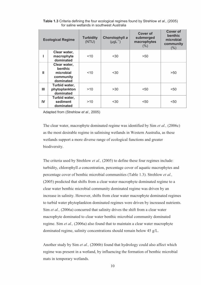
Table 1.3 Criteria defining the four ecological regimes found by Strehlow et al., (2005) for saline wetlands in southwest Australia
Ecological Regime Turbidity (NTU)
Chorolophyll a (μgL-1)
Cover of submerged
macrophytes (%)
Cover of benthic
microbial community
(%)
I Clear water, macrophyte dominated
<10 <30 >50
II
Clear water, benthic
microbial community dominated
<10 <30 >50
III Turbid water,
phytoplankton dominated
>10 >30 <50 <50
IV Turbid water,
sediment dominated
>10 <30 <50 <50
Adapted from (Strehlow et al., 2005)
The clear water, macrophyte dominated regime was identified by Sim et al., (2006c)
as the most desirable regime in salinising wetlands in Western Australia, as these
wetlands support a more diverse range of ecological functions and greater
biodiversity.
The criteria used by Strehlow et al., (2005) to define these four regimes include:
turbidity, chlorophyll a concentration, percentage cover of aquatic macrophytes and
percentage cover of benthic microbial communities (Table 1.3). Strehlow et al.,
(2005) predicted that shifts from a clear water macrophyte dominated regime to a
clear water benthic microbial community dominated regime was driven by an
increase in salinity. However, shifts from clear water macrophyte dominated regimes
to turbid water phytoplankton dominated regimes were driven by increased nutrients.
Sim et al., (2006a) concurred that salinity drives the shift from a clear water
macrophyte dominated to clear water benthic microbial community dominated
regime. Sim et al., (2006a) also found that to maintain a clear water macrophyte
dominated regime, salinity concentrations should remain below 45 g/L.
Another study by Sim et al., (2006b) found that hydrology could also affect which
regime was present in a wetland, by influencing the formation of benthic microbial
mats in temporary wetlands.

11
1.3 Resilience Resilience is defined as the ability of the biotic components of the ecosystem to
maintain ecological function in the face of disturbance and variability, in this case,
salinity concentrations (James et al., 2003; Jin, 2008). Resilience and tolerance are
important concepts when considering the alternative stable states and other
modelling theories. The resilience of the community determines if the system is able
to maintain ecological function during or after a disturbance or disturbances have
occurred (Scheffer et al., 2001; Carpenter, 2003). Carpenter (2003), defined
resilience as having three different properties: the amount of change a system can
undergo, the degree to which the system is self-organising and the degree to which
the system can adapt. The tolerance of the community defines the amount of change
the ecosystem can withstand before there is a change in stable states or ecological
regimes (Scheffer et al., 2001; Carpenter, 2003).
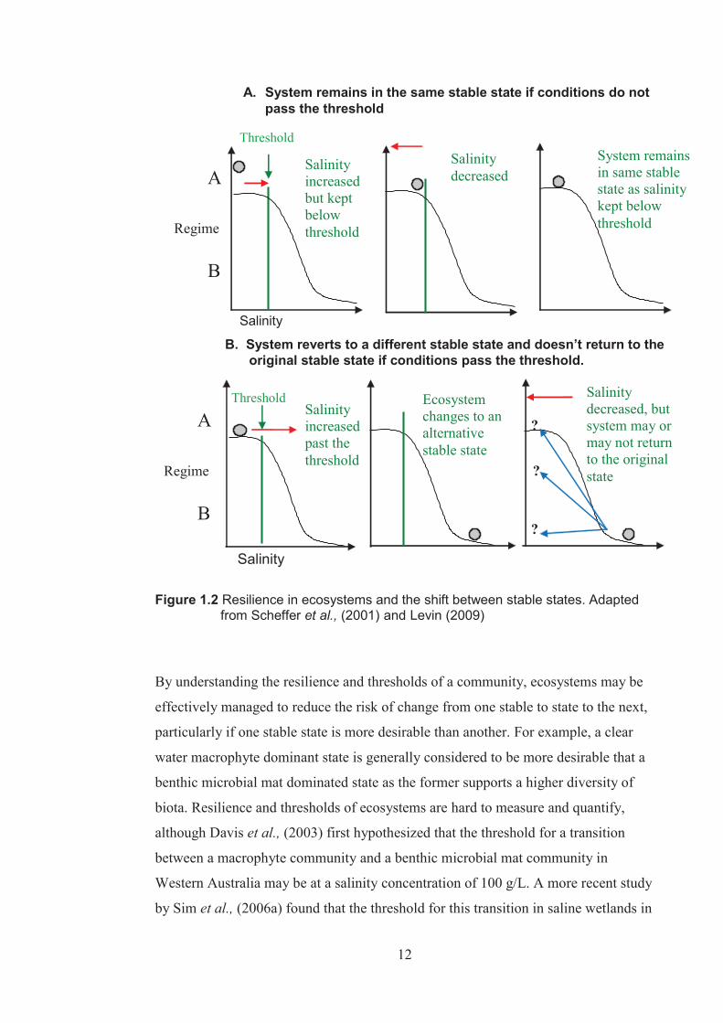
Often an ecosystem can tolerate some change in conditions without significantly
altering states and therefore in this scenario, when and if conditions revert back to
those first experienced, the ecosystem remains in its original condition (Figure 1.2A).
Once the threshold of the system is passed and the ecosystem changes states, a return
to the original conditions does not necessarily mean a return to the original state
depending on how resilient the ecosystem is (Figure 1.2B).
12
Salinity
A. System remains in the same stable state if conditions do not pass the threshold
Threshold
Salinity
B. System reverts to a different stable state and doesn’t return to the original stable state if conditions pass the threshold.
Salinity increased but kept below threshold
System remains in same stable state as salinity kept below threshold
Salinity decreased
Salinity increased past the threshold
Ecosystem changes to an alternative stable state
A
B
Regime
A
B
Regime
Salinity decreased, but system may or may not return to the original state
Threshold
?
?
?
Figure 1.2 Resilience in ecosystems and the shift between stable states. Adapted
from Scheffer et al., (2001) and Levin (2009)
By understanding the resilience and thresholds of a community, ecosystems may be
effectively managed to reduce the risk of change from one stable to state to the next,
particularly if one stable state is more desirable than another. For example, a clear
water macrophyte dominant state is generally considered to be more desirable that a
benthic microbial mat dominated state as the former supports a higher diversity of
biota. Resilience and thresholds of ecosystems are hard to measure and quantify,
although Davis et al., (2003) first hypothesized that the threshold for a transition
between a macrophyte community and a benthic microbial mat community in
Western Australia may be at a salinity concentration of 100 g/L. A more recent study
by Sim et al., (2006a) found that the threshold for this transition in saline wetlands in

13
Western Australia is probably much lower than this and has suggested an upper
salinity threshold for macrophyte communities at 45 g/L.
Resilience is also an important concept when considering individual species
responses to increased salinity concentrations in aquatic ecosystems. The resilience
of a species can differ between populations depending on their past exposure to
environmental conditions. Studies on Eucalyptus camaldulensis Dehnh have found
that seeds obtained from differing soil salinities showed differing resilience to
salinity treatments tested, with those seeds from low soil salinity sources having a
lower tolerance to raised salinity concentrations (Sands, 1981). Similar results have
been found in other Australian plants including members from Eucalyptus,
Melaleuca and Casuarina genera (Sands, 1981; Van der Moezel et al., 1989; Van der
Moezel et al., 1991). Dixon (2007), also reported that populations of the fish species
Craterocephalus fluviatilis (Murray Hardyhead) McCulloch, 1913 from different
lakes had differing tolerances of raised salinity concentrations. It is important to note
that for plants that seeds are not the only method for plant survival and dispersal,
especially in weltands. A number of wetland plant species exhibit clonial growth in
many different ways including turons, stolons, tubers, rhizomes and plantlets. These
methods provide an alternative to seeds which may not always be produced from
wetland plants (Grace, 1993).
Aspects of resilience traits that enable organisms to exist in high salinity
environments include acclimation and avoidance. When salinity increases gradually
within an aquatic system, some organisms are able to acclimatise to the elevated salt
concentrations. But these same organisms may not be able to tolerate such elevated
salt concentrations if the increases occurred rapidly (Rai and Rai, 1998).
Other species use a range of avoidance strategies including, dispersal to less saline
habitats, the use of a less saline microhabitat within a salinising patch, or remaining
in a salinising area in a dormant phase until conditions become less saline (for
example seeds, asexual progagules and invertebrate eggs that remain in the
propagule bank) (James et al., 2003). James et al. (2003) in their review of the
literature reported that both acclimation and the avoidance mechanisms used by
individuals can make it hard to generalise and quantify the tolerance and resilience of
an ecosystem because different populations of a particular species may have differing

14
threshold limits, depending on their location and past exposure to elevated salinity
concentrations.
1.4 Biota of wetlands of intermediate salinity Saline wetlands are often association as being of low value, however many studies
have shown that weltands of intermediate salinity do have a number of economic,
social, environmental, educational and scientific values (Lugg et al., 1989; Williams,
1993a; 1993b; 1998b; 2001). The flora and fauna of wetlands of intermediate salinity
are often characterized by low diversity yet high productivity leading to systems that
can support numerous water birds and fish populations (Brock, 1986; Timms, 1993;
Kingsford and Porter, 1994). ( ; ; ; ; ).
1.4.1 Aquatic macrophytes Aquatic macrophytes are an important food source and provide habitat for many
species in wetland systems including invertebrates, fish and water birds. Hart et al.,
(1991), identified plant communities as being the most sensitive of wetland biota to
salinity increases. However, as previously mentioned while most aquatic
macrophytes are salt sensitive, there are a few species that can tolerate wide salinity
ranges. The salt tolerant submerged aquatic macrophytes include Potamogeton
pectinatus L. (Sago pondweed) which can tolerate salinities of above 10 g/L, many
species of Ruppia (Wigeongrass) Lepilaena (Watermats) some species of which are
able to tolerate salinities of above 100 g/L and the charophyte species
Lamprothamnium macropogon (A. Braun) L.Ophel (Stonewort) which has a
tolerance range of 2 to 58 g/L (Brock, 1986; Hart et al., 1991; Garcia, 1999). The salt
tolerant species are usually found as a component of macrophyte communities with
other species in fresh to hyposaline wetlands (up to 10 g/L). Wetlands of
intermediate salinity (10 – 45 g/L) are often characterised by these salt tolerant
macrophyte species. Two genera of submerged aquatic macrophytes (Ruppia and
Lamprothamnium), and two gerera of emergent macrophytes were found in wetlands
of intermediate salinity in north western Victoria throughout this study.
Four different species of Ruppia occur within Australia, three of which are endemic.
All species are tolerant of hyposaline to saline waters (3 g/L to 100 g/L), but can also
occur in freshwater habitats (Jacobs and Brock, 1982). There have been many studies
on the Ruppia genus with many focusing on Ruppia maritima L. (Wigeongrass).

15
Ruppia maritima is the most salt tolerant of the angiosperms and it has been
suggested that this species can tolerate salinities of over 100 g/L (Hart et al., 1991;
Murphy et al., 2003). Studies by La Peyre and Rowe (2003) and Murphy et al.,
(2003) focussed on the short-term effects of elevated salinity concentrations on this
species. Both studies found that short-term changes in salinity concentrations, either
increased or decreased concentrations, had few negative effects on R. maritima.
Murphy et al., (2003) noted that while the initial change in salinity was stressful, this
species was able to physiologically adapt after several days. Ruppia maritima is able
to osmoregulate in low and high salinities by adjusting the amount of proline
accumulated within the plant cells, and can more easily adjust when allowed to
acclimate at intermediate concentrations, rather than when exposed to more extreme
changes in salinity (Murphy et al., 2003). Little work has been done on the impact of
salinity on the sensitive life stages of plants (Nielsen et al., 2003b), however it has
been identified that salt sensitivity of various life stages of a species may differ
(Bailey and James, 2000). Brock (1982a) found that the germination of Ruppia
megacarpa R. Mason (Large Fruit Tassel) decreased with increasing salinity
concentrations, but for Ruppia tuberosa J.S. Davis and Toml. (Tuberous Tassel),
increased salinity concentrations produced increased germination. This further shows
that biota within a taxa can vary in their tolerance to increased salinity
concentrations.
There are two Lamprothamnium species growing in Australia, but until recently all
species in Australia were listed as Lamprothamnium papulosum (Wallroth) J.
Groves. (Stonewort), and as such there is little ecological information for each
individual species (Garcia and Chivas, 2004; Sim et al., 2006a). The two species that
occur in Australia: Lamprothamnium succinctum (A. Braun) R.D. Woods
(Stonewort), is found in coastal lagoons, and L. macropogan, is widespread in saline
wetlands, particularly in Victoria (Garcia and Chivas, 2004). Lamprothamnium
macropogan is found in shallow alkaline waters in salinities ranging from 2 to
76 g/L. Generally in inland wetlands with salinity > 5 g/L, L. macropogan exists in
monospecific stands with no other charophyte species. A propagule bank study by
Sim et al., (2006a) found that L. succinctum was able to germinate in salinities up to
and including 45 g/L, and L. macropogan was able to germinate in salinities up to
and including 30 g/L.
16
Emergent macrophytes and riparian vegetation are also an important food source and
provide habitat for many species in wetland systems. A number of emergent
macrophytes have been associated with hyposaline waters including Phragmites spp.,
Typha spp. and Juncus spp (Hart et al., 1991). Typha domingensis is known to only
tolerate small increases in salinity and reduced growth in this species have been
recorded between salinities of 2.8 g/L and 5.9 g/L (Hocking, 1981). Juncus acutus is
known to tolerate higher salinity increases and can be found in waters of 10g/L
(Greenwood and MacFarlane, 2009). Riparian vegetation associated with weltands of
intermediate salinity often includes Eucalyptus largiflorens F. Muell, which is the
more salt tolerant of riparian species and can tolerate salinities of up to 3.2 g/L
(Roberts and Marston, 2011).
1.4.2 Macroinvertebrates Macroinvertebrates, like aquatic macrophytes, are also an important food source for
fish and waterfowl in saline wetlands. As a group, macroinvertebrates contain
species that represent the most salt sensitive to the most salt tolerant of taxa. For
example Timms (1993; 1998) found that members of Class Crustacea (e.g. copepods)
have very salt sensitive species (with upper tolerance level of around 0.67 g/L) and
also have very salt tolerant species (with an upper tolerance level of approximately
177.5 g/L). Unlike many salt tolerant macrophyte species, macroinvertebrates with a
salinity tolerance of above 18 g/L are unable to tolerate low concentrations of salinity
(Clunie et al., 2002). Also, it is hard to generalise as to which species of aquatic
macroinvertebrates are commonly found in saline wetlands, as there are strong
regional differences in macroinvertebrate community species composition (Williams,
1984). However, some species of chironomids, ostracods e.g. Mytilocypris henricae
Chapman 1966, amphipods e.g. Austrochiltonia subtenuis Sayce 1902, and shrimps
are known to be saline water specialists (James et al., 2003; Nielsen et al., 2003b;
Shelley, 2008).
While the salinity tolerances of adult life stages of macroinvertebrates are well
documented, there has been very little research on the sub-lethal effects of salinity on
the larval stages of many species. One study on salinity tolerance of the early life
stages of selected macroinvertebrates found that the early life stages (eggs) for 60 to
70% of freshwater macroinvertebrates have a lower salinity tolerance than their adult
17
life stage (Kefford et al., 2007). Kefford et al., (2007) also found that young
crustaceans, e.g. Paratya australiensis (Cherry shrimp) Kemp 1917 and Caridina
nilotica (Freshwater shrimp) Roux 1833, are more tolerant of elevated salinity
concentrations than the early life stages of other macroinvertebrate groups studied.
1.4.3 Fish A review of Australian adult freshwater fish found that they tend to be tolerant of
salinities from 7 g/L to 13 g/L (James et al., 2003). While data on many species are
lacking, few species are able to tolerate salinity concentrations > 13 g/L (James et al.,
2003). Some fish species are tolerant of salinities above that of seawater (35 g/L),
and these include but are not limited to, Craterocephalus stercusmuscarum fulvus
Günther 1867 (Unspecked Hardyhead), Craterocephalus fluviatilis (Murray
Hardyhead), Galaxias maculatus Jenyns 1842 (Common galaxias), Hypseleotris sp.
(Carp Gudgeons) and Retropinna semoni Weber 1895 (Australian smelt). There are
introduced species that are tolerant of salinities above 10 g/L, the most tolerant being
the Gambusia holbrooki Girard 1859 (Eastern mosquito fish) which has a reported
direct acute LC50 (Lethal Concentration 50% - the concentration of a toxicant
(salinity) that results the death of half the individuals in a population tested) of
25 g/L (Nordlie and Mirandi, 1996). The adults of most species are able to
acclimatise to elevated salinity concentrations, however juveniles appear to be less
tolerant (James et al., 2003).
It is important to note that the majority of studies on the salinity tolerance of fish in
Australia are based on laboratory studies involving the development of LC50 values.
Kefford et al., (2004) found that direct acute LC50 values and LC50 values for early
life stages in freshwater fish tended to be a poor estimate of maximum field
observations for many species. This was attributed to the fact that changes in salinity
in the field (or in situ) are often gradual, which allows the individuals to acclimatise
to increased salinity concentrations. Also adult fish, being highly mobile organisms,
are able move away from saltier environments that their early life stages are unable
to tolerate or easily avoid. Kefford et al., (2004) found that gradual increases in
salinity concentrations, LC50 values were a more accurate measure in the prediction
if a species maximum field observation salinity tolerance level.
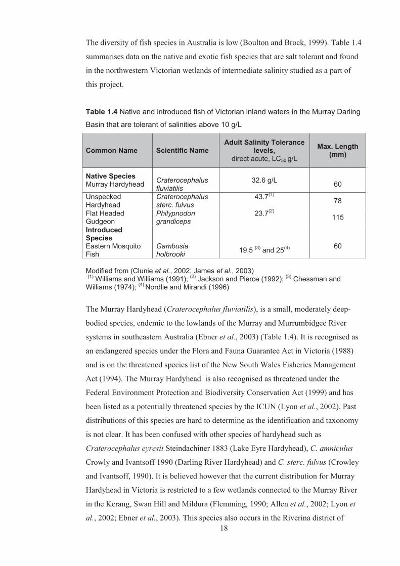
18
The diversity of fish species in Australia is low (Boulton and Brock, 1999). Table 1.4
summarises data on the native and exotic fish species that are salt tolerant and found
in the northwestern Victorian wetlands of intermediate salinity studied as a part of
this project.
Table 1.4 Native and introduced fish of Victorian inland waters in the Murray Darling
Basin that are tolerant of salinities above 10 g/L
Common Name Scientific Name Adult Salinity Tolerance
levels, direct acute, LC50 g/L
Max. Length (mm)
Native Species Murray Hardyhead
Craterocephalus fluviatilis
32.6 g/L
60
Unspecked Hardyhead
Craterocephalus sterc. fulvus
43.7(1) 78
Flat Headed Gudgeon
Philypnodon grandiceps
23.7(2) 115
Introduced Species Eastern Mosquito Fish
Gambusia holbrooki
19.5 (3) and 25(4)
60
Modified from (Clunie et al., 2002; James et al., 2003) (1) Williams and Williams (1991); (2) Jackson and Pierce (1992); (3) Chessman and Williams (1974); (4) Nordlie and Mirandi (1996)
The Murray Hardyhead (Craterocephalus fluviatilis), is a small, moderately deep-
bodied species, endemic to the lowlands of the Murray and Murrumbidgee River
systems in southeastern Australia (Ebner et al., 2003) (Table 1.4). It is recognised as
an endangered species under the Flora and Fauna Guarantee Act in Victoria (1988)
and is on the threatened species list of the New South Wales Fisheries Management
Act (1994). The Murray Hardyhead is also recognised as threatened under the
Federal Environment Protection and Biodiversity Conservation Act (1999) and has
been listed as a potentially threatened species by the ICUN (Lyon et al., 2002). Past
distributions of this species are hard to determine as the identification and taxonomy
is not clear. It has been confused with other species of hardyhead such as
Craterocephalus eyresii Steindachiner 1883 (Lake Eyre Hardyhead), C. amniculus
Crowly and Ivantsoff 1990 (Darling River Hardyhead) and C. sterc. fulvus (Crowley
and Ivantsoff, 1990). It is believed however that the current distribution for Murray
Hardyhead in Victoria is restricted to a few wetlands connected to the Murray River
in the Kerang, Swan Hill and Mildura (Flemming, 1990; Allen et al., 2002; Lyon et
al., 2002; Ebner et al., 2003). This species also occurs in the Riverina district of
19
South Australia. There are no known populations in New South Wales with no
recorded sightings since the 1970s despite efforts to locate the species over the past
20 years (Ebner et al., 2003).
The Unspecked Hardyhead (Craterocephalus stercusmuscarum fulvus), is a small
slender fish (Table 1.4). It is generally only found in lowland areas of river systems
throughout eastern Australia (Lintermans, 2007). It was formerly an abundant
species but its distribution has reduced and it is now considered a rare species in the
southern part of its range (Lintermans, 2007). In Victoria, the Unspecked Hardyhead
is listed as threatened under the Flora and Fauna Guarantee Act (1988). This species
is generally found in slow flowing lowland rivers, lakes, backwaters and billabongs
and prefers habitats with aquatic vegetation. It is a carnivorous species feeding on
small insects such as mosquito larvae and micro crustaceans (Lintermans, 2007).
Scientists often have trouble distinguishing between the Murray and the Unspecked
Hardyhead and both are known to co-exist in waterbodies such as Lake Hawthorn in
Mildura, Victoria, which makes studies of the distribution of both species unreliable
(Ellis, 2005b).
The Flat Headed Gudgeon Philypnodon grandiceps Krefft 1864 (Flat Headed
Gudgeon), is a small fish with a broad head and large mouth (Lintermans, 2007)
(Table 1.4). It is common in wetlands and tributaries of the lower Murray River
(New South Wales, Victoria and South Australia), along the edges of the lower lakes
of South Australia and it also occurs in coastal streams in Victoria, New South
Wales, South Australia and Queensland (Lintermans, 2007). It is a carnivorous
species that feeds on aquatic insects, molluscs, tadpoles, micro crustaceans and
smaller fish (Lintermans, 2007).
The introduced Eastern Mosquito fish, (G. holbrooki), is a small fish that is abundant
and common in wetlands and still or slow-flowing streams, particularly around
aquatic vegetation (Lintermans, 2007) (Table 1.4). The Eastern Mosquito fish is an
aggressive species that is believed to prey on the eggs of native fish and frogs, and
the juvenile stages of native fish. This species has been implicated in the decline of 9
species of Australian fish and 10 species of frog (Lintermans, 2007).

20
1.4.4 Waterfowl As waterfowl are highly mobile they are able to use productive saline water bodies
for feeding if fresh drinking water is nearby and as such they are often tolerant of
saline conditions (Kingsford and Porter, 1994). Waterfowl chicks however may be
more vulnerable due to their reduced mobility (James et al., 2003). Given the
mobility of waterfowl, their presence on a wetland is often regarded as being as
influenced as much by conditions elsewhere as by those on the particular wetland
(Lyons et al., 2007).
Saline wetlands with a macrophyte-dominated ecosystem support a larger number of
birds than freshwater lakes, as food sources (both macrophytes and macro and
microinvertebrates) are more abundant in these productive saline lakes (Kingsford
and Porter, 1994; Kingsford, 1995). Two species of waterfowl that are particularly
tolerant of highly saline environments are Tadorna tadornoides Jardine and Selby
1828 (Australian shelduck) which has been reported to tolerate salinity
concentrations up to 125 g/L and the Anas gracilis Buller 1869 (Grey teal) which can
tolerate salinity concentrations up to 64 g/L (Chapman and Lane, 1997).
1.4.5 Benthic microbial mats At high salinities the biological communities of wetlands can be dominated by
benthic microbes which form a thick or thin, cohesive or non-cohesive layers on the
substrate (Bauld, 1981). Benthic microbial mats are defined as ‘layered microbial
communities made up of accretionary, cohesive microbial populations’ (Guerrero et
al., 2002) and are comprised of phototrophic and chemotropic bacteria, fungi and
micro algae (Kushner 1993). They range in thickness from several millimetres to a
few centimetres (Guerrero et al., 2002). Benthic microbial mats have been recorded
in a number of different environments including: intertidal coastal sediments, marine
salterns, hypersaline lakes, thermal springs, dry and hot deserts and Antarctic lakes
(Jorgensen et al., 1983; Taton et al., 2006; McGregor and Rasmussen, 2007).
These mats are often associated with extreme environmental conditions such as high
salinities, high temperatures, very clear waters and extreme light conditions. They
are found in a variety of habitats including hypersaline lagoons, alkaline lakes, hot
springs, sulphur springs and deep-sea hydrothermal vents (Guerrero et al., 2002).
21
While microbial communities are known to occur at low as well as high salinities,
they are often out-competed by aquatic macrophytes at low salinities and therefore
only become dominant in highly saline systems (Kushner, 1993). It has also been
suggested by Pinckney et al., (1995), that microbial mats grow best during seasonal
periods of reduced salinity of around 45 g/L and that when salinities rise to
concentrations > 90 g/L, microbial mats do not grow and instead exist in a state of
near dormancy.
1.4.6 Phytoplankton There have been few studies on the phytoplankton of saline lakes. Oren (2006)
reported that the main planktonic primary producers in saline to hypersaline lakes
were species from the genus Dunaliella. Borowitska (1981) reported that the species
Dunaliella salina (Dunal) Teodoresco, was tolerant of a broad salinity range. Skinner
et al., (2001) also found that some phytoplankton were able to emerge in substantial
numbers from the dry sediments of a wetland when exposed to saline water, but the
diversity was reduced. Studies have also reported that diatom communities are
sensitive to increases in salinity (Blinn et al., 2004; James et al., 2009).
1.5 Hypotheses This study aims to investigate the resilience of biota exposed to increased salinity
concentrations, in wetlands of intermediate salinity in northwestern Victoria. The
hypothesis tested in this study were
Have wetlands of intermediate salinity and their associated biota that occur
within the Kerang, Mildura and Swan Hill areas of Victoria changed in
salinity and watering regimes overtime?
What are the salinity thresholds for submerged aquatic macrophyte
communities in these regions?
Are submerged aquatic macrophyte communities found in wetlands of
intermediate salinities able to tolerate periods of drying?
Do the salinity tolerance thresholds of the invertebrate species present
correspond closely to the salinity and watering regime thresholds determined
for submerged aquatic macrophyte communities
Do the sub lethal and indirect effects of increasing salinity affect the biota
found in wetlands of intermediate salinity?

22
2.0 The distribution of intermediate saline wetlands in northwest Victoria and their associated biota including the threatened fish Craterocephalus fluviatilis (Murray Hardyhead)
2.1 Introduction Saline wetlands make up a significant part of the Australian landscape particularly in
arid and semi arid regions (Williams, 1993b). They are often undervalued as they are
areas with low diversity, but if salinity concentrations are not excessive, the
individuals present are numerous and thus saline wetlands tend to be areas of high
productivity (Brock, 1986; Timms, 1993; Williams, 1993a; Kingsford and Porter,
1994). Many of the saline wetlands in northwestern Victoria have been engineered
for the delivery of irrigation waters from the Torrumbarry Irrigation Scheme to farms
and many are at risk from a number of threats including increased salinisation,
altered flow regimes, saline water disposal, mineral harvesting, and the effects of
introduced species (KLAWG, 1992; Williams, 1993b).
This chapter contains two sections; the first explores the complexity of the
management of the wetlands in this region through a case study. This case study
focuses on the management and consequent changes in salinity and biota, and was
prepared by undertaking an extensive literature review, covering the major wetlands
of the Kerang - Swan Hill region. The second section details the results of a
fieldword study focusing on four wetlands found in the northwest Vitocia region.
2.1.1 Case study – Changes in salinity and distribution of key biota of selected wetlands in the Kerang to Swan Hill region of northwest Victoria.
This case study focuses on wetlands in three regions of northwestern Victoria: the
Kerang region, the Lake Charm region, and the Lake Boga region, (Figure 2.1).
There are hundreds of wetlands in the Kerang to Swan Hill region forming what is
commonly known as the Kerang Lakes Area. The Kerang Lakes area located
approximately 300 km northwest of Melbourne along the Loddon River and is made
up of wetlands ranging from fresh to hypersaline with a range of hydrological
regimes. Wetlands within this region have been recognised as significant areas for

23
Fi
gure
2.1
Cas
e St
udy
– Lo
catio
ns o
f the
nor
thw
est K
eran
g, L
ake
Cha
rm a
nd L
ake
Bog
a re
gion
s an
d se
lect
ed a
ssoc
iate
d w
etla
nds,
not
to s
cale
. M
odifi
ed fr
om D
epar
tmen
t of S
usta
inab
ility
and
Envi
ronm
ent (
2010
).
Lake
Bog
a re
gion
Lake
Cha
rm
regi
on
Nor
thw
est K
eran
g re
gion
Key
Irr
igat
ion
Lake
s (T
orru
mba
rry
Irrig
atio
n Sc
hem
e)
Bar
r cre
ek s
alt
sche
me
Oth
er la
kes
Roa
d
Murra
y Va
lley H
wy

24
water bird habitat and as a result have been listed under the Ramsar convention,
JAMBA and CAMBA treaties (KLAWG, 1992).
Many of the wetlands in each of these regions have been altered since European
settlement to assist in the storage, transport and distribution of irrigation waters
throughout the Torrumbarry Irrigation Scheme (KLAWG, 1992). The Torrumbarry
Irrigation Scheme consists of a series of engineered and natural channels, rivers,
weirs, streams and wetlands that transport water from the Murray River for irrigators
in various districts including Tresco, Mystic Park, Woorinen and Fish Point, all of
which are located around Kerang and Swan Hill (KLAWG, 1992). Changes in the
hydrological regimes and salinity concentrations of wetlands in this area have
resulted in changes to the biota that these wetlands support (KLAWG, 1992; Shelley,
2008).
The areas selected for this study, do not contain all of the wetlands of the region but
instead focus on those where historical data about the biota were available. This case
study investigates fluctuations in salinity and changes in the distribution of the fish
species, Murray Hardyhead, Craterocephalus fluviatilis, from 1975 to 2003, based
on information gathered in an extensive literature review. As discussed in Chapter 1,
C. fluviatilis is of particular interest in the region as it is an endangered species which
was once common in the area, but is now restricted to a few wetlands within the
Kerang – Swan Hill region. Historically C. fluviatilis has been recorded in the
Cardross Lakes, Lake Boga, Lake Cullen, Lake Elizabeth, Lake Golf Course, Lake
Hawthorn, Lake Wandella, Lake Woorinen North, Long Lake and Round Lake. All
of these locations have been included in this case study except Lake Hawthorn, Lake
Woorinen North and the Cardross Lakes. These lakes were omitted due to a lack of
historical information about the salinity and fish populations present over time
(Hardie, 2000; Ebner and Raadik, 2001; Lyon et al., 2002; Ebner et al., 2003;
Backhouse et al., 2006).
Northwest Kerang region The wetlands studied include Lake Wandella, Pelican Lake, Lake Elizabeth, Duck
Lake North, Duck Lake South, Cranes Lake and Lake Cullen. Cranes Lake, Duck

25
Lake
Cul
len
Duc
k La
ke N
orth
an
d S
outh
Lake
Eliz
abet
h
Lake
Wan
della
Lake
Pel
ican
Cra
nes
Lake
Fi
gure
2.2
Nor
thw
est K
eran
g re
gion
– c
hang
es in
sal
inity
and
dis
tribu
tion
of
Cra
tero
ceph
alus
fluv
iatil
is (M
urra
y H
ardy
head
) in
sele
cted
wet
land
s be
twee
n 19
75 to
200
3
26
Lake North and South (Figure 2.2) have been hypersaline lakes since the mid 1970s
and have changed very little in terms of their salinity since then (Corrick and
Cowling, 1975; Lugg et al., 1989; Flemming, 1990; O'Donnell, 1990; Anderson,
1991; KLAWG, 1992). Two of these wetlands, Cranes Lake and Duck Lake South
are used for commercial salt and gypsum harvesting respectively. Given the high
salinity of these lakes, no macrophyte or fish species were recorded from 1975 to
2003 (Corrick and Cowling, 1975; Lugg et al., 1989; Flemming, 1990; O'Donnell,
1990; Anderson, 1991; KLAWG, 1992) (Figure 2.2).
Lake Pelican is a semi-permanent hypersaline lake, whilst Lake Wandella was
considered a saline lake from the mid 1970s to 1990s (Corrick and Cowling, 1975;
Lugg et al., 1989; Flemming, 1990; O'Donnell, 1990; Anderson, 1991; KLAWG,
1992). Given its high salinity, Lake Pelican has not supported any macrophytes or
fish species since 1975, whereas Lake Wandella has supported Ruppia spp. and
Chara spp. as well as Gambusia holbrooki Girard 1859 (Eastern mosquito fish) and
C. fluviatilis populations (Corrick and Cowling, 1975; Lugg et al., 1989; Flemming,
1990; O'Donnell, 1990; Anderson, 1991; KLAWG, 1992). Both wetlands are
completely disconnected from the Loddon River and as a result do not receive any
irrigation outfalls and cannot receive any environmental water allocations. In 2003
both wetlands dried out, apart from a groundwater intrusion filling a small part of
Lake Wandella (KLAWG, 1992; Hardie, 2000) (Figure 2.2).
In the past, Lake Cullen and Lake Elizabeth were the only freshwater wetlands
within this region connected to the Torrumbarry Irrigation Scheme. Whilst both
wetlands are still connected to the irrigation scheme, neither lake is currently used
for the storage of irrigation waters and both have become progressively more saline
over time (Lugg et al., 1989; Nolan ITU et al., 2000). Lake Cullen was removed
from the irrigation system in 1969 and was initially managed as a permanent saline
wetland filled by excess flood waters (State Rivers and Water Supply Commission,
1982). Being a terminal lake, increasing salinity became an issue in the late 1980s
after which it was allowed to dry and was then managed as a semi-permanent saline
lake to control the salinity concentrations (Lugg et al., 1989; Nolan ITU et al., 2000).
Since the 1980, Lake Cullen has been filled by environmental water allocations and
allowed to dry (Department of Sustainability and Environment, 2004). In the past
Lake Cullen supported aquatic macrophytes including: Potamogeton pectinatus L.
27
(Sago Pondweed), Ruppia spp., Nitella spp., Lepilaena cylindrocarpa (Muell.
Stuttg.) Benth. (Long Fruit Watermat) and Valisneria spiralis L. (Eelgrass). It is
important to note here that past identification of charophytes (Nitella spp, Chara spp
and Lamprothamnium spp.) in Austrlian lakes have often been misidentified (Garcia
and Chivas, 2004) thus I have included here the species that were reported in the
literature, however the accuracy of these identifications is unknown. The wetland
also provided habitat for C. fluviatilis (Murray Hardyhead), Philypnodon grandiceps
Krefft 1864 (Flat Headed Gudgeon), Carassius carassius Linneaus 1758 (Crucian
Carp) and Cyprinis carpio Linnaeus, 1758 (European Carp) (Bennison, 1978;
Flemming, 1990). Since being managed as a semi permanent wetland, Lake Cullen
supports Ruppia megacarpa R. Mason (Large Fruit Tassel) and Lamprothamnium
macropogon (A. Braun) I.L. Ophel (Stonewort) (Bradbury, 2002). Cuprinis carpio
(European Carp) were also observed in 2002, but any fish carried into the wetland
with the environmental water allocation or flood waters, ultimately die when the lake
dries out. This wetland is a terminal one, and as such, fish populations are
unsustainable under the current flow management regime (Figure 2.2).
Lake Elizabeth was originally described as a permanent freshwater wetland, but
salinity in the area increased in response to the rising water table, and groundwater
intrusions into the lake resulted in dramatic increases in salinity concentrations.
Consequently since the 1970s, Lake Elizabeth has been classed as a permanent saline
wetland (Corrick and Cowling, 1975; Lugg et al., 1989; Flemming, 1990; O'Donnell,
1990; Anderson, 1991; KLAWG, 1992; Kelly, 1996; Delany, 2004). Like Lake
Cullen, Lake Elizabeth is a terminal lake that has become increasingly saline as the
lake no longer receives regular flows of fresh water (Lugg et al., 1989; KLAWG,
1992; Kelly, 1996; Delany, 2004). In the past Lake Elizabeth originally supported
Ruppia spp. and Chara spp. and the fish species C. fluviatilis (Lugg et al., 1989;
Flemming, 1990; O'Donnell, 1990; Anderson, 1991; KLAWG, 1992; Kelly, 1996;
Delany, 2004). Given the lake’s increasing salinity it is doubtful that it still supports
populations of C. fluviatilis (Ellis, 2005c; 2005b; Backhouse et al., 2006; Ellis 2006)
(Figure 2.2). ( ; ; ; )
Lake Charm region The wetlands in this case study include: Lake Charm, Little Lake Charm, Lake
Racecourse, Lake Kangaroo, Lake Kelly, Little Lake Kelly, Lake William and Lake

28
Tutchewop (Figure 2.3). The Lake Charm region forms a part of the Torrumbarry
Irrigation Scheme delivering water from the Murray River to farms in the Kerang –
Swan Hill area, and as a result many of these wetlands have experienced dramatic
changes in their management since the scheme was designed (Lugg et al., 1989;
KLAWG, 1992). Wetlands of this region can be separated into two distinct groups,
Lake Charm, Little Lake Charm, Lake Racecourse and Lake Kangaroo are currently,
or have been used for storage and transport of irrigation waters and as such most of
these wetlands contain fresh water. These lakes will be referred to as the ‘irrigation
lakes’. Lake Charm was removed from the irrigation scheme in 1964 and since then
has only received top up fresh water from Little Lake Charm during floods
(KLAWG, 1992). As a result, this wetland has become a terminal lake, gradually
increasing in salinity and is now hyposaline (State Rivers and Water Supply
Commission, 1982; KLAWG, 1992) (Figure 2.3).
The second group of wetlands in this area include Lake Kelly, Little Lake Kelly,
Lake William and Lake Tutchewop which together form the Barr Creek Salt
Disposal Scheme (KLAWG, 1992). This salt disposal scheme was implemented in
1960 when a pumping channel was constructed to carry saline water from Barr
Creek, through Lake Kelly, Little Lake Kelly, Lake William and finally to Lake
Tutchewop. The scheme was seen as an important way of stopping saline water
entering the Murray River, but has severely impacted the flora of Lake Tutchewop
(KLAWG, 1992) in particular. As a result of the scheme these lakes have become
permanent and more saline over time (KLAWG, 1992) (Figure 2.3).
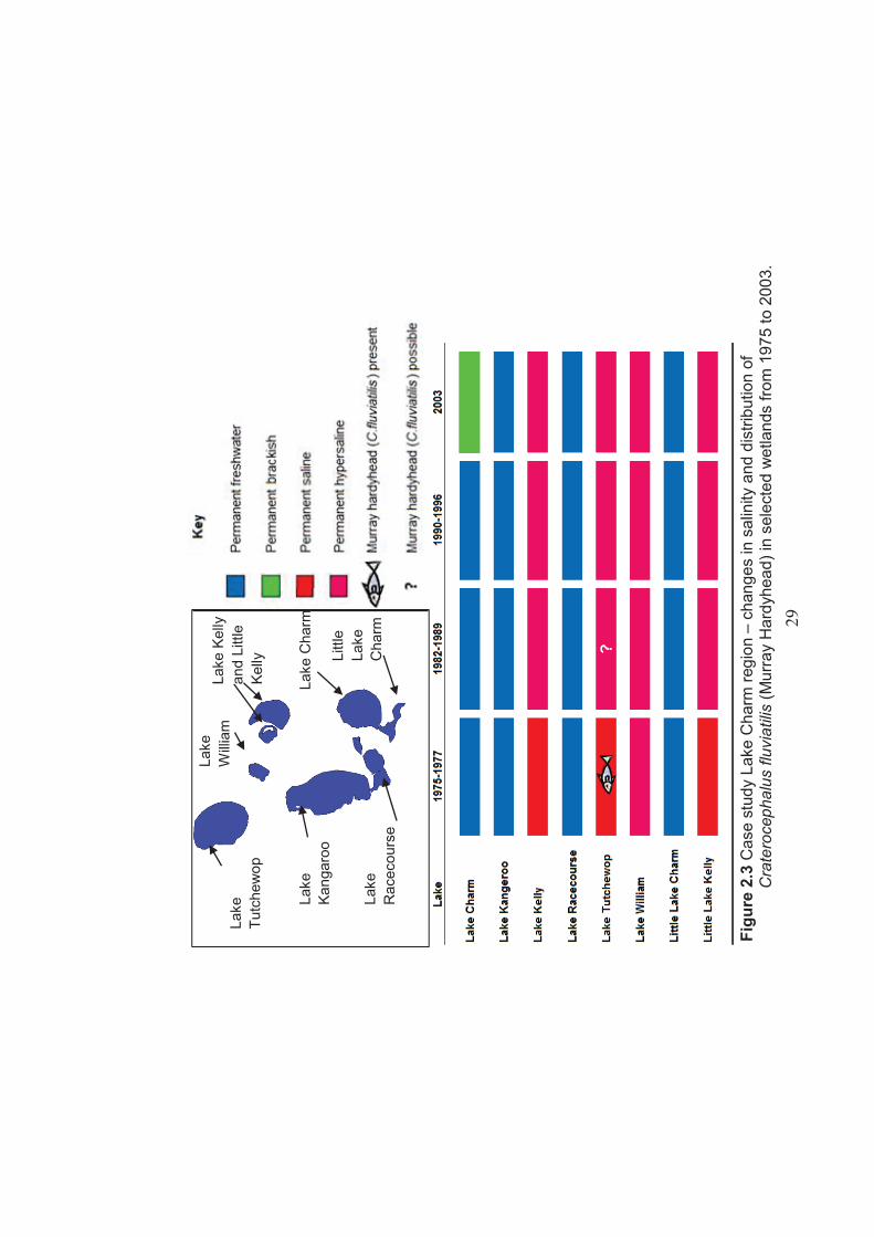
29
Lake
Tu
tche
wop
Lake
W
illiam
La
ke K
elly
an
d Li
ttle
Kelly
Lake
Ka
ngar
oo
Lake
Cha
rm
Lake
R
acec
ours
e
Littl
e La
ke
Cha
rm
Fi
gure
2.3
Cas
e st
udy
Lake
Cha
rm re
gion
– c
hang
es in
sal
inity
and
dis
tribu
tion
of
Cra
tero
ceph
alus
fluv
iatil
is(M
urra
y H
ardy
head
) in
sele
cted
wet
land
s fro
m 1
975
to 2
003.
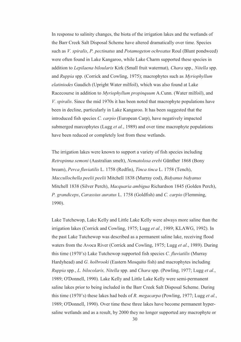
30
In response to salinity changes, the biota of the irrigation lakes and the wetlands of
the Barr Creek Salt Disposal Scheme have altered dramatically over time. Species
such as V. spiralis, P. pectinatus and Potamogeton ochreatus Roul (Blunt pondweed)
were often found in Lake Kangaroo, while Lake Charm supported these species in
addition to Lepilaena biloularis Kirk (Small fruit watermat), Chara spp., Nitella spp.
and Ruppia spp. (Corrick and Cowling, 1975); macrophytes such as Myriophyllum
elatiniodes Gaudich (Upright Water milfoil), which was also found at Lake
Racecourse in addition to Myriophyllum propinquum A.Cunn. (Water milfoil), and
V. spiralis. Since the mid 1970s it has been noted that macrophyte populations have
been in decline, particularly in Lake Kangaroo. It has been suggested that the
introduced fish species C. carpio (European Carp), have negatively impacted
submerged marcophytes (Lugg et al., 1989) and over time macrophyte populations
have been reduced or completely lost from these wetlands.
The irrigation lakes were known to support a variety of fish species including
Retropinna semoni (Australian smelt), Nematolosa erebi Günther 1868 (Bony
bream), Perca fluviatilis L. 1758 (Redfin), Tinca tinca L. 1758 (Tench),
Maccullochella peelii peelii Mitchell 1838 (Murray cod), Bidyanus bidyanus
Mitchell 1838 (Silver Perch), Macquaria ambigua Richardson 1845 (Golden Perch),
P. grandiceps, Carassius auratus L. 1758 (Goldfish) and C. carpio (Flemming,
1990).
Lake Tutchewop, Lake Kelly and Little Lake Kelly were always more saline than the
irrigation lakes (Corrick and Cowling, 1975; Lugg et al., 1989; KLAWG, 1992). In
the past Lake Tutchewop was described as a permanent saline lake, receiving flood
waters from the Avoca River (Corrick and Cowling, 1975; Lugg et al., 1989). During
this time (1970’s) Lake Tutchewop supported fish species C. fluviatilis (Murray
Hardyhead) and G. holbrooki (Eastern Mosquito fish) and macrophytes including
Ruppia spp., L. bilocolaris, Nitella spp. and Chara spp. (Powling, 1977; Lugg et al.,
1989; O'Donnell, 1990). Lake Kelly and Little Lake Kelly were semi-permanent
saline lakes prior to being included in the Barr Creek Salt Disposal Scheme. During
this time (1970’s) these lakes had beds of R. megacarpa (Powling, 1977; Lugg et al.,
1989; O'Donnell, 1990). Over time these three lakes have become permanent hyper-
saline wetlands and as a result, by 2000 they no longer supported any macrophyte or

31
fish species (Hardie, 2000). In contrast, Lake William, the fourth wetland of the Barr
creek salt disposal scheme, has always been a hypersaline with no macrophyte or fish
species present in the past and has changed very little over time (Powling, 1977;
Lugg et al., 1989; O'Donnell, 1990).
Lake Boga region The wetlands included in this case study include: Lake Boga, Lake Golf Course,
Round Lake, and Long Lake. Lake Boga was the only wetland connected to the
Torrumbarry Irrigation Scheme and as such was classed as a permanent freshwater
lake (1975 to 2003) (KLAWG, 1992). Little is known of the macrophytes present in
this wetland, but it supports a range of fish species including C. fluviatilis, R. semoni,
N. erebi, P. fluviatilis, T. tinca, M. peelii peelii, B. bidyanus, M. ambigua, C. auratus
and C. carpio. It no longer supports C. fluviatilis, and the reason for its
disappearance is not known (Lugg et al., 1989; Flemming, 1990; O'Donnell, 1990;
KLAWG, 1992; Cottingham, 1996) (Figure 2.4).
In the past Long Lake, Lake Golf Course and Round Lakes were used for storing
saline tile drain waters from the nearby Tresco farming region (KLAWG, 1992). Tile
drains are networks of small drains designed to collect and drain sub surface waters
away from irrigated fields (Swinton et al., 2000). All three lakes were known to
support macrophytes such as, Ruppia spp. and the fish species C. fluviatilis. It should
be noted that fish were recorded at Long and Golf Course Lakes as Craterocephalus
eyresii Steindachner 1883 (Lake Eyre Hardyhead). Given advances in taxonomy
however it is more likely that these populations were C. fluviatilis (Crowley and
Ivantsoff, 1990). More recently both Long Lake and Golf Course Lake have dried
out. Long Lake is considered to habe become a semi-permanent hypersaline wetland
and Gold Course Lake has become a semi-permanent, saline wetland resulting in the
loss of this fish species (Tunbridge and Glennane, 1984; Flemming, 1990).
In 2003, Round Lake was still classed as a permanent saline wetland and continued
to receive tile drain water run off. Unlike many other saline wetlands in the region,
Round Lake is not a terminal lake and excess water flows into Lake Golf Course, so
salinity concentrations within Round Lake remain relatively stable. It is believed that
populations of Ruppia spp. and C. fluviatilis still exist within this lake (Lyon et al.,
2002; Backhouse et al., 2006) (Figure 2.4).

32
Long
Lak
e La
ke B
oga
Lake
Gol
f C
ours
e
Rou
nd
Lake
Fi
gure
2.4
Cas
e st
udy
Lake
Bog
a re
gion
- ch
ange
s in
sal
inity
and
dis
tribu
tion
of
Cra
tero
ceph
alus
fluv
iatil
is (M
urra
y H
ardy
head
) in
sele
cted
wet
land
s fro
m 1
975
- 200
3.
33
As shown in Figures 2.2 to 2.4, many of the wetlands discussed have changed
dramatically since European settlement and in particular the construction of the
Torrumbarry Irrigation Scheme (Corrick and Cowling, 1975; Powling, 1977;
Tunbridge and Glennane, 1984; Lugg et al., 1989; Flemming, 1990; O'Donnell,
1990; KLAWG, 1992; Cottingham, 1996; Hardie, 2000). Given that these wetlands
are now completely cut off from their floodplain and associated rivers, and are
managed for a number of anthropogenic uses, it is imperative that we understand the
biota of these systems and their response to disturbance, in order to maintain
biodiversity whilst balancing the needs of surrounding landholders. For C. fluviatilis
in particular, the appropriate management of the few lakes that still support
populations of this fish is vital for their survival within Victoria and even perhaps
Australia (Backhouse et al., 2006).
2.1.2 Hypotheses This chapter investigates the biota of four wetlands of intermediate salinity in north
western Victoria, these are: Lake Elizabeth, Round Lake, Woorinen North Lake, and
Lake Hawthorn, all of which are known to support populations of C. fluviatilis. The
hypotheses tested in this study were:
Are C. fluviatilis (Murray Hardyhead) populations present within these
wetlands of intermediate salinity?
Which submerged aquatic macrophytes are associated with C. fluviatilis
(Murray Hardyhead) populations?
What are the salinity thresholds for C. fluviatilis (Murray Hardyhead)
populations

34
2.2 Methods
Aquatic flora and fauna were investigated in four lakes in northwestern Victoria:
Lake Elizabeth (near Kerang), Round Lake (near Lake, Boga), Lake Woorinen (near
Swan Hill), and Lake Hawthorn (near Mildura) (Figure 2.5). These lakes were
selected for this study because: they contained water, were of intermediate salinity
(between 10 g/L and 50 g/L) and were sites where C. fluviatilis (Murray Hardyhead)
and submerged aquatic macrophyte populations had been recorded since the
hydrology of the lakes was modified by their incorporation into the various irrigation
schemes. All field studies were conducted from July to August 2005.
2.2.1 Site descriptions Lake Elizabeth Lake Elizabeth is approximately 10 km northwest of Kerang in Victoria and is
around 94 hectares in size (Lugg et al., 1989) (Figure 2.6). Lake Elizabeth is a
terminal lake, connected to the Torrumbarry Irrigation Scheme via the Macorna
channel (Lugg et al., 1989). This lake was used for storing irrigation waters for
surrounding farms until in the 1970s. Subsequently the underlying saline water table
rose as a result and the lake changed from permanent freshwater to being a
permanent saline lake (Kelly, 1996). Lake Elizabeth is 94 hectares in size and has an
average depth of > 2 meters (Kelly, 1996).
Lake Elizabeth is surrounded by scattered areas of Eucalyptus largiflorens F. Muell
(Black box) and extensive areas of chenopod shrub land and a reed bed community
dominated by the introduced Juncus acutus L. (Spiny rush) (Figure 2.6). The aquatic
plant community of this lake has been surveyed in the past and Ruppia spp. and
charophytes were recorded (Lugg et al., 1989; Kelly, 1996).

35
Fi
gure
2.5
Loc
atio
n of
Lak
e E
lizab
eth,
Rou
nd L
ake,
Woo
rinen
Nor
th L
ake
and
Lake
Haw
thor
n in
nor
th w
este
rn V
icto
ria (n
ot to
sca
le),
mod
ified
from
D
epar
tmen
t of S
usta
inab
ility
and
Envi
ronm
ent (
2010
)
Key
W
etla
nds
surv
eyed
Oth
er w
etla
nds
Maj
or T
owns
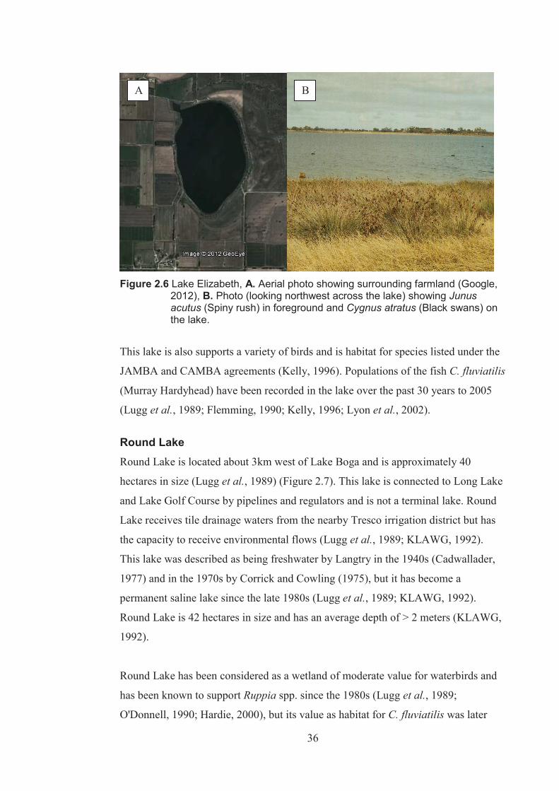
36
Figure 2.6 Lake Elizabeth, A. Aerial photo showing surrounding farmland (Google,
2012), B. Photo (looking northwest across the lake) showing Junus acutus (Spiny rush) in foreground and Cygnus atratus (Black swans) on the lake.
This lake is also supports a variety of birds and is habitat for species listed under the
JAMBA and CAMBA agreements (Kelly, 1996). Populations of the fish C. fluviatilis
(Murray Hardyhead) have been recorded in the lake over the past 30 years to 2005
(Lugg et al., 1989; Flemming, 1990; Kelly, 1996; Lyon et al., 2002).
Round Lake Round Lake is located about 3km west of Lake Boga and is approximately 40
hectares in size (Lugg et al., 1989) (Figure 2.7). This lake is connected to Long Lake
and Lake Golf Course by pipelines and regulators and is not a terminal lake. Round
Lake receives tile drainage waters from the nearby Tresco irrigation district but has
the capacity to receive environmental flows (Lugg et al., 1989; KLAWG, 1992).
This lake was described as being freshwater by Langtry in the 1940s (Cadwallader,
1977) and in the 1970s by Corrick and Cowling (1975), but it has become a
permanent saline lake since the late 1980s (Lugg et al., 1989; KLAWG, 1992).
Round Lake is 42 hectares in size and has an average depth of > 2 meters (KLAWG,
1992).
Round Lake has been considered as a wetland of moderate value for waterbirds and
has been known to support Ruppia spp. since the 1980s (Lugg et al., 1989;
O'Donnell, 1990; Hardie, 2000), but its value as habitat for C. fluviatilis was later
A B
37
recognised when this species was recorded there in 1999 and 2000 (Hardie, 2000). A
previous study by Flemming (1990) found no fish species in the lake.
Figure 2.7 Round Lake, A. Aerial photo showing surrounding farmland (Google,
2012), B. Photo (looking southwest across the lake) showing Junus acutus (Spiny rush) in foreground and numerous Cygnus atratus (Black Swans) on the lake.
Woorinen North Lake Woorinen North Lake is located between Swan Hill and Nyah in northwest Victoria,
and in the past was used a drainage lake for the surrounding irrigated farms of the
Woorinen area (Lugg et al., 1989; Lyon et al., 2002) (Figure 2.8). This lake once
received runoff from surrounding farms as well as surplus irrigation flows. But in
2003 a pipeline was constructed in the area to reduce water loss by evaporation from
existing open irrigation channels. Since then an annual environmental water
allocation has been pumped to Woorinen North Lake. This lake is not a terminal lake
and when water concentrations are high, water flows through to another nearby
drainage lake (Hollway’s basin) (Lugg et al., 1989; Lyon et al., 2002). Woorinen
North Lake is 63 hectares in size and has an average depth of less than 2 meters
(Lyon et al., 2002).
There is very little riparian vegetation surrounding Woorinen North Lake, but the
lake has been surveyed and a submerged aquatic vegetation community consisting of
Ruppia spp. has been recorded (Lugg et al., 1989; Lyon et al., 2002). This lake is
also an important habitat for waterbirds and bird species listed under the JAMBA and
CAMBA agreements have been recorded there. Populations of C. fluviatilis have also
been recorded at Woorinen North Lake in the past 20 years (Lugg et al., 1989; Lyon
et al., 2002).
A B
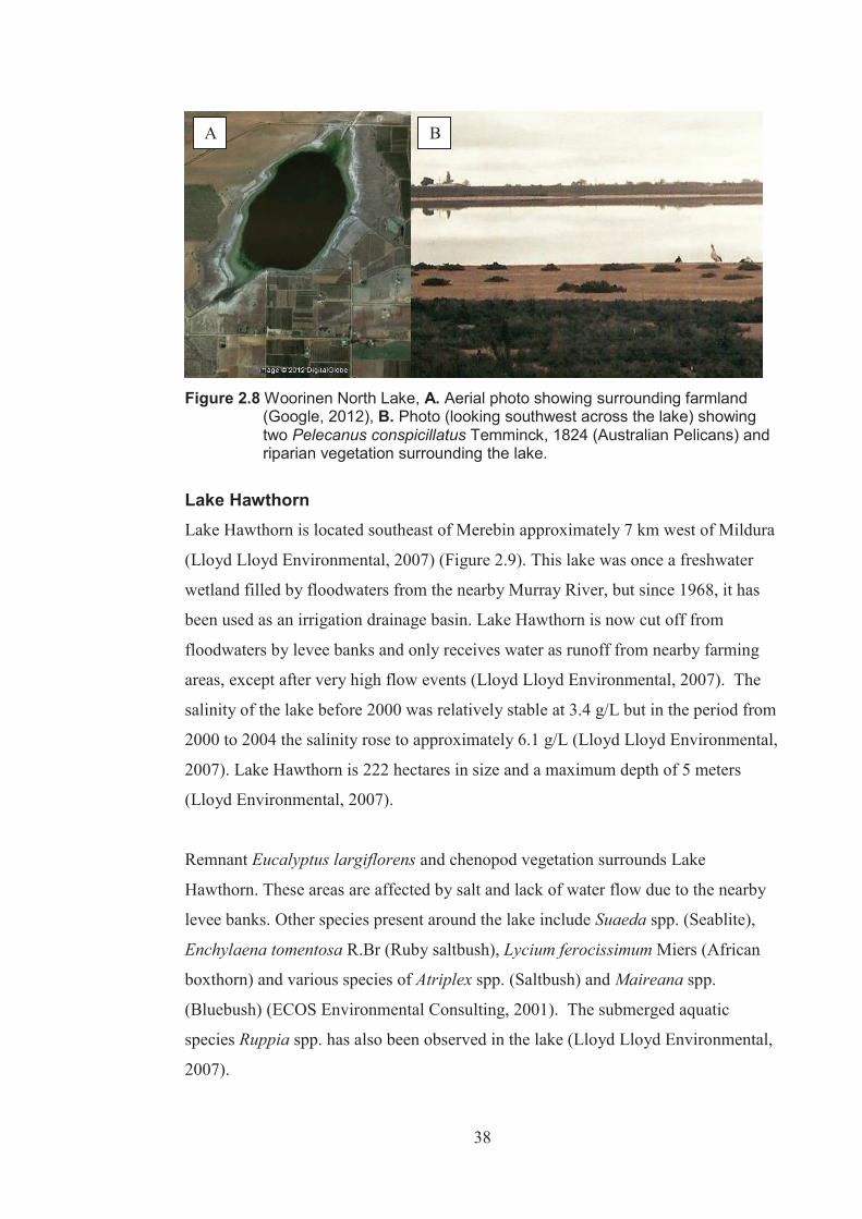
38
Figure 2.8 Woorinen North Lake, A. Aerial photo showing surrounding farmland
(Google, 2012), B. Photo (looking southwest across the lake) showing two Pelecanus conspicillatus Temminck, 1824 (Australian Pelicans) and riparian vegetation surrounding the lake.
Lake Hawthorn Lake Hawthorn is located southeast of Merebin approximately 7 km west of Mildura
(Lloyd Lloyd Environmental, 2007) (Figure 2.9). This lake was once a freshwater
wetland filled by floodwaters from the nearby Murray River, but since 1968, it has
been used as an irrigation drainage basin. Lake Hawthorn is now cut off from
floodwaters by levee banks and only receives water as runoff from nearby farming
areas, except after very high flow events (Lloyd Lloyd Environmental, 2007). The
salinity of the lake before 2000 was relatively stable at 3.4 g/L but in the period from
2000 to 2004 the salinity rose to approximately 6.1 g/L (Lloyd Lloyd Environmental,
2007). Lake Hawthorn is 222 hectares in size and a maximum depth of 5 meters
(Lloyd Environmental, 2007).
Remnant Eucalyptus largiflorens and chenopod vegetation surrounds Lake
Hawthorn. These areas are affected by salt and lack of water flow due to the nearby
levee banks. Other species present around the lake include Suaeda spp. (Seablite),
Enchylaena tomentosa R.Br (Ruby saltbush), Lycium ferocissimum Miers (African
boxthorn) and various species of Atriplex spp. (Saltbush) and Maireana spp.
(Bluebush) (ECOS Environmental Consulting, 2001). The submerged aquatic
species Ruppia spp. has also been observed in the lake (Lloyd Lloyd Environmental,
2007).
A B

39
This lake provides habitat for native fish including C. fluviatilis (Murray Hardyhead),
C. sterc. fulvus (Unspeked Hardyhead) Hypseleotris spp. (Carp Gudgeons), N. erebi
(Boney bream), P. grandiceps (Flat Headed Gudgeon), and M. ambigua (Golden
Perch). Lake Hawthorn also supports the introduced fish species G. holbooki
(Eastern Mosquito Fish) and C. carpio (Common Carp) (ECOS Environmental
Consulting, 2001). Other vertebrates including three turtle species; Chelodina
expansa Gray 1857 (Broad Shelled Turtle), Chelodina longicollis Shaw 1794
(Eastern Long-Necked Turtle) and Emydura macquarii Gray 1830 (Murray Turtle),
as well as Cherax spp. (Yabbies), shrimp, and prawns. Up to 60 species of waterbirds
are also found in and around this lake (ECOS Environmental Consulting, 2001).
Figure 2.9 Lake Hawthorn, A. Aerial photo showing surrounding farmland (Google,
2012), B. Photo (looking southwest across the lake) showing Junus acutus (Spiny rush) in foreground.
2.2.2 Water quality Water quality parameters were assessed at four sites around each wetland. Sites were
selected by marking out 12 points on a map of each lake like a clock face (Figure
2.10) and using four random numbers (from 1 to 12, Appendix 1) to specify the sites.
At each of these sites salinity (g/L), dissolved oxygen (mg/L), water temperature
(oC), and pH were measured using an Orion Multimeter Model No. 1230. Turbidity
(NTU) was measured using a turbidity tube. Nutrient analysis was also carried out to
at each site to determine the total phosphates (mg/L) and total nitrates (mg/L) of the
water using a Palintest Nutrient Analysis kit, following manufacturer’s instructions.
A B

40
Figure 2.10 Random selection of sites for water quality measurements using a table
of random numbers and a clock face method.
2.2.3 Aquatic macrophytes – belt transects Percentage cover, dry weight biomass (g) and biovolume (mL), of aquatic
macrophytes were assessed along belt transects within the lakes. The size of quadrats
used in the belt transects was determined by completing a species area curve at 8
random sites within each lake. Quadrat sizes tested were 0.25m2, 1m2, 4m2, 9 m2, 16
m2, and 25 m2. A 0.5 meter by 0.5 metre (0.25m2) quadrat proved to be most
appropriate for all lakes surveyed (Appendix 2).
Four 0.5m wide and 15m long belt transects were established perpendicular to the
shoreline at the same sites where water quality was assessed at each lake to
investigate how plant density responded to water depth (transects A, B, C and D). A
further two 0.5 meter wide and 15m long belt transects were run parallel to the shore
to assess how plant density varied across the lake (transects E and F). The sites for
the paraellel transects were next to two of the perpendicular transects (transects A
and C) (Figure 2.11).
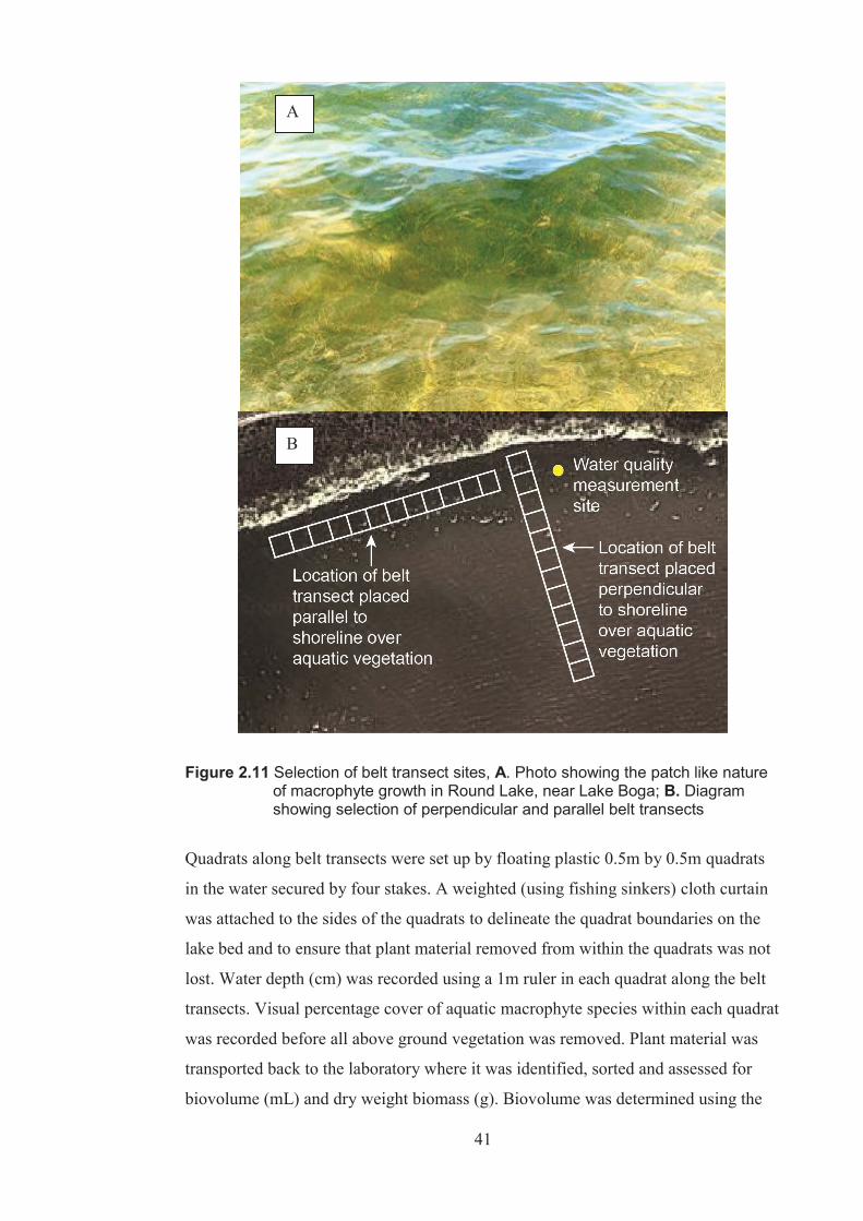
41
Figure 2.11 Selection of belt transect sites, A. Photo showing the patch like nature
of macrophyte growth in Round Lake, near Lake Boga; B. Diagram showing selection of perpendicular and parallel belt transects
Quadrats along belt transects were set up by floating plastic 0.5m by 0.5m quadrats
in the water secured by four stakes. A weighted (using fishing sinkers) cloth curtain
was attached to the sides of the quadrats to delineate the quadrat boundaries on the
lake bed and to ensure that plant material removed from within the quadrats was not
lost. Water depth (cm) was recorded using a 1m ruler in each quadrat along the belt
transects. Visual percentage cover of aquatic macrophyte species within each quadrat
was recorded before all above ground vegetation was removed. Plant material was
transported back to the laboratory where it was identified, sorted and assessed for
biovolume (mL) and dry weight biomass (g). Biovolume was determined using the
A
B
42
Archimedes’ Principle of the displacement of liquid wich states that the amount of
water displaced by a submerged object is equal to the volume of that object in water
(Pickover, 2008). The biovolume measurement gives an indication of the space
(volume) that submerged aquatic take up in the water column and has been used in
previous studies of aquatic macrophytes (Valley and Drake, 2007; Valley et al.,
2010). The biovolume of each species was determined by placing the plant material
in a measuring cylinder of appropriate volume, depending on the amount of
vegetation present. Then a known amount of water was added to the cylinder. The
total volume of water and vegetation was recorded and the biovolume of the plant
sample was determined using the following equation:
Plant Biovolume (mL) = Total volume of plants and water – Volume of water added to
measuring cylinder
To determine the dry weight of the biomass (g), vegetation was removed from the
cylinder and left to drain. Drained plant material was placed in a paper bag of known
weight that had been dried in an oven 70oC for 48 hours. Bags were reweighed and
the dry weight biomass was determined using the equation below:
Dry weight biomass (g) = Total dry weight of plants and bag – Weight of pre dried bag
2.2.4 Aquatic macrophytes – boat survey While the belt transects are useful for determining the biovolume and biomass of
aquatic macrophytes, they can only be used in shallow waters. It is much more
difficult to determine the density and biomass of plants in deeper waters, a visual
assessment of plant cover was conducted from a boat. A 0.5m by 0.5m quadrat was
floated on the side of an anchored boat at 100 random points in each lake. At each
point total percentage cover of all macrophytes was recorded, because it was not
possible to distinguish individual species in deep water.
2.2.5 Murray Hardyhead fish survey A fish survey was conducted at the first three water quality monitoring sites in each
lake. At each site 3 seine net hauls were conducted using a 10m long, 1mm mesh
seine net. The live fish were caught by extending the entire length of the net from the

43
shore out into the water. The net was pulled approximately 10 metres parallel to the
shore, over submerged macrophytes, before being pulled in a horseshoe shape until
both ends met back at the shore. The net was then removed from the water and any
fish caught were transferred to an aerated tank, where they were sedated using
Alphaxon Quatazone, injected into the tank (1.5mL per 10 L of water). The first 100
Murray Hardyhead (C. fluviatilis) individuals caught at each wetland were measured
for fork length (Figure 2.12). In accordance with animal ethics, no more than 100
Murray Hardyhead from any wetland were measured during this survey. Any other
fish species caught were identified and the total length of the fish measured (Figure
2.12). Forked length is the preferred measurement in fish species with a forked tail,
as the measurement is not biased by any damage the individual fish may sustain to
the end of the tail (Jennings et al., 2001).
Figure 2.12 Diagram showing measurement methods used in fish survey for
forked tailed fish (left), and those without a forked tail (right)
All fish were returned live to the lake at the site where they were caught. Fish were
handled using “wet” gloves to prevent any stress or damage to their scales. They
were also given an antifungal wash to reduce the chance of infection, prior to being
released at the site where they were captured.
2.2.6 Data Analysis The mean percentage cover of awautic macrophytes determined in the boat survey
was analysed using a One way ANOVA using the following model:
ModelDV = constant + Lake Location Where the results of the ANOVA indicated that there was a significant difference
between lakes, a post hoc Tukeys test was undertaken to determine which lakes
differed significantly in percentage cover of aquatic macrophytes. All data analysis
was undertaken using the PASW 18 statistical software (previously known as SPSS).

44
2.3 Results
2.3.1 Water quality As shown in Table 2.1, the mean salinity of the four lakes varied greatly with the
freshest wetland being Lake Hawthorn (mean salinity 8.2 g/L ± 0.023 g/L S.E) and
the saltiest Lake Elizabeth (mean salinity 29.3 g/L ± 0.48 g/L S.E). The turbidity of
the wetlands also varied with the saltier lakes (Round Lake and Lake Elizabeth)
being clearer (mean turbidity concentrations 0 to 3 NTU respectively) than the
fresher lakes (Lake Hawthorn and Woorinen North Lake) with mean turbidity
concentrations of 29 and 34 NTUs respectively. The pH and dissolved oxygen results
were similar across the four lakes with means ranging from pH of 8.2 to 8.8 and
dissolved oxygen 8.6 mg/L to 9.6 mg/L. Mean phosphate concentrations were quite
low at each lake, with mean phosphate concentrations ≤ 0.1 mg/L, with the exception
of Woorinen North (0.3 mg/L ± 0.1 mg/L S.E). Mean nitrate concentrations varied
across the different lakes with lower concentrations recorded at Lake Hawthorn and
Lake Elizabeth and mean concentrations > 1.5 mg/L recorded at Round Lake and
Woorinen North Lake (Table 2.1).
Table 2.1 Water quality results for four lakes of intermediate salinity in northwest
Victoria, figures shown are means (± standard error).
Lake Salinity (g/L)
Turbidity (NTU)
pH
DO
(mg/L) Phosphates
(mg/L) Nitrates (mg/L)
Hawthorn
8.2 (±<0.1)
28.8 (± 4.19)
8.6 (± 0.1)
8.6 (± 0.5)
< 0.1 (±<0.1)
0.93 (± 0.18)
Woorinen North
15.2 (±0.3)
33.5 (± 8.46)
8.2 (± 0.3)
9.4 (± 0.2)
0.3 (± 0.1)
1.56 (± 0.32)
Round
22.0 (±0.2)
0.0 (± 0)
8.6 (± 0.1)
9.1 (± 0.3)
0.1 (±<0.1)
2.17 (± 0.57)
Elizabeth
29.3 (±0.5)
2.5 (± 2.5)
8.8 (± 0.1)
9.6 (± 0.2)
<0.1 (± <0.1)
0.98 (±0.32)

45
2.3.2 Aquatic macrophytes Lake Elizabeth Two species of aquatic plants were present at Lake Elizabeth, both being submerged
macrophytes R. megacarpa and L. macropogon. Lake vegetation in all transects
except Transect C, was found to be continuous with vegetation present in the
majority of quadrats with the exception of those close to the shore (Table 2.2 and
Table 2.3). Although the vegetation was thick and continuous in many parts of the
lake, the biovolume and dry weight biomass of both species was found to be
“patchy” with no obvious pattern between increasing depth and the amount of
vegetation present (Appendix 3). This lack of relationship was also found with the
parallel transects where vegetation in terms of biomass and biovolume varied across
very similar depths and percentage cover (Appendix 3). The lake vegetation was very
thick in Transect A, with up to 10 000 mL of biovolume and > 700 g of dry weight
biomass being recorded in some quadrats. R. megacarpa was the dominant species in
the lake, contributing approximately 90% of overall biovolume and biomass in many
quadrats (Table 2.4).

46
Tabl
e 2.
2 La
ke E
lizab
eth
belt
trans
ects
– p
rese
nce/
abse
nce
of R
uppi
a m
egac
arpa
in th
e la
ke
Ke
y
Abs
ence
of s
peci
es
P
rese
nce
of s
peci
es
Tran
sect
1
2 3
4 5
6 7
8 9
10
11
12
13
14
15
A - p
erpe
ndicu
lar
B
- per
pend
icular
C - p
erpe
ndicu
lar
D
- per
pend
icular
E – p
arall
el
F – p
arall
el
Tabl
e 2.
3 La
ke E
lizab
eth
belt
trans
ects
– p
rese
nce/
abse
nce
of L
ampr
otha
mni
um m
acro
pogo
n in
the
lake
Tr
anse
ct
1 2
3 4
5 6
7 8
9 10
11
12
13
14
15
A
- per
pend
icular
B - p
erpe
ndicu
lar
C
- per
pend
icular
D - p
erpe
ndicu
lar
E
– par
allel
F
– par
allel
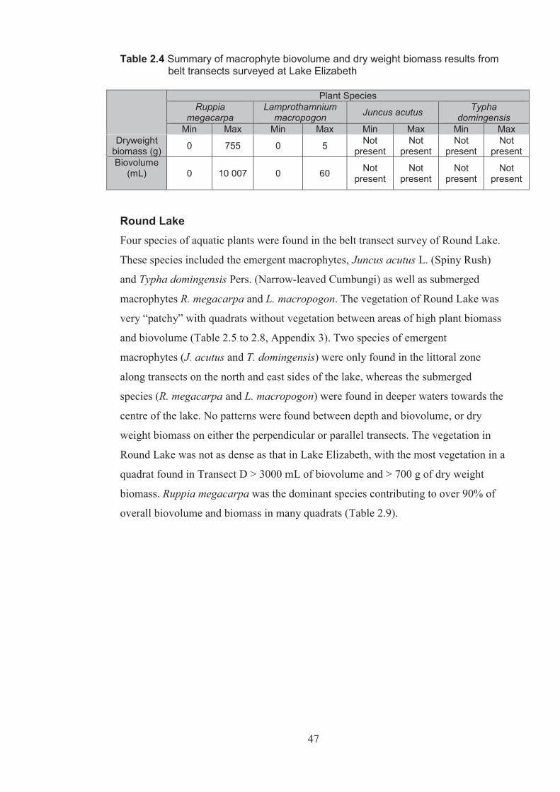
47
Table 2.4 Summary of macrophyte biovolume and dry weight biomass results from belt transects surveyed at Lake Elizabeth
Plant Species Ruppia
megacarpa Lamprothamnium
macropogon Juncus acutus Typha domingensis
Min Max Min Max Min Max Min Max Dryweight
biomass (g) 0 755 0 5 Not present
Not present
Not present
Not present
Biovolume (mL)
0 10 007 0 60 Not
present Not
present Not
present Not
present
Round Lake Four species of aquatic plants were found in the belt transect survey of Round Lake.
These species included the emergent macrophytes, Juncus acutus L. (Spiny Rush)
and Typha domingensis Pers. (Narrow-leaved Cumbungi) as well as submerged
macrophytes R. megacarpa and L. macropogon. The vegetation of Round Lake was
very “patchy” with quadrats without vegetation between areas of high plant biomass
and biovolume (Table 2.5 to 2.8, Appendix 3). Two species of emergent
macrophytes (J. acutus and T. domingensis) were only found in the littoral zone
along transects on the north and east sides of the lake, whereas the submerged
species (R. megacarpa and L. macropogon) were found in deeper waters towards the
centre of the lake. No patterns were found between depth and biovolume, or dry
weight biomass on either the perpendicular or parallel transects. The vegetation in
Round Lake was not as dense as that in Lake Elizabeth, with the most vegetation in a
quadrat found in Transect D > 3000 mL of biovolume and > 700 g of dry weight
biomass. Ruppia megacarpa was the dominant species contributing to over 90% of
overall biovolume and biomass in many quadrats (Table 2.9).

48
Tabl
e 2.
5 R
ound
Lak
e be
lt tra
nsec
ts –
pre
senc
e/ab
senc
e of
Rup
pia
meg
acar
pa in
the
lake
Key
Ab
senc
e of s
pecie
s
Pres
ence
of sp
ecies
Tran
sect
1
2 3
4 5
6 7
8 9
10
11
12
13
14
15
A – p
erpe
ndicu
lar
B
– per
pend
icular
C – p
erpe
ndicu
lar
D
– per
pend
icular
E – p
arall
el
F – p
arall
el
Tabl
e 2.
6 R
ound
Lak
e be
lt tra
nsec
ts –
pre
senc
e/ab
senc
e of
Lam
prot
ham
nium
mac
ropo
gon
in th
e la
ke
Tran
sect
1
2 3
4 5
6 7
8 9
10
11
12
13
14
15
A – p
erpe
ndicu
lar
B
– per
pend
icular
C – p
erpe
ndicu
lar
D
– per
pend
icular
E – p
arall
el
F – p
arall
el
Tabl
e 2.
7 R
ound
Lak
e be
lt tra
nsec
ts –
pre
senc
e/ab
senc
e of
Typ
ha d
omin
gens
is in
the
lake
Tr
anse
ct
1 2
3 4
5 6
7 8
9 10
11
12
13
14
15
A
– per
pend
icular
B – p
erpe
ndicu
lar
C
– per
pend
icular
D – p
erpe
ndicu
lar
E
– par
allel
F
– par
allel
Ta
ble
2.8
Rou
nd L
ake
belt
trans
ects
– p
rese
nce/
abse
nce
of J
uncu
s ac
utus
in th
e la
ke
Tran
sect
1
2 3
4 5
6 7
8 9
10
11
12
13
14
15
A – p
erpe
ndicu
lar
B
– per
pend
icular
C – p
erpe
ndicu
lar
D
– per
pend
icular
E – p
arall
el
F – p
arall
el

49
Table 2.9 Summary of macrophyte biovolume and dry weight biomass results from
belt transects surveyed at Round Lake
Plant Species
Ruppia megacarpa Lamprothamnium macropogon Juncus acuta Typha
domingensis Min Max Min Max Min Max Min Max
Dryweight biomass (g) 0 702 0 6 0 86 0 392
Biovolume (mL)
0 2995 0 64 0 290 0 1174
Woorinen North Lake Only one aquatic macrophyte was present at Woorinen North Lake, the submerged
species R. megacarpa. Density and percentage cover of vegetation at this lake was
very patchy and much lower than all other lakes. In fact many quadrats were devoid
of vegetation between areas of R.megacarpa growth (Table 2.10, Appendix 3). No
patterns were found between depth and biovolume or dry weight biomass on either
the perpendicular or parallel transects. The biovolume and dry weight biomass found
in this lake was much lower than all other lakes with a maximum of 1064 mL
biovolume and a maximum of 755g dry weight biomass measures in any quadrat
(Table 2.11).
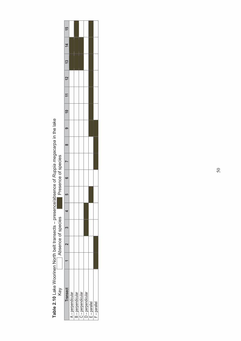
50
Tabl
e 2.
10 L
ake
Woo
rinen
Nor
th b
elt t
rans
ects
– p
rese
nce/
abse
nce
of R
uppi
a m
egac
arpa
in th
e la
ke
Ke
y
Abs
ence
of s
peci
es
P
rese
nce
of s
peci
es
Tran
sect
1
2 3
4 5
6 7
8 9
10
11
12
13
14
15
A – p
erpe
ndicu
lar
B
– per
pend
icular
C – p
erpe
ndicu
lar
D
– per
pend
icular
E – p
arall
el
F – p
arall
el

51
Table 2.11 Summary of macrophyte biovolume and dry weight biomass results from belt transects surveyed at Lake Woorinen North
Plant Species
Ruppia megacarpa Lamprothamnium macropogon Juncus acutus Typha
domingensis Min Max Min Max Min Max Min Max
Dryweight biomass (g) 0 755 Not
present Not
present Not
present Not
present Not
present Not
present Biovolume
(mL)
0 1064 Not present
Not present
Not present
Not present
Not present
Not present
Lake Hawthorn Three macrophytes were found in the belt transect survey of Lake Hawthorn. Species
included the emergent macrophyte, T. domingensis and submerged macrophytes R.
megacarpa and L. macropogon. The vegetation of Lake Hawthorn was very “patchy”
with quadrats without vegetation between areas of dense vegetation (Table 2.12 to
2.14, Appendix 3). The emergent species T. domingensis was only found in the
littoral zone of the lake on Transect A, (on the east side of the lake), whereas the
submerged species were found in deeper waters towards the centre of the lake. No
patterns were found between depth and biovolume or dry weight biomass on either
the perpendicular or parallel transects. The vegetation was not as dense as that of
Lake Elizabeth, with the greatest vegetation cover found on Transect B with
> 2100 mL of biovolume and > 500g of dry weight biomass. Again R. megacarpa
was the dominant species contributing to over 90% of overall biovolume and
biomass in many quadrats (Table 2.15).
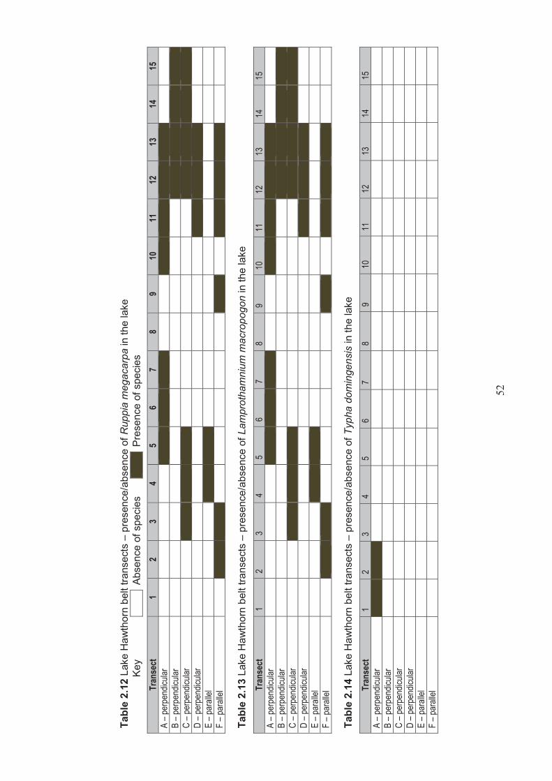
52
Tabl
e 2.
12 L
ake
Haw
thor
n be
lt tra
nsec
ts –
pre
senc
e/ab
senc
e of
Rup
pia
meg
acar
pa in
the
lake
Key
A
bsen
ce o
f spe
cies
Pre
senc
e of
spe
cies
Tran
sect
1
2 3
4 5
6 7
8 9
10
11
12
13
14
15
A – p
erpe
ndicu
lar
B
– per
pend
icular
C – p
erpe
ndicu
lar
D
– per
pend
icular
E – p
arall
el
F – p
arall
el
Tabl
e 2.
13 L
ake
Haw
thor
n be
lt tra
nsec
ts –
pre
senc
e/ab
senc
e of
Lam
prot
ham
nium
mac
ropo
gon
in th
e la
ke
Tran
sect
1
2 3
4 5
6 7
8 9
10
11
12
13
14
15
A – p
erpe
ndicu
lar
B
– per
pend
icular
C – p
erpe
ndicu
lar
D
– per
pend
icular
E – p
arall
el
F – p
arall
el
Tabl
e 2.
14 L
ake
Haw
thor
n be
lt tra
nsec
ts –
pre
senc
e/ab
senc
e of
Typ
ha d
omin
gens
is in
the
lake
Tr
anse
ct
1 2
3 4
5 6
7 8
9 10
11
12
13
14
15
A
– per
pend
icular
B – p
erpe
ndicu
lar
C
– per
pend
icular
D – p
erpe
ndicu
lar
E
– par
allel
F
– par
allel

53
Table 2.15 Summary of macrophyte biovolume and dry weight biomass results from belt transects surveyed at Lake Hawthorn
Plant Species
Ruppia megacarpa Lamprothamnium macropogon Juncus acutus Typha
domingensis Min Max Min Max Min Max Min Max
Dryweight biomass (g) 0 506 0 9 Not
present Not
present 0 189
Biovolume (mL)
0 2080 0 66 Not
present Not
present 0 548
Results from the boat based macrophyte survey showed that the mean percentage
cover varied for each lake, with the lowest mean cover recorded at Woorinen North
Lake and the highest at Round Lake (Figure 2.13). Results of a one way ANOVA
showed that there was a significant (p <0.01) difference in the mean percentage
cover of aquatic macrophytes between the lakes (p <0.001, F =37.281, df = 3, 396).
A post hoc Tukey’s test showed that there was a significant difference (p < 0.001)
between all the lakes surveyed with the exception of Lake Hawthorn and Lake
Elizabeth (Table 2.16).
Figure 2.13 Mean aquatic macrophyte % cover as observed from boat at the four
wetlands – Lake Elizabeth, Round Lake, Woorinen North Lake and Lake Hawthorn (n = 100).
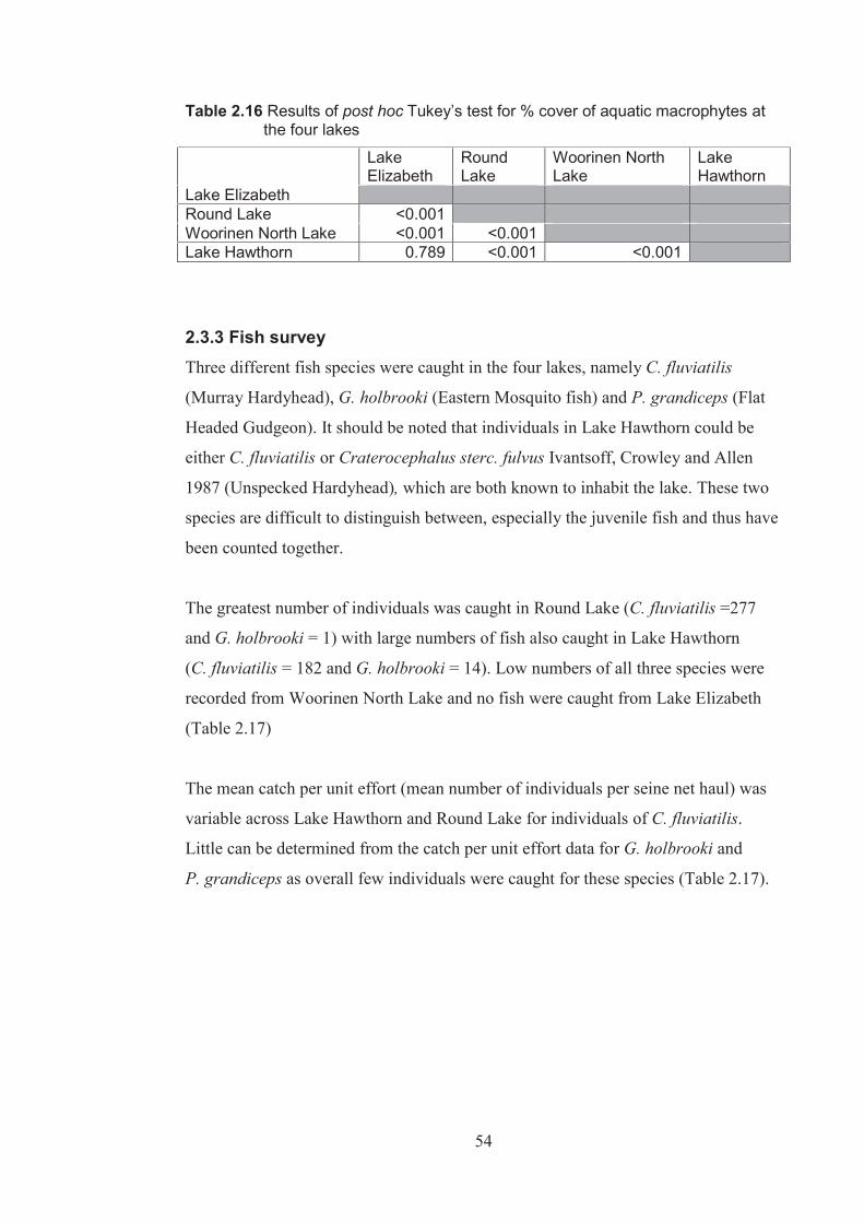
54
Table 2.16 Results of post hoc Tukey’s test for % cover of aquatic macrophytes at
the four lakes
Lake Elizabeth
Round Lake
Woorinen North Lake
Lake Hawthorn
Lake Elizabeth Round Lake <0.001 Woorinen North Lake <0.001 <0.001 Lake Hawthorn 0.789 <0.001 <0.001
2.3.3 Fish survey Three different fish species were caught in the four lakes, namely C. fluviatilis
(Murray Hardyhead), G. holbrooki (Eastern Mosquito fish) and P. grandiceps (Flat
Headed Gudgeon). It should be noted that individuals in Lake Hawthorn could be
either C. fluviatilis or Craterocephalus sterc. fulvus Ivantsoff, Crowley and Allen
1987 (Unspecked Hardyhead), which are both known to inhabit the lake. These two
species are difficult to distinguish between, especially the juvenile fish and thus have
been counted together.
The greatest number of individuals was caught in Round Lake (C. fluviatilis =277
and G. holbrooki = 1) with large numbers of fish also caught in Lake Hawthorn
(C. fluviatilis = 182 and G. holbrooki = 14). Low numbers of all three species were
recorded from Woorinen North Lake and no fish were caught from Lake Elizabeth
(Table 2.17)
The mean catch per unit effort (mean number of individuals per seine net haul) was
variable across Lake Hawthorn and Round Lake for individuals of C. fluviatilis.
Little can be determined from the catch per unit effort data for G. holbrooki and
P. grandiceps as overall few individuals were caught for these species (Table 2.17).
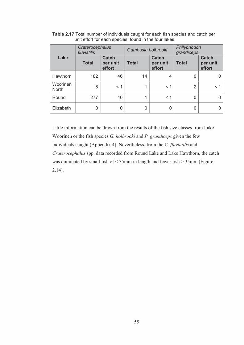
55
Table 2.17 Total number of individuals caught for each fish species and catch per unit effort for each species, found in the four lakes.
Lake
Craterocephalus fluviatilis Gambusia holbrooki Philypnodon
grandiceps
Total Catch per unit effort
Total Catch per unit effort
Total Catch per unit effort
Hawthorn 182 46 14 4 0 0
Woorinen North 8 < 1 1 < 1 2 < 1
Round 277 40 1 < 1 0 0
Elizabeth 0 0 0 0 0 0
Little information can be drawn from the results of the fish size classes from Lake
Woorinen or the fish species G. holbrooki and P. grandiceps given the few
individuals caught (Appendix 4). Nevertheless, from the C. fluviatilis and
Craterocephalus spp. data recorded from Round Lake and Lake Hawthorn, the catch
was dominated by small fish of < 35mm in length and fewer fish > 35mm (Figure
2.14).
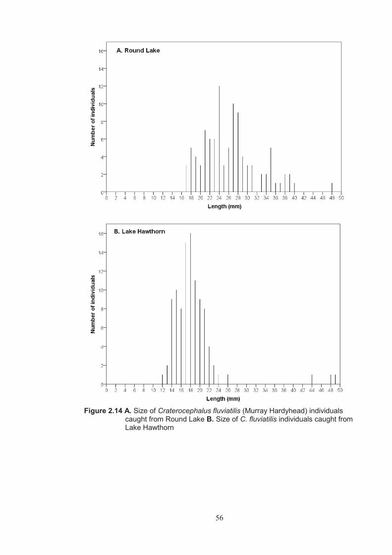
56
Figure 2.14 A. Size of Craterocephalus fluviatilis (Murray Hardyhead) individuals
caught from Round Lake B. Size of C. fluviatilis individuals caught from Lake Hawthorn
57
2.4 Discussion
All four lakes surveyed in this study were saline (ranging from 8.2 g/L ± <0.1 g/L
S.E to 29.3 g/L ± 0.5 g/L S.E) and supported few aquatic plants and fish species,
which is typical of saline lakes in Australia (Brock, 1986; Timms, 1993; Kingsford
and Porter, 1994). Whilst these lakes have low diversity of biota, they were found to
be similar to many other saline lakes in that they very productive with extensive
cover of submerged aquatic macrophytes (Timms, 1997).
2.4.1 Water quality The water quality results were similar to those recorded in other saline wetlands in
Australia with low turbidity (mean <34 NTU) and high pH (mean pH >8). High pH
levels have been recorded in lakes in western Victoria (Williams, 1981; Khan, 2003)
and in other desert salt lakes in New South Wales (Timms, 1993). Alkaline pH levels
have been linked to increased photosynthetic activity in inland waters (López-
Archilla et al., 2004), and given the high productivity of the wetlands is a plausible
explanation for the high pH levels recorded.
Turbidity concentrations < 30 NTU, are often found in saline lakes and have been
recorded in previous studies of saline lakes by Davis et al., (2003) and Timms
(1997). It should be noted that a number of factors including wind and time of day of
the testing can impact on turbidity readings and as such no conclusions can be drawn
from one assessment. But given the extensive cover of macrophytes in the wetlands
surveyed, especially Lake Elizabeth and Round Lake, light is probably not a limiting
factor for macrophyte distribution and growth.
Dissolved oxygen concentrations were not limiting to fish populations with mean
dissolved oxygen concentrations ranging between 8.6 mg/L to 9.6 mg/L across the
four lakes which is well above the ANZECC recommended minimum of 6 mg/L
(ANZECC and ARMCANZ, 2000).
Nutrient analysis of the wetlands indicated that phosphorus concentrations for Lake
Elizabeth, Lake Hawthorn and Round Lake were all within acceptable concentrations

58
as recommended for Australian waters with concentrations less than 0.05 mg/L
(ANZECC and ARMCANZ, 2000). Mean phosphate concentrations in Lake
Woorinen were 0.3 mg/L (± 0.1 mg/L S.E). This high concentration is probably due
to one sample, with a phosphate concentration of 0.7 mg/L being recorded. Although
it should be noted that many other samples had high phosphate concentrations of
between 0.1 and 0.3 mg/L.
Nitrate concentrations in these lakes were much higher than those recommended for
Australian waters (between 0.1 mg/L and 0.5 mg/L) (ANZECC and ARMCANZ,
2000). Results of this study varied between 1.0 mg/L (± 0.3 mg/L S.E) and 2.1 mg/L
(± 0.6 mg/L S.E) nitrate. There are a number of factors that may influence nutrient
concentrations in wetlands, particularly runoff from surrounding farms through
agricultural fertilizers or via sewage (Boulton and Brock, 1999) and also from
waterbirds that utilize the wetlands. Mitchell and Wass (1995) found that when Black
Swans (Cygnus atratus Latham 1790), were present in high numbers, they contribute
a large amount of nutrients to the waters. Many C. atratus were observed on all
wetlands included in this study and their contribution to nutrient concentrations
warrants further study.
2.4.2 Aquatic macrophyte composition and abundance Clear water is often associated with saline lakes and thus light is generally not
considered a limiting factor for macrophyte growth in shallow saline lakes (Davis et
al., 2003; Sim et al., 2006a). Previous studies have shown that saline lakes have low
plant diversity, but tend to have high productivity and the lakes surveyed in this
study exhibit this (Brock, 1986; Timms, 1993; Kingsford and Porter, 1994). Round
Lake and Lake Elizabeth in particular supported extensive areas of submerged
aquatic macrophyte beds throughout the lake, with an average of 74% (± 4% S.E),
and 73% (± 17% S.E) cover across the lakes respectively. In comparison, less
macrophyte cover was found in Lake Hawthorn and Woorinen North Lake with
average of 48% (± 5% S.E) and 14% (± 3% S.E) cover respectively. The percentage
cover of aquatic macrophytes in all lakes (in particular those with a lower overall
percentage cover) was heterogeneous across the wetlands with some areas showing
100% cover of an aquatic macrophytes, and other areas with 0% vegetation cover.
No relationship was found between the average percentage cover of aquatic

59
macrophytes and salinity. But wetlands with lower percentage cover of macrophytes,
did have higher turbidity suggesting that turbidity influences macrophyte growth.
Lakes with higher turbidity will have higher suspended sediments in the water
column thus reducing light and covering macrophyte leaves leading to reduced
photosynthesis (Groves, 1994). More detailed field surveys need to be conducted to
investigate the effect of turbidity on plant growth, as this pattern was observed in a
simple field assessment.
Plant species composition was very similar across the four lakes with R. megacarpa
found in all lakes, and L. macropogan found in all lakes except Lake Woorinen
North. These species are known for their tolerance of salinities ranging from fresh to
intermediate salinity concentraion (Brock and Lane, 1983; Brock, 1986; Hart et al.,
1991; Garcia and Chivas, 2004; Sim et al., 2006a). The emergent macrophytes J.
acutus and T. domingensis were also recorded at Lake Hawthorn and Round Lake.
These emergent macrophytes were dominant in the littoral zone and were not found
in deeper waters, which is characteristic of these species. All of these species were
recorded at these locations in previous surveys (Anderson, 1991).
Submerged macrophytes recorded had higher biomass within the deeper parts (>1m)
of the lake, where plants were tall compared to the short individuals growing in the
shallower sections of the lakes. Some very high dry weight biomass and biovolume
were recorded in Lake Elizabeth and Round Lake with over 700g per 0.5m2
dryweight biomass recorded in some quadrats. Hartke et al., (2009) studied Ruppia
biomass along the Texas Gulf coast and recorded biomass of 202 g/m2 which is
considerably lower than maximums recorded in this study, indicating that Lake
Elizabeth and Round Lake in particular are extremely productive. Productive lakes
provide more food resources and habitat for invertebrates, fish and waterbird
communities, making these lakes of high ecological value in the landscape. No
relationship was found between salinity concentration and biomass, indicating that
salinity had little impact on biomass weights observed in this study.

60
2.4.3 Fish community composition and abundance Three species of fish (C. fluviatilis, G. holbrooki and P. grandiceps) were found in
three of the four wetlands. The only lake where no fish were recorded was Lake
Elizabeth which was the saltiest of the four wetlands in this study. These three fish
species have been identified by Wedderburn et al., (2007), as being present in
wetlands of the Murray Darling Basin. Populations of C. fluviatilis were found in
Round Lake and Lake Hawthorn (over 100 individuals caught in each lake, with
mean catch per unit effort of over 30 individuals per seine net) with much lower
numbers recorded Woorinen North Lake.
Philypnodon grandiceps was only recorded in Woorinen North Lake which was
expected, as the salinity concentation of the other lakes in this study were too high
for this species to tolerate (Jackson and Pierce, 1992), whilst the introduced species
G. holbrooki was recorded at all locations where C. fluviatilis was present. The effect
of G. holbrooki on C. fluviatilis populations is unknown but has been suggested as a
possible reason for the decline of this species (Ellis, 2005a; Backhouse et al., 2006).
In particular it has been suggested that these two species may compete for food
resources thus the effect of G. holbrooki on C. fluviatilis warrants further study
(Ellis, 2005b; Backhouse et al., 2006). Of the three species found in this study, C.
fluviatilis was the most abundant; whilst the catch per unit effort results were high
for C. fluviatilis, they were also extremely variable with high standard errors. This is
due to C. fluviatilis being a schooling species, so if fish were caught in the nets, they
were caught in large numbers. A range of sizes were present in fish populations in
Round Lake and Lake Hawthorn, but very little information can be gained from the
results in Woorinen North Lake given the low number of individuals caught. For
most fish species, size is a good indicator of age (Pitcher, 2002), but as discussed by
Ellis (2006) C. flvuviatilis is an annual species with individuals rarely surviving more
than one year. Size class range data for this species may be used to monitor the
success of spawning seasons in these lakes.
Loss of Craterocephalus fluviatilis populations from Lake Elizabeth Fish populations have been recorded in Lake Elizabeth in past studies (Lugg et al.,
1989; Flemming, 1990; Anderson, 1991; Kelly, 1996; Delany, 2004; Ellis, 2005b),
but no fish were found in this study, or another completed by the Department of
61
Sustainability and Environment in 2005 (Ellis, 2005b). Much discussion has focused
on reasons for the loss of the C. fluviatilis from this lake. Possible suggestions
include increased salinity concentations and acid sulphate soils. Many studies have
looked at the formation of acid sulphate soils, where sulphidic materials such as
pyrite (FeS2) and monosulphides (FeS) have accumulated in the sediments. When
these materials are oxidised, a range of water quality issues can arise, including the
development of acidic waters and low dissolved oxygen concentration (Environment
Protection and Heritage Council and the Natural Resources Management Ministerial
Council, 2011). An acidic pH (4.83) was recorded in Lake Elizabeth in September
2004 by the Department of Sustainability and Environment (Ellis, 2006).
Interestingly results in this study were in direct contrast with high pH and dissolved
oxygen concentations recorded (Table 2.1). The possibility of acid sulphate soils at
Lake Elizabeth requires further investigation.
As suggested by Dixon (2007), high salinity concentrations are a more plausible
reason for the loss of fish from Lake Elizabeth, where salinity concentrations peaked
at 40.8 g/L in 2001. Fish were able to tolerate this because surveys in 2002 found a
large population of C. fluviatilis living in the lake (Lyon et al., 2002). It is important
to note that all individuals found in this survey were comparatively large, indicating
that they were adults with few juveniles in the population. Between 2002 and 2005
salinity concentrations were maintained at lower concentrtations, yet the fish
population did not survive. One possible reason for the loss of this population is that
whilst the high salinity concentrations in 2002 may not have been lethal for the adult
fish, it may have prevented reproduction of this species. Given that C. fluviatilis is an
annual species (Ellis, 2006), the lack of reproduction in one year could lead to the
loss of populations.
Little research has been conducted on the sublethal effects of salinity on C.
fluviatilis, however research of sublethal effects on other fish have been conducted
(Guo et al., 1993). Guo et al., (1993) reported that the LC50 for eggs and larvae of
Macquarua australasica Cuvier, 1930 (Macquarie perch) and Maccullochella
macquariensis Cuvier, 1829 (Trout cod) was as low as 2.1 g/L and that in general,
pre hardened fish eggs have an upper salinity threshold of approximately 2 g/L to
4.5 g/L and juvenile fish have an upper salinity tolerance of 3 g/L to 5 g/L.

62
Ellis (2006) studied the reproduction of C. fluviatilis and found that this species is an
annual species (with life span of about 1 year) meaning that it is quite short lived so
spawning is required each year in order for the populations to exist long term. Whilst
this species can tolerate high salinities, even one season of salinities past the
threshold (yet to be determined) can have dramatic impacts on the survival of the
population within a wetland.
The salinity range that C. fluviatilis tolerates is very wide; from fresh water locations
in South Australia (between 0.5 g/L to 2.7 g/L) to the saline wetlands in Victoria
(over 40.8 g/L). Studies by Wedderburn et al., (2008), found that C. fluviatilis are
extremely good osmoregulators, thus allowing them to inhabit a range of saline
environments. The exact salinity tolerance range for this species has been tested
using both field and laboratory studies. The upper salinity ranges where C. fluviatilis
have been recorded include 45.9 g/L at Lake Golf Course (McGuckin, 1999), and
populations were known to exist after a salinity peak of 40.8 g/L in Lake Elizabeth
(Ellis, 2006). Laboratory testing has shown that the salinity tolerance of adults tends
to be lower than these reported concentrations. Dixon (2007) conducted laboratory
tests on the salinity tolerance range of C. fluviatilis individuals taken from Lake
Woorinen North and found that individuals of this species from Lake Woorinen
North had an LC50 acute salinity tolerance of 59.5 g/L. Dixon (2007), indicating that
individual populations of C. fluivatilis may have varying salinity tolerance ranges,
suggesting that acclimation of the species to its environment may be important and
that gradual increases in salinity may have less of an impact on populations than
sudden marked increases. It is important to note that these tests have been conducted
only on adult life stages and that larval stages and the eggs of this species are
probably more susceptible to increases in salinity. In particular, the loss of the
species from Lake Elizabeth when adults had survived a high salinity peak of
40.8 g/L and yet the population did not survive the subsequent lower salinity
concentrations suggests that reproduction, spawning and early more sensitive life
stages have a much lower tolerance of increased salinity concentrations.
63
2.4.4 Management implications for saline wetlands in northwest Victoria It has been reported that there has been a decline in submerged aquatic macrophyte
density in wetlands in the Kerang Lakes area since the introduction of the
Torrumbarry Irrigation Scheme (KLAWG, 1992). The loss of submerged aquatic
macrophytes is thought to be a consequence of a number of anthropogenic changes
including increased turbidity in freshwater wetlands used for irrigation water storage,
increased salinity due to land clearing, irrigation and salt disposal practises.
Additionally, drying out, lack of connectivity to the floodplain and reduced water
availability as a result of climate change and irrigation practices in the region have
also reduced macrophyte density and diversity (KLAWG, 1992). Therefore the
management of saline wetlands with a clear water, macrophyte dominated regime
would benefit from the conservation of submerged aquatic plant communities in the
area. This would also provide lakes with high productivity enabling them to support
invertebrate, fish and waterbird communities often associated with saline lakes
(Timms, 1993; Kingsford and Porter, 1994; Kingsford, 1995; Timms, 1997).
In wetlands were C. fluviatilis populations are no longer present, permanent
hydrological regimes are not required as both R. megacarpa and L. macropogon have
propagules that can withstand drying (Brock, 1982a; Brock, 1982b; Bradbury, 2002;
Sim et al., 2006a). There are also invertebrate species that can produce eggs that
survive by entering diapause within the substrate and emerge upon flooding (Nielsen
et al., 2002; Brock et al., 2003; Nielsen et al., 2003a; Brock et al., 2005; Nielsen et
al., 2007; Nielsen et al., 2008). There is some evidence to suggest that Lake
Elizabeth in particular would be best managed as a semi-permanent lake. Interactions
between the water in the lake and the underlying water table have been thought to
cause potential salinity issues in surrounding farmland (Delany, 2004) and thus this
lake may be better managed as a semi-permanent lake. However, this requires further
investigation.
The water regime in lakes with populations of C. fluviatilis need to be monitored
carefully to ensure the survival of this endangered species. Early studies of C.
fluviatilis in Victoria suggested that the presence of Ruppia spp. maybe a good
indicator of the presence of C. fluvatilis populations (Lyon et al., 2002).
Craterocephalus fluviatilis was thought to be reliant on Ruppia for survival, as all
populations of this fish were found in wetlands in Victoria that supported Ruppia
64
growth. In contrast studies in South Australia (Wedderburn et al., 2007; Wedderburn
et al., 2008), have found C. fluviatilis in areas without Ruppia, but have been found
where Myriophyllum is present. Craterocephalus fluviatilis are known to deposit
eggs on submerged vegetation, so the plant species it is not as important, as the
presence of submerged vegetation is for the survival of this species.
Whilst maintaining salinity at acceptable concentrations is extremely important, lack
of water seems to also be a major risk to the survival of this fish species. During the
recent drought (2003 to 2012) some of the lakes studied completely dried out.
Populations of C. fluviatilis were kept in captive breeding programs in Mildura and
South Australia to ensure the species was not lost completely, and reintroductions of
C. fluviatilis have taken place at sites around Victoria (Brock, 2011). Since this study
was completed the Kerang Lakes area was also extensively flooded (Seabloom et al.,
1998; Darvas, 2007). Recent investigations of irrigation lakes in the Kerang area
have found populations of C. fluviatilis in Middle Reedy lake, a site that previously
did not support this species (Williams, 1966). Further studies on the wetlands in the
region may be useful in seeing if refuge populations have migrated to new locations
that had previously been dry or disconnected from the flood plain. It may also be
possible for C. fluviatilis to be re-introduced back to wetlands that in the past had
become too saline and/or were dry.

65
3.0 Effect of salinity on the egg and propagule bank of Lake Cullen, an ephemeral saline wetland of northwestern Victoria
3.1 Introduction Secondary salinisation is recognized as an increasing problem throughout Australia
and it has been reported that by 2050 almost 14% of the total area of Victoria will be
affected by increased salinity (Morgan, 2001). Whilst salt is considered a natural part
of the Australian landscape and much of the inland groundwater is of a saline nature,
secondary salinisation has caused major changes to the landscape across parts of
Australia. Secondary salinity is a consequence of the large scale clearing of deep
rooted native vegetation to make way for shallow rooted grass crops. Without the
deep rooted native plants to soak up the rainfall, excess water has entered these
inland salty groundwater systems causing water tables to rise towards the surface.
The rise of groundwater tables has caused excess salt to accumulate in the soil and in
some low lying areas the water table actually intersects the beds of rivers, creeks and
lakes causing groundwater intrusions which raise salinity concentrations dramatically
(Aplin, 1998). Causes of secondary salinisation also include irrigation practices
where salty waters are discharged into freshwater systems (Williams, 2001), which
subjects aquatic ecosystems are subjected to the negative effects of increasing
salinity. Recently some studies have also focused on the effects of climate change on
wetlands and have identified that decreased rainfall and increased temperatures may
increase the risk of rising salinity in many waterways across Australia (Herbst and
Blinn, 1998; James, 2005; Nielsen and Brock, 2009).
Saline wetlands with submerged aquatic macrophyte species tend to have less
biodiversity than freshwater systems. They can be very productive with few species,
producing a large amount of aquatic plant biomass. These macrophytes support large
numbers of salt tolerant invertebrate and vertebrate taxa (Brock, 1986; Timms, 1993;
Kingsford and Porter, 1994). However once salinity exceeds the threshold for
germination and growth, the loss of macrophytes from the wetland results in a
hypersaline system that is less complex (and may be dominated by microbial mats)
that can no longer support a diverse range of animal species (Bauld, 1981; Davis,
2002; Davis et al., 2003; Strehlow et al., 2005; Sim et al., 2006a; Sim et al., 2006b;
Sim et al., 2006c; Davis et al., 2010). Many studies have suggested an upper salinity

66
threshold for macrophyte dominated systems (Hammer, 1986; Davis et al., 2003;
James et al., 2003). Sim et al., (2006a) suggested that the upper salinity threshold
for macrophyte dominated saline wetlands, is approximately 45 g/L.
3.1.1 Lake Cullen Lake Cullen is a large (632 ha), but shallow (maximum depth 2m) wetland, located
330 km northwest of Melbourne, near Kerang, Victoria (Figure 3.1). It is part of the
Kerang Wetlands Ramsar site and the Torrumbarry Irrigation Scheme, which
delivers water from the Murray River along engineered and natural channels, weirs
and wetlands. It receives water through an irrigation channel connecting it to
Racecourse and Kangaroo Lakes. Lake Cullen is surrounded on three sides by
lunettes as well as engineered structures such as a railway line, levee banks and
roads. As a result natural water flows into the lake are completely cut off and water
management authorities currently control the flooding regime (KLAWG, 1992).
Before 1970, Lake Cullen was used for storing irrigation waters which were drawn
directly from this lake to nearby farms. After this time the lake was no longer used
for irrigation water storage because high evaporation rates from the site deemed the
practice wasteful. The lake progressively became salty through evaporation,
changing it from permanent freshwater to a permanent saline wetland, topped up by
floodwaters (KLAWG, 1992). The increased salinity of Lake Cullen became a
concern in the early 1980s, and as a result, possible management options were
investigated in an attempt to reduce salinity. It was recommended that the lake be
allowed to dry and then flushed with freshwater to force salt back into the water table
in a process called “lake bed flushing” (Department of Sustainability and
Environment, 2004). The lake dried out in 1996 and since then has been managed to
receive water on a one in five year regime (Department of Sustainability and
Environment, 2004).
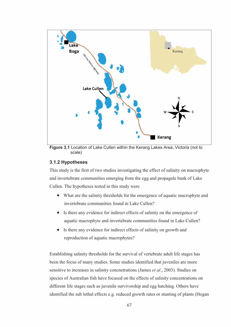
67
Figure 3.1 Location of Lake Cullen within the Kerang Lakes Area, Victoria (not to
scale)
3.1.2 Hypotheses This study is the first of two studies investigating the effect of salinity on macrophyte
and invertebrate communities emerging from the egg and propagule bank of Lake
Cullen. The hypotheses tested in this study were
What are the salinity thresholds for the emergence of aquatic macrophyte and
invertebrate communities found in Lake Cullen?
Is there any evidence for indirect effects of salinity on the emergence of
aquatic macrophyte and invertebrate communities found in Lake Cullen?
Is there any evidence for indirect effects of salinity on growth and
reproduction of aquatic macrophytes?
Establishing salinity thresholds for the survival of vertebrate adult life stages has
been the focus of many studies. Some studies identified that juveniles are more
sensitive to increases in salinity concnetrations (James et al., 2003). Studies on
species of Australian fish have focused on the effects of salinity concentrations on
different life stages such as juvenile survivorship and egg hatching. Others have
identified the sub lethal effects e.g. reduced growth rates or stunting of plants (Hogan
Kerang

68
and Nicholson, 1987; Williams, 1987; Bacher and O'Brien, 1989; Hart et al., 1991;
Guo et al., 1993; Guo et al., 1995; O'Brian and Ryan, 1999). It is important to
consider that any sub lethal effects and salinity thresholds identified for adults may
not be the same for all life stages of plants and animals. For example, James et al.,
(2003) found in their review of the literature that whilst adult Australian fish are
often able to tolerate salinities of up to 8.8 g/L, sub lethal and adverse effects on fish
eggs, juvenile growth rates and survivorship as well as sperm motility were observed
at salinities of between 4.5 to 5.0 g/L. For invertebrates Kefford et al., (2007) found
that early larval stages had lower salinity tolerance concentrations than adult life
stages in 60% to 70% of freshwater species studied. There were some species e.g.,
Glossiponiidae species (Leeches), however where the salinity tolerance
concentrations for earlier life stages were very similar to that of the adults.
The sub lethal and lethal effect of salinity on the life stages of plants has not been
widely studied. This study aims to investigate if salinity affects the reproductive
success and growth of plant species establishing from the propagule bank. Aquatic
plant reproduction is an important issue because it is not known how long propagules
in a propagule bank can remain viable. Given that Lake Cullen is filled only once
every 5 years under the current management regime, it is essential that aquatic plant
propagules and invertebrates are able to remain viable in the propagule bank during
dry periods and that these species are able to contribute to the seed and egg bank of
the lake before it dries out (Department of Sustainability and Environment, 2004).
This study also aims to provide information to enable adaptive management of the
flooding regime of this lake.

69
3.2 Methods The effect of increasing salinity on the propagule bank and invertebrate egg bank of
Lake Cullen was investigated by subjecting lake substrate to nine salinity treatments.
Saline lakes of Australia are mostly dominated by sodium chloride and often mimic
the ionic concentration of sea water (Bayly and Williams, 1966; Williams, 1966;
Williams, 1998c), thus “Ocean Nature” sea salt was used throughout this experiment.
The salinity of the treatments (measured in g/L) was determined using a partial
Fibonacci sequence, so the treatments represented a natural logarithmic relationship
(Table 3.1). Fibonacci sequences are known numeric patterns to occur in the living
world with many animal population models, plant structures and animal shells
following Fibonacci number patterns (Darvas, 2007).
Table 3.1 Salinity treatments tested in this study, using Lake Cullen substrate samples.
** Due to difficulties in dissolving salts to the required 159.7 g/L concentration, treatment 9 was set at 136.0 g/L.
Sediment from Lake Cullen was collected in September 2005, when the wetland was
dry, prior to an environmental water allocation in October 2005. Lake sediments
were collected from the top 5cm of the wetland substrate using a spade. Sites for
sediment collection were chosen from randomly selected locations within 50 meters
of the wetland edge. Sediments were then transported back to the laboratory where
they were stored in dark conditions at 4o for two months. The soil was dried
thoroughly under a hessian cover in a glasshouse (to prevent contamination from
airborne propagules), and then passed through a soil crusher set at a diameter of 6mm
(Jaw Crusher PEX 60 x 100). Any dead vegetation was removed during this process.
Crushed samples were mixed thoroughly to minimise the influence of spatial
variation in the wetland sediment propagule bank.
Treatment Number Concentration g/L 1 3.4 2 5.5 3 8.9 4 14.4 5 23.3 6 37.7 7 61.0 8 98.7 9 159.7** (136)

70
A total of fifty-five 20 L clear plastic tubs were used in this experiment. There were
5 replicates set up for each of the 9 treatments plus the control treatment which
consisted of 10 tubs. The tubs were arranged randomly throughout an air conditioned
glasshouse. Their position was determined by a table of random numbers (Appendix
5 and Figure 3.2). Each tub contained a total of 1kg of sediment from Lake Cullen,
distributed between two 500 mL plastic trays (120mm x 175mm x 60mm). The 10
control tubs contained 1 kg of sterilised sand distributed between two 500mL trays,
to test for contamination by airborne propagules throughout the experiment. The
control tubs contained 3.4 g/L saline solution and no plants or animals were found in
the tubs at the conclusion of the experiments. Tubs were filled with 15 L of solution
of the required salinity and the depth of the liquid was marked. Tubs were checked
three times a week and topped up with tap water if necessary over a 14 week period
to ensure that salinity concentrations were maintained close to the treatment
concentrations (± 16%).
Figure 3.2 A. Glasshouse set up showing random allocation of tubs. B. Close up of one of the tubs showing plant growth in two plastic trays.
3.2.1 Air temperature and water quality monitoring Maximum air temperature of the glasshouse was regulated using an air conditioner
set to come on at 25 oC to reduce maximum air temperatures. Maximum and
minimum air temperature (oC) was monitored weekly at two locations in the
glasshouse (Appendix 5). A digital max/min thermometer (Temp Tec Max-Min
thermometer) was used and reset every week after the maximum and minimum
temperatures were recorded. Water temperature (oC) was also monitored on a weekly
basis in four of the control treatment tubs (Appendix 5). Temperatures (oC) were
monitored using standard manual max/min thermometers that were reset after the
A B

71
temperatures were recorded each week. Salinity (g/L) and pH of the water in each
tub was also monitored on a fortnightly basis using an Orion Multimeter (Model No.
1230).
3.2.2 Monitoring of aquatic macrophytes and invertebrate emergence from the propagule bank, plus algal blooms
Plant growth and invertebrate hatching from the propagule bank was monitored each
week for 14 weeks. For aquatic angiosperms the following was recorded:
species presence
number of shoots (only possible up to 25 as after this point it was difficult to determine the number of individual shoots in the tubs due to crowding in the trays)
number of flowers
fruit production
For any charophytes the following was recorded:
species presence
production of antheridia
The presence of invertebrates and algal blooms was also recorded for each tub on a
weekly basis.
3.2.3 Invertebrate emergence and identification At the end of the 14 week experiment invertebrates that had hatched from the
sediments were collected by filtering the liquid in the tubs through graded sieves
(40 mm 10 mm, and 108 μm). The larger sieves were checked for invertebrates and
added to the smallest sieve, before the contents of the smallest sieve were rinsed into
a sample jar and preserved using 70% ethanol. In the laboratory the invertebrates
collected by the 108 μm sieve were sorted according to size by sieving the sample
through another series of graded sieves (500 μm, 250 μm and 108 μm).
To assist in removing invertebrates from detritus in the greater than 500 μm size
cohort, a flotation method was used, using a sucrose solution (Anderson, 1959;

72
Britton and Greeson, 1987; Rosillon, 1987). This method was used as there was a
copious amount of detritus present in these samples which made counting difficult. A
sugar solution with a specific gravity of 1.12 (360g per litre of water) was added to
the samples and stirred. This solution was left to stand for 2 minutes before
invertebrates were collected from the surface. All invertebrates collected were
counted and identified to species level where possible using published keys (De
Deckker, 1974; De Deckker, 1978; De Deckker, 1981b; De Deckker, 1981c; De
Deckker, 1981a)and dissecting microscope (Nikon optical, model SMZ-1B). The
sampling efficiency of this method was also checked using a QA/QC (Quality
Assurance/Quality Control) check, where 5 samples (10% of the total number of
samples) were subjected to the sugar floatation method, and then the detritus was
searched. Any extra invertebrates remaining in the sample were counted to determine
the percentage of invertebrates captured by this method.
For the 500 μm, 250 μm and the 108 μm size classes, no flotation method was
necessary and the invertebrates were identified to genus concentration and counted
using the same dissecting microscope.
3.2.4 Harvesting of aquatic macrophytes Above ground aquatic macrophyte material was harvested and sorted to species,
species were identified using Jacobs and Brock (1982). For each aquatic angiosperm
species the following characteristics were recorded, the number of:
shoots
reproductive individuals
flowers budding
mature flowers
fruit
seeds
For each charophyte species (identified by Michelle Casanova) the following
characteristics were recorded, the number of:
individuals
reproductive individuals

73
individuals containing antheridia
individuals containing immature oospores
individuals containing mature oospores
individuals containing aborted oogonis
The biovolume (mL) and dry weight biomass (g) of the aboveground plant material
of each species was measured. Biovolume was determined using the Archimedes’
Principle of the displacement of liquid which states that the amount of water
displaced by a submerged object is equal to the volume of that object in water
(Pickover, 2008). The biovolume (mL) of each species was determined by placing
the plant material in a measuring cylinder of appropriate volume, depending on the
amount of vegetation present. Then a known amount of water was added to the
cylinder. The total volume of water and vegetation was recorded and the biovolume
of the plant sample was determined using the following equation:
Plant biovolume (mL) = Total volume of plants and water – Volume of water added to
measuring cylinder
To determine the dry weight biomass (g) of each species, plant material was removed
from the cylinder and drained. Drained plant material was placed in a paper bag of
known weight that had been dried in an oven at 70oC for 48 hours. The bag of plant
material was then placed in an oven at 70oC for 48 hours. Bags were reweighed and
the dry weight biomass was determined using the equation below:
Dry weight biomass (g) = Total dry weight of plants and bag – Weight of pre-dried bag
3.2.5 Results of sugar floatation method for invertebrate sorting Results of a quality assurance/quality control (QA/QC) to check of the effectiveness
of the sugar floatation method in 10% of replicates showed that a minimum of 94%
of invertebrates for each species were successfully extracted from the organic
material present using this method (Appendix 6).
74
3.2.6 Data analysis Data was analysed for linear, quadratic, and cubic regressions to determine how the
species responded to increased salinity concentrations and to ascertain an upper
salinity threshold. Results were also analysed using one way ANOVA's to determine
if there was any significant difference (p < 0.05) between salinity treatments, the
model for the ANOVA’s was:
DV = constant + salinity treatment
Where the results of the one way ANOVA’s indicated that there was a significant
difference between treatmetns, a post hoc Tukey’s test was conducted to determine
which treatments were significantly different. Square root transformations of the
dependent variable were undertaken when the data from this experiment did not meet
the assumptions of normality or homogeneity of variances for parametric tests which
were analysed using a Levenes test. The one way ANOVA’s and post hoc Tukey’s
tests were conducted using the PASW 18 (previously known as SPSS statistics)
software package.
Multivariate analysis of the total number of individuals for each species for each
replicate using Plymouth Routines in Multivariate Ecological Research (PRIMER)
statistical software (Version 6.1.6). The data were square root transformed before
analysis. A non-metric multi-dimensional scaling (MDS) plot and a hierarchical
clustering analysis was constructed from a Bray-Curtis similarity matrix.

75
3.3 Results
3.3.1 Air temperature and water quality monitoring Maximum air temperatures were between 28.5oC and 40.5oC, while minimum air
temperatures ranged from 10.7 oC to 14.7 oC. Maximum water temperatures ranged
from 20oC to 32oC, while minimum water temperatures were between 11oC and 25oC
(Appendix 7). Monitoring results of salinity concentrations for each replicate showed
that on average, maximum salinity concentrations were maintained within 16% of
target treatment concentration. The monitoring results for pH showed that solutions
remained alkaline, between 7.4 and 9.9 (Appendix 7).
3.3.2 Emergence of aquatic macrophyte and invertebrate taxa Only two aquatic macrophyte and two invertebrate species emerged from the
sediments of Lake Cullen in this experiment. The two macrophytes were the
angiosperm Ruppia megacarpa R. Mason and the charophyte species
Lamprothamnium macropogon (A. Braun) I.L. Ophel. The two invertebrates were
ostracod species Mytilocypris henricae (Chapman 1966) and Australocypris spp.
Salinity treatment concentrations of 61.0 g/L or above resulted in no taxa being
found in any replicates. All four of these plant and invertebrate species emerged from
sediment in all replicates in the lower salinity treatments (3.4 g/L to 37.7 g/L). In
contrast, in all replicates of the 61.0 g/L treatment no plant species germinated and
only the invertebrate Australocypris spp. emerged from the sediments. No plant or
invertebrate species emerged from the sediments in all replicates of the highest
salinity treatments (98.7 g/L and 136.0 g/L) (Table 3.2).
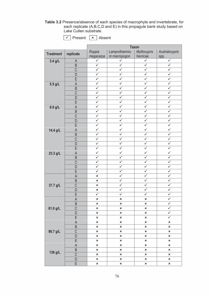
76
Table 3.2 Presence/absence of each species of macrophyte and invertebrate, for each replicate (A,B,C,D and E) in this propagule bank study based on Lake Cullen substrate.
Present Absent Taxon Treatment replicate Ruppia
megacarpa Lamprothamnium macropogon
Mytilocypris henricae
Australocypris spp.
3.4 g/L
A B C D E
5.5 g/L
A B C D E
8.9 g/L
A B C D E
14.4 g/L
A B C D E
23.3 g/L
A B C D E
37.7 g/L
A B C D E
61.0 g/L
A B C D E
98.7 g/L
A B C D E
136 g/L
A B C D E
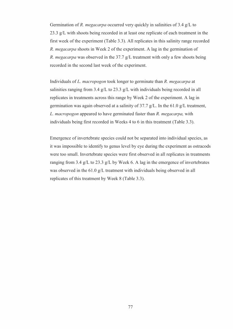
77
Germination of R. megacarpa occurred very quickly in salinities of 3.4 g/L to
23.3 g/L with shoots being recorded in at least one replicate of each treatment in the
first week of the experiment (Table 3.3). All replicates in this salinity range recorded
R. megacarpa shoots in Week 2 of the experiment. A lag in the germination of
R. megacarpa was observed in the 37.7 g/L treatment with only a few shoots being
recorded in the second last week of the experiment.
Individuals of L. macropogon took longer to germinate than R. megacarpa at
salinities ranging from 3.4 g/L to 23.3 g/L with individuals being recorded in all
replicates in treatments across this range by Week 2 of the experiment. A lag in
germination was again observed at a salinity of 37.7 g/L. In the 61.0 g/L treatment,
L. macropogon appeared to have germinated faster than R. megacarpa, with
individuals being first recorded in Weeks 4 to 6 in this treatment (Table 3.3).
Emergence of invertebrate species could not be separated into individual species, as
it was impossible to identify to genus level by eye during the experiment as ostracods
were too small. Invertebrate species were first observed in all replicates in treatments
ranging from 3.4 g/L to 23.3 g/L by Week 6. A lag in the emergence of invertebrates
was observed in the 61.0 g/L treatment with individuals being observed in all
replicates of this treatment by Week 8 (Table 3.3).

78
Table 3.3 The week in which macrophyte and invertebrates were first observed, for each replicate (A,B,C,D and E) in this propagule bank study based on Lake Cullen substrate. Invertebrate species could not be identified at this early stage.
Treatment Replicate Ruppia megacarpa Lamprothamnium macropogon Invertebrate spp.
3.4 g/L
A 1 2 4 B 1 2 4 C 1 2 4 D 1 2 5 E 1 2 4
5.5 g/L
A 1 2 4 B 1 2 4 C 1 2 4 D 2 2 4 E 1 2 4
8.9 g/L
A 1 2 4 B 1 2 4 C 1 2 4 D 2 2 5 E 1 2 4
14.4 g/L
A 1 2 4 B 1 2 4 C 1 2 4 D 2 2 4 E 1 2 4
23.3 g/L
A 2 2 4 B 1 2 4 C 1 2 4 D 2 2 4 E 1 2 4
37.7 g/L
A 5 4 B 13 4 4 C 5 6 D 6 4 E 5 4
61.0 g/L
A 8 B 8 C 6 D 8 E 8
98.7 g/L
A B C D E
136 g/L
A B C D E

79
3.3.3 Ruppia megacarpa germination Figure 3.3 shows that there was a decrease in germination success and plant growth in
R. megacarpa as salinity increased. When salinity treatments 3.4 g/L to 37.7 g/L were
included in analysis (all treatments with germination of aquatic macrophytes), a
significant negative linear regression (p <0.001, R2 = 0.915) in the germination success of
R. megacarpa (measured as number of shoots) was found with increasing salinity (Figure
3.3a and Appendix 8). There was a slight increase in the number of R. megacarpa shoots
present at 5.5 g/L when compared to 3.4 g/L, however this increase was not significant.
Results of a one way ANOVA indicated a significant difference in the number of shoots
with increasing salinity (p < 0.001, F = 31.704 df = 5, 24). A post hoc Tukey’s test
showed that there was no significant difference between 3.4 g/L, 5.5 g/L or 8.9 g/L
treatments, nor was there any significant difference between 8.9 g/L and 14.4 g/L or
between 14.4 g/L and 23.3 g/L. There were significant differences however between all
other treatments (Appendix 8).
A significant negative linear regression was also found between total biovolume
(p < 0.001, R2 = 0.850) and increasing salinity, and between total biomass (p < 0.001,
R2 = 0.826) and increasing salinity (Figure 3.3b and c respectively, Appendix 8). The
results of a one way ANOVA indicated a significant difference between the total
biovolume of R. megacarpa as salinity increased (p < 0.001, F = 16.266 df = 5, 24).
These results show that the amount of R. megacarpa biovolume present in each treatment
was affected by increasing salinity. A post hoc Tukey’s test showed that there was only a
significant difference in salinity treatments ranging from 3.4 g/L to 23.3 g/L and the
highest salinity concentration at 37.7 g/L. But there was no significant difference found
between any of the treatments ranging from 3.4 g/L and 23.3 g/L (Appendix 8). This
suggests that salinity significantly affected the biovolume of R. megacarpa at 37.7 g/L
treatment.
Results of another one way ANOVA also showed significant difference between the total
dry weight biomass of R. megacarpa as salinity increased (p <0.001, F = 17.564 df = 5,
24). These results indicate that the amount of R. megacarpa dry weight biomass present
in each treatment was affected by increasing salinity. A post hoc Tukey’s test showed
very similar results to that of the effect of salinity on R. megacarpa biovolume, as there
was only a significant difference in salinity treatments ranging from 3.4 g/L to 23.3 g/L

80
Figure 3.3 Regressions showing the effect of salinity on the a) germination, b) biovolume and c) dry weight biomass of Ruppia megacarpa, (n=5, square root transformation), trend lines only shown where regressions were found to be significant (p < 0.05).
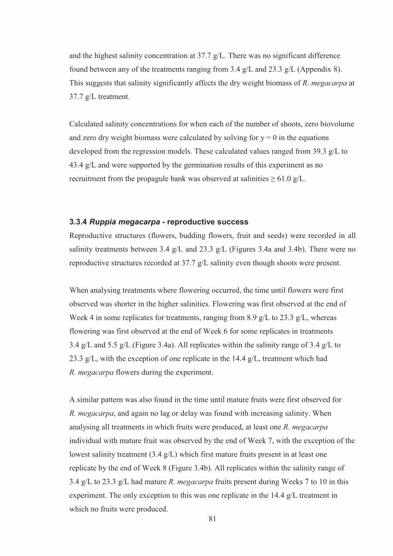
81
and the highest salinity concentration at 37.7 g/L. There was no significant difference
found between any of the treatments ranging from 3.4 g/L and 23.3 g/L (Appendix 8).
This suggests that salinity significantly affects the dry weight biomass of R. megacarpa at
37.7 g/L treatment.
Calculated salinity concentrations for when each of the number of shoots, zero biovolume
and zero dry weight biomass were calculated by solving for y = 0 in the equations
developed from the regression models. These calculated values ranged from 39.3 g/L to
43.4 g/L and were supported by the germination results of this experiment as no
recruitment from the propagule bank was observed at salinities ≥ 61.0 g/L.
3.3.4 Ruppia megacarpa - reproductive success Reproductive structures (flowers, budding flowers, fruit and seeds) were recorded in all
salinity treatments between 3.4 g/L and 23.3 g/L (Figures 3.4a and 3.4b). There were no
reproductive structures recorded at 37.7 g/L salinity even though shoots were present.
When analysing treatments where flowering occurred, the time until flowers were first
observed was shorter in the higher salinities. Flowering was first observed at the end of
Week 4 in some replicates for treatments, ranging from 8.9 g/L to 23.3 g/L, whereas
flowering was first observed at the end of Week 6 for some replicates in treatments
3.4 g/L and 5.5 g/L (Figure 3.4a). All replicates within the salinity range of 3.4 g/L to
23.3 g/L, with the exception of one replicate in the 14.4 g/L, treatment which had
R. megacarpa flowers during the experiment.
A similar pattern was also found in the time until mature fruits were first observed for
R. megacarpa, and again no lag or delay was found with increasing salinity. When
analysing all treatments in which fruits were produced, at least one R. megacarpa
individual with mature fruit was observed by the end of Week 7, with the exception of the
lowest salinity treatment (3.4 g/L) which first mature fruits present in at least one
replicate by the end of Week 8 (Figure 3.4b). All replicates within the salinity range of
3.4 g/L to 23.3 g/L had mature R. megacarpa fruits present during Weeks 7 to 10 in this
experiment. The only exception to this was one replicate in the 14.4 g/L treatment in
which no fruits were produced.
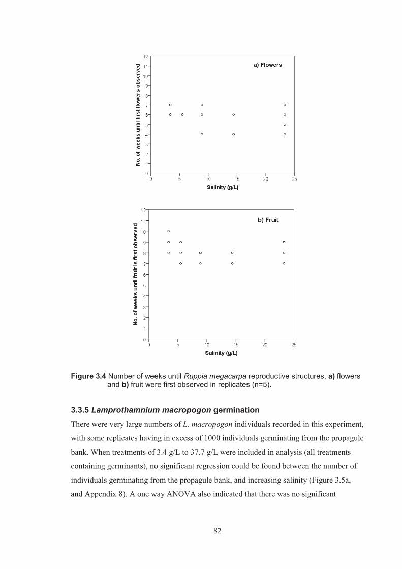
82
Figure 3.4 Number of weeks until Ruppia megacarpa reproductive structures, a) flowers and b) fruit were first observed in replicates (n=5).
3.3.5 Lamprothamnium macropogon germination There were very large numbers of L. macropogon individuals recorded in this experiment,
with some replicates having in excess of 1000 individuals germinating from the propagule
bank. When treatments of 3.4 g/L to 37.7 g/L were included in analysis (all treatments
containing germinants), no significant regression could be found between the number of
individuals germinating from the propagule bank, and increasing salinity (Figure 3.5a,
and Appendix 8). A one way ANOVA also indicated that there was no significant

83
difference in the number of individuals germinating for L. macropogon as salinity
increased (p > 0.05).
Figure 3.5 b and c show that with increasing salinity there is a decrease in growth for
L. macropogon. Significant declining linear relationships were found for the biovolume (p
<0.001, R2 = 0.599) and dry weight biomass (p = 0.002, R2 = 0.534) of L. macropogon
with increasing salinity. This suggests that while increased salinities below the threshold
level had little affect on the number of individuals germinating, it did have an effect on
the charophyte growth (Figures 3.5b and 3.5c, and Appendix 6).
A one way ANOVA indicated a significant difference in the biovolume of L. macropogon
with increased salinity (p 0.034, F = 2.992 df = 5, 24). A post hoc Tukey’s test showed
that there was only a significant difference (p < 0.05) between the 5.5 g/L and 37.7 g/L
treatments (Appendix 8). A one way ANOVA indicated that there was a significant
difference between dry weight biomass at increasing salinities (p = 0.007, F = 4.164 df =
5, 24). A post hoc Tukey’s test indicated a significant difference between all treatments
and the 37.7 g/L treatment (Appendix 8).
Calculated salinity concentrations for the biovolume and dry weight biomass of L.
macropogon were calculated by solving for y = 0 in the equations developed from the
regression models. These calculated values were found to be 52.6 g/L and 57.6 g/L
respectively. The maximum calculated values for biovolume was supported by the results.
The maximum calculated value for dry weight biomass, however was not supported by
the results of this experiment as no germination was observed at salinities ≥ 61.0 g/L.

84
Figure 3.5 Regressions showing the effect of salinity on the a) germination, b) biovolume and c) dry weight biomass of Lamprothamnium macropogon, (n=5), trend lines only shown where regressions were significant (p < 0.05)

85
3.3.6 Lamprothamnium macropogon - reproductive success Reproductive whorls (containing antheridia and oogonia) on L. macropogon were
recorded in all salinity treatments containing germinants from 3.4 g/L to 37.7 g/L.
Analysis of the different types of antheridia and oogonia present on L. macropogon
individuals was calculated as percentage of total reproductive individuals (antheridia and
oogonia) in order to take into account the varying number of individuals present in each
replicate. The cumulative percentages for each replicate in most cases exceeded 100% as
individuals often contained more than one type of antheridia or oogonia.
The percentage of reproductive individuals containing antheridia was very high with
percentages exceeding 80% in some replicates. No significant regression was found for
the percentage of reproductive individuals containing antheridia with increasing salinity
(Figure 3.6a and Appendix 8). The percentage of individuals containing immature
oogonia, mature oogonia and aborted oogonia were lower, (0 to 10%) in all replicates. A
significant declining linear relationship (p <0.001, R2 = 0.695) was found for the
percentage of reproductive individuals containing immature oogonia with increasing
salinity (Figure 3.6b and Appendix 8). Results of a one way ANOVA indicated that there
was a significant difference between the treatments (p = 0.001, F = 5.835, df = 5, 24). A
post hoc Tukey’s test showed that there was only a significant difference between the
lower salinity treatments (3.4 g/L, 5.5 g/L and 8.9 g/L) and the 37.7 g/L treatment
(Appendix 8) and also between the 8.9 g/L and 23.3 g/L treatments.
A significant linear relationship (p = 0.003, R2 = 0.442) was also found for mature
oogonia and increasing salinity, a maximum number of mature oogonia being produced in
treatments 3.4 g/L to 14.4 g/L (Figure 3.6c and Appendix 8). Results of a one way
ANOVA indicated that there was a significant difference between the treatments (p =
0.015, F = 3.565, df = 5, 24). A post hoc Tukey’s test showed that there was only a
significant difference between the 14.4 g/L and 37.7 g/L treatments (Appendix 8).
The percentage of individuals with aborted oogonia did increase with increasing salinity,
and a significant linear relationship (p = 0.001, R2 = 0.576) found between the percentage
of reproductive individuals with aborted oogonia and increasing salinity (Figure 3.6d and
Appendix 8). Results of a one way ANOVA indicated that there was a significant

86
difference between the treatments (p = 0.017, F = 3.460, df = 5, 24). A post hoc Tukey’s
test showed that there was only a significant difference between the lower salinity
treatments (3.4 g/L, 5.5 g/L and 8.9 g/L) and the 37.7 g/L treatment (Appendix 8).
Figure 3.6 The percentage of Lamprothamnium macropogon individuals containing each
type of reproductive structures, (n=5, square root transformation), regression trend lines only shown where regressions were significant (p <0.05)
Increased salinity concentrations in this experiment had little affect on the time until
antheridia were first observed in each replicate. All treatments in which germination of
L. macropogon occurred (salinity range 3.4 g/L to 37.7 g/L) had at least one replicate
with antheridia present at the end of Week 7, with the exception of one treatment in
8.9 g/L which did not have any individuals with antheridia until Week 9 (Figure 3.7). All
replicates within this salinity range (3.7 g/L to 37.7 g/L) contained antheridia for
L. macropogon during weeks 7 to 12. When compared to the time until flowering and
fruit development in R. megacarpa (Weeks 4 to 7 and Weeks 7 to 10 respectively), these
results suggest that L. macropogon (Weeks 7 to 12) takes a longer than R. megacarpa to
become reproductive (Figures 3.4a and 3.4b and 3.7).
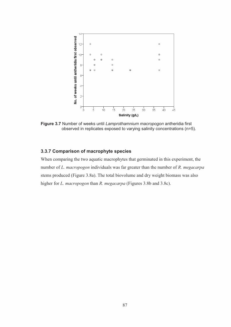
87
Figure 3.7 Number of weeks until Lamprothamnium macropogon antheridia first observed in replicates exposed to varying salinity concentrations (n=5).
3.3.7 Comparison of macrophyte species When comparing the two aquatic macrophytes that germinated in this experiment, the
number of L. macropogon individuals was far greater than the number of R. megacarpa
stems produced (Figure 3.8a). The total biovolume and dry weight biomass was also
higher for L. macropogon than R. megacarpa (Figures 3.8b and 3.8c).
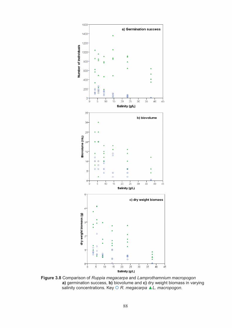
88
Figure 3.8 Comparison of Ruppia megacarpa and Lamprothamnium macropogon
a) germination success, b) biovolume and c) dry weight biomass in varying salinity concentrations. Key R. megacarpa ▲L. macropogon.
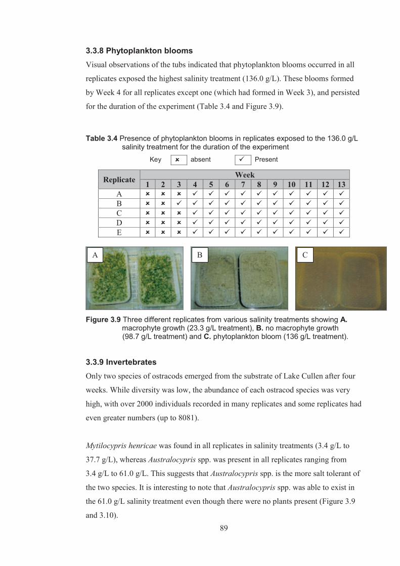
89
3.3.8 Phytoplankton blooms Visual observations of the tubs indicated that phytoplankton blooms occurred in all
replicates exposed the highest salinity treatment (136.0 g/L). These blooms formed
by Week 4 for all replicates except one (which had formed in Week 3), and persisted
for the duration of the experiment (Table 3.4 and Figure 3.9).
Table 3.4 Presence of phytoplankton blooms in replicates exposed to the 136.0 g/L
salinity treatment for the duration of the experiment
Key absent Present
Replicate Week 1 2 3 4 5 6 7 8 9 10 11 12 13
A B C D E
Figure 3.9 Three different replicates from various salinity treatments showing A. macrophyte growth (23.3 g/L treatment), B. no macrophyte growth
(98.7 g/L treatment) and C. phytoplankton bloom (136 g/L treatment).
3.3.9 Invertebrates Only two species of ostracods emerged from the substrate of Lake Cullen after four
weeks. While diversity was low, the abundance of each ostracod species was very
high, with over 2000 individuals recorded in many replicates and some replicates had
even greater numbers (up to 8081).
Mytilocypris henricae was found in all replicates in salinity treatments (3.4 g/L to
37.7 g/L), whereas Australocypris spp. was present in all replicates ranging from
3.4 g/L to 61.0 g/L. This suggests that Australocypris spp. is the more salt tolerant of
the two species. It is interesting to note that Australocypris spp. was able to exist in
the 61.0 g/L salinity treatment even though there were no plants present (Figure 3.9
and 3.10).
A B C
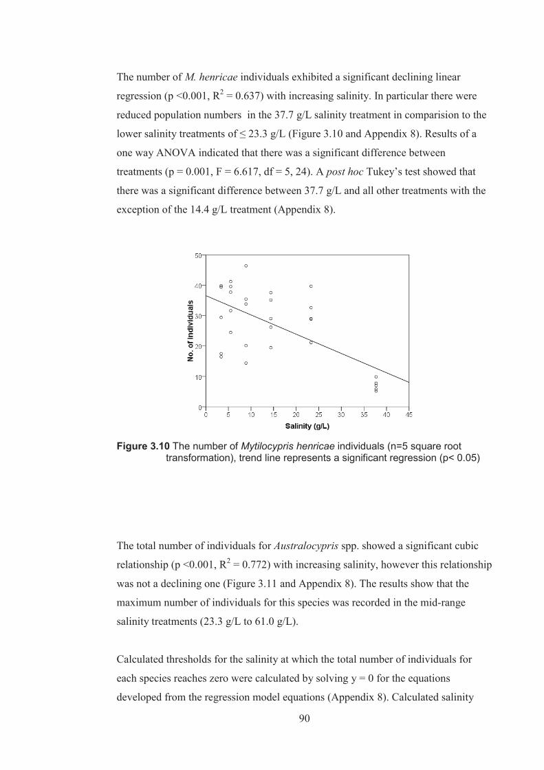
90
The number of M. henricae individuals exhibited a significant declining linear
regression (p <0.001, R2 = 0.637) with increasing salinity. In particular there were
reduced population numbers in the 37.7 g/L salinity treatment in comparision to the
lower salinity treatments of ≤ 23.3 g/L (Figure 3.10 and Appendix 8). Results of a
one way ANOVA indicated that there was a significant difference between
treatments (p = 0.001, F = 6.617, df = 5, 24). A post hoc Tukey’s test showed that
there was a significant difference between 37.7 g/L and all other treatments with the
exception of the 14.4 g/L treatment (Appendix 8).
Figure 3.10 The number of Mytilocypris henricae individuals (n=5 square root transformation), trend line represents a significant regression (p< 0.05)
The total number of individuals for Australocypris spp. showed a significant cubic
relationship (p <0.001, R2 = 0.772) with increasing salinity, however this relationship
was not a declining one (Figure 3.11 and Appendix 8). The results show that the
maximum number of individuals for this species was recorded in the mid-range
salinity treatments (23.3 g/L to 61.0 g/L).
Calculated thresholds for the salinity at which the total number of individuals for
each species reaches zero were calculated by solving y = 0 for the equations
developed from the regression model equations (Appendix 8). Calculated salinity
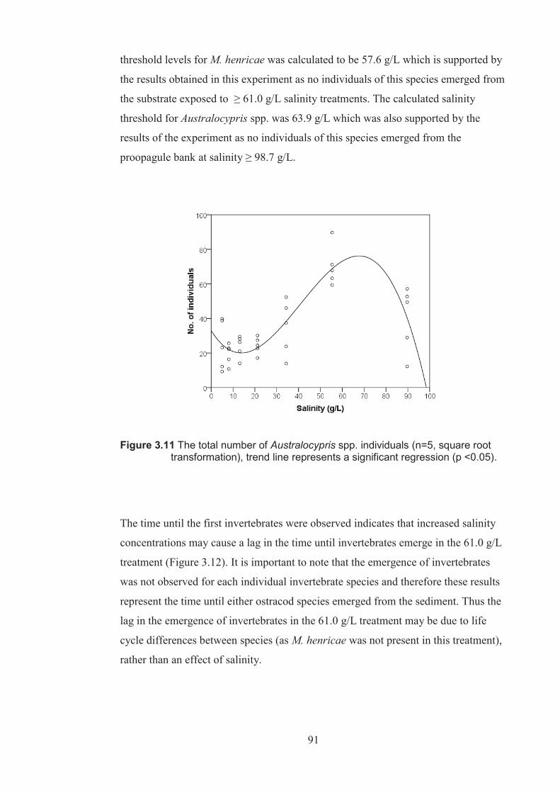
91
threshold levels for M. henricae was calculated to be 57.6 g/L which is supported by
the results obtained in this experiment as no individuals of this species emerged from
the substrate exposed to ≥ 61.0 g/L salinity treatments. The calculated salinity
threshold for Australocypris spp. was 63.9 g/L which was also supported by the
results of the experiment as no individuals of this species emerged from the
proopagule bank at salinity ≥ 98.7 g/L.
Figure 3.11 The total number of Australocypris spp. individuals (n=5, square root
transformation), trend line represents a significant regression (p <0.05).
The time until the first invertebrates were observed indicates that increased salinity
concentrations may cause a lag in the time until invertebrates emerge in the 61.0 g/L
treatment (Figure 3.12). It is important to note that the emergence of invertebrates
was not observed for each individual invertebrate species and therefore these results
represent the time until either ostracod species emerged from the sediment. Thus the
lag in the emergence of invertebrates in the 61.0 g/L treatment may be due to life
cycle differences between species (as M. henricae was not present in this treatment),
rather than an effect of salinity.
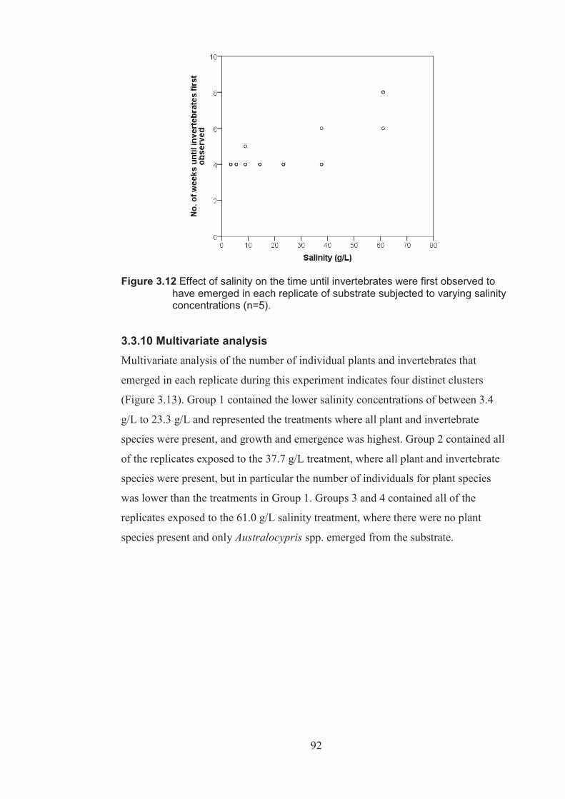
92
Figure 3.12 Effect of salinity on the time until invertebrates were first observed to
have emerged in each replicate of substrate subjected to varying salinity concentrations (n=5).
3.3.10 Multivariate analysis Multivariate analysis of the number of individual plants and invertebrates that
emerged in each replicate during this experiment indicates four distinct clusters
(Figure 3.13). Group 1 contained the lower salinity concentrations of between 3.4
g/L to 23.3 g/L and represented the treatments where all plant and invertebrate
species were present, and growth and emergence was highest. Group 2 contained all
of the replicates exposed to the 37.7 g/L treatment, where all plant and invertebrate
species were present, but in particular the number of individuals for plant species
was lower than the treatments in Group 1. Groups 3 and 4 contained all of the
replicates exposed to the 61.0 g/L salinity treatment, where there were no plant
species present and only Australocypris spp. emerged from the substrate.
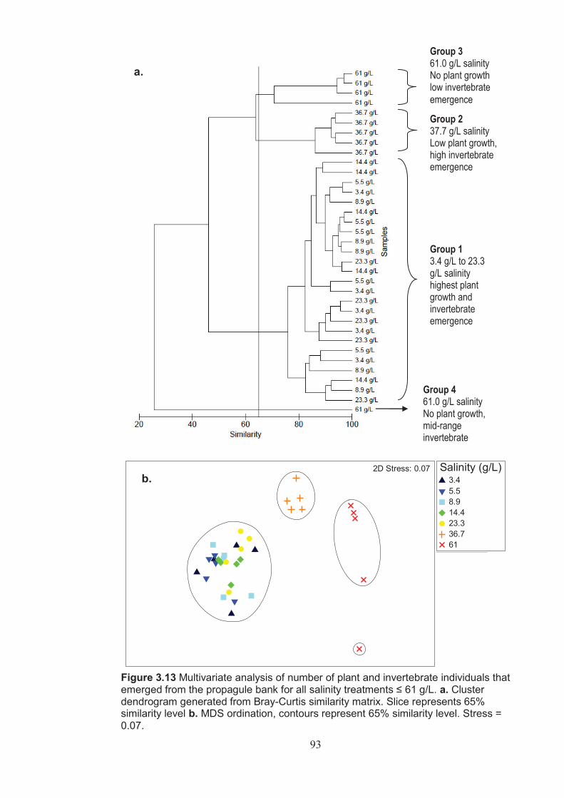
93
Salinity (g/L)
3.45.58.914.423.336.761
Similarity65
2D Stress: 0.07
Figure 3.13 Multivariate analysis of number of plant and invertebrate individuals that emerged from the propagule bank for all salinity treatments ≤ 61 g/L. a. Cluster dendrogram generated from Bray-Curtis similarity matrix. Slice represents 65% similarity level b. MDS ordination, contours represent 65% similarity level. Stress = 0.07.
Group 3 61.0 g/L salinity No plant growth low invertebrate emergence
Group 2 37.7 g/L salinity Low plant growth, high invertebrate emergence
Group 1 3.4 g/L to 23.3 g/L salinity highest plant growth and invertebrate emergence
Group 4 61.0 g/L salinity No plant growth, mid-range invertebrate
a.
b.

94
3.4 Discussion The results of this study indicated four differing regimes or states: a submerged
aquatic macrophyte regime with two aquatic macrophyte and two invertebrate
species, a clear water state with no macrophytes and one invertebrate species, a clear
water state with no macrophytes and no invertebrate species and an algal bloom
state. No microbial mat state was observed in this study.
3.4.1 Effect of salinity on the germination of aquatic macrophytes Both Ruppia megacarpa and Lamprothamnium macropogon are known to be
perennial aquatic macrophyte species, although R. megacarpa can act as an annual
species in ephemeral systems. It is therefore not surprising for a perennial species to
be present in the propagule bank of this wetland, given its past flooding regime and
management as a permanent storage lake for irrigation waters (KLAWG, 1992). The
presence of these perennial species needs to be considered when determining a future
watering regime for Lake Cullen. Perennial species tend to be found in permanent
systems, however as evidenced by this study both species are able to survive periods
of drying. Whether these species are able to persist under a more ephemeral watering
regime in the long term is something that warrants investigation. A basic requirement
would be that the timing and duration of inundation needs to be long enough to allow
plants to reach maturity and contribute propagules to the propagule bank for these
species to persist into the future.
The germination of R. megacarpa seeds in the experiment was quick, with shoots
being recorded across all replicates in salinity treatments ranging from 3.4 g/L to
23.3 g/L within the first one or two weeks of the experiment. Other similar propagule
bank studies have reported much slower germination rates of 15 days or longer in
Ruppia species (Kahn and Durako, 2005; Sim et al., 2006a). The short time
observed until germination first occurred in this experiment may be attributed to
environmental factors such as the high water temperatures (≥ 30oC) experienced
during the initial stages of this study (Appendix 7). Previous experiments have also
found that high temperatures increase the germination success of seeds of a species
from the same genus, Ruppia maritima (Verhoeven, 1980; Koch and Seeliger, 1988;
Malea et al., 2004).

95
A lag phase in germination of R. megacarpa and L. macropogon at a salinity of
37.7 g/L was apparent with first germinants observed at 12 weeks and 5 weeks
respectively. Similar delays in germination of aquatic macrophytes at higher
salinities have been recorded by Sim et al., (2006a) and Kim et al., (2013).
Germination lags can present problems if these plant species are to persist when a
wetland dries out too quickly or becomes too salty for germination to occur. These
lags can also be problematic if germination occurs late in the watering period and
salinity concentrations are not kept at low concentrations long enough to enable
plants to reproduce. Thus over time propagule banks can become depleted and
species may be lost from wetland ecosystems.
There has been little research into the longevity of saline wetland propagule banks.
Recent studies on freshwater wetland species by Brock (2011) have shown that
wetland seeds can persist in propagule banks and be viable after 12 years without
inundation. Additionally, Brock (2011) found that the mean survival time seeds
could remain dry for was 7.4 years, but the longevity of individual wetland plant
species varied greatly, so further research is warranted.
Germination of both R. megacarpa and L. macropogon occurred in all salinity
concentrations up to and including 37.7 g/L, with no germination recorded at or
above 61.0 g/L. This concurs with the salinity threshold of 45 g/L for macrophyte
dominated wetlands proposed by Sim et al., (2006a) and shows a higher germination
threshold that than posed by Kim et al.,(2013) who found that R. megacarpa seeds
did not germinate in waters > 30 g/L. Regression analysis showed that salinity
impacted the number of R. megacarpa shoots produced at salinities of 14.4 g/L and
above, suggesting that salinity concentrations below the germination threshold level
affect the number of shoots produced in this species. A gradual decline in the number
of Ruppia polycarpa shoots was found in a similar study by Sim et al., (2006a).
There was a slight increase in the number of R. megacarpa shoots present at 5.5 g/L
when compared to 3.4 g/L, which may be due to natural variations in seed numbers
across the replicates, however this pattern of reduced germination success at lower
salinities has been recorded in other studies of Ruppia species (Sim et al., 2006a)
suggesting that these macrophytes may have greater germination success rate in
slightly elevated salt concentrations.

96
A very different response was observed for the effect of salinity on the germination
of L. macropogon with results showing that salinity concentrations below 37.7 g/L
had little or no effect on the number of individuals germinating from the sediments
of Lake Cullen. Sim et al., (2006a) also found no relationship between increased
salinity and the number of individuals of L. macropogon when salinity
concentrations were below 37.7 g/L. High numbers of L. macropogon individuals
have germinated in this experiment, suggesting the presence of a large number of
propagules in the propagule bank.
3.4.2 Effects of salinity on macrophyte growth Salinity negatively impacted the total biovolume and dry weight biomass of
R. megacarpa and L. macropogon. Post hoc Tukey’s test results demonstrated that
increasing salinity to 37.7 g/L or higher had a significant impact on the total
biovolume and dry weight biomass for R. megacarpa. This suggests that increased
salinity concentrations may impact growth by causing stunting of these plants at
higher salinities. Post hoc Tukey’s tests for L. macropogon only showed significant
differences between lower salinity concentrations of 5.5 g/L and 37.7 g/L for total
biovolume; and between 3.4 g/L and 37.7 g/L, 5.5 g/L and 37.7 g/L for total dry
weight biomass. These results indicate that salinity concentrations below 5.5 g/L are
optimal for L. macropogon growth and salinity concentrations below 23.3 g/L are
optimal for R. megacarpa growth. This finding supports results from Robertson and
Funnell (2012) who found that there was reduced growth and cover of R. megacarpa
in a New Zealand lagoon that was subjected to increased salinities of between 10g/L
to 20 g/L.
These results may not be a true indication of the effect of salinity on the growth of
these species, given that the lag time in germination at the 37.7 g/L salinity
concentration effectively reduced the length of time successful germinants had to
grow, in comparison to those germinated in lower salinity treatments. In particular,
this may have affected results for R. megacarpa, as individuals of this species did not
germinate until the last week of the experiment in the 37.7 g/L salinity treatment. If
the experiment had been extended for extra time, growth may not have been limited
at this salinity concentrations.
97
3.4.3 Effects of salinity on aquatic macrophyte reproductive success No R. megacarpa reproductive structures were produced at the 37.7 g/L salinity
concentration, even though germinants were present in this treatment. This is
possibly due to the lag in germination time occurring in this treatment, as shoots
were not recorded until the last week of the experiment. Reproductive whorls for L.
macropogon were recorded in all salinity treatments containing germinants, up to
and including 37.7 g/L. In a similar study by Sim et al., (2006a), Lamprothamnium
macropogon reproductive structures were only produced in individuals up to 15 g/L.
As such, this study indicates that this species is viable at salinities up to 37.7 g/L,
which is higher than R. megacarpa.
The type of reproductive structures produced by L. macropogon showed differing
relationships to increased salinity. The most significant results were that number of
aborted oogonia increased with increasing salinity, and results of a post hoc Tukey’s
test showing that there was a significant difference between both 3.4 g/L and
37.7 g/L and 5.5 g/L and 37.7 g/L, suggesting that an increase in salinity over 5.5 g/L
may significantly impact the number of aborted oogonia and therefore affect
reproductive success of L. macropogon.
While Sim et al., (2006a), have shown that an increase in salinity can cause a delay
in the time it takes until plants to become reproductive, there was no lag or delay
apparent in the time taken for the R. megacarpa to flower or until first antheridia
were observed on L. macropogon in this experiment. It should be noted however that
the aquatic macrophytes in the study by Sim et al., (2006a), were monitored more
regularly than that of this study and included other species of Ruppia. Also, whilst
Sim et al., (2006a) did find a significant delay in germination of L. macropogon
individuals, the lag time was only slight, with individuals germinating after 36 days
at a salinity of 30 g/L compared to 30 days at 0 g/L. Compared to the results by Sim
et al., (2006a) germination occurred more rapidly in this current study, with
individuals germinating in all salinity treatments at or below 37.7 g/L within the first
two weeks. This highlights that salinity alone may not be affecting germination
success in these species, it may also be influenced by other environmental factors
such as temperature or photoperiod which may be important in breaking dormancy in
seeds and spores.
98
3.4.4 Comparison of macrophyte species The number of L. macropogon individuals germinated in this experiment far
outweighed the number of R. megacarpa shoots, and similarly there was a higher
total biovolume and biomass for L. macropogon compared to that of R. megacarpa.
These results can be attributed to the different colonising strategies shown by each of
these species. R. megacarpa produced fewer stems, fewer sexual propagules and thus
had fewer germinating propagules in the propagule bank. This species is also able to
spread across the wetland substrate through asexual reproductive structures such as
rhizomes. For the charophyte species L. macropogon the colonising strategy is quite
different, as large numbers of individuals germinated from the propagule bank
indicating that this species produces large numbers of viable spores. But unlike R.
megacarpa these individuals are not able to colonise vast areas via asexual
reproduction. Similar colonising strategies for other species of the Lamprothamnium
and Ruppia species were found in a study by Sim et al., (2006a) and Porter (2007).
3.4.5 Effect of salinity on the number of invertebrates in populations developing from the propagule bank
Two species of ostracods emerged from the Lake Cullen sediments namely,
M. henricae and Australocypris spp. Ostracods are known to be less salt sensitive
than many other invertebrates (Pinder et al., 2005). The salinity tolerances of
individual species within this group are variable, with some species only found in
waters with salinities below 0.5 g/L, while others have been recorded in water with
salt concentrations of up to 288 g/L (De Deckker, 1974; De Deckker, 1981b; De
Deckker, 1981a; Morris et al., 2002; Martens et al., 2008).
The number of individuals of M. henricae emerging reduced with salinity
concentrations ≥ 37.7 g/L, with a significantly lower number of individuals in the
populations that developed during the experiment, at the higher salinity
concentration. Results also suggest that individuals of M. henricae are unable to
emerge at salinities ≥ 61.0 g/L. This species is known to live on halophytes such as
R. megacarpa (De Deckker, 1981b; Williams, 1981) and has been recorded laying
eggs in the hollow stems of R. megacarpa (Martens et al., 1985). Thus even if this
species was able to tolerate higher salinities than the macrophyte community, the

99
threshold salinity of this ostracod species will reflect that of the aquatic macrophyte
community it relies on for food and refuge.
Australocypris spp. has been recorded in a number of saline lakes throughout
Victoria, South Australia and Western Australia (De Deckker, 1974; De Deckker and
Geddes, 1980; De Deckker, 1981b; Shelley, 2008). This species had a different
response to increasing salinities, with individuals emerging from the sediments at
61.0 g/L, in the absence of aquatic macrophyte species. This suggests that this
species is not reliant on the macrophyte community and species from this genera
have been reported as feeding on algae (De Deckker, 1974).
3.4.6 Salinity thresholds for submerged aquatic macrophyte and invertebrate communities
Results suggest that the upper salinity threshold for a macrophyte dominated systems
lies between 37.7 g/L and 61.0 g/L, and the majority of calculated threshold values
determined by the regression models in this study, further support a threshold limit
between these values. Sim et al., (2006a), also suggested that 45 g/L is the upper
salinity threshold for macrophyte dominated communities. These concentration
values however need to be used cautiously, as results of this study have shown that
salinity can affect the reproduction of aquatic macrophytes below this salinity
concentration, and may also impact their growth.
One factor not considered in this study is the effect of time and there have been few
long term studies on the effects of long term disturbances on seed and egg banks.
Brock (2011) found that in a long term study of plant propagule banks that some
species were still viable after 12 years without inundation, however the longevity of
individual species varied greatly. Waterkeyn et al., (2011) conducted a long term (3
year) study on the effects of salinity (up to 5 g/L) and watering regime on crustacean
eggs in diapause present in the substrate and found that the crustacean community
was able to re-establish after disturbances.
The frequency of flooding and salinity concentrtations however affected species
differently. Results of this study indicated that if subjected to salinities of between
37.7 g/L and the suggested salinity threshold of 45 g/L, for a long enough period, or
in temporary wetlands over sufficient wetting cycles, that species such as R.
100
megacarpa could be lost from the system due to decreased germination and
reproduction rates. It was also found that number of individuals of the ostracod M.
henricae and growth of L. macropogon could also be affected at these salinities.
Thus maintaining a wetland below these threshold levels for the majority of the
flooding period would be optimal for maintaining viable populations of macrophyte
species present in the propagule bank. If the wetland reaches threshold salinity levels
too early during the flooding period, or if high salinity concentrations persist for long
periods of time, plants may be less able to reproduce thereby reducing their
contribution to the propagule bank over time. These species may not be resilient
enough to survive high salinity periods or be able to re-establish after wetlands dry
out due to the scarcity of propagules present in the lake sediments.
The salinity threshold for the emergence of macrophyte and invertebrate species
present in the Lake Cullen aquatic community was between 37.7 g/L and 61.0 g/L.
But in order to maintain biodiversity of all species present in the propagule bank long
term, salinity concentrations need to be kept below 37.7 g/L and close to 24.4 g/L,
especially for aquatic macrophytes during their reproductive stages. While aquatic
macrophytes will persist in salinities of ≥ 37.7 g/L, the reproductive success and
growth of these species will be affected. If the wetland is maintained at high salinity
concentrations for an extended period of time during the lake’s wetting phase, plants
will have reduced reproductive success and therefore contribute fewer propagules to
the propagule bank.
Additionally, a higher salinity will decrease the amount of biomass, indirectly
impacting the number of waterbirds that the wetland can support. This is particularly
important for Ruppia species which are an important food source for waterbirds as
well as the invertebrate species M. henricae (Martens et al., 1985; Lugg et al., 1989).
A lower salinity concentration (24.4 g/L) would also correspond to optimal
concentrations for the maximum number of individuals emerging from the wetland
sediments for both invertebrate species as seen in this study.
101
4.0 An investigation of the effect of high salinity disturbances on the propagule bank of Lake Cullen
4.1 Introduction This chapter covers the second part of the glasshouse experiments testing the effects
of salinity on the propagule bank of Lake Cullen. Whilst the previous chapter
(Chapter 3) investigated the response of the propagule bank to 9 salinity treatments,
this chapter investigates the response of the propagule bank to 4 high salinity
disturbances, and the effect of up to 8 recovery salinity treatments on the propagule
bank of Lake Cullen. This study aims to determine not only the effect of high level
disturbances, but also whether recovery salinity concentrations impact germination
and emergence of species from the propagule bank.
4.1.1 Models for predicting the effect of salinity on the loss of macrophytes from wetlands
Many models have been devised to explain the loss of macrophytes from wetlands,
and it has been long accepted that loss of these species from wetlands occurs in a
non-linear fashion (Williams et al., 1990; Williams, 1998c; Davis, 2002). An
alternative stable state model has been thoroughly investigated as a possible model to
explain how salinity affects wetland communities (Davis et al., 2003; Strehlow et al.,
2005; Sim et al., 2006a; Sim et al., 2006b; Sim et al., 2006c), as opposed to a
continuous or threshold model (Figure 4.1a-c). An alternative stable states model has
been used to describe other types of disturbances in various ecosystems (Scheffer
and Carpenter, 2003; Folke et al., 2004), particularly the eutrophication of shallow
lakes (Scheffer and Carpenter, 2003), catastrophic changes in coral reefs
(McClanahan et al., 2002; Mumby et al., 2007) and in the loss of vegetation through
grazing in terrestrial ecosystems (May, 1977; Rietkerk and van de Koppel, 1997).
More recently Gordon et al., (2008) and Davis et al., (2010) have posed an additional
model based on the alternative stable states model which shows how some systems
may be unable to recover after a disturbance. This model shows that the threshold
level for recovery between regime ‘B” and “A” may need to be much lower than the
threshold where changes originally collapsed from regime ‘A’ and ‘B’ (Figure 4.1).
This type of regime is characterised by the presence of hysteresis, where after a
disturbance such as high salinity, the system may only return to its original if the
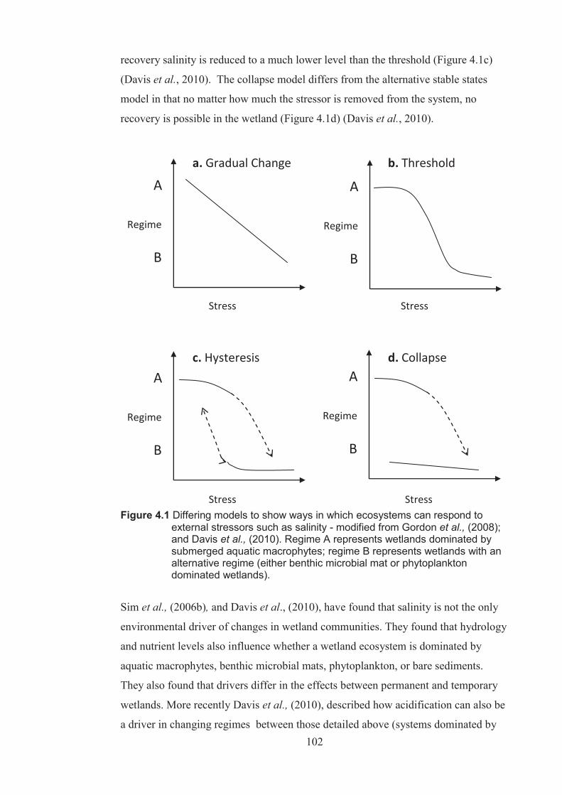
102
recovery salinity is reduced to a much lower level than the threshold (Figure 4.1c)
(Davis et al., 2010). The collapse model differs from the alternative stable states
model in that no matter how much the stressor is removed from the system, no
recovery is possible in the wetland (Figure 4.1d) (Davis et al., 2010).
A
B
Regime
a. Gradual Change
A
B
Regime
b. Threshold
A
B
Regime
c. Hysteresis A
B
Regime
d. Collapse
Stress Stress
Stress Stress
Figure 4.1 Differing models to show ways in which ecosystems can respond to external stressors such as salinity - modified from Gordon et al., (2008); and Davis et al., (2010). Regime A represents wetlands dominated by submerged aquatic macrophytes; regime B represents wetlands with an alternative regime (either benthic microbial mat or phytoplankton dominated wetlands).
Sim et al., (2006b), and Davis et al., (2010), have found that salinity is not the only
environmental driver of changes in wetland communities. They found that hydrology
and nutrient levels also influence whether a wetland ecosystem is dominated by
aquatic macrophytes, benthic microbial mats, phytoplankton, or bare sediments.
They also found that drivers differ in the effects between permanent and temporary
wetlands. More recently Davis et al., (2010), described how acidification can also be
a driver in changing regimes between those detailed above (systems dominated by

103
aquatic macrophytes, benthic microbial mats, phytoplankton, or bare sediments), and
that it is not as simple as a single environmental factor influencing what regime a
wetland shows, rather it is the interaction between watering regimes, salinity,
nitrification and acidification that can drive these systems (Figure 4.2). Ultimately
there are multiple stressors on any wetland system and as such relationships between
one regime and the next may not be as straightforward as models represented in
Figure 4.1.There may in fact be models nested within a larger and an overarching
complex model.
The changes in community structure with increasing salinity found in the Lake
Cullen propagule bank experiment (Chapter 3), did not follow the same patterns
described in similar studies (Sim et al., 2006a; Sim et al., 2006b; Sim et al., 2006c).
Instead, a change from a macrophyte dominated community to that of a
phytoplankton dominated community was found with increasing salinity. A clear
water transitional stage occurred between the two “states”, rather than a benthic
microbial community. This provides further support for the theory that there are
multiple stressors influencing wetland conditions and that wetlands do not always
change from a macrophyte dominated community to a benthic microbial mat
community with increased salinity (Davis et al., 2010).
The presence of hysteresis and alternative stable states within an ecosystem is not
easily demonstrated. Scheffer and Carpenter (2003) suggested that through
controlled experiments, changes in the structure of an ecosystem can be explained by
the alternative stable states model, whether it be the hysteresis model (Figure 4.1c) or
the collapse model (Figure 4.1d).
The following factors are thought to exert such an influence:
different initial states leading to differing final states
disturbances triggering a shift to another permanent state
presence of hysteresis in response to increases and decreases in disturbance
(i.e. salinity)

104
Cl
ear w
ater
mac
roph
yte
dom
inat
ed c
omm
unity
Clea
r wat
er
mac
roph
yte
dom
inat
ed
com
mun
ity
Turb
id
phyt
opla
nkto
n do
min
ated
co
mm
unity
Bent
hic
mic
robi
al
mat
dom
inat
ed
com
mun
ity
Turb
id
sedi
men
t do
min
ated
w
etla
nd
No
Chan
ge
Perm
anen
t w
ater
Pr
olon
ged
dryi
ng
Orig
inal
ec
olog
ical
re
gim
e
Hydr
olog
ical
Ch
ange
Stre
sses
Resu
lting
ec
olog
ical
re
gim
e
Salin
isatio
n Ac
idifi
catio
n
Salin
isatio
n &
Eu
trop
hica
tion
Salin
isatio
n &
Ac
idifi
catio
n
Eutr
ophi
catio
n
Figu
re 4
.2: T
he p
ropo
sed
inte
ract
ions
bet
wee
n hy
drol
ogic
al re
gim
e, s
alin
isat
ion,
eut
roph
icat
ion
and
acid
ifica
tion
on th
e st
ate
of s
hallo
w fr
eshw
ater
sys
tem
s in
sou
thw
este
rn A
ustra
lia
mod
ified
from
Dav
is e
t al.,
(201
0)
105
Many studies of wetland propagule banks have focussed on determining the floral or
invertebrate communities that emerge from sediments at various salinity
concentrations after a period of drying or drought (Brock and Britton, 1995; Brock et
al., 2003; Nielsen et al., 2003a; Nielsen et al., 2003b; Brock et al., 2005; Sim et al.,
2006a; Sim et al., 2006b; Nielsen et al., 2007; Nielsen et al., 2008). One study by
Sim et al., (2006b) investigated the effect of increasing salinity concentrations on the
plant germination from two saline wetlands in Western Australia and the effect of
increasing salinities over a period of time on the health of Ruppia polycarpa (R.
Mason) plants. Sim et al., (2006b) not only tested the effect of increasing salinities
on this macrophyte, but also the effect of the rate of increasing salinity
concentrations. Results of this study showed that plant condition declined rapidly at
salinities > 45 g/L and that rapid increases in salinity caused a rapid decline in plant
condition.
Another study by Robinson et al., (2006), tested the effect of preliminary exposure of
Melaleuca ericifolia seeds on germination success. Seeds were exposed to a number
of preliminary saline treatments up to and including 16 g/L before being returned to
distilled water. Robinson et al., (2006) found that seeds were able to germinate in all
preliminary saline treatments. They also found that returning the seeds to distilled
water greatly increased Melaleuca ericifolia germination success.
4.1.2 Hypotheses Few propagule bank studies have focussed on species recovery after a period of high
saline disturbance with the exception of Neilsen et al., (2007) and Waterkeyn (2011).
Neilsen et al., (2007) investigated how 14 day high and low salinity pulses affected
the plant and zooplankton from the propagule banks of three freshwater wetlands.
Pulse events are short term increases in salinity, often associated with saline water
disposal in rivers and wetlands (Nielsen et al., 2007). Salinity pulses were found to
have no effect on the emergence of plants from the propagule banks, but did have a
positive effect on zooplankton emergence. All three wetlands had increased
emergence of zooplankton after the low and high pulses of salinity (Nielsen et al.,
2007). Waterkeyn et al., (2011), investigated the effect of flooding frequency and
increase salinity (up to 5 g/L) on the emergence of crustaceans from the propagule

106
bank over a 3 year period. Waterkeyn et al., (2011), found that the crustacean
community was able to re-establish after disturbances, however the frequency of
flooding and salinity concentrations affected species differently.
It should be noted that the high and low pulses of salinity (5 g/L and 1 g/L
respectively) of the study by Neilsen et al., (2007) and Waterkeyn et al., (2011) were
much lower than the salinities tested in both this experiment and that by Sim et al.,
(2006b), and thus the findings may not be applicable for higher salinity disturbances.
The hypotheses were tested in this study:
Do high salinity disturbances affect the recovery of the dominant species
present in the propagule bank of Lake Cullen and is the salinity threshold for
germination the same as those propagules not subjected to a high salinity
disturbance?
What type of threshold response occurs with changing recovery salinity
concentrations? Does the response follow a hysteresis, threshold response or
irreversible change model?
How do varying response salinity levels affect individual species emergence,
growth or reproduction?

107
4.2 Methods The effect of changing salinity regimes on the propagule bank of Lake Cullen was
investigated by subjecting sediments to four high salinity treatments for 14 weeks
(Disturbance Phase) before the water in these treatments was changed and the
sediments were subjected to various salinity treatments which were lower or
equivalent to those used in the disturbance phase for a further 12 weeks (Recovery
Phase) (Figure 4.3). All treatments were determined by using a partial Fibonacci
numeric sequence, which represented a natural logarithmic relationship, with the
exception of the highest salinity treatment that was set at 136.0 g/L as the solution
became saturated.
Sediment from Lake Cullen was collected in September 2005, when the wetland was
dry and before it received an environmental water allocation. Sediments from the top
5 cm of the wetland surface were collected using a spade. Sediment collection sites
were chosen from random locations 0 and 50 meters from the wetland edge.
Sediment samples were transported back to the laboratory where they were stored in
the dark at ± 4oC for two months to prevent propagule germination. Samples were
then dried thoroughly under cover in a glasshouse (to prevent contamination from
airborne propagules) before being passed through a soil crusher set at a diameter of 6
mm (Jaw Crusher PEX 60 x 100). Dead vegetation was removed during this process.
Crushed samples were mixed thoroughly with a spade, to minimise the influence of
spatial variation in the wetland soil propagule banks.
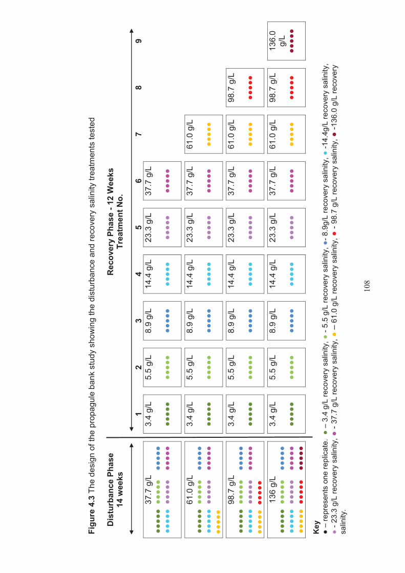
108
Figu
re 4
.3 T
he d
esig
n of
the
prop
agul
e ba
nk s
tudy
sho
win
g th
e di
stur
banc
e an
d re
cove
ry s
alin
ity tr
eatm
ents
test
ed
D
istu
rban
ce P
hase
14
wee
ks
Rec
over
y Ph
ase
- 12
Wee
ks
Trea
tmen
t No.
1
2
3
4
5
6
7
8
9 37
.7 g
/L
●●●●
● ●●●
●●
●●●
●●
●●●●
● ●●●
●●
●●●
●●
3.
4 g/
L
●●●●
●
5.
5 g/
L
●●●●
●
8.
9 g/
L
●●●●
●
14.4
g/L
●●●●
●
23
.3 g
/L
●●
●●●
37
.7 g
/L
●●
●●●
61.0
g/L
●●
●●●
●●●
●●
●●●
●●
●●●●
● ●●●
●●
●●●
●●
●●●●
●
3.
4 g/
L
●●●●
●
5.
5 g/
L
●●●●
●
8.
9 g/
L
●●●●
●
14
.4 g
/L
●●
●●●
23
.3 g
/L
●●
●●●
37
.7 g
/L
●●
●●●
61
.0 g
/L
●●
●●●
98.7
g/L
●●
●●●
●●●
●●
●●●
●●
●●●●
● ●●●
●●
●●●
●●
●●●●
● ●●●
●●
3.
4 g/
L
●●●●
●
5.
5 g/
L
●●●●
●
8.
9 g/
L
●●●●
●
14
.4 g
/L
●●
●●●
23
.3 g
/L
●●
●●●
37
.7 g
/L
●●
●●●
61
.0 g
/L
●●
●●●
98
.7 g
/L
●●
●●●
136
g/L
●●●●
● ●●●
●●
●●●
●●
●●●●
● ●●●
●●
●●●
●●
●●●●
● ●●●
●●
●●●
●●
3.
4 g/
L ●●
●●●
5.
5 g/
L
●●●●
●
8.
9 g/
L
●●●●
●
14
.4 g
/L
●●
●●●
23
.3 g
/L
●●
●●●
37
.7 g
/L
●●
●●●
61
.0 g
/L
●●
●●●
98
.7 g
/L
●●
●●●
13
6.0
g/L
●●●●
●
Key
●
– re
pres
ents
one
repl
icat
e. ●
– 3
.4 g
/L re
cove
ry s
alin
ity, ●
- 5.
5 g/
L re
cove
ry s
alin
ity, ●
- 8.9
g/L
reco
very
sal
inity
, ● -1
4.4g
/L re
cove
ry s
alin
ity,
● - 2
3.3
g/L
reco
very
sal
inity
, ● -
37.7
g/L
reco
very
sal
inity
, ● –
61.
0 g/
L re
cove
ry s
alin
ity, ●
- 98
.7 g
/L re
cove
ry s
alin
ity, ●
-136
.0 g
/L re
cove
ry
salin
ity.
109
A total of 160, 20L clear plastic tubs were used in this experiment. There were 5
replicates for each of the 30 treatments with exception of the control treatment that
consisted of 10 tubs. The tubs were arranged randomly throughout an air conditioned
glasshouse. Their position was determined using a random numbers table (Appendix
9). Each tub contained a total of 1kg of sediment from Lake Cullen, distributed
between two small plastic trays (120mm x 175mm x 60mm) (500 g in each). There
were also 10 control tubs set up with 1 kg of sterilised sand distributed between two
plastic trays, to test for contamination by airborne propagules throughout the
experiment. The control tubs contained 3.4 g/L saline solution and no plants or
animals were found in the tubs at the conclusion of the experiments. Tubs were filled
with 15 L of solution at the required salinity and the depth of the solution was
marked on the side of the tub. Salinity concentrations were checked weekly with a
conductivity meter to ensure that salinity concentrations remained within the range of
± 16% for the appropriate treatment concentrations. Tubs were topped up with tap
water if necessary over a 14 week period.
At the end of the Disturbance Phase (14 weeks) saline solution was drained from all
replicates to a depth of 7 cm using a 25 μm mesh filter attached to a syphon to ensure
that no phytoplankton, zooplankton or other invertebrates were lost from the sample.
Propagules caught in the mesh were returned to the tub immediately. No plant,
invertebrate or algal material was removed from the tubs at the end of the
disturbance phase. Tubs were then refilled to the marked level with water to the
required Recovery Phase salinity. Tubs were checked regularly and topped up with
tap water if necessary over a 12 week period (Recovery Phase) to ensure that salinity
concentrations remained within the desired treatment range (± 10%).
4.2.1 Air temperature and water quality monitoring The method described in Chapter 3 was used for this study to monitor air and water
quality.

110
4.2.2 Monitoring of aquatic macrophyte germination (seeds and asexual
propagules) and invertebrate hatching from the propagule bank
The method described in Chapter 3 was used for this study to monitor aquatic
macrophyte germination and invertebrate hatching from the propagule bank.
4.2.3 Invertebrate sampling The method described in Chapter 3 was used for this study to capture and count the
invertebrates that emerged during the experiment. To facilite sorting of invertebrates
from detritus, the same sugar floatation method was used and the sampling efficiency
(QA/QC check) of this method was conducted as described in Chapter 3.
Results of the QA/QC check of the effectiveness of the sugar flotation method
showed that minimum of 95% of invertebrates for each species were successfully
removed from the organic material present in the (Appendix 10). The sugar flotation
method was deemed to be a successful and efficient method in sorting invertebrates
from organic materials collected in the > 500 μm sieve. For the 250 μm to 500 μm
and the 108 μm to 250 μm size invertebrates, no flotation method was necessary as
less detritus was present in these samples.
4.2.4 Harvesting aquatic macrophytes At the end of the 26 week study period, all emergent aquatic macrophytes were
harvested and sorted according to species. For each aquatic angiosperm species the
number of shoots, reproductive individuals, flowers budding, mature flowers, fruit,
reproductive structures, aborted sexual reproductive structures and seeds produced
by the plants were recorded. For the charophytes the number of individuals,
reproductive individuals, and number of reproductive structures on whorls were
recorded.
The aboveground biovolume and dry weight biomass of the measured plant material
of each species was then measured using the methods and equations described in
Chapter 3.
111
4.2.5 Data analysis Data was analysed for linear, quadratic, and cubic regressions to determine how the
species responded to increased salinity concentrations and to ascertain an upper
salinity threshold. Results were also analysed using two way ANOVA tests to
determine if there was any significant difference (p < 0.05) between salinity
treatments, using the following model.
DV = constant + Disturbance Phase salinity + Recovery Phase salinity + Distrubance
Phase salinity x Recovery phase salinity
Where results of the two way ANOVA’s were significant, post hoc Tukey’s tests
were conducted to determine which treatments were significantly different. All
statistical tests were conducted using the PASW 18 (previously known as SPSS
statistics) software package. Square root transformations of the dependent variable
were undertaken when the data from this experiment did not meet the assumptions of
normality or homogeneity of variances for parametric tests (Levene’s test).

112
4.3 Results
4.3.1 Air temperature and water quality monitoring Maximum air temperature ranged between 20.1 oC and 40.5 oC, while minimum air
temperatures ranged from 6.0 oC to 14.7 oC. Maximum water temperatures ranged
between 15 oC and 32 oC, while minimum water temperatures ranged from 8 oC to 25
oC (Appendix 11). Monitoring results of salinity concentrations for each replicate
showed that on average maximum salinity concentrations were maintained within
16% of target treatment concentration. The monitoring results for pH indicated that
waters were alkaline, ranging from pH 7.35 to 9.90 (Appendix 11).
4.3.2 Emergence of aquatic macrophyte and invertebrate taxa Three species of aquatic macrophyte germinated in this experiment; Ruppia
megacarpa, Lamprothamnium macropogon and an unidentified Ruppia spp. The
unidentified Ruppia spp. only occurred in one replicate (Disturbance Phase salinity
98.7 g/L, Recovery Phase salinity 14.4 g/L treatment) and was not possible to
identify to species level as it did not flower during the experiment.
Figure 4.4, shows that the germination of aquatic macrophytes only occurred within
the Disturbance Phase of this experiment (first 14 weeks) in the treatment where the
salinity was ≤ 37.7 g/L. In treatments where Disturbance Phase salinity was ≤ 37.7
g/L germination did not occur at the same time for the two dominant aquatic
macrophyte species. Lamprothamnium macropogon germinated in all replicates with
a Disturbance Phase salinity concentrations of 37.7 g/L by Week 7 of the experiment.
Results for R. megacarpa was less uniform with individuals observed to have
germinated during the Disturbance Phase (salinity 37.7 g/L) of the experiment in 11
replicates, whilst other replicates were only observed to have individuals germinating
much later in the Recovery Phase after salinity concentrations were reduced (Figure
4.4).
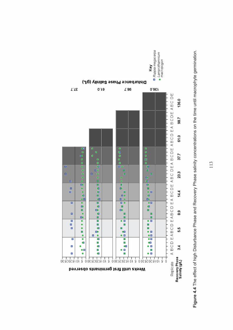
113
Fi
gure
4.4
The
effe
ct o
f hig
h D
istu
rban
ce P
hase
and
Rec
over
y Ph
ase
salin
ity c
once
ntra
tions
on
the
time
until
mac
roph
yte
germ
inat
ion.
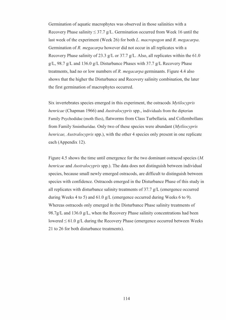
114
Germination of aquatic macrophytes was observed in those salinities with a
Recovery Phase salinity ≤ 37.7 g/L. Germination occurred from Week 16 until the
last week of the experiment (Week 26) for both L. macropogon and R. megacarpa.
Germination of R. megacarpa however did not occur in all replicates with a
Recovery Phase salinity of 23.3 g/L or 37.7 g/L. Also, all replicates within the 61.0
g/L, 98.7 g/L and 136.0 g/L Disturbance Phases with 37.7 g/L Recovery Phase
treatments, had no or low numbers of R. megacarpa germinants. Figure 4.4 also
shows that the higher the Disturbance and Recovery salinity combination, the later
the first germination of macrophytes occurred.
Six invertebrates species emerged in this experiment, the ostracods Mytilocypris
henricae (Chapman 1966) and Australocypris spp., individuals from the dipterian
Family Psychodidae (moth flies), flatworms from Class Turbellaria, and Collembollans
from Family Sminthuridae. Only two of these species were abundant (Mytliocypris
henricae, Australocypris spp.), with the other 4 species only present in one replicate
each (Appendix 12).
Figure 4.5 shows the time until emergence for the two dominant ostracod species (M.
henricae and Australocypris spp.). The data does not distinguish between individual
species, because small newly emerged ostracods, are difficult to distinguish between
species with confidence. Ostracods emerged in the Disturbance Phase of this study in
all replicates with disturbance salinity treatments of 37.7 g/L (emergence occurred
during Weeks 4 to 5) and 61.0 g/L (emergence occurred during Weeks 6 to 9).
Whereas ostracods only emerged in the Disturbance Phase salinity treatments of
98.7g/L and 136.0 g/L, when the Recovery Phase salinity concentrations had been
lowered ≤ 61.0 g/L during the Recovery Phase (emergence occurred between Weeks
21 to 26 for both disturbance treatments).
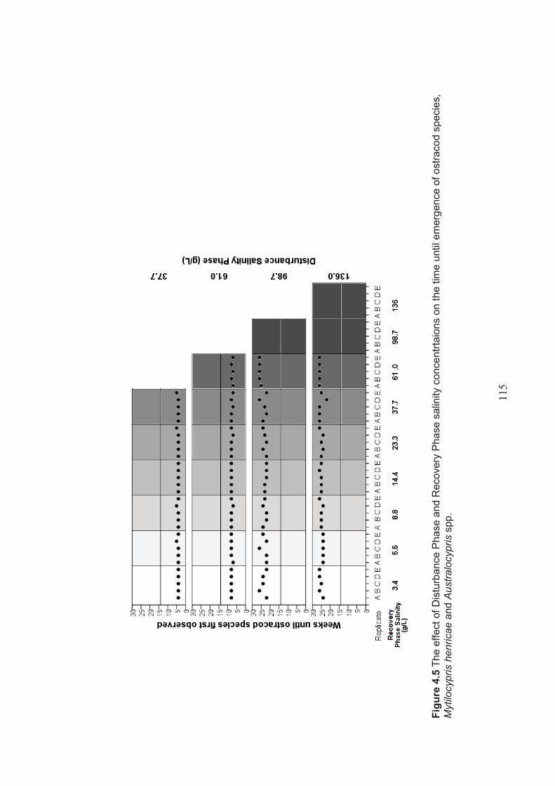
115
Fi
gure
4.5
The
effe
ct o
f Dis
turb
ance
Pha
se a
nd R
ecov
ery
Pha
se s
alin
ity c
once
ntrta
ions
on
the
time
until
em
erge
nce
of o
stra
cod
spec
ies,
M
ytilo
cypr
is h
enric
ae a
nd A
ustra
locy
pris
spp
.

116
4.3.3 Aquatic macrophyte germination - Ruppia megacarpa In 3 out of the 4 Disturbance Phase salinity treatments, the number of R. megacarpa
stems produced as Recovery Phase salinity increased showed significant negative
linear regressions (p <0.05) (Figure 4.6). Results of significant linear regressions for
the 61.0 g/L (p < 0.001, R2 = 0.519), 98.7 g/L (p < 0.001, R2 = 0.586) and 136 g/L
(p < 0.001, R2 = 0.592) treatments were very similar indicating that whilst the
Recovery Phase salinity concentrations did impact the number of R. megacarpa
stems produced, this was minimal despite the differences in initial Disturbance Phase
salinity concentrations the propagule banks were exposed to (Figure 4.6 and
Appendix 13). The lowest Disturbance Phase salinity treatment (37.7 g/L) showed
no significant regression, although the numbers of stems produced was similar to that
of the other three Disturbance Phase salinity concentrations.
Results of a two way ANOVA showed that there was a main effect of Disturbance
Phase salinity concentration on the number of R. megacarpa stems produced (p =
0.046, F = 2.743, df = 3, 120). There was also a main effect of Recovery Phase
salinity concentration on number of R. megacarpa stems produced (p < 0.001, F =
29.246, df = 8, 120) and a significant interaction of Disturbance Phase salinity and
Recovery Phase salinity on the number of R. megacarpa stems produced (p = 0.042,
F = 1.734, df = 8, 120). This indicates that not only did both the Disturbance and
Recovery salinities affect the number of R. megacarpa stems produced, but that the
effect of the Recovery Phase salinity concentratons was different depending on the
Disturbance Phase salinity treatment the seedbank was subjected to. Post hoc
Tukey’s tests indicated that there was no significant difference between any of the
Disturbance phase salinity treatments. However there were significant differences
found between many of the Recovery Phase salinity treatments, please refer to
Appendix 13.
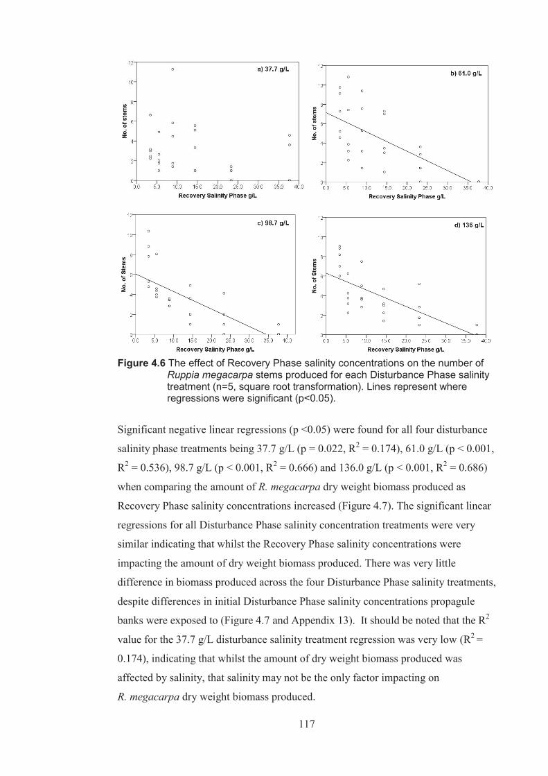
117
Figure 4.6 The effect of Recovery Phase salinity concentrations on the number of
Ruppia megacarpa stems produced for each Disturbance Phase salinity treatment (n=5, square root transformation). Lines represent where regressions were significant (p<0.05).
Significant negative linear regressions (p <0.05) were found for all four disturbance
salinity phase treatments being 37.7 g/L (p = 0.022, R2 = 0.174), 61.0 g/L (p < 0.001,
R2 = 0.536), 98.7 g/L (p < 0.001, R2 = 0.666) and 136.0 g/L (p < 0.001, R2 = 0.686)
when comparing the amount of R. megacarpa dry weight biomass produced as
Recovery Phase salinity concentrations increased (Figure 4.7). The significant linear
regressions for all Disturbance Phase salinity concentration treatments were very
similar indicating that whilst the Recovery Phase salinity concentrations were
impacting the amount of dry weight biomass produced. There was very little
difference in biomass produced across the four Disturbance Phase salinity treatments,
despite differences in initial Disturbance Phase salinity concentrations propagule
banks were exposed to (Figure 4.7 and Appendix 13). It should be noted that the R2
value for the 37.7 g/L disturbance salinity treatment regression was very low (R2 =
0.174), indicating that whilst the amount of dry weight biomass produced was
affected by salinity, that salinity may not be the only factor impacting on
R. megacarpa dry weight biomass produced.
118
Results of a two way ANOVA showed that there was no significant main effect of
Disturbance Phase salinity concentration on R. megacarpa dryweight biomass
produced (p = 0.803). There was also no significant intereaction effect of
Disturbance phase salinity and Recovery Phase salinity on the amount of
R. megacarpa dryweight biomass produced (p = 0.493). There was however a main
effect of Recovery Phase salinity concentration on on the amount of R. megacarpa
dryweight biomass produced (p < 0.001, F = 0.330, df = 8, 120). This indicates that
only the Recovery salinity treatments affected the amount of R. megacarpa
dryweight biomass produced. Post hoc Tukey’s tests indicated that there was
significant differences found between many of the Recovery Phase salinity
treatments, please refer to Appendix 13.
Reproductive structures (flowers and fruit) on R. megacarpa were recorded in a few
replicates exposed to the lowest Disturbance Phase salinity treatment of 37.7 g/L and
only one flower was recorded in the 61.0 g/L Disturbance Phase salinity and 5.5 g/L
Recovery Phase salinity treatments. Little more can be deduced from these results
and regarding the effects of Disturbance and Recovery Phase salinity concentrations
on reproduction in this species, given the low concentrations of reproduction.
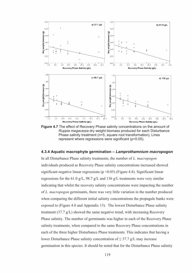
119
Figure 4.7 The effect of Recovery Phase salinity concentrations on the amount of
Ruppia megacarpa dry weight biomass produced for each Disturbance Phase salinity treatment (n=5, square root transformation), Lines represent where regressions were significant (p<0.05).
4.3.4 Aquatic macrophyte germination – Lamprothamnium macropogon In all Disturbance Phase salinity treatments, the number of L. macropogon
individuals produced as Recovery Phase salinity concentrations increased showed
significant negative linear regressions (p <0.05) (Figure 4.8). Significant linear
regressions for the 61.0 g/L, 98.7 g/L and 136 g/L treatments were very similar
indicating that whilst the recovery salinity concentrations were impacting the number
of L. macropogon germinants, there was very little variation in the number produced
when comparing the different initial salinity concentrations the propagule banks were
exposed to (Figure 4.8 and Appendix 13). The lowest Disturbance Phase salinity
treatment (37.7 g/L) showed the same negative trend, with increasing Recovery
Phase salinity. The number of germinants was higher in each of the Recovery Phase
salinity treatments, when compared to the same Recovery Phase concentrations in
each of the three higher Disturbance Phase treatments. This indicates that having a
lower Disturbance Phase salinity concentration of ≤ 37.7 g/L may increase
germination in this species. It should be noted that for the Disturbance Phase salinity

120
treatments of 37.7 g/L and 61.0 g/L that the R2 values were low (<0.3) indicating that
the Reovery Phase salinity may not be the only factor affecting results. All other
regressions were much stronger with R2 values of > 0.6.
Results of a two way ANOVA showed that there was a main effect of Disturbance
Phase salinity concentration on the number of L.macropogon germinants
(p = <0.001, F = 260.486, df = 3, 120). There was also a main effect of Recovery
Phase salinity concentration on number of L.macropogon germinants (p < 0.001,
F = 113.037, df = 8, 120) and a significant interaction of Disturbance Phase salinity
and Recovery Phase salinity on the number of L.macropogon germinants (p = 0.005,
F = 2.246, df = 18, 120). This indicates that not only did both the Disturbance and
Recovery salinities affect the number of L.macropogon germinants, but that the
effect of the Recovery Phase salinity concentratons was different depending on the
Disturbance Phase salinity treatment the seedbank was subjected to. Post hoc
Tukey’s tests indicated that there was a significant difference between all of the
Disturbance phase salinity treatments. There were also significant differences found
between many of the Recovery Phase salinity treatments, please refer to Appendix
13.
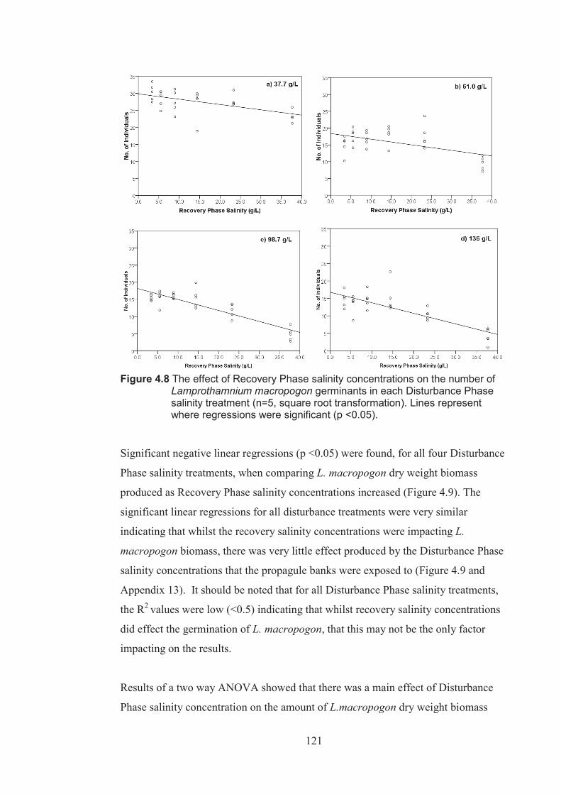
121
Figure 4.8 The effect of Recovery Phase salinity concentrations on the number of
Lamprothamnium macropogon germinants in each Disturbance Phase salinity treatment (n=5, square root transformation). Lines represent where regressions were significant (p <0.05).
Significant negative linear regressions (p <0.05) were found, for all four Disturbance
Phase salinity treatments, when comparing L. macropogon dry weight biomass
produced as Recovery Phase salinity concentrations increased (Figure 4.9). The
significant linear regressions for all disturbance treatments were very similar
indicating that whilst the recovery salinity concentrations were impacting L.
macropogon biomass, there was very little effect produced by the Disturbance Phase
salinity concentrations that the propagule banks were exposed to (Figure 4.9 and
Appendix 13). It should be noted that for all Disturbance Phase salinity treatments,
the R2 values were low (<0.5) indicating that whilst recovery salinity concentrations
did effect the germination of L. macropogon, that this may not be the only factor
impacting on the results.
Results of a two way ANOVA showed that there was a main effect of Disturbance
Phase salinity concentration on the amount of L.macropogon dry weight biomass
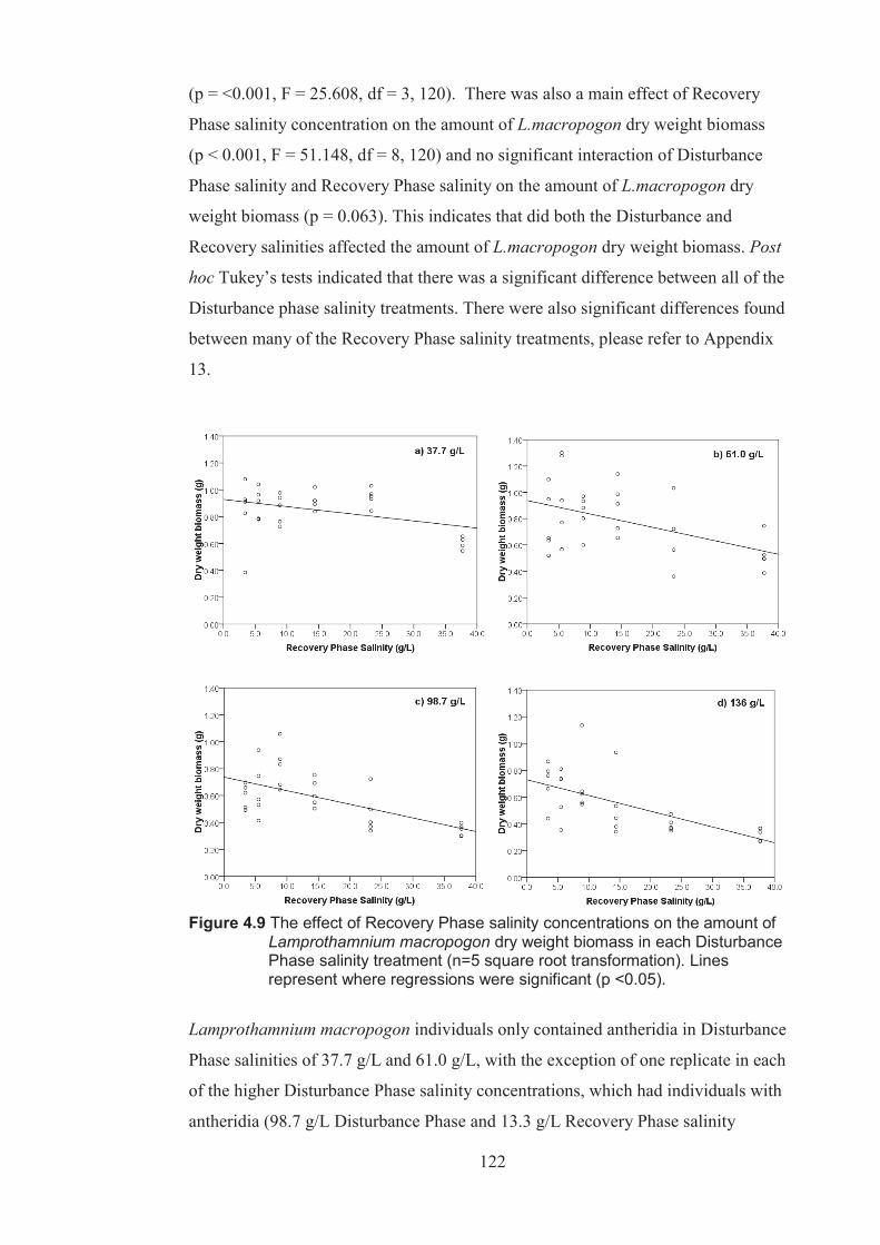
122
(p = <0.001, F = 25.608, df = 3, 120). There was also a main effect of Recovery
Phase salinity concentration on the amount of L.macropogon dry weight biomass
(p < 0.001, F = 51.148, df = 8, 120) and no significant interaction of Disturbance
Phase salinity and Recovery Phase salinity on the amount of L.macropogon dry
weight biomass (p = 0.063). This indicates that did both the Disturbance and
Recovery salinities affected the amount of L.macropogon dry weight biomass. Post
hoc Tukey’s tests indicated that there was a significant difference between all of the
Disturbance phase salinity treatments. There were also significant differences found
between many of the Recovery Phase salinity treatments, please refer to Appendix
13.
Figure 4.9 The effect of Recovery Phase salinity concentrations on the amount of
Lamprothamnium macropogon dry weight biomass in each Disturbance Phase salinity treatment (n=5 square root transformation). Lines represent where regressions were significant (p <0.05).
Lamprothamnium macropogon individuals only contained antheridia in Disturbance
Phase salinities of 37.7 g/L and 61.0 g/L, with the exception of one replicate in each
of the higher Disturbance Phase salinity concentrations, which had individuals with
antheridia (98.7 g/L Disturbance Phase and 13.3 g/L Recovery Phase salinity
123
treatment and 136 g/L Disturbance Phase and 24.4 g/L Recovery Phase salinity
treatment). A higher percentage of individuals had antheridia in the Disturbance
Phase salinity of 37.7 g/L when compared to the Disturbance Phase salinity of 61.0
g/L (Appendix 13). There were no oogonia observed to be produced on any L.
macropogon individuals in this experiment.
4.3.5 Phytoplankton Blooms Visual observations of the tubs indicated that phytoplankton blooms occurred in all
replicates in the highest disturbance salinity treatment (136.0 g/L). These blooms
formed by Week 4 and persisted for the duration of the disturbance phase of the
experiment (Table 4.1). In the recovery phase of the experiment, phytoplankton
blooms were only present in the treatment with Recovery Phase salinity of 136.0 g/L,
however these algal blooms occurred in every replicate with this salinity.

124
Tabl
e 4.
1 Pr
esen
ce o
f phy
topl
ankt
on b
loom
s in
repl
icat
es in
the
136.
0 g/
L D
istu
rban
ce P
hase
sal
inity
trea
tmen
t for
the
dura
tion
of th
e ex
perim
ent.
Num
bers
(up
to 5
) ind
icat
e th
e nu
mbe
r of r
eplic
ates
wer
e al
gal b
loom
s w
ere
pres
ent.
Ke
y
abse
nt
pr
esen
t
Repl
icate
W
eek
Dist
urba
nce P
hase
Re
cove
ry P
hase
Di
stur
banc
e Ph
ase
g/L
Reco
very
Ph
ase
g/L
1 2
3 4
5 6
7 8
9 10
11
12
13
14
15
16
17
18
19
20
21
22
23
24
25
26
136.0
3.4
0
0 0
5 5
5 5
5 5
5 5
5 5
5 0
0 0
0 0
0 0
0 0
0 0
0 13
6.0
5.5
0 0
0 5
5 5
5 5
5 5
5 5
5 5
0 0
0 0
0 0
0 0
0 0
0 0
136.0
8.9
0
0 0
5 5
5 5
5 5
5 5
5 5
5 0
0 0
0 0
0 0
0 0
0 0
0 13
6.0
14.4
0 0
0 5
5 5
5 5
5 5
5 5
5 5
0 0
0 0
0 0
0 0
0 0
0 0
136.0
23
.3 0
0 0
5 5
5 5
5 5
5 5
5 5
5 0
0 0
0 0
0 0
0 0
0 0
0 13
6.0
37.7
0 0
0 5
5 5
5 5
5 5
5 5
5 5
0 0
0 0
0 0
0 0
0 0
0 0
136.0
61
.0 0
0 0
5 5
5 5
5 5
5 5
5 5
5 0
0 0
0 0
0 0
0 0
0 0
0 13
6.0
98.7
0 0
0 5
5 5
5 5
5 5
5 5
5 5
0 0
0 0
0 0
0 0
0 0
0 0
136.0
13
6.0
0 0
0 5
5 5
5 5
5 5
5 5
5 5
5 5
5 5
5 5
5 5
5 5
5 5
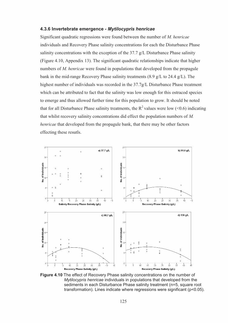
125
4.3.6 Invertebrate emergence - Mytilocypris henricae Significant quadratic regressions were found between the number of M. henricae
individuals and Recovery Phase salinity concentrations for each the Disturbance Phase
salinity concentrations with the exception of the 37.7 g/L Disturbance Phase salinity
(Figure 4.10, Appendix 13). The significant quadratic relationships indicate that higher
numbers of M. henricae were found in populations that developed from the propagule
bank in the mid-range Recovery Phase salinity treatments (8.9 g/L to 24.4 g/L). The
highest number of individuals was recorded in the 37.7g/L Disturbance Phase treatment
which can be attributed to fact that the salinity was low enough for this ostracod species
to emerge and thus allowed further time for this population to grow. It should be noted
that for all Disturbance Phase salinity treatments, the R2 values were low (<0.6) indicating
that whilst recovery salinity concentrations did effect the population numbers of M.
henricae that developed from the propagule bank, that there may be other factors
effecting these resutls.
Figure 4.10 The effect of Recovery Phase salinity concentrations on the number of
Mytilocypris henricae individuals in populations that developed from the sediments in each Disturbance Phase salinity treatment (n=5, square root transformation). Lines indicate where regressions were significant (p<0.05).

126
Results of a two way ANOVA showed that there was a main effect of Disturbance Phase
salinity concentration on the number of M. henricae individuals (p = <0.001,
F = 33.157, df = 3, 120). There was also a main effect of Recovery Phase salinity
concentration on number of M. henricae individuals (p < 0.001, F = 16.961, df = 8, 120)
and a significant interaction of Disturbance Phase salinity and Recovery Phase salinity on
the number of M. henricae individuals (p = 0.024, F = 1.872, df = 18, 120). This indicates
that not only did both the Disturbance and Recovery salinities affect the number of M.
henricae individuals, but that the effect of the Recovery Phase salinity concentratons was
different depending on the Disturbance Phase salinity treatment the propagule bank was
subjected to. Post hoc Tukey’s tests indicated that there was only a significant difference
between the higher Disturbance Phase salinity treatments (61 g/L, 98.7 g/L and 136 g/L)
and the lowest Disturbance Phase salinity treatment (37.7 g/L). There were also
significant differences found between many of the Recovery Phase salinity treatments,
please refer to Appendix 13.
4.3.7 Invertebrate emergence - Australocypris species
Significant quadratic regressions were found with Recovery Phase salinities for the
Disturbance Phase salinity concentrations of 61.0 g/L and 98.7 g/L (Figure 4.11,
Appendix 13). No significant regressions were found for Disturbance Phase salinity
treatments of 37.7 g/L or 136 g/L. It should also be noted that the R2 value for all
quadratic regressions were quite low (< 0.5). The results show that higher numbers of
Australocypris spp. individuals in populations that had developed from the sediments in
the 37.7g/L and 61.0 g/L Disturbance Phase salinity concentrations compared with the
two higher Disturbance Phase salinity treatments. This may be attributed to this species
being able to emerge in these salinity concentrations during the Disturbance Phase of the
experiment, thus allowing extra time for these populations to grow. The results also show
that the Recovery Phase salinity treatments had little effect on the population numbers of
Australocypris spp. as there was little difference in the number of individuals in the
populations that developed from the propagule bank across the different recovery salinity
concentrations within a Disturbance Phase treatment.

127
Figure 4.11 The effect of Recovery Phase salinity concentrations on the number of
Australocypris spp. individuals that emerged from the sediments in each Disturbance Phase salinity treatment (n=5, square root transformation). Lines indicate where regressions were significant (p <0.05).
Results of a two way ANOVA showed that there was a main effect of Disturbance Phase
salinity concentration on the number of Australocypris spp. individuals (p = <0.001,
F = 132.585, df = 3, 120). There was also a main effect of Recovery Phase salinity
concentration on number of Australocypris spp.individuals (p < 0.001, F = 7.532, df = 8,
120) and a significant interaction of Disturbance Phase salinity and Recovery Phase
salinity on the number of Australocypris spp.individuals (p = 0.003, F = 2.364, df = 18,
120). This indicates that not only did both the Disturbance and Recovery salinities affect
the number of Australocypris spp.individuals, but that the effect of the Recovery Phase
salinity concentratons was different depending on the Disturbance Phase salinity
treatment the propagule bank was subjected to. Post hoc Tukey’s tests indicated that
there was a significant difference between all Disturbance Phase salinity treatments.
There were also significant differences found between many of the Recovery Phase
salinity treatments, please refer to Appendix 13.
128
4.4 Discussion The abundant macrophytes, Ruppia megacarpa (Large Fruit Tassel), and L. macropogon
(Stonewort) and two abundant invertebrate species Mytilocypris henricae (Chapman
1966) and Australocypris spp. (both ostracods) were present in the majority of replicates
in the Recovery Phase salinity treatments ≤ 37.7 (threshold between 37.7 g/L and
61.0 g/L), regardless of the Disturbance Phase salinity concentrations these replicates
were subjected to. This suggests that emergence of these species is not affected by high
salinity disturbances experienced over a short period of time. In particular,
L. macropogon and M. henricae were found in all replicates with a Recovery Phase
salinity concentration ≤ 37.7 g/L and Australocypris spp. which was present in all
replicates with a Recovery Phase salinity ≤ 61.0 g/L. These results correspond to the
salinity threshold levels found for all three of these species in Chapter 3. The only species
with a less uniform pattern of emergence (refer to Chapter 3), was the angiosperm R.
megacarpa which was present in all replicates with Recovery Phase salinity treatments ≤
14.4 g/L but only some replicates with a Recovery Phase salinity concentration of 23.3
g/L and 37.7 g/L (Figure 4.5).
4.4.1 Evidence for models predicting the effect of increased salinity concentrations on community change in the propagule bnak biota
Results of species presence or absence for each treatment indicated that the aquatic
macrophyte and invertebrate communities have recovered in way that reflects the salinity
threshold levels determined in Chapter 3 (salinity threshold of levels from 37.7 g/L to
61.0 g/L for R. megacarpa, L. macropogon and M. henricae and a salinity threshold of
between 61.0 g/L and 98.7 g/L for Australocypris spp.). For all abundant species, with the
exception of R. megacarpa, varying Disturbance Phase salinity concentrations had little
effect on their germination in the Recovery Phase. The similarity in threshold levels
shown in this experiment and those of Chapter 3 indicates that this aquatic community
recovery followed a threshold model, rather than an alternative stable states model, a
linear model, or a collapse model (Figure 4.1).
Results of other experimental studies have found that hysteresis is apparent in field data
from Western Australia, where macrophyte dominated wetlands and benthic microbial
mat dominated wetlands occur in the same salinities (Sim et al., 2006c). Hysteresis is
where systems show both alternative states at the same salinity level. For example, in this

129
current experiment some replicates had macrophyte dominated communities whilst others
exposed to the same salinity had predominately phytoplankton communities (Scheffer and
Carpenter, 2003). In this study however, hysteresis was not evident as all replicated
exposed to the same salinity showed the same community, e.g. all treatments with a
recovery concentration ≤ 37.7 g/L showed a macrophyte community (conisisting of R.
megacarpa and L. macropogon) and contained two ostracod species (M. henricae and
Australocypris spp).
Sim et al., (2006c), suggested that other factors apart from salinity may be adding to the
conflicting results reported in different studies. In particular, Sim et al., (2006c) found
that the way in which wetlands fill with water, the permanence of the watering regime
and the nutrient load are important in determining the biota that establishes within a
wetland. Sim et al., (2006c) and Strelow et al., (2005) also reported four differing
‘regimes/states’ being present in wetlands in south western, Western Australia (namely
aquatic macrophyte dominated, clear water dominated, benthic microbial mat dominated
and phytoplankton dominated), further complicating the model, if an alternative stable
states system actually exists.
Scheffer and Carpenter (2003) state that the following factors are all experimental
evidence for the existence of alternative stable states:
different initial states leading to different final states
disturbances triggering a shift to another permanent state
or presence of hysteresis in response to changes back and forth between differing states
Taking the points above into account, the results of this current study show little evidence
supporting the presence of hysteresis or alternative stable states. The higher salinity
treatments did affect the number or growth of some species when recovery salinity
concentrations were below 37.7 g/L. Communities in these treatments however still
exhibited the characteristics of a submerged aquatic community and thus the clear water
or algal bloom “state” did not persist in any of the recovery treatments of ≤ 37.7 g/L.
Also, the differing initial (disturbance) salinity concentrations tested did not result in
differing final states with all Recovery treatments at ≤ 37.7 g/L resulting in a macrophytes
dominated system, and Recovery treatments set at ≥ 61.0 g/L resulted in a clear water
system or algal bloom.
130
Whilst alternative stable states were suggested as a possible model describing how
communities change from macrophyte dominated to benthic microbial mat dominated
wetlands in Western Australia (Davis, 2002; Strehlow et al., 2005; Sim et al., 2006a; Sim
et al., 2006b; Sim et al., 2006c), studies have stressed that there may be multiple
influences from a number of stressors including salinity, watering regime and
eutrophication affecting wetlands and thus simple models may not be very useful for
predicting community change (Davis et al., 2010). The results of this study and those of
the previous chapter are in support of this multiple stresses model. This is particularly
evident given that the shift between “states” in this current experiment and those
described in the previous chapter are different to those reported from Western Australia
(Davis, 2002; Strehlow et al., 2005; Sim et al., 2006a; Sim et al., 2006b; Sim et al.,
2006c). Studies in Western Australia have noted the change from a macrophyte
dominated wetland to a benthic microbial mat community with increased salinity (Davis,
2002; Strehlow et al., 2005; Sim et al., 2006a; Sim et al., 2006b; Sim et al., 2006c), in
contrast to this study where a change from a macrophyte dominated to a phytoplankton
dominated community was observed.
Whilst in terms of presence or absence of plant and invertebrate species responses to each
treatment, the overall aquatic community was very similar to the results of Chapter 3. But
individual species responses to Recovery salinity concentrations in terms of number of
individuals, biomass, and production of reproductive structures were different. Number of
individuals, biomass, and the production of reproductive structures were much lower in
this study compared to results reported in Chapter 3.
4.4.2 Effect of disturbance and recovery salinities on germination and growth of individual aquatic macrophyte species
The various Disturbance Phase salinity treatments had a similar effect on the number of
shoots or dry weight biomass for R. megacarpa, or the number of individuals or dry
weight biomass of L. macropogon. It was only the Recovery Phase salinity treatments that
appeared to affect the number of shoots and dry weight biomass for R. megacarpa and the
number of individuals or dry weight biomass of L. macropogon.
These results indicate that both species are able to recover from hypersaline disturbance
(e.g. 136 g/L) in a similar way to intermediate salinity disturbances of 37.7 g/L. This is
despite the fact that germination had occurred in the Disturbance Phase of the experiment

131
in the 37.7 g/L Disturbance Phase salinity treatment, whereas no germination occurred in
the Disturbance Phase salinity concentrations ≥ 61.0 g/L. This indicates that germination
was suppressed by the high salinity but also demonstrates the resilience of both plant
species as the propagules were not killed by the high salinity disturbance. This form of
resilience by suppression of germination is common in wetland plants and not only allows
some species to tolerate short periods of increased salinity by also other disturbances such
as drying (Brock and Casanova, 1991: Brock and Britton, 1995; Brock and Rogers, 1998;
Casanova and Brock, 1999; Leck and Brock, 2000; Skinner et al., 2001; Brock et al.,
2003; Nicol et al., 2003; Nielson et al., 2003a; Capon and Brock 2006; Sim et al., 2006a;
2006b; Nielson et al., 2007; Porter, 2007; Roberton and James, 2007; Goodman et al.,
20011). ( ; ; ; ; ; ; ; ; ; ; ; ; ; ; ; ).
Goodman et al., (2010), also conducted an experiment on four common wetland plants
Triglochin procerum R. Brown (Water ribbon), Myriophyllum simulans Orchard
(Milfoil), Cotula coronopifolia L. (Water buttons) and Baumea arthrophylla (Nees)
Boeckeler (Fine twig sedge) investigating the effect of 3 and 6 week duration salinity
disturbances (4 g/L and 8 g/L) on the survivorship and growth of adult plants. Results of
Goodman et al., (2010) study were also consistent with those presented here as all four
species were able to survive short term exposure to high salinities. They also reported that
these salinity disturbances could impact on growth and thus recovery of submerged plant
species. Whilst lower dry weight biomass results were reported in this current study when
compared to that of Chapter 3, it is hard to ascertain whether the lower biomass is a result
of the high salinity concentrations or as result of lower ambient temperatures, as the
experiments reported in the previous chapter were undertaken in summer whilst the
Recovery Phase of this experiment occurred during the cooler autumn and winter months
(Appendix 11). There have been a number of studies suggesting seasonality (and thus day
length, temperature and rainfall) can affect not only plant growth but also influence the
species that emerge from propagule banks (Britton and Brock, 1994; Casanova and
Brock, 2000; Warwick and Brock, 2003). As such the effect of season on growth, as well
as high salinity disturbances warrant further investigation.
132
4.4.3 Effect of disturbance and recovery salinities on aquatic macrophyte reproductive structures
It was difficult to determine the effects of Disturbance and Recovery Phase salinity
treatments on the reproductive output of R. megacarpa in this experiment, as flowering in
this species and many other aquatic angiosperms seems to be affected by other
environmental factors such as water temperature. During this study there was a difference
in the temperature and photoperiod that replicates were exposed to in Disturbance Phase
when compared to the environmental conditions in Recovery Phase of the experiment, as
shown by the minimum and maximum temperatures recorded throughout the experiment
(Disturbance Phase air temperatures = 8.7 oC to 40.5 oC, Recovery Phase air temperatures
= 5.3 oC to 35.1oC, see Appendix 11). Therefore the result of flowering only occurring in
the Disturbance Phase salinity treatment of 37.7 g/L needs to be treated with caution as
flowering may have occurred in response to warmer temperatures. If the response shown
here is due to an indirect effect of salinity in a lag in flowering rather than a direct result
of salinity in reduced concentrations of flowering, this still has implications for
management. Wetlands would need to be maintained at lower salinites during the warmer
months to allow for maximum flowering for this species (R. megacarpa).
Increased salinity has been reported to cause delayed and reduced flowering in a number
of plant species. Van Zant (2002) reported that increases in salinity concentrations above
4 g/L delayed flowering in Iris hexagona Walt. (Dixie iris) and that this effect of delayed
flowering continues even after salinity concentrations are lowered. Sim et al., (2006a);
James et al., (2003) and James et al., (2009) also reported that plants exposed to
treatments of ≤ 6 g/L flowered later than those in 0 g/L salinity treatments for R.
polycarpa. In order for species to persist long term in wetlands they must be able to
complete their life cycle and contribute viable propagules to the propagule bank. Thus
any delay in germination or flowering can impact the long term viability of wetland
species over the long term. Further investigation into the effect of Disturbance Phase
salinities and time on the production of R. megacarpa flowers is needed.
Lamprothamnium macropogon individuals containing reproductive structures (antheridia)
were only found in the lower Disturbance Phase salinity treatments of 37.7 g/L and
61.0 g/L with the exception of one replicate in 98.7 g/L, and one replicate in the
136 g/L Disturbance Phase salinity treatment which produced oogonia. Similar to the
number of reproductive structures recorded for R. megacarpa, these results need to be
133
treated with caution as germination of this species in some replicates occurred late in the
experiment (Figure 4.1). This is particularly relevant in the higher Disturbance Phase
salinity concentrations of 98.7 g/L and 136 g/L. Therefore the lack of individuals
containing reproductive spores in these treatments may not be due to Disturbance Phase
salinity treatments, but because there was insufficient time for these individuals to mature
and produce reproductive structures. Again if the response shown here is a result of an
indirect effect of salinity as a lag in production of antheridia and oogonia rather than a
direct effect of salinity in a reduced production of spores, this still has implications for
management. Wetlands would need to be maintained at lower salinites during the warmer
months to allow for maximum production of reproductive antheridia and oogonia for this
species (R. megacarpa).
4.4.4 Effect of disturbance and recovery salinities on invertebrate emergence from the propagule bank
The two dominant invertebrate species exhibited complex responses to varying
Disturbance and Recovery Phase salinity treatments in this experiment. The ostracod
M. henricae had peak emergence recorded in the Disturbance Phase 37.7 g/L salinity
treatment, which was lower than the threshold (between 37.7 g/L and 61.0 g/L) reported
for this species (Chapter 3). The results also showed that fewer individuals were observed
in the 61.0 g/L Disturbance Phase salinity treatment, with Disturbance Phase salinity
concentrations of 98.7 g/L and 136 g/L recording more individuals emerging from the
propagule bank after the Recovery Phase was complete. This may be due to competition
between M. henricae and Australocypris spp., as Australocypris spp. emerged in the first
phase of the experiment (Disturbance Phase salinity of 61.0 g/L), whereas M. henricae
only emerged in the second phase of the experiment after the salinity concentrations had
been lowered to 37.7 g/L. The number of individuals for Australocypris spp. was much
higher in the 37.7 g/L and 61.0 g/L Disturbance Phase salinity treatments, which is
probably because salinity concentrations were lower than the reported threshold (Chapter
3) (≥ 61.0 g/L) for this species thus allowing emergence to occur in the first phase of the
experiment.
These results indicate that Disturbance Phase salinity concentrations did impact the
recovery of these invertebrate species. The increased numbers in the lower concentrations
of the Disturbance Phase (37.7 g/L and 61.0 g/L) however may be due to the length of

134
time available for species to emerge from the propagule bank rather than salinity. If the
lag in emergence is due to elevated salinity concentrations, this may impact the species
indirectly over time as individuals would have less time to reach reproductive maturity
and may also be affected by a lack of available food caused by increased salinity
concentrations (James et al., 2003).
Many studies on the effects of salinity disturbances focus on freshwater communities;
many field studies have indicated that salinity increases negatively impact the wetland
biota (Brock and Lane, 1983; Brock and Sheil, 1983; Hart et al., 1990; Hart et al., 1991;
Clunie et al., 2002; James et al., 2003; Nielsen et al., 2003b). In contrast, studies on the
effects of salinity pulses on the emergence of invertebrates from the propagule bank have
found the reverse, i.e. salinity pulses increase the invertebrates abundance (Nielsen et al.,
2007). Neilsen et al., (2007) suggested that these field studies may be including
invertebrate species that drift into wetlands or streams, whereas the propagule bank
studies only measure those invertebrates that emerge from the sediments. Further study is
also required in this area.
Overall, results of this study show that the plant and invertebrate communities of Lake
Cullen recover from high salinity disturbances in a very similar way to that described in
Chapter 3. Threshold concentrations established for each individual species in the
previous chapter were consistent to those of this study, with R. megacarpa, L.
macropogon, and M. henricae all germinating or emerging from the propagule bank in
salinities of ≤ 37.7 g/L and Australocypris spp. emerging in salinities of ≤ 61.0 g/L.

135
5.0 The effects of environmental conditions on the germination of Ruppia megacarpa seeds
5.1 Introduction The germination requirements of seeds vary considerably depending on the species, and
different environmental factors that can inhibit or promote germination. Factors known to
affect germination of wetland plants include: physiological responses e.g. seed coat
breakage or age of the seed, and environmental factors such as water temperature,
salinity, as well as the influence of photoperiod at the time of germination, or between
seed maturity and germination (Crowther and Hynes, 1977; Baskin and Baskin, 1998;
Casanova and Brock, 2000; Taton et al., 2006)
Field studies of wetland plant germination from the propagule bank have focused on large
propagule bank studies where environmental factors such as temperature and photoperiod
are difficult to control. Even when experiments are conducted in glasshouses often
temperature and photoperiod will vary throughout the experiment especially in long term
studies such as those described in Chapters 3 and 4. Optimal temperature or photoperiod
conditions for the germination of individual plant species are hard to determine from
these studies. There have been few highly controlled germination studies conducted to
investigate the impact of environmental factors on the germination of Ruppia species. The
most notable studies are those conducted by Brock (1982a) and Vollenberg and Congdon
(1986).
Brock (1982a) conducted a series of experiments to investigate the effects of cold pre-
treatment, salinity, seed coat breakage and photoperiod on the germination of Ruppia
megacarpa R. Mason (Large-Fruit Widgeon Grass) and Ruppia tuberosa J.S. Davis and
Toml. (Tuberous Tassel). This study found that cold pre-treatment had no effect on the
germination of either species. Additionally it found that mechanical seed coat breakage
had no affect on the germination of R. megacarpa. Germination of R. tuberosa however
was positively affected by scarification of the seed coat and exposure to wetting and
drying events. A higher percentage of seeds germinated when they had undergone seed
coat scarification as well as being exposed to wetting and drying events when compared
to scarification of seed coat alone (Brock, 1982a). These results suggest that in the field
this species will respond with a higher germination rate when flooding and drying events
occur in ephemeral aquatic habitats, and seeds are subjected to scarification.

136
Brock (1982a) found that changes in salinity had different effects on germination in
R. megacarpa and R. tuberosa. Increased germination rates for R. megacarpa were found
in the lowest salinity treatment (0 g/L), whereas increased germination rates for R.
tuberosa were found in the highest salinity treatment (32 g/L). This corresponds to the
environments that these two species are found, as R. megacarpa is often distributed in
fresher conditions than R. tuberosa. Additionally Brock (1982a) found that photoperiod
had little affect on the germination of R. tuberosa, but a shorter photoperiod of 8 hours
light/16 hours dark was optimal for the germination of R. megacarpa when compared to
the other photoperiod treatments (16 hours light/ 8 hours dark; 24 hours light/0 hours dark
and 0 hours light/24 hours dark).
An experiment investigating the effect of an after ripening time period on the germination
of R. megacarpa, R. tuberosa and Ruppia polycarpa R. Mason (Many-Fruit Widgeon
Grass) was also conducted by Brock (1982a). Mature seeds were collected in the field to
ensure the seeds were all the same age. These seeds were placed in four different
treatments: distilled water (0 g/L), saline solution (19 g/L), saline solution with lake
substrate (19 g/L), and ephemeral conditions. Seeds were stored in lake water and
maintained at 18oC or kept outdoors under normal diurnal temperature and light
conditions. Seed germination was then monitored over an 18 month period. Results of this
study found that germination was recorded in the first growing season for all species. In
the second growing season a larger number of R. megacarpa seeds germinated than in the
initial growing season suggesting that an after ripening period had a positive effect on
seed germination of this species. The opposite was found for R. tuberosa and
R. polycarpa with maximum number of seeds germinating in the first growing season
(Brock, 1982a).
Seeds without substrate germinated in distilled water but not in the saline solution (Brock,
1982a). In the second growing season, seeds with substrate under saline conditions did
germinate but only after seasonal rains diluted the overlying water suggesting that
R. megacarpa can germinate with or without substrate, but only when salinity
concentrations are reduced.
Another germination study by Vollenbergh and Congdon (1986) investigated the effects
of salinity and temperature on the germination of macrophytes including R. polycarpa

137
Results of this study found that R. polycarpa had increased germination rates at lower
salinities (0 to 35 g/L) when compared to the higher salinity concentrations (78.8 g/L and
157.5 g/L). Vollenbergh and Congdon (1986) also found that soaking R. polycarpa seeds
in a 157.5 g/L salt concentration for 6 days before returning the seeds to freshwater had
little effect on the germination success. Temperatures from 10oC to 30oC had little affect
on the number of R. polycarpa seeds germinating.
5.1.1 Hypotheses Previous studies show that favourable environmental conditions for successful
germination can vary within a genus, and therefore are species specific (Crowther and
Hynes, 1977; Brock, 1982b; Brock, 1982a; Vollebergh and Congdon, 1986; Casanova
and Brock, 2000; Taton et al., 2006). These studies also indicated that environmental
conditions can impact the germination success of a species. The purpose of the following
investigation is to build on the findings of Brock (1982a) and to test the following
hypotheses:
What effects do changes environmental conditions such as the presence of
substrate, temperature and photoperiod have on the germination success of R.
megacarpa?
Do R. megacarpa seeds from different locations have varying germination
success?

138
5.2 Methods 5.2.1 The effect of environmental variables on the germination of Ruppia
megacarpa seeds.
The germination of R. megacarpa seeds was tested over a four week period to determine
if the location of the seed source or the presence or absence of lake substrate affected
germination success. Two different salinities were tested to determine which was optimal
for R. megacarpa seed germination as results from Chapter 3 and Sim et al., (2006a)
suggest that Ruppia spp. may require slightly elevated saline conditions for optimal
germination rates. Seeds were collected from the dry bed of Lake Cullen, Golf Course
Lake and Lake Wandella in November 2006. Lake substrate, with seeds was collected and
stored in 20 L dry plastic containers, transported back to the laboratory where the seeds
were removed from the sediment. Seeds were removed from the sediment by hand as they
are easy to see. Average R. megacarpa seed size is 3mm (Brock, 1982). Twelve
treatments were set up with the following as variables: location (Lakes Cullen, Golf
Course or Wandella), substrate (present or absent) and salinity (1.4 g/L or 3.4 g/L), (Table
5.1).
Table 5.1 Treatments testing the effect of locality, substrate presence and salinity on germination success of Ruppia megacarpa.
Treatment No. Location Substrate Salinity (g/L)
1 Lake Cullen Present 1.4 2 Lake Cullen Absent 1.4 3 Lake Cullen Present 3.4 4 Lake Cullen Absent 3.4 5 Golf Course Lake Present 1.4 6 Golf Course Lake Absent 1.4 7 Golf Course Lake Present 3.4 8 Golf Course Lake Absent 3.4 9 Lake Wandella Present 1.4 10 Lake Wandella Absent 1.4 11 Lake Wandella Present 3.4 12 Lake Wandella Absent 3.4
Sixty 500 mL plastic sample jars were used, with five replicates for each of the 12
treatments. A total of 150 R. megacarpa seeds were used for each treatment so each
replicate contained 30 R. megacarpa seeds. For treatments without substrate the seeds
were placed directly in the jar. For treatments with substrate, 2 cm of sediment (with all
seeds removed) was placed in the bottom of the jar and seeds were placed on the substrate
surface. Tap water was used to make up the required salinity concentration by adding
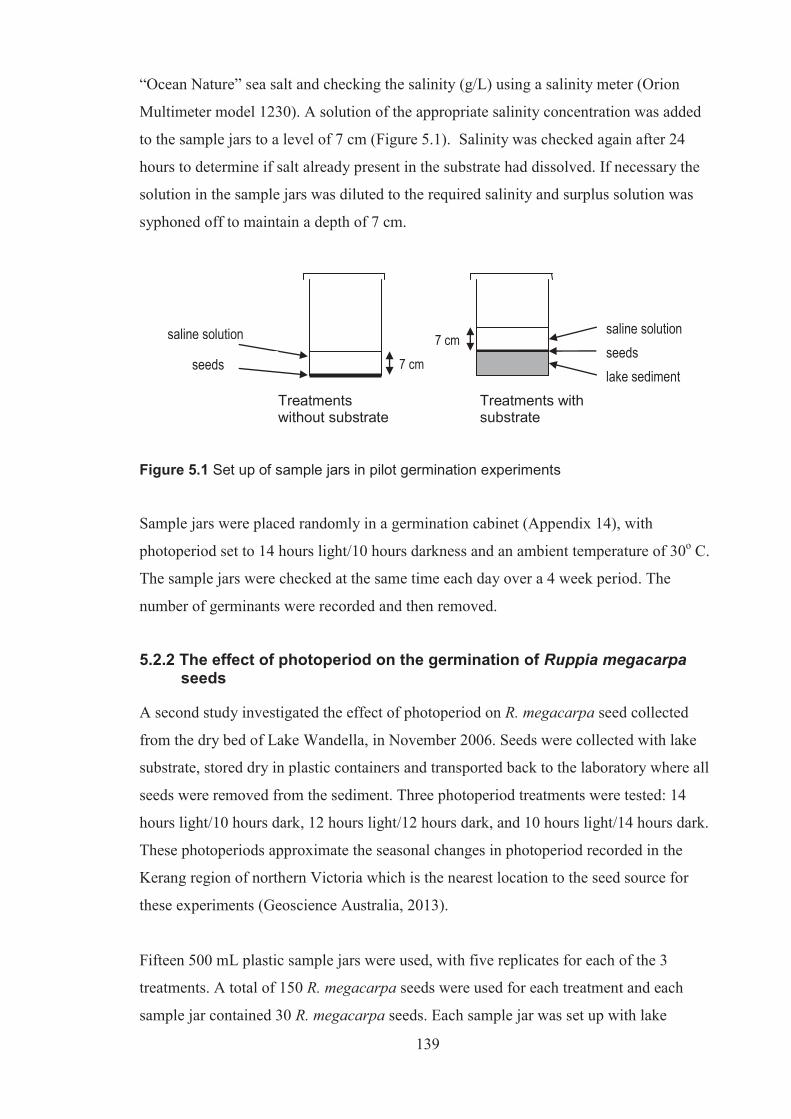
139
“Ocean Nature” sea salt and checking the salinity (g/L) using a salinity meter (Orion
Multimeter model 1230). A solution of the appropriate salinity concentration was added
to the sample jars to a level of 7 cm (Figure 5.1). Salinity was checked again after 24
hours to determine if salt already present in the substrate had dissolved. If necessary the
solution in the sample jars was diluted to the required salinity and surplus solution was
syphoned off to maintain a depth of 7 cm.
Figure 5.1 Set up of sample jars in pilot germination experiments
Sample jars were placed randomly in a germination cabinet (Appendix 14), with
photoperiod set to 14 hours light/10 hours darkness and an ambient temperature of 30o C.
The sample jars were checked at the same time each day over a 4 week period. The
number of germinants were recorded and then removed.
5.2.2 The effect of photoperiod on the germination of Ruppia megacarpa seeds
A second study investigated the effect of photoperiod on R. megacarpa seed collected
from the dry bed of Lake Wandella, in November 2006. Seeds were collected with lake
substrate, stored dry in plastic containers and transported back to the laboratory where all
seeds were removed from the sediment. Three photoperiod treatments were tested: 14
hours light/10 hours dark, 12 hours light/12 hours dark, and 10 hours light/14 hours dark.
These photoperiods approximate the seasonal changes in photoperiod recorded in the
Kerang region of northern Victoria which is the nearest location to the seed source for
these experiments (Geoscience Australia, 2013).
Fifteen 500 mL plastic sample jars were used, with five replicates for each of the 3
treatments. A total of 150 R. megacarpa seeds were used for each treatment and each
sample jar contained 30 R. megacarpa seeds. Each sample jar was set up with lake
lake sediment seeds saline solution saline solution
seeds
Treatments without substrate
Treatments with substrate
7 cm 7 cm

140
substrate, seeds and a saline solution (3.4 g/L concentration), as described in Methods
5.2.1.
Each treatment was carried out one at a time; the order of which the treatments were
conducted was determined using random numbers (Appendix 15). The position of the jars
within each germination cabinet was also determined using random numbers (Appendix
16). The temperature of the germination cabinet was 30oC for all three treatments. Sample
jars were left in the cabinets for four weeks and were checked at the same time each day
for this period. The number of germinants was recorded and then the germinants were
removed.
5.2.3 The affect of temperature on the germination of Ruppia megacarpa seeds
A third study tested the effect of temperature on germination of R. megacarpa seeds
collected from the dry bed of Lake Wandella, in November 2006. Seeds were collected
with the lake substrate, stored dry in plastic containers and transported back to the
laboratory where the seeds were removed from the lake sediment. Two temperature
treatments (25oC and 30oC) were applied which are typical ambient daytime air
temperatures recorded in the Kerang region (Bailey et al., 2006).
Ten 500 mL plastic sample jars were used, with five jars for each of the two treatments. A
total of 150 R. megacarpa seeds were used for each treatment with each replicate
containing 30 R. megacarpa seeds. Each sample jar was set up with lake substrate, seeds
and a saline solution (3.4 g/L), as described in Methods 5.2.1.
Each treatment was carried out one at a time; the order that the treatments were conducted
was determined using random numbers (Appendix 15). The position of the jars within
each germination cabinet was also determined using random numbers (Appendix 17). The
photoperiod in the germination cabinet was 14 hours light and 10 hours dark for both
treatments. Samples were checked at the same time each day, for a four week period with
the number of germinants was recorded and then the germinants were removed.

141
5.2.4 Data Analysis Results were analysed using either one way ANOVA or where there were only two
treatments, independent T-tests, to determine if there was any significant difference (p <
0.05) between treatments. The ANOVA model tested was as follows
DV = constant + treatment (either presence of substrate, location of seed source,
temperature or photoperiod)
Where results of the one way ANOVA’s were significant, post hoc Tukey’s tests were
conducted to determine which treatments were significantly different. All statistical tests
were conducted using the PASW 18 (previously known as SPSS statistics) software
package. Square root transformations of the dependent variable were undertaken when the
data from this experiment did not meet the assumptions of normality or homogeneity of
variances for parametric tests (Levene’s test).

142
5.3 Results
5.3.1 The effect of environmental variables on the germination of Ruppia megacarpa seeds
There was little difference in the germination success across the three different seed
sources (Figure 5.2, Table 5.2). Results of a one-way ANOVA showed that the only
treatment to show any significant difference (p <0.05) in mean number of germinated
seeds for the different seed sources was the substrate present, 3.4 g/L treatment (Table
5.2). Results of a post hoc Tukey’s test showed that there was only a significant
difference between the mean number of R. megacarpa seeds germinated between Lake
Cullen and Lake Wandella in the 3.4 g/L with substrate present treatment (Table 5.3).
Figure 5.2 The effect of different seed sources on the germination rate for Ruppia
megacarpa seeds in a) no substrate 1.4 g/L, b) no substrate 3.4 g/L, c) substrate 1.4 g/L, d) substrate 3.4 g/L treatments (n=5, square root transformed)
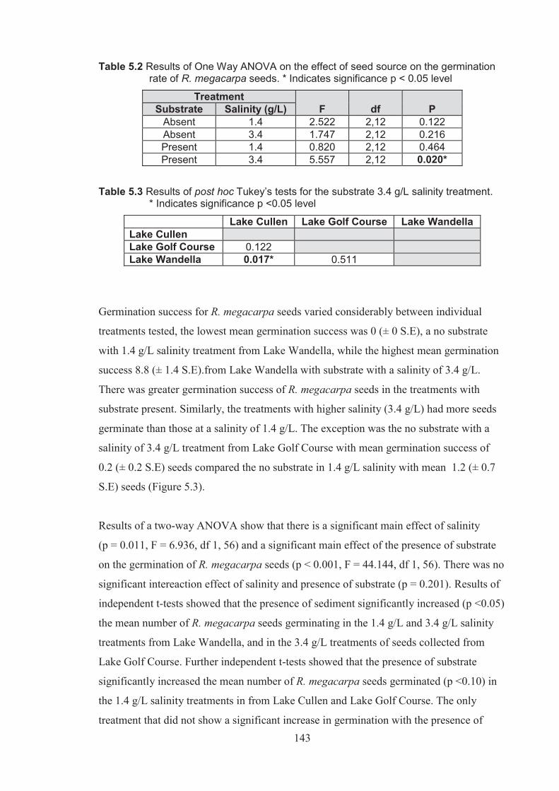
143
Table 5.2 Results of One Way ANOVA on the effect of seed source on the germination rate of R. megacarpa seeds. * Indicates significance p < 0.05 level
Treatment F df P Substrate Salinity (g/L)
Absent 1.4 2.522 2,12 0.122 Absent 3.4 1.747 2,12 0.216 Present 1.4 0.820 2,12 0.464 Present 3.4 5.557 2,12 0.020*
Table 5.3 Results of post hoc Tukey’s tests for the substrate 3.4 g/L salinity treatment.
* Indicates significance p <0.05 level
Lake Cullen Lake Golf Course Lake Wandella Lake Cullen Lake Golf Course 0.122 Lake Wandella 0.017* 0.511
Germination success for R. megacarpa seeds varied considerably between individual
treatments tested, the lowest mean germination success was 0 (± 0 S.E), a no substrate
with 1.4 g/L salinity treatment from Lake Wandella, while the highest mean germination
success 8.8 (± 1.4 S.E).from Lake Wandella with substrate with a salinity of 3.4 g/L.
There was greater germination success of R. megacarpa seeds in the treatments with
substrate present. Similarly, the treatments with higher salinity (3.4 g/L) had more seeds
germinate than those at a salinity of 1.4 g/L. The exception was the no substrate with a
salinity of 3.4 g/L treatment from Lake Golf Course with mean germination success of
0.2 (± 0.2 S.E) seeds compared the no substrate in 1.4 g/L salinity with mean 1.2 (± 0.7
S.E) seeds (Figure 5.3).
Results of a two-way ANOVA show that there is a significant main effect of salinity
(p = 0.011, F = 6.936, df 1, 56) and a significant main effect of the presence of substrate
on the germination of R. megacarpa seeds (p < 0.001, F = 44.144, df 1, 56). There was no
significant intereaction effect of salinity and presence of substrate (p = 0.201). Results of
independent t-tests showed that the presence of sediment significantly increased (p <0.05)
the mean number of R. megacarpa seeds germinating in the 1.4 g/L and 3.4 g/L salinity
treatments from Lake Wandella, and in the 3.4 g/L treatments of seeds collected from
Lake Golf Course. Further independent t-tests showed that the presence of substrate
significantly increased the mean number of R. megacarpa seeds germinated (p <0.10) in
the 1.4 g/L salinity treatments in from Lake Cullen and Lake Golf Course. The only
treatment that did not show a significant increase in germination with the presence of

144
substrate (p >0.10) was the 3.4 g/L salinity treatment from Lake Cullen (Tables 5.4a, 5.5a
and 5.6a). Results of independent t-tests showed that an increase in salinity from 1.4 g/L
to 3.4 g/L significantly increased (p <0.05) the mean number of R. megacarpa seeds
germinated in the substrate and no substrate treatments from Lake Wandella, and the
substrate treatment from Lake Golf Course (Tables 5.4b, 5.5b, and 5.6b).
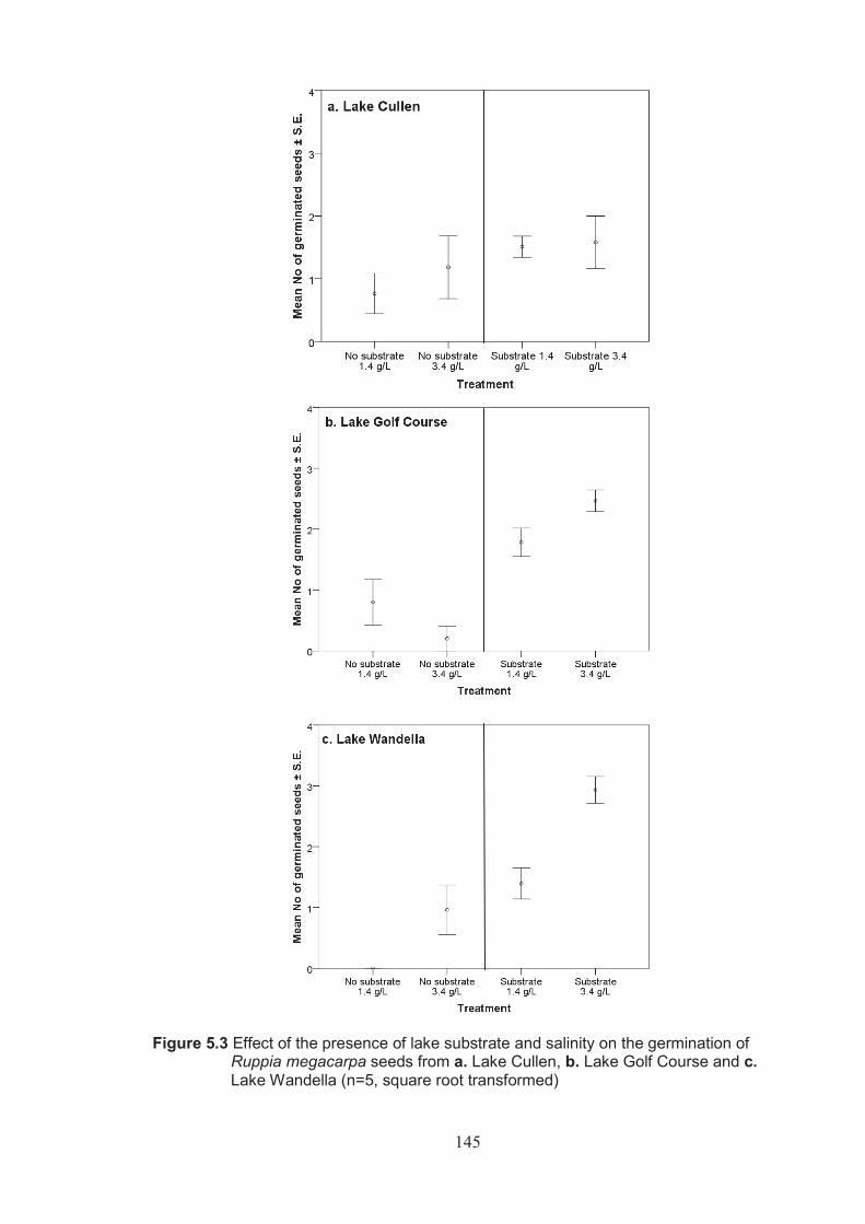
145
Figure 5.3 Effect of the presence of lake substrate and salinity on the germination of
Ruppia megacarpa seeds from a. Lake Cullen, b. Lake Golf Course and c. Lake Wandella (n=5, square root transformed)
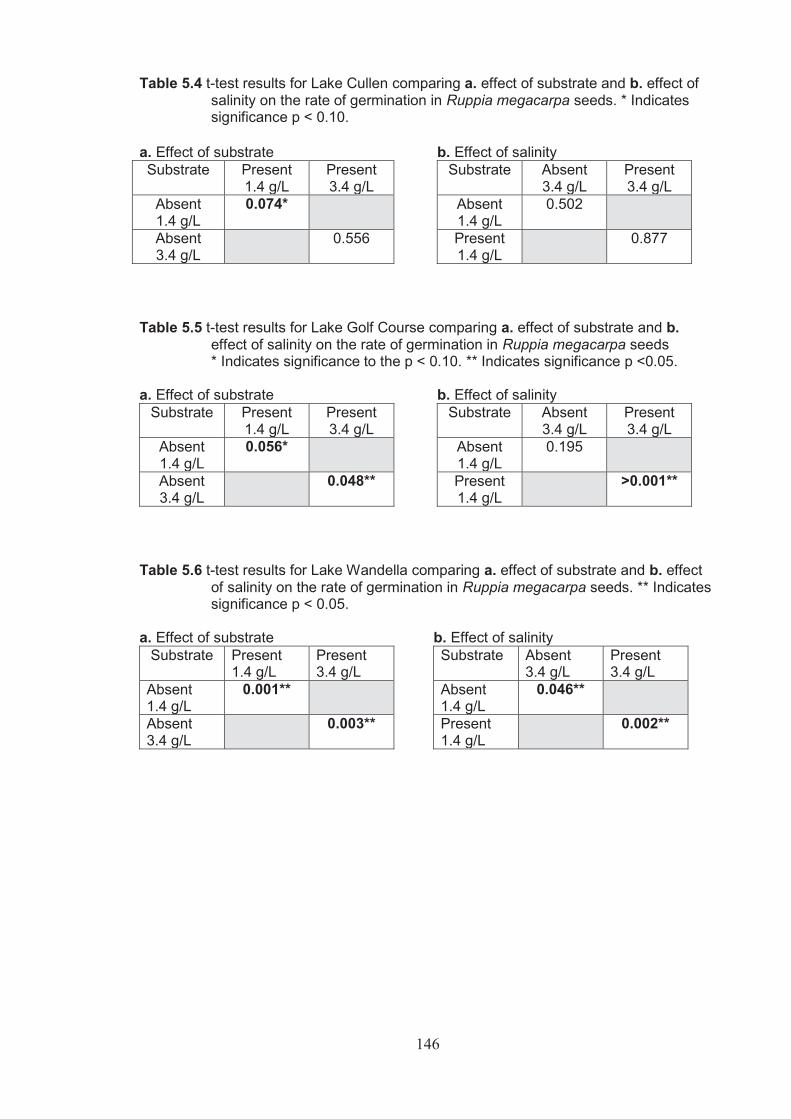
146
Table 5.4 t-test results for Lake Cullen comparing a. effect of substrate and b. effect of salinity on the rate of germination in Ruppia megacarpa seeds. * Indicates significance p < 0.10.
a. Effect of substrate Substrate Present
1.4 g/L Present 3.4 g/L
Absent 1.4 g/L
0.074*
Absent 3.4 g/L
0.556
b. Effect of salinity Substrate Absent
3.4 g/L Present 3.4 g/L
Absent 1.4 g/L
0.502
Present 1.4 g/L
0.877
Table 5.5 t-test results for Lake Golf Course comparing a. effect of substrate and b.
effect of salinity on the rate of germination in Ruppia megacarpa seeds * Indicates significance to the p < 0.10. ** Indicates significance p <0.05.
a. Effect of substrate
Substrate Present 1.4 g/L
Present 3.4 g/L
Absent 1.4 g/L
0.056*
Absent 3.4 g/L
0.048**
b. Effect of salinity Substrate Absent
3.4 g/L Present 3.4 g/L
Absent 1.4 g/L
0.195
Present 1.4 g/L
>0.001**
Table 5.6 t-test results for Lake Wandella comparing a. effect of substrate and b. effect
of salinity on the rate of germination in Ruppia megacarpa seeds. ** Indicates significance p < 0.05.
a. Effect of substrate
Substrate Present 1.4 g/L
Present 3.4 g/L
Absent 1.4 g/L
0.001**
Absent 3.4 g/L
0.003**
b. Effect of salinity Substrate Absent
3.4 g/L Present 3.4 g/L
Absent 1.4 g/L
0.046**
Present 1.4 g/L
0.002**

147
5.3.2 The effect of photoperiod on Ruppia megacarpa seed germination The results indicate that germination success between the 14 hour light/10 hour dark and
12 hour light/12 hour dark photoperiod treatments were very similar, with mean of 8.8 (±
1.4 S.E.) and 8.0 (± 1.7 S.E) seeds germinating in these treatments respectively. The third
photoperiod treatment of 14 hours light/ 10 hours dark had lower germination success
with mean 4.0 (± 1.6 S.E) seeds germinating over the four week period (Table 5.7).
Table 5.7 The total, percentage and mean number of Ruppia megacarpa seeds
germinated for each photoperiod treatment
Seed source Photoperiod No of seeds
germinated % of seeds germinated
Mean number of germinated
seeds (± S.E)
Lake Wandella
14 hours light/10 hours dark 44 29.3% 8.8 (± 1.4) 12 hours light/12 hours dark 40 26.7% 8.0 (± 1.7) 10 hours light/14hours dark 20 13.3% 4.0 (± 1.6)
Results of a one-way ANOVA found no significant difference (p <0.05) between the
results, even though there was a reduction in the number of germinants in the 10 light/14
hours dark treatment.
5.3.3 The effect of temperature on Ruppia megacarpa seed germination The germination of R. megacarpa was very different in the two temperature treatments
with mean 3.11 (± 1.4 S.E) seeds germinating at 30oC and a mean of 0.55 (± 0.2 S.E)
seeds germinating at 25oC (Table 5.8).
Table 5.8 The total, percentage and mean number of germinated Ruppia megacarpa seeds from a total of 150 seeds, at two different temperatures
Seed Source Temperature (oC)
Number of germinated
seeds
% of germinated
seeds
Mean number of germinated
seeds (± S.E)
Lake Wandella 30 44 29.3 3.11 (± 1.4)
25 13 8.7 0.55 (± 0.2)
Results of an independent t-test showed that there was a significant difference (p <0.05)
between the two temperatures, indicating that germination of R. megacarpa is
significantly reduced at 25oC.

148
5.4 Discussion
Results show that there was a low germination of R. megacarpa seeds across all
treatments with maximum germination success of less than 30%. Brock (1982a) also
reported germination rates in both R. megacarpa and R. tuberosa of less than 30%. Brock
(1982a) found that R. megacarpa seeds required an after ripening period because not all
seeds germinated within one growth cycle or wetting phase period. This could explain the
lower germination success found in other Ruppia studies (Brock, 1982a; Vollebergh and
Congdon, 1986). Low germination success could also be due to non-viable seeds within
the propagule bank.
Results from R. megacarpa germination studies demonstrate that differing environmental
conditions can affect germination. The findings of this study show that:
1. Seed source location had little effect on the germination success of Ruppia megacarpa seeds
Overall there was no significant difference in seed viability regardless of the seed source
location in this study. Results of this study indicated that generally there was no
significant difference in the germination success between seeds sourced from different
locations. The exception was one treatment (3.4 g/L salinity with substrate present) with a
significant difference between Lake Wandella and Golf Course Lake (p <0.05).
2. The presence of substrate increases the germination success of Ruppia megacarpa seeds
In most seed source locality and salinity treatments the presence of substrate increased
R. megacarpa seed germination success (p < 0.10). One exception was the Lake Cullen
3.4 g/L salinity treatment where no significant difference was found between number of
germinants from the substrate and no substrate treatments. Whilst these results were not
significant there was a trend to suggest that there was an increase in the number of seeds
germinating in the presence of substrate.
A possible reasons why the germination success of R. megacarpa seeds is increased with
the presence of substrate is that lake substrates may promote the germination of seeds
through a mycorrhizal association, similar to that seen in orchids (Stewart and Kane,
149
2007). Whilst this relationship is not common in wetland plants, mycorrhizal associations
have been found in some submerged and emergent aquatic macrophyte species (Khan and
Belik, 1995; Cooke and Lefor, 1998; Ingham and Wilson, 1999). Zhongqiang et al.,
(2005) found that there was a significant increase in the number of seeds germinated in
three species of Vallisneria (Eelgrass) in the presence of freshwater microalgae. The
association between the presence of substrate and the increase in germination of
R. megacarpa seeds needs further investigation.
3. Photoperiod had little effect on the germination success of Ruppia megacarpa seeds
No significant difference was found between the germination success of R. megacarpa
seeds exposed to three different photoperiod regimes. There was however a lower
germination recorded in the 10 hours light/14 hours dark treatment (mean 4 ± 1.6 S.E)
compared to the 12 hour light/12 hour dark and 14 hour light and/10 hour dark treatments
(mean 8.8 ± 1.4 S.E and 8.0 ± 1.7 S.E. respectively). Results suggest that more seeds
germinate when exposed to photoperiods with a longer light phase. Brock (1982a),
reported a different pattern, with higher germination success between 24% and 30% at a
photoperiod of 8 hours light/16 hours dark compared to germination success between
18% and 20 % in the 16 hours light/8 hours dark photoperiod treatment. It should be
noted that whilst an increased number of seeds germinating was found in the 8 hours
light/16 hours dark photoperiod treatment, no significant difference was found between
the two treatments. This present study indicates that R. megacarpa seed germination
increased in longer light photoperiods, but these results need to be treated with caution as
neither study demonstrates conclusively that photoperiod has an effect on germination
success. Photoperiod could be a less important factor as day length not only varies from
year to year, but also day to day depending on cloud cover. Also aquatic vegetation can
experience shadowing from riparian vegetation or other aquatic plants. Brock (1982a)
also reported that a number of seeds remain viable in the propagule bank and do not
germinate until the following year. These seeds would experience a range of photoperiods
throughout the year. Further study is warranted to determine the effects of varying
photoperiods on the germination success of R. megacarpa with confidence.

150
4. Increased temperature, increased the germination success of Ruppia megacarpa seeds
There was a significant difference in the number of R. megacarpa germinants observed in
the two different temperature treatments with increased germination success at 30oC.
There have been no previous studies on the effect of water temperature on the
germination of R. megacarpa seeds. This higher temperature however, does correspond
with mean maximum summer air temperature (31.8oC) in the Kerang region as it is likely
that high water tmepreatures would occur in these wetlands over summer (Bailey et al.,
2006).
Studies on other species of submerged macrophytes have demonstrated the effect of
temperature on germination success. Temperatures of above 15oC resulted in increased
germination success in Myriophyllum spicatum L. (Water Milfoil) seeds and temperatures
of above 20oC resulted in increased germination success in Potamogeton malaianus Miq.
(Pondweed) seeds (Xiao et al., 2010). Other species studied include Hydrilla verticillata
(L.f) Royle (Water Thyme) with optimal germination success at 28oC (Lal and Gopal,
1993), Vallisneria americana Michx. (American Eelgrass) with an optimal germination
success at 22oC (Jarvis and Moore, 2008) and Vallisneria natins (Lou) H. Hara with
optimal germination at 25oC (Ke and Li, 2006). It is thought that temperature triggers
germination and may enable plants to begin growth under conditions supporting optimal
growth (Xiao et al., 2010).
Given the low rates of R. megacarpa seed germination it is important that further studies
investigating the effects of salinity are conducted in optimal environmental conditions.
The results of this study indicate that seed source location has no effect on germination
success in R. megacarpa. This suggests that seeds are fairly homogenous across the
different wetlands in the region. Photoperiod was also found to have no significant effect
on the germination success of R. megacarpa. The presence of substrate and a temperature
of 30oC did significantly affect germination success in R. megacarpa.
151
6.0 The effect of salinity and desiccation disturbances on germination success of Ruppia megacarpa 6.1 Introduction The germination requirements of seeds is species specific and environmental factors can
either inhibit or promote germination in wetland plants (Brock, 1982a; Britton and
Brock, 1994; Baskin and Baskin, 1998; Casanova and Brock, 2000; Kahn and Durako,
2005; Taton et al., 2006; Cho and Sanders, 2009; Goodman et al., 2010). Salinity and
drying periods are two such environmental factors that can affect a wetland plant’s
germination success (Cho and Sanders, 2009). Many studies have shown that flood
frequency and timing, depth, and duration can strongly influence species composition in
wetland plant communities (Casanova and Brock, 2000; Nicol et al., 2003; Porter et al.,
2007). Drying periods after floods can break dormancy and thus increase germination in
some species growing in ephemeral habitats during the next wetting phase (Bonis et al.,
1995; Casanova and Brock, 1996). In some species however this is not the case and
macrophytes that grow in these temporary habitats must at least have seeds or propagules
that are able to survive periods of desiccation between flooding events. This survival trait
is essiential for macrophyte establishment in wetlands in northwestern Victoria as water
availability is becoming an increasingly important issue due to drought and climate
change. These factors have resulted in a number of permanently inundated wetlands
drying out and becoming temporary habitats (as discussed in Chapter 2).
Many studies of temporary wetlands have investigated how propagule banks contribute to
the plant and invertebrate communities that become established after dry substrates are
rehydrated by floods (Brock and Lane, 1983; Casanova and Brock, 1990; Brock and
Casanova, 1991; Brock and Britton, 1995; Brock, 1997; Casanova and Brock, 2000;
Nielsen et al., 2002; Brock et al., 2003; Sim et al., 2006a). Some of these studies,
together with past germination studies and investigations discussed in Chapter 4 have
shown that Ruppia megacarpa R. Mason (Large-Fruit Widgeon Grass), and many other
species of Ruppia, are able to tolerate periods of desiccation (Brock, 1982a; Brock,
1982b; Sim et al., 2006a). But the effect of desiccation on propagule bank viability and
germination success is not as well understood. In some cases researchers are unsure
whether drying enhances or inhibits germination success in Ruppia species. Koch and
Seeliger (1988) found that drying enhanced the germination of Ruppia seeds collected
152
from an ephemeral habitat. In contrast, seed viability tests (Tetrezolium tests) conducted
by Cho and Sanders (2009) found that drying greatly reduced seed viability when
comparing Ruppia maritima L. (Widgeon Grass) seeds dried over a ten month period with
seeds that had just been deposited.
Many wetland propagule bank and germination studies have also investigated the effect
of salinity on various macrophytes species (Galinato and Van Der Valk, 1986; Salter et
al., 2010; Goodman et al., 2011). Results from the propagule bank studies discussed in
Chapters 3 and 4 indicated that R. megacarpa seeds are able to germinate in salinities of ≥
37.7 g/L. These findings concur with propagule bank studies conducted by Sim et al.,
(2006a) who reported that Ruppia polycarpa R. Mason (Many-fruit widgeon grass) was
able to germinate in salinities ≤ 45 g/L and that seeds of R. megacarpa germinated in
salinities ≤ 30 g/L. Vollenbergh and Congdon (1986) found that the optimal salinity range
for the germination of R. polycarpa seeds was 0 g/L to 35 g/L.
It is important to note that different species within the same genus can have varied
responses to salinity. Brock (1982a) found that the germination success of R. megacarpa
seeds increased in freshwater (0 g/L) whereas for Ruppia tuberosa J.S. Davis and Toml.
(Tuberous Tassle) germination success was greater in higher salinity concentrations (42
g/L). This reflects the environments that these two species are distributed in, as R.
megacarpa is often found under fresher conditions that R. tuberosa (Brock, 1982a).
Few controlled studies have focused on the effect of decreasing salinities after a period of
high salinity disturbance, on the germination success of wetland plants. Results from the
propagule bank studies discussed in Chapter 4 suggest that higher salinity concentrations
had little affect on the germination success of R. megacarpa seeds, once they had been
returned to the recovery phase. Vollenberg and Congdon (1986) reported similar results
for
R. polycarpa seeds soaked in high salt solution (up to 157.5 g/L) for 6 days before
returning the seeds to freshwater (0 g/L).

153
6.1.1 Hypotheses The purpose of this study is to further build on the findings of Chapters 3, 4 and 5 and to
look specifically test the following hypotheses
Does a drying period affect the germination success of R. megacarpa?
Does the combination of a drying period and decreasing salinity, post exposure to
high salinity affect the germination success of R. megacarpa?

154
6.2 Methods The effect of drying and lowering of salinity concentrations on Ruppia megacarpa seed
germination was tested over a 50 day period. Seeds were collected from the dry bed of
Lake Wandella in November 2006, stored dry in plastic containers and transported back
to the laboratory where they were removed from the substrate. Eleven treatments were
selected to test the effects of the following parameters on R. megacarpa germination
success (Table 6.1) namely the effects of:
desiccation
reducing salinity concentrations
desiccation as well as reducing salinity concentrations
This 50 day period was divided into two phases (Phase 1 and 2), each of 25 days in
length, with an extra two days (dry phase) between each phase for treatments subjected to
desiccation.
Table 6.1 Description of treatments used to test germination success of Ruppia megacarpa seeds collected from Lake Wandella
Treatment Type Phase 1 (25 days)
Salinity (g/L)
Dry Phase (2 days)
Phase 2 (25 days)
Salinity (g/L) Controls, no change in salinity, no desiccation period
10 N/A 10 30 N/A 30 50 N/A 50
No change in salinity, desiccation period
10 Dry 10 30 Dry 30 50 Dry 50
Reducing salinity, no desiccation
30 N/A 10 50 N/A 10
Reducing salinity and desiccation period
30 Dry 10 50 Dry 10 50 Dry 30
A total of fifty-five 500mL plastic sample jars were used, with five jars for each treatment
(11 treatments). A total of 150 R. megacarpa seeds were used, with each sample jar
containing 30 R. megacarpa seeds. Each sample jar contained 2 cm of substrate (with all
seeds removed) and R. megacarpa seeds were placed on the surface of this substrate.
Saline solutions were made up to the required concentration by adding Ocean Nature Sea
Salt to tap water and checking the salinity with a salinity meter (Orion Multimeter Model
No. 1230). Solutions of the required salinity (g/L) were added to the sample jars to a
depth of 7 cm. The salinity of the solution was checked after 24 hours to determine if any

155
salt present in the substrate had dissolved. If necessary the solution in the sample jars was
diluted to the desired salinity concentration and any surplice water was syphoned off so
that the solution depth remained at 7 cm (see Figure 5.1 in chapter 5).
Sample jars were arranged in a germination cabinet according to a random number
generated pattern (Appendix 18). Photoperiod of the germination cabinet was 14 hours
light/10 hours dark and the ambient temperature was 30oC, as these were the optimal
conditions found for R. megacarpa in the experiments discussed in Chapter 5. Sample jars
were checked, at the same time each day over 25 days, the germinants were counted and
removed.
At the end of the first phase (25 days), the solution was syphoned off from the “control”
and “effect of reducing salinity, no desiccation” treatments taking care not to disturb the
R. megacarpa seeds. A solution was made up to the required Phase 2 salinity
concentration by adding Ocean Nature Sea Salt to tap water, using a salinity meter (Orion
Multimeter Model No. 1230) to check salinity concentrations (g/L) and then added to the
sample jars to a depth of 7 cm. The solution concentration was checked after 24 hours to
determine if salt present in the substrate had dissolved. If necessary the solution in the
sample jars was diluted to the required salinity and any surplus solution syphoned off so
that the depth remained at 7 cm. Sample jars were returned to the germination cabinet
with the same photoperiod and temperature conditions as applied in Phase 1, for a further
25 days. Sample jars were checked, at the same time each day over this period and
germinants were counted and removed.
At the end of the first phase (25 days), the solution was also syphoned off from the “effect
of desiccation, no change in salinity” and “effect of reducing salinity and desiccation”
treatments. These jars were placed in an oven at 40oC for 2 days (48 hours) to allow the
substrate to dry out. After this drying period a solution was made up to the required Phase
2 salinity concentration and checked as previously described, prior to being added to the
sample jars to a depth of 7 cm. The salinity of the solution was checked after 24 hours to
determine if salt present in the substrate had dissolved. If necessary the solution was
diluted to the required salinity and surplus water was syphoned off so that the depth of the
solution remained at 7 cm. Sample jars were returned to the germination cabinet with the
same photoperiod and temperature conditions as applied in Phase 1 of the experiment, for

156
a further 25 days. Sample jars were checked, at the same time each day over this period
and the germinants were counted and removed.
6.2.1 Data Analysis Results were analysed using three way mixed ANOVA to determine if there was any
significant difference (p < 0.05) between salinity treatments, using the following model.
DV = constant + Phase 1 salinity + Phase 2 salinity + Presence of desiccation + Phase 1
salinity x Phase 2 salinity + Phase 1 salinity x Presence of desiccation + Phase 2 salinity x Presence of desiccation + Phase 1 salinity x Phase 2 salinity x Presence of desiccation
Where results of the three way ANOVA were significant, post hoc Tukey’s tests were
conducted to determine which treatments were significantly different. All statistical tests
were conducted using the PASW 18 (previously known as SPSS statistics) software
package. Square root transformations of the dependent variable were undertaken when the
data from this experiment did not meet the assumptions of normality or homogeneity of
variances for parametric tests (Levene’s test).
157
6.3 Results Ruppia megacarpa seeds germinated in the two lower salinity treatments of 10 g/L and
30 g/L and no germinants were recorded when seeds were subjected to the highest salinity
concentration of 50 g/L (Table 6.2). Overall germination success was below 30%.
Germination was higher in treatments where R. megacarpa seeds were subjected to the
lowest salinity (10 g/L) (Table 6.2). The greatest germination success was recorded in the
effect of reducing salinity and drying treatment of 30 g/L, Phase 1 salinity and 10 g/L
Phase 2 salinity where 26% (39) seeds germinated. A lag in the time before germination
of up to four days was also observed in the 30 g/L treatments, compared to the lower
salinity treatment of 10 g/L (Appendix 19).

158
Tabl
e 6.
2 O
vera
ll ge
rmin
atio
n ra
tes
of R
uppi
a m
egac
arpa
see
ds c
olle
cted
from
Lak
e W
ande
lla in
eac
h tre
atm
ent a
t the
com
plet
ion
of th
e ex
perim
ent,
high
light
ed tr
eatm
ents
(bol
d) re
pres
ent t
he h
ighe
st a
nd lo
wes
t ger
min
atio
n ra
tes.
Tr
eatm
ent T
ype
Phas
e 1
(25
days
) Sa
linity
(g
/L)
Dry
Ph
ase
(2
days
)
Phas
e 2
(25
days
) Sa
linity
(g
/L)
Tota
l no.
of
seed
s ge
rmin
ated
at
end
of
phas
e 1
Tota
l no.
of
seed
s ge
rmin
ated
at
end
of
phas
e 2
% o
f see
ds
germ
inat
ed
Mea
n no
. of
see
ds
germ
inat
ed
per j
ar
Stan
dard
er
ror o
f the
m
ean
no.
seed
s ge
rmin
ated
pe
r jar
(±
) C
ontro
ls n
o ch
ange
in
sal
inity
, no
dryi
ng
perio
d
10
N/A
10
29
32
21
.3
5.3
2.4
30
N/A
30
8
16
10.7
3.
2 1.
8 50
N
/A
50
0 0
0 0
0
Effe
ct o
f dry
ing,
no
chan
ge in
sal
inity
10
Dry
10
19
29
19
.3
5.8
1.8
30
Dry
30
19
38
25
.3
8 2
50
Dry
50
0
0 0
0 0
Effe
ct o
f low
erin
g sa
linity
, no
dryi
ng
30
N/A
10
13
19
12
.7
3.8
1.2
50
N/A
10
0
21
14.0
4.
2 1.
2
Effe
ct o
f low
erin
g sa
linity
and
dry
ing
30
Dry
10
14
39
26
.0
7.8
1.4
50
Dry
10
0 20
13
.3 4
1.4
50
Dry
30
0 10
6.7
2
0.9

159
Results of the within treatment effects in the mixed three-way ANOVA showed that only
Phase 2 salinity levels had a significant (p < 0.05) main effect on the number of
R. megacarpa germinants (Table 6.4). There were no other significant (p < 0.05) main or
significant (p < 0.05) interaction effects found between the different treatments (Table
6.3). Table 6.2 further supports these findings as the lower the Phase 2 salinity
concentration the greater the number of R. megacarpa germinants were recorded overall.
Table 6.3 Results of a mixed three-way ANOVA testing the effect of Phase 1 salinity,
Phase 2 salinity and presence of desiccation period on the number of Ruppia megacarpa germinants. ** Indicates significance to the p < 0.05 level
Factors df F p Phase 1 Salinity 2,45 2.727 0.076 Phase 2 Salinity 2,45 3.709 0.006** Desication 1,45 0.021 0.887 Phase 1 salinity x Phase 2 salinity 1,45 0.291 0.592 Phase 1 salinity x Desication 1,45 0.047 0.830 Phase 2 salinity x Desication 1,45 <0.01 1.000 Phase 1 salinity x Phase 2 salinity x Desication 1,45 <0.01 1.000
Results of post hoc Tukey’s tests indicated a significant difference (p < 0.05) between the
lowest salinity treatments of 10 g/L and the highest salinity treatment of 50 g/L (Table
6.4).
Table 6.4 Results of post hoc Tukey’s test comparing Phase 2 salinity treatments on number of Ruppia megacarpa germinants. ** Indicates significance p < 0.05 level
Salinity (g/L) 10 30 50 10 30 0.101 50 < 0.001** 0.064

160
6.4 Discussion Results of this study further build on the results of Chapter 5 by investigating how other
environmental conditions such as lowering salinity concentrations and drying can affect
the germination of Ruppia megacarpa seeds. The results of this study indicate that:
1. The presence of a drying period had no effect on Ruppia megacarpa seed germination
A 48 hour drying period had no significant effect on the number of R. megacarpa seeds
germinating in this experiment. But this result must be treated with caution as the seeds
were collected from the dry bed of Lake Wandella and thus had already been exposed to a
much longer drying period. Additionally, the age of these seeds was not known. Cho and
Sanders (2009) used Tetrazolium tests to revel that exposing R. maritima seeds to a 10
month drying period reduced seed viability by 35.7%. In a germination study, Cho and
Sanders (2009) observed a 90% to 95% germination success rate in newly formed R.
maritima seeds compared to a 18% to 30% germination rate in R. maritima seeds that had
been desiccated for 10 months. This is in contrast to the findings of Salter et al., (2010)
who found that a drying period increased the germination success of Vallisneria australis
seeds.
Germination success of R. megacarpa seeds in this study were also low, with less than
30% of seeds germinating in all treatments. This suggests that the conditions seeds were
exposed to prior to this experiment may have affected their viability. Similar low
germination rates in R. megacarpa seeds were reported in Chapter 5, as well as in studies
by Brock (1982a).
Brock (1982a), conducted an after ripening trial on three Ruppia species to determine if
all seeds germinated in the first growing season. Results indicated that the greatest
germination success in R. megacarpa was in the second growing season, after either
permanent wet, or dry, and rewetting regimes. This suggests that R. megacarpa seeds
need an after ripening period to optimise germination. The findings of this current study
did not concur with those of Brock (1982a), with only one treatment showing a significant
effect of phase and no treatments demonstrating a significant effect in response to a
drying period. But this current study was conducted over 50 days at a controlled
temperature and photoperiod environment with a short desiccation event, whereas the

161
study by Brock (1982a) was conducted over 15 months in the field. As such, the
environmental conditions that the seeds were exposed to differed greatly.
Many other wetland plants have shown increased germination success after periods of
drying and after ripening. Brock (2011) reported that seeds can be long lived and that
some wetland species were able to germinate after a dry period of 12 years. Brock (2011)
also found that some species germinated from wetland sediments that had been subjected
to several wetting and drying regimes over a 7 year period, even when new plants were
prevented from contributing new propagules to the seed bank. Carta et al., (2013) found
that an after ripening period increased germination success in wetland species from the
Mediterranean Basin, whilst Jensen (2004) found similar patters in fen grassland species
from Northern Germany. Thus the mechanism of after ripening in R. megacarpa seeds
and the possible effects of other environmental conditions between growing seasons
requires further investigation.
2. Lower salinity concentrations and freshening salinity concentrations had a positive effect on the germination of Ruppia megacarpa seeds
Both Phase 1 and Phase 2 salinity concentrations had a significant effect on the
germination of R. megacarpa seeds. Results indicated that the lower the salinity
concentration, the higher the germination success in R. megacarpa seeds. Significant
differences were found between all salinity treatments, with the exception of the Phase 1
salinity treatments of 10 g/L and 30 g/L. No germination occurred in the 50 g/L salinity
treatment, which also supports the findings of propagule bank studies previously
discussed (Chapters 3 and 4) where the highest salinity in which germination occurred
was 37.7 g/L. This also concurred with the propagule bank studies conducted by Sim et
al., (2006a) where the germination of R. megacarpa was observed in salinity treatments
of up to 30 g/L. Maximum germination was found in the lowest salinity treatment of 10
g/L, which is also supported by the findings of Brock (1982a) who reported that the
lowest salinity concentration promoted the highest germination success in R. megacarpa
seeds, when compared to the higher salinity treatments of 19 g/L and 42 g/L.
Few studies have investigated the effect of briefly reducing salinity concentrations on the
germination success of wetland plants. In this study, every instance where salinity
concentrations were reduced resulted in increased R. megacarpa seed germination,
especially when salinity concentrations were dropped to the lowest salinity concentration
162
(10 g/L). The initial high salinity concentrations had little impact on the overall
germination of R. megacarpa when salinities were later reduced, and the germination
success in these treatments was similar to those of the controls after Phase 1. Similar
observations are discussed in Chapter 4, where initial high salinity variations were found
to have little impact in the overall germination of R. megacarpa during a Recovery Phase.
Although some germination occurred in 30 g/L salinity, the germination success was
significantly lower and there was a short lag in time until germinants appeared. Delays in
the germination of seeds can be problematic for a species survival in wetlands. If
germination occurs late in the wetting cycle, there may not be enough time before the
wetland dries for plants to reach maturity and reproduce. As a result, propagule banks can
become depleted over time. Lag times in the germination of R. megacarpa at intermediate
salinity concentrations are discussed in the propagule bank experiments described in
Chapters 3 (see section 3.4.1), and also in the propagule bank studies conducted by Sim et
al., (2006a).
Brock (1982a) and van Vierssen et al., (1982) concluded that R. megacarpa was a
perennial species found in permanently watered, relatively stable environments. Brock
(1982a) also suggested that R. megacarpa seeds remain dormant within the propagule
bank and that high germination success of this species only occurs in the field when
salinities are reduced by heavy rains. This may have implications for how wetlands with
R. megacarpa present are managed, if this species is considered important in maintaining
ecosystem function. Through this study and those previously discussed (Chapters 3, 4
and 5) it is clear that R. megacarpa seeds can survive periods of desiccation. But, the long
term effect on the viability, germination and colonisation success of R. megacarpa is
unknown and will need to be monitored into the future when managing these wetlands as
ephemeral habitats.
Many plant and animal species can survive not only periods of high salinity, but also
periods of drying by producing seeds or eggs with the ability to persist in the substrate
until conditions become more favourable. Ruppia megacarpa seeds avoid increased
salinity by remaining dormant until fresher conditions predominate, indicating that this
species can be resilient not only to higher salinity concentrations but also to periods of
desiccation (Skinner et al., 2001; James et al., 2003). Managers however need to be
careful when applying this knowledge to management regimes and watering plans for

163
wetlands. An important factor that needs to be considered, is the maximum length of time
these propagules are able to remain viable in the propagule bank. As already discussed
there is evidence to suggest that R. megacarpa seeds have reduced viability if dried for
extended periods of time (10 months) before germination occurs (Cho and Sanders,
2009). Further long-term studies into this area are required to determine the effect of
drying and salinity concentrations on the viability of these propagules.
Overall this study found that increased salinity concentrations negatively impact the
germination success of R. megacarpa seeds, and that no germination occurred in the
highest salinity treatment of 50 g/L. Reducing salinity concentrations was found to
positively impact germination success, particularly when levels were lowered to a salinity
of 10 g/L. The presence of a short drying period however, did not have any significant
impact on the germination of R. megacarpa seeds. Further studies are needed to
understand the effect of both after ripening and drying on the seeds of this species, given
the low germination success observed, and the findings of Cho and Sanders (2009)
regarding the negative impacts of drying in R. maritima seeds.

164
7.0 Implications for management of wetlands of intermediate salinity in northwest Victoria Wetlands of intermediate salinity are often characterized as areas of low flora and fauna
diversity, yet high productivity, leading to systems that support numerous water bird and
fish populations (Brock and Lane, 1983; Brock, 1986; Timms, 1993; Kingsford and
Porter, 1994). These wetlands are of high ecological value especially in comparison to
hypersaline lakes which are often less complex systems (Bauld, 1981; Davis, 2002; Davis
et al., 2003; Strehlow et al., 2005; Sim et al., 2006a; 2006b; 2006c; Davis et al., 2010).
Management of these wetlands in the past focused on providing adequate water flows in
order to maintain salinity concentrations low enough to support plant and animal
communities. The negative impacts of increased salinity and reduced water flows on
wetlands of intermediate salinity in northwestern Victoria will only be exacerbated in the
future as the effects of climate change and alterations in weather patterns occur (Herbst
and Blinn, 1998; James, 2005; Nielsen and Brock, 2009). There are many policies and
agencies responsible for the management saline lakes in northwestern Victoria and as a
result coordinated efforts will be required between these agencies to effectively manage
these systems. Results of this study not only provide further evidence of how productive
saline wetlands can be, but additionally they have demonstrated how careful management
of these wetlands is crucial for maintaining viable plant and animal communities into the
future. Many of the wetlands in this study are subjected to a number of environmental
stressors that may impact on their future ability to support a macrophyte dominated
community that provides viable habitat for vertebrate and invertebrate species.
Currently there are a number of state and national Acts governing the management of
wetlands in northwestern Victoria and their implementation Acts falls to a number of
agencies and organizations (Table 7.1). Consequently the management of these wetlands
is often a cooperative partnership between differing agencies and organisations (Table
7.1).

165
Table 7.1 Australian and Victorian Acts, and the agencies and organisations responsible for the management of wetlands in northwestern Victoria
Australian and Victorian Acts relating to the management of wetlands
Agencies and organisations responsible for the management of wetlands in northwestern Victoria.
Environmental Protection and Biodiversity Act (1999 - National)
Department of Environment and Primary Industries
Flora and Fauna Guarantee Act (1988 - Victoria)
Environmental Protection agency
Planning and Environment Act (1987 - Victorian)
Local Catchment Management Authorities (Mallee CMA and North Central CMA)
Catchment and Land Management Act (1994 - Victorian)
Victorian Catchment Management Council
Environment Protection Act (1970 - Victorian)
Goulburn Murray Water
Water Act (1989 – Victorian), Water Act (2007 – National)
Department of Planning and Community Development
The most important aspect of the management of these wetlands in terms of their salinity
is the watering regime. The watering regimes of wetlands considered in this study
included Lake Elizabeth, Lake Cullen, Lake Wandella, Long Lake, Golf Course Lake,
Round Lake, Woorinen North Lake. These watering regimes of wetlands in northwestern
Victoria and the allocations of environmental flows is decided based on three factors,
firstly the presence of any endangered species, secondly connectivity to the irrigation
channels, and thirdly the amount of water available, which varies from year to
year(Seabloom et al., 1998).
7.1 The distribution of biota in wetlands of intermediate salinity in
northwestern Victoria
Historically wetlands of northwestern Victoria have been a mosaic of fresh, hyposaline,
saline and hypersaline lakes across the landscape, with varied flooding regimes. The
development of farms, irrigation schemes, towns and levee banks over time has resulted
in dramatic changes in salinity concentrations and reduced permanence of wetlands in this
area. In the Kerang to Swan Hill region many wetlands have become increasingly saline
or hypersaline, and some have become completely dry (KLAWG, 1992). This has
affected the distribution of biota in the region over time, in particular Craterocephalus

166
fluviatilis (Murray Hardyhead) which is now restricted to just a few wetlands in Victoria,
and is now considered to be endangered (Ebner and Raadik, 2001).
Wetlands investigated in Chapter 2, (Lake Elizabeth, Round Lake, Woorinen North Lake
and Lake Hawthorn) were all found to be wetlands of intermediate salinity (mean salinity
range of 8.22 g/L to 29.28 g/L), with low turbidity (mean < 30 NTU) and tended to be
alkaline (mean range of pH 8.15 to 8.80). Although the biotic diversity of these saline
wetlands is low, their productivity is generally very high which is a common finding in
this type of system and concurs with the work of Timms (1997). Wetlands investigated in
Chapter 2 were highly productive and supported the growth of the submerged aquatic
macrophyte Ruppia megacarpa R. Mason (large-fruit widgeon grass) and most supported
the charophyte Lamprothamnium macropogon (A. Braun) L.Ophel (Stonewort). Whilst
productivity was high in all wetlands investigated, the distribution of these macrophyte
species was heterogeneous across wetlands, with some areas supporting extensive
macrophyte beds and other areas of the wetlands being bare substrate with little or no
plant cover.
All wetlands studied, (except Lake Elizabeth, where no fish were caught) supported
communities of C. fluviatilis and Gambusia holbrooki (Eastern Mosquito fish), in
addition to these species Woorinen North Lake also supported populations of
Philypnodon grandiceps (Flat Headed Gudgeon). These wetlands are able to support
productive invertebrate, fish and water bird populations, providing salinity concentrations
remain low enough (< 16 g/L), and where possible should be managed to support such
communities.
7.1.1 The distribution of Craterocephalus fluviatilis (Murray Hardyhead) in
wetlands of northwest Victoria
Craterocephalus fluviatilis has a restricted distribution within Victoria and is mainly
found within lakes of intermediate salinity. The distribution of this species was thought to
be restricted to the Cardross Lakes (Mildura), Lake Hawthorn (Mildura), Lake Woorinen
North (Swan Hill), Round Lake (near Lake Boga) and Lake Elizabeth (Kerang)
(Flemming, 1990; Allen et al., 2002; Lyon et al., 2002; Ebner et al., 2003). Previous
studies also suggested that this species was reliant on Ruppia spp. for survival, and that
Ruppia spp. may be used as an indicator species for the presence of C. fluviatilis in

167
wetlands (Lyon et al., 2002). Results of this study (Chapter 2) indicate that C. fluviatilis
populations no longer exist in Lake Elizabeth but populations were found in Lake
Hawthorn, Lake Woorinen North and Round Lake. Populations of C. fluviatilis, are
associated with Ruppia megacarpa stands in Victorian wetlands, but this fish does not co-
occur with R. megacarpa in South Australia (Wedderburn et al., 2007; Wedderburn et al.,
2008). In South Australia populations are associated with Myriophyllum spp., which
suggests that C. fluviatilis is not reliant on Ruppia spp. per se, but is actually reliant on
the presence of submerged macrophyte cover for egg laying (Ellis, 2005a). Thus the
existence of this type of macrophyte in healthy stands in important for the survival of C.
fluviatilis populations in saline wetlands in Victoria.
The loss of the C. fluviatilis population from Lake Elizabeth and surrounding areas has
been attributed to a number of possible environmental stressors including increased
salinity, acid sulphate events, drying of wetlands, introduced fish species, as well as loss
of connectivity to the flood plain (Backhouse et al., 2006). Lake Elizabeth is no longer
connected to the flood plain and only receives flood waters under extreme floods due to a
number of anthropogenic changes in the area including the implementation of irrigation
schemes, elevated roads and railway lines, and levee banks (KLAWG, 1992). Whilst
many of these factors have occurred, the suggestion that acid sulphate soils are
responsible for the loss of this species from Lake Elizabeth seems unlikely given the
extensive growth of macrophytes and presence of water bird and invertebrate species in
this lake (Chapter 2). Increased salinity concentrations are the most probable reason for
the loss of this population, as salinity concentrations were high in past (up to 35 g/L) and
may have been elevated above the threshold that this species can tolerate (Kelly, 1996).
Given C. fluviatilis is an annual species (Ellis, 2006); populations may have been lost
quickly from Lake Elizabeth as a result of extreme salinity concentrations preventing
reproduction.
Populations of C. fluviatilis in South Australian wetlands, occur in less saline
environments than those in Victoria (Wedderburn et al., 2008). Results of the case study
discussed in Chapter 2 indicate that historically C. fluviatilis was distributed in fresher
waters in areas around Kerang and Swan Hill. One factor that may have contributed to the
loss C. fluviatilis in fresher systems of the Kerang Lakes region is the reduction in
submerged macrophyte cover. Many of the lakes within the Kerang Lakes area that are
fresh in nature have been used for irrigation water storage and water transport. This

168
anthropogenic use has resulted in increased turbidity and subsequent loss of macrophyte
cover (KLAWG, 1992). Which may be the reason that C. fluviatilis populations have
been lost from wetlands such as Lake Boga (which is used to store irrigation and flood
waters), and others along the irrigation system. Loss of C. fluviatilis populations from
many of the other lakes in the district is probably due to increased salinity (e.g. Lake
Tutchewop and Lake Elizabeth), or wetlands completely drying out (e.g. Lake Golf
Course, Long Lake, Lake Wandella and Lake Cullen) (Ebner and Raadik, 2001;
Backhouse et al., 2006; Wedderburn et al., 2008).
The most important factors affecting the distribution of C. fluviatilis in wetlands in
Victoria are salinity concentrations, presence of submerged macrophytes and a permanent
watering regime. There are hundreds of wetlands in the Kerang Lakes area that range in
salinity from fresh to hypersaline. Some of these wetlands may be suitable for
reintroduction of C. fluviatilis. Wetlands in this region should be screened for appropriate
salinity concentrations (approximately < 22 g/L), presence of submerged macrophytes
and low turbidity, and have a permanent water supply.
For the 2013/2014 watering season Round Lake and Lake Elizabeth were identified as
priority wetlands due to receive environmental flows even under drought conditions.
Round Lake was identified as a priority wetland as it currently supports a population of
C. fluviatilis which rely on freshwater flows for survival, whereas Lake Elizabeth was
identified as a potential site for the reintroduction of C. fluviatilis from captive breeding
programs and thus would requires an environmental flow to maintain salinity at a
concentration suitable for their release.
Other sites where C. fluviatilis populations occur, or where reintroductions of
C. fluviatilis have occurred (e.g. Cardross Lakes, Lake Koorlong and Brickworks Lagoon,
all lakes not included in this study) will receive environmental flows under dry, average
or wet conditions (Seabloom et al., 1998). Woorinen North Lake is managed as a
permanent lake and has secured flows under the Woorinen pipeline scheme, and Middle
Reedy Lake (not included in this study) is an irrigation lake and is therefore also managed
as a permanent lake as a part of the Torrumbarry scheme (KLAWG, 1992; Lyon et al.,
2002).

169
The remaining wetlands of intermediate salinity that do not have C. fluviatilis
populations, are managed either as temporary wetlands with set flooding regimes (e.g.
Lake Cullen is currently managed to flood one in every four years), flood storage areas in
times of high flows (i.e. Lake Golf Course), or if they are disconnected from water
supplies there is no management of the watering regime (i.e. Lake Wandella) (KLAWG,
1992; Department of Sustainability and Environment, 2004). Given the existing
knowledge and management of these wetlands and the findings of this study, managers of
intermediate saline wetlands in northwestern Victoria should consider the following
management options:
In all wetlands of intermediate salinity in northwestern Victoria
Wetlands without C. fluviatilis populations can be managed as semi-permanent
systems and may be allowed to dry. Watering regimes should include a flooding
period over the summer months to allow for maximum macrophyte germination,
growth and reproduction.
Salinities should be maintained below 45 g/L for as long as possible during the
flooding period to allow for the establishment of a clear water, macrophyte
dominated wetlands.
Monitoring of water quality parameters (especially salinity, dissolved oxygen and
turbidity) and extensive surveys of biota (macrophyte, fish and invertebrate
species) should be conducted within wetlands during the flooding period.
Monitoring of fish populations should include methods for catching smaller
bodied species such as C. fluviatilis, so that any migration of this species to new
sites can be monitored.
In wetlands where Craterocephalus fluviatilis (Murray Hardyhead) populations are present:
Wetlands should be managed to ensure the presence of permanent water at
intermediate salinity concentrations, as this species is not able to survive
desiccation or hypersaline conditions.
Salinities should be kept low. For Round Lake, populations proved to be tolerant
of salinities ≤ 22 g/L. It would be advisable to maintain lower salinity
concentrations
170
(<16 g/L) at Lake Hawthorn and Woorinen North Lake. This would also support
P. grandiceps (Flat Headed Gudgeon) populations in Woorinen North Lake that
prefer lower salinity concentrations.
Monitoring of C. fluviatilis populations should be conducted every 6 – 12 months
to assess their health and abundance in these wetlands. Monitoring of other biota
(especially submerged macrophytes) should also occur, but could be less frequent.
Monitoring of water quality parameters (especially salinity, dissolved oxygen and
turbidity), should occur regularly throughout the year to ensure salinity
concentrations are maintained within acceptable limits.
7.2. The effect of salinity on aquatic macrophyte dominated communities
Results discussed in Chapters 3 and 4, have supported previous studies by Sim et al.,
(2006a) that macrophyte dominated wetlands cease to exist in salinities above 45 g/L. In
propagule bank studies of sediments from Western Australian wetlands, Sim et al.,
(2006a; 2006b; 2006c) found that microbial mat communities developed in salinity
treatments above 45 g/L. As shown in this current study (Chapters 3 and 4) however,
microbial mat communities did not develop. However Sim et al., (2006b: 2006c) did find
that the establishment of benthic microbial mats not only driven by salinity but also by
water regimes. Thus the absence of microbial mat dominated communities may be due to
the ephemeral watering regime of the Lake Cullen study site, as microbial mats tend to
develop in wetlands that remain inundated (Sim et al., 2006b). Phytoplankton blooms
may have also developed in response to elevated nutrient concentrations in the wetland
substrate (Sim et al., 2006c). Four different communities were identified including:
Macrophyte and invertebrate dominated (3.4 g/L to 37.7 g/L)
Clear water, invertebrate (developed in 61.0 g/L salinity)
Clear water, no macrophyte or invertebrate emergence (developed in 98.7 g/L
salinity)
Phytoplankton bloom (developed in 136 g/L salinity)
Only two species of aquatic macrophytes germinated (R. megacarpa and L. macropogon)
and two species of ostracod emerged namely Mytilocypris henricae (Chapman 1966) and
Australocypris spp. from the propagule bank of Lake Cullen in the propagule bank
171
investigation. The upper salinity threshold for most of these macrophyte and invertebrate
species was between 37.7 g/L and 61.0 g/L, with Australocypris spp. having a greater
salinity tolerance of between 61.0 g/L and 89.7 g/L.
This study also investigated the sub lethal effects of salinity on the aquatic macrophytes
R. megacarpa and L. macropogon (Chapter 3). Whilst both of these species were able to
germinate in salinities ≤ 37.7 g/L, a number of adverse effects where identified at
concentrations below this threshold including:
Lag in germination of R. megacarpa (12 weeks) and L. macropogon (5 weeks)
in salinities of 37.7 g/L
Reduced number of R. megacarpa shoots in salinities > 14.4 g/L
Reduced growth of R. megacarpa (in salinities > 5.5 g/L) and L. macropogon
(in salinities > 23.3 g/L)
No R. megacarpa flowers produced in salinities of 37.7 g/L, and increased
number of aborted spores in L. macropogon with increased salinity
Whilst this suggests that elevated salinities, below the threshold concentration may
impact growth and reproduction in aquatic macrophytes, these results need to be
interpreted with caution. The lag in germination of these species observed in the 37.7 g/L
salinity treatment meant that germinants had less time to grow before harvesting occurred
and thus reduced dry weight biomass and biovolumes may be due to this delay in
germination, rather than a direct effect on growth. However in wetlands that are managed
as ephemeral systems, the salinity continues to increase as the wetlands dry. Thus lags in
germination will have a significant impact on the macrophyte community as plants would
be unable to grow as well as those germinating under lower salinity.
The results recorded in Chapters 3 and 4 indicated that the propagule bank of Lake Cullen
is resilient to high salinity disturbances and that macrophyte dominated communities can
return once salinity concentrations are established below threshold concentrations. These
results indicate that these plant species may also be resilient to the possible impacts of
climate change on wetlands in Victoria. Recent studies have predicted that wetlands in
northwestern Victoria will probably experience longer periods of drought, reduced water
flows and pulsed flooding regimes as a result of climate change (Swinton et al., 2000;
James, 2005; Nielsen and Brock, 2009). The macrophyte and invertebrate species that
emerged from the Lake Cullen propagule bank in this experiment could be resilient to the

172
effects of climate change as they had the ability to reestablish after periods of drying and
do not need a long watering cycle to complete flowering and propagule production.
Further investigations on the effects of prolonged drought, short pulsed flooding and the
overall longevity of these propagule banks is required to provide additional evidence for
resilience of these species to climate change.
7.3 The existence of alternative stable state and the response of the Lake
Cullen propagule bank to high salinity disturbance
The adverse effects of increased salinity on the distribution of biota in Australian
wetlands and other freshwater systems has been researched extensively over many years
through surveys of biota and propagule bank analyses (Brock and Lane, 1983; Brock and
Sheil, 1983; Hart et al., 1990; Hart et al., 1991; Clunie et al., 2002; James et al., 2003;
Nielsen et al., 2003b). Studies have focused on the relationship between salinity and
changes in community structure, with Sim et al., (2006b; 2006c) and Davis et al., (2003)
reporting that the relationship between increased salinity and community structure could
be best explained by an alternative stable states model, and more recently Davis et al.,
(2010) proposed a multiple stressor model.
The study discussed in Chapter 4 further tested the multiple stressor model on the
propagule bank of Lake Cullen by subjecting sediments to four high salinity disturbances
and then up to 9 recovery phase salinity treatments. Results from this study found little
evidence to suggest that alternative stable states existed. The alternative stable states
described by Sim et al., (2006c), were not the same as the communities produced during
the propagule bank experiments conducted on Lake Cullen (Chapters 3 and 4). During
these experiments, four distinct communities developed at differing salinity
concentrations. In the fresher treatments (3.4 g/L to 37.7 g/L), macrophyte dominated
community was found in all replicates. This community consisted of the aquatic
macrophytes R. megacarpa and L. macropogon and the invertebrates M. henricae and
Australocypris spp. The second community that developed in all replicates in the 61.0 g/L
salinity treatment was a clear water community with no macrophytes and only a single
ostracod species Australocypris spp. A clear water, no macrophyte or invertebrate regime
developed in the 98.7 g/L salinity concentrations. The final community was one
dominated by phytoplankton blooms that were observed in all replicates of the 136 g/L
salinity treatments.
173
Another key aspect of an alternative stable states model is the concept of hysteresis,
where more than one regime may be present at a particular environmental level (Davis et
al., 2010). Thus if the model of alternative stable states was correct in describing the
relationship between change in community structure and increased salinity in wetlands,
then the presence of two alternative states should be present around threshold salinity
levels. This however was not the case as discussed in results of the popagule bank studies
in Chapters 3 and 4. The response of the Lake Cullen sediments to a high salinity
disturbance, followed by a recovery phase, (Chapter 4) showed the same pattern in terms
of species emerging from the popagule bank, as that of the first propagule bank
experiment where sediments were not subjected to high salinity disturbances (Chapter 3).
There was also no evidence supporting the need for a lower salinity threshold to initiate
the transition back to a macrophyte dominated community.
Results discussed in Chapter 4 support the multiple stressors model described by Davis et
al., (2010). This model suggests that wetland community structure is affected by a range
of stressors (including nutrient concentrations, acidification, salinity and watering regime)
and that these stressors may act independently or synergistically to affect community
structure. Davis et al., (2010) identified that linear, threshold, alternative stable state and
collapse models are oversimplified and that a combination of these models nested within
a more complex model was required to explain how wetlands react to not only to
increased salinity but other stressors as well. Regression analysis of propagule bank
experiment results, investigating the recovery of the Lake Cullen propagule bank exposed
to high salinity disturbances indicated that the macrophyte community response was
similar to a threshold model. This was in direct contrast to similar experiments conducted
by Sim et al., (2006b) who proposed an alternative stable states model. One plausible
reason for the difference in the results is that the wetlands of south west Western
Australia are seasonally drying wetlands were as Lake Cullen in Victoria undergoes a
more prolonged wetting and drying cycle. Many studies have identified that salinity is not
the only driver for change in wetlands and that watering regime in particular is an
important factor in influencing wetland community structure (Sim et al., 2006c; Davis et
al., 2010; Raulings et al., 2011). Davis et al., (2010) and specifically identified that
seasonally drying wetlands appeared to follow simple threshold models whereas wetlands
with a permanent watering regime were more likely to show hysteresis following an
alternative stable states model.
174
Results of Chapters 3 and 4 indicated that there was dramatically higher plant growth in
the propagule bank study conducted over the summer months (Chapter 3), in comparison
to those conducted over winter months (Chapter 4). Thus seasonality may affect the
emergence and productivity of the propagule bank, and consequently salinity
concentrations should be kept as low as possible during the summer months to promote
plant germination and growth. Salinity is also known to effect sensitive life stages in
organisms such as flowering for angiosperms (Van Zandt and Mopper, 2002) or survival
of juvenile vertebrates (James et al., 2003). Results of this current study indicated that
salinity may have impacted flowering. Results presented in Chapter 3 demonstrated that
no flowering occurred at a salinity concentration of 37.7 g/L, despite the fact that plants
had germinated in this high salinity treatment. The lag in germination observed in this
treatment may have contributed to the absence of flowers, as flowering was observed in
the second propagule bank experiment (Chapter 4) at a salinity concentration of 37.7 g/L.
Lags in germination or flowering can still impact on wetland community structure as
flooding of wetlands needs to be long enough to allow flowering and seed production to
occur. Results presented in Chapter 4 also indicated that flowering only occurred in the
high salinity disturbance treatment of 37.7 g/L. This result may be attributed to not only
the lower disturbance phase salinity concentration, but also that plants germinated earlier
in these treatments during the disturbance phase. Thus allowing more time for flower
development, and also these plants were exposed to a higher ambient temperature. The
development of flowers has been linked to increased temperatures (Seabloom et al.,
1998), which further supports the management option of keeping salinity concentrations
lower over the summer months to promote flowering and seed production.
7.4 Effect of environmental factors on germination of Ruppia megacarpa seeds
Germination experiments described in Chapters 5 and 6 identified a number of
environmental factors that affected germination of R. megacarpa seeds. The presence of
substrate, a temperature of 30 oC, and reduced salinity of 10 g/L were found to optimize
R. megacarpa germination. Photoperiod, seed source location and desiccation period were
found to have no affect on germination. These results indicated that germination of this
species is likely to occur in the warmer months, when salinity concentrations are lower
due to environmental flows being released into wetlands. Therefore wetlands where
watering occurs during summer and salinity concentrations are kept low (>10 g/L) are
likely to promote the germination of R. megacarpa. Warwick and Brock (2003), reported
175
similar findings in other submerged macrophyte species, in their study of watering
regimes and seasonality and their effects on propagule banks. They found that a higher
number of species germinated, higher biomass was produced and more species were
reproducing in the treatments inundated in summer in comparison those inundated in
winter.
7.5 Further Research Results of this study have addressed a number of knowledge gaps about the resilience of
wetlands of intermediate salinity. More specifically:
Identified the distribution of wetlands of intermediate salinity in selected regions
of northwest Victoria and documented some their plant and fish biota
Identified optimum salinity thresholds suitable for submerged macrophyte and
invertebrate communities in wetlands of intermediate salinity (including the
identification of salinity thresholds for individual plant and invertebrate species)
Investigated possible sub-lethal and indirect effects of salinity on individual plant
and invertebrate species
Identified ideal and practical watering regimes designed to promote the
germination of plants and emergence of invertebrates from propagule banks of
intermediate saline wetlands.
There are however aspects of the ecology and management of intermediate saline
wetlands that warrant further investigation.
7.5.1 Further investigations into the effect of salinity on, and the management of Craterocephalus fluviatilis populations
This study and surveys conducted by Arthur Rylah Institute for Environmental Research,
have identified that C. fluviatilis populations no longer exist in Lake Elizabeth (Dixon,
2007). Populations that were there, were known to survive periods of salinity of up to
35 g/L (Kelly, 1996; Dixon, 2007). One plausible reason for this is that whilst individual
adults were able to tolerate the high salinity concentrations, they may not have been able
to breed. Thus the effect of salinity on the breeding success of C. fluviatilis and salinity
tolerances of egg, fry, juvenile and adults of this species warrants further investigation.
Studies by Dixon (2007) reported that individual populations of C. fluviatilis may have

176
varying salinity tolerances so an investigation into the acclimation and possible
differences in salinity tolerances of different populations of C. fluviatilis is also required.
As already discussed, C. fluviatilis was once thought to rely on Ruppia spp. for breeding
as this species was only found in wetlands with Ruppia spp. present. Populations of C.
fluviatilis however have been found associated with Myriophyllum spp. in South
Australia. Craterocephalus fluviatilis are known to rely on submerged macrophytes to lay
their eggs on. Thus further investigation of the relationship between breeding success of
C. fluviatilis and the presence of other species submerged macrophytes is warranted as it
could identify other wetlands where the successful reintroduction of C. fluviatilis is
possible.
Since this study was completed the Kerang Lakes area was extensively flooded
(Seabloom et al., 1998; Darvas, 2007). Recent investigations of irrigation lakes in the
Kerang area have found populations of C. fluviatilis in Middle Reedy lake, a site that
previously did not support this species (Williams, 1966). A captive breeding program for
C. fluviatilis was also conducted during the drought by the Murray Darling Freshwater
Research Institute and reintroductions of C. fluviatilis have taken place at sites around
Victoria (Brock, 2011). Further investigation could identify other sites for the
reintroductions of C. fluviatilis, particularly in the Kerang Lakes area. Possible sites could
include Lake Golf Course, Long Lake, Lake Cullen and Lake Wandella, which all
supported C. fluviatilis populations in the past. Suitable wetlands would need to be able to
maintain a permanent watering regime, salinities < 22 g/L, and the presence of
submerged macrophyte species.
7.5.2 Further investigations into the effect of salinity on propagule banks of wetlands of intermediate salinity This study investigated the effects of salinity on the vegetation and invertebrate
community emerging from the propagule bank of Lake Cullen. Further investigations
using the same methodology on other wetlands of intermediate salinity are warranted to
determine if the same response is apparent in other locations, and by the same or different
macrophyte and invertebrate species. In particular studies focusing on the types of
stressors that drive community changes in wetlands would be useful in determining which
177
model is able to explain how wetlands change, and what stressors drive community
changes.
Results from this study were able to establish that the propagule bank of Lake Cullen was
resilient to short term, high salinity disturbances. Longevity of the propagule bank
however is yet to be determined and thus long term studies into the effect of high salinity
concentrations on propagule bank viability would be useful in identifying the impact of
increased time and disturbance on the recovery of communities subjected to hypersaline
conditions. Given the potential effects of climate change, it is projected that wetlands in
Victoria will be subjected to extreme weather events, and that overall, there will be less
run off to wetlands (James, 2005; Nielsen and Brock, 2009). Thus understanding
propagule bank longevity will be important to ensure macrophyte communities can
continue to exist under these altered climatic conditions.
Findings of the propagule bank studies (Chapter 3 and 4), indicated that reproductive
success of the macrophytes may have been affected by increased salinity. Further
investigations to determine if reduced reproductive success and growth of R. megacarpa
and L. macropogon is due to increased salinity, or lag times in germination of these
species is warranted and will inform the management of intermediate saline wetlands.
178
References
Allen, G.R., Midgley, S.H. & Allen, M. (2002) Field guide to the freshwater fishes of Australia, W.A. Museum, CSIRO publishing.
Anderson, J.R. (1991) The implications of salinity and salinity management initiatives on fish and fish habitat in the Kerang Lakes Management Area. Arthur Rylah Insitute for Environmental Research, Shepparton, Australia.
Anderson, R.O. (1959) A modified flotation technique for sorting bottom fauna samples. Limnology and Oceanography, 4, 223-225.
Anzecc & Armcanz (2000) Australian guidelines for water quality monitoring and reporting. In: National Water Quality Management Strategy Paper No 7. (Ed^Eds. Australian and New Zealand Environment and Conservation Council and Agriculture and Resource Management Council of Australia and New Zealand, Canberra, Australia.
Aplin, G. (1998) Australians and their Environment: An introduction to Environmental Studies, Oxford University Press Australia, Singapore.
Bacher, G.J. & O'brien, T.A. (1989) Salinity tolerance of the eggs and larvae of the Australian Grayling, Protoroctes maraena Gunther (Salmoniformes: Prototroctidae). Australian Journal of Marine and Freshwater Research, 40, 227-230.
Backhouse, G., Lyon, J. & Cant, B. (2006) National recovery plan for the Murray Hardyhead Craterocephalus fluviatilis. Department of Sustainability and Environment.
Bailey, P.C.E. (1998) Effects of increased salinity on riverine and wetland biota. Land and Water Resource Research and Development Corporation Canberra.
Bailey, P.C.E., Boon, P., Blinn, D.W. & Williams, W.D. (2006) Salinisation as an ecological perturbation to rivers, streams and wetlands of arid and semi-arid zones. In: Changeable, changed, changing: The ecology of rivers from the World's dry regions. (Ed^Eds R.T. Kingsford). Cambridge University Press, Cambridge.
Bailey, P.C.E. & James, K. (2000) Riverine and wetlands salinity impacts - Assessment of R and D needs. Land and Water Resource Research and Development Corporation Occasional Paper 25/99, Canberra, Australia.
Baskin, C. & Baskin, J. (1998) Seeds: Ecology, biogeography, and evolution of dormancy and germination, Academic Press, California, USA.
Bauld, J. (1981) Occurance of benthic microbial mats in saline lakes. Hydrobiologia, 81, 87-111.
Bayly, I.a.E. & Williams, W.D. (1966) Chemical and biological studies on some saline lakes of south-east Australia. Australian Journal of Marine and Freshwater Resources, 17, 177-228.
Beatty, S.J., Morgan, D.L., Rashnavadi, M. & Lymbery, A.J. (2011) Salinity tolerances of endemic freshwater fishes of south-western Australia: implications for
179
conservation in a biodiversity hotspot. Marine and Freshwater Research, 62, 91-100.
Beisner, B.E., Haydon, D.T. & Cuddington, K. (2003) Alternative stable states in ecology. Frontiers in Ecology, 1, 376-382.
Bennison, G.L. (1978) A report on the macroinvertebrates, fish and wildfowl from eleven lakes in the Kerang District. State Rivers and Water Supply Comission, Victoria.
Blinn, D.W., Halse, S.A., Pinder, A.M., Sheil, R.J. & Mcrae, J.M. (2004) Diatom and micro-invertebrate communities and environmental determinants in the Western Australia wheatbelt: a response to salinization. Hydrobiologia, 528, 229-248.
Bonis, A., Lepart, J. & Grillas, P. (1995) Seed bank dynamics and coexistance of annual macrophytes in a temporary and variable habitat. Oikos, 74, 81-92.
Boon, P. (2006) Biogeography, ecology and management of hydrogically dynamic wetlands. In: The ecology of freshwater and estuarine wetlands. (Ed^Eds D.P. Batzer & R.R. Sharitz), pp. 115-176. University of California Press, Berkeley.
Boon, P. & Bailey, P.C.E. (1998) Implications of nutrient enrichment for management of primary productivity in wetlands. In: Wetlands in a dry land: understanding for management. (Ed^Eds W.D. Williams), pp. 223-235. Environment Australia, Canberra.
Borowitzka, L.J. (1981) The Microflora: Adaptations to life in extremely saline lakes. Hydrobiologia, 81, 33-46.
Boulton, A.J. & Brock, M.A. (1999) Australian freshwater ecology: Processes and management, Gleneagles Publishing, Glen Osmond, Australia.
Bradbury, S. (2002) An investigation of the effects of salinity on the aquatic vegetation of Cullen's Lake, Kerang. Bachelor of Environmental Science (Honours), Deakin University, Melbourne, Australia.
Brendonck, L. & Williams, W.D. (2000) Biodiversity in wetlands of dry regions (drylands). In: Biodiversity in wetlands: assessment, function and conservation. (Ed^Eds B. Gopal & W.D. Junk & J.A. Davis). Backkhuys Publishers, Leiden, The Netherlands.
Britton, D.L. & Brock, M.A. (1994) Seasonal germination from wetland seed banks. Australian Journal of Marine and Freshwater Research, 45, 1445-1458.
Britton, L.J. & Greeson, P.E. (1987) Methods for collection and anaylsis of aquatic biological and microbiological samples. In: Techniques for collection and anaylsis of aquatic biological and microbiological samples. (Ed^Eds. Unitied States Geological Survey.
Brock, M.A. (1982a) Biology of the salinity tolerant genus Ruppia L. in saline lakes in South Australia I. Morphological variation within and betweeen species and ecophysiology. Aquatic Botany, 13, 219-248.
Brock, M.A. (1982b) Biology of the salt tolerant genus Ruppia L. in saline lakes in South Australia II. Population Ecology and Reproductive Biology. Aquatic Botany, 13, 249-268.
180
Brock, M.A. (1986) Adaptations to fluctuations rather than to extremes of environmental parameters. In: Limnology in Australia. (Ed^Eds P. De Deckker & W.D. Williams). CSIRO/Junk, Melbourne, Australia.
Brock, M.A. (1997) Understanding plant germination establishment and reproduction for wetland restoration. In: Wetlands in a dry land: understanding for management. (Ed^Eds W.D. Williams). Environment Australia and Biodiversity group, Department of Environment, Canberra, Australia.
Brock, M.A. (2011) Persistence of seed banks in Australian temporary wetlands. Freshwater Biology, 56, 1312-1327.
Brock, M.A. & Britton, D.L. (1995) The role of seed banks in the revegetation of Australian temporary wetlands. In: Restoration of temperate wetlands. (Ed^Eds B.D. Wheeler & S.C. Shaw & W. Fojt & R.A. Robertson). John Wiley and Sons.
Brock, M.A. & Casanova, M.T. (1991) Plant survival in temporary waters: A comparision of charophytes and angioperms. Verhandlungen der Internationalen Vereinigung fur Theoretische und Angewandte Limnologie, 24, 2668-2672.
Brock, M.A. & Lane, J.a.K. (1983) The aquatic macrophyte flora of saline wetlands in Western Australia in realtion to salinity and permanence. Hydrobiologia, 105, 63-76.
Brock, M.A., Nielsen, D.L. & Crosslé, K. (2005) Changes in biotic communities developing from freshwater wetland sediments under experimental salinity and water regimes. Freshwater Biology, 50, 1376-1390.
Brock, M.A., Nielsen, D.L., Sheil, R.J., Green, J.D. & Langley, J.D. (2003) Drought and aquatic community resilence: the role of eggs and seeds in sediments of temporary wetlands. Freshwater Biology, 48, 1207-1218.
Brock, M.A. & Rogers, K.H. (1998) The regeneration potential of the seed bank of an ephemeral floodplain in South Africa. Aquatic Botany, 61, 123-135.
Brock, M.A. & Sheil, R.J. (1983) The composition of aquatic communities in saline wetlands in Western Australia. Hydrobiologia, 36, 247-254.
Cadwallader, P.L. (1977) J.O. Langtry's 1949-1950 Murray River investigations Fisheries and Wildlife Divison, Melbourne.
Capon, S.J. & Brock, M.A. (2006) Flooding, soil seed bank dynamics and vegetation resilience of a hydrologically variable desert floodplain. Freshwater Biology, 51, 206-223.
Capon, S.J., Chambers, L.E., Mac Nally, R., Naiman, R.J., Davies, P.D., Marshall, N., Pittock, J., Reid, M.A., Capon, T., Douglas, M., Catford, J., Baldwin, D.S., Stewardson, M., Roberts, J., Parsons, M. & Williams, S.E. (2013) Riparian Ecosystems in the 21st Century: Hotspots for Climate Change Adaptation? Ecosystems, 16, 359-381.
Carpenter, S.R. (2003) Regime shifts in lake ecosystems: Pattern and variation, Oldendr/Luhe, Germany.
Carta, A., Bedini, G., Müller, J.V. & Probert, R.J. (2013) Comparitive seed dormancy and germination of eight annual species of ephemeral wetland vegetation in a Mediterrenean climate. Plant Ecology, 214

181
Casanova, M.T. & Brock, M.A. (1990) Charophyte germinaton and establishment from the seed bank of an Australian termporary lake. Aquatic Botany, 36, 247-254.
Casanova, M.T. & Brock, M.A. (1996) Can oospore germination patterns explain charophyte distribution in permanent and temporary wetlands? Aquatic Botany, 54, 297-312.
Casanova, M.T. & Brock, M.A. (1999) Charophyte Occurance, Seed Banks and Establishment in Farm Dams in New South Wales. Australian Journal of Botany, 47, 437-444.
Casanova, M.T. & Brock, M.A. (2000) How do depth, duration and frequency of flooding influence the establishment of wetland plant communities? Plant Ecology, 147, 237-250.
Chapman, A. & Lane, J.a.K. (1997) Waterfowl usage of wetlands in the south-east arid interior of Western Australia 1992-93. Emu, 97, 51-59.
Chessman, B.C. & Williams, W.D. (1974) Distribution of fish in inland saline waters in Victoria, Australia. Australian Journal of Marine and Freshwater Resources, 25, 167-172.
Cho, H.J. & Sanders, Y.L. (2009) Note on organic dormancy of estuarine Ruppia maritima L. seeds. Hydrobiologia, 617, 197-201.
Clunie, P., Ryan, T., James, K. & Cant, B. (2002) Implications for rivers from salinity hazards: scoping study. State Government of Victoria, Department of Natural Resources and Environment.
Cooke, J.C. & Lefor, M.W. (1998) The mycorrhizal status of selected plant species from Connecticut wetlands and transition zones. Restoration Ecology, 6, 214-222.
Corrick, A.H. & Cowling, S.J. (1975) A survey of the wetlands of Kerang. Victoria. Fisheries and Wildlife Division, Ministry for Conservation, Melbourne.
Cottingham, P. (1996) Lake Boga wetland management strategy. Water Ecoscience, Nolan Consulting Pty Ltd, Department of Natural Resources and Environment, Golburn Murray Water.
Crowley, L.E.L.M. & Ivantsoff, W. (1990) A review of species previously identified as Craterocephalus eyresii (Pisces: Antherinidae). Proceedings of the Linnean Society of New South Wales, 112, 87-103.
Crowther, R.A. & Hynes, H.B.N. (1977) The effect of road deicing salt on the drift of stream benthos. Environmental Pollution, 14, 113-126.
Darvas, G. (2007) Symmetry: Cultural-historical and ontological aspects of science–arts relations - The natural and man-made world in an interdisciplinary approach, Die Deutsche Bibliothek, Germany.
Davis, J.A. (2002) Alternative ecological states: a potiential paradigm for managing salinized ecosystems. Riprap, 20.
Davis, J.A., Mcguire, M., Halse, S.A., Hamilton, D., Horwitz, P., Mccomb, A.J., Froend, R.H., Lyons, M.N. & Sim, L. (2003) What happens when you add salt: predicting impacts of secondary salinisation on shallow aquatic ecosystems by using an alternative sable-states model. Australian Journal of Botany, 51, 715-724.

182
Davis, J.A., Sim, L. & Chambers, J. (2010) Multiple stressors and regime shifts in shallow aquatic ecosystems in antipodean landscapes. Freshwater Biology, 55 5-18.
De Deckker, P. (1974) Australiocypris a new ostracod genus from Australia. Australian Journal of Zoology, 22, 91-104.
De Deckker, P. (1978) Comparitive Morphology and Review of Mytilocyprinid Ostracods (Family Cyprididae). Australian Journal of Zoology, Supplementary Series No. 58, 1-62.
De Deckker, P. (1981a) Ostracoda from Australian inland waters - notes on taxonomy and ecology. Proceedings of the Royal Society of Victoria, 93.
De Deckker, P. (1981b) Ostracods of athalassic saline lakes: A reveiw. Hydrobiologia, 81, 131-144.
De Deckker, P. (1981c) Taxonomy and ecological notes of some Ostracoda from Australian inland waters. Transations of the Royal Society of South Australia, 105, 91-138.
De Deckker, P. & Geddes, M.C. (1980) Seasonal fauna of ephemeral saline lakes near the Coorong Lagoon, South Australia. Australian Journal of Marine and Freshwater Resources, 31, 677-699.
Delany, A. (2004) Lake Elizabeth surface-groundwater Iiteractions: Summary of Dr Phillip Macumber's report: A review of the hydrology of Lake Elizabeth and lake-groundwater interactions. State Government of Victoria, Department of Primary Industries, Kerang, Australia.
Department of Sustainability and Environment (2004) Going with the flow: Case studies on the use of an environmental water allocation. Department of Sustainability and Environment, Melbourne, Australia.
Department of Sustainability and Environment (2010) IWC Wetland mapping tool 1/3/2012 http://www.dse.vic.gov.au/about-dse/interactive-maps
Dixon, W.J. (2007) Uncertainty propagation in population level salinity risk models. Technical Report Series No. 164, Department of Sustainability and Environment, Heidelberg, Australia.
Ebner, B. & Raadik, T. (2001) Threatened species profile: Murray Hardyhead Craterocephalus fluviatilis. Australian Society for Fish Biology Inc Newsletter, 31, 2.
Ebner, B., Raadik, T. & Ivantsoff, W. (2003) Threatened fishes of the world: Craterocephalus fluviatilis McCulloch, 1913 (Antherinidae). Experimental Biology of Fishes, 68, 390.
Ecos Environmental Consulting (2001) Environmental values of the Wargan Basins, Lake Ranfurly (East and West) and Lake Hawthorn. ECOS Environmental Consulting.
Ellis, I. (2005a) Ecology and breeding seasonality of the Murray hardyhead Craterocephalus fluvitilis (McCulloch), Family Antherinidae, in two lakes near Mildura, Victoria. MDFRC and Mallee CMA.
183
Ellis, I. (2005b) Ecology of the Murray Hardyhead Craterocephalus fluviatilis (McCulloch), Family Antherinidae. MCFRC and Mallee CMA, Mildura, Australia.
Ellis, I. (2006) Age structure and dietry anaylsis of the Murray hardyhead Craterocephalus fluviatilis (McCulloch), Family Antheridae, in two lakes near Mildura, Victoria. MDFRC and Mallee CMA, Mildura, Australia.
Environment Protection and Heritage Council and the Natural Resources Management Ministerial Council (2011) National guidance for the management of acid sulfate soils in inland aquatic ecosystems. Environment Protection and Heritage Council and the Natural Resources Management Ministerial Council,, Canberra, Australia.
Flemming, G. (1990) Report to the Kerang Lakes Working Group. Report no. 3. The aquatic invertebrate and fish faunas of the Kerang Lakes Area. Department of Conservation and Environment, Bendigo, Australia.
Folke, C., Carpenter, S.R., Walker, B., Scheffer, M., Elmqvist, T., Gunderson, L. & Holling, C.S. (2004) Regime shifts, resilience and biodiversity in ecosystem management. Annual Review of Ecology, Evolution, and Systematics, 35, 557-581.
Galinato, M.I. & Van Der Valk, A.G. (1986) Seed germination traits of annuals and emergents recruited during drawdowns in the Delta Marsh, Manitoba, Canada. Aquatic Botany, 26, 89-102.
Garcia, A. (1999) Charophyte flora of south-eastern South Australia and south-western Vicotria, Australia: Systematics, distribution and ecology. Australian Journal of Botany, 47, 407-426.
Garcia, A. & Chivas, A.R. (2004) Quaternary and extant euryhaline Lamprothamnium Groves (Charales) from Australia: Gyrogonite morphology and paleolimnological significance. Journal of Paleolimnology, 31, 321-341.
Geoscience Australia (2013) Geoscience Australia: Compute sunrise, sunset and twilight times 10/10/2013 http://www.ga.gov.au/geodesy/astro/sunrise.jsp24/11/2012
Goodman, A.M., Ganf, G.G., Dandy, G.C., Maier, H.R. & Gibbs, M.S. (2010) The response of freshwater plants to salinity pulses. Aquatic Botany, 93, 59-67.
Goodman, A.M., Ganf, G.G., Maier, H.R. & Dandy, G.C. (2011) The effect of inundation and salinity on the germination of seed banks from wetlands in South Australia. Aquatic Botany, 94, 102-106.
Google (2012) Google Earth version 6.2.2.6613 Google Inc
Gordon, L.J., Peterson, G.D. & Bennett, E.M. (2008) Agricultural modifications of hydrological flows create ecological surprises. Trends in Ecology and Evolution, 23, 211-219.
Grace, J.B. (1993) The adaptive significance of clonal reproduction in angiosperms: an aquatic perpective. Aquatic Botany, 44, 159-180.
Greenwood, M.E. & Macfarlane, G.R. (2009) Effects of salinity on competitive interactions between two Juncus species. Aquatic Botany, 90, 23-29.
Groves, R.H. (1994) Australian Vegetation, Cambridge University Press, Cambridge.
184
Guerrero, R., Piqueras, M. & Berlanga, M. (2002) Microbial mats and the search for minimal ecosystems. International Microbiology, 5, 177-188.
Guo, R., Mather, P. & Capra, M.F. (1993) Effect of salinity on the development of silver perch (Bidyanus bidyanus) eggs and larvae. Comparitive Biochemistry and Physiology, 104A, 531-535.
Guo, R., Mather, P. & Capra, M.F. (1995) Salinity tolerance and osmoregulation in the silver perch, Bidyanus bidyanus Mitchell (Teraponidae), an endemic Australian freshwater teleost. Marine and Freshwater Research, 46, 947-952.
Halse, S.A., Sheil, R.J. & Williams, W.D. (1998) Aquatic invertebrates of Lake Gregory, northwestern Australia, in relation to salinity and ionic composition. Hydrobiologia, 381, 15-29.
Hammer, U.T. (1986) Saline lake ecosystems of the world, Dr W. Junk Publishers, Boston, USA.
Hardie, S. (2000) Examination of fish and invertebrate fauna in seven lakes in the Swan Hill- Kerang Region, Northern Victoria. Department of Natural Resources and Environment, Kerang, Australia.
Hart, B.T., Bailey, P.C.E., Edwards, R., Hortle, K., James, K., Mcmahon, A., Meredith, C. & Swadling, K. (1990) Effects of salinity on river stream and wetland ecosystems in Victoria, Australia. Water Research, 24, 1103-1117.
Hart, B.T., Bailey, P.C.E., Edwards, R., Hortle, K., James, K., Mcmahon, A., Meredith, C. & Swadling, K. (1991) A reveiw of the salt sensitivity of the Australian freshwater biota. Hydrobiologia, 210, 105-144.
Hartke, K.M., Kriegal, K.H., Nelson, G.M. & Merendino, M.T. (2009) Abundance of wigeongrass during winter and use by herbivorous waterbirds in a texas coastal marsh. Wetlands, 29, 288-293.
Herbst, D.B. & Blinn, D.W. (1998) Experimental mesocosm studies of salinity effects on the benthic algal community of a saline lake. Journal of Phycology, 34, 772-778.
Hocking, P.J. (1981) Response of Typha domingensis to salinity and high leveks of manganese in the rooting medium. Australian Journal of Marine and Freshwater Research, 32, 907-919.
Hogan, A.E. & Nicholson, J.C. (1987) Sperm motility of sooty grunter, Hephaestus fuliginosus (Macleay), and jungle perch, Kuhlia rupestris (Lacepede), in different salinities. Australian Journal of Marine and Freshwater Research, 38, 523-528.
Ingham, E.R. & Wilson, M.V. (1999) The mycorrhizal colonization of six wetland plant species at sites differing in land use history. Mycorrhiza, 9, 233-235.
Jackson, G. & Pierce, B. (1992) Salinity tolerance of selected adult Murray-Darling Basin fishes. Newsletter of the Australian Society for Fish Biology, 22.
Jacobs, S.W.L. & Brock, M.A. (1982) A revision of the genus Ruppia (Potamogetonaceae) in Australia. Aquatic Botany, 14, 325-337.
James, K. (2005) Biovolume measurement techniques for wetland marcophytes (Personal Communication).
185
James, K., Cant, B. & Ryan, T. (2003) Reponses of freshwater biota to rising salinity levels and implications for saline water management. Australian Journal of Botany, 51, 703-713.
James, K. & Hart, B.T. (1993) Effect of salinity on four freshwater macrophytes. Australian Journal of Marine and Freshwater Resources, 44, 769-777.
James, K.R., Hart, B.T., Bailey, P.C.E. & Blinn, D.W. (2009) Impact of secondary salinisation on freshwater ecosystems: effect of experimentally increased salinity on an intermittent floodplain wetland. Marine and Freshwater Research, 60, 246-258.
Jarvis, J. & Moore, K.A. (2008) Influence of environmental factors on Vallisneria americana seed germination. Aquatic Botany, 88, 283 - 294.
Jennings, S., Kaiser, M.J. & Reynolds, J.D. (2001) Marine fisheries ecology, Blackwell Science, Oxford.
Jensen, K. (2004) Dormancy patters, germination ecology and seedbank types of twenty temperate fen grassland species. Wetlands, 24, 152-166.
Jin, C. (2008) Biodiversity dynamics of freshwater wetland ecosystems affected by secondary salinisation and seasonal hydrology variation: a model-based study. Hydrobiologia, 598, 257-270.
Jorgensen, B.B., Revsbech, N.R. & Cohen, Y. (1983) Photosynthesis and structure of benthic microbial mats: microeletrode and SEM studies of four cynobacterial communities. Limnology and Oceanography, 28, 1075-1093.
Kahn, A.E. & Durako, M.J. (2005) The effect of salinity and ammonium on seed germination in Ruppia maritima from Florida Bay. Bulletin of Marine Science, 77, 453-458.
Ke, X. & Li, W. (2006) Germination requirement of Vallisneria natins seeds: Implications for restoration in Chinese Lakes. Hydrobiologia, 559, 357-362.
Kefford, B.J., Nugegoda, D., Zalizniak, L., Fields, E.J. & Hassell, K.L. (2007) The salinity tolerance of freshwater macroinvertebrate eggs and hatchlings in comparision to their older life-stages: a diversity of responses. Aquatic Ecology, 41, 335-348.
Kefford, B.J., Papas, P.J., Metzeling, L. & Nugegoda, D. (2004) Do laboratory salinity tolerances of freshwater animals correspond with their field salinity? Environmental Pollution, 129, 355-362.
Kelly, M.J. (1996) Wetland management strategy: Lake Elizabeth, Kerang. Department of Conservation and Natural Resources, Kerang, Australia.
Khan, A.G. & Belik, M. (1995) Occurance and ecological significance of mycorrhizal symbiosis in aquatic plants. In: Mycorrhiza: Structure, function, molecular biology and biotechnology. (Ed^Eds A. Varma & B. Hook). Germany, Berlin.
Khan, T.A. (2003) Limnology of four saline lakes in western Victoria, Australia. I. Physio-chemical parameters. Limnologia, 33, 316-326.
Kim, D.H., Aldridge, K.T., Brooks, J.D. & Ganf, G.G. (2013) The effect of salinity on germination of Ruppia tuberosa and Ruppia megacarpa and implications for the Coorong: A coastal lagoon of southern Australia. Aquatic Botany, 111, 81-88.

186
Kingsford, R.T. (1995) Occurance of high concentrations of waterbirds in arid Australia. Journal of Arid Environments, 29, 421-425.
Kingsford, R.T. & Porter, J.L. (1994) Waterbirds on an adjacent freshwater lake and salt lake in arid Australia. Biological Conservation, 69, 219-228.
Klawg (1992) Communities in partnership. The Kerang Lakes area draft management plan. Kerang Lakes Area Working Group, Kerang, Australia.
Koch, E.W. & Seeliger, U. (1988) Germination ecology of two Ruppia maritima L. populations in Southern Brazil. Aquatic Botany, 31, 321-327.
Kushner, D.J. (1993) Growth and nutrition of halophilic bacteria. In: The biology of halophilic bacteria. (Ed^Eds R.H. Vreeland & L.I. Hochstein). CRC Press, Baca Ration, Florida, USA.
La Peyre, M.K. & Rowe, S. (2003) Effects of salinity changes on growth of Ruppia maritima L. Aquatic Botany, 77, 235-241.
Lal, C. & Gopal, B. (1993) Production and germination of seeds in Hydrilla verticillata. Aquatic Botany, 45, 257-261.
Leck, M.A. & Brock, M.A. (2000) Ecological and evolutionary trends in wetlands: Evidence from seeds and seed banks in New South Wales, Australia and New Jersey, USA. Plant Species Biology, 15, 97-112.
Levin, S.A. (2009) The Princeton guide to ecology, Princeton University, USA.
Lintermans, M. (2007) Fishes of the Murray Darling Basin: An introductory guide, Murray Darling Basin Commission, Canberra, Australia.
Lloyd Environmental (2007) Habitat management plan at Lake Hawthorn: Water delivery issues paper. Lloyd Environmental and Australian Water Environments.
López-Archilla, A., Moreira, D., López-García, P. & Guerrero, C. (2004) Phytoplankton diversity and cynobacterial dominance n a hypereutrophic shallow lake with biologically produced alkaline pH. Extremophiles, 8, 109-115.
Lugg, A., Heron, S., Flemming, G. & O'donnell, T. (1989) Report to the Kerang Lakes Area Working Group. Report no 1: Conservation value of the wetlands in the Kerang Lakes Area. Department of Conservation, Forests and Lands.
Lymbery, A.J., Doupé, R.G. & Pettit, N.E. (2003) Effects of salinisation on riparian plant communities in experimental catchments on the Collie River, Western Australia. Australian Journal of Botany, 51, 667-672.
Lyon, J., Ryan, T., Papas, P.J., Dale, T., O'brien, T. & Lennie, R. (2002) Aquatic fauna of the Woorinen Lakes: Survey and recommendations for management. Arthur Rylah Insititute for Environmental Studies, Heildelberg, Australia.
Lyons, M.N., Halse, S.A., Gibson, N., Cale, D.J., Lane, J.a.K., Walker, C.D., Mickle, D.A. & Froend, R.H. (2007) Monitoring wetlands in a salinizing landscape: case studies from the Wheatbelt region of Western Australia. Hydrobiologia, 591.
Malea, P., Kevrekidis, T. & Mogias, A. (2004) Annual verus perennial growth cycle in Ruppia maritima L.: temporal variation in population characteristics in

187
Mediterranean lagoons (Monolimni and Drana Lagoons, Northern Aegean Sea). Botanica Marina, 47, 357-366.
Martens, K., De Deckker, P. & Marples, T.G. (1985) Life History of Mytilocypris henricae (Chapman) (Crustacea: Ostracoda) in Lake Bathurst, New South Wales. Australian Journal of Marine and Freshwater Resources, 36, 807-819.
Martens, K., Schön, I. & Meisch, C. (2008) Global diversity of ostracods (Ostracoda, Crustacea) in freshwater. Hydrobiologia, 595, 185-193.
May, R.M. (1977) Thresholds and breakpoints in ecosystems with multiplicity of stable states. Nature, 269, 471-477.
Mcclanahan, T., Pulunin, N. & Done, T. (2002) Ecological states and the resilience of coral reefs. Conservation Ecology, 6, 18.
Mcgregor, G.B. & Rasmussen, J.P. (2007) Cyanobacterial composition of microbial mats from an Australian thermal spring: a polyphasic evaluation. FEMS Microbiology Ecology, 63, 23-35.
Mcguckin, J. (1999) The fish fauna of Round, Golf Course, North Woorinen and South Woorinen Lakes. Department of Natural Resources and Environment, Steamline Research, Melbourne, Australia.
Metzeling, L., Doeg, T. & O'conner, W. (1995) The impact of salinization and sedimentation on aquatic biota. In: Conserving biodiversity: Treats and solutions. (Ed^Eds R.A. Brandstock & T.D. Auld & D.A. Keith & R.T. Kingsford & D. Lunney & D.P. Sivertsen). Surrey Beatty and Sons.
Mitchell, S.F. & Wass, R.T. (1995) Food consumption and faecal deposition of pant nutrients by black swans (Cygnus atratus Latham) in a shallow New Zealand lake. Hydrobiologia, 306, 189-197.
Morgan, G. (2001) Landscape health in Australia: a rapid assessment of the relative condition of Australia’s bioregions and subregions. Environment Australia and National Land and Water Resources Audit, Canberra, Australia.
Morris, K., Bailey, P.C.E. & Boon, P. (2002) Australian Biodiversity Salt Sensitivity Database. Land and Water Australia.
Morris, K., Bailey, P.C.E. & Boon, P. (2003a) State states in the aquatic vegetation of shallow lakes II. A novel mechanism for the catastrophic loss of macrophytes in shallow lakes. Marine and Freshwater Research, 54, 185-200.
Morris, K., Boon, P., Bailey, P.C.E. & Hughes, L. (2003b) Stable states in the aquatic vegetation of shallow lakes I. Effects of nutrient enrichment and plant harvesting on primary producers. Marine and Freshwater Research, 54, 201-215.
Morris, K., Harrison, K.A., Bailey, P.C.E. & Boon, P. (2004) Domain shifts in the aquatic vegetation of shallaw urban lakes: the relative roles of light limiation and anoxia in the catastrophic loss of the submerged angiosperm Vallisneria americana. Marine and Freshwater Research, 55, 749-758.
Mumby, P.J., Hastings, A. & Edwards, H.J. (2007) Thresholds and the resilence of Caribbean coral reefs Nature, 450, 98-101.

188
Murphy, L.R., Kinsey, S.T. & Durako, M.J. (2003) Physiological effects of short term salinity changes on Ruppia maritima. Aquatic Botany, 75, 293-309.
Nicol, J.M., Ganf, G.G. & Pelton, G.A. (2003) Seed banks of a southern Australian wetland: the influence of waer regime on the final floristic composition. Plant Ecology, 168, 191-205.
Nielsen, D.L. & Brock, M.A. (2009) Modified water regime and salinity as a consequence of climate change: prospects for wetlands of Southern Australia. Climatic Change, 95, 523-533.
Nielsen, D.L., Brock, M.A., Crosslé, K., Harris, K., Healey, M. & Jarosinski, I. (2003a) The effects of salinity on aquatic plant germination and zooplankton hatching form two wetland sediments. Freshwater Biology, 48, 2214-2223.
Nielsen, D.L., Brock, M.A., Petrie, R. & Crosslé, K. (2007) The impact of salinity pulses on the emergence of plant and zooplankton from wetland seed and egg banks. Freshwater Biology, 52, 784-795.
Nielsen, D.L., Brock, M.A., Rees, G.N. & Baldwin, D.S. (2003b) Effects of increasing salinity on freshwater ecosystems in Australia. Australian Journal of Botany, 51, 655-665.
Nielsen, D.L., Brock, M.A., Vogal, M. & Petrie, R. (2008) From fresh to saline: a comparison of zooplankton and plant communities developing under a gradient of salinity with communities developing under constant salinity levels. Marine and Freshwater Research, 59, 549-559.
Nielsen, D.L., Hillman, T.J., Smith, F.J. & Sheil, R.J. (2002) The influence of seasonality and duration of flooding on zooplankton in experimental billabongs. River Research and Applications, 18, 227-237.
Nolan Itu, Moore Environmental Consulting & Lloyd Environmental (2000) Lake Cullen feasibility study and operational guidelines. Department of Natural Resources and Environment, Victoria, Australia.
Nordlie, F.G. & Mirandi, A. (1996) Salinity relationships in a freshwater population of Eastern Mosquitofish. Journal of Fish Biology, 49, 1226-1232.
O'brian, T. & Ryan, T. (1999) Impact of saline drainage on key Murray-Darling Basin fish species: final report to the Murray-Darling Basin Commission. NRMS Project 5004.
O'donnell, T. (1990) Report to the Kerang Lakes Area Working Group. Report no. 2: Vegetation of the wetlands of the Kerang Lakes Area. Department of Conservation, Forests and Lands, Kerang, Australia.
Oren, A. (2006) Life at high salt concentrations. Prokaryotes, 2, 263-282.
Pickover, C. (2008) Archimedes to Hawking: Laws of science and the great minds behind them, Oxford University Press, USA.
Pinckney, J., Pearl, H.W. & Bebout, B.M. (1995) Salinity control of benthic microbial mat community production in a Bahamian hypersaline lagoon. Journal of Experimental Marine Biology and Ecology, 187, 223-237.
189
Pinder, A.M., Halse, S.A., Mcrae, J.M. & Sheil, R.J. (2005) Occurance of aquatic invertebrates if the wheatbelt region of Western Australia in relation to salinity. Hydrobiologia, 543, 1-24.
Pitcher, T.J. (2002) A bumpy old road: Size-based methods in fisheries assessment. In: Handbook of fish biology and fisheries. (Ed^Eds P.J.B. Hart & J.D. Reynolds). Blackwell Publishers, Malden, MA.
Porter, J.L. (2007) Contrasting emergence patterns of Lamprothamnium macropogon (Characeae, Charophyceae) and Ruppia tuberosa (Potamogetonaceae) from arid-zone saline wetlands in Australia Charophytes, 1, 19-27.
Porter, J.L., King, A.J. & Brock, M.A. (2007) Seed banks in arid wetlands with contrasting flooding, salinity and turbidity regimes. Plant Ecology, 188, 215-234.
Powling, J. (1977) Report on the second biological investigation Kerang Lakes 23rd - 25th March, 1977. State Rivers and Water Supply Commission, Victoria.
Rai, V. & Rai, A.I.C. (1998) Growth behaviour of Azolla pinnata at various salinity levels and induction of high salt tolerance. Plant and Soil, 206, 79-84.
Raulings, E., Morris, K., Roache, M. & Boon, P. (2011) Is hydrological manipulation an effective management tool for rehabilitating chronically flooded, brackish-water wetlands? . Freshwater Biology, 56, 2347-2369.
Rietkerk, M. & Van De Koppel, J. (1997) Alternative stable states and threshold effects in semi-arid grazing systems. Oikos, 79, 69-76.
Roberts, J. & Marston, F. (2011) Water regime for wetland and floodplain plants: a source book for the Murray–Darling Basin. National Water Commission, Canberra.
Robertson, H.A. & Funnell, E.P. (2012) Aquatic plant dynamics of Waituna Lagoon, New Zealand: trade offs in managing opening events of a Ramsar site. Wetland Ecology and Management, 20, 433-455.
Robertson, H.A. & James, K.R. (2007) Plant establishment from the seed bank of a degraded floodplain wetland: a comparison of two alternative management senarios. Plant Ecology, 188, 145-164.
Rosillon, D. (1987) About the separation of benthos from stream samples. International Association of Theoretical and Applied Limnology, 110, 469-475.
Salter, J., Morris, K., Read, J. & Boon, P. (2010) Effect of drying, salinity and temperature on seed germination of the submersed wetland monocot, Vallisneria australis. Fundamental and Applied Limnology, 177, 105-114.
Sands, R. (1981) Salt resistance in Ecalyptus camaldelensis Dehnh. from three different seed sources. Australian Forest Research, 11, 93 -100.
Scheffer, M. & Carpenter, S.R. (2003) Catastrophic regime shifts in ecosystems: Linking theory to observation. Trends in Ecology and Evolution, 18, 648-656.
Scheffer, M., Carpenter, S.R., Foley, J.A., Folke, C. & Walker, B. (2001) Catastrophic shifts in ecosystems. Nature, 413, 591-596.
190
Seabloom, E.W., Van Der Valk, A.G. & Moloney, K.A. (1998) The role of water depth and soil temperature in determining initial composition of prairie wetland coenoclines. Plant Ecology, 138, 203–216.
Shelley, L.D. (2008) Water regime and salinity changes in wetland macroinvertebrate communities PhD, Deakin University, Melbourne.
Sim, L., Chambers, J. & Davis, J.A. (2006a) Ecological regime shifts in salinised wetland systems. I. Salinity thresholds for the loss of submerged macrophytes. Hydrobiologia, 573, 89-107.
Sim, L., Davis, J.A. & Chambers, J. (2006b) Ecological regime shifts in salinised wetland systems. II. Factors affecting the dominance of benthic microbial communities. Hydrobiologia, 573, 109-131.
Sim, L., Davis, J.A., Chambers, J. & Strehlow, K. (2006c) What evidence exists for ecological regimes in salinising wetlands? Freshwater Biology, 51.
Skinner, R., Sheldon, F. & Walker, K.F. (2001) Propagules in dry land sediments as indicators of ecological health: effects of salinity. Regulated Rivers: Research and Management, 17, 191-197.
Smith, M.J., Schreiber, E.S.G., Scroggie, M.P., Kohout, M., Ough, K., Potts, J., Lennie, R., Turnbull, D., Jin, C. & Clancy, T. (2007) Associations between anuran tadpoles and salinity in a landscape mosaic of wetlands impacted by secondary salinisation. Freshwater Biology, 52, 75-84.
State Rivers and Water Supply Commission (1982) Future water management of Lake Charm: Comprehensive report to serve as an EES. State Rivers and Water Supply Commission, Victoria, Australia.
Stewart, S.L. & Kane, M.E. (2007) Symbiotic seed germination and evidence for invitro mycobiont specificity in Spiranthes brevilsbris (Orchidaceae) and its implications for species level conservation. Developmental Biology - Plant, 43, 178-186.
Strehlow, K., Davis, J.A., Sim, L., Chambers, J., Halse, S.A., Hamilton, D., Horwitz, P., Mccomb, A.J. & Froend, R.H. (2005) Temporal changes between ecological regimes in a range of primary and secondary salinised wetlands. Hydrobiologia, 552, 17-31.
Swinton, R., Gibbs, S. & Grogan, A. (2000) Irrigation salinity facts: Drainage and reusing irrigation water. S. Action). NSW Agriculture and Works Publishing, NSW.
Taton, A., Grubisic, S., Balthasart, P., Hodgson, D.A., Laybourn-Parry, J. & Wilmotte, A. (2006) Biogeographical distribution and ecological ranges of benthic cyanobactera in East Antarctic lakes. FEMS Microbiology Ecology, 57, 272-289.
Timms, B.V. (1993) Saline lakes of the Paroo, inland New South Wales, Australia. Hydrobiologia, 267, 269-289.
Timms, B.V. (1997) A comparision between saline and freshwater wetlands on Bloodwood Station, the Paroo, Australia, with special reference to their use by waterbirds. International Journal of Salt Lake Research, 5, 287-313.
Timms, B.V. (1998a) Further Studies on the saline lakes of the eastern Paroo, inland New South Wales, Australia. Hydrobiologia, 381, 31-42.

191
Timms, B.V. (1998b) A study of Lake Wyara, an episodically filled saline lakes in southwest Queensland, Australia. International Journal of Salt Lake Research, 7, 113-132.
Timms, B.V. (2005) Salt lakes in Australia: present problems and prognosis for the future. Hydrobiologia, 552, 1-15.
Timms, B.V. (2009) Waterbirds of the saline lakes of the Paroo, arid-zone Australia: A review with special reference to diversity and conservatiion. Natural Resources and Environmental Issues, 15, 46.
Tunbridge, B.R. & Glennane, T.G. (1984) Fisheries value and classification of fresh and estuarine waters in Victoria. Fisheries and Wildlife Victoria, Melbourne.
Valley, R.D. & Drake, M.T. (2007) What does resilience of an clear-water state in lakes mean for the spatial hetergeneity of submerged aquatic macrophytes. Aquatic Botany, 87, 307-319.
Valley, R.D., Habrat, M.D., Dibble, E.D. & Drake, M.T. (2010) Movement patterns and habitat use of three declining littoral fish species in a north-temperate mesotrophic lake. Hydrobiologia, 644, 385-399.
Van Der Moezel, P.G., Pearce-Pinto, G.V.N. & Bell, D.T. (1991) Screening for salt and waterlogging tolerance in Eucalyptus and Melaleuca species. Forest Ecology and Management, 40, 27-37.
Van Der Moezel, P.G., Walton, C.S., Pearce-Pinto, G.V.N. & Bell, D.T. (1989) Screening for salt and waterlogging toerance in five Casuarina species Landscape and Urban Planning, 17, 331-337.
Van Vierssen, W., Van Wijk, R.J. & Van Der Zee, J.R. (1982) On the pollination mechanism of some eurysaline Potamogetonaceae. Aquatic Botany, 14, 339-347.
Van Zandt, P.A. & Mopper, S. (2002) Delayed and carryover effects of salinity on flowering in Iris hexagona (Iridaceae). American Journal of Botany, 89, 1847-1851.
Verhoeven, J.T.A. (1980) The ecology of Ruppia-dominated communities in Western Europe. III. Aspects of production, consumption and decomposition. Aquatic Botany, 8, 209-253.
Vollebergh, P.J. & Congdon, R.A. (1986) Germination and growth of Ruppia polycarpa and Lepilaena cylindrocarpa in ephemeral saltmarsh pools, Westernport Bay, Victoria. Aquatic Botany, 26, 165-179.
Warwick, N.W.M. & Brock, M.A. (2003) Plant reproduction in temporary wetlands: the effects of seasonal timing, depth and duratiion of flooding. Aquatic Botany, 77, 153-167.
Waterkeyn, A., Vanschoenwinkel, B., Vercampt, H., Grillas, P. & Brendonck, L. (2011) Long term effects of salinity and distrubance regime on active and dormant crustacean communities. Limnology and Oceanography, 56, 1008-1022.
Wedderburn, S.D. & Walker, K.F. (2008) Osmoregualation in populations of an endangered hardyhead (Atherinidae: Craterocephalus fluviatilis McCulloch, 1912) from different salinity regimes. Ecology of Freshwater Fish, 17, 653-658.
192
Wedderburn, S.D., Walker, K.F. & Zampatti, B.P. (2007) Habitat separation of Craterocephalus (Atherinidae) species and populations in off-channel areas of the lower River Murray, Australia. Ecology of Freshwater Fish, 16, 442-449.
Wedderburn, S.D., Walker, K.F. & Zampatti, B.P. (2008) Salinity may cause fragmentation of hardyhead (Teleostei: Atheerinidae) populations in the River Murray, Australia. Marine and Freshwater Research, 59, 254-258.
Williams, M.D. & Williams, W.D. (1991) Salinity tolerances of four species of fish from the Murray-Darling River system. Hydrobiologia, 210, 145-160.
Williams, W.D. (1966) Conductivity and the concentration of total dissolved soilds in Australian lakes. Australian Journal of Marine and Freshwater Research, 17, 169-176.
Williams, W.D. (1981) The limnology of saline wetlands in Western Victoria. Hydrobiologia, 82, 233-259.
Williams, W.D. (1984) Chemical and biological features of salt lakes on the Eyre Peninula, South Australia, and an explaination of regional difference in fauna of Australian salt lakes. Verhandlungen der Internationalen Vereinigung fur Theoretische und Angewandte Limnologie, 22, 1208-1215.
Williams, W.D. (1987) Salinization of rivers and streams: An important environmental hazard. Ambio, 16, 180-185.
Williams, W.D. (1993a) Conservation of salt lakes. Hydrobiologia, 267, 291-306.
Williams, W.D. (1993b) The importance of salt lakes in Australia. Search, 24, 197-200.
Williams, W.D. (1998a) Biodiversity in salt lakes. In: Wetlands for the Future. (Ed^Eds A.J. Mccomb & J.A. Davis). Gleneagles Agency, Glen Osmond, Australia.
Williams, W.D. (1998b) Dryland wetlands. In: Wetlands for the Future. (Ed^Eds A.J. Mccomb & J.A. Davis). Gleneagles Agency, Glen Osmond, Australia.
Williams, W.D. (1998c) Salinity as a determinant of the structure of biological communities in salt lakes. Hydrobiologia, 381, 191-201.
Williams, W.D. (2001) Anthroprogenic salinization of inland waters. Hydrobiologia, 466, 329-337.
Williams, W.D. (2002) Environmental threats to salt lakes and the likely status of inland saline ecosystems in 2025. Environmental Conservation, 29, 154-167.
Williams, W.D., Boulton, A.J. & Taaffe, R.G. (1990) Salinity as a determinant of salt lake fauna: a question of scale. Hydrobiologia.
Xiao, C., Wang, X., Xia, J. & Liu, G. (2010) The effect of temperature, water level, burial depth on seed germination of Myriophyllum spicatum and Potamogeton malcuanus. Aquatic Botany, 92, 28 - 32.
Zhongqiang, L., Yu, D. & Manghui, T. (2005) Seed germination of three species of Vallisneria (Hydrocharitaceae), and the effects of freshwater microalgae. Hydrobiologia, 544, 11-18.

193
Appendix 1 Table of random numbers to indicate sites for water quality monitoring
Table A1.1 Table of Random numbers to indicate sites for water quality montioring
Lake Hawthorn
Woorinen North Lake Round Lake Lake Elizabeth
7 11 8 12 1 6 3 4 9 9 10 6 3 4 4 7
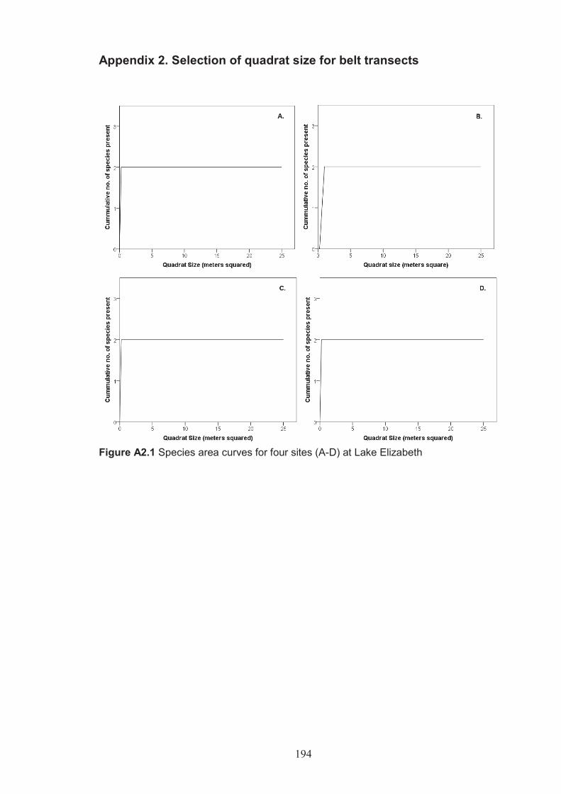
194
Appendix 2. Selection of quadrat size for belt transects
Figure A2.1 Species area curves for four sites (A-D) at Lake Elizabeth

195
Figure A2.2 Species area curves for four sites (A-D) at Round Lake

196
Figure A2.3 Species area curves for four sites (A-D) at Lake Woorinen North
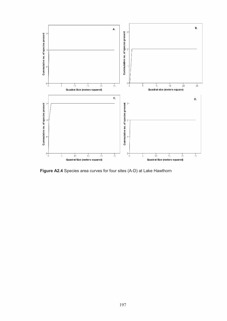
197
Figure A2.4 Species area curves for four sites (A-D) at Lake Hawthorn

19
8
App
endi
x 3
Bel
t tra
nsec
t res
ults
(dep
th, p
erce
ntag
e ve
geta
tion
cove
r, dr
y w
eigh
t bio
mas
s an
d bi
ovol
ume)
Fi
gure
A3.
1 La
ke E
lizab
eth
Tran
sect
A. a
) Dep
th o
f tra
nsec
t (so
lid li
ne) a
nd to
tal p
erce
ntag
e co
ver o
f veg
etat
ion
(das
hed
line)
, b) T
otal
bio
volu
me
(sol
id li
ne),
and
tota
l bio
mas
s (d
ashe
d lin
e); c
) and
d) s
how
s bi
ovol
ume
(sol
id li
ne) a
nd b
iom
ass
(das
hed
line)
for R
. meg
acar
pa, a
nd L
. m
acro
pogo
n.

19
9
Fi
gure
A3.
2 La
ke E
lizab
eth
Tran
sect
B. a
) Dep
th o
f tra
nsec
t (so
lid li
ne) a
nd to
tal p
erce
ntag
e co
ver o
f veg
etat
ion
(das
hed
line)
, b) T
otal
bio
volu
me
(sol
id li
ne),
and
tota
l bio
mas
s (d
ashe
d lin
e); c
) and
d) s
how
s bi
ovol
ume
(sol
id li
ne) a
nd b
iom
ass
(das
hed
line)
for R
. meg
acar
pa, a
nd L
. m
acro
pogo
n.
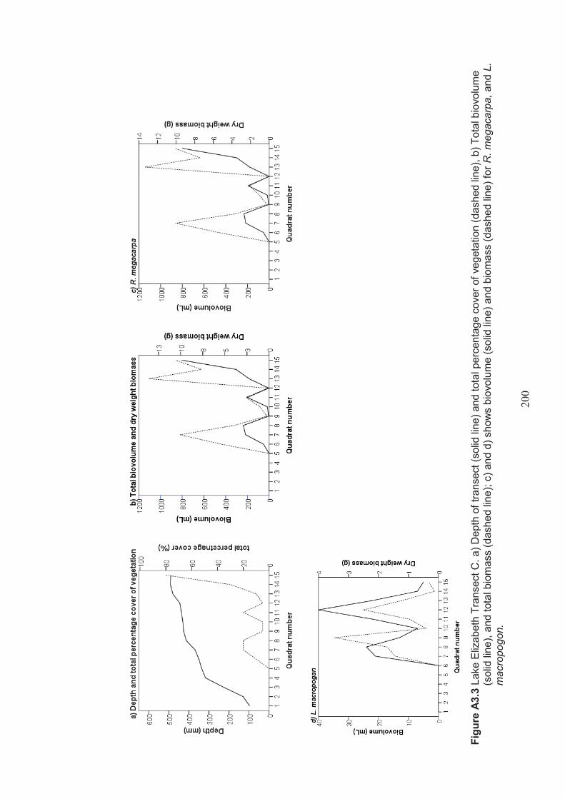
20
0
Fi
gure
A3.
3 La
ke E
lizab
eth
Tran
sect
C. a
) Dep
th o
f tra
nsec
t (so
lid li
ne) a
nd to
tal p
erce
ntag
e co
ver o
f veg
etat
ion
(das
hed
line)
, b) T
otal
bio
volu
me
(sol
id li
ne),
and
tota
l bio
mas
s (d
ashe
d lin
e); c
) and
d) s
how
s bi
ovol
ume
(sol
id li
ne) a
nd b
iom
ass
(das
hed
line)
for R
. meg
acar
pa, a
nd L
. m
acro
pogo
n.
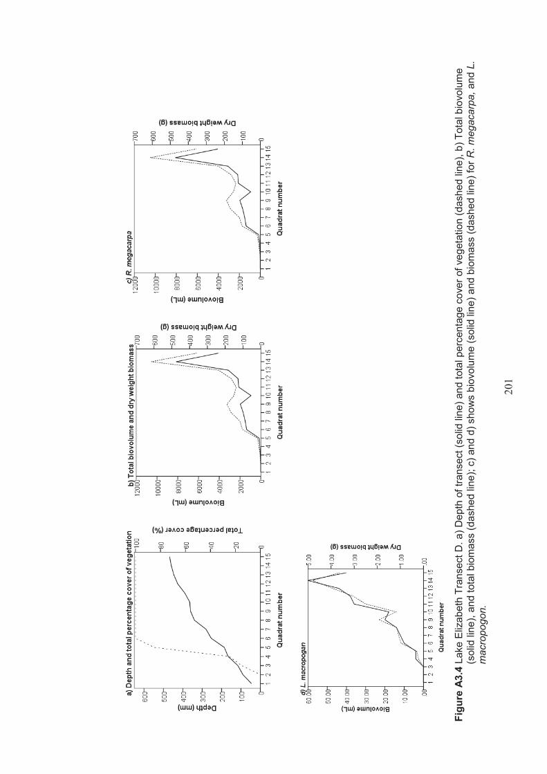
20
1
Fi
gure
A3.
4 La
ke E
lizab
eth
Tran
sect
D. a
) Dep
th o
f tra
nsec
t (so
lid li
ne) a
nd to
tal p
erce
ntag
e co
ver o
f veg
etat
ion
(das
hed
line)
, b) T
otal
bio
volu
me
(sol
id li
ne),
and
tota
l bio
mas
s (d
ashe
d lin
e); c
) and
d) s
how
s bi
ovol
ume
(sol
id li
ne) a
nd b
iom
ass
(das
hed
line)
for R
. meg
acar
pa, a
nd L
. m
acro
pogo
n.

20
2
Fi
gure
A3.
5 La
ke E
lizab
eth
Tran
sect
E. a
) Dep
th o
f tra
nsec
t (so
lid li
ne) a
nd to
tal p
erce
ntag
e co
ver o
f veg
etat
ion
(das
hed
line)
, b) T
otal
bio
volu
me
(sol
id li
ne),
and
tota
l bio
mas
s (d
ashe
d lin
e); c
) and
d) s
how
s bi
ovol
ume
(sol
id li
ne) a
nd b
iom
ass
(das
hed
line)
for R
. meg
acar
pa, a
nd L
. m
acro
pogo
n.
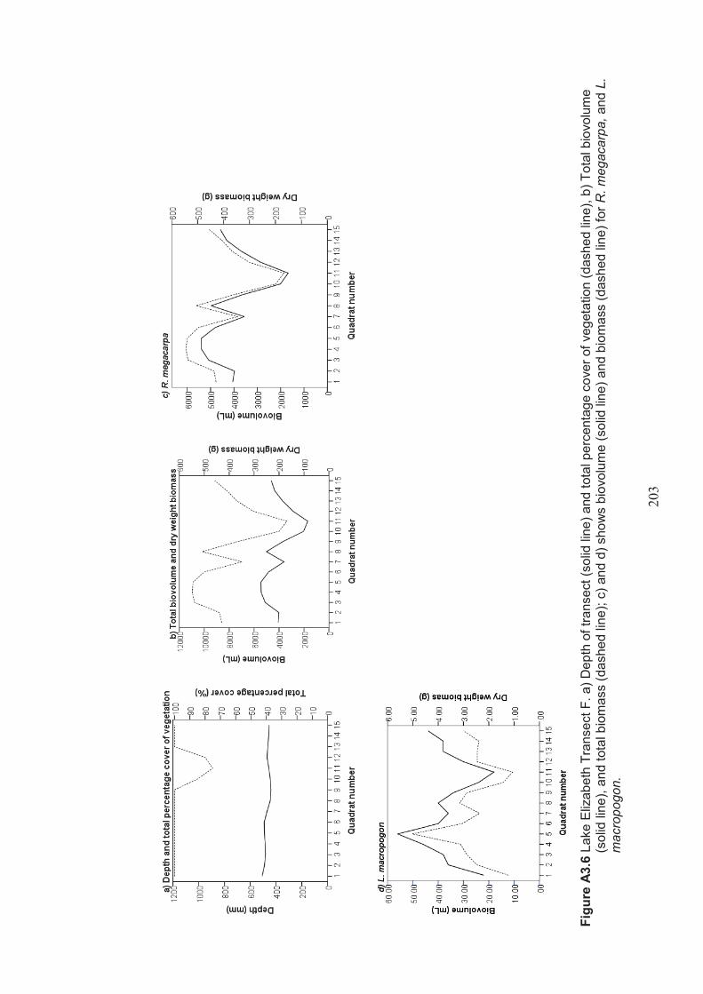
20
3
Fi
gure
A3.
6 La
ke E
lizab
eth
Tran
sect
F. a
) Dep
th o
f tra
nsec
t (so
lid li
ne) a
nd to
tal p
erce
ntag
e co
ver o
f veg
etat
ion
(das
hed
line)
, b) T
otal
bio
volu
me
(sol
id li
ne),
and
tota
l bio
mas
s (d
ashe
d lin
e); c
) and
d) s
how
s bi
ovol
ume
(sol
id li
ne) a
nd b
iom
ass
(das
hed
line)
for R
. meg
acar
pa, a
nd L
. m
acro
pogo
n.

20
4
Fi
gure
A3.
7 R
ound
Lak
e Tr
anse
ct A
. a) D
epth
of t
rans
ect (
solid
line
) and
tota
l per
cent
age
cove
r of v
eget
atio
n (d
ashe
d lin
e), b
) Tot
al b
iovo
lum
e (s
olid
lin
e), a
nd to
tal b
iom
ass
(das
hed
line)
; c),
d), e
) and
f) s
how
s bi
ovol
ume
(sol
id li
ne) a
nd b
iom
ass
(das
hed
line)
for R
. meg
acar
pa, L
. m
acro
pogo
n, J
. acu
tus
and
T. d
omin
gens
is.
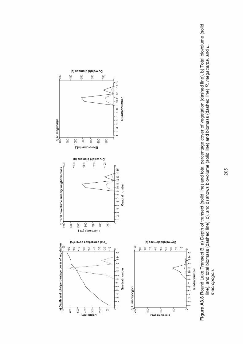
20
5
Fi
gure
A3.
8 R
ound
Lak
e Tr
anse
ct B
. a) D
epth
of t
rans
ect (
solid
line
) and
tota
l per
cent
age
cove
r of v
eget
atio
n (d
ashe
d lin
e), b
) Tot
al b
iovo
lum
e (s
olid
lin
e), a
nd to
tal b
iom
ass
(das
hed
line)
; c),
and
d) s
how
s bi
ovol
ume
(sol
id li
ne) a
nd b
iom
ass
(das
hed
line)
R. m
egac
arpa
, and
L.
mac
ropo
gon.

20
6
Fi
gure
A3.
9 R
ound
Lak
e Tr
anse
ct C
. a) D
epth
of t
rans
ect (
solid
line
) and
tota
l per
cent
age
cove
r of v
eget
atio
n (d
ashe
d lin
e), b
) Tot
al b
iovo
lum
e (s
olid
lin
e), a
nd to
tal b
iom
ass
(das
hed
line)
; c),
and
d) s
how
s bi
ovol
ume
(sol
id li
ne) a
nd b
iom
ass
(das
hed
line)
R. m
egac
arpa
, and
L.
mac
ropo
gon.
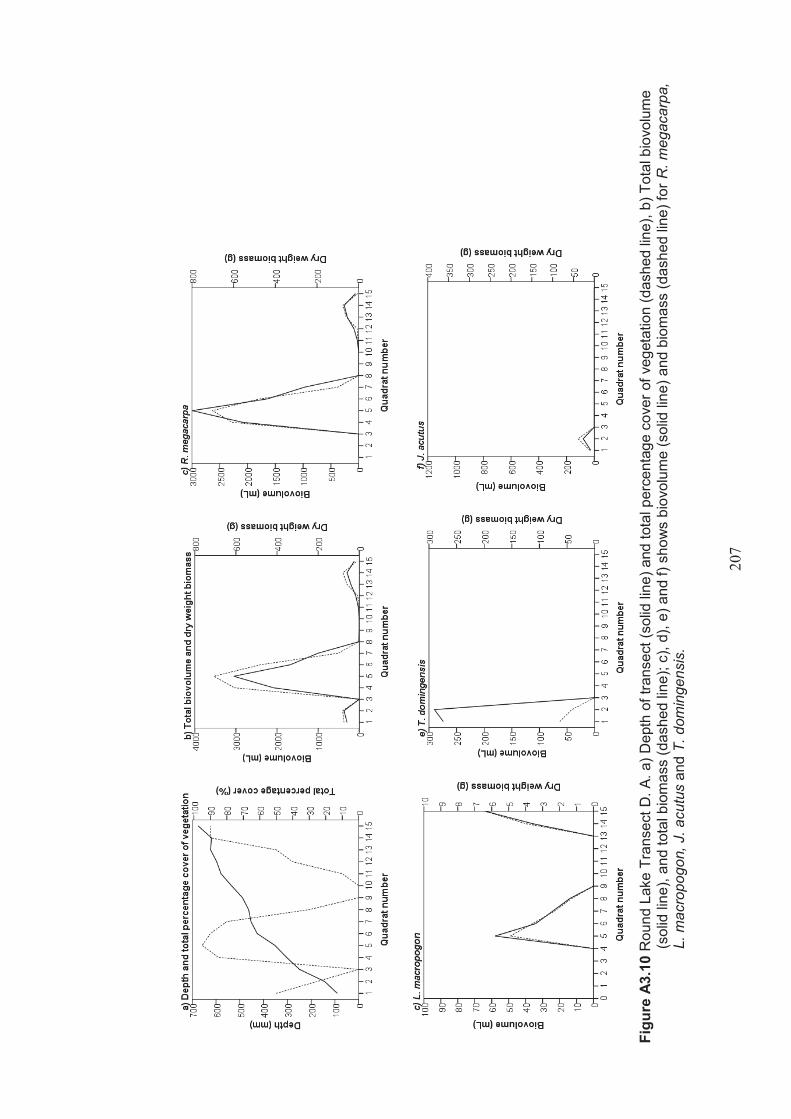
20
7
Fi
gure
A3.
10 R
ound
Lak
e Tr
anse
ct D
. A. a
) Dep
th o
f tra
nsec
t (so
lid li
ne) a
nd to
tal p
erce
ntag
e co
ver o
f veg
etat
ion
(das
hed
line)
, b) T
otal
bio
volu
me
(sol
id li
ne),
and
tota
l bio
mas
s (d
ashe
d lin
e); c
), d)
, e) a
nd f)
sho
ws
biov
olum
e (s
olid
line
) and
bio
mas
s (d
ashe
d lin
e) fo
r R. m
egac
arpa
, L.
mac
ropo
gon,
J. a
cutu
s an
d T.
dom
inge
nsis
.

20
8
Fi
gure
A3.
11 R
ound
Lak
e Tr
anse
ct E
. a) D
epth
of t
rans
ect (
solid
line
) and
tota
l per
cent
age
cove
r of v
eget
atio
n (d
ashe
d lin
e), b
) Tot
al b
iovo
lum
e (s
olid
line
), an
d to
tal b
iom
ass
(das
hed
line)
; c),
and
d) s
how
s bi
ovol
ume
(sol
id li
ne) a
nd b
iom
ass
(das
hed
line)
R. m
egac
arpa
, and
L.
mac
ropo
gon.

20
9
Fi
gure
A3.
12 R
ound
Lak
e Tr
anse
ct F
. a) D
epth
of t
rans
ect (
solid
line
) and
tota
l per
cent
age
cove
r of v
eget
atio
n (d
ashe
d lin
e), b
) Tot
al b
iovo
lum
e (s
olid
line
), an
d to
tal b
iom
ass
(das
hed
line)
; c),
and
d) s
how
s bi
ovol
ume
(sol
id li
ne) a
nd b
iom
ass
(das
hed
line)
R. m
egac
arpa
, and
L.
mac
ropo
gon

21
0
Figu
re A
3.13
Woo
rinen
Nor
th T
rans
ect A
. a) D
epth
of t
rans
ect (
solid
line
) and
tota
l per
cent
age
cove
r of v
eget
atio
n (d
ashe
d lin
e), b
) Tot
al b
iovo
lum
e (s
olid
line
), an
d to
tal b
iom
ass
(das
hed
line)
; c),
show
s bi
ovol
ume
(sol
id li
ne) a
nd b
iom
ass
(das
hed
line)
for R
. meg
acar
pa.
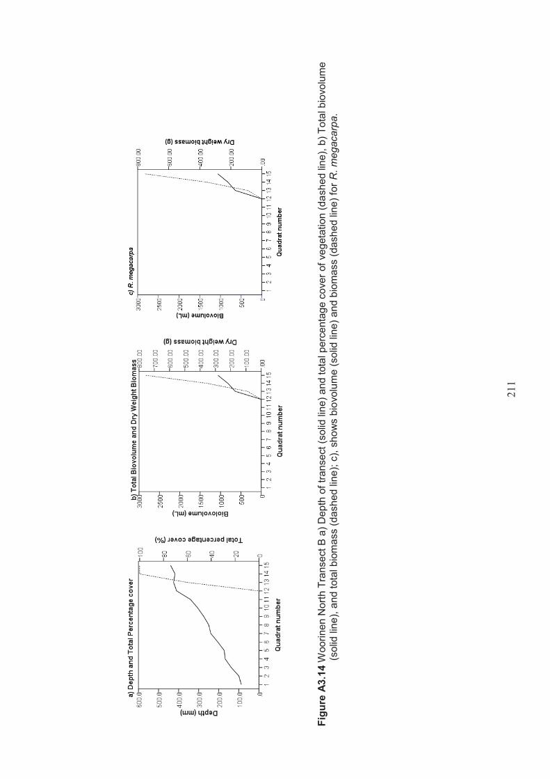
21
1
Figu
re A
3.14
Woo
rinen
Nor
th T
rans
ect B
a) D
epth
of t
rans
ect (
solid
line
) and
tota
l per
cent
age
cove
r of v
eget
atio
n (d
ashe
d lin
e), b
) Tot
al b
iovo
lum
e (s
olid
line
), an
d to
tal b
iom
ass
(das
hed
line)
; c),
show
s bi
ovol
ume
(sol
id li
ne) a
nd b
iom
ass
(das
hed
line)
for R
. meg
acar
pa.
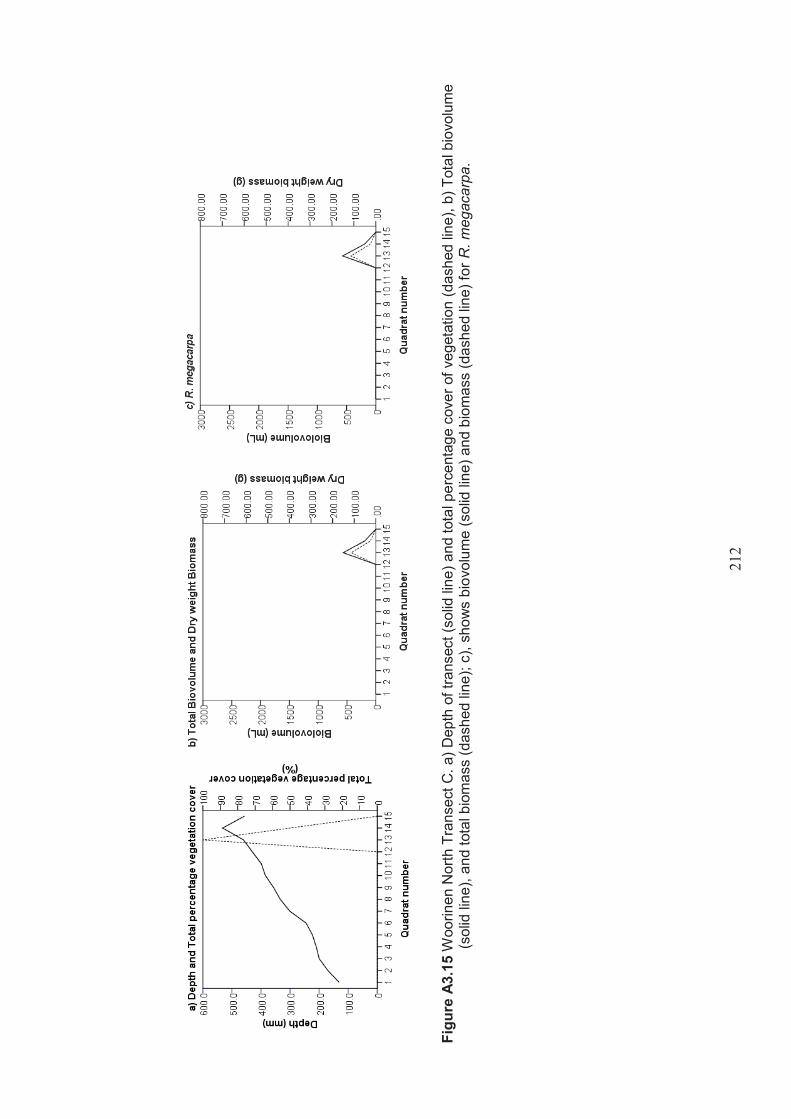
21
2
Figu
re A
3.15
Woo
rinen
Nor
th T
rans
ect C
. a) D
epth
of t
rans
ect (
solid
line
) and
tota
l per
cent
age
cove
r of v
eget
atio
n (d
ashe
d lin
e), b
) Tot
al b
iovo
lum
e (s
olid
line
), an
d to
tal b
iom
ass
(das
hed
line)
; c),
show
s bi
ovol
ume
(sol
id li
ne) a
nd b
iom
ass
(das
hed
line)
for R
. meg
acar
pa.
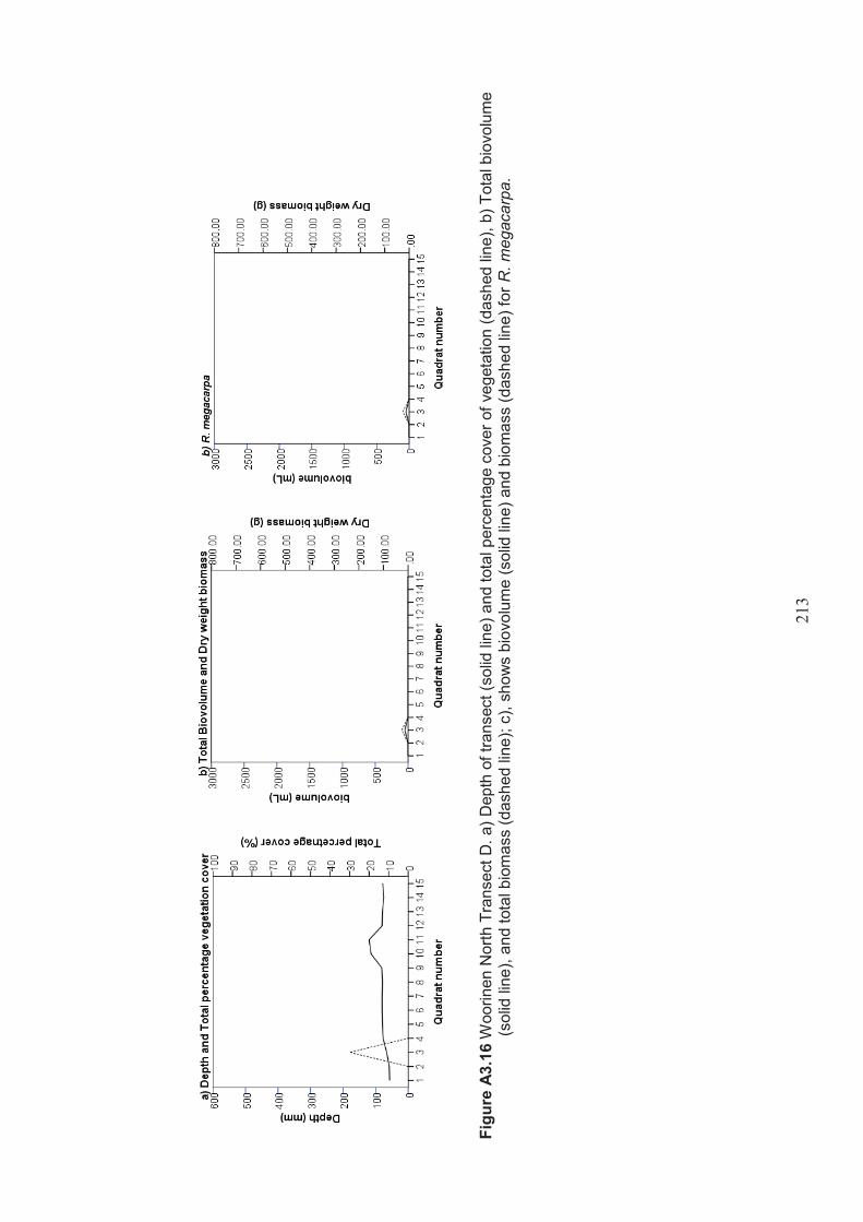
21
3
Figu
re A
3.16
Woo
rinen
Nor
th T
rans
ect D
. a) D
epth
of t
rans
ect (
solid
line
) and
tota
l per
cent
age
cove
r of v
eget
atio
n (d
ashe
d lin
e), b
) Tot
al b
iovo
lum
e (s
olid
line
), an
d to
tal b
iom
ass
(das
hed
line)
; c),
show
s bi
ovol
ume
(sol
id li
ne) a
nd b
iom
ass
(das
hed
line)
for R
. meg
acar
pa.

21
4
Figu
re A
3.17
Woo
rinen
Nor
th T
rans
ect E
. a) D
epth
of t
rans
ect (
solid
line
) and
tota
l per
cent
age
cove
r of v
eget
atio
n (d
ashe
d lin
e), b
) Tot
al b
iovo
lum
e (s
olid
line
), an
d to
tal b
iom
ass
(das
hed
line)
; c),
show
s bi
ovol
ume
(sol
id li
ne) a
nd b
iom
ass
(das
hed
line)
for R
. meg
acar
pa.
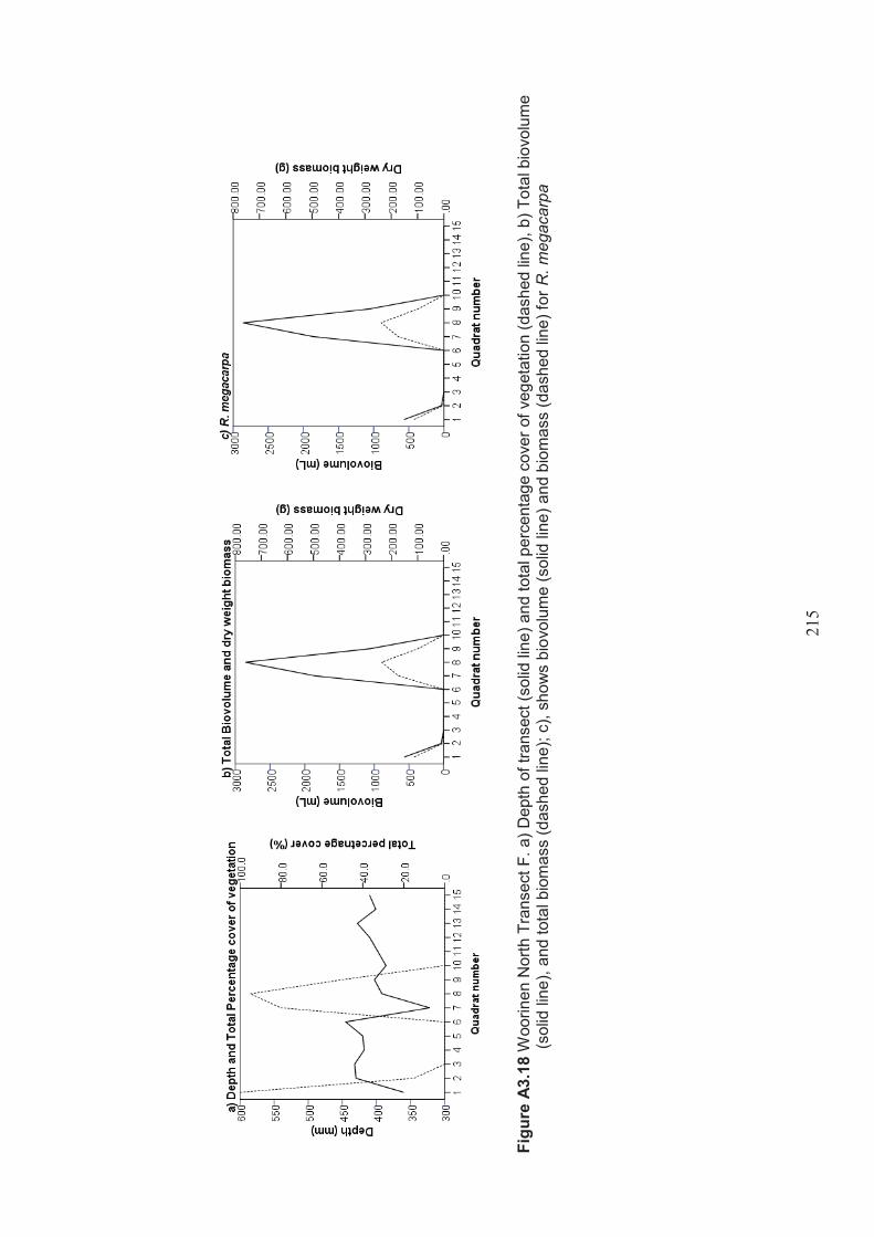
21
5
Figu
re A
3.18
Woo
rinen
Nor
th T
rans
ect F
. a) D
epth
of t
rans
ect (
solid
line
) and
tota
l per
cent
age
cove
r of v
eget
atio
n (d
ashe
d lin
e), b
) Tot
al b
iovo
lum
e (s
olid
line
), an
d to
tal b
iom
ass
(das
hed
line)
; c),
show
s bi
ovol
ume
(sol
id li
ne) a
nd b
iom
ass
(das
hed
line)
for R
. meg
acar
pa
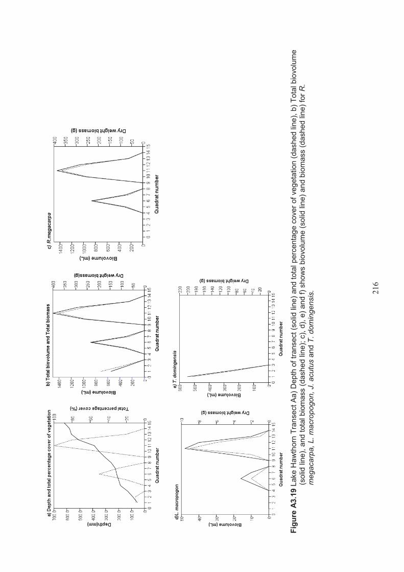
21
6
Figu
re A
3.19
Lak
e H
awth
orn
Tran
sect
Aa)
Dep
th o
f tra
nsec
t (so
lid li
ne) a
nd to
tal p
erce
ntag
e co
ver o
f veg
etat
ion
(das
hed
line)
, b) T
otal
bio
volu
me
(sol
id li
ne),
and
tota
l bio
mas
s (d
ashe
d lin
e); c
), d)
, e) a
nd f)
sho
ws
biov
olum
e (s
olid
line
) and
bio
mas
s (d
ashe
d lin
e) fo
r R.
meg
acar
pa, L
. mac
ropo
gon,
J. a
cutu
s an
d T.
dom
inge
nsis
.
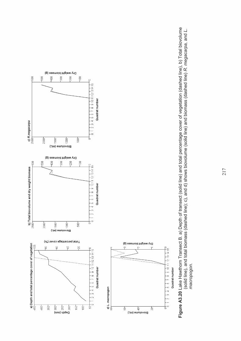
21
7
Fi
gure
A3.
20 L
ake
Haw
thor
n Tr
anse
ct B
. a) D
epth
of t
rans
ect (
solid
line
) and
tota
l per
cent
age
cove
r of v
eget
atio
n (d
ashe
d lin
e), b
) Tot
al b
iovo
lum
e (s
olid
line
), an
d to
tal b
iom
ass
(das
hed
line)
; c),
and
d) s
how
s bi
ovol
ume
(sol
id li
ne) a
nd b
iom
ass
(das
hed
line)
R. m
egac
arpa
, and
L.
mac
ropo
gon.

21
8
Fi
gure
A3.
21 L
ake
Haw
thor
n Tr
anse
ct c
. a) D
epth
of t
rans
ect (
solid
line
) and
tota
l per
cent
age
cove
r of v
eget
atio
n (d
ashe
d lin
e), b
) Tot
al b
iovo
lum
e (s
olid
line
), an
d to
tal b
iom
ass
(das
hed
line)
; c),
and
d) s
how
s bi
ovol
ume
(sol
id li
ne) a
nd b
iom
ass
(das
hed
line)
R. m
egac
arpa
, and
L.
mac
ropo
gon.
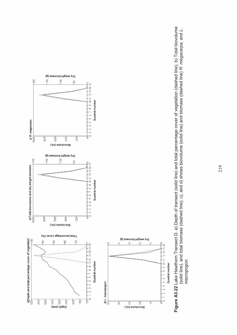
21
9
Fi
gure
A3.
22 L
ake
Haw
thor
n Tr
anse
ct D
. a) D
epth
of t
rans
ect (
solid
line
) and
tota
l per
cent
age
cove
r of v
eget
atio
n (d
ashe
d lin
e), b
) Tot
al b
iovo
lum
e (s
olid
line
), an
d to
tal b
iom
ass
(das
hed
line)
; c),
and
d) s
how
s bi
ovol
ume
(sol
id li
ne) a
nd b
iom
ass
(das
hed
line)
R. m
egac
arpa
, and
L.
mac
ropo
gon.

22
0
Fi
gure
A3.
23 L
ake
Haw
thor
n Tr
anse
ct E
. a) D
epth
of t
rans
ect (
solid
line
) and
tota
l per
cent
age
cove
r of v
eget
atio
n (d
ashe
d lin
e), b
) Tot
al b
iovo
lum
e (s
olid
line
), an
d to
tal b
iom
ass
(das
hed
line)
; c),
and
d) s
how
s bi
ovol
ume
(sol
id li
ne) a
nd b
iom
ass
(das
hed
line)
R. m
egac
arpa
, and
L.
mac
ropo
gon.
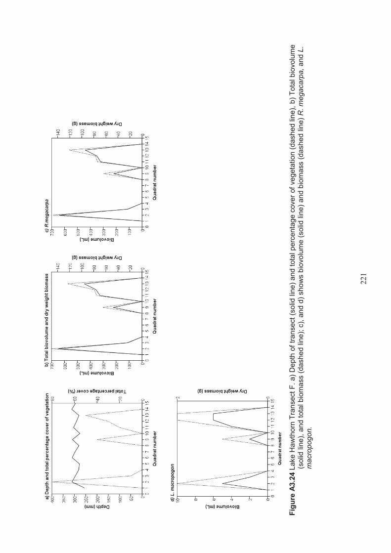
22
1
Fi
gure
A3.
24 L
ake
Haw
thor
n Tr
anse
ct F
. a) D
epth
of t
rans
ect (
solid
line
) and
tota
l per
cent
age
cove
r of v
eget
atio
n (d
ashe
d lin
e), b
) Tot
al b
iovo
lum
e (s
olid
line
), an
d to
tal b
iom
ass
(das
hed
line)
; c),
and
d) s
how
s bi
ovol
ume
(sol
id li
ne) a
nd b
iom
ass
(das
hed
line)
R. m
egac
arpa
, and
L.
mac
ropo
gon.

222
Appendix 4 Results of fish survey in wetlands of intermediate salinity in northwest Victoria – detailed results
Table A4.1 Fish measurements Round Lake
Murray Hardyhead Craterocephalus fluviatilis
Eastern Mosquito fish Gambusia holbrooki
Length (mm) No. of fish Length
(mm) No. of fish
12 19 13 20 14 21 15 22 16 23 17 3 24 18 5 25 19 4 26 1 20 3 27 21 7 28 22 6 29 23 6 30 24 12 31 25 3 32 26 5 33 27 10 34 28 9 35 29 4 36 30 3 37 31 3 38 32 39 33 2 40 34 2 41 35 5 42 36 1 43 37 1 44 38 2 45 39 2 46 40 1 47 41 48 42 49 43 50 44 51 45 52 46 53 47 54 48 1 55 49 56 57 58

223
Table A4.2 Fish measurements Lake Woorinen North
Murray Hardyhead Craterocephalus fluviatilis
Eastern Mosquito fish Gambusia holbrooki
Flat Headed Gudgeon Philypnodon grandiceps
Length (mm) No. of fish Length
(mm) No. of fish Length (mm) No. of fish
12 19 29 2 13 20 30 14 21 31 15 22 32 16 23 33 17 24 34 1 18 25 1 35 19 26 36 20 27 37 21 28 38 22 29 39 23 30 40 24 31 41 25 32 42 26 33 43 27 34 44 28 35 45 29 36 46 30 37 47 31 38 48 32 1 39 49 33 40 50 34 41 51 35 1 42 52 36 43 53 37 1 44 54 38 45 55 39 1 46 56 40 47 57 41 2 48 58 42 2 49 59 43 50 60 44 51 61 45 52 62 46 53 63 47 54 64 48 55 65 49 56 66 1 57 58
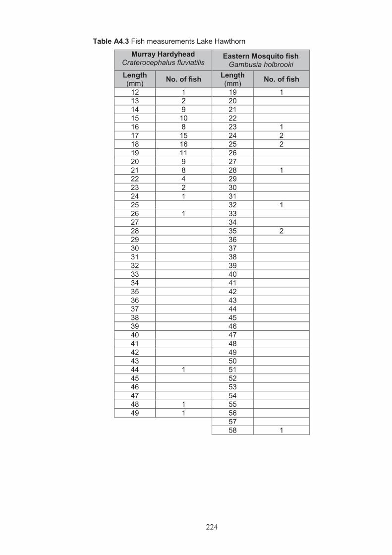
224
Table A4.3 Fish measurements Lake Hawthorn
Murray Hardyhead Craterocephalus fluviatilis
Eastern Mosquito fish Gambusia holbrooki
Length (mm) No. of fish Length
(mm) No. of fish
12 1 19 1 13 2 20 14 9 21 15 10 22 16 8 23 1 17 15 24 2 18 16 25 2 19 11 26 20 9 27 21 8 28 1 22 4 29 23 2 30 24 1 31 25 32 1 26 1 33 27 34 28 35 2 29 36 30 37 31 38 32 39 33 40 34 41 35 42 36 43 37 44 38 45 39 46 40 47 41 48 42 49 43 50 44 1 51 45 52 46 53 47 54 48 1 55 49 1 56 57 58 1

225
Appendix 5 Random location of replicates for the experiment investigating the effect of salinity on the egg and propagule bank of Lake Cullen
Key Door
Water max/min
thermometer Air max/min thermometer
3.4 g/L treatment
5.5 g/L treatment
8.9 g/L treatment
14.4 g/L treatment
23.3 g/L treatment
37.7 g/L treatment
61 g/L treatment
98.7 g/L treatment
136 g/L Treatment
Control/blank (3.4 g/L)
replicates used in 2nd experiment

22
6
App
endi
x 6
QA
/QC
che
cks
of th
e ef
fect
iven
ess
of s
ugar
flot
atio
n m
etho
ds fo
r sep
arat
ing
inve
rteb
rate
s fr
om th
e or
gani
c m
ater
ial (
Cha
pter
3 e
xper
imen
ts).
Tabl
e A9
.1 Q
A/Q
C re
sults
of t
he e
ffect
iven
ess
of th
e su
gar f
lota
tion
met
hod
on s
epar
atin
g in
verte
brat
es fr
om o
rgan
ic m
ater
ials
in >
500μ
m s
ize
clas
s fo
r see
dban
k ex
perim
ent 1
.
Rep
licat
e
Inve
rteb
rate
spe
cies
N
umbe
r col
lect
ed
usin
g su
gar f
lota
tion
met
hod
Tota
l num
ber o
f ind
ivid
uals
in
sam
ple
Perc
enta
ge o
f ind
ivid
uals
so
rted
by
suga
r flo
atat
ion
met
hod
3.4
g/L
A M
ytilo
cypr
is h
enri
cae
15
32
1553
99
%
Aust
ralo
cypr
is s
pp.
62
62
100%
3.4
g/L
D
Myt
ilocy
pris
hen
rica
e 15
74
1590
99
%
Aust
ralo
cypr
is s
pp.
94
100
94%
8.9
g/L
C
Myt
ilocy
pris
hen
rica
e 21
52
2155
10
0%
Aust
ralo
cypr
is s
pp.
538
538
100%
13.4
g/L
D
Myt
ilocy
pris
hen
rica
e 11
59
1237
94
%
Aust
ralo
cypr
is s
pp.
53
53
100%
24.4
g/L
D
Myt
ilocy
pris
hen
rica
e 83
3 83
3 99
%
Aust
ralo
cypr
is s
pp.
216
216
100%

227
Appendix 7 Air temperature and water quality monitoring for experiment investigating the effect of salinity on the egg and propagule bank of Lake Cullen
Table A6.1 Maximum/minimum air temperature monitoring in the glasshouse
Date Thermometer 1 Thermometer 2
Min (oC)
Max (oC)
Min (oC)
Max (oC)
23/11/05 9.9 31.4 8.7 33.1 30/11/05 11.5 34.5 9.9 36.2 7/12/05 13.3 34.5 11.6 40.5 14/12/05 12.3 31.1 10.5 33.5 21/12/05 12.7 28.5 11.1 32.1 28/12/05 13.1 31.3 11.3 32.9 3/1/06 14.7 32.1 13.6 36.3
11/1/06 12.3 28.5 9.9 36.3 18/1/06 13.5 28.8 11.5 33.0 25/1/06 13.3 34.3 11.7 38.3 1/2/06 12.9 31.3 11.8 32.0 8/2/06 13.1 27.5 11.9 31.1
15/2/06 12.3 33.3 10.7 39.3 22/2/06 12.2 30.7 10.9 33.5
Table A6.2 Maximum/minimum water temperature monitoring in the glasshouse
Date Thermometer 1 Thermometer 2 Thermometer 3 Thermometer 4
Min (oC)
Max (oC)
Min (oC)
Max (oC)
Min (oC)
Max (oC)
Min (oC)
Max (oC)
23/11/05 13 26 15 23 13 26 15 23 30/11/05 15 28 17 26 15 23 14 29 7/12/05 11 29 18 29 16 22 15 32
14/12/05 15 27 17 24 16 21 16 25 21/12/05 16 26 18 21 16 22 14 26 28/12/05 15 27 18 25 16 25 15 26 3/1/06 16 30 18 28 18 26 17 29 11/1/06 15 27 18 26 15 23 15 28 18/1/06 16 26 18 24 18 25 16 25 25/1/06 15 32 19 29 17 26 16 31 1/2/06 17 30 17 23 18 29 17 30 8/2/06 18 27 20 25 19 26 16 27 15/2/06 16 29 17 20 18 23 15 24 22/2/06 17 27 16 25 16 24 17 28

22
8
Tabl
e A7
.3 S
alin
ity m
onito
ring
of re
plic
ates
for t
he e
xper
imen
t inv
estig
atin
g th
e ef
fect
of s
alin
ity o
n th
e eg
g an
d pr
opag
ule
bank
of L
ake
Cul
len,
for
al tr
eatm
ents
(all
mea
sure
men
ts a
re in
g/L
)
Trea
tmen
t 3.
4 g/
L 5.
5 g/
L 8.
9 g/
L W
eek
A B
C
D
E A
B C
D
E
A B
C
D
E 1
3.4
3.4
3.4
3.4
3.4
5.5
6.0
5.5
5.5
5.5
8.9
8.9
8.9
8.9
8.9
3 4.
0 4.
0 3.
9 4.
2 4.
1 6.
2 6.
1 6.
1 6.
3 6.
3 9.
7 9.
6 9.
5 9.
5 9.
8 5
4.4
4.3
4.2
4.5
4.4
6.6
6.5
6.6
6.7
6.8
10.3
10
.3
10.1
10
.3
10.3
7
4.4
4.4
4.3
4.7
4.4
6.5
6.4
6.6
6.7
6.6
10.2
10
.1
10.0
10
.0
10.2
9
4.7
4.4
4.2
4.5
4.4
6.6
6.4
6.6
6.7
6.6
10.0
10
.0
9.9
9.8
10.0
11
4.
4 4.
4 4.
3 4.
7 4.
4 6.
5 6.
2 6.
5 6.
7 6.
5 9.
9 9.
9 9.
8 9.
9 10
.0
13
4.6
4.6
4.5
4.8
4.6
6.6
6.6
6.7
7.0
6.7
10.4
10
.1
10.0
9.
8 10
.2
Mea
n 4.
3 4.
2 4.
1 4.
4 4.
2 6.
4 6.
3 6.
4 6.
5 6.
4 9.
9 9.
8 9.
7 9.
7 9.
9 S
tand
ard
devi
atio
n ±
0.4
± 0.
4 ±
0.3
± 0.
4 ±
0.4
± 0.
4 ±
0.2
± 0.
4 ±
0.5
± 0.
4 ±
0.5
± 0.
4 ±
0.4
± 0.
4 ±
0.4
Trea
tmen
t 14
.4 g
/L
23.3
g/L
37
.7 g
/L
Wee
k A
B C
D
E
A B
C
D
E A
B C
D
E
1 14
.4
14.4
14
.4
14.4
14
.4
23.3
23
.3
23.3
23
.3
23.3
37
.7
37.7
37
.7
37.7
37
.7
3 15
.0
14.9
15
.3
15.1
15
.0
23.7
23
.9
24.0
23
.1
24.4
38
.8
37.2
38
.2
38.4
38
.9
5 15
.8
15.6
16
.9
16.3
15
.7
25.4
25
.8
25.2
25
.1
25.8
41
.6
38.7
40
.1
40.0
40
.9
7 15
.5
15.2
15
.4
15.4
15
.2
23.9
24
.2
23.9
23
.9
24.7
39
.2
38.8
38
.7
38.5
39
.6
9 15
.2
14.8
15
.2
15.4
15
.3
23.7
23
.9
23.7
23
.1
23.9
38
.4
37.9
38
.8
38.5
37
.9
11
15.2
15
.0
15.4
15
.2
15.0
23
.9
23.9
23
.5
23.6
24
.2
38.6
36
.7
37.9
38
.3
38.6
13
15
.2
14.8
15
.5
15.5
15
.1
23.7
24
.5
23.7
23
.3
24.3
38
.9
38.1
37
.7
39.9
38
.2
Mea
n 15
.2
15.0
15
.4
15.3
15
.1
23.9
24
.2
23.9
23
.6
24.4
39
.0
37.9
38
.4
38.8
38
.8
Sta
ndar
d de
viat
ion
± 0
.4
± 0.
3 ±
0.7
± 0.
5 ±
0.4
± 0.
6 ±
0.7
± 0.
6 ±
0.7
± 0.
7 ±
1.1
± 0.
7 ±
0.8
± 0.
8 ±
1.0
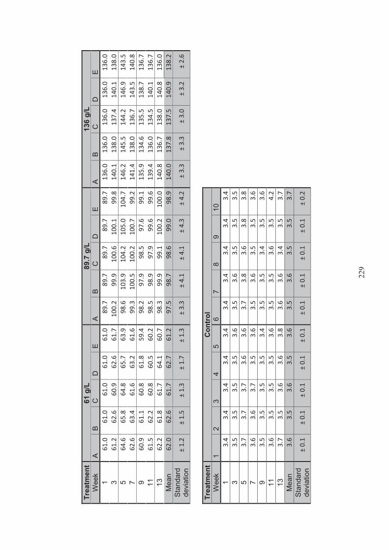
22
9
Trea
tmen
t 61
g/L
89
.7 g
/L
136
g/L
Wee
k A
B C
D
E
A B
C
D
E A
B C
D
E
1 61
.0
61.0
61
.0
61.0
61
.0
89.7
89
.7
89.7
89
.7
89.7
13
6.0
136.
0 13
6.0
136.
0 13
6.0
3 61
.2
62.6
60
.9
62.6
61
.7
100.
2 99
.9
100.
6 10
0.1
99.8
14
0.1
138.
0 13
7.4
140.
1 13
8.0
5 64
.6
65.8
64
.8
65.7
63
.9
98.6
10
3.9
104.
2 10
5.0
104.
7 14
6.2
145.
5 14
4.2
146.
9 14
3.5
7 62
.6
63.4
61
.6
63.2
61
.6
99.3
10
0.5
100.
2 10
0.7
99.2
14
1.4
138.
0 13
6.7
143.
5 14
0.8
9 60
.9
61.1
60
.8
61.8
59
.4
98.2
97
.9
98.5
97
.6
99.1
13
5.9
134.
6 13
5.5
138.
7 13
6.7
11
61.5
62
.2
60.8
60
.5
60.2
98
.5
98.9
97
.9
99.6
99
.6
139.
4 13
6.0
134.
5 14
0.1
136.
7 13
62
.2
61.8
61
.7
64.1
60
.7
98.3
99
.9
99.1
10
0.2
100.
0 14
0.8
136.
7 13
8.0
140.
8 13
6.0
Mea
n 62
.0
62.6
61
.7
62.7
61
.2
97.5
98
.7
98.6
99
.0
98.9
14
0.0
137.
8 13
7.5
140.
9 13
8.2
Sta
ndar
d de
viat
ion
± 1.
2 ±
1.5
± 1.
3 ±
1.7
± 1.
3 ±
3.3
± 4.
1 ±
4.1
± 4.
3 ±
4.2
± 3.
3 ±
3.3
± 3.
0 ±
3.2
± 2.
6
Trea
tmen
t C
ontr
ol
Wee
k 1
2 3
4 5
6 7
8 9
10
1 3.
4 3.
4 3.
4 3.
4 3.
4 3.
4 3.
4 3.
4 3.
4 3.
4 3
3.5
3.5
3.5
3.5
3.6
3.5
3.6
3.5
3.5
3.5
5 3.
7 3.
7 3.
7 3.
6 3.
6 3.
7 3.
8 3.
6 3.
8 3.
8 7
3.6
3.6
3.7
3.5
3.6
3.5
3.6
3.5
3.5
3.6
9 3.
5 3.
5 3.
5 3.
5 3.
4 3.
5 3.
5 3.
4 3.
5 3.
6 11
3.
6 3.
5 3.
5 3.
5 3.
6 3.
5 3.
5 3.
6 3.
5 4.
2 13
3.
7 3.
5 3.
6 3.
6 3.
8 3.
6 3.
6 3.
4 3.
5 3.
7 M
ean
3.6
3.5
3.6
3.5
3.6
3.5
3.6
3.5
3.5
3.7
Sta
ndar
d de
viat
ion
± 0.
1 ±
0.1
± 0.
1 ±
0.1
± 0.
1 ±
0.1
± 0.
1 ±
0.1
± 0.
1 ±
0.2

23
0
App
endi
x 8
Det
aile
d re
gres
sion
ana
lysi
s an
d A
NO
VA re
sults
for e
xper
imen
t inv
estig
atin
g th
e ef
fect
of s
alin
ity o
n th
e eg
g an
d pr
opag
ule
bank
of L
ake
Cul
len
Tabl
e A
7.1
Reg
ress
ion
resu
lts fo
r Rup
pia
meg
acar
pa
Var
iabl
e Tr
ansf
orm
atio
n M
odel
Eq
uatio
n R
2 df
F
P N
umbe
r of s
tem
s pe
r rep
licat
e √x
Li
near
y
= 13
.67-
0.3
48x
0.91
5 1,
28
143.
27
<0.0
01
Biov
olum
e √x
Li
near
y
= 3.
577-
0.0
84x
0.85
0 1,
28
72.9
99
<0.0
01
Dry
wei
ght B
iom
ass
√x
Line
ar
y =
1.08
4 –
0.02
5x
0.82
6 1,
28
59.9
16
<0.0
01
Ta
ble
A7.2
Tuk
ey’s
test
for n
umbe
r of R
uppi
a m
egac
arpa
ste
ms
3.
4 g/
L 5.
5 g/
L 8.
9 g/
L 14
.4
g/L
23.3
g/
L 37
.7
g/L
3.4
g/L
5.5
g/L
0.85
6
8.9
g/L
0.92
5 .0
316
14.4
g/L
0.
020
0.00
1 0.
15
23
.3 g
/L
0.00
1 <
0.00
1 0.
014
0.86
7
37
.7 g
/L
< 0.
001
< 0.
001
< 0.
001
< 0.
001
< 0.
001
Ta
ble
A7.3
Tuk
ey’s
test
for R
uppi
a m
egac
arpa
bio
volu
me
3.
4
g/L
5.5
g/L
8.9
g/L
14.4
g/
L 23
.3
g/L
37.7
g/
L 3.
4 g/
L
5.
5 g/
L 0.
999
8.
9 g/
L 0.
839
0.65
0
14
.4 g
/L
0.76
1 0.
557
1.00
0
23.3
g/L
0.
141
0.07
1 0.
730
0.81
2
37
.7 g
/L
< 0.
001
< 0.
001
< 0.
001
< 0.
001
< 0.
001
Tabl
e A7
.4 T
ukey
’s te
st fo
r tot
al R
uppi
a m
egac
arpa
dry
wei
ght
biom
ass
3.
4
g/L
5.5
g/L
8.9
g/L
14.4
g/
L 23
.3
g/L
37.7
g/
L 3.
4 g/
L
5.
5 g/
L 0.
932
8.
9 g/
L 0.
809
0.27
9
14
.4 g
/L
0.33
4 0.
059
0.96
0
23.3
g/L
0.
443
0.09
0 0.
999
1.00
0
37
.7 g
/L
< 0.
001
< 0.
001
< 0.
001
< 0.
001
< 0.
001
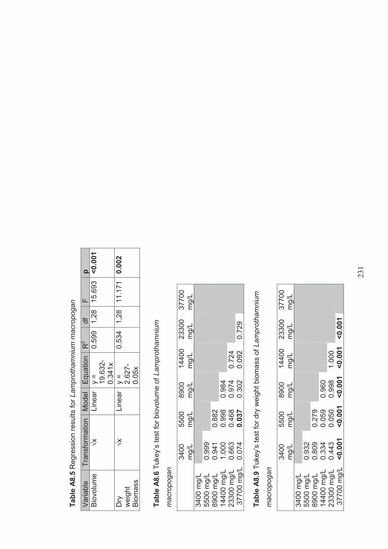
23
1
Tabl
e A8
.5 R
egre
ssio
n re
sults
for L
ampr
otha
mni
um m
acro
poga
n
Var
iabl
e Tr
ansf
orm
atio
n M
odel
Eq
uatio
n R
2 df
F
p B
iovo
lum
e √x
Li
near
y
= 19
.632
- 0.
341x
0.59
9 1,
28
15.6
93
<0.0
01
Dry
w
eigh
t Bi
omas
s
√x
Line
ar
y =
2.62
7-0.
05x
0.53
4 1,
28
11.1
71
0.00
2
Tabl
e A8
.6 T
ukey
’s te
st fo
r bio
volu
me
of L
ampr
otha
mni
um
mac
ropo
gan
34
00
mg/
L 55
00
mg/
L 89
00
mg/
L 14
400
mg/
L 23
300
mg/
L 37
700
mg/
L 34
00 m
g/L
5500
mg/
L 0.
999
89
00 m
g/L
0.94
1 0.
882
1440
0 m
g/L
1.00
0 0.
998
0.98
4
2330
0 m
g/L
0.66
3 0.
468
0.97
4 0.
724
377
00 m
g/L
0.07
4 0.
037
0.30
2 0.
092
0.72
9
Tabl
e A8
.9 T
ukey
’s te
st fo
r dry
wei
ght b
iom
ass
of L
ampr
otha
mni
um
mac
ropo
gan
34
00
mg/
L 55
00
mg/
L 89
00
mg/
L 14
400
mg/
L 23
300
mg/
L 37
700
mg/
L 34
00 m
g/L
5500
mg/
L 0.
932
89
00 m
g/L
0.80
9 0.
279
1440
0 m
g/L
0.33
4 0.
059
0.96
0
2330
0 m
g/L
0.44
3 0.
050
0.99
8 1.
000
377
00 m
g/L
<0.0
01
<0.0
01
<0.0
01
<0.0
01
<0.0
01
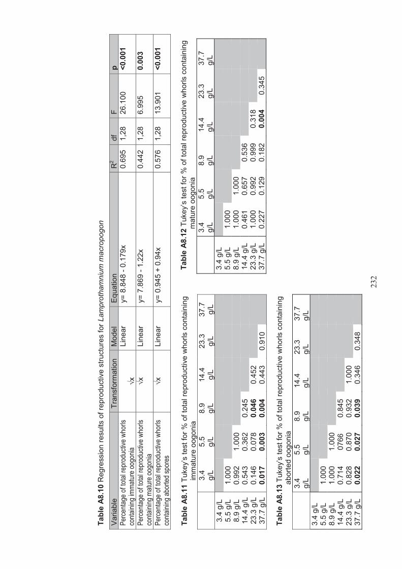
23
2
Tabl
e A8
.10
Reg
ress
ion
resu
lts o
f rep
rodu
ctiv
e st
ruct
ures
for L
ampr
otha
mni
um m
acro
pogo
n
Var
iabl
e Tr
ansf
orm
atio
n M
odel
Eq
uatio
n R
2 df
F
p Pe
rcenta
ge of
total
repr
oduc
tive w
horls
co
ntaini
ng im
matur
e oog
onia
√x
Line
ar
y= 8
.848
- 0.
179x
0.
695
1,28
26
.100
<0
.001
Perce
ntage
of to
tal re
prod
uctiv
e who
rls
conta
ining
matu
re oo
gonia
√x
Li
near
y=
7.8
69 -
1.22
x 0.
442
1,28
6.
995
0.00
3
Perce
ntage
of to
tal re
prod
uctiv
e who
rls
conta
ining
abor
ted sp
ores
√x
Li
near
y=
0.9
45 +
0.9
4x
0.57
6 1,
28
13.9
01
<0.0
01
Tabl
e A
8.11
Tuk
ey’s
test
for %
of t
otal
repr
oduc
tive
who
rls c
onta
inin
g
im
mat
ure
oogo
nia
3.
4 g/
L 5.
5 g/
L 8.
9 g/
L 14
.4
g/L
23.3
g/
L 37
.7
g/L
3.4
g/L
5.5
g/L
1.00
0
8.9
g/L
0.99
2 1.
000
14.4
g/L
0.
543
0.36
2 0.
245
23
.3 g
/L
0.14
6 0.
078
0.04
6 0.
452
37.7
g/L
0.
017
0.00
3 0.
004
0.44
3 0.
910
Ta
ble
A8.1
2 Tu
key’
s te
st fo
r % o
f tot
al re
prod
uctiv
e w
horls
con
tain
ing
m
atur
e oo
goni
a
3.
4
g/L
5.5
g/L
8.9
g/L
14.4
g/
L 23
.3
g/L
37.7
g/
L 3.
4 g/
L
5.
5 g/
L 1.
000
8.
9 g/
L 1.
000
1.00
0
14
.4 g
/L
0.46
1 0.
657
0.53
6
23.3
g/L
1.
000
0.99
2 0.
999
0.31
8
37
.7 g
/L
0.22
7 0.
129
0.18
2 0.
004
0.34
5
Ta
ble
A8.1
3 Tu
key’
s te
st fo
r % o
f tot
al re
prod
uctiv
e w
horls
con
tain
ing
a
borte
d oo
goni
a
3.4
g/
L 5.
5 g/
L 8.
9 g/
L 14
.4
g/L
23.3
g/
L 37
.7
g/L
3.4
g/L
5.5
g/L
1.00
0
8.9
g/L
1.00
0 1.
000
14.4
g/L
0.
714
0766
0.
845
23
.3 g
/L
0.82
8 0.
870
0.93
2 1.
000
37.7
g/L
0.
022
0.02
7 0.
039
0.34
6 0.
348
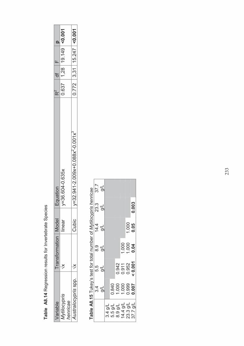
23
3
Tabl
e A
8.14
Reg
ress
ion
resu
lts fo
r Inv
erte
brat
e S
peci
es
Var
iabl
e Tr
ansf
orm
atio
n M
odel
E
quat
ion
R2
df
F p
Myt
ilocy
pris
he
nric
ae
√x
linea
r y=
36.6
04-0
.635
x 0.
637
1,28
19
.149
<0
.001
Aus
tralo
cypr
is s
pp.
√x
Cub
ic
y=32
.941
-2.0
09x+
0.08
8x2 -0
.001
x3 0.
772
3,31
15
.247
<0
.001
Ta
ble
A8.1
5 Tu
key’
s te
st fo
r tot
al n
umbe
r of M
ytilo
cypr
is h
enric
ae
3.
4 g/
L 5.
5 g/
L 8.
9 g/
L 14
.4
g/L
23.3
g/
L 37
.7
g/L
3.4
g/L
5.5
g/L
0.84
0
8.9
g/L
1.00
0 0.
942
14.4
g/L
1.
000
0.91
1 1.
000
23
.3 g
/L
0.99
9 0.
952
1.00
0 1.
000
37.7
g/L
0.
007
< 0.
001
0.04
0.
05
0.00
3

234
Appendix 9 Random location of replicates experiment investigating the effect of high salinity disturbances on the propagule bank of Lake Cullen
3 2 9 1
4 6
3
3 8 2 1 9
4 6 1 8 4
4 6 1
1
8
4 2
3 2
1 1 6
7 3
4 3 5
1
7
1
5
3
3 3
5
7
1
5 2
6 4
3 5
7
7
4
8 3 3
4
5 5
6 6
5
4
8
2 8
4 5 7
9 1 2
7
1
9
8
3 1
7 3
2
3 4
1
2
1 1
2
2 6
5
3
2 6
5
4
4
3 6
2
3
1
2
4 6
4 5
3
2 3
4
5
7
7
8 5
1
6
4
2 6
1 7
7
5 5
6
6
6
6
7 5
7
5 4
7
1
2
5
8
8
6
6
6
7
9
2
2
2 Key Door
Water Max/Min thermometer
Air max/min thermometer
Control/Blank Treatment
(3400 mg/L)
Replicates used in 1st seed bank experiment
Disturbance Phase Salinity level
37 700 mg/L Treatment
61 000 mg/L Treatment
98 700 mg/L Treatment
159 700 mg/L Treatment
Recovery Phase
Salinity 1 3 400 mg/L 2 5 500 mg/L
3 8 900 mg/L 4 14 400 mg/L
5 23 300 mg/L 6 37 700 mg/L
7 61 000 mg/L 8 98 700 mg/L
9 159 700 mg/L
5
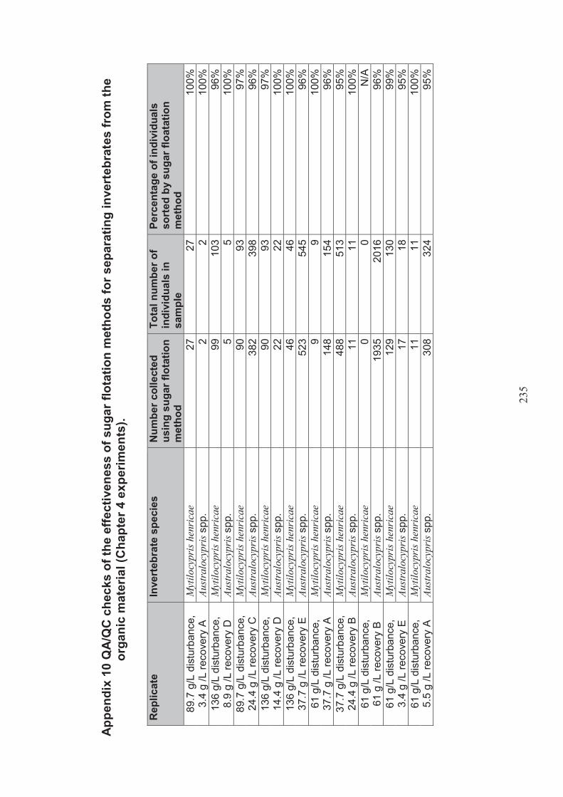
23
5
App
endi
x 10
QA
/QC
che
cks
of th
e ef
fect
iven
ess
of s
ugar
flot
atio
n m
etho
ds fo
r sep
arat
ing
inve
rteb
rate
s fr
om th
e or
gani
c m
ater
ial (
Cha
pter
4 e
xper
imen
ts).
Rep
licat
e
Inve
rteb
rate
spe
cies
N
umbe
r col
lect
ed
usin
g su
gar f
lota
tion
met
hod
Tota
l num
ber o
f in
divi
dual
s in
sa
mpl
e
Perc
enta
ge o
f ind
ivid
uals
so
rted
by
suga
r flo
atat
ion
met
hod
89.7
g/L
dis
turb
ance
, 3.
4 g
/L re
cove
ry A
M
ytilo
cypr
is h
enri
cae
27
27
10
0%
Aust
ralo
cypr
is s
pp.
2 2
100%
13
6 g/
L di
stur
banc
e,
8.9
g /L
reco
very
D
Myt
ilocy
pris
hen
rica
e 99
10
3 96
%
Aust
ralo
cypr
is s
pp.
5 5
100%
89
.7 g
/L d
istu
rban
ce,
24.4
g /L
reco
very
C
Myt
ilocy
pris
hen
rica
e 90
93
97
%
Aust
ralo
cypr
is s
pp.
382
398
96%
13
6 g/
L di
stur
banc
e,
14.4
g /L
reco
very
D
Myt
ilocy
pris
hen
rica
e 90
93
97
%
Aust
ralo
cypr
is s
pp.
22
22
100%
13
6 g/
L di
stur
banc
e,
37.7
g /L
reco
very
E
Myt
ilocy
pris
hen
rica
e
46
46
100%
Au
stra
locy
pris
spp
. 52
3 54
5 96
%
61 g
/L d
istu
rban
ce,
37.7
g /L
reco
very
A
Myt
ilocy
pris
hen
rica
e 9
9 10
0%
Aust
ralo
cypr
is s
pp.
148
154
96%
37
.7 g
/L d
istu
rban
ce,
24.4
g /L
reco
very
B
Myt
ilocy
pris
hen
rica
e 48
8 51
3 95
%
Aust
ralo
cypr
is s
pp.
11
11
100%
61
g/L
dis
turb
ance
, 61
g /L
reco
very
B
Myt
ilocy
pris
hen
rica
e 0
0 N
/A
Aust
ralo
cypr
is s
pp.
1935
20
16
96%
61
g/L
dis
turb
ance
, 3.
4 g
/L re
cove
ry E
M
ytilo
cypr
is h
enri
cae
129
130
99%
Au
stra
locy
pris
spp
. 17
18
95
%
61 g
/L d
istu
rban
ce,
5.5
g /L
reco
very
A
Myt
ilocy
pris
hen
rica
e 11
11
10
0%
Aust
ralo
cypr
is s
pp.
308
324
95%
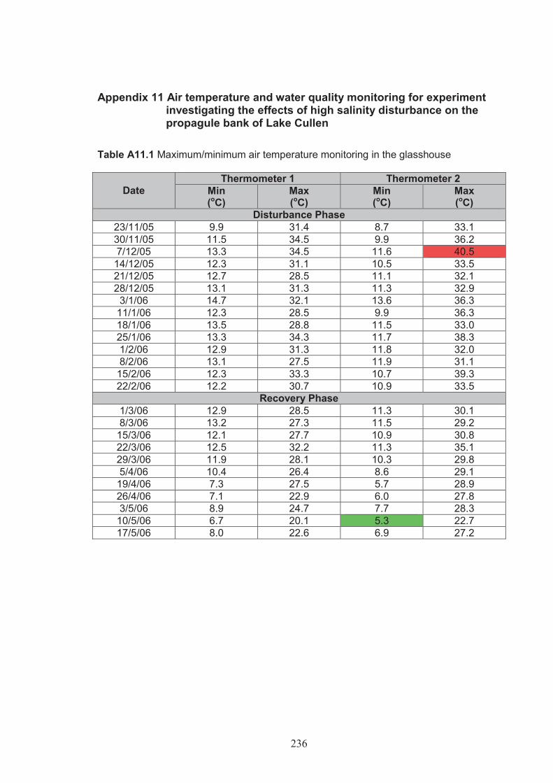
236
Appendix 11 Air temperature and water quality monitoring for experiment investigating the effects of high salinity disturbance on the propagule bank of Lake Cullen
Table A11.1 Maximum/minimum air temperature monitoring in the glasshouse
Date Thermometer 1 Thermometer 2
Min (oC)
Max (oC)
Min (oC)
Max (oC)
Disturbance Phase 23/11/05 9.9 31.4 8.7 33.1 30/11/05 11.5 34.5 9.9 36.2 7/12/05 13.3 34.5 11.6 40.5 14/12/05 12.3 31.1 10.5 33.5 21/12/05 12.7 28.5 11.1 32.1 28/12/05 13.1 31.3 11.3 32.9 3/1/06 14.7 32.1 13.6 36.3
11/1/06 12.3 28.5 9.9 36.3 18/1/06 13.5 28.8 11.5 33.0 25/1/06 13.3 34.3 11.7 38.3 1/2/06 12.9 31.3 11.8 32.0 8/2/06 13.1 27.5 11.9 31.1
15/2/06 12.3 33.3 10.7 39.3 22/2/06 12.2 30.7 10.9 33.5
Recovery Phase 1/3/06 12.9 28.5 11.3 30.1 8/3/06 13.2 27.3 11.5 29.2
15/3/06 12.1 27.7 10.9 30.8 22/3/06 12.5 32.2 11.3 35.1 29/3/06 11.9 28.1 10.3 29.8 5/4/06 10.4 26.4 8.6 29.1
19/4/06 7.3 27.5 5.7 28.9 26/4/06 7.1 22.9 6.0 27.8 3/5/06 8.9 24.7 7.7 28.3
10/5/06 6.7 20.1 5.3 22.7 17/5/06 8.0 22.6 6.9 27.2

237
Table A11.2 Maximum/minimum water temperature monitoring in the glasshouse
Date Thermometer 1 Thermometer 2 Thermometer 3 Thermometer 4
Min (oC)
Max (oC)
Min (oC)
Max (oC)
Min (oC)
Max (oC)
Min (oC)
Max (oC)
Disturbance Phase 23/11/05 13 26 15 23 13 26 15 23 30/11/05 15 28 17 26 15 23 14 29 7/12/05 11 29 18 29 16 22 15 32
14/12/05 15 27 17 24 16 21 16 25 21/12/05 16 26 18 21 16 22 14 26 28/12/05 15 27 18 25 16 25 15 26 3/1/06 16 30 18 28 18 26 17 29 11/1/06 15 27 18 26 15 23 15 28 18/1/06 16 26 18 24 18 25 16 25 25/1/06 15 32 19 29 17 26 16 31 1/2/06 17 30 17 23 18 29 17 30 8/2/06 18 27 20 25 19 26 16 27 15/2/06 16 29 17 20 18 23 15 24 22/2/06 17 27 16 25 16 24 17 28
Recovery Phase 1/3/06 25 26 25 27 20 24 21 27 8/3/06 18 27 18 25 16 23 16 31 15/3/06 12 25 11 23 11 24 12 23 22/3/06 14 24 13 23 15 24 13 23 29/3/06 10 23 10 22 10 21 9 23 5/4/06 13 24 13 24 12 20 11 27 19/4/06 10 24 8 24 11 24 9 28 26/4/06 10 23 11 23 10 20 8 25 3/5/06 11 24 14 21 12 22 11 22 10/5/06 8 19 10 15 9 16 8 20 17/5/06 11 22 10 21 9 22 7 25

23
8
Tabl
e A1
1.3
Sal
inity
mon
itorin
g of
repl
icat
es fo
r the
exp
erim
ent i
nves
tigat
ing
the
effe
ct o
f hig
h sa
linity
dis
turb
ance
s on
the
prop
agul
e ba
nk o
f Lak
e C
ulle
n, s
elec
ted
treat
men
ts (a
ll m
easu
rem
ents
are
in g
/L)
Trea
tmen
t 37
.7g/
L D
istu
rban
ce/ 3
.4 g
/L
reco
very
37
.7g/
L D
istu
rban
ce/ 5
.5 g
/L
reco
very
37
.7g/
L D
istu
rban
ce/ 8
.9 g
/L
reco
very
W
eek
A B
C
D
E A
B C
D
E
A B
C
D
E D
istu
rban
ce P
hase
1
37.7
37
.7
37.7
37
.7
37.7
37
.7
37.7
37
.7
37.7
37
.7
37.7
37
.7
37.7
37
.7
37.7
3
37.6
40
.1
38.9
39
.2
38.9
37
.9
38.4
38
.6
39.0
38
.8
38.2
38
.4
38.4
38
.4
38.4
5
40.1
38
.8
40.5
40
.7
40.2
40
.5
40.5
41
.0
40.1
40
.9
39.8
41
.0
41.3
40
.5
41.3
7
38.1
39
.2
38.8
39
.3
38.8
39
.6
39.3
38
.9
39.3
39
.4
39.0
38
.7
39.8
39
.7
39.2
9
37.4
38
.9
40.7
38
.5
37.1
39
.6
37.6
38
.4
38.4
38
.6
38.5
38
.0
38.3
38
.2
38.1
11
37
.1
38.8
38
.3
38.1
37
.8
38.4
38
.3
38.3
37
.7
38.2
37
.2
37.9
38
.1
38.8
37
.9
13
37.7
38
.1
38.3
38
.7
38.3
37
.9
37.8
39
.5
37.8
37
.8
38.1
38
.5
37.9
38
.1
39.2
R
ecov
ery
Phas
e 15
3.
8 3.
8 3.
9 3.
6 3.
9 5.
5 5.
6 5.
7 6.
3 6.
0 8.
7 9.
2 8.
7 8.
9 8.
6 17
4.
5 4.
1 4.
1 4.
1 4.
2 5.
7 5.
8 6.
1 5.
9 6.
1 9.
3 9.
3 9.
3 9.
3 8.
8 19
4.
1 3.
9 3.
9 4.
0 3.
7 5.
7 5.
7 5.
9 5.
9 5.
7 9.
0 9.
2 8.
8 9.
0 8.
9 21
3.
9 3.
8 4.
0 4.
0 3.
8 5.
6 5.
7 5.
8 5.
8 5.
8 8.
6 9.
2 8.
4 9.
1 8.
9 23
4.
3 3.
9 4.
2 4.
1 4.
2 5.
7 5.
8 6.
2 5.
9 6.
2 8.
6 9.
4 9.
1 9.
4 9.
1 25
3.
8 3.
8 3.
9 3.
6 3.
9 5.
5 5.
6 5.
7 6.
3 6.
0 8.
7 9.
2 8.
7 8.
9 8.
6 Me
an di
sturb
ance
phas
e 38
.0
38.8
39
.0
38.9
38
.4
38.8
38
.5
38.9
38
.6
38.8
38
.4
38.6
38
.8
38.8
38
.8
Mean
reco
very
phas
e 4.
1 3.
9 4.
0 3.
9 4.
0 5.
6 5.
7 5.
9 6.
0 6.
0 8.
8 9.
3 8.
8 9.
1 8.
8 St
anda
rd de
viatio
n dist
urba
nce p
hase
±
1.0
± 0.
8 ±
1.1
± 1.
0 ±
1.0
± 1.
1 ±
1.1
±1.1
±
0.9
± 1.
1 ±
0.9
±1.1
±
1.3
± 1.
0 ±
1.2
Stan
dard
devia
tion d
istur
banc
e pha
se
± 0.
3 ±
0.1
± 0.
1 ±
0.2
± 0.
2 ±
0.1
± 0.
1 ±0
.2
± 0.
2 ±
0.2
± 0.
3 ±0
.1
± 0.
3 ±
0.2
± 0.
2
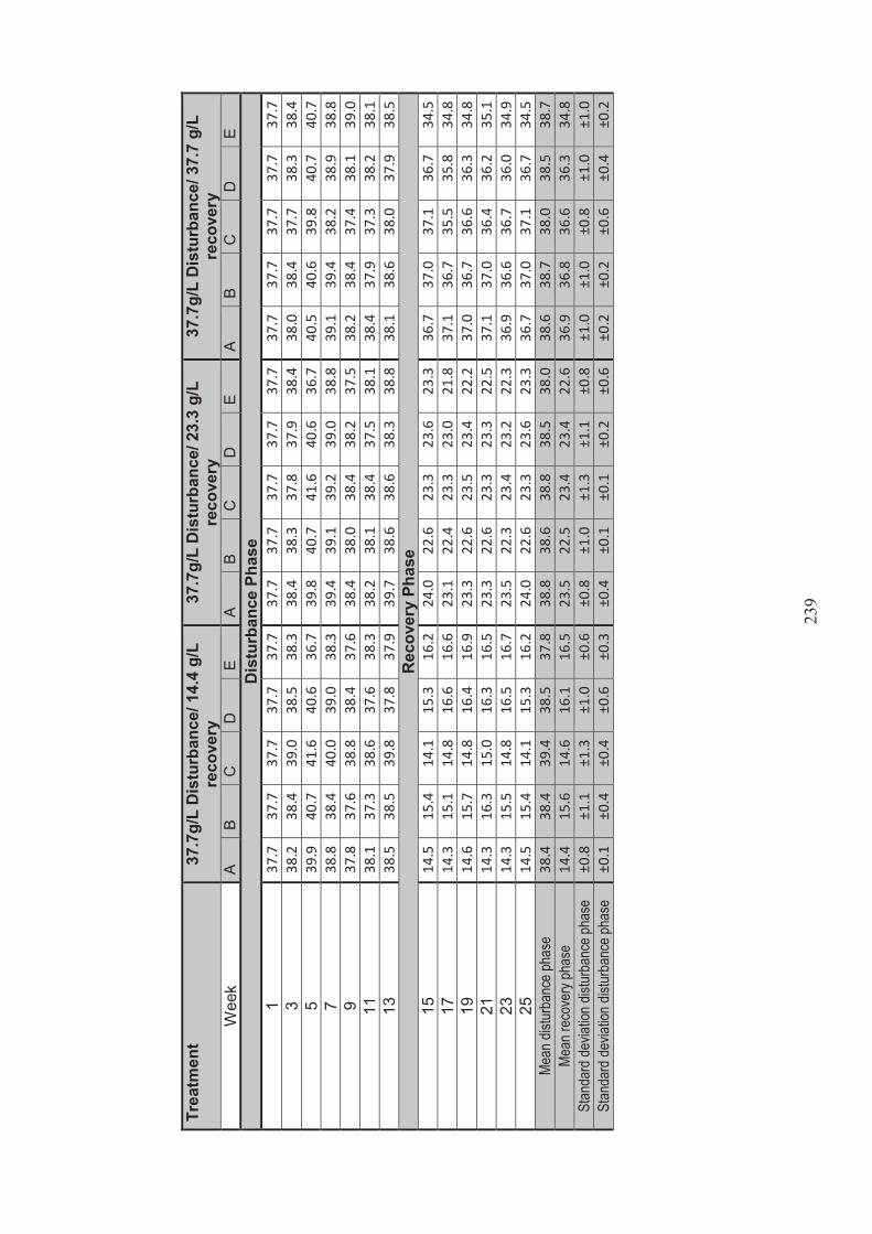
23
9
Trea
tmen
t 37
.7g/
L D
istu
rban
ce/ 1
4.4
g/L
re
cove
ry
37.7
g/L
Dis
turb
ance
/ 23.
3 g/
L re
cove
ry
37.7
g/L
Dis
turb
ance
/ 37.
7 g/
L re
cove
ry
Wee
k A
B C
D
E
A B
C
D
E A
B C
D
E
Dis
turb
ance
Pha
se
1 37
.7
37.7
37
.7
37.7
37
.7
37.7
37
.7
37.7
37
.7
37.7
37
.7
37.7
37
.7
37.7
37
.7
3 38
.2
38.4
39
.0
38.5
38
.3
38.4
38
.3
37.8
37
.9
38.4
38
.0
38.4
37
.7
38.3
38
.4
5 39
.9
40.7
41
.6
40.6
36
.7
39.8
40
.7
41.6
40
.6
36.7
40
.5
40.6
39
.8
40.7
40
.7
7 38
.8
38.4
40
.0
39.0
38
.3
39.4
39
.1
39.2
39
.0
38.8
39
.1
39.4
38
.2
38.9
38
.8
9 37
.8
37.6
38
.8
38.4
37
.6
38.4
38
.0
38.4
38
.2
37.5
38
.2
38.4
37
.4
38.1
39
.0
11
38.1
37
.3
38.6
37
.6
38.3
38
.2
38.1
38
.4
37.5
38
.1
38.4
37
.9
37.3
38
.2
38.1
13
38
.5
38.5
39
.8
37.8
37
.9
39.7
38
.6
38.6
38
.3
38.8
38
.1
38.6
38
.0
37.9
38
.5
Rec
over
y Ph
ase
15
14.5
15
.4
14.1
15
.3
16.2
24
.0
22.6
23
.3
23.6
23
.3
36.7
37
.0
37.1
36
.7
34.5
17
14
.3
15.1
14
.8
16.6
16
.6
23.1
22
.4
23.3
23
.0
21.8
37
.1
36.7
35
.5
35.8
34
.8
19
14.6
15
.7
14.8
16
.4
16.9
23
.3
22.6
23
.5
23.4
22
.2
37.0
36
.7
36.6
36
.3
34.8
21
14
.3
16.3
15
.0
16.3
16
.5
23.3
22
.6
23.3
23
.3
22.5
37
.1
37.0
36
.4
36.2
35
.1
23
14.3
15
.5
14.8
16
.5
16.7
23
.5
22.3
23
.4
23.2
22
.3
36.9
36
.6
36.7
36
.0
34.9
25
14
.5
15.4
14
.1
15.3
16
.2
24.0
22
.6
23.3
23
.6
23.3
36
.7
37.0
37
.1
36.7
34
.5
Mean
distu
rban
ce ph
ase
38.4
38
.4
39.4
38
.5
37.8
38
.8
38.6
38
.8
38.5
38
.0
38.6
38
.7
38.0
38
.5
38.7
Me
an re
cove
ry ph
ase
14.4
15
.6
14.6
16
.1
16.5
23
.5
22.5
23
.4
23.4
22
.6
36.9
36
.8
36.6
36
.3
34.8
St
anda
rd de
viatio
n dist
urba
nce p
hase
±0
.8
±1.1
±1
.3
±1.0
±0
.6
±0.8
±1
.0
±1.3
±1
.1
±0.8
±1
.0
±1.0
±0
.8
±1.0
±1
.0
Stan
dard
devia
tion d
istur
banc
e pha
se
±0.1
±0
.4
±0.4
±0
.6
±0.3
±0
.4
±0.1
±0
.1
±0.2
±0
.6
±0.2
±0
.2
±0.6
±0
.4
±0.2

24
0
Trea
tmen
t 61
g/L
Dis
turb
ance
/ 3.4
g/L
re
cove
ry
61 g
/L D
istu
rban
ce/ 5
.5 g
/L
reco
very
61
g/L
Dis
turb
ance
/ 8.9
g/L
re
cove
ry
Wee
k A
B C
D
E
A B
C
D
E A
B C
D
E
Dis
turb
ance
Pha
se
1 61
.0
61.0
61
.0
61.0
61
.0
61.0
61
.0
61.0
61
.0
61.0
61
.0
61.0
61
.0
61.0
61
.0
3 62
.8
61.8
62
.4
62.3
62
.5
61.8
61
.5
61.5
62
.5
61.3
62
.8
62.6
61
.9
63.2
61
.6
5 66
.7
63.9
64
.0
65.3
65
.8
64.6
64
.6
60.9
66
.8
64.2
66
.8
65.1
66
.4
66.7
64
.0
7 62
.6
63.4
61
.6
63.2
61
.6
63.6
61
.7
61.3
63
.3
63.1
61
.8
60.7
59
.7
63.1
60
.6
9 61
.9
63.0
60
.8
61.8
59
.4
61.6
61
.1
61.2
61
.5
60.6
60
.8
60.2
62
.5
61.5
60
.5
11
62.7
60
.6
60.7
61
.7
61.3
60
.5
60.5
58
.1
61.5
59
.8
61.7
60
.6
60.9
61
.9
59.6
13
62
.2
60.3
60
.9
60.4
60
.7
61.3
61
.3
58.1
64
.5
60.9
63
.7
63.0
62
.9
62.3
61
.2
Rec
over
y Ph
ase
15
3.9
4.3
5.8
3.7
3.8
5.9
5.6
5.7
5.6
5.8
9.6
8.8
9.0
8.4
8.8
17
4.4
3.9
4.3
4.3
4.1
5.8
5.7
5.9
6.1
6.0
10.0
9.
3 9.
7 9.
3 9.
3 19
4.
2 4.
0 4.
0 4.
2 4.
3 5.
7 5.
6 5.
8 5.
7 5.
9 9.
4 9.
0 9.
6 9.
2 9.
0 21
3.
8 3.
9 4.
0 4.
0 4.
1 5.
9 5.
7 5.
9 5.
7 5.
8 9.
2 8.
9 9.
1 8.
9 8.
9 23
4.
4 4.
0 4.
4 4.
5 4.
4 6.
3 6.
2 6.
2 6.
0 6.
2 10
.1
9.4
9.7
9.4
9.3
25
3.9
4.3
5.8
3.7
3.8
5.9
5.6
5.7
5.6
5.8
9.6
8.8
9.0
8.4
8.8
Mean
distu
rban
ce ph
ase
62.8
62
.0
61.6
62
.2
61.8
62
.1
61.7
60
.3
63.0
61
.6
62.7
61
.9
62.2
62
.8
61.2
Me
an re
cove
ry ph
ase
4.1
4.1
4.7
4.1
4.1
5.9
5.7
5.9
5.8
5.9
9.7
9.0
9.4
8.9
9.0
Stan
dard
devia
tion d
istur
banc
e pha
se
±1.8
±1
.4
±1.2
±1
.6
±2.0
±1
.5
±1.3
±1
.5
±2.1
±1
.5
±2.1
±1
.8
±2.1
±1
.9
±1.4
St
anda
rd de
viatio
n dist
urba
nce p
hase
±0
.3
±0.2
±0
.9
±0.3
±0
.2
±0.2
±0
.2
±0.2
±0
.2
±0.2
±0
.3
±0.3
±0
.4
±0.4
±0
.2

24
1
Trea
tmen
t 61
g/L
Dis
turb
ance
/ 14.
4 g/
L
reco
very
61
g/L
Dis
turb
ance
/ 23.
3 g/
L
reco
very
61
g/L
Dis
turb
ance
/ 37.
7 g/
L
Rec
over
y W
eek
A B
C
D
E A
B C
D
E
A B
C
D
E D
istu
rban
ce P
hase
1
61.0
61
.0
61.0
61
.0
61.0
61
.0
61.0
61
.0
61.0
61
.0
61.0
61
.0
61.0
61
.0
61.0
3
62.8
61
.8
62.4
62
.3
62.5
61
.8
61.5
61
.5
62.5
61
.3
62.8
62
.6
61.9
63
.2
61.6
5
66.7
63
.9
64.0
65
.3
65.8
64
.6
64.6
60
.9
66.8
64
.2
66.8
65
.1
66.4
66
.7
64.0
7
62.6
63
.4
61.6
63
.2
61.6
63
.6
61.7
61
.3
63.3
63
.1
61.8
60
.7
59.7
63
.1
60.6
9
61.9
63
.0
60.8
61
.8
59.4
61
.6
61.1
61
.2
61.5
60
.6
60.8
60
.2
62.5
61
.5
60.5
11
62
.7
60.6
60
.7
61.7
61
.3
60.5
60
.5
58.1
61
.5
59.8
61
.7
60.6
60
.9
61.9
59
.6
13
62.2
60
.3
60.9
6.
4 60
.7
61.3
61
.3
58.1
64
.5
60.9
63
.7
63.0
62
.9
62.3
61
.2
Rec
over
y Ph
ase
15
14.6
14
.5
15.0
14
.3
15.1
22
.6
23.7
23
.5
2.5
23.4
37
.1
36.3
36
.0
37.1
37
.7
17
15.2
15
.0
15.2
14
.8
15.2
22
.0
24.5
24
.4
22.6
20
.4
37.9
35
.8
35.6
37
.9
38.5
19
15
.2
14.9
15
.3
15.0
15
.3
22.6
23
.3
24.5
23
.0
20.5
36
.4
35.8
35
.8
38.4
37
.9
21
15.4
15
.1
15.2
14
.7
15.3
23
.0
23.9
24
.4
23.2
21
.3
36.8
35
.8
35.6
38
.1
38.0
23
15
.3
15.0
15
.4
15.0
15
.4
22.4
24
.6
24.5
23
.3
20.4
38
.1
36.2
35
.8
37.9
38
.6
25
14.6
14
.5
15.0
14
.3
15.1
22
.6
23.7
23
.5
2.5
23.4
37
.1
36.3
36
.0
37.1
37
.7
Mean
distu
rban
ce ph
ase
62.8
62
.0
61.6
54
.5
61.8
62
.1
61.7
60
.3
63.0
61
.6
62.7
61
.9
62.2
62
.8
61.2
Me
an re
cove
ry ph
ase
15.1
14
.8
15.2
14
.7
15.2
22
.5
24.0
24
.1
16.2
21
.6
37.2
36
.0
35.8
37
.8
38.1
St
anda
rd de
viatio
n dist
urba
nce p
hase
±1
.8
±1.4
±1
.2
±21.
3 ±2
.0
±1.5
±1
.3
±1.5
±2
.1
±1.5
±2
.1
±1.8
±2
.1
±1.9
±1
.4
Stan
dard
devia
tion r
ecov
ery p
hase
±0
.4
±0.3
±0
.2
±0.3
±0
.1
±0.3
±0
.5
±0.5
±1
0.6
±1.5
±0
.7
±0.3
±0
.2
±0.5
±0
.4

24
2
Trea
tmen
t 61
g/L
Dis
turb
ance
/ 61
g/L
re
cove
ry
89.7
g/L
Dis
turb
ance
/ 3.4
g/L
re
cove
ry
89.7
g/L
Dis
turb
ance
/ 5.5
g/L
re
cove
ry
Wee
k A
B C
D
E
A B
C
D
E A
B C
D
E
Dis
turb
ance
Pha
se
1 61
.0
61.0
61
.0
61.0
61
.0
61.0
61
.0
61.0
61
.0
61.0
61
.0
61.0
61
.0
61.0
61
.0
3 62
.8
61.9
61
.5
62.8
63
.0
60.6
61
.5
62.6
61
.9
61.9
61
.9
61.5
62
.2
61.9
61
.3
5 65
.1
64.9
65
.8
65.3
64
.3
63.4
66
.4
66.1
64
.9
63.2
65
.8
63.0
65
.5
64.9
65
.2
7 63
.6
62.5
62
.6
64.2
61
.1
62.9
62
.8
61.1
62
.4
61.7
61
.3
62.4
62
.2
62.6
61
.1
9 61
.4
60.7
61
.2
62.5
59
.6
62.4
61
.5
60.3
60
.4
60.5
60
.3
61.2
61
.0
60.8
60
.1
11
61.3
60
.5
61.1
60
.4
59.7
60
.5
61.2
60
.9
61.1
58
.8
61.6
59
.2
61.2
61
.0
61.7
13
62
.5
62.3
63
.6
60.1
66
.5
61.3
62
.6
61.3
61
.3
60.2
60
.2
59.6
61
.5
60.6
62
.0
Rec
over
y Ph
ase
15
61.5
61
.7
60.9
60
.2
60.5
3.
3 3.
3 3.
5 3.
7 3.
8 6.
0 5.
7 5.
4 5.
6 5.
6 17
60
.3
60.0
59
.3
59.0
58
.5
4.4
4.3
4.3
4.4
4.1
6.7
5.9
5.8
6.0
6.0
19
59.4
60
.9
59.4
59
.6
59.0
4.
0 3.
9 4.
1 4.
4 4.
1 6.
1 5.
8 5.
5 5.
9 5.
8 21
60
.8
59.6
59
.6
59.9
58
.4
3.9
3.9
4.0
4.1
4.1
5.9
5.6
5.8
5.6
5.7
23
60.9
61
.6
59.9
60
.5
59.7
4.
6 4.
2 4.
3 4.
5 4.
6 6.
3 6.
0 6.
3 6.
1 6.
4 25
61
.5
61.7
60
.9
60.2
60
.5
3.3
3.3
3.5
3.7
3.8
6.0
5.7
5.4
5.6
5.6
Mean
distu
rban
ce ph
ase
62.5
62
.0
62.4
62
.3
62.2
61
.7
62.4
61
.9
61.9
61
.0
61.7
61
.1
62.1
61
.8
61.8
Me
an re
cove
ry ph
ase
60.7
60
.9
60.0
59
.9
59.4
3.
9 3.
8 4.
0 4.
1 4.
1 6.
2 5.
8 5.
7 5.
8 5.
9 St
anda
rd de
viatio
n dist
urba
nce p
hase
±1
.5
±1.5
±1
.8
±2.0
±2
.6
±1.2
±1
.9
±2.0
±1
.5
±1.4
±1
.9
±1.4
±1
.6
±1.5
±1
.6
Stan
dard
devia
tion r
ecov
ery p
hase
±0
.8
±0.9
±0
.7
±0.5
±0
.9
±0.5
±0
.4
±0.4
±0
.4
±0.3
±0
.3
±0.1
±0
.3
±0.2
±0
.3

24
3
Trea
tmen
t 89
.7 g
/L D
istu
rban
ce/ 8
.9 g
/L
reco
very
89
.7 g
/L D
istu
rban
ce/ 1
4.4
g/L
re
cove
ry
89.7
g/L
Dis
turb
ance
/ 23.
3 g/
L
Rec
over
y W
eek
A B
C
D
E A
B C
D
E
A B
C
D
E D
istu
rban
ce P
hase
1
61.0
61
.0
61.0
61
.0
61.0
98
.7
98.7
98
.7
98.7
98
.7
98.7
98
.7
98.7
98
.7
98.7
3
62.2
62
.3
61.4
61
.9
61.8
10
0.7
101.
0 10
0.9
101.
7 10
2.8
100.
6 10
1.4
99.6
10
1.8
100.
7 5
65.8
66
.6
63.9
66
.1
64.5
10
7.7
105.
7 10
4.7
102.
4 10
7.5
106.
2 10
3.2
105.
5 10
5.8
103.
6 7
63.4
60
.5
62.1
61
.7
60.9
99
.3
99.9
10
0.6
101.
0 10
3.8
99.5
10
1.0
101.
0 10
1.7
99.3
9
61.5
59
.7
61.3
60
.5
60.9
98
.2
97.9
98
.5
97.6
99
.1
99.3
98
.9
97.9
98
.9
97.7
11
61
.3
61.0
60
.9
61.1
60
.6
99.3
98
.9
97.9
97
.9
100.
6 98
.5
97.9
97
.8
99.8
98
.0
13
62.0
62
.8
61.2
61
.1
61.2
10
0.1
100.
2 10
0.9
97.9
10
0.4
100.
4 98
.8
99.5
10
1.9
99.3
R
ecov
ery
Phas
e 15
9.
2 8.
7 9.
1 9.
5 9.
4 16
.2
16.0
14
.9
15.1
15
.0
23.0
22
.8
22.8
23
.5
22.7
17
9.
7 9.
5 9.
6 9.
5 10
.1
16.7
16
.3
14.9
15
.2
15.9
23
.7
23.4
22
.0
23.9
23
.6
19
9.1
9.0
9.2
9.0
9.5
16.4
16
.4
15.0
14
.9
15.8
23
.9
23.1
22
.2
23.9
23
.8
21
8.7
9.0
8.9
9.1
9.1
16.5
16
.6
14.8
15
.0
15.8
23
.7
23.1
22
.0
23.9
23
.7
23
10.2
9.
5 9.
9 10
.2
10.4
16
.5
16.5
15
.0
15.3
16
.0
23.8
23
.3
20.8
23
.9
23.5
25
9.
2 8.
7 9.
1 9.
5 9.
4 16
.2
16.0
14
.9
15.1
15
.0
23.0
22
.8
22.8
23
.5
22.7
Me
an di
sturb
ance
phas
e 62
.5
62.0
61
.7
61.9
61
.6
100.
6 10
0.3
100.
3 99
.6
101.
8 10
0.5
100.
0 10
0.0
101.
2 99
.6
Mean
reco
very
phas
e 9.
4 9.
1 9.
3 9.
5 9.
7 16
.4
16.3
14
.9
15.1
15
.6
23.5
23
.1
22.1
23
.8
23.3
St
anda
rd de
viatio
n dist
urba
nce p
hase
±1
.7
±2.3
±1
.1
±1.9
±1
.4
±3.3
±2
.6
±2.3
±2
.0
±3.1
±2
.7
±1.9
±2
.7
±2.4
±2
.0
Stan
dard
devia
tion r
ecov
ery p
hase
±0
.5
±0.4
±0
.4
±0.4
±0
.5
±0.2
±0
.3
±0.1
±0
.1
±0.5
±0
.4
±0.2
±0
.7
±0.2
±0
.5

24
4
Trea
tmen
t 89
.7 g
/L D
istu
rban
ce/ 3
7.7
g/L
re
cove
ry
89.7
g/L
Dis
turb
ance
/ 61
g/L
re
cove
ry
89.7
g/L
Dis
turb
ance
/ 89.
7 g/
L
reco
very
W
eek
A B
C
D
E A
B C
D
E
A B
C
D
E D
istu
rban
ce P
hase
1
98.7
98
.7
98.7
98
.7
98.7
98
.7
98.7
98
.7
98.7
98
.7
98.7
98
.7
98.7
98
.7
98.7
3
104.
1 10
0.6
102.
4 10
0.8
101.
4 99
.7
99.8
10
0.6
103.
6 10
1.0
99.6
10
1.6
100.
8 10
0.7
100.
0 5
104.
7 10
5.9
103.
6 10
5.0
102.
7 10
7.0
104.
7 10
7.1
106.
8 10
3.6
105.
5 10
6.8
104.
4 10
5.8
101.
9 7
101.
6 10
0.3
100.
0 10
0.2
100.
8 99
.6
99.0
10
1.6
97.7
99
.4
100.
0 10
2.5
100.
8 10
1.0
97.8
9
99.6
97
.9
98.3
10
0.5
97.9
98
.5
98.7
98
.8
99.6
97
.6
98.1
98
.9
97.8
96
.4
98.9
11
97
.4
97.8
97
.4
100.
6 97
.4
98.2
98
.5
99.3
98
.9
98.4
99
.5
99.1
97
.2
99.5
97
.4
13
97.8
10
0.4
97.5
97
.1
99.0
98
.0
101.
3 98
.6
100.
0 97
.5
99.1
98
.0
100.
2 99
.1
97.5
R
ecov
ery
Phas
e 15
36
.9
37.5
38
.6
36.2
36
.7
59.9
61
.8
60.9
61
.5
60.6
99
.3
97.6
99
.1
98.6
98
.7
17
37.0
37
.7
36.7
35
.4
37.0
61
.0
59.2
59
.9
59.2
60
.8
97.0
97
.0
95.7
94
.2
97.3
19
37
.3
38.2
36
.5
35.7
37
.5
61.7
59
.8
60.1
59
.4
60.7
97
.5
96.8
96
.2
94.9
97
.9
21
37.2
37
.7
36.9
35
.5
37.5
60
.9
60.2
60
.1
59.9
60
.9
97.4
97
.2
96.2
95
.2
98.1
23
37
.5
37.7
36
.8
36.0
37
.5
61.7
59
.8
60.0
59
.7
61.1
97
.7
97.6
96
.6
95.7
98
.3
25
36.9
37
.5
38.6
36
.2
36.7
59
.9
61.8
60
.9
61.5
60
.6
99.3
97
.6
99.1
98
.6
98.7
Me
an di
sturb
ance
phas
e 10
0.6
100.
2 99
.7
100.
4 99
.7
100.
0 10
0.1
100.
7 10
0.8
99.5
10
0.1
100.
8 10
0.0
100.
2 98
.9
Mean
reco
very
phas
e 37
.1
37.7
37
.4
35.8
37
.2
60.9
60
.4
60.3
60
.2
60.8
98
.0
97.3
97
.2
96.2
98
.2
Stan
dard
devia
tion d
istur
banc
e pha
se
±3.0
±2
.8
±2.4
±2
.4
±2.0
±3
.2
±2.3
±3
.0
±3.3
±2
.2
±2.5
±3
.1
±2.4
±2
.9
±1.6
St
anda
rd de
viatio
n rec
over
y pha
se
±0.2
±0
.3
±1.0
±0
.4
±0.4
±0
.8
±1.1
±0
.5
±1.0
±0
.2
±1.0
±0
.4
±1.5
±1
.9
±0.5
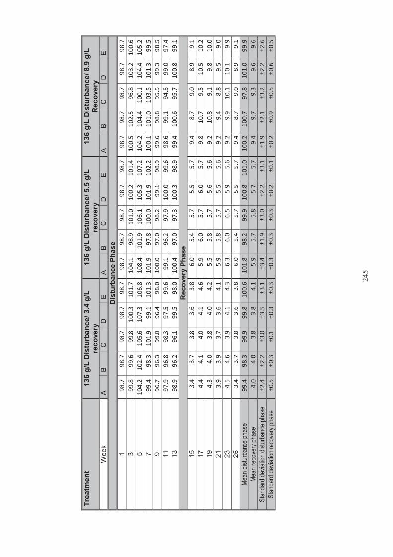
24
5
Trea
tmen
t 13
6 g/
L D
istu
rban
ce/ 3
.4 g
/L
reco
very
13
6 g/
L D
istu
rban
ce/ 5
.5 g
/L
reco
very
13
6 g/
L D
istu
rban
ce/ 8
.9 g
/L
Rec
over
y W
eek
A B
C
D
E A
B C
D
E
A B
C
D
E D
istu
rban
ce P
hase
1
98.7
98
.7
98.7
98
.7
98.7
98
.7
98.7
98
.7
98.7
98
.7
98.7
98
.7
98.7
98
.7
98.7
3
99.8
99
.6
99.8
10
0.3
101.
7 10
4.1
98.9
10
1.0
100.
2 10
1.4
100.
5 10
2.5
96.8
10
3.2
100.
6 5
104.
2 10
2.4
105.
6 10
7.3
106.
8 10
8.4
101.
9 10
6.1
105.
3 10
7.2
104.
2 10
4.4
100.
1 10
4.4
105.
2 7
99.4
98
.3
101.
9 99
.1
101.
3 10
1.9
97.8
10
0.0
101.
9 10
2.2
100.
1 10
1.0
103.
5 10
1.3
99.5
9
96.7
96
.3
99.0
96
.4
98.0
10
0.0
97.0
98
.2
99.1
98
.9
99.6
98
.8
95.5
99
.3
98.5
11
97
.9
96.8
98
.3
97.5
99
.6
99.1
96
.2
97.9
10
0.0
99.6
98
.6
99.1
94
.5
99.0
97
.4
13
98.9
96
.2
96.1
99
.5
98.0
10
0.4
97.0
97
.3
100.
3 98
.9
99.4
10
0.6
95.7
10
0.8
99.1
R
ecov
ery
Phas
e 15
3.
4 3.
7 3.
8 3.
6 3.
8 6.
0 5.
4 5.
7 5.
5 5.
7 9.
4 8.
7 9.
0 8.
9 9.
1 17
4.
4 4.
1 4.
0 4.
1 4.
6 5.
9 6.
0 5.
7 6.
0 5.
7 9.
8 10
.7
9.5
10.5
10
.2
19
4.3
4.0
3.8
4.0
4.2
5.5
5.8
5.7
5.6
5.6
9.2
10.8
9.
1 9.
8 10
.0
21
3.9
3.9
3.7
3.6
4.1
5.9
5.8
5.7
5.5
5.6
9.2
9.4
8.8
9.5
9.0
23
4.5
4.6
3.9
4.1
4.3
6.3
6.0
6.5
5.9
5.6
9.2
9.9
10.1
10
.1
9.9
25
3.4
3.7
3.8
3.6
3.8
6.0
5.4
5.7
5.5
5.7
9.4
8.7
9.0
8.9
9.1
Mean
distu
rban
ce ph
ase
99.4
98
.3
99.9
99
.8
100.
6 10
1.8
98.2
99
.9
100.
8 10
1.0
100.
2 10
0.7
97.8
10
1.0
99.9
Me
an re
cove
ry ph
ase
4.0
4.0
3.8
3.8
4.1
5.9
5.7
5.8
5.7
5.7
9.4
9.7
9.3
9.6
9.6
Stan
dard
devia
tion d
istur
banc
e pha
se
±2.4
±2
.2
±3.0
±3
.5
±3.1
±3
.4
±1.9
±3
.0
±2.2
±3
.1
±1.9
±2
.1
±3.2
±2
.2
±2.6
St
anda
rd de
viatio
n rec
over
y pha
se
±0.5
±0
.3
±0.1
±0
.3
±0.3
±0
.3
±0.3
±0
.3
±0.2
±0
.1
±0.2
±0
.9
±0.5
±0
.6
±0.5

24
6
Trea
tmen
t 13
6 g/
L D
istu
rban
ce/ 1
4.4
g/L
re
cove
ry
136
g/L
Dis
turb
ance
/ 23.
3 g/
L
reco
very
13
6 g/
L D
istu
rban
ce/ 3
7.7
g/L
R
ecov
ery
Wee
k A
B C
D
E
A B
C
D
E A
B C
D
E
Dis
turb
ance
Pha
se
1 13
6.0
136.
0 13
6.0
136.
0 13
6.0
136.
0 13
6.0
136.
0 13
6.0
136.
0 13
6.0
136.
0 13
6.0
136.
0 13
6.0
3 13
8.7
135.
3 14
0.8
139.
4 13
8.7
128.
6 13
8.0
130.
7 15
0.6
136.
0 13
8.0
138.
0 15
0.0
138.
0 13
6.0
5 14
4.2
143.
5 14
7.6
146.
2 14
6.9
128.
2 14
4.2
136.
7 14
3.5
144.
2 14
6.2
145.
5 14
6.9
144.
8 14
4.8
7 14
1.4
138.
0 13
6.7
143.
5 14
0.8
140.
8 13
6.7
141.
4 13
9.4
138.
0 12
9.4
138.
0 14
2.1
139.
4 13
5.3
9 13
5.7
133.
4 14
0.1
135.
2 13
5.9
126.
9 13
4.8
127.
2 13
6.0
133.
8 13
5.1
136.
0 13
4.6
136.
0 13
4.9
11
136.
0 13
4.6
140.
1 13
6.0
137.
4 12
7.2
137.
4 13
6.0
135.
9 13
3.1
136.
0 13
6.0
135.
4 13
7.4
135.
3 13
13
6.7
140.
1 13
7.4
138.
0 13
6.0
136.
0 14
0.1
135.
7 13
5.0
134.
2 13
8.0
140.
8 14
2.8
139.
4 13
8.0
Rec
over
y Ph
ase
15
17.3
15
.7
15.6
15
.2
15.1
22
.9
23.1
22
.4
23.7
23
.2
36.4
37
.1
37.2
37
.6
37.3
17
16
.9
16.6
16
.6
16.5
15
.8
22.2
23
.7
23.8
23
.9
24.3
37
.1
36.5
37
.4
37.6
38
.4
19
17.3
15
.5
16.7
16
.3
16.3
22
.6
23.9
23
.7
24.0
24
.2
37.1
36
.9
36.9
37
.7
38.4
21
16
.7
15.3
16
.5
16.4
16
.3
22.6
23
.8
23.8
24
.1
24.1
37
.5
37.4
38
.3
37.8
37
.0
23
17.7
16
.6
16.7
16
.4
16.4
22
.6
23.8
21
.4
23.9
23
.7
37.3
36
.7
35.6
38
.0
38.7
25
17
.3
15.7
15
.6
15.2
15
.1
22.9
23
.1
22.4
23
.7
23.2
36
.4
37.1
37
.2
37.6
37
.3
Mean
distu
rban
ce ph
ase
138.
4 13
7.3
139.
8 13
9.2
138.
8 13
2.0
138.
2 13
4.8
139.
5 13
6.5
137.
0 13
8.6
141.
1 13
8.7
137.
2 Me
an re
cove
ry ph
ase
17.2
15
.9
16.3
16
.0
15.8
22
.6
23.6
22
.9
23.9
23
.8
37.0
37
.0
37.1
37
.7
37.9
St
anda
rd de
viatio
n dist
urba
nce p
hase
±3
.3
±3.5
±3
.9
±4.2
±4
.0
±5.5
±3
.1
±4.6
±5
.7
±3.8
±5
.0
±3.5
±6
.0
±3.0
±3
.5
Stan
dard
devia
tion r
ecov
ery p
hase
±0
.4
±0.6
±0
.5
±0.6
±0
.6
±0.3
±0
.4
±1.0
±0
.2
±0.5
±0
.5
±0.3
±0
.9
±0.2
±0
.7

24
7
Trea
tmen
t 13
6 g/
L D
istu
rban
ce/ 6
1 g/
L
reco
very
13
6 g/
L D
istu
rban
ce/ 8
9.7
g/L
re
cove
ry
136
g/L
Dis
turb
ance
/ 136
g/L
R
ecov
ery
Wee
k A
B C
D
E
A B
C
D
E A
B C
D
E
Dis
turb
ance
Pha
se
1 13
6.0
136.
0 13
6.0
136.
0 13
6.0
136.
0 13
6.0
136.
0 13
6.0
136.
0 13
6.0
136.
0 13
6.0
136.
0 13
6.0
3 13
7.4
134.
0 13
7.4
137.
4 13
7.4
134.
7 13
5.0
130.
6 13
8.7
138.
0 13
6.7
137.
4 13
6.0
138.
0 13
8.0
5 14
4.8
140.
8 14
5.5
144.
8 14
2.1
144.
2 14
2.8
147.
6 14
6.2
146.
9 14
4.2
146.
2 13
6.7
144.
2 14
4.2
7 13
6.0
139.
4 13
8.7
139.
4 13
8.0
139.
4 13
5.0
137.
4 14
0.1
138.
0 13
7.4
138.
0 13
8.0
140.
8 14
0.8
9 13
5.5
132.
5 13
4.6
136.
0 13
5.5
133.
8 13
3.8
137.
4 13
6.0
136.
7 13
3.8
135.
7 13
5.0
135.
1 13
5.5
11
136.
0 13
2.6
135.
5 13
7.4
136.
7 13
3.6
134.
5 13
9.4
139.
4 13
8.0
136.
0 13
6.0
136.
0 13
6.0
137.
4 13
14
2.1
135.
7 14
0.1
140.
8 13
5.5
142.
1 14
0.1
143.
5 13
7.4
137.
4 13
5.0
137.
4 13
5.3
135.
1 13
7.4
Rec
over
y Ph
ase
15
57.3
61
.0
60.4
61
.2
60.5
98
.7
99.0
98
.7
95.5
99
.8
134.
6 13
5.0
136.
7 13
5.8
136.
7 17
60
.9
63.0
60
.7
59.9
58
.2
97.3
97
.4
98.9
97
.9
98.7
13
5.4
135.
2 13
4.6
132.
7 13
3.8
19
61.4
60
.6
61.3
60
.0
58.7
97
.5
98.1
98
.3
99.2
98
.7
134.
8 13
4.5
135.
5 13
3.6
134.
6 21
61
.1
61.6
61
.1
60.2
59
.4
97.9
97
.3
99.7
98
.8
99.3
13
6.7
135.
0 13
5.8
133.
5 13
4.6
23
61.2
63
.0
61.3
59
.5
59.5
99
.0
96.6
99
.6
99.7
99
.5
137.
4 13
5.9
135.
7 13
4.4
134.
8 25
57
.3
61.0
60
.4
61.2
60
.5
98.7
99
.0
98.7
95
.5
99.8
13
4.6
135.
0 13
6.7
135.
8 13
6.7
Mean
distu
rban
ce ph
ase
138.
3 13
5.9
138.
3 13
8.8
137.
3 13
7.7
136.
7 13
8.8
139.
1 13
8.7
137.
0 13
8.1
136.
1 13
7.9
138.
5 Me
an re
cove
ry ph
ase
59.9
61
.7
60.9
60
.3
59.5
98
.2
97.9
99
.0
97.8
99
.3
135.
6 13
5.1
135.
8 13
4.3
135.
2 St
anda
rd de
viatio
n dist
urba
nce p
hase
±3
.7
±3.2
±3
.7
±3.2
±2
.3
±4.3
±3
.4
±5.5
±3
.5
±3.7
±3
.4
±3.7
±1
.0
±3.4
±3
.0
Stan
dard
devia
tion r
ecov
ery p
hase
±2
.0
±1.1
±0
.4
±0.7
±0
.9
±0.7
±1
.0
±0.6
±1
.9
±0.5
±1
.2
±0.5
±0
.8
±1.3
±1
.2
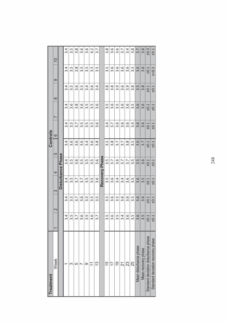
24
8
Trea
tmen
t C
ontr
ols
Wee
k 1
2 3
4 5
6 7
8 9
10
Dis
turb
ance
Pha
se
1 3.
4 3.
4 3.
4 3.
4 3.
4 3.
4 3.
4 3.
4 3.
4 3.
4 3
3.5
3.5
3.5
3.5
3.6
3.5
3.6
3.5
3.5
3.5
5 3.
7 3.
7 3.
7 3.
6 3.
6 3.
7 3.
8 3.
6 3.
8 3.
8 7
3.6
3.6
3.7
3.5
3.6
3.5
3.6
3.5
3.5
3.6
9 3.
5 3.
5 3.
5 3.
5 3.
4 3.
5 3.
5 3.
4 3.
5 3.
6 11
3.
6 3.
5 3.
5 3.
5 3.
6 3.
5 3.
5 3.
6 3.
5 4.
2 13
3.
7 3.
5 3.
6 3.
6 3.
8 3.
6 3.
6 3.
4 3.
5 3.
7 R
ecov
ery
Phas
e 15
3.
5 3.
5 3.
5 3.
5 3.
5 3.
4 3.
5 3.
8 3.
5 3.
8 17
3.
6 3.
6 3.
6 3.
7 3.
8 3.
7 3.
6 3.
8 3.
6 3.
6 19
3.
5 3.
5 3.
4 3.
6 3.
7 3.
6 3.
5 3.
9 3.
6 3.
6 21
3.
4 3.
6 3.
4 3.
7 3.
7 3.
6 3.
6 3.
6 3.
6 3.
7 23
3.
6 3.
6 3.
6 3.
7 3.
8 3.
6 3.
6 3.
9 3.
6 3.
4 25
3.
5 3.
5 3.
5 3.
5 3.
5 3.
4 3.
5 3.
8 3.
5 3.
8 Me
an di
sturb
ance
phas
e 3.
6 3.
6 3.
6 3.
5 3.
6 3.
6 3.
6 3.
5 3.
6 3.
7 Me
an re
cove
ry ph
ase
3.5
3.6
3.5
3.6
3.7
3.6
3.6
3.8
3.6
3.6
Stan
dard
devia
tion d
istur
banc
e pha
se
±0.1
±0
.1
±0.1
±0
.1
±0.1
±0
.1
±0.1
±0
.1
±0.1
±0
.3
Stan
dard
devia
tion r
ecov
ery p
hase
±0
.1
±0.1
±0
.1
±0.1
±0
.1
±0.1
±0
.1
±0.1
±<
0.1
±0.1

249
Appendix 12 The abundance of minor invertebrate species for the
experiment investigating the effect of high salinity disturbances on the propagule bank of Lake Cullen
Table A12.1 The presence of the 4 minor invertebrate species.
Species Treatment where individuals were observed to emerge from
sediments
Number of individuals
Class Insecta Order Diptera, Family Psychodidae
61.0 g/L disturbance phase salinity/ 5.5 g/L recovery phase salinity
4
Class Turbellaria 136.0 g/L disturbance phase salinity/ 5.5 g/L recovery phase salinity
1
Class Insecta Order Collembola Sminthuridae spp.
136.0 g/L disturbance phase salinity/ 5.5 g/L recovery phase salinity
1
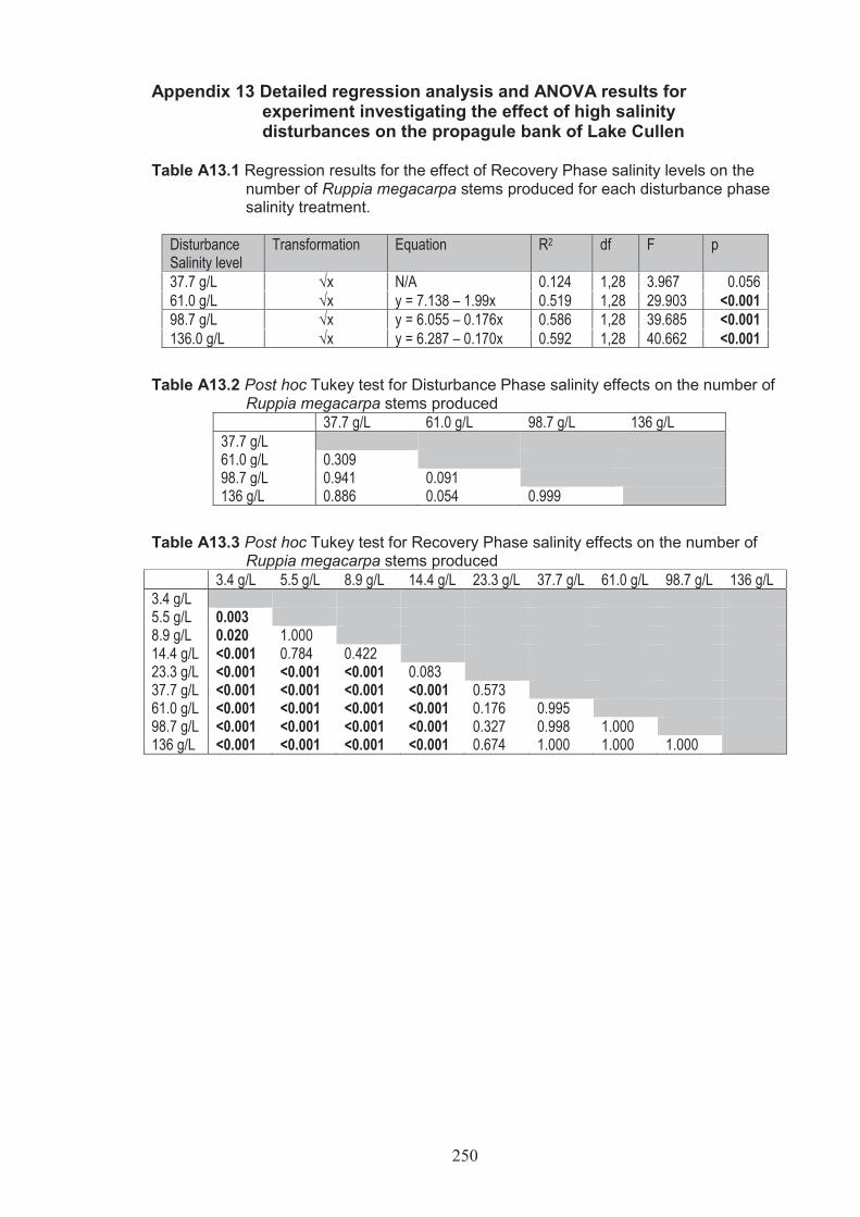
250
Appendix 13 Detailed regression analysis and ANOVA results for experiment investigating the effect of high salinity disturbances on the propagule bank of Lake Cullen
Table A13.1 Regression results for the effect of Recovery Phase salinity levels on the
number of Ruppia megacarpa stems produced for each disturbance phase salinity treatment.
Disturbance Salinity level
Transformation Equation R2 df F p
37.7 g/L √x N/A 0.124 1,28 3.967 0.056 61.0 g/L √x y = 7.138 – 1.99x 0.519 1,28 29.903 <0.001 98.7 g/L √x y = 6.055 – 0.176x 0.586 1,28 39.685 <0.001 136.0 g/L √x y = 6.287 – 0.170x 0.592 1,28 40.662 <0.001
Table A13.2 Post hoc Tukey test for Disturbance Phase salinity effects on the number of Ruppia megacarpa stems produced
37.7 g/L 61.0 g/L 98.7 g/L 136 g/L 37.7 g/L 61.0 g/L 0.309 98.7 g/L 0.941 0.091 136 g/L 0.886 0.054 0.999
Table A13.3 Post hoc Tukey test for Recovery Phase salinity effects on the number of Ruppia megacarpa stems produced
3.4 g/L 5.5 g/L 8.9 g/L 14.4 g/L 23.3 g/L 37.7 g/L 61.0 g/L 98.7 g/L 136 g/L 3.4 g/L 5.5 g/L 0.003 8.9 g/L 0.020 1.000 14.4 g/L <0.001 0.784 0.422 23.3 g/L <0.001 <0.001 <0.001 0.083 37.7 g/L <0.001 <0.001 <0.001 <0.001 0.573 61.0 g/L <0.001 <0.001 <0.001 <0.001 0.176 0.995 98.7 g/L <0.001 <0.001 <0.001 <0.001 0.327 0.998 1.000 136 g/L <0.001 <0.001 <0.001 <0.001 0.674 1.000 1.000 1.000

251
Table A13.4 Regression results for the effect of Recovery Phase salinity levels on the amount of Ruppia megacarpa biomass produced for each disturbance phase salinity treatment (p<0.05).
Disturbance Salinity level
Transformation Equation R2 df F p
37.7 g/L y = √x y = 0.477 – 0.008x 0.174 1, 28 5,910 0.022 61.0 g/L y = √x y = 0.528 – 0.012x 0.536 1, 28 32.365 <0.001 98.7 g/L y = √x y = 0.518 – 0.012x 0.666 1, 28 55.833 <0.001
136.0 g/L y = √x Y = 0.555 – 0.012x 0.686 1, 28 60.465 <0.001
Table A13.5 Post hoc Tukey test for Recovery Phase salinity effects on the amount of Ruppia megacarpa biomass produced
3.4 g/L 5.5 g/L 8.9 g/L 14.4 g/L 23.3 g/L 37.7 g/L 61.0 g/L 98.7 g/L 136 g/L 3.4 g/L 5.5 g/L 0.361 8.9 g/L 0.905 0.992 14.4 g/L 0.135 1.000 0.899 23.3 g/L <0.001 0.002 <0.001 0.010 37.7 g/L <0.001 <0.001 <0.001 <0.001 0.095 61.0 g/L <0.001 <0.001 <0.001 <0.001 <0.001 0.366 98.7 g/L <0.001 <0.001 <0.001 <0.001 0.001 0.543 1.000 136 g/L <0.001 <0.001 <0.001 <0.001 0.025 0.828 1.000 1.000

252
Table A13.6 Regression results for the effect of Recovery Phase salinity levels on the number of Lamprothamnium macropogon individuals germinated for each disturbance phase salinity treatment (p<0.05).
Disturbance Salinity level
Transformation Equation R2 df F p
37.7 g/L √x y = 29.816 – 0.155x 0.284 1, 28 10.700 0.003 61.0 g/L √x y = 18.383 – 0.167x 0.267 1, 28 10.186 0.003 98.7 g/L √x y = 18.199 – 0.320x 0.755 1, 28 86.511 <0.001 136.0 g/L √x y = 16.788 – 0.303x 0.609 1, 28 43.533 <0.001
Table A13.7 Post hoc Tukey test for Disturbance Phase salinity effects on the number of Lamprothamnium macropogon individuals germinated
37.7 g/L 61.0 g/L 98.7 g/L 136 g/L 37.7 g/L 61.0 g/L <0.001 98.7 g/L <0.001 <0.001 136 g/L <0.001 <0.001 0.002
Table A13.8 Post hoc Tukey test for Recovery Phase salinity effects on the number of Lamprothamnium macropogon individuals germinated
3.4 g/L 5.5 g/L 8.9 g/L 14.4 g/L 23.3 g/L 37.7 g/L 61.0 g/L 98.7 g/L 136 g/L 3.4 g/L 5.5 g/L 1.000 8.9 g/L 1.000 1.000 14.4 g/L 1.000 1.000 1.000 23.3 g/L 0.180 0.237 0.238 0.147 37.7 g/L <0.001 <0.001 <0.001 <0.001 <0.001 61.0 g/L <0.001 <0.001 <0.001 <0.001 <0.001 <0.001 98.7 g/L <0.001 <0.001 <0.001 <0.001 <0.001 <0.001 1.000 136 g/L <0.001 <0.001 <0.001 <0.001 <0.001 <0.001 1.000 1.000
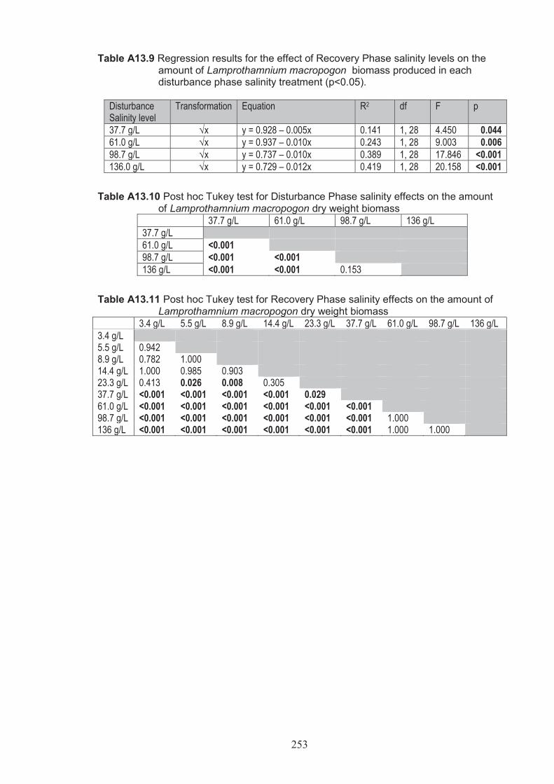
253
Table A13.9 Regression results for the effect of Recovery Phase salinity levels on the amount of Lamprothamnium macropogon biomass produced in each disturbance phase salinity treatment (p<0.05).
Disturbance Salinity level
Transformation Equation R2 df F p
37.7 g/L √x y = 0.928 – 0.005x 0.141 1, 28 4.450 0.044 61.0 g/L √x y = 0.937 – 0.010x 0.243 1, 28 9.003 0.006 98.7 g/L √x y = 0.737 – 0.010x 0.389 1, 28 17.846 <0.001 136.0 g/L √x y = 0.729 – 0.012x 0.419 1, 28 20.158 <0.001
Table A13.10 Post hoc Tukey test for Disturbance Phase salinity effects on the amount of Lamprothamnium macropogon dry weight biomass
37.7 g/L 61.0 g/L 98.7 g/L 136 g/L 37.7 g/L 61.0 g/L <0.001 98.7 g/L <0.001 <0.001 136 g/L <0.001 <0.001 0.153
Table A13.11 Post hoc Tukey test for Recovery Phase salinity effects on the amount of Lamprothamnium macropogon dry weight biomass
3.4 g/L 5.5 g/L 8.9 g/L 14.4 g/L 23.3 g/L 37.7 g/L 61.0 g/L 98.7 g/L 136 g/L 3.4 g/L 5.5 g/L 0.942 8.9 g/L 0.782 1.000 14.4 g/L 1.000 0.985 0.903 23.3 g/L 0.413 0.026 0.008 0.305 37.7 g/L <0.001 <0.001 <0.001 <0.001 0.029 61.0 g/L <0.001 <0.001 <0.001 <0.001 <0.001 <0.001 98.7 g/L <0.001 <0.001 <0.001 <0.001 <0.001 <0.001 1.000 136 g/L <0.001 <0.001 <0.001 <0.001 <0.001 <0.001 1.000 1.000

254
Table A13.12 Regression results for the effect of Recovery Phase salinity levels on the number of Mytilocypris henricae individuals in the population developed from the propagule bank in each disturbance phase salinity treatment (p<0.05).
Disturbance Salinity level
Transformation Equation R2 Df F P
61.0 g/L √x y = 0.621 +0.428x – 0.009x2 0.557 2, 27 6.071 0.007 98.7 g/L √x y = 3.34 + 0.482x – 0.013x2 0.595 2, 27 7.401 0.003 136.0 g/L √x y = 6.216 + 0.223x – 0.007x2 0.551 2, 27 5.887 0.008
Table A13.13 Post hoc Tukey test for Disturbance Phase salinity effects on the number of Mytilocypris henricae individuals in the population developed from the propagule bank
37.7 g/L 61.0 g/L 98.7 g/L 136 g/L 37.7 g/L 61.0 g/L <0.001 98.7 g/L <0.001 0.324 136 g/L <0.001 0.121 0.960
Table A13.14 Post hoc Tukey test for Recovery Phase salinity effects on the number of Mytilocypris henricae individuals in the population developed from the propagule bank
3.4 g/L 5.5 g/L 8.9 g/L 14.4 g/L 23.3 g/L 37.7 g/L 61.0 g/L 98.7 g/L 136 g/L 3.4 g/L 5.5 g/L 0.333 8.9 g/L <0.001 0.155 14.4 g/L <0.001 0.405 1.000 23.3 g/L 0.008 0.805 0.934 0.997 37.7 g/L 0.990 0.903 0.002 0.014 0.124 61.0 g/L 0.001 <0.001 <0.001 <0.001 <0.001 <0.001 98.7 g/L 0.004 <0.001 <0.001 <0.001 <0.001 <0.001 1.000 136 g/L 0.065 <0.001 <0.001 <0.001 <0.001 0.011 1.000 1.000
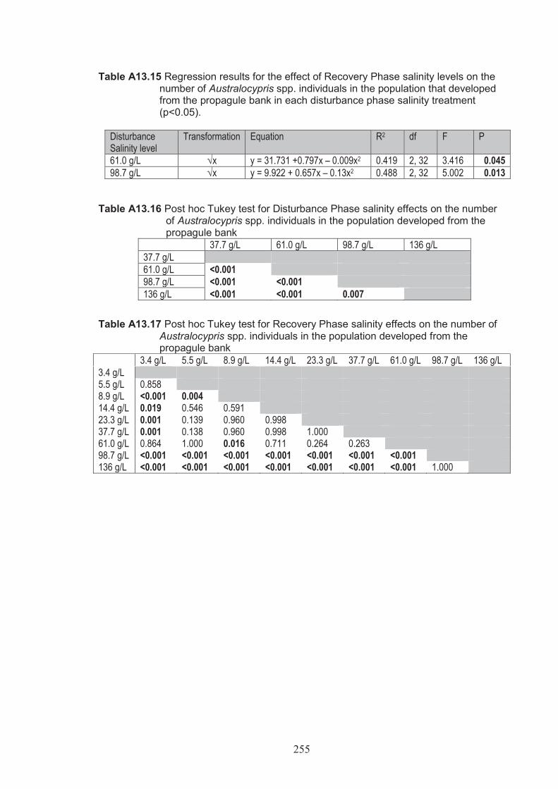
255
Table A13.15 Regression results for the effect of Recovery Phase salinity levels on the number of Australocypris spp. individuals in the population that developed from the propagule bank in each disturbance phase salinity treatment (p<0.05).
Disturbance Salinity level
Transformation Equation R2 df F P
61.0 g/L √x y = 31.731 +0.797x – 0.009x2 0.419 2, 32 3.416 0.045 98.7 g/L √x y = 9.922 + 0.657x – 0.13x2 0.488 2, 32 5.002 0.013
Table A13.16 Post hoc Tukey test for Disturbance Phase salinity effects on the number
of Australocypris spp. individuals in the population developed from the propagule bank
37.7 g/L 61.0 g/L 98.7 g/L 136 g/L 37.7 g/L 61.0 g/L <0.001 98.7 g/L <0.001 <0.001 136 g/L <0.001 <0.001 0.007
Table A13.17 Post hoc Tukey test for Recovery Phase salinity effects on the number of Australocypris spp. individuals in the population developed from the propagule bank
3.4 g/L 5.5 g/L 8.9 g/L 14.4 g/L 23.3 g/L 37.7 g/L 61.0 g/L 98.7 g/L 136 g/L 3.4 g/L 5.5 g/L 0.858 8.9 g/L <0.001 0.004 14.4 g/L 0.019 0.546 0.591 23.3 g/L 0.001 0.139 0.960 0.998 37.7 g/L 0.001 0.138 0.960 0.998 1.000 61.0 g/L 0.864 1.000 0.016 0.711 0.264 0.263 98.7 g/L <0.001 <0.001 <0.001 <0.001 <0.001 <0.001 <0.001 136 g/L <0.001 <0.001 <0.001 <0.001 <0.001 <0.001 <0.001 1.000

256
Appendix 14 Random location of replicates in germination cabinet for the experiment investigating the effect of location of seed source and presence of substrate on the germination of Ruppia megacarpa seeds at two differing salinities.
I
D
J
C
C
F
I
E
J
C
G
L
E
K
F
K
F
D
B
G
I
D
B
B
K
F
C
K
G
K
L
I
H
A
E
H
A
L
A
L
H
D
F
A
H
G
E
G
C
B
B
L
I
J
A
D
J
H
J
E
Back of Cabinet
Back of Cabinet
Front of Cabinet
Front of Cabinet
Top Shelf
Middle Shelf
Key
Location Substrate Salinity mg/L
Location Substrate Salinity mg/L
A Lake Cullen No 1 360 G Lake Golf Course Yes 1 360 B Lake Cullen No 3 400 H Lake Golf Course Yes 3 400 C Lake Cullen Yes 1 360 I Lake Wandella No 1 360 D Lake Cullen Yes 3 400 J Lake Wandella No 3 400 E Lake Golf Course No 1 360 K Lake Wandella Yes 1 360 F Lake Golf Course No 3 400 L Lake Wandella Yes 3 400
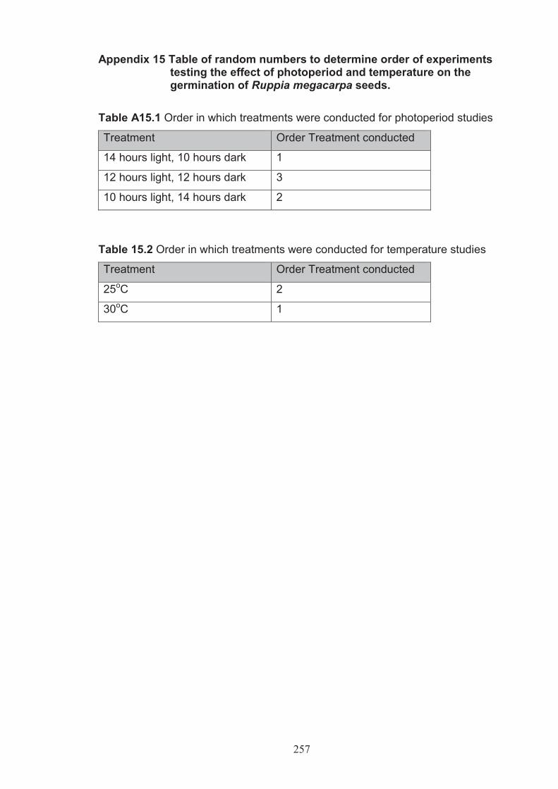
257
Appendix 15 Table of random numbers to determine order of experiments testing the effect of photoperiod and temperature on the germination of Ruppia megacarpa seeds.
Table A15.1 Order in which treatments were conducted for photoperiod studies
Treatment Order Treatment conducted
14 hours light, 10 hours dark 1
12 hours light, 12 hours dark 3
10 hours light, 14 hours dark 2
Table 15.2 Order in which treatments were conducted for temperature studies
Treatment Order Treatment conducted
25oC 2
30oC 1
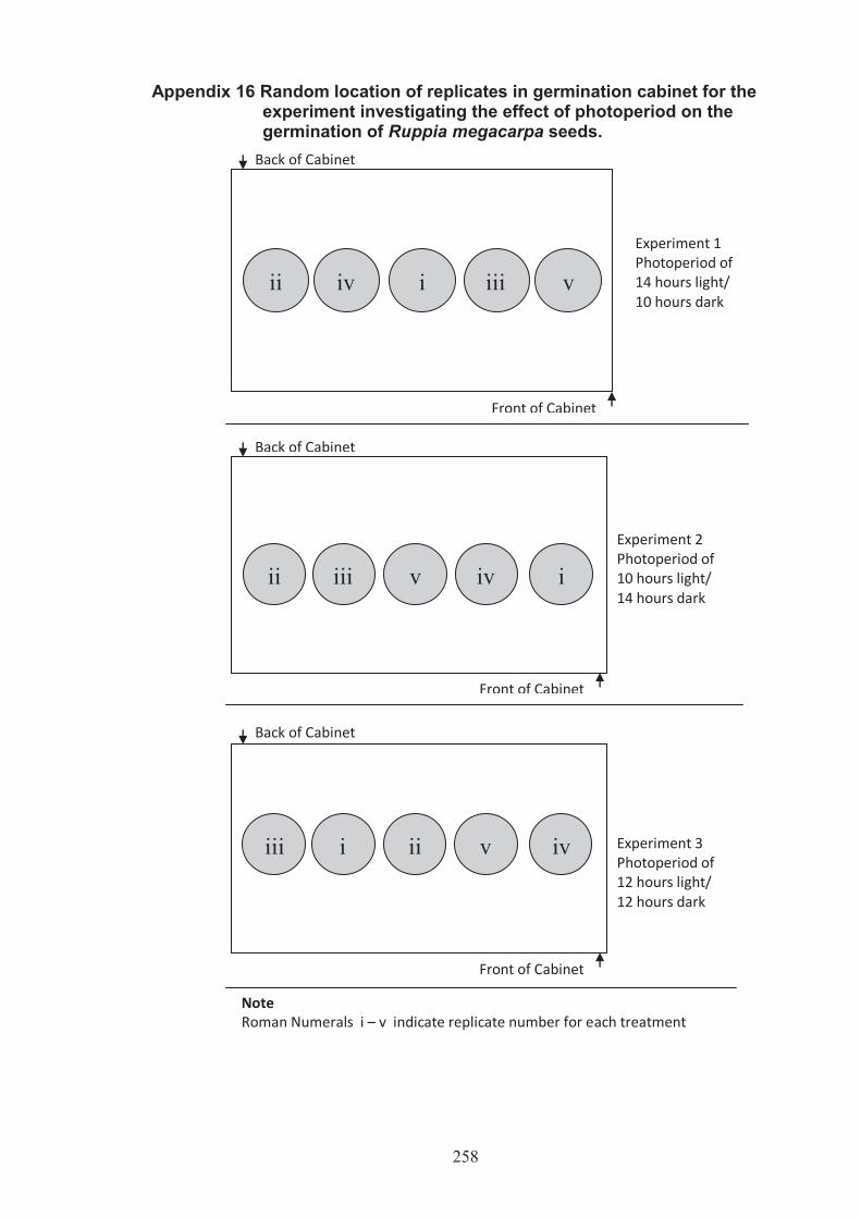
258
Appendix 16 Random location of replicates in germination cabinet for the experiment investigating the effect of photoperiod on the germination of Ruppia megacarpa seeds.
Back of Cabinet
Back of Cabinet
Back of Cabinet
Front of Cabinet
Front of Cabinet
Front of Cabinet
Experiment 1 Photoperiod of 14 hours light/ 10 hours dark
Experiment 2 Photoperiod of 10 hours light/ 14 hours dark
Experiment 3 Photoperiod of 12 hours light/ 12 hours dark
ii iv i iii v
ii iii v iv i
Note Roman Numerals i – v indicate replicate number for each treatment
iii i ii v iv
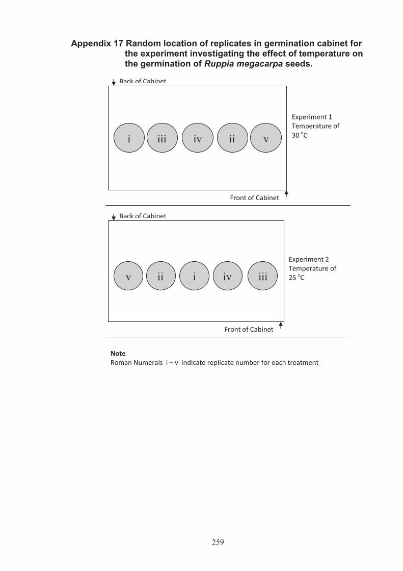
259
Appendix 17 Random location of replicates in germination cabinet for the experiment investigating the effect of temperature on the germination of Ruppia megacarpa seeds.
Back of Cabinet
Back of Cabinet
Front of Cabinet
Front of Cabinet
Experiment 1 Temperature of 30 oC
Experiment 2 Temperature of 25 oC
i iii iv ii v
v ii i iv iii
Note Roman Numerals i – v indicate replicate number for each treatment
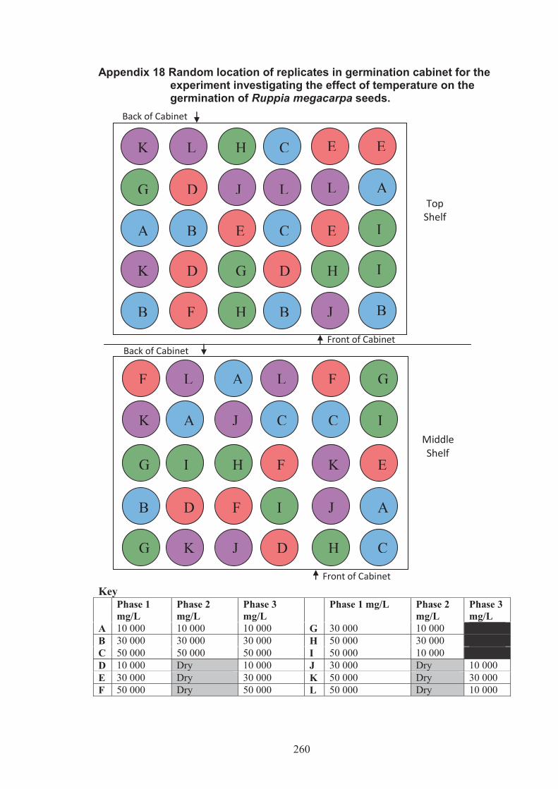
260
Appendix 18 Random location of replicates in germination cabinet for the
experiment investigating the effect of temperature on the germination of Ruppia megacarpa seeds.
K
G
A
K
B
L
D
B
D
F
H
J
E
G
H
C
L
C
D
B
E
L
E
H
J
E
A
I
I
B
F
K
G
B
G
L
A
I
D
K
A
J
H
F
J
L
C
F
I
D
F
C
K
J
H
G
I
E
A
C
Back of Cabinet
Back of Cabinet Front of Cabinet
Front of Cabinet
Top Shelf
Middle Shelf
Key Phase 1
mg/L Phase 2 mg/L
Phase 3 mg/L
Phase 1 mg/L Phase 2 mg/L
Phase 3 mg/L
A 10 000 10 000 10 000 G 30 000 10 000 B 30 000 30 000 30 000 H 50 000 30 000 C 50 000 50 000 50 000 I 50 000 10 000 D 10 000 Dry 10 000 J 30 000 Dry 10 000 E 30 000 Dry 30 000 K 50 000 Dry 30 000 F 50 000 Dry 50 000 L 50 000 Dry 10 000

26
1
App
endi
x 19
Day
to D
ay R
esul
ts –
The
effe
ct o
f var
ious
dry
ing
perio
ds a
nd s
alin
ity tr
eatm
ents
on
the
germ
inat
ion
of R
uppi
a m
egac
arpa
see
ds
Fi
gure
A19
.1 D
ay to
Day
Res
ults
– T
he e
ffect
of v
ario
us d
ryin
g pe
riods
and
sal
inity
trea
tmen
ts o
n th
e ge
rmin
atio
n of
R. m
egac
arpa
se
eds
a) C
ontro
l tre
atm
ents
, b) e
ffect
of d
esic
catio
n

26
2
Fi
gure
A19
.2 D
ay to
Day
Res
ults
– T
he e
ffect
of v
ario
us d
ryin
g pe
riods
and
sal
inity
trea
tmen
ts o
n th
e ge
rmin
atio
n of
R. m
egac
arpa
se
eds
c) c
hang
ing
salin
ity, b
) effe
ct o
f des
icca
tion
and
chan
ge in
sal
inity