Residential Location Choice Modeling: Accommodating Sociodemographic, School Quality and Accessibility Effects

Jessica Guo and Chandra Bhat Department of Civil Engineering, ECJ 6.8

University of Texas at Austin, Austin TX 78712 Phone: 512-471-4535, Fax: 512-475-8744,

Email: bhat@mail.utexas.edu, jessica.guo@mail.utexas.edu

ABSTRACT

This paper examines household residential location choice behavior using a sample of single

wage-earner households from the Dallas-Fort Worth region in Texas. The study considers several

potential determinants of residence location choice, including socio-demographic status, stage of

life cycle and racial composition. In addition, the study is one of the few research efforts that

recognizes the impact of school quality on household residential location choice. The study also

accommodates the effects of accessibility to different activity purposes on residential choice

decisions.

Guo and Bhat 1

1. INTRODUCTION

It is conventional wisdom that land-use patterns and travel patterns are closely interlinked (see

for example Mitchell and Rapkin, 1954; Jones et al., 1983; Jones, 1990; Banister, 1994; Hanson,

1996). With the passage of the Intermodal Surface Transportation Efficiency (ISTEA) and the

Transportation Equity Act for the 21st Century (TEA-21), the integrated analysis of land-use and

transportation interactions has gained renewed interest and importance. However, the behavioral

linkages between activity patterns and long-term household choices that influence land use have

been explored in only a limited fashion. Given that residential land use occupies about two-

thirds of all urban land, and that home-based trips account for a large proportion of all travel

(Harris, 1996), one of the most important household long-term land use-related decisions is that

of residential location. This decision not only determines the association between the household

with the rest of the urban environment, but also influences the household’s budgets for activity

participation. Meeting the expectations of households in this regard is a major component of

public policy related to housing markets, job location, and transportation (Oryani and Harris,

1996).

This current study is in the same direction as earlier research in the area of discrete choice

residential models, with the objective of gaining insights into the urban spatial location process.

A better understanding of the linkage between households’ characteristics and residential

location characteristics will facilitate improved and integrated land-use and transportation

modeling (see Waddell, 2000).

The current study examines the location choice behavior of households using data from

the Dallas-Fort Worth region in Texas. As the intention is to gain an in-depth understanding of

residential location choice, the model does not consider other potentially interdependent

Guo and Bhat 2

decisions such as work location, tenure status and car ownership. Further, since the number of

workers in a household has a major effect on households’ location choice (Waddell, 1993), this

study focuses on households with only one wage earner. Within the narrow scope of the

residential location of single wage-earner households, the study considers a comprehensive set of

determinants of residential location decisions. These factors include socio-demographic status,

stage of life cycle, ethnicity and accessibility to different types of activities. In addition, the

study is one of the few research efforts that recognizes the impact of school quality on household

residential location choice.

The remainder of this paper is organized as follows. Section 2 provides an overview of

previous studies on residential location choice, with specific emphasis on the exogenous

variables used to explain residential choice behavior. Section 3 presents the development and

formulation of the residential location choice multinomial logit model. Section 4 focuses on the

preparation and assembly of the data for model estimation. Section 5 discusses model

specification issues and presents the empirical results. Finally, section 6 summarizes major

findings of this study and their policy implications.

2. LITERATURE REVIEW

Modern research on housing choice began with the study of Alonso (1964), who considers a city

in which employment opportunities are located in a single center (a monocentric city). In

Alonso’s study, the residential choice of households is based on maximizing a utility function

that depends upon the expenditure in goods, size of the land lots, and distance from the city

center. Harris (1963), Mills (1972) and Wheaton (1974) extended the work of Alonso by

Guo and Bhat 3

relaxing the assumption of a monocentric city of employment opportunities. One of the most

criticized aspects of these early research works is that location is represented as a one-

dimensional variable - distance from the CBD. These models are therefore incapable of handling

dispersed employment centers and asymmetric development patterns (Waddell, 1996).

Even before Alonso’s (1964) work, geographers and transportation planners had

developed the “gravity model” that provides a reasonable basis for the prediction of zone-to-zone

trips. Lowry applied the gravity model to residential location modeling in the well-known Lowry

Model (1964). Specifically, Lowry assumed that retail trade and services are located in relation

to residential demand, and that residences are located in relation to combined retail and basic

employment. Workers are hypothesized to start their trips to home from work, and distribute

themselves at available residential sites according to a gravity model, which attenuates their trips

over increasing distance. This vital feature of the Lowry model continues to dominate models of

residential location in many practical applications (Harris, 1996).

Another stream of research on modeling residential location is based on discrete choice

theory. In the context of residential location, the consumption decision is a discrete choice

between alternative houses or neighborhoods. The work by McFadden (1978) represents the

earliest attempt to apply discrete choice modeling to housing location. More recent works using

this approach include Gabriel and Rosenthal (1989), Waddell (1993, 1996), and Ben-Akiva and

Bowman (1998). As discussed next, these studies differ essentially in their model structures, the

choice dimensions modeled, the study region examined, and the explanatory variables considered

in the analysis.

The study by Gabriel and Rosenthal (1989) develops and estimates a multinomial logit

model of household location among mutually exclusive counties in the Washington, D.C.

Guo and Bhat 4

metropolitan area. The findings indicate that race is a major choice determinant for that area, and

that further application of MNL models to the analysis of urban housing racial segregation is

warranted. Furthermore, the effects of household socio-demographic characteristics on

residential location are found to differ significantly by race. Waddell (1993) examines the

assumption implicit in most models of residential location that the choice of workplace is

exogenously determined. A nested logit model is developed for worker’s choice of workplace,

residence, and housing tenure for the Dallas-Fort Worth metropolitan region. The results

confirm that a joint choice specification better represents household spatial choice behavior. The

study also reaffirms many of the influences posited in standard urban economic theory, as well as

the ecological hypothesis of residence clustering by socio-demographic status, stage of life cycle,

and ethnicity. In a later study, Waddell (1996) focuses on the implications of the rise of dual-

worker households. The choices of work place location, residential mobility, housing tenure and

residential location are examined jointly. The hypothesis is that home ownership and the

presence of a second worker both add constraints on household choices that should lead to a

combination of lower mobility rates and longer commutes. The results indicate gender

differences in travel behavior; specifically, the female work commute distance has less influence

on the residential location choice than the male commute. Ben-Akiva and Bowman (1998)

presented a nested logit model for Boston, integrating a household’s residential location choice

and its members’ activity schedules. Given a residential location, the activity schedule model

assigns a measure of accessibility for each household member, which then enters the utility

function in the model of residential location choice. The results statistically invalidate the

expected decision hierarchy in which the daily activity pattern is conditioned on residential

choice.

Guo and Bhat 5

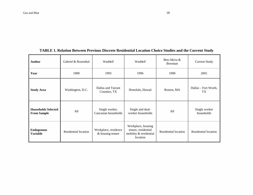
The study area, sample characteristics, and choice dimensions modeled in the

aforementioned studies and the current study are summarized in Table 1. Table 2, on the other

hand, provides a comparative listing of the exogenous variables considered in these studies. The

variables found to have a statistically significant effect on residential location choice are

identified with a check mark, while the variables that were tested but excluded from the final

model specification due to statistical insignificance are labeled with a question mark. This listing

forms the basis of variable selection for the present study. It also highlights the objective of the

current study to account for as many locational and household attributes as possible, within the

constraints of data availability from the Dallas-Fort Worth area.

3. RESIDENTIAL LOCATION CHOICE MODELING

There are a number of estimation issues involved in developing the multinomial logit model for

residential choice. This section first discusses the spatial scale at which residential location

choices are defined, and describes the process of generating choice alternatives for each

household. The model structure adopted in the study is then presented.

3.1. Definition and Choice Set Generation of Residential Location Alternatives

The proposed location choice model predicts the individual household’s choice of residence to

aggregated zones rather than specific dwelling units. In the context of the Dallas-Fort Worth

data, the spatial scale of the aggregated zones corresponds to the transport analysis and

processing (TAP) zone. There are over 900 TAP zones in the universal choice set for the chosen

study region. However, by assuming an identically and independently distributed (IID) structure

Guo and Bhat 6

for the error terms across the alternatives in the universal choice set, the residential location

model can be consistently estimated with only a subset of the choice alternatives (McFadden,

1978). One way of drawing a choice subset from the universal set without jeopardizing the

consistency of the parameter estimates is the random sampling technique (Ben-Akiva and

Lerman, 1993). The approach involves combining the chosen alternative with a subset of

randomly selected non-chosen alternatives.

3.2. Model Structure

As indicated earlier, the model structure used in this study for residential location choice is the

multinomial logit model. The probability of a household n choosing zone i is written as:

,∑

′

′=

i

V

V

ni in

ni

eeP (1)

where niV is expressed in a linear-in-parameter form as follows:

niini XZV βα ′+′= . (2)

In the above expression, iZ is a vector of zonal attractiveness measures; and niX represents

interaction terms of socio-demographic characteristics of household n with the attractiveness

measures of zone i. α and β are parameter vectors to be estimated.

In theory, a constant should be introduced for each of the zonal choice alternatives to

account for the effect of the mean of unobserved zonal factors and the range of explanatory

variables. However, since the number of zones is very large, and only a sample of zones is used

in the estimation, such constants are not introduced in our model.

A final note about model structure is in order here. It is likely that the sensitivity of

households to zonal attractiveness measures will be a function of unobserved household

Guo and Bhat 7

characteristics, which suggests treating α as a random parameter vector. Such a specification

leads to a random-coefficients logit (RCL) framework and requires the use of simulation-based

estimation techniques. The authors are currently pursuing such an effort and should have the

results of the RCL model within the next month.

4. DATA SOURCES AND SAMPLE

The primary source of data for the current modeling effort is the 1996 Dallas-Fort Worth

metropolitan area household activity survey. This survey collected information about travel and

non-travel activities undertaken during a weekday by members of 4839 households, as well as the

residential locations of households. The survey also obtained individual and household socio-

demographic information. In addition to the activity household survey, five other data sources

were also used: the zone-to-zone travel level-of-service (LOS) data, land-use coverage data,

accessibility data, school-rating data, and census data. Both the LOS and the land-use data files

were obtained from the North Central Texas Council of Governments (NCTCOG), which is a

voluntary association of local governments from 16 counties centering from two urban centers of

Dallas and Fort Worth. The LOS file provides information on travel between each pair of the

919 Transportation Analysis Process (TAP) zones in the North Central Texas region. The file

contains the inter-zonal distances as well as peak and off-peak travel times and costs for transit

and highway modes. The land-use coverage file contains acreage by land-use purposes

(including water area, park land, roadway, office, retail and etc.) for each of 5938 disaggregate

traffic survey zones (TSZ). The accessibility measures are derived from zonal employment data,

LOS data and land-use coverage data, as discussed in Section 5.1.1. Data about school ratings is

Guo and Bhat 8

compiled in-house from the 1996 district summary of the Accountability Rating System (ARS)

for Texas Public Schools and School Districts. The ARS is released on a yearly basis by the

Texas Education Agency. The schools are classified into 4 levels: exemplary, recognized,

acceptable and low performing (or unacceptable). The criteria for ranking are summarized in

Table 3. The census data is used to compute the ethnic composition of each TAP.

Several data cleaning and assembly steps were undertaken in developing the sample used

in estimation. The steps are as follows: (a) Extract the home and work locations of single wage-

earner households from the survey file, and assign these locations to TAP zones; (b) Aggregate

the land-use information from the disaggregate TSZ level to TAP zone level; (c) Map the values

of school ratings from the spatial level of Independent School Districts to the more disaggregate

TAP level used in the current analysis; and (d) Generate the choice set for each household by

randomly selecting four non-chosen TAP zonal alternatives and adding the chosen alternative.

Details of the sample formation process and procedures to develop the final sample are available

from the authors. The final sample comprised 1472 households, with five zonal choice

alternatives for each household.

5. EMPIRICAL ANALYSIS

Data for the 1472 sample households was imported into LIMDEP for model estimation. The

next section discusses the specification of the explanatory variables considered for analysis. The

subsequent section presents and interprets the estimation results.

Guo and Bhat 9

5.1. Variable Specifications

The explanatory variables considered for inclusion in the residential location model include (1)

zonal size and attractiveness measures, and (2) interaction of socio-demographic variables with

zonal attractiveness variables.

5.1.1. Zone Size and Attractiveness Measures

The zonal size and attractiveness measures consist of five groups of variables: (1) zonal size

measures, (2) percentage land use acreages, (3) density measures, (4) homogeneity measures and

(5) accessibility measures. These measures are discussed briefly in the next few paragraphs.

The zonal size measure proxies the number of elemental residential opportunities in the

zone and is represented by the number of housing units in the zone.

The percentage land use acreages are computed by normalizing the acreage in different

types of land uses by the total zonal acreage. The land use types considered include: lakes and

water, residential, industrial, offices, retail and services, institutions (schools, churches, etc.), and

infrastructure.

The density measures are computed by dividing the total number of households or people

in a zone by the zone size (in acre). The density variables are introduced to capture the clustering

effect of households.

The homogeneity measures, defined in terms of household income, are used to test the

presence of income segregation; that is, to test if households locate themselves with other

households of similar income level. The measure is defined by the absolute difference between

the household income and the median zonal income. Thus, if income segregation is present, the

parameter should have a negative sign.

Guo and Bhat 10

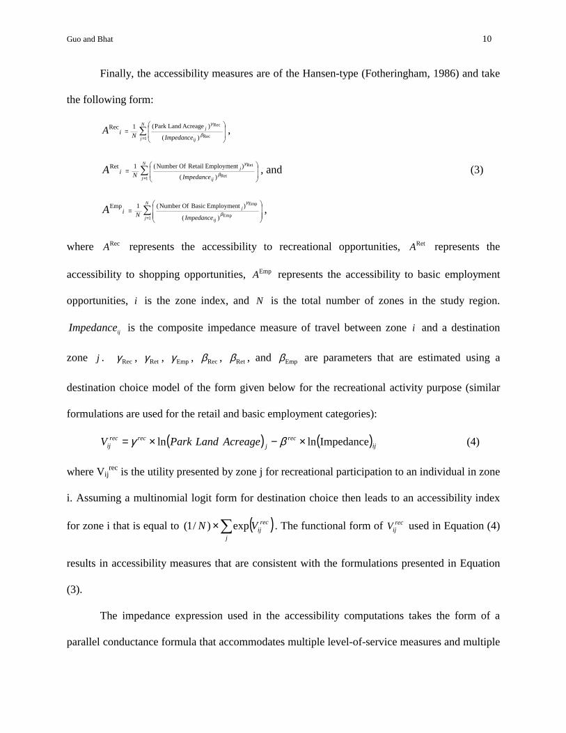
Finally, the accessibility measures are of the Hansen-type (Fotheringham, 1986) and take

the following form:

∑=

=

N

j ij

j

ImpedanceNiA1 Rec

Rec

)(

)Acreage LandPark (1Recβ

γ

,

∑=

=

N

j ij

j

ImpedanceNiA1 Ret

Ret

)(

)t Employmen RetailOfNumber (1Retβ

γ

, and (3)

∑=

=

N

j ij

j

ImpedanceNiA1 Emp

Emp

)(

)t Employmen BasicOfNumber (1Empβ

γ

,

where RecA represents the accessibility to recreational opportunities, RetA represents the

accessibility to shopping opportunities, EmpA represents the accessibility to basic employment

opportunities, i is the zone index, and N is the total number of zones in the study region.

ijImpedance is the composite impedance measure of travel between zone i and a destination

zone j . Recγ , Retγ , Empγ , Recβ , Retβ , and Empβ are parameters that are estimated using a

destination choice model of the form given below for the recreational activity purpose (similar

formulations are used for the retail and basic employment categories):

( ) ( )ijrec

jrecrec

ij AcreageLandParkV Impedancelnln ×−×= βγ (4)

where Vijrec is the utility presented by zone j for recreational participation to an individual in zone

i. Assuming a multinomial logit form for destination choice then leads to an accessibility index

for zone i that is equal to ( )∑×j

recijVN exp)/1( . The functional form of rec

ijV used in Equation (4)

results in accessibility measures that are consistent with the formulations presented in Equation

(3).

The impedance expression used in the accessibility computations takes the form of a

parallel conductance formula that accommodates multiple level-of-service measures and multiple

Guo and Bhat 11

modes (see Bhat et al, 1998 for a discussion of this formula). However, in the current empirical

context, only highway auto level-of-service measures are used because of the lack of adequate

transit observations in the destination choice model estimation. The highway auto impedance

measure is in effective in-vehicle time units (in minutes) and is expressed as follows:

cents)(in minutes)(in minutes) IVTT(in COSTOVTTIVTTImpedance ×+×+= ηδ . (5)

The estimated values of the δ , and η scalar parameters, and the γ and β vector parameters, are

provided in Table 4. As can be observed, the only level of service variable that is relevant for

recreational destination choice is in-vehicle time, while cost is not significant for employment

destination choice. These results are perhaps a consequence of the strong multicollinearity in

time and cost measures. For retail destination choice, the implied money value of time is $6.05

per hour. The smaller estimated coefficient on out-of-vehicle time for the basic employment

category suggests that, unlike in mode choice decisions, individuals place a smaller value on out-

of-vehicle time than in-vehicle time when selecting employment destinations. This result may be

a consequence of the dominance of in-vehicle time as the spatial separation measure when

making destination choice decisions.

The reader will note that large values of the accessibility measures indicate more

opportunities for activities in close proximity of that zone, while small values indicate zones that

are spatially isolated from such opportunities.

5.1.2. Interaction of Household Sociodemographics with Zonal Characteristics

The motivation for considering interaction effects between household sociodemographics and the

zonal attractiveness variables is to accommodate the differential sensitivity of households to

zone-related attributes. For instance, households with children may be more sensitive to the

Guo and Bhat 12

quality of schools. The interaction effects involving household structure are introduced by

creating dummy variables characterizing the presence or absence of children and other

dependents. Similarly, dummy variables corresponding to different income levels are created

and interacted with other zonal measures.

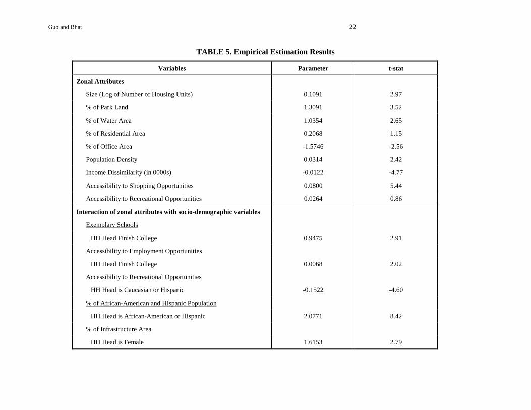
5.2. Modeling Results

The estimation results of the multinomial logit residential location choice model are presented in

Table 5. The coefficient for the zonal size measure has the expected positive sign, indicating that

zones where more housing units are available have a higher probability of being chosen. The

results also show that zones with higher percentage of parkland, water area and residential area

are generally preferred. Zones with higher percentage of office area, on the other hand, are less

preferred, suggesting that mixed land use of residential and business purposes is undesirable.

Households are more likely to locate themselves at zones with higher population density. This

may be due to better housing availability at these zones or merely a reflection of population

clustering. The income dissimilarity measure also has the expected sign, confirming the income

segregation phenomenon observed in previous studies (Waddell, 1993). Finally, the coefficients

on the accessibility measures indicate that households prefer locations that offer good

accessibility to shopping opportunities. The coefficients on accessibility to recreational

opportunities should be interpreted in combination with the interaction effect of this variable

with Caucasian or Hispanic households (see under interaction of zonal attributes with socio-

demographic variables). The results indicate that African-American households prefer locations

with good accessibility to recreational opportunities, while Caucasian and Hispanic households

prefer residential locations distant from recreational opportunities. Further research to better

Guo and Bhat 13

understand the differential preferences of households by race regarding accessibility to

recreational opportunities would be valuable.

The variables representing the interaction effects of socio-demographic variables with

zonal attributes indicate that households whose heads have at least a college degree show

preference for proximity to exemplary public schools. This is perhaps a reflection of the

premium placed by well-educated individuals on locations that offer a good education to their

children. Households whose heads have a college education are also more sensitive to

accessibility to employment opportunities. This may reflect the ability of households with highly

educated individuals to locate in expensive areas with a high employment density. People of

different ethnic groups show different sensitivities to accessibility to recreational opportunities.

Specifically, Caucasian and Hispanic households are more likely to locate in zones with higher

accessibility to social-recreational sites than African-Americans. The coefficient on the “% of

African-American and Hispanic Population” variable indicates that African-American and

Hispanic households tend to locate in zones with a high African-American/Hispanic population.

This observation of racial segregation is either due to the racial discrimination presented in the

housing market or the differences between racial groups in preferences for neighborhood

attributes (Gabriel and Rosenthal, 2001). Finally, households with female workers are more

likely to choose zones with higher percentage of infrastructure areas than households with male

workers. This probably relates to the postulation on females’ spatial entrapment.

Guo and Bhat 14

6. CONCLUSIONS

This paper presents an empirical analysis of the residential choice behavior of households using a

sample from the Dallas-Fort Worth urban area. Since the choice of residential zone is

characterized by a large number of alternatives, a random subset of the zones is chosen during

the estimation of model parameters. The important findings from the empirical analysis are as

follows:

• Zones characterized by higher percentages of water area, parkland and residential area are

preferred as residential locations.

• Zones characterized by higher percentages of office space are less preferred to those with

more residential or other land use purposes.

• School quality has a significant impact on households’ residential location choice. In

particular, households whose heads have college education are likely to locate close to

school districts with exemplary ratings.

• There is evidence of racial segregation. This may be attributed either to the racial

discrimination presented in the housing market or the differences between racial groups in

preferences for neighborhood attributes.

• Other socio-demographics are found to have an important role in residential location choice.

For instance, households with female workers are likely to choose zones with higher

percentage of infrastructure areas, possibly reflecting the spatial entrapment of females.

The foregoing results have substantial implications on land use - transportation modeling and

planning. In particular, the empirical analysis indicates significant differences in the decision

process underlying recreational location choice based on the socio-demographics of the

households. Recognizing these socio-demographic effects is very important in developing land-

Guo and Bhat 15

use policies that are consistent with the housing needs and preferences of the population.

Furthermore, while accessibility is generally recognized as the dominating factor in residential

location choice, accessibility to basic employment opportunities does not appear to be an

influencing factor except for better-educated workers. Other factors identified in this study, such

as school quality and land use mix, should not be overlooked as they are also important factors

influencing residential location choices and, to a broader extent, urban form.

The residential location model presented in this paper can be extended in several ways as

summarized below:

• Discrete choice models can be applied to analyze the residential location choice of

households with more than one worker.

• The model specification in the current paper can be improved by adding other explanatory

variables. Candidate variables include zonal housing supply, housing costs, tax rates and

crime rates. The authors developed aggregate level (i.e., nine-county level) spatial measures

of housing costs and tax rates from the census data for use in the current study, but obtained

rather counter-intuitive results in the model. The authors are currently pursuing efforts to

obtain more disaggregate measures of housing costs and tax rates.

• As indicated earlier, the use of a random-coefficients logit framework for residential choice

modeling is likely to be more appropriate than a simple MNL framework. The authors

should have the results of such a mixed logit estimation in the next month.

• The model is based on an arbitrary aggregated spatial scale, namely the TAPs. Issues such

as spatial autocorrelations and intra-zonal heterogeneity may violate the IID assumption

underlying the model structure. Further research is needed to examine the impact of these

Guo and Bhat 16

issues on the validity of the model. Alternative aggregation method or a hierarchical model

structure may be required to overcome the problem.

7. ACKNOWLEDGEMENTS

The authors would like to thank the North Central Texas Council of Governments for providing

the data used in the analysis. Huimin Zhao and Qinglin Chen helped with accessibility

computations.

Guo and Bhat 17

REFERENCES 1. Alonso, W. (1964) Location and Land Use, Cambridge: Harvard University Press. 2. Banister, D. (1994) Transport Planning. London: Chapman & Hall. 3. Ben-Akiva, M. and S.R. Lerman (1993) Discrete Choice Analysis: Theory and Application

to Travel Demand, MIT Press, Cambridge, MA. 4. Ben-Akiva, M. and J.L. Bowman (1998) Integration of an activity-based model system and

a residential location model, Urban Studies, 35 (7), 1131-1153. 5. Bhat, C.R., Govindarajan, A., and V. Pulugurta (1998) Disaggregate attraction-end choice

modeling, Transportation Research Record, 1645, 60-68. 6. Fotheringham, A.S. (1986) Modeling hierarchical destination choice, Environment and

Planning, 18A, 401-418. 7. Gabriel, S.A. and S.S. Rosenthal (1989) Household location and race: estimates of a

multinomial logit model, The Review of Economics and Statistics, 17 (2), 240-249. 8. Hanson, S. (1986) ‘Dimension of urban transportation problem’, in S. Hanson (ed.) The

Geography of Urban Transportation. New York: Macmillan Publishing Company. 9. Harris, B. (1963) Linear programming and the projection of land use, Penn- Jersey Paper

No. 20, Philadelphia, PA. 10. Harris, B. (1996) Land use models in transportation planning: a review of past

developments and current practice, [http://www.bts.gov/other/MFD_tmip/papers/landuse/compendium/dvrpc_appb.htm]

11. Jones, P. (1990) (ed.) Developments in Dynamic and Activity-Based Approaches to Travel Analysis. Aldershot: Avebury.

12. Jones, P., Clarke, M. and Dix, M. (1983) Understanding Travel Behaviour. Aldershot: Gower.

13. Lowry, I. (1964) A Model of Metropolis, RM-4035-RC, The Rand Corporation, Santa Monica, CA.

14. McFadden, D (1978) Modeling the choice of residential location, In Spatial Interaction Theory and Planning Models, edited by A. Karlqvist et al. Amsterdam: North Holland Publishers.

15. Mills, E.S. (1972) Urban Economics, Scott Foresman, Glenview, IL. 16. Mitchell, R. and Rapkin, C. (1954) Urban Traffic – A Function of Land Use. New York:

Columbia University Press. 17. Oryani, K. and B. Harris (1996) Review of land use models and recommended model for

DVRPC, report prepared for the Delaware Valley Regional Planning Commission. 18. Waddell, P. (2000) Towards a behavioral integration of land use and transportation

modeling, presented at the 9th International Association for Travel Behavior Research Conference, Queensland, Australia.

19. Waddell, P. (1996) Accessibility and residential location: the interaction of workplace, residential mobility, tenure, and location choices, presented at the Lincoln Land Institute TRED Conference. (http://www.odot.state.or.us/tddtpan/modeling.html)

20. Waddell, P. (1993) Exogenous workplace choice in residential location models: Is the assumption valid?, Geographical Analysis, 25, 65-82.

21. Weaton, W.C. (1974) Linear programming and locational equilibrium: the Herbert-Stevens model revisited, Journal of Urban Economics, 1, 278-287.

Guo and Bhat 18

TABLE 1. Relation Between Previous Discrete Residential Location Choice Studies and the Current Study

Author Gabriel & Rosenthal Waddell Waddell Ben-Akiva & Bowman Current Study

Year 1989 1993 1996 1998 2001

Study Area Washington, D.C. Dallas and Tarrant Counties, TX Honolulu, Hawaii Boston, MA Dallas – Fort Worth,

TX

Households Selected From Sample All Single worker,

Caucasian households Single and dual-

worker households All Single worker households

Endogenous Variable Residential location Workplace, residence

& housing tenure

Workplace, housing tenure, residential

mobility & residential location

Residential location Residential location

Guo and Bhat 19

TABLE 2. Exogenous Variables Considered in Various Studies

Author Gabriel & Rosenthal Waddell Waddell Ben-Akiva &

Bowman Current Study

Year 1989 1993 1996 1998 2001

Zonal Characteristics Distance to CBD ????

Housing opportunity √√√√ √√√√ Population density √√√√ √√√√ √√√√

Racial composition √√√√ √√√√ Income similarity ???? √√√√

Commute distance √√√√ Population accessibility √√√√

Employment accessibility √√√√ √√√√ Recreation accessibility √√√√ Shopping Accessibility √√√√

Activity accessibility √√√√ Crime rate √√√√

Proximity to industry area ???? Culture and recreation expenditure ????

Residential tax rate ???? ???? School quality ???? √√√√

Land use coverage by type √√√√ Household characteristics

Household income ???? √√√√ √√√√ ???? √√√√ Family status √√√√ ???? √√√√ √√√√ √√√√

Number/presence of workers √√√√ ???? √√√√ Race √√√√ √√√√

Age (worker) ???? ???? ???? Gender (worker) ???? ???? √√√√ √√√√

Education (worker) ???? √√√√ Tenure status √√√√ √√√√

Exog

enou

s Var

iabl

es

Activity patterns ????

Guo and Bhat 20

TABLE 3. School Quality Ranking System Used by the Texas Education Agency

School Ranking Dropout Rate Attendance Rate Percent of Students Passing TAAS

Exemplary 1% or less At least 94% At least 90%

Recognizable 3.5% or less At least 94% At least 80%

Acceptable 6% or less At least 94% At least 40%

Low Performance More than 6% Less than 94% Less than 40%

Guo and Bhat 21

TABLE 4. Summary of destination choice model results for use in computing accessibility

Purpose

Recreation Retail

Basic Employment Variable / Fit Measures

Parameter t-stat Parameter t-stat Parameter t-stat

Size measure Recγ = 0.1376 8.92 Retγ = 0.2868 8.71 Empγ = 0.7554 61.40

Composite highway impedance Recβ = -2.6771 -40.92 Retβ = -3.0779 -31.72 Empβ = -2.6507 -86.15

In-vehicle time 1 (in mins.) 1.0000 -- 1.0000 -- 1.0000 --

Out-of-vehicle time (in mins.) -- -- -- -- 0.3385 8.13

Cost (in cents) -- -- 0.0992 2.5 -- --

Number of observations 1817 1206 4561

Log-likelihood at convergence -1912.60 -939.57 -4519.95

Log-likelihood at equal shares -3535.72 -2346.77 -8875.29

Rho-squared value 2 0.459 0.600 0.491

1. Coefficient on this variable is constrained to one for identification purposes. 2. Computed as

share equalat likelihoodlogeconvergenc of likelihoodlog

1−

−−

Guo and Bhat 22

TABLE 5. Empirical Estimation Results

Variables Parameter t-stat

Zonal Attributes

Size (Log of Number of Housing Units) 0.1091 2.97

% of Park Land 1.3091 3.52

% of Water Area 1.0354 2.65

% of Residential Area 0.2068 1.15

% of Office Area -1.5746 -2.56

Population Density 0.0314 2.42

Income Dissimilarity (in 0000s) -0.0122 -4.77

Accessibility to Shopping Opportunities 0.0800 5.44

Accessibility to Recreational Opportunities 0.0264 0.86

Interaction of zonal attributes with socio-demographic variables

Exemplary Schools

HH Head Finish College 0.9475 2.91

Accessibility to Employment Opportunities

HH Head Finish College 0.0068 2.02

Accessibility to Recreational Opportunities

HH Head is Caucasian or Hispanic -0.1522 -4.60

% of African-American and Hispanic Population

HH Head is African-American or Hispanic 2.0771 8.42

% of Infrastructure Area

HH Head is Female 1.6153 2.79