reservoir simulation of co sequestration and … · reservoir simulation of co 2 sequestration and...
TRANSCRIPT
RESERVOIR SIMULATION OF CO2 SEQUESTRATION AND ENHANCED
OIL RECOVERY IN THE TENSLEEP FORMATION, TEAPOT DOME FIELD
A Thesis
by
RICARDO GAVIRIA GARCIA
Submitted to the Office of Graduate Studies of Texas A&M University
in partial fulfillment of the requirements for the degree of
MASTER OF SCIENCE
December 2005
Major Subject: Petroleum Engineering

RESERVOIR SIMULATION OF CO2 SEQUESTRATION AND ENHANCED
OIL RECOVERY IN THE TENSLEEP FORMATION, TEAPOT DOME FIELD
A Thesis
by
RICARDO GAVIRIA GARCIA
Submitted to the Office of Graduate Studies of Texas A&M University
in partial fulfillment of the requirements for the degree of
MASTER OF SCIENCE
Approved by: Chair of Committee, David Schechter Committee Members, Daulat Mamora Steven Dorobek Head of Department, Stephen A. Holditch
December 2005
Major Subject: Petroleum Engineering
iii
ABSTRACT
Reservoir Simulation of CO2 Sequestration and Enhanced Oil Recovery in the Tensleep
Formation, Teapot Dome Field. (December 2005)
Ricardo Gaviria Garcia, B.S., Universidad Industrial de Santander
Chair of Advisory Committee: Dr. David Schechter
Teapot Dome field is located 35 miles north of Casper, Wyoming in Natrona County.
This field has been selected by the U.S. Department of Energy to implement a field-size
CO2 storage project. With a projected storage of 2.6 million tons of carbon dioxide a
year under fully operational conditions in 2006, the multiple-partner Teapot Dome
project could be one of the world’s largest CO2 storage sites.
CO2 injection has been used for decades to improve oil recovery from depleted
hydrocarbon reservoirs. In the CO2 sequestration technique, the aim is to “co-optimize”
CO2 storage and oil recovery.
In order to achieve the goal of CO2 sequestration, this study uses reservoir simulation to
predict the amount of CO2 that can be stored in the Tensleep Formation and the amount
of oil that can be produced as a side benefit of CO2 injection.
This research discusses the effects of using different reservoir fluid models from EOS
regression and fracture permeability in dual porosity models on enhanced oil recovery
and CO2 storage in the Tensleep Formation. Oil and gas production behavior obtained
from the fluid models were completely different.
Fully compositional and pseudo-miscible black oil fluid models were tested in a quarter
of a five spot pattern. Compositional fluid model is more convenient for enhanced oil
recovery evaluation.
iv
Detailed reservoir characterization was performed to represent the complex
characteristics of the reservoir. A 3D black oil reservoir simulation model was used to
evaluate the effects of fractures in reservoir fluids production. Single porosity
simulation model results were compared with those from the dual porosity model.
Based on the results obtained from each simulation model, it has been concluded that the
pseudo-miscible model can not be used to represent the CO2 injection process in Teapot
Dome. Dual porosity models with variable fracture permeability provided a better
reproduction of oil and water rates in the highly fractured Tensleep Formation.

v
DEDICATION
To
God, for being with me always.
To
My lovely wife, Laura, for her love, trust and continuous encouragement.
For being my best friend and the “soul out of my soul”
To
My happy, shining and creative daughters, Maria Fernanda and Maria Paula
My energetic, bright, boundless son, Juan Felipe
You keep my spirit alive!
To
My parents and all my family for their guidance, support, love and enthusiasm.

vi
ACKNOWLEDGEMENTS
I would like to express my sincere gratitude to my research advisor, Dr. David S.
Schechter, for assisting and supporting this research. His knowledge, support, and
friendship have made my work possible and enjoyable.
I also wish to thank Dr. Daulat Mamora and Dr. Steven Dorobek for their advice and for
serving as members of my graduate advisory committee.
I would like to extend my appreciation to Dr. Erwinsyah Putra for his guidance and
support during the development of this research.
It has been a pleasure to work with all members of the brilliant Reservoir Management
group: Deepak, Kim, Vivek, Matew and Zuher.
I would like to thank the professors and staff at the Department of Petroleum
Engineering at Texas A&M University for all of their support.
Last, I wish to express my gratitude to the U.S. Department of Energy for sponsoring
this study.
vii
TABLE OF CONTENTS
Page
ABSTRACT………... ................................................................................................ iii
DEDICATION……. ................................................................................................... v
ACKNOWLEDGEMENTS ...................................................................................... vi
TABLE OF CONTENTS .......................................................................................... vii
LIST OF FIGURES...................................................................................................... ix
LIST OF TABLES... ................................................................................................ xiii
CHAPTER
I INTRODUCTION ........................................................................................... 1
1.1 Background ......................................................................................... 1 1.2 Problem Description ............................................................................ 3 1.3 Objectives ............................................................................................ 3
II LITERATURE REVIEW ................................................................................ 4
2.1 CO2 Flooding Mechanisms ................................................................. 4 2.2 CO2 Storage ......................................................................................... 5 2.3 Parameters Affecting a CO2 Storage Process ...................................... 8
III GEOLOGY REVIEW.................................................................................... 12
3.1 Introduction ....................................................................................... 12 3.2 Stratigraphy and Depositional Environment ..................................... 15 3.3 Seismic Interpretation ....................................................................... 17 3.4 Fracture Evaluation from Cores......................................................... 22 3.5 Lithologic Controls ............................................................................ 26
IV RESERVOIR PERFORMANCE....................................................................... 27
4.1 Reservoir Basic Data ........................................................................... 27 4.2 Reservoir Develop ............................................................................... 28
V SIMULATION PARAMETERS AND MODEL ............................................. 30
5.1 Numerical Simulator............................................................................ 30 5.2 Relative Permeability........................................................................... 31 5.3 Capillary Pressure ................................................................................ 34 5.4 Wettability ........................................................................................... 36

viii
CHAPTER Page
5.5 Fracture Spacing .................................................................................. 37 5.6 Fluid Properties.................................................................................... 37 5.7 Fluid Model Selection.......................................................................... 40 5.8 Compositional vs. Pseudo-Miscible Models ....................................... 48 5.9 Reservoir Simulation Model................................................................ 54
VI HISTORY MATCHING.................................................................................... 57
6.1 Aquifer Dimensioning ......................................................................... 58 6.2 Single Porosity Model ......................................................................... 59 6.3 Dual Porosity Model............................................................................ 60 6.4 History Matching Using Compositional and Pseudo-Miscible Simulation............................................................................................ 73
VII ENHANCED OIL RECOVERY AND CO2 STORAGE EVALUATION .. 74
7.1 Quarter Pattern Compositional Model................................................. 74 7.2 Field Compositional Model ................................................................. 78
VIII CONCLUSIONS ............................................................................................. 79
8.1 Recommendations................................................................................ 79
NOMENCLATURE................................................................................................ 81
REFERENCES........................................................................................................ 82
VITA ....................................................................................................................... 85

ix
LIST OF FIGURES
FIGURE Page
1.1 Location map of Teapot Dome field ............................................................. 2
2.1 One-dimensional schematic showing CO2 flooding ..................................... 5
2.2 CO2 geological storage .................................................................................. 6
2.3 Effect of gravity during WAG injection ....................................................... 8
2.4 Two-phase relative permeability diagram ..................................................... 9
3.1 Location of Teapot Dome Field in the Permian Basin ................................ 13
3.2 Generalized stratigraphic column showing Permian section at the
Teapot Dome field........................................................................................ 14
3.3 Late Paleozoic stratigraphic chart of part of Wyoming ............................... 16
3.4 Tensleep Formation type log well 11-MX-11.............................................. 16
3.5 Time map showing seismic coverage at Tensleep Formation...................... 17
3.6 Seismogram log from well 62-X-11............................................................. 19
3.7 Synthetic seismogram from well 62-X-11 ................................................... 19
3.8 Cross line A-A’ ............................................................................................ 20
3.9 Inline B-B’.................................................................................................... 20
3.10 Isochron map for Tensleep Formation at Teapot Dome .............................. 21
3.11 Structural map for Tensleep Formation ....................................................... 23
3.12 Highly fractured Tensleep sandstone ........................................................... 24
3.13 Natural fracture face partially covered with crystalline dolomite................ 25
4.1 Tensleep Formation production history ....................................................... 29

x
FIGURE Page
5.1 Water-oil relative permeability curves as a function of water saturation...... 32
5.2 Water-oil relative permeability curves ......................................................... 33
5.3 Gas-oil relative permeability curves............................................................. 33
5.4 Capillary pressure curves at laboratory and reservoir conditions ................ 35
5.5 Laboratory and average reservoir capillary pressure curves ........................ 36
5.6 Phase diagrams for C6+ and C30+................................................................. 40
5.7 Initial swelling factor for C6+ sample .......................................................... 42
5.8 Match of swelling factor splitting C6+. ........................................................ 44
5.9 Match of swelling factor using lumped model............................................. 45
5.10 Comparison of oil production between lumped and no lumped fluid model 47
5.11 Qo and Np for pseudo-miscible models C6+ vs. C30+.................................. 50
5.12 Qo and Np for compositional models C6+ vs. C30+. .................................... 51
5.13 Qo and Np for compositional and pseudo-miscible models ........................ 53
5.14 Simulation grid for Tensleep Formation. ..................................................... 54
6.1 Water production in single porosity models ............................................... 60
6.2 Water production of dual and single porosity models................................. 61
6.3 Water production of dual porosity models with constant Kf. ...................... 62
6.4 Natural fracture face. .................................................................................... 63
6.5 Tensleep fractured core sample. ................................................................... 64
6.6 CT X-Ray images from Tensleep core sample. ........................................... 65
6.7 Comparison of CT number for different fracture sizes. ............................... 66
6.8 Integrated CT signal vs. fracture aperture. ................................................... 67

xi
FIGURE Page
6.9 Variable fracture permeability model........................................................... 68
6.10 Water production, dual porosity models with constant and variable Kf. ..... 69
6.11 Water production history match. .................................................................. 70
6.12 Water cut history match. .............................................................................. 70
6.13 History match in Well W10439. .................................................................. 71
6.14 History match in Well W10610. .................................................................. 72
6.15 History match in Well W11207 ................................................................... 72
7.1 Quarter pattern compositional model ........................................................... 75
7.2 Oil recovery from compositional model ...................................................... 76
7.3 Oil recovery as a function of injection rates................................................. 77

xii
LIST OF TABLES
TABLE Page
4.1 Summary of reservoir data………... .............................................................. 28
5.1 Reservoir fluid composition in mole fractions ………... ............................... 38
5.2 PVT experimental data................................................................................... 39
5.3 Description of Tensleep reservoir fluid sample ............................................. 48
5.4 Net pay, porosity and permeability in the simulation model ......................... 55
6.1 Reservoir simulation cases ............................................................................. 58
1
CHAPTER I
2. INTRODUCTION
1.1 Background
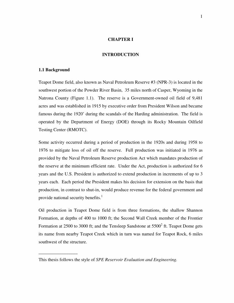
Teapot Dome field, also known as Naval Petroleum Reserve #3 (NPR-3) is located in the
southwest portion of the Powder River Basin, 35 miles north of Casper, Wyoming in the
Natrona County (Figure 1.1). The reserve is a Government-owned oil field of 9,481
acres and was established in 1915 by executive order from President Wilson and became
famous during the 1920’ during the scandals of the Harding administration. The field is
operated by the Department of Energy (DOE) through its Rocky Mountain Oilfield
Testing Center (RMOTC).
Some activity occurred during a period of production in the 1920s and during 1958 to
1976 to mitigate loss of oil off the reserve. Full production was initiated in 1976 as
provided by the Naval Petroleum Reserve production Act which mandates production of
the reserve at the minimum efficient rate. Under the Act, production is authorized for 6
years and the U.S. President is authorized to extend production in increments of up to 3
years each. Each period the President makes his decision for extension on the basis that
production, in contrast to shut-in, would produce revenue for the federal government and
provide national security benefits.1
Oil production in Teapot Dome field is from three formations, the shallow Shannon
Formation, at depths of 400 to 1000 ft; the Second Wall Creek member of the Frontier
Formation at 2500 to 3000 ft; and the Tensleep Sandstone at 55002 ft. Teapot Dome gets
its name from nearby Teapot Creek which in turn was named for Teapot Rock, 6 miles
southwest of the structure.
_________________
This thesis follows the style of SPE Reservoir Evaluation and Engineering.

2
Teapot Dome is considered as an extension of the much larger Salt Creek anticline; an
oil field operated by Anadarko Petroleum Co.
Primary depletion drive production of the Tensleep Formation began in 1978 with single
well production rates no greater than 150 STBD
Teapot Dome field initially contained more than 5 million barrels of oil in the oil column
(OC), which is the interval of the San Andres hydrocarbon accumulation above the
producing oil/water contact (OWC). The field’s producing oil water contact (POWC),
above which oil is produced water-free during primary recovery is -400 ft below sea
level. Tensleep Formation does not contain a primary gas cap.
Figure 1.1 - Location map of Teapot Dome Field.

3
1.2 Problem Description
This research evaluates the effects of natural fractures and the hydrocarbon
characterization in CO2 storage process in the Tensleep Formation. Due to the presence
of high permeability channels in the reservoir, the amount of CO2 that can be injected
varies across the field affecting the overall CO2 storage goals in the project.
Tensleep reservoir fluid composition indicates dead oil characteristics. CO2 injection
and miscibility process response depends on how the reservoir oil has been
characterized. Evaluation of different reservoir fluid models via reservoir simulation
will provide additional evidence to establish the fluid model to be used in field scale CO2
injection.
1.3 Objectives
The main objective of this research is establish the amount of CO2 that can be storage
and the additional oil that can be recovered from Tensleep Formation, Teapot Dome
field by the CO2 injection process.
The specific objectives are to evaluate how fracture permeability and reservoir
hydrocarbon model affects CO2 injection process to “co-optimize” the CO2 storage and
enhanced oil recovery performance using single and dual porosity simulation models.
Fracture permeability will be incorporated from fracture aperture measurements in core
samples using X-Ray Computer Tomography Scanner.

4
CHAPTER II
LITERATURE REVIEW
2.1 CO2 Flooding Mechanisms
Carbon dioxide injection has been used in enhanced oil recovery (EOR) processes
applicable to light to medium oil reservoirs since the 1970s; the traditional approach is
oriented to recover the higher amount of oil from the reservoir injecting the minimum
amount of gas.
There is a significant experience and knowledge in the oil industry to separate, transport,
inject and process the quantities of CO2 required in different projects.
The recovery mechanisms in immiscible processes involve reduction in oil viscosity, oil
swelling, and dissolved-gas drive. CO2 has a viscosity similar to miscible or light
hydrocarbon components. Miscible displacement between crude oil and CO2 is caused
by extraction of hydrocarbons from the oil into the CO2 and by dissolution of CO2 into
the oil. In general, CO2 is very soluble in crude oils at reservoir pressures swelling the
oil and reducing its viscosity.3
Multiple-contact miscibility process governs the mixture between CO2 and crude starting
with CO2 as a dense-phase and hydrocarbon liquid. CO2 first condenses into the oil,
making it lighter and extracting methane from the oil bank. The lighter components of
the oil then vaporize into the CO2-rich phase, making it denser, more like the oil, and
thus more easily soluble in the oil. Mass transfer continues between the CO2 and the oil
until the two mixtures become indistinguishable in terms of fluid properties. Figure 2.1
illustrates the condensing/vaporizing mechanisms for miscibility.4

5
CO2 CO2Wat
er
DriverWater
Oil
bank
Mis
cibl
e zo
ne
Add
ition
al
oil
CO2 CO2Wat
er
DriverWater
Oil
bank
Mis
cibl
e zo
ne
Add
ition
al
oil
Figure 2.1 - One-dimensional schematic showing CO2 flooding.4
Because of this mechanism, oil recovery may occur at pressures high enough to achieve
miscibility. CO2 needs to be compressed at high pressures to reach a density at which it
becomes a solvent for the lighter hydrocarbons in the crude oil. This pressure is known
as “minimum miscibility pressure” (MMP) and it is the minimum pressure at which
miscibility between CO2 and crude oil can occur.3
2.2 CO2 Storage
The CO2 storage from the flu gases did not start because environmental concerns about
green house effect, instead, it gained attention as a source for enhance oil recovery
processes. It is very likely that fossil fuels will be the main source of energy in the 21 st
century. However increased concentrations of carbon dioxide due to carbon emissions
are expected.
6
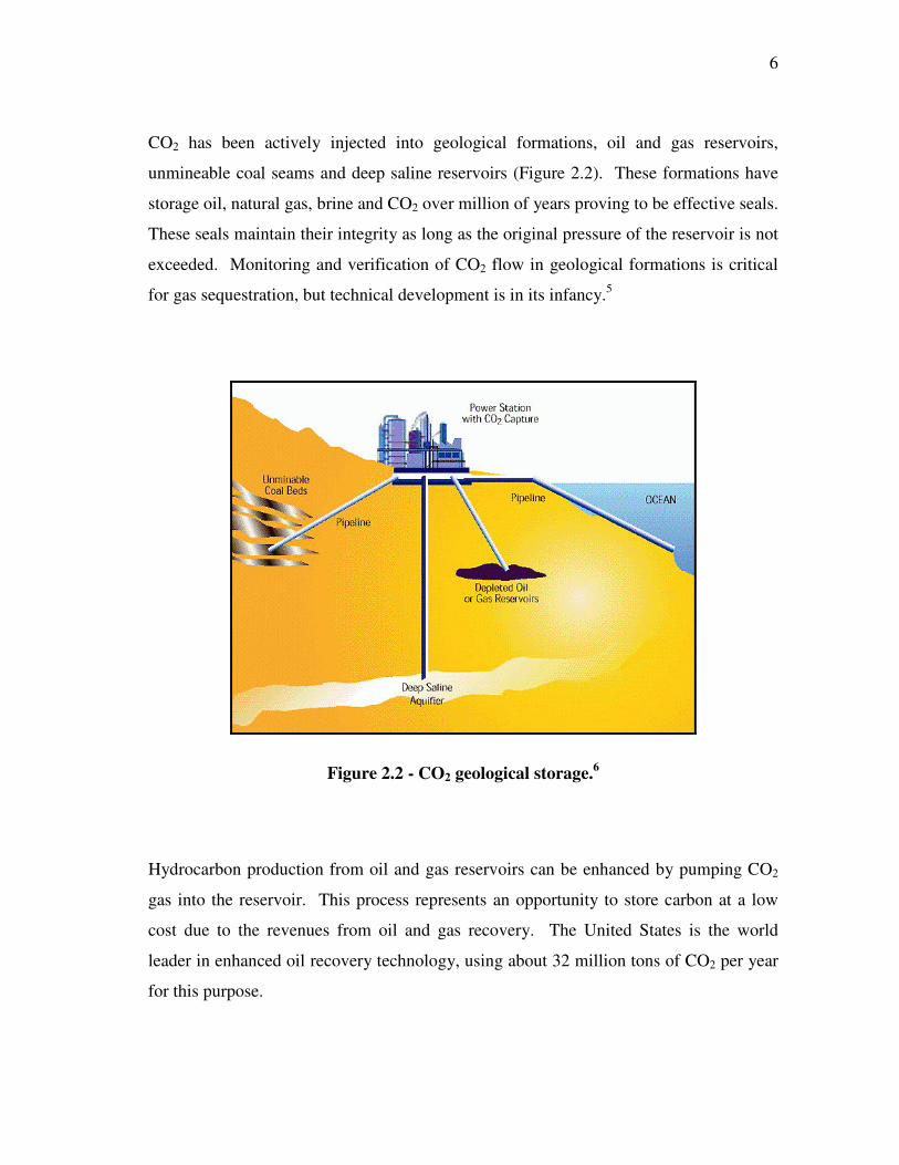
CO2 has been actively injected into geological formations, oil and gas reservoirs,
unmineable coal seams and deep saline reservoirs (Figure 2.2). These formations have
storage oil, natural gas, brine and CO2 over million of years proving to be effective seals.
These seals maintain their integrity as long as the original pressure of the reservoir is not
exceeded. Monitoring and verification of CO2 flow in geological formations is critical
for gas sequestration, but technical development is in its infancy.5
Figure 2.2 - CO2 geological storage.6
Hydrocarbon production from oil and gas reservoirs can be enhanced by pumping CO2
gas into the reservoir. This process represents an opportunity to store carbon at a low
cost due to the revenues from oil and gas recovery. The United States is the world
leader in enhanced oil recovery technology, using about 32 million tons of CO2 per year
for this purpose.

7
Coal beds typically contain large amounts of methane adsorbed onto the surface of the
coal. The current practices to recover the methane are depressurizing the coal bed or
inject CO2. CO2 have twice the methane adsorption rate and tend to remain storage in
the carbon bed.7 Methane provides a value-added revenue stream to the carbon storage
process.
Saline formations do not provide products economically exploitable when carbon is
storage, but it has other advantages. The storage capacity of saline formations in United
States has been estimated at up to 500 billion tones of CO2 and carbon sources are within
easy access to saline injection points.
Before CO2 can be stored, it must be captured as a relatively pure gas. In the United
States, however, CO2 is routinely separated and captured as a by-product from industrial
processes. Usually power plants exhaust CO2 diluted with nitrogen as flue gas.
Commonly coal-fired power plant flue gas contains 10-12 % of CO2 by volume and
from natural gas plants between 3-6 %. Existing capture technologies are not cost-
effective when considered in the context of CO2 storage from power plants.
Good oil response, gas injectivity and gas production within designed limits are
considered as positives aspects from the CO2 injection process. Simultaneously one of
the main concerns in the projects performed has been the early CO2 breakthrough, which
compromises gas processing facilities.
2.3 Parameters Affecting a CO2 Storage Process
2.3.1 Reservoir Heterogeneity
Reservoir heterogeneity has a strong influence on the gas/oil displacement process.8 The
degree of vertical reservoir heterogeneity can affect the CO2 performance. Formations
with higher vertical permeability such as naturally fractured reservoirs are influenced by
8
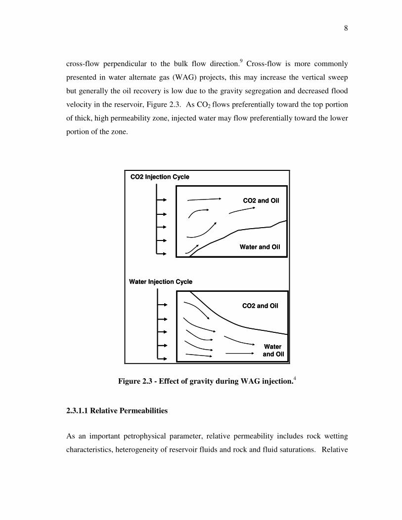
cross-flow perpendicular to the bulk flow direction.9 Cross-flow is more commonly
presented in water alternate gas (WAG) projects, this may increase the vertical sweep
but generally the oil recovery is low due to the gravity segregation and decreased flood
velocity in the reservoir, Figure 2.3. As CO2 flows preferentially toward the top portion
of thick, high permeability zone, injected water may flow preferentially toward the lower
portion of the zone.
CO2 and Oil
Water and Oil
CO2 Injection Cycle
Water Injection Cycle
Water and Oil
CO2 and Oil
CO2 and Oil
Water and Oil
CO2 Injection Cycle
Water Injection Cycle
Water and Oil
CO2 and Oil
Figure 2.3 - Effect of gravity during WAG injection.4
2.3.1.1 Relative Permeabilities
As an important petrophysical parameter, relative permeability includes rock wetting
characteristics, heterogeneity of reservoir fluids and rock and fluid saturations. Relative

9
permeability commonly changes during alternate water/CO2 injection, water injectivity is
significantly reduced after the first gas injection cycle due to the effect of CO2 on water
relative permeability. It is very important to have a good understanding of the relative
permeability curves to be used in reservoir simulators to predict the CO2 storage.4
Laboratory experiments have showed hysteresis effects in the water relative permeability
between the drainage and imbibition curves. Irreducible water saturations after drainage
cycles were 15 to 20% higher than the initial connate water saturation.10
Hysteresis refers to the directional saturation phenomena exhibited by many relative
permeability and capillary pressure curves when a given fluid phase saturation is
increased or decreased.11 This phenomena is illustrated in Figure 2.4.
Water Saturation, fraction0.2 0.3 0.4 0.5 0.6 0.7 0.8
Oil
Water
Water(hysteresis)
1.0
0.1
0.01
0.001
Maximum Krwfor waterflood
Rel
ativ
e P
erm
eabi
lity,
frac
tion
Water Saturation, fraction0.2 0.3 0.4 0.5 0.6 0.7 0.8
Oil
Water
Water(hysteresis)
1.0
0.1
0.01
0.001
Maximum Krwfor waterflood
Rel
ativ
e P
erm
eabi
lity,
frac
tion
Figure 2.4 - Two-phase relative permeability diagram.7

10
2.3.1.2 Natural Fractures
Structures such as fractures, fracture networks, and faults can influence permeability and
therefore fluid flow within an aquifer or petroleum reservoir. Distinct permeability
anisotropy has been observed in reservoirs with low matrix permeability and a well
developed open fracture systems, with the highest permeability parallel to the fractures.
Within a given rock volume, fractures generally result in an overall permeability
increase. Significant interaction between the fracture surface and the matrix allows
better drainage of the rock matrix. This matrix/fracture interaction could allow for a
substantial increase in recoverable hydrocarbon reserves.
In contrast, mineralized fractures and deformation bands (i.e., small displacement faults
characterized by tight cataclasis and/or pore reduction through compaction) are typically
characterized by significant permeability reduction. Where fractures are mineralized or
the rock is cut by deformation bands, the rock matrix is more permeable than the
structures, so the rock is more permeable parallel to, and between, fractures and
deformation bands. Therefore, within a given rock volume containing mineralized
fractures and/or deformation bands, there will be overall permeability decrease and
possible reservoir compartmentalization. Partially mineralized fractures may still have
some permeability. However, there could be a significant reduction in the interaction
between the remaining open fracture fluid pathway and the rock matrix. Either
mineralized or partially mineralized fractures could have the effect of decreasing the
total amount of recoverable reserves.
Fractures commonly increase or decrease permeability in certain directions and thus
introduce permeability anisotropy and heterogeneity; and it is important, from a
production standpoint, that they can be modeled accurately. It can be very difficult,
however, to predict the location, spacing and orientation of fractures and small-
displacement faults in the subsurface. Most regional fractures are sub-vertical, and are
thus unlikely to be sampled in vertical boreholes. Reasonable predictions of
11
permeability anisotropy require an understanding of controls on the distribution and
orientations of such features. Fractures can have predictable orientations with regard to
large-scale structures such as anticlines.
For modeling and production purposes, it is important to document directions of
preferred fracture and fault orientations within primary hydrocarbon traps, such as
anticlines. By understanding controls on fracture and fault orientation and distribution in
a given reservoir, the accuracy of flow modeling can be improved, thereby increasing
primary and secondary hydrocarbon recovery.12
2.3.2 Reservoir Fluids
Reservoir fluid composition controls the miscible process between the reservoir fluid
and injected CO2. CO2 is less dense and viscous than reservoir fluids
Complete dissolution of injected CO2 takes place in a scale of hundred to thousand of
years, this depending on the gas migration and fluids reaction.13
When reservoir characterization is well understood and described, CO2 injection process
has performed as expected.
As carbon dioxide CO2 is injected in the formation, it mobilizes oil, dissolves into brine
and promotes dissolution of carbonates cements.14 Brine can become supersaturated
with dissolved solids and when pressure drops as it advances through the reservoir,
precipitates such as gypsum can form.5
12
CHAPTER III
2. GEOLOGY REVIEW
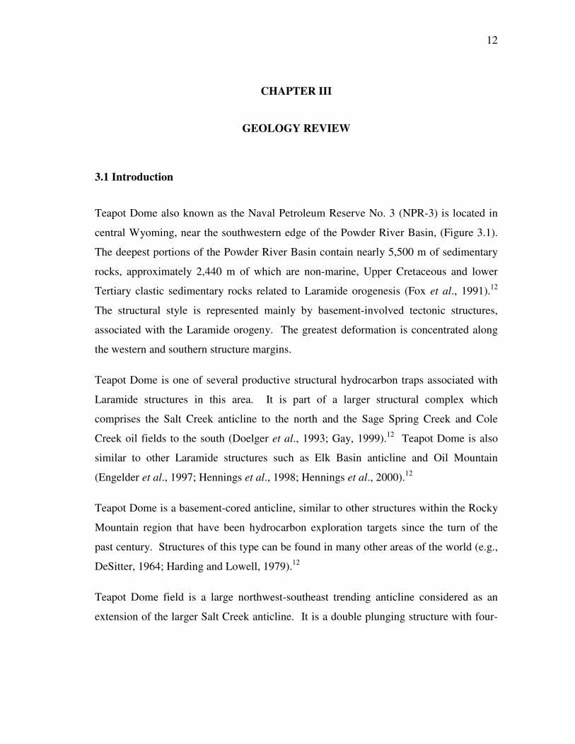
3.1 Introduction
Teapot Dome also known as the Naval Petroleum Reserve No. 3 (NPR-3) is located in
central Wyoming, near the southwestern edge of the Powder River Basin, (Figure 3.1).
The deepest portions of the Powder River Basin contain nearly 5,500 m of sedimentary
rocks, approximately 2,440 m of which are non-marine, Upper Cretaceous and lower
Tertiary clastic sedimentary rocks related to Laramide orogenesis (Fox et al., 1991).12
The structural style is represented mainly by basement-involved tectonic structures,
associated with the Laramide orogeny. The greatest deformation is concentrated along
the western and southern structure margins.
Teapot Dome is one of several productive structural hydrocarbon traps associated with
Laramide structures in this area. It is part of a larger structural complex which
comprises the Salt Creek anticline to the north and the Sage Spring Creek and Cole
Creek oil fields to the south (Doelger et al., 1993; Gay, 1999).12 Teapot Dome is also
similar to other Laramide structures such as Elk Basin anticline and Oil Mountain
(Engelder et al., 1997; Hennings et al., 1998; Hennings et al., 2000).12
Teapot Dome is a basement-cored anticline, similar to other structures within the Rocky
Mountain region that have been hydrocarbon exploration targets since the turn of the
past century. Structures of this type can be found in many other areas of the world (e.g.,
DeSitter, 1964; Harding and Lowell, 1979).12
Teapot Dome field is a large northwest-southeast trending anticline considered as an
extension of the larger Salt Creek anticline. It is a double plunging structure with four-

13
way closure, asymmetrical and SW verging; limited on its west flank by a large regional
fault.
One of the primary reasons basement-cored anticlines are exploration targets is that they
can provide excellent four-way closure. Four-way closure can allow the entrapment of
migrating hydrocarbons in economically significant amounts. To maximize recovery of
these trapped hydrocarbons, it is essential to accurately model any permeability
anisotropy associated with these structures.
A total of nine (9) productive horizons (Figure 3.2) including the shales of Shannon,
Steele and Niobara formations are present, Second Wall Creek and Tensleep sandstone
formations being the most productive. Tensleep is the lowest producing formation found
in Teapot Dome and is generally found at the bottom of each well, which complicates
the formation evaluation as the layer is not completely logged.15
Figure 3.1 - Location of Teapot Dome Field in the Permian Basin.17

14
Figure 3.2 - Generalized stratigraphic column showing Permian section at the
Teapot Dome field.16
15
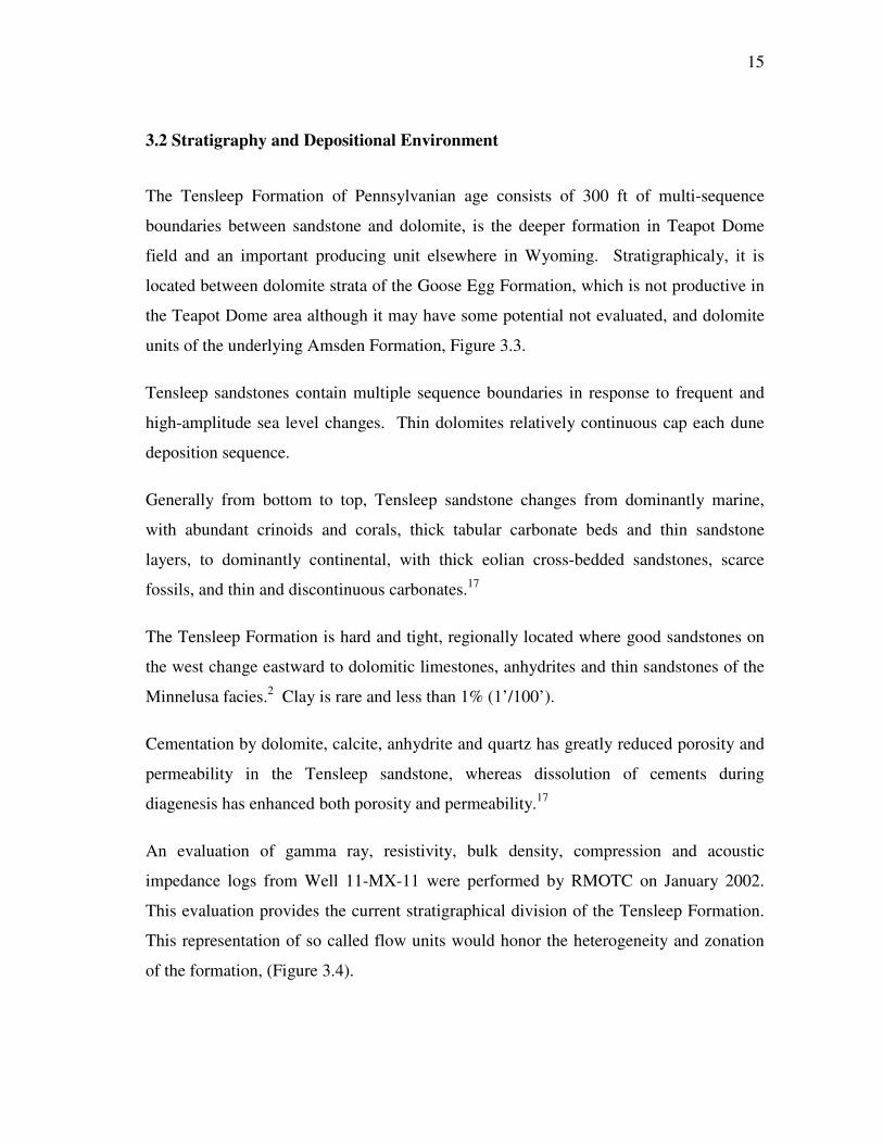
3.2 Stratigraphy and Depositional Environment
The Tensleep Formation of Pennsylvanian age consists of 300 ft of multi-sequence
boundaries between sandstone and dolomite, is the deeper formation in Teapot Dome
field and an important producing unit elsewhere in Wyoming. Stratigraphicaly, it is
located between dolomite strata of the Goose Egg Formation, which is not productive in
the Teapot Dome area although it may have some potential not evaluated, and dolomite
units of the underlying Amsden Formation, Figure 3.3.
Tensleep sandstones contain multiple sequence boundaries in response to frequent and
high-amplitude sea level changes. Thin dolomites relatively continuous cap each dune
deposition sequence.
Generally from bottom to top, Tensleep sandstone changes from dominantly marine,
with abundant crinoids and corals, thick tabular carbonate beds and thin sandstone
layers, to dominantly continental, with thick eolian cross-bedded sandstones, scarce
fossils, and thin and discontinuous carbonates.17
The Tensleep Formation is hard and tight, regionally located where good sandstones on
the west change eastward to dolomitic limestones, anhydrites and thin sandstones of the
Minnelusa facies.2 Clay is rare and less than 1% (1’/100’).
Cementation by dolomite, calcite, anhydrite and quartz has greatly reduced porosity and
permeability in the Tensleep sandstone, whereas dissolution of cements during
diagenesis has enhanced both porosity and permeability.17
An evaluation of gamma ray, resistivity, bulk density, compression and acoustic
impedance logs from Well 11-MX-11 were performed by RMOTC on January 2002.
This evaluation provides the current stratigraphical division of the Tensleep Formation.
This representation of so called flow units would honor the heterogeneity and zonation
of the formation, (Figure 3.4).
16
Figure 3.3 - Late Paleozoic stratigraphic chart of part of Wyoming.17
TOP TNSP
UNIT 1
UNIT 2
UNIT 3
UNIT 4
UNIT 5
UNIT 6
TNSP BASE NOT DEFINED
TOP TNSP
UNIT 1
UNIT 2
UNIT 3
UNIT 4
UNIT 5
UNIT 6
TNSP BASE NOT DEFINED
Figure 3.4 - Tensleep Formation type log well 11-MX-11.

17
3.3 Seismic Interpretation
A 3D seismic survey designed to image the Pennsylvanian Tensleep Formation was shot
in the field on January 2001, with a coverage of 72.3 square kilometers (17800)
consisting of 345 in-lines and 188 cross-lines with a bin size of 110 ft. 38 km2 was
available for interpretation. This 3D seismic information covers the Teapot Dome
structure completely as shown in Figure 3.5.
Figure 3.5 – Time map showing seismic coverage at Tensleep Formation.

18
From a gravity survey view point, the basement rock, referred to as granite, will be
approximately 750 feet closer to the surface at the top of the anticline than at the edges.
The density contrast in the overlying formations is essentially the intrusion of the higher
density granite basement as compared with the marine shales and sandstones of the
producing formations.15
3.3.1 Time Interpretation
A post-stack migrated volume acquired on January 2001 was interpreted in time. Well
log information and geological tops measured in Well 62-X-11 were used to generate a
velocity log and a synthetic seismogram (Figure 3.6). This well provides useful
information to assist with the interpretation. The synthetic seismogram allowed the
identification of a dolomite marker at the top of Tensleep Formation (TNSP) (Figure
3.7). This marker has good seismic continuity in the area of interpretation.
NORMAL REVERSE DT VELOCITY
TNSP 6000
Alcova
Crow Mt
Second Wall
Dolo
NORMAL REVERSE DT VELOCITY
TNSP 6000
Alcova
Crow Mt
Second Wall
Dolo
Figure 3.6 - Seismogram log from well 62-X-11.

19
Figure 3.7 - Synthetic seismogram from well 62-X-11.
The interpretation of the dolomite marker provided a top isochron map that indicates a
semi-regular spaced northeast-southwest trending fault system cutting the horizon with
major faults approximately every mile.
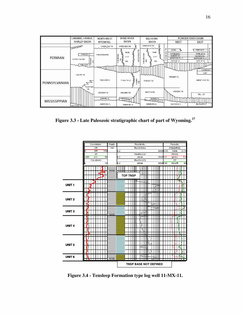
The main fault (MF1) is a reverse fault that strikes NW-SE, and is considered to be the
west limit of the field, A second system of normal faults with N45E direction is present,
where fault 3 (F3) divides the Tensleep structure in Teapot Dome field from Salt Creek
field, Figure 3.8.
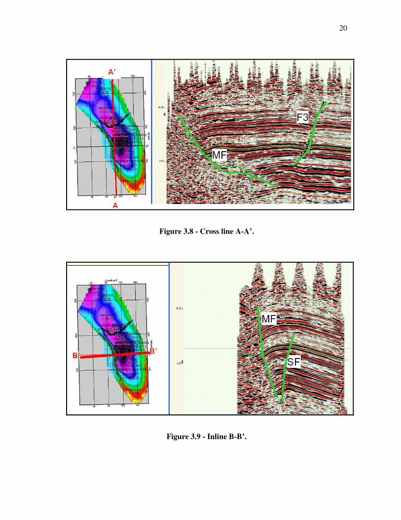
A third strike fault (SF) located south of fault F3 is at crest of the structure. This area
can be considered of good productivity because most of the wells are located near this
fault, (Figure 3.9). The Final isochron map at top of Tensleep Formation can be observed
in Figure 3.10.
20
Figure 3.8 - Cross line A-A’.
Figure 3.9 - Inline B-B’.

21
Figure 3.10 - Isochron Map for Tensleep Formation at Teapot Dome.
22
3.3.2 Time to Depth Conversion
A structural map at the top of the Tensleep Formation was generated by integrating
seismic time interpretation and well depths information, (Figure 3.11). The conversion
was done by the multiplication of the isochron grid with the average velocity or pseudo-
velocity grid. The pseudo-velocity map came from the Tensleep depth in the wells and
the time in the isochron map, this velocity is in agreement with the velocity calculated
from the sonic log.
No check shots or vertical seismic profiles (VSP) data have been taken in the field. An
average of 4267 m/sec was used to generate a projection from the time surface into
elevation map.
The structural map has the sub sea level as reference and it was weighted with the well
tops information in the field.
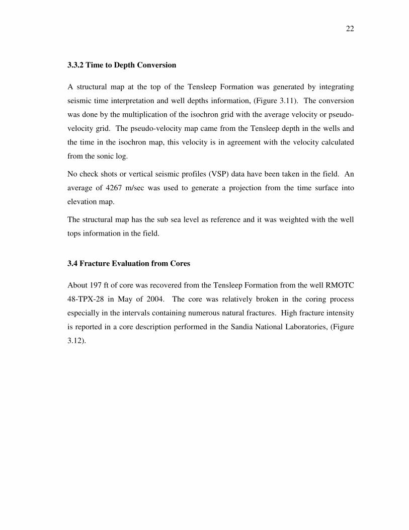
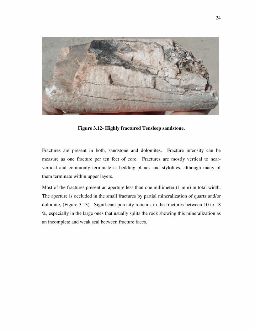
3.4 Fracture Evaluation from Cores
About 197 ft of core was recovered from the Tensleep Formation from the well RMOTC
48-TPX-28 in May of 2004. The core was relatively broken in the coring process
especially in the intervals containing numerous natural fractures. High fracture intensity
is reported in a core description performed in the Sandia National Laboratories, (Figure
3.12).

23
Figure 3.11- Structural Map for Tensleep Formation.
24
Figure 3.12- Highly fractured Tensleep sandstone.
Fractures are present in both, sandstone and dolomites. Fracture intensity can be
measure as one fracture per ten feet of core. Fractures are mostly vertical to near-
vertical and commonly terminate at bedding planes and stylolites, although many of
them terminate within upper layers.
Most of the fractures present an aperture less than one millimeter (1 mm) in total width.
The aperture is occluded in the small fractures by partial mineralization of quartz and/or
dolomite, (Figure 3.13). Significant porosity remains in the fractures between 10 to 18
%, especially in the large ones that usually splits the rock showing this mineralization as
an incomplete and weak seal between fracture faces.

25
Figure 3.13- Natural fracture face partially covered with crystalline dolomite.
Some parallel and intersecting fractures were found in fine-grained dolomites where one
of them was filled with dolomite in a 70% to 80%.
Bitumen lined fractures was observed in the fine-grained, white dolomite facies that
overlies oil-stained reservoir sandstone.
A zone of inclined fractures, possibly a conjugated shear system is very similar to that
seen in Tensleep outcrops at south of Alcova reservoir. FMI log indicates that the
maximum horizontal in-situ compressive stress and most of the natural fractures strike
E-W to WNW-ESE.
High degree of fracture connectivity supported by past pressure interference tests is
present. A pump-off operations of a Tensleep completion, was felt impacted by
operational swings in high volume Salt Creek field Tensleep producers.18

26
3.5 Lithologic Controls
Both fracture spacing and orientation vary with lithology at Teapot Dome. In general,
fractures are most closely spaced in carbonaceous shales (Unit 4), more widely spaced in
fluvial (Unit 5) and beach (Unit 2) sands, and most widely spaced in marine shales (Unit
1). Fractures are generally absent, replaced by deformation bands; within the white
beach sandstones of Unit 3.18

27
CHAPTER IV
RESERVOIR PERFORMANCE
4.1 Reservoir Basic Data
Teapot Dome Field is considered as the continuation of the Salt Lake Field operated by
Anadarko Petroleum Company. Teapot Dome produces light and sweet (low sulfur
content, 0.16 %) oil from nine different formations. Just Tensleep Formation produces a
lower gravity, sulfurous oil. This oil is mainly used for oiling roads and other lease uses.
Tensleep the lower productive unit is located at subsea depths approximately at 5500
feet (5000 ft-ss).
Tensleep Formation is Pennsylvanian dolomite cemented sandstone with a gross
thickness that varies between 250 and 300 ft. A net oil pay thickness about 75 feet has
been measured from logs. It has been estimated that Tensleep Formation initially
contains nearly 4.5 million barrels of oil in place. Hydrocarbon is accumulated between
the high structural point at 80 ft-ss and the producing oil/water contact (OWC) estimated
at 400 ft-ss.
No pressure data have been recorded in the formation, water production rates indicates
that underlying formations are influenced by a strong aquifer. The aquifer has
maintained almost constant reservoir pressure during the course of the field life. The
pressure drop is less than 100 psi through out the Tensleep Formation. Water drive then
considered as the primary producing mechanism in the reservoir. Table 4.1 summarizes
basic reservoir and fluid data.

28
Table 4.1 - Summary of reservoir data.
Reservoir Characteristics ValuesProducing area 440 acresFormation Pennsylvanian Dolomitic TensleepAverage Depth 5500 ftGas-oil Contact No presentAverage Matrix Permeability 80 mDAverage Porosity 13.50%Oil Gravity 31 °APIReservoir Temperature 190 °FPrimary production mechanism Water DriveOriginal reservoir pressure 2300 psiBubble point pressure 40-70 psiAverage pressure at start of CO2 injection 2000± 100 psiInitial FVF 1.312 RB/BBLSolution GOR at original pressure 4 SCF/BBL
Oil viscosity at 60° F and 42 psi 3.5 cpMinimum miscibility pressure 1300 psi
4.2 Reservoir Development History
Teapot Dome field had its first production from the so-called “Dutch” well with 200
BOPD from First Wall Creek sandstone in 1908. In 1909 a few wells value were drilled
to develop the Shannon sand.
Prior to initiating the development and exploration program at Teapot Dome in 1976,
233 wells were drilled in all the producing formations. At 1996 additional 1007
development wells and 90 exploratory wells were drilled. 27 of the 1007 wells were
drilled in fiscal year 1996 targeting Tensleep Formation. Two of these wells
experienced the highest initial production rates of any wells in Wyoming at that time
paying for their capital cost in less than 3 months.

29
Primary depletion began on 1977 when six wells were drilled in Tensleep Formation,
however just one the structurally highest is capable of production (Well 74-CMX-10)
with intermittent rates lower than 10 BOPD.2
Historical oil and water production from Tensleep Formation can be observed in Figure
4.1.
PRODUCTION DATA FIELD HISTORY FILEDefault-Field-PRO Production rates.fhf
Oil Rate SC Water Rate SC
Time (Date)
Oil
Rat
e S
C (b
bl/d
ay)
1980 1985 1990 1995 2000 20051.00e+1
1.00e+2
1.00e+3
1.00e+4
1.00e+5
Figure 4.1 - Tensleep Formation production history.

30
CHAPTER V
SIMULATION PARAMETERS AND MODEL
All the reservoir parameters used in the simulation model are described in this chapter.
Evaluation and definition of rock properties to be used in reservoir simulation is
presented. Matrix and fractures relative permeabilities and capillary pressure data from
Tensleep cores were defined. Matrix wettability and fracture spacing is established.
Calibration of equation-of-state to describe phase behavior of the reservoir fluid was
obtained. Evaluation of compositional Vs pseudo-miscible approach is presented. The
number of components in the fluid sample and component lumping process were
compared to obtain the best fluid model in terms of accuracy in laboratory data
reproduction and efficiency in simulation run time.
The initialization of the simulation model was conducted to assess the volume of the
original hydrocarbon in place.
5.1 Numerical Simulator
One of the concerns about the reservoir fluid model was to select the simulator that best
represents CO2 displacement process. Compositional simulation and pseudo-miscible
black oil models have been widely used to reproduce CO2 displacement processes. The
compositional simulators GEMTM 19 and, the black oil finite-difference simulator
IMEXTM 20 were used in this study.
One compositional and one pseudo-miscible model were built to evaluate the accuracy
of the black to represent CO2 displacement process. Compositional simulation use
equations of state (EOS) with theoretical parameters that are able to predict fluid
behavior of hydrocarbon mixtures commonly encountered in oil and gas reservoirs.
31
Pseudo-miscibility simulator is a black oil approximation that takes into account only the
gas dissolution.
Compositional model construction is time consuming and expensive. Pseudo-miscible
option is capable of modeling the essential features of miscible displacement while
leaving the fine structure of unstable miscible flow unresolved, making it possible to
represent the reservoir by a fairly coarse numerical grid.21
5.2 Relative Permeability
5.2.1 Matrix Relative Permeability
Four rock samples were used in relative permeability laboratory tests. One sample A
from 62-TPX-10 well (5443’) and three samples from 43-TPX-10 well; sample B
(5486’), sample C (5492’) and sample D (5500’). The tests were performed using
simulated reservoir brine and mineral oil with a viscosity of 30 cp.
Similar rock compositions have been encountered in the samples, sandstones with fine to
very fine grains and well indurate are basic characteristics. Despite the similar
composition, relative permeability experiments show important differences in the end-
points. Initial water saturations (Swi) are between 12.5% to 22.1 and residual oil
saturations (Sro) are between 28.7% and 56.3%, Figure 5.1.

32
������������������
���
���
���
���
���
���
� �� �� �� �� ���
������������������
������������������ ������
��� � ���� � ����� ������
����� ������ ����� ������
�����������������������������
���
���
���
���
���
���
� �� �� �� �� ���
������������������
������������������ ������
��� � ���� � ����� ������
����� ������ ����� ������
Figure 5.1 – Water-oil relative permeability curves as a function of water
saturation.
The two phase oil-water at Sg = 0 and gas-oil relative permeability curves used for the
CO2 simulation are shown in Figures 5.2 and 5.3. To avoid complication and make the
model simulation simple, this set of curves was used to describe both the oil column and
the transition zone.

33
0.00
0.20
0.40
0.60
0.80
1.00
krw
0.00 0.20 0.40 0.60 0.80 1.00Sw
krw vs Swkrow vs Sw
Figure 5.2 – Water-oil relative permeability curves.
0.00
0.20
0.40
0.60
0.80
1.00
krg
0.00 0.20 0.40 0.60 0.80 1.00Sl
krg vs Slkrog vs Sl
Figure 5.3 - Gas-oil relative permeability curves.

34
The maximum oil relative permeability is 0.65 at connate water saturation (Swc = 15%).
At 60% water saturation, the oil relative permeability is almost zero. As water saturation
increases in the reservoir, the water relative permeability increases, reaching a maximum
value of 0.04 at 94% water saturation.
Hysteresis effect is not considered in the simulation, after the drainage process of water
displacing oil, CO2 injection is going to be the governing displacement process.
5.2.2 Fracture Relative Permeability
A lot of research have been done in the characterization of relative permeability in
fractures, it have been found that fracture aperture changes due to compaction,22
mineralization and other factors affect the fluid flow. Roughness, capillary pressure and
wettability constitute influence factors in the fluid flow interference; therefore, the
assumption of straight lines in oil-water relative permeability would not the best
representation.23
However, considering very high fracture permeability values, straight line relative
permeability curves were used in this study.
5.3 Capillary Pressure
Three rock samples from Tensleep were selected for capillary pressure data, this samples
were extracted from well 56-TPX-10; samples E (5391’) and F (5400’) and from well
44-1-TPX-10; sample G (5538’).
The samples indicate a very similar lithological description, however, the initial water
saturation values observed vary widely from 10.8% to 20.4%. Capillary pressure curves
in the three samples show low displacement pressure (about 1 psi), this is an indication
of good reservoir; very good sorting and big pore throats (W. Ahr, Carbonate Reservoir
Course, Professor, Department of Geology and Geophysics, Texas A&M University).

35
Capillary pressure laboratory tests were performed using an air-brine system. These data
were corrected to obtain oil-water capillary pressure values at reservoir conditions as
shown in Figure 5.4. In order to do this correction, the following equation was applied:
( )( ) labPc
labres
resPc ,coscos
,θσθσ=
where σ is interfacial tension and θ is the contact angle.
Laboratory Capillary Pressure
0
5
10
15
20
25
30
35
40
0 20 40 60 80 100
Water Saturation (%)
Pre
ssur
e (p
si)
Sample E Sample F Sample G
Reservoir Capillary Pressure
0
5
10
15
20
25
30
35
40
0 20 40 60 80 100
Water Saturation (%)
Pre
ssur
e (p
si)
Sample E Sample F Sample G
Figure 5.4- Capillary pressure curves at laboratory and reservoir conditions.
In order to account for porosity and permeability changes, normalization of capillary
values, were conducted using the Leverett J function as follows:
( ) φθσkPc
SJ n cos*2166.0
)( =
36
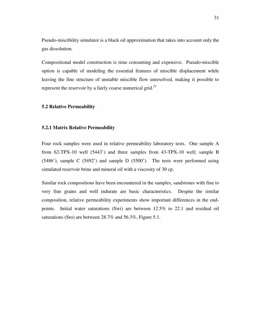
Matrix capillary pressure was calculated from the average J curve using a regression of
all data points in Sw vs. J plot as sown in Figure 5.5. Capillary pressure for fractures
was assumed to be zero.
Leverett J Function
������������������
�����������
���
���
���
���
���
���
� �� �� �� �� ���
Water Saturation (%)
J (S
w)
����� �����������
Reservoir Capillary Pressure
0
5
10
15
20
25
30
35
40
0 20 40 60 80 100
Water Saturation (%)
Pre
ssur
e (p
si)
Sample E Sample F
Sample G Average Pc
Figure 5.5 - Laboratory and average reservoir capillary pressure curves.
5.4 Wettability
A wettability test was performed in a core sample from the well 62-TPX-10 (5418’) at
reservoir temperature of 190 °F. Synthetic brine and crude oil were flushed through the
sample. Evaluation of results provides a water-wet indicator of 0.402 versus oil-wet
indicator of 0.033.

37
The water-wet indicator is a relation between the volume oil displaced spontaneously
when the oil saturated rock sample is submerged in the synthetic brine, and the total oil
volume displaced injecting brine in the sample up to residual oil saturation conditions.
5.5 Fracture Spacing
According with the measurements of fracture spacing in Tensleep core samples, a
homogeneous matrix dimension of 10 ft were used in the dual-porosity simulation
model.
5.6 Fluid Properties
The reservoir oil is sulfurous saturated black oil with a stock tank gravity of 31.4 °API
and with a laboratory initial gas-oil ratio between 2 and 4 SCF/STB. Initial reservoir
pressure and temperature are 2300 psi at reference depth of 5500 ft and 190 °F, bubble
pressure and minimum miscibility pressure was determined experimentally to be of 42
psia and 1,300 psi respectively
5.6.1 PVT Information
Two bottom-hole oil samples were recollected and tested in the wells 54-TPX-10
(sample A) on June 15, 1984 and 62-TPX-10 (sample B) on April 28, 1986. The
saturation pressure measured in the samples is between 61 to 76 psia. Very low value
considering that higher saturation pressures can be expected in oil samples with stock
tank API gravity of 31.4° and 31.1° in samples A and B, respectively. Table 5.1 shows
the fluid composition.

38
Table 5.1 - Reservoir fluid composition in mole fractions.
Sample A Sample B Sample C
CO2 0.04 0.03 0.08
N2 1.08 0.05 0.13
C1 0.01 0.01 0.02
C2 0.03 0.04 0.12
C3 0.13 0.03 0.17
i-C4 0.1 0.01 0.08
n-C4 0.29 0.02 0.22
i-C5 0.59 0.01 0.15
n-C5 0.39 0.01 0.3
C6 0.98 0.02 1.29
C7+ 96.36 99.7 97.44
Mw C7+ 285 270 303.85
Density C7+ @ 60°F, gr/cm3 0.8284 0.8694 0.8972
Temperature (°F) 190 190 190.4
Mol FractionComponent
Composition analysis for the samples A and B show very low content of light
components, where almost 100% mole percent of plus fraction were found.
Fluid composition, constant composition expansion, differential liberation and separator
tests were performed. Values of solution gas-oil ratio between 1 and 4 SCF/STB were
measured at standard conditions and supported by the zero gas-oil ratio found in
production reports. The amount of gas dissolved in the oil is very low and almost
impossible to measure in the field.
A third PVT (sample C) was taken in 2004 from well 72-TPX-10 at surface conditions.
Oil sample was recombined with a gas sample to obtain a reservoir fluid sample and
performed a miscibility evaluation. Composition up to C30+ was measured in this
sample.

39
Constant composition expansion (CCE) was run on the reservoir fluid adding four (4)
different CO2 amounts for a known volume of reservoir fluid at reservoir temperature of
190.4 °F. Swelling Factor (SF), density and viscosity were measured for the different
oil-CO2 mixtures.
The three oil reservoir samples show the basic characteristics of the reservoir fluid have
remained the same. Molar percentage of plus fraction between 95 to 98% and small oil-
gas ratio were found. These data were used to tune an EOS capable of characterizing the
CO2/reservoir-oil system above the minimum miscibility pressure (MMP).
Table 5.2 lists the experiments and the measured parameters loaded into the PVT
software.
Table 5.2 - PVT experimental data.
Experiment Description
Reservoir Fluid Composition Mole fractions, C30+ density and molecular weight
Constant Composition Expansion Relative Volumes, saturation pressure, oil density
Injection Test Swelling test
Phase diagrams for samples A and C were generated to evaluate the possible changes of
the reservoir fluid characteristics after two decades of production. The two phase
diagrams are representatives of black oil fluids. At reservoir temperature phase
diagrams show a saturation pressure near 20 psi, this value is lower than the values
measured in the lab from the two samples.
Sample C, the latest oil sample was chosen to evaluate the reservoir simulation of CO2
injection process, because it is the only tests that includes swelling information.

40
5.7 Fluid Model Selection
In compositional simulation, the computational time is proportional to the number of
components considered in the fluids model. Therefore it is necessary to evaluate the
effect of the number of components in the EOS tuning, this considering that the sample
with swelling information is characterized up to C30+ component.
Two different compositions were used, the original components that goes up to C30+ and
a compressed one with components up to C6+. For the last one, plus component was
splitted into five pseudo-components. Simulation results from the compressed
components were compared with the results from the original components. The results
of these simulations are presented late in this chapter. The fluid models have different
critical points and the phase diagrams. However at reservoir temperature (190 °F) the
equilibrium lines of initial component behave very similar to those for the compressed
components as shown in Figure 5.6.
Tensleep C6 Plus SplittingC6 plus : P-T Diagram
0
100
200
300
400
500
600
-200 0 200 400 600 800 1000 1200 1400
Temperature (deg F)
Pre
ssu
re (
psi
a)
2-Phase boundary Critical 20.000 volume %
40.000 volume % 60.000 volume % 80.000 volume %
Tensleep Full Composition Fluid ModelFull Comp C30+ : P-T Diagram
0
50
100
150
200
250
300
350
-200 0 200 400 600 800 1000
Temperature (deg F)
Pre
ssu
re (
psi
a)
2-Phase boundary Critical 20.000 volume %
40.000 volume % 60.000 volume % 80.000 volume %
99.000 volume %
Figure 5.6- Phase diagrams for C6+ and C30+.
41
5.7.1 Equation-of-State Characterization
CO2 injection in an oil reservoir as a miscible process needs the best phase equilibrium
prediction during the CO2 injection process. EOS has general acceptance as tools
calculate the complex phase behavior associated with rich condensates, volatile oils and
gas injection processes.24 Tuning an equation-of-state (EOS) that reproduces the
observed fluid behavior is required to accurately predict the CO2 /oil phase behavior in
the compositional simulation.
WinProp, a CMGTM software was used in the EOS tuning process. The characterization
of CO2-oil mixtures process follows the methodology suggested by Khan.25 The Peng-
Robinson26 EOS was chosen because it is applicable for low-temperature CO2/oil
mixtures.25 The viscosity model from Lohrenz-Bray-Clark (LBC)27 was considered.
5.7.2 EOS Tuning Process for C6+ Sample
PVT simulation model for EOS tuning process was performed using Peng-Robinson
EOS. First, a model with no regression of any parameters (Initial curve) was run. Then
a second model by changing plus fraction critical properties and binary interaction
coefficients between CO2 and the plus fraction (Final curve) was generated, (Figure 5.7).
Results from the runs show a very poor reproduction of the laboratory observations
(PVT-lab). Neither the original Peng-Robinson EOS nor the modified EOS with
regressed C6+ critical properties could reproduce swelling factor and saturation pressure.

42
Swelling Factor and Saturation Pressure Calculation Regression Summary
0
500
1000
1500
2000
2500
0.0 0.1 0.2 0.3 0.4 0.5 0.6 0.7 0.8Composition (mol fraction)
Sat
urat
ion
Pre
ssur
e (p
sia)
(
0
20
40
60
80
100
120
Sw
ellin
g F
acto
r (
Exp. Psat Init. Psat Final Psat Exp. S.F. Init. S.F. Final S.F.
Figure 5.7 - Initial swelling factor for C6+ sample.
The EOS tuning was a multi-step process starting by splitting the heavy component C6+
as proposed by Whitson.28 Whitson’s method uses a three-parameter gamma probability
function to characterize the molar distribution (mole fraction / molecular weight relation)
and physical properties of petroleum fractions such as heptanes-plus (C7 +), preserving
the molecular weight of the plus fraction.29 This method is used to enhance the EOS
predictions.
Since a single heavy fraction lumps thousands of compounds with a carbon number
higher than seven, the properties of the heavy component C7+ are usually not known
precisely, and thus represent the main source of error in the EOS and reducing its
predictive accuracy. For this reason, regressions were performed against the pseudo-
components to improve the EOS predictions.

43
The C6+ component was splitted into five pseudo-components based on its relative mole
fraction as suggested by Khan.25 The pseudo components were identified as C6-C12(1),
C13-C19(2), C20-C27(3), C28-C29(4) and C30+. By splitting the heavy component (C6+),
the total number of components of the reservoir fluid was then increased from 9 to 13
components. This 13-component mixture was used to tune the EOS to match data.
WinPropTM suggest some parameters to be changed in an initial regression. A total of 21
parameters were changed including critical pressure (Pc), critical temperature (Tc),
critical volume (Vc), molecular weight (MW) of the heavy pseudo-components. Also
binary interaction coefficients between the carbon dioxide and the heavy pseudo-
components were modified. Although a good match was achieved, this model is not
efficient, because many number of parameters need to be modified to match laboratory
data.
In the attempt to reduce the number of parameters to be changed and preserve the EOS
as original as possible, several models with less number of parameters were run.
Finally, only modifications of the heaviest pseudo component C30+ critical properties
(Pc and Tc), and binary interaction coefficients CO2-C1 and CO2-C30+ were necessary to
match swelling data (Figure 5.8). Swelling factor is not only function of the amount of
CO2 dissolved, but also of the size of the oil molecules.30 Plus fraction molar weight
was also used as regression parameter to obtain a confident match in the swelling and
saturation pressure calculation.

44
Swelling Factor and Saturation Pressure CalculationRegression Summary
0
500
1000
1500
2000
2500
3000
0.00 0.10 0.20 0.30 0.40 0.50 0.60 0.70 0.80
Composition (mol fraction)
Sat
urat
ion
Pre
ssur
e (p
sia)
()
0.00
0.20
0.40
0.60
0.80
1.00
1.20
1.40
Sw
ellin
g Fa
ctor
(
Exp. Psat Init. Psat Final Psat Exp. S.F. Init. S.F. Final S.F.
Figure 5.8 - Match of swelling factor splitting C6+.
Simultaneously the sample with composition up to C30+ was tuned following the same
procedure described before. No splitting process was applied to the C30+ component.
The regression parameters used to match the swelling experiment were Pc, Tc and
molecular weight in the heaviest pseudo-component, as in the C6+ sample.
A reservoir fluid model with 30 components represents a large number of equations to
be solved in reservoir simulation, which is the reason why this model is not practical in
terms of simulation running time.
Pseudoize, group or lump the components into a fewer number of pseudo-components is
performed primarily for speeding up the simulation running time. Fewer components
result in faster run time. The Fevang31 lumping process consists of forming new pseudo-
components from existing 13 was used.
45
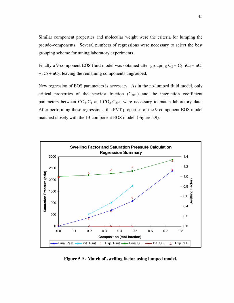
Similar component properties and molecular weight were the criteria for lumping the
pseudo-components. Several numbers of regressions were necessary to select the best
grouping scheme for tuning laboratory experiments.
Finally a 9-component EOS fluid model was obtained after grouping C2 + C3, iC4 + nC4
+ iC5 + nC5, leaving the remaining components ungrouped.
New regression of EOS parameters is necessary. As in the no-lumped fluid model, only
critical properties of the heaviest fraction (C30+) and the interaction coefficient
parameters between CO2-C1 and CO2-C30+ were necessary to match laboratory data.
After performing these regressions, the PVT properties of the 9-component EOS model
matched closely with the 13-component EOS model, (Figure 5.9).
Swelling Factor and Saturation Pressure Calculation Regression Summary
0
500
1000
1500
2000
2500
3000
0.0 0.1 0.2 0.3 0.4 0.5 0.6 0.7 0.8
Composition (mol fraction)
Sat
urat
ion
Pre
ssur
e (p
sia)
(
0.0
0.2
0.4
0.6
0.8
1.0
1.2
1.4
Sw
ellin
g Fa
ctor
(
Final Psat Init. Psat Exp. Psat Final S.F. Init. S.F. Exp. S.F.
Figure 5.9 - Match of swelling factor using lumped model.

46
The low saturation pressure of the reservoir fluid measured in the laboratory (42 psia)
indicates that the oil is currently in under-saturation conditions. No oil viscosity or
density under saturation pressure was measured in the laboratory.
The low gas oil ratio (4 SCF/STB) measured in the field, suggests that no big variations
in reservoir fluid viscosity or density can be expected when CO2 is injected. In the mean
time viscosity and oil density measured above saturation pressure at different CO2 mole
fractions could not be represented by PR-EOS.
5.7.3 Tuned Fluid Sample Evaluation
Lumped and no lumped fluid samples reproduce the experimental swelling factor very
well, however several lump schemes could match laboratory data while provide different
results when they are used in reservoir simulation.
Taking into consideration that only swelling factor test is available for Tensleep oil to
tune the EOS, evaluation of the two fluid samples (lumped and no lumped) using a
synthetic reservoir model was performed.
A quarter of a 40-acre inverted five spot pattern was built. The 10 acres single porosity
model contains two vertical wells, one producer and one injector. The 20 x 20 x 1 grid
contains 4000 cells with 66 ft on the sides. Rock properties were taken from core
analysis and compositional fluid model for C6+ was used in the comparison.
Porosity and permeability modifications were applied to the peripheral cells to avoid
adding extra pore volume to the one quarter of pattern. Well fraction in producer and
injector were set to 0.25.
Two compositional fluid models, one from the lumped sample and one from the no
lumped sample were used in a simulation model. Different oil production behaviors
were observed for those two models.
47
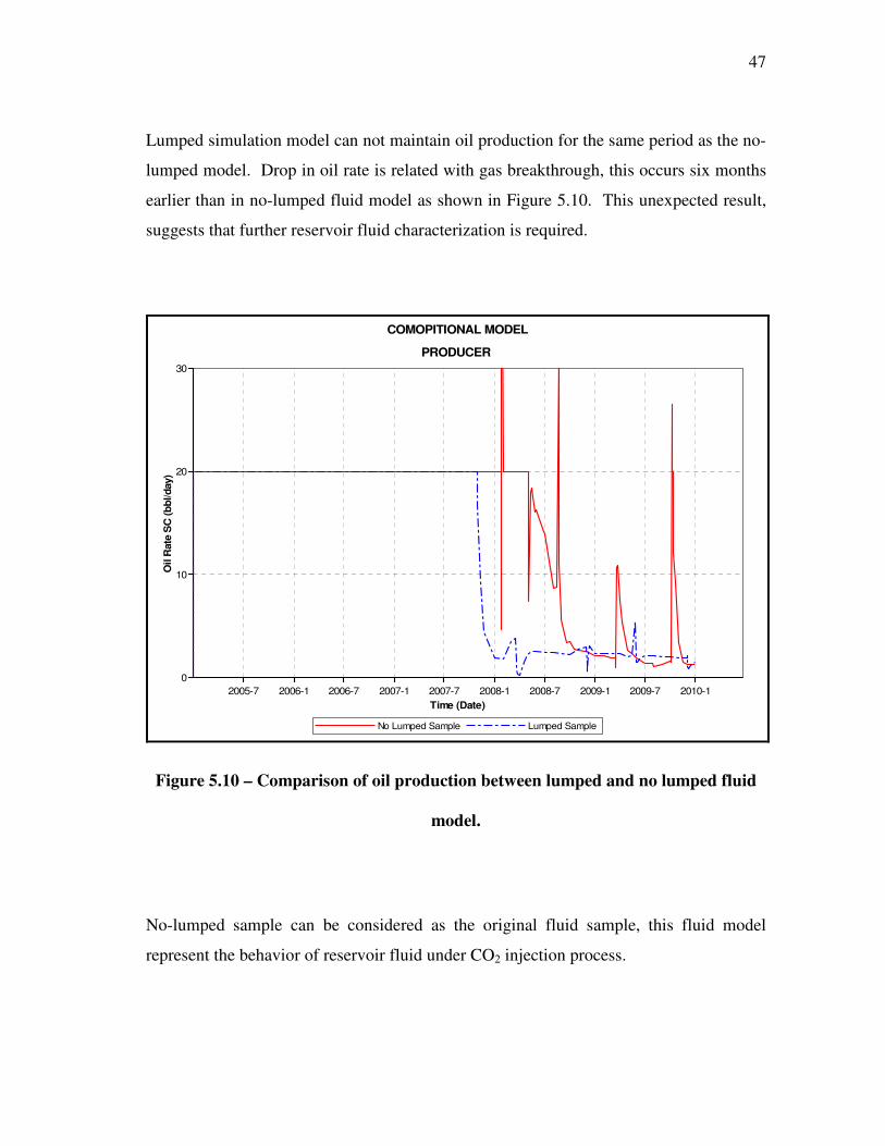
Lumped simulation model can not maintain oil production for the same period as the no-
lumped model. Drop in oil rate is related with gas breakthrough, this occurs six months
earlier than in no-lumped fluid model as shown in Figure 5.10. This unexpected result,
suggests that further reservoir fluid characterization is required.
COMOPITIONAL MODEL
PRODUCER
No Lumped Sample Lumped Sample
Time (Date)
Oil
Rat
e S
C (b
bl/d
ay)
2005-7 2006-1 2006-7 2007-1 2007-7 2008-1 2008-7 2009-1 2009-7 2010-10
10
20
30
Figure 5.10 – Comparison of oil production between lumped and no lumped fluid
model.
No-lumped sample can be considered as the original fluid sample, this fluid model
represent the behavior of reservoir fluid under CO2 injection process.
48
To understand how the number of components in the fluid sample or the reservoir fluid
model can affect reservoir simulation performance, evaluation of different fluid samples
will be carry on as follows.
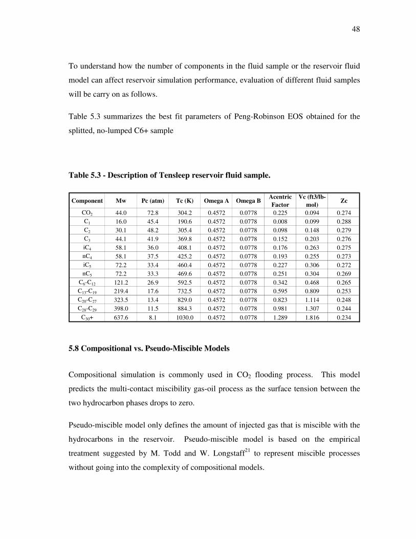
Table 5.3 summarizes the best fit parameters of Peng-Robinson EOS obtained for the
splitted, no-lumped C6+ sample
Table 5.3 - Description of Tensleep reservoir fluid sample.
Component Mw Pc (atm) Tc (K) Omega A Omega B Acentric Factor
Vc (ft3/lb-mol) Zc
CO2 44.0 72.8 304.2 0.4572 0.0778 0.225 0.094 0.274C1 16.0 45.4 190.6 0.4572 0.0778 0.008 0.099 0.288C2 30.1 48.2 305.4 0.4572 0.0778 0.098 0.148 0.279C3 44.1 41.9 369.8 0.4572 0.0778 0.152 0.203 0.276iC4 58.1 36.0 408.1 0.4572 0.0778 0.176 0.263 0.275nC4 58.1 37.5 425.2 0.4572 0.0778 0.193 0.255 0.273iC5 72.2 33.4 460.4 0.4572 0.0778 0.227 0.306 0.272nC5 72.2 33.3 469.6 0.4572 0.0778 0.251 0.304 0.269
C6-C12 121.2 26.9 592.5 0.4572 0.0778 0.342 0.468 0.265C13-C19 219.4 17.6 732.5 0.4572 0.0778 0.595 0.809 0.253C20-C27 323.5 13.4 829.0 0.4572 0.0778 0.823 1.114 0.248C28-C29 398.0 11.5 884.3 0.4572 0.0778 0.981 1.307 0.244
C30+ 637.6 8.1 1030.0 0.4572 0.0778 1.289 1.816 0.234
5.8 Compositional vs. Pseudo-Miscible Models
Compositional simulation is commonly used in CO2 flooding process. This model
predicts the multi-contact miscibility gas-oil process as the surface tension between the
two hydrocarbon phases drops to zero.
Pseudo-miscible model only defines the amount of injected gas that is miscible with the
hydrocarbons in the reservoir. Pseudo-miscible model is based on the empirical
treatment suggested by M. Todd and W. Longstaff21 to represent miscible processes
without going into the complexity of compositional models.
49
Pseudo-miscible model considers three components system, reservoir oil, injection gas
(solvent) and water. The reservoir oil component consists of stock tank oil together with
the associated solution gas. The solvent and reservoir oil components are assumed to be
miscible in all proportions and consequently only one hydrocarbon phase exists in the
reservoir.
Tensleep reservoir fluid can be considered as dead oil. Small interaction between CO2
and the scare light components in the oil is expected.
In this study, I evaluate the use of pseudo-miscible fluid models to describe the CO2
injection process in Tensleep Formation. Results from this model were compared with
results from compositional simulation. Pseudo-miscible model was considered because
is faster as previous discussed.
Results provided from the pseudo-miscible and compositional models show that for
Tensleep reservoir fluid, pseudo-miscible option do not behave closely to the
compositional approach.
Tuned PR-EOS was used to generate two oil PVT models (C6+ and C30+) for pseudo-
miscible and compositional simulators. The synthetic reservoir model mentioned before
was used.
5.8.1 Comparison of Pseudo-Miscible C6+ and C30+ Models
Two pseudo-miscible simulation models were generated. One of the models used fluid
description with components up to C6+ and other using components up to C30+. Oil and
gas production rates and reservoir pressure were plotted to describe the effect of the
number of components on oil production rate.
Both fluid samples show similar oil rate production profile, CO2 breakthrough time
differs on one month, 6% of the time, (Figure 5.11). Only slight differences in the

50
average reservoir pressure are observed; reservoir pressure drops slightly faster in the
C30+ model.
These results suggest that to save simulation running time, C6+ fluid sample can be used
in the field simulation model with assurance.
PSEUDO-MISCIBLE MODELC6+ Vs C30+ Comparison
Oil Rate, C6+ Sample Cum Oil, C6+ SampleOil Rate, C30+ Sample Cum Oil, C30+ Sample
Time (Date)
Oil
Rat
e S
C (b
bl/d
ay)
Cum
ulat
ive
Oil
SC
(bbl
)
2005-7 2006-1 2006-7 2007-1 2007-7 2008-1 2008-7 2009-1 2009-7 2010-10
5
10
15
20
25
0
5,000
10,000
15,000
20,000
Figure 5.11 - Qo and Np for pseudo-miscible models C6+ vs C30+.

51
5.8.2 Comparison of Compositional C6+ and C30+ Models
Using the compositional fluid models, similar behavior as in the pseudo-miscible model
was observed. Similar CO2 breakthrough time was obtained from the two fluid models.
Flat oil production period last for 3.5 years, this is two more years than in pseudo-
miscible model, (Figure 5.12).
As the objective of the CO2 storage is to maximize the amount of gas dissolved in the
reservoir fluid, a late gas breakthrough time is desired. After gas breakthrough occurs,
commonly liquid production is constrained to avoid gas recirculation.
COMPOSITIONAL MODELC6+ Vs C30+ Comparison
Oil Rate, C6+ Sample Cum Oil, C6+ SampleOil Rate, C30+ Sample Cum Oil, C30+ Sample
Time (Date)
Oil
Rat
e S
C (b
bl/d
ay)
Cum
ulat
ive
Oil
SC
(bbl
)
2005-7 2006-1 2006-7 2007-1 2007-7 2008-1 2008-7 2009-1 2009-7 2010-10
5
10
15
20
25
0
10,000
20,000
30,000
Figure 5.12- Qo and Np for compositional models C6+ vs C30+.

52
Comparison of compositional fluid models provides similar results as in pseudo-miscible
models. However in this case using C6+ sample a difference of 4 months in gas
breakthrough time are observed, this is a 7% more time than using C30+ model.
Compositional simulation also demonstrates that C6+ fluid model can be used with
confidence, this reducing simulation complexity and run time.
5.8.3 Comparison of Compositional and Pseudo-Miscible Models
From previous fluid evaluation have been recognized that no-lumped C6+ fluid sample
can be used in the numerical simulation of CO2 storage in Tensleep Formation. Now it
is necessary to establish which fluid model, pseudo-miscible or compositional should be
used in order to have accurate forecast results.
Figure 5.13 shows oil production performance from the two models. Earlier gas
breakthrough is observed in the pseudo-miscible model, then lower cumulative oil
production is obtained. Basically, compositional fluid model produces twice the oil
volume than pseudo-miscible model.
This is a big difference, considering that due to the dead oil characteristic of Tensleep
reservoir fluid; similar oil production behavior can be expected from the two fluid
models.
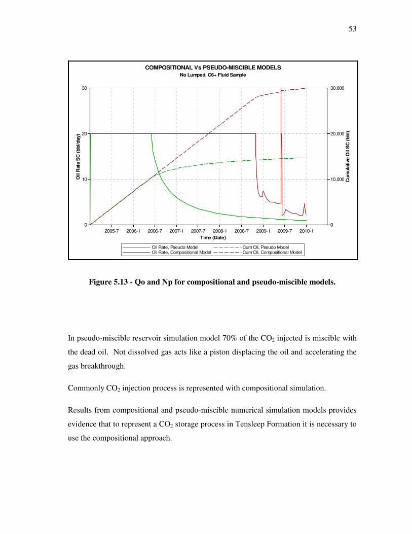
53
COMPOSITIONAL Vs PSEUDO-MISCIBLE MODELSNo Lumped, C6+ Fluid Sample
Oil Rate, Pseudo Model Cum Oil, Pseudo ModelOil Rate, Compositional Model Cum Oil, Compositional Model
Time (Date)
Oil
Rat
e S
C (b
bl/d
ay)
Cum
ulat
ive
Oil
SC
(bbl
)
2005-7 2006-1 2006-7 2007-1 2007-7 2008-1 2008-7 2009-1 2009-7 2010-10
10
20
30
0
10,000
20,000
30,000
Figure 5.13 - Qo and Np for compositional and pseudo-miscible models.
In pseudo-miscible reservoir simulation model 70% of the CO2 injected is miscible with
the dead oil. Not dissolved gas acts like a piston displacing the oil and accelerating the
gas breakthrough.
Commonly CO2 injection process is represented with compositional simulation.
Results from compositional and pseudo-miscible numerical simulation models provides
evidence that to represent a CO2 storage process in Tensleep Formation it is necessary to
use the compositional approach.

54
5.9 Reservoir Simulation Model
The reservoir simulation model covers 400 acres and contains 15 production wells. All
the wells are vertical and completed in the 4th layer of the simulation model. The grid
was 50 x 30 x 6 with 9000 total cells in the model. There are 5088 active cells with 300
x 300 ft. The model consists of the main faults that limit the structure at west and north
locations. Figure 5.14 shows a 3D view of the simulation grid for Teapot Dome field.
Six layers described in the geologic model of Tensleep Formation as main units,
represent an intercalation of sandstones and dolomites. Layers 1, 3 and 5 were defined
as dolomites with low matrix porosity and low permeability. Layers 2, 4 and 6 are
sandstones with better values of porosity and permeability. The main productive unit is
located in 4th layer.
Figure 5.14 - Simulation grid for Tensleep Formation.
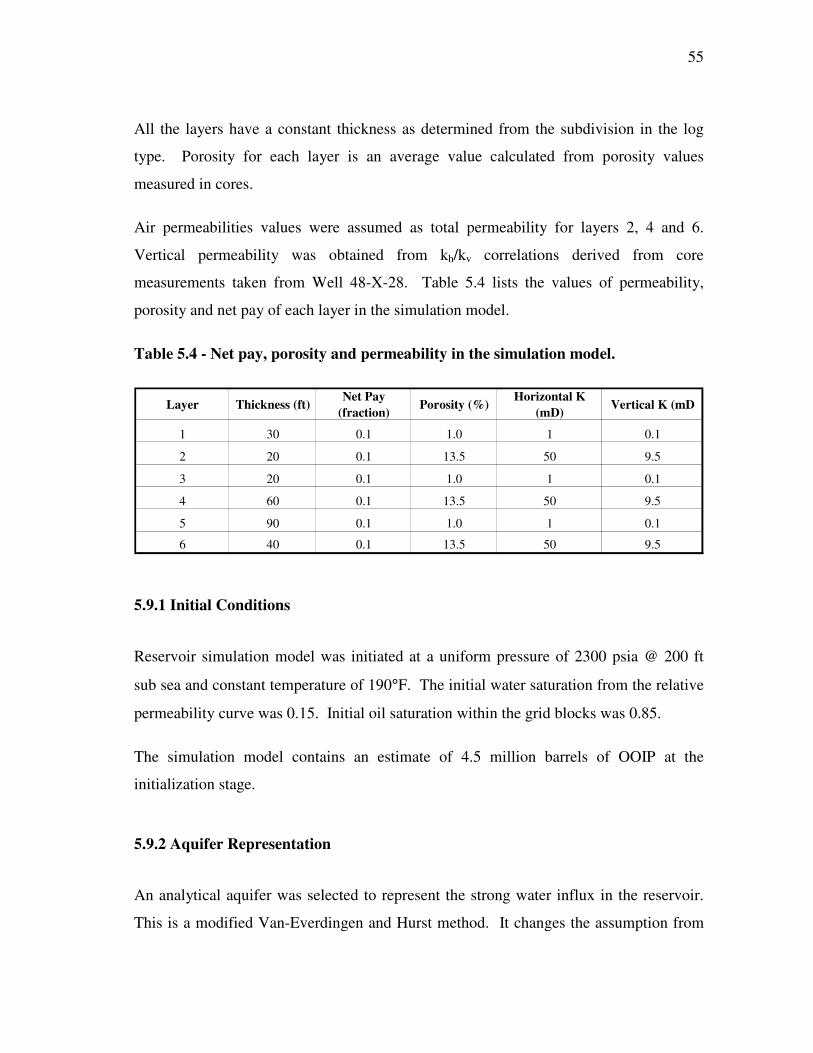
55
All the layers have a constant thickness as determined from the subdivision in the log
type. Porosity for each layer is an average value calculated from porosity values
measured in cores.
Air permeabilities values were assumed as total permeability for layers 2, 4 and 6.
Vertical permeability was obtained from kh/kv correlations derived from core
measurements taken from Well 48-X-28. Table 5.4 lists the values of permeability,
porosity and net pay of each layer in the simulation model.
Table 5.4 - Net pay, porosity and permeability in the simulation model.
Layer Thickness (ft) Net Pay (fraction) Porosity (%) Horizontal K
(mD) Vertical K (mD
1 30 0.1 1.0 1 0.1
2 20 0.1 13.5 50 9.5
3 20 0.1 1.0 1 0.1
4 60 0.1 13.5 50 9.5
5 90 0.1 1.0 1 0.1
6 40 0.1 13.5 50 9.5
5.9.1 Initial Conditions
Reservoir simulation model was initiated at a uniform pressure of 2300 psia @ 200 ft
sub sea and constant temperature of 190°F. The initial water saturation from the relative
permeability curve was 0.15. Initial oil saturation within the grid blocks was 0.85.
The simulation model contains an estimate of 4.5 million barrels of OOIP at the
initialization stage.
5.9.2 Aquifer Representation
An analytical aquifer was selected to represent the strong water influx in the reservoir.
This is a modified Van-Everdingen and Hurst method. It changes the assumption from

56
“a field producing at a constant hydrocarbon rate” to “an aquifer with influx water at a
constant rate”. This assumption simplifies the solution implemented in the simulator.19
The precise extension and strength is not known because no pressure data have been
collected from the reservoir.

57
CHAPTER VI
HISTORY MATCHING
In this chapter the technique to reproduce historical fluid production rates and field
pressure behavior is presented, along with validating and tuning the geological model to
predict the future performance of the reservoir in different scenarios.
Initially, Black oil simulator IMEXTM was used as a first approximation to evaluate the
accuracy of the simulation models. Black oil simulator is simplest in terms of reservoir
fluid description; this is the reason why it runs faster than compositional simulation.
As described in the geological evaluation, Teapot Dome formation is a highly fractured
formation. Effects of fractures in reservoir fluids production will be evaluated. Single
porosity simulation model results will be compared with those from dual porosity model.
Dual porosity models with constant and variable fracture permeability will be compared.
Variable fracture permeability will be generated fracture aperture using the cubic law.
Has been found that fracture aperture measured with X-Ray CT scanner follows
lognormal distribution.
Historical oil production and water rates of each well were used with the simulation
results to compare the effectiveness of those models. Gas production was not considered
due to the dead oil nature of the reservoir fluid. The quality of the models was judged
from how well the simulated water and oil production rates fit with historical data.
Analytical aquifer was used to reproduce the slight pressure drop present in the field.
Size and strength of the aquifer were defined by trial and error process.
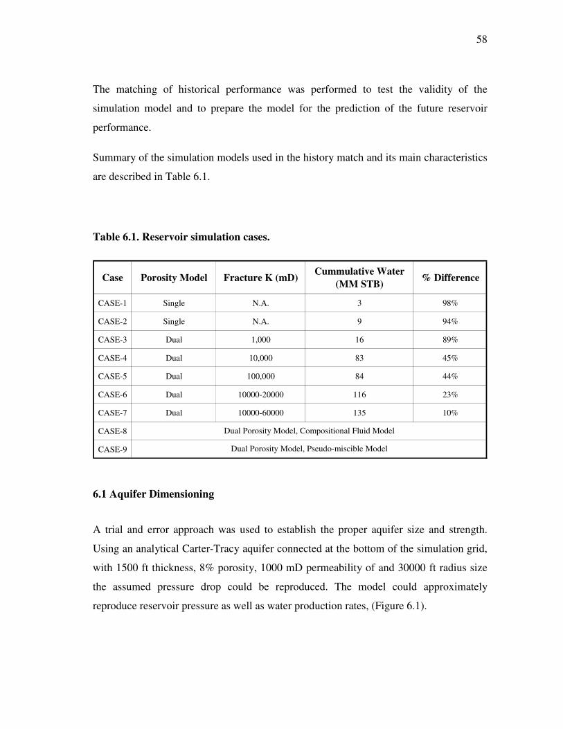
58
The matching of historical performance was performed to test the validity of the
simulation model and to prepare the model for the prediction of the future reservoir
performance.
Summary of the simulation models used in the history match and its main characteristics
are described in Table 6.1.
Table 6.1. Reservoir simulation cases.
Case Porosity Model Fracture K (mD) Cummulative Water (MM STB) % Difference
CASE-1 Single N.A. 3 98%
CASE-2 Single N.A. 9 94%
CASE-3 Dual 1,000 16 89%
CASE-4 Dual 10,000 83 45%
CASE-5 Dual 100,000 84 44%
CASE-6 Dual 10000-20000 116 23%
CASE-7 Dual 10000-60000 135 10%
CASE-8
CASE-9
Dual Porosity Model, Compositional Fluid Model
Dual Porosity Model, Pseudo-miscible Model
6.1 Aquifer Dimensioning
A trial and error approach was used to establish the proper aquifer size and strength.
Using an analytical Carter-Tracy aquifer connected at the bottom of the simulation grid,
with 1500 ft thickness, 8% porosity, 1000 mD permeability of and 30000 ft radius size
the assumed pressure drop could be reproduced. The model could approximately
reproduce reservoir pressure as well as water production rates, (Figure 6.1).
59
6.2 Single Porosity Model
Single porosity model is commonly used in the reservoir simulation of detritus
formations where intergranular porosity is considered the main storage and fluid flow
media. In this case permeability is function of pore throat size, pore space tortuosity,
shale content and mineralization through the rock pores.
In the CASE-1, relative permeabilities and capillary pressure measured in the cores were
used. As expected, this model is limited to reproduce the high water production volumes
observed in the field. Although the model can reproduce specified oil rates, water
breakthrough times are too long and water rates are less than the observed values.
In an attempt to increase the field water production, capillary pressure, OWC depth and
vertical permeability were changed. However the field water production can not match
the observed data.
In the simulation CASE-2 a straight line for water relative permeability from 0 (Sw =
Swc) to 0.5 (Sw = 1-Sor) was used to increase water mobility. Even though, this change
increase water rate but it is still not enough to reach historical water production rates,
(Figure 6.1).

60
SINGLE POROSITY MODELSIncreasing Water Relative Permeability
Water Water, Historic Data Cum Water, Historic DataWater Rate, CASE-1 Cum Water, CASE-1Water Rate, CASE-2 Cum Water, CASE-2
Time (Date)
Wat
er R
ate
RC
(bbl
/day
)
Cum
ulat
ive
Wat
er S
C (b
bl)
1980 1985 1990 1995 20001.00e+0
1.00e+1
1.00e+2
1.00e+3
1.00e+4
1.00e+5
0.00e+0
5.00e+7
1.00e+8
1.50e+8
2.00e+8
Figure 6.1 - Water production in single porosity models.
A reservoir model that has high permeability channels is required. Fractures will
improve water flow thorough the reservoir, then field water production can be
reproduced.
6.3 Dual Porosity Model
Dual porosity model, consider that fluids exist in two interconnected systems; the rock
matrix, which usually provides the bulk of the reservoir volume and fractures which
provide the main flow path. Traditional approach uses a constant fracture permeability
value. This study uses variable fracture permeability calculated from fracture aperture
distribution measured in fracture core samples.

61
6.3.1 Constant Fracture Permeability
In order to investigate the effect of fractures in reservoir performances, a constant
fracture permeability of 1000 mD was used as an initial approach (CASE-3). This
model was compared to single porosity model. Figure 6.2 shows the potential of using
the dual porosity model to reproduce field production. Introduced fractures in the
reservoir model improve simulated water rates. The fracture permeability is one of main
issues in using dual porosity model. Usually permeability values obtained from pressure
build-up test analysis are used. Permeabilities are tuned to match production rates and
bottom-hole pressures in the tested well. Unfortunately in Teapot Dome, field pressure
information in the Tensleep Formation is not available and a comparison with wells data
is not possible.
SINGLE vs. DUAL POROSITY MODELSFracture Permeability = 1000 md
Water Water, Historic Data Cum Water, Historic DataWater Rate, CASE-2 Cum Water, CASE-2Water Rate, CASE-3 Cum Water, CASE-3
Time (Date)
Wat
er R
ate
RC
(bbl
/day
)
Cum
ulat
ive
Wat
er S
C (b
bl)
1980 1985 1990 1995 20001.00e+0
1.00e+1
1.00e+2
1.00e+3
1.00e+4
1.00e+5
0.00e+0
5.00e+7
1.00e+8
1.50e+8
2.00e+8
Figure 6.2 - Water production, dual and single porosity models.

62
Three cases with different fracture permeability values were run to investigate the
magnitude of fracture permeability values that could reproduce observed water
production. The cases are defined as CASE-3 with a permeability of 1.000 mD, CASE-4
with 10.000 mD and CASE-5 with 100.000 mD.
The CASE-4 results show a significant improvement compared to CASE-3, (Figure 6.3).
The CASE-4 model could give a closer water production to observed data.
In the mean time, CASE-5 that has higher fracture permeability produces extremely high
water rate at initial period. After 20 years of field production cumulative water produced
is one third the historic value, At this time the average reservoir pressure have dropped
more than 1500 psi and the model is not able to produce the oil rate constrained.
DUAL POROSITY MODELSFracture Permeability Sensibility
Water Rate, Historic Data Cum Water, Historic DataWater Rate, CASE-3 Cum Water, CASE-3Water Rate, CASE-4 Cum Water, CASE-4Water Rate, CASE-5 Cum Water, CASE-5
Time (Date)
Wat
er R
ate
RC
(bbl
/day
)
Cum
ulat
ive
Wat
er S
C (b
bl)
1980 1985 1990 1995 20001.00e+0
1.00e+1
1.00e+2
1.00e+3
1.00e+4
1.00e+5
0.00e+0
5.00e+7
1.00e+8
1.50e+8
2.00e+8
Figure 6.3 - Water production of dual porosity models with constant Kf.
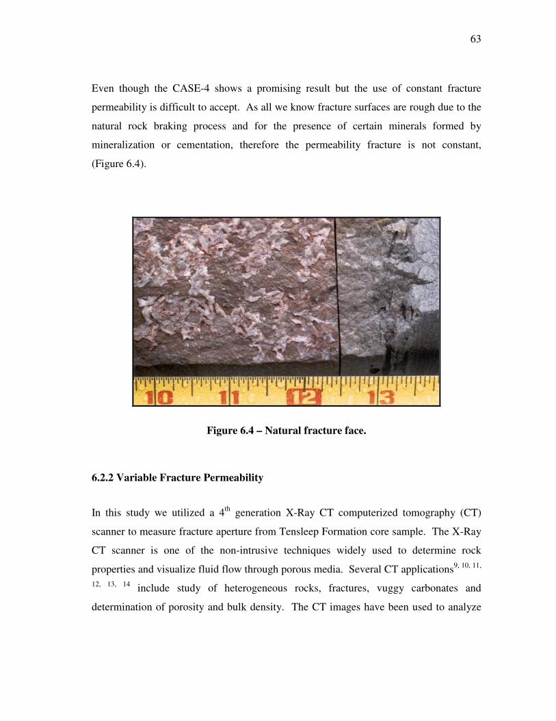
63
Even though the CASE-4 shows a promising result but the use of constant fracture
permeability is difficult to accept. As all we know fracture surfaces are rough due to the
natural rock braking process and for the presence of certain minerals formed by
mineralization or cementation, therefore the permeability fracture is not constant,
(Figure 6.4).
Figure 6.4 – Natural fracture face.
6.2.2 Variable Fracture Permeability
In this study we utilized a 4th generation X-Ray CT computerized tomography (CT)
scanner to measure fracture aperture from Tensleep Formation core sample. The X-Ray
CT scanner is one of the non-intrusive techniques widely used to determine rock
properties and visualize fluid flow through porous media. Several CT applications9, 10, 11,
12, 13, 14 include study of heterogeneous rocks, fractures, vuggy carbonates and
determination of porosity and bulk density. The CT images have been used to analyze
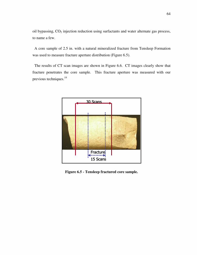
64
oil bypassing, CO2 injection reduction using surfactants and water alternate gas process,
to name a few.
A core sample of 2.5 in. with a natural mineralized fracture from Tensleep Formation
was used to measure fracture aperture distribution (Figure 6.5).
The results of CT scan images are shown in Figure 6.6. CT images clearly show that
fracture penetrates the core sample. This fracture aperture was measured with our
previous techniques.19
��� !"#$
%"!&'�
�� !"#$
��� !"#$
%"!&'�
�� !"#$
Figure 6.5 - Tensleep fractured core sample.
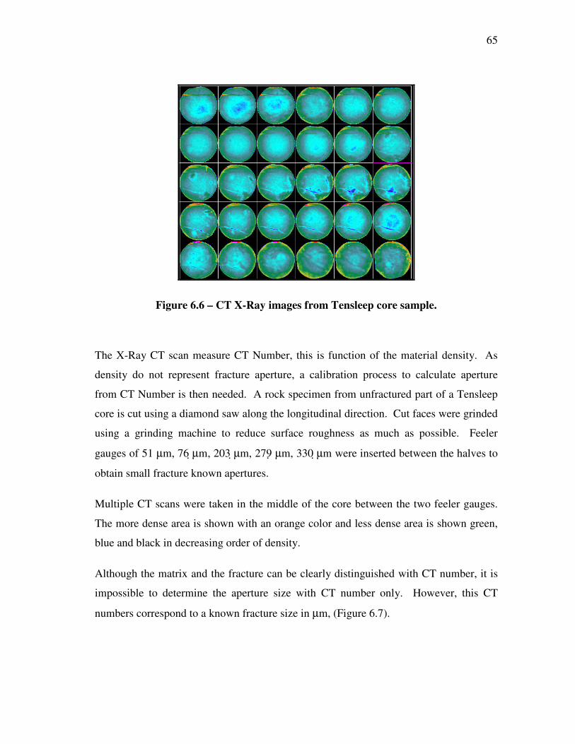
65
Figure 6.6 – CT X-Ray images from Tensleep core sample.
The X-Ray CT scan measure CT Number, this is function of the material density. As
density do not represent fracture aperture, a calibration process to calculate aperture
from CT Number is then needed. A rock specimen from unfractured part of a Tensleep
core is cut using a diamond saw along the longitudinal direction. Cut faces were grinded
using a grinding machine to reduce surface roughness as much as possible. Feeler
gauges of 51 µm, 76 �µm, 203 �µm, 279 � µm, 330 �µm were inserted between the halves to
obtain small fracture known apertures.
Multiple CT scans were taken in the middle of the core between the two feeler gauges.
The more dense area is shown with an orange color and less dense area is shown green,
blue and black in decreasing order of density.
Although the matrix and the fracture can be clearly distinguished with CT number, it is
impossible to determine the aperture size with CT number only. However, this CT
numbers correspond to a known fracture size in µm, (Figure 6.7).
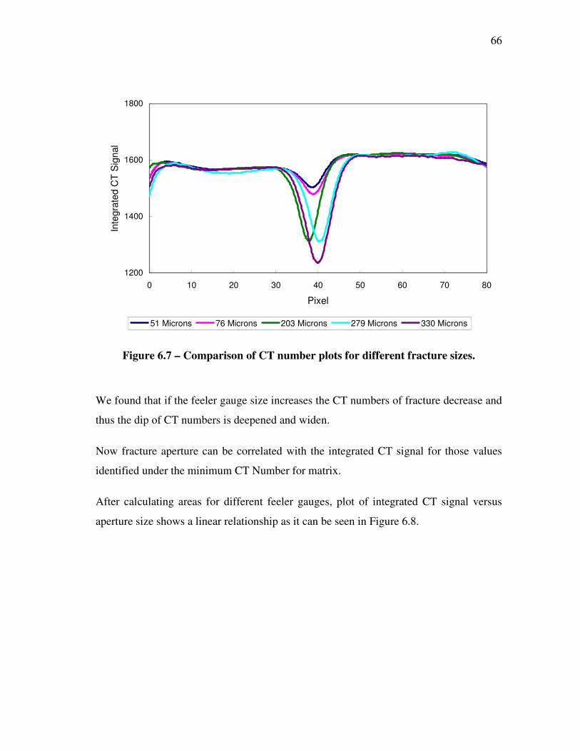
66
1200
1400
1600
1800
0 10 20 30 40 50 60 70 80
Pixel
Inte
grat
ed C
T S
igna
l
51 Microns 76 Microns 203 Microns 279 Microns 330 Microns
Figure 6.7 – Comparison of CT number plots for different fracture sizes.
We found that if the feeler gauge size increases the CT numbers of fracture decrease and
thus the dip of CT numbers is deepened and widen.
Now fracture aperture can be correlated with the integrated CT signal for those values
identified under the minimum CT Number for matrix.
After calculating areas for different feeler gauges, plot of integrated CT signal versus
aperture size shows a linear relationship as it can be seen in Figure 6.8.

67
y = 6.5458x + 360.99R2 = 0.9589
0
500
1000
1500
2000
2500
3000
0 50 100 150 200 250 300 350
Aperture (µm)
Inte
grat
ed C
T S
igna
l
Figure 6.8 – Integrated CT signal vs. fracture aperture.
Once fracture aperture was measure a long the core, these values were found lognormal
distributed. It is distributed with mean value of 22 �m and standard deviation of 500.
This fracture aperture data can be converted to fracture permeability by the following
equation32
[ ]mdw.k f2910458 ×=
where, w is in microns.
This distribution will be converted into fracture permeability via cubic law equation.
The calculated fracture permeability then could be used as input data in dual porosity
simulation model.
However there is no methodology to upscale fracture permeability values calculated in a
core sample (micro scale) to reservoir simulations models (macro scale). Therefore, we

68
randomly generated several fracture permeability models using a lognormal distribution.
Different minimum and maximum values between 1000 and 100000 mD were used to
avoid unrealistic permeability values that may cause reservoir simulation calculations
instability.
After several simulation runs using different fracture permeability distributions we found
that the model with fracture permeability values between 20000 mD to 40000 mD shows
a better match to observed data (Figure 6.9).
As a result, an additional improvement in the water production rates was obtained as
show in CASE-6 model (Figure 6.10).
File: Base2poro-22-4.irfUser: r0g2920Date: 2005-08-23Z/X: 3.00:1
20,044
24,023
28,002
31,980
35,960
39,938
43,917
47,896
51,875
55,854
59,833
DUALPORO, BLACK-OIL, ORATPermeability I - Fracture (md) 1977-01-01
Figure 6.9 – Variable fracture permeability model.
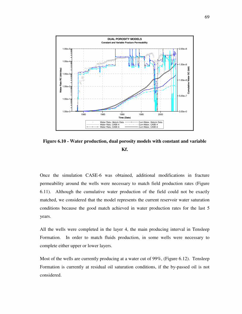
69
DUAL POROSITY MODELSConstant and Variable Fracture Permeability
Water Rate, Historic Data Cum Water, Historic DataWater Rate, CASE-4 Cum Water, CASE-4Water Rate, CASE-6 Cum Water, CASE-6
Time (Date)
Wat
er R
ate
RC
(bbl
/day
)
Cum
ulat
ive
Wat
er S
C (b
bl)
1980 1985 1990 1995 20001.00e+0
1.00e+1
1.00e+2
1.00e+3
1.00e+4
1.00e+5
0.00e+0
5.00e+7
1.00e+8
1.50e+8
2.00e+8
Figure 6.10 - Water production, dual porosity models with constant and variable
Kf.
Once the simulation CASE-6 was obtained, additional modifications in fracture
permeability around the wells were necessary to match field production rates (Figure
6.11). Although the cumulative water production of the field could not be exactly
matched, we considered that the model represents the current reservoir water saturation
conditions because the good match achieved in water production rates for the last 5
years.
All the wells were completed in the layer 4, the main producing interval in Tensleep
Formation. In order to match fluids production, in some wells were necessary to
complete either upper or lower layers.
Most of the wells are currently producing at a water cut of 99%, (Figure 6.12). Tensleep
Formation is currently at residual oil saturation conditions, if the by-passed oil is not
considered.

70
DUAL POROSITY MODELVariable Fracture Permeability
Water Rate, Historic Data Cum Water, Historic DataWater Rate, CASE-7 Water Rate, CASE-7
Time (Date)
Wat
er R
ate
RC
(bbl
/day
)
Cum
ulat
ive
Wat
er S
C (b
bl)
1980 1985 1990 1995 20001.00e+0
1.00e+1
1.00e+2
1.00e+3
1.00e+4
1.00e+5
0.00e+0
5.00e+7
1.00e+8
1.50e+8
2.00e+8
Figure 6.11 - Water production history match.
DUAL POROSITY MODELVariable Fracture Permeability
WCut CASE-7 Historical WCut
Time (Date)
Wat
er C
ut S
C
1980 1985 1990 1995 20000.00
0.20
0.40
0.60
0.80
1.00
Figure 6.12 - Water cut history match.

71
In most of the wells, a good match of oil and water rates was obtained. Figures 6.13 to
6.15 show examples of history match in some wells.
Based on these results, we considered that the simulation model has been properly
calibrated and furthermore it can be used to run prediction cases.
DUAL POROSITY MODELVariable Fracture Permeability
W10439
Oil Rate, Historic Data WCut, Historic DataOil Rate, CASE-7 WCut, CASE-7
Time (Date)
Wat
er C
ut S
C -
%
Oil
Rat
e S
C (b
bl/d
ay)
1980 1985 1990 1995 20000
20
40
60
80
100
0
50
100
150
200
Figure 6.13 - History match in Well W10439.
Lack of information related with location of perforated intervals in previous Tensleep
zones division and the simplified homogeneous geological model difficult to match the
observed data.

72
DUAL POROSITY MODELVariable Fracture Permeability
W10610
Oil Rate, Historic Data WCut, Historic DataOil Rate, CASE-7 WCut, CASE-7
Time (Date)
Oil
Rat
e S
C (b
bl/d
ay)
Wat
er C
ut S
C
1980 1985 1990 1995 20000
100
200
300
400
0.00
0.20
0.40
0.60
0.80
1.00
Figure 6.14 - History match in Well W10610.
DUAL POROSITY MODELVariable Fracture Permeability
W11207
Oil Rate, Historic Data WCut, Historic DataOil Rate, CASE-7 WCut, CASE-7
Time (Date)
Oil
Rat
e S
C (b
bl/d
ay)
Wat
er C
ut S
C -
%
1980 1985 1990 1995 20000
10
20
30
40
50
0
20
40
60
80
100
Figure 6.15 - History match in Well W11207.

73
In the simulation model, Tensleep Formation initially contained 5.8 MMSTBO. At the
end of the history match period, 1.52 MMSTB have been produced or 26% of the OOIP.
The remaining oil in place is 4.28 MMSTBO. Despite the high water cut in all the wells,
the average remaining oil saturation at the end of the history match was 40%.
Water breakthrough in the wells through the fracture system, his causes a non-uniform
advance of the water front and therefore poor sweep efficiency. High-permeability
fractures ease water breakthrough earlier than the low-permeability fractures, leaving
some untapped oil reserves behind.
6.3 History Matching Using Compositional and Pseudo-Miscible Simulation
A full field simulation model was generated to obtain current saturation conditions using
the geological grid of CASE-7 and the compositional fluid model described in Chapter
V. Unfortunately, in this field compositional simulation case (CASE-8), very small time
steps are necessary and the numerical solution procedure asked for non practical
computer memory to reach a solution. High material balance errors, around 20% in the
gas were observed. Several attempts to correct the compositional model increasing
available computer memory for the simulation were unsuccessfully tested.
A CASE-9 was run using the pseudo-compositional fluid model. As in the CASE-8,
pseudo-miscible model showed calculation difficulties at field scale. Reservoir fluid
model appear to be confident and reliable, however no improvement in the simulation
time and stability was possible.

74
CHAPTER VII
ENHANCED OIL RECOVERY AND CO2 STORAGE EVALUATION
In this chapter, the enhanced oil recovery and CO2 storage process evaluation is
discussed. Several problems were obtained running the dual porosity field simulation
model either with compositional or pseudo-miscible fluid models.
Enhanced oil recovery evaluation was perform using the quarter pattern model described
Chapter V. This model was converted to dual porosity model and CO2 injection rate
sensitivity was evaluated.
CO2 storage process was calculated at the breakthrough time and scaled to field size.
7.1 Quarter Pattern Compositional Model
The quarter pattern model used in the comparison of compositional vs. pseudo-miscible
simulators was convert to dual porosity and used in this evaluation, (Figure 7.1).
Fracture permeability of 10000 mD was used. The model was initialized with matrix So
= 40% and fracture So = 99% to represent the current saturation conditions in the
reservoir. The possible by-passed oil is not considered in this evaluation; only additional
recovery due to residual oil saturation reduction is contemplated.
Compositional fluid models were used to represent the miscible process of enhanced oil
recovery in Tensleep formation.
Synthetic model has a hydrocarbon pore volume of 208 MSTB.

75
To investigate the effect of CO2 injection rate on the enhanced oil recovery process, five
sensitivities cases were run. Injection rates at reservoir conditions of 100, 200, 300, 400
and MSCFD of CO2 were used.
Formation fracture pressure was assumed to be the initial reservoir pressure, then
maximum injection pressure of 2300 psi at the well head was specified in the injectors.
Producer is constrained by bottom-hole pressure of 2000 psi.
INJECTOR
PRODUCER
-200 -100 0 100 200 300 400 500 600 700 800 900 1,000 1,100 1,200 1,300 1,400 1,500 1,600
-200 -100 0 100 200 300 400 500 600 700 800 900 1,000 1,100 1,200 1,300 1,400 1,500 1,600
-1,400-1,200
-1,000-800
-600-400
-2000
100
-1,3
00-1
,100
-900
-700
-500
-300
-100
0
File: Comp-6-1.irfUser: r0g2920Date: 2005-08-09
Scale: 1:3338Y/X: 1.00:1Axis Units: ft
0.00
0.04
0.08
0.12
0.16
0.20
0.24
0.28
0.32
0.36
0.40
Compositional ModelOil Saturation 2005-01-01 K layer: 1
Figure 7.1 – Quarter pattern compositional model.
Injection gas rate sensitivity using compositional fluid model shows that at CO2 volume
injected of 0.6 PV, oil recovery decrease as injection rate increases, (Figure 7.2). Good
oil recovery is observed in all injection cases.

76
OIL RECOVERY FROM COMPOSITIONAL MODEL
0.00
0.05
0.10
0.15
0.20
0.25
0.30
0.35
0.0 0.1 0.2 0.3 0.4 0.5 0.6 0.7
CO2 Injected (PV)
Oil
Rec
over
y (f
rac)
100 Mscfd 200 Mscfd 300 Mscfd 400 Mscfd 500 Mscfd
Figure 7.2 – Oil recovery from compositional model.
Comparison of final oil recovery as function of gas pore volume injected shows that a
maximum recovery of 32% of the residual oil saturation can be obtained when gas is
injected at 200 MSCFD, (Figure 7.3).
Acceleration in CO2 gas breakthrough is observed when injection rate is increases. Dual
porosity simulation models involve fractures; these fractures represent high permeability
channels. These channels accelerate breakthrough of fluid with favorable mobility like
CO2.
These results can be used evaluate enhanced oil recovery at reservoir scale. Field
simulation shows 33 times the quarter pattern hydrocarbon pore volume. Field model
have an OOIP of 5.8 MMSTB. With a residual oil saturation of 40%, 2.32 MMSTB can
be expected to remain in the reservoir.
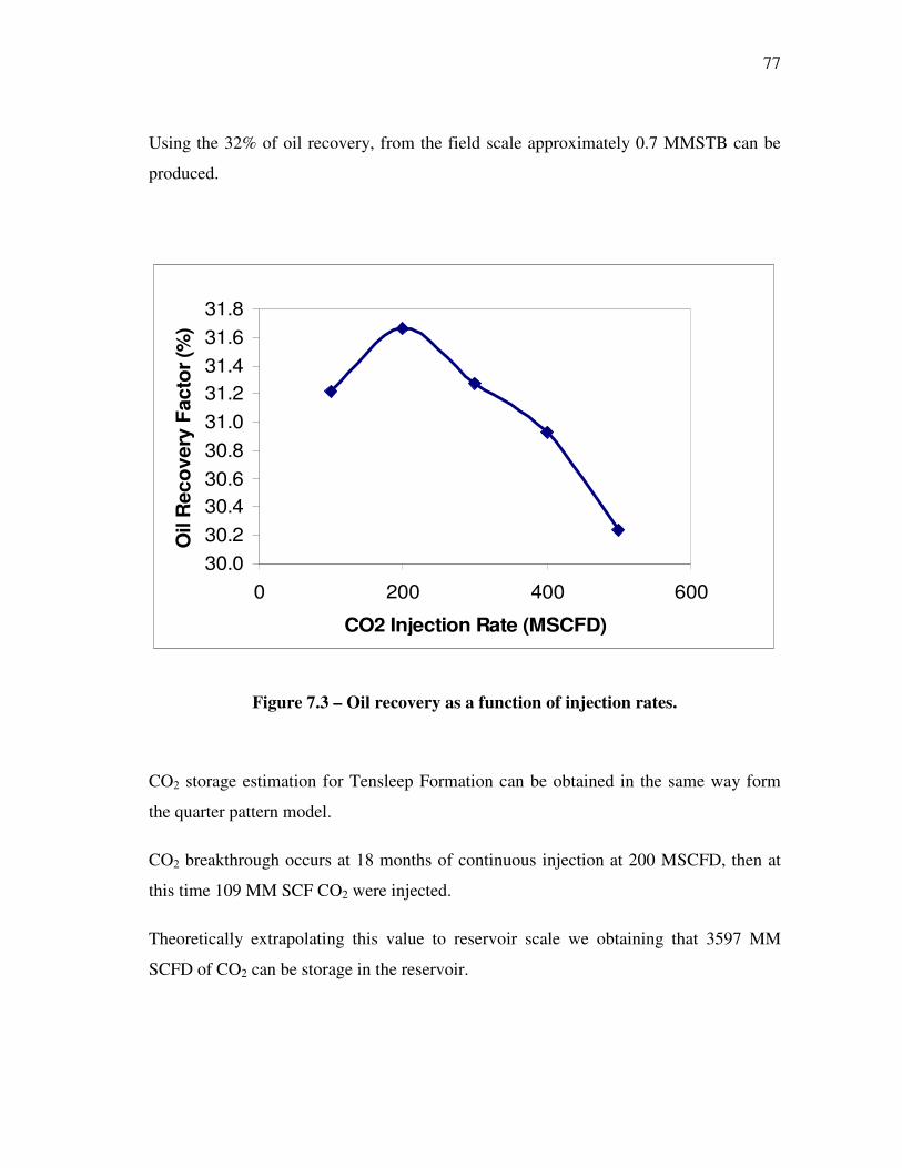
77
Using the 32% of oil recovery, from the field scale approximately 0.7 MMSTB can be
produced.
30.030.230.430.630.831.031.231.431.631.8
0 200 400 600
CO2 Injection Rate (MSCFD)
Oil
Rec
ove
ry F
acto
r (%
) (
Figure 7.3 – Oil recovery as a function of injection rates.
CO2 storage estimation for Tensleep Formation can be obtained in the same way form
the quarter pattern model.
CO2 breakthrough occurs at 18 months of continuous injection at 200 MSCFD, then at
this time 109 MM SCF CO2 were injected.
Theoretically extrapolating this value to reservoir scale we obtaining that 3597 MM
SCFD of CO2 can be storage in the reservoir.

78
7.2 Field Compositional Model
The dual porosity black oil simulation model used in the history match process was
converted to compositional model. The no-lumped fluid model with 13 components was
used in the evaluation.
The models start running without reporting any error in the simulation data file, this
present calculation problems at the first day and the run can not continue.
Several attempts were made to run the compositional model changing different reservoir
properties and conditions; however no stable runs could be obtained.
79
CHAPTER VIII
CONCLUSIONS
From the evaluation performed to the field data from Tensleep Formation, the next
conclusions can be derived:
1. Compositional simulation should be used to evaluate CO2 injection process.
2. Pseudo-miscible model is not able to represent the miscible process between CO2
and reservoir fluid in Tensleep Formation.
3. Variable fracture permeability lognormal distributed depicts better the water
advance thorough the highly fractured Tensleep Formation.
4. Additional PVT experiments like constant composition expansion and differential
liberation are necessary to improve the hydrocarbon model.
5. A maximum of 32% of the residual oil volume can be recovered from a quarter
pattern reservoir model when CO2 is injected at 200 MSCFD.
6. 3597 MM SCFD of CO2 can be storage in Tensleep Formation using the quarter
pattern analogy.
8.1 Recommendations
7. Velocity information should be acquired in Teapot Dome in order to improve the
geological model.
8. Sealing capacity of faults should be evaluated to improve the CO2 storage capacity
in Tensleep Formation.
80
9. For future field compositional simulation evaluation, lumped and no-lumped fluid
samples should be tested.
10. Techniques to upscale fracture permeability values from cores to dual porosity
simulation models should be evaluated.
11. Use of field simulation model in CO2 storage evaluation in Tensleep Formation is
necessary to know field response under different injection/production scenarios.

81
NOMENCLATURE
Z = gas deviation factor
φ = porosity
K = permeability, mD.
µ = viscosity, cp
ρ = fluid density, lbm/ft3
σ = interfacial tension
θ = contact angle.
FVF= formation volume factor
GOR=Gas-oil ratio
Subscripts
g = gas
w = water
o = oil
f = fracture
m = matrix

82
REFERENCES
1. Olsen, D.K., Sarathi, P.S., Hendricks, M.L., Schulte, R.K., Giangiacomo, L.A.: “Case History of Steam Injection Operations at Naval Petroleum Reserve No. 3, Teapot Dome Field, Wyoming: A Shallow Heterogeneous Light-Oil Reservoir,” paper SPE 25786 presented at the 1993 International Thermal Operations Symposium, Bakersfield, CA, 8-10 February.
2. Curry, W.: “Teapot Dome – Past, Present and Future,” AAPG Bulletin V. 61 No. 5 (May 1977), 671.
3. Martin, F.D. and Taber, J.J.: “Carbon Dioxide Flooding,” SPE Technology Today Series (April 1992) 396 – 400.
4. Jarrel, P.M., Fox, C.E., Stein, M.H. and Webb, S.L.: F.: Practical Aspects of CO2
Flooding, Monograph Series, SPE, Richardson, TX (2002).
5. Grigg, R.B.: “Long Term CO2 Storage Using Petroleum Industry Experience,” final technical report, CCP Subcontract # 3961, U.S. DOE, Washington DC (December 2002).
6. Options for CO2 Storage, IEA Greenhouse Gas R&D Programme, www.ieagreen.org.uk/4.pdf, July 2005.
7. “Carbon Sequestration R&D,” U.S. DOE, www.fossil.energy.gov/programs/sequestration/, June 2005.
8. Sanchez, N.L.: “Management of Water Alternating (WAG) Injection Projects,” paper SPE 53714 presented at the 1999 Latin American and Caribbean Petroleum Engineering Conference, Caracas, Venezuela, 21-23 April.
9. Kulkarni, M. M. and Rao, D. N.: “Experimental Investigation of Various Methods of Tertiary Gas Injection,” SPE 90589, paper presented at the 2004 Society of Petroleum Engineers Annual Technical Conference and Exhibition, Houston, TX, September 26 -29.
10. Rogers, J.D., Reid B. and Grigg, R.B.: “A Literature Analysis of the WAG Injectivity Abnormalities in the CO2 Process,” paper SPE 59329 presented at the 2000 Improved Oil Recovery Symposium, Tulsa, OK, 3-5 April.
11. Bennion, D.B., Thomas, F.B., Jamaluddin, A.K.M. and Ma, T.: “The Effect of Trapped Critical Fluid Saturations on Reservoir Permeability and Conformance,” paper presented at the 1998 Annual Technical Meeting of the Petroleum Society of CIM, Calgary, Alberta, Canada, 8 -10 June.
83
12. Cooper, S.P., Lorenz, J.C. and Goodwin, L.B.: ‘Lithologic and Structural Controls on Natural Fracture Characteristics Teapot Dome, Wyoming,” Sandia Report, contract No. DE-AC04-94AL85000, U.S. DOE , Albuquerque, NM (June 2001).
13. Ennis-King, J. and Paterson, L.: “Engineering Aspects of Geological Sequestration of Carbon Dioxide,” paper SPE 77809 presented at the 2002 Asia Pacific Oil and Gas Conference and Exhibition, Melbourne, Australia, 8-10 October.
14. Krumhansl, J., Pawar R., Grigg R., Westrich H., Warpinski N., et al.: “Geological Sequestration of Carbon Dioxide in a Depleted Oil Reservoir,” paper SPE 75256 presented at 2002 SPE/DOE Improved Oil Recovery Symposium, Tulsa, OK, 13-17 April.
15. Schulte, R.: “Airborne Survey,” final report, contract No. DOE/RMOTC – 020139, Casper, WY (June 2001).
16. Teapot Dome Geological Column, Rocky Mountain Oil Field Testing, www.rmotc.com/Facilities/Geo-sample.html, July 2005.
17. Zhang, Q., Nummedal, D. and Yin, P.: “Stratigraphy, Sedimentology and Petrophysics of the Tensleep Sandstone at Teapot Dome and in Outcrop,” http://aapg.confex.com/aapg/rm2005/techprogram/A100171.htm, June 13 2005.
18. Zhang, Q., Nummedal, D. and Yin, P.: “Reservoir Heterogeneity Caused by Diagenesis in Tensleep Sandstones, Teapot Dome, Wyoming,” presented at the 2005 AAPG Annual Meeting, Calgary, Alberta, Canada, June 19-22.
19. IMEX, Version 2004.11, User Manual, Computer Modeling Group, Calgary (2004).
20. GEM, Version 2004.10, User Manual, Computer Modeling Group, Calgary (2004).
21. Todd, M.R. and Longstaff, W.J.: “The Development, Testing, and Application of a Numerical Simulator for Predicting Miscible Flood Performance,” paper SPE 3484, JPT (July 1972) 874.
22. Muralidharan, V., Chakravarthy, D., Putra, E., and Schechter, D.S.: "Investigating Fracture Aperture Distributions under Various Stress Conditions Using X-Ray Scanner," paper CIPC 2004-230 presented at 2004 Annual Technical Meeting of the Petroleum Society, Calgary, Alberta, Canada, 8-10 June.
23. McDonald A.E., Beckner, B.L., Chan, H.M., Jones, T.A., Wooten, S.O.: ”Some Important Considerations in the Simulation of Naturally Fractured Reservoirs,” SPE 21814, presented in Rocky Mountain Regional Meeting and Low-Permeability Reservoirs Symposium, Denver, CO, April 15-17, 1991.

84
24. Merrill, R.C., Hartman, K.J. and Creek, J.L.: “A Comparison of Equation of State Tuning Methods,” paper SPE 28589 presented at the 69th Annual Technical and Exhibition New Orleans, LA, 25-28 September.
25. Khan, S.A., Pope, G.A. and Sepehrnoori, K.: “Fluid Characterization of Three-Phase CO2/Oil Mixtures,” paper SPE/DOE 24130 presented at the 8th Symposium Oil Recovery, Tulsa, OK, 22-24 April, 1992.
26. Peng, D.Y. and Robinson, D.B.: “A New Two-Constant Equation of State,” Ind. & Eng. Chem. Fund. (1976) 15, No. 1, 59-64.
27. Lohrenz, J., Bray, B.G. and Clark, C.R.: “Calculating Viscosities of Reservoir Fluids from Their Compositions,” JPT (Oct. 1964) 16, 1171-1176.
28. Whitson, C.H.: “Characterizing Hydrocarbon Plus Fraction,” SPEJ, 23, 1983, 683-684.
29. Aguilar, R.A. and McCain, W.D.: “An Efficient Tuning Strategy to Calibrate Cubic EOS for Compositional Simulation,” paper SPE 77382 presented at the 2002 Annual Technical Conference and Exhibition, San Antonio, TX, 29 September – 2 October
30. Simon, R. and Graue, D.J.: “Generalized Correlations for Predicting Solubility, Swelling and Viscosity Behavior of CO2 -Crude Oil Systems,” paper SPE 917, JPT (January 1965) 102.
31. Fevang, O., Singh, K. and Whitson, C.H.: “Guidelines for Choosing Compositional and Black-Oil Models for Volatile Oil and Gas Condensate Reservoirs,” paper SPE 63087 presented at the 2000 SPE Annual Technical Conference and Exhibition, Dallas, TX, 1-4 October.
32. Witherspoon, P.A., Wang, J.S.Y., Iwai, K. and Gale, J.E.: “Validity of Cubic Law for Fluid Flow in a Deformable Rock Fracture,” Water Resources Research,” (1980) V. 16 No. 6, 1016-1024.

85
VITA
Name: Ricardo Gaviria Garcia
Permanent Address: Harold Vance Department of Petroleum
Engineering.
Texas A&M University
507 Richardson Building
College Station, TX 77843-3116, U.S.A.
Email: [email protected]
Education: B. S., Petroleum Engineering,
Universidad Industrial de Santander,
Bucaramanga, Colombia
(November 1998)
M.S., Petroleum Engineering
Texas A&M University
College Station, TX 77843-3116, U.S.A.
(December 2005)