research open access robust fuzzy scheme for ... open access robust fuzzy scheme for gaussian...

Rosales-Silva et al. EURASIP Journal on Image and Video Processing 2014, 2014:20http://jivp.eurasipjournals.com/content/2014/1/20

RESEARCH Open Access

Robust fuzzy scheme for Gaussian denoising of3D color videoAlberto Jorge Rosales-Silva*, Francisco Javier Gallegos-Funes, Ivonne Bazan Trujillo and Alfredo Ramírez García

Abstract

We propose a three-dimensional Gaussian denoising scheme for application to color video frames. The time isselected as a third dimension. The algorithm is developed using fuzzy rules and directional techniques. A fuzzyparameter is used for characterization of the difference among pixels, based on gradients and angle of deviations, aswell as for motion detection and noise estimation. By using only two frames of a video sequence, it is possible toefficiently decrease Gaussian noise. This filter uses a noise estimator that is spatio-temporally adapted in a localmanner, in a novel way using techniques mentioned herein, and proposing a fuzzy methodology that enhancescapabilities in noise suppression when compared to other methods employed. We provide simulation results thatshow the effectiveness of the novel color video denoising algorithm.

Keywords: Fuzzy theory; Video frames; Motion detection; Directional processing; Gaussian noise

1. IntroductionAll pixels in digital color video frames are commonlyaffected by Gaussian-type noise due to the behavior ofthe image acquisition sensor; in accordance with this, wemake the following assumptions as to the noise:

G xβ� � ¼ N 0; σð Þ ¼ 1ffiffiffiffiffiffi

2πp

⋅ σexp

−xβ2

2 ⋅ σ2

� �; ð1Þ

where xβ represents the original pixel component value,β = {Red, Green, Blue} are the notations on each pixelcolor component (or channel), and σ is the standarddeviation of the noise. In our case, the Gaussian functionis independently used on the pixel component of eachchannel of the frame in order to obtain the corruptedvideo sequence.A pre-processing procedure to reduce noise effect is the

main stage of any computer vision application. It shouldinclude procedures to reduce the noise impact in a videowithout degrading the quality, edges, fine detail, and colorproperties.The current proposal is an attempt to enhance the qual-

ity while processing the color video sequences corruptedby Gaussian noise; this methodology is an extension of the

* Correspondence: [email protected] of Advanced Mechanical and Electrical Engineering, U.P.A.L.M, Av.Instituto Politécnico Nacional S/N, ESIME Zacatenco, Col. Lindavista, MéxicoD.F. 07738, Mexico

© 2014 Rosales-Silva et al.; licensee Springer. ThCommons Attribution License (http://creativecoreproduction in any medium, provided the orig

method proposed for impulsive noise removal [1]. Thereexist numerous algorithms that perform the processing of3D signals using only the spatial information [2]. Otherapplications use only the temporal information [3,4]; anexample is one that uses wavelet procedures to reduce thedelay in video coding [5]. There exist also some interestingapplications that use spatio-temporal information [6-13].The disadvantage of these 3D solutions is that they oftenrequire large memory and may introduce a significanttime delay in cases where there is a need for more than oneframe to be processed. This is undesirable in interactiveapplications such as infrared camera-assisted driving orvideoconferencing. Moreover, full 3D techniques tend torequire more computation than separable ones, and theiroptimal performance can be very difficult to determine.For example, integrating video coding and denoising is anovel processing paradigm and brings mutual benefits toboth video processing tools. In Jovanov et al. [14], themain idea is the reuse of motion estimation resources fromthe video coding module for the purpose of videodenoising. Some disadvantages of the work done byDai et al. [15] is that they use a number of reference framesthat increases the computational charge; the algorithmMHMCF was originally applied to grayscale video signal;and in the paper referenced [14], it was adapted to colorvideo denoising, transforming the RGB video in a luminancecolor difference space proposed by the authors.

is is an open access article distributed under the terms of the Creativemmons.org/licenses/by/2.0), which permits unrestricted use, distribution, andinal work is properly cited.

mailto:[email protected]

http://creativecommons.org/licenses/by/2.0

Rosales-Silva et al. EURASIP Journal on Image and Video Processing 2014, 2014:20 of 17http://jivp.eurasipjournals.com/content/2014/1/20

Other state-of-the-art algorithms found in literature workin the same manner; for example in Liu and Freeman [16],a framework that integrates robust optical flow into anon-local means framework with noise level estimation isused, and the temporal coherence is taken into account inremoving structured noise. In the paper by Dabov et al.[17], it is interesting to see how they propose a methodbased on highly sparse signal representation in local 3Dtransform domain; a noisy video is processed in blockwisemanner, and for each processed block, they form dataarray by stacking together blocks found to be similarto the currently processed one. In [18], Mairal et al.presented a framework for learning multiscale sparserepresentations of color images and video with overcom-plete dictionaries. They propose a multiscaled learnedrepresentation obtained by using an efficient quadtreedecomposition of the learned dictionary and overlappingimage patches. This provides an alternative to predefineddictionaries such as wavelets.The effectiveness of the algorithm designed is justified

by comparing it with four other state-of-the-art approaches:‘Fuzzy Logic Recursive Spatio-Temporal Filter’ (FLRSTF),where a fuzzy logic recursive scheme is proposed formotion detection and spatio-temporal filtering capableof dealing with Gaussian noise and unsteady illuminationconditions in both the temporal and the spatial directions[19]. Another algorithm used for comparison is the ‘FuzzyLogic Recursive Spatio-Temporal Filter using Angles’(FLRSTF_ANGLE). This algorithm uses the angle devia-tions instead of gradients as a difference between pixelsin the FLRSTF algorithm. The ‘Video Generalized VectorDirectional Filtering in Gaussian Denoising’ (VGVDF_G)[20] is a directional technique that computes the angledeviations between pixels as a difference criterion amongthem. As a consequence, the vector directional filters(VDF) do not take into account the image brightness whenprocessing the image vectors. Finally, the ‘Video MedianM-type K-Nearest Neighbor in Gaussian Denoising’ filter(VMMKNN_G) [21,22] uses order statistics techniques tocharacterize the pixel differences.The proposed algorithm employs only two frames in

order to reduce the computational processing charge andmemory requirements, permitting one to produce anefficient denoising framework. Additionally, it applies therelationship that the neighboring pixels have to the centralone in magnitude and angle deviation, connecting themby fuzzy logic rules designed to estimate the motion andnoise parameters. The effectiveness of the present ap-proach is justified by comparing it with four state-of-the-art algorithms found in literature as explained before.The digital video database is formed by theMiss America,

Flowers, and Chair color video sequences; this databaseis well known in scientific literature [23]. Frames weremanipulated to be 24 bits in depth to form true-color

images with 176 × 144 pixels, in order to work with theQuarter Common Intermediate Format (QCIF). Thesevideo sequences were selected because of their differentnatures and textures. The database was contaminatedby Gaussian noise at different levels of intensity for eachchannel in an independent manner. This was used tocharacterize the performance, permitting the justificationof the robustness of the novel framework.

2. Proposed fuzzy designThe first frame of the color video sequence is processedas follows. First, the histogram and the mean value �xβ

� �for each pixel component are calculated, using a 3 × 3processing window. Then, an angle deviation betweentwo vectors �x andxcð Þ containing components in theRed, Green, and Blue channels is computed as θc ¼ A

�x; xcð Þ, where θc ¼ cos−1 �x⋅xc�xj j⋅ xcj j

n ois the angle deviation of

the mean value vector �xð Þ with respect to the central pixelvector (xc) in a 3 × 3 processing window. Color-image pro-cessing has traditionally been approached in a component-wise manner, that is, by processing the image channelsseparately. These approaches fail to consider the inherentcorrelation that exists between the different channels, andthey may result in pixel output values that are differentfrom the input values with possible shifts in chromaticity[24]. Thus, it is desirable to employ vector approaches incolor image processing to obtain the angle deviations.The angle interval [0, 1] is used to determine the histo-

gram. The pixel intensity takes values from 0 to 255 ineach channel; the angle deviation θc for any given pixelwith respect to another one falls within the interval 0; π2

� �.

The angle deviations outside the proposed interval ([0, 1])are not taken into account in forming the histogram.Therefore, the noise estimator is obtained using onlyvalues inside this interval; this is to avoid the smoothnessof some details and improve the criteria results.It is common practice to normalize a histogram by

dividing each of its components by the total number ofpixels in the image; this is an estimate of the probabilityof occurrence of intensity levels in the image. Using thissame principle, we propose the use of a normalizedhistogram based on angle deviations; this normalizedhistogram being an estimate of the probability of occur-rence of the angle deviations between pixels. The procedureused to obtain the histogram is that of using the vectorialvalues: if [(F − 1)/255] ≤ θc ≤ [F/255], the histogram is in-creased by ‘1’ in the F position; the parameter F increasesfrom 1 to 255; if the aforementioned condition does nothold for the range of F, the histogram remains unchangedfor F, where θc is the angle deviation of the central pixelwith respect to one of its neighboring pixel. The parameterF is proposed only to determine to which value of pixelintensity in a histogram the angle deviation belongs.


After obtaining the histogram, the probability of occurrencefor each one of the elements of the histogram must be cal-

culated. After the mean value μ ¼X255j¼0

j⋅pj is computed (where

pj is the probability of occurrence of each element in the

histogram), the variance σ2β ¼X255j¼0

j−μð Þ2⋅ pj

(where j repre-

sents each element inside the histogram) and the general

standard deviation (SD) σ0β ¼

ffiffiffiffiffiσ2β

qare determined. The SD

parameter is used as the noise estimator for the purposeof decreasing Gaussian noise only for the first frame of thevideo sequence. In this step of the algorithm, σ

0β is the

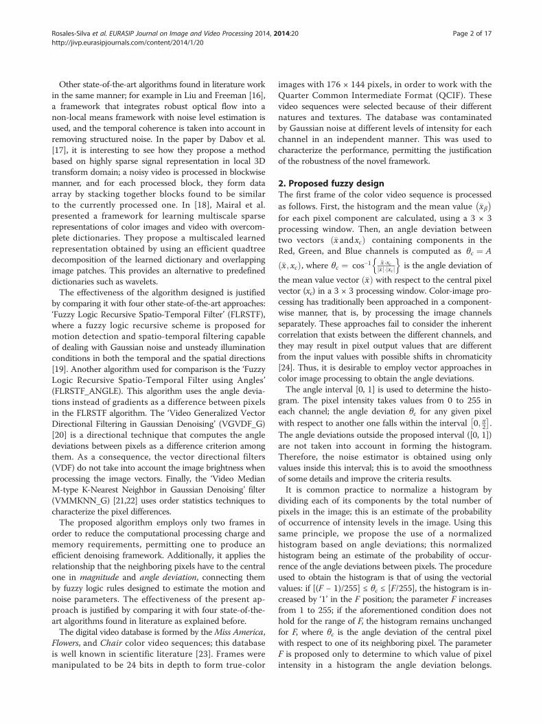
same for all three channels of a color image for the generalprocess of the Gaussian denoising algorithm, as Figure 1indicates. The SD parameter is used to find the deviationsrepresenting the data in its distribution from the arith-metic mean. This is in order to present them more realis-tically when it comes to describing and interpreting themfor decision-making purposes. We estimate the SD par-ameter of the Gaussian noise from the input video se-quence only for the first frame (t = 0) and subsequentlytry to adapt the SD to the input video and noise changesby spatio-temporal adaptation of the noise estimator SD.To summarize, we use the SD parameter as an esti-

mate of the noise to be applied in the spatial algorithm,which will be renewed on a temporary adaptive filter inorder to ultimately generate an adaptive spatio-temporalnoise estimator.

Figure 1 General scheme of the algorithm for Gaussian denoising.

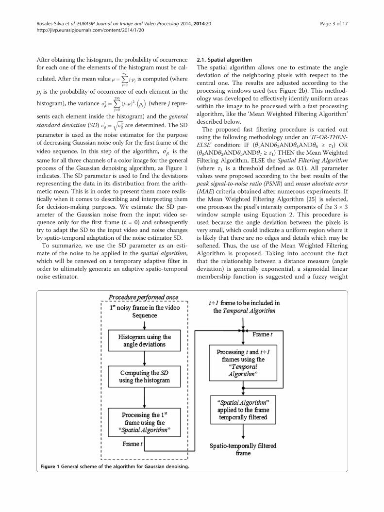
2.1. Spatial algorithmThe spatial algorithm allows one to estimate the angledeviation of the neighboring pixels with respect to thecentral one. The results are adjusted according to theprocessing windows used (see Figure 2b). This method-ology was developed to effectively identify uniform areaswithin the image to be processed with a fast processingalgorithm, like the ‘Mean Weighted Filtering Algorithm’described below.The proposed fast filtering procedure is carried out

using the following methodology under an ‘IF-OR-THEN-ELSE’ condition: IF (θ1ANDθ3ANDθ4ANDθ6 ≥ τ1) OR(θ0ANDθ2ANDθ5ANDθ7 ≥ τ1) THEN the Mean WeightedFiltering Algorithm, ELSE the Spatial Filtering Algorithm(where τ1 is a threshold defined as 0.1). All parametervalues were proposed according to the best results of thepeak signal-to-noise ratio (PSNR) and mean absolute error(MAE) criteria obtained after numerous experiments. Ifthe Mean Weighted Filtering Algorithm [25] is selected,one processes the pixel's intensity components of the 3 × 3window sample using Equation 2. This procedure isused because the angle deviation between the pixels isvery small, which could indicate a uniform region where itis likely that there are no edges and details which may besoftened. Thus, the use of the Mean Weighted FilteringAlgorithm is proposed. Taking into account the factthat the relationship between a distance measure (angledeviation) is generally exponential, a sigmoidal linearmembership function is suggested and a fuzzy weight

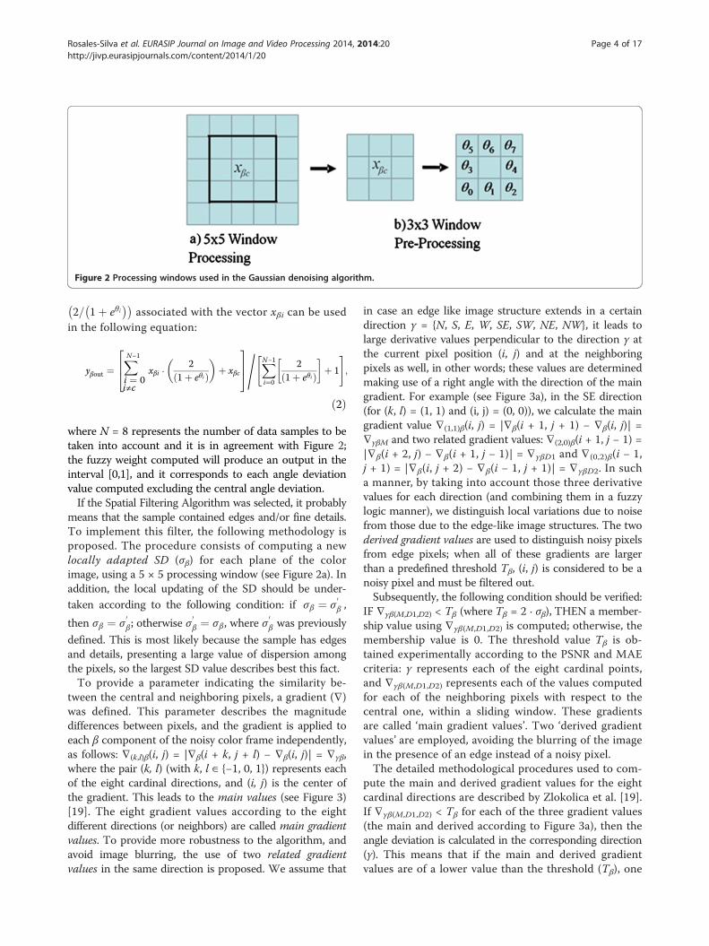
Figure 2 Processing windows used in the Gaussian denoising algorithm.


2= 1þ eθi� ��

associated with the vector xβi can be usedin the following equation:

yβout ¼Xi ¼ 0i≠c

N−1

xβi ⋅2

1þ eθið Þ� �

þ xβc

264

375= XN−1

i¼0

21þ eθið Þ

� �þ 1

" #;

ð2Þ

where N = 8 represents the number of data samples to betaken into account and it is in agreement with Figure 2;the fuzzy weight computed will produce an output in theinterval [0,1], and it corresponds to each angle deviationvalue computed excluding the central angle deviation.If the Spatial Filtering Algorithm was selected, it probably

means that the sample contained edges and/or fine details.To implement this filter, the following methodology isproposed. The procedure consists of computing a newlocally adapted SD (σβ) for each plane of the colorimage, using a 5 × 5 processing window (see Figure 2a). Inaddition, the local updating of the SD should be under-taken according to the following condition: if σβ ¼ σ

0β ,

then σβ ¼ σ0β; otherwise σ

0β ¼ σβ, where σ

0β was previously

defined. This is most likely because the sample has edgesand details, presenting a large value of dispersion amongthe pixels, so the largest SD value describes best this fact.To provide a parameter indicating the similarity be-

tween the central and neighboring pixels, a gradient (∇)was defined. This parameter describes the magnitudedifferences between pixels, and the gradient is applied toeach β component of the noisy color frame independently,as follows: ∇(k,l)β(i, j) = |∇β(i + k, j + l) − ∇β(i, j)| = ∇γβ,where the pair (k, l) (with k, l ∈ {−1, 0, 1}) represents eachof the eight cardinal directions, and (i, j) is the center ofthe gradient. This leads to the main values (see Figure 3)[19]. The eight gradient values according to the eightdifferent directions (or neighbors) are called main gradientvalues. To provide more robustness to the algorithm, andavoid image blurring, the use of two related gradientvalues in the same direction is proposed. We assume that

in case an edge like image structure extends in a certaindirection γ = {N, S, E, W, SE, SW, NE, NW}, it leads tolarge derivative values perpendicular to the direction γ atthe current pixel position (i, j) and at the neighboringpixels as well, in other words; these values are determinedmaking use of a right angle with the direction of the maingradient. For example (see Figure 3a), in the SE direction(for (k, l) = (1, 1) and (i, j) = (0, 0)), we calculate the maingradient value ∇(1,1)β(i, j) = |∇β(i + 1, j + 1) − ∇β(i, j)| =∇γβM and two related gradient values: ∇(2,0)β(i + 1, j − 1) =|∇β(i + 2, j) − ∇β(i + 1, j − 1)| = ∇γβD1 and ∇(0,2)β(i − 1,j + 1) = |∇β(i, j + 2) − ∇β(i − 1, j + 1)| = ∇γβD2. In sucha manner, by taking into account those three derivativevalues for each direction (and combining them in a fuzzylogic manner), we distinguish local variations due to noisefrom those due to the edge-like image structures. The twoderived gradient values are used to distinguish noisy pixelsfrom edge pixels; when all of these gradients are largerthan a predefined threshold Tβ, (i, j) is considered to be anoisy pixel and must be filtered out.Subsequently, the following condition should be verified:

IF ∇γβ(M,D1,D2) < Tβ (where Tβ = 2 · σβ), THEN a member-ship value using ∇γβ(M,D1,D2) is computed; otherwise, themembership value is 0. The threshold value Tβ is ob-tained experimentally according to the PSNR and MAEcriteria: γ represents each of the eight cardinal points,and ∇γβ(M,D1,D2) represents each of the values computedfor each of the neighboring pixels with respect to thecentral one, within a sliding window. These gradientsare called ‘main gradient values’. Two ‘derived gradientvalues’ are employed, avoiding the blurring of the imagein the presence of an edge instead of a noisy pixel.The detailed methodological procedures used to com-

pute the main and derived gradient values for the eightcardinal directions are described by Zlokolica et al. [19].If ∇γβ(M,D1,D2) < Tβ for each of the three gradient values(the main and derived according to Figure 3a), then theangle deviation is calculated in the corresponding direction(γ). This means that if the main and derived gradientvalues are of a lower value than the threshold (Tβ), one

Figure 3 Main and derived values (a) involved in 5 × 5 processing window; angle deviation (b) for only one plane, β = R.


gets the angle deviations from the values for the threegradients; however, if any of these values do not satisfythe condition, the angle deviation is set to 0 for thevalues that do not comply.Another way to characterize the difference between

pixels is by calculating the angle deviation from the cen-tral pixel and its neighbors; this is called the main andderived vectorial values. Calculated angle deviations inthe cardinal directions are taken as the weight valuesfor each color plane of an image (Equation 3). Theseweights provide a relationship between pixels in a singleplane at a given angle deviation. Equation 3 illustrates thecalculation of the angle deviation to obtain the weightvalues, where

θβ ¼ cos−12 255ð Þ2 þ xγβ M;D1;D2ð Þ⋅x0γβ M;D1;D2ð Þffiffiffiffiffiffiffiffiffiffiffiffiffiffiffiffiffiffiffiffiffiffiffiffiffiffiffiffiffiffiffiffiffiffiffiffiffiffiffiffiffiffiffiffiffiffiffiffiffiffiffi

2⋅ 255ð Þ2 þ xγβ M;D1;D2ð Þ� �2q

⋅

ffiffiffiffiffiffiffiffiffiffiffiffiffiffiffiffiffiffiffiffiffiffiffiffiffiffiffiffiffiffiffiffiffiffiffiffiffiffiffiffiffiffiffiffiffiffiffiffiffiffiffiffi2⋅ 255ð Þ2 þ x0γβ M;D1;D2ð Þ

2r

8>><>>:

9>>=>>;;

these values range from 0 to 1 according to Figure 3b.

αγβ ¼ 2

1þ exp θ β� �� ; ð3Þ

where xγβ(M,D1,D2) is the pixel component in the associateddirection. For example, for the xγβM component of thepixel, the coordinate is (0, 0) as shown in Figure 3a.Therefore, for component x ' γβM, the coordinate shouldbe (1, 1) for the ‘SE’ cardinal direction, and so on. Thisparameter indicates that the smaller the difference inangle between the pixels involved, the greater the weightvalue of the pixel in the associated direction.Finally, the main and derived vectorial gradient values

are used to find a degree of membership using member-ship functions, which are functions that return a valuebetween 0 and 1, indicating the degree of membershipof an element with respect to a set (in our case, we definea BIG fuzzy set). Then, we can characterize the level ofproximity of the components of the central pixel withrespect to its neighbors, and see if it is a noisy or in motioncomponent, or free of motion and/or low noise.As mentioned above, we have defined a BIG fuzzy set;

it will feature the presence of noise in the sample to be

processed. The values that belong to this fuzzy set, inwhole or in part, will represent the level of noise presentin the pixel.The membership function used to characterize the ‘main

and derived vectorial gradient values’ is defined by:

μBIG ¼ max 1− ∇γβ M;D1;D2ð Þ=Tβ

� �� ; αγβ M;D1;D2ð Þ

�; if ∇γβ < Tβ

0 ; otherwise;

�

ð4Þ

A fuzzy rule is created from this membership function,which is simply the application of the membership functionby fuzzy operators. In this case, fuzzy operator OR isdefined as OR(f1, f2) = max(f1, f2).Each pixel has one returned value defined by the level

of corruption present in the pixel. That is, one says ‘thepixel is corrupted’ if its BIG membership value is 1, and‘the pixel is low-noise corrupted’ when its BIG membershipvalue is 0. The linguistics ‘the pixel is corrupted’ and‘the pixel is low-noise corrupted’ indicate the degree ofbelonging to each of the possible states in which the pixelcan be found.From the fuzzy rules, we obtain outputs, which are used

to make decisions. The function defined by Equation 4returns values between 0 and 1. It indicates how theparameter behaved with respect to the proposed fuzzyset. Finally, the following fuzzy rule is designed to connectgradient values with angle deviations, thus forming the‘fuzzy vectorial-gradient values’.Fuzzy rule 1 helps to detect the edges and fine details

using the membership values of the BIG fuzzy set ob-tained by Equation 4. The fuzzy values obtained by thisrule are taken as fuzzy weights and used in a fast pro-cessing algorithm to improve the computational load.This fast processing algorithm is defined by means ofEquation 5.Fuzzy rule 1: the fuzzy vectorial-gradient value is defined

as ∇γβαγβ, so: IF ((∇γβM, αγβ) is BIG AND (∇γβD1, αγβD1) isBIG) OR ((∇γβM, αγβ) is BIG AND (∇γβD2, αγβD2) is BIG),THEN ∇γβαγβ is BIG. In this fuzzy rule, the ‘AND’and ‘OR’ operators are defined as algebraic operations,consequently: AND = A · B, and OR = A + B − A · B.


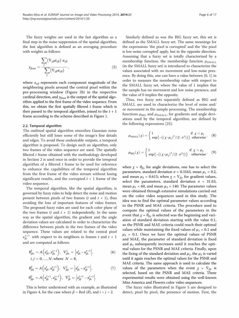
The fuzzy weights are used in the fast algorithm as afinal step in the noise suppression of the spatial algorithm;the fast algorithm is defined as an averaging procedurewith weights as follows:

yβout ¼

Xγ

∇γβαγβ� �

⋅xγβXγ

∇γβαγβ� � ; ð5Þ

where xγβ represents each component magnitude of theneighboring pixels around the central pixel within thepre-processing window (Figure 2b) in the respectivecardinal direction, and yβout is the output of the spatial algo-rithm applied to the first frame of the video sequence. Fromthis, we obtain the first spatially filtered t frame which isthen passed to the temporal algorithm, joined to the t + 1frame according to the scheme described in Figure 1.

2.2. Temporal algorithmThe outlined spatial algorithm smoothes Gaussian noiseefficiently but still loses some of the image's fine detailsand edges. To avoid these undesirable outputs, a temporalalgorithm is proposed. To design such an algorithm, onlytwo frames of the video sequence are used. The spatiallyfiltered t frame obtained with the methodology developedin Section 2 is used once in order to provide the temporalalgorithm of a filtered t frame to be used for referenceto enhance the capabilities of the temporal algorithmfrom the first frame of the video stream without losingsignificant results, and the corrupted t + 1 frame of thevideo sequence.The temporal algorithm, like the spatial algorithm, is

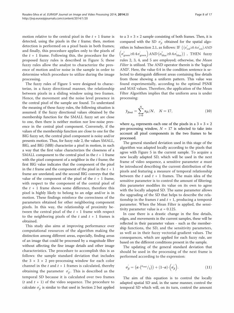
governed by fuzzy rules to help detect the noise and motionpresent between pixels of two frames (t and t + 1), thusavoiding the loss of important features of video frames.The proposed fuzzy rules are used for each color plane ofthe two frames (t and t + 1) independently. In the sameway as the spatial algorithm, the gradient and the angledeviation values are calculated in order to characterize thedifference between pixels in the two frames of the videosequence. These values are related to the central pixelx tþ1βc with respect to its neighbors in frames t and t + 1

and are computed as follows:

θ1βic ¼ A xtβi; xtþ1βc

; ∇1

βic ¼ xtβi − xtþ1βc

�� ;i; j ¼ 0;…;N ;where N ¼ 8;

ð6Þ

θ2βij ¼ A xtβi; xtþ1βj

; ∇2

βij ¼ xtβi − xtþ1βj

�� ;θ3βjc ¼ A xtþ1

βj ; xtþ1βc

; ∇3

βj ¼ xtþ1βj − xtþ1

βc

�� :ð7Þ

This is better understood with an example, as illustratedin Figure 4, for the case where β = Red (R), and i = j = 2.

Similarly defined as was the BIG fuzzy set, this set isdefined as the SMALL fuzzy set. The same meanings forthe expressions ‘the pixel is corrupted’ and the ‘the pixelis low-noise corrupted’ apply, but in the opposite direction.Assuming that a fuzzy set is totally characterized by amembership function, the membership function μSMALL

(in the SMALL fuzzy set) is introduced to characterize thevalues associated with no movement and low-noise pres-ence. By doing this, one can have a value between [0, 1] inorder to measure the membership value with respect tothe SMALL fuzzy set, where the value of 1 implies thatthe sample has no movement and low noise presence, andthe value of 0 implies the opposite.Thus, two fuzzy sets separately defined as BIG and

SMALL are used to characterize the level of noise and/or movement in the sample processing. The membershipfunctions μBIG and μSMALL, for gradients and angle devi-ations used by the temporal algorithm, are defined bythe following expressions [25]:

μSMALL χð Þ ¼ 1 if χ < μ1exp − χ−μ1ð Þ2= 2 ⋅ σ2ð Þ� � �

otherwise ;

�ð8Þ

μBIG χð Þ ¼ 1 if χ > μ2exp − χ−μ2ð Þ2= 2 ⋅ σ2ð Þ� � �

otherwise ;

�ð9Þ

when χ = θβγ for angle deviations, one has to select theparameters, standard deviation σ = 0.3163, mean μ1 = 0.2,and mean μ2 = 0.615; when χ = ∇βγ for gradient values,select the parameters, standard deviation σ = 31.63,mean μ1 = 60, and mean μ2 = 140. The parameter valueswere obtained through extensive simulations carried outon the color video sequences used in this study. Theidea was to find the optimal parameter values accordingto the PSNR and MAE criteria. The procedure used tocompute the optimal values of the parameters in theevent that χ = θβγ is selected was the beginning and vari-ation of standard deviation starting with the value 0.1,so the PSNR and MAE criteria could reach their optimalvalues while maintaining the fixed values of μ1 = 0.1 andμ2 = 0.1. Once we have the optimal values of PSNRand MAE, the parameter of standard deviation is fixedand μ1 subsequently increases until it reaches the opti-mal values for the PSNR and MAE criteria. Finally, uponthe fixing of the standard deviation and μ1, the μ2 is varieduntil it again reaches the optimal values for the PSNR andMAE criteria. The same approach is used to calculate thevalues of the parameters when the event χ = ∇βγ isselected, based on the PSNR and MAE criteria. Theseexperimental results were obtained using the well-knownMiss America and Flowers color video sequences.The fuzzy rules illustrated in Figure 5 are designed to

detect, pixel by pixel, the presence of motion. First, the

Figure 4 Application example for Equations 6 and 7, where β = R, and i = j = 2.

Figure 5 Fuzzy rules 2, 3, 4, and 5 used to determine the motion level for t and t + 1 frames. (a) Fuzzy rule 2 SBBβic. (b) Fuzzy rule 3SSSβic. (c) Fuzzy rule 4 BBBβic. (d) Fuzzy rule 5 BBSβic.



motion relative to the central pixel in the t + 1 frame isdetected, using the pixels in the t frame; then, motiondetection is performed on a pixel basis in both frames;and finally, this procedure applies only to the pixels ofthe t + 1 frame. Following this, the procedure for theproposed fuzzy rules is described in Figure 5; thesefuzzy rules allow the analyst to characterize the pres-ence of motion and/or noise in the sample in order todetermine which procedure to utilize during the imageprocessing.The fuzzy rules of Figure 5 were designed to charac-

terize, in a fuzzy directional manner, the relationshipbetween pixels in a sliding window using two frames.Hence, the movement and the noise level presence inthe central pixel of the sample are found. To understandthe meaning of these fuzzy rules, the following situation isassumed: if the fuzzy directional values obtained by themembership function for the SMALL fuzzy set are closeto one, then there is neither motion nor low-noise pres-ence in the central pixel component. Conversely, if thevalues of the membership function are close to one for theBIG fuzzy set, the central pixel component is noisy and/orpresents motion. Thus, for fuzzy rule 2, the values SMALL,BIG, and BIG (SBB) characterize a pixel in motion, in sucha way that the first value characterizes the closeness of aSMALL component to the central pixel in the t + 1 framewith the pixel component of a neighbor in the t frame; thefirst BIG value indicates that the component of the pixelin the t frame and the component of the pixel in the t + 1frame are unrelated; and the second BIG conveys that thevalue of the component of the pixel of the t + 1 frame,with respect to the component of the central pixel ofthe t + 1 frame shows some difference, therefore thispixel is highly likely to belong to an edge and/or is inmotion. These findings reinforce the correctness of theparameters obtained for other neighboring componentpixels. In this way, the relationship of proximity be-tween the central pixel of the t + 1 frame with respectto the neighboring pixels of the t and t + 1 frames isobtained.This study also aims at improving performance over

computational resources of the algorithm making thedistinction among different areas, especially, finding areasof an image that could be processed by a magnitude filterwithout affecting the fine image details and other imagecharacteristics. The procedure to accomplish this is asfollows: the sample standard deviation that includesthe 3 × 3 × 2 pre-processing window for each colorchannel in the t and t + 1 frames is calculated, thereby

obtaining the parameter σ}β . This is described as the

temporal SD because it is calculated over two frames(t and t + 1) of the video sequence. The procedure to

calculate σ}β is similar to that used in Section 2 but applied

to a 3 × 3 × 2 sample consisting of both frames. Then, it iscompared with the SD σ}β obtained for the spatial algo-

rithm in Subsection 2.1, as follows: IF σ00red≥0:4σ

0red

� �AND

σ

00green≥0:4σ

0green

AND σ

00blue≥0:4σ

0blue

� �g , THEN fuzzy

rules 2, 3, 4, and 5 are employed; otherwise, the MeanFilter is utilized. The AND operator therein is the ‘logicalAND’. Here, the value 0.4 in the condition sentence is se-lected to distinguish different areas containing fine detailsfrom those showing a uniform pattern. This value wasfound experimentally, according to the optimal PSNRand MAE values. Therefore, the application of the MeanFilter Algorithm implies that the uniform area is underprocessing:

�yβout ¼XNi¼0

xβi=N ; N ¼ 17; ð10Þ

where xβi represents each one of the pixels in a 3 × 3 × 2pre-processing window, N = 17 is selected to take intoaccount all pixel components in the two frames to beprocessed.The general standard deviation used in this stage of the

algorithm was adapted locally according to the pixels thatagree with Figure 5 in the current sample. To acquire anew locally adapted SD, which will be used in the nextframe of video sequence, a sensitive parameter α mustbe introduced describing the current distribution of thepixels and featuring a measure of temporal relationshipbetween the t and t + 1 frames. The main idea of thesensitive parameter is to control the amount of filtering;this parameter modifies its value on its own to agreewith the locally adapted SD. The same parameter allowsthe upgrading of the SD that helps to describe the rela-tionship in the frames t and t + 1, producing a temporalparameter. When the Mean Filter is applied, the sensi-tivity parameter value is α = 0.125.In case there is a drastic change in the fine details,

edges, and movements in the current samples, these will bereflected in their parameter values - such as the member-ship functions, the SD, and the sensitivity parameters,as well as in their fuzzy vectorial-gradient values. Theconsequences, which are applied for each fuzzy rule, arebased on the different conditions present in the sample.The updating of the general standard deviation that

should be used in the processing of the next frame isperformed according to the expression:

σ0β ¼ α⋅ σ total=5

� �� þ 1−αð Þ⋅ σ0β

: ð11Þ

The aim of this equation is to control the locallyadapted spatial SD and, in the same manner, control thetemporal SD which will, on its turn, control the amount


of filtering modifying the Tβ threshold as will be shownlater.Parameters σ

0β; σ

00β; and σ total describe how the pixels in

the t and t + 1 frames are related to each other in a spatial

σ0β

and temporal σ}β; and σ total

way. The SD updating

of σtotal is achieved through: σ total ¼ σ00Redþσ

00Greenþσ

00Blueð Þ.

3;

this is the average value of the temporal SD using the threecolor planes of the images. This relationship is designed tohave the other color components of the image contribute tothe sensitivity parameter.The structure of Equation 11 can be illustrated using

an example: if the Mean Filter Algorithm was selectedfor application instead of fuzzy rules 2, 3, 4, and 5, thesensitive parameter α = 0.125 used for the algorithmdescribes that the t and t + 1 frames are closely related.This means that the pixels in the t frame bear low noisedue to the fact that the spatial algorithm was applied tothis frame (see Subsection 2.1) and that the pixels in thet + 1 frame are probably low-noise too. However, at thistime, because the t frame has only been filtered by thespatial algorithm (see Subsection 2.1), it seems better toincrease the weight obtained by the t frame in the spatialSD σ

0β

, rather than using that obtained by the t + 1

frame temporalSD σ00β

. That is why the weights of σtotal

multiplied by α = 0.125, and the weight of σ0β multiplied

by (1 − α) = 0.875 are used.The application of fuzzy rules to pixels allows a better

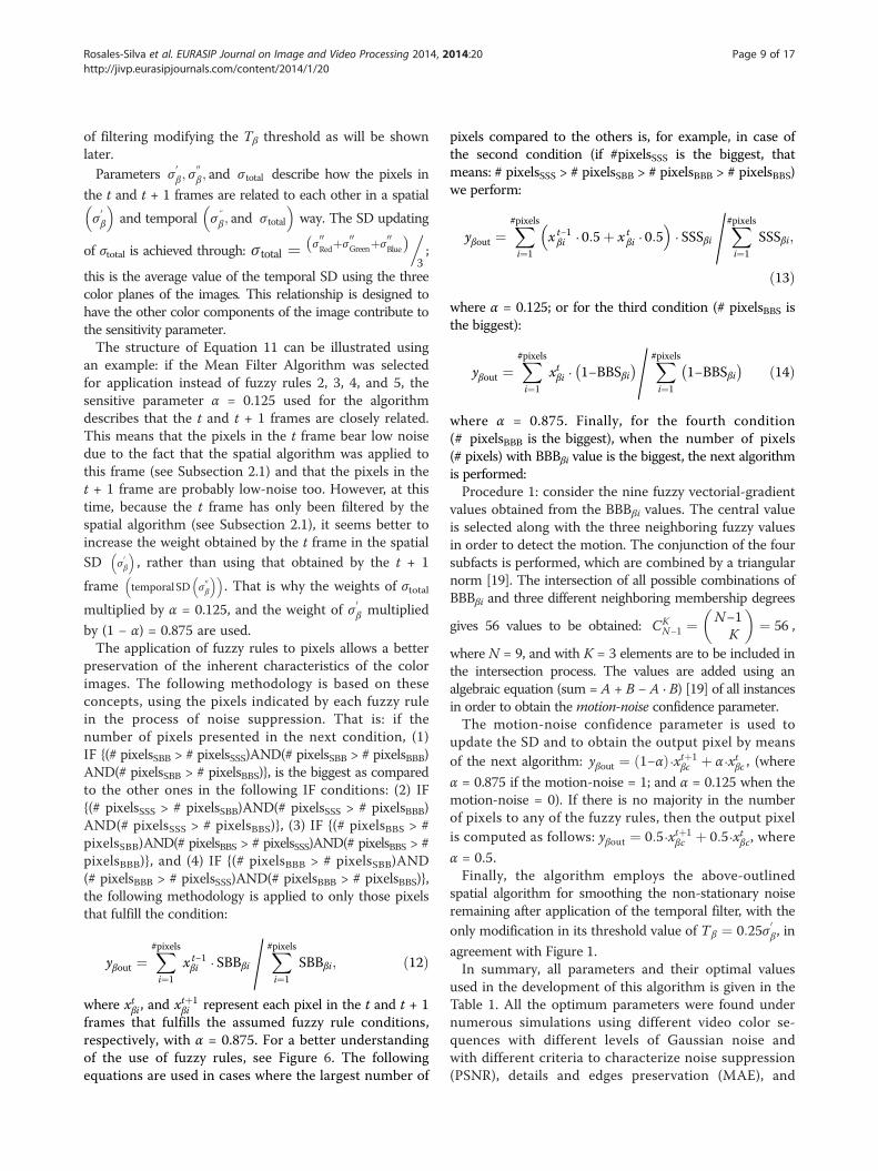
preservation of the inherent characteristics of the colorimages. The following methodology is based on theseconcepts, using the pixels indicated by each fuzzy rulein the process of noise suppression. That is: if thenumber of pixels presented in the next condition, (1)IF {(# pixelsSBB > # pixelsSSS)AND(# pixelsSBB > # pixelsBBB)AND(# pixelsSBB > # pixelsBBS)}, is the biggest as comparedto the other ones in the following IF conditions: (2) IF{(# pixelsSSS > # pixelsSBB)AND(# pixelsSSS > # pixelsBBB)AND(# pixelsSSS > # pixelsBBS)}, (3) IF {(# pixelsBBS > #pixelsSBB)AND(# pixelsBBS > # pixelsSSS)AND(# pixelsBBS > #pixelsBBB)}, and (4) IF {(# pixelsBBB > # pixelsSBB)AND(# pixelsBBB > # pixelsSSS)AND(# pixelsBBB > # pixelsBBS)},the following methodology is applied to only those pixelsthat fulfill the condition:

yβout ¼X#pixelsi¼1

x t−1βi ⋅ SBBβi= X#pixels

i¼1

SBBβi; ð12Þ

where xtβi , and xtþ1βi represent each pixel in the t and t + 1

frames that fulfills the assumed fuzzy rule conditions,respectively, with α = 0.875. For a better understandingof the use of fuzzy rules, see Figure 6. The followingequations are used in cases where the largest number of

pixels compared to the others is, for example, in case ofthe second condition (if #pixelsSSS is the biggest, thatmeans: # pixelsSSS > # pixelsSBB > # pixelsBBB > # pixelsBBS)we perform:


x t−1βi ⋅ 0:5þ x t

βi ⋅ 0:5

⋅ SSSβi=X#pixelsi¼1

SSSβi;

ð13Þwhere α = 0.125; or for the third condition (# pixelsBBS isthe biggest):


xtβi ⋅ 1−BBSβi� �= X#pixels

i¼1

1−BBSβi� � ð14Þ

where α = 0.875. Finally, for the fourth condition(# pixelsBBB is the biggest), when the number of pixels(# pixels) with BBBβi value is the biggest, the next algorithmis performed:Procedure 1: consider the nine fuzzy vectorial-gradient

values obtained from the BBBβi values. The central valueis selected along with the three neighboring fuzzy valuesin order to detect the motion. The conjunction of the foursubfacts is performed, which are combined by a triangularnorm [19]. The intersection of all possible combinations ofBBBβi and three different neighboring membership degrees

gives 56 values to be obtained: CKN−1 ¼

N−1K

� �¼ 56 ,

where N = 9, and with K = 3 elements are to be included inthe intersection process. The values are added using analgebraic equation (sum = A + B − A · B) [19] of all instancesin order to obtain the motion-noise confidence parameter.The motion-noise confidence parameter is used to

update the SD and to obtain the output pixel by meansof the next algorithm: yβout ¼ 1−αð Þ⋅xtþ1

βc þ α⋅xtβc , (whereα = 0.875 if the motion-noise = 1; and α = 0.125 when themotion-noise = 0). If there is no majority in the numberof pixels to any of the fuzzy rules, then the output pixelis computed as follows: yβout ¼ 0:5⋅xtþ1

βc þ 0:5⋅xtβc, whereα = 0.5.Finally, the algorithm employs the above-outlined

spatial algorithm for smoothing the non-stationary noiseremaining after application of the temporal filter, with theonly modification in its threshold value of Tβ ¼ 0:25σ

0β, in

agreement with Figure 1.In summary, all parameters and their optimal values

used in the development of this algorithm is given in theTable 1. All the optimum parameters were found undernumerous simulations using different video color se-quences with different levels of Gaussian noise andwith different criteria to characterize noise suppression(PSNR), details and edges preservation (MAE), and

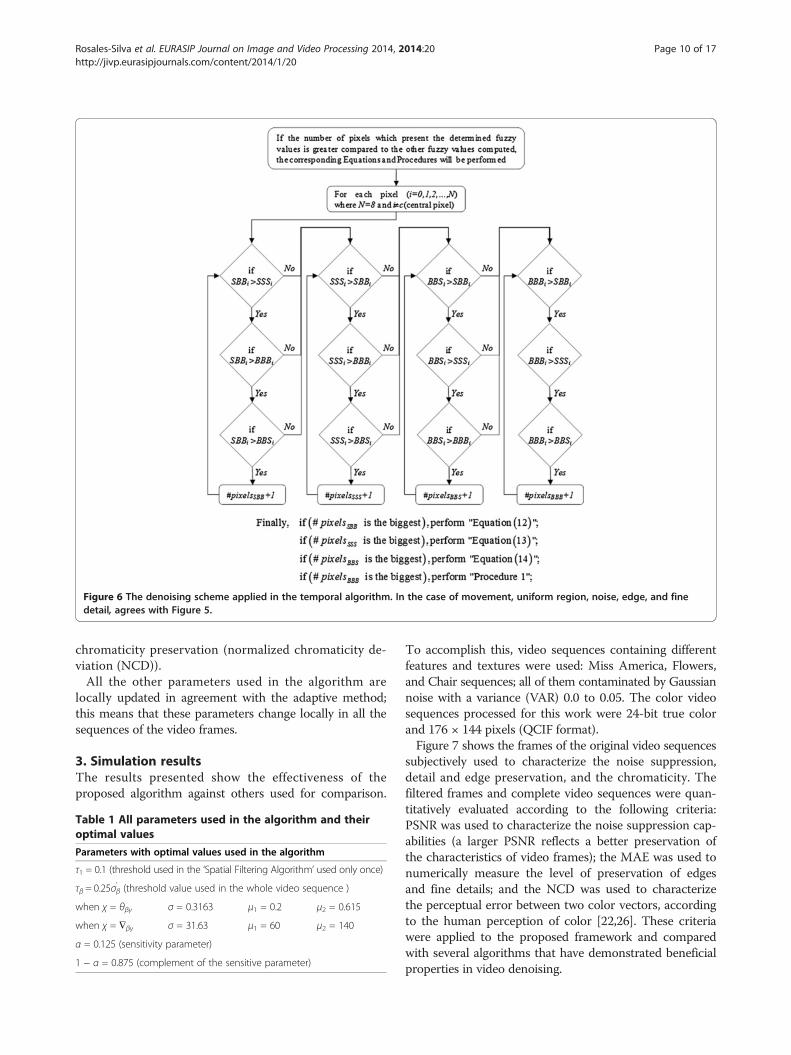
Figure 6 The denoising scheme applied in the temporal algorithm. In the case of movement, uniform region, noise, edge, and finedetail, agrees with Figure 5.


chromaticity preservation (normalized chromaticity de-viation (NCD)).All the other parameters used in the algorithm are

locally updated in agreement with the adaptive method;this means that these parameters change locally in all thesequences of the video frames.

3. Simulation resultsThe results presented show the effectiveness of theproposed algorithm against others used for comparison.

Table 1 All parameters used in the algorithm and theiroptimal values

Parameters with optimal values used in the algorithm

τ1 = 0.1 (threshold used in the ‘Spatial Filtering Algorithm’ used only once)

τβ = 0.25σ'β (threshold value used in the whole video sequence )

when χ = θβγ σ = 0.3163 μ1 = 0.2 μ2 = 0.615

when χ = ∇βγ σ = 31.63 μ1 = 60 μ2 = 140

α = 0.125 (sensitivity parameter)

1 − α = 0.875 (complement of the sensitive parameter)

To accomplish this, video sequences containing differentfeatures and textures were used: Miss America, Flowers,and Chair sequences; all of them contaminated by Gaussiannoise with a variance (VAR) 0.0 to 0.05. The color videosequences processed for this work were 24-bit true colorand 176 × 144 pixels (QCIF format).Figure 7 shows the frames of the original video sequences

subjectively used to characterize the noise suppression,detail and edge preservation, and the chromaticity. Thefiltered frames and complete video sequences were quan-titatively evaluated according to the following criteria:PSNR was used to characterize the noise suppression cap-abilities (a larger PSNR reflects a better preservation ofthe characteristics of video frames); the MAE was used tonumerically measure the level of preservation of edgesand fine details; and the NCD was used to characterizethe perceptual error between two color vectors, accordingto the human perception of color [22,26]. These criteriawere applied to the proposed framework and comparedwith several algorithms that have demonstrated beneficialproperties in video denoising.

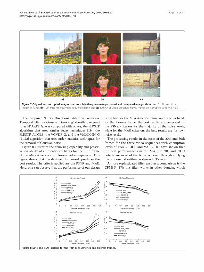
Figure 7 Original and corrupted images used to subjectively evaluate proposed and comparative algorithms. (a) 10th Flowers videosequence frame, (b) 10th Miss America video sequence frame, and (c) 10th Chair video sequence frame. Frames are corrupted with VAR = 0.01.


The proposed ‘Fuzzy Directional Adaptive RecursiveTemporal Filter for Gaussian Denoising’ algorithm, referredto as FDARTF_G, was compared with others, the FLRSTFalgorithm that uses similar fuzzy techniques [19], theFLRSTF_ANGLE, the VGVDF_G, and the VMMKNN_G[21,22] algorithm that uses order statistics techniques forthe removal of Gaussian noise.Figure 8 illustrates the denoising capability and preser-

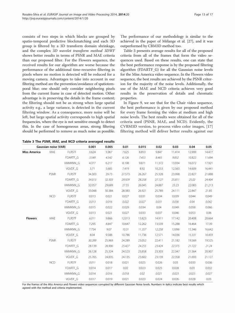
vation ability of all mentioned filters for the 10th frameof the Miss America and Flowers video sequences. Thisfigure shows that the designed framework produces thebest results. The criteria applied are the PSNR and MAE.Here, one can observe that the performance of our design

Figure 8 MAE and PSNR criteria for the 10th Miss America and Flowe

is the best for the Miss America frame; on the other hand,for the Flowers frame, the best results are generated bythe PSNR criterion for the majority of the noise levels,while for the MAE criterion, the best results are for low-noise levels.The processing results in the cases of the 20th and 30th

frames for the three video sequences with corruptionlevels of VAR = 0.005 and VAR =0.01 have shown thatthe best performances in the MAE, PSNR, and NCDcriteria are most of the times achieved through applyingthe proposed algorithm, as shown in Table 2.A more sophisticated filter used as a comparison is the

CBM3D [17]; this filter works in other domain, which

rs frames.

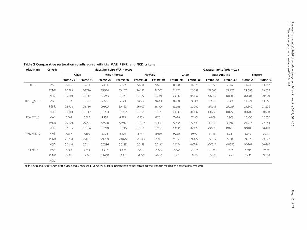
Table 2 Comparative restoration results agree with the MAE, PSNR, and NCD criteria

Algorithm Criteria Gaussian noise VAR = 0.005 Gaussian noise VAR = 0.01

Chair Miss America Flowers Chair Miss America Flowers

Frame 20 Frame 30 Frame 20 Frame 30 Frame 20 Frame 30 Frame 20 Frame 30 Frame 20 Frame 30 Frame 20 Frame 30

FLRSTF MAE 6.375 6.613 5.818 5.622 9.628 9.551 8.400 8.325 7.477 7.362 11.932 11.652

PSNR 28.979 28.720 29.926 30.157 26.192 26.263 26.701 26.589 27.686 27.720 24.363 24.559

NCD 0.0110 0.0112 0.0263 0.0261 0.0167 0.0168 0.0140 0.0137 0.0257 0.0260 0.0205 0.0203

FLRSTF_ANGLE MAE 6.374 6.620 5.826 5.629 9.825 9.643 8.458 8.319 7.500 7.386 11.971 11.661

PSNR 28.968 28.716 29.905 30.133 26.007 26.164 26.638 26.605 27.681 27.687 24.340 24.556

NCD 0.0110 0.0112 0.0263 0.0262 0.0175 0.0171 0.0140 0.0137 0.0258 0.0259 0.0205 0.0203

FDARTF_G MAE 5.501 5.603 4.459 4.279 8.503 8.281 7.416 7.245 6.069 5.909 10.438 10.056

PSNR 29.170 29.291 32.510 32.917 27.309 27.611 27.454 27.391 30.059 30.300 25.717 26.054

NCD 0.0105 0.0106 0.0219 0.0216 0.0155 0.0151 0.0135 0.0128 0.0220 0.0216 0.0185 0.0182

VMMKNN_G MAE 7.987 7.886 6.178 6.103 8.777 8.459 9.250 9.677 8.143 8.081 9.916 9.634

PSNR 25.368 25.607 29.799 29.826 25.348 25.801 25.159 24.427 27.612 27.683 24.629 24.978

NCD 0.0146 0.0141 0.0286 0.0285 0.0153 0.0147 0.0174 0.0164 0.0287 0.0282 0.0167 0.0167

CBM3D MAE 4.863 4.854 3.512 3.509 7.821 7.795 7.712 7.729 4.518 4.526 9.934 9.896

PSNR 33.185 33.193 33.658 33.931 30.790 30.670 32.1 32.06 32.58 32.87 29.45 29.363

NCD - - - - - - - - - - - -

For the 20th and 30th frames of the video sequences used. Numbers in italics indicate best results which agreed with the method and criteria implemented.

Rosales-Silvaet

al.EURA

SIPJournalon

Image

andVideo

Processing2014,2014:20

Page12

of17

http://jivp.eurasipjournals.com/content/2014/1/20


consists of two steps in which blocks are grouped byspatio-temporal predictive blockmatching and each 3Dgroup is filtered by a 3D transform domain shrinkage,and the complex 3D wavelet transform method 3DWFshows better results in terms of PSNR and MAE criteriathan our proposed filter. For the Flowers sequence, thereceived results for our algorithm are worse because theperformance of the additional time-recursive filtering inpixels where no motion is detected will be reduced for amoving camera. Advantages to take into account in ourfiltering method are the prevention/avoidance of spatiotem-poral blur; one should only consider neighboring pixelsfrom the current frame in case of detected motion. Otheradvantage is in preserving the details in the frame content;the filtering should not be as strong when large spatialactivity e.g., a large variance, is detected in the currentfiltering window. As a consequence, more noise will beleft, but large spatial activity corresponds to high spatialfrequencies, where the eye is not sensitive enough to detectthis. In the case of homogeneous areas, strong filteringshould be performed to remove as much noise as possible.

Table 3 The PSNR, MAE, and NCD criteria averaged results

Gaussian noise (VAR) 0.001 0.005

Miss America MAE FLRSTF 3.624 5.967

FDARTF_G 3.549 4.542

VMMKNN_G 4.377 6.217

VGVDF_G 3.71 5.685

PSNR FLRSTF 34.303 29.73

FDARTF_G 34.013 32.303

VMMKNN_G 32.057 29.689

VGVDF_G 33.048 30.384

NCD FLRSTF 0.013 0.021

FDARTF_G 0.013 0.016

VMMKNN_G 0.015 0.022

VGVDF_G 0.013 0.021

Flowers MAE FLRSTF 6.011 9.866

FDARTF_G 7.295 8.847

VMMKNN_G 7.754 9.07

VGVDF_G 8.04 9.588

PSNR FLRSTF 30.289 25.969

FDARTF_G 28.139 26.906

VMMKNN_G 26.128 25.324

VGVDF_G 25.765 24.835

NCD FLRSTF 0.011 0.018

FDARTF_G 0.014 0.017

VMMKNN_G 0.014 0.016

VGVDF_G 0.017 0.019

For the frames of the Miss America and Flowers video sequences corrupted by diffeagreed with the method and criteria implemented.

The performance of our methodology is similar to theachieved in the paper of Mélange et al. [27], and it wasoutperformed by CBM3D method too.Table 3 presents average results for all of the proposed

criteria from all of the frames that form the video se-quences used. Based on these results, one can state thatthe best performance response is by the proposed filteringalgorithm (FDARTF_G) for all the Gaussian noise levelsfor the Miss America video sequence. In the Flowers videosequence, the best results are achieved by the PSNR criter-ion for the majority of the noise levels. Additionally, theuse of the MAE and NCD criteria achieves very goodresults in the preservation of details and chromaticproperties.In Figure 9, we see that for the Chair video sequence,

the best performance is given by our proposed methodfor every frame forming the video at medium and highnoise levels. The best results were obtained for all of thecriteria used (PSNR, MAE, and NCD). Evidently, theCVBM3D version, to process video color images, [17]filtering method will deliver better results against our

0.01 0.015 0.02 0.03 0.04 0.05

7.625 8.853 9.847 11.414 12.999 14.477

6.126 7.453 8.465 9.832 10.822 11.694

8.198 9.871 11.372 13.934 16.072 17.921

7.419 8.92 10.253 12.563 14.609 16.441

27.573 26.267 25.328 23.998 22.827 21.888

29.929 28.258 27.127 25.811 25.02 24.404

27.55 26.045 24.887 23.23 22.083 21.213

28.383 26.921 25.789 24.111 22.847 21.85

0.027 0.031 0.034 0.039 0.044 0.049

0.022 0.027 0.031 0.036 0.04 0.042

0.029 0.034 0.04 0.049 0.058 0.066

0.027 0.033 0.037 0.046 0.053 0.06

12.013 13.823 14.911 17.142 20.408 20.664

10.647 12.262 13.539 15.288 16.464 17.39

10.31 11.357 12.258 13.896 15.346 16.642

10.786 11.736 12.571 14.036 15.331 16.459

24.289 23.052 22.411 21.182 19.569 19.525

25.427 24.255 23.424 22.375 21.722 21.24

24.523 23.858 23.303 22.347 21.564 20.907

24.135 23.602 23.139 22.358 21.693 21.127

0.021 0.025 0.026 0.03 0.033 0.036

0.02 0.023 0.025 0.028 0.03 0.032

0.018 0.02 0.021 0.023 0.025 0.027

0.021 0.023 0.024 0.026 0.028 0.03

rent Gaussian Noise levels. Numbers in italics indicate best results which

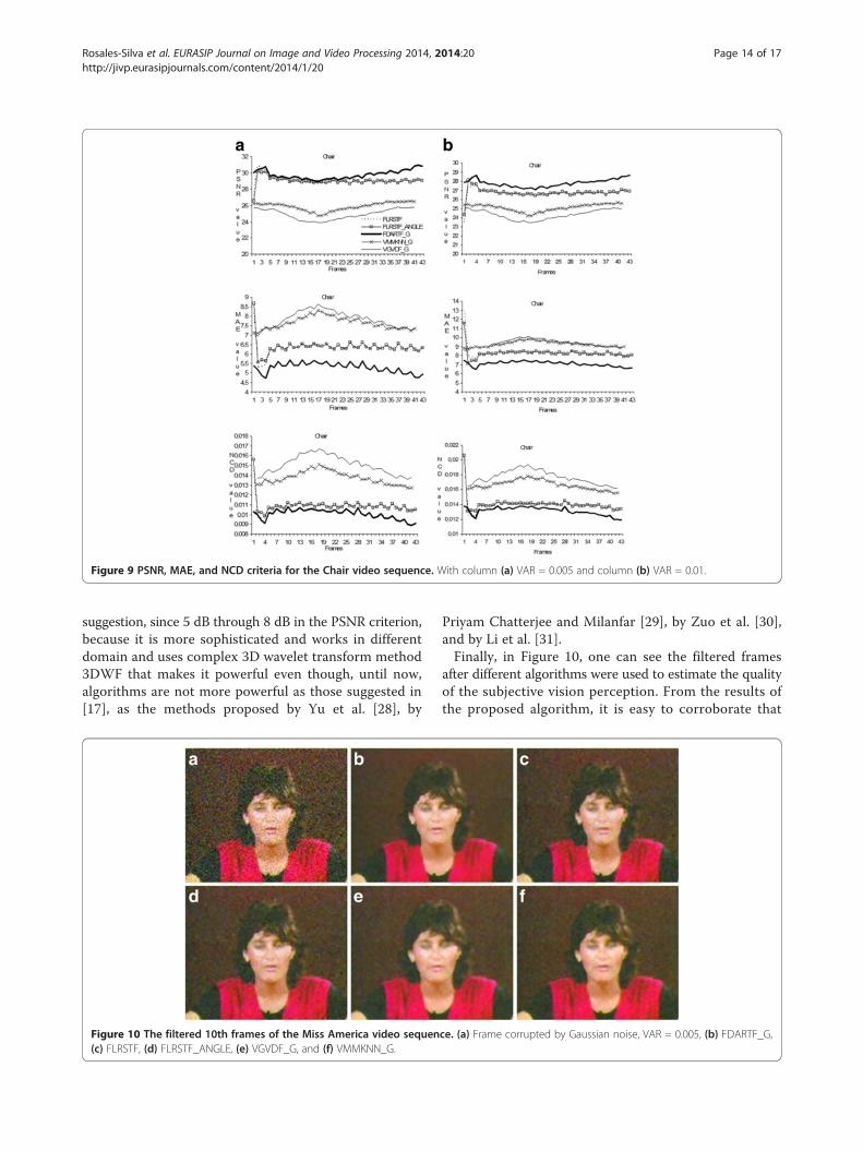
Figure 9 PSNR, MAE, and NCD criteria for the Chair video sequence. With column (a) VAR = 0.005 and column (b) VAR = 0.01.


suggestion, since 5 dB through 8 dB in the PSNR criterion,because it is more sophisticated and works in differentdomain and uses complex 3D wavelet transform method3DWF that makes it powerful even though, until now,algorithms are not more powerful as those suggested in[17], as the methods proposed by Yu et al. [28], by

Figure 10 The filtered 10th frames of the Miss America video sequen(c) FLRSTF, (d) FLRSTF_ANGLE, (e) VGVDF_G, and (f) VMMKNN_G.

Priyam Chatterjee and Milanfar [29], by Zuo et al. [30],and by Li et al. [31].Finally, in Figure 10, one can see the filtered frames

after different algorithms were used to estimate the qualityof the subjective vision perception. From the results ofthe proposed algorithm, it is easy to corroborate that

ce. (a) Frame corrupted by Gaussian noise, VAR = 0.005, (b) FDARTF_G,

Figure 11 The filtered 10th frames of the Flowers video sequence. (a) Image corrupted by Gaussian noise, VAR = 0.01, (b) FDARTF_G,(c) FLRSTF, (d) FLRSTF_ANGLE, (e) VGVDF_G, and (f) VMMKNN_G.


this filter has the best performance in detail preserva-tion and noise suppression. In the FDARTF_G filteredimage, one can observe cleaner regions with betterpreservation of fine details and edges, as compared toother algorithms.In Figure 11 below, the proposed framework produces

the best results in the areas of detail preservation andnoise suppression. One can perceive (in the vicinity of thetree) that in the case of the FDARTF_G filtering, theresulting image is less influenced by noise compared tothe image produced by other filters. In addition, the new

Figure 12 The filtered 10th frames of the Chair video sequence. (a) Im(c) FLRSTF, (d) FLRSTF_ANGLE, (e) VGVDF_G, and (f) VMMKNN_G.

filter preserves more details of the features displayed inthe background environment.From Figure 12, one can see that the proposed

framework achieves the best results in details, edges,and preservation of chromaticity. We can observe thatthe uniform regions are free from noise influence in thecase of the FDARTF_G filtering than with the other filtersimplemented. Also, the new filter preserves more detailsin the features seen in the background environment.Since the proposed algorithm is adaptive, it is difficult

to obtain computational information related to how many

age corrupted by Gaussian noise, VAR = 0.01, (b) FDARTF_G,


adds, multiplies, or divisions among other operations liketrigonometrical ones were carried out; we provide real-timeperformance using a DSP from Texas Instruments, Dallas,TX, USA; this was the DM642 [32] giving the followingresults: for our proposed FDARTF_G, it spent an averagetime of 17.78 s per frame, but in a complete directional(VGVDF_G) processing algorithm, it spent an average timeof 25.6 s per frame, both in a QCIF format.

4. ConclusionsThe fuzzy and directional techniques working togetherhave proven to be a powerful framework for image filteringapplied in color video denoising in QCIF sequences.This robust algorithm performs motion detection andlocal noise standard deviation estimation. These propervideo-sequence characteristics have been obtained andconverted into parameters to be used as thresholds indifferent stages of the novel proposed filter. This algo-rithm permits the processing of t and t + 1 video frames,producing an appreciable savings of time and resourcesexpended in computational filtering.Using the advantages of both techniques (directional

and diffuse), it was possible to design an algorithm thatcan preserve edges and fine details of video frames besidesmaintaining their inherent color, improving the preserva-tion of the texture of the colors versus results obtained bythe comparative algorithms. Other important conclusionis that for sequences obtained by a still camera, ourmethod has a better performance in terms of PSNR thanother multiresolution filters of a similar complexity, but itis outperformed by some more sophisticated methods(CBM3D).The simulation results under the proposed criteria

PSNR, MAE, and NCD were used to characterize analgorithm's efficiency in noise suppression, fine details,edges, and chromatic properties preservation. The percep-tual errors have demonstrated the advantages of the pro-posed filtering approach.

Competing interestsThe authors declare that they have no competing interest.

AcknowledgementsThe authors thank the Instituto Politécnico Nacional de México (NationalPolytechnic Institute of Mexico) and CONACYT for their financial support.

Received: 2 March 2012 Accepted: 12 March 2014Published: 2 April 2014

References1. AJ Rosales-Silva, FJ Gallegos-Funes, V Ponomaryov, Fuzzy Directional (FD)

Filter for impulsive noise reduction in colour video sequences. J. Vis. Commun.Image Represent. 23(1), 143–149 (2012)

2. A Amer, H Schrerder, A new video noise reduction algorithm using spatialsubbands. Int. Conf. on Electronic Circuits and Systems 1, 45–48(13-16 October 1996)

3. G De Haan, IC for motion-compensated deinterlacing, noise reduction, andpicture rate conversion. IEEE Trans. On Consumers Electronics45(3), 617–624 (1999)

4. R Rajagopalan, M Orchard, Synthesizing processed video by filteringtemporal relationships. IEEE Trans. Image Process. 11(1), 26–36 (2002)

5. V Seran, LP Kondi, New temporal filtering scheme to reduce delay inwavelet-based video coding. IEEE Trans. Image Process. 16(12), 2927–2935(2007)

6. V Zlokolica, M De Geyter, S Schulte, A Pizurica, W Philips, E Kerre, Fuzzy logicrecursive change detection for tracking and denoising of video sequences,in Paper presented at the IS&T/SPIE Symposium on Electronic Imaging, SanJose, California, USA, 14 March 2005. doi: 10.1117/12.585854

7. A Pizurica, V Zlokolica, W Philips, Noise reduction in video sequences usingwavelet-domain and temporal filtering, in Paper presented at the SPIE Conferenceon Wavelet Applications in Industrial Processing, USA, 27 February 2004.doi:10.1117/12.516069

8. W Selesnick, K Li, Video denoising using 2d and 3d dual-tree complex wave-let transforms, in Paper presented at the Proc. SPIE on Wavelet Applications inSignal and Image Processing, USA, volume 5207, pp. 607-618; 14 November2003. doi: 10.1117/12.504896

9. N Rajpoot, Z Yao, R Wilson, Adaptive wavelet restoration of noisy videosequences, in Paper presented at the IEEE International Conference on ImageProcessing, pp. 957-960, October 2004. doi: 10.1109/ICIP.2004.1419459

10. C Ercole, A Foi, V Katkovnik, K Egiazarian, Spatio-temporal pointwise adaptivedenoising of video: 3d nonparametric regression approach (Paper presentedat the First Workshop on Video Processing and Quality Metrics forConsumer Electronics, January, 2005)

11. D Rusanovskyy, K Egiazarian, Video denoising algorithm in sliding 3D DCTdomain. Lecture Notes in Computer Science 3708 (Springer Verlag, AdvancedConcepts for Intelligent Vision Systems, 2005), pp. 618–625

12. V Ponomaryov, A Rosales-Silva, F Gallegos-Funes, Paper presented at the Proc.of SPIE-IS&T, Published in SPIE Proceedings Vol. 6811: Real-Time ImageProcessing 2008, 4 March 2008. doi:10.1117/12.758659

13. G Varghese, Z Wang, Video denoising based on a spatio-temporal Gaussianscale mixture model. IEEE Trans. Circ. Syst. Video. Tech. 20(7), 1032–1040(2010)

14. L Jovanov, A Pizurica, S Schulte, P Schelkens, A Munteanu, E Kerre, W Philips,Combined wavelet-domain and motion-compensated video denoising basedon video codec motion estimation methods. IEEE Trans. Circ. Syst. Video. Tech.19(3), 417–421 (2009)

15. J Dai, C Oscar, W Yang, C Pang, F Zou, X Wen, Color video denoising basedon adaptive color space conversion, in Proceedings of 2010 IEEE InternationalSymposium on Circuits and Systems (ISCAS), June 2010, pp. 2992-2995. doi:10.1109/ISCAS.2010.5538013

16. C Liu, WT Freeman, A high-quality video denoising algorithm based onreliable motion estimation, in Paper presented at the Proceedings of the 11thEuropean conference on computer vision conference on Computer vision: PartIII (Springer-Verlag, Heraklion, Crete, Greece, 2010), pp. 706–719

17. K Dabov, A Foi, K Egiazarian, Video denoising by sparse 3D transform-domaincollaborative filtering, in Proc. 15th European Signal Processing Conference,EUSIPCO 2007 (, Poznan, Poland, September 2007)

18. J Mairal, G Sapiro, M Elad, Learning multiscale sparse representations forimage and video restoration. SIAM Multiscale Modeling and Simulation7(1), 214–241 (2008)

19. V Zlokolica, S Schulte, A Pizurica, W Philips, E Kerre, Fuzzy logic recursivemotion detection and denoising of video sequences. J. Electron. Imag.15(2), 1–13 (2006). doi:10.1117/1.2201548

20. PE Trahanias, D Karakos, AN Venetsanopoulos, Directional processing ofcolor images: theory and experimental results. IEEE Trans. Image Process.5(6), 868–880 (1996)

21. VI Ponomaryov, Real-time 2D-3D filtering using order statistics basedalgorithms. J. Real-Time Image Proc. 1(3), 173–194 (2007)

22. V Ponomaryov, A Rosales-Silva, V Golikov, Adaptive and vector directionalprocessing applied to video color images. Electron. Lett. 42(11), 1–2 (2006)

23. Arizona State University, http://trace.eas.asu.edu/yuv/, October-201024. J Zheng, KP Valavanis, JM Gauch, Noise removal from color images. J. Intell.

Robot. Syst. 7, 3 (1993)25. KN Plataniotis, AN Venetsanopoulos, Color Image Processing and Applications

(Springer-Verlag, 26 May 2000)26. A Pearson, Fuzzy Logic Fundamentals. Chapter 3, 2001, pp. 61–103. www.

informit.com/content/images/0135705991/samplechapter/0135705991.pdf.August 2008

27. T Mélange, M Nachtegael, EE Kerre, V Zlokolica, S Schulte, VD Witte, APizurica, W Philips, Video denoising by fuzzy motion and detail adaptive

http://trace.eas.asu.edu/yuv/

http://www.informit.com/content/images/0135705991/samplechapter/0135705991.pdf

http://www.informit.com/content/images/0135705991/samplechapter/0135705991.pdf


averaging. J. Electron. Imag. 17(4), 043005-1–043005-19 (2008). http://dx.doi.org/10.1117/1.2992065

28. S Yu, O Ahmad, MNS Swamy, Video denoising using motion compensated3-D wavelet transform with integrated recursive temporal filtering. IEEETrans. Circ. Syst. Video. Tech. 20(6), 780–791 (2010)

29. P Chatterjee, P Milanfar, Clustering-based denoising with locally learneddictionaries. IEEE Trans. Image Process. 18(7), 1438–1451 (2009)

30. C Zuo, Y Liu, X Tan, W Wang, M Zhang, Video denoising based on aspatiotemporal Kalman-bilateral mixture model. Scientific World Journal(Hindawi) (2013)

31. S Li, H Yin, L Fang, Group-sparse representation with dictionary learning formedial image denoising and fusion. IEEE Transaction on BiomedicalEngineering 59(12) (2012)

32. Texas Instruments. http://www.ti.com/tool/tmdsevm642, January 2008

doi:10.1186/1687-5281-2014-20Cite this article as: Rosales-Silva et al.: Robust fuzzy scheme for Gaussiandenoising of 3D color video. EURASIP Journal on Image and VideoProcessing 2014 2014:20.

Submit your manuscript to a journal and benefi t from:

7 Convenient online submission

7 Rigorous peer review

7 Immediate publication on acceptance

7 Open access: articles freely available online

7 High visibility within the fi eld

7 Retaining the copyright to your article

Submit your next manuscript at 7 springeropen.com

http://dx.doi.org/10.1117/1.2992065

http://dx.doi.org/10.1117/1.2992065

http://www.ti.com/tool/tmdsevm642

research open access robust fuzzy scheme for ... open access robust fuzzy scheme for gaussian...

Documents