Research on a Path Tracking Control System for Articulated

Tracked Vehicles

Da Cui-Guoqiang Wang-Huanyu Zhao-Shuai Wang*

Jilin University, School of Mechanical and Aerospace Engineering, China

To achieve path tracking control of articulated tracked vehicles (ATVs), a control system is designed

according to the structural characteristics of the ATVs. The distance deviation and heading angle deviation

between the vehicle and the preset trajectory are employed as input variables to the controller to control

the relative deflection angle of the hinge of the vehicle and the velocity of the sprockets and realize the

function of the path tracking control. The effects of two control algorithms are simulated by a

RecurDyn/Simulink co-simulation, the results show that the fuzzy Proportional-Integral-Derivative (PID)

has a better control effect and precision when compared with the PID method. To verify the effect of the

proposed controller, a scaled model test platform that is based on visual navigation is developed. Physical

experiments were conducted to show the efficacy of the proposed path tracking control system, which can

effectively track the preset trajectory and achieve an optimal control outcome.

Keywords: articulated tracked vehicle, path tracking, fuzzy PID controller, co-simulation,

visual navigation

Highlights

The kinematics model and dynamic model of the articulated vehicle are established.

A path tracking controller based on fuzzy PID is proposed.

The parameters of the controller are selected based on RecurDyn/Simulink co-simulation.

The experimental results based on visual navigation demonstrate the effectiveness of the controller.

0 INTRODUCTION

An articulated tracked vehicle (ATV),

which is one of four tracked vehicles, is composed

of two groups of double-track vehicle units that are

connected in series by an articulated structure.

Different from four-track [1] and six-track steering

vehicles [2], this vehicle is driven by actuators,

such as hydraulic or electric cylinders, which

produce relative deflection of the front and rear

around the hinge point to enable steering [3].

Compared with traditional two-track vehicles, the

ATVs have low ground pressure and excellent

mobility. Due to these advantages, ATVs have been

employed in various applications, such as military,

agriculture and forestry [4]. For example, Fig. 1

shows a typical ATV that is employed for military

purposes. Complex and hazardous working

environments require autonomous or semi-

autonomous navigation systems to minimize the

exposure of the humans to the risk. Therefore,

research on the automatic motion control system

for ATVs is imperative.

The motion of an ATV is a complex

problem that has attracted considerable attention.

Based on the steady-state and unsteady-state plane

steering performance of a single tracked vehicle,

Watanabe et al. [5] established a mathematical

model for plane steering of an ATV including the

vehicle and ground characteristics. Alhimdani [6]

theoretically analyzed the steering of the wagon-

type articulation of tracked vehicles and indicated

the effects of the articulated structure and

geometric dimensions of trailers on the steering

process. Sasaki et al. [7] introduced the design,

structural, and driving characteristics of a four

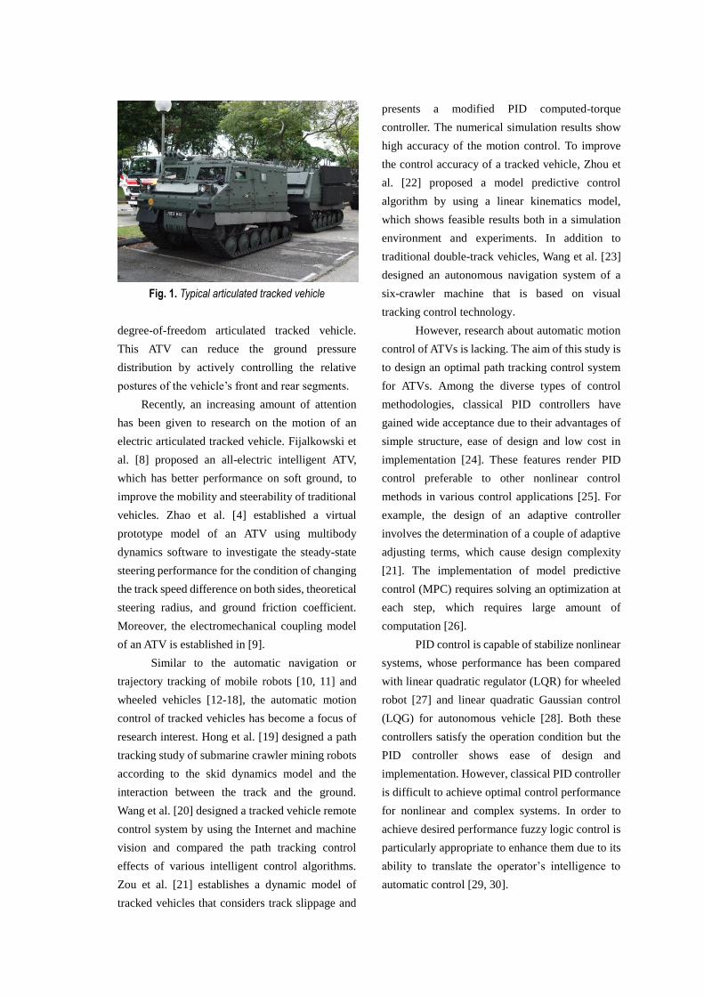
Fig. 1. Typical articulated tracked vehicle

degree-of-freedom articulated tracked vehicle.

This ATV can reduce the ground pressure

distribution by actively controlling the relative

postures of the vehicle’s front and rear segments.

Recently, an increasing amount of attention

has been given to research on the motion of an

electric articulated tracked vehicle. Fijalkowski et

al. [8] proposed an all-electric intelligent ATV,

which has better performance on soft ground, to

improve the mobility and steerability of traditional

vehicles. Zhao et al. [4] established a virtual

prototype model of an ATV using multibody

dynamics software to investigate the steady-state

steering performance for the condition of changing

the track speed difference on both sides, theoretical

steering radius, and ground friction coefficient.

Moreover, the electromechanical coupling model

of an ATV is established in [9].

Similar to the automatic navigation or

trajectory tracking of mobile robots [10, 11] and

wheeled vehicles [12-18], the automatic motion

control of tracked vehicles has become a focus of

research interest. Hong et al. [19] designed a path

tracking study of submarine crawler mining robots

according to the skid dynamics model and the

interaction between the track and the ground.

Wang et al. [20] designed a tracked vehicle remote

control system by using the Internet and machine

vision and compared the path tracking control

effects of various intelligent control algorithms.

Zou et al. [21] establishes a dynamic model of

tracked vehicles that considers track slippage and

presents a modified PID computed-torque

controller. The numerical simulation results show

high accuracy of the motion control. To improve

the control accuracy of a tracked vehicle, Zhou et

al. [22] proposed a model predictive control

algorithm by using a linear kinematics model,

which shows feasible results both in a simulation

environment and experiments. In addition to

traditional double-track vehicles, Wang et al. [23]

designed an autonomous navigation system of a

six-crawler machine that is based on visual

tracking control technology.

However, research about automatic motion

control of ATVs is lacking. The aim of this study is

to design an optimal path tracking control system

for ATVs. Among the diverse types of control

methodologies, classical PID controllers have

gained wide acceptance due to their advantages of

simple structure, ease of design and low cost in

implementation [24]. These features render PID

control preferable to other nonlinear control

methods in various control applications [25]. For

example, the design of an adaptive controller

involves the determination of a couple of adaptive

adjusting terms, which cause design complexity

[21]. The implementation of model predictive

control (MPC) requires solving an optimization at

each step, which requires large amount of

computation [26].

PID control is capable of stabilize nonlinear

systems, whose performance has been compared

with linear quadratic regulator (LQR) for wheeled

robot [27] and linear quadratic Gaussian control

(LQG) for autonomous vehicle [28]. Both these

controllers satisfy the operation condition but the

PID controller shows ease of design and

implementation. However, classical PID controller

is difficult to achieve optimal control performance

for nonlinear and complex systems. In order to

achieve desired performance fuzzy logic control is

particularly appropriate to enhance them due to its

ability to translate the operator’s intelligence to

automatic control [29, 30].

Fig. 2. Steering movement diagram of an ATV

In this paper, we proposed a path tracking

control system for articulated tracked vehicles

based on fuzzy PID control and visual navigation.

This study analyzes the steering characteristics of

ATV, and the dynamic model of an ATV is

introduced. Considering the distance and heading

angle deviations between the vehicle and the preset

path as the input variables and the deflection angle

of the hinge point and the speed of the driving

sprockets as the outputs of the controller, an ATV

path tracking control system is developed based on

fuzzy PID control algorithm. The control system is

being tested by a co-simulation in

RecurDyn/Simulink. An experimental platform for

path tracking control is created to verify the effect

in practical applications. The experimental

platform uses a camera to obtain the deviation,

which is processed as a controller input. The

experimental results show agreement with the

simulation results, indicating that the designed

controller can effectively track the preset trajectory.

1 DYNAMIC MODELING

1.1 Kinematics

An ATV consists of two identical vehicles,

a front vehicle and a rear vehicle, linked with a

rigid articulated joint. The articulated steering is

being performed on the middle joint, by changing

the corresponding articulated angle between the

front vehicle and the rear vehicle as it is being

indicated in Fig. 2. The articulating device is

driven by actuators such as hydraulic or electric

cylinders, which respectively push the front and

rear vehicles to deflect around the articulated joint

at the same time. Compared with the skid steering,

articulated steering requires less power for steering.

The steering motion of the vehicle in the

inertial coordinate system XOY is shown in Fig. 2,

where xoy and x'o'y' are vehicle coordinate systems

fixed at the center of the body of the front vehicle

and the rear vehicle, respectively. Assume that the

parameters of the front and rear vehicle bodies are

identical. In the following expressions, m is the

mass of the single vehicle, l is the grounding length

of the crawler, b is the distance of the center

between the two crawlers, d is the distance between

the articulated steering center and the center of the

front and rear vehicle, and ZI is the moment of

inertia of the single vehicle. When the deflection

angle between the front vehicle and the rear vehicle

is , the motion relationship between them can be

expressed as

'

' cos sin

' ' sin cos

x x y d

y d x y d

，

(1)

where x and y are components of the total

velocity v of the front vehicle combination, 'x

and 'y are components of the total velocity 'v

of the rear vehicle combination, and and '

are the heading angle of the front vehicle and the

rear vehicle, respectively. The velocities v and 'v

are considered to have the same changing with

respect to the deflection angle velocity of the

articulated joint, indicated by and ' .

During steering, the deviation between the

actual speed direction of the vehicle and the

longitudinal direction of the vehicle body is the

sideslip angle, represented as and ' , which

can be calculated by:

arctan /

' arctan '/ ' .

y x

y x

(2)

By defining the state space vector as

T

X Y ξ , the complete kinematics

expression based on the front vehicle can be given

as:

c( ) 0

s( ) 0

s c c s c ' ,

c ' c c ' c

0 1

X

vY

l

(3)

where X and Y denote the position of the center of

mass of the front vehicle in the inertial coordinate

system. Define = ' and = ' , c(·) and

s(·) stand for cos(·) and sin(·) respectively.

The track slips for each track can be

calculated by the following formula [19]:

( / 2)1 1 ,

( / 2)1 1 ,

L

L

L L

R

R

R R

v x bi

r r

v x bi

r r

(4a)

' ( / 2) '' 1 1 ,

' '

' ( / 2) '' 1 1 ,

' '

L

L

L L

R

R

R R

v x bi

r r

v x bi

r r

(4b)

where L , R , 'L and 'R are the sprocket

velocities of each track, r is the pitch radius of the

sprocket, and Lv , Rv , 'Lv and 'Rv are the

actual velocities of each track.

1.2 Dynamic Model

As shown in Fig. 2, LF , RF , 'LF and

'RF denote the tractive forces of the tracks, LR ,

RR , 'LR and 'RR denote the longitudinal

resistance. txF , tyF , 'txF and 'tyF are the

forces that act on the articulation joint, tM and

'tM are the steering torque. The nonlinear

dynamic model of the ATV can be expressed as

follows [5]:

For the front vehicle:

( ) ( )

.

L R L R tx

y ty

z L R ty t

mx my F F R R F

my mx F F

I M M F d M

(5)

For the rear vehicle:

' ' ' ' ( ' ') ( ' ') '

' ' ' ' ' '

' ' ' ' ' '.

l r l r tx

y ty

z l r ty t

m x my F F R R F

m y mx F F

I M M F d M

(6)

Detailed expressions of the dynamic model

are presented as follows.

1.2.1 Tractive Force

The maximum tractive force produced by a

track is determined by the contact area 𝐴 between

the track and terrain and the maximum shear

strength of the terrain max [31]:

max max ( tan ),F A A c p (7)

where c is the apparent cohesion, is the angle

of internal shearing resistance of the terrain, and p

is the normal pressure. The load is assumed to be

uniformly distributed over the contact area.

When the track slip is i, the tractive force of

a track can be calculated by [32]:

/

max 1 (1 ) ,il KKF F e

il

(8)

where K is the soil shear deformation modulus.

1.2.2 Resistance Forces

The longitudinal resistance force is created

by sinkage and rut formation. When driving on

hard pavement, the value is relatively small

compared with the tractive force. The longitudinal

resistance force can be expressed as

,2

L R f

WR R (9a)

'' ' ,

2L R f

WR R (9b)

where f is the coefficient of longitudinal

motion resistance and 'W W mg are the

normal load on the track.

The lateral resistance forces yF and 'yF

can be calculated by:

0

0

/ 2

/2

0

2sgn( )2 2

2sgn( ) ,

s l

y tl s

t

W WF dx dx

l lW

sl

(10a)

0

0

' '/ 2

'/ 2 '

0

' '' 2sgn( ')

2 ' 2 ''

2sgn( ') ' ,'

s l

y tl s

t

W WF dx dx

l lW

sl

(10b)

where t is the motion resistance coefficient in

the lateral direction.

1.2.3 Moment of the Longitudinal Forces and

Lateral Forces

The steering moments caused by the

longitudinal forces that act on the front and rear

tracks with respect to their respective centroids can

be expressed as follows:

For the front vehicle:

( ) ( )2 2

( ) .2

l L L R R

L R

b bM F R F R

bF F

(11a)

For the rear vehicle:

' ( ' ') ( ' ')2 2

( ' ') .2

l L L R R

L R

b bM F R F R

bF F

(11b)

The moment of the lateral forces is given

by:

0

0

/ 2

/2

22

2sgn( )2 2

sgn( ) ,4

s l

r tl s

t o

W WM xdx xdx

l l

W ls

l

(12a)

0

0

' '/ 2

'/ 2 '

22

0

' '' 2sgn( ')

2 ' 2 '

'sgn( ) ' .

' 4

s l

r tl s

t

W WM xdx xdx

l l

W ls

l

(12b)

1.2.4 Interaction Force Between Front and Rear

Vehicles

As mentioned above, steering of the

articulated vehicle is accomplished by relative

turns in the front-rear vehicle plane. The steering

torques of the front and rear vehicles actuated by

the articulating device are equal and opposite

directions [5]. For a decomposition of the forces on

the articulated joint, the balance is expressed as

follows:

'c s 0s c 0 ' .0 0 1 '

tx tx

ty ty

t t

F FF F

M M

(13)

Substitute these formulas into formulas (5)-(6), a

non-linear dynamics model of the ATV can be

expressed in terms of , ,x y as:

2 2

2

m(2 s c ) s c s c

s (1 c )

s (c 1) 2 c

(1)c (2)s (3)

(1)s (2)c (4) ,

(2) (4) (5) (6)

m md x

m m md y

md md I md

f f f

f f f

f f f f I

(14)

where f (1) ~ f (6) are expressed as

(1) (1) (2) ( ' '),L Rf m g g F F (15)

(2) (3) (4) ',yf m g g F (16)

(3) ( ),L Rf my F F (17)

(4) ,yf mx F (18)

(5) ( ) ( ' '),2 2

L R L R

b bf F F F F (19)

(6) (5)+g(6),2

bf g (20)

where g (1) ~ g (6) are expressed as follows:

(1) c s c ,g x d (21)

(2) ' s ' c ,g d x y d (22)

(3) c ' + s ,g x d y d (23)

(4) c c ',g x x d (24)

(5) ' ' ,L R L Rg R R R R (25)

(6) ',r rg M M (26)

In this system, the control quantity is

selected as ,T

v u and the output variables

are selected as , , , , ,T

dyn X Y x y ξ .

1.3 Virtual Prototyping Dynamic Model

The dynamic system of an articulated

tracked vehicle is a complex non-linear system.

The mathematical model is often simplified to

solve the dynamic equation of its steering, while

the virtual prototype simulation can yield

simulation results that are closer to the real value

by establishing relevant parameters that can more

intuitively observe the actual driving process.

Professional crawler modules exist in the

multi-body dynamics software RecurDyn. The

dynamic model of an ATV is established in

RecurDyn, as shown in Fig. 3, and the control

model is established in Simulink. The trajectory of

the mathematical model and the virtual prototype

model is compared using the same control input to

verify the accuracy of the virtual prototype model.

From the comparison of the results in Fig. 4, the

change in the vehicle trajectory in both the

Fig. 3. Virtual prototype model

(a) Steady-state steering (δ=20°)

(b) Unsteady-state steering

Fig. 4. Comparison of simulation results

steady-state steering process and the unsteady state

steering process is consistent. This model will be

employed in the simulation of the following path

tracking control algorithm.

2 CONTROLLER DESIGN

The controller is designed to enable the

ATV to track a reference path. The maximum

deflection angle of the ATV is 20° and the

corresponding theoretical turning radius is 14.8 m

in this case [4]. Since the research on research on

automatic motion control of ATVs is lacking, the

performance of controller is designed refer to the

six-crawler machine [23] as the similar dynamic

behavior. The maximum percentage overshoot is

set to 20% and the settling time ts is set to 10ey,max/v

where ey,max is the maximum distance deviation.

In this path tracking problem, the reference

pose , ,T

r r r rX Y p and current pose

, ,T

c X Y p are defined. The deviation

between the two poses is defined as the path

tracking error, pe , and the path tracking error

based on the coordinate system of the front vehicle

can be expressed as follows:

= ( )

c s 0s c 0 .0 0 1

T

p x y r c

r

r

r

e e e

X XY Y

e R p p

(27)

Considering the nearest point between the

reference trajectory and the center of the front

vehicle as the reference point, the longitudinal

tracking control deviation based on xoy-coordinate

is set to zero, and the vehicle velocity is constant.

The lateral error and heading angle deviation of the

vehicle are considered as the control deviation and

input into the controller. The control deviation is

defined as follows:

arctan .ye

e e kv

(28)

Based on this description, the fuzzy PID

controller of an ATV is proposed as

0( ) ,

t

p i d

det K e K e dt K

dt

(29)

where Kp, Ki and Kd are the proportional, integral

and derivative gains, respectively, all positive. The

proportional gain provides an overall control

action proportional to the error signal through the

all-pass gain factor. The functionality of integral

gain is reducing steady-state errors through low

frequency compensation by an integrator. The

functionality of derivative gain is improving

transient response through high frequency

compensation by a differentiator [33].

The gains of the PID are determined online,

and the corrected PID controller gains are obtained

by fuzzy inference as follows [34]:

max min min

max min min

max min min

' ,

' ,

' ,

p p p p p

i i i i i

d d d d d

K K K K K

K K K K K

K K K K K

(30)

where [Kpmin; Kpmax], [Kimin; Kimax] and [Kdmin; Kdmax]

are the ranges of Kp, Ki and Kd respectively.

The procedure of finding the PID gains is

called tuning. Many PID tuning methods had been

derived to determine the value of the three

parameters to obtain a controller with good

performance and robustness [35]. However, no

tuning method so far can replace the simple

Fig. 5. Model of path following control for an ATV

Ziegler-Nichols (Z-N) method in terms of

familiarity and ease of use to start with [33].

Tuning by experience is also a common method

[21][34], which means that tuning through

different simulation tests. In this work, the three

parameters are tuned by experience with reference

to the Z-N method. Furthermore, the ranges of Kp,

Ki and Kd are determined based on the comparative

tuning method [36]. The ranges are tuned to

achieve a faster response and a smaller steady state

error compared with the well-tuned PID gains

through simulation tests.

The ATV path tracking control aims to

maintain agreement between the position and

posture of the vehicle and the preset path. The

distance and heading angle deviations are as close

as possible to zero under the effect of the controller.

The complete control scheme of the path tracking

for ATVs is illustrated in Fig. 5.

2.1 Sprocket Velocity Control

According to the kinematics and dynamics

analysis, the ATV driven independently by each

tracked motor has no differential device. During

the steering process, if the sprocket on both sides

of the vehicle maintain the same velocity, then the

winding velocity of the outer track, relative to the

body of the vehicle, will be less than the actual

speed of the track. The force generated between the

track and the ground will be opposite to the

forward direction, which not only reduces the

driving efficiency but also makes the actual

steering radius of the vehicle substantially larger

than the theoretical steering radius and increases

the wear on the vehicle. Therefore, we propose an

adaptive control of the velocity of the sprocket.

According to Equations (4) and (8), to generate the

same forward traction force on both sides of the

track during steering, the velocity of the sprocket

on both sides of the track should be expressed as

follows:

1( / 2) ,

1( / 2) ,

1' ' ( / 2) ' ,

1' ' ( / 2) ' .

L

R

L

R

x br

x br

x br

x br

(31)

2.2 Fuzzy Rule

The fuzzy PID controller of the articulated

tracked vehicle has two input variables and three

output variables. The input variables are the

distance deviation ey and heading angle deviation

e . The output variables are the control parameters

Kp, Ki, and Kd of the PID controller. The position

and attitude adjustment of the articulated tracked

vehicle is based on the deflection angle 𝛿 of the

articulated joint.

After adjusting to the appropriate position

and attitude, adjustment within a smaller range is

performed to improve the accuracy of the vehicle

path tracking. When the variation is high, the

distance deviation should be reduced immediately.

After adjusting to the appropriate position and

attitude, the control range should be reduced to

improve the accuracy of the vehicle path tracking.

Therefore, setting the fuzzy field of the distance

and the heading angle deviations of the articulated

tracked vehicle is necessary. The fuzzy field for

establishing the range variation is [−6 m, 6 m], and

that of the heading angle deviation is [−30°, 30°].

The two input variables are divided into five grades,

namely NB (negative large), NM (negative

medium), Z (zero), PM (positive middle), and PB

Fig. 6. Membership function of distance deviation and

heading angle deviation

(positive large). When the distance and heading

angle deviations exceed the corresponding

adjustment range, the speed difference between the

two sides of the ATV and articulated point

deflection angle will be matched to the minimum

turning radius to make the vehicle run to the preset

path as soon as possible. The membership function

of distance and heading angle deviations are shown

in Fig. 6.

A reasonable range for the output variables

Kp, Ki, and Kd of the fuzzy PID controller is

selected by parameter testing to achieve the

accuracy requirement for the control of the ATV.

Increasing the proportional coefficient Kp in the

PID controller can accelerate the response speed

and improve the regulation accuracy of the system.

The membership adjustment range of Kp is divided

into five grades, i.e., Kp1, Kp2, Kp3, Kp4, and Kp5,

within the range [1.3, 1.7]. The integral coefficient

Ki can eliminate the system residual error and its

membership adjustment range is [0.1, 0.15], which

is divided into five grades, i.e., Ki1, Ki2, Ki3, Ki4, and

Ki5. The derivative coefficient Kd can improve the

dynamic performance of the system, and its

membership adjustment range is [0.01, 0.015],

which is divided into five grades, i.e., Kd1, Kd2, Kd3,

Kd4, and Kd5. By adjusting and grading the three

parameters according to this range, the rapid

Table 1. Fuzzy control rule

𝑒𝑦

𝑒𝜓 NB NM Z PM PB

NB Kp5/Ki1/Kd5 Kp5/Ki1/Kd3 Kp5/Ki1/Kd1 Kp3/Ki2/Kd3 Kp2/Ki2/Kd5

NM Kp4/Ki1/Kd5 Kp5/Ki2/Kd4 Kp4/Ki2/Kd2 Kp2/Ki3/Kd4 Kp1/Ki4/Kd5

Z Kp1/Ki4/Kd1 Kp1/Ki5/Kd1 Kp2/Ki5/Kd1 Kp1/Ki5/Kd1 Kp1/Ki4/Kd1

PM Kp3/Ki4/Kd5 Kp2/Ki3/Kd4 Kp4/Ki2/Kd2 Kp4/Ki2/Kd4 Kp5/Ki1/Kd5

PB Kp2/Ki2/Kd5 Kp3/Ki2/Kd3 Kp5/Ki1/Kd1 Kp5/Ki1/Kd4 Kp5/Ki1/Kd5

response and high control precision of the ATV

control system can be achieved. The corresponding

membership function is shown in Fig. 7.

The control method for the ATV is

expressed as follows:

(1) When the deviation of the distance and

heading angle is high, Kp assumes a higher value

for fast response. With a decrease in the total

deviation, the increase in Kp enables the vehicle to

maintain the current direction approaching the

preset path. When the distance deviation of the

articulated tracked vehicle is further reduced, the

heading angle is the main deviation, and the Kp

should be higher.

(2) The parameter Ki is primarily used to

eliminate the residual error caused by the

proportional link. Although the parameter can

improve the control accuracy and accelerate the

response of the system, it can also make the system

produce higher oscillation amplitudes. In the

process of approaching the preset path, Ki should

be smaller when the deviation of the distance and

heading angle is high to avoid excessive oscillation

of the system. When the deviation is small,

increasing Ki can correspondingly improve the

accuracy of the system. After passing the marking

line, Ki is higher to increase the response speed of

the system and make the vehicle return to the preset

path as soon as possible.

(3) Parameter Kd has an excellent

regulating effect on the dynamic characteristics of

the system. When the deviation of distance and

Fig. 7. Membership function of PID controller

parameters

heading angle is large, Kd assumes a higher value

to reduce the shock of the system. When the

deviation of the system is small, the Kd value is

reduced, to enable the integral link to better adjust

the error and increase the adjusting precision of the

system.

The fuzzy rule for the control system, which

is designed based on previous work in [20][34] and

modified through simulation tests, is shown in

Table 1. The relationship between the inputs and

outputs are shown in Fig. 8.

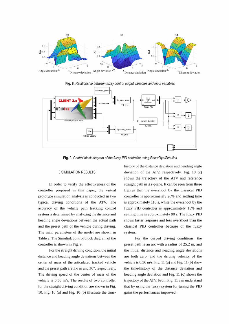
Fig. 8. Relationship between fuzzy control output variables and input variables

Fig. 9. Control block diagram of the fuzzy PID controller using RecurDyn/Simulink

3 SIMULATION RESULTS

In order to verify the effectiveness of the

controller proposed in this paper, the virtual

prototype simulation analysis is conducted in two

typical driving conditions of the ATV. The

accuracy of the vehicle path tracking control

system is determined by analyzing the distance and

heading angle deviations between the actual path

and the preset path of the vehicle during driving.

The main parameters of the model are shown in

Table 2. The Simulink control block diagram of the

controller is shown in Fig. 9.

For the straight driving condition, the initial

distance and heading angle deviations between the

center of mass of the articulated tracked vehicle

and the preset path are 5.6 m and 30°, respectively.

The driving speed of the center of mass of the

vehicle is 0.56 m/s. The results of two controller

for the straight driving condition are shown in Fig.

10. Fig. 10 (a) and Fig. 10 (b) illustrate the time-

history of the distance deviation and heading angle

deviation of the ATV, respectively. Fig. 10 (c)

shows the trajectory of the ATV and reference

straight path in XY-plane. It can be seen from these

figures that the overshoot by the classical PID

controller is approximately 26% and settling time

is approximately 110 s, while the overshoot by the

fuzzy PID controller is approximately 15% and

settling time is approximately 90 s. The fuzzy PID

shows faster response and less overshoot than the

classical PID controller because of the fuzzy

system.

For the curved driving conditions, the

preset path is an arc with a radius of 25.2 m, and

the initial distance and heading angle deviations

are both zero, and the driving velocity of the

vehicle is 0.56 m/s. Fig. 11 (a) and Fig. 11 (b) show

the time-history of the distance deviation and

heading angle deviation and Fig. 11 (c) shows the

trajectory of the ATV. From Fig. 11 can understand

that by using the fuzzy system for tuning the PID

gains the performances improved.

Table 2. Design parameters for simulation

Vehicle Parameters Values

Ground contact length: l 1953 [mm]

Mass: m 14.78 [t]

Track gauge: b 1500 [mm]

Track width: h 600 [mm]

Pitch radius of the sprocket: r 375 [mm]

Distance from the articulation

point to the center of mass: d

2625 [mm]

Terrain Parameters Values

Soil shear deformation

modulus: K

0.02 [m]

Apparent cohesion: c 70000

Angle of internal shear: 0.67

Friction coefficient between the

tracks and the terrain:

0.9

Coefficients of lateral motion

resistance: t

0.8

Coefficients of longitude

motion resistance: f

0.6

(a) Distance deviation

(b) Heading angle deviation

(c) Trajectory of the XY-plane

Fig. 10. Simulation results for the two controllers in a

straight trajectory

(a) Distance deviation

(b) Heading angle deviation

(c) Trajectory of the XY-plane

Fig. 11. Simulation results for the two controllers in a

circular trajectory

4 EXPERIMENTAL VERIFICATION

The control effect of the ATV path tracking

control system is experimentally investigated to

verify the fuzzy PID control algorithm. The overall

scheme of the ATV path tracking control test

platform is shown in Fig. 12. The test platform is

composed of the ATV test prototype, data

acquisition and processing scheme, and computer

control system. The latter is mainly employed to

run the path tracking control system based on

visual navigation and collect and analyze relevant

data.

In the experiment, the preset path is set on

the horizontal ground. A reduced scale model was

employed for the experimental prototype with a

ratio of 14:1. Since the purpose of the experiment

is to verify the feasibility of the control algorithm

based on visual navigation, the adoption of a small-

sized model is acceptable. The data

Fig. 12. General scheme of the path tracking control

test platform

Fig. 13. Overview of the path tracking control test

platform

acquisition and processing scheme are input into

the computer control system to obtain the running

state of the test prototype in the process. The fuzzy

PID controller provides the control commands to

the actuator of the articulated tracked vehicle to

follow the preset path. The path tracking control

platform based on visual navigation is shown in

Fig. 13.

A monocular camera is used to collect road

information in front of the test prototype. The

collected image is processed by binarization to

identify clear landmark information. A matrix is

created by extracting the values of each pixel in the

binary image. The sudden change in pixel values is

determined and recorded from the starting position

to obtain the centerline coordinates of the

navigation line. The least squares method is used

to fit the centerline coordinates, and the fitting

curve of the road navigation line is obtained.

According to the similarity principle and the

triangle relationship, the lateral deviation 𝑒𝑦 and

heading angle deviation 𝑒𝜓 can be calculated.

According to the road navigation

information collected by the visual navigation path

tracking system and by using the designed fuzzy

PID controller, the test prototype is automatically

controlled to run along the preset path. The

distance and heading angle deviations between the

actual running and the preset path and the track

speed on both sides of the prototype are analyzed

in straight and curve driving conditions.

In the straight traveling condition, the initial

distance and heading angle deviations between the

center of mass and the path of the test prototype are

0.4 m and 30°, respectively. The speed of the

driving track is set to 0.1 m/s. Fig. 14 (a) and Fig.

14 (b) illustrate the variation in the distance and

heading angle deviations with time. Fig. 14 (c)

shows the trajectory in the XY-plane. The control

inputs are shown in Fig. 14 (d) and Fig. 14 (e).

In the case of driving along a curved path,

the preset path is a curve with a 2.5 m radius. The

initial distance and heading angle deviations

between the center of mass and the preset path are

0.4 m and 30°, respectively. Fig. 15 (a) and Fig. 15

(b) show the variation in the distance and heading

angle deviations with time. The XY-plane motion

is shown in Fig. 15 (c). The corresponding control

inputs are demonstrated in Fig. 15 (d) and Fig. 15

(e).

According to the tests and analysis, the

control system can effectively realize the path

tracking of the articulated tracked vehicles by

adjusting the sprocket velocity of both sides and

the deflection angle of the articulated points in

accordance with the different driving paths.

5 CONCLUSIONS

A control system for path tracking for an

ATV based on the fuzzy PID algorithm is proposed

in this study. The control system uses the distance

and heading angle deviations between the actual

trajectory and the preset path as inputs, and the

outputs are the deflection angle and track velocity

(a) Distance deviation

(b) Heading angle deviation

(c) Trajectory of the XY-plane

(d) Articulated angle of rotation

(e) Velocities of sprockets

Fig. 14. Experimental results from a straight path

(a) Distance deviation

(b) Heading angle deviation

(c) Trajectory of the XY-plane

(d) Articulated angle of rotation

(e) Velocities of sprockets

Fig. 15. Experimental results from a circular path

on both sides of the ATV. The fuzzy PID controller

is the core of the control system, which adjusts the

parameters Kp, Ki, and Kd according to the

prescribed fuzzy rules to achieve effective vehicle

tracking. The mathematical model of the ATV is

proposed, and a virtual prototype model of the

ATV is established in RecurDyn. The validity of

the virtual prototype model is verified by a

simulation comparison between the prototype and

mathematical models. A fuzzy PID control system

model is established in Simulink, and the virtual

prototype co-simulation analysis is conducted for

two typical working conditions, i.e., straight and

curve path traveling. The simulation results show

that the ATV can effectively track the preset path

under the control of the fuzzy PID controller.

An ATV path tracking control test platform

that is based on visual navigation was developed to

test the effects of the control system in a practical

application. The vision navigation system is used

to collect path tracking information. The fuzzy PID

controller is applied for real-time control of vehicle

tracking. The distance and heading angle deviation

variations during tracking are analyzed by the path

tracking test for straight and curve driving paths,

and the deflection angle and track speed on both

sides of the articulated track are adjusted. The

experimental results show that the ATV tracking

control system is effective in practice.

6 ACKNOWLEDGMENTS

This work was supported by the National

Natural Science Foundation of China (Grant No.

51775225)

7 NOMENCLATURES

x , y centroid point velocity component of front vehicle, [m/s]

'x , 'y centroid point velocity component of front

vehicle, [m/s]

, ' yaw angle, [rad]

deflection angle between the front vehicle

and the rear vehicle, [rad]

, ' side slip angle, [rad]

X, Y centroid coordinates of front vehicle in global coordinate system, [m]

v , 'v front and rear vehicle centroid velocity, [m/s]

m mass of the single vehicle, [kg]

l grounding length of the crawler, [m]

b track gauge, [m]

d distance between the center point and the

articulated point, [m]

h width of link pad, [m]

IZ the moment of inertia of the single vehicle,

[kg·m2]

iL, iR track slips of front vehicle

'Li , 'Ri track slips of rear vehicle

L , R sprocket velocity of front vehicle, [rad/s]

'L , 'R sprocket velocity of front vehicle, [rad/s]

Lv , Rv actual velocity of the crawlers of front

vehicle, [m/s]

'Lv , 'Rv actual velocity of the crawlers of rear vehicle,

[m/s]

LF , RF tractive force of the crawlers of the front

vehicle, [N]

'LF , 'RF tractive force of the crawlers of the rear vehicle, [N]

LR , RR longitudinal resistance of the front vehicle, [N]

'LR , 'RR longitudinal resistance of the rear vehicle,

[N]

txF , tyF force component between front vehicle and

articulated point, [N]

'txF , 'tyF force component between rear vehicle and

articulated point, [N]

M drag moment of centroid point in front

vehicle, [N·m]

'M drag moment of centroid point in rear vehicle, [N·m]

maxF maximum tractive force produced by a track, [N]

max maximum shear strength of the terrain,

[N/m2]

c apparent cohesion, [N/m2]

angle of internal shearing resistance of the

terrain, [N/m2]

p normal pressure, [kPa]

K soil shear deformation modulus, [m]

f coefficient of longitudinal motion resistance, [-]

t coefficients of lateral motion resistance, [-]

yF , 'yF lateral resistance force of the front vehicle

and rear vehicle respectively, [N]

0s , 0 's longitudinal slip of track velocity

instantaneous center, [m]

lM , 'lM turning moment produced by longitudinal

forces, [N·m]

rM , 'rM turning moment produced by lateral forces,

[N·m]

rX , rY , r components of reference pose, [-]

xe , ye , e deviation components between current pose

and reference pose, [-]

Kp proportional gain, [-]

Ki integral gain, [-]

Kd derivative gain, [-]

8 REFERENCES

[1] Watanabe, K., Kitano, M., & Fugishima, A. (1995).

Handling and stability performance of four-track steering

vehicles. Journal of terramechanics, vol. 32, no. 6, p.

285-302, DOI: 285-302, 10.1016/0022-4898(95)00022-

4.

[2] Zongwei, Y., Guoqiang, W., Rui, G., & Xuefei, L.

(2013). Theory and experimental research on six-track

steering vehicles. Vehicle System Dynamics, vol. 51, no.

2, p. 218-235, DOI: 10.1080/00423114.2012.722647.

[3] Nuttall Jr, C. J. (1964). Some notes on the steering

of tracked vehicles by articulation. Journal of

Terramechanics, vol. 1, no. 1, p. 38-74, DOI:

10.1016/0022-4898(64)90123-5.

[4] Zhao, H., Wang, G., Wang, S., Yang, R., Tian, H.,

& Bi, Q. (2018). The Virtual Prototype Model Simulation

on the Steady-state Machine Performance.

INTELLIGENT AUTOMATION AND SOFT

COMPUTING, vol. 24, no. 3, p. 581-592, DOI:

10.31209/2018.100000025.

[5] Watanabe, K., & Kitano, M. (1986). Study on

steerability of articulated tracked vehicles—part 1.

Theoretical and experimental analysis. Journal of

Terramechanics, vol. 23, no. 2, p. 69-83, DOI:

10.1016/0022-4898(86)90015-7.

[6] Alhimdani, F. F. (1982). Steering analysis of

articulated tracked vehicles. Journal of Terramechanics,

vol. 19, no. 3, p. 195-209, DOI: 10.1016/0022-

4898(82)90004-0.

[7] Sasaki, S., Yamada, T., & Miyata, E. (1991).

Articulated tracked vehicle with four degrees of freedom.

Journal of Terramechanics, vol. 28, no. 2-3, p. 189-199,

DOI: 10.1016/0022-4898(91)90033-3.

[8] Fijalkowski, B. T. (2003, June). Novel mobility and

steerability enhancing concept of all-electric intelligent

articulated tracked vehicles. In IEEE IV2003 Intelligent

Vehicles Symposium. Proceedings (Cat. No. 03TH8683)

(pp. 225-230). IEEE, DOI: 10.1109/IVS.2003.1212913.

[9] Wu, J., Wang, G., Zhao, H., & Sun, K. (2019).

Study on electromechanical performance of steering of

the electric articulated tracked vehicles. Journal of

Mechanical Science and Technology, 33(7), 3171-3185,

DOI: 10.1007/s12206-019-0612-7.

[10] Karabegović, I., Karabegović, E., Mahmić, M., &

Husak, E. (2015). The application of service robots for

logistics in manufacturing processes. Advances in

Production Engineering & Management, 10(4), DOI:

10.14743/apem2015.4.201.

[11] Muthukumaran, S., & Sivaramakrishnan, R. (2019).

Optimal Path Planning for an Autonomous Mobile Robot

Using Dragonfly Algorithm. International Journal of

Simulation Modelling (IJSIMM), 18(3). DOI:

10.2507/IJSIMM18(3)474.

[12] Kadir, Z. A., Mazlan, S. A., Zamzuri, H., Hudha, K.,

& Amer, N. H. (2015). Adaptive fuzzy-PI control for active

front steering system of armoured vehicles: outer loop

control design for firing on the move system. Strojniški

vestnik-Journal of Mechanical Engineering, 61(3), 187-

195, DOI: 10.5545/sv-jme.2014.2210.

[13] Popovic, V., Vasic, B., Petrovic, M., & Mitic, S.

(2011). System approach to vehicle suspension system

control in CAE environment. Strojniški vestnik-Journal of

Mechanical Engineering, 57(2), 100-109. DOI:

10.5545/sv-jme.2009.018.

[14] Zhao, P. X., Luo, W. H., & Han, X. (2019). Time-

dependent and bi-objective vehicle routing problem with

time windows. Advances in Production Engineering &

Management, 14(2), 201-212, DOI:

10.14743/apem2019.2.322

[15] Martin, T. C., Orchard, M. E., & Sánchez, P. V.

(2013). Design and simulation of control strategies for

trajectory tracking in an autonomous ground vehicle.

IFAC Proceedings Volumes, vol. 46, no. 24, p. 118-123,

DOI: 10.3182/20130911-3-BR-3021.00096.

[16] Haddad, A., Aitouche, A., & Cocquempot, V.

(2015). Active Fault Tolerant Decentralized Control

Strategy for an Autonomous 2WS4WD Electrical Vehicle

Path Tracking. IFAC-PapersOnLine, vol. 48, no. 21, p.

492-498, DOI: 10.1016/j.ifacol.2015.09.574.

[17] Bascetta, L., Cucci, D. A., & Matteucci, M. (2016).

Kinematic trajectory tracking controller for an all-terrain

Ackermann steering vehicle. IFAC-PapersOnLine, vol.

49, no. 15, p. 13-18, DOI: 10.1016/j.ifacol.2016.07.600.

[18] Li, X., Sun, Z., Cao, D., Liu, D., & He, H. (2017).

Development of a new integrated local trajectory

planning and tracking control framework for autonomous

ground vehicles. Mechanical Systems and Signal

Processing, vol. 87, p. 118-137, DOI:

10.1016/j.ymssp.2015.10.021.

[19] Hong, S., Choi, J. S., Kim, H. W., Won, M. C., Shin,

S. C., Rhee, J. S., & Park, H. U. (2009). A path tracking

control algorithm for underwater mining vehicles.

Journal of mechanical science and technology, vol. 23,

no. 8, p. 2030-2037, DOI: 10.1007/s12206-009-0436-y.

[20] Wang, S., Zhang, S., Ma, R., Jin, E., Liu, X., Tian,

H., & Yang, R. (2018). Remote control system based on

the Internet and machine vision for tracked vehicles.

Journal of Mechanical Science and Technology, vol. 32,

no. 3, p. 1317-1331, DOI: 10.1007/s12206-018-0236-3.

[21] Zou, T., Angeles, J., & Hassani, F. (2018).

Dynamic modeling and trajectory tracking control of

unmanned tracked vehicles. Robotics and Autonomous

Systems, vol. 110, p. 102-111, DOI:

10.1016/j.robot.2018.09.008.

[22] Zhou, L., Wang, G., Sun, K., & Li, X. (2019).

Trajectory Tracking Study of Track Vehicles Based on

Model Predictive Control. Strojniski Vestnik/Journal of

Mechanical Engineering, 65(6), DOI: 10.5545/sv-

jme.2019.5980.

[23] Wang, S., Ge, H., Ma, R., Cui, D., Liu, X., & Zhang,

S. (2019). Study on the visual tracking control

technology of six-crawler machine. Proceedings of the

Institution of Mechanical Engineers, Part C: Journal of

Mechanical Engineering Science, 233(17), 6051-6075,

DOI: 10.1177/0954406219858168.

[24] Kumar, V., Nakra, B. C., & Mittal, A. P. (2011). A

review on classical and fuzzy PID controllers.

International Journal of Intelligent Control and Systems,

16(3), 170-181.

[25] Choi, Y. J., & Chung, W. K. (2004). PID trajectory

tracking control for mechanical systems-Introduction.

PID Trajectory Tracking Control for Mechanical Systems,

298, 3-+.

[26] Morari, M., & Lee, J. H. (1999). Model predictive

control: past, present and future. Computers & Chemical

Engineering, 23(4-5), 667-682, DOI: 10.1016/S0098-

1354(98)00301-9.

[27] Nasir, A. N. K., Ahmad, M. A., & Ismail, R. R.

(2010). The control of a highly nonlinear two-wheels

balancing robot: A comparative assessment between

LQR and PID-PID control schemes. World Academy of

Science, Engineering and Technology, 70, 227-232, DOI:

10.1109/ICI.2011.37.

[28] Carlucho, I., Menna, B., De Paula, M., & Acosta,

G. G. (2016, June). Comparison of a PID controller

versus a LQG controller for an autonomous underwater

vehicle. In 2016 3rd IEEE/OES South American

International Symposium on Oceanic Engineering

(SAISOE) (pp. 1-6). IEEE, DOI:

10.1109/SAISOE.2016.7922475.

[29] Khan, A. A., & Rapal, N. (2006, April). Fuzzy PID

controller: design, tuning and comparison with

conventional PID controller. In 2006 IEEE International

Conference on Engineering of Intelligent Systems (pp.

1-6). IEEE, DOI: 10.1109/ICEIS.2006.1703213.

[30] Kumar, V., Nakra, B. C., & Mittal, A. P. (2011). A

review on classical and fuzzy PID controllers.

International Journal of Intelligent Control and Systems,

16(3), 170-181.

[31] Bekker, M. G. (1956). Theory of land locomotion:

the mechanics of vehicle mobility. Ann Arbor: The

University of Michigan Press.

[32] Wong, J. Y. (2008). Theory of ground vehicles.

John Wiley & Sons.

[33] Ang, K. H., Chong, G., & Li, Y. (2005). PID control

system analysis, design, and technology. IEEE

transactions on control systems technology, 13(4), 559-

576, DOI: 10.1109/TCST.2005.847331.

[34] Lee, K., Im, D. Y., Kwak, B., & Ryoo, Y. J. (2018).

Design of fuzzy-PID controller for path tracking of mobile

robot with differential drive. International Journal of

Fuzzy Logic and Intelligent Systems, vol. 18, no. 3, p.

220-228, DOI: 10.5391/IJFIS.2018.18.3.220.

[35] Wu, H., Su, W., & Liu, Z. (2014, June). PID

controllers: Design and tuning methods. In 2014 9th

IEEE Conference on Industrial Electronics and

Applications (pp. 808-813). IEEE, DOI:

10.1109/ICIEA.2014.6931273.

[36] Li, H. X. (1997). A comparative design and tuning

for conventional fuzzy control. IEEE Transactions on

Systems, Man, and Cybernetics, Part B (Cybernetics),

27(5), 884-889, DOI: 10.1109/3477.623242.