research development 2015 - gek.szie.hu · tÁmop-4.2.1.b-11/2/kmr-2011-003 mechanical engineering...
TRANSCRIPT

TÁMOP-4.2.1.B-11/2/KMR-2011-003
Research Development
2015

TÁMOP-4.2.1.B-11/2/KMR-2011-003
Mechanical Engineering Letters, Szent István University
Annual Technical-Scientific Journal of the Mechanical Engineering Faculty, Szent István University, Gödöllő, Hungary
Editor-in-Chief: Dr. István SZABÓ
Editor:
Dr. Gábor KALÁCSKA
Executive Editorial Board: Dr. István BARÓTFI
Dr. János BEKE Dr. István FARKAS
Dr. László FENYVESI
Dr. István HUSTI Dr. Sándor MOLNÁR Dr. Péter SZENDRŐ Dr. Zoltán VARGA
International Advisory Board: Dr. Patrick DE BAETS (B) Dr. Radu COTETIU (Ro) Dr. Manuel GÁMEZ (Es)
Dr. Klaus GOTTSCHALK (D) Dr. Yurii F. LACHUGA (Ru)
Dr. Elmar SCHLICH (D) Dr. Nicolae UNGUREANU (Ro)
Cover design:
Dr. László ZSIDAI
HU ISSN 2060-3789
All Rights Reserved. No part of this publication may be reproduced, stored in a retrieval system or transmitted in any form or by any means, electronic,
mechanical, photocopying, recording, scanning or otherwise without the written permission of Faculty.
Páter K. u. 1., Gödöllő, H-2103 Hungary [email protected], www.gek.szie.hu,
Volume 13 (2015)

TÁMOP-4.2.1.B-11/2/KMR-2011-003
Selected Collection from Synergy 2015 International Conference
organized by the Faculty of Mechanical Engineering, Szent István University

TÁMOP-4.2.1.B-11/2/KMR-2011-003
TÁMOP-4.2.1.B-11/2/KMR-2011-003
Contents
V. ERDÉLYI, L. JÁNOSI: Agriculture 4.0 or the complex optimization of agricultural tasks based on the experience of industry 4.0 7
Z. BLAHUNKA, Z. BÁRTFAI, D. FAUST: Measurement optimalization by information entropy Synergy international conferences, Gödöllő, Hungary 14
D. NAGY, P. SZENDRŐ, J. NAGY, L. BENSE: Surface description with LASER light 21
A. DIMITRIJEVIC, B. SUNDEK, S. BLAZIN, D. BLAZIN: Conditions for vegetable production in different types of tunnel greenhouses 29
A. LÁGYMÁNYOSI, I. SZABÓ: Pear classification using 3D image processing 38
M. GHARIBKHANI, R. C. AKDENIZ: Determination of some shape factors of fish and larvae feed using digital image processing method 45
A. BABLENA: Modeling the soil-wheel interaction with discrete element method 58
K. OROVA, K. PETRÓCZKI, J. BEKE: Mechanization in greenhouse tomato culture and indoor culture for research purposes 66
F. SAFRANYIK: Determination of micromechanical parameters of granulars based on standard shear test 74
P. GÁRDONYI, L. KÁTAI, I. SZABÓ: Relationship between the drive installation and V-belt temperature conditions 81
Á. KOVÁCS, I. J. JÓRI, K. GAÁL,
A. PIROS, Gy. KERÉNYI: Development of measurement methods for a numerical simulation of corn plants 88

TÁMOP-4.2.1.B-11/2/KMR-2011-003
C. ABBATE, R. Di FOLCO, I. De BELLIS, Z. VARGA: Stability analysis of igbt based on simulation and measurement of scatter parameters 97
H. SCAAR, F. WEIGLER, J. MELLMANN, K. GOTTSCHALK, Á. BÁLINT, Cs. MÉSZÁROS, I. FARKAS: Numeric simulation of heat and mass transport in soil samples 106
R. KOSZTOLÁNYI, Á. BÁLINT, K. GOTTSCHALK, J. MELLMANN, I. KOZMA, J. TÓTH, Cs. MÉSZÁROS: Analysis of heat transport in soil column measurements simulating sun cycle 115
L. PITLIK, Z. VARGA: The operationalism of sustainability is a mathematical issue 122
Gy. PILLINGER, A. GÉCZY, L. MÁTHÉ, P. KISS: Identification of soil deformation with the reological model of tire-terrain interaction 130
A. NAGYMÁNYAI, L. SIKLÓSI, Z. BÁRTFAI: Lubricant technical service of ENI Hungary 140
A. VARGA: Identification of soil deformation with the reological model of tire-terrain interaction 146
Z. BÁRTFAI, I. BORBÁS, Sz. POÓR: Is it a gage or a measure? Application of the endoscope technology in the industry 152
D. PÁLEŠ, M. BALKOVÁ, J. RÉDL, J. MAGA, G. KALÁCSKA: Application of bézier surface algorithm for distribution of daylight 157

Selected papers from „Synergy” International Conference 2015
TÁMOP-4.2.1.B-11/2/KMR-2011-003 7
Agriculture 4.0 or the complex optimization of agricultural tasks based on the experience
of industry 4.0
V. ERDÉLYI1, L. JÁNOSI2 1Department of Mech. Eng. Faculty,
Dept. of Mechatronics, Szent István University 2Department of Mech. Eng. Faculty,
Dept. of Mechatronics, Szent István University
Abstract
This paper shows the potential of revolutionary alteration of agriculture following the instance of Industry 4.0. The compilation surveys the existing level of automation and mechanization of agriculture and also demonstrates the transition of the industry under the principle of Industry 4.0. Investigate and reflect the question whether the new method applied pilotly in industry is that worth to apply in agriculture?
Keywords
Smart Agriculture, IoT, Industry 4.0, Smart Farming, Agromechatronics
1. Introduction
Nowadays – because of the overpopulation of world - it is too pressing to permit a longer delay (Glaeser, 1989) mitigating food crisis. More than 1.9 billion people exists on the Globe of 6.7 billion who are suffering of malnutrition. The number of people existing near to critical starvation exceeds 600 million (Szakály, 2004).
At a guess the population of the World could reach 9.6 billion inhabitants by the time 2050. This increase requires to enlarge the food production by 70 % (FAO 2015) and still we will be able to keep only the present condition.
Besides we are in a shortage of food in the World we have less and less area where we could produce that (EEA 2006). The better utilization of arable land seems to be a good solution. In this problem some example and experience coming from the industry could be of assistance of building a new system in agriculture. Many industrial examples show extraordinary data and could give assistance to the development.
2. Industry 4.0 - the 4th industrial revolution
The expressions Industry 4.0, or IoT, Internet of Things are more and more common. What are these phrases mean? So, these days we live the Industrial Revolution 4.0.

Selected papers from „Synergy” International Conference 2015
TÁMOP-4.2.1.B-11/2/KMR-2011-003 8
The first industrial revolution (I 1.0) has happened in the eighteen century and in the nineties up to 1850. In this time some new energy sources and engines were developed and applied in different technologies. The steam engine and some other water energy driven engine were introduced and made revolution in the industrial production. In many instants the human work was replaced by the new water or steam driven engines (Ashton 1948).
Figure 1. Watt’s steam engine replica (source: Enciclopedia Libre)
Figure 2. Ford T-modell series production (source: supercompressor)
The second industrial revolution (I 2.0) has happened between 1870 and 1914 when Henry Ford and the Hungarian Josef Galamb created the first automobile manufactured on a automatic assembly line. On this way the production was cheaper and could produce in large scale.
Selected papers from „Synergy” International Conference 2015
TÁMOP-4.2.1.B-11/2/KMR-2011-003 9
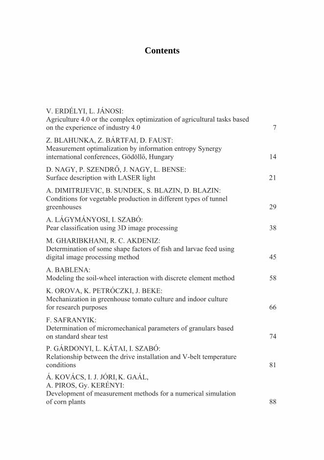
The third industrial revolution (I 3.0) started after the first world war and was running up to these days. The computer controlled machine tools were appeared and the computer studies were spreading not only in the production but in the design field as well.
Figure 3. Robots in manufacturing (cource: richpoi)
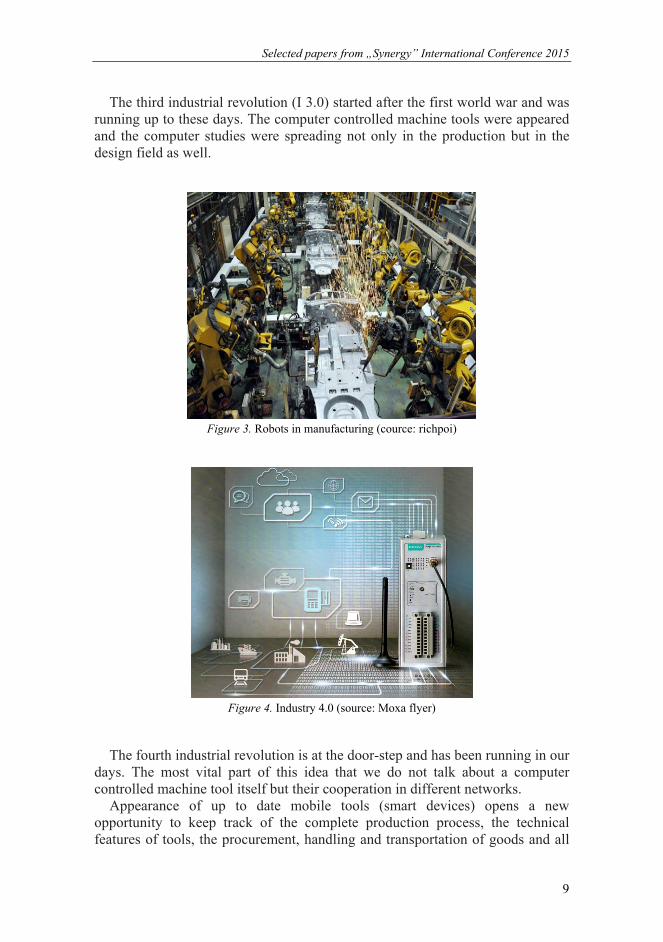
Figure 4. Industry 4.0 (source: Moxa flyer)
The fourth industrial revolution is at the door-step and has been running in our days. The most vital part of this idea that we do not talk about a computer controlled machine tool itself but their cooperation in different networks.
Appearance of up to date mobile tools (smart devices) opens a new opportunity to keep track of the complete production process, the technical features of tools, the procurement, handling and transportation of goods and all

Selected papers from „Synergy” International Conference 2015
TÁMOP-4.2.1.B-11/2/KMR-2011-003 10
other part of the whole production procedure including the financial aspects anywhere, anytime in real time. This progress will result a hardly foreseeable change in the field of efficiency, the quantity and quality of production.
3. Agriculture today
Precision agriculture, livestock farming and biomass utilization are all separate fields and have been investigating for a long time. All of These fields reached significantly increased production (Tóth 2002). Complex integrated solutions are hardly applied or not used at all in agriculture but single areas are well investigated. The agricultural automation industry typically concentrates on small, singular parts of the whole deal. (Yao et. Al. 2011, Yifan et. Al. 2011, Yuan et. Al. 2014).
Although the precision agriculture is approaching to cloud thinking, this does not extend to the entire agricultural sector. Considering the presently available literature the integration of agriculture on the same level as of industry 4.0 is, it has been only a vision (Beecham Research, 2015).
4. Agricultural revolution?
Of course what appears in the industry, sooner or later may appear in many areas of other fields of life. So in application for private people, but also in agriculture.
Figure 5. Agriculture today
(source: Harvard Business Review)
The topicality of this subject is shown by the recent investment of Bosch Company. They launched an Industry 4.0 type factory, and the development of appropriate tools. This factory is a so-called pilot project, which is intended to assess whether the new, smart manufacturing technology is effective enough. The numbers are encouraging, since Bosch announced that they could increase their output about 10% and decrease their stock inventory by 30%.

Selected papers from „Synergy” International Conference 2015
TÁMOP-4.2.1.B-11/2/KMR-2011-003 11
Figure 6. Agriculture today and tomorrow (source: Harvard Business Review)
According to my research, the development of a similar agricultural system is already on the go, to improve the productivity already under way, but these attempts are still in very early stages. Computer control systems have been applied in modern agriculture for a long time, but still, these systems are very rarely connected. The BigDuchman is one of the sponsors of such developments. This company - an international corporation - is a livestock-farm technology solution provider. They are developing the application called BigFarmNet, which is actually an Internet of Things solution. This software is capable of collecting data of both air-conditioning, feeding and the use of feed, and the software can intervene to the processes as well.
In addition, all data is collected from connected units, and the system is evaluating them. Here comes the big data into the picture. This in itself is a very good initiative, but the agriculture itself is an enormous area, and this solution covers only a very small segment. I think, in the near future a significant transition can start in agriculture, based on the industry 4.0. This will be a change in direction of the use in co-operation of connected elements, smart equipment, remote accessed devices by supporting of cloud computing.
In my experience, a comprehensive system could possible prevent problems that may arise from a simple mistake of administration. For example, not to apply an advanced feed management systems though it is available or applies but improperly way may cause damage of thousands of Euros. (For example a certain company ordered a surplus of 40’000 kg fodder into an almost fully loaded silo) It was a real experience, and if the company would have been used a simple automated system they could have been avoided the damage.
The same way a lot of time and money could be saved if the goods that sent to the consumer could be monitored on their way. It is also a real experience that inadequate monitoring of goods and information flow disruptions can cause significant problems – and significant loss of income. If more than one farm unit - including agriculture, crop production, livestock production, animal breeding,

Selected papers from „Synergy” International Conference 2015
TÁMOP-4.2.1.B-11/2/KMR-2011-003 12
feed production, feed mixers, biomass utilization, renewable energy, etc. - would be tied to a large system, it is likely to realize even better efficiency improvements.
Figure 7. Internet of Things in Agriculture
Conclusion
Even the Industry 4.0 has been in a fairly early stage but already it is obvious that there is a huge potential in it. Both Bosch’s, Festo’s, Claas’ and Moxa’s (and the list could be continued long) efforts and expenses in trying to achieve 4.0 Industry-based production, shows us that we have to think in the new network oriented paradigm. We can say with this in mind, that it is important to further deal with the topic, because in the industry they have more than encouraging results of the pilot projects. Since agriculture – as a system - isn’t differ fundamentally from industry, we can possibly apply the basic concept of the system in agricultural sector with some modifications.
References
[1] Ashton, Thomas S. (1948). "The Industrial Revolution (1760–1830)". Oxford University Press.
[2] Beecham Research Limited (2015): Towards Smart Farming: Agriculture Embracing the IoT Vision
[3] EEA Report (2006): Urban sprawl in Europe, The ignored challenge, European Environment Agency Report, No 10 ISSN 1725-9177
[4] FAO (Food and Agriculture Organisation of the United Nations) (2015):2050: A third more mouths to feed

Selected papers from „Synergy” International Conference 2015
TÁMOP-4.2.1.B-11/2/KMR-2011-003 13
[5] GLAESER, Bernhard (1989): Umweltpolitik zwischen Reparatur und Vorbeugung. Eine Einführunh am Beispiel Bundesrepublik im internationalen Kontext. Westdeutscher Verlag GmbH. Oplade, p.14-15
[6] Szakály Sándor (2004): Táplálkozási dilemmák és az élelmiszerek fejlesztésének világstratégiai irányai, Élelmiszer, Táplálkozás és Marketing, Évf. 1, Szám 1-2.
[7] Tóth László (2002): Elektronika és automatika a mezőgazdaságban ISBN:9638617063
[8] Yao Shifeng,Feng Chungui,He Yuanyuan,Zhu Shiping (2011): Application of IOT in Agriculture, Journal of Agricultural Mechanization Research
[9] Yifan Bo, Haiyan Wang (2011): The Application of Cloud Computing and the Internet of Things in Agriculture and Forestry, Service Sciences
[10] Yuan Chen, Lihua Zheng, Changyi Xiao, Wei Yang, Minzan Li (2014): An Information Acquisition System of Vegetable Safety Based on Web Service American Society of Agricultural and Biological Engineers
[11] Fig 1 :http://enciclopedia.us.es/index.php/ Archivo:Maquina_vapor_ Watt_ETSIIM.jpg
[12] Fig 2: http://www.supercompressor.com/rides/henry-ford-quotes-about-cars-and-business-model-t
[13] Fig 3: http://richpoi.com/cikkek/uzlet_gazdasag/hoditanak-a-robotok-a-gyarakban---szakkepzett-munkavegzes-ember-nelkul.html
[14] Fig 4: Moxa flyer: Connecting to the Last Mile of the Industrial IoT [15] Fig 5 and 6: https://hbr.org/2014/11/how-smart-connected-products-are-
transforming-competition

Selected papers from „Synergy” International Conference 2015
TÁMOP-4.2.1.B-11/2/KMR-2011-003 14
Measurement optimalization by information entropy Synergy international conferences, Gödöllő, Hungary
Z. BLAHUNKA, Z. BÁRTFAI, D. FAUST
Engineering Faculty, Szent István University
Abstract
Stochastic processes are always changing. Measuring the process parameters never gives us a stable end value. In our institute we develop a statistical surface metrology method. To calculate the optimal length of measurement we use information entropy. The entropy is a saturating function. By exponential regression we are able to forecast the optimal length of measurement.
Keywords
soil surface, roughness, entropy, optimization, mobile robot
1. Introduction
In our institute we developed a new method for soil surface monitoring (Blahunka, Faust, Bártfai, & Lefénti, 2011) (Blahunka, Bártfai, & Lefánti, 2012). A mobile robot is moving over the field. The mobile robot has and 6 DOF IMU device (Bose, 2009). The IMU measures the acceleration (all three dimensions, 3 DOF) and angle speed (all three dimensions, 3 DOF). At the beginning we used the vertical acceleration. There are many issues with this acceleration. The IMU measures the sum of gravity and kinetically acceleration. The vertical axle changes by the mobile robot body. Finally we are calculating the height different between the axles by the angel speed.
The method give us a distribution which specific to the field. The classification based on agricultural needs, the site of the clots.
Like every stochastic process monitoring, we had a question: how long should it take? To answer this question we used information entropy.
2. Entropy
The entropy shows how much new information we get. Shannon defines it at 1949 (Shannon & Weaver, 1949).
ii ppH 2log (1)
Selected papers from „Synergy” International Conference 2015
TÁMOP-4.2.1.B-11/2/KMR-2011-003 15
Equation 1 shows the entropy for discrete events. pi–s are the probabilities of events. Because of log2 the entropy is calculated by binary bits.
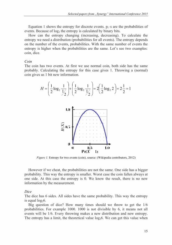
How can the entropy changing (increasing, decreasing). To calculate the entropy we need a distribution (probabilities for all events). The entropy depends on the number of the events, probabilities. With the same number of events the entropy is higher when the probabilities are the same. Let’s see two examples: coin, dice.
Coin The coin has two events. At first we use normal coin, both side has the same probably. Calculating the entropy for this case gives 1. Throwing a (normal) coin gives us 1 bit new information.
12
122log
2
12
211
log2
1
211
log2
1222
H
Figure 1. Entropy for two events (coin), source: (Wikipedia contributors, 2012)
However if we cheat, the probabilities are not the same. One side has a bigger probability. This way the entropy is smaller. Worst case the coin fallen always at one side. At this case the entropy is 0. We know the result, there is no new information by the measurement.
Dice The dice has 6 sides. All sides have the same probability. This way the entropy is equal log26.
Big question of dice? How many times should we throw to get the 1/6 probabilities. For example 1000. 1000 is not divisible by 6, it means not all events will be 1/6. Every throwing makes a new distribution and new entropy. The entropy has a limit, the theoretical value log26. We can get this value when

Selected papers from „Synergy” International Conference 2015
TÁMOP-4.2.1.B-11/2/KMR-2011-003 16
all events have the same probability. If we are lucky it can be after 6 throwing. But for 7th throwing the entropy will deceasing.
5850,26logloglog1
11
log1
2222
nn
nn
nn
nH
We use this experience to define the optimal length of (stochastic) measurement.
Based on dice we introduce three type of relative entropy. As we throwing the dice, we know the final entropy. Calculating the rate of current entropy and the final (H∞) is a relative entropy based on H∞.
H
Hh (2)
h∞ shows us how many information we get. The theoretical maximum is 100%. If we plan a measure error level, we can check if the relative entropy reached this level.
Another opportunity to calculate relative entropy is based on theoretical maximum entropy. In this case (all events have the same probability) the Hmax and H∞ is equal.
max
max H
Hh (3)
Based on theoretical maximum entropy (it is depend on the number of events) we can check how many information we get based on the maximum. In general (events have different probabilities) it cannot reach 100%. Also the smaller value can describe a good measurement.
Finally we calculate the rate of hmax and h∞. It shows the difference between all events are the same probability and the current process distribution.
maxh
hhrel
(4)
We throw 500 times a dice. The last result are in the next table. The first column shows the number of throwing. A second yellow column
shows the current value of the dice. For example the last throwing was 6. The next 6 columns show the number of value throwing. Theoretical it should be 500/6=83.333. It is very interesting that some values have big different from it ±5, but the entropy is 99,9% of the maximum value.

Selected papers from „Synergy” International Conference 2015
TÁMOP-4.2.1.B-11/2/KMR-2011-003 17
Table 1. Entropy after 500 times throwing a dice
3. Method
Our measurement result is a histogram. The soil surface is classified by clot size and a distance between clots. This histogram gives a distribution which is specific for the surface. We calculate the entropy after every clot.
Figure 2. Entropy by distance
The entropy shows a saturating function. Why should it be a saturating function?

Selected papers from „Synergy” International Conference 2015
TÁMOP-4.2.1.B-11/2/KMR-2011-003 18
At the beginning there are new columns in the histogram. More events make higher entropy. That’s way at the beginning it raising fast.
When all events appear the value of entropy depend on the final distribution. As we measure more the final distribution stabilizing. Of course every clot makes a small change on the distribution but the main concept doesn’t change. That’s why the ending section approximate the theoretical limit of the entropy.
Figure 3. Exponential regression
Figure 3 shows the measured entropy and the result of the exponential regression (Seber & Wild, 2005). The regression find the parameters for the following equation:
)1()( )/( TteHtH (5)
Where, H is the theoretical limit of entropy, t is the time of the measurement, T is the parameter of growing, saturating. Parameter T shows, how fast the saturation.
4. Results
In our method every clot changes the distribution. After histogram changing we calculate the entropy. Based on the entropy function we calculate the regression.
Our previous publication (Blahunka, Bártfai, & Faust, 2013) on this topic used different equation.
))( baxeHH (6)

Selected papers from „Synergy” International Conference 2015
TÁMOP-4.2.1.B-11/2/KMR-2011-003 19
We found parameter b is zero. T is 1/a. Before the measurement we know the level of precision. Based on this level
and equation number 5, the optimal time is:
Topt=T ln(error) (7)
Finally we implement this algorithm at National Instruments LabVIEW environment. The software gets the entropy values and calculates the exponential regression. At figure 4 the white graph shows the measured and calculated entropy. The red exponential graph shows the calculated entropy based on the regression. The green line is the maximum entropy level. It is interesting that in the measurement the entropy can be higher than the final. It is because the entropy shows how equals the events probability. If they getting equals the entropy increasing, if it is getting different the entropy value is decreasing.
Based on the green line and the given error level, the horizontal yellow line shows the level of entropy for a good measuring (entropy is bigger than the lowest limit). The vertical yellow line shows where crossing the horizontal level and the regression graph. The vertical yellow line shows the optimal length of the measurement.
We validate the calculation by R2. When R2 is lower than 90% the calculation is not valid. This can be at the beginning of the measurement. There are just a few result and the R2 is low. As figure 4 shows it is 95% so the entropy regression calculation is valid.
Figure 4. Exponential regression user interface
Conclusions
To know a stochastic process is an endless measurement. A process, surface is changing continuously. Also if we know that this is a homogeny surface, the

Selected papers from „Synergy” International Conference 2015
TÁMOP-4.2.1.B-11/2/KMR-2011-003 20
statistical parameters became nearly constant. In other hand nowadays the precision agriculture technologies try to serve every clods like a unique item. It is good for general working (the tractors are working on the whole fields) but control measurements should be optimal length.
Our method big advantage is, that we are able to forecast the optimal length of a stochastically measurement. Using exponential regression we get the parameters of entropy function. With a given accuracy we are able to calculate the optimal length of measurement. After this point we will have more value about surface but our knowledge won’t be more.
Nomenclature
DOF Degree-of-freedom IMU Inertial Measurement Unit
Acknowledgements
This publication is a result of a research work performed in the project called: TÁMOP-4.2.1.D-15/1/KONV-2015-0007 Smart City: Innovatív kutatási hálózatok fejlesztése Gyula és Salgótarján városokban.
References
[1] Blahunka, Z., Bártfai, Z., & Faust, D. (2013). Measurement optimalization by information entropy. Synergy 2013 - Book of Abstract: 3rd International Conference of CIGR Hungarian National Committee and Szent István University, Faculty of Mechanical Engineering & 36th R&D Conference of Hungarian Academy of Sciences, Committee of Agricultural and Biosystem Engineering, “Engineering, Agriculture, Waste Management and Green Industry Innovation”., 23.
[2] Blahunka, Z., Bártfai, Z., & Lefánti, R. (2012). Soil surface monitoring with gyroscope. Mechanical Engineering Letters, 8, 10–16.
[3] Blahunka, Z., Faust, D., Bártfai, Z., & Lefánti, R. (2011). Mobile robot soil surface monitoring. In L. Magó, Z. Kurják, & I. Szabó (Eds.), (p. 104). Gödöllő: SZIE Gépészmérnöki Kar.
[4] Bose. (2009). Modern Inertial Sensors And Systems. PHI Learning Pvt. Ltd. [5] Seber, G. A. F., & Wild, C. J. (2005). Nonlinear Regression. John Wiley & Sons. [6] Shannon, C. E., & Weaver, W. (1949). The mathematical theory of
communication. University of Illinois Press. [7] Wikipedia contributors. (2012, August 15). Entropy (information theory). In
Wikipedia, the free encyclopedia. Wikimedia Foundation, Inc. Retrieved from http://en.wikipedia.org/w/index.php?title=Entropy_(information_theory)&oldid=507540588

Selected papers from „Synergy” International Conference 2015
TÁMOP-4.2.1.B-11/2/KMR-2011-003 21
Researches based on the temperature measurement of non-metallic bearings
D. NAGY, P. SZENDRŐ, J. NAGY, L. BENSE
Department of Mechanics and Machinery, Szent István University
Abstract
The widely used metal rolling bearings are only suitable for use in a process fluid by solving serious difficulties in sealing. Process fluids (water, alkali or acid fluids, apple juice, wine or perhaps milk…) have an adverse effect on the operation of bearings.
In these cases, on the one hand the occurring corrosive effects must be expected as well as the inadequate lubrication of bearings. By now, due to the large development of materials science and manufacturing processes bearings with plastic outer and inner race and some kind of aseptic rolling element (e.g. glass, acid-resistant steel or ceramic) have appeared in the areas of rolling bearings.
In the Institute of Mechanics and Machinery of Gödöllő Szent István University there are studies conducted as to how these bearings made of non-standard materials behave in different process fluids.
Keywords
plastic rolling bearings, thermal imaging camera, thermal imaging camera tests
1. Timeliness and significance of the study of rolling element bearings
The use of rolling bearings plays an important role in all areas of technological life. A wide range of rolling-element bearings has been used for the energetically active support of the rolling parts of machinery and equipment. These machine elements must be adequate for a wide variety of load conditions and operating media without failure. Rolling bearings can be found in a laboratory environment as well as in extreme weather conditions or in installed, fixed manufacturing lines or mobile machines.
Since they have become widely used, adequate attention has been paid to their improvement and study in technology. When rolling bearings appeared, materials science and engineering were not at such a high level as today. In the 1960s there were efforts to make rolling bearings from new materials (plastic) versus metal. However, these efforts proved unsuccessful as plastics used and manufactured at the time did not meet the requirements of being used as the

Selected papers from „Synergy” International Conference 2015
TÁMOP-4.2.1.B-11/2/KMR-2011-003 22
materials of bearings. Because of these failures only a few large companies continued developing plastic rolling bearings further, but non-metallic bearings were not capable of fulfilling a good position in technology.
However, nowadays thanks to the strong development of materials science and manufacturing processes new materials have also appeared in the areas of rolling bearings. The rapid development of plastics and the appearance of technical plastics have made it possible to use new materials in the case of rolling bearings as well. Today, bearings are available in different materials for the technology for designers and users from plastic through glass and ceramic to conventional metals. These new materials have made it possible to apply rolling bearings in new areas of use, such as in the textile industry, pharmaceutical industry and increasingly in the food industry (R.G. Mirzojev, 1974).
Figure 1. IGUS Xiros B180 polyamide bearings with
glass (left) and steel (right) balls
Although the technical development of non-metallic bearings and the extent of their use have shown a clearly growing trend in the past 20 years, these directions of development have not been accompanied by laboratory research. Current research deals with either the properties of specific non-metallic bearing materials or the comparison of metal and non-metallic bearings. The fundamental direction of research by C. Morillo and fellow researchers was the comparison of non-metallic bearings to metal ones based on certain bearing features. (C.Morillo et al., 2013). The findings by Hitonobu Koike PEEK-PTFE were aimed at bearing wear (Hitonobu Koike, 2013). The efficiency of certain lubricants in the case of plastic bearing races was studied by J. Sukumaran et al. The primary focus of their work was the analysis of water lubrication; however the effects of other process fluids were not studied (J. Sukumaran et al., 2012). The self-lubricating ability of non-metallic bearings was studied by K. Kida, whose suggestion was that the PEEK bearing could be outstanding among plastic bearings due to its self-lubricating property (K. Kida et al., 2011). The question, problem of how bearings behave in process fluids (different liquid materials) has not been studied by any researchers in the case of the basic properties of bearings. Therefore, this topic can be considered rather timely, its significance is far-reaching.

Selected papers from „Synergy” International Conference 2015
TÁMOP-4.2.1.B-11/2/KMR-2011-003 23
2. The objective of the analyses
The aim of our study is to conduct a research program whose result can provide a tool for designers and operators using non-metallic bearings. It is important to define the limits of operations of these machine parts made of unconventional materials essentially on the basis of their operating temperature. Another direction of research could provide results for the selection of proper fitting joints in the case of different process fluids.
3. Material and method
It is important that we should be able to examine the operation of bearings among industrial operating conditions and then these conditions could be reproduced with the help of laboratory background thus the data and information experienced during the operation can be validated. The plant measurements are taken in the Bosch RUR washer machine operating in the LIO and CITO section of the LIO and Eye Drop plant of TEVA Pharmaceutical Factory in Gödöllő, and the control tests are performed under laboratory conditions.
Two main sets of tests were conducted. The temperature change in non-metallic rolling-element bearings was monitored with different load and run (revolution) settings during operation in a dry environment. In the design phase of the bearing test bench built in the Institute of Machinery of Szent István University it was an important aspect that the parameters basically impacting the operation of bearings like radial load, axial load or revolution should be freely adjustable and verifiable. The other criterion was that during the test runs performed in process fluids the test bench should be capable of receiving a climatic chamber which would function as a climatic cabinet, where the cabinet air humidity, dry matter content or temperature can be programmed under controlled conditions. Where appropriate, there may be flood tests in which the non-metallic bearings would operate in a process fluid and at this time the climatic cabinet would even function as a pool.
In addition to the temperature measurements of bearings the geometric parameter change of bearings was also tested in different process fluids. These measurements are interesting because of one of the most characteristic properties of plastics, the tendency of swelling. The change in those four main bearing geometrical parameters must be tested which fundamentally influence the operation of bearings – not only the operation of non-metallic bearings. These are the change in the diameter of the inner and outer race of the bearing due to the effect of the process fluid, which basically influence bearing installation instructions. If these parameters change, the tolerance pairs, fits recommended by the bearing manufacturer can also change. The change in these parameters puts the questions of installation technology into a new perspective. In addition to the outer and inner diameter the change in the clearance of bearing was measured since the change in this parameter impacts the running accuracy of

Selected papers from „Synergy” International Conference 2015
TÁMOP-4.2.1.B-11/2/KMR-2011-003 24
bearings. The fourth tested geometric parameter is the change in bearing weight because of the process fluid. Although it can be felt the extent of change in weight resulting from swelling will not impact the proper operation of the bearing, still it may be interesting since the assumption that non-metallic rolling bearings are prone to moisture absorption, consequently swelling i.e. size change may be substantiated with this data.
4. Equipment used during the laboratory tests of non-metallic rolling bearings
A test bench capable of examining non-metallic bearings was created in the Department of Machine Structures in the Faculty of Mechanical Engineering of Szent István University (Fig 2).
When the technical documentation was prepared the fundamental goal was to be able to adjust the radial and axial load as well as the revolution affecting the bearing running parameters and to be able to monitor the changes in these data in real time with the help of load cells and rotary encoder and also to be able to collect these data for later processing.
Figure 2. Special purpose equipment for testing non-metallic bearings
The other important criterion was that the structure of the test bench should be constructed of corrosion resistant materials so it cannot be damaged by the corrosive fluid to be used as planned. The base plate of the test bench was made of high precision aluminium preform, and due to the plate structure the other parts were also made of aluminium preforms. One of the most important construction elements of the test bench is the axle which was made by a high-precision manufacturing process from acid resistant steel. In the case of the axle and the axle lead-in the robust, rigid axle guide must be mentioned as an important construction criterion. High precision is significant in order to exclude any improper bearing operation due to axle faults (Fig 3).
The adjustment of accurate test revolution is done manually on the drive unit for the time being. There is a more interesting solution for the programming of the other two parameters to be adjusted (radial and axial load). The adjustment of the parameters affecting the operation can be realized by pulling, displacing

Selected papers from „Synergy” International Conference 2015
TÁMOP-4.2.1.B-11/2/KMR-2011-003 25
axially and perpendicularly to the axle the bearing housing created for the geometry of the bearing to be tested. The bearing housing can move on a guided course, the adjustment of the load of the tested bearing can be fixed with the help of a screw-spindle actuator (Fig 4).
Figure 3. The input axle and the axial and radial tensioning unit
Figure 4. Bearing housing and base plates capable of moving axially and radially
In the construction design phase of the test bench it was a basic condition that during the measurements all the variable bearing properties (e.g. change in bearing temperature) should occur by adjusting the test parameters according to the researcher’s intention and no uninterpretable factors should get into the experimental system due to some construction fault or non-compliance (e.g. undersized axle or improper support).
The measurements related to the temperature change in bearings are performed with the NEC thermal imaging camera of the Institute of Machinery (Figure 4), the images are processed with the default software of the camera, Image Processor Pro II (Figure 4) and then the data are evaluated. The

Selected papers from „Synergy” International Conference 2015
TÁMOP-4.2.1.B-11/2/KMR-2011-003 26
measurements of the temperature change are taken while constantly monitoring the radial and axial loads and the revolution. Data acquisition is performed by a SPIDER 8 data acquisition system, and data processing is done by the HBMI CATMAN system (Fig 5).
Figure 5. (From left to right) NEC thermal imaging camera, CATMAN
monitoring system, Image Process Pro II
The other main experimental direction recently has been the study of the size changes of rolling bearings due to the effect of process fluids of different properties. The size change in the weight, inner and outer race and clearance of bearings was measured at predetermined intervals. Weight measurements were taken using a KERN PCB with a readout accuracy of 0.01 grams (every 48 hours), the change in outer and inner diameter was measured with a micrometer and inside micrometer with a readout accuracy of 0.01 mm (Fig 6).
Figure 6. Measuring instruments used in the measurement of geometry change
During the measurements of the geometrical parameters of bearings the most complex task was the inspection of bearing clearance change since the feeler gauge with blades generally accepted and easily usable in the industry did not prove appropriate to measure the clearance of bearings with plastic outer and inner race. The main reason for this is the vulnerability of polyamide bearing races. So in this case the solution was to use a custom-designed measuring target device. The construction requirements of the device were the following: the high strength, robust securing of the axle ends manufactured according to factory
Selected papers from „Synergy” International Conference 2015
TÁMOP-4.2.1.B-11/2/KMR-2011-003 27
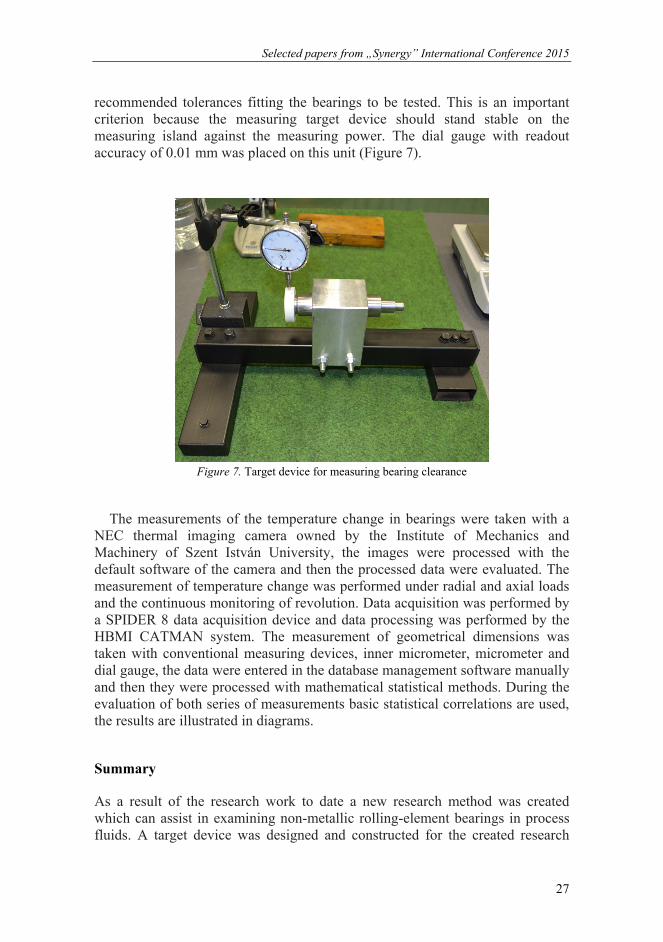
recommended tolerances fitting the bearings to be tested. This is an important criterion because the measuring target device should stand stable on the measuring island against the measuring power. The dial gauge with readout accuracy of 0.01 mm was placed on this unit (Figure 7).
Figure 7. Target device for measuring bearing clearance
The measurements of the temperature change in bearings were taken with a NEC thermal imaging camera owned by the Institute of Mechanics and Machinery of Szent István University, the images were processed with the default software of the camera and then the processed data were evaluated. The measurement of temperature change was performed under radial and axial loads and the continuous monitoring of revolution. Data acquisition was performed by a SPIDER 8 data acquisition device and data processing was performed by the HBMI CATMAN system. The measurement of geometrical dimensions was taken with conventional measuring devices, inner micrometer, micrometer and dial gauge, the data were entered in the database management software manually and then they were processed with mathematical statistical methods. During the evaluation of both series of measurements basic statistical correlations are used, the results are illustrated in diagrams.
Summary
As a result of the research work to date a new research method was created which can assist in examining non-metallic rolling-element bearings in process fluids. A target device was designed and constructed for the created research

Selected papers from „Synergy” International Conference 2015
TÁMOP-4.2.1.B-11/2/KMR-2011-003 28
method which device can also be installed with a climatic cabinet for bearing tests.
During the tests performed so far a conclusion was drawn regarding the changes in physical and geometrical parameters impacting the operation of bearings, due to the effect of process fluids. The main objective of the near future will be the itemized confirmation of the received partial results. In addition to the changes in physical and geometrical parameters due to the effect of process fluids, the relationship between the revolution and the inner temperature of the bearing was determined.
References
[1] C. Morillo, E. C. Santos et al. (2013), Comparative Evaluation Of Metal And Polymer Ball Bearings, In Journal Wear, pp. 1499-1505
[2] Hitonobu Koike et al. (2013), Observation Of Wear On PEEK-PTFE Hybrid Radial Bearings, In Journal Advanced Materials Research, pp. 683
[3] J. Sukumaran, V. Rodriguez, P. De Baets, Y. Perez et al., (2012), A Review On Water Lubrication Of Polymers, Presented A Review In Ghent University and Catholic University Of Leuven, K.U. Leuven
[4] K. Kida et al., (2012), Self-Lubrication Of PEEK Polymer Bearing In Rolling Contact Fatigue, In Journal Tribology International, pp. 30-38
[5] R. G. Mirzojev (1974), Gépelemek műanyagból, Műszaki Tankönyvkiadó, Budapest, 95-99 o.
[6] Gárdonyi P., Kátai L., Szabó I., (2015) Az ékszíjtárcsa átmérők és az ékszíjak melegedési viszonyainak kapcsolata, Fiatal Műszakiak Tudományos ülésszaka, XX, Kolozsvár, 26-29. p., ISSN 2067-6808
[7] Kátai L., Szabó I., Gárdonyi P. (2013), Az ékszíjak melegedés viszonyainak vizsgálata, A Gépipari Tudományos Egyesület Műszaki Folyóirata, LXIV. évf. 6. szám, Miskolc, p. 58-61., ISSN 0016-8572

Selected papers from „Synergy” International Conference 2015
TÁMOP-4.2.1.B-11/2/KMR-2011-003 29
Conditions for vegetable production in different types of tunnel greenhouses
A. DIMITRIJEVIC1, B. SUNDEK1, S. BLAZIN2, D. BLAZIN2
1University of Belgrade, Faculty of Agriculture 2Agricultural High school Josif Pancic, Pancevo
Abstract
The aim of this research was to investigate the microclimatic parameters in the different tunnel greenhouse constructions in order to see if the choice of the greenhouse construction can improve the production conditions inside the greenhouse enabling the better energy efficiency and lower energy input for heating / cooling. Air temperature, relative humidity and solar radiation were tracked in the open field and in the two types of tunnel greenhouses in tomato and cucumber production. Results show that temperature pattern and its values during the night and day depend on the greenhouse construction, plant specie and production season.
Keywords
vegetables, tunnel greenhouse, air temperature, air humidity, solar radiation, uniformity.
1. Introduction
Tomato and cucumber are most important vegetables in the human nutrition. These can be grown in the open filed, in the semi-controlled production conditions and in the greenhouses. In the open field and in the semi-controlled production conditions, they cover large surfaces and the adequate technical systems for the open filed production are used (Mago et al. 2005, 2006). Greenhouse cucumber production is more sophisticated. The species are adapted on the specific conditions in the greenhouse and are sensitive to the conditions outside the greenhouse. Concerning this, special attention is carried in controlling the production conditions in the greenhouse production.
Factors that determine the greenhouse production system are air temperature, relative humidity of air and soil, air quality and light conditions. Tracking these micro-climatic conditions is of a great importance for the successful greenhouse production (Ponjican et al., 2011). Purpose of tracking the greenhouse production continuously is to optimize the plant productions in the greenhouse. It is necessary to know the correlation between greenhouse construction, covering material and type of the plant production.
Temperature conditions in the greenhouses influence the overall plant growth, yield and fruit quality. If the air temperature and relative humidity in the greenhouse

Selected papers from „Synergy” International Conference 2015
TÁMOP-4.2.1.B-11/2/KMR-2011-003 30
are lower than optimal plants will be shorter with smaller dark green leaves. In the case of lower temperature and higher relative air humidity flowering of the plants will be delayed and the yield will be lower. Higher night temperatures cause the higher consumption of organic matter by plants which grow with the long pale green gently leaves with the lower yield and deformed fruits. It is stated (Lazić Branka et al., 2001, Hanan, 1998, Nelson, 2003) that night temperatures and the temperatures during the day should be 3–5° C lower compared outside temperatures during the sunny days. It is also stated that temperature variations during the day should not be more than 2 do 3° C. Literature sources (Lazić Branka et al., 2001, Hanan, 1998, Nelson, 2003, Sengar and Kothari, 2008, Singh and Tiwari, 2000) confirm the statement that temperature in greenhouses varies along their length, width and height. The pattern of this variation is influenced by the greenhouse type of construction and its dimensions, covering material, orientation and applied heating and venting systems.
The aim of this paper was to show how the type of greenhouse construction and plant species can influence the uniformity of the micro-climatic conditions in the tunnel type of greenhouses.
2. Material and method
For the purpose of the research a tunnel type (TUN 1) 5.5 x 24 m covered with 180 µm PE UV IR outside folia and a tunnel type (TUN 2) greenhouse 8 x 60 m and with 180 µm inner folia and 220 µm outside folia were used. Production surface of the tunnel 1 greenhouse (TUN 1) was 132 m2 its specific volume was 12.56 m3/m. Tunnel greenhouse 2 (TUN 2) had the 480 m2 production surface and specific volume of 25.12 m3/m. Experiment was carried out at the private property in Pancevo (44° 52’ 46’’N, 20° 38’ 50’’E) and at a private property near Jagodina (44° 02’ 14’’N, 21° 16’ 15’’E) (Serbia).
Temperature and air humidity were measured using the sets of WatchDog Data loggers 150 Temp/RH, t= 0.6 °C and RH= 3% and a WatchDog Data Logger Model 450 – Temp, Relative Humidity - Temp/RH, t= 0.6 °C and RH= 3%. In the greenhouses tomato and cucumber production conditions were analysed for the summer 2015 production season.
Statistical analysis of the results was based on variance analysis, F tests and LZD tests which were used to determine if the temperature and relative humidity are uniform along the greenhouses and if the type of construction influences the temperature, relative humidity uniformity and solar radiation transmition. Data used for the analysis represent the five days average values.
3. Results and discussion
Temperature distribution Tunnel greenhouses are considered to be the simplest form of the greenhouses in which temperature and the other production parameters vary during the day

Selected papers from „Synergy” International Conference 2015
TÁMOP-4.2.1.B-11/2/KMR-2011-003 31
significantly depending on the outside climatic parameters (Enoch, 1978, Hanan, 1998, Nelson, 2003).
Temperature measurements in both of the tunnel greenhouses show that temperature varies along the greenhouse (Tab. 1, Fig. 1, Fig. 2). During the night hours the highest temperature was observed in the central part of both of the tunnels. In the TUN 1 lowest temperature was measured in the north part while in the TUN 2 the lowest temperature was observed in the south part. Statistical analysis of the data showed that temperature differences of 0.83°C along the TUN 1 and 1.05°C in the TUN 2 greenhouse during the night are not significant.
Temperature measurements at 7h in the morning also show that there are differences in the air temperature distribution along both of the tunnel greenhouses. In both cases the highest temperature was in the south part of the greenhouse (Tab. 2). The lowest temperature in the TUN1 was measured in the north part while for the TUN 2 the lowest temperature was measured in the central part. Variance analysis confirmed that these differences are not significant for the TUN1 greenhouse but are very significant in the TUN 2 greenhouse. Based on the LSD test it was concluded that difference of 6.92°C were very significant (Fig. 3).
Table 1. Temperature variation inside and outside the greenhouses in the lettuce production, °C
Time of the day 1h 7h 13h 19h TUN
1 TUN
2 TUN
1 TUN
2 TUN
1 TUN
2 TUN
1 TUN
2 INSIDE North side 15.80 17.06 22.87 24.70 37.26 45.17 25.35 30.24 Centre part 16.63 17.75 23.05 20.05 38.56 36.80 27.97 27.78 South side 16.10 16.68 24.13 26.97 36.26 44.89 26.20 29.29 Average 16.07 17.16 23.32 23.91 37.36 42.89 26.51 29.10 OUTSIDE 14.93 16.37 15.71 15.93 29.05 32.88 24.35 28.86 Inside/outside difference 1.14 0.79 7.61 7.98 8.31 10.01 2.16 0.01
Measurements at 13 h (Tab. 1) show that there are differences in the temperature along the both of greenhouses. The patterns are different. For the TUN 1 the highest temperature was measured in the central part and the lowest in the south part. Statistical analysis showed that the temperature differences of 2.4°C are not significant. In the case of TUN 2 the highest temperature was observed in the north part and the lowest in the central part. Statistical analysis showed that the differences of 8.370 C are very significant (Fig. 3).
Temperature measurements in the 19h also showed that temperature varies along the both tunnel structures but with the different patterns (Tab. 1). In the TUN1 the highest temperature was measured in the central part while the lowest

Selected papers from „Synergy” International Conference 2015
TÁMOP-4.2.1.B-11/2/KMR-2011-003 32
was measured in the north part of the tunnel. However, variance analysis confirmed that these differences are not significant. As for the TUN 2 structure, the highest temperature was measured in the north part while the lowest was observed in the central part. In this case also, variance analysis showed that these differences are not significant.
0
5
10
15
20
25
30
35
40
45
50
1h 7h 13h 19h 1h 7h 13h 19h 1h 7h 13h 19h 1h 7h 13h 19h 1h 7h 13h 19h
Temperature, 0C
Time of the day
Outside the greenhouse
South part of the greenhouse
Central part of the greenhouse
North part of the greenhouse
Figure 1. Temperature variation in the TUN 1 greenhouse
0
5
10
15
20
25
30
35
40
45
50
7h 13h 19h 1h 7h 13h 19h 1h 7h 13h 19h 1h 7h 13h 19h 1h 7h 13h 19h 1h
Tem
per
atu
re, 0
C
Time of the day
North side
Central part
South side
Outside the greenhouse
Figure 2. Temperature variation in the TUN 2 greenhouse

Selected papers from „Synergy” International Conference 2015
TÁMOP-4.2.1.B-11/2/KMR-2011-003 33
1h Δt=1.050 C7h Δt=6.920 C **
13h Δt=8.370 C **
19h Δt=3.500 C
t 1h Δt=0.830 C7h Δt=1.260 C 13h Δt=2.300 C 19h Δt=2.620 C
t
Figure 3. Temperature variation inside the TUN 2
and TUN 1 tunnel greenhouses
Differences between inside and outside temperatures are very important parameter that defines the ventilation system capacity and operation. In the summer production, temperature in the greenhouses is always much higher than the outside. With the appropriate venting system, optimized based on the type of plant species and greenhouse construction, it is possible to regulate these temperature. In the summer greenhouse vegetable production it is important to have good ventilation systems that will lower the temperature in the greenhouses and that will eliminate parts of the greenhouses with high temperature.
Statistical analysis for testing the mean values showed that there are differences between inside and outside temperature in the tunnel structure and that these differences are very significant in the afternoon hours (Fig. 4). This means that during the evening and night hours one should not expect significantly higher temperatures inside the greenhouse compared to the outside temperatures. In both tunnel structures statistical analysis showed that temperature in the morning and noon are to be expected significantly higher if compared with the outside temperatures.
1h Δt=0.790 C7h Δt=7.980 C **
13h Δt=9.390 C **
19h Δt=0.250 C
tt 1h Δt=1.250 C
7h Δt=7.640 **C 13h Δt=8.310 **C 19h Δt=2.160 C
tt
Figure 4. Temperature inside and outside the TUN 2
and TUN 1 greenhouse
In this way it can be concluded that in the summer tomato production in the tunnel (TUN 1) greenhouse temperature conditions in the greenhouse do not vary much along the greenhouse length. Significant differences were only observed in the inside and outside temperatures in both greenhouses in the early morning hours and at noon. Concerning the temperature values, these oscillations can be considered as acceptable. As for the TUN 2 summer cucumber production temperatures inside the greenhouse are not uniform, especially during the day. There are “hot” spots in the greenhouse and this must be regulated by using the roof openings or introducing the forced ventilation.

Selected papers from „Synergy” International Conference 2015
TÁMOP-4.2.1.B-11/2/KMR-2011-003 34
Relative humidity Optimal relative humidity for cucumber is very high (90 - 95%) while for the tomato it is 50 - 65%. Literature (Lazić Branka et al., 2001, Hanan, 1998, Nelson, 2003, Sengar and Kothari, 2008, Singh and Tiwari, 2000) states that air humidity varies during the day and along the greenhouse length and height. It is stated that the pattern of variation depends on greenhouse type of construction its dimensions, covering material and the plant species that is produced in the greenhouse.
Table 2. Relative air humidity inside and outside the tunnel greenhouses, %
Time of the day 1h 7h 13h 19h TUN
1 TUN
2 TUN
1 TUN
2 TUN
1 TUN
2 TUN
1 TUN
2 INSIDE 94.05 85.06 88.75 89.83 29.99 26.99 77.62 31.06 OUTSIDE 64.65 49.02 65.94 40.52 27.55 24.68 46.00 20.04 Inside/outside difference 29.40 36.04 22.81 49.31 2.44 2.31 31.62 11.02
Measurement of the air relative humidity in both of the tunnel greenhouses
show that air relative humidity has the same pattern of change for both of greenhouses (Fig. 5). It is significantly higher in all periods of the day except in the noon where differences between outside and inside air relative humidity exist but are not significant.
RHRH 1h ΔRH=29.4% **
7h ΔRH=22.81% **
13h ΔRH=2.44%19h ΔRH=31.61% **
1h ΔRH=36.04% **
7h ΔRH=49.31% **
13h ΔRH=2.31%19h ΔRH=11.02% **
RHRH
Figure 5. Outside / inside air relative humidity differences
for the TUN 2 and TUN 1 greenhouse
So, regarding the air relative humidity, the type of tunnel structure does not influence significantly on its behaviour pattern.
Solar radiation Solar radiation is one of the most important factors that influences overall energy efficiency of the vegetable production in the greenhouses (Hanan, 1998, Nelson, 2003, Kozai et al, 1978). The solar radiation energy that comes to the

Selected papers from „Synergy” International Conference 2015
TÁMOP-4.2.1.B-11/2/KMR-2011-003 35
plants depends on the greenhouse construction type, greenhouse covering material, greenhouse orientation and the time of the year.
Measurements of the solar radiation outside and inside the tunnel greenhouses showed that there are differences (Tab. 3) and that are not the same in the two types of greenhouse structures.
Statistical analysis showed that in the morning hours the quantity of solar radiation that enters the greenhouses is not significantly lower than the outside solar radiation. So, the properties of the covering material and these types of greenhouse constructions are beneficial for the solar radiation transmission.
Table 3. Solar radiation inside and outside the tunnel greenhouses, W/m2
Time of the day 1h 7h 13h 19h TUN
1 TUN
2 TUN
1 TUN
2 TUN
1 TUN
2 TUN
1 TUN
2 INSIDE 0.00 0.00 61.23 97.56 357.88 553.08 31.74 46.69 OUTSIDE 0.00 0.00 76.09 153.72 831.69 930.82 44.47 108.27 Inside/outside difference 0.00 0.00 14.86 56.16 473.81 377.74 12.73 58.58
Measurements in 13h show that solar radiation that has reached the plants
inside both of the greenhouses was significantly lower than the outside solar radiation. In the TUN1 the losses were 37.71 – 68.44%. In the TUN 2 structure the losses were lower and were 37.18 – 44.29%.
7h ΔRad=14.9W/m2
13h ΔRad=473.8W/m2 **
19h ΔRad=12.73W/m2
Max Losses=68.44%
7h Δrad=56.16 W/m2
13h Δrad=377.74 W/m2 **
19h ΔRad=58.58 W/m2 **Max Losses=50.10% Figure 6. Outside / inside solar radiation for the TUN 2 and TUN 1 greenhouse
Measurements in the 19h showed that TUN 1 had the better conditions regarding the solar radiation transmittance. The energy that was entering the greenhouse was not significantly lower compared the outside values. The losses were 5.39 – 35.61%. TUN 2 construction showed higher losses in the solar radiation transmittance (36.18 – 62.70%). The solar energy that was reaching the plants in the TUN 2 greenhouse was significantly lower compared to values outside.

Selected papers from „Synergy” International Conference 2015
TÁMOP-4.2.1.B-11/2/KMR-2011-003 36
Conslusions
Obtained results show that micro-climatic conditions in the greenhouse vary during the day and along the greenhouse length. The variation pattern depends on the greenhouse type of construction. In the TUN 1 structure, with the smaller specific volume, more uniform temperature conditions along the greenhouse were observed. The reason for this can be the size of the TUN 1 and the fact that it was shorter and that ventilation was along the central part of the greenhouse, where data loggers were placed. TUN 2 has the higher specific volume so it is difficult to ventilate the area only with the natural ventilation. In this case either side ventilation must be introduced or forced ventilation since it is 60 m long. Concerning the relative air humidity the type of construction had no influence on the conditions inside both of the tunnel structures. Concerning the solar radiation transmittance the smaller tunnel (TUN 1) had a higher transmittance compared to the TUN 2 structure. Concerning all these differences and unstable production conditions, tunnel structures can not be suggested as a balanced environment for the vegetable summer production. Great care must be taken in order to optimize the venting systems in such greenhouses.
Acknowledgements
The authors wish to thank to the Ministry of education, science and technological development, Republic of Serbia, for financing the TR 31051 Project.
References
[1] Enoch, H.Z. (1978), A theory for optimalization of primary production in protected cultivation, I Influence of aerial environment upon primary plant production, Symposium on More Profitable use of Energy in Protected Cultivation, Sweden.
[2] Hanan, J.J. (1998), Greenhouses – Advanced Technology for Protected Horticulture, CRC Press, Boca Raton, USA.
[3] Kozai, T., Goudriaan, J., Kimura, M. (1978), Light transmition and photosynthesis in greenhouses. Simultaion Monograph, Wageningen.
[4] Lazić, Branka, Marković, V., Đurovka, M., Ilin, Ž. (2001), Vegetable production in the greenhouses, Partenon, Belgrade (in Serbian).
[5] Magó L., Jakovác F.: (2005) Economic Analysis of Mechanisation Technology of Field Vegetable Production. Hungarian Agricultural Engineering, 18: 55-58.
[6] Magó L, Jakovác F: (2006) Economical Analysis of the Mechanised Field Cucumber Production and Grading Technology, Agricultural Engineering Scientific Journal, Belgrade-Zemun, Serbia, December 2006. Vol. XXXI. No 4., p. 43-50.

Selected papers from „Synergy” International Conference 2015
TÁMOP-4.2.1.B-11/2/KMR-2011-003 37
[7] Nelson, P.V. (2003), Greenhouse Operation and management, Sixth Edition, Prentice Hall, New Jersey.
[8] Ponjican O., Bajkin A., Dimitrijevic A., Mileusnic Z., Miodragovic R. (2011), In: Kosutic S (ed) Proc 39th International Symposium on agricultural Engineering Actual Tasks on Agricultural Engineering, Opatija, Croatia, pp. 393-401.
[9] Sengar, S. H., Kothari, S. (2008), Thermal modelling and performance evaluation of arch shape greenhouse for nursery raising. African Journal of Mathematics and Computer Science Research Vol. 1, No.1, pp. 1–9.
[10] Singh, R.D., Tiwari, G.N. (2000), Thermal heating of controlled environment greenhouse: a transient analysis. Energy Conversion and Management, Vol. 41, pp. 505–522.

Selected papers from „Synergy” International Conference 2015
TÁMOP-4.2.1.B-11/2/KMR-2011-003 38
Pear classification using 3D image processing
A. LÁGYMÁNYOSI, I. SZABÓ
Faculty of Mechanical Engineering, Szent István University
Abstract
In agricultural crop classification colour and shape are the mostly investigated characteristics. In most cases classification is traditionally carried out by people using simple visualization or by automated image processing. The aim of the image processing analysis, is to search for specific shape properties of crop class, or give a description of the specific geometry of the total crop. The applied image resolution is critical parameter regarding image processing procedures. The high-resolution image data might be significantly large and so the processing usually slow, while on the other hand the essential shape characteristics may be lost due to the few pixels in the case of low resolution. In the imaging studies of shape characteristics fundamentally two main lines are being distinguished. One is the conventional two-dimensional imaging, and the other is the image analyses applied on 3D images. In this article a 3D image based evaluation technique is presented which provides an additional method to pear grade classifications. With this method the conventional identification used to classify pears can be extended and so the accuracy can be improved.
Keywords
image processing, 3D surface description, Computer-Aided Engineering
1. Introduction
There are several different features need to be defined together in order to precisely describe an pear. These main characteristics are colour, smell, flavour and shape. Traditionally, to assess these features the manual examination by using human sensory organs, such as vision, scent and taste, is inevitable. To define shape and colour the vision of the inspector is needed.
When machines are used for identification of the above mentioned characteristics devices with various operational principles are needed (Kátai L, et al., 2011). For example, in case of flavour the so called artificial tongue, while to recognize shape and colour artificial vision or machine vision is the appropriate solution (Bense and Nagy 2013). The applied image processing procedure needs entirely different principles for colour and shape description.
Some of the shape characteristics of an pear can be derived from a conventional two-dimensional image (Blahunka et al., 2011). In this case, the information is provided by the shape of the pear’s projection. The inspector,

Selected papers from „Synergy” International Conference 2015
TÁMOP-4.2.1.B-11/2/KMR-2011-003 39
however, evaluates the fruit in three-dimension as default. Therefore, the person also sees the shape of those parts which remain hidden on a projected image. So as to describe an pear’s characteristic shape in two dimensions it is sliced lengthwise and width wise resulting in longitudinal and cross section.
After the fruit has been sliced sections can be well defined by means of two-dimensional image acquisition methods. This way the features of core can also be assessed which, in this particular case, is another important piece of information. Nevertheless, it is a destructive method in which the value of the fruit will finally be lost.
In classification for quality the core parameters are usually not relevant. In this case, the main classification features are shape, colour and size which are external characteristics (Hajagos A, et al, 2012). The shape characteristics are specific to a variety and changes (possible deformations) are used as basic quality classification factor. This is underpinned by the fact that specific shape does not necessarily define a variety but a variety has specific shape characteristics.
Figure 1. The pear section planes
By using three-dimensional imaging the 3D image of the pear can be acquired. Compared to a two-dimensional image this contains numerous pieces of information concerning shape (Molto, E. et al., 1996). The information, however, remains hidden within the data. Dataset can be larger with orders than in case of a simple two-dimensional image. So the hidden information within a three-dimensional image can provide with many additional shape attributes but these can only be derived from the descriptive dataset with an appropriately chosen mathematical model. At present, the most limiting factor detaining the spread and use of 3D technologies is the difficulties with handling such large volume of data. Therefore, the general aim of the researchers, working on the

Selected papers from „Synergy” International Conference 2015
TÁMOP-4.2.1.B-11/2/KMR-2011-003 40
area of 3D imaging, is to search and develop such algorithms by which data volume and processing time be reduced significantly (Kátai and Szabó, 1997). There are no universal, generally applicable image processing methods! With regard to this, the ultimate aim is to always identify and develop a problem-specifically designed and tuned algorithm. In case of the 3D-image-based-pear-classification, the aim has been the same.
2. Applied system elements
In order to exclude the measuring errors originated in the operational principle 3D scanner two 3D scanners, with two operational principles, were used.
a./ A laser scanning: 3D laser scanner of the type Zscanner 700 was used. The main technical parameters were: sampling rate 18000 sample / sec., 2 built in cameras, improved resolution of 0,1 mm, maximal accuracy of XY positioning is 50 μm if the investigated volume is 100 mm x 100 mm.
b./ Procedure based on a projected contrast grid (dark and bright bands): Breuckmann optoTOP –HE 1097 where the Sensor Principle of operation Miniaturised Projection Technique with Light source 100 W halogen, Imaging High resolution digital camera Digitizing 1384 x 1036 pixels, Operating distance from approx. 50 mm, Min. depth resolution 2 μm, Acquisition time < 1s.
For 3D image acquisition to evaluate an pear the original software of scanners were used.
Files were saved with *.stl extension. For mathematical transformation Matlab and MS Excel software were used.
3. Applied methode
According to the hypothesis a given pear variety is usually classified for quality based on primarily size and then on deviation from the ideal shape. By considering the size based classification solved the shape characteristics remain in the centre of interest.
An ideal pear is considered as symmetric on the axis that connects the stem and the calyx. Parameterizing the deviation from the ideal the increase of deviation can be defined as quality reduction. By having an unambiguously quantified value which expresses the deviation of an ideal pear an exact classification into quality classes will be feasible.
The deviation can be measured in several ways. From these methods the one, which can squarely described, repeated and validated must be selected. Furthermore, the selected method should use simple calculation mechanism on preferably few input data.
Selected papers from „Synergy” International Conference 2015
TÁMOP-4.2.1.B-11/2/KMR-2011-003 41
The above described criteria can only be fulfilled if a well-defined reference system can also be provided. For example, the lengthwise section of an pear will obviously depend on the direction of slicing even if it is absolutely perpendicular to the width wise axis.
The fundaments of the new method, developed by authors are the followings: – ensuring standard resolution in case of all measurement, – transformation to a uniform orientation system, – easily calculated and validated quality parameters.
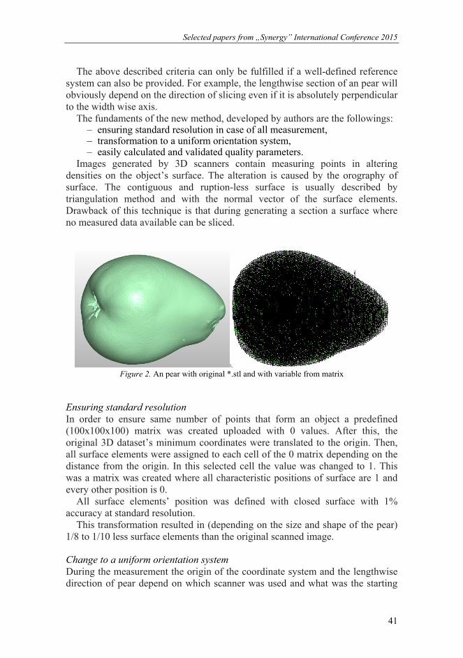
Images generated by 3D scanners contain measuring points in altering densities on the object’s surface. The alteration is caused by the orography of surface. The contiguous and ruption-less surface is usually described by triangulation method and with the normal vector of the surface elements. Drawback of this technique is that during generating a section a surface where no measured data available can be sliced.
Figure 2. An pear with original *.stl and with variable from matrix
Ensuring standard resolution In order to ensure same number of points that form an object a predefined (100x100x100) matrix was created uploaded with 0 values. After this, the original 3D dataset’s minimum coordinates were translated to the origin. Then, all surface elements were assigned to each cell of the 0 matrix depending on the distance from the origin. In this selected cell the value was changed to 1. This was a matrix was created where all characteristic positions of surface are 1 and every other position is 0.
All surface elements’ position was defined with closed surface with 1% accuracy at standard resolution.
This transformation resulted in (depending on the size and shape of the pear) 1/8 to 1/10 less surface elements than the original scanned image.
Change to a uniform orientation system During the measurement the origin of the coordinate system and the lengthwise direction of pear depend on which scanner was used and what was the starting

Selected papers from „Synergy” International Conference 2015
TÁMOP-4.2.1.B-11/2/KMR-2011-003 42
position of pear at the beginning of scan. The logging of minimal values was done during ensuring the standard resolution. Nevertheless, due to the differently positioned pears the translation solely does not ensure uniform reference system.
As an origin of the uniform orientation system the pears’ centre of gravity was chosen. In order to eliminate the effect of random rotation among the rotation axes along the centre of gravity of an pear, considered as homogenous body, the so called inertial main axes were selected. These axes are perpendicular to each other, pair wise.
Like this, a reference system was created where all pears’ longitudinal axis overlaps with one of the reference system’s main axes and the origin is situated in all pears’ centre of gravity.
The procedure was carried out by with the following mathematical apparatus: If the x, y, z variables represents the pear surface points. Js the tensor of the moment of inertial to mass centre
22
22
22
yxzyzx
zyzxyx
zxyxzy
Js
Js_p the tensor of the primary axis, where the 1, 2, 3 the Js eigenvalues
3
2
1
_
00
00
00
psJ
With the Js_p create the Q matrix where the column represents the 1 .... 3 eigenvectors
zzz
yyy
xxx
Q
321
321
321
Finally to the coordinate transformation was used the next equation
z
y
x
Q
z
y
x
'
'
'
The selection and creation of the quality parameters By using the standard resolution and uniform direction of matrixes several attributes were examined. These were the comparison of torque on the selected

Selected papers from „Synergy” International Conference 2015
TÁMOP-4.2.1.B-11/2/KMR-2011-003 43
main axes, the torque ratios on the main axes of a particular pear’s and the distance between the origin and main axes’ points intersecting the surface.
According to authors’ experience the deviation from an eye-appeal, variety specific shaped pear are basically not the knobs on the surface but distortions, assumingly originated in development disorder. These distortions occurred near the stem and the calyx in various levels.
That is why the selected parameter, primarily due to the simple and quick calculation method, is the distance between the stem and/or calyx and the nearest main axis.
Figure 3. 2D slice with the difference from primary axis
Conclusions
Authors have developed a method that creates a uniform reference system for evaluating the shape attributes of the pear. It is capable of treating the characteristic dataset uniformly, independently from size and orientation. Out of several shape features on have been selected that can be used to describe the pear distortion’s level (deviation from ideal) by using a simple value, or value pair.
By completing the automatic classification of pears with this characteristic the quality of classification can be further increased.
References
[1] Bense L, Nagy I. Robotok a gyümölcsösben. Agrofórum, 2013. 03: 146-149. ISSN 1788-5884
[2] Hajagos A, et al The effect of rootstocks on development of fruit quality parameters of some sweet cherry (Prunus avium L.) cultivars, ‘Regina’ and

Selected papers from „Synergy” International Conference 2015
TÁMOP-4.2.1.B-11/2/KMR-2011-003 44
‘Kordia’, during the ripening process. 2012, Acta Universitatis Sapientiae, Agriculture and Enviroment, 4, pp. 59–70.
[3] Kátai L, et al 3D Scanning and Computer Analysis of Morphological Aspects for Agricultural Applications. In: Hungarian Agricultural Engineering, 23/2011 December p.105-108. HU ISSN 0864-7410
[4] Blahunka Z. Faust D, Bártfai Z, Lefánti R. Synergy of optical insect counter and mobile robot, Synergy in The Technical Development of Agriculture and Food Industry 2011, Gödöllő, ISBN:978-963-269-250-0
[5] Kátai L, Szabó I. Digital Image Processing for Qualifying Chopped Plant Bulks. In: Hungarian Agricultural Engineering, 1997. 10. p.35-36.
[6] Molto, E. et al An artificial vision system for fruit quality assessment Conference of European Agricultural Engineering, Madrid 1996, 96F-078

Selected papers from „Synergy” International Conference 2015
TÁMOP-4.2.1.B-11/2/KMR-2011-003 45
Determination of some shape factors of fish and larvae feed using digital image
processing method
M. GHARIBKHANI, R. C. AKDENIZ Department of Agricultural Machinery and Technologies Engineering
Abstract
The digestibility, mechanical properties, nutrient leakage rate and also the marketability of many kinds of micro-particle feeds are affected by the size and physical properties of particles. Use of reliable and accurate methods for the measurement of particle size and shape are of great importance for characterization of particulate feed in fish and larvae feed production process. In this study, using seven different types of fish and larvae feeds as test material, an image processing approach was proposed and results were evaluated. MATLAB software was used to process the images of samples. Some important shape factors such as roundness, extent, eccentricity, equivalent diameter, solidity, convex area and elongation were obtained from the sample images. The results obtained from software were compared with manually measured data to determine the accuracy of the method. The accuracy was between 0.77 and 0.98% for different types of feed. The proposed image processing method would be considered good enough to use for determining the physical properties of feed particles instead of conventional mechanical methods.
Keywords
micro-particle feed, size and shape factors, image processing, marketability
1. Introduction
In recent years, a great deal of interest has emerged in the development of micro-diets as an economic alternative to live feed, in the larval culture of marine fish species (Pousao-Ferreira et al., 2003). As well known, particle size, particle size distribution (PSD), and shape properties of micro-particle feeds are important parameters for many industrial fish and fish feed producers, since the digestibility, mechanical properties, nutrient leakage rates and also the marketability of many kinds of micro-particle feeds are affected by the size and physical properties of particles.
The size of feed used for fish and especially fish larvae affects the feeding success. The importance of prey size proportion with mouth gape, especially for larvae fish should not be neglected (Rowland et al., 2006). Fish larvae tend to

Selected papers from „Synergy” International Conference 2015
TÁMOP-4.2.1.B-11/2/KMR-2011-003 46
ingest prey with a size similar to their mouth gape. Prey/mouth gape ratio deter-mined in different species usually ranges between 25 and 60% (Cunha and Planas, 1999; Ostergaard et al., 2005). Therefore, a reliable and accurate measurement of particle shape and size is central to characterization of particulate feed. Several researches were conducted to produce feed to meet needs of different fish species in different stages of growth and development. Also, some different technologies are being used to prepare micro-particles for rearing fish. Some important of these technologies include micro extruded marumerization (MEM), particle-assisted rotational agglomeration (PARA) (Barrows et al, 1993; Barrows et al, 2000), and spray bead production (Onal and Langdob, 2000). All these methods are designed to produce feeds with high quality, efficient amount of feedstuffs (Parker, 2000), low leakage rate, the proper size and shape for different species of fish or larvae demands. However, sometimes the feed produced with some methods such as spraying or extruding does not have a homogeneous in size and must be sieved to obtain appropriate size categories. Also, sometimes it is necessary to test and control the particle size and shape factors (e.g. area, perimeter, major and minor axis length and roundness) of feed particle to find the size distribution, maximum and minimum diameter of feed during production or before using it to understand if it is suitable for target fish or larvae to be used or not. Prey size is the primary characteristic defining choice in early larvae. Mouth gape limits the dimensions of prey that can be ingested (Holt, 2011). The roughness and area/mass of particle also has a direct relation to the solubility and leakage rate of particles in aqueous medium which seems as important factor in feed quality.
Mechanical sieving is one of the oldest methods (Leschonski, 1979; Allen, 2003) of particle size distribution analysis. It gives a mass distribution and a size known as the sieve diameter. If the standard procedures are followed and the methods are conducted carefully, sieving gives reliable and consistent size analysis (Rhodes, 2008). But, determination of particle size of feed particles using mechanical sieving systems is time consuming. Also, determination of shape factors is impossible using this method. On the other hand, as the fish and larvae feed has low density, they may be damaged by vibration and impacts applied by mechanical sieving. Though, using the mechanical sieving may lead to breaking of particles and affects the particle size distribution of material and sensitivity of the testing method. For these reasons, there is a genuine need to develop techniques for determining the particle size, shape factors and number of particles in a sample, nondestructive, accurate and fast manner.
Machine vision would be considered as an alternative method instead of conventional mechanical methods for determining physical properties of feed particles. The computer or machine vision technique is envisioned as an easy and quick way to acquire a variety of data that would otherwise be difficult to obtain manually (Lefebvre et al., 1993). The image processing method has been considered the reference method for the advanced particle analysis equipment that uses laser diffraction, acoustic spectroscopy, and light scattering principles

Selected papers from „Synergy” International Conference 2015
TÁMOP-4.2.1.B-11/2/KMR-2011-003 47
for size measurements (Igathinathane, 2012). This approach is inexpensive, quick and provides accurate measurements, especially for material with small size. On the other hand, physical parameters like area, compactness, major and minor axis length, perimeter, aspect ratio, compactness, convexity roundness or derived ratios are the most common features extracted from shape to classify or identify the product using machine vision methods (Blasco et al., 2009).
The primary object of this study is to determine the particle size, number of particles and some shape factors of feed in the sample by a cheap, nondestructive, accurate, fast and robust technique of image processing. This paper is an approach to use a multi-scale segmentation method for analysis of images obtained from different kinds of larvae feed of different size, components, shape and colors.
2. Materials and methods
Fish and larvae feed serves as the primary experiment materials. Seven types of extruded and crumbled feed that commonly used for rearing fish and larvae in Turkey were used for the experiments. More than 4500 samples were used as a data base for experiments. The feed samples were obtained from fish feed producers and sellers in Izmir, Turkey. These feeds were of different types and sizes. Three different types of extruded feed (a, b and d), one type of flake feed (c), and three different types of crumble feeds (e, f and g) were used as materials for the experiments (Fig. 1).
Figure 1. Different kinds of fish and larvae feeds used in experiments. a, b and d are three different types of extruded feed, c is flake feed, and e, f and g are
three different types of crumble feed used for fish and larvae rearing.
Equipment and software In order to benefit from this method some essential equipment is needed as device for image acquisition, an input image and an image processing algorithm.

Selected papers from „Synergy” International Conference 2015
TÁMOP-4.2.1.B-11/2/KMR-2011-003 48
For the experiments the hardware equipment include one flatbed document scanner (1200 x 2400 DPI; HP Scanjet 3770) (Shahin et al, 2006; Igathinathane et al., 2008a; Igathinathane et al., 2008b, Igathinathane et al., 2009a) and a computer (Acer laptop computer: Intel B960, 2.2GHz, 2MB L3 cache, 2GB DDR3 Memory). The MATLAB (R2012a) programming software is used for the image analysis and the scanning software for windows 7 was used for scanning the images.
Image acquisition To acquire the image of the test materials, feed particles were well spread and singulated in a manner that particles do not touch or overlap one another on the scanner surface. The singulated arrangement of particles makes the preprocessing algorithm simpler avoiding the need for specialized singularization algorithms like watershed or successive erosion and dilation (Shahin and Symons, 2005). All the images were scanned at 200 dots per inch (DPI) on both horizontal and vertical direction using the scanning software. White color was chosen for background color during all experiments which provides the best contrast for all feed from different kinds and sizes.
Preprocessing of image To start the image processing the color image of the test material was acquired. Preprocessing steps, including binary image extraction and filtering was conducted before main image processing. Though, the original color image first converted to grayscale image and then to binary image. Different values for threshold binary images were tested to get the best values for upper and lower limits that best fit for all types and size of feeds. As the background for all images was white, the particles of interest were covered precisely using a constant threshold range from 0.95 to 1. In order to remove the unwanted noises that might lead to inaccuracy in determining particle number and shape parameters, the opening and closing operations were applied. These operations may be considered as second level operations in that they build on the basic operations of dilation and erosion. Opening and closing operations were selected to ensure coverage of the whole particles, and the exclusion of holes, if any. The processing time of image depends on the image size and number of particles in the image. As the image size and particle number increases, the time needed for image processing would increase.
Particle properties calculating method The perimeter is the distance around the boundary of the target region. To compute the perimeter, the distance between each adjoining pair of pixels around the border of the region was calculated. The area of each object was estimated by counting the number of pixels belonging to that object. The digital images in computer are composed of pixels, and each pixel represents a certain area in a real feed particle. If we scan an object with a certain area previously and find out how many pixels its scanned image contains as a reference, then we
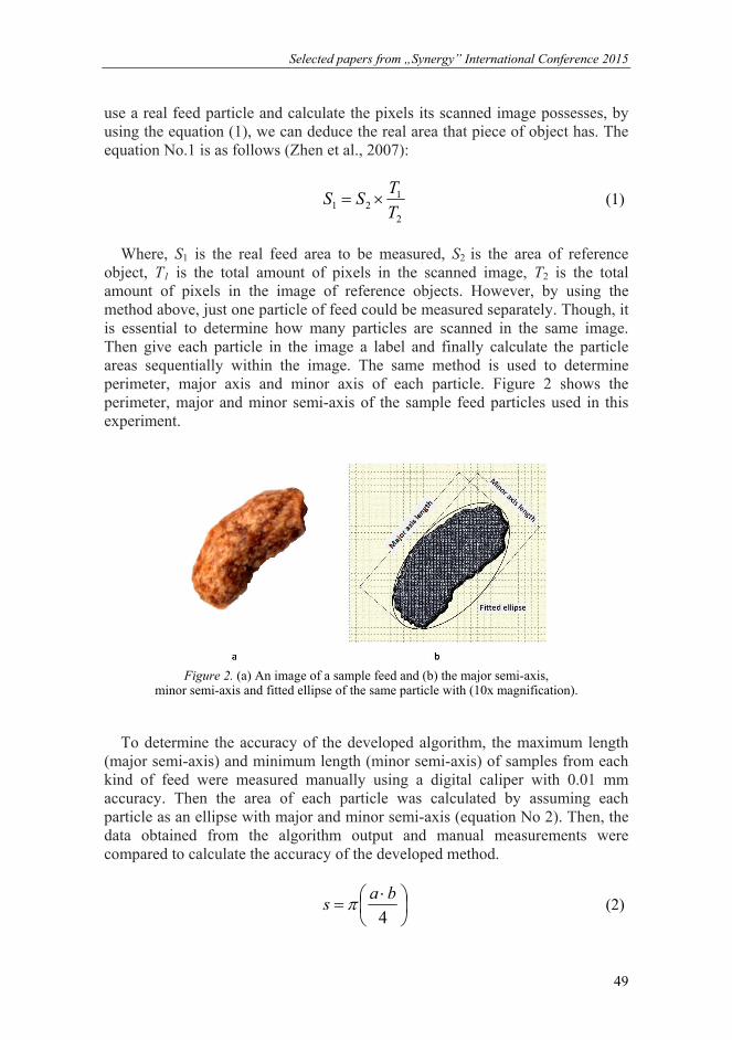
Selected papers from „Synergy” International Conference 2015
TÁMOP-4.2.1.B-11/2/KMR-2011-003 49
use a real feed particle and calculate the pixels its scanned image possesses, by using the equation (1), we can deduce the real area that piece of object has. The equation No.1 is as follows (Zhen et al., 2007):
2
121 T
TSS (1)
Where, S1 is the real feed area to be measured, S2 is the area of reference object, T1 is the total amount of pixels in the scanned image, T2 is the total amount of pixels in the image of reference objects. However, by using the method above, just one particle of feed could be measured separately. Though, it is essential to determine how many particles are scanned in the same image. Then give each particle in the image a label and finally calculate the particle areas sequentially within the image. The same method is used to determine perimeter, major axis and minor axis of each particle. Figure 2 shows the perimeter, major and minor semi-axis of the sample feed particles used in this experiment.
Figure 2. (a) An image of a sample feed and (b) the major semi-axis,
minor semi-axis and fitted ellipse of the same particle with (10x magnification).
To determine the accuracy of the developed algorithm, the maximum length (major semi-axis) and minimum length (minor semi-axis) of samples from each kind of feed were measured manually using a digital caliper with 0.01 mm accuracy. Then the area of each particle was calculated by assuming each particle as an ellipse with major and minor semi-axis (equation No 2). Then, the data obtained from the algorithm output and manual measurements were compared to calculate the accuracy of the developed method.
4
bas (2)

Selected papers from „Synergy” International Conference 2015
TÁMOP-4.2.1.B-11/2/KMR-2011-003 50
The definitions of the particle shape for explaining physical properties of feed materials are as given below. One of the most widespread and dimensionless indexes used for measurements is eccentricity. The eccentricity (e) is a number that expresses the degree of roundness of the elliptical particle and is a measure of how nearly circular the ellipse. The value would be between 0 and 1 (equation No. 3). The eccentricity value for feed particles with completely circular shape would be equal to zero.
a
ce (3)
Where c is the distance from the center to the focus of the ellipse and a is half of the length of the major axis. Equivalent diameter (ED) is a scalar that specifies the diameter of a circle with the same area with the feed particle and is computed using equation No. 4. Solidity (Sl) is a scalar specifying the proportion of the pixels in the convex hull that are also in the region and computed using equation No. 5. The extent (Ex) is a scalar that specifies the ratio of pixels in the target region to pixels in the total bounding box and is computed as the area divided by the area of the bounding box (Gonzalez and Wood, 2004). Roundness (Ro) is a dimensionless measure of the sharpness of corners and edges of a given particle and is associated with sphericity and the compactness of a shape (equation No. 6). Elongation (El) is another dimensionless shape factor that would be useful for evaluating the shape of feed particles. This factor determines the ratio of the minor axis to the major axis of the feed particle. Elongation is computed using equation No. 7.
SED
4 (4)
CA
SSl (5)
2
0
AxMaj
EDR (6)
AxisMajor
AxisMinorEl (7)
Where CA stands for the convex area which is a scalar that specifies the number of pixels in convex image. The algorithm coding followed the overall process is depicted in the form of a flowchart (Fig. 3).

Selected papers from „Synergy” International Conference 2015
TÁMOP-4.2.1.B-11/2/KMR-2011-003 51
Figure 3. Flowchart of image analysis process.
3. Results and discussion
The full views of the original color image with white background (a), grayscale conversion (b), binary threshold image (c), and segmented and numbered particles of sample feed after filtering (d) are given in Fig. 4. In this instant replication, the number of particles, recognized by the algorithm was 599 out of 599 valid particles. The algorithm has the capability of including all particles in the analysis without removing any small particle during all replications. However the particles smaller than 0.01 mm2 of the area are removed using opening and closing operations as they were considered to be source of inaccuracy and noise in the analysis. The minimum area of the experimental feed was higher than 0.05 mm2. It is possible to change this value based on the minimum size of the test materials.
This method was capable of predicting the total number of particles with an area over the 0.01mm2 with an accuracy of 100%. To gain this aim, the materials should not overlap each other and placed in a singulated arrangement on the scanner surface. The overlapping leads to mistakes in segmentation and numbering process. Otherwise, some addition algorithms like watershed algorithm (Igathinathane et al., 2012) would be applicable for resolving the touching particles which leads to complexity of the algorithm and longer processing time.

Selected papers from „Synergy” International Conference 2015
TÁMOP-4.2.1.B-11/2/KMR-2011-003 52
Figure 4. The procedure of processing an image: (a) color image, (b) gray scale conversion, (c) binary threshold and (d) segmented
and numbered particles of sample feed. Image resolution is 200DPI; size of the image is 1671 x 2323 pixels; number of particles is 599.
The algorithm was developed to determine some physical properties and shape factors of the tested samples. One of the most important factors measured was the major and minor axis of the feed samples. The algorithm was capable of determining and plotting the value related to this factor accurately. For instance, results obtained from two different samples are given in Fig.5. This figure shows particle area plot (left) and particle length plot (right) for 1200 and 4500 particle samples, respectively. The maximum value for the major axis of the tested material, was obtained from feed type (a) which is an extrude feed with 8.111 mm length, and the minimum value for the miner length, was related to the feed type (g) which is a crumble feed with 0.397 mm length.
Figure 5. Sample tables obtained from software displaying particle area distribution (left) and
particle length distribution (right) of two different processed samples.

Table 1. The average value of Shape factors related to each type of feed
Feed type
Area (mm2)
Perimeter
(mm)
Major Axis
Length (mm)
Minor Axis Length (mm)
Roundness(Ro)
Extent (Ex)
Eccentricity (e)
Equivalent Diameter
(ED)
Solidity(Sl)
Convex Area
(mm2)
Elongation(El)
a 9.5708 12.6787 5.0324 2.4717 0.4922 0.7489 0.8588 3.4643 0.9514 10.155 0.5036
b 7.1725 10.0905 3.2424 2.8287 0.8677 0.7683 0.4729 3.0154 0.9667 7.4191 0.8743
c 3.4254 6.9227 2.3208 1.9085 0.8124 0.7583 0.5432 2.0864 0.9651 3.5495 0.8243
d 5.325 8.5544 2.7628 2.4676 0.8883 0.7812 0.4250 2.6008 0.9715 5.4812 0.8944
e 1.31 4.1213 1.4144 1.2116 0.7648 0.7197 0.5158 1.2914 0.9776 1.34 0.8566
f 0.514 2.4776 0.9248 0.7218 0.7589 0.7238 0.5774 0.8001 0.9627 0.534 0.7873
g 0.4595 2.2608 0.8541 0.6872 0.7776 0.7377 0.5754 0.7534 0.9686 0.475 0.8025

Selected papers from „Synergy” International Conference 2015
TÁMOP-4.2.1.B-11/2/KMR-2011-003 54
Another important factor for determining the size of the particles is the area of the scanned surface of each particle. The algorithm could measure this data accurately, too. The accuracy of this measurement closely depends on the shape and size of the particles. The minimum and maximum areas of feed material were equal to 0.05 mm2 and 14.89 mm2, which related to feed type (a) and (g), respectively (Fig. 4).
The average data related to all measured shape factors are given in table 1. As it can be seen from the Table 1, the particle type with minimum average length owns the minimum area and minimum perimeter of all particle types, which is reasonable. Also, particles with more round shapes have the higher roundness value and the lower eccentricity value in comparing to other particles (b, c, and d type feeds). The highest mean value of roundness (0.8883) and lowest eccentricity (0.4250) relates to feed type d, which is an extrude feed with spherical shape, and the lowest mean value of roundness (0.4922) and highest eccentricity (0.8588) relates to extruded feed (type a) which has the lowest minor to major axis ratio (0.5036).
Figure 6. The sensitivity evaluation tables for measured
lengths of different types of feed (type a, b, c, d, e, f and g).
To determine how accurate the data obtained from the algorithm is, the accuracy test was conducted for length of particles as explained in materials and

Selected papers from „Synergy” International Conference 2015
TÁMOP-4.2.1.B-11/2/KMR-2011-003 55
methods. In order to compare the data obtained from the algorithm with manually attained data, the accuracy tables were mapped for each type of feed, separately (Fig. 6). The horizontal axis of each table stand for manually measured through the caliper as given by the methods section length of the particles and the vertical axis for predicted lengths from algorithm. The maximum accuracy level relates to extruded feed (type a) with R2= 0.979 and the lowest accuracy relates to flake feed (type c) with R2= 0.772. It is remarkable that the R2 value of accuracy test for smaller feeds (type e, f and g) were over 0.90. The higher accuracy value of feed type (a) can be inferred to the bigness of particle size of this type of feed. On the other hand the higher value of R2 for length prediction of small feeds (e, f and g types) might be related to the low particle thickness of these feeds. The thickness might be considered as an inaccuracy source in size prediction of particles, because it leads to the creation of large shadows during the image acquisition. During preprocessing of the images the images are converted to gray level, and sometimes it would be hard to remove the shadow from the real boundary of the particles using preprocessing algorithms.
The mean values for the equivalent diameter of each type of feeds are in agreeing with the other shape factors of the feed.
Conclusion
The algorithm has been developed successfully for measurement of size and shape factors of different types of fish and larvae feed with different colors and size distribution. It would be applied as a reproducible and inexpensive method for particles shape and size determination of feed with different size and colors without damaging the particles. The only problem might be encountered during working with feed particles using this method relates to the shadows of particles with high thickness values which would unpreventable during image acquisition using a flatbed scanner. By the way, using of effective preprocessing methods would effectively remove the shadow effect. This method also would be suitable to be used for particles with much smaller PSD. The only restricting factor would be the difficulty in singulating the particles for image acquisition if the particles are very small. This method would be considered as a useful and fast alternative for conventional mechanical methods.
Acknowledgment
This study was supported by the Scientific and Technological Research Council of Turkey (TÜBİTAK, Project Numbers: 113O435).
References
[1] Allen, T. (2003), Powder sampling and particle size determination. Elsevier Science Ltd. 208–250.

Selected papers from „Synergy” International Conference 2015
TÁMOP-4.2.1.B-11/2/KMR-2011-003 56
[2] Barrows F.T., R.E. Zitzow and G.A. Kindschi (1993), Effects of surface water spray, diet, and phase feeding on swim bladder inflation, survival, and cost of production of intensively reared larval walleyes. The Progressive Fish Culturist, 55: pp 224-228.
[3] Barrows, F.T. and W.A. Lellis (2000), Microbound feeds. In: Stickney, R.R. (ed.) Encyclopedia of Aquaculture. John Wiley & Sons, Inc., New York, pp 525-528.
[4] Blasco J., N. Aleixos, S. Cubero, J. Gómez-Sanchís and E. Moltó (2009), Automatic sorting of satsuma (Citrus unshiu) segments using computer vision and morphological features. Computers and Electronics in Agriculture, 66: pp 1–8.
[5] Cunha, I. and M. Planas (1999), Optimal prey size for early turbot larvae (Scophthalmus maximus L.) based on mouth and ingested prey size. Aquaculture, 175: pp 103-110.
[6] Gonzalez C.R. and E.R. Woods (2004), Digital image processing. In: Prentice-Hall, 2rd edn. Upper Saddle River, New Jersey, USA.
[7] Holt, G.J. (2011), Larval fish nutrition. 1st ed. 291-292, Wiley & sons, USA. [8] Igathinathane C., L.O. Pordesimo and W.D. Batchelor (2009a), Major
orthogonal dimensions measurement of food grains by machine vision using ImageJ. Food Res. Int., 42: pp 76–84.
[9] Igathinathane C., L.O. Pordesimo, E.P. Columbus, W.D. Batchelor and S.R. Methuku (2008b), Shape identification and particles size distribution from basic shape parameters using ImageJ. Comput. Electron. Agric, 63: pp 168–182.
[10] Igathinathane C., L.O. Pordesimo, W.D. Batchelor (2008a), Ground biomass sieve analysis simulation by image processing and experimental verification of particle size distribution. ASABE Paper, No. 084126, ASABE, St. Joseph, MI.
[11] Igathinathane C., U. Ulusoy and L.O. Pordesimo (2012), Comparison of particle size distribution of celestite mineral by machine vision ΣVolume approach and mechanical sieving. Powder Technology, 215–216, pp 137–146.
[12] Lefebvre M., S. Gil, D. Brunet, E. Natonek, C. Baur, P. Gugerli and T. Pun (1993), Computer vision and agricultural robotics for disease control: the potato operation. Computers and Electronics in Agriculture, 9: pp 85–102.
[13] Leschonski, K. (1979), Sieve analysis, the cinderella of particle size analysis methods. Powder Technology, 24: pp 115–124.
[14] Onal, U. and C.J. Langdon (2000), Characterization of two micro particle types for delivery of food to altricial fish larvae. Aquaculture Nutrition, 6: pp 159-170.
[15] Ostergaard P., P. Munk and V. Janekarn (2005), Contrasting feeding patterns among species of fish larvae from the tropical Andaman Sea. Marine Biology, 146: pp 595-606.
[16] Parker, R. (2012), Aquaculture science. Clifton Park, NY 12065-2919, USA. ISBN-13: 978-1-4354-8812-0.

Selected papers from „Synergy” International Conference 2015
TÁMOP-4.2.1.B-11/2/KMR-2011-003 57
[17] Pousao-Ferreira P., P. Santos, A.P. Carvalho, S. Morais and L. Narciso (2003), Effect of an experimental microparticulate diet on the growth, survival and fatty acid profile of gilthead seabream (Sparus aurata L.) larvae. Aquaculture International, 11: pp 491–504.
[18] Rhodes, M.J. (2008), Introduction to particle technology. John Wiley & Sons Ltd., 12–13.
[19] Rowlands W.L., M. Dickey-Collas, A.J. Geffen (2006), Gape morphology of cod Gadus morhua, L., haddock Melanogrammus aeglefinus (L.) and whiting Merlangius merlangus (L.) through metamorphosis from larvae to juveniles in the Western Irish Sea. Journal of Fish Biology, 69: pp 1379-1395.
[20] Shahin M., S.J.S. Symons, V. Poysa (2006), Determining soya bean seed size uniformity with image analysis. Biosyst. Eng. 94: pp 191–198.
[21] Shahin M.A. and S.J. Symons (2005), Seed sizing from images of non-singulated grain samples. Can. Biosyst. Eng., 47: pp 49–54.
[22] Zhen L, H. Tian-sheng, W. Wei-bin and L. Min-juan (2007) A Novel Method of Object Identification and Leaf Area Calculation in Multi-leaf Image. An ASABE Meeting Presentation, 073047.

Selected papers from „Synergy” International Conference 2015
TÁMOP-4.2.1.B-11/2/KMR-2011-003 58
Modeling the soil-wheel interaction with discrete element method
A. BABLENA
NARIC Institute of Agricultural Engineering
Abstract
Significant part of energy demand during operation of agricultural machines is turned to overcome the rolling resistance. Soil and deformable tire are such complex mechanical systems, that exact modeling of this system is not possible with analytical models based on classical continuum mechanical theories. Rapid development of computers in the last decades allows us the numerical modeling of soil-wheel interactions. In this article, a discrete element method based simulation of drawbar pull - slip diagram is presented.
Keywords
soil-wheel interaction, discrete element method, slip curve
1. Introduction
Since Bernstein’s pioneering work (Bernstein, 1913), mechanics of soil-wheel interaction has been investigated by many researchers. Goriatchkin (1936) and Bekker (1956) created analytical soil-wheel interaction models. Their results were improved by Reece (1964), Saakyan (1965) and Wong and Reece (1967). Despite their efforts, the average deviation of the analytically predicted soil-wheel interaction forces from the experimental results is still too large.
Urbán et al. (2012) applied a new method the so called Smooth Particle Hydrodynamics (SPH) to soil modeling. This method was developed for fluid examination but it may be appropriate to soil modeling according to them. They modeled the soil-tool interaction in 2 and also 3 dimensions. According to their results, this method may be appropriate to model cohesive soil with the same accuracy but with much lower computing time.
Discrete element method developed by Cundall (1979) gives possibility to examine mechanical behavior of each particle of the soil. This allows us to create more accurate soil models. In this method soil model has automatically non-linear behavior and gives behavior of the interface of soil-wheel interaction.
Tanaka et al. (2000), Cheng et al. (2003), Potyondy and Cundall (2004) and Zhang and Li (2006) modeled soil with discrete element method. First Nakashima and Oida (2004) modeled soil-wheel interaction with discrete element method but this was a FEM-DEM hybrid. The first article which

Selected papers from „Synergy” International Conference 2015
TÁMOP-4.2.1.B-11/2/KMR-2011-003 59
contains a pure discrete element model of soil-wheel interaction is an article of Khot et al. (2007). Then discrete element models were made by Nakashima et al. (2007, 2010), Knuth et al. (2012) and Smith & Peng (2013). They all modeled a “lunar wheel” or “Mars rover wheel”-soil interaction.
2. Discrete element method
Discrete element method (DEM) is a numerical method, which is specifically developed for the analysis of the mechanical behavior of granular materials. The method is based on solving the equation of motion for all the individual particles of the granular assembly. Every discrete element model is assembled from separate elements and connections from contact of grains.
A method is called discrete element method (Bagi, 2009), when: – it is built from clearly separated elements, – elements have independent motion possibilities like the model can go
after finite-sized displacements and deformations of elements, – between the elements new connections can be come into being and
existed connections can be disconnected. Discrete element method models mechanical behavior of granular assembly
by describing state of motion of particles from assembly. During application of this method particles come interaction to each other, walls and the wheel and on the basis of linear and angular momentum theorem differential equations must be solved by numerical methods.
During discrete element modeling, the equation of motion of the particles is based on linear and angular momentum theorem, by knowing the contact forces and moments acting between them. In our case the used contact model is so called ’Hertz-Mindlin with bonding” model. In this model cohesion between particles can be set. Contact forces and moments are determined according to Potyondy & Cundall (2004):
is
in
i tFnFF (1)
is
in
i tMnMM (2)
Growths of contact forces and moments which sum give forces and moments mentioned above are the following:
nBA
Cnnn URRR
EUAkF
2 (3)
s
BAsnCsss UR
RRkk
EUAkF
2
/ , (4)
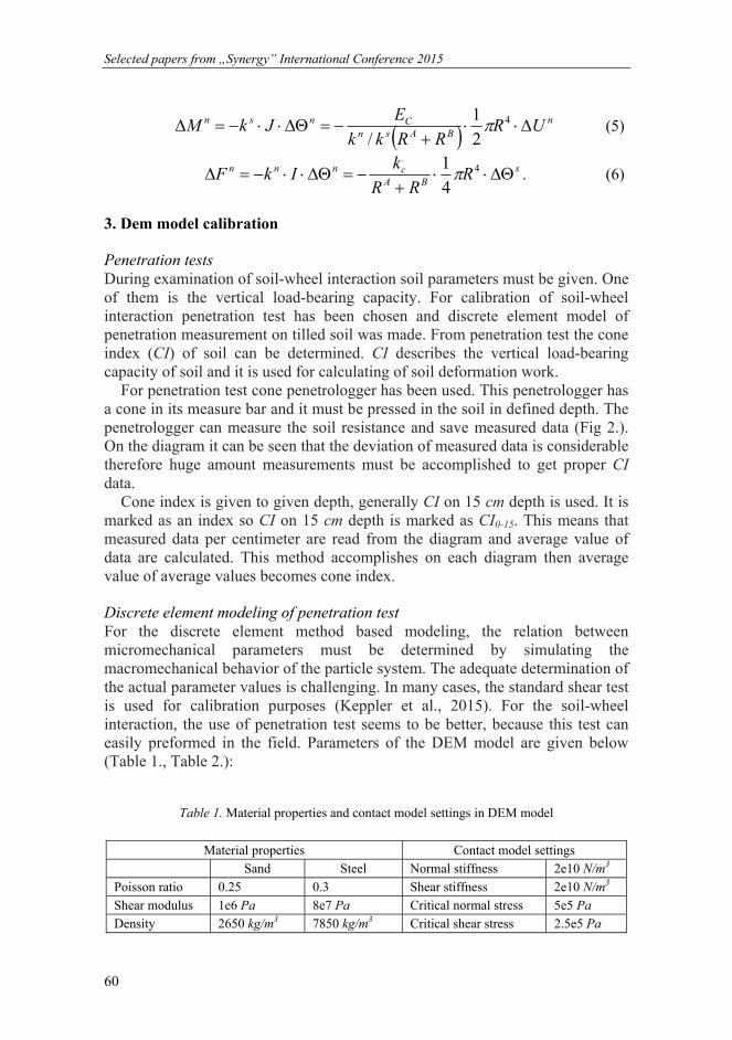
Selected papers from „Synergy” International Conference 2015
TÁMOP-4.2.1.B-11/2/KMR-2011-003 60
n
BAsnCnsn UR
RRkk
EJkM
4
2
1
/ (5)
sBA
cnnn RRR
kIkF
4
4
1 . (6)
3. Dem model calibration
Penetration tests During examination of soil-wheel interaction soil parameters must be given. One of them is the vertical load-bearing capacity. For calibration of soil-wheel interaction penetration test has been chosen and discrete element model of penetration measurement on tilled soil was made. From penetration test the cone index (CI) of soil can be determined. CI describes the vertical load-bearing capacity of soil and it is used for calculating of soil deformation work.
For penetration test cone penetrologger has been used. This penetrologger has a cone in its measure bar and it must be pressed in the soil in defined depth. The penetrologger can measure the soil resistance and save measured data (Fig 2.). On the diagram it can be seen that the deviation of measured data is considerable therefore huge amount measurements must be accomplished to get proper CI data.
Cone index is given to given depth, generally CI on 15 cm depth is used. It is marked as an index so CI on 15 cm depth is marked as CI0-15. This means that measured data per centimeter are read from the diagram and average value of data are calculated. This method accomplishes on each diagram then average value of average values becomes cone index.
Discrete element modeling of penetration test For the discrete element method based modeling, the relation between micromechanical parameters must be determined by simulating the macromechanical behavior of the particle system. The adequate determination of the actual parameter values is challenging. In many cases, the standard shear test is used for calibration purposes (Keppler et al., 2015). For the soil-wheel interaction, the use of penetration test seems to be better, because this test can easily preformed in the field. Parameters of the DEM model are given below (Table 1., Table 2.):
Table 1. Material properties and contact model settings in DEM model
Material properties Contact model settings
Sand Steel Normal stiffness 2e10 N/m3
Poisson ratio 0.25 0.3 Shear stiffness 2e10 N/m3
Shear modulus 1e6 Pa 8e7 Pa Critical normal stress 5e5 Pa
Density 2650 kg/m3 7850 kg/m3 Critical shear stress 2.5e5 Pa

Selected papers from „Synergy” International Conference 2015
TÁMOP-4.2.1.B-11/2/KMR-2011-003 61
Table 2. Interaction, geometry and dynamics properties in DEM model
Settings of interaction between particles
Sand-Sand Sand-Steel
Coefficient of restitution 0.05 0.5
Coefficient of static friction 0.5 0.75
Coefficient of rolling friction 0.01 0.015
Geometry and dynamics
Number of balls 2 Cone angle 30°
Ball radius 0.002 m Cone area 3.3 cm2
Ball shift 0.001 m Cylinder radius 0.03 m
Velocity of penetration
1 m/s Time step 0.5%
In this case soil particles were assembled from two balls (Keppler et al. 2012).
Particles are generated in a cylinder. Model of the penetrometer is a cone and a bar, this model penetrometer was pressed into the granular assembly with given velocity (Fig 1.).
Figure 1.
Simulation of penetration test
Figure 2. Results from measured and simulated penetration
By knowing Z components of forces cone index were determined and illustrated in a diagram as a function of depth. On Fig. 2. diagrams from measured and simulated data can be seen. Knowing huge deviation of cone index diagram it can be said that simulation curve fits well in measured data.

Selected papers from „Synergy” International Conference 2015
TÁMOP-4.2.1.B-11/2/KMR-2011-003 62
4. Discrete element model of soil-wheel interaction
Measurements on field During drawbar tests drawbar pull (DP) of the tractor is measured. In many case DP-slip function might be interesting.
Drawbar pull is made by a dynamometer cell which is found in the dynamometer vehicle’s drawbar. Slip can be determined from travel speed, angular velocity and rolling radius of the wheel:
R
vR . (7)
During drawbar test data acquisition system records measured data with a software in which calculated parameters for example slip are also visualized immediately by giving formula mentioned above (Eq. 7.).
Discrete element modeling of drawbar-slip curve In the simulation a lugged rigid wheel was used, material properties, contact model and soil model were the same as in penetration test simulation. Geometrical and kinematical parameters of the model are the following (Table 3.):
Table 3. Geometrical and kinematical parameters of the DEM model
Geometry
Soil bin length: 2.325 m Wheel width: 0.09 m
Soil bin width: 0.2 m Wheel diameter with lugs: 0.3 m
Soil bin height: 0.2 m Number of lugs: 60
Periodic boundaries: X, Y Height of lugs: 0.005 m
Width of lugs: 0.005 m
Dynamics
Initial velocity (1. section): 0 m/s Initial velocity (2. section): 3 m/s
Acceleration (1. section): 20 m/s2 Acceleration (2. section): 0 m/s2
Initial angular velocity (1. section):
0 1/s Initial angular velocity (2. section):
26.596 1/s
Angular acceleration (1. section):
177.305 1/s2
Angular acceleration (2. section):
44.326 1/s2
For DP-slip diagram rolling radius of the wheel must be known. In this case
rolling radius is the distance between horizontal centerline of the wheel and resultant of line of action of horizontal components of forces acted on the wheel. Line of action of the resultant force cannot be determined directly so on the premise that during pure rolling where slip is zero, the value of drawbar force is also zero. So rolling radius was determined from a three-step experiment. It was

Selected papers from „Synergy” International Conference 2015
TÁMOP-4.2.1.B-11/2/KMR-2011-003 63
supposed that the value of rolling radius is between 0.3D and 0.5D. Travel speed was constant 3 m/s in every time and the angular velocities form given radii were valid until Δt = 0.01 s.
In first round radius step was ΔR1 = 0.05D between 0.3D and 0.5D and sign change was looked for. This change was between 0.35D and 0.4D.
In second round radius step was ΔR2 = 0.01D between 0.35D and 0.4D and sign change occurred between 0.37D and 0.38D. In third round radius step was ΔR3 = 0.002D and the radius with lowest absolute value became the rolling radius of the wheel. This value was 0.376D. After determination of rolling radius angular velocity of pure rolling was given which can be seen in Table 3. as initial angular velocity in the 2. section.
Determination of DP-slip function was performed between 0 and 0.5 slip in the 2. section of wheel rolling (Fig 3.), rolling time was t = 0.6 s and sampling time was Δt = 0.01 s. From these initial values kinematical parameters in table 2. could be determined.
Figure 3. Soil-wheel interaction simulation
DP-slip diagram can be seen on Fig 4. between 0 and 0.5 slip values. It follows visibly the characteristics of theoretical slip curve.
Figure 4. DP-slip diagram
Selected papers from „Synergy” International Conference 2015
TÁMOP-4.2.1.B-11/2/KMR-2011-003 64
Conclusions
In this paper a soil calibration model and a slip curve determination from a discrete element model were presented. In the future previous and present works can be harmonized and drawbar performance might be determined from a calibrated DEM model.
Nomenclature
A: area, Ec: Young-modulus, I, J: moment of inertia, kn: normal stiffness, ks: shear stiffness, kn/ks: stiffness ratio, ni: unit vector (normal direction), R: rolling radius, RA, RB: radius of particle A and B, ti: unit vector (tangential direction), v: travel speed, δ: slip,
n : relative rotation around ni axis, s : relative rotation around ti axis, nU : relative displacement in the direction of ni, sU : relative displacement in the direction of ti,
ω: angular velocity.
References
[1] Bagi, K. (2007), Diszkrét elemek módszere, Budapesti Műszaki Egyetem, Budapest.
[2] Bekker, M. G. (1956), Theory of land locomotion, University of Michigan Press, Michigan.
[3] Bernstein, R. (1913), Probleme zur experimentellen motorpflugmechanik, Der Motorwagen, Vol. 16, pp. 199-227.
[4] Cheng, Y. P. et al. (2003), Discrete element simulation of crushable soil, Géotechnique Vol. 53, pp. 633-641.
[5] Cundall, P.A. and Strack, O.D.L. (1979), A discrete numerical model for granular assemblies, Geotechnique, Vol. 29 pp. 47–65.
[6] Goriatschkin, B. P. (1936), Teorija i proisvodstvo szelskohozjajszvennüh mashin, Moszkva.
[7] Keppler, I. et al. (2015), Discrete element modeling of vibrating tillage tools, Engineering Computations, Vol 32. pp. 308-328.

Selected papers from „Synergy” International Conference 2015
TÁMOP-4.2.1.B-11/2/KMR-2011-003 65
[8] Keppler, I. et al. (2012), Grain velocity distribution in a mixed flow dryer, Advanced Powder Technology, Vol. 23, pp. 826-827.
[9] Khot, L.R. et al. (2007), Experimental validation of distinct element simulation for dynamic wheel-soil interaction, Journal of Terramechanics, Vol. 44, pp. 429-437.
[10] Knuth, M.A., et al. (2012), Discrete element modeling of a Mars Exploration Rover wheel in granular material, Journal of Terramechanics, Vol. 49, pp. 27-36.
[11] Nakashima, H. and Oida, A. (2004), Algorythm and implementation of soil-tire contact analysis code based on dynamic FE-DE method, Journal of Terramechanics ,Vol. 41, pp. 127-137.
[12] Nakashima, H. et al. (2007), Parametric analysis of lugged wheel performance for a lunar microrovel by means of DEM, Journal of Terramechanics, Vol. 44, pp. 153-162.
[13] Nakashima, H. et al. (2010), Discrete element method analysis of single wheel performance for a small lunar rover on sloped terrain, Journal of Terramechanics, Vol. 47, pp. 307-321.
[14] Potyondy, D.O. and Cundall, P.A. (2004), A bonded-particle model for rock, International Journal of Rock Mechanics and Mining Sciences, Vol. 41, pp. 1329-1364.
[15] Reece, A.R. (1964), A principles of soil-vehicle mechanics, Proceedings of the Institution of Mechanical Engineers, Part A: Journal of Power and Energy, Vol. 180, pp. 45-67.
[16] Smith, W. and Peng, H. (2013), Modeling of wheel-soil interaction over rough terrain using discrete element method, Journal of Terramechanics, Vol. 50, pp. 277-287.
[17] Saakyan, S. (1965): O zakonomernosztyi szoprotyivlenija pocsvibdavlibaniju, Moszkva.
[18] Tanaka, H. et al. (2000), Simulation of soil deformation and resistance at bar penetration by the distinct element method, Journal of Terramechanics, Vol. 37, pp. 41-56.
[19] Urbán M. et al. (2012), Investigation of the soil-tool interaction by SPH based simulation, CIGR AgEng, Valencia, Spain.
[20] Zhang, R. and Li, J. (2006), Simulation on mechanical behavior of cohesive soil by Distinct Element Method, Journal of Terramechanics, Vol. 43, pp. 303-316.

Selected papers from „Synergy” International Conference 2015
TÁMOP-4.2.1.B-11/2/KMR-2011-003 66
Mechanization in greenhouse tomato culture and indoor culture for research purposes
K. OROVA, K. PETRÓCZKI, J. BEKE Institute for Process Engineering, Szent István University
Abstract
Following a state-of-the-art review on the mechanization of greenhouse tomato production, this article presents an indoor tomato culture necessary for the research and development of greenhouse robotics.
First a brief description is given on the main economic features of tomato production. Production cost is a crucial factor where mechanization of certain tasks could cut labor costs. After clarifying high-tech mechanization versus industrial automation, existing solutions are presented focusing on the middle phase of the crop production process. Finally an indoor tomato culture is presented for research and development of robotic vision application.
Keywords
greenhouse tomato, mechanization, robotic harvester, indoor crop culture
1. Introduction
Due to more frequent extreme weather conditions production of tomatoes for fresh consumption is most practical in greenhouses where optimal growing conditions can be maintained. In the Netherlands, leader in greenhouse technology, 100 percent of tomato production is realized in such installations.
Production efficiency is the highest in covered and heated growing systems. In spite of the highly advanced technology crop production still requires a huge amount of skilled handwork. Labor cost is an important part of the total operational cost. Automation of the more simple uniform tasks in the beginning and end phase of the production is already solved. On the contrary the middle phase including plant maintenance and harvesting relies almost completely on human workforce. Therefore mechanization of these tasks is an actual challenge.
2. Tomato production: worldwide and in Hungary
Tomatoes are the most important fresh vegetable produced in the world. According to FAO statistics 164 million tonnes of tomatoes were produced in 2013. Tomato is the 11th crop worldwide with regard to the quantity produced.

Selected papers from „Synergy” International Conference 2015
TÁMOP-4.2.1.B-11/2/KMR-2011-003 67
The first five producers are China, India, the United States of America, Turkey and Egypt (FAOSTAT, 2013). In the European Union, leading countries are Italy, Spain, Portugal, Greece, the Netherlands, Poland and Romania, with Italy and Spain being in the first 10 most important producers in the world. See Figure 1.
Figure 1. Top 10 countries of tomato production (FAOSTAT, 2013)
In Hungary, the total area for tomato production was 1800 hectares in 2012 out of which 22.7 percent was realized in greenhouses. See Table°1.
Regarding the overall greenhouse area for vegetable production 10.9 percent (410 hectares) were used for tomato in 2012. The most important vegetable was pepper occupying 1550 hectares (41.1 percent). (Németh et al., 2014a)
Out of all greenhouse vegetables produced in Hungary in 2012 the quantity of peppers was the most important (43.4 percent, 143 thousand tonnes) followed by tomatoes (27.8 percent, 91.6 thousand tonnes). See Figure 2.
Table 1. Tomato production area (open field and greenhouse) in the main producers of the European Union (in 1000 hectares) (Németh et al., 2014a)
2010 2011 2012 Country
Open field
Greenhouse Open field
Greenhouse Open field
Greenhouse
France 4.00 1.90 4.00 2.00 3.20 2.00
Greece 21.60 2.60 16.90 2.80 16.00 2.80
Hungary 1.40 0.50 1.30 0.50 1.39 0.41
Italy 113.02 5.78 96.19 7.61 85.49 6.36
Netherlands 0.00 1.70 0.00 1.70 0.00 1.70
Poland 10.59 1.51 8.73 2.37 11.40 2.30
Romania 27.30 1.20 30.00 1.60 26.50 1.30
Spain 41.10 18.20 34.20 17.00 30.10 18.50

Selected papers from „Synergy” International Conference 2015
TÁMOP-4.2.1.B-11/2/KMR-2011-003 68
The total area of greenhouse tomato production in Hungary was 410 hectares in 2012. According to experts’ estimations 100 – 120 hectares out of this represent high-technology installations using advanced systems. In general in Hungary and in other European countries as well the majority of new installations are for tomato production. (Németh et al., 2014d)
Figure 2. Quantity of most important greenhouse vegetables in Hungary
(2007 – 2012) (Németh et al., 2014a)
3. Driving forces of greenhouse mechanization
As shown in the previous section tomato is an important crop with increasing popularity. Therefore optimizing production flow and cutting production costs are actual challenges. Mechanization represents one of the means by which these objectives can be met.
Several factors motivate the mechanization of greenhouse tomato production. Van Henten (2006) lists a few of them considering the Dutch example. Moreover a recent agro-economic study focusing on greenhouse tomato production collected valuable data for Hungary. (Németh et al., 2014a-d)
First the increasing size of production facilities is mentioned. In the Netherlands this trend already started at the end of the last century and has not changed since then. The average size of a vegetable greenhouse was 4.8 hectares in 2012 which is a 94 percent increase compared to 2000. Regarding tomato production the average size of a greenhouse facility was 5.1 hectares in 2012. The most important increase in size between 2010 and 2012 was observed in the case of tomato. According to CBS (Statistics Netherlands) overall production area expanded from 1175 hectares to 1691 hectares during the same period. (Németh et al., 2014b) In Hungary almost 100 percent of new greenhouses are built for tomato production. The maximum area of a facility is 2 hectares even

Selected papers from „Synergy” International Conference 2015
TÁMOP-4.2.1.B-11/2/KMR-2011-003 69
though this is too small to be truly economically competitive. (Németh et al., 2014c)
Secondly high labor costs suggest that mechanization of certain tasks demanding extensive human handwork can be a solution. In Dutch vegetable greenhouses labor was the largest cost factor with 34% of the total production costs in 2000 and the trend was increasing. In Hungary this same ratio is 20%. (Németh et al., 2014c)
Thirdly problems with the availability of skilled labor arise. Uncomfortable working conditions (heat, humidity, repetitive work) and low wages make the work in greenhouses unattractive. In Hungary the situation is aggravated by the lack of professionals having the necessary educational background and expertise in the operation of high-tech growing systems. (Németh et al., 2014b)
Further factors mentioned by Van Henten (2006) are workers’ health problems, high product quality and food safety expected by consumers and growing market competition.
4. High-tech mechanization
Industrial automation vs. high-tech mechanization Van Henten (2006) distinguishes two types of mechanization based on industrial experience: industrial automation and high-tech mechanization or robotics. Both are aiming to replace a human being or a human activity but they have different characteristics with regards to the complexity, flexibility and the type of system used in their realization. See Table 2 for a detailed comparison. However in practice clear separation of the two is not possible in certain cases.
Table 2. Industrial automation vs. high-tech mechanization (Van Henten, 2006)
Industrial automation High-tech mechanization
One simple task More than one task Re-programmable system
Not flexible (task, object, environment)
Flexible (task, object, environment)
Few sensors Many sensors
Not much “intelligence” “Intelligent” system
Purely mechanical system Mechatronical system
Considering the generic crop production process different phases can be
identified, all with different levels of mechanization. According to Van Henten (2006) the first phase comprising seeding, cutting, grafting and transplanting are fully mechanized. The same is true for the final phase including sorting and packing the harvested produce. All of the above mentioned processes mainly

Selected papers from „Synergy” International Conference 2015
TÁMOP-4.2.1.B-11/2/KMR-2011-003 70
follow the ideas of industrial automation making their mechanization possible for more than a decade now.
More interesting is the middle phase of crop production including crop maintenance and harvest where delicate tasks are to be performed needing skilled human labor. Tomato crop maintenance includes attaching the plant stem to the trellis string, side-shoot removal, cluster thinning, leaf and root pruning, leaning and lowering and pesticide spraying (Hochmuth, 2012; Van Henten, 2006). These tasks require human intelligence as well as fast and accurate eye-hand coordination. From a technical point of view it needs the integration of the information from a high number of sensors by an artificial intelligence.
In addition to the difficulty inherent to the performance of these tasks come challenges due to the unstructured environment, the biological variability of the crop and the growing system itself. One way to achieve better results in robotic harvesting is the reduction of biological variability and the use of more structured growing systems. (Van Henten, 2006) An example illustrating the success of the last-mentioned approach is the cucumber de-leafing robot developed by Van Henten et al. (2002).
Plant maintenance mechanization Since a large number of greenhouse processes are already fully automated as described in the previous section this article focuses on high-tech mechanization in the middle phase of tomato production. Examples of tools for crop maintenance operations and robotic tomato harvesters are presented.
Tomato plant maintenance operations require precise and delicate movements in order not to damage the plant, the fruit or to cause important scarfs that are likely to be the point of attack for fungal or other diseases. Since the intelligence needed in the control of such a machine is so high to the authors’ knowledge there exists no fully autonomous robot for any of the tasks mentioned in the previous section yet.
However mechanized tools aiding maintenance tasks have been used for more than a decade such as electric lifts, clipping hand tools e.g. the Ringmaster (Van Henten, 2006) or tapeners (Hochmuth, 2012). A new system for tying the main stem to the wire is the tomsystem from Agrifast which operates much like a stapler using metallic clips providing a fast way to complete the task (TOMSYSTEM, 2015).
Tomato harvesters Bac et al. (2014) gives a literature review on the state-of-the-art of harvesting robots for high-value crops including greenhouse tomatoes. Quantitative measures allow for the comparison of the numerous machines developed by researchers. They collected information not only to uniformly present several performance indicators (autonomy, fruit location success, false-positive fruit determination, harvest success, damage rate, cycle time, laboratory or field tests), but also to analyze the design process, the hardware design choices and the algorithm.

Selected papers from „Synergy” International Conference 2015
TÁMOP-4.2.1.B-11/2/KMR-2011-003 71
Kondo et al. (2009) presents an autonomous harvesting robot for cluster tomatoes developed in Japan. The end-effector was designed to grasp the peduncle, cut and hold it. The machine vision system consisted of two RGB TV cameras, halogen lamps as lighting and VGA image capture boards. The image processing algorithm had to recognize the crossing point of the main stem with the peduncle using tomato plant properties. Average success rate was 65%.
Ling et al. (2004) reports on a tomato harvesting robot in Ohio aiming to work in long-term space missions. A sensing unit and a robotic hand unit were developed and integrated with a commercial robotic manipulator. Sizes and locations of mature tomatoes were determined by image processing algorithms. The machine was tested in laboratory and commercial greenhouse environments. Fruit sensing success rate was 95% whereas fruit picking success was 85%.
Buemi et al. (1996) describes the Italian AGROBOT project aiming at the development of a robotic system for the complete production cycle of greenhouse tomatoes. The robot consists of a vehicle carrying the picking arm, the head with two micro cameras and the control system. The robot is able to navigate between rows of plants, stop near each plant to identify the relevant objects and finally pick ripe tomatoes or spray diseased areas of the plant. Fruit location success was reported to be 90%.
Bac et al. (2014) mentions a few more systems from the 1990s developed mainly in Japan and one in France. Most of them were autonomous, however reports on performance data were highly incomplete.
5. Indoor tomato culture
Research in the field of greenhouse robotics starts with tests in laboratory conditions before going out to real-life greenhouse environment. Therefore it is practical to have a crop culture accessible any time independent of the growing season. For this reason an indoor tomato plant culture with artificial lighting was installed by researchers of Szent István University in Gödöllő.
The growing system was an indoor grow tent HOMEbox Classic XXL. Its dimensions are 240 x 120 x 200 cm providing enough space for the elven buckets containing the plants. HOMEbox grow tents meet high quality standards thanks to the materials used in their production. The three layers of polyamide (PA), black and white polyethylene (PE) guarantee for the tent to be strong, light-proof, air-tight with an optimal light distribution and heat absorption inside. All materials are food-grade quality preventing softeners harmful to human and plant health to be evaporated.
The grow-tent is easy to assemble especially because closing the shield is done by strong zippers and Velcro belts. The tent provides sealable openings for the ventilation system. Two Phytolyte Grow-Bloom Extreme high-pressure sodium (HPS) lights with 600W each provide light and heat during the day. The overall weight tolerance of the ceiling bars is 2 x 50 kg.
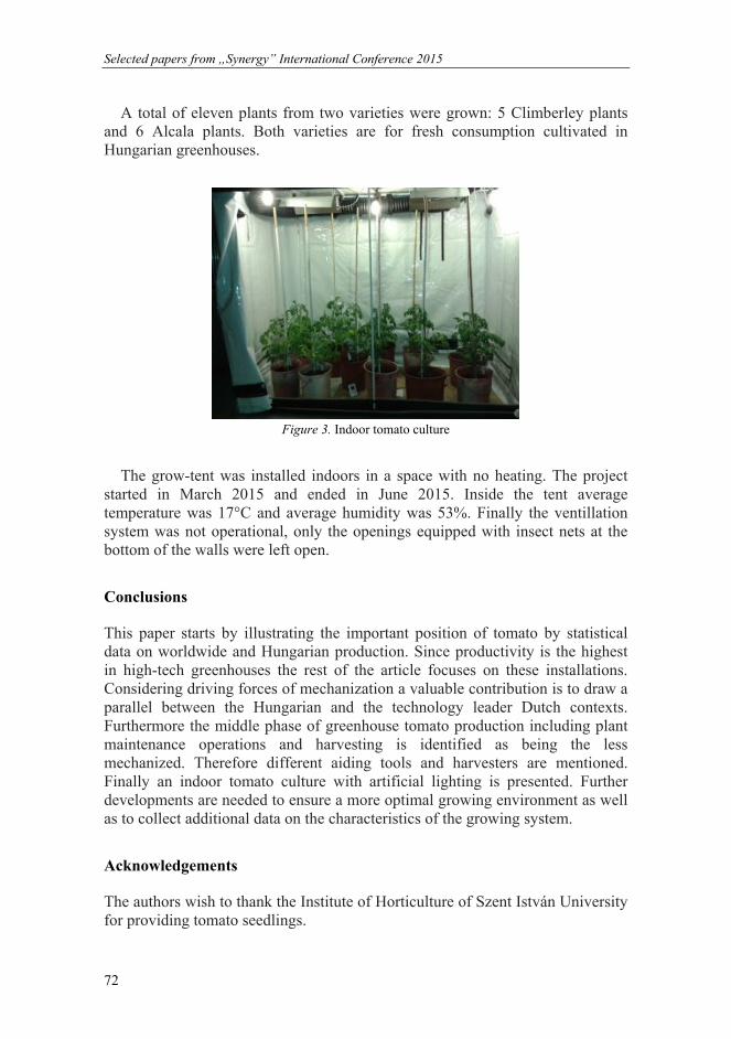
Selected papers from „Synergy” International Conference 2015
TÁMOP-4.2.1.B-11/2/KMR-2011-003 72
A total of eleven plants from two varieties were grown: 5 Climberley plants and 6 Alcala plants. Both varieties are for fresh consumption cultivated in Hungarian greenhouses.
Figure 3. Indoor tomato culture
The grow-tent was installed indoors in a space with no heating. The project started in March 2015 and ended in June 2015. Inside the tent average temperature was 17°C and average humidity was 53%. Finally the ventillation system was not operational, only the openings equipped with insect nets at the bottom of the walls were left open.
Conclusions
This paper starts by illustrating the important position of tomato by statistical data on worldwide and Hungarian production. Since productivity is the highest in high-tech greenhouses the rest of the article focuses on these installations. Considering driving forces of mechanization a valuable contribution is to draw a parallel between the Hungarian and the technology leader Dutch contexts. Furthermore the middle phase of greenhouse tomato production including plant maintenance operations and harvesting is identified as being the less mechanized. Therefore different aiding tools and harvesters are mentioned. Finally an indoor tomato culture with artificial lighting is presented. Further developments are needed to ensure a more optimal growing environment as well as to collect additional data on the characteristics of the growing system.
Acknowledgements
The authors wish to thank the Institute of Horticulture of Szent István University for providing tomato seedlings.
Selected papers from „Synergy” International Conference 2015
TÁMOP-4.2.1.B-11/2/KMR-2011-003 73
References
[1] Bac C. W., E. J. van Henten, J. Hemming and Y. Edan (2014), Harvesting robots for high-value crops: state-of-the-art review and challenges ahead, Journal of Field Robotics Vol. 31, No.6, pp. 888-911.
[2] Buemi F., M. Massa, G. Sandini and G. Costi (1996), The AGROBOT project, Advances in space research, Vol. 18, Issues 1-2, 1996, pp. 185-189.
[3] FAOSTAT (2013), http://faostat3.fao.org/browse/Q/QC/E, visited on August 26, 2015
[4] Hochmuth, G. J. (2012), Production of greenhouse tomatoes – Florida greenhouse vegetable handbook, Vol. 3, UF/IFAS Extension, 2012, reviewed in 2015, pp. 9-14.
[5] HOMEbox catalog (2012), http://pflanzenlicht24.de/images/HOMEbox-Catalog-English.pdf, visited on Augus 29, 2015
[6] Kondo N., K. Yamamoto, H. Shimizu, K. Yata, M. Kurita, T. Shiigi, M. Monta and T. Nishizu (2009), A machine vision system for tomato cluster harvesting robot, Engineering in Agriculture, Environment and Food Vol. 2, No. 2, pp. 60-65
[7] Ling P. P., R. Ehasani, K. C. Ting, Y. Chi, N. Ramalingam, M. H. Klingman and C. Draper (2004), Sensing and end-effector for a robotic tomato harvester. ASAE Annual International Meeting, Ottawa, Canada, August 1 - 4, 2004, Paper number 043088
[8] Németh, Sz., B. I. Ehretné, A. Isépy and V. Varga (2014a), A magyarországi paradicsomhajtatás helyzetének elemzése, Agrárgazdasági Könyvek, 2014, pp.10-12.
[9] Németh, Sz., B. I. Ehretné, A. Isépy and V. Varga (2014b), A magyarországi paradicsomhajtatás helyzetének elemzése, Agrárgazdasági Könyvek, 2014, pp.34-37.
[10] Németh, Sz., B. I. Ehretné, A. Isépy and V. Varga (2014c), A magyarországi paradicsomhajtatás helyzetének elemzése, Agrárgazdasági Könyvek, 2014, pp.47-51.
[11] Németh, Sz., B. I. Ehretné, A. Isépy and V. Varga (2014d), A magyarországi paradicsomhajtatás helyzetének elemzése, Agrárgazdasági Könyvek, 2014, pp.73.
[12] TOMSYSTEM (2015), http://www.thetomsystem.com/en/index.html, visited on August 29, 2015
[13] Van Henten E. J., J. Hemming, B. van Tuijl, J. Kornet, J. Meuleman, J. Bontsema and E. van Os (2002), An autonomous robot for harvesting cucumbers in greenhouses, Autonomous Robots, Vol. 13, No. 3, pp. 241–258.
[14] Van Henten E. J. (2006), Greenhouse mechanization: state of the art and future perspective, Acta Horticulturae 710, pp 55–69.

Selected papers from „Synergy” International Conference 2015
TÁMOP-4.2.1.B-11/2/KMR-2011-003 74
Determination of micromechanical parameters of granulars based on standard shear test
F. SAFRANYIK
NARIC Institute of Agricultural Engineering
Abstract
Nowadays the Discrete Element Method (DEM) is a developing numerical technique to modeling granular assemblies. Main point of this method is a simulation cycle wherein all of particles are individually modeled and interaction forces and moments are calculated. Currently this is the most accurate method to model mechanical behavior of granular materials, nevertheless industrial adaptation of this is very limited, because lack of micromechanical parameters for different granulars. To promote industrial propagation of DEM, aim of this work is presentation of a new calibration method for determination micromechanical properties of granular materials based on standard shear test.
Keywords
granular materials, micromechanical parameters, standard shear test, DEM
1. Introduction
Storing, transporting and handling of granular materials have great importance in almost all fields of agriculture, since most of raw materials and products are in granular form. By reason of particular mechanical properties of these materials design of technological equipment in agriculture is empirical and in many cases very complicated. To simplify design processes the modeling of granular materials has long been a subject of interest researchers.
In our days Discrete Element Method (DEM) is a continuously developing numerical technique by Cundall and Strack (1979) to modeling mechanical behavior of granular assemblies. Core of this method is a simulation cycle wherein all of particles are individually modeled and interaction forces and moments are calculated based on Newton’s second law of motion. To make adequate models micromechanical parameters of particulate materials need to use which means also in simplest case six different parameters (some of these can be just indirectly measure or immeasurable) (Coetzee and Els, 2009).
Currently DEM is the best and most accurate method to model mechanical behavior or motion of granular materials. With help of this design process of technological equipment could be simplified and operation of devices could be

Selected papers from „Synergy” International Conference 2015
TÁMOP-4.2.1.B-11/2/KMR-2011-003 75
optimized. However two main disadvantage of DEM are the great computational demand and determination of micromechanical parameters (calibration of the model). With daily modern industrial workstations the computational effort is not a problem but lack of micromechanical parameters increases modeling time and limits industrial applying. At the present time there is not a uniform, standardized calibration method, nowadays usually the micromechanical parameters are determined by trial and error method. To promote industrial propagation of DEM, aim of this work is a presentation of a new method for determination micromechanical properties of granulars based on standard shear test.
2. Materials and methods
Main problems of discrete modeling During discrete modeling equations of motion on single particles are solved by a simulation cycle. To describe movement of single particles, Newton’s second law of motion and the general rotational dynamics equation are repeatedly used. Contact forces and moments are calculated based on contact models in every time steps (Raji and Favier, 2004). The micromechanical parameters have influence on both normal- and tangential forces (Fn, Ft) and moments (M) between interacting particles. Usually Hertz-Mindlin no slip contact model (see Fig. 1) is used for modeling cohesionless materials, which is elastic non-linear and takes viscous and frictional damping into consideration (Ketterhagen et al., 2009).
Figure 1. Hertz-Mindlin no slip contact model
(Raji and Favier, 2004)
Behavior of particles and interactions depends on the geometry and the micromechanical properties (e.g. Young modulus, Poisson ratio, density, friction coefficient) of particles and their contacts. In contradistinction to modeling continuums in case of discrete modeling direct measurements of model parameters most of times is impossible.
Essence of calibration is that to find a set of micromechanical parameters by simulating macromechanical behavior of the granular assembly. In practice it means the modeling of a process and after experimentally validating the results

Selected papers from „Synergy” International Conference 2015
TÁMOP-4.2.1.B-11/2/KMR-2011-003 76
with measurements. In the literature many calibration method could be find however the modeled macromechanical behavior is not uniform. Although it is a very important question namely it is possible that there are multiple combinations of micromechanical parameters result the same macro behavior, since the parameters of numerical contact models just approximate the real micromechanical parameters of particles (Asaf et al., 2007). To calibrate their discrete model Gonzalez-Montanello et al. (2011) used silo outflow, Derekshani et al. (2015) used pipe- and sandglass experiments, even in addition slump or penetration tests and standard shear test are also suitable for calibration.
Aim of calibration is the finding of material parameters which are universal and suitable for model a number of processes. To get micromechanical parameters which are usable in wide range of compression force our research group on Szent István University used direct shear test and failure curve, since two main parameters of this characterize macromechanical behavior of granular assemblies (Keppler et al., 2012).
Direct shear test With direct shear test macromechanical behavior of particulate solids can examine which is developed by Jenike in 1964 (Jenike, 1964). During standard shear test the granular sample is compressed in a two-parted shear ring with constant normal load, after that the moveable ring shears the sample (see Fig. 2). During the experiment shear force in function of displacement is measured.
Figure 2. Jenike’s shear cell and shear diagrams (Jenike, 1964)
Usually the shear force is increasing to a peak and reaches a steady-state value but depending on the mechanical behavior of particulate material and the normal load initial section of shearing diagram could be different (see Fig. 2). Shear tests with different normal loads result different steady-state shear force and shear stress. If the shear stress is plotted in function of compression stress the result is a linear function which describes maromechanical behavior of particulate(c – cohesion and φ – angle of internal friction):
cNT )( . (1)

Selected papers from „Synergy” International Conference 2015
TÁMOP-4.2.1.B-11/2/KMR-2011-003 77
Two parameters of the linear function characterize the mechanical properties of granular assembly: slope of linear is the angle of internal friction, intercept of line is cohesion of the material (see Fig. 3). In case of certain particulate materials the failure curve is not linear, nevertheless linear approximation is adequate result for practice.
Figure 3. Failure line of a particulate solid (Jenike, 1964)
Simulation algorithm to make failure line In this work YADE, freeware discrete element software was used (Kozicki and Donzé, 2009). Main advantage of this software is that the simulations can be made with python scripts. In this way arbitrary simulations can be made and any kind of data could be query and process. Aim of this work is the creation of a simulation algorithm with which the standard shear test can be ran with different normal loads and based on results the failure line – macromechanical behavior (cohesion and angle of internal friction) – and standard deviations can be solved.
First parametric numerical model of modified direct shear test (shear box with rectangular cross section) was made (see Fig. 4). During discrete simulations spherical elements and the Hertz-Mindlin no slip contact model was used with randomly selected micromechanical parameters.
Figure 4. Discrete model of modified direct shear test

Selected papers from „Synergy” International Conference 2015
TÁMOP-4.2.1.B-11/2/KMR-2011-003 78
Initial step of simulation was the creation of particles. The generated particles were allowed to fall under gravity in the shear cell. After the particles reached a static state (kinetic energy of whole system is about zero) then the load plate was generated and compression of the particles was started. The load plate was moved downward while the normal load reached a maximum value. After this the plate was moved upward while normal force reached a minimum value. In this way an average – constant – normal load could be used during the shearing test. After normal force is applied on elements, shearing was started. When the shear force value was decreased 15% compared to maximum value the simulation was stopped and average value of normal stress and the steady-state value of shear stress were saved.
Using opportunities offered by YADE the above simulation could be easily use in an algorithm with the change of normal load. To make a failure line four different normal loads with four times repetition (see Fig. 5) were applied in all cases (it means sixteen simulation for one failure curve). With linear regression macormechanical properties (cohesion and angle of internal friction) of the assembly and standard deviation of these were determined.
Figure 5. Failure line with the new simulation algorithm
3. Results and conclusions
In course of up to now used calibration methods numerous single simulations had to make to get a failure line. Approach of every simulation is very time consuming challenge and during calibration it needed to make again and again (until the correct micromechanical parameters are get). With the above presented algorithm the calibration process is simplified because do not need separately set and run the simulations for a failure line (at least sixteen times per calculation). Duration of calibration micromechanical parameters of sand with help of the new algorithm was less by 40% than duration of conventional, manual calibration.

Selected papers from „Synergy” International Conference 2015
TÁMOP-4.2.1.B-11/2/KMR-2011-003 79
With usage of failure curve algorithm also a sensitivity test referring to micromechanical parameters could be easily make. For this reason a further aim of our research group the development of an absolutely automatic calibration procedure based on detailed sensitivity test of also cohesive and cohesionless particulate solids.
Nomenclature
N compression stress kNm-2 T shear stress kNm-2
c cohesion kNm-2
Greek letters
ϕ angle of internal friction -
References
[1] Asaf Z., Rubinstein D., Shmulevich I. (2007), Determination of discrete element model parameters required for soil tillage, Soil & Tillage Research, Vol. 92. (1-2), pp. 227–242.
[2] Coetzee C.J., Els D.N.J. (2009), Calibration of discrete element parameters and the modelling of silo discharge and bucket filling, Computers and electronics in agriculture, Vol. 65, pp. 198–212.
[3] Cundall P.A., Strack O.D.L. (1979), A discrete numerical model for granular assemblies, Geotechnique, Vol. 29, pp. 47-65.
[4] Derakhshani S. M., Dingena L., S., Lodewijks, G. (2015), Micro–macro properties of quartz sand: Experimental investigation and DEM simulation, Powder Technology, Vol. 269, pp. 127–138.
[5] Gonzalez-Montanello C., Ramírez A., Gallego E., Ayuga F. (2011), Validation and experimental calibration of 3D discrete element models for the simulation of the discharge flow in silos, Chemical Engineering Science, Vol. 66 (21), pp. 5116-5126.
[6] Jenike, A. W. (1964), Storage and Flow of solids, Bulletin No. 123, Utah Engineering Experiment Station, University of Utah, Salt Lake City
[7] Keppler I., Kocsis L., Oldal I., Farkas I., Csatár A. (2012), Grain velocity distribution in a mixed flow dryer, Advanced Powder Technology, Vol. 23, pp. 824-832.
[8] Ketterhagen W.R., Curtis J.S., Wassgren C.R., Hancock B.C. (2009), Predicting the flow mode from hoppers using the discrete element method, Powder Technology, Vol. 195 (1), pp. 1-10.
[9] Kozicki, J. and Donzé, F. V. (2009), Yade–open DEM: an open–source software using a discrete element method to simulate granular material Engineering Computations, Vol. 26 (7), pp. 786–805.

Selected papers from „Synergy” International Conference 2015
TÁMOP-4.2.1.B-11/2/KMR-2011-003 80
[10] Raji A.O., Favier J.F. (2004), Model for deformation in agricultural and food particular materials under bulk compressive loading using discrete element method I, Theory, model development and validation, Journal of Agricultural Engineering Research, Vol. 64 (3), pp. 359-371.

Selected papers from „Synergy” International Conference 2015
TÁMOP-4.2.1.B-11/2/KMR-2011-003 81
Relationship between the drive installation and V-belt temperature conditions
P. GÁRDONYI, L. KÁTAI, I. SZABÓ
Institute of Mechanics and Machinery, Szent István University
Abstract
The efficiency of V-belt drives is determined by several factors collectively: the slip occurring during drive transmission, the external friction occurring when the belt enters and exits the pulley as well as the hysteresis loss resulting from inner friction. Main objective of this paper is analyzing the temperature conditions of V-belt by infrared thermal camera depending on various belt pulley misalignment and tension. In this study an experimental method was developed to define the V-belt temperature increase in function of belt pulley parallel and angle misalignment and tension. On the bases of the test results optimal parameters can be calculated that serve as beneficial references for designing and tuning V-belt drives.
Keywords
belt efficiency, belt misalignment, temperature conditions, V-belt
1. Introduction
V-belt drives are widely used on agricultural machinery due to their beneficial properties. Relatively complicated drive arrangements can be realized, large shaft spacing can be bridged, they can be used with parallel and out-of-line shafts, and the construction of the drive does not require complex structural elements. The reliability and planned maintenance of these drives is essential for efficient agricultural production.
For V-belt drive sizing standardized calculation methods as well as experimental factors and design factors supported by laboratory experiments are utilized, which are valid for properly adjusted drives and normal operating conditions. The service life of V-belt drives created in this way, typical of agricultural machines and operating in extreme conditions will not be adequate and predictable and will not provide clear information for maintenance planning. In such cases the results of our own service life tests conducted under the given circumstances can be relied on, which are rather expensive and take a long time.
The belt drives used on agricultural machines can only be adjusted with a certain accuracy since it is usually a large piece of equipment whose frame structure is made up of plate elements. The distance between the shafts involved
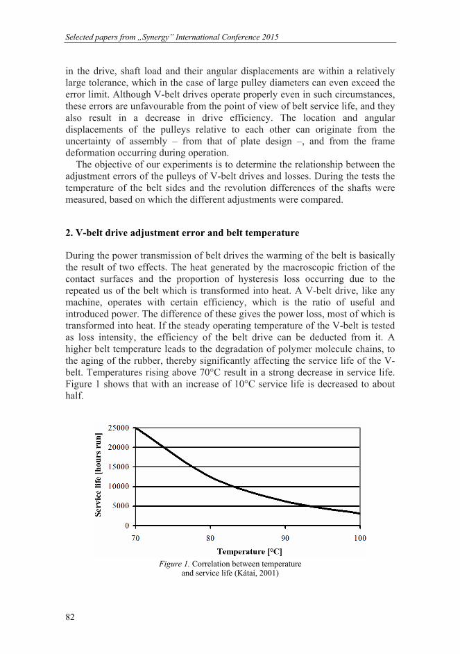
Selected papers from „Synergy” International Conference 2015
TÁMOP-4.2.1.B-11/2/KMR-2011-003 82
in the drive, shaft load and their angular displacements are within a relatively large tolerance, which in the case of large pulley diameters can even exceed the error limit. Although V-belt drives operate properly even in such circumstances, these errors are unfavourable from the point of view of belt service life, and they also result in a decrease in drive efficiency. The location and angular displacements of the pulleys relative to each other can originate from the uncertainty of assembly – from that of plate design –, and from the frame deformation occurring during operation.
The objective of our experiments is to determine the relationship between the adjustment errors of the pulleys of V-belt drives and losses. During the tests the temperature of the belt sides and the revolution differences of the shafts were measured, based on which the different adjustments were compared.
2. V-belt drive adjustment error and belt temperature
During the power transmission of belt drives the warming of the belt is basically the result of two effects. The heat generated by the macroscopic friction of the contact surfaces and the proportion of hysteresis loss occurring due to the repeated us of the belt which is transformed into heat. A V-belt drive, like any machine, operates with certain efficiency, which is the ratio of useful and introduced power. The difference of these gives the power loss, most of which is transformed into heat. If the steady operating temperature of the V-belt is tested as loss intensity, the efficiency of the belt drive can be deducted from it. A higher belt temperature leads to the degradation of polymer molecule chains, to the aging of the rubber, thereby significantly affecting the service life of the V-belt. Temperatures rising above 70°C result in a strong decrease in service life. Figure 1 shows that with an increase of 10°C service life is decreased to about half.
Figure 1. Correlation between temperature
and service life (Kátai, 2001)
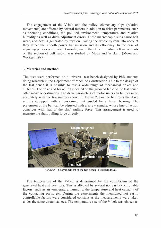
Selected papers from „Synergy” International Conference 2015
TÁMOP-4.2.1.B-11/2/KMR-2011-003 83
The engagement of the V-belt and the pulley, elementary slips (relative movements) are affected by several factors in addition to drive parameters, such as operating conditions, the polluted environment, temperature and relative humidity as well as drive adjustment errors. These macroscopic slips cause belt wear, and heat is generated by friction. Taking the whole system into account they affect the smooth power transmission and its efficiency. In the case of adjusting pulleys with parallel misalignment, the effect of radial belt movements on the section of belt lead-in was studied by Moon and Wickert. (Moon and Wickert, 1999).
3. Material and method
The tests were performed on a universal test bench designed by PhD students doing research in the Department of Machine Construction. Due to the design of the test bench it is possible to test a wide range of mechanical drives and clutches. The drive and brake units located on the grooved table of the test bench offer many opportunities. The drive parameters of motor units can be measured accurately with the transmitters shown in Figure 2. For the belt tests the drive unit is equipped with a tensioning unit guided by a linear bearing. The pretension of the belt can be adjusted with a screw spindle, whose line of action coincides with that of the shaft pulling force. This arrangement is used to measure the shaft pulling force directly.
Figure 2. The arrangement of the test bench to test belt drives
The temperature of the V-belt is determined by the equilibrium of the generated heat and heat loss. This is affected by several not easily controllable factors, such as air temperature, humidity, the temperature and heat capacity of the contacting parts, etc. During the experiments the mentioned not easily controllable factors were considered constant as the measurements were taken under the same circumstances. The temperature rise of the V-belt was chosen as

Selected papers from „Synergy” International Conference 2015
TÁMOP-4.2.1.B-11/2/KMR-2011-003 84
the test parameter, which means the power loss between the two equilibria – between the steady state of the workshop temperature and operating temperature.
Figure 3. The test arrangement
Figure 4. Thermal camera image and its evaluation
The test arrangement can be seen in Figure 3, where images were taken with a high-resolution infrared camera at 0.2 Hz frequency for a 10-minute period. During our experiments the sidewalls of the belt coming in contact with the groove were tested, which contained more information about the operation of the drive. Data regarding the temperature were obtained from the thermal images taken of the active surface of the V-belt after the images were processed (Lágymányosi and Szabó, 2014). The average temperature of the marked area in Figure 4 was used for the evaluation, which shows the temperature change of the belt if it is illustrated according to time. The warming of the V-belt is described by the Baule-Mitscherlich saturation function, in which the measured parameters change along a decreasing gradient going toward the saturation maximum. The steady operational temperature was accurately estimated through the mathematical model. This was necessary because each adjustment converged to different saturation during different times, and the duration of the experiments was decided to be 10 minutes.

Selected papers from „Synergy” International Conference 2015
TÁMOP-4.2.1.B-11/2/KMR-2011-003 85
The general equation of the saturation function
.1 XczeAY (1)
The simplified form
,1 mAY (2)
where A is the upper limit of the saturation function. The Xczem is the relative unsaturation (Sváb,1973).
4. The results of the tests
In the other experiments SPZ V-belts were used, where the pulleys were set in the plane of the drive, at the recommended error limit, at a value one order of magnitude larger, and at double that value. The position of the pulleys relative to each other was created with parallel alignment and the angular alignment of the shafts.
Figure 5. The temperature increase of the V-belt drive due to geometrical
adjustment errors as a function of the extent of the error ( SPZ; d1 = 150 mm; i = 1; Ld = 1207; f0 =15 s-1; M1 = 8 Nm; FH = 119 N )
Due to the adjustment errors of the pulleys the V-belt drives operate at a higher temperature, thereby the efficiency of the drive becomes worse and the service life of the V-belt decreases. Figure 5 shows that in addition to the extent of the adjustment error the temperature increase of the V-belt is also affected by the nature of the error. The angular misalignment of the pulleys results in

Selected papers from „Synergy” International Conference 2015
TÁMOP-4.2.1.B-11/2/KMR-2011-003 86
different warming on the sidewalls of the belt, which is caused by the previously mentioned different friction influence on the active sidewalls of the V-belt. Heat generation is more intensive on the strained sidewalls, however the temperature of the unstrained side could be lower than the values within the error limits.
Within the error limits given by the manufacturers no significant difference can be experienced between the temperature increase of the V-belts. Exceeding the permissible error value the V-belts converge to different temperatures.
Figure 6. The temperature increase of the V-belt drive versus shaft load
(SPZ; d1 = 60; 90; 118; 150; 180 mm; i = 1; Ld = 1207; f0 =15 s-1; P=PN )
From Figure 6. it can be stated that the shaft load has no worthwhile influence for the belt temperature in the examined interval (50% under and 50% over the nominal load).
Conclusions
In this study the losses of V-belt drives were studied through experiments in relation to the adjustment errors of pulleys and shaft load. The temperature increase of the belt was chosen as the test parameter. Basically the warming of the V-belt is the result of two effects: the heat generated due to the macroscopic friction of the contact surfaces; and the proportion of hysteresis loss occurring due to the repeated strain of the belt which is transformed to heat. The increased friction conditions, which cause a decrease in efficiency and service life, play a significant role in the temperature increase of V-belts originating from the adjustment errors of pulleys. At the same time it can be stated that the shaft load has minimal influence for the belt temperature in the interval of 50% under and 50% over the nominal load.

Selected papers from „Synergy” International Conference 2015
TÁMOP-4.2.1.B-11/2/KMR-2011-003 87
References
[1] Kátai L. (2001): Terménybetakarító gépeken alkalmazott ékszíjak élettartam növelésének egyes kérdései, Doktori értekezés, Gödöllő, p. 32-41.
[2] Kátai L., Szabó I., Gárdonyi P. (2013), Az ékszíjak melegedés viszonyainak vizsgálata, A Gépipari Tudományos Egyesület Műszaki Folyóirata, LXIV. évf. 6. szám, Miskolc, p. 58-61., ISSN 0016-8572
[3] Lágymányosi A., I. Szabó (2014), APPLE CLASSIFICATION WITH SHAPE DESCRIPTION USING 3D IMAGING TECHNOLOGIES, Hungarian Agricultural Engineering, 26/2014, pp. 29-31, HU ISSN 0864-7410
[4] Moon, J., Wickert, J. A. (1999), RADIAL BOUNDARY VIBRATION OF MISALIGNED V-BELT DRIVES, Journal of Sound and vibration, 225(3). pp. 527-541.
[5] Sváb J. (1973), Biometriai módszerek a kutatásban, Mezőgazdasági Kiadó, Budapest, p. 390-397.

Selected papers from „Synergy” International Conference 2015
TÁMOP-4.2.1.B-11/2/KMR-2011-003 88
Development of measurement methods for a numerical simulation of corn plants
Á. KOVÁCS1, I. J. JÓRI1, K. GAÁL2,
A. PIROS1, Gy. KERÉNYI1 1Department of Machine and Product Design,
Budapest University of Technology and Economics 2NARIC Institute of Agricultural Engineering,
Energetic examination laboratory,
Abstract
Considering the 1 billion tons corn production in the world annually, it is clear that agricultural processing of corn plants and ears is extremely relevant. Consequently, this study focuses on comparative measures for numerical modeling of the mechanical and physical behavior of corn stalks which later will be used to investigate the interaction between the corn plant and the different machine parts.
Keywords
corn stalk, moisture content, physical parameters, mechanical tests, numerical simulation
1. Introduction
The utilization of corn plants and crops is remarkable worldwide, the corn production in the world is almost 1000 million tons. In 2014 almost 10 million tons of corn have been harvested by farmers in Hungary (KSH 2015), so it plays a significant role in our country`s agriculture. The in-work investigation of newly developed equipments and units is time limited and often an expensive work, because of the agricultural products seasonality. A numerical method is not yet available in case of agricultural machine design, which could replace plough field investigations. That is why the development of a comparative measurement method is in our research focus, which we can use later to model the corn`s physical and mechanical properties in order to investigate the interaction between the machine unit and the plant.
2. Collection and preparation of samples
The samples were collected from a stand following a 30 m long stubble track which was at the side of a plough field in Baranya county on 12.07.2014. We

Selected papers from „Synergy” International Conference 2015
TÁMOP-4.2.1.B-11/2/KMR-2011-003 89
have collected every 10th plant in every 10th line, all in all 100 plants cut by shank cutters near the stool, through the brace roots. Injured stalks were not collected noticeably, in these cases we have collected neighboring stalks. The plants were tied together in bundles of 10 with cable ties, taking care of the integrity of the stalks. The stalk bundles were transported by car to the workshop of the Department of Machine and Product Design at BUTE, where we stored the stalks separately at room temperature and humidity.
We investigated the different parts of the corn plant separately. The stalk nodes and the stalk sections between the nodes were distinguished. We denoted with the first number the stalk node which can be found right above the soil. The first stalk section between the first and second stalk node was named the first stalk middle section. We divided the corn stalk following this logic. The samples were prepared for the measurements, through which we measured the physical parameters needed for the evaluation. The foliage and crop have been removed from the plants. We cleaned the stalk from any contamination (either vegetal or soil remains), then we cut it to size for the measurement. When it was needed we stored the samples in air permeable packets until the beginning of the measurements.
3. Measurement of humidity
The humidity of the stalk affects the mechanical and physical properties of it. Because of this we conducted humidity measurements before the mechanical measurements at the Institute of Agricultural Engineering at Gödöllő. Through the measurement we have cut to size the chosen samples, then we placed them in ceramic bowls. We weighted the ceramic bowls 3 times separately and then 3 times with the samples. The samples stayed 21 hours in the drying chamber on 105°C. After the drying process we weighted the mass of the bowls and samples together, the humidity has been calculated from the two different masses. The humidity of the stalk samples are: mean humidity level 72,37%, minimum humidity level 67,46%, maximum humidity level 77,72%. Because of the small sample number it is not reasonable to do a more detailed statistical analyzation. With these results the state of the biological matter can be satisfactorily characterized, which is dominant in case of measurements of other physical and mechanical properties.
4. Measurement of geometry and mass
The reason of the measurement is to make a general statistical statement of the plant`s physical properties and to calculate the parameters from the measured properties, nondimensionalized over the stalk`s length. We conducted the measurement series to identify the corn stalk`s main characteristic sizes and the distribution of the mass over the stalk`s length. The length, diameter and mass of the samples were measured. In case of the measurements of the stalk section`s

Selected papers from „Synergy” International Conference 2015
TÁMOP-4.2.1.B-11/2/KMR-2011-003 90
cross-sections the mean diameter of the given cross-section were approximated by the measured cross sizes. In every sample`s case, the first stalk node`s mean diameter has given the base for nondimensionalization, so that the other node`s calculated diameters were nondimensionalized with the first. Figure 1. a) represents the identified sections. It is important to notice that the trend like change of the diameters does not correlate with physical length, but with biological distribution. Typically, the stalk diameter of the samples change after the seventh stalk node where the corn ear hang. The length of each stalk section was calculated from the difference between the measured section lengths. Because of the samples with different number of stalk sections, the comparative evaluation was made with only thirteen stalk sections. In each case the nondimensionalization was made with the overall length of the thirteen stalk sections. These ratios give the base of the statistical statement, this can be seen on figure 1. b). The nondimensionalization of each stalk section`s mass was made with the overall mass of the thirteen stalk sections. The calculated result`s general statistical indicators can be seen on figure 1. c).
Figure 1. Results of geometry and mass measurement a) Mean diameter proportionality factor
characterizing the diameters of the nodes and stalk middle sections b) Nondimensionalized mean values of stalk section lengths c) Nondimensionalized mean values of stalk section masses
5. Bending test at the plough field
In order to determine the bending stiffness of the corn stalk and to investigate the interaction of the roots and the soil we conducted plough field measurements
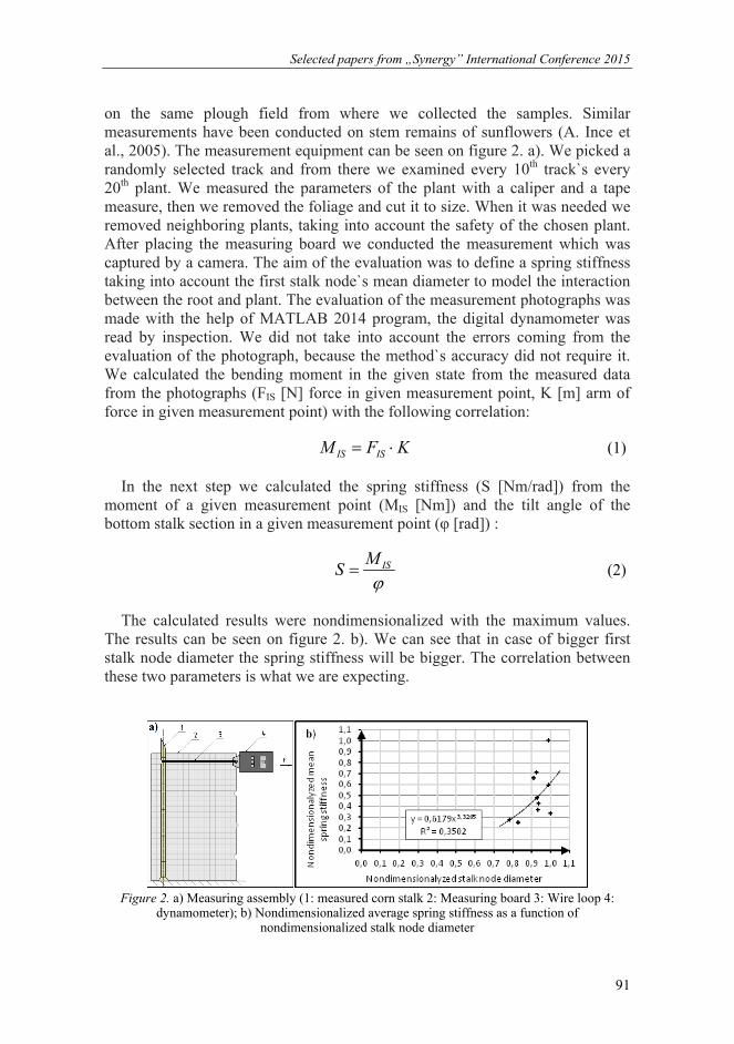
Selected papers from „Synergy” International Conference 2015
TÁMOP-4.2.1.B-11/2/KMR-2011-003 91
on the same plough field from where we collected the samples. Similar measurements have been conducted on stem remains of sunflowers (A. Ince et al., 2005). The measurement equipment can be seen on figure 2. a). We picked a randomly selected track and from there we examined every 10th track`s every 20th plant. We measured the parameters of the plant with a caliper and a tape measure, then we removed the foliage and cut it to size. When it was needed we removed neighboring plants, taking into account the safety of the chosen plant. After placing the measuring board we conducted the measurement which was captured by a camera. The aim of the evaluation was to define a spring stiffness taking into account the first stalk node`s mean diameter to model the interaction between the root and plant. The evaluation of the measurement photographs was made with the help of MATLAB 2014 program, the digital dynamometer was read by inspection. We did not take into account the errors coming from the evaluation of the photograph, because the method`s accuracy did not require it. We calculated the bending moment in the given state from the measured data from the photographs (FIS [N] force in given measurement point, K [m] arm of force in given measurement point) with the following correlation:
KFM ISIS (1)
In the next step we calculated the spring stiffness (S [Nm/rad]) from the moment of a given measurement point (MIS [Nm]) and the tilt angle of the bottom stalk section in a given measurement point (φ [rad]) :
ISMS (2)
The calculated results were nondimensionalized with the maximum values. The results can be seen on figure 2. b). We can see that in case of bigger first stalk node diameter the spring stiffness will be bigger. The correlation between these two parameters is what we are expecting.
Figure 2. a) Measuring assembly (1: measured corn stalk 2: Measuring board 3: Wire loop 4:
dynamometer); b) Nondimensionalized average spring stiffness as a function of nondimensionalized stalk node diameter

Selected papers from „Synergy” International Conference 2015
TÁMOP-4.2.1.B-11/2/KMR-2011-003 92
6. Laboratory measurements
A Zwick Z250 type computer controlled testing machine was used for the laboratory measurements. Through the measurement we used the device`s accessories when it was enough, when it wasn`t we developed equipments to satisfy our needs.
Two-point bending test The aim of the measurement is to determine the bending stiffness of the corn stalk in order to calibrate the model. The samples were fixed in the gripping device designed and manufactured by Ádám Kovács, then we made a slit on the free end and applied a metal wire loop. The other end of the wire was applied to the measuring device, thus conveying the forces of the bending stalk (see Figure 3 a)). The crossbeam of the test device was moving with the speed of 200 mm/min. For comparability, we nondimensionalized every data with its corresponding maximum value. It can be seen, that in every case the rising initial linear phase is apparent, then after the peak value (the fracture of the stalk) the bending force rapidly decrease. Typically, the peak values appeared at 60% of the total path length. We calculated the maximum bending moment from the measured maximum bending force and arm of force. For comparability we have calculated the maximum bending moments in reference of the circular cross section`s area approximated by the first node`s average node diameter. The measured plants` mean maximum specific bending moment is 30,67 [N/mm].
Figure 3. a) Sketch of two point bending test (1: measured corn stalk 2: stalk gripping device
3: Wire loop 4: gripping device 5: Clamp 6: Dynamometer 7: Guided beam of the testing machine 8: Pointer) b) Two point bending diagram of the plants
Three point bending test The aim of the measurement is to determine the bending resistance over the length of the stalk. Similar measurements were conducted on corn plants (Leblicq, T. at al, 2015 and Qin Tongdi, 2011). We calculated separately the bending resistance of the stalk nodes and stalk middle sections. Thus node samples and middle section samples were taken from separate plants. At first we fixed the zero point by touching the sample in each case, then we started the
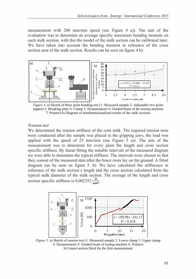
Selected papers from „Synergy” International Conference 2015
TÁMOP-4.2.1.B-11/2/KMR-2011-003 93
measurement with 200 mm/min speed (see Figure 4 a)). The aim of the evaluation was to determine an average specific maximum bending moment on each stalk section, with this the model of the stalk section can be calibrated later. We have taken into account the bending moment in reference of the cross section area of the stalk section. Results can be seen on figure 4 b).
Figure 4. a) Sketch of three point bending test (1: Measured sample 2: Adjustable two point support 3: Breaking plate 4: Clamp 5: Dynamometer 6: Guided beam of the testing machine
7: Pointer) b) Diagram of nondimensionalized results of the stalk sections
Tension test We determined the tension stiffness of the corn stalk. The required tension tests were conducted after the sample was placed in the gripping jaws, the load was applied with the speed of 25 mm/min (see Figure 5 a)). The aim of the measurement was to determine for every plant the length and cross section specific stiffness. By linear fitting the suitable intervals of the measured diagram we were able to determine the typical stiffness. The intervals were chosen so that they consist of the measured data after the brace roots lay on the ground. A fitted diagram can be seen on figure 5. b). We have calculated the stiffnesses in reference of the stalk section`s length and the cross section calculated from the typical stalk diameter of the stalk section. The average of the length and cross section specific stiffness is 0,002352 .
Figure 5. a) Sketch of tension test (1: Measured sample 2: Lower clamp 3: Upper clamp
4: Dynamometer 5: Guided beam of testing machine 6: Pointer) b) Linear section fitted for the first measurement

Selected papers from „Synergy” International Conference 2015
TÁMOP-4.2.1.B-11/2/KMR-2011-003 94
Dynamic cutting test The aim of the measurement was to determine the dynamic cutting work of the stalk section over the stalk length. Similar measurements were conducted on plough fields (Azadbakht, M., 2014). We reformed a measuring device used for Charpy type impact tests for our measurements. For the reform we used developed stalk and blade grippers, the development was made by Ádám Kovács. The special stalk and blade grippers were applied on the testing machine in our measurements. We adjusted the position of the gripper and the blade so that the gap between the support and the cutting edge was minimal. We fixed the samples in the gripper, then we performed the measurements, the blade has cut the samples with 3,47 m/s speed. The aim of the evaluation was to determine the cutting work for the samples and the specimen size independent interpretation of the cutting work. The sketch of the testing machine can be seen on figure 6 a). The cutting work (K [J]) needed for the cut can be calculated from the correlation between the measured data (α and β [rad] angles marked on figure 6 b)), gravitational acceleration (g[m/s2]), length of the flywheel arm (l [m]) and the mass of the cutting head (m [kg]) :
coscos lgmK (3)
The nondimensionalization was made by the maximum value, results can be seen on figure 6. c).
Figure 6. a) Sketch of dynamic cutting test (1: Measured sample 2: Stalk gripper 3: Fixing unit 4: Cutting blade 5: Blade gripper 6: Flywheel arm) b) Interpretation of geometrical sizes for the calculation of potential energy c) Work in reference of cross section of different stalk sections

Selected papers from „Synergy” International Conference 2015
TÁMOP-4.2.1.B-11/2/KMR-2011-003 95
Sideway pressing test The aim of the measurement was to determine the side pressing resistance of the corn stalk and the crossway and residual sideway deformation over the stalk length. We used a universal mechanical measuring machine and its accessories for the measurements (see Figure 7 a)). Placing the samples in the clamp jaws we performed the measurements, the clamp head was moving with the speed of 100 mm/min. After the measurement we fixed the width of the pressed sample. The aim of the evaluation was the specimen size independent interpretation of the resistance caused by the deformation and the measurement of sideway residual and crossway deformations. Two typical curve-characteristic can be identified from the measured resistance curves, this can be seen on figure 7 b) and c). The different nature is likely caused by the stalk section trough orientation to the press direction, which was not recorded in the measurement. The resistances appearing in case of the biggest press direction deformations were used for the base of the evaluation of the measured resistance curves. We have taken into account the force values in reference of the press direction deformation percentage value. The typical mean value of the given section has been calculated by averaging the results of specimens with same identification numbers (see Figure 7. d)).
Figure 7. a) Sketch of sideway pressing test (1: Measured sample 2: Lower pressing head
3: Upper pressing head 4: Dynamometer 5: Guided beam of testing machine) b) Two typical characteristic curve c) Average press direction deformation specific resistance of 100 long stalk
pieces containing stalk node and stalk middle section.

Selected papers from „Synergy” International Conference 2015
TÁMOP-4.2.1.B-11/2/KMR-2011-003 96
Conclusions
Through the investigations we developed a comparable measurement series that can calibrate a numerical method for modeling the plant`s physical and mechanical properties. The parameters and curves calculated from mathematical and statistical methods on the measured data of the plough field and laboratory bending, tension, pressing and cutting tests can be used for further investigations.
We would like to thank the help of Katalin Gaál from the Institute of Agricultural Engineering at Gödöllő, Dr. Gábor Szebényi from the Department of Polymer Engineering at BUTE, Dr. Imre Obrulov from the Department of Material Science and Engineering at BUTE and Dr. Tibor Poós from the Department of Building Services and Process Engineering at BUTE.
Nomenclature
MIS In-situ bending moment Nm FIS In-situ bending force N k In-situ arm of force m S In-Situ spring stiffness Nm/rad K Cutting work J g Gravitational acceleration m/s2 l Length of flywheel arm m m Mass of cutting head kg
Greek letters φ Tilt angle of bottom stalk section rad α Angle, before cutting rad β Angle, after cutting rad
References
[1] A. Ince, S. Ugurluay, E. Güzel, M. T. Özcan (2005), Bending and Shearing Characteristics of Sunflower Stalk Residue, Biosystalks Engineering, Vol. 92(2), pp. 175-181.
[2] Leblicq, T., Vanmaercke, S., Ramon, H., Saeys, W. (2015), Mechanical analysis of the bending behavior of plant stalks, Biosystalks Engineering, vol. 129, pp. 87-99.
[3] Qin Tongdi, Li Yaoming, Chen Jin (2011), Experimental Study on Flexural Mechanical Properties of Corn Stalks, 2011 International Conference on New Technology of Agricultural Engineering, China, 27-29 May 2011, pp. 130-134.
[4] Azadbakht, M., Rezaei Asl, A., Tamaskani Zahedi, K. (2014) Energy Requirement for Cutting Corn Stalks (Single Cross 704 Var.), International Journal of Biological, Veterinary, Agricultural and Food Engineering, Vol. 8(5), pp. 467-470.
Selected papers from „Synergy” International Conference 2015
TÁMOP-4.2.1.B-11/2/KMR-2011-003 97
Stability analysis of igbt based on simulation and measurement of scatter parameters
C. ABBATE1, R. Di FOLCO2, I. De BELLIS2, Z. VARGA3
1DIEI, University of Cassino and Southern Lazio 2L.I.S.A. University of Cassino and Southern Lazio,
Department of Economics and Law 3Institute of Mathematics and Informatics, Szent István University
Abstract
An insulated-gate bipolar transistor (IGBT) operated at high voltage and currents can exhibit instability which may affect the reliability of the whole system. In particular, when both voltage and current are simultaneously high, as happens during short circuit condition (SC), the power device can become unstable under particular driving and load conditions. The paper presents a new experimental and simulative approach to study the stability of the IGBT based on the simulation and measurement of the scattering parameters for calculating the Stern stability factor (K-factor) in order to individuate the frequency range were the device can be potentially unstable.
Keywords
IGBT stability, short circuit, high frequency oscillations, electromagnetic interference (EMI)
1. Introduction
Power IGBT devices are extensively used in motor drives and switching converters thanks to the easy controllability of the on-off status and the good switching performances. However during the normal operating conditions and/or during overload conditions the device inserted in a circuit can become unstable and can compromise the reliability of the entire system. The unstable phenomena have been widely studied in short circuit, SC, where the device at the same time holds high voltages and currents. In these test conditions oscillations are observed at the external leads of the device. Several studies (Omura et al., 1997, 1999, Milady et al., 2009 and Abbate et al., 2013) have attributed these oscillations to a negative gate capacitance which appears at the input leads of the Device Under Test, DUT. The negative capacitance is evidenced by the fact that a positive variation of the gate voltage corresponds to a negative variation of the gate current (Omura et al., 1997). This behaviour is due to a layer of holes coming from the collector which accumulates below the gate region. A positive variation of the gate
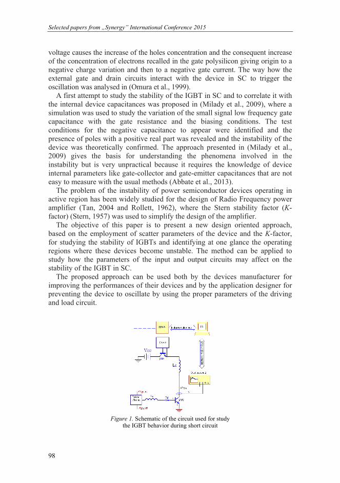
Selected papers from „Synergy” International Conference 2015
TÁMOP-4.2.1.B-11/2/KMR-2011-003 98
voltage causes the increase of the holes concentration and the consequent increase of the concentration of electrons recalled in the gate polysilicon giving origin to a negative charge variation and then to a negative gate current. The way how the external gate and drain circuits interact with the device in SC to trigger the oscillation was analysed in (Omura et al., 1999).
A first attempt to study the stability of the IGBT in SC and to correlate it with the internal device capacitances was proposed in (Milady et al., 2009), where a simulation was used to study the variation of the small signal low frequency gate capacitance with the gate resistance and the biasing conditions. The test conditions for the negative capacitance to appear were identified and the presence of poles with a positive real part was revealed and the instability of the device was theoretically confirmed. The approach presented in (Milady et al., 2009) gives the basis for understanding the phenomena involved in the instability but is very unpractical because it requires the knowledge of device internal parameters like gate-collector and gate-emitter capacitances that are not easy to measure with the usual methods (Abbate et al., 2013).
The problem of the instability of power semiconductor devices operating in active region has been widely studied for the design of Radio Frequency power amplifier (Tan, 2004 and Rollett, 1962), where the Stern stability factor (K-factor) (Stern, 1957) was used to simplify the design of the amplifier.
The objective of this paper is to present a new design oriented approach, based on the employment of scatter parameters of the device and the K-factor, for studying the stability of IGBTs and identifying at one glance the operating regions where these devices become unstable. The method can be applied to study how the parameters of the input and output circuits may affect on the stability of the IGBT in SC.
The proposed approach can be used both by the devices manufacturer for improving the performances of their devices and by the application designer for preventing the device to oscillate by using the proper parameters of the driving and load circuit.
Figure 1. Schematic of the circuit used for study
the IGBT behavior during short circuit

Selected papers from „Synergy” International Conference 2015
TÁMOP-4.2.1.B-11/2/KMR-2011-003 99
Figure 2. Typically oscillation waveforms during short circuit
2. Unstable behaviour of igbt during short circuit
Fig. 1 shows the schematic of the circuit used for study the behaviour of IGBTs operating during short circuit operation. The collector biasing supply voltage, Vcc, is applied to the collector through the series switch and Lc which accounts for the stray inductance offered by the SC. The series switch sets the duration of the short circuit and is used to control the power dissipated on the device. The driver circuit with Lg and Rg constitute the gate bias circuit that supply the gate voltage and then fix the value of the collector current to be used in the test.
Figure 3. Schematic of the experimental
set up used for S-parameter measure
The typical waveforms measured during a short circuit are reported in Fig. 2 for a discrete 1200V-20A IGBT. The duration of the SC was set to about 15µs.

Selected papers from „Synergy” International Conference 2015
TÁMOP-4.2.1.B-11/2/KMR-2011-003 100
The test conditions were: Rg=10Ω, Vcc=400V, Ic=38A, obtained with a gate voltage of 12V. We can see high frequency oscillations on collector voltage and current waveforms and on gate voltage. In order to have oscillation, we had to make a proper choice of Rg, Lg and Lc. In fact, it was demonstrated in (Abbate et al., 2013) that for having oscillations is not sufficient that the device exhibits a negative input capacitance but the external circuit it is also required to have proper values of the input and output impedance.
The time domain analysis, which can be achieved with the circuit of Fig. 2, is very important for getting information regarding the device tendency to be unstable but it is unpractical for identifying the external biasing parameters (Lc, Rg, Lg) which bring and sustain the device in the instability. In fact, it would require a large number of experiments to be performed. Moreover, this approach does not supply any information regarding the stability grade of the device with reference to the external circuit parameters.
Figure 4. Representation of DUT with driving and load circuit
3. Experimental procedure
Fig. 3 shows the schematic of the set-up used for the measurement of the S-parameters. The biasing circuit includes the AC blocking inductances, Lgg and Lcc. The IGBT under test is placed in a shielded box. The static decoupling capacitors, Cg and Cc, are used to connect the DUT with the network analyzer trough the output ports whereas Rg-Lg and Lc correspond to the driving and load components of the switching circuit, respectively. C1 and C2 correspond to the DC blocking capacitances.
The first operation to be performed before each test is the calibration procedure of the network analyzer. This operation is executed directly on the connection ports of the DUT by making four calibration measurements with different input and output loads: shorted, open, loaded with 50 and through connection. In such a way, we can account for all the stray elements of the measurement circuit and our measurements are not affected by them.
The K-factor (Stern, 1957, Rollett, 1962) is proposed to be used to analyze the stability of IGBT. It is related to scatter parameters by the equation:

Selected papers from „Synergy” International Conference 2015
TÁMOP-4.2.1.B-11/2/KMR-2011-003 101
||2
||||||1
2112
221122211
222
211
SS
SSSSSSK
(1)
with S11: Input reflection coefficient, S12: Reverse Isolation, S21: Gain, S22: Output reflection coefficient.
From the stability theory, the device is stable if K>1. This condition refers to the device linearized around the biasing point. For guarantying the unconditional stability the condition K>1 must be verified for all possible biasing points. In practice, we know that for high collector currents the IGBT becomes unstable and this condition is correctly described by the plot of K as a function of the frequency as it will be shown in the next section.
Figure 5. Stability factor as a function of the frequency at Vce=100V,
for different collector currents, with min|ZC|>1k and Rg1M(isolated device)
Figure 6. Values of Rg and Lg for which the IGBT is stable
(above the curve) or unstable (below the curve) for different values of the collector stray inductance. Experimental test conditions: Vce=100V Ic=50mA
Selected papers from „Synergy” International Conference 2015
TÁMOP-4.2.1.B-11/2/KMR-2011-003 102
For obtaining the K-factor we perform the measurement of the scattering parameters associated with the DUT isolated, namely in the conditions of high input and output impedance that is min|ZC|>1k and RG1M. Then by using the theory of cascaded systems we can calculate K for any input and output systems considered to be generic complex networks. Due to the complexity of the calculation of the S parameter for cascaded systems, in order to reduce the calculation effort, we convert the S matrix to ABCD matrix. As known, the resulting matrix for ABCD representation can be obtained by the matrix product of single systems. Finally the ABCD matrix is converted back in the S parameters in order to obtain the scatter parameters of complete system. The entire system is represented in Fig. 4 where the DUT is connected to the driving and output circuits.
A first example of K-factor measured on a 1200V-30A Field-Stop Trench-gate IGBT is reported in Fig. 5 for collector currents between 1A and 50mA obtained with gate voltages fixed between 2V and 6.1V, respectively. The figure shows wide ranges of instability (K<1) for 30mA and 50mA. Unfortunately, the measure of each curve requires several minutes to be performed while keeping the device in active region. So to avoid IGBT thermal problems we had to limit the power dissipated on the DUT and, consequently, we were not able to measure K at IC>50mA and VCE>100V. Nevertheless the analysis can be extended to higher voltage and currents values using FEM simulation.
4. Instability analysis of igbt in short circuit
The proposed approach is very powerful. In fact, starting from the scatter parameters measured on the DUT in the isolated conditions, we can compute the stability factor in any input and output load conditions. The procedure has been applied to identify the values of the resistance, Rg, and inductance, Lg, of the gate (driver) circuit for which the IGBT is stable or unstable for a fixed load inductance Lc starting from the scatter parameters measured in the case of Fig. 5. In particular, a numerical procedure has been implemented for calculating the stability factor K for different Rg and Lg values.
The results are reported in Fig. 6 where three curves are plotted for three values of the collector load inductance, Lc. It can be recognized that the area of instability becomes smaller at increasing LC. Moreover, the device becomes stable for higher values of Lg and Rg. The stability map of Fig. 6 was successfully verified by performing several SC experimental tests with different values of Lc, Lg and Rg. We can underline that the boundary curve corresponds to an unstable condition, where stable oscillations can be identified.
The scatter parameters approach was extended to FEM Silvaco ATLAS simulation (SILVACO, 2008). As a first step, for tuning and verifying the simulation, a comparison between measured and simulated K-factor at low current (Ic=50mA) is reported in Fig. 7. We can see a good agreement between experiment and simulation.

Selected papers from „Synergy” International Conference 2015
TÁMOP-4.2.1.B-11/2/KMR-2011-003 103
Figure 7. Stability factor vs frequency for isolated device: simulation
(blue line) and measure (red line)
Figure 8. Simulated stability factor vs frequency in the test conditions:
Vce=400V, Ic=40A, Rg=15, Lg=50nH and Lc=40nH
Figure 9. Simulated stability map at Vce=400V, Ic=40A and Lc=40nH
The stability factor was then computed at high collector current and voltage during short circuit conditions (Vce=400V, Ic=40A, Rg=15, Lg=50nH and

Selected papers from „Synergy” International Conference 2015
TÁMOP-4.2.1.B-11/2/KMR-2011-003 104
Lc=40nH). The results are reported in Fig. 8 which indicates that the device, in these test conditions, becomes unstable for frequency >20MHz. A short circuit experimental test, not reported for brevity, showed oscillations at 37MHz in these test conditions.
The proposed method was also applied to compute the stability map of IGBT at high voltage and current. The results are reported in Fig. 9 in the case of Vce=400V, Ic=40A and Lc=40nH. These results can be used by converter designer for setting the Rg and Lg driving parameters in order to avoid the IGBT oscillations. On the other hand, the procedure can be used by the device manufacturers in order to improve the parameters of semiconductor process.
Conclusions
A scatter parameters approach to efficiently study the stability of the IGBTs in SC is presented. It allows us to perform a complete stability analysis on the basis of a single set of measurements of the scattering parameters performed on the isolated IGBT (high input and output impedance).
The proposed approach can be used by the devices manufacturers for quickly verifying the effects induced on the SC stability of IGBT as a consequence of the improvement of process parameters. Moreover, the approach can be very useful for the application designers which can use it for preventing the device to oscillate by using the proper parameters of the driving and load circuits.
References
[1] I. Omura, H. Ohashi, W. Fichtner (1997) IGBT Negative Gate Capacitance and Related Instability Effects, IEEE Electron Device Letters, Vol. 18, No. 12, December 1997, pp.622 - 623.
[2] I. Omura, W. Fichtner, H. Ohashi (1999), Oscillation Effects in IGBT’s Related to Negative Capacitance Phenomena, IEEE Trans. on Electron Devices, Vol. 46, No. 1, January 1999, pp.237-244.
[3] S. Milady, D. Silber, F. Pfirsch and F.-J. Niedernostheide (2009), Simulation studies and modeling of Short Circuit current oscillations in IGBTs, ISPSD’09, pp. 37 – 40, 2009.
[4] C. Abbate, G. Busatto, A. Sanseverino, F. Velardi, C. Ronsisvalle, H. Fischer, K.S. Park (2013), High Frequency Capacitive behavior of field stop trench gate IGBTs operating in Short Circuit, Proc. of Applied Power Electronics Conference, APEC 2013, pp. 183-188, 2013.
[5] E.L. Tan (2004), Rollett-based single-parameter criteria for unconditional stability of linear two-ports, IEE Proceedings on Microwaves, Antennas and Propagation, Vol.151, Issue: 4, pp 299-302, 2004.
[6] J.M. Rollett (1962), Stability and Power-Gain Invariants of Linear Twoports, IRE Transactions on Circuit Theory, pp. 29- 32, 1962.

Selected papers from „Synergy” International Conference 2015
TÁMOP-4.2.1.B-11/2/KMR-2011-003 105
[7] Arthur P. Stern (1957), Stability and Power Gain of Tuned Transistor Amplifiers, Proceedings of the IRE, vol. 45, pp. 335 - 343, 1957.
[8] M. Tsukuda, K. Kawakami, I. Omura (2012), Scattering parameter approach to power MOSFET design for EMI, ISPSD’12, pp. 181 – 184, 2012.
[9] SILVACO International. “ATLAS user’s manual: Device simulation software”, vols.1 and 2. SILVACO International, Santa Clara, CA 95054, 2008.

Selected papers from „Synergy” International Conference 2015
TÁMOP-4.2.1.B-11/2/KMR-2011-003 106
Numeric simulation of heat and mass transport in soil samples
H. SCAAR1, F. WEIGLER1, J. MELLMANN1, K. GOTTSCHALK1, Á. BÁLINT3, Cs. MÉSZÁROS2, I. FARKAS2
1Department Postharvest Techn., Leibnitz-Institut für Argartechnik Potsdam-Bornim (ATB), 2Department of Physics and Process Control, Szent István University
3Institute of Environmental Engineering, Óbuda University
Abstract
Heat and mass transport in soil columns is investigated by using modelling techniques as DEM (Discrete Element Method) and CFD (Computational Fluid Dynamics). Coupling of both methods is one of the objectives. In a parallel project measurements of temperature by using an infrared camera and moisture content distributions in soil samples are performed. The objectives are to find the influences of soil structure on convection and diffusion, and the influences of drying processes on changes of soil structure.
Keywords
soil, heat and mass transfer, DEM, CFD, infrared camera
1. Introduction
Soil is a granular medium, composed of discrete particles which interact only at contact points between them. The discrete character of the soil results in a complex behavior, between the liquid and solid phase. These structures of agricultural soils influences water saving capabilities and has a big impact on the crop yield and product quality. Hence, it is an important factor for field cultivation and fertilization. Experiments were performed by Baliant Et.al. (2013) to determine the water-households of different soils under natural day-night shifts. From it a DEM-CFD were developed to study the water diffusion in soils in detail. Therefore, the numerical solvers ANYS CFX® and ITASCA PFC® were used. For simplification the bed could considered as a porous medium. The main object of this work is the investigation of the convection process on soil surface during sun radiation.
Methodology The heat and mass transfer in soil columns is investigated with the phenomena of coupled convection and diffusion. The influence of the day-night cycle is simulated with an IR heat lamp. The model is developed with the objective:
Selected papers from „Synergy” International Conference 2015
TÁMOP-4.2.1.B-11/2/KMR-2011-003 107
? : Influence of soil structure on convection and diffusion ? : Influence of drying processes on changes of soil structure In parallel within this project measurements of temperature and moisture
content distributions in soil samples are performed. Experimental and modelling results are compared for validation.
Heat and mass transport in soil columns is investigated by using modelling techniques as DEM (Discrete Element Method) and CFD (Computational Fluid Dynamics). Coupling of both methods is one of the objectives.
Simulations of the dynamics of particle-based systems with basic geometry of spherical (2D or 3D) particles are made with DEM (Fig. 1a). Solid and granular materials are composed of basic geometry (bond, adhesive forces). Material properties and structures (arrangement of particles with random size distribution) must be determined firstly (Fig. 1b). Simulation of the movement and interaction of discrete structures is made. Automatic detection of contacts throughout the calculation cycle can be done. For fully dynamic simulation the Newton's law (F = m · a) is solved with explicit finite difference method (FDM). The time step is automatically adapted to the local conditions.
Consecutive transient CFD simulations result in temperature, Fig. 1 (c), and moisture content distribution in the soil. It can be demonstrated that coupling DEM (structure model) with CFD (air flow model) is possible, but needs highly extended implementation to produce sequences automatically. Air flow pattern in porous structure (soil) and change of structure due to drying (shrinking / shifting / clumping) with consequences to formation of macropores can be modeled.
DEM - Discrete Element Method The Discrete Element Method (DEM) allows to model the dynamics of particle based systems. Here, a bulk of spherical particles in a cylinder is used as the basic geometry. Bulks of solids and granular materials are composed of basic geometry with physical effects as bonds and adhesive forces. Material properties are defined appropriately.
Table 1. Bed material properties used in the simulation.
Simulation parameters Symbol Unit Value
Particle density p kg m-3 1500
Particle friction coefficient µp - 0.6
Wall friction coefficient µw - 0.35
particle stiffness in normal direction kn N m-1 6108
particle stiffness in shear direction ks N m-1 6108
Viscous damping coefficient in normal direction - - 0.7
The structure of the bulk is determined as being filled with particles with an
arbitrary size distribution into the domain and randomly arranged. The

Selected papers from „Synergy” International Conference 2015
TÁMOP-4.2.1.B-11/2/KMR-2011-003 108
movements and the interaction of the discrete structures can be simulated and investigated. The contacts are automatically detected during the calculation cycle. Newton's law of motion (F = m · a) and the force-displacement law using the explicit finite difference method (FDM) is taken into account. During transient simulation the time step is automatically adapted to the local conditions.
Numerical simulation of soil structure with DEM Following steps have to be performed prior simulation runs:
– Determination of physical soil properties – Mathematical description of the bulk structure
For creating a realistic soil structure the ‘sedimentation’ of particles is generated by random. After this step, the porosity distribution in the bulk is determined. This is necessary as input into the Computational Fluid Dynamic model, to calculate the air flow resistance in the bulk. So, the data structure is transferred to CFD.
The bulk structure (2D or 3D) is created by random arrangement of particles having a characteristic size distribution of sandy soil: 0.2 mm – 1.0 mm. An auxiliary network of ‘circles’ determinates the porosity of the bulk. The coordinates and the porosity of each individual ‘measuring circle’ is stored in a text file and transferred to ANSYS CFX (CFD), fig. 1 (a).
CFD Model A CFD model for the soil drying test station were developed to investigate the heat and mass transfer between the soil sample and the ambient air. The ambient air was modelled by an ideal mixture of water vapour and air gas. The soil probe was assumed to be an ideal solid. A transfer variable was established to the solid model which represents the water content in the soil probe. The conservation equations of heat, mas and momentum of the ambient air were solved for the mixture model by using air as the constraint component. Hence, the amount of air in the gas mixture was calculated with
va 1 (1)
where φ is the mass fraction (w.b.) of the specified component. The thermo physical properties of the mixture were calculated with where effective viscosity were calculated by SST-Reynolds Stress Model according to Menter (1994).
aavv kkk (2)
For the fluid domain the mass transfer equation were solved for each individual component:
0)~()(
,
aeffaa
a ut
(3)

Selected papers from „Synergy” International Conference 2015
TÁMOP-4.2.1.B-11/2/KMR-2011-003 109
1
,)~()(
Side
Vapourveffvv
v
nMRu
t
(4)
The heat an impulse transfer equation which were solved for the component mixture can be written as followed:
ii
j
j
ieff
jji
j
i
xx
u
x
u
xuu
xt
u
' (5)
1
2
2
2
Pr
~2
1~)~
2
1(
Sidek t
tkk nTR
thkhT
uhut
p
t
uh
(6)
Equivalently, the mass and heat transfer equation for the soil can be written as:
2,
Side
vvssv
ts
nTRt
p
(7)
2Side
ssss
nTR
TT
t
Tc
(8)
The moisture- (MR) and temperature (TR) contact resistance can be calculated by the Nusselt and Sherwood criteria according to the free convection equation after Churchill and Chu (1975) as followed:
MMSh
MqMMRandNu
TR eqaea
1111 (9)
with
94169
41
94169
41
/492,01
67,068,0
Pr/492,01
67,068,0
Sc
Ra
ShandRa
Nu
m
h
(10)

Selected papers from „Synergy” International Conference 2015
TÁMOP-4.2.1.B-11/2/KMR-2011-003 110
Therefore, the Raleigh number of heat transfer is described by the Grashoff and Prandtl and for mass transfer by Grashoff and Schmidt
ScGrRaandGrRa mh Pr (11)
Numerical simulation of soil drying with CFD The numerical simulation of flow inside the bulk is performed in consecutive steps: Importing the structure data from the DEM (porosity distribution) in ANSYS CFX, Create porosity distribution in the domain by means of interpolation, setting the boundary conditions (cylinder with closed walls, and opened bottom and top),
The air inlet can be set from the bottom while the air outlet is at the top. A free convection process is assumed. Alternatively, forced air flow can be initiated from the bottom. Placing a heat (radiation) above the top simulates sun radiation day-night-cycles. Possibly forced cross flow along the surface may be allowed. The bulk property is assumed as isotropic. According to the drying model, calculation of the drying process can be done.
The CFD is implemented in ANSYS CFX. The finite volume grid is generated by using ANSYS ICEM.
The material properties of air and water / vapor are set during pre-processing, such are: density, kinematic viscosity, specific heat capacity, thermal conductivity, saturated water vapor pressure, specific enthalpy of water evaporation, etc. The CFD simulation resulted in temperature and moisture distribution in bulk (inside soil sample), fig 1 (c) and.in air (above the soils sample), fig 2 and fig 3.
(a) (b) (c)
Figure 1. Simulation results for soil sample, (a): Bulk material (DEM) - (b): Porosity distribution (DEM) -
(c) Temperature (CFD) in soil

Selected papers from „Synergy” International Conference 2015
TÁMOP-4.2.1.B-11/2/KMR-2011-003 111
Figure 2. Simulation results of air temperature distribution above soil sample.
Experimental setup The soil sample is filled in a cylindrical tube and placed in a heat isolated test chamber, equipped with an infrared camera, three temperature sensors inside the soil at three levels (bottom, middle, top), three tensiometers for moisture determination, and a reference sensor (temperature and air humidity). An IR lamp is placed above the sample to simulate day-night-cycles. Paper strips are placed to identify air flow by its temperature, fig. 5. The temperature sensors in the chamber and inside the soil record the temperature profile for different heights; the effect of the day/night cycle simulation can be seen, fig. 6.
Conclusion
Coupling DEM (structure model) with CFD (air flow model) is possible to transfer structural data to flow calculation modeling. Principally, air flow pattern in porous structure (soil) becomes visible. It pointed out that a heat conduction/diffusion model for the soil as porous media is more suitable for a stable CFD simulation. The drying process can be reproduced by simulation. Extensions prospected: reaction kinetics, hence: microbial mass transfer; gas development in soil, dependent on T, rH, c. (gas components).
Figure 3. Simulation results of moisture distribution inside the soil sample.

Selected papers from „Synergy” International Conference 2015
TÁMOP-4.2.1.B-11/2/KMR-2011-003 112
a) b)
Figure 4. Simulation results of a) moisture and b) velocity distribution in air above the soil sample.
Figure 5. Infrared camera temperature measurement in test chamber with
soil sample and air flow sensors
Figure 6. Temperature profile measured inside the soil sample
at 3 positions and in air above the sample
Nomenclature
h enthalpy kJ kg-1 ki physical property of component I (for e.g. heat capacity) MR moisture resistance of surface m2 s kg-1 p pressure Pa
soil sample
paper strips
tensiometers T-sensors
IR-lamp

Selected papers from „Synergy” International Conference 2015
TÁMOP-4.2.1.B-11/2/KMR-2011-003 113
T temperature K TR temperaure resistance of surface m2 K W-1 t time s u velocity m s-1 Y moisture content d.b. kgH2O kgdryAir
-1 x length m
Greek letters heat transfer coefficient W m-2 K-1 transport variable kgi kgmix
-1
diffusion coefficient m2 s-1 heat conduction W m-1 K-1 mass density kg m-3 viscosity m2 s-1
Subscripts a dry air eff effective value (including laminar and turbulent flow) i,j direction in space h heat k component m mass s solid t turbulent v vapour
Acknowledgements
The project is funded by DAAD (D) and MÖB (HU) under the project-ID 57061276, 2014-2015.
References
[1] Balint, A.; Nagy, N.; Gyarmati, B.; Mészáros, Cs.; Farkas, I.; Gottschalk, K. (2013). DRYING TECHNOLOGY AND EQUIPMENT. GANZAO JISHU YU SHEBEI 2013, 11(1),43-51.
[2] Cundall, P.A. (1970). A computer model for simulating progressive large scale movements in blocky rock systems. In Proceedings of the symposium of the international society of rock mechanics, Nancy, France 1971, Vol. 1, Paper No. II-8.
[3] Cundall, P.A.; Strack, O.D.L. (1979). A discrete numerical model for granular assemblies, Geotechnique 1979, 29 (1), 47-65.

Selected papers from „Synergy” International Conference 2015
TÁMOP-4.2.1.B-11/2/KMR-2011-003 114
[4] ANSYS. ANSYS CFX-Solver Theory Guide. Release 14.0; ANSYS Inc.: Canonsburg, PA, 2012.
[5] Menter, F.R. Two-equation eddy-viscosity turbulence models for engineering applications. AIAA-Journal 1994, 32 (8), 1598-1605.
[6] Verein Deutscher Ingenieure (VDI). VDI-Wärmeatlas; Springer Verlag: Berlin, Germany, 2006
[7] Churchill, Stuart W.; Chu, Hubert H.S. Correlating equations for laminar and turbulent free convection from a vertical plate. International Journal of Heat and Mass Transfer 1975, 18 (11), 1323-1329

Selected papers from „Synergy” International Conference 2015
TÁMOP-4.2.1.B-11/2/KMR-2011-003 115
Analysis of heat transport in soil column measurements simulating sun cycle
R. KOSZTOLÁNYI1, Á. BÁLINT2, K. GOTTSCHALK3, J. MELLMANN3, I. KOZMA4, J. TÓTH1, Cs. MÉSZÁROS1
1Department of Physics and Process Control, Szent István University 2Institute of Environmental Engineering, Óbuda University
3Department Postharvest Techn., Leibnitz-Institut für Argartechnik Potsdam-Bornim (ATB)
4Department of Material Sciences and Technology, Széchenyi István University
Abstract
Analysis of mass transport problems at the soil-atmosphere interface was studied by the help of undisturbed soil samples from 3 different sample places from agriculturally cultivated fields. The purpose of the measurement was to compare the effects of the cultivation methods with each other. In order to simulate the sunshine, an infrared lamp (with efficiency of 100W) was used to heat up the soil surface. A special paper layer was applied to measure the temperature and the heat transport above the soil surface.
In order to avoid the effect of the interference with room temperature, an isolation box was built, and each sensor was put inside.
In the soil matter, the temperature, and the humidity data were measured by Almemo 2890-9. The thermo images have been made by the Dias Infrared System Proview 380L. In the soil 3 tensiometers were put, at 60mm, 120mm and 180 mm, respectively. 3 temperature sensors were placed into soil samples at the same depth as the tensiometers and in the air, as well. There was a sensor on the surface of the soil, too. The time interval of the measurement was 48 hours. In the first 12 hours the lamp was switched off, between 7 pm and 7am. Then, the lamp was switched on between 7am to 7 pm. For data analyzing the Origin Pro 8.5 computer algebra system was used.
Keywords
infrared radiation, heat transport, soil column, experimental simulation
1. Introduction
High percentage of the radiation which comes from the Sun, and reaches the surface of the Earth is infrared radiation. The complete range of infrared radiation can be divided into several parts. These are the near infrared radiation, (NIR, IR-A, 0,75-1,4 µm) hort-wavelength infrared radiation(SWIR, IR-B, 1,4-3

Selected papers from „Synergy” International Conference 2015
TÁMOP-4.2.1.B-11/2/KMR-2011-003 116
µm), medium wavelength infrared radiation (MWIR, IR-C 3-8 microns), the far infrared radiation (FIR, from 15 to 1000 microns) and long-wavelength infrared radiation (LWIR, IR-C, 8-15 microns) e.g. (Molnár, 1998).
The total radiation reaching Earth's surface in the infrared range consists of rays and visible light rays. The surface energy of global radiation reaching optimal 45%, approx. 450-500 W/m2 within the infrared range in terms of total value, which is 1120 W/m2. The wavelength of visible light is about 380-760 nm, and it represents the remainder of radiation exposure surface of approx. 50 to 55% of the total.
Figure 1. Infrared spectral energy distribution of the light versus wavelength
The infrared energy (see Fig.1.) passing through the air with almost no energy losses (IR-A, IR-B). Consequently, the infrared rays are more than 80% is heated by the body itself, and less than 20% of the surrounding air. In order to modelling the heating effect of the sun we used an infrared lamp for the modelling. The lamp's maximum spectral energy point is approximatively 1 µm.
2. Materials and methods
The Soil columns and the sampling During the experiments, 3 soil samples were used with different physical structures. All the well-established methods were respected during our study characteristic for soil sciences (Attenberg, 1912; Hillel, 1980; Koorevar et al., 1983; [Klute and Dirksen, 1986; Kutílek and Nielsen, 1994; Liebethal et al., 2005; Gaoa et al., 2007). These soil samples were taken into account as quasi-undisturbed soils. The soil sample called "Grape 1.EGER" was brought from Eger, sampling location coordinates were the follows: Lat.: 47˚53'45.3 " and Long.: 20˚24'12.0" (Fig.2). In this area was brown forest soil. In this soil type, the top 20-30 cm was brownish, granular, or crumbly structure, pH neutral or slightly acid.
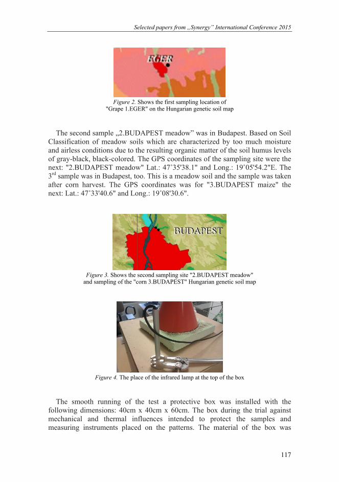
Selected papers from „Synergy” International Conference 2015
TÁMOP-4.2.1.B-11/2/KMR-2011-003 117
Figure 2. Shows the first sampling location of
"Grape 1.EGER" on the Hungarian genetic soil map
The second sample „2.BUDAPEST meadow” was in Budapest. Based on Soil Classification of meadow soils which are characterized by too much moisture and airless conditions due to the resulting organic matter of the soil humus levels of gray-black, black-colored. The GPS coordinates of the sampling site were the next: "2.BUDAPEST meadow" Lat.: 47˚35'38.1" and Long.: 19˚05'54.2"E. The 3rd sample was in Budapest, too. This is a meadow soil and the sample was taken after corn harvest. The GPS coordinates was for "3.BUDAPEST maize" the next: Lat.: 47˚33'40.6" and Long.: 19˚08'30.6".
Figure 3. Shows the second sampling site "2.BUDAPEST meadow"
and sampling of the "corn 3.BUDAPEST" Hungarian genetic soil map
Figure 4. The place of the infrared lamp at the top of the box
The smooth running of the test a protective box was installed with the following dimensions: 40cm x 40cm x 60cm. The box during the trial against mechanical and thermal influences intended to protect the samples and measuring instruments placed on the patterns. The material of the box was
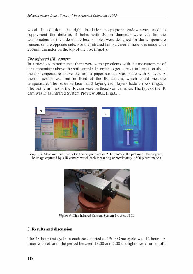
Selected papers from „Synergy” International Conference 2015
TÁMOP-4.2.1.B-11/2/KMR-2011-003 118
wood. In addition, the right insulation polystyrene endowments tried to supplement the defense. 3 holes with 30mm diameter were cut for the tensiometers on the side of the box. 4 holes were designed for the temperature sensors on the opposite side. For the infrared lamp a circular hole was made with 200mm diameter on the top of the box (Fig.4.).
The infrared (IR) camera In a previous experiments, there were some problems with the measurement of air temperature above the soil sample. In order to get correct information about the air temperature above the soil, a paper surface was made with 3 layer. A thermo sensor was put in front of the IR camera, which could measure temperature. The paper surface had 3 layers, each layers hade 5 rows (Fig.5.). The isotherm lines of the IR cam were on these vertical rows. The type of the IR cam was Dias Infrared System Proview 380L (Fig.6.).
Figure 5. Measurement lines set in the program called “Thermo” (a: the picture of the program;
b: image captured by a IR camera which each measuring approximately 2,800 pieces made.)
Figure 6. Dias Infrared Camera System Proview 380L
3. Results and discussion
The 48-hour test cycle in each case started at 19: 00.One cycle was 12 hours. A timer was set so in the period between 19:00 and 7:00 the lights were turned off.

Selected papers from „Synergy” International Conference 2015
TÁMOP-4.2.1.B-11/2/KMR-2011-003 119
Then, the lights were automatically turned on between 7: 00 to 19: 00. The chart (Fig.7.) clearly showed that the maximum temperatures were at the end of the 12-hour period. At the end of the two days the temperature pikes were not on the same value. On the first day, the starting temperature of the soil was lower, therefore the first pike was lower.
Figure 7. Temperature changes in the soil column,
and on the soil surface"1.EGER Grape"
Three tensiometers were set in 60, 120, 180 mm depth. There was no significant difference between the data of the 3 depth (Fig. 8.).
Figure 8. Changes of soil moisture in the column named "2.BUDAPEST meadow"
In Fig. 9. can be seen the temperature changes in function of depth and time (3 dimensions). It is well observed, that in the upper part of the soil the temperature is the highest until -20 mm, the temperature suddenly dropped, and -

Selected papers from „Synergy” International Conference 2015
TÁMOP-4.2.1.B-11/2/KMR-2011-003 120
40 mm again rises and only from there can be observed in the depth a decreasing in the temperature in first 12 hours (IR lamp worked in this period). In the next 12 hour increased the temperature, when IR lamp worked, but can be seen the same tendency as earlier.
Figure 9. Temperature data of the thermocam 3D ("2.BUDAPEST meadow",
vertical line 3, row 2).
Conclusions
The experimental results presented here may strongly support detailed modelling of the moisture level distributions nearby soil-air interfaces taking into account earlier relevant successful methods (Márfy and Ács, 2001). Finally, the results obtained may also contribute to further improvements of the surface energy budget parametrizations for urban scale models (Nickelson and Smiley, 1975).
Acknowledgement
The authors gratefully acknowledge support of the MÖB/DAAD Project No. 55731. (2015).
References
[1] Atterberg, A., (1912): Die Plastiztat der Tone. Internationale Mitteilungen für Bodenkunde 2. Berlin, pp. 312-316.
[2] Gaoa, Z., L. Bianc L., Hua Y., Wanga L., Fand J., (2007): Determination of soil temperature in an arid region, Journal of Arid Environments, Vol. 71, pp.157–168.

Selected papers from „Synergy” International Conference 2015
TÁMOP-4.2.1.B-11/2/KMR-2011-003 121
[3] Hillel, D., (1980): Foundations of soil physics, Academic Press, San Diego, pp. 137-138.
[4] Koorevaar, P.G. Menelik & C. Dirksen, (1983): Elements of soil physics, pp. 86-87.
[5] Klute, A., C. Dirksen, (1986): Methods of soil analysis (2nd edition) Part 1., ASA-SSSA, Medison Wisconsin USA, pp. 687-732.
[6] Kutílek, M., D.R. Nielsen, (1994): Soil hydrology, Catena Verlang, 38162 Cremlingen-Destedt, Germany, pp. 73-75.
[7] Liebethal, C., Huve, B. and Foken, T., (2005): Sensitivity analysis for two ground heat flux calculation approaches. Agricultural and Forest Meteorology 132, pp. 253–262.
[8] Molnár, I., (1998): A csupasz talaj párolgás és a környezeti tényezők kapcsolata mikroskálán – Connection of the evaporation of bare soils and environmental factors on microscales, ELTE TTK, Meteorológiai Tanszék – Department of Meteorology
[9] Márfy, J., Ács F., (2001): A csupasz talajfelszínközeli réteg nedvességi viszonyainak modellezése a Penman-Monteith-féle képlet alapján – Modelling of moisture level conditions of the bare near-interface soil layers on the base of the Penman-Monteith formula – a case study.
[10] Nickerson, E.C., E.V. Smiley, (1975): Surface energy budget parametrizations for urban scale models. J. Appl. Meteor 14, pp. 297-300.

Selected papers from „Synergy” International Conference 2015
TÁMOP-4.2.1.B-11/2/KMR-2011-003 122
The operationalism of sustainability is a mathematical issue
L. PITLIK, Z. VARGA
Reseach group My-X, Szent István University
Abstract
The hypothesis of this article is: Constellations of phenomena can be seen as sustainable, if the facts of the past in case of each object and attribute are arbitrary close to the norm values, where norm values are the levels of attributes, which should be given based on each other circumstances. Similarity analysis is a modelling tool, which is able to build models in an automated way to detect lacks of sustainable constellation e.g. in agricultural databases. Software products based on similarity analyses (SeaLog 2012, NGStress 2014) was prized by innovation experts on the field of IT-stress and human stress.
Keywords
artificial intelligence, automated swot-analysis, virtual robot farmer
1. Introduction
In general, the keyword “sustainability” is used without any proofs, like a kind of buzz-word. On the other hand, the phenomenon “sustainability” seems to be one of the most important phenomena – both on ethical and on professional level. Therefore it should be a real scientific question: what is sustainability at all?
The classic knowledge representation tries to deliver definitions based on words. But words are products of the “magic” of human intuitions, where intuition - according Konrad Lorenz (Lorenz, 1944) - seems to be available in case of each living creature. Intuition is the source (fountainhead) of human knowledge. However, intuition is always presented in subjective forms – in connection to humans. Fortunately, artificial intelligence research is already able to create terms based on measured logs about arbitrary phenomena. Parallel, definitions - based on words – are inefficient exact. Therefore a kind of motto for knowledge representation issues could be: knowledge is what can be described in form of source codes – each other form of publications should be seen as best-letters or literature – literally.
After the more or less (unavoidable) philosophical opening about the problem described in the title of this article, it is necessary to change the point of view towards mathematic/modeling: based on bubble-effects, where it is assumed,

Selected papers from „Synergy” International Conference 2015
TÁMOP-4.2.1.B-11/2/KMR-2011-003 123
that a value of an attribute in case of an object is too low or too high, norm-values seems to be existent. Norm-values are not medians or averages. Norm-values are products of models. Norm-like is a level, where the exact value of the level is appropriate to the force-fields driven by each elements of the circumstances. With other words, it means: no pressure for norm-values can be detected to initialize changes in the given attribute. Sustainable is therefore each constellation, where indications for changing cannot be identified in the big data.
Naïve solutions like classic SWOT analysis try to approximate the complex phenomenon of sustainability. A SWOT analysis should declare bubbles: S stand for effect too high, W stands for effect too low, O = effects of improving and T = effects of depreciation. Unfortunately, the well-known SWOT could not be transformed into source code – it means: SWOT is a matured phenomenon of the “magic” of words – without any evidences behind of the declared bubble-effects. Whether a SWOT analysis could really be transformed into source codes?
2. Similarity analysis
The following chapter tries to give a short description about the know-how developed by the My-X research group for deriving norm-values in a context dependent way.
Theory Similarity analysis is a specific modeling technique. First, it needs an object-attribute matrix like Fig.1, where O stands for objects, X and Y for attributes and OAM means: object-attribute-matrix, where the raw inputs of X(i) should be ranked. This quasi universal form of fact-representation can be used for a lot of analytical techniques (like regressions, neural networks, etc.).
Similarity analysis delivers as solution optimized staircase-function, where a set of descending rank/stair-values will be calculated for each known attribute-level based on linear programming, if direction (preferred orientation like the more the more, or the less the more are given for each attribute). In this context, norm-values are the (cumulative and/or additive) aggregated values being created as a possible set of stairs. Each attribute can be seen as Y or X(i). Therefore it is possible to derive a specific norm-value for each position in the OAM.
Measured facts and estimated norm-values can have a difference. The direction and the level of these differences can be interpreted as an automated SWOT analysis, where the static differences are the Strengths and the Weaknesses depending on the preferred orientation of the bubbles. The dynamic differences between a set of facts and norm-values ordered in a time series can be seen as Opportunities and Threats (also depending on the direction of preferred constellation).
In extreme case, the directions can be eliminated and instead of stair cases polynomial function will be explored. But the norm-values can always be
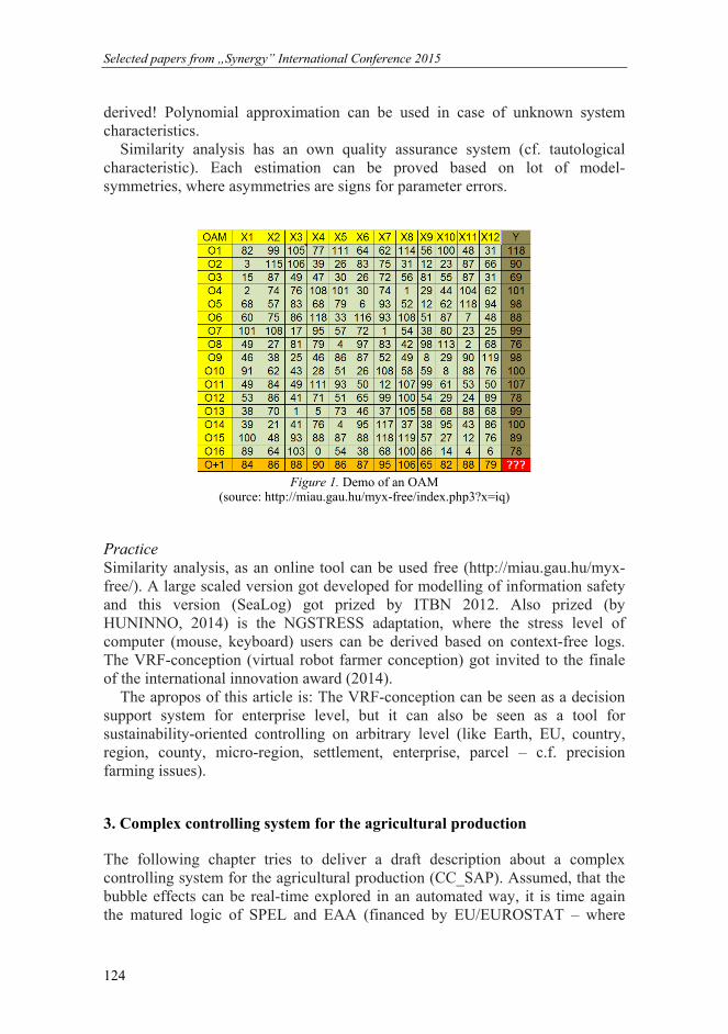
Selected papers from „Synergy” International Conference 2015
TÁMOP-4.2.1.B-11/2/KMR-2011-003 124
derived! Polynomial approximation can be used in case of unknown system characteristics.
Similarity analysis has an own quality assurance system (cf. tautological characteristic). Each estimation can be proved based on lot of model-symmetries, where asymmetries are signs for parameter errors.
Figure 1. Demo of an OAM
(source: http://miau.gau.hu/myx-free/index.php3?x=iq)
Practice Similarity analysis, as an online tool can be used free (http://miau.gau.hu/myx-free/). A large scaled version got developed for modelling of information safety and this version (SeaLog) got prized by ITBN 2012. Also prized (by HUNINNO, 2014) is the NGSTRESS adaptation, where the stress level of computer (mouse, keyboard) users can be derived based on context-free logs. The VRF-conception (virtual robot farmer conception) got invited to the finale of the international innovation award (2014).
The apropos of this article is: The VRF-conception can be seen as a decision support system for enterprise level, but it can also be seen as a tool for sustainability-oriented controlling on arbitrary level (like Earth, EU, country, region, county, micro-region, settlement, enterprise, parcel – c.f. precision farming issues).
3. Complex controlling system for the agricultural production
The following chapter tries to deliver a draft description about a complex controlling system for the agricultural production (CC_SAP). Assumed, that the bubble effects can be real-time explored in an automated way, it is time again the matured logic of SPEL and EAA (financed by EU/EUROSTAT – where
Selected papers from „Synergy” International Conference 2015
TÁMOP-4.2.1.B-11/2/KMR-2011-003 125
SPEL = sektorales Produktions- und Einkommensmodell der Landwirtschaft, and EAA = Economic Accounts of Agriculture) to follow. Each measured fact should be collected in a central (driven) database and each new fact should be compared / benchmarked based on all the data being already available, in order to detect bubble-effects
The holistic project can be organized step-wise: – partial data assets (in Hungary: KSH, AKII) should be monitored at once
in the frame of the given infrastructure – complex databases (in Hungary: TEIR, in EU-level: FADN) should be
analyzed – parts of databases should be integrated in a virtual system
The holistic project needs following large-scale developments, if databases are already given:
– OAM-generator, where the potential learning patterns should be extracted from the databases with the raw/measured data incl. pattern-generation for symmetry-analyses in the quality assurance/consistence-control layers
– parallel processed SWOT-generator, where the pattern-generator and optimization tasks should be run in the most efficient way
– interpretation-generator, where the facts and estimated values should be converted to text schemes based on the classic rule of “magic” of words
– data-visualization tool, in order to be capable to generate the most adequate visual effects
Manual-driven solutions are now available for permanent experimentations. The large scale prototype of SeaLog should be optimized and adapted. Further necessary steps before implementation:
– comparative studies are needed in order to demonstrate for the standard users (e.g. politicians, farmers) the differences of the hermeneutical potentials between classic and similarity-based approaches
– e-learning tools (c.f. MOOC-based) should be developed to ensure everyone can access the knowledge about sustainability analyses
4. Specific interpretation of cc_sap
The databases - listed above – deliver mostly ecological and financial data items. However, the analytical potential of CC_SAP is quasi unlimited (context-free). It is also possible to search for bubble-effects in case of
– mechanical constellations (e.g. modelling of depreciation of machines in diverse cases of using)
– physiological constellations (e.g. stress-detection of living creatures) – weather constellations – market constellations (c.f. PÁIR, stock markets) and – behavior-patterns of humans (c.f. information units from Google
Trends), etc. Besides the direct adaptation, there are new ways already prepared to re-
interpret specific problems:

Selected papers from „Synergy” International Conference 2015
TÁMOP-4.2.1.B-11/2/KMR-2011-003 126
– diagnoses and therapies for humans/animals/plants/ecosystems/markets can be re-interpreted as a kind of bubble-effect, assumed, that the sustainability of life and the a cured constellation are the same phenomena
– classic forecasting problems can be transformed into bubble-analyses, without exact time-information about changing bubbles
5. Case study: dynamic force-fields behind sustainable surfaces
Sustainability is a process. This process should be detectable starting from a randomized-chosen constellation (s. Fig.2., where I1 shows a random matrix with values between 0 to 99 and O(i) = objects, A(j) = attributes, i=1,…10, j=1,...,5).
Figure 2. Iterations (Source: http://miau.gau.hu/miau/206/super_evolution.xls - sheet(‘view’)
Figure 3-4-5. Estimations/Ranking values/Differences
(Source: http://miau.gau.hu/miau/206/super_evolution.xls)

Selected papers from „Synergy” International Conference 2015
TÁMOP-4.2.1.B-11/2/KMR-2011-003 127
If standard similarity analyses (see: http://miau.gau.hu/myx-free/coco/beker_std.php) run step by step (according to the more the more direction for each attribute), where each attribute should be modelled based on the other attributes in two layers for further symmetry-analyses being able to explore invalid estimations), then each valid estimation can be seen/accepted as strategic relevant target-value. Parallel, it is necessary to ensure, that the anti-discriminative model (see: http://miau.gau.hu/myx-free/coco/beker_y0.php) for the first phase (I1) can be evaluated as static sustainable (s. Fig.3., where behind the surface-sustainability /I1/ force-fields can be identified towards exploring real potentials of objects).
Figure 4. shows ranking values of the estimations in Fig.3. Parallel, Fig.5. declares differences between iterations for each object in percent to the total of prescripted valid changes of raw-values in the previous phase.
Figure 6-7. Steps of evaluation of iterations: raw data / ranking values (Source:
http://miau.gau.hu/miau/206/super_evolution.xls)
Figure 8. Evaluation of iterations
(Source: http://miau.gau.hu/miau/206/super_evolution.xls)
The iterations can have a lot of consequences. To be able to define, which phase can be seen as the best approximation, a kind of analysis based on the idea of Occam’s razor (see Fig.6-7-8, where the consequences are: difference between the sum of the raw values in the first phase and each other phase: direction = the less the more ideal / sum of each valid changes with/without position affected by integer-transformation and between of raw values of two neighboured phases: direction = the less the more ideal / amount of unchanged position: direction = the more the more ideal / average changing rate: direction = the less the more ideal).
Selected papers from „Synergy” International Conference 2015
TÁMOP-4.2.1.B-11/2/KMR-2011-003 128
Conclusions
Based on the principle and the detailed result of the case study, following interpretation can be formulated:
– between static sustainability, there are deep force-fields catalising changes,
– the highest average change rate can be seen in case of the king-object (O1=22%) and the also in case og the slave-object (O6=18%), it means the population of objects tries to determine a best object at any rate,
– the rank and row correlation between neighboured iteration phases let identify an approximation to a relative stable constellation (I6),
– the ranking values of the objects makes possible to realize changes according to ideality of the object compared to each other,
– similar effect can be found in case of price/performance-analyses (cf. STEP-IX - http://miau.gau.hu/myx-free/index_e8.php3?x=e08), where close to seemingly rational prices a kind of confidence interval can be identified to see the ratio of current price and the tresholds of its interval,
– after realizing the most matured iteration phase, further changes of the raw values let start a new cycle of approximation,
– the above described logic can be seen as potential interpretation for chosing a queen for bees among potential identical candidates (or waiting list in health care/front acitivities) and also as a dynamic (hidden) force-fields behind the surface of static derived sustainability (like a frozen lake),
– therefore sustainabilty is a kind of compass and not a target position, – the compass and the appropriate navigation system can be realized based
on a chain of similarity analyses, – depending from starting values in the first raw matrix different ways can
be realized based on the above described steps.
Summary
The above mentioned principles and steps can be interpreted as a new type of decision making. First, sustainability can be measured based on object-attribute-matrices and their bubble-effects in case of each matrix-position. It is also possible to classify objects with static seemingly same potentials of sustainability. After creating diagnoses (or risk analyses), therapies can be derived for each objects concerning each attributes in frame of a cybernetic system, whose objects are unlimited able to follow rules.
References
[1] Pitlik L. (2014), About Occam’s razor http://miau.gau.hu/miau2009/ index.php3?x=e0&string=occam

Selected papers from „Synergy” International Conference 2015
TÁMOP-4.2.1.B-11/2/KMR-2011-003 129
[2] Pitlik L. (2014), My-X team – an idea breeding farm, https://www.researchgate.net/publication/280086739_My-X_Team_an_innovative_idea-breeding_farm, Noble Ideas Project – Virtual Robot Farmer (VRF)
[3] Pitlik L. (2015), Modules of My-X online analytical tool, http://miau.gau.hu/myx-free/coco/index.html
[4] ITBN (2012), https://www.itbn.hu/index.php/hu/itbn-biztonsagi-dij/2012-dijazottjai
[5] HUNINNO-NGSTRESS (2014), http://www.ddriu.hu/htmls/?ID=594

Selected papers from „Synergy” International Conference 2015
TÁMOP-4.2.1.B-11/2/KMR-2011-003 130
Identification of soil deformation with the reological model of tire-terrain interaction
Gy. PILLINGER1, A. GÉCZY2, L. MÁTHÉ1, P. KISS1
1Institute of Process Engineering, Szent István University 2Department of Electronics Technology,
Budapest University of Technology and Economics
Abstract
The paper compares deformations calculated with the rheological model of tire-terrain interaction during the travel of a vehicle and measured soil-deformation under the wheels. Three different soil states were compared during a vehicle towing experiment, with a fix terrain moving vehicle. The obtained soil deformation measurement data was compared with the calculated results of a rheological model. The comparison gives exact data about the applicability and the precision of the model, which provided appropriate results for the investigated tire-terrain interaction.
Keywords
deformation, soil, tire, tire-terrain interaction, road, towing, stubble
1. Introduction
Tire-terrain interaction is a complex phenomenon, where numerous parameters are affecting the vertical deformation of the soil, the vertical acceleration of oscillation, and the energy required for the rolling of the tire. Experimenting is difficult on the terrain, while the profile and the state of the terrain is inconsistent. Thus it is also problematic to define any parameters as a stationary constant value. During the modelling of tire-terrain interaction, with fixed specific parameters, it becomes possible investigate the effect of different other parameters on the soil deformation. In the model, it is possible to change the boundary conditions, enabling to investigate different aspects of the occurring deformations.
Numerous modelling methods can be found in the literature for the given problem, such as finite and discrete element approaches (FEM and DEM respectively). The shape of the soil particle is an important parameter of the discrete element modelling. Tsuji et al. used smooth spherical elements for their model, then a slab was forced perpendicularly into the modelled soil, then the force values required for the impression were recorded. Sitkei also Li et al. used a more sophisticated element in their modelling, where the shape was defined from a special
Selected papers from „Synergy” International Conference 2015
TÁMOP-4.2.1.B-11/2/KMR-2011-003 131
union of separate spheres. Smith and Peng used a stiff, finned wheel for their work, where the soil was also described with DEM approach. Large computing requirements is a considerable disadvantage of the FEM and DEM calculations.
There are models where the tire and the terrain are investigated as separate units, with several rheological elements (small sets of rheology elements). The terrain was investigated as a viscoelastic material by Sitkei, also by Huszár and Müller. Viscoelastic materials can be modelled with basic, linear material laws. Sitkei used the three-elemental Kelvin models for describing the rheological parameters of the terrain. Mahyuddin et al. also used viscoelastic modelling for investigating extracted soil by a grabber crane vehicle. They used spring damping and wet damping in parallel connection for the model. They connected a spring element to the model from the top and an attenuating element from the bottom. The viscoelastic terrain model of Tran and Muro connected a spring and a wet damping element in serial connection. Their investigation involved a tracked vehicle, so they used a similarly paired element for the horizontal direction as well. The damping coefficient of the soil was calculated according to their measurement results (3,74·102 Ns/cm). Hildebrand et al. also used viscoelastic elements for their modelling, Park et al. used rheology elements for their tire model. (Maxwell, Bringham, Poynting-Thomson)
Surface of different terrains can be varying, and the shape of the surfaces can be measured with profiling devices. Gedeon investigated the stochastic nature of soil. The profile of the soil generates the vertical oscillation acceleration, which also causes additional deformation (Kiss). Due to the oscillating movement, larger adhesion force occurs. The soil profile is also usually investigated in the case of vehicles accidentally running off the road (Máthé), or at the mechanical stability design of agricultural vehicles (Gurmai).
2. Aim
The paper aims to describe a novel rheological model of tire-terrain interaction. With the help of the model, simulation of soil-deformation under the loaded tire becomes possible. An advantage of the novel approach is that there is no need for extensive parameter-space for the boundary condition system. Thus calculation requirements can be reduced, and the calculation itself is able to give fast and precise results during its application.
3. Preliminary work
The initial input parameters of the model were defined with towing measurements on the field with a Gaz 69 off-road vehicle. The vehicle was towed on terrain with different characteristics (Fig. 1). The investigated terrain types were sandy adobe soil, stubble, and stubble soil in cultivated and husked form. Their parameters are detailed in Table 1.

Selected papers from „Synergy” International Conference 2015
TÁMOP-4.2.1.B-11/2/KMR-2011-003 132
Figure 1. Towing the investigated vehicle on a stubble
Table 1. Investigated soil compositions
Sample 0,25-2
mm sand
0,05-0,25 mm
sand
0,02-0,05 mmsludge
0,01-0,02 mm sludge
0,005-0,01 mmsludge
0,002-0,005 mm
sludge
0,002 mm > loam
1. 32% 55,80% 8,80% 0,80% 0,00% 0,50% 8,80%
Sum 87,80% 3,40% 8,80%
2. 79,80% 10,10% 6,10% 0% 4% 0% 6,10%
Sum 89,90% 4% 6,10%
3. 63,20% 30,60% 3,90% 0% 1,90% 0,40% 3,90%
Sum 93,80% 2,30% 3,90%
Avg. 58,30% 32,20% 6,30% 0,20% 2% 0,30% 6,30%
Sum avg.: 90,50% 3,20% 6,30%
The length of the towing was 10 m, the measured sections were profiled. The
soil deformations were calculated with the results of profiling for the given soil states and compositions. The load on the wheel and the spring constant was determined with scaling, the attenuation was determined with oscillating method. The vehicle was equipped with a Voltyre 215/90-15C tire. The soil parameters were calculated with the parameters of the tire size and the towing speed. A penetrologger device was used on the field. On the right side of the front axis, near to the hub of the wheel an accelerometer device logged the vertical oscillating accelerations.
4. Developing the rheological model of tire-terrain interaction
The rolling tire is affected by both the excitation and the attenuation at the same time. The excitation is caused by the changing terrain profile and soil inhomogeneity. On the other hand, the attenuation is mostly caused by attenuation effect of the soil and also by the inner friction of the tire.

Selected papers from „Synergy” International Conference 2015
TÁMOP-4.2.1.B-11/2/KMR-2011-003 133
To describe the tire-terrain interaction, the tire and the terrain was separately modelled. The tire affects the terrain, and vice-versa the terrain affects the tire. During tire-terrain interaction the deformations occur mainly along the vertical axes. So the aforementioned effects of interaction are described with forces locked to one degree of freedom, along the vertical axis. (They are not able to move along the horizontal axis or rotate at all). The model is dealing with one tire at a time.
Tire model The tire model receives its excitation from the terrain. The terrain deforms slower than the tire, so the soil profile affects the tire itself first. This generates yg movement at the bottom of the tire, at the tire-terrain boundary, which is basically the track excitation (Fig. 2). The difference of the runner and mass of the mk tire load movement will lead to the extension and compression of the elements in between the two – from these information, the damping and the spring forces can be calculated. As seen in Figure 2, the elements form a parallel connection of a dry damping coefficient (hg), a spring stiffness coefficient (cg) and a wet damping coefficient (kg). The presented description is similar to the Voigt-Kelvin model, which is extended with a dry damping module.
Figure 2. The mechanical model of the tire
The describing differential equation for the investigated model is the following:
)sgn()( aggaggagakg yhyycyykymty (1)
where: mt,a – mass of the deformed soil/tire cubature [kg] ct,a – spring stiffness of the terrain/tire [N/m] ht,a – dry damping coefficient of the terrain/tire [N] kt,a –wet damping coefficient of the terrain/tire [Ns/m] yt,a – vertical movement of the center of mass (soil/tire) [m]

Selected papers from „Synergy” International Conference 2015
TÁMOP-4.2.1.B-11/2/KMR-2011-003 134
yt,a’ – velocity of the center of mass (soil/tire) [m/s] yt,a” – acceleration of the center of mass (soil/tire) [m/s2].
According to the tire parameters, the track excitation causes pressure and resulting deformation on the tire, so an offset is observable on the center of mk mass as well. The reactional force which acts at the boundary of the runner (pointing vertically up- or downwards) excites the model of the terrain. The input of the tire model is the track excitation, its output is the occurring adhesion force, and the location of the mk center of mass.
Terrain model The terrain model is also an excited and attenuated oscillating system (presented in Figure 3), where the affecting F parameter comes from the output adhesion force of the tire model. The terrain model is different from the aforementioned tire model in its composition by the difference in the given parameter values. The mt is practically the mass of the investigated soil cubature, which is affected by the deformation. Offset is also observable on center of mass in this case as well.
Figure 3. Mechanical model of the terrain
The input of the terrain model is the adhesion force (F) which depends on the time; its output is the deformation (offset) of the terrain surface (basically the top side of the mt mass). The terrain model is not affected by the upwards pointing forces, from an other point of view, the tire can not pull the terrain in upwards direction. The excited soil cubature can only suffer the compression effect, any reverse suspension is negligible. The differential equation of the model is the following:
)sgn()( tttttttt yhycykymtF (2)
The differential equation is simpler in the case of the terrain model, while only the upper part is able to move. Thus it is a simpler task to specify the movement of the viscoelastic elements.

Selected papers from „Synergy” International Conference 2015
TÁMOP-4.2.1.B-11/2/KMR-2011-003 135
Solving the tire-terrain interaction model The differential equations (1) and (2) were solved with the Kelvin-Thomson solution in Matlab-Simulink in a programming environment.
After providing the input parameters, the output will give the deformation of the tire. From this deformation and the geometry data of the tire, the central position of the tire can be calculated. Also at the tire-terrain boundary an adhesion force acts, which causes a deformation. The deformation is connected back to the input of the tire model, so that it can modify the position of the tire with the values of deformation.
Figure 4. Block diagram of the terrain model
Table 2. Tire parameters
mk – mass of tire load [kg]:
p – pressure inside the tire
[bar]:
cg – spring stiffness [N/m]:
kg – wet damping coefficient
[Ns/m]:
hg – dry damping coefficient
[N]:
395 1,8 305770 58 18
Figure 5. Determining the spring stiffness of the tire
The viscoelastic parameters of the tire are constant and independent from the normal, ambient circumstances. The temperature differences were mainly negligible during towing and the determination of the parameters. (20 ± 5 °C).
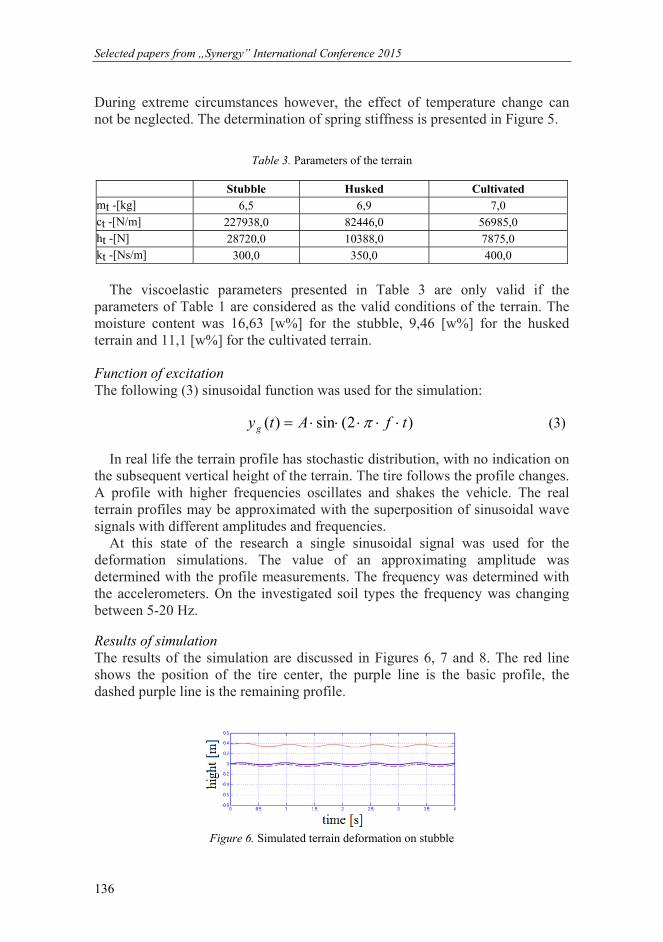
Selected papers from „Synergy” International Conference 2015
TÁMOP-4.2.1.B-11/2/KMR-2011-003 136
During extreme circumstances however, the effect of temperature change can not be neglected. The determination of spring stiffness is presented in Figure 5.
Table 3. Parameters of the terrain
Stubble Husked Cultivated mt -[kg] 6,5 6,9 7,0 ct -[N/m] 227938,0 82446,0 56985,0 ht -[N] 28720,0 10388,0 7875,0 kt -[Ns/m] 300,0 350,0 400,0
The viscoelastic parameters presented in Table 3 are only valid if the
parameters of Table 1 are considered as the valid conditions of the terrain. The moisture content was 16,63 [w%] for the stubble, 9,46 [w%] for the husked terrain and 11,1 [w%] for the cultivated terrain.
Function of excitation The following (3) sinusoidal function was used for the simulation:
)2(sin)( tfAtyg (3)
In real life the terrain profile has stochastic distribution, with no indication on the subsequent vertical height of the terrain. The tire follows the profile changes. A profile with higher frequencies oscillates and shakes the vehicle. The real terrain profiles may be approximated with the superposition of sinusoidal wave signals with different amplitudes and frequencies.
At this state of the research a single sinusoidal signal was used for the deformation simulations. The value of an approximating amplitude was determined with the profile measurements. The frequency was determined with the accelerometers. On the investigated soil types the frequency was changing between 5-20 Hz.
Results of simulation The results of the simulation are discussed in Figures 6, 7 and 8. The red line shows the position of the tire center, the purple line is the basic profile, the dashed purple line is the remaining profile.
Figure 6. Simulated terrain deformation on stubble

Selected papers from „Synergy” International Conference 2015
TÁMOP-4.2.1.B-11/2/KMR-2011-003 137
In Figure 6, the results of the towing simulation on stubble is presented. The tire follows the excitation profile. In the very beginning the total deformation does not occurs immediately – this is the point when the tire makes its first contact with the terrain, then it increasingly causes the deformation. The CI index of the stubble was 0,246 MPa.
Figure 7. Simulated terrain deformation on husked soil
In Figure 7 the results of towing simulation on husked soil is presented. It can be concluded that the deformation is larger than in the case of the stubble, but it is more moderate than in the case of cultivated soil (Figure 8). The CI index of the husked soil is 0,194 MPa. For the cultivated soil the CI index is 0,081 MPa.
Figure 8. Simulated terrain deformation on cultivated soil
With the investigation of the curves, it can be concluded that the deformation is increasing significantly, meanwhile the CI index values are decreasing.
Discussion
During measurements the soil deformation was varying according to the inhomogeneity of the terrain, and an extensive range can be observed in the deformation. Larger and smaller deformations are observable along the towing course, which cause resistance change along the course of the investigated vehicle. During the simulation, the terrain was modelled as a homogeneous medium. Thus, deformation is apparently even along the course of the vehicle. Small deformation changes are due to the vertical oscillations caused by the profile. Due to the periodic excitation, the output signals are also periodic. An

Selected papers from „Synergy” International Conference 2015
TÁMOP-4.2.1.B-11/2/KMR-2011-003 138
excitation with larger frequency and amplitude may cause more extensive deformation changes.
The deformations were modelled with viscoelastic elements. We have concluded that the simulation results gave appropriate values from the aspect of practical application. The profile and the inhomogeneity of the terrain however, must be taken into account during the investigations. If the terrain has considerably increased inhomogeneity, the difference between the simulated and measured results may also increase.
During the simulation the soil deformation values were averaged, then compared with measurement results. Table 4 presents the comparison, where appropriate correlation can be found. The comparison between field measurement and simulation fall into the precision of ±10 % error, so the results can be accepted from practical point of view. The error between the simulation and measurement was 2,4 % in the case of stubble. The husked soil case gave 3,6 %, the cultivated soil case gave 3,7 % precision. The increase of error is not consequential from any aspect. The range of CI indexes may also affect the precision, while the parameter differences from the measurement averages may differ similarly to the CI differences. With the amount of agricultural processing on the terrain, the homogeneity also increases. The range of CI indexes are 1,29 MPa for the stubble, 2,11 MPa for the husked soil and 0,1 MPa for the cultivated soil. Husking only takes place in the upper layer of the soil, so in deeper regions the original CI state remains. Thus this is the cause for the highest range in the case of husked soil.
Table. 4. Comparing measured and simulated deformations.
Soil Case Measured Simulated Error Stubble 1,7 cm 1,66 cm 2,4 % Husked soil 4,7 cm 4,53 cm 3,6 % Cultivated soil 6,8 cm 6,55 cm 3,7 % The errors can be reduced with more precise measurement methods, refined
calculations, and better rheology parameter specification methods. The errors however cannot be reduced in a controlled manner, while the inhomogeneity of the terrain always have a significant effect on the measurements.
Summary
In our research we have compared the calculated deformations of the tire-terrain interaction rheological model and the size of soil deformation which has been formed under the wheel while the vehicle was driven. Vehicle towing experiments have been carried out in three different soil conditions with a

Selected papers from „Synergy” International Conference 2015
TÁMOP-4.2.1.B-11/2/KMR-2011-003 139
selected off-road vehicle. The obtained measurement data was compared with the calculated soil deformation size which was calculated from the rheological model. As a result of the comparison the developed rheological model’s application and accuracy can be stated as the researched tire-soil interaction gave appropriate results.
References
[1] GEDEON J. (1993): On Some Basic Problems of Stohastic Modelling. Periodica Polytechnica, Transp. Eng., pp. 89-100.
[2] GURMAI L. (2009): A Comparative study of methods used for testing towed vehicles, Hungarian Agricultural Engineering 22, pp. 46-48.
[3] HILDEBRAND R., KESKINEN E., NAVARRETE R. A. J. (2008): Vehicle vibrating on soft compacting soil half-space: Ground vibrations, terrain damage, and vehicle vibrations. Journal of Terramechanics. 45:4, pp.121-136.
[4] HUSZÁR I., MÜLLER Z. (1977): Mezőgazdasági termények mechanikai vizsgálata. Járművek, Mezőgazdasági Gépek, 24/12.
[5] KISS P. (2009): Components of rolling resistance on terrain. In: Mechanical Engineering Letters Vol. 3. pp.54-64. HU ISSN 2060-3789.
[6] LI W., DING L., GAO H., DENG Z.,LI N. (2013): ROSTDyn: Rover simulation based on terramechanics and dynamics. Journal of Terramechanics 50:3, pp. 199-210.
[7] MAHYUDDIN A. I., SILIMAN N., SUHARTO D. (2011): Dynamic response of shallow burided structures associated with landmine clearing operations. Journal of Terramechanics. 48:3, pp.215-224.
[8] MÁTHÉ L. (2012): Terepre futó jármű menetellenállásai, Mezőgazdasági technika 53:(1) pp. 2-5.
[9] PARK S., POPOV A.A., COLE D.J. (2004): Influence of soil deformation on off-road heavy vehicle suspension vibration. Journal of Terramechanics 41:1, pp.41-68
[10] SITKEI GY. (1972): Die viskoelastischen Eigenschaften von Ackerböden und deren Einfluss auf die Boden-Rad Wechselwirkung. Proceedings of the 4th. Int. Conf. of the ISTVS, Stockholm.
[11] SITKEI GY. (1981): Mezőgazdasági anyagok mechanikája. Akadémiai Kiadó, Budapest
[12] SITKEI GY. (1967): Mezőgazdasági gépek talajmechanikai problémái, Budapest, Akadémia kiadó.141-142. o.
[13] TRAN T. D., MURO T. (2004): Effect of an innovative vertical vibro-tracked vehicle on soil compaction. Journal of Terramechanics 41:1, pp. 1-23.
[14] TSUJI T., NAKAGAWA Y., MATSAMUTO N., KADONO Y., TAKAYAMA T.
[15] TANAKA T. (2012): 3-D DEM simulation of cohesive soil-pushing behavior by bulldozer blade. Journal of Terramechanics 49:1, pp. 37-47.

Selected papers from „Synergy” International Conference 2015
TÁMOP-4.2.1.B-11/2/KMR-2011-003 140
Lubricant technical service of ENI Hungary
A. NAGYMÁNYAI1, L. SIKLÓSI1, Z. BÁRTFAI2 1ENI Hungaria Zrt. Budaörs, Hungary
2Szent István Universiy Gödöllő, Hungary
Abstract
Please, give a short abstract of the paper (maximum 100 words) here, not that version which was submitted before. In this template you can read important details about the formal instructions for preparing the full paper, please keep them strictly. Beside the instructions some useful web-links can be found on Gödöllő, the host city of the conference. Here you can check the deadlines as well.
Keywords
paper format, template document, Synergy2015, important information, deadlines of conference
1. Abstract
– Structure of lubricant maintenance and scheduling software (KEN) – Development of Lubricant service (AKSZ) – MWFA metalworking fluid analyser – Gas Engine oil Controlling Unit – Storage and display of laboratory test results. – The homepage of KEN system
2. History
Figure 1. The organization structure of Lubricant maintenance and scheduling software (KEN)

Selected papers from „Synergy” International Conference 2015
TÁMOP-4.2.1.B-11/2/KMR-2011-003 141
– About eight-ten years ago we started lubricant service improvements at ENI - Agip Hungary.
– This lubricant service development contains four main groups. – During the operation of the lubricant service, we had to be lot of
lubricant data processed and stored. – For storage of lubrication dates and for organize of service activities we
have created the lubricant maintenance and scheduling (KEN) software. – Lubricant maintenance and scheduling software (KEN).
This lubricant maintenance and scheduling software (KEN) have five separated but relating functions:
– Central function – Lubricant maintenance and scheduling activity and planning at ENI
lubricant partners. – The lubes point indicated with bar code in order to identify every
parameters (lube type, last activity,) and easy to load the operations in data base.
– The activity of service car can be schedule – Customer is able to follow the data on web base
Management of Metal Working Fluid Analiser What we can do? Acquisition of new customers. We can perform well documented comparing
tests between the old (competitor) product and our Eni/Agip branded products. (All parameters are automatically controlled and registered.)
We can calculate on the base of measured data the dragg out of fluid, feeding volumes, etc in order to calculate in economic model of total costs of using our metalworking fluid.
Providing partially automatic Fluid Management for mainly centralized emulsion systems
Figure 2. The MWFA is working in the workshop

Selected papers from „Synergy” International Conference 2015
TÁMOP-4.2.1.B-11/2/KMR-2011-003 142
Figure 3. Change of measurement parameters of MWFA
Gas Engine oil Controlling Unit We have important partners in gas engine oil market. For these partners we
had a common innovation with Institute of Physics at Pannon University for gas engine oil controlling unit (GMOS).
We taken the samples from the gas engine oil every 50 hours and we measured parameters in laboratory.
The software can communicate (on-line) with the GMOS unit via mobile internet connection, so on-site permanent personal attendance not needed. The partner also can follow the changes of the parameters under password protection.
Figure 4. Gas engine oil controlling unit (GOMS)

Selected papers from „Synergy” International Conference 2015
TÁMOP-4.2.1.B-11/2/KMR-2011-003 143
Figure 5. Test results: Relative degradation of lubes (in %) vs time
The use of gas engine oil controlling unit we can reduce laboratory tests. Continuous monitoring is a major safety for the partner. Storage and display of laboratory test results. We are performing approximately 800 used oil analysis for our partners. The
evaluations of the results was difficult and time demanding. For years, the lab results came in Excel sheet from laboratory to ENI. After evaluation of the results we sent by Excel sheet to the partner.
With the support of this software (preset some limitation) we can provide on-line results to the customers through web side. Naturally the results could be available for the partner (under password protection) when it has been checked and approved by the technical staff. The partner in this case – like at the MWFA and GMOSz system – can reach some diagrams and follow-up on his previous data.
It doesn’t need more than basic knowledge of computing. The KEN system can be access on the Internet on multi language form
– Hungarian – English – German – Italian
www.eniken.hu The described lubricant services to ensure that customers of ENI Hungary are
able to use lubricants with high confidence.

Selected papers from „Synergy” International Conference 2015
TÁMOP-4.2.1.B-11/2/KMR-2011-003 144

Selected papers from „Synergy” International Conference 2015
TÁMOP-4.2.1.B-11/2/KMR-2011-003 145
Figure 6. Lab. report with evaluation of results

Selected papers from „Synergy” International Conference 2015
TÁMOP-4.2.1.B-11/2/KMR-2011-003 146
Experimental apparatus to determine the optimal kinematical parameters of open mixing screws
A. VARGA
NARIC Institute of Agricultural Engineering
Abstract
Mixing is a common task in agricultural and pharmaceutical industry. A good example of this is the case of the drying of agricultural crop products, by using silodryers, where a thick layer of granular material stored in silos must be dried by using the inflow of hot air from below. The main problem of drying processes that the distribution of the moisture content is not homogeneous at the end of the drying. To reduce the possibility of such losses, there are mixing screws inside such silos, which are designed to cease all of such inhomogeneity. In this paper, development of our experimental apparatus to examine the distribution of moisture content within the storage area is proposed. This apparatus is attached to the drying machine which can be found in the NARIC Institute of Agricultural Engineering. The new measurement system is suitable for drying used screw conveyors with different rotation speed. Based on experiments with this apparatus drying tests can be made with different temperature and rotation speed, so the evolved moisture content can be better understood.
Keywords
silodryer, mixing system, discrete element methods, experimental apparatus
1. Introduction
Mixing is a common task in agricultural and pharmaceutical industry. Design of mixing process and operation are very difficult. Design of mixing process and operation are also difficult, being largely based on judgment rather than science (Bridgwater, 2012). The guidelines for the selections of particle mixers are still not fully developed and predictions of the mixture quality after mixing operations are still not possible (Huang and Kuo, 2014). There are cases, when the mixing process can only be performed by using open mixing screws. During mixing – in most of the cases – we would like to reach the optimal level of mixing during the shortest possible time. In the other hand, excessive mixing could worsen the quality of the mixed material and the mixture quality also. Because of these contradictory criteria, it is a difficult challenge for the practicing engineers to find the optimal mixing intensity.
A good example of this is the case of the drying of agricultural crop products, by using silodryers, where a thick layer of granular material stored in silos must

Selected papers from „Synergy” International Conference 2015
TÁMOP-4.2.1.B-11/2/KMR-2011-003 147
be dried by using the inflow of hot air from below. Without the constant mixing of wet and dry layers of material, such kind of uneven distribution of dry and wet grains can take form, which results over or under dried granular material, and at the end, loss of revenue (Keppler et. al. 2012). To reduce the possibility of such losses, there are mixing screws inside such silos, which are designed to cease all of such inhomogeneity. The number of such screws, the geometry and kinematical parameters of their operation are determined by using experimental investigations, but little is known about what happens around the rotating mixing screw, and because of this, there are no clear guidelines for planning of them. (Keppler et al., 2015).
In our previous work, we demonstrate that the discrete element method is suitable for investigations of behavior of the granular materials in silodryers. The particle motion around the screw conveyors is determined by a new experimental apparatus and discrete element simulations. In the next step we would like to take account of the thermodynamical effects. In this case an apparatus and the method of measurements had to be modified. This new apparatus is attached to the drying machine which can be found in the NARIC Institute of Agricultural Engineering. This article demonstrates the new measurement system.
2. Material and method
To examine the distribution of moisture content during the drying process (with-, and without mixing) we modified and attached our apparatus to the drying machine. The following pictures show the mixing apparatus and the drying machine.
Figure 1. Mixing apparatus and the drying machine

Selected papers from „Synergy” International Conference 2015
TÁMOP-4.2.1.B-11/2/KMR-2011-003 148
The wall of a mixing apparatus is a transparent cylinder having 450mm diameter and 3mm of wall thickness. The top of the cylinder is open. In the center of the cylinder there is the mixing screw, having a V-belt drive connection to an electric motor. The laboratory drying machine is designed to simulate the drying processes of different crops. Different crops and fibers can be dryed with the equipment, pre-setting the different parameters and drying systems that are used in practice. Main drying technological characteristics:
– dryed layer thickness – dryed medium speed – dryed medium temperature – dryed medium relative humidity
Based on the requirements of the research objective, these characteristics can be adjusted within a wide range. The adjusted speed of the air flow is measured by an orifice pressure gauge system and controlled through a frequency changer. The drying machine effects controlled drying; the required drying temperature or the moisture content can be set. The water loss during the drying process is measured by a built-in balance with 4 measuring points, with gravimetric method. The temperature and air handling characteristics are measured by an AHLBORN type measuring and data collection system. Taking account of these characteristics carried out in the assembly. In the following picture, the modified and assembled parts can be seen.
Figure 2. The modified drying system
Methods of measurements The measurements were done with wheat. Before filling of the cylinder, the moisture level had to be determined with ten-fold repetition by GAC 2100 moisture tester. The next step was to set up the drying heat, measured moisture level and the required moisture level in the controlling unit of the drying machine. To fill a cylinder was the last step. After the wheat reached the desired moisture content, we pressed in the sampler tubes from above into the mixed/ unmixed assembly in different distances from the rotating/standing screw by this

Selected papers from „Synergy” International Conference 2015
TÁMOP-4.2.1.B-11/2/KMR-2011-003 149
way (Fig. 3/a). The 1st sample were taken beside the wall, the 2nd sample was taken between the screw and a wall, and the 3rd sample was taken beside the screw. We divided the samples in the sampler tubes into 5 parts and measured the moisture content of the parts (Fig. 3/b).
a)
b)
Figure 3. Mixing experiment and the sampling method
Results
Figure 4. The distribution of moisture
content without mixing

Selected papers from „Synergy” International Conference 2015
TÁMOP-4.2.1.B-11/2/KMR-2011-003 150
Figure 5. The distribution of moisture content with mixing
Conclusions
Based on the above the modified apparatus is suitable for examine the evolved moisture content and comparing the efficiency of drying processes in case of rotating and standing screws. We analyzed the moisture contents in different distances from the rotating/standing screw. The results showed on fig 5. demonstrate, that by using the rotating screw, we are able to create a more even moisture distribution within the container. This is good from practical point of view, as our goal was to create an even moisture distribution inside the whole granular assembly to avoid the under- or overdrying loss mentioned in the introduction.
Our further aim is to experimentally determine the optimal screw rotation angular velocity for the proper mixing of the material and to determine the heat- and mass transfer processes taking place inside the miced granular assembly.
Acknowledgements
I offer my sincerest gratitude to my colleague, Sandor Takacs, who has helped me in the designing and assembly of the apparatus.
References
[1] A. Huang and H. Kuo (2014), Developments in the tools for the investigation of mixing in particulate systems – A review, Advanced Powder Technology 25 pp. 163–173.

Selected papers from „Synergy” International Conference 2015
TÁMOP-4.2.1.B-11/2/KMR-2011-003 151
[2] J. Bridgwater (2012), Mixing of powders and granular materials by mechanical means—A perspective, Particuology 10 pp. 397– 427.
[3] I. Keppler, L. Kocsis, I. Oldal, I. Farkas, A. Csatar, Grain velocity distribution in a mixed flow dryer, Advanced Powder Technology 23 (2012), pp. 824-832
[4] I. Keppler, A. Varga, L. Fenyvesi, I. Kátai, I. Szabó (2015), Particle motion around open mixing screws: optimal screw angular velocity, Engineering Computations (accepted)

Selected papers from „Synergy” International Conference 2015
TÁMOP-4.2.1.B-11/2/KMR-2011-003 152
Is it a gage or a measure? Application of the endoscope technology
in the industry
Z. BÁRTFAI1, I. BORBÁS2, Sz. POÓR2 1Institute of Mechanics and Machinery, Szent István University
2ENDO2000 Ltd.
Abstract
Nowadays the application of the endoscope technology is widespread. It plays an important role in the quality insurance of the manufacturing process and in the operational process as well. In this period of the machine lifecycle - known as machinery management- the endoscopy helps to control the technical condition. Through on some examples our article discuses the application possibilities of the endoscope technology in the production process as a gage and in the operational process as a measure. Video endoscopes constitute the technical support of our research project and they were produced by Karl Storz GmbH & Co.KG.
Keywords
technical condition, diagnostics, endoscope technology
The main objective of the application of the endoscope technology (endoscopy) in the machinery management is to discover the technical condition, or to determine the possible cause of the failure before any maintenance arrangements.
The main advantages of this kind of application of the endoscope technology: 1. Possibilities for exploration of the technical condition without any
disassemble. This method gives a faster and more cost-effective procedure than some other traditional methods for examining the technical condition. With the usage of this method the period of breakdown can also be shortened.
2. Comparing with those methods that based on the operational features of the machine, more direct information can be gathered from the machine condition.
The endoscope, a measuring instrument using for examining the inside of a hollow construction is basicly a gage. Just like the gages used in the manufacturing for providing the so called go, dosn’t go information, endoscope can be used to detect any mistakes: for example: cracks or flashes.
As practical examples some picture are given below taken by a Storz GmbH & Co.KG videoendoscope.

Selected papers from „Synergy” International Conference 2015
TÁMOP-4.2.1.B-11/2/KMR-2011-003 153
Figure 1. Controll of the fitting of a power plant unit
In many cases it is required to get more information about the inside structure of the machine or its deformation defined by the measured value and the measure. This endeavour resulted to develop those kinds of endoscopes that are able to measure geometrical parameters (exactly the lenghth).
Figure 2. Quality in a heating pipe
The endoscopes that are able to determine the geometrical parameters can be divided into two groups:
1. Endoscope providing reference information 2. Endoscope providing absolute value
In the first case the measuring process means a comparison with a gage that is placed in a good direction. The calibration process is based on the well known
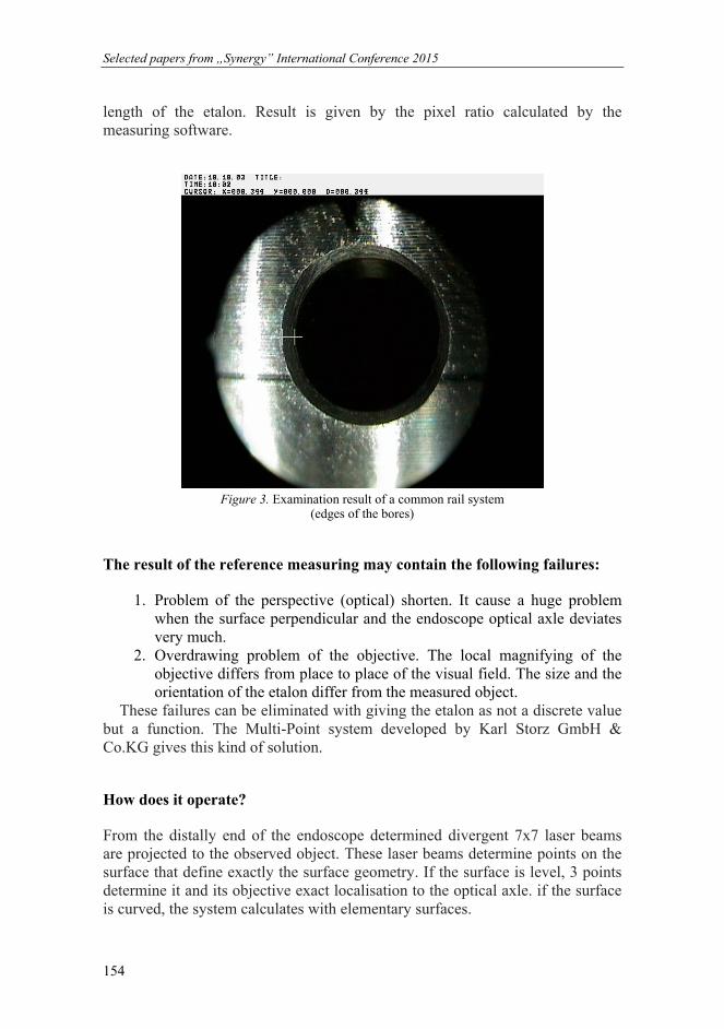
Selected papers from „Synergy” International Conference 2015
TÁMOP-4.2.1.B-11/2/KMR-2011-003 154
length of the etalon. Result is given by the pixel ratio calculated by the measuring software.
Figure 3. Examination result of a common rail system
(edges of the bores)
The result of the reference measuring may contain the following failures:
1. Problem of the perspective (optical) shorten. It cause a huge problem when the surface perpendicular and the endoscope optical axle deviates very much.
2. Overdrawing problem of the objective. The local magnifying of the objective differs from place to place of the visual field. The size and the orientation of the etalon differ from the measured object.
These failures can be eliminated with giving the etalon as not a discrete value but a function. The Multi-Point system developed by Karl Storz GmbH & Co.KG gives this kind of solution.
How does it operate?
From the distally end of the endoscope determined divergent 7x7 laser beams are projected to the observed object. These laser beams determine points on the surface that define exactly the surface geometry. If the surface is level, 3 points determine it and its objective exact localisation to the optical axle. if the surface is curved, the system calculates with elementary surfaces.
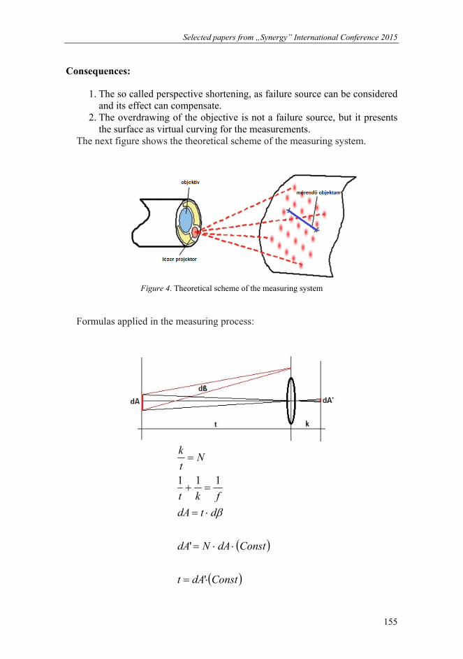
Selected papers from „Synergy” International Conference 2015
TÁMOP-4.2.1.B-11/2/KMR-2011-003 155
Consequences:
1. The so called perspective shortening, as failure source can be considered and its effect can compensate.
2. The overdrawing of the objective is not a failure source, but it presents the surface as virtual curving for the measurements.
The next figure shows the theoretical scheme of the measuring system.
Figure 4. Theoretical scheme of the measuring system
Formulas applied in the measuring process:
ConstdAt
ConstdANdA
dtdA
fkt
Nt
k
'
'
111

Selected papers from „Synergy” International Conference 2015
TÁMOP-4.2.1.B-11/2/KMR-2011-003 156
Considering the above mentioned formulas it can be sad that section determined by the pixels is definitive to the length size of the flat. Because of this measuring the length is possible in the case of a broken curve as well.
Furthermore the distance of a given point from a line can be determined. The perimeter and the area of a curve (rounded by lines) can also be determined. The method can be used for depth measuring as well.
As an example the result of the analysis performed by a Karl Storz GmbH & CO.KG produced videoscope is introduced below.
Figure 5. Measuring the length, broken edge size, and the peeling on a turbine blade
As a result of our investigation we can said that an endoscope can function as a gage or a measure as well depending on the utilisation.

Selected papers from „Synergy” International Conference 2015
TÁMOP-4.2.1.B-11/2/KMR-2011-003 157
Application of bézier surface algorithm for distribution of daylight
D. PÁLEŠ1, M. BALKOVÁ2, J. RÉDL1, J. MAGA3, G. KALÁCSKA4
1Department of Machine Design, Faculty of Engineering, Slovak University of Agriculture in Nitra, Slovakia 2Department of Buildings, Faculty of Engineering, Slovak University of Agriculture in Nitra, Slovakia
3Department of Machines and Production Systems, Faculty of Engineering, Slovak University of Agriculture in Nitra, Slovakia
4Institute of Industrial Technologies, Mechanical Engineering Faculty,
Szent István University, Gödöllő, Hungary
Abstract
In the area of building have been measured in 55 control points values of daylight. We put over these points Bézier surface, which a brief theoretical interpretation we supply. On a simple example of 3 x 3 control points we debugged program for generation of basis functions as well as for the creation of the surface itself. In that manner formed process we applied to 5 x 11 measured points of daylight in the building. Discrete values of measurements were by Bézier surface smoothed and its corner values constitute the edge measurement points. The resulting surface allowed to take into account the irregular distribution of measured points in the plan.
Keywords
Approximation, mathematical modelling, surface fitting.
1. Introduction
In the present, computer use creates the requirement definition of the geometry, which is easy to handle without the need for complex analytical expressions. This condition very well satisfy Bézier curves [4], [6], B-spline [5] and NURBS curves [7]. Analogously to express curves can be quite flexible expression of surfaces like referred to as Bézier and B-spline surfaces. The article deals with first of all Bézier surface and in addition to its relatively detailed description we practically apply definiton to the values of daylight in the building.

Selected papers from „Synergy” International Conference 2015
TÁMOP-4.2.1.B-11/2/KMR-2011-003 158
2. Material and methods
Bézier surface Bézier surface [7] is defined by two-dimensional set of control points Pi,j, where i is between 0 to m and j is between 0 to n. We receive so (m+1) rows and (n+1) columns of control points and the control point in the i-th row and in the j-th column is designated as Pi,j. Overall this therefore gives (m+1) . (n+1) control points. Formula for Bézier surface has form
m n
m,i n, j i, ji 0 j 0
P u, v B u B (v) P
(1)
where Bm,i(u) and Bn,j(v) are i-th and j-th Bézier basis function in the direction u and in the direction v. Just as for Bézier curve are these functions defined
i m im,i
mB u .u .(1 u)
i
j n jn, j
nB v .v .(1 v)
j
(2)
Due to the fact that Bm,i(u) and Bn,j(v) have order m, respectively n, Bézier
surface has order (m,n). Set of control points is sometimes called Bézier net or control net. Parameters u and v take values between 0 to 1 and consequently Bézier surface transforms unit square on area surface.
Important properties of Bézier surface 1st Surface P(u,v) (1) passes through the control points in four corners of control net P0,0, Pm,0, Pm,n a P0,n. Really true that P(0,0) = P0,0 , P(1,0) = Pm,0 , P(0,1) = P0,n, P1,1 = Pm,n.
2nd Product Bm,i(u) Bn,j(v) is nonnegative for all m, n, i, j, for u and v between 0 to 1.
3rd Sum of all Bm,i(u) Bn,j(v) is 1 for all u and v between 0 to 1.
m n
m,i n, ji 0 j 0
B u B (v) 1
(3)

Selected papers from „Synergy” International Conference 2015
TÁMOP-4.2.1.B-11/2/KMR-2011-003 159
4th Bézier surface is located in convex hull of its control points. P(u,v) is linear combination of all control points with positive coefficients which sum is equal one, properties 2nd a 3rd.
5th Bézier surface is affine invariance, when we want aply affine transformation on Bézier surface, just use it for all control points and surface arising from transformed points is identical as for the transformation of original Bézier surface.
Basis functions Basis functions of Bézier surface (1) are the coefficients of the control points indicated as (2). The definition (1) shows that the two-dimensional basis functions are products of two one-dimensional basis functions. The algorithm for their generation is presented by relationship (4). In Figure 1 are drawn basis functions for m = 2 and n = 2, that is, for example, the top picture on the left shows the control point P0,0, which has a two-dimensional basis functions given as multiplication B2,0(u) in the direction u and B2,0(v) in the direction v. Analogously are constructed nine basis functions following lines for control points P0,0, P0,1, P0,2, P1,0, P1,1, P1,2, P2,0, P2,1, P2,2.
Bézier surface is set up always as by multiplying two curves. Basis functions of the first curve are multiplied by basis functions of the second curve, generating so basis functions for a two-dimensional set of control points. Like this constructed surfaces are sometimes called surfaces of the tensor product.
(4)

F
igur
e 1.
Bas
is fu
nctio
ns o
f Béz
ier s
urfa
ce fo
r m=2
and
n=2
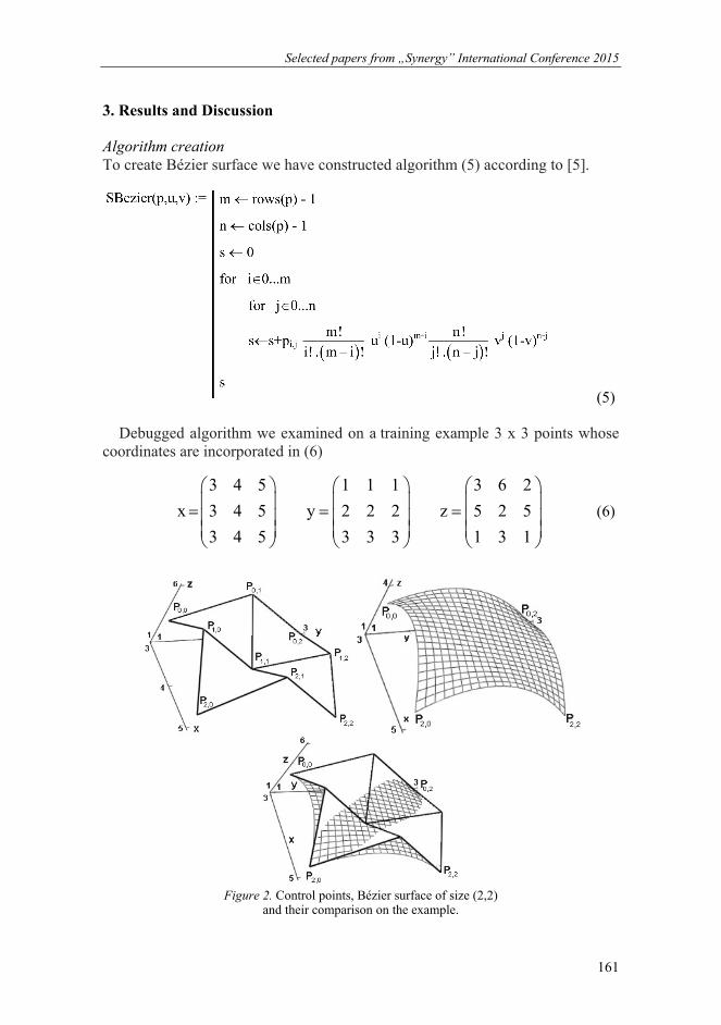
Selected papers from „Synergy” International Conference 2015
TÁMOP-4.2.1.B-11/2/KMR-2011-003 161
3. Results and Discussion
Algorithm creation To create Bézier surface we have constructed algorithm (5) according to [5].
(5)
Debugged algorithm we examined on a training example 3 x 3 points whose coordinates are incorporated in (6)
3 4 5 1 1 1 3 6 2
x 3 4 5 y 2 2 2 z 5 2 5
3 4 5 3 3 3 1 3 1
(6)
Figure 2. Control points, Bézier surface of size (2,2)
and their comparison on the example.
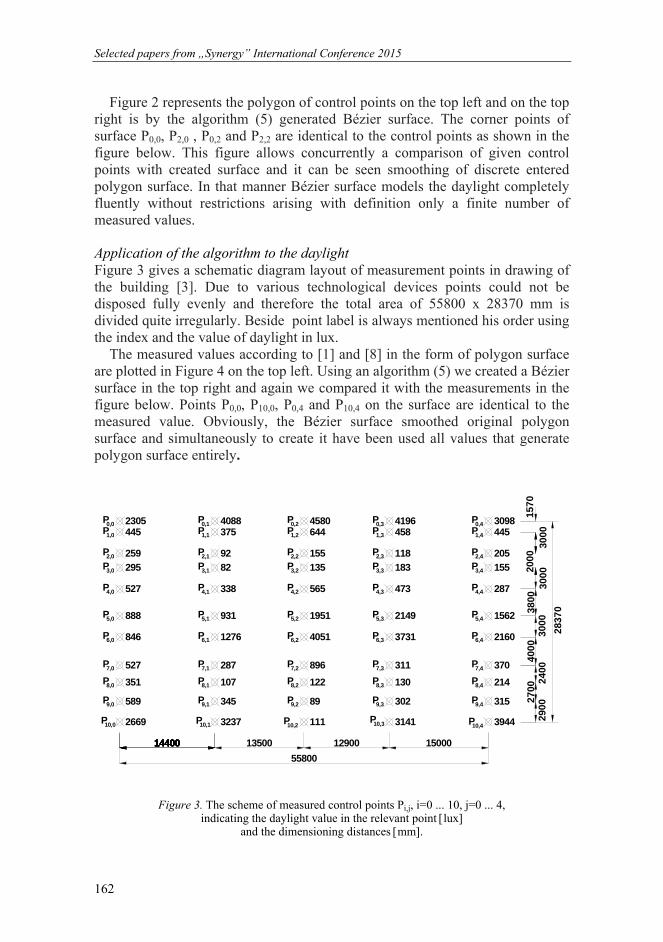
Selected papers from „Synergy” International Conference 2015
TÁMOP-4.2.1.B-11/2/KMR-2011-003 162
Figure 2 represents the polygon of control points on the top left and on the top right is by the algorithm (5) generated Bézier surface. The corner points of surface P0,0, P2,0 , P0,2 and P2,2 are identical to the control points as shown in the figure below. This figure allows concurrently a comparison of given control points with created surface and it can be seen smoothing of discrete entered polygon surface. In that manner Bézier surface models the daylight completely fluently without restrictions arising with definition only a finite number of measured values.
Application of the algorithm to the daylight Figure 3 gives a schematic diagram layout of measurement points in drawing of the building [3]. Due to various technological devices points could not be disposed fully evenly and therefore the total area of 55800 x 28370 mm is divided quite irregularly. Beside point label is always mentioned his order using the index and the value of daylight in lux.
The measured values according to [1] and [8] in the form of polygon surface are plotted in Figure 4 on the top left. Using an algorithm (5) we created a Bézier surface in the top right and again we compared it with the measurements in the figure below. Points P0,0, P10,0, P0,4 and P10,4 on the surface are identical to the measured value. Obviously, the Bézier surface smoothed original polygon surface and simultaneously to create it have been used all values that generate polygon surface entirely.
P 23050,0P 4451,0
P 2592,0
P 2953,0
P 5274,0
P 8885,0
P 8466,0
P 5277,0
P 3518,0
P 5899,0
P 266910,0
P 40880,1P 3751,1
P 922,1
P 823,1
P 3384,1
P 9315,1
P 12766,1
P 2877,1
P 1078,1
P 3459,1
P 323710,1
P 45800,2P 6441,2
P 1552,2
P 1353,2
P 5654,2
P 19515,2
P 40516,2
P 8967,2
P 1228,2
P 899,2
P 11110,2
P 41960,3P 4581,3
P 1182,3
P 1833,3
P 4734,3
P 21495,3
P 37316,3
P 3117,3
P 1308,3
P 3029,3
P 314110,3
P 30980,4P 4451,4
P 2052,4
P 1553,4
P 2874,4
P 15625,4
P 21606,4
P 3707,4
P 2148,4
P 3159,4
P 394410,4
1570
3000
2000
3000
3800
3000
4000
2900
14400 13500 12900 15000
55800
2837
0
14400144001440014400
2400
2700
Figure 3. The scheme of measured control points Pi,j, i=0 ... 10, j=0 ... 4, indicating the daylight value in the relevant point lux
and the dimensioning distances mm.

Selected papers from „Synergy” International Conference 2015
TÁMOP-4.2.1.B-11/2/KMR-2011-003 163
Figure 4. Measured values of daylight in the control points,
Bézier surface approximated by the control points and their mutual comparison.
Conclusion
Bézier surface excels for its simple definition and easy application to set the spatial location of points. As seen in Figure 4, the corner points of the surface are identical to the edge points of the intended space polygon and other given discrete points of the polygon the surface makes smooth and continuous. We created an algorithm for the creation of basis functions of Bézier surface and for drawing the surface itself. This can be applied to any spatial points assignment and use it for the other technical issue .
References
[1] Journal of the Ministry of Health of Slovak Republic, 29th November 2013. Professional guideline, which establishes the procedure for the measurement and evaluation of lighting, Section 15, pp. 210-249.
[2] MEUNG J. KIM 2014. Geometric modeling, Department of Mechanical Engineering, Northern Illinois University, DeKalb, URL: http://www.ceet.niu.edu/faculty/kim/mee430/chapter-5.pdf
Selected papers from „Synergy” International Conference 2015
TÁMOP-4.2.1.B-11/2/KMR-2011-003 164
[3] POGRAN Š. – BIEDA W. – GÁLIK R. – LENDELOVÁ J. - ŠVENKOVÁ J. 2011. Kvalita vnútorného prostredia ustajňovacích objektov, 1st ed. Nitra: SPU, 242 pp.,
ISBN 978-80-552-0557-1. [4] PÁLEŠ D. – RÉDL J. 2014. Beziér curve and its application, Mathematics in
education, research and application, Slovak university of agriculture, Faculty of economics and management, Department of mathematics, Nitra, Vol. 1, No. 2, 49-55, ISSN 2453-6881.
[5] PÁLEŠ D., VÁLIKOVÁ V., ANTL J., TÓTH F., 2015. APPROXIMATION OF VEHICLE TRAJECTORY WITH THE B-SPLINE CURVE, ACTA TECHNOLOGICA AGRICULTURAE, IN PRINT.
[6] RÉDL J. - PÁLEŠ D. - MAGA J. - KALÁCSKA G. - VÁLIKOVÁ V. - ANTL J. 2014. Technical Curve Approximation, Mechanical engineering letters, Szent István University, Gödöllö, Vol. 11 (2014), pp. 186-191, ISSN 2060-3789.
[7] SHENE, C.-K. 2014. Introduction to Computing with Geometric Notes, Department of Computer Science, Michigan Technological University. URL: http://www.cs.mtu.edu/~shene/COURSES/cs3621/NOTES/
[8] Slovak Technical Norm, STN 36 0088, 1993. Lighting in agricultural establishments.