research article stabilization of inﬁnitesimally rigid

June 18, 2008 16:28 International Journal of Control KriBroFra

International Journal of ControlVol. 00, No. 00, Month 200x, 1–25

RESEARCH ARTICLE

Stabilization of Infinitesimally Rigid Formations of Multi-Robot Networks

Laura Kricka, Mireille E. Brouckea∗ , and Bruce A. Francisa

aEdward S. Rogers Sr. Department of Electrical and Computer Engineering, University of Toronto,

Toronto, ON M5S 3G4, Canada;

(June 18, 2008)

This paper considers the design of a formation control for multivehicle systems that uses only local information.The control is derived from a potential function based on an undirected infinitesimally rigid graph that specifiesthe target formation. A potential function is obtained from the graph, from which a gradient control is derived.Under this controller the target formation becomes a manifold of equilibria for the multivehicle system. Itis shown that infinitesimal rigidity is a sufficient condition for local asymptotical stability of the equilibriummanifold. A complete study of the stability of the regular polygon formation is presented and results for directedgraphs are presented as well. Finally, the controller is validated experimentally.

Keywords: Cooperative control, multiagent formations, graph rigidity.

1 Introduction

This paper considers distributed control of systems of agents that are interconnected dynamicallyor have a common objective, and where control is local, with the possible exception of high-level intermittent centralized supervision. Undoubtedly these kinds of systems will become moreand more prevalent as embedded hardware evolves. An interesting example and area of ongoingresearch is the control of a group of autonomous mobile robots, ideally without centralized controlor a global coordinate system, so that they work cooperatively to accomplish a common goal.The aims of such research are to achieve systems that are scalable, modular, and robust. Thesegoals are similar to those of sensor networks—networks of inexpensive devices with computing,communications, and sensing capabilities. Such devices are currently commercially available andinclude products like the Intel Mote. A natural extension of sensor networks would be to addsimple actuators to the sensors to make them mobile, and then to adapt the network configurationto optimize network coverage.

If global coordinates are known and there is an omniscient supervisor, these problems areroutine: Each robot could be stabilized to its assigned location. The current technology to provideglobal coordinates is the Global Positioning System (GPS). However, the use of GPS for positioninformation in multi-agent applications has several problems: The precision of GPS depends onthe number of satellites currently visible; during periods of dense cloud cover, in urban areas,and under dense vegetation, there may be no line of sight between the receiver and the GPSsatellite. These problems in obtaining global coordinates make it natural to study decentralizedcontrol.

The simplest problem is stabilizing the robots to a common location, frequently called therendezvous problem. Many different techniques have been used to solve this problem, for example,cyclic pursuit (Marshall et al. 2004) and the circumcentre law (Cortes et al. 2004). The solutionin Lin et al. (2004) involves asynchronous stop-and-go cycles. Goldenberg et al. (2004) considers

∗Corresponding author. Email: [email protected]: 0020-7179 print/ISSN 1366-5820 onlinec© 200x Taylor & FrancisDOI: 10.1080/0020717YYxxxxxxxxhttp://www.informaworld.com


2

a problem of decentralized, self organizing communication nodes with mobility. In this case, themobility is used to improve communication performance. Another possible goal for mobile sensornetworks is to optimize sensor placement by minimizing a cost function. This type of problemis studied in Cortes et al. (2004).

An interesting approach to formation control is that of Olfati-Saber (2006). The robots arepoint masses (double integrators) with limited vision, and he proposes using rigid graph theoryto define the formation; he also proposes a gradient control law involving prescribed distances.The limitation is that the network is not homogeneous—special so-called γ-agents are requiredto achieve flocking.

Finally Smith et al. (2006) considers the problem of achieving polygon formations withoutglobal coordinates, but the solution is complete only for three robots.

The starting point for our paper is Olfati-Saber and Murray (2002). Following that paper, weuse graphs to define formations, but instead of global rigidity we use infinitesimal rigidity andinstead of the double integrator model we use the simpler single integrator (kinematic point).More substantially, our stability analysis is complete whereas, being a conference paper, Olfati-Saber and Murray (2002) provides only a sketch. In particular, Olfati-Saber and Murray (2002)has no topological analysis of the equilibrium set and does not note that the equilibrium set is notcompact. Moreover, Olfati-Saber and Murray (2002) uses a LaSalle argument to prove stability,but since the equilibrium set is not compact, this is open to question. Furthermore, Olfati-Saberand Murray (2002) does not address if the trajectories have a limit on the equilibrium set.Additional, more technical remarks follow in Remark 2.

The first contribution of the paper is a decentralized gradient control law to stabilize a groupof point mass robots to any formation corresponding to an infinitesimally rigid framework. Acomplete stability analysis is provided in Section 5. Regular polygon formations are studied inSection 6, where it is shown that the conditions of our theory can be applied to this case. Adrawback of the proposed controller is that it requires two-way communication between robots:if robot i can sense robot j, then robot j can sense robot i. In Section 7 we address the formationstabilization problem under the constraint that, instead, the sensor graph is directed. It is shownthat when the formation graph is constructed using a Henneberg insertion procedure to achievean infinitesimally rigid framework, the foregoing stability analysis for undirected graphs stillapplies.

Before presenting the main results in Sections 5, 6, and 7, we first give an overview of conceptsfrom graph theory and particularly graph rigidity theory in Section 2. In Section 3 the stabiliza-tion problem is formulated and in Section 4 the gradient control law is proposed and some of itsproperties are analyzed.

2 Background

2.1 Notation

We denote the Jacobian of a function f : Rn → Rm evaluated at a point x as Jf (x). In thespecial case when f : Rn → R, the Jacobian of f is the gradient of f and we denote it by ∇f(x).Occasionally for convenience during calculations of the Jacobian, the notation ∂

∂xwill be used

to represent Jf (x) = ∂∂xf(x).

2.2 Graph Theory

A directed graph G = (V,E) is a pair consisting of a finite set of vertices V := {1, . . . , n} anda set of edges E ⊂ V × V . We assume the edges are ordered; that is E = {1, . . . ,m}, wherem ∈ {1, . . . , n(n−1)}. We exclude the possibility of self loops. An undirected graph is a directedgraph such that if there is an edge ei from vertex j to vertex k, then there is also an edge el fromvertex k to vertex j. For undirected graphs, we omit the arrows in the pictorial representation


3

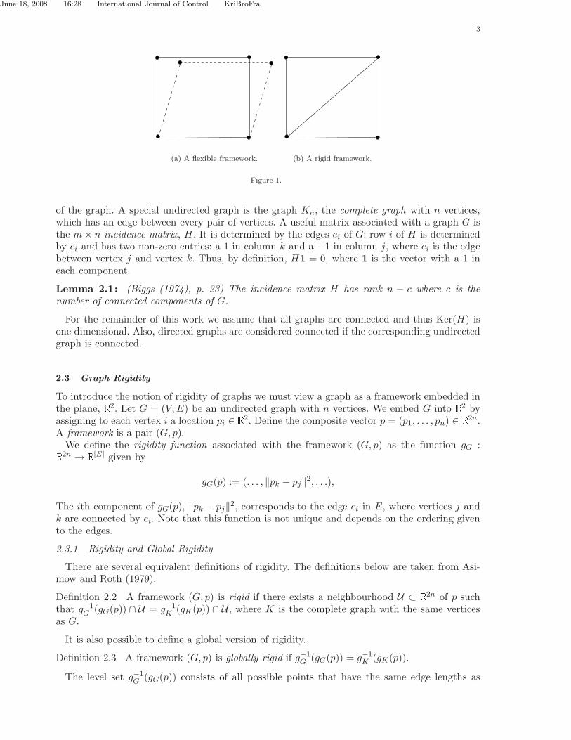
(a) A flexible framework. (b) A rigid framework.

Figure 1.

of the graph. A special undirected graph is the graph Kn, the complete graph with n vertices,which has an edge between every pair of vertices. A useful matrix associated with a graph G isthe m× n incidence matrix, H. It is determined by the edges ei of G: row i of H is determinedby ei and has two non-zero entries: a 1 in column k and a −1 in column j, where ei is the edgebetween vertex j and vertex k. Thus, by definition, H1 = 0, where 1 is the vector with a 1 ineach component.

Lemma 2.1: (Biggs (1974), p. 23) The incidence matrix H has rank n − c where c is thenumber of connected components of G.

For the remainder of this work we assume that all graphs are connected and thus Ker(H) isone dimensional. Also, directed graphs are considered connected if the corresponding undirectedgraph is connected.

2.3 Graph Rigidity

To introduce the notion of rigidity of graphs we must view a graph as a framework embedded inthe plane, R2. Let G = (V,E) be an undirected graph with n vertices. We embed G into R2 byassigning to each vertex i a location pi ∈ R2. Define the composite vector p = (p1, . . . , pn) ∈ R2n.A framework is a pair (G, p).

We define the rigidity function associated with the framework (G, p) as the function gG :R2n → R|E| given by

gG(p) := (. . . , ‖pk − pj‖2, . . .),

The ith component of gG(p), ‖pk − pj‖2, corresponds to the edge ei in E, where vertices j andk are connected by ei. Note that this function is not unique and depends on the ordering givento the edges.

2.3.1 Rigidity and Global Rigidity

There are several equivalent definitions of rigidity. The definitions below are taken from Asi-mow and Roth (1979).

Definition 2.2 A framework (G, p) is rigid if there exists a neighbourhood U ⊂ R2n of p suchthat g−1

G (gG(p)) ∩ U = g−1K (gK(p)) ∩ U , where K is the complete graph with the same vertices

as G.

It is also possible to define a global version of rigidity.

Definition 2.3 A framework (G, p) is globally rigid if g−1G (gG(p)) = g−1

K (gK(p)).

The level set g−1G (gG(p)) consists of all possible points that have the same edge lengths as


4

t

1 4

32

(a)

4 1

3 2

(b)

1 4

3

2

(c)

1

2

4

3

(d)

Figure 2. Possible embeddings of a graph with four vertices.

the framework (G, p). For the complete graph K the set g−1K (gK(p)) consists of points related

by rotations and translations, i.e., rigid body motions, of the framework (K, p). We concludethat a graph G is rigid if the level set g−1

G (gG(p)) in a neighbourhood of p contains only pointscorresponding to rotations and translations of the formation at p. For example, consider theframework in Figure 1(a). It is possible to translate the top two points of the framework whilemaintaining the four edge lengths to obtain a graph that is not isomorphic to the original graph;the lengths of the diagonals change, so the framework is not rigid. If we add one more edge tothe framework we obtain the framework in Figure 1(b). For this framework, every perturbationof the vertices that maintains the edge lengths is isomorphic to the original framework, so thisgraph is rigid.

To illustrate the difference between rigidity and global rigidity consider the example of a graphwith four vertices and

gG(z) =

||z1 − z2||2||z2 − z3||2||z3 − z4||2||z4 − z1||2||z3 − z1||2

and d =

122

122

5

. (1)

There are four possible distinct frameworks for this graph, as shown in Figure 2. Each of theseframeworks is rigid, but not globally rigid, since solutions z of gG(z) = d can correspond toeither of two different complete graphs (when part of the graph is flipped over). Instead, if thegraph were also globally rigid, then gG(z) = d would have solutions corresponding to only onecomplete graph and only two distinct embeddings. These two embeddings would be reflectionsof one another. Figure 3 illustrates this case.

2.3.2 Infinitesimal Rigidity

We refer to the matrix JgG(p) as the rigidity matrix of (G, p). The rigidity matrix is useful in

defining some other concepts related to graph rigidity. (Note that we consider graphs with atleast two vertices; otherwise the concepts introduced here will not be well-defined).

Definition 2.4 A point p is a regular point of the graph G with n vertices if

rankJgG(p) = max

{

rankJgG(q) | q ∈ R2n

}

.

In Figure 4(a) we see that the graph K3 is embedded at a regular point. Instead, Figure 4(b)shows the graph K3 embedded at a point that is not regular.

The idea of infinitesimal rigidity is to allow the vertices to move infinitesimally, while keepingthe rigidity function constant up to first order. Let δp be an infinitesimal motion of the framework


5

1

4 3

2

(a)

43

2 1

(b)

Figure 3. The two possible embeddings of the graph K4. Note that Figure 3(a) is a reflection of Figure 3(b).

(a) A rigid andinfinitesimally rigidframework.

(b) A rigid but notinfinitesimally rigidframework.

(c) A rigid but not infinitesimally rigidframework.

Figure 4.

(G, p). Then the Taylor series expansion of gG about p is

gG(p+ δp) = gG(p) + JgG(p)δp + higher order terms.

The rigidity function remains constant up to first order when JgG(p)δp = 0, that is, when δp

belongs to KerJgG(p). The dimension of this kernel is at least 3 because gG(p) will not change if

p is perturbed by a rigid body motion. Infinitesimal rigidity is when the dimension of the kernelis not larger than 3.

Definition 2.5 (Asimow and Roth (1979) ) A framework (G, p) is infinitesimally rigid in theplane if dim(KerJgG

(p)) = 3, or equivalently if

rankJgG(p) = 2n− 3.

If a framework is infinitesimally rigid, then it is also rigid. The converse is not true. Thefollowing theorem outlines when rigidity and infinitesimal rigidity are equivalent.

Theorem 2.6 : ( Asimow and Roth (1979) ) A framework (G, p) is infinitesimally rigid if andonly if (G, p) is rigid and p is a regular point.

Observe that for a graph to be infinitesimally rigid in the plane it must have at least 2n − 3edges. If it has exactly 2n − 3 edges, we say that the graph is minimally rigid.


6

The two different embeddings of K3 shown in Figure 4(a)-(b) illustrate some of the rigidityproperties. Both frameworks shown are embeddings of the complete graph. They are both rigidand globally rigid. The framework shown in Figure 4(a) is also infinitesimally rigid. If we checkthe rigidity matrix for any point p where the vertices are not collinear we will find it has rank3. The framework in Figure 4(b) is not infinitesimally rigid. We can check this using the rigiditymatrix. Let the embedding of the points in the plane be z1 = (0, 0), z2 = (0, 1), z3 = (0, 2). Therigidity function for this graph is

gG(z) =

||z1 − z2||2||z2 − z3||2||z3 − z1||2

.

Then

JgG(p) = 2

zT1 − zT2 zT2 − zT1 00 zT2 − zT3 zT3 − zT2

zT1 − zT3 0 zT3 − zT1

.

If we check the rank at a collinear point p we obtain rank JgG(p) = 2 < 2n − 3. As the rigidity

matrix does not have maximal rank, p is not a regular point; consistent with Theorem 2.6, arigid framework is not infinitesimally rigid at a non-regular point.

Typically, frameworks that are rigid but fail to be infinitesimally rigid have collinear or paralleledges. For instance the graph in Figure 4(c) is rigid but not infinitesimally rigid because theframework could undergo an infinitesimal distortion by perturbing the top link horizontally; thetwo triangles would then rotate infinitesimally, and the middle link rotate infinitesimally.

2.3.3 Constructing Rigid Graphs

Any collection of n points in the plane can be connected to form a rigid framework. Forinstance, we can connect the points using Kn, the complete graph. In subsequent sections wewill find that the complexity of the control is proportional to the number of edges in a certaingraph. Using the complete graph will result in a design that is not scalable: as the number ofconnections needed for n vertices is n2−n

2 . Instead, from the definition of infinitesimal rigidity,we see a graph can be infinitesimally rigid with only 2n− 3 edges. For n > 3, this is fewer edgesthan the complete graph.

A rigid graph can be constructed for any embedding of n vertices in the plane in the followingmanner. First, number all the vertices. Next, add an edge between vertex 1 and vertex 2. If weconsider the framework formed by vertex 1 and vertex 2, we see that it is the complete graph, andthus is rigid. The remaining vertices are added in order to the connected component of the graph,connecting each one to the previously connected graph structure by two edges. This operationis sometimes referred to as a Henneberg insertion, Bereg (2005). This type of insertion preservesgraph rigidity because each vertex has two degrees of freedom. By connecting the vertex to thepreviously connected graph structure by two edges the position of the vertex is subject to twoconstraints, removing both degrees of freedom. This procedure results in a framework that is notonly rigid but also minimally rigid; that is, if we remove any edge the framework is no longerrigid.

3 Problem Formulation

Consider n robots in the plane, R2. The robots are wheeled vehicles with sensors that allow themto measure the relative positions of some of the other vehicles. Such data can be obtained usinga camera or a radar system. The simplest model for a wheeled vehicle is the kinematic unicycle.To simplify the analysis, using a standard procedure we assume the unicycle model has been


7

feedback linearized about a point some distance in front of each unicycle. The robots then havea point kinematic model given by the differential equation

zi = ui, i ∈ {1, . . . , n} (2)

where zi = (xi, yi) ∈ R2 is the location of the ith robot in the plane and ui ∈ R2 is the controlinput for the ith robot. We define the composite state vector z = (z1, . . . , zn), as a vector in(R2)n.

The target formation is described by a pair {G, d} where G is an undirected graph whosevertices represent the robots, and vector d ∈ Rm specifies m target lengths for the edges. Werefer to G as the formation graph. The robots achieve the target formation when the length ofedge i is the prescribed distance di > 0.

Associated with the formation control problem is also a sensor graph that describes the sensordata seen by each robot in the closed-loop system. The sensor graph is a directed graph witheach robot represented as a vertex in the graph. Given a controller u, if ui is a function of zj ,then the sensor graph will have an edge from vertex i to vertex j. Also, we require that thecontrol be a function only of relative measurements. For example if robot 1 can see robots 3 and5, then the measurements available to robot 1 are z3 − z1 and z5 − z1, and u1 can be a functionof these two measurements. We refer to this as a distributed control law. We have the followingproblem.

Problem 3.1 Given the system (2) and a target formation {G, d} such that g−1G (d) 6= ∅ and such

that the framework (G, p) is infinitesimally rigid at each p ∈ g−1G (d), design a distributed control

law u whose sensor graph is G with the following two properties: (1) every p ∈ g−1G (d) is a stable

equilibrium of the closed-loop system, and (2) for every initial condition in a neighborhood ofg−1G (d), the closed-loop trajectory tends to a unique equilibrium point in g−1

G (d).

4 Gradient Control

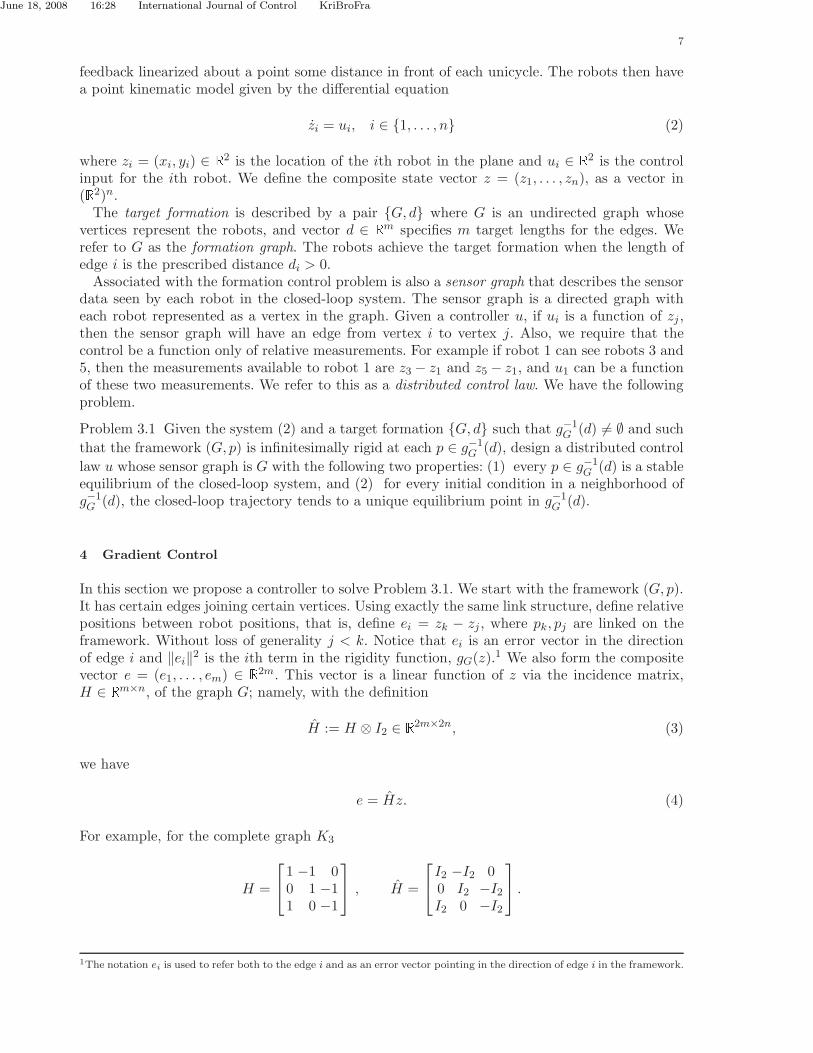
In this section we propose a controller to solve Problem 3.1. We start with the framework (G, p).It has certain edges joining certain vertices. Using exactly the same link structure, define relativepositions between robot positions, that is, define ei = zk − zj , where pk, pj are linked on theframework. Without loss of generality j < k. Notice that ei is an error vector in the directionof edge i and ‖ei‖2 is the ith term in the rigidity function, gG(z).1 We also form the compositevector e = (e1, . . . , em) ∈ R2m. This vector is a linear function of z via the incidence matrix,H ∈ Rm×n, of the graph G; namely, with the definition

H := H ⊗ I2 ∈ R2m×2n, (3)

we have

e = Hz. (4)

For example, for the complete graph K3

H =

1 −1 00 1 −11 0 −1

, H =

I2 −I2 00 I2 −I2I2 0 −I2

.

1The notation ei is used to refer both to the edge i and as an error vector pointing in the direction of edge i in the framework.


8

4.1 Special Case: The Rendezvous Problem

The rendezvous problem is the special case of the formation stabilization problem where d = 0.If L denotes the Laplacian of the graph G, and L = L⊗ I2, a linear solution to this problem isto let u = −Lz, and then

z = −Lz. (5)

If G is connected, then 0 is a simple eigenvalue of L (Frobenius’ theorem) and rendezvous follows.Recall that if G is undirected, the Laplacian is a symmetric matrix. Furthermore, the Laplacianand incidence matrices are related by L = HT H ( Proposition 4.8 in Biggs (1974)). Thus

Lz =

[

∇(

1

2‖Hz‖2

)]T

.

The function 12‖Hz‖2 is positive semidefinite. So the control law in (5) is not only a gradient

control law, as all symmetric linear controls are, but a gradient control law for a positive semidef-inite potential function. This suggests considering a gradient control of a positive semidefinitepotential function for the general formation stabilization problem.

4.2 Control Law

We now consider a gradient control law to maintain an arbitrary formation of robots. First wedefine a vector norm function v : R2m → Rm:

v(e) = (||e1||2, . . . , ||em||2).

Then using (4) we define g : R2n → Rm by

g(z) := v(e) = v(Hz). (6)

Notice that g(z) is precisely the rigidity function gG(z) (henceforth the subscript is dropped).As a candidate potential function, we consider the positive definite function of g(z) − d

φ(z) =1

2‖g(z) − d‖2. (7)

Note that φ(z) is a positive semidefinite function of z and φ(z) = 0 if and only if g(z) = d. Wepropose the gradient control

u = −(∇φ(z))T .

It follows from (2) and applying the chain rule to (7) that

z = − (Jg(z))T (g(z) − d)

= −HTJv(Hz)T (v(Hz) − d)

= −HTJv(e)T (v(e) − d) , (8)


9

where the Jacobian of v is

Jv(e) = 2

eT1 . . . 0...

. . ....

0 . . . eTm

. (9)

It is evident that the control is a function only of the relative measurements, as required by theproblem specification. More specifically, the control law for each robot is

zi = ui = −∑

j∈{edges leaving i}

1

2(‖ej‖2 − dj)ej , (10)

consistent with the problem specification that the sensor graph be identically the same as theformation graph. In the following lemma we list further interesting properties of the controlledsystem (8). Proofs are omitted since the results are easily verified.

Lemma 4.1:

(1) The centroid z◦ := 1n

∑ni=1 zi is stationary: z◦ = 0.

(2) The control in (8) is independent of the system of global coordinates; that is, for everyw ∈ R2,

∇φ(z + 1⊗ w) = ∇φ(z),

and for every orthogonal matrix R ∈ R2×2,

∇φ(z)RT = ∇φ(Rz),

where R = In ⊗R.(3) Define the collinear set C := {z ∈ R2n | (∃w ∈ R2)(∀i) (zi − z◦) ∈ span(w)}. Then C isinvariant under (8).

4.3 Coordinate Transformation

In this section we perform a coordinate transformation that separates the centroid dynamicsfrom the remaining dynamics of the system. This will be particularly helpful in several of theanalyses that follow.

Let P be an orthonormal matrix whose first two rows are 1n1T ⊗ I2. Then consider the trans-

formation

z =

[

z◦

z

]

= Pz,

where z◦ is the centroid of z, as discussed in Lemma 4.1. Define

H = HP−1. (11)

From the definition of H it is clear that Hz = Hz. We now solve for the z dynamics, obtaining

˙z = P z

= −HT(

Jv(Hz))T

(v(Hz) − d). (12)


10

So, ˙z = −[∇φ(z)]T , where φ(z) = 12‖v(Hz) − d‖2.

Next we consider an interesting property of H. Note that since the first two columns of P−1

are in Ker(H), H has the form[

0 H]

. From Lemma 2.1, dim(Ker(H)) = 1, so dim(Ker(H)) = 2.

Then by using the dimension of Ker(H), the invertibility of P , and the block form of H, weknow that Ker(H) = {0}.

Now expand Hz:

Hz =[

0 H]

[

z◦

z

]

= Hz . (13)

So the z dynamics from (12) can be rewritten using (11) and (13) as

[

z◦

z

]

= −[

0

HT

]

(

Jv(Hz))T

(v(Hz) − d). (14)

If we define φ(z) := 12‖v(Hz) − d‖2 then z = −(∇φ(z))T , and so z is again a gradient system.

4.4 Existence and Uniqueness of Solutions

Using the coordinate transformation of the previous section it is possible to confirm existenceand uniqueness of solutions in the (z◦, z) coordinates. The z◦ dynamics and the z dynamics aredecoupled, so we can analyze solutions independently. From Lemma 4.1 we know that z◦ = 0so solutions trivially exist for all time. The dynamics of z evolve according to a gradient systemwith potential function φ(z), a radially unbounded function. Consider the sublevel set

Ua := { z ∈ R2n−2 | φ(z) ≤ a}

and define a Lyapunov function to be V (z) := φ(z). Denote by −L∇φV (z) the Lie derivative of

−∇φ(z)T . For the z system −L∇φV (z) = −‖∇φ(z)‖2, a negative semidefinite function. So the

set Ua is invariant for any a > 0. Furthermore, on the set Ua, the function ∇φ(z) is Lipschitzcontinuous. Therefore, solutions z(t) exist for all time and are unique, for all initial conditionsstarting in Ua.

4.5 Simulations

In this section we simulate the control law (8) for two graphs to gain some intuitive understandingabout the controller’s behaviour.

Example 4.2 Consider the complete graph K4 with the rigidity function

g(z) =

||z1 − z2||2||z2 − z3||2||z3 − z4||2||z4 − z1||2||z3 − z1||2||z4 − z2||2

and d =

122

122

55

.

This graph is globally rigid and a point p in g−1(d) forms a rectangle with side lengths 1 and 2.Figure 5(a) shows the robots achieve the rectangle formation under the control (8). Figure 5(b)is for a different initial condition and here the final formation is a “twisted” rectangle; thisequilibrium is not in g−1(d). Also, if the robots are initialized on a collinear configuration, then


11

6 8 10 12 14 16

4

5

6

7

8

9

10

11

12

(a)

5 6 7 8 9 10 11 12 13 145.5

6

6.5

7

7.5

8

8.5

9

9.5

10

10.5

(b)

Figure 5. Four robots converge to an equilibrium that is a target formation and an equilibrium that is not a target formation.

they remain collinear; the collinear set is invariant and stable collinear equilibria exist. Weconclude that the control (8) produces equilibria other than the target formation, so the setg−1(d) is not globally attractive. However, simulations suggest that it may be locally stable.

Example 4.3 Consider the control law derived from the minimally rigid graph G with fourvertices with g and d given in (1). This graph has one fewer edge than the one used in theprevious example. Additionally, if we remove any edge the graph will no longer be a rigid graph.Since G is a subgraph of K4, the target set in Example 4.2 is a subset of the target set in thisexample. This is confirmed in simulation. Although we have introduced additional equilibriain g−1

G (d), no twisted or undesired equilibrium has been found in simulation—other than thecollinear equilibria. We conjecture that this may be because the minimally rigid frameworkleads to fewer terms in the control law; thus, there is less likelihood for terms in the control lawto cancel each other to generate undesired equilibria.

5 Stability Results

In this section we present our main stability result. First, we identify several equilibrium setsassociated with the formation control problem and we expose important properties of the desiredset of equilibria, called E1. Then, we linearize the dynamics (8) and, using infinitesimal rigidityof the formation graph, determine the eigenvalues of the linearized dynamics. Finally, we usecenter manifold theory to show that the set E1 is locally asymptotically stable. We conclude thesection by comparing with several other proof techniques. To begin, the following assumption iscrucial to our approach.

Assumption 5.1 Given a target formation {G, d}, we assume that g−1G (d) 6= ∅ and the framework

(G, p) is infinitesimally rigid at each p ∈ g−1G (d) .

5.1 Equilibria

We are interested in studying the equilibria of (8). First we have the equilibrium set E1 = g−1(d),which represents the desired formations as specified by the formation graph:

E1 := {z | g(z) − d = 0 } ≡ {z | φ(z) = 0 }.


12

Unfortunately, these are not the only equilibria of (8). There is also a larger set of equilibria

E2 := {z | Jv(Hz)T (g(z) − d) = 0 }.

The matrix

Jv(Hz)T = 2

e1 . . . 0...

. . ....

. . . em

has a nontrivial kernel if and only if some ei = 0, that is, two robots are collocated. So for apoint z to be an equilibrium in E2, for all i, ||ei||2 = di or ||ei||2 = 0. Finally the complete set ofequilibria of (8) is

E = {z | ∇φ(z) = 0 } .

Notice that E1 ⊂ E2 ⊂ E . Simulation has shown that, in general, E2 6= E . These extra equilibriaare not unexpected: The matrix HT is 2n × 2m, so if m > n, then HT has a nontrivial kernel.In particular, the set E includes equilibria where the robots are collinear.

It is also possible to define equilibrium sets for the reduced state z. In particular, the desiredtarget formations are

E1 = { z ∈ R2N−2 | v(Hz) = d }.

The advantage of using E1 rather than E1 in the ensuing stability analysis is that (it is easilyshown that) E1 is compact, whereas E1 is not.

To conclude this section, we examine some of the algebraic and geometric properties ofE1 = g−1(d). First, observe that E1 is a real algebraic variety, since it is the intersection ofthe zero level sets of polynomial functions. This implies it has a finite number of connectedcomponents Whitney (1957). Under Assumption 5.1, E1 inherits further properties summarizedin the following lemma.

Lemma 5.2: If Assumption 5.1 holds, a set S ⊂ g−1(d) is a topologically connected componentof g−1(d) if and only if for each p, p′ ∈ g−1(d), p and p′ are related by a combination of rotationsand translations of R2, and S is maximal with respect to rotations and translations. Moreover,E1 is a three dimensional embedded submanifold of R2n.

Proof For the first statement, if G is globally rigid, then the result is immediately true becausewe know for all p ∈ g−1(d), g−1(d) = g−1

K (gK(p)), where K is the complete graph associated with

G, and the connected components of g−1K (gK(p)) are generated by translations and rotations in

the plane Asimow and Roth (1978). If G is not globally rigid, then g−1(d) contains additionalpoints corresponding to parts of G being reflected. But if the points in p are not collinear—asthey must be for G to be infinitesimally rigid—then any reflection in the plane of part of G at pcorresponds to an embedding that is not in the same component of g−1(d) as p. Therefore, theproperty that points in a connected component of g−1(d) are generated only by translations androtations in the plane is preserved.

For the proof of the second statement, if there are 2n − 3 edges in the graph, then sincerankJg(p) = 2n − 3 for all p ∈ g−1(d), the result is an immediate application of the Preimagetheorem (Boothby (1986), p. 80). However, if m > 2n − 3, a slightly more subtle argument isneeded.

Fix p ∈ g−1(d) and suppose, without loss of generality, that g := (g1, . . . , g2n−3), the first

2n − 3 components of g, satisfy rank Jg(p) = 2n − 3. Let G denote the reduced graph withedges corresponding to g. Denote by Mp the maximal set of points related by a combination of


13

rotations and translations to p. A simple calculation shows that Jg(q) and Jg(p) are related by an

invertible matrix when q ∈ Mp . So rank Jg(q) = 2n−3 for all q ∈ Mp. This implies that (G, q) isinfinitesimally rigid, and therefore rigid, for all q ∈ Mp. Thus, there exists an open neighborhoodUq of q such that Mp ∩ Uq = g−1(g(p)) ∩ Uq. Let U := ∪q∈Mp

Uq, a 2n-dimensional manifold, bean open cover of Mp. Then Mp∩U = g−1(g(p))∩U . Thus, we have that g : U → R2n−3 has rank2n − 3 for all q ∈ Mp. Again by the Preimage theorem we obtain that Mp is a 3-dimensionalembedded submanifold of U ⊂ R2n. In addition, from the first statement of the lemma, we knowthat Mp is also a connected component of g−1(d). Thus, the result follows. �

Remark 1 : On a first reading, the infinitesimal rigidity condition in Assumption 5.1 seemsdifficult to check, since E1 is not compact. However, only a finite number of calculations mustbe made. It is easily verified that g is invariant under rigid body motions; that is, g(z) =

g(R(z + 1 ⊗ w)) where w ∈ R2, R ∈ R2×2 is a rotation matrix and R = In ⊗ R. Therefore theJacobian of g(z) has constant rank on the components of E1, so we must check the rank of therigidity matrix at only one point on each component of E1, or on one possible embedding. Thisis a finite test.

5.2 Linearized Dynamics

In order to study the stability of the equilibrium manifold E1, we will consider the linearizedz-dynamics on E1.

Theorem 5.3 : The matrix Jf (z) evaluated at a point on E1 has three zero eigenvalues; therest are real and negative.

Proof Let z0 ∈ E1 and define e0 = Hz0. Also, let f(z) = −Jg(z)T (g(z) − d), the vector field forthe z dynamics. Applying the product rule to f and using the fact that g(z0) − d = 0 it followsthat

Jf (z0) = −Jg(z0)TJg(z0) . (15)

The matrix Jf (z0) is symmetric and thus has real eigenvalues, and also Ker(Jf (z0)) =Ker(Jg(z0)). The function g(z) is the rigidity function for graph G and Jg(z) is the rigid-ity matrix, so by Assumption 5.1, the rank of Jg(z) is 2n − 3 at all points on E1. Therefore,dim(KerJg(z0)) = 3, so Jf (z0) has three zero eigenvalues. Moreover, the structure of Jf (z0)implies that it is a negative semidefinite matrix, so the non-zero eigenvalues are negative. �

The previous results can also be extended to the reduced system z = −(∇φ(z))T . Let

f(z) := −HT (

Jv(Hz))T

(v(Hz) − d) .

Also define the function g : R2n−2 → Rm by

g(z) := v(Hz) .

Corollary 5.4: The matrix Jf (z) evaluated at a point on E1 has one zero eigenvalue; the restare real and negative.

Proof First, analogous to the arguments above, we obtain that for z0 ∈ E1

Jf(z0) = −Jg(z0)TJg(z0).

Now we show that Jf(z0) has one zero eigenvalue and the remaining eigenvalues are stable. If


14

we linearize the (z◦, z) dynamics at a point (z◦0 , z0) = Pz0 on E1 we obtain

[

˙δz◦

δz

]

=

[

0 00 Jf (z0)

] [

δz◦

δz

]

.

Since PJfP−1 and Jf (z0) have the same eigenvalues, we know two zero eigenvalues correspond

to the first two rows of PJfP−1, while, by Theorem 5.3, the eigenvalues in the remaining block

Jf (z0) are all stable except for one zero eigenvalue.�

5.3 Main Result

In this section we present our main result concerning asymptotic stability of the set E1. Thisrequires some background on set stability and on center manifold theory Carr (1981), which isour main tool for proving stability. After presenting the main result we discuss alternative proofapproaches.

Let S ⊂ Rν be a set and x ∈ Rν a point. Then the point to set distance is dist(x,S) =infy∈S ||x− y||. With respect to a dynamical system with state x we say a set S is stable if

(∀ǫ > 0)(∃δ > 0) dist(x(0),S) < δ ⇒ (∀t ≥ 0) dist(x(t),S) < ǫ.

We say a set S is locally asymptotically stable if it is stable and if

(∃δ > 0) dist(x(0),S) < δ ⇒ limt→∞

dist(x(t),S) = 0 .

Next we review center manifold theory. Consider a system in normal form

θ = Aθ + f1(θ, ρ) (16)

ρ = Bρ+ f2(θ, ρ), (17)

where θ ∈ Rν−κ, ρ ∈ Rκ, A has eigenvalues only on the imaginary axis, B is Hurwitz, f1(0, 0) = 0and f2(0, 0) = 0. The C∞ functions f1 and f2 are restricted in order such that Jf1(0, 0) = 0and Jf2(0, 0) = 0. An invariant manifold M is a center manifold of (16)-(17) if it can be locallyrepresented as

M := { (θ, ρ) ∈ U | ρ = h(θ) }

where U is a sufficiently small neighbourhood of the origin, h(0) = 0, and Jh(0) = 0. It can beshown that a center manifold always exists Carr (1981) and the dynamics of (16)-(17) restrictedto the center manifold are

ξ = Aξ + f1(ξ, h(ξ)) (18)

for a sufficiently small ξ ∈ Rν−κ. The stability of the system (16)-(17) can then be analyzed fromthe dynamics on the center manifold using the next theorem.

Theorem 5.5 : (Wiggins (1990), p. 195) If the origin is stable under (18), then the originof (16)-(17) is also stable. Moreover there exists a neighbourhood W of the origin such that for


15

every (θ(0), ρ(0)) ∈ W there is a solution ξ(t) of (18) and constants ci > 0, γ > 0 such that

θ(t) = ξ(t) + r1(t)

ρ(t) = h(ξ(t)) + r2(t),

where ‖ri(t)‖ < cie−γt.

The following is our main result.

Theorem 5.6 : (Main Result) Suppose Assumption 5.1 holds. Then E1 is locally asymptoticallystable. Moreover, there exists a neighborhood U of E1 such that for each z(0) ∈ U there exists apoint p ∈ E1 where

limt→∞

z(t) = p.

Proof To prove E1 is stable we study the (z◦, z) dynamics. First apply the linear transformationP ∈ R2n×2n of Section 4.3 to separate the system into (z◦, z) components. The z◦ dynamics arestationary, so we study only the reduced z system. Without loss of generality assume z0 = 0. FromCorollary 5.4 and the symmetry of Jf (0) we know there exists an orthonormal transformation

Q ∈ R(2n−2)×(2n−2) such that QJf(0)QT is in block diagonal form with a zero for the first term

and a block B ∈ R(2n−3)×(2n−3) that is Hurwitz. Then rewrite the z dynamics near 0 ∈ E1 as

z = Jf (0)z + (f(z) − Jf (0)z) .

and define (θ, ρ) = Qz. Then it is easily verified that the (θ, ρ) dynamics have the form

θ = f1(θ, ρ) (19)

ρ = Bρ+ f2(θ, ρ) , (20)

where f1(0, 0) = 0 and f2(0, 0) = 0, and Jf1(0, 0) = 0 and Jf2(0, 0) = 0.

Now we claim that M := {(θ, ρ) | (∃z ∈ E1) (θ, ρ) = Qz} is a center manifold for the system(19)-(20). First, M is invariant because it consists of equilibria of (19)-(20). Second it is tangentto the θ-axis at 0. This can be seen as follows. Let

g(θ, ρ) := g

(

QT[

θρ

])

.

Then M = {(θ, ρ) | g(θ, ρ) − d = 0}. We must show that the row vectors {dg1(0), . . . , dgm(0)}that span the normal space of M at 0, have their first entry equal to zero. Now observe that

dg1(0)...

dgm(0)

= Jg(0)QT ,

so we must show that the first column of Jg(0)QT is zero. But this follows from the fact thatthe first entry of QJf (0)QT = −(Jg(0)QT )T (Jg(0)QT ) is zero. Thus, there exists a function h(θ)such that in a neighborhood W0 of 0

M∩W0 = {(θ, ρ)|ρ = h(θ)}.

Since M is an equilibrium manifold, we know that f1(θ, h(θ)) = 0 on W0. It follows that thedynamics restricted to M are ξ = 0, and thus ξ(t) = ξ(0).


16

Now applying Theorem 5.5, we obtain the solutions for (θ, ρ) starting in W0 are

θ(t) = ξ(0) + r1(t)

ρ(t) = h(ξ(0)) + r2(t),

where ‖ri(t)‖ < cie−γt for some c1, c2, γ > 0. This implies limt→∞(θ(t), ρ(t)) = (ξ(0), h(ξ(0)) ∈

M, so limt→∞ z(t) = QT (ξ(0), h(ξ(0))) ∈ E1, and limt→∞ z(t) = P−1(z◦(0), QT (ξ(0), h(ξ(0)))) ∈E1, as desired.

This argument can be repeated for each point on E1 to obtain a cover {Wk} of E1. Since E1 iscompact, we pass to a finite subcover to form a neighborhood of E1. Local asymptotic stabilityof E1 then follows. Finally, this argument can be trivially lifted to E1 since the center of massdynamics are stationary. �

In summary, the infinitesimal rigidity of the formation graph was the key assumption inproving that the target set is an embedded submanifold and that the linearized dynamics havethe required structure to apply center manifold theory. The local stability of the formationimplies that if the robots experience small perturbations away from an equilibium formationthey will converge back to another nearby equilibrium point in the target set.

Remark 2 : The proof approach of Olfati-Saber and Murray (2002) is to quotient out thedynamics on the equilibrium manifold so the equilibrium is topologically equivalent to a point.Suppose we have a system x = f(x) where x ∈ Rn and E is an (n − k)-dimensional manifold ofequilibrium solutions. Quotienting out the dynamics on the manifold is equivalent to asking ifthere exists a diffeomorphism ϕ : Rn → Rn−k × Rk such that

θ = f1(θ, ρ)

ρ = f2(ρ),

where (θ, ρ) = ϕ(x), ∂f1∂θ

∣

∣

∣

θ=0= 0 and E = { x ∈ Rn | x = ϕ−1(θ, 0) }. If such a normal form

exists then the stability of the equilibrium set becomes a study of the stability of ρ = 0. Thereare several difficulties in this approach. First, the change of coordinates must be global on themanifold E . More importantly, it is not known if such a diffeomorphism exists for the formationproblem (it was not derived in Olfati-Saber and Murray (2002)), and it can be computationally

difficult to show ∂f1∂θ

∣

∣

∣

θ=0= 0. A few examples of this type of analysis for multi-agent systems

exist in the literature (Marshall et al. (2006), p. 8), but they are rare due to the complexity ofthe computations.

Remark 3 : It is possible to obtain the main result by other proof approaches. One approachis via Malkin’s theorem (Malkin 1958), which provides the same result using standard Lyapunovarguments. However, Malkin’s theorem requires that the system be placed in a normal formthat is more difficult to obtain than the normal form for center manifold theory. In addition,Malkin’s theorem is itself a special case of center manifold theory and indeed can be provedusing center manifold theory (Sundarapandian 2003). LaSalle’s theorem (Theorem 4.4, p. 128in Khalil (2002)) can also be used to obtain a stability result, with the advantage that it doesnot require an eigenvalue analysis. However, it has several disadvantages. First, one must find asuitable Lyapunov function (this is not difficult in our case since φ is an obvious choice). Second,to conclude stability of E1 it must be proved that E1 is isolated from all other equilibrium sets.One way to do this is to exploit properties of gradient systems ( Lojawiewicz 1959). Third, andmost importantly, LaSalle’s theorem gives no information about the behavior of trajectories asthey approach E1. In particular, it cannot be concluded that trajectories converge to a point onE1. In summary, center manifold theory is the most concise and elegant way to obtain our result.


17

z1

z2

z3

z4z5

z6

e1

e2

e7

Figure 6. The graph G∗

6.

6 Regular Polygon Formations

An application of the formation stabilization control developed in the previous sections is tostabilize the robots to a regular polygon. A regular polygon is a useful formation for forming alarge aperture antenna array.

We must first design a formation graph with a corresponding framework that is infinitesimallyrigid. We can use the procedure outlined in Section 2.3.3 to build this graph, but there are otherpossible graphs. In particular, we are interested in graphs that result in cyclically homogeneouscontrols. Cyclical homogeneity is a type of symmetry in the control law such that when the indices1 to n undergo a cyclic permutation, the control law is permuted by the same permutation. Anexample of cyclically homogeneous control laws is cyclic pursuit: u1 = z2 − z1, . . . , un = z1 − zn.Cyclically homogeneous controls are desirable because an identical controller on each robotmakes implementation easier. For our two dimensional robots the cyclic homogeneity propertycan be stated precisely in the following way: we define the 2n × 2n fundamental permutationmatrix P ∗ whose first block row is

[

0 I2 0 0 . . . 0]

.

Then for a closed-loop system of the form x = f(x), if it has the symmetry f(P ∗z) = P ∗f(z)we say that f has the property of cyclic homogeneity.

Now consider a graph denoted G∗ with n vertices and 2n edges, such that vertex i is connectedto vertices i+ 1, i+ 2, i− 1 and i− 2. The graph G∗

6 is shown in Figure 6. We order the edges

in the graph so that the expanded incidence matrix H = H ⊗ I2 ∈ R4n×2n is

H :=

[

I2n − P ∗

I2n − (P ∗)2

]

.

Note that

H =

[

I2nI2n + P ∗

]

(I2n − P ∗)

thus if e = Hz then[

I2n + P ∗ −I2n]

e = 0. Thus the components of e have a special form withei+n = ei + ei+1 for i = 1, . . . , n. Let

d∗ :=

[

c1c∗1

]

,


18

where√c ∈ R is the side length of the regular polygon and

c∗ := 4c cos2 π

n.

We assume that c 6= 0. If p is a point where the robots form a regular polygon, then gG∗(p) = d∗.By construction, g−1

G∗(d∗) 6= ∅. Techniques from graph theory can be used to show that the

framework (G∗, p) is globally rigid and therefore, the robots located at p ∈ R2n form a regularpolygon if and and only if p ∈ g−1

G∗(d∗). Thus, the regular polygon formation is the only formation

in the set E1, with two distinct embeddings (up to translation and rotation), corresponding toreflections of each other. All that remains to be done to apply our theory is to check the rankof the rigidity matrix on E1.

Lemma 6.1: The framework (G∗, p) is infinitesimally rigid for all p ∈ g−1G∗ (d∗).

Proof The rigidity matrix is JgG∗(p) = Jv(e)H , with e = Hp. The graph G∗ is connected, so

from Lemma 2.1 we know that dim(Ker(H)) = 2. The strategy of the proof is to show that

Im(H) ∩ Ker(Jv(e)) = 1, from which it follows that

rank(Jg∗G(p)) = 2n− dim(Ker(H)) − dim(Im(H) ∩ Ker(Jv(e))) = 2n − 3 .

Without loss of generality, we consider the counterclockwise embedding of G∗. Let ξ :=(ξ1, . . . , ξ2n) ∈ R4n, with ξi ∈ R2, be a vector of the form

ξ = (w,Rw,R2w, . . . , Rn−1w, (I +R)w,R(I +R)w, . . . Rn−1(I +R)w) ,

where w ∈ Ker(eT1 ), and R ∈ R2×2 is the rotation matrix by 2π/n radians. We claim thatKer(Jv(e)) = span{ξ}. Since Jg∗G(p) cannot have rank greater than 2n−3 the result immediatelyfollows.

From the geometry of the regular polygon we have that

ei = Ri−1e1 i = 1, . . . , n (21)

en+i = Ri−1(I +R)e1 i = 1, . . . , n . (22)

To show ξ ∈ Ker(Jv(e)), we must show eTi ξi = 0, i = 1, . . . , 2n. From (21) we have thateTi ξi = (Ri−1e1)T (Ri−1w) = eT1 w = 0, for i = 1, . . . , n. From (22) we have that eTn+iξn+i =

(Ri−1(I + R)e1)T (Ri−1(I + R)w) = 0, for i = 1, . . . , n, as desired. Conversely, suppose η ∈Ker(Jv(e)); that is, eTi ηi = 0, and eTn+iηn+i = 0, for i = 1, . . . , n. But this immediately implies,

from the geometry of the plane, that ηi = Ri−1η1 and ηn+i = Ri−1(I + R)η1, for i = 1, . . . , n,with eT1 η1 = 0, as desired.

�

Since graph G∗ forms an infinitesimally rigid framework at regular points our gradient controlcan be applied to stabilize a regular polygon. Figure 7 shows six robots converging to a regularpolygon using this control. In simulation, only initial conditions in the colinear set C have beenfound to converge to collinear equilibria.

7 Directed Graphs

A drawback to the control designed so far is that it relies on two-way communication: If roboti’s control uses the position of robot j, then robot j’s uses the position of robot i. This maymake implementation difficult when using cameras with a limited field of view. A control basedon a directed graph may be easier to implement and is currently an area of active research in


19

4 6 8 10 12 14

2

4

6

8

10

12

Figure 7. Six robots converging to a regular polygon.

the field of formation control (Hendrickx et al. 2006a). In this section we extend our procedureto the case of directed graphs.

7.1 Rigidity and Persistence

In this section we define rigidity and persistence in the context of directed graphs. Let G be adirected graph with n vertices. A directed framework for a directed graph is a pair (G, p), wherep ∈ R2n. Also denote by gG(p) the same rigidity function as before. Then the directed framework(G, p) is rigid if the corresponding undirected framework is rigid. Similarly, we define a directedframework (G, p) to be infinitesimally rigid if rank JgG

(p) = 2n−3. When using a directed graphto maintain a formation, it is not enough that the framework be rigid. There can be situationswhere some inter-robot distances are correct but it is impossible to satisfy the remaining distanceconstraints. If such a situation cannot happen, the graph is said to be constraint consistent. Theprecise definition of constraint consistence from Hendrickx et al. (2006a) is complex and beyondwhat is needed for the implementation proposed in this work. Instead, we will use the followingsufficient condition from Hendrickx et al. (2006a).

Definition 7.1 A directed framework (G, p) is constraint consistent if each vertex has two orfewer outgoing edges.

Finally, a framework is persistent if it is both rigid and constraint consistent. A graph isminimally persistent if it is minimally rigid and constraint consistent.

Figure 8 shows why constraint consistency is needed in addition to rigidity when consideringdirected formations. Both graphs in Figure 8 are rigid: Figure 8(a) is also constraint consistentand thus persistent, whereas Figure 8(b) is not. If vertex 4 moves while still maintaining thedistance to vertex 1 it is no longer possible for vertex 3 to maintain the lengths of its threeoutgoing edges.

The following useful theorem characterizes minimal persistence.

Theorem 7.2 : ( Theorem 4, Hendrickx et al. (2006a) ) A rigid graph is minimally persistentif and only if either

(1) there are three vertices that have one outgoing edge, and the remaining vertices have twooutgoing edges, or(2) there is one vertex that has no outgoing edge, one vertex that has one outgoing edge, andthe remaining vertices have two outgoing edges.


20

z1

z4

z3 z2

(a) Example of a persistent framework.

z1

z4

z3 z2

(b) Example of a non-persistent but rigidframework.

Figure 8. Two different rigid frameworks with four nodes.

z5

z1

z3

z4

z2

e1

e2

e3

e4

e5

e6e7

Figure 9. Graph created by recursively adding vertices in numerical order.

7.1.1 Constructing a Persistent Graph

To construct a persistent directed graph we use a modification of the Henneberg insertiontechnique described in Section 2.3.3. Let p be the location of the vertices in the plane. The firststep is to add a directed edge from vertex 2 to vertex 1. All remaining vertices are connectedto the graph in numerical order by creating two edges leaving from the vertex and going to twoalready added distinct vertices. Figure 9 shows a graph created using this procedure. Note thatdirected graphs formed by a sequence of Henneberg insertions are persistent and satisfy case 2in Theorem 7.2.

7.2 Control Law

In this section we develop a control law for directed graphs. The primary modification is thatinstead of using a global potential function, each robot has its own potential function. Let φi(z)

be the potential function for robot i. Also define e := Hz.In Figure 9, robot 1 has no outgoing edges so define φ1(z) := 0. Robot 2 has only one outgoing

edge, so let φ2(z) := 12(‖e1‖2 − d1)2. All other robots have two outgoing edges. For robot i > 2

with outgoing edges ej and ek, define the potential function

φi(z) :=1

2(‖ej‖2 − dj)

2 +1

2(‖ek‖2 − dk)2.


21

z2 = (0, 2)

z1 = (0, 0) z3 = (1, 0) z4 = (2, 0)

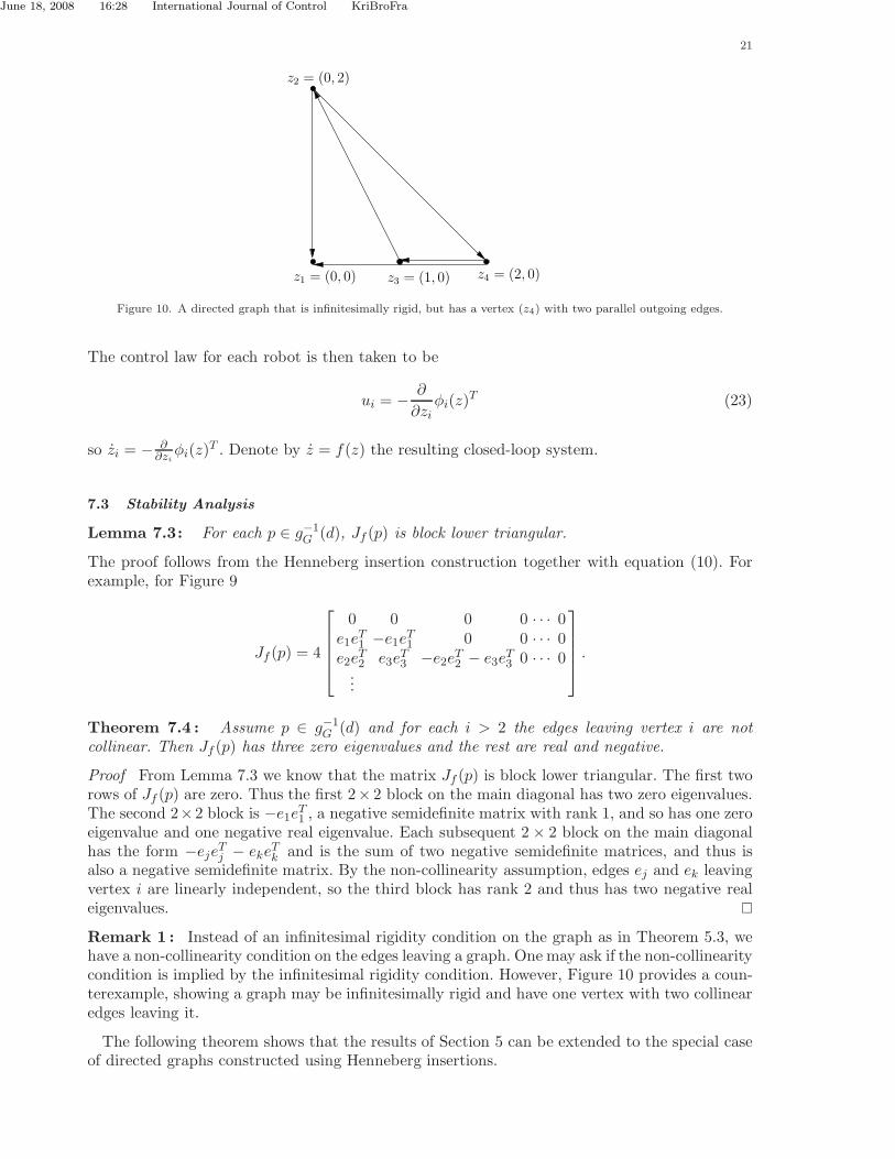
Figure 10. A directed graph that is infinitesimally rigid, but has a vertex (z4) with two parallel outgoing edges.

The control law for each robot is then taken to be

ui = − ∂

∂ziφi(z)

T (23)

so zi = − ∂∂ziφi(z)

T . Denote by z = f(z) the resulting closed-loop system.

7.3 Stability Analysis

Lemma 7.3: For each p ∈ g−1G (d), Jf (p) is block lower triangular.

The proof follows from the Henneberg insertion construction together with equation (10). Forexample, for Figure 9

Jf (p) = 4

0 0 0 0 · · · 0e1e

T1 −e1eT1 0 0 · · · 0

e2eT2 e3e

T3 −e2eT2 − e3e

T3 0 · · · 0

...

.

Theorem 7.4 : Assume p ∈ g−1G (d) and for each i > 2 the edges leaving vertex i are not

collinear. Then Jf (p) has three zero eigenvalues and the rest are real and negative.

Proof From Lemma 7.3 we know that the matrix Jf (p) is block lower triangular. The first tworows of Jf (p) are zero. Thus the first 2× 2 block on the main diagonal has two zero eigenvalues.The second 2×2 block is −e1eT1 , a negative semidefinite matrix with rank 1, and so has one zeroeigenvalue and one negative real eigenvalue. Each subsequent 2 × 2 block on the main diagonalhas the form −ejeTj − eke

Tk and is the sum of two negative semidefinite matrices, and thus is

also a negative semidefinite matrix. By the non-collinearity assumption, edges ej and ek leavingvertex i are linearly independent, so the third block has rank 2 and thus has two negative realeigenvalues. �

Remark 1 : Instead of an infinitesimal rigidity condition on the graph as in Theorem 5.3, wehave a non-collinearity condition on the edges leaving a graph. One may ask if the non-collinearitycondition is implied by the infinitesimal rigidity condition. However, Figure 10 provides a coun-terexample, showing a graph may be infinitesimally rigid and have one vertex with two collinearedges leaving it.

The following theorem shows that the results of Section 5 can be extended to the special caseof directed graphs constructed using Henneberg insertions.


22

Theorem 7.5 : Let G be a directed graph constructed using a sequence of Henneberg insertions.If, for each p ∈ g−1

G (d), G is infinitesimally rigid and no vertex has collinear outgoing edges,then E1 is locally asymptotically stable. Moreover, there exists a neighborhood U of E1 such thatfor each z(0) ∈ U there exists a point p ∈ E1 such that limt→∞ z(t) = p.

Proof The proof largely follows from the results of Section 5. First we separate the stationaryz1 dynamics from the rest of the system. Define

P2 =

I2 0 0 . . . 0−I2 I2 0 . . . 0−I2 0 I2 . . . 0

......

. . . . . ....

−I2 0 . . . . . . I2

.

and (z1, ψ) = P2z. Thus ψ = (z2 − z1, . . . , zN − z1). Note that if ei = zj − z1, then ei = ψj , and ifei = zj − zk, then ei = ψj − ψi. So it is possible to find a matrix M such that e = Mψ. Furtherdefine

E1 := { ψ ∈ R2N−2 | v(e) = v(Mψ) = d}.

Note that E1 = R2 × E1. Additionally, we see that E1 is compact and each component is diffeo-morphic to S1. Define ψ = fψ(ψ) to be the closed-loop ψ dynamics. To prove E1 is stable we

study these ψ dynamics. From the structure of f(z) it is clear that E1 is stable if and only ifE1 is stable. In order to apply Theorem 5.6 it remains to show only that the Jacobian of the ψdynamics meets the eigenvalue requirement. But this follows from Theorem 7.4 and argumentsanalogous to those in the proof of Corollary 5.4. �

7.4 General Directed Graphs

If an arbitrary directed graph is used to derive the potential functions for each robot, the analysisof the linearized dynamics is not so simple. However, if the linearized dynamics have three zeroeigenvalues and the rest have negative real parts it is still possible to apply Theorem 5.6 toconclude that the formation is stable. The following example has linearized dynamics that arenot upper triangular, but by checking the eigenvalues numerically we can see that the results ofSection 5 apply.

Example 7.6 Consider the framework in Figure 11. Let the location of the vertices be p. Thegraph is infinitesimally rigid, and thus E1 is an embedded submanifold.

If we linearize we see that for z ∈ E1

Jf (z) = 4

0 0 0 0e1e

T1 −e1eT1 − e2e

T2 e2e

T2 0

e3eT3 0 −e2eT2 − e4e

T4 e4e

T4

0 e5eT5 0 −e5eT5

.

Note that Jf (z) is not block lower triangular, nor is there any way to permute the indices tomake the matrix block lower triangular. The graph in Figure 11 could not have been createdusing the Henneberg insertion method. Hendrickx et al. (2006b) discusses other operations thatcan produce such a directed graph.) If we evaluate the eigenvalues of Jf (z) numerically we seethat there are three zero eigenvalues and the rest are real and stable. Thus, Theorem 5.6 appliesand the formation is locally asymptotically stable. This example shows that the procedure inSection 7.1.1 to construct a directed graph to stabilize formations is sufficient but not necessaryfor stability.


23

z2 = (0, 0)

e1

z3 = (1, 1)

e5

e4

e3

e2

z4 = (1, 0)

z1 = (0, 1)

Figure 11. Due to the arrangement of the edges leaving vertex 3 this graph could not have been created using the Henneberginsertion procedure.

z2 = (0, 0)

z3 = (1, 1)

z6 = (3, 0)

z5 = (3, 3)

z4 = (2, 2)

z1 = (0, 2)

e1

e2

e3

e4

e5

e6

e7

e8

e9

(a)

z2 = (0, 0)

z3 = (1, 1)

z6 = (3, 0)

z1 = (0, 2)

e1

e2

e3

z4 = (3, 3)

z5 = (2, 2)

e4

e5

e6

e7

e8

e9

(b)

Figure 12. Embeddings of a directed graph for six robots.

Conversely, there are some directed graphs where we cannot apply our results. Related toFigure 12(a) Jf (z) has 4 zero eigenvalues and the rest are real and stable. Thus the conditionsto apply Theorem 5.6 do not hold as there are more zero eigenvalues than the dimension of theequilibrium manifold and we can make no conclusion about the stability of this formation usingthis analysis technique. It turns out that if we modify the graph as shown in Figure 12(b) (notethat now there is no directed edge from z5 to z3), then there are three zero eigenvalues and therest have negative real parts. Thus we can conclude that this formation is stable.

8 Conclusion

This paper considers the problem of stabilizing a group of robots to a desired target formationusing decentralized control. The target formation is defined in terms of a set of inter-robotdistances and we place the restriction that these distances correspond exactly to the sensorcapabilities of each robot. A gradient control law based on a potential function derived from thetarget distances is proposed. Our results show that the crucial property to achieve local stability


24 REFERENCES

is that the framework corresponding to the target formation be infinitesimally rigid. Under theassumption of infinitesimal rigidity, the set of equilibria of the gradient dynamics correspondingto the target formation becomes an embedded submanifold, and further, this submanifold is acenter manifold. Thus, standard tools from center manifold theory are applied to obtain a localstability result. Next, we address the particular case of regular polygon formations where it isshown that the main assumption of infinitesimal rigidity holds for a suitable formation graph.A shortcoming of the approach is that it assumes two-way sensor capability of the robots.This drawback is overcome by extending the theory to the case of directed sensor graphs. Itis shown that the main stability result extends to directed graphs when the target formationis constructed using a Henneberg insertion procedure. Examples are given to show when ourtheory does not apply to more general directed sensor graphs. An experimental validation of theproposed controller was carried out, though not described here, and details of those results canbe found in Krick (2007).

Acknowledgements. The authors thank Manfredi Maggiore for a helpful discussion on centermanifold theory.

References

Marshall, J., Broucke, M., and Francis, B. (2004), “Formations of Vehicles in Cyclic Pursuit,” IEEETransactions on Automatic Control, 9(11), 1963–1974.

Cortes, J., Martınez, S., and Bullo, F. (2004), “Robust Rendezvous for Mobile Autonomous Agents viaProximity Graphs in d Dimensions,” IEEE Transactions on Automatic Control, 51(8), 1289–1298.

Lin, J., Morse, A., and Anderson, B. (2004), “The Multi-Agent Rendezvous Problem - The AsynchronousCase,” in Proceedings of the 43rd IEEE Conference on Decision and Control, December, Vol. 2, Atlantis,Bahamas, pp. 1926–1931.

Goldenberg, D., Lin, J., Morse, A., Rosen, B., and Yang, Y. (2004), “Towards Mobility As A Network Con-trol Primitive,” in Proceedings of the 5th ACM International Symposium on Mobile ad hoc Networkingand Computing, Tokyo, Japan, pp. 163–174.

Cortes, J., Martınez, S., Karatas, T., and Bullo, F. (2004), “Coverage Control for Mobile Sensing Net-works,” IEEE Transactions on Robotics and Automation, 2(2), 243–255.

Olfati-Saber, R. (2006), “Flocking for multi-agent dynamic systems: Algorithms and theory,” IEEE Trans-actions on Automatic Control, 51, 401–420.

Smith, S., Broucke, M., and Francis, B. (2006), “Stabilizing a Multi-Agent System to an EquilateralPolygon Formation,” in Proceeds of the 17th International Symposium on Mathematical Theory ofNetworks and Systems (MTNS2006), Kyoto, Japan, pp. 2415–2424.

Olfati-Saber, R., and Murray, R. (2002), “Distributed Cooperative Control of Multiple Vehicle Formationsusing Structural Potential Functions,” in Proceedings of the 15th IFAC World Congress, Barcelona,Spain.

Biggs, N., Algebraic Graph Theory, Cambridge University Press (1974).Asimow, L., and Roth, B. (1979), “The Rigidity of Graphs II,” Journal of Mathematical Analysis and

Applications, 68(1), 171–190.Bereg, S. (2005), “Certifying and Constructing Minimally Rigid Graphs in the Plane,” in Proceedings of

the Twenty-First Annual Symposium on Computational Geometry, Pisa, Italy: Annual Symposium onComputational Geometry, pp. 73–80.

Whitney, H. (1957), “Elementary Structure of Real Algebraic Varieties,” The Annals of Mathematics,66(3), 545–556.

Asimow, L., and Roth, B. (1978), “The Rigidity of Graphs,” Transactions of the American MathematicalSociety, 245, 279–289.

Boothby, W., An Introduction to Differentiable Manifolds and Reimannian Geometry, Academic PressInc. (1986).

Carr, J., Applications of Centre Manifold Theory, Springer-Verlag (1981).Wiggins, S., Introduction to Applied Nonlinear Dynamical Systems and Chaos, Springer-Verlag (1990).Marshall, J., Broucke, M., and Francis, B. (2006), “Pursuit Formations of Unicycles.,” Automatica, 42(1),

3–12.


REFERENCES 25

Malkin, I., Theory of Stability of Motion, United States Atomic Energy Commission Technical InformationService (1958).

Sundarapandian, V. (2003), “A Geometric Proof of Malkin’s Stability Theorem,” Indian Journal of Pureand Applied Mathematics, 34(7), 1085–1088.

Khalil, H., Nonlinear Systems, Prentice Hall (2002). Lojawiewicz, S. (1959), “Sur le probleme de la division,” Studia Mathmatica, 18, 87–136.Hendrickx, J., Anderson, B., Delvenne, J.C., and Blondel, V. (2006a), “Directed Graphs for the Analy-

sis of Rigidity and Persistence in Autonomous Agent Systems,” International Journal of Robust andNonlinear Control, 17(10-11), 960–981.

Hendrickx, J., Fidan, B., Changbin, Y., Anderson, B., and Blondel, V. (2006b), “Elementary Operationsfor the Reorganization of Minimally Persistent Formations,” in Proceeds of the 17th InternationalSymposium on Mathematical Theory of Networks and Systems (MTNS2006), June, Kyoto, Japan, pp.859–873.

Krick, L., “Application of Graph Rigidity in Formation Control of Multi-Robot Networks,” MASc Thesis,University of Toronto, Electrical and Computer Engineering Dept. (2007).

research article stabilization of inﬁnitesimally rigid

Documents