research article positive almost periodic solutions for - downloads

Hindawi Publishing CorporationInternational Journal of Differential EquationsVolume 2011, Article ID 354016, 12 pagesdoi:10.1155/2011/354016

Research ArticlePositive Almost Periodic Solutions fora Time-Varying Fishing Model with Delay

Xia Li, Yongkun Li, and Chunyan He

Department of Mathematics, Yunnan University, Yunnan, Kunming 650091, China

Correspondence should be addressed to Yongkun Li, [email protected]

Received 19 May 2011; Revised 8 August 2011; Accepted 12 August 2011

Academic Editor: Dexing Kong

Copyright q 2011 Xia Li et al. This is an open access article distributed under the CreativeCommons Attribution License, which permits unrestricted use, distribution, and reproduction inany medium, provided the original work is properly cited.

This paper is concerned with a time-varying fishing model with delay. By means of thecontinuation theorem of coincidence degree theory, we prove that it has at least one positive almostperiodic solution.

1. Introduction

Consider the following differential equation which is widely used in fisheries [1–4]:

N = N[L(t,N) −M(t,N)] −NF(t), (1.1)

where N = N(t) is the population biomass, L(t,N) is the per capita fecundity rate, M(t,N)is the per capita mortality rate, and F(t) is the harvesting rate per capita.

In (1.1), let L(t,N) be a Hills’ type function ([1, 2])

L(t,N) =a

1 + (N/K)γ (1.2)

and take into account the delay and the varying environments; Berezansky and Idels [5]proposed the following time-lag model based on (1.1) [1–6]

N(t) = N(t)[

a(t)1 + (N(θ(t))/K(t))γ

− b(t)], (1.3)

where b(t) = M(t,N) + F(t).

2 International Journal of Differential Equations

The model (1.3) has recently attracted the attention of many mathematicians andbiologists; see the differential equations which are widely used in fisheries [1, 2]. However,one can easily see that all equations considered in the above-mentioned papers are subject toperiodic assumptions, and the authors, in particular, studied the existence of their periodicsolutions. On the other hand, ecosystem effects and environmental variability are veryimportant factors and mathematical models cannot ignore, for example, reproduction rates,resource regeneration, habitat destruction and exploitation, the expanding food surplus, andother factors that affect the population growth. Therefore it is reasonable to consider thevarious parameters of models to be changing almost periodically rather than periodicallywith a common period. Thus, the investigation of almost periodic behavior is consideredto be more accordant with reality. Although it has widespread applications in real life, thegeneralization to the notion of almost periodicity is not as developed as that of periodicsolutions; we refer the reader to [7–18].

Recently, the authors of [19] proved the persistence and almost periodic solutionsfor a discrete fishing model with feedback control. In [20, 21], the contraction mappingprinciple and the continuation theorem of coincidence degree have been employed toprove the existence of positive almost periodic exponential stable solutions for logarithmicpopulation model, respectively. A primary purpose of this paper, nevertheless, is to utilizethe continuation theorem of coincidence degree for this purpose. To the best of the authors’observation, there exists no paper dealing with the proof of the existence of positive almostperiodic solutions for (1.3) using the continuation theorem of coincidence degree. Therefore,our result is completely different and presents a new approach.

2. Preliminaries

Our first observation is that under the invariant transformation N(t) = ey(t), (1.3) reduces to

y(t) =a(t)

1 +(ey(θ(t))/K(t)

)γ − b(t) (2.1)

for γ > 0, with the initial function and the initial value

y(t) = φ(t), y(0) = y0, t ∈ (−∞, 0). (2.2)

For (2.1) and (2.2), we assume the following conditions:

(A1) a(t), b(t) ∈ C([0,+∞), [0,+∞)) and K(t) ∈ C([0,+∞), (0,+∞));

(A2) θ(t) is a continuous function on [0,+∞) that satisfies θ(t) ≤ t;

(A3) φ(t) : (−∞, 0) → [0,∞) is a continuous bounded function, φ(t) ≥ 0, y0 > 0.

By a solution of (2.1) and (2.2) we mean an absolutely continuous function y(t)defined on (−∞,+∞) satisfying (2.1) almost everywhere for t ≥ 0 and (2.2). As we areinterested in solutions of biological significance, we restrict our attention to positive ones.

According to [22], the initial value problem (2.1) and (2.2) has a unique solutiondefined on (−∞,∞).

International Journal of Differential Equations 3

Let X,Y be normed vector spaces, L : Dom L ⊂ X → Y be a linear mapping, andN : X → Y be a continuous mapping. The mapping L will be called a Fredholm mappingof index zero if dim KerL = codim ImL < +∞ and Im L is closed in Y . If L is a Fredholmmapping of index zero and there exist continuous projectors P : X → X and Q : Y → Ysuch that Im P = Ker L, KerQ = ImL = Im(I −Q), it follows that the mapping L|Dom L∩KerP :(I − P)X → Im L is invertible. We denote the inverse of that mapping by KP . If Ω is anopen bounded subset of X, then the mapping N will be called L-compact on Ω, if QN(Ω)is bounded and KP (I − Q)N : Ω → X is compact. Since ImQ is isomorphic to KerL, thereexists an isomorphism J : ImQ → KerL.

Theorem 2.1 (see [19]). Let Ω ⊂ X be an open bounded set and let N : X → Y be a continuousoperator which is L-compact on Ω. Assume that

(1) Ly /=λNy for every y ∈ ∂Ω ∩Dom L and λ ∈ (0, 1);

(2) QNy/= 0 for every y ∈ ∂Ω ∩ Ker L;

(3) the Brouwer degree deg{JQN,Ω ∩ Ker L, 0}/= 0.

Then Ly = Ny has at least one solution in Dom L ∩Ω.

3. Existence of Almost Periodic Solutions

LetAP(R) denote the set of all real valued almost periodic functions on R, for f ∈ AP(R)wedenote by

Λ(f)=

{λ ∈ R : lim

T →∞1T

∫T

0f(s)e−iλsds /= 0

},

mod(f)=

⎧⎨⎩

m∑j=1

njλj : nj ∈ Z, m ∈ N, λj ∈ Λ(f), j = 1, 2, . . . , m

⎫⎬⎭,

(3.1)

the set of Fourier exponents and the module of f , respectively. Let K(f, ε, S) denote the setof ε-almost periods for f with respect to S ⊂ C((−∞, 0],R), l(ε) denote the length of theinclusion interval, and m(f) = lim

T →∞(1/T)

∫T0 f(s) ds denote the mean value of f .

Definition 3.1. y(t) ∈ C(R,R) is said to be almost periodic onR if for any ε > 0 the setK(y, ε) ={δ : |y(t + δ) − y(t)| < ε, ∀t ∈ R} is relatively dense; that is, for any ε > 0 it is possible to finda real number l(ε) > 0 for any interval with length l(ε); there exists a number δ = δ(ε) in thisinterval such that |y(t + δ) − y(t)| < ε for any t ∈ R.

Throughout the rest of the paper we assume the following condition for (2.1):

(H) a(t), b(t), K(t), t − θ(t) ∈ AP(R), m(b/Kγ)/= 0 and m(a)/=m(b).

In our case, we set

X = Y = V1 ⊕ V2, (3.2)


where

V1 ={y ∈ AP(R) : mod

(y) ⊆ mod(F), ∀μ ∈ Λ

(y)satisfies

∣∣μ∣∣ > α},

V2 ={y(t) ≡ k, k ∈ R

},

(3.3)

where

F = F(t, φ)=

a(t)1 +(eφ(θ(0))/K(t)

)γ − b(t), φ ∈ C([−∞, 0],R) (3.4)

and α is a given constant; define the norm

∥∥y∥∥ = supt∈R

∣∣y(t)∣∣, y ∈ X (or Y). (3.5)

Remark 3.2. If f is ε-almost periodic function, then∫ tf(s)ds is ε-almost periodic if and only

if m(f) = 0. Whereas f ∈ AP(R) does not necessarily have an almost periodic primitive,m(f) = 0. That is why we can not make V1 = {z ∈ AP(R) : m(z) = 0} and let V1 = {y ∈AP(R) : mod(y) ⊂ mod(F), ∀μ ∈ Λ(y) satisfy |μ| > α}.

We start with the following lemmas.

Lemma 3.3. X and Y are Banach spaces endowed with the norm ‖ · ‖.

Proof. If yn ∈ V1 and yn converge to y0, then it is easy to show that y0 ∈ AP(R) with mod(y0) ⊂ mod(F). Indeed, for all |λ| ≤ α we have

limT →∞

1T

∫ t

0yn(s)e−iλsds = 0. (3.6)

Thus

limT →∞

1T

∫T

0y0(s)e−iλsds = 0, (3.7)

which implies that y0 ∈ V1. One can easily see that V1 is a Banach space endowed with thenorm ‖ · ‖. The same can be concluded for the spaces X and Y . The proof is complete.

Lemma 3.4. Let L : X → Y and

Ly =a(t)

1 +(ey(θ(t))/K(t)

)γ − b(t), (3.8)

where Ly = y′ = dy/dt. Then L is a Fredholmmapping of index zero.


Proof. It is obvious that L is a linear operator and Ker L = V2. It remains to prove that Im L =V1. Suppose that φ(t) ∈ Im L ⊂ Y . Then, there exist φ1 ∈ V1 and φ2 ∈ V2 such that

φ = φ1 + φ2. (3.9)

From the definitions of φ(t) and φ1(t), one can deduce that∫ tφ(s)ds and

∫ tφ1(s)ds are almost

periodic functions and thus φ2(t) ≡ 0, which implies that φ(t) ∈ V1. This tells us that

Im L ⊂ V1. (3.10)

On the other hand, if ϕ(t) ∈ V1 \ {0} then we have∫ t0 ϕ(s)ds ∈ AP(R). Indeed, if λ /= 0 then we

obtain

limT →∞

1T

∫T

0

[∫ t

0ϕ(s)ds

]e−iλtdt =

1

iλlimT →∞

1T

∫T

0ϕ(t)e−iλt dt. (3.11)

It follows that

Λ

[∫ t

0ϕ(s)ds −m

(∫ t

0ϕ(s)ds

)]= Λ(ϕ(t)). (3.12)

Thus

∫ t

0ϕ(s)ds −m

(∫ t

0ϕ(s)ds

)∈ V1 ⊂ X. (3.13)

Note that∫ t0 ϕ(s)ds − m(

∫ t0 ϕ(s)ds) is the primitive of ϕ in X; therefore we have ϕ ∈ Im L.

Hence, we deduce that

V1 ⊂ Im L, (3.14)

which completes the proof of our claim. Therefore,

Im L = V1. (3.15)

Furthermore, one can easily show that Im L is closed in Y and

dim Ker L = 1 = codim Im L. (3.16)

Therefore, L is a Fredholm mapping of index zero.


Lemma 3.5. LetN : X → Y , P : X → X, and Q : Y → Y such that

Ny =a(t)

1 +(ey(θ(t))/K(t)

)γ − b(t), y ∈ X,

Py = m(y), y ∈ X, Qz = m(z), z ∈ Y.

(3.17)

Then, N is L-compact on Ω (Ω is an open and bounded subset of X).

Proof. The projections P and Q are continuous such that

Im P = Ker L, Im L = Ker Q. (3.18)

It is clear that

(I −Q)V2 = {0},

(I −Q)V1 = V1.(3.19)

Therefore

Im(I −Q) = V1 = Im L. (3.20)

In view of

Im P = Ker L,

Im L = Ker Q = Im(I −Q),(3.21)

we can conclude that the generalized inverse (of L) KP : Im L → Ker P ∩Dom L exists andis given by

KP (z) =∫ t

0z(s)ds −m

[∫ t

0z(s)ds

]. (3.22)

Thus

QNy = m

[a(t)

1 +(ey(θ(t))/K(t)

)γ − b(t)

],

KP (I −Q)Ny = f[y(t)] −Qf

[y(t)],

(3.23)

where f[y(t)] is defined by

f[y(t)]=∫ t

0

[Ny(s) −QNy(s)

]ds. (3.24)


The integral form of the terms of both QN and (I − Q)N implies that they arecontinuous. We claim that KP is also continuous. By our hypothesis, for any ε < 1 and anycompact set S ⊂ C((−∞, 0],R), let l(ε, S) be the inclusion interval of K(F, ε, S). Suppose that{zn(t)} ⊂ ImL = V1 and zn(t) uniformly converges to z0(t). Because

∫ t0 zn(s)ds ∈ Y (n =

0, 1, 2, 3, . . .), there exists ρ(0 < ρ < ε) such thatK(F, ρ, S) ⊂ K(∫ to zn(s) ds, ε). Let l(ρ, S) be the

inclusion interval of K(F, ρ, S) and

l = max{l(ρ, S), l(ε, S)

}. (3.25)

It is easy to see that l is the inclusion interval of both K(F, ε, S) and K(F, ρ, S). Hence, for allt /∈ [0, l], there exists μt ∈ K(F, ρ, S) ⊂ K(

∫ t0 zn(s)ds, ε) such that t + μt ∈ [0, l]. Therefore, by

the definition of almost periodic functions we observe that

∥∥∥∥∥∫ t

0zn(s)ds

∥∥∥∥∥ = supt∈R

∣∣∣∣∣∫ t

0zn(s)ds

∣∣∣∣∣

≤ supt∈[0,l]

∣∣∣∣∣∫ t

0zn(s)ds

∣∣∣∣∣ + supt/∈[0,l]

∣∣∣∣∣(∫ t

0zn(s)ds −

∫ t+μt

0zn(s)ds

)+∫ t+μt

0zn(s)ds

∣∣∣∣∣

≤ 2 supt∈[0,l]

∣∣∣∣∣∫ t

0zn(s)ds

∣∣∣∣∣ + supt/∈[0,l]

∣∣∣∣∣∫ t

0zn(s)ds −

∫ t+μt

0zn(s)ds

∣∣∣∣∣

≤ 2∫ l

0|zn(s)|ds + ε.

(3.26)

By applying (3.26), we conclude that∫ t0 z(s)ds(z ∈ Im L) is continuous and consequentlyKP

and KP (I −Q)Ny are also continuous.

From (3.26), we also have that∫ t0 z(s)ds and KP (I − Q)Ny are uniformly bounded

in Ω. In addition, it is not difficult to verify that QN(Ω) is bounded and KP (I − Q)Ny isequicontinuous in Ω. Hence by the Arzela-Ascoli theorem, we can immediately concludethat KP (I −Q)N(Ω) is compact. ThusN is L-compact on Ω.

Theorem 3.6. Let condition (H) hold. Then (2.1) has at least one positive almost periodic solution.

Proof. It is easy to see that if (2.1) has one almost periodic solution y, thenN = ey is a positivealmost periodic solution of (1.3). Therefore, to complete the proof it suffices to show that (2.1)has one almost periodic solution.

In order to use the continuation theorem of coincidence degree theory, we set theBanach spaces X and Y the same as those in Lemma 3.3 and the mappings L, N, P , Q thesame as those defined in Lemmas 3.4 and 3.5, respectively. Thus, we can obtain that L is aFredholm mapping of index zero and N is a continuous operator which is L-compact on Ω.


It remains to search for an appropriate open and bounded subset Ω. Corresponding to theoperator equation

Ly = λNy, λ ∈ (0, 1), (3.27)

we may write

y(t) = λ

[a(t)

1 +(ey(θ(t))/K(t)

)γ − b(t)

]. (3.28)

Assume that y = y(t) ∈ X is a solution of (3.28) for a certain λ ∈ (0, 1). Denote

y∗ = supt∈R

y(t), y∗ = inft∈R

y(t). (3.29)

In view of (3.28), we obtain

m(a(t) − b(t)) = m

(b(t)Kγ(t)

(ey(θ(t))

)γ)(3.30)

and consequently,

m(a(t) − b(t)) ≥ m

(b(t)Kγ(t)

)eγy∗ , (3.31)

which implies from (H) that

y∗ ≤ γ−1 ln(

m[a(t) − b(t)]m(b(t)/Kγ(t))

). (3.32)

Similarly, we can get

y∗ ≥ γ−1 ln(

m(a(t) − b(t))m(b(t)/Kγ(t))

). (3.33)

By inequalities (3.32) and (3.33), we can find that there exists t1 ∈ R such that

∣∣y(t1)∣∣ ≤ M, (3.34)

where

M =∣∣∣∣γ−1 ln

(m(a(t) − b(t))m(b(t)/Kγ(t))

)∣∣∣∣ + 1. (3.35)


Then from (3.26), we have

∥∥y(t)∥∥ ≤ ∣∣y(t1)∣∣ + supt∈R

∣∣∣∣∣∫ t

t2

y′(s)ds

∣∣∣∣∣ ≤ M + 2 supt∈[t2,t2+l]

∫ t

t2

∣∣y′(s)∣∣ds + ε (3.36)

or

∥∥y(t)∥∥ ≤ M + 2∫ t2+l

t2

∣∣y′(s)∣∣ds + 1. (3.37)

Choose the point ν − t2 ∈ [l, 2l] ∩ K(F, ρ, S), where ρ(0 < ρ < ε) satisfies K(F, ρ) ⊂ K(z, ε).Integrating (3.28) from t2 to ν, we get

λ

∫ν

t2

a(t)1 + [K(s)]−γeγy(θ(s))

ds = λ

∫ν

t2

|b(s)|ds +∫ν

t2

y′(s)ds

≤ λ

∫ν

t2

|b(s)|ds + ε.

(3.38)

However, from (3.28) and (3.38), we obtain

∫ν

t2

∣∣y′(s)∣∣ds ≤ λ

∫ν

t2

|b(s)|ds + λ

∫ν

t2

a(t)1 + [K(s)]−γeγy(θ(s))

ds,

≤ 2∫ν

t2

|b(s)|ds + ε

≤ 2∫ν

t2

|b(s)|ds + 1.

(3.39)

Substituting back in (3.37) and for ν ≥ t2 + l, we have

∥∥y(t)∥∥ ≤ M′, (3.40)

where

M′ = M + 4∫ν

0|b(s)|ds + 3. (3.41)

Let M = M +M′. Obviously, it is independent of λ. Take

Ω ={y ∈ X :

∥∥y∥∥ < M}. (3.42)


0 10 20 30 40 500

1

2

3

4

5

6

7

8

Time (t)

N(t)

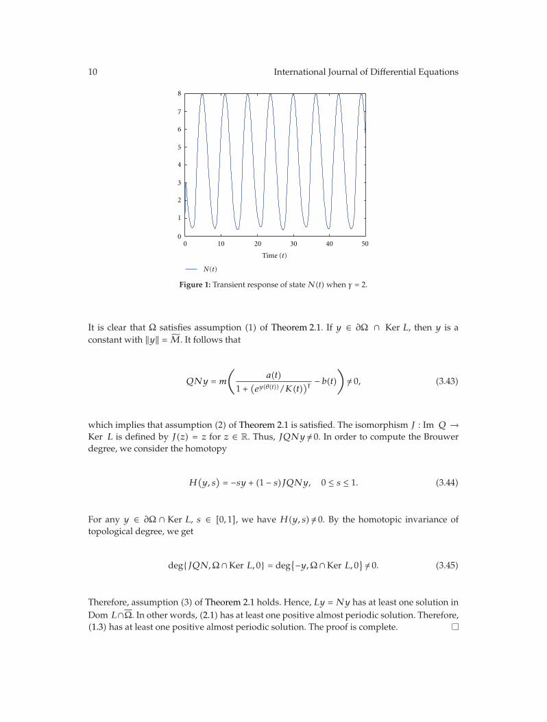
Figure 1: Transient response of state N(t) when γ = 2.

It is clear that Ω satisfies assumption (1) of Theorem 2.1. If y ∈ ∂Ω ∩ Ker L, then y is aconstant with ‖y‖ = M. It follows that

QNy = m

(a(t)

1 +(ey(θ(t))/K(t)

)γ − b(t)

)/= 0, (3.43)

which implies that assumption (2) of Theorem 2.1 is satisfied. The isomorphism J : Im Q →Ker L is defined by J(z) = z for z ∈ R. Thus, JQNy /= 0. In order to compute the Brouwerdegree, we consider the homotopy

H(y, s)= −sy + (1 − s)JQNy, 0 ≤ s ≤ 1. (3.44)

For any y ∈ ∂Ω ∩ Ker L, s ∈ [0, 1], we have H(y, s)/= 0. By the homotopic invariance oftopological degree, we get

deg{JQN,Ω ∩ Ker L, 0} = deg{−y,Ω ∩ Ker L, 0

}/= 0. (3.45)

Therefore, assumption (3) of Theorem 2.1 holds. Hence, Ly = Ny has at least one solution inDom L∩Ω. In other words, (2.1) has at least one positive almost periodic solution. Therefore,(1.3) has at least one positive almost periodic solution. The proof is complete.


4. An Example

Let a(t) = eπ(3 + cos√2t), b(t) = (1/2)eπ(3 + cos

√2t), K(t) = 4 + sin

√t, γ > 0, θ(t) = t − 2 −

sin√3t. Then (1.3) has the form

N(t) = N(t)

⎡⎢⎣

eπ(3 + cos

√2t)

1 +(N(t − 2 − sin

√3t)/(4 + sin

√t))γ − 1

2eπ(3 + cos

√2t)⎤⎥⎦. (4.1)

One can easily realize that m(b(t)/[K(t)]γ) > 0 and m(a(t)) > m(b(t)); thus condition (H)holds. Therefore, by the consequence of Theorem 3.6, (4.1) has at least one positive almostperiodic solution (Figure 1).

Acknowledgment

This work is supported by the National Natural Sciences Foundation of People’s Republic ofChina under Grant 10971183.

References

[1] M. Kot, Elements of Mathematical Ecology, Cambridge University Press, Cambridge, UK, 2001.[2] L. Berezansky, E. Braverman, and L. Idels, “Delay differential equations with Hill’s type growth rate

and linear harvesting,” Computers & Mathematics with Applications, vol. 49, no. 4, pp. 549–563, 2005.[3] K. Gopalsamy, Stability and Oscillations in Delay Differential Equations of Population Dynamics, vol. 74,

Kluwer Academic Publishers, Dordrecht, The Netherlands, 1992.[4] Y. Kuang, Delay Differential EquationsWith Applications in Population Dynamics, vol. 191, Academic

Press, Boston, Mass, USA, 1993.[5] L. Berezansky and L. Idels, “Stability of a time-varying fishingmodel with delay,”AppliedMathematics

Letters, vol. 21, no. 5, pp. 447–452, 2008.[6] X. Wang, “Stability and existence of periodic solutions for a time-varying fishing model with delay,”

Nonlinear Analysis. Real World Applications, vol. 11, no. 5, pp. 3309–3315, 2010.[7] S. Ahmad and G. Tr. Stamov, “Almost periodic solutions of n-dimensional impulsive competitive

systems,” Nonlinear Analysis. Real World Applications, vol. 10, no. 3, pp. 1846–1853, 2009.[8] S. Ahmad and G. Tr. Stamov, “On almost periodic processes in impulsive competitive systems with

delay and impulsive perturbations,” Nonlinear Analysis. Real World Applications, vol. 10, no. 5, pp.2857–2863, 2009.

[9] Z. Li and F. Chen, “Almost periodic solutions of a discrete almost periodic logistic equation,”Mathematical and Computer Modelling, vol. 50, no. 1-2, pp. 254–259, 2009.

[10] B. Lou and X. Chen, “Traveling waves of a curvature flow in almost periodic media,” Journal ofDifferential Equations, vol. 247, no. 8, pp. 2189–2208, 2009.

[11] J. O. Alzabut, J. J. Nieto, and G. Tr. Stamov, “Existence and exponential stability of positive almostperiodic solutions for a model of hematopoiesis,” Boundary Value Problems, Article ID 127510, 10pages, 2009.

[12] R. Yuan, “On almost periodic solutions of logistic delay differential equations with almost periodictime dependence,” Journal of Mathematical Analysis and Applications, vol. 330, no. 2, pp. 780–798, 2007.

[13] W.Wu and Y. Ye, “Existence and stability of almost periodic solutions of nonautonomous competitivesystems with weak Allee effect and delays,” Communications in Nonlinear Science and NumericalSimulation, vol. 14, no. 11, pp. 3993–4002, 2009.

[14] G. T. Stamov and N. Petrov, “Lyapunov-Razumikhin method for existence of almost periodicsolutions of impulsive differential-difference equations,”Nonlinear Studies, vol. 15, no. 2, pp. 151–161,2008.


[15] G. T. Stamov and I. M. Stamova, “Almost periodic solutions for impulsive neutral networks withdelay,” Applied Mathematical Modelling, vol. 31, pp. 1263–1270, 2007.

[16] Q. Wang, H. Zhang, and Y. Wang, “Existence and stability of positive almost periodic solutions andperiodic solutions for a logarithmic population model,” Nonlinear Analysis, vol. 72, no. 12, pp. 4384–4389, 2010.

[17] A. S. Besicovitch, Almost Periodic Functions, Dover Publications, New York, NY, USA, 1954.[18] A. Fink, Almost Periodic Differential Equations: Lecture Notes in Mathematics, vol. 377, Springer, Berlin,

Germany, 1974.[19] T. Zhang, Y. Li, and Y. Ye, “Persistence and almost periodic solutions for a discrete fishing model with

feedback control,” Communications in Nonlinear Science and Numerical Simulation, vol. 16, no. 3, pp.1564–1576, 2011.

[20] J. O. Alzabut, G. Tr. Stamov, and E. Sermutlu, “On almost periodic solutions for an impulsive delaylogarithmic population model,” Mathematical and Computer Modelling, vol. 51, no. 5-6, pp. 625–631,2010.

[21] J. O. Alzabut, G. T. Stamov, and E. Sermutlu, “Positive almost periodic solutions for a delaylogarithmic population model,” Mathematical and Computer Modelling, vol. 53, no. 1-2, pp. 161–167,2011.

[22] V. Kolmanovskii, Introduction to the Theory and Applications of Functional Differential Equations, vol. 463,Kluwer Academic Publishers, Dordrecht, The Netherlands, 1999.

Submit your manuscripts athttp://www.hindawi.com

Hindawi Publishing Corporationhttp://www.hindawi.com Volume 2014

MathematicsJournal of


Mathematical Problems in Engineering

Hindawi Publishing Corporationhttp://www.hindawi.com

Differential EquationsInternational Journal of

Volume 2014

Applied MathematicsJournal of


Probability and StatisticsHindawi Publishing Corporationhttp://www.hindawi.com Volume 2014

Journal of


Mathematical PhysicsAdvances in

Complex AnalysisJournal of


OptimizationJournal of


CombinatoricsHindawi Publishing Corporationhttp://www.hindawi.com Volume 2014

International Journal of


Operations ResearchAdvances in

Journal of


Function Spaces

Abstract and Applied AnalysisHindawi Publishing Corporationhttp://www.hindawi.com Volume 2014

International Journal of Mathematics and Mathematical Sciences


The Scientific World JournalHindawi Publishing Corporation http://www.hindawi.com Volume 2014


Algebra

Discrete Dynamics in Nature and Society



Decision SciencesAdvances in

Discrete MathematicsJournal of

Hindawi Publishing Corporationhttp://www.hindawi.com

Volume 2014 Hindawi Publishing Corporationhttp://www.hindawi.com Volume 2014

Stochastic AnalysisInternational Journal of

research article positive almost periodic solutions for - downloads

Documents