research article an optimized method based on...
TRANSCRIPT

Research ArticleAn Optimized Method Based on Digitalized LissajousCurve to Determine Lifetime of Luminescent Materials onOptical Fiber Sensors
Adriaacuten Ridruejo Nerea De Acha Ceacutesar Elosuacutea Ignacio R Matiacuteas and Francisco J Arregui
Department of Electrical and Electronic Engineering Public University of Navarra 31006 Pamplona Spain
Correspondence should be addressed to Cesar Elosua cesarelosuaunavarraes
Received 3 January 2016 Revised 29 April 2016 Accepted 10 May 2016
Academic Editor Hai Xiao
Copyright copy 2016 Adrian Ridruejo et al This is an open access article distributed under the Creative Commons AttributionLicense which permits unrestricted use distribution and reproduction in any medium provided the original work is properlycited
A method is proposed to determine lifetime of luminescent emissions based on the phase shift measurement employing thedigitalized Lissajous representation this diagram has been typically used with analogical algorithms whereas the proposedmethodis performed in digital domain showing an improved accuracy and repeatability The procedure is studied and tested with twodifferent oxygen sensors that show different sensitivities and signal levels in order to confirm the no influence of the signals intensityon the calibration process The computational cost of the proposed method is low which makes it possible to monitor in real timeluminescence sensors based on reversible quenching with a potential low cost system based on a digital signal processor (DSP)
1 Introduction
Technological research assigns many resources to the devel-opment of sensors for a specific purpose which is providingmore independency to the products and systems that improvehuman quality of live Nowadays smart cities require theinformation of sensors of different types to enhance the per-formance of the urban services reducing cost and pollutionas well as using natural resources more efficiently [1] To beable to react against changes in the environment it is neededto monitor every parameter involved that is the reason whysensors take on a special relevancy in these systems Sensorsare devices able to sense a wide range of differentmagnitudesso the information provided by them has to be registeredand processed by the systems to offer an answer as better aspossible
Therefore it is important to have sensors able to measuredistinct physical or chemical magnitudes Furthermore eachtype of sensor needs a processing unit that can registerand monitor the transduction between the measurementand the parameter recorded by the sensor This step can beas critical as the sensor construction itself and determinesdrastically the whole performance of the system In this
context optical fiber sensors show a relevant potential due tothe advantages of using optical fiber against electric cables inseveral scenarios [2 3] However the implementation in realapplications is not as extended as it could be because there areeffects whichmodify the light behavior along the time one ofthe most challenging ones is produced by undesired artifactsin the intensity of the sensor signal when the transduction isbased on this parameter
Luminescent sensors register the emission of a specificmaterial when it is illuminated with a light source at a certainwavelength The transduction takes place when the targetmagnitude modifies the properties of the sensing materialemission for example its intensity [4] One way to detectthis variation consists of coupling it into an optical fiber andthen registering it In most cases the chemical dye suffers aquenching that alters the lifetime of the fluorescent emissionwhich is the mean time that an electron takes to recoverits quiescent state (at the lowest conducting band) froman excited one [5] Materials such as metallic porphyrinsshow this behavior in the presence of some gases oneof the most relevant applications where they are used isoxygen detection and concentration measurement [6] Forthis specific case lifetime is reduced as the gas concentration
Hindawi Publishing CorporationJournal of SensorsVolume 2016 Article ID 6019439 10 pageshttpdxdoiorg10115520166019439
2 Journal of Sensors
increases this effect is directly measurable by the magnitudeof the luminescent emission which is used in intensity basedsensors [7ndash9] However there are many artifacts that canmodify the intensity level altering the final measurement aswell as photobleaching [10] This dependence on the signallevel limits the use of intensity based sensors in real scenarios
There are approaches that analyze other parameters inorder to overcome this problem lifetime is an interestingalternative because it is a temporal parameter and thereforeit is not affected by signal level fluctuations [11 12] Thisparameter can be obtained by measuring other ones thatdepend directly on it in the case the exciting signal ismodulated the luminescent emitted one is also modulatedtherefore the phase shift between them is defined by thelifetime value [13 14] Moreover in case the modulation issinusoidal [15] the relation between the phase shift and thelifetime can be described as shown in
tan120593 = 2120587119891120591 (1)
where 120593 is the phase shift 119891 is the frequency of the excitingsignal and 120591 is the luminescence lifetime As it can beinferred when using this relation intensity fluctuations haveno influence so that the system becomes more robust Inmost cases the luminescent signal shows a lower signal-to-noise ratio (SNR) compared to the excitation one so thatit has to be properly conditioned to be able to measure thephase shift between the signals Typically the emitted signalis converted to the electrical domain to be regenerated by alock-in amplifier and then it is digitalized to be processedin the discrete time domain [16] In this manner the lock-in amplifier is required to measure the phase shift so thatthis procedure is not able to handle directly with the lowSNR electric signal obtained from the sensor Alternativesbased on nonstandard fibers or complex methods to excitethe sensor have been developed trying to avoid the use of thiskind of instrumentation [17] however the high cost of thesedevices compromises the potentiality of the final system
In this paper a fluorescence lifetime system is proposedbased on phase shift measurement so it is independent onthe light intensity A specific algorithm has been developed tocalculate the phase shift it works with the Lissajous curve inthe digital domain and it handles the low level signal emittedby the sensing material it improves the results obtained bytraditional methods such as Fast Fourier Transform (FFT) orzero crossing Moreover the calculations are done entirely inthe digital domain highlighting the originality of the workbecause these techniques were traditionally employed in theanalog domain Therefore the whole signal processing (eventhe modulation of the interrogating signal) can be performedby a single embedded system such as DSP without any signalconditioning in the analogic domain The proposed methodis focused on obtaining lifetime measurements independentof artifacts under conditions where the signal level is lowand noisy The algorithm has been optimized in terms ofstandard deviation (measured in degrees) following fivedifferent implementationsThe procedure has been applied totwo different optical fiber sensors with different sensitivitiesto measure distinct oxygen concentrations although one
of them showed a significantly lower signal they bothwere correctly calibrated in the 0ndash20 oxygen range whichverifies the robustness of the proposed method
2 Materials and Methods
21 Sensing Material In this work two sensors with a differ-ent behavior have been implemented and studied providingtwo scenarios well differentiated They have been preparedwith the same sensing material which was platinum tetrakispentafluorophenyl porphine (Pt-TFPP)When this product isilluminated with a light source centered on 395 nm it showsa luminescent emission located at 650 nm Furthermore dueto its chemical structure the compound is not soluble inwater The lifetime of this emission depends on the environ-mental oxygen concentration by a quenching effect whichis reversible [18] This porphine has been used to developoxygen sensors on different substrates and transductionprinciples based on either intensity modulation [19 20]or lifetime measurement [21] The behavior of the sensorsdeveloped with this material has been described with theStern-Vollmer equation [22] Moreover it shows an optimalthermal and chemical stability [23] so that it was chosen toprepare the sensors to test the performance of the algorithmunder study
22 Sensors Construction Process Two oxygen sensors wereimplemented with the same sensing material but usingdistinct supporting matrices to attach it onto the opticalfiber All the chemical compounds employed were boughtfrom SigmaAldrich but the Pt-TFPP from Frontier Scientificall of them were used without any purification Before thedeposition of the sensing material the fibers were cleanedwith a 1M potassium hydroxide (KOH) aqueous solution
The supporting matrix used to implement the first probenamed Sensor A was a plastic one specifically polyvinylchloride (PVC) was used as polymer [24] For its fabrication6mg of Pt-TFPP 160mg of PVC and 320 120583L of tributylphos-phate (TBP) were dissolved in 4mL of tetrahydrofuran Themixture was sonicated for 30 minutes to get it as uniform aspossible [25] The deposition of the sensing layer was madeby the dip-coatingmethod the fiber was dipped and removedfrom the cocktail at a constant velocity of 11mms
The second sensor was prepared following Layer-by-Layer (LbL) method Briefly this procedure is based on theassembly of polymer chains with an electrical charge by elec-trostatic forces [26] In this manner the substrate (the opticalfiber pigtail) is dipped alternatively into a polycationic and apolyanionic water solution so that once the polymer chainsget assembled they form a bilayer The most relevant con-struction parameters of thismethod are the concentrations ofthe polymer solutions their respective pH and the numberof bilayers assembled onto the substrate [27] The sensor wasprepared employing Polyallylamine Hydrochloride (PAH) aspolycation in a 10mM aqueous solution in which pH wasset at 10 The nonmiscibility in water of the sensing materialwas overcome by preparing negatively charged micelles toachieve it 04mg of Pt-TFPP was firstly dissolved in 1mL ofacetone and thereafter in 9mL of a 10mM Sodium Dodecyl
Journal of Sensors 3
RS232
USB
AD 2 ch
Wave generator
HPF
LED source
Gas mixer
Bifurcatedfiber Optical fiber
sensor
PMT
MFC
O2 N2
O2N2 flow
Figure 1 Experimental set-up used for the experiments The three main blocks are surrounded by colored dotted lines (red) optical fibersensor configuration (green) oxygen flow system and (purple) electronic devices used for signal modulation and conditioning The wholesystem is controlled by a personal computer
Sulfate (SDS which acts as anionic surfactant) solution Dueto the negative charged micelles present in this last solutionit was considered as the anionic one Each bilayer was builtfollowing these steps optical fiber was firstly dipped for 2minutes in the PAH solution and then rinsed for 1 minutein ultrapure water thereafter it was immersed for 4 minutesin the SDS and Pt-TFPP emulsion and washed again for1 minute in ultrapure water [28] The immersion into thedifferent solutions was controlled by a programmable roboticarm obtained from Nadetech Innovations SL This processwas repeated until 40 bilayers were built The probe preparedin this way was called Sensor B
3 Experimental Set-Up
The experimental set-up can be divided into three mainblocks the first one is related to the optical fiber sensorthe second one includes the electronic devices required tomodulate the excitation signal and conditioning the emittedone the third one is formed by the valves and the systemthat sets the different oxygen concentrations A scheme of thewhole set-up is shown in Figure 1
The fiber used to prepare the sensors is Plastic CladdingSilica (PCS) whose core has a diameter of 1000120583m(UMT1000) and it was acquired from Thorlabs The sensorwas connected to a 600 120583m core bifurcated optical fiber(QBIF600-UV-VIS) purchased from Ocean Optics Inc toobtain the best signal coupling [28] Following a reflectionconfiguration the exciting signal from the LED source travelsto the sensor head through one of the branches of the bifur-cated fiber meanwhile the reflected signal from the sensor
is guided back through the other branch towards the opticalreceiver as well as a nonnegligible contribution from the LEDsource In order to attenuate the remaining excitation signalfrom the sensor response the second branch of the bifurcatedfiber was connected to a high pass filter (LVF-H also boughtat Ocean Optics) whose cutoff wavelength was set at 600 nm
The excitation signal was modulated at a frequency of500Hz with a wave generator Tektronix CFG280 by a 1 Vpeak to peak sinusoidal signal (to modulate the intensityof the LED emission) with a +3VDC offset (to set the LEDconducting)This modulating frequency was chosen becausefor a certain oxygen concentration (room conditions 21) itwas checked that this value produced the highest phase shiftThe optical signal from the HPF is taken into a photomul-tiplier from Hamamatsu (module H6780-20) to increase itsamplitude The amplified signal was converted to the digitaldomain and acquired by a USB-202 AD 2 channel converterfrom measurement computing Its sampling frequency was50KHz The data were analyzed by Labview virtual instru-ments
The gas flow used to interrogate the sensors was amixtureof gaseous oxygen and nitrogenThe flow rate was similar forall the experiments and it was set at 250mLmin The com-position of the flow (expressed in oxygen ) was controlledwith120583-mass flow valves fromBronkhorst Inc so that the sumof the flow rate of both gases was always 250mLmin alteringthe rate of each gas different oxygen concentrations could beset The accuracy of the devices is 01 so that the precisionof the different oxygen concentrations was 01 Both gasflows were driven into amixing chamber and from this pointtowards the corresponding optical fiber sensor Electronic
4 Journal of Sensors
Excitation signalLuminescent signalLuminescent signal998400
minus350
minus250
minus150
minus50
50
150
250
350A
mpl
itude
(mV
)
500 1000 1500 20000Time (120583s)
(a)
Excitation signalLuminescent signal998400
500 1000 1500 20000Time (120583s)
0
1
2
3
4
5
6
7
8
9
120590(m
V)
(b)
Figure 2 (a) Excitation signal (blue) and luminescent signal before (red) and after weighing it (green) so both of them show a similarRMS value (b) Standard deviation expressed in mV for each sample of the signals under study The values corresponding to the maximumminimum and zero crossing for each signal are pointed for each signal
sensors could be used to measure the real concentration butthe ratio set by the mass flow controllers was found enoughto estimate the actual concentration
4 Phase Shift Measurement Methods
The objective of the procedure is to determine the phaseshift between the exciting and the luminescent signals andthen use this parameter to estimate the lifetime emissionBoth the excitation and luminescent signals were analyzedby averaging 30 cycles in each case The number of averagedcycles was optimized by considering a different number ofcycles (from 1 up to 55) evaluating the resulting standarddeviation for each case The luminescent signal was chosento estimate the optimal number of cycles to be sampledbecause it is weaker than the exciting one It was foundthat the standard deviation reached a minimum for 30sampled cycles and its value was slightly increased of ahigher number of averaged samples (as it can be observedin Figure A1 in Supplementary Material available online athttpdxdoiorg10115520166019439) therefore in order toreduce the preprocessing time the number of averaged cycleswas set at 30
The description of the proposed method is based on thesignals registered from Sensor A at room conditions (21oxygen concentration) and they are displayed in Figure 2(a)(excitation signal in blue registered luminescent signal inred and weighted luminescent signal in green) if excitationand luminescent signals are compared it is evident thatthe second one shows a much lower amplitude Moreoverthe standard deviation 120590 of both signals was analyzed inorder to find the points with the lowest value because theywould be optimal to perform the algorithm The standard
deviation from the different samples of both signals is plottedin Figure 2(b) It can be checked that the standard deviationis lower when each signal reaches its maximum or minimumamplitude compared to the zero crossing points this behaviorcan be caused by the trigger performance a small variation ofthe excited signal frequency or the sample frequency or dueto a DC variation Under these circumstances estimating thephase shift based on the zero crossing points would yield ahigh error rate as it will be checked later
The proposedmethod tomeasure the phase shift betweenthe excitation signal and the luminescent one is based onthe Lissajous curve which is firstly applied for this type ofsensors [29] The Lissajous diagram is the representationof the parametric equation system which describes thesuperposition of two simple harmonic signals as follows
119883(119905) = 1198601sdot sin (2120587119891
1sdot 119905 + 120593
1)
119884 (119905) = 1198602sdot sin (2120587119891
2sdot 119905 + 120593
2)
(2)
In our scenario 119883(119905) is the excitation signal and 119884(119905) isthe luminescent one 119860
1and 119860
2are the amplitudes of the
excitation and emitted signals respectively the signals showa similar frequency 119891
1= 1198912= 119891 but a phase shift between
them which is 120593 = 1205932minus 1205931
The representation 119883119884 of the parametric equationsshows an ellipse where 120593 can be obtained solving (2) when119883 = 0 and 119884 = 0 respectively
119884 = 0 997888rarr 1198830= plusmn119860
1sdot sin (120593) (3)
119883 = 0 997888rarr 1198840= plusmn119860
2sdot sin (120593) (4)
120593 = arcsin(1198850
119860) (5)
Journal of Sensors 5
where1198850can show the values119883
0or1198840and119860 does so with119860
1
and 1198602 The phase shift has two possible solutions to know
which is the correct one it is only needed to check whichquadrants are crossed by the major axis of the ellipse [30]
The noise present in the signals is supposed to beGaussian therefore it was decided to evaluate the rootmean square (RMS) of both digitalized signals using the30 sampled cycles to calculate it (this number period isenough to minimize the noise effect over the RMS value)Once these parameters were obtained the luminescent signalwas weighed in order to adjust its RMS value to the oneof the excitation signal The resulting signal is displayed inFigure 2(a) According to these data there is an importantdifference between both signals the maximumminimumdeviation in the excitation signal is 10 times lower than thatat the zero crossing in the case of the luminescent signalthe deviation is of the same order in the three points understudy As it was excepted the first signal is less noisy andthe maximum minimum points show the lowest deviationtherefore working with them would yield results with highprecision
Taking into account that the excitation signal shows alower noise level at the maximum and minimum pointsthe parametric equations can be rewritten considering 119883(119905)like a nonnoise signal for the equations in this manner theresulting equations are
119883 (119905) = 1198601sdot sin (2120587119891 sdot 119905)
119884 (119905) = 1198602sdot sin (2120587119891 sdot 119905 + 120593) + 119873
0(119905)
(6)
At this point the signals are sinusoidal and with thesame RMS value so that it can be assumed that both ofthem have the same maximum amplitude neglecting theGaussian noise effect from the sensing signalTherefore if thephase shift is obtained from the ratio between the maximumand minimum of both signals the precision of the phaseshift estimation would be improvedThe digitalized Lissajouscurve obtained from the signals with the same RMS valueis displayed in Figure 3 the different sampled cycles aresuperposed to remark the variability of the signal it can beobserved that the lowest values of the deviation are obtainedfor the distances119883max and119883
1015840
max All the cycles were averagedand the resulting one is also plotted in the graph this lastrepresentation was the one used to determine the values ofthe distances 119883max 119883
1015840
max 119884max or 1198841015840
max 1198830 1198831015840
0 1198840 or 11988410158400in
the digital domain (also indicated in Figure 3)Equation (5) shows how to calculate the phase shift
between the signals once the ellipse has been built there aredifferent possibilities to get the phase shift value dependingon the parameters 119885
0(119883011988310158400 1198840 or 11988410158400) and 119860 (119883max119883
1015840
max119884max or 119884
1015840
max) Figure 3 shows that the signal variation ishigher for 119884max or 119884
1015840
max compared to the values of 119883max or1198831015840
max in this background if it was assumed that the amplitudeis similar for both signals because they show the same RMSvalue (as well as a similar frequency) then 119883max119883
1015840
max couldbe used to estimate the phase shift instead of 119884max or 119884
1015840
maxwhich would yield a lower error rate in the final result
minus350
minus250
minus150
minus50
50
150
250
350
Y(t) (
mV
)
minus250 minus150 minus50 50 150 250 350minus350X(t) (mV)
YmaxXmax
X0
Y0
Y998400max
X998400max
X9984000
Y9984000
Figure 3 Lissajous parametric representation for excitation andweighed luminescent signal The distances required to calculate thephase shift are indicated
Taking this hypothesis into account the following approaches(summarized in Table 1) were proposed
Method 1119883 The set of values of1198830and1198831015840
0of119883max and119883
1015840
maxare used to estimate 119885
0and 119860 respectively This approach
only takes into account the significant points of excitationsignal specifically the oneswith the lowest standard deviation(119883max and119883
1015840
max) and the ones with the highest value (1198830 and1198831015840
0)
Method 2119883 The phase shift is calculated twice firstly using1198830and 119883max and the other one using 1198831015840
0and 1198831015840max Finally
the average value between them determines 120593
Method 1119884 This method is similar to the first one proposedbut the different values are obtained from the luminescentsignal which shows worse standard deviation values
Method 21198841015840 The approach combines parameters from boththe excitation and the luminescent signals assuming that theyboth have a similar RMS value after weighting the last one Inthis manner 120593 is calculated twice firstly using 119884
0and 119883max
and secondly employing11988410158400and1198831015840maxThe angles obtained are
averaged to get the phase shift
Method 11198831015840-11198841015840 Two phase shifts are estimatedThe first oneis obtained applying method 1119883 whereas for the second one1198851015840
0is the mean of 119884
0and 1198841015840
0 119860 is calculated as averaged
value between 119883max and 1198831015840
max following the hypothesis thatthe signals show the same RMS value are sinusoidal andtherefore have an equal amplitude The final value is theaverage of these two phase shifts
The results for the distinct methods just described forSensor A at room conditions are around 72∘ The phaseshift has an offset component due to time delay producedby the high pass filter the photo multiplier and the elec-tronic instrumentation this parameter has to be measuredand compensated from the measurements in order to get
6 Journal of Sensors
Table 1 Mathematical expressions to determine the phase shift by the proposed methods based on the Lissajous curve
Phase shift
Method 1119883 120593 = arcsin(1198830+ 1198831015840
0
119883max + 1198831015840
max)
Method 2119883 120593 = average(arcsin(1198830
119883max) | arcsin(
1198831015840
0
1198831015840max))
Method 1119884 120593 = arcsin(1198840+ 1198841015840
0
119884max + 1198841015840
max)
Method 21198841015840 120593 = average(arcsin(1198840
119883max) | arcsin(
1198841015840
0
1198831015840max))
Method 11198831015840-11198841015840 120593 = average(arcsin(1198830+ 1198831015840
0
119883max + 1198831015840
max) | arcsin(
1198840+ 1198841015840
0
119883max + 1198831015840
max))
Table 2 Phase shift calculated with the different Lissajous based methods in terms of averaged value and standard deviation
O2concentration 1119883 2119883 1119884 2119884
101584011198831015840-11198841015840
120583 (∘) 120590 (∘) 120583 (∘) 120590 (∘) 120583 (∘) 120590 (∘) 120583 (∘) 120590 (∘) 120583 (∘) 120590 (∘)0 902 023 907 012 905 017 917 029 901 0092 844 021 860 021 797 023 833 031 823 01175 668 018 733 014 682 024 724 026 687 01115 546 016 623 013 478 026 566 028 542 01160 362 021 452 016 371 028 410 036 386 015100 263 034 260 031 356 052 207 059 309 013
the shift produced by the quenching effect and in thismanner calculate the lifetime of the emission To get thisbaseline the excitation signal was allowed to pass throughthe filter and a naked fiber optic pigtail was used as sensorIn this manner it was possible to measure the phase shiftinduced by the circuit in the excitation signal which is 67∘(this parameter was obtainedwith themethod that has shownthe best performance which will be indicated later) Thusthis value was subtracted from the measured values whichallowed the real phase shift to be calculated
In order to evaluate the different methods Sensor Awas exposed to distinct oxygen concentrations specifically0 2 75 15 60 and 100 The most critical condi-tions were under a 100 oxygen concentration because theluminescence signal got highly quenched The registrationand processing of the signals were performed by a Labviewvirtual instrument in this manner the value of the phaseshift between signals was determined on real time by thedifferent methods while the working conditions changedEach concentration was kept for 5 minutes and the phaseshift was calculated every second The average and standarddeviation values while the concentration was constant wereused to evaluate the proposed methods The results obtainedare plotted in Figure 4(a) and detailed in Table 2
In Figure 4(a) it can be observed that the temporalevolution of the phase shift that shows lower fluctuations isthe one obtained with the 11198831015840-11198841015840 methodThemethods thatuse the values of 119883max 119883
1015840
max yield better results in terms ofstandard deviation than the ones based on 119884max or 119884
1015840
max atthese points the deviation in the Lissajous curve is high and
the resulting phase shifts show the highest standard deviationvalues even in the case of 21198841015840 (which uses119883max119883
1015840
max) On thecontrary the approaches based on119883max and119883
1015840
max offer lowerdeviations However it is important to remark that althoughmethods 1119883 and 2119883 offer a good precision they only takeinto account the crossing points in the 119874119883 axis so that theaccuracy could be poor In the case of method 11198831015840-11198841015840119883max1198831015840
max are used instead of119884max and1198841015840
max as well as the averagedvalue of 119884
0and 1198841015840
0 on one hand the error from 119883 crossing
points is reduced on the other hand averaging a phase shiftobtained from119883
0and1198831015840
0with another one calculatedwith119884
0
and 11988410158400enhances the accuracy of the method As a result the
lowest error is obtained for this method as it can be checkedin Figure 4(b) and in Table 2 it is significant that for the100 oxygen concentration the standard deviation is half ofthe result obtained with 1119883 method and three times lowercompared with 1119884 approach
5 Experimental Results and Discussion
To verify the validity of the proposed method two differentexperiments were carried out the first one consists of thecalibration of Sensor A and Sensor B following zero crossingapproach and 11198831015840-11198841015840 method (results obtained with FFTwere similar to the ones registered with this traditionalapproach) The second sensor showed a lower emissionintensity to get a similar signal level for both sensors atthe spectrometer integration time had to be set at 750msfor Sensor B whereas for Sensor A it was 25ms In thesecond test Sensor A was studied under different conditions
Journal of Sensors 7
0
1
2
3
4
5
6
7
8
9
10Ph
ase s
hift
(∘)
5 10 15 20 250Time (min)
1X998400-1Y9984002Y998400
1Y
2X
1X
0
275
15 60100
(a)
0 2 75 15 60 100Oxygen concentration ()
0
01
02
03
04
05
06
Stan
dard
dev
iatio
n (∘
)1X998400-1Y9984002Y998400
1Y
2X
1X
(b)
Figure 4 (a) Temporal response from Sensor A when exposed to different oxygen concentrations in terms of the phase shift calculated withthe proposed methods based on Lissajous representation (b) Standard deviation for each method at the different concentrations
Zero crossing
5 10 15 200Oxygen concentration ()
1X998400-1Y998400 Lissajous
0
10
20
30
40
50
60
120591(120583
s)
(a)
Zero crossing1X998400-1Y998400 Lissajous
5 10 15 200Oxygen concentration ()
0
10
20
30
40
50
60
120591(120583
s)
(b)
Figure 5 Comparison between the lifetime parameter estimated with zero crossing and 11198831015840-11198841015840 methods for (a) Sensor A and (b) Sensor B
specifically reducing the signal level of the excitation light70 in this manner it was possible to check if the proposedsystem is independent on the amplitude of the signals
51 Comparison between Digitalized Lissajous Based Methodand Zero Crossing Estimation The response of the sensorswas analyzed for oxygen concentrations between 0 and20 where the sensitivity was higher for both of them
The registered data were processed following the zero cross-ing approach and the 11198831015840-11198841015840 procedure For both casesthe calculated phase shift was used to determine lifetimeemission applying (1) Figure 5(a) displays the results in termsof lifetime for Sensor A and Figure 5(b) does so for SensorB In the case of Sensor A the results calculated for thedifferent concentrations show a similar trending for bothapproaches The deviation obtained from the zero crossing
8 Journal of Sensors
1205910120591I0I
R2 = 0996
R2 = 09893
0
02
04
06
08
1
12
14
16
18
2St
ern-
Volm
er ca
libra
tion
5 10 15 200Oxygen concentration ()
(a)
R2 = 0991
R2 = 09863
1205910120591I0I
0
1
2
3
4
5
6
Ster
n-Vo
lmer
calib
ratio
n
5 10 15 200Oxygen concentration ()
(b)
Figure 6 Stern-Volmer representation of the estimated lifetime parameter calculated with method 11198831015840-11198841015840 compared to the one usingintensity values for (a) Sensor A and (b) Sensor B Inset the 1198772 factor when applying by LMS
method increases from 15120583s for 0 concentration up to30 120583s when O
2is set at 20 however the deviation observed
when the proposed method was applied is around 07120583s forevery case it performs better in terms of standard deviationbecause it is at least half compared to the best one registeredwith zero crossing approach Sensor B scenario was differentbecause the intensity level of the luminescent signal wassignificantly lower as it can be observed in Figure 5(b)the phase shift obtained by zero crossing approach doesnot follow any trend On the contrary in the case of theLissajous method the error remains always below 3 120583s evenas the oxygen concentration increases and what is morethe obtained values describe a trending curve so that 11198831015840-11198841015840 method is applicable to sensors with low signal levelsRegarding the standard deviation in the worst case applyingthe zero crossing is up to 8 times higher than the one obtainedwith the 11198831015840-11198841015840 method (the detailed standard deviationdata are available as Supplementary Material results fromFFT were similar to the ones registered with zero crossing)
In light of these results it can be inferred that whenthe signal level is high enough although both methods offersimilar values the proposed one yields a higher accuracymoreover when the amplitude of the sensor signal is lowthe zero crossing method is not reliable whereas 11198831015840-11198841015840performs properly For the probes under study Sensor Bshows a higher dynamic range in terms of lifetime emissionso that it offers a better sensitivity therefore method 11198831015840-11198841015840allows working with the sensor that although it has a lowersignal level shows a better sensitivity
52 Validation of the Lissajous Based Method 11198831015840-11198841015840 Lumi-nescent sensors can be characterized by means of light inten-sity and luminescence lifetime both types of measurementswere carried out and compared because if both of them are
correct their calibration curves must be similar and agreewith the Stern-Volmer equation
1198680
119868=1205910
120591= 1 + 119870SV [O2] (7)
In order to validate the proposed method the sensorsunder study were calibrated in terms of (7) using intensityand lifetime emission data as it can be seen in the equationthe calibration obtained with both types of measurements(based on intensity and lifetime resp) should yield similar119870SV constantTherefore intensity based characterization wasperformed just to validate the lifetime measurements Toachieve it the high pass filter the photomultiplier and theAD converter were substituted by a spectrometer (USB2000-FLG from Ocean Optics Inc)
The calibration lines obtained for each device followingStern-Volmer equation are plotted in Figure 6(a) (SensorA) and in Figure 6(b) (Sensor B) It can be observed thatalthough there is a compensable offset the sensitivity issimilar when calibrating the sensors with intensity or lifetimeinformation Therefore the Lissajous based method allowsus to calibrate the sensors in a reliable way Moreoveras it was reported in the previous section Sensor B hashigher sensitivity which matches the lifetime dynamic rangeobserved in Figure 5(b)The trending lines obtained by LeastMean Square (LMS) method are detailed in Table 3
As the signal from Sensor A was higher it was decidedto calibrate it attenuating the LED source in order to check ifthe intensity level of the signal has no effect on the lifetimemeasurements To verify this point a filter which induced70 intensity losses was placed after the light source Thesensor was exposed again to different oxygen concentrationsas in previous experiments Regarding the calculated life-time emission the results matched the ones obtained with
Journal of Sensors 9
Table 3 Comparison between the calibration expressions for both sensors using intensity and lifetime information
Sensor A Sensor B1198680
119868= 1 + 119870SV [O2]
1198680
119868= 0953 + 0048 [O
2]
1198680
119868= 1192 + 0215 [O
2]
1205910
120591= 1 + 119870SV [O2]
1205910
120591= 0960 + 0049 [O
2]
1205910
120591= 1001 + 0204 [O
2]
NonattenuatedAttenuated (70)
R2 = 09919
R2 = 09958
5 10 15 200Oxygen concentration ()
0
02
04
06
08
1
12
14
16
18
2
Ster
n-Vo
lmer
calib
ratio
n
Figure 7 Stern-Volmer calibrations obtained for the same sensorworking at different signal levels
the higher signal level it can be checked in Figure 7 There-fore the proposed method allows the sensor to be calibratedwith no dependence on signal level which validates itsoperation
6 Conclusions
An improved method has been proposed to characterizeluminescence based sensors in terms of the phase shiftbetween the exciting signal and the luminescent emissionfrom the sensor and this parameter was used to estimate theemission lifetime Phase shift parameter is obtained by digitalsignal processing of both signals at the points that show alower noise deviation this information is processed in thedigital domain to get the best accuracy and precision In thismanner the modulation acquisition and processing of thedifferent signals could be embedded in a single system toenhance the features of the proposed approach
The Lissajous parametrical representation in the digitaldomain is employed to estimate the phase shift using thepoints that show the smallest deviation Compared withtraditional approaches the proposed procedure offers betterresults in terms of accuracy and precision What is moreimportant in the case of the sensors with low signal level11198831015840-11198841015840 method allows handling with low intensity signalsensors and calibrating them properly The lifetime calibra-tions obtained match the ones based on intensity for the
studied sensors Moreover one of them was studied withdifferent signal levels and it is observed that the calibration isnot affected by this intensity change These tests validate theperformance of the method
Competing Interests
The authors declare that they have no competing interests
Acknowledgments
This work was supported in part by the Spanish Ministry ofEconomy and Competitiveness FEDER TEC2013-43679-R
References
[1] M Bourmpos A Argyris and D Syvridis ldquoSmart city surveil-lance through low-cost fiber sensors in metropolitan opticalnetworksrdquo Fiber and Integrated Optics vol 33 no 3 pp 205ndash223 2014
[2] A D Kersey ldquoA review of recent developments in fiber opticsensor technologyrdquo Optical Fiber Technology vol 2 no 3 pp291ndash317 1996
[3] M Pospısilova G Kuncova and J Trogl ldquoFiber-optic chemicalsensors and fiber-optic bio-sensorsrdquo Sensors vol 15 no 10 pp25208ndash25259 2015
[4] X Wang and O S Wolfbeis ldquoOptical methods for sensing andimaging oxygen materials spectroscopies and applicationsrdquoChemical Society Reviews vol 43 no 10 pp 3666ndash3761 2014
[5] M Schaferling ldquoThe art of fluorescence imaging with chemicalsensorsrdquo Angewandte ChemiemdashInternational Edition vol 51no 15 pp 3532ndash3554 2012
[6] S B Bambot G Rao M Romauld et al ldquoSensing oxygenthrough skin using a red diode laser and fluorescence lifetimesrdquoBiosensors and Bioelectronics vol 10 no 6-7 pp 643ndash652 1995
[7] C Elosua N de Acha D Lopez-Torres I R Matias and FJ Arregui ldquoLuminescent optical fiber oxygen sensor followinglayer-by-layer methodrdquo Procedia Engineering vol 87 pp 987ndash990 2014
[8] O S Wolfbeis Fiber Optic Chemical Sensors and BiosensorsCRC Press Boca Raton Fla USA 1991
[9] M Valledor J C Campo I Sanchez-Barragan J C Viera JM Costa-Fernandez and A Sanz-Medel ldquoLuminescent ratio-metric method in the frequency domain with dual phase-shiftmeasurements application to oxygen sensingrdquo Sensors andActuators B Chemical vol 117 no 1 pp 266ndash273 2006
[10] M A Bopp Y Jia L Li R J Cogdell and R M HochstrasserldquoFluorescence and photobleaching dynamics of single light-harvesting complexesrdquo Proceedings of the National Academy ofSciences of the United States of America vol 94 no 20 pp10630ndash10635 1997
10 Journal of Sensors
[11] M E Lippitsch S Draxler and D Kieslinger ldquoLuminescencelifetime-based sensing newmaterials newdevicesrdquo Sensors andActuators B Chemical vol 38 no 1ndash3 pp 96ndash102 1997
[12] Y Kostov P Harms and G Rao ldquoRatiometric sensing usingdual-frequency lifetime discriminationrdquo Analytical Biochem-istry vol 297 no 1 pp 105ndash108 2001
[13] B B Collier andM J McShane ldquoTime-resolved measurementsof luminescencerdquo Journal of Luminescence vol 144 pp 180ndash1902013
[14] P A S Jorge P Caldas C C Rosa A G Oliva and J L SantosldquoOptical fiber probes for fluorescence based oxygen sensingrdquoSensors and Actuators B Chemical vol 103 no 1-2 pp 290ndash299 2004
[15] K T V Grattan and Z Zhang Fiber Optic Fluorescence Ther-mometry Chapman amp Hall London UK 1995
[16] Y Yan C Petchprayoon S Mao and G Marriott ldquoReversibleoptical control of cyanine fluorescence in fixed and livingcells optical lock-in detection immunofluorescence imagingmicroscopyrdquo Philosophical transactions of the Royal Society ofLondonmdashSeries B Biological sciences vol 368 no 1611 ArticleID 20120031 2013
[17] S Medina-Rodrıguez A de la Torre-Vega C Medina-Rod-rıguez J F Fernandez-Sanchez and A Fernandez-GutierrezldquoOn the calibration of chemical sensors based onphotolumines-cence selecting the appropriate optimization criterionrdquo Sensorsand Actuators B Chemical vol 212 pp 278ndash286 2015
[18] F Baldini A N Chester J Homola and S Martellucci Opti-cal Chemical Sensors vol 224 of NATO Science Series2003 httpwwwscopuscominwardrecordurleid=2-s20-40449135046amppartnerID=tZOtx3y1
[19] C-S Chu and Y-L Lo ldquoRatiometric fiber-optic oxygen sensorsbased on sol-gel matrix doped with metalloporphyrin and 7-amino-4-trifluoromethyl coumarinrdquo Sensors and Actuators BChemical vol 134 no 2 pp 711ndash717 2008
[20] P J Cywinski A J Moro S E Stanca C Biskup and G JMohr ldquoRatiometric porphyrin-based layers and nanoparticlesfor measuring oxygen in biosamplesrdquo Sensors and Actuators BChemical vol 135 no 2 pp 472ndash477 2009
[21] C-S Chu and S-W Chu ldquoPortable optical oxygen sensor basedon time-resolved fluorescencerdquo Applied Optics vol 53 no 32pp 7657ndash7663 2014
[22] C-S Chu and Y-L Lo ldquoHighly sensitive and linear calibrationoptical fiber oxygen sensor based on Pt(II) complex embeddedin sol-gel matrixrdquo Sensors and Actuators B Chemical vol 155no 1 pp 53ndash57 2011
[23] C-S Chu Y-L Lo and T-W Sung ldquoReview on recent devel-opments of fluorescent oxygen and carbon dioxide optical fibersensorsrdquo Photonic Sensors vol 1 no 3 pp 234ndash250 2011
[24] C Elosua C Bariain I R Matias et al ldquoPyridine vaporsdetection by an optical fibre sensorrdquo Sensors vol 8 no 2 pp847ndash859 2008
[25] F J Sainz-Gonzalo C Popovici M Casimiro et al ldquoA noveltridentate bis(phosphinic acid)phosphine oxide based europi-um(iii)-selective Nafion membrane luminescent sensorrdquo Ana-lyst vol 138 no 20 pp 6134ndash6143 2013
[26] G Decher ldquoFuzzy nanoassemblies toward layered polymericmulticompositesrdquo Science vol 277 no 5330 pp 1232ndash1237 1997
[27] F Hua and Y M Lvov ldquoLayer-by-layer assemblyrdquo in The NewFrontiers of Organic and Composite Nanotechnology chapter 1pp 1ndash44 Elsevier 2008
[28] C Elosua N De Acha M Hernaez I R Matias and F JArregui ldquoLayer-by-Layer assembly of a water-insoluble plat-inum complex for optical fiber oxygen sensorsrdquo Sensors andActuators B Chemical vol 207 pp 683ndash689 2015
[29] V I Arnold Mathematical Methods of Classical Mechanicsvol 60 of Graduate Texts in Mathematics 2003 httpwwwscopuscominwardrecordurleid=2-s20-84861591712amppar-tnerID=tZOtx3y1
[30] M L Sanderson ldquoElectrical measurementsrdquo in InstrumentationReference Book W Boyes Ed chapter 27 pp 439ndash498 ElsevierSan Diego Calif USA 4th edition 2010
International Journal of
AerospaceEngineeringHindawi Publishing Corporationhttpwwwhindawicom Volume 2014
RoboticsJournal of
Hindawi Publishing Corporationhttpwwwhindawicom Volume 2014
Hindawi Publishing Corporationhttpwwwhindawicom Volume 2014
Active and Passive Electronic Components
Control Scienceand Engineering
Journal of
Hindawi Publishing Corporationhttpwwwhindawicom Volume 2014
International Journal of
RotatingMachinery
Hindawi Publishing Corporationhttpwwwhindawicom Volume 2014
Hindawi Publishing Corporation httpwwwhindawicom
Journal ofEngineeringVolume 2014
Submit your manuscripts athttpwwwhindawicom
VLSI Design
Hindawi Publishing Corporationhttpwwwhindawicom Volume 2014
Hindawi Publishing Corporationhttpwwwhindawicom Volume 2014
Shock and Vibration
Hindawi Publishing Corporationhttpwwwhindawicom Volume 2014
Civil EngineeringAdvances in
Acoustics and VibrationAdvances in
Hindawi Publishing Corporationhttpwwwhindawicom Volume 2014
Hindawi Publishing Corporationhttpwwwhindawicom Volume 2014
Electrical and Computer Engineering
Journal of
Advances inOptoElectronics
Hindawi Publishing Corporation httpwwwhindawicom
Volume 2014
The Scientific World JournalHindawi Publishing Corporation httpwwwhindawicom Volume 2014
SensorsJournal of
Hindawi Publishing Corporationhttpwwwhindawicom Volume 2014
Modelling amp Simulation in EngineeringHindawi Publishing Corporation httpwwwhindawicom Volume 2014
Hindawi Publishing Corporationhttpwwwhindawicom Volume 2014
Chemical EngineeringInternational Journal of Antennas and
Propagation
International Journal of
Hindawi Publishing Corporationhttpwwwhindawicom Volume 2014
Hindawi Publishing Corporationhttpwwwhindawicom Volume 2014
Navigation and Observation
International Journal of
Hindawi Publishing Corporationhttpwwwhindawicom Volume 2014
DistributedSensor Networks
International Journal of
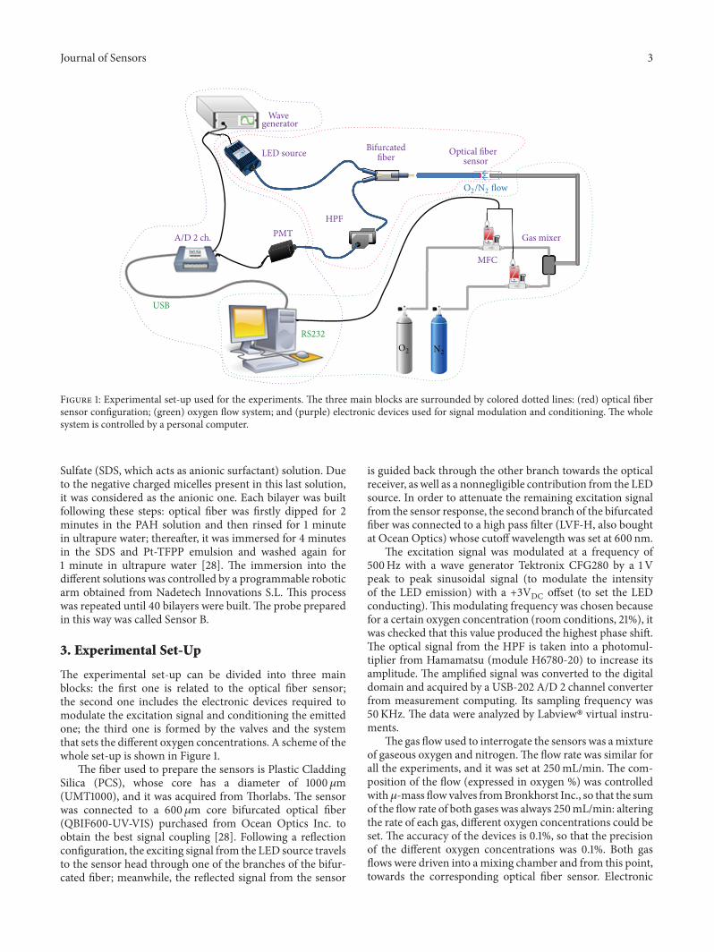
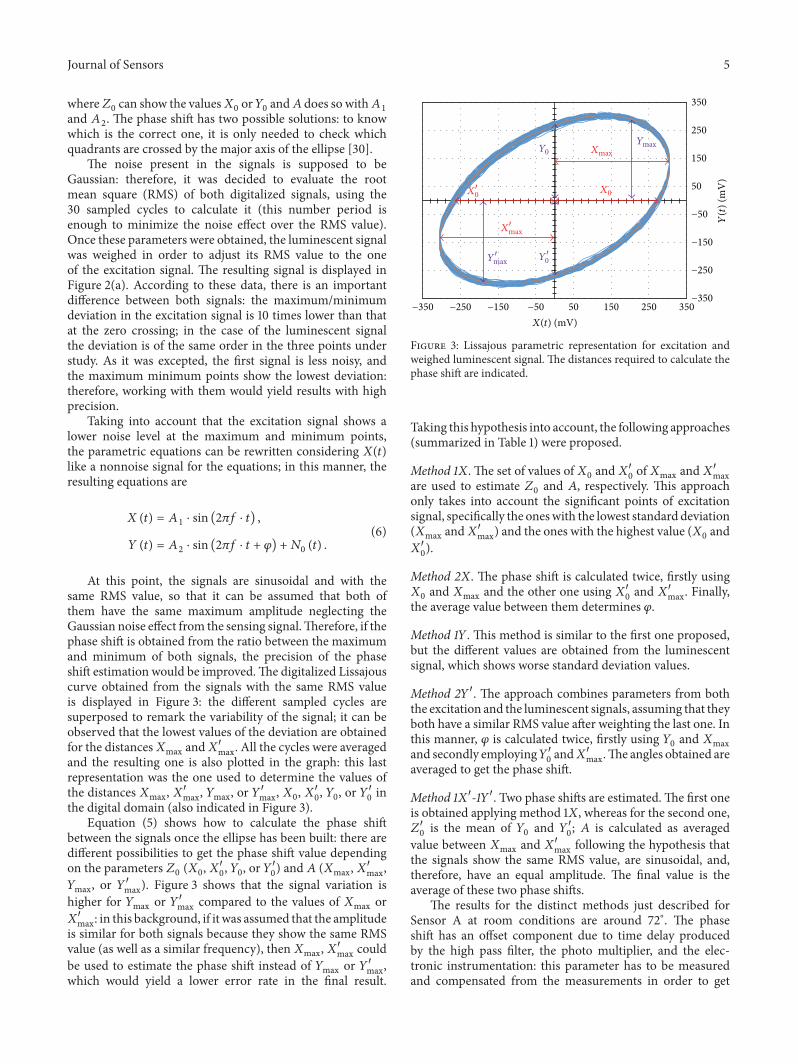
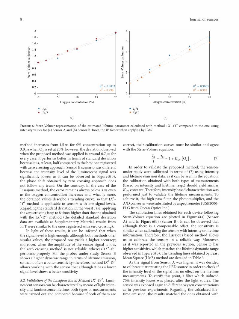
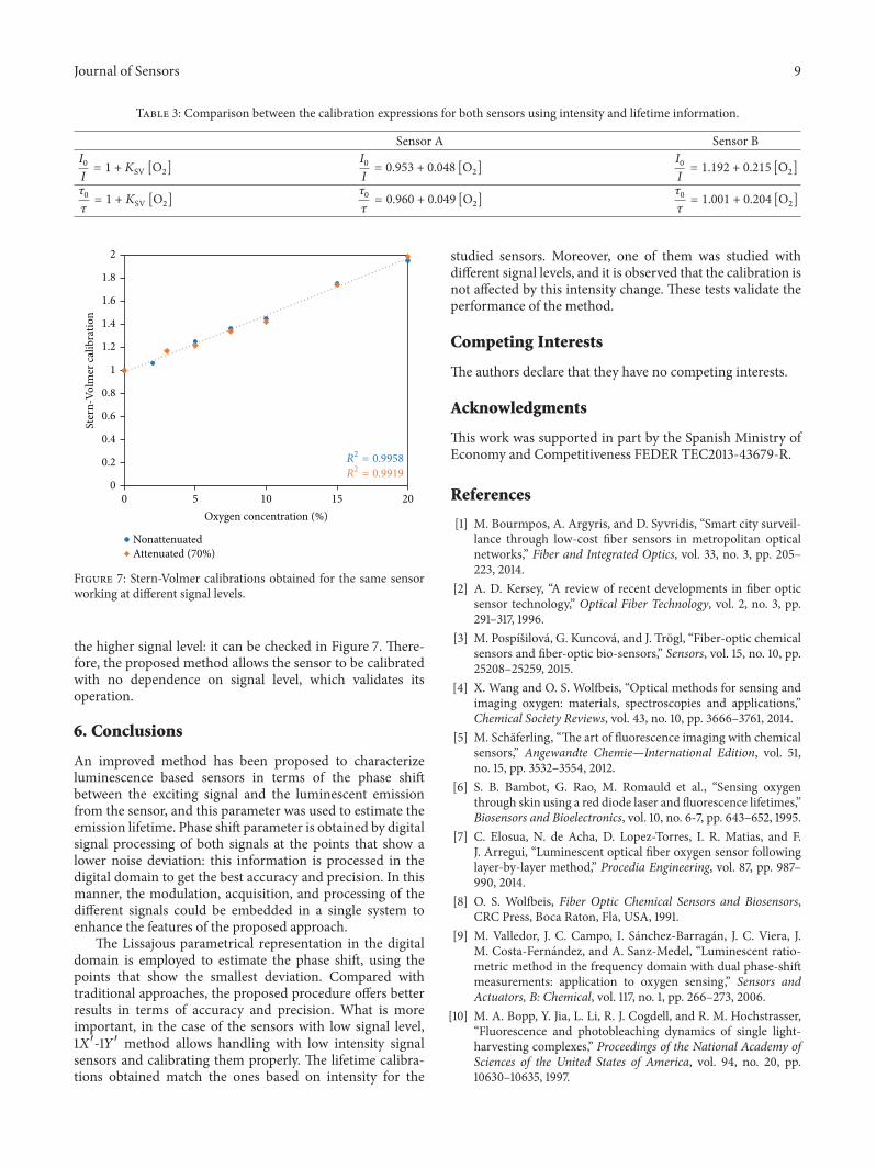

International Journal of
AerospaceEngineeringHindawi Publishing Corporationhttpwwwhindawicom Volume 2014
RoboticsJournal of
Hindawi Publishing Corporationhttpwwwhindawicom Volume 2014
Hindawi Publishing Corporationhttpwwwhindawicom Volume 2014
Active and Passive Electronic Components
Control Scienceand Engineering
Journal of
Hindawi Publishing Corporationhttpwwwhindawicom Volume 2014
International Journal of
RotatingMachinery
Hindawi Publishing Corporationhttpwwwhindawicom Volume 2014
Hindawi Publishing Corporation httpwwwhindawicom
Journal ofEngineeringVolume 2014
Submit your manuscripts athttpwwwhindawicom
VLSI Design
Hindawi Publishing Corporationhttpwwwhindawicom Volume 2014
Hindawi Publishing Corporationhttpwwwhindawicom Volume 2014
Shock and Vibration
Hindawi Publishing Corporationhttpwwwhindawicom Volume 2014
Civil EngineeringAdvances in
Acoustics and VibrationAdvances in
Hindawi Publishing Corporationhttpwwwhindawicom Volume 2014
Hindawi Publishing Corporationhttpwwwhindawicom Volume 2014
Electrical and Computer Engineering
Journal of
Advances inOptoElectronics
Hindawi Publishing Corporation httpwwwhindawicom
Volume 2014
The Scientific World JournalHindawi Publishing Corporation httpwwwhindawicom Volume 2014
SensorsJournal of
Hindawi Publishing Corporationhttpwwwhindawicom Volume 2014
Modelling amp Simulation in EngineeringHindawi Publishing Corporation httpwwwhindawicom Volume 2014
Hindawi Publishing Corporationhttpwwwhindawicom Volume 2014
Chemical EngineeringInternational Journal of Antennas and
Propagation
International Journal of
Hindawi Publishing Corporationhttpwwwhindawicom Volume 2014
Hindawi Publishing Corporationhttpwwwhindawicom Volume 2014
Navigation and Observation
International Journal of
Hindawi Publishing Corporationhttpwwwhindawicom Volume 2014
DistributedSensor Networks
International Journal of