research article an investigation of the southern ocean...

Hindawi Publishing CorporationISRN OceanographyVolume 2013, Article ID 392632, 9 pageshttp://dx.doi.org/10.5402/2013/392632

Research ArticleAn Investigation of the Southern Ocean Surface TemperatureVariability Using Long-Term Optimum Interpolation SST Data

Megha Maheshwari, Rajkumar Kamaljit Singh, Sandip Rashmikant Oza, and Raj Kumar

Space Applications Centre, Indian Space Research Organisation, Ahmedabad 380015, India

Correspondence should be addressed to Rajkumar Kamaljit Singh; [email protected]

Received 12 June 2013; Accepted 10 July 2013

Academic Editors: S. Focardi, C. Grenz, and M. Lipinski

Copyright © 2013 Megha Maheshwari et al. This is an open access article distributed under the Creative Commons AttributionLicense, which permits unrestricted use, distribution, and reproduction in any medium, provided the original work is properlycited.

An attempt is made to understand the long-term variability of SST using NOAA optimum interpolation SST data for the period(1982–2011) in the Southern Ocean. This dataset has been used (i) to study the interannual variability in SST anomaly and (ii) tocarry out regression analysis to compute linear trend in the annual averaged SouthernOcean SST. It is observed that summer seasonexhibits more variability than winter. Moreover, El Nino/La Nina events apparently play a critical role in the variability of SouthernOcean SST. Thus, higher SST anomalies were observed in El Nino years (e.g., 1983), while cooler anomalies were seen during LaNina years (e.g., 1985). In addition, the eastern and western sides of Antarctica experience episodes of warm and cold SST. Westernparts of the Southern Ocean experienced higher anomalies during 1992, 1993, and 1994, while the eastern part experienced positiveanomalies in 1997, 1998, 2002, and 2003.The paper also highlights the different regions of the Southern Ocean showing statisticallysignificant positive/negative trends in the variability of interannual average SST.However, in general, the SouthernOcean as a wholeis showing a weak interannual cooling trend in SST.

1. Introduction

Sea surface temperature (SST) plays an important role inoceanic heat content controlling the interactions betweenocean and atmosphere [1]. Changes in SST can be consideredas one of the most important indicators of climate change.Oceans are huge reservoirs of heat, and the heat release playsa major role in climate both in regional as well as globalscale. SST is a one of the parameters directly related to thisheat release. Thus, studying the variations of SST over a longperiod is important in understanding the nature of globalclimate change.

As observed by many researchers [2–5], the distributionof temperature on the sea surface is apparently zonal inbehaviour, with the warmest water near the equator andthe colder ones in the polar regions. Deviations from thisbehaviour are small. However, Deser et al. [6] evaluated the20th century SST trends using 5 different datasets, and asignificant global warming trend was observed, except in

some regions like the northwestern Atlantic. They reportedthe largest warming trends in the midlatitudes.

In the polar regions, surface temperature regulates thegrowth of sea ice, its melt, and the energy exchange betweensurface and atmosphere [7]. Comiso [8] evaluated thethermal infrared (TIR) data from the advanced very highresolution radiometer (AVHRR) for the period from 1979 to1998 (20 yr data) to study the trends in surface temperaturein the Antarctic region and found a slightly negative trend.The result was found to be consistent with the slightly positivetrend in sea ice extent observed by Cavalieri et al. [9]. Usingsatellite remote sensing data from AVHRR over a period of24 years from 1982 to 2005, Lebedev [10] has found a negativetrend of SST over the entire Southern Ocean.

Kwok and Comiso [11] studied the relationship betweenSouthern Oscillation and the anomalies of Southern Oceanclimatic parameters, namely, sea level pressure, wind, surfaceair temperature, and sea surface temperature fields and seaice variables including extent, concentration, motion, and

2 ISRN Oceanography

surface temperature. These climatic variables were correlatedwith the Southern Oscillation Index (SOI) for study periodspanning 17 years from 1982 to 1998, with strong correlationsobtaining around the regions of Bellingshausen, Amundsen,and Ross Seas.

In the polar oceans, sea ice generally forms when thetemperature of seawater reaches below −1.8∘C. Owing toits high albedo, sea ice reflects most of the incoming solarradiation, cooling down the polar environment. Increase inglobal SST will affect upon the polar environment via theoceanic circulations. This would inhibit the formation of seaice and would lead to more absorption of the incoming solarradiation, thereby warming up the polar regions (positivealbedo-temperature feedback) [12].

Studies show that the thinning of ice shelves and drainageof glacier in Antarctica, could be the result of warmingocean temperature rather than warming air temperature [13].Thus, SST over the Southern Ocean is a sensitive parameterby which the climate change signals are expected to berecognised [14, 15].

Our paper is organized into four sections, with theconcluding remarks briefed in Section 4. Section 2 describesthe data and the overall methodology of this study.

In Section 3, we present our findings on the interan-nual variability in SST anomaly over the Southern Ocean(Section 3.1) and the warming/cooling trends (Section 3.2)observed in interannual average surface temperature.

Some significant features were observed in four sectors,namely, theWeddell Sea-Ross Sea sectors and theAmundsen-Bellingshausen Seas (ABS)-Indian Ocean sectors, and this isdiscussed in detail in Section 3.3.These sectors are importantbecause of various reasons. The Weddell and Ross Seas areregarded as the regions of key sources of cold and densebottom water that influences global ocean circulation [16].Ross Sea andABS sectors are influenced by El Nino-SouthernOscillation (ENSO) episodes [11]. In addition, the ice coverin the Bellingshausen Sea is the habitat for a wide variety ofmarine life and is crucial to their survival.

Our study heremay be regarded as an extension to similarother studies by many researchers mentioned earlier in thisfield, and in that, we have extended the period of study tothe recent times, which will therefore incorporate signals ofrecent climate change.

2. Data and Methodology

Oceanographic changes in the SST for different regions ofSouthern Ocean were observed with the help of NOAAoptimum interpolation (OISST Version 2) [17] (henceforthOI.v2) for the period from January 1982 to October 2011.The OI.v2 dataset contains monthly SST fields derived by alinear interpolation of the weekly OI fields to produce dailyfields then averaging the appropriate daily values within amonth to produce monthly averages. The analysis uses in-situ and satellite SSTs plus SSTs simulated by sea ice coverover the marginal ice zone (MIZ) where both in situ aswell as satellite observations is sparse due to navigationhazards and cloud cover, respectively. The OI.v2 analysis has

a modest improvement over the version 1 [18] in the biascorrection because of the addition of more in situ data. TheSST dataset is on a 1∘ × 1∘ grid resolution. The first gridbox is centered on 0.5∘E, 89.5∘S. The points move eastwardto 359.5∘E and northward to 89.5∘N. These datasets areobtained from NOAA/OAR/ESRL PSD, Boulder, Colorado,USA, (website: http://www.esrl.noaa.gov/psd/) and are inter-polated into the polar stereographic projection using cubicconvolution resampling technique [19].

For distinguishing El Nino and La Nino events, we usethe Oceanic Nino Index (ONI), a standard index used by theClimate Prediction Center-NOAA [20].

In this paper, we first study the inter-annual variabilityin surface temperature over the entire Southern Ocean bycomparing among the annual anomaly maps generated asa difference between each yearly SST and the long-term(1982–2010) average SST. We computed annual (Jan.–Dec.)averages in order to remove seasonal variations in the surfacetemperature fields. We then perform a regression analysisto compute the inter-annual trend in the Antarctic and theregions with statistically significant trends are marked withcontours.

A discussion on the decadal variations of SST duringthree distinct decades, namely, 1982–1991, 1992–2001, and2002–2011, is presented in this paper. For this, the decadalmonthly anomalies were generated by first creating thedecadal means and then removing the monthly climatologyfrom each decade for the same month.

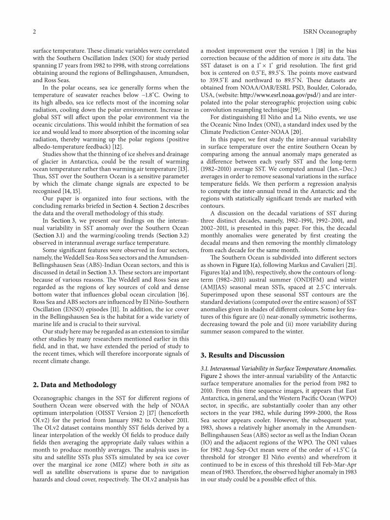
The Southern Ocean is subdivided into different sectorsas shown in Figure 1(a), following Markus and Cavalieri [21].Figures 1(a) and 1(b), respectively, show the contours of long-term (1982–2011) austral summer (ONDJFM) and winter(AMJJAS) seasonal mean SSTs, spaced at 2.5∘C intervals.Superimposed upon these seasonal SST contours are thestandard deviations (computed over the entire season) of SSTanomalies given in shades of different colours. Some key fea-tures of this figure are (i) near-zonally symmetric isotherms,decreasing toward the pole and (ii) more variability duringsummer season compared to the winter.

3. Results and Discussion

3.1. Interannual Variability in Surface Temperature Anomalies.Figure 2 shows the inter-annual variability of the Antarcticsurface temperature anomalies for the period from 1982 to2010. From this time sequence images, it appears that EastAntarctica, in general, and theWestern Pacific Ocean (WPO)sector, in specific, are substantially cooler than any othersectors in the year 1982, while during 1999-2000, the RossSea sector appears cooler. However, the subsequent year,1983, shows a relatively higher anomaly in the Amundsen-Bellingshausen Seas (ABS) sector as well as the Indian Ocean(IO) and the adjacent regions of the WPO. The ONI valuesfor 1982 Aug-Sep-Oct mean were of the order of +1.5∘C (athreshold for stronger El Nino events) and wherefrom itcontinued to be in excess of this threshold till Feb-Mar-Aprmean of 1983.Therefore, the observed higher anomaly in 1983in our study could be a possible effect of this.

ISRN Oceanography 3

0.4

1.2

2.0

0

10

20∘E

90∘E

180∘E 160∘E

230∘E

300∘E

WAIS EAIS

IndianOcean (IO)

WesternPacific Ocean (WPO)

Ross Sea (RS)

Amundsen andBellingshausen

Seas(ABS)

Weddell Sea (WS)

Summer

(∘C)

(a)

0.4

1.2

2.0

010 Winter

(∘C)

(b)

Figure 1: Long-term mean SSTs (contours) and standard deviations of SST anomalies (shading) for the (a) austral summer (ONDJFM) and(b) winter (AMJJAS) season. Contour interval is 2.5∘C; 0∘C and 10∘C isotherms aremarked. Also, the different sectors of Antarctica are shownrelevant to this present study. EAIS and WAIS represent East Antarctic Ice Sheet and West Antarctic Ice Sheet, respectively.

West Antarctica experienced higher anomalies during1992, 1993, 1994, 1995, and so forth, whereas in years like 1997,1998, 2002, 2003, and so forth, East Antarctica experiencedpositive anomalies. Comiso [8] has also found the years 1994–1996 to be warmer. However, it may be noted here that hehad used only the July month anomalies for the period from1979 to 1998; while in our case, we have used annual averageanomalies. The year 1992 experienced moderately strong ElNino event and thus the higher surface temperature anomalyobserved in our study, while 1994-95 had a weak El Nino.The year 1997, showing an overall warming in almost all thesectors of Southern Ocean, was a strong El Nino year. Thecolder anomalies observed in our study could possibly beexplained in terms of the La Nina event. Hence, years like1999 and 2000 having strong La Nina events show colderanomalies in the eastern as well as the western Antarcticwaters, for example, the WPO and the ABS sectors.

Time series plot of temperature anomalies in ∘C for theSouthernOcean (here taken to be the oceanic regions beyond∼45∘S up to the Antarctic continent boundaries) is givenin Figure 3. The mean anomaly (black), maximum values(red), minimum (blue), and standard deviations (dashed)are plotted in it. In the plot, each mean value representsthe average temperature anomaly over the entire SouthernOcean for a particular year; minimum (maximum) is a valueat a particular pixel with the lowest (highest) temperature;standard deviations represent the fluctuations around themean over the entire period of study.The statistics shown arefor the linear regression over the yearly mean SST.

The highest temperature (0.12 ± 0.21∘C) anomaly overthe entire Southern Ocean is observed in the year 1997,while 2008 with an anomaly temperature of −0.12 ± 0.21∘Crepresents the coldest year in our study. We performeda linear regression over the annual-averaged temperatureanomaly data, and we found that over the entire region, thereis a weak negative trend. However, at 95% confidence, the

negative trend is not statistically significant as suggested bythe statistical 𝑃 value (>0.05).We will discuss about the trendanalysis on a grid-wise scale in the following subsection.

3.2. Trend Analysis of Interannual Average Temperatures. Agrid-wise trend analysis is carried out using linear regressionin order to see if there is any significant trend in the variationsof the inter-annual average surface temperatures. A trendmap is generated as shown in Figure 4. In the figure, regionswith statistically significant trends are marked by a dashedcontour.

Oza et al. [22] used the entire life span (1999–2009) dataof QuikSCAT to study the inter-annual variations in thesummer and spring sea ice extent in the Arctic as well as theAntarctic. They found a significant positive sea ice trend inthe IO sector. This can be explained by the observed coolingtrend of surface temperature visible in the IO sector.

TheWPO sector close to the coast shows a cooling trend.However, farther away from the coast (<60∘S toward theequator), a significant warming trend is observed. Duringsummer season, this region is almost entirely ice-free.

Majority of the Ross Sea sector is showing a cooling trend.However, there is a small region near the Ross shelf showingboth slight warming and cooling trend. Moving toward 60∘S,a more prominent cooling trend is observed.

The ABS sector is showing statistically significant warm-ing trend in consistency with the findings of decreasing seaice trend by Oza et al. [22, 23]. Likewise, here too, around60∘S, the SST anomaly trend is more toward cooling thanwarming. In the Weddell Sea sector (WS), majority of theregion is showing a significant cooling trend.

In addition to this, we also present here in Figure 5a colour-coded map showing the difference between theannual average surface temperature in 2010 and 1982, theend and beginning of our analysis period. This image will

4 ISRN Oceanography

1982

61∘S

180∘E

0∘E1983

61∘S

180∘E

0∘E1984

61∘S

180∘E

0∘E1985

61∘S

180∘E

0∘E

1986

61∘S

180∘E

0∘E1987

61∘S

180∘E

0∘E1988

61∘S

180∘E

0∘E1989

61∘S

180∘E

0∘E

1990

61∘S

180∘E

0∘E1991

61∘S

180∘E

0∘E1992

61∘S

180∘E

0∘E1993

61∘S

180∘E

0∘E

1994

61∘S

180∘E

0∘E1995

61∘S

180∘E

0∘E1996

61∘S

180∘E

0∘E1997

61∘S

180∘E

0∘E

1998

61∘S

180∘E

0∘E1999

61∘S

180∘E

0∘E2000

61∘S

180∘E

0∘E2001

61∘S

180∘E

0∘E

2002

61∘S

180∘E

0∘E2003

61∘S

180∘E

0∘E2004

61∘S

180∘E

0∘E2005

61∘S

180∘E

0∘E

2006

61∘S

180∘E

0∘E

2010

61∘S

180∘E

0∘E

2007

61∘S

180∘E

0∘E2008

61∘S

180∘E

0∘E2009

61∘S

180∘E

0∘E

0.48

0.42

0.33

0.24

0.15

0.03

−0.06

−0.15

−0.24

−0.33

−0.42

−0.51

−0.60

−0.69

−0.78

(∘C)

Interannual anomaly maps (1982–2010)

Figure 2: Antarctic annual (January–December) anomaly maps of surface temperatures for the period from 1982 to 2010. Anomalies arecomputed by subtracting the long-term average from the yearly average.

ISRN Oceanography 5

YearMinimum

MeanMaximumLinear (mean)

1980

1982

1984

1986

1988

1990

1992

1994

1996

1998

2000

2002

2004

2006

2008

2010

2012

−2

−1.5

−1

−0.5

0

0.5

1

1.5

2

SST

anom

aly

(∘C)

±St.dev.

y = −0.001x + 3.401

R2 = 0.04P = 0.27

Figure 3: Time series showing the variation of Southern Oceansurface temperature anomalies (in ∘C). Black line shows the meananomaly, red line gives the maximum values, blue line, minimum,and the dashed lines represent ±sigma. Here, mean represents theaverage temperature anomaly over the entire region; minimum(maximum) is a value at a particular pixel with the lowest (highest)temperature; standard deviation represents the fluctuations aroundthe mean over the entire period of study. A linear trend (greenstraight line) is also shown, with the regression statistics given at thetop left corner.

180∘E

0∘E

61∘S

0.0290

0.0198

0.0106

0.0014

−0.0078

−0.0169

−0.0261

(∘C/

yr)

Figure 4: Trends in SouthernOcean surface temperature anomaliesfor the period from 1982 to 2010. Regionswith statistically significanttrends are marked by the dashed contours.

help in visualising the magnitude of change in the surfacetemperatures during this period of study. The warming andcooling trends observed in the previous figure, Figure 4,are also, in general, visible in this difference map, Figure 5.However, the strong warming trend in the ABS as observedin Figure 4 is not widespread as shown in Figure 5. Anotherpoint of difference is at the South Atlantic Ocean at around15∘–0∘E and 53∘S where a strong warming is observed.

180∘E

0∘E

61∘S

1.83

1.24

0.65

0.07

−1.11

(∘C)

−0.52

Figure 5: Difference map between annual average surface tempera-ture of 2010 and 1982.

From both these images, a very important observationcan be made; that is, the part of the Southern Ocean in theEast Antarctic sector is experiencing a significant warmingwhile the West Antarctic sector, a more significant cooling,in general. However, as a whole, the area experiencingcooling over the entire Southern Ocean is larger than thatexperiencing warming.

3.3. Regional Assessment of the Variations in Decadal SSTAnomalies. In our analysis, it was found that four differentsectors in the Antarctic (the ABS-Ross Sea and the WeddellSea-IO sectors) were showing some distinct patterns of SSTvariation during the austral summer month of February. Itappears that there exists a linkage between the temperaturepatterns in one sector with that in another sector. For theentire study period from 1982 to 2011, a negative correlationof ∼ −0.43 (𝑃 = 0.01) is observed in the ABS-Ross sectorpair and a statistically weak negative correlation of ∼ −0.27(𝑃 = 0.15) at the Weddell-IO sector. We discuss here thepatterns of SST variations in three discrete decades, namely,1982–91, 1992–2001, and 2002–11.

3.3.1. Amundsen-Bellingshausen Sea-Ross Sea Sector Pair. Inthe Bellingshausen Sea, the February decadal mean anomalyfor the period (1982–91) shows a large cold anomaly near theGeorge VI Sound Ice Shelf (Figure 6(a)). This was around0.6∘C colder than the decadal average value for the period1982–91. However, a positive anomaly of around 0.5∘C wasobserved in the Drake Passage. The result so obtained in thewestern part of the Antarctic Peninsula is consistent withthose reported byMeredith andKing [24] using hydrographicdata of the region west to the Western Antarctic Peninsula.

Apparently, the cold surface temperature episode in theABS sector during 1982–91 gradually gave way to a warmerepisode of 2002–11. The temperature anomaly in 2002–11 was∼0.4∘C. It may, however, be noted that in 2002–11, the DrakePassage experienced a cooler anomaly (∼0.3∘C lesser than thedecadal average around this region).

6 ISRN Oceanography

270∘E

60∘S

240∘E 210∘E

270∘E

60∘S

240∘E 210∘E

75∘S75∘S

270∘E

60∘S

240∘E 210∘E

75∘S

−0.66 −0.51 −0.36 −0.21 −0.06 0.09 0.24 0.39 0.54

(∘C)

1982–1991 1992–2001 2002–2011

(a)

−0.66 −0.51 −0.36 −0.21 −0.06 0.09 0.24 0.39 0.54

180∘E 150∘E 180∘E 150∘E 180∘E 150∘E

60∘S 60∘S60∘S

75∘S75∘S 75∘S

(∘C)

1982–1991 1992–2001 2002–2011

(b)

Figure 6: Color coded maps for the month of February (austral summer) representing decadal SST anomalies for three successive decades:1982–1991, 1992–2001 and 2002–2011. (a) shows the variations of SST anomalies over Amundsen-Bellingshausen Seas sector; anomalyvariations over Ross Sea sector are shown in (b). Negative anomaly in the ABS sector during the period 1982–91 is visible which progressivelybecomes positive in 2002–11. However, Ross Sea shows intense warmer SST during 1982–91 and slowly changes to colder SST during 2002–11.Gray color represents the continent. Regions of study are marked by white circles.

The situation in the Ross Sea sector (Figure 6(b)) shows acomplete reversal of the anomaly pattern as observed in theABS sector. Here, warmer temperature was observed for thedecade 1982–91 with a temperature anomaly of ∼0.6∘C whichchanged to a colder temperature in 2002–11 with an anomalyof ∼ −0.4∘C. El Nino events in the years such as 1983, 1987,1992, and 1998 might have significantly contributed to theanomaly patterns so observed in these sectors.

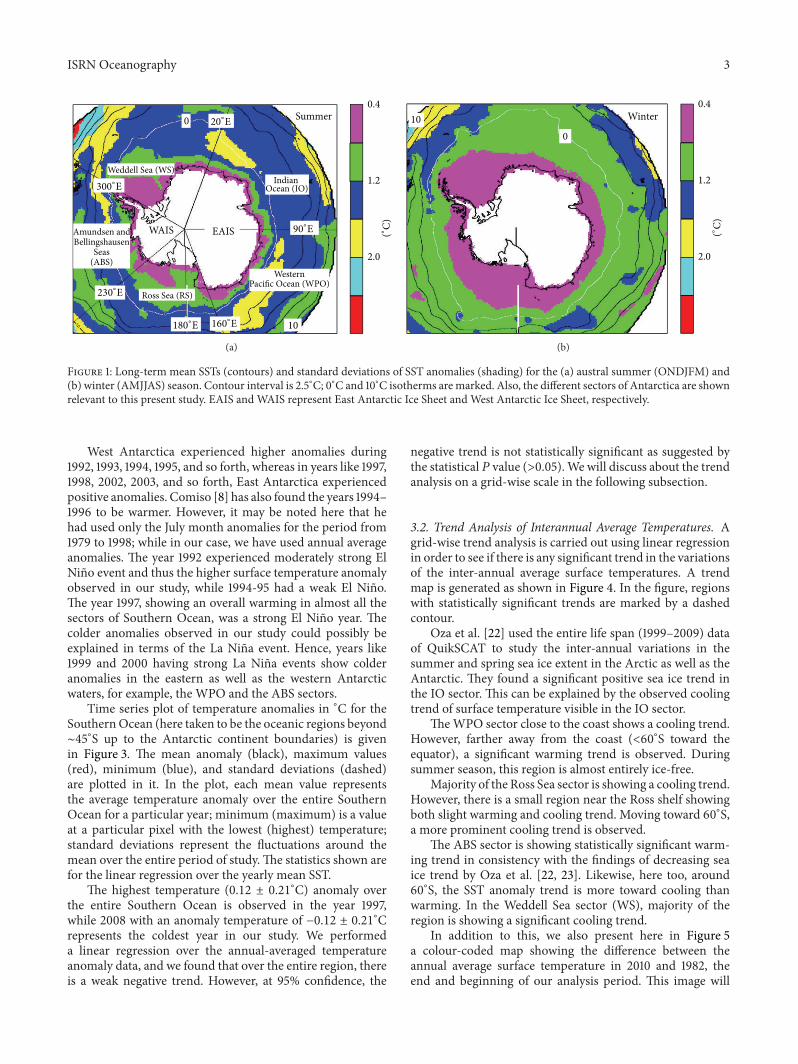
3.3.2. Weddell Sea-Indian Ocean Sector Pair. An almost simi-lar behaviour is observed in the Weddell Sea-Indian Oceansectors (Figures 7(a) and 7(b)). Even though the surfacetemperature cooled down from 0.5∘ to −0.3∘C in the three

successive decades, the change in the Weddell Sea is not thatgradual as observed in the Ross sea sector. As evident, the twodecades, 1982–92 and 1992–2001, have almost comparablepositive anomalies around the Weddell Sea region, while thecooling became apparent only during the last decade 2002–11.In the Indian Ocean sector, a trivial warming was observednear the Amery shelf basin (left of the ellipse in Figure 7(b))in the period 1982–91 which moved toward the northern sideand amplified at around 45∘S in 2002–11. In this region, thesurface temperature deviates from the mean by as much as0.4∘C for the period of the three decades 1982–91 to 2002–11.

In order to gain more insight about this behaviour in thetemporal domain, a 30-year trend analysis of SST anomalyhas been carried out for the month of February. It has been

ISRN Oceanography 7

330∘E 345∘E 0∘E 15∘E

60∘S

75∘S

330∘E 345∘E 0∘E 15∘E 330∘E 345∘E 0∘E 15∘E

60∘S

75∘S

60∘S

75∘S

−0.66 −0.51 −0.36 −0.21 −0.06 0.09 0.24 0.39 0.54

(∘C)

1982–1991 1992–2001 2002–2011

(a)

−0.66 −0.51 −0.36 −0.21 −0.06 0.09 0.24 0.39 0.54

(∘C)

75∘E

90∘E

105∘E

45∘S

60∘S

75∘E

90∘E

105∘E

45∘S

60∘S

75∘E

90∘E

105∘E

45∘S

60∘S

1982–1991 1992–2001 2002–2011

(b)

Figure 7: As in Figure 6, but for the (a) Weddell Sea and (b) Indian Ocean sectors of Southern Ocean. Temperature anomaly in Weddell Seasector has decreased by 0.2∘C from the period 1982–91 to 2002–11. However, in Indian Ocean sector (around 90∘E), the surface temperatureof ocean deviates up to 0.4∘C from the average from 1982–91 to 2002–11.

found that the time sequence of SST anomalies shows largeryear-to-year variability for all the four regions (Figure 8).Thestudy reveals that the ABS sector has a positive trend at a rateof 0.02±0.01∘C/yr.The temperature anomaly varies from thelowest of −0.67∘C in 1986 to the highest of 0.70∘C in 2003.However, in the adjacent seas: Ross andWeddell seas coolingtrends of−0.04±0.01∘C/yr and−0.02±0.01∘C/yr, respectively,were observed. In case of Indian Ocean sector, 2011 was thewarmest year (0.68∘Cmore than the average).There is a steepincrease in the surface temperature from 2005 to 2011, anincrease of about 0.97∘C. Overall, a positive trend has beenobserved in the Indian Ocean sector, which is amplifying at arate of 0.02 ± 0.01∘C/year.

The comparative investigation provided an interestingresult that during the 30-year time period both the lowest aswell the highest temperature anomalies occurred only over

the Ross Sea sector among all the four with −0.81∘C in 1995and 1.08∘C in 1984, respectively.

4. Conclusion

In this study, the variations of NOAA analysed sea surfacetemperatures over the Southern Ocean have been investi-gated for the period from 1982 to 2011. Inter-annual variabilityof the Antarctic surface temperature anomalies for the periodfrom 1982 to 2010 is studied. The Western Pacific Ocean(WPO) sector experienced a substantially colder surfacetemperature than any other sectors in 1982. As expected, theEl Nino events have impacts on the Antarctic waters, and in1983, a higher surface temperature over the Southern Oceanhas been reported.

8 ISRN Oceanography

y = 0.02x − 42.34

R2 = 0.32

−0.8

−0.6

−0.4

−0.2

0

0.2

0.4

0.6

0.8SS

T an

omal

y (∘

C)

1980

1982

1984

1986

1988

1990

1992

1994

1996

1998

2000

2002

2004

2006

2008

2010

2012

Year

P < 0.05

(a)

y = −0.04x + 79.41

R2 = 0.43

−1

−0.8

−0.6

−0.4

−0.2

00.20.40.60.8

11.2

SST

anom

aly

(∘C)

Year

1980

1982

1984

1986

1988

1990

1992

1994

1996

1998

2000

2002

2004

2006

2008

2010

2012

P < 0.05

(b)

−0.8

−0.6

−0.4

−0.2

0

0.2

0.4

0.6

SST

anom

aly

(∘C)

1980

1982

1984

1986

1988

1990

1992

1994

1996

1998

2000

2002

2004

2006

2008

2010

2012

Year

y = −0.02x + 32.41

R2 = 0.25

P < 0.05

(c)

−0.6

−0.4

−0.2

0.2

0.4

0.6

0.8

SST

anom

aly

(∘C)

1980

1982

1984

1986

1988

1990

1992

1994

1996

1998

2000

2002

2004

2006

2008

2010

2012

Year

0

R2 = 0.22

P < 0.05

y = 0.02x − 31.71

(d)

Figure 8: A 30-year trend analysis of surface temperature anomalies over four different sectors of the Southern Ocean summer month ofFebruary over four different sectors of (a) Amundsen-Bellingshausen Seas, (b) Ross Sea, (c) Weddell Sea, and (d) Indian Ocean sectors. ABSand Indian Ocean sectors are showing positive trends at per year rate of 0.02 ± 0.01∘C. However, negative trends of −0.04 ± 0.01∘C/yr and−0.02 ± 0.01

∘C/yr have been computed over Ross Sea and Weddell Sea sectors, respectively.

East and West Antarctic waters experienced differentepisodes of warming and cooling events. Thus, West Antarc-tica experienced higher anomalies during 1992, 1993, 1994,1995, and so forth, whereas in years like 1997, 1998, 2002 and2003, East Antarctic experienced positive anomalies.

From the time series analysis of the variation of SouthernOcean surface temperature anomalies, a slightly negative(i.e., cooling) trend in average temperature anomaly overthe entire region is obtained. However, this trend is veryweak and found to be statistically insignificant. However,on a regional scale, there are regions showing statisticallysignificant trends in warming/cooling surface temperatures.Thus, regions like Amundsen-Bellingshausen Seas sector areshowing statistically significant warming trend, while theWestern Pacific Ocean sector close to the continental coastis showing a cooling trend, and the far off regions over theocean are, however, giving a warming trend.

We have also studied in this paper the variation of decadalanomalies for the month of February (austral summer) for 4different sectors in Antarctica. It is found that the warming

trend is dominant over ABS and Indian Ocean sectors, whilethe Ross Sea and Weddell Sea are experiencing a coolingtrend.

One of the very important findings of this analysis is thesteep rise in summer surface temperature observed in theIndian Ocean from 2005 to 2011. If this rise continues formore years to come, it would have an adverse effect on thethickness of Amery ice shelf [13].

There are other significant cryospheric impacts of thesefindings. Majority of the glaciers in the Antarctic regionare retreating at an accelerating rate. It is found that themelt rate of ice shelves is directly related to the surfacetemperature of the ocean [25]. Therefore, our study on thesurface temperature variability and the findings, thereof, ofa very strong surface warming over some sectors of theAntarctic Ocean would have significant implications on thefuture of the ice shelves and global climate change.

A prolonged change in the ocean temperature wouldchange the sea ice cover, and this will affect the regional-scaleecosystem. As pointed out by Jacobs and Comiso [26], the

ISRN Oceanography 9

exact cause of SST variations is not yet well know; however,these changes in surface temperature of oceans are linked to alarger scale climate phenomena, which needs to be addressedin more elaborate ways.

Acknowledgments

The authors are thankful to Shri A. S. Kiran Kumar, Directorof SAC-ISRO, for his constant encouragement and guidanceto carry out the activities in the field of polar science.The valuable comments given by Dr. J. S. Parihar, Dr. P.K. Pal, Dr. Abhijit Sarkar, and Dr. N. K. Vyas are alsoacknowledged. NOAA analysed SST data (OISST Version2) are obtained from NOAA/OAR/ESRL PSD, Boulder, Col-orado, USA (website: http://www.esrl.noaa.gov/psd/) and areacknowledged here.

References

[1] R. W. Reynolds, T. M. Smith, C. Liu, D. B. Chelton, K. S. Casey,and M. G. Schlax, “Daily high-resolution-blended analyses forsea surface temperature,” Journal of Climate, vol. 20, no. 22, pp.5473–5496, 2007.

[2] P. K. Rao, W. L. Smith, and R. Koffler, “Global sea-surfacetemperature distribution determined from and environmentalsatellite,”MonthlyWeather Review, vol. 100, no. 1, pp. 10–14, 1971.

[3] G. W. Paltridge, “Latitudinal variation in the change of seasurface temperature from 1880 to 1977,” Monthly WeatherReview, vol. 112, no. 5, pp. 1093–1095, 1984.

[4] ADEOS Earth View, “Global Sea Surface Temperature Dis-tribution. Japan Aerospace Exploration Agency, Japan,” 1999,http://suzaku.eorc.jaxa.jp/GLI2/adeos/Earth View/eng/adeos-08e.pdf.

[5] NASA Science, “Temperature,” National Aeronautics and SpaceAgency, USA, 2012, http://science.nasa.gov/earth-science/oceanography/physical-ocean/temperature/.

[6] C. Deser, A. S. Phillips, and M. A. Alexander, “Twentiethcentury tropical sea surface temperatures revisited,”GeophysicalResearch Letters, vol. 37, no. 10, 2010.

[7] J. R. Key, J. B. Collins, C. Fowler, and R. S. Stone, “High-latitude surface temperature estimates from thermal satellitedata,”Remote Sensing of Environment, vol. 61, no. 2, pp. 302–309,1997.

[8] J. C. Comiso, “Variability and trends in Antarctic surfacetemperatures from In Situ and satellite infraredmeasurements,”Journal of Climate, vol. 13, no. 10, pp. 1674–1696, 2000.

[9] D. J. Cavalieri, P. Gloersen, C. L. Parkinson, J. C. Comiso, andH. J. Zwally, “Observed hemispheric asymmetry in global seaice changes,” Science, vol. 278, no. 5340, pp. 1104–1106, 1997.

[10] S. A. Lebedev, “Inter-annual trends in the southern ocean seasurface temperature and sea level from remote sensing data,”Russian Journal of Earth Sciences, vol. 9, Article IDES3003, 2007.

[11] R. Kwok and J. C. Comiso, “Southern Ocean climate and sea iceanomalies associated with the Southern Oscillation,” Journal ofClimate, vol. 15, no. 5, pp. 487–501, 2002.

[12] J. A. Curry, J. L. Schramm, and E. E. Ebert, “Sea ice-albedoclimate feedback mechanism,” Journal of Climate, vol. 8, no. 2,pp. 240–247, 1995.

[13] E. Rignot, G. Casassa, P. Gogineni, W. Krabill, A. Rivera, and R.Thomas, “Accelerated ice discharge from the Antarctic Penin-sula following the collapse of Larsen B ice shelf,” GeophysicalResearch Letters, vol. 31, no. 18, 2004.

[14] A. Mitra, I. M. L. Das, M. K. Dash, S. M. Bhandari, and N.K. Vyas, “Impact of ice-albedo feedback on hemispheric scalesea-ice melting rates in the antarctic using multi-frequencyscanning microwave radiometer data,” Current Science, vol. 94,no. 8, pp. 1044–1048, 2008.

[15] M. I. Budyko, “Polar ice and climate,” in Proceedings of the Sym-posium on the Arctic Heat Budget and Atmospheric Circulation.RM, 5233-NSF, J. O. Fletcher, Ed., pp. 3–32, Rand Corporation,Santa Monica, Calif, USA, 1966.

[16] G. Budillon, G. Fusco, and G. Spezie, “A study of surface heatfluxes in the Ross Sea (Antarctica),” Antarctic Science, vol. 12,no. 2, pp. 243–254, 2000.

[17] R. W. Reynolds, N. A. Rayner, T. M. Smith, D. C. Stokes, andW. Wang, “An improved in situ and satellite SST analysis forclimate,” Journal of Climate, vol. 15, no. 13, pp. 1609–1625, 2002.

[18] R. W. Reynolds and T. M. Smith, “Improved global sea surfacetemperature analyses using optimum interpolation,” Journal ofClimate, vol. 7, no. 6, pp. 929–948, 1994.

[19] J. A. Richards and X. Jia, Remote Sensing Digital Image Analysis,Springer, Berlin, Germany, 1999.

[20] Climate Prediction Center-NOAA, “Cold &Warm Episodes bySeason. NOAA/ National Weather Service, Center for Weatherand Climate Prediction, Climate Prediction Center,” 2012,http://www.cpc.ncep.noaa.gov/products/analysis monitoring/ensostuff/ensoyears.shtml.

[21] T. Markus and D. J. Cavalieri, “Interannual and regional vari-ability of SouthernOcean snowon sea ice,”Annals of Glaciology,vol. 44, pp. 53–57, 2006.

[22] S. R. Oza, R. K. K. Singh, A. Srivastava et al., “Inter-annualvariations observed in spring and summer antarctic sea iceextent in recent decade,”Mausam, vol. 62, pp. 633–640, 2011.

[23] S. R. Oza, R. K. K. Singh, N. K. Vyas, and A. Sarkar, “Recenttrends of arctic and antarctic summer sea-ice cover observedfrom space-borne scatterometer,” Journal of the Indian Societyof Remote Sensing, vol. 38, no. 4, pp. 611–616, 2010.

[24] M. P. Meredith and J. C. King, “Rapid climate change in theocean west of the antarctic peninsula during the second half ofthe 20th century,” Geophysical Research Letters, vol. 32, 2005.

[25] A. Shepherd, D. Wingham, and E. Rignot, “Warm ocean iseroding west antarctic ice sheet,” Geophysical Research Letters,vol. 31, 2004.

[26] S. S. Jacobs and J. C. Comiso, “Climate variability in theAmundsen and Bellingshausen Seas,” Journal of Climate, vol. 10,no. 4, pp. 697–709, 1997.

Submit your manuscripts athttp://www.hindawi.com

Hindawi Publishing Corporationhttp://www.hindawi.com Volume 2014

ClimatologyJournal of

EcologyInternational Journal of


EarthquakesJournal of


Hindawi Publishing Corporationhttp://www.hindawi.com

Applied &EnvironmentalSoil Science

Volume 2014

Mining


Journal of

Hindawi Publishing Corporation http://www.hindawi.com Volume 2014

International Journal of

Geophysics

OceanographyInternational Journal of


Journal of Computational Environmental SciencesHindawi Publishing Corporationhttp://www.hindawi.com Volume 2014

Journal ofPetroleum Engineering


GeochemistryHindawi Publishing Corporationhttp://www.hindawi.com Volume 2014

Journal of

Atmospheric SciencesInternational Journal of


OceanographyHindawi Publishing Corporationhttp://www.hindawi.com Volume 2014

Advances in


MineralogyInternational Journal of


MeteorologyAdvances in

The Scientific World JournalHindawi Publishing Corporation http://www.hindawi.com Volume 2014

Paleontology JournalHindawi Publishing Corporationhttp://www.hindawi.com Volume 2014

ScientificaHindawi Publishing Corporationhttp://www.hindawi.com Volume 2014


Geological ResearchJournal of


Geology Advances in

research article an investigation of the southern ocean...

Documents