research article accurate simulation of mppt methods...

Research ArticleAccurate Simulation of MPPT Methods Performance WhenApplied to Commercial Photovoltaic Panels

Javier Cubas, Santiago Pindado, and Ángel Sanz-Andrés

ETSI Aeronauticos, Instituto Universitario de Microgravedad “Ignacio Da Riva” (IDR/UPM), Universidad Politecnica de Madrid,Plaza del Cardenal Cisneros 3, 28040 Madrid, Spain

Correspondence should be addressed to Javier Cubas; [email protected]

Received 27 June 2014; Revised 17 September 2014; Accepted 18 September 2014

Academic Editor: Hua Bai

Copyright © 2015 Javier Cubas et al. This is an open access article distributed under the Creative Commons Attribution License,which permits unrestricted use, distribution, and reproduction in any medium, provided the original work is properly cited.

A new, simple, and quick-calculationmethodology to obtain a solar panelmodel, based on themanufacturers’ datasheet, to performMPPT simulations, is described. The method takes into account variations on the ambient conditions (sun irradiation and solarcells temperature) and allows fast MPPT methods comparison or their performance prediction when applied to a particular solarpanel. The feasibility of the described methodology is checked with four different MPPT methods applied to a commercial solarpanel, within a day, and under realistic ambient conditions.

1. Introduction

Oil prices soared in the second half of the 20th century, themain causes being sociopolitical instabilities such as revolu-tions or wars, shortage of supply, stockmarket speculation, orthe increasing demand from emerging nations [1]. The eco-nomic problems derived from the unstable situation of theenergy market forced both the development of renewableenergy sources (photovoltaic energy, solar thermal energy,andwind energy) [2–4] and the increase in efficiency in termsof energy generation, transportation, and consumption. Inaddition, the demand for more efficient energy supply sys-tems has been increased as societies all over the world areincreasingly aware of the consequences of the global climatechange produced by greenhouse gas emissions.

Among the different renewable energy sources that havebeen developed and spread in the past half century, thephotovoltaic energy is a good example of the above two ten-dencies. On the one hand, the installed power has increasedenormously in some parts of the world, as it has beenmainly supported by government investment [5, 6]. On theother hand, technology improvements have produced moreefficient solar cells in terms of energy (from 11% efficiency ofsilicon solar cells in the 1950s [7], so that now it is possibleto get gallium-arsenide solar cells of above 30% efficiency [8–11]), cheaper cells based on organic technologies [12–14], and

better control processes to maximize the energy supply inevery irradiation and temperature conditions.

It is well known that photovoltaic systems are affected byfactors that reduce their efficiency such as

(i) changes on irradiation,(ii) changes on cells temperature,(iii) impedance variations at the system output,(iv) partial shading on the photovoltaic panel.

All these factors change the behavior of the panel, whichis normally defined by the output current-output voltagecurve (hereinafter, the I-V curve); see Figure 2 further in thetext, and, consequently, the maximum power point (MPP)of the panel is also modified. Therefore, if a photovoltaicsystem needs to be optimized in terms of power production,implementation on the system of a methodology to “follow”the changes of the MPP is required.

To the authors’ knowledge, the first works to analyze andtrack themaximumpower point of photovoltaic systemswerecarried out in the late 1960s [15]. Since then, the number ofpapers produced has broadly increased in line with the oilprices evolution. See in Figure 1 the number of papers relatedto photovoltaic maximum power point tracking (MPPT)methods that, according to Esram and Chapman, were

Hindawi Publishing Corporatione Scientific World JournalVolume 2015, Article ID 914212, 16 pageshttp://dx.doi.org/10.1155/2015/914212

2 The Scientific World Journal

0

5

10

15

20

25

30

0

25

50

75

100

125

150

1960 1980 2000 2020M

PPT

pape

rs

Oil

pric

e ($/

barr

el)

Year

BrentTexanEsram and Chapman (2007)

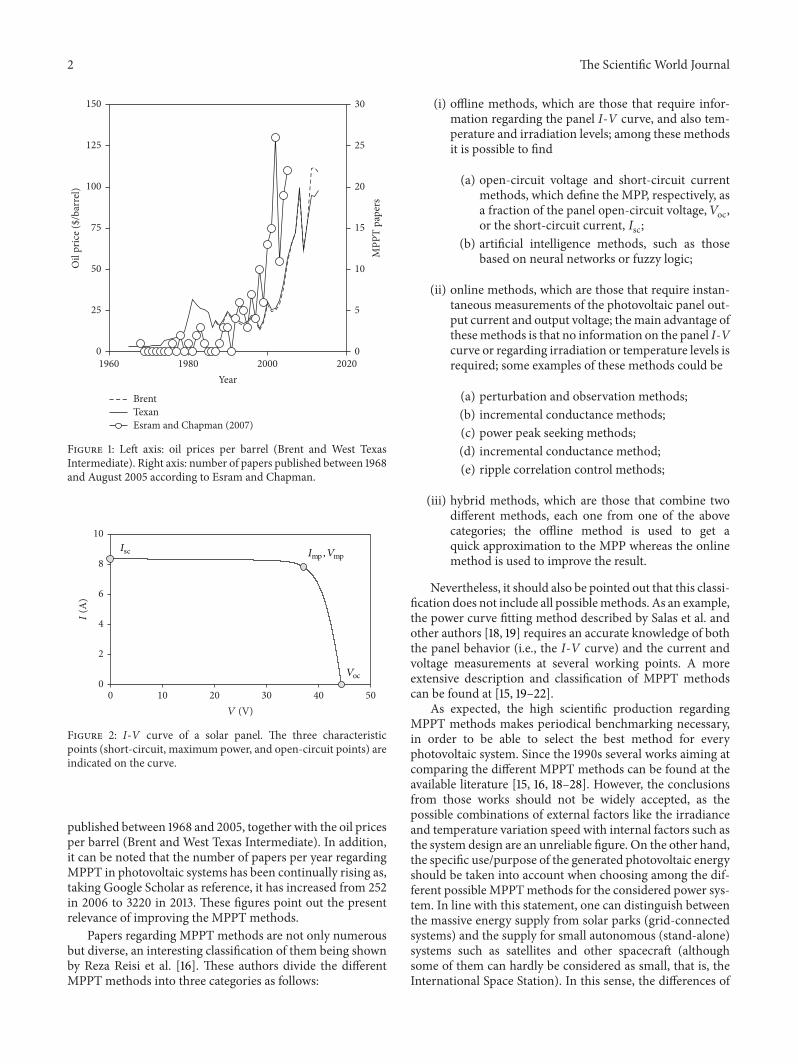
Figure 1: Left axis: oil prices per barrel (Brent and West TexasIntermediate). Right axis: number of papers published between 1968and August 2005 according to Esram and Chapman.

0

2

4

6

8

10

0 10 20 30 40 50

I (A

)

V (V)

Isc Imp , Vmp

Voc

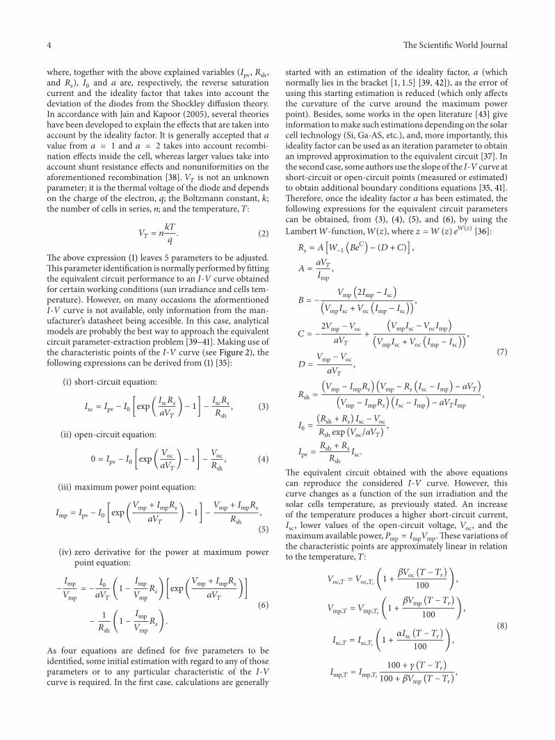
Figure 2: I-V curve of a solar panel. The three characteristicpoints (short-circuit, maximum power, and open-circuit points) areindicated on the curve.

published between 1968 and 2005, together with the oil pricesper barrel (Brent and West Texas Intermediate). In addition,it can be noted that the number of papers per year regardingMPPT in photovoltaic systems has been continually rising as,taking Google Scholar as reference, it has increased from 252in 2006 to 3220 in 2013. These figures point out the presentrelevance of improving the MPPT methods.

Papers regarding MPPT methods are not only numerousbut diverse, an interesting classification of them being shownby Reza Reisi et al. [16]. These authors divide the differentMPPT methods into three categories as follows:

(i) offline methods, which are those that require infor-mation regarding the panel I-V curve, and also tem-perature and irradiation levels; among these methodsit is possible to find

(a) open-circuit voltage and short-circuit currentmethods, which define the MPP, respectively, asa fraction of the panel open-circuit voltage, 𝑉oc,or the short-circuit current, 𝐼sc;

(b) artificial intelligence methods, such as thosebased on neural networks or fuzzy logic;

(ii) online methods, which are those that require instan-taneous measurements of the photovoltaic panel out-put current and output voltage; themain advantage ofthesemethods is that no information on the panel I-Vcurve or regarding irradiation or temperature levels isrequired; some examples of these methods could be

(a) perturbation and observation methods;(b) incremental conductance methods;(c) power peak seeking methods;(d) incremental conductance method;(e) ripple correlation control methods;

(iii) hybrid methods, which are those that combine twodifferent methods, each one from one of the abovecategories; the offline method is used to get aquick approximation to the MPP whereas the onlinemethod is used to improve the result.

Nevertheless, it should also be pointed out that this classi-fication does not include all possiblemethods. As an example,the power curve fitting method described by Salas et al. andother authors [18, 19] requires an accurate knowledge of boththe panel behavior (i.e., the I-V curve) and the current andvoltage measurements at several working points. A moreextensive description and classification of MPPT methodscan be found at [15, 19–22].

As expected, the high scientific production regardingMPPT methods makes periodical benchmarking necessary,in order to be able to select the best method for everyphotovoltaic system. Since the 1990s several works aiming atcomparing the different MPPT methods can be found at theavailable literature [15, 16, 18–28]. However, the conclusionsfrom those works should not be widely accepted, as thepossible combinations of external factors like the irradianceand temperature variation speed with internal factors such asthe system design are an unreliable figure. On the other hand,the specific use/purpose of the generated photovoltaic energyshould be taken into account when choosing among the dif-ferent possible MPPTmethods for the considered power sys-tem. In line with this statement, one can distinguish betweenthe massive energy supply from solar parks (grid-connectedsystems) and the supply for small autonomous (stand-alone)systems such as satellites and other spacecraft (althoughsome of them can hardly be considered as small, that is, theInternational Space Station). In this sense, the differences of

The Scientific World Journal 3

MPPT methods applied to mass energy generation or grid-connected systems and to power generation on spacecraftcan be underlined. The grid-connected photovoltaic systemsneed to maximize the production at the lower cost impact,taking into account the fact that a small increase in efficiencycan be translated into a huge growth of revenues after someyears of operation. This is achieved through MPPT methodswith high dynamic and tracking capacities. On the otherhand, it is also true that spacecraft require the best possibleenergy efficiency, but only after considering the reliabilityof the system [29] and some other associated problems,such as the thermal control [30]. Therefore, in stand-alonesystems, especially in spacecraft, simple but more reliableMPPTmethods are normally chosen, thereby excludingmoreefficient, but also more complicated methods.

Validation or comparison of MPPT methods is usu-ally carried out either based on experimental testing [31,32] results or based on computer simulations [25, 33, 34]although sometimes both kinds of procedures are combined[23, 24]. Experimental comparisons of MPPT methods arelogically more realistic, but it should be pointed out thatsimulations have some important advantages in terms of fastresults, cost, and versatility, whichmake them the best optionfor algorithms development or efficiency estimations.

One of the most significant difficulties of computationalanalysis lies in the solar panel behavior simulation. The mostcommon way to do it is through equivalent circuit models, asthis has proven to be very accurate [35]. Nevertheless, it mustbe underlined that different sun irradiation and temperaturelevels on the panel, as is required by any MPPT validation,involve the recalculation of the different parameters whichdefine the aforementioned equivalent circuit. In many cases,some simplifications of the equivalent circuit are considered,taking into account the fact that multiple recalculations area quite complicated task. An example of these simplificationscould be a circuit without series resistor [34], without parallelresistor [23], or without any resistor [25]. However, series andshunt resistances are directly related to the slope of the I-V curve at open-circuit and short-circuit points, respectively(𝑑𝐼/𝑑𝑉|sc ≈ −𝑅

−1

𝑠

and 𝑑𝐼/𝑑𝑉|oc ≈ −𝑅−1

sh ), and not takingthem into account modifies the shape of the I-V curve and,therefore, the position of the MPP. These simplificationsmake the behavior of theMPPTnumerical simulation slightlydiverge from the real performance of the photovoltaic system.

In the present paper a simple, direct, and analytical wayto define the behavior of a photovoltaic system under anysun irradiation and cells temperature conditions is presented.Based on the proposed method, solar panel models that fitperfectly to manufacturers’ datasheet experimental data canbe defined.The equivalent circuit model proposed consists ofone diode and two resistors (one in series and the other onein parallel), with no further simplification considered.

Through the methodology presented in this work, accu-rate simulations of MPPT strategies/algorithms can beachieved, bearing in mind different irradiance and solar celltemperature level and also different DC-DC convertors tobe connected to the panel. The aforementioned methodol-ogy is based on the 5-parameter equivalent circuit model

Ipv ID

Rsh

Rs

I

VD

Figure 3: Typical 1-diode equivalent circuit of a solar panel.

of a photovoltaic device (i.e., solar panel), the parameter-extraction being analytical (described in Section 2). Thisanalytical extraction to fit the equivalent circuit behavior ofthe I-V curves corresponding to solar cell has proven to beaccurate in previous works, in which different photovoltaictechnologies (monocrystalline/polycrystalline) [36] or mate-rials (Si/GaAs) [35] were analyzed. Also, if the equations areadjusted to reflect the number of cells connected in series andin parallel, this model can be used to analyze multijunctioncells, solar panels, or even groups of solar panels [37]. Nev-ertheless, it should also be mentioned that the low numberof the I-V curve points used for extrapolating the curve itselfis the greater limitation of the analytical methods, as thesepoints need to be very accurately measured (any deviation atthose points will be extrapolated along the I-V curve). On theother hand, some optimization of the analytical results can beintroduced if some extra data is available [37].

The text is organized as follows. In Section 2 solar panelanalytical modeling is described. In Section 3 the way to takeinto account ambient condition variations in the modelingis shown. In Section 4 four different MPPT methods arepresented, whereas calculations and results regarding theMPPT methods comparison carried out with the proposedmethodology are included in Section 5. Finally, a case study isincluded in Section 6, whereas the conclusions of the presentwork are summarized in Section 7.

2. Solar Panel Modeling

In Figure 2, a typical solar cell/panel I-V curve is shown.The characteristic points, short-circuit [𝐼sc, 0], open-circuit[0, 𝑉oc], and maximum power [𝐼mp, 𝑉mp] points are indicatedin the graph.This behavior is similar to the one from a circuitformed by a source of current, 𝐼pv, in parallel to a diode (seeFigure 3). Two resistors, one in parallel (shunt resistor), 𝑅sh,and the other one in series (series resistor), 𝑅

𝑠

, are added totake into account losses, such as the ones produced in cellsolder bonds, interconnection, and junction box, togetherwith current leakage through the high conductivity shuntsacross the p-n junction [35].

The equation that defines the behavior of the 1-diode/2-resistors equivalent circuit of Figure 3 is

𝐼 = 𝐼pv − 𝐼0 [exp(𝑉 + 𝐼𝑅

𝑠

𝑎𝑉𝑇

) − 1] −𝑉 + 𝐼𝑅

𝑠

𝑅sh, (1)


where, together with the above explained variables (𝐼pv, 𝑅sh,and 𝑅

𝑠

), 𝐼0

and 𝑎 are, respectively, the reverse saturationcurrent and the ideality factor that takes into account thedeviation of the diodes from the Shockley diffusion theory.In accordance with Jain and Kapoor (2005), several theorieshave been developed to explain the effects that are taken intoaccount by the ideality factor. It is generally accepted that 𝑎value from 𝑎 = 1 and 𝑎 = 2 takes into account recombi-nation effects inside the cell, whereas larger values take intoaccount shunt resistance effects and nonuniformities on theaforementioned recombination [38]. 𝑉

𝑇

is not an unknownparameter; it is the thermal voltage of the diode and dependson the charge of the electron, 𝑞; the Boltzmann constant, 𝑘;the number of cells in series, 𝑛; and the temperature, 𝑇:

𝑉𝑇

= 𝑛𝑘𝑇

𝑞. (2)

The above expression (1) leaves 5 parameters to be adjusted.This parameter identification is normally performedby fittingthe equivalent circuit performance to an I-V curve obtainedfor certain working conditions (sun irradiance and cells tem-perature). However, on many occasions the aformentionedI-V curve is not available, only information from the man-ufacturer’s datasheet being accesible. In this case, analyticalmodels are probably the best way to approach the equivalentcircuit parameter-extraction problem [39–41]. Making use ofthe characteristic points of the I-V curve (see Figure 2), thefollowing expressions can be derived from (1) [35]:

(i) short-circuit equation:

𝐼sc = 𝐼pv − 𝐼0 [exp(𝐼sc𝑅𝑠𝑎𝑉𝑇

) − 1] −𝐼sc𝑅𝑠𝑅sh

, (3)

(ii) open-circuit equation:

0 = 𝐼pv − 𝐼0 [exp(𝑉oc𝑎𝑉𝑇

) − 1] −𝑉oc𝑅sh

, (4)

(iii) maximum power point equation:

𝐼mp = 𝐼pv − 𝐼0 [exp(𝑉mp + 𝐼mp𝑅𝑠

𝑎𝑉𝑇

) − 1] −

𝑉mp + 𝐼mp𝑅𝑠

𝑅sh,

(5)

(iv) zero derivative for the power at maximum powerpoint equation:

−

𝐼mp

𝑉mp= −

𝐼0

𝑎𝑉𝑇

(1 −

𝐼mp

𝑉mp𝑅𝑠

)[exp(𝑉mp + 𝐼mp𝑅𝑠

𝑎𝑉𝑇

)]

−1

𝑅sh(1 −

𝐼mp

𝑉mp𝑅𝑠

) .

(6)

As four equations are defined for five parameters to beidentified, some initial estimation with regard to any of thoseparameters or to any particular characteristic of the I-Vcurve is required. In the first case, calculations are generally

started with an estimation of the ideality factor, 𝑎 (whichnormally lies in the bracket [1, 1.5] [39, 42]), as the error ofusing this starting estimation is reduced (which only affectsthe curvature of the curve around the maximum powerpoint). Besides, some works in the open literature [43] giveinformation tomake such estimations depending on the solarcell technology (Si, Ga-AS, etc.), and, more importantly, thisideality factor can be used as an iteration parameter to obtainan improved approximation to the equivalent circuit [37]. Inthe second case, some authors use the slope of the I-V curve atshort-circuit or open-circuit points (measured or estimated)to obtain additional boundary conditions equations [35, 41].Therefore, once the ideality factor 𝑎 has been estimated, thefollowing expressions for the equivalent circuit parameterscan be obtained, from (3), (4), (5), and (6), by using theLambert𝑊-function,𝑊(𝑧), where 𝑧 = 𝑊 (𝑧) 𝑒

𝑊(𝑧) [36]:

𝑅𝑠

= 𝐴 [𝑊−1

(𝐵𝑒𝐶

) − (𝐷 + 𝐶)] ,

𝐴 =𝑎𝑉𝑇

𝐼mp,

𝐵 = −

𝑉mp (2𝐼mp − 𝐼sc)

(𝑉mp𝐼sc + 𝑉oc (𝐼mp − 𝐼sc)),

𝐶 = −

2𝑉mp − 𝑉oc

𝑎𝑉𝑇

+

(𝑉mp𝐼sc − 𝑉oc𝐼mp)

(𝑉mp𝐼sc + 𝑉oc (𝐼mp − 𝐼sc)),

𝐷 =

𝑉mp − 𝑉oc

𝑎𝑉𝑇

,

𝑅sh =(𝑉mp − 𝐼mp𝑅𝑠) (𝑉mp − 𝑅𝑠 (𝐼sc − 𝐼mp) − 𝑎𝑉𝑇)

(𝑉mp − 𝐼mp𝑅𝑠) (𝐼sc − 𝐼mp) − 𝑎𝑉𝑇𝐼mp,

𝐼0

=(𝑅sh + 𝑅𝑠) 𝐼sc − 𝑉oc

𝑅sh exp (𝑉oc/𝑎𝑉𝑇),

𝐼pv =𝑅sh + 𝑅𝑠𝑅sh

𝐼sc.

(7)

The equivalent circuit obtained with the above equationscan reproduce the considered I-V curve. However, thiscurve changes as a function of the sun irradiation and thesolar cells temperature, as previously stated. An increaseof the temperature produces a higher short-circuit current,𝐼sc, lower values of the open-circuit voltage, 𝑉oc, and themaximum available power,𝑃mp = 𝐼mp𝑉mp.These variations ofthe characteristic points are approximately linear in relationto the temperature, 𝑇:

𝑉oc,𝑇 = 𝑉oc,𝑇𝑟

(1 +𝛽𝑉oc (𝑇 − 𝑇𝑟)

100) ,

𝑉mp,𝑇 = 𝑉mp,𝑇𝑟

(1 +

𝛽𝑉mp (𝑇 − 𝑇𝑟)

100) ,

𝐼sc,𝑇 = 𝐼sc,𝑇𝑟

(1 +𝛼𝐼sc (𝑇 − 𝑇𝑟)

100) ,

𝐼mp,𝑇 = 𝐼mp,𝑇𝑟

100 + 𝛾 (𝑇 − 𝑇𝑟

)

100 + 𝛽𝑉mp (𝑇 − 𝑇𝑟),

(8)


where 𝑇𝑟

is the reference temperature; 𝛽𝑉oc and 𝛽𝑉mp are,respectively, the percentage variation of the open-circuitand maximum power point voltages when the temperatureincreases one degree; 𝛼𝐼sc and 𝛼𝐼mp are the percentagevariation of the short-circuit and maximum power pointcurrents when the temperature increases one degree; finally,𝛾 is the percentage variation of the maximum power withtemperature.

As aforementioned, sun irradiation variations also mod-ify the I-V curve. However, manufacturers normally do notinclude any information regarding these variations in thesolar panel datasheets. Commonly, the shape of the I-Vcurve is considered essentially invariant with irradiationlevels within ranges around one solar constant, so this leadsto the following equation, considering, respectively, linearand exponential variations of the short-circuit current, 𝐼sc,and the open-circuit voltage, 𝑉oc, with temperature, whereas𝑅𝑠

remains unaffected for temperature variations [44]. Thoseconditions lead to the following equation [39]:

𝐼pv,𝐺 = 𝐼pv,𝐺𝑟

𝐺

𝐺𝑟

. (9)

In the above equation 𝐺 is the irradiance on the cell/solarpanel, 𝐼pv,𝐺 is the photocurrent delivered by the currentsource of the equivalent circuit, and 𝐺

𝑟

and 𝐼pv,𝐺𝑟

are thereference values.

Taking all the above statements into account, a simple butaccurate (i.e., strictly respecting the data from the manufac-turer’s datasheet) way to model a solar panel for any irradia-tion and temperature levels could be summarized as follows.

(i) Estimate the ideality factor 𝑎.(ii) Establish the temperature range in which the solar

panel behavior should bemodeled and calculate the I-V curve characteristic points in that range by makinguse of (8).

(iii) Obtain from expressions (7) the equivalent circuitparameters within the selected temperature range.

(iv) Fit a polynomial expression to the variations of theequivalent circuit parameters as a function of tem-perature.

(v) Introduce the effect of the irradiance in the parameter𝐼pv by using expression (9).

The above explained process has been applied to the YL280C-30b solar panel manufactured by Yingli Solar (Baoding,China), whichwill be used in theMPPT simulations includedin Section 5. Data regarding the characteristic points of theI-V curve from the manufacturer’s datasheet are included inTable 1.The temperature range considered for the simulationsis from 10∘C to 65∘C.

With regard to the ideality factor some additional consid-erations have been made. Although taking into account thesilicon monocrystalline technology a value 𝑎 = 1.2 shouldbe selected [43], a lower value has finally been chosen, 𝑎 =

1.05, as this parameter decreases with temperature and thesolar panel is supposed to operate at higher temperaturesthan the reference one, 𝑇 = 25

∘C, from the Standard Test

Table 1: Characteristic points of YL280C-30b solar panel (YingliSolar), included in the manufacturer’s datasheets [ref] at StandardTest Conditions (STC): 1000W/m2 irradiance, 25∘C cell tempera-ture, and AM1.5 g spectrum according to EN 60904-3 [17].

YL280C-30b (monocrystalline)𝑛 60 𝑇

𝑟

(∘C) 25𝑃mp (W) 280 𝛾 (%/∘C) −0.42𝐼mp (A) 8.96 𝛼𝐼mp (%/∘C) —𝑉mp (V) 31.3 𝛽𝑉mp (%/∘C) −0.41𝐼sc (A) 9.50 𝛼𝐼sc (%/∘C) 0.04𝑉oc (V) 39.1 𝛽𝑉oc (mV/

∘C) −0.31

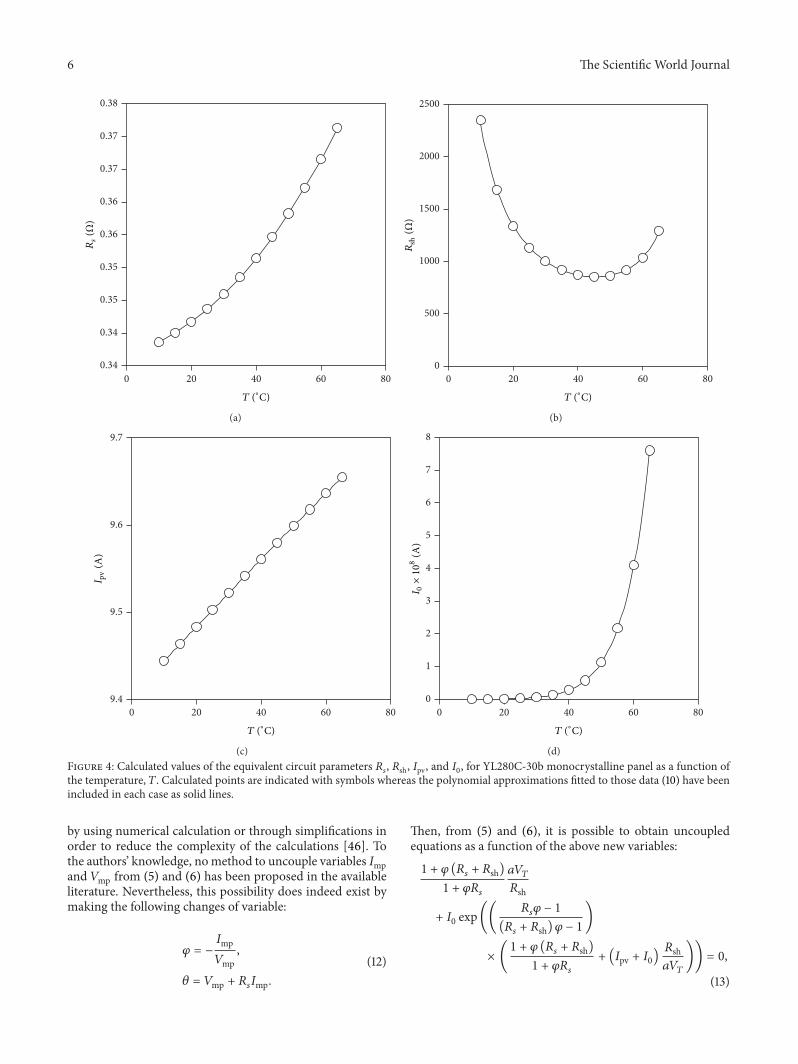
Conditions (STC). After choosing the value for the idealityfactor, the other parameters have been calculated using (7);see Figure 4. The polynomial fittings to the data have alsobeen included in the graphs of the figure, the irradiance level,𝐺, being considered in the case of the photocurrent, 𝐼pv; seethe following:

𝐼pv (𝑇, 𝐺) = (9.50 + 3.89 ⋅ 10−3

Δ𝑇

− 1.09 ⋅ 10−6

Δ𝑇2

− 2.96 ⋅ 10−8

Δ𝑇3

)𝐺

𝐺𝑟

,

𝑅𝑠

(𝑇) = 3.44 ⋅ 10−1

+ 4.23 ⋅ 10−4

Δ𝑇

+ 5.90 ⋅ 10−6

Δ𝑇2

+ 1.93 ⋅ 10−8

Δ𝑇3

,

𝑅sh (𝑇) = (8.83 ⋅ 10−4

+ 2.57 ⋅ 10−5

Δ𝑇

− 4.02 ⋅ 10−7

Δ𝑇2

− 7.56 ⋅ 10−9

Δ𝑇3

)−1

,

𝐼0

(𝑇) = exp (−2.19 ⋅ 101 + 1.56 ⋅ 10−1Δ𝑇

− 5.20 ⋅ 10−4

Δ𝑇2

+ 1.52 ⋅ 10−6

Δ𝑇3

) .

(10)

When evaluating an MPPT method the maximum possiblepower that could be extracted from the panel 𝑝max (𝑡) =

𝐼mp (𝑡) 𝑉mp (𝑡) has to be calculated in every instant, 𝑡. Then,the efficiency of the method can be estimated with the fol-lowing expression [45]:

𝜂MPPT =∫𝑇

𝑇

0

𝑝MPPT (𝑡) 𝑑𝜏

∫𝑇

𝑇

0

𝑝max (𝑡) 𝑑𝜏, (11)

where𝑝MPPT (𝑡) is the instantaneous power obtained from thepanel using the selected MPPT method and 𝑇

𝑇

is the totalperiod of time in which the aforementioned MPPT methodis evaluated.

In case of evaluation through experimental procedures,the maximum possible power, 𝑝max (𝑡), cannot be directlyobtained from the solar panel, being instead estimated fromthe sun irradiance and temperature levels combined withthe panel efficiency at STC. On the other hand, in case ofanalytical modeling, voltage sampling can be applied to (1)in order to find the highest value of the product V ⋅I [39],or the maximum power point variables, 𝐼mp and 𝑉mp, can beobtained from expressions (5) and (6). As these expressionsare implicit and coupled, their resolution needs to be done


0.34

0.34

0.35

0.35

0.36

0.36

0.37

0.37

0.38

0 20 40 60 80

Rs

(Ω)

T (∘C)

(a)

0

500

1000

1500

2000

2500

0 20 40 60 80

Rsh

(Ω)

T (∘C)

(b)

9.4

9.5

9.6

9.7

0 20 40 60 80

I pv

(A)

T (∘C)

(c)

0

1

2

3

4

5

6

7

8

0 20 40 60 80

T (∘C)

I 0×108

(A)

(d)Figure 4: Calculated values of the equivalent circuit parameters 𝑅

𝑠

, 𝑅sh, 𝐼pv, and 𝐼0, for YL280C-30b monocrystalline panel as a function ofthe temperature, 𝑇. Calculated points are indicated with symbols whereas the polynomial approximations fitted to those data (10) have beenincluded in each case as solid lines.

by using numerical calculation or through simplifications inorder to reduce the complexity of the calculations [46]. Tothe authors’ knowledge, nomethod to uncouple variables 𝐼mpand 𝑉mp from (5) and (6) has been proposed in the availableliterature. Nevertheless, this possibility does indeed exist bymaking the following changes of variable:

𝜑 = −

𝐼mp

𝑉mp,

𝜃 = 𝑉mp + 𝑅𝑠𝐼mp.

(12)

Then, from (5) and (6), it is possible to obtain uncoupledequations as a function of the above new variables:

1 + 𝜑 (𝑅𝑠

+ 𝑅sh)

1 + 𝜑𝑅𝑠

𝑎𝑉𝑇

𝑅sh

+ 𝐼0

exp((𝑅𝑠

𝜑 − 1

(𝑅𝑠

+ 𝑅sh) 𝜑 − 1)

× (1 + 𝜑 (𝑅

𝑠

+ 𝑅sh)

1 + 𝜑𝑅𝑠

+ (𝐼pv + 𝐼0)𝑅sh𝑎𝑉𝑇

)) = 0,

(13)


0

200

400

600

800

1000

1200

6 8 10 12 14 16 18 20Time, hours, May 13, 1971

Sola

r irr

adia

nce G

SFC

(Wm

−2)

(a)

0

2

4

6

8

10

0

5

10

15

20

25

6 8 10 12 14 16 18 20

TemperatureWind velocity

(ms−

1)

(∘C)

Time, hours, May 13, 1971

(b)

0

200

400

600

800

1000

1200

6 8 10 12 14 16 18 20

Sola

r irr

adia

nce G

SFC

(Wm

−2)


(c)

0

2

4

6

8

10

0

10

20

30

6 8 10 12 14 16 18 20

TemperatureWind velocity

(ms−

1)

(∘C)


(d)

Figure 5: Ambient conditions on May 13, 1971 (a), (b), and May 14, 1971 (c), (d). Solar irradiance is represented in left side, and temperatureand wind velocity are in right side.

𝜃 = 𝑎𝑉𝑇

(𝑅𝑠

𝜑 − 1

(𝑅𝑠

+ 𝑅sh) 𝜑 − 1)

× (1 + 𝜑 (𝑅

𝑠

+ 𝑅sh)

1 + 𝜑𝑅𝑠

+ (𝐼pv + 𝐼0)𝑅sh𝑎𝑉𝑇

) .

(14)

The variable 𝜑 can be calculated solving the implicit (13), andthen 𝜃 can be obtained directly from (14). Then, unmakingthe change of variables, 𝐼mp and𝑉mp, can be derived after onlyone implicit equation resolution:

𝐼mp =𝜑𝜃

𝑅𝑠

𝜑 − 1, (15)

𝑉mp =𝜃

1 − 𝑅𝑠

𝜑. (16)

This procedure gives the values of current and voltage atthe MPP in a very easy way, avoiding voltage sampling orsimplifications that could reduce the accuracy of the results.In order to speed up the numerical resolution of (13) it mightbe useful to start it with the initial value of 𝜑

0

= −𝐼sc/𝑉oc.

3. Ambient Conditions

Two different ambient conditions (sun irradiance and tem-perature levels) have been considered for the simulationscarried out. The first one is a cloudy day, with low but veryunstable irradiance level, and the second one is a sunnyday; see graphs in Figure 5. These data are, respectively, theirradiance level at the Goddard Space Flight Center (GSFC)on May 13 (cloudy day) and May 14, 1971 (sunny day), andhave been extracted from the work by Thekaekara [47].Temperature and wind speed conditions corresponding to


0

10

20

30

40

50

60

6 8 10 12 14 16 18 20

Tem

pera

ture

of p

anel

(∘C)


(a)

0

10

20

30

40

50

60

6 8 10 12 14 16 18 20

Tem

pera

ture

of p

anel

(∘C)


(b)

Figure 6: Solar panel temperatures on May 13, 1971 (a), and May 14, 1971 (b), at the Goddard Space Flight Center (GSFC).These graphs werecalculated according to ambient conditions for those days; see Figure 5 and (17).

those days have been obtained from the measurements doneat Washington, DC, this city being quite close to GSFC [48].

With the data of Figure 5 regarding sun irradiance andambient temperature it is possible to calculate temperature ofthe solar panel with the equation

𝑇𝑝

= 𝑇𝑎

+𝐺

800(NOCT − 20∘C) , (17)

where𝑇𝑎

is the ambient temperature,𝐺 is the irradiance level,andNOCT is the open-circuitmodule operation temperatureat 800W/m2 irradiance, 20∘C ambient temperature, and1m s−1 wind speed. This last parameter is normally includedin the manufacturers’ datasheet. Although some authors takewind speed variations into account [49], in the present workthey are not considered, as a constant thermal loss coefficientis assumed for wind speeds higher than 1m s−1. Making useof (17), combined with the data from Figure 5, temperatureof solar panels located at the Goddard Space Flight Center(GSFC) on March 13 and March 14, 1971, can be estimated;see Figure 6.

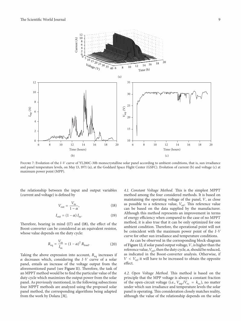
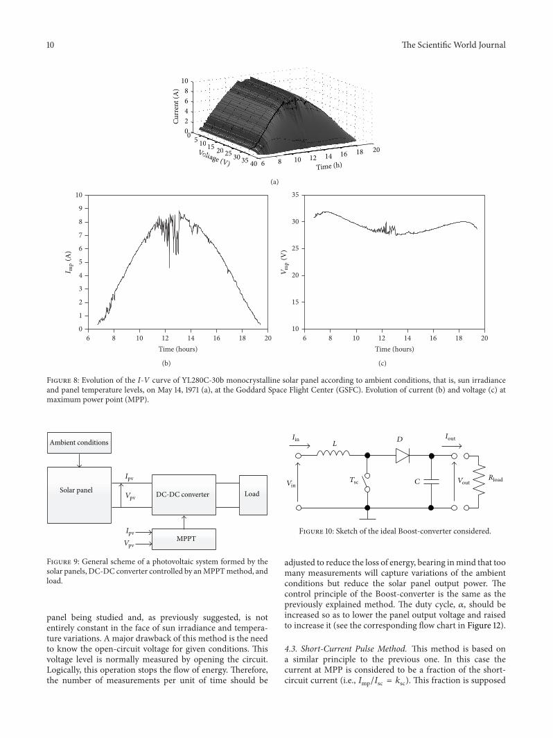
Following the procedure described in the previous sec-tion and taking into account the aforementioned sun irra-diance (Figure 5) and panel temperature (Figure 6) data, itis possible to calculate the I-V curve of the selected solarpanel (YL280C-30b) in each instant of the specified cloudyand sunny days. In Figures 7 and 8, the evolution of the I-Vcurve along those days is shown (for one value of time, 𝑡, theshape of the I-V curve (see Figure 2) can be appreciated). Onthe surface plotted in the figures, a thick line has been drawnto indicate the maximum power point (MPP) which, as canbe observed, indicates variations regarding the current andvoltage at the aforementioned MPP during the chosen days.These current and voltage levels at MPP have been separatelyplotted in Figures 7(b), 7(c), 8(b), and 8(c). These values ofthe maximum power available from the solar panel are usedin the following section as a reference to compare the studiedMPPT methods.

4. MPPT Methods Studied

As mentioned in Section 1, the aim of the present work isto describe a simple methodology to model a solar paneloperating within a wide range of ambient conditions andto analyze different MPPT options for photovoltaic systems(see in Figure 9 the block-diagram corresponding to a pho-tovoltaic system equipped with a MPPT). In the followingsubsections four MPPT methods are studied as an exampleof the proposed method:

(i) constant voltage method,

(ii) open voltage method,

(iii) short-current pulse method,

(iv) perturb and observe method.

In this comparison example the ideal Boost-converter hasbeen selected due to its simplicity (see Figure 10). However,it should be underlined that other more sophisticated DC-DC converter possibilities could also be included in thesimulation with the proposed methodology, this possibilitybeing out of the scope of the present work, which is focusedon the solar panel accurate modeling for MPPT analysis.

The principle of the Boost-converter consists of twooperational modes, depending on the position of the switch,𝑇sc. When the switch is closed (on-state) the inductor 𝐿stores the energy of the source while the capacitor feedsthe load. Otherwise, when the switch is opened (off-state)the only path available for the current is through the diode𝐷 and the source feeds the load and charges the capacitor.If the converter works with a commutation period, 𝑇

0

, theduty cycle, 𝛼, is the fraction of that period in which 𝑇scis connected; therefore 𝛼 ranges between 0 (𝑇sc is neveron) and 1 (𝑇sc is always on). For an ideal Boost-converter,


6 8 10 12

68

1012

14 16 18 20

Time (h)

10 15 20 25 30 35

0 5

40

420

Curr

ent (

A)

Voltage (V)

(a)

0

2

4

6

8

10

12

6 8 10 12 14 16 18 20Time (hours)

I mp

(A)

(b)

Time (hours)

10

15

20

25

30

35

6 8 10 12 14 16 18 20

Vm

p(V

)

(c)

Figure 7: Evolution of the I-V curve of YL280C-30b monocrystalline solar panel according to ambient conditions, that is, sun irradianceand panel temperature levels, on May 13, 1971 (a), at the Goddard Space Flight Center (GSFC). Evolution of current (b) and voltage (c) atmaximum power point (MPP).

the relationship between the input and output variables(current and voltage) is defined by

𝑉out =𝑉in1 − 𝛼

, (18)

𝐼out = (1 − 𝛼) 𝐼in. (19)

Therefore, bearing in mind (17) and (18), the effect of theBoost-converter can be considered as an equivalent resistor,whose value depends on the duty cycle:

𝑅eq =𝑉in𝐼in

= (1 − 𝛼)2

𝑅load. (20)

Taking the above expression into account, 𝑅eq increases if𝛼 decreases which, considering the I-V curve of a solarpanel, entails an increase of the voltage output from theaforementioned panel (see Figure 11). Therefore, the task ofanMPPTmethod would be to find the particular value of theduty cycle which maximizes the output power from the solarpanel. As previously mentioned, in the following subsectionsfour MPPT methods are analyzed using the proposed solarpanel method, the corresponding algorithms being adaptedfrom the work by Dolara [31].

4.1. Constant Voltage Method. This is the simplest MPPTmethod among the four considered methods. It is based onmaintaining the operating voltage of the panel, 𝑉, as closeas possible to a reference value, 𝑉ref. This reference valuecan be based on the data supplied by the manufacturer.Although this method represents an improvement in termsof energy efficiency when compared to the case of no MPPTmethod, it is also true that it can be only optimized for oneambient condition. Therefore, the operational point will notbe coincident with the maximum power point of the I-Vcurve for other sun irradiance and temperature conditions.

As can be observed in the corresponding block-diagramof Figure 12, if solar panel output voltage,𝑉, is higher than thereference value,𝑉ref, then the duty cycle,𝛼, should be reduced,as indicated in the Boost-converter analysis. Otherwise, if𝑉 < 𝑉ref it will have to be increased to obtain the oppositeeffect.

4.2. Open Voltage Method. This method is based on theprinciple that the MPP voltage is always a constant fractionof the open-circuit voltage (i.e., 𝑉mp/𝑉oc = 𝑘oc), no matterunder which sun irradiance and temperature levels the solarpanel is operating.This consideration closely matches reality,although the value of the relationship depends on the solar


6 8 10 12

68

10

14 16 18 20

Time (h)

10 15 20 25 30 35

0 5

40

420

Curr

ent (

A)

Voltage (V)14 16

10 15 20 25 30Volt

(a)

0

1

2

3

4

5

6

7

8

9

10

6 8 10 12 14 16 18 20Time (hours)

I mp

(A)

(b)

10

15

20

25

30

35

6 8 10 12 14 16 18 20Time (hours)

Vm

p(V

)

(c)

Figure 8: Evolution of the I-V curve of YL280C-30b monocrystalline solar panel according to ambient conditions, that is, sun irradianceand panel temperature levels, on May 14, 1971 (a), at the Goddard Space Flight Center (GSFC). Evolution of current (b) and voltage (c) atmaximum power point (MPP).

Solar panel

Ambient conditions

DC-DC converter Load

MPPT

Ipv

Ipv

Vpv

Vpv

Figure 9: General scheme of a photovoltaic system formed by thesolar panels, DC-DC converter controlled by anMPPTmethod, andload.

panel being studied and, as previously suggested, is notentirely constant in the face of sun irradiance and tempera-ture variations. A major drawback of this method is the needto know the open-circuit voltage for given conditions. Thisvoltage level is normally measured by opening the circuit.Logically, this operation stops the flow of energy. Therefore,the number of measurements per unit of time should be

LD

C

Iout

Vout

Iin

VinRloadTsc

Figure 10: Sketch of the ideal Boost-converter considered.

adjusted to reduce the loss of energy, bearing inmind that toomany measurements will capture variations of the ambientconditions but reduce the solar panel output power. Thecontrol principle of the Boost-converter is the same as thepreviously explained method. The duty cycle, 𝛼, should beincreased so as to lower the panel output voltage and raisedto increase it (see the corresponding flow chart in Figure 12).

4.3. Short-Current Pulse Method. This method is based ona similar principle to the previous one. In this case thecurrent at MPP is considered to be a fraction of the short-circuit current (i.e., 𝐼mp/𝐼sc = 𝑘sc). This fraction is supposed


Table 2: Energy obtained fromYL280C-30bmonocrystalline solar panel calculated with ambient conditions measured at the Goddard SpaceFlight Center (GSFC) on May 13, 1971 (cloudy day), and May 14, 1971 (sunny day).

MPPT method Sunny day Cloudy dayEnergy [Wh] 𝜂MPPT Rank Energy [Wh] 𝜂MPPT Rank

Ideal 1880 1 — 526 1 —Constant voltage 1826 0.971 4 496 0.943 4Open voltage 1860 0.989 3 513 0.976 3Short-current pulse 1867 0.993 2 518 0.985 2Perturb and observe 1871 0.995 1 522 0.992 1

6

8

10

0

4

2

010 20 30 40

Isc

Voc

𝛼

Req

I (A

)

V (V)50

Figure 11: Effect of Boost-converter duty cycle (i.e., the equivalentresistor) variations on the operational point of a solar panel.

to remain constant in every ambient condition. As withthe previous case, this closely matches reality, althoughthere are slight variations depending on sun irradiance andtemperature changes. In this case part of the power is lostduring the short-circuit current measurements. In this casean increase of the duty cycle, 𝛼, raises the solar panel outputcurrent, the decrease of the duty cycle produces the oppositeeffect (see the corresponding flow chart in Figure 12).

4.4. Perturb and Observe Method. This algorithm is basedon continuous modifications of the solar panel operationalvoltage, checking after each perturbation if the generatedpower has increased or decreased. If the power increases thenext voltage perturbation will go in the same direction and ischanged if the power decreases. This process is indicated inthe corresponding block-diagram in Figure 12.

5. Results

Simulations were carried out with MATLAB. The solarpanels were modeled following indications from Section 2.The ambient conditions considered are those described inSection 3, the temperature of the solar panels being calculatedwith (16). In all cases a 10ms time step has been consideredfor data acquisition and control, for every MPPT methodanalyzed. Regarding the short-current pulse method and theopen voltage method a measurement of 𝐼sc and𝑉oc was taken

every 3 seconds (300 time steps). Duty cycle was varied insteps of Δ𝛼 = 0.005 for all methods, the initial value inevery calculation being 𝛼

0

= 0.12. The control parameterscorresponding to the studied methods were optimized, forthe solar panel considered in the present work, followingthese criteria.

(i) Constant voltage method: for the reference voltagevalue, 𝑉ref, the voltage level at MPP, 𝑉mp, indicated bythe manufacturer at 35∘C, was selected:

𝑉ref = 31.07 − 0.41 ⋅ 10 = 27.2V. (21)

(ii) Open voltage method: as control constant, 𝑘oc, theratio of voltage level at MPP, 𝑉mp, to the open-circuitvoltage, 𝑉oc, at STC, was chosen:

𝑘oc =31.3

39.1= 0.8. (22)

(iii) Short-current pulse method: as control constant, 𝑘sc,the ratio of current level at MPP, 𝐼mp, to the short-circuit current, 𝐼sc, at STC, was chosen:

𝑘sc =8.96

9.5= 0.94. (23)

Results are included in Table 2 and Figure 13, togetherwith the maximum extractable power from the solar panelobtained with expressions (13) and (14). The high efficiencyobtained for all MPPT methods can be explained as in everycase an ideal DC-DC converter (without energy losses) hasbeen considered. The best performance of MPPT method(for the studied conditions) seems to be the perturb andobserve method, the reason being the noninterrupted powerextraction from the solar panel. The worst performance ofMPPT method is the constant voltage method, as it showsthe larger influence from the ambient conditions. The openvoltage and short-current pulse methods show a quite goodperformance, the grey zone below the plots being producedby the switching that disconnect the solar panel to performthemeasurements of𝑉oc and 𝐼sc.The better efficiency showedby the short-current pulse method when compared to theopen voltage method could be explained as the ratio 𝐼mp/𝐼scis less dependent on the temperature than the ratio 𝑉mp/𝑉oc.

Logically, the efficiency of the studied MPPT methods isworse in case of cloudy days than in case of sunny days. Thisis clear due to the faster variations on the ambient conditions.


Measurement of Vpv

Measurement of Vpv

Vpv = Vref

Vpv = Vref

Vpv > VrefVpv > Vref

𝛼(n) = 𝛼(n − 1)

𝛼(n) = 𝛼(n − 1) − Δ𝛼

𝛼(n) = 𝛼(n − 1) + Δ𝛼

𝛼(n) = 𝛼(n − 1)

𝛼(n) = 𝛼(n − 1) − Δ𝛼

𝛼(n) = 𝛼(n − 1) + Δ𝛼

Measure Voc

Refreshreference?

PV in work

PV in open-circuit

condition

Yes

Yes

No

No

Yes

Yes

Yes

No

No

No

Constant voltage Open voltage

Vref = koc · Voc

Perturb and observe

Short-current pulse

Measure Isc

Iref = ksc · Isc

Vpv(n), Ipv(n)

Ppv(n) − Ppv(n − 1)

Vpv(n) − Vpv(n − 1)> 0

Measurement of

Refreshreference?

YesYes

Yes

Yes

No

No

No

No

Measurement of Ipv

𝛼(n) = 𝛼(n − 1)

𝛼(n) = 𝛼(n − 1) − Δ𝛼

𝛼(n) = 𝛼(n − 1) + Δ𝛼

𝛼(n) = 𝛼(n − 1) − Δ𝛼

𝛼(n) = 𝛼(n − 1) + Δ𝛼

Ipv = Iref

Ipv < Iref

PV in work

PV in short-circuit

condition

Ppv(n) = Vpv(n) · Ipv(n)

Figure 12: Block-diagrams of the different MPPT used in the present work.

6. Case Study

In order to check the proposed methodology, a real photo-voltaic facility, whose behavior was measured, together withthe ambient conditions, by Houssamo et al. [50], has beenstudied. This photovoltaic facility is formed by eight Q125PIsolar panels manufactured by Conergy, organized in fourtwo-panel series connected in parallel. The characteristics ofthe panels are included in Table 3, whereas the sun radiationand the panel temperature during the measurements areincluded in Figure 14.

The procedure described in Section 4 was followed inorder tomodel the studied photovoltaic facility.The extracted

Table 3: Characteristic points of Q125PI solar panel (Conergy),included in the manufacturer’s datasheets at Standard Test Con-ditions (STC): 1000W/m2 irradiance, 25∘C cell temperature, andAM1.5 g spectrum according to EN 60904-3 [17].

Conergy Q125Pl (polycrystalline)𝑛 36 𝑇

𝑟

(∘C) 25𝑃mp (W) 125 𝛾 (%/∘C) −0.426𝐼mp (A) 7.36 𝛼𝐼mp (%/∘C) —𝑉mp (V) 17 𝛽𝑉mp (%/∘C) −0.352𝐼sc (A) 7.94 𝛼𝐼sc (%/∘C) 0.035𝑉oc (V) 21 𝛽𝑉oc (V/

∘C) −0.074


6 8 10 12 14 16 18 200

50

100

150

200

250

300

Time (h)

Pow

er (W

)

Constant voltage method (cloudy day)

(a)

Constant voltage method (sunny day)

6 8 10 12 14 16 18 200

50

100

150

200

250

Time (h)

Pow

er (W

)

(b)

Open voltage method (cloudy day)

6 8 10 12 14 16 18 200

50

100

150

200

250

300

Time (h)

Pow

er (W

)

(c)

Open voltage method (sunny day)

6 8 10 12 14 16 18 200

50

100

150

200

250

Time (h)

Pow

er (W

)

(d)

Short-current pulse method (cloudy day)

6 8 10 12 14 16 18 200

50

100

150

200

250

300

Time (h)

Pow

er (W

)

(e)

Short-current pulse method (sunny day)

6 8 10 12 14 16 18 200

50

100

150

200

250

Time (h)

Pow

er (W

)

(f)

Perturb and observe method (cloudy day)

Ideal powerMPPT power

6 8 10 12 14 16 18 200

50

100

150

200

250

300

Time (h)

Pow

er (W

)

(g)

Perturb and observe method (sunny day)

6 8 10 12 14 16 18 200

50

100

150

200

250

Time (h)

Pow

er (W

)

Ideal powerMPPT power

(h)Figure 13: Power produced by YL280C-30b monocrystalline solar panel calculated with the studied MPPTmethods, for ambient conditionsmeasured at the Goddard Space Flight Center (GSFC) on May 13, 1971 (cloudy day), and May 14, 1971 (sunny day). Maximum extractablepower (ideal) has been also included.


41.5

42.0

42.5

43.0

43.5

44.0

44.5

45.0

0

200

400

600

800

1000

1200

1400

0 20 40 60 80 100 120t (s)

Irradiance (solar radiation)Panel temperature

Tem

pera

ture

(∘C)

Irra

dian

ce (W

)

Figure 14: Ambient conditions (irradiance and solar panels tem-perature) during operation of the photovoltaic facility studied from[50].

power was calculated using the perturb and observe (P&O)MPPT algorithm.This power was compared to the measuredone from the facility [50], which was programmed followingtwo different MPPT algorithms, perturb and observe (P&O)and incremental conductance (INC). The results from thesimulation show a higher extracted power when comparedto the behavior measured directly on the facility, this dis-crepancy between results being explained as no power losses(wiring, connections, dirt over the panels, degradation, lossesat the Boost-converter, etc.) were taken into account in thesimulation carried out. Bearing in mind that no informationregarding these losses was included in [50], the results werescaled down by multiplying by a constant (0.64) and, as aresult, a much better correlation was obtained (see Figure 15).Also, an equivalent resistor can be then considered in order totake into account the power losses.The results correspondingto the simulation carried outwith a 1.375Ω resistor connectedin series with each pair of solar panels are included inFigure 15. A quite good correlation between the resultsobtained with the present methodology and the ones mea-sured by Houssamo et al. [50] can be observed in the figure.To obtain a better approximation to the measured results, acombination of the scaled results (losses proportional to theextracted power like the ones produced by dirt in the panels)and the losses resulting from electrical current (taken intoaccount with equivalent resistors) should be considered.Thisresult has been included in Figure 15 combining both kindsof power losses at 50% each one. An excellent correlationwith the measured extracted power can be observed, thehigher deviation being located where the effect of the MPPTalgorithm selection is relevant. The highest differences inextracted power between both MPPT algorithms selected bythe authors of [50] were measured in period from 20 s to25 s, which is precisely the period where the higher deviationof the results obtained by present methodology from themeasurement results is observed.

0

100

200

300

400

500

600

700

800

0 20 40 60 80 100 120

Pow

er (W

)

Scaled resultsPower losses considered

t (s)

Scaled (50%) + power losses (50%)INCP&O

Figure 15: Power from an 8-panel photovoltaic facility calculatedwith the proposed methodology and P&OMPPT algorithm (scaledresults and results with power losses considered). The results fromthe testing measurements [50] (considering P&O and INC MPPTalgorithms) are also included in the figure (P&O: blue line; INC: redline).

7. Conclusions

In the present work a solar panel modelling to analyzeMPPTmethods is described. The most significant conclusionsderived from the work are the following.

(i) It represents a simple and quick-calculation method-ology to obtain a solar panel model to performMPPTsimulations, from the manufacturers’ datasheet.

(ii) The developed method takes into account for the cal-culations possible variations on the ambient condi-tions (sun irradiation and solar cells temperature).

(iii) The proposed analytical methodology allows fastMPPT methods comparison.

(iv) Based on the developed methodology the perfor-mance of a specific MPPT method can be foreseenwhen applied to a particular solar panel from whichonly manufacturer’s datasheet information is avail-able.

(v) Simple, accurate, and low calculation resourcesdemanding way to obtain the maximum extractablepower from solar panels are presented.

(vi) The feasibility of the described methodology hasbeen checked with four different MPPT methodsapplied to a commercial solar panel, within a day, andunder realistic ambient conditions. Also a case studywas analyzed, the results being compared to testingmeasured with good correlation.


(vii) Finally, it should also be mentioned that althoughthe parameter-extraction analytical model which isthe core of the proposed methodology has provento be as accurate as several numerical methods [35],the most recently developed algorithms can be animprovement in terms of accuracy (at least if the pho-tovoltaic device is partially shaded).

Conflict of Interests

The authors declare that there is no conflict of interestsregarding the publication of this paper.

Acknowledgments

Thepresent work is part of the research framework associatedwith the design and construction of the UPMSat-2 satellite,IDR/UPM Institute (Instituto de Universitario Microgravedad“IgnacioDaRiva”), PolytechnicUniversity ofMadrid (Univer-sidad Politecnica de Madrid). The authors are indebted to thesupport from all the staff of the IDR/UPM Institute. They aretruly grateful to Brian Elder for his kind help in improvingthe style of the text. Also, they are truly indebted to thestaff of the Library at the Aeronautics and Space EngineeringSchool (Escuela de Ingenierıa Aeronautica y del Espacio) of thePolytechnic University of Madrid (Universidad Politecnica deMadrid), for their constant support to the research carried outregarding photovoltaic technology.

References

[1] S. Pindado, Elementos de Transporte Aereo, 2006.[2] F. Aminzadeh and S. Pindado, “How has Spain become a leader

in thewind energy industry during the last decade? (An analysisof influential factors on the development of wind energy inSpain),” in Proceedings of the EWEA Annual Event, 2011.

[3] C. T. Vazquez, Energıa Solar Fotovoltaica, Ediciones Ceysa,Madrid, Spain, 2008.

[4] V. R. Hernandez, Solar Thermal Power. History of a ResearchSuccess, Protermosolar, Sevilla, Spain, 2010.

[5] F. Dincer, “The analysis on photovoltaic electricity generationstatus, potential and policies of the leading countries in solarenergy,” Renewable and Sustainable Energy Reviews, vol. 15, no.1, pp. 713–720, 2011.

[6] K. H. Solangi, M. R. Islam, R. Saidur, N. A. Rahim, and H.Fayaz, “A review on global solar energy policy,” Renewable andSustainable Energy Reviews, vol. 15, no. 4, pp. 2149–2163, 2011.

[7] G. K. Singh, “Solar power generation by PV (photovoltaic) tech-nology: a review,” Energy, vol. 53, pp. 1–13, 2013.

[8] N. H. Karam, R. R. King, B. Terence Cavicchi et al., “Devel-opment and characterization of high-efficiency Ga

0.5

In0.5

P/GaAs/Ge dual- and triple-junction solar cells,” IEEE Transac-tions on Electron Devices, vol. 46, no. 10, pp. 2116–2125, 1999.

[9] R. W. Miles, “Photovoltaic solar cells: choice of materials andproduction methods,” Vacuum, vol. 80, no. 10, pp. 1090–1097,2006.

[10] T. Takamoto, T. Agui, A. Yoshida et al., “World’s highest effi-ciency triple-junction solar cells fabricated by inverted layerstransfer process,” in Proceedings of the 35th IEEE PhotovoltaicSpecialists Conference (PVSC ’10), pp. 412–417, June 2010.

[11] M. A. Green, K. Emery, Y. Hishikawa, W. Warta, and E. D.Dunlop, “Solar cell efficiency tables (version 39),” Progress inPhotovoltaics: Research and Applications, vol. 20, no. 1, pp. 12–20, 2012.

[12] A. Moliton and J.-M. Nunzi, “How to model the behaviour oforganic photovoltaic cells,” Polymer International, vol. 55, no. 6,pp. 583–600, 2006.

[13] T. Bendib, F. Djeffal, D. Arar, and M. Meguellati, “Fuzzy-logic-based approach for organic solar cell parameters extraction,” inProceedings of theWorld Congress on Engineering (WCE ’13), vol.2, pp. 1–4, July 2013.

[14] L. Zuo, J. Yao, H. Li, andH. Chen, “Assessing the origin of the S-shaped I-V curve in organic solar cells: an improved equivalentcircuit model,” Solar Energy Materials and Solar Cells, vol. 122,pp. 88–93, 2014.

[15] T. Esram andP. L. Chapman, “Comparison of photovoltaic arraymaximum power point tracking techniques,” IEEE Transactionson Energy Conversion, vol. 22, no. 2, pp. 439–449, 2007.

[16] A. Reza Reisi, M. HassanMoradi, and S. Jamasb, “Classificationand comparison of maximum power point tracking techniquesfor photovoltaic system: a review,” Renewable and SustainableEnergy Reviews, vol. 19, pp. 433–443, 2013.

[17] Yingli Energy, “Panda 60 Cell 40mm Series,” 2008.[18] V. Salas, E. Olıas, A. Barrado, and A. Lazaro, “Review of the

maximum power point tracking algorithms for stand-alonephotovoltaic systems,” Solar Energy Materials and Solar Cells,vol. 90, no. 11, pp. 1555–1578, 2006.

[19] P. Bhatnagar and R. K. Nema, “Maximum power point trackingcontrol techniques: State-of-the-art in photovoltaic applica-tions,” Renewable and Sustainable Energy Reviews, vol. 23, pp.224–241, 2013.

[20] M. D. Goudar, B. P. Patil, and V. Kumar, “A review of improvedmaximum peak power tracking algorithms for photovoltaicsystems,” International Journal of Electrical Engineering, vol. 1,pp. 85–107, 2010.

[21] A. N. A. Ali, M. H. Saied,M. Z.Mostafa, and T.M. Abdel-Mon-eim, “A survey of maximum PPT techniques of PV systems,” inProceedings of the IEEE Energytech, pp. 1–17, May 2012.

[22] K. Ishaque and Z. Salam, “A review of maximum power pointtracking techniques of PV system for uniform insolation andpartial shading condition,” Renewable and Sustainable EnergyReviews, vol. 19, pp. 475–488, 2013.

[23] C.Hua andC. Shen, “Comparative study of peak power trackingtechniques for solar storage system,” in Proceedings of the 13thAnnual Applied Power Electronics Conference and Exposition(APEC’98), pp. 679–685, February 1998.

[24] D. P. Hohm and M. E. Ropp, “Comparative study of maximumpower point tracking algorithms,” Progress in Photovoltaics:Research and Applications, vol. 11, no. 1, pp. 47–62, 2003.

[25] R. Faranda, S. Leva, P. Milano, and P. Leonardo, “Energy com-parison of MPPT techniques for PV systems department ofenergy,”Wseas Transactions on Power Systems, vol. 3, no. 6, pp.446–455, 2008.

[26] R. Faranda, S. Leva, and V. Maugeri, “MPPT techniques for PVsystems: energetic and cost comparison,” in Proceedings of theIEEE 21st Power and Energy Society GeneralMeeting: Conversionand Delivery of Electrical Energy in the Century (PES ’08), July2008.

[27] M. Berrera, A. Dolara, R. Faranda, and S. Leva, “Experimentaltest of seven widely-adopted MPPT algorithms,” in Proceedingsof the IEEE Bucharest PowerTech: Innovative Ideas Toward theElectrical Grid of the Future, pp. 1–8, July 2009.


[28] D. S. Karanjkar, S. Chatterji, S. L. Shimi, and A. Kumar, “Realtime simulation and analysis ofmaximumpower point tracking(MPPT) techniques for solar photo-voltaic system,” in Proceed-ings of the Recent Advances in Engineering and ComputationalSciences (RAECS ’14), pp. 1–6, March 2014.

[29] K. K. Choi, J.-C. Llorens, G.Maral, andA. Barnaba, “Applicationof themaximumpower point trackingmethod to the adaptativepower supply sub-system of a microsatellite,” 1998.

[30] C. de Manuel, J. Cubas, and S. Pindado, “On the simulationof the UPMSat-2 microsatellite power,” in Proceedings of theEuropean Space Power Conference, pp. 1–7, April 2014.

[31] A. Dolara, “Energy comparison of seven MPPT techniques forPV systems,” Journal of Electromagnetic Analysis and Applica-tions, vol. 1, no. 3, pp. 152–162, 2009.

[32] T. Esram, J.W.Kimball, P. T. Krein, P. L. Chapman, andP.Midya,“Dynamic maximum power point tracking of photovoltaicarrays using ripple correlation control,” IEEE Transactions onPower Electronics, vol. 21, no. 5, pp. 1282–1290, 2006.

[33] N. S. D’Souza, L. A. C. Lopes, and X. Liu, “Comparative studyof variable size perturbation and observation maximum powerpoint trackers for PV systems,” Electric Power Systems Research,vol. 80, no. 3, pp. 296–305, 2010.

[34] K. Ding, X. Bian, H. Liu, and T. Peng, “A MATLAB-simulink-based PV module model and its application under conditionsof nonuniform irradiance,” IEEE Transactions on Energy Con-version, vol. 27, no. 4, pp. 864–872, 2012.

[35] J. Cubas, S. Pindado, and M. Victoria, “On the analyticalapproach for modeling photovoltaic systems behavior,” Journalof Power Sources, vol. 247, pp. 467–474, 2014.

[36] J. Cubas, S. Pindado, and C. de Manuel, “Explicit expressionsfor solar panel equivalent circuit parameters based on analyticalformulation and the Lambert W-function,” Energies, vol. 7, no.7, pp. 4098–4115, 2014.

[37] J. Cubas, S. Pindado, andA. Farrahi, “Newmethod for analyticalphotovoltaic parameter extraction,” in Proceedings of the 2ndInternational Conference on Renewable Energy Research andApplications (ICRERA ’13), pp. 873–877, October 2013.

[38] A. Jain and A. Kapoor, “A new approach to study organic solarcell using Lambert W-function,” Solar Energy Materials andSolar Cells, vol. 86, no. 2, pp. 197–205, 2005.

[39] M.G. Villalva, J. R. Gazoli, and E. Ruppert Filho, “Modeling andcircuit-based simulation of photovoltaic arrays,” in Proceedingsof the Brazilian Power Electronics Conference (COBEP ’09), pp.1244–1254, October 2009.

[40] D. S. H. Chan and J. C. H. Phang, “Analytical methods for theextraction of solar-cell single- and double-diode model param-eters from I-V characteristics,” IEEE Transactions on ElectronDevices, vol. 34, no. 2, pp. 286–293, 1987.

[41] J. C.H. Phang,D. S.H. Chan, and J. R. Phillips, “Accurate analyt-ical method for the extraction of solar cell model parameters,”Electronics Letters, vol. 20, no. 10, pp. 406–408, 1984.

[42] M. G. Villalva, J. R. Gazoli, and E. R. Filho, “Comprehensiveapproach to modeling and simulation of photovoltaic arrays,”IEEE Transactions on Power Electronics, vol. 24, no. 5, pp. 1198–1208, 2009.

[43] P.M. Cuce and E. Cuce, “A novelmodel of photovoltaicmodulesfor parameter estimation and thermodynamic assessment,”International Journal of Low-Carbon Technologies, vol. 7, no. 2,pp. 159–165, 2012.

[44] H. S. Rauschenbach, Solar Cell Array Design Handbook: ThePrinciples and Technology of Photovoltaic Energy Conversion,Van Nostrand Reinhold Company, New York, NY, USA, 1980.

[45] K. H. Hussein, I. Muta, T. Hoshino, and M. Osakada, “Max-imum photovoltaic power tracking: an algorithm for rapidlychanging atmospheric conditions,” IEE Proceedings: Generation,Transmission and Distribution, vol. 142, no. 1, pp. 59–64, 1995.

[46] C.Hua andC. Shen, “Comparative study of peak power trackingtechniques for solar storage system,” in Proceedings of the 13thAnnual Applied Power Electronics Conference and Exposition(APEC’98), vol. 2, pp. 679–685, February 1998.

[47] M. P. Thekaekara, “Solar radiation measurement: techniquesand instrumentation,” Solar Energy, vol. 18, no. 4, pp. 309–325,1976.

[48] National Oceanic and Atmospheric Administration’s, NationalWeather Service, http://www.nws.noaa.gov/climate/.

[49] E. Skoplaki and J. A. Palyvos, “Operating temperature of photo-voltaic modules: a survey of pertinent correlations,” RenewableEnergy, vol. 34, no. 1, pp. 23–29, 2009.

[50] I. Houssamo, F. Locment, and M. Sechilariu, “Maximumpower tracking for photovoltaic power system: developmentand experimental comparison of two algorithms,” RenewableEnergy, vol. 35, no. 10, pp. 2381–2387, 2010.

TribologyAdvances in

Hindawi Publishing Corporationhttp://www.hindawi.com Volume 2014

International Journal of

AerospaceEngineeringHindawi Publishing Corporationhttp://www.hindawi.com Volume 2014

FuelsJournal of


Journal ofPetroleum Engineering


Industrial EngineeringJournal of


Power ElectronicsHindawi Publishing Corporationhttp://www.hindawi.com Volume 2014

Advances in

CombustionJournal of


Journal of


Renewable Energy

Submit your manuscripts athttp://www.hindawi.com


StructuresJournal of

International Journal of

RotatingMachinery


EnergyJournal of


Hindawi Publishing Corporation http://www.hindawi.com

Journal ofEngineeringVolume 2014

Hindawi Publishing Corporation http://www.hindawi.com Volume 2014

International Journal ofPhotoenergy


Nuclear InstallationsScience and Technology of


Solar EnergyJournal of


Wind EnergyJournal of


Nuclear EnergyInternational Journal of


High Energy PhysicsAdvances in

The Scientific World JournalHindawi Publishing Corporation http://www.hindawi.com Volume 2014

research article accurate simulation of mppt methods...

Documents