C S A S

Canadian Science Advisory Secretariat

S C C S

Secrétariat canadien de consultation scientifique

* This series documents the scientific basis for the evaluation of fisheries resources in Canada. As such, it addresses the issues of the day in the time frames required and the documents it contains are not intended as definitive statements on the subjects addressed but rather as progress reports on ongoing investigations.

* La présente série documente les bases scientifiques des évaluations des ressources halieutiques du Canada. Elle traite des problèmes courants selon les échéanciers dictés. Les documents qu’elle contient ne doivent pas être considérés comme des énoncés définitifs sur les sujets traités, mais plutôt comme des rapports d’étape sur les études en cours.

Research documents are produced in the official language in which they are provided to the Secretariat. This document is available on the Internet at:

Les documents de recherche sont publiés dans la langue officielle utilisée dans le manuscrit envoyé au Secrétariat. Ce document est disponible sur l’Internet à:

http://www.dfo-mpo.gc.ca/csas/

ISSN 1499-3848 (Printed / Imprimé) © Her Majesty the Queen in Right of Canada, 2008 © Sa Majesté la Reine du Chef du Canada, 2008

Research Document 2007/082

Document de recherche 2007/082

Not to be cited without permission of the authors 1

Ne pas citer sans autorisation des auteurs 1

Estimated size of the Northwest Atlantic grey seal population 1977-2007

Évaluation de la population de phoques gris de l’Atlantique Nord-Ouest, 1977 – 2007

L. Thomas1, M.O.Hammill2, and W.D. Bowen3

1Centre for Research into Ecological and Environmental Modelling, University of St Andrews

St Andrews, Fife KY16 9LZ. Scotland.

2Maurice Lamontagne Institute, Dept of Fisheries and Oceans P.O. Box 1000, Mont Joli QC. G5H 3Z4. Canada.

3Population Ecology Division, Bedford Institute of Oceanography, Dept of Fisheries and Oceans

Dartmouth NS. B2Y 4A2. Canada.

iii

ABSTRACT We constructed a stochastic model of Northwest Atlantic grey seal population dynamics and fit it to available pup production data from 1977-2007 divided into three breeding regions: Sable Island, Gulf of St. Lawrence, and Eastern Shore (including Hay Island and other small colonies along coastal Nova Scotia). The model assumes that fecundity rates are age-dependent but are constant over time, that adult survival rates are constant, and that pup survival is density dependent. Females are assumed to be able to move to a new region to breed if pup survival is higher there, but once they start breeding they do not move. We used a Bayesian computer-intensive method (particle filtering) to fit the model, with informative priors on model parameters. The posterior estimates for some parameters were close to their priors, indicating little information about these parameters in the pup production data and highlighting the importance of carefully choosing the priors. Other parameters were far from the prior: in particular the posterior estimates of carrying capacity were far higher than the prior values, indicating little evidence of density dependent population regulation at current levels of pup production. The total estimated population size at the end of the 2007 breeding season (i.e., including pups) was 304,000 (95% CI 242,000-371,000). This is 6% higher than the equivalent estimate for 2006 of 285,000 (95%CI 230,000-344,000) and 750% higher than the estimate for 1977 of 41,000 (95%CI 31,000-51,000). Average annual rates of population increase are estimated to be 4% in the 1980s (lower due to greater harvests in the Gulf), 9% in the 1990s and 8% in the 2000s. These estimates should be treated with some caution because: (1) the biological model showed clear lack of fit, particularly to the Gulf data where extending the model to account for ice and weather conditions would be useful; (2) sensitivity of the results to the priors used has not been assessed; and (3) the fitting algorithm may have caused some biases.

iv

RESUMÉ

Nous avons élaboré un modèle stochastique de la dynamique de la population de phoques gris de l’Atlantique Nord-Ouest et y avons intégré les données existantes de production des jeunes phoques de 1977 à 2007, issues de trois aires de reproduction : l’île de Sable, le golfe du Saint-Laurent et la côte est (y compris la colonie de l’île Hay et d’autres petites colonies situées le long de la plateforme Néo-Écossaise). Le modèle permet de supposer que les taux de fécondité dépendent de l’âge, mais qu’ils demeurent néanmoins constants dans le temps, que les chances de survie des petits phoques sont liées à la densité, que les femelles sont capables de se déplacer vers une autre région pour se reproduire si les chances de survie des bébés phoques y sont plus élevées, mais qu’une fois fécondées, elles ne bougent plus. Nous avons employé une méthode bayésienne reposant largement sur le traitement informatique (filtrage de particules) pour l’adaptation d’information a priori sur les paramètres du modèle. Les estimations postérieures de certains paramètres se sont montrées relativement proches des données a priori, révélant l’existence de très peu d’information sur ces paramètres dans les données sur la production des bébés phoques et faisant ressortir l’importance de bien choisir les éléments a priori. Par contre, d’autres paramètres étaient très éloignés de l’information a priori, surtout dans le cas des évaluations postérieures de la capacité de charge, qui étaient beaucoup plus élevées que les valeurs a priori, montrant très peu de signes d’une dépendance de la régulation de la population à l’égard de la densité, au taux actuel de production des petits. En 2007, l’estimation de la population (comprenant les petits) au terme de la saison de reproduction était de 304 000 (IC de 95 % = 242 000 – 371 000). Cela représente une hausse de 6 % par rapport à l’estimation comparable de 2006 qui totalisait 285 000 (IC de 95 % = 230 000 – 344 000) et de 750 % comparativement à celle de 1977 qui était de 41 000 (IC de 95 % = 31 000 – 51 000). Au cours des années 1980, la progression annuelle de la population était évaluée à 4 % (en raison des captures plus nombreuses dans le Golfe), à 9 % durant les années 1990 et à 8 % pendant les années 2000. Il importe toutefois d’user de prudence dans la mention de ces estimations puisque : 1) le modèle biologique a révélé une très faible corrélation, surtout en ce qui concerne les données du Golfe où il serait utile d’élargir la capacité du modèle de manière à tenir compte de l’état des glaces et des conditions météorologiques, 2) la sensibilité des résultats aux valeurs a priori n’a pas été évaluée et 3) l’algorithme employé est susceptible d’avoir introduit certaines erreurs.

1

INTRODUCTION

The aim of this paper is to present preliminary estimates of population size for the Northwest Atlantic grey seal (Halichoerus grypus). Seals (and marine mammals in general) are notoriously difficult to census: they spend much of their time at sea and most of that underwater. The only time a substantial part of the population is in one place is during the breeding season, when pre-weaned pups are readily counted on breeding colonies, and for this reason pup production estimates form the principal tool for population monitoring. The breeding population of Northwest Atlantic grey seals is normally divided into two components for management purposes, based on the locations of the largest breeding colonies. These are the Sable Island component and traditionally a Gulf of St. Lawrence (Gulf) component (Mansfield and Beck 1977). However, recent changes in the distribution of pupping warrant dividing the population into three parts, for the purposes of modelling, which we refer to as “regions”: Sable Island, Gulf and Eastern Shore (Fig. 1). Pup production on Sable Island has been relatively well monitored, with pup production estimated in most years from 1962 to 1990 by tagging all weaned pups (Mansfield and Beck 1977, Stobo and Zwanenburg 1990) and more recently at longer intervals via aerial photography (Bowen et al. 2007). The Gulf region comprises animals that whelp primarily on the drifting pack ice in Northumberland Strait and those born on small islands located within the southern Gulf of St. Lawrence. Pup production here has been estimated approximately every 4 years from mark-recapture studies (Hammill et al. 1992, 1998, Myers et al. 1997) and aerial surveys (Hammill and Gosselin 2005; Hammill et al. 2007). The estimates have higher standard errors (SEs) than those from Sable Island because of more difficult conditions in this area (Myers et al. 1997, Hammill et al. 1998). The third region, the Eastern shore, is by far the smallest part of the population. It comprises seals that whelp primarily on Hay Island, but also includes some other small islands along the eastern shore of Nova Scotia. These have been monitored intermittently by visual counts or year-class tagging (Hammill et al. 2007). All three regions were surveyed most recently in spring 2007 (Hammill et al. this meeting). The pup production data used here are shown in Appendix Table A1. To estimate total population size from pup production data, it is necessary to make assumptions about the relationship between pup production and numbers of seals in other age classes, and between observed and actual pup production. We do this using a stochastic discrete-time modelling framework called a state-space model. The use of this framework to describe and fit models of wildlife population dynamics is described by Buckland et al. (2004), and examples of its application to the British population of grey seals are given by Thomas et al. (2005), Newman et al. (2006) and Buckland et al. (2007). Similar models to those employed here have been used to provide advice on British grey seals population size to the UK Special Committee on Seals since 2003 (Thomas and Harwood 2003, 2004a, b, 2005, 2006, 2007). We follow the most recent population analysis of Northwest Atlantic grey seal pup production data (Trzcinksi et al. 2006) in considering population dynamics models that allow for density dependent declines in vital rates in response to increases in population size. We initially considered as feasible that there is either density dependent decline in age-specific fecundity or pup survival.

2

Specifying complex models for wildlife population dynamics is relatively simple, but fitting them to observed data is often not so straightforward (Buckland et al. 2007, Newman et al. in revision). We employ a computer-intensive Bayesian fitting method called Monte Carlo particle filtering (also called sequential importance sampling). A particle filter is an algorithm that produces a set of weighted samples (particles) taken from the prior distributions on the parameters and states (seal numbers) and projected forward stochastically through the time series. The weights relate to the manner in which the particles were sampled, how they were projected forward and the likelihood of the observed pup production given the simulated pup numbers. An accessible tutorial in the context of state-space models for wildlife population dynamics is given by Newman et al. (2006), and applications using particle filters are given by Thomas et al. (2005) and Thomas and Harwood (2003, 2004a, b, 2005, 2006, 2007). A general comparison between particle filtering and other fitting methods, such as Markov chain Monte Carlo (MCMC) in this context is given by Buckland et al. (2007), and a detailed comparison using a state-space model for British Grey seals applied to real and simulated data is given by Newman et al. (in revision). Bayesian methods require prior distributions to be specified for all random quantities. We use informative prior distributions on model parameters, such as survival rates, fecundity rates and movement parameters. These are mostly taken from expert opinion, but our prior on fecundity rates comes from an analysis of pregnancy rates as a function of age in a sample of females taken as part of a scientific sampling program between 1969 and 2007. This analysis is also informative about suitable choice of biological model, in that it is possible to examine whether pregnancy rate has changed over time, possibly as a result of density dependence.

MATERIALS AND METHODS

Analysis of pregnancy rate data

Samples of females were shot between 1969 and 2007 and examined for pregnancy status and age. Pregnancy rates are known to vary with age, and are thought to have declined in recent years, particularly in immature females (around age 4) (Hammill and Gosselin, this meeting). We examined this, using the above data, initially graphically and then using generalized additive modelling (GAM), with the response variable (pregnancy status) being binomial and potential covariates age and year (as either factors or smooth functions). These analyses were performed using the mgcv package in R version 2.5.1 (R Development Core Team 2007).

Smooths produced by GAM do not make ideal prior distributions as they are not simply expressed in terms of a low-dimensional parametric function. Therefore, to provide priors distributions for age-specific fecundity rates for the state-space model fitting, we searched for a low-dimension curve that was a good approximation to the above analysis results, using nonlinear least squares to fit suitable candidate models (function nls in R 2.5.1). The dependent variable in this analysis was observed proportion pregnant, and each observation of the proportion pregnant was weighted by the square root of sample size.

3

State-space model

A state-space model has two components: (1) the state process, which models the true but unknown state of the population (in this case numbers of seals of different ages in different regions); and (2) the observation process, which models how the survey data are generated given the true states. Our findings from the analysis of pregnancy rate data (see Results, below) guided many of our choices in constructing the state process. We divided the seal population in each breeding region into 7 age classes: pups (age 0), age 1 to 5 adult females, and age 6 and older females. Note that our model does not explicitly include adult males – see below for assumptions required to calculate male population numbers. The time step for the process model is 1 year, beginning just after the breeding season. The model is made up of 5 sub-processes: harvest, survival, ageing, movement of age 3 females, and breeding. Harvest consists of removal of what are assumed to be known numbers of animals, killed as a result of the commercial hunt as well as scientific sampling. The annual harvest data were divided into pups, “juveniles” (assumed to be age 1-3) and “adults” (age 4+). Within these latter two groups, the numbers of each age removed from the population were assumed to be in proportion to their relative frequency in the population. For example, if 72 juveniles were known to have been removed in a particular year, and there were estimated to be 100, 80 and 60 seals of age 1, 2 and 3 respectively, then we assumed that 30, 24 and 18 animals were removed from each age class, respectively. Survival is modelled as a binomial random process, and is assumed additive to harvest (i.e., occurring after numbers removed by harvest). We assume that pup survival is density dependent, and follows a Beverton-Holt function of the form:

1,,0

max,, 1 −+=

trr

ptrp nβ

φφ (1)

where 1,,0 −trn is the number of pups born in region r in year t-1, trp ,,φ is survival rate of these pups, maxpφ is maximum pup survival rate, and rβ is inversely proportional to the carrying capacity of the region ( 0≥β ). We assume that half of the pups born will be male; hence the expected number of female pups surviving will be 1,,0,,5.0 −trtrp nφ . We assume that adult female survival rate, aφ is constant across regions and time. Ageing is deterministic – all seals age by one year (although those in the age 6+ category remain there). To model movement, we assume that only females age 3 (i.e., before breeding age) may move from their natal region, and thereafter females remain in the region they are in. We assume that movement is fitness dependent, such that females will only move if the expected survival of their future offspring is higher elsewhere, and the probability of movement is proportional to the expected survival difference. We measure the propensity for fitness-dependent movement relative to a competing propensity for site fidelity, which means that many females will not move even if conditions for their pups

4

would be better elsewhere. We assume that numbers in each region after movement is a multinomial random variable: ( ) ⎟

⎠⎞⎜

⎝⎛∑ =

31 ,3,2,1

*,,2,3,2,2,2,1,2 ,,,~,,

r ttttrttt pppnlMultinomiannn (2)

where *

,,2 trn and trn ,,2 denote numbers of age 2 females in region r before and after movement respectively, and trp , is the probability that a seal aged 2 is in region r after movement. We model this probability as

∑

∑=

= →= 3

1*

,,2

31 ,

*,,2

,

j tj

j trjtjtr

n

np

δ (3)

where

[ ] ( ) [ ]

( )0,max10,max

,,,,

,,,,,

tjptrp

tjptrptrj

rjIrjIφφγφφγ

δ−+

≠−+==→ (4)

with [ ].I being an indicator function that takes value 0 if the condition inside the bracket is met and zero otherwise, and γ being a parameter regulating the strength of density-dependent movement versus site fidelity (the larger γ , the stronger the effect of density dependence; 0≥γ ). This movement model is a simpler version of that used by Newman et al. (in revision), which had an additional parameter to make movement less likely among more widely spaced regions. We model breeding by assuming that the number of pups produced is a binomial random variable. Following the analysis of pregnancy rate data reported below, we assume the rate is age dependent, but not time dependent. We assume that females age 3 or less at the time of the breeding season do not breed, while fecundity rate for females of age 6+ at the time of the breeding season is governed by a model parameter

maxα . For females age 4 and 5, fecundity rates are given by ( )( )5.4itlog 1

max −= − aa ραα (5) where ρ is a model parameter that determines how fecundity rate increases with age ( 10 <≤ ρ ) towards maxα . For the observation process, we assume that pup production estimates follow a normal distribution, with known standard error. In summary, there are 8 model parameters: adult survival aφ , maximum pup survival

maxpφ , one carrying capacity parameter-related parameter for each region 31 ββ − , a parameter regulating movement rates γ , maximum fecundity maxα , and a parameter regulating increase in fecundity with age, ρ .

5

Data and priors

The input data were pup production estimates for 1977-2007, together with their estimated standard errors (SEs, Appendix Table A1). To allow the fitting algorithm to produce reliable results in the time available to run it, the SEs in Table A1 were multiplied by 3 in the analyses reported here (see Discussion). Both aerial survey and mark recapture based estimates were available for the Gulf region for 1984, 1985, 1986, 1989 and 1990; in these case a variance-weighted mean of the estimates and corresponding SE was calculated. No SE estimates were available for Sable Island from 1977 to 1989 and for Eastern Shore for 1996, 1997 and 2000 because these were all complete counts. However, it is not appropriate to assume zero error both because this is likely inaccurate in fact, and also because the particle filtering algorithm used here will not work if with zero error values. Therefore, SEs were estimated by assuming that the ratio of estimate to variance of estimate was constant, and using a constant of proportionality for this relationship estimated from the Sable and Eastern Shore regions data that did have SE estimates associated with them. Harvest data (Fig. 2 and Appendix Table A2) were segregated into pups, juvenile females (ages 1-3) and adult females (ages 4+), as described previously. Prior parameter estimates are given in Table 1. Priors on fecundity rates come from the analysis of pregnancy rate data. Priors on other parameters came from previously published papers, supplemented by expert opinion. We followed Thomas and Harwood (2005, 2006, 2007) in using a re-parameterization to specify the prior on the rβ s in terms of a prior on the pup production at carrying capacity,

rχ , conditional on the values of the other model parameters. For the model outlined above, it can be shown that expected pup survival rate at equilibrium, *

pφ is given by

⎟⎟⎠

⎞⎜⎜⎝

⎛

−++

=+

a

aaa

p

σαφ

αφαφ

φ

15.0

1

62

543

* (6)

Substituting (6) into (1) and re-arranging, we find that for a given carrying capacity of pup production at equilibrium, rχ ,

⎟⎟⎠

⎞⎜⎜⎝

⎛−⎟

⎟⎠

⎞⎜⎜⎝

⎛

−++= + 1

15.01 6

2

543

maxa

aaap

rr σ

αφαφαφφ

χβ (7)

The priors on carrying capacity of pups at equilibrium were set by specifying a prior mean of approximately twice the largest observed count in each region, with a large prior variance (equivalent to CV of 50%) to reflect the uncertainty in specifying these values a priori.

6

The prior mean on the movement parameter was specified by calculating the value that would lead to a 10% emigration of age 3 seals from a region to one where pup survival was 0.1 higher. This value (2.5) was also given a large variance (equivalent to a CV of 100%) to reflect the arbitrary nature with which it was chosen. Prior distributions are also required on seal population size by age and region for the first year (1977); the Markovian nature of the model means that prior distributions on population size for other years are defined automatically after specifying those in the first year and the parameters. We based our method of specifying priors on the population size in the first year on that of Thomas et al. (2005). This method uses the first year of data to specify a prior distribution on pup numbers in each region, and then uses this distribution together with the demographic parameters to derive priors for the other age classes (see Thomas et al. 2005 for details). However, pup production estimates are not available in 1977 for the Gulf or Eastern Shore regions. For the Gulf, the only available data prior to 1977 is a relatively course aerial survey estimate of pup production in 1966 in the order of 1,500 (Mansfield 1966, Mansfield and Beck 1977). The first estimate after 1977 was 7151 in 1984 (Appendix Table A1). Assuming exponential growth between these time points yields an estimated growth rate of 9% per year and an estimate of approximately 3900 pups in 1977. This value was used as the prior mean, with a large variance (equivalent to a CV of 50%) such that an prior 95% CI on pup production in the Gulf was that it was between approximately 0 and 7800. This was achieved in practice by adding a fabricated observation to the pup production dataset: an observation of 3900 pups in 1977 with SE 1950. For the Eastern Shore region, there are no relevant data available; however our prior belief is that there were very few seals breeding there in 1977. We therefore set the pup production in that region to zero by adding a fabricated observation to the pup count dataset of zero pups in 1977 along the Eastern Shore, with zero SE. Fitting method

The particle filtering algorithm we used is similar to that described by Thomas and Harwood (2007) and Newman et al. (2007), implemented in the C programming language. An outline of the main features of the algorithm is given below, for completeness – it is not necessary to read the rest of this sub-section to understand the results that follow. For reference, we highlight any differences from the Thomas and Harwood (2007) algorithm.

Initial rejection control. The aim of this procedure is to weed out at an early stage sets of parameter and state combinations that are simulated from the prior but clearly have very low density in the posterior, so that computer time can be focussed on areas of parameter and state space that have higher posterior density. We simulated sets of 1,000,000 particles from the prior distributions, projected them forwards from 1977 to 1978 and calculated likelihood weights based on the 1978 data. We then applied rejection control, an algorithm that probabilistically removes particles with low weight (Liu 2001), using the mean of the particles weights as the rejection control criterion. This typically resulted in about a quarter of the particles being retained. We repeated this process until we had at least 1,000,000 particles surviving the initial rejection control stage.

7

Auxiliary particle filter (Liu and West 2001). With this procedure, we projected forward one time step at a time, starting in 1978, initially deterministically. We then resampled the particles using the deterministic weights – i.e., according to the expected pup production in the next time period – thereby producing a set of “promising” particles. Because data for the Gulf and Eastern Shore regions were missing in many years, it seemed prudent not to follow the usual convention of resampling with probability proportional to the weights. Instead, we used the more conservative strategy (Liu 2001) of resampling with probability proportional to the square root of the weights (this is one point of difference from the Thomas and Harwood (2007) algorithm). Resampled copies of the same ancestor particle will have the same parameter values, so to maintain parameter diversity we used kernel smoothing to jitter the parameter values (see Liu and West 2001 for details). This can cause bias (Newman et al. in revision), so we kept the amount of kernel smoothing to a minimum, using a discount value of 0.9997 (a value of 1.0 results in no jittering at all; a value of 0.997 was used by Thomas and Harwood (2007)). After kernel smoothing, particles were then projected forward stochastically to the next time period, and weights were adjusted to take account of the initial resampling. The auxiliary particle filter was not used in years where there was no data in any region – in this case particles simply projected forward stochastically, without any re-weighting or resampling.

Final rejection control. At the last time period, rejection control was used to reduce the number of particles that must be stored. The rejection control criterion was the mean of the particle weights. This reduced the number of particles stored per run from 1,000,000 to between 600,000 and 700,000.

Multiple runs. The above procedures generated samples based on 1,000,000 particles (although fewer were stored after the final rejection control). However, even this many samples gave a very imprecise estimate of the posterior distributions of interest for all models. Hence, many multiple runs (100 or more) were required to reduce Monte Carlo error to acceptable levels. To reduce the resulting outputs down to a manageable level for post-processing (i.e., calculating posterior distributions on quantities of interest), it was necessary to apply further rejection control, this time using a rejection control criterion of the 99.999th percentile of the particle weights from all of the multiple runs for a particular model.

One last difference between the algorithm of Thomas and Harwood (2007) and that used here was that the former used an analytic integration procedure to enable efficient estimation of an observation error parameter; here the observation SEs were assumed known. Estimating total population size

Our state-space model does not include adult males. Nevertheless, if we follow Hammill et al. (2005) and Trzcinski et al. (2006) in assuming male and female survival rates are the same, then total population size can be estimated as twice the adult female population size plus the estimated pup production. We take this approach in giving total population size estimates by region and year, and summed over regions.

8

RESULTS

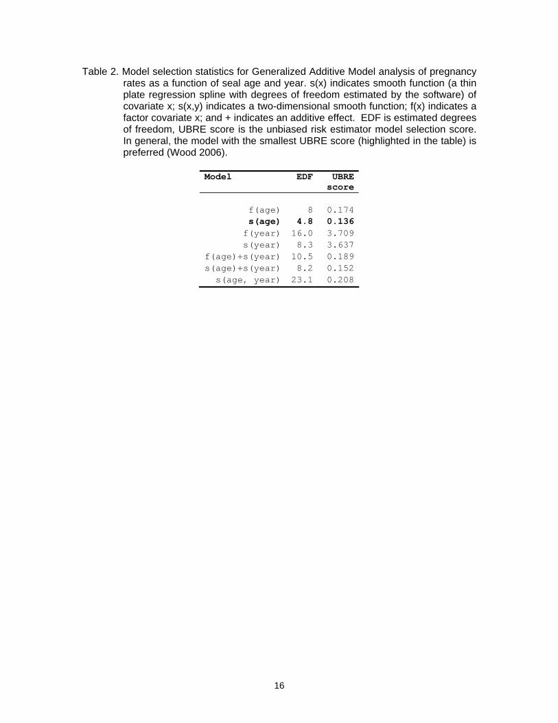
Pregnancy rates The data came from 748 females aged between 2 and 9, of which 509 were found to be pregnant. Plots of age-specific pregnancy rates against time period (1960-70, 1980-90 and 2000-07, Fig. 3) showed no convincing evidence of temporal pattern, although there is a clear increase in pregnancy rate with age. These observations were confirmed by the GAM analysis: a model with age as a smooth function was slightly preferred (using an unbiased risk estimator model selection statistic, Wood 2006) over models including both age and year (Table 2). In addition, the year term was not statistically significant (p>0.05) in either the year-only or the age and year models. We therefore did not consider further models where age-specific fecundity changes over time. We found that a 2-parameter curve of the form ( )( )5.3itlog)( 1

max −= − agepregp ρα (6) fit the observed age-specific pregnancy rates well (Fig. 4), since it allowed pregnancy rates to be near zero at age 2, and rapidly increase thereafter to be very close to the asymptote by age 6. Nonlinear least squares regression gave estimates of maximum pregnancy rate of α =0.876 (SE 0.015), with rate parameter ρ =2.318 (SE 0.289). Note, when applying these results to the population dynamics model, the ages used in that model are one year greater, since a female that was sampled for the pregnancy rate analysis at age a would have given birth at age a+1.

State-space model The results reported here are based on 150 runs of 1 million particles. This represents approximately 150 hours of computer time, although in practice runs were made in parallel on up to 8 processors so results were available in 1-2 days. After the final rejection control step of the particle filtering algorithm, 10.4 million particles remained.

Since the resampling step of the auxiliary particle filter makes multiple copies of the same particles, the surviving particles are no longer independent, so the true sample size of independent particles is much lower than total sample size. A useful approximate index of whether there have been enough runs for Monte-Carlo error to be acceptably low is the total number of unique ancestral particles (i.e., independent samples from the prior) surviving in the final results – for example Thomas and Harwood (2007) aimed to achieve >1000 ancestral particles. The 10.4 million particles contained 11,445 ancestral particles, so we expect Monte-Carlo error to be low. This was confirmed by dividing the particles into two equal halves and checking some inferences on both subsets: for example posterior mean on aφ was 0.967 and 0.969 from the two halves; for maxpφ the two values were 0.746 and 0.742; for γ the two values were 0.138 and 0.141.

9

Estimated pup production1 for the three regions is shown in Fig. 5, and values are given in Appendix Table A3. The estimated trajectory for the Sable region fits the data quite well. The trajectory appears near-exponential, but there is some evidence that the rate of population increase is slowing: mean annual rate of population change was estimated to be 1.12 from 1980-89, 1.11 from 1990-1999 and 1.09 from 2000-2007. The fit to the Gulf region data is rather less impressive, and it is clear that there is something missing from the model to account for the unexplained variation in pup production estimates between closely spaced years. The estimated pup production in 1977 is in the upper part of the prior range, and the estimates show generally decreasing pup production from 1978 through to the late 1980s, corresponding with the higher harvest levels in this period. Pup production has been estimated to be increasing thereafter. The fit to the Eastern Shore data is satisfactory, with the estimated trajectory being one of near exponential increase. Estimates of total population size at the beginning of each year (i.e., just after the breeding season, and so including pups, but before hunting or natural mortality) are shown by region in Fig. 6 and in Appendix Table A4. The trajectories generally mirror those of the pups. Estimated total population size in 2007, combined over all 3 regions is 304,000 (95% CI 242,000-371,000). This is 6% higher than the equivalent estimate for 2006 of 285,000 (95%CI 230,000-344,000) and 750% higher than the estimate for 1977 of 41,000 (95%CI 31,000-51,000). Estimates of overall mean annual population change were 1.04 from 1980-1989 (depressed due to harvest in the Gulf), 1.09 in 1990-1999, and 1.08 in 2000-2007.

Posterior parameter distributions are shown in Fig. 7, together with the corresponding priors. The fecundity parameters ( maxα and ρ ) are almost identical to their priors, indicating that effectively nothing has been learnt about these from the pup production data over the information specified in the prior distribution. Posterior maximum juvenile survival ( maxpφ ) is similar to the prior, although the mean is slightly higher. Posterior mean adult survival ( aφ ) is also slightly higher (0.97 vs 0.95 in the prior), but the posterior standard error is around a third that of the prior, so the data have somewhat informative about this parameter. The posterior mean on the movement parameter γ is a twentieth that specified by the prior (0.14 vs 2.5), and the standard error is much reduced, implying very little movement of females between regions given the model and data. All three carrying capacity parameters ( χ s) have much higher posterior means than priors – for example the prior mean carrying capacity for Sable Island was 100,000 pups (95% CI 27,000-220,000), but the posterior is 417,000 (95% CI 213,000-880,000). Note, however, that the standard errors on the posterior estimates (and hence the CIs) are high – similar to the prior specification of a 50% CV.

1 Note that all results reported here on states are smoothed rather than filtered estimates, sensu e.g., Cappé 2005. This just means that they are estimates computed using all the data, rather than just the data up to the time point for which the estimate is being made.

10

DISCUSSION

Reliability of results There are three reasons why we may wish to interpret the results with caution. Firstly, the model is clearly inadequate in some respects. It does not explain the large variation between closely-spaced surveys in observed pup production in the Gulf region. We therefore recommend viewing with caution the estimated pup production and total population size coming from this region. We discuss later possible extensions to address this. Our assumption that adult male and female survival is identical is questionable, given that males often have lower survival than females in body-size dimorphic species such as grey seals, as is the assumption that pregnancy rates and fecundity rates are equal among regions. Secondly, being a Bayesian analysis, it is important to consider the sensitivity of the results to the priors. We anticipate high sensitivity of estimated parameter distributions in parameters where the posterior is very similar to the prior ( maxα , ρ and maxpφ ), and less for the other parameters. This sensitivity may affect the population size estimate somewhat – for example fecundity rate is closely related to population size since the number of breeding females is given by the estimated pup production divided by the fecundity rate. We anticipate that our priors on initial population sizes in 1977 will have little effect on estimates of current population size. These intuitions should, however, be tested. We note that the posterior on carrying capacity for the Eastern Shore region is extremely different from the prior, and this deserves more investigation. Lastly, the fitting method may have influenced the result, although probably not to any significant extent. We do not think there is much Monte-Carlo error in our results. However, we achieved low MC error in part by trebling the observed SEs on pup production estimates, when evaluating the particle weights. The models should be re-run with the correct SEs – although it will take very significantly more particles to achieve the same reliability in the estimated posterior distributions. Our intuition is that this will have little effect on the posterior means, although it may reduce the SEs a little. We also made an arbitrary assumption to obtain SEs on total counts – although this probably had little effect on the inferences. The particle filtering algorithm included an auxiliary particle filter with kernel smoothing of parameters, and this is known to cause bias in theory, although Newman et al. (in revision) found no discernable difference between PF estimates and those from an MCMC sampler that was used as the “gold standard”, with both simulated and real data applied to a seal model similar to the one used here. They used a kernel smoothing discount parameter of 0.997, while we used 0.9997, so we expect even less bias here – although the model and data are different so it is something worth investigating if possible. Attempting very large runs with no kernel smoothing is one possible way to attempt this. Inferences about grey seal population dynamics We found that the model used here does not show much evidence of a recent density-dependent slow-down in population growth, when calibrated with the pup production

11

data. Our posterior estimates of carrying capacity are 6-10 times higher than current estimated levels of pup production; hence if the model is correct then in the absence of changes in management practices, seal populations will continue to rise at similar rates to those seen in the recent past. There are several reasons why this inference may be incorrect. Some were discussed in the previous section. In addition, carrying capacity is notoriously difficult to estimate from populations still growing rapidly. There is also every reason to expect that changing environmental conditions, or other limitations such as food stocks, may place a limit on seal numbers long before our estimated carrying capacities are reached. We also found that rather less movement between colonies is required to fit the data than we had anticipated. This is something that bears further investigation. The analysis of shot adult female seals we performed showed no convincing evidence for a decline in age-specific pregnancy rates. By contrast, data from resightings of branded (marked) animals on Sable Island have shown an increase in mean age at first birth (Bowen et al. 2007). This suggests that density dependent factors may be beginning to operate in this segment of the population, and therefore that different factors may be operating in the different regions. It would be useful to include the Sable Island marked animal data in future analyses of population dynamics. Future work There are several directions in which this work could be extended. As mentioned above, the prior sensitivity needs investigating as does any bias caused by the fitting algorithm. There is a clear need to extend the biological model to better match conditions in the Gulf region. Both pre- and post-weaning pup mortality in the Gulf is strongly decreased under a combination of poor ice conditions and storms, and it would be very useful to be able to introduce a covariate to account for this. In addition, it is likely that maximum pup survival is lower in the Gulf than the other regions. Other biological models could be considered, and model selection methods used to evaluate support for each. However, as with British Grey Seals (Thomas and Harwood 2006, 2007), it is likely that there is little information in the data to distinguish between various plausible models. Nevertheless, unlike for British seals, the presence of a time series of information on pregnancy rates means that alternative plausible models are unlikely to predict extremely different total population sizes. Including additional information on survival, particularly adult male survival, would help considerably to improve the reliability of the modelling process.

ACKNOWLEDGEMENTS

We thank Ken Newman, John Harwood, Steve Buckland, Carmen Fernández, Jason Matthiopoulos and many other current and former members of CREEM and SMRU for insightful discussions about models for wildlife population dynamics and methods of fitting these models.

12

LITERATURE CITED

Bowen, W. D., J. W. Lawson, and B. Beck. 1993. Seasonal and geographic variation in the species composition and size of prey consumed by grey seals (Halichoerus grypus) on the Scotian shelf. Canadian Journal of Fisheries and Aquatic Science 50:1768–1778.

Bowen, W.D., J.I. McMillan and W. Blanchard. 2007. Reduced population growth of gray

seals at Sable Island: evidence from pup production and age of primiparity. Marine Mammal Science 23: 48-64.

Buckland, S.T., K.B. Newman, C. Fernández, L. Thomas and J. Harwood. 2007.

Embedding population dynamics models in inference. Statistical Science 22: 44-58.

Buckland, S.T., K.B. Newman, L. Thomas & N.B. Koesters. 2004. State-space models

for the dynamics of wild animal populations. Ecological modelling 171: 157-175.

Cappé, O., E. Moulines and T. Rydén. 2005. Inference in Hidden Markov Models.

Springer, NY, USA. Hammill, M. O., and J.-F. Gosselin. 2005. Pup production of non-Sable Island grey

seals, in 2004. DFO Can. Sci. Advis. Sec. Res. Doc. 2005/033. Hammill, M.O., J.F. Gosselin and G.B. Stenson. 2007. Changes in abundance of grey

seals in the NW Atlantic. Pages 99-115. In T. Haug, M. Hammill and D. Olafsdottir. (eds). Grey seals in the North Atlantic and the Baltic. NAMMCO Scientific publication 6. 227 pp.

Hammill, M. O., G. B. Stenson, R. A. Myers, and W. T. Stobo. 1992. Mark–recapture

estimates of non-Sable Island grey seal (Halichoerus grypus) pup production. CAFSAC Res. Doc. 92/91.

Hammill, M. O., G. B. Stenson, R. A. Myers, and W. T. Stobo. 1998. Pup production and

population trends of the grey seal (Halichoerus grypus) in the Gulf of St. Lawrence. Canadian Journal of Fisheries and Aquatic Sciences 55:423–430.

Lui, J.S. 2001. Monte Carlo Strategies in Scientific Computing. Springer-Verlag, New

York. Liu, J., and West, M. (2001). Combined parameter and state estimation in simulation-

based filtering. In Sequential Monte Carlo Methods in Practice., eds. Doucet, A., de Freitas, N., and Gordon, N. 197–223. Berlin: Springer-Verlag.

Mansfield, A.W. 1966. The grey seal in eastern Canadian waters. Canadian Audubon

Magazine 28: 161-166. Mansfield, A. W., and B. Beck. 1977. The grey seal in eastern Canada. Fisheries Marine

Service Technical Report 704:1–81.

13

Myers, R. A., M. O. Hammill, and G. B. Stenson. 1997. Using mark–recapture to estimate the numbers of a migrating stage-structured population. Canadian Journal of Fisheries and Aquatic Sciences 54:2097–2104.

Newman, K.B., S.T. Buckland, S.T. Lindley, L. Thomas & C Fernández. 2006. Hidden

process models for animal population dynamics. Ecological Applications 16: 74-86.

Newman, K.B., C. Fernández, L. Thomas and S.T. Buckland. in revision. Monte Carlo

inference for state-space models of wild animal populations R Development Core Team. 2007. R: A language and environment for statistical

computing. R Foundation for Statistical Computing, Vienna, Austria. ISBN 3-900051-07-0, URL http://www.R-project.org.

Stobo, W. T., and K. C. T. Zwanenburg. 1990. Grey seal(Halichoerus grypus) pup

production on Sable Island and estimates of recent production in the Northwest Atlantic. Pages 171–184 in W. D. Bowen, editor. Population biology of sealworm (Pseudoterranova decipiens) in relation to its intermediate and seal hosts. Canadian Bulletin of Fisheries and Aquatic Sciences, Number 222.

Thomas, L., S.T. Buckland, K.B. Newman & J. Harwood. 2005. A unified framework for

modelling wildlife population dynamics. Australian and New Zealand Journal of Statistics 47: 19-34.

Thomas, L. and J. Harwood. 2003. Estimating grey seal population size using a

Bayesian state-space model. NERC Special Committee on Seals Briefing paper 03/3.

Thomas, L. and J. Harwood. 2004a. A comparison of grey seal population models

incorporating density dependent pup survival and fecundity. NERC Special Committee on Seals Briefing paper 04/6.

Thomas, L. and J. Harwood. 2004b. Possible impacts on the British grey seal population

of deliberate killing related to salmon farming. NERC Special Committee on Seals Briefing paper 04/7.

Thomas, L. and J. Harwood. 2005. Estimating the size of the UK grey seal population

between 1984 and 2004: model selection, survey effort and sensitivity to priors. NERC Special Committee on Seals Briefing Paper 05/3.

Thomas, L. and J. Harwood. 2006. Estimating the size of the UK grey seal population

between 1984 and 2005, and related research. NERC Special Committee on Seals Briefing Paper 06/3.

Thomas, L. and J. Harwood. 2007. Estimating the size of the UK grey seal population

between 1984 and 2006. NERC Special Committee on Seals Briefing Paper 07/3.

14

Trzcinski, M.K., R. Mohn and W.D. Bowen. 2006. Continued decline of an Atlantic cod population: how important is grey seal predation? Ecological Applications, 16: 2276–2292

Wood, S.N. 2006. Generalized Additive Models: An introduction with R. Chapman and

Hall, Boca Raton, USA.

15

Table 1. Prior parameter distributions for the state-space model of grey seal population dynamics.

Param Distribution Mean Stdev

aφ Be(27.25,1.43) 0.95 0.04

maxpφ Be(14.00,6.00) 0.7 0.1

1χ Ga(4,25000) 100000 50000

2χ Ga(4, 7500) 30000 15000

3χ Ga(4,1500) 6000 3000

maxα Be(427.50,60.59) 0.876 0.015 ρ Ga(64.29, 3.61x10-

2) 2.319 0.29

γ Ga(1.00,2.5) 2.5 2.5

16

Table 2. Model selection statistics for Generalized Additive Model analysis of pregnancy rates as a function of seal age and year. s(x) indicates smooth function (a thin plate regression spline with degrees of freedom estimated by the software) of covariate x; s(x,y) indicates a two-dimensional smooth function; f(x) indicates a factor covariate x; and + indicates an additive effect. EDF is estimated degrees of freedom, UBRE score is the unbiased risk estimator model selection score. In general, the model with the smallest UBRE score (highlighted in the table) is preferred (Wood 2006).

Model EDF UBRE

score

f(age) 8 0.174s(age) 4.8 0.136f(year) 16.0 3.709s(year) 8.3 3.637

f(age)+s(year) 10.5 0.189s(age)+s(year) 8.2 0.152s(age, year) 23.1 0.208

17

Figure 1. Area of interest in Eastern Canada showing locations where grey seal

colonies can be found. The arrow represents the general direction of ice drift for pups born on the pack ice in Northumberland Strait.

18

1980 1990 2000

050

010

0015

00

Pups

Year

Har

vest

1980 1990 2000

050

100

200

300

Juveniles (Age 1-3)

Year

Har

vest

1980 1990 2000

020

040

060

0

Adults (Age 4+)

Year

Har

vest

Figure 2. Number of seals harvested by commercial hunt and scientific sampling. Almost

are assumed to come from the Gulf region (see Appendix Table A2 for values by region).

19

Age 2

Year

p(pr

eg)

20 57 11

1960-1970 1980-1990 2000-2007

0.0

0.4

0.8

Age 3

Year

p(pr

eg)

12 39 22

1960-1970 1980-1990 2000-2007

0.0

0.4

0.8

Age 4

Year

p(pr

eg)

7 51 19

1960-1970 1980-1990 2000-2007

0.0

0.4

0.8

Age 5

Year

p(pr

eg)

9 49 16

1960-1970 1980-1990 2000-2007

0.0

0.4

0.8

Age 6

Year

p(pr

eg)

6 34 13

1960-1970 1980-1990 2000-2007

0.0

0.4

0.8

Age 7

Year

p(pr

eg)

6 23 9

1960-1970 1980-1990 2000-2007

0.0

0.4

0.8

Age 8

Year

p(pr

eg)

4 30 15

1960-1970 1980-1990 2000-2007

0.0

0.4

0.8

Age 9

Year

p(pr

eg)

26 215 55

1960-1970 1980-1990 2000-2007

0.0

0.4

0.8

Figure 3. Estimated pregnancy rate by age and time period, with associated 95%

binomial confidence intervals. Sample sizes are given below each estimate.

20

2 3 4 5 6 7 8 9

0.0

0.2

0.4

0.6

0.8

1.0

age

p(pr

eg)

88 73 77 74 53 38 49 296

Figure 4. Observed proportion pregnant (p(preg)) at each age class (circles), together

with 95% binomial CIs (horizontal lines), and fitted curve of the form ( )( )5.3itlog)( 1

max −= − agepregp ρα . Sample sizes are given along the bottom.

21

Figure 5. Estimates of true pup production from a model of grey seal population

dynamics fit to pup production estimates from 1977-2007 in three regions. The smooth lines show the posterior mean bracketed by the 95% posterior credibility interval. The filled circles show estimated pup production from survey data and the vertical lines denote +/- 2 standard errors on these estimates. Note that the values for Gulf and Eastern Shore in 1977 are not actual data, but used to form the priors on pup production in the first year of the model.

22

Figure 6. Estimates of total population size (including pups) from a model of grey seal population dynamics fit to pup production estimates from 1977-2007 in three regions. The smooth lines show the posterior mean bracketed by the 95% posterior credibility interval.

23

Figure 7. Posterior parameter estimates (histograms) and priors (solid lines) a model of

grey seal population dynamics fit to pup production estimates from 1977-2007. The vertical line shows the posterior mean; its value (and standard error) is given in the title of each plot after the parameter name.

24

Appendix Table A1. Pup production data and associated SEs used in the state-space model analysis. Note that the values for Gulf and Eastern Shore in 1977 (shown in italics) are not actual data, but used to form the priors on pup production in the first year of the model.

Year Sable Island Gulf Eastern Shore Estimate SE Estimate SE Estimate SE 1977 2181 173 3900 1950 0 01978 2687 192 1979 2933 201 1980 3344 214 1981 3143 208 1982 4489 248 1983 5435 273 1984 5856 283 7151 907 1985 5606 277 6668 784 1986 6301 294 5607 654 1987 7391 318 1988 8593 343 1989 9712 365 9710 901 1990 10451 575 9049 639 1991 1992 1993 15500 463 1994 1995 1996 10715 2240 395 741997 25400 750 6229 1190 1061 1211998 1999 2000 5389 810 799 1052001 2002 2003 2004 41100 4381 13431 1200 2469 762005 2006 2007 54482 1288 9948 594 3017 40

25

Appendix Table A2. Harvest data used in the state-space model analysis. Age and region categories not shown are all zero.

Year Sable Island

Gulf Eastern Shore

Adults Pups Juveniles Adults Pups Adults 1977 0 1229 0 342 0 01978 0 882 58 147 0 01979 0 875 146 45 0 01980 0 1298 164 211 0 01981 0 1535 182 397 0 01982 0 1230 149 731 0 01983 108 1886 168 682 0 01984 16 128 35 41 0 01985 0 113 177 91 0 01986 0 242 327 228 0 01987 0 672 248 505 0 01988 0 121 246 506 0 01989 0 1799 108 79 0 01990 0 38 39 13 0 01991 0 0 0 13 0 01992 0 44 119 106 0 01993 0 0 1 12 0 01994 0 7 11 11 0 01995 0 7 2 1 0 01996 0 4 10 55 0 01997 0 23 19 14 0 01998 0 1 13 6 0 01999 0 2 34 20 0 02000 0 9 51 37 0 02001 0 2 33 15 0 02002 0 8 63 31 0 02003 0 2 46 18 0 02004 0 31 65 82 0 02005 0 85 15 0 494 02006 0 1200 10 9 830 02007 0 887 6 20 0 91

26

Appendix Table A3. Posterior estimates of pup production with 95% symmetric Bayesian Credibility Intervals (CIs). Year Sable Island Gulf Eastern Shore Total 1977 2 (1.5 2.7) 5.7 (2.7 9) 0 (0 0) 7.7 (4.2 11.6) 1978 2.7 (2.3 3.2) 8.2 (5.4 11) 0 (0 0) 10.9 (7.7 14.2) 1979 3.1 (2.6 3.6) 8.1 (5.6 10.9) 0 (0 0) 11.2 (8.2 14.4) 1980 3.4 (3 3.9) 8.2 (5.9 11) 0 (0 0.1) 11.7 (8.9 15) 1981 3.8 (3.4 4.3) 7.9 (5.8 10.7) 0.1 (0 0.1) 11.8 (9.2 15.1) 1982 4.2 (3.8 4.8) 7.3 (5.3 10) 0.1 (0 0.2) 11.6 (9.1 14.9) 1983 4.8 (4.3 5.3) 6.2 (4.3 8.7) 0.1 (0 0.2) 11 (8.7 14.2) 1984 5.2 (4.7 5.8) 5.2 (3.4 7.6) 0.1 (0 0.2) 10.6 (8.2 13.6) 1985 5.9 (5.3 6.5) 5.4 (3.6 7.6) 0.1 (0.1 0.3) 11.5 (9 14.4) 1986 6.7 (6.1 7.4) 5.6 (3.8 7.6) 0.2 (0.1 0.3) 12.5 (10 15.3) 1987 7.6 (6.9 8.3) 5.4 (3.6 7.4) 0.2 (0.1 0.4) 13.2 (10.7 16.1) 1988 8.6 (7.8 9.4) 4.7 (2.9 6.7) 0.2 (0.1 0.4) 13.5 (10.8 16.5) 1989 9.6 (8.8 10.5) 4 (2.2 5.9) 0.3 (0.2 0.5) 13.9 (11.1 16.9) 1990 10.8 (9.8 11.8) 4.1 (2.2 5.9) 0.3 (0.2 0.5) 15.2 (12.2 18.3) 1991 12.1 (11 13.2) 4.3 (2.4 6.1) 0.4 (0.2 0.6) 16.8 (13.6 19.9) 1992 13.5 (12.2 14.8) 4.6 (2.7 6.4) 0.4 (0.3 0.7) 18.6 (15.2 21.9) 1993 15 (13.6 16.6) 4.8 (2.8 6.6) 0.5 (0.4 0.8) 20.3 (16.8 24) 1994 16.8 (15.1 18.5) 4.9 (2.9 6.9) 0.6 (0.4 0.9) 22.3 (18.4 26.2) 1995 18.6 (16.8 20.6) 5.2 (3.2 7.2) 0.7 (0.5 1) 24.5 (20.4 28.7) 1996 20.7 (18.6 22.8) 5.7 (3.6 7.6) 0.8 (0.6 1.1) 27.1 (22.8 31.5) 1997 22.9 (20.6 25.3) 6.1 (4 8.1) 0.9 (0.7 1.2) 29.8 (25.2 34.5) 1998 25.2 (22.7 27.9) 6.6 (4.4 8.6) 1.1 (0.8 1.4) 32.8 (27.9 37.8) 1999 27.8 (25 30.7) 7.1 (4.9 9.1) 1.2 (1 1.5) 36.1 (30.8 41.4) 2000 30.5 (27.4 33.8) 7.6 (5.4 9.7) 1.4 (1.1 1.7) 39.4 (33.9 45.1) 2001 33.4 (30.1 37) 8.1 (5.8 10.3) 1.5 (1.3 1.8) 43 (37.2 49.1) 2002 36.5 (32.8 40.5) 8.6 (6.3 10.9) 1.7 (1.5 2) 46.8 (40.6 53.4) 2003 39.8 (35.6 44.3) 9.1 (6.8 11.5) 2 (1.7 2.2) 50.9 (44.1 58) 2004 43.2 (38.5 48.3) 9.7 (7.2 12.2) 2.2 (2 2.4) 55.1 (47.7 62.9) 2005 46.9 (41.5 52.5) 10.2 (7.6 12.8) 2.4 (2.2 2.7) 59.5 (51.4 68) 2006 50.6 (44.5 57) 10.8 (8.1 13.6) 2.7 (2.5 2.9) 64.1 (55 73.5) 2007 54.6 (47.5 61.8) 11.4 (8.4 14.4) 3 (2.8 3.2) 69 (58.7 79.4)

27

Appendix Table A4. Posterior estimates of total population size at the end of each breeding season (i.e., including pups), with 95% symmetric Bayesian Credibility Intervals (CIs). Year Sable Island Gulf Eastern Shore Total 1977 11.9 (10.2 14.3) 28.7 (20.6 37) 0 (0 0) 40.6 (30.8 51.2) 1978 13.6 (11.5 16.3) 31.4 (23.6 39.9) 0.1 (0 0.2) 45.2 (35.2 56.4) 1979 15.4 (13 18.2) 31.4 (23.8 39.5) 0.1 (0.1 0.3) 47 (36.9 58) 1980 17.5 (15 20.4) 31.8 (24.9 39.6) 0.2 (0.1 0.5) 49.5 (39.9 60.5) 1981 19.7 (17.1 23.1) 31.2 (24.3 38.5) 0.3 (0.1 0.7) 51.2 (41.5 62.3) 1982 22.2 (19.5 25.7) 29.4 (22.6 36.5) 0.4 (0.1 0.8) 52 (42.2 63.1) 1983 25.1 (22.1 28.7) 26 (19.3 32.8) 0.5 (0.2 1) 51.5 (41.5 62.5) 1984 27.6 (24.3 31.5) 22.2 (15 29.2) 0.6 (0.3 1.2) 50.4 (39.6 61.9) 1985 31 (27.4 35.1) 23.4 (16.4 30.2) 0.8 (0.4 1.4) 55.1 (44.1 66.7) 1986 34.8 (31 39.4) 23.9 (17.1 30.4) 0.9 (0.5 1.7) 59.6 (48.6 71.4) 1987 39 (34.8 43.9) 23 (16.2 29.4) 1.1 (0.6 1.9) 63.1 (51.6 75.2) 1988 43.7 (39.1 48.7) 20.5 (13.5 27) 1.3 (0.8 2.2) 65.5 (53.3 77.9) 1989 48.9 (43.7 54.1) 18.1 (11 24.9) 1.5 (0.9 2.5) 68.6 (55.6 81.5) 1990 54.5 (48.7 60.2) 17.4 (10.2 24.7) 1.7 (1.1 2.8) 73.6 (60 87.7) 1991 60.6 (54.4 67.1) 18.8 (11.2 26) 2 (1.3 3.1) 81.5 (67 96.2) 1992 67.4 (60.5 74.5) 20.4 (12.7 27.7) 2.3 (1.6 3.5) 90.1 (74.8 105.7) 1993 74.7 (67.1 82.7) 21 (13.1 28.4) 2.7 (1.9 3.9) 98.4 (82.1 115) 1994 82.6 (74.1 91.6) 22.5 (14.4 30.1) 3.1 (2.2 4.4) 108.2 (90.7 126) 1995 91.1 (81.6 101.1) 24.1 (15.8 31.9) 3.6 (2.7 4.8) 118.8 (100.1 137.9) 1996 100.3 (89.6 111.7) 25.9 (17.4 34) 4.1 (3.1 5.4) 130.4 (110.1 151.1) 1997 110.1 (98.2 123.1) 27.5 (18.9 35.9) 4.7 (3.7 6) 142.3 (120.8 164.9) 1998 120.6 (107 135.3) 29.5 (20.9 38.1) 5.3 (4.3 6.6) 155.4 (132.3 180) 1999 131.7 (116.3 148.3) 31.5 (22.8 40.5) 6 (5 7.2) 169.2 (144.1 196) 2000 143.5 (125.8 162.3) 33.4 (24.5 42.7) 6.8 (5.8 8) 183.6 (156 213) 2001 155.9 (135.4 177.1) 35.4 (26.2 45.2) 7.6 (6.6 8.8) 198.8 (168.2 231) 2002 168.9 (145.2 193.1) 37.5 (27.9 47.9) 8.5 (7.5 9.6) 214.9 (180.6 250.5) 2003 182.5 (155.1 210.3) 39.6 (29.6 50.6) 9.4 (8.5 10.6) 231.6 (193.2 271.5) 2004 196.8 (165.2 228.9) 41.7 (31 53.5) 10.4 (9.4 11.7) 248.9 (205.5 294.1) 2005 211.5 (175.4 248.7) 43.7 (32.2 56.6) 11.5 (10.2 12.9) 266.7 (217.8 318.2) 2006 226.8 (185.6 269.6) 46.1 (33.6 60.2) 12.6 (11 14.2) 285.4 (230.3 344) 2007 242.2 (195.8 291.6) 48.2 (34.7 63.5) 13.5 (11.9 15.4) 303.9 (242.4 370.5)