The Stanford Institute for Mathematical Studies in the Social Sciences

APPLIED MATHEMATICS AND STATISTICS LABORATORIES STANFORD UNIVERSITY

Reprint No. 33

Application of Stimulus Sampling Theory

To Situations Involving Social Pressure

PATRICK SUPPES AND FRANKLIN KRASNE

Reprinted from

Psychological Review Vol. 68, No. L 1961

Psycho/oeiciJl Review 1961, voi. 68, No.1. 46-59

APPLICATIOX OF STIMULUS SAi\lPLING THEORY TO SITUATIO~S INVOLVING SOCIAL PRESSURE 1

P.-i.TRICK SUPPES A:i'D FR .. \:\KLl)J KRAS;jE

Stanford University

Much contemporary social psycho­logical theory appears to be theory of group behavior qua group. While group oriented concepts may be tran­siently useful in classifying and sys­tematizing the vast experimel1talliter­ature of social psychology, we hold that ultimately group behavior can be explained entirely in terms of the behavior of the individuals who con­stitute the group. In other words we regard the theory of social behavior as a highly important special case of the general theory of individual behavior. Furthermore, to our minds recent quantitative formulations of stimulus­response-reinforcement theory provide excellent conceptual tools for effecting such a sUbsumption.

This is not to claim that we are pre­pared to give a detailed stimulus­response-reinforcement analysis of every experimental situation now considered important by· social psy­chologists, but it is to claim that the general lines of such an analysis are clear and in fact may be given in detail, as we shall see for a representa­tive example, for a rather large class of social interaction situations. \Ve conceive of an interaction situation as one in which each member of a group (potentially) provides stimuli and reinforcements for every other mem­ber of the group with the behavior of each member entirely explicable on an individual basis given the sequence

1 This research was supported by the Rocke· feller Foundation and the Group Psychology Branch of the Office of Naval Research. This paper will be included in the Reprint Series of the Stanford Institute for Mathe­matical Studies in the Social Sciences.

46

of stimuli and reinforcements im­pinging on him. Examples of small group experiments analyzed from this point of view are Hays and Bush (1954), Atkinson and Suppes (1958, 1959), Burke (1959), and Suppes and Atkinson (1960).

Here we wish to consider the theory of social comparison processes, an area of social psychology usually spoken of in terms of frames of reference, social pressure, group norms, and the like, whose experimental work is both especially provocative and particularly well suited to precise experimentation.

Using strictly the notions of stimu­lus, response, and reinforcement, it is natural to construe the kinds of social situations with which we are concerned as classical or "almost classical" discrimination experiments. The problem, of course, is to identify in each experiment just what is to be considered as stimulus, what as re­sponse, and especially difficult what as reinforcement. Once the identifi­cations have been made it is easy enough to assume that a response reinforced in some stimulus situation will have an increased tendency to be emitted on future occasions of that situation.

In the social situation objective stimuli and the beha"vior of other members of a group combine to form the relevant stimulus situations for each subject. Response classes arein principle arbitrary, and if an experi­ment is well structured for the sub­ject, the experimenter wiII be easily led to a "natural" classification of responses.

ApPLICATION OF STIMUL1:.iS SAMPLING THEORY 47

Considerable difficulty arises in making reinforcement identifications, because subjects bring \vith them to an experiment a large number of cov­ert verbal responses having secondary reinforcing properties. Consequently, we are simply forced to limit the number of reinforcers which we wish to recognize as important and for analytical purposes to ignore the rest. We shaH suppose first that social support per se is reinforcing; although admittedly there will frequently be factors working against it, we will consider them explicitly when they seem important. The proprioceptive stimuli. produced by an overlearned response have consistently preceded reinforcement, and therefore the mak­ing of an overlearned response is se1£­reinforcing via the mechanism of seconda.ry reinforcement; thus, we shall assume secondly that there is some (secondary) reinforce-ment making responses which have been well overlearned in every­day eXperience, Lastly, there may be experimenter-controlled rewards of a less ambiguous nature such as money payoffs, and primary drive reduction,

As a specific of the type analysis which \ve are suggesting we shaH study in in the remainder of this paper an experimental situa­tion which is similar in certain respects to the classic experiments of Sherif (1935) and in other respects to of Asch (1956), The theoretical ideas which been described will be embedded in a stochastic model of the general described by Suppes and Atkinson (1960), which is a variant of the stimulus sampling theory of and Burke,

In the experiment to be described subjects were required to make a choice on the basis of an objective but slightly ambiguous stimulus situa­tion; in particular they were asked to

indicate which of two lines thev thought was lodger, This choice wa's followed by an indication of what the

were instructed to believe was the correct answer.

From a social psychological point of view the subject plus the experi­menter form a dyad which is the simplest case of a small group. Ac­cording to the social orientation the experimenter exerts (social) "pres-

on the subject to modify his choices in the direction which the ex~ perimenter calls correct. In this sense there are certain similarities to Asch's (1956) study; however, since the subject does not find out what the experimenter considers as correct until after his own response made, one might suppose, following Sherif (1935), that tr.1.e effect of the social· lr,",""""-'" imposed by the experimenter

to modify the subject's frame of reference on future stimulus pres­entations.

Our approach to the problem will be to treat the experimental situation as a stimulus discrimination experi. ment. The situation is complicated _u,,""Y in that subjects have strongly overlearned a relevant visual discrimi-

prior to this ; we acknowledge the strong of this

learning by positing a secondary reinforcer which may to ac~ centuate or attenuate of the experimenter-controlled reinforcer of social support.

I t is the conflict past learn-and the experimenter-controlled

which social pres~ sure that does not exist in the usual discrimination experiment. The sub­ject holds Opinion A (here interpreted as a response probability) and another· person (in this case the experimenter), who has for one reason or another the power to reinforce the subject, holds B, a potentially different opinion. That the person giving the second re-

48 PATRICK SUPPES AND FRA)l"KLIN KRASNE

sponse is the experimenter is irrele­vant. It could equally well have been another subject, and by the same token we could easily pass from the dyad to a larger group. This would involve a more laborious but strictly analogous treatment.

THE EXPERD1ENT AND ITS THEORY

On each of a sequence of trials, a pair of lines, one slightly longer than the other, was projected for a few seconds on a screen. The subjects were asked to record on answer sheets which of the two lines (labeled Line 1 and Line 2; they thought was longer. They were then told (what they had been instructed to believe would be) the correct answer; however, it was in reality correct only on a randomly chosen subset of the trials.

In order to describe the situation more precisely, let us introduce some notation:

Sl = Event of projecting a line pair of which Line 1 is longer

Sz = Event of projecting a line pair of which Line 2 is longer

A 1 = Response of subject on answer sheet in­dicating that he thinks Line 1 is longer

A2 = Response of subject on answer sheet in­dicating that he thinks Line 2 is longer

El = Reinforcing event of experimenter say­ing, "Line 1 is longer."

E2 = Reinforcing event of experimenter say-ing, "Line 2 is longer."

Ol = Secondary reinforcement of Al response 02 = Secondary reinforcement of A2 response '11'1 =P(E1iSl) '11'2 = P(E2 iS2)

'Y = P(Sl) il = Probability that a subject makes a cor­

rect discrimination in a control experi­ment where no information is being given him regarding the correctness of his responses

We will be primarily concerned with the behavior of various condi­tional probabilities of response as a function of 71"1, 71"2, and o.

On any trial first a stimulus event (Sl or S2), then a response (Al or A 2),

and then a reinforcing event (El or E 2) occurs. In addition 'we intro­duce automatic secondary reinforcing events, I)) and 1)2, which reinforce the "perceptually correct" response. Thus, on any trial of an experiment the sequence of events may be indi­cated by the string of symbols,

C --+ S --+ A --+ I) --+ E --+ C'

where C and C' represent conditioning before and after the trial and where we say that a response is conditioned to a stimulus event if the response is elicited as a result of that stimulus event. At all times exactly one re­sponse is conditioned to a particular stimulus event.

Independently of what response was actually made on a trial we will say that both Ek and Q/, reinforce AI<. If a reinforcement is effective, then the reinforced response becomes con­ditioned to the stimulus event occur­ring on the trial.· If no reinforcement is effective, then conditioning remains unchanged. It will be assumed that exactly one of the following occurs on every trial: social support is effective, secondary self-reinforcement is effec­tive, neither is effective. Since these events are mutually exclusive and exhaustive, we define

(it = P (Ak is effectively re­inforced by Qklnk, E j )

82 = P (A j is effectively re­inforced by E j Ink, E j )

1 - 81 - 82 = P (No reinforcement is effective [Qk' E j )

Consider the subsequence of trials on which S1 and S2, respectively, occur. Since the conditioning of a response to a stimulus event can be affected only if that stimulus event occurs, we can treat these two subse­quences as separate and independent simple learning situations (simple learning as opposed to discrimination

ApPLICATION OF STIMULUS SAMPLING THEORY 49

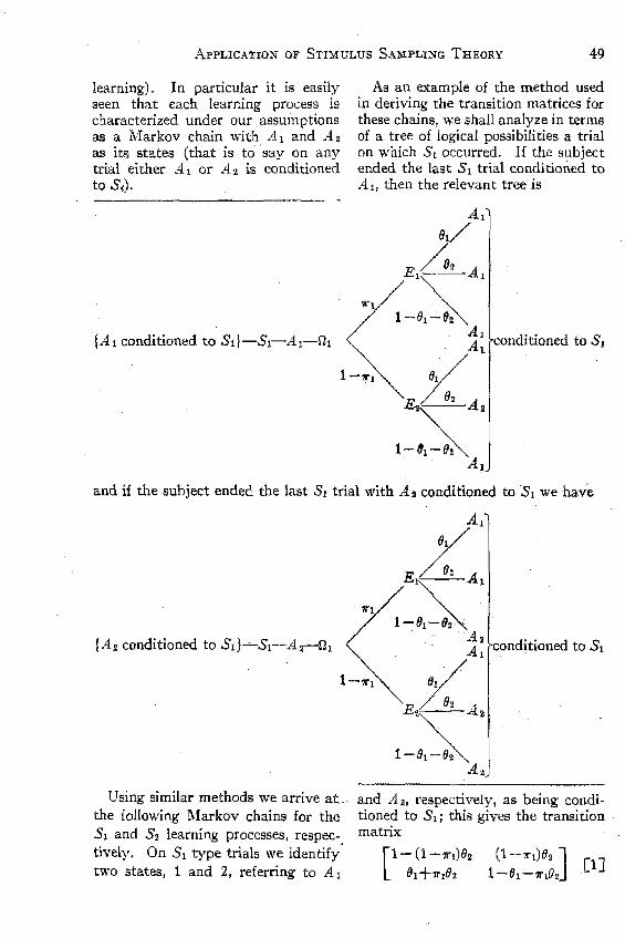
learning). In particular it is easily seen that each learning process is characterized under our assum ptions as a Markov chain with Al and All as its states (that is to say on any trial either A 1 or A 2 is conditioned to S,).

As an example of the method used in deriving the transition matrices for these chains, we shall analyze in terms of a tree of logical possibilities a trial on which S1 occurred. If the subject ended the last Sl trial conditioned to A 11 then the relevant tree is

Al (h/

E//~2 Al

/~

~'II"l/l_fh_~

. t conditioned to S,

1-11"1 . (It/ E 7 __ 88 22_ A2

I-S . Al

and if the subject ended the last SI trial with Aa conditioned to S1 we have

Using similar methods we arrive at-­the following Markov chains for the 8 1 and S2 learning processes, respec­tively. On S1 type trials we identify' two states, 1 and 2, referring to Al

conditioned to S1

and A 2, respectively, as being condi­tioned to S1; this gives the transition matrix

[1-(1-11"1)82 (1-'11"1)02] [lJ

61 +'11"192 1-81-'lI"182

50 PA'l'IUCK SUPPES AND FRANKLIN KRAS~E

Similarly on S2 trials identifying states 1 and 2 referring to A 1 and A 2, respec~ tively, being conditioned to S2 the transition matrix is

[2J

Using the fact that the sequence of Sl'S and S2'S dccur in accordance with a binomial distribution with param~ eter 1', we may combine the above processes to obtain Pit (A 11 S 1) and Pit (A 11 S2) representing the probabili~ ties of A 1 responses on the nth trial of the full experiment given Sl and S2 stimulus events, respectively;

P,,(At/Sl)

= ['-~::'l X [1- l' (81 +82)],,-1 [3J

Pn(AdSz)

1- f1- O- 1.-?l"2] ~+1 ~+1 th l 82

X[1-(1-1')(81+82)],,-1 [4J ~n=l, 2, .• ,

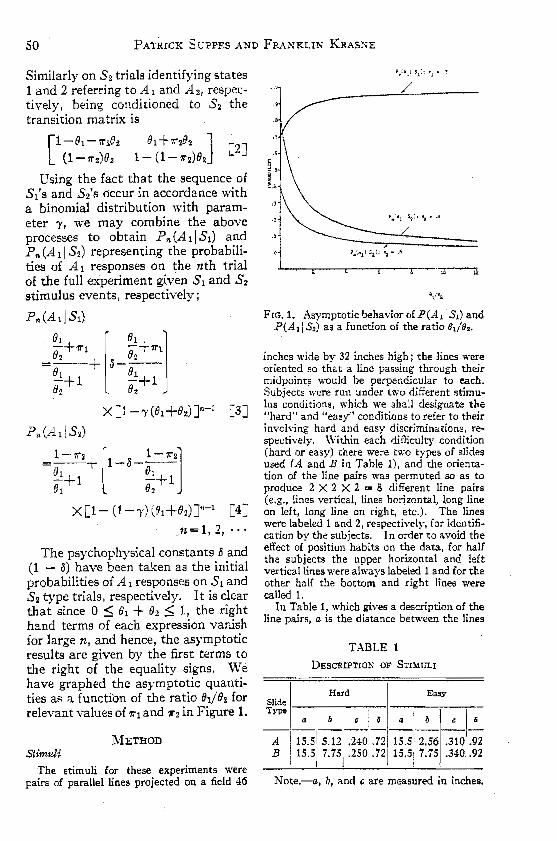
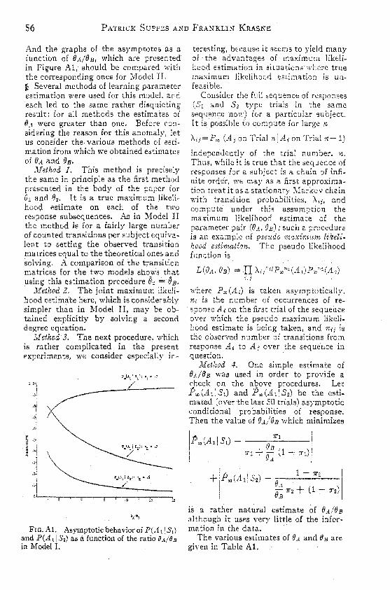
The psychophysical constants Q and (1 - 0) have been taken as the initial probabilities of A 1 responses on S1 and S2 type trials, respectively. It is clear that since 0 ~ 81 + 82 ~ 1, the right hand terms of each expression vanish for large n, and hence, the asymptotic results are given by the first terms to the right of the equality signs. We have graphed the asymptotic quanti­ties as a function of the ratio fh/82 for relevant values of ?l"l and 11"2 in Figure 1.

METHOD Stimuli

The stimuli for these experiments were pairs of parallel lines. projected on a field 46

FIG.1. Asymptotic behavior of P(A11 Sl) and P(A11 S2) as a function of the ratio eJ/fJ2.

inches wide by 32 inches high; the lines were oriented so that a line passing through their midpoints would be perpendicular to each. Subjects were run under two different stimu­lus conditions, which we shall designate the "hard" and conditions to refer to their involving hard and easy discriminations, re­spectively. Within each difficulty condition (hard or easy) there were two types of slides used (A and B in Table 1), and the orienta­tion of the line pairs was permuted so as to produce 2 X 2 X 2 = 8 different line pairs (e.g., lines vertical, lines horizontal, long line on .left, long line on right, etc.). The lines were labeled 1 and 2, respectively, for identifi­cation by the subjects. In order to avoid the effect of position habits on the data, for half the subiects the upper horizontal and left vertical lines were always labeled 1 and for the other half the bottom and right lines were called 1.

In Table 1, which gives a description of the line pairs, a is the distance between the lines

TABLE 1

DESCRIPTION OF STIMt;1.I

Hard Easy Slide Type

a b c • a b c

AI 15.5 ----

.72115.5 ----

5.12 .240 2.56 .310 B ,15.5 7.75 .250 .72) 15.5 7.75 .340

I

.8 -.92 .92

Note.-a, b, and c are measured in inches.

ApPLICATION OF STIMULUS SAMPLING THEORY 51

TABLE 2

GRoup-DESCRIPTlO:.1S

Description

Easy, low symmetry Hard, low symmetry Hard, medium symmetry

of the pair; b is the half-length of the shorter line i c is the difference in half-lengths between the longer and shorter iines; /l is the ability of the subject making a correct dis­crimination when no exoerimenter controlled reinforcing events are influencing his behavior.

Room and Apparatus

The line pairs were projected by an Argus 300 Projector '>vlth a Sylvania 300-watt pro­jector lamp on to a beaded screen 146 inches away. The subjects (from one to five in num­ber) were seated at a distance of about 96 inches from the front of the screen .. The room illumination was about .3 Weston II units.

The subjects responded on answer sheets nr<'n~r"r< in essentially the same way as stand­

score sheets. For half the subiects the left column was used to indicate an Al response and for half the

Experimental Groups

Three groups of subiects whose conditions are described in Table 2 were run. The degree of symmetry under "Description" refers to relative similarity of reinforcing situations on 51 and 52 type trials. For all groups 'Y "" .5.

Subjects

The subjects, who were students at Stanford University, were obtained from the student employment service, an introductory psychol­ogy class, and a university dormitory. With the exception of a few of those from the psy­choiogy class all subjects were male. There were 26, 25, and 18 subjects in Groups I, II, and III, respectively. Because of certain technical difficulties in preparing the stimuli, subjects were not placed randomly in groups.

Procedure

There were from one to five subjects per experimental session. The subjects, having been seated and given answer sheets, were given the following instructions. (Asample

slide was projected on the screen throughout the instructions.)

This is an experiment on judgment of length. I am going to flash a number of slides on the screen each of which has two lines on it i your job ill each case will be to decide which 9f the two lines is the longer and to mark your judgment on the answer sheet in the appropriate column opposite ~he number of the slide weare on. For ~xample: if on the slide I showed, the hne next to the figure one on the screen Was longer, you would mark the answer sheet like this [show marked answer sheet]. Sometimes the pair of lines will be vertical rather than horizontal; then the line here would be Hne one and the One here line two [point to' screen to illustrate what I am saying]. Please mark the answer sheets heavily and completely as though you were filling in an IBM score sheet. I will an­nounce the number of the slide weare on before each judgment and will tell you the correct answer after each judgment. You must make your decisions quickly and re­cord them BEFORE I tell you the answer. Each slide will appear for about 2 seconds. One of the two lines will always be longer than the other; however, some of the judg­ments may be difficult. If you are not sure which line is longer, then guess. Since I want you to work' completely independ­ently of each other, I must request that you remain absolutely silent during the experi­ment. Are there any questions?

The trials then proceeded at a rate of about seven per minute. Each stimulus presema­tion lasted for approximately 2 seconds. Oc­casionally the experimenter found it neces­sary to repeat early in the sessions "this is a test of sorts; you must remain completely silent. It Each subject received a total of 250 trials.

After the experiment the subjects were in­structed: "Will you please write a brief state­ment of your reactions to this experiment?" The responses to this question indicated that the subjects understood and believed the instructions.

ESTIMATION METHODS

Two methods will be presented for estimating the parameters (h and 112 from the data of our experiments. First we shall make maximum likeli­hood. estimates based on the separate 8 1 and 8 2 response subsequences

S2 PATRICK SUPPES AND FRANKLIN KRASNE

(Anderson & Good~an. 1957); ~hen. taking advantage ot the mutual l11de­pendence oi the S1 and S2 learning processes, we sh~n maximize .the joint likelihood funct10n to obtaIn slngle estimates of 81 and 82•

It can be shown that the first method is essentially equivalent to setting the expressions for the theo­retical transition probabilities equal to their estimates and solving for lh and fh.

The estimates based on maximizing the joint likelihood function are not quite so simple. The. derivation, which is reasonably stralghtfonvard but tedious, leads to a tenth degree equation for the. unknown, (h; ~oiu­tlons were obtawed by apprOXIma­tion_methods.

RESULTS AN"D DISCUSSION

Tables 3 and 4 present learning parameter estimates obtained the two methods described above.

The most important observation to be made is that for all estimates 81/8. is less on hard than on easy discrimi~ nations. One can go even further and point out that with exception c:f the S2 trial estimate in Group III this learning parameter ratio is greater than one for the easy discriminations and less than one for the hard ones. This says essentially (for our experi­mental situation) that if the physical stimulus situation is fairly unambigu­ous, subjects will "prefer" to derive their reinforcement from it via !:h and fh while if it is not, they will depend primarily on social support .. This makes good intuitive sense and m fact has been adopted as a postulate by Festinger (1954) in his theory of social comparison processes.

In spite of the fact that we get these intergroup differences for all estimates, it is interesting and rather odd that, as will be seen by studying

T/\BLE 3

SEPARATE :VIAxnfnr LIKELlIIOOD E5TJ~rArES OF Ih, Ih A:-;D DERIVED QUANTITIES

81 .42 .36 .48 ii, .27 .36 .45

lJ:!e2 1.6 81 + Ilz .69

1.0 1.1 .72 .92

Table 3, the effects described above show up much more markedly on S 1

than on S2 type trials. Since the actual stimulus and response labeling was randomized over subjects, and since the stimuli and responses were physically symmetrical, the relation between 71"1 and 71"2 must be responsible for this rather surprising phenomenon.

Reference to the tables under dis­cussion will show that the over-all effectiveness of reinforcement, 171 + fh, increased from the easy to the hard condit,ions. One might argue that the harder a discrimination, the more attentive the subject ·will be to all events surrounding him; thus, rein­forcements are generally more effec­tive when a is smalL Although it is true that via Equations 3 and 4 one can estimate the ratio fjI/fh directly from asymptotic data, \ve have pre­ferred to make much more efficient

TABLE 4

JOIKT MAXI}HL,f LIKELIHOOD ESTIMATES OF 8J, (Jz, AKD DERIVED Qt:ANTITIES

Quantity Group I Group II'! Grnu>, III

81 ,44 .39 AD 82 '" .~" .42 .52

eJ/52 1.8 .92 .77 01 + 82 .69 ., .81 .92

ApPLICATION OF STIMGLUS SAMPLING THEORY 53

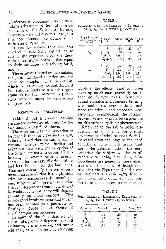
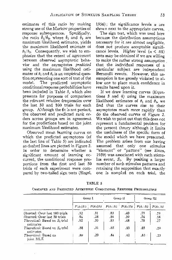
estimates of this ratio by making strong use of the Markov properties of response subsequences. Specifically. the ratio 61/02, where 01 and O2 are maximum likelihood estimates, yields the maximum likelihood estimate of (jl/(j2' Consequently, we wish to em­phasize that the extent of agreement between observed asymptotic beha­'vior and the asymptotes predicted using the maximum likelihood esti­mates of (jl and {}2 is an empirical ques­tion representing one sort of test of the model. The predicted asymptotic conditional response probabilities have been included in Table 5, which also presents for purposes of comparison the relevant relative frequencies over the last 50 and 100 trials for each group. Although the fit is not perfect, the observed and predicted rank or­ders across groups are in agreement for the predictions based on the joint maximum likelihood estimates.

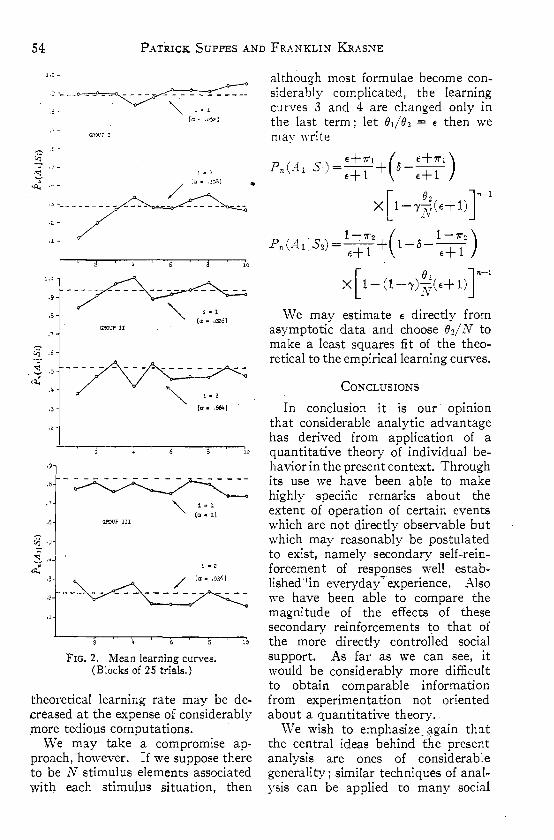
Observed mean learning curves on which the predicted asymptotes (of the last line of Table 5) are indicated as dashed lines are plotted in Figure 2. In order to determine whether a significant amount of learning oc­curred, the conditional response pro­portions from the first and last 50 trials of experiment were com­pared by two~tai1ed sign tests (Siegel,

1956); the significance levels a are shown next to the appropriate curves.

The sign test, which was used here because the distribution assumptions necessary for it are almost negligible, does not produce acceptable signifi­cance levels. Higher level (a < .01) tests may be obtained if we are willing to make the rather strong assumption that the individual responseS of a particular subject are independent Bernoulli events. However, this as­sumption is too grossly violated to al­low one to place much confidence in results based upon it.

If we draw learning curves (Equa­tions 3 and 4) using the maximum likelihood 'estimates' of ElI and 82, we find that the curves rise to their asymptotes much more rapidly than do the observed curves of Figure 2. We wish to point out that this does 110t represent a fundamental problem for the present theory although it limits the usefulness of the specific form of the model which we have presented. The problem arises from our having assumed that only one stimulus "element" or Hpattern" (see Estes, 1959) was associated with each stimu­lus event, S;. By positing a larger number of such stimulus patterns and retaining the supposition that exactly one is sampled on each trial, the

TABLE 5

OBSERVED AND PREDICTED ASYMPTOTIC CONDITIONAL RESPONSE PROBABILITIES

Group I Group II Group III

P(A,jS,) P(A.IS,) P(A.;S,) l P(AtIS') P(A,;S,) P(A,lS,)

Observed: Over last 100 trials .92 ,31 .83 .40 .79 .19 Observed: Over last 50 trials .94 .28 .84 .39 .74 .18 Theoretical: Based on Sl trial .92 .20 .83 .48 .79 .27

estimates Theoretical: Based on 52 tria! .88 .31 .85 .40 .85 .19

estimates Theoretical: Based on .89 .29 .8'! .42 .83 .23

joint l\ILE i,

54 PATRICK SUPPES AND FRANKLIN KRASNE

.8 ", i "l

ra: ... 0521

GPGl'PI

1 a 2

/ [a •. 308J

.3 _ _ _ _ _ _ _ _ _ __ _

.8

.7

0' ,6

.j

.)

.1

'=1 la •. 026]

1.' (a.,J

i = 2

10 = .0)6J

FIG. 2. Mean learning curves. (Blocks of 2S trials.)

10

theoretical learning rate may be de­creased at the expense of considerably more tedious computations.

\Ve may take a compromise ap­proach, however. If we suppose there to be N stimulus elements associated with each stimulus situation, then

although most formulae become con­siderably complicated, the learning curves 3 and 4 are changed only in the last term; let 01/02 = € then we may write

We may estimate e directly from asymptotic data and choose Od N to make a least squares fit of the theo­retical to the empirical learning curves.

CONCLUSIONS

In conclusion it is our opinion that considerable analytic advantage has derived from application of a quantitative theory of individual be­haviorin the present context. Through its use we have been able to make highly specific remarks about the extent of operation of certain events which are not directly observable but which may reasonably be postulated to exist, namely secondary self-rein­forcement of responses well estab­lished'iin everyday""experience. Also we have been able to compare the magni tude of the effects of these secondary reinforcements to that of the more directly controlled social support. As far as we can see, it would be considerably more difficult to obtain comparable information from experimentation not oriented about a quantitative theory ..

We wish to emphasize ~gain that the central ideas behind the present analysis are ones of considerable generality; similar techniques of anal­YSlS can be applied to many social

ApPLICATION OF STIMULUS SAMPLING THEORY 55

psychological situations by a fairly straightforward extension of the idea's presented here. .

REFERENCES

ANDERSON, T. W., & Goomu.N, L. A. Sta­tistical inference about Markov chains. Ann. ma,th. Statist., 1957, 28, 89-109.

ASCii, S. E. Studies of independence and sub­. mission to group pressure: 1. A minority

of one against a unanimous majority. Psychol. }.{onogr., 1956, 70(9, Whole No. 416).

ATKINSON, R. C., & P. An analysis . of two-person game situations in terms of

statistical learning theory. J. expo Psyckol., 1958, 55, 369-378.

ATKINSON, R. C., & SUPPES, P. Application of a Markov model to two-person non­cooperative games. In R. R. Bush & W. K. Estes (Eds.), Studies in mathematical learning theory. Stanford: Stanford Gniver. Press, 1959. Ch. 3.

BURKE, C. J. Applications of a linear model to two-person interactions. III R. R. Bush

& W. K. Estes (Eds.), Studies in mathe­matical learning theory. Stanford: Stanford Univer. Press, 1959. Ch. 9.

BUSH, R. R., & ESTES, W. K. (Eds.), Stud,tes in mathematical learning theory. Stanford: Stanford Univer. Press, 1959.

ESTES, W. K, Component and pattern models with Markovian In R. R. Bush & W. K. Estes (Eds.) Studies in mathema,tical learning theory' Stanford: Stanford Univer. 1959: Ch. 1.

FE STINGER, L. A theory of social comparison processes. Hum. Relat., 1954,7,117-140.

HAYS, D. G., & BUSH, R. R. A study of group action. Amer. sociol. Rev., 1954 19 693-701. ' ,

SHERIF, M. A study in some social factors in perception. Arch. Psyckol., 1935, No. 181-

SIEGEL, S. Nonparametric statistics the behavioral sciences. New York: HilI,1956.

SUPPES, P., & ATKIXSON', R. C. Jfarkov learning models for multiperson interactions. Stanford: Stanford Univer. Press, 1960.

(Received October 5, 1959)

APPENDIX A

The model (Model I) originally pro­posed for the experimental situation studied in the body of this paper differed in its reinforcement mechanisms from the one (Model II) actually discu5sed there. Since rather extensive work was done on it and since we consider some of its failings to be we pre~ sent here some detailed comments on Model I.

Let us call those trials on which the subscripts of E, and S, do not agree "conflict trials." Rather than intro­ducing secondary reinforcers (h and Qz, we assume that the reinforcing event Elo is effective with probability B.4. on non­conflict trials and with probability BB < OA on conflict trials. While we make no explicit psychological assump­tions regarding the reasons for attenuat­ing the learning parameter on conilict trials, the intuitive reasons are clear.

Markov process state identifications are exactly the same as in Model II, and we here present those results for ?l-1odel I which correspond to those indicated for Model II in the body of the paper. On Sl trials the transition matrix is

[1 - (1 - 'iT'l)8S

'iT'16.<.

and on S2 trials it is

[ 1 - 'iT'zB.4. 'iT'28A ]

(1":" 'iT'z)8n 1 - (1 - 'iT'2)8s

The learning curves are

+(0- 'iT'1 ) 'iT'1+ :: (1-'iT'1)

X (1-'Y[8B(1-7T'1)+8A'iT'lJl,,-1 [A3J

1 l-'iT'o

Pn(Al,S2)=OA • ei'2+ (1- 7T'2)

+((1-0)- 1-1!'2 )

:~7T'2+(1 7T'z)

X \1- (1-"Y)[Os(1-7T'z)+8A'iT'2Jl-1

56 PATRICK SUPPES AND FRANKLIN KRASNE

And the graphs of the asymptotes as a function of (J,t/8 B, which are presented in Figure AI, should be compared with the corresponding ones for:\1odel II. ~ Several methods of learning parameter estimation were used for this modeJ, and each led to the same rather disquieting

for all methods the estimates of iJA were greater than one. Before Con· sidering the reason for this anomaly, let us consider the various methods of esti­mation from which we obtained estimates of iJA and (JB.

]l;!ethod 1. This method is precisely the same in principle as the first method presented in the body of the paper for (h and iJ2• It is a true maximum like!i· hooq estimate on each of the two response subsequences. As in Model II the method is for a fairly large number of counted transitions per subject equiva­lent to setting the observed transition matrices equal to the theoretical ones and solving. A comparison of the transition matrices for the two models that using this estimation procedure = e B.

Meth()d 2. The joint maximum iikeli­hood estimate here, which is considerably simpler than in Model II, may be ob­tained explicitly by solving a second degree equation.

lvlethod3. The next procedure, which is rather complicated in the present experiments, we consider especially in-

FIG. A1. Asymptotic behavior of P(A: St) and P(At I S2) as a function of the ratio in ModelL

because it seems to yield many of· the advantages of maximum likeli­huod estimation in situations whf~re true maximum likelihood estimation is un· feasible.

Consider the ful1 sequence of responses and S2 trials in the same

now) a particular subject. possible to compute for n

(Aj on Trial on Trial n-l)

indepeidently of the trial number. n. Thus. while it is true that the sequence of responses for a subject is a chain of infi­nite order, ,ve may as a first approxima­tion treat it as a stationary l\Iarkov chain with trans! tion probabilities, and compute under this assumption the maximum likelihood estimate of the parameter pair (BA. aB ) i such a pcocedure is an example of pseudo maximum likeU· hood estimation. The pseudo likelihood function is

Len) = II -: Ii

where P",(Ai) is taken asymptotically, ni is the number of occurrences of re­sponse Ai on the first trial oi the sequence over which the pseudo maximum likeli­hood estimate is being taken, and n'i is the observed number of transitions from response Ai to A j over the sequence in question.

lv[ethod 4. One estimate of BAiBB was used in order to provide a check on the above procedures. Let P",(A1IS1) and P",(AdS2) be the esti. mated (over the last 50 trials) asymptotic conditional probabilities of response. Then the value of (J.~/()B which minimizes

is a rather natural estimate of B.i/B B

although it uses very little of the infor­mation in the data.

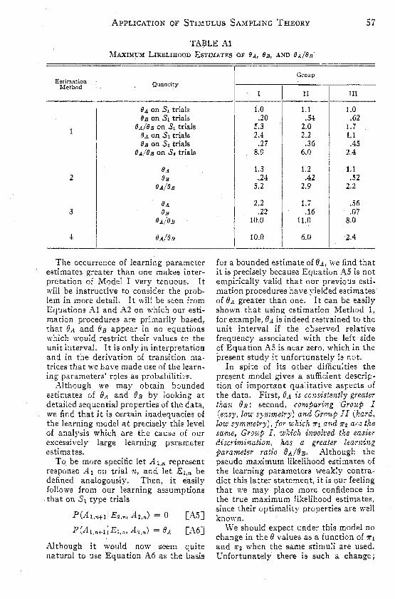
The various estimates of e d and 8 Bare given in Table Ai.

ApPLICATION OF STIMULUS SAMPLING THEORY 57

T,,\BLE A1 MAXIMUM LIKELIHOOD ESTIMATES OF 0.1, OB, AND OA/OB'

Estimation Quantity Method

(j A on Sl trials flll on Sl trials

1 th/1J1l on Sl trials I:lA on S2 trials I:l.s on S2 trials

()A!OIl on Sa trials

()A

2 OIl OA/flB

IJA 3 IJIl

IJA/fhJ

4 i

O.4./()1l

The occurrence of learning parameter estimates greater than one makes, inter­pretation of Model I very tenuous. It will be instructive to consider the prob­lem in more detail. It will be seen from Equations A1 and A2 on which our esti­mation procedures are primarily based, that fJA and fJB in no equations which would their values to the unit interval. It is in interpretation and in the derivation of transition ma­trices that we have made use of the learn­ing parameters' roles as probabilities.

Although we obtain bounded estimates of fJA fiB by looking at detailed sequential of the data, we find that it is inadequacies of the learning model at precisely this level of analysis which are the cause of our excessively learning parameter estimates.

To be more specific let AI,,. represent response Al on trial n, and let EI,n be defined analogously, Then, it e'asily follows from our learning assumptions that on Sl type trials

P(Al,n+1iE2.n, A 2•n) = 0 [AS]

P(A 1,n+11 A 2,n) = fJ,1 [A6]

Although it would now seem quite natural to use Equation A6 as the basis

Group

I II II!

1.0 1.1 1.0 .20 .54 .62

5.3 2.0 1.7 2.4 2.2 1,1

.27 .36 .45 8.9 6.0 2.4

1.3 1.2 1.1 .24 .42 .52

5.2 2.9 2.2

2.2 1.7 .56 .22 .16 .07

10.0 11.0 8.0

10.0 6.0 2.4

for a bounded estimate OffJA, we find that it is precisely because Equation A5 is not empirically valid that our previous esti­mation procedures have yielded estimates of fiA greater than one. It can be easily shown that using estimation Method 1, for example, 0.4 is indeed restrained to the unit interval if the observed relative frequency associated with the left side of Equation AS 15 near zero, which in the present study it unfortunately is not.

In spite of its other difficulties the present model gives a sufficient tion of important qualitative aspects the data. First, (fA is consistently greater than fJ B i second, comparing Group I (easy, low symmetry) and Group II (hard, low symmetry), for which 71"1 and 1i2 are the same, Group I, which involved the easier discrimination, has a greater learning parameter ratio e .... /OB. Although the pseudo maximum likelihood estimates of the learning parameters weakly contra­dict this latter statement, it is our that we may place more confidence the true maximum likelihood estimates, since their optimality properties are well known.

We should expect under this model no change in the fJ values as a function of 1il

and 1i2 when the same stimuli are used. Unfortunately there is such a change j

58 PATRICK SUPPES AND FRANKLIN KRASNE

indeed, we notice that when the subject makes the less frequently reinforced response and is reinforced, this reinforce­ment tends to have a greater probability of being effective than it would have

otherwise had. This can be seen by com· paring the 8 estimates made on 5\ and 52 type subsequences; the Os estimates in Group I, however, are contrary to this generalization.

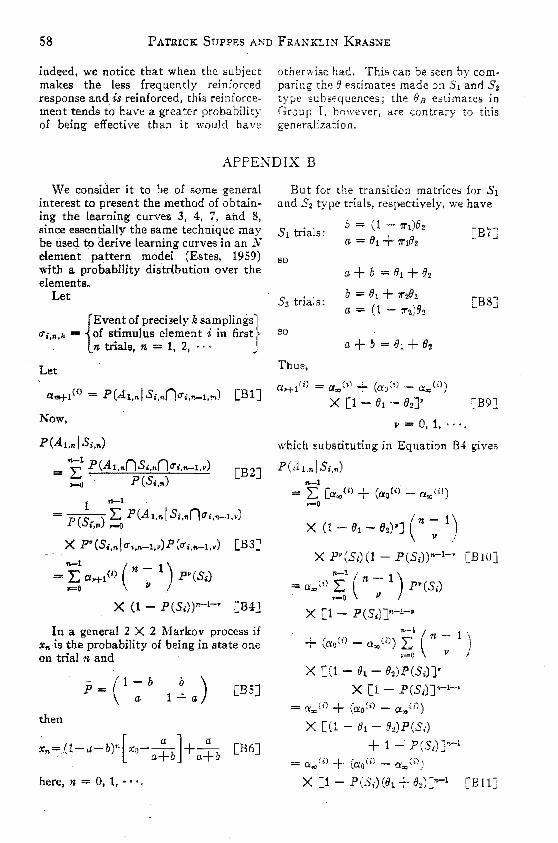
APPENDIX B

We consider it to be of some general interest to present the method of obtain~ ing the learning curves 3, 4, 7, and 8, since essentially the same technique may be used to derive learning curves in an N element pattern model (Estes, 1959) with a probability distribution over the elements.

Let

{

Event of precisely k samPlingS} O';,,,.k - of stimulus element i in first

n trials, n = 1, 2, ...

Let

£lm+1(i) = P(A1,,,~S;,nnO"i.n-l,m) [Bl]

Now,

P(Al."l S.,,,)

== E p(A1 ... nS •. "nO"i,nr-l .• ) [B2] ,.....0. . peS.,,,)

1 _1

= peSt,,,) Eo P(Al ... ! S.,,,nUi,n-l,.)

x P'(S .... I Ui,n-l,.)P (U;.ft-l .• ) [B3}

= z:: £l>'f-l(i) n - pV(S.) _1 ( 1) >=0 /I

In a general 2 X 2 Markov process if x,. is the probability of being in state one on trial nand

p = (1 - b ~) CBS] a 1- a

then

x = rt-a-b)n[xo-_a_J .. ," a+b [B6]

here, n = 0, 1, •• '.

But for the transition matrices for Sl and S2 type trials, respectively, we nave

SI trials: b = (1 - 1r1)82

a = (h + 1r182 [B7]

so

52 trials:

so

Thus,

a + b = til + fJz

b = 81 + 7r.jJ2

a = (1 - 1r2)02

a>'f-l(i) = a",(i) + (aQ(i) - a",(i»)

X [1 - Ih - 8zJ' 11 = 0, 1, "',

[88]

which substituting in Equation B4 gives

peA l,n lSi, .. ) 11-1

= z:: [a .. (i) + (ao(i) - a., W) ,...0

X (1 - 81 - 82)'J ( n ~ 1)

X P'(Si)(l - P(Si))",-I-, [BlO]

= a",,(i) 3:1

(n - l) P'(S,) .-0 II

X [1 - P(S.)],,-l-.

(ao(!) _ a",U)) i l (n - 1 )'

_Q II

X [(1 - fh - Itz)P(S,)]'

X [1 - P(S.)]fl-l-'Y

X [(1 - 81 - Oz)P(5,)

+ 1 - P(S,):,,--l

ApPLICATION OF STIMULUS SAMPLING THEORY S9

This becomes for 51 trials. letting

ao(l) = 0 p(AI,,,1 Sl, .. )

= (h + 7rl02 + [0 _ 01 + 7rl02 ]

81 + O2 01 + O2

X [1 - 'Y(81 + 8z)]n-l [B12]

and for 52 trials becomes, letting

ao(2) = 1 - 0 '

P(A l , .. 152, .. )

= (1- 7r2)82 + [(1-0- (l-7rz)8z] 01+02 01+82 .

X[l- (1-'Y)(81+8z)]n-l [B13]