Partnership for AiR Transportation Noise and Emission Reduction An FAA/NASA/TC-sponsored Center of Excellence

Representing and AnalyzingRepresenting and AnalyzingUncertainty in Large-ScaleUncertainty in Large-ScaleComplex System ModelsComplex System Models

Doug Allaire

2

Outline

1. Modeling Uncertainty

2. Research Objectives

3. The Aviation Environmental Portfolio Management Tool

4. Global Sensitivity Analysis

5. Future Work

3

Modeling Uncertainty

• Uncertainties in modeling are unavoidable• Uncertainty should be properly represented

– Estimates and predictions– Risk analysis– Cost-benefit analysis– Furthering model development

• Uncertainty in models can be represented with threedifferent methodologies– Probabilistic (aleatory)– Fuzzy sets (epistemic)– Fuzzy Randomness (both)

4

Large-Scale Complex System Models

• Multiple disciplines– Economics, aerodynamics, atmospheric science, …

• Many inputs, many outputs• Systems of models of different character

– Physics-based, empirical

• Many assumptions– Subjective, objective

• Computationally intensive• Characterizing, representing, quantifying, and accounting

for uncertainty is key– To both development and application of models

5

Uncertainty in Large-ScaleComplex System Models

Goals of a formal uncertainty analysis:• Further the development of a model

– Identify gaps in functionality that significantly impact theachievement of model requirements, leading to the identificationof high-priority areas for further development.

– Rank inputs based on contributions to output variability to informfuture research

• Inform decision-making– Provide quantitative evaluation of the performance of the model

relative to fidelity requirements for various analysis scenarios.– Properly represent different types of uncertainty in the model

Especially important for complex systems that comprisemultiple models of different disciplines, differentcharacter, different assumptions

6

What exists today

• Probabilistic and fuzzy random uncertainty models• Rigorous model independent sensitivity analysis method

– Expensive

• Several model dependent sensitivity analysis methods– Inexpensive but difficult to ensure proper use

• Limited research into the use of surrogate models inuncertainty analysis– Critical for models with long runtimes

• Numerous sampling techniques for improving runtimes ofprobabilistic analyses

7

Research Objectives

• For specific large-scale, complex system models,identify how to properly represent and analyzeuncertainty.

• Systematically develop surrogate models forsituations where proper representation and analysis ofuncertainty is computationally prohibitive. Limitationsand uncertainty associated with the use of a surrogateshould be identified.

• Use appropriate sampling techniques to improvecomputational costs in uncertainty analysis. Limitationsand uncertainty associated with the use of chosensampling methods should be identified.

8

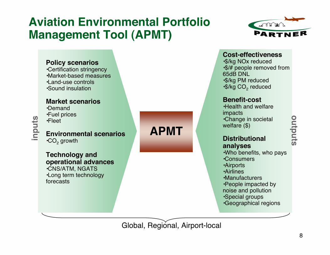
Aviation Environmental PortfolioManagement Tool (APMT)

APMT

Policy scenarios•Certification stringency•Market-based measures•Land-use controls•Sound insulation

Market scenarios•Demand•Fuel prices•Fleet

Environmental scenarios•CO2 growth

Technology andoperational advances•CNS/ATM, NGATS•Long term technologyforecasts

Cost-effectiveness•$/kg NOx reduced•$/# people removed from65dB DNL•$/kg PM reduced•$/kg CO2 reduced

Benefit-cost•Health and welfareimpacts•Change in societalwelfare ($)

Distributionalanalyses•Who benefits, who pays•Consumers•Airports•Airlines•Manufacturers•People impacted bynoise and pollution•Special groups•Geographical regions

Global, Regional, Airport-local

inpu

tsoutputs

9

APMT PARTIALEQUILIBRIUM BLOCK

NOISE IMPACTS

LOCAL AIR QUALITYIMPACTS

CLIMATE IMPACTS

APMT COSTS & BENEFITS

New Aircraft

Emissions

Noise

APMT BENEFITSVALUATION BLOCK

Monetized Benefits

CollectedCosts

Emissions

Emissions & Noise

Policy and Scenarios

AEDT

Fares

DEMAND(Consumers)

SUPPLY(Carriers)

Operations

Schedule&

Fleet

Airport-levelEmissions

Tools

GlobalNoise

Assessment

Airport-levelNoiseTools

GlobalEmissionsInventories

EDS VehicleNoiseDesignTools

VehicleEmissions

DesignTools

TechnologyImpact

Forecasting

VehicleCost

Assessment

DesignTools

Interface

APMT approach

10

APMT Uncertainty Analysis Goals

• AQ1. What are the key assumptions employed within the module?How do these assumptions translate into quantifiable uncertainty inmodule outputs?

• AQ2. What are the key assumptions employed within the moduledatabases? How do these assumptions translate into quantifiableuncertainty in module outputs?

• AQ3. How do assumptions/limitations in modeling and databasesimpact the applicability of the module for certain classes ofproblems? What are the implications for future development efforts?

• AQ4. How do uncertainties in module inputs propagate touncertainties in module outputs? Further, what are the key inputsthat contribute to variability in module outputs?

• AQ5. For assumptions, limitations and inputs where effects cannotbe quantified, what are the expected influences (qualitatively) onmodule outputs

• AQ6. How do assessment results translate into guidelines for use?

11

Answering AQ4 Probabilistically

• AQ4. How do uncertainties in module inputs propagateto uncertainties in module outputs? Further, what are thekey inputs that contribute to variability in moduleoutputs?

• Assign factor distributions

• Propagate uncertainty

• Apportion output variance to model factors

12

Assigning Factor Distributions

• Example: APMT Aircraft Emissions Module

EINOx: ( )( )( )

17.36 .24 , .24 0

17.36 .24 , 0 .24EI

x for xP x

x for x

+ ! " "#$= %

! " "$&

( )( )( )

82.64 .11 , .11 0

82.64 .11 , 0 .11T

x for xP x

x for x

+ ! " "#$= %

! " "$&Temperature:

( )( )( )

1111.11 .03 , .03 0

1111.11 .03 , 0 .03P

x for xP x

x for x

+ ! " "#$= %

! " "$&Pressure:

( )( )( )

34.60 .17 , .17 0

34.60 .17 , 0 .17H

x for xP x

x for x

+ ! " "#$= %

! " "$&Rel. Humidity:

( ) 10, .05 .05FFP x for x= ! " "Fuel Flow:

.24-.24 0

4.17

-.11 0 .11

9.09

-.03 0 .03

33.33

-.17 0 .17

5.88

-.05 0 .05

10

13

Propagate Uncertainty

gT g(T)Assume a model:

[ ]1

0

00

1 1( ) ( ) ( ) , ,

2

m

T n T m n

n

n ng T g t P t dt w g P w w w

m m m m=

! " ! "# = $ = = =% & % &

' ( ' ()* o.w.

• Would like to compute the mean value of g(T)

( )2m!"• Trapezoidal Rule Error goes as and 1/

1s

m N= !

[2][1]

14

Propagate Uncertainty: Monte CarloSimulation

• Assume is a random variable with a probability densityfunction fX(x).

• Monte Carlo mean estimate (for any number of factors)

• Error goes probabilistically as– Strong law of large numbers– Central limit theorem

( ) ( ) ( ) ( )1

1

s

N

nX

nI

g X g x f x d x g xN =

! = "# $% & '(

X

( )1/ 2N

!"

• Compute mean value of g(X) using random samples• X is any factor (temperature, pressure, etc.)

gX g(X)Assume same model:

15

Partitioning Output Variance

Analysis of Variance (ANOVA)– Assumes a linear statistical model– Requires specification of factors and factor interactions total to

be comprehensive, where S is the number of factors

Vary-all-but-one methods– Calculate factor variance contributions by fixing a factor and performing

a Monte Carlo simulation.– Requires specification of where to fix a factor– N(S+1) model evaluations

Global Sensitivity Analysis– All factors varying– Computes total sensitivity indices for each factor in N(S+1) model

evaluations using Monte Carlo simulation– Variance contributions take into account underlying factor distributions

( )2 1S!

16

Global Sensitivity Analysis

• What is the goal?• ANOVA Decomposition• Partitioning output variance• Monte Carlo Estimates• Total Sensitivity Indices

17

The goal of Global Sensitivity Analysis

• Ranking model factors on the basis of contribution tooutput variability– Useful for model development– Useful for understanding model outputs

• The goal is to partition output variance amongst thefactors of the model– Main effects– Interaction effects

Factor 1

Factor 2

Factor 1, Factor 2Interaction

OutputVariance

18

ANOVA Decomposition

• High-Dimensional Model Representation of f(x) [4]

• Example HDMR for a function of three parameters

19

ANOVA Decomposition

• High-Dimensional Model Representation of f(x) [4]

• Example HDMR for a function of three parameters

Mean value

20

ANOVA Decomposition

• High-Dimensional Model Representation of f(x) [4]

• Example HDMR for a function of three parameters

Mean value Main effects

21

ANOVA Decomposition

• High-Dimensional Model Representation of f(x) [4]

• Example HDMR for a function of three parameters

Mean value Main effects

First-order interactions

22

ANOVA Decomposition

• High-Dimensional Model Representation of f(x) [4]

• Example HDMR for a function of three parameters

Mean value Main effects

First-order interactions

Second-order interaction

23

Example of ANOVA Decomposition

• Consider a function

• Then the ANOVA decomposition is:

24

Calculating Variances

• Given a function f(x) that is square integrable,

• Similarly,

• Example for a function of two parameters:

25

The goal of global sensitivity analysis

• The goal is to partition output variance amongst thefactors of the model– Main effects– Interaction effects

Factor 1

Factor 2

Factor 1, Factor 2Interaction

OutputVariance

D D1

D12

D2

26

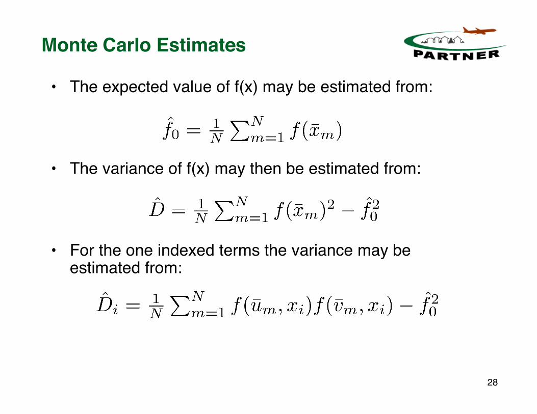
Monte Carlo Estimates

• The expected value of f(x) may be estimated from:

27

Monte Carlo Estimates

• The expected value of f(x) may be estimated from:

• The variance of f(x) may then be estimated from:

28

Monte Carlo Estimates

• The expected value of f(x) may be estimated from:

• The variance of f(x) may then be estimated from:

• For the one indexed terms the variance may beestimated from:

29

Total Sensitivity Indices

• Sensitivity indices:

• Total Sensitivity indices:

30

APMT ResultsGlobal Sensitivity Analysis

0

0.2

0.4

0.6

0.8

Housing

Growth Rate

Discount

Rate

Quiet Level Contour

Uncertainty

NDI

Tota

l G

lob

al S

en

sit

ivit

y I

nd

ex

Total Sensitivity Indices

0.69 0.670.67

0.360.300.28

0.110.05 0.010.02 0.02

0

0.2

0.4

0.6

0.8

1.0

1.2

IntegratedTemperature Change

Damage NPV

OthersRF* short-livedclimate sensitivityDamage coefficient

BVB-Noise Module Analysis

BVB-Climate Module Analysis

31

Future WorkUncertainty Model

Selection

Problem StatementDefine model

Define methods

Compare methods Test functions

Surrogate Reqs.Sampling Reqs.

ApplicationLarge-scale model

(APMT Module)

Probabilistic

Problem StatementDefine model

Define methods

Compare methods Test functions

ApplicationLarge-scale model

(APMT Module)

Fuzzy Random

Surrogate Reqs.Sampling Reqs.

Compare

32

Questions?

33

References

[1]http://www.krellinst.org/UCES/archive/modules/potential/trap/index.html[2]http://www.statisticalengineering.com/curse_of_dimensionality.htm[3] T. Homma, A. Saltelli, “Importance Measures in Global Sensitivity Analysis of

Nonlinear Models.” Reliability Engineering and System Safety, 52(1996) pp1-17.

[4] I.M. Sobol’, “Global Sensitivity Indices for Nonlinear Mathematical Modelsand their Monte Carlo Estimates,” Mathematics and Computation inSimulation 55(2001) 271-280.

34

Aviation Environmental PortfolioManagement Tool (APMT): Motivation

• Aviation benefits and environmental effects result from a complexsystem of interdependent technologies, operations, policies andmarket conditions

• Community responses, policy and R&D options typically consideredin a limited context

– only noise, only local air quality, only climate change

– only partial economic effects

• Actions in one domain may produce unintended negativeconsequences in another

• Tools and processes do not support recommended practice

– NPV of benefits-costs is recommended basis for informing policydecisions in U.S., Canada and Europe

35

ANOVA Decomposition (Cont.)

• A high-dimensional model representation is unique if

where and

• The individual functions are orthogonal

• The expected value of each individual function is zero

e.g.

• The expected value of f(x) is then

1 1

1

,...,

0

( ,..., ) 0s si i i i kf x x dx =! 1

,...,s

k i i= 1,2,...,s n=

1 1 1 1( , , ) ( , , ) 0

s s t ti i i i j j j jf x x f x x dx =! K KK K

1 1 1( ) 0f x dx =!

0( )f x dx f=!

36

Improving Runtime: Surrogate Modeling

• A surrogate is a less expensive, (often) lower-fidelitymodel that represents the system input/output behavior

• Surrogates are often classified into three categories:1. Data fit, e.g. response surface models, Kriging models ⇒ EDS2. Reduced-order models, derived using

system mathematical structure3. Hierarchical models,

e.g. coarser grid, neglectedphysics, aggregation ⇒ AEDT

• Why surrogates?– If one analysis takes 1 minute, then a Monte Carlo simulation

with 10,000 samples takes 10,000 minutes = 7 days– A global sensitivity analysis requiring a Monte Carlo simulation

for each factor would take 7(S+1) days, where S is the numberof factors

• Relating uncertainty analysis results done with asurrogate model to results from the full model is critical

37

Surrogate Modeling Approach forAPMT• Adaptive approach for Aircraft Emissions Module

– Monte Carlo Simulation of a single day of flights– Build up from a small number of flights to representative set

• Statistical approach for Aircraft Performance Module– Determine critical factors using expert opinion

• Fuel burn per meter• Emissions per meter• Segment level thrust distribution• …

– Group aircraft/engine pairs based on statistical similarities– Select representative from each group

• Important questions to ask– How do these surrogates impact Monte Carlo results?– How do these surrogates impact global sensitivity results?

38

Improving Runtime: Sampling Methods

• Some well-known methods:– Brute-force Monte Carlo Methods

• Use pseudorandom numbers on [0,1] and the inversion method• The probabilistic error bound is .

– Quasi-Monte Carlo Methods• Use well-chosen deterministic points rather than random samples• Low discrepancy sequences (e.g. Halton, Hammersley)• Deterministic error bound

– Stratification -- Latin Hypercube Sampling• Stratify on all factor dimensions simultaneously• Leads to lower variance in integral estimates than independent,

identically distributed samples• Probabilistic error bound .

• Things to keep in mind– How bias in sampling impacts analysis metrics– Obtaining more samples if a metric has not converged sufficiently

( )1/ 2N

!"

((log ) / )sN N!

( )1/ 2N

!"