representations of the symmetric group -...

Diploma Thesis

Representations of the

Symmetric Group

Author: Manjil P. Saikia

Supervisor: Prof. Fernando R. Villegas

The Abdus Salam International Centre for Theoretical Physics

Trieste, Italy

A thesis submitted in partial fulfillment of the requirements for

the Postgraduate Diploma in Mathematics.

August 2015

Dedicated to

Prof. Mangesh B. Rege

i

Abstract

In this project, we first study the preliminary results of Representation The-

ory of Finite Groups (in characteristic zero) and the combinatorics of Young

Tableaux. We then use these techniques to explicitly give the irreducible

representations of the symmetric group, Sn.

ii

Acknowledgments

First, I would like to thank my supervisor, Prof. Fernando R. Villegas for his

help and encouragement throughout this project. Heart felt gratitude to all

the members of the Mathematics Section of ICTP for their support during

the programme, specially Tarig for making the material of this project more

understandable.

Thanks to Prof. Fernando Quevedo, Director of ICTP under whose guid-

ance the centre is functioning and scaling new heights. Thank you Patrizia

and Sandra for making the past year go easy on us.

I express my deep gratitude to my parents and sister for their uncondi-

tional love and support in every step of my life. Thank you mentors Prof.

M. B. Rege, Prof. R. Sujatha, Prof. N. D. Baruah, Dr. R. Barman and Dr.

A. Saikia for placing mathematics in an enjoyable platter.

I am thankful to the new friends that I made in Italy, specially Angela,

Ismail, Mariam, Noor, Prosper, Ajayi, Kamal, Kirk, Marcos and Rodrigo,

whose company will be remembered fondly in the days to come. Thank you

Sirat, Parama, Madhurrya, Kantadorshi, Dhritishna, Salik and Hrishikesh

for remembering me even when I am thousands of miles away.

Last but not the least, I acknowledge the financial support from UN-

ESCO, IAEA and the Italian Government which enabled me to come to

ICTP and spend an amazing year learning mathematics.

iii

Contents

Abstract ii

Acknowledgments iii

Contents iv

1 Introduction to Representation Theory 1

1.1 Generalities on Linear Representations . . . . . . . . . . . . . 2

1.2 Character Theory . . . . . . . . . . . . . . . . . . . . . . . . . 6

1.3 Restricted and Induced Representations . . . . . . . . . . . . 12

2 Irreducible Representations of S3, S4 and S5 14

2.1 S3 . . . . . . . . . . . . . . . . . . . . . . . . . . . . . . . . . 14

2.2 S4 . . . . . . . . . . . . . . . . . . . . . . . . . . . . . . . . . 16

2.3 S5 . . . . . . . . . . . . . . . . . . . . . . . . . . . . . . . . . 17

3 Representations of Sn 19

3.1 Preliminaries . . . . . . . . . . . . . . . . . . . . . . . . . . . 19

3.2 Specht Modules . . . . . . . . . . . . . . . . . . . . . . . . . . 23

3.3 RSK Correspondence . . . . . . . . . . . . . . . . . . . . . . . 27

3.4 Symmetric Functions . . . . . . . . . . . . . . . . . . . . . . . 30

3.5 Frobenius Character Formula . . . . . . . . . . . . . . . . . . 34

iv

1Introduction to Representation Theory

Representation theory is the branch of mathematics that studies abstract

algebraic structures by representing their elements as linear transformations

of vector spaces, as well as modules over these abstract algebraic structures.

In essence, a representation makes an abstract algebraic object more concrete

by describing its elements with the help of matrices and consequently the

algebraic operations in terms of matrix addition and matrix multiplication.

The main goal is to represent the group in question in a concrete way.

In this thesis, we shall specifically study the representations of the sym-

metric group, Sn. To do this, we shall need some preliminary concepts from

the general theory of Group Representations which is the motive of this

chapter.

1

Chapter 1. Introduction to Representation Theory

1.1 Generalities on Linear Representations

Throughout, we shall assume that V is a vector space over the field C of

complex numbers and denote the set of all invertible linear operators on V

by GL(V ). This set forms a group with respect to a composition. The

material in this chapter has been borrowed from the wonderful expositions

of [2], [3] and [4]. [6] has been referred to for some examples. For brevity, in

most of the cases we shall either omit the proofs of the results or give only

a sketch of the proof. Detailed proofs can be found in the references at the

end of this thesis. Unless otherwise mentioned, all groups considered here

will be of finite order.

Definition 1.1.1. Let G be a finite group with identity 1 and composition

defined as (s, t) 7→ st for some elements s and t in G. A linear represen-

tation of G in V is a homomorphism

ρ : G −→ GL(V ).

We shall use the convention of denoting an element ρ(s) by ρs where

s ∈ G. By definition ρst = ρsρt for all s, t ∈ G, ρ1 = 1 and ρs−1 = ρ−1s . In

this thesis, we shall only consider the case when V is finite dimensional. The

dimension of V is called the degree of the linear representation ρ.

Definition 1.1.2. An n-dimensional matrix representation of a group G

is a homomorphism

R : G −→ GLn(C),

where GLn(C) is the group of all n× n matrices over C.

Let ρ : G −→ GL(V ) be a linear representation of degree n. Let

(e1, e2, . . . , en) be a basis for V and Rs be the matrix of ρs w.r.t to this

basis. Then we have the following:

1. For all s ∈ Gρs is invertible if detRs 6= 0 , and

2


2. For all s, t ∈ Gρst = ρsρt if Rst = RsRt .

For Rs = (rij(s)) where (rij(s)) denotes the matrix elements for some i

and j the second formula is equivalent to

rik(st) =∑j

rij(s)rjk(t).

With the above notation, we can go from a linear representation to a matrix

representation where Rs is the matrix of ρs as defined earlier. Conversely, if

we have invertible matrices we can get the other correspondence from this

formula.

Definition 1.1.3. Two representations ρ : G −→ GL(V ) and ρ′ : G −→GL(V ′) are isomorphic if there exists a linear isomorphism θ : V −→ V ′

which satisfies θ ◦ ρ(s) = ρ′(s) ◦ θ for all s ∈ G.

Example 1.1.4. A representation of degree 1 of a group G is a homomor-

phism ρ : G −→ C∗, where C∗ is the multiplicative group of non-zero complex

numbers. Here, since G has finite order the values of ρ(s) are roots of unity.

If ρ(s) = 1 for all s ∈ G, then this representation is called the trivial rep-

resentation.

Example 1.1.5. Let the group G act on the finite set X. If V is a vector

space whose basis (ex) is indexed by the elements of X, then the permu-

tation representation of G associated with X is given by the linear map

ρs : V −→ V where ex 7→ esx and s ∈ G. In the final chapter we shall be

interested in permutation representations where X is the general symmet-

ric group on n elements. For X = G, then this representation is called the

regular representation of G.

Definition 1.1.6. A subspace W of a vector space V is stable under the

action of a finite group G if ρsw ∈ W for all s ∈ G and w ∈ W , where

ρ : G −→ GL(V ) is a linear representation.

3


Definition 1.1.7. Let ρ : G −→ GL(V ) be a linear representation of G in

V . Let W be a subspace of V that is stable under the action of G, then ρs∣∣∣W

defines a linear representation of G in W , called the subrepresentation of

V .

For example, if V is a regular representation of G and W is the subspace

of dimension 1, then it is a subrepresentation of V which is isomorphic to

the trivial representation.

Definition 1.1.8. A linear representation ρ : G −→ GL(V ) is said to be

irreducible if V is not the zero space and there exists no proper subspace

of V that is stable under G.

We notice that the above definition is equivalent to saying that V is

not the sum of two representations. A representation of degree 1 is always

irreducible. We now come to the first theorem of the theory.

Theorem 1.1.1. Every representation is a direct sum of irreducible repre-

sentations.

The proof of this theorem is by induction on the degree of the represen-

tation. Before proceeding to the proof, we work a little with direct sums.

A vector space V is said to be the direct sum of its subspaces W and Z

if each vector v ∈ V can be written uniquely as the sum v = w + z for some

elements w ∈ W and z ∈ Z. We then write V = W ⊕ Z and say that Z is

the complement of W in V . The proof of Theorem 1.1.1 uses the following

result whose proof we shall omit.

Theorem 1.1.2. Let ρ : G −→ GL(V ) be a linear representation of G in

V and let W be a vector subspace of V stable under G. Then there exists a

complement Z of W in V which is stable under G.

Now, we can prove Theorem 1.1.1.

4


Proof. If dim(V ) = 0 then there is nothing to prove. So, we assume dim(V ) =

n, where n ≥ 1. If V is irreducible then we are done. If V is not irreducible

then it has a nontrivial proper subspace W that is stable under G. So by

Theorem 1.1.2 we have V = W ⊕ Z for Z, the complement of W . Now, we

use induction on W and Z to get the result.

Definition 1.1.9. Let V1 and V2 be two vector spaces. The tensor product

of V1 and V2 is a vector space W with a map from V1 × V2 into W given by

(x1, x2) 7→ x1 ⊗ x2 which satisfies the following conditions:

(i) x1 ⊗ x2 is linear in both the variables, and

(ii) If (ei) is a basis of V1 and (ej) is a basis of V2 then (ei ⊗ ej) is a basis

of W .

It is clear from this definition that, dim(V1 ⊗ V2) = dim(V1). dim(V2).

Definition 1.1.10. Let ρ1 : G −→ GL(V1) and ρ2 : G −→ GL(V2) be two

linear representations of a group G. For s ∈ G, we define ρs ∈ GL(V1 ⊗ V2)by

ρs(x1 ⊗ x2) = ρ1s(x1)⊗ ρ2s(x2)

for x1 ∈ V1 and x2 ∈ V2. Then, we write ρs = ρ1s⊗ρ2s and this defines a linear

representation of G in V1⊗V2 which is called the tensor product of the given

representations.

If in the above V1 = V2 = V and θ be an automorphism of V ⊗ V such

that θ(ei⊗ ej) = ej ⊗ ei for all pairs (i, j), then we have θ(x⊗ y) = y⊗ x for

x, y ∈ V . Hence, we see that θ is independent of the basis that we choose.

We now define subsets of V ⊗ V as follows

Sym2(V ) = {z ∈ V ⊗ V | θ(z) = z}

and

Alt2(V ) = {z ∈ V ⊗ V | θ(z) = −z}

5


which are called the symmetric power and the alternating power. We

can similarly define higher order powers, but for this thesis we consider only

second order powers . As an automorphism,θ is linear. Hence, the above two

sets are subspaces of V ⊗ V .

Proposition 1.1.3. Let ρ1 = ρ⊗ ρ be a representation of G in V ⊗ V , then

the subspaces Sym2(V ) and Alt2(V ) are stable under G.

The proof of this proposition is a simple algebraic argument and is omitted

here.

Proposition 1.1.4. The space V ⊗ V decomposes as

V ⊗ V = Sym2(V )⊕ Alt2(V ).

The proof is very elementary, which is omitted here.

1.2 Character Theory

Now we come to a significant part of the theory of representations of a finite

group. The characters of a representation that we shall study in this section

encodes all the important information about a representation. The results

mentioned in this section will be of paramount importance in the next chapter

where we find representations of the first few symmetric groups using the

content of this chapter.

Definition 1.2.1. Let ρ : G −→ GL(V ) be a linear representation of a finite

group G in the vector space V . The complex valued function χρ defined on

G by

χρ(s) = Tr(ρs),

where Tr(ρs) is the trace of ρs, is called the character of the representation

ρ.

6


The degree of the character is defined to be the degree of the representation

ρ, and the character of an irreducible representation is called the irreducible

character.

Proposition 1.2.1. If χ is the character of a representation ρ of degree n,

then we have the following:

(i) χ(1) = n,

(ii) χ(s−1) = χ(s)∗ for s ∈ G, and

(iii) χ(tst−1) = χ(s) for s, t ∈ G.

The proof of this result is very simple and we shall omit it here.

Proposition 1.2.2. Let ρ1 : G −→ GL(V1) and ρ2 : G −→ GL(V2) be two

linear representations of G and let χ1 and χ2 be their characters. Then we

have the following:

(i) The character χ of the direct sum representation V1 ⊕ V2 is equal to

χ1 + χ2, and

(ii) The character χ of the tensor product representation V1 ⊗ V2 is equal

to χ1.χ2.

Proof. (i) Let (ei1) be a basis of V1 and R1s be the matrix of ρ1s w.r.t this

basis. Similarly, let (ei2) be a basis of V2 and R2s be the matrix of ρ2s

w.r.t this basis. If we list these bases in order (ei1 , ei2) we shall get the

basis for V1 ⊕ V2. Then the matrix Rs of ρs is given by

Rs =

R1s 0

0 R2s

and from here we shall get the desired result.

7


(ii) Let R1s = ri1j1(s) and R2

s = ri2j2(s). Then we have

χ1(s) =∑i1

ri1j1(s)

and

χ2(s) =∑i2

ri2j2(s).

It is not very difficult to see that the matrix of the tensor product

representation will be ri1j1(s).ri2j2(s) and hence the character will be

given by

χ(s) =∑i1,i2

ri1j1(s)ri2j2(s) =∑i1

ri1j1(s)∑i2

ri2j2(s)

and from this the result follows.

By using similar arguments with the matrices of the representations and

their eigenvalues we can get the following result which will be useful later.

Proposition 1.2.3. Let ρ : G −→ GL(V ) be a linear representation of G

and let χ be its character. Let χσ be the character of Sym2(V ) of V and χα

be that of Alt2(V ). Then we have

χσ(s) =1

2

(χ(s)2 + χ(s2)

),

χα(s) =1

2

(χ(s)2 − χ(s2)

)and

χσ + χα = χ2.

We are now in a position to state some important results related to linear

representations. We begin with the following important theorem.

8


Theorem 1.2.4 (Schur’s Lemma). Let ρ1 : G −→ GL(V1) and ρ2 : G −→GL(V2) be two irreducible representations of G and let f be a linear mapping

from V1 to V2 such that ρ2s ◦ f = f ◦ ρ1s, for all s ∈ G. Then we have the

following:

(i) If ρ1 and ρ2 are not isomorphic, then f = 0, and

(ii) If V1 = V2 and ρ1 = ρ2, then f is a scalar multiple of the identity.

We shall omit the proof of the above result.

If φ and ψ are two complex-valued functions on G, we define their inner

product by

〈φ, ψ〉 =1

g

∑t∈G

φ(t)ψ(t)∗

where g is the order of the group G. Clearly, this is linear in φ and semilinear

in ψ and 〈φ, φ〉 > 0 for all φ 6= 0. If χ is the character of a representation of

G then we have χ(t)∗ = χ(t−1). So, we have the following for all functions φ

on G

〈φ, χ〉 =1

g

∑t∈G

φ(t)χ(t)∗ =1

g

∑t∈G

φ(t)χ(t−1).

Theorem 1.2.5. (i) If χ is a character of an irreducible representation

then 〈χ, χ〉 = 1.

(ii) If χ1 and χ2 are the characters of two non-isomorphic irreducible rep-

resentations then 〈χ1, χ2〉 = 0.

The proof is a routine use of the definitions and some simple algebraic

manipulation and is omitted here. This theorem shows that the irreducible

characters form an orthonormal system.

Theorem 1.2.6. Let V be a linear representation of G with character φ and

let V decompose into a direct sum of irreducible representations as follows

V = W1 ⊕ · · · ⊕Wk.

9


Then, if W is an irreducible representation with character χ, the number of

Wi’s isomorphic to W is equal to 〈φ, χ〉.

The proof follows from definition and Theorem 1.2.5.

Corollary 1.2.7. The number of Wi’s isomorphic to W does not depend on

the decomposition.

Corollary 1.2.8. Two representations with the same character are isomor-

phic.

These results mean that the study of representations can be done by

studying their characters instead (which is generally easier to do).

Theorem 1.2.9. If φ is a character of a representation V of G, then 〈φ, φ〉 >0 and it is equal to 1 if and only if V is irreducible.

The proof is a nice combination of the previous results and is not very

difficult. We shall omit the proof here. Next we turn to a short study on

regular representations that we defined earlier in this chapter.

Proposition 1.2.10. The character rG of a regular representation on a group

G of order g is given by

rG(s) =

g if s = 1,

0 if s 6= 1.

Corollary 1.2.11. Every irreducible representation Wi could be obtained

from the regular representation with multiplicity equal to the degree of the

representation.

Corollary 1.2.12. (i) The degrees (ni’s) of the irreducible representations

Wi’s satisfy the formula∑ki=1 n

2i = g.

(ii) If s ∈ G is not the identity then we have∑ki=1 niχi(s) = 0.

10


We will use these results extensively in the next chapter to calculate the

character table of some groups.

The character of the permutation representation that we defined earlier

will be called the permutation character ahead.

Proposition 1.2.13. The permutation character is given by the number of

elements of the set X that is fixed by s (s ∈ G) that acts on X.

Proposition 1.2.14. Let χ be the permutation character of G, then the

function χ′ : G −→ C defined by χ′(s) = χ(s)− 1 is also a character of G.

Since every representation decomposes into irreducibles, so the study of

irreducible representation is very important. We focus on this for a while.

Definition 1.2.2. A complex-valued function f : G −→ C which is constant

on each conjugacy class is called a class function.

Proposition 1.2.15. Let f be a class function on G and let ρ : G −→ GL(V )

be a linear representation of G. Let ρf be the linear mapping of V into itself

defined by

ρf =∑t∈G

f(t)ρt.

If V is irreducible of degree n and character χ, then ρf is a homothety of

ratio λ, given by

λ =1

n

∑t∈G

f(t)χ(t) =g

n〈f, χ∗〉.

Theorem 1.2.16. The irreducible characters χ1, . . . , χk form an orthonor-

mal basis of the space of class functions.

Theorem 1.2.17. The number of irreducible representations of G up to iso-

morphisms is equal to the number of conjugacy classes of G.

Proposition 1.2.18. Let s ∈ G and let c(s) be the number of elements in

the conjugacy class of s. Then

11


(i)∑ki=1 χi(s)

∗χi(s) =g

c(s).

(ii) For t ∈ G which is not conjugate to s, we have∑ki=1 χi(s)

∗χi(t) = 0.

The proof of the above results are routine and we omit them here.

Let χ1, . . . , χk be the distinct characters of the irreducible representa-

tions W1, . . . ,Wk of G and n1, . . . , nk be their respective degrees. Let V =

Z1⊕ · · ·⊕Zh be a decomposition of V into a direct sum of irreducible repre-

sentations. For i = 1, 2, . . . , k let Vi denote the direct sum of those Zj’s that

are isomorphic to Wi. Then, we have

V = V1 ⊕ · · · ⊕ Vk.

This decomposition of V into a direct sum of irreducible representations is

called the canonical decomposition of V .

1.3 Restricted and Induced Representations

In this short section, we introduce very briefly some special type of represen-

tations.

We start with a question. Given a finite group G with a subgroup H, is

there a natural way to get representations of G from H and vice-versa? The

following definition brings help.

Definition 1.3.1. Let X be the matrix representation of G, then the re-

striction of X to H denoted by X ↓GH or ResGH is given by X ↓GH (s) = X(s)

for all s ∈ H. If X has character χ, then we denote the character of the

restriction by χ ↓GH .

In a similar way we can induce a representation of G from that of H by

looking at the matrix representation. In this case we denote the representa-

tion by X ↑GH or IndGH and the associated character by χ ↑GH . We come back

to this when we do the representations of Sn.

12


We close this section with the following result that will be used in the

final chapter.

Theorem 1.3.1 (Frobenius Reciprocity). Let H be a subgroup of a finite

group G and let ψ and χ be their respective characters. Then we have

〈ψ ↑GH , χ〉 = 〈ψ, χ ↓GH〉,

where the left inner product is on G and the right is on H.

Proof. Let G and H have orders g and h respectively. We have the following:

〈ψ ↑GH , χ〉 =1

g

∑t∈G

ψ ↑GH (t)χ(t−1) (1.1)

=1

gh

∑x∈G

∑t∈G

ψ(x−1tx)χ(t−1)

=1

gh

∑x∈G

∑y∈G

ψ(y)χ(xy−1x−1)

=1

gh

∑x∈G

∑y∈G

ψ(y)χ(y−1)

=1

h

∑y∈G

ψ(y)χ(y−1)

=1

h

∑y∈H

ψ(y)χ(y−1)

= 〈ψ, χ ↓GH〉.

13

2Irreducible Representations of S3, S4

and S5

In this chapter we compute the character tables of the first few instances

of the symmetric group. We will use the results from the previous chapter

without much commentary. We follow [2] very closely.

2.1 S3

We begin with two simple representations of S3 (which also works for any Sn)

namely the trivial and alternating representation. The trivial representation

U is the one where every element is sent into the identity and the alternating

representation U ′ is the one defined by gv = sgn(g)v, where sgn(g) is the

14

Chapter 2. Irreducible Representations of S3, S4 and S5

sign of the permutation g.

As there are three conjugacy classes of S3, referring to Theorem 1.2.17, we

know that there is one more irreducible representation of S3 . So, we consider

the natural representation of S3 in which S3 acts on C3 by permuting the

coordinates. This representation has dimension 3. But there is an invariant

subspace of this representation which is generated by (1, 1, 1). Let us consider

V = {(a, b, c) ∈ C3 | a+ b+ c = 0} which is a representation of dimension 2.

Now, we compute the characters of U and U ′ before looking at V . The

three conjugacy classes of S3 are the identity with one element, the trans-

positions represented by (12) with three elements and the three cycles rep-

resentetd by (123) with two elements. Clearly the character of the trivial

representation is 1 for all three conjugacy classes and for the alternating

representation it is 1,−1 and 1 respectively.

Next, we compute χV . We have C3 = U ⊕ V , so χC3 = χU + χV . Here

χC3 = (Tr(Id),Tr(ρ(12)),Tr(ρ(123))) = (3, 1, 0).

This immediately gives us χV = (2, 0,−1). To verify that U,U ′ and V

are indeed the required irreducible representations, we use the orthogonality

relations to get the following:

〈χV , χV 〉 = 1

and

〈χU , χU ′〉 = 〈χU , χV 〉 = 〈χU ′ , χV 〉 = 0.

Thus we have the following character table for S3.

S3 1 (12) (123)

U 1 1 1

U ′ 1 −1 1

V 2 0 −1

15


2.2 S4

We work out the character table for S4 in a similar way. Here we have five

conjugacy classes comprising of the identity, six transpositions, eight 3-cycles,

six 4-cycles and three products of two disjoint transpositions which will be

represented by (12)(345). From the above section, we can readily make the

first three irreducible representations U , U ′ and V given by the following

table:

S4 1 (12) (123) (1234) (12)(345)

U 1 1 1 1 1

U ′ 1 −1 1 −1 1

V 3 1 0 −1 −1

From Corollary 1.2.12 we have that the sum of squares of the degrees of

representations will be equal to order of S4, which is 24. Let us denote the

degrees of the two missing representations as x and y. Then we have

12 + 12 + 32 + x2 + y2 = 24,

which gives us x = 3 and y = 2 as the only possibility.

Let V ′ = V ⊗ U ′, then χV ′ = χV .χU ′ = (3,−1, 0, 1,−1). We can verify

that this representation is irreducible. Thus, we have four irreducible repre-

sentations of S4 and to get the fifth representation, say W , we need to solve

the orthogonality relations that we used in the last section. The complete

character table is given below.

S4 1 (12) (123) (1234) (12)(345)

U 1 1 1 1 1

U ′ 1 −1 1 −1 1

V 3 1 0 −1 −1

V ′ 3 −1 0 1 −1

W 2 0 −1 0 2

16


2.3 S5

We close this chapter by computing the character table of S5. Much of the

procedure is like earlier and for the sake of brevity we shall avoid some routine

steps.

There are seven conjugacy classes of S5 corresponding to the seven par-

titions of 5: the identity, ten transpositions, twenty 3-cycles, thirty 4-cycles,

twenty four 5-cycles, fifteen products of two transpositions denoted by (12)(34)

and twenty products of a transposition with a 3-cycle denoted by (12)(345).

We can compute the characters of U,U ′, V and V ′ like earlier to get the

following table.

S5 1 (12) (123) (1234) (12345) (12)(34) (12)(345)

U 1 1 1 1 1 1 1

U ′ 1 −1 1 −1 1 1 −1

V 4 2 1 0 −1 0 −1

V ′ 4 −2 1 0 −1 0 1

There are three more representations left. Like before we shall tensor

some of the above representations to see if we get any other. We consider

V ⊗V , but this is equal to Alt2(V )⊕Sym2(V ). So, we have two possibilities.

We compute χAlt2(V ) using Proposition 1.2.3 to get

χAlt2(V ) = (6, 0, 0, 0, 1,−2, 0).

We see that 〈χAlt2(V ), χAlt2(V )〉 = 1 and hence we get one more irreducible

representation.

Now, let us denote the dimension of the two remaining representations

by x and y and like before after simplification and using Corollary 1.2.12 we

have x2 + y2 = 50. This gives us two possibilities for (x, y). Either it is (1, 7)

or (5, 5). But there cannot be any more degree 1 representations of S5 since

then the image of S5 will be abelian by this representation. But the only

17


normal subgroups of S5 are {1}, A5 and S5 ,so, the only abelian quotients of

S5 are S5/A5 = {±1} and S5/S5 = {1}.Denote one of these degree 5 representations by W . We have

χW = (5, a1, a2, a3, a4, a5, a6).

If we tensor W with U ′ we get W ′ = W ⊗ U ′ with character

χW ′ = (5,−a1, a2,−a3, a4, a5,−a6).

However if, W = W ′ then we must have a1 = a3 = a6 = 0 which will not

be possible due to orthogonality relations. Hence, W 6= W ′ and by solving a

system of linear equations which we shall get from the orthogonality relations

we can deduce the values of ai’s for i = 1, . . . , 6. The complete character table

for S5 is given below.

S5 1 (12) (123) (1234) (12345) (12)(34) (12)(345)

U 1 1 1 1 1 1 1

U ′ 1 −1 1 −1 1 1 −1

V 4 2 1 0 −1 0 −1

V ′ 4 −2 1 0 −1 0 1

Alt2(V ) 6 0 0 0 1 −2 0

W 5 1 −1 −1 0 1 1

W ′ 5 −1 −1 1 0 1 −1

In the next chapter we shall give results for the irreducible representations

of the general symmetric group on n elements and ways to compute the

character.

18

3Representations of Sn

The purpose of this chapter is to present the representations of the symmetric

group, Sn focussing on its combinatorial aspects. While developing the theory

we shall use the definitions that presented in the first chapter. In the final

section we will also show some beautiful interplay between combinatorics and

algebra. The material is this chapter is taken from a variety of sources: [1],

[3], [7] and [8]. Throughout this chapter we consider the ground field to be

of characteristic 0 unless otherwise mentioned.

3.1 Preliminaries

Some definitions:

Definition 3.1.1. A partition of a positive integer n is a sequence of pos-

19

Chapter 3. Representations of Sn

itive numbers λ = (λ1, λ2, . . . , λk) satisfying λ1 ≥ λ2 ≥ . . . ≥ λk > 0 and

n = λ1 + λ2 + · · ·+ λk. We write λ ` n to denote that λ is a partition of n.

Definition 3.1.2. A Young diagram is a finite collection of boxes (called

nodes) arranged in left-justified rows, with the row sizes weakly decreasing.

The Young diagram associated with the partition λ = (λ1, λ2, . . . , λl) is the

one with l rows and λi boxes in the ith row.

For instance, the Young diagram corresponding to the partition (3, 1) of

4 is given below.

Clearly there is a one-to-one correspondence between partitions and Young

diagrams, so we shall use these two terms interchangeably.

Definition 3.1.3. A Young tableau t of shape λ, is a Young diagram of

λ ` n with 1, 2, . . . , n filled in the boxes (nodes) of the Young diagram, where

each number occurs exactly once. In this case, we say that t is a λ-tableau.

For example, all possible tableaux corresponding to the partition (2, 1)

are given below:

1 23

2 13

1 32

3 12

2 31

3 21

Definition 3.1.4. A standard Young tableau is a Young tableau whose

entries are increasing across each row and each column.

The standard tableaux for (2, 1) are

1 23 and

1 32

Definition 3.1.5. A Young tabloid is an equivalence class of Young tableau

under the relation where two tableau are equivalent if each row contains the

same elements.

20


We observe that Sn acts on the set of λ-tableau: if m is any number in

a node of the λ tabloid t then mσ is the number in the corresponding node

in the new tableau. The new tableau is then tσ. This action gives an n!

dimensional representation of Sn, where elements of the group act on the

right.

Definition 3.1.6. Let Mλ be the representation of Sn whose basis is indexed

by the set of Young tabloids and the action on the basis is the action on the

tabloids.

This is an example of a permutation representation that we discussed

earlier. In fact, Mλ is known as the permutation module corresponding

to λ. Some examples of Mλ

Example 3.1.7. Let λ = (n), then we see that Mλ is the vector space

generated by the single tabloid with just one row. Since this tabloid is fixed

by Sn so, M (n) is the one-dimensional trivial representation.

Example 3.1.8. Let λ = (1n) = (1, 1, . . . , 1), then the λ-tabloid is just a

permutation of {1, 2, . . . , n} into n rows and Sn acts on it by acting on the

corresponding permutation. Thus, we see here that Mλ is isomorphic to the

regular representation which we discussed in the previous chapter.

Example 3.1.9. We now consider λ = (n − 1, 1), and let {ti} be the λ-

tabloid with i in the node of the second row. Then, Mλ has basis {ti}’s.The action of π ∈ Sn sends ti to tπ(i). So here Mλ is isomorphic to the

defining representation which decomposes as the direct sum of the trivial

and standard representations.

Proposition 3.1.1. If λ = (λ1, λ2, . . . , λk), then

dimMλ =n!

λ1!λ2! · · ·λk!.

21


The proof is very easy once we notice that any permutation that fixes

rows preserves the equivalence classes of Young tabloids. So, there are λi!

permutations that permute the ith row and hence we get the result.

Proposition 3.1.2. Let λ = (λ1, λ2, . . . , λk) be a partition of n and g ∈Sn. Let (m1,m2, . . . ,mr) be the cycle type of g. Then, the character of

the representation of Sn on Mλ evaluated at g is equal to the coefficient of

xλ11 xλ22 . . . xλkk in the product

r∏i=1

(xmi1 + xmi2 + · · ·+ xmik ).

To prove this result, we notice that Mλ is realised as a permutation

representation on the tabloids, so its character at an element π ∈ Sn is

equal to the number of tabloids that will be fixed by π. The result follows

by some generating function arguments. We can also note that Proposition

3.1.1 follows from Proposition 3.1.2 as the dimension is just the value of the

character at the identity element.

Example 3.1.10. Now, we compute the characters of the permutation mod-

ule for S4 to illustrate the above. From Proposition 3.1.1 we see that the char-

acter of M (2,1,1) at identity is 12. We use Proposition 3.1.2 to find the other

values, for instance, the character of M (2,2) at the permutation (12) which

has cycle type (2, 1, 1) is equal to the coefficient of x21x22 in (x21 +x22)(x1 +x2)

2

and so on. The complete character table thus obtained is given below.

permutation 1 (12) (12)(34) (123) (1234)

cycle type (1, 1, 1, 1) (2, 1, 1) (2, 2) (3, 1) (4)

M (4) 1 1 1 1 1

M (3,1) 4 2 0 1 0

M (2,2) 6 2 2 0 0

M (2,1,1) 12 2 0 0 0

M (1,1,1,1) 24 0 0 0 0

22


On comparing this table with the one that we obtained in the previous

chapter we see that these Mλ’s are not irreducible. So, our next task would

be to construct the irreducible representations of Sn.

3.2 Specht Modules

In the previous section, we constructed a representation of Sn which was not

necessarily irreducible. In this section, our aim is to construct irreducible

representations of Sn. We shall consider an irreducible representation of Mλ

that will correspond uniquely to λ.

We observe that a tabloid is fixed by the permutations which only per-

mutes the entries of the rows among themselves in the action of Sn on

tabloids. This gives us the motivation to have the following definition.

Definition 3.2.1. For a tableau t of size n, the row group of t, denoted by

Rt is the subgroup of Sn consisting of permutations which only permutes the

elements within each row of t. Similarly we can define the column group

of t, denoted by Ct to be the subgroup of Sn which consists of permutations

that only permute the elements within each column of t.

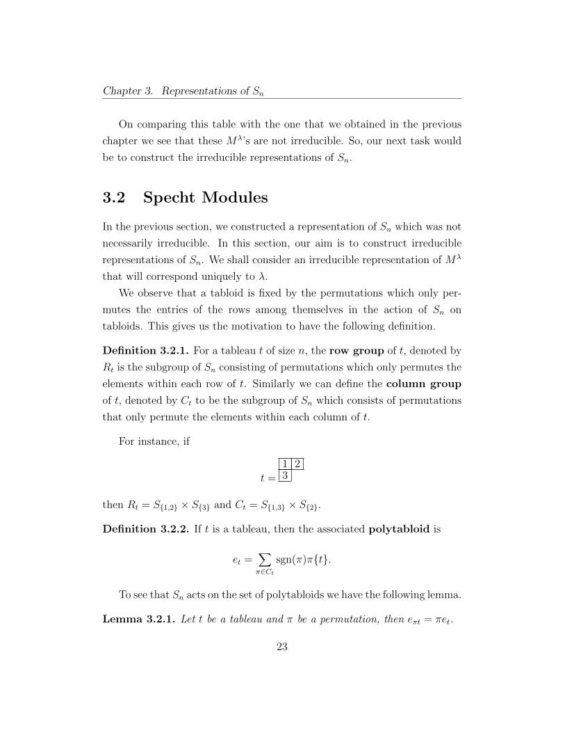
For instance, if

t =

1 23

then Rt = S{1,2} × S{3} and Ct = S{1,3} × S{2}.

Definition 3.2.2. If t is a tableau, then the associated polytabloid is

et =∑π∈Ct

sgn(π)π{t}.

To see that Sn acts on the set of polytabloids we have the following lemma.

Lemma 3.2.1. Let t be a tableau and π be a permutation, then eπt = πet.

23


Proof. We first observe that Cπt = πCtπ−1 and then we have

eπt =∑σ∈Cπt

sgn(σ)σ{πt} (3.1)

=∑

σ∈πCtπ−1

sgn(σ)σ{πt}

=∑σ′∈Ct

sgn(πσ′π−1)πσ′π−1{πt}

= π∑σ′∈Ct

sgn(σ′)σ′{t}

= eπt.

Definition 3.2.3. The Specht module corresponding to a partition λ de-

noted by Sλ is the submodule of Mλ spanned by the polytabloids et, where

t is taken over all tabloids of shape λ.

We look at some standard examples before discussing the properties of

these objects and note that Lemma 3.2.1 shows that Sλ is a representation

of Sn.

Example 3.2.4. Let λ = (n). As before Sλ is the one dimensional trivial

representation.

Example 3.2.5. Let λ = (1n) = (1, 1, . . . , 1) and t be given by the following

tabloid

12...n

24


By definition, et is the sum of all λ-tabloids multiplied by the sign of the

permutation. For any other tabloid t′, we have et = ±et′ , so we see that here

Sλ is the alternating representation.

Example 3.2.6. Taking λ = (n−1, 1), using the same notations as Example

3.1.9 we see that the polytabloids have the form {ti} − {tj}. Then, Sλ is

spanned by elements of the form Ei −Ej where Ei is the tabloid {ti}. Thus

we have

Sλ = {c1E1 + c2E2 + · · ·+ cnEn | c1 + c2 + · · ·+ cn = 0}.

This is the standard representation that we found in the previous chapter.

Also, S(n−1,1) ⊕ S(n) = M (n−1,1).

From the above examples, we see that Sλs have described all the irre-

ducible representations of S3. This is in general also true.

Theorem 3.2.2. The Specht modules Sλ forms a complete list of irreducible

representations of Sn, where λ ` n.

The proof of this result is in two parts which we sketch here. A detailed

proof can be found in [2] or [3]. First, we have to show that Sλ is an irre-

ducible sub-module of Mλ and then we show that Sλ 6= Sµ if λ 6= µ. Since

the number of conjugacy classes of Sn is equal to the number of partitions,

so we will have a complete list of the irreducible representations of Sn.

To prove that the Specht modules are irreducible, we have three main

things to do. First, we define an inner product onMλ, then we do a projection

operation like we defined the polytabloids above. Finally we use the following

lemma to complete the proof.

Lemma 3.2.3 (Submodule Lemma). Let V be a sub-module of Mλ, then

either Sλ ⊂ V or V ⊂ (Sλ)⊥.

To prove that the Specht modules are distinct we need the following

definition.

25


Definition 3.2.7. Let λ = (λ1, λ2, . . . , λl) and µ = (µ1, µ2, . . . , µr), then we

say that λ dominates µ, written as λ ≥ µ, if for each 1 ≤ i ≤ max(l, r) we

have

λ1 + λ2 + · · ·+ λi ≥ µ1 + µ2 + · · ·+ µi.

If l > r, we set µi = 0 for i > r and vice-versa.

For example,

≥

This is a partial ordering on the set of partitions of n via the Young diagrams.

Lemma 3.2.4 (Dominance Lemma). Let t and s be tableaux of shape λ

and µ respectively. If for each i, the elements of row i of s are all in different

columns of t, then λ ≥ µ.

Proof. We sort the entries in each column of t so that the elements in the

first i rows of s occurs in the first i rows of t. This is possible because the

elements of row i of t are in different columns of s. And then we have the

result.

Theorem 3.2.5. Let θ ∈ Hom(Sλ,Mµ) be a non-zero map of representa-

tions. Then λ ≥ µ.

Corollary 3.2.6. If Sλ ' Sµ then µ = λ.

Proof. We have Sµ ↪→ Mµ and Sλ ↪→ Mλ. By the above theorem we have

λ ≥ µ and µ ≥ λ and hence the result.

Corollary 3.2.7. The only irreducible representations in Mµ are Sλ for

λ ≥ µ.

26


3.3 RSK Correspondence

In general, the polytabloids that we defined earlier are not independent.

In fact, any pair of polytabloids in S(1n) are linearly dependent. So, our

immediate task is to find a suitable basis for Sλ to have some knowledge

about its dimension and character. The first step in this direction is the

Richardson-Schensted-Knuth (RSK) correspondence. The results will

be briefly sketched here. We follow the exposition in [2], [3] and [5], where a

more rigorous treatment is available.

We denote by fλ the number of standard tableau of shape λ. A tableau

is called semi-standard if the entries are not necessarily distinct, but the

rows are weakly increasing and columns are strictly increasing. The basic

operation in the RSK algorithm is row insertion in a semi-standard tableau.

To row insert the number m into row j of the tableau t we proceed as follows:

If no number in row j exceeds m then we put m at the end of row j, else,

we find the smallest number not less than m and replace it with m, choosing

the leftmost if there are more than one such number. The number that we

replaced will be called the bumped out number and we row insert it into

row j + 1 and continue the process over. If at any point we are in an empty

row then we just create a new box in that row and insert our number. Such

a row inserted tableau is denoted by m← t.

Example 3.3.1. We shall row insert 2 into the semi-standard tableau

1 2 2 3 52 3 5 54 4 7

Here 2 bumps 3 out of the first row, 3 bumps the first 5 out of the second

row, 5 then bumps the 7 out of the third row, which then goes into the final

row to give us the following tableau.

27


1 2 2 2 52 3 3 54 4 57

A reverse algorithm also exists to recover our original tableau if we are

given the final tableau and the final box that was added to the tableau. We

note that if t is standard and m does not lie in t then m← t is also standard

and the same is true if t is semi-standard. The RSK algorithm is in fact a

bijection between the 2×n lexicographically ordered arrays with entries from

[1, 2, . . . , n], and pairs (s, t) of semi-standard tableau, where the entries of s

are the numbers in the bottom row of the array and the entries of t are the

numbers in the top row of the array. An array is ordered lexicographically if

for j ≤ l, whenever(ij

)occurs before

(kl

)then either i < k or i = k. Such an

array is actually a permutation. We now briefly sketch the RSK algorithm

for an array.

In the first step, we start with two empty tableaux, say s0 and t0. If the

first entry in our two line array is(ij

)then we row insert j into the first row

of s. This creates a new box in s. We then find the corresponding box in t

and put i in that box. This gives us two new tableaux, say s1 and t1.

Then, we repeat the first step for each pair in the array and end up with

two tableaux, sn = s and tn = t. Here s will be semi-standard because we

are just performing row insertions. If i′ is inserted in a box below k in t, then

l will bump an entry from a row above. So, k is smaller than some previous

entry in the array. As we are in lexicographic order, this happens if k > i

and hence, t is also semi-standard.

For example, if we have the following array

1 1 2 3 3 3

3 3 2 1 2 4

we get the following two semi-standard tableau at the end of our process.

28


1 2 42 33 and

1 1 32 33

This algorithm is also reversible: given a pair of semi-standard tableaux

(s, t) we can get the corresponding two-row array. However, we skip the

proof, which can be found in [2].

Theorem 3.3.1. The RSK correspondence is a bijection between lexicograph-

ically ordered (2 × n) arrays and pairs of semi-standard tableaux (s, t) with

shape λ for some partition of n. If we restrict the arrays to permutations,

then the RSK correspondence gives a bijection between elements of Sn and

pairs of standard tableaux with entries from [1, 2, . . . , n].

Corollary 3.3.2. We have

∑λ`n

(fλ)2 = n!.

Theorem 3.3.3. The standard polytabloids form a basis of Sλ.

We only sketch the proof here, which can be found in [2] or [3]. First,

we impose a partial ordering on the tabloids and then show that a greatest

element in this ordering cannot be cancelled by adding a linear combination

of other tabloids. Then using induction, the linear independence can be

proved.

Corollary 3.3.4. Let λ ` n, then dimSλ = fλ.

Proof. From Corollary 1.2.12 we have that if the irreducible representations

of a group G of order g are V1, . . . , Vr then

g =r∑i=1

dim(Vi)2.

We also know that each Specht module has dimension at least fλ since it

contains fλ linearly independent polytabloids. We have also seen in this

29


chapter that two Specht modules for different partitions are not isomorphic.

So,

n! ≥∑λ`n

(dimSλ)2 ≥∑λ`n

(fλ)2 = n!.

Thus, there is equality everywhere and we get our desired result.

We note that still we do not have an explicit formula for the dimension

of the Specht module. This is derived in the following sections.

3.4 Symmetric Functions

In this section, we study the symmetric functions briefly and relate the char-

acteristic zero representations of Sn to the theory of symmetric polynomials.

This section facilitates the next section where we derive a formula for the

character of Sλ.

The ring of symmetric polynomials is constructed in m variables as a ring

of fixed points in Z(x1, x2, . . . , xn) under the action of Sm. For any σ ∈ Sm,

it acts on the monomials in this ring by xa11 xa22 · · ·xamm σ = xa11σx

a22σ · · ·xammσ.

For convenience, if λ ` n we write xλ = xλ11 xλ22 · · ·xλmm for m ≥ k, where

k is the number of rows of λ. If t is a semi-standard λ-tableau we write

xt = xa11 xa22 · · · xann where ai’s are the number of times i occurs in t provided

n ≥ m. If µ is a partition of n with ai parts of size i, then we denote

z(µ) = 1a1a1!2a2a2! . . . n

anan!. An easy exercise in algebra is to show that the

number of conjugacy classes of Sn is given by z(µ)/n!.

Definition 3.4.1. A symmetric polynomial is a polynomial in n variables

such that the polynomial remains unchanged if we change the order of the

variables.

Definition 3.4.2. A symmetric function of degree n is a collection of

symmetric polynomials, f i(x1, x2, . . . , xi) for i ≥ k, for some fixed k. If

j > i ≥ k then f j(x1, . . . , xi, 0, . . . , 0) = f i(x1, . . . , xi). We denote the

collection of all symmetric functions of degree n by Λn.

30


When the context is clear, we will denote the symmetric functions by just

f and drop the superscripts and variables. We add and multiply symmetric

functions by adding and multiplying the associated symmetric polynomials.

Multiplication is a bilinear map Λp×Λq −→ Λp+q and with these conditions

we see that Λ = ⊕n≥0Λn, is the ring of all symmetric functions.

The next natural step is to look for a basis of Λ, but for that we shall

need some more definitions.

Definition 3.4.3. In the following we have λ ` n and q ∈ N.

(i) The monomial symmetric polynomial mλ(x1, x2, . . . , xm) is the

sum of all monomials arising from xλ = xλ11 xλ22 · · ·xλkk by the action

of Sm

mλ(x) =∑σ∈Sm

xλσ.

(ii) The complete symmetric polynomial hq(x1, . . . , xm) is the sum of

all monomials arising from products of x1, x2, . . . , xm such that the total

degree of each monomial is q. So,

hq(x) =∑µ`q

mµ(x).

(iii) The elementary symmetric polynomial eq(x1, x2, . . . , xm) is the

sum of all monomials arising from products of x1, . . . , xm of total degree

q where each xi is used at most once. So, if m < q, then eq vanishes.

(iv) The power sum symmetric polynomial pq(x1, . . . , xm) is the sum

of the qth powers of the variables. So,

pq(x1, . . . , xm) =m∑i=1

xqi .

31


(v) The Schur polynomial sλ is

sλ(x1, . . . , xm) =∑

xt,

where the sum is over all semi-standard λ-tableau t with entries in

[1, 2, . . . ,m]. If m < k, then sλ vanishes.

If f(x1, x2, . . . , xm) is a symmetric polynomial and the monomial xλ oc-

curs in f then mλ occurs in f and hence the mλs forms a basis for Λn. So,

dim Λn = p(n) (the number of partitions of n). For convenience, we denote

hλ = hλ1hλ2 . . . hλk , eλ = eλ1eλ2 . . . eλk and pλ = pλ1pλ2 . . . pλk

Example 3.4.4. (i) m(2,1)(x1, x2, x3) = x21x2+x1x22+x21x3+x21x

23+x22x3+

x2x23.

(ii) h(2,1)(x1, x2) = (x21 + x22 + x1x2)(x1 + x2).

(iii) e(2,1)(x1, x2) = x1x2(x1 + x2).

Theorem 3.4.1. The Schur polynomial, sλ is symmetric.

Since Sm is generated by transpositions, so it is sufficient for us to prove that

sλ(x1, x2, . . . , xm)(i i+ 1) = sλ(x1, x2, . . . , xm) for each 1 ≤ i ≤ m− 1.

From [2] we know that the generating functions for en(x) and hn(x) are

as follows:

∑n≥0

hn(x)tn =m∏i=1

1

1− xit

andm∑n=0

(−1)nen(x)tn =m∏i=1

(1− xit).

Multiplying these together and finding the coefficients of tn will give us

n∑i=1

(−1)n−ihi(x)en−i(x) = 0

32


which shows that 〈hi(x)〉 = 〈ei(x)〉 and hence (hλ : λ ` n) is also a basis for

Λn.

Following some more algebraic manipulations and comparing coefficients

we get the following identity

hn(x) =∑µ`n

1

z(µ)pµ(x).

So, Λn = 〈pµ : µ ` n〉Q. Finally, we have that the Schur polynomials also

give a basis for Λn, the proof of which depends on the following result which

we shall not prove here.

Theorem 3.4.2 (Pieri’s Rule). Let λ ` n and q ∈ N, then we have

sλ(x).hq(x) =∑µ

sµ(x),

where the sum is taken over all µ ` n+ q which we obtain by adding q boxes

into λ, no two in the same column.

We now prove that the Schur functions form a basis for Λn. We have

hq(x) = s(q)(x). Expanding hλ(x) as a sum of Schur polynomials by consid-

ering the hλ1 as s(λ1) and then using Pieri’s Rule to multiply it with hλ2 and

repeating the process until we can write it in the form

hµ(x) =∑λ

Kλµsλ(x).

Here the coefficients are called Kostka numbers, which is the number of

semi-standard λ-tabloids t with µi i’s. We then say that λ is of the type µ.

If Kλµ 6= 0 then λ dominates µ. We now introduce an inner product on Λ

defined by an orthonormal basis formed by the Schur functions sλ.

Theorem 3.4.3. Let λ, µ ` n. Then we have the following:

(i) 〈sλ, sµ〉 = δλµ,

33


(ii) 〈mλ,mµ〉 = δλµ,

(iii) 〈pλ, pµ〉 =δλµz(λ)

.

Definition 3.4.5. Let λ, µ ` n, we define the coefficients ξλµ and χλµ by

pµ =∑λ`n

ξλµmλ

and

pµ =∑λ`n

χλµslb.

Using Theorem 3.4.3 we can also derive the following equivalent identities

hλ =∑µ`n

ξλµz(µ)

pµ

and

sλ =∑µ`n

χλµz(µ)

pµ.

3.5 Frobenius Character Formula

The aim of this section is to enunciate the character of the Specht modules

and to state an important result in combinatorics, called the hook length

formula. We also go through the induced and restricted representations of

Sn.

Theorem 3.5.1 (Frobenius Character Formula). Let λ ` n with k rows and

also let li = λi + k− i. Then the character of Sλ on the conjugacy class of a

partition µ, denoted by χλµ is the coefficient of xl11 xl22 . . . x

lkk in the polynomial

∏1≤i<j≤k

(xi − xj).pµ(x1, x2, . . . , xk).

34


This theorem is a consequence of the following theorem, which we state

without proof.

Theorem 3.5.2 (Jacobi-Trudi Formula). Let λ ` n with k rows. We define

∆λ(x) to be the determinant of the k×k matrix A, where Aij = xλj+k−ji . We

also let ∆0(x) to be the Vandermonde determinant det(xj−1i ) =∏i<j(xi−xj).

Then we have

sλ(x1, . . . , xk) =∆λ(x)

∆0(x).

A proof of this result can be found in [5].

We now find the dimension of Sλ by evaluating its character on the iden-

tity. Thus, by Theorem 3.5.1, it is the coefficient of xl in

∏1≤i<j≤n

(xi − xj)(x1 + · · ·+ xk)n.

After expanding the Vandermonde deteminant and using the multinomial

theorem in the other expansion along with some algebraic manipulations, we

get

dimSλ =n!∏k

i=1 li!∏

1≤i<j≤k(li − lj).

We now introduce the concept of a hook in a partition λ. The hook on

a given node is the number of boxes to the right as well as below that node

plus counting the node we are in, once. The hook-length of a hook is the

number of boxes that the hook involves. For example in the Young diagram

below, we mark each box with its hook-length.

6 4 2 13 11

The li’s that we defined earlier are just the hook-length of the nodes in the

first column of λ. If α is a node on λ, then we denote its hook-length by hα.

d

35


Proof. We have to show

n!∏ki=1 li!

∏1≤i<j≤k(li − lj)

=n!∏α hα

.

We shall use induction on the columns of λ. If λ has only one column,

then λ = (1n) and we have

dimSλ =n!

n!(n− 1)! · · · 1!

n−1∏i=1

(n− i)! = 1

which is the same as the hook-length formula.

Let λ′ be the partition of n− k that is obtained after removing the first

column of λ. Let k′ be the number of rows of λ′, and let l′i be the hook length

of the ith node in the first column of λ′. Then, we have l′i − l′i+1 = li − li+1

and l′i = li − (k − k′)− 1. Now, using the induction hypothesis we have,

dimSλ =n!∏ki=1 l

∏(li − lj)∏k

i=1(li − 1)!(3.2)

=n!∏

α∈λ hα

∏ki=1 l

′i!∏k

i=1(li − 1)!

∏1≤i<j≤k,j>k

(li − lj).

It remains to show that the last terms in the product cancel out to get

the desired result. We have, if i > k′, li = k − i+ 1, then

∏1≤i<j≤k,j>k′

(li − lj) =k∏i=1

∏j>max(i,k′)

(li − lj) (3.3)

=k−1∏i=1

∏j>max(i,k′)

(li − 1)!

(li − 1 + k + max(i, k′))!

=k′∏i=1

(li − 1)!

l′i!

k∏i=k′+1

(li − 1)!

The hook length formula follows from this.

36


We now come to the final topic of our thesis: the induced and restricted

representations of Sn to Sn+1 and Sn−1 respectively. We will only mention

the results here, without proofs. More details can be found in [2] or [3].

Much like partitions, Young diagrams can also be partially ordered by

inclusion. The resulting partially ordered set is called a Young’s lattice.

Let λ ↗ µ denote that µ can be obtained from λ by adding a box to λ to

get a new partition. Continuing this way from the empty Young digram we

can move upwards adding one box at a time, and get all the partitions of n

at the nth level of this lattice.

Theorem 3.5.3 (Branching Rule). Let λ ` n, then we have

ResSnSn−1Sλ ∼= ⊕µ:µ↗λSµ

and

IndSn+1

Sn Sλ ∼= ⊕µ:λ↗µSµ.

The proof of this result uses the Frobenius Reciprocity Theorem, that

we derived in the first chapter. Before proceeding further, we look at an

example. Let us look at the trivial representation of the trivial group, which

corresponds to the partition (1) of S1. Inducing to S2 we have

IndS2S1S(1) = S(1,1) ⊕ S(2).

Again inducing it to S3 and then finally to S4 we shall get

IndS4S1S(1) = S(4) ⊕ (S(3,1))3 ⊕ (S(2,1,1))3 ⊕ (S(2,2))2 ⊕ S(1,1,1,1).

So far, we have constructed Mλ and from it we found irreducible repre-

sentations Sλ which forms a complete list of such representations for Sn as

λ varies over all partitions of n. But we have not yet discussed about the

decomposition of these Mλ. We have the following results in this direction.

37


Theorem 3.5.4. Mµ contains Sλ as a subrepresentation if and only if λ ≥ µ.

Also, Mµ contains only one copy of Sµ.

Now, we are interested in finding the number of copies of Sλ in Mµ, and

for this we must make use of the Kostka numbers. One basic property of

these numbers is that Kλλ = 1. This is clear because there can be only one

semi-standard tableau of the partition λ of type λ. We now have the final

result on decomposition of the Mµ’s.

Theorem 3.5.5 (Young’s Rule).

Mµ ∼= ⊕λ≥µKλµSλ.

We close this chapter with the following examples.

Example 3.5.1. We have K(n)µ = 1 as there is only one possible (n)-

semistandard tableau of type µ. Young’s rule then says that every Mµ

contains exactly one copy of the trivial representation S(n), which we have

already seen in a previous example.

Example 3.5.2. We note that Kλ(1n) = fλ, so by Young’s Rule we have

M (1n) ∼= ⊕λfλSλ.

By taking the magnitude of the characters in the above, we get another proof

of the fact that n! =∑λ`n(fλ)2.

38

Bibliography

[1] William Fulton. Young Tableaux. LMSST 35, Cambridge University

Press, 1997.

[2] William Fulton and Joe Harris. Representation Theory: A First Course.

GTM 129, Springer, 1991.

[3] Bruce E Sagan. The Symmetric Group: Representations, Combinatorial

Algorithms, and Symmetric Functions (2nd ed.). GTM 203, Springer,

2001.

[4] Jean-Pierre Serre. Linear Representations of Finite Groups. GTM 42,

Springer, 1977.

[5] Richard P. Stanley. Ennumerative Combinatorics II. Cambridge Studies

in Advanced Mathematics 62, 1999.

[6] Fernando R. Villegas. Representations of Finite Groups. lecture notes,

2011.

[7] Mark Wildon. A Combinatorial Introduction to the Representation The-

ory of Sn. lecture notes, 2001.

[8] Yufei Zhao. Young tableaux and the representations of the symmetric

group. The Harvard College Mathematics Review, 2(2):33–45, 2008.

39

representations of the symmetric group -...

Documents