representations modelling, analysis and control of linear ...o.sename/docs/sem.pdf · properties...

State spacerepresentations

(SEM)

O.Sename

Introduction

Modelling ofdynamicalsystems

Properties

Discrete-timesystems

State feedbackcontrol

Observer

Integral Control

A polynomialapproach

Further indiscrete-timecontrol

Conclusion

Modelling, analysis and control of linearsystems using state space

representations

O. Sename1

1Gipsalab, CNRS-INPG, [email protected]

www.lag.ensieg.inpg.fr/sename

Approche Etat pour la commande / IEG- SEM


(SEM)

O.Sename

Introduction


Properties



Observer

Integral Control



Conclusion

Outline

Introduction

Modelling of dynamical systems

Properties

Discrete-time systems

State feedback control

Observer

Integral Control

A polynomial approach

Further in discrete-time control

Conclusion


(SEM)

O.Sename

Introduction


Properties



Observer

Integral Control



Conclusion

References

Some interesting books:◮ K.J. Astrom and B. Wittenmark, Computer-Controlled

Systems, Information and systems sciences series.Prentice Hall, New Jersey, 3rd edition, 1997.

◮ R.C. Dorf and R.H. Bishop, Modern Control Systems,Prentice Hall, USA, 2005.

◮ G.C. Goodwin, S.F. Graebe, and M.E. Salgado,Control System Design, Prentice Hall, New Jersey,2001.

◮

◮


(SEM)

O.Sename

Introduction


Properties



Observer

Integral Control



Conclusion

Objective of any control system:

Nominal stability (NS): The system is stable with thenominal model (no model uncertainty)

Nominal Performance (NP): The system satisfies theperformance specifications with the nominalmodel (no model uncertainty)

Robust stability (RS): The system is stable for allperturbed plants about the nominal model, upto the worst-case model uncertainty(including the real plant)

Robust performance (RP): The system satisfies theperformance specifications for all perturbedplants about the nominal model, up to theworst-case model uncertainty (including thereal plant).


(SEM)

O.Sename

Introduction


Properties



Observer

Integral Control



Conclusion

Recall of the "control design" process:◮ Plant study and modelling◮ Determination of sensors and actuators (measured

and controlled outputs, control inputs)◮ Performance specifications◮ Control design (many methods)◮ Simulation tests◮ Implementation, tests and validation


(SEM)

O.Sename

Introduction


Properties



Observer

Integral Control



Conclusion

Different issues for modelling:Identification based method

◮ System excitations using PRBS (Pseudo RandomBinary Signal) or sinusoïdal signals

◮ Determination of a transfer function reproducing theinput/ouput system behavior

Knowledge-based method:◮ Represent the system behavior using differential

and/or algebraic equations, based on physicalknowledge.

◮ Formulate a nonlinear state-space model, i.e. a matrixdifferential equation of order 1.

◮ Determine the steady-state operating point aboutwhich to linearize.

◮ Introduce deviation variables and linearize the model.


(SEM)

O.Sename

Introduction


Properties



Observer

Integral Control



Conclusion

Why state space equations ?◮ dynamical systems where physical equations can be

derived : electrical engineering, mechanicalengineering, aerospace engineering, microsystems,process plants ....

◮ include physical parameters: easy to use whenparameters are changed for design

◮ State variables have physical meaning.◮ Easy to extend to Multi-Input Multi-Output (MIMO)

systems◮ Advanced control design method are based on state

space equations (reliable numerical optimisation tools)


(SEM)

O.Sename

Introduction


Properties



Observer

Integral Control



Conclusion

Some physical examples


(SEM)

O.Sename

Introduction


Properties



Observer

Integral Control



Conclusion

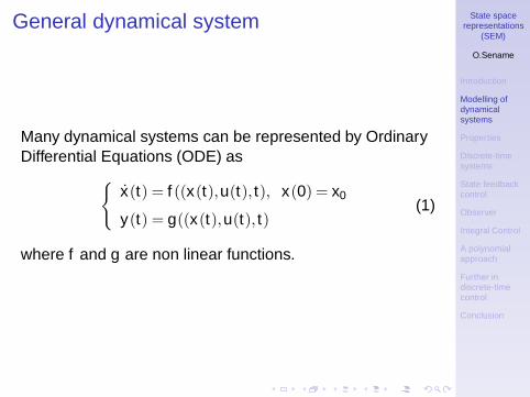
General dynamical system

Many dynamical systems can be represented by OrdinaryDifferential Equations (ODE) as

{

x(t) = f ((x(t),u(t), t), x(0) = x0

y(t) = g((x(t),u(t), t)(1)

where f and g are non linear functions.


(SEM)

O.Sename

Introduction


Properties



Observer

Integral Control



Conclusion

Example: Inverted pendulumIt is described by:

Parameters:


(SEM)

O.Sename

Introduction


Properties



Observer

Integral Control



Conclusion

Example: Inverted pendulum

The dynamical equations are as follows:


(SEM)

O.Sename

Introduction


Properties



Observer

Integral Control



Conclusion

Example: Lateral vehicle model

The dynamical equations are as follows:


(SEM)

O.Sename

Introduction


Properties



Observer

Integral Control



Conclusion

Definition of state space representations

A continuous-time LINEAR state space system is givenas : {

x(t) = A(x(t)+Bu(t), x(0) = x0

y(t) = Cx(t)+Du(t)(2)

where x(t) ∈ Rn is the system state (vector of state

variables), u(t) ∈ Rm the control input and y(t) ∈ R

p themeasured output. A, B, C and D are real matrices ofappropriate dimensions. x0 is the initial condition.n is the order of the state space representation.Matlab : ss(A,B,C,D) creates a SS objectSYS representing a continuous-timestate-space model


(SEM)

O.Sename

Introduction


Properties



Observer

Integral Control



Conclusion

A first example: DC Motor

The dynamical equations are :

Ri +Ldidt

+e = u e = Keω

Jdωdt

= −f ω + Γm Γm = Kc i

System of 2 equations of order 1 =⇒ 2 state variables. A

possible choice x =

(ωi

)

It gives:

A =

(−f/J Kc/J−Ke/L −R/L

)

B =

(0

1/L

)

C =(

0 1)

Extension: measurment= motor angular position


(SEM)

O.Sename

Introduction


Properties



Observer

Integral Control



Conclusion

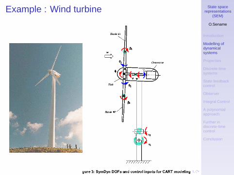
Example : Wind turbine


(SEM)

O.Sename

Introduction


Properties



Observer

Integral Control



Conclusion

A linearisation within 2 regions gives{

x(t) = Ax(t)+Bu(t)+Ed(t)y(t) = Cx(t)

with

A =

γ−CdIrot

−1Irot

CdIrot

Kd 0 −KdCdIgen

−1Igen

CdIgen

, B =

00−1Igen

,E =

αIrot

00

,

and C =(

0 0 1)

x1 = rotor-speed x2 = drive-train torsion spring force, x3=rotational generator speedu = generator torque, d : wind speedIrot : rotor rotational inertia, Igen : generator rotational inertia, Kd :spring constant, Cd : torsional damping constant, α partialderivative of rotor aerodynamic torque with respect blade pitchangle, γ: partial derivative of rotor aerodynamic torque withrespect to rotor speed


(SEM)

O.Sename

Introduction


Properties



Observer

Integral Control



Conclusion

Examples: SuspensionLet the following mass-spring-damper system.

where x1 is the relative position, M1 the system mass, k1

the spring coefficient, u the force generated by the activedamper, and F1 is an external disturbance. Applying themechanical equations it leads:

M1x1 = −k1x1 +u +F1 (3)


(SEM)

O.Sename

Introduction


Properties



Observer

Integral Control



Conclusion

Examples: Suspension cont.

The choice x =

(x1

x1

)

gives

{x(t) = Ax(t)+Bu(t)+Ed(t)y(t) = Cx(t)

where d = F1 , y = x1 with

A =

(0 1

−k1/M1 0

)

, B = E =

(0

1/M1

)

,and C =(

0 1)


(SEM)

O.Sename

Introduction


Properties



Observer

Integral Control



Conclusion

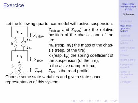
Exercice

Let the following quarter car model with active suspension.

Zcaisse and Zroue) are the relativeposition of the chassis and of thetire,mc (resp. mr ) the mass of the chas-sis (resp. of the tire),k (resp. kp) the spring coefficient ofthe suspension (of the tire),u the active damper force,Zsol is the road profile.

Choose some state variables and give a state spacerepresentation of this system


(SEM)

O.Sename

Introduction


Properties



Observer

Integral Control



Conclusion

Linearisation


(SEM)

O.Sename

Introduction


Properties



Observer

Integral Control



Conclusion

Equilibrium point

An equilibrium point satisfies:

0 = f ((xeq(t),ueq(t), t) (4)

For the pendulum, we can choose y = θ = f = 0.


(SEM)

O.Sename

Introduction


Properties



Observer

Integral Control



Conclusion

Linearisation Method (1)

The linearisation can be done around an equilibrium pointor around a particular point.


(SEM)

O.Sename

Introduction


Properties



Observer

Integral Control



Conclusion

Linearisation Method (2)

This leads to a linear state space representation of thesystem, around the equilibrium point.Defining x = x −xeq, u = u−ueq and y = y −yeq we get

{˙x(t) = Ax(t)+Bu(t),

y(t) = Cx(t)+Du(t)(5)

with A = ∂ f∂x |x=xeq ,u=ueq , B = ∂ f

∂u |x=xeq ,u=ueq ,

C = ∂g∂x |x=xeq ,u=ueq and D = ∂g

∂u |x=xeq ,u=ueq


(SEM)

O.Sename

Introduction


Properties



Observer

Integral Control



Conclusion

Example: Inverted pendulum (2)

Applying the linearisation method leads to :


(SEM)

O.Sename

Introduction


Properties



Observer

Integral Control



Conclusion

Linear systems :transfer function


(SEM)

O.Sename

Introduction


Properties



Observer

Integral Control



Conclusion

Equivalence transfer function - state spacerepresentation

Consider a linear system given by:{

x(t) = Ax(t)+Bu(t), x(0) = x0

y(t) = Cx(t)+Du(t)(6)

Using the Laplace transform (and assuming zero initialcondition x0 = 0), (6) becomes:

s.x(s) = Ax(s)+Bu(s) ⇒ (s.In −A)x(s) = Bu(s)

Then the transfer function matrix of system (6) is given by

G(s) = C(sIn −A)−1B +D =N(s)

D(s)(7)

Matlab: if SYS is an SS object, then tf(SYS) gives theassociated transfer matrix. Equivalent to tf(N,D)


(SEM)

O.Sename

Introduction


Properties



Observer

Integral Control



Conclusion

Conversion TF to SS

There mainly three cases to be considered

Simple numerator

yu

= G(s) =1

s3 +as12+a2s +a3

Numerator order less than denominator order

yu

= G(s) =b1s2 +b2s +b3

s3 +as12+a2s +a3

=N(s)

D(s)

Numerator equal to denominator order

yu

= G(s) =b0s3 +b1s2 +b2s +b3

s3 +as12+a2s +a3

=N(s)

D(s)


(SEM)

O.Sename

Introduction


Properties



Observer

Integral Control



Conclusion

Canonical forms


(SEM)

O.Sename

Introduction


Properties



Observer

Integral Control



Conclusion

Canonical forms

Some specific state space representations are well-knownand often used as the so-called controllable canonical form

A =

0 1 0 . . . 00 0 1 0 . . ....

......

. . ....

0... 0 1

−a0 −a1 . . . . . . −an−1

, B =

0......01

and

C =[

c0 c1 . . . cn−1].

It corresponds to the transfer function:

G(s) =c0 +c1s + . . .+cn−1sn−1

a0 +a1s + . . .+an−1sn−1 +sn

In Matlab, use canon


(SEM)

O.Sename

Introduction


Properties



Observer

Integral Control



Conclusion

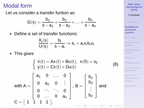
Modal formLet us consider a transfer funtion as:

G(s) =b1

s−a1+

b2

s−a2+ . . .+

bn

s−an

◮ Define a set of transfer functions:

Xi(s)

U(s)=

bi

s−ai⇒ xi = aixibiui

◮ This gives{

x(t) = Ax(t)+Bu(t), x(0) = x0

y(t) = Cx(t)+Du(t)(8)

with A =

a1 0 . . . 0

0 a2 0...

0. . . . . . 0

0 . . . 0 an

, B =

b1

b2...

bn

and

C =[

1 1 1 1].


(SEM)

O.Sename

Introduction


Properties



Observer

Integral Control



Conclusion

Solution of state spacelinear systems


(SEM)

O.Sename

Introduction


Properties



Observer

Integral Control



Conclusion

Solution of state space equations - continuouscase

The state x(t), solution of x(t) = Ax(t), with initialcondition x(0) = x0 is given by

x(t) = eAtx(0) (9)

This requires to compute eAt . There exist 3 methods tocompute eAt :

1. Inverse Laplace transform of (sIn −A)−1 :

2. Diagonalisation of A

3. Cayley-Hamilton method


(SEM)

O.Sename

Introduction


Properties



Observer

Integral Control



Conclusion

Complete state solution

The state x(t), solution of system (6), is given by

x(t) = eAtx(0)︸︷︷︸

free response

+

∫ t

0eA(t−τ)Bu(τ)dτ

︸︷︷︸

forced response

(10)

In Matlab : use expm and not exp.

Simulation of state space systemsUse lsim.Example:t = 0:0.01:5; u = sin(t); lsim(sys,u,t)


(SEM)

O.Sename

Introduction


Properties



Observer

Integral Control



Conclusion

Non unicity


(SEM)

O.Sename

Introduction


Properties



Observer

Integral Control



Conclusion

Non unicityGiven a transfer function, there exists an infinity of statespace representations (equivalent in terms of input-outputbehavior). Let

{x(t) = Ax(t)+Bu(t),y(t) = Cx(t)+Du(t)

(11)

the transfer matrix being G(s) = C(sIn −A)−1B +D, andconsider the change of variables x = Tz (T being aninvertible matrix). Replacing x = Tz in the previous systemgives:

T z(t) = ATz(t)+Bu(t) (12)

y(t) = CTz(t)+Du(t) (13)

Hence

z(t) = T−1ATz(t)+T−1Bu(t) (14)

y(t) = CTz(t)+Du(t) (15)


(SEM)

O.Sename

Introduction


Properties



Observer

Integral Control



Conclusion

Defining A = T−1AT , B = T−1B and C = CT , the transferfunction of the previous system is:

G(s) = C(sIn − A)−1B +D (16)

= C T (sIn −T−1AT )−1 T−1 B +D (17)

(18)

Using In = T−1T , we get

G(s) = C T T−1 (sIn −A)−1 T T−1 B +D = G(s) (19)


(SEM)

O.Sename

Introduction


Properties



Observer

Integral Control



Conclusion

Stability


(SEM)

O.Sename

Introduction


Properties



Observer

Integral Control



Conclusion

Stability

DefinitionAn equilibrium point xeq is stable if, for all ρ > 0, thereexists a η > 0 such that:

‖x(0)−xeq‖ < η =⇒‖x(t)−xeq‖ < ρ ,∀t ≥ 0

DefinitionAn equilibrium point xeq is asymptotically stable if it isstable and, there exists η > 0 such that:

‖x(0)−xeq‖ < η =⇒ x(t) → xeq , when t → ∞

These notions are equivalent for linear systems (not fornon linear ones).


(SEM)

O.Sename

Introduction


Properties



Observer

Integral Control



Conclusion

Stability Analysis

The stability of a linear state space system is analyzedthrough the characteristic equation det(sIn −A) = 0.The system poles are then the eigenvalues of the matrix A.It then follows:

PropositionA system x(t) = Ax(t), with initial condition x(0) = x0, isstable if Re(λi) < 0, ∀i , where λi , ∀i , are the eigenvalues ofA.

Using Matlab, if SYS is an SS object then pole(SYS)computes the poles P of the LTI model SYS. It isequivalent to compute eig(A).


(SEM)

O.Sename

Introduction


Properties



Observer

Integral Control



Conclusion

Stability Analysis - LyapunovThe stability of a linear state space system can beanalysed through the Lyapunov theory.It is the basis of all extension of stability for non linearsystems, time-delay systems, time-varying systems ...

TheoremA system x(t) = Ax(t), with initial condition x(0) = x0, isasymoptotically stable at x = 0 if and only if there existsome matrices P = PT > 0 and Q > 0 such that:

AT P +PA = −Q (20)

see lyap in MATLAB.Proof: The Lyapunov theory says that a linear system isstable if there exists a continuous function V (x) s.t.:

V (x) > 0 with V (0) = 0 and V (x) =dVdx

≥ 0

A possible Lyapunov function for the above system is :


(SEM)

O.Sename

Introduction


Properties



Observer

Integral Control



Conclusion

About zeros

◮ Roots of the transfer function numerator are called thesystem zeros.

◮ Need to develop a similar way of defining/computingthem using a state space model.

◮ Zero: is a generalized frequency α for which thesystem can have a non-zero input u(t) = u0eα t , butexactly zero output y(t) = 0.

◮ The zeros are found by solving:[

A−λ In BC D

]

= 0 (21)

In Matlab use zero

Example: find the zero of : s+3s2+5s+2


(SEM)

O.Sename

Introduction


Properties



Observer

Integral Control



Conclusion

Controllability


(SEM)

O.Sename

Introduction


Properties



Observer

Integral Control



Conclusion

Controllability

Controllability refers to the ability of controlling astate-space model using state feedback.

DefinitionGiven two states x0 and x1, the system (6) is controllable ifthere exist t1 > 0 and a piecewise-continuous control inputu(t), t ∈ [0, t1], such that x(t) takes the values x0 for t = 0and x1 for t = t1.


(SEM)

O.Sename

Introduction


Properties



Observer

Integral Control



Conclusion

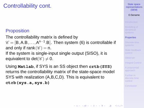
Controllability cont.

PropositionThe controllability matrix is defined byC = [B,A.B, . . . ,An−1.B]. Then system (6) is controllable ifand only if rank(C ) = n.If the system is single-input single output (SISO), it isequivalent to det(C ) 6= 0.

Using Matlab, if SYS is an SS object then crtb(SYS)returns the controllability matrix of the state-space modelSYS with realization (A,B,C,D). This is equivalent toctrb(sys.a,sys.b)


(SEM)

O.Sename

Introduction


Properties



Observer

Integral Control



Conclusion

Exercices

Test the controllability of the previous examples: DC motor,suspension, inverted pendulum.


(SEM)

O.Sename

Introduction


Properties



Observer

Integral Control



Conclusion

Observability


(SEM)

O.Sename

Introduction


Properties



Observer

Integral Control



Conclusion

Observability

Observability refers to the ability to estimate a statevariable.

DefinitionA linear system (2) is completely observable if, given thecontrol and the output over the interval t0 ≤ t ≤ T , one candetermine any initial state x(t0).It is equivalent to characterize the non-observability as :A state x(t) is not observable if the corresponding outputvanishes, i.e. if the following holds:y(t) = y(t) = y(t) = . . . = 0


(SEM)

O.Sename

Introduction


Properties



Observer

Integral Control



Conclusion

Where does observability come from ?

Compare the transfer function of the two different systems*

x = −x +u

y = 2x

and

x =

[−1 00 −2

]

x +

[11

]

u

y =[

2 0]x


(SEM)

O.Sename

Introduction


Properties



Observer

Integral Control



Conclusion

Observability cont.

Proposition

The observability matrix is defined by O =

CCA...

CAn−1

.

Then system (6) is observable if and only if rank(O) = n.If the system is single-input single output (SISO), it isequivalent to det(O) 6= 0.

Using Matlab, if SYS is an SS object then obsv(SYS)returns the observability matrix of the state-space modelSYS with realization (A,B,C,D). This is equivalent toOBSV(sys.a,sys.c).


(SEM)

O.Sename

Introduction


Properties



Observer

Integral Control



Conclusion

Exercices

Test the observability of the previous examples: DC motor,suspension, inverted pendulum.Analysis of different cases, according to the considerednumber of sensors.


(SEM)

O.Sename

Introduction


Properties



Observer

Integral Control



Conclusion

Minimality


(SEM)

O.Sename

Introduction


Properties



Observer

Integral Control



Conclusion

Minimality

DefinitionA state space representation of a linear system (2) of ordern is said to be minimal if it is controllable and observable.

In this case, the corresponding transfer function G(s) is ofminimal order n, i.e is irreducible (no cancellation of polesand zeros).When the transfer function is not of minimal order, thereexists non controllable or non observable modes.


(SEM)

O.Sename

Introduction


Properties



Observer

Integral Control



Conclusion

Kalman decomposition


(SEM)

O.Sename

Introduction


Properties



Observer

Integral Control



Conclusion

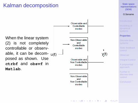
Kalman decomposition

When the linear system(2) is not completelycontrollable or observ-able, it can be decom-posed as shown. Usectrbf and obsvf inMatlab.


(SEM)

O.Sename

Introduction


Properties



Observer

Integral Control



Conclusion

Toward digital control

Digital controlUsually controllers are implemented in a digital computeras:

This requires the use of the discrete theory.m (Sampling theory + Z-Transform) m


(SEM)

O.Sename

Introduction


Properties



Observer

Integral Control



Conclusion

Z-Transform


(SEM)

O.Sename

Introduction


Properties



Observer

Integral Control



Conclusion

Definitions

Mathematical definitionBecause the output of the ideal sampler, x∗(t), is a seriesof impulses with values x(kTe), we have:

x∗(t) =∞

∑k=0

x(kTe)δ (t −kTe)

by using the Laplace transform,

L [x∗(t)] =∞

∑k=0

x(kTe)e−ksTe

Noting z = esTe , we can derive the so called Z-Transform

X (z) = Z [x(k)] =∞

∑k=0

x(k)z−k


(SEM)

O.Sename

Introduction


Properties



Observer

Integral Control



Conclusion

Properties

Definition

X (z) = Z [x(k)] =∞

∑k=0

x(k)z−k

Properties

Z [αx(k)+ βy(k)] = αX (z)+ βY (z)

Z [x(k −n)] = z−nZ [x(k)]

Z [kx(k)] = −zddz

Z [x(k)]

Z [x(k)∗y(k)] = X (z).Y (z)

limk→∞

x(k) = lim1→z−1

(z −1)X (z)

The z−1 can be interpreted as a pure delay operator.


(SEM)

O.Sename

Introduction


Properties



Observer

Integral Control



Conclusion

ExerciseDetermine the Z-Transform of the step function (1) and ofthe ramp function (2)

xstep(k) = 1 if k ≥ 0 xramp(k) = k if k ≥ 0= 0 if k < 0 = 0 if k < 0


(SEM)

O.Sename

Introduction


Properties



Observer

Integral Control



Conclusion

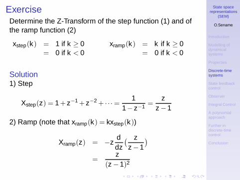
ExerciseDetermine the Z-Transform of the step function (1) and ofthe ramp function (2)

xstep(k) = 1 if k ≥ 0 xramp(k) = k if k ≥ 0= 0 if k < 0 = 0 if k < 0

Solution1) Step

Xstep(z) = 1+z−1 +z−2 + · · · =1

1−z−1 =z

z −1

2) Ramp (note that xramp(k) = kxstep(k))

Xramp(z) = −zddz

( zz −1

)

=z

(z −1)2


(SEM)

O.Sename

Introduction


Properties



Observer

Integral Control



Conclusion

Zero order holder

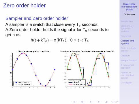
Sampler and Zero order holderA sampler is a switch that close every Te seconds.A Zero order holder holds the signal x for Te seconds toget h as:

h(t +kTe) = x(kTe), 0 ≤ t < Te


(SEM)

O.Sename

Introduction


Properties



Observer

Integral Control



Conclusion

Zero order holder (cont’d)

Model of the Zero order holderThe transfer function of the zero-order holder is given by:

GBOZ (s) =1s−

e−sTe

s

=1−e−sTe

s

Influence of the D/A and A/DNote that the precision is also limited by the availableprecision of the converters (either A/D or D/A).This error is also called the amplitude quantization error.


(SEM)

O.Sename

Introduction


Properties



Observer

Integral Control



Conclusion

Representation of the discrete linear systemsThe discrete output of a system can be expressed as:

y(k) =∞

∑n=0

h(k −n)u(n)

hence, applying the Z-transform leads to

Y (z) = Z [h(k)]U(z) = H(z)U(z)

H(z) =b0 +b1z + · · ·+bmzm

a0 +a1z + · · ·+anzn =YU

where n (≥ m) is the order of the systemCorresponding difference equation:

y(k) =1an

[b0u(k −n)+b1u(k −n +1)+ · · ·+bmu(k −n +m)

− a0y(k −n)−a2y(k −n +1)−·· ·−an−1y(k −1)]


(SEM)

O.Sename

Introduction


Properties



Observer

Integral Control



Conclusion

Some useful transformations

x(t) X(s) X(z)δ (t) 1 1

δ (t −kTe) e−ksTe z−k

u(t) 1s

zz−1

t 1s2

zTe(z−1)2

e−at 1s+a

zz−e−aTe

1−e−at 1s(s+a)

z(1−e−aTe )

(z−1)(z−e−aTe )

sin(ω t) ωs2+ω2

zsin(ωTe)

z2−2zcos(ωTe)+1

cos(ω t) ss2+ω2

z(z−cos(ωTe))

z2−2zcos(ωTe)+1

ExerciseDiscretize (sampling time Te) the system described by theLaplace function (using a Zero order holder):

H(s) =Y (s)

U(s)=

1s(s +1)


(SEM)

O.Sename

Introduction


Properties



Observer

Integral Control



Conclusion

ExerciseDiscretize the system described by the Laplace function(using a Zero order holder):

H(s) =Y (s)

U(s)=

1s(s +1)

Adding the Zero order holder leads to:

GBOZ (s)H(s) =1−e−sTe

s1

s(s +1)

=1−e−sTe

s2(s +1)

= (1−e−sTe)( 1

s2 −1s

+1

s +1

)

hence

Z [GBOZ (s)H(s)] = (1−z−1)Z[ 1s2 −

1s

+1

s +1

]


(SEM)

O.Sename

Introduction


Properties



Observer

Integral Control



Conclusion

Exercise (cont’d)

Z [GBOZ (s)H(s)] = (1−z−1)Z[ 1s2 −

1s

+1

s +1

]

= (1−z−1)[ zTe

(z −1)2 −z

z −1+

zz −e−Te

]

=(ze−Te −z +zTe)+ (1−e−Te −Tee−Te)

(z −1)(z −e−Te)

if Te = 1, we have

Z [GBOZ (s)H(s)] =(ze−Te −z +zTe)+ (1−e−Te −Tee−Te)

(z −1)(z −e−Te)

=ze−1 +1−2e−1

(z −1)(z −e−1)

=b1z +b0

z2 +a1z +a0


(SEM)

O.Sename

Introduction


Properties



Observer

Integral Control



Conclusion

Exercise (cont’d)Let us return back to sampled-time domain

Y (z)U(z) = b1z+b0

z2+a1z+a0

⇔ Y (z) = b1z+b0z2+a1z+a0

U(z)

⇔ Y (z)(z2 +a1z +a0) = (b1z +b0)U(z)⇔ y(n +2)+a1y(n +1)+a0y(n) = b1u(n +1)+b0u(n)

With an unit feedback, the closed loop function is given by:

Fcl(z) =G(z)

1+G(z)


(SEM)

O.Sename

Introduction


Properties



Observer

Integral Control



Conclusion

Poles, Zeros andStability


(SEM)

O.Sename

Introduction


Properties



Observer

Integral Control



Conclusion

Equivalence {s} ↔ {z}

{s}→ {z}The equivalence between the Laplace domain and the Zdomain is obtained by the following transformation:

z = esTe

Two poles with a imaginary part witch differs of 2π/Te givethe same pole in Z.

Stability domain


(SEM)

O.Sename

Introduction


Properties



Observer

Integral Control



Conclusion

Approximations

Forward difference (Rectangle inferior)

s =z −1Te

Backward difference (Rectangle superior)

s =z −1zTe


(SEM)

O.Sename

Introduction


Properties



Observer

Integral Control



Conclusion

Approximations (cont’d)

Trapezoidal difference (Tustin)

s =2Te

z −1z +1


(SEM)

O.Sename

Introduction


Properties



Observer

Integral Control



Conclusion

Systems definition

A discrete-time state space system is as follows:{

x((k +1)h) = Adx(kh)+Bdu(kh), x(0) = x0

y(kh) = Cdx(kh)+Dd u(kh)(22)

where h is the sampling period.Matlab : ss(Ad,Bd,Cd,Dd,h) creates a SSobject SYS representing a discrete-timestate-space model


(SEM)

O.Sename

Introduction


Properties



Observer

Integral Control



Conclusion

Relation with transfer function

For discrete-time systems,{

x((k +1)h) = Ad x(kh)+Bdu(kh), x(0) = x0

y(kh) = Cdx(kh)+Ddu(kh)(23)

the discrete transfer function is given by

G(z) = Cd(zIn −Ad)−1Bd +Dd (24)

where z is the shift operator, i.e. zx(kh) = x((k +1)h)


(SEM)

O.Sename

Introduction


Properties



Observer

Integral Control



Conclusion

Recall Laplace & Z-transform

From Transfer Function to State Space

H(s) to state space H(z) to state space

XU = den(s) X

U = den(z)YX = num(s) Y

X = num(z)

X = AX +BU Xk+1 = FXk +GUkY = CX +DU Yk = CXk +DUk

Y (s) =[C[sI−A]−1B +D

]

︸︷︷︸

H(s)

U(s) Y (z) =[C[zI−F ]−1G +D

]

︸︷︷︸

H(z)

U(z)


(SEM)

O.Sename

Introduction


Properties



Observer

Integral Control



Conclusion

Solution of state space equations - discretecase

The state xk , solution of system xk+1 = Adxk with initialcondition x0, is given by

x1 = Adx0 (25)

x2 = A2dx0 (26)

xn = Andx0 (27)

The state xk , solution of system (22), is given by

x1 = Adx0 +Bdu0 (28)

x2 = A2dx0 +AdBdu0 +Bdu1 (29)

xn = Andx0 +

n−1

∑i=0

An−1−id Bdui (30)


(SEM)

O.Sename

Introduction


Properties



Observer

Integral Control



Conclusion

State space analysis (discrete-time systems)

StabilityA system (state space representation) is stable iff all theeigenvalues of the matrix F are inside the unit circle.

Controllability definition

DefinitionGiven two states x0 and x1, the system (22) is controllableif there exist K1 > 0 and a sequence of control samplesu0,u1, . . . ,uK1

, such that xk takes the values x0 for k = 0and x1 for k = K1.

Observability definition

DefinitionThe system (22) is said to be completely observable ifevery initial state x(0) can be determined from theobservation of y(k) over a finite number of samplingperiods.


(SEM)

O.Sename

Introduction


Properties



Observer

Integral Control



Conclusion

State space analysis (2)

ControllabilityThe system is controllable iff

C⌈(Ad ,Bd )= rg[Bd AdBd . . .An−1

d Bd ] = n

ObservabilityThe system is observable iff

O(Ad ,Cd ) = rg[Cd Cd Ad . . .CdAn−1d ]T = n

DualityObservability of (Cd ,Ad) ⇔ Controllability of (AT

d ,CTd ).

(proof. . . )Controllability of (Ad ,Bd ) ⇔ Observability of (BT

d ,ATd ).

(proof. . . )


(SEM)

O.Sename

Introduction


Properties



Observer

Integral Control



Conclusion

State feedback

A state feedback controller for a continuous-time system is:

u(t) = −Fx(t) (31)

where F is a m×n real matrix.When the system is SISO, it corresponds to :u(t) = −f1x1 − f2x2 − . . .− fnxn with F = [f1, f2, . . . , fn].When the system is MIMO we have

u1

u2...

um

=

f11 . . . f1n...

...fm1 . . . fmn

x1

x2...

xn


(SEM)

O.Sename

Introduction


Properties



Observer

Integral Control



Conclusion

State feedback (2)

Using state feedback controllers (31), we get inclosed-loop (for simplicity D = 0)

{x(t) = (A−BF )x(t),y(t) = Cx(t)

(32)

and the stability (and dynamics) of the closed-loop systemis then given by the eigenvalues of A−BF .For discrete-time system we get:

{x(k +1) = (A−BF )x(k),y(k) = Cx(k)

(33)


(SEM)

O.Sename

Introduction


Properties



Observer

Integral Control



Conclusion

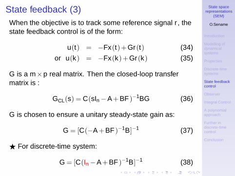
State feedback (3)When the objective is to track some reference signal r , thestate feedback control is of the form:

u(t) = −Fx(t)+Gr(t) (34)

or u(k) = −Fx(k)+Gr(k) (35)

G is a m×p real matrix. Then the closed-loop transfermatrix is :

GCL(s) = C(sIn −A+BF )−1BG (36)

G is chosen to ensure a unitary steady-state gain as:

G = [C(−A+BF )−1B]−1 (37)

⋆ For discrete-time system:

G = [C(In −A+BF )−1B]−1 (38)


(SEM)

O.Sename

Introduction


Properties



Observer

Integral Control



Conclusion

Pole placement control

PropositionLet a linear system given by A, B, and let γi , i = 1, ...,n , aset of complex elements (i.e. the desired poles of theclosed-loop system). There exists a state feedback controlu = −Fx such that the poles of the closed-loop system areγi , i = 1, ...,n if and only if the pair (A,B) is controllable.


(SEM)

O.Sename

Introduction


Properties



Observer

Integral Control



Conclusion

Why state feedback and not output feedback?

Example: G(s) = 1s2−s

Consider the canonical form.Case of output feedback : u = −LyThen x(t) = (A−BLC)x(t)For the example, the characteristic polynomial isPBF (s) = s2 −s−L. The closed-loop system cannot bestabilized.Case of state feedback : u = −FxLet F = [f1, f2]. Then PBF (s) = s2 +(−1+ f2)s + f1So we can choose any F . For instance f1 = 1, f2 = 3 givesPBF (s) = (s +1)2


(SEM)

O.Sename

Introduction


Properties



Observer

Integral Control



Conclusion

Pole placement control (1)

First case: controllable canonical form

A =

0 1 0 . . . 00 0 1 0 . . ....

......

. . ....

0... 0 1

−a0 −a1 . . . . . . −an−1

, B =

0......01

and

C =[

c0 c1 . . . cn−1].

Let F = [ f1 f2 . . . fn ]Then

A−BF =

0 1 0 . . . 00 0 1 0 . . ....

......

. . ....

0... 0 1

−a0 − f1 −a1 − f2 . . . . . . −an−1− fn

(39)


(SEM)

O.Sename

Introduction


Properties



Observer

Integral Control



Conclusion

Pole placement control (2)

Consider the desired clos-ed-loop polynomial:(s− γ1)(s− γ2)...(s− γn) = sn + αn−1sn−1 + . . .+ α1s + α0

The solution:

fi = −ai−1 + αi−1, i = 1, ..,n

ensures that the poles of A−BF are {γi}, i = 1,nWhen we consider a general state space representation, itis first necessary to use a change of basis to make thesystem under canonical form.Use F=acker(A,B,P)where P is the set of desiredclosed-loop poles.


(SEM)

O.Sename

Introduction


Properties



Observer

Integral Control



Conclusion

Pole placement control (3)Procedure for the general case:

1. Check controllability of (A, B)2. Calculate C = [B,AB, . . . ,An−1B].

Note C−1 =

q1...

qn

. Define T =

qn

qnA...

qnAn−1

−1

3. Note A = T−1AT and B = T−1B (which are under thecontrollable canonical form)

4. Choose the desired closed-loop poles and define thedesired closed-loop characteristic polynomial:sn + αn−1sn−1 + . . .+ α1s + α0

5. Calculate the state feedback u = −F x with:

fi = −ai−1 + αi−1, i = 1, ..,n

6. Calculate (for the original system):

u = −Fx , with F = FT−1


(SEM)

O.Sename

Introduction


Properties



Observer

Integral Control



Conclusion

Observer

Problem: To implement a state feedback control, themeasurement of all the state variables is necessary. If thisis not available, we will use a state estimation through aso-called Observer.Observer form:

˙x(t) = Ax(t)+Bu(t)−L(Cx(t)−y(t))x0

(40)

where x(t) ∈ Rn is the estimated state of x(t) and L is the

n×p constant observer gain matrix to be designed.


(SEM)

O.Sename

Introduction


Properties



Observer

Integral Control



Conclusion

Observer

Th estimated error, e(t) := x(t)− x(t), satisfies:

e(t) = (A−LC)e(t) (41)

If L is designed such that A−LC is stable, then x(t)converges asymptotically towards x(t).

Proposition(40) is an observer for system (2) if and only if the pair(C,A) is observable, i.e.

rank(O) = n

where O =

CCA...

CAn−1

.


(SEM)

O.Sename

Introduction


Properties



Observer

Integral Control



Conclusion

Observer design

The observer design is restricted to find L such that A−LCis stable. This is still a pole placement problem.In order to use the acker Matlab function, we will use theduality property between observability and controllability,i.e. :(C,A) observable ⇔ (AT ,CT ) controllable.Then there exists LT such that the eigenvalues ofAT −CT LT can be randomly chosen. As(A−LC)T = AT −CT LT then L exists such that A−LC isstable.Matlab : use L=acker(A’,C’,Po)’ where Pois the set of desired observer poles.Remark : usually the observer poles are chosen around 5to 10 times higher than the closed-loop system, so that thestate estimation is good as early as possible. This is quiteimportant to avoid that the observer makes the closed-loopsystem slower.


(SEM)

O.Sename

Introduction


Properties



Observer

Integral Control



Conclusion

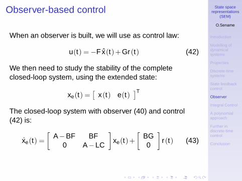
Observer-based control

When an observer is built, we will use as control law:

u(t) = −Fx(t)+Gr(t) (42)

We then need to study the stability of the completeclosed-loop system, using the extended state:

xe(t) =[

x(t) e(t)]T

The closed-loop system with observer (40) and control(42) is:

xe(t) =

[A−BF BF

0 A−LC

]

xe(t)+

[BG0

]

r(t) (43)


(SEM)

O.Sename

Introduction


Properties



Observer

Integral Control



Conclusion

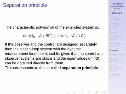
Separation principle

The characteristic polynomial of the extended system is:

det(sIn −A+BF )×det(sIn−A+LC)

If the observer and the control are designed separatelythen the closed-loop system with the dynamicmeasurement feedback is stable, given that the control andobserver systems are stable and the eigenvalues of (43)can be obtained directly from them.This corresponds to the so-called separation principle.


(SEM)

O.Sename

Introduction


Properties



Observer

Integral Control



Conclusion

Stabilisation/ Detectability

When the linear system (2) is not completely controllableor observable, it is then important to study the stability ofthe non controllable and non observable modes.Use ctrbf and obsvf Matlab commands


(SEM)

O.Sename

Introduction


Properties



Observer

Integral Control



Conclusion

Integral Control

A state feedback controller may not allow to reject theeffects of disturbances (particularly of input disturbances).A very useful method consists in adding an integral term toensure a unitary static closed-loop gain .Considered system:

{x(t) = Ax(t)+Bu(t)+Ed(t), x(0) = x0

y(t) = Cx(t)(44)

where d is the disturbance.The objective is to keep y close to a reference signal r ,even in the presence of d , i.e to keep r −y asymptoticallystable.


(SEM)

O.Sename

Introduction


Properties



Observer

Integral Control



Conclusion

Integral Control

The method consists in extending the system by adding anew state variable:

z(t) = r(t)−y(t)

and to use a new state feedback:

u(t) = −Fx(t)−Hz(t)

We get[

x(t)z(t)

]

=

[A−BF BH−C 0

][xz

]

+

[01

]

r(t)+

[E0

]

d(t)


(SEM)

O.Sename

Introduction


Properties



Observer

Integral Control



Conclusion

Integral control scheme

The complete structure has the following form:

When an observer is to be used, the control action simplybecomes:

u(t) = −Fx(t)−Hz(t)


(SEM)

O.Sename

Introduction


Properties



Observer

Integral Control



Conclusion

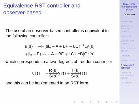
Equivalence RST controller andobserver-based

The use of an observer-based controller is equivalent tothe following controller :

u(s) = −F (sIn −A+BF +LC)−1Ly(s)

+[In −F (sIn −A+BF +LC)−1B]Gr(s)

which corresponds to a two-degrees of freedom controller

u(s) = −R(s)

S(s)y(s)+

T (s)

S(s)r(s)

and this can be implemented in an RST form.


(SEM)

O.Sename

Introduction


Properties



Observer

Integral Control



Conclusion

About sampling period and time response

Influence of the sampling period on the time response

Impose a maximal time response to a discrete system isequivalent to place the poles inside a circle defined by theupper bound of the bound given by this time response.The more the poles are close to zero, the more the systemis fast.


(SEM)

O.Sename

Introduction


Properties



Observer

Integral Control



Conclusion

Frequency analysisAs in the continuous time, the Bode diagram can also beused.Example with sampling TimeTe = 1s ⇔ fe = 1Hz ⇔ we = 2π):

Note that, in our case, the Bode is cut at the pulse w = π.see SYSD = c2d(SYSC,Ts,METHOD) in MATLAB.


(SEM)

O.Sename

Introduction


Properties



Observer

Integral Control



Conclusion

Frequency analysisAs in the continuous time, the Bode diagram can also beused.Example with sampling TimeTe = 1s ⇔ fe = 1Hz ⇔ we = 2π):

Note that, in our case, the Bode is cut at the pulse w = π.see SYSD = c2d(SYSC,Ts,METHOD) in MATLAB.

Sampling ↔ LimitationsRecall the Shannon theorem that impose the samplingfrequency at least 2 times higher that the systemmaximum frequency. Related to the anti-aliasing filter. . .


(SEM)

O.Sename

Introduction


Properties



Observer

Integral Control



Conclusion

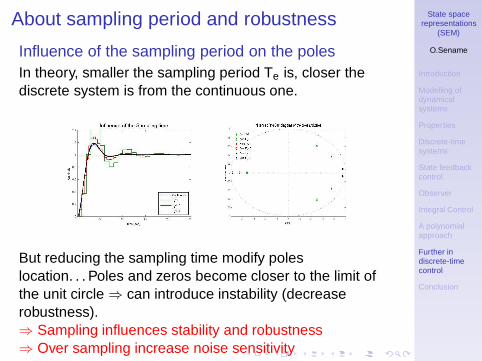
About sampling period and robustness

Influence of the sampling period on the polesIn theory, smaller the sampling period Te is, closer thediscrete system is from the continuous one.

But reducing the sampling time modify poleslocation. . . Poles and zeros become closer to the limit ofthe unit circle ⇒ can introduce instability (decreaserobustness).⇒ Sampling influences stability and robustness⇒ Over sampling increase noise sensitivity


(SEM)

O.Sename

Introduction


Properties



Observer

Integral Control



Conclusion

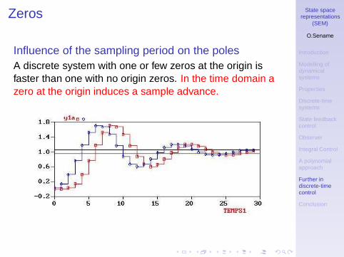
Zeros

Influence of the sampling period on the polesA discrete system with one or few zeros at the origin isfaster than one with no origin zeros. In the time domain azero at the origin induces a sample advance.


(SEM)

O.Sename

Introduction


Properties



Observer

Integral Control



Conclusion

Stability

RecallA linear continuous feedback control system is stable if allpoles of the closed-loop transfer function T (s) lie in the lefthalf s-plane.The Z-plane is related to the S-plane byz = e−sTe = e(σ+jω)Te. Hence

|z| = eσTe and ∠z = ωTe


(SEM)

O.Sename

Introduction


Properties



Observer

Integral Control



Conclusion

Stability (cont’d)

Jury criteriaThe denominator polynomial(den(z) = a0zn +a1zn−1 + · · ·+an = 0) has all its rootsinside the unit circle if all the first coefficients of the oddrow are positive.

1 a0 a1 a2 . . . an−k . . . an

2 an an−1 an−2 . . . ak . . . a0

3 b0 b1 b2 . . . bn−1

2 bn−1 bn−2 bn−3 . . . b0...

...2n +1 s0

b0 = a0 −anan

a0

b1 = a1 −an−1an

a0

bk = ak −an−kan

a0

ck = bk −bn−1−kbn−1

b0


(SEM)

O.Sename

Introduction


Properties



Observer

Integral Control



Conclusion

Example

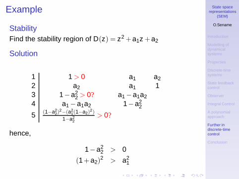
StabilityFind the stability region of D(z) = z2 +a1z +a2


(SEM)

O.Sename

Introduction


Properties



Observer

Integral Control



Conclusion

Example

StabilityFind the stability region of D(z) = z2 +a1z +a2

Solution

1 1 > 0 a1 a2

2 a2 a1 13 1−a2

2 > 0? a1 −a1a2

4 a1 −a1a2 1−a22

5 (1−a22)

2−(a21(1−a2)

2)

1−a22

> 0?

hence,

1−a22 > 0

(1+a2)2 > a2

1


(SEM)

O.Sename

Introduction


Properties



Observer

Integral Control



Conclusion

How to get a discrete controller

First way

◮ Obtain a discrete-time plant model (by discretization)◮ Design a discrete-time controller◮ Derive the difference equation

Second way

◮ Design a continuous-time controller◮ Converse the continuous-time controller to discrete

time (c2d)◮ Derive the difference equation

Now the question is how to implement the computedcontroller on a real-time (embedded) system, and what arethe precautions to take before?


(SEM)

O.Sename

Introduction


Properties



Observer

Integral Control



Conclusion

Implementationcharacteristics


(SEM)

O.Sename

Introduction


Properties



Observer

Integral Control



Conclusion

Anti-aliasing & Sampling

Anti-aliasingPractically it is smart to use a constant high samplingfrequency with an analog filter matching this frequency.Then, after the A/D converter, the signal is down-sampledto the frequency used by the controller. Remember thatthe pre-filter introduce phase shift.

Sampling frequency choiceThe sampling time for discrete-time control are based onthe desired speed of the closed loop system. A rule ofthumb is that one should sample 4−10 times per rise timeTr of the closed loop system.

Nsample =Tr

Te≈ 4−10

where Te is the sampling period, and Nsample the numberof samples.


(SEM)

O.Sename

Introduction


Properties



Observer

Integral Control



Conclusion

Delay

ProblematicSampled theory assume presence of clock thatsynchronizes all measurements and control signal. Hencein a computer based control there always is delays (controldelay, computational delay, I/O latency).

OriginsThere are several reasons for delay apparition

◮ Execution time (code)◮ Preemption from higher order process◮ Interrupt◮ Communication delay◮ Data dependencies

Hence the control delay is not constant. The delayintroduce a phase shift ⇒ Instability!


(SEM)

O.Sename

Introduction


Properties



Observer

Integral Control



Conclusion

Delay (cont’d)

Admissible delay (Bode)

◮ Measure the phase margin: PM = 180+ϕw0 [r], whereϕw0 is the phase at the crossover frequency w0, i.e.|G(jw0)| = 1

◮ Then the delay margin is

DM =PMπ

180w0[s]

Exercise: compute delay margin for these 3 cases


(SEM)

O.Sename

Introduction


Properties



Observer

Integral Control



Conclusion

Delay (cont’d)

Static scheduling vs Minimal control delay


(SEM)

O.Sename

Introduction


Properties



Observer

Integral Control



Conclusion

Delay (cont’d)

How to compensate the delay?There are several ways

◮ Minimize the delay (case B - Minimal control delay)◮ Compensate it off-line◮ Make the controller robust (case A - static scheduling)◮ Compensate on-line

Exple: Code that minimize the delay

LOOP %%% At each clock interruptADinCalculateOutputDAoutUpdateStatesIncTime %%% Evaluate remaining timeWaitUntilTe

END


(SEM)

O.Sename

Introduction


Properties



Observer

Integral Control



Conclusion

Delay (cont’d)

ExerciseConsider the following controller,

x(k +1) = Fx(k)+Gy(k)

u(k) = Cx(k)+Dy(k)


(SEM)

O.Sename

Introduction


Properties



Observer

Integral Control



Conclusion

Delay (cont’d)

ExerciseConsider the following controller,

x(k +1) = Fx(k)+Gy(k)

u(k) = Cx(k)+Dy(k)

LOOPADin(y);%%% CalculateOutputu := u1 + D*y;DAout(u)%%% UpdateStatesx := F*x + G*y;u1 := C*x;%%% Wait for the nextIncTime;

Note that such a structure is notthe only one! Controller can workon interrupts (exple: Brushlessmotor)


(SEM)

O.Sename

Introduction


Properties



Observer

Integral Control



Conclusion

Quantification

Effects

◮ Non linear phenomena◮ Limit cycles

Example (stable for K<2)

H(z) =0.25

(z −1)(z −0.5)


(SEM)

O.Sename

Introduction


Properties



Observer

Integral Control



Conclusion

Quantification (cont’d)

Results


(SEM)

O.Sename

Introduction


Properties



Observer

Integral Control



Conclusion

Discretisation

The idea behind discretisation of a controller is to translateit from continuous-time to discrete-time, i.e.

A/D + algorithm +D/A ≈ G(s)

To obtain this, few methods exists that approach theLaplace operator (see lecture 1-2).

Recall

s =z −1

Te

s =z −1zTe

s =2Te

z −1z +1


(SEM)

O.Sename

Introduction


Properties



Observer

Integral Control



Conclusion

Conclusion

◮ A state space approach to pole placement control◮ A similar design can be done using a polynomial

approach◮ Continuous but directly extended to discrete-time

systems.

representations modelling, analysis and control of linear ...o.sename/docs/sem.pdf · properties...

Documents