Representation of data

----histogram

Alpha

Part One : Class boundaries

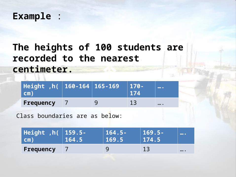
The heights of 100 students are recorded to the nearest centimeter.

Height ,h(cm) 160-164 165-169 170-174 ….

Frequency 7 9 13 ….

Class boundaries are as below:

Height ,h(cm) 159.5-164.5 164.5-169.5 169.5-174.5 ….

Frequency 7 9 13 ….

Example :

The mass of 40 students are recorded to the nearest kilogram.

Mass ,m(kg) 45-55 55-65 65-75 ….

Frequency 7 9 13 ….

Class boundaries are as below:45 55 65 75 so the table are rewrote as below

Height ,h(cm) 45≤m<55 55≤m<65 65≤m<75 ….

Frequency 7 9 13 ….

If there is no gap between each class, then what are the boundaries?

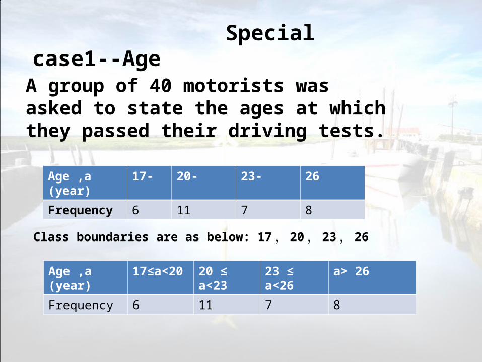
Special case1--Age

A group of 40 motorists was asked to state the ages at which they passed their driving tests.

Age ,a (year) 17- 20- 23- 26

Frequency 6 11 7 8

Class boundaries are as below: 17 ， 20 ， 23 ， 26

Age ,a (year) 17≤a<20 20 ≤ a<23 23 ≤ a<26 a> 26

Frequency 6 11 7 8

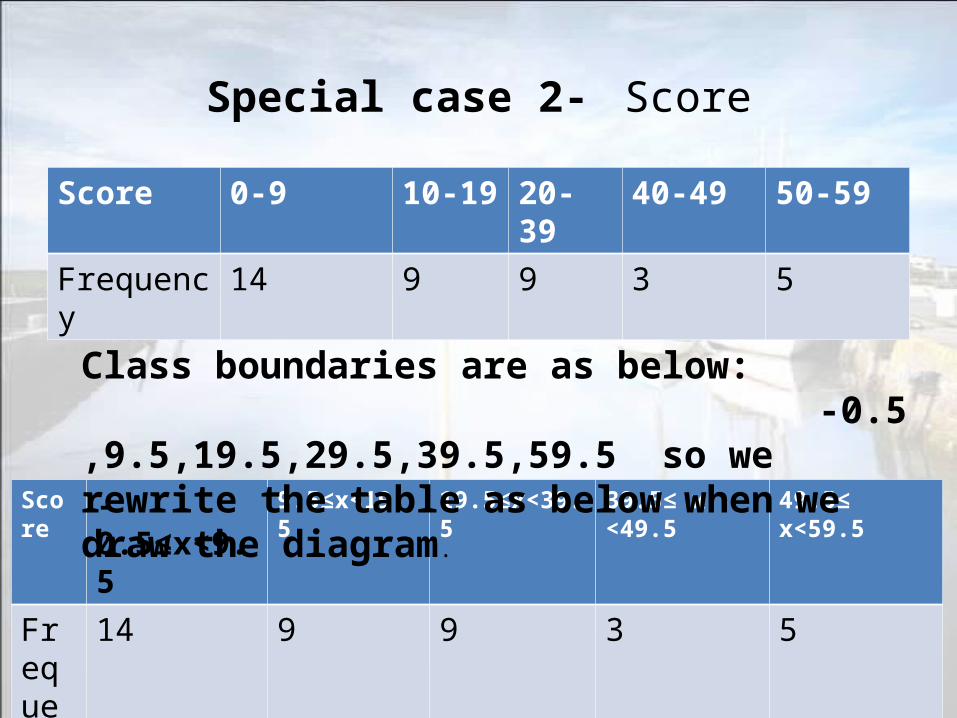
Special case 2- Score

Score 0-9 10-19 20-39 40-49 50-59Frequency 14 9 9 3 5

Score -0.5≤x<9.5 9.5≤x<19.5 19.5≤x<39.5 39.5≤ x <49.5 49.5≤ x<59.5

Frequency

14 9 9 3 5

Class boundaries are as below: -0.5 ,9.5,19.5,29.5,39.5,59.5 so we rewrite the table as below when we draw the diagram.

Part two : frequency density

Two important properties of histogram

• The bars have no spaces between them( though there may be some bars of height zero, which look like spaces)

• The area of each bar is proportional to the frequency

Note: the first one is the main difference between bar chart and histogram

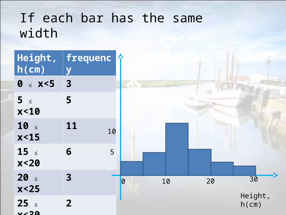
Height, h(cm)

frequency

0 ≤ x<5 3

5 ≤ x<10 5

10 ≤ x<15 11

15 ≤ x<20 6

20 ≤ x<25 3

25 ≤ x<30 2

0 10

5

20

10

30

Height, h(cm)

If each bar has the same width

Height, h(cm)

frequency

0 ≤ x<5 3

5 ≤ x<10 5

10 ≤ x<15 11

15 ≤ x<20 6

20 ≤ x<30 5

10

0 10

5

20 30

Height, h(cm)

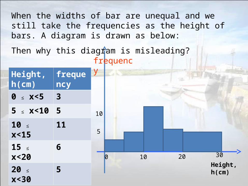
When the widths of bar are unequal and we still take the frequencies as the height of bars. A diagram is drawn as below:

Then why this diagram is misleading?

frequency

Height, h(cm)

frequency

0≤ x<5 3

5 ≤x<10 5

10 ≤ x<15 11

15 ≤x<20 6

20 ≤x<30 5

0 10

5

20

10

30Height, h(cm)

Frequency density

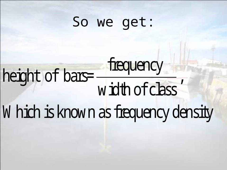
So we get:

frequency height of bars= ,

width of clasWhich is known as frequency dens

sity

Now let us draw a histogram

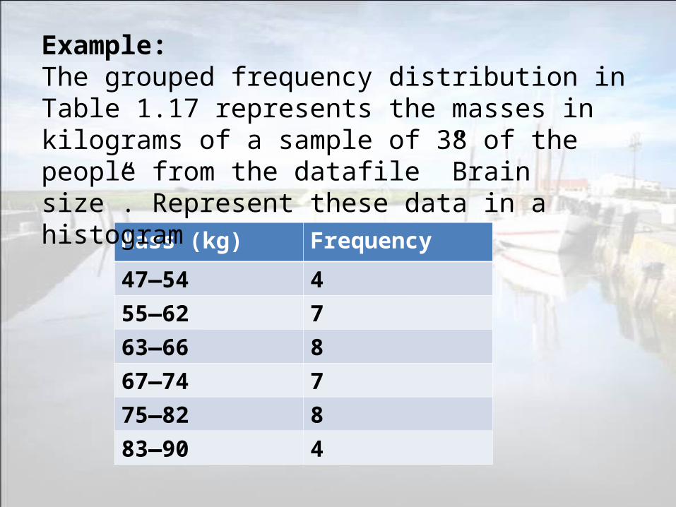
Mass (kg) Frequency

47—54 455—62 763—66 867—74 775—82 883—90 4

Example: The grouped frequency distribution in Table 1.17 represents the masses in kilograms of a sample of 38 of the people from the datafile ”Brain size”. Represent these data in a histogram

Mass, m(kg)

Class boundaries

Class width

frequency

Frequency density

47—54 46.5 ≤x<54.5 8 4 0.555—62 54.5 ≤x<62.5 8 7 0.87563—66 62.5 ≤x<66.5 4 8 267—74 66.5 ≤x<74.5 8 7 0.87575—82 74.5 ≤x<82.5 8 8 183—90 82.5 ≤x<90.5 8 4 0.5

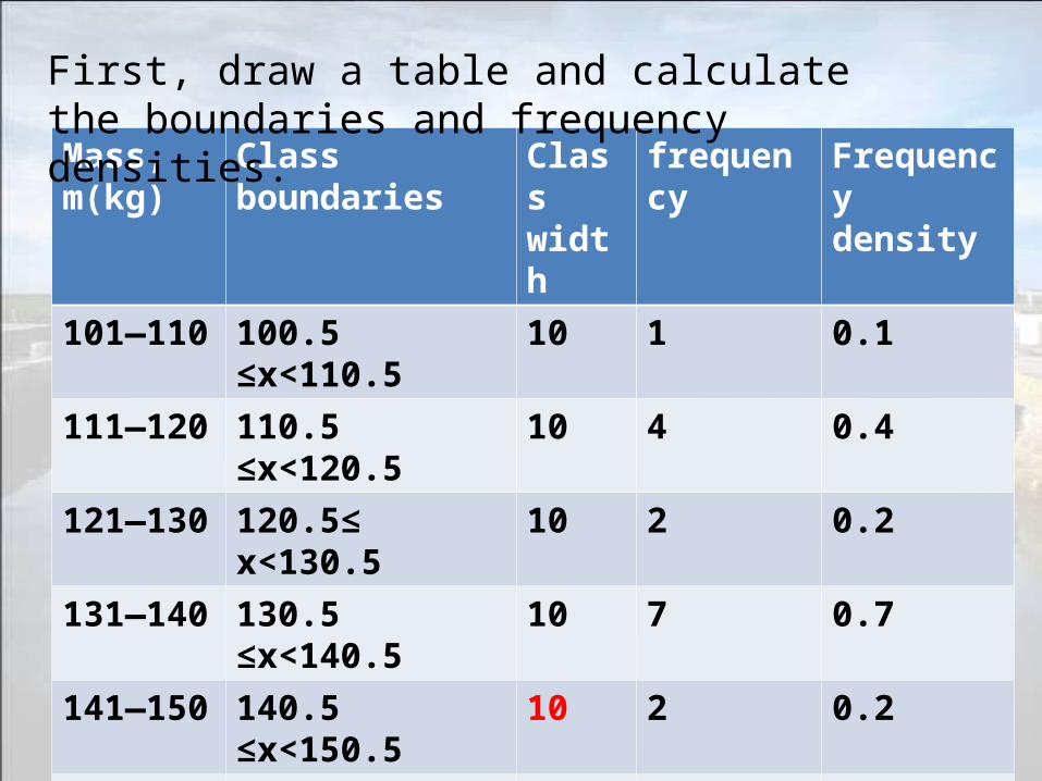
First, draw a table and calculate the boundaries and frequency densities.

50 60 70 9080 Mass, m(kg)

1

2

Frequency density

• Label the two axes with given labels• The height of each bars should be correct• The boundaries should be right• The scale should be 40----95 and 0---2• The frequency density should be given.

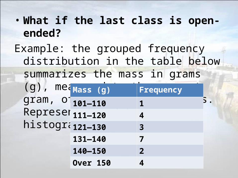
• What if the last class is open-ended?

Example: the grouped frequency distribution in the table below summarizes the mass in grams (g), measured to the nearest gram, of sample of 20 pebbles. Represent the data in a histogram

Mass (g) Frequency

101—110 1111—120 4121—130 3131—140 7140—150 2Over 150 4

Mass, m(kg)

Class boundaries Class width

frequency Frequency density

101—110 100.5 ≤x<110.5 10 1 0.1

111—120 110.5 ≤x<120.5 10 4 0.4

121—130 120.5≤ x<130.5 10 2 0.2

131—140 130.5 ≤x<140.5 10 7 0.7

141—150 140.5 ≤x<150.5 10 2 0.2

Over 150 150.5≤ x<170.5 20 4 0.2

First, draw a table and calculate the boundaries and frequency densities.

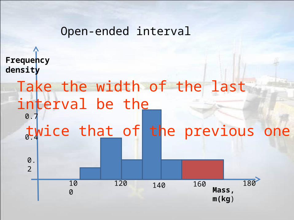
100 180120 160140Mass, m(kg)

0.2

0.4

Frequency density

0.7

Open-ended interval

Take the width of the last interval be the

twice that of the previous one

• What if the first class is open?• What are the advantages and disadvantages

of the histogram?• What are the advantages and disadvantages

of the stem and leaf diagram?

End