Representation and Invarianceof Scientific Structures

Representation and Invarianceof Scientific Structures

Patrick Suppes

Center for the Study ofLanguage and InformationStanford, California

CSL IPUBLICATIONS

Copyright c© 2002CSLI Publications

Center for the Study of Language and InformationLeland Stanford Junior University

Printed in the United States06 05 04 03 02 5 4 3 2 1

Library of Congress Cataloging-in-Publication Data

Suppes, Patrick, 1922–Representation and invariance of scientific structures /

Patrick Suppes.p. cm. – (CSLI lecture notes ; no. 130)

Includes bibliographical references and index.

ISBN 1-57586-333-2 (cloth : alk. paper)

1. Science–Philosophy.I. Title. II. Series.

Q175 .S93945 2001501—dc21 2001035637

CIP

∞ The acid-free paper used in this book meets the minimum requirements of the AmericanNational Standard for Information Sciences—Permanence of Paper for Printed Library

Materials, ANSI Z39.48-1984.

CSLI was founded early in 1983 by researchers from Stanford University, SRI International, andXerox PARC to further research and development of integrated theories of language, information, and

computation. CSLI headquarters and CSLI Publications are located on the campus of StanfordUniversity.

CSLI Publications reports new developments in the study of language, information, and computation.In addition to lecture notes, our publications include monographs, working papers, revised

dissertations, and conference proceedings. Our aim is to make new results, ideas, and approachesavailable as quickly as possible. Please visit our web site at

http://cslipublications.stanford.edu/

for comments on this and other titles, as well as for changes and corrections by the author andpublisher.

To My Children

Patricia, Deborah, John,

Alexandra and Michael

Contents

Preface xiii

1 Introduction 1

1.1 General Viewpoint 1

1.2 What Is a Scientific Theory? 2The traditional sketch. 2

Models versus empirical interpretations of theories. 3

Intrinsic-versus-extrinsic characterization of theories. 5

Coordinating definitions and the hierarchy of theories. 7

Instrumental view of theories. 8

1.3 Plan of the Book 10

1.4 How To Read This Book 14

2 Axiomatic Definition of Theories 17

2.1 Meaning of Model in Science 17Comments on quotations. 20

2.2 Theories with Standard Formalization 24Example: ordinal measurement. 25

Axiomatically built theories. 26

Difficulties of scientific formalization. 27

Useful example of formalization 28

2.3 Theories Defined by Set-theoretical Predicates 30Example: theory of groups. 31

Meaning of ‘set-theoretical predicate’. 32

Set theory and the sciences. 33

Basic structures. 33

Reservations about set theory. 34

2.4 Historical Perspective on the Axiomatic Method 35Before Euclid. 35

vii

viii Representation and Invariance of Scientific Structures

Euclid. 36

Archimedes. 37

Euclid’s Optics. 40

Ptolemy’s Almagest. 41

Jordanus de Nemore. 43

Newton. 44

Modern geometry. 45

Hilbert and Frege. 47

Physics. 48

3 Theory of Isomorphic Representation 51

3.1 Kinds of Representation 51Definitions as representations. 53

3.2 Isomorphism of Models 54

3.3 Representation Theorems 57Homomorphism of models. 58

Embedding of models. 62

3.4 Representation of Elementary Measurement Structures 63Extensive measurement. 63

Difference measurement. 66

Bisection measurement. 67

Conjoint measurement. 69

Proofs of Theorems 2–4 70

3.5 Machine Representation of Partial Recursive Functions 74Unlimited register machines (URM). 76

Partial recursive functions over an arbitrary finite alphabet. 80

3.6 Philosophical Views of Mental Representations 81Aristotle. 81

Descartes. 83

Hume. 83

Kant. 86

James. 88

Special case of images. 92

Psychological views of imagery. 93

4 Invariance 97

4.1 Invariance, Symmetry and Meaning 97Meaning. 102

Objective meaning in physics. 103

4.2 Invariance of Qualitative Visual Perceptions 105Oriented physical space. 106

Contents ix

4.3 Invariance in Theories of Measurement 110Second fundamental problem of measurement: invariance theorem. 112

Classification of scales of measurement. 114

4.4 Why the Fundamental Equations of Physical Theories Are NotInvariant 120Beyond symmetry. 122

Covariants. 122

4.5 Entropy as a Complete Invariant in Ergodic Theory 123Isomorphism of ergodic processes. 125

5 Representations of Probability 1295.1 The Formal Theory 130

Primitive notions. 130

Language of events. 132

Algebras of events. 133

Axioms of probability. 134

Discrete probability densities. 136

Conditional probability. 138

Independence. 144

Random variables. 146

Joint distributions. 153

Modal aspects of probability. 154

Probabilistic invariance. 155

5.2 Classical Definition of Probability 157Laplace. 159

Classical paradoxes. 163

Historical note on Laplace’s principles 3–10. 166

5.3 Relative-frequency Theory for Infinite Random Sequences 167Von Mises. 171

Church. 173

5.4 Random Finite Sequences 178Kolmogorov complexity. 179

Universal probability. 182

Relative frequencies as estimates of probability. 183

5.5 Logical Theory of Probability 184Keynes. 184

Jeffreys. 185

Carnap’s confirmation theory. 190

Hintikka’s two-parameter theory. 198

Kyburg. 200

Model-theoretic approach. 200

Chuaqui. 200

x Representation and Invariance of Scientific Structures

5.6 Propensity Representations of Probability 202Propensity to decay. 203

Discrete qualitative densities. 210

Propensity to respond. 211

Propensity for heads. 214

Propensity for randomness in motion of three bodies. 218

Some further remarks on propensity. 220

5.7 Theory of Subjective Probability 225De Finetti’s qualitative axioms. 226

General qualitative axioms. 230

Qualitative conditional probability. 234

Historical background on qualitative axioms. 238

De Finetti’s representation theorem. 240

Defense of objective priors. 241

General issues. 242

Decisions and the measurement of subjective probability. 245

Inexact measurement of belief: upper and lower probabilities. 248

5.8 Epilogue: Pragmatism about Probability 256Early statistical mechanics. 256

Quantum mechanics. 257

Pragmatism in physics. 261

Statistical practice. 262

6 Representations of Space and Time 265

6.1 Geometric Preliminaries 2666.2 Classical Space-time 269

Historical remarks. 272

6.3 Axioms for Special Relativity 275Historical remarks. 278

Later qualitative axiomatic approaches. 281

6.4 How to Decide if Visual Space is Euclidean 282The hierarchy of geometries. 287

6.5 The Nature of Visual Space: Experimental and PhilosophicalAnswers 288

6.6 Partial Axioms for the Foley and Wagner Experiments 2976.7 Three Conceptual Problems About Visual Space 300

Contextual geometry. 300

Distance perception and motion. 301

Objects of visual space. 302

6.8 Finitism in Geometry 303Quantifier-free axioms and constructions. 305

Contents xi

Affine Axioms. 306

Theorems. 308

Analytic representation theorem. 309

Analytic invariance theorem. 310

7 Representations in Mechanics 3137.1 Classical Particle Mechanics 313

Assumed mathematical concepts. 313

Space-time structure. 318

Primitive notions. 319

The axioms. 320

Two theorems—one on determinism. 323

Momentum and angular momentum. 325

Laws of conservation. 327

7.2 Representation Theorems for Hidden Variables in QuantumMechanics 332Factorization. 333

Locality. 335

GHZ-type experiments. 338

Second-order Gaussian theorems. 342

7.3 Weak and Strong Reversibility of Causal Processes 343Weak reversibility. 344

Strong reversibility. 346

Ehrenfest model. 348

Deterministic systems. 349

8 Representations of Language 3538.1 Hierarchy of Formal Languages 354

Types of grammars. 356

Normal forms. 357

Operations on languages. 359

Unsolvable problems. 360

Natural-language applications. 361

8.2 Representation Theorems for Grammars 361Finite automata. 361

Languages accepted by finite automata. 364

Regular grammars and finite automata. 367

Remark on the empty sequence. 371

Pushdown automata and context-free languages. 371

Turing machines and linear bounded automata. 373

8.3 Stimulus-response Representation of Finite Automata 374Stimulus-response theory. 377

xii Representation and Invariance of Scientific Structures

Representation of finite automata. 380

Response to criticisms. 387

Another misconception: restriction to finite automata. 394

Axioms for register learning models. 397

Role of hierarchies and more determinate reinforcement. 401

8.4 Representation of Linear Models of Learning by Stimulus-samplingModels 403Modification of general axioms. 404

Preliminary theorems. 405

Theorems involving the sequence ωn. 411

Limit assumptions. 414

8.5 Robotic Machine Learning ofComprehension Grammars for TenLanguages 419Problem of denotation. 420

Background cognitive and perceptual assumptions. 421

Internal language. 424

General learning axioms. 425

Specialization of certain axioms and initial conditions. 429

The Corpora. 432

Empirical results. 433

Grammatical rules. 438

Related work and unsolved problems. 441

8.6 Language and the Brain. 442Some historical background. 442

Observing the brain’s activity. 444

Methods of data analysis. 446

Three experimental results. 450

Criticisms of results and response. 453

Computation of extreme statistics. 456

Analysis of earlier studies. 458

Other pairs in the first experiment with 48 sentences. 461

Test of a timing hypothesis for the experiment with 100 sentences. 461

Censoring data in the visual-image experiment. 463

8.7 Epilogue: Representation and Reduction in Science 465

Summary Table of Representation and Invariance Theorems byChapter 471

References 475

Author Index 503

Index 511

Preface

This book has a long history of development. My earliest preliminary edition, entitledSet-theoretical Structures in Science, with temporary binding and cover, dates from1962, but I know that even earlier drafts were produced for the lectures I gave inthe basic undergraduate course in the philosophy of science at Stanford, in the 1950s.Course notes materials were developed rather quickly that conceptually followed the finalchapter on the set-theoretical foundations of the axiomatic method of my Introductionto Logic, first published in 1957.

I can remember being asked on several occasions in those early years, But what is thegeneral point of having set-theoretical structures play a central role in the philosophyof science? At first, I answered with a stress on the many general intellectual virtuesof the axiomatic method apparent since the appearance long ago of Euclid’s Elements.But I gradually came to see there was a better answer, of more philosophical interest.This was that such structures provided the right settings for investigating problemsof representation and invariance in any systematic part of past or present science. Ofcourse, this answer prompts another question. Why are representation and invarianceimportant in the foundations or philosophy of science? In a sense, it is the purpose ofthis entire book to provide an answer. But some standard examples can be helpful, evenwithout any serious details.

One of the great intellectual triumphs of the nineteenth century was the mechanicalexplanation of such familiar concepts as temperature and pressure by their represen-tation simply in terms of the motion of particles. An equally great triumph, one moredisturbing on several counts, was the realization at the beginning of the twentieth cen-tury that the separate invariant properties of space and time, standard in classicalphysics, even if often only implicitly recognized, must be replaced by the space-time ofEinstein’s special relativity and its new invariants.

But physics is not the only source of such examples. Sophisticated analysis of thenature of representation in perception is to be found already in Plato and Aristotle, andis still alive and well in the controversies of contemporary psychology and philosophy.

So I offer no apologies for my emphasis on representation and invariance, reflectedin the revised title of this book. Central topics in foundational studies of different sortsthrough the ages easily fall under this heading. Certainly it is not the whole of philosophyof science, but it is a major part.

xiii

xiv Representation and Invariance of Scientific Structures

The first four chapters offer a general introduction to the concepts of representationand invariance. The last four provide applications to four areas of thought, important inthe philosophy of science, but important because they are, more generally, of scientificsignificance. They are the nature of probability, concepts of space and time, both physi-cal and psychological, representations in classical and quantum mechanics, and, finally,representations of language examined from several different angles. I include at the endof the book a summary table of the representation and invariance theorems stated anddiscussed in various chapters. Many are not proved and represent famous results in themathematical and scientific literature. Those that are proved usually, but not always,represent some aspect of my own work, and most of the proofs given are elementaryfrom a mathematical standpoint. As will be evident to any persistent reader, analysisand clarification of concepts, not formal proofs, are the main focus.

Although I have been devoted to formal methods in the philosophy of science, thereare two other approaches to which I am nearly as faithful, and consequently they havehad a big influence. One is concern for empirical details. This is reflected in the many ex-periments, especially in psychology, I consider at various points. Moreover, the content ofthis book does not adequately reflect the large number of experiments I have conductedmyself, almost always in conjunction with colleagues, in many areas of psychology. Ioriginally intended to write a long final chapter on set-theoretical representations ofdata as a necessary, but still desirable, abstraction of the complicated activity of con-ducting experiments. With the rapid increase in computer power in the last decade orso, the analysis of data in many parts of science is being radically transformed. I hopeto extend the present work in that direction, perhaps in a new chapter to be madeavailable on the internet, which will surely become the medium for the majority of de-tailed scientific publications in the next decade or so. The next-to-last section of thelast chapter, 8.6, exemplifies what I have in mind.

The other approach close to my heart is concern for the historical background anddevelopment of many different scientific ideas. There is a rich and attractive tradition inphilosophy of being concerned with the historical development of concepts and theories.Analysis, even of an often rather sketchy kind, of the background of a new idea aboutprobability, physical invariance, visual space, mental representation or nearly any otherimportant scientific concept I almost always find enlightening and helpful. I hope thatsome readers will feel the same about my many historical excursions, which do not giveanything like a fully detailed account of the evolution of a single concept.

The writing of a book like this over many years entails indebtedness for corrections,insights and suggestions on innumerable topics by more people than I can possiblythank explicitly. By now, many are gone and many others will have forgotten how theycontributed to what is said here. I thank them one and all. I certainly do want tomention those from whom I still have relevant remarks, or with whom I have written ajoint article, used and acknowledged at one or more points in this book.

Chapter 2. Dana Scott at the beginning, later Rolando Chuaqui, Newton da Costa,Francisco Doria, Jaakko Hintikka, Alfred Tarski, Paul Weingartner and Jules Vuillemin.Chapter 3. Dana Scott again, Kenneth Arrow, Dagfinn Follesdal, Duncan Luce andJesus Mosterin. Chapter 4. Nancy Cartwright, Maria Luisa Dalla Chiara, Jan Drosler

Preface xv

and Donald Ornstein. Chapter 5. In alphabetical order and over many years, DavidBlackwell, Thomas Cover, Persi Diaconnis, Jean Claude Falmagne, Jens Erik Fenstad,Terence Fine, Maria Carla Galavotti, Ian Hacking, Peter Hammond, Paul Holland,Joseph Keller, Duncan Luce, David Miller, Marcos Perreau-Guimaraes, Karl Popper,Roger Rosenkrantz, Henri Rouanet and Mario Zanotti. Chapter 6. Jan Drosler, TarowIndow, Brent Mundy, Gary Oas, Victor Pambuccian, Fred Roberts and Herman Rubin.Chapter 7. Acacio de Barros, Arthur Fine, Ubaldo Garibaldi, Gary Oas, Adonai S. Sant’Anna and Mario Zanotti. Chapter 8. Theodore W. Anderson, Michael Bottner, WilliamEstes, Bing Han, Lin Liang, Zhong-Lin Lu, Marcos Perreau-Guimaraes and TimothyUy.

I have also benefited from the penetrating questions and skeptical comments of manygenerations of students, who read various chapters in courses and seminars over thesemany years. I mention especially a group of former graduate students of mine whosecomments and corrections of mistakes were numerous to say the least: Colleen Cran-gle, Zoltan Domotor, Anne Fagot-Largeault, Paul Holland, Paul Humphreys, ChristophLehner, Michael Levine, Brent Mundy, Frank Norman, Fred Roberts, Deborah Rosen,Roger Rosenkrantz, Joseph Sneed, Robert Titiev, Raimo Tuomela and Kenneth Wexler.

In the final throes of publication, I must thank Ben Escoto, who read the entiremanuscript most carefully, looking for misprints and mistakes, and also Ann Gunderson,who has labored valiantly to produce the camera-ready copy for the printer. ClaudiaArrighi has done as much as I have in organizing and checking the extensive referencesand constructing the subject index. Ernest Adams read the entire next-to-final draftand made many important suggestions for improvements in content and style, most ofwhich I have been able to accomodate. Once again, as I have for many years, I benefitedfrom his well thought-out criticisms.

I began this book as a young man. Well, at least I think of under 40 as being young,certainly now. I finish it in my tenth year of retirement, at the age of 80. As I look backover the pages, I can see many places that could still stand improvement and, perhapsabove all, additional details and more careful perusal for errors. But I know it is timeto stop, and so I do.

I dedicate this book to my five children. I have been working on it during their entirelives, except for the oldest, Patricia, but she was a young child when I began. I alsoexpress my gratitude to my wife Christine for her patience and tolerance of my manyyears of intermittent effort, now, at last, at an end.

Patrick Suppes

Stanford, CaliforniaMarch, 2002.

1

Introduction

1.1 General Viewpoint

There is no simple or direct way to characterize the philosophy of science. Even the muchnarrower and more well-defined discipline of formal logic is not really subject to an exactdefinition. Individual philosophers have widely varying conceptions of the philosophy ofscience, and there is less agreement about what are the most important topics. All thesame, there is a rather wide consensus about certain topics like causality, induction,probability and the structure of theories. In this book I approach these and relatedtopics with certain formal methods and try to show how we can use these methods tomake clear distinctions that can easily be lost at the level of general discourse. On theother hand, it is my aim not to let formal matters get out of hand. I have tried to followa path that will not lose the reader in the underbrush of purely technical problems.

It might be thought that the emphasis on formal methods follows from a desire toemphasize a discussion of particular well-developed theories in science which are usuallygiven a mathematical formulation. Undoubtedly this consideration has weighed to someextent, but it is not the most important. From my own point of view, there are tworeasons of a more fundamental character for emphasizing the role of formal methodsin a systematic discussion of the philosophy of science. One is the desirability for anylarge-scale discussion of having a fixed frame of reference, or a fixed general method,that may be used to organize and criticize the variety of doctrines at hand. Formal, set-theoretical methods provide such a general framework for discussion of the systematicproblems of the philosophy of science. Such methods are more appropriate here than inthe foundations of mathematics, because the foundations of set theory are themselvesa central subject of investigation in the foundations of mathematics. It seems a wisedivision of labor to separate problems in the foundations of mathematics from problemsin the foundations of science. As far as I can see, most problems of central importanceto the philosophy of science can be discussed in full detail by accepting something like astandard formulation of set theory, without questioning the foundations of mathematics.In the discussion of problems of the philosophy of science, I identify formal methodswith set-theoretical methods. The reasons for this identification I pursue later in moredetail, but I do wish to make the point that I do not have any dogmatic commitmentto the ultimate character of this identification, or even to the ultimate character of aset-theoretical approach. It will be clear from what I have to say in Chapter 8 about

1

2 Introduction

behavioristic and neural theories of language that my own conception of an ultimatelysatisfactory theory of these phenomena will fall outside the standard set-theoreticalapproach.

However, a virtue of the set-theoretical approach is that we may easily meet a frequentcriticism of the artificial languages often introduced in the philosophy of science–namely,that such languages are not powerful enough to express most scientific results. The set-theoretical devices and framework we use are powerful enough easily to express anyof the systematic results in any branch of empirical science or in the general logic ofscience.

Another reason for advocating formal methods in the philosophy of science is theconviction that both the commonsense treatment and the artificial-language treatmentof problems of evidence are inadequate. Both these approaches give a much too simplifiedaccount of the extraordinarily complex and technically involved practical problems ofassessing evidence in the empirical sciences. Various parts of the long fifth chapter onprobability provide examples of the many subtle issues involved.

Before turning in the second chapter to a detailed consideration of set-theoreticalmethods, it will be useful in this introductory chapter to have an informal discussion ofscientific theories. This discussion is intended to adumbrate many of the issues that areexamined more thoroughly later.

1.2 What Is a Scientific Theory?

Often when we ask what is a so-and-so, we expect a clear and definite answer. If, forexample, someone asks me what is a rational number, I may give the simple and preciseanswer that a rational number is the ratio of two integers. There are other kinds of simplequestions for which a precise answer can be given, but for which ordinarily a rather vagueanswer is given and accepted. Someone reads about nectarines in a book but has neverseen a nectarine, or possibly has seen nectarines but is not familiar with their Englishname. He may ask me, ‘What is a nectarine?’ and I would probably reply, ‘a smooth-skinned sort of peach’. Certainly, this is not a very exact answer, but if my questionerknows what peaches are, it may come close to being satisfactory. The question, ‘Whatis a scientific theory?’, fits neither one of these patterns. Scientific theories are not likerational numbers or nectarines. Certainly they are not like nectarines, for they are notphysical objects. They are like rational numbers in not being physical objects, but theyare totally unlike rational numbers in that scientific theories cannot be defined simplyor directly in terms of other nonphysical, abstract objects.

Good examples of related questions are provided by the familiar inquiries, ‘What isphysics?’, ‘What is psychology?’, ‘What is science?’. To none of these questions do weexpect a simple and precise answer. On the other hand, many interesting remarks canbe made about the sort of thing physics or psychology is. I hope to show that this isalso true of scientific theories.

The traditional sketch. The traditional sketch of scientific theories–and I emphasizethe word ‘sketch’–runs something like the following. A scientific theory consists of twoparts. One part is an abstract logical calculus, which includes the vocabulary of logic

1.2 What Is a Scientific Theory? 3

and the primitive symbols of the theory. The logical structure of the theory is fixed bystating the axioms or postulates of the theory in terms of its primitive symbols. Formany theories the primitive symbols are thought of as theoretical terms like ‘electron’or ‘particle’, which cannot be related in any simple way to observable phenomena.

The second part of the theory is a set of rules that assign an empirical contentto the logical calculus by providing what are usually called ‘coordinating definitions’or ‘empirical interpretations’ for at least some of the primitive and defined symbolsof the calculus. It is always emphasized that the first part alone is not sufficient todefine a scientific theory; for without a systematic specification of the intended empiricalinterpretation of the theory, it is not possible in any sense to evaluate the theory as apart of science, although it can be studied simply as a piece of pure mathematics.

The most striking thing about this characterization is its highly schematic nature.Concerning the first part of a theory, there are virtually no substantive examples ofa theory actually worked out as a logical calculus in the writings of philosophers ofscience. Much hand waving is indulged in to demonstrate that working out the logicalcalculus is simple in principle and only a matter of tedious detail, but concrete evidenceis seldom given. The sketch of the second part of a theory, that is, the coordinatingdefinitions or empirical interpretations of some of the terms, is also highly schematic.A common defense of the relatively vague schema offered is that the variety of differentempirical interpretations, for example, the many different methods of measuring mass,makes a precise characterization difficult. Moreover, as we move from the preciselyformulated theory to the very loose and elliptical sort of experimental language used byalmost all scientists, it is difficult to impose a definite pattern on the rules of empiricalinterpretation.

The view I want to support is not that this standard sketch is flatly wrong, butrather that it is far too simple. Its very sketchiness makes it possible to omit bothimportant properties of theories and significant distinctions that may be introducedbetween theories.

Models versus empirical interpretations of theories. To begin with, there hasbeen a strong tendency on the part of many philosophers to speak of the first part ofa theory as a logical calculus purely in syntactical terms. The coordinating definitionsprovided in the second part do not in the sense of modern logic provide an adequatesemantics for the formal calculus. Quite apart from questions about direct empiricalobservations, it is pertinent and natural from a logical standpoint to talk about themodels of the theory. These models are abstract, nonlinguistic entities, often remotein their conception from empirical observations. So, apart from logic, someone mightwell ask what the concept of a model can add to the familiar discussions of empiricalinterpretation of theories.

I think it is true to say that most philosophers find it easier to talk about theoriesthan about models of theories. The reasons for this are several, but perhaps the mostimportant two are the following. In the first place, philosophers’ examples of theories areusually quite simple in character, and therefore, are easy to discuss in a straightforwardlinguistic manner. In the second place, the introduction of models of a theory inevitably

4 Introduction

introduces a stronger mathematical element into the discussion. It is a natural thingto talk about theories as linguistic entities, that is, to speak explicitly of the preciselydefined set of sentences of the theory and the like, when the theories are given inwhat is called standard formalization. Theories are ordinarily said to have a standardformalization when they are formulated within first-order logic. Roughly speaking, first-order logic is just the logic of sentential connectives and predicates holding for onetype of object. Unfortunately, when a theory assumes more than first-order logic, it isneither natural nor simple to formalize it in this fashion. For example, if in axiomatizinggeometry we want to define lines as certain sets of points, we must work within aframework that already includes the ideas of set theory. To be sure, it is theoreticallypossible to axiomatize simultaneously geometry and the relevant portions of set theory,but this is awkward and unduly laborious. Theories of more complicated structure,like quantum mechanics, classical thermodynamics, or a modern quantitative version oflearning theory, need to use not only general ideas of set theory but also many resultsconcerning the real numbers. Formalization of such theories in first-order logic is utterlyimpractical. Theories of this sort are very similar to the theories mainly studied in puremathematics in their degree of complexity. In such contexts it is very much simplerto assert things about models of the theory rather than to talk directly and explicitlyabout the sentences of the theory. Perhaps the main reason for this is that the notionof a sentence of the theory is not well defined, when the theory is not given in standardformalization.

I would like to give just two examples in which the notion of model enters in a naturaland explicit way in discussing scientific theories. The first example is concerned withthe nature of measurement. The primary aim of a given theory of measurement is toshow in a precise fashion how to pass from qualitative observations to the quantitativeassertions needed for more elaborate theoretical stages of science. An analysis of howthis passage from the qualitative to the quantitative may be accomplished is provided byaxiomatizing appropriate algebras of experimentally realizable operations and relations.Given an axiomatized theory of measurement of some empirical quantity such as mass,distance or force, the mathematical task is to prove a representation theorem for modelsof the theory which establishes, roughly speaking, that any empirical model is isomorphicto some numerical model of the theory.1 The existence of this isomorphism betweenmodels justifies the application of numbers to things. We cannot literally take a numberin our hands and apply it to a physical object. What we can do is show that the structureof a set of phenomena under certain empirical operations is the same as the structureof some set of numbers under arithmetical operations and relations. The definition ofisomorphism of models in the given context makes the intuitive idea of same structureprecise. The great significance of finding such an isomorphism of models is that wemay then use all our familiar knowledge of computational methods, as applied to the

1The concept of a representation theorem is developed in Chapter 3. Also of importance in this

context is to recognize that the concept of an empirical model used here is itself an abstraction from

most of the empirical details of the actual empirical process of measurement. The function of the

empirical model is to organize in a systematic way the results of the measurement procedures used. I

comment further on this point in the subsection below on coordinating definitions and the hierarchy of

theories.

1.2 What Is a Scientific Theory? 5

arithmetical model, to infer facts about the isomorphic empirical model. It is extremelyawkward and tedious to give a linguistic formulation of this central notion of an empiricalmodel of a theory of measurement being isomorphic to a numerical model. But inmodel-theoretic terms, the notion is simple, and in fact, is a direct application of thevery general notion of isomorphic representation used throughout all domains of puremathematics, as is shown in Chapter 3.

The second example of the use of models concerns the discussion of reductionism inthe philosophy of science. Many of the problems formulated in connection with the ques-tion of reducing one science to another may be formulated as a series of problems usingthe notion of a representation theorem for the models of a theory. For instance, for manypeople the thesis that psychology may be reduced to physiology would be appropriatelyestablished by showing that for any model of a psychological theory, it is possible toconstruct an isomorphic model within some physiological theory. The absence at thepresent time of any deep unitary theory either within psychology or physiology makespresent attempts to settle such a question of reductionism rather hopeless. The classicalexample from physics is the reduction of thermodynamics to statistical mechanics. Al-though this reduction is usually not stated in absolutely satisfactory form from a logicalstandpoint, there is no doubt that it is substantially correct, and it represents one ofthe great triumphs of classical physics.

One substantive reduction theorem is proved in Chapter 8 for two closely relatedtheories of learning. Even this conceptually rather simple case requires extensive tech-nical argument. The difficulties of providing a mathematically acceptable reduction ofthermodynamics to statistical mechanics are formidable and well recognized in the foun-dational literature (see, e.g., Khinchin (1949), Ruelle (1969)).

Intrinsic-versus-extrinsic characterization of theories. Quite apart from the twoapplications just mentioned of the concept of a model of a theory, we may bring thisconcept to bear directly on the question of characterizing a scientific theory. The contrastI wish to draw is between intrinsic and extrinsic characterization. The formulation ofa theory as a logical calculus or, to put it in terms that I prefer, as a theory witha standard formalization, gives an intrinsic characterization, but this is certainly notthe only approach. For instance, a natural question to ask within the context of logicis whether a certain theory can be axiomatized with standard formalization, that is,within first-order logic. In order to formulate such a question precisely, it is necessaryto have some extrinsic way of characterizing the theory. One of the simplest ways ofproviding such an extrinsic characterization is simply to define the intended class ofmodels of the theory. To ask if we can axiomatize the theory is then just to ask if wecan state a set of axioms such that the models of these axioms are precisely the modelsin the defined class.

As a very simple example of a theory formulated both extrinsically and intrinsically,consider the extrinsic formulation of the theory of simple orderings that are isomorphicto a set of real numbers under the familiar less-than relation. That is, consider the classof all binary relations isomorphic to some fragment of the less-than relation for the realnumbers. The extrinsic characterization of a theory usually follows the sort given for

6 Introduction

these orderings, namely, we designate a particular model of the theory (in this case,the numerical less-than relation) and then characterize the entire class of models of thetheory in relation to this distinguished model. The problem of intrinsic characterizationis now to formulate a set of axioms that will characterize this class of models withoutreferring to the relation between models, but only to the intrinsic properties of any onemodel. With the present case the solution is relatively simple, although even it is notnaturally formulated within first-order logic.2

A casual inspection of scientific theories suggests that the usual formulations areintrinsic rather than extrinsic in character, and therefore, that the question of extrinsicformulations usually arises only in pure mathematics. This seems to be a happy result,for our philosophical intuition is surely that an intrinsic characterization is in generalpreferable to an extrinsic one.

However, the problem of intrinsic axiomatization of a scientific theory is more com-plicated and considerably more subtle than this remark would indicate. Fortunately,it is precisely by explicit consideration of the class of models of the theory that theproblem can be put in proper perspective and formulated in a fashion that makes pos-sible consideration of its exact solution. At this point I sketch just one simple example.The axioms for classical particle mechanics are ordinarily stated in such a way that acoordinate system, as a frame of reference, is tacitly assumed. One effect of this is thatrelationships deducible from the axioms are not necessarily invariant with respect toGalilean transformations. We can view the tacit assumption of a frame of reference asan extrinsic aspect of the familiar characterizations of the theory. From the standpointof the models of the theory the difficulty in the standard axiomatizations of mechanicsis that a large number of formally distinct models may be used to express the samemechanical facts. Each of these different models represents the tacit choice of a differentframe of reference, but all the models representing the same mechanical facts are relatedby Galilean transformations. It is thus fair to say that in this instance the differencebetween models related by Galilean transformations does not have any theoretical sig-nificance, and it may be regarded as a defect of the axioms that these trivially distinctmodels exist. It is important to realize that this point about models related by Galileantransformations is not the kind of point usually made under the heading of empiricalinterpretations of the theory. It is a conceptual point that just as properly belongs tothe theoretical side of physics. I have introduced this example here in order to providea simple instance of how the explicit consideration of models can lead to a more subtlediscussion of the nature of a scientific theory. It is certainly possible from a philosophicalstandpoint to maintain that particle mechanics as a scientific theory should be expressedonly in terms of Galilean invariant relationships, and that the customary formulationsare defective in this respect. These matters are discussed in some detail in Chapter 6;the more general theory of invariance is developed in Chapter 4.

2The intrinsic axioms are just those for a simple ordering plus the axiom that the ordering must

contain in its domain a countable subset, dense with respect to the ordering in question. The formal

details of this example are given in Chapter 3.

1.2 What Is a Scientific Theory? 7

Coordinating definitions and the hierarchy of theories. I turn now to the sec-ond part of theories mentioned above. In the discussion that has just preceded we havebeen using the word ‘theory’ to refer only to the first part of theories, that is, to theaxiomatization of the theory, or the expression of the theory, as a logical calculus; butas I emphasized at the beginning, the necessity of providing empirical interpretationsof a theory is just as important as the development of the formal side of the theory.My central point on this aspect of theories is that the story is much more complicatedthan the familiar remarks about coordinating definitions and empirical interpretations oftheories would indicate. The kind of coordinating definitions often described by philoso-phers have their place in popular philosophical expositions of theories, but in the actualpractice of testing scientific theories more elaborate and more sophisticated formal ma-chinery for relating a theory to data is required. The concrete experience that scientistslabel an experiment cannot itself be connected to a theory in any complete sense. Thatexperience must be put through a conceptual grinder that in many cases is excessivelycoarse. What emerges are the experimental data in canonical form. These canonical dataconstitute a model of the results of the experiment, and direct coordinating definitionsare provided for this model rather than for a model of the theory. It is also characteristicthat the model of the experimental results is of a relatively different logical type fromthat of any model of the theory. It is common for the models of a theory to containcontinuous functions or infinite sequences, but for the model of the experimental resultsto be highly discrete and finitistic in character.

The assessment of the relation between the model of the experimental results andsome designated model of the theory is a characteristic fundamental problem of mod-ern statistical methodology. What is important about this methodology for presentpurposes is that, in the first place, it is itself formal and theoretical in nature; and,second, a typical function of this methodology has been to develop an elaborate theoryof experimentation that intercedes between any fundamental scientific theory and rawexperimental experience. My only point here is to make explicit the existence of thishierarchy and to point out that there is no simple procedure for giving coordinatingdefinitions of a theory. It is even a bowdlerization of the facts to say that coordinatingdefinitions are given to establish the proper connections between models of the theoryand models of the experimental results, in the sense of the canonical form of the data justmentioned. The elaborate methods, for example, for estimating theoretical parametersin the model of the theory from models of the experimental results are not adequatelycovered by a reference to coordinating definitions.3

If someone asks ‘What is a scientific theory?’ it seems to me there is no simple responseto be given. Are we to include as part of the theory the well-worked-out statisticalmethodology for testing the theory? If we are to take seriously the standard claims thatthe coordinating definitions are part of the theory, then it would seem inevitable that we

3It would be desirable also to develop models of the experimental procedures, not just the results.

A really detailed move in this direction would necessarily use psychophysical and related psychological

concepts to describe what experimental scientists actually do in their laboratories. This important

foundational topic is not developed here and it has little systematic development in the literature of

the philosophy of science.

8 Introduction

must also include in a more detailed description of theories a methodology for designingexperiments, estimating parameters and testing the goodness of fit of the models of thetheory. It does not seem to me important to give precise definitions of the form: X isa scientific theory if, and only if, so-and-so. What is important is to recognize that theexistence of a hierarchy of theories arising from the methodology of experimentation fortesting the fundamental theory is an essential ingredient of any sophisticated scientificdiscipline.

In the chapters that follow, the important topic of statistical methodology for testingtheories is not systematically developed. Chapter 5 on interpretations or representationsof probability, the longest in the book, is a detailed prolegomena to the analysis ofstatistical methods. I have written about these matters in several earlier publications,4

and there is a fairly detailed discussion of experiments on the nature of visual spacein Chapter 6, as well as data on brain-wave representations of words and sentences inthe final section of Chapter 8, with empirical application of the concept of an extremestatistics.

Instrumental view of theories. I have not yet mentioned one view of scientific the-ories which is undoubtedly of considerable importance; this is the view that theoriesare to be looked at from an instrumental viewpoint. The most important function of atheory, according to this view, is not to organize or assert statements that are true orfalse but to furnish material principles of inference that may be used in inferring one setof facts from another. Thus, in the familiar syllogism ‘all men are mortal; Socrates is aman; therefore, Socrates is mortal’, the major premise ‘all men are mortal’, according tothis instrumental viewpoint, is converted into a principle of inference. And the syllogismnow has only the minor premise ‘Socrates is a man’. From a logical standpoint it is clearthat this is a fairly trivial move, and the question naturally arises if there is anythingmore substantial to be said about the instrumental viewpoint. Probably the most inter-esting argument for claiming that there is more than a verbal difference between thesetwo ways of looking at theories or laws is the argument that when theories are regardedas principles of inference rather than as major premises, we are no longer concerneddirectly to establish their truth or falsity but to evaluate their usefulness in inferringnew statements of fact. No genuinely original formal notions have arisen out of thesephilosophical discussions which can displace the classical semantical notions of truthand validity. To talk, for instance, about laws having different jobs than statements offact is trivial unless some systematic semantical notions are introduced to replace thestandard analysis.

From another direction there has been one concerted serious effort to provide a formalframework for the evaluation of theories which replaces the classical concept of truth.What I have in mind is modern statistical decision theory. It is typical of statisticaldecision theory to talk about actions rather than statements. Once the focus is shiftedfrom statements to actions it seems quite natural to replace the concept of truth bythat of expected loss or risk. It is appropriate to ask if a statement is true but does

4Suppes and Atkinson 1960, Ch. 2; Suppes 1962, 1970b, 1973a, 1974b, 1979, 1983, 1988; Suppes and

Zanotti 1996.

1.2 What Is a Scientific Theory? 9

not make much sense to ask if it is risky. On the other hand, it is reasonable to askhow risky is an action but not to ask if it is true. It is apparent that statistical decisiontheory, when taken literally, projects a more radical instrumental view of theories thandoes the view already sketched. Theories are not regarded even as principles of inferencebut as methods of organizing evidence to decide which one of several actions to take.When theories are regarded as principles of inference, it is a straightforward matter toreturn to the classical view and to connect a theory as a principle of inference with theconcept of a theory as a true major premise in an argument. The connection betweenthe classical view and the view of theories as instruments leading to the taking of anaction is certainly more remote and indirect.

Although many examples of applications of the ideas of statistical decision theoryhave been worked out in the literature on the foundations of statistics, these examplesin no case deal with complicated scientific theories. Again, it is fair to say that whenwe want to talk about the evaluation of a sophisticated scientific theory, disciplines likestatistical decision theory have not yet offered any genuine alternative to the seman-tical notions of truth and validity. In fact, even a casual inspection of the literatureof statistical decision theory shows that in spite of the instrumental orientation of thefundamental ideas, formal development of the theory is wholly dependent on the stan-dard semantical notions and in no sense replaces them. What I mean by this is that inconcentrating on the taking of an action as the terminal state of an inquiry, the deci-sion theorists have found it necessary to use standard semantical notions in describingevidence, their own theory, and so forth. For instance, I cannot recall a single discussionby decision theorists in which particular observation statements are treated in terms ofutility rather than in terms of their truth or falsity.

It seems apparent that statistical decision theory does not at the present time offera genuinely coherent or deeply original new view of scientific theories. Perhaps futuredevelopments of decision theory will proceed in this direction. Be that as it may, thereis one still more radical instrumental view that I would like to discuss as the final pointin this introduction. As I have already noted, it is characteristic of many instrumentalanalyses to distinguish the status of theories from the status of particular assertions offact. It is the point of a more radical instrumental, behavioristic view of the use of lan-guage to challenge this distinction, and to look at the entire use of language, includingthe statement of theories as well as of particular matters of fact, from a behavioristicviewpoint. According to this view of the matter, all uses of language are to be analyzedwith strong emphasis on the language users. It is claimed that the semantical analysisof modern logic gives a very inadequate account even of the cognitive uses of language,because it does not explicitly consider the production and reception of linguistic stimuliby speakers, writers, listeners and readers. It is plain that for the behaviorist an ulti-mately meaningful answer to the question “What is a scientific theory?” cannot be givenin terms of the kinds of concepts considered earlier. An adequate and complete answercan only be given in terms of an explicit and detailed consideration of both the produc-ers and consumers of the theory. There is much that is attractive in this behavioristicway of looking at theories or language in general. What it lacks at present, however,is sufficient scientific depth and definiteness to serve as a genuine alternative to the

10 Introduction

approach of modern logic and mathematics. Moreover, much of the language of modelsand theories discussed earlier is surely so approximately correct that any behavioristicrevision of our way of looking at theories must yield the ordinary talk about models andtheories as a first approximation. It is a matter for the future to see whether or not thebehaviorist’s approach will deepen our understanding of the nature of scientific theo-ries. Some new directions are considered at the end of Chapter 8, the final section of thebook, for moving from behavioristic psychology to cognitive neuroscience as the properframework for extending the analysis of language to its brain-wave representations.

A different aspect of the instrumental view of science is its affinity with pragmatism,especially in the radical sense of taking seriously only what is useful for some other pur-pose, preferably a practical one. This pragmatic attitude toward theories of probabilityis examined in some detail in the final section of Chapter 5, which, as already remarked,is entirely focused on representations of probability.

1.3 Plan of the Book

Of all the remarkable intellectual achievements of the ancient Greeks, perhaps the mostoutstanding is their explicit development of the axiomatic method of analysis. Euclid’sElements, written about 300 BC, has probably been the most influential work in thehistory of science. Every educated person knows the name of Euclid and in a rough waywhat he did—that he expounded geometry in a systematic manner from a set of axiomsand geometrical postulates.

The purpose of Chapter 2 is to give a detailed development of modern conceptions ofthe axiomatic method. The deviation from Euclid is not extreme, but there are manyformal details that are different. The central point of this chapter on modern methods ofaxiomatization is to indicate how any branch of mathematics or any scientific theory maybe axiomatized within set theory. The concentration here is on scientific theories, noton parts of mathematics, although simple mathematical examples are used to illustratekey conceptual points. The axiomatization of a scientific theory within set theory isan important initial step in making its structure both exact and explicit. Once suchan axiomatization is provided, it is possible to ask the kind of structural questionscharacteristic of modern mathematics. For instance, when are two models of a theoryisomorphic, that is, when do they have exactly the same structure? Above all, Chapter2 is focused on showing how, within a set-theoretical framework, to axiomatize a theoryis, as I have put it for many years, to define a set-theoretical predicate.

After the exposition of the axiomatic method in Chapter 2, the next two chaptersare devoted to problems of representation, the central topic of Chapter 3, and problemsof invariance, the focus of Chapter 4. Here I only want to say briefly what each of thesechapters is about.

The first important distinction is that in talking about representations for a giventheory we are not talking about the theory itself but about models of the theory. Whenthe special situation obtains that any two models for a theory are isomorphic, then thetheory is said to be categorical. In standard formulations, the theory of real numbersis such an example. Almost no scientific theories, on the other hand, are meant to becategorical in character. When a theory is not categorical, an important problem is

1.3 Plan of the Book 11

to discover if an interesting subset of models for the theory may be found such thatany model is isomorphic to some member of this subset. To find such a distinguishedsubset of models for a theory and show that it has the property indicated, is to provea representation theorem for the theory. The purpose of Chapter 3 is to provide arather wide-ranging discussion of the concept of representation, and initially not berestricted to just models of theories. The general concept of representation is now verypopular in philosophy and, consequently, many different delineations of what is meantby representation are to be found in the literature. I do not try to cover this wide rangeof possibilities in any detail, but concentrate on why I think the set-theoretical notionof isomorphic representation just described in an informal way is the most importantone.

Chapter 4 is devoted to the more subtle concept of invariance. Many mathematicalexamples of invariance can be given, but, among scientific theories, the two principleareas in which invariance theorems are prominent are theories of measurement andphysical theories. Here is a simple measurement example. If we have a theory of thefundamental measurement of mass, for example, then any empirical structure satisfyingthe axioms of the theory will be isomorphic, or something close to isomorphic, to anumerical model expressing numerical measurements for the physical objects in theempirical structure. Now, as we all know, these measurements are ordinarily expressedwith a particular unit of mass or weight, for example, grams, kilograms or pounds. Thepoint of the analysis of invariance is to show that any other numerical model related tothe first numerical model by a change in the unit of measurement, which is arbitraryand not a reflection of anything in nature, is still a satisfactory numerical model froma structural standpoint. This seems simple enough, but, as the variety of theories ofmeasurement is expanded upon, the questions become considerably more intricate.

Another way to think about invariance is in terms of symmetry. Symmetry andinvariance go hand in hand, as I show at the beginning of Chapter 4. The shape of asquare is invariant under rotations of 90 around the center of the square, because ofthe obvious properties of symmetry of a square. A rectangle that is not a square doesnot possess such symmetry, but invariance only under rotations of 180.

The second sort of invariance I mentioned is that of particular physical theories.Perhaps the most familiar and important example is the concept of invariance associatedwith the special theory of relativity. As physicists are inclined to formulate the matter, amodern physical theory dealing with physical phenomena approaching the speed of lightin terms of their motion must be relativistically invariant. I shall not try to say exactlywhat this means at this point, but, in addition to the general exposition in Chapter 4,there is a rather thorough discussion of such matters in Chapter 6.

It is worth noting that many philosophical discussions of representation do not seemto take any notice of the problems of invariance. But in scientific theories of a definitekind, for which representation theorems can be proved, the notion of invariance is rec-ognized as of critical importance. One of the purposes of Chapter 4 is to try to explainwhy this is so.

In Chapter 5, I turn to perhaps the central philosophical topic in the general method-ology of science, namely, the nature of probability. Probability does not enter into many

12 Introduction

scientific theories. The most important examples are the theories of classical physics,ranging from Newton’s theory of particle mechanics through the theory of fluid mechan-ics, Cauchy’s theory of heat and on to Maxwell’s theory of electromagetic phenomena.But probability was important already in the eighteenth and nineteenth centuries whenit was recognized that errors of measurement somehow had to be taken account of in thetesting of such theories. Fundamental memoirs on the probabilistic analysis of errors inobservation were written by Simpson, Lagrange, Laplace, Gauss and others. Ever sincethat time and, especially starting roughly at the beginning of the twentieth century,probability and statistics have been a major component of all detailed discussions ofscientific methodology.

In spite of the recognized importance of probability in the methodology of science,there has been no wide agreement on the nature of probability. The purpose of Chapter5 is to give a leisurely analysis of the most prominent views that have been held. Togive this discussion focus, as much as possible, I formulate for each of the characteristicviews, from Laplace’s conception of probability to Kolmogorov’s complexity view, somekind of representation theorem. Philosophical discussion often accompanies the formalpresentation of much of the material and accounts for the length of the chapter, thelongest in the book.

The importance of probability, not only in the methodology, but also in the theoreticalformulation, of science has come to be widely recognized. It is now an integral andfundamental concept in the very formulation of theories in many domains of science.The most important of these in the twentieth century were statistical mechanics andquantum mechanics, certain fundamental features of which are discussed in Chapter 7.

Because some interested philosophical readers will not be familiar with the standardformal theory of probability developed from the classic axiomatization given by Kol-mogorov in the 1930s, I include a detailed and elementary exposition at the beginningof Chapter 5, before turning to any of the variety of representations or interpretationsof the nature of probability.

The last three chapters deal with representation and invariance problems in thespecial sciences. Chapters 6 and 7 focus on physics and psychology. The final chapter,Chapter 8, focuses on linguistics, psychology and, at the very end, neuroscience.

The particular focus of Chapter 6 is representations of space and time. The firstpart deals with classical space-time and the second, relativistic space-time (in the senseof special relativity), the main results concern invariance; the representation is moreor less assumed. This is because of the great importance of questions of invariance inclassical and relativistic physics. Sections 6.4–6.7 move to questions of invariance invisual space and, more generally, problems of invariance in perception, so that here, thefocus is psychological rather than physical. The questions addressed in these sectionsare more particular, they are less well-established as timeless matters, and they reflectrather particular interests of my own. Another reason for such an extended treatmentis that it is certainly the case that philosophers of science are ordinarily more familiarwith the topics discussed in classical and relativistic physics than they are with theexperiments and concepts used in the analysis of visual space. The last section is onfinitism in geometry, a topic that has its roots in ancient Greek geometry, and is related

1.3 Plan of the Book 13

to finitism in the applications and foundations of mathematics more generally.

Chapter 7 turns to representations in mechanics. I originally intended for this chap-ter to focus entirely on one of my earliest interests, the foundations of classical particlemechanics. I enjoyed reworking those old foundations to give here a somewhat differ-ent formulation of the axioms. But as I reflected on the nature of representations inphysics, I could not resist adding sections covering more recent topics. I have in mindhere, above all, the extensive work by many people on the problem of hidden variablesin quantum mechanics. I summarized several years ago with two physicists, Acacio deBarros and Gary Oas, a number of theorems and counterexamples about hidden vari-ables. It seemed appropriate to include a version of that work, because there are manydifferent representation theorems involved in the formulation of the results. I have alsoincluded still more recent work by de Barros and me. The subtle problems of distantentanglement and nonlocality associated with the nonexistence of local hidden variablespresent, in my opinion, the most perplexing philosophical puzzle of current quantummechanical developments. I also include a final section on problems of reversibility incausal processes. The approach is written to include both deterministic and stochas-tic processes. The probabilistic concepts introduced in Chapter 5 are extended to covertemporal processes, especially dynamic ones. I think the distinction I introduce betweenweak and strong reversibility, although it is a distinction sometimes used in the litera-ture on stochastic processes, does not seem to have had the emphasis in philosophicaldiscussions of reversibility it should have. In any case, thinking through these problemsled again to useful results about representation and, particularly, invariance of causalprocesses of all sorts.

The final chapter, Chapter 8, is a kind of donnybrook of results on representations oflanguage accumulated over many years. It reflects the intersection of my own interestsin psychology and linguistics. The chapter begins with a review of the beautiful classicresults of Noam Chomsky, Stephen Kleene and others on the mutual representation the-orems holding between grammars of a given type and automata or computers of a givenstrength. These results, now more than 40 years old, will undoubtedly be part of thepermanent literature on such matters for a very long time. The organization of conceptsand theorems comes from the lectures I gave in a course on the theory of automata Itaught for many years in the 1960s and 1970s. After the sections on these results, I turnto more particular work of my own on representations of automata in terms of stimulus-response models. It is useful, I think, to see how to get from very simple psychologicalideas that originated in classical behaviorism, but need mathematical expression, torepresentations of automata and, therefore, equivalent grammars. The following sectionis entirely focused on proving a representation theorem for a behavioral learning modelhaving concepts only of response and reinforcement. Given just these two concepts, theprobability of a response depends on the entire history of past reinforcements. To trun-cate this strong dependence on the past, models of a theory that is extended to stimuliand their conditioning (or associations) are used to provide means of representation thatis Markov in nature, i.e., dependence on the past is limited to the previous trial. Thenext section (8.5) goes on to some detailed work I have done in recent years on machinelearning of natural language. Here, the basic axioms are carefully crafted to express

14 Introduction

reasonable psychological ideas, but quite explicit ones, on how a machine (computeror robot) can learn fragments of natural language through association, abstraction andgeneralization. Finally, in the last section I include some of my most recent work onbrain-wave representations of words and sentences. The combination of the empiricaland the conceptual, in providing a tentative representation of words as processed in thebrain, is a good place to end. It does not have the timeless quality of many of the resultsI have analyzed in earlier pages, but it is an opportunity I could not resist to exhibitideas of representation and invariance at work in a current scientific framework.

1.4 How To Read This Book

As is evident from my description in the preceding section of the chapters of this book,the level of detail and technical difficulty vary a great deal. So, I try to provide inthis section some sort of reading guide. It is written with several different kinds ofreaders in mind, not just philosophers of science, but also scientists of different disciplinesinterested in foundational questions. The historical background of many concepts andtheories is sketched. It satisfies my own taste to know something about the predecessorsof a given theory, even when the level of detail is far short of providing a full history.

It is my intention that Chapters 1–4 provide a reasonably elementary introductionto the main topics of the book, especially those of representation and invariance. Thereare two exceptions to this claim. First, the machine representation of partial recursivefunctions, i.e., the computable functions, in Section 3.5 is quite technical in style, eventhough in principle everything is explained. The general representation result is usedat various later points in the book, but the proof of it is not needed later. Second,the final section of Chapter 4 on the role of entropy in ergodic theory requires somespecific background to fully appreciate, but this example of invariance is so beautifuland stunning that I could not resist including it. I also emphasize that none of thecentral theorems are proved; they are only stated and explained with some care. Thereader can omit this section, 4.5, without any loss of continuity. Another point aboutChapters 1–4 is that what few proofs there are, with the exception of Section 3.5, havebeen confined to footnotes, or, in the case of Section 3.4, placed at the end of the section.

As I have said already, I count probability as perhaps the single most importantconcept in the philosophy of science. But here I have a problem of exposition for thegeneral reader. Probability is not discussed at all in any detail in Chapters 1–4, with theexception of the final section of Chapter 4. So how should a general reader interested inan introduction to the foundations of probability tackle Chapter 5? First, someone notfamiliar with modern formal concepts of probability, such as the central one of randomvariable, should read the rather detailed introduction to the formal theory in Section 5.1.Those already familiar with the formal theory should skip this section. The real problemis what to do about the rest of the sections, several of which include a lot of technicaldetail, especially the long section (5.6) on propensity representations of probability andthe equally long next section (5.7) on subjective views of probability. I suggest that areader who wants a not-too-detailed overview read the nontechnical parts of each of thesections after the first one. Proofs and the like can easily be omitted. Another strategyuseful for some readers will be to scan sections that cover views of probability that are

1.4 How To Read This Book 15

less familiar, in order to decide if they are worth a more careful look.In the case of the last three chapters, many topics are covered. Fortunately, most

of the sections are nearly independent of each other. For example, someone interestedin perceptual and psychological concepts could read Sections 6.4–6.7 without readingSections 6.2 and 6.3 on classical and relativistic space-time, and vice versa for someoneinterested primarily in the foundations of physics.

All sections of Chapter 7 are relevant to physics, although the last section (7.3) onreversibility is of broader interest and applies to processes much studied in biology andthe social sciences. On the other hand, no section of Chapter 8 is really relevant tocentral topics in the foundations of physics. The focus throughout is on language, butas much, or perhaps more, on psychological rather than linguistic questions.

I repeat here what I said in the preface about the Summary Table of Theorems atthe end of the book. This table provides a list, by chapter, of the representation andinvariance theorems explicitly stated, but not necessarily proved. The table is the bestplace to find quickly the location of a specific theorem.

As in love and warfare, brief glances are important in philosophical and scientificmatters. None of us have time to look at all the details that interest us. We get newideas from surprising places, and often through associations we are scarcely consciousof, while superficially perusing unfamiliar material. I would be pleased if this happensto some readers of this book.

2

Axiomatic Definition of Theories

This chapter begins with a detailed examination of some of the meanings of the wordmodel which may be inferred from its use.1 The second section gives a brief overviewof the formalization of theories within first-order logic. Examples of models of suchtheories are considered. The third section, the core of the chapter, develops the axiomaticcharacterization of scientific theories defined by set-theoretical predicates. This approachto the foundations of theories is then related to the older history of the axiomaticmethod in Section 4. Substantive examples of axiomatized theories are to be found inlater chapters.

2.1 Meaning of Model in Science

The use of the word model is not restricted to scientific contexts. It is used on allsorts of ordinary occasions. Everyone is familiar with the idea of a physical model ofa building, a ship, or an airplane. Indeed, such models are frequently bought as giftsfor young children, especially model airplanes and cars. (This usage also has a widetechnical application in engineering.) It is also part of ordinary discourse to refer tomodel armies, model governments, model regulations, and so forth, where a certaindesign standard, for example, has been satisfied. In many cases, such talk of modelgovernment, for example, does not have reference to any actual government but to a setof specifications that it is felt an ideal government should satisfy. Still a third usage isto use an actual object as an exemplar and to refer to it as a model object of a givenkind. This is well illustrated in the following quotation from Joyce’s Ulysses (1934, p.183):

—The schoolmen were schoolboys first, Stephen said superpolitely. Aristotle was once

Plato’s schoolboy.

—And has remained so, one should hope, John Eglinton sedately said. One can see him,

a model schoolboy with his diploma under his arm.

In most scientific contexts, the use of model in the sense of an exemplar seldom occurs.But in the sense of a design specification abstracted from the full details, we come closeto the usage that seems to be dominant. How to explain this in a more formal andmathematical way is the subject of the next section. However, in turning to a number

1The analysis given draws heavily on Suppes (1960a).

17

18 Axiomatic Definition of Theories

of quotations from scientific contexts, I begin with a formal and mathematical one.2

A possible realization in which all valid sentences of a theory T are satisfied is called a

model of T . (Tarski 1953, p. 11)

Quotations from the physical sciences.

In the fields of spectroscopy and atomic structure, similar departures from classical

physics took place. There had been accumulated an overwhelming mass of evidence

showing the atom to consist of a heavy, positively charged nucleus surrounded by neg-

ative, particle-like electrons. According to Coulomb’s law of attraction between electric

charges, such a system will collapse at once unless the electrons revolve about the nucleus.

But a revolving charge will, by virtue of its acceleration, emit radiation. A mechanism

for the emission of light is thereby at once provided.

However, this mechanism is completely at odds with experimental data. The two major

difficulties are easily seen. First, the atom in which the electrons revolve continually

should emit light all the time. Experimentally, however, the atom radiates only when

it is in a special, ‘excited’ condition. Second, it is impossible by means of this model to

account for the occurrence of spectral lines of a single frequency (more correctly, of a

narrow range of frequencies). The radiating electron of our model would lose energy; as

a result it would no longer be able to maintain itself at the initial distance from the

nucleus, but fall in toward the attracting center, changing its frequency of revolution as

it falls. Its orbit would be a spiral ending in the nucleus. By electrodynamic theory, the

frequency of the radiation emitted by a revolving charge is the same as the frequency of

revolution, and since the latter changes, the former should also change. Thus, our model

is incapable of explaining the sharpness of spectral lines.

(Lindsay and Margenau 1936, pp. 390-391)

The author [Gibbs] considers his task not as one of establishing physical theories directly,

but as one of constructing statistic-mechanical models which have some analogies in

thermodynamics and some other parts of physics; hence he does not hesitate to introduce

some very special hypotheses of a statistical character. (Khinchin 1949, p. 4)

The modern quantum theory as associated with the names of de Broglie, Schrodinger, and

Dirac, which of course operates with continuous functions, has overcome this difficulty

by means of a daring interpretation, first given in a clear form by Max Born: —the space

functions which appear in the equations make no claim to be a mathematical model of

atomic objects. These functions are only supposed to determine in a mathematical way

the probabilities of encountering those objects in a particular place or in a particular

state of motion, if we make a measurement. This conception is logically unexceptionable,

and has led to important successes. But unfortunately it forces us to employ a continuum

of which the number of dimensions is not that of previous physics, namely 4, but which

has dimensions increasing without limit as the number of the particles constituting the

system under consideration increases. I cannot help confessing that I myself accord to this

interpretation no more than a transitory significance. I still believe in the possibility of

giving a model of reality, a theory, that is to say, which shall represent events themselves

and not merely the probability of their occurrence. On the other hand, it seems to me

certain that we have to give up the notion of an absolute localization of the particles

in a theoretical model. This seems to me to be the correct theoretical interpretation of

2In all of the quotations in this section, I have italicized the word ‘model’.

2.1 Meaning of MODEL in Science 19

Heisenberg’s indeterminacy relation. And yet a theory may perfectly well exist, which

is in a genuine sense an atomistic one (and not merely on the basis of a particular

interpretation), in which there is no localizing of the particles in a mathematical model.

(Einstein 1934, pp. 168-169)

Quotations from the biological sciences.

There are two important ways in which a chemist can learn about the three-dimensional

structure of a substance. One is to apply a physical tool, which depends on a property

of matter, to provide information on the relative spatial positions of the atoms in the

molecules. The most powerful technique developed to do this is X-ray diffraction. The

other approach is model building. A model of the molecule in question is constructed

using scale models of the atoms present in it, with accurate values of the bond angles

and bond distances between these atoms. The basic information of these parameters

must, of course, come from physical measurements, such as X-ray diffraction studies on

crystals, a technique known as X-ray crystallography. Thus, our understanding of the

actual structure of DNA, and how it became known, must start with a consideration of

X-rays and how they interact with matter. (Portugal and Cohen 1977, p. 204)

To begin to study the effects of duplication and dispersion of loci on such simple net-

works, I ignored questions of recombination, inversion, deletion, translocation, and point

mutations completely, and modelled dispersion by using transposition alone. I used a

simple program which decided at random for the haploid chromosome set whether a

duplication or transposition occurred at each iteration, over how large a range of loci,

between which loci duplication occurred, and into which position transposition occurred.

Even with these enormous simplifications, the kinetics of this system is complex and

scantily explored. Since to simplify the model, loci cannot be destroyed, the rate of

formation of a locus depends upon the number of copies already in existence, and ap-

proximately stochastic exponential growth of each locus is expected. This is modified

by the spatial range of duplication, which affords a positive correlation of duplication

of neighboring loci, and further modified by the frequency ratio of duplication to trans-

position. The further assumption of first-order destruction of loci would decrease the

exponential growth rates. However, the kinetics are not further discussed here, since the

major purpose of this simple model is to examine the regulatory architecture after many

instances of duplication and transposition have occurred. (Kaufmann 1982, p. 28)

Quotations from the social sciences.

Thus, the model of rational choice as built up from pair-wise comparisons does not seem to

suit well the case of rational behavior in the described game situation. (Arrow 1951, p. 21)

In constructing the model we shall assume that each variable is some kind of average

or aggregate for members of the group. For example, D might be measured by locating

the opinions of group members on a scale, attaching numbers to scale positions and

calculating the standard deviation of the members’ opinions in terms of these numbers.

Even the intervening variables, although not directly measured, can be thought of as

averages of the values for individual members. (Simon 1957, p. 116)

This work on mathematical models for learning has not attempted to formalize any

particular theoretical system of behavior; yet the influences of Guthrie and Hull are

most noticeable. Compared with the older attempts at mathematical theorizing, the

20 Axiomatic Definition of Theories

recent work has been more concerned with detailed analyses of data relevant to the

models and with the design of experiments for directly testing quantitative predictions

of the models. (Bush and Estes 1959, p. 3)

Quotation from mathematical statistics.

I shall describe . . . various criteria used in adopting a mathematical model of an observed

stochastic process. . . . For example, consider the number of cars that have passed a given

point by time t. The first hypothesis is a typical mathematical hypothesis, suggested by

the facts and serving to simplify the mathematics. The hypothesis is that the stochastic

process of the model has independent increments. . . . The next hypothesis, that of

stationary increments, states that, if s < t, the distribution of x(t) − x(s) depends only

on the time interval length t − s. This hypothesis means that we cannot let time run

through both slack and rush hours. Traffic intensity must be constant.

The next hypothesis is that events occur one at a time. This hypothesis is at least natural

to a mathematician. Because of limited precision in measurements it means nothing to

an observer. . . . The next hypothesis is a more quantitative kind, which also is natural

to anyone who has seen Taylor’s theorem. It is that the probability that at least one car

should pass in a time interval of length h should be ch+ o(h). (Doob 1960, p. 27)

Quotation from applied mathematics.

To deny the concept of infinity is as unmathematical as it is un-American. Yet, it is

precisely a form of such mathematical heresy upon which discrete model theory is built.

(Greenspan 1973, p. 1)

Comments on quotations. The first of these quotations is taken from mathematicallogic, the next three from the physical sciences, the following two from biology, the nextthree from the social sciences, the next one from mathematical statistics, and the lastfrom applied mathematics. These quotations do not by any means exhaust the variantuses that might easily be collected.

It may well be thought that it is impossible to put under one concept the severaluses of the word model exhibited by these quotations. It would, I think, be too muchto claim that the word model is being used in exactly the same sense in all of them.The quotation from Doob exhibits one very common tendency, namely, to confuse orto amalgamate what logicians would call the model and the theory of the model. It isvery widespread practice in mathematical statistics and in the behavioral sciences touse the word model to mean the set of quantitative assumptions of the theory, that is,the set of sentences which in a precise treatment would be taken as axioms, or, if theyare themselves not explicit enough, would constitute the intuitive basis for formulatinga set of axioms. In this usage a model is a linguistic entity and is to be contrasted withthe usage characterized by the definition from Tarski, according to which a model is anonlinguistic entity in which a theory is satisfied.

We also should note a certain technical usage in econometrics of the word model. Inthis sense a model is a class of models in the sense of logicians, and what logicians calla model is called by econometricians a structure.

It does not seem to me that these are serious difficulties. I claim that the concept ofmodel in the sense of Tarski may be used without distortion as a fundamental concept

2.1 Meaning of MODEL in Science 21

in all of the disciplines from which the above quotations are drawn. In this sense I wouldassert that (the meaning of) the concept of model is the same in mathematics and theempirical sciences. The difference between these disciplines is to be found in their use ofthe concept. In drawing this comparison between constancy of meaning and differenceof use, the sometimes difficult semantical question of how one is to explain the meaningof a concept without referring to its use does not actually arise. When I speak of themeaning of the concept of a model I shall always be speaking in well-defined technicalcontexts. What I shall be claiming is that, given this technical meaning of the concept ofa model, mathematicians ask a certain kind of question about models, while empiricalscientists tend to ask another kind of question.

It will be instructive to defend this thesis about the concept of model by analyzinguses of the word in the above quotations. As already indicated, the quotation fromTarski represents a standard definition of model in mathematical logic. At this point,I shall not enter into a technical characterization of models, which will be done in thenext section of this chapter. Roughly speaking, a possible realization of a theory is aset-theoretical entity of the appropriate logical type. For example, a possible realizationof the theory of groups is any ordered couple whose first member is a nonempty set andwhose second member is a binary operation on this set. A model is then just a possiblerealization in which the theory is satisfied. An important distinction we shall need isthat a theory is a linguistic entity consisting of a set of sentences, while models are ingeneral nonlinguistic entities in which the theory is satisfied. (Theories could be takento be collections of propositions rather than of sentences. This would not affect the mainpoint being made here, but it would change the approach of the next section.)

I think that the use of the notion of models in the quotation from Lindsay and Mar-genau could be recast in these terms in the following manner. The orbital theory of theatom is formulated as a theory. The question then arises, whether a possible realizationof this theory, in terms of entities defined in close connection with experiments, actuallyconstitutes a model of the theory; or, put in perhaps a simpler way, do models of anorbital theory correspond well to data obtained from physical experiments with atomicphenomena? It is true that many physicists want to think of a model of the orbital theoryof the atom as being more than a certain kind of set-theoretical entity. They envisageit as a very concrete physical thing built on the analogy of the solar system. I think itis important to point out that there is no real incompatibility in these two viewpoints.To define a model formally as a set-theoretical entity, which is a certain kind of orderedtuple consisting of a set of objects and relations and operations on these objects, is notto rule out the kind of physical model which is appealing to physicists. The physicalmodel may be simply taken to define the set of objects in the set-theoretical model.Because of the importance of this point it may be well to illustrate it in somewhatgreater detail. I select as an example classical particle mechanics, which is discussed atlength in Chapter 7. We may axiomatize classical particle mechanics in terms of the fiveprimitive notions of a set P of particles, an interval T of real numbers correspondingto elapsed times, a position function s defined on the Cartesian product of the setof particles and the time interval, a mass function m defined on the set of particles,and a force function f defined on the Cartesian product of the set of particles, the

22 Axiomatic Definition of Theories

time interval and the set of positive integers (the set of positive integers enters intothe definition of the force function simply in order to provide a method of naming theforces). A possible realization of the axioms of classical particle mechanics would thenbe an ordered quintuple (P, T, s,m, f). A model of classical particle mechanics wouldbe such an ordered quintuple. (In fact, a more complex analysis is actually given inChapter 7.) It is simple enough to see how an actual physical model in the physicist’ssense of classical particle mechanics is related to this set-theoretical sense of models.For example, in the case of the solar system we simply can take the set of particles tobe the set of planetary bodies. Another slightly more abstract possibility is to take theset of particles to be the set of centers of mass of the planetary bodies. This generallyexemplifies the situation. A set-theoretical model of a theory will have among its partsa basic set which will consist of the objects ordinarily thought to constitute the physicalmodel being considered, and the given primitive relations and functions may be thoughtof the same way. In the preceding paragraphs we have used the phrases, ‘set-theoreticalmodel’ and ‘physical model’. There would seem to be no use in arguing about whichuse of the word model is primary or more appropriate in the empirical sense. My owncontention is that the set-theoretical usage is the more fundamental. The highly phys-ically minded or empirically minded scientists, who may disagree with this thesis andwho believe that the notion of a physical model is the more important in a given branchof empirical science, may still agree with my systematic remarks.

An historical illustration of this point is Kelvin’s and Maxwell’s efforts to find amechanical model of electromagnetic phenomena.3 Without doubt they both thought ofpossible models in a literal physical sense, but it is not difficult to recast their publishedmemoirs on this topic as a search for set-theoretical models of the theory of continuummechanics which will account for observed electromagnetic phenomena. Moreover, it isreally the formal parts of their memoirs which have had permanent value. Ultimatelyit is the mathematical theory of Maxwell which has proved to be permanently usefulto later generations of scientists, not the physical image of an ether behaving like anelastic solid. However, the historical and even current importance of iconic models inmany aspects of science is evident (cf. Harre 1999).

The third quotation is from Khinchin’s book on statistical mechanics. The phrase ‘theauthor’ refers to Gibbs, whom Khinchin is discussing at this point. The use of the wordmodel in this quotation is particularly sympathetic to the set-theoretical viewpoint, forKhinchin is claiming that Gibbs did not appeal directly to physical reality or attempt toestablish true physical theories in his work on the foundations of statistical mechanics;rather, he tried to construct models or theories having partial analogies to the compli-cated empirical facts of thermodynamics and other branches of physics. Perhaps evenmore directly than in the case of Doob, this quotation illustrates the tendency towarda confusion of the logical type of theories and models; but again this does not create adifficulty. The work of both Gibbs and Khinchin can easily and directly be formulatedso as to admit explicitly and exactly the distinction between theories and models inmathematical logic. The abstractness of Gibb’s work in statistical mechanics furnishes

3As examples of extended mathematical analysis of natural phenomena these efforts are heroic. See

Kelvin (1846) and Maxwell (1861-1862).

2.1 Meaning of MODEL in Science 23

a particularly good example for applying the exact notion of model used by logicians,for there is no direct and immediate tendency to think of Gibb’s statistical mechanicalmodels as being the theory of the one physical universe.

Models in physics. I think the following observation is empirically sound concerningthe use of the word model in physics. In old and established branches of physics, whichcorrespond well with the empirical phenomena they attempt to explain, there is onlya slight tendency ever to use the word model. The language of theory, experiment andcommon sense is blended into one realistic whole. Sentences of the theory are assertedas if they are the one way of describing the universe. Experimental results are describedas if there were but one obvious language for describing them. Notions of common sense,perhaps refined here and there, are taken to be appropriately homogeneous with thephysical theory. On the other hand, in those branches of physics which as yet give aninadequate account of the detailed physical phenomena with which they are concerned,there is a much more frequent use of the word model. The connotation of the use of theword is that the model is like a model of an airplane or ship. It simplifies drasticallythe true physical phenomena and accounts only for certain major aspects. Again, insuch uses of the word it is to be emphasized that there is a constant interplay betweenthe model as a physical or nonlinguistic object and the model as a theory. This is wellexemplified in an interesting negative way in the quotation from Einstein, who lamentsthe absence of an appropriate mathematical model of the motion of particles in quantummechanics.

Models in biology. The two quotations from biology do not differ in any drastic way inthe use of the word model from the physical concept of model as a definite simplificationof the complex real phenomena. It seems likely that the complexity of the structureof biological entities will necessarily keep this kind of simplification in vogue for theindefinite future. (In case there is any possible uncertainty about the context of thesecond quotation from biology, that of Kauffman, it is dealing directly with moderntheories of genetics.)

Models in the social sciences. The quotation from Arrow exemplifies a similar necessarytendency in the social sciences to follow a course of extreme simplification. Arrow refersto the model of rational choice, because the theory he has in mind does not give anadequate description of the phenomena with which it is concerned, but only providesa highly simplified schema. The same remarks apply fairly well to the quotation fromSimon. In Simon we have an additional phenomenon exemplified which is very commonin the social and behavioral sciences. A certain theory is stated in broad and generalterms. Some qualitative experiments to test this theory are performed. Because of thesuccess of these experiments, scientists interested in more quantitative and exact theoriesthen turn to what is called the ‘the construction of a model’ for the original theory. In thelanguage of logicians, it would be more appropriate to say that rather than constructinga model they are interested in constructing a quantitative theory to match the intuitiveideas of the original theory.

24 Axiomatic Definition of Theories

In the quotation from Bush and Estes and the one from Doob, there is introducedan important line of thought which is, in fact, very closely connected with the conceptof model as used by logicians. I am thinking here of the notion of model in mathemat-ical statistics, the extensive literature on estimating parameters in models and testinghypotheses about them. In a statistical discussion of the estimation of the parametersof a model it is usually a trivial task to convert the discussion into one where the usageof terms is in complete agreement with that of logicians. The detailed consideration ofstatistical questions almost requires the consideration of models as mathematical or set-theoretical rather than simple physical entities. The question, ‘How well does the modelfit the data?’ is a natural one for statisticians and behavioral scientists. Only recentlyhas it begun to be so for physicists, and it is still true that some of the experimentalwork in physics is reported in terms of a rather primitive brand of statistics.

In citing and analyzing these many quotations, I have tried to argue that the conceptof model used by mathematical logicians is the basic and fundamental one needed foran exact statement of any branch of empirical science. To agree with this thesis it is notnecessary to rule out or to deplore variant uses or variant concepts of model now abroadin the empirical sciences. As has been indicated, I myself am prepared to admit thesignificance and practical importance of the notion of physical model current in muchdiscussion in physics and engineering. What I have tried to claim is that in the exactstatement of the theory or in the exact analysis of data, the notion of model in the senseof logicians is the appropriate one.

Much of the remainder of this book will be concerned to show how the set-theoreticalnotion of model may be used to clarify and deepen discussions of general topics inthe philosophy of science. The rest of this chapter, however, is mainly reserved forclarification of the notion of model itself. Thus far, what has been said is not veryprecise or detailed. I now turn to various more formal considerations.

2.2 Theories with Standard Formalization

A theory with standard formalization is one that is formalized within first-order pred-icate logic with identity. The usual logical apparatus of first-order logic is assumed,mainly variables ranging over the same set of elements and logical constants, in particu-lar, the sentential connectives and the universal and existential quantifiers, as well as theidentity symbol. Three kinds of nonlogical constants occur: the predicates or relationsymbols, the operation symbols and the individual constants.

The expressions of the theory, i.e., finite sequences of symbols of the language of thetheory, are divided into terms and formulas. Recursive definitions of each are ordinarilygiven, and in a moment we shall consider several simple examples. The simplest termsare variables or individual constants. New terms are built up by combining simplerterms with operation symbols in the appropriate fashion. Atomic formulas consist of asingle predicate and the appropriate number of terms. Molecular formulas, i.e., com-pound formulas, are built from atomic formulas by means of sentential connectives andquantifiers. A general characterization of how all this is done is quite familiar from anydiscussion of such matters in books on logic. We shall not enter into details here. Theintuitive idea can easily be best conveyed by examples. In considering these examples,

2.2 Theories with Standard Formalization 25

we shall not say much of an explicit nature about first-order logic itself, but assumesome familiarity with it. In a theory with standard formalization we must first beginwith a recursive definition of terms and formulas based on the primitive nonlogicalconstants of the theory. Secondly, we must say what formulas of the theory are takenas axioms.4 (Appropriate logical rules of inference and logical axioms are assumed asavailable without further discussion.)

Example: ordinal measurement. As a first example of a theory with standard for-malization, we may consider the simple theory of ordinal measurement. To begin with,we use one standard notation for logical symbols. The sentential connectives ‘&’, ‘∨’,‘→’, ‘↔’, and ‘¬’ have the usual meaning of ‘and’, ‘or’, ‘if. . .then’, ‘if and only if’, and‘not’, respectively. I use ‘∀’ for the universal and ‘∃’ for the existential quantifier. Paren-theses are used in the familiar way for punctuation and are also omitted in practice whenno ambiguity of meaning will arise. Mention of the identity symbol ‘=’ and variables‘x’, ‘y’, ‘z’,. . . completes the description of the logical notation.

The language of the theory O of ordinal measurement, considered as an example here,has a single primitive nonlogical constant, the two-place relation symbol ‘’. Becausethe language of O has no operation symbols among its primitive nonlogical constants,the definition of the terms of O is extremely simple.5 The terms of O are just thevariables ‘x’, ‘y’, ‘z’, . . . . We use these variables to make up formulas of O. First, wedefine atomic formulas of O. An atomic formula of O is a sequence of three symbols,namely, a variable, followed by ‘=’ or by ‘’, followed by a variable. Thus ‘x = y’ and‘zz’ are examples of atomic formulas of O. In terms of atomic formulas we may thengive what is called a recursive definition of formulas.

(a) Every atomic formula is a formula.

(b) If S is a formula, then ¬(S) is a formula.

(c) If R and S are formulas then (R) & (S), (R) ∨ (S), (R) → (S), and (R) ↔ (S)are formulas.

(d) If R is a formula and v is any variable then (∀v)(R) and (∃v)(R) are formulas.

(e) No expression is a formula unless its being so follows from the above rules.

This definition of formulas is called recursive because, given any finite sequence of sym-bols of the language of O, we can apply this definition to decide in a finite number ofsteps if the sequence is a formula of O. It should also be apparent that this definitionwill be precisely the same for all theories with standard formalization. What will changefrom theory to theory is the definition of terms and atomic formulas.

4More needs to be said about how we describe or pick out the axioms of a theory, and also how

the concept of a valid sentence of the theory may replace the usual concept of an axiomatized theory

for certain purposes, but these matters can, I think, be safely ignored here. For an excellent intuitive

discussion the reader is referred to the opening pages of Tarski (1953).5To simplify the exposition I say ‘terms of O’ rather than ‘terms of the language of O’, in this

passage and later. Using ‘O’ to refer both to the language and the theory should, in the context of

this section, cause no confusion.

26 Axiomatic Definition of Theories

The two axioms of O are just the two sentences:

1. (∀x)(∀y)(∀z)(xy & yz → xz)2. (∀x)(∀y)(xy ∨ yx) .

Intuitively the first axiom says that the relation designated by is transitive, and thesecond axiom that it is weakly connected (for a discussion of these and similar propertiesof relations, see Suppes (1957/1999, Ch. 10, and 1960b, Ch. 3)).

I next turn to the definition of models of the theory. To begin with, we define possiblerealizations of O, already mentioned in Sec. 2.1. Let A be a nonempty set and abinary relation defined on A, i.e., is a subset of the Cartesian product A×A. Thenthe structure A = (A,) is a possible realization of O. The set A, it may be noted, iscalled the domain or universe of the realization A. I shall assume it to be intuitively clearunder what circumstances a sentence of O, i.e., a formula of O without free variables,is true of a possible realization. (For an explicit definition of truth in this sense, see theclassical work of Tarski (1935).) We then say that a model of O is a possible realizationof O for which the axioms of O are true. For example, let

A = 1, 2and

= (1, 1), (2, 2), (1, 2).Then A = (A,) is a possible realization of O, just on the basis of its set-theoreticalstructure, but it is also easy to check that A is also a model of O, because the relation is transitive and weakly connected in the set A. On the other hand, let

A′ = 1, 2, 3and

′= (1, 2), (2, 3).Then A′ = (A′,′) is a possible realization of O, but it is not a model of O, becausethe relation ′ is neither transitive nor weakly connected in the set A′.

Axiomatically built theories. I began this chapter with Tarski’s definition of amodel of a theory as any possible realization of the theory in which all valid sentencesof the theory are satisfied. Just above, I stated a variant of this formulation by requiringthat the axioms of the theory be satisfied in the possible realization. When the set ofvalid sentences of a theory is defined as a set of given axioms of the theory togetherwith their logical consequences, then the theory is said to be axiomatically built. Gen-erally speaking, the analysis in this book shall be restricted to theories that are builtaxiomatically, but within the framework laid down in the next section rather than inthis one. As we shall see, this is not a severe restriction of any theory with a well-definedscientific content.

Granted then that the models of the ordinal theory of measurement are just thepossible realizations satisfying the two axioms of the theory, we may ask other sorts ofquestions about the theory O.

The kinds of questions we may ask naturally fall into certain classes. One class ofquestion is concerned with relations between models of the theory. Investigation of

2.2 Theories with Standard Formalization 27

such structural questions is widespread in mathematics, and, as we shall see, does notrequire that the theory O be given a standard formalization. Another class of ques-tions does depend on this formalization. For example, metamathematical questions ofdecidability—is there a mechanical decision procedure for asserting whether or not aformula of the theory is a valid sentence of the theory?

A third class of questions concerns empirical interpretations and tests of the theory,which shall not be considered in much detail in this book, but suffice it to say that astandard formalization of a theory is almost never required to discuss questions of thisclass.

Difficulties of scientific formalization. I have written as though the decision togive a standard formalization of a theory hinged entirely upon the issue of subsequentusefulness of the formalization. Unfortunately the decision is not this simple. A majorpoint I want to make is that a simple standard formalization of most theories in theempirical sciences is not possible. The source of the difficulty is easy to describe. Al-most all systematic scientific theories of any interest or power assume a great deal ofmathematics as part of their formal background. There is no simple or elegant way toinclude this mathematical background in a standard formalization that assumes onlythe apparatus of elementary logic. This single point has been responsible for the lack ofcontact between much of the discussion of the structure of scientific theories by philoso-phers of science and the standard scientific discussions of these theories. (For supportof this view, see van Fraassen (1980).)

Because the point under discussion furnishes one of the important arguments foradopting the set-theoretical approach outlined in the next section, it will be desirableto look at one or two examples in some detail.

Suppose we want to give a standard formalization of elementary probability theory.On the one hand, if we follow the standard approach, we need axioms about sets tomake sense even of talk about the joint occurrence of two events, for the events arerepresented as sets and their joint occurrence as their set-theoretical intersection. Onthe other hand, we need axioms about the real numbers as well, for we shall want totalk about the numerical probabilities of events. Finally, after stating a group of axiomson sets, and another group on the real numbers, we are in a position to state the axiomsthat belong just to probability theory as it is usually conceived. In this welter of axioms,those special to probability can easily be lost sight of. More important, it is senselessand uninteresting continually to repeat these general axioms on sets and on numberswhenever we consider formalizing a scientific theory. No one does it, and for good reason.

A second important example is mechanics. In this case we need to have available forthe formulation of interesting problems not only the elementary theory of real numbersbut much of standard mathematical analysis, particularly of the sort relevant to thesolution of differential equations. Again, as a tour de force we can use any one of severalapproaches to bring this additional body of mathematical concepts within a standardformalization of mechanics, but the result is too awkward and ungainly.

Unfortunately, because a standard formalization of a scientific theory is usually notpractical, some philosophers of science and scientists seem to think that any rigorous

28 Axiomatic Definition of Theories

approach is out of the question. To show that this is not the case is the main objectiveof the next section.

Useful example of formalization.6 Before turning to that task I would like toconsider one example of how treatment of a theory in terms of its standard formalizationcan have interesting consequences within the philosophy of science. The problem I havein mind is one of finite axiomatizability of a particular theory of measurement. To setthe scene we may briefly return to the ordinal theory O. We need not prove here theintuitively obvious fact that for any finite model A = (A,) of the theory O (i.e., theset A is finite), there exists a real-valued function f defined on A such that forevery x and y in A

x y if and only if f(x) ≥ f(y). (1)

In algebraic terms, any finite model of O is homomorphic to a numerical model, and it isthis simple theorem that is the basis for calling the theory O a theory of measurement.(The theorem is not true, of course, for arbitrary models of O, a point discussed in moredetail below.)

For numerous applications in psychology it is natural to pass from the ordinal theoryto the theory in which differences between the ordinal positions of objects are alsoordered. Thus we ask what axioms must be imposed on a quaternary relation D andthe finite set A on which D is defined, such that there is a real-valued function f

with the property that for every x, y, z and w in A7

xyDzw if and only if f(x) − f(y) ≥ f(z) − f(w). (2)

(For extensive discussion of applications of the quaternary difference relation D inpsychological theories of preference and measurement, see Suppes and Winet 1955;Davidson, Suppes and Siegel 1957; Luce and Suppes 1965; Suppes and Zinnes 1963;and Krantz et al. 1971.) We can use equivalence (2) to obtain an immediate extrinsicaxiomatization of the theory of this difference relation, which it is natural to call thetheory of hyperordinal measurement. This is, of course, just a way of making a well-defined problem out of the question of intrinsic axiomatization, as discussed in Chapter1. We want elementary axioms in the technical sense of a standard formalization ofthe theory H of hypordinal measurement such that a finite realization A = (A,D)of the theory H is a model of H if, and only if, there exists a real-valued functionf on A such that (2) holds. Still other restrictions need to be imposed to make theproblem interesting. If we are willing to accept a countable infinity of elementary axiomsa positive solution may be found by enumerating for each n all possible isomorphismtypes, but this sort of axiomatization gives little insight into the general structuralcharacteristics that must be possessed by any model of the theory H. So we turn to thepossibility of a finite axiomatization. Unfortunately, questions of finite axiomatizabilityare difficult to settle. In the present case, however, we want to catch with our axiomsall finite models of the theory; so, it is reasonable to ask for axioms all of which areuniversal sentences, i.e., sentences all of whose quantifiers stand in front and have the

6This rather technical subsection may be omitted without any loss of continuity.7In Chapter 3 I replace ‘D’ by the general weak inequality symbol ‘’.

2.2 Theories with Standard Formalization 29

remainder of the sentences as their scopes. The point is that such sentences are closedunder submodels. This means that if a sentence is true of a realization A = (A,D), thenit is also true of B = (B,D′) where B is a subset of A and D′ is the relationD restricted to the set B. Such closure under submodels is characteristic of universalsentences, and also such a closure property is required if we intend to axiomatize allfinite models of the theory.

As it turns out, the structure of the theory H is quite complex when expressed interms of elementary universal sentences, for Dana Scott and I (1958) were able to provethat no finite set of universal sentences could provide an adequate set of axioms for H.The method of proof consists of constructing a sequence of finite possible realizations ofH with increasingly large domains and with each realization having the property thatthe deletion of any element in the domain of the realization yields a model of H, butthe full realization itself is not such a model. It follows, from a general axiomatizabilitycriterion of Vaught (1954), that when such a sequence of realizations can be found, thetheory cannot be axiomatized by a finite set of universal sentences, or, what comes tothe same thing, by a single universal sentence.8

Negative results of this sort are particularly dependent on working within the frame-work of standard formalizations. In fact, few if any workable criteria exist for axioma-tizability of theories outside the framework of standard formalization. For a theory likeH, significant light is shed on its structure by the sort of negative result just described,but for the reasons stated earlier few scientific theories have the simplicity of theoriesO and H. In fact, it is not easy to find other empirically significant examples of theoriesof comparable simplicity outside the area of measurement.

An elegant axiomatization of H in terms of a schema that stands for an infinitecollection of elementary axioms has been given by Scott (1964).9 However, his schema,expressed in terms of all possible permutations of the elements of the domain of a modelof H, does not provide the kind of intrinsic feeling for the structure of the theory weget from axioms like those of transitivity or connectivity. Moreover, the negative resultabout finite axiomatizability in terms of universal sentences shows that the search for asimple, intuitive intrinsic characterization of H is probably hopeless.

Even the characterization of the ordinal theory O as a theory of measurement isnot possible in first-order predicate logic, i.e., in a standard formalization, with asthe only nonlogical primitive constant, once we try to capture the infinite as well as thefinite models. The difficulty centers around the fact that if a set of first-order axiomshas one infinite model then it has models of unbounded cardinalities, and it easilyfollows from this fact that, for the infinite models of any additional axioms we impose,we cannot prove the existence of a real-valued function f satisfying (1). A minorcomplication arises from the fact that models of arbitrarily large cardinality might stillbe homomorphic to a numerical model, but this can be got around fairly directly, and

8Tait (1959) has shown that it is not possible to just consider universal sentences, even when clo-

sure under submodels is required, in establishing general results about finite axiomatizability of finite

models. More general results on finite axiomatizability without restriction to universal sentences are

too complicated to discuss here. For presentation of some previously unpublished results of Lindstrom

that H is not finitely axiomatizable, see Luce et al. (1990).9A related result of Scott’s for probability is stated as Theorem 3 of Section 5.7.

30 Axiomatic Definition of Theories

could have been avoided in the first place by postulating that is an antisymmetricrelation, i.e., by adding the axiom

(∀x)(∀y)(xy & yx → x = y).

Once this axiom is included any homomorphism must also be an isomorphism, and ofcourse, no isomorphic numerical model can be found for a model of cardinality greaterthan that of the continuum. The necessary and sufficient condition to impose on infinitemodels of O to guarantee they are homomorphic to numerical models is not a first-ordercondition, i.e., is not formulated with the language of the theory O, but it does have anatural expression in the set-theoretical framework discussed in the next section, and isexplicitly considered in Chapter 3.

2.3 Theories Defined by Set-theoretical Predicates10

Although a standard formalization of most empirically significant scientific theoriesis not a feasible undertaking for the reasons set forth in the preceding section, thereis an approach to an axiomatic formalization of such theories that is quite precise andsatisfies all the standards of rigor of modern mathematics. From a formal standpoint theessence of this approach is to add axioms of set theory to the framework of elementarylogic, and then to axiomatize scientific theories within this set-theoretical framework.From the standpoint of the topics in the remainder of this book, it is not importantwhat particular variant of set theory we pick for an axiomatic foundation. From anoperational standpoint what we shall be doing could best be described as operatingwithin naive set theory. The only important distinction between axiomatic and naiveset theory is that in axiomatic set theory one continually must consider questions aboutthe existence of sets, since it is precisely around such questions that problems of paradoxand inconsistency arise. In naive set theory one proceeds as if there were no paradoxesand blithely assumes that all sets exist in the intended intuitive fashion. Althoughquestions about the existence of sets shall not be considered explicitly here, it is asimple and routine matter to embed everything that is said in the remainder of thisbook within some well-defined axiomatic set theory, for example, the Zermelo-Fraenkelversion described and worked out in detail in several books, including my own (Suppes1960b). For some reservations about this point see the last part of this section.

My slogan for many years has been ‘to axiomatize a theory is to define a set-theoretical predicate’. Perhaps the most important point of confusion to clear up aboutthis slogan is the intimate relation between axiomatization and definition. We may be-gin by considering some purely mathematical examples of axiomatized theories. As wesaw in the last section, we can treat simple theories as purely autonomous disciplines bygiving them a formalization, which in a systematic sense will require only elementarylogic and no other mathematics as a background. However, this is scarcely the standardway of doing mathematics among contemporary mathematicians, for the reason that hasalso been made clear, namely, the awkwardness of handling theories of any complexitywithin this restricted framework.

10The general viewpoint of this section is the same as that set forth many years ago in the last chapter

of Suppes (1957/1999). For more general discussion of it and related viewpoints, see Suppe (1974) and

van Fraassen (1980).

2.3 Theories Defined by Set-theoretical Predicates 31

Example: theory of groups. Let us first consider the axioms for a group, which arenow often discussed in high-school mathematics texts. A standard formulation is thefollowing:

A1. x (y z) = (x y) z.

A2. x e = x.

A3. x x−1 = e.

Here is the binary operation of the group, e is the identity element and −1 is theinverse operation. The difficulty with these axioms, taken in isolation, is that one doesnot quite understand how they are related to other axioms of other theories, or exactlyhow they are related to mathematical objects themselves. These uncertainties are easilycleared up by recognizing that in essence the axioms are part of a definition, namely,the definition of the predicate ‘is a group’. The axioms are the most important part ofthe definition of this predicate, because they tell us the most important properties thatmust be possessed by a mathematical object which satisfies the predicate ‘is a group’, orin other words, by a mathematical object that is a group. In order to make the axiomsa part of a proper definition, one or two technical matters have to be settled, and it isone of the main functions of our set-theoretical framework to provide the methods forsettling such questions. It is clear from the axioms that in some sense a group must bean object that has a binary operation, an identity element and an inverse operation.How exactly are we to talk about such an object? One suggestion is to formulate thedefinition in the following fashion:

A nonempty set A is a group with respect to the binary operation , the identity element

e, and the inverse operation −1 if and only if for every x, y and z in A the three

axioms given above are satisfied.

The first thing to note about this definition is that it is not a definition of a one-placepredicate, but actually of a four-place predicate. This point is somewhat masked bythe way in which the definition was just formulated. If we gave it an exact formulationwithin set theory, the definition would make it clear that not only the letter ‘A’ butalso the operation symbols and the symbol for the identity element are variables thattake as values arbitrary objects. Thus a formally exact definition, along the lines of theabove but within set theory, would be the following.

A is a group with respect to , e, and −1 if and only if A is a nonempty set, is

a binary operation on A, e is an element of A, and −1 is a unary operation on A,

such that for every x, y, and z in A, the three axioms given above are satisfied.

The real difficulty with this last version is that it is natural to want to talk about groupsas objects. But in this version we talk instead about a four-place predicate as definedabove, i.e., we talk about a set and three other objects simultaneously. Our next stepis to take care of this difficulty.

A is a group if and only if there exists a nonempty set A, a binary operation on A, an

element e of A and an inverse operation −1 on A such that A= (A, , e,−1 ) and

for every x, y, and z in A the three axioms given above are satisfied.

32 Axiomatic Definition of Theories

The point of this definition is to make the predicate ‘is a group’ a one-place predicate,and thus to introduce talk about groups as definite mathematical objects. As can be seenfrom this definition, a group is a certain kind of ordered quadruple. This characterizationof the set-theoretical structure of a group answers the general question of what kind ofobject a group is. In ordinary mathematical practice, it is common to define the kindof entities in question, for example, ordered quadruples, which correspond to possiblerealizations in the sense defined in the preceding section, and then not to repeat insuccessive definitions the set-theoretical structure itself. For example, we might welldefine algebras which are ordered quadruples A = (A, , e,−1 ), where is a binaryoperation on A, e is an element of A, and −1 is a unary operation on A. Havingintroduced this notion of algebra we could then shorten our definition of a group to thefollowing sort of standard format.

DEFINITION 1. An algebra A = (A, , e,−1 ) is a group if and only if for every x,y, and z in A the three axioms given above are satisfied.

The format exemplified by this last definition is the one that we shall most often usein subsequent parts of this book. For those who prefer their definitions straight, it is asimple and routine matter to convert the sort of statement just used into a completelyexplicit formal definition in the style of the preceding definition.

To make the variety of possibilities more evident, we can also take algebras to bestructures consisting just of a nonempty set and a binary operation on the set. Groupsare then defined slightly differently.

DEFINITION 2. An algebra A = (A, ) is a group if and only if for every x, y,and z in A

Axiom 1. x (y z) = (x y) z.Axiom 2. There is a w in A such that

x = y w.

Axiom 3. There is a w in A such that

x = w y.

Meaning of ‘set-theoretical predicate’. Because I have expounded these mattersof definition in great detail elsewhere (Suppes 1957/1999, Chapters 8 and 12), I shallnot go into them further here, except for one or two general remarks. In the first place,it may be well to say something more about the slogan ‘to axiomatize a theory isto define a set-theoretical predicate’. It may not be entirely clear what is meant bythe phrase ‘set-theoretical predicate’. Such a predicate is simply a predicate that canbe defined within set theory in a completely formal way. For a version of set theorybased only on the primitive predicate of membership, ‘∈’ in the usual notation, thismeans that ultimately any set-theoretical predicate can be defined solely in terms ofmembership. Any standard mathematical notions will be used freely in the definitionof such a predicate, for we shall assume that these standard notions have already beenfully developed and formalized. Whenever a previous set-theoretical formalization of a

2.3 Theories Defined by Set-theoretical Predicates 33

scientific theory is assumed, this shall be explicitly so indicated. In actual fact this willnot be the case for many of the examples considered in this book.

Set theory and the sciences. This last remark suggests there may be some system-atic difference between a set-theoretical definition embodying concepts of pure mathe-matics and one involving concepts of some particular science. I do not mean to suggestanything of the sort. It is one of the theses of this book that there is no theoreticalway of drawing a sharp distinction between a piece of pure mathematics and a piece oftheoretical science. The set-theoretical definitions of the theory of mechanics, the theoryof thermodynamics, and a theory of learning, to give three rather disparate examples,are on all fours with the definitions of the purely mathematical theories of groups, rings,fields, etc. From a philosophical standpoint there is no sharp distinction between pureand applied mathematics, in spite of much talk to the contrary. The continuity betweenpure and applied mathematics, or between mathematics and science, will be illustratedhere by many examples drawn from both domains.

Basic structures. The viewpoint of this section, which provides a general viewpointfor this book, could be formulated as saying that set-theoretical predicates are usedto define classes of structures. The class of structures consists of those structures thatsatisfy the predicate. When the approach is set-theoretical rather than syntactic orformal in the sense of logic, the kind of approach described is similar to the well-known approach of Bourbaki to mathematics. (Bourbaki is the pseudonym for a groupof mathematicians who have jointly written a many-volume treatise covering large partsof mathematics.) Someone familiar with the Bourbaki approach would regard what hasbeen said thus far as unsatisfactory, insofar as the approach I am describing is meantto be like the Bourbaki approach to mathematics but with that approach applied tothe empirical sciences. The source of the criticism is easy to state. Bourbaki assertsin a number of places, but especially in the general article (1950), that it is not at alla question of simply giving independent axiomatizations in the sense of characterizingstructures for different parts of mathematics. What is much more important about theBourbaki program is the identification of basic structures (Bourbaki calls them motherstructures). Given this identification, the focus is then to explore with care the waythe various basic structures are used in many different parts of mathematics. Simpleexamples of basic structures in the sense of Bourbaki would be groups as defined earlier,ordering relations or order structures, and also topological structures.

There is still another particular point of importance. In various places Bourbakidiscusses the methods for generating the most familiar structures. Da Costa and Chuaqui(1988) have given an analysis in terms of Cartesian products and power sets of a givenbasic set which will cover a large number of structures defined in the present book. Inthis case the approach is to show how a restricted number of basic operations on a givenset of objects is sufficient for generating the structures of interest.

It seems to me that the approach of da Costa and Chuaqui for generating structures isa fruitful one and can be used for theoretical study of many different scientific disciplines.On the other hand, it seems premature to hope for anything like the kind of identification

34 Axiomatic Definition of Theories

of basic structures that Bourbaki has considered important for mathematics.There is also a sense of structuralism that has been discussed in relation to the

framework of ideas set forth in this section. Here I refer to the work of Sneed (1971),Stegmuller (1976, 1979), Moulines (1975, 1976), Moulines and Sneed (1979), and Balzer(1978), together with a number of other articles or books by these authors. The literatureis now large and it will not be possible to survey it in detail. There are some importantpoints raised by the structuralist viewpoint represented by Sneed, Stegmuller, and theircolleagues. The general idea, beginning with Sneed’s book (1971), is to start from theframework of characterizing theories by set-theoretical predicates and using the sort ofaxiomatization discussed in this chapter, but then to go on to the much more difficultproblem of characterizing the concepts of a theory that are theoretical as opposed toempirical in nature.

Reservations about set theory. Total adherence to a reduction of all entities to sets,or sets and individuals, is not really crucial to the viewpoint adopted here. It is alsonatural and sometimes easier to use creative definitions of identity to make availablenew abstract entities that are not necessarily sets. Such definitions are called creativebecause new propositions can be proved with their introduction. Already in my book onset theory (1960b) I departed from pure set theory both by introducing individuals andusing Tarski’s axiom for cardinal numbers. Two sets A and B have the same cardinalnumber if and only if they are equipollent, i.e., can be put in one-one correspondence.This is a creative definition.11 In symbols:

K(A) = K(B) iff A ≈ B.

When this creative definition is added to Zermelo-Fraenkel set theory it is undecidablewhether or not cardinal numbers are sets. An even more elementary example is thecreative definition of ordered pairs:

(x, y) = (u, v) iff x = u & y = v. (1)

To me this approach to ordered pairs seems the most natural and obvious, in spite ofthe historical interest in the definition of ordered pairs as certain sets by Kuratowski(1921) and Wiener (1914). As new objects are created by such definitions as (1) we canadd them to our universe as new individuals, or, in a category of new abstract objects,but in any case as potential members of sets. This way of looking at abstract objectswill not satisfy those who want to create all such objects at the beginning in one fixedset of axioms, but I find the process of ‘creating as needed’ more appealing. Above all,abstract objects defined by creative definitions of identity carry no excess baggage ofirrelevant set-theoretical properties. For example, Kuratowski’s definition

(x, y) = x, x, ygenerates an asymmetry between the sets to which x and y belong. This does notseem an intuitive part of our concept of ordered pair. I find this even more true of thevarious set-theoretical reductions of the concept of natural number, and therefore preferTarski’s axiom given above as a creative definition.

11For a detailed but elementary discussion of creative definitions, see Suppes (1957/1999, Ch. 8).

2.4 Historical Perspective on the Axiomatic Method 35

Nonetheless, this reservation will not play an important role in the sequel. I havesketched it here to show that a pluralistic attitude toward the concept of structure canbe taken. The modern mathematical theory of categories provides other arguments of adifferent sort. A very accessible introduction to these ideas is to be found in MacLaneand Birkhoff (1967).

2.4 Historical Perspective on the Axiomatic Method

Before concluding this chapter, it will perhaps be of interest to examine, even if not infull detail, the history of the development of the axiomatic method.

Before Euclid. That the axiomatic method goes back at least to ancient Greek mathe-matics is a familiar historical fact. However, the story of this development in the centuryor two prior to Euclid and its relation to earlier Babylonian and Egyptian mathemat-ics is not wholly understood by scholars. The axiomatic method, as we think of it ascrystallized in Euclid’s Elements, seems to have originated in the fourth century BC,or possibly somewhat earlier, primarily at the hands of Eudoxus. The traditional sto-ries that name Thales as the father of geometry are poorly supported by the existingevidence, and certainly it seems mistaken to attribute to Thales the sophisticated ax-iomatic method exhibited in Euclid, and already partly evident in Plato’s Meno. It isalso important to keep the relatively modest role of Plato in appropriate perspective(Neugebauer 1957, pp. 151-152). An excellent detailed discussion of the historical de-velopment of Euclid’s Elements in Greek mathematics is given by Knorr (1975),12 butbefore turning to this work, something needs to be said about Aristotle.

In various places Aristotle discusses the first principles of mathematics, but the mostexplicit and detailed discussions are to be found in the Posterior Analytics (72a14-24,and 76a3l-77a4). According to Aristotle, a demonstrative science must start from in-demonstrable principles. The impossibility of having a demonstration of everything isespecially emphasized in various passages in the Metaphysics (997a5-8, 1005b11-18, and1006a5-8). Of these indemonstrable principles, Aristotle says in the Posterior Analyt-ics that some are common to all sciences. These are the axioms (αξιωµατα). Otherprinciples are special to some particular science.

The standard examples of axioms for Aristotle are the principle that ‘if equals besubtracted from equals, the remainders are equal’, and the logical principle ‘of twocontradictories one must be true’. Aristotle called axioms by other names, for example‘common (things)’ (τα κoινα), or ‘common opinions’ (κoιναι δoξαι).

12A more general analysis of the controversial history of the pre-Euclidean development of the ax-

iomatic method in Greek mathematics may be found in Knorr (1986). I say ‘controversial history’

because the extant evidence is so fragmentary. Some more comments on this history, with some empha-

sis on applications are to be found in Section 6.8, the last section of Chapter 6. Knorr is more balanced

than Neugebauer in his evaluation. Knorr’s view is that there was a serious interaction between the

geometers and philosophers in Plato’s Academy. Various passages in Plato’s Republic (510C–511C,

527A, 528B–D) criticize the rigor of the geometers. These philosophical views about the foundations

probably had an impact on Eudoxus and other geometers in their development of formal methods. But,

and this is the other side of the coin, philosophers like Plato had little impact on the many technical

developments of geometry occurring at the same time. There was no foundational crisis stopping these

ever deeper technical results.

36 Axiomatic Definition of Theories

As for the principles special to a science, Aristotle divided them in two: first, hypothe-ses which assert existence, for example, the existence of the genus or subject matter,which is magnitude in the case of geometry. The second kind of thesis is definition. Thus,for Aristotle the first principles of a science are divided into axioms, hypotheses, anddefinitions. It is worth noting that although Aristotle gives a rather thorough generaldiscussion of these ideas, nowhere does he present an extensive and detailed example ofa discipline with its principles so formulated. He does have the merit of giving the firstextant discussion of first principles in a general and systematic fashion.

Euclid. Admitting that not much is to be said about precursors of Euclid, let us turnnow to a somewhat more detailed discussion of the axiomatic method as reflected inhis Elements. Euclid begins Book I with a list of 23 definitions, 5 postulates, and 5axioms or common notions (Heath translation, 2nd ed., 1926).13 The standard of rigorfollowed by Euclid in deriving the 48 propositions of Book I is remarkably high. Onthe other hand, as might be expected, his approach is not in complete agreement withmodern conceptions of the axiomatic method. He does not seem to see clearly that theaxiomatic development of geometry must begin with some primitive ideas which arenot themselves defined in terms of others. Perhaps it is fair to say that in this respecthe confuses formal or axiomatic questions with problems concerning the application ofgeometry. For example, Definition 1 of Book I asserts that a point is that which has noparts. Definition 2 asserts that a line is length without breadth, but subsequent proofsdo not really appeal to either of these definitions. What is closer to the case is this.The concepts of point and line are in practice primitive for Euclid and are characterizedintuitively but not defined mathematically by the explicit and tacit assumptions hemakes.

Another distinction not carried over into modern discussions is Euclid’s distinctionbetween postulates and axioms. Proclus, in his famous commentary on Euclid (about450 AD), has this to say about the distinction:

They differ from one another in the same way as theorems are also distinguished from

problems. For, as in theorems we propose to see and determine what follows on the

premises, while in problems we are told to find and do something, in like manner in the

axioms such things are assumed as are manifest of themselves and easily apprehended by

our untaught notions, while in the postulates we assume such things as are easy to find

and effect (our understanding suffering no strain in their assumption), and we require

no complication of machinery. . . . Both must have the characteristic of being simple

and readily grasped, I mean both the postulate and the axiom; but the postulate bids

us contrive and find some subject-matter (υλψ) to exhibit a property simple and easily

grasped, while the axiom bids us assert some essential attribute which is self-evident to

the learner . . .

13Interestingly enough, Euclid does not actually use the term ‘axioms’ but only ‘common notions’

(κoιναδ), although the meaning is the same as Aristotle’s meaning of axioms or common things. On

the other hand, Euclid replaces Aristotle’s terminology of hypotheses by postulates (αιτoυµενα). In

spite of the great influence of Euclid, this terminology is not fixed in Greek mathematics but continues

to change; for example, the Greek terms for postulates, hypotheses, and assumptions are all to be found

in various works of Archimedes. But in all these cases, essentially the same thing is meant as was meant

by Aristotle in the discussion of hypotheses or by Euclid in the introduction of postulates.

2.4 Historical Perspective on the Axiomatic Method 37

Thus it is the geometer who knows that all right angles are equal and how to produce

in a straight line any limited straight line, whereas it is a common notion that things

which are equal to the same thing are also equal to one another, and it is employed by

the arithmetician and any scientific person who adapts the general statement to his own

subject.14

It is perhaps the last distinction introduced, between postulates as peculiar to geometricsubject matter and axioms as assumptions common to all investigation, which bestrepresents the view adopted by Euclid himself. Although it is easy enough to pick outcertain flaws in Euclid’s Elements, and to emphasize differences between his conceptionof the axiomatic method and modern ones, the essential point remains that in basicconception and execution the axiomatic method as reflected in his Elements is extremelyclose to modern views.

It will perhaps be instructive to look at a few historical examples across the centuries.Because of the interest in the theoretical sciences in this book, I shall draw mainlyupon examples which would ordinarily be associated with physics rather than with puremathematics, even though the distinction between the two is not clear from a formalstandpoint, as has already been emphasized. The discussion of these historical examplesis meant to highlight two important points. The first is the existence of a continuousEuclidean-Archimedean mathematical tradition that reaches all the way to Newton andis almost completely independent of the Aristotelian tradition of analysis, which wasdominant among philosophers from the Hellenistic age to the seventeenth century. Thesecond point is that the standards of rigor in physics, although meant to imitate thosein geometry, have never actually been as strict, starting with what is probably the firsttreatise on mathematical physics as we would define it, Archimedes’ treatise on staticequilibrium.15

Archimedes. We may begin by looking at Archimedes’ postulates in Book I of histreatise On the Equilibrium of Planes (taken from Heath’s edition of Archimedes’ works,1897, pp. 189–190).

I postulate the following:

1. Equal weights at equal distances are in equilibrium, and equal weights at unequal

distances are not in equilibrium but incline towards the weight which is at the greater

distance.

2. If, when weights at certain distances are in equilibrium, something be added to one

of the weights, they are not in equilibrium but incline towards that weight to which the

addition was made.

14The passages quoted are taken from T. L. Heath’s introduction and commentary on Euclid’s Ele-

ments (Heath 1926, pp. 122–123).15But not the first work on mathematical physics. That signal honor belongs to the Babylonian

astronomers, at least as early as the reign of Nabonassar (746-732 BC) and over the following several

centuries, a fact now widely recognized. For recent analysis of the Babylonian astronomers’ beginning

of the historically first mathematical science, see Swerdlow (1998). Also to be emphasized is that

the detailed mathematical computations about astronomical phenomena flourished only after several

thousand years of preceding observations.

38 Axiomatic Definition of Theories

3. Similarly, if anything be taken away from one of the weights, they are not in equilibrium

but incline towards the weight from which nothing was taken.

4. When equal and similar plane figures coincide if applied to one another, their centres

of gravity similarly coincide.

5. In figures which are unequal but similar the centres of gravity will be similarly situated.

By points similarly situated in relation to similar figures I mean points such that, if

straight lines be drawn from them to the equal angles, they make equal angles with the

corresponding sides.

6. If magnitudes at certain distances be in equilibrium, (other) magnitudes equal to them

will also be in equilibrium at the same distances.

7. In any figure whose perimeter is concave in (one and) the same direction the centre

of gravity must be within the figure.

Before examining in detail the character of these seven postulates, it may be usefulto say something about the historical setting of this treatise of Archimedes. The exactdate at which it was written is certainly not known. The usual, but not fully verified,dates for his life are 287 BC to 212 BC; the date of his death seems fairly reliablebecause according to several sources he was killed in 212 BC at the time of the Romanconquest of Syracuse. A good deal of Greek mathematics precedes the present treatisebut it occupies a unique place in the long history of mathematical physics, becauseit is apparently the first systematic treatise to establish a close relationship betweenmathematics and mechanics. The postulates that Archimedes enunciates would now beregarded as postulates for that part of mechanics labeled statics.

There are a number of methodological comments to be made about Archimedes’axioms. Many of the difficulties that beset them are characteristic of the problems thathave arisen throughout the centuries in attempting to give a finished formulation to thefundamental assumptions of various branches of physics. In terms of the viewpoint thathas been developed thus far in this chapter, probably the most striking characteristic ofArchimedes’ axioms is their lack of completeness. The reader feels immediately that amathematically complete account of the assumptions intended has not been given. It isfair to suppose that certain of the geometric notions are meant to be taken over directlyfrom Greek geometry—for example, the notion of similarity introduced in Postulate5—but this is not true of the concept of equal distance, of being at equilibrium, or inparticular of the concept of center of gravity. Without question, elementary propertiesof the relation of two objects being in equilibrium are tacitly assumed, for example,that the relation is transitive and symmetric. The most obvious problem centers aroundthe concept of the center of gravity of a plane figure. This concept is essential to theformulation of Postulates 4, 5, and 7, but it is quite evident on the other hand that thesepostulates in themselves do not provide a complete characterization of the concept. Bythis I mean that if we knew nothing about centers of gravity except what is stated inPostulates 4, 5, and 7, we would not be able to derive the theorems in which Archimedesis interested, and which he does derive. As Dijksterhius (1957) points out in his bookon Archimedes, it is possible to argue that the concept of center of gravity is beingtaken over by Archimedes from more elementary discussions and thus really has the

2.4 Historical Perspective on the Axiomatic Method 39

same status as the geometric concept of similarity in his treatise. On the face of it thisargument seems sounder than that of Toeplitz and Stein (published in Stein (1930)),who propose that the postulates are to be taken as explicitly defining centers of gravityonce the postulates are enlarged by the obvious and natural assumptions.

It is also clear that a standard formalization of Archimedes’ theory, in the senseof the second section of this chapter, cannot be given in any simple or elegant way.It is possible to give a standard formalization of the part of the theory embodied inPostulates 1, 2, 3, and 6. (For an argument that this is the first axiomatic example ofthe theory of conjoint measurement, see Suppes 1980.16) Quite apart from the ques-tion of standard formalization, which we could hardly expect for a subject like statics,there are serious problems involved in giving a reconstruction in set-theoretical terms ofArchimedes’ postulates. In such a set-theoretical formulation, we can without difficultyuse a geometric notion like similarity. If we take over from prior developments a defini-tion of center of gravity, then it would seem that Postulate 4, for example, would simplybe a theorem from these earlier developments and would not need separate statement.Put another way, under this treatment of the concept of center of gravity, no primitivenotion of Archimedes’ theory would appear in Proposition 4 and thus it would clearlybe an eliminable postulate. The same remarks apply to Postulates 5 and 7. It wouldseem that Archimedes has constructed a sort of half-way house; his postulates do notgive a complete characterization of center of gravity, but on the other hand, they cannotbe said to depend upon a completely independent characterization of this concept.

These difficulties are the sort that have plagued foundational studies of physics andother empirical sciences from the very beginning. The case of geometry is deceptive.Geometry can be erected on a fairly small number of concepts, and even though Eu-clid’s Elements do not represent a perfect axiomatic development, it is a straightforwardmatter today to provide a completely rigorous development. In Archimedes’ treatise onstatics, as in all cases of physical treatment of the empirical world, it is necessary tointroduce more than geometric concepts. In spite of the elementary character of Pos-tulates 1, 2, 3, and 6, a host of notions is introduced, which from a formal standpointwould have to be considered as primitive. The list is formidable considering the sim-plicity of the axioms: the concept of two objects being of equal weight; a relation ofcomparative distance (from a fulcrum); a binary relation for equilibrium, or at least abinary weak ordering relation in terms of which we may define both equilibrium andthe relation of inclination; and finally a binary operation for combining objects, neededfor the formulation of Postulates 2 and 3. The explicit analysis of all these concepts,many of which have a very well-defined intuitive meaning, undoubtedly seemed unnec-essary to Archimedes as it has to most of his successors in mathematical physics. Butthis remark about intuitive meaning is far too simplistic. If this line of thought wereto be pursued with any thoroughness, it would leave as an unexplained mystery theextraordinary Greek concern for rigor and the deductive structure of mathematics. It isperhaps reasonable to suppose that the treatise was written at a rather advanced level,and a good deal of prior analysis of the subject was assumed. To determine the extentto which this is true would require more textual analysis than is possible in the present

16Elementary axioms of conjoint measurement are given in Definition 9 of Section 3.4.

40 Axiomatic Definition of Theories

context.Archimedes’ treatise is in no sense an isolated case. Other advanced ancient treatises

often state no axioms, but give at the beginning a list of definitions. Two examplesare Apollonius’ treatise Conics, famous for its mathematical rigor, and Archimedes’own short treatise On Spirals. A different, more physical example, but at the samelevel of rigor, is Diocles’ On Burning Mirrors. What does seem correct is that theseworks all characteristically accepted without question the axiomatic framework andthe level of deductive rigor set by Euclid’s Elements. This broad acceptance of theElements corresponds, to a surprising degree, to a similar twentieth-century acceptanceof Zermelo-Fraenkel set theory with the axiom of choice (ZFC), or some minor variant ofZFC, as a proper framework for almost all of modern pure mathematics. An elementaryexposition may be found in Suppes (1960b).

In closing the discussion of Archimedes’ treatise, it is worth noting that Mach, in hisfamous treatise on mechanics, seems to be badly confused about Archimedes’ proofs. Thefocus of Mach’s discussion is Proposition 6 in the treatise which asserts that commen-surable magnitudes are in equilibrium at distances reciprocally proportional to theirweights, which is just Archimedes’ formulation of the famous principle of the lever.Mach (1942, p. 20) is particularly exercised by the fact that ‘the entire deduction (ofthis proposition) contains the proposition to be demonstrated, by assumption if not ex-plicitly’. A central point of Mach’s confusion seems to be a complete misunderstandingas to the nature of the application of mathematics to physics. Mach seems to have noreal conception as to how mathematics is used to derive particular propositions fromgeneral assumptions, and what the relation of these general assumptions to the partic-ular proposition is. He seems mistakenly to think that any such proposition as the onejust quoted must somehow be established directly from experience. His sentiments onthese matters are clearly expressed in the following passage:

From the mere assumption of the equilibrium of equal weights at equal distances is

derived the inverse proportionality of weight and lever arm! How is that possible? If we

were unable philosophically and a priori to excogitate the simple fact of the dependence

of equilibrium on weight and distance, but were obliged to go for that result to experience,

in how much less degree shall we be able, by speculative methods, to discover the form

of this dependence, the proportionality! (Mach 1942, p. 19)

Mach’s mistaken views about the relation between mathematics and physics had avery unfortunate influence on discussions of the philosophy of physics throughout thetwentieth century.

To show that Archimedes’ lack of explicit axiomatic rigor was characteristic of othertheoretical work in ancient science I discuss briefly two other ancient examples.

Euclid’s Optics. It is important to emphasize that Euclid’s Optics is really a theoryof vision and not a treatise on physical optics. A large number of the propositions areconcerned with vision from the standpoint of perspective in monocular vision. Indeed,Euclid’s Optics could be characterized as a treatise on perspective within Euclideangeometry. The tone of Euclid’s treatise can be seen from quoting the initial part, whichconsists of seven ‘definitions’:

2.4 Historical Perspective on the Axiomatic Method 41

1. Let it be assumed that lines drawn directly from the eye pass through a space of great

extent;

2. and that the form of the space included within our vision is a cone, with its apex in

the eye and its base at the limits of our vision;

3. and that those things upon which the vision falls are seen, and that those things upon

which the vision does not fall are not seen;

4. and that those things seen within a larger angle appear larger, and those seen within

a smaller angle appear smaller, and those seen within equal angles appear to be of the

same size;

5. and that those things seen within the higher visual range appear higher, while those

within the lower range appear lower;

6. and, similarly, that those seen within the visual range on the right appear on the right,

while those within that on the left appear on the left;

7. but that things seen within several angles appear to be more clear.

(The translation is taken from that given by Burton in 1945.) The development ofEuclid’s Optics is mathematical in character, but it is not axiomatic in the same way thatthe Elements are. For example, Euclid later proves two propositions, ‘to know how greatis a given elevation when the sun is shining’ and ‘to know how great is a given elevationwhen the sun is not shining’. As would be expected, there is no serious introduction ofthe concept of the sun or of shining but they are treated in an informal, commonsense,physical way with the essential thing for the proof being rays from the sun falling uponthe end of a line. Visual space is of course treated by Euclid as Euclidean in character.

It might be objected that there are similar formal failings in Euclid’s Elements. Butit does not take much reflection to recognize the very great difference between theintroduction of many sorts of physical terms in these definitions from the Optics andthe very restrained use of language to be found in the Elements. It seems to me that theformulation of fundamental assumptions in Euclid’s Optics is very much in the spirit ofwhat has come to be called, in our own time, physical axiomatics. There is no attemptat any sort of mathematical rigor but an effort to convey intuitively the underlyingassumptions.

Ptolemy’s Almagest. The third and most important example I cite is Ptolemy’sAlmagest. It is significant because it is the most important scientific treatise of ancienttimes and because it does not contain any pretense of an axiomatic treatment. Ptolemydoes use mathematical argument, and indeed mathematical proof, with great facility,but he uses the mathematics in an applied way. He does not introduce explicit axiomsabout the motion of stellar bodies, but reduces the study of their motion to geometricpropositions, including of course the important case of spherical trigonometry.

The following passage near the beginning of the Almagest illustrates very well thespirit in which Ptolemy brings in assumptions:

The general preliminary discussion covers the following topics: the heaven is spherical in

shape, and moves as a sphere; the earth too is sensibly spherical in shape, when taken

as a whole; in position it lies in the middle of the heavens very much like its centre; in

42 Axiomatic Definition of Theories

size and distance it has the ratio of a point to the sphere of the fixed stars; and it has

no motion from place to place.

(H10, Toomer translation, 1984, p. 38)

There then follows a longer and more detailed discussion of each of these matters, suchas the proposition that the heavens move spherically. My point is that the discussionand the framework of discussion are very much in the spirit of what we think of asnonaxiomatic theoretical science today. There is not a hint of organizing these ideas inaxiomatic fashion.

When Ptolemy gets down to details he has the following to say:

We are now about to begin the individual demonstrations, the first of which, we think,

should be to determine the size of the arc between the aforementioned poles [of the

ecliptic and equator] along the great circle drawn through them. But we see that it is

first necessary to explain the method of determining chords: we shall demonstrate the

whole topic geometrically once and for all.

(H31, Toomer translation, 1984)

The detailed calculations, then, on the size of chords inscribed in a circle emphasizes,above all, calculation and would make a modern physicist happy by its tone and resultsas well. This long and important analysis of computations is concluded with a numericaltable of chords.

The thesis I am advancing is illustrated, in many ways even more strikingly, by thetreatment of the motion of the moon in Book IV. Here Ptolemy is concerned with thekind of observations that are appropriate for a study of the moon’s motion and especiallywith the methodology of how a variety of observations are to be rectified and put intoa single coherent theory.

Various hypotheses introduced in later books, e.g., the hypothesis of the moon’s dou-ble anomaly in Book V, are in the spirit of modern astronomy or physics, not axiomaticmathematics. Moreover, throughout the Almagest, Ptolemy’s free and effective use ofgeometric theorems and proofs seems extraordinarily similar to the use of the differen-tial and integral calculus and the theory of differential equations in a modern treatiseon some area of mathematical physics.17

In this analysis of the use of axiomatic methods and their absence in explicit formfrom ancient theoretical sciences such as optics and astronomy, I have only partiallyentered into a discussion of the philosophical analysis of the status of axioms, postulatesand hypotheses. There is a substantial ancient literature on these matters running fromPlato to Proclus, who was quoted earlier. Perhaps the best and most serious extant

17With some reservations the same thing can be said about Euclid’s fourth century BC treatise

Phaenomena (Berggren and Thomas translation 1996) on spherical astronomy. Incidentally, Proposition

1 was famous in the ancient world as a serious mathematical proof from the astronomical assumptions

made that, to quote, “The Earth is in the middle of the cosmos and occupies the position of centre

with respect to the cosmos” (p. 52). Several hundred years later, about 130 AD, Galen, in his treatise

On the Doctrine of Hippocrates and Plato, had this to say about this result,

Euclid showed in Theorem 1 of the Phaenomena in a few words that the Earth is in the midst of thecosmos, as a point or a centre, and the students trust the proof as if it were two and two is four. (Berggrenand Thomas, p. 8).

2.4 Historical Perspective on the Axiomatic Method 43

discussion is to be found in Aristotle’s Posterior Analytics. Aristotle explains in a veryclear and persuasive way how geometric proofs can be appropriately used in mechanicsor optics (75b14ff). But just as Aristotle does not really have any developed examplesfrom optics, mechanics or astronomy, so it seems to me that the interesting distinctionshe makes do not help us understand any better the viewpoint of Euclid toward thedefinitions of his optics or the postulates of Archimedes about centers of gravity citedabove.

Jordanus de Nemore. The kind of axiomatic approach used by Archimedes had avery strong influence on discussions of physics in the middle ages. Readers interested in acomprehensive history of mechanics in this period are referred to the classical volume ofClagett (1959). I consider here only one important example. Contrary to some popularopinions about the absence of any serious scientific and mathematical developmentsin medieval times, scholarship in the twentieth century, beginning with Duhem andsince 1950 spearheaded by Marshall Clagett and his collaborators and colleagues, hasdemonstrated otherwise. The many medieval treatises now edited and translated bythis group show clearly enough how much was going on. Moreover, in many cases themethods used were axiomatic in the spirit of Euclid and Archimedes. There is, in thiscollection, a large body of works on the theory of weights, an important sample ofwhich is published in Moody and Clagett (1952). Probably the most important of thesetreatises on weight was the Liber de ratione ponderis by the thirteenth-century Parisianmathematician Jordanus de Nemore.

The postulates and especially the theorems of Jordanus make use of the classicalconcepts and theorems of Euclidean geometry—without explicitly saying so, in confor-mity with long-standing tradition. Here is an English translation of Jordanus’ sevensuppositiones or postulates (Moody and Clagett 1952, p. 175):

Postulates

1. The movement of every weight is toward the center (of the world), and its force is

a power of tending downward and of resisting movement in the contrary direction.

2. That which is heavier descends more quickly.

3. It is heavier in descending, to the degree that its movement toward the center (of

the world) is more direct.

4. It is heavier in position when in that position its path of descent is less oblique.

5. A more oblique descent is one which, in the same distance, partakes less of the

vertical.

6. One weight is less heavy in position, than another, if it is caused to ascend by the

descent of the other.

7. The position of equality is that of equality of angles to the vertical, or such that

these are right angles, or such that the beam is parallel to the plane of the horizon.

I quote here only the second theorem of Part One, which is especially interesting becauseof its clear formulation (and proof) of the stable horizontal equilibrium of an equal-armbalance with equal weights suspended.

Theorem 2. When the beam of a balance of equal arms is in the horizontal position,

then, if equal weights are suspended from its extremities, it will not leave the horizontal

44 Axiomatic Definition of Theories

position, and if it is moved from the horizontal position, it will revert to it, but if unequal

weights are suspended, the balance will fall on the side of the heavier weight until it

reaches the vertical position. (p. 177)

Newton. I next look at the initial definitions and axioms of what has been probablythe most important work in the history of modern science. The main historical point Iwant to emphasize is that Newton wrote his Principia in the Greek tradition of Euclid’sElements. The mathematical methods of attack he used, and even more the style of for-mulation, are very much in that tradition. In considering either Archimedes or Newton,as well as Euclid, it is important not to be put off by the verbal formulation of axiomsand theorems. This again represents a well-established Greek mathematical tradition.Even though the mathematical treatises of these authors are formulated in verbal termsto a very large extent, there is a very sharp conceptual difference between their formu-lation and that to be found in Aristotle’s Physics and in the medieval tradition thatderives from Aristotle rather than from Archimedes and Euclid. Treatises written inthe Aristotelian tradition are genuinely nonmathematical in character. Their basic as-sumptions do not have any natural mathematical formulation, and mathematical proofsof conclusions are almost nonexistent. From the standpoint of method Descartes’s fa-mous Principles of Philosophy, first published in 1644, is in the Aristotelian tradition,whereas Newton’s Principia, first published in 1687, is in the tradition of Euclid andArchimedes.

It is often asserted that the mathematical methods of modern physics originatedin the seventeenth century, and arose after a tortuous evolution from the Aristoteliantradition of the middle ages. The facts certainly do not seem to support such a thesis.There is a continuous mathematical tradition in the spirit of Euclid and Archimedesrunning down through the middle ages up to the seventeenth century. Certainly thecontinuity of this mathematical approach strongly influenced Galileo as well. The branchof physics that perhaps most clearly shows this continuity is astronomy.18 The historyof both observational and mathematical astronomy has an essentially unbroken line ofdevelopment running back to the pre-Greek astronomers of Babylon, and has scarcelybeen affected in any period by Aristotelian modes of analysis, in spite of Ptolemy’sacceptance of Aristotle’s general cosmology.

Newton begins his Principia with the following eight definitions and three axioms orlaws of motion (I have drawn upon the Cajori translation of 1946):

Definition I. The quantity of matter is the measure of the same, arising from its density

and bulk conjointly.

Definition II. The quantity of motion is the measure of the same, arising from the velocity

and quantity of matter conjointly.

Definition III. The vis insita, or innate force of matter, is a power of resisting, by which

every body, as much as in it lies, continues in its present state, whether it be of rest, or

of moving uniformly forwards in a right line.

18An important exception is Huygens’ Pendulum Clock (1673/1986). It is easy to argue that the last

two great original works of mathematical physics written in the traditional geometric style were this

treatise of Huygens and Newton’s Principia.

2.4 Historical Perspective on the Axiomatic Method 45

Definition IV. An impressed force is an action exerted upon a body, in order to change

its state, either of rest, or of uniform motion in a right line.

Definition V. A centripetal force is that by which bodies are drawn or impelled, or any

way tend, towards a point as to a centre.

Definition VI. The absolute quantity of a centripetal force is the measure of the same,

proportional to the efficacy of the cause that propagates it from the centre, through the

space round about.

Definition VII. The accelerative quantity of a centripetal force is the measure of the

same, proportional to the velocity which it generates in a given time.

Definition VIII. The motive quantity of a centripetal force is the measure of the same,

proportional to the motion which it generates in a given time.

Law I. Every body continues in its state of rest, or of uniform motion in a right line,

unless it is compelled to change that state by forces impressed upon it.

Law II. The change of motion is proportional to the motive force impressed; and is made

in the direction of the right line in which that force is impressed.

Law III. To every action there is always opposed an equal reaction: or, the mutual actions

of two bodies upon each other are always equal, and directed to contrary parts.

It should be remarked at once that each of these definitions and laws is accompaniedby additional comments and explanation. What is important from a methodologicalstandpoint is how closely the initial organization of the Principia resembles Euclid’sElements. Just as in the case of Euclid, Newton begins with a series of definitions thatattempt to define his key concepts in terms of more familiar notions. As has already beenremarked, from a formal axiomatic standpoint, such definitions are out of place. Theycertainly do have a place, on the other hand, in giving the intended empirical meaning.However, the definitions play a more systematic role than that of simply providing suchan empirical interpretation, for they relate in a systematic formal way various conceptsoccurring essentially in the formal statement of the theory. There is no clear separationof these two aspects of theory construction in Euclid or Newton.19

Modern geometry. The historical source of the modern axiomatic method was theintense scrutiny of the foundations of geometry in the nineteenth century. Undoubtedlythe most important driving force behind this effort was the discovery and develop-ment of non-Euclidean geometry at the beginning of the nineteenth century by Bolyai,Lobachevski and Gauss. Serious logical deficiencies in Euclid’s Elements were also givensustained attention. Early in the century, e.g., Poncelet (1822) introduced his ratherunsatisfactorily formulated principle of continuity, which he could use to prove that ifa straight line has one point inside and one point outside a circle then it must havetwo points of intersection with the circle—a result that could not be proved from Eu-

19The Elements and Principia do differ radically in that Newton included detailed astronomical data

(Book III) and even some data on fluids relevant to fluid mechanics (Book II) rather than astronomy.

In this respect the Principia is closer to Ptolemy’s Almagest than the Elements. On the other hand,

the strict axiomatic and mathematical development of Book I is much closer in spirit to the Elements

than the Almagest.

46 Axiomatic Definition of Theories

clid’s postulates. Later, this result was shown to follow from Dedekind’s Postulate ofCompleteness (1872/1963) which had a satisfactory formulation:

If all points of a straight line fall into two classes such that every point of the first class

lies to the left of every point of the second class, there exists one and only one point

which produces this division of all the points into two classes, this division of the straight

line into two parts. (Dedekind 1872/1963, p. 11)

A more directly geometric and thus more intuitively appealing axiom that closed agap in Euclid was Pasch’s axiom (1882). This axiom asserts that if a line intersects oneside of a triangle it must also intersect a second side.

It was Pasch, above all, who led the way to the modern formal conception of geometryin his influential book of 1882. (An excellent detailed discussion of these developments isto be found in Nagel (1939a). Here is what Pasch says about the meaning of geometricconcepts (translation taken from Nagel’s article):

Indeed, if geometry is to be really deductive, the deduction must everywhere be inde-

pendent of the meaning of geometric concepts, just as it must be independent of the

diagrams; only the relations specified in the propositions and definitions employed may

legitimately be taken into account. During the deduction it is useful and legitimate, but

in no way necessary, to think of the meanings of the terms; in fact, if it is necessary to

do so, the inadequacy of the proof is made manifest. If, however, a theorem is rigorously

derived from a set of propositions—the basic set—the deduction has a value which goes

beyond its original purpose. For if, on replacing the geometric terms in the basic set

of propositions by certain other terms, true propositions are obtained, then correspond-

ing replacements may be made in the theorem; in this way we obtain new theorems as

consequences of the altered basic propositions without having to repeat the proof.

(pp. 237-238)

Pasch’s viewpoint is in all essential respects in agreement with the set-theoretical ap-proach to axiomatic theories outlined in the preceding section.

Pasch’s formal axiomatic approach was extensively commented on and extended bythe Italian geometers Pieri and Veronese, as well as by Peano. But clearly the mostinfluential work in this line of development was Hilbert’s Grundlagen der Geometrie, firstedition, 1897. Not only was Hilbert one of the most prominent European mathematiciansat that time, his short treatise was written in a very clear, but elementary, way with aminimum use of mathematical notation. After Euclid it may be the most widely citedbook in the history of geometry—at least in the twentieth century. But it is importantto keep in mind that it was really Pasch, rather than Hilbert, who gave the first explicitformulation of the modern axiomatic approach to geometry, which has been so influentialin the development of modern mathematics.

A superficial glance at the history of geometry in the nineteenth century raises a nat-ural question about the development of the axiomatic method as it reached conceptualand logical maturity, especially in the work of Pasch and Hilbert. Why was projectivegeometry rather than non-Euclidean geometry not the basis of this axiomatic focus?From a modern standpoint it seems strange. For example, we get hyperbolic geom-etry, the most important non-Euclidean geometry, by changing only one axiom of along list needed for Euclidean geometry in the meticulous axiomatization of Borsuk and

2.4 Historical Perspective on the Axiomatic Method 47

Szmielew (1960). In contrast, any of the standard modern axiomatizations of projec-tive geometry look, feel and are very different from the Euclidean ones. But, all thesame, the answer to the question is simple. The early and even the flourishing periodof development of projective geometry, associated with the work of Poncelet, Chasles,Steiner and von Staudt, stayed within the Euclidean analytic framework. They typicallystudied what were called the graphical properties of figures represented analytically. Forexample, Poncelet studied invariant properties which did not keep invariant magnitudesof distances or angles, but were preserved under projective transformations of theircoordinates.20

Hilbert and Frege. These developments, however, have not been without their philo-sophical critics, especially Frege. Although Frege corresponded with Pasch, Frege’s partof the correspondence is lost. In contrast, the surviving correspondence between Fregeand Hilbert has been widely discussed. Here is the core of Frege’s criticisms of Hilbert’sGrundlagen expressed in a letter to Hilbert on December 27, 1899:

The explanation of sections 1 and 3 are apparently of a very different kind, for here the

meanings of the words ‘point’, ‘line’, ‘between’ are not given, but are assumed to be

known in advance. At least it seems so. But it is also left unclear what you call a point.

One first thinks of points in the sense of Euclidean geometry, a thought reinforced by the

proposition that the axioms express fundamental facts of our intuition. But afterwards

you think of a pair of numbers as a point. I have my doubts about the proposition that

a precise and complete description of relations is given by the axioms of geometry (sect.

1) and that the concept ‘between’ is defined by axioms (sect. 3). Here the axioms are

made to carry a burden that belongs to definitions. To me this seems to obliterate the

dividing line between definitions and axioms in a dubious manner, and beside the old

meaning of the word ‘axiom’, which comes out in the proposition that the axioms express

fundamental facts of intuition, there emerges another meaning but one which I can no

longer quite grasp.

(Frege 1899/1980, pp. 35-36)

A little later in his long letter Frege remarks, “Thus axioms and theorems can never tryto lay down the meaning of a sign or word that occurs in them, but it must already belaid down”.

Hilbert responds with firm words of disagreement in a letter to Frege two days later,December 29, 1899. A central passage in the letter is the following:

You write: ‘I call axioms propositions . . . From the truth of the axioms it follows that

they do not contradict one another.’ I found it very interesting to read this very sentence

in your letter, for as long as I have been thinking, writing and lecturing on these things,

I have been saying the exact reverse: if the arbitrarily given axioms do not contradict

one another with all their consequences, then they are true and the things defined by

the axioms exist. This is for me the criterion of truth and existence.

(Hilbert 1899/1980, pp. 39-40)

A way of focusing on the difference is Frege’s objection to Hilbert’s analytic modelof the Euclidean plane—with points represented by pairs of numbers—to prove the

20This remark was added after a discussion of Poncelet with Jules Vuillemin.

48 Axiomatic Definition of Theories

consistency of the axioms. Frege cannot accept that this is an acceptable model of theaxioms. He is far removed in spirit from the set-theoretical viewpoint I have adopted.The axioms of geometry are supposed to be true only of ‘genuine’ geometric objects.

In a later letter of January 6, 1900, Frege does concede that Hilbert’s viewpointcould be seen as one of ‘placing yourself in a higher position from which Euclideangeometry appears as a special case of a more comprehensive theoretical structure . . .’(Frege 1900/1980, p. 43). Frege makes this statement in commenting on Hilbert’s proofsof independence of various of his axioms. The statement by Frege just quoted seemssympathetic to a set-theoretical approach, but Frege goes on to express his uncertaintyabout its correctness.

It also must be noted that Hilbert’s own views are not as clearly put as might bedesired, but his viewpoint and intuitions became those of most mathematicians workingin the foundations of geometry. The absence of explicit discussion in this correspondenceand elsewhere at the time of the need for representation theorems is considered in thenext chapter, where this historical perspective is extended.

Subsequent to this correspondence, Frege published several articles on the foundationsof geometry (1903a,b, 1906a,b,c) in which he spelled out in greater detail the ideassketched in his letters to Hilbert. By ordinary standards, the articles are in fact prolixand far too detailed and repetitious. All the same, Frege does end up formulating moreclearly than Hilbert, how Hilbert’s axiomatic treatment of Euclidean geometry could beproperly treated as a second-level formal theory. In the end, however, it is Pasch’s andHilbert’s approach to the axiomatic method that has triumphed, not Frege’s, as far asgeneral use in mathematics is concerned.

Physics. There is not a clear separation between mathematics and mathematicalphysics in either Archimedes or Newton; this is to be regarded as a modern distinction.From the standpoint of the axiomatic method, what is interesting historically is thatthe mathematical physics of the seventeenth century is written as part of mathematicaltreatises, and in the same, mainly geometric, fashion. In the nearly three centuries sincethe publication of Newton’s Principia, the divergence between the deductive methodsused in mathematics and in mathematical physics has become quite pronounced. Thedirection of mathematics has been to move toward increasingly well-defined standardsof rigor; the kind of set-theoretical approach outlined in the preceding section is now theapproach characteristic of the great bulk of published mathematical research. Naturally,minor differences in style and verbal formulation of set-theoretical definitions are to befound; but in almost all cases reconstruction of the set-theoretical characterization is aroutine affair.

This is far from being the case in physics, although even here a distinction existsbetween mathematical physics and theoretical physics. Mathematical physics is increas-ingly a subject done by mathematicians and a concern for questions of rigor and clarityof assumptions is evident. Theoretical physics, on the other hand, is done in a fashionthat is very far from satisfying modern mathematical standards. None of the historicallyimportant papers of this century in the theory of relativity or in quantum mechanicswere written in clearly delineated axiomatic fashion. (In referring to relativity theory, I

2.4 Historical Perspective on the Axiomatic Method 49

have in mind the early papers of Einstein and Lorentz, not the later mathematical workof Minkowski, Veblen, Robb, and others.21) Even von Neumann’s book on quantummechanics (1932) does not give an axiomatic development of quantum mechanics, butonly of Hilbert space.

What has not been properly studied is the wonderful use of physical intuition byphysicists to replace mathematical rigor. A fine example of this is the last sentence ofEinstein’s reply to Godel’s construction of periodic cosmological solutions to Einstein’sgravitational equations permitting, in principle, ‘a round trip on a rocket ship in a suffi-ciently wide curve . . . to travel into any region of the past, present and future and backagain . . . ’ (Godel 1949, p. 560). Here is Einstein’s reply, referring to Godel’s cosmolog-ical solutions: “It will be interesting to weigh whether these are not to be excluded onphysical grounds” (Einstein 1949, p. 688).

Physics is focused on problem solving. When mathematical rigor gets in the way, it,like other concepts or techniques, is downplayed. This pragmatic attitude is discussedmore generally in an earlier article of mine (Suppes 1998). See also the analysis ofphysicists’ pragmatic attitudes toward the nature of probability in Section 5.8.

It is difficult to predict the general future of axiomatic methods in the empirical sci-ences. Economists use them extensively. In any case, axiomatic methods are now widelyused in foundational investigations of particular sciences, as well as in the pursuit ofcertain general questions of methodology, especially those concerning probability, statis-tics and induction. The use of such methods permits us to bring to the philosophy ofscience the standards of rigor and clarity that are an accepted part of the mathematicalsciences. A conservative prediction is that they will continue to be applied in founda-tional work throughout this century, even when surrounded by a context of informalphilosophical or scientific analysis. Such a mixture of the formal and informal is to befound in all the chapters that follow. This is both desirable and necessary, in the sensethat many significant ideas in the philosophy of science are not expressed in a way thatmakes them suitable to formulate in terms of systematic axioms. Experimental and sta-tistical practices in all parts of science are the source of the largest numbers of suchexamples. But granting this,–and I consider it important to do so–, there remains muchuseful work to be done in clarifying the nature of theories, by examining as thoroughlyas possible questions of representation and invariance of the structures satisfying theexplicit theoretical axioms of different theories.

21For further relevant details about relativity theory, see Section 6.3.

3

Theory of Isomorphic Representation

A central topic in the philosophy of science is the analysis of the structure of scientifictheories. Much of my own work has been concerned with this topic, but in a particularguise. The fundamental approach I have advocated for a good many years is the analysisof the structure of a theory in terms of the models of the theory. In a general way,the best insight into the structure of a complex theory is by seeking representationtheorems for its models, for the syntactic structure of a complex theory ordinarily offerslittle insight into the nature of the theory. I develop that idea here in a general way,and expand upon things I have written earlier. I begin, in the first section, with someinformal remarks about the nature of representations. The second section is devotedto the central concept of isomorphism of models of a theory. The third section focuseson some simple but significant representation theorems. The fourth section considerssome elementary measurement examples of numerical representation. The fifth sectionconcerns an important formal result, that of the representation of any partial recursivefunction by a program for an unlimited register machine or a universal Turing machine.The sixth section, partially historical in character, turns to philosophical views of mentalrepresentations and the extent to which they require some notion of isomorphism.

3.1 Kinds of Representation

A representation of something is an image, model, or reproduction of that thing. Refer-ences to representations are familiar and frequent in ordinary discourse.1 Some typicalinstances are these:

Sleep is a certain image and representation of death.The Play is a representation of a world I once knew well.

1Other meanings of representation will not be analyzed here, even though a close affinity can be found

for many of them, as in The representation of the union approached management yesterday. A familiar

contrast between objective and subjective representations is nicely drawn in G. H. Lewes’ review (1847)

of Charlotte Bronte’s novel Jane Eyre (1847/1971) “In her delineation of the country-houses and good

society there is the ease and accuracy of one who has well known what she describes. . . . This faculty

for objective representation is also united to a strange power of subjective representation. We do not

simply mean the power over the passions–the psychological intuition of the artist, but the power also of

connecting external appearances with internal effects–of representing the psychological interpretation

of material phenomena. This is shewn in many a fine description; but we select that of the punished

child shut up in the old bedroom, because it exhibits at the same time the power we speak of, and the

power before-mentioned of representing the material aspects of things.”

51

52 Theory of Isomorphic Representation

It is the very representation of heaven on earth.The representation of Achilles in the painting was marvelous.This is a representation of the triumphal arch erected by Augustus.An intuitive and visual representation of nuclear forces is not possible.

In some cases we can think of a representation as improving our understanding ofthe object represented. Many of us certainly understand the proportions of a buildingbetter—especially the layout of the interior—, after examining its architectural draw-ings.

The formal or mathematical theory of representation has as its primary goal suchan enrichment of the understanding, although there are other goals of representationof nearly as great importance—for instance, the use of numerical representations ofmeasurement procedures to make computations more efficient. Representation, in theformal sense to be developed here, has also been closely associated with reduction. Anadmirable goal accepted on almost all sides is to reduce the unknown to the known.Controversies arise when claims about reduction are ideological rather than scientific incharacter. It is not usually appreciated how involved and technical the actual reductionof one part of science—even a near neighbor—is to another.

Philosophical claims about the reduction—and thus representation—, of one kind ofphenomenon or set of ideas by another are as old as philosophy itself. Here is Epicurus’reduction of everything to simple bodies, i.e., atoms, and space:

Moreover, the universe is bodies and space: for that bodies exist, sense itself witnesses

in the experience of all men, and in accordance with the evidence of sense we must of

necessity judge of the imperceptible by reasoning, as I have already said. And if there

were not that which we term void and place and intangible existence, bodies would have

nowhere to exist and nothing through which to move, as they are seen to move. And

besides these two nothing can even be thought of either by conception or on the analogy

of things conceivable such as could be grasped as whole existences and not spoken of

as the accidents or properties of such existences. Furthermore, among bodies some are

compounds, and others those of which compounds are formed. And these latter are

indivisible and unalterable. (Epicurus, Oates edition, p. 4)

This passage from Epicurus, written about 300 BC, is nearly duplicated in several placesin Lucretius’ long poem De Rerum Natura (Oates 1940, pp. 69–219) written about 250years later. The reduction of all phenomena to the motion of atoms in the void was acentral theme of ancient atomism, and the speculative development of the ideas were ofsignificance for the scientific developments that occurred much later.

A claimed reduction much closer to the formal spirit promoted here and one of greatimportance in the history of ideas is Descartes’ reduction of geometry to algebra. Heputs the matter this way in the opening lines of his La Geometrie (1637/1954, p. 2):

Any problem in geometry can easily be reduced to such terms that a knowledge of the

lengths of certain straight lines is sufficient for its construction. Just as arithmetic consists

of only four or five operations, namely, addition, subtraction, multiplication, division and

the extraction of roots, which may be considered a kind of division, so in geometry, to

find required lines it is merely necessary to add or subtract other lines; or else, taking

one line which I shall call unity in order to relate it as closely as possible to numbers,

and which arbitrarily, and having given two other lines, to find a fourth line which shall

3.1 Kinds of Representation 53

be to one of the given lines as the other is to unity . . .

The difference between these two theses of reduction could hardly be greater in thedegree to which they were carried out at the time of their conception. The ancientatomists could establish in a satisfactory scientific sense practically nothing about theirreductive thesis. Descartes’ detailed mathematical treatment constituted one of the mostimportant conceptual breakthroughs of early modern mathematics. On the other hand,Descartes’ attempted reduction of matter to nothing but extension in his Principles ofPhilosophy (1644) was in its way just as speculative as that of Epicurus or Lucretius.

I emphasize that these comparisons are not meant to encourage a reductionisticmethodology that asserts we should only talk about reductions that can be fully carriedout from a formal standpoint. Nothing could be further from the truth. As an unre-constructed pluralist, I am happy to assign a place of honor to speculation as well asresults, especially in view of how difficult it is to establish specific results on reductionfor any advanced parts of science. We just need to recognize speculation for what it is.

Definitions as representations. Before turning to isomorphism of models of a theoryas the general formal approach to representation, it is important to consider explicitlythe most significant way to think about the representation of concepts of a theory thatis not in terms of its models. This approach is the useful and widespread practice ofdefining new concepts within a theory in terms of the primitive concepts of the theory.

To be more explicit, the first definition in a theory is a sentence of a certain formwhich establishes the meaning of a new symbol of the theory in terms of the primitivesymbols of the theory. The second definition in a theory is a sentence of a certainform which establishes the meaning of a second new symbol of the theory in termsof the primitive symbols and the first defined symbol of the theory. And similarly forsubsequent definitions. The point to be noted is that the definitions in a theory areintroduced one at a time in some fixed sequence. Because of this fixed sequence we mayalways speak meaningfully of preceding definitions in the theory. Often it is convenientto adopt the viewpoint that any defined symbol must be defined in terms only of theprimitive symbols of the theory. In this case there is no need to introduce definitions insome fixed sequence. However, the common mathematical practice is to use previouslydefined symbols in defining new symbols; and to give an exact account of this practice,a fixed sequence of definitions is needed.

From the standpoint of the logic of inference a definition in a theory is simply regardedas a new axiom or premise. But it is not intended that a definition shall strengthen thetheory in any substantive way. The point of introducing a new symbol is to facilitatedeductive investigation of the structure of the theory, but not to add to that structure.Two criteria which make more specific these intuitive ideas about the character ofdefinitions are that (i) a defined symbol should always be eliminable from any formulaof the theory, and (ii) a new definition does not permit the proof of relationships amongthe old symbols which were previously unprovable; that is, it does not function as acreative axiom.2

2See Suppes (1957/1999, Ch. 8) for a detailed exposition of the theory of definition. A related

question, discussed in the same chapter, concerns the possible definability of one primitive concept of

54 Theory of Isomorphic Representation

A trivial but ubiquitous example of such representation by definition is the definitionin terms of the weak inequality of the strict order , the equivalence ≈, and thereverse inequality .

The great successful example of representation by definition is the defining of all stan-dard mathematical concepts within set theory, beginning with just the single primitiveconcept of set membership. (For this development, see Suppes (1960b).)

3.2 Isomorphism of Models

One of the most general and useful set-theoretical notions that may be applied to atheory is the concept of two models or structures of a theory being isomorphic. Roughlyspeaking, two models of a theory are isomorphic when they exhibit the same structurefrom the standpoint of the basic concepts of the theory. The point of the formal defi-nition of isomorphism for a particular theory is to make this notion of same structureprecise. It is to be emphasized, however, that the definition of isomorphism of models ofa theory is not dependent on the detailed nature of the theory, but is in fact sufficientlyindependent often to be termed ‘axiom free’. The use of the phrase ‘axiom free’ indi-cates that the definition of isomorphism depends only on the set-theoretical character ofmodels of a theory. Thus two theories whose models have the same set-theoretical char-acter, but whose substantive axioms are quite different, would use the same definitionof isomorphism.3

These ideas may be made more definite by giving the definition of isomorphism foralgebras as defined in Chapter 2. Here a structure (A, , e,−1 ) is an algebra if A is anonempty set, is a binary operation from A×A to A, e is an element of A, and −1 isa unary operation from A to A.

DEFINITION 1. An algebra A = (A, , e,−1 ) is isomorphic to an algebra A′ =(A′, ′, e′,−1′

) if and only if there is a function f such that

(i) the domain of f is A and the range of f is A′,

(ii) f is a one-one function,

(iii) if a and b are in A, then f(a b) = f(a) ′ f(b),

(iv) if a is in A, then f(a−1) = f(a)−1′,

(v) f(e) = e′.

a theory in terms of the others. Padoa’s principle (1902) provides a clear intuitive method for proving

independence, i.e., nondefinability of a concept, in terms of the other concepts of the theory. The

principle is simple: to prove the independence of a given concept, give two models of the axioms of the

theory such that the given primitive concept is different in the two models, but the remaining primitive

concepts are the same in both models.3The etymological derivation of isomorphism is from the Greek meaning same form. As I argue in

the final section of this chapter (3.6) the concept of form in Aristotle, and also in Plato, is very close

to that of structure used here. It is very natural to say that two structures that are isomorphic have

the same form. Moreover, the insistence on making clear exactly what structural part of one entity

is isomorphic to that of some other entity corresponds rather closely to Aristotle’s relative concept of

form–the house is the form of the matter, the bricks out of which it is built, but a brick is the form of

the matter out of which it is shaped. From a more technical and abstract viewpoint, we could say that,

extensionally, the form of a structure, in the sense used here, is the class of all structures isomorphic

to it, where we may want to restrict this class to some given domain, to avoid possible paradox.

3.2 Isomorphism of Models 55

When we ask ourselves whether or not two distinct objects have the same structure, weobviously ask relative to some set of concepts under which the objects fall. It is an easymatter to show that the relation of isomorphism just defined is an equivalence relationamong algebras, i.e., it is reflexive, symmetric, and transitive. As a rather interestingexample, we might consider two distinct but isomorphic groups which have applicationin the theory of measurement. Let one group be the additive group of integers. In thiscase, the set A is the set of all integers, the operation is the operation of addition,the identity element e is 0, and the inverse operation −1 is the negative operation. Asthe second group, isomorphic to the first, consider the multiplicative group of all integerpowers of 2. In this case, the set A′ is the set of all numbers that are equal to 2 to someinteger power, the operation ′ is the operation of multiplication, the identity elementis the integer 1, and the inverse operation is the standard reciprocal operation, i.e., theinverse of x is 1/x. To establish the isomorphism of the two groups A = (A,+, 0,−)and A′ = (A′, ·, 1,−1 ), we may use the function f such that for every integer n inthe set A

f(n) = 2n.

Then it is easy to check that the range of f is A′, that f is one-one, and

f(m n) = f(m+ n) = 2m+n = 2m · 2n = f(m) · f(n) = f(m) ′ f(n)

f(n−1) = f(−n) = 2−n =12n

= f(n)−1′,

andf(0) = 20 = 1.

It should be apparent that the same isomorphism between additive and multiplicativegroups is possible if we let the set of objects of the additive group be the set of allreal numbers, positive or negative, and the set of objects of the multiplicative group bethe set of all positive real numbers. From the standpoint of the theory of measurement,this isomorphism is of interest primarily because it means that there is no mathematicalbasis for choosing between additive and multiplicative representations. Standard discus-sions of extensive quantities, for example, those concerning the measurement of mass ordistance, often do not emphasize that a multiplicative representation is as acceptableand correct as an additive representation. Because measurements of mass or distanceare never negative, it may be thought that the remarks about groups do not applyprecisely, for the additive groups considered all have negative numbers as elements ofthe group. The answer is that in considering the actual measurements of mass or dis-tance, we restrict ourselves to the semigroup of positive elements of the additive groupin question. However, the details of this point are not relevant here. Concerning theearlier remark that isomorphism or sameness of structure is relative only to a given setof concepts, note that the integers and the multiplicative group of powers of two differin many number-theoretical properties.

As another simple example of a theory axiomatized by defining a set-theoreticalpredicate, we may consider the ordinal theory of measurement discussed in Chapter 2.Models of this theory are customarily called weak orderings and we shall use this ter-minology in defining the appropriate predicate. The set-theoretical structure of models

56 Theory of Isomorphic Representation

of this theory is a nonempty set A and a binary relation R defined on this set. Letus call such a couple A = (A,R) a simple relation structure. In the style of Definition 1of Chapter 2, we then have the following.4

DEFINITION 2. A simple relation structure A = (A,R) is a weak ordering if andonly if for every a, b, and c in A

(i) if aRb and bRc then aRc,

(ii) aRb or bRa.

The definition of isomorphism of simple relation structures should be apparent, butfor the sake of explicitness I give it anyway, and emphasize once again that the definitionof isomorphism depends only on the set-theoretical structure of the simple relationstructures and not on any of the substantive axioms imposed.

DEFINITION 3. A simple relation structure A = (A,R) is isomorphic to a simplerelation structure A′ = (A′, R′) if and only if there is a function f such that

(i) the domain of f is A and the range of f is A′,

(ii) f is a one-one function,

(iii) if a and b are in A then aRb if and only if f(a) R′ f(b).

To illustrate this definition of isomorphism let us consider the question, “Are anytwo finite weak orderings with the same number of elements isomorphic?” Intuitively itseems clear that the answer should be negative, because in one of the weak orderings allthe objects could stand in the relation R to each other and not so in the other. Whatis the counterexample with the smallest domain we can construct to show that suchan isomorphism does not exist? It is clear at once that two one-element sets will notdo, because within isomorphism there is only one weak ordering with a single element,namely, the ordering that makes that single element stand in the given relation R toitself. However, a counterexample can be found by adding one more element. In oneof the weak orderings we can let R be the universal relation, i.e., R = A × A, theCartesian product of A with itself, and in the other, let R′ be a ‘minimal’ relationsatisfying the axioms for a weak ordering. More formally, let

A = 1, 2

R = (1, 1), (2, 2), (1, 2), (2, 1)

A′ = A

R′ = (1, 1), (2, 2), (1, 2).Then it is easily checked that A = (A,R) and A′ = (A′, R′) are both weak orderingswith domains of cardinality two, but A cannot be isomorphic to A′. For suppose therewere a function f establishing such an isomorphism. Then we would have

1 R 2 if and only if f(1) R′ f(2)

4For analysis of isomorphism I use the general binary relation symbol ‘R’ here, rather than the

suggestive symbol ‘’ introduced in Section 2 of Chapter 2. Later, where convenient, I also use ‘’, for

the converse of .

3.3 Representation Theorems 57

and2 R 1 if and only if f(2) R′ f(1),

but we also have 1 R 2 and 2 R 1, whence

f(1) R′ f(2) and f(2) R′ f(1), (1)

but this is impossible, for if f(1) = 1, then f(2) = 2, and thus from (1) 2 R′ 1, but wedo not have 2 R′ 1. On the other hand, as the only other possible one-one function,if f(1) = 2 then f(2) = 1, and again we must have from (1) 2 R′ 1, contrary to thedefinition of R′.

3.3 Representation Theorems

In attempting to characterize the nature of the models of a theory, the notion of iso-morphism enters in a central way. Perhaps the best and strongest characterization ofthe models of a theory is expressed in terms of a significant representation theorem.As outlined informally earlier, by a representation theorem for a theory the followingis meant. A certain class of models of a theory, distinguished for some intuitively clearconceptual reason, is shown to exemplify within isomorphism every model of the theory.More precisely, let M be the set of all models of a theory, and let B be some distin-guished subset of M. A representation theorem for M with respect to B would consistof the assertion that given any model M in M there exists a model in B isomorphicto M. In other words, from the standpoint of the theory every possible variation ofmodel is exemplified within the restricted set B. It should be apparent that a trivialrepresentation theorem can always be proved by taking B= M. A representation the-orem is just as interesting as the intuitive significance of the class B of models andno more so. An example of a simple and beautiful representation theorem is Cayley’stheorem that every group is isomorphic to a group of transformations. One source ofthe concept of a group, as it arose in the nineteenth century, comes from considerationof the one-one functions which map a set onto itself. Such functions are usually calledtransformations. It is interesting and surprising that the elementary axioms for groupsare sufficient to characterize transformations in this abstract sense, namely, in the sensethat any model of the axioms, i.e., any group, can be shown to be isomorphic to a groupof transformations. (For a discussion and proof of this theorem, see Suppes 1957/1999,Ch. 12.)

Certain cases of representation theorems are of special interest. When the set B isa unit set, i.e., a set with exactly one element, then the theory is said to be categorical.Put another way, a theory is categorical when any two models are isomorphic. Thus, acategorical theory has within isomorphism really only one model. Examples of categori-cal theories are the elementary theory of numbers when a standard notion of set is used,and the elementary theory of real numbers with the same standard notion of set. Ithas sometimes been asserted that one of the main differences between nineteenth- andtwentieth-century mathematics is that nineteenth-century mathematics was concernedwith categorical mathematical theories, while the latter deals with noncategorical theo-ries. It is doubtful that this distinction can be made historically, but there is certainly arather sharp conceptual difference between working with categorical and noncategorical

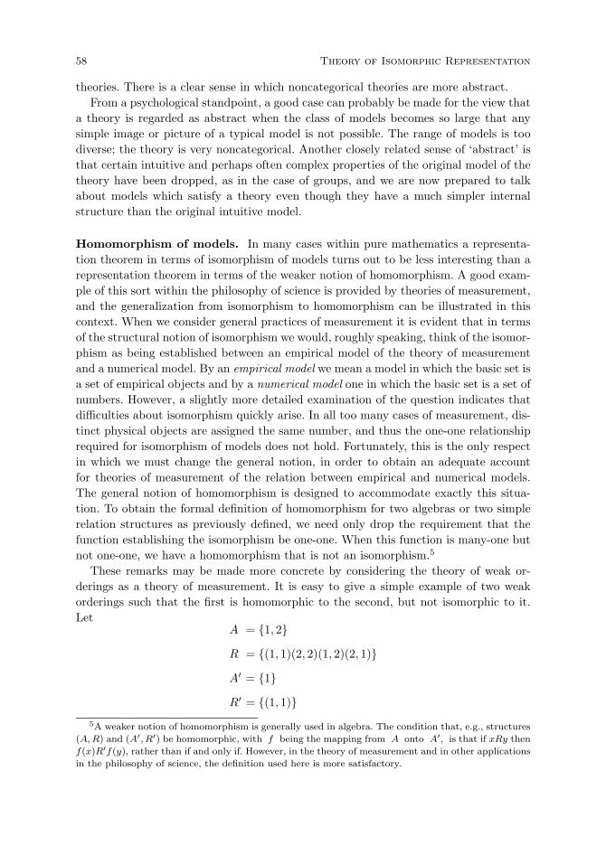
58 Theory of Isomorphic Representation

theories. There is a clear sense in which noncategorical theories are more abstract.From a psychological standpoint, a good case can probably be made for the view that

a theory is regarded as abstract when the class of models becomes so large that anysimple image or picture of a typical model is not possible. The range of models is toodiverse; the theory is very noncategorical. Another closely related sense of ‘abstract’ isthat certain intuitive and perhaps often complex properties of the original model of thetheory have been dropped, as in the case of groups, and we are now prepared to talkabout models which satisfy a theory even though they have a much simpler internalstructure than the original intuitive model.

Homomorphism of models. In many cases within pure mathematics a representa-tion theorem in terms of isomorphism of models turns out to be less interesting than arepresentation theorem in terms of the weaker notion of homomorphism. A good exam-ple of this sort within the philosophy of science is provided by theories of measurement,and the generalization from isomorphism to homomorphism can be illustrated in thiscontext. When we consider general practices of measurement it is evident that in termsof the structural notion of isomorphism we would, roughly speaking, think of the isomor-phism as being established between an empirical model of the theory of measurementand a numerical model. By an empirical model we mean a model in which the basic set isa set of empirical objects and by a numerical model one in which the basic set is a set ofnumbers. However, a slightly more detailed examination of the question indicates thatdifficulties about isomorphism quickly arise. In all too many cases of measurement, dis-tinct physical objects are assigned the same number, and thus the one-one relationshiprequired for isomorphism of models does not hold. Fortunately, this is the only respectin which we must change the general notion, in order to obtain an adequate accountfor theories of measurement of the relation between empirical and numerical models.The general notion of homomorphism is designed to accommodate exactly this situa-tion. To obtain the formal definition of homomorphism for two algebras or two simplerelation structures as previously defined, we need only drop the requirement that thefunction establishing the isomorphism be one-one. When this function is many-one butnot one-one, we have a homomorphism that is not an isomorphism.5

These remarks may be made more concrete by considering the theory of weak or-derings as a theory of measurement. It is easy to give a simple example of two weakorderings such that the first is homomorphic to the second, but not isomorphic to it.Let

A = 1, 2

R = (1, 1)(2, 2)(1, 2)(2, 1)

A′ = 1

R′ = (1, 1)5A weaker notion of homomorphism is generally used in algebra. The condition that, e.g., structures

(A, R) and (A′, R′) be homomorphic, with f being the mapping from A onto A′, is that if xRy then

f(x)R′f(y), rather than if and only if. However, in the theory of measurement and in other applications

in the philosophy of science, the definition used here is more satisfactory.

3.3 Representation Theorems 59

andf(1) = 1

f(2) = 1.From these definitions it is at once obvious that the weak ordering A= (A,R) is homo-morphic under the function f to the weak ordering A′= (A′, R′). The point is that wehave

1 R 2 if and only if f(1) R′ f(2),

as well as2 R 1 if and only if f(2) R′ f(1),

and both these equivalences hold just because

f(1) = f(2) = 1.

On the other hand, it is also clear simply on the basis of cardinality considerations thatA is not isomorphic to A′, because the set A has two elements and the set A′ has oneelement. It is also evident that A′ is not homomorphic to A. This also follows fromcardinality considerations, for there is no function whose domain is the set A′ andwhose range is the set A. As this example illustrates, the relation of homomorphismbetween models of a theory is not an equivalence relation; it is reflexive and transitive,but not symmetric.

By a numerical weak ordering I shall mean a weak ordering A = (A,≤) where A isa set of numbers. The selection of the numerical relation ≤ to represent the relation R

in a weak ordering is arbitrary, in the sense that the numerical relation ≥ could just aswell have been chosen, but it is slightly more natural to use ≤ if there is a first elementbut not a last one, as is the case for the set of natural numbers. However, choice of one ofthe two relations ≤ or ≥ is the only intuitively sound possibility. The following theoremprovides a homomorphic numerical representation theorem for finite weak orderings,and thus makes the theory of finite weak orderings a theory of measurement, becauseof its numerical representation.

THEOREM 1. Every finite weak ordering is homomorphic to a numerical weak order-ing.6

6Proof of Theorem 1. Let A = (A,) be a finite weak ordering. Probably the simplest approach

is first to form equivalence classes of objects in A, with respect to the obvious equivalence relation ≈defined in terms of :

a ≈ b if and only if a b & b a.

Thus, using the standard notation ‘[a]’ for equivalence classes, i.e.,

[a] = b : b ∈ A & a ≈ b,we first order the equivalence classes according to . Explicitly, we define

[a] ∗ [b] if and only if a b.

It is straightforward to prove that ∗ is reflexive, antisymmetrical, transitive, and connected in the

set A/ ≈ of equivalence classes, or, in other words, that it is a simple ordering of A/ ≈. By hypothesis

A is a finite set, and so necessarily A/ ≈ is finite. Let [a1] be the first element of A/ ≈ under the

ordering ∗, [a2] the second, . . . and [an] the last element. Consider now the numerical function g

defined on A/ ≈, defined as follows:

g([ai]) = i for i = 1, ..., n.

60 Theory of Isomorphic Representation

Theorem 1 was restricted to finite weak orderings for good reason; it is false if thisrestriction is removed. The classic counterexample is the lexicographical ordering of theplane. Let A be the set of all ordered pairs of real numbers, and let the relation bedefined by the equivalence (x1, x2) (y1, y2) if and only if x1 < y1, or x1 = y1 andx2 ≤ y2. Suppose that there exists a real-valued function f satisfying the equivalence:

f(x1, x2) ≤ f(y1, y2) if and only if (x1, x2) (y1, y2). (1)

We fix x2 and y2 with x2 < y2 and define for each x1:

f ′(x1) = f(x1, x2)

f ′′(x1) = f(x1, y2).

In terms of these functions we define the following function g from real numbers tointervals:

g(x1) = [f ′(x1), f ′′(x1)].

On the assumption that the ordering is lexicographic, g must be one-one since twodistinct numbers are mapped into two disjoint intervals. For instance, if x1 > x′1 thenf ′(x1) = f(x1, x2) > f(x′1, y2) = f ′′(x′1). But it is well known that there can be noone-one correspondence between the uncountable set of real numbers and the countableset of nondegenerate disjoint intervals. Thus no such function g can exist, and a fortiorithere can be no function f satisfying (1) for the lexicographic ordering.

The remarks earlier about models of arbitrarily large cardinality of first-order theo-ries also provide a proof that the restriction to finite weak orderings in Theorem 1 isnecessary. In the preceding section, one advantage of formulating theories within a set-theoretical framework was brought out in our consideration of the axioms that must beadded to those for a weak ordering in order to guarantee that an infinite weak orderingis homomorphic to a numerical weak ordering. It was stated at that time that the neces-sary and sufficient conditions adequate to guarantee this result had no simple first-orderstatement. The reason for the difficulty of formulating the necessary conditions withina first-order framework is the need to quantify over infinite subsets of the basic set A

of the weak ordering.In order to state the desired theorem one preliminary notion is needed. Let A =

(A,) be a simple relation structure, and let B be a subset of A. Define the strictordering relation ≺ in terms of by the equivalence

a ≺ b if and only if a b & not b a.

Then we say that B is -order-dense in A if and only if for every a and b in A

and not in B such that a ≺ b there is a c in B such that a c and c b. Notethat the denumerable set of rational numbers is order-dense in the nondenumerable setof all real numbers with respect to the natural numerical ordering ≤. This relationship

Then g establishes an isomorphism between the ordering A/≈= (A/≈,∗) and the numerical ordering

N = (N,≤), where N is the set of first n positive integers. (The details of this part of the proof are

tedious but obvious.) We then define the numerical function f on A, for every b in A, by:

f(b) = i if and only if b ∈ [ai],

i.e., if b is in the ith equivalence class under the ordering ∗. The function f establishes a

homomorphism between A and N, as desired.

3.3 Representation Theorems 61

between the denumerable rational numbers and all real numbers is just the one that isnecessary and sufficient for the existence of a homomorphism between an infinite anda numerical weak ordering. A minor complication arises in applying the denumerabilitycondition, namely, the elements of the order-dense subset must not be equivalent. Thisadditional condition is made precise in the statement of the theorem.

THEOREM 2. Let A = (A,) be an infinite weak ordering. Then a necessary andsufficient condition that A be homomorphic to a numerical weak ordering is that thereis a denumerable subset B of A such that (i) B is -order-dense in A and (ii) notwo elements of B stand in the relation ≈.7

7Proof of Theorem 2. The proof is related to the classical ordinal characterization of the continuum

by Cantor (1895). We do not give all details here, but sketch the main outlines; for some additional

details and related theorems, see Sierpenski (1958, Ch. 11).

To prove the sufficiency of the condition, let B be a denumerable subset with properties (i) and (ii).

Moreover, if A has end points relative to the ordering we may without loss of generality include them

in B. First, we know that there exists a real-valued function f on B, establishing that B = (B,) is

homomorphic to a numerical weak ordering, just because B is denumerable (for proof of this see, e.g.,

Suppes and Zinnes, 1963, Theorem 6). Now by the -order-dense condition on B, each element b of

A that is not in B defines a cut in B, i.e., the partition of B into two sets, X = a : a ∈ B & a band Z = c : c ∈ B & b c. Let

r1 = g.l.b. f(a)

a ∈ X

andr2 = l.u.b. f(c).

c ∈ Z

We then extend f to b by defining

f(b) =r1 + r2

2.

It is easy to show that the function f thus extended from B to A establishes the homomorphism

of A to a numerical ordering. For example, if a1 and a2 are in A but not in B, then if a1 a2,

there is a c in B such that a1 c a2 and thus

f(a1) ≤ f(c) ≤ f(a2).

The remaining details of this part of the argument may be supplied by the reader.

To prove the necessity of (i) and (ii), we assume we have a function f establishing that A is

homomorphic to a numerical ordering. The set of nonempty intervals Ii of the real numbers with

rational end points is a denumerable set, because of the denumerability of the rational numbers. We

next construct corresponding intervals Ji of A by taking the inverse image under f of each interval

Ii. From each Ji that is not empty we select an element ai. Since the set of intervals is denumerable,

the set X of elements ai of A is denumerable. Secondly, let Re be the set of real numbers r such

that for some b in A, f(b) = r and

f(b)− l.u.b.f(a) > 0

a ∈ Y

where

Y = a : a ∈ A & a b.Because the set Re of real numbers defines a set of nonoverlapping intervals of real numbers, it is at

most denumerable (of course, Re can be, and in some cases would be, empty). Let X′ be the inverse

image under f of Re. Then X ∪X′ is denumerable. To show that X ∪X′ is order-dense in A, let c1and c2 be two elements of A but not in X ∪ X′ such that c1 ≺ c2. Now if there are no elements

of A between c1 and c2 then c1 is in X′, contrary to hypothesis. On the other hand, if there are

elements between c1 and c2 then at least one, say d, will be such that f(d) lies in an interval with

rational end points which is nested in the interval [f(c1), f(c2)], and thus, X ∪ X′ is order-dense in

A. This completes the proof.

62 Theory of Isomorphic Representation

It has already been remarked that there is no direct way to formulate the existenceof the denumerable set B, as required in Theorem 2, within first-order logic. Perhapsa still more obvious point, but one that has not been sufficiently recognized within thephilosophy of science, is that the proof of Theorem 2 uses a great deal more mathematicalapparatus than elementary logic. The restriction of the discussion of theoretical issuesin the philosophy of science to the framework of first-order logic has too often meanta restriction of the extent to which the discussion could come into contact with otherthan highly simplified scientific theories especially constructed for the purpose at hand.An advantage of the set-theoretical formulation of theories is that all the necessarymathematical tools are immediately available for both the formulation of the theoryand the deductive analysis of the structure of its models.

Embedding of models. We have seen that the notion of two models being homo-morphic is a generalization of the notion of two models being isomorphic. A still moregeneral and therefore weaker relation between models is that of one model being embed-ded in another. To prove an embedding theorem for a theory is to prove that there is aninteresting class B of models such that every model of the theory is isomorphic, or atleast homomorphic, to a submodel belonging to B. The exact definition of submodelwill vary slightly from one theory to another depending on the set-theoretical characterof its models. For example, if A = (A, , e,−1 ) is an algebra as defined above, thenan algebra A′ = (A′, ′, e′,−1′

) is a subalgebra of A if A′ is a subset of A, ′ isthe operation restricted to A′ (i.e., ′ = ∩ (A′ × A′), e′ = e, and −1′

is theoperation −1 restricted to A′. In the case of simple relation structures the definitionis still simpler. Let A = (A,R) and A′ = (A′, R′) be two such structures. Then A′ isa submodel of A if A′ is a subset of A and R′ is the relation R restricted to A′,i.e., R′ = R ∩ (A′ ×A′).

Theorem 1 could have been formulated as an embedding theorem along the followinglines. Let Re be the set of real numbers. Then it is apparent at once that (Re,≤)is a numerical weak ordering as defined earlier, and every finite weak ordering can behomomorphically embedded in (Re,≤), i.e., is homomorphic to a submodel of (Re,≤).

At this point I close the general discussion of models and theories.8 The next twosections of this chapter are devoted to examples of representation theorems, the firstfor elementary theories of measurement, and the next the important representation ofany computable function by a program for an abstract universal computer. The sectionfollowing these two, the final one of this chapter, returns to a more general topic, in

8I do add as a final general remark in this footnote that the language of a representation theorem

often does not make explicit the nature of the isomorphism, but instead familiar idioms of a particular

discipline are used. Here are two examples of what I mean.

(i) “The center of mass of a system of particles moves like a particle that has mass equal to the

mass of the system . . . ” instead of “The center of mass of a system of particles is in its motion

isomorphic to the motion of a one-particle system that has mass . . . ” (Theorem 4 of Section 7.1)

(ii) “The four observables satisfy the Bell inequalities if and only if they have a joint probability

distribution”, instead of “The given six pairwise distributions of the four observables can be

isomorphically embedded in a common joint distribution of the four observables”. (Theorem 6

of Section 7.2)

3.4 Elementary Measurement Structures 63

particular, views on the nature of mental representation, especially with respect toquestions of isomorphism.

3.4 Representation of Elementary Measurement Structures

In this section I consider some of the simplest nontrivial examples of measurementstructures. The basic sets of objects or stimuli will in all cases be finite, and the adequacyof the elementary axioms for various structures depends heavily on this finiteness. Inaddition to their finiteness, the distinguishing characteristic of the structures consideredis that the objects are equally spaced in an appropriate sense along the continuum, so tospeak, of the property being measured. The restrictions of finiteness and equal spacingenormously simplify the mathematics of measurement, but it is fortunately not the casethat the simplification is accompanied by a total separation from realistic empiricalapplications. Finiteness and equal spacing are characteristic properties of many standardscales, for example, the ordinary ruler, the set of standard weights used with an equal-arm balance in the laboratory or shop, or almost any of the familiar gauges for measuringpressure, temperature, or volume.

Four kinds of such structures, and their representations, are dealt with. Each of themcorresponds to a more general set of structures analyzed in the comprehensive treatise ofKrantz, Luce, Suppes and Tversky (1971). The four kinds of structures are for extensive,difference, bisection, and conjoint measurement. The analysis given here is taken fromSuppes (1972).

Extensive measurement. The distinction between extensive and intensive propertiesor magnitudes is a very old one in the history of science and philosophy. Extensivemagnitudes are ones that can be added; e.g., mass and length are extensive magnitudesor quantities. Intensive magnitudes, in contrast, cannot be added, even though they canbe measured. Two volumes of gas, e.g., with the same temperature, do not combineto form a gas with twice the temperature. It has been claimed by some theorists, e.g.,Campbell (1920, l928), that fundamental measurement of intensive magnitudes is notpossible. The negative arguments of Campbell and others are not at all persuasive, andmany examples of measurement structures provide a concrete refutation of Campbell’sthesis, including those given later in this section.

I develop the axioms of extensive measurement in this section with three specificinterpretations in mind. One is for the measurement of mass on an equal-arm balance,one is for the measurement of length of rigid rods, and one is for the measurement ofsubjective probabilities.9 Other interpretations are certainly possible, but I shall restrictdetailed remarks to these three.

From a formal standpoint the basic structures are triples 〈Ω,F ,〉 where Ω is anonempty set, F is a family of subsets of Ω and the relation is a binary relation onF . By using subsets of Ω as objects, we avoid the need for a separate primitive conceptof concatenation. As a general structural condition, it shall be required that F be an

9Because of the extensive use of this probability interpretation in Chapter 5, I adopt below the

standard notation ‘Ω’ for the set of possible outcomes of a probability space as the general notation for

extensive measurement in this section.

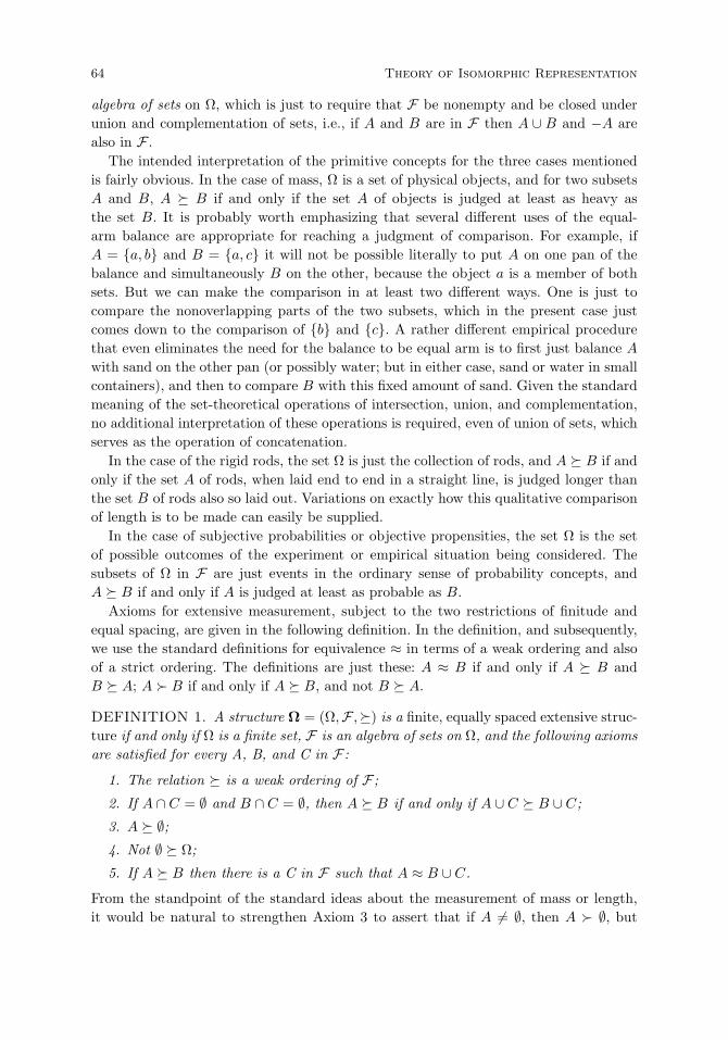
64 Theory of Isomorphic Representation

algebra of sets on Ω, which is just to require that F be nonempty and be closed underunion and complementation of sets, i.e., if A and B are in F then A ∪ B and −A arealso in F .

The intended interpretation of the primitive concepts for the three cases mentionedis fairly obvious. In the case of mass, Ω is a set of physical objects, and for two subsetsA and B, A B if and only if the set A of objects is judged at least as heavy asthe set B. It is probably worth emphasizing that several different uses of the equal-arm balance are appropriate for reaching a judgment of comparison. For example, ifA = a, b and B = a, c it will not be possible literally to put A on one pan of thebalance and simultaneously B on the other, because the object a is a member of bothsets. But we can make the comparison in at least two different ways. One is just tocompare the nonoverlapping parts of the two subsets, which in the present case justcomes down to the comparison of b and c. A rather different empirical procedurethat even eliminates the need for the balance to be equal arm is to first just balance Awith sand on the other pan (or possibly water; but in either case, sand or water in smallcontainers), and then to compare B with this fixed amount of sand. Given the standardmeaning of the set-theoretical operations of intersection, union, and complementation,no additional interpretation of these operations is required, even of union of sets, whichserves as the operation of concatenation.

In the case of the rigid rods, the set Ω is just the collection of rods, and A B if andonly if the set A of rods, when laid end to end in a straight line, is judged longer thanthe set B of rods also so laid out. Variations on exactly how this qualitative comparisonof length is to be made can easily be supplied.

In the case of subjective probabilities or objective propensities, the set Ω is the setof possible outcomes of the experiment or empirical situation being considered. Thesubsets of Ω in F are just events in the ordinary sense of probability concepts, andA B if and only if A is judged at least as probable as B.

Axioms for extensive measurement, subject to the two restrictions of finitude andequal spacing, are given in the following definition. In the definition, and subsequently,we use the standard definitions for equivalence ≈ in terms of a weak ordering and alsoof a strict ordering. The definitions are just these: A ≈ B if and only if A B andB A; A B if and only if A B, and not B A.

DEFINITION 1. A structure Ω = (Ω,F ,) is a finite, equally spaced extensive struc-ture if and only if Ω is a finite set, F is an algebra of sets on Ω, and the following axiomsare satisfied for every A, B, and C in F :

1. The relation is a weak ordering of F ;

2. If A ∩ C = ∅ and B ∩ C = ∅, then A B if and only if A ∪ C B ∪ C;

3. A ∅;4. Not ∅ Ω;

5. If A B then there is a C in F such that A ≈ B ∪ C.

From the standpoint of the standard ideas about the measurement of mass or length,it would be natural to strengthen Axiom 3 to assert that if A = ∅, then A ∅, but

3.4 Elementary Measurement Structures 65

because this is not required for the representation theorem and is unduly restrictive inthe case of probabilities, the weaker axiom seems more appropriate.

In stating the representation theorem, we use the notion of an additive measure µfrom F to the real numbers, i.e., a function µ such that, for any A and B in F ,

i. µ(∅) = 0,

ii. µ(A) ≥ 0,

iii. if A ∩B = ∅ then µ(A ∪B) = µ(A) + µ(B).

THEOREM 1. Let Ω = (Ω,F ,) be a finite, equally spaced extensive structure. Thenthere exists an additive measure µ such that for every A and B in F

µ(A) ≥ µ(B) if and only if A B.

Moreover, all singleton sets fall into at most two equivalence classes in F ; if there aretwo, one of these equivalence classes contains the empty set.

The proof of this theorem and some of the preceding discussion is to be found in Suppes(1969a, pp. 4–8).

It is important to point out that, for all three of the empirical interpretations ofthe primitive concepts used in the theory of extensive measurement characterized inDefinition 1, many important empirical procedures required for each interpretation aremissing. Students in elementary engineering or physics laboratories are taught manydetails about measuring mass, or weight if you will, with equal-arm balances, or lengthwith measuring rods or tapes. But even these details are inadequate as an accountof fundamental measurement. For such measurement must be used at an earlier stageto validate the weights or rods used by the students. The empirical procedures aremuch more elaborate for creating a set of standard weights, for example. The axiomsof Definition 1 come into play in creating ‘equal’ standard weights or checking that agiven set of standard weights does seem satisfactory. I say ‘seem’ deliberately, for thereis no natural end to the empirical investigation of standard measurement proceduresor instrumentation in physics or other sciences. The art of creating good measuringinstruments is a complicated and subtle one, certainly so at the frontier of many sciences.Such art, I have argued repeatedly, cannot be adequately described in a manual, butrequires an apprenticeship of training, many components of which are nonverbal. Canyou imagine, for example, becoming a good tennis player by just reading a book aboutit or listening to a few lectures? The same is true of any laboratory or manufacturingset of skills required to produce good measurement instruments.10

The elementary theory of measurement of different formal kinds set forth in thissection is an important formal aspect of measurement, but in no sense provides a fullfoundation, which, as is evident from what has been said thus far, I believe impossible toformalize fully in an explicit way. But exactly where to stop is not formally clear. We canbuild and then program a smart robot to do the job of producing standard measuringinstruments that satisfy to a good approximation the axioms of Definition 1. We can,of course, formalize the program the robot is given, even though I have reservations on

10Even Descartes recognized this, as can be seen in his description of how to cut lenses, i.e., make

lenses, in the Tenth Discourse of his Optics (1967/2001, pp. 162–173).

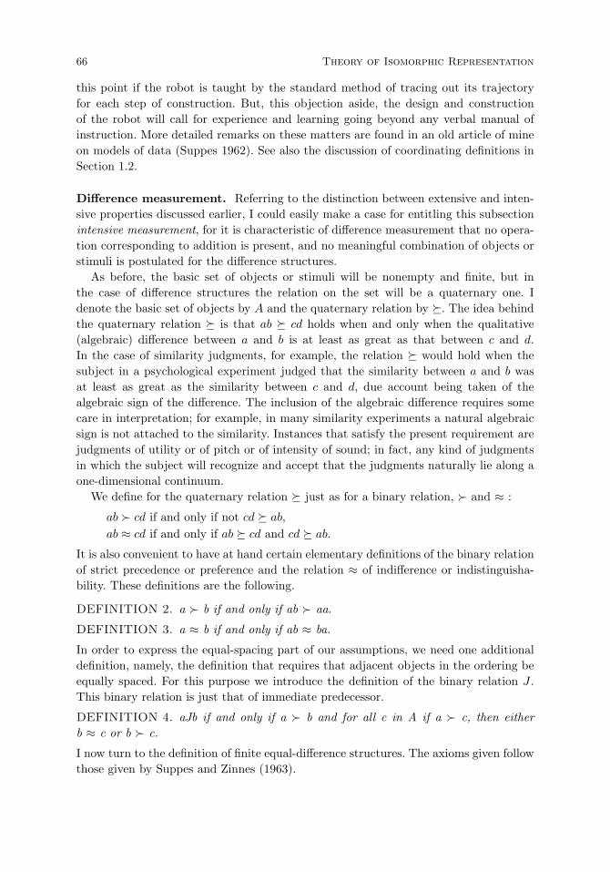
66 Theory of Isomorphic Representation

this point if the robot is taught by the standard method of tracing out its trajectoryfor each step of construction. But, this objection aside, the design and constructionof the robot will call for experience and learning going beyond any verbal manual ofinstruction. More detailed remarks on these matters are found in an old article of mineon models of data (Suppes 1962). See also the discussion of coordinating definitions inSection 1.2.

Difference measurement. Referring to the distinction between extensive and inten-sive properties discussed earlier, I could easily make a case for entitling this subsectionintensive measurement, for it is characteristic of difference measurement that no opera-tion corresponding to addition is present, and no meaningful combination of objects orstimuli is postulated for the difference structures.

As before, the basic set of objects or stimuli will be nonempty and finite, but inthe case of difference structures the relation on the set will be a quaternary one. Idenote the basic set of objects by A and the quaternary relation by . The idea behindthe quaternary relation is that ab cd holds when and only when the qualitative(algebraic) difference between a and b is at least as great as that between c and d.In the case of similarity judgments, for example, the relation would hold when thesubject in a psychological experiment judged that the similarity between a and b wasat least as great as the similarity between c and d, due account being taken of thealgebraic sign of the difference. The inclusion of the algebraic difference requires somecare in interpretation; for example, in many similarity experiments a natural algebraicsign is not attached to the similarity. Instances that satisfy the present requirement arejudgments of utility or of pitch or of intensity of sound; in fact, any kind of judgmentsin which the subject will recognize and accept that the judgments naturally lie along aone-dimensional continuum.

We define for the quaternary relation just as for a binary relation, and ≈ :

ab cd if and only if not cd ab,

ab ≈ cd if and only if ab cd and cd ab.

It is also convenient to have at hand certain elementary definitions of the binary relationof strict precedence or preference and the relation ≈ of indifference or indistinguisha-bility. These definitions are the following.

DEFINITION 2. a b if and only if ab aa.

DEFINITION 3. a ≈ b if and only if ab ≈ ba.

In order to express the equal-spacing part of our assumptions, we need one additionaldefinition, namely, the definition that requires that adjacent objects in the ordering beequally spaced. For this purpose we introduce the definition of the binary relation J .This binary relation is just that of immediate predecessor.

DEFINITION 4. aJb if and only if a b and for all c in A if a c, then eitherb ≈ c or b c.

I now turn to the definition of finite equal-difference structures. The axioms given followthose given by Suppes and Zinnes (1963).

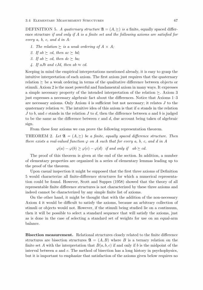
3.4 Elementary Measurement Structures 67

DEFINITION 5. A quaternary structure A = (A,) is a finite, equally spaced differ-ence structure if and only if A is a finite set and the following axioms are satisfied forevery a, b, c, and d in A:

1. The relation is a weak ordering of A × A;2. If ab cd, then ac bd;3. If ab cd, then dc ba;4. If aJb and cJd, then ab ≈ cd.

Keeping in mind the empirical interpretations mentioned already, it is easy to grasp theintuitive interpretation of each axiom. The first axiom just requires that the quaternaryrelation be a weak ordering in terms of the qualitative difference between objects orstimuli. Axiom 2 is the most powerful and fundamental axiom in many ways. It expressesa simple necessary property of the intended interpretation of the relation . Axiom 3just expresses a necessary algebraic fact about the differences. Notice that Axioms 1–3are necessary axioms. Only Axiom 4 is sufficient but not necessary; it relates J to thequaternary relation ≈. The intuitive idea of this axiom is that if a stands in the relationJ to b, and c stands in the relation J to d, then the difference between a and b is judgedto be the same as the difference between c and d, due account being taken of algebraicsign.

From these four axioms we can prove the following representation theorem.

THEOREM 2. Let A = (A,) be a finite, equally spaced difference structure. Thenthere exists a real-valued function ϕ on A such that for every a, b, c, and d in A

ϕ(a) − ϕ(b) ≥ ϕ(c) − ϕ(d) if and only if ab cd.

The proof of this theorem is given at the end of the section. In addition, a numberof elementary properties are organized in a series of elementary lemmas leading up tothe proof of the theorem.

Upon casual inspection it might be supposed that the first three axioms of Definition5 would characterize all finite-difference structures for which a numerical representa-tion could be found. However, Scott and Suppes (1958) showed that the theory of allrepresentable finite difference structures is not characterized by these three axioms andindeed cannot be characterized by any simple finite list of axioms.

On the other hand, it might be thought that with the addition of the non-necessaryAxiom 4 it would be difficult to satisfy the axioms, because an arbitrary collection ofstimuli or objects would not. However, if the stimuli being studied lie on a continuum,then it will be possible to select a standard sequence that will satisfy the axioms, justas is done in the case of selecting a standard set of weights for use on an equal-armbalance.

Bisection measurement. Relational structures closely related to the finite differencestructures are bisection structures A = (A,B) where B is a ternary relation on thefinite set A with the interpretation that B(a, b, c) if and only if b is the midpoint of theinterval between a and c. The method of bisection has a long history in psychophysics,but it is important to emphasize that satisfaction of the axioms given below requires no

68 Theory of Isomorphic Representation

assumptions of an underlying physical measurement. All we need is the intuitive ideaof a qualitative continuum, and even that is not needed for formal purposes. After thefundamental psychological measurement in terms of the method of bisection has beenmade, it is desirable when possible to find a computationally simple psychophysicalfunction relating physical measurements of the same magnitude to the psychologicalmeasurements.

The axioms given below for the method of bisection imply a number of checks thatshould be satisfied before it is asserted that a numerical representing function exists,but these checks have often been ignored in the experimental literature that reportsuse of the method of bisection. For the simplest set of axioms and definitions, we takeboth the bisection relation B and the ordering relation as primitive, but it is easy toeliminate by definition. We use the binary relation J as defined earlier (Definition 4).

DEFINITION 6. A structure A = (A,, B) is a finite, equally spaced bisection struc-ture if and only if the set A is finite and the following axioms are satisfied for every a,a′, b, c, and c′ in A:

1. The relation is a weak ordering of A;

2. If B(abc) and B(abc′) then c ≈ c′;

3. If B(abc) and B(a′bc) then a ≈ a′;

4. If B(abc) then a b and b c;

5. If aJb and bJc then B(abc);

6. If B(abc) and a′Ja and cJc′ then B(a′bc′).

The intuitive interpretation of the axioms is relatively transparent. The first axiom isalready familiar. Axioms 2 and 3 require uniqueness of the endpoints up to equivalence,which clearly separates bisection from betweenness. Axiom 4 relates the ternary bisec-tion relation and the binary ordering relation in a natural way, although it imposes aformal constraint on the bisection relation which would often be omitted. Inclusion ofthis order property as part of the relation B simplifies the axioms. Axiom 5 is a strongassumption of equal spacing, and Axiom 6 expresses an additional feature of this equalspacing. In view of the axioms given earlier for difference structures, it is somewhatsurprising that Axiom 6 can be shown to be independent of Axiom 5, but it is easy togive a model of Axioms 1-5 to show that this is the case. For we can take a model with

B(abc) if and only if aJb and bJc

and satisfy all of the first five axioms.The representation theorem assumes the following form.

THEOREM 3. Let A = (A,, B) be a finite equally spaced bisection structure. Thenthere exists a real-valued function ϕ defined on A such that for every a, b, and c in A

(i) ϕ(a) ≥ ϕ(b) if and only if a b,

(ii) 2ϕ(b) = ϕ(a) + ϕ(c) and ϕ(a) > ϕ(b) > ϕ(c) if and only if B(a, b, c).

The proof of this theorem is given at the end of the section.

3.4 Elementary Measurement Structures 69

Conjoint measurement. In many kinds of experimental or observational environ-ments, it turns out to be the case that the measurement of a single magnitude orproperty is not feasible or theoretically interesting. What is of interest is the jointmeasurement of several properties simultaneously. In this case we consider axioms foradditive conjoint measurement. The intended representation is that we use ordered pairsof objects or stimuli. The first members of the pairs are drawn from one set and conse-quently represent one kind of property or magnitude. The second members of the pairsare objects drawn from a second set representing a different magnitude or property.Given the ordered-pair structure, we shall only require judgments of whether or not onepair jointly has more of the ‘conjoined’ attribute than a second pair.

It is easy to give examples of interpretations for which this way of looking at orderedpairs is natural. Suppose we are asked to judge the capabilities of individuals to assumea position of leadership in an organization. What we are given about the individuals areevaluations of their technical knowledge on an ordinal scale and a charisma measure onan ordinal scale. Thus for each individual we can say how he compares on each scale withany other individual. The problem is to make judgments as between the individuals interms of their overall capabilities. The axioms given below indicate the kind of furtherconjoint ordinal conditions that are sufficient to guarantee finite equally spaced conjointmeasurement, where in this case the equal spacing is along each dimension.

As a second example, a pair (a, p) can represent a tone with intensity a and frequencyp, and the problem is to judge which of two tones sounds louder. Thus the subject judges(a, p) (b, q) if and only if tone (a, p) seems at least as loud as (b, q). Other examplesfrom disciplines as widely separated as economics and physics are easily given, and arediscussed in considerable detail in Krantz, Luce, Suppes and Tversky (1971, Ch. 6).

It is to be stressed that the additive representation sought in this section is a specialcase. Generalizations of additivity are discussed in the reference just cited. It is also tobe noted that the restriction in this section to ordered pairs rather than ordered n-tuplesis not essential.

Before turning to the axioms of (additive) conjoint measurement, we need a coupleof elementary definitions that permit us to define ordering relations on the individualcomponents. On the basis of the axioms on the ordering relation between pairs, weshall be able to prove that these ordering relations on the components are also weakorderings. In the following elementary definitions A1 is the set of first components andA2 the set of second components. Thus, when reference is made to an ordered pair (a, p),it is understood that a is in A1 and p is in A2.

DEFINITION 7. a b if and only if for all p in A2, (a, p) (b, p).

In terms of this relation we define a b and a ≈ b in the usual fashion. Also, a similardefinition is needed for the second component.

DEFINITION 8. p q if and only if for all a in A1, (a, p) (a, q).

We also use the notation already introduced for the relation on A1 × A2, namely,(a, p) (b, q) if and only if not (b, q) (a, p), and (a, p) ≈ (b, q) if and only if(a, p) (b, q) and (b, q) (a, p). The axioms for additive conjoint measurement inthe finite, equally spaced case are embodied in the following definition.

70 Theory of Isomorphic Representation

DEFINITION 9. A structure (A1, A2,) is a finite, equally spaced additive conjointstructure if and only if the sets A1 and A2 are finite and the following axioms aresatisfied for every a and b in A1 and every p and q in A2:

1. The relation is a weak ordering on A1 ×A2;

2. If (a, p) (b, p) then (a, q) (b, q);

3. If (a, p) (a, q) then (b, p) (b, q);

4. If aJb and pJq then (a, q) ≈ (b, p).

The intuitive content of the four axioms of Definition 9 is apparent, but requires somediscussion. Axiom 1, of course, is the familiar requirement of a weak ordering. Axioms2 and 3 express an independence condition of one component from the other. ThusAxiom 2 says that if the pair (a, p) is at least as great as the pair (b, p) then the samerelationship holds when p is replaced by any other member q of A2, and Axiom 3 saysthe same thing about the second component. Axiom 4 is sufficient but not necessary.It states the equal-spacing assumption, and corresponds closely to the correspondingaxiom for finite, equally spaced difference structures.

It might be thought the monotonicity assumption that if (a, p) ≈ (b, q) and a b,then q p, also needs to be assumed as an axiom, but as we show in the proof of therepresentation theorem, this additional assumption is not necessary: it can be provedfrom the first four axioms alone.

The statement of the representation theorem, to which we now turn, assumes exactlythe expected form. The only thing to note is that the two real-valued functions oneach component are welded together by the same unit. This is reflected by the commonchange of unit α in the theorem, but a different origin is permitted, as is shown inChapter 4 (Theorem 4.5.4).

THEOREM 4. Let (A1, A2,) be a finite, equally spaced additive conjoint structure.Then there exist real-valued functions ϕ1 and ϕ2 on A1 and A2 respectively such thatfor a and b in A1 and p and q in A2

ϕ1(a) + ϕ2(q) ≥ ϕ1(b) + ϕ2(p) if and only if (a, q) (b, p).

Proofs of Theorems 2–4.11

Proof of Theorem 2. Although the following elementary lemmas are not necessary togive a proof of Theorem 2, they are needed in a completely explicit discussion, and theirinclusion will perhaps be useful in organizing the reader’s thinking about differencestructures, which are not as familiar as extensive structures. Indications of the proofsof the elementary lemmas are given only in a few instances.

All of the lemmas refer to a fixed quaternary structure A = (A,), and the binaryrelations , ≈, and J defined earlier.

Lemma 1. The relation is asymmetric and transitive on A.

11The proofs given, which occupy the remainder of this section, may be omitted without loss of

continuity.

3.4 Elementary Measurement Structures 71

Lemma 2. The relation ≈ is reflexive, symmetric, and transitive on A.

Lemma 3. Exactly one of the following holds for any a and b in A: a b, b a,a ≈ b.

Lemma 4. If aJnb, then a b. (The proofs require use of induction on n in this andmost of the following lemmas.)12

Lemma 5. If a b, then there is a (positive integer) n such that aJnb.

Lemma 6. If aJnb and aJnc, then b ≈ c.

Lemma 7. If aJmb and bJnc, then aJm+nc.

Lemma 8. If aJmb and aJm+nc, then bJnc.

Lemma 9. If aJm+nb, then there is a c in A such that aJmc.

Lemma 10. If aJnb and cJnd, then ab ≈cd.

Lemma 11. If ab ≈ cd then either there is some n such that aJnb and cJnd, or thereis some n such that bJna and dJnc, or a ≈ b and c ≈ d.

We turn now to a sketch of the proof of Theorem 2. Let c∗ be the first element of Awith respect to the ordering .13 Define the numerical function ϕ on A as follows forevery a in A:14

ϕ(a) =

1 if a ≈ c∗,−n+ 1 if c∗Jna.

Then using the elementary lemmas we may prove:

(i) ϕ(a) > ϕ(b) if and only if a b;

(ii) ϕ(a) − ϕ(b) ≥ ϕ(d) − ϕ(e) if and only if ab de.

Proof of Theorem 3. We begin with the proof of two lemmas. The first corresponds toLemma 10 in the proof of Theorem 2 and the second to Lemma 11. It should be notedthat the lemmas of Theorem 2 which are just about the relations and J also applyhere.

Lemma 12. If aJnb and bJnc then B(abc).

Proof. We proceed by induction. For n = 1, we have Axiom 5. Suppose now thatour inductive hypothesis holds and we have

(1) aJn+1b and bJn+1c.

12In this and subsequent lemmas, as well as in the proof of Theorem 2 and later theorems, the

concept of the nth power of the binary relation J is repeatedly used. This concept is defined recursively:

aJ1b if and only if aJb; aJnb if and only if there is a c such that aJn−1c and cJb.13As the definition of ϕ(a) makes clear, c∗ is not unique as a first element. So it is better to say ‘let c∗

be a first element of A.’ So all members of A that are equivalent to c∗ in the ordering are first elements.

In more technical language they are members of the equivalence class [c∗] = a : a ≈ c∗& a ∈ A.14As the definition of ϕ(a) shows, it is actually more natural to use rather than throughout

this section, so that c∗ is a minimum rather than a maximal element of the ordering and then when

c∗Jna, ϕ(a) = n + 1. I have used here, however, because we used it in the treatise on measurement

(Krantz et al. 1971).

72 Theory of Isomorphic Representation

Then we know at once from properties of J that there are elements a′ and c′ in A suchthat

(2) aJa′ and a′Jnb,

(3) bJnc′ and c′Jc.

Whence by inductive hypothesis from (2) and (3)

(4) B(a′bc′),

and then from (2) and (3) again, as well as (4) and Axiom 6, we infer

B(abc)

as desired.Lemma 13. If B(abc) then there is an n such that aJnb and bJnc.

Proof. From the hypothesis of the theorem and Axiom 4 we have

a b and b c,

whence from familiar properties of J , there are m and n such that

aJmb and bJnc.

Suppose now m = n; for definiteness and without loss of generality we may supposethat m < n. Then there is d such that

bJmd,

whence by Lemma 1B(abd),

but by hypothesis B(abc), whence by Axiom 2

c ≈ d.

But then we havebJmc and bJnc,

which is impossible, and so we conclude m = n, as desired.Given Lemmas 1 and 2, the proof of the existence of a function ϕ such that

(i) ϕ(a) > ϕ(b) if and only if a b

and

(ii) ϕ(b) = 12 (ϕ(a) + ϕ(c)) and ϕ(a) > ϕ(b) > ϕ(c) if and only if B(a, b, c)

is similar to the proof of the corresponding part of Theorem 2 and need not be developedin detail.

Proof of Theorem 4. First of all, on the basis of Axioms 1–3 of Definition 9 the followingelementary lemmas about the ordering induced on the two components A1 and A2 areeasily proved.

Lemma 14. The relation ≈ on Ai, for i = 1, 2, is an equivalence relation, i.e., it isreflexive, symmetric, and transitive.

Lemma 15. The relation on Ai, for i = 1, 2, is a symmetric and transitive.

3.4 Elementary Measurement Structures 73

Lemma 16. For a and b in A1 exactly one of the following is true: a ≈ b, a b,b a. For p and q in A2, exactly one of the following is true: p ≈ q, p q, q p.

We next prove the two lemmas mentioned earlier in the discussion of the axioms ofDefinition 9.

Lemma 17. If (a, p) ≈ (b, q) and a b then q p.

Proof. Suppose it is not the case that q p. Then by Lemma 3 either p ≈ q orp q. If p ≈ q, then (a, p) ≈ (a, q), whence by transitivity and the hypothesis of thelemma, (b, q) ≈ (a, q), and thus b ≈ a, which contradicts Lemma 3 and the hypothesisthat a b. On the other hand, a contradiction also follows from the supposition of theother alternative, i.e., p q. For we have (a, p) (a, q), whence by familiar propertiesof weak orderings and the hypothesis of the lemma, (b, q) (a, q) and thus b a, whichagain contradicts Lemma 3 and the hypothesis that a b. Thus, we conclude that fromthe hypothesis of the lemma it follows that q p, as desired.

Lemma 18. If (a, p) ≈ (b, q) and p q then b a.

Proof. Identical in structure to that for Lemma 4.

We turn next to the proof of Theorem 4. The proof closely resembles that of Theorem2. Let a1 be a first element of A1 with respect to the ordering on A1, and let p1 bea first element of A2 with respect to the ordering on A2. Define, then, the numericalfunctions ϕ1 and ϕ2 on A1 and A2 as follows (for a in A1 and p in A2):

ϕ1(a) =

1 if a ≈ a1,

−n+ 1 if a1Jna,

ϕ2(p) =

1 if p ≈ p1,

−n+ 1 if p1Jnp.

As in the case of the proof of Theorem 2, it is easy to show:

ϕ1(a) > ϕ1(b) if and only if a b,

ϕ2(p) > ϕ2(q) if and only if p q.

Moreover, Lemmas 1–9 proved in preparation for the proof of Theorem 2 also hold inthe present setting, for they just depend on the binary relations on the components. Ofcourse, for each of these lemmas, there is, strictly speaking, now a pair of lemmas, onefor the ordering on each component.

Corresponding to Lemma 10 of this earlier list, we can prove by the same inductiveargument, using Axiom 4 of Definition 9 that if aJnb and pJnq then (a, q) ≈ (b, p).Second, we can prove the elementary fact that if (a, q) ≈ (b, p) then either (i) there issome n such that aJnb and pJnq, or (ii) there is some n such that bJna and qJnp, or(iii) a ≈ b and p ≈ q. From these results we prove then the fundamental result thatϕ1(a) + ϕ2(q) = ϕ1(b) + ϕ2(p) if and only if (a, q) ≈ (b, p), which completes the proofof Theorem 4.

74 Theory of Isomorphic Representation

3.5 Machine Representation of Partial Recursive Functions15

The representation of most mathematical objects as sets with some particular structureis rightly regarded as a great philosophical achievement in the foundations of math-ematics at the beginning of the twentieth century. In many ways an even deeper ac-complishment several decades later was the proof that seemingly different definitions ofcomputable functions all lead to the same class of functions. Here I restrict the formaldevelopments to showing that any partial recursive function (partial recursive being oneimportant formulation of computable) can be represented by a program of an unlimitedregister machine. Many other equivalent representations are known in the literature.

It is necessary to recognize that two computer programs that compute the samemathematical function can differ in many observable ways: the space or time needed forthe computation, the number of lines or characters in the programs, etc. As in a varietyof other representations considered in this and other chapters, structural isomorphismneed not imply, and usually does not imply, observational or computational equivalencein all respects.

Before giving a formal definition of effective calculability or partial recursiveness, letus consider some examples of functions which are effectively calculable.16 We may beginwith addition. The recursive definition of addition in terms of the successor function Sis given by the following pair of equations for the function f of addition. The recursionis on n.

f(0, n) = n

f(S(n),m) = S(f(n,m)).For example, in the usual notation for numerals,

S(0) = 1,

S(1) = 2,

etc., where S is the successor function. Then in a finite number of steps we can findthe answer to a sum such as f(3, 2), or 3 + 2.

f(3, 2) = S(f(2, 2))

= SS(f(1, 2))

= SSS(f(0, 2))

= SSS(2)

= SS(3)

= S(4)

= 5.15This rather technical section may be omitted without substanial loss of continuity, except for

Sections 8.2 and 8.3. The general reader may find it useful to look at the first two paragraphs, for the

clarification of the concept of being computable is one of the great twentieth-century achievements in

the foundations of mathematics.16The class of partial recursive functions was first characterized, but in different ways, by Church

(1936), Kleene (1936), Post (1936), Turing (1936), Markov (1951) and others in the same period.

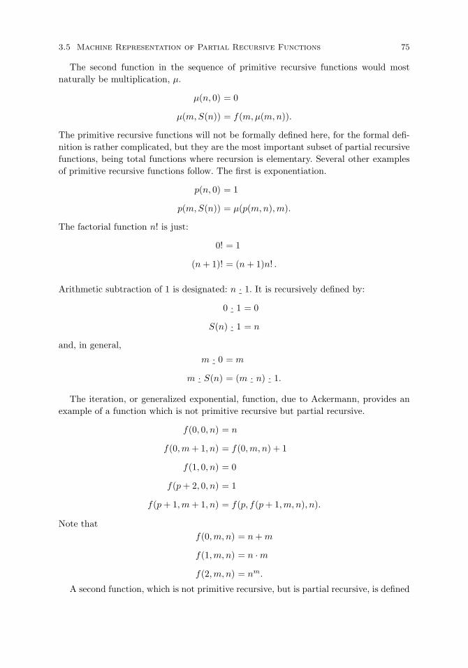
3.5 Machine Representation of Partial Recursive Functions 75

The second function in the sequence of primitive recursive functions would mostnaturally be multiplication, µ.

µ(n, 0) = 0

µ(m,S(n)) = f(m,µ(m,n)).

The primitive recursive functions will not be formally defined here, for the formal defi-nition is rather complicated, but they are the most important subset of partial recursivefunctions, being total functions where recursion is elementary. Several other examplesof primitive recursive functions follow. The first is exponentiation.

p(n, 0) = 1

p(m,S(n)) = µ(p(m,n),m).

The factorial function n! is just:

0! = 1

(n+ 1)! = (n+ 1)n! .

Arithmetic subtraction of 1 is designated: n · 1. It is recursively defined by:

0 · 1 = 0

S(n) · 1 = n

and, in general,

m · 0 = m

m · S(n) = (m · n) · 1.

The iteration, or generalized exponential, function, due to Ackermann, provides anexample of a function which is not primitive recursive but partial recursive.

f(0, 0, n) = n

f(0,m+ 1, n) = f(0,m, n) + 1

f(1, 0, n) = 0

f(p+ 2, 0, n) = 1

f(p+ 1,m+ 1, n) = f(p, f(p+ 1,m, n), n).

Note thatf(0,m, n) = n+m

f(1,m, n) = n ·m

f(2,m, n) = nm.

A second function, which is not primitive recursive, but is partial recursive, is defined

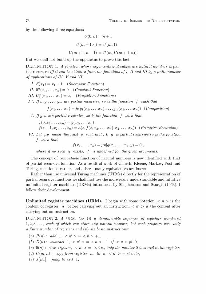
76 Theory of Isomorphic Representation

by the following three equations:

U (0, n) = n+ 1

U (m+ 1, 0) = U (m, 1)

U (m+ 1, n+ 1) = U (m,U (m+ 1, n)).

But we shall not build up the apparatus to prove this fact.

DEFINITION 1. A function whose arguments and values are natural numbers is par-tial recursive iff it can be obtained from the functions of I, II and III by a finite numberof applications of IV, V and VI:

I. S(x1) = x1 + 1 (Successor Function)II. 0n(x1, . . . , xn) = 0 (Constant Function)

III. Uni (x1, . . . , xn) = xi (Projection Functions)

IV. If h, g1, . . . , gm are partial recursive, so is the function f such that

f(x1, . . . , xn) = h(g1(x1, . . . , xn), . . . , gm(x1, . . . , xn)) (Composition)

V. If g, h are partial recursive, so is the function f such that

f(0, x2, . . . , xn) = g(x2, . . . , xn)f(z + 1, x2, . . . , xn) = h(z, f(z, x2, . . . , xn), x2, . . . , xn)) (Primitive Recursion)

VI. Let µy mean ‘the least y such that’. If g is partial recursive so is the functionf such that

f(x1, . . . , xn) = µy[g(x1, . . . , xn, y) = 0],

where if no such y exists, f is undefined for the given arguments.

The concept of computable function of natural numbers is now identified with thatof partial recursive function. As a result of work of Church, Kleene, Markov, Post andTuring, mentioned earlier, and others, many equivalences are known.

Rather than use universal Turing machines (UTMs) directly for the representation ofpartial recursive functions we shall first use the more easily understandable and intuitiveunlimited register machines (URMs) introduced by Shepherdson and Sturgis (1963). Ifollow their development.

Unlimited register machines (URM). I begin with some notation: < n > is thecontent of register n before carrying out an instruction; < n′ > is the content aftercarrying out an instruction.

DEFINITION 2. A URM has (i) a denumerable sequence of registers numbered1, 2, 3, . . . , each of which can store any natural number, but each program uses onlya finite number of registers and (ii) six basic instructions:

(a) P (n) : add 1, < n′ > = < n > +1,(b) D(n) : subtract 1, < n′ > = < n > −1 if < n > = 0,(c) 0(n) : clear register, < n′ > = 0, i.e., only the number 0 is stored in the register.(d) C(m,n) : copy from register m to n, < n′ > = < m >,(e) J [E1] : jump to exit 1,

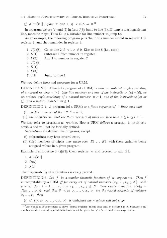
3.5 Machine Representation of Partial Recursive Functions 77

(f) J(m)[E1] : jump to exit 1 if < m > = 0.17

In programs we use (e) and (f) in form J[3]: jump to line (3). If jump is to a nonexistentline, machine stops. Thus E1 is a variable for line number to jump to.

As an example, the following program puts ‘half’ of a number stored in register 1 inregister 2, and the remainder in register 3.

1. J(1)[8] Go to line 2 if < 1 > = 0. Else to line 8 (i.e., stop)2. D(1) Subtract 1 from number in register 13. P (2) Add 1 to number in register 24. J(1)[8]5. D(1)6. P (3)7. J [1] Jump to line 1

We now define lines and programs for a URM.

DEFINITION 3. A line (of a program of a URM) is either an ordered couple consistingof a natural number n ≥ 1 (the line number) and one of the instructions (a) − (d), oran ordered triple consisting of a natural number n ≥ 1, one of the instructions (e) or(f), and a natural number m ≥ 1.

DEFINITION 4. A program (of a URM) is a finite sequence of l lines such that

(i) the first member of the ith line is i,(ii) the numbers m that are third members of lines are such that 1 ≤ m ≤ l + 1.

We also refer to programs as routines. How a URM follows a program is intuitivelyobvious and will not be formally defined.

Subroutines are defined like programs, except

(i) subroutines may have several exits,(ii) third members of triples may range over E1, . . . , Ek, with these variables being

assigned values in a given program.

Example of subroutine 0(n)[E1]: Clear register n and proceed to exit E1.

1. J(n)[E1]2. D(n)3. J [1]

The dispensability of subroutines is easily proved.

DEFINITION 5. Let f be a number-theoretic function of n arguments. Then f

is computable by a URM iff for every set of natural numbers x1, . . . , xn, y,N withy = xi for i = 1, . . . , n, and x1, . . . , xn, y ≤ N there exists a routine RN (y =f(x1, . . . , xn)) such that if < x1 >, . . . , < xn > are the initial contents of registersx1 . . . , xn then

(i) if f(< x1 >, . . . , < xn >) is undefined the machine will not stop;

17Note that it is convenient to have ‘empty register’ mean that only 0 is stored in it, because if no

number at all is stored, special definitions must be given for < n > −1 and other expressions.

78 Theory of Isomorphic Representation

(ii) if f(< x1 >, . . . , < xn >) is defined, the machine will stop with < y >, the finalcontent of register y, equal to f(< x1 >, . . . , < xn >), and with the final contentsof all registers 1, 2, . . . , N , except y, the same as initially.

Because the proof of the main theorem consists of writing subroutines for each of thesix schemata used to define the set of partial recursive functions, some more remarksabout subroutines may be useful.

From a logical standpoint, subroutines are similar to definitions in a theory. Themathematical development of set theory just in terms of the primitive concept of mem-bership would be not only intolerable but practically impossible. The same remarkapplies to programming. To write really complex programs in bare machine language isintolerable. From a formal standpoint the theory of definitions is thoroughly developed,and it is easy to give rules of definition that guarantee an absence of problems arisingfrom idiosyncrasies or unsuspected peculiarities in the definitions introduced. Good def-initions should satisfy the criteria of noncreativity and eliminability. The criterion ofnoncreativity requires that it not be possible to prove any theorem formulated in theoriginal notation only because of the introduction of the definition. Here is a simpleexample to illustrate the need for this criterion. We take as the single axiom of ourtheory just the axiom of associativity:

(1) x (y z) = (x y) z.We now introduce the ‘definition’ of the constant e:

(2) xoe = x.

From this definition, but not from the axioms above, we can prove

(∃y)(∀x)(x y = x),

and thus the proposed definition is unsatisfactory because it violates the criterion of non-creativity. Intuitively it is clear that (2) is unsatisfactory as a definition in conjunctionwith (1) because it adds conceptual content to the theory.

In similar fashion a subroutine must be noncreative. Any function that is computableby a program using the subroutine must be computable by a program that does not useit.

The criterion of eliminability demands that in all contexts a defined symbol be elim-inable in terms of previously defined or primitive symbols, and, of course, that anequivalence hold between the statement using the symbol and the corresponding state-ment from which the symbol is eliminated. (For a more detailed discussion of these twocriteria of definition, one reference is Suppes (1957/1999, Ch. 8.))

Here is an example of a pair of subroutines that do not satisfy the criterion of elim-inability.

01(n) : 02(n) :1. 02(n) 1. 01(n)2. P (n) 2. D(n)

In other words, subroutine 02(n) is defined in terms of 01(n), and 01(n) is definedin terms of 02(n), so that we have a vicious circle with no way of defining or writing aprogram for either 01(n) or 02(n) in terms of the six basic instructions. Circular sub-

3.5 Machine Representation of Partial Recursive Functions 79

routines, just like circular definitions, are prohibited by requiring that the subroutinesbe introduced in a fixed linear order, and the nth subroutine can use in its programonly basic instructions and the preceding n−1 subroutines. (As is apparent, this linearrequirement can be weakened.)

We turn now to the representation theorem.

THEOREM 1. (Machine Representation). A number-theoretic function is partial re-cursive iff it is computable by a URM.

Proof. The proof that functions computable by a URM are partial recursive is notdifficult: check that each line of a program causes a change in registers given by apartial recursive function and then show that the sequence of changes is partial recursivebecause of closure properties of the set of partial recursive functions.

The argument the other way is the interesting part, because of the great simplicityof instructions of a URM. The proof, due to Shepherdson and Sturgis (1963), is simplerthan the corresponding proof for Turing machines. It just consists of writing URMsubroutines for Schemata I-VI of Definition 1 that define partial recursive functions.

I. Subroutine RN (y = S(x))1. C(x, y)2. P (y)

II. Subroutine RN (y = 0n(x1, . . . , xn))1. 0(y)

III. Subroutine RN (y = Uni (x1, . . . , xn))

1. C(xi, y)IV. Composition RN (y = f(x1, . . . , xn)) where we use subroutines for gi, h to define

f : f(x1, . . . , xn) = h(g1(x1, . . . , xm), . . . , gm(x1, . . . , xn))1. RN+1(N + 1 = g1(x1, . . . , xn))

...m. RN+m(N +m = gm(x1, . . . , xn))

m + 1. RN+m(y = h(N + 1, . . . , N +m)).VI. Subroutine for RN (y = f(x1, . . . , xn)) where we use subroutine for g to define f

by VI: f(x1, . . . , xn) = µy[g(x1, . . . , xn, y) = 0]1. 0(y)2. RN+1(N + 1 = g(x1, . . . , xn, y))3. J(N + 1)[6]4. P (y)5. J [2]

Note that after instruction 1, < y > = 0. If < N + 1 > = 0 (step 3), then we are doneand go to nonexistent line 6. If not, we augment < y > by 1 and go back to line 2 totry again for the least y.

Schema V is somewhat more complicated. There are two matters of notation to dealwith. First, we now only number necessary lines–subroutines or jumps. Second, we usea notation for iteration of instructions. If I is a single-exit instruction or subroutine

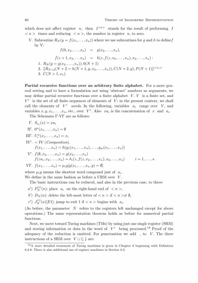
80 Theory of Isomorphic Representation

which does not affect register n, then I<n> stands for the result of performing I

< n > times and reducing < n >, the number in register n, to zero.

V. Subroutine RN (y = f(x1, . . . , xn)) where we use subroutines for g and h to definefby V:

f(0, x2, . . . , xn) = g(x2, . . . , xn),

f(z + 1, x2, . . . xn) = h(z, f(z, x2, . . . , xn), x2, . . . , xn) :1. RN (y = g(x2, . . . , xn)), 0(N + 1)2. RN+2(N + 2 = h(N + 1, y, x2, . . . , xn)), C(N + 2, y), P (N + 1)<x1>

3. C(N + 1, x1).

Partial recursive functions over an arbitrary finite alphabet. For a more gen-eral setting and to have a formulation not using ‘abstract’ numbers as arguments, wemay define partial recursive functions over a finite alphabet V . V is a finite set, andV ∗ is the set of all finite sequences of elements of V ; in the present context, we shallcall the elements of V ∗ words. In the following, variables ai range over V , andvariables x, y, x1, . . . , xn, etc., over V ∗. Also xai is the concatenation of x and ai.

The Schemata I′-VI′ are as follows:

I′. Sai(x) = xai

II′. 0n(x1, . . . , xn) = ∅III′. Un

i (x1, . . . , xn) = xi

IV′. = IV (Composition).f(x1, . . . , xn) = h(g1(x1, . . . , xn), . . . , gm(x1, . . . , xn))

V′. f(∅, x2, . . . , xn) = g(x2, . . . , xn)f(zai, x2, . . . , xn) = hi(z, f(z, x2, . . . , xn), x2, . . . , xn) i = 1, . . . , s.

VI′. f(x1, . . . , xn) = µiy[g(x1, . . . , xn, y) = ∅]

where µiy means the shortest word composed just of ai.We define in the same fashion as before a URM over V .

The basic instructions can be reduced, and also in the previous case, to three:

a′) P (i)N (n): place ai on the right-hand end of < n >,

b′) DN (n): delete the left-most letter of < n > if < n >= ∅,

c′) J (i)N (n)[E1]: jump to exit 1 if < n > begins with ai.

(As before, the parameter N refers to the registers left unchanged except for aboveoperations.) The same representation theorem holds as before for numerical partialfunctions.

Next, we move toward Turing machines (TMs) by using just one single register (SRM)and storing information or data in the word of V ∗ being processed.18 Proof of theadequacy of the reduction is omitted. For punctuation we add , to V . The threeinstructions of a SRM over V ∪ , are:

18A more detailed treatment of Turing machines is given in Chapter 8 beginning with Definition

8.2.9. There is also additional use of register machines in Section 8.3.

3.6 Philosophical Views of Mental Representations 81

a”) P (i) : x → xai (add ai to right-hand end of x)

b”) D : aix → x (delete first letter)

c”) J (i)[E1]: jump to exit 1 if x begins with ai.

Let V = 1 and take , as 0. Then the results for a SRM show that any partialrecursive function of natural numbers is computable by a machine with a single one-waytape (on which x is printed), two tape symbols 0 and 1, and two heads, a reading headat the left and writing head at the right.

Many other detailed results about register machines are given in Shepherdson andSturgis (1963). For comparable detailed results on Turing machines there are manysources, e.g., Davis (1958), Rogers (1967) and at a more advanced level Soare (1987).

3.6 Philosophical Views of Mental Representations

Without attempting anything like a detailed and accurate account of the long andcomplicated history of the concept of mental representation in philosophy, it can beenlightening and relevant to review some of the standard conceptions and issues fromAristotle onward. The main point will not be to assess the correctness or to criticizethe adequacy of the analysis given, but to reflect on whether or not there is a notion ofisomorphism in the background, as reflected in such concepts as likeness or resemblance.Comment will also be made as to how such notions are tied to representations.

Aristotle. That the defining feature of sense perception is receiving the form of aphysical object is, in general terms, the view of perception for which Aristotle is mostfamous. As he works out the details it is not a bad view at all, even though it is quiteobvious from a modern viewpoint that it cannot be entirely correct.

The background of Aristotle’s discussion of perception and implicitly, therefore, ofmental representation, is his distinction between form and matter, which applies toobjects and phenomena of all kinds. For example, the form of an axe is different fromthe matter that receives that form. This distinction is also relative in the sense that,for example, the matter of a house can be made up of bricks, which, in turn, have theirown form and matter, of which they are made up. I defend the continued viability ofthis general concept of matter in Suppes (1974c).

Aristotle makes use of the distinction between form and matter in his theory ofperception. It is the role of the sense organ to have the potential to receive the form butnot the matter of a physical object, as described in this passage from the second bookof the De Anima:

We must understand as true generally of every sense (1) that sense is that which is

receptive of the form of sensible objects without the matter, just as the wax receives the

impression of the signet-ring without the iron or the gold, and receives the impression of

the gold or bronze, but not as gold or bronze; so in every case sense is affected by that

which has colour, or flavour, or sound, but by it, not qua having a particular identity,

but qua having a certain quality, and in virtue of its formula; (2) the sense organ in its

primary meaning is that in which this potentiality lies. (De Anima, 424a17–424a25)

So, if in perceiving the candle we receive exactly the form of the candle, but not the

82 Theory of Isomorphic Representation

matter, then we have a representation of the physical candle that is isomorphic to itin the mind, just because of the sameness of form. The relevant point here is that thenotion of the sameness of form corresponds very closely to the concept of isomorphismthat I have been arguing for as a central concept of representation. The concept of formcatches nicely that of isomorphism in the sense that the form does not thereby refer toall the properties of the candle, but only to the properties perceived by the various sensesof sight, touch, etc. This kind of restriction to the properties considered is, as alreadynoted in earlier discussions, characteristic of any workable notion of isomorphism.

Upon reading the above passage and my comments, someone might reflect that this isnot a very rich theory of the mental, but only of immediate sense perception. Aristotle,however, goes on to extend the same ideas about forms to the intellect. It is not possiblehere to discuss all the subtleties involved in his worked-out theory, but the followingpassage makes clear how the part of the soul that thinks and judges operates in the sameway with forms and, thus, the characteristic notion of isomorphism is again applicable:

Concerning that part of the soul (whether it is separable in extended space, or only in

thought) with which the soul knows and thinks, we have to consider what is its distin-

guishing characteristic, and how thinking comes about. If it is analogous to perceiving,

it must be either a process in which the soul is acted upon by what is thinkable, or

something else of a similar kind. This part, then, must (although impassive) be receptive

of the form of an object, i.e., must be potentially the same as its object, although not

identical with it: as the sensitive is to the sensible, so must mind be to the thinkable.

. . . Hence the mind, too, can have no characteristic except its capacity to receive. That

part of the soul, then, which we call mind (by mind I mean that part by which the soul

thinks and forms judgements) has no actual existence until it thinks. So it is unreason-

able to suppose that it is mixed with the body; for in that case it would become somehow

qualitative, e.g., hot or cold, or would even have some organ, as the sensitive faculty has;

but in fact it has none. It has been well said that the soul is the place of forms, except

that this does not apply to the soul as a whole, but only in its thinking capacity, and

the forms occupy it not actually but only potentially. (De Anima, 429a10-18, a23-30)

It is a definite part of Aristotelian thought that the forms are the focus of the con-templation of the intellect but do not exist separate from individual bodies. There is noseparate universe of Platonic forms. A very clear statement on this Aristotelian view ismade by St. Thomas Aquinas in the following passage.

I say this, because some held that the form alone belongs to the species, while matter

is part of the individual, and not of the species. This cannot be true, for to the nature

of the species belongs what the definition signifies, and in natural things the definition

does not signify the form only, but the form and the matter. Hence, in natural things

the matter is part of the species; not, indeed, signate matter, which is the principle of

individuation, but common matter. For just as it belongs to the nature of this particular

man to be composed of this soul, of this flesh, and of these bones, so it belongs to the

nature of man to be composed of soul, flesh, and bones; for whatever belongs in common

to the substance of all the individuals contained under a given species must belong also

to the substance of the species. (Summa Theologica, I, Q.75. Art. 4)19

19Translation taken from Basic Writings of Saint Thomas Aquinas (1944).

3.6 Philosophical Views of Mental Representations 83

Descartes. Without holding to all of the psychological machinery introduced by Aris-totle and developed further by Aquinas, Descartes still holds to the scholastic view thatthe visual perception of an object reflects the form of the object. This comes from thephysical fact that ‘the light reflected from its body depicts two images of it, one in eachof our eyes.’ So he is here using natural facts about physiological optics to end up withan account of images or forms in the soul. Here is the best passage I know of in thePassions of the Soul.

Thus, for example, if we see some animal approach us, the light reflected from its body

depicts two images of it, one in each of our eyes, and these two images form two others,

by means of the optic nerves, in the interior surface of the brain which faces its cavities;

then from there, by means of the animal spirits with which its cavities are filled, these

images so radiate towards the little gland which is surrounded by these spirits, that the

movement which forms each point of one of the images tends towards the same point of

the gland towards which tends the movement which forms the point of the other image,

which represents the same part of this animal. By this means the two images which are

in the brain form but one upon the gland, which, acting immediately upon the soul,

causes it to see the form of this animal. . . . (Article XXXV)

Descartes, in general, certainly rejects much scholastic doctrine, but in his psychologyof vision, very much stays with the natural idea of the soul or the mind having imagesthat reflect just the form of the object seen. This is the core of the Aristotelian doctrineof perception and remains constant in Descartes in spite of many other changes. It isradically changed by Hume.

Hume. On various grounds, in the Treatise of Human Nature (1739/1951), Humeargues vigorously against any direct concept of mental representation between objectsin the external world and what is in the mind. He has many things to say about thesematters. I only will quote and comment upon some key passages.

The first point to emphasize is that the mechanism of the mind for Hume is asso-ciation, and he proudly, and in many ways, rightly, thinks of association as playingthe role in the theory of the mind that gravitation plays in Newton’s system of theworld. In other words, the causal principle, beyond which it is not possible to seek forexplanation, is, in the case of the problem of falling bodies on Earth and of motion ofthe planets in the heavens, gravitational attraction between bodies. In the mind themechanism is that of association, both between impressions, which in many cases canbe identified with perceptions, and ideas, which are always derived from impressions.There are three characteristics of impressions and ideas which give rise to associations.They are resemblance, contiguity in time or place, and cause and effect. It is impor-tant to emphasize that for Hume, the only characteristic giving rise to associations ofimpression is that of resemblance. So that all inferences, for example, about cause andeffect, must be between association of ideas. After naming these three properties, Humedefends resemblance:

The qualities, from which this association arises, and by which the mind is after this man-

ner convey’d from one idea to another, are three, viz. RESEMBLANCE, CONTIGUITY

in time or place, and CAUSE and EFFECT. . . .

84 Theory of Isomorphic Representation

. . . I believe it will not be very necessary to prove, that these qualities produce an asso-

ciation among ideas, and upon the appearance of one idea naturally introduce another.

’Tis plain, that in the course of our thinking, and in the constant revolution of our ideas,

our imagination runs easily from one idea to any other that resembles it, and that this

quality alone is to the fancy a sufficient bond and association. (Treatise, p. 11)

The rest of the paragraph makes a similar defense of contiguity and signals the moreextensive discussion of cause and effect later.

The important point relevant to the discussion here is the pride of place that Humegives to resemblance, since only it is a quality, as he puts it, that holds between impres-sions. And, of course, resemblance is exactly Hume’s notion close to that of the modernnotion of isomorphism as a basis of representation.

I said earlier that Hume denies a direct resemblance between fragmentary perceptionsand the real objects posited to generate those perceptions, but he does defend a realisticnotion of real objects and their continued identity in time. His long and complicatedargument about these matters is one of the most interesting parts of Book I of hisTreatise. I want to point out various ways in which he uses the concept of resemblanceor isomorphism. The following passage is particularly striking, because he argues for theconstancy of our perception of something like the sun or other very stable objects byusing the fact that our successive perceptions, though interrupted, resemble each otherand justify, therefore, as he argues in detail, the inference to identity across time of theobject. Here is the key passage about this use of resemblance.

When we have been accustom’d to observe a constancy in certain impressions, and have

found, that the perception of the sun or ocean, for instance, returns upon us after an

absence or annihilation with like parts and in a like order, as at its first appearance, we are

not apt to regard these interrupted perceptions as different, (which they really are) but on

the contrary consider them as individually the same, upon account of their resemblance.

But as this interruption of their existence is contrary to their perfect identity, and makes

us regard the first impression as annihilated, and the second as newly created, we find

ourselves somewhat at a loss, and are involv’d in a kind of contradiction. In order to

free ourselves from this difficulty, we disguise, as much as possible, the interruption, or

rather remove it entirely, by supposing that these interrupted perceptions are connected

by a real existence, of which we are insensible. This supposition, or idea of continu’d

existence, acquires a force and vivacity from the memory of these broken impressions,

and from that propensity, which they give us, to suppose them the same; and according

to the precedent reasoning, the very essence of belief consists in the force and vivacity

of the conception. (Treatise, p. 199)

Hume does not stop here. Over several pages he explains four different aspects ofthis set-up in the inference from interrupted perceptions to identity of objects throughtime. It is one of the most sustained arguments in the Treatise and a wonderful piece ofphilosophical analysis. He first explains the basis for the principle of the individuation ofobjects, and he introduces here something that is very much in the spirit of isomorphismand a relevant notion of invariance. This is the final short paragraph on discussing theprinciple.

3.6 Philosophical Views of Mental Representations 85

Thus the principle of individuation is nothing but the invariableness and uninterrupted-

ness of any object, thro’ a suppos’d variation of time, by which the mind can trace it in

the different periods of its existence, without any break of the view, and without being

oblig’d to form the idea of multiplicity or number. (Treatise, p. 201)

The principle of invariance is a principle of invariance through time, justifying theinference to constancy of the object. The second explanation is the inference of constancyto the concept of perfect numerical identity. Here is the final paragraph of this longargument. Hume summarizes very well why we come to believe in the continued existenceof objects.

Our memory presents us with a vast number of instances of perceptions perfectly re-

sembling each other, that return at different distances of time, and after considerable

interruptions. This resemblance gives us a propension to consider these interrupted per-

ceptions as the same; and also a propension to connect them by a continu’d existence,

in order to justify this identity, and avoid the contradiction, in which the interrupted

appearance of these perceptions seems necessarily to involve us. Here then we have a

propensity to feign the continu’d existence of all sensible objects; and as this propensity

arises from some lively impressions of the memory, it bestows a vivacity on that fiction;

or in other words, makes us believe the continu’d existence of body. If sometimes we

ascribe a continu’d existence to objects, which are perfectly new to us, and of whose

constancy and coherence we have no experience, ’tis because the manner, in which they

present themselves to our senses, resembles that of constant and coherent objects; and

this resemblance is a source of reasoning and analogy, and leads us to attribute the same

qualities to the similar objects. (Treatise, pp. 208–209)

In this closing passage, the key role of resemblance as Hume’s concept of isomorphismis evident throughout.

The conclusion of the argument at this point is not the end of the matter for Hume.His detailed and complicated attack on the problem of the existence of external objects,including at a later stage the problem of personal identity, continues for another sixtysome pages to the end of Book I of the Treatise. It would be diversionary to exposethe details, but there are one or two points directly relevant to the consideration ofhis use of isomorphism in the concept of resemblance. In the remaining part of Book I,resemblance, contiguity and cause and effect keep their central position as the importantrelations between ideas or impressions. A good example of this extended use is in thecharacterization of memory in terms of resemblance.

For what is the memory but a faculty, by which we raise up the images of past percep-

tions? And as an image necessarily resembles its object, must not the frequent placing of

these resembling perceptions in the chain of thought, convey the imagination more easily

from one link to another, and make the whole seem like the continuance of one object?

In this particular, then, the memory not only discovers the identity, but also contributes

to its production, by producing the relation of resemblance among the perceptions.

(Treatise, pp. 260–261)

In this respect, Hume’s view, as he so often remarks, resembles the vulgar opinion,namely, the important feature of memory is just that of producing images resemblingthe perceptions of the past. In my own view, it is hard to have a general view of memory

86 Theory of Isomorphic Representation

radically different from this. The details, of course, are vastly complicated and nowmuch studied. It is characteristic of some of Hume’s basic mechanisms that they bothcontribute to and also distort accurate memories. I have in mind the extensive studiesof the way in which associations contribute to accurate recall and also to misleadingintrusions and inaccuracies. What is surprising is how little the theory of memory hasadvanced in describing in modern terms specific neural mechanisms of memory. A goodexample would be a detailed physical or chemical description of the mechanisms bywhich items are retrieved from memory—for example, words when reading or listeningto speech. Of all mechanisms of memory, this is one of those most constantly in demandin every kind of situation. It is important not to be misunderstood on this point. Theresearch on characteristics of memory is enormous in scope. For an excellent recentreview see Tulving and Craik (2000). What is still missing is much deeper insight intothe physical and chemical mechanisms supporting the cognitive activities of memory.(Something is said about these matters in Chapter 8 in the closing section on brain-waverepresentations of language.)

To finish with Hume’s complicated further arguments, I mention only one generalline of thought that is important in discussions of representation and, even more, ofconcepts of isomorphism. Hume’s central attack on overly simple ideas of external orpersonal identity consists of pointing out how we use the concept of sameness in ordi-nary language and experience. Thus we will say that a ship is the same even thoughmany parts have been repaired or replaced. We recognize that plants, animals and chil-dren change enormously over short periods of time, yet we refer to them as the sametree, same horse or same child. In some cases, there can be quite drastic changes. Hementions a church being completely rebuilt in a different style. We may still talk aboutit being the same parish church. The point is that the notion of sameness, which wethink of as a surrogate for identity, really is relative to many aspects of perception,use, intention and custom. It is different with resemblance. Resemblance is somethingfundamental for Hume and it remains so in any sound philosophy. The real point isto be skeptical of claims of identity and to recognize what is critical is the notion ofapproximate isomorphism or resemblance between experiences at different times andplaces, as the basis on which we build our more elaborate theories of persons, placesand things.

Kant. Kant was the first major philospher to break the longstanding link betweenisomorphism and representation. He has many things to say about representation, butoffers no version of the concept of isomorphism. It is remarkable that it has not beenmore noted that, in the long history of thought on these matters reaching from Aristotleto Hume, Kant is really the first major figure to move away from any working conceptof isomorphism as central to his concept of representation. The vitality of this link,broken by Kant, has not been completely restored in subsequent philosophy, full as itis of skepticism about the Aristotelian theory of perception resting on the concept ofsensible and intelligible forms, and equally so of the empirical tradition culminating inHume.

3.6 Philosophical Views of Mental Representations 87

My reading of the history is that both Hume and Kant took as their model of sciencethe natural philosophy of Newton, and what it had achieved, as worked out in suchdetail in Newton’s Principia Mathematica (1687). But they took very different turns.Hume had as his goal the development of an empirical theory of human nature as ascience comparable to that of Newton, with Hume’s concept of association playing therole that attraction did in the Newtonian system. For Hume, as for Newton, there was noexplanation at present possible beyond that of association in the case of human natureor gravitation (and like forces) in the case of nature. They were both, in Hume’s terms,original qualities. Kant had a different agenda. He was concerned that the Humeanapproach to science led only to a contingent relation of cause and effect and, moregenerally, merely contingent knowledge of the world. For him the virtue of Newton’swork was its establishment in clear and definitive form of necessary laws of nature. Togive knowledge in its best sense such a necessary foundation was the goal of Kant’senterprise. In working out the details of his elaborate system, he had much to say aboutrepresentation and little about isomorphism. Hume wanted to give what he thoughtwas a genuinely empirical account of how the mind works. Kant was concerned, rather,to establish by transcendental argument how the mind is able to establish necessarytruths about the world, but also how these truths must be limited and fenced off frommetaphysical speculation.

In what is surely meant to be a reference to Hume, Kant has this to say in the divisionof the Critique of Pure Reason (1781/1997) entitled “Transcendental Analytic”:

It is, to be sure, a merely empirical law in accordance with which representations that

have often followed or accompanied one another are finally associated with each other and

thereby placed in a connection in accordance with which, even without the presence of

the object, one of these representations brings about a transition of the mind to the other

in accordance with a constant rule. This law of reproduction, however, presupposes that

the appearances themselves are actually subject to such a rule, and that in the manifold

of their representations an accompaniment or succession takes place according to certain

rules; for without that our empirical imagination would never get to do anything suitable

to its capacity, and would thus remain hidden in the interior of the mind, like a dead

and to us unknown faculty. (Critique, A100-A101)20

Two pages later Kant puts himself in direct opposition to Hume’s deep use of resem-blance between successive perceptions to permit the ‘fancy of permanent objects’ to bemade. He gives a transcendental argument that there must be something more given apriori in the mind beyond the mere succession of resembling perceptions. (A102)21

There is an important and significant aspect of Kant’s working out of his system thatI do not want to neglect or undervalue. He did try, in a magnificent way, to provide ana priori synthetic foundation for Newtonian science in his Metaphysical Foundations ofNatural Science (1786/1970). He claims to derive, in a priori synthetic fashion, Proposi-tion I of the chapter “Metaphysical Foundations of Dynamics” which asserts that matterfills the space, not by its mere existence, but by a special moving force, and then inthe explanation of this proposition he introduces the two possibilities of attractive and

20p. 229 in the recent translation of Guyer and Wood (1997).21p. 230.

88 Theory of Isomorphic Representation

repulsive forces. He does not attempt to claim he can derive, in this a priori syntheticframework, the actual inverse square law of gravitational attraction.

A final comment on Kant. I close these remarks with a revealing quotation from thebeginning of “The Analytic of Concepts” in the first Critique. It shows how Kant is notconcerned to use associations to understand how concepts are empirically constructed.It is the unity of apperception, to use the technical Kantian phrase, that pulls everythingtogether and permits relating one concept to another, but the unity of apperception isnot an empirical feature of the way the mind works. It is an a priori concept madenecessary by the need for understanding or knowledge. Notice that in the last sentenceof this quotation we come to representations of representations and judgments, butthere is no detailed claim about any kind of isomorphism in the relation between theseor other representations.

The understanding has been explained above only negatively, as a nonsensible faculty

of cognition. Now we cannot partake of intuition independently of sensibility. The un-

derstanding is therefore not a faculty of intuition. But besides intuition there is no kind

of cognition than through concepts. Thus the cognition of every, at least human, un-

derstanding is a cognition through concepts, not intuitive but discursive. All intuitions,

as sensible, rest on affections, concepts therefore on functions. By a function, however,

I understand the unity of the action of ordering different representations under a com-

mon one. Concepts are therefore grounded on the spontaneity of thinking, as sensible

intuitions are grounded on the receptivity of impressions. Now the understanding can

make no other use of these concepts than that of judging by means of them. Since no

representation pertains to the object immediately except intuition alone, a concept is

thus never immediately related to an object, but is always related to some other repre-

sentation of it (whether that be an intuition or itself already a concept). Judgment is

therefore the mediate cognition of an object, hence the representation of a representation

of it. (Critique, A68-B93)22

James. Writing a century after Kant and a century and a half after Hume, James hasmuch to say about the nature of laws of association. I confine myself here to ChapterXIV of his Principles of Psychology (1890/1950), although there are many pertinent dis-cussions and analyses in other chapters, especially Chapter IX, The Stream of Thought,and Chapter X, The Consciousness of Self. The one central aspect of the thought ofHume and of British philosophers following Hume, like James Mill, of which James isskeptical, is that complex ideas are built up from simple ideas by association or by anyother mechanism. He totally rejects the composition of complex thoughts from simpleones. Apart from that, however, he very much agrees on the importance of associationas the fundamental causal account of how the mind or, as he often puts it, the brainworks. Here is what he says in the last page of the chapter on association:

In the last chapter we already invoked association to account for the effects of use in

improving discrimination. In later chapters we shall see abundant proof of the immense

part which it plays in other processes, and shall then readily admit that few principles

of analysis, in any science, have proved more fertile than this one, however vaguely

formulated it often may have been. Our own attempt to formulate it more definitely,

22pp. 204-205.

3.6 Philosophical Views of Mental Representations 89

and to escape the usual confusion between causal agencies and relations merely known,

must not blind us to the immense services of those by whom the confusion was unfelt.

From this practical point of view it would be a true ignoratio elenchi to flatter one’s

self that one has dealt a heavy blow at the psychology of association, when one has

exploded the theory of atomistic ideas, or shown that contiguity and similarity between

ideas can only be there after association is done. The whole body of the associationist

psychology remains standing after you have translated ‘ideas’ into ‘objects’, on the one

hand, and ‘brain-processes’ on the other; and the analysis of faculties and operations is

as conclusive in these terms as in those traditionally used. (Principles, p. 604)

James’s discussion of the laws of association and related matters is too extensive andvaried to try to summarize in a serious way here. I will mention only salient points relatedto my theme of isomorphism being at the heart of one central notion of representation.To begin with, James refers, not only in this chapter but in many other places, to imagesand to imagery. It is quite evident from the context of these many different passages thatalmost always he has in mind something like an isomorphic relationship between the ob-ject or phenomena generating the image and the image itself. This continual use of somenotion of isomorphism seems almost inevitable in any detailed study of the psychologyof visual images. It is also supported by James’ adoption in the opening pages of thePrinciples (p. vi of the Preface) of an attitude of scientific realism toward the externalworld. At the same time, it is important to emphasize that these references to imagesin the mind, casual or systematic, are almost never accompanied by any serious formalor quantitative attempt to characterize exactly the relation between the image and thatwhich generates it, or, as in Hume’s case, the relation between successive perceptions orimages. As we know already from projective geometry and the theory of perspective, theexact characterization of certain necessary constraints in the representation of physicalobjects, for example by binocular vision, is intricate and complicated. It is a specializedsubject to investigate this topic, and it is not ordinarily a part of the general discussionof images or of mental representations. Formal developments of related, but not exactlycorresponding, problems of perspective are discussed in some mathematical detail inSections 4–7 of Chapter 6, the sections on visual space.

I have six summary points concerning James’s analysis and remarks on the psycho-logical phenomena of association. For each, I indicate relevant page numbers in thestandard edition already cited.

First, James makes the point in several places (p. 554) that association is not betweenideas but between things thought of. Although he is not clear about this, he perhapsaccepts that the associative relation is between images of these things. He does considerit part of his general denial of there being simple ideas as the atoms of psychologicalthought.

Second, for James there are many kinds of association and it is important to recognizethis, whatever may be said about general laws. He formulates this in terms of connections‘thought of.’

The jungle of connections thought of can never be formulated simply. Every conceiv-

able connection may be thought of—of coexistence, succession, resemblance, contrast,

contradiction, cause and effect, means and end, genus and species, part and whole, sub-

90 Theory of Isomorphic Representation

stance and property, early and late, large and small, landlord and tenant, master and

servant,—Heaven knows what, for the list is literally inexhaustible. (Principles, p. 551)

Third, the one important elementary law of association is that of contiguity, especiallyin time, either simultaneous or in close succession (pp. 563-566). Moreover, fourth, forthis one fundamental law of association, that of contiguity, he does give a qualitativeexplanation in terms of the law of habit in the nervous system. Here is a summary of along discussion:

The psychological law of association of objects thought of through their previous conti-

guity in thought or experience would thus be an effect, within the mind, of the physical

fact that nerve-currents propagate themselves easiest through those tracts of conduction

which have been already most in use. (Principles, p. 563)

What James says in this quotation and in the discussion accompanying it is modern inspirit and follows from his thorough treatment of brain activity, as known in his time,in Chapter II. On the other hand, the discussion is so qualitative that it adds littlein terms of actually offering a scientific explanation of association, something which,of course, Hume deemed not possible, at least within the conceptual framework of histime.

Fifth, and importantly for our discussion here, James denies that there is a funda-mental or elementary law of association by similarity, which I take to be similar toHume’s concept of resemblance (pp. 578ff). He says, in terms of compound thoughts orideas, some positive things about association. Towards the end of the chapter, he hasthe following very definite statement about similarity not being of any true importance.

The similarity between the objects, or between the thoughts (if similarity there be be-

tween these latter), has no causal agency in carrying us from one to the other. It is

but a result—the effect of the usual causal agent when this happens to work in a certain

particular and assignable way. But ordinary writers talk as if the similarity of the objects

were itself an agent, co-ordinate with habit, and independent of it, and like it able to

push objects before the mind. This is quite unintelligible. The similarity of two things

does not exist till both things are there—it is meaningless to talk of it as an agent of

production of anything, whether in the physical or the psychical realms.

(Principles, p. 591)

In contrast to this passage, however, he does have positive things to say about a conceptof congruity earlier in the chapter:

Habit, recency, vividness, and emotional congruity are, then, all reasons why one rep-

resentation rather than another should be awakened by the interesting portion of a

departing thought. We may say with truth that in the majority of cases the coming rep-

resentation will have been either habitual, recent, or vivid, and will be congruous. . . . . In

spite of the fact, however, that the succession of representations is thus redeemed from

perfect indeterminism and limited to a few classes whose characteristic quality is fixed

by the nature of our past experience, it must still be confessed that an immense number

of terms in the linked chain of our representations fall outside of all assignable rule.

(Principles, p. 577)

3.6 Philosophical Views of Mental Representations 91

In characterising what he means by emotional congruity, he gives vivid examples interms of the relation between the images we bring to mind and the emotional mood weare in. So, for example, if we are joyous we do not think of depressing images. On theother hand, if we are in a melancholic or sad state of mind, then we will have images ofa negative and dark sort.

James’s thought on these matters is tangled and complex. As the above passageshows, he does not think that similarity can be the basis of association. Yet he quoteswith approval in the last section of the chapter, a long passage from Alexander Bain,who gives this beautifully detailed example. The discoverers of new sources of energyor power, as exemplifed in water mills and, later, steam engines, must have associatedin terms of use, and not in terms of physical properties, because the physical propertiesof human methods of generating energy, of using objects to move energy, for example,is so very different from either a water mill or a steam engine, and a steam engine isitself so physically different from a water mill. In quoting this kind of example, he isalso saying something similar to what he said about emotional congruity. And as inthe earlier passage on the many kinds of association, James, with his very pluralisticattitude, seems willing to accept that whenever there is a quality in two phenomenaor two things that is in ordinary terms, similar, then that form of isomorphism, asI would put it, can form the basis of an association. The property does not have tobe a defined physical property, or even a defined physical relation of the object orphenomena in question, but can be something arising out of intentions and uses. Whenwe put the matter this way, we can even go further back and recognize that the principleof contiguity is itself a special form of isomorphism, because of the shared space andtime. But as James points out, it is not that we associate anything to anything elseequally, but we have great selectivity even in what we associate by contiguity.

James’ unsystematic and wide-ranging discussion of many examples brings variousconcepts of resemblance or similarity back into play after their neglect by Kant. Buthe does not do this in a systematic and formal way. There is no doubt that in somesense, resemblance, similarity or isomorphism, call it what you will, has lost ground inthe move from Hume to James, more or less independent of what happened in the caseof Kant.

A final point about James. He makes, towards the end of the chapter, the importantdistinction between spontaneous association and what he calls voluntary association,what we might currently call intentional association (pp. 583–588). Spontaneous orfree association is very often the focus of these discussions, but, as James points out,focused or intentional association is very much the important mechanism in recall,especially when the recall does not come easily without some intentional effort, as in thecase of forgetting someone’s name. The other important intentional use of associationis in problem solving where new associations are required in a focused way to findthe solution. James mentions rightly in this context the importance of association inmathematical and scientific thinking, as a subject as yet too little investigated in asystematic way. I won’t develop the theme here. It is touched upon by James, but it isclear that such intentional associations make use of coherent or congruous associationsin succession to put together the conceptual pieces needed for a given piece of problem

92 Theory of Isomorphic Representation

solving. Here again we have moved the concept of isomorphism away from the visualor physical properties of objects or phenomena to association between the way they areused.

Special case of images. The modern literature, in the more than 100 years sinceJames published Principles of Psychology, is enormous and varied, both in philosophyand psychology. I will not attempt any kind of survey of most aspects of this literature,but only concentrate here on mental imagery, with a particular effort to contrast thethings that in recent years philosophers have said, as opposed to the kinds of questionsupon which psychologists have focused their experiments and theoretical analyses.

First of all, perhaps the most striking conclusion is how little discussion there isof imagery in spite of its long philosophical history as a topic, in the writings of manyphilosophers concerned with mental activity. A good example would be Peacocke (1983).This serious and complicated work, focused on sense and content, with special referenceto experience, does not even have a single index entry under imagery. This absence ofexplicit references does not mean Peacocke is not discussing what is ordinarily thoughtof as perception or what, in even more ordinary parlance, would be talked about as themental image of a physical object at which one was looking. In many ways he wants toreplace remarks about imagery by talk about content. And talk about content, as hewould like to put it, is the kind of thing that is said as finishing the phrase ‘it visuallyappears to the subject that . . . ’ (Peacocke 1983, p. 8). That he wants not to associatecontent with an image in any direct sense can be seen from his characterization of whathe means by representational content, which must have two features.

The first is that the representational content concerns the world external to the experi-

encer, and as such is assessable as true or false. The second feature is that this content is

something intrinsic to the experience itself—any experience which does not represent to

the subject the world as being the way that this content specifies is phenomenologically

different, an experience of a different type. It is quite consistent with these two features

that the presence of experiences with a given representational content has been caused

by past experience and learning. (Peacock 1983, pp. 9–10)

Peacocke has many interesting things to say about distinctions, some traditional, somenew, between sensation, perception and judgment, to use old-fashioned terminologythat he mainly avoids. His concept of representational content is most certainly to bedistinguished from sensation, as he points out in many different ways and many differentplaces. In spite of the fact that he concentrates on visual representation and has manyfamiliar examples, he avoids not simply using the term ‘image’ but, more importantly,avoids making any claims about any kind of isomorphism between representationalcontent and physical properties of objects in the external world. Again, so as not to bemisunderstood in what I am claiming about Peacocke’s analysis, this is not to say heavoids mentioning physical properties, but, as can be seen from the quotation above,he mainly wants to refer to these properties simply as being properties of the object,and not to distinguish between a systematic visual image in the mind and the physicalobject being looked at. It is exactly the point of much of the psychological literature,which I review below, to concentrate on just the salient properties of the visual images

3.6 Philosophical Views of Mental Representations 93

in the mind, and how these relate systematically by various kinds of isomorphisms tophysical objects themselves.

An outsider, casually familiar with the traditional literature from Hume and earlier,might think, as he approached a modern careful study like that of Peacocke, that thegeneral notion of Hume of resemblance, or the earlier Aristotelian notion of form, wouldnow be spelled out in sophisticated formal language of projective transformations andtheir invariance in a way that would bring a needed deeper, systematic element to theearlier philosophical thought. In spite of the carefulness and seriousness of many aspectsof Peacocke’s analysis, nothing could be further from the endeavor. His concerns areelsewhere, in terms of epistemic, linguistic and semantic distinctions. Perhaps the moststriking evidence that Peacocke avoids any complex problems of spatial imagery, andof the relation of those images to the geometrical aspects of physical objects, is in histhird chapter, entitled, ‘Spatial Contents and Constraints’, which is remarkable for theabsence of all but the most trivial kinds of geometrical distinctions. It is characteristicof Peacocke’s viewpoint that he makes contact only with the older, more elementary,psychological literature and not the modern one. It would be interesting to know how hewould approach the analysis of one of Roger Shepard’s (1960) most intriguing examplesof the use of imagery. In this experiment, a person is asked to tell how many windowsthere are in the house in which he lives. Ordinarily, this number is not immediatelyknown to a person and ordinarily, most subjects given this task will report that whatthey do is imagine looking at each room while counting up the total number of windows.Now, in order for this imagining to work, there must be back of it appropriate notionsof isomorphism between imagined room and the real room itself, for each of the roomsin the house. And, of course, most of us can do a pretty good job of answering Shepard’squestion. In this framework the theoretical point of great importance is the study ofwhat isomorphic relations we do and do not have, in terms of how our mental imageryof familiar but complex physical objects works.

The imagery debate has gone on for some time in psychology, with lots of experi-ments and analysis brought to bear. Recently, a number of philosophers have waded intothis debate as well. A good example that analyzes both sides of the argument is Rollins(1989). He presents in a reasonable way the argument for some kind of isomorphism,what he calls ‘nomic similarity’, much supported by those believing in images. But healso summarizes the arguments against such isomorphism by descriptionists, who main-tain that cognitive content is not to be found in images of objects, but in descriptions ofthe objects, represented best of all by sentences describing the objects. Support for thisview is to be found in a well-known article by Fodor and Pylyshyn (1988). These andother philosophical aspects of the debate are also well reviewed in the book by MichaelTye (1991). On the other hand, this literature, fair as it often is to both sides, is markedby an absence of detailed consideration of what a real theory of isomorphism, similarityor resemblance would look like. In other words, no serious details are developed from ageometrical or structural standpoint.

Psychological views of imagery. So, having emphasized this point about the ab-sence of details in the philosophical literature—absent in a way they are not absent in

94 Theory of Isomorphic Representation

Hume or James—I turn finally to a good review of the psychological literature by Finke(1989), who surveys a vast number of psychological experiments on imagery and alsotakes a fair-minded attitude toward the many intricacies, arguments and counterargu-ments that have been raised in the debates about imagery. Finke organizes his analysis ofthe psychological literature on mental imagery around five principles, for each of whichhe offers both supporting experiments and analysis as well as corresponding criticism.

The first concerns information retrieval using mental imagery. Here experiments onmemory take center stage. The second is on visual characteristics of mental images. Hestates, as the principle to be defended or criticized, a principle of perceptual equivalence:

Imagery is functionally equivalent to perception to the extent that similar mechanisms

in the visual system are activated when objects or events are imagined as when the same

objects or events are actually perceived. (Principles of Mental Imagery, p. 41)

It is easy enough to name some philosophers who would have apoplexy at the suggestionthat this principle is really true of human mental imagery.

The third principle concerns spatial characteristics of mental images. Labelling it theprinciple of spatial equivalence, Finke gives it the following formulation:

The spatial arrangement of the elements of a mental image corresponds to the way

objects or their parts are arranged on actual physical surfaces or in an actual physical

space. (Principles of Mental Imagery, p. 61)

It is easy enough to think of objections to this principle, but it also has a substantiveappeal that can be defended both by ordinary experience and a great variety of psy-chological experiments. Probably the psychologist most identified with this principle isStephen Kosslyn, who has defended it vigorously on many different occasions (1973,1975, 1976, 1978, 1980).

The fourth principle concerns transformations of mental images and is especiallyassociated with the experiments of Roger Shepard and his associates on mental rotationof images, e.g., Shepard and Metzler (1971). Shepard and Cooper (1982) contains a fulldescription of earlier experiments and much other detail. Finke gives the principle oftransformational equivalence the following formulation:

Imagined transformations and physical transformations exhibit corresponding dynamic

characteristics and are governed by the same laws of motion.

(Principles of Mental Imagery, p. 93)

Although Shepard’s experiments certainly demonstrate something like a commonsensenotion of mental rotation takes place, the stark form and strong isomorphic suppositionunderlying Finke’s statement of the principle is, to experimental psychologists who donot really believe strongly in images, rather like throwing raw meat to lions—theycan’t wait to get at it and show by experiments what is wrong with it. Any one who hasdabbled in the imagery debate, either philosophically or psychologically, will know whereopponents strike at principles such as those formulated by Finke. They will bring in themany ways in which interpretation and context affect the correspondences found indifferent situations. So, at the very least, strong ceteris paribus conditions would needto be formulated at the beginning to accept Finke’s formulations as they are statedwithout reservation. On the other hand, those who defend the principles have much on

3.6 Philosophical Views of Mental Representations 95

their side. The difficulty of providing a reasonable theory without any such approximateisomorphisms is much harder than many of the critics recognize.

Finally, and perhaps most controversally, Finke states as the final of his five principlesthat of structural equivalence. “The structure of mental images corresponds to that ofactual perceived objects” (p. 120).

The idea of this principle is that structural relations, relations among the parts ofcomplex geometrical patterns, can often be found to be preserved in mental images.As Finke points out, one of the common misconceptions about mental imagery is thatimages are generated in flashes or all at once, rather than being constructed in partsover time. (I must say that construction in parts is very much more in the general spiritof how memories are constructed. Much research shows that memories are not simplydata accessed, as in a digital computer, but are constructed step by step by processesof association.)

An experiment that brings out how structure plays a role is one by Kosslyn, Reiser,Farah and Fliegel (1983). Subjects were shown drawings of patterns that were them-selves constructed out of simple geometric forms, for example, squares, rectangles andtriangles. Subjects were given different descriptions which varied in the number of partsused to describe the pattern. For example, two rectangles, one vertical and one horizon-tal, centered about their midpoint can be described as five squares or as two overlappingrectangles. Subjects were given both kinds of descriptions, both minimal in number forthe parts and maximal. Subjects were then instructed to generate an image of the givenpattern according to the description. Their generation times were recorded. There was,to a remarkable degree, a very nice linear relation between the mental time needed togenerate the image and the number of parts used in the description of the pattern. Muchof this kind of thing, of course, is reminiscent of the Gestalt psychological experimentsof more than half a century ago. I would find it astounding if all aspects of use of im-agery in such experiments could be boldly cast in doubt by alternative explanations ofdescriptionists or those believing in purely proposition-like accounts of mental activity.But this is not the place to carry that debate further.

What I have tried to defend in this final section is the importance, even if controver-sial, of some notion of sameness of structure or isomorphism, not just in straightforwardmathematical examples, as in the theory of measurement or in geometry, but also insomething as complex and rich as mental imagery. In this case the complexity is verymuch reflected in the complexity of the as yet unending debate, both in philosophyand in psychology, over the status of mental images. I have made my own sympathiesclear, but I acknowledge that the critics of imagery have done much to help deepen bothexperiments and the thinking about them.23

23Further complexities abound. When visual diagrams or sketches are used in mathematical or sci-

entific research or teaching, psychological features that I have not tried to consider here, even at the

most superficial level, play a key role. I mention here only the eye movements that can be observed

during problem-solving activity. They tell us much about the continual and rapid interaction between

scanning the diagrams and storing images or descriptions in necessarily limited working memory. For

extensive details on these matters, see Epelboim and Suppes (2001). The often quicksilver nature of

animal and human problem solving has not as yet been adequately reflected in the debate on mental

imagery.

4

Invariance

Intricately associated with the idea of representation is that of invariance of the rep-resentation. In this chapter I begin by exploring in the first section the close relationbetween invariance and symmetry, as reflected in visual designs. Already, even for themost simple designs, we can add to our understanding by computing their elementarysymmetry groups, as I hope to make clear with appropriate examples and definitions. Itis easy to move from these intuitive ideas to more formal ideas of invariance, symmetryand meaning.

The second section examines questions of invariance of qualitative visual perceptionsas expressed in ordinary language, especially prepositions in English. These first twosections are meant to be relatively informal and intuitive in spirit. In the third sectionI return to more formal but elementary matters, the problem of invariance for the the-ories of equal-interval measurement analyzed from the standpoint of the representationtheorems in Chapter 3. In the fourth section the lack of invariance of fundamental phys-ical equations is examined, and in the fifth section, the final one, the elegant results onentropy as a complete invariant for many ergodic processes are outlined.

4.1 Invariance, Symmetry and Meaning

The ordinary or common meaning of invariance gives a very nice sense, qualitatively,of its technical meaning. Something is invariant if it is unalterable, unchanging, orconstant. Of course, the first question that then arises, is this: “What is unalterableor unchanging?” The intuitive answer, which again matches well, in a general way, thetechnical answers I shall examine later, is that a property of an object, collection ofobjects or more generally, some phenomenon, is constant. Familiar examples are theshape of a cup as we move the cup around, rotate it, turn it upside down, etc. Theshape of the cup does not change, nor does its weight. An important physical exampleis that the speed of light in a vacuum is invariant with respect to any inertial frame ofreference with which we measure it, contrary to the simple addition of velocities familiarin classical physics.

It is the idea of invariance expressing constancy that is especially important. Thus, wesay, psychologically, someone’s attitudes are invariant or unchanging, just because theyare constant over the years. Of course, all of the meanings I’ve stated are approximatesynonyms for each other. Something that is constant is unalterable. Something that is

97

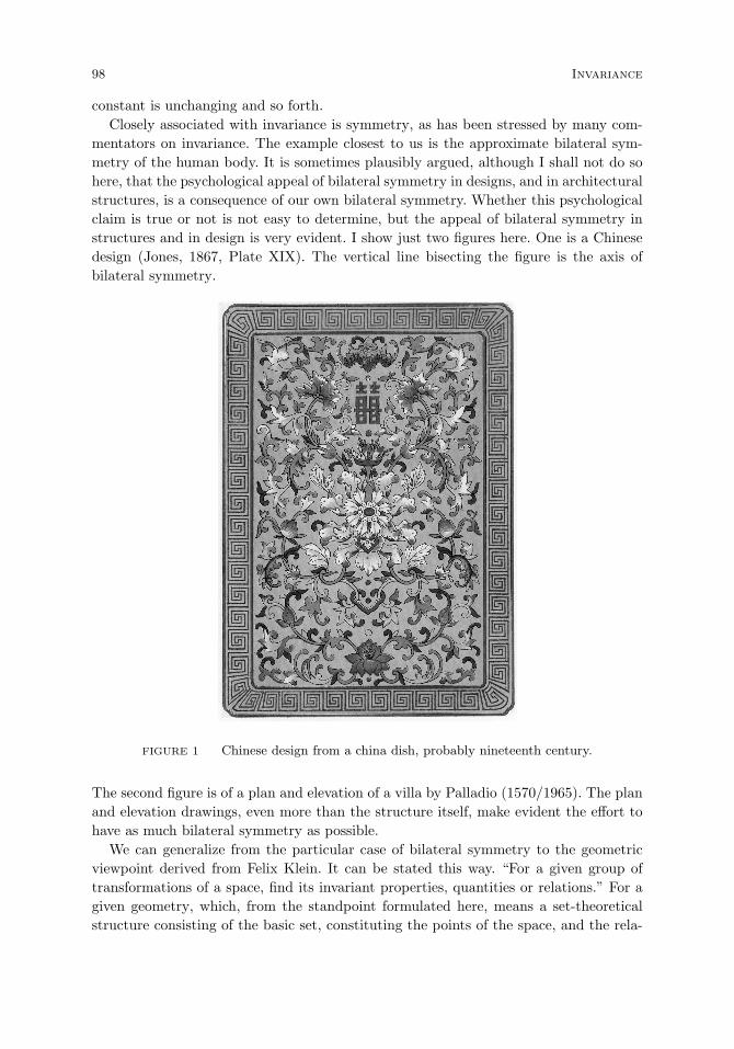
98 Invariance

constant is unchanging and so forth.Closely associated with invariance is symmetry, as has been stressed by many com-

mentators on invariance. The example closest to us is the approximate bilateral sym-metry of the human body. It is sometimes plausibly argued, although I shall not do sohere, that the psychological appeal of bilateral symmetry in designs, and in architecturalstructures, is a consequence of our own bilateral symmetry. Whether this psychologicalclaim is true or not is not easy to determine, but the appeal of bilateral symmetry instructures and in design is very evident. I show just two figures here. One is a Chinesedesign (Jones, 1867, Plate XIX). The vertical line bisecting the figure is the axis ofbilateral symmetry.

FIGURE 1 Chinese design from a china dish, probably nineteenth century.

The second figure is of a plan and elevation of a villa by Palladio (1570/1965). The planand elevation drawings, even more than the structure itself, make evident the effort tohave as much bilateral symmetry as possible.

We can generalize from the particular case of bilateral symmetry to the geometricviewpoint derived from Felix Klein. It can be stated this way. “For a given group oftransformations of a space, find its invariant properties, quantities or relations.” For agiven geometry, which, from the standpoint formulated here, means a set-theoreticalstructure consisting of the basic set, constituting the points of the space, and the rela-

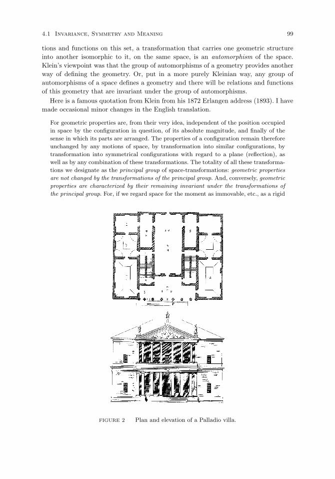
4.1 Invariance, Symmetry and Meaning 99

tions and functions on this set, a transformation that carries one geometric structureinto another isomorphic to it, on the same space, is an automorphism of the space.Klein’s viewpoint was that the group of automorphisms of a geometry provides anotherway of defining the geometry. Or, put in a more purely Kleinian way, any group ofautomorphisms of a space defines a geometry and there will be relations and functionsof this geometry that are invariant under the group of automorphisms.

Here is a famous quotation from Klein from his 1872 Erlangen address (1893). I havemade occasional minor changes in the English translation.

For geometric properties are, from their very idea, independent of the position occupied

in space by the configuration in question, of its absolute magnitude, and finally of the

sense in which its parts are arranged. The properties of a configuration remain therefore

unchanged by any motions of space, by transformation into similar configurations, by

transformation into symmetrical configurations with regard to a plane (reflection), as

well as by any combination of these transformations. The totality of all these transforma-

tions we designate as the principal group of space-transformations: geometric properties

are not changed by the transformations of the principal group. And, conversely, geometric

properties are characterized by their remaining invariant under the transformations of

the principal group. For, if we regard space for the moment as immovable, etc., as a rigid

FIGURE 2 Plan and elevation of a Palladio villa.

100 Invariance

manifold, then every figure has an individual character; of all the properties possessed by

it as an individual, only the properly geometric ones are preserved in the transformations

of the principal group.

(Klein, p. 218)

Within this framework, we say that a geometric figure is symmetric under a givengroup if every automorphism of the group maps the figure into itself. For example, abilaterally symmetric figure is so mapped by a mirror reflection along what we familiarlycall a line of symmetry, in the case of plane figures. Figures symmetric under variousrotations are also familiar examples of symmetry, the circle above all, but, of course,the square is also symmetric under any 90-degree rotation about its center. Noticethe difference. The square has a very small finite group of rotations under which it isinvariant, whereas the circle is invariant under an infinite group of rotations.

In similar fashion three-dimensional figures like spheres and cubes are also invariantunder various groups of motions or transformations. Idealization is important here. Mostreal physical objects look, or are different, in some observable, even if minute, way, underrotations or reflections.

Familiar examples of geometric invariants are the relation of betweenness and therelation of congruence of Euclidean geometry, which can be axiomatized just in termsof these two concepts.

It is worth remarking why symmetry and groups naturally go together. We maythink of it this way. A geometric figure F in a space A is symmetric under a singletransformation ϕ mapping A onto A if ϕ maps F onto itself. Now if this holds, so shouldthe inverse mapping ϕ−1, since ϕ−1 ϕ is just the identity map of A. In addition, itis natural to expect closure of this symmetry property. If ϕ1 and ϕ2 both map F ontoitself then so should their composition ϕ1 ϕ2. These two properties of a set G oftransformations:

(i) If ϕ ∈ G then ϕ−1 ∈ G,

(ii) If ϕ1, ϕ2 ∈ G then ϕ1 ϕ2 ∈ G,

are sufficient to guarantee G is a group of transformations or automorphisms of the givenspace A, since composition of transformations is necessarily associative, and ϕ ϕ−1 isthe identity. This same argument also shows why invariance and groups so naturally gotogether.1

When artists or architects draw a symmetric figure or design, it is undoubtedly usuallythe case that they do not explicitly think in terms of the automorphisms of the space inwhich the figure or design is implicitly embedded. Even sophisticated mathematiciansof ancient Greek times did not have an explicit group concept, but once uncovered, itseems a natural formalization of the intuitive idea of symmetry.

Various kinds of symmetries in design have been recognized for thousands of years.The square with its two diagonals shown in Figure 3 looks the same, i.e., is invariant in

1The general axioms for groups, not just groups of transformations, were given in Section 2.3, but as

was mentioned at the beginning of Section 3.3, every group is isomorphic to a group of transformations,

which is one reason for thinking of groups of transformations as the most intuitive models of groups.

For a detailed history of the development of the abstract concept of group, see Wussing (1984).

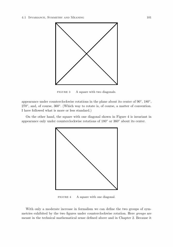
4.1 Invariance, Symmetry and Meaning 101

FIGURE 3 A square with two diagonals.

appearance under counterclockwise rotations in the plane about its center of 90, 180,270, and, of course, 360. (Which way to rotate is, of course, a matter of convention.I have followed what is more or less standard.)

On the other hand, the square with one diagonal shown in Figure 4 is invariant inappearance only under counterclockwise rotations of 180 or 360 about its center.

FIGURE 4 A square with one diagonal.

With only a moderate increase in formalism we can define the two groups of sym-metries exhibited by the two figures under counterclockwise rotation. Here groups aremeant in the technical mathematical sense defined above and in Chapter 2. Because it

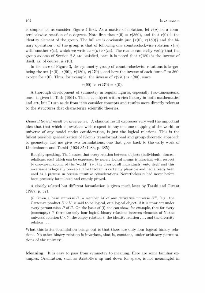
102 Invariance

is simpler let us consider Figure 4 first. As a matter of notation, let r(n) be a coun-terclockwise rotation of n degrees. Note first that r(0) = r(360), and that r(0) is theidentity element of the group. The full set is obviously just r(0), r(180) and the bi-nary operation of the group is that of following one counterclockwise rotation r(m)with another r(n), which we write as r(n) r(m). The reader can easily verify that thegroup axioms of Section 2.3 are satisfied, once it is noted that r(180) is the inverse ofitself, as, of course, is r(0).

In the case of Figure 3, the symmetry group of counterclockwise rotations is larger,being the set r(0), r(90), r(180), r(270), and here the inverse of each “sums” to 360,except for r(0). Thus, for example, the inverse of r(270) is r(90), since

r(90) r(270) = r(0).

A thorough development of symmetry in regular figures, especially two-dimensionalones, is given in Toth (1964). This is a subject with a rich history in both mathematicsand art, but I turn aside from it to consider concepts and results more directly relevantto the structures that characterize scientific theories.

General logical result on invariance. A classical result expresses very well the importantidea that that which is invariant with respect to any one-one mapping of the world, oruniverse of any model under consideration, is just the logical relations. This is thefullest possible generalization of Klein’s transformational and group-theoretic approachto geometry. Let me give two formulations, one that goes back to the early work ofLindenbaum and Tarski (1934-35/1983, p. 385):

Roughly speaking, Th. 1 states that every relation between objects (individuals, classes,

relations, etc.) which can be expressed by purely logical means is invariant with respect

to one-one mapping of the ‘world’ (i.e., the class of all individuals) onto itself and this

invariance is logically provable. The theorem is certainly plausible and had already been

used as a premiss in certain intuitive considerations. Nevertheless it had never before

been precisely formulated and exactly proved.

A closely related but different formulation is given much later by Tarski and Givant(1987, p. 57):

(i) Given a basic universe U , a member M of any derivative universe U≈, [e.g., the

Cartesian product U ×U ] is said to be logical, or a logical object, if it is invariant under

every permutation P of U . On the basis of (i) one can show, for example, that for every

(nonempty) U there are only four logical binary relations between elements of U : the

universal relation U×U , the empty relation ∅, the identity relation . . . , and the diversity

relation . . . .

What this latter formulation brings out is that there are only four logical binary rela-tions. No other binary relation is invariant, that is, constant, under arbitrary permuta-tions of the universe.

Meaning. It is easy to pass from symmetry to meaning. Here are some familiar ex-amples. Orientation, such as Aristotle’s up and down for space, is not meaningful in

4.1 Invariance, Symmetry and Meaning 103

Euclidean geometry.2 Why? It is not invariant under the Euclidean group of motions,i.e., rotations, translations and reflections.

In Euclidean geometry it is meaningful to compare the lengths of two line segments,regardless of whether they are parallel or not. In affine geometry for such a comparisonto be meaningful, however, the line segments must be parallel, which includes lying onthe same line. It is a distinguishing feature of affine geometry, in fact, that it is not ametric space. There is no common measure along lines as we change direction from oneline to another. It is only for parallel segments that there is a meaningful concept ofcongruence, which is what we mean when we speak of affine congruence.

In projective geometry, even the affine concept of betweenness is not preserved underprojections from one line to another from a given point of perspective. In this case, wemust go to a four-place relation, the relation of separation: ab S cd if and only if a and bseparate c and d, and conversely. Figure 5 shows how separation is preserved underprojection, but betweenness is not. For example, we can easily see in the figure that blies between a and d, but the projection b′ does not lie between a′ and d′. On the otherhand, the pair ab separates the pair cd, and conversely; moreover, under projection thepair a′b′ separates the pair c′d′, and conversely.

FIGURE 5 Drawing showing the noninvariance of betweenness and the invariance of separa-

tion under projection from one line to another from a given point of perspective p.

Objective meaning in physics. In physics, there is a tendency to go beyond sim-ply talking about meaningfulness and to talk about objective meaning. The importantconcept is that of invariant relations, or invariance more generally, for observers movingrelative to each other with constant velocity. So, for example, in classical physics, twoinertial observers moving relative to each other should confirm the same measurementsof that which is genuinely invariant. This doesn’t mean that they don’t make correct

2Here is a well-known passage from Aristotle in On the Heavens.

There are certain things whose nature it is always to move away from the centre, and others alwaystowards the centre. The first I speak of as moving upwards, the second downwards. Some deny thatthere is an up or down in the world, but this is unreasonable.

(Aristotle, 308a14–17, Guthrie translation, 1960)

104 Invariance

measurements in their own frames of reference, using their individual measurement pro-cedures.3 But, as we know, directions, for example, will in general be different for thetwo observers, as will other properties. On the other hand, what we expect to hold isthat the numerical distance between two simultaneous spatial points is the same forall observers using the same calibration of their measurement instruments. The sameis true of time. Temporal intervals are the same for all inertial classical observers usingclocks with the same calibration. As is emphasized in foundational discussions of clas-sical physics, spatial and temporal intervals are observer-independent, but the conceptsof the center of the universe, the beginning of time, or being in a state of absoluterest are not invariant. They have no physical meaning, in spite of earlier views, such asthose of Aristotelian physics, to the contrary. Of course, the use of these concepts byAristotle was in no sense ridiculous. Phenomenological experience certainly gives us anatural concept of absolute rest, i.e., of being at rest with respect to the Earth, and thesame for the center of the universe. On the other hand, as a matter much farther fromfamiliar experience, Aristotle famously argued that the world is eternal, i.e., time has nobeginning, creating problems for later Christian theologians, such as John Philoponusof the sixth century.

Here is a second example from special relativity. Invariance for two inertial observersof the ‘proper’ time of a moving particle is sufficient to derive that their observationswith respect to their own frames of reference are related by a Lorentz transformation.The proper time interval τ12 of two points on the trajectory of an inertial particlesatisfies the following equation:

τ212 = (t1 − t2)2 − 1

c2[(x1 − x2)2 + (y1 − y2)2 + (z1 − z2)2

].

The important concept here is that proper time has objective meaning independent ofthe observer’s particular frame of reference. Moreover, proper time has the importantfeature of being a complete invariant, since its invariance determines the group of Lorentztransformations (Suppes 1959). More details about these two examples are given inChapter 6.

A third example is the classic theorem of Noether (1918). Roughly speaking, it saysthat to every conservation law of mechanics there corresponds an invariant quantity,which is a first integral of the equations of motion.

Example A. Conservation of momentum of a system of particles implies that thecenter of mass of the system moves with constant, i.e., invariant, velocity.

Example B. A system admits rotations around a given line. Then the angular mo-mentum with respect to this line as axis is invariant, i.e., constant, in time.

These various geometric and physical examples make clear that the concept of invari-ance is relative not only to some group of transformations, but more fundamentally and

3Observers moving relatively to each other on trajectories that are not parallel record very different

velocities for the same observed body, but this does not mean their observations are subjective in

the usual epistemological sense. Many observers at rest with respect to each other could have full

intersubjective agreement on their measurements. The concept of objective meaning introduced here is

common in physics, but not in general philosophical discussions of meaning. Within the philosophy of

science it is a good way of defining meaningful with respect to a theory, namely, that which is invariant

with respect to the theory.

4.2 Qualitative Visual Perceptions 105

essentially, relative to some theory. Invariant properties of models of a theory are thefocus of investigations of invariance. So, for example, Aristotle’s theory of the heavensled naturally to their being eternal, since they were unchanging, and consequently therecould be no beginning of time.

An invariance holding across many theories is the implicitly or explicitly assumedflatness of space in Ptolemaic, Copernican, Galilean, Newtonian and Einsteinian special-relativity theories of the physical universe. A technical geometric way of formulating thematter is the fundamental assumption that space-time is a four-dimensional affine space,which has many invariant consequences, as is explained in Chapter 6.

4.2 Invariance of Qualitative Visual Perceptions

In this section, various ordinary spatial expressions are introduced with their ordinarymeaning, and the question asked is this. What is the natural geometrical theory withrespect to which each expression is invariant? In Chapter 6, similar questions are askedabout the results of various experiments on visual space, which challenge the thesis thatvisual space is Euclidean. As already hinted at, I shall follow the practice in geometryand physics of relating invariance under a given group of transformations to a principleof symmetry. Invariance implies symmetry and symmetry implies invariance.

The concepts, results and problems that fall under the general heading of this sectionhave not been studied very intensely in the past but have received more attention inthe last twenty years or so. I mention in this connection especially Bowerman (1989),Crangle and Suppes (1989), and Levelt (1982, 1984). The references in these publicationsprovide good leads back into the older literature. A typical problem that I have in mindhere is the sort of thing that Levelt has investigated thoroughly, for example, the waylanguage is used to give spatial directions, and the limitations of our ability to give suchdirections or describe visual scenes with accuracy. In the case of my own earlier workwith Crangle, we were concerned especially to analyze the geometry underlying the useof various common prepositions in English.

The results of that analysis can be easily summarized in Table 1 which is reproducedwith some modifications from Crangle and Suppes (1989). The kinds of geometry re-ferred to are standard, with the exception perhaps of the geometry of oriented physicalspace. For example, in the case of the sentence The pencil is in the box (where it isassumed the box is closed), it is clear that only a purely topological notion of invarianceis needed. On the other hand, in the sentence Mary is sitting between Jose and Maria,it is easy to see that the geometry needs to be affine. And once the idea of a metricis introduced, as in the sentence The pencil is near the box, we must go from affinegeometry to some underlying notion of congruence as reflected in Euclidean geometry.Although we may be more refined in the analysis, note that in this sentence it is quitesatisfactory to use absolute geometry which is Euclidean geometry minus the standardEuclidean axiom. This axiom asserts that given a point a and a line L on which thepoint does not lie, then there exists at most one line through a in the plane formed byaL which does not meet the line. We get hyperbolic rather than Euclidean geometry byadding the negation of this axiom to absolute geometry. It seems to me that the notionof nearness used in ordinary talk is satisfied well enough by the congruence relation of

106 Invariance

TABLE 1 Kinds of geometry and examples of prepositional use

Topology The pencil is in the box. (box closed)One piece of rope goes over andunder the other.

Affine geometry The pencil is in the box. (box open)Mary is sitting between Jose andMaria.

The geometry of oriented The book is on the table.physical space Adjust the lamp over the table.

Projective geometry The post office is over the hill.The cup is to the left of the plate.

Geometries that include The dog is in front of the house.figures and shapes with The pencil is behind the chair.orienting axes

Geometry of She peeled apples in the kitchen.classical space-time

absolute geometry. In fact, relatively technical geometrical results are required to moveus from absolute to Euclidean geometry, the sort of technical facts required, for exam-ple, in architecture and construction. Another way of noting the adequacy of absolutegeometry to express many of the elementary results of Euclidean geometry is that thefirst 26 propositions of Book I of Euclid’s Elements are provable in absolute geometry.On the other hand, in the case of the preposition on, it is clear that a notion of verticalorientation is required, a notion completely absent from Euclidean geometry, and infact not definable within Euclidean geometry. A different kind of orientation is requiredin the case of objects that have a natural intrinsic orientation. Consider for instance,the sentence given in Table 1, The dog is in front of the house. Finally, in the case ofmany processes it is not sufficient to talk about static spatial geometry but for a fulldiscussion one needs the assumption of space-time. An example is given at the end ofTable 1.

What I now want to look at are the kinds of axioms needed to deal with the cases ofgeometry that are not standard. It would not be appropriate simply to repeat standardaxioms for topological, projective, affine, absolute, and Euclidean geometry. A ratherthorough recent presentation of these geometries is to be found in Suppes et al. (1989,Ch. 13). What I shall do is make reference to the primitive notions on which thesevarious axioms are based.

Oriented physical space. Undoubtedly, the aspect of absolute or Euclidean geome-try which most obviously does not satisfy ordinary talk about spatial relations is thatthere is no concept of vertical orientation. Moreover, on the basis of well-known resultsof Lindenbaum and Tarski (1934-35/1983) concerning the fact that no nontrivial binaryrelations can be defined in Euclidean geometry, the concept is not even definable in Eu-

4.2 Qualitative Visual Perceptions 107

clidean geometry. For definiteness I have in mind as the primitive concepts of Euclideangeometry the affine ternary relation of betweenness for points on a line and the conceptof congruence for line segments. In many ways I should mention, however, it is moreconvenient to use the notions of parallelism and perpendicularity, and in any case I shallassume these latter two notions are defined. There are many different ways, of course,of axiomatizing as an extension of Euclidean geometry the concept of verticality. Onesimple approach is to add as a primitive the set V of vertical lines, and then to addaxioms of the following sort to three-dimensional Euclidean geometry. Given any pointa there is a vertical line through a. If K is a vertical line and L is parallel to K, then Lis a vertical line.

There are however, two different kinds of difficulties with this approach. The first andconceptually the most fundamental difficulty is that our natural notion of physical space,as we move around in our ordinary environment, is that its orientation, both verticallyand horizontally, is fixed uniquely. We do not have arbitrary directional transformationsof verticality nor of horizontal orientation. We naturally have a notion of north, east,south, and west, with corresponding degrees. Secondly, and closely related to this, veryearly in the discussion of the nature of physical space, it was recognized that we havedifficulties with treating the surface of the earth as a plane with horizontal lines beingin this plane and vertical lines being perpendicular to them. The natural geometry oforiented physical space in terms of ordinary experience—a point to be expanded uponin a moment—is in terms of spherical geometry, with the center of the earth being animportant concept, as it was for Aristotle and Ptolemy in ancient times.

Aristotle directly uses perceptual evidence as part of his argument for the conclusionthat the earth is spherical (On the Heavens , Book II, Ch. 14, 297b): “If the earthwere not spherical, eclipses of the moon would not exhibit the shapes they do, andobservation of the stars would not show the variation they do as we move to the northor south.”

Ptolemy’s argument in the Almagest is even better. Because it will not be familiarto many readers, I quote it in full, for the arguments are perceptual throughout. Thispassage occurs in Book I, Section 4 of the Almagest, written more than four hundredyears after Aristotle’s work.

That the earth, too, taken as a whole, is sensibly spherical can best be grasped from

the following considerations. We can see, again, that the sun, moon and other stars do

not rise and set simultaneously for everyone on earth, but do so earlier for those more

towards the east, later for those towards the west. For we find that the phenomena at

eclipses, especially lunar eclipses, which take place at the same time [for all observers],

are nevertheless not recorded as occurring at the same hour (that is at an equal distance

from noon) by all observers. Rather, the hour recorded by the more easterly observers

is always later than that recorded by the more westerly. We find that the differences in

the hour are proportional to the distances between the places [of observation]. Hence one

can reasonably conclude that the earth’s surface is spherical, because its evenly curving

surface (for so it is when considered as a whole) cuts off [the heavenly bodies] for each

set of observers in turn in a regular fashion.

If the earth’s shape were any other, this would not happen, as one can see from the

following arguments. If it were concave, the stars would be seen rising first by those

108 Invariance

more towards the west; if it were a plane, they would rise and set simultaneously for

everyone on earth; if it were triangular or square or any other polygonal shape, by a

similar argument, they would rise and set simultaneously for all those living on the

same plane surface. Yet it is apparent that nothing like this takes place. Nor could it be

cylindrical, with the curved surface in the east-west direction, and the flat sides towards

the poles of the universe, which some might suppose more plausible. This is clear from the

following: for those living on the curved surface none of the stars would be ever-visible,

but either all stars would rise and set for all observers, or the same stars, for an equal

[celestial] distance from each of the poles, would always be invisible for all observers. In

fact, the further we travel toward the north, the more of the southern stars disappear

and the more of the northern stars appear. Hence it is clear that here too the curvature

of the earth cuts off [the heavenly bodies] in a regular fashion in a north-south direction,

and proves the sphericity [of the earth] in all directions.

There is the further consideration that if we sail towards mountains or elevated places

from and to any direction whatever, they are observed to increase gradually in size as if

rising up from the sea itself in which they had previously been submerged: this is due to

the curvature of the surface of the water. (Almagest, pp. 40–41)

Aristotle’s concept of natural motion, which means that heavy bodies fall toward thecenter of the earth, is well argued for again by Ptolemy in Section 7 of Book I.

. . . the direction and path of the motion (I mean the proper, [natural] motion) of all

bodies possessing weight is always and everywhere at right angles to the rigid plane

drawn tangent to the point of impact. It is clear from this fact that, if [these falling

objects] were not arrested by the surface of the earth, they would certainly reach the

center of the earth itself, since the straight line to the center is also always at right angles

to the plane tangent to the sphere at the point of intersection [of that radius] and the

tangent. (Almagest, pp. 43-44)

What is important to notice about this argument, and similar but less clear argumentsof Aristotle, is that the notion of vertical or up is along radii extended beyond thesurface of the earth, and not in terms of lines perpendicular to one given horizontalplane. Thus the perceptual notion of verticality is in terms of a line segment thatpasses through the center of the earth. The notion of horizontal is that of a planeperpendicular to a vertical line at the surface of the earth. The strongest argument forthis viewpoint is the perceptual evidence of the nature of the natural falling motion ofheavy bodies.

Ptolemy also uses observations of the motion of the stars and the planets to fix thedirection of east and west, and also the poles of north and south. We use in ordinaryexperience such arguments as the rising and setting of the sun to fix the direction ofeast and west.

These perceptual arguments about physical space—including of course perceptualarguments about gravity—reduce the group of Euclidean motions to the trivial auto-morphism of identity. This means that from a global standpoint the concept of invarianceis not of any real significance in considering the perceptual aspects of oriented physicalspace. On the other hand the strong sense of the concept of global that is being used heremust be emphasized. From the standpoint of the way the term global is used in general,there remain many symmetries of a less sweeping sort that are important and that are

4.2 Qualitative Visual Perceptions 109

continually used in perceptual or physical analysis of actual objects in space. Indeedthis is a very intuitive outcome from the standpoint of ordinary perception. Combiningboth our visual sense of space and our sense of space arising from gravitational effects, itis wholly unnatural to think of anything like the group of Euclidean motions being thefundamental group for physical space in the sense of direct experience or perception. Itis in fact a remarkable abstraction of the Greeks that orientation was not made a partof the original axioms of Euclid.

On the other hand, the notion of invariance in perception arises continually in a lessglobal fashion in considering the symmetry of perceived figures or perceived phenomenaarising from not just visual but also auditory or haptic data.

The classification of geometries for the prepositions used in Table 1 may be regardedas an external view from the standpoint of space as a whole. Perceptually, however,this is not the way we deal with the matter. In ordinary experience, we begin with theframework of a fixed oriented physical space as described above. Within this frameworkwe can develop an internal view of spatial relations as expressed in ordinary language.

As an example, I examine the invariance of the preposition in. In this and subsequentanalysis the relation expressed by in shall be restricted to pairs of rigid bodies. Eventhough it is ultimately important to characterize invariance for other situations, e.g.,the sugar being in the water, a good sense of the fundamental approach to invariancebeing advocated can be conveyed with consideration only of familiar situations withrigid bodies.

Let a and b be rigid bodies with a in b. As in Table 1 there are two cases of bodyb to consider. The first is when b has a closed hollow interior and a is in this interior.For simplicity of notation and analysis, I introduce the restrictive assumption that a isa spherical ball, so that the orientation of a can be ignored. Define I(a, b) = the set ofpoints in the closed hollow interior of b that the center of a can occupy. Let Φ(a, b) bethe set of all transformations of I(a, b) onto itself that represent possible changes in theposition of a relative to b. For example, if the position of the center of a is on one sideof the hollow interior of b it could be transformed, i.e., moved, to the other side of theinterior without affecting the truth of the assertion that a is in b.

The set Φ(a, b) is the symmetry group (under the operation of function composition)of the position of a inside b, but because the hollow interior of b can be quite irregularin shape Φ(a, b) may not have standard properties of Euclidean isometries. It does havethe expected invariance properties, namely, if ϕ ∈ Φ(a, b), then a with center c at pointp is in b if and only if a with center c at point ϕ(p) is in b.

Body b is itself subject to rigid motion in the fixed physical space. If b is closed,rotations around a horizontal axis are permitted, but if b is open, possible rigid motionsof b must be restricted to those that preserve vertical orientation. And, of course, whenb is subject to a rigid motion ψ, body a must be subject to the same transformation ψ,in order to preserve the invariance of the relation of being inside. Obviously, a may alsobe transformed by ϕ ∈ Φ(a, b), so that its full transformation could be the compositionϕ ψ with invariance of in preserved.

Similar analyses can be given of the internal invariance properties of the other prepo-sitions listed in Table 1. They all have different symmetry groups, but the exact nature

110 Invariance

of each group is determined by the particular shape and size of the relevant bodies,which may vary drastically from one context to another. It is not surprising that nocomputationally simple theory of invariance works for ordinary spatial relations as ex-pressed in natural language, for the robust range of applicability of such relations is fartoo complex to have a simple uniform geometry.

Further applications. In addition to providing an analysis of spatial terms, the kind ofapproach outlined above can be used in a comparison of different languages. A naturalquestion is whether there is a universal semantics of spatial perception or differentlanguages have intrinsically different semantics. Certainly there are subtle differencesin the range of prepositions. Bowerman (1989) points out, for example, that whereaswe can say in English both The cup is on the table and The fly is on the window, inGerman we use the preposition auf for being on the table, but an for being on thevertical window.

Such differences are to be expected, although it is a matter of considerable interest tostudy how the prepositions of different languages overlap in their semantic coverage. It isa well-known fact that learning the correct use of prepositions is one of the most difficultaspects of learning a second language within the family of Indo-European languages.

One hope might be that there is a kind of universal spatial perception, so we mightsearch for geometrical invariance across languages. But if we fit the geometries closelyto individual languages, the primitives but not the theorems may be different in thesense of having a different geometrical meaning. A related set of questions can be askedabout the order of developmental use of spatial prepositions by children. This seemsto present a particularly good opportunity for careful examination of what happens indifferent languages, because of the relatively concrete and definite rules of usage thatgovern spatial prepositions in each language in their literal use. Bowerman (1989) hasan excellent discussion of many details, but does not focus on systematic geometricalaspects.

4.3 Invariance in Theories of Measurement

In connection with any measured property of an object, or set of objects, it may beasked how unique is the number assigned to measure the property. For example, themass of a pebble may be measured in grams or pounds. The number assigned to measuremass is unique once a unit has been chosen.

The measurement of temperature in C or F has different characteristics. Here anorigin as well as a unit is arbitrarily chosen. Other formally different kinds of measure-ment are exemplified by (1) the measurement of probability, which is absolutely unique,and (2) the ordinal measurement of such physical properties as hardness of minerals, orsuch psychological properties as intelligence and racial prejudice.

Use of these different kinds of transformations is basic to the main idea of this chap-ter. An empirical hypothesis, or any statement in fact, which uses numerical quantitiesis empirically meaningful only if its truth value is invariant under the appropriate trans-formations of the numerical quantities involved. As an example, suppose a psychologisthas an ordinal measure of I.Q., and he thinks that scores S(a) on a certain new test T

4.3 Theories of Measurement 111

have ordinal significance in ranking the intellectual ability of people. Suppose furtherthat he is able to obtain the ages A(a) of his subjects. The question then is: Should heregard the following hypothesis as empirically meaningful?

HYPOTHESIS 1. For any subjects a and b, if S(a)/A(a) < S(b)/A(b), thenI.Q.(a) < I.Q.(b).

From the standpoint of the invariance characterization of empirical meaning, the an-swer is negative. To see this, let I.Q.(a) ≥ I.Q.(b), let A(a) = 7, A(b) = 12, S(a) = 3,S(b) = 7. Make no transformations on the I.Q. data, and make no transformations onthe age data. But let φ be an increasing transformation which carries 3 into 6 and 7into itself. Then we have

37<

712,

but67

≥ 712,

and the truth value of Hypothesis 1 is not invariant under φ.The empirically significant thing about the transformation characteristic of a quantity

is that it expresses in precise form how unique the structural isomorphism is between theempirical operations used to obtain a given measurement and the corresponding arith-metical operations or relations. If, for example, the empirical operation is simply that ofordering a set of objects according to some characteristic, then the corresponding arith-metical relation is that of less than (or greater than), and any two functions which mapthe objects into numbers in a manner preserving the empirical ordering are adequate.

It is then easy to show that, if f1 and f2 are adequate in this sense, then they arerelated by a monotone-increasing transformation. Only those arithmetical operationsand relations which are invariant under monotone-increasing transformations have anyempirical significance in this situation.

When we turn from the examination of numerical quantities to models of more com-plex theories, we obtain results of a similar character. For example, in examining classicalmechanics we get a representation that is unique, when units of measurement are fixed,up to a Galilean transformation, that is, a transformation to some other inertial sys-tem. In the case of relativistic structures of particle mechanics, the uniqueness is up toLorentz transformations. These two kinds of transformations are analyzed in Chapter 6.

To give an elementary example, we can state the uniqueness result corresponding tothe representation theorem (Theorem 3.3.1) for finite weak orders. Let A = (A,) be afinite weak order. Then any two numerical weak orderings to which it is homomorphicare related by a strictly increasing numerical function. Put in other language, the nu-merical representation of finite weak orders is unique up to an ordinal transformation.Invariance up to ordinal transformations is not a very strong property of a measurement,and it is for this reason that Hypothesis 1 turned out not to be meaningful.

Moving back to the general scheme of things, a representation theorem should ordi-narily be accompanied by a matching invariance theorem stating the degree to which arepresentation of a structure is unique. In the mathematically simple and direct casesit is easy to identify the group as some well-known group of transformations. For morecomplicated structures, for example, structures that satisfy the axioms of a scientific

112 Invariance

theory, it may be necessary to introduce more complicated apparatus, but the objectiveis the same, to wit, to characterize meaningful concepts in terms of invariance.

One note to avoid confusion: it is when the concepts are given in terms of therepresentation, for example, a numerical representation in the case of measurement,or representation in terms of Cartesian coordinates in the case of geometry, that thetest for invariance is needed. When purely qualitative relations are given, which aredefined in terms of the qualitative primitives of a theory, for example, those of Eu-clidean geometry, then it follows at once that the defined relations are invariant andtherefore meaningful. On the other hand, the great importance of the representationsis the reduction in computations and notation they achieve, as well as understanding ofstructure. This makes it imperative that we have a clear conception of invariance andmeaningfulness for representations which may be, in appearance, rather far removedfrom the qualitative structures that constitute models of the theory.

In the case of physics, the primitive notions themselves of a theory are not necessarilyinvariant. For example, if we axiomatize mechanics in a given frame of reference, thenthe notion of position for a particle is not invariant but is subject to a transformationitself. A more complicated analysis of invariance and meaningfulness is then required insuch cases (see Chapter 6 for such an analysis). The general point is clear, however: thestudy of representation is incomplete without an accompanying study of invariance ofrepresentation. We amplify this point with a detailed analysis of measurement theories.

Second fundamental problem of measurement: invariance theorem. Solutionof the representation problem for a theory of measurement does not completely lay barethe structure of the theory, for it is a banal fact of methodology that there is oftena formal difference between the kind of assignment of numbers arising from differentprocedures of measurement. As an illustration, consider the following five statements:

(1) The number of people now in this room is 7.(2) Stendhal weighed 150 on September 2, 1839.(3) The ratio of Stendhal’s weight to Jane Austen’s on July 3, 1814 was 1.42.(4) The ratio of the maximum temperature today to the maximum temperature

yesterday is 1.1.(5) The ratio of the difference between today’s and yesterday’s maximum temperature

to the difference between today’s and tomorrow’s maximum temperature will be .95.The empirical meaning of statements (1), (3), and (5) is clear, provided we make

the natural assumptions, namely, for (3) that the same scale of weight, whether it beavoirdupois or metric, was being used, and for (5) that the same temperature scaleis being used, whether it be Fahrenheit or Celsius. In contrast, (2) and (4) do nothave a clear empirical meaning unless the particular scale used for the measurement isspecified. On the basis of these five statements we may formally distinguish three kindsof measurement. Counting is an example of an absolute scale. The number of membersof a given collection of objects is determined uniquely. There is no arbitrary choice of aunit or zero available. In contrast, the measurement of mass or weight is an example ofa ratio scale. Any empirical procedure for measuring mass does not determine the unitof mass. The choice of a unit is an empirically arbitrary decision made by an individual

4.3 Theories of Measurement 113

or group of individuals. Of course, once a unit of measurement has been chosen, such asthe gram or pound, the numerical mass of every other object in the universe is uniquelydetermined. Another way of stating this is to say that the measurement of mass is uniqueup to multiplication by a positive constant. (The technical use of ‘up to’ will becomeclear later.) The measurement of distance is a second example of measurement of thissort. The ratio of the distance between Palo Alto and San Francisco to the distancebetween Washington and New York is the same whether the measurement is made inmiles or kilometers.

To avoid certain common misunderstandings, amplification is needed of the claim thatno empirical procedure for measuring mass determines the unit of mass. A chemist, mea-suring a sample of a certain ferric salt on an equal-arm balance with a standard series ofmetric weights, might find this claim surprising, for he might suppose that the selectionof a standard series of metric weights had fixed as part of his empirical procedure onegram as the unit of measurement. There are at least two lines of argument that shouldprove effective in convincing the chemist that his supposition was incorrect. In the firstplace, it would be pertinent to point out that exactly the same information could be ex-pressed by converting this final measurement into a measurement in pounds or ounces.To express the measurement in this latter form, no further empirical operations with theequal-arm balance would have to be performed. But, it must be admitted, the chemistcould well reply that, although no further empirical operations had to be performedwith the present balance, the use of the conversion factor from grams to pounds entailsappealing to empirical operations previously performed by some Bureau of Standardsin determining the conversion factor. An analysis of his retort takes us to the secondline of argument, which goes deeper and is more fundamental. To begin with, his appealto previous empirical operations on other balances may be turned back on him, for tojustify labeling his measurement with his given standard series as a measurement ingrams, appeal must also be made to previously performed empirical operations, namely,those which constituted the calibration of his series of weights as a standard metricseries. The important point is that the empirical operations performed by the chemisthimself establish no more or less than the ratio of the mass of the ferric salt sample toa subset of weights in his standard series. And the same kind of ratio statement may bemade about the empirical operations that led to the calibration of his standard seriesby the technicians of the firm which produced the series. In other words, the statementby the chemist:

(6) This sample of ferric salt weighs 1.679 gramsmay be replaced by the statement:

(7) The ratio of the mass of this sample of ferric salt to the gram weight of mystandard series is 1.679, and the manufacturer of my series has certified that the ratioof my gram weight to the standard kilogram mass of platinum-iridium alloy at theInternational Bureau of Weights and Measures, near Paris, is .0010000.4

The measurement of temperature is an example of the third formally distinct kind

4As is evident, I am ignoring problems of the accuracy of measurement, which are of great importance

in many areas of science. The subject, when carefully discussed, uses extensively the probability concepts

developed in Chapter 5.

114 Invariance

of measurement mentioned earlier. An empirical procedure for measuring temperatureby use of a thermometer determines neither a unit nor an origin.5 In this sort of mea-surement the ratio of any two intervals is independent of the unit and zero point ofmeasurement. For obvious reasons, measurements of this kind are called interval scales.Examples other than measurement of temperature are measurements of temporal dates,linear position, or cardinal utility.6

In terms of the notion of absolute, ratio, and interval scales we may formulate thesecond fundamental problem for any exact analysis of a procedure of measurement:determine the scale type of the measurements resulting from applying the procedure. Asthe heading of this section we have termed this problem the invariance problem fora theory of measurement. From a mathematical standpoint the determination of thescale type of measurement arising from a given algebra of empirical operations andrelations is the determination of the way in which any two numerical models of thealgebra isomorphic to a given empirical model are related. For example, in the case ofmass, we may make four equivalent statements:

(8) Mass is a ratio scale.(9) The measurement of mass is unique up to multiplication by a positive number

(the number corresponding to a change of unit).(10) The measurement of mass is unique up to a similarity transformation (such a

transformation is just multiplication by a positive number).(11) Given any model of an appropriate algebra of operations and relations for mea-

suring mass, then any two numerical models (of this algebra) that are isomorphic to thegiven model are related by a similarity transformation.

The precise meaning of ‘isomorphic’ in (11) was given in Chapter 3.7 At this pointthe only aim is to give a general sense of what is meant by the invariance problem. The‘unique up to’ terminology of (9) and (10) is often used in purely mathematical contexts.Another formulation of the uniqueness problem is one which uses the mathematicalnotion of invariance: determine the set of numerical transformations under which agiven procedure of measurement is invariant.8 In detailed work in later chapters thenotion of invariance will often not be used in a technical way, but it will be obviouswhat definition would be appropriate in a given context and how the uniqueness resultsobtained could be sharply formulated in terms of invariance.

Classification of scales of measurement. The general notion of a scale is notsomething we need to define in an exact manner for subsequent developments. For thepurpose of systematizing some of the discussion of the uniqueness problem, we maydefine a scale as a class of measurement procedures having the same transformation

5Naturally we are excluding from consideration here the measurement of absolute temperature whose

zero point is not arbitrary.6Cardinal utility is economists’ term for an interval-scale measurement of utility, as opposed to

merely ordinal measurement of utility.7Sometimes, when two different physical objects have the same weight measure, the mapping to a

numerical algebra is homomorphic, rather than isomorphic, as is also explained in Chapter 3.8I did not say group of transformations because there are procedures of measurement for which the

invariant set of transformations is not a group.

4.3 Theories of Measurement 115

properties. Examples of three different scales have already been mentioned, namely,counting as an absolute scale, measurement of mass as a ratio scale, and measurementof temperature as an interval scale.9

Still another type of scale is one which is arbitrary except for order. A number is as-signed to give a rough-and-ready ordinal classification. Moh’s hardness scale, accordingto which minerals are ranked in regard to hardness as determined by a scratch test,and the Beaufort wind scale, whereby the strength of a wind is classified as calm, lightair, light breeze, etc., are examples of this fourth, very weak kind of scale. The socialsciences abound with ordinal scales, the significance of which is discussed below.

Numbers are also sometimes used for pure classification. For example, in some statesthe first number on an automobile license indicates the county in which the owner lives.The assignment of numbers in accordance with such a scale is arbitrary except for theassignment of the same number to people in the same county, and distinct numbers topeople in distinct counties.

The weakest scale is one where numbers are used simply to name an object or person.The assignment is completely arbitrary. Draft numbers and the numbers of footballplayers are examples of this sort of measurement. Such scales are usually called nominalscales.

We have distinguished, in an intuitive fashion, six types of scales. We will in thefollowing pages primarily confine our discussion to an analysis of the first four. Theyare not, however, the only scales of measurement, and we shall upon occasion mentionothers.

We now want to characterize each of these six scales in terms of their transformationproperties. For future reference each of the six transformations mentioned is formallydefined. To begin with, an absolute scale is unique up to the identity transformation.

DEFINITION 1. The identity transformation on the set of real numbers is the func-tion f such that for every real number x, f(x) = x.

So far, counting has been our only example of an absolute scale. For the momentwe shall also include probability, but later we shall discuss the naturalness of the usualnormalizing assumption, that is, that probabilities add up to one.

A ratio scale is unique up to a similarity transformation.

DEFINITION 2. Let f be a real-valued function whose domain is the set of real num-bers. Then f is a similarity transformation if and only if there exists a positive realnumber α such that for every real number x

f(x) = αx.

Measurement of mass and of distance have been our two examples of ratio scales. Forthe case of mass, if we wish to convert from pounds to ounces, the appropriate similaritytransformation is to take α = 16. If in the measurement of distance we wish to changefeet to yards we set α = 1

3 . The identity transformation is the similarity transformationwith α = 1.

9Counting, etc., is not the absolute scale, but technically a member of the absolute scale under our

class definition. The usage here conforms to ordinary usage, which tends to treat classes as properties.

116 Invariance

Third, an interval scale is unique up to a linear transformation.

DEFINITION 3. Let f be a real-valued function whose domain is the set of real num-bers. Then f is a linear transformation if and only if there is a positive number α anda number β such that for every number x

f(x) = αx+ β.

If in the measurement of temperature we wish to convert x in degrees Fahrenheit toCelsius we use the linear transformation defined by α = 5

9 and β = −1609 . That is,

y =59(x− 32) =

59x− 160

9.

Obviously every similarity transformation is a linear transformation with β = 0.An ordinal scale is unique up to a monotone transformation. Rather than define mono-

tone transformation directly it will be convenient first to define monotone-increasing andmonotone-decreasing transformations.

DEFINITION 4. Let f be a real-valued function whose domain is some set of realnumbers. Then f is a monotone-increasing transformation if and only if for every x

and y in the domain of f if x < y then f(x) < f(y).

Obviously every linear transformation is a monotone-increasing transformation onthe set of all real numbers. The squaring function, that is, the function f such that

f(x) = x2, (1)

is not a linear transformation but it is monotone increasing on the set of non-negativereal numbers. Notice that it does not have this property on the set of all real numbersfor −5 < 4 but

f(−5) = 25 > 16 = f(4).

It is important to realize that a monotone-increasing transformation need not be defin-able by some simple equation like (1). For example, consider the set

A = 1, 3, 5, 7and let f be the function defined on A such that

f(1) = −5f(3) = 5f(5) = 289f(7) = 993.

Clearly f is monotone increasing on A, but it does not satisfy any simple equation.

DEFINITION 5. Let f be a real-valued function whose domain is some set of realnumbers. Then f is a monotone-decreasing transformation if and only if for every x

and y in the domain of f if x < y then f(x) > f(y).

Two examples of monotone-decreasing transformations on the set of all real numbersare:

f(x) = −xand

f(x) = −x3 + 2.

4.3 Theories of Measurement 117

As another instance, consider the set A again, and let f be defined on A such that

f(1) = 6

f(3) = 4

f(5) = 2

f(7) = −10.

Obviously f is monotone decreasing on A.

DEFINITION 6. Let f be a real-valued function whose domain is some set of realnumbers. Then f is a monotone transformation if and only if f is a monotone-increasingtransformation or a monotone-decreasing transformation.

Obviously monotone transformations characterize ordinal scales. The obvious invari-ance theorem for finite weak orders, as important examples of ordinal scales, is thefollowing.

THEOREM 1. Let A = (A,) be a finite weak order. Then any two numerical rep-resentations of A are related by a monotone transformation.

In practice it is often convenient to consider only monotone-increasing or monotone-decreasing transformations, but this restriction is mainly motivated by hallowed customsand practices rather than by considerations of empirical fact.

Classificatory and nominal scales are unique up to a 1-1 transformation which issimply a one-to-one function.

In addition to these six classical scale types, which are essentially those proposedby Stevens (1947), there are others which will be discussed later. An example is theclass of procedures which we shall call hyperordinal scales. They are characterized bytransformations which preserve first differences and which we label hypermonotone. Herewe may roughly characterize them as empirical structures which just lack being intervalscales. Various methods of measuring sensation intensities or utility provide examples.

DEFINITION 7. Let f be a real-valued function whose domain is some set of realnumbers. Then f is a hypermonotone transformation if and only if f is a monotonetransformation and for every x, y, u and v in the domain of f , if

|x− y| < |u− v|then

|f(x) − f(y)| < |f(u) − f(v)|.Naturally every linear transformation is a hypermonotone-increasing transformation,

but the converse is not true. Consider, for example,

A = 1, 2, 3, 8and the function f such that

f(1) = 1

f(2) = 2

f(4) = 5

f(8) = 15.

118 Invariance

Clearly f is hypermonotone increasing but not linear on A.There is, strictly speaking, a nondenumerable infinity of scales which are characterized

by various groups of numerical transformations, but most of them are not of any realempirical significance. Also, it is possible to extend the notion of measurement to orderstructures like lattices and partial orderings which cannot be represented numerically inany natural way. My own view is that this extension is undesirable, for in the languageof Scott and Suppes (1958) it identifies the class of theories of measurement with theclass of finite relational structures, and the general theory of finite relational structuresextends far beyond any intuitive conceptions of measurement.10

The classificatory analysis of this section is summarized in Table 2.

TABLE 2 Classification of Scales and Measurement

Scale Transformation Properties ExamplesAbsolute Identity Counting, relative frequencyRatio Similarity Mass, distance, electric

(Multiplication by a current, voltagepositive number)

Interval Linear (multiplication Temperature, potentialby a positive number energy, linear position,and addition of an cardinal utilityarbitrary number)

Hyperordinal Hypermonotone (preserva- Pitch, loudness, utilitytion of order of firstdifferences)

Ordinal Monotone or monotone Moh’s scale, Beaufort windincreasing scale, qualitative

preferencesNominal 1-1 Phone numbers, Social

Security numbers

I now turn to the invariance theorems corresponding to the four measurement repre-sentation theorems of Section 3.4

THEOREM 2. Let A = (A,F ,) be a finite, equally spaced extensive structure. Thena numerical representation of A is invariant under the group of similarity transforma-tions of Table 2.

The proof of this elementary theorem is left to the reader.

THEOREM 3. Let A = (A,) be a finite, equally spaced difference structure. Thena numerical representation of A is invariant under the group of linear transformations

10As is probably obvious, a finite relational structure is a relational structure whose domain is a finite

set. Given this finiteness, some numerical representation can be constructed in a more or less arbitrary

manner, which will consequently be of little if any scientific interest. Only those reflecting some actual

procedures of measurement, perhaps somewhat idealized, will be of any interest.

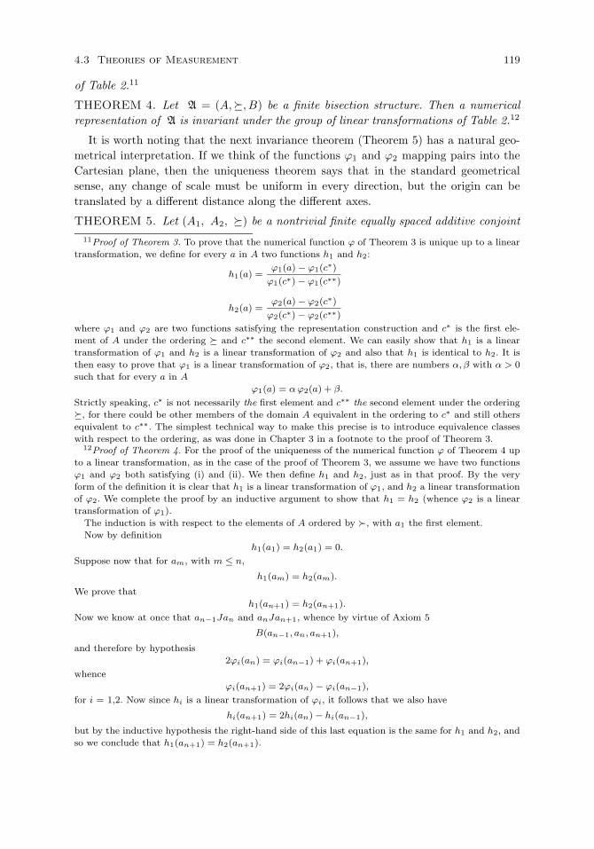
4.3 Theories of Measurement 119

of Table 2.11

THEOREM 4. Let A = (A,, B) be a finite bisection structure. Then a numericalrepresentation of A is invariant under the group of linear transformations of Table 2.12

It is worth noting that the next invariance theorem (Theorem 5) has a natural geo-metrical interpretation. If we think of the functions ϕ1 and ϕ2 mapping pairs into theCartesian plane, then the uniqueness theorem says that in the standard geometricalsense, any change of scale must be uniform in every direction, but the origin can betranslated by a different distance along the different axes.

THEOREM 5. Let (A1, A2, ) be a nontrivial finite equally spaced additive conjoint11Proof of Theorem 3. To prove that the numerical function ϕ of Theorem 3 is unique up to a linear

transformation, we define for every a in A two functions h1 and h2:

h1(a) =ϕ1(a) − ϕ1(c∗)

ϕ1(c∗) − ϕ1(c∗∗)

h2(a) =ϕ2(a) − ϕ2(c∗)

ϕ2(c∗) − ϕ2(c∗∗)

where ϕ1 and ϕ2 are two functions satisfying the representation construction and c∗ is the first ele-

ment of A under the ordering and c∗∗ the second element. We can easily show that h1 is a linear

transformation of ϕ1 and h2 is a linear transformation of ϕ2 and also that h1 is identical to h2. It is

then easy to prove that ϕ1 is a linear transformation of ϕ2, that is, there are numbers α, β with α > 0

such that for every a in A

ϕ1(a) = α ϕ2(a) + β.

Strictly speaking, c∗ is not necessarily the first element and c∗∗ the second element under the ordering

, for there could be other members of the domain A equivalent in the ordering to c∗ and still others

equivalent to c∗∗. The simplest technical way to make this precise is to introduce equivalence classes

with respect to the ordering, as was done in Chapter 3 in a footnote to the proof of Theorem 3.12Proof of Theorem 4. For the proof of the uniqueness of the numerical function ϕ of Theorem 4 up

to a linear transformation, as in the case of the proof of Theorem 3, we assume we have two functions

ϕ1 and ϕ2 both satisfying (i) and (ii). We then define h1 and h2, just as in that proof. By the very

form of the definition it is clear that h1 is a linear transformation of ϕ1, and h2 a linear transformation

of ϕ2. We complete the proof by an inductive argument to show that h1 = h2 (whence ϕ2 is a linear

transformation of ϕ1).

The induction is with respect to the elements of A ordered by , with a1 the first element.

Now by definition

h1(a1) = h2(a1) = 0.

Suppose now that for am, with m ≤ n,

h1(am) = h2(am).

We prove that

h1(an+1) = h2(an+1).

Now we know at once that an−1Jan and anJan+1, whence by virtue of Axiom 5

B(an−1, an, an+1),

and therefore by hypothesis

2ϕi(an) = ϕi(an−1) + ϕi(an+1),

whence

ϕi(an+1) = 2ϕi(an) − ϕi(an−1),

for i = 1,2. Now since hi is a linear transformation of ϕi, it follows that we also have

hi(an+1) = 2hi(an) − hi(an−1),

but by the inductive hypothesis the right-hand side of this last equation is the same for h1 and h2, and

so we conclude that h1(an+1) = h2(an+1).

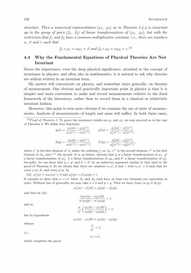
120 Invariance

structure. Then a numerical representation (ϕ1, ϕ2) as in Theorem 3.4.4 is invariantup to the group of pairs (f1, f2) of linear transformations of (ϕ1, ϕ2), but with therestriction that f1 and f2 have a common multiplicative constant, i.e., there are numbersα, β and γ such that

f1 ϕ1 = αϕ1 + β and f2 ϕ2 = αϕ2 + γ.13

4.4 Why the Fundamental Equations of Physical Theories Are NotInvariant

Given the importance, even the deep physical significance, attached to the concept ofinvariance in physics, and often also in mathematics, it is natural to ask why theoriesare seldom written in an invariant form.

My answer will concentrate on physics, and somewhat more generally, on theoriesof measurement. One obvious and practically important point in physics is that it issimpler and more convenient to make and record measurements relative to the fixedframework of the laboratory, rather than to record them in a classical or relativisticinvariant fashion.

Moreover, this point is even more obvious if we examine the use of units of measure-ments. Analysis of measurements of length and mass will suffice. In both these cases,

13Proof of Theorem 5. To prove the invariance results on ϕ1 and ϕ2, we may proceed as in the case

of Theorem 3. We define four functions:

g(a) =ϕ1(a) − ϕ1(c∗)

ϕ1(c∗) − ϕ1(c∗∗)g′(a) =

ϕ′1(a) − ϕ′

1(c∗)

ϕ′1(c

∗) − ϕ′1(c∗∗)

h(p) =ϕ2(p) − ϕ2(r∗)

ϕ2(r∗) − ϕ2(r∗∗)h′(p) =

ϕ′2(p) − ϕ′

2(r∗)

ϕ′2(r

∗) − ϕ′2(r

∗∗),

where c∗ is the first element of A, under the ordering on A1, c∗∗ is the second element, r∗ is the first

element of A2, and r∗∗ the second. It is, as before, obvious that g is a linear transformation of ϕ1, g′

a linear transformation of ϕ′1, h a linear transformation of ϕ2, and h′ a linear transformation of ϕ′

2.

Secondly, we can show that g = g′ and h = h′ by an inductive argument similar to that used in the

proof of Theorem 4. So we obtain that there are numbers α, α′, β and γ with α, α′ > 0 such that for

every a in A1 and every p in A2

(iii) ϕ′1(a) = αϕ1(a) + β and ϕ′

2(p) = α′ϕ2(p) + γ.

It remains to show that α = α′ when A1 and A2 each have at least two elements not equivalent in

order. Without loss of generality we may take a b and p q. Then we have, from (a, q) ≈ (b, p),

ϕ′1(a) − ϕ′

1(b) = ϕ′2(p) − ϕ′

2(q),

and thus by (iii)αϕ1(a) − αϕ1(b)

α′ϕ2(p) − α′ϕ2(q)= 1,

and soα

α′

ϕ1(a) − ϕ1(b)

ϕ2(p) − ϕ2(q)

= 1;

but by hypothesis

ϕ1(a) − ϕ1(b) = ϕ2(p) − ϕ2(q),

whenceα

α′ = 1;

i.e.,

α = α′,which completes the proof.

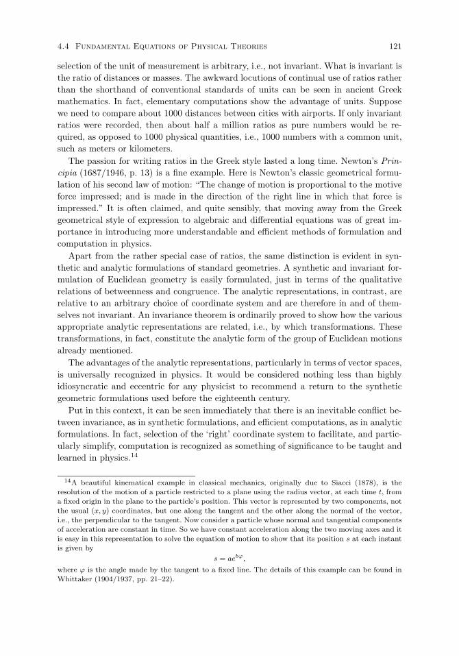
4.4 Fundamental Equations of Physical Theories 121

selection of the unit of measurement is arbitrary, i.e., not invariant. What is invariant isthe ratio of distances or masses. The awkward locutions of continual use of ratios ratherthan the shorthand of conventional standards of units can be seen in ancient Greekmathematics. In fact, elementary computations show the advantage of units. Supposewe need to compare about 1000 distances between cities with airports. If only invariantratios were recorded, then about half a million ratios as pure numbers would be re-quired, as opposed to 1000 physical quantities, i.e., 1000 numbers with a common unit,such as meters or kilometers.

The passion for writing ratios in the Greek style lasted a long time. Newton’s Prin-cipia (1687/1946, p. 13) is a fine example. Here is Newton’s classic geometrical formu-lation of his second law of motion: “The change of motion is proportional to the motiveforce impressed; and is made in the direction of the right line in which that force isimpressed.” It is often claimed, and quite sensibly, that moving away from the Greekgeometrical style of expression to algebraic and differential equations was of great im-portance in introducing more understandable and efficient methods of formulation andcomputation in physics.

Apart from the rather special case of ratios, the same distinction is evident in syn-thetic and analytic formulations of standard geometries. A synthetic and invariant for-mulation of Euclidean geometry is easily formulated, just in terms of the qualitativerelations of betweenness and congruence. The analytic representations, in contrast, arerelative to an arbitrary choice of coordinate system and are therefore in and of them-selves not invariant. An invariance theorem is ordinarily proved to show how the variousappropriate analytic representations are related, i.e., by which transformations. Thesetransformations, in fact, constitute the analytic form of the group of Euclidean motionsalready mentioned.

The advantages of the analytic representations, particularly in terms of vector spaces,is universally recognized in physics. It would be considered nothing less than highlyidiosyncratic and eccentric for any physicist to recommend a return to the syntheticgeometric formulations used before the eighteenth century.

Put in this context, it can be seen immediately that there is an inevitable conflict be-tween invariance, as in synthetic formulations, and efficient computations, as in analyticformulations. In fact, selection of the ‘right’ coordinate system to facilitate, and partic-ularly simplify, computation is recognized as something of significance to be taught andlearned in physics.14

14A beautiful kinematical example in classical mechanics, originally due to Siacci (1878), is the

resolution of the motion of a particle restricted to a plane using the radius vector, at each time t, from

a fixed origin in the plane to the particle’s position. This vector is represented by two components, not

the usual (x, y) coordinates, but one along the tangent and the other along the normal of the vector,

i.e., the perpendicular to the tangent. Now consider a particle whose normal and tangential components

of acceleration are constant in time. So we have constant acceleration along the two moving axes and it

is easy in this representation to solve the equation of motion to show that its position s at each instant

is given by

s = aebϕ,

where ϕ is the angle made by the tangent to a fixed line. The details of this example can be found in

Whittaker (1904/1937, pp. 21–22).

122 Invariance

Beyond symmetry. From what I have said, it might be misleadingly inferred thatin choosing convenient laboratory coordinate systems physicists neglect considerationsof invariance. In practice, physicists hold on to invariance by introducing and using theconcept of covariants. Before introducing this concept, it will be useful to survey thenatural generalizations beyond symmetry in familiar geometries.

The most general automorphisms of Euclidean space are transformations that arecompositions of rotations, reflections and translations. We have already considered ro-tations and reflections in Section 4.1. Familiar figures such as circles, squares and equi-lateral triangles are invariant under appropriate groups of rotations and reflections—aninfinite group for circles, and finite groups for squares and equilateral triangles.

On the other hand, none of these familiar figures are invariant under automorphismsthat include translations. In fact, no point is, so that the only invariant is that of theentire space being carried onto itself. But translations are important not only in puregeometry but in many applications, especially in physics, where the Galilean transfor-mations of classical physics and the Lorentz transformations of special relativity playan important role, and both include translations.

In the last paragraph an unnoted shift was made from automorphisms of a qualita-tive form of Euclidean geometry, based on such primitive concepts as betweenness andcongruence, to the numerical coordinate frames of reference of the Galilean and Lorentzgroups of transformations. Such frames are needed to give an explicit account of thephysicists’ concept of covariants of a theory.

Typical examples of such covariants are velocity and acceleration, both of which arenot invariant from one coordinate frame to another under either Galilean or Lorentziantransformations, because, among other things, the direction of the velocity or accelera-tion vector of a particle will in general change from one frame to another. (The scalarmagnitude of acceleration is invariant.)

Covariants. The laws of physics are written in terms of such covariants. Withoutaiming at the most general formulation, the fundamental idea is conveyed by the follow-ing. Let Q1, . . . , Qn be quantities that are functions of the space-time coordinates, withsome Qi’s being derivatives of others, for example. Then in general, as we go from onecoordinate system to another, Q′

1, . . . , Q′n will be covariant, rather than invariant, and

so their mathematical form is different in the new coordinate system. But any physicallaw involving them, say,

F (Q1, . . . , Qn) = 0 (1)

must have the same formF (Q′

1, . . . , Q′n) = 0 (2)

in the new coordinate frame. This requirement of same form is the important invariantrequirement. Equations (1) and (2) are, in the usual language of physicists, also calledcovariant. So, the term covariant applies both to quantities and equations. I omit anexplicit formal statement of these familiar ideas.

Here is a simple example from classical mechanics. Consider the conservation ofmomentum of two particles before and after a collision, with vi the velocity before, wi

the velocity afterward, and mi the mass, i = 1, 2, of each particle. The law, in the form

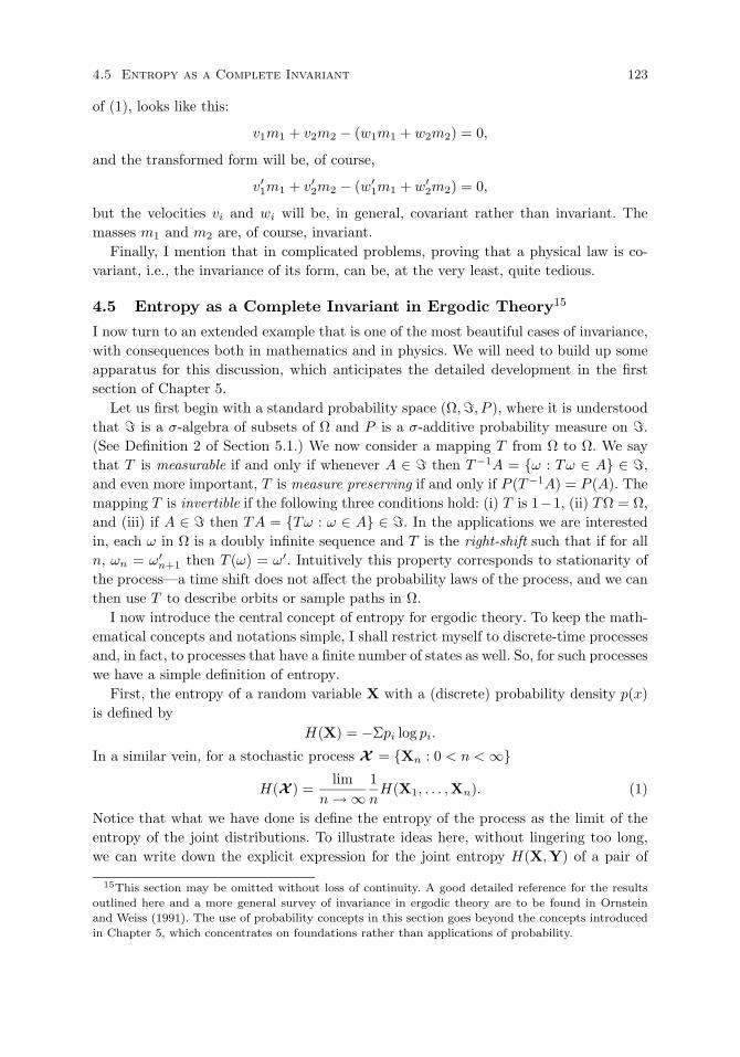
4.5 Entropy as a Complete Invariant 123

of (1), looks like this:

v1m1 + v2m2 − (w1m1 + w2m2) = 0,

and the transformed form will be, of course,

v′1m1 + v′2m2 − (w′1m1 + w′

2m2) = 0,

but the velocities vi and wi will be, in general, covariant rather than invariant. Themasses m1 and m2 are, of course, invariant.

Finally, I mention that in complicated problems, proving that a physical law is co-variant, i.e., the invariance of its form, can be, at the very least, quite tedious.

4.5 Entropy as a Complete Invariant in Ergodic Theory15

I now turn to an extended example that is one of the most beautiful cases of invariance,with consequences both in mathematics and in physics. We will need to build up someapparatus for this discussion, which anticipates the detailed development in the firstsection of Chapter 5.

Let us first begin with a standard probability space (Ω,, P ), where it is understoodthat is a σ-algebra of subsets of Ω and P is a σ-additive probability measure on .(See Definition 2 of Section 5.1.) We now consider a mapping T from Ω to Ω. We saythat T is measurable if and only if whenever A ∈ then T−1A = ω : Tω ∈ A ∈ ,and even more important, T is measure preserving if and only if P (T−1A) = P (A). Themapping T is invertible if the following three conditions hold: (i) T is 1−1, (ii) TΩ = Ω,and (iii) if A ∈ then TA = Tω : ω ∈ A ∈ . In the applications we are interestedin, each ω in Ω is a doubly infinite sequence and T is the right-shift such that if for alln, ωn = ω′

n+1 then T (ω) = ω′. Intuitively this property corresponds to stationarity ofthe process—a time shift does not affect the probability laws of the process, and we canthen use T to describe orbits or sample paths in Ω.

I now introduce the central concept of entropy for ergodic theory. To keep the math-ematical concepts and notations simple, I shall restrict myself to discrete-time processesand, in fact, to processes that have a finite number of states as well. So, for such processeswe have a simple definition of entropy.

First, the entropy of a random variable X with a (discrete) probability density p(x)is defined by

H(X) = −Σpi log pi.

In a similar vein, for a stochastic process X = Xn : 0 < n < ∞

H(X ) =lim

n → ∞1nH(X1, . . . ,Xn). (1)

Notice that what we have done is define the entropy of the process as the limit of theentropy of the joint distributions. To illustrate ideas here, without lingering too long,we can write down the explicit expression for the joint entropy H(X,Y) of a pair of

15This section may be omitted without loss of continuity. A good detailed reference for the results

outlined here and a more general survey of invariance in ergodic theory are to be found in Ornstein

and Weiss (1991). The use of probability concepts in this section goes beyond the concepts introduced

in Chapter 5, which concentrates on foundations rather than applications of probability.

124 Invariance

discrete random variables with a joint discrete density distribution p(X,Y).

H(X,Y) = −∑

x

∑y

p(x, y) log p(x, y),

which can also be expressed as

H(X,Y) = −E log p(X,Y)

where E stands for expectation. Notice, of course, there is a requirement for (1) thatI have been a little bit casual about. It is important to require that the limit exist. Sothe entropy of the stochastic process will not be defined if the limit of the entropies ofthe finite joint distributions does not exist as n goes to infinity.

For a Bernoulli process, that is, a process that has on each trial identically and inde-pendently distributed random variables (i.i.d.), we have a particularly simple expressionfor the entropy. It is just the entropy of a single one of the random variables, as thefollowing equations show:

H(X ) = limn→∞

1nH(X1,X2, . . . ,Xn)

=nH(X1)

n= H(X1) = −Σpi log pi.

We require only a slightly more complex definition for the case of a Markov chain,again, of course, with the provision that the limit exists.

H(X ) = limn→∞H(Xn | Xn−1, . . . ,X1)

= H(X2 | X1)

= −ΣipiΣjpij log pij .

Now we give, without detailed technical explanations, because the examples willbe simple, the definition of ergodicity. Let (Ω,F , P, T ) be a probability space withmeasure-preserving transformation T . Then T is stationary if for any measurable setA, µ(TA) = µ(A), and transformation T is called ergodic if for every set A such thatTA = A, the measure of A is either 0 or 1. We obtain a stochastic process by definingthe random variable Xn in terms of Tn, namely, for every ω in Ω, Xn(ω) = X(Tnω). Itis easy to see that Bernoulli processes as defined above are stationary and also ergodic.A more intuitive characterization of stationarity of a stochastic process is that everyjoint distribution of a finite subset of random variables of the process is invariant undertime translation. So, for every k,

p(xt1+k, xt2+k, . . . , xtm+k) = p(xt1 , xt2 , . . . , xtm).

Perhaps the simplest example of a nonergodic process is the Markov chain in headsand tails:

h t

h 1 0t 0 1

Given that the initial probability p1(h) = p1(t) = 12 , the event A consisting of the sample

path having heads on every trial has probability 12 , i.e., p(A) = 1

2 , but T (A) = A andthus the process is not ergodic. It is intuitively clear, already from this example, what

4.5 Entropy as a Complete Invariant 125

we expect from ergodic processes: a mixing that eliminates all dependence on the initialstate.

On the other hand, we have an ergodic process, but the entropy is 0, when the matrixis slightly different and the probability of heads on the first trial is now 1.

h t

h 0 1 p(h1) = 1.t 1 0

It is clear enough from the one possible sequence hththt . . . that all measurementsor outcomes are predictable and so the entropy must be 0. Note what this process is.It is not a Bernoulli process, but a very special deterministic Markov chain with twostates. In connection with this example, I mention that the standard definition in theliterature for ergodic Markov chains does not quite require stationarity. The definitionordinarily used is that a Markov chain is ergodic if it has a unique asymptotic probabilitydistribution of states independent of the initial distribution. So it is the independenceof initial distribution rather than stationarity that is key. Of course, what is obvioushere is that the process must be asymptotically stationary to be ergodic.

There are some further important distinctions we can make when a stochastic processhas positive entropy; not all measurements are predictable, but some may be. We candetermine, for example, a factor of the process, which is a restriction of the processto a subalgebra of events. A factor is, in the concepts used here, always just such asubalgebra of events. The concept of a K process (K for Kolmogorov), is that of astochastic process which has no factor with 0 entropy, that is, has no factor that isdeterministic. Bernoulli processes are K processes, but there are many others as well.

One important fact about ergodic processes is the fundamental ergodic theorem. Toformulate the theorem we need the concept of the indicator function of a set A. For anyevent A, let IA be the indicator function of A. That is, for ω ∈ A

IA(ω) =

1 if ω ∈ A,

0 if ω ∈ A.

The meaning of the fundamental ergodic theorem is that the time averages equal thespace or ensemble averages, that is, instead of examining a temporal cross-section forall ω’s having a property expressed by an event A, we get exactly the same thing byconsidering the shifts or transformations of a single sample path ω. The theorem holdsfor all ω’s except for sets of measure 0.

THEOREM 1. For almost any ω in Ω

limn→∞

1n

n−1∑k=0

IA(T kω) = P (A).

Isomorphism of ergodic processes. We define two stationary stochastic processesas being isomorphic (in the measure-theoretic sense) if we can map events of one toevents of the other, while preserving probability. The intuitive meaning of this is thattheir structural uncertainty is the same.

More technically, we define isomorphism in the following way. Given two probability

126 Invariance

spaces (Ω,, P ) and (Ω′,′, P ′) and two measure-preserving transformations T and T ′

on Ω and Ω′ respectively, then we say that (Ω,, P, T ) is isomorphic in the measure-theoretic sense to (Ω′,′, P ′, T ′) if and only if there exists a function ϕ : Ω0 → Ω′

0,where Ω0 ∈ ,Ω′

0 ∈ ′, P (Ω0) = P (Ω′0) = 1, that satisfies the following conditions:

(i) ϕ is 1 − 1,(ii) If A ⊂ Ω0 and A′ = ϕA then A ∈ iff A′ ∈ ′, and if A ∈

P (A) = P ′(A′),

(iii) TΩ0 ⊆ Ω0 and T ′Ω′0 ⊆ Ω′

0,(iv) For any ω in Ω0

ϕ(Tω) = T ′ϕ(ω).

The mapping of any event A to an event A′ of the same probability, i.e, condition (ii),is conceptually crucial, as is the commutativity expressed in (iv).

A problem that has been of great importance has been to understand how stochasticprocesses are related in terms of their isomorphism. As late as the middle 1950s, itwas an open problem whether two Bernoulli processes, one with two states, each witha probability of a half, B( 1

2 ,12 ), and one with three states, each having a probability

of one third, B( 13 ,

13 ,

13 ), are isomorphic, in accordance with the definition given above.

The problem was easy to state, but difficult to solve. Finally, the following theorem wasproved by Kolmogorov and Sinai.

THEOREM 2. (Kolmogorov 1958, 1959; Sinai 1959). If two Bernoulli processes areisomorphic then their entropies are the same.

Since B( 12 ,

12 ) and B( 1

3 ,13 ,

13 ) have different entropies, by contraposition of Theorem 2,

they are not isomorphic. It was not until twelve years later that Ornstein proved theconverse.

THEOREM 3. (Ornstein 1970). If two Bernoulli processes have the same entropy theyare isomorphic.

With these two theorems, extension to other processes, in particular, Markov pro-cesses, was relatively straightforward. And so, the following theorem was easily proved.

THEOREM 4. Any two irreducible, stationary, finite-state discrete Markov processesare isomorphic if and only if they have the same periodicity and the same entropy.

Out of this came the surprising and important invariant result. Entropy is a completeinvariant for the measure-theoretic isomorphism of aperiodic, ergodic Markov processes.Being a complete invariant also means that two Markov processes with the same peri-odicity are isomorphic if and only if their entropy is the same. What is surprising andimportant about this result is that the probabilistic structure of a Markov process islarge and complex. The entropy, on the other hand, is a single real number. It is hardto think of an invariance result for significant mathematical structures in which thedisparity between the complexity of the structures and the easy statement of the com-plete invariant is so large. Certainly, within probability theory, it is hard to match asan important invariance result. It is also hard to think of one in physics of comparablesimplicity in terms of the nature of the complete invariant.

4.5 Entropy as a Complete Invariant 127

On the other hand, it is important to note that even though a first-order ergodicMarkov process and a Bernoulli process may have the same entropy rate and, therefore,be isomorphic in the measure-theoretic sense, they are in no sense the same sort of pro-cess. We can, for example, show by a very direct statistical test whether a given samplepath of sufficient length comes from the Bernoulli process or the first-order Markovprocess. There is, for example, a simple chi-square test for distinguishing between thetwo. It is a test for first-order versus zero-order dependency in the process.

But this situation is not at all unusual in the theory of invariance. We can certainlydistinguish, as inertial observers, between a particle that is at rest in our inertial frameof reference, and one that is moving with a constant positive speed. What is observedcan be phenomenologically very different for two different inertial observers, Galilean orLorentzian. This way of formulating matters may seem different from the approach usedin the geometrical or ergodic cases, but this is so only in a superficial way. At a deeperand more general level, all the cases of invariance surveyed here have the common themeof identifying some special properties that are constant or unchanging.

5

Representations of Probability

No major contemporary school of thought on the foundations of probability disputesany of the axioms, definitions, or theorems considered in Section 1, with some minorexceptions to be noted. From the standpoint of the concepts introduced in Section 1, thelong-standing controversies about the foundations of probability can be formulated asdisputes about which models of the theory of probability as characterized in Definition2 are to be regarded as genuine probability spaces. Put another way, the controversiescenter around how the axioms of Definition 2 are to be extended to include only the“genuine” cases of probability spaces. In this and the following sections, we shall dividethe many variant positions on the nature of probability into the six most importantclasses of opinion. Section 2 is devoted to the classical definition, which was given arelatively definitive formulation by Laplace at the beginning of the nineteenth century.The next section is devoted to the relative-frequency view of probability, first formulatedin a reasonably clear fashion by John Venn at the end of the nineteenth century, andlater investigated and extended by Richard von Mises and others. Section 4 is focusedon the more recent theories of randomness in finite sequences and measures of theircomplexity as defined by Kolmogorov. Section 5 is devoted to logical theories of proba-bility, with particular emphasis on Jeffreys and on confirmation theory as developed byCarnap and others. Section 6 considers propensity theories of probability, especially interms of concrete physical or psychological examples, which lead to qualitative invariantrelations that are often not noticed. Section 7 concerns subjective theories, with whichde Finetti, I. J. Good, Lindley and L. J. Savage are particularly associated. Section 8,the final section, surveys pragmatic views about the nature of probability, which donot wholeheartedly endorse any one of the six main positions analyzed in the precedingsections.

In the statistical, more than the philosophical, literature on foundations of probabilitythere is a close association with the foundations of statistical inference, or, what somephilosophers would call, inductive inference. Because the literature on these two relatedfoundational topics is now so large, I have limited myself in the chapter to the foun-dations of probability, with only some superficial remarks about statistical inference,where the nature of probability is deeply intertwined with a specific form of statisticalinference. The present chapter, already very long, is still far from adequate in conveyingmany important aspects of the various representations or interpretations of probability.

129

130 Representations of Probability

A chapter of similar length would be required to give a comparable analysis of the mainalternative approaches to the foundations of statistics.

5.1 The Formal Theory

Our axiomatization of probability proceeds by defining the set-theoretic predicate ‘is aprobability space’. The intellectual source of the viewpoint presented is Kolmogorov’sclassic work (1933/1950). The main purpose of this section is to set forth the standardaxioms and concepts of probability theory as background for the study of the foundationsof probability in the rest of this chapter. Readers familiar with the standard formaldevelopment, as taught in modern probability courses, should omit this section. Almostall of the philosophical discussion of probability is to be found later in the chapter.Also, some much less standard formal theory is to be found in Section 7.2 on hiddenvariables in quantum mechanics, in Section 7.3 on concepts of reversibility for stochasticprocesses and in Sections 8.3 and 8.4 on stochastic learning models.

Primitive notions. The axioms are based on three primitive notions: a nonempty setΩ of possible outcomes, a family of subsets of Ω representing possible events,1 anda real-valued function P on , i.e., a function whose range is a set of real numbers;for E ∈ , P (E) is interpreted as the probability of E. These three notions may beillustrated by a simple example. Let Ω be the set of all possible outcomes of three tossesof a coin.

Ω = hhh, hht, hth, htt, thh, tht, tth, ttt,where hhh is the event of getting three heads in a row, etc. Let be the family of allsubsets of Ω. The event of getting at least two heads is the set

A = hhh, hht, hth, thh.The event of getting exactly two heads is the set

B = hht, hth, thh,and so on. The important point is this. Any event that could occur as a result oftossing the coin three times may be represented by a subset of Ω. This subset has aselements just those possible outcomes, the occurrence of any one of which would implythe occurrence of the event. Thus, the event of getting at least two heads occurs if anyone of four possible outcomes occurs.

This representation of events as sets is one of the more important aspects of theapplication of probability theory to empirical data. To decide what sets are to representthe events is to make the major decision about the canonical form of the data from anexperiment. As we can see in the simple case of tossing a coin three times, we representthe outcomes of the experiment in such a way that most of the physical detail of theactual tossing of the coin is ignored. We do not, for example, record the time at whichthe coin came to rest, nor the time between tosses. We do not describe the mechanismused to make the tosses. We are interested only in a very simplified, and, in fact, verysimpleminded abstraction of what actually happened.

1In what follows, possible events will be referred to simply as ‘events’.

5.1 The Formal Theory 131

The language of events and the representation of events as subsets of the set of allpossible outcomes are now standard in textbooks on probability theory. Perhaps theonly major exception is to be found in the literature on logical theories of probabilityby philosophers and logicians; but it is easy to give a set-theoretical version of thistheory that in no way affects its substantive content, as we shall see later. However,this language of events has not always been universally accepted. The earlier difficultieswith this language stem from the lack of a clearly defined formal basis for it, as is givenby the standard set-theoretical interpretation now used. Prior to the characterizationof events as subsets of the set of all possible outcomes, or, as we shall often put it, assubsets of the sample space or probability space, the logical structure of an event wasnot well defined, and it was not always clear what was to count as an event.2 Objectionto the vagueness of the notion of the occurrence of an event is found in the followingpassage from Keynes’ treatise on probability (1921, p. 5).

With the term “event”, which has taken hitherto so important a place in the phraseology

of the subject, I shall dispense altogether. Writers on probability have generally dealt

with what they term the “happening” of “events”. In the problems which they first

studied this did not involve much departure from common usage. But these expressions

are now used in a way which is vague and ambiguous; and it will be more than a verbal

improvement to discuss the truth and the probability of propositions instead of the

occurrence and the probability of events.

It is to be noted that Keynes’ objections appeared more than ten years before the con-cept of event was clarified in Kolmogorov’s classical treatise. Many of the difficultiesin Keynes’ own views of probability arise from the vagueness of the notion of proposi-tion. The essentially intensional character of this notion makes it difficult to use as afundamental concept in probability theory if standard mathematical methods are sub-sequently to be applied. I shall consider this point again in discussing logical theories ofprobability in Section 5.

Let us return to the coin-tossing example. If the coin is fair, then for each ω in Ω,

Pω =18.

The probability of any other event may be obtained simply by adding up the number ofelements of Ω in the subset. Thus the probability of getting at least two heads in threetosses of the coin is P (A) and

P (A) = hhh, hht, hth, thh

= Phhh + Phht + Phth + Pthh

= 18 + 1

8 + 18 + 1

8 = 12 .

The additive property just exemplified is one of the fundamental properties of proba-bility postulated as an axiom: the probability of either one of two mutually exclusive

2I make no formal distinction between ‘sample space’ and ‘probability space’, but it is natural to

refer to the sample space of an experiment, which is usually finite, and the probability space of a

theory, which is often infinite. The set-theoretical definition that follows (Definition 2) mentions only

‘probability space’.

132 Representations of Probability

events is equal to the sum of their individual probabilities, that is, if A ∩B = ∅ then

P (A ∪B) = P (A) + P (B).

Language of events. Since throughout the remainder of this book we shall applyprobability language to sets which are interpreted as events, it will be useful to have atable relating set-theoretical notation to probability terms. To begin with, the assertionthat A ∈ corresponds to asserting that A is an event. At first glance the notion of thefamily of subsets may seem superfluous. It may seem reasonable to treat as events allpossible subsets of the sample space Ω. When Ω is a finite set, this is a reasonable andnatural approach; but it is not an acceptable treatment for very large spaces of the sortthat arise in many applications of probability theory. An example is given below to showwhy it is unreasonable to assume that all subsets of Ω may be considered as events. Togive another example from the table, the assertion that A ∩ B = ∅ corresponds to theassertion that events A and B are incompatible. In this table and subsequently, we usea compact notation for the intersection or union of a finite or infinite number of sets:

n⋂i=1

Ai = Ai ∩A2 ∩ · · · ∩An

n⋃i=1

Ai = A1 ∪A2 ∪ · · · ∪An

∞⋂i=1

Ai = A1 ∩A2 ∩ · · ·

∞⋃i=1

Ai = A1 ∪A2 ∪ · · · .

We use the same sort of notation for sums:n∑

i=1

P (Ai) = P (A1) + P (A2) + · · · + P (An).

Also, if Ω is a finite set, for example, and f is a numerical function defined on Ω, thenif Ω = a, b, c, ∑

ωεΩ

f(ω) = f(a) + f(b) + f(c).

5.1 The Formal Theory 133

SET-THEORETICAL NOTATION AND PROBABILITY TERMS

Set Theory Probability Theory

(a) A ∈ (a) A is an event.(b) A ∩B = ∅ (b) Events A and B are incompatible.(c) Ai ∩Aj = ∅ for i = j (c) Events A1, A2, . . . , An are pairwise incompat-

ible.

(d)n⋂

i=1

Ai = B (d) B is the event which occurs when eventsA1, A2, . . . , An occur together.

(e)n⋃

i=1

Ai = B (e) B is the event which occurs when at least oneof the events A1, A2, . . . , An occurs.

(f) B = −A (f) B is the event which occurs when A does not.(g) A = ∅ (g) Event A is impossible.(h) A = Ω (h) Event A is inevitable or certain.(i) B ⊆ A (i) If event B occurs, then A must occur.

In (f), complementation is, of course, with respect to Ω. For instance, if A is the event ofgetting at least two heads as in our example above, then −A is the event of not gettingat least two heads and

−A = Ω −A = tht, tth, htt, ttt.

Algebras of events. In order that the family of events has the appropriate set-theoretical structure, we must postulate certain closure properties for the family. Bypostulating that the union of any two events is also an event and that the complementof any event is also an event, the family of sets representing events becomes in the usualset-theoretical language an algebra of sets. By postulating in addition that the unionof any infinite sequence of elements of is also in , the algebra becomes a σ-algebra.Without these closure properties awkward situations arise in talking about events thatnaturally should be available. For example, if the event A is a head on the first toss ofa coin and B is the event of a tail on the second toss, it would be strange not to beable to consider the event A∩B, which is the event of the joint occurrence of A and B.The countable unions required for σ-algebras are not intuitively too obvious, but thisproperty is often required for more advanced work. We shall include it explicitly herein order to discuss later the kind of examples that do or do not have this property, andthe extent to which in more complicated contexts it is an intuitively desirable propertyto have. These notions are formalized in the following definition.

DEFINITION 1. is an algebra of sets on Ω if and only if is a nonempty familyof subsets of Ω and for every A and B in :

1. −A ∈ ;2. A ∪B ∈ .

Moreover, if is closed under countable unions, that is, if for A1, A2, . . . , An, . . . ∈ ,∪∞

i=1Ai ∈ , then is a σ-algebra on Ω.

134 Representations of Probability

The proof of the following theorem about elementary properties of algebras of sets isleft as an exercise for the reader.

THEOREM 1. If is an algebra of sets on Ω then

(i) Ω ∈ ,(ii) ∅ ∈ ,(iii) If A ∈ and B ∈ , then

A ∩B ∈ ,(iv) If A ∈ and B ∈ , then

A−B ∈ ,(v) If is a σ-algebra as well, and A1, A2, · · · ∈ , then

∞⋂i=1

Ai ∈ .

Theorem 1 tells us a good deal about the structure of algebras of sets. It should beapparent that an algebra of sets can be very trivial in character. For example, if Ω isthe sample space on which we plan to define probability, we can choose as an algebraof sets the family consisting just of Ω and the empty set. It is obvious, of course,that there is no interest whatsoever in this particular algebra. It is also not difficultto select some intuitively natural families of sets that are not algebras of sets. In thecase of our coin-tossing example, the family of sets consisting just of the unit sets ofthe outcomes, which are sometimes called the atomic events, is not an algebra of sets,because the union of two of these outcomes is not itself in the family of sets.3 Again,considering this example, the family of all subsets of Ω containing at least one h is alsonot an algebra of sets, because the complement of the largest such subset is not itselfin the family.

An example of an algebra which is not a σ-algebra is easily constructed from thenatural numbers. Let be all finite subsets of Ω together with the complements of suchfinite subsets. Then the set of even natural numbers is not in the algebra, though it isin the σ-algebra, because it is the countable union of finite sets in the algebra.

Axioms of probability. We are now ready to define probability spaces. In the defi-nition we assume the set-theoretical structure of Ω, , and P already mentioned: Ω is anonempty set, is a nonempty family of subsets of Ω, and P is a real-valued functionon . Thus the definition applies to ordered triples (Ω,, P ), which we shall call setfunction structures, since P is a function on a family of sets.

DEFINITION 2. A set function structure Ω = (Ω,, P ) is a finitely additive proba-bility space if and only if for every A and B in :

P1. is an algebra of sets on Ω;P2. P (A) ≥ 0;P3. P (Ω) = 1;P4. If A ∩B = ∅, then P (A ∪B) = P (A) + P (B).

3A unit set is a set having just a single element as its only member.

5.1 The Formal Theory 135

Moreover, Ω is a probability space (without restriction to finite additivity) if the followingtwo axioms are also satisfied:

P5. is a σ-algebra of sets on Ω;P6. If A1, A2, . . . is a sequence of pairwise incompatible events in

, i.e., Ai ∩ Aj = ∅ for i = j, then

P (∞⋃

i=1

Ai) =∞∑

i=1

P (Ai).

The properties expressed in P5 and P6 can be separated. For example, a probabilitymeasure P satisfying P6 is said to be countably additive, and we can concern ourselveswith countably additive probability measures on algebras that are not σ-algebras. Onthe other hand, for full freedom from a mathematical standpoint it is desirable to haveboth P5 and P6 satisfied, and for this reason we have assumed that probability spacessatisfy both P5 and P6.4 In particular, this full freedom is essential for the standarddevelopment of the asymptotic theory as sample size or number of trials approachesinfinity. It should be apparent that if the set Ω is finite then every finitely additiveprobability space is also a probability space. It may be mentioned that an additionalpostulate is sometimes required of probability spaces. The postulate asserts that ifA ⊆ B,B ∈ , and P (B) = 0, then A ∈ . When a probability space satisfies thisadditional postulate it is called complete.

We now turn to a number of elementary concepts and theorems. Most of them holdfor finitely additive probability spaces, and, thus, do not require any use of Axioms P5and P6.

THEOREM 2.

(i) P (∅) = 0.(ii) For every event A,P (A) + P (−A) = 1.(iii) If the events Ai are pairwise incompatible for 1 ≤ i ≤ n, then

P (n⋃

i=1

Ai) =n∑

i=1

P (Ai).

Proof. We prove only (iii), which requires use of mathematical induction. For n = 1,clearly

P (A1) = P (A1).

Our inductive hypothesis for n is that

P (n⋃

i=1

Ai) =n∑

i=1

P (Ai).

Now consider

P (n+1⋃i=1

Ai).

4A simple example, given after Definition 14 of this section, is the computation of the mean of the

Poisson distribution. The computation is for an infinite sequence of probabilities and requires Axioms

P5 and P6.

136 Representations of Probability

Sincen+1⋃i=1

Ai = (n⋃

i=1

Ai) ∪An+1,

P (n+1⋃i=1

Ai) = P ((n⋃

i=1

Ai) ∪An+1)

= P (n⋃

i=1

Ai) + P (An+1) By P4 andhypothesis ofthe theorem

=n∑

i=1

P (Ai) + P (An+1) By inductivehypothesis

=n+1∑i=1

P (Ai)

Q.E.D.

Discrete probability densities. We next define discrete probability densities on aset Ω. Such a discrete probability density on a set Ω is a point function analogous tothe set function P . For many kinds of applications the use of a discrete or continuousprobability density function is essential, or at least highly desirable, in carrying outdetailed computations.

DEFINITION 3. A discrete probability density on a nonempty set Ω is a non-negativereal-valued function p defined on Ω such that for all ω ∈ Ω, p(ω) = 0 except for an atmost countable number of elements of Ω and

∑ω∈Ω p(ω) = 1.

It should be apparent that a discrete probability density can always be used togenerate a unique probability measure on a given algebra of sets, as expressed in thefollowing theorem, whose proof is omitted.

THEOREM 3. Let Ω be a nonempty set, let p be a discrete probability density on Ω,let be a σ-algebra of sets on Ω, and let P be a real-valued function defined on suchthat if A ∈ then P (A) =

∑ω∈A p(ω). Then Ω = (Ω,, P ) is a probability space.

For the present, we shall defer consideration of continuous densities on infinite sets.Here are four of the more important discrete densities. First, there is the distributionof a simple toss of a coin, usually called a Bernoulli density, because there are only twopossible values, i.e., only two elements in the probability space Ω. The sample spaceΩ = 0, 1, and p(1) = p, p(0) = q = 1 − p, where 0 ≤ p ≤ 1.5 For a fair coin, p = 1

2 .Second, there is the closely related binomial density, which arises from n independentBernoulli trials. The probability space Ω = 0, 1, ..., n, i.e., the probability space is the

5A grammatical ambiguity is tolerated continually in the notation used here, and in many other

places in this book. In the sentence “Ω = (Ω,F , P ) is a probability space” the expression ‘Ω = (Ω,F , P )’

is a noun phrase, but in the sentence “The sample space Ω = 0, 1” the main verb is ‘=’. Without use

of this ambiguity, resolved easily in each particular context, we need to use too many lengthy explicit

formulations.

5.1 The Formal Theory 137

set of non-negative integers 0 ≤ k ≤ n, and

p(k) = (nk )pk(1 − p)n−k,

where (nk ) is the binomial coefficient:(

n

k

)=

n!k!(n− k)!

.

The classic case of the binomial density is tossing a coin n times with p the probabilityof a head on each trial. The probability p(k) is the probability of k heads. It is commonto refer to the binomial distribution as frequently as the binomial density, when Ω is aset of numbers, so we need to define this important associated concept of distribution.Let f be a discrete density on a nonempty numerical set Ω. Define on Ω

F (x) =∑y≤x

f(y).

Then F is the (cumulative) probability distribution defined in terms of f . Notice thatwhen Ω is an arbitrary finite set, the concept of distribution is not well defined. Togeneralize beyond numerical sets, a meaningful linear ordering of the elements of Ω isneeded.

Third, there is the Poisson density with parameter λ, where λ ≥ 0.6 The probabilityspace Ω = 0, 1, 2, ... and

p(k) =e−λλk

k!.

The applications of the Poisson density or distribution complement those of the binomialdistribution. In applying the binomial distribution, we count the occurrences of somephenomena such as heads on given trials or presence of a disease on a given date. So, forexample, a head may occur on the first trial but not the second. In contrast, there aremany other phenomena for which our interest is in the number of occurrences in a giventime interval, for instance an hour, a day, a year. Other examples would be the numberof phone calls going through a given exchange in 24 hours, the number of airplaneslanding at an airport in one week, and the number of discharges of a Geiger counterin two minutes. The Poisson distribution can also be applied to spatial phenomena; forinstance, the number of bacteria of a given kind found in one-liter samples of waterfrom a city’s water supply. Implicit in these examples of either a spatial or temporalsort is that successive samples will be taken. For instance, we might look at telephoneexchange data for 200 successive days. Although none of the phenomena described wouldever have even a large finite number of occurrences, say 10100, in a realistic temporalinterval or spatial extent, it is mathematically convenient to define the density for everynon-negative integer. A reason, of course, is that there is no natural stopping point, butthis is certainly not the main reason. It is always easy to pick a finite domain more thanadequate to deal with actual observations, but when a large finite domain is used it isharder to determine the mathematical or theoretical properties of the distribution.

6Poisson (1781–1840) was one of the great French mathematical physicists of the nineteenth century.

His derivation of the Poisson density was published in 1837, but not really recognized as a significant

contribution until the end of the century.

138 Representations of Probability

Fourth, there is the geometric density with parameter p, with 0 ≤ p ≤ 1. The proba-bility space Ω = 1, 2, 3, ... and

p(k) = p(1 − p)k−1.

A theoretically important example is the density of the number k of trials to get thefirst head in successive Bernoulli trials with probability p of success. For instance, theprobability of getting the first head on the fifth toss of a biased coin with p = .25is 0.079 (approximately). The geometric density is the natural one to use in studyingradioactive decay when discrete trials are used, as we shall see in the section on thepropensity interpretation of probability.

Conditional probability. We next consider the important concept of conditionalprobability. Its central role comes from the fact that dependencies, especially temporalones, are expressed in conditional terms.

DEFINITION 4. If A and B are in and P (B) > 0, then

P (A|B) =P (A ∩B)P (B)

.

We call P (A|B) the conditional probability of event A, given the occurrence of eventB. As an example, consider the situation in which a coin is tossed twice. Ω =hh, ht, th, tt, is the set of all subsets of Ω, and p(ω) = 1

4 for all ω in Ω. Thereare two events A and B such that A is the event of exactly one head in two tosses andB is the event of at least one head in two tosses. Clearly, P (A) = 1

2 whereas P (B) = 34 .

Since A ∩B = A,P (A ∩B) = P (A) = 12 . Therefore, P (A|B) = P (A)

P (B) = ( 12 )

( 34 )

= 23 .

For reasons that are apparent, the following theorem about conditional probabilitiesis usually labeled the multiplication theorem.

THEOREM 4. (Multiplication Theorem). If A1, A2, A3, . . . , An are in andP (∩n

i=1Ai) > 0, then

P (n⋂

i=1

Ai) = P (A1) · P (A2|A1) · P (A3|2⋂

i=1

Ai) · · ·P (An|n−1⋂i=1

Ai).

Proof. We use induction on n. For n = 1, clearly P (A1) = P (A1). Our inductivehypothesis for n is that

P (n⋂

i=1

Ai) = P (A1) · · ·P (An|n−1⋂i=1

Ai). (1)

But by the definition of conditional probability

P (n+1⋂i=1

Ai) = P (n⋂

i=1

Ai) · P (An+1|n⋂

i=1

Ai).

Therefore, using (1)

P (n+1⋂i=1

Ai) = P (A1) · P (A2|A1) · · ·P (An|n−1⋂i=1

Ai) · P (An+1|n⋂

i=1

Ai). Q.E.D.

5.1 The Formal Theory 139

Applications of the multiplication theorem usually involve other simplifying assump-tions. Markov chains provide good examples. Intuitively, a sequence of trials in whichthe probability of what happens on a trial depends on what occurred on the immedi-ately preceding trial, but not on earlier trials, is a (first-order) Markov chain. (A formaldefinition will not be given at this point.7) A slightly artificial example will provide asimple illustration. Suppose that remembering a given algorithm, let us say, dependsonly on whether it was remembered on the last trial of learning, and no earlier one. Letr be remembering and f forgetting. Then the transition matrix is:

r f

r

f

(.75 .25.10 .90

)

where the two rows show the state on trial n − 1 and the two columns the possiblestates on trial n. Thus if on trial n− 1, the algorithm was remembered, the probabilityis .75 it will be remembered on trial n. Assume we have the sequence of observationsffffrrfrrr, and suppose further that on trial 1, the probability of forgetting is 1.0—onthe first exposure. Then we can use these specialized assumptions and the multiplicationtheorem to compute the probability of our observed sequence.

p(ffffrrfrrr) = p(f)p(f |f)3p(r|f)p(r|r)p(f |r)p(r|f)p(r|r)2

= (1)(.9)3(.10)(.75)(.25)(.10)(.75)2

= .0007689 (approximately).

That conditional probabilities behave like ordinary probabilities is shown by the nexttwo theorems.

THEOREM 5. If A,B, and C are in and if P (A) > 0, then:

(i) P (B|A) ≥ 0,

(ii) P (Ω|A) = 1,

(iii) P (A|A) = 1,

(iv) If B ∩ C = ∅, then P (B ∪ C|A) = P (B|A) + P (C|A),

(v) If P (B) > 0, then P (A|B) = P (A) · P (B|A)P (B) ,

(vi) If A ∩B = ∅, then P (B|A) = 0,

(vii) If A ⊆ B, then P (B|A) = 1.

THEOREM 6. If A ∈ and P (A) > 0, then (Ω,, PA) is a finitely additive probabilityspace such that for every B in , PA(B) = P (B|A). Moreover, if (Ω,, P ) is countablyadditive, so is (Ω,, PA).

Proof. It is given that is an algebra on Ω. From Theorem 5(i) we have PA(B) ≥ 0,which satisfies P2 of Definition 2. From Theorem 5(ii) PA(Ω) = 1, which satisfies P3.From Theorem 5(iv), if B ∩ C = ∅, then PA(B ∪ C) = PA(B) + PA(C), which satisfiesP4, and similarly for countable additivity. Q.E.D.

7A detailed formal treatment of Markov chains is given in the last section of Chapter 7, which is on

reversibility of causal processes. A less thorough development, but one emphasizing ergodic properties,

is to be found in Section 4.5.

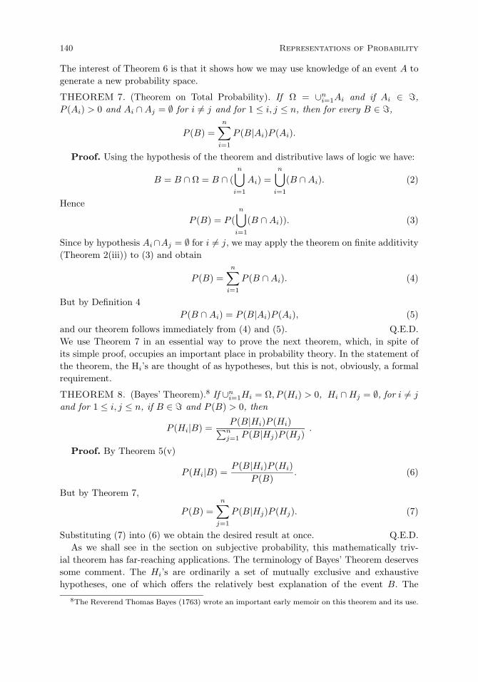
140 Representations of Probability

The interest of Theorem 6 is that it shows how we may use knowledge of an event A togenerate a new probability space.

THEOREM 7. (Theorem on Total Probability). If Ω = ∪ni=1Ai and if Ai ∈ ,

P (Ai) > 0 and Ai ∩Aj = ∅ for i = j and for 1 ≤ i, j ≤ n, then for every B ∈ ,

P (B) =n∑

i=1

P (B|Ai)P (Ai).

Proof. Using the hypothesis of the theorem and distributive laws of logic we have:

B = B ∩ Ω = B ∩ (n⋃

i=1

Ai) =n⋃

i=1

(B ∩Ai). (2)

Hence

P (B) = P (n⋃

i=1

(B ∩Ai)). (3)

Since by hypothesis Ai ∩Aj = ∅ for i = j, we may apply the theorem on finite additivity(Theorem 2(iii)) to (3) and obtain

P (B) =n∑

i=1

P (B ∩Ai). (4)

But by Definition 4P (B ∩Ai) = P (B|Ai)P (Ai), (5)

and our theorem follows immediately from (4) and (5). Q.E.D.We use Theorem 7 in an essential way to prove the next theorem, which, in spite ofits simple proof, occupies an important place in probability theory. In the statement ofthe theorem, the Hi’s are thought of as hypotheses, but this is not, obviously, a formalrequirement.

THEOREM 8. (Bayes’ Theorem).8 If ∪ni=1Hi = Ω, P (Hi) > 0, Hi ∩Hj = ∅, for i = j

and for 1 ≤ i, j ≤ n, if B ∈ and P (B) > 0, then

P (Hi|B) =P (B|Hi)P (Hi)∑n

j=1 P (B|Hj)P (Hj).

Proof. By Theorem 5(v)

P (Hi|B) =P (B|Hi)P (Hi)

P (B). (6)

But by Theorem 7,

P (B) =n∑

j=1

P (B|Hj)P (Hj). (7)

Substituting (7) into (6) we obtain the desired result at once. Q.E.D.As we shall see in the section on subjective probability, this mathematically triv-

ial theorem has far-reaching applications. The terminology of Bayes’ Theorem deservessome comment. The Hi’s are ordinarily a set of mutually exclusive and exhaustivehypotheses, one of which offers the relatively best explanation of the event B. The

8The Reverend Thomas Bayes (1763) wrote an important early memoir on this theorem and its use.

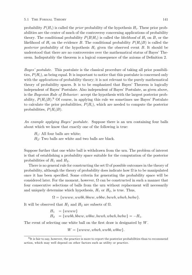
5.1 The Formal Theory 141

probability P (Hi) is called the prior probability of the hypothesis Hi. These prior prob-abilities are the center of much of the controversy concerning applications of probabilitytheory. The conditional probability P (B|Hi) is called the likelihood of Hi on B, or thelikelihood of Hi on the evidence B. The conditional probability P (Hi|B) is called theposterior probability of the hypothesis Hi given the observed event B. It should beunderstood that there are no controversies over the mathematical status of Bayes’ The-orem. Indisputably the theorem is a logical consequence of the axioms of Definition 2.

Bayes’ postulate. This postulate is the classical procedure of taking all prior possibili-ties, P (Hi), as being equal. It is important to notice that this postulate is concerned onlywith the applications of probability theory; it is not relevant to the purely mathematicaltheory of probability spaces. It is to be emphasized that Bayes’ Theorem is logicallyindependent of Bayes’ Postulate. Also independent of Bayes’ Postulate, as given above,is the Bayesian Rule of Behavior: accept the hypothesis with the largest posterior prob-ability, P (Hi|B).9 Of course, in applying this rule we sometimes use Bayes’ Postulateto calculate the prior probabilities, P (Hi), which are needed to compute the posteriorprobabilities, P (Hi|B).

An example applying Bayes’ postulate. Suppose there is an urn containing four ballsabout which we know that exactly one of the following is true:

H1: All four balls are white;H2: Two balls are white and two balls are black.

Suppose further that one white ball is withdrawn from the urn. The problem of interestis that of establishing a probability space suitable for the computation of the posteriorprobabilities of H1 and H2.

There is no general rule for constructing the set Ω of possible outcomes in the theory ofprobability, although the theory of probability does indicate how Ω is to be manipulatedonce it has been specified. Some criteria for generating the probability space will beconsidered later. For the moment, however, Ω can be constructed in such a manner thatfour consecutive selections of balls from the urn without replacement will necessarilyand uniquely determine which hypothesis, H1 or H2, is true. Thus,

Ω = wwww,wwbb, bbww,wbbw, bwwb, wbwb, bwbw.

It will be observed that H1 and H2 are subsets of Ω.

H1 = wwwwH2 = wwbb, bbww,wbbw, bwwb, wbwb, bwbw = −H1.

The event of selecting one white ball on the first draw is designated by W .

W = wwww,wbwb, wwbb, wbbw.

9It is fair to say, however, the practice is more to report the posterior probabilities than to recommend

action, which may well depend on other factors such as utility or practice.

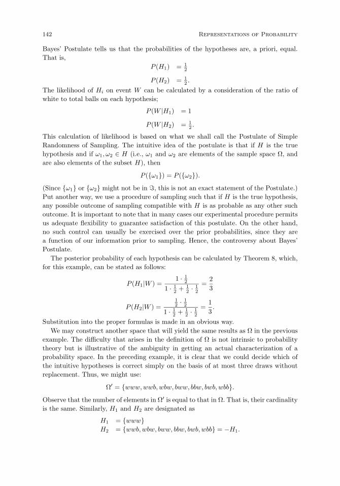
142 Representations of Probability

Bayes’ Postulate tells us that the probabilities of the hypotheses are, a priori, equal.That is,

P (H1) = 12

P (H2) = 12 .

The likelihood of Hi on event W can be calculated by a consideration of the ratio ofwhite to total balls on each hypothesis;

P (W |H1) = 1

P (W |H2) = 12 .

This calculation of likelihood is based on what we shall call the Postulate of SimpleRandomness of Sampling. The intuitive idea of the postulate is that if H is the truehypothesis and if ω1, ω2 ∈ H (i.e., ω1 and ω2 are elements of the sample space Ω, andare also elements of the subset H), then

P (ω1) = P (ω2).

(Since ω1 or ω2 might not be in , this is not an exact statement of the Postulate.)Put another way, we use a procedure of sampling such that if H is the true hypothesis,any possible outcome of sampling compatible with H is as probable as any other suchoutcome. It is important to note that in many cases our experimental procedure permitsus adequate flexibility to guarantee satisfaction of this postulate. On the other hand,no such control can usually be exercised over the prior probabilities, since they area function of our information prior to sampling. Hence, the controversy about Bayes’Postulate.

The posterior probability of each hypothesis can be calculated by Theorem 8, which,for this example, can be stated as follows:

P (H1|W ) =1 · 1

2

1 · 12 + 1

2 · 12

=23

P (H2|W ) =12 · 1

2

1 · 12 + 1

2 · 12

=13.

Substitution into the proper formulas is made in an obvious way.We may construct another space that will yield the same results as Ω in the previous

example. The difficulty that arises in the definition of Ω is not intrinsic to probabilitytheory but is illustrative of the ambiguity in getting an actual characterization of aprobability space. In the preceding example, it is clear that we could decide which ofthe intuitive hypotheses is correct simply on the basis of at most three draws withoutreplacement. Thus, we might use:

Ω′ = www,wwb,wbw, bww, bbw, bwb, wbb.

Observe that the number of elements in Ω′ is equal to that in Ω. That is, their cardinalityis the same. Similarly, H1 and H2 are designated as

H1 = wwwH2 = wwb,wbw, bww, bbw, bwb, wbb = −H1.

5.1 The Formal Theory 143

A moment’s reflection is sufficient to see that Ω and Ω′ will be the same in all remainingaspects and that H1 will again have the higher posterior probability.

If sets instead of ordered n-tuples were used to represent elements of Ω or Ω′, adifficulty would obviously arise. We would then have:

Ω′′ = w, w, b

and H1 and H2 would become

H1 = w

H2 = w, b.The algebra appropriate to this example is

′′ = ∅, w, w, b,Ω′′.

The problem then is: what subset of is W , the event of getting one white ball? ClearlyW cannot be appropriately characterized when Ω′′ is the basic space.

However, Ω and Ω′ do not represent the only legitimate possibilities. For severalreasons, many statisticians would prefer the following space:

Ω′′′ = (4, w), (2, w), (2, b),

and thusH1 = (4, w)

H3 = (2, w), (2, b).The number which is the first member of each ordered couple indicates the total numberof white balls in the urn on the given hypothesis (H1 or H2). The second memberindicates a possible outcome of drawing one ball. Note that there are only three elementsin Ω′′′, which is an advantage over Ω and Ω′. A second reason for preferring Ω′′′ is thatthe possible outcome of just one drawing is indicated, where elements of Ω indicatethe outcome of four samples without replacement, and Ω′ of three samples withoutreplacement. Thus the redundancy in the number of elements in Ω and Ω′. The spaceΩ′′′ is tailored to the problem in a way in which Ω and Ω′ are not.

Whatever sample space is used, the critical point lies in accepting Bayes’ Postulate.Many experts are critical of the reasonableness of this postulate, particularly expertswho advocate an objective interpretation of probability. Unfortunately, without Bayes’Postulate or some analogue which yields prior probabilities, it is impossible directly toapply the Bayesian rule of behavior previously stated.

One suggestion for meeting this difficulty is the following principle, the principle ofmaximum likelihood: accept that hypothesis whose likelihood for the observed event ismaximum. Hj is accepted if and only if

P (E|Hj) = maxiP (E|Hi).

We have as an obvious result:10

10For generalization of this theorem to infinite sets, see Theorem 3 of Section 5, formulated within

the framework of infinitesimal, i.e., nonstandard analysis.

144 Representations of Probability

THEOREM 9. If the number of hypotheses Hi is finite, then the Bayesian rule ofbehavior together with Bayes’ Postulate leads to acceptance of the same hypothesis asthe principle of maximum likelihood.

Concept of an experiment. We next turn to the concept of an experiment. We define anexperiment, relative to the sample space Ω, as any partition of Ω, i.e., any collection ofnonempty subsets of Ω, such that (i) the collection is a subset of the algebra of sets,(ii) the intersection of any two distinct sets in the collection is empty, and (iii) the unionof the collection is Ω itself. This definition of an experiment originates, as far as I know,with Kolmogorov (1933/1950). It is to be noticed that it is a technical concept withinprobability theory and is not meant to capture many of the nuances of meaning impliedin the general scientific use of the term. Nonetheless, it is easy to give examples to showthat the technical notion defined here corresponds to many of our intuitive ideas aboutexperimental data. Consider the complicated, continuous-time record from a satelliterecording many sorts of data. The full sample space Ω has as its elements all possibleobservable records for the time period and the variables under study. A meteorologistinterested only in sunspot data defines an experiment with respect to Ω by partitioningthe possible observable records according and only according to sunspot data. Dataon other variables of any sort are ignored in this data reduction. Such reduction isusually necessary in any detailed application of a quantitative theory to the results ofan experiment.

Independence. We now define the important concept of mutual independence ofexperiments.

DEFINITION 5. The n experiments M (1), . . . ,M (n) are (mutually) independent ifand only if for every Ai ∈ M (i) where 1 ≤ i ≤ n,

P (n⋂

i=1

Ai) =n∏

i=1

P (Ai).

Notice that A1 is any set in M (1), and so forth, andn∏

i=1

is the arithmetical product of

the n probabilities.The n events A1, A2, . . . , An are (mutually) independent if and only if the n experi-

ments M (1),M (2), . . . ,M (n) are mutually independent, where

M (i) = Ai,−Ai.We consider two examples to illustrate the concept of independence.

First example. Consider three consecutive tosses of a coin, for which

Ω = hhh, hht, hth, htt, thh, tht, tth, ttt.Let be the set of all subsets of Ω, and for all ω ∈ Ω, let p(ω) = 1

8 . This lattercondition guarantees that the coin is fair. Experiment M (1) is defined as follows: fori = 0, 1, 2, 3, Ai ∈ M (1) if and only if Ai is the event of getting exactly i heads. Wecan easily verify that M (1) is an experiment since M (1) is obviously a partition of Ω.

5.1 The Formal Theory 145

Similarly, experiment M (2) is defined for i = 0, 1, 2 such that Bi ∈ M (2) if and only ifBi is the event of getting exactly i alternations of heads and tails.

The question is then to determine if M (1) and M (2) are mutually independent ex-periments. There are 12 cases to consider, since M (1) has four elements and M (2) hasthree elements. But take, for example, the case of i = 0. In this case, A0 = ttt forwhich P (A0) = 1

8 and B0 = hhh, ttt for which P (B0) = 14 . It is clear that

P (A0 ∩B0) = P (A0) =18,

butP (A0) · P (B0) =

132.

Thus experiments M (1) and M (2) are not independent.

Second example. Consider the simultaneous toss of a pair of coins twice. One coin isred and one black. For the red coin a head is designated as ‘H’, whereas for the blackcoin a head is designated ‘h’, etc. For this example, the probability space is

Ω = HhHh,HhHt,HhTh, ..., T tT t;

as before, let be the set of all subsets of Ω and for all ω ∈ Ω, p(ω) = 116 . An experiment

M (1) is described for i = 0,1,2 in which Ai ∈ M (1) if and only if Ai is the event of exactlyi heads on the red coin. Experiment M (2) for i = 0, 1 is defined so that Bi ∈ M (2) ifand only if Bi is the event of exactly i alternations of heads and tails for the black coin.There are, of course, six separate cases to consider. Take, for example, A0 and B1. Then

A0 = ThTh, ThT t, T tTh, T tT t,

for which P (A0) = 14 and

B1 = HhHt,HtHh,HtTh,HhTt, ThHt, T tHh, T tTh, ThT t,

for which P (B1) = 12 . Furthermore,

A0 ∩B1 = TtTh, ThT t

P (A0 ∩B1) = 18

P (A0) · P (B1) = 14 · 1

2 = 18 .

Similar computations for the other five cases establish that experiments M (1) and M (2)

are mutually independent.The following theorem is obvious, and its converse is false.

THEOREM 10. If n experiments are mutually independent, then any m of themare mutually independent, for m < n.

It is clear that pairwise independence of events A1, A2, . . . , An does not guarantee mu-tual independence of these events. Consider the following example (due to S. Bernstein).Let Ω = a1, a2, a3, a4 and A1 = a1, a2, A2 = a1, a3, and A3 = a1, a4. For everyω in Ω, p(ω) = 1

4 . It is easy to compute that

P (A1) = P (A2) = P (A3) =12

146 Representations of Probability

P (A1 ∩A2) = P (A2 ∩A3) = P (A1 ∩A3) =14,

which establishes pairwise independence. But in contrast,

P (A1 ∩A2 ∩A3) = 14 and not 1

8 ,

as would be expected. The three events are pairwise independent, but they are notmutually independent.11

In the important case of two events A and B, it is easily shown from the precedingdefinitions that they are independent if and only if

P (A ∩B) = P (A)P (B).

The concept of independence is one of the most profound and fundamental ideas,not only of probability theory but of science in general. The exactly defined probabilitynotions of independence express very well the central intuitive idea back of the generalconcept. The two most basic ideas are concerned with the independence of what ishappening here and now from the remote past or far distant places. Any claim thatthere is immediate causation at a spatial or temporal distance is met with skepticismand usually by an effort to explain away such action at a distance by intermediateproximate causes.12 The probabilistic concept of independence provides a central toolfor analyzing these ideas about causation in a quite general way (Suppes 1970a).

Random variables. We now turn to the important concept of random variable. Inmany applications of probability theory in the sciences, the underlying sample spacehas a very complicated set-theoretical structure, and yet, at any given moment, we areinterested only in certain aspects of that space. To this end, we define certain real-valuedfunctions on the sample space and study the probabilistic behavior of these functions.

To conform to a notation common in statistics we shall henceforth use boldface ‘X’,‘Y’, and so forth, to denote random variables.

DEFINITION 6. X is a random variable if and only if X is a real-valued func-tion whose domain is the probability space Ω, and for each real number x, the setω : X(ω) < x is in .

The requirement that ω : X(ω) < x be in is no restriction at all on finite probabilityspaces for which is the set of all subsets. How a random variable may represent anexperiment is made clear in the next definition.

DEFINITION 7. Let M be an experiment and let X be a real-valued function definedon Ω. Then X is a random variable with respect to the experiment M if and only if foreach A in M there is a real number kA such that for every ω in A, X(ω) = kA.

In discussing a non-numerical discrete sample space such as

Ω = hh, ht, th, tt11For another example, one physically motivated that comes directly from the theory of quantum

entanglement, see footnote 15.12It was not always so. In the eighteenth century gravitation was the great example of action at a

distance, and there were respectable action-at-a-distance theories of electricity and magnetism in the

nineteenth century.

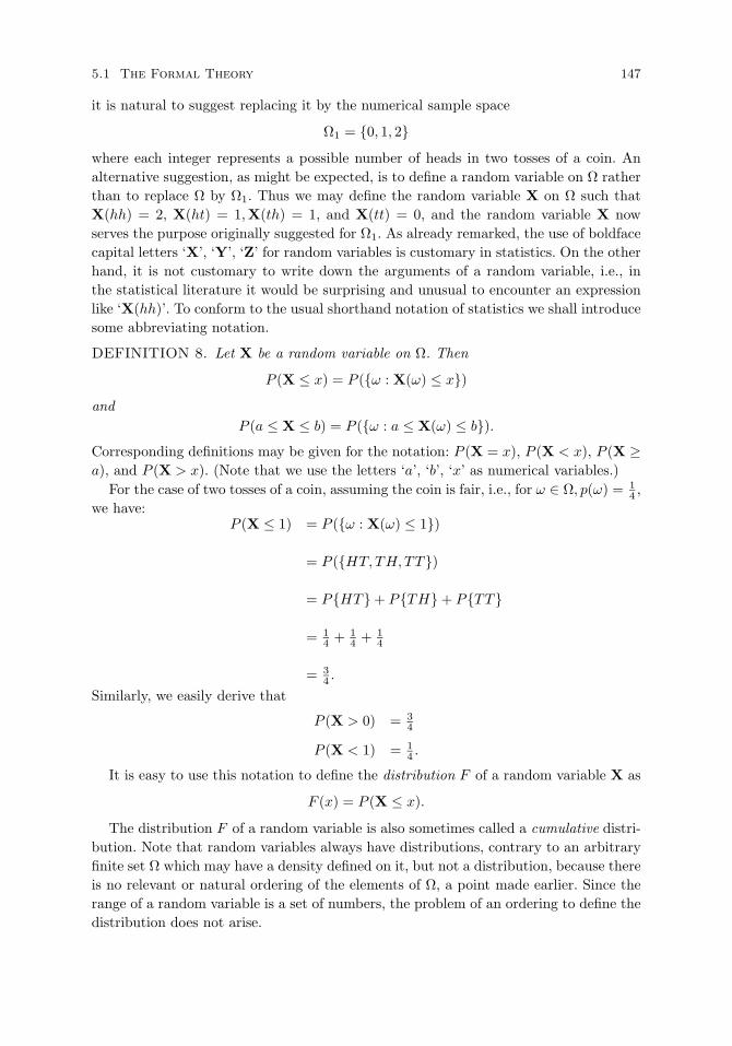
5.1 The Formal Theory 147

it is natural to suggest replacing it by the numerical sample space

Ω1 = 0, 1, 2

where each integer represents a possible number of heads in two tosses of a coin. Analternative suggestion, as might be expected, is to define a random variable on Ω ratherthan to replace Ω by Ω1. Thus we may define the random variable X on Ω such thatX(hh) = 2, X(ht) = 1,X(th) = 1, and X(tt) = 0, and the random variable X nowserves the purpose originally suggested for Ω1. As already remarked, the use of boldfacecapital letters ‘X’, ‘Y’, ‘Z’ for random variables is customary in statistics. On the otherhand, it is not customary to write down the arguments of a random variable, i.e., inthe statistical literature it would be surprising and unusual to encounter an expressionlike ‘X(hh)’. To conform to the usual shorthand notation of statistics we shall introducesome abbreviating notation.

DEFINITION 8. Let X be a random variable on Ω. Then

P (X ≤ x) = P (ω : X(ω) ≤ x)

andP (a ≤ X ≤ b) = P (ω : a ≤ X(ω) ≤ b).

Corresponding definitions may be given for the notation: P (X = x), P (X < x), P (X ≥a), and P (X > x). (Note that we use the letters ‘a’, ‘b’, ‘x’ as numerical variables.)

For the case of two tosses of a coin, assuming the coin is fair, i.e., for ω ∈ Ω, p(ω) = 14 ,

we have:P (X ≤ 1) = P (ω : X(ω) ≤ 1)

= P (HT, TH, TT)

= PHT + PTH + PTT

= 14 + 1

4 + 14

= 34 .

Similarly, we easily derive that

P (X > 0) = 34

P (X < 1) = 14 .

It is easy to use this notation to define the distribution F of a random variable X as

F (x) = P (X ≤ x).

The distribution F of a random variable is also sometimes called a cumulative distri-bution. Note that random variables always have distributions, contrary to an arbitraryfinite set Ω which may have a density defined on it, but not a distribution, because thereis no relevant or natural ordering of the elements of Ω, a point made earlier. Since therange of a random variable is a set of numbers, the problem of an ordering to define thedistribution does not arise.

148 Representations of Probability

Although the classification is not exhaustive, it is useful to distinguish between dis-crete and continuous random variables. The definition does not allow us to infer fromthe fact that a random variable is discrete that the underlying probability space Ω isalso discrete.

DEFINITION 9. A random variable X is discrete iff the set of values of X is count-able.

In other words, a discrete random variable is a function whose range is a countable set.The discrete density of a discrete random variable is easily defined.

DEFINITION 10. Let X be a discrete random variable. Then the discrete density ofX is the function p such that for any value x of X

p(x) = P (X = x).

In the case of the experiment consisting of tossing a fair coin twice in which thevalues of the numerical random variable X represent the number of heads obtained intwo tosses, the discrete density p of X is:

p(0) = 14

p(1) = 12

p(2) = 14 .

Note how the phrase ‘density of a random variable X’ is to be interpreted. The densityis actually on the set of possible values of the random variable, and the density f

or distribution F may always be defined in terms of the random variable X and theprobability measure P on the basic sample space.

Piecewise continuous densities and distributions. In the next definition we use thenotion of a piecewise continuous function. This a function that is continuous except at afinite number of points and at each point of discontinuity the right-hand and left-handlimits exist.

DEFINITION 11. A random variable X is piecewise continuous iff there is a piecewisecontinuous density f such that for every two real numbers a and b with a ≤ b

P (a ≤ X ≤ b) =∫ b

a

f(x)dx.

Ordinarily, we shall always say what the density of a piecewise continuous randomvariable is. Generalizations of Definition 11 are important in the mathematical literaturebut will not be considered here.

Note, once again, the obvious relation between the density f of a random variable Xand its distribution F .

F (x) =∑y≤x

f(y) (discrete case)

F (x) =∫ x

−∞ f(x)dx (piecewise continuous case).

5.1 The Formal Theory 149

From these equations it is obvious why a distribution F is also called a cumulativedistribution.

An example of a continuous random variable on a non-numerical sample space is thefollowing. (When the random variable has a continuous, not just piecewise continuousdensity, we shall refer to it simply as continuous.) Consider an experiment which isdesigned to test the accuracy of a new type of rocket. The rocket is aimed at a targetthree thousand miles away, and the experiment consists of determining where the rocketactually landed. Our basic sample space is the set of points of the earth’s surface. Onenumerical random variable of interest here is the one whose value, for any outcome ofthe experiment, is the distance between the target and the actual location of the rocket.

Expectation of a random variable. We now turn to the definitions of several fundamentalproperties of random variables. The definitions are given for both discrete and piecewisecontinuous random variables. We begin with the expected value or mean of a randomvariable.

DEFINITION 12. Let X be a discrete or piecewise continuous random variable withdensity f . Then the expected value or mean E(X) of X is given by:13

E(X) =∑xf(x) (discrete case)

E(X) =∫ ∞

−∞xf(x)dx (piecewise continuous case)

provided the sum or integral exists.

It should be apparent that the expectation of a random variable does not necessarilyexist. For example, the expectation of the Cauchy density

f(x) =1

π(1 + x2)does not exist.

It is also desirable to extend the definition of expected value to any continuousnumerical function of a random variable.

DEFINITION 13. Let X be a discrete or piecewise continuous random variable withdensity f , and let h be a continuous function in the latter case. Then the expectedvalue or mean E(h(X)) of h(X) is given by:

E(h(X)) =∑h(x)f(x) (discrete case)

E(h(X)) =∫ ∞

−∞h(x)f(x)dx (piecewise continuous case)

provided the sum or integral exists.

We may use Definition 14 to define moments about the origin and about the meanof a random variable.

DEFINITION 14. Let X be a discrete or piecewise continuous random variable withdensity f . Then:

13The sum is taken over the set of possible numerical values of the random variable.

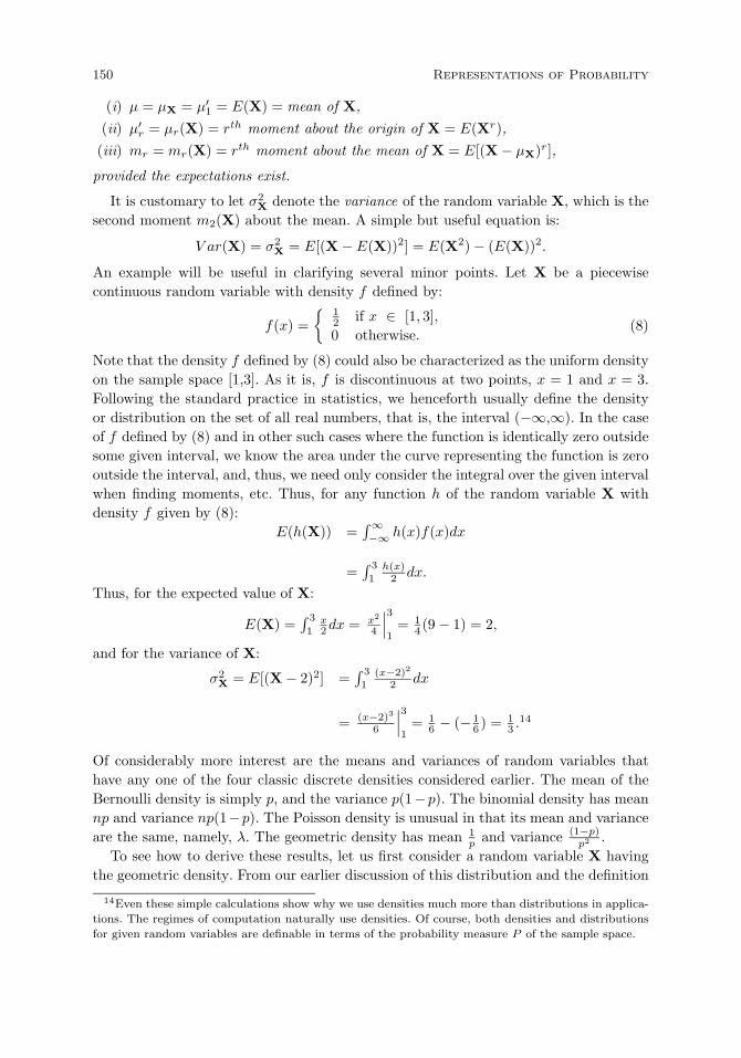
150 Representations of Probability

(i) µ = µX = µ′1 = E(X) = mean of X,

(ii) µ′r = µr(X) = rth moment about the origin of X = E(Xr),

(iii) mr = mr(X) = rth moment about the mean of X = E[(X − µX)r],

provided the expectations exist.

It is customary to let σ2X denote the variance of the random variable X, which is the

second moment m2(X) about the mean. A simple but useful equation is:

V ar(X) = σ2X = E[(X −E(X))2] = E(X2) − (E(X))2.

An example will be useful in clarifying several minor points. Let X be a piecewisecontinuous random variable with density f defined by:

f(x) =

12 if x ∈ [1, 3],0 otherwise.

(8)

Note that the density f defined by (8) could also be characterized as the uniform densityon the sample space [1,3]. As it is, f is discontinuous at two points, x = 1 and x = 3.Following the standard practice in statistics, we henceforth usually define the densityor distribution on the set of all real numbers, that is, the interval (−∞,∞). In the caseof f defined by (8) and in other such cases where the function is identically zero outsidesome given interval, we know the area under the curve representing the function is zerooutside the interval, and, thus, we need only consider the integral over the given intervalwhen finding moments, etc. Thus, for any function h of the random variable X withdensity f given by (8):

E(h(X)) =∫∞−∞ h(x)f(x)dx

=∫ 3

1h(x)

2 dx.

Thus, for the expected value of X:

E(X) =∫ 3

1x2dx = x2

4

∣∣∣31

= 14 (9 − 1) = 2,

and for the variance of X:

σ2X = E[(X − 2)2] =

∫ 3

1(x−2)2

2 dx

= (x−2)3

6

∣∣∣31

= 16 − (−1

6 ) = 13 .

14

Of considerably more interest are the means and variances of random variables thathave any one of the four classic discrete densities considered earlier. The mean of theBernoulli density is simply p, and the variance p(1 − p). The binomial density has meannp and variance np(1−p). The Poisson density is unusual in that its mean and varianceare the same, namely, λ. The geometric density has mean 1

p and variance (1−p)p2 .

To see how to derive these results, let us first consider a random variable X havingthe geometric density. From our earlier discussion of this distribution and the definition

14Even these simple calculations show why we use densities much more than distributions in applica-

tions. The regimes of computation naturally use densities. Of course, both densities and distributions

for given random variables are definable in terms of the probability measure P of the sample space.

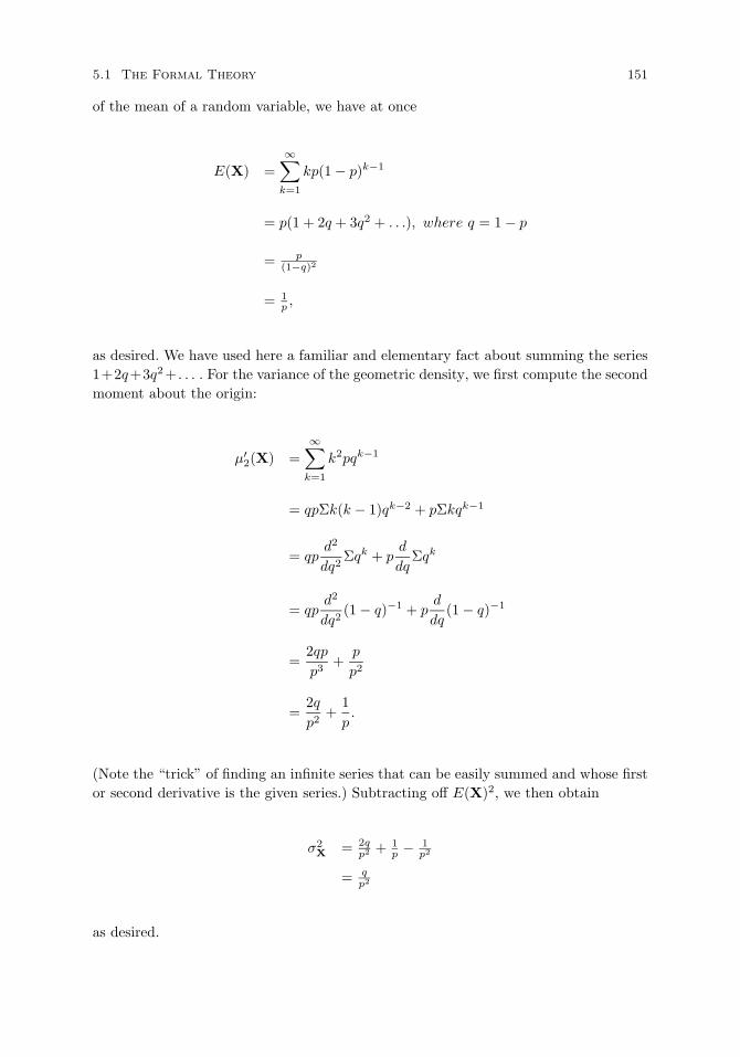
5.1 The Formal Theory 151

of the mean of a random variable, we have at once

E(X) =∞∑

k=1

kp(1 − p)k−1

= p(1 + 2q + 3q2 + . . .), where q = 1 − p

= p(1−q)2

= 1p ,

as desired. We have used here a familiar and elementary fact about summing the series1+2q+3q2+ . . . . For the variance of the geometric density, we first compute the secondmoment about the origin:

µ′2(X) =

∞∑k=1

k2pqk−1

= qpΣk(k − 1)qk−2 + pΣkqk−1

= qpd2

dq2Σqk + p

d

dqΣqk

= qpd2

dq2(1 − q)−1 + p

d

dq(1 − q)−1

=2qpp3

+p

p2

=2qp2

+1p.

(Note the “trick” of finding an infinite series that can be easily summed and whose firstor second derivative is the given series.) Subtracting off E(X)2, we then obtain

σ2X = 2q

p2 + 1p − 1

p2

= qp2

as desired.

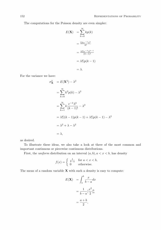
152 Representations of Probability

The computations for the Poisson density are even simpler:

E(X) =∞∑

k=0

kp(k)

= Σke−λλk

k!

= λΣe−λλk−1

(k−1)!

= λΣp(k − 1)

= λ.

For the variance we have:

σ2X = E(X2) − λ2

=∞∑

k=0

k2p(k) − λ2

=∞∑

k=1

ke−λλk

(k − 1)!− λ2

= λΣ(k − 1)p(k − 1) + λΣp(k − 1) − λ2

= λ2 + λ− λ2

= λ,

as desired.To illustrate these ideas, we also take a look at three of the most common and

important continuous or piecewise continuous distributions.First, the uniform distribution on an interval (a, b), a < x < b, has density

f(x) =

1b−a for a < x < b,

0 otherwise.

The mean of a random variable X with such a density is easy to compute:

E(X) =∫ b

a

x

b− adx

=1

b− a[x2

2]ba

=a+ b

2,

5.1 The Formal Theory 153

and by similar methods we easily show:

σ2X =

(b− a)2

12.

Second, the normal or Gaussian distribution on −∞ < x < ∞ has density

f(x) =1

σ√

2πe−

12 ( x−µ

σ )2 ,

with mean µ and variance σ2. (Statisticians call this the normal distribution, and physi-cists call it the Gaussian distribution–two distinct names for the same object.)

Third, the exponential distribution for −∞ < x < ∞ has the density

f(x) =λe−λx for x > 0,0 otherwise.

The mean is 1λ and the variance 1

λ2 .

Joint distributions. Extension of these ideas to several random variables is impor-tant for the analysis of many phenomena. For simplicity of notation I shall restrictmyself to continuous or piecewise continuous variables, but the concepts defined allhave immediate generalizations to arbitrary random variables.

DEFINITION 15. Let X and Y be two random variables.

(i) Their joint distribution is the function F such that for all real numbers x and y:

F (x, y) = P (X ≤ x,Y ≤ y);

(ii) Their joint density function f is defined by:

f(x, y) =∂2F (x, y)∂x∂y

;

(iii) Their marginal densities f1(x) and f2(x) are defined by:

f1(x) =∫ ∞

−∞f(x, y)dy

f2(y) =∫ ∞

−∞f(x, y)dx,

provided that the derivatives and integrals exist.

We may show that the two random variables are independent if for all x and y

f(x, y) = f1(x)f2(y).

In many ways the most theoretically important measure of dependence of two randomvariables is their covariance, which we define together with their correlation.

DEFINITION 16. Let X and Y be two random variables, whose means and variancesexist. The covariance of X and Y is defined as:

cov(X,Y) =∫ ∞

−∞

∫ ∞

−∞(x− E(X))(y −E(Y))f(x, y)dxdy,

154 Representations of Probability

provided that the double integral exists, and the correlation of X and Y is defined as:

ρ(X,Y) =cov(X,Y)σ(X)σ(Y)

,

provided that σ(X) = 0 and σ(Y) = 0.

It is important to note that if X and Y are independent, then the covariance andcorrelation equal zero, but the converse is not always true.15

These ideas generalize directly to n random variables X1, . . . ,Xn. First, the jointdistribution is the function F such that for all real numbers x1, . . . , xn

F (x1, . . . , xn) = P (X1 ≤ x1, . . . ,Xn ≤ xn).

Second, the joint density function f is defined by:

f(x1, . . . , xn) =∂n

∂x1 . . . ∂xnF (x1, . . . , xn)

given that the derivatives exist. Given the joint density of the n random variables, theyare independent iff

f(xi, . . . , xn) =n

Πi=1

fi(x).

Modal aspects of probability. Questions of modality are often raised about state-ments of probability, and I examine briefly some of the issues. To illustrate modal ideas,it will be sufficient to consider once again the simple example of tossing a coin threetimes. The sample space consists of eight outcomes corresponding to the eight possiblesequences of heads and tails that may be observed in three trials, as discussed earlier indetail. We can make a number of modal statements about the experiment representedby the sample space. In particular, the following statements, one about possibility andthe other about necessity, are certainly true:

(1) It is possible that the event of getting heads on all three trials will occur.(2) It is necessary that either at least one head or one tail occur on the three trials.

Other statements of possibility and necessity are easily constructed, but such statementsare ordinarily of little interest in a probability context, because of their obviousness ortriviality. The probability statements in which we are ordinarily interested, however,also have a clear modal character. Suppose that in our simple experiment the trials areBernoulli with p = 1

2 . We would then accept the following statements as also true:

(3) The probability of getting a head on the third trial is independent of the outcomeof the second trial.

15A physically interesting, but simple example of absence of a converse arises in quantum mechanics.

The physical setting of this example is the kind of quantum entanglement analyzed for GHZ-type

experiments at the end of Section 7.2. But the example can be completely understood on its own terms

without any reference to quantum phenomena. Let X,Y,Z be three random variables whose values

are ±1, let E(X) = E(Y) = E(Z) = 0, and let the third moment E(XYZ) = 1. Then it is easy to

prove that the covariances equal zero, i.e., E(XY) = E(YZ) = E(XZ) = 0. Since the third moment is

a direct statement of deterministic dependence, that the covariances are zero obviously does not imply

independence of X,Y and Z.

5.1 The Formal Theory 155

(4) The probability of getting exactly two heads, given that at least two heads occur,is greater than 1

2 .

From a modal standpoint the semantics of this setup is relatively straightforward be-cause the set of possible worlds is just the set of possible outcomes in the sample space.On the other hand, in almost all cases of application the set of possible outcomes asreflected in the sample space is much more restricted than the set of possible worldsordinarily discussed in modal logic. Many set-theoretical and other mathematical rela-tions are accepted as fixed across the set of possible outcomes in the sample space, andare not subject to variation as they often are in accounts of possible worlds.

A more important divergence from modal logic is apparent in the mathematical andscientific practice of using probability concepts. The probability measure and statementsabout probability are all handled in a purely extensional fashion, and the extensionalstatus of probability concepts is no different from that of other scientific concepts. Thisis even true of subjectivistic theories of probability where strong intensional notionscorresponding to assertions about belief would seem to play a natural role. (Occasionallysome subjectivists have taken account of this problem but it is certainly not standard.)

There is a deeper reason, however, why the modality of probability is left implicit.This is the fact that in most complicated applications the explicit sample space is not setforth. In fact, the problem is so formulated that there is not a unique probability spacebut a plethora of them. A problem, either theoretical or applied, is stated in terms of afamily of random variables. The consistency requirement is that the family of randomvariables have a joint distribution compatible with the joint distributions of all finitesubsets of the random variables, but there is no uniqueness to the definition of samplespace. What I have said, taken literally, would seem to run against the earlier definitionof random variables as requiring them to be functions defined on the sample space.In practice, however, it is clear that the specific sample space plays no real role andwhat is important is the distribution of the random variable, that is, the distributionof the values of the random variable. From a modal standpoint this means that theset of possible worlds is left implicit. A sustained effort to avoid having a sample spaceanywhere in sight is to be found in de Finetti’s two-volume treatise on probability (1974),where to avoid confusion of terminology he talks about random quantities rather thanrandom variables. All the same, it is to be emphasized that de Finetti’s terminologyand conceptual analysis are not in agreement with that generally used by almost allcontemporary statisticians, including many that are quite sympathetic to de Finetti’ssubjectivistic view of probability.

Probabilistic invariance. In Section 4.1, I described an important logical result oninvariance. As stated by Tarski and Givant (1987, p. 57), there are just four binaryrelations between elements of a given universe invariant under every permutation ofthe elements of the universe. These four relations are the universal relation, the emptyrelation, the identity relation and the diversity relation.

No such simple and general result holds for probability theory, but many particu-lar invariance results for particular probabilistic theories are known. In Section 4.5 animportant instance was described, entropy as a complete invariant for Bernoulli and

156 Representations of Probability

ergodic Markov processes that are isomorphic in the sense that there is a mapping fromone process to another preserving probability of events.

There are many important, but more elementary, invariant results in probability,several of which we will consider as the final topic of this section. There are usuallyseveral different ways to formulate the same invariant result. Here, for simplicity’s sake,I restrict consideration to finite sample spaces, i.e., one for which the set Ω of possibleoutcomes is finite. The second restriction, in the spirit of Tarski’s results for logic, and,more generally, the geometric invariance Erlangen program of Felix Klein, as discussedin Section 4.1, is to formulate the results in terms of one-one transformations of Ω ontoitself, i.e., in terms of bijections of Ω. I give simple informal proofs for special cases only.

Independence. Let X1, . . . ,Xn be n random variables representing n tosses of a coin.So Ω has 2n possible outcomes. Then probability is invariant, i.e., constant, under anybijection of Ω onto itself if and only if the random variables Xi are independent andfair, i.e., P (Xi = 1, for heads) = 1

2 . Here is the proof for n = 2. The random variablesX1 and X2 are independent if and only if their joint density p(x, y) = p(x)p(y), wherewe write ‘p’ instead of ‘f ’ for the discrete density. Then using obvious notation for thepossible outcomes, we first prove

p(h1h2) = p(h1)p(h2). (9)

Since all four possible outcomes are equal in probability by our invariance assumption,

p(h1h2) =14,

but p(h1) = p(h1h2)+p(h1t2) = 12 and by a similar argument p(h2) = 1

2 . Since 14 = 1

2 · 12 ,

(9) is established, and likewise by the same kind of argument, the other three, and wehave already shown that the coin is fair, since p(h1) = p(h2) = 1

2 . This proof is trivial,but it exhibits the germ of the general method.

Notice that this case is close to the logical result and the reason is obvious. Onprobability grounds, when we have both independence and fairness there is no proba-bilistic way of distinguishing between two possible outcomes. They are probabilisticallyequivalent.

Exchangeability. Again, consider coin tossing, but this time, we do not assume fairness.The coin may be biased. But we may, under the usual assumptions about coin tossing,assume a weaker kind of invariance. We assume that if the number of heads in twodifferent possible outcomes is the same, then a bijection of Ω onto itself will preserveprobability, i.e., be invariant, for all outcomes with the same number of heads. In otherwords, as seems intuitively clear, the order in which heads appear in a sequence of ntosses does not affect the probability. Put in a way more congenial to bijections of Ω, letan outcome of n trials be given. Then any permutation of this outcome must have thesame probability under our invariance hypothesis. For example, consider three tosses.Then, using ≈ for equivalence in probability:

hht ≈ hth ≈ thh,

htt ≈ tht ≈ tth,

5.2 Classical Definition of Probability 157

but there are no such equivalences for hhh and ttt. We also have a simple representationpossible for this exchangeable setup. Namely, a representation of the invariance is caughtby a single counting random variable Y, whose values, for the example, are simply 0,1, 2 and 3. So Y(hht) = 2, the number of heads. There is much more to be said aboutexchangeability, which is touched on in Section 7, but here we see the dramatic reductionfrom the 2n possible outcomes to just a single random variable Y with n + 1 possiblevalues. When the random variables X1, . . . ,Xn are exchangeable, all that can be saidprobabilistically can be said just with the random variable Y.

Exponential decay. A third example, given in detail in Section 6 on propensity theoriesof probability, introduces a different kind of invariance, but one quite familiar in manyapplications of probability theory. I have in mind the memoryless property of the ex-ponential distribution, or its discrete analogue, the geometric distribution. If an eventanticipated has not occurred up to time t, then its probability of occurring ∆t lateris no different than it was at some earlier time t′. Another way of putting the matter,there is no aging of the process, no becoming more likely to occur sooner as the presentmoves forward. Here is the notation used to develop this example in detail in Section 6.Let p(a1) be the probability of a radium atom decaying at time t1, and let p(an+1|An)be the conditional probability that the atom will decay on trial tn+1, given the eventAn of not decaying by time tn. The invariance condition is then

p(an+1|An) = p(a1).

Imagine how different the life of organisms would be if the expected age of dying obeyedsuch an invariant exponential law. There are, of course, many physical processes thatare of this exponential kind.

Note that in the last two examples of invariance, exchangeability and exponentialdecay, the invariant properties of the process do not uniquely determine the probabilitydistribution, but rather place important constraints on it. It is characteristic of the gen-eral invariant properties of most physical or psychological processes that they determinethe form of the density or distribution up to a small number of parameters that mustbe estimated empirically from data. This point is taken up in more detail in Section 6on propensity theories of probability.

5.2 Classical Definition of Probability

Considering the ubiquitous character of probability, and the widespread interest in gam-bling in all segments of the population, both now and throughout a large part of recordedhistory, it is surprising to find that systematic discussions of probability constitute avery late intellectual development. Apart from a few minor things in the sixteenth cen-tury, there is no serious work in probability theory before the seventeenth century. Inspite of the deep developments in Greek mathematics and astronomy, questions aboutprobability apparently did not receive any systematic treatment in Greek thought. Itappears that nowhere in Greek science or mathematics was the problem of handlingerrors of measurement discussed as a probabilistic phenomenon, subject to quantitativeanalysis.

158 Representations of Probability

Traditionally, the main origin of systematic probability theory is attributed to thework of Pascal and Fermat in the seventeenth century, and there does not seem to bemuch modern evidence to challenge this attribution. The traditional account is that theChevalier de Mere proposed certain questions to Pascal involving the computation ofodds in games of chance. Pascal corresponded with Fermat on these matters, and out ofthis correspondence was formed the mathematical theory of probability. It is interestingto note that the problem discussed in the first letter extant in the correspondencebetween Pascal and Fermat, namely, the letter dated July 29, 1654, is already of a fairlydifficult sort. It is called the problem of points. Two players in a game each need a givennumber of points to win, and on each move have equal chances of winning a single point.Suppose the players separate without finishing the game. The problem is to determinehow the stakes should be divided on the basis of their current scores. This is the sameas asking for the probability of winning the game, which each player has at any givenstage. Pascal did not give the complete solution of this problem, nor shall we discuss ithere. He did exhibit all the cases that can occur in a game of six points, and he alsocovered the case when one player lacks only a single point of winning and the secondplayer has no points, as well as the case when one player has one point and the secondplayer has no points.

In the same letter to Fermat, Pascal also discusses a paradoxical problem that arisesin computing the odds of throwing a 6 with one die in four throws, which are 671 to625, and the odds of throwing two 6’s with two dice. The odds of throwing two 6’s arenot in favor of doing it in twenty-four throws, in spite of the fact that 24 is to 36 as 4is to 6, where 36 is the number of cases with two dice and 6, of course, is the numberof cases with one die. This problem is a simple one and Pascal treats it lightly, eventhough de Mere claimed he found in this apparent paradox a source of contradictionwithin arithmetic. I mention the example here, because I want to emphasize later thatalready in the very early discussions of probability questions, the classical definitionthat the probability of an event is the number of favorable cases divided by the numberof possible cases was being used, easily and naturally, probably because of the obvioussymmetric shape of a die.

Readers interested in the history of the theory of probability during the seventeenthand eighteenth centuries are referred to the standard work of Todhunter (1865, reprintedin 1949), and also to the more recent, less mathematical and more philosophical accountof Hacking (1975). A discussion of the early history of gambling, including some inter-esting speculations on why the theory of probability did not develop earlier, in spiteof the great interest in gambling during ancient times, is to be found in David (1962).Also, an article by Sambursky (1956) contains a detailed discussion of the concepts ofthe possible and the probable in ancient Greek thought.

In the period between the middle of the seventeenth century, when Pascal and Fermatwere writing, and the end of the eighteenth century, when Laplace was the dominantfigure, the most important works on probability were probably: (i) an early treatise byHuygens, De Ratiociniis in Ludo Aleae, first published in 1657, (ii) Jacob Bernoulli’s ArsConjectandi, first published in 1713, and (iii) A. de Moivre’s The Doctrine of Chances,first published in 1718. Important mathematical results were obtained during this period

5.2 Classical Definition of Probability 159

by Lagrange, Euler, and others. Also, the famous memoir of the Reverend Thomas Bayeswas published posthumously in the Philosophical Transactions of the Royal Society inthe volume for 1763.

Laplace. The work, however, that towers over all others in this period is that ofLaplace, beginning with two long memoirs of 1774(a,b) and culminating in the treatiseby Laplace, first published in 1812, Theorie Analytique des Probabilites. This large trea-tise is of great conceptual and mathematical depth and maturity. From the standpointof our interest here, the important part is the conceptual analysis of the foundations ofprobability in the introduction. This introduction was published separately early in thenineteenth century and is available in an English translation under the title, A Philo-sophical Essay on Probabilities (1951). Because this essay of Laplace’s is the standardsource of the classical definition of probability, we shall want to analyze the main pointsof Laplace’s views.

In the first place, it is important to emphasize that for Laplace the universe is deter-ministic, and probability arises simply from our ignorance of the exact causes of events.He puts the matter very succinctly in the opening lines of Chapter II:

All events, even those which on account of their insignificance do not seem to follow the

great laws of nature, are a result of it just as necessarily as the revolutions of the sun.

In ignorance of the ties which unite such events to the entire system of the universe,

they have been made to depend upon final causes or upon hazard, according as they

occur and are repeated with regularity, or appear without regard to order; but these

imaginary causes have gradually receded with the widening bounds of knowledge and

disappear entirely before sound philosophy, which sees in them only the expression of

our ignorance of the true causes.

Present events are connected with preceding ones by a tie based upon the evident prin-

ciple that a thing cannot occur without a cause which produces it. This axiom, known

by the name of the principle of sufficient reason, extends even to actions which are

considered indifferent . . .

(Laplace, A Philosophical Essay on Probabilities, p. 3)

Laplace follows this passage with his famous statement on the deterministic characterof the universe. From a knowledge of the present state of the universe, an “intelligence”,or as perhaps we might say in modern terminology ‘a computer adequate to submitthe data to computation’, would be able to determine the entire past and future of theuniverse.

We ought then to regard the present state of the universe as the effect of its anterior

state and as the cause of the one which is to follow. Given for one instant an intelligence

which could comprehend all the forces by which nature is animated and the respective

situation of the beings who compose it—an intelligence sufficiently vast to submit these

data to analysis—it would embrace in the same formula the movements of the greatest

bodies of the universe and those of the lightest atom; for it, nothing would be uncertain

and the future, as the past, would be present to its eyes. The human mind offers, in the

perfection which it has been able to give to astronomy, a feeble idea of this intelligence. Its

discoveries in mechanics and geometry added to that of universal gravity, have enabled

160 Representations of Probability

it to comprehend in the same analytical expressions the past and the future states of the

system of the world. Applying the same method to some other objects of its knowledge,

it has succeeded in referring to general laws observed phenomena and in foreseeing those

which given circumstances ought to produce. All these efforts in the search for truth

tend to lead it back continually to the vast intelligence which we have just mentioned,

but from which it will always remain infinitely removed. This tendency, peculiar to the

human race, is that which renders it superior to animals; and their progress in this respect

distinguishes nations and ages and constitutes their true glory.16

(Laplace, A Philosophical Essay on Probabilities, pp. 4-5)

As we turn to the formal statement of the definition of probability itself, it is essentialto realize that for Laplace probability has this subjective connection with ignorance. Inthis sense the classical definition of probability is very much in agreement with subjectiveviews of probability, as opposed to the objective relative-frequency sort of view discussedin the next section.

In Chapter III Laplace turns to the general principles of the calculus of probability.He begins immediately with the statement of the first two principles, of which the firstprinciple is just the classical definition of probability.

First Principle.—The first of these principles is the definition itself of probability, which,

as has been seen, is the ratio of the number of favorable cases to that of all the cases

possible.

Second Principle.—But that supposes the various cases equally possible. If they are not

so, we will determine first their respective possibilities, whose exact appreciation is one

of the most delicate points of the theory of chance. Then the probability will be the sum

of the possibilities of each favorable case.

(Laplace, A Philosophical Essay on Probabilities, p. 11)

Laplace goes on to state a number of additional principles, which I shall discuss sub-sequently; but the first two just quoted constitute the heart of the classical definitionof probability, and, thus, a detailed examination of their import is warranted at thispoint. In turning to an analysis of Laplace’s definition, I should emphasize at the be-ginning that I shall no longer be concerned with the history of probability theory, andin particular of the criticisms of the classical theory as they have developed historically.Instead, I want to concentrate on the logical analysis of the definition and its defects.

From a formal standpoint, it is quite easy to see how Definition 2 of Section 1 can beextended so that the formal definition of probability agrees with the classical definitionas formulated in Laplace’s first principle. For simplicity, let us restrict ourselves to thecase of finite sets of possible outcomes. Because the inclusion of Laplace’s first principlerenders redundant most of the axioms of Definition 2, it will perhaps be instructive tobegin anew by first stating a definition and then asserting a simple theorem relatingmodels of this definition to models of Definition 2. In the statement of this new definitionwe use Cantor’s double-bar notation for the cardinality of a set; for instance, A is thecardinality of the set A.

16Roger Hahn (1967) has made the important historical point that Laplace actually stated his views

on determinism in one of his early memoirs (1773). He was obviously influenced, as Hahn shows, by an

earlier statement of a similar sort by Condorcet in a published letter to D’Alembert (1768).

5.2 Classical Definition of Probability 161

DEFINITION 1. A structure Ω = (Ω,, P ) is a finite Laplacean probability space ifand only if:

1. Ω is a finite set;2. is an algebra of sets on Ω;3. For A in ,

P (A) =A

Ω.

It seems evident that Definition 1 expresses in a well-defined formal fashion the intent ofLaplace’s first principle. It is also clear that the following theorem is a trivial consequenceof the definition.

THEOREM 1. Any finite Laplacean probability space (Ω,, P ) is a finitely additiveprobability space in the sense of Definition 2 of Section 1.

For the discussion of games of chance, certainly the most popular probability subjectin the seventeenth and eighteenth centuries, Laplacean probability spaces seem naturaland appropriate, because the symmetries imposed on dice or randomly shuffled decksof cards lead very easily to satisfaction of Axiom 3 of Definition 1.

Before we turn to specific reasons for rejecting Laplacean probability spaces as beingan adequate device for formulating all probability questions, we should consider an im-portant philosophical issue involved in the arguments we shall use. The nature of thisissue may be made clear by drawing a parallel to the set-theoretical construction of thenatural numbers. In set-theoretical developments of mathematics, it is now customaryto identify the natural numbers with either the finite cardinals or the finite ordinals. Infact, if we follow the von Neumann construction of the ordinal numbers, we may have athree-way identification of natural numbers, finite cardinals, and finite ordinals. It is notappropriate to give technical details here of how this construction is made within theframework provided by general axioms about sets, except to emphasize that one of thetouchstones of any such construction is satisfaction of Peano’s axioms for the naturalnumbers. Now it is a familiar fact of the history of mathematics that difficult and subtletheorems about the natural numbers were proved before these axioms were formulated,or any subsequent set-theoretical construction of the natural numbers was carried out.Axiom systems like Peano’s, or set-theoretical constructions like von Neumann’s, whichdo not yield these theorems would be rejected, because quite independently of eitherthe axioms or the construction, we have a clear notion of what is true or false of thenatural numbers, or, more conservatively, of what we are willing to accept as true orfalse of the natural numbers. In my own view, the appropriate account of the reasonsfor this clarity is to be given in terms of the empirical facts at the basis of arithmetic,but reasons for holding that arithmetic is primarily an empirical science cannot be goneinto in this work. What does have to be faced in a discussion of successive positionson the foundations of probability is that on the basis of ill-defined intuitions we shallproduce arguments for accepting or rejecting various probability spaces. In most cases,I shall take it that the intuitive ground for the adequacy of the example or counterex-ample will be definite enough not to require any general methodological argument insupport of it. We would reject any axiom system for the natural numbers which gave an

162 Representations of Probability

account of even and odd numbers that did not square with the familiar truths acceptedsince Pythagoras; similarly, we reject any account of how probability spaces should beconstructed if it does not give an intuitively acceptable account of experiments withbiased dice or unfair coins. The reasons why such constructions are not acceptable Ishall take to be obvious, once the explicit counterexample is produced.

As we turn to the detailed analysis of the classical definition of probability, it is worthnoting initially that it is not too easy to square Laplace’s first and second principleswith one another. The first principle gives an unequivocal and well-defined, but highlyrestricted, definition of probability, just that which is embodied in Axiom 3 of Definition1, earlier in this section. The second principle, on the other hand, gives a rather vaguestatement of what is to be done when the cases are not equally possible. For the moment,we shall ignore the second principle and emphasize only the first one. When we try tostick to the definition embodied in the first principle, difficulty arises at once concerningthe representation of experiments with biased mechanisms. For example, within theclassical definition, how are we to represent the possible outcomes of tossing a biasedcoin twice? For definiteness, suppose we are dealing with a coin that on the basis ofconsiderable experience we have found to have a probability of .55 that in a standard tossa head will come up. It is obvious that there is no way of defining a Laplacean probabilityspace in the sense of Definition 1 that will represent in a natural way the result oftossing such a coin twice; for the event structure determines in a definite fashion whatthe set Ω should be, and once this event structure is determined, Axiom 3 adds little.This observation about the event structure’s determining the probability, accordingto Axiom 3 of Definition 1, is a conceptually significant, even though mathematicallytrivial, conclusion about Laplacean probability spaces. As should be apparent fromDefinition 1, the Laplacean concept of probability is definable in terms of the set Ωof possible outcomes and the algebra of events. This means that from a conceptualstandpoint there are no substantive assumptions in the general formulation of Laplaceanprobability spaces beyond the requirement that be an algebra (or σ-algebra) of setson Ω. Moreover, as is natural in the finite case, we simply take to be the set of allsubsets of Ω, and we are left with no substantive axioms of any sort, except possiblyfiniteness of the set of possibilities.17

Now it might be thought that what should replace the obviously substantive axioms ofDefinition 2 of Section 1 are the principles of symmetry used in talking about games withdice or cards, but it is clear that from a formal standpoint these principles of symmetryare redundant. I mean by this that the sample space Ω is determined solely by the eventstructure. If we take the classical definition seriously, then the definition of the samplespace Ω for the rolling of a die three times or the tossing of a coin twice, whatever theexample may be, is solely determined by a characterization of the possible outcomes,and not at all by any considerations of symmetry. Principles of symmetry enter only intelling us intuitively whether or not a particular application of the classical definition issensible. In order to incorporate any principles of symmetry into the formal definition

17Theorem 3 of Section 5 shows how from a formal standpoint Laplacean probability spaces can be

generalized to provide a near equivalent to any probability space, once the apparatus of infinitesimals

is introduced.

5.2 Classical Definition of Probability 163

of probability, it would be necessary to weaken the classical definition in the followingway. We would need to make the application of Laplace’s first principle conditionalon the satisfaction of certain principles of geometrical and physical symmetry. Fromone standpoint this seems to be a reasonable procedure to follow, for it is clear in allcases of familiar application that some such principles are satisfied, and are, in fact,the key to the intuitively acceptable application of the classical definition. On the otherhand, to bring such principles explicitly into the systematic definition of probabilityis to complicate enormously the formal task, for it is by no means clear how one cansatisfactorily state the general principles of symmetry involved.18

Classical paradoxes. I now turn to the consideration of several classical paradoxesthat arise when we attempt to apply Definition 1.

Bertrand’s paradox. Consider the following simple problem. A bottle contains a mixtureof water and wine. All that is known about the mixture is that the ratio of water to wineis not less than 1, and not more than 2. Extending Axiom 3 of Definition 1 in the obviousway to the continuous case, the principle of indifference or symmetry expressed in Axiom3 says that we should assume that the probability of a mixture lying anywhere betweena ratio of 1 and 2 of water to wine arises from a uniform distribution on this interval.Thus the probability of concentration of the mixture lying between 1 and 1.25 is .25.The probability of its lying between 1.6 and 2 is .4, etc. This all seems straightforwardenough.

However, now examine the other way of looking at the problem. Instead of the ratioof water to wine, we consider the inverse ratio of wine to water. From the informationgiven in the initial statement of the problem, we know that the ratio of wine to waterlies between 1

2 and 1. Once again we assume a uniform distribution on this interval.Thus the probability that the true ratio of wine to water lies in the interval from 1

2 to34 is .50. Now the wine-to-water ratio 3

4 corresponds to the water-to-wine ratio 43 , but

on the assumption of a uniform distribution for both ways of putting the ratio, we havearrived at a contradiction. Let ‘H’ stand for water and ‘W’ for wine. For

P (43

≤ W

H≤ 2) =

23, (1)

andP (

12

≤ H

W≤ 3

4) =

12, (2)

butP (

43

≤ W

H≤ 2) = P (

12

≤ H

W≤ 3

4), (3)

because it is a truth of arithmetic that43

≤ W

H≤ 2 if and only if

12

≤ H

W≤ 3

4.

Clearly equations (1), (2), and (3) are mutually inconsistent. This paradox was given

18In contrast, particular principles of symmetry are easy to state and use in applications. See, for

example, the discussion of invariance at the end of Section 1, or of qualitative discrete densities at the end

of Section 6.

164 Representations of Probability

the name of ‘Bertrand’s Paradox’ by Poincare after a French mathematician who wasthe first to discuss this example (Bertrand 1888).

The source of the difficulty in Bertrand’s Paradox is the introduction of a randomvariable whose range is an infinite set, in this case, a finite interval of real numbers. Theuniform distribution is determined not by counting the number of possible values of therandom variable and assigning the prior probability 1

N to each point, but by measuringthe length of the interval and assigning equal prior measure to any two subintervalsof equal length. Difficulty then arises because we may consider a transformation ofthe random variable that is not a linear transformation, in this case, the nonlineartransformation of passing from a number to its reciprocal. It might be thought that wecould avoid the paradox by simply restricting ourselves to a finite number of points;but this is certainly not the case once we are in a situation like the present one wherethere is a natural metric or measure on the set of points. If, for example, we restrictedourselves in considering the ratio of water to wine to the finite set of points

1.1, 1.2, 1.3, 1.4, 1.45, 1.46, 1.47, 1.5, 1.8, 1.9,

most people would be startled indeed to find us assigning equal weight to all thesepoints, particularly if we were proceeding on the general assumption of ignorance as tothe nature of the mixture beyond the specification that it lies between 1 and 2. Thereason for the surprise is apparent; namely, the points selected are not equally spacedin the natural metric we impose on the interval of possible values. If we take seriouslythe idea of such a natural metric then, of course, the paradox arises even for a finite setof points. For example, if we select the equally spaced ratios in the following set

1.0, 1.1, 1.2, 1.3, 1.4, 1.5, 1.6, 1.7, 1.8, 1.9, 2.0,

it is natural to assign an equal prior probability to each ratio, but when we consider theinverse problem and look at the ratio of wine to water, this same set then becomes thefollowing

.50, .53, .56, .59, .63, .67, .71, .77, .83, .91, 1.00,

and it would seem very unnatural to assign an equal prior probability to members ofthis nonequally spaced set of numbers. A still older problem is the following.

Buffon’s needle problem (1733, 1777). A number of parallel lines are drawn on the floorand a needle is dropped at random. What is the probability that the needle will crossone of the lines on the floor? We are concerned to predict the position of the needle inrelation to the system of parallel lines on the floor. Now the position of the needle canbe described by coordinates, and the contradiction arises from the fact that differentkinds of coordinates related by nonlinear transformations may be used. Two familiarexamples are ordinary Cartesian coordinates and polar coordinates. Certainly we willobtain different results if we assign a uniform distribution, first with respect to Cartesiancoordinates, and then with respect to polar coordinates.

Bertrand’s random chord paradox (1888). The problem is to find the probability thata “random chord” of a circle of unit radius has a length greater than

√3 (where, of

5.2 Classical Definition of Probability 165

course,√

3 is the length of the side of an inscribed equilateral triangle). As Bertrandremarks, there are three obvious and simple solutions of this problem.

1. Because any chord of the circle intersects the circle in two points, we may supposethese two points to be independently distributed on the circumference of the circle.Without loss of generality, we may suppose one of the two points to be at a vertex of aninscribed equilateral triangle. The three vertices of the equilateral triangle then dividethe circumference into three equal parts, so there is just 1

3 of the circumference in whichthe other point can lie in order that the resulting chord will be greater than

√3. Thus,

the probability of finding such a chord is 13 .

2. If we now consider the length of the chord directly, we see at once that its lengthdepends on its distance from the center of the circle and not on its direction. To expressthis fact about its distance from the center, we may suppose that it has a fixed directionperpendicular to a given diameter of the circle, with distance along this diameter mea-suring its distance from the center. We may then suppose that its point of intersectionwith this diameter has a uniform distribution. For the chord to have a length greaterthan

√3, the distance of the point of intersection from the center of the circle must be

less than 12 , so that the probability of finding such a random chord is 1

2 .3. Any chord is uniquely defined by the point of intersection of the chord and a radius

perpendicular to the chord. One natural assumption is that this point of intersectionis distributed uniformly over the circle. Then the probability of its lying in any regionof area A is A

π , since the total area of the circle is π, and, hence, the probability ofobtaining a random chord of length greater than

√3 is 1

4 .Without doubt other natural properties of chords could be used to generate distribu-

tions other than these three.19 This example should make it clear that the applicationof the classical definition of probability is not determined in a conceptually definite andclear fashion. It is important to note that this problem does not arise after a particularprobability space has been selected. The application of Definition 1 of this section, andin particular of Axiom 3 of that definition, is completely straightforward for a particularprobability space and algebra of sets on that space. What is neither clear nor evidentis what particular probability space should be selected to represent in the appropriatefashion a given problem. Once again we must go beyond Definition 1 to ask for themore fundamental principles of symmetry that should be used to construct the appro-priate probability space. As far as I know, no extended discussion of these principles ofsymmetry has ever been undertaken, although, from one standpoint, the selection of aparticular measure in confirmation theory, which is discussed in Section 5, hinges verymuch upon the application of some simple principles of symmetry. On the other hand,discussions of principles of symmetry in confirmation theory have not got beyond a veryrudimentary stage, and are not adequate to decide what prior probability measure touse in a simple, but relatively sophisticated, problem like that of the random chord. De-spair of finding any simple and natural principles of symmetry that would be accepted

19Note that without being explicit about it, we have moved to an implicit use of probability spaces

with an infinite set of outcomes. Formal analysis of such cases was not made explicit before the twen-

tieth century, and then scarcely before Kolmogorov’s classic work (1933) provided a widely accepted

approach, which is embodied in the definition of probability spaces given in Section 1 as Definition 2.

166 Representations of Probability

in all circumstances is perhaps one of the main lines of defense of the subjective theoriesof probability, which are discussed in Section 7.

Historical note on Laplace’s principles 3–10. In connection with Laplace’s firsttwo principles of probability, which formulate the classical definition of probability, Imentioned that attention would also be given to the other principles stated by Laplace.It is, I think, a matter of some historical interest to review them briefly, and to see howthey relate to the formal reconstruction of the classical definition given in this section.These additional principles are stated in Chapters III and IV of Laplace’s PhilosophicalEssay on Probabilities, to which we have already referred.

The third principle simply states the product rule for independent events. The fourthprinciple states the product rule for events that are not independent, and, thus, is simplya form of the definition of conditional probability as given in Section 1. The form of thefourth principle is then

P (A ∩B) = P (A|B)P (B).

The fifth principle is just another formulation of the fourth principle, in this case in theform we used as a definition of conditional probability:

P (A|B) =P (A ∩B)P (B)

.

The sixth principle is a statement of Bayes’ Theorem. It is perhaps important to notethat in the formulation of the sixth principle Laplace takes explicit account of how thetheorem is to be formulated in case the prior probabilities of the causes or hypothesesare unequally probable. Thus, his formulation just corresponds to the formulation ofBayes’ Theorem given in Section 1 as Theorem 8. The seventh principle is a formulationof the theorem on total probability given as Theorem 7.

The eighth principle opens Chapter IV of his Introduction. With the considerationof the last three principles, we turn from questions purely of probability to questions ofexpectation or, as Laplace puts it, questions concerning hope. The eighth principle tellsus how to calculate the mathematical expectation from the probability of occurrencesof events that will cause a favorable outcome. Laplace’s simple example will make thepoint clear:

Let us suppose that at the play of heads and tails Paul receives two francs if he throws

heads at the first throw and five francs if he throws it only at the second. Multiplying

two francs by the probability 12

of the first case, and five francs by the probability 14

of

the second case, the sum of the products, or two and a quarter francs, will be Paul’s

advantage. It is the sum which he ought to give in advance to that one who has given

him this advantage; for, in order to maintain the equality of the play, the throw ought

to be equal to the advantage which it produces.

If Paul receives two francs by throwing heads at the first and five francs by throwing

it at the second throw, whether he has thrown it or not at the first, the probability of

throwing heads at the second throw being 12, multiplying two francs and five francs by

12

the sum of these products will give three and one half francs for Paul’s advantage and

consequently for his stake at the game.

(Laplace, Philosophical Essay on Probabilities, pp. 20-21)

5.3 Infinite Random Sequences 167

The ninth principle extends the eighth principle to the case when losses as well as gainscan accrue. Finally, the tenth principle is a not-too-clear verbal formulation of DanielBernoulli’s principle of moral expectation (1738), which is discussed in Section 7 of thischapter under the name of expected utility.

It should be clear that Principles 3–8 are all fairly immediate consequences of theformal definition of probability spaces given in Section 1, and do not in fact depend onthe classical definition of probability itself.

Finally, it is important to remark that even though the classical definition of prob-ability is vague and difficult to apply, it continues to be important because it is, ineffect, the definition of probability that is used in many important applications in whichthe guiding principles of symmetry are clear and generally well agreed upon. It is theclassical definition of probability that is used to make standard calculations in gamesof chance.

5.3 Relative-frequency Theory for Infinite Random Sequences

This section is devoted to a discussion of the relative-frequency theory (see, e.g., Nagel1939b). We begin with a theorem. This is followed by examples and criticisms whichpurport to examine the reasonableness of using the theorem for the application of prob-ability theory. The theorem uses the notion of a finite sequence of length N . Such asequence is just a function whose domain of definition is the first N positive integers.The formal statement of the theorem should not obscure its simple idea of just usingrelative frequencies to define probabilities.

THEOREM 1. Let f be a finite sequence of length N , let be an algebra of sets onthe range of f , that is, the set R(f), and let the function P be defined for each A in as follows:

P (A) =i : fi ∈ A

N(that is, the number of i’s such that fi is in A, divided by N , is equal to the valueP (A)). Then (R(f),, P ) is a finitely additive probability space.

Proof. Clearly P (A) ≥ 0. Since i : fi ∈ R(f) = N , then also P (R(f)) = 1. And ifA and B are in and A ∩B = ∅, then

P (A ∪B) =i : fi ∈ A ∪B

N

=i : fi ∈ A

N+

i : fi ∈ BN

= P (A) + P (B).

As an example illustrating the above theorem, let f record 20 tosses of a coin. Thusf records an experiment. It is important to notice that f is not the set of all possibleoutcomes of the 20 tosses, but is some particular outcome. On a very simple relative-frequency theory, we would use this actual outcome to compute probabilities. Rememberthat we are now dealing with applications and want to know how to assign actual

168 Representations of Probability

probabilities. Givenf = thtttthhththhthhttht

Suppose A is the event of getting a head. Then,

P (A) =i : fi ∈ A

N=

920.

The major criticisms of the above method of empirically defining a probability—by theuse of a finite sequence of trials—will be discussed. Alternative empirical methods willbe presented subsequently.

The relative-frequency theory purports to be an objective theory. The probability ofa given event is independent of our knowledge of the event. Put another way, for therelative-frequency theorist, the probability that a given coin will come up heads in onetoss is a physical property of the coin and the experimental conditions under which thecoin is tossed; it is not a function of our knowledge or lack of knowledge of the coin orthe tossing (as a subjectivist would say).

From a formal standpoint the problem of applying a relative-frequency theory ofprobability is initially the problem of deciding which finitely additive probability spacesare admissible. The basic idea of the relative-frequency view is that probability spacesshould be generated from sequences (finite or infinite) in the manner illustrated byTheorem 1. The difficult problem has been to find an adequate definition of the notionof random sequence. We shall consider several possibilities in this section, ending up withChurch’s definition, but first I want to mention the criticisms of using finite sequencesas a basis.

The two major criticisms of finite sequences are: (i) instability of probabilities thusdefined; (ii) difficulty of defining randomness for finite sequences. For example, in thecase of the coin above, P (A) would quite likely change if new trials were added to the20 already given. Certainly the choice of exactly 20 trials is arbitrary. This criticismconcerning instability can be met at least partially by insisting on a large number oftrials. But even with a large number of trials it is difficult to give an adequate formaldefinition of randomness. Thus, from a mathematical standpoint, the natural thingis to “pass to the limit” and consider infinite sequences. Empirical criticisms of thisintroduction of infinite sequences will be mentioned later, and in the next section wereturn to the detailed consideration of finite random sequences.

Classically, infinite sequences have been the basis of the relative-frequency theory.Formal problems which arise in connection with them have attracted the attention ofnumerous mathematicians. After some mathematical preliminaries, three definitions ofrandom sequences are examined, each definition being stronger than its predecessor.

An (infinite) sequence is a function whose domain of definition is the set of positiveintegers. If s is a sequence then sn is the nth term of the sequence s. A sequence ofpositive integers is a sequence all of whose terms are positive integers.

Let s be a sequence of real numbers, then the limn→∞ sn = k if and only if forevery ε > 0, there is an integer N such that for all integers n if n > N then

|sn − k| < ε.

DEFINITION 1. If s and t are sequences of real numbers, then

5.3 Infinite Random Sequences 169

(i) s+ t is the sequence such that (s+ t)n = sn + tn,(ii) s · t is the sequence such that (s · t)n = sn · tn,(iii) if sn = 0 for every n, then 1

s is the sequence such that ( 1s )n = 1

sn.

The proof of the following elementary theorem about limits is omitted.

THEOREM 2. If s and t are sequences whose limits exist, then

(i) lim (s+ t) = lim s + lim t,(ii) lim (s · t) = lim s · lim t,(iii) if sn = 0 for every n, then if lim s = 0 then lim 1

s = 1lim s .

We next introduce a frequency function.

DEFINITION 2. Let s be a sequence and let be the family of all subsets of R(s),the range of s. Let t be the function defined on × I+ where I+ is the set of allpositive integers, such that for all A in ,

t(A, n) = i : i ≤ n & si ∈ A.We call the number t(A,n)

n the relative frequency of A in the first n terms of s. Ifthe limit of the function t(A,n)

n exists as n → ∞, then this limit is the limiting relativefrequency of A in s.

THEOREM 3. Let s be a sequence and an algebra of sets on R(s) such that ifA ∈ then the limiting relative frequency of A in s exists. Let P be the functiondefined on such that for every A in

P (A) = limn→∞

t(A, n)n

.

Then (R(s),, P ) is a finitely additive probability space.

Proof. Since for every n, t(A,n)n ≥ 0 then certainly

limn→∞

t(A, n)n

≥ 0.

Furthermore, for every n, t(R(s), n) = n and hence

limn→∞

t(R(s), n)n

= 1.

Finally, if A ∩B = ∅ then

limt(A ∪B, n)

n= lim

[t(A, n)n

+t(B, n)n

]

= limt(A, n)n

+ limt(B, n)n

.

And thus we see that (R(s),, P ) is a finitely additive probability space.An example of the above infinite sequence formulation is the following: Consider the

coin sequence(h, h, t, h, h, t, h, h, t, h, h, t, . . . , h, h, t, . . .).

Clearly, if A is the event consisting of the occurrence of heads, that is, if A = h,then

lim[t(A, n)n

]=

23

= P (A).

170 Representations of Probability

If, on the other hand, B = t, then

lim[t(B, n)n

]=

13

= P (B).

Although the intuitive concept of randomness is not entirely clear, it seems obviousthat this sequence of tosses is not random. There is a repetition of the basic unit hhtfor which we would be tempted to search for some causal explanation. If probability isan objective characteristic of the system, then any simply selected subsequence shouldyield the same probability for an event as the initial infinite sequence. More precisely,since the probability of an outcome is an objective property of the sequence, we wouldexpect to get the same numerical probability if we picked any infinite subsequencehaving the property that each term of the subsequence is chosen independently of theoutcome of that term. But in our example, if we take the subsequence beginning withthe third term and consisting of every third term thereafter, we get the infinite sequence(t, t, t, t, t, . . . , t, . . .) and, in this sequence, the probability of tails is 1.

That limiting relative frequencies do not even always exist can be shown by thefollowing example. Consider the sequence of 1’s and 0’s formed by the following pattern:

s = (1, 0, 0, 1, 1, 1, 1, 0, 0, 0, 0, 0, 0, 0, 0, 1, 1, ...)

where sn = 0 if the k such that 2k−1 ≤ n < 2k is even and sn = 1 if the k such that2k−1 ≤ n < 2k is odd. If a is even, then the relative frequency of 1’s in the first 2a − 1terms is 1

3 . If a is odd, the relative frequency of 1’s in the first 2a − 1 terms is greaterthan 2

3 , but approaches 23 asymptotically as a increases.

Furthermore, it is possible to have a sequence s and a family of subsets of R(s)such that the limiting relative frequency of each member of the family exists, but thefamily is not an algebra. In other words, lim(t(A, n)/n) and lim(t(B, n)/n) may existin s but lim(t(A ∪ B, n)/n) may not. The following example is due to Herman Rubin(oral communication).

Consider the elements 00, 11, 01, 10 which are alternated in pairs, e.g., 00, 11 and 01,10, in a manner similar to that given for the sequence whose limiting relative frequencydid not exist, i.e., in terms of powers of 2.

s = (00, 01, 10, 11, 00, 11, 00, 01, 10, . . .).

Thus

sn =

00 if n is odd and the k such that 2k−1 ≤ n < 2k is odd,11 if n is even and the k such that 2k−1 ≤ n < 2k is odd,01 if n is even and the k such that 2k−1 ≤ n < 2k is even,10 if n is odd and the k such that 2k−1 ≤ n < 2k is even.

We define A as the event of getting a zero in the first member of a term and B asthe event of getting a one in the second member of the term. Thus,

A = 00, 01

B = 01, 11

A ∩B = 01,

5.3 Infinite Random Sequences 171

for whichP (A) =

12

and P (B) =12.

For n even we have that for every n > 1

t[(A ∩B), 2n − 1](2n − 1)

=13,

whereas for n oddt[(A ∩B), 2n − 1]

(2n − 1)→ 1

6as n → ∞.

Thus P (A ∩B) does not exist, and it easily follows that P (A ∪B) does not exist.

Von Mises. Our next major problem is to characterize sequences which have theproper sort of randomness. The first systematic effort is arguably the important workof von Mises (1919).

Two intuitive principles are used by von Mises in his definition of a random sequence(collective). A sequence s is a random sequence if and only if (i) the limiting relativefrequency of every real number r in R(s) exists, and (ii) if a gambler uses a systemwhereby he bets or doesn’t bet (on a given r ∈ R(s)) on any arithmetic rule (such asbetting only on odd numbered occasions), then the limiting relative frequency of r inthe subsequence chosen by him is identical to the limiting relative frequency of r in thewhole sequence.

The second principle is known as the principle excluding gambling systems, althoughits name is a bit misleading since it does not take care of all systems of gambling (e.g.,doubling your bet each time). We shall see that it is far from easy to give an adequateformal reconstruction of this principle. We begin with several preliminary definitions.

A sequence s is a monotone-increasing sequence of positive integers if and only ifits range R(s) is a set of positive integers, and sm < sn if m < n. A sequence s is asubsequence of t if, and only if, t is a sequence and there exists an r such that r is amonotone-increasing sequence of positive integers and s = t r.DEFINITION 3. A place-selection rule is a monotone-increasing sequence of positiveintegers.

Intuitively, a gambler always plays according to some place-selection rule (consciouslyor unconsciously).

DEFINITION 4. Let s be a sequence and let be an algebra of sets on R(s). Thens is a random sequence in sense one with respect to if and only if

(i) for every A in the limiting relative frequency of A in s exists,(ii) for every A in and every place-selection rule g, the limiting relative frequency

of A in s g exists and has the same value as the limiting relative frequency ofA in s.

This definition is, unfortunately, too strong. The following theorem shows that thereare no nontrivial random sequences in the sense of Definition 4.

THEOREM 4. Let s be a sequence and let be an algebra of sets on R(s). If s

172 Representations of Probability

is a random sequence in sense one with respect to then for every A in P (A) = 0 or P (A) = 1.

(That is, there are no nontrivial random sequences in sense one.)

Proof. Suppose A is in and P (A) = 0 and P (A) = 1. Then we know that A

occurs an infinite number of times in the sequence. So for the subsequence of termswhere A occurs, there is a place selection rule g such that s g is that subsequence.But P (A) in s g is 1, contrary to our definition of random sequences in sense one.

Definition 4 is formally precise, but its very general notion of a place-selection ruledoes not in any sense catch the intuitive idea of von Mises’ principle excluding gamblingsystems, since there is no condition in the definition of the place-selection rule requiringthat the nth term (choice) be a function only of n and the n − 1 preceding outcomes.The next definition tries to express this idea.

Let I+ be the set of positive integers, let S be the set of all sequences of 0’s and 1’s,i.e., the set of all sequences whose range is the set 0,1, and for any sequence s in S,let [s]n be the set of all sequences in S that are identical to s in their first n terms.In other words,

[s]n = t : t in S & (∀ m ≤ n)(sm = tm).In order to try to catch the intuitive idea that a place-selection rule used on trial n

should depend only on the trial numbers and n− 1 preceding outcomes, we define

DEFINITION 5. Let φ be a function that maps the set S × I+ onto the set 0, 1.Then φ is a strict place-selection rule if and only if whenever [s]n−1 = [t]n−1 for any n

and any two sequences s and t in S,

φ(s, n) = φ(t, n).

We use this definition of a strict place-selection rule to construe a new sense ofrandomness. At first glance, Definition 5 may seem to be a definite improvement on theoverly broad generality of Definition 3. The role of the function φ is to tell the gamblerwhen to bet, just as in the case of a place-selection rule in the sense of Definition 3. Inthe intended interpretation the gambler should place a bet whenever the value of φ is1, as is made clear in the following definition.

DEFINITION 6. A sequence s of 0’s and 1’s is a random sequence in sense twoif and only if

(i) the limiting relative frequency of 1’s in s exists,(ii) for every strict place-selection rule φ, the limiting relative frequency of 1’s in the

subsequence s φs exists and has the same limiting value as in s itself.

Unfortunately, the first-glance impression of randomness in sense two is mistaken. It doesnot represent any real improvement on sense one, because each monotone-increasingsequence of positive integers is just some strict place-selection rule φs. We thus have,corresponding to Theorem 4, the following:

THEOREM 5. There are no nontrivial random sequences in sense two.

There seems little hope of improving on randomness in sense two in any simple way.Our difficulty is that the uninhibited use of the obvious set-theoretical constructions of

5.3 Infinite Random Sequences 173

subsequences or place-selection rules always ends up being the full, classical set of suchrules, which in view of Theorems 4 and 5 is far too large. The depth of the difficulties forrelative-frequency theory created by Theorems 4 and 5 has not always been appreciatedby advocates of this theory, who have been reluctant to take their own ideas in acompletely literal sense.

Church. We now turn to the best known approach to the difficulties encountered. Thebasic ideas are due to Church (1940). We shall end up restricting place-selection rules torules that are recursive. Although several technical definitions are needed to make thedevelopment systematic and formal, we give at this point our final formal definition ofrandomness, and some readers who wish to skip the rather technical discussion followingthis definition may go at once to Theorem 6. We use the concept of partial recursivefunction introduced earlier in Section 5 of Chapter 3.

DEFINITION 7. A sequence s of 0’s and 1’s is a random sequence in Church’ssense if and only if

(i) the limiting relative frequency of 1’s in s exists,

(ii) if φ is any partial recursive function mapping the set of positive integers onto0, 1, and if b is the sequence

b1 = 1,

bn+1 = 2bn + sn,

then the limiting relative frequency of 1’s in the subsequence s φ b exists andhas the same limiting value as in s itself.

As the following examples illustrate, the purpose of the sequence b is to represent afunction of a variable number of variables as a function of one variable, for, as hasalready been remarked, it is the intent of von Mises’s principle that the decision toplay on the nth occasion should be a function only of the previous n − 1 outcomesand the number n. However, this means that the number of arguments of the place-selection function varies with each n, which is technically inconvenient in characterizingφ as partial recursive. Hence we introduce the sequence b. We shall usually write φ(bn),rather than (φ b)(n). As before, the role of the function φ in the definition is to tell thegambler when to bet, but not on what event or how much. The gambler should place abet when the value of φ is 1. The following examples should make all this a good dealclearer.

First example of the φ function of Definition 7. This φ picks out the subsequenceconsisting of every odd-numbered term. Intuitively, we bet on the nth occasion if andonly if φ(bn) = 1. We want to find a φ such that for every k, φ(b2k) = 0 and φ(b2k+1) = 1.

174 Representations of Probability

To begin, let us look at the bn’s for any possible sequence of 0’s and 1’s. We see that

b1 = 1,

b2 = 2b1 + s1 =

2 for s1 = 0,3 for s1 = 1,

b3 = 2b2 + s2 =

4 for s1 = 0 and s2 = 0,5 for s1 = 0 and s2 = 1,6 for s1 = 1 and s2 = 0,7 for s1 = 1 and s2 = 1.

In general, the possible values of bn are just the integers k such that 2n−1 ≤ k < 2n.We know, for example,

21−1 = 20 ≤ b1 < 21,

22−1 = 21 ≤ b2 < 22,

23−1 = 22 ≤ b3 < 23.

The intuitive idea of the bn’s is so to construct them that regardless of the actualoutcomes, we always have bn = bm if n = m.

For a sequence of all 0’s the value of bn is 2n−1, whereas for all 1’s it is 2n − 1. Theφ that will select every odd term is the following:

ϕ(a) =

0 if the unique k such that 2k−1 ≤ a < 2k is odd,

1 if the unique k such that 2k−1 ≤ a < 2k is even.

For example,φ(b1) = φ(1) = 1 since k = 1,

φ(b2) =φ(2) = 0 since k = 2,φ(3) = 0 since k = 2.

The above example depended only on the integer n.

Second example of the φ function of Definition 7. This example depends upon theoutcome in a sequence of 1’s and 0’s. For a gambler who believes that the appearanceof a zero will improve his luck, we want to find a φ such that φ(bn) = 1 if and only ifsn−1 = 0. That is, he bets after each appearance of a zero. Here the appropriate φ is

φ(a) =

1 if a is even,

0 if a is odd.

Third example of the φ function of Definition 7. Find the appropriate φ for the manwho bets when and only when the previous two outcomes were zero.

φ(a) =

1 if a is divisible by 4,

0 otherwise.

General method. We can now derive a general method for finding the appropri-ate φ for the gambler who bets only after the occurrence of a given finite sequence(t1, t2, . . . , tk) where the ti’s take on the values 0 and 1.20

20This derivation is due to Richard L. Jacob (oral communication).

5.3 Infinite Random Sequences 175

More precisely, we want φ(bn) = 1 if and only if

sn−k = t1,

sn−k+1 = t2,

· · ·· · ·· · ·

sn−1 = tk.

By definition of the bn’s,

bn−k+1 = 2bn−k + sn−k = 2bn−k + t1,

bn−k+2 = 2bn−k+1 + sn−k+1 = 2(2bn−k + t1) + t2,

= 22bn−k + 2t1 + t2,

bn−k+3 = 2bn−k+2 + sn−k+2 = 2(22bn−k + 2t1 + t2) + t3,

= 23bn−k + 22t1 + 2t2 + t3,

· · ·· · ·· · ·

bn = 2bn−1 + sn−1 = 2kbn−k + 2k−1t1 + . . .+ 2tk−1 + tk

= 2kbn−k +k∑

i=1

2k−iti.

But by definition of the bn’s, bn−k must be a positive integer. Hence the φ we wantis:

ϕ(a) =

1 if there exists a positive integer m such that a = 2km+k∑

i=1

2k−iti ,

0 otherwise.

Example: Find the φ for the gambler who bets only after the occurrence of thesequence (0, 1, 1). Here k = 3, sn−3 = t1 = 0, sn−2 = t2 = 1, sn−1 = t3 = 1.

2km+∑k

i=1 2k−iti = 23m+ 22t1 + 21t2 + 20t3

= 23m+ 22 · 0 + 21 · 1 + 20 · 1 = 8m+ 3.

Hence the φ we want is

ϕ(a) =

1 if there exists a positive integer m such that a = 8m+ 3,

0 otherwise.

We can also use the expression we have derived for bn in quite a different way. Considerthe case where k = n− 1. Then bn−k = b1 = 1, and ti = sn−k−1+i = si. Therefore,

bn = 2kbn−k +k∑

i=1

2k−iti = 2n−1 +n−1∑i=1

2n−1−isi.

176 Representations of Probability

Now if we are given the value of bn we can find the value of n and also the first n− 1terms of the sequence s simply by expressing bn as a sum of powers of 2.

Example: We are given bn = 107 = 64+32+8+2+1 = 26 +25 +23 +21 +20. Hence,n− 1 = 6 and so n = 7. Now if we write bn as follows,

b7 = 26 + 25 · 1 + 24 · 0 + 23 · 1 + 22 · 0 + 21 · 1 + 20 · 1

we can immediately write down the first six terms of the sequence since they are coef-ficients of the powers of 2:

s = (1, 0, 1, 0, 1, 1, . . .).

It is worth noting that if we drop the requirement that φ be partial recursive, we can finda φ such that φ selects a subsequence all of whose terms are 1. Consider, for example,the following:

φ(a) = sµ(a)

where µ(a) is equal to the least positive integer m such that 2m is greater than a.Details are left to the reader.

Let us now turn to Church’s proposal that φ be partial recursive. His solution hingesupon the requirement that φ be effectively calculable. Effective calculability of a functionintuitively means that if we are given the arguments of the function we have an algorithmfor computing the value of the function in a finite number of steps. It is obvious that thefunction φ last defined is not effectively calculable, for given a positive integer x, thereis no method whatsoever of computing φ(x). We first must have given the sequence s.

Using results from analysis and probability theory, the following theorem may beproved.

THEOREM 6. There exist nontrivial random sequences in Church’s sense. Indeed,given any number a between 0 and 1, there exists a random sequence in Church’s senseof 0’s and 1’s such that the limiting relative frequency of 1’s is a.

As Church (1940) has emphasized, the proof of Theorem 6 depends upon powerfulnonconstructive methods of proof, which is one of the chief formal criticisms of therelative-frequency theory; namely, that elementary combinatorial problems in probabil-ity are made to depend on powerful, nonelementary methods of analysis. The probability,for example, of obtaining at least two heads in three tosses of a fair coin rests upon The-orem 6. It is true that dependence on the theorem could be avoided by using conditionalassertions, but the central fact remains that it seems very unsatisfactory to require theconcept of probability, ubiquitous as it is in ordinary experience, to depend upon suchan elaborate framework of concepts that are not even familiar to many mathematicalstatisticians. For example, the treatment of these matters best known to statisticiansis probably that of Wald (1936), which is far from satisfactory from a mathematicalstandpoint, because of the absence of an exact definition of what he means by requiringthat a place-selection rule be definable within a fixed system of logic.21

21It should also be remarked that Copeland’s concept of an admissible number (1928) and Reichen-

bach’s equivalent concept of a normal sequence (1932) anticipate Church’s analysis, but are not as

satisfactory for technical reasons that will not be examined here.

5.3 Infinite Random Sequences 177

From a formal standpoint probably the historically most important criticism of thischaracterization of random sequences has been that of Ville (1939, pp. 58–63). He showsthat the von Mises-Church concept of a random sequence includes binary sequences of1’s and 0’s in which all initial segments of the sequences contain at least as many 1’sas 0’s. As any casino owner or gambler would see at once, such sequences are unfairin the sense that betting on 1’s is always a nonlosing proposition. Ville also used theimportant concept of a martingale to strengthen the concept of a fair gambling system.22

A gambling system is a martingale if a gambler’s expected fortune after the next playis the same as his actual fortune after the play just completed. More technically, butwithout being fully explicit about all the assumptions (see Feller 1966, p. 210 ff), asequence of random variables Xn is a martingale if and only if

E(Xn+1|Xn,Xn−1, . . . ,X1) = Xn.

Still more demanding, a sequence of random variables Xn is absolutely fair if andonly if

E(X1) = 0

andE(Xn+1|Xn,Xn−1, . . . ,X1) = 0.

(I have formulated these conditions in measure-theoretic terms, not in terms of collec-tives, because such measure-theoretic language is now the universal language of proba-bility, regardless of the attitude toward foundations.)

For a spirited defense of von Mises against the criticisms of Ville, see van Lambalgen(1987a, pp. 43-54; 1996).

More recent work has strengthened the characterization of random sequences in a dif-ferent direction. The most important viewpoint is that of the computational complexityof a sequence as a conceptually different way to judge its randomness. The detailedhistory is too tangled to enter into here. But the main points are the following. In 1964Kolmogorov (1965) introduced the concept of the complexity of a finite sequence ofsymbols, e.g., 1’s and 0’s, drawn from a fixed finite alphabet. He defined the complexityof such a sequence as the length of a minimum program required to encode the sequence,with the minimum being relative to a given computer and programming language, as isdiscussed in more detail in the next section. The natural setting of Kolmogorov’s ideasare finite rather than infinite sequences. Related work of Martin-Lof is also mentionedin the next section.

Indeed, the von Mises relative-frequency theory ultimately seems to fall between twostools. On the one hand, it is a very awkward and unnatural mathematical theory ofprobability as compared to the standard measure-theoretic approach outlined in Section1 of this chapter. Yet, despite its technical complexity, it fails to provide an adequatetheory of application for dealing with finite sequences. Casual philosophical writingson the foundations of probability have not emphasized sufficiently the mathematicaldifficulties involved in giving a complete and literal statement of this relative-frequencytheory, adequate for the study of complicated probability phenomena. Certainly as far

22The term martingale was introduced by Ville, but the concept was anticipated in earlier work of

P. Levy and possibly others.

178 Representations of Probability

as I know, there has not been a serious analysis of stochastic processes from a relative-frequency standpoint. Once dependencies in a sequence of events are admitted, as instochastic processes, then, except for the special case of independent events, an appro-priate definition of randomness becomes even more hair-raising in its complexity if theoriginal ideas of von Mises are to be carried out. The mathematical problems besettingthe theory of stochastic processes are more than sufficient in the much simpler measure-theoretic setting to justify remaining in this framework and avoiding the unnecessarycomplications of relative-frequency theory. With respect to questions of application, it isa patent fact that applications of probability theory deal with finite sequences and notwith infinite sequences. What is needed for application is a more exact and satisfactorytheory of randomness in finite sequences.

Finally, in explaining why the von Mises-Church relative-frequency theory is now notgenerally accepted as a theoretical basis for probability, we should reemphasize Church’simportant point already stated above. It seems clear that the subtle nonconstructivemethods required to deal with random sequences as defined by Definition 7 are certainlynot going to seem satisfactory for handling the simple intuitive problems of throwingdice or tossing coins, which receive such a natural treatment in the classical theory.Any theory that proposes to replace the classical theory must surely give a comparablysimple treatment of games of chance in order to be judged ultimately satisfactory. This,the relative-frequency theory of probability, or at least current versions of it, cannotdo in a fully formal way. Van Lambalgen (1987a) emphasizes the importance of thepropensity interpretation as the most physically appealling alternative (see Section 6 ofthis chapter).

It is also important that when the complexity concepts introduced for finite sequencesby Kolmogorov and others are extended to infinite sequences, then the definition of ran-domness is stricter than that of von Mises-Church, so that there are sequences randomin the von Mises-Church sense but not in that of Kolmogorov.

The limited character of the analysis given here, in relation to a large and complicatedliterature, is to be emphasized. For an excellent overview, the reader is referred to vanLambalgen (1987a,b); unfortunately his (1987a) is not as accessible as it should be, butsee also his (1990), (1992), and (1996). For more general references, see those given atthe end of the next section.

5.4 Random Finite Sequences

A main argument for the move from infinite to finite sequences is that in scientific prac-tice only finite sequences are encountered. A central idea of Kolmogorov’s complexitydefinition (1963, 1965) is that a finite sequence is random if its description is of aboutthe same length. Still a different intuitive idea is to give a procedural characterizationof randomness. A finite sequence is random if it is produced by a random procedure.To a certain extent the contrast between actual finite sequences and procedures mirrorsthe contrast between collectives and the measure-theoretic approach, as reflected in afamous debate on these matters (Doob 1941; von Mises 1941).23 A typical mathematical

23The term measure-theoretic just refers to the kind of formal probability measure introduced by

Kolmogorov (1933) and used in Definition 2 of Section 1.

5.4 Random Finite Sequences 179

move is to represent procedures by functions, and there is a literature on random func-tions (e.g., Goldreich, Goldwasser and Micali 1986). The intuitive idea of these authorsis that a function is poly-random if no polynomial-time algorithm asking for the valuesof the function, for arguments chosen by the algorithm, can distinguish a computationthat is valid for the function from a computation that just represents the outcome ofindependent coin tosses.

Although the details are not clear, from this definition it would seem to follow thatTarski’s decision procedure for elementary algebra is poly-random, because it is anexponential-time algorithm. Obviously, the idea of poly-randomness is not in any sensean absolute notion of randomness, for processes that we clearly recognize as not intu-itively random satisfy the definition. Another unsatisfactory feature of the definition ofpoly-random functions is that it reduces the notion to one that is dependent on theoutcome of independent coin tosses, itself an intuitively random process. From a broadphilosophical standpoint, such a reduction is not very helpful because one of our objec-tives is to characterize when a coin-tossing process, or a sequence of actual tosses, is tobe regarded as random.

Another intuitive idea of random function is the idea back of the standard notion ofrandom variable. We expect to have unexplainable variability in the values of a function.It is clear from how close the idea here is to standard statistical practice that somethingcan be worked out. Martin-Lof’s characterization of random (infinite) sequences proceedsvery much along these lines and is part of the development of the preceding section. Thecore idea of Martin-Lof’s (1966) is that a sequence is random with respect to a measure ifit is not rejected at arbitrarily small levels of significance by any effective statistical test.There is much to be said about moving from this general characterization for infinitesequences to significance tests for finite samples. Although there are problems to beovercome, there would seem to me to be no essential obstacle to developing a theoryof finite random sequences along the lines of significance tests for finite samples anymore than there is an essential obstacle to taking Kolmogorov’s route, if nonabsoluteresults are acceptable. Notice that there is a real conceptual difference between these twoapproaches. The latter approach, i.e., via significance tests, we might call the stochasticapproach, and the route that Kolmogorov takes, following the literature, the complexityapproach. There is no a priori reason that these two approaches should come out thesame although we would expect some common asymptotic results, unless one of theapproaches is clearly defective in catching the intuition of randomness we seem to have.For more on this point, see Theorem 4 below.

Kolmogorov complexity. One of Kolmogorov’s earliest statements that some ac-count of relative frequency as a key aspect of probability is needed is made in thecontext of proposing statistical tests for the randomness of finite sequences. Here iswhat he says.

I have already expressed the view (see Kolmogorov 1933, Ch. 1) that the basis for the

applicability of the results of the mathematical theory of probability to real ‘random phe-

nomena’ must depend on some form of the frequency concept of probability, the unavoid-

able nature of which has been established by von Mises in a spirited manner. However,

180 Representations of Probability

for a long time I had the following views.

1. The frequency concept based on the notion of limiting frequency as the number of

trials increases to infinity, does not contribute anything to substantiate the applica-

bility of the results of probability theory to real practical problems where we have

always to deal with a finite number of trials.

2. The frequency concept applied to a large but finite number of trials does not admit

a rigorous formal exposition within the framework of pure mathematics.

Accordingly I have sometimes put forward the frequency concept which involves the con-

scious use of certain not rigorously formal ideas about ‘practical reliability’, ‘approximate

stability of the frequency in a long series of trials’, without the precise definition of the

series which are ‘sufficiently large’ etc. . . .

. . . I still maintain the first of the two theses mentioned above. As regards the second,

however, I have come to realise that the concept of random distribution of a property

in a large finite population can have a strict formal mathematical exposition. In fact,

we can show that in sufficiently large populations the distribution of the property may

be such that the frequency of its occurrence will be almost the same for all sufficiently

large sub-populations, when the law of choosing these is sufficiently simple. Such a con-

ception in its full development requires the introduction of a measure of the complexity

of the algorithm. I propose to discuss this question in another article. In the present

article, however, I shall use the fact that there cannot be a very large number of simple

algorithms. (Kolmogorov 1963, p. 369)

Kolmogorov never waivered from his conviction that finite, rather than infinite, se-quences provide the proper scientific setting for the analysis of randomness.

I now turn to Kolmogorov’s formal theory of complexity (1963, 1965). (Independentlya similar concept was introduced by Solomonoff (1964) and also in related work byChaitin (1966, 1969).)

We all recognize that some sequences are very simple. For example, considering nowsequences of length n, a sequence of nothing but 1’s, or a sequence of nothing but0’s, is clearly very simple in structure. We feel the same way about simple periodicsequences, for example, the sequence that simply alternates 1’s and 0’s. The problem ishow to define complexity of finite sequences in a general way. The brilliant intuition ofKolmogorov is that a way of measuring the complexity of a sequence is by the length ofthe minimal program required to generate it. Before considering the formal definitionsrequired to characterize Kolmogorov complexity, it is useful to issue a warning as to whythe definitions are as complex as they are. The intuitive idea is quite natural. It wouldseem that we could pick some simple universal Turing machine, or some simple registermachine, and use that as our fixed computer for computing effectively the complexityof any finite sequence. The matter, however, is very much more complicated, as anyperusal of tricks of programming used to encode various complicated instructions willshow. Because we insist on the minimal length program, we will be caught in a familiarproblem for any computer of any power. It is not simple to deal with programs thatrecognize peculiar features of individual sequences. The upshot of all of this will be thatthe notion of Kolmogorov complexity is not an effectively computable function, that is,it is not a partial recursive function. If we think of the central feature of collectives it

5.4 Random Finite Sequences 181

is perhaps not surprising that it is not effectively computable, although naive intuitionmight suggest that it should be.

With these complexities in mind we turn to the formal characterization. First of all,we shall take a suitable general class of universal computers such as unlimited registermachines or universal Turing machines, which were characterized in Chapter 3, as havingthe capability of computing any partial recursive function.

Let x be a finite binary sequence of 0’s and 1’s, let U be a universal computer, letU(p) be the output of U when program p is run by U , and let l(p) be the length ofprogram p.

DEFINITION 1. The Kolmogorov complexity KU (x) of a string x with respect to U isdefined as the minimum length taken over all programs that print x as output and halt,i.e., in symbols,

KU (x) = minp:U(p)=x

l(p).

The most essential property of this measure of complexity is that it is universal, in thesense that any other universal computer V will give a measure of x’s complexity thatis within a constant that is independent of x.

THEOREM 1. (Universality). Let V be any other universal computer. Then there isa constant c(V ) such that for any finite binary sequence x

KU (x) ≤ KV (x) + c(V ).

The idea of the proof is that since U is a universal computer it can simulate V by afinite program of length c(V ), and so always satisfy the inequality.

In view of this theorem I drop subsequently references to U , even though for shortprograms there can be a big difference, because of the length of the simulation program.This should not be the case for the measure of long complex sequences.

Obviously, Definition 1 above is not really what we want because, roughly speaking, itis clear that complexity simply increases in general with the length of the sequence. Whatwe want to be able to judge is, for sequences of fixed length, their relative complexityand to judge as random those of sufficient complexity. This means that we really need aconditional notion of complexity where some information is given about the sequence.

So, an important modification of Definition 1 is to conditionalize the measure ofcomplexity given the length, l(x), of the string x. In symbols

KU (x|l(x)) = minp:U(p,l(x))=x

l(p).

Here is a natural result relating the complexity of a sequence and its length.

THEOREM 2. The conditional complexity of a finite binary sequence is less than itslength plus a fixed constant independent of x.

The proof rests on having the equivalent of a simple print command:

PRINT x1, x2 . . . xl(x).

THEOREM 3. The Kolmogorov complexity measure K is not a computable function.

Proof. The proof depends upon the fact that as we examine programs P in searchof the minimum program we are not able to effectively decide whether a given P is a

182 Representations of Probability

candidate, because we are unable to decide in an effective way whether a given programP halts or not. If it does halt for input s, then it is a candidate; if it does not, it is not.Remember that to be effectively computable, we must be able to give an algorithm suchthat for any program and any sequence s we can compute whether the program willhalt. This we cannot do, on the basis of the well-known undecidability of the haltingproblem. Obviously, for a particular sequence we can make a particular argument, butthis is not what is meant in saying that the complexity measure is not computable. Wehave in mind giving an algorithm that works for all cases.

Universal probability. Let p be a program such that U(p) = x. If p is produced atrandom by a Bernoulli process of tossing a fair coin l(p) times, then the probability ofp is

2−l(p).

So, for the universal probability PU (x) of x we sum over the probability of producing atrandom, i.e., by coin tossing, at least one of the programs p such that U(p) = x:

PU (x) =∑

p:U(p)=x2−l(p).

Although I have not been as formal as possible in this definition, it should be clear thatthe universal probability PU (x) is a measure-theoretic concept of probability in no waydependent on the Kolmogorov complexity of the finite sequence x.

This is the significance of the following theorem relating the two concepts, the uni-versal probability of a finite sequence x and its Kolmogorov complexity.

THEOREM 4. There exists a constant c such that for every finite binary sequence x

2−K(x) ≤ PU (x) ≤ c2−K(x).

The full proof of this theorem is too intricate to give here. In fact, the whole devel-opment of this section has been less detailed than is desirable for a full grasp of theideas. Fortunately, there are many good detailed expositions in the literature: Coverand Thomas (1991); Cover, Gacs and Gray (1989); Li and Vitanyi (1993); Martin-Lof(1969); Zvonkin and Levin (1970).

The final still unsettled question for this section is how we should define the conceptof randomness for finite binary sequences. Kolmogorov (1968) proposes Theorem 2 asa basis for characterizing randomness of finite sequences, namely, a finite sequence x israndom if its conditional complexity is close to the upper limit, i.e., close to the lengthof x plus a constant independent of x. Kolmogorov points out what is obvious aboutthe definition. It is necessarily relative in nature. The same relative remark applies tostatistical tests for randomness in a finite sequence. As Kolmogorov (1963) remarks, thenumber of tests and their simplicity must be considered, but again, there is no absolutedefinition. Too many tests and tests that are too algorithmically complex will reject afinite sequence as being random, no matter what.

Perhaps not surprising, it is generally recognized that an absolute notion of random-ness can only be given for infinite sequences, but such an ideal result, without possibilityof direct scientific applicability in either the design of experiments or the statistical test

5.4 Random Finite Sequences 183

of experimental results relative to a hypothesis, model or theory, as the case may be, istypical of much scientific theorizing.

Relative frequencies as estimates of probability. In actual practice, pragmaticrules about the randomness of finite sequences work well when applied by experiencedstatisticians or scientists. Here is a simple example of the kind of pragmatism I mean.Suppose in a learning experiment I need to randomize 200 trials for rewarding an R1

or an R2 response. Independent of response, the reward schedule is Bernoulli withprobability 1

2 of rewarding R1 on any trial, and therefore also 12 for rewarding R2 (but

never both). Then the number of reward sequences, 2200, is enormous. For computationalpurposes we want to preserve the Bernoulli measure of p(R1) = p(R2) = 1

2 , but withoutnoticeably affecting this computation we can exclude from use the 220 or so lowestcomplexity sequences. Now we would ordinarily not actually compute this set of low-complexity sequences, but would just reject one that seemed too regular. The storyI am telling is too simple, but there is an obvious serious pragmatic point behind it.More careful elaboration can be supplied as needed or requested, in a given scientificcontext, but in practice the low probability of getting a sequence of low complexityis usually relied on, without specific complexity computations being made for a givenfinite sequence.

The more fundamental point, emphasized by numerous quotations in Section 8 fromphysicists, is that statisticians and scientists, even though holding widely varying viewsabout the nature of probability, all use relative frequencies obtained from finite se-quences of observations to estimate probabilities, the moments of random variables, pa-rameters of theoretical models and so forth. There is really no serious school of thoughtabout the nature of probability and its role in science which simply rejects any seri-ous role for observed relative frequencies of phenomena. Nor is it common to say thatprobabilities are just relative frequencies obtained from observed and necessarily finitedata.

All the same, there is a deep and serious controversy about the role of relative fre-quencies which goes back at least to the end of the nineteenth century. The controversyis at the heart of modern statistics since the middle of the twentieth century. It is nowmuch too convoluted and elaborate to analyze in any detail in this book, but I hopea few paragraphs will show how one side in the controversy, the frequentists, as theirname suggests, support a frequency representation or interpretation of probability. (Foran excellent recent more detailed account of this controversy for the general scientificreader, see Rouanet et al. (1998).)

The classic nineteenth-century controversy was between epistemic probabilities ex-pressing beliefs, especially about single events such as rain in Palo Alto tomorrow, andfrequentist probabilities, meaning probabilities estimated from observed finite sequencesof events. Thus epistemic represents a subjective viewpoint, which is analyzed in Section7, and frequentist represents an objective view of probability. Bayes and Laplace are nowviewed as the early proponents of the epistemic view, although other persons play animportant role as well. The frequentist view, developing at the end of the nineteenthcentury and beginning of the twentieth century, was promoted by the British school

184 Representations of Probability

of statisticians Karl Pearson (1857–1963), R. A. Fisher (1890–1962) and later by JerzyNeyman and Egon Pearson, Karl Pearson’s son. Apart from any technical details, thefrequentist view rejected any subjective probabilities as having a systematic place in sci-ence. Broad acceptance of this objective viewpoint, endorsed by such influential figuresas Kolmogorov, was dominant, and the Neyman-Pearson approach to statistics was, by1950 or so, often labeled the orthodox view.24 The Bayesian revival in the second half ofthe twentieth century is mainly a statistical story, but it is, not surprisingly, the sourceof the revival of subjective theories of probability, which are examined in Section 7.

5.5 Logical Theory of Probability

As opposed to the classical theory which I categorize as subjective, based as it is, inLaplace’s phrase, on our ignorance of true causes, or the objective relative-frequencytheory, there is also a substantial view, not so prominent now, of probability as an ex-tension of logic. The logical relation of probability is the relation between propositions,which are to count as evidence, and conclusions, which are propositions on which theevidence bears. This logical relation, like rules of inference, is to be thought of in norma-tive and not psychological terms. Advocates of this view can be found in the nineteenthcentury, but in this century the position was first set forth in the most sustained andpersuasive manner by John Maynard Keynes (1921).

Keynes. He credits Leibniz for first conceiving the idea that probability is a branchof logic, but it is not my objective to trace the history prior to Keynes.25 As wasalready mentioned in Section 1, Keynes strongly advocated that probability be thoughtof in terms of propositions rather than events. The only variation on this theme amongthose who have advocated a logical view of probability is whether to choose sentences,as syntactical objects, or propositions, as semantical objects, as the primary subjectmatter.

It will not be to the point to quote Keynes’ axioms here. As opposed to his manyinteresting and controversial remarks about probability, the axioms are generally unex-ceptionable. They are mainly stated in conditional form and, as is so often characteristicof the formal side of various theories of probability, represent properties of probabilitythat essentially all schools of thought agree on. From the standpoint of the objectivesof this chapter, it is not possible to prove an interesting representation theorem forKeynes’ viewpoint. However, there is one point about his axioms that is curious andworth noting. He says in the first axiom:

Provided that a and h are propositions or conjunctions of propositions or disjunctions

of propositions, and that h is not an inconsistent conjunction, there exists one and only

24For a spirited philosophical defense of the Neyman-Pearson approach to statistics, see Mayo (1996),

and for an excellent retrospective account, Neyman (1971). Much more can be said about these matters,

but they concern the foundations of statistics rather than the foundations of probability, so my remarks

and references are mostly superficial, as far as statistics as such is concerned. This is regrettable, but

a proper treatment would have required too much space.25For an informative analysis of Leibniz’s contribution to ideas about probability in the seventeenth

century, see Hacking (1975, Ch. 10). The young Leibniz developed his ideas of probability in the context

of legal reasoning, his own early education being the law rather than mathematics or philosophy.

5.5 Logical Theory of Probability 185

one relation of probability P between a as conclusion and h as premise. Thus any

conclusion a bears to any consistent premise h one and only one relation of probability.

(Keynes 1921, p. 135)

As ordinarily stated we would consider it a problem to prove that there exists sucha relation of probability and, where possible, the stronger result that the relation ofprobability is unique. Keynes simply postulates this and thus eliminates any interestinganalysis of what conditions are needed to guarantee existence and uniqueness.

A surprising aspect of Keynes’ views is his holding that not all probabilities can benumerically expressed:26

The recognition of the fact, that not all probabilities are numerical, limits the scope of

the Principle of Indifference. It has always been agreed that a numerical measure can

actually be obtained in those cases only in which a reduction to a set of exclusive and

exhaustive equiprobable alternatives is practicable. . . . But the recognition of this same

fact makes it more necessary to discuss the principles which will justify comparisons of

more and less between probabilities, where numerical measurement is theoretically, as

well as practically, impossible.

(Keynes 1921, p. 65)

Jeffreys. A figure of greater historical importance than Keynes is Harold Jeffreys,27

who is often cited as a subjective Bayesian, even though he clearly believed in objectiveprobabilities.28 He is often cited by Bayesians because of his many important applica-tions in geophysics using prior probabilities. The depth and skill of his thinking aboutsuch applications is what marks him as historically important.29 His defense of objectiveprior probabilities is much less well worked out. I mention some features. His theoryof probability seems best characterized as a normative theory of reasonable beliefs andtherefore, the natural inductive extension of deductive logic. Jeffreys says this in a veryclear way.

We must notice at the outset that induction is more general than deduction. The answers

given by the latter are limited to a simple ‘yes’, ‘no’, or ‘it doesn’t follow’. Inductive logic

must split up the last alternative, which is of no interest to deductive logic, into a number

of others, and say which of them it is most reasonable to believe on the evidence available.

Complete proof and disproof are merely the extreme cases. Any inductive inference

involves in its very nature the possibility that the alternative chosen as the most likely

may in fact be wrong. Exceptions are always possible, and if a theory does not provide

for them it will be claiming to be deductive when it cannot be. On account of this extra

26This attitude of Keynes influenced the later and more detailed work on partially ordered qualitative

probabilities by B. O. Koopman (1940a,b), although Koopman’s views were more aligned to subjective

rather than logical theories of probability.27There have been four editions of Jeffreys’ Theory of Probability: 1939, 1948, 1961 and 1983. Only

the second edition of 1948 was seriously revised. My citations and quotations are from it.28This subsection on Jeffreys has benefited from reading the recent article on Jeffreys of Galavotti

(in press).29Jeffreys (1948, 2nd edition) has this to say about Keynes’ treatise. “This book is full of interesting

historical data and contains many important critical remarks. It is not very successful on the construc-

tive side, since an unwillingness to generalize the axioms has prevented Keynes from obtaining many

important results.”

186 Representations of Probability

generality, induction must involve postulates not included in deduction. Our problem is to

state these postulates. It is important to notice that they cannot be proved by deductive

logic. If they could, induction would be reduced to deduction, which is impossible. Equally

they are not empirical generalizations; for induction would be needed to make them and

the argument would be circular. We must in fact distinguish the general rules of the

theory from the empirical content. The general rules are a priori propositions, accepted

independently of experience, and making by themselves no statement about experience.

Induction is the application of the rules to observational data.

(Jeffreys 1948, pp. 7–8)

The closeness to logic and mathematics is stated in a closely following paragraph:

The test of the general rules, then, is not any sort of proof. This is no objection because

the primitive propositions of deductive logic cannot be proved either. All that can be

done is to state a set of hypotheses, as plausible as possible, and see where they lead us.

The fullest development of deductive logic and of the foundations of mathematics is that

of Principia Mathematica, which starts with a number of primitive propositions taken

as axioms; if the conclusions are accepted, that is because we are willing to accept the

axioms, not because the latter are proved. The same applies, or used to apply, to Euclid.

We must not hope to prove our primitive propositions when this is the position in pure

mathematics itself. But we have rules to guide us in stating them, largely suggested by

the procedure of logicians and pure mathematicians.

(Jeffreys 1948, p. 8)

Jeffreys’ attitude toward judging reasonable degrees of belief is rather like judging theresult of any procedure of measurement. Observers may differ, errors may occur, butjust as in the case of physical measurement, this does not mean there is no impersonalstandard of reasonableness. Here is what he says on this score.

Differences between individual assessments that do not agree with the results of the

theory will be part of the subject-matter of psychology. Their existence can be admitted

without reducing the importance of a unique standard of reference. It has been said that

the theory of probability could be accepted only if there was experimental evidence to

support it; that psychology should invent methods of measuring actual degrees of belief

and compare them with the theory. I should reply that without an impersonal method of

analysing observations and drawing inferences from them we should not be in a position

to interpret these observations either. . . . Nobody says that wrong answers invalidate

arithmetic, and accordingly we need not say that the fact that some inferences do not

agree with the theory of probability invalidates the theory. It is sufficiently clear that the

theory does represent the main features of ordinary thought. The advantage of a formal

statement is that it makes it easier to see in any particular case whether the ordinary

rules are being followed.

This distinction shows that theoretically a probability should always be worked out com-

pletely. We have again an illustration from pure mathematics. What is the 1,000th figure

in the expansion of e? Nobody knows; but that does not say that the probability that it

is a 5 is 0.1. By following the rules of pure mathematics we could determine it definitely,

and the statement is either entailed by the rules or contradicted; in probability language,

on the data of pure mathematics it is either a certainty or an impossibility. Similarly, a

guess is not a probability. Probability theory is more complicated than deductive logic,

5.5 Logical Theory of Probability 187

and even in pure mathematics we must often be content with approximations.

(Jeffreys 1948, pp. 37–38)

Jeffreys’ treatise is a wonderful source of carefully worked out case studies and is alsoexcellent in its many critical remarks about other views of probability or of particularstatistical methods. Here is a long passage criticizing Laplace’s definition of probabilityand also relative-frequency definitions.

Most of current statistical theory, as it is stated, is made to appear to depend on one

or other of various definitions of probability that claim to avoid the notion of degrees

of reasonable belief. Their object is to reduce the number of postulates, a very laudable

aim; if this notion could be avoided our first axiom would be unnecessary. My contention

is that this axiom is necessary, and that in practice no statistician ever uses a frequency

definition, but that all use the notion of degree of reasonable belief, usually without even

noticing that they are using it and that by using it they are contradicting the principles

they have laid down at the outset. I do not offer this as a criticism of their results. Their

practice, when they come to specific applications, is mostly very good; the fault is in the

precepts.

Three definitions have been attempted:

1. If there are n possible alternatives, for m of which p is true, then the probability

of p is defined to be m/n.

2. If an event occurs a large number of times, then the probability of p is the limit of

the ratio of the number of times when p will be true to the whole number of trials,

when the number of trials tends to infinity.

3. An actually infinite number of possible trials is assumed. Then the probability of p

is defined as the ratio of the number of cases where p is true to the whole number.

The first definition is sometimes called the ‘classical’ one, . . . The second is the Venn

limit, its chief modern exponent being R. Mises. The third is the ‘hypothetical infinite

population’, and is usually associated with the name of Fisher, though it occurred earlier

in statistical mechanics in the writings of Willard Gibbs, whose ‘ensemble’ still plays a

ghostly part. The three definitions are sometimes assumed to be equivalent, but this is

certainly untrue in the mathematical sense.

The first definition appears at the beginning of de Moivre’s book. It often gives a definite

value to a probability; the trouble is that the value is often one that its user immediately

rejects. Thus suppose that we are considering two boxes, one containing one white and

one black ball, and the other one white and two black. A box is to be selected at random

and then a ball at random from that box. What is the probability that the ball will be

white? There are five balls, two of which are white. Therefore, according to the definition,

the probability is 25. But most statistical writers, including, I think, most of those that

professedly accept the definition, would give 12· 12+ 1

2· 13

= 512. This follows at once on the

present theory, the terms representing two applications of the product rule to give the

probability of drawing each of the two white balls. These are then added by the addition

rule. But the proposition cannot be expressed as the disjunction of 5 alternatives out of

12. . . .

With regard to the second and third definitions, we must remember our general criteria

with regard to a theory. Does it actually reduce the number of postulates, and can it

be applied in practice? Now these definitions plainly do not satisfy the second criterion.

188 Representations of Probability

No probability has ever been assessed in practice, or ever will be, by counting an infinite

number of trials or finding the limit of a ratio in an infinite series. Unlike the first defi-

nition, which gave either an unacceptable assessment or numerous different assessments,

these two give none at all. A definite value is got on them only by making a hypothe-

sis about what the result would be. The proof even of the existence is impossible. On

the limit definition, without some rule restricing the possible orders of occurrence, there

might be no limit at all. The existence of the limit is taken as a postulate by Mises,

whereas Venn hardly considered it as needing a postulate.

(Jeffreys 1948, pp. 341–342, 345)

Jeffreys’ criticisms are excellent, but violate the old adage that people in glass housesshould not throw stones, in the sense that his own account of probability is quite lackingin clarity and rigor. Both in his treatise (2nd ed., 1948) and his small book ScientificInference (2nd ed., 1957), he gives some clear qualitative axioms of probability, butnever a set sufficient to prove a representation theorem, nor does he seem to recognizethe need for such a theorem.

In a more general sense of representation, he has, as already indicated, many interest-ing things to say. For example, he proposes essentially two prior probability distributionsto represent total ignorance, both familiar and used earlier by others, but his argumentfor them is worth noticing.30

Our first problem is to find a way of saying that the magnitude of a parameter is unknown,

when none of the possible values need special attention. Two rules appear to cover the

commonest cases. If the parameter may have any value in a finite range, or from −∞ to

+∞, its prior probability should be taken as uniformly distributed. If it arises in such

a way that it may conceivably have any value from 0 to ∞, the prior probability of its

logarithm should be taken as uniformly distributed. There are cases of estimation where

a law can be equally well expressed in terms of several different sets of parameters, and

it is desirable to have a rule that will lead to the same results whichever set we choose.

Otherwise we shall again be in danger of using different rules arbitrarily to suit our taste.

It is now known that a rule with this property of invariance exists, and is capable of very

wide, though not universal, application.

The essential function of these rules is to provide a formal way of expressing ignorance

of the value of the parameter over the range permitted. They make no statement of

how frequently that parameter, or other analogous parameters, occur within different

ranges. Their function is simply to give formal rules, as impersonal as possible, that will

enable the theory to begin. Starting with any distribution of prior probability and taking

account of successive batches of data by the principle of inverse probability, we shall in

any case be able to develop an account of the corresponding probability at any assigned

state of knowledge. There is no logical problem about the intermediate steps that has not

already been considered. But there is one at the beginning: how can we assign the prior

probability when we know nothing about the value of the parameter, except the very

vague knowledge just indicated? The answer is really clear enough when it is recognized

that a probability is merely a number associated with a degree of reasonable confidence

and has no purpose except to give it a formal expression. If we have no information

30These prior distributions of Jeffreys are well-known examples of improper priors, since they sum to

∞, not to 1. How they are used in practice can be seen from the example from Jeffreys given below.

5.5 Logical Theory of Probability 189

relevant to the actual value of a parameter, the probability must be chosen so as to

express the fact that we have none. It must say nothing about the value of the parameter,

except the bare fact that it may possibly, by its very nature, be restricted to lie within

certain definite limits.

(Jeffreys 1948, pp. 101–102)

Using these ideas, here is Jeffreys’ solution to a problem that bothers relative-frequentists.How can we estimate a probability when only a single observation is given? On the as-sumption of complete ignorance apart from the one observation, it must be emphasizedthat Jeffreys fully understands his estimate is reasonable, but not necessarily highlyaccurate.

The following problem was suggested to me several years ago by Professor M. H. A.

Newman. A man travelling in a foreign country has to change trains at a junction, and

goes into the town, of the existence of which he has only just heard. He has no idea of

its size. The first thing that he sees is a tramcar numbered 100. What can he infer about

the number of tramcars in the town? It may be assumed for the purpose that they are

numbered consecutively from 1 upwards.

The novelty of the problem is that the quantity to be estimated is a positive integer, with

no apparent upper limit to its possible values. A uniform prior probability is therefore

out of the question. For a continuous quantity with no upper limit the dv/v rule is the

only satisfactory one, . . .

(Jeffreys 1948, pp. 213–214)

Here is Jeffreys’ analysis, where I have changed the notation to fit this chapter. Let Xbe the random variable for the single numerical observation and let Y be the randomvariable for the total number of tramcars in the town. Then the prior for discrete valuesof Y is:

P (Y = n) ∝ 1n,

i.e., is proportional to 1n . The likelihood is:

P (X = m|Y = n) =1n,

provided m ≤ n. So, the posterior probability is:31

P (Y = n|X = m) ∝ 1n2,

provided, of course, m ≤ n. So we now compute:

P (Y > 2m|Y ≥ m) =∞∑

n=2m+1

1n2

/∞∑

n=m

1n2

=

(π2

6−

2m∑n=1

1n2

)/

(π2

6−

m−1∑n=1

1n2

),

since∞∑

n=1

1n2

=π2

6. This probability is very close to 1

2 , and so the probability

P (Y ≤ 2m|Y ≥ m) (1)

31Worth noting here is something many Bayesians accept. The prior is improper, but the posterior

probability distribution, as the product of the prior and the likelihood, is proper, and this is what

matters to Jeffreys.

190 Representations of Probability

is close to 12 . In particular if m = 50, (1) = 0.5075; if m = 100, (1) = 0.5037; if m = 1000,

(1) = 0.5004; if m = 10, 000, (1) = 0.5000.It is Jeffreys’ confidence in such objective priors that separates him from the leading

subjectivists like de Finetti, discussed in Section 7, and, as I already remarked, why Ihave included notice of his work in the present section. Most subjectivists would insistthat Jeffreys’ prior is unrealistic, since without any information of a particular characterabout the problem, everyone knows that the number of tramcars in any city in the worldcannot exceed 100,000 or so, under any conditions. But, of course, fixing the maximumvalue of n at 100,000 would not much change Jeffreys’ posterior probability analysis.Other issues that arise about this kind of analysis cannot be gone into here.

The rest of this section will be devoted to two versions of the logical theory of proba-bility that are more explicit. The first is Carnap’s theory of confirmation, including theextension by Hintikka and later Kyburg, and the second is the model-theoretic approachof Gaifman, Krauss, and Scott, and also that of Chuaqui.

Carnap’s confirmation theory. Three basic references to this subject are Carnap(1945, 1950, 1952). Excellent critiques of Carnap’s ideas by Burks, Kemeny, Nagel andPutnam, and Carnap’s replies, are to be found in Schlipp (1963). The fundamental ideaof the theory is to develop the notion of degree of confirmation of a hypothesis withrespect to a given body of evidence. For example, what degree of confirmation of thehypothesis that all sheep are black is given by the evidence consisting of the observationof six black cows and one black sheep? From a probability standpoint we expect thenotion of degree of confirmation to have the formal properties of conditional probability.

Following the tradition of Carnap and others, we shall begin by working within anexplicit linguistic framework. (However, this is not necessary, and, as we shall see, wecan proceed purely by consideration of set-theoretical entities.) We consider languageswhich consist of the following:

(i) parentheses,(ii) sentential connectives,(iii) finite number of predicates,(iv) individual names,(v) individual variables which take as values an at most countable number of individ-

uals,(vi) quantifiers using the individual variables,(vii) identity sign.

For the present, we shall restrict ourselves to one-place predicates. So, within this frame-work:

DEFINITION 1. LmN is a language satisfying (i)–(vii), having m one-place predicates

and N individual names.

Since initially we shall be concerned with elementary notions of an arbitrary languageLm

N , we shall omit formal reference to LmN in definitions and theorems. We shall also

require that a language LmN satisfy two requirements or conventions:

5.5 Logical Theory of Probability 191

Convention 1. Distinct individual names designate distinct individuals.Convention 2. All predicates (in a given language) are logically independent. For

example, in the same language we would not permit the predicate ‘is colored’ and thepredicate ‘is green’, since any green thing is colored.

We take the general notion of a well-formed formula to be already defined, as inSection 2.2, but some further special notions will be useful.

DEFINITION 2. A sentence s is atomic if and only if s is a well-formed formulaconsisting of a predicate and an individual name.

For purposes of illustration here and subsequently, let us consider a particular lan-guage, L2

3, whose predicates are ‘R’ (‘is red’) and ‘G’ (‘is glossy’). The three individualnames are ‘a’, ‘b’, and ‘c’. Examples of atomic sentences would include ‘Ra’ and ‘Gc’.

DEFINITION 3. A sentence s is a state description if and only if s is a well-formedformula consisting of a lexicographically ordered conjunction of atomic sentences andnegations of atomic sentences such that in s each predicate followed by each individualname appears exactly once.

Two examples of state descriptions in L23 are the following.

s1 = ‘Ga & Gb & −Gc & Ra & −Rb & −Rc’

s2 = ‘ −Ga & −Gb & −Gc & −Ra & −Rb & Rc’.

We understand that to make the conjunction of Definition 3 unique, we must fix onsome lexicographic indexing of predicates and individual names. The number of statedescriptions in L2

3 is ((2)2)3 or 64. And, in general, the number of state descriptionsin any language Lm

N is 2m·N . Intuitively, each state description corresponds to a possi-ble world; distinct state descriptions correspond to distinct possible worlds, or, in thelanguage of standard probability theory (see Section 1), to distinct possible outcomes.We now turn to the explicit definition of some standard logical notions.

DEFINITION 4. The range of a sentence s is the set of all state descriptions inwhich the sentence holds. That is, if a state description in the range of s is true, s

must be true.

DEFINITION 5. A sentence is L-true if its range is the set of all state descriptions.

DEFINITION 6. A sentence is L-false if its range is the empty set.

For example, ‘Ra & −Ra’ is L-false.

DEFINITION 7. Sentence s1 L-implies sentence s2 if and only if the range of s2contains the range of s1, that is, R(s1) ⊆ R(s2).

DEFINITION 8. X is the set of all sentences s.

We next define the important concept of a regular measure (Carnap’s terminology)on the set of sentences of a language Lm

N . Such a measure is just a discrete probabilitydensity on the set of state descriptions of the language, and the extension to othersentences of the language is by the obvious additivity condition.

DEFINITION 9. A real-valued function m is a regular measure function if and onlyif

192 Representations of Probability

(i) The domain of m is X;

(ii) If s is a state description, m(s) ≥ 0;

(iii)∑s∈S

m(s) = 1, where S is the set of state descriptions;

(iv) If s is L-false then m(s) = 0;

(v) If s1 is not L-false and R(s1) is the range of s1 then m(s1) =∑

s∈R(s1)

m(s).

For a logical theory of probability, we need to develop, as an extension of the notionof logical deduction, a somewhat weaker notion relating evidence and hypothesis. Onlyrarely are evidence and hypothesis connected by a system of deductive inference. Thus,in practice, we need a device which will show a fixed relation between evidence andhypothesis. We could study a comparative notion of confirmation:

C(h, e;h′, e′).

The relation holds when the confirmation of h by e is greater than that of h′

by e′. Instead, however, we start with a quantitative notion of a measure function.The central problem is what regular measure function to choose. Among the infinity ofregular measure functions, which one best approximates our intuitive idea of a rationaldistribution prior to any information? We could make a qualitative approach to the classof feasible measures. For example, we could attempt to lay down qualitative postulateswhich would yield a regular measure function, but this approach will be developed indetail later for other concepts of probability. Following Carnap, we shall instead placea priori conditions directly on the possible measures.

First we note that with a measure function at hand, we may immediately define aconfirmation function.

c(h, e) =m(h & e)m(e)

,

provided m(e) > 0. For example, suppose e L-implies h. Then, from our concept ofmeasure,

m(h & e) = m(e),

so the confirmation in this case is 1, i.e., c(h,e) = 1. On the other hand, if e L-implies−h, then

m(h & e) = 0,

and the confirmation is 0, i.e., c(h, e) = 0. Because the confirmation function is im-mediately definable in terms of the measure function, the whole of our analysis will beconcerned with what properties it is reasonable to require of a measure function. FromCarnap’s standpoint, this is not an empirical problem, but a normative or logical one.

We first introduce the notion of state-symmetric measure functions. (In Carnap’sterminology, the measure is just symmetric, but I want to name two different kinds ofsymmetry.) Intuitively, the idea is that, a priori, we should not discriminate in any waybetween different individuals. For example, in L2

3 a symmetrical measure function m

would have the following property:

m(‘Ra’) = m(‘Rb’), (2)

5.5 Logical Theory of Probability 193

and:

m(‘ −Ra & Gb’) = m(‘ −Rc & Ga’). (3)

If we take a sentence and consider any permutation of the individual names, a symmetricmeasure of the sentence remains the same. In (3) above we use the permutation a →c, b → a, and c → b. This corresponds intuitively to changing variables in deductiveinferences. This concept is in itself not as strong as the indifference principle (Bayes’Postulate), because it does not determine a unique a priori probability distribution onthe state descriptions.

DEFINITION 10. Two state descriptions s1 and s2 are isomorphic if and only ifs1 may be obtained from s2 by a permutation of the individual names.

A permutation is, in this context, a 1-1 function mapping a set of names onto itself.

DEFINITION 11. A regular measure function m on X is state-symmetric if andonly if m assigns the same measure to isomorphic state descriptions.

It has sometimes been suggested that we go beyond state symmetry and select asthe a priori measure the unique regular state-symmetric measure function that assignsthe same measure to all state descriptions. I call this measure mw, because it is theone suggested somewhat obscurely by Wittgenstein in his treatise Tractatus Logico-Philosophicus (1922). (See ∗4.4, ∗4.26, ∗5.101, and ∗5.15; also Carnap 1945, pp. 80-81.)

An example can be given which intuitively establishes the inadequacy of the confir-mation function which is based upon mw. Consider the language L1

101. The number ofstate descriptions is clearly 2101. For any state description s the measure is given by:

mw(s) =(

12

)101

.

Now let the evidence e be ‘Pa1 & Pa2 & . . . & Pa100’ and the hypothesis h be‘Pa101’. Then h & e is a state description and so

mw(h & e) =(

12

)101

.

Of course, e holds in only two state descriptions; namely, h & e, and −h & e. Hence,

mw(e) =(

12

)101

.

Thus,

cw(h, e) =mw(h & e)mw(e)

=12.

If e is replaced by e′ which results from e by negating the m occurrences of ‘P ’in e, for 1 ≤ m ≤ 100, we still get cw(h, e′) = 1

2 , which is highly unsatisfactory.We now turn to Carnap’s important concept of a structure description. His use of

this concept is the most distinctive feature of his confirmation theory.

DEFINITION 12. Let s be a state description. Then the structure description gen-erated by s is the sentence that is the lexicographically ordered disjunction of all statedescriptions isomorphic to s.

194 Representations of Probability

Informally we shall often find it convenient to treat structure descriptions as sets ofstate descriptions.

For example, consider the language L12. The state descriptions si and structure

descriptions Sj are:s1 = ‘Ra & Rb’

s2 = ‘Ra & −Rb’

s3 = ‘ −Ra & Rb’

s4 = ‘ −Ra & −Rb’

S1 = s1

S2 = s2, s3

S3 = s4.We now define the structure-symmetric measure.

DEFINITION 13. The regular measure function m on X is structure-symmetricif and only if m assigns the same measure to all structure descriptions.

Carnap did not formulate things exactly this way but it is an immediate consequenceof the definitions we have given in this development that we have the following repre-sentation theorem whose proof is obvious.

THEOREM 1. (Carnap’s Representation Theorem). For any language LmN there is

a unique regular measure that is both state-symmetric and structure-symmetric.

This unique measure was labeled by Carnap m∗. Carnap did not use the languagestructure-symmetric, but it seems natural to have the two kinds of symmetry explicitlyintroduced in the terminology.

In the example of the language L12 the measure m∗ would be:

m∗(S1) = m∗(S2) = m∗(S3) =13,

from whichm∗(s1) = m∗(s4) = 1

3

m∗(s2) = m∗(s3) = 16 ,

because m∗ is also state-symmetric.The following theorem applies to languages which have many-place predicates. Note

that the theorem is independent of the exact number of predicates, the result dependingonly on the number of individual names. Later we shall use this theorem to establishan undesirable property of m∗.

THEOREM 2. In a language that consists of a finite number of predicates (which neednot be one-place) and N individual names, the number of state descriptions in astructure description is a divisor of N !.

For example, in the case of N = 5 and a single one-place predicate, we have aspossible numbers of state descriptions in any given structure description: 1, 2, 3, 4, 5,6, 8, 10, 12, 15, 20, 24, 30, 40, 60, and 120.

5.5 Logical Theory of Probability 195

The proof of Theorem 2 involves some simple facts about finite groups which will notbe explained here. The reader who has no knowledge of group theory is advised to omitthe proof.

Proof. Let S be a structure description (of a language LN satisfying our hypothe-sis) and let s be an arbitrary state description in S. Let SN be the symmetric groupof N letters, let π be a permutation in SN , and let π∗s be the state descriptionwhich results from s by applying the permutation π to the individual names (of LN ).It is easily verified that for every π in SN , π∗s is in S. Also, for π, γ in SN

π∗(γ∗s) = π(γ)∗s.

We define the set S of permutations as follows:

S = π : π ∈ SN & π∗S = S.If π, γ ∈ S, then

s = π∗s = γ∗s = π−1γ∗s.

Hence, it is clear that S is a subgroup of SN . Now if σ e SN , then σG(s) is a leftcoset of G in SN such that ρ ∈ σG(s) if and only if there is a π in G such thatρ = σπ.

We easily obtain that if ρ and σ are in SN , then

ρ∗s = σ∗s if and only if ρ ∈ σG(s),

for if ρ∗s = σ∗s then (σ−1ρ)∗s = s, σ−1ρ ∈ G(s), and ρ ∈ σG(s); and if ρ ∈ σG(s),then there is a π in G such that ρ = σπ and hence

ρ∗s = σπ∗s = σ∗π∗s = σ∗s.

Therefore,ρ∗s = σ∗s if and only if ρ ∈ σG(s),

and the number of distinct state descriptions in S is simply the number of left cosetsof S in SN , which is the index of G in SN . But the index of G(s) is a divisor ofN !, i.e., a divisor of the order of SN . Q.E.D.

We will conclude this analysis of confirmation theory with a few criticisms and re-marks, moving in order from the particular to the general. First, we will consider themeasure function m∗; next the state description concept, and then more general topics.

I. The predicates of the language must be complete in some strong sense, since c∗(h, e)is changed by the addition to the language of a one-place predicate which occurs neitherin h nor in e. This result is very counterintuitive.

II. In Lm∞ , the confirmation under c∗ of any universal law as a result of a finite

sample is zero. (Here L∞ has an infinite sequence of distinct individual names.) For avariety of pertinent results, see Fagin (1976).

III. Let h be a sentence of LmN . Then m∗ is fitting if for every N the measure of

h in LmN is equal to the measure of h in Lm

N+1. Carnap proves that m∗ is fittingwhen we restrict ourselves to one-place predicates. This is intuitively a quite desirableproperty, for surely the confirmation of h on evidence e should not vary with theintroduction of a new individual name that occurs neither in h nor in e. The followingcounterexample shows that m∗ is not fitting for a language having two-place predicates

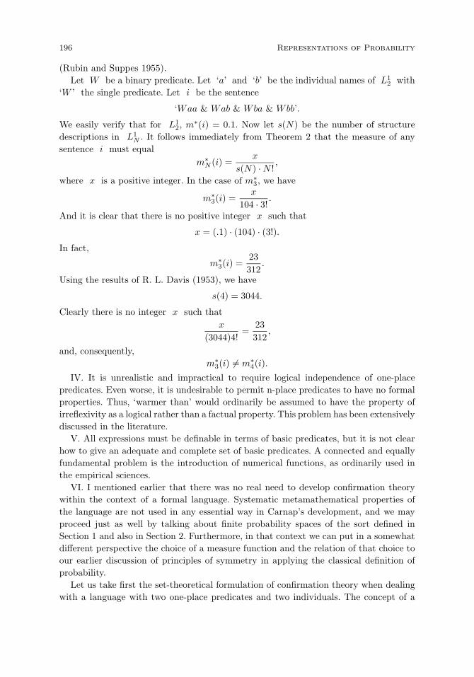
196 Representations of Probability

(Rubin and Suppes 1955).Let W be a binary predicate. Let ‘a’ and ‘b’ be the individual names of L1

2 with‘W ’ the single predicate. Let i be the sentence

‘Waa & Wab & Wba & Wbb’.

We easily verify that for L12, m

∗(i) = 0.1. Now let s(N) be the number of structuredescriptions in L1

N . It follows immediately from Theorem 2 that the measure of anysentence i must equal

m∗N (i) =

x

s(N) ·N !,

where x is a positive integer. In the case of m∗3, we have

m∗3(i) =

x

104 · 3!.

And it is clear that there is no positive integer x such that

x = (.1) · (104) · (3!).

In fact,

m∗3(i) =

23312

.

Using the results of R. L. Davis (1953), we have

s(4) = 3044.

Clearly there is no integer x such thatx

(3044)4!=

23312

,

and, consequently,m∗

3(i) = m∗4(i).

IV. It is unrealistic and impractical to require logical independence of one-placepredicates. Even worse, it is undesirable to permit n-place predicates to have no formalproperties. Thus, ‘warmer than’ would ordinarily be assumed to have the property ofirreflexivity as a logical rather than a factual property. This problem has been extensivelydiscussed in the literature.

V. All expressions must be definable in terms of basic predicates, but it is not clearhow to give an adequate and complete set of basic predicates. A connected and equallyfundamental problem is the introduction of numerical functions, as ordinarily used inthe empirical sciences.

VI. I mentioned earlier that there was no real need to develop confirmation theorywithin the context of a formal language. Systematic metamathematical properties ofthe language are not used in any essential way in Carnap’s development, and we mayproceed just as well by talking about finite probability spaces of the sort defined inSection 1 and also in Section 2. Furthermore, in that context we can put in a somewhatdifferent perspective the choice of a measure function and the relation of that choice toour earlier discussion of principles of symmetry in applying the classical definition ofprobability.

Let us take first the set-theoretical formulation of confirmation theory when dealingwith a language with two one-place predicates and two individuals. The concept of a

5.5 Logical Theory of Probability 197

state description is simply replaced by the standard concept of a possible outcome, andthe other definitions go through in terms of the standard relationships between logicalconcepts and set-theoretical concepts. For example, talk about one sentence L-implyinganother is replaced by talk about one event implying another, and this is interpreted tomean simply that the first event is a subset of the second.

Within this set-theoretical framework it is clear how we may express Carnap’s partic-ular choice of m∗ as a preferred measure function. It is the measure function that arisesfrom applying two principles of symmetry. In the case of possible outcomes defined interms of a finite set of elementary properties, a structure description is now definedsimply as the set of all possible outcomes that may be obtained from a given outcomeby a permutation of the individuals—just the definition of state-symmetry given earlier.The other principle is that of structure-symmetry as already defined.

A simple example in which this a priori structuring of the set of possible outcomesdoes not seem natural is afforded by the tossing of a coin N times. The possibleoutcomes are just the finite sequences of length N reflecting every possible sequence ofheads and tails. A structure description is the set of possible outcomes having the samenumber of heads. If we apply Carnap’s measure m∗ to this situation, we assign muchmore weight to the possible outcome all of whose tosses eventuate in heads than we doto one whose number of heads is, for example, approximately N

2 . For this situation, infact, we may prefer the Wittgenstein measure mw to Carnap’s measure m∗. In otherwords, Carnap’s principles of symmetry do not seem nearly as natural and appropriatein this case.

Furthermore, in the design of many experiments, principles of symmetry are appliedthat force the choice of an a priori distribution in a fairly effective way, regardless ofwhether the set of possible outcomes is finite or infinite. For example, in an experimentdealing with a continuum of responses, the labeling of the parts of the continuum interms of left-right and top-bottom is arbitrarily randomized across subjects. This is donein such a way that quite strong simple principles of symmetry are necessarily satisfiedin the initial distribution of responses, regardless of initial biases of subjects. Of course,it is true that such an example is not the sort of thing envisaged by Carnap in his owndiscussion of a choice of a measure function; but in my own judgment, the relationsbetween the two are closer than he might have been willing to admit.

VII. Carnap (1950, pp. 19–51) makes a point of emphasizing that in his view there aretwo distinct concepts of probability. One concept is that of empirical relative-frequency,and the other is the concept of probability expressed in confirmation theory. He em-phasizes most strongly that the statistical concept is empirical, while the confirmation-theory concept is analytical or logical in character. Although this distinction seems tohave been accepted by a great many philosophers, it is not at all clear that a persuasivecase has been made by Carnap for this dualistic approach.

I certainly would admit that in all theoretical science there are almost always twoclosely connected models of the theory, one model being given as a purely mathemat-ical model, and the other as a model derived in some more-or-less direct fashion fromempirical data. However, the existence of these two kinds of models does not justifythe distinction between the two concepts of probability urged by Carnap. As Carnap

198 Representations of Probability

suggests, there is a natural dichotomy between probabilities determined theoreticallyand probabilities determined empirically, but the thrust of this dichotomy is not at allthe one he suggests. It is not a comparison between confirmation theory on the onehand and statistical theory on the other, but is simply the garden-variety comparisonbetween a theoretical model and experimental data.

There is another way of looking at m∗ that also runs against Carnap’s. This is tolook upon m∗ as an objective prior distribution in the sense of Bayesians. Then theconfirmation c∗(h, e) of hypothesis h on evidence e is just the posterior probabilityin the Bayesian sense. On this view, there are definitely not two kinds of probability,logical and statistical, with some statistical probability to be used to supplement m∗

and c∗, or the associated likelihood of e given h. As some Bayesians like to say, if anobjective prior derived from principles of symmetry is used, then the statistics is purelymathematical or deductive in character. The evidence e is empirical, of course, but, itmight be maintained, the likelihood of e given h is not. Looked at still another way,we can compute c∗(h, e) for any possible evidence e. The computation is not empirical,and no statistical sense of probability enters, only the nonstatistical empirical questionof what the actual evidence is. I emphasize that I have only touched on important andsubtle issues here, and it is not possible within the framework of the present chapterto examine them in adequate detail. However, I hope I have said enough to generateskepticism about the validity of Carnap’s dual conception of probability.32

Hintikka’s two-parameter theory. Given the many difficulties in defending a uniquechoice such as m∗, Carnap retreated to a measure mλ with λ a free parameter (Carnap1952). This new measure, like m∗, has the property of state-symmetry. It seems obviousthat unless particular arguments can be given for choosing a few special values of λ,and thereby selecting variant inductive logics, there is little reason to regard this newtheory as a purely logical theory of probability. Inevitably, the selection of a particularvalue of λ to uniquely determine a measure seems in the grand tradition of subjectivetheories of probability.

But rather than explore Carnap’s λ-theory of inductive logic, I think it is more usefulto examine the later generalization of it to two parameters by Hintikka (1966), who alsoprovides an excellent detailed comparison between his system and Carnap’s.

Hintikka introduces two parameters α and λ, with λ being essentially the same asCarnap’s λ. The main rationale for Hintikka’s second parameter α is to provide a frame-work in which sentences that are not logically true may still receive a nonzero degreeof confirmation, i.e., positive conditional probability, in an infinite universe of individ-uals, provided the finite evidence is positive enough. Roughly speaking, Carnap’s andHintikka’s λ is an index of the weight given to the a priori probabilities determinedby various kinds of symmetry. The larger λ the greater the weight of these a prioriconsiderations.

Especially to deal with the asymptotic case of an infinite universe, it is essential

32For an excellent recent general review of confirmation theory, full of nice counterexamples and argu-

ments against various proposals in the literature in the years after Carnap’s long work on confirmation

theory, see Fitelson (2001).

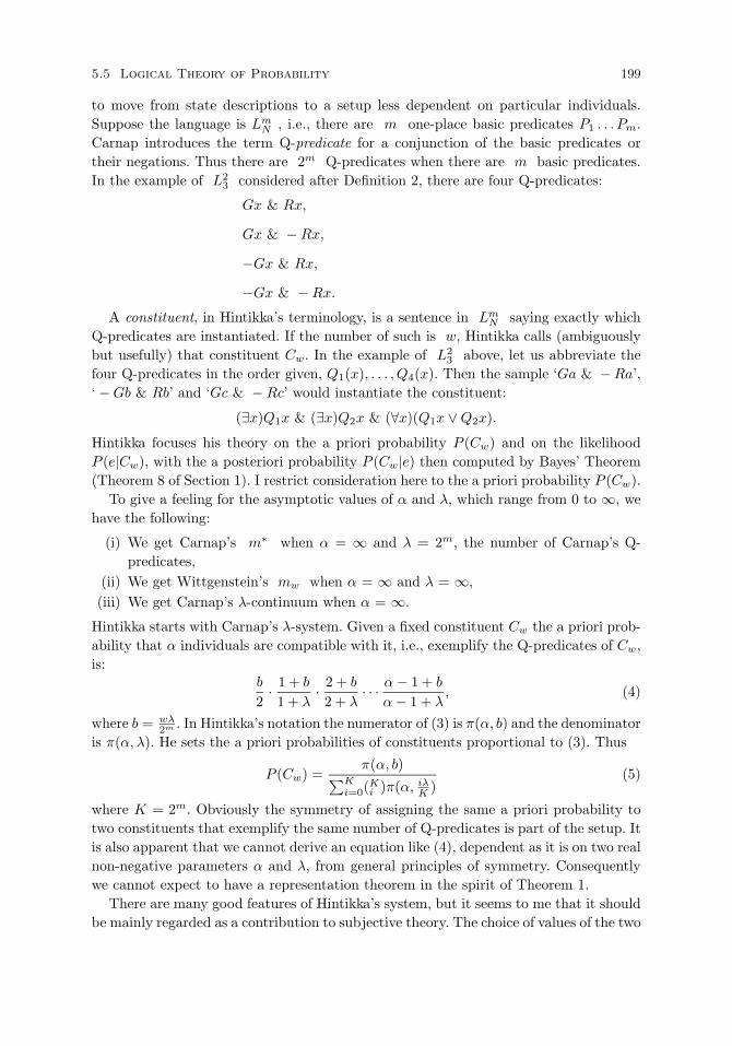
5.5 Logical Theory of Probability 199

to move from state descriptions to a setup less dependent on particular individuals.Suppose the language is Lm

N , i.e., there are m one-place basic predicates P1 . . . Pm.Carnap introduces the term Q-predicate for a conjunction of the basic predicates ortheir negations. Thus there are 2m Q-predicates when there are m basic predicates.In the example of L2

3 considered after Definition 2, there are four Q-predicates:

Gx & Rx,

Gx & −Rx,

−Gx & Rx,

−Gx & −Rx.

A constituent, in Hintikka’s terminology, is a sentence in LmN saying exactly which

Q-predicates are instantiated. If the number of such is w, Hintikka calls (ambiguouslybut usefully) that constituent Cw. In the example of L2

3 above, let us abbreviate thefour Q-predicates in the order given, Q1(x), . . . , Q4(x). Then the sample ‘Ga & −Ra’,‘ −Gb & Rb’ and ‘Gc & −Rc’ would instantiate the constituent:

(∃x)Q1x & (∃x)Q2x & (∀x)(Q1x ∨Q2x).

Hintikka focuses his theory on the a priori probability P (Cw) and on the likelihoodP (e|Cw), with the a posteriori probability P (Cw|e) then computed by Bayes’ Theorem(Theorem 8 of Section 1). I restrict consideration here to the a priori probability P (Cw).

To give a feeling for the asymptotic values of α and λ, which range from 0 to ∞, wehave the following:

(i) We get Carnap’s m∗ when α = ∞ and λ = 2m, the number of Carnap’s Q-predicates,

(ii) We get Wittgenstein’s mw when α = ∞ and λ = ∞,(iii) We get Carnap’s λ-continuum when α = ∞.

Hintikka starts with Carnap’s λ-system. Given a fixed constituent Cw the a priori prob-ability that α individuals are compatible with it, i.e., exemplify the Q-predicates of Cw,is:

b

2· 1 + b

1 + λ· 2 + b

2 + λ· · · α− 1 + b

α− 1 + λ, (4)

where b = wλ2m . In Hintikka’s notation the numerator of (3) is π(α, b) and the denominator

is π(α, λ). He sets the a priori probabilities of constituents proportional to (3). Thus

P (Cw) =π(α, b)∑K

i=0(Ki )π(α, iλ

K )(5)

where K = 2m. Obviously the symmetry of assigning the same a priori probability totwo constituents that exemplify the same number of Q-predicates is part of the setup. Itis also apparent that we cannot derive an equation like (4), dependent as it is on two realnon-negative parameters α and λ, from general principles of symmetry. Consequentlywe cannot expect to have a representation theorem in the spirit of Theorem 1.

There are many good features of Hintikka’s system, but it seems to me that it shouldbe mainly regarded as a contribution to subjective theory. The choice of values of the two

200 Representations of Probability

free parameters may be expected to vary from person to person and from one situationto another. This is exactly the sort of thing pure Bayesians, the strongest advocates ofthe subjective view, expect to be the case.

Kyburg. A richer and more realistic logical theory has been developed by Kyburg(1974). It is still in the tradition of an explicit logical language, emphasized so much inthe earlier work of Carnap. Here is why Kyburg’s formulation is both richer and morerealistic than that begun by Carnap. First, he introduces a richer formal language, muchmore adequate to express in a formal way standard statistical concepts such as randomsampling and testing hypotheses. Second, because of this richer language a much morerealistic class of examples and problems from statistical practice—at least classroompractice in teaching statistics—can be analyzed. Third, the theory as developed is notformulated to require a single prior probability or distribution for a given problem orexperiment, but will work well with a family of distributions.

Kyburg has many interesting remarks about the foundations of probability. His wellworked-out treatise should have had more impact than it did over the past severaldecades. I am not certain why it has not, but I conjecture this is mainly because itmakes heavy use of logical notation and formal logical concepts, such as defining ran-domness and probability as metalinguistic concepts. The great majority of statisticiansand mathematicians have little taste for this heavily formal approach. Carnap had littleinfluence on this majority of workers also, but Kyburg deserved a better hearing, for hemade a detailed effort to deal with many of the standard puzzles about statistics andprobability, as formulated independent of any explicit logically formal language.

Model-theoretic approach. Gaifman (1964), Scott and Krauss (1966), Krauss(1969), and also Gaifman and Snir (1982) have been concerned to develop the con-cept of a probabilistic measure for general first-order languages, and also to extend thedevelopments to infinitary languages with the benefit of having a σ-additive theory.The spirit of this work is not to justify by presumably logical arguments the selectionof a unique a priori probability measure. Rather, the intent is to generalize ordinarylogic to probability logic. The central concept for Scott and Krauss is that of a sentenceholding in a probability system Ω with probability α. This concept is the analogue ofTarski’s concept of satisfaction for ordinary logic. From this and related concepts theauthors construct an elegant formal theory.

However, this model-theoretic approach is not really to be taken as a contribution tothe logical foundations of probability in Jeffreys’ or Carnap’s sense. In fact, most of theresults of Gaifman, Scott, and Krauss have analogues in standard probability theoryderived from Kolmogorov’s axioms, which are essentially neutral toward foundations.In the sense of this section, their model-theoretic approach does not contribute a newrepresentation theory to the foundations of probability.

Chuaqui. A significant representation theorem is proved by Rolando Chuaqui (1977,1991) using a model-theoretic approach and a semantic definition of probability. Butthe representation theorem he proves does not really depend on his model-theoretic

5.5 Logical Theory of Probability 201

methods, but rather on their extension to nonstandard infinitesimal analysis. It is toomuch of a technical digression to introduce appropriate formal concepts and notation forinfinitesimal analysis here, but I believe it is possible to give a clear intuitive descriptionof Chuaqui’s representation result. A standard stochastic process is just a family of ran-dom variables Xt : t ∈ T indexed by a set T , discrete or continuous. A nonstandardsuch process is indexed by infinitesimals or their reciprocals, hypereal numbers, as well.The point, made most clearly in Nelson (1987), is that by using nonstandard infinitesi-mal methods we can drastically simplify many parts of probability that seem burdenedby scientifically unimportant, but mathematically real, technical complications. For ex-ample, it is easy to define a continuous-time, discrete-state stochastic process that canpass through an infinite number of states in finite time. Much worse are the endlessmeasure-theoretic questions that burden continuous-time, continuous-state stochasticprocesses. Nelson provides important guidelines for a simpler theory of such matters,usable in all ordinary scientific contexts.

In Nelson’s setup the usual continuous-time process is replaced by a hyperfinite one.For example, let the index set T be the set of natural numbers. It can be replaced by0, 1, . . . , ν, where ν is an infinite natural number. (A natural number ν is infinite if 1

ν

is an infinitesimal, say, ε, and ε has the property that for all standard finite real numbersx, 0 < ε < x.) As a second example, let T be the closed interval [0, 1]. We define thediscrete-time set T ′ = 0, dt, 2dt, . . . , 1, where dt = 1

ν for some infinite natural numberν. So T ′ is hyperfinite. T ′ is said to be a near interval for T = [0, 1]. Nelson (1987) provesthat any standard stochastic process is approximated within infinitesimal equivalenceof all probabilistic quantities by a nearby process indexed by a near index set. Thisinformally stated theorem is in itself a significant formal representation theorem forstochastic processes.

Chuaqui uses it to prove the following representation theorem (here I state the Corol-lary of his basic theorem, Chuaqui 1991, p. 351).

THEOREM 3. (Chuaqui 1991). For any stochastic process indexed by a hyperfinite setT , there is a nearby infinitesimally equivalent stochastic process over a probability spacewhose elements are all equally probable.

As Chuaqui notes, using the theorem of Nelson informally stated above, it is then easyto extend his theorem to what I call the Laplacean representation of any standard,stochastic process—Laplacean because the representing probability space satisfies theextended version of Laplace’s first principle of probability, a uniform distribution overthe set of possibilities.

This representation theorem is not as surprising as it may seem. It was emphasizedalready in the introduction of random variables in Section 1 that the probability spaceon which a random variable is defined is not uniquely determined by the distribution ofthe random variable, the object of major interest. So for finite probability spaces it isnot hard to find an equivalent space with equiprobable atoms, for any random variabledefined on the finite space. Nonstandard infinitesimal analysis permits a direct intuitivegeneralization of these ideas to any stochastic process with a hyperfinite index set.

202 Representations of Probability

5.6 Propensity Representations of Probability33

In recent years a propensity interpretation of probability, thought of primarily as anobjective interpretation, has become popular with a number of philosophers, and therehas developed a rather large philosophical literature on it. The concept of propensityitself is not a new one. The Oxford English Dictionary cites clear and simple uses ofpropensity and its general meaning already in the seventeenth century, for example,from 1660 ‘Why have those plants . . . a propensity of sending forth roots?’34 The ideaof this interpretation of probability is to use the general idea of objects having variousphysical propensities, for example, a propensity to dissolve when placed in water, andto extend this idea to probability. As is also clear from these discussions, propensitiescan be looked upon as dispositions. (A rather detailed discussion of this point can befound in Chapter 4 of Mellor (1971).)

The most prominent advocate of the propensity interpretation of probability has beenPopper, who set forth the main ideas in two influential articles (1957, 1959). Popper givesas one of his principal motivations for developing a propensity interpretation the needto give an objective interpretation of single-case probabilities in quantum mechanics,that is, an objective interpretation of the probabilities of individual events. Single-case probabilities, as they are called in the literature, are of course no problem forsubjectivists, but they have been a tortuous problem for relative-frequency theorists.A good detailed discussion of how we are to think of propensities in relation both tosingle-case probabilities and to relative frequencies is to be found in Giere (1973). Iagree with Giere that one of the real reasons to move away from the relative-frequencytheory is the single-case problem and that therefore we should regard as fundamentalor primary the propensity interpretation of singular events. Giere gives a number oftextual quotations to show that Popper wavers on this point.

As I pointed out in Suppes (1974a), what is missing in these excellent intuitive dis-cussions of the philosophical and scientific foundation of a propensity interpretation isany sense that there needs to be something proved about the propensity interpretation.Within the framework I propose, this would amount to proving a representation the-orem. In Popper’s (1974) response to my criticisms, he mentions his own ideas aboutconditional probability and how to handle the problem of evidence that has zero prob-ability. There are some other fine points as well, but he misses the real point of mycriticism by not giving a conceptually different analysis of propensities, so that some-thing of genuine interest can be proved about the interpretation. The request for sucha proof is not an idle or a merely formal request. In order for an interpretation of prob-ability to be interesting, some clear concepts need to be added beyond those in theformal theory as axiomatized by Kolmogorov. The mere hortatory remark that we caninterpret propensities as probabilities directly, which seems to be a strong propensity ofsome advocates, is to miss the point of giving a more thorough analysis.

Because I think there are many good things about the propensity interpretation, asI indicated in my 1974 article on Popper, I want to prove three different representationtheorems, each of which is intended to give an analysis for propensity that goes beyond

33This section draws heavily on Suppes (1987).34Moreover, there are many uses in Hume’s Treatise of Human Nature (1739).

5.6 Propensity Representations of Probability 203

the formal theory of probability, and to state as well, as a fourth example, a surprisingtheorem from classical mechanics.

The first representation theorem is closest to probability itself and it applies to ra-dioactive phenomena. The second is for psychological phenomena with propensity beingrealized as strength of response. The probabilities are then derived explicitly from re-sponse strengths. The third example, the most important historically, is the derivationof the behavior of coins, roulette wheels and similar devices, purely on the basis of con-siderations that belong to classical mechanics. The fourth example shows how randomphenomena can be produced by purely deterministic systems.

These four different examples of propensity representation theorems do not in anydirect sense force the issue between single-case and relative-frequency views of propen-sity. But I certainly see no general reason for not using them to compute single-caseprobabilities. It seems natural to do so whenever a relatively detailed account of thestructure of a given propensity is given.

Propensity to decay. Before turning to technical developments, there are some gen-eral remarks to be made about the approach followed here, which are largely taken fromSuppes (1973a).

The first remark concerns the fact that in the axioms that follow, propensities, as ameans of expressing qualitative probabilities, are properties of events and not of objects.Thus, for example, the primitive notation is interpreted as asserting that the event A,given the occurrence of the event B, has a propensity to occur at least as great asthe event C, given the occurrence of the event D. Moreover, the events B and D maynot actually occur. What we are estimating is a tendency to occur or a propensity tooccur, given the occurrence of some other event. If the use of the language of propensityseems awkward or unnatural in talking about the occurrence of events, it is easy enoughsimply to use qualitative probability language and to reserve the language of propensityfor talking about the properties of objects, although I am opposed to this move myself.In any case, the issue is peripheral to the main problem being addressed.

The second remark concerns the clear distinction between the kind of representationtheorem obtained here and the sort of theorem ordinarily proved for subjective theo-ries. It is characteristic of subjective theories, as considered in Section 7, to introducestructural axioms strong enough to impose a unique probability measure on events. Itis this uniqueness that is missing from the objective theory as formulated here, and inmy own judgment, this lack of uniqueness is a strength, not a weakness. Take the caseof radioactive decay. From the probabilistic axioms, without specific experimentationor identification of the physical substance that is decaying, we certainly do not antici-pate being able to derive a priori the single parameter of the geometric distribution fordecay. It is exactly such a parametric result, i.e., uniqueness up to a set of parameters,that is characteristic of objective theory, and, I would claim, characteristic of standardexperimentation in broad areas of science ranging from physics to psychology. In otherwords, the structural axioms of probability, together with the necessary ones, fix theparametric form of the probability measure but do not determine it uniquely. Specificexperiments and specific methods of estimation of parameters on the basis of empirical

204 Representations of Probability

data are needed to determine the numerical values of the parameters. Subjectivists oftenend up with a working procedure similar to the present one by assuming a probabilitydistribution over the space of parameters. Such procedures are close to what is beingdiscussed here, and so they should be, because there is great agreement on how one pro-ceeds in practice to estimate something like a parameter of a geometric or exponentialdistribution.

The important point I want to emphasize is that, in the fundamental underpinningsof the theory, subjectivists have ordinarily insisted upon a unique probability measure,and this commitment to an underlying unique probability measure seems to me tobe an unrealistic premise for most scientific applications. It is not that there is anyinconsistency in the subjectivistic approach; it is simply that the present objectivisticviewpoint is a more natural one from the standpoint of ordinary scientific practice. (Aswas already noted in Section 3, support for this view of the propensity representationis to be found in various remarks in van Lambalgen (1987a).)

I emphasize also that the intuitive meaning of the weaker structural axioms of ob-jective theory is different from that of the stronger axioms of subjective theory. Theobjective structural axioms are used to express specific qualitative hypotheses or lawsabout empirical phenomena. Their form varies from one kind of application to another.A specific structural axiom provides a means of sharply focusing on what fundamentalempirical idea is being applied in a given class of experiments. More is said about thispoint later for the particular case of radioactive decay.

I turn now to the formal developments. First of all, in stating the necessary axiomsI shall use qualitative probability language of the sort that is standard in subjectivetheories of probability. The real place for propensity comes in the discussion of therather particular structural axioms which reflect strong physical hypotheses about thephenomena of radioactive decay.

The axioms given in the following definition will not be discussed because the ones Igive here represent only a minor modification of the first six axioms of Definition 8 ofKrantz et al. (1971, p. 222), plus an alternative axiom that is Axiom 7 below.35 Notethat ≈ is equivalence, i.e.,

A|B ≈ C|D iff A|B C|D and C|D A|B.DEFINITION 1. A structure Ω = (Ω,,) is a qualitative conditional proba-bility structure if and only if is a σ-algebra of sets on Ω and for everyA,B,C,D,E, F,G,Ai, Bi, i = 1, 2, . . ., in with B,D, F,G ∅ the following ax-ioms hold:

Axiom 1. If A|B C|D and C|D E|F then A|B E|F ;

Axiom 2. A|B C|D or C|D A|B;

Axiom 3. Ω ∅;Axiom 4. Ω|B A|D;

Axiom 5. A ∩B|B ≈ A|B;

35Related but simpler necessary and sufficient axioms for qualitative conditional expectation are

given in Definition 3 of Section 7 on subjective probability.

5.6 Propensity Representations of Probability 205

Axiom 6. If Ai ∩ Aj = Bi ∩ Bj = ∅ for i = j and Ai|D Bi|F for i =1, 2, . . . , then ∪Ai|D ∪Bi|F ; moreover, if for some i, Ai|D Bi|F , then∪Ai|D ∪Bi|F ;

Axiom 7. If A ⊆ B ⊆ D,E ⊆ F ⊆ G, A|B E|F and B|D F |G thenA|D E|G; moreover, A|D E|G unless A ≈ ∅ or both A|B ≈ E|F andB|D ≈ F |G;

Axiom 8. If A ⊆ B ⊆ D,E ⊆ F ⊆ G,B|D E|F and A|B F |G, thenA|D E|G; moreover, if either hypothesis is then the conclusion is .

To say that the axioms of Definition 1 are necessary means, of course, that they area mathematical consequence of the assumption that a standard probability measure P

is defined on such that

A|B C|D iff P (A|B) ≥ P (C|D). (1)

Precisely which necessary axioms are needed in conjunction with the sufficient struc-tural axioms to guarantee the existence of a probability measure satisfying (1) will varyfrom case to case. It is likely that most of the eight axioms of Definition 1 will ordinarilybe needed. In many cases an Archimedean axiom will also be required; the formulationof this axiom in one of several forms is familiar in the literature. The following versionis taken from Krantz et al. (1971, p. 223).

DEFINITION 2. A qualitative conditional probability structure Ω = (Ω,,) isArchimedean if and only if every standard sequence is finite, where (A1, A2, . . .) is astandard sequence iff for all i, Ai ∅, Ai ⊆ Ai+1 and Ω|Ω Ai|Ai+1 ≈ A1|A2.

I turn now to a theorem that seems to have been first stated in the literature ofqualitative probability in Suppes (1973a). The reason it did not appear earlier seemsto be that the solvability axioms ordinarily used in subjective theories of probabilityoften do not hold in particular physical situations when the probabilistic considerationsare restricted just to that situation. Consequently the familiar methods of proof of theexistence of a representing probability measure must be changed. Without this change,the theorem is not needed.

The theorem is about standard sequences. Alone, the theorem does not yield a prob-ability measure, but it guarantees the existence of a numerical function that can beextended to all events, and thereby it becomes a measure when the physical hypothesesexpressing structural, nonnecessary constraints are sufficiently strong.

THEOREM 1. (Representation Theorem for Standard Sequences). Let (A1, . . . , An)be a finite standard sequence, i.e., Ai ∅, Ai ⊆ Ai+1, and Ω|Ω Ai|Ai+1 ≈ A1|A2.Then there is a numerical function Q such that

(i) Ai ⊆ Aj iff Q(Ai) ≤ Q(Aj),

(ii) if Ai ⊆ Aj and Ak ⊆ Al then Ai|Aj ≈ Ak|Al iff Q(Ai)Q(Aj)

= Q(Ak)Q(Al)

.

Moreover, for any Q satisfying (i) and (ii) there is a q with 0 < q < 1 and a c > 0such that

Q(Ai) = cqn+1−i.

206 Representations of Probability

Proof. Let 0 < q < 1. Define Q(Ai) as

Q(Ai) = qn+1−i. (2)

Then obviously (i) is satisfied, since the members of a standard sequence are distinct;otherwise there would be an i such that Ai = Ai+1 and thus Ai|Ai+1 ≈ Ω|Ω, contraryto hypothesis. So we may turn at once to (ii). First, note the following.

Ai|Ai+m ≈ Aj |Aj+m. (3)

The proof of (3) is by induction. For m = 1, it is just the hypothesis that for every i,Ai|Ai+1 ≈ A1|A2 . Assume now it holds for m− 1; we then have

Ai|Ai+(m−1) ≈ Aj |Aj+(m−1),

and also for any standard sequence

Ai+(m−1)|Ai+m ≈ Aj+(m−1)|Aj+m,

whence by Axiom 7, Ai|Ai+m ≈ Aj |Aj+m, as desired. Next, we show that if Ai ⊆Aj , Ak ⊆ Al and Ai|Aj ≈ Ak|Al, then there is an m ≥ 0 such that j = i + m andl = k +m. Since Ai ⊆ Aj and Ak ⊆ Al, there must be non-negative integers m andm′ such that j = i+m and l = k+m′. Suppose m = m′, and without loss of generalitysuppose m+ h = m′, with h > 0. Then obviously

Ai|Ai+m ≈ Ak|Ak+m.

In addition,Ai+m|Ai+m ≈ Ω|Ω Ak+m|Ak+m+h,

and so again by Axiom 7Ai|Ai+m Ak|Ak+m′ ,

contrary to our hypothesis, and so we must have m = m′.With these results we can establish (ii). We have as a condition that Ai ⊆ Aj and

Ak ⊆ Al. Assume first that Ai|Aj ≈ Ak|Al. Then we know that there is an m suchthat j = i+m and l = k +m, whence

Q(Ai)Q(Aj)

= qn+1−i

qn+1−i−m

= qn+1−k

qn+1−k−m

= Q(Ak)Q(Al)

.

Second, we assume thatQ(Ai)Q(Aj)

=Q(Ak)Q(Al)

.

From the definition of Q it is a matter of simple algebra to see that there must be anm′ such that j = i+m′ and l = k+m′, whence by our previous result, Ai|Aj ≈ Ak|Al.

Finally, we must prove the uniqueness of q as expressed in the theorem. Supposethere is a Q′ satisfying (i) and (ii) such that there is no c > 0 and no q such that0 < q < 1 and for all i

Q′(Ai) = cqn+1−i.

5.6 Propensity Representations of Probability 207

LetQ′(An) = q1

Q′(An−1) = q2.

Letq =

q2q1

c =q21q2.

Obviously,Q′(An) = cq

Q′(An−1) = cq2.

On our supposition about Q′, let i be the largest integer (of course i ≤ n) such that

Q′(Ai) = cqn+1−i.

We haveAi|Ai+1 ≈ An−1|An,

whence by (ii)Q′(Ai)cqn−1

=cq2

cq,

and soQ′(Ai) = cqn+1−i,

contrary to hypothesis, and the theorem is proved.I turn now to radioactive decay phenomena. One of the best-known physical examples

of a probabilistic phenomenon, for which hardly anyone pretends to have a deeperunderlying deterministic theory, is that of radioactive decay. Here I shall consider forsimplicity a discrete-time version of the theory which leads to a geometric distributionof the probability of decay. Extension to continuous time is straightforward but will notbe considered here. In the present context the important point is conceptual, and I wantto minimize technical details. Of course, the axioms for decay have radically differentinterpretations in other domains of science, and some of these will be mentioned later.

In a particular application of probability theory, the first step is to characterizethe sample space, i.e., the set of possible experimental outcomes, or as an alternative,the random variables that are numerical-valued functions describing the phenomenaat hand. Here I shall use the sample-space approach, but what is said can easily beconverted to a random-variable viewpoint.

From a formal standpoint, the sample space Ω can be taken to be the set of allinfinite sequences of 0’s and 1’s containing exactly one 1. The single 1 in each sequenceoccurs as the nth term of the sequence representing the decay of a particle on the nthtrial or during the nth time period, with its being understood that every trial or periodis of the same duration as every other. Let En be, then, the event of decay on trial n.Let Wn be the event of no decay on the first n trials, so that

Wn = −n⋃

i=1

Ei.

208 Representations of Probability

The single structural axiom is embodied in the following definition. The axiom justasserts that the probability of decay on the nth trial, given that decay has not yetoccurred, is equivalent to the probability of decay on the first trial. It thus expresses ina simple way a qualitative principle of constancy or invariance of propensity to decaythrough time.

DEFINITION 3. Let Ω be the set of all sequences of 0’s and 1’s containing exactlyone 1, and let be the smallest σ-algebra on Ω which contains the algebra of cylindersets. A structure Ω = (Ω,,) is a qualitative waiting-time structure with indepen-dence of the past iff Ω is a qualitative conditional probability structure and in additionthe following axiom is satisfied for every n, provided Wn−1 ∅:

Waiting-time axiom. En|Wn−1 ≈ E1.

The structures characterized by Definition 3 are called waiting-time structures withindependence of the past, because this descriptive phrase characterizes their generalproperty abstracted from particular applications like that of decay. A useful shorterdescription is memoryless waiting-time structure.

The simplicity of this single structural axiom may be contrasted with the ratherinvolved axioms characteristic of subjective theories of probability (Section 7). In ad-dition, the natural form of the representation theorem is different. The emphasis is onsatisfying the structural axioms—in this case, the waiting-time axiom—and having aunique parametric form, rather than a unique distribution.

THEOREM 2. (Representation Theorem for Decay). Let Ω = (Ω,,) be a qualita-tive waiting-time structure with independence of the past. Then there exists a probabilitymeasure on such that the waiting-time axiom is satisfied, i.e.,

(i) P (En|Wn−1) = P (E1) iff En|Wn−1 ≈ E1,

and there is a number p with 0 < p ≤ 1 such that

(ii) P (En) = p(1 − p)n−1.

Moreover, any probability measure satisfying (i) is of the form (ii).

Proof. The events En uniquely determine an atom or possible experimental outcomeω of Ω, i.e., for each n, there is an ω in Ω such that

En = ω,a situation which is quite unusual in sample spaces made up of infinite sequences, forusually the probability of any ω is strictly zero.

If E1 ≈ Ω, then P (E1) = 1, and the proof is trivial. On the other hand, if Ω E1,then for each n, (Wn, . . . ,W1) is a standard sequence satisfying the hypotheses of therepresentation theorem for standard sequences. The numbering is inverted, i.e., Wi+1 ⊆Wi and Wi+1|Wi ≈ W2|W1. (If (W1, . . . ,Wn) were a standard sequence, then so wouldbe the infinite sequence (W1, . . . ,Wn, . . .) in violation of the necessary Archimedeanaxiom.)36 That Wi+1 ⊆ Wi is obvious from the definition of Wi. By virtue of the

36The Archimedean axiom is necessary, because the algebra of events is not finite.

5.6 Propensity Representations of Probability 209

waiting-time axiomWi+1|Wi ≈ W1,

since Ei = Wi−1 −Wi, and W1 = −E1, so

E1 ≈ Ei+1|Wi ≈ Wi −Wi+1|Wi

≈ −Wi+1|Wi,

and then by elementary manipulations

W1 ≈ −E1 ≈ Wi+1|Wi.

Using the representation theorem for standard sequences, we know there is a numericalfunction P ′ and numbers c and q with 0 < q < 1 and c > 0 such that

P ′(Wi) = cqi.

(Let i′ be the numbering in the reverse order (n, . . . , 1); then i′ = n − (i − 1), and theexponent n + 1 − i in the representation theorem becomes i′.) Starting with a fixedstandard sequence of length n, P ′ can be extended to every i > n in an obvious fashion.

The next step is to extend P ′ as an additive set function to all atoms Ei by theequations

P ′(Ei) = P ′(Wi−1 −Wi)

= P ′(Wi−1) − P (Wi)

= c(qi−1 − qi)

= cqi−1(1 − q).The consistency and uniqueness of this extension is easy to check. Now

∞∑i=1

P ′(Ei) = c,

so we set c = 1 to obtain a measure P normed on 1 from P ′ and let p = 1 − q. Wethen have

P (Ei) = p(1 − p)i−1

P (Wi) = (1 − p)i.

The function P just defined is equivalent to a discrete density on Ω, since Ei = ωfor some ω in Ω, and thus P may be uniquely extended to the σ-algebra of cylindersets of Ω by well-known methods.

Finally, the proof of (ii) is immediate. If we suppose there is an n such thatP (En) = p(1 − p)n−1, where p = P (E1), we may use the waiting-time axiom to ob-tain a contradiction, for by hypothesis P (Wn−1) = (1 − p)n−1 and P (En|Wn−1) = p,whence P (En) = pP (Wn−1) = p(1 − p)n−1, the standard density of the geometricdistribution.

Q.E.D.I quite accept that a criticism of this particular representation theorem is that the

analysis of propensity is too close to the analysis of probability from a formal stand-point, a complaint I made earlier about some of the literature on propensity. In general,propensities are not probabilities, but provide the ingredients out of which probabilities

210 Representations of Probability

are constructed. I think the favorable positive argument for what I have done has got tobe put on a more subtle, and therefore more fragile, basis. The point has been made, butI will make it again to emphasize how propensities enter. The memoryless waiting-timeaxiom is a structural axiom that would never be encountered in the standard theory ofsubjective probability as a fundamental axiom. It is an axiom special to certain physicalphenomena. It represents, therefore, a qualitative expression of a propensity. Second,the probabilities we obtain from the representation theorem are not unique but are onlyunique up to fixing the decay parameter. Again, this is not a subjective concept butvery much an objective one. Identifying and locating the number of physical parametersto be determined is a way of emphasizing that propensities have entered and that apurely probabilistic theory with a unique measure has not been given.

Discrete qualitative densities. The qualitative point just made can be nicely am-plified by restricting the qualitative axioms mainly to the discrete atoms, thereby sim-plifying the qualitative axioms considerably.

As is familiar in all sorts of elementary probability examples, when a distribution hasa given form it is often much easier to characterize it by a density than by a probabilitymeasure on events. In the discrete case, the situation is formally quite simple. Eachatom, i.e., each atomic event, has a qualitative probability and we need only judgerelations between these qualitative probabilities. We require of a representing discretedensity function p the following three properties:

(i) p(ai) ≥ 0.

(ii)n∑

i=1

p(ai) = 1.

(iii) p(ai) ≥ (aj) iff ai aj .

Note that the ai are not objects or stimuli in an experiment, but qualitative atomicevents, exhaustive and mutually exclusive.

We also need conditional discrete densities. For this purpose, we assume the under-lying probability space Ω is finite or denumerable, with probability measure P on thegiven family F of events. The relation of the density p to the measure P is, for ai anatom of Ω,

p(ai) = P (ai).

Then if A is any event such that P (A) > 0,

p(ai|A) = P (ai|A),

and, of course, p(ai|A) is now a discrete density itself, satisfying (i)–(iii). Here are somesimple, but useful, examples of this approach.

Uniform density. The uniform density on Ω is characterized by all atoms being equiv-alent in the qualitative ordering , i.e.,

ai ≈ aj .

5.6 Propensity Representations of Probability 211

We may then easily show that the unique density satisfying this equivalence and (i)–(iii)is

p(ai) =1n,

where n is the number of atoms in Ω.

Geometric density. We can simplify considerably the argument leading up to Theorem2. The space Ω is that for Theorem 2. It is the discrete but denumerable set of atomicevents (a1 . . . , an . . .) on each of which there is a positive qualitative probability of thechange of state occurring. The numbering of the atoms intuitively corresponds to thetrials of an experiment. The atoms are ordered in qualitative probability by the relation. We also introduce a restricted conditional probability. If i > j then ai|Aj is theconditional atomic event that the change of state will occur on trial i given that it hasnot occurred on or before trial j. (Note that here Aj means, as before, no change ofstate from trial 1 through j. ) The qualitative probability ordering relation is extendedto include these special conditional events as well.

The two postulated properties, in addition to (i)–(iii) given above, are these:

(iv) Order property: ai aj iff j ≥ i;(v) Memoryless property: ai+1|Ai ≈ a1.

It is easy to prove that (iv) implies a weak ordering of . We can then prove that p(an)has the form of the geometric density

p(an) = c(1 − c)n−1 (0 < c < 1),

but, of course, Axioms (i)–(v) do not determine the value of the parameter c.

Exchangeability. Sequences of outcomes that are exchangeable, i.e., invariant undera permutation of trial number, were mentioned at the end of Section 1. They alsobelong here, as an important physical invariant of many processes, but further analysis isdelayed until the next section on subjective probability, where de Finetti’s fundamentaltheorem on exchangeable sequences is analyzed.

Stationarity. Processes that are stationary in time are common in representing manyfundamental physical processes, such as those of equilibrium statistical mechanics. Anyprocess that is ergodic is necessarily required to be stationary, as was already madeclear in Section 4.5. For processes with a discrete set of states and discrete time indices,stationarity has a simple qualitative formulation: for any finite sequence of trials n1 <

n2 < · · · < nm, and any positive integer k,

an1an2 · · · anm≈ an1+kan2+k · · · anm+k,

where an1 is the discrete outcome on trial n1, etc. The essence of stationarity is invari-ance under a time shift such as k.

Propensity to respond. There is a long history of various theoretical models beingproposed in psychology to represent response strength, which in turn is the basis for

212 Representations of Probability

choice probabilities. By a ‘choice probability’ I mean the probability that a given itema will be selected from a set A in some given experimental or naturalistic setting.The fact that the choice is to be represented by a probability is a reflection that thestandard algebraic model of expected utility does not adequately represent much actualbehavior. Whatever one may think individuals should do, it is a fact of life, documentedextensively both experimentally and in other settings, that individuals, when presentedwith what appear to be repetitions of the same set of alternatives to choose from, donot repeatedly choose the same thing. The formal study of such situations has alsobeen a matter of intensive work in the past several decades. One of the most simple andelegant models is the choice model proposed by Luce (1959). In Luce’s own developmenthe proceeds from his choice axiom, which is stated in terms of observable probabilities,to the existence of response strengths. To illustrate the kind of idea we want here we shallbegin the other way, that is, by postulating a response strength, and then showing howfrom this postulate we easily derive his choice axiom. Second, an advantage of responsestrengths over response probabilities is to be seen in the formulation of Luce’s alphamodel of learning, where the transformations that represent learning from one trial toanother are linear when formulated in terms of response strengths, but nonlinear whenformulated in terms of choice probabilities.

We turn now to the formal development of these ideas. In the intended interpretationT is a presented set of alternatives to choose from, and the numerical function v isthe measure of response (or stimulus) strength.

DEFINITION 4. Let T be a nonempty set, and let v be a non-negative real-valuedfunction defined on T such that for at least one x in T , v(x) > 0, and

∑x∈T v(x)

is finite. Then T = (T, v) is a response-strength model (of choice).

The general requirements put on a response-strength model are obviously very weak,but we can already prove a representation theorem that is more special than earlierones, in the sense that in addition to satisfying the axioms of finitely additive probabil-ity spaces, Luce’s Choice Axiom is satisfied as well. Moreover, to get various learningmodels, we impose further conditions.

THEOREM 3. (Representation Theorem). Let T = (T, v) be a response-strengthmodel, and define for U in P(T ), the power set of T ,

PT (U) =∑

x∈U v(x)∑x∈T v(x)

.

Then (T,P(T ), PT ) is a finitely additive probability space. Moreover, the probabilitymeasure PT satisfies Luce’s choice axiom, i.e., for V in P(T ), with

∑x∈V v(x) = 0,

and with v′ being v restricted to V,V = (V, v′) is a response-strength model such thatfor U ⊆ V

PV (U) = PT (U |V ).

Proof. The general representation part of the theorem is obvious. To prove Luce’s

5.6 Propensity Representations of Probability 213

axiom, we note that because U ⊆ V

PT (U |V ) = PT (U∩V )PT (V )

=

∑x∈U

v(x)

∑x∈T

v(x)

/∑x∈V

v(x)

∑x∈T

v(x)

=∑x∈U

v(x)

/∑x∈V

v(x)

= PV (U).

Q.E.D.The notation used in the theorem is slightly subtle and can be initially confusing.Note that the set referred to by the subscript represents the full physical set of choicealternatives. The set conditioned on, V in the case of PT (U |V ), is information aboutthe choice actually occurring from among the elements of a subset of T . It is not at alltautological that Luce’s axiom should hold. In fact, there is a sizable statistical literatureon how to best estimate response strengths for observed choice probabilities (Bradleyand Terry 1952; Bradley 1954a,b, 1955; Abelson and Bradley 1954; Ford 1957).

To illustrate how the formulation of theory in terms of a propensity can simplifysome analyses, we sketch the situation for Luce’s alpha model of learning. Let f be thelearning function mapping the finite vector of response strengths v = (v1, . . . , vr) fromone trial to the next. Here we assume T is finite—in particular has cardinality r. Weassume that response strengths are unbounded, i.e., for any real number α there is ann such that |fn(v)| > α, where fn represents n iterations of the learning function.Second, superposition of learning holds, i.e., for any v, v∗ > 0

f(v + v∗) = f(v) + f(v∗).

Third, independence of scale or units holds, i.e., for v > 0 and any real number k > 0

f(kv) = kf(v).

But it is a well-known result in linear algebra that the assumed conditions imply thatf is a linear operator on the given r-dimensional vector space. In contrast, underthese assumptions, but no stronger ones, the behavior from trial-to-trial of the responseprobabilities PT (U) is complicated; in particular, they are not related by a linear trans-formation of the probabilities.

Although the proof of Theorem 3 is very simple and in the development thus far littlestructure has been imposed on the response-strength function, the intended interpreta-tion fits in very nicely with the propensity concept of probability—at least as I envisagethe development of representation theorems for various propensities. In fact, a plural-istic aspect of propensities that I like is that there is no single natural representationtheorem. Many different physical and psychological propensities should produce uniquerepresentation theorems. On the other hand, an obvious deficiency of Theorem 3, andother similarly “direct” representations of probability in terms of some propensity, isthat no guarantee of randomness is provided. This is also a deficiency of the radioac-tive decay example as well. In both cases, adding axioms to deal with randomness is

214 Representations of Probability

difficult. In the decay case, what is naturally a real-time phenomenon has to be dealtwith, rather than the typical multinomial case. In the response-strength models, onewould immediately expect learning from repetition and thus the obvious sequences oftrials would not represent stationary processes. In principle the standard machinery fordefining finite random sequences could be used, as analyzed in Section 4, but the detailswill not be repeated here.

Propensity for heads. There is a tradition that begins at least with Poincare (1912)of analyzing physical systems that we ordinarily consider chance devices as classicalmechanical systems. More detailed applications to chance devices were given by Smolu-chowski (1918) and, in particular, by Hopf (1934). The history of these ideas has beennicely chronicled by von Plato (1983). The simple approach developed here, which re-quires only Riemann integration, is mainly due to Keller (1986).

We shall analyze the mechanics of coin tossing, but, as might be expected, underseveral simplifying assumptions that would be only partly satisfied in practice. First,we consider a circular coin of radius a whose thickness is negligible. Second, we assumeperfect uniformity in the distribution of the metal in the coin, so that its center ofgravity is also its geometrical center. The difference in the marking for a head and a tailis thus assumed to be negligible. Third, we neglect any friction arising from its spinningor falling. Fourth, we carry the analysis only to the first point of impact with the surfaceon which it lands. We assume it does not change the face up from this point on. Wethereby ignore any problems of elasticity that might lead to bouncing off the surface,spinning and landing again before coming to rest. As Hopf points out, real systemsare dissipative rather than conservative, but the mathematical analysis that replacesall of the above assumptions with the most realistic ones we can formulate is still notavailable in complete form. On the other hand, the idealizations we make are not totallyunrealistic; there are good physical reasons for believing that more realistic assumptionsabout dissipation due to friction, etc., would not affect the conceptual character of theanalysis at all, but only the quantitative details, which are not critical for our purposes.

It is also useful to ask whether the analysis to be given fits into the standard theoryof particle mechanics. The answer is ‘almost but not quite’. To take account of spinwe treat the coin as a rigid body, not as a particle, although we could imitate thespin properties exactly by a finite collection of particles whose mutual distances remainconstant.

Now to the formal details. We use a Cartesian coordinate system with x and z inthe horizontal plane and with y being the measure of height, so that y(t) is the heightof the center of gravity of the coin at time t. The only vertical force is the force ofgravity, so the Newtonian equation of motion is

d2y(t)dt2

= −g, (4)

where g is the constant acceleration of gravity. As initial conditions at time t = 0, wesuppose the height is a and the toss gives the coin an upward velocity u, i.e.,

y(0) = a, y(0) = u. (5)

5.6 Propensity Representations of Probability 215

Equations (4) and (5) uniquely determine y(t) up to the point of impact. As is easilyshown

y(t) = −gt2

2+ ut+ a. (6)

As for spin, we assume the coin is rotating about a horizontal axis which lies alonga diameter of the coin; we fix the z-coordinate axis to be parallel to this rotation axis,and we measure angular position as follows. The angle θ(t) is the angle between thepositive y-axis and a line perpendicular to the head-side of the coin—both these lineslie in the x, y plane as can be seen from Figure 1, taken from Keller (1986). We assume

x

y

a

a

θ

FIGURE 1 The x, y plane intersects the coin along a diameter of length 2a. The normal to

the side of the coin marked heads makes the angle θ with the positive y-axis.

that initially the coin is horizontal with heads up, and the toss gives it positive angularvelocity ω. So that at t = 0, the initial spin conditions are:

θ(0) = 0, θ(0) = ω. (7)

Moreover, assuming no dissipation, as we do, the equation governing the rotationalmotion of the coin is just that of constant velocity.

d2θ(t)dt2

= 0. (8)

The unique solution of (7) and (8) is:

θ(t) = ωt. (9)

Let ts be the point in time at which the coin makes contact with the surface on whichit lands, which we take to be the plane y = 0. Given the earlier stated assumption thatthe coin does not bounce at all, the coin will have a head up iff

2nπ − π

2< θ(ts) < 2nπ +

π

2, n = 0, 1, 2, . . . . (10)

216 Representations of Probability

We now want to find ts. First, we note that at any time t, the lowest point of the coinis at y(t) − a| sin θ(t)|. So ts is the smallest positive root of the equation

y(ts) − a| sin θ(ts)| = 0. (11)

We next want to find what Keller calls the pre-image of heads, i.e., to find the set ofinitial values of velocity u and angular velocity ω for which the coin ends with a headup. Let us call this set of points in the u, ω plane, H.

We look first at the endpoints defined by (10). These together with (9) yield—justfor the endpoints—,

ωts = (2n± 12)π, (12)

and also at these endpoints sin θ(ts) = ± 1, so (11) in these cases simplifies to

y(ts) − a = 0, (13)

which combined with (8) yields

uts − gt2s2

= 0. (14)

The importance of the endpoints is that they determine the boundaries of the region H.In particular, we examine solutions of (14) to determine ts and then (12) to determinethe boundaries. Equation (14) has two solutions:

ts = 0, ts =2ug.

The first one yields only trivial results, so we use the second solution in (12) to obtaina relation in terms only of ω and u:

ω =(2n± 1

2 )πg2u

, n = 0, 1, 2, . . . . (15)

The relationship (15) is graphed in Figure 2 (after Keller 1986) for various values of n.As can be seen from (15), each curve is a hyperbola. On the axis ω = 0, a head remainsup throughout the toss, so the strip bordered by the axis belongs to H. The next stripis part of T , the complement of H, and, as is obvious, the alternation of strips beingeither part of H or T continues. From (15) we can infer that the strips are of equalvertical separation, namely, πg

2u , except for n = 0 for the lowest one where the verticaldistance from the axis is πg

4u .The critical observation is that, as the initial velocity u of the toss increases, the

vertical separation decreases and tends to zero. This means that as u increases thealternation between H and T is generated by small changes in velocity.

As we shall show, essentially any mathematically acceptable probability distributionof u and ω, at time t = 0, will lead to the probability of heads being approximately 0.5.The mechanical process of tossing dominates the outcome. Small initial variations in uand ω, which are completely unavoidable, lead to the standard chance outcome. Putexplicitly, the standard mechanical process of tossing a coin has a strong propensity toproduce a head as outcome with probability 0.5.

To calculate PH , the probability of heads, we assume an initial continuous probabilitydensity p(u, ω) > 0, for u > 0 and ω > 0. It is important to note that no features of

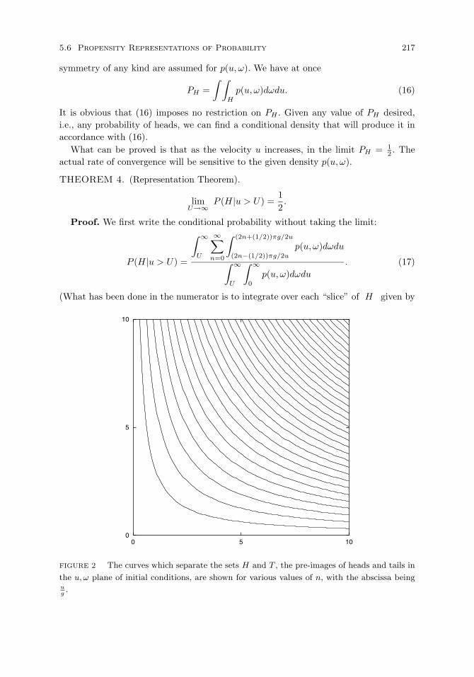
5.6 Propensity Representations of Probability 217

symmetry of any kind are assumed for p(u, ω). We have at once

PH =∫ ∫

H

p(u, ω)dωdu. (16)

It is obvious that (16) imposes no restriction on PH . Given any value of PH desired,i.e., any probability of heads, we can find a conditional density that will produce it inaccordance with (16).

What can be proved is that as the velocity u increases, in the limit PH = 12 . The

actual rate of convergence will be sensitive to the given density p(u, ω).

THEOREM 4. (Representation Theorem).

limU→∞

P (H|u > U) =12.

Proof. We first write the conditional probability without taking the limit:

P (H|u > U) =

∫ ∞

U

∞∑n=0

∫ (2n+(1/2))πg/2u

(2n−(1/2))πg/2u

p(u, ω)dωdu

∫ ∞

U

∫ ∞

0

p(u, ω)dωdu. (17)

(What has been done in the numerator is to integrate over each “slice” of H given by

0

5

10

0 5 10

FIGURE 2 The curves which separate the sets H and T , the pre-images of heads and tails in

the u, ω plane of initial conditions, are shown for various values of n, with the abscissa beingug.

218 Representations of Probability

(15).) The set T is the complement of H, and so the boundaries of slices of T are:

ω =(2n+ 1 ± 1

2 )πg2u

(18)

and we can write the denominator of (17) as:∫ ∞

U

∞∑n=0

∫ (2n+(1/2))πg/2u

(2n−(1/2))πg/2u

p(u, ω)dωdu+∫ ∞

U

∞∑n=0

∫ (2n+(3/2))πg/2u

(2n+(1/2))πg/2u

p(u, ω)dωdu. (19)

We next want to evaluate the numerator of the right-hand side of (17) as U → ∞.From the definition of the Riemann integral, we can approximate each integral insidethe summation side by the length of the interval, which is πg/2u, and the value of theintegral at the midpoint of the interval, which is p(u, nπg

u ).

limU→∞

∫ ∞

U

∞∑n=0

∫ (2n+(1/2))πg/2u

(2n−(1/2))πg/2u

p(u, ω)dωdu = limU→∞

∫ ∞

U

∞∑n=0

p(u,nπg

u)πg

2udu. (20)

And it is straightforward to show that as U → ∞ the integral on the right converges to12P (u > U). From this result, (17), (19), and (20), we have as desired:

limU→∞

P (H|u > U) =limU→∞ 1

2P (u > U)limU→∞ 1

2P (u > U) + limU→∞ 12P (u > U)

=12.

Without pursuing the details, it is worth sketching a more realistic approximateanalysis, based only on linear and angular velocities in the range of what would actuallybe observed in usual coin tossing. To do this, rather than take a physically unrealisticlimit, we introduce more restrictions of the density p(u, ω):

(i) The density p(u, ω) is single peaked.(ii) The intersection of p(u, ω) with any plane of fixed height parallel to the (u, ω)

coordinate plane is convex.(iii) The density p(u, ω) is positive only on a finite region of the u, ω plane. In particular

there is a u∗ and an ω∗ such that p(u, ω) = 0 if u > u∗ or ω > ω∗.(iv) A further lower bound on the variance of u and ω is required, so that there is not

too much concentration on a single small region of Figure 2, so as to produce toomany heads in relation to tails, or vice versa.

With empirically reasonable choices for (i), (iii) and (iv), a pretty good bound, closeto one-half, can be established for the probability of heads or tails. Some additionalsmoothing conditions on p(u, ω) might be made to facilitate computation; even a bi-variate normal distribution might fit real data reasonably well.

Propensity for randomness in motion of three bodies. This fourth example is aspecial case of the three-body problem, certainly the most extensively studied problemin the history of mechanics. Our special case is this. There are two particles of equalmass m1 and m2 moving according to Newton’s inverse-square law of gravitation inelliptic orbits relative to their common center of mass, which is at rest. The third particlehas a nearly negligible mass, so it does not affect the motion of the other two particles,but they affect its motion. This third particle is moving along a line perpendicular to

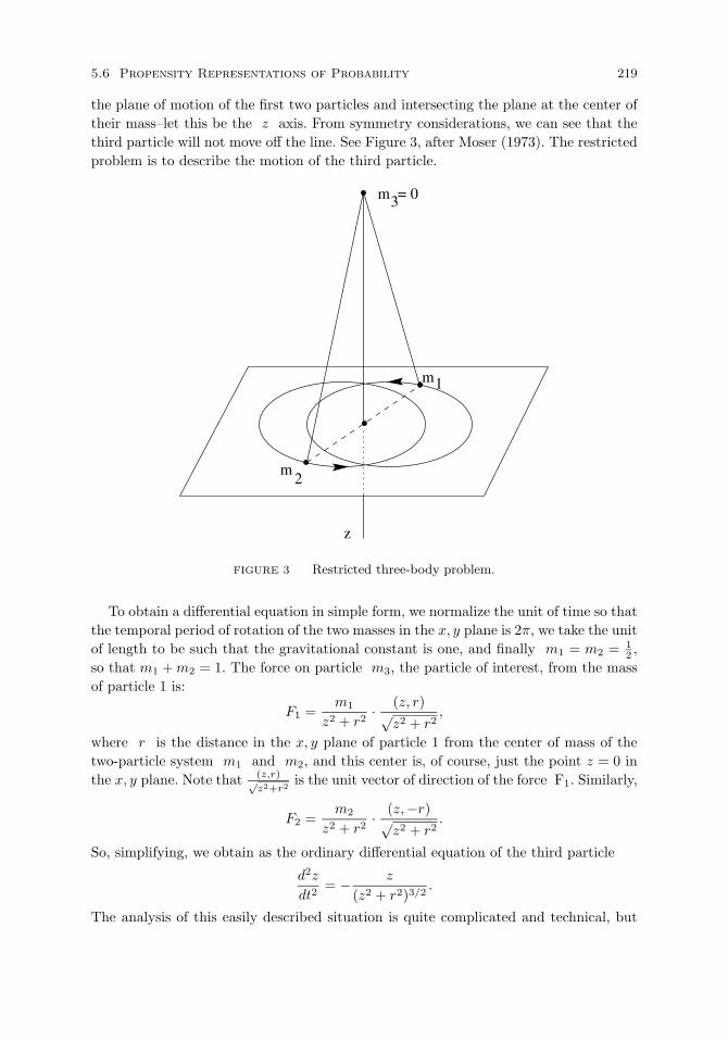
5.6 Propensity Representations of Probability 219

the plane of motion of the first two particles and intersecting the plane at the center oftheir mass–let this be the z axis. From symmetry considerations, we can see that thethird particle will not move off the line. See Figure 3, after Moser (1973). The restrictedproblem is to describe the motion of the third particle.

m = 03

m1

m2

z

FIGURE 3 Restricted three-body problem.

To obtain a differential equation in simple form, we normalize the unit of time so thatthe temporal period of rotation of the two masses in the x, y plane is 2π, we take the unitof length to be such that the gravitational constant is one, and finally m1 = m2 = 1

2 ,so that m1 +m2 = 1. The force on particle m3, the particle of interest, from the massof particle 1 is:

F1 =m1

z2 + r2· (z, r)

√z2 + r2

,

where r is the distance in the x, y plane of particle 1 from the center of mass of thetwo-particle system m1 and m2, and this center is, of course, just the point z = 0 inthe x, y plane. Note that (z,r)√

z2+r2 is the unit vector of direction of the force F1. Similarly,

F2 =m2

z2 + r2· (z,−r)

√z2 + r2

.

So, simplifying, we obtain as the ordinary differential equation of the third particle

d2z

dt2= − z

(z2 + r2)3/2.

The analysis of this easily described situation is quite complicated and technical, but

220 Representations of Probability

some of the results are simple to state in informal terms. Near the escape velocity forthe third particle—the velocity at which it leaves and does not periodically return, theperiodic motion is very irregular. In particular, the following remarkable theorem can beproved. Let t1, t2 . . . be the times at which the particle intersects the plane of motion ofthe other two particles. Let sk be the largest integer equal to or less than the differencebetween tk+1 and tk times a constant.37 Variation in the sk’s obviously measures theirregularity in the periodic motion. The theorem, due to the Russian mathematiciansSitnikov (1960) and Alekseev (1969a,b), as formulated in Moser (1973), is this.

THEOREM 5. Given that the eccentricity of the elliptic orbits is positive but not toolarge, there exists an integer, say α, such that any infinite sequence of terms sk withsk ≥ α, corresponds to a solution of the deterministic differential equation governingthe motion of the third particle.38

A corollary about random sequences immediately follows. Let s be any random (finiteor infinite) sequence of heads and tails—for this purpose we can use any of the severalvariant definitions—Church, Kolmogorov, Martin-Lof, etc. We pick two integers greaterthan α to represent the random sequence—the lesser of the two representing heads,say, and the other tails. We then have:

COROLLARY 1. Any random sequence of heads and tails corresponds to a solutionof the deterministic differential equation governing the motion of the third particle.

In other words, for each random sequence there exists a set of initial conditions thatdetermines the corresponding solution. Notice that in essential ways the motion of theparticle is completely unpredictable even though deterministic. This is a consequence atonce of the associated sequence being random. It is important to notice the differencefrom the earlier coin-tossing case, for no distribution over initial conditions and thus nouncertainty about them is present in this three-body problem. No single trajectory inthe coin-tossing case exhibits in itself such random behavior.

In this fourth case, propensity may be expressed as the tendency of the third particleto behave with great irregularity just below its escape velocity. In ordinary terms, wemight want to say that the propensity is one for irregularity, but of course we can saymore for certain solutions, namely, certain initial conditions lead to a propensity toproduce random behavior, made explicit at the level of symbolic dynamics.39

Some further remarks on propensity. Galavotti’s (1987) commentary on my viewsraises a number a fundamental questions about propensity that have been importantin the philosophical literature. She raises too many issues for me to hope to reply indetail to all of them, but I think there are some points that I can take up explicitly that

37The constant is the reciprocal of the period of the motion of the two particles in the plane.38The correspondence between a solution of the differential equation and a sequence of integers is

the source of the term symbolic dynamics. The idea of such a correspondence originated with G. D.

Birkhoff in the 1930s.39For a recent review on chaotic motion in the solar system, based on research over the past decade

showing that the orbits of the planets are inherently chaotic, see Murray and Holman (2001).

5.6 Propensity Representations of Probability 221

will help clarify the discussion, or at least clarify my own position about the concept ofpropensity.

Propensity or objective probability. One of the first issues that Galavotti raises iswhether my account is not really an account of objective chance rather than of propen-sity. I certainly answer negatively to this question. In my view, an objective theoryof probability is just required to be objective as opposed to subjective, and no causalaccount of the kind implied in a propensity account is necessary. For example, purelylogical theories of probability are intended to be objective, as opposed to subjective,as are also accounts based upon relative frequency or on a concept of complexity offinite sequences. It is certainly the view of the proponents of these various views that anobjective theory of probability has been given. Moreover, the four extended examplesconsidered certainly do not say anything about the relative frequency or complexity ac-counts of probability just mentioned. It seems to me that it is a virtue of the propensitytheory to provide a particular causal view of probability, which will qualify as a specialkind of objective probability.

This leaves open the question whether all objective accounts of probability should beencompassed by a propensity account. Philosophers such as Mellor (1971) seem to thinkso, but I hold a more pluralistic view. There is no reason in principle that accounts ofprobability or of randomness in terms of complexity can always be reduced to accountsin terms of propensity.

Question of details. Galavotti refers to the many detailed philosophical discussions ofpropensity by Popper, Mellor, Giere, and others. She rightly notes that my analysisdoes not go into the details of the views held by these various authors. I attempted togo into details in a different sense, namely, the mathematical and scientific details ofspecific examples that exhibit propensities. One purpose of the examples I selected wasto illustrate the pluralism of the concept of propensity. It seems to me that Galavotti isasking for a more specific and more monolithic concept of propensity than I would beprepared to offer. I am skeptical that there is a technical general account of propensity,any more than there is a technical general account of the concept of disposition orthat of tendency. The term propensity itself would not, in my view, occur ordinarilyin any well worked out scientific theory. It might occur in the informal descriptions ofexperiments, but not at all in the statement of theories. This means that the conceptdiffers from other general concepts that do occur in scientific theories, but it in noway challenges the usefulness of the concept. The same thing can be said about theconcept of cause. The term cause never, or almost never, occurs in detailed scientifictheories, but it certainly occurs in informal talk surrounding the theory and often ininformal descriptions of experiments or of observational procedures. The fact that theterm cause does not occur in the formulation of most scientific theories does not supportthe argument that the concept of cause is not important in science. It is just that in theformulation of theories we deal with more specific properties and concepts. The same isthe case with propensity, which I take to be a way of talking about dispositional causalphenomena. Just as many different kinds of processes or things are causes, so many

222 Representations of Probability

different kinds of processes or things are propensities.To emphasize this point, let me just ring the changes on one of the natural ways

to formulate talk about propensity in each of the four examples considered earlier:propensity to decay, propensity to respond, propensity for heads, and propensity forrandomness. Notice that in the first two cases the propensity is referred to in relationto an event or an action, and in the last two cases to a standing phenomenon, but thesegrammatical differences are not as important as the various way in which the specifictheories are formulated. The third and fourth examples are particularly interesting onthis point, because they both are built in a general way within the framework of classicalmechanics. On the other hand, the third example requires the introduction of an initialprobability distribution on the initial conditions of vertical velocity and rate of rota-tion. Without this distribution expressing the variation in initial conditions the resultscertainly cannot be derived purely from physical considerations. The fourth examplehas quite a different character. No extraneous assumptions about probability are intro-duced. The random sequences exhibiting any probability desired are generated purelyby the different objective initial conditions of the restricted three-body problem. I willreturn to this fourth example later in showing how it refutes many of the things thatare said about the relation between propensity and indeterminism. The point for themoment is that the third and fourth examples illustrate that even within the frameworkof classical mechanics we can have very different talk of propensities in relation to prob-abilistic phenomena. The existence of so much pluralism, also exhibited in other waysin the first two examples, makes me skeptical of having any unified theory of propensityof any depth, just as I think we cannot have any fully satisfactory unified single theoryof the general concept of cause. We can have, for example, a good general theory ofprobabilistic causality but not a detailed theory of causality that is meant to accuratelyreflect the relevant nuances of causal phenomena in diverse parts of science.

Single-case versus long-run frequencies. Various philosophers have differed on the ap-plication of propensities and have taken quite different views on whether propensityapproaches to probability should apply to single-case phenomena or only to long-runfrequencies. My general view is that this is a red herring and consequently I shall notsay much about it. The most important point is that the problem is mainly one of sta-tistical inference, not one of probability as such. I am happy to use propensity theoryto make single-case predictions and also long-run frequency predictions, but how thesepredictions are to be tested is a matter of statistical methodology and not a matter ofthe foundations of probability. This is a summary way of dispensing with this issue andnot, I recognize, fully satisfactory, but I want to avoid entering into the discussion ofthe methodological issues involved, which seem to me not special to propensity viewsof probability.

Propensities and indeterminism. From the standpoint of what has been said in thephilosophical literature, Galavotti is certainly right in saying that propensities haveoften implied a commitment to indeterminism. Mellor (1971) begins his chapter ondeterminism and the laws of nature by saying “If propensities are ever displayed, deter-

5.6 Propensity Representations of Probability 223

minism is false.” The same view is held by Humphreys (1985), who says in his openingparagraph, “Although chance is undeniably a mysterious thing, one promising way toapproach it is through the use of propensities—indeterministic dispositions possessedby systems in a particular environment . . . ”. (I return later to other issues raised byHumphreys’ article.) One reason for the inclusion of my fourth example was to give aparticular detailed and sophisticated instance of the generation of random phenomenaby a system that all would ordinarily classify as purely deterministic. Note that in therestricted three-body problem outlined in this example there is no question of collisions,which are sometimes used as the basis for introducing indeterminism in classical me-chanics. In the ordinary sense, as reflected in the theory of differential equations, inthe philosophical talk of determinism, etc., the three-body problem described is purelydeterministic in character and yet randomness of any desired sort can be generatedby appropriate initial conditions. The wedge that has sometimes been driven betweenpropensity and determinism is illusory. There is a lot more to be said about indetermin-ism and the closely related concept of instability within the framework of determinism,but it would take us too far afield to develop the details here.

Propensities are not probabilities. In one of the better worked-out articles on propensi-ties, Humphreys (1985) presents good arguments for why propensities cannot be prob-abilities. Humphreys makes the point that although propensities, as he puts it, are‘commonly held’ to have the properties of probabilities, he thinks this is not the case,and in this I concur. He goes on to take this argument to be ‘a reason for rejecting thecurrent theory of probability as the correct theory of chance’. I strongly disagree with hisconclusion and so I want to disentangle the basis of my agreements and disagreementswith the various theses in his article, to which Galavotti refers in her commentary.

First he gives a formal argument in terms of Bayes’ Theorem and inverse probabilitiesto show that propensities cannot have these properties. I will not go over the argumentin detail, for I agree with it, but in my own case I never for a moment thought thatpropensities did have the properties of probability. It is my reason for rejecting this viewinitially but also leads to my rejection of Humphreys’ conclusion.

The central point is based upon the nature of representation theorems, as exemplifiedin this chapter. It is standard that in proving a representation theorem, the objectsout of which a representation is constructed do not themselves have the properties ofthe represented objects. The third and fourth examples in this section, which drawextensively on classical mechanics, illustrate the point. It is unusual, to say the least,in philosophical circles to assert that classical mechanics exemplifies the properties ofprobability. What we get in the coin-tossing example is a combination of an arbitraryinitial probability distribution and the strong symmetry properties in a mechanical senseof a tossed coin. From these diverse ingredients we obtain a symmetric distribution forthe actual tosses. The physical analysis that uses two simple differential equations ofmechanics is far removed from any feature of probability. In the fourth case of therestricted three-body problem this strictly deterministic theory in itself certainly is notto be thought of as part of probability theory. It is one of the most surprising theorems inmechanics that we can represent in such a clearly deterministic way within such a purely

224 Representations of Probability

deterministic framework any random sequence. But again, the well-known gravitationalmechanical properties exhibited in the restricted three-body problem have not at all theproperties of probability structures.

The first example is, as I said earlier, close to probability and therefore not a goodexample of how the representation of probability in terms of propensities is built upfrom ingredients that are themselves far from being probabilities. The second exampleis closer, because the intuitive notion of a response strength as in principle unboundedis not at all a feature of probability. The absence of constancy as, for instance, in afinite measure that always has a constant sum, is again a feature not characteristic ofprobability theory.

Other classical examples of representation theorems show the same sorts of things.Among the best known is the representation of thermodynamical properties by statis-tical aggregates of particles. The macroscopic thermodynamical properties of bodies, ofgases, let us say, are represented by aggregates of particles for which the properties inquestion are not even defined, e.g., there is not a meaningful concept of temperature fora single particle.

So it is in terms of separating the represented objects from those ingredients out ofwhich the representation is constructed that I reject Humphreys’ conclusion that thecurrent theory of probability should be rejected. It is the basis on which I argue for aclassical conception of probability in quantum mechanics, but it is not appropriate hereto enter into the quantum-mechanical example. In any case, in Humphrey’s rejection ofthe standard theory of probability as an adequate theory of chance I do not think hehas in mind the nonstandard features of probability theory characteristic of quantummechanics.

In a related vein, there is much in Salmon’s review article on propensities (1979) withwhich I agree. He certainly seems to concur with Humphreys that propensities are notprobabilities. On the other hand, he does not go on to set forth a formal representationtheory of propensity as I have attempted to do, and in my own judgment this is themost important missing ingredient needed to bring propensity theory to the same level oftechnical detail that is characteristic of relative-frequency theories or subjective theoriesof probability. The absence of a clear view about representation theorems is, I should alsosay, very much a missing ingredient of Mellor’s book (1971), which has many useful andinteresting things to say about propensities, but also, in that long Cambridge traditionof books on probability, is lacking a kind of formal clarity that a representation-theoryview would bring to it.

Pluralism reemphasized. Finally, I want to comment on the last paragraphs of Galavotti’sremarks. She compares the examples that I have given with her work with Costantiniand Rosa on elementary-particle statistics. She remarks on their analysis of the phe-nomenological characteristics of elementary particle statistics in contrast to a propensitytheory, which would presumably try to give an explanatory account of how and whythe various types of statistics of Bose-Einstein and Fermi-Dirac, for example, arise.Unfortunately it seems to me that here she has missed the point of representationtheorems and my claim for pluralism in the account of propensities. There is not going

5.7 Theory of Subjective Probability 225

to be a deep general account of propensity, just as there will not be a deep generalaccount of the physical properties of the world. We have many different subdisciplinesin physics, each dealing in depth with particular properties of a class of phenomena.We do not naturally move in any easy way across the whole spectrum. The same is trueof propensities. If we prove a representation theorem for given phenomena, it will be interms of specific characteristics of those phenomena, and that particular account willnot work well when transferred to another environment. This can already be seen inmy four examples. It is a long way from response strengths to tossing a coin and evenfarther to the restricted three-body problem, yet in each case propensities of a certainkind form the ingredients out of which a representation theorem in terms of probabilitycan be constructed.

There will be, I claim, no precise general account of propensity. There will be a plural-istic unfolding of many accounts of propensities for many different empirical situations.It is no more feasible to give a detailed general account of propensities than it is to givea detailed general theory of properties.

5.7 Theory of Subjective Probability

In the preceding sections I have mainly examined what might be termed the ‘strongextensions’ of the formal theory of probability. In each of these cases there has beenat least one proposed method of uniquely determining the probability measure on thesample space, or the distribution of given random variables. We may use a term fromChapter 2 to characterize in a somewhat more technical way what these strong exten-sions attempt. Recall that a theory is categorical if any two models of the theory areisomorphic. Moreover, if the models of a theory have a reasonably simple structure,namely, a basic set constituting the domain of the model, and operations and relationsdefined on that domain, then the theory is said to be semicategorical if any two modelswhose domains have the same cardinality are isomorphic. The natural extension of thesenotions of categoricity to the present situation is to define (Ω,)-categoricity for proba-bility spaces. We then say that the classical definition of Laplace, the relative-frequencytheory, confirmation theory, and propensity theory provide four different theories ofprobability that are (Ω,)-categorical. I mean by this that once the structure of thesample space is determined and the algebra of events is fixed, then any one of these fourtheories uniquely (or at least up to a small set of parameters) determines the probabilitymeasure on the sample space. We have also examined in some detail the difficulties thatarise for each of these (Ω,)-categorical theories. A common failing of all of them isclearly that they attempt to do too much. The many heterogeneous and diverse circum-stances in which we want to apply probability concepts make it seem doubtful that any(Ω,)-categorical theory is possible.

Because we want to use probability concepts to talk about everything from the chanceof drawing four aces in a hand of poker to the probability of rain tomorrow or theprobability distribution of position in a quantum-mechanical experiment, it is hardlysurprising that no simple categorical theory of probability can be found. The subjectivetheory of probability accepts this diversity of applications, and, in fact, utilizes it toargue that the many ways in which information must be processed to obtain a probabil-

226 Representations of Probability

ity distribution do not admit of categorical codification. Consequently, two reasonablepersons in approximately the same circumstances can hold differing beliefs about theprobability of an event as yet unobserved. For example, according to the subjectivetheory of probability, two meteorologists can be presented with the same weather mapand the same history of observations of basic meteorological variables such as surfacetemperature, air pressure, humidity, upper air pressures, wind, etc., and yet still differin the numerical probability they assign to the forecast of rain tomorrow morning. Ihasten to add, however, that the term ‘subjective’ can be misleading. It is not partof the subjective theory of probability to countenance every possible diversity in theassignment of subjective probabilities. It is a proper and important part of subjectivetheory to analyze, e.g., how classical relative-frequency data are to be incorporated intoproper estimates of subjective probability. Such data are obviously important in anysystematic estimate of probabilities, as we can see from examination of the scientificliterature in which probabilities play a serious part. It is also obvious that the principlesof symmetry naturally applied in the classical definition play an important role in theestimation of subjective probabilities whenever they are applicable.

The discussion of Bayes’ Theorem in Section 1 has already provided an example ofthe sort of strong constraints to be placed on any subjective theory. The prior probabil-ity distributions selected by different investigators can differ widely without violatingthe subjective theory; but if these investigators agree on the method of obtaining fur-ther evidence, and if common observations are available to them, then these commonlyaccepted observations will usually force their beliefs to converge.

De Finetti’s qualitative axioms. Let us turn now to a more systematic discus-sion of the major aspects of the subjective theory. For a more detailed treatment ofmany questions the reader is referred to the historically important article of de Finetti(1937/1964), which has been translated in Kyburg and Smokler (1964), and also to deFinetti’s treatise (1974, 1975). The 1937 article of de Finetti’s is one of the most impor-tant pieces of work in the subjective foundations of probability in the twentieth century.Probably the most influential work on these matters since 1950 is the book by Savage(1954). Savage extends de Finetti’s ideas by paying greater attention to the behavioralaspects of decisions, and I shall have more to say later in this section about the relationbetween the subjective theory of probability and decision theory. Systematic works thatare more philosophical and less mathematical are Jeffrey (1965) and Levi (1980).

Perhaps the best way to begin a systematic analysis of the subjective theory is bya consideration of de Finetti’s axioms for qualitative probability. The spirit of theseaxioms is to place restraints on qualitative judgments of probability sufficient to prove astandard representation theorem, i.e., to guarantee the existence of a numerical proba-bility measure in the standard sense. From this standpoint the axioms may be regardedas a contribution to the theory of measurement, with particular reference to compar-ative judgments of probability. The central question for such a set of axioms is howcomplicated the condition on the qualitative relation more probable than must be inorder to obtain a numerical probability measure over events.

The intuitive idea of using a comparative qualitative relation is that individuals can

5.7 Theory of Subjective Probability 227

realistically be expected to make such judgments in a direct way, as they cannot whenthe comparison is required to be quantitative. On most occasions I can say unequivocallywhether I think it is more likely to rain or not in the next four hours at Stanford, butI cannot in the same direct way make a judgment of how much more likely it is not torain than rain. Generalizing this example, it is a natural move to ask next what formalproperties a qualitative comparative relation must have in order to be represented bya standard probability measure. (Later I review some of the empirical literature onwhether people’s qualitative judgments do have the requisite properties.)

We begin with the concept of a qualitative probability structure, the axioms forwhich are similar formally to those for the extensive structures of Section 3.3. The set-theoretical realizations of the theory are structures (Ω,,) where Ω is a nonemptyset, is a family of subsets of Ω, and the relation is a binary relation on . I initiallyfollow the discussion given in Luce and Suppes (1965).

DEFINITION 1. A structure Ω = (Ω,,) is a qualitative probability structure ifand only if the following axioms are satisfied for all A, B, and C in :

S1. is an algebra of sets on Ω;S2. If A B and B C, then A C;S3. A B or B A;S4. If A ∩ C = ∅ and B ∩ C = ∅, then A B if and only if A ∪ C B ∪ C;S5. A ∅;S6. Not ∅ Ω.

The first axiom on is the same as the first axiom of finitely additive probability spaces.Axioms S2 and S3 just assert that is a weak ordering of the events in . AxiomS4 formulates in qualitative terms the important and essential principle of additivityof mutually exclusive events. Axiom S5 says that any event is (weakly) more probablethan the impossible event, and Axiom S6 that the certain event is strictly more probablethan the impossible event. Defining the strict relation in the customary fashion:

A B if and only if not B A,

we may state the last axiom as: Ω ∅.To give a somewhat deeper sense of the structure imposed by the axioms, we state

some of the intuitively desirable and expected consequences of the axioms. It is conve-nient in the statement of some of the theorems also to use the (weakly) less probablerelation, defined in the usual manner:

A B if and only if B A.

The first theorem says that is an extension of the subset relation.

THEOREM 1. If A ⊆ B, then A B.

Proof. Suppose, on the contrary, that not A B, i.e., that A B. By hypothesisA ⊆ B, so there is a set C disjoint from A such that A ∪ C = B. Then, becauseA ∪ ∅ = A, we have at once

A ∪ ∅ = A B = A ∪ C,

whence by contraposition of Axiom S4, ∅ C, which contradicts Axiom S5. Q.E.D.

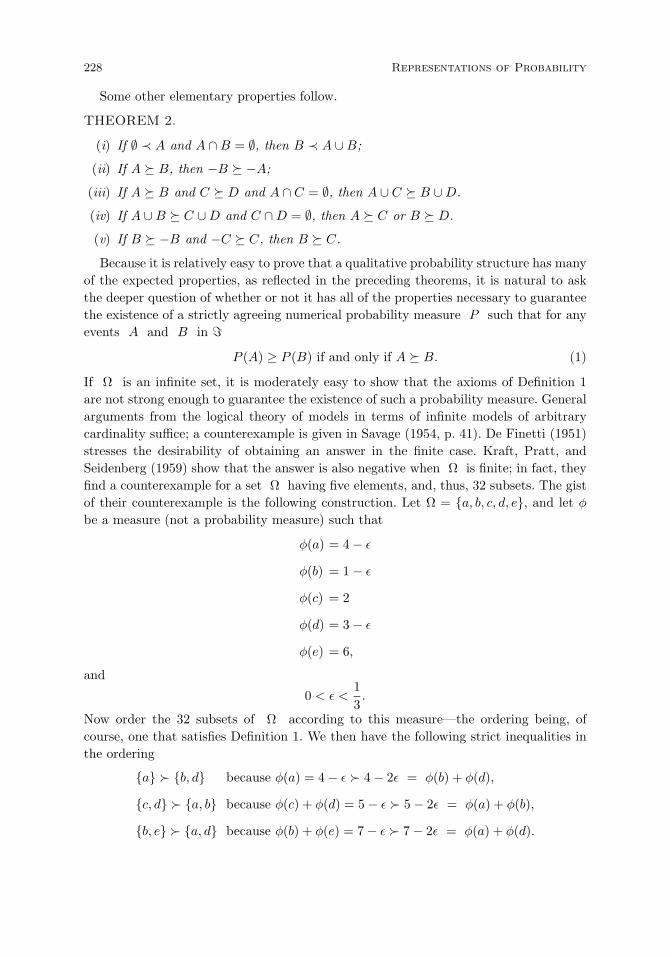
228 Representations of Probability

Some other elementary properties follow.

THEOREM 2.

(i) If ∅ ≺ A and A ∩B = ∅, then B ≺ A ∪B;

(ii) If A B, then −B −A;

(iii) If A B and C D and A ∩ C = ∅, then A ∪ C B ∪D.

(iv) If A ∪B C ∪D and C ∩D = ∅, then A C or B D.

(v) If B −B and −C C, then B C.

Because it is relatively easy to prove that a qualitative probability structure has manyof the expected properties, as reflected in the preceding theorems, it is natural to askthe deeper question of whether or not it has all of the properties necessary to guaranteethe existence of a strictly agreeing numerical probability measure P such that for anyevents A and B in

P (A) ≥ P (B) if and only if A B. (1)

If Ω is an infinite set, it is moderately easy to show that the axioms of Definition 1are not strong enough to guarantee the existence of such a probability measure. Generalarguments from the logical theory of models in terms of infinite models of arbitrarycardinality suffice; a counterexample is given in Savage (1954, p. 41). De Finetti (1951)stresses the desirability of obtaining an answer in the finite case. Kraft, Pratt, andSeidenberg (1959) show that the answer is also negative when Ω is finite; in fact, theyfind a counterexample for a set Ω having five elements, and, thus, 32 subsets. The gistof their counterexample is the following construction. Let Ω = a, b, c, d, e, and let φbe a measure (not a probability measure) such that

φ(a) = 4 − ε

φ(b) = 1 − ε

φ(c) = 2

φ(d) = 3 − ε

φ(e) = 6,

and

0 < ε <13.

Now order the 32 subsets of Ω according to this measure—the ordering being, ofcourse, one that satisfies Definition 1. We then have the following strict inequalities inthe ordering

a b, d because φ(a) = 4 − ε 4 − 2ε = φ(b) + φ(d),

c, d a, b because φ(c) + φ(d) = 5 − ε 5 − 2ε = φ(a) + φ(b),

b, e a, d because φ(b) + φ(e) = 7 − ε 7 − 2ε = φ(a) + φ(d).

5.7 Theory of Subjective Probability 229

We see immediately also that any probability measure P that preserves these threeinequalities implies that

c, e a, b, d,as may be seen just by adding the three inequalities. In the case of φ

φ(c) + φ(e) = 8 > 8 − 3ε = φ(a) + φ(b) + φ(d).

However, no set A different from c, e and a, b, d has the property that

φ(c, e) ≥ φ(A) ≥ φ(a, b, d).

Thus, we can modify the ordering induced by φ to the extent of setting

a, b, d c, e (2)

without changing any of the other inequalities. But no probability measure can pre-serve (2) as well as the three earlier inequalities, and so the modified ordering satisfiesDefinition 1, but cannot be represented by a probability measure.

Of course, it is apparent that by adding special structural assumptions to the axiomsof Definition 1, such as Axiom 5 of Definition 1 of Section 3.3, it is possible to guaranteethe existence of a strictly agreeing probability measure satisfying (1). In the finite case,for example, we can demand that all the atomic events be equiprobable, although thisis admittedly a very strong requirement to impose.

Fortunately, a simple general solution of the finite case has been found by Scott(1964). (Necessary and sufficient conditions for the existence of a strictly agreeing prob-ability measure in the finite case were formulated by Kraft, Pratt, and Seidenberg, buttheir multiplicative conditions are difficult to understand. Scott’s treatment representsa real gain in clarity and simplicity.) The central idea of Scott’s formulation is to im-pose an algebraic condition on the indicator (or characteristic) functions of the events.Recall that the indicator function of a set is just the function that assigns the value 1to elements of the set and the value 0 to all elements outside the set. For simplicity ofnotation, if A is a set we shall denote by Ai its indicator function, which is a randomvariable. Thus, if A is an event

Ai(ω) =

1 if ω ∈ A,

0 otherwise.

Scott’s conditions are embodied in the following theorem, whose proof I do not give.

THEOREM 3. (Scott’s Representation Theorem). Let Ω be a finite set and abinary relation on the subsets of Ω. Necessary and sufficient conditions that there existsa strictly agreeing probability measure P on Ω are the following: for all subsets A

and B of Ω,

(1) A B or B A;(2) A ∅;(3) Ω ∅;(4) For all subsets A0, . . . , An, B0, . . . , Bn of Ω, if Ai Bi for 0 ≤ i < n, and for

all ω in ΩAi

0(ω) + . . .+ Ain(ω) = Bi

0(ω) + . . .+ Bin(ω),

then An Bn.

230 Representations of Probability

To illustrate the force of Scott’s Condition (4), we may see how it implies transitivity.First, necessarily for any three indicator functions

Ai + Bi + Ci = Bi + Ci + Ai;

i.e., for all elements ω

Ai(ω) + Bi(ω) + Ci(ω) = Bi(ω) + Ci(ω) + Ai(ω).

By hypothesis, A B and B C, whence by virtue of Condition (4),

C A,

and thus, by definition, A C, as desired. The algebraic equation of Condition (4)just requires that any element of Ω, i.e., any atomic event, belong to exactly the samenumber of Ai and Bi, for 0 ≤ i ≤ n. Obviously, this algebraic condition cannot beformulated in the simple set language of Definition 1 and thus represents quite a strongcondition.

General qualitative axioms. In the case that Ω is infinite, a number of strongstructural conditions have been shown to be sufficient but not necessary. For example,de Finetti (1937/1964) and independently Koopman (1940a,b, 1941) use an axiom tothe effect that there exist partitions of Ω into arbitrarily many events equivalent inprobability. This axiom, together with those of Definition 1, is sufficient to prove theexistence of a numerical probability measure. Related existential conditions are discussedin Savage (1954). A detailed review of these various conditions is to be found in Chapters5 and 9 of Krantz et al. (1971).

However, as is shown in Suppes and Zanotti (1976), by going slightly beyond theindicator functions, simple necessary and sufficient conditions can be given for boththe finite and infinite case. The move is from an algebra of events to the algebra ∗ ofextended indicator functions relative to . The algebra ∗ is just the smallest semigroup(under function addition) containing the indicator functions of all events in . In otherwords, ∗ is the intersection of all sets with the property that if A is in then Ai isin ∗ and if A∗ and B∗ are in ∗, then A∗ +B∗ is in ∗. It is easy to show that anyfunction A∗ in ∗ is an integer-valued function defined on Ω. It is the extension fromindicator functions to integer-valued functions that justifies calling the elements of ∗

extended indicator functions, which, like indicator functions, are random variables.The qualitative probability ordering must be extended from to ∗, and the intuitive

justification of this extension must be considered. Let A∗ and B∗ be two extendedindicator functions in ∗. Then, to have A∗ B∗ is to have the expected value of A∗

equal to or greater than the expected value of B∗. The qualitative comparison is now notone about the probable occurrences of events, but about the expected value of certainrestricted random variables. The indicator functions themselves form, of course, a stillmore restricted class of random variables, but qualitative comparison of their expectedvalues is conceptually identical to qualitative comparison of the probable occurrencesof events.

There is more than one way to think about the qualitative comparisons of the ex-pected value of extended indicator functions, and so it is useful to consider several

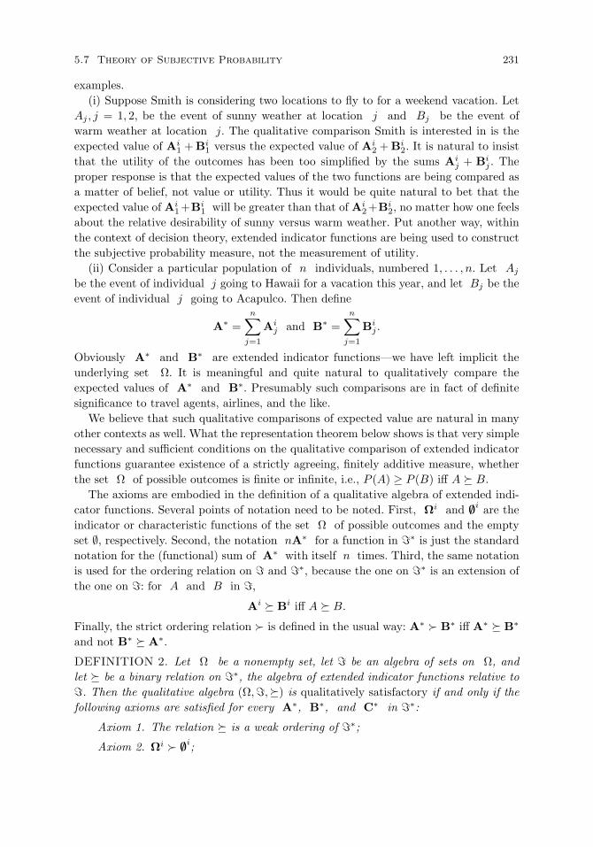
5.7 Theory of Subjective Probability 231

examples.(i) Suppose Smith is considering two locations to fly to for a weekend vacation. Let

Aj , j = 1, 2, be the event of sunny weather at location j and Bj be the event ofwarm weather at location j. The qualitative comparison Smith is interested in is theexpected value of Ai

1 + Bi1 versus the expected value of Ai

2 + Bi2. It is natural to insist

that the utility of the outcomes has been too simplified by the sums Aij + Bi

j . Theproper response is that the expected values of the two functions are being compared asa matter of belief, not value or utility. Thus it would be quite natural to bet that theexpected value of Ai

1+Bi1 will be greater than that of Ai

2+Bi2, no matter how one feels

about the relative desirability of sunny versus warm weather. Put another way, withinthe context of decision theory, extended indicator functions are being used to constructthe subjective probability measure, not the measurement of utility.

(ii) Consider a particular population of n individuals, numbered 1, . . . , n. Let Aj

be the event of individual j going to Hawaii for a vacation this year, and let Bj be theevent of individual j going to Acapulco. Then define

A∗ =n∑

j=1

Aij and B∗ =

n∑j=1

Bij .

Obviously A∗ and B∗ are extended indicator functions—we have left implicit theunderlying set Ω. It is meaningful and quite natural to qualitatively compare theexpected values of A∗ and B∗. Presumably such comparisons are in fact of definitesignificance to travel agents, airlines, and the like.

We believe that such qualitative comparisons of expected value are natural in manyother contexts as well. What the representation theorem below shows is that very simplenecessary and sufficient conditions on the qualitative comparison of extended indicatorfunctions guarantee existence of a strictly agreeing, finitely additive measure, whetherthe set Ω of possible outcomes is finite or infinite, i.e., P (A) ≥ P (B) iff A B.

The axioms are embodied in the definition of a qualitative algebra of extended indi-cator functions. Several points of notation need to be noted. First, Ωi and ∅i are theindicator or characteristic functions of the set Ω of possible outcomes and the emptyset ∅, respectively. Second, the notation nA∗ for a function in ∗ is just the standardnotation for the (functional) sum of A∗ with itself n times. Third, the same notationis used for the ordering relation on and ∗, because the one on ∗ is an extension ofthe one on : for A and B in ,

Ai Bi iff A B.

Finally, the strict ordering relation is defined in the usual way: A∗ B∗ iff A∗ B∗

and not B∗ A∗.

DEFINITION 2. Let Ω be a nonempty set, let be an algebra of sets on Ω, andlet be a binary relation on ∗, the algebra of extended indicator functions relative to. Then the qualitative algebra (Ω,,) is qualitatively satisfactory if and only if thefollowing axioms are satisfied for every A∗, B∗, and C∗ in ∗:

Axiom 1. The relation is a weak ordering of ∗;

Axiom 2. Ωi ∅i;

232 Representations of Probability

Axiom 3. A∗ ∅i;

Axiom 4. A∗ B∗ iff A∗ + C∗ B∗ + C∗;

Axiom 5. If A∗ B∗ then for every C∗ and D∗ in ∗ there is a positiveinteger n such that

nA∗ + C∗ nB∗ + D∗.

These axioms should seem familiar from the literature on qualitative probability.Note that Axiom 4 is the additivity axiom that closely resembles de Finetti’s additivityaxiom for events: If A∩C = B∩C = ∅, then A B iff A∪C B∪C. As we move fromevents to extended indicator functions, functional addition replaces union of sets. Whatis formally of importance about this move is seen already in the exact formulation ofAxiom 4. The additivity of the extended indicator functions is unconditional—there isno restriction corresponding to A ∩C = B ∩C = ∅. The absence of this restriction hasfar-reaching formal consequences in permitting us to apply without any real modificationthe general theory of extensive measurement. Axiom 5 has, in fact, the exact form of theArchimedean axiom used in Krantz et al. (1971, p. 73) in giving necessary and sufficientconditions for extensive measurement.

THEOREM 4. Let Ω be a nonempty set, let be an algebra of sets on Ω, and let be a binary relation on . Then a necessary and sufficient condition that there existsa strictly agreeing probability measure on is that there be an extension of from to ∗ such that the qualitative algebra of extended indicator functions (Ω,∗,) isqualitatively satisfactory. Moreover, if (Ω,∗,) is qualitatively satisfactory, then thereis a unique strictly agreeing expectation function on ∗ and this expectation functiongenerates a unique strictly agreeing probability measure on .

Proof. As already indicated, the main result used in the proof is from the theory ofextensive measurement: necessary and sufficient conditions for existence of a numericalrepresentation. In particular, let A be a nonempty set, a binary relation on A,and a binary operation closed on A. Then there exists a numerical function φ on A

unique up to a positive similarity transformation (i.e., multiplication by a positive realnumber) such that for a and b in A

(i) φ(a) ≥ φ(b) iff a b,

(ii) φ(a b) = φ(a) + φ(b)

if and only if the following four axioms are satisfied for all a, b, c, and d in A:

E1. The relation is a weak ordering of A;

E2. a (b c) ≈ (a b) c, where ≈ is the equivalence relation defined in terms of ;

E3. a b iff a c b c iff c a c b;E4. If a b then for any c and d in A there is a positive integer n such that

na c nb d, where na is defined inductively.

It is easy to check that qualitatively satisfactory algebras of extended indicator func-tions as defined above satisfy these four axioms for extensive measurement structures.First, we note that functional addition is closed on ∗. Second, Axiom 1 is identical to

5.7 Theory of Subjective Probability 233

E1. Extensive Axiom E2 follows immediately from the associative property of numericalfunctional addition, that is, for any A∗, B∗, and C∗ in ∗

A∗ + (B∗ + C∗) = (A∗ + B∗) + C∗,

and so we have not just equivalence but identity. Axiom E3 follows from Axiom 4 andthe fact that numerical functional addition is commutative. Finally, E4 follows from theessentially identical Axiom 5.

Thus, for any qualitatively satisfactory algebra (Ω,∗,) we can infer there is anumerical function φ on ∗ such that for A∗ and B∗ in ∗

(i) φ(A∗) ≥ φ(B∗) iff A∗ B∗,

(ii) φ(A∗ + B∗) = φ(A∗) + φ(B∗),

(iii) min(A∗) ≤ ϕ(A∗) ≤ max(A∗),

since the min and max exist for any A∗.Second, since for every A∗ in ∗

A∗ + ∅i = A∗,

we have at once that from (ii)φ(∅i) = 0.

Since Ωi is identically 1, to satisfy (iii)

φ(Ωi) = 1.

And thus φ is a standard (unique) expectation function E for extended indicatorfunctions:

(i) E(∅i) = 0

(ii) E(Ωi) = 1

(iii) E(A∗ + B∗) = E(A∗) +E(B∗).

But such an expectation function for ∗ defines a unique probability measure P on when it is restricted to the indicator functions in ∗, i.e., for A in , we define

P (A) = E(Ai).

Thus the axioms are sufficient, but it is also obvious that the only axioms, Axioms 2 and3, that go beyond those for extensive structures are also necessary for a probabilisticrepresentation. From the character of extended indicator functions, it is also clear thatfor each probability measure there is a unique extension of the qualitative ordering from to ∗. Q.E.D.

The proof just given, even more than the statement of the theorem itself, showswhat subset of random variables defined on a probability space suffices to determinethe probability measure in a natural way. Our procedure has been to axiomatize inqualitative fashion the expectation of the extended indicator functions. There was noneed to consider all random variables, and, on the other hand, the more restricted setof indicator functions raises the same axiomatic difficulties confronting the algebra ofevents.

234 Representations of Probability

Qualitative conditional probability. One of the more troublesome aspects of thequalitative theory of conditional probability is that A|B is not an object—in particularit is not a new event composed somehow from events A and B. Thus the qualitativetheory rests on a quaternary relation A|B C|D, which is read: event A given eventB is at least as probable as event C given event D. There have been a number ofattempts to axiomatize this quaternary relation (Koopman 1940a,b; Aczel 1961, 1966,p. 319; Luce 1968; Domotor 1969; Krantz et al., 1971; and Suppes 1973a). The onlyone of these axiomatizations to address the problem of giving necessary and sufficientconditions is the work of Domotor, which approaches the subject in the finite case in astyle similar to that of Scott (1964).

By using indicator functions or, more generally, extended indicator functions, thedifficulty of A|B not being an object is eliminated, for Ai|B is just the indicator functionof the set A restricted to the set B, i.e., Ai|B is a partial function whose domainis B. In similar fashion if X is an extended indicator function, X|A is that functionrestricted to the set A. The use of such partial functions requires care in formulatingthe algebra of functions in which we are interested, for functional addition X|A+ Y|Bwill not be well defined when A = B but A ∩ B = ∅. Thus, to be completely explicitwe begin, as before, with a nonempty set Ω, the probability space, and an algebra of events, i.e.,subsets of Ω, with it understood that is closed under union andcomplementation. Next we extend this algebra to the algebra ∗ of extended indicatorfunctions, i.e., the smallest semigroup (under function addition) containing the indicatorfunctions of all events in . This latter algebra is now extended to include as well allpartial functions on Ω that are extended indicator functions restricted to an event in. We call this algebra of partial extended indicator functions ∗, or, if completeexplicitness is needed, ∗(Ω). From this definition it is clear that if X|A and Y|B arein ∗, then40

If A = B, X|A+ Y|B is in ∗.

If A ∩B = ∅, X|A ∪ Y|B is in ∗.

In the more general setting of decision theory or expected utility theory, there hasbeen considerable discussion of the intuitive ability of a person to directly compare hispreferences or expectations of two decision functions with different domains of restric-tion. Without reviewing this literature, we do want to state that we find no intuitivegeneral difficulty in making such comparisons. Individual cases may present problems,but not necessarily because of different domains of definition. In fact, we believe com-parisons of expectations under different conditions is a familiar aspect of ordinary expe-rience. In the present setting the qualitative comparison of restricted expectations maybe thought of as dealing only with beliefs and not utilities. The fundamental orderingrelation is a weak ordering of ∗ with strict order and equivalence ≈ defined inthe standard way.

Following Suppes and Zanotti (1982), we give axioms that are strong enough toprove that the probability measure constructed is unique when it is required to cover

40In this subsection the notation A∗ and B∗ for extended indicator functions is changed to X and

Y to avoid any confusions in the conditional notation X|A, etc.

5.7 Theory of Subjective Probability 235

expectation of random variables. It is worth saying something more about this problemof uniqueness. The earlier papers mentioned have all concentrated on the existence ofa probability distribution, but from the standpoint of a satisfactory theory it seemsobvious for many different reasons that one wants a unique distribution. For example, ifwe go beyond properties of order and have uniqueness only up to a convex polyhedronof distributions, as is the case with Scott’s axioms for finite probability spaces, we arenot able to deal with a composite hypothesis in a natural way, because the addition ofthe probabilities is not meaningful.

DEFINITION 3. Let Ω be a nonempty set, let ∗(Ω) be an algebra of partial ex-tended indicator functions, and let be a binary relation on ∗. Then the structure(Ω,∗,) is a partial qualitative expectation structure if and only if the followingaxioms are satisfied for every X,Y,X1,X2,Y1 and Y2 in ∗ and every A, B andC in with A,B ∅:

Axiom 1. The relation is a weak ordering of ∗;

Axiom 2. Ωi ∅i;

Axiom 3. Ωi|A Ci|B ∅i|A;

Axiom 4a. If X1|A Y1|B and X2|A Y2|B then

X1|A+ X2|A Y1|B + Y2|B;

Axiom 4b. If X1|A Y1|B and X1|A+ X2|A Y1|B + Y2|B then

X2|A Y2|B;

Axiom 5. If A ⊆ B then

X|A Y|A iff X·Ai|B Y ·Ai|B;

Axiom 6. (Archimedean). If X|A Y|B then for every Z in ∗ there is apositive integer n such that

nX|A nY|B + Z|B.The axioms are simple in character and their relation to the axioms of Definition 2

is apparent. The first three axioms are very similar. Axiom 4, the axiom of addition,must be relativized to the restricted set. Notice that we have a different restriction onthe two sides of the inequality.

I have been unable to show whether or not it is possible to replace the two partsof Axiom 4 by the following weaker and more natural axiom. If X2|A ≈ Y2|B, thenX1|A Y1|B iff X1|A + X2|A Y1|B + Y2|B. The really new axiom is Axiom 5.In terms of events and numerical probability, this axiom corresponds to the following:If A ⊆ B, then P (C|A) ≥ P (D|A) iff P (C ∩ A|B) ≥ P (D ∩ A|B). Note that inthe axiom itself, function multiplication replaces intersection of events. (Closure of ∗

under function multiplication is easily proved.) Axiom 6 is the familiar and necessaryArchimedean axiom.

We now state and prove the main theorem. In the theorem we refer to a strictly agree-ing expectation function on ∗ (Ω). From standard probability theory and conditional

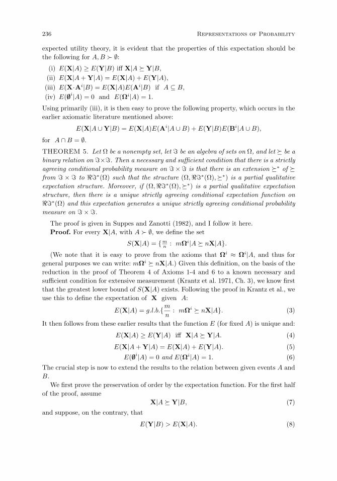
236 Representations of Probability

expected utility theory, it is evident that the properties of this expectation should bethe following for A,B ∅:

(i) E(X|A) ≥ E(Y|B) iff X|A Y|B,(ii) E(X|A+ Y|A) = E(X|A) +E(Y|A),(iii) E(X·Ai|B) = E(X|A)E(Ai|B) if A ⊆ B,(iv) E(∅i|A) = 0 and E(Ωi|A) = 1.

Using primarily (iii), it is then easy to prove the following property, which occurs in theearlier axiomatic literature mentioned above:

E(X|A ∪ Y|B) = E(X|A)E(Ai|A ∪B) + E(Y|B)E(Bi|A ∪B),

for A ∩B = ∅.

THEOREM 5. Let Ω be a nonempty set, let be an algebra of sets on Ω, and let be abinary relation on ×. Then a necessary and sufficient condition that there is a strictlyagreeing conditional probability measure on × is that there is an extension ∗ of from × to ∗(Ω) such that the structure (Ω,∗(Ω),∗) is a partial qualitativeexpectation structure. Moreover, if (Ω,∗(Ω),∗) is a partial qualitative expectationstructure, then there is a unique strictly agreeing conditional expectation function on∗(Ω) and this expectation generates a unique strictly agreeing conditional probabilitymeasure on × .

The proof is given in Suppes and Zanotti (1982), and I follow it here.Proof. For every X|A, with A ∅, we define the set

S(X|A) = mn : mΩi|A nX|A.

(We note that it is easy to prove from the axioms that Ωi ≈ Ωi|A, and thus forgeneral purposes we can write: mΩi nX|A.) Given this definition, on the basis of thereduction in the proof of Theorem 4 of Axioms 1-4 and 6 to a known necessary andsufficient condition for extensive measurement (Krantz et al. 1971, Ch. 3), we know firstthat the greatest lower bound of S(X|A) exists. Following the proof in Krantz et al., weuse this to define the expectation of X given A:

E(X|A) = g.l.b.mn

: mΩi nX|A. (3)

It then follows from these earlier results that the function E (for fixed A) is unique and:

E(X|A) ≥ E(Y|A) iff X|A Y|A. (4)

E(X|A+ Y|A) = E(X|A) +E(Y|A). (5)

E(∅i|A) = 0 and E(Ωi|A) = 1. (6)

The crucial step is now to extend the results to the relation between given events A andB.

We first prove the preservation of order by the expectation function. For the first halfof the proof, assume

X|A Y|B, (7)

and suppose, on the contrary, that

E(Y|B) > E(X|A). (8)

5.7 Theory of Subjective Probability 237

Then there must exist natural numbers m and n such that

E(Y|B) >m

n> E(X|A), (9)

and so from the definition of the function E, we have

mΩi ≺ nY|B, (10)

andmΩi nX|A, (11)

whencenY|B nX|A, (12)

but from (7) and Axiom 4a we have by a simple induction

nX|A nY|B, (13)

which contradicts (12), and thus the supposition (8) is false.Assume now

E(X|A) ≥ E(Y|B), (14)

and supposeY|B X|A. (15)

Now if E(X|A) > E(Y|B), by the kind of argument just given we can show at oncethat

X|A Y|B, (16)

which contradicts (15). On the other hand, if

E(X|A) = E(Y|B), (17)

then we can argue as follows. By virtue of (15) and Axiom 6, there is an n such that

nY|B (n+ 1)X|A, (18)

whence by the earlier argument

E(nY|B) ≥ E((n+ 1)X|A), (19)

and by (5)nE(Y|B) ≥ (n+ 1)E(X|A), (20)

and so by (17) and (20)E(Y|B) ≤ 0, (21)

but from (4)–(6) it follows easily that

E(Y|B) ≥ 0, (22)

whenceE(Y|B) = 0. (23)

But then, using again (4)–(6), we obtain

Y|B ≈ ∅i|B, (24)

and by virtue of Axiom 3X|A ∅i|B, (25)

238 Representations of Probability

whence from (24) and (25) by transitivity

X|A Y|B, (26)

contradicting (15). We have thus now shown that

E(X|A) ≥ E(Y|B) iff X|A Y|B. (27)

Finally, we need to prove that for A ∅ and A ⊆ B

E(X·Ai|B) = E(X|A)E(Ai|B). (28)

We first note that by putting mΩi for X and nX for Y in Axiom 5, we obtain

mΩi ≥ nX|A iff mAi|B ≥ nX·Ai|B. (29)

It follows directly from (29) that

mn

: mΩi nX|A = mn

: mAi|B nX·Ai|B (30)

whence their greatest lower bounds are the same, and we have

E(X|A) = E′Ai|B(X·Ai|B), (31)

where E′ is the measurement function that has Ai|B as a unit, that is,

E′Ai|B(Ai|B) = 1.

As is familiar in the theory of extensive measurement, there exists a positive real numberc such that for every X

cE′Ai|B(X·Ai|B) = E(X·Ai|B). (32)

Now by (31) and taking X = Ωi

cE(Ωi|A) = E(Ωi ·Ai|B),

but E(Ωi|A) = 1, soc = E(Ωi ·Ai|B) = E(Ai|B). (33)

Combining (31), (32) and (33) we obtain (28) as desired.The uniqueness of the expectation function follows from (6) and the earlier results

of Theorem 4 about unconditional probability.For A ∅, we then define for every B in ,

P (B|A) = E(Bi|A),

and it is trivial to show the function P is a conditional probability measure on ,which establishes the sufficiency of the axioms. The necessity of each of the axioms iseasily checked.

Historical background on qualitative axioms. The qualitative axioms of deFinetti (1937/1964) were, as already indicated, not the first ones.41 Various incompletesets of such axioms were given much earlier by Keynes (1921) and Jeffreys and Wrinch(1919) in the framework of logical theories of probability. Undoubtedly the historically

41A particularly early source of much detailed discussion of the use of probability qualitatively in

ordinary affairs is to be found in various sections of Hume’s Treatise (1739), especially Section XIII,

Part III, Bk I, entitled “Of Unphilosophical Probability”.

5.7 Theory of Subjective Probability 239

most important predecessor of de Finetti, within the framework of subjective theoriesof probability, was Ramsey’s (1931) “Truth and Probability”, published posthumously,but written in 1926. Ramsey’s basic approach differs from de Finetti’s in that he beginswith actions and expected utility, or, in terms now familiarly used, both beliefs anddesires, not beliefs alone. He describes this general program well in the following twoparagraphs.

In order therefore to construct a theory of quantities of belief which shall be both general

and more exact, I propose to take as a basis a general psychological theory, which is now

universally discarded, but nevertheless comes, I think, fairly close to the truth in the

sort of cases with which we are most concerned. I mean the theory that we act in a way

we think most likely to realize the objects of our desires, so that a person’s actions are

completely determined by his desires and opinions. This theory cannot be made adequate

to all the facts, but it seems to me a useful approximation to the truth particularly in

the case of our self-conscious or professional life, and it is presupposed in a great deal

of our thought. It is a simple theory and one which many psychologists would obviously

like to preserve by introducing unconscious desires and unconscious opinions in order to

bring it more into harmony with the facts. How far such fictions can achieve the required

result I do not attempt to judge: I only claim for what follows approximate truth, or

truth in relation to this artificial system of psychology, which like Newtonian mechanics

can, I think, still be profitably used even though it is known to be false.

It must be observed that this theory is not to be identified with the psychology of the

Utilitarians, in which pleasure had a dominating position. The theory I propose to adopt

is that we seek things which we want, which may be our own or other people’s pleasure,

or anything else whatever, and our actions are such as we think most likely to realize

these goods. But this is not a precise statement, for a precise statement of the theory

can only be made after we have introduced the notion of quantity of belief.

(Ramsey 1931, p. 173)

As Ramsey himself says, his ideas are only sketched in the article cited—the only onehe wrote on the topic. But even this sketch is important, for he outlines a simple clearway to find an ‘ethically neutral proposition p believed to degree 1

2 ’—his first axiom. Henext introduces an ordering relation for preference over “worlds”, as he puts it, amplifiedby further axioms to measure value, although his axioms are only casually formulated.He then proposes to use the measure of value to measure by the usual method of bettingratios the quantity, or probability, of belief.42

Ramsey’s ideas were later used directly as a basis of a detailed finitistic axiomatiza-tion of subjective probability and utility by Davidson and Suppes (1956). Slightly laterthese ideas were then used in experiments concerned to measure individuals’ personalprobability and utility (Davidson, Suppes and Siegel 1957).

But the essential point to keep in mind is that de Finetti developed his ideas ingreat detail, both mathematically and philosophically, in many publications, in contrastto Ramsey, whose death at 26 abruptly ended any further work. The much greatersubsequent influence of de Finetti is hardly surprising.

42As de Finetti says in a footnote (p. 102) added to the English translation of his 1937 article, he did

not know about Ramsey’s work before 1937, two years after his lectures, on which the article is based,

were given in Paris.

240 Representations of Probability

De Finetti’s representation theorem. A central problem for subjectivists such asde Finetti is how to deal with the standard, even if artificial, problem of estimating theobjectively unknown probability p of observing heads with a fair toss of a possibly biasedcoin. The relative-frequency approach is just to estimate p from an infinite sequenceof trials. (The artificiality comes from the use of an infinite sequence, which it is notpossible to produce or observe in finite time.) De Finetti’s response is that, assuming thesame artificial use of an infinite sequence, this is not a problem for subjectivists.43 Theconcept he uses, already mentioned several times, is that of exchangeability, which wenow define for infinite sequences. A sequence of 0, 1 random variables X1,X2, . . . ,Xn, . . .

on a probability space is exchangeable if for every n and every permutation σ of the firstn integers, X1,X2, . . .Xn has the same probability distribution as Xσ1,Xσ2, . . .Xσn.

The other concept we need to state in the theorem is that of a mixture of probabilities.Here we simplify slightly and write the mixture as a probability density f on the interval[0, 1]. So f has the properties:

(i) f(p) ≥ 0, for p in [0, 1],(ii)

∫ 1

0f(x)dx = 1.

Now it is easy to show that any mixture f of independent sequences X1,X2, . . .Xn . . .

is exchangeable. De Finetti proved the hard part, the converse.

THEOREM 6. (de Finetti 1937/1964). A sequence of random variables X1,X2, . . .Xn

. . . taking only the values 0 and 1 is exchangeable if and only if there exists a mixturedensity f on [0, 1] such that the probability that for any sample of n trials with m

successes, 0 ≤ m ≤ n, the probability of the sample is∫ 1

0

pm(1 − p)n−mf(p)dp.

Another appealing formulation is that in a sample of n trials, the probability of the finitesequence of heads and tails observed depends just on two numbers, n, the length of thesample and m, the number of heads. This is an invariance statement corresponding tothe formulation given at the end of Section 1. Note also the important fact that givenp, the outcomes of the sample are independent. De Finetti’s (1937/1964) careful anddetailed philosophical discussion of the theorem is highly recommended. The proof is alsopresented in detail by de Finetti, as well as the generalization to random quantities, deFinetti’s term for general random variables. I cannot do better than end this discussionwith one of de Finetti’s own summarizing paragraphs:

The result at which we have arrived gives us the looked-for answer, which is very sim-

ple and very satisfactory: the nebulous and unsatisfactory definition of “independent

events with fixed but unknown probability” should be replaced by that of “exchangeable

events”. This answer furnishes a condition which applies directly to the evaluations of

the probabilities of individual events and does not run up against any of the difficulties

that the subjectivistic considerations propose to eliminate. It constitutes a very natural

and very clear condition, of a purely qualitative character, reducing to the demand that

certain events be judged equally probable, or, more precisely, that all the combinations

43Explicit results on exchangeability for finite sequences may be found in Diaconis (1977) and Diaconis

and Freedman (1980).

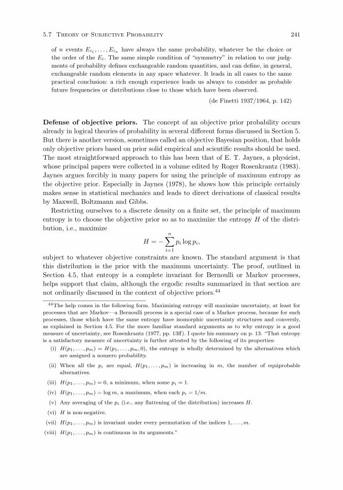
5.7 Theory of Subjective Probability 241

of n events Ei1 , . . . , Ein have always the same probability, whatever be the choice or

the order of the Ei. The same simple condition of “symmetry” in relation to our judg-

ments of probability defines exchangeable random quantities, and can define, in general,

exchangeable random elements in any space whatever. It leads in all cases to the same

practical conclusion: a rich enough experience leads us always to consider as probable

future frequencies or distributions close to those which have been observed.

(de Finetti 1937/1964, p. 142)

Defense of objective priors. The concept of an objective prior probability occursalready in logical theories of probability in several different forms discussed in Section 5.But there is another version, sometimes called an objective Bayesian position, that holdsonly objective priors based on prior solid empirical and scientific results should be used.The most straightforward approach to this has been that of E. T. Jaynes, a physicist,whose principal papers were collected in a volume edited by Roger Rosenkrantz (1983).Jaynes argues forcibly in many papers for using the principle of maximum entropy asthe objective prior. Especially in Jaynes (1978), he shows how this principle certainlymakes sense in statistical mechanics and leads to direct derivations of classical resultsby Maxwell, Boltzmann and Gibbs.

Restricting ourselves to a discrete density on a finite set, the principle of maximumentropy is to choose the objective prior so as to maximize the entropy H of the distri-bution, i.e., maximize

H = −n∑

i=1

pi log pi,

subject to whatever objective constraints are known. The standard argument is thatthis distribution is the prior with the maximum uncertainty. The proof, outlined inSection 4.5, that entropy is a complete invariant for Bernoulli or Markov processes,helps support that claim, although the ergodic results summarized in that section arenot ordinarily discussed in the context of objective priors.44

44The help comes in the following form. Maximizing entropy will maximize uncertainty, at least for

processes that are Markov—a Bernoulli process is a special case of a Markov process, because for such

processes, those which have the same entropy have isomorphic uncertainty structures and conversly,

as explained in Section 4.5. For the more familiar standard arguments as to why entropy is a good

measure of uncertainty, see Rosenkrantz (1977, pp. 13ff). I quote his summary on p. 13. “That entropy

is a satisfactory measure of uncertainty is further attested by the following of its properties:

(i) H(p1, . . . , pm) = H(p1, . . . , pm, 0), the entropy is wholly determined by the alternatives which

are assigned a nonzero probability.

(ii) When all the pi are equal, H(p1, . . . , pm) is increasing in m, the number of equiprobable

alternatives.

(iii) H(p1, . . . , pm) = 0, a minimum, when some pi = 1.

(iv) H(p1, . . . , pm) = log m, a maximum, when each pi = 1/m.

(v) Any averaging of the pi (i.e., any flattening of the distribution) increases H.

(vi) H is non-negative.

(vii) H(p1, . . . , pm) is invariant under every permutation of the indices 1, . . . , m.

(viii) H(p1, . . . , pm) is continuous in its arguments.”

242 Representations of Probability

A second argument is familiar from statistical mechanics. The maximum-entropydistribution is the one to choose because, under the null hypothesis that no other con-straints are present besides those already taken account, most of the possible distribu-tions will be close to it. Here is a familiar example from Jaynes (1979) that illustratesthis point and also shows how the principle works.

Suppose a die is tossed N = 1000 times. If the die were “true”, the expected numberof spots up should be 3.5. But we are told the correct expectation for the slightly biaseddie is 4.5. So

6∑i=1

ifi = 4.5.

The result, derived in detail in Jaynes (1978) is: (f1, . . . , f6) = (0.05, 0.08, 0.11, 0.17,0.24, 0.35). The bias toward the faces with more spots is evident. The computation,even of this simple example, is nontrivial, a point sometimes stated in criticism of themaximum entropy principle. A good discussion of this and other points may be foundin Rosenkrantz’s (1977) book on these and related topics, especially Chapter 3.

The objective Bayesian viewpoint, defended most clearly and effectively by Jaynes inthe context of many physical examples, has not won out over the personal subjectivismof de Finetti. Perhaps the main difficulty of objective approaches, emphasized by deFinetti, arises from attempts to apply them when it is not appropriate. The subjectiveBayesian always has a prior, even if he cannot explain or justify it. This is an attitudewell suited to any complex and subtle domain of investigation or application, such asforecasting the weather. But, all the same, some of Jaynes’ applications in statisticalmechanics are very appealing, special though they may be. Moreover, as de Finettiattests, “objectivity has its rightful, important place”.45

General issues. I now want to turn to a number of general issues that arise in evalu-ating the subjective view of probability.

Use of symmetries. A natural first question is to ask how subjective theory utilizesthe symmetries that are such a natural part of the classical, Laplacean definition ofprobability. If we think in terms of Bayes’ Theorem the answer seems apparent. Thesymmetries that we all accept naturally in discussing games of chance are incorporatedimmediately in the subjective theory as prior probabilities. Thus, for example, if I wishto determine the probability of getting an ace in the next round of cards dealt faceup in a hand of stud poker, given the information that one ace is already showing onthe board, I use as prior probabilities the natural principles of symmetry for games ofchance, which are a part of the classical definition. Of course, if I wish to introducerefined corrections I could do so, particularly corrections arising from the fact that inordinary shuffling, the permutation groups introduced are groups of relatively smallfinite order, and, therefore, there is information carry-over from one hand to another,in spite of the fact that a rather thorough shuffling may have been given the cards

45This brief quotation is taken from de Finetti (1975, p. 201), but his lengthy philosophical analysis

on this and the following pages is very pertinent to the conceptual problems of inductive inference.

5.7 Theory of Subjective Probability 243

by the dealer. These second-order refinements with respect to shuffling are simply anindication of the kind of natural corrections that arise in the subjective theory and thatwould be hard to deal with in principle within the framework of the classical definitionof probability. On the other hand, I emphasize that the principles of symmetry usedin the classical definition are a natural part of the prior probabilities of an experiencedcard player. The extent to which these symmetries are compelling is a point I shallreturn to later.

Use of relative frequencies. It should also be clear that the proper place for the useof relative-frequency data in the subjective theory is in the computation of posteriorprobabilities. The example given earlier of the application of Bayes’ Theorem providesan artificial but simple instance in which such use is made of relative-frequency data.It is clear what is required in order to get convergence of opinion between observerswhose initial opinions differ. The observers must agree on the method of sampling, and,of course, they must also agree on the observations that result from this sampling.Under very weak restrictions, no matter how much their initial opinions differ, theycan be brought arbitrarily close to convergence on the basis of a sufficient amount ofsampled observations. The obvious requirement is that the individual observations beapproximately independent, or at least exchangeable. If, for example, the observationsare temporally strongly dependent, then many observations will count for no more thana single observation. Since these matters have already been considered, we will notdiscuss them again in detail.

Reflection upon the conditions under which convergence of beliefs will take place alsothrows light on the many situations in which no such convergence occurs. The radicallydiffering opinions of men and women about religion, economics, and politics are excellentexamples of areas in which there is a lack of convergence; no doubt a main source ofthis divergence is the lack of agreement on what is to count as evidence, or, put anotherway, inability to agree on an experiment, or some other regime of collecting data, whichmay be summarized in an agreed-upon likelihood function.

Problem of the forcing character of information. As already indicated, it is an importantaspect of the subjective theory to emphasize that equally reasonable persons may holdrather different views about the probability of the same event. The ordinary use ofthe word rational seems to go beyond what is envisaged in the subjective theory ofprobability. Let us consider one or two examples of how this difference in usage may beexpressed.

The first kind of example deals with the nonverbal processing of information bydifferent individuals. One man is consistently more successful than another in predictingtomorrow’s weather. At least before the advent of powerful mathematical methods ofpredicting weather, which are now just beginning to be a serious forecasting instrument,it was the common observation of experienced meteorologists that there was a greatdifference in the ability of meteorologists with a common training and background, andwith a common set of observations in front of them, to predict successfully tomorrow’sweather in a given part of the world. As far as I can see, in terms of the standard

244 Representations of Probability

subjective theory as expressed, for example, by de Finetti, there is no very clear wayof stating that on a single occasion the better predictor is in some sense more rationalin his processing of information than the other man; yet in common usage we wouldbe very inclined to say this. It is a stock episode in novels, and a common experiencein real life for many people, for someone to denigrate the intelligence or rationality ofindividuals who continue to hold naive beliefs about other people’s behavior in the faceof much contrary, even though perhaps subtle, evidence.

But successive predictions can be studied like any other empirical phenomena, andthere is a large literature on evaluating the performance of forecasters, an importantpractical topic in many arenas of experience. Examination of quantitative methods ofevaluation of subjective, as well as objective, forecasts lies outside the scope of thischapter. The Journal of Forecasting is entirely devoted to the subject. See also, forexample, Makridakis et al. (1984) and Dawid (1986).

Contrary to the tenor of many of de Finetti’s remarks, it seems fair to say thatthe subjective theory of probability provides necessary but not sufficient conditions ofrationality.

Bayesian probabilities and the problem of concept formation. An important point re-volving around the notion of mistaken belief is involved in the analysis of how informa-tion is processed. In common usage, a belief is often said to be mistaken or irrationalwhen later information shows the belief to be false. According to the subjective the-ory of probability, and much sensible common usage in addition, this view of mistakenbeliefs is itself a mistake. A belief is not shown to be mistaken on the basis of subse-quent evidence not available at the time the belief was held. Proper changes in beliefare reflected in the change from a prior to a posterior probability on the basis of newinformation. The important point for subjective theory is that the overall probabilitymeasure does not itself change, but rather we pass from a prior to a posterior, condi-tional probability. Applications of Bayes’ Theorem that we have considered demonstratethis well enough. The following quotation from de Finetti (1937/1964, p. 146) illustratesthis point beautifully.

Whatever be the influence of observation on predictions of the future, it never implies and

never signifies that we correct the primitive evaluation of the probability P (En+1) after it

has been disproved by experience and substitute for it another P ∗(En+1) which conforms

to that experience and is therefore probably closer to the real probability; on the contrary,

it manifests itself solely in the sense that when experience teaches us the result A on the

first n trials, our judgment will be expressed by the probability P (En+1) no longer, but

by the probability P (En+1|A), i.e., that which our initial opinion would already attribute

to the event En+1 considered as conditioned on the outcome A. Nothing of this initial

opinion is repudiated or corrected; it is not the function P which has been modified

(replaced by another P ∗), but rather the argument En+1 which has been replaced by

En+1|A, and this is just to remain faithful to our original opinion (as manifested in the

choice of the function P ) and coherent in our judgment that our predictions vary when

a change takes place in the known circumstances.

5.7 Theory of Subjective Probability 245

In spite of the appeal of what de Finetti says, there seems to be a wide class of casesin which the principles he affirms have dubious application. I have in mind all thosecases in which a genuinely new concept is brought to bear on a subject. I do not meannecessarily the creation of a new scientific concept, but rather any situation in whichan individual applies a concept that he was not previously using in his analysis of thedata in front of him.46

Problem of unknown probabilities. Another feature of the subjective theory of proba-bility that is in conflict with common usage of probability notions is the view that thereare no unknown probabilities. If someone asks me what is the probability of rain in theFiji Islands tomorrow, my natural inclination is to say, ‘I don’t know’, rather than to tryto give a probability estimate. If another person asks me what I think the probability isthat Stanford University will have an enrollment of at least 50,000 students 500 yearsfrom now, I am naturally inclined simply to say, ‘I haven’t the faintest idea what theprobability or likelihood of this event is’. De Finetti insists on the point that a personalways has an opinion, and, therefore, a probability estimate about such matters, butit seems to me that there is no inherent necessity of such a view. It is easy to see onesource of it. The requirement that one always have a probability estimate of any event,no matter how poor one’s information about the circumstances in which that eventmight occur may be, arises from a direct extension of two-valued logic. Any statementis either true or false, and, correspondingly, any statement or event must always havea definite probability for each person interrogated. From a formal standpoint it wouldseem awkward to have a logic consisting of any real number between 0 and 1, togetherwith the quite disparate value, ‘I don’t know’.

A little later we shall examine the view that one can always elicit a subjective prob-ability for events about which the individual has very little background information byasking what sort of bet he will make concerning the event. Without anticipating thatdiscussion, I still would like to insist that it does not really seem to be a proper partof the subjective theory to require an assignment of a probability to every imaginableevent. In the same spirit with which we reply to a question about the truth of a state-ment by saying that we simply don’t know, we may also reply in the same fashion to arequest for an estimate of a probability.

Decisions and the measurement of subjective probability. It is commonplaceto remark that a man’s actions or decisions, and not his words, are the true mark of hisbeliefs. As a reflection of this commonly accepted principle, there has been considerablediscussion of how one may measure subjective probabilities on the basis of decisionsactually made. This is a complex subject, and I shall not attempt to give it a fullydetailed treatment.

The classical response in terms of subjective probability is that we may find out the

46I. J. Good (1983) emphasizes this point well in many passages, indexed under the heading ‘evolving

probabilities’. An even more important point is that conditionalization on new information, fundamental

though it may be, as de Finetti emphasizes, does not replace the need for an explicit development of

Bayesian statistics. An excellent and quite accessible introduction is Lindley (1971).

246 Representations of Probability

subjective probabilities a man truly holds by asking him to place wagers. For example, ifhe thinks the probability of rain tomorrow is really 1

2 , then he will be willing to place aneven-money bet on this occurrence. If he thinks that the probability of snow tomorrowhas a subjective probability of 0.1, then he will bet against snow at odds of 1:9. It is alsoclear how this same procedure may be used to test precise statements. For example, if aman says the probability of rain tomorrow is at least 1

2 , then presumably he will acceptany bet that provides odds at least this favorable to him.

Unfortunately, there is a central difficulty with this method of measuring subjectiveprobability. Almost all people will change the odds at which they will accept a bet ifthe amount of money varies. For example, the man who will accept an even-money beton the probability of rain tomorrow with the understanding that he wins the bet if infact it does rain, will not accept an even-money bet if the amount of money involvedmoves from a dollar on each side to a hundred dollars on each side. Many people whowill casually bet a dollar will not, in the same circumstances and at the same odds, bewilling to bet a hundred dollars, and certainly not a thousand dollars. The man whowill accept an even-money bet on its raining tomorrow will perhaps be willing to acceptodds of two to one in his favor only if the wager is of the order of a hundred dollars,while he will accept only still more favorable odds for a bet involving a larger sum ofmoney. What then are we to say is his true estimate of the probability of rain tomorrowif we use this method of wagers to make the bet?

In spite of this criticism, there have been a number of interesting empirical studiesof the measurement of subjective probability using the simple scheme we have justdescribed. A brief diversion which describes some of these empirical results may be ofinterest. Again I follow the discussion in Luce and Suppes (1965).

The first attempt to measure subjective probability experimentally was apparentlyby Preston and Baratta (1948). Subjects were run in groups of two or more, and theyused play money to bid for gambles in a simple auction game. The successful bidderwas permitted to roll a set of dice after the bidding was completed. The probabilityof winning with the dice corresponded exactly to the probability stated on the cardpresented for auction. For example, on a given play, subjects might bid for a prize of250 points with probability of 0.25 of winning. If for this gamble the average successfulbid was 50, then the authors computed the psychological probability to be 50

250 = .20.Using this method of computation, perhaps their most interesting conclusion was thatobjective probabilities less than 0.20 are systematically overestimated, and objectiveprobabilities greater than 0.20 are systematically underestimated.

Two other conclusions are noteworthy. First, by comparing the data of sophisticatedsubjects with those of subjects who were relatively naive about the facts of probability,they concluded that the underestimating and overestimating effects just described existin both kinds of subjects. Second, an increase in the number of players, and, therefore,an increase in the competition among them, tended to increase the underestimationof high probabilities and the overestimation of low probabilities, which is a somewhatsurprising result.

A ready-made, real-life comparison of subjective and objective probabilities is pro-vided by the betting on horses under the parimutuel system as compared with the

5.7 Theory of Subjective Probability 247

objective probabilities of winning, as determined a posteriori after the races. The to-tal amount of money bet on a horse divided by the net total bet on all horses in arace determines the odds, and, thus, the collective subjective probability that the horsewill win. Griffith (1949) examined data from 1,386 races run in 1947; his results arein remarkable qualitative agreement with those obtained by Preston and Baratta. Lowobjective probabilities are systematically overestimated by the subjective probabilities,and high objective probabilities are systematically underestimated. For Griffith’s data,objective and subjective probability are equal at 0.16, which is close to the 0.20 valueobtained by Preston and Baratta. Griffith remarks in a final footnote that the samecomputations were carried through for all races run at the same tracks in August, 1934,and essentially the same results were obtained. In this case the indifference point fell at0.18 rather than at 0.16. The invariance of the results from the depression economy of1934 to the relative affluence of 1947 increases their significance.

A still more extensive study very similar to Griffith’s has been made by McGloth-lin (1956) of 9,605 races run from 1947 to 1953, mostly on California tracks. As onewould expect, the general character of his results agrees closely with those of the ear-lier study. The objective and subjective probability curves intersect between 0.15 and0.22. McGlothlin also found some interesting tendencies during the course of the usualeight races on a given day. First, there was an increasing tendency to overestimate lowprobabilities, and this phenomenon was particularly striking for the final race of theday. There seems to be evidence that on the last race of the day many bettors areuninterested in odds that are not sufficient to recoup their losses from the earlier races.This phenomenon is so striking that bets placed on low-odds horses had a net positiveexpectation even after subtracting the tracks’ take, which was at the time 13 percent inCalifornia.

Toda (1951, 1958) proposed a two-person game method for measuring subjectiveprobability that is very similar to the auction procedure of Preston and Baratta. One ofits more interesting applications has been made by Shuford (1959) to obtain extensivemeasurements of subjective probability of both elementary and compound events. Sub-jects rolled a 20-face die (with the integers 1 to 20 on the faces) twice to select the rowand column of a 20 × 20 matrix of vertical and horizontal bars. The subjects, 64 airmenin training at an airbase, were run in pairs. The sequence of events on a given trial wasas follows. The matrix of horizontal and vertical bars was projected on a screen. SubjectA wrote down his bid x that a horizontal bar, say, would be selected (0 ≤ x ≤ 10);subject B decided to ‘buy’ or ‘sell’ A’s bid; the die was rolled by the experimenter todecide the bet, that is, which element of the projected matrix was selected; and, finally,the subjects scored themselves for the play. It can be shown that A’s optimal (minimax)strategy in this game is to set x equal to 10 times his subjective probability of thefavorable outcome.

Two games were played with each pair of subjects. In the first game the payoff wasdetermined by the occurrence of a horizontal or vertical bar, as the case might be, inthe position of the matrix selected by the two rolls of the 20-face die. In the secondgame, the bet paid off if two successive selections of elements of the matrix made withthe die resulted in two bars of the same type.

248 Representations of Probability

Confirming the earlier findings of Preston and Baratta, Griffith, and McGlothlin, afairly large fraction of the subjects overestimated low probabilities and underestimatedhigh ones. This was true for both the elementary and the compound events. On theother hand, Shuford found that the subjective probability estimates of a number of thesubjects were fit quite well by a linear function of objective probability, although theslope and intercept of this function varied from one subject to another. His findingsabout the estimation of compound events are particularly interesting. A majority of thesubjects approximated the correct rule, that is, they estimated the probability of thecompound event as approximately the square of the probability of the elementary event.That the application of the correct rule was so common is surprising, because when thesubjects were asked at the end of the series of trials what rule they had used, only twostated the correct one.

It is apparent from the studies cited that it is possible empirically to measure sub-jective probabilities, and, also, that the obvious method of doing this is in terms of thekind of wagers individuals will make. On the other hand, recall the objections offeredabove to this method of measurement, because of the lack of invariance of the odds atwhich wagers will be made when the amounts of money involved are changed. Theyhave prompted a deeper theoretical development in terms of the concept of expectedutility, which I will not explore here. For references see Savage (1954), Luce and Suppes(1965), Fishburn (1970), Krantz et al. (1971, Ch. 8) and Luce (2000). Savage’s axiomsare discussed in the next subsection, but not his basic representation theorem.

Inexact measurement of belief: upper and lower probabilities.47 Almost ev-eryone who has thought about the problems of measuring beliefs in the tradition ofsubjective probability or Bayesian statistical procedures concedes some uneasiness withthe problem of always asking for the next decimal of accuracy in the prior estimation ofa probability or of asking for the parameter of a distribution that determines the prob-abilities of events. On the other hand, the formal theories that have been developedfor rational decision-making under uncertainty by Ramsey (1931), de Finetti (1931,1937/1964), Koopman (1940a,b), Savage (1954) and subsequent authors have almostuniformly tended to yield a result that guarantees a unique probability distribution onstates of nature or whatever other collection of entities is used for the expression of priorbeliefs. I examine some of these standard theories and address the question of how wecan best criticize the claims they make. Among other points, I consider the claim thatthe idealizations expressed in the axioms can be regarded as theories of pure rationality.

Because the standard theories mentioned earlier reach essentially the same formalresults, namely, the existence of a unique probability distribution on states of nature,criticisms of one will pretty much apply to criticisms of the lot. For this reason, it maypay to concentrate on Savage’s (1954) axioms, because of their familiarity to a wideaudience and because they have been much discussed in the literature. I emphasize,however, that what I have to say about Savage’s axioms will apply essentially withoutchange to other standard theories.

Because Savage’s axioms are rather complicated from a formal standpoint, I shall not47Much of this subsection is drawn from Suppes (1974d).

5.7 Theory of Subjective Probability 249

TABLE 1 Decision matrix for buying bread.

d1 d2 d3

buy 700 buy 800 buy 900loaves loaves loaves

s1–rain $21.00 $19.00 $17.00s2–no rain $21.00 $24.00 $26.50

state them explicitly here, but shall try to describe their intuitive content. The axiomsare about preference among decisions, where decisions are mappings or functions fromthe set of states of nature to the set of consequences. To illustrate these ideas, let meuse an example I have used before (Suppes 1956).

A certain independent distributor of bread must place his order for a given day byten o’clock of the preceding evening. His sales to independent grocers are affected bywhether or not it is raining at the time of delivery, for if it is raining, the grocers tend tobuy less on the accumulated evidence that they have fewer customers. On a rainy daythe maximum the distributor can sell is 700 loaves; on such a day he makes less moneyif he has ordered more than 700 loaves. On the other hand, when the weather is fair, hecan sell about 900 loaves. If the simplifying assumption is made that the consequencesto him of a given decision with a given state of nature (s1–rain or s2–no rain) may besummarized simply in terms of his net profits, the situation facing him is representedin Table 1. The distributor’s problem is to make a decision.

Clearly, if he knows for certain that it is going to rain, he should make decision d1,and if he knows for certain that it is not going to rain, he should make decision d3. Thepoint of Savage’s theory, expanded to more general and more complex situations, is toplace axioms on choices or preferences among the decisions in such a way that anyonewho satisfies the axioms will be maximizing expected utility. This means that the wayin which he satisfies the axioms will generate a subjective probability distribution abouthis beliefs concerning the true state of nature and a utility function on the set of con-sequences such that the expectation of a given decision is defined in a straightforwardway with respect to the subjective probability distribution on states of nature and theutility function on the set of consequences. As one would expect, Savage demands, infact in his first axiom, that the preference among decisions be transitive and that givenany two decisions one is at least weakly preferred to the other. Axiom 2 extends thisordering assumption to having the same property hold when the domain of definition ofdecisions is restricted to a given set of states of nature; for example, the decision-makermight know that the true state of nature lies in some subset of the whole set. Axiom3 asserts that knowledge of an event cannot change preferences among consequences,where preferences among consequences are defined in terms of preferences among de-cisions. Axiom 4 requires that given any two sets of states of nature, that is, any twoevents, one is at least as probable as the other, that is, qualitative probability amongevents is strongly connected. Axiom 5 excludes the trivial case in which all consequencesare equivalent in utility and, thus, every decision is equivalent to every other. Axiom6 says essentially that if event A is less probable than event B (A and B are subsets

250 Representations of Probability

of the same set of states of nature), then there is a partition of the states of naturesuch that the union of each element of the partition with A is less probable than B.As is well known, this axiom of Savage’s is closely related to the axiom of de Finettiand Koopman, which requires the existence of a partition of the states of nature intoarbitrarily many events that are equivalent in probability. Finally, his last axiom, Axiom7, is a formulation of the sure-thing principle.

My first major claim is that some of Savage’s axioms do not in any direct senserepresent axioms of rationality that should be satisfied by any ideally rational personbut, rather, they represent structural assumptions about the environment that may ormay not be satisfied in given applications.

Many years ago, at the time of the Third Berkeley Symposium (1955), I intro-duced the distinction between structure axioms and rationality axioms in the theoryof decision-making (Suppes 1956). Intuitively, a structure axiom as opposed to a ratio-nality axiom is existential in character. In the case of Savage’s seven postulates, two (5and 6) are structure axioms, because they are existential in character.

Savage defended his strong Axiom 6 by holding it applicable if there is a coin thata decision-maker believes is fair for any finite sequence of tosses. There are however,several objections to this argument. First of all, if it is taken seriously then one ought toredo the entire foundation and simply build it around Bernoulli sequences with p = 0.5and get arbitrarily close approximations to the probability of any desired event. Moreimportantly, without radical changes in human thinking, it is simply not natural onthe part of human beings to think of finite sequences of tosses of a coin in evaluatinglikelihoods or probabilities, qualitative or quantitative, of significant events with whichthey are concerned.

Consider the case of a patient’s deciding whether to follow a surgeon’s advice to havemajor surgery. The surgeon, let us suppose, has evaluated the pros and cons of theoperation, and the patient is now faced with the critical decision of whether to take therisk of major surgery with at least a positive probability of death, or whether to takethe risk of having no surgery and suffering the consequences of the continuing disease. Ifind it very unlikely and psychologically very unrealistic to believe that thinking aboutfinite sequences of tosses of a fair coin will be of any help in making a rational decisionon the part of the patient.

On the other hand, other axioms like those on the ordering of preferences or qualita-tive probability seem reasonable in this framework and are not difficult to accept. Butthe important point is this. In a case in which uncertainty has a central role, in prac-tice, decisions are made without any attempt to reach the state of having a quantitativeprobability estimate of the alternatives or, if you like, a computed expected utility.

It is, in fact, my conviction that we usually deal with restricted situations in whichthe set of decisions open to us is small and in which the events that we consider relevantare small in number. The kind of enlarged decision framework provided by standardtheories is precisely the source of the uneasiness alluded to in the first sentence ofthis subsection. Intuitively we all move away from the idea of estimating probabilitieswith arbitrary refinement. We move away as well from the introduction of an elaboratemechanism of randomization in order to have a sufficiently large decision space. Indeed,

5.7 Theory of Subjective Probability 251

given the Bayesian attitude towards randomization, there is an air of paradox about theintroduction a la Savage of finite sequences of tosses of a fair coin.

Another way of putting the matter, it seems to me, is that there is a strong intuitivefeeling that a decision-maker is not irrational simply because a wide range of decisionpossibilities or events is not available to him. It is not a part of rationality to require thatthe decision-maker enlarge his decision space, for example, by adding a coin that may betossed any finite number of times. I feel that the intrinsic theory of rationality should beprepared to deal with a given set of states of nature and a given set of decision functions,and it is the responsibility of the formal theory of belief or decision to provide a theoryof how to deal with these restricted situations without introducing strong structuralassumptions.

A technical way of phrasing what I am saying about axioms of pure rationality isthe following. For the moment, to keep the technical apparatus simple, let us restrictourselves to a basic set S of states of nature and a binary ordering relation of qualitativeprobability on subsets of S, with the usual Boolean operations of union, intersectionand complementation having their intuitive meaning in terms of events. I then say thatan axiom about such structures is an axiom of pure rationality only if it is closed undersubmodels. Technically, closure under submodels means that if the axiom is satisfied fora pair (S,) then it is satisfied for any nonempty subset of S with the binary relation restricted to the power set of the subset, i.e., restricted to the set of all subsets of thegiven subset. (Of course, the operations of union, intersection and complementation areclosed in the power set of the subset.) Using this technical definition, we can easily seethat of Savage’s seven axioms, five of them satisfy this restriction, and the two alreadymentioned as structure axioms do not.

Let me try to make somewhat more explicit the intuition which is behind the re-quirement that axioms of pure rationality should satisfy the condition of closure undersubmodels. One kind of application of the condition is close to the axiom on the inde-pendence of irrelevant alternatives in the theory of choice. This axiom says that if weexpress a preference among candidates for office, for example, and if one candidate isremoved from the list due to death or for other reasons, then our ordering of preferencesamong the remaining candidates should be unchanged. This axiom satisfies closure un-der submodels. The core idea is that existential requirements that reach out and makespecial requirements on the environment do not represent demands of pure rationalitybut rather structural demands on the environment, and such existential demands areruled out by the condition of closure under submodels.

A different, but closely related, way of defining axioms of pure rationality is thatsuch an axiom must be a logical consequence of the existence of the intended numericalrepresentation. This criterion, which I shall call the criterion of representational conse-quence, can be taken as both necessary and sufficient, whereas the criterion of closureunder submodels is obviously not sufficient. On the other hand, the extrinsic characterof the criterion of representational consequence can be regarded as unsatisfactory. It isuseful for identifying axioms that are not necessary for the intended representation andthus smuggle in some unwanted arbitrary structural assumption. As should be clear,Savage’s Axioms 5 and 6 do such smuggling.

252 Representations of Probability

I am quite willing to grant the point that axioms of rationality of a more restrictedkind could be considered. One could argue that we need special axioms of rationalityfor special situations, and that we should embark on a taxonomy of situations provid-ing appropriate axioms for each of the major classes of the taxonomy. In the presentprimitive state of analysis, however, it seems desirable to begin with a sharp distinctionbetween rationality and structure axioms and to have the concept of pure rationalityuniversal in character.

Returning now to my criticisms of Savage’s theory, it is easy to give finite or infinitemodels of Savage’s five axioms of rationality for which there exists no numerical rep-resentation in terms of utility and subjective probability. In the language I am usinghere, Savage’s axioms of pure rationality are insufficient for establishing the existenceof representing numerical utility and subjective probability functions.

Moreover, we may show that no finite list of additional elementary axioms of a uni-versal character will be sufficient to guarantee the existence of appropriate numericalfunctions. By elementary axioms I mean axioms that can be expressed within first-orderlogic. As was explained in Chapter 2, first-order logic essentially consists of the concep-tual apparatus of sentential connectives, one level of variables and quantifiers for thesevariables, together with nonlogical predicates, operation symbols and individual con-stants. Thus, for example, the standard axioms for groups or for ordered algebraic fieldsare elementary, but the least upper-bound axiom for the field of real numbers is not. Itis possible to formulate Savage’s Axiom 5 in an elementary way, but not his Axiom 6.

In the case of infinite models, the insufficiency of elementary axioms, without restric-tion to their being of a universal character, follows from the upward Lowenheim-Skolem-Tarski theorem, plus some weak general assumptions. This theorem asserts that if a setof elementary axioms has an infinite model (i.e., a model whose domain is an infiniteset, as is the case for Savage’s theory), then it has a model of every infinite cardinality.Under quite general assumptions, e.g., on the ordering relation of preference or greatersubjective probability, it is impossible to map the models of high infinite cardinalityinto the real numbers, and thus no numerical representation exists.

In the case of finite models, the methods of Scott and Suppes (1958), discussed inSection 2.2, apply to show that no finite set of universal elementary axioms will suffice.The system consisting of Savage’s five axioms of pure rationality has finite models, butby the methods indicated we can show there is no finite elementary extension by meansof universal axioms of rationality that will be strong enough to lead to the standardnumerical representation.

Qualitative axioms for upper and lower probabilities. I introduce purely in terms of be-lief or subjective probability what I consider the appropriate finitistic analogue of Sav-age’s axioms. These constitute an extension of de Finetti’s qualitative axioms, stated inDefinition 1, and lead to simple approximate measurement of belief in arbitrary events.The axioms require something that I partly criticized earlier, namely, the existence ofsome standard set of events whose probability is known exactly. They would, for exam-ple, be satisfied by tossing a fair coin n times for some fixed n. They do not requirethat n be indefinitely large and therefore n may be looked upon as more realistic. I give

5.7 Theory of Subjective Probability 253

the axioms here in spite of my feeling that, from the standpoint of a serious decisionlike that on surgery mentioned earlier, they may be unsatisfactory. They do provide acombination of de Finetti’s ideas and a finite version of the standard structural axiomon infinite partitions.

The concept of upper and lower probabilities seems to be rather recent in the lit-erature, but it is obviously closely related to the classical concepts of inner and outermeasure, which were introduced by Caratheodory and others at the end of the nine-teenth century and the beginning of the twentieth century. Koopman (1940b) explicitlyintroduces upper and lower probabilities but does nothing with them from a concep-tual standpoint. He uses them as a technical device, as in the case of upper and lowermeasures in mathematical analysis, to define probabilities. The first explicit conceptualdiscussions seem to be quite recent (Smith, 1961; Good, 1962). Smith especially entersinto many of the important conceptual considerations, and Good states a number ofthe quantitative properties it seems natural to impose on upper and lower probabilities.Applications to problems of statistical inference are to be found in Dempster (1967).However, so far as I know, no other simple axiomatic treatment starting from purelyqualitative axioms does yet exist in the literature, and the axioms given below representsuch an effort. It is apparent that they are not the most general axioms possible, butthey do provide a simple and rather elegant qualitative base.

From a formal standpoint, the basic structures to which the axioms apply are quadru-ples (Ω, , S, ), where Ω is a nonempty set, is an algebra of subsets of Ω, that is, isa nonempty family of subsets of Ω and is closed under union and complementation, S isa similar algebra of sets, intuitively the events that are used for standard measurements,and I shall refer to the events in S as standard events S, T , etc. The relation is thefamiliar ordering relation on . I use familiar abbreviations for equivalence and strictordering in terms of the weak ordering relation. (As has been mentioned earlier, a weakordering is transitive and strongly connected, i.e., for any events A and B, either A B

or B A.)

DEFINITION 4. A structure Ω = (Ω, , S, ) is a finite approximate measurementstructure for beliefs if and only if Ω is a nonempty set, and S are algebras of sets onΩ, and the following axioms are satisfied for every A, B and C in and every S andT in S:

Axiom 1. The relation is a weak ordering of ;

Axiom 2. If A∩C = ∅ and B∩C = ∅ then A B if and only if A∪C B∪C;

Axiom 3. A ∅;Axiom 4. Ω ∅;Axiom 5. S is a finite subset of ;

Axiom 6. If S = ∅ then S ∅;Axiom 7. If S T then there is a V in S such that S ≈ T ∪ V .

In comparing Axioms 3 and 6, note that A is an arbitrary element of the general algebra, but event S (referred to in Axiom 6) is an arbitrary element of the subalgebra S. Also

254 Representations of Probability

in Axiom 7, S and T are standard events in the subalgebra S, not arbitrary events in thegeneral algebra. Axioms 1–4 are just the familiar de Finetti axioms without any change.Because all the standard events (finite in number) are also events (Axiom 5), Axioms1–4 hold for standard events as well as arbitrary events. Axiom 6 guarantees that everyminimal element of the subalgebra S has positive qualitative probability. Technically aminimal element of S is any event A in S such that A = ∅, and it is not the case thatthere is a nonempty B in S such that B is a proper subset of A. A minimal open interval(S, S′) of S is such that S ≺ S′ and S′ − S is equivalent to a minimal element of S.Axiom 7 is the main structural axiom, which holds only for the subalgebra and not forthe general algebra; it formulates an extremely simple solvability condition for standardevents. It was stated in this form in Suppes (1969a, p. 6) but in this earlier case for thegeneral algebra .

In stating the representation and uniqueness theorem for structures satisfying Defini-tion 4, in addition to an ordinary probability measure on the standard events, I shall useupper and lower probabilities to express the inexact measurement of arbitrary events.A good discussion of the quantitative properties one expects of such upper and lowerprobabilities is found in Good (1962). All of his properties are not needed here becausehe dealt with conditional probabilities. The following properties are fundamental, whereP∗(A) is the lower probability of an event A and P ∗(A) is the upper probability (forevery A and B in ):

I. P∗(A) ≥ 0.

II. P∗(Ω) = P ∗(Ω) = 1.

III. If A ∩B = ∅ then P∗(A) + P∗(B) ≤ P∗(A ∪B) ≤ P∗(A) + P ∗(B) ≤ P ∗(A ∪ B)≤ P ∗(A) + P ∗(B).

Condition (I) corresponds to Good’s Axiom D2 and (III) to his Axiom D3.For standard events P (S) = P∗(S) = P ∗(S). For an arbitrary event A not equivalent

in qualitative probability to a standard event, I think of its “true” probability as lyingin the open interval (P∗(A), P ∗(A)).

Originally I included as a fourth property

P∗(A) + P ∗(¬A) = 1,

where ¬A is the complement of A, but Mario Zanotti pointed out to me that thisproperty follows from (II) and (III) by the following argument:

1 = P∗(Ω) = P∗(A ∪ ¬A) ≤ P∗(A) + P ∗(¬A) ≤ P ∗(A ∪ ¬A) = P ∗(Ω) = 1.

In the fourth part of Theorem 7, I define a certain relation and state it is a semiorderwith an implication from the semiorder relation holding to an inequality for upper andlower probabilities. Semiorders have been fairly widely discussed in the literature as ageneralization of simple orders, first introduced by Duncan Luce. I use here the axiomsgiven by Scott and Suppes (1958). A structure (A, ∗) where A is a nonempty set and∗ is a binary relation on A is a semiorder if and only if for all a, b, c, d ∈ A:

Axiom 1. Not a ∗ a;

Axiom 2. If a ∗ b and c ∗ d then either a ∗ d or c ∗ b;

5.7 Theory of Subjective Probability 255

Axiom 3. If a ∗ b and b ∗ c then either a ∗ d or d ∗ c.48

THEOREM 7. Let Ω = (Ω,, S,) be a finite approximate measurement structure forbeliefs. Then

(i) there exists a probability measure P on S such that for any two standard events Sand T

S T if and only if P (S) ≥ P (T ),

(ii) the measure P is unique and assigns the same positive probability to each minimalevent of S,

(iii) if we define P∗ and P ∗ as follows:(a) for any event A in equivalent to some standard event S,

P∗(A) = P ∗(A) = P (S),(b) for any A in not equivalent to some standard event S, but lying in the

minimal open interval (S, S′) for standard events S and S′

P∗(A) = P (S) and P ∗(A) = P (S′),

then P∗ and P ∗ satisfy conditions (I)–(III) for upper and lower probabilitieson , and

(c) if n is the number of minimal elements in S then for every A in P ∗(A) − P∗(A) ≤ 1/n,

(iv) if we define for A and B in A ∗ B if and only if ∃S in S such that A S B,

then ∗ is a semiorder on , if A ∗ B then P∗(A) ≥ P ∗(B), and ifP∗(A) ≥ P ∗(B) then A B.

Proof. Parts (i) and (ii) follow from the proof given in Suppes (1969a, pp. 7–8) onceit is observed that the subalgebra S is isomorphic to a finite algebra of sets with theminimal events of S corresponding to unit sets, i.e., atomic events.

As to part (iii), conditions (I) and (II) for upper and lower probabilities are verifiedimmediately. To verify condition (III) it will be sufficient to assume that neither A norB is equivalent to a standard event, for if either is, the argument given here is simplified,and if both are, (III) follows at once from properties of the standard measure P . So wemay assume that A is in a minimal interval (S, S′) and B in a minimal interval (T, T ′),i.e., S ≺ A ≺ S′ and T ≺ B ≺ T ′. Since by hypothesis of (III), A∩B = ∅, T ¬S for ifT ¬S, we would have A ∪B S ∪ ¬S, which is impossible. Now it is easily checkedthat for standard events if T ¬S then ∃T ∗ in S such that T ∗ ≈ T and T ∗ ⊆ ¬S. Sowe have

P∗(A) + P∗(B) ≤ P (S) + P (T ∗) = P (S ∪ T ∗) ≤ P∗(A ∪B),

with the last inequality following from S∪T ∗ < A∪B, which is itself a direct consequenceof S ≺ A, T ∗ ≺ B,A ∩ B = ∅ and Axiom 2. For the next step, if ∃T ∗∗ in S such that

48In the article cited it is shown that, when A is a finite set, then the following representation theorem

can be proved for semiorders. There is a numerical function ϕ defined on A such that for all a and b in

A

ϕ(a) > ϕ(b) + 1 iff a ∗ b.

However, this representation does not necessarily hold if A is an infinite set, so it cannot be used in

clause (iv) of Theorem 7 below.

256 Representations of Probability

T ∗∗ ≈ T ′ and T ∗∗ ⊆ ¬S′, then A∪B ≺ S′ ∪T ∗∗ and let A∪B be in the minimal closedinterval [V, V ′], i.e., V A∪B V ′. Then it is easy to show that V S ∪T ∗∗, whence

P∗(A ∪B) = P (V ) ≤ P (S ∪ T ∗∗) = P (S) + P (T ∗∗) = P∗(A) + P ∗(B)

and since S∪T ∗ ≺ A∪B, and V S∪T ∗∗, either A∪B S∪T ∗∗ or A∪B S′ ∪T ∗∗.In either case

P∗(A) + P ∗(B) = P (S ∪ T ∗∗) ≤ P ∗(A ∪B) ≤ P (S′ ∪ T ∗∗)= P (S′) + P (T ∗∗) = P ∗(A) + P ∗(B).

On the other hand, if there were no T ∗∗ such that T ∗∗ ≈ T ′ and T ∗∗ ⊆ ¬S′, thenT ′ ¬S′, so that S ∪ T ∗ = S ∪ ¬S, and consequently A ∪ B ≈ S ∪ T ∗, so that A S

or B T ∗ contrary to hypothesis, which completes the proof of (III).Proof of (c) of part (iii) follows at once from (ii) and the earlier parts of (iii). Proof

of (iv) is also straightforward and will be omitted.In my opening remarks I mentioned the embarrassing problem of being asked for

the next decimal of a subjective probability. Without claiming to have met all suchproblems, the results embodied in Theorem 7 show that the axioms of Definition 4provide a basis for a better answer. If there are n minimal standard events, then theprobabilities of the 2n standard events are known exactly as rational numbers of theform m/n, with 0 ≤ m ≤ n, and further questions about precision are mistaken. Theupper and lower probabilities of all other events are defined in terms of the probabilitiesof the 2n standard events, and so the upper and lower probabilities are also knownexactly as rational numbers of the same form m/n.

Finally, I note explicitly that there is no need in Definition 4 to require that thesample space Ω be finite. The only essential requirement is that the set S of standardevents be finite. The algebra could even have a cardinality greater than that of thecontinuum and thus the order relation on might not be representable numerically,and yet the upper and lower probabilities for all events in would exist and be definedas in the theorem.

5.8 Epilogue: Pragmatism about Probability

This long survey of the main conceptual ways of representing probability might mislead-ingly suggest that when scientists use probability concepts, they choose their favoriterepresentation to serve as a foundation. As in the case of most other foundational issuesof a similar character, the scientific practice is rather different. Perhaps the two subjectsin which we most naturally might expect to find a foundational commitment to someone representation of probability are statistical mechanics and quantum mechanics, butthis is far from being the case. I will not try to document in detail what I think the lit-erature since Maxwell shows for statistical mechanics or the literature since Heisenbergand Dirac show for quantum mechanics. I will just give a few illustrations.

Early statistical mechanics. In the early days, for instance, Maxwell’s famous pa-pers of 1860 and 1867 on the dynamical theory of gases, there was a variety of prob-ability calculations, but no mention of how probability should be interpreted. From1860 until the end of the century there evolved an ever more sophisticated analysis on

5.8 Epilogue: Pragmatism about Probability 257

how probability concepts could be used in statistical physics. Such well-known figuresas Boltzmann, Gibbs, Loschmidt, Kirchhoff, Planck, Poincare and Zermelo argued ingreat detail about the foundations of statistical physics, but not about the foundationsof probability. A good discussion of these matters and extensive references are to befound in Brush (1976).

Quantum mechanics. An even more austere attitude toward probability dominatesthe early papers on quantum mechanics. The famous 1925 paper by Heisenberg andthe two papers published early in 1926 by Dirac do not mention probability at all.(Reprints of these and other early papers on quantum mechanics are to be found in vander Waerden (1968).) In his well-known treatise on quantum mechanics, Dirac (1947,pp. 47–48) has a clear discussion of computing mean values of observables and theprobability of an observable having a given value, but not a word is said about howprobability is to be interpreted.

Fock. A philosophically deeper and more interesting discussion is to be found in the textby the well-known Russian quantum physicist V. A. Fock (1931/1978), but his analysisdoes not fit into the various major interpretations of probability discussed earlier inthis chapter. He emphasizes in a careful way two points. The first is that probability inquantum mechanics is an expression of potential possibilities, and the second is that theprobabilistic difficulties of understanding the Heisenberg uncertainty relations disappearif we fully admit the dual wave-corpuscular nature of the electron (p. 93). This briefsummary does not give a rich or even fair summary of what Fock has to say, so let megive some extensive quotations, which may not be well known to some philosophers ofscience. Here is a good passage about potential possibility:

If we take the act of interaction between an atomic object and a measuring instrument as

the source of our judgements about the object’s properties and if in studying phenomena

we allow for the concept of relativity with respect to the means of observation, we are

introducing a substantially new element into the description of the atomic object and

its state and behaviour, that is, the idea of probability and thereby the idea of potential

possibility. The need to consider the concept of probability as a substantial element

of description rather than a sign of incompleteness of our knowledge follows from the

fact that for given external conditions the result of the object’s interaction with the

instrument is not, generally speaking, predetermined uniquely but only has a certain

probability of occurring. With a fixed initial state of the object and with given external

conditions a series of such interactions results in a statistics that corresponds to a certain

probability distribution. This probability distribution reflects the potential possibilities

that exist in the given conditions.

(Fock 1931/1978, p. 19)

And here is a good passage on statistical ensembles and the uncertainty relations:

In the first years of development of quantum mechanics, in the early attempts to find a

statistical (probabilistic) interpretation, physicists were still bound by the notion of the

electron being a classical mass point. Even when de Broglie’s idea on the wave nature of

matter emerged, waves of matter were at times interpreted as something that carries the

258 Representations of Probability

mass points. Later, when Heisenberg’s relations appeared, they were interpreted as inac-

curacy relations, and not as uncertainty relations. For instance, it was thought that the

electron had definite position and velocity but that there was no possibility of determin-

ing either. The square of the modulus of the wave function was interpreted as probability

density for a particle—irrespective of the conditions of the actual experiment—to have

given coordinates (the coordinates were thought of as definite). A similar interpretation

was given to the square of the modulus of the wave function in momentum space. Both

probabilities (in ordinary space and in momentum space) were considered simultaneously

as the probability of a certain compound event, specifically that the particle has definite

values of coordinates and momemtum. The actual impossibility, expressed by Heisen-

berg’s relations, of their simultaneous measurement therefore appeared as a paradox or

caprice of nature, according to which not everything existing is cognizable.

All these difficulties vanish if we fully admit the dual wave-corpuscular nature of the

electron, establish its essence, and grasp what the quantum mechanical probabilities

refer to and what statistical ensemble they belong to.

First, let us try to give a general definition of a statistical ensemble. We assume an

unlimited set of elements having various features, which make it possible to sort these

elements and to observe the frequency of occurrence of an element with a given feature.

If for this there exists a definite probability (that is, for each element of the set), the set

constitutes a statistical ensemble.

In quantum mechanics, as in classical physics, the only sets that can be considered are

those whose elements have definite values of the parameters (features) according to which

sorting can be done. This implies that the elements of a statistical ensemble must be

described in a classical language, and that a quantum object cannot be an element of a

statistical ensemble even if a wave function can be ascribed to the object.

The elements of statistical ensembles considered in quantum mechanics are not the micro-

objects themselves but the results of experiments with them, a definite experimental

arrangement corresponding to a definite ensemble. These results are described classically

and thus can serve as a basis for sorting the elements of the ensemble. Since for different

quantities the probability distribution arising from a given wave function correspond to

different experimental arrangements, they belong to different ensembles.

(Fock 1931/1978, pp. 93–94)

Slightly later Fock does say this about relative frequency.

The probability of this or that behaviour of an object with a given initial state is de-

termined by the internal properties of the object and by the nature of the external

conditions; it is a number characterizing the potential possibilities of this or that be-

haviour of the object. And the probability manifests itself in the frequency of occurrence

of a given behaviour of the object; the relative frequency is its numerical measure. The

probability thus belongs, in essence, to the individual object (and not to an ensemble of

objects) and characterizes its potential possibilities. At the same time, to determine its

numerical value from experiment one must have the statistics of the realization of these

possibilities, so that the experiment must be repeated many times. It is clear from this

that the probabilistic character of the quantum theory does not exclude the fact that

the theory is based on the properties of an individual object.

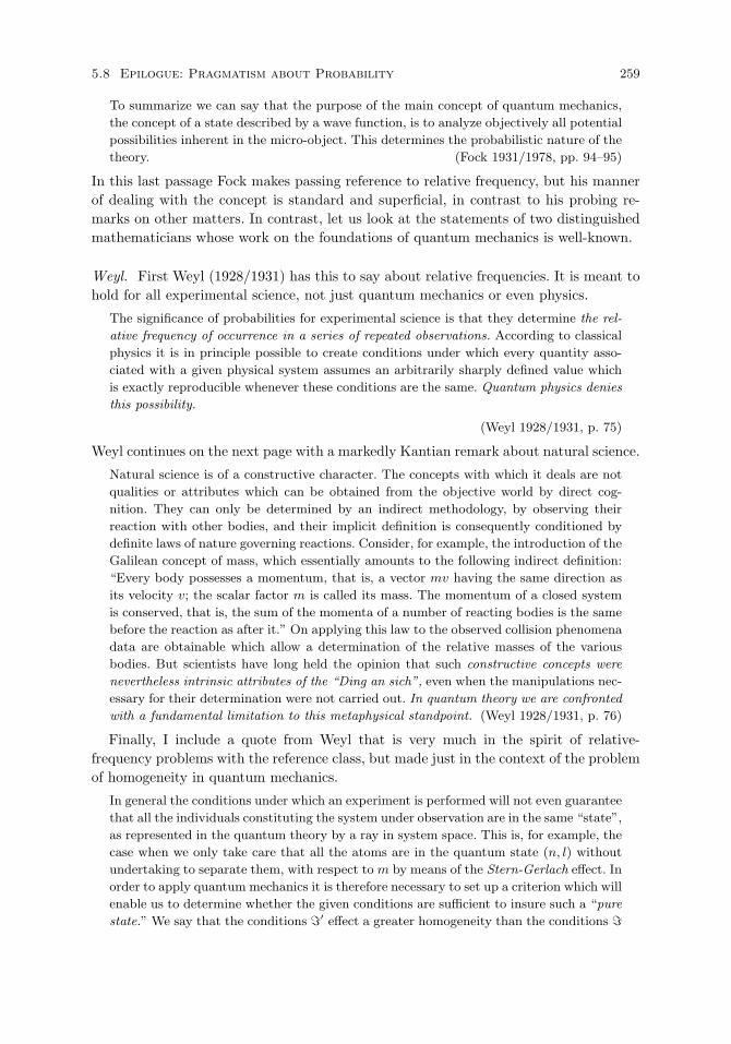
5.8 Epilogue: Pragmatism about Probability 259

To summarize we can say that the purpose of the main concept of quantum mechanics,

the concept of a state described by a wave function, is to analyze objectively all potential

possibilities inherent in the micro-object. This determines the probabilistic nature of the

theory. (Fock 1931/1978, pp. 94–95)

In this last passage Fock makes passing reference to relative frequency, but his mannerof dealing with the concept is standard and superficial, in contrast to his probing re-marks on other matters. In contrast, let us look at the statements of two distinguishedmathematicians whose work on the foundations of quantum mechanics is well-known.

Weyl. First Weyl (1928/1931) has this to say about relative frequencies. It is meant tohold for all experimental science, not just quantum mechanics or even physics.

The significance of probabilities for experimental science is that they determine the rel-

ative frequency of occurrence in a series of repeated observations. According to classical

physics it is in principle possible to create conditions under which every quantity asso-

ciated with a given physical system assumes an arbitrarily sharply defined value which

is exactly reproducible whenever these conditions are the same. Quantum physics denies

this possibility.

(Weyl 1928/1931, p. 75)

Weyl continues on the next page with a markedly Kantian remark about natural science.

Natural science is of a constructive character. The concepts with which it deals are not

qualities or attributes which can be obtained from the objective world by direct cog-

nition. They can only be determined by an indirect methodology, by observing their

reaction with other bodies, and their implicit definition is consequently conditioned by

definite laws of nature governing reactions. Consider, for example, the introduction of the

Galilean concept of mass, which essentially amounts to the following indirect definition:

“Every body possesses a momentum, that is, a vector mv having the same direction as

its velocity v; the scalar factor m is called its mass. The momentum of a closed system

is conserved, that is, the sum of the momenta of a number of reacting bodies is the same

before the reaction as after it.” On applying this law to the observed collision phenomena

data are obtainable which allow a determination of the relative masses of the various

bodies. But scientists have long held the opinion that such constructive concepts were

nevertheless intrinsic attributes of the “Ding an sich”, even when the manipulations nec-

essary for their determination were not carried out. In quantum theory we are confronted

with a fundamental limitation to this metaphysical standpoint. (Weyl 1928/1931, p. 76)

Finally, I include a quote from Weyl that is very much in the spirit of relative-frequency problems with the reference class, but made just in the context of the problemof homogeneity in quantum mechanics.

In general the conditions under which an experiment is performed will not even guarantee

that all the individuals constituting the system under observation are in the same “state”,

as represented in the quantum theory by a ray in system space. This is, for example, the

case when we only take care that all the atoms are in the quantum state (n, l) without

undertaking to separate them, with respect to m by means of the Stern-Gerlach effect. In

order to apply quantum mechanics it is therefore necessary to set up a criterion which will

enable us to determine whether the given conditions are sufficient to insure such a “pure

state.” We say that the conditions ′ effect a greater homogeneity than the conditions

260 Representations of Probability

if (1) every quantity which has a sharp, reproducible value under has the same definite

value under ′ and if (2) there exists a quantity which is strictly determinate under ′

but not under . The desired criterion is obviously this: The conditions guarantee a

pure state if it is impossible to produce a further increase in homogeneity. (This maximum

of homogeneity was obtained in classical physics only when all quantities associated with

the system had definite values.) (Weyl 1928/1931, pp. 77–78)

von Neumann. Even today in many ways the most detailed discussion of probabilityin quantum mechanics is to be found in von Neumann’s (1932/1955) classic treatise.Most of the analysis of a probabilistic character focuses on two problems. The firstis the contrast between causal and noncausal processes. The time evolution of a stateaccording to the time-dependent Schrodinger equation is deterministic and causal incharacter. On the other hand, the measurement of a system in a state with a discretespectrum can undergo a change to any one of several possible states. Because of itsprobabilistic nature this measurement process in quantum mechanics is noncausal. Asis evident, in making this distinction, von Neumann is using the strictly deterministiccausal stance of classical physics. The second problem he addresses is closely relatedto this one, namely, the possibility of deterministic hidden variables that will convertthe probabilistic measurement process into a classical deterministic process. He gives aproof, now regarded as not quite satisfactory, that there can be no such hidden variables.A survey of more recent results on hidden variables for quantum mechanics is given inChapter 7, and so will not be pursued here.

A third problem that has attracted more attention in statistical mechanics than inquantum mechanics is that of the ergodic character of quantum processes, to which vonNeumann contributed but which he only mentions in the book on quantum mechanics,probably because he did not want to add another layer of concepts to present ergodicideas in any detail. An elementary introduction to ergodic processes is given here in thelast section of Chapter 4 on invariance, but applications to quantum mechanics are nottouched upon.

In his final chapter, which is on the measurement process, von Neumann has oneof the most famous passages on the subjectivity of observation in physics to be foundanywhere in the large literature on the foundations of quantum mechanics. I quote asubstantial part of it.

First, it is inherently entirely correct that the measurement or the related process of

the subjective perception is a new entity relative to the physical environment and is

not reducible to the latter. Indeed, subjective perception leads us into the intellectual

inner life of the individual, which is extra-observational by its very nature (since it must

be taken for granted by any conceivable observation or experiment). (Cf. the discussion

above.) Nevertheless, it is a fundamental requirement of the scientific viewpoint—the

so-called principle of the psycho-physical parallelism—that it must be possible so to

describe the extra-physical process of the subjective perception as if it were in reality

in the physical world—i.e., to assign to its parts equivalent physical processes in the

objective environment, in ordinary space. (Of course, in this correlating procedure there

arises the frequent necessity of localizing some of these processes at points which lie

within the portion of space occupied by our own bodies. But this does not alter the

5.8 Epilogue: Pragmatism about Probability 261

fact of their belonging to the “world about us,” the objective environment referred to

above.) In a simple example, these concepts might be applied about as follows: We wish

to measure a temperature. If we want, we can pursue this process numerically until we

have the temperature of the environment of the mercury container of the thermometer,

and then say: this temperature is measured by the thermometer. But we can carry the

calculation further, and from the properties of the mercury, which can be explained in

kinetic and molecular terms, we can calculate its heating, expansion, and the resultant

length of the mercury column, and then say: this length is seen by the observer. Going still

further, and taking the light source into consideration, we could find out the reflection

of the light quanta on the opaque mercury column, and the path of the remaining light

quanta into the eye of the observer, their refraction in the eye lens, and the formation

of an image on the retina, and then we would say: this image is registered by the retina

of the observer. And were our physiological knowledge more precise than it is today, we

could go still further, tracing the chemical reactions which produce the impression of this

image on the retina, in the optic nerve tract and in the brain, and then in the end say:

these chemical changes of his brain cells are perceived by the observer. But in any case,

no matter how far we calculate—to the mercury vessel, to the scale of the thermometer,

to the retina, or into the brain, at some time we must say: and this is perceived by the

observer. That is, we must always divide the world into two parts, the one being the

observed system, the other the observer. In the former, we can follow up all physical

processes (in principle at least) arbitrarily precisely. In the latter, this is meaningless.

The boundary between the two is arbitrary to a very large extent. In particular we saw

in the four different possibilities in the example above, that the observer in this sense

needs not to become identified with the body of the actual observer: In one instance in

the above example, we included even the thermometer in it, while in another instance,

even the eyes and optic nerve tract were not included. That this boundary can be pushed

arbitrarily deeply into the interior of the body of the actual observer is the content of

the principle of the psycho-physical parallelism—but this does not change the fact that

in each method of description the boundary must be put somewhere, if the method is

not to proceed vacuously, i.e., if a comparison with experiment is to be possible. Indeed

experience only makes statements of this type: an observer has made a certain subjective

observation; and never any like this: a physical quantity has a certain value.

(von Neumann 1932/1955, pp. 418–420)

It is obvious that the emphasis by von Neumann on subjective perception resonates withthe basic ideas of subjective probability, although the wider literature on subjectiveprobability is not discussed. Secondly, his undeveloped remarks about psychophysicalparallelism suggest a more radical subjectivism than is characteristic of typical Bayesianviews of probability.

Pragmatism in physics. This survey of the attitude toward probability in physicscould easily be extended. But pragmatism, in the sense of using the formal methodsof probability, without much attention to foundational questions of interpretation orrepresentation of probability, wholly dominates the use of probability in physics. Thereis wide agreement on one point by everyone, including von Neumann. That is the idea ofconfirming or testing quantum mechanics by the relative frequency of observed phenom-ena in repeated experiments of the same design. The statement quoted above from p. 75

262 Representations of Probability

of Fock’s work would be endorsed by almost every physicist. But this statement aboutexperiments would be acceptable to almost every view of the interpretation of proba-bility, as well, from the most extreme Bayesian to the most extreme propensity view.Moreover, the characterization of randomness, the bete noire of the relative-frequencyinterpretation of probability, is seldom if ever mentioned in the physics literature. Moregenerally, in a recent article (Suppes 1998) I tried to make a broader case for the prag-matic exuberance of most physics, now and in the past.49

Statistical practice. The previous paragraphs have emphasized the pragmatic char-acter of the attitude toward the nature of probability in physics. Surprisingly enough,in view of the many conceptual disputes between Bayesians and non-Bayesians withinstatistics itself, a much more explicit attitude about pragmatism in statistical practicecan be found among statisticians concerned with detailed problems of some intricacy. Ishall not try to survey the literature on this point, but rather quote from one splendidexample, far from physics and quantum mechanics, but from a statistical standpointmore sophisticated than almost any quantum mechanical example I can think of.

The example I have in mind is the statistical analysis of the Federalist Papers todetermine whether the author of certain disputed parts was Hamilton or Madison. ThePapers constitute one of the most famous series of political documents written about thetime of the American Revolution. They are still much read and the disputed authorshipis a continuing problem of historical interest. The wonderfully detailed statistical studyby Mosteller and Wallace (1964/1984) settles the question about as definitively as it everwill be, even with continued improvements in statistical and computational methods inthe future. Here is the skeptical and pragmatic attitude they express in the preface tothe first edition.

Some may feel that we should make more definite pronouncements about the comparative

value of different methods of inference—especially Bayesian versus classical. Obviously

we are favorably disposed toward the Bayesian approach, but in the field of data analysis

at least, the techniques are in their infancy. As these techniques evolve, their merits and

demerits may be easier to judge.

Even though individual statisticians may claim generally to follow the Bayesian school

or the classical school, no one has an adequate rule for deciding what school is being

represented at a given moment. When we have thought we were at our most Bayesian,

classicists have told us that we were utterly classical; and when we have thought ourselves

to be giving classical treatment, Bayesians have told us that the ideas are not in the

classical lexicon. So we cannot pretend to speak for anyone but ourselves.

(Mosteller and Wallace 1964/1984, p. ix)

49That such a pragmatic attitude dominates physics and should dominate economics is well-argued

for in Cartwright (1999). On the other hand, the excellent book of T. L. Fine (1973), which covers,

from a different angle, many of the sections of this chapter, is focused on the continued need for deeper

satisfactory representations of probability. The conflicts in viewpoint represented by the pragmatism of

physicists and Fine’s plea for greater and more specific depth of interpretation and practice are central

to the philosophical foundations of scientific methods. For reasons that cannot be spelled out in detail

here, I predict that the physicists’ minimalist program of interpretation will continue to dominate the

use of probability concepts in scientific theories, which is why I have included this final section of an

already overly long chapter.

5.8 Epilogue: Pragmatism about Probability 263

Bayesian concepts and methods have been extensively developed since Mosteller andWallace first published this passage in 1964, but Bayesian methods are in fact still usedrelatively rarely in scientific papers, in spite of such excellent recent texts as Rouanetet al. (1998). But this is not because scientists are devoted to an objective rather thansubjective view of probability—the “classical school” of statisticians, in Mosteller andWallace’s terminology, holding the objective view of probability. No, it is because byand large scientists in most disciplines remain indifferent to the conceptual foundationsof probability and pragmatically apply statistical concepts without any foundationalanxiety, just computing the statistical tests someone has taught them to use. But indif-ference, on the other hand, sometimes disappears when statistical analysis is requiredof some process or phenomenon with strong practical implications.

Other forces of a purely scientific nature can also create a change in attitude, whichis most likely to occur throughout this century. Statistics itself is now in the midst of arevolution much more far-reaching in its implications than the conflict between objectiveand subjective views of probability that dominated the last half of the twentieth century.This revolution has been started by the demand for new statistical methods for analyzingvery large data bases, now prevalent in almost every area of science. The new methodsalready developed are intensely computational in nature, and will, no doubt, continue tobe so. There is much about this new context and focus that is more like that of physicsthan the scientific sources of data associated with the preceding fifty years of statistics.It is not unreasonable to believe that the pragmatic attitude so well exemplified byphysicists, and also by some of the best statistical practice, will be the dominant onetoward the nature of probability for quite some time. From a foundational standpoint, Icannot help observing how much the qualitative axiomatic methods used in Section 6 foranalyzing objective propensity interpretations and those used in Section 7 for subjectiveinterpretations of probability are essentially the same, and, in retrospect, I see could beimproved by more unification of the formal results.

This leads to the kind of pragmatism I am happy to endorse. Uniform formal methodsare accompanied by a rich variety of interpretations or representations of the conceptsused. Probability is too rich and diversified in application to be restricted to one singleoverweening representation. The pragmatic context of use will sometimes fix the rep-resentation chosen, but more often, a deeper pragmatic attitude will dominate and noexplicit choice of representation will be made, as is well illustrated statistically in thework of Mosteller and Wallace (1964/1984) referred to earlier, and more recently, in anavalanche of papers on data mining, adaptive statistics, boosting, neural networks anda variety of other approaches to large-scale data analysis.50

50For a good not-too-technical overview of these recent developments, see Hastie, Tibshirani and

Friedman (2001).

6

Representations of Space and Time

Well before Aristotle’s famous extended and complicated argument that the world iseternal, without beginning or end, and there cannot be more than one world (On theHeavens, Book I), varying representations of space and time were a central topic inGreek philosophy. This emphasis continued for many centuries. Perhaps the last majorphilosopher to consider representations of space and time as central to his philosophy inthe detailed context of the physics of his time was Kant in the Critique of Pure Reasonand the Metaphysical Foundations of Natural Science. In any case, detailed conceptualanalysis of space and time is no longer a central topic for most philosophers, but aflourishing activity for those with specialized knowledge and interest in the foundationsof physics. The focus of the first three sections of this chapter is of this latter sort. Thefirst section states some necessary geometric preliminaries. The second one assumes astandard analytic geometric representation used in classical physics and concentrates onstudying the invariant properties of this representation, but only kinematical propertiesof classical mechanics are needed to prove the invariance. The third section provides asimilar analysis of the space-time of special relativity. The analysis reflects the impor-tance of questions of invariance in classical and relativistic physics; some fairly extensivehistorical remarks are made at the end of both sections. The strong simplifying assump-tion used, and not built up from more primitive physical concepts, is that both classicaland restricted relativistic space-time structures are special cases of affine structures,which are defined in the first section.

This affine unification has several justifications. First, many properties of both theclassical and the space-time of special relativity are invariant under the general affinegroup of transformations—for example, the linearity of inertial paths and conservationof their being parallel. More importantly, the group of Galilean transformations of clas-sical physics and the group of Lorentz transformations of special relativity are bothsubgroups of the affine group. These common features are often not given much noticein philosophical discussions of space and time.

In the fourth section, the focus moves from physics to psychology, in particular, tothe question of how we can decide if visual space is Euclidean. Because there has beenmuch less consideration of spatial perceptual phenomena by philosophers, the treatmentis much more detailed. As might be expected, the results are less definitive in character.Continuing in this line of thought, the fifth section examines a variety of philosophical

265

266 Representations of Space and Time

and experimental claims about the nature of visual space. The psychological experi-ments of Foley and Wagner, discussed in some detail in this section, provide, in Section6, the framework for some restricted axioms of congruence. These axioms extend thepurely affine axioms of Definition 1, but avoid the paradoxes for any space of constantcurvature, not just the Euclidean one, posed by the Foley and Wagner experiments.The seventh section concludes the examination of visual space with reflection on threemajor problems for any spatial theory of visual phenomena.

In the last section, the eighth one, I turn briefly to a related topic in the philosophyof mathematics, finitism in geometry. Conceptually what is considered is the finitarynature of geometric constructions throughout a very long tradition going back to theearliest times of ancient Greek geometry, and the kind of problems that can be solvedby such methods.

As can be seen, various sections of this chapter move from physics to psychologyand finally to geometry itself. This seems like a bit of a mixture and it is. The secondand third sections on invariance in physics could have been placed at the beginning ofthe next chapter, Chapter 7, on representations in mechanics. But I kept them here forthree reasons. First, no dynamical assumptions are used formally in these two sections,so the use of mechanical ideas is pretty thin. Second, the derivation of the Lorentztransformations is more relevant to electromagnetic theory, especially historically, thanto mechanics. Third, I wanted to emphasize in this chapter the many different ways ofthinking about the representations of space and time. Different disciplines concernedwith spatial and temporal phenomena pose problems that require different approaches.

6.1 Geometric Preliminaries

The viewpoint toward space-time developed in this chapter is that standard geometricconcepts and objects shall be assumed and not developed in detail. What is needed infact are the concepts of an affine and of a Euclidean space, and the geometric relationssuch as betweenness in terms of which such spaces are constructed.

To keep the initial focus on the special axioms needed for classical or Minkowski space-time, standard and familiar axioms for affine and Euclidean spaces will be reviewed onlybriefly. The representation and invariance theorems will be formulated for later use.

Ordered affine spaces are axiomatized, in one standard version, in terms of a nonemptyset A of points and the ternary relation B of betweenness. (I also used the standard briefnotation a|b|c for B(a, b, c).) In the coordinate representation of such spaces, pointsare ordered n-tuples of real numbers forming the standard n-dimensional Cartesianspace Rn. Let x,y, and z be any three such Cartesian points. Then, in the intendedinterpretation, the Cartesian relation of betweenness BR(x,y, z) holds iff there existsan α ∈ [0, 1] such that

y = αx + (1 − α)z.

The structure (Rn, BR) is the n-dimensional affine Cartesian space.We need the following definitions. For a = b, a line ab is the set of all points c such

that a|b|c, b|c|a or c|a|b, and abc is a triangle if the points a, b and c are noncollinear,i.e., do not lie on a line. (Note that here a triangle is just an ordered triple of threenoncollinear points. With some abuse of notation, the same notation is used for the

6.1 Geometric Preliminaries 267

plane consisting of the set of points defined by such a triple of points.)Let a, b, c be noncollinear; then the plane abc is defined as follows:

abc = d | (∃e)(∃f)(e = f and e, f ∈ ab ∪ ac ∪ bc

and d, e, f are collinear).(By requiring e|d|f rather than just collinearity, we define the triangular region abc.)For 3-spaces, we use a tetrahedron abcd with the four points noncoplanar. Followingthe usual terminology, a, b, c, and d are the vertices of the tetrahedron, the segmentsab, bc, ac, ad, bd, and cd are the edges, and the four triangular regions abc, bcd, cda,and dab are the faces. The 3-space abcd is then the set of all points collinear with pairsof points in one or two faces of the tetrahedron abcd.

We proceed in the same way for the 4-space, a concept that we need for the spacesof classical and special relativity. A quintuple abcde is a simplex if and only if the fivepoints do not all lie in a common 3-space. The cells of the simplex are the five tetrahedralregions determined by four points of the simplex. The 4-space abcde is then the set ofpoints collinear with pairs of points on one or two cells of the simplex.

DEFINITION 1. A structure A = (A,B) is an affine space if and only if the followingaxioms are satisfied for a, b, c, d, e, f, g, a′, b′ and c′ in A:

1. If a|b|a, then a = b.2. If a|b|c, then c|b|a.3. If a|b|c and b|d|c, then a|b|d.4. If a|b|c and b|c|d and b = c, then a|b|d.5. (Connectivity) If a|b|c, a|b|d, and a = b, then b|c|d or b|d|c.6. (Extension) There exists f in A such that f = b and a|b|f .7. (Pasch’s Axiom) If abc is a triangle, b|c|d, and c|e|a, then there is on

line de a point f such that a|f |b.8. (Axiom of Completeness) For every partition of a line into two nonempty sets Y

and Z such that(i) no point b of Y lies between any a and c of Z and(ii) no point b′ of Z lies between any a′ and c′ of Y,there is a point b of Y ∪ Z such that for every a in Y and c in Z, b lies betweena and c.

9. (Dimensionality). Moreover, if all points of A lie on a plane, but not on a line,A is two-dimensional; if all points of A lie in a 3-space but not on a plane, A isthree-dimensional; if all points of A lie in a 4-space but not in a 3-space, A isfour-dimensional.1

The formulation just in terms of betweenness is rather complicated, and so I haveavoided it by using the concepts defined before Definition 1.2

1Axiom 9 is in the form of a definition, but it gives the forms of axioms needed to specify the

dimensionality. For example, if someone wants to focus on two-dimensional affine space, the axiom of

dimensionality is: all points of A lie on a plane, but not on a line.2I remark that an entirely different, but equivalent, approach to affine geometry is to begin with

a projective space, say three-dimensional as an example, and then remove a plane, labeled the ‘plane

268 Representations of Space and Time

THEOREM 1. Every n-dimensional affine space (A,B) for n = 2, 3, 4, is isomorphicto the n-dimensional affine Cartesian space (Rn, BR), i.e., there is a one-one functionf mapping A onto Rn such that for any points a, b and c in A

B(a, b, c) iff BR(f(a), f(b), f(c)).

Moreover, any two n-dimensional affine spaces are isomorphic.

In other words, the theorem asserts the categorical character of affine spaces of a givendimension. (The elementary axioms for finite affine constructions introduced later inSection 8 are noncategorical.)

Of equal importance, although neglected by some, is the companion theorem onthe invariance or uniqueness of the representation. In standard geometric terms, theinvariance is simply uniqueness up to the group of affine transformations. An affinetransformation is any linear transformation ϕ of n-dimensional Cartesian space suchthat for every vector x3

ϕ(x) = Ax + b,

where A is a nonsingular n × n matrix and b is any n-dimensional vector, that is,any n-tuple of real numbers. Intuitively, the matrix A represents a rotation togetherwith stretches in different amounts along the n Cartesian coordinates. The vector brepresents a translation of the origin of the Cartesian space. Two familiar facts aboutsuch transformations are these: they preserve collinearity, and they transform parallellines into parallel lines. It is also apparent that the set of affine transformations is agroup under functional composition.

THEOREM 2. The representation of an n-dimensional affine space in terms of then-dimensional affine Cartesian space over the field of real numbers is invariant underthe group of affine transformations. In particular, if f and f ′ are two functions mappingthe given affine space isomorphically onto Rn, then there exists an affine transformationϕ such that f ′ = ϕ f ; also if f is a function so mapping the given affine space ontoRn and ϕ is any affine transformation, then ϕ f is also such an isomorphic mapping.

Both Galilean and Lorentz transformations are special kinds of affine transformations,as will be spelled out later.

To obtain Euclidean spaces from affine ones we need add only the quaternary relationof congruence or equidistance: ab ≈ cd iff points a and b are the same distance apart asare points c and d. In other terms, the line segment with endpoints a and b is congruentto the line segment with endpoints c and d. The interpretation of equidistance in theCartesian space Rn is familiar: for any vectors x, y, u and v of Rn the relation xy ≈R uvholds iff

n∑i=1

(xi − yi)2 =n∑

i=1

(ui − vi)2.

I omit the familiar axioms of congruence for Euclidean spaces, which need to be added

at infinity’. The resulting space is affine. In the two-dimensional case, a line at infinity is removed to

obtain the affine plane.3A change in the conventions of notation of Chapter 5 is made in the first three sections of this

chapter. Bold-face capital letters such as X or A no longer denote random variables, but rather matrices,

and now boldface lower-case letters such as x and y denote vectors.

6.2 Classical Space-time 269

to the affine axioms of Definition 1. They extend the concept of affine congruence, whichholds just for parallel segments. Implicitly assuming the congruence axioms, we thenhave the standard representation:

THEOREM 3. Every n-dimensional Euclidean space (A,B,≈) is isomorphic to the n-dimensional Euclidean Cartesian space (Rn, BR,≈R), i.e., there is a one-one functionf mapping A onto Rn such that

(i) for any points a, b and c in A

B(a, b, c) iff BR(f(a), f(b), f(c)),

and

(ii) for any points a, b, c and d in A

ab ≈ cd iffn∑

i=1

(fi(a) − fi(b))2 =n∑

i=1

(fi(c) − fi(d))2,

where fi(a) is the ith coordinate of the Cartesian vector f(a). Moreover, any two n-dimensional Euclidean spaces are isomorphic.

Again, of equal importance is the invariance theorem that is a companion to Theorem3. An affine transformation ϕ(x) = Ax + b, as defined above, is a similarity transfor-mation iff the matrix A is a similarity matrix, i.e., there is an orthogonal matrix A′ anda positive real number δ such that A = δA′. In other words, a similarity transforma-tion permits only a uniform stretch of units in all directions, whereas a general affinetransformation imposes no such restriction.

THEOREM 4. The representation of an n-dimensional Euclidean space in terms ofthe n-dimensional Euclidean Cartesian space over the field of real numbers is invariantunder the group of similarity transformations.

In contrast to the earlier statement, it is obvious, but worth noting, that an ar-bitrarily selected Galilean or Lorentz transformation will not be a general similaritytransformation in its spatial part, because the unit of measurement for spatial distanceis held constant. This will become clear in the next two sections.

6.2 Classical Space-time

Rather than give a purely qualitative geometric formulation, as may be found in Suppeset al. (1989, Ch. 13) with references to the history of such qualitative formulations, it isalso physically natural to introduce frames of reference, one-dimensional temporal onesand three-dimensional spatial ones, with Cartesian, i.e., orthogonal, axes.

Formally, a space-time measurement frame f is a pair of functions (s, r) mapping eachspace-time point a to a spatial vector (x1, x2, x3, ) in Cartesian space (R3, BR, ≈R),where spatially si(a) = xi and temporally r(a) = t. These space and time functionsexpressing measurements relative to a frame of reference are the same for classical andspecial relativistic physics. As we go from the classical to the relativistic case, the lab-oratory or observatory methods of measurement do not change, but the fundamentalinvariants do. In the axioms given below we refer to inertial frames, but nothing beyond

270 Representations of Space and Time

affineness and the appropriate invariance are assumed for these frames.4 It is a conse-quence, not an assumption back of the invariance axioms, that any two inertial framesare related by a constant relative velocity.

DEFINITION 1. A structure A = (A, B, F) is a four-dimensional classical space-time structure with inertial frames iff the following axioms are satisfied:

Axiom 1. The structure (A, B) is a four-dimensional affine space.Axiom 2. F is a nonempty collection of (inertial) frames f = (s, r) that are isomor-

phic mappings of (A, B) onto the affine Cartesian space (R4, BR).Axiom 3. (Temporal invariance). For any two points a and b of A, and for any two

frames f = (s, r) and f ′ = (s′, r′) in F , the temporal distance is invariant, i.e.,

|r(a) − r(b)| = |r′(a) − r′(b)|. (I)

Axiom 4. (Spatial Invariance). For any two points a and b of A, and for any twoframes (s, r) and (s′, r′) in F , the spatial distance is invariant, i.e.,

3∑i=1

(si(a) − si(b))2 =3∑

i=1

(s′i(a) − s′i(b))2. (II)

Axiom 5. (Closure of Invariant Frames). If f = (s, r) is in F and if ϕ is an affinetransformation of (R4, BR) such that f and ϕ f satisfy (I) and (II), then ϕ f is inF .

The intuitive meaning of each of the axioms should be clear, but some commentsmay be useful. Axiom 1, which in the analysis given here is common to both classicaland relativistic space-time, expresses the affine character of the spaces. The flatnessor linearity of both kinds of spaces is obviously one of their most important sharedcharacteristics. The assumption of an affine four-dimensional space-time structure isnot always used in foundational analyses of the space and time of classical physics.Often a separate analysis is given for space and for time, but the unification used hereis natural to make clear just how classical and restricted relativistic space-time rest oncommon assumptions and how they differ. From a qualitative geometric standpoint, theaffine framework axiomatized just in terms of betweenness must be supplemented byadditional qualitative primitives if a completely qualitative approach to physical spaceand time is to be developed. A concept of congruence for the spatial distance betweensimultaneous point events is the natural addition for classical space-time. However,physicists almost always avoid this qualitative geometric approach, even in foundationaldiscussions. The use of frames here is much closer to physical ways of thinking. Anotherjustification for assuming a common four-dimensional affine space for both classical and

4From a physical standpoint, it would be desirable to postulate the existence of one fixed frame ‘at

rest with respect to the fixed stars’, as the classical phrase goes. But this introduction would obviously

disturb the purely formal character of the axiomatic characterization given in Definition 1. Still, the

intuition is physically important that an inertial frame is one moving with a constant velocity with

respect to some reference point that has a massive or eternal character, absolute space for Newton, a

triad of fixed, i.e., distant, stars for some, the center of mass of the solar system for others, or finally,

in more grandiose terms, the center of mass of the universe, the last three of which are apparently

empirically very similar, in the sense of moving relative to each other with a nearly constant velocity.

6.2 Classical Space-time 271

relativistic space-time is that a common invariant of both is the linearity of inertial pathsof particles, i.e., the space-time trajectories of particles acted on by a null resultant force.

A separate representation theorem for classical space-time structures is not required,for the representing functions are just the inertial frames postulated in Axiom 2 ofDefinition 1. What is needed is the Galilean invariance theorem.

The invariance theorem for classical space-time structures is a specialization of The-orem 6.1.2 on the invariance of the representation of affine spaces. Recall that theuniqueness was up to an arbitrary affine transformation. We now put additional condi-tions on the matrix A of such transformations. We say that a four-dimensional matrixA is a Galilean matrix with respect to a frame f in F if and only if there exist athree-dimensional vector u, an orthogonal matrix E of order 3, and δ = ±1 such that

A =(E 00 δ

)(I −u∗

−u 1

)

where I is the identity matrix of order 3.The interpretation of the constants is as follows. The number δ represents a possible

transformation in the direction of time—if δ = 1 there is no change and if δ = −1 thedirection is reversed; u is the relative velocity of the new inertial frame of reference withrespect to the old one; and the matrix E represents a rotation of the spatial coordinates.The vector b of the affine transformation also has a simple interpretation. The first threecoordinates represent a translation of the origin of the spatial coordinates of f , and thefourth coordinate a translation of the origin of the one-dimensional coordinate systemfor measurement of time of f . We are thus assuming that the same measurement scalesof space and time are used by all the different frames in F , as is implicit in Axioms 3and 4, but a translation of spatial or temporal position is permitted in moving from oneframe to another.

We say that an affine transformation is Galilean if and only if its four-dimensionalmatrix is Galilean. Using these concepts we then may state the following invariancetheorem for classical space and time.

THEOREM 1. The representation of a classical space-time structure with inertialframes in terms of the four-dimensional affine Cartesian space over the field of realnumbers is invariant under the group of Galilean transformations.

Proof. Let f and f ′ be two frames in F . We analyze the affine transformation ϕ

such that for every four-dimensional Cartesian vector x of f , ϕ(x) = x′. By virtue ofTheorem 6.1.2 there is a nonsingular matrix A of order 4 and a four-dimensional b suchthat for every four-dimensional Cartesian vector x of f

ϕ(x) = Ax + b.

The proof reduces to showing that A is a Galilean matrix. Since A is nonsingular, wemay decompose A as follows:

A =(D e∗

h g

),

where D is a 3 × 3 nonsingular matrix acting on the three spatial coordinates x1, x2,x3 of any vector x of f , h is a row vector, e∗ is a column vector and g = 0 is a real

272 Representations of Space and Time

number.First, suppose D is not an orthogonal matrix. Then it is easy to show there exist

vectors x and y such that the spatial distance between x and y is not preserved by ϕ,contrary to Axiom 4, i.e.∑

(xi − yi)2 =∑

(ϕ(xi) − ϕ(yi))2.

By a similar argument we can show that by virtue of Axiom 3, g = δ = ±1.Some general theorems about classical mechanics are to be found in Section 7.1, but

they necessarily go beyond the kinematical framework of the present section.

Historical remarks. The formal invariance axioms of Definition 1, or even the firstaxiom on affine spaces providing the general setting, will not be intuitively obviousto readers unfamiliar with the foundations of classical mechanics, where these ideasoriginate, and have since been abstracted away from their mechanical context to becomegeometric in character. The only remnant of classical physics left, but an essential one ofcourse, is that the first three coordinates of a frame’s location of a space-time point arespatial coordinates, in the sense of physical space, and the fourth coordinate locationof a space-time point in physical time.

The discovery of this invariance is relatively late. It certainly does not fit in withAristotle’s physics, which holds that the center of the universe is the center of theEarth. And, more importantly, from observation it is inferred that the natural uniformmotion of the heavens, i.e., the planets and the stars, is circular.

Here is Ptolemy’s cogent summary of these views:

The general preliminary discussion covers the following topics: the heaven is spherical in

shape, and moves as a sphere; the Earth too is sensibly spherical in shape, when taken

as a whole; in position it lies in the middle of the heavens very much like its centre;

in size and distance it has the ratio of a point to the sphere of the fixed stars; and it

has no motion from place to place. . . . It is plausible to suppose that the ancients got

their first notions on these topics from the following kind of observations. They saw that

the sun, moon and other stars were carried from east to west along circles which were

always parallel to each other, that they began to rise up from below the Earth itself, as

it were, gradually got up high, then kept on going round in similar fashion and getting

lower, until, falling to Earth, so to speak, they vanished completely, then, after remaining

invisible for some time, again rose afresh and set; and [they saw] that the periods of these

[motions], and also the places of rising and setting, were, on the whole, fixed and the

same.

What chiefly led them to the concept of a sphere was the revolution of the ever-visible

stars, which was observed to be circular, and always taking place about one centre, the

same [for all]. For by necessity that point became [for them] the pole of the heavenly

sphere: those stars which were closer to it revolved on smaller circles, those that were

farther away described circles ever greater in proportion to their distance, until one

reaches the distance of the stars which become invisible. In the case of these, too, they

saw that those near the ever-visible stars remained invisible for a short time, while those

farther away remained invisible for a long time, again in proportion [to their distance].

The result was that in the beginning they got to the aforementioned notion soley from

such considerations; but from then on, in their subsequent investigation, they found that

6.2 Classical Space-time 273

everything else accorded with it, since absolutely all phenomena are in contradiction to

the alternative notions which have been propounded.

For if one were to suppose that the stars’ motion takes place in a straight line towards

infinity, as some people have thought, what device could one conceive of which would

cause each of them to appear to begin their motion from the same starting-point every

day? How could the stars turn back if their motion is towards infinity? Or, if they did

turn back, how could this not be obvious? [On such a hypothesis], they must gradually

diminish in size until they disappear, whereas, on the contrary, they are seen to be greater

at the very moment of their disappearance, at which time they are gradually obstructed

and cut off, as it were, by the Earth’s surface. . . .

To sum up, if one assumes any motion whatever, except spherical, for the heavenly

bodies, it necessarily follows that their distances, measured from the Earth upwards,

must vary, wherever and however one supposes the Earth itself to be situated. Hence the

sizes and mutual distances of the stars must appear to vary for the same observers during

the course of each revolution, since at one time they must be at a greater distance, at

another at a lesser. Yet we see that no such variation occurs.

(Ptolemy, Almagest, pp. 38–39)

The point to be emphasized above all is that this conclusion about uniform circularmotion was not from a priori arguments,5 but an inference from astronomical observa-tions recorded over many hundreds of years. Given the great success and comparativeaccuracy it is no wonder that it took many more hundreds of years to dislodge theseAristotelian conclusions.

Moreover, it is not surprising that the development of new ideas came from earthlyphenomena, not astronomical observations. Out of the long development of impetusconcepts in medieval mechanics, Benedetti (1585/1959) was perhaps the first to insiston a rectilinear path exclusively for a freely moving body. Here is what he says about abody thrown from a rotating sling:

Indeed the circular motion, as the body rotates, makes it so that the body by natural

inclination (naturalis inclinatio) and under the force of impetus already initiated pursues

a rectilinear path (recta iter peragere).

(Benedetti, in Clagett, The Science of Mechanics in the Middle Ages, p. 664)

Only a little later Galileo’s own progress toward conceiving inertial motion as rectilinearwas slow and complicated.6

The rapid developments in the seventeenth century cannot be surveyed in detail here,

5The well-known physicist, David Bohm (1965, p. 5) supports this mistaken a priori view whole-

heartedly in the following passage, taken from his textbook on special relativity:

A part of Aristotle’s doctrine was that bodies in the Heavens (such as planets), being more perfect thanEarthly matter, should move in an orbit which expresses the perfection of their natures. Since the circlewas considered to be the most perfect geometrical figure, it was concluded that a planet must movein a circle around the Earth. When observations failed to disclose perfect circularity, this discrepancywas accommodated by the introduction of “epicycles,” or of “circles within circles.” In this way, thePtolemaic theory was developed, which was able to “adjust” to any orbit whatsoever, by bringing inmany epicycles in a very complicated way.

6See, for example, the discussion of Clagett against the background of medieval mechanics (Clagett

1959, pp. 666–671).

274 Representations of Space and Time

but an early, clear formulation almost equivalent to Newton’s first law is to be found inDescartes’ Principles of Philosophy, Book II, (1644/1983, pp. 59–60), Propositions 37and 39:

37. The first law of nature: that each thing, as far as is in its power, always remains in

the same state; and that consequently, when it is once moved, it always continues

to move.

39. The second law of nature: that all movement is, of itself, along straight lines; and

consequently, bodies which are moving in a circle always tend to move away from

the center of the circle which they are describing.

It was this clear rectilinear concept of inertial motion, along with the rejection of afixed, unmoved center point, that was needed to clear the way for the classical notionof invariance.7

Undoutedly one reason for Descartes emphasizing the relativity of motion was so thatin Part III of the Principles of Philosophy he could use the Copernican system, but stillnot require that the Earth moves. Here is Proposition 19 of Book III (1644/1983, p. 91).

19. That I deny the motion of the Earth more carefully than Copernicus and more

truthfully than Tycho.8

Descartes was an adept fence-straddler on difficult points of conflict between scienceand Catholic theology.

Although Newton introduces the concept of absolute rest in the opening pages ofhis Principia (1687/1946, p. 9), in his prudent, careful way he asserts ‘that absolutespace cannot be determined from the position of bodies in our regions’. He goes on toelaborate the uses and need for a concept of relative motion as well as that of truemotion.

But, it is still a long time before invariance in classical physics is fully recognized andused. In Mach’s (1883/1942) important but flawed foundational study The Science ofMechanics, A Critical and Historical Account of Its Development, there is no systematicconsideration of any questions of invariance in, I believe, any of its nine editions. Thisis also true of a work of a very different character, E. T. Whittaker’s (1904/1937) well-known treatise on analytic dynamics.

In truth, it is rather like an induction backward in time. Einstein’s theory of specialrelativity had to be introduced first with an emphasis on invariants coming to thefore as a natural way to explain the differences from classical physics. It was only inthis late context that the affine assumptions and the invariants of Definition 1 werefully and systematically formulated, including the explicit identification of the Galileantransformations.9

7Descartes rejects the unmoved center in the discussion of Proposition 13 of Book II, and in other

places as well.8‘Tycho’ refers to Tycho Brahe (1546–1601), famous for his excellent systematic astronomical ob-

servations, and of great importance for Kepler’s theoretical work.9According to Abraham Pais (1982, p. 140), the term Galilean was first introduced by Frank (1909,

p. 382).

6.3 Axioms for Special Relativity 275

6.3 Axioms for Special Relativity

The purpose of this section is to characterize the invariance properties of special rel-ativity. As in the case of the previous section, the geometric points of the space areinterpreted as four-dimensional point-events. The desired invariance result is given interms of the group of Lorentz transformations.

As in the classical case, linearity is introduced by means of the ternary relationof betweenness. The approach used here is to keep in the foreground the question ofcongruence of segments, i.e., equidistance. Of course, the simple classical formulation ofthe separate invariance of spatial and temporal measurements of distance is not possible.However, as was pointed out by Robb (1936) many years ago, there is a meaningfulnotion of congruence in special relativity for segments of inertial lines, i.e., possiblepaths of particles moving uniformly. This congruence is that of the proper time of inertialsegments. There is also a separate notion of congruence for segments of separation orspatial lines, i.e., lines determined by two points that determine neither an inertial linenor an optical line. In contrast, there is no natural notion of congruence for segmentsof optical lines, i.e., lines representing optical paths.

The intuition back of these ideas is most easily explained by introducing the usualcoordinate representation for special relativity. The four real coordinates (x1, x2, x3, t)of a point-event are measured relative to an inertial space-time frame f of reference,just as in classical physics. As in the preceding section, the coordinates x1, x2 and x3

are the three orthogonal spatial coordinates and t is the time coordinate of f . It is oftennotationally convenient to replace t by x4. The relativistic distance, or proper time,between two points x = (x1, x2, x3, x4) and y = (y1, y2, y3, y4) is given by the indefinitequadratic metric, relative to frame f = (s, r), as:

If (xy) =

√√√√c2(x4 − y4)2 −3∑

i=1

(xi − yi)2 (1)

where c is the numerical velocity of light. It is simpler to use the square of the relativisticdistance.10 It is easy to see that I2

f (xy) > 0 if x and y lie on an inertial line, I2(xy) < 0 ifx and y lie on a separation line, and I2(xy) = 0 if x and y lie on an optical line. In theseterms, two inertial segments xy and uv, i.e., segments of inertial lines, are congruent iff

I2f (xy) = I2

f (uv) (2)

and a similar condition holds for two segments of separation lines. On the other hand,this equality does not work at all for optical lines, because the relativistic length of anyoptical segment is zero.

Given an affine space-time structure, invariance of the speed of light in a vacuum,c, and invariance of proper time of inertial segments for different inertial frames is asufficient condition to prove that inertial frames must be related by Lorentz transforma-

10Equation (1) is convenient for computation, but conceptually it is natural to divide by c, so that

in any given coordinate system f the units of proper time are temporal, i.e.,

Proper timef (x, y) =1

cIf (x, y).

276 Representations of Space and Time

tions. The restriction to inertial segments is physically natural, for such segments aremore susceptible to direct measurement than are segments of separation lines.

The axioms for restricted relativistic space-time require only a change in the in-variance axioms of classical space-time. The separate measurement of space and timerelative to an inertial frame is unchanged.

We now add to the structure (A, B, F) the invariant constant c for the speed of light.

DEFINITION 1. A structure A = (A, B, F , c) is a (four-dimensional) restricted rel-ativistic space-time structure with inertial frames if and only if the following axiomsare satisfied:

Axiom 1. Same affine axiom as Definition 1, Section 2.Axiom 2. Same frame axiom as Definition 1, Section 2.Axiom 3. (Invariance of speed of light). The positive real number c, representing the

measurement of the speed of light in a vacuum, is invariant, i.e., constant, for everyframe f in F .

Axiom 4. (Invariance of proper time of inertial segments). For any two points a andb of A such that for some frame f of F , I2

f (ab) > 0, the proper time of the segment abis invariant in F , i.e., for any two frames f and f ′ in F ,

If (ab) = If ′(ab). (III)

Axiom 5. (Closure of Invariant Frames). If f is in F and if ϕ is any affine transfor-mation of (R4, BR) such that f and ϕ f satisfy (III), then ϕ f is in F .

We next need to define formally the concept of a Lorentz matrix and then that of aLorentz transformation.

DEFINITION 2. A matrix A (of order 4) is a Lorentz matrix if and only if there existreal numbers β, δ, a three-dimensional vector u, and an orthogonal matrix E of order 3such that

β2(1 − u2

c2

)= 1

δ2 = 1

A =(E 00 δ

) (I + β−1

u2 u∗u −βu∗

c2

−βu β

).

(In this definition and elsewhere, if A is a matrix, A∗ is its transpose, and vectors likeu are vectors—thus u∗ is a column vector.11) The physical interpretation of the variousquantities in Definition 2 should be obvious. The number β is the Lorentz contractionfactor. When δ = −1, we have a reversal of the direction of time. The matrix E representsa rotation of the spatial coordinates of f , or a rotation followed by a reflection. The vectoru is the relative velocity of the two frames of reference. For future reference it may benoted that every Lorentz matrix is nonsingular.

DEFINITION 3. A Lorentz transformation is a one-one function ϕ mapping R4 ontoitself such that there is a Lorentz matrix A and a four-dimensional vector b with respect

11For simplicity of notation I sometimes omit the transpose * on column vectors.

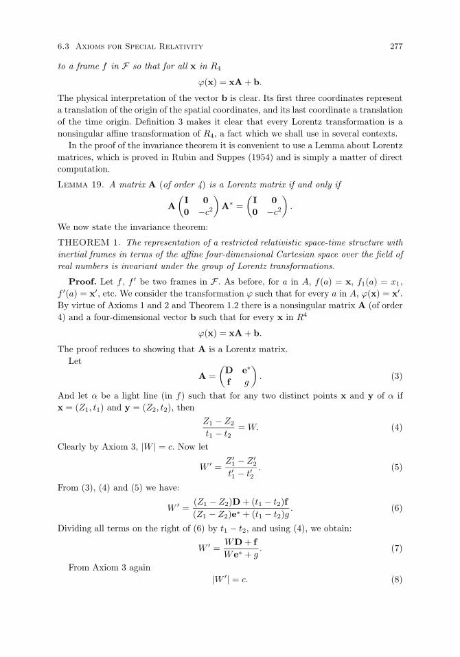
6.3 Axioms for Special Relativity 277

to a frame f in F so that for all x in R4

ϕ(x) = xA + b.

The physical interpretation of the vector b is clear. Its first three coordinates representa translation of the origin of the spatial coordinates, and its last coordinate a translationof the time origin. Definition 3 makes it clear that every Lorentz transformation is anonsingular affine transformation of R4, a fact which we shall use in several contexts.

In the proof of the invariance theorem it is convenient to use a Lemma about Lorentzmatrices, which is proved in Rubin and Suppes (1954) and is simply a matter of directcomputation.

Lemma 19. A matrix A (of order 4) is a Lorentz matrix if and only if

A(

I 00 −c2

)A∗ =

(I 00 −c2

).

We now state the invariance theorem:

THEOREM 1. The representation of a restricted relativistic space-time structure withinertial frames in terms of the affine four-dimensional Cartesian space over the field ofreal numbers is invariant under the group of Lorentz transformations.

Proof. Let f , f ′ be two frames in F . As before, for a in A, f(a) = x, f1(a) = x1,f ′(a) = x′, etc. We consider the transformation ϕ such that for every a in A, ϕ(x) = x′.By virtue of Axioms 1 and 2 and Theorem 1.2 there is a nonsingular matrix A (of order4) and a four-dimensional vector b such that for every x in R4

ϕ(x) = xA + b.

The proof reduces to showing that A is a Lorentz matrix.Let

A =(D e∗

f g

). (3)

And let α be a light line (in f) such that for any two distinct points x and y of α ifx = (Z1, t1) and y = (Z2, t2), then

Z1 − Z2

t1 − t2= W. (4)

Clearly by Axiom 3, |W | = c. Now let

W ′ =Z ′

1 − Z ′2

t′1 − t′2. (5)

From (3), (4) and (5) we have:

W ′ =(Z1 − Z2)D + (t1 − t2)f(Z1 − Z2)e∗ + (t1 − t2)g

. (6)

Dividing all terms on the right of (6) by t1 − t2, and using (4), we obtain:

W ′ =WD + fWe∗ + g

. (7)

From Axiom 3 again|W ′| = c. (8)

278 Representations of Space and Time

Since |W ′| = c, we have by squaring (7):

WDD∗W ∗ + 2WDf∗ + |f |2(We∗ + g)2

= c2, (9)

and consequently

W (DD∗ − c2e∗e)W ∗ + 2W (Df∗ − c2e∗g) + |f |2 − c2g2 = 0. (10)

Since (10) holds for an arbitrary light line, we may replace W by −W , and obtain(10) again. We thus infer:

W (Df∗ − c2e∗g) = 0,but the direction of W is arbitrary, whence

Df∗ − c2e∗g = 0. (11)

Now let x = (0, 0, 0, 0) and y = (0, 0, 0, 1). Then

I2f (xy) = c2.

But it is easily seen from (3) that

I2f ′(xy) = c2g2 − |f |2,

and thus by our fundamental invariance axiom (Axiom 4)

c2g2 − |f |2 = c2. (12)

From (10), (11), (12) and the fact that |W |2 = c2, we infer:

W (DD∗ − c2e∗e)W ∗ = |W |2,and because the direction of W is arbitrary, we conclude:

DD∗ − c2e∗e = I, (13)

where I is the identity matrix.Now by direct computation on the basis of (3),

A(I 00 −c2

)A∗ =

(DD∗ − c2e∗e Df∗ − c2e∗g

(Df∗ − c2e∗g)∗ ff∗ − c2g2

). (14)

From (11), (12), (13) and (14) we arrive finally at the result:

A(I 00 −c2

)A∗ =

(I 00 −c2

),

and thus by virtue of Lemma 1, A is a Lorentz matrix. Q.E.D.

Historical remarks. As already stated, explicit questions of invariance were madeprominent in the earliest development of the special theory of relativity, quite the op-posite of the corresponding case for classical physics.

The predecessors of Einstein are Voigt, FitzGerald, Lorentz and Poincare, none ofwhom explicitly formulated a relativistic invariance principle. In fact, much of the effortwas still implicitly motivated by search for an ether absolutely at rest, as the basis of asingle preferred reference frame. Voigt (1887) was apparently the first actually to pub-lish a version of the Lorentz transformations, but his concern was the Doppler shift.12

12Here and in what follows up to the publication of Einstein (1905/1923) I have used the excellent

historical analysis in Pais (1982).

6.3 Axioms for Special Relativity 279

The Irish physicist G. F. FitzGerald (1889), much impressed by the famous Michelson-Morley (1887) experiment on the null result on the motion of the Earth in the ether,was the first to propose the contraction factor

√1 − v2/c2 in the length of a body in

the direction of its motion with velocity v relative to the measurement frame of refer-ence. But for FitzGerald the change was real, as he put it “. . . the length of materialbodies changes, according as they are moving through the aether . . . ”. Without knowl-edge of FitzGerald’s article, Lorentz (1892) also proposed such a contraction factor.Then Lorentz (1895) derived a form of Lorentz transformations useful in terrestrial op-tical experiments, as part of his development of electromagnetic theory. Poincare (1898)discusses with wonderful clarity, but with only programmatic remarks, the obvious op-erational difficulties of judging two distant events simultaneous.

Publication of Einstein (1905/1923) is the decisive event, with a clear statement ofinvariance, the crucial step in the move from Maxwell’s electromagnetic theory to thekinematical special theory of relativity. Here is the English translation (1923) of thefirst two paragraphs of this justly famous article.

It is known that Maxwell’s electrodynamics—as usually understood at the present time—

when applied to moving bodies, leads to asymmetries which do not appear to be inherent

in the phenomena. Take, for example, the reciprocal electrodynamic action of a magnet

and a conductor. The observable phenomenon here depends only on the relative motion

of the conductor and the magnet, whereas the customary view draws a sharp distinction

between the two cases in which either the one or the other of these bodies is in motion. For

if the magnet is in motion and the conductor at rest, there arises in the neighbourhood

of the magnet an electric field with a certain definite energy, producing a current at the

places where parts of the conductor are situated. But if the magnet is stationary and

the conductor in motion, no electric field arises in the neighbourhood of the magnet.

In the conductor, however, we find an electromotive force, to which in itself there is

no corresponding energy, but which gives rise—assuming equality of relative motion in

the two cases discussed—to electric currents of the same path and intensity as those

produced by the electric forces in the former case.

Examples of this sort, together with the unsuccessful attempts to discover any motion of

the Earth relatively to the “light medium,” suggest that the phenomena of electrodynam-

ics as well as of mechanics possess no properties corresponding to the idea of absolute

rest. They suggest rather that, as has already been shown to the first order of small

quantities, the same laws of electrodynamics and optics will be valid for all frames of

reference for which the equations of mechanics hold good.13 We will raise this conjecture

(the purport of which will hereafter be called the “Principle of Relativity”) to the status

of a postulate, and also introduce another postulate, which is only apparently irrecon-

cilable with the former, namely, that light is always propagated in empty space with

a definite velocity c which is independent of the state of motion of the emitting body.

These two postulates suffice for the attainment of a simple and consistent theory of the

electrodynamics of moving bodies based on Maxwell’s theory for stationary bodies. The

introduction of a “luminiferous ether” will prove to be superfluous inasmuch as the view

here to be developed will not require an “absolutely stationary space” provided with

special properties, nor assign a velocity-vector to a point of the empty space in which

electromagnetic processes take place. (Einstein 1905/1923, pp. 37–38)

13The reference here is to the inertial frames of classical physics, which are, of course, the same for

special relativity.

280 Representations of Space and Time

The first paragraph of Einstein’s article is focused on defining simultaneity of distantevents, hinted at by Poincare (1898) earlier, but only here stated exactly and boldly used.I give an equivalent affine geometric formulation. Let a be any space-time, i.e., affine,point. Let L be an inertial line through a; here L serves as the time axis of the inertialframe with respect to which simultaneity is defined. Any affine line is orthogonal to L ifthe two lines form the diagonals of an optical parallelogram, i.e., an affine parallelogramwhose sides are segments of optical lines, as defined earlier.

ThenS(a, L) = b : line ab is orthogonal to L ∪ a

is the set of points simultaneous to a, relative to L. Note that the definition of simul-taneity must be relative to a given frame of reference. The absolute simultaneity ofclassical physics is given up.

In qualitative axiomatizations of the geometric structure of special relativity it isnatural to postulate that for every affine space-time point a and any inertial line througha, the set S(a, L) is a three-dimensional Euclidean space with respect to the affinebetweenness relation and a congruence relation ≈ satisfying the standard Euclideancongruence axioms.

Section 2 of this famous 1905 article explicitly states the two principles Einstein uses:

The following reflexions are based on the principle of relativity and on the principle of

the constancy of the velocity of light. These two principles we define as follows:

1. The laws by which the states of physical systems undergo change are not affected,

whether these changes of state be referred to the one or the other of two systems

of coordinates in uniform translatory motion.

2. Any ray of light moves in the “stationary” system of coordinates with the deter-

mined velocity c, whether the ray be emitted by a stationary or by a moving body.

(Einstein 1905/1923, p. 41)

These principles are then used to show the relativity of lengths and time.In Section 3 a form of the Lorentz transformations is derived, but, as noted earlier,

without awareness of Lorentz’s earlier paper. Section 4 considers the physical meaningof the transformations derived. Here Einstein introduces the proper time τ of a movingbody, i.e., the time ‘when at rest relatively to the moving system,’ and derives theequation

τ = t

√1 − v2

c2.

In Section 5 the relativistic composition of velocities is derived.The remainder of the article is devoted to electromagnetic theory. In particular, the

covariance14 of Maxwell’s equations under Lorentz transformations is derived.Einstein submitted his paper to the Annalen der Physik on June 30, 1905. Poincare’s

article (1905) was submitted on June 5, 1905 and his second, published in 1906, wascompleted in July 1905. Of course, neither author was aware of the other’s publication atthe time. In the second paper Poincare gave a completely detailed proof of the covarianceof Maxwell’s equations. But curiously enough, Poincare apparently did not fully grasp

14The relation between covariance and invariance was analyzed in Section 4.4.

6.3 Axioms for Special Relativity 281

the sense of special relativity. In later lectures given at Gottingen in 1909, publishedin 1910, he still introduced, beyond the two principles used by Einstein in Section 2of the 1905 article and quoted above, as a third hypothesis the physical reality of theFitzGerald-Lorentz contraction, a clear confusion about the essential nature of specialrelativity.

Later qualitative axiomatic approaches. In the case of special relativity, the prim-itive binary relation after of temporal order is a sufficient structural basis for the entiregeometry. This was shown many years ago by Robb (1911, 1914, 1921, 1928, 1930, 1936).The most extensive exposition of his ideas is to be found in his 1936 book. A detailed dis-cussion and some extensions of Robb’s work can be found in Winnie (1977). Alexandrov(1950, 1975) showed that invariance of the numerical representation of Robb’s single bi-nary relation is sufficient to imply the Lorentz transformations. This was also shownlater and independently by Zeeman (1964, 1967). Surprisingly, this natural question wasnot discussed at all by Robb.

Since the time of Robb’s early work, a number of papers have been published onqualitative axiomatic approaches to the geometry of special relativity. An early approachwas that of Wilson and Lewis (1912), who gave an incomplete axiomatization of thetwo-dimensional case with an affine emphasis on parallel transformations. Reichenbach(1924) gave a philosophically interesting and intuitively appealing axiomatic discussion,but it was more in the spirit of physics than of an explicit and precise geometricalaxiomatization. He emphasized the analysis of simultaneity and philosophical issues ofconventionalism. Walker (1948, 1959), building on the physical approach to relativityof the British physicist E. A. Milne (1948), took as undefined, in addition to space-timepoints, particles as certain classes of such points (intuitively the classes are particlepaths) and Robb’s binary relation of after, with one particle being distinguished as theparticle-observer. In addition, he assumed a primitive relation of signal correspondencebetween the space-time points of any two particles. Perhaps the most unsatisfactoryfeature of Walker’s approach is that the signal-mappings are complex functions that, atone stroke, do work that should be done by a painstaking buildup of more elementaryand more intuitively characterizable operations or relations. An independent but relatedapproach to that of Walker was given by Hudgin (1973), who began with timelikegeodesics and signal correspondence represented by a communication function. LikeWalker, Hudgin used the physical ideas of Milne.

Domotor (1972) published a detailed discussion of Robb and provided another view-point on Robb’s approach by giving a vector-space characterization. Latzer (1972)showed that it is possible to take a binary relation of light signaling as primitive. Hedid not give a new axiomatic analysis but showed how Robb’s ordering relation can bedefined in terms of his symmetric light relation. From a purely geometrical standpoint,there is a good argument for adopting such a symmetric relation because there is nononarbitrary way of distinguishing a direction of time on purely geometrical grounds. Itactually follows from much earlier work of Alexandrov (1950, 1975) that Latzer’s binaryprimitive is adequate.

282 Representations of Space and Time

One of the most detailed recent efforts, roughly comparable to that of Robb, is thework of Schutz (1973), which is in the spirit of the work of Walker. Schutz’s axiomsystem goes beyond Walker’s in two respects. First, Walker did not state axioms strongenough to characterize completely the space-time of restricted relativity; and, second,more than half of the axioms have a form that is not closely related to any of thosegiven by Walker, though in several cases they have a rather strong appeal in terms ofphysical intuition. As Schutz indicated, the most important immediate predecessor ofhis book is the article by Szekeres (1968), whose approach resembled that of Walker,but Szekeres treated both particles and light signals as objects rather than treating lightsignals as formally being characterized by a binary relation of signaling. Later, Schutz(1979) simplified his axioms and cast them in better form, but with essentially the sameapproach.

Also important is the recent work of Mundy (1986a, 1986b). In (1986b) Mundy gavea detailed analysis of the physical content of Minkowski geometry. He also included asurvey of other axiomatizations more oriented toward physics, such as that of Mehlberg(1935, 1937). Mundy stressed in his axiomatization the constancy of the speed of lightas the physical core of Minkowski geometry.

In (1986a) Mundy gave an optical axiomatization that is close in spirit to that ofRobb, although the single binary primitive is close to Latzer’s (1972). Mundy’s formu-lation is certainly an improvement on Robb’s and is the best set of axioms thus far thatdepends on a single binary relation.

In a more recent work, Goldblatt (1987) emphasizes, probably for the first time in theliterature, the central role that can be played by the concept of orthogonality generalizedto relativistic space-time. In a Euclidean vector space with the standard inner product,two vectors x and y are orthogonal iff x · y = 0. Using the indefinite quadratic metricI2(x,y), we obtain the following: when two distinct lines are orthogonal, one must betimelike (an inertial line) and the other spacelike (a separation line); an optical lineis orthogonal to itself. Axiomatically, Goldblatt adds to the affine axioms based onbetweenness, additional axioms based on the quaternary relation of ab being orthogonalto cd.

6.4 How to Decide if Visual Space is Euclidean15

Philosophers of past times have claimed that the answer to the question of whethervisual space is Euclidean can be found by a priori or purely philosophical methods.Today such a view is presumably held only by a few redoutable Kantians. It would begenerally agreed that one way or another the answer is surely empirical, but it might beempirical for indirect reasons. It could be decided by physical arguments that physicalspace is Euclidean and then by conceptual arguments about perception that necessarilyvisual space must be Euclidean. To some extent this must be the view of many laymenwho accept that to a high degree of approximation physical space is Euclidean, andtherefore automatically hold the view that visual space is Euclidean.

I begin with the question, How do we test the proposition that visual space is Eu-clidean? This section is devoted to this problem of methodology and includes a brief

15Much of the material in this section and the next is taken from Suppes (1977a).

6.4 How to Decide if Visual Space is Euclidean 283

overview of the hierarchy of geometries relevant to visual phenomena. The next sectionreviews a number of answers that have been given to the question. I examine bothphilosophical and psychological claims. Section 7 is devoted to central issues raised bythe variety of answers that have been given.

What would seem to be, in many ways, the most natural mathematical approach tothe question has also been the method most used experimentally. It consists of con-sidering a finite set of points. Experimentally, the points are approximated by smallpoint sources of light of low illumination intensity, displayed in a darkened room. Theintuitive idea of the setting is to make only a finite number of point-light sources visibleand to make these light sources of sufficiently low intensity to exclude illumination ofthe surroundings. The second step is to ask the person making visual judgments to statewhether certain geometric relations hold between the points. For example, are points aand b the same distance from each other as points c and d? (Hereafter in this discussionI shall refer to points but it should be understood that I have in mind the physicalrealization in terms of point-light sources.) Another kind of question might be, Is theangle formed by points a b c congruent or equal in measure to the angle formed bypoints d e f?

Another approach to such judgments is not to ask whether given points have a certainrelation, but rather to permit the individual making the judgments to manipulate someof the points. For example, first fix points a, b and c and then ask him to adjust d so thatthe distance between c and d is the same as the distance between a and b. Althoughthe formulation I am giving of these questions sounds as if they might be metric incharacter, they are ordinarily of a qualitative nature—for example, that of congruenceof segments, which I formulate as having the same distance. No metric requirementsare imposed upon the individuals making such judgments. For instance, no one wouldnaturally ask subjects in the experiments relevant to our question to set the distancebetween two points to be approximately 1.3 meters or to determine an angle of, say, 21degrees.

Once such judgments are obtained, whether on the basis of fixed relations or byadjusting the position of points, the formal or mathematical question to ask is whetherthe finite relational structure can be embedded in a two- or three-dimensional Euclideanspace. The dimensionality depends upon the character of the experiment. In many casesthe points will be restricted to a plane and therefore embedding in two dimensionsis required; in other cases embedding in three dimensions is appropriate. By a finiterelational structure I mean a relational structure whose domain is finite. To give asimple example, suppose that A is the finite set of points and the judgments we haveasked for are judgments of equidistance of points. Let E be the quaternary relationof equidistance. Then to say that the finite relational structure A = (A,E) can beembedded in three-dimensional Euclidean space is to say that there exists a function ϕdefined on A such that ϕ maps A into the set of triples of real numbers and such thatfor every a, b, c, and d in A the following relation holds:

ab E cd iff3∑

i=1

(ϕi(a) − ϕi(b))2 =3∑

i=1

(ϕi(c) − ϕi(d))2,

284 Representations of Space and Time

where ϕi(a) is the ith coordinate of ϕ(a). Note that the mapping into triples of realnumbers is just mapping visual points into a Cartesian representation of three-dimen-sional Euclidean space.

In principle, it is straightforward to answer the question raised by this embeddingprocedure. So that, given a set of data from an individual’s visual judgments of equidis-tance between points, we can determine in a definite and constructive mathematicalmanner whether such isomorphic embedding is possible.

Immediately, however, a problem arises. This problem can be grasped by consideringthe analogous physical situation. Suppose we are making observations of the stars andwant to test a similar proposition, or some more complex proposition of celestial me-chanics. We are faced with the problem recognized early in the history of astronomy, andalso in the history of geodetic surveys, that the data are bound not to fit the theoreticalmodel exactly. The classical way of putting this is that errors of measurement arise, andour problem is to determine if the model fits the data within the limits of the errorsof measurement. In examining data on the advancement of the perihelion of Mercury,which is one of the important tests of Einstein’s general theory of relativity, the mosttedious and difficult aspect of the data analysis is to determine whether the theory andthe observations are in agreement within the estimated error of measurement.

Laplace (1799/1966), for example, used such methods with unparalleled success. Hewould examine data from some particular aspect of the solar system, for example, ir-regularities in the motion of Jupiter and Saturn, and would then raise the question ofwhether these observed irregularities were due to errors of measurement or to the exis-tence of ‘constant’ causes. When the irregularities were too great to be accounted for byerrors of measurement, he then searched for a constant cause to explain the deviationsfrom the simpler model of the phenomena. In the case mentioned, the irregularities inthe motion of Jupiter and Saturn, he was able to explain them as being due to themutual gravitational attraction of the two planets, which had been ignored in the sim-ple theory of their motion. But Laplace’s situation is different from the present one inthe following important respect. The data he was examining were already rendered inquantitative form and there was no question of having a numerical representation. Ourproblem is that we start from qualitative judgments and we are faced with the problemof simultaneously assigning a measurement and determining the error of that measure-ment. Because of the complexity and subtlety of the statistical questions concerningerrors of measurement in the present setting, for purposes of simplification I shall ig-nore them, but it is absolutely essential to recognize that they must be dealt with inany detailed analysis of experimental data.

Returning to the formal problem of embedding qualitative relations among a finiteset of points into a given space, it is surprising to find that the results of the kinds thatare needed in the present context are not really present in the mathematical literatureon geometry. There is a very large literature on finite geometries; for example, Dem-bowski (1968) contains over 1200 references. Moreover, the tradition of considering finitegeometries goes back at least to the beginning of this century. Construction of such ge-ometries by Veblen and others was a fruitful source of models for proving independence

6.4 How to Decide if Visual Space is Euclidean 285

of axioms, etc.16 On the other hand, the literature that culminates in Dembowski’s mag-isterial survey consists almost entirely of projective and affine geometries that have arelatively weak structure. From a mathematical standpoint, such structures have beenof considerable interest in connection with a variety of problems in abstract algebra.The corresponding theory of finite geometries of a stronger type, for example, finiteEuclidean, finite elliptic, or finite hyperbolic geometries, is scarcely developed at all. Asa result, the experimental literature does not deal directly with such finite geometries,although they are a natural extension of the weaker finite geometries on the one handand finite measurement structures on the other. (For more details, see Section 8.)

A second basic methodological approach to the geometric character of visual spaceis to assume that a standard metric representation already exists and then to exam-ine which kind of space best fits the data. An excellent example of this methodologyis to be found in various publications of Foley (1964, 1972). Foley shows experimen-tally that the size-distance invariance hypothesis, which asserts that the perceived size-distance ratio is equal to the physical size-distance ratio, is grossly incorrect. At thesame time he also shows that perceived visual angles are about ten percent greaterthan physical angles. These studies are conducted on the assumption that a varietyof more primitive and elementary axioms are satisfied. In contrast, Luneburg (1948)assumes that the perceived visual angle equals the physical angle, that is, that thetransformation between the two is conformal, but what is back of the use of this as-sumption is a whole variety of assumptions that both physical space and visual spaceare homogeneous spaces of constant curvature, that is, are Riemannian spaces, and es-sentially Luneburg does not propose to test in any serious way the many consequencesimplied by this very rich assumption of having a homogeneous space with constantcurvature. In other words, in this second approach there is no serious attempt to pro-vide tests that will show if all of the axioms that hold for a given type of space aresatisfied.

A third approach is to go back to the well-known Helmholtz-Lie problem on thenature of space and to replace finiteness by questions of continuity and motion. In afamous lecture of 1854, Riemann (1866-1867) discussed the hypotheses on which thefoundations of geometry lie. More than a decade later, Helmholtz (1868) respondedin a paper entitled “Uber die Tatsachen, die der Geometrie zu Grunde liegen”. Thebasic argument of Helmholtz’s paper was that, although arbitrary Riemannian spacesare conceivable, actual physical space has, as an essential feature, the free mobilityof rigid bodies. From a mathematical standpoint, such motions are characterized inmetric geometry as transformations of a space onto itself that preserve distances. Suchtransformations are called isometries, meaning metrically isomorphic. Because of theextensive mathematical development of the topic (for modern review, see Busemann1955, Section 48, or Freudenthal 1965), an excellent body of formal results is availableto facilitate use of this viewpoint in the investigation of the character of visual space.Under various axiomatizations of the Helmholtz-Lie approach, it can be proved that theonly spaces satisfying the axioms are the following three kinds of elementary spaces:Euclidean, hyperbolic, and elliptic.

16See Veblen (1904) and Veblen and Young (1910, 1918)

286 Representations of Space and Time

From a philosophical standpoint, it is important to recognize that considerations ofcontinuity and motion are probably more fundamental in the analysis of the nature ofvisual space than the mathematically more elementary properties of finite spaces. Unfor-tunately, I am not able to report any experimental literature that uses the Helmholtz-Lieapproach as a way of investigating the nature of visual space. Although it is implicit insome of the results reported below, it would be difficult to interpret the experimentalresults as satisfying an axiom of free mobility. Let me be clear on this point. Some of theexperimental investigations lead to the result that visual space cannot be elementaryin the sense just defined, but these investigations do not explicitly use the kind of ap-proach to motion suggested by the rich mathematical developments that have followedin response to the Helmholtz-Lie problem, i.e., the study of spaces that permit the freemobility of rigid bodies.

A fourth approach, which lies outside the main body of the literature to be con-sidered in this chapter, is the approach through picture grammars and the analysis ofperceptual scenes. Its growing literature has been in response especially to problems ofpattern recognition that center on construction of computer programs and peripheraldevices that have rudimentary perceptual capacities. Although this approach has a for-mal character quite different from the others considered and it has not been used toaddress directly the question about the Euclidean character of visual space, it should bementioned because it does provide an approach that in many respects is very naturalpsychologically and that is in certain aspects more closely connected to the psychologyof perception than most of the classical geometric approaches that have been used thusfar in the analysis of visual space. (An elementary introduction and references to theearlier literature are to be found in Suppes and Rottmayer (1974); an encyclopedic re-view is given by Fu (1974). The literature of the last 25 years is too large to cite singlesurvey references. Important recent statistical trends are discussed in Attias (1999),Breiman (1999) and Friedman, Hastie and Tibshirani (2000).)

A typical picture grammar has the following character. Finite line segments or finitecurves of a given length and with a given orientation are concatenated together asbasic elements to form geometric figures of greater complexity. A typical problem in theliterature of pattern recognition is to provide such a concatenation (not necessarily onedimensional) so as to construct handwritten characters, or, as a specialized examplethat has received a fair amount of attention, to recognize handwritten mathematicalsymbols. These approaches are often labelled picture grammars, because they adoptthe approach used in mathematical linguistics for writing phrase-structure grammarsto generate linguistic utterances. Picture grammars can in fact be characterized ascontext free, context sensitive, etc., depending upon the exact character of the rulesof production. What is missing is the question, Can the set of figures generated bythe picture grammars be embedded in Euclidean space or other metric spaces of anelementary character? This question would seem to have some conceptual interest fromthe standpoint of the theory of perception. It is clearly not of the same importance for thetheory of pattern recognition. Picture grammars base perception on a set of primitiveconcepts that seem much more natural than the more abstract concepts familiar inclassical geometry. Moreover, extensive results on the behavior of single neurons in the

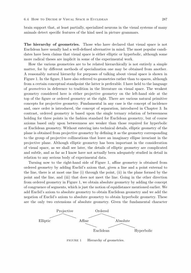
6.4 How to Decide if Visual Space is Euclidean 287

brain support that, at least partially, specialized neurons in the visual systems of manyanimals detect specific features of the kind used in picture grammars.

The hierarchy of geometries. Those who have declared that visual space is notEuclidean have usually had a well-defined alternative in mind. The most popular candi-dates have been claims that visual space is either elliptic or hyperbolic, although somemore radical theses are implicit in some of the experimental work.

How the various geometries are to be related hierarchically is not entirely a simplematter, for by different methods of specialization one may be obtained from another.A reasonably natural hierarchy for purposes of talking about visual space is shown inFigure 1. In the figure, I have also referred to geometries rather than to spaces, althoughfrom a certain conceptual standpoint the latter is preferable. I have held to the languageof geometries in deference to tradition in the literature on visual space. The weakestgeometry considered here is either projective geometry on the left-hand side at thetop of the figure or ordered geometry at the right. There are various natural primitiveconcepts for projective geometry. Fundamental in any case is the concept of incidenceand, once order is introduced, the concept of separation, introduced in Chapter 3. Incontrast, ordered geometry is based upon the single ternary relation of betweennessholding for three points in the fashion standard for Euclidean geometry, but of courseaxioms based only upon betweenness are weaker than those required for hyperbolicor Euclidean geometry. Without entering into technical details, elliptic geometry of theplane is obtained from projective geometry by defining it as the geometry correspondingto the group of projective collineations that leave an imaginary ellipse invariant in theprojective plane. Although elliptic geometry has been important in the considerationof visual space, as we shall see later, the details of elliptic geometry are complicatedand subtle, and as far as I know have not actually been adequately studied in detail inrelation to any serious body of experimental data.

Turning now to the right-hand side of Figure 1, affine geometry is obtained fromordered geometry by adding Euclid’s axiom that, given a line and a point external tothe line, there is at most one line (i) through the point, (ii) in the plane formed by thepoint and the line, and (iii) that does not meet the line. Going in the other directionfrom ordered geometry in Figure 1, we obtain absolute geometry by adding the conceptof congruence of segments, which is just the notion of equidistance mentioned earlier. Weadd Euclid’s axiom to absolute geometry to obtain Euclidean geometry and we add thenegation of Euclid’s axiom to absolute geometry to obtain hyperbolic geometry. Theseare the only two extensions of absolute geometry. Given the fundamental character

PPPP

ProjectivePPPP

Ordered

EllipticPPP

AffinePPPP

Absolute

Euclidean Hyperbolic

FIGURE 1 Hierarchy of geometries.

288 Representations of Space and Time

of absolute geometry in relation to the claims often made that visual space is eitherEuclidean or hyperbolic, it is somewhat surprising that there has been no more detailedinvestigation experimentally of whether the axioms of absolute geometry hold for visualspace.

There is another way of organizing the hierarchy of geometries in terms of metricspaces. Recall that a metric space is a pair (A, d) such that A is a nonempty set, dis a real-valued function defined on the Cartesian product A × A, such that for alla, b, c in A, (i) d(a, a) = 0 and if a = b, d(a, b) > 0; (ii) d(a, b) = d(b, a); and (iii)d(a, b) + d(b, c) ≥ d(a,c). The elements of the set A are called points. The first axiomasserts that distances are positive, except for the distance between identical points,which is zero. The second axiom asserts that distance is symmetric; that is, it is afunction only of the unordered pair of points, not a function of their order. The thirdaxiom is the triangle inequality.

Most of the metric spaces important for the theory of perception have the propertythat any two points can be joined by a segment. Such spaces are called metric spaceswith additive segments. These spaces are naturally divided into two broad subclasses,affine metrics and coordinate-free metrics. By further specialization of each of thesesubclasses we are led naturally to the Euclidean, hyperbolic, and spherical spaces, aswell as to generalizations of the Euclidean metric in terms of what are called Minkowskimetrics. An important subclass of the coordinate-free metrics is the family of Rieman-nian metrics. It may be shown that the only spaces that are Riemannian and affinemetric are either Euclidean or hyperbolic. We shall not use these concepts in detail, butit is important to mention that this alternative hierarchy of metric spaces is as naturalto use as the more classical hierarchy exhibited in Figure 1. All of the concepts I haveintroduced in this brief survey of the hierarchy of geometries are familiar in the math-ematical literature of geometry. More details are to be found in Suppes et al. (1989,Chs. 12 & 13).

6.5 The Nature of Visual Space: Experimental and PhilosophicalAnswers

My main purpose in this section is to provide a survey of the answers that have beengiven to the nature of visual space. The natural place to begin is with Euclid’s Optics, theoldest extant treatise on mathematical optics. As stated in Section 2.4, it is importantto emphasize that Euclid’s Optics is really a theory of vision, not a treatise on physicaloptics.

Euclid’s restriction to monocular vision is one that we shall meet repeatedly in thissurvey. However, it should be noted that he proves several propositions involving morethan one eye; for example, “If the distance between the eyes is greater than the diameterof the sphere, more than the hemispheres will be seen”. Euclid is not restricted to somesimple geometric optics but is indeed concerned with the theory of vision, as is evidentfrom the proposition that “if an arc of a circle is placed on the same plane as theeye, the arc appears to be a straight line”. This kind of proposition is a precursor oflater theories—for example, that of Thomas Reid (1764/1967)—which emphasize thenon-Euclidean character of visual space.

6.5 Visual Space: Experimental and Philosophical Answers 289

I skip rapidly through the period after Euclid to the eighteenth century, not becausethere are not matters of interest in this long intervening period but because there do notseem to be salient changes of opinion about the character of visual space, or at least ifthere are, they are not known to me. I looked, for example, at the recent translation byDavid C. Lindberg (1970) of the thirteenth-century treatise Perspectiva Communis ofJohn Pecham and found nothing to report in the present context, although the treatiseitself and Lindberg’s comments on it are full of interesting matter of great importanceconcerning other questions in optics, as, for example, theories about the causes of light.

Newton’s Opticks (1704/1931) is in marked contrast to Euclid’s. The initial defini-tions do not make any mention of the eye until Axiom VIII, and then in very restrainedfashion. Almost without exception, the propositions of Newton’s optics are concernedwith geometric and especially physical properties of light. Only in several of the Queriesat the end are there any conjectures about the mechanisms of the eye, and these con-jectures do not bear on the topic at hand.

Five years after the publication of the first edition of Newton’s Opticks, Berkeley’sAn Essay towards a New Theory of Vision (1709/1901) appeared in 1709. Berkeleydoes not have much of interest to say about the geometry of visual space, except in anegative way. He makes the point that distance cannot be seen directly and, in fact,seems to categorize the perception of distance as a matter of tactile, rather than visual,sensation, because the muscular convergence of the eyes is tactile in character. He em-phatically makes the point that we are not able geometrically to observe or computethe optical angle generated by a remote point as a vertex, with sides pointing towardthe centers of the two eyes. Here is what he says about the perception of optical angles.“Since therefore those angles and lines are not themselves perceived by sight, it follows,. . . that the mind does not by them judge the distance of objects” (# 13). What he saysabout distance he also says about magnitude not being directly perceived visually. Inthis passage (# 53), he is especially negative about trying to use the geometry of thevisual world as a basis for visual perception.

It is clear from these and other passages that for Berkeley visual space is not Eu-clidean, because there is no proper perception of distance or magnitude; at least, visualspace is not a three-dimensional Euclidean space. What he seems to say is also am-biguous as to whether one should argue that it is at least a two-dimensional Euclideanspace. My own inclination is to judge that his views on this are more negative thanpositive. Perhaps a sound negative argument can be made up from his insistence onthere being a minimum visible. As he puts it, “It is certain sensible extension is notinfinitely divisible. There is a minimum tangible, and a minimum visible, beyond whichsense cannot perceive. This everyone’s experience will inform him” (# 54).

In fact, toward the end of the essay, Berkeley makes it clear that even two-dimensionalgeometry is not a proper part of visual space or, as we might say, the visual field. As hesays in the final paragraph of the essay, “By this time, I suppose, it is clear that neitherabstract nor visible extension makes the object of geometry”.

Of much greater interest is Thomas Reid’s Inquiry into the Human Mind, first pub-lished in 1764 (1764/1967). Chapter 6 deals with seeing, and Section 9 is the celebratedone entitled ‘Of the geometry of visibles’. It is sometimes said that this section is a

290 Representations of Space and Time

proper precursor of non-Euclidean geometry, but if so, it must be regarded as an im-plicit precursor, because the geometry explicitly discussed by Reid as the geometry ofvisibles is wholly formulated in terms of spherical geometry, which had of course beenrecognized as a proper part of geometry since ancient times. The viewpoint of Reid’sdevelopment is clearly set forth at the beginning of the section: “Supposing the eyeplaced in the centre of a sphere, every great circle of the sphere will have the sameappearance to the eye as if it was a straight line; for the curvature of the circle beingturned directly toward the eye, is not perceived by it. And, for the same reason, anyline which is drawn in the plane of a great circle of the sphere, whether it be in realitystraight or curve, will appear to the eye.” It is important to note that Reid’s geometry ofvisibles is a geometry of monocular vision. He mentions in other places binocular vision,but the detailed geometric development is restricted to the geometry of a single eye.The important contrast between Berkeley and Reid is that Reid develops in some detailthe geometry in a straightforward, informal, mathematical fashion. No such comparabledevelopment occurs in Berkeley.

Daniels (1972) has argued vigorously that Reid’s geometry of visibles is not simplya use of spherical geometry but is an introduction by Reid of a double elliptic space. Asimilar argument is made by Angell (1974). I am sympathetic with these arguments, butit seems to me that they go too far, and for a fairly straightforward reason not discussedby either Daniels or Angell. Let us recall how elliptic geometry was created by FelixKlein at the end of the nineteenth century. He recognized that a natural geometry, verysimilar to Euclidean geometry or hyperbolic geometry, could be obtained from sphericalgeometry by identifying antipodal points as a single point. The difficulty with sphericalgeometry as a geometry having a development closely parallel to that of Euclideangeometry is that two great circles, which correspond to lines, have two points, not onepoint, of intersection. However, by identifying the two antipodal points as a single point,a fair number of standard Euclidean postulates remain valid. It is quite clear that nosuch identification of antipodal points was made by Reid, for he says quite clearly in thefifth of his propositions, “Any two right lines being produced will meet in two points,and mutually bisect each other”. This property of meeting in two points rather thanone is what keeps his geometry of visibles from being a proper elliptic geometry andforces us to continue to think of it in terms of the spherical model used directly by Reidhimself.

In spite of the extensive empirical and theoretical work of Helmholtz on vision, hedoes not have a great deal to say that directly bears on this question, and I move alongto experiments and relevant psychological theory in the twentieth century. The initialstopping point is Blumenfeld (1913). (See Table 1 for the chronology.)

Blumenfeld was among the first to perform a specific experiment to show that, inone sense, phenomenological visual judgments do not satisfy all Euclidean properties.Blumenfeld performed experiments with so-called parallel and equidistance alleys. Ina darkened room the subject sits at a table, looking straight ahead, and he is askedto adjust two rows of point sources of light placed on either side of the normal plane,i.e., the vertical plane that bisects the horizontal segment joining the centers of the twoeyes. The two furthest lights are fixed and are placed symmetrically and equidistant

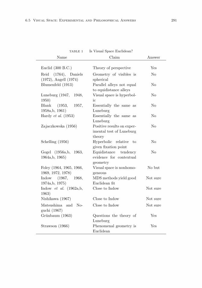
6.5 Visual Space: Experimental and Philosophical Answers 291

TABLE 1 Is Visual Space Euclidean?

Name Claim Answer

Euclid (300 B.C.) Theory of perspective Yes

Reid (1764), Daniels(1972), Angell (1974)

Geometry of visibles isspherical

No

Blumenfeld (1913) Parallel alleys not equalto equidistance alleys

No

Luneburg (1947, 1948,1950)

Visual space is hyperbol-ic

No

Blank (1953, 1957,1958a,b, 1961)

Essentially the same asLuneburg

No

Hardy et al. (1953) Essentially the same asLuneburg

No

Zajaczkowska (1956) Positive results on exper-imental test of Luneburgtheory

No

Schelling (1956) Hyperbolic relative togiven fixation point

No

Gogel (1956a,b, 1963,1964a,b, 1965)

Equidistance tendencyevidence for contextualgeometry

No

Foley (1964, 1965, 1966,1969, 1972, 1978)

Visual space is nonhomo-geneous

No but

Indow (1967, 1968,1974a,b, 1975)

MDS methods yield goodEuclidean fit

Not sure

Indow et al. (1962a,b,1963)

Close to Indow Not sure

Nishikawa (1967) Close to Indow Not sure

Matsushima and No-guchi (1967)

Close to Indow Not sure

Grunbaum (1963) Questions the theory ofLuneburg

Yes

Strawson (1966) Phenomenal geometry isEuclidean

Yes

292 Representations of Space and Time

from the normal plane. The subject is then asked to arrange the other lights so thatthey form a parallel alley extending toward him from the fixed lights. His task is toarrange the lights so that he perceives them as being straight and parallel to each otherin his visual space. This is the task for construction of a parallel alley. The second taskis to construct a distance alley. In this case, all the lights except the two fixed lightsare turned off and a pair of lights is presented, which are adjusted as being at the samephysical distance apart as the fixed lights—the kind of equidistance judgments discussedearlier. That pair of lights is then turned off and another pair of lights closer to him ispresented for adjustment, and so forth. The physical configurations do not coincide, butin Euclidean geometry straight lines are parallel if and only if they are equidistant fromeach other along any mutual perpendiculars. The discrepancies observed in Blumenfeld’sexperiment are taken to be evidence that visual space is not Euclidean. In both theparallel-alley and equidistance-alley judgments the lines diverge as you move away fromthe subject, but the angle of divergence tends to be greater in the case of parallel thanin the case of equidistance alleys. The divergence of the alleys as one moves away fromthe subject has been taken by Luneburg to support his hypothesis that visual space ishyperbolic.

In fact, Luneburg, in several publications in the late forties, has been by far thestrongest supporter of the view that visual space is hyperbolic. He, in conjunction withhis collaborators, has set forth a detailed mathematical theory of binocular vision andat the same time has generated a series of experimental investigations to test the basictenants of the theory. In many respects, Luneburg’s article (1947) remains the bestdetailed mathematical treatment of the theory of binocular vision. Without extensivediscussion, Luneburg restricts himself to Riemannian geometries of constant curvature inorder to preserve rigid motions, that is, free mobility of rigid bodies. Luneburg develops,in a coordinate system natural for binocular vision, the theory of Riemannian spaces ofconstant curvature in a quite satisfactory form, although an explicit axiomatic treatmentis missing. In orthogonal sensory coordinates the line element ds can be represented interms of sensory coordinates α, β and γ (these Greek letters are not the ones used byLuneburg) by:

ds2 =dα2 + dβ2 + dγ2[

(1 + 14K(α2 + β2 + γ2)

]2 , (1)

where

K = 0 for Euclidean space,K < 0 for hyperbolic space,K > 0 for elliptic space.

The best more recent treatment is Indow (1979).It is important to recognize that the Luneburg approach is strictly a psychophysical

approach to visual space. It assumes a transformation of physical Euclidean space toyield a psychological one. In this sense it is not a fundamental qualitative approach tothe axioms of visual space. Luneberg nowhere examines with any care or explicitnessthe more general primitive assumptions that lead to the proof that visual space is aRiemannian space of constant curvature.

6.5 Visual Space: Experimental and Philosophical Answers 293

After these general developments he turns to the detailed arguments for the viewthat the appropriate space of constant curvature for visual space is hyperbolic (K < 0in equation (1)). It is not possible to enter into the details of Luneburg’s argumenthere, but he bases it on three main considerations, all of which have had a great deal ofattention in the theory of vision: first, the data arising from the frontal-plane horopterwhere curves which appear as straight are physically curved (data on these phenomenago back to the time before Helmholtz); second, the kind of alley phenomena concern-ing judgments of parallelness mentioned earlier; and, third, accounting for judgmentsof distorted rooms in which appropriate perspective lines are drawn and which conse-quently appear as rectangular or regular. In this last case, Luneburg draws on someunpublished classic and spectacular demonstrations by A. Ames, Jr. For related work,see Ames (1946). One of the difficulties of this field is that the kind of detailed math-ematical and quantitative arguments presented by Luneburg in connection with thesethree typical kinds of problems are not always satisfactorily analyzed in the later lit-erature. Rather, new data of a different sort are often presented to show that differentphenomena argue against Luneburg’s hypothesis that visual space is hyperbolic. Still,the literature in both directions is substantial. The numerous references given in therest of this chapter are by no means complete in scope.

Luneburg died in 1949, but a number of his former students and collaborators havecontinued his work and provided additional experimental support as well as additionalmathematically based arguments in favor of his views. I refer especially to Blank (1953,1957, 1958a, 1958b, 1961) and Hardy et al. (1953), although this is not an exhaustivelist. Another positive experimental test was provided by Zajaczkowska (1956).

Schelling (1956) agrees with Luneburg but makes an important point of modifica-tion, namely, the metrics of negative curvature—that is, of the hyperbolic spaces thatLuneburg argues for—are essentially momentary metrics. At a given instant the eye hasa certain fixation point, and relative to this fixation point Luneburg’s theory is, accord-ing to Schelling, probably approximately correct, but the applicability of the theory isseverely restricted because the eyes are normally moving about continuously and thepoints of fixation are continually changing. This fundamental fact of change must betaken account of in any fully adequate theory.

Gogel (1956a,b, 1963, 1964a,b, 1965) has studied what is called the equidistancetendency, or what in the context of this chapter we might term the Berkeley tendency.Remember that Berkeley held that distance from the observer was not a visual ideaat all, but derived from the tactile sense. Without entering into a precise analysis ofBerkeley’s views, Gogel has provided an important body of evidence that when othercues are missing there is a strong tendency to view objects as being at the same distancefrom the observer. These careful and meticulous studies of Gogel are important forestablishing not only the equidistance tendency but also its sensitivity to individualvariation, on the one hand, and to the presence of additional visual cues on the other.The equidistance tendency is certainly present as a central effect, but any detailed theoryof visual space has a bewildering complexity of contextual and individual differences toaccount for, and it seems to me that Gogel’s experiments are essentially decisive on thispoint. In the papers referred to, Gogel does not give a sharp answer to the question

294 Representations of Space and Time

about the character of visual space. But I have listed him in Table 1 because it seemsto me that the impact of his studies is to argue strongly for skepticism about fixingthe geometry of visual space very far up in the standard hierarchy. Rather, his studiessupport the point that the full geometry is strongly contextual in character and thereforequite deviant from the classical hierarchy.

A number of interesting experimental studies of the geometry of visual space havebeen conducted by John Foley. In Foley (1964) an experiment using finite configurationsof small point sources of light was conducted to test the Desarguesian property ofvisual space.17 (Of course, the property was tested on the assumption that a numberof other axioms were valid for visual space.) The results confirmed the Desarguesianproperty for most observers but not for all. In Foley (1966), perceived equidistance wasstudied as a function of viewing distance. Like most of Foley’s experiments, this wasconducted in the horizontal eye-level plane. The locus of perceived equidistance wasdetermined at distances of 1.2, 2.2, 3.2, and 4.2 meters from the observer. As in otherFoley experiments, the stimuli were small, point-like light sources viewed in completedarkness. The observer’s head was held fixed but his eyes were permitted to move freely.There were five lights, one in the normal plane, which was fixed, and four variable lightson each side of the normal plane at angles of 12 degrees and 24 degrees with respect tothe normal plane. The locus of perceived equidistance was found to be concave towardthe observer at all distances. Perhaps most importantly, the locus was found to varywith viewing distance, which indicates that the visual space does not depend on thespatial distribution of retinal stimulation alone. Again, there is here a direct argumentfor a contextual geometry and results are not consistent with Luneburg’s theory. Theequidistance judgments were of the following sort. A subject was instructed to set eachof the lights, except the fixed light, in the normal plane to be at the same distance fromhimself as the fixed light. Thus, it should appear to him that the lights lie on a circle,with himself as observer at the center. The important point is that for none of the tensubjects in the experiment did the judgments of the locus for equidistance lie on theVieth-Mueller horopter or circle mentioned earlier as one of the supporting argumentsfor Luneburg’s theory. Also important for the fundamental geometry of visual space isthe fact that the loci determined by the observers were not symmetric about the normalplane.

Here is another beautiful experiment by Foley (1972). The situation is shown inFigure 2. The instructions to the subject are to make judgments of perpendicularity(⊥) and congruence (≈) as follows, with the subject given point A as fixed in the depthaxis directly in front of his position as observer O:

17First, in explaining Desargues’ proposition, we need two definitions. Two triangles are perspective

from a point if and only if there is a one-to-one correspondence between the vertices of the two triangles

such that the three lines passing through the three pairs of corresponding vertices meet in a common

point, the perspective point. Two triangles are perspective from a line if and only if there is a one-to-

one correspondence between the lines forming the sides of the two triangles such that the three pairs

of corresponding lines forming the sides of the two triangles meet at points that themselves lie on a

common line. The Desarguesian property or proposition is that two triangles that are perspective from

a point are also perspective from a line. In projective geometry, planes can be either Desarguesian or

not, in three-dimensional projective geometry the property is provable from other standard axioms.

6.5 Visual Space: Experimental and Philosophical Answers 295

1. Find point B so that AB ⊥ OB & AB ≈ OB.2. Find point C so that OC ⊥ OB & OC ≈ OB.3. Judge the relative lengths of OA & BC.

The results are that the 24 subjects in 40 of 48 trials judged BC significantly longerthan OA. This judgment that BC is longer than OA contradicts properties of any spaceof constant curvature, whether that curvature is positive, negative, or zero.

O (Observer)

BC

A (fixed)

FIGURE 2 Foley experiment.

Foley’s (1972) study shows experimentally that, on the one hand, the size-distanceinvariance hypothesis is incorrect, and that in fact the ratio of perceived frontal extentto perceived egocentric distance greatly exceeds the physical ratio, while, on the otherhand, perceived visual angles are quite close to physical ones. These results, togetherwith other standard assumptions, are inconsistent with the Luneburg theory that visualspace is hyperbolic. Foley describes the third experiment in this paper in the followingway:

How can it be that in the primary visual space reports of perceived size-distance ratio

are not related to reports of perceived visual angle in a Euclidean way? One possibility

is that the two kinds of judgments are in part the product of different and independent

perceptual processes . . . . The results are consistent with the hypothesis that the two

kinds of judgments are the product of independent processes. They also show that no

one geometric model can be appropriate to all stimulus situations, and they suggest

that the geometry may approach Euclidean geometry with the introduction of cues to

distance. (Foley 1972, p. 328)

Again, there is in Foley’s analysis a strong case for a contextual geometry. A number ofother detailed experimental studies of Foley that have not been referenced here build acase for the same general contextual view, which I discuss in more detail below.

A number of detailed investigations on the geometry of visual space have been con-ducted by Tarow Indow (1967, 1968, 1974a,b, 1975) and other Japanese investigators

296 Representations of Space and Time

closely associated with him (Indow et al. 1962a, 1962b, 1963; Matsushima and Noguchi1967; Nishikawa 1967). They have found, for example, that multidimensional scalingmethods (MDS), which have been intensively developed in psychology, in many casesyield extremely good fits to Euclidean space (Indow 1982). Indow has experimentallytested the Luneburg theory based upon the kind of alley experiments that go back toBlumenfeld (1913). As might be expected, he duplicates the result that the equidistancealleys always lie outside the parallel alleys, which, under the other assumptions that arestandard, implies that the curvature of the space is negative and therefore it must behyperbolic. But Indow (1974a,b) properly challenges the simplicity of the Luneburg as-sumptions, especially the constancy of curvature. It is in this context that he has alsotried the alternative approach of determining how well multidimensional scaling will fita Euclidean metric. As he emphasizes, the Luneburg approach is fundamentally basedupon differential geometry as a method of characterizing Riemannian spaces with con-stant curvature, but for visual judgments it is probably more appropriate to dependupon judgments in the large, and therefore upon a different conceptual basis for visualgeometry. Throughout his writings, Indow recognizes the complexity and difficulty ofreaching any simple answer to give the proper characterization of visual space. Thewealth of detail in his articles and those of his collaborators is commended to the readerwho wants to pursue these matters in greater depth.

I myself have learned more about the theory of visual space from Indow and hiscolleagues than from anyone else. I was initially enormously skeptical of the Luneburgideas and I came to realize they could be converted into a realistic program, just becauseof the extraordinarily careful experiments performed by Indow and his colleagues. In thiscase the fact that the program has not turned out to be more satisfactory than it is, is notbecause of the weakness of the experiments, but in fact because of their very strength.They have given us confidence to recognize that there are fundamental things wrongwith the Luneburg approach to visual space. Above all, as Indow and his colleagueshave brought out on several occasions, there is a complete lack of parametric stabilityonce we assume that a space of constant curvature, for example, negative curvature inthe hyperbolic case, is a reasonable hypothesis. When we estimate the curvature we findthat, even for the same experiments, the results are not stable from day to day for agiven subject, and certainly when we transfer from one kind of experiment, for example,the classical alley experiments, to judgments of a different kind, there is little transferat all of the parametric values estimated in one situation to the next.

Careful mathematical analysis of several different features of visual space relevant tothe preceding review has been given by Jan Drosler in a series of articles (1966, 1979a,b,c,1987, 1988, and 1992). The topics range from multidimensional scaling in Cayley-Kleingeometries (1979c) to the psychophysical function of binocular space perception (1988),which is especially pertinent to the more detailed development of the psychophysicalideas of Luneburg in a richer psychological setting.

Another experiment (Wagner 1985) dealt with perceptual judgments about distancesand other measures among 13 white stakes in an outdoor viewing area. In physical coor-dinates let x equal measurement along the depth axis and y along the frontal axis and letperceptual judgments of distance be shown by primes (see Figure 3 for depth and frontal

6.6 Foley and Wagner Experiments 297

axis). Then the general result of Wagner is that x′ ≈ 0.5y′ if physically x = y. Noticehow drastic the foreshortening is along the depth axis. This result of Wagner’s is notanomalous or peculiar but represents a large number of different perception experimentsshowing dramatic foreshortening along the depth axis.

In his important book on the philosophy of space and time, Grunbaum (1963) rejectsthe Luneburg theory and affirms that, in order to yield the right kinds of perceptualjudgments, visual space must be Euclidean. His argument is rather brief and I shall notexamine it in any detail. It would be my own view that he has not given proper weightto the detailed experimental studies or to the details of the various theoretical proposalsthat have been made.

I close this survey by returning to a philosophical response to the question, that ofStrawson (1966) in his book on Kant’s Critique of Pure Reason. From the standpointof the large psychological literature I have surveyed, it is astounding to find Straw-son asserting as a necessary proposition that phenomenal geometry is Euclidean. Thefollowing quotation states the matter bluntly:

With certain reservations and qualifications, to be considered later, it seems that Eu-

clidean geometry may also be interpreted as a body of unfalsifiable propositions about

phenomenal straight lines, triangles, circles, etc.; as a body of a priori propositions about

spatial appearances of these kinds and hence, of course, as a theory whose application is

restricted to such appearances.

(Strawson 1966, p. 286)

The astounding feature of Strawson’s view is the absence of any consideration thatphenomenal geometry could be other than Euclidean and that it surely must be amatter, one way or another, of empirical investigation to determine what is the case.The qualifications he gives later do not bear on this matter, but pertain rather toquestions of idealization and of the nature of constructions, etc. The absence of anyattempt to deal in any fashion whatsoever with the large theoretical and experimentalliterature on the nature of visual space is surprising.

6.6 Partial Axioms for the Foley and Wagner Experiments18

I am not able to give a fully satisfactory geometric analysis of the strongly supportedexperimental facts found in these experiments but do think there are some things ofinterest to be said that will help clarify the foundational situation. I have divided theaxioms that I propose into various groups.Affine plane. These I take to be the standard axioms of Definition 1.1. We could ofcourse, reduce them and not require the whole plane but that is not important here. Wecan take as primitives, either betweenness, or parallelness and some concept like that ofa midpoint algebra. Again the decision is not critical for considerations here. We nowadd judgments of perceived congruence (≈).Three distinguished points. Intuitively, let o1 be the center of the left eye, o2 the center ofthe right eye and o the bisector of the segment o1o2. Explicitly, they satisfy the followingtwo axioms.

18This section draws on the material in Suppes (1995).

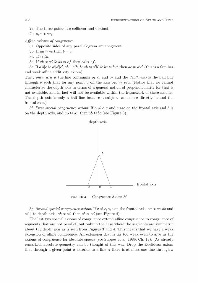
298 Representations of Space and Time

2a. The three points are collinear and distinct;2b. o1o ≈ oo2.

Affine axioms of congruence.3a. Opposite sides of any parallelogram are congruent.3b. If aa ≈ bc then b = c.3c. ab ≈ ba.3d. If ab ≈ cd & ab ≈ ef then cd ≈ ef .3e. If a|b|c & a′|b′|c′, ab ‖ a′b′ & ab ≈ a′b′ & bc ≈ b′c′ then ac ≈ a′c′ (this is a familiar

and weak affine additivity axiom).The frontal axis is the line containing o1, o, and o2 and the depth axis is the half linethrough o such that for any point a on the axis o1a ≈ o2a. (Notice that we cannotcharacterize the depth axis in terms of a general notion of perpendicularity for that isnot available, and in fact will not be available within the framework of these axioms.The depth axis is only a half line because a subject cannot see directly behind thefrontal axis.)

3f. First special congruence axiom. If a = c, a and c are on the frontal axis and b ison the depth axis, and ao ≈ oc, then ab ≈ bc (see Figure 3).

frontal axisa o c

b

depth axis

FIGURE 3 Congruence Axiom 3f.

3g. Second special congruence axiom. If a = c, a, c on the frontal axis, ao ≈ oc, ab andcd ‖ to depth axis, ab ≈ cd, then ob ≈ od (see Figure 4).

The last two special axioms of congruence extend affine congruence to congruence ofsegments that are not parallel, but only in the case where the segments are symmetricabout the depth axis as is seen from Figures 3 and 4. This means that we have a weakextension of affine congruence. An extension that is far too weak even to give us theaxioms of congruence for absolute spaces (see Suppes et al. 1989, Ch. 13). (As alreadyremarked, absolute geometry can be thought of this way. Drop the Euclidean axiomthat through a given point a exterior to a line α there is at most one line through a

6.6 Foley and Wagner Experiments 299

frontal axisa o c

b d

depth axis

FIGURE 4 Congruence Axiom 3g.

that is parallel to α and lies in the plane formed by a and α. Adding this axiom to theaxioms of absolute geometry gives us Euclidean geometry, as is obvious. What is muchmore interesting is that adding the negation of this axiom to those of absolute geometrygives us hyperbolic geometry.) We can prove the following theorem.

THEOREM 1. Let the halfspace consisting of all points on the same side of the frontalaxis as the depth axis be designated the frontal half plane:

(1). The frontal halfplane is isomorphic under a real-valued function ϕ to a two-dimensional affine halfplane over the field of real numbers, with the x-axis the depthaxis and the y-axis the frontal axis. Moreover, congruence as measured by the Euclideanmetric is satisfied when line segments are congruent, i.e., if ab ≈ cd then

∑2i=1(ϕi(a) −

ϕi(b))2 =∑2

i=1(ϕi(c) − ϕi(d))2.(2). The only affine transformations possible are those consisting of stretches α of

the frontal axis and stretches β of the depth axis with α, β > 0.

The proof of (1) is obvious from familiar results of classical geometry. The proof of (2)follows from observing that the affine transformations described are the only ones thatpreserve the symmetry around the depth axis required by the two special congruenceaxioms.

It is clear that the results of Theorem 1 are quite weak. The theorem is not contra-dicted by the Foley and Wagner experiments, but this is not surprising, for the apparatusof betweenness plus symmetric congruence about the depth axis cannot describe the re-sults of either experiment. If we were to add a concept of perpendicularity, as requiredby the Foley procedure, then we would essentially get a Euclidean halfplane, and theresulting structure would contradict the Foley results.

Correspondingly, we cannot describe the Wagner psychophysical results of extensiveperceptual foreshortening along the depth axis, without adding some psychophysicalassumptions radically different from those of Luneburg. Of course, the Foley resultsalso are best interpreted as perceptual foreshortening along the depth axis. The natural

300 Representations of Space and Time

conclusion is that we cannot consistently describe visual geometric relations in any spaceclose to the specificity and simplicity of structure of a space of constant curvature.

Even the weak affine structure of Theorem 1 is too strong, and probably should bereplaced by a standard version of absolute geometry, but with the congruence axiomsweakened as given above. Such an absolute geometry can be extended to hyperbolicgeometry, but the affine structure cannot. What we seem to end up with is a varietyof fragments of geometric structures to describe different experiments. A hyperbolicfragment perhaps for alley experiments, a fragment outside the standard ones for theFoley experiments, etc.

The goal of having a unified structure of visual space adequate to account for all theimportant experimental results now seems mistaken. Only a pluralistic and fragmentaryapproach seems possible.

6.7 Three Conceptual Problems About Visual Space

In this section, I center my remarks around three clusters of issues. The first is concernedwith the contextual character of visual geometry, the second with problems of distanceperception and motion, and the third with the problem of characterizing the nature ofthe objects of visual space.

Contextual geometry. A wide variety of experiments and ordinary experience as welltestify to the highly contextual character of visual space. The presence or absence of‘extraneous’ points can sharply affect perceptual judgments. The whole range of visualillusions, which I have not discussed here, also provides a broad body of evidence forthe surprising strength of these contextual effects.

As far as I can tell, no one has tried seriously to take account of these contextualeffects from the standpoint of the axiomatic foundations of visual geometry. In a wayit is not surprising, for the implications for the axiomatic foundations are, from theordinary standpoint, horrendous. Let us take a simple example to illustrate the point.

In ordinary Euclidean geometry, three points form an isosceles triangle just whentwo sides of the triangle are of the same length. Suppose now that Euclidean geometryhad the much more complicated aspect that whether a triangle were isosceles or notdepended not simply on the configuration of the three points but also on whether therewas a distinguished point lying just outside the triangle alongside one of the dual sides.This asymmetry may well make the visual triangle no longer appear isosceles. This is butone simple instance of a combinatorial nightmare of contextual effects that can easilybe imagined and, without much imagination or experimental skill, verified as being real.For a bewildering, diverse collection of examples of visual illusions and a history of thesubject, see Coren and Girgus (1978).

What are we to say about such effects? It seems to me the most important thing isto recognize that perceptual geometry is not really the same as classical geometry atall, but in terms of the kinds of judgments we are making it is much closer to physics.Consider, for example, the corresponding situation with bodies that attract each otherby gravitation. The introduction of a third body makes all the difference to the motionsof the two original bodies and it would be considered bizarre for the situation to be

6.7 Conceptual Problems About Visual Space 301

otherwise. This also applies to electromagnetic forces, mechanical forces of impact, etc.Contextual effects are the order of the day in physics, and the relevant physical theoriesare built to take account of such effects.

Note that physical theories depend upon distinguished objects located in particularplaces in space and time. Space-time itself is a continuum of undistinguished points,and it is characteristic of the axiomatic foundations of classical geometry that there areno distinguished points in the space. But it is just a feature of perception that we arealways dealing with distinguished points which are analogous to physical objects, notgeometric points. Given this viewpoint, we are as free to say that we have contextualeffects in visual geometry as we are to make a similar claim in general relativity due tothe presence of large masses in a given region.

Interestingly enough, there is some evidence that as we increase the visual cues, thatis, as we fill up the visual field with an increasingly complex context of visual imagery,the visual space becomes more and more Euclidean. It is possible that we have here theexact opposite of the situation that exists in general relativity. In the case of perceptionit may be that spaces consisting of a very small number of visible points may be easilymade to deviate from any standard geometry.

The geometric viewpoint can be brought into close alignment with the physical one,when the isomorphic embedding of finite sets of points in some standard geometry istaken as the appropriate analysis of the nature of visual space. This approach wasmentioned earlier and is implicit in some of the experimental literature discussed. It hasnot sufficiently been brought to the surface, and the full range of qualitative axioms thatmust be satisfied for the embedding of a finite collection of points in a unique way ina given space, whether Euclidean, hyperbolic, elliptic, or whatever, needs more explicitand detailed attention.

It also seems satisfactory to avoid the problems of contextual effects in initial studyof this kind by deliberately introducing symmetries and also certain additional assump-tions such as quite special relations of a fixed kind to the observer. The many differentexperimental studies, and the kind of mathematical analysis that has arisen out of theLuneburg tradition, suggest that a good many positive and almost definitive results canbe achieved under special restrictive assumptions. It seems that making these resultsas definitive as possible, admitting at the same time their specialized character andaccepting the fact that the general situation is contextual in character, is an appropri-ate research strategy. It also seems likely that for these special situations one can givea definitely negative answer to the question, Is visual space Euclidean?, and respondthat, to high approximation, in many special situations it is hyperbolic and possiblyin certain others elliptic in character. This restricted answer is certainly negative. Ageneral answer at the present time does not seem available as to how to characterize thegeometry in a fully satisfactory way that takes account of the contextual effects thatare characteristic of visual illusions, equidistance tendencies, etc.

Distance perception and motion. As indicated earlier in the brief discussion ofthe Helmholtz-Lie problem, most of the work surveyed in the preceding section hasnot taken sufficient account of problems of motion. There is an excellent survey ar-

302 Representations of Space and Time

ticle of Foley (1978) on distance perception which indicates that eye motion duringthe initial stage of focusing on an object is especially critical in obtaining informationabout perceptual distance. Philosophical traditions in perception have tended to ignorethe complicated problems of motion of the eyes or head as an integral part of visualperception, but the most elementary considerations are sufficient to demonstrate theirfundamental importance. It was a fundamental insight of Luneburg to recognize that itis important to characterize invariance properties of motions of the eyes and head thatcompensate each other. The deeper aspects of scanning that determine the character ofthe visual field have not really been studied in a thoroughly mathematical and quan-titative fashion. There is little doubt in my mind that this is the area most importantfor future developments in the theory of visual space. We should, I would assume, endup with a kinematics of visual perception replacing the geometry of visual perception.For example, Lamb (1919) proves that under Donders’ law, which asserts that the po-sition of the eyeball is completely determined by the primary position and the visualaxis aligned to the fixation point, it is not possible for every physically straight linesegment to be seen as straight. This kinematical theorem of Lamb’s, which is set forthin detail in Roberts and Suppes (1967), provides a strong kinematical argument againstthe Euclidean character of visual space. I cite it here simply as an example of the kindof results that one should expect to obtain in a more thoroughly developed kinematicsof visual perception.

Objects of visual space. Throughout the analysis given in this chapter the exactcharacterization of what are to be considered as the objects of visual space has not beensettled in any precise or definitive way. This ambiguity has been deliberate, because thewide range of literature to which I have referred does not have a settled account of whatare to be regarded as visual objects. The range of views is extreme—from Berkeley,who scarcely even wants to admit a geometry of pure visual space, to those who holdthat visual space is simply a standard Euclidean space and there is little real distinctionbetween visual objects and physical objects. In building up the subject axiomaticallyand systematically, clearly some commitments are needed, and yet it seems that one canhave an intelligible discussion of the range of literature considered here without havingto fix upon a precise characterization, because there is broad agreement on the look ofthings in the field of vision. From the standpoint of the geometry of visual space, wecan even permit such wide disagreement as to whether the objects are two dimensionalor three dimensional in order to discuss the character of the geometry. Thomas Reidwould lean strongly toward the two-dimensional character of visual space. Foley wouldhold that visual space is three dimensional; note, however, that most of his experimentshave been restricted to two dimensions. At the very least, under several different naturalcharacterizations of the objects of visual space, it is apparent that strong claims can bemade that visual space is not Euclidean, and this is a conclusion of some philosophicalinterest.

6.8 Finitism in Geometry 303

6.8 Finitism in Geometry19

Developments in the foundations of mathematics in the twentieth century have beendominated by a concern to provide an adequate conceptual basis for classical analysis,as well as classical number theory. The attitude of Frege, Hilbert, Russell and Brouwer,along with others who have followed them, have had a continual focus on providing aproper conceptual foundation for classical parts of pure mathematics. What is remark-able about this history is how little attention has been paid to finitism in the applicationof mathematics. Attention to various applied traditions would have supported a muchmore radical finitism than was possible, as long as the viewpoint was that of providingan adequate basis for classical elementary number theory. Even the weakest systems ofrecursive arithmetic have closure conditions that lead to constructions far more complexthan are needed in any standard applications. The passions for closure and for complete-ness are in themselves wonderful intellectual passions, but they run counter to the drivefor solutions of applied problems by limited means, ones that are computationally fea-sible. This line of thought easily leads to finitism in the applications of mathematics tothe real world.

Those whose focus is pure mathematics might immediately respond to my emphasison finitism by saying that there is already a considerable emphasis on finitism in puregeometry, and by then citing the extensive and deep research on finite geometries in thelast half century. It is also natural to think of this work as an extension in many waysof Felix Klein’s Erlangen program, that is, the approach to geometry that emphasizes,above all, the structure of the group of automorphisms of the geometry.20 The study ofautomorphisms is also an important way of studying finite geometries, for given a finitegeometry, the group of automorphisms is a finite group. Also given a finite group, anatural problem is to determine its finite geometry. As noted earlier, a survey up untilthe mid-sixties of the twentieth century is to be found in Dembowski (1968). In thelast thirty years there has also been a substantial body of work, and a number of openproblems of a purely mathematical sort have been solved, especially in the relation offinite geometries to finite simple groups.

However, this large body of research is not the topic of this section. I have in mindmore elementary mathematical problems, ones that are focused on applications. Whatare the applications I have in mind? I begin with the mathematical methods usedby architects since ancient times. As early as the sixth century BC, architects wereapplying geometry to detailed questions of construction. It was not that they weresimply mechanically using the elementary geometry familiar from the philosophical andmathematical tradition of that time, but they were using detailed geometric ideas toprovide visual illusions. These methods of providing for visual illusions led to what arecalled in the architectural literature, then and now, ‘refinements’. A principal exampleis entasis, which is a geometric construction that makes the vertical outline of marblecolumns convex rather than linear. Here is what Vitruvius in the first century BC hasto say about this construction.

19The material in this section is drawn from Suppes (2001a).20See Section 4.3.

304 Representations of Space and Time

These proportionate enlargements are made in the thickness of columns on account of the

different heights to which the eye has to climb. For the eye is always in search of beauty,

and if we do not gratify its desire for pleasure by a proportionate enlargement in these

measures, and thus make compensation for ocular deception, a clumsy and awkward

appearance will be presented to the beholder. With regard to the enlargment made at

the middle of columns, which among the Greeks is called εντασις, at the end of the book

a figure and calculation will be subjoined, showing how an agreeable and appropriate

effect may be produced by it. (Vitruvius, 1960 edition, p. 86)

Entasis is, of course, a famous example, but there are many more; the most extensiveextant written record is Vitruvius’ Roman treatise, written in the time of Augustus.The detailed applications to be found in Vitruvius are not exceptional but standard.It is a justified lament that the book on architecture written by Ictinus, architect ofthe Parthenon, is now lost. The important point in the present context is that, longbefore Ictinus and long after Vitruvius, architects were trained in geometry and howto apply it in a detailed way to the construction of buildings. As I like to put it, thesearchitects were not proving theorems, but doing constructions (problems in the lan-guage of Euclid). The constructions were not all just simple and obvious; in fact, thelost drawing of Vitruvius’ diagram of the construction of entasis was more complicatedin its mathematical content than what can be found in most well-known architecturaltreatises today. (But certainly not more so than the mathematics back of modern com-puter programs for architectural design.) More than a thousand years after Vitruvius,in Palladio’s famous four books of architecture (1570/1965), the Greek tradition of pro-portion, rather than direct numerical computation, continued to dominate the detailedthinking of architects, as may be seen in many places in Palladio’s exposition. In variousways, the computer resources now available are encouraging once again the emphasison proportion.

Beyond entasis and other visual illusions, the most important mathematical or ge-ometric discovery already used by architects of the fifth century was the discoveryof perspective, traditionally attributed to the painter Agatharchus, who designed thebackground set for the staging of a tragedy by Aeschylus and wrote a book about scenepainting, as a consequence of this experience. Mathematical investigation of the theoryof perspective began as early as Democritus and Anaxagoras. This is what Vitruvius hadto say about this early work on perspective, writing half a millenium later in Rome.21

Agatharcus, in Athens, when Aeschylus was bringing out a tragedy, painted a scene,

and left a commentary about it. This led Democritus and Anaxagoras to write on the

same subject, showing how, given a centre in a definite place, the lines should naturally

correspond with due regard to the point of sight and the divergence of the visual rays,

so that by this deception a faithful representation of the appearance of buildings might

be given in painted scenery, and so that, though all is drawn on a vertical flat facade,

some parts may seem to be withdrawing into the background, and others to be standing

out in front. (Vitruvius, 1960 edition, p. 198)

21According to Alexander Jones (2000), the only two writers on mathematical optics in antiquity

who studied problems of perspective were Ptolemy in Book VII of his Geography and Pappus in Book

VI of his Collection.

6.8 Finitism in Geometry 305

What is important about this variety of applications of geometry, including, of course,the important case of perspective, is that the methods and results are highly finitisticin character, just as are, in fact, most, if not all, the results of Greek geometry.

So, if we look at the applications of geometry in this long and important architecturaltradition, which includes the thorough development of the mathematical theory of per-spective and also of projective geometry, one is naturally struck by the tight interactionbetween the finitistic character of the mathematics and the familiar applications. Theapplications of numerical methods in ancient times have the same finitistic character,but I do not try to consider the details here.

At a certain point in the nineteenth century, nonfinitistic methods entered classicalanalysis and were extended, in some sense, to geometry, due to several different forcesat work. I would stress especially the demand for representation theorems in completeform, because the representations of geometric spaces came to be formulated so as to beisomorphic to a given Cartesian product of the real number system, the product itselfdepending upon the dimension of the space. Such a search for representation theoremsis not at all a part of the Greek tradition in much earlier times. One way of putting thematter, in terms of many different discussions of the foundations of mathematics, is thatsuch representation theorems demand a representation of the actual infinite. It is thisrepresentation of the actual infinite, or, to put it in more pedantic terms, sets of infinitecardinality, which are mapped from the geometric space onto a Cartesian product of theset of real numbers isomorphically preserving the structure of the geometric space. Thestronger sense of nonfinitistic methods involving the axiom of choice, or its equivalent,is a still further remove from the finitism of applications I am focusing on here.

It is a separate question to what extent the parts of classical analysis actually usedin applications of mathematics in physics and elsewhere can avoid commitments notonly to any results using the axiom of choice, but, also, any sets of an actually infinitecharacter.22 My own conviction is that one can go the entire distance, or certainly almostthe entire distance, in a purely finitistic way, but this is not what I focus on here.

Quantifier-free axioms and constructions. One requirement of very strict con-structive methods is that the axioms of the theory in question should be quantifier-freeand thus avoid all purely existential assumptions. Such existential demands are replacedby specific constructions, which are either primitive or definable, in a quantifier-free way,in terms of the given primitive constructions. Often, in traditional formulations of ge-ometry, existential axioms are innocuous, in the sense that they can easily be replacedby essentially equivalent quantifier-free axioms which use a fixed finite number of givenconstants.

22The foundational effort leading to the arithmetization of analysis in the nineteenth century forced

even the most elementary concepts to have as extensions infinite sets, e.g., the representation of a given

rational number as the equivalence class of all fractions equal in the usual sense to a representative

fraction. Thus, the rational number [ 12] = p

q: 2p = q & q = 0. But such unintuitive abstractions

never played a serious part in applications and do not in proving standard theorems of analysis.

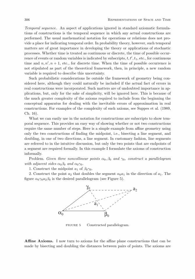
306 Representations of Space and Time

Temporal sequence. An aspect of applications ignored in standard axiomatic formula-tions of constructions is the temporal sequence in which any actual constructions areperformed. The usual mathematical notation for operations or relations does not pro-vide a place for indicating temporal order. In probability theory, however, such temporalmatters are of great importance in developing the theory or applications of stochasticprocesses. Whether time is treated as continuous or discrete, the time of possible occur-rence of events or random variables is indicated by subscripts, t, t′, t1, etc., for continuoustime and n, n′, n + 1, etc., for discrete time. When the time of possible occurrence isnot stipulated as part of the theoretical framework, then, in principle, a new randomvariable is required to describe this uncertainty.

Such probabilistic considerations lie outside the framework of geometry being con-sidered here, although they could naturally be included if the actual fact of errors inreal constructions were incorporated. Such matters are of undoubted importance in ap-plications, but, only for the sake of simplicity, will be ignored here. This is because ofthe much greater complexity of the axioms required to include from the beginning theconceptual apparatus for dealing with the inevitable errors of approximation in realconstructions. For examples of the complexity of such axioms, see Suppes et al. (1989,Ch. 16).

What we can easily use in the notation for constructions are subscripts to show tem-poral sequence. This provides an easy way of showing whether or not two constructionsrequire the same number of steps. Here is a simple example from affine geometry usingonly the two constructions of finding the midpoint, i.e., bisecting a line segment, anddoubling, in one of two directions, a line segment. In customary fashion, line segmentsare referred to in the intuitive discussion, but only the two points that are endpoints ofa segment are required formally. In this example I formulate the axioms of constructioninformally.

Problem. Given three noncollinear points α0, β0 and γ0, construct a parallelogramwith adjacent sides α0β0 and α0γ0.

1. Construct the midpoint a1 of β0γ0.2. Construct the point a2 that doubles the segment α0a1 in the direction of a1. The

figure α0γ0a2β0 is the desired parallelogram (see Figure 5).

FIGURE 5 Constructed parallelogram.

Affine Axioms. I now turn to axioms for the affine plane constructions that can bemade by bisecting and doubling the distances between pairs of points. The axioms are

6.8 Finitism in Geometry 307

quantifier-free, as would be expected from my earlier remarks. I have, in stating theaxioms, dropped the notation for temporal order of construction, but the appropriatesubscripts can be added, if desired, when presenting constructions, in an obvious manner.The subscripts are less useful in stating the axioms.

A few elementary definitions and theorems follow the axioms, but no proofs are givenhere, except the representation theorem for introducing coordinates. (More theoremsand proofs are to be found in Suppes (2000), although in a slightly different notation.) Toavoid closure conditions on operations, the bisection construction is formally expressedas a relation B(ab, c), with the intuitive meaning that c is the constructed point bisectingsegment ab. Correspondingly, D(ab, c) is the doubling construction in the direction b.Intuitively, the position of c is shown in Figure 6. Also needed as a primitive ternaryrelation is that of linearity. Intuitively L(abc) if a, b and c all lie on a line.

FIGURE 6 The doubling construction.

First, the axioms involving just linearity.

L1. If a = b, a = c or b = c, then L(abc).L2. If a = b, L(abp), L(abq) and L(abr), then L(pqr).

Next, the axioms just involving bisection. Note that the first axiom asserts that whenpoints a and b, not necessarily distinct, are given, then the constructed point is unique.

B1. If B(ab, c) and B(ab, c)′ then c = c′. (Uniqueness)B2. B(aa, a). (Idempotency)B3. If B(ab, c) then B(ba, c). (Commutativity)B4. If B(ab, c), B(de, f), B(ad, g), B(be, h), B(cf, i) and B(gh, j), then i = j.

(Bicommutativity)B5. If B(ab, c) and B(ab′, c) then b = b′. (Cancellation)

Axiom B4 illustrates well the simplification of understanding introduced by usingalgebraic-operation notation. This axiom then has the much simpler form:

(a⊕ b) ⊕ (d⊕ e) = (a⊕ d) ⊕ (b⊕ e).

As should be clear from what I said already, I use the awkward relation-style notationto make the restriction to finite configurations transparent later.

The four axioms for the doubling construction are the following.

D1. If D(ab, c) and D(ab, c′), then c = c′. (Uniqueness)D2. If D(ab, c) and D(ba, c), then a = b. (Antisymmetry)D3. If D(ab, c) and D(ab′, c), then b = b′. (Left cancellation)D4. If D(ab, c) and D(a′b, c) then a = a′. (Right cancellation)

Finally, there are three axioms using more than one relation.

BD. If D(ab, c) then B(ac, b). (Reduction)

308 Representations of Space and Time

LB. If B(ab, c) then L(abc). (Linearity of Bisection)LBL. If B(ab, d), B(bc, e), B(ac, f) and L(def) then L(abc). (Linearity of Midpoints)

I introduce two conditional definitions to reintroduce the simplifying operationalnotation.

Definition 1. If B(ab, c) then a⊕ b = c.Definition 2. If D(ab, c) then a ∗ b = c.

In other words, ⊕ is the conditional operation of bisecting and ∗ of doubling. In thefollowing theorems and definitions, which use the operational notation, the conditionsrequired by Definitions 1 and 2 to employ the operations ⊕ and ∗ are assumed satisfiedin all cases, but without explicit statement.

Theorems. First, I summarize in one theorem the elementary properties of collinear-ity.

THEOREM 1. (Collinearity).

(i) If L(abc) then L holds for any permutation of abc.(ii) L(aba).(iii) If a = b, L(abc) and L(abd) then L(acd).(iv) If p = q, L(abp), L(abq) and L(pqr) then L(abr).

Szmielew (1983) points out that (i), (ii) and (iii) of Theorem 1 are equivalent to AxiomsL2 and L3—actually a weaker form of (i), namely, if L(abc) then L(bac).

THEOREM 2. (a⊕ b) ⊕ c = (a⊕ c) ⊕ (b⊕ c) (Self-distributivity).

THEOREM 3. If a⊕ b = a then a = b.

The next theorem shows that reduction and linearity hold for doubling.

THEOREM 4. a ∗ (a⊕ b) = b and L(ab(a ∗ b)).Any three noncollinear points ‘form’ a triangle, so we may define the ternary relation

T of triangularity as the negation of L.

DEFINITION 1. T (abc) iff it is not the case L(abc).

In the next definition, the quaternary relation P defined has the intuitive meaningthat four points standing in this relation form a parallelogram (thus ‘P ’ for ‘parallelo-gram’).

DEFINITION 2. P (abcd) iff T (abc) and a⊕ c = b⊕ d.

This definition characterizes parallelograms, which do the work ‘locally’ of parallel linesin standard nonconstructive affine geometry. The triangularity or nonlinearity conditioneliminates degeneracy. The important condition is that a convex quadrilateral abcd(see Figure 7) is a parallelogram if and only if the midpoints of the diagonals ac andbd coincide, which is a familiar property of parallelograms, but also sufficient for thedefinition. Concave quadrilaterals violate the midpoint condition.

I now define informally what a construction is in terms of the concepts alreadyintroduced. Given three noncollinear points α0, β0 and γ0, a construction is a finitesequence of terms (C1, . . . , Cn), with each term Ck, k = 1, . . . , n being an ordered triple:

6.8 Finitism in Geometry 309

FIGURE 7 Intersection of diagonals of a parallelogram.

(i) whose first member is a point ak provided ak is neither α0, β0, γ0 nor a previouslyconstructed point;23

(ii) whose second member is a pair of points (ai, aj) which are either α0, β0, γ0 orpoints previously constructed in the sequence, i.e., i, j < k;

(iii) and whose third member is either ‘B’ standing for use of bisection or ‘D’ fordoubling such that the operation shown is applied to the pair of points (ai, aj) toconstruct ak.

Thus, the earlier construction of a parallelogram with adjacent sides α0β0 and α0γ0

is the sequence:((a1, β0γ0, B), (a2, α0a1, D)).

As already remarked, a construction requires the construction of a new point at ev-ery step. The constructive method of verifying that a point has not been previouslyintroduced is by introducing coordinates inductively at each step to make a simple nu-merical test possible. In many applications this theoretical coordinate check is ordinarilyreplaced by a quick visual inspection of the construction at each stage.

Analytic representation theorem. Here is the finitistic representation theorem.

THEOREM 5. Given three noncollinear points α0, β0, γ0 and a construction C =(C1, . . . , Cn) based on these three points, then the pair (ϕ1, ϕ2) of rational numericalfunctions as defined below provide an analytic representation of the points (a1, . . . , ak)constructed by C, where:

(i) ϕ1(α0) = 0, ϕ2(α0) = 0, ϕ1(β0) = 1, ϕ2(β0) = 0, ϕ1(γ0) = 0, ϕ2(γ0) = 1,(ii) ϕi(a⊕ b) = ϕi(a)+ϕi(b)

2 , i = 1, 2, (bisecting),(iii) ϕi(a ∗ b) = 2ϕi(b) − ϕi(a), i = 1, 2, (doubling).

Outline of Proof: By induction: For n = 1, if C1 = (a1, α0β0, B), then

ϕ1(a1) =0 + 1

2=

12,

ϕ2(a1) =0 + 0

2= 0.

And similarly for the remaining 11 possible cases of C1.

23The condition that ak is not previously given or constructed is not really needed. Such a condition

is not standard, for example, in the usual formal recursive definitions of proofs. On the other hand, it

is an intuitively natural restriction.

310 Representations of Space and Time

If the representation holds for 1, . . . , n − 1, then, although there are many possibleCn’s, for the given construction, Cn is unique, with the coordinates inductively definedup to n− 1 being used to check that the point an constructed is new. So if the generalterm is of the form Cn = (an, aiaj , B), i, j < n,

ϕ1(an) =ϕ1(ai) + ϕ1(aj)

2,

ϕ2(an) =ϕ2(ai) + ϕ2(aj)

2.

If the general form is Cn = (an, aiaj , D), i, j < n, then

ϕ1(an) = 2ϕ1(aj) − ϕ1(ai),

ϕ2(an) = 2ϕ2(aj) − ϕ2(ai).

As is evident, the method of inductively assigning numerical coordinates is obviousand so is the proof, which is how it should be for the standard geometric constructions,as opposed to the necessarily lengthy and complicated proofs for the affine, projective orEuclidean representation of the entire real plane or three-dimensional space. A rigorousexample of such a proof is developed over many pages in Borsuk and Szmielew (1960).

Analytic invariance theorem. There is also a finitistic affine invariance theoremthat holds for the introduction of coordinates, which I state without proof.

THEOREM 6. (Invariance Theorem). Let C be a construction based on three non-collinear points α0, β0 and γ0, and let (ϕ1, ϕ2) be coordinate functions as defined above.Let

ϕ′1 = aϕ1 + b, a = 0

ϕ′2 = cϕ2 + d, c = 0,

then (ϕ′1, ϕ

′2), is also a coordinate representation of C with the origin possibly changed

(if b = 0 or d = 0) and with affine changes of scale unless a = 1 or c = 1, where nowϕ′

1(α0) = b, ϕ′2(α0) = d, ϕ1(β0) = a+ b, ϕ2(β0) = d, ϕ1(γ0) = b and ϕ2(γ0) = c+ d.

It should be obvious that for each particular construction something more is needed,namely, the kind of proof, so familiar in Euclid, that the construction actually carriesout what was intended as the construction. Constructions are like proofs in that eachstep can be valid, but what is constructed, like what is proved, is not for what wasgiven as the problem or theorem. So accompanying each construction there should bea matching proof, which can be either direct or use the analytic representation.

Second, we in general want for constructions an independence-of-path theorem. Ifwe are given a finite configuration of points we can prove the configuration has certainproperties independent of the particular construction used to generate it.

None of these additional proof requirements for particular constructions take us out-side the finitistic framework already described. In Suppes (2000) an additional trapezoidconstruction is introduced to permit the easy, finitistic construction of any rational num-ber.

6.8 Finitism in Geometry 311

Algebraic problems. The emphasis on introducing coordinates via constructions simpli-fies drastically the analytic representation theorem. A purely algebraic approach witha general representation for finite models of the axioms, but with the order of construc-tion of points not given, requires additional algebraic identities as axioms and a morecomplicated representation theorem. Examples of the sorts of identities that are neededare the following, which is not complete:

(a ∗ b) ∗ b = a,

(a ∗ b) ⊕ (b ∗ a) = a⊕ b,

(a ∗ b) ∗ (a⊕ b) = b ∗ a.It is easy to check that the intended coordinate representation requires that these be

satisfied. It is also apparent that these and similar identities represent redundant steps inconstructions, which are eliminated by the requirement that each point constructed bea new one. These identities show well enough why the restricted nature of constructionsdrastically simplifies the theory, which should be the aim of any theory intended tobe used in a variety of applications, as has historically been the case for the classicalgeometric constructions that preceded by many centuries the theory of real numbers.

Final remark. The main philosophical point that I have tried to illustrate in this sectionis that the foundations of many parts of applied mathematics can be given a simplefinitistic formulation, and, if desired, a finitistic numerical representation. Some effortsin this direction for the more complicated case of applications of analysis are to be foundin my joint articles with Rolando Chuaqui (1990, 1995) or Richard Sommer (1996, 1997),and Suppes and Chuaqui (1993) as well, listed in the references.

A different way to make the point is to examine empirically the mathematics used inmost published articles and textbooks of physics. Most of what is standardly taught orused in articles is surprisingly constructive in character, and very finitistic in practice.Scarcely any proofs by induction will be found, and almost never an ε− δ proof aboutcontinuity or convergence. The widespread use of Taylor’s theorem by physicists requiresonly the first few terms of the expansion. For the elementary derivation of some standarddifferential equations that appear often in physics, see Suppes and Chuaqui (1993).But the strongest new support for finitistic mathematical methods in science is thenow nearly universal use of finitistic discrete methods in almost all complex problems,because of their implementation on digital computers, a situation which seems unlikelyto change in the near future.

7

Representations in Mechanics

In this chapter I survey some of the many topics on representation and invariance thathave played a prominent role in mechanics. The first section focuses on classical par-ticle mechanics. The concept of a real affine space introduced in this chapter as thespace-time structure of classical physics is, of course, in a sense easy to see, a vector for-mulation of the affine space of classical space-time introduced in Section 6.1. The secondsection focuses on quantum mechanics, but really only on the philosophically interestingquestion of hidden variables, for which various representation theorems are given. It isworth emphasizing that nonlocal quantum entanglement of particles and the accompa-nying nonexistence of classical common causes, otherwise known as hidden variables,is the most persistent foundational puzzle of standard quantum mechanics. The lastsection, the third one, analyzes two important but different senses of reversibility forcausal chains. Temporal reversibility of physical systems is the most important naturalconcept of invariance for the time domain. Philosophical reflections on the meaning ofreversibility have often not been sensitive to the fundamental distinction between weakand strong reversibility, a distinction which is more familiar in the theory of stochasticprocesses than in the philosophy of science.

7.1 Classical Particle Mechanics

As another example of a substantive theory, I have selected classical particle mechanicsfor several reasons. In the first place, the intuitive content of this theory is widelyfamiliar. Secondly, the general mathematical framework required is relatively simpleand straightforward, but at the same time, the theory is rich enough to generate a largenumber of significant problems, both in terms of its philosophical foundations and interms of its systematic applications to the real world.

Assumed mathematical concepts. Before turning to mechanics proper, it will bedesirable to review some of the mathematical, especially geometric, notions that willbe used in the statement of the axioms and in subsequent discussion of the significanceand meaning of these axioms. To begin with, I review quickly some notions introducedin earlier chapters. The closed interval [a, b] is the set of all real numbers x such thata ≤ x ≤ b. The open interval (a, b) is the interval which is the set of all numbers x

such that a < x < b. Correspondingly, (a, b] is a half-open, half-closed interval, and

313

314 Representations in Mechanics

so forth. The interval (−∞, a) is the set of all real numbers x such that x < a,the interval (a,∞) is the set of all real numbers x such that a < x, and theinterval (−∞,∞) is the set Re of all real numbers. We assume as given all the familiaroperations on real numbers and their properties.

In particular, we take as given the field of real numbers, which is just the givenstructure (Re,+, ·, 0, 1), where + is the operation of addition on real numbers, · isthe operation of multiplication, 0 is the number zero, and 1 is the number one.

We now turn to vector spaces over the field of real numbers. A vector space hasthe set-theoretical structure (V,+, ·,0), where V is a nonempty set, + is a binaryoperation on V (vector addition), · is a function from Re×V into V (multiplicationof a vector by a real number to yield another vector), and 0 is the null vector. Theaxioms for vector spaces are given in the following definition.

DEFINITION 1. A structure V = (V,+, ·,0) is a vector space over Re iff the fol-lowing axioms hold for all x,y, z in V and all a, b in Re:

1. (x + y) + z = x + (y + z)2. x + y = y + x3. x + 0 = x4. There exists u in V such that x + u = 05. a(x + y) = ax + ay6. (a+ b)x = ax + bx7. (ab)x = a(bx)8. 1x = x.

The notation of Axioms 5-8 is informal. In a style that is widely used, beginning withelementary arithmetic, juxtaposition is used to denote multiplication, and the explicitsymbol ‘·’ is omitted. In the spirit of Definition 3.1 for groups it would have beennatural to introduce as primitive the unary operation −x and have written Axiom4 as: x + −x = 0. In deference to most standard axiomatizations of vector spaces wedid not do this, but hereafter we shall treat this additive inverse notation as properlydefined and use it as desired. Of course, to treat −x as well defined, we must alsoprove that the vector u of Axiom 4 not only exists but for each x is unique. But thisis easily done. We can establish the following identities to show that we cannot haveu = u′ and x + u = x + u′ = 0.

u′ = 0 + u′ by Axioms 2, 3

= (x + u) + u′ by hypothesis on u

= (x + u′) + u by Axioms 1, 2

= 0 + u by hypothesis on u′

= u by Axioms 2, 3.

A succinct way of reformulating Axioms 1-4 is that (V,+) is a commutative group,or, in the sense of Definition 2.3.1, (V,+,0,−) is a commutative group. In linearalgebra a more general form of Definition 1 would ordinarily be given. A vector spacewould be defined over an arbitrary field, and not simply the given field of real numbers,

7.1 Classical Particle Mechanics 315

but for purposes of mechanics the restriction to the field of real numbers is a naturalone. Instead of saying V is a vector space over Re, we shall often say that V is a realvector space.

The most familiar model of a vector space is Re3, i.e., the model in which a vectoris an ordered triple of real numbers, the familiar three-dimensional Cartesian space ofanalytic geometry. This Cartesian model was used extensively in Chapter 6, but themore abstract view taken here could also have been used. However, I believe the moreconcrete Cartesian model is better, especially for the extensive discussion of visual space.Within physics the usual interpretation of vectors is that they represent the magnitudeand direction of some physical quantity such as force, with respect to perpendicularspatial coordinate axes.

Binary operations on vectors, or vectors and real numbers, are defined in a naturalway. Thus if x = (x1, x2, x3) is a vector and a is a real number

ax = a(x1, x2, x3) = (ax1, ax2, ax3) = (x1a, x2a, x3a) = (x1, x2, x3)a = xa.

If x = (x1, x2, x3) and y = (y1, y2, y3) are vectors then

x + y = (x1, x2, x3) + (y1, y2, y3) = (x1 + y1, x2 + y2, x3 + y3)

and−x = −(x1, x2, x3) = (−x1,−x2,−x3).

Also the vector 0 = (0, 0, 0). It is easy to check that the structure (Re3,+, ·,0) asjust defined is a vector space over Re.

We next define the scalar product—also called inner product—of two vectors, whichis a mapping or function from V × V to Re. The scalar product (x,y) of any twovectors has the following defining properties:

1. (Bilinearity)

(x + y, z) = (x, z) + (y, z)

(x,y + z) = (x,y) + (x, z)

(ax,y) = a(x,y) = (x, ay)

2. (Symmetry)(x,y) = (y,x)

3. (Positive definite)If x = 0 then (x,x) > 0.

Moreover, the Euclidean norm |x| is the non-negative-valued function defined by

|x| = (x,x)12

and the Euclidean metric d(x,y) is the non-negative function defined by

d(x,y) = |x − y| = (x − y,x − y)12 .

The scalar product has the geometric interpretation:

(x,y) = |x||y| cos(x,y),

where cos(x,y) is the cosine of the angle between the vectors x and y. In the

316 Representations in Mechanics

Cartesian model of a vector space already discussed, the scalar product is:

((x1, x2, x3), (y1, y2, y3)) = x1y1 + x2y2 + x3y3.

For expressing Newton’s third law in simple vectorial form we also need to state thedefining properties of the vector product—also called exterior product—of two vectors,which is a mapping from V × V to V . The vector product [x,y] of any two vectorshas the following defining properties:

1. (Bilinearity)

[x + y, z] = [x, z] + [y, z]

[x,y + z] = [x,y] + [x, z]

[ax,y] = a[x,y] = [x, ay]

2. (Skew symmetry)[x,y] = −[y,x]

3. (Jacobi identity)[[x,y], z] + [[y, z],x] + [[z,x],y] = 0

4. (Orthogonality)[[x,y],x] = 0.

In the Cartesian model of a vector space discussed earlier, the vector product has thefollowing characterization:

[(x1, x2, x3), (y1, y2, y3)] = (x2y3 − x3y2, x3y1 − x1y3, x1y2 − x2y1).

There are certain standard vector concepts we also need in this section. First, vec-tors x1, . . . ,xn ∈ V are linearly independent iff for any real numbers a1, . . . , an if∑

n aixi = 0 then all xi = 0. The vector space V has dimension n over Re iffn is the maximal number of linearly independent vectors of V. If V has dimensionn then a basis of V is any set of n linearly independent vectors of V. Althoughclassical physical space is 3-dimensional, larger dimensional vector spaces are needed inmechanics.

The next concept needed is that of an affine space to represent the positions of parti-cles. In prior axiomatizations of classical mechanics (McKinsey, Sugar, and Suppes 1953;Suppes 1957/1999) we represented position by a vector in Re3, but a more coordinate-free representation is desirable. Already a vector space is an improvement in this respect,but because a vector space has a natural origin it is not entirely satisfactory either. Anarbitrary affine space seems the appropriate framework for representing classical spaceand time, and therefore the positions of particles1.

There are several different but essentially equivalent ways of axiomatizing the conceptof a real affine space, i.e., the concept of an affine space associated with a vector spaceover the field of real numbers. Let A be an arbitrary nonempty set which we shall

1As the reader can easily determine, this analysis is closely related to that in Section 6.1, where

affine spaces are first characterized from the standpoint of synthetic geometry, using really just the

ternary relation of betweenness as primitive.

7.1 Classical Particle Mechanics 317

endow with an affine structure. The elements of A we call points. One way to so endowA is by the action of the assumed real vector space V on A, more precisely, by theaction of the additive group of V on A. Such an action is a function from V ×A toA, which we also denote by the symbol of addition, and which satisfies the followingthree axioms:

(1) If x,y are in V and P is in A then

(x + y) + P = x + (y + P ).

(2) 0 + P = P , where 0 is the zero vector in V .

(3) For every ordered pair of points (P,Q) of A, there is exactly one vector x inV such that

x + P = Q.

Especially because of this last equation, the additive group of V is often referred to asthe group of parallel displacements of V .

Although this approach and its associated terminology is popular (see, for example,Snapper & Troyer 1971, and Arnold 1978), it seems unnatural, especially in notation,because it is unusual to use ‘+’ for a binary operation combining different types ofobjects, and addition is not defined for two points P and Q. A slightly different approachemphasizes that the meaningful operation on points is that of difference, which is amapping from A×A to V . It is customary not to write the difference as Q−P butrather as PQ (or sometimes with an arrow on top of ‘PQ’ to indicate the vector runsfrom P to Q). Both the notations Q− P and PQ will be used here. In any case, itis this difference approach that I shall mainly use in subsequent developments, but theadditive displacement operation is easily defined in terms of difference:

x + P = Q iff Q− P = x.

DEFINITION 2. A structure A = (A,V) is a real affine space iff A is a nonemptyset, V is a real vector space, and the following axioms are satisfied:

1. For any point P in A and vector x in V there is exactly one point Q in A

such that PQ = x.2. For any points P , Q and R in A

PQ+QR = PR.2

The second axiom is the important vector law of addition for points.

P

·QPPPi.R

It will be useful to prove a few elementary facts about real affine spaces. First, in Axiom2 we set Q = P and obtain

PP + PR = PR,

2Contrast this definition of affine spaces with that in Section 6.1. Here much more is assumed in the

definition, namely, a real vector space. I leave it to the reader to construct the appropriate isomorphism

between the structures satisfying these two different definitions.

318 Representations in Mechanics

whence PP = 0 for every point P in A—note that 0 is the zero vector of V.Setting now R = P in Axiom 2 we have

PQ+QP = PP,

and soPQ = −QP.

We leave it to the reader to show that P1Q1 = P2Q2 implies that P1P2 = Q1Q2, whichis a form of the parallelogram law. The dimension of the real affine space (A, V) isjust the dimension of the real vector space V. To distinguish dimensions we sometimeswrite V(3) or V(4), with the three-dimensional vector space V(3) ordinarily beinga subspace of the four-dimensional vector space V(4). When V has an inner productand Euclidean norm as defined earlier, (A, V) is said to be a Euclidean space, and thedistance d(P,Q) between two points P and Q is just the Euclidean norm of thevector PQ, i.e.,

d(P,Q) = |PQ| = (PQ,PQ)12 .

It is easy to show that the distance between points has the properties of a metric space:

1. d(P,Q) ≥ 0,

2. d(P,Q) = 0 iff P = Q,

3. d(P,Q) = d(Q,P ),

4. d(P,Q) ≤ d(P,R) + d(R,Q).

Space-time structure. The next important structure to define is that of a classicalspace-time structure.

DEFINITION 3. Let A = (A,V) be a four-dimensional real affine space, let τ be amapping from A to Re, and let α be a mapping from the range of τ to A. Then(A,τ,α) is a classical space-time structure iff for every point P in A, Q|τ(Q) −τ(P ) = 0 is a three-dimensional Euclidean space with the distance function definedearlier on the three-dimensional real vector space V(3), and α(τ(P )) is a point inthis three-dimensional Euclidean space, i.e.,

τ(α(τ(P ))) − τ(P ) = 0.

As should be apparent, the mapping τ is the clock time-function that gives the timeof occurrence of any space-time point-event in A. The set Q|τ(Q) − τ(P ) = 0 is theset of all points or, more vividly, point-events, in A that are simultaneous with P . Foreach t in the range of τ , we shall use the notation A(t) for the three-dimensional affinesubspace of A that consists of all point-events occurring at time t. As is immediate fromDefinition 3, A(t) is Euclidean. Note that A itself is not a Euclidean space, but onlyaffine, for no objective meaning can be assigned to the comparison of distances betweenpairs of nonsimultaneous events, a matter we explored in more detail in the previouschapter, when we considered the representation theorem for classical structures. In thepresent context this means the vector space associated with the four-dimensional affinespace does not have an inner product.

7.1 Classical Particle Mechanics 319

The function α from the range of τ , i.e., measured instants of time, to A has anobvious and important physical meaning. For each instant of time t, the point α(t) ofA is the origin of the fixed inertial frame of reference to which motions are referred. Amore invariant formulation could be given by generalizing α to the family of all inertialframes of reference. This is done for special relativity explicitly in Hermes (1938) andin Suppes (1959), but for present purposes it introduces too much apparatus and takesus too far from the traditional notation of mechanics toward which we converge later inthis section.

The meaning of the formal requirement on α is apparent. The origin of the inertialframe of reference must be temporally present at all times.

In stating the axioms for classical mechanics we assume the concept of a positionfunction s, from an interval T of real numbers to a real vector space with given innerproduct, being differentiable or twice differentiable at every point of T , and thereforeon T . Similarly, we assume it is understood what is meant when the first and secondderivatives of s with respect to T , written as d

dts and d2

dt2 s, or as Ds and D2s, oras s and s, are referred to. (Following familiar practice in mathematics and physics,more than one notation for derivatives will be used; when the notation D or D2 isused, the variable of differentiation will be obvious.)

It is easy to show that the usual product rule for differentiation holds for the scalarand vector products. For explicitness, let x(t) and y(t) be differentiable vector-valuedfunctions. Then

scalar product:d

dt(x(t),y(t)) = (

d

dtx(t),y(t)) + (x(t),

d

dty(t))

andvector product:

d

dt[x(t),y(t)] = [

d

dtx(t),y(t)] + [x(t),

d

dty(t)].

We also need the concept of absolute convergence for a denumerable sum of vec-tors, i.e., an infinite series of vectors. The requirement is just that the numerical series∑∞

i=1 |xi| is absolutely convergent, where |xi| is the Euclidean norm.

Primitive notions. Our next task is to characterize the primitive notions of theaxiomatization of mechanics to be given here. The axiomatization is with respect to agiven classical space-time structure. Let T be the range of τ . We use five primitivenotions: a set P of particles; a position function s from the Cartesian product P ×T

to A, the given affine space; a mass functionm from the set P of particles to Re; a forcefunction f for internal forces which is a function from the Cartesian product of the setof particles with itself and the time interval T , i.e., P ×P ×T , to the three-dimensionalvector space V(3); and an external force function g from the Cartesian product of theset of particles, the set T and the set of positive integers, i.e., P × T × I+ to V(3).The positive integers enter into the definition of the external force function in order toprovide a method of enumerating the forces.

To make these notions completely definite, I state in a slightly different way theirintended interpretation. If p ∈ P and t ∈ T , then s(p, t) is physically interpretedas the position of particle p at time t. Of course, what is observable is the vectors(p, t) − α(t), not s(p, t) simpliciter. For each p in P we will often write its position

320 Representations in Mechanics

function as sp. For p in P , m(p) is interpreted as the numerical value of the massof the particle p. If p and q are in P and t is in T , then f(p, q, t) is the forcewhich particle q exerts upon particle p at time t. Such forces are the internal forcesof the mechanical system. If p is in P , t is in T , and n is a positive integer theng(p, t, n) is the nth external force acting on particle p at time t.

In characterizing the primitive notions of mechanics we use the customary assumptionthat the primitive functions and relations are not defined over any sets larger than thosementioned in the axioms. Thus, for example, m(p) is defined only when p is in P ;similarly, s(p, t) is defined only when p is in P and t is in T , and so forth. Itfollows from these considerations that the primitive P is actually definable in termsof the domain of the mass function m. However, it is also customary in the usualmathematical formulations of axioms not to eliminate such primitives just because theyare definable, and so we do not insist on formulating the axioms in terms of a set ofindependent primitive notions.

The axioms. We are now ready to formulate the axioms for systems of particle me-chanics. The axioms assume no other parts of physics and only those mathematicalconcepts that have been explicitly discussed. Thus the axioms do provide the core ofa purely set-theoretical definition of the predicate ‘is a system of classical particle me-chanics’. The axioms themselves are divided along classical lines into kinematical anddynamical axioms. The intuitive idea behind this distinction is that the kinematical ax-ioms are those required just to describe the motion of particles. The dynamical axiomsenter into any considerations concerned with the causes of motion. We expand on thisdistinction further, after the axioms are explicitly stated.

DEFINITION 4. A structure P = (P, s,m, f ,g) is a system of (classical) particlemechanics with respect to the classical space-time structure (A, τ,α) iff the followingaxioms are satisfied:

Kinematical Axioms

1. The set T , the range of τ , is an interval of real numbers.

2. The set P is finite and nonempty.

3. For every p in P and t in T , sp(t) is in A(t).

4. For every p in P and t in T , the vector function sp(t) − α(t) is twicedifferentiable at t.

Dynamical Axioms

5. For p in P , m(p) is a positive real number.

6. For p and q in P and t in T

f(p, q, t) = −f(q, p, t).

7. For p and q in P and t in T

[s(p, t) − s(q, t), f(p, q, t) − f(q, p, t)] = 0.

7.1 Classical Particle Mechanics 321

8. For p in P and t in T , the series∞∑

n=1

g(p, t, n) is absolutely convergent.

9. For p in P and t in T ,

m(p)D2(sp(t) − α(t)) =∑q∈P

f(p, q, t) +∞∑

n=1

g(p, t, n).

The coordinate-free formulation and the explicit introduction of the affine space A arethe main differences between the above axioms and those to be found in McKinsey,Sugar, and Suppes (1953) and Suppes (1957/1999). The explicit introduction of theaffine space makes the axioms more complicated, but is, in my judgment, a decidedimprovement over the earlier formulation mentioned in making more fully explicit thephysical content of mechanics. In the earlier formulations a Cartesian coordinate systemwas assumed from the beginning, and the affine character of space-time was not madeevident. What now seems particularly important is to introduce the point of referenceα(t), i.e., the origin of the ‘fixed’ frame of reference.3 Absolute position in the affinespace A(t) has no empirical meaning, only relative position, which is as matters shouldbe. Second, by placing positions in the affine space and forces in the associated vectorspace the physical difference is emphasized, as it was not in the earlier work.

There are several further intuitive and conceptual remarks to be made about the ax-ioms. I first comment on the kinematical axioms. In the case of Axiom 1 we are willingto take as a measurement of time any interval of real numbers. It is certainly not nec-essary for many applications, in fact, most practical applications, that this interval bethe entire set of real numbers. It should also be noted that already in this axiom we seean element of mathematical convenience entering, quite independently of any questionsabout empirical constraints. From an empirical standpoint it would certainly be impos-sible to distinguish between Axiom 1 and the axiom that the set T of elapsed timesis the set of algebraic numbers or even the set of rational numbers in the theoreticallydesirable full interval of real numbers, although this change would require modificationof other axioms, especially Axiom 9. The full interval of real numbers is useful for pur-poses of applying mathematical analysis, in particular, the standard apparatus of thecalculus and differential equations, but it is important to recognize that this apparatusis justified in terms of the kind of computational results it produces, not because thedifferentiability of the position function can be verified directly in observable empiricaldata, or even by any quite indirect argument from empirical data.

The requirement expressed in Axiom 2 that the set of particles is finite agrees withthe usual formulations of particle mechanics. If this requirement were rejected then itwould be necessary to put in some kind of convergence condition on the internal forcesin order for the expression of the second law of motion in Axiom 9 to be satisfactory.Moreover, we might wish to add additional constraints that would require the total mass

3From an intuitive and informal standpoint this is done very nicely in Appell’s classic treatise (1941,

Tome I, p. 100) by assuming that (t) is the center of mass of the solar system.

322 Representations in Mechanics

of the system, and also perhaps the kinetic energy of the system, to be finite.4

Concerning Axiom 4 it should be noted that a slightly weaker requirement is imposedby an axiom of Hamel (1958), which requires merely that the position function bepiecewise twice differentiable (a function is piecewise differentiable if with the exceptionof a finite number of points it is differentiable at all points of any finite interval onwhich it is defined). The piecewise restriction is convenient for the idealized analysisof the effects of impact. It is, for example, a reasonable approximation to assume thatwhen two rigid bodies collide, at the point of collision their position functions are notdifferentiable although they are continuous. For the conceptual purposes of the presentdiscussion, this slightly more realistic assumption of Hamel’s introduces complicationsthat need not be gone into, and, therefore, the more restricted and simpler Axiom 4 hasbeen used.

As indicated, the first four axioms constitute the kinematical axioms for systems ofparticle mechanics. It is apparent that these axioms are quite weak in their general form,but it is to be emphasized that particular problems can be extraordinarily difficult.Perhaps the two most beautiful classical examples are the Ptolemaic analysis of themotion of the planets and Kepler’s derivation of his three kinematical laws for the motionof the planets. The detailed results embodied in Ptolemy’s Almagest concerning themotion of the planets represent the most significant work in empirical science in ancienttimes. Ancient astronomy refutes the claim that the Greek heritage in science wasnonempirical in character. In any case I mention these important historical kinematicalresults to emphasize that the development of mechanics over centuries has entailedmuch more than the discovery of the dynamical or causal laws. Without the kinematicalregularities abstracted from refractory astronomical observations for more than 2,000years before Newton, it is doubtful he could have been so successful in formulating andsolving the two-body gravitational problem, his greatest achievement.5

The first dynamical axiom, Axiom 5, asserts the standard requirement that the massof a particle be positive. Various generalizations of this axiom exist in the literature,

4In general terms, the move from assuming a finite set of particles to an infinite set is characteristic

of continuum mechanics. And, as might be expected, the axioms are much more complicated, as can

be seen by perusing the important papers of Walter Noll, reprinted in Noll (1974). Noll is one of the

pre-eminent contributors to the modern foundations of continuum mechanics. Of course, there is an

important denumerably infinite case as well, namely, idealized versions of statistical mechanics. For

many excellent insights on the history of both continuum and statistical mechanics, Truesdell (1968) is

much to be recommended for its lively style and unvarnished opinions. From a purely epistemological

standpoint I would argue strongly for the number of particles always being finite, but the number, if

it is merely finite, is so large that asymptotic methods assuming an infinity are all that are practical

for obtaining concrete results. But my view, so easy to state, in some sense represents a philosophical

prejudice that has a distinguished pedigree. The field approach to matter, which dominates many

aspects of modern physics, does not yield pride of fundamental place to the particle view of matter.

Noll (1955) shows that under rather general conditions the mean quantities of statistical mechanics,–

mean velocity, mean flow of energy, for instance–, satisfy the field equations for continuous materials.

So, we cannot theoretically distinguish between the particle or molecular view of a fluid or solid and

the field view, as far as the most important physical quantities are concerned.5That Newton’s results for earthly finite bodies moving in a fluid, an important part of continuum

or fluid mechanics, were much less impressive can partly be explained by the absence of an earlier

extensive development of the purely descriptive, noncausal theory. In any case, for a good discussion

and appraisal of Newton’s work in fluid mechanics, see Truesdell (1968, Ch. 3).

7.1 Classical Particle Mechanics 323

for example, generalizations that permit massses to be either zero or negative or alsogeneralizations that permit mass to vary with time, but it does not seem pertinent toexamine these technical variations here.

Axioms 6 and 7 together provide an exact formulation of Newton’s Third Law ofMotion. Axiom 6 corresponds to what Hamel (1958, p. 25) calls the first completereaction principle. It requires that the force that particle q exerts on particle p benumerically equal and opposite to the force that particle p exerts on particle q. Axiom7, which Hamel calls the second complete reaction principle, requires that the line ofaction of the forces be parallel to the line joining the positions of the two particles. (Weleave it as an exercise for the reader to show that it follows from the definition of thevector product that Axiom 7 does indeed require that the line of action of the forces beparallel to the line joining the positions of particles p and q.)

Axiom 8 requires that the sum of the external forces acting on a particle be absolutelyconvergent. The reason for requiring absolute convergence rather than simple conver-gence is that the motion of the particle should be independent of the order of namingthe particles applied to it. In the present context, absolute convergence is a principleof symmetry or invariance that has a strong physical basis. The arbitrary ordering as-signed by number-names to external forces acting on a particle has no obvious physicalsignificance.

Finally, Axiom 9 is the formulation in the present context of Newton’s Second Law.There are two other axioms that are often discussed in considering the foundations ofparticle mechanics. The first is simply the expression of Newton’s First Law. I haveomitted this as an axiom because it is a trivial consequence of the present axioms (seeTheorem 1 below). The second example is an axiom of impenetrability, which might beformulated as follows. For any two distinct particles p and q of P and any time t

in T , s(p, t) is not equal to s(q, t). Such an axiom of impenetrability has been omittedprimarily because one of the standard interpretations of systems of particle mechanicsis in terms of the particles’ being the centers of mass of rigid bodies, and it is easy tothink of physical examples in which the centers of mass of distinct bodies may at certainmoments coincide, for example, when a ball is thrown through a ring, a bullet is firedthrough the hole of a doughnut, a person is sitting at a certain point in an airplane.On the other hand, it should be noted that the axiom of impenetrability played animportant role in the eighteenth-century discussions of the theory of matter by Eulerand others.6

Two theorems—one on determinism. As mentioned earlier, the first theorem isa formulation of Newton’s First Law. In this and subsequent theorems it is understoodthat the systems of mechanics are with respect to a given classical space-time structure(A, τ ,α).

6Euler discusses impenetrability in many different places, but perhaps his best philosophical discus-

sion is in the first two letters (21 October 1760 and 25 October 1760) of the Second Part of his Lettres

de Euler a une Princesse d’Allemagne, sur divers sujets de physique et de philosophie (1842), where

he also criticizes Descartes’ theory of matter as pure extension.

324 Representations in Mechanics

THEOREM 1. Let P = (P, s,m, f ,g) be a system of particle mechanics, and let p

be a member of P such that, for all t in T , the range of τ ,∑q∈P

f(p, q, t) +∞∑

n=1

g(p, t, n) = 0.

Then there are vectors a and b such that, for all t in T ,

s(p, t) − α(t) = a + bt.

The proof of this theorem follows at once from Axioms 4, 5, and 9.The next theorem is a classic expression of the fact that particle mechanics is a

thoroughly deterministic science. The theorem says that the whole history of a systemis determined by P , T , m, f , g, and appropriate initial conditions. In particular, ifwe know the masses and the forces acting on a collection of particles, as well as theirpositions and velocities at a given moment of time, we know the entire history of thesystem. The proof rests upon elementary considerations concerning the uniqueness ofsolutions of the kind of differential equation exemplified by Newton’s Second Law andis thus omitted here.

THEOREM 2. Let P = (P, s,m, f ,g) and P′ = (P, s′,m, f ,g) be two systems ofparticle mechanics such that for some t in T and every p in P

s(p, t) − α(t) = s′(p, t) − α(t)

andD(sp(t) − α(t)) = D(s′p(t) − α(t)).

Then for every t in T and every p in P

s(p, t) − α(t) = s′(p, t) − α(t).

Because the trajectory or path of a particle is fully determined by the forces actingon it and “initial” conditions of position and velocity at some time t, it can easily bemistakenly thought that we can often or usually directly solve the vectorial equationof motion—three equations in Cartesian coordinates—to obtain the trajectory of theparticle as an explicit function of t, built up from a finite number of known mathematicalfunctions. Unfortunately, this is far from being the case. Even for physical situationsthat have a simple formulation and consequently an easy derivation of the equations ofmotion, it is likely that no closed solution of the sort just described can be found. Themost celebrated example is the three-body problem: to determine the motion of threeparticles acted upon only by their mutual forces of gravitational attraction. In this caseas in others it is always possible to express the solution in power series, but such infiniteseries are not at all satisfactory for studying either the qualitative or long-term behaviorof a system. The complexity of the three-body problem has already been exhibited for animportant special case in Section 5.6.7 The glory of mechanics is the ingenuity that hasbeen used in the solution of various special cases, of which the most famous historicalexample is Newton’s solution of the two-body problem for gravitational attraction.

7For a readable account of some recent surprising progress on some new special solutions of the

three-body problem, see Montgomery (2001).

7.1 Classical Particle Mechanics 325

Momentum and angular momentum. The remainder of this section on classicalmechanics is oriented toward some general theorems on momentum and angular mo-mentum, which also require the explicit introduction of several of the most significantmechanical concepts not required for statement of the axioms.

To have a more compact notation for the position vector of a particle at time t, weshall use the familiar notation qi(t), where now we also replace ‘p’ for the particle p,by the numerical index i, so:

qi(t) = s(i, t) − α(t),

and where there is little possibility of confusion, we shall write qi rather than qi(t),in order to conform more closely to the standard notation of physics. We also need anotation for the resultant force on a particle i, where N is the number of particles:

Fi(t) =N∑

j=1

f(i, j, t) +∞∑

n=1

g(i, t, n),

and again we shall often write Fi rather than Fi(t). Second, we need a notation forthe resultant external force on a particle i :

Gi(t) =∞∑

n=1

g(i, t, n).

The (linear) momentum of particle i is miqi. From this definition it follows that therate of change of momentum of a particle is equal to the resultant force on the particle.In symbols,

d

dt(miqi) = Fi.

In this form the law is often referred to as the principle of linear momentum. Theapplication of the principle to a system yields a significant result. First we define themomentum, P(t), of a system of particles by:

P(t) =N∑

i=1

miqi(t)

where N is the number of particles.

THEOREM 3. The rate of change of the momentum of a system of particles is equalto the sum of the external resultant forces on the particles, i.e.,

d

dtP(t) =

N∑i=1

Gi(t).

The proof is simple. It depends particularly on Axiom 6, the principle of equal andopposite internal forces, which is the basis of their cancellation in determining the rateof change of P(t).

We now extend Theorem 3 to the center of mass of a system. Let

m =N∑

i=1

mi ,

i.e., let m be the total mass of the system. The center of mass, c(t), of a system isdefined as follows. Let b(t) be any affine point in A(t). The (linear) moment L(t)

326 Representations in Mechanics

about b(t) of the system P of particles is defined as:

L(t) =N∑

i=1

mi(si(t) − b(t)).

Then the center of mass of P is defined as the point c(t) such that the (linear) momentabout c(t) of P is zero. Of course, for the definition to be a proper one, we must showthat such a point c(t) exists and is unique. Consider the vector∑

mi(si(t) − α(t))m

and the affine point α(t). By Definition 2 of affine spaces, a unique point c(t) existssuch that ∑

mi(si(t) − α(t))m

= c(t) − α(t),

and so ∑mi(si(t) − α(t)) = m(c(t) − α(t)).

Then ∑mi(si(t) − c(t)) = m(α(t) − α(t)) = 0, (1)

and since for any three affine points P,Q and R

PQ+QR = PR,

i.e.,QR = PR− PQ,

or in difference notationQ−R = (P −R) − (P −Q), (2)

we infer from (1) and (2) ∑mi(si(t) − c(t)) = 0.

so that the center of mass as defined always exists and is unique.We leave to the reader proof of the following classical representation.

THEOREM 4. The center of mass of a system of particles moves like a particle thathas mass equal to the total mass of the system and that is acted on by a force equal tothe resultant external force of the system.

We now turn to angular momentum. The angular momentum M(t) of a particlerelative to a point b(t) is the moment of the (linear) momentum relative to b(t), i.e.,the vector product of the position vector of the particle i relative to b(t) and itsmomentum. In symbols

Mi(t) = [si(t) − b(t),miD(si(t) − b(t))].

In case b(t) is chosen to be α(t), we have the familiar formula

Mi(t) = [qi,miqi].

The angular momentum of a system of particles relative to a point is just

M(t) =N∑

i=1

Mi(t).

7.1 Classical Particle Mechanics 327

The torque, or moment of a force F on a particle i about a point b(t) is just

[s(i, t) − b(t),F].

THEOREM 5. The rate of change of the angular momentum of a system of particlesabout a point is equal to the sum of the moments of the external forces acting on theparticles of the system. In symbols,

dM(t)dt

=N∑

i=1

[s(i, t) − b(t),Gi].

Proof. From the definition of M(t)

dM(t)dt

=N∑

i=1

([D(si(t) − b(t)),miD(si(t) − b(t))] + [s(t) − b(t),miD2(si(t) − b(t))]).

The first vector product is zero, and the second term of the second vector product canbe replaced by the sum of forces—using directly Axiom 9, i.e., Newton’s second law. So

dM(t)dt

=N∑

i=1

[si(t) − b(t),Fi + Gi],

but the moments of the internal forces cancel, for fij = −fji and thus

[si(t) − b(t), fij ] + [sj(t) − b(t), fji] = [si(t) − sj(t), fij ] = 0,

by Axiom 7, which proves the theorem.

Laws of conservation. If there are no resultant external forces on any particles, i.e.,if for all particles i and times t, Gi(t) is zero, then the system of particles is said tobe closed. For closed systems we have as immediate consequences of Theorems 3 and 5,two important laws of conservation:

THEOREM 6. For closed systems of particles, momentum P(t) and angular momen-tum M(t) are conserved, i.e., both P(t) and M(t) are constants.

Some form of the law of conservation of momentum goes back at least to Descartes’Principles of Philosophy (1644), but the account is, from our vantage point, enormouslyconfused. Descartes defined the quantity of motion as the product of the size of a bodyand its velocity as a scalar. Conservation is formulated in this way (II, 36):8

That God is the primary cause of motion; and that He always maintains an equal quantity

of it in the universe.

That Descartes did have in mind size and not mass is supported by statements in thefollowing articles: II, 36, 40, 43, 47-52; IV, 199, 203. The classical controversy betweenCartesians and Lebnizians about the correct definition of quantity of motion was notreally settled until the eighteenth century. Modern usage is close to that of Euler, as inmany other related matters of mathematics and mechanics.

8This reference is to Part II, Article 36, of the Principles. Any quotations are from the translation

of Miller and Miller (1983).

328 Representations in Mechanics

Newton did informally state the law of conservation of momentum in a correct fashionfor bodies acted upon only by forces of mutual attraction. In the Introduction to SectionXI of Book I of the Principia, he says this:

And if there be more bodies, which either are attracted by one body, which is attracted

by them again, or which all attract each other mutually, these bodies will be so moved

among themselves, that their common centre of gravity will either be at rest, or move

uniformly forwards in a right line.

Conservation of angular momentum is a more recent concept. Although the momentof momentum, or angular momentum, was used in various ways, e.g., in the theory ofrigid bodies, in the eighteenth century, according to Truesdell (1968), Theorem 5 wasprobably first proved by Poisson in 1833 in the second edition of his Traite de Mecanique.

These conservation laws have important applications in a great variety of problems,sometimes in order to reduce the number of independent variables, in other cases toprovide a general law that can be used to derive a great deal of information about asystem, even though a full dynamical specification of the forces may not be feasible.

The first kind of application can be illustrated by the classical reduction of indepen-dent variables in the three-body problem, already mentioned as the most celebratedproblem of classical mechanics. In Cartesian coordinates we begin with 18 independentvariables—nine of position and nine of velocity. The conservation of momentum meansthat the center of mass of the system moves with uniform velocity, and this translatesinto six constants for the center’s motion, thus reducing the number of variables to12. The conservation of angular momentum imposes three more equations and thus afurther reduction of the number of variables to nine. Finally, the conservation of energy,discussed below, leads to one more equation and thus a reduction to a total of eightvariables. Bruns (1887) showed that these ten conditions of conservation are the onlyalgebraic constraints possible on the three-body problem. Note in summary that theycome from the three laws of conservation of classical mechanics.

Fortunately these conservation laws generalize to relativistic (nonquantum) mechan-ics and classical quantum mechanics. An important application in which the full dy-namical system is not specified is the Compton effect (1923). Einstein had pointed outearlier that photons should have a definite momentum in spite of their zero rest mass.Compton argued that the law of conservation of momentum should hold for collisionsbetween photons and electrons. Therefore the scattering of photons by electrons shouldlead to a transfer of momentum to the electrons, as well as a reduction in frequencyfrom the scattering of the photons. Compton showed experimentally that the reductionin frequency did occur in the scattering of x-rays (the Compton effect) and the transferof momentum to electrons doing the scattering could be observed. What is method-ologically important about this example is that no assumption about the quantitativenature of the interacting forces was made.

The philosophical idea of conservation is implicit in a number of places in pre-modernphysics. The Aristotelian theory of the motion of the heavens as something permanentand unchanging in its character represented one important idea of constancy or con-servation. Another is Aristotle’s concept of matter as the substratum of that which ischanging. The scholastic dictum on this is:

7.1 Classical Particle Mechanics 329

Matter cannot be generated nor can it be corrupted, since all that is generated, is gen-

erated from matter, and all that perishes, perishes into matter.9

Apparently the actual term conservation was first used (in French) by Leibniz (1692)in his controversies concerning vis viva and its proper quantitative definition.10 At leastsince the middle of the nineteenth century the laws of conservation have been rightlyregarded as among the most universal and significant laws of physics. Not only are theypowerful in application, but they also satisfy a deep philosophical need to identify thatwhich is unchanging and permanent in the world. The conservation laws of momentum,angular momentum, and energy are perhaps the first great global laws of physics whichcan be applied to an isolated physical system without knowing many things about itsdetailed dynamical structure.11

Embedding in closed systems. I consider now a theorem asserting that any system ofparticle mechanics can be embedded in a closed system. To formulate our embeddingresults we need the notion of two systems of mechanics being equivalent. This conceptof equivalence is somewhat weaker than the strictest notion of isomorphism we mightdefine for systems of particle mechanics. It is weaker in the sense that we do not requirethat the structure of the individual forces be the same but just that the resultant forcesbe identical.

DEFINITION 5. Two systems of particle mechanics P = (P, s,m, f ,g) and P′ =(P ′, s′,m′, f ′,g′) are equivalent if and only if

P = P ′

s = s′

m = m′.

Notice that this notion of equivalence is one of several concepts which are bothweaker and stronger than the “natural” notion of isomorphism; it is weaker in thattwo equivalent systems do not have the same structure of individual forces, but it isstronger in that two equivalent systems must be kinematically identical and identical intheir mass functions.

We also need to define the notion of one system of particle mechanics being a sub-system of another. This definition follows the discussion already given for the conceptof subsystem in a simpler algebraic setting.

DEFINITION 6. Let P = (P, s,m, f ,g) be a system of particle mechanics, let P ′

be a nonempty subset of P , let s′ and m′ be the functions s and m with theirfirst arguments restricted to P ′, let f ′ be the function f with its first two arguments

9Cited in Jammer (1961, p. 41). The Latin is: “Materia non est generabilis nec corruptibilis, quia

omne quod generatur, generatur ex materia, et quod corrumpitur, corrumpitur in materiam.” The

dictum is attributed by some to Thomas Aquinas. Also, see Chapter IX of Book I of Aristotle’s Physics

192 a30 for a very similar statement.10See Leibniz’s Werke, edited by Pertz, Mathematics VI, p. 217.11The relation of conservation laws to invariance is discussed briefly at the end of Section 4.1, in

connection with Noether’s (1918) famous theorem. The theorem on conservation of energy is stated

later, as Theorem 8, because the concept of a conservative system, a condition stronger than that for

a closed system, must first be introduced.

330 Representations in Mechanics

restricted to P ′, and let g′ be the function such that for every p in P ′ and t in T

g′(p, t, 1) =∑

q∈P−P ′f(p, q, t),

and for every i

g′(p, t, i+ 1) = g(p, t, i).

Then P′ = (P ′, s′,m′, f ′,g′) is a subsystem of P.

The embedding representation theorem is then just the following simple result.

THEOREM 7. Every system of particle mechanics is equivalent to a subsystem of aclosed system of particle mechanics.

The proof of this theorem may be found in Suppes (1957/1999, pp. 302-304) and there-fore will be omitted here. The interpretation raises a rather interesting problem fromthe standpoint of physics. Embedding theorems of this sort are standard in mathemat-ics, but they have a more restricted significance in physics, for the simple reason thatthe larger closed system in which we embed a given system consists of the initial sys-tem augmented by imagined or purely conceptualized particles and not by real physicalparticles. In other words, when we embed a system in a closed system we are not guar-anteeing the actual existence of the additional particles in the larger closed system. Theconceptual point of the theorem, however, remains the same as it would be generally inmathematics. What we have shown is that any sorts of motion that may be produced inan arbitrary system of particle mechanics with arbitrary external forces acting on it canbe reproduced and represented in an enlarged closed system of particle mechanics. Sothe theorem has significance in terms of conceptual arguments about the adequacy ofmechanics to explain the origin of all the motions that may be found in actual objectsin the universe. What the theorem shows is that we may always give an account of themotion of a system by conceptualizing it in terms of internal forces satisfying Newton’sThird Law of equal and opposite forces.

Conservative systems. Of great importance, in ways that will at least be partiallypointed out, is the representation of the forces acting on the particle of a system by apotential energy function. The concept was introduced by Lagrange in 1773 (Oeuvres,VI, p. 335), and the name potential is due to the British mathematician and scientistGeorge Green (1828).

DEFINITION 7. Let P = (P, T,m, s, f ,g) be a system of particle mechanics with n

particles. Then the system is conservative iff there exists a differentiable function U

(the potential energy function of P) from E3n to R, such that for 1 ≤ i ≤ n and t

in T

Fi(t) = − ∂U

∂qi(q1(t), . . . ,qn(t)), i = 1, . . . , n.

As the definition makes clear, the resultant forces in a conservative system are rep-resented by the partial derivatives of the potential energy function. The definition hasbeen given in this form to emphasize this point, but the traditional formulation is toput miqi on the left-hand side of the defining equation, rather than Fi(t). Within

7.1 Classical Particle Mechanics 331

the present framework, where we start from forces and Newton’s second law, the twoformulations are obviously equivalent.

Here are some simple but important examples of conservative systems.

Falling stone. The problem is one-dimensional, with x(t) the height of the stone abovethe surface of the earth at time t. The equation of motion is

mx = −gm,where m is the mass of the stone and g is the gravitational constant, with g beingapproximately 9.8 meters/sec. Then

U(x) = gmx.

Harmonic oscillator. This simple mechanical system consisting of a single particle hasmany diverse applications in both classical and quantum mechanics. Classical instancesare these: simple pendulum executing small oscillations, small extensions of the sort ofspring that is used in a spring balance. The one-dimensional equation of motion is

mx = −mα2x,

where m is the mass of the particle and α is a physical constant varying from onekind of application to another. Here

U(x) =mα2x2

2,

and we can write the equation of motion as

mx =∂U(x)∂x

.

Three-body problem. This celebrated problem concerning three particles of masses m1,m2 and m3 with the only forces being those of mutual gravitational attraction hasthe following potential energy function:

U(q1,q2,q3) = − m1m2

|q1 − q2| − m2m3

|q2 − q3| − m3m1

|q3 − q1| .

We now want to prove an important theorem about conservation of total energy ina conservative system. First, for any system of n particles the kinetic energy T (t) asa function of time is defined by:

T (t) =12

n∑i=1

miq2i .

This quantity has a long and complicated history in mechanics. It was essentially firstintroduced by Leibniz (Acta erud., 1695). He called the mass of a particle multipliedby the square of its velocity the vis viva. The total energy E of a conservative systemwith potential energy function U is:

E = T + U,

where the arguments of the functions have been omitted. More explicitly

E(t) = T (t) + U(qi(t), . . . ,qn(t)).

332 Representations in Mechanics

THEOREM 8. (Law of Conservation of Energy). The total energy of a conservativesystem is constant in time.

Proof. Using the definitions given above of T and U , it is easy to show that

d

dt(T + U) = 0.

The following theorem relates closed systems–no external forces–, and conservativesystems. The proof is omitted.

THEOREM 9. If a system of particles is closed and the internal forces of interactiondepend only on the distances between the particles, i.e., for all particles i and j andtimes t

f(i, j, t) = f(|qi − qj |),then the system is conservative, i.e., it has a potential energy function.

7.2 Representation Theorems for Hidden Variables in QuantumMechanics

The literature on hidden variables in quantum mechanics is now enormous. This sectioncovers mainly the part dealing with probabilistic representation theorems for hiddenvariables, even when the hidden variables may be deterministic. Fortunately, this bodyof results can be understood without an extensive knowledge of quantum mechanics,which is not developed ab initio here.12

First, we state, and sketch the proof, of the fundamental theorem of the collectionwe consider: there is a factoring hidden variable, i.e., formally a common cause, for afinite set of finite or continuous observables, i.e., random variables in the language ofprobability theory, if and only if the observables have a joint probability distribution.The physically important aspect of this theorem is that under very general conditionsthe existence of a hidden variable can be reduced completely to the relationship betweenthe observables alone, namely, the problem of determining whether or not they have ajoint probability distribution compatible with the given data, e.g., means, variances andcorrelations of the observables.

We emphasize that although most of the literature is restricted to no more thansecond-order moments such as covariances and correlations, there is no necessity tomake such a restriction. It is in fact violated in the third-order or fourth-order mo-ment that arises in the well-known Greenberger, Horne and Zeilinger (1989) three- andfour-particle configurations providing new Gedanken experiments on hidden variables.For our probabilistic proof of an abstract GHZ result, see Theorem 7, and for relatedinequalities, see Theorem 8.

As is familiar, Bell’s results on hidden variables were mostly restricted to ±1 observ-ables, such as spin or polarization. But there is nothing essential about this restriction.Our general results cover any finite or continuous observables. At the end we give var-ious results on hidden variables for Gaussian observables and formulate as the final

12Many of the results given are taken from joint work with Acacio de Barros and Gary Oas (Suppes,

de Barros and Oas 1998; de Barros and Suppes 2000).

7.2 Hidden Variables in Quantum Mechanics 333

theorem a nonlinear inequality that is necessary and sufficient for three Gaussian ran-dom variables to have a joint distribution compatible with their given means, variancesand correlations.

Factorization. In the literature on hidden variables, the principle of factorization issometimes baptized as a principle of locality. The terminology is not really critical,but the meaning is. We have in mind a quite general principle for random variables,continuous or discrete, which is the following. Let X1, . . . ,Xn be random variables, thena necessary and sufficient condition that there is a random variable λ, which is intendedto be the hidden variable, such that X1 . . . ,Xn are conditionally independent given λ, isthat there exists a joint probability distribution of X1, . . . ,Xn, without consideration ofλ. This is our first theorem, which is the general fundamental theorem relating hiddenvariables and joint probability distributions of observable random variables.

THEOREM 1. (Suppes and Zanotti 1981; Holland and Rosenbaum 1986). Let n ran-dom variables X1, . . . , Xn, finite or continous, be given. Then there exists a hiddenvariable λ such that there is a joint probability distribution F of (X1, . . . ,Xn,λ) withthe properties

(i) F (x1, . . . , xn | λ) = P (X1 ≤ x1, . . . ,Xn ≤ xn | λ = λ)(ii) Conditional independence holds, i.e., for all x1, . . . , xn, λ,

F (x1, . . . , xn | λ) =n∏

j=1

Fj(xj |λ),

if and only if there is a joint probability distribution of X1, . . . ,Xn. Moreover, λ maybe constructed so as to be deterministic, i.e., the conditional variance given λ of eachXi is zero.

To be completely explicit in the notation

Fj(xj |λ) = P (Xj ≤ xj |λ = λ). (1)

Idea of the proof. Consider three ±1 random variables X, Y and Z. There are 8possible joint outcomes (±1,±1,±1). Let pijk be the probability of outcome (i, j, k).Assign this probability to the value λijk of the hidden variable λ we construct. Thenthe probability of the quadruple (i, j, k, λijk) is just pijk and the conditional probabilitiesare deterministic, i.e.,

P (X = i,Y = j,Z = k | λijk) = 1,

and factorization is immediate, i.e.,

P (X = i,Y = j,Z = k | λijk) = P (X = i | λijk)P (Y = j | λijk)P (Z = k | λijk).

Extending this line of argument to the general case proves the joint probability dis-tribution of the observables is sufficient for existence of the factoring hidden variable,i.e., common cause. From the formulation of Theorem 1 necessity is obvious, since thejoint distribution of (X1, . . . ,Xn) is a marginal distribution of the larger distribution(X1 . . . ,Xn,λ).

It is apparent that the construction of λ is purely mathematical. It has in itselfno physical content. In fact, the proof itself is very simple. All the real mathematical

334 Representations in Mechanics

difficulties are to be found in giving workable criteria for observables to have a jointprobability distribution. As we remark in more detail later, we still do not have goodcriteria in the form of inequalities for necessary and possibly sufficient conditions for ajoint distribution of three random variables with m > 2 finite values, as in higher spincases.

When additional physical assumptions are imposed on the hidden variable λ, thenthe physical content of λ goes beyond the joint distribution of the observables. A simpleexample is embodied in the following theorem about two random variables. We imposean additional condition of symmetry on the conditional expectations, and then a hiddenvariable exists only if the correlation of the two observables is non-negative, a strongadditional restriction on the joint distribution. The proof of this representation theoremis found in the article cited with its statement.

THEOREM 2. (Suppes and Zanotti 1980). Let X and Y be two-valued random vari-ables, for definiteness with possible values 1 and −1, and with positive variances, i.e.,σ(X), σ(Y) > 0. In addition, let X and Y be exchangeable, i.e.,

P (X = 1,Y = −1) = P (X = −1,Y = 1).

Then a necessary and sufficient condition that there exist a hidden variable λ such that

E(XY | λ = λ) = E(X | λ = λ)E(Y | λ = λ)

andE(X | λ = λ) = E(Y | λ = λ)

for every value λ (except possibly on a set of measure zero) is that the correlation of Xand Y be non-negative.

Often, in physics, as in the present section, we are interested only in the means,variances and covariances—what is called the second-order probability theory, becausewe consider only second-order moments. We say that a hidden variable λ satisfies theSecond-Order Factorization Condition with respect to the random variables X1, . . . ,Xn

whose two first moments exist if and only if

(a) E(X1 · · ·Xn|λ) = E(X1|λ) · · ·E(Xn|λ),

(b) E(X21 · · ·X2

n|λ) = E(X21|λ) · · ·E(X2

n|λ).

We then have as an immediate consequence of Theorem 1 the following representa-tion.

THEOREM 3. Let n random variables discrete or continuous be given. If there is ajoint probability distribution of X1, . . . ,Xn, then there is a deterministic hidden vari-able λ such that λ satisfies the Second-Order Factorization Condition with respect toX1, . . . ,Xn.

The informal statement of Theorems 1 and 3, which we call the Factorization The-orems, is that the necessary and sufficient condition for the existence of a factorizinghidden variable λ is just the existence of a joint probability distribution of the givenrandom variables Xi. In our view, the condition of factorizability is often too strong acondition for hidden variables. A striking example is that gravitational phenomena inclassical mechanics satisfy locality but not factorizability.

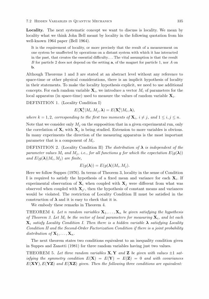
7.2 Hidden Variables in Quantum Mechanics 335

Locality. The next systematic concept we want to discuss is locality. We mean bylocality what we think John Bell meant by locality in the following quotation from hiswell-known 1964 paper (Bell 1964).

It is the requirement of locality, or more precisely that the result of a measurement on

one system be unaffected by operations on a distant system with which it has interacted

in the past, that creates the essential difficulty.. . . The vital assumption is that the result

B for particle 2 does not depend on the setting a, of the magnet for particle 1, nor A on

b.

Although Theorems 1 and 3 are stated at an abstract level without any reference tospace-time or other physical considerations, there is an implicit hypothesis of localityin their statements. To make the locality hypothesis explicit, we need to use additionalconcepts. For each random variable Xi, we introduce a vector Mi of parameters for thelocal apparatus (in space-time) used to measure the values of random variable Xi.

DEFINITION 1. (Locality Condition I)

E(Xki |Mi,Mj ,λ) = E(Xk

i |Mi,λ),

where k = 1, 2, corresponding to the first two moments of Xi, i = j, and 1 ≤ i, j ≤ n.

Note that we consider only Mj on the supposition that in a given experimental run, onlythe correlation of Xi with Xj is being studied. Extension to more variables is obvious.In many experiments the direction of the measuring apparatus is the most importantparameter that is a component of Mi.

DEFINITION 2. (Locality Condition II) The distribution of λ is independent of theparameter values Mi and Mj, i.e., for all functions g for which the expectation E(g(λ))and E(g(λ)|Mi,Mj) are finite,

E(g(λ)) = E(g(λ)|Mi,Mj).

Here we follow Suppes (1976). In terms of Theorem 3, locality in the sense of ConditionI is required to satisfy the hypothesis of a fixed mean and variance for each Xi. Ifexperimental observation of Xi when coupled with Xj were different from what wasobserved when coupled with Xj′ , then the hypothesis of constant means and varianceswould be violated. The restriction of Locality Condition II must be satisfied in theconstruction of λ and it is easy to check that it is.

We embody these remarks in Theorem 4.

THEOREM 4. Let n random variables X1, . . . ,Xn be given satisfying the hypothesisof Theorem 3. Let Mi be the vector of local parameters for measuring Xi, and let eachXi satisfy Locality Condition I. Then there is a hidden variable λ satisfying LocalityCondition II and the Second-Order Factorization Condition if there is a joint probabilitydistribution of X1, . . . ,Xn.

The next theorem states two conditions equivalent to an inequality condition givenin Suppes and Zanotti (1981) for three random variables having just two values.

THEOREM 5. Let three random variables X,Y and Z be given with values ±1 sat-isfying the symmetry condition E(X) = E(Y) = E(Z) = 0 and with covariancesE(XY), E(YZ) and E(XZ) given. Then the following three conditions are equivalent:

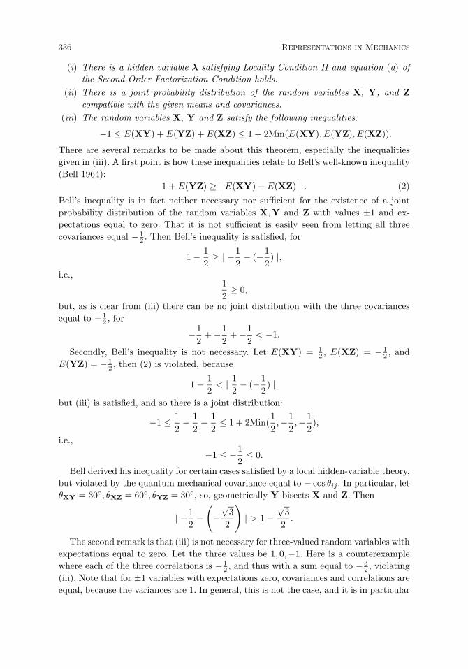
336 Representations in Mechanics

(i) There is a hidden variable λ satisfying Locality Condition II and equation (a) ofthe Second-Order Factorization Condition holds.

(ii) There is a joint probability distribution of the random variables X, Y, and Zcompatible with the given means and covariances.

(iii) The random variables X, Y and Z satisfy the following inequalities:

−1 ≤ E(XY) + E(YZ) +E(XZ) ≤ 1 + 2Min(E(XY), E(YZ), E(XZ)).

There are several remarks to be made about this theorem, especially the inequalitiesgiven in (iii). A first point is how these inequalities relate to Bell’s well-known inequality(Bell 1964):

1 +E(YZ) ≥ | E(XY) −E(XZ) | . (2)

Bell’s inequality is in fact neither necessary nor sufficient for the existence of a jointprobability distribution of the random variables X,Y and Z with values ±1 and ex-pectations equal to zero. That it is not sufficient is easily seen from letting all threecovariances equal −1

2 . Then Bell’s inequality is satisfied, for

1 − 12

≥ | −12

− (−12) |,

i.e.,12

≥ 0,

but, as is clear from (iii) there can be no joint distribution with the three covariancesequal to −1

2 , for

−12

+ −12

+ −12< −1.

Secondly, Bell’s inequality is not necessary. Let E(XY) = 12 , E(XZ) = −1

2 , andE(YZ) = −1

2 , then (2) is violated, because

1 − 12< | 1

2− (−1

2) |,

but (iii) is satisfied, and so there is a joint distribution:

−1 ≤ 12

− 12

− 12

≤ 1 + 2Min(12,−1

2,−1

2),

i.e.,

−1 ≤ −12

≤ 0.

Bell derived his inequality for certain cases satisfied by a local hidden-variable theory,but violated by the quantum mechanical covariance equal to − cos θij . In particular, letθXY = 30, θXZ = 60, θYZ = 30, so, geometrically Y bisects X and Z. Then

| −12

−(

−√

32

)| > 1 −

√3

2.

The second remark is that (iii) is not necessary for three-valued random variables withexpectations equal to zero. Let the three values be 1, 0,−1. Here is a counterexamplewhere each of the three correlations is −1

2 , and thus with a sum equal to −32 , violating

(iii). Note that for ±1 variables with expectations zero, covariances and correlations areequal, because the variances are 1. In general, this is not the case, and it is in particular

7.2 Hidden Variables in Quantum Mechanics 337

not the case for our counterexample. Except for the special case mentioned, inequalitiesshould be written in terms of correlations rather than covariances to have the propergenerality (see, e.g., Theorem 10 below).

There is a joint probability distribution with the following values. Let p(x, y, z) bethe probability of a given triple of values, e.g., (1,−1, 0). Then, of course, we must havefor all x, y and z

p(x, y, z) ≥ 0 and∑x,y,z

p(x, y, z) = 1,

where x, y and z each have the three values 1, 0,−1. So, let

p(−1, 0, 1) = p(1,−1, 0) = p(0, 1,−1) = p(1, 0,−1) = p(−1, 1, 0) = p(0,−1, 1) =16

and the other 21 p(x, y, z) = 0. Then it is easy to show that in this model E(X) =E(Y) = E(Z) = 0,Var(X) = Var(Y) = Var(Z) = 2

3 , and Cov(XY) = Cov(YZ) =Cov(XZ) = −1

3 , so that the correlations

ρ(XY) = ρ(YZ) = ρ(XZ) = −12.

The sum of the three correlations is then −32 .

It is a somewhat depressing mathematical fact that even for three random variableswith n-values and with expectations equal to zero, a separate investigation seems to beneeded for each n to find necessary and sufficient conditions to have a joint probabilitydistribution compatible with given means, variances and covariances. A more generalrecursive result would be highly desirable, but seems not to be known. Such results arepertinent to the study of multi-valued spin phenomena.

The next well-known theorem states two conditions equivalent to Bell’s Inequalitiesfor random variables with just two values. This form of the inequalities is due to Clauser,Horne, Shimony, and Holt(1969), referred to as CHSH. The equivalence of (ii) and (iii)is due to Fine (1982).

THEOREM 6. (Bell’s Inequalities). Let n random variables be given satisfying the lo-cality hypothesis of Theorem 4. Let n = 4, the number of random variables, let each Xi

be discrete with values ±1, let the symmetry condition E(Xi) = 0, i = 1, . . . , 4 be satis-fied, let X1 = A, X2 = A′, X3 = B, X4 = B′, with the covariances E(AB), E(AB′),E(A′B) and E(A′B′) given. Then the following three conditions are equivalent.

(i) There is a hidden variable λ satisfying Locality Condition II and equation (a) ofthe Second-Order Factorization Condition holds.

(ii) There is a joint probability distribution of the random variables A, A′, B and B′

compatible with the given means and covariances.(iii) The random variables A, A′, B and B′ satisfy Bell’s inequalities in the CHSH

form−2 ≤ E(AB) + E(AB′) +E(A′B) −E(A′B′) ≤ 2

−2 ≤ E(AB) + E(AB′) −E(A′B) +E(A′B′) ≤ 2

−2 ≤ E(AB) − E(AB′) +E(A′B) +E(A′B′) ≤ 2

−2 ≤ −E(AB) + E(AB′) +E(A′B) +E(A′B′) ≤ 2.

338 Representations in Mechanics

It will now be shown that the CHSH inequalities remain valid for three-valued ran-dom variables (spin-1 particles). Consider a spin-1 particle with the 3-state observables,A(a, λ) = +1, 0,−1, B(b, λ) = +1, 0,−1. λ is a hidden variable having a normalizedprobability density, ρ(λ). The expectation of these observables is defined as,

E(a, b) =∫ABρ(λ)dλ. (3)

We have suppressed the variable dependence on A and B for clarity. Consider thefollowing difference,

|E(a, b) − E(a, b′)| =∣∣∣∫ A[B −B′]ρ(λ)dλ

∣∣∣. (4)

Since the density ρ > 0 and |A| = 1, 0 we have the following inequality,

|E(a, b) − E(a, b′)| ≤∫

|A[B −B′]|ρ(λ)dλ, (5)

≤∫

|[B −B′]|ρ(λ)dλ. (6)

Similarly we have the following inequality,

|E(a′, b) +E(a′, b′)| =∣∣∣∫ A′[B +B′]ρ(λ)dλ

∣∣∣, (7)

≤∫

|[B +B′]|ρ(λ)dλ. (8)

Adding the two expressions we arrive at the following inequality,

|E(a, b) −E(a, b′)| + |E(a′, b) +E(a′, b′)|

=∫

(|[B −B′]| + |[B +B′]|)ρ(λ)dλ. (9)

The term in square brackets is equal to 2 in all cases except whenB andB′ are both equalto zero; there the right-hand side vanishes. With this and the normalization condition forthe hidden variable density, we have the same inequality as the spin-1

2 CHSH inequality,

|E(a, b) − E(a, b′)| + |E(a′, b) +E(a′, b′)| ≤ 2. (10)

Note that we could create a stronger inequality by adding the function 2(|E(a, b)| −1)(|E(a, b′)| − 1) to the left-hand side.

For higher spins we can proceed analogously and derive the following inequality whichmust be satisfied for spin-j particles,

|E(a, b) −E(a, b′)| + |E(a′, b) +E(a′, b′)| ≤ 2j. (11)

If we define normalized observables A(a,λ)j , the original CHSH inequality will need to

be satisfied for local hidden variable theories, although stronger inequalities could beconstructed.

In Peres’ work on higher spin particles, the observable is defined by a mapping fromthe multistate operator to a two-state operator (Peres 1992). Under this mapping it wasshown that Bell’s inequality is violated for certain parameter settings of the detectors.

GHZ-type experiments. Changing the focus, we now first consider a three-particleversion of GHZ-type experiments. All arguments known to us, in particular GHZ’s

7.2 Hidden Variables in Quantum Mechanics 339

(Greenberger, Horne and Zeilinger 1989) own argument, the more extended one inGreenberger, Horne, Shimony and Zeilinger (1990) and Mermin’s (1990a, 1993) pro-ceed by assuming the existence of a deterministic hidden variable and then deriving acontradiction. It follows immediately from Theorem 1 that the nonexistence of a hid-den variable is equivalent to the nonexistence of a joint probability distribution for thegiven observable random variables. The next theorem states this purely probabilisticGHZ result, and, more importantly, the proof is purely in terms of the observables, withno consideration of possible hidden variables.

THEOREM 7. Let A,B, and C be ±1 random variables having a joint probabilitydistribution such that E(A) = E(B) = E(C) = 1. Then E(ABC) = 1.

Proof. Since E(A) = 1, P (a) = P (abc) = P (abc) = P (abc) = P (abc) = 0, whereP (abc) = P (A = −1,B = 1,C = 1), etc. By similar argument for E(B) and E(C), weare left with P (abc) = 1, which implies at once the desired result.

I now follow the quantum-mechanical argument given in Mermin (1990b). We startwith the three-particle entangled state characteristic of GHZ-type experiments.

|ψ〉 =1√2(|+〉1|+〉2|+〉3 + |−〉1|−〉2|−〉3). (12)

This state is an eigenstate of the following spin operators:

A = σ1xσ2yσ3y, B = σ1yσ2xσ3y, (13)

C = σ1yσ2yσ3x, D = σ1xσ2xσ3x. (14)

If we compute quantum mechanically the expected values for the correlations above, weobtain at once that EQ(A) = EQ(B) = EQ(C) = 1 and EQ(D) = −1. (To exhibit allthe details of this setup is too lengthy to include here, but the argument is elementaryand standard, in the context of quantum mechanics.) Moreover,

EQ(ABC) = (s1xs2ys3y)(s1ys2xs3y)(s1ys2ys3x) (15)

= s1xs2xs3x(s21ys22ys

23y). (16)

Since the sij can only be 1 or −1, s21y = s22y = s23y = 1, and we obtain from (16) that

EQ(ABC) = s1xs2xs3x = EQ(D). (17)

So we have a contradiction. Classically

E(ABC) = 1

but quantum mechanicallyEQ(ABC) = −1.

It is clear from the above derivation that one could avoid contradictions if we allowed thevalue of λ to depend on the experimental setup, i.e., if we allowed λ to be a contextualhidden variable. In other words, what the GHZ theorem proves is that noncontextualhidden variables cannot reproduce quantum mechanical predictions.

Detector inefficiencies. This striking characteristic of GHZ’s predictions, however, hasa major problem. How can one verify experimentally predictions based on correlation-one statements, since experimentally one cannot obtain events perfectly correlated?

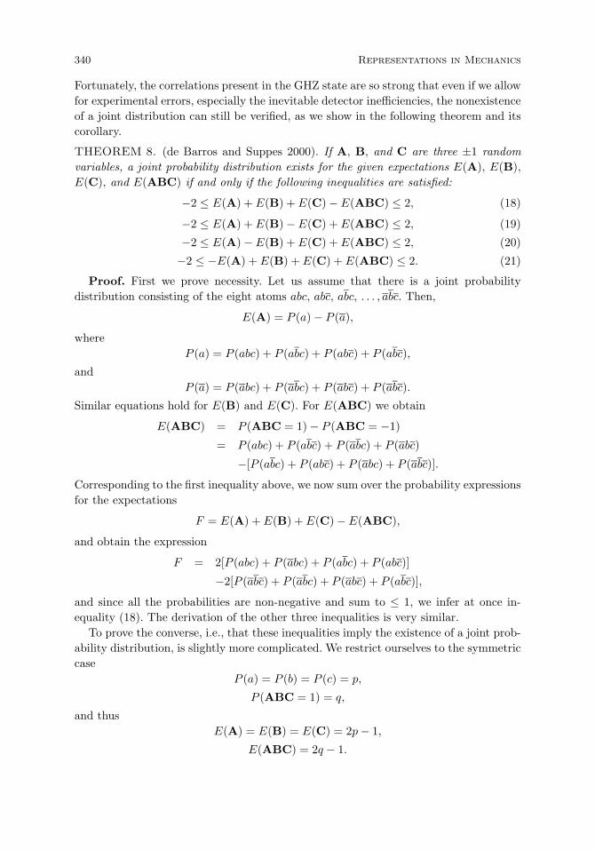
340 Representations in Mechanics

Fortunately, the correlations present in the GHZ state are so strong that even if we allowfor experimental errors, especially the inevitable detector inefficiencies, the nonexistenceof a joint distribution can still be verified, as we show in the following theorem and itscorollary.

THEOREM 8. (de Barros and Suppes 2000). If A, B, and C are three ±1 randomvariables, a joint probability distribution exists for the given expectations E(A), E(B),E(C), and E(ABC) if and only if the following inequalities are satisfied:

−2 ≤ E(A) + E(B) + E(C) −E(ABC) ≤ 2, (18)

−2 ≤ E(A) + E(B) − E(C) +E(ABC) ≤ 2, (19)

−2 ≤ E(A) − E(B) + E(C) +E(ABC) ≤ 2, (20)

−2 ≤ −E(A) +E(B) +E(C) + E(ABC) ≤ 2. (21)

Proof. First we prove necessity. Let us assume that there is a joint probabilitydistribution consisting of the eight atoms abc, abc, abc, . . . , abc. Then,

E(A) = P (a) − P (a),

whereP (a) = P (abc) + P (abc) + P (abc) + P (abc),

andP (a) = P (abc) + P (abc) + P (abc) + P (abc).

Similar equations hold for E(B) and E(C). For E(ABC) we obtain

E(ABC) = P (ABC = 1) − P (ABC = −1)

= P (abc) + P (abc) + P (abc) + P (abc)

−[P (abc) + P (abc) + P (abc) + P (abc)].

Corresponding to the first inequality above, we now sum over the probability expressionsfor the expectations

F = E(A) + E(B) + E(C) −E(ABC),

and obtain the expression

F = 2[P (abc) + P (abc) + P (abc) + P (abc)]

−2[P (abc) + P (abc) + P (abc) + P (abc)],

and since all the probabilities are non-negative and sum to ≤ 1, we infer at once in-equality (18). The derivation of the other three inequalities is very similar.

To prove the converse, i.e., that these inequalities imply the existence of a joint prob-ability distribution, is slightly more complicated. We restrict ourselves to the symmetriccase

P (a) = P (b) = P (c) = p,

P (ABC = 1) = q,

and thusE(A) = E(B) = E(C) = 2p− 1,

E(ABC) = 2q − 1.

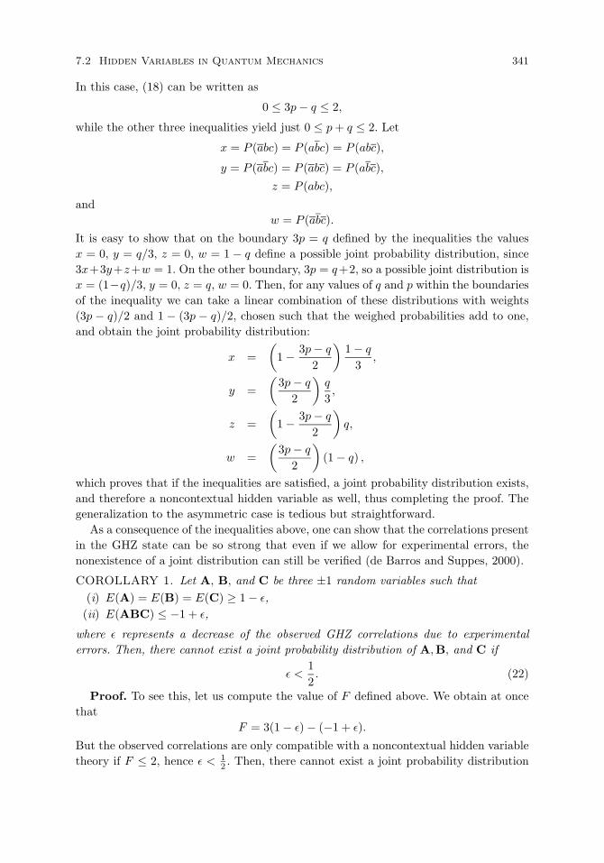
7.2 Hidden Variables in Quantum Mechanics 341

In this case, (18) can be written as

0 ≤ 3p− q ≤ 2,

while the other three inequalities yield just 0 ≤ p+ q ≤ 2. Let

x = P (abc) = P (abc) = P (abc),

y = P (abc) = P (abc) = P (abc),

z = P (abc),

andw = P (abc).

It is easy to show that on the boundary 3p = q defined by the inequalities the valuesx = 0, y = q/3, z = 0, w = 1 − q define a possible joint probability distribution, since3x+3y+z+w = 1. On the other boundary, 3p = q+2, so a possible joint distribution isx = (1−q)/3, y = 0, z = q, w = 0. Then, for any values of q and p within the boundariesof the inequality we can take a linear combination of these distributions with weights(3p − q)/2 and 1 − (3p − q)/2, chosen such that the weighed probabilities add to one,and obtain the joint probability distribution:

x =(

1 − 3p− q

2

)1 − q

3,

y =(

3p− q

2

)q

3,

z =(

1 − 3p− q

2

)q,

w =(

3p− q

2

)(1 − q) ,

which proves that if the inequalities are satisfied, a joint probability distribution exists,and therefore a noncontextual hidden variable as well, thus completing the proof. Thegeneralization to the asymmetric case is tedious but straightforward.

As a consequence of the inequalities above, one can show that the correlations presentin the GHZ state can be so strong that even if we allow for experimental errors, thenonexistence of a joint distribution can still be verified (de Barros and Suppes, 2000).

COROLLARY 1. Let A, B, and C be three ±1 random variables such that(i) E(A) = E(B) = E(C) ≥ 1 − ε,(ii) E(ABC) ≤ −1 + ε,

where ε represents a decrease of the observed GHZ correlations due to experimentalerrors. Then, there cannot exist a joint probability distribution of A,B, and C if

ε <12. (22)

Proof. To see this, let us compute the value of F defined above. We obtain at oncethat

F = 3(1 − ε) − (−1 + ε).

But the observed correlations are only compatible with a noncontextual hidden variabletheory if F ≤ 2, hence ε < 1

2 . Then, there cannot exist a joint probability distribution

342 Representations in Mechanics

of A, B, and C satisfying (i) and (ii) if

ε <12. (23)

From the inequality obtained above, it is clear that any experiment that obtainsGHZ-type correlations stronger than 0.5 cannot have a joint probability distribution.For example, the recent experiment made at Innsbruck (Bouwmeester et al., 1999) withthree-photon entangled states supports the quantum mechanical result that no noncon-textual hidden variable exists that explains their correlations. Thus, with this refor-mulation of the GHZ theorem it is possible to use strong, yet imperfect, experimentalcorrelations to prove that a noncontextual hidden-variable theory is incompatible withthe experimental results.

Second-order Gaussian theorems. A fundamental second-order representation the-orem about finite sequences of continuous random variables is the following:

THEOREM 9. Let n continuous random variables be given, let their means, variancesand covariances all exist and be finite, with all the variances nonzero. Then a necessaryand sufficient condition that a joint Gaussian probability distribution of the n randomvariables exists, compatible with the given means, variances and covariances, is that theeigenvalues of the correlation matrix be non-negative.

A thorough discussion and proof of this theorem can be found in Loeve (1978). It isimportant to note that the hypothesis of this theorem is that each pair of the randomvariables has enough postulated for there to exist a unique bivariate Gaussian distribu-tion with the given pair of means and variances and the covariance of the pair. Moreover,if, as required for a joint distribution of all n variables, the eigenvalues of the correlationmatrix are all non-negative, then there is a unique Gaussian joint distribution of the nrandom variables.

We formulate the next representation theorem to include cases like Bell’s inequalitieswhen not all the correlations or covariances are given.

THEOREM 10. Let n continuous random variables be given such that they satisfy thelocality hypothesis of Theorem 4, let their means and variances exist and be finite, withall the variances nonzero, and let m ≤ n(n − 1)/2 covariances be given and be finite.Then the following two conditions are equivalent.

(i) There is a joint probability distribution of the n random variables compatible withthe given means, variances and covariances.

(ii) Given the m ≤ n(n−1)/2 covariances, there are real numbers that may be assignedto the missing correlations so that the completed correlation matrix has eigenvaluesthat are all non-negative.

Moreover, (i) or (ii) implies that there is a hidden variable λ satisfying LocalityCondition II and the Second-Order Factorization Condition.

The proof of Theorem 10 follows directly from Theorem 9.Using Theorem 9, we can also derive a nonlinear inequality necessary and sufficient

for three Gaussian random variables to have a joint distribution. In the statement of

7.3 Weak and Strong Reversibility 343

the representation theorem ρ(X,Y) is the correlation of X and Y .

THEOREM 11. Let X,Y and Z be three Gaussian random variables whose means,variances and correlations are given, and whose variances are nonzero. Then there existsa joint Gaussian distribution of X,Y and Z (necessarily unique) compatible with thegiven means, variances and correlations if and only if

ρ(XY)2 + ρ(XZ)2 + ρ(YZ)2 ≤ 2ρ(XY)ρ(YZ)ρ(XZ) + 1.

The proof comes directly from the determinant of the correlation matrix. For a matrixto be non-negative definite the determinant of the entire matrix and all principal minorsmust be greater than or equal to zero,

Det

1 ρ(XY) ρ(XZ)ρ(XY) 1 ρ(YZ)ρ(XZ) ρ(YZ) 1

≥ 0. (24)

Including the conditions for the minors we have,

ρ(XY)2 + ρ(XZ)2 + ρ(YZ)2 − 2ρ(XY)ρ(XZ)ρ(YZ) ≤ 1

ρ(XY)2 ≤ 1

ρ(YZ)2 ≤ 1. (25)

The last two inequalities are automatically satisfied since the correlations are boundedby ±1.

Simultaneous observations and joint distributions. When observations are simultane-ous and the environment is stable and stationary, so that with repeated simultaneousobservations satisfactory frequency data can be obtained, then there exists a joint distri-bution of all of the random variables representing the simultaneous observations. Notewhat we can then conclude from the above: in all such cases there must be, therefore, afactorizing hidden variable because of the existence of the joint probability distribution.From this consideration alone, it follows that any of the quantum mechanical examplesthat violate Bell’s inequalities or other criteria for hidden variables must be such thatnot all the observations in question can be made simultaneously. The extension of thiscriterion of simultaneity to a satisfactory relativistic criterion is straightforward.

7.3 Weak and Strong Reversibility of Causal Processes13

It is widely known, and often commented upon, that the basic equations of classicalphysics remain valid under a transformation from time t to −t. It is often also remarkedthat this invariance under a change of direction of time is completely contrary to ordi-nary experience. So the invariance of well-established classical physics, as well as otherparts of physics, for example, relativistic mechanics and the Schrodinger equation inquantum mechanics, creates a natural philosophical tension about the nature of causalprocesses. The purpose of the present section is not to resolve in any complete way thistension between physics and ordinary experience, but to at least reduce the tension byintroducing two concepts of reversibility. The first is that of weak reversibility, which

13Most of the material in this section also appeared in Suppes (2001b).

344 Representations in Mechanics

is what is exemplified in the invariance of the equations of classical physics under timereversal. This is the weak sense of reversibility, because we can usually distinguish byobservation whether a system of particle mechanics is running one way or the other.The appearance is not the same when we go to a reversal of time. Elementary exampleswould be measuring the velocity of a particle accelerating from rest, moving in a straightline and hitting an impenetrable wall. The picture of change of velocity, especially, willbe very different under time reversal. Under such reversal, the particle has a very largevelocity immediately, as motion begins, and will continue to decelerate until it finallyreaches the state of rest, quite contrary to what would be observed in the usual direc-tion of time. Of course, this difference is well accepted in discussions of the invarianceof classical physics under time reversal.

The concept of strong reversibility introduced here, and used in various analyses ofa variety of natural phenomena, including stochastic processes, has a much strongercondition for reversibility. A process, deterministic or stochastic, is said to be stronglyreversible if we are unable to distinguish whether the process is running forward orbackward. To put it in vivid terms often used, the backward movie, that is, runningthe film in reverse, of the observation of the process, is indistinguishable by observationfrom the forward movie. In what follows, these ideas are made more precise, especiallyfor stochastic processes. I should mention that the concept of strong reversibility usedhere corresponds to what is often defined in the stochastic-process literature as simplyreversible. So the condition given below for a Markov chain to be strongly reversible isthe same as the standard concept to be found, for example, in Feller (1950, p. 342) forMarkov chains.

Although many of the formal distinctions introduced in what follows are familiarin the literature of probability theory, especially of stochastic processes, it is my im-pression that the distinction introduced here has not been sufficiently emphasized, asa distinction, in the philosophical discussions of time reversibility. Its introduction ismeant to reduce the tension I mentioned at the beginning, in the sense that there isa close alignment between ordinary experience not being strongly reversible, and, sim-ilarly, for many trajectories of idealized particles or other processes of importance inphysics.

Weak reversibility. As already remarked, it is well known that classical particle me-chanics and relativistic particle mechanics have the property of being weakly reversible,i.e., the transformation changing the direction of the time always carries systems of clas-sical particle mechanics into systems of classical particle mechanics and, correspondingly,for the relativistic case. Detailed proofs of these results are to be found in McKinseyand Suppes (1953) for classical particle mechanics and in Rubin and Suppes (1954) forrelativistic particle mechanics.

The proof that first-order Markov chains are carried into first-order Markov chainsunder time reversal is straightforward. Here is the elementary proof for first-order chainswith a finite number of states. In the proof it is assumed that all the probabilities thatoccur in the denominators of expressions have probability greater than zero.

7.3 Weak and Strong Reversibility 345

THEOREM 1. All first-order Markov chains are weakly reversible.

Proof. (for finite-state, discrete-time processes)

P (in−1 | jnkn+1) =P (in−1jnkn+1)

P (kn+1 | jn)P (jn)

=P (kn+1 | jn)P (jn | in−1)P (in−1)

P (kn+1 | jn)P (jn)

=P (jnin−1)P (jn)

= P (in−1 | jn).

The situation in quantum mechanics is somewhat more complicated concerning weakreversibility. Certainly, the Schrodinger equation is so reversible. It is weakly reversibleunder transformations changing the direction of time. On the other hand, in the standardaccounts, this is not true of the measurement process (von Neumann 1932/1955, Ch. 5).

Finally, from a common-sense standpoint, ordinary experience is certainly not weaklyreversible. Time has a fixed direction and the empirical evidence in terms of humanexperience of this direction is overwhelming.

Forward = Backward

People almost never walk up stairs backward. No races are run backward, etc. This isnot to claim the ‘backward movies’ violate laws of mechanics, only inductive laws andfacts of experience, most especially the universally accepted nature of human memory:

unknown future = known past.

Some definitions. Before going further, it is desirable to introduce some standardstochastic concepts, implicitly assumed in Theorem 1. First, let X(t) be a stochasticprocess such that for each time t, X(t) takes values in a finite set, a restriction im-posed only for simplicity of exposition. Any finite family X(t1),X(t2), . . . ,X(tn) has ajoint probability distribution. Using an obvious simplification of notation, a process is(first-order) Markov if and only if for any times t1 < t2, . . . , tn,

P (xn | xn−1, . . . , x1) = P (xn | xn−1), (1)

where the simplified notation is defined as follows:

P (xn | xn−1) = P (X(tn) = jn | X(tn−1) = in−1).

A Markov process is homogeneous if the transition probabilities such as (1) do notdepend on time, and it is irreducible if any state j can be reached from any other statein a finite number of steps. For a discrete-time homogeneous Markov process, I writethe transition probabilities in several different, but useful notations

Pij = pi,j = P (jn | in−1) = P (Xn = j | Xn−1 = i)= P (X(tn) = jn | X(tn−1) = in−1),

all of these often used in the probability literature.Let Pii(n) be the probability of returning to state i in n transitions. The period r(i)

of a state i is the greatest common divisor of the set of integers n for which Pii(n) > 0.A state is aperiodic if it has period 1. Moreover, it is easy to show that if a Markov

346 Representations in Mechanics

process is irreducible every state has the same period. So an aperiodic process is one inwhich every state has period 1.

Hereafter, when I refer to a Markov chain, I am assuming a Markov process that isfinite-state, discrete-time, homogeneous, irreducible and aperiodic.

The definitions of being Markov, homogeneous and irreducible all apply withoutchange to continuous-time processes, but there are some further conditions to imposeto avoid physically unlikely cases. First, we require such a process to remain in anystate for a positive length of time, and, second, the process cannot pass through aninfinite sequence of states in a finite time. Corresponding to the transition probabilityfor discrete-time processes, the transition rate for continuous-time processes is definedas:

qij = limτ→0

P (X(t+ τ) = j | X(t) = i)τ

, i = j,

and for definitional purposes, we set qii = 0. Hereafter, when I refer to a Markov process,I will mean a continuous-time one. Such a process remains in each state for a length oftime exponentially distributed with the parameter q(i) defined as:

q(i) =∑

j

qij ,

and when it leaves state i it moves to state j with the probability

pij =qijqi.

Note that in general ∑j

qij = 1,

i.e., transition rates from i to another state need not add up to 1, as must be the case fortransition probabilities from state i in the discrete-time processes. (A good discussionof such continuous-time processes may be found in Kelly (1979).)

Strong reversibility. The intuitive idea of strong reversibility is easily characterizedin terms of movies. A movie is strongly reversible if an observer cannot tell whetherthe movie is being run forward or backward. There is no perceptual difference in thetwo directions. Now, as our ordinary movie experience tells us at once, this is a prettyexceptional situation. On the other hand, there are important physical processes, afew of which we will discuss, that do have strong reversibility. An interesting case tobegin with is this. When is a Markov chain strongly reversible? The right setting forthis is to restrict ourselves at once to stationary, ergodic Markov chains. A Markovchain is stationary if its mean distribution is the same for all times. It is ergodic if ithas a unique asymptotic distribution independent of the initial distribution. Note thatunder these definitions, a Markov chain can be ergodic but not stationary if its initialdistribution is different from its unique, asymptotic one. But here I assume ergodicchains are stationary.

An ergodic Markov chain is strongly reversible if

πipij = πjpji (2)

7.3 Weak and Strong Reversibility 347

for all states i and j, where π is the unique asymptotic density. The equations (2) areoften called the detailed balance conditions for strong reversibility. Bernoulli processes,such as coin tossing, are strongly reversible processes, because there is no memory ofpast states: pij = pj and pji = pi, so we satisfy (2). Moreover, any 2-state ergodicMarkov chain is strongly reversible. Here is the proof. Since the process is ergodic

π1 = π1p11 + π2p21

= π1(1 − p12) + π2p21,

soπ1p12 = π2p21.

On the other hand, many 3-state chains are not strongly reversible. Here is an exampleof a three-color spinner.

B R Y

B 12

14

14

R 38

12

18

Y 18

38

12

We have at once for the mean density π of the three states:

πb = 12πb + 3

8πr + 18 (1 − πb − πr)

πr = 14πb + 1

2πr + 38 (1 − πb − πr);

solving the two equations, we find:

πb =1337, πr =

1437, πy =

1037.

Here is the proof that it is not strongly reversible:

πbpbr =1317

· 14

= 1437

· 38

= πrprb.

We can summarize what we have been saying about Markov chains in the followingtheorem, where in the notation of the theorem, d= means equal in distribution.

THEOREM 2. If an ergodic Markov chain is strongly reversible, then it is impossibleto distinguish whether a movie of it is running forward or backward, that is, any finitesequence of random variables of the process has the same distribution when the order ofthe random variables is reversed:

(X0,X1, . . .Xn) d= (Xn,Xn−1, . . .X0).

I give the proof for n = 2:

P (X0 = i,X1 =j) = P (X1 =j|X0 = i)P (X0 = i)

= πipij

= πjpji by (2)

= P (X1 = i|X0 =j)P (X0 =j)

= P (X1 = i,X0 =j).

The concepts introduced hold for finite-state continuous-time changes by replacing tran-sition probabilities by transition rates qij , i = j with qij ≥ 0, as defined above. The

348 Representations in Mechanics

detailed balance conditions defining strong reversibility are the same in form as thoseof (2) with the πi ≥ 0 and summing to 1, as before:

πiqij = πjqji. (3)

With a proof just like that of Theorem 2, we have at once:

THEOREM 3. If an ergodic continuous-time Markov process is strongly reversible,then it is impossible to distinguish whether a movie of it is running forward or backward.

In the present context, there is nothing special about first-order Markov chains. Asecond-order ergodic Markov chain is strongly reversible iff

πiπijpijk = πkπkjpkji, (4)

where a chain is second-order Markov if

P (xn | xn−1, . . . , x1) = P (xn | xn−1, xn−2),

corresponding to (1) for first-order.

THEOREM 4. If a second-order Markov chain is ergodic and strongly reversible, thenit is impossible to distinguish a movie of it running forward or backward, i.e.,

(X0,X1, . . .Xn) d= (Xn,Xn−1, . . .X0).

Proof for n = 3:

P (X0 = i,X1 = j,X2 = k)

= P (X2 = k|X1 = j,X0 = i)P (X1 = j|X0 = i)P (X0 = i)

= pijkπijπi

= πkπkjpkji by (4)

= P (X2 = i|X1 = j,X0 = k)P (X1 = j|X0 = k)P (X0 = k)

= P (X2 = i,X1 = j,X0 = k).

As is obvious, this proof also works for continuous-time second-order Markov processes.Without too much effort, this same sort of proof can be extended to chains of infiniteorder that are ergodic and stationary. The line of reasoning required is developed inLamperti and Suppes (1959).

Turning again from Markov chains to continuous-time Markov processes, simple ex-amples of strongly reversible processes are ergodic birth and death processes, definedby the transition rates being zero except for q(i, i + 1) > 0, representing a birth, andq(i, i − 1) > 0 representing a death. The detailed balance conditions (3) then assumethe form

πiqi,i+1 = πi+1qi+1,i, (5)

where the πi’s form the stationary probability density of the finite set of states.

Ehrenfest model. A simplified model of statistical mechanics nicely exemplifies abirth and death process that is strongly reversible. In the spirit of Maxwell’s demon,there are two containers of particles, thought of as ideal gas molecules. Let X(t) bethe number of particles in container I, and, so, k − X(t) is the number of particles in

7.3 Weak and Strong Reversibility 349

container II. The “birth and death” process corresponds to increasing or decreasing thenumber of particles in container I, with the transition rates being:

qi,i−1 = iλ, i = 1, 2, . . . , k,qi,i+1 = (k − i)λ, i = 0, 1, . . . , k − 1,

where λ is the rate parameter. The stationary density may be shown to be

πi = 2−k

(k

i

)i = 0, 1, . . . , k,

where (k

i

)=

k!(k − i)!i!

and 0! = 1.

That the process is strongly reversible may be seen by checking the detailed balanceconditions (5).

πiqi,i+1 = 2−k(ki

)(k − i)λ

= 2−kk!(k−i)λ(k−i)!i!

= 2−kk!λ(k−(i+1))!i! since k−i

(k−i)! = 1(k−(i+1))!

= 2−kk!(i+1)λ(k−(i+1))!(i+1)! since 1

i! = i+1(i+1)!

= 2−k(

ki+1

)(i+ 1)λ

= πi+1qi+1,i.

Without attempting a detailed discussion of entropy for this process, I note thateven though it is stationary and strongly reversible, the mean fluctuation from momentto moment is always stronger toward the equal distribution of particles in the twocontainers rather than away from this equal distribution, for

qi,i−1 = iλ < (k − i)λ = qi,i+1

if and only if i < k2 , independent of the rate parameter λ. If we compute the entropy by

the relative frequency f(t) at time t of the number of particles in container I, then the‘momentary’ entropy of the process at t is

H(t) = −(f(t) log f(t) + (1 − f(t)) log(1 − f(t))

and by the analysis just given the mean rate of change of entropy is always increasing,i.e., is positive, in spite of the strong reversibility of the process. But there is, obviously,no contradiction between these two features of the model, even at equilibrium, i.e.,when stationary. An excellent detailed analysis of the Ehrenfest model and also of theBoltzmann equation, and of the associated “paradoxes” of Loschmidt and Zermelo, isto be found in Kac (1959).

Deterministic systems. I now turn to deterministic classical physical systems. Itshould be evident enough that only very special ones are strongly reversible. Any sortof dissipative system will, in general, not be. A real billiard ball on a real table is notstrongly reversible. We start the motion and it comes to a halt somewhere, due to frictionon the table. We can easily distinguish the forward from the backward picture. On the

350 Representations in Mechanics

other hand, an idealized billiard ball on an idealized table with total conservation ofenergy and exact satisfaction of the equality of the angle of incidence and the angleof reflection can be put in periodic motion and, once in motion, will continue forever.Moreover, this idealized motion will, of course, be strongly reversible. By “observing”it, we cannot decide whether we are seeing the forward or the backward movie. (Iput ‘observing’ in scare quotes, for there is, in fact, no such billiard case, but we canartificially simulate it well for a finite period of time.)

A simple, but important, example of a classical system that has strong reversibilityis an undamped and undriven one-dimensional harmonic oscillator. The differentialequation for such an oscillator is:

d2x

dt2+ ω2x = 0,

where ω is the natural frequency of the oscillator when undamped and undriven, andthe initial conditions at time t = 0 are:

x0 = α,

dx0

dt= 0.

(When the model is a pendulum, the initial conditions correspond to the pendulumbeing at rest at time t = 0 with displacement α.) The general solution of (1) is:

x(t) = A cosωt+B sinωt,

anddx

dt= −Aω sinωt+Bω cosωt,

so at t = 0, B = 0, whence

A cosωt = α at t = 0, and A = α.

Thend2x

dt= −Aω2 cosωt

and finallyx(t) = A cosωt. (6)

We have at once that such an oscillator is strongly reversible, since for all t

x(−t) = A cos −ωt = A cosωt = x(t).

Notice that this solution holds for −∞ < t < ∞, and the conditions at t = 0 are notreally initial conditions, but just conditions for some t that yield a solution simple inform.

On the other hand, the damped, undriven harmonic oscillator, whose differentialequation is:

d2x

dt2+ 2k

dx

dt+ ω2x = 0,

where k is the damping coefficient, is easily shown not to be strongly reversible. Thisresult is scarcely surprising, since a damped oscillator (in one dimension) is one ofthe simplest physical examples of a dissipative system. In the standard case where thedamping is not too heavy, the oscillating function decreases in amplitude with time.

7.3 Weak and Strong Reversibility 351

More specifically the envelope of the oscillations is a negative exponential of the forme−kt on the positive side and −e−kt on the negative side.

Without question, if the aim is to find examples of systems in classical physics thatare not strongly reversible, and, therefore, the causal analysis is not strongly reversible,the place to look is among the many kinds of dissipative systems. The great prevalenceof such systems in nature reinforces our personal experience to support the common-sense view that, as the saying goes, “. . . of course time is not reversible. Who could everthink otherwise?”

8

Representations of Language

In this chapter various representations of languages, for example, context-free languages,are given. The first representations are in terms of automata of various strengths, andthe representations go both ways, i.e., languages in terms of automata, and automatarepresented by languages. That the two are so closely entwined is perhaps surprising,but understandable once the problem of how a language is to be parsed or compiledis raised. These matters occupy the first two sections. The content is now part of theeducation of every young computer scientist. I taught it for many years in the 1970s aspart of a course on the theory of automata.

The next two sections are more special and directly related to earlier work of my own.Section 3 is concerned to show how simple abstract ideas of conditioning and reinforce-ment are sufficient, when properly axiomatized, to show that stimulus-response struc-tures of learning can represent any finite automaton, and thereby the regular languagesthe automata can represent. The last part of the section extends the representation toany computable function via the stimulus-response representation of unlimited registermachines. It is probably true that most linguists are deeply skeptical that simple mech-anisms of association or conditioning are adequate to account for complex and subtlelinguistic phenomena. What is proved in this section will be too abstract mathemati-cally to persuade many of them, but that is not the task undertaken. The objective isjust to show in a rigorous way how “in principle” such a reduction can be made. Someof the kinds of further detailed work needed are to be found in Sections 5 and 6 of thischapter.

Section 4 focuses on the relation of stimulus-response models, as developed in theprevious section, to learning models formulated in terms only of behavioral variables.The main theorem is about the representation of the latter models in terms of the formerones. The long proof is testimony to the difficulties of proving detailed representationtheorems to reduce one theory to another, even for relatively simple cases. The rep-resentation theorem also has some interest in showing how models that have currentevents depending on the remote past can be represented by first-order Markov pro-cesses, once additional theoretical notions are introduced. Almost everyone believes, forexample, that any lasting effects of childhood events on an adult must be embodied inthe current physical and mental structure of the person, and not by direct, unmediatedaction of the events at a distance across the years. But describing in detail the current

353

354 Representations of Language

structural embodiment is not, for most cases, possible with the data and scientific con-cepts now available. The example of this section indicates the kind of considerationsthat must be entered into even in the most simplified cases of such structural analysis.

Section 5 is devoted to machine learning of robotic natural language. The phrase‘machine learning’ refers, in fact, to the development of computer programs that arelearning programs. Here the results of such learning are expressed as comprehensiongrammars that have an associated semantics. The relevant sense of representation is thatof learning how simple robotic commands are represented in any one of ten languages,English, Chinese (Mandarin), etc. This case study, as it were, is meant to show howa systematic fragment of a natural language can be learned by using principles that,broadly speaking, apply to human language learning as well. However, the machinelearning exemplified here is by no means meant to be a simulation of human languagelearning, as is evident enough from the details given in the section.

Section 6 turns away from learning to survey some of my own most recent work withyounger colleagues on language and the brain. The focus is on brain-wave representationsof words and sentences. The current work is aimed at trying to represent correctly howthe brain represents language, at least immediately after hearing or seeing some singlewords or sentences. Some interesting invariance results have already been found. A moregeneral aim of this section is to give a somewhat detailed sense of the methodology usedin these studies, especially the probabilistic aspects.

In this chapter no invariance theorems are stated or proved. Some are, of course,possible, but they lie outside the main development of the concepts and theories con-sidered. But some significant empirical invariances, found experimentally in the neuralprocessing of language, are presented in Section 6.

Section 7, the final one, is an epilogue on representation and reduction in science. Theremarks are mainly historical and are meant to provide a perspective on the detailedwork earlier in this chapter and those that preceded.

8.1 Hierarchy of Formal Languages

We begin with the definitions of formal languages much used in contemporary linguisticsand computer science. The basic concepts of this hierarchy are originally due to Chomsky(1959). We begin with the general concept of an arbitrary phrase-structure grammar.By adding restrictions we get grammars whose powers of expression are ever morerestricted.

Let V be a finite, nonempty set. Then V ∗ is the set of all finite sequences of elementsof V . Let ∅ be the empty sequence. Then V + = V ∗ − ∅. V is the vocabulary. V ∗

is the set of strings.

DEFINITION 1. A structure G = (V,N, P, S) is a phrase-structure grammar iff

1. V, N and P are nonempty finite sets,2. N ⊆ V ,3. P ⊆ V + × V ∗,4. S ∈ N .

The standard terminology is this. The set N is the set of nonterminal symbols, or

8.1 Hierarchy of Formal Languages 355

variables. VT = V−N is the set of terminal symbols or words. P is the set of productions.If (α, β) ∈ P we ordinarily write: α → β, to indicate that from α we may “produce”β. Finally, S is the start symbol with which derivations begin. The weakness of theaxioms matches the great generality of the definition of phrase-structure grammars.Most interest centers around various restricted classes defined below.

If γ and δ are in V ∗ then γαδ ⇒G γβδ iff α → β is a production, i.e., (α, β) ∈ P .We say in this case that the string γβδ is directly derivable from the string γαδ ingrammar G. We next define the notion of a derivation in a grammar in terms of directderivations. Intuitively a derivation is the way we show that a particular string belongsto the language generated by the grammar.

If γ1, γm ∈ V ∗, then γ1 ⇒∗G γm iff ∃γ2, . . . , γm−1 ∈ V ∗ such that γ1 ⇒G

γ2, . . . , γm−1 ⇒G γm. The language generated by a grammar G, denoted L(G), is:

L(G) = w|w ∈ V ∗T & S ⇒∗

G w.

Note that for a string to be in the language it must consist only of terminal words andits derivation in G must begin with the start symbol S.

We say that two grammars G1 and G2 are weakly equivalent if and only if theygenerate the same language, i.e., L(G1) = L(G2). Notice that this does not say verymuch about the structure of the utterances. It is just that they produce the same set ofstrings without attention to structure.

An important application of formal languages is to the analysis of the structureof natural languages. Indeed, it can be claimed that natural languages fit within thehierarchy that we shall be defining. The rather complicated question of whether this istrue in any satisfactory way will not really be examined here. Certainly the evidenceis substantial that important fragments of natural languages can be analyzed with thegrammatical concepts introduced in this section. We now consider one simple example.

N = S,NP, V P, PN,AdjP,Adj, CN,Art, IV, TV ,

where S is the start symbol, NP is for noun phrases, VP for verb phrases, PN forproper nouns, AdjP for adjectival phrases, Adj for adjectives, CN for common nouns,Art for articles, IV for intransitive verbs, and TV for transitive verbs.VT = you pick the terminal English words with their usual grammatical categories,P = the following set of production rules, with the lexical rules omitted for the

terminal words—a lexical rule is one whose right-hand member is a terminal word:

1. S → NP + V P 5. AdjP → Adj

2. NP → PN 6. AdjP → Art

3. NP → AdjP + CN 7. V P → IV

4. AdjP → AdjP +Adj 8. V P → TV +NP.

These rules should seem familiar but of course incomplete. In stating the rules the plussign is used just to show concatenation, in order to avoid confusion in concatenation ofstrings.

356 Representations of Language

Here is a sample derivation.

1. S Start symbol2. NP + VP By Rule 13. AdjP + CN + VP By Rule 34. AdjP + Adj + CN + VP By Rule 45. Art + Adj + CN + VP By Rule 66. Art + Adj + CN + TV + NP By Rule 87. Art + Adj + CN + TV + PN By Rule 28. The large ball hit John By Lexical Rules.

In many respects more natural than a linear derivation is the derivation tree. Theexample just given generates the following tree.

S

NP VP

AdjP CN TV NP

AdjP Adj PN

Art

The large ball hit John

We shall not formally define derivation trees in spite of their importance for context-freegrammars.

Types of grammars. We turn now to types of grammar. Type-0 grammars are char-acterized by Definition 1. To obtain a type-1 or context-sensitive grammar, we add therestriction that for every production α → β, |α| ≤ |β|, where |α| is the length of α, orthe number of symbols in α. This restriction can be shown equivalent to

α1Aα2 → α1βα2

with β = ∅ and A ∈ N .To obtain type-2 or context-free grammars, we add the stronger restriction: if α →

β ∈ P then

(i) α is a variable, i.e., α ∈ N , so productions are of the form A → β,(ii) β = ∅.

To obtain type-3 or regular grammars, we add the still stronger restriction: any pro-duction must be of the form

(i) A → aB or(ii) A → a,

with A,B ∈ N, a ∈ VT . (We can have instead of (i), (i′)A → Ba, but the change fromright-linear to left-linear is trivial, even though all rules of form (i) must be changed.)

8.1 Hierarchy of Formal Languages 357

Note that we could write (i) as A → a + B, to show the familiar use of the plus signto denote concatenation in writing individual rules. The definitions of context-sensitive,context-free, and regular grammars are such that the languages they generate excludethe empty string, which is not true of type-0 grammars as such. For some technicalpurposes it is desirable not to make this exclusion, but it simplifies the exposition to doso here.

For an example of a regular grammar, we may slightly change our previous example,by making VT just the symbols of the grammatical categories of some words.

N = S,NP, V P,AdjPVT = PN,CN,Adj,Art, IV, TV .

If we drop Rule 8 and rewrite Rule 1 as 1′, S → NP + IV , we can immediately checkthat the grammar is regular. To rewrite Rule 8 is more troublesome and requires morevariables, i.e., elements of N . I only sketch the attack. We add rules like these

S → X + CN

X → Y +Adj

X → Y +Art

Y → V P ′ +Adj

Y → V P ′ +Art

V P ′ → TV.

In general, it is not easy to see if a language has a grammar of a given type.The abstractness of the definitions of various types of phrase-structure grammars is

typical of what happens in every area of science when theories are axiomatically definedas certain set-theoretical predicates. Without further restrictions on the kinds of objectsthat may occur in the sets of vocabulary, etc., intuitively very odd grammars can beconstructed—odd not because of their structural characteristics but because of theirmaterial features.

In this section a few important theorems about the types of grammars defined areconsidered. I first state some results on normal forms for grammars of a given lan-guage, then some theorems about set-theoretical operations on languages, followed by asample of results on unsolvable problems and problems of ambiguity. An important po-tential natural-language application of context-sensitive languages as defined by lexical-functional grammars is the final topic touched on in this section.

It is not my intention to give anything like a thorough development of formal lan-guages in this chapter, but only a sense of the kinds of questions that have been inves-tigated for these theoretical structures.

Normal forms. I begin with a theorem about context-sensitive and type-0 languages.Note that a language is context-sensitive, for example, if there is at least one context-sensitive grammar that generates the language.

THEOREM 1. Every context-sensitive language can be generated by a grammar inwhich all productions are of the form a → b, where a and b are strings of variablesonly, or of the form A → b, where A is a variable and b is a terminal word. Moreover,

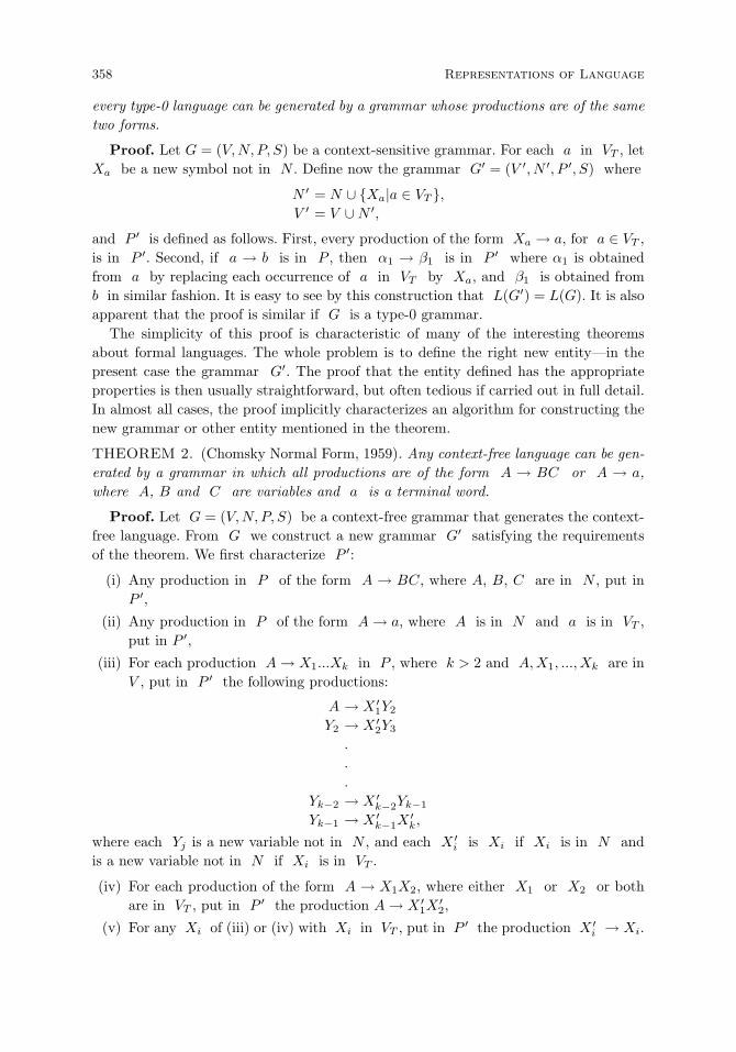
358 Representations of Language

every type-0 language can be generated by a grammar whose productions are of the sametwo forms.

Proof. Let G = (V,N, P, S) be a context-sensitive grammar. For each a in VT , letXa be a new symbol not in N . Define now the grammar G′ = (V ′, N ′, P ′, S) where

N ′ = N ∪ Xa|a ∈ VT ,V ′ = V ∪N ′,

and P ′ is defined as follows. First, every production of the form Xa → a, for a ∈ VT ,is in P ′. Second, if a → b is in P , then α1 → β1 is in P ′ where α1 is obtainedfrom a by replacing each occurrence of a in VT by Xa, and β1 is obtained fromb in similar fashion. It is easy to see by this construction that L(G′) = L(G). It is alsoapparent that the proof is similar if G is a type-0 grammar.

The simplicity of this proof is characteristic of many of the interesting theoremsabout formal languages. The whole problem is to define the right new entity—in thepresent case the grammar G′. The proof that the entity defined has the appropriateproperties is then usually straightforward, but often tedious if carried out in full detail.In almost all cases, the proof implicitly characterizes an algorithm for constructing thenew grammar or other entity mentioned in the theorem.

THEOREM 2. (Chomsky Normal Form, 1959). Any context-free language can be gen-erated by a grammar in which all productions are of the form A → BC or A → a,where A, B and C are variables and a is a terminal word.

Proof. Let G = (V,N, P, S) be a context-free grammar that generates the context-free language. From G we construct a new grammar G′ satisfying the requirementsof the theorem. We first characterize P ′:

(i) Any production in P of the form A → BC, where A, B, C are in N , put inP ′,

(ii) Any production in P of the form A → a, where A is in N and a is in VT ,put in P ′,

(iii) For each production A → X1...Xk in P , where k > 2 and A,X1, ..., Xk are inV , put in P ′ the following productions:

A → X ′1Y2

Y2 → X ′2Y3

.

.

.

Yk−2 → X ′k−2Yk−1

Yk−1 → X ′k−1X

′k,

where each Yj is a new variable not in N , and each X ′i is Xi if Xi is in N and

is a new variable not in N if Xi is in VT .

(iv) For each production of the form A → X1X2, where either X1 or X2 or bothare in VT , put in P ′ the production A → X ′

1X′2,

(v) For any Xi of (iii) or (iv) with Xi in VT , put in P ′ the production X ′i → Xi.

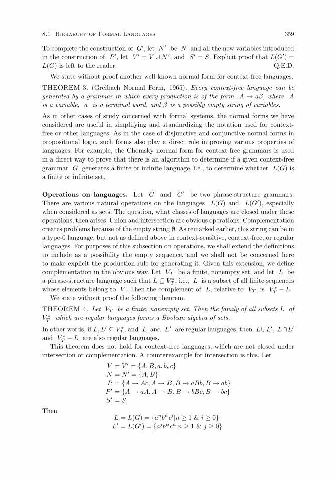
8.1 Hierarchy of Formal Languages 359

To complete the construction of G′, let N ′ be N and all the new variables introducedin the construction of P ′, let V ′ = V ∪N ′, and S′ = S. Explicit proof that L(G′) =L(G) is left to the reader. Q.E.D.

We state without proof another well-known normal form for context-free languages.

THEOREM 3. (Greibach Normal Form, 1965). Every context-free language can begenerated by a grammar in which every production is of the form A → aβ, where A

is a variable, a is a terminal word, and β is a possibly empty string of variables.

As in other cases of study concerned with formal systems, the normal forms we haveconsidered are useful in simplifying and standardizing the notation used for context-free or other languages. As in the case of disjunctive and conjunctive normal forms inpropositional logic, such forms also play a direct role in proving various properties oflanguages. For example, the Chomsky normal form for context-free grammars is usedin a direct way to prove that there is an algorithm to determine if a given context-freegrammar G generates a finite or infinite language, i.e., to determine whether L(G) isa finite or infinite set.

Operations on languages. Let G and G′ be two phrase-structure grammars.There are various natural operations on the languages L(G) and L(G′), especiallywhen considered as sets. The question, what classes of languages are closed under theseoperations, then arises. Union and intersection are obvious operations. Complementationcreates problems because of the empty string ∅. As remarked earlier, this string can be ina type-0 language, but not as defined above in context-sensitive, context-free, or regularlanguages. For purposes of this subsection on operations, we shall extend the definitionsto include as a possibility the empty sequence, and we shall not be concerned hereto make explicit the production rule for generating it. Given this extension, we definecomplementation in the obvious way. Let VT be a finite, nonempty set, and let L bea phrase-structure language such that L ⊆ V ∗

T , i.e., L is a subset of all finite sequenceswhose elements belong to V . Then the complement of L, relative to VT , is V ∗

T − L.We state without proof the following theorem.

THEOREM 4. Let VT be a finite, nonempty set. Then the family of all subsets L ofV ∗

T which are regular languages forms a Boolean algebra of sets.

In other words, if L,L′ ⊆ V ∗T , and L and L′ are regular languages, then L∪L′, L∩L′

and V ∗T − L are also regular languages.

This theorem does not hold for context-free languages, which are not closed underintersection or complementation. A counterexample for intersection is this. Let

V = V ′ = A,B, a, b, cN = N ′ = A,BP = A → Ac,A → B,B → aBb,B → abP ′ = A → aA,A → B,B → bBc,B → bcS′ = S.

ThenL = L(G) = anbnci|n ≥ 1 & i ≥ 0L′ = L(G′) = ajbncn|n ≥ 1 & j ≥ 0.

360 Representations of Language

ButL(G) ∩ L(G′) = anbncn|n ≥ 1,

and the language L(G)∩L(G′) is a standard example of a language that is not context-free, a fact I shall not prove here (for details, see Aho and Ullman 1972, vol. 1, pp.195–196). Context-free languages are closed under union, a fact which we shall returnto. So it follows by the counterexample just given that they cannot be closed undercomplementation, for

L ∩ L′ = −(−L ∪ −L′).

We define the product or concatenation of two languages L and L′ by

LL′ = x|x = uv, u is in L, v is in L′.

We then have the following theorem for all four types of languages. The proof is ratherlong and is therefore omitted.

THEOREM 5. Let VT be a finite, nonempty set. Then the families of regular, context-free, context-sensitive and type-0 languages that are subsets of V ∗

T are each closed underunion and concatenation.

Unsolvable problems. A problem about formal languages is said to be unsolvableiff there is no algorithm or mechanical decision procedure for deciding it. Problems ofthis kind are ordinarily said to be undecidable in logic. For example, it is undecidablewhether any arbitrarily given sentence in elementary number theory is provable—oneof Godel’s famous results. It is even undecidable whether an arbitrary formula of first-order logic is valid—a result due to Church and, independently, Turing. Here are somesample results for context-free languages–for a more detailed discussion, see Hopcroftand Ullman (1969, Ch. 14):

(i) It is unsolvable whether or not the intersection of two arbitrary context-free lan-guages is empty;

(ii) It is unsolvable whether or not a context-free grammar generates the set of allstrings over its terminal vocabulary;

(iii) It is unsolvable whether or not two context-free grammars generate the samelanguage.

We turn now to some results about ambiguity. We first define the concept of a leftmostderivation. We say that a derivation is leftmost iff at every step (n) the variable beingreplaced by a production rule of the grammar has no variable to its left in the string ofstep (n). For example, if in a derivation, step (n) has string BA and the productionrule A → a is used to derive as step (n + 1) the string Ba, the derivation is notleftmost. It can be shown that any derivation of a terminal string u in a context-freegrammar can be replaced by a leftmost derivation of u. A context-free grammar G

is said to be ambiguous iff there is a string in L(G) that has at least two distinctleftmost derivations. A context-free language L is said to be inherently ambiguous iffevery context-free grammar generating L is ambiguous. The following theorem aboutambiguity can then be proved.

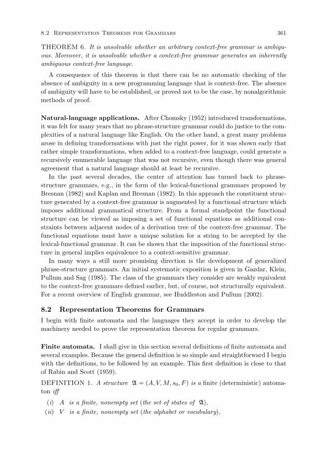
8.2 Representation Theorems for Grammars 361

THEOREM 6. It is unsolvable whether an arbitrary context-free grammar is ambigu-ous. Moreover, it is unsolvable whether a context-free grammar generates an inherentlyambiguous context-free language.

A consequence of this theorem is that there can be no automatic checking of theabsence of ambiguity in a new programming language that is context-free. The absenceof ambiguity will have to be established, or proved not to be the case, by nonalgorithmicmethods of proof.

Natural-language applications. After Chomsky (1952) introduced transformations,it was felt for many years that no phrase-structure grammar could do justice to the com-plexities of a natural language like English. On the other hand, a great many problemsarose in defining transformations with just the right power, for it was shown early thatrather simple transformations, when added to a context-free language, could generate arecursively enumerable language that was not recursive, even though there was generalagreement that a natural language should at least be recursive.

In the past several decades, the center of attention has turned back to phrase-structure grammars, e.g., in the form of the lexical-functional grammars proposed byBresnan (1982) and Kaplan and Bresnan (1982). In this approach the constituent struc-ture generated by a context-free grammar is augmented by a functional structure whichimposes additional grammatical structure. From a formal standpoint the functionalstructure can be viewed as imposing a set of functional equations as additional con-straints between adjacent nodes of a derivation tree of the context-free grammar. Thefunctional equations must have a unique solution for a string to be accepted by thelexical-functional grammar. It can be shown that the imposition of the functional struc-ture in general implies equivalence to a context-sensitive grammar.

In many ways a still more promising direction is the development of generalizedphrase-structure grammars. An initial systematic exposition is given in Gazdar, Klein,Pullum and Sag (1985). The class of the grammars they consider are weakly equivalentto the context-free grammars defined earlier, but, of course, not structurally equivalent.For a recent overview of English grammar, see Huddleston and Pullum (2002).

8.2 Representation Theorems for Grammars

I begin with finite automata and the languages they accept in order to develop themachinery needed to prove the representation theorem for regular grammars.

Finite automata. I shall give in this section several definitions of finite automata andseveral examples. Because the general definition is so simple and straightforward I beginwith the definitions, to be followed by an example. This first definition is close to thatof Rabin and Scott (1959).

DEFINITION 1. A structure A = (A, V,M, s0, F ) is a finite (deterministic) automa-ton iff

(i) A is a finite, nonempty set (the set of states of A),(ii) V is a finite, nonempty set (the alphabet or vocabulary),

362 Representations of Language

(iii) M is a function from the Cartesian product A×V to A (M defines the transitiontable of A),

(iv) s0 is in A (s0 is the initial state of A),

(v) F is a subset of A (F is the set of final states of A).

The generality of this definition is apparent. It is also indicative of the weakness ina certain sense of the general notion of a finite automaton. About the only restrictionsare that the sets A and V be finite. On the other hand, these finite restrictions arecritical.

It is evident that we can have some extremely trivial models of Definition 1. Here isthe simplest: A = s0, V = 0,M(s0, 0) = s0, F = .

Perhaps the simplest nontrivial example of a finite automaton is the following. Wehave a two-letter alphabet, which we may as well take to be the symbols ‘1’ and ‘0’,and two internal states, which we may take to be s0 and s1. The transition functionof the automaton is defined by the following table:

s0 s1s00

√

s01√

s10√

s11√

Finally, we select the internal state s1 as the only member of the set F of finalstates. I have said that this is the simplest nontrivial automaton. I mean by this thatthe transition table depends both on the internal state and the input letter. From amore general conceptual standpoint, it is clear that the device is itself pretty trivial.

If we examine our ordinary experience for instances of finite automata that are notquite so trivial, that do important jobs and yet that are simple enough to describe rathereasily and quickly, it is pretty clear that one of the most evident areas of application isthat of elementary arithmetic. Intuitively most of us recognize that there is somethingmechanical or algorithmic about the arithmetical operations we are taught to performin elementary school. Without any formal definitions it is clear in a general way thatthe standard algorithms of arithmetic can be defined in a completely objective andmechanical fashion and the work can be turned over to a machine that is not veryclever at all. In fact, in an intuitive sense the machine has no cleverness whatsoeverbecause it always does exactly the same thing when presented with a similar situationand there is no consideration of strategy or contingencies whatsoever in its makeup.What I have said here is vague, but I intend to convey an intuitive idea we all have afairly good grasp of.

There is one trouble about Definition 1 when we consider our ordinary way of doingarithmetic. We are expected to output an answer, and not simply to move into a finalstate. For theoretical work and for a good many applications Definition 1 has greatsimplicity. However, it is also natural to seek a second closely related definition. Laterwe shall study briefly the relation between these two definitions. In this new definitionwe eliminate the set of final states and introduce an output function as well as an outputvocabulary or alphabet.

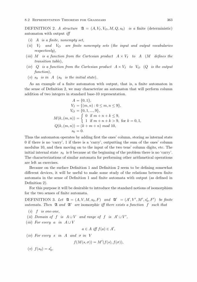
8.2 Representation Theorems for Grammars 363

DEFINITION 2. A structure A = (A, VI , VO,M,Q, s0) is a finite (deterministic)automaton with output iff

(i) A is a finite, nonempty set,(ii) VI and VO are finite nonempty sets (the input and output vocabularies

respectively),(iii) M is a function from the Cartesian product A × VI to A (M defines the

transition table),(iv) Q is a function from the Cartesian product A × VI to VO (Q is the output

function),(v) s0 is in A (s0 is the initial state).

As an example of a finite automaton with output, that is, a finite automaton inthe sense of Definition 2, we may characterize an automaton that will perform columnaddition of two integers in standard base-10 representation.

A = 0, 1,VI = (m,n) : 0 ≤ m,n ≤ 9,VO = 0, 1, ..., 9,

M(k, (m,n)) =

0 if m+ n+ k ≤ 9,1 if m+ n+ k > 9, for k = 0, 1,

Q(k, (m,n)) = (k +m+ n) mod 10,s0 = 0.

Thus the automaton operates by adding first the ones’ column, storing as internal state0 if there is no ‘carry’, 1 if there is a ‘carry’, outputting the sum of the ones’ columnmodulus 10, and then moving on to the input of the two tens’ column digits, etc. Theinitial internal state s0 is 0 because at the beginning of the problem there is no ‘carry’.The characterizations of similar automata for performing other arithmetical operationsare left as exercises.

Because on the surface Definition 1 and Definition 2 seem to be defining somewhatdifferent devices, it will be useful to make some study of the relations between finiteautomata in the sense of Definition 1 and finite automata with output (as defined inDefinition 2).

For this purpose it will be desirable to introduce the standard notions of isomorphismfor the two senses of finite automata.

DEFINITION 3. Let A = (A, V,M, s0, F ) and A′ = (A′, V ′,M ′, s′0, F′) be finite

automata. Then A and A′ are isomorphic iff there exists a function f such that

(i) f is one-one,(ii) Domain of f is A ∪ V and range of f is A′ ∪ V ′,(iii) For every a in A ∪ V

a ∈ A iff f(a) ∈ A′,

(iv) For every s in A and σ in V

f(M(s, σ)) = M ′(f(s), f(σ)),

(v) f(s0) = s′0,

364 Representations of Language

(vi) For every s in A

s ∈ F iff f(s) ∈ F ′.

It is apparent that conditions (i)-(iii) of the definition imply that for every a in A∪Va ∈ V if and only if f(a) ∈ V ′,

and consequently this condition on V need not be stated. From the standpoint of thegeneral algebraic or set-theoretical concept of isomorphism, it would have been morenatural to define an automaton in terms of a basic set B = A ∪ V , and then requirethat A and V both be subsets of B. Rabin and Scott (1959) avoid the problem bynot making V a part of the automaton. They define the concept of an automaton A

= (A,M, s0, F ) with respect to an alphabet V , but for our purposes it is also desirableto include the alphabet V in the definition of A in order to make explicit the naturalplace of the alphabet in the general scheme of things, and above all, to provide a simplesetup for going from one alphabet V to another V ′. In any case, exactly how thesematters are handled is not of central importance.

DEFINITION 4. Let A = (A, VI , VO,M,Q, s0) and A′ = (A′, V ′I , V

′O,M

′, Q′, s′0) befinite automata with output. Then A and A′ are isomorphic iff there exists a functionf such that

(i) f is one-one,(ii) Domain of f is A ∪ VI ∪ VO and range of f is A′ ∪ V ′

I ∪ V ′O,

(iii) For every s in A ∪ VI ∪ VO

s ∈ A iff f(s) ∈ A′,

(iv) For every σ in A ∪ VI ∪ VO

σ ∈ VI iff f(σ) ∈ V ′I ,

(v) For every s in A and σ in VI

f(M(s, σ)) = M ′(f(s), f(σ)),

(vi) For every s in A and σ in VI

f(Q(s, σ)) = Q′(f(s), f(σ)),

(vii) f(s0) = s′0.

Definitions 3 and 4 are so similar it is somewhat redundant to write them bothout explicitly. However, with both definitions in front of us it should be apparent thatgeneral set-theoretical methods for defining the isomorphism of like structures applyhere as well. In the usual sense the two definitions of isomorphism are axiom-free, inthe sense that they do not depend on the substantive assumptions in Definition 1 or 2.As has already been remarked, these assumptions are just the assumptions of finiteness.For this reason the axiom-free character of the definitions of isomorphism is not tooevident in these two instances.

Languages accepted by finite automata. We want to describe the language thata given finite automaton can accept or recognize. The definitions given at this point arefor a finite automaton A = (A, V,M, s0, F ), in the sense of Definition 1.

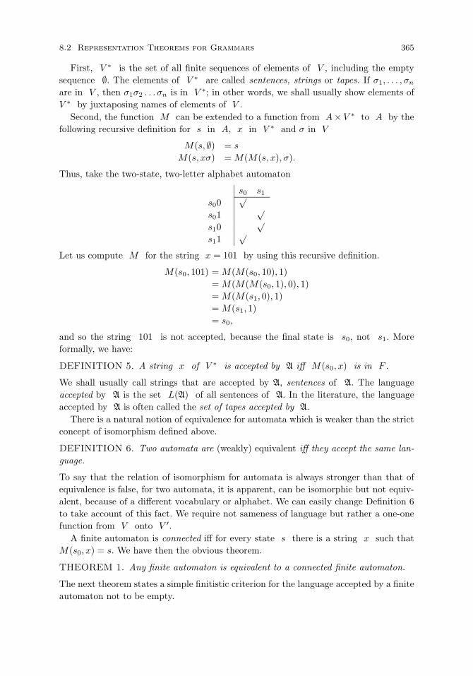
8.2 Representation Theorems for Grammars 365

First, V ∗ is the set of all finite sequences of elements of V , including the emptysequence ∅. The elements of V ∗ are called sentences, strings or tapes. If σ1, . . . , σn

are in V , then σ1σ2 . . . σn is in V ∗; in other words, we shall usually show elements ofV ∗ by juxtaposing names of elements of V .

Second, the function M can be extended to a function from A× V ∗ to A by thefollowing recursive definition for s in A, x in V ∗ and σ in V

M(s, ∅) = s

M(s, xσ) = M(M(s, x), σ).

Thus, take the two-state, two-letter alphabet automaton

s0 s1s00

√

s01√

s10√

s11√

Let us compute M for the string x = 101 by using this recursive definition.

M(s0, 101) = M(M(s0, 10), 1)= M(M(M(s0, 1), 0), 1)= M(M(s1, 0), 1)= M(s1, 1)= s0,

and so the string 101 is not accepted, because the final state is s0, not s1. Moreformally, we have:

DEFINITION 5. A string x of V ∗ is accepted by A iff M(s0, x) is in F .

We shall usually call strings that are accepted by A, sentences of A. The languageaccepted by A is the set L(A) of all sentences of A. In the literature, the languageaccepted by A is often called the set of tapes accepted by A.

There is a natural notion of equivalence for automata which is weaker than the strictconcept of isomorphism defined above.

DEFINITION 6. Two automata are (weakly) equivalent iff they accept the same lan-guage.

To say that the relation of isomorphism for automata is always stronger than that ofequivalence is false, for two automata, it is apparent, can be isomorphic but not equiv-alent, because of a different vocabulary or alphabet. We can easily change Definition 6to take account of this fact. We require not sameness of language but rather a one-onefunction from V onto V ′.

A finite automaton is connected iff for every state s there is a string x such thatM(s0, x) = s. We have then the obvious theorem.

THEOREM 1. Any finite automaton is equivalent to a connected finite automaton.

The next theorem states a simple finitistic criterion for the language accepted by a finiteautomaton not to be empty.

366 Representations of Language

THEOREM 2. The set of sentences accepted by a finite automaton with n states isnonempty iff the finite automaton accepts a sentence of length less than n.

Proof. If a word of length less than n is accepted, then the language is nonempty,and by way of contradiction, let the smallest sentence w accepted be of length ≥n. The first point to note is that A must pass through some state at least twice inprocessing w—this follows at once from the definition of M for any string. Let thisstate be s. We can break up w then into three parts with

w = w1w2w3

and w2 = ∅, and by assumption on s

M(s0, w1) = M(s, w2) = s,

andM(s, w3) ∈ F.

Now either w1 or w3 = ∅, for otherwise w2 = w and we have not broken up w

properly in terms of repetitions of s. So we now have

M(s0, w1w3) = M(s0, w1w2w3) ∈ F,

and|w1w3| < |w1w2w3|,

contrary to supposition. Q.E.D.More surprising, there also exists a strict finitistic test of when the language accepted

by a finite automaton is infinite.

THEOREM 3. The language (i.e., set of sentences) accepted by a finite automatonwith n states is infinite iff the automaton accepts a sentence w of length equal to orgreater than n and less than 2n, i.e., n ≤ |w| < 2n.

Proof. First, assume there is a sentence w accepted and n ≤ |w| < 2n. Then as inthe proof of Theorem 2, we can find a repeated state s such that

w = w1w2w3

w2 = ∅M(s0, w1) = M(s, w2) = s

M(s, w3) = F.

It then follows that for all i,w1w

i2w3

is accepted, where wi is a string of w’s of length i, and this set of sentences is clearlyinfinite.

On the other hand, let us now assume that A accepts an infinite number of sentencesbut none is of length between n and 2n − 1 (inclusive). Let w be a sentence ofminimum length ≥ 2n that is accepted. Then by the argument given in the proof ofTheorem 2 we can find a repeated state s and a sentence w2 of length 1 ≤ |w2| < n

such thatw = w1w2w3

8.2 Representation Theorems for Grammars 367

and w1w3 is accepted. Then either n ≤ |w1w3| < 2n, or the argument can berepeated if |w1w3| ≤ 2n. In a finite number of steps we will obtain w′

1w′3 such that

n ≤ |w′1w

′3| < 2n, contrary to our supposition.

Q.E.D.It follows from Theorems 2 and 3 that there exists the following algorithm.

THEOREM 4. There is an algorithm for determining whether the language acceptedby a finite automaton is empty, finite but nonempty, or infinite.

Regular grammars and finite automata. To establish the equivalence betweenregular grammars and finite automata, it is in many ways natural to bring in probabilis-tic or nondeterministic automata. We have not previously considered nondeterministicautomata. Roughly speaking, we can get from a probabilistic automaton a nondeter-ministic automaton by ignoring the actual probabilities of transitions and only permitthe transitions with positive probability. The concept is not in my opinion a very in-tuitive one, and so we should use probabilistic rather than nondeterministic automata,but I note that the approach I take here differs on this point from much of the standardliterature. The definition of probabilistic automata is a direct generalization of the onefor deterministic automata.

DEFINITION 7. A structure A = (A, V, p, s0, F ) is a (finite) probabilistic automatonif and only if

(i) A is a finite, nonempty set,

(ii) V is a finite, nonempty set,

(iii) p is a function on A × V such that for each s in A and σ in V , ps,σ is aprobability density over A, i.e.,(a) for each s′ in A, ps,σ(s′) ≥ 0,(b)

∑s′∈A

ps,σ(s′) = 1,

(iv) s0 is in A,

(v) F is a subset of A.

Let A = (A, V, p, s0, F ) be a probabilistic automaton as just defined. Then we mayextend p to V ∗

ps,∅(s′) =

1 if s′ = s

0 otherwise.

ps,xσ(s′) =∑

s′′∈A

ps,x(s′′) · ps′′,σ(s′).

A sentence x is accepted by A if∑

s∈F ps0,x(s) > 0, i.e., if the probability of enteringa final state, i.e., a state in F is positive. Note that all variables are bound in thisdefinition of accept and so we may simply write p(x) for the probability of acceptingstring x in V ∗. Using this definition of acceptance we want to show that the languageaccepted by a probabilistic automaton is also accepted by a finite automaton. Later weshall briefly discuss a different definition of acceptance for which this is not true.

368 Representations of Language

THEOREM 5. If a language L is accepted by a probabilistic automaton, then it isaccepted by a finite automaton.

Proof. The most important step is to identify the states of the finite automaton assets of states of the probabilistic automaton. The rest follows as the night the day.

Let A = (A, V, p, s0, F ) be a probabilistic automaton that accepts language L(A).Define the deterministic automaton as follows:

A′ = 2A = the power set of A,V ′ = V (the same vocabulary),s′0 = s0,

M(B, σ) = s′ : ps,σ(s′) > 0 for some s in B,For B in A′, i.e., B a subset of A and σ in V

F ′ = B : B ∈ A′ & B ∩ F = ∅.We now need to show A′ = (A′, V ′,M, s′0, F

′) accepts the same language as A.We show by induction on the length of x that

M(s′0, x) = B iffps0,x(s′) > 0 ↔ s′ ∈ B, i.e.M(s′0, x) = s′ : ps0,xf(s′) > 0.

If |x| = 0M(s′0, ∅) = s′0 = s0,

andps0,∅(s0) = 1, so there is nothing else to show.

We now use strong induction on the length of x. Suppose the result holds for |x| < n.Consider then xσ. By the inductive hypothesis

M(s′0, x) = s′′ : ps0,x(s′′) > 0 = B

and by definition of M

M(B, σ) = s′ : ps′′,σ(s′) > 0 for some s′′ in B.

SoM(s′0, xσ) = s′ :

∑s′′∈A

ps0,x(s′′)ps′′,σ(s′) > 0,

i.e.,M(s′0, xσ) = s′ : ps0,xσ(s′) > 0.

Finally it is easy to verify that

M(s′0, x) ∈ F iff∑s∈F

ps0,x(s) > 0,

and soL(A) = L(A′).

Q.E.D.However, as has already been noted, we may strengthen the definition of acceptance

for probabilistic automata and get a different result. Let A be a probabilistic automaton

8.2 Representation Theorems for Grammars 369

and let λ ∈ [0, 1]. Then L(A,λ) is the set of sentences accepted with cutpoint λ. Formally:

L(A, λ) = x : x ∈ V ∗ & p(x) > λ.An example may be found in Rabin (1963) for which L(A,λ) is not a regular language.If λ is rational, L(A,λ) is regular.

Now to the main business at hand. We first prove that any regular language isaccepted by some finite automaton. The proof proceeds by first constructing an ap-propriate probabilistic automaton and then using the preceding theorem. The naturalcorrespondence is to have the nonterminal vocabulary N map onto the states of theautomaton and the terminal vocabulary VT onto the vocabulary V of the automaton.Indeterministic or probabilistic transitions are expected in most grammars, e.g., we haveseveral rewrite or production rules for noun phrases or verb phrases.

THEOREM 6. If G is a regular grammar, there is a finite automaton that will acceptL(G).

Proof. Let G = (V,N, P, S) be a regular grammar. For the automaton

A = N ∪ q, q ∈ N

(in other words the states are N together with one other symbol, q).

V ′ = VT

s0 = S

F = q.We now define p:

(i) if α → a is a production, i.e., in P ,

pα,a(q) > 0,

(ii) if α → aβ is in P (α, β ∈ N)

pα,a(β) > 0,

(iii) pq,a(q) = 1.

So A = (A, V ′, p, s0, F ) is the probabilistic automaton constructed from the grammarG. We first show that L(G) ⊆ L(A). Let x be a sentence in L(G). Then there is aderivation of x = a1 . . . an in G of the form

S ⇒ a1α1 ⇒ a1a2α2 ⇒ . . . ⇒ a1 . . . an−1αn−1 ⇒ a1 . . . an.

From the definition of the discrete probability distribution p as given by (i)-(iii), it isclear that each step of the derivation has positive probability, say, εi > 0, and therefore

n∏i=1

εi > 0,

whence by the definition of acceptance for probabilistic automata, x is accepted byL(A).

We next show by a similar sort of argument that L(A) ⊆ L(G). Let x ∈ L(A).Then there exists a sequence of states S, α1, . . . , αn−1, q such that pS,a1(α1) > 0,pαi−1,αi

(αi) > 0, pαn−1,an(q) > 0, where, of course, x = a1 . . . an. But it then follows

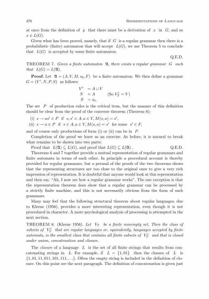
370 Representations of Language

at once from the definition of p that there must be a derivation of x in G, and sox ∈ L(G).

Given what has been proved, namely, that if G is a regular grammar then there is aprobabilistic (finite) automaton that will accept L(G), we use Theorem 5 to concludethat L(G) is accepted by some finite automaton.

Q.E.D.

THEOREM 7. Given a finite automaton A, there exists a regular grammar G suchthat L(G) = L(A).

Proof. Let A = (A, V,M, s0, F ) be a finite automaton. We then define a grammarG = (V ′, N, P, S) as follows:

V ′ = A ∪ V

N = A (So V ′T = V )

S = s0.

The set P of production rules is the critical item, but the manner of this definitionshould be clear from the proof of the converse theorem (Theorem 6):

(i) s → as′ ∈ P if s, s′ ∈ A, a ∈ V,M(s, a) = s′,(ii) s → a ∈ P if s ∈ A, a ∈ V,M(s, a) = s′ for some s′ ∈ F,

and of course only productions of form (i) or (ii) can be in P .Completion of the proof we leave as an exercise. As before, it is natural to break

what remains to be shown into two parts:Proof that L(A) ⊆ L(G), and proof that L(G) ⊆ L(A) . Q.E.D.Theorems 6 and 7 together provide a mutual representation of regular grammars and

finite automata in terms of each other. In principle a procedural account is therebyprovided for regular grammars, but a perusal of the proofs of the two theorems showsthat the representing structures are too close to the original ones to give a very richimpression of representation. It is doubtful that anyone would look at this representationand then say, “Ah, I now see how a regular grammar works”. The one exception is thatthe representation theorem does show that a regular grammar can be processed bya strictly finite machine, and this is not necessarily obvious from the form of suchgrammars.

Many may feel that the following structural theorem about regular languages, dueto Kleene (1956), provides a more interesting representation, even though it is notprocedural in character. A more psychological analysis of processing is attempted in thenext section.

THEOREM 8. (Kleene 1956). Let VT be a finite nonempty set. Then the class ofsubsets of V ∗

T that are regular languages or, equivalently, languages accepted by finiteautomata, is the smallest class that contains all finite subsets of V ∗

T and that is closedunder union, concatenation and closure.

The closure of a language L is the set of all finite strings that results from con-catenating strings in L. For example, if L = 1, 01 then the closure of L is1, 01, 11, 011, 101, 111, . . .. Often the empty string is included in the definition of clo-sure. On this point see the next paragraph. The definition of concatenation is given just

8.2 Representation Theorems for Grammars 371

before Theorem 5.

Remark on the empty sequence. In the definition of regular, context-free andcontext-sensitive grammars, we have not permitted a production rule of the form

α → ∅,

with α ∈ V ∗. It is possible to extend matters to include this special rule—or rather,rules of this special form. Tedious account then has to be taken of their presence orabsence in the proof of theorems like the two for regular languages just considered. Fora good discussion of the empty-sequence type production rule, see Hopcroft and Ullman(1969, pp. 15 ff.).

Pushdown automata and context-free languages. First, we define a probabilisticpushdown automaton. The probabilistic part is a natural generalization of the conceptof a probabilistic finite automaton. The new idea, and the important one, is that ofthe pushdown store, which is a restricted form of memory. The automaton can storestructured information in this store, but it can make state transitions only in terms ofthe top symbol on the store—the store operates like a stack of cafeteria trays on theprinciple of “first-in and last-out”. A special store vocabulary is provided the machine.The transition function depends now, not just on the input symbol and the currentstate, but also on the top symbol on the store. Of course, in the probabilistic case wehave a conditional probability distribution depending on these three things: s in A, αin V , and γ in Γ (the store vocabulary).

An indeterminate or nondeterministic pushdown automaton is obtained from a prob-abilistic one by ignoring the probability distribution. This remark is made more preciselater.

DEFINITION 8. A structure A = (A, V,Γ, p, s0, γ0, F ) is a probabilistic pushdownautomaton iff

(1) A is a nonempty, finite set (set of states).

(2) V is a nonempty, finite set (input vocabulary).

(3) Γ is a nonempty, finite set (store vocabulary).

(4) For each s in A, σ in V ∪ ∅, γ in Γ, ps,σ,γ is a probability density on afinite subset of A× Γ∗ (probability transition table).

(5) s0 ∈ A (initial state).

(6) γ0 ∈ Γ (start store symbol).

(7) F ⊆ A (set of final states).

Several remarks about Definition 8 are in order. First, although Γ∗, not just Γ isinvolved in the definition of p, only a fixed finite number of different words (the elementsof Γ) can be stored, although the sequence of them can be indefinitely long. Second,state transitions can take place without input, because σ can be ∅, as can be seenfrom clause (4) of the definition. Third, we get a nondeterministic automaton from aprobabilistic pushdown automaton by replacing the conditional probability density p

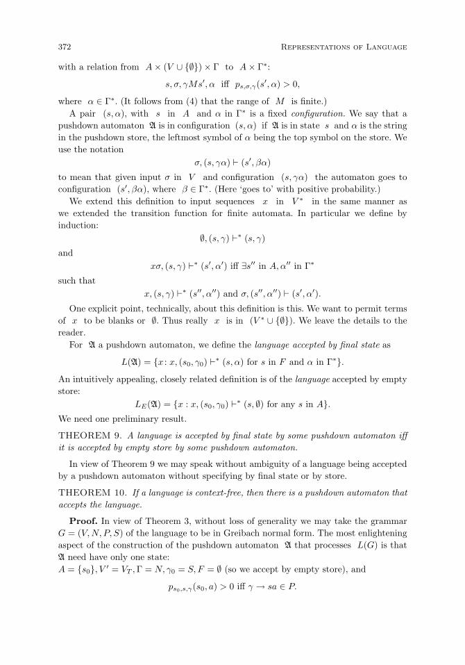
372 Representations of Language

with a relation from A× (V ∪ ∅) × Γ to A× Γ∗:

s, σ, γMs′, α iff ps,σ,γ(s′, α) > 0,

where α ∈ Γ∗. (It follows from (4) that the range of M is finite.)A pair (s, α), with s in A and α in Γ∗ is a fixed configuration. We say that a

pushdown automaton A is in configuration (s, α) if A is in state s and α is the stringin the pushdown store, the leftmost symbol of α being the top symbol on the store. Weuse the notation

σ, (s, γα) " (s′, βα)

to mean that given input σ in V and configuration (s, γα) the automaton goes toconfiguration (s′, βα), where β ∈ Γ∗. (Here ‘goes to’ with positive probability.)

We extend this definition to input sequences x in V ∗ in the same manner aswe extended the transition function for finite automata. In particular we define byinduction:

∅, (s, γ) "∗ (s, γ)

andxσ, (s, γ) "∗ (s′, α′) iff ∃s′′ in A,α′′ in Γ∗

such thatx, (s, γ) "∗ (s′′, α′′) and σ, (s′′, α′′) " (s′, α′).

One explicit point, technically, about this definition is this. We want to permit termsof x to be blanks or ∅. Thus really x is in (V ∗ ∪ ∅). We leave the details to thereader.

For A a pushdown automaton, we define the language accepted by final state as

L(A) = x : x, (s0, γ0) "∗ (s, α) for s in F and α in Γ∗.

An intuitively appealing, closely related definition is of the language accepted by emptystore:

LE(A) = x : x, (s0, γ0) "∗ (s, ∅) for any s in A.We need one preliminary result.

THEOREM 9. A language is accepted by final state by some pushdown automaton iffit is accepted by empty store by some pushdown automaton.

In view of Theorem 9 we may speak without ambiguity of a language being acceptedby a pushdown automaton without specifying by final state or by store.

THEOREM 10. If a language is context-free, then there is a pushdown automaton thataccepts the language.

Proof. In view of Theorem 3, without loss of generality we may take the grammarG = (V,N, P, S) of the language to be in Greibach normal form. The most enlighteningaspect of the construction of the pushdown automaton A that processes L(G) is thatA need have only one state:A = s0, V ′ = VT ,Γ = N, γ0 = S, F = ∅ (so we accept by empty store), and

ps0,s,γ(s0, a) > 0 iff γ → sa ∈ P.

8.2 Representation Theorems for Grammars 373

The proof is completed by an inductive argument showing that

S ⇒∗G x iff x, (s0, γ0) "∗ (s0, ∅).

We leave the argument as an exercise. Q.E.D.As the proof shows, the pushdown store is really doing all the computational work, sothat in fact context-free languages can be represented by a narrow class of pushdownautomata, namely, those with only one state.

THEOREM 11. If A is a pushdown automaton, then L(A) is a context-free language.

Proof. Let A = (A, V,Γ, p, s0, γ0, ∅) and so A accepts by empty store. We definethe context-free grammar that accepts L(A) as follows:

V ′T = V

N = A× Γ ×A ∪ S, S ∈ A× Γ ×A.

Thus V ′ = N ∪ V ′T .

More important, note that the elements of N are triples, except for S. The productionrules in P are of three forms:

(i) S → (s0, γ0, s) for every s in A,(ii) (s, γ, s′) → σ iff ps,σ,γ(s′, ∅) > 0,(iii) (s, γ, s′) → σ(s1, γ1, s2)(s2, γ2, s3) . . . (sm, γm, s

′) iff ps,σ,γ(s1, γ1 . . . γm) > 0 withσ ∈ V ∪ ∅ .

The proof is completed by an inductive argument showing that

S ⇒∗G x iff x, (s0, γ0) "∗ (s, ∅) for some s in A,

—very similar in form to the proof of Theorem 10, but somewhat more complex. Weleave this step as an exercise. Q.E.D.

Turing machines and linear bounded automata. First, we need to introduceTuring machines.1 A Turing machine has a single read-write head. Given an internalstate and the scan of an input letter, the Turing machine executes a move by

(i) changing internal state,(ii) printing a nonblank symbol on the cell scanned, thereby replacing the symbol

scanned,(iii) moving its head left or right one cell.

DEFINITION 9. A structure A = (A, V,Γ,M, s0, F ) is a Turing machine iff

(1.) A is nonempty and finite (set of states),(2.) V is nonempty and finite (input alphabet),(3.) Γ is nonempty and finite, and V ⊆ Γ (set of tape symbols with blank symbol B

in Γ − V ),(4.) M : A× Γ → A× (Γ − B) × L,R, where M is the next move function,(5.) s0 ∈ A (start state),(6.) F ⊆ A (set of final states).

1Turing machines were discussed briefly in Section 3.5 in connection with register machines and

computability.

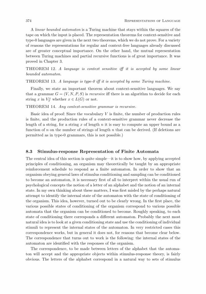
374 Representations of Language

A linear bounded automaton is a Turing machine that stays within the squares of thetape on which the input is placed. The representation theorems for context-sensitive andtype-0 languages are given in the next two theorems, which we do not prove. For a varietyof reasons the representations for regular and context-free languages already discussedare of greater conceptual importance. On the other hand, the mutual representationbetween Turing machines and partial recursive functions is of great importance. It wasproved in Chapter 3.

THEOREM 12. A language is context sensitive iff it is accepted by some linearbounded automaton.

THEOREM 13. A language is type-0 iff it is accepted by some Turing machine.

Finally, we state an important theorem about context-sensitive languages. We saythat a grammar G = (V,N, P, S) is recursive iff there is an algorithm to decide for eachstring x in V ∗

T whether x ∈ L(G) or not.

THEOREM 14. Any context-sensitive grammar is recursive.

Basic idea of proof: Since the vocabulary V is finite, the number of production rulesis finite, and the production rules of a context-sensitive grammar never decrease thelength of a string, for a string x of length n it is easy to compute an upper bound as afunction of n on the number of strings of length n that can be derived. (If deletions arepermitted as in type-0 grammars, this is not possible.)

8.3 Stimulus-response Representation of Finite Automata

The central idea of this section is quite simple—it is to show how, by applying acceptedprinciples of conditioning, an organism may theoretically be taught by an appropriatereinforcement schedule to respond as a finite automaton. In order to show that anorganism obeying general laws of stimulus conditioning and sampling can be conditionedto become an automaton, it is necessary first of all to interpret within the usual run ofpsychological concepts the notion of a letter of an alphabet and the notion of an internalstate. In my own thinking about these matters, I was first misled by the perhaps naturalattempt to identify the internal state of the automaton with the state of conditioning ofthe organism. This idea, however, turned out to be clearly wrong. In the first place, thevarious possible states of conditioning of the organism correspond to various possibleautomata that the organism can be conditioned to become. Roughly speaking, to eachstate of conditioning there corresponds a different automaton. Probably the next mostnatural idea is to look at a given conditioning state and use the conditioning of individualstimuli to represent the internal states of the automaton. In very restricted cases thiscorrespondence works, but in general it does not, for reasons that become clear below.The correspondence that turns out to work is the following: the internal states of theautomaton are identified with the responses of the organism.

The correspondence, to be made between letters of the alphabet that the automa-ton will accept and the appropriate objects within stimulus-response theory, is fairlyobvious. The letters of the alphabet correspond in a natural way to sets of stimulus

8.3 Stimulus-response Representation of Finite Automata 375

elements presented on a given trial to an organism. It may seem like a happy accident,but the correspondences between inputs to the automata and stimuli presented to theorganism, and between internal states of the machine and responses of the organism,are conceptually very natural.

Because of the conceptual importance of the issues that have been raised by linguistsfor the future development of psychological theory, perhaps above all because languagebehavior is the most characteristically human aspect of our behavior patterns, it isimportant to be as clear as possible about the claims that can be made for a stimulus-response theory whose basic concepts seem so simple and to many so woefully inadequateto explain complex behavior, including language behavior. I mention two examples thatpresent very useful analogies. The first is the reduction of standard mathematics to theconcept of set and the simple relation of an element being a member of a set. From anaive standpoint, it seems unbelievable that the complexities of higher mathematics canbe reduced to a relation as simple as that of set membership. But this is indubitablythe case, and we know in detail how the reduction can be made. This is not to suggest,for instance, that in thinking about a mathematical problem or even in formulating andverifying it explicitly, a mathematician operates simply in terms of endlessly complicatedstatements about set membership. By appropriate explicit definition we introduce manyadditional concepts, the ones actually used in discourse. The fact remains, however,that the reduction to the single relationship of set membership can be made and infact has been carried out in detail. The second example, which is close to our presentinquiry, is the status of simple machine language for computers. Again, from the naivestandpoint it seems incredible that modern computers can do the things they can interms either of information processing or numerical computing when their basic languageconsists essentially just of finite sequences of 1’s and 0’s; but the more complex computerlanguages that have been introduced are not at all for the convenience of the machinesbut for the convenience of human users. It is perfectly clear how any more complexlanguage, like Visual C, can be reduced by a compiler or other device to a simplemachine language. The same attitude, it seems to me, is appropriate toward stimulus-response theory. We cannot hope to deal directly in stimulus-response connections withcomplex human behavior. We can hope, as in the two cases just mentioned, to constructa satisfactory systematic theory in terms of which a chain of explicit definitions of newand ever more complex concepts can be introduced. It is these new and explicitly definedconcepts that will be related directly to the more complex forms of behavior.

Before turning to specific mathematical development, it will be useful to make explicithow the developments in this section may be used to show that many of the commonconceptions of conditioning, and particularly the claims that conditioning refers onlyto simple reflexes like those of eye blinking, are mistaken. The mistake is to confuseparticular restricted applications of the fundamental theory with the range of the the-ory itself. Experiments on classical conditioning do indeed represent a narrow range ofexperiments from a broader conceptual standpoint. It is important to realize, however,that experiments on classical conditioning do not define the range and limits of con-ditioning theory itself. The main aim of the present section is to show how any finiteautomaton, no matter how complicated, may be constructed purely within stimulus-

376 Representations of Language

response theory. But from the standpoint of automata, classical conditioning representsa particularly trivial example of an automaton. Classical conditioning may be repre-sented by an automaton having a one-letter alphabet and a single internal state. Thenext simplest case corresponds to the structure of classical discrimination experiments.Here there is more than a single letter to the alphabet, but the transition table of theautomaton depends in no way on the internal state of the automaton. In the case ofdiscrimination, we may again think of the responses as corresponding to the internalstates of the automaton. In this sense there is more than one internal state, contrary tothe case of classical conditioning, but what is fundamental is that the transition table ofthe automaton does not depend on the internal states but only on the external stimulipresented according to a schedule fixed by the experimenter. It is of the utmost impor-tance to realize that this restriction, as in the case of classical conditioning experiments,is not a restriction that is in any sense inherent in conditioning theory itself. It merelyrepresents concentration on a certain restricted class of experiments.

Leaving the technical details for later, it is still possible to give a very clear exampleof conditioning that goes beyond the classical cases and yet represents perhaps thesimplest nontrivial automaton. By nontrivial I mean: there is more than one letter inthe alphabet; there is more than one internal state; and the transition table of theautomaton is a function of both the external stimulus and the current internal state.As an example, we may take a rat being run in a maze. The reinforcement schedulefor the rat is set up so as to make the rat become a two-state automaton. We will useas the external alphabet of the automaton a two-letter alphabet consisting of a blackor a white card. Each choice point of the maze will consist of either a left turn or aright turn. At each choice point either a black card or a white card will be present. Thefollowing table describes both the reinforcement schedule and the transition table of theautomaton.

L RLB 1 0LW 0 1RB 0 1RW 1 0

Thus the first row shows that when the previous response has been left (L) and a blackstimulus card (B) is presented at the choice point, with probability one the animal isreinforced to turn left. The second row indicates that when the previous response is leftand a white stimulus card is presented at the choice point, the animal is reinforced 100%of the time to turn right, and so forth, for the other two possibilities. From a formalstandpoint this is a simple schedule of reinforcement, but already the double aspect ofcontingency on both the previous response and the displayed stimulus card makes theschedule more complicated in many respects than the schedules of reinforcement thatare usually run with rats.

There is no pretense that this simple two-state automaton is in any sense adequate toserious learning. I am not proposing, for example, that there is much chance of teachingeven a simple regular grammar to rats. I am proposing to psychologists, however, thatalready automata of a small number of states present immediate experimental challenges

8.3 Stimulus-response Representation of Finite Automata 377

in terms of what can be done with animals of each species. For example, what is themost complicated automaton a monkey may be trained to imitate? In this case, thereseems some possibility of approaching at least reasonably complex regular grammars(using Theorem 10 of the previous section that any regular grammar is representableby a finite-state automaton). In the case of the lower species, it will be necessary toexploit to the fullest the kind of stimuli to which the organisms are most sensitive andresponsive in order to maximize the complexity of the automata they can imitate.

Stimulus-response theory. The formalization of stimulus-response theory given herefollows closely that in Suppes (1969b). The theory is based on six primitive concepts,each of which has a direct psychological interpretation. The first one is the set S ofstimuli, which we shall assume is not empty, but which we will not restrict to beingeither finite or infinite on all occasions. The second primitive concept is the set R ofresponses and the third primitive concept the set E of possible reinforcements. As inthe case of the set of stimuli, we need not assume that either R or E is finite, but inthe present applications to the theory of finite automata we shall make this restrictiveassumption.

The fourth primitive concept is that of a measure µ on the set of stimuli. In case theset S is finite, this measure is often the number of elements in S. For the generaltheory we shall assume that the measure of S itself is always finite, i.e., µ(S) < ∞.

The fifth primitive concept is the sample space Ω. Each element ω of the samplespace represents a possible experiment, that is, an infinite sequence of trials. In thepresent theory, each trial may be described by an ordered quintuple (C, T, s, r, e), whereC is the conditioning function, T is the subset of stimuli presented to the organism onthe given trial, s is the sampled subset of T , r is the response made on the trial, and e

is the reinforcement occurring on that trial. It is not possible to make all the commentshere that are required for a full interpretation and understanding of the theory. For thosewanting a more detailed description, the two references already given will prove useful.A very comprehensive set of papers on stimulus-sampling theory has been put togetherin the collection edited by Neimark and Estes (1967); see also Estes (1959a,b). Thepresent version of stimulus-response theory should in many respects be called stimulus-sampling theory, but I have held to the more general stimulus-response terminology toemphasize the juxtaposition of the general ideas of behavioral psychology on the onehand and linguistic theory on the other. In addition, in the theoretical applications to bemade here the specific sampling aspects of stimulus-response theory are not as centralas in the analysis of experimental data.

Because of the importance to be attached later to the set T of stimuli presented oneach trial, its interpretation in classical learning theory should be explicitly mentioned.In the case of simple learning, for example, in classical conditioning, the set T is thesame on all trials and we would ordinarily identify the sets T and S. In the caseof discrimination learning, the set T varies from trial to trial, and the applicationwe are making to the theory of automata falls generally under the discrimination case.The conditioning function C is defined over the set R of responses and Cr isthe subset of S conditioned or connected to response r on the given trial. How

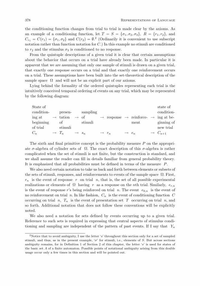
378 Representations of Language

the conditioning function changes from trial to trial is made clear by the axioms. Asan example of a conditioning function, let T = S = σ1, σ2, σ3, R = r1, r2, andCr1 = C(r1) = σ1, σ2 and C(r2) = ∅.2 (Ordinarily it is convenient to use subscriptnotation rather than function notation for C.) In this example no stimuli are conditionedto r2 and the stimulus σ3 is conditioned to no response.

From the quintuple descriptions of a given trial it is clear that certain assumptionsabout the behavior that occurs on a trial have already been made. In particular it isapparent that we are assuming that only one sample of stimuli is drawn on a given trial,that exactly one response occurs on a trial and that exactly one reinforcement occurson a trial. These assumptions have been built into the set-theoretical description of thesample space Ω and will not be an explicit part of our axioms.

Lying behind the formality of the ordered quintuples representing each trial is theintuitively conceived temporal ordering of events on any trial, which may be representedby the following diagram:

State of state ofcondition- presen- sampling condition-ing at → tation → of → response → reinforce- → ing at be-beginning of stimuli ment ginning ofof trial stimuli new trialCn → Tn → sn → rn → en → Cn+1

The sixth and final primitive concept is the probability measure P on the appropri-ate σ-algebra of cylinder sets of Ω. The exact description of this σ-algebra is rathercomplicated when the set of stimuli is not finite, but the construction is standard, andwe shall assume the reader can fill in details familiar from general probability theory.It is emphasized that all probabilities must be defined in terms of the measure P .

We also need certain notation to take us back and forth between elements or subsets ofthe sets of stimuli, responses, and reinforcements to events of the sample space Ω. First,rn is the event of response r on trial n, that is, the set of all possible experimentalrealizations or elements of Ω having r as a response on the nth trial. Similarly, er,n

is the event of response r’s being reinforced on trial n. The event e0,n is the event ofno reinforcement on trial n. In like fashion, Cn is the event of conditioning function C

occurring on trial n, Tn is the event of presentation set T occurring on trial n, andso forth. Additional notation that does not follow these conventions will be explicitlynoted.

We also need a notation for sets defined by events occurring up to a given trial.Reference to such sets is required in expressing that central aspects of stimulus condi-tioning and sampling are independent of the pattern of past events. If I say that Yn

2Notice that to avoid ambiguity, I use the letter ‘s’ throughout this section only for a set of sampled

stimuli, and thus, as in the present example, ‘σ’ for stimuli, i.e., elements of S. But across sections

ambiguity remains, for in Definition 1 of Section 2 of this chapter, the letter ‘s’ is used for states of

the basic set A of a finite automaton. Possible points of notational ambiguity arising from this double

usage occur only a few times in this section and will be pointed out.

8.3 Stimulus-response Representation of Finite Automata 379

is an n-cylinder set, I mean that the definition of Yn does not depend on any eventoccurring after trial n. However, an even finer breakdown is required that takes accountof the postulated sequence Cn → Tn → sn → rn → en on a given trial, so in sayingthat Yn is a Cn-cylinder set what is meant is that its definition does not depend onany event occurring after Cn on trial n, i.e., its definition could depend on Tn−1 orCn, for example, but not on Tn or sn. As an abbreviated notation, I shall write Y (Cn)for this set and similarly for other cylinder sets. The notation Yn without additionalqualification shall always refer to an n-cylinder set.

Moreover, to avoid an overly cumbersome notation, event notation of the sort alreadyindicated will be used, e.g., er,n, for reinforcement of response r on trial n, but alsothe notation σ ∈ Cr,n for the event of stimulus σ’s being conditioned to responser on trial n. To simplify the formal statement of the axioms it is assumed withoutrepeated explicit statement that any given events on which probabilities are conditionedhave positive probability. Thus, for example, the tacit hypothesis of Axiom S2 is thatP (Tm) > 0 and P (Tn) > 0.

The axioms naturally fall into three classes. Stimuli must be sampled in order to beconditioned, and they must be conditioned in order for systematic response patterns todevelop. Thus, there are naturally three kinds of axioms: sampling axioms, conditioningaxioms, and response axioms. A verbal formulation of each axiom is given together withits formal statement. From the standpoint of formulations of the theory already in theliterature, perhaps the most unusual feature of the present axioms is not to require thatthe set S of stimuli be finite. It should also be emphasized that for any one specific kindof detailed application, additional specializing assumptions are needed. Some indicationof these will be given in the particular application to the theory of automata, but itwould take us too far afield to explore these specializing assumptions in any detail andwith any faithfulness to the range of assumptions needed for different experimentalapplications.

DEFINITION 1. A structure S = (S,R,E, µ,Ω, P ) is a stimulus-response model ifand only if the following axioms are satisfied:

Sampling Axioms

S1. P (µ(sn) > 0) = 1.(On every trial a set of stimuli of positive measure is sampled with probability 1.)

S2. P (sm|Tm) = P (sn|Tn).(If the same presentation set occurs on two different trials, then the probability ofa given sample is independent of the trial number.)

S3. If s ∪ s′ ⊆ T and µ(s) = µ(s′), then P (sn|Tn) = P (s′n|Tn).(Samples of equal measure that are subsets of the presentation set have an equalprobability of being sampled on a given trial.)

S4. P (sn|Tn, Yn(Cn)) = P (sn|Tn).(The probability of a particular sample on trial n, given the presentation set ofstimuli, is independent of any preceding pattern Yn (Cn) of events.)

380 Representations of Language

Conditioning Axioms

C1. If r, r′ ∈ R, r = r′ and Cr ∩ Cr′ = ∅, then P (Cn) = 0.(On every trial with probability 1 each stimulus element is conditioned to at mostone response.)

C2. There exists c > 0 such that for every σ,C, r, n, s, er, and Yn

P (σ ∈ Cr,n+1|σ ∈ Cr,n, σ ∈ sn, er,n, Yn) = c.

(The probability is c of any sampled stimulus element’s becoming conditioned tothe reinforced response if it is not already so conditioned, and this probability isindependent of the particular response, trial number, or any preceding pattern Yn

of events.)

C3. P (Cn+1|Cn, e0,n) = 1.(With probability 1, the conditioning of all stimulus elements remains the same ifno response is reinforced.)

C4. P (σ ∈ Cr,n+1|σ ∈ Cr,n, σ ∈ sn, Yn) = 1.(With probability 1, the conditioning of unsampled stimuli does not change.)

Response Axioms

R1. If⋃r∈R

Cr ∩ s = ∅ then

P (rn|Cn, sn, Y (sn)) =µ(s ∩ Cr)µ(s ∩ ∪Cr)

.

(If at least one sampled stimulus is conditioned to some response, then the prob-ability of any response is the ratio of the measure of sampled stimuli conditionedto this response to the measure of all the sampled conditioned stimuli, and thisprobability is independent of any preceding pattern Y (sn) of events.)

R2. If ∪r∈RCr ∩ s = ∅ then there is a number ρr such that

P (rn|Cn, sn, Y (sn)) = ρr.

(If no sampled stimulus is conditioned to any response, then the probability of anyresponse r is a constant guessing probability ρr that is independent of n andany preceding pattern Y (sn) of events.)

Representation of finite automata. A useful beginning for the analysis of how wemay represent finite automata by stimulus-response models is to examine what is wrongwith the most direct approach possible. The difficulties that turn up may be illustatedby the simple example of a two-letter alphabet (i.e., two stimuli σ1 and σ2, as well asthe “start-up” stimulus σo) and a two-state automaton (i.e., two responses r1 and r2).Consideration of this example will be useful for several points of later discussion.

By virtue of Axiom S1, the single presented stimulus must be sampled on each trial,and we assume that for every n,

0 < P (σ0 ∈ sn), P (σ1 ∈ sn), P (σ2 ∈ sn) < 1.

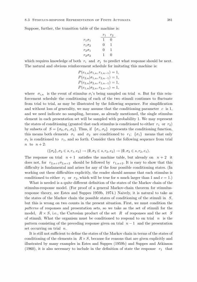
8.3 Stimulus-response Representation of Finite Automata 381

Suppose, further, the transition table of the machine is:

r1 r2r1σ1 1 0r1σ2 0 1r2σ1 0 1r2σ2 1 0

which requires knowledge of both ri and σj to predict what response should be next.The natural and obvious reinforcement schedule for imitating this machine is:

P (e1,n|σ1,n, r1,n−1) = 1,P (e2,n|σ1,n, r2,n−1) = 1,P (e2,n|σ2,n, r1,n−1) = 1,P (e1,n|σ2,n, r2,n−1) = 1,

where σi,n is the event of stimulus σi’s being sampled on trial n. But for this rein-forcement schedule the conditioning of each of the two stimuli continues to fluctuatefrom trial to trial, as may be illustrated by the following sequence. For simplificationand without loss of generality, we may assume that the conditioning parameter c is 1,and we need indicate no sampling, because, as already mentioned, the single stimuluselement in each presentation set will be sampled with probability 1. We may representthe states of conditioning (granted that each stimulus is conditioned to either r1 or r2)by subsets of S = σ0, σ1, σ2. Thus, if σ1, σ2 represents the conditioning function,this means both elements σ1 and σ2 are conditioned to r1; σ1 means that onlyσ1 is conditioned to r1, and so forth. Consider then the following sequence from trialn to n+ 2:

(σ2, σ2 ∈ s, r1, e2) → (∅, σ2 ∈ s, r2, e2) → (∅, σ2 ∈ s, r2, e1).

The response on trial n + 1 satisfies the machine table, but already on n + 2 itdoes not, for r2,n+1σ2,n+2 should be followed by r1,n+2. It is easy to show that thisdifficulty is fundamental and arises for any of the four possible conditioning states. (Inworking out these difficulties explicitly, the reader should assume that each stimulus isconditioned to either r1 or r2, which will be true for n much larger than 1 and c = 1.)

What is needed is a quite different definition of the states of the Markov chain of thestimulus-response model. (For proof of a general Markov-chain theorem for stimulus-response theory, see Estes and Suppes 1959b, 1974.) Naively, it is natural to take asthe states of the Markov chain the possible states of conditioning of the stimuli in S,but this is wrong on two counts in the present situation. First, we must condition thepatterns of responses and presentation sets, so we take as the set of stimuli for themodel, R × S, i.e., the Cartesian product of the set R of responses and the set S

of stimuli. What the organism must be conditioned to respond to on trial n is thepattern consisting of the preceding response given on trial n− 1 and the presentationset occurring on trial n.

It is still not sufficient to define the states of the Markov chain in terms of the states ofconditioning of the elements in R×S, because for reasons that are given explicitly andillustrated by many examples in Estes and Suppes (1959b) and Suppes and Atkinson(1960), it is also necessary to include in the definition of state the response r1 that

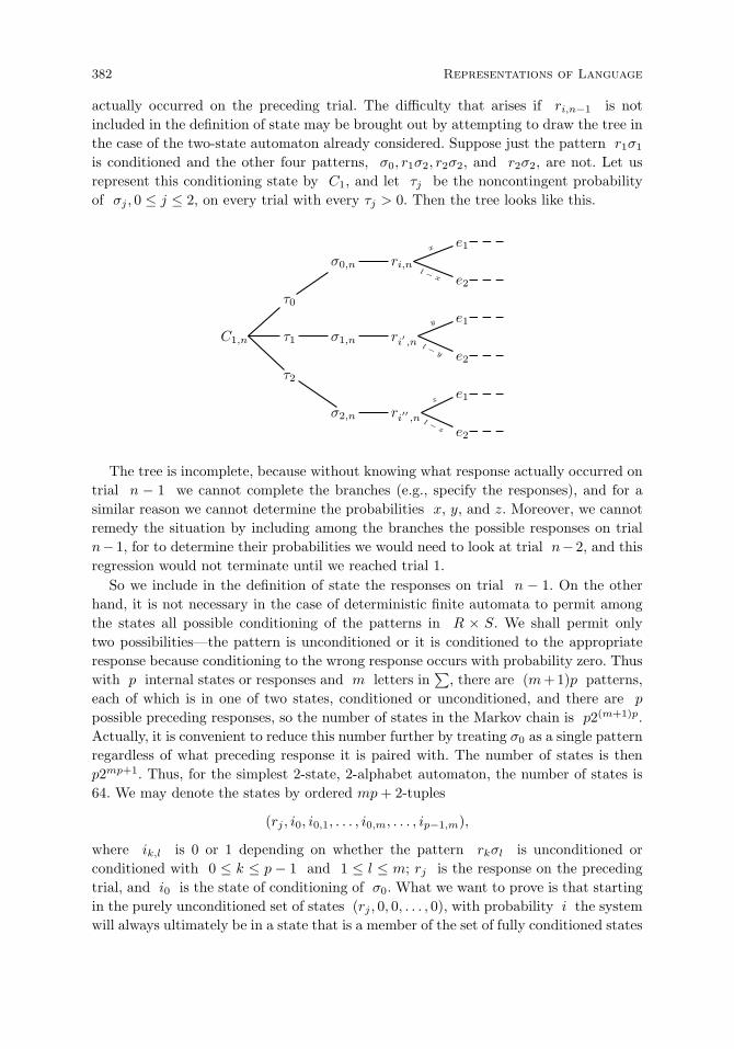
382 Representations of Language

actually occurred on the preceding trial. The difficulty that arises if ri,n−1 is notincluded in the definition of state may be brought out by attempting to draw the tree inthe case of the two-state automaton already considered. Suppose just the pattern r1σ1

is conditioned and the other four patterns, σ0, r1σ2, r2σ2, and r2σ2, are not. Let usrepresent this conditioning state by C1, and let τj be the noncontingent probabilityof σj , 0 ≤ j ≤ 2, on every trial with every τj > 0. Then the tree looks like this.

e1σ0,n ri,n

e2τ0

e1C1,n τ1 σ1,n ri′ ,n

e2τ2

e1σ2,n ri′′ ,n

e2l −

z

z

l −y

y

l −x

x

The tree is incomplete, because without knowing what response actually occurred ontrial n − 1 we cannot complete the branches (e.g., specify the responses), and for asimilar reason we cannot determine the probabilities x, y, and z. Moreover, we cannotremedy the situation by including among the branches the possible responses on trialn−1, for to determine their probabilities we would need to look at trial n−2, and thisregression would not terminate until we reached trial 1.

So we include in the definition of state the responses on trial n − 1. On the otherhand, it is not necessary in the case of deterministic finite automata to permit amongthe states all possible conditioning of the patterns in R × S. We shall permit onlytwo possibilities—the pattern is unconditioned or it is conditioned to the appropriateresponse because conditioning to the wrong response occurs with probability zero. Thuswith p internal states or responses and m letters in

∑, there are (m+1)p patterns,

each of which is in one of two states, conditioned or unconditioned, and there are p

possible preceding responses, so the number of states in the Markov chain is p2(m+1)p.Actually, it is convenient to reduce this number further by treating σ0 as a single patternregardless of what preceding response it is paired with. The number of states is thenp2mp+1. Thus, for the simplest 2-state, 2-alphabet automaton, the number of states is64. We may denote the states by ordered mp+ 2-tuples

(rj , i0, i0,1, . . . , i0,m, . . . , ip−1,m),

where ik,l is 0 or 1 depending on whether the pattern rkσl is unconditioned orconditioned with 0 ≤ k ≤ p − 1 and 1 ≤ l ≤ m; rj is the response on the precedingtrial, and i0 is the state of conditioning of σ0. What we want to prove is that startingin the purely unconditioned set of states (rj , 0, 0, . . . , 0), with probability i the systemwill always ultimately be in a state that is a member of the set of fully conditioned states

8.3 Stimulus-response Representation of Finite Automata 383

(rj , 1, 1, . . . , 1). The proof of this is the main part of the proof of the basic representationtheorem.

Before turning to the theorem, we need to define explicitly the concept of a stimulus-response model’s asymptotically becoming an automaton. As has already been sug-gested, an important feature of the definition is this. The basic set S of stimulicorresponding to the alphabet

∑of the automaton is not the basic set of stimuli of

the stimulus-response model, but rather, this basic set is the Cartesian product R×S,where R is the set of responses.3 Moreover, the definition has been framed in such away as to permit only a single element of S to be presented and sampled on each trial;this, however, is an inessential restriction used here in the interest of conceptual andnotational simplicity. Without this restriction the basic set would be not R × S, butR× P(S), where P(S) is the power set of S, i.e., the set of all subsets of S, and theneach letter of the alphabet

∑would be a subset of S rather than a single element of

S. What is essential is to have R× S rather than S as the basic set of stimuli.For example, the pair (ri, σj) must be sampled and conditioned as a pattern, and

the axioms are formulated to require that what is sampled and conditioned be a subsetof the presentation set T on a given trial. In this connection, to simplify notation Ishall often write Tn = (ri,n−1, σj,n) rather than

Tn = (ri, σj),

but the meaning is clear. Tn is the presentation set consisting of the single pattern (orelement) made up of response ri on trial n − 1 and stimulus element σj on trialn, and from Axiom S1 we know that the pattern is sampled because it is the only onepresented.

The use of R×S is formally convenient, but is not at all necessary. The classical S-Rtradition of analysis suggests a formally equivalent, but psychologically more realisticapproach. Each response r produces a stimulus σr, or more generally, a set of stimuli.Assuming again, for formal simplicity just one stimulus element σr, rather than a setof stimuli, we may replace R by the set of stimuli SR, with the purely contingentpresentation schedule

P (σr,n|rn−1) = 1,

and in the model we now consider the Cartesian product (SR ×S) rather than R×S.Within this framework the important point about the presentation set on each trialis that one component is purely subject-controlled and the other purely experimenter-controlled—if we use familiar experimental distinctions. The explicit use of SR ratherthan R promises to be important in training animals to perform like automata, becausethe external introduction of σr reduces directly and significantly the memory load onthe animal. The importance of SR for models of children’s language learning is lessclear.

Still another interpretation of the theory can be given by going from psychology toneuroscience in the spirit of the final section of this chapter. This move means replacingthe response itself by the brain’s representation of the response. Again, this biologically

3This distinction is important to keep in mind in what follows. Note that replacing R by SR is

discussed two paragraphs further on, to help emphasize it.

384 Representations of Language

more realistic move would not change the formal structure of the basic argument of thissection, but an empirically realistic account would entail many more details of the kindgiven in Section 6.

DEFINITION 2. Let S = (R× S,R,E, µ,Ω, P ) be a stimulus-response model where

R = r0, . . . , rp−1,S = σ0, . . . , σm,E = e0, . . . , ep−1,

and µ(S′) is the cardinality of S′ for S′ ⊆ S. Then S asymptotically becomes theautomaton A(S) = (R,S − σ0,M, r0, F ) if and only if

(i) as n → ∞ the probability is 1 that the presentation set Tn is (ri,n−1, σj,n) forsome i and j,

(ii) M(ri, σj) = rk if and only if limn→∞ P (rk,n|Tn = (ri,n−1, σj,n)) = 1 for 0 ≤i ≤ p− 1 and 1 ≤ j ≤ m,

(iii) limn→∞ P (r0,n|Tn = (ri,n−1, σ0,n)) = 1 for 0 ≤ i ≤ p− 1,(iv) F ⊆ R.

A minor but clarifying point about this definition is that, as already remarked, thestimulus σ0 is not part of the alphabet of the automaton A(S), because a stimulusis needed to put the automaton in the initial state r0, and from the standpoint of thetheory being worked out here, this requires a stimulus to which the organism will giveresponse r0. That stimulus is σ0. The definition also requires that asymptotically thestimulus-response model S is nothing but the automaton A(S). It should be clear thata much weaker and more general definition is possible. The automaton A(S) couldmerely be embedded asymptotically in S and be only a part of the activities of S. Thesimplest way to achieve this generalization is to make the alphabet of the automatononly a proper subset of S − σ0 and correspondingly for the responses that makeup the internal states of the automaton; they need be only a proper subset of the fullset R of responses. This generalization will not be pursued here, although somethingof the sort will be necessary to give an adequate account of the semantical aspects oflanguage.

THEOREM 1. (Representation Theorem for Finite Automata). Given any connectedfinite automaton, there is a stimulus-response model that asymptotically becomes iso-morphic to it. Moreover, the stimulus-response model may have all responses initiallyunconditioned.

Proof. Let A = (A,∑,M, s0, F ) be any connected finite automaton. As indicated

already, we represent the set A of internal states by the set R of responses ri, for0 ≤ i ≤ p− 1, where p is the number of states. We represent the alphabet

∑by the

set of stimuli σ1, . . . , σm, and, for reasons already made explicit, we augment this setof stimuli by σ0, to obtain

S = σ0, σ1, . . . , σm.For subsequent reference let f be the function defined on A ∪

∑that establishes

the natural one-one correspondence between A and R, and between∑

and S−σ0.(To avoid some trivial technical points, I shall assume that A and

∑are disjoint.)

8.3 Stimulus-response Representation of Finite Automata 385

We take as the set of reinforcements

E = e0, e1, . . . , ep−1,and the measure µ(S′) is the cardinality of S′ for S′ ⊆ S, so that as in Definition 2, weare considering a stimulus-response model S= (R× S,R,E, µ,Ω, P ). In order to showthat S asymptotically becomes an automaton, we impose five additional restrictionson S. They are these.

First, in the case of reinforcement e0 the schedule is this:

P (e0,n|σ0,n) = 1, (1)

i.e., if σ0,n is part of the presentation set on trial n, then with probability 1 responser0 is reinforced—note that the probability of the reinforcing event e0,n is independentof the actual occurrence of the response r0,n .

Second, the remaining reinforcement schedule is defined by the transition table M

of the automaton A. Explicitly, for j, k = 0 and for all i and n

P (ek,n|σj,nri,n−1)=1 if and only if M(f−1(ri), f−1(σj))=f−1(rk). (2)

Third, essential to the proof is the additional assumption beyond (1) and (2) that thestimuli σ0, . . . , σm each have a positive, noncontingent probability of occurrence on eachtrial (a model with a weaker assumption could be constructed but it is not significant toweaken this requirement). Explicitly, we then assume that for any cylinder set Y (Cn)such that P (Y (Cn)) > 0

P (σi,n) = P (σi,n|Y (Cn)) ≥ τi > 0 (3)

for 0 ≤ i ≤ m and for all trials n.Fourth, we assume that the probability ρi of response ri occurring when no condi-

tioned stimuli is sampled is also strictly positive, i.e., for every response ri

ρi > 0, (4)

which strengthens Axiom R2.Fifth, for each integer k, 0 ≤ k ≤ mp+ 1, we define the set Qk as the set of states

that have exactly k patterns conditioned, and Qk,n is the event of being in a statethat is a member of Qk on trial n. We assume that at the beginning of trial 1, nopatterns are conditioned, i.e.,

P (Q0,1) = 1. (5)

It is easy to prove that given the sets R, S, E and the cardinality measure µ, thereare many different stimulus-response models satisfying restrictions (1)-(5), but for theproof of the theorem it is not necessary to select some distinguished member of the classof models because the argument that follows shows that all the members of the classasymptotically become isomorphic to A.

The main thing we want to prove is that

limn→∞P (Qmp+1,n) = 1. (6)

We first note that if j < k the probability of a transition from Qk to Qj is zero,i.e.,

P (Qj,n|Qk,n−1) = 0, (7)

386 Representations of Language

moreover,P (Qj,n|Qk,n−1) = 0, (8)

even if j > k holds, unless j = k + 1. In other words, in a single trial, at most onepattern can become conditioned.

To show that asymptotically (6) holds it will suffice to show that there is an ε > 0such that on each trial n for 0 ≤ k ≤ mp < n if P (Qk,n) > 0,

P (Qk+1,n+1|Qk,n) ≥ ε. (9)

To establish (9) we need to show that there is a probability of at least ε of a stimuluspattern that is unconditioned at the beginning of trial n becoming conditioned onthat trial. The argument given will be a uniform one that holds for any unconditionedpattern. Let r∗σ∗ be such a pattern on trial n.

Now it is well known that for a connected automaton, for every internal state s,there is a tape x such that4

M(s0, x) = s (10)

and the length of x is not greater than the number of internal states. In terms ofstimulus-response theory, x is a finite sequence of length not greater than p ofstimulus elements. Thus we may take x = σi1 , . . . , σip

with σip= σ∗. We know by

virtue of (3) thatmin

0≤i≤mτi = τ > 0. (11)

The required sequence of responses ri1 , . . . , rip−1 will occur either from prior condi-tioning or if any response is not conditioned to the appropriate pattern, with guessingprobability ri. By virtue of (4)

min0≤i≤p−1

ρi = ρ > 0. (12)

To show that the pattern r∗σ∗ has a positive probability ε of being conditioned ontrial n, we need only take n large enough for the tape x to be ‘run’, say, n > p+ 1,and consider the joint probability

P ∗ = P (σ∗n, r

∗n−1σip−1,n−1, . . . , r0,n−ip−1σ0,n−ip−1). (13)

The basic axioms and the assumptions (1)-(5) determine a lower bound on P ∗

independent of n. First we note that for each of the stimulus elements σ0, σ1, . . . , σ∗,

by virtue of (3) and (11)

P (σ∗n| . . .) ≥ τ, . . . , P (σ0,n−ip−1) ≥ τ.

Similarly, from (4) and (12), as well as the response axioms, we know that for each ofthe responses r0, ri1 , . . . , r

∗

P (r∗n−1| . . .) ≥ ρ, . . . , P (r0,n−ip−1|σ0,n−ip−1) ≥ ρ.

Thus we know thatP ∗ ≥ ρpτp+1,

4In equation (10) we have one of the few cases in this section where ‘s’ and ‘s0’ refer to states of

the automaton being modeled, not sets of sampled stimuli.

8.3 Stimulus-response Representation of Finite Automata 387

and given the occurrence of the event σ∗nr

∗n−1, the probability of conditioning is c,

whence we may takeε = cρpτp+1 > 0,

which establishes (9) and completes the proof.Given the theorem just proved, there are several significant corollaries whose proofs

are almost immediate. The first combines the representation theorem for regular lan-guages with that for finite automata to yield:

THEOREM 2. Any regular language is generated by some stimulus-response model atasymptote.

Once probabilistic considerations are introduced, we can in several different ways gobeyond the restriction of stimulus-response generated languages to regular languages.This is done later in this section.

I suspect that many psychologists or philosophers who are willing to accept thesense given here to the reduction of finite automata and regular languages to stimulus-response models will be less happy with the claim that one well-defined sense of theconcepts of intention, plan, and purpose can be similarly reduced. However, without anysubstantial new analysis on my part this can be done by taking advantage of an analysisalready made by Miller and Chomsky (1963). The story goes like this. In 1960 Miller,Galanter and Pribram published a provocative book entitled Plans and the Structure ofBehavior. In this book they severely criticized stimulus-response theories for being ableto account for so little of the significant behavior of humans and the higher animals.They especially objected to the conditioned reflex as a suitable concept for buildingup an adequate scientific psychology. It is my impression that a number of cognitivelyoriented psychologists felt that the critique of S-R theory in this book was devastating.

As I indicated earlier, I would agree that conditioned reflex experiments are indeedfar too simple to form an adequate scientific basis for analyzing more complex behavior.This is as hopeless as would be the attempt to derive the theory of differential equations,let us say, from the elementary algebra of sets. Yet the more general theory of sets doesencompass in a strict mathematical sense the theory of differential equations.

The same relation may be shown to hold between stimulus-response theory and thetheory of plans, insofar as the latter theory has been systematically formulated by Millerand Chomsky. This point was developed informally by Millenson (1967). The theory ofplans is formulated in terms of tote units (‘tote’ is an acronym for the cycle test-operate-test-exit). A plan is then defined as a tote hierarchy, which is just a form of orientedgraph, and every finite oriented graph may be represented by a finite automaton. So wehave the result:

THEOREM 3. Any tote hierarchy in the sense of Miller and Chomsky is isomorphicto some stimulus-response model at asymptote.

Response to criticisms.5 Arbib’s (1969) comments on the stimulus-response theoryof finite automata raise issues that continue to divide cognitive and stimulus-response

5The remainder of this section draws on Suppes (1969c, 1989).

388 Representations of Language

psychologists. I am not persuaded by any of his arguments that a viable alternative tostimulus-response theory has yet been defined, although I am willing to admit that afully adequate stimulus-response theory of complex learning and behavior has yet tobe developed. Arbib’s comments and arguments can be analyzed under five headings. Ideal with each in turn, and in several cases, amplify my own views as well.

Matters of proof. Arbib alleges that he has given a much simpler derivation of my maintheorem: given any connected finite automaton, there is a stimulus-response modelasymptotically isomorphic to it. He simplifies the proof by assuming that “for eachstimulus-response table there is a stimulus-response model that asymptotically becomesisomorphic to it [p. 507]”; but as Bertrand Russell said long ago, such procedures ofpostulation instead of proof have all the virtues of theft over honest toil. In other words,Arbib has not shown how the fundamental result follows from simple general assump-tions about stimulus-response connections—my main objective. To put the matter tech-nically, he is faced with the problem of showing that his very powerful postulate, whichcorresponds to a theorem in my framework, is consistent with the simple assumptionsabout conditioning and sampling of stimuli that are an integral part of any standardstimulus-response theory.

Stimulus traces and mediating responses. Arbib seems to have a rather simple view ofhow an organism can remember its previous responses. He mentions the natural deviceused in experimentation with animals of having the previous response externalized byan appropriate stimulus. Exactly this approach has been used in the conditioning ofpigeons to behave as simple automata, but it is not a general approach. Certainly it isnot adequate to the problems of language learning to which my own research is primarilyaddressed, or even to the problems of children learning arithmetic.

Within classical stimulus-response theory, it is natural to talk about stimulus traces,and I mentioned this possibility originally. In terms of later stimulus-response theories,especially those associated with Osgood, Maltzman, Berlyne, the Kendlers, and oth-ers, it is natural to talk about mediating responses internal to the organism. Either ofthese concepts provides a natural framework to replace or to extend the very narrowexternalization approach used by Arbib. He objects to having some representation ofthe previous response in the organism for fear “that the input channels would be com-pletely overloaded if they must carry not only representations of external stimuli butalso complete information about the current state of execution of the TOTE hierarchy[p. 509]”. This comment, like most of Arbib’s other comments, however, is not backedup by a detailed analysis. It is not at all clear that this is a problem. Put in this generalway, one may as well express concern over the internal processing also and simply saythat it is found to be an overweening mystery of how the organism can work at all.

Number of states. In many ways I think the most serious and important issue raisedby Arbib is the query of whether it is possible for an organism ever to have adequatetime to learn the apparently large number of stimulus-response connections needed forit to become a suitably large automaton. This is a central issue that has been raised

8.3 Stimulus-response Representation of Finite Automata 389

continually, particularly by psycholinguists critical of stimulus-response theories of lan-guage learning. The negative claims that Arbib makes concerning a TOTE hierarchyinvolving eight components with four states each are familiar, and his arguments alsoassume a familiar theological tone of saying it simply cannot be done.

Because of the many arguments I have had about these matters over the years, Ihave come to make a distinction between negative dogma and negative proof. A widerange of psycholinguists and cognitive psychologists have asserted the negative dogmathat stimulus-response ideas can never account for complex learning, because suitableconditioning connections could never be learned in sufficient time by organisms exhibit-ing complex behavior. This negative dogma seems to be an article of faith, and not anarticle of proof on the part of almost all who assert it, including Arbib. Certainly hedoes not give a proof that a device with 48 states is needed for any cognitive processinghe cares to define. In view of his familiarity with the formal literature in the theoryof automata on these problems, I suspect he is somewhat more wary than many ofthe psycholinguists in venturing to give what would appear to be a detailed argument.For an example of a presumed negative proof as opposed to a negative dogma, butwhat is in fact a melange of confusions from end to end, see the proposed proof byBever, Fodor, and Garrett (1968) that a formal limitation of stimulus-response theoryor associationism can be established.

It is generally recognized in mathematics and associated disciplines that negativearguments must be formulated in a more formal and explicit fashion than positive ar-guments. There is also a long history in mathematics and philosophy of establishingexplicit and carefully defined systematic standards for evaluating the validity of a neg-ative argument. It seems to me that Arbib does not work at all within this classicaltradition. He makes a few casual statements about number of states, but offers no seri-ous negative argument about the size of automata required for any cognitive processesunderstood well enough to be characterized in relatively exact terms. I will return tothis point subsequently.

I think that the problem of the number of states required for various tasks is indeeda fundamental one, and I am certainly not prepared to establish small upper bounds onthe number of states needed for a very large number of tasks. On the other hand, I amskeptical of the large claims so often made by psycholinguists or automaton theorists. Imention just two examples. At the end of Suppes (1969b), I gave a detailed analysis ofthe kind of automaton required for column addition of two numbers, and I showed howit can be related in realistic fashion to the actual behavior of students.6 The number ofstates required is just two. Casual thought without detailed analysis might lead to thesuggestion that the number of states would need to be large. This is not the case.

My second example, which I will not give in detail, concerns efforts to write prob-abilistic grammars for the spoken speech of 2- and 3-year-old children. Although I donot want to claim that these efforts are wholly successful, it is clear from scanning thelength of sentences uttered by young children that the number of states required forproduction of the grammar is relatively small, and probably a larger number of states isrequired just for the handling of the lexical vocabulary. I should add that I have yet to

6This example is also given earlier in this section.

390 Representations of Language

meet anyone, linguist or automaton theorist, who would want to claim that vocabularycan be acquired by any way other than some rather direct empirical process of learning.I would conjecture that the number of states required for any cognitive task, includinglanguage comprehension or production, will turn out to be a lot smaller than any of usoriginally thought. I readily admit that this is simply a conjecture, but I have enoughconfidence in it to insist that those who wish to claim that stimulus-response theory isinadequate, because of the problem of the number of states that must be conditioned,should offer negative proofs and not simply negative dogmas. The central focus of myown research efforts is to convert my own positive dogmas into positive proofs. (On thequestion of number of states, it is perhaps worth noting that a universal Turing machinecan be constructed with only seven states.)

A simple example will illustrate an important point in talking about the number ofstates. If we toss a coin 100 times, the number of possible outcomes is 2100. Each ofus can perform this experiment, but we could set the entire population of the world totossing coins and not approach the number of possible outcomes. The number of actualstates in a process, it is essential to note, is usually incredibly smaller, by orders andorders of magnitude, than the number of possible states, and so it is with the relationbetween the number of actual and the number of possible conditioning connections.

Real versus metaphorical learning. Arbib argues in several places that learning simplycould not take place according to stimulus-response conceptions because the numberof states required is too large and the amount of time needed for conditioning is toorestricted. I have already expressed my central argument against his claims about thenumber of states. I am willing to agree that if the number of states that must beconditioned individually is very large, then there will not be time for the task. What isinteresting is the vagueness and weakness of the alternatives considered by Arbib. Heexpresses clear preference for TOTE hierarchies, without considering these hierarchiesas special cases of stimulus-response models, according to the first corollary of my maintheorem. What he does not say or even sketch is how, within the framework of TOTEhierarchies, a theory can be given of the organism’s acquiring cognitive skills. He doesmention casually some references to neurons and biochemical changes in the brain, butno serious ideas are set forth in this physiological framework. The reader is left totallyuninformed as to what serious alternative Arbib would propose, with the single possibleexception of his final remark about the computer as a metaphorical brain. Presumably,metaphorical brains engage in metaphorical learning. If this is what he is suggestingas a theory of learning, he cannot mean for his remarks in this direction to be takenseriously. An account of how organisms learn must be stated with sufficient definitenessand in sufficiently nonmetaphorical terms for it to be tested experimentally. CertainlyArbib himself makes no positive or definite suggestions of how to deal with any of themain difficulties facing theories of machine or human learning.

Indeed, it is surprising that in view of his opinions about the adequacy of psycho-logical theories of learning he does not have more to say about the virtues of computertheories of learning, i.e., machine learning. I think the reasons, however, are really clearenough. It does not take a very serious or systematic study of the literature of artificial

8.3 Stimulus-response Representation of Finite Automata 391

intelligence to reach the conclusion that, although psychological theories of learning arecertainly far from being sufficiently developed, so are theories of how computers shouldbe programmed to learn.7

Problem of hierarchies. I have stated already that the issue about the number of statesraised by Arbib is indeed a serious one. I think the other serious issue raised by himis the problem of hierarchies. It seems to be a matter of belief on the part of almostall cognitively oriented psychologists that conditioning theories must treat each simpleconditioning connection as separate and equal. The concept of a hierarchy, it seems to besuggested, is contrary to the spirit of stimulus-response ideas. That a clear theoreticalcounterexample exists is shown at once by the corollary to the main theorem of mypaper, namely, the theorem that every TOTE hierarchy in the sense of Miller andChomsky is isomorphic to some stimulus-response model at asymptote. The abstractionof this result may be unsatisfactory to some readers, but its meaning is clear. Anyintuitive hierarchy that may be represented formally by a TOTE hierarchy, a finiteoriented graph, a finite tree, or a finite automaton may be represented just as well by astimulus-response model; in fact, better, for the stimulus-response model also includesan account of how the hierarchy is learned if the stimulus-response connections are notalready coded in the genes.

Criticism of the representation theorem. A technically detailed and interesting criti-cism of Theorem 1, the representation theorem for finite automata, has been given byKieras (1976). The intuitive source of Kieras’ confusion in his claim that the theoremas stated is too strong is easy to identify.8 Because I identified the internal states of agiven automaton with the responses of the representing stimulus-response model, Kierasinferred I had unwittingly restricted my analysis to automata that have a one-one cor-respondence between their internal states and responses. On the basis of this confusionon his part he asserts that the representation theorem is not correct as it stands.

My purpose now is to lay out this dispute in an explicit and formal way in order toshow unequivocally that Kieras is mistaken and the representation theorem is correctas originally stated. From a mathematical standpoint, Kieras’ mistake rests on a misun-derstanding of representation theorems. The isomorphism of a representation theoremis a formal one. In the case of Theorem 1 above, the isomorphism is between the internalstates of the automaton and the responses of the representing stimulus-response model.The Rabin-Scott definition of automata used in my 1969 article does not have an ex-plicit response mechanism, but that this is a trivial addition to their definition is shownby Definition 2 of Section 2, for finite automata with output, as well as by the generaldefinition of a sequential machine with output given by Harrison (1965, p. 294), who isreferenced by Kieras and who acknowledges he is mainly following the terminology of

7What kind of details are needed in the theory of machine learning of language, even for a simple

fragment of natural language, is well illustrated in Section 5 of this chapter. This is not to suggest the

specific approach used there is the only one. It is just, at the present time anyway, hard to see how a

host of explicitly worked out details can be avoided.8Criticisms by Anderson (1976, pp. 81–89) are based on essentially the same confusion.

392 Representations of Language

Rabin and Scott (1959). An automaton or sequential machine with output is for Har-rison just an automaton in the sense of Rabin and Scott with the additional conditionthat the set F of final states are those ‘giving a one output’. As Harrison and othershave remarked, a restriction of output to 1’s and 0’s is no restriction on the generalityof the sequential machine.

The addition of this output apparatus to the formal definitions I gave in the originalarticle is trivial. We just pick two responses r0 and r1 not used to represent internalstates, but one of them, say r0, represents 0 and the other 1. Whenever the machine is inan internal state that is not a final state but a response is required, it outputs r0. Whenit is in a final state it outputs r1. To modify Definition 1 to take account of these outputresponses is easy. I note once again that the two output responses are in no way intendedto correspond to internal states of the automata being represented. Other responses ofthe stimulus-response model represent the internal states. I emphasize, also, that thismodification of adding output responses would not be correcting an error in Theorem1 but would only be providing an additional closely related result.

Problem of determinate reinforcement. As has been noticed by several critics, and asI have remarked on several occasions, for example, Suppes (1975), in many kinds oflearning environments strict determinate reinforcement of the response is not feasible,contrary to the demands of the proof of Theorem 1. For example, if I ask a child thesum of 7 + 5, then a determinate reinforcement would be giving the correct answer, 12,when he gave an incorrect answer. An example of nondeterminate reinforcement wouldbe simply to tell him that the answer was incorrect and to ask him to try again. Whendeterminate reinforcement is used, it is clear that in some sense the responses have to beobservable in order to correct each incorrect response. Theorem 1 used an assumptionof determinate reinforcement. It seems to me that it is this assumption of determinatereinforcement rather than any of the informal remarks I made about responses beingobservable or internal states being identifiable with outputs that is the central limitationof the result.

From the standpoint of giving an account of complex learning, especially in nat-ural settings as opposed to simple laboratory situations, it was clear to me beforeTheorem 1 was published that the most essential extension was to obtain simi-lar results with nondeterminate reinforcement. This problem was tackled in con-junction with my former student, William Rottmayer, and detailed results are em-bodied in his 1970 dissertation. An informal and rather brief statement of the re-sults appears in a survey article we published on automata (Suppes and Rottmayer1974).

Because the formal statement of stimulus-response theory with nondeterminate re-inforcement is rather complicated, I shall give only a brief informal statement similarto that in Suppes and Rottmayer (1974). Before doing so, let me formulate a canonicalclass of problems that can be used for intuitive reference in digesting the content of theindividual axioms. The organism is presented with a potentially infinite class of stimulusdisplays, for example, line drawings. A subclass of the entire class is characterizable bya finite automaton. The problem for the learner is to learn the concept characterized

8.3 Stimulus-response Representation of Finite Automata 393

by the finite automaton, given on each trial only the information of whether or nothis classification of a given stimulus display is correct. I have mentioned line drawingshere because I do not want to concentrate entirely on language, but it would also bepossible to think of the learning in terms of recognizing grammatical strings of someregular language. Because I do not like to think of language learning wholly in termsof grammar, I prefer in the present context a geometrical example. Let us suppose thateach line drawing consists of a finite number of line segments. A typical example mightbe a line drawing consisting of three segments forming a triangle but with one of theline segments, and only one, extending beyond the triangle. On each trial the learneris asked to say whether the particular line drawing shown is an instance of the displayand after he has given this information he is told simply that his answer is correct orincorrect.

What the theory postulates is a sequence of implicit responses or, if you prefer,internal responses by the learner prior to giving the answer of ‘yes’ or ‘no’ to classifythe display. Informally it is assumed that the implicit or internal responses are notavailable for observation and cannot be directly reinforced. The theory does not requirethis as an assumption, but it is implicit in any experimental application of the theory.Reinforcement takes place not after each internal response occurs, which is considereda subtrial, but only after a trial consisting of a sequence of subtrials.

In other words, putting the matter in standard experimental terms, a subtrial corre-sponds to what we usually think of as a trial, but no reinforcement or conditioning takesplace and we cannot observe the response that was actually made. Conditioning occursonly after a sequence of subtrials, and the whole sequence of subtrials is called a trial. Inautomaton terms, a subtrial corresponds to an automaton making one transition, thatis, from one internal state to another, and a trial to processing an entire tape or inputstring.

Conditioning occurs on trials that have a correct response, and deconditioning occurson trials that have an incorrect response. Thus learning occurs on all trials, regardlessof whether the response is correct or not. On the basis of these axioms, the followingtheorem, which represents a considerable improvement of the basic theorem in my 1969article, can be proved. The improvement is due to the weakening of the methods ofreinforcement.

THEOREM 4. If D is any set of perceptual displays and G is a subset of D that can berecognized by a finite automaton, then there is a stimulus-response model that can alsolearn to recognize G, with performance at asymptote matching that of the automaton.

One important point to note is that with nondeterminate reinforcement the theoremis, as one would expect, weaker. In the case of determinate reinforcement the stimulus-response model at asymptote becomes isomorphic to the given finite automaton. In thepresent case, the result can only be one of behavioral equivalence or, in the ordinarylanguage of automaton theory, the result is one of weak equivalence.

It is clear that the nondeterminate reinforcement used in the theory I have justformulated is about the weakest version of reinforcement that is interesting, with thepossible exception of giving only partial reinforcement, that is, reinforcement on certain

394 Representations of Language

trials. In actual learning, for example, in the learning of mathematics or in the learningof language, there are many situations in which much more decisive and informativereinforcement is given. It is not difficult to show that the more determinate the rein-forcement, the faster learning will be in general for organisms of a given capacity. Inthe long and tangled history of the concept of reinforcement it has not been sufficientlyemphasized that reinforcement is delivery of information, and a particular structure ofinformation is implicit in any particular scheme of reinforcement. An exhausting but notexhaustive analysis of different structures of reinforcement is to be found in Jamison,Lhamon and Suppes (1970). (So many detailed theoretical computations were made inthis article that it has scarcely been read by anyone; it does provide a good sense ofhow complex things rapidly become when reinforcement schemes that have even mildlycomplex information structures are used.)

It is important for the present discussion to consider one of the weakest structures ofnondeterminate reinforcement and to emphasize the point that it is the nondeterminatecharacter of the reinforcement that moves us out of the arena of classical observability ofresponses and permits the introduction of a repertoire of implicit or internal responsesthat are not in general observable. The reinforcement does not create the implicit re-sponses, but when we have determinate reinforcement the theory is not applicable tosituations in which implicit or internal responses occur.

It is also important to note that it is really a matter of terminology, and not ofsubstantive theory, whether these implicit responses are called responses as such or arecalled internal states. It would be easy enough to reformulate the axioms given aboveand to replace responses with internal states except for the response that occurs at theend of a trial. This terminological change would not affect the axioms in any way.

It is worth mentioning that the implicit responses that we might want to baptize asinternal states are often observed as taking place even when we do not know their exactform. A good example occurs in the case of subvocalized articulatory responses thatare characteristic of most silent adult readers. Self-awareness of such subvocal responsesis unusual, and I hasten to add that it is not usually possible to ‘read off’ from thesubvocal responses the words being read.

Another misconception: restriction to finite automata. Another misconceptionin the literature is that stimulus-response theory can only deal with machines thathave the power of finite automata. The purpose of this subsection is to show that thisis not the case by giving the construction of register machines, which are equivalentto Turing machines. The development here extends and modifies substantially that inSuppes (1977b). To give the results formal definiteness, we shall develop a learningtheory for any partial recursive function. Such functions can be defined explicitly in afairly direct way, but we shall not do so here. I shall rely upon the fact that partialrecursive functions are computable functions. We then use the basic theorem in theliterature, whose technical framework we shall expand upon somewhat later, that anyfunction is partially recursive if and only if it is computable by a register machine or,equivalently, by a Turing machine. The concept of a register machine used here wasintroduced in Section 3.5. The reason for using register machines rather than Turing

8.3 Stimulus-response Representation of Finite Automata 395

machines is that their formal structure is simpler. For example, the proof of equivalencebetween a function being a partial recursive function and being computable by a registermachine is much simpler than the corresponding proof for Turing machines. First, let merecall from Section 3.5 how simple a classical register machine for a finite vocabulary is.All we have is a potentially infinite list or sequence of registers, but any given programuses only a finite number. Exactly three simple kinds of instructions are required foreach register. The first is to place any element of the finite vocabulary at the top ofthe content of register n; the second is to delete the bottommost letter of the contentof register n if the register is nonempty; because any computation takes place in afinite number of steps, the content of any register must always be finite in length. Thethird instruction is a jump instruction to another line of the program, if the content ofregister n is such that the bottommost or beginning letter is ai; in other words, this isa conditional jump instruction. Thus, if we think of the contents of registers as beingstrings reading from left to right, we can also describe the instructions as placing newsymbols on the right, deleting old symbols on the left, and using a conditional jumpinstruction in the register when required.

It is straightforward to give a formal definition of programs for such an unlimitedregister machine, but I delay this for the moment. It is clear that a program is simplymade up of lines of instructions of the sort just described. The potentially infinitememory of an unlimited register machine both in terms of the number of registers andthe size of each register is a natural mathematical idealization. It is also possible todefine a single-register machine with instructions of the kind just stated and to showthat a single register is also adequate.

An important point about the revision of stimulus-response theory given here is thatthe internal language used for encoding stimulus displays is all that is dealt with. Inother words, in the present formulation of the register-machine theory I shall not enterinto the relation between the set of external stimuli and the encoding language, but dealonly with the already encoded representation of the display. This level of abstractionseems appropriate for the present discussion, but of course is not appropriate for a fullyworked out theory. It is a proper division of labor, however, with the proper modularity. Iam assuming that the sensory system passes to the central nervous system such encodedinformation, with the first level of encoding taking place well outside the central nervoussystem. Thus, in one sense the concept of stimulus becomes nonfunctional as such, butonly because the encoding is already assumed. It is obvious enough that no seriousassumptions about the actual perceptual character of stimuli is a part of classical S-Rtheory. Secondly, the concept of a program internally constructed replaces the directlanguage of responses being conditioned to stimuli. A natural question would be whynot try to give a more neural version of this construction. Given how little we knowabout the actual way in which information is transduced to the central nervous systemand then used for encoding and programming, it seems premature. Certainly what doesseem to be the case is that there is internal programming. I am not suggesting thatthe abstract simple theory of a register machine catches the details of that internalprogramming—it is only a way of representing it—, and it is a matter for detailedadditional theory to modify the abstract representation to make it more realistic.

396 Representations of Language

On the other hand, without giving anything like a detailed neural analysis, theregister-machine programs can be replaced by computationally equivalent stimulus-response connections, but without further specification such postulated S-R conditioningconnections are no more concrete, i.e., closer to empirical realization, than the register-machine programs. It seems to me that it is therefore better to think of the programsas being realized by neural ‘hardware’ we cannot presently specify. What is presentedin the remainder of this section is formally adequate, but can surely be improved uponin many ways, either to more closely imitate the learning of different organisms or tomake machine learning more efficient. Moreover, given some feature coding of presentedstimuli, there is good reason to think that to any software program there is a corre-sponding neural network, and vice versa, for solving a particular class of problems withessentially the same rate of learning.

To make matters more explicit and formal but without attempting a complete formal-ization, I recall the following definitions from Section 3.5, in particular, the subsectionon recursive functions over an arbitrary finite alphabet. First, < n > is the content ofregister n before carrying out an instruction; < n′ > is the content of register n aftercarrying out an instruction. Second, a register machine has (1) a denumerable sequenceof registers numbered 1,2,3, . . ., each of which can store any finite sequence of symbolsfrom the finite alphabet V , and (2) three basic kinds of instructions:

(a) P (i)N (n): Place ai on the right-hand end of < n >.

(b) DN (n): Delete the leftmost letter of < n > if < n >= ∅.

(c) J (i)N (n)[q]: Jump to line q if < n > begins with ai.9

If the jump is to a nonexistent line, then the machine stops. The parameter N shown asa subscript in the instructions refers to the set of feature registers holding sensory dataand not used as working computation registers. (This point is made more explicitly inthe definition given below.)

A line of a program of a register machine is either an ordered couple consisting of anatural number m ≥ 1 (the line number) and one of the instructions (a) or (b), or anordered triple consisting of a natural number m ≥ 1, one of the instructions (c), and anatural number q ≥ 1. The intuitive interpretation of this definition is obvious and willnot be given.

A program (of a register machine) is a finite sequence of k lines such that (1) thefirst number of the ith line is i, and (2) the numbers q that are third members of linesare such that 1 ≤ q ≤ k + 1. The parameter k is, of course, the number of lines of theprogram. I shall also refer to programs as routines. How a register machine follows aprogram or routine is intuitively obvious and will not be formally defined. Subroutinesare defined like programs except (1) subroutines may have several exits, and (2) thirdmembers of triples may range over q1, . . . , qk—these variables being assigned values ina given program.

The formal definition of a partial recursive function defined over the alphabet Vis given at the end of Section 3.5. I repeat briefly the essentials. Such a function is

9A slight change in the notation of Section 3.5 is made here, using ‘q’ rather than ‘E1’ for the line

to jump to. It is convenient for the proof given later.

8.3 Stimulus-response Representation of Finite Automata 397

any intuitively computable function. Given V , the finite vocabulary, then, as usual insuch matters, V ∗ is the set of finite sequences of elements of V ; in the present context,I shall call the elements of V ∗ feature codings. Let f be a function of n argumentsfrom V ∗ × · · · × V ∗ (n times) to V ∗. The basic definition is that f is computableby a register machine if and only if for every register xi, y and N with y = xi fori = 1, . . . , n and x1, . . . , xn, y ≤ N there exists a routine RN (y = f(x1 . . . , xn)) suchthat if < x1 >, . . . , < xn > are the initial contents of registers x1, . . . , xn then

1. if f(< x1 >, . . . , < xn >) is undefined the machine will not stop;2. if f(< x1 >, . . . , < xn >) is defined, the machine will stop with < y >, the final

content of register y, equal to f(< x1 >, . . . , < xn >), and with the final contentsof all registers 1, 2, . . . , N, except y, the same as initially.

Axioms for register learning models. I turn now to the axioms for register learningmodels that in a very general way parallel those given for stimulus-response models withnondeterminate reinforcement in Suppes and Rottmayer (1974). I axiomatize only themodel, and not the full probability space that serves as a formal framework for thelearning trials. Extension to the latter, possibly via random variables and leaving theprobability space implicit, is straightforward but tedious.

The axioms are based on the following structural concepts:

(i) the set R of registers,(ii) the vocabulary V of the model,(iii) the subset F of feature registers,(iv) the subset C of computation registers,(v) the subset Rp of response registers,(vi) the working memory WM ,(vii) the long-term memory LTM ,(viii) the responses r0 and r1,(ix) the real parameters p and c.

It will perhaps be useful to say something briefly and informally about each of theprimitive concepts. The feature registers in F just encode the features of the presentedstimulus. This encoding and computation are done by using the finite vocabulary V .The computer registers in C are working registers available as needed for computation.The working memory WM stores programs being constructed. For simplicity here Ishall assume there is only one such memory, but clearly this is too restrictive for generalpurposes. The long-term memory LTM is where programs that are found by repeatedtrials to be correct are stored.

One distinction is essential between the two memories and the registers. The memoriesstore the program, so the feature vocabulary v1, . . . , vn in V is added notation for thethree types of instruction: P for placing or adding on the right, D for deleting on theleft, and J for a jump instruction. The vocabulary V must also include notation forreferring to registers used and to program lines. For this purpose I add the single digit1 (thus 2 = 11, 3 = 111, etc.), the most rudimentary counting notation.

398 Representations of Language

The set Rp of response registers is also here, for simplicity, assumed to be a singletonset. This register corresponds, in the general register machine characterized earlier, tothe register that holds the value of the partial recursive function being computed. Aninessential simplifying assumption is that learning will be restricted to concept learning,which is in principle no restriction on the set of computable functions. In the presentcase, given that the program is completed, if the register is cleared, the response isr0, which means that the stimulus displayed—whose features are encoded in F—is aninstance of the concept being learned; and if the register is not empty the response isr1, which means the stimulus presented is not an instance of the concept. Moreover, ifthe program at any step is halted before completion, the response is r0 with guessingprobability p, and r1 with probability 1 − p.

The two real parameters p and c enter in the axioms in quite different ways. As justindicated, p is the response guessing probability, and c is the constant probability ofstopping construction of a program. These parameters, and others introduced implicitlyin the axioms, are surely context dependent, and will naturally vary from task to task.

As formulated here, each line of a program is run as it is selected for the programconstruction and placed in working memory (WM). A program is transferred to long-term memory (LTM) only when it is completed and is successful in correctly identifyingan instance of the concept being learned. The mechanism of completely erasing a con-structed program that is in error is too severe, but is a simplifying assumption that holdsfor some animal learning, e.g., the all-or-none elimination of habituation in aplysia bysensitiving stimuli (Kandel 1985).

The three types of register-machine instructions—adding on the right, deleting onthe left, or conditional jump—mentioned earlier are modified in one respect. To jumpto a nonexistent line and thereby halt the program, rather than jumping to m + 1where m is the number of lines, the jump is to 0, which is a possible number for noline. The reason for this change should be apparent. As the program is probabilisticallyconstructed line by line by the learning model, there is no way of knowing in advancehow long the program will be. So it is convenient to have in advance a fixed ‘place’ tojump to in order to halt the program.

DEFINITION 3. A structure R = (R, V, F, C,Rp,WM,LTM, r0, r1, p, c) is a registerlearning model of concept formation if and only if the following axioms are satisfied:

Register Structure Axioms

R1. The subsets F,C, and Rp of registers are nonempty and pairwise disjoint.R2. Subsets F and Rp, and the set V are finite and nonempty.R3. Each register in R can hold any word of V ∗

1 , i.e., any finite string of elements ofV1 = V − 1, P,D, J.

Stimulus Encoding Axiom

D1. At the start of each trial, the stimulus presented is encoded as having features< f > in the registers f of F .

Program Construction Axioms

P1. If at the start of the trial, the LTM is nonempty, no program construction occurs.

8.3 Stimulus-response Representation of Finite Automata 399

P2. Given that LTM is empty:(i) With probability c, 0 < c < 1, construction of the program in WM terminates

after each line, independent of the trial number and any preceding subsequenceof events;

(ii) Given that a line is to be added to the program, the probability of samplingan instruction of any type with any argument is positive, independent of thetrial number and any preceding subsequence of events; in the case of the linenumber n to which a jump is to be made the probability is geometricallydistributed.

Program Execution Axioms

E1. If LTM is nonempty, the contents are copied into WM , and then the program isexecuted.

E2. If LTM is empty, then a program is constructed probabilistically, line by lineaccording to Construction Axioms P1 and P2, and is executed as each line isconstructed.

E3. When a jump instruction is executed, there is a fixed positive probability the pro-gram is halted after one step, with this probability being independent of the trialnumber and any preceding subsequence of events.

Response Axioms

Rp1. If when the program is complete, register Rp is empty, the response is r0.Rp2. If when the program is complete, register Rp is nonempty, the response is r1.Rp3. If the program is halted by Axiom E3, response r0 is made with guessing probability

p, and response r1 with probability 1 − p; the probability p is independent of thetrial number and any preceding subsequence of events.

Reinforcement Axioms

Er1. If positive reinforcement occurs at the end of a trial, the program in WM is copiedin LTM if LTM is empty.

Er2. If negative reinforcement occurs at the end of a trial, the program in WM is erasedand so is the program in LTM if it is nonempty.

A few of the axioms require comments that were not made earlier in the informaldiscussion. The probabilistic program construction axiom P2 is similar to a stimulussampling axiom which guarantees accessibility for conditioning of all relevant stimuli.Axiom P2 is obviously formulated in such a way as to bound sampling probabilities awayfrom asymptotically approaching zero except in the case of the geometric distribution forsampling line numbers. The stopping probability required in program execution axiomE3 is required in order to prevent staying with programs that generate infinite loops.Finally, the informal concept of reinforcement used in the axioms has an obvious mean-ing and is easily formalized. Positive reinforcement here just means that the conceptclassification of a stimulus by the response r0 or r1 is correct, and negative reinforce-ment that it is incorrect. Obviously, more informative reinforcement methods can andare widely used in learning and without question facilitate the speed of learning. Moreis said on this point in the final remarks on hierarchical learning.

400 Representations of Language

On the basis of the axioms stated above we may prove an asymptotic learning theoremcorresponding in a general way to Theorem 1 for stimulus-response models.

THEOREM 5. Let f be any partial function of n arguments over the finite alphabetV and having just two values in V . Then f is a partial recursive function if and onlyif f is asymptotically learnable with probability one by a register learning model R ofconcept formation.

Proof. Let P be a program for R that computes f . We know there must be such aprogram by virtue of the fact that a function f over a finite alphabet is partial recursiveif and only if it is computable by a register machine. Furthermore, given a definitionof f we have a constructive method for producing P. Our objective is to show thatin the learning environment described by the axioms there is a positive probability ofconstructing P on each trial.

Let C ⊆ V ∗ × · · · × V ∗ (n times) be the set of encoded stimulus instances of the f -computable concept C—without loss of generality in this context I identify the conceptwith its set of instances, and let ¬C be the complement of C. We take as a presentationdistribution of stimuli, where (< f1 >, . . . , < fn >) is the feature-encoding representa-tion of a stimulus,

P ((< f1 >, . . . , < fn >) ∈ C) = P ((< f1 >, . . . , < fn >) ∈ ¬C) =12.

Moreover, we design the experiment to sample from C and ¬C in the following geometricfashion. Let fi be the coding in V ∗ of feature i of stimulus σ and let |fi| be the numberof symbols in fi. Then

∑|fi| is the total number of symbols used to encode σ. We use

a geometric distribution for the total number of symbols, and a uniform distribution forselecting among those of the same total number of symbols. (In a completely formalizedtheory, these assumptions about probabilistic selection of presented stimuli would bepart of the axioms, which I have restricted here just to the register learning model, andhave not included axioms on stimulus presentation or reinforcement procedures in anydetail.)

Suppose now that initially LTM is nonempty. If the program stored in LTM correctlycomputes f , we are done. If the program does not for some stimulus σ, then by theassumptions just stated there is a fixed positive probability that σ will be presentedon every trial and hence with probability one asymptotically LTM will be cleared byvirtue of Axiom Er2.

The probability of then constructing P is positive on every trial. The detailed calcu-lation is this. First, let P have m lines. By Axiom P2(i), the probability of constructinga program of exactly m lines is equal to c(1 − c)m−1. If line i is not a jump instruction,then by Axiom P2(ii), the probability of line i being of the desired form is greater thansome ε1 > 0. And if line i is a conditional jump instruction, where the jump is to lineni, then also by Axiom P2(ii), the probability of line i being exactly line i of programP is equal to ε22(1 − ε2)ni−1 for some ε2 > 0.

So, independent of trial number, the finite product of these probabilities is positiveon every trial. Explicitly, let i1, . . . , im1 be the lines that are not jump instructions and

8.3 Stimulus-response Representation of Finite Automata 401

let j1, . . . , jm2 be the lines that are, with m = m1 +m2. Then

Prob of P > εm11 Πi=jm2

i=j1ε22(1 − ε2)ni−1 · c(1 − c)m−1 > 0. (I)

From this inequality, we infer at once that asymptotically P will be learned with prob-ability one, which completes the proof, except to remark that to prove the constructedprogram characterizes a partial recursive function is straightforward.

Role of hierarchies and more determinate reinforcement. For the theory ofregister-model concept learning, as formulated in Definition 3, we cannot improve oninequality (I). Treating it as an equality it is evident that for programs P of any lengthlearning will be very slow, much slower than we observe in most human learning andeven much animal learning.

Within the framework of the present theory, the only practical hope for learning tooccur in a reasonable time is to organize learning into a hierarchy of relatively small tasksto be mastered. It might be thought that this conclusion could be avoided by making thereinforcement more informative or determinate than what was assumed in Axioms Er1and Er2 above. There is something correct and important about this view, and it can besupported by detailed computations on significant examples. On the other hand, there isalso a question of interpretation. For the completely deterministic reinforcement used inthe proof of Theorem 1, we could regard conditioning of each internal state of the finiteautomaton as a task—here task is defined by what gets reinforced, and in this view, themost fine-grained hierarchy is created by completely deterministic reinforcement.

It will be useful to end with application of the theory to a small, familiar task, toshow that the theory can be brought down to earth and applied to data. Of course,in the present context I shall not try to be serious about actual parameter estimation.The task selected is that of 5-year-old children learning the concept of a triangle byrecognizing triangles when presented with triangles, quadrilaterals and pentagons.

I make the following assumptions about the register model being used by the children.(It has the sort of simplifications necessary in such matters.)

(i) The language V1 has a single element, α, which is used for counting.(ii) There are two feature registers, #1 for number of segments and #2 for size, with

α = small, αα = medium and ααα = large.(iii) The conditional jump is either to a previous line or to 0 (for a nonexistent line

and stop).(iv) To simplify formulation, computations are made directly on the feature registers

rather than first copying their contents to a working register. (Characterizingcopying from one register to another in terms of the three types of primitiveinstructions is straightforward.)

(v) Rp is the single response register.(vi) Let a be the probability of selecting the delete instruction, b the probability for

the jump instruction, and 1−a− b the probability of the place or add instruction.(vii) Let p be the probability of selecting feature register 1, and 1 − p that of selecting

feature register 2 for reference in a line of program.

402 Representations of Language

A simple correct program is:

1. D(1) Delete α from register 1.

2. D(1) Delete α from register 1.

3. D(1) Delete α from register 1.

4. Copy(1,Rp) Copy the contents of register 1 in the response register Rp.

All programs, in the short form used here, must end in copying the contents of afeature or working register to the response register. A response is then made. So theprobability of lines 1–3 is: p3a3c(1 − c)2, where c is the parameter for the distributionof number of lines introduced in Axiom P2(i).

It is important to recognize that many different programs will produce the cor-rect response, and so the probability of a correct response is considerably greater thanp3a3c(1 − c)2. The complexity of a full analysis even for the simple experimental situa-tion considered is much greater if the task is recognition of quadrilaterals rather thantriangles. Still, under reasonable assumptions, the probabilities of the correct programsthat are near the minimum length should dominate the theoretical computation of acorrect response.

The learning setup defined axiomatically here is, in terms of its scope, comparableto the definition of partial recursive functions or the definition of register machines forcomputing such functions—namely, the definitions apply to each function consideredindividually. But for extended learning of a hierarchy of concepts, the structure must beenriched to draw upon concepts that have been previously learned in order to reach apractical rate of learning. Here is a very simple example to illustrate the point. Considera disjunctive concept made up of n disjoint cases. Only one register is required, thealphabet V1 is the set α, β, and there is no jump instruction, but only the fourinstructions for deleting letters on the left or adding them on the right. Let the programbe at most 10 lines for each case. Then assuming a uniform distribution on samplingof instructions and of the number of lines (1 to 10), the probability of each program ofat most 10 lines can be directly computed. More importantly in the present instance,we can easily compute the possible number of programs: 4 of length 1, 16 of length 2,and in general 4n of length n, with 1 ≤ n ≤ 10, for a total of (411 − 4)/3, which isapproximately 410. If now at the second stage programs are put together using onlyoriginal instructions and the n subroutines from individual cases, with programs oflength at most 2n permitted, then there are [(n + 4)2n+1 − (n + 4)]/(n + 3) possibleprograms, which is approximately (n+ 4)2n. On the other hand, if a single program isdeveloped in one step with 10n lines, the number of possible programs is approximately410n. Consider, for example, the case n = 3. Then 430 is many orders of magnitudelarger than 76 + 3(410). The details of this example are not important, and I havenot attempted to fix them sufficiently to determine in each of the two approaches thenumber of possible programs that are correct. Ordinarily in both the hierarchical andnonhierarchical approach this number would be a very small percentage of the total.The gain from the hierarchical approach is evident enough.

More generally, clever ways of dynamically changing the probability of using a pre-viously defined concept, i.e., its recognition program, are critical to actual machine

8.4 Representation of Linear Models of Learning 403

learning, for example, and sound hypotheses about such methods seem essential to anysophisticated study of human or animal learning of an extended hierarchy of concepts.Of equal importance is the introduction of forms of information feedback richer than thesimple sort postulated in Definition 2, but the mathematical study of alternatives seemsstill to be in its infancy—only the extreme cases are relatively well understood. Muchhuman learning depends upon verbal instruction and correction, but an approximatelyadequate theory of this process of feedback is as yet out of reach from a fundamentalstandpoint. Various gross simplifying assumptions, as used, for example, in protocolanalysis, seem uneliminable at the present time. This is one measure of how much re-mains to be done.

8.4 Representation of Linear Models of Learning byStimulus-sampling Models10

To show how intricate and technical even conceptually relatively simple representationscan be of one theory in terms of another, I prove here a theorem about two closely relatedtheories of learning. The theorem and its proof are taken from an unpublished technicalreport of a good many years ago (Estes and Suppes 1959b). A simpler but restrictedversion of the theorem and its proof was published by Norman (1972). The restrictionof Norman’s is severe. It is a restriction to the reinforcement schedule depending onlyon events that happen on the same trial that the reinforcement occurs.

The example considered here is simple and mathematically elementary compared tothe intricacies of giving a really satisfactory proof of the reduction of classical ther-modynamics to statistical mechanics. This latter reduction is one, of course, of greatscientific importance, but it is probably not sufficiently realized how complicated it isto give an adequate theoretical development of the reduction and what restrictions haveto be imposed to get a completely satisfactory mathematical argument.11

The present simple example, already intricate and technical in its own right, providessome sense of the difficulties of establishing significant and satisfactory reductions ofone theory to another by means of appropriate representation theorems in any area ofscience. It is important to note that the reduction of one scientific theory to another isconceptually a very different thing from proving a representation theorem for a theoryof measurement or a theory of geometry. In the latter kind of case the relationshipbetween the structure of models of theory and the particular representing models isstraightforward and apparent. Indeed, usually the theory of measurement or geometrictheory has been constructed with a very definite numerical interpretation in mind. Theaxioms are guided to a large extent by this intended numerical interpretation. Thereduction of one scientific theory to another is operating in quite a different conceptualframework ordinarily.

In this section we represent various linear models which have been much discussedin the literature (Bush and Mosteller 1955). Most applications of linear models havebeen to simple learning experiments, that is, experiments for which the presentation set

10This highly technical section may be omitted without loss of continuity. It does provide a real

example of reduction of one theory to another via isomorphism of models.11Compare remarks in Ruelle (1969) on the corresponding situation in statistical mechanics.

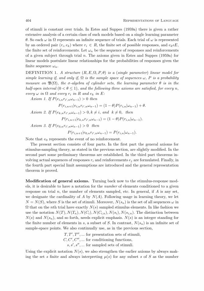
404 Representations of Language

of stimuli is constant over trials. In Estes and Suppes (1959a) there is given a ratherextensive analysis of a certain class of such models based on a single learning parameterθ. So each ω in Ω represents an infinite sequence of trials. Each trial of ω is representedby an ordered pair (ri, ek) where ri ∈ R, the finite set of possible responses, and ekεE,the finite set of reinforcements. Let ωn be the sequence of responses and reinforcementsof a given subject through trial n. The axioms given in Estes and Suppes (1959a) forlinear models postulate linear relationships for the probabilities of responses given thefinite sequence ωn.

DEFINITION 1. A structure (R,E,Ω, P, θ) is a (single parameter) linear model forsimple learning if, and only if, Ω is the sample space of sequences ω, P is a probabilitymeasure on B(Ω), the σ-algebra of cylinder sets, the learning parameter θ is in thehalf-open interval (0 < θ ≤ 1), and the following three axioms are satisfied, for every n,every ω in Ω and every ri in R and ek in E:

Axiom 1. If P (ei,nri′,nωn−1) > 0 then

P (ri,n+1|ei,nri′,nωn−1) = (1 − θ)P (ri,n|ωn−1) + θ.

Axiom 2. If P (ek,nri′,nωn−1) > 0, k = i, and k = 0, then

P (ri,n+1|ek,nri′,nωn−1) = (1 − θ)P (ri,n|ωn−1).

Axiom 3. If P (e0,nri′,nωn−1) > 0 then

P (ri,n+1|e0,nri′,nωn−1) = P (ri,n|ωn−1).

Note that e0 represents the event of no reinforcement.The present section consists of four parts. In the first part the general axioms for

stimulus-sampling theory, as stated in the previous section, are slightly modified. In thesecond part some preliminary theorems are established. In the third part theorems in-volving actual sequences of responses ri and reinforcements ej are formulated. Finally, inthe fourth part special limit assumptions are introduced and the general representationtheorem is proved.

Modification of general axioms. Turning back now to the stimulus-response mod-els, it is desirable to have a notation for the number of elements conditioned to a givenresponse on trial n, the number of elements sampled, etc. In general, if A is any set,we designate the cardinality of A by N(A). Following usage in learning theory, we letN = N(S), where S is the set of stimuli. Moreover, N(sn) is the set of all sequences ω inΩ that on the nth trial have exactly N(s) sampled stimulus elements. In like fashion weuse the notation N(T ), N(Tn), N(Ci), N(Ci,n), N(si), N(si,n). The distinction betweenN(s) and N(sn), and so forth, needs explicit emphasis. N(s) is an integer standing forthe finite number of elements in s, a subset of S. In contrast, N(sn) is an infinite set ofsample-space points. We also continually use, as in the previous section,

T, T ′, T ′′, ... for presentation sets of stimuli,C,C ′, C ′′, ... for conditioning functions,s, s′, s′′, ... for sampled sets of stimuli.

Using the explicit notation N(s), we also strengthen the earlier axioms by always mak-ing the set s finite and always interpreting µ(s) for any subset s of S as the number

8.4 Representation of Linear Models of Learning 405

of elements in s, and therefore write N(s) instead of µ(s), and reserve µ(i) for theprobabilistic mean of some quantity i.

We also require the notion of an experimenter’s partition, already introduced in Estesand Suppes (1959a). We give a verbal definition of such a partition. An experimenter’spartition H(n) for trial n, with elements η, η′, η′′, . . ., is a partition of the samplespace Ω such that each element η of H(n) is defined only in terms of events Tn′ ,ri,n′′ , ej,n′′′ , with 1 ≤ n′, n′′, n′′′ ≤ n. And it should be clear that the elements of anexperimenter’s partition H(n) are simply special sorts of n-dimensional cylinder sets.

Reinforcement axiom.

E1. The probability of a reinforcement depends only on previous observables, namely,preceding presentation sets of stimuli, preceding responses, and preceding out-comes.There is an experimenter’s partition H(n) such that if Wn−1 is any n − 1cylinder set, Y ⊆ Wn−1 ∩ Cn ∩ sn, η ∈ H(n), and P (Y ∩ η) > 0 then

P (ej,n|Y ∩ η) = P (ej,n|η).

Presentation axiom.

P1. The probability of a stimulus presentation set depends only on previous observ-ables.There is an experimenter’s partition H(n− 1) such that if Wn−1 is any n− 1cylinder set, Y ⊆ Wn−1 ∩ Cn, η ∈ H(n− 1) and P (Y ∩ η) > 0, then

P (Tn|Y ∩ η) = P (Tn|η).

Preliminary theorems. We establish a number of theorems and corollaries whichare preliminary to the main theorem. Because we are restricting ourselves to simplelearning, all theorems of the section are based on the hypothesis

(I) The set S of stimuli is the presentation set on every trial.

By virtue of (I) we may omit all consideration of presentation sets T in the sequel.To obtain results independent of n, we also assume that the probability of response i

given the empty sample so is ρi, i.e., for every i and n

(II) ρi,n = ρi.

Third, as a matter of notation, we explicitly define the mean of the number of sampledstimuli:

(III) s =N∑

N(s)=1

N(s)P (N(s)).

The corollaries of the first five theorems show more clearly than do the theoremsthemselves how the theorems provide a stepping stone for deriving the linear model. Thefirst two theorems vary the response on trial n. The second two change the reinforcingevent on trial n. The fifth theorem deals with the case of no reinforcement on trial n.

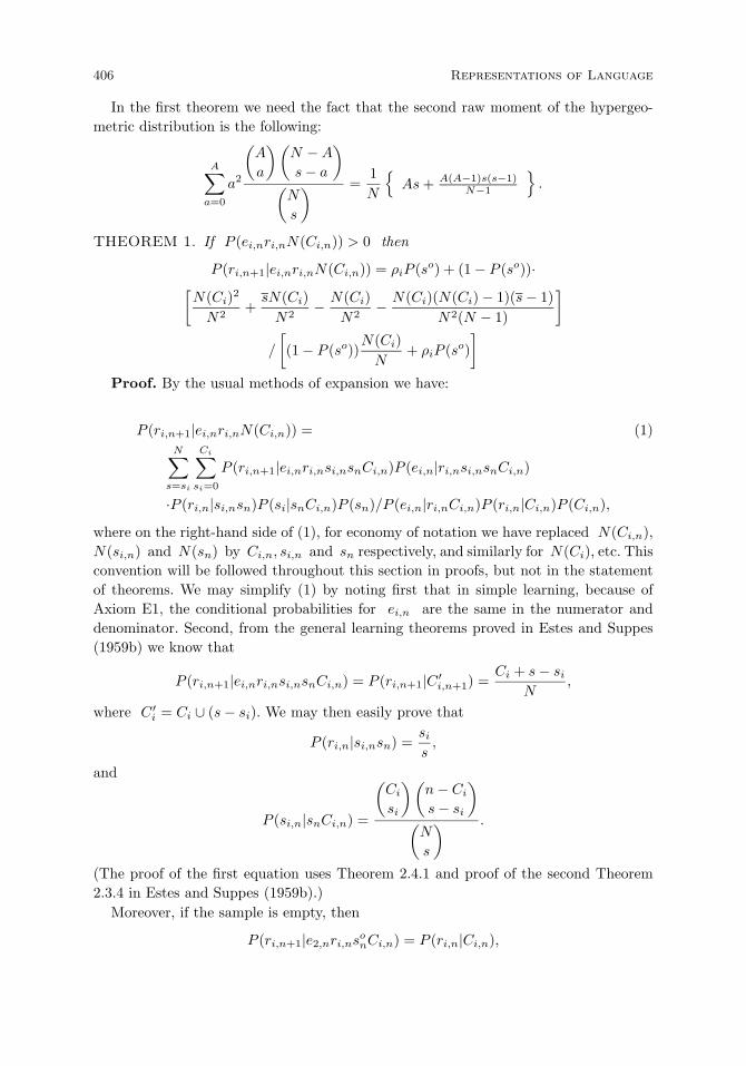
406 Representations of Language

In the first theorem we need the fact that the second raw moment of the hypergeo-metric distribution is the following:

A∑a=0

a2

(A

a

)(N −A

s− a

)(N

s

) =1N

As+ A(A−1)s(s−1)

N−1

.

THEOREM 1. If P (ei,nri,nN(Ci,n)) > 0 then

P (ri,n+1|ei,nri,nN(Ci,n)) = ρiP (so) + (1 − P (so))·[N(Ci)2

N2+sN(Ci)N2

− N(Ci)N2

− N(Ci)(N(Ci) − 1)(s− 1)N2(N − 1)

]

/

[(1 − P (so))

N(Ci)N

+ ρiP (so)]

Proof. By the usual methods of expansion we have:

P (ri,n+1|ei,nri,nN(Ci,n)) = (1)N∑

s=si

Ci∑si=0

P (ri,n+1|ei,nri,nsi,nsnCi,n)P (ei,n|ri,nsi,nsnCi,n)

·P (ri,n|si,nsn)P (si|snCi,n)P (sn)/P (ei,n|ri,nCi,n)P (ri,n|Ci,n)P (Ci,n),

where on the right-hand side of (1), for economy of notation we have replaced N(Ci,n),N(si,n) and N(sn) by Ci,n, si,n and sn respectively, and similarly for N(Ci), etc. Thisconvention will be followed throughout this section in proofs, but not in the statementof theorems. We may simplify (1) by noting first that in simple learning, because ofAxiom E1, the conditional probabilities for ei,n are the same in the numerator anddenominator. Second, from the general learning theorems proved in Estes and Suppes(1959b) we know that

P (ri,n+1|ei,nri,nsi,nsnCi,n) = P (ri,n+1|C ′i,n+1) =

Ci + s− si

N,

where C ′i = Ci ∪ (s− si). We may then easily prove that

P (ri,n|si,nsn) =si

s,

and

P (si,n|snCi,n) =

(Ci

si

)(n− Ci

s− si

)(N

s

) .

(The proof of the first equation uses Theorem 2.4.1 and proof of the second Theorem2.3.4 in Estes and Suppes (1959b).)

Moreover, if the sample is empty, then

P (ri,n+1|e2,nri,nsonCi,n) = P (ri,n|Ci,n),

8.4 Representation of Linear Models of Learning 407

and for the empty sample case the two terms cancel; also, of course, P (ri,n|son) = ρi.

Combining these various remarks and applying them to (1), we infer:

P (ri,n+1|ei,nri,nCi,n) = (2)

ρiP (so) +

N∑s=si

Ci∑si=1

(Ci + s− si)N

· si

s·

(Ci

si

)(N − Ci

s− si

)(N

s

) P (s)

/ P (ri,n|Ci,n).

Summing out si in (2) and using the expression for the second raw moment of the hy-pergeometric distribution mentioned before the theorem, and the fact that the expectedvalue of the distribution is sCi

N , we have:

P (ri,n+1|ei,nri,nCi,n) = (3)

ρiP (so) +∑s=1

[C2

i

N2+sCi

N2− 1sN2

(sCi +Ci(Ci − 1)s(s− 1)

N − 1)]P (s) /P (ri,n|Ci,n).

Summing now over s, we obtain:

P (ri,n+1|ei,nri,nCi,n) = (4)

ρiP (so) + (1 − P (so))[C2

i

N2+sCi

N2− Ci

N2− Ci(Ci − 1)(s− 1)

N2(N − 1)

]/P (ri,n|Ci,n).

It is easy to show we may replace P (ri,n|Ci,n) by (1 − P (so))Ci

N + ρiP (so). We thenobtain the desired result. Q.E.D.

Obviously the theorem has a much simpler form if we assume that the probability ofthe empty sample is zero.

COROLLARY 1. If P (so) = 0, then

P (ri,n+1|ei,nri,nN(Ci,n)) =(N − s)N − 1

N(Ci)N

+s− 1N − 1

.

Proof. On the basis of the hypothesis of the Corollary, we have at once from thetheorem

P (ri,n+1|ei,nri,nCi) = NCi

[ C2i

N2 + sCi

N2 − Ci

N2 − Ci(Ci−1)(s−1)N2(N−1) ]

= (1 + 1−sN−1 )Ci

N + s−1N + s−1

N(N−1)

= N−sN−1

Ci

N + (s− 1)( 1N−1 ) Q.E.D.

The second corollary states a limiting result as N → ∞. The limiting process weuse will be discussed later in more detail, but in essence for a fixed experimenter’sschedule we choose a sequence of stimulus-sampling models S(N) such that for eachi, limN→∞

N(Ci,1)N exists, limN→∞

s(N)N exists, and the variance 1

N2

∑NN(s)=0(N(s)−

s)2P (s) has a limit which is zero. (That such a sequence can be selected is made clearlater.) For purposes of making connections with the linear model intuitively clear, wedefine the learning parameter θ of the linear model as follows:

θ = limN→∞

s(N)N

.

We then have:

408 Representations of Language

COROLLARY 2.

limN→∞

P (ri,n+1|ei,nri,nN(Ci,n)) = (1 − θ) limN→∞

Ci

N+ θ.

The next four theorems and their corollaries are similar in structure to the first group,so routine details will be omitted in proofs. In the second theorem we need the fact thata certain cross-moment of a multivariate hypergeometric distribution is given by thefollowing expression.

r∑a=0

B∑b=0

ab

(A

a

)(B

b

)(N −A−B

s− a− b

)(N

s

) =ABs(s− 1)N(N − 1)

.

THEOREM 2. If i = j and P (ei,nrj,nN(Ci,n)N(Cj,n)) > 0 then

P (ri,n+1|ei,nrj,nN(Ci,n)N(Cj,n)) = ρjP (so)[(1−P (so))N(Ci)

N +ρiP (so)]

(1−P (so))N(Cj )

N +ρjP (so)

+ (1 − P (so))[N(Ci)N(Cj)N2 + sN(Cj)

N2 − N(Ci)N(Cj)(s−1)N2(N−1) ]

/ [(1 − P (so))N(Cj)N + ρjP (so)].

Proof. To begin with we have:

P (ri,n+1|ei,nrj,nCi,nCj,n) (5)

=N∑

s=si+sj

Ci∑si=0

Cj∑sj=0

P (ri,n+1|ei,nrj,nsi,nsj,nsnCi,n)P (rj,n|sj,nsn)

· P (si,nsj,n|snCi,nCj,n)P (sn) / P (rj,n|Cj,n).

On the right-hand side of (5) we have canceled the conditional probability of ei,n fromthe numerator and denominator. To obtain P (si,nsj,n|snCi,nCj,n), we apply Theorem2.3.5 of Estes and Suppes (1959b).12 Thus by the same lines of argument as used forTheorem 1, we infer from (5):

P (ri,n+1|ei,nrj,nCi,nCj,n) = ρjP (so)P (ri,n|Ci,n) / P (rj,n|Cj,n) (6)

+

N∑s=si+sj

Ci∑si=0

Cj∑sj=1

·

(Ci

si

)(Cj

sj

)(N − Ci − Cj

s− si − sj

)(N

s

) P (s)

/ P (rj,n|Cj,n).

12This theorem is a straightforward sampling theorem:

Theorem 2.3.5 If P (N(sn)Cn) > 0 then P (∩ri=1N(si,n)|N(sn)Cn) = πr

i=1

Ci

si

N

s

, where r is

the number of responses.

8.4 Representation of Linear Models of Learning 409

Summing out si and sj in (6) and using the cross-moment of the hypergeometric dis-tribution stated prior to the theorem, we obtain:

P (ri,n+1|ei,nrj,nCi,nCj,n) = ρjP (so)P (ri,n|Ci,n) / P (rj,n|Cj,n) (7)

+N∑

s=1

[CiCj

N2+sCj

N2− 1sN

(CiCjs(s− 1)N(N − 1)

)]P (s) / P (rj,n|Cj,n).

Summing now over s we obtain:

P (ri,n+1|ei,nrj,nCi,nCj,n) = ρjP (so)P (ri,n|Ci,n) / P (rj,n|Cj,n) (8)

+(1 − P (so))[CiCj

N2+sCj

N2− CiCj(s− 1)

N2(N − 1)] / P (rj,n|Cj,n).

Using then Theorem 2.4.5 of Estes and Suppes (1959b) to replace P (ri,n|Ci,n) andP (rj,n|Cj,n) in (8), we obtain the desired result.13 Q.E.D.

We state without proof the two corollaries.

COROLLARY 1. If P (so) = 0, then

P (ri,n+1|ei,nrj,nN(Ci,n)N(Cj,n)) =(N − s

N − 1

)N(Ci)N

+s

N.

COROLLARY 2.

limN→∞

P (ri,n+1|ei,nrj,nN(Ci,n)N(Cj,n)) = (1 − θ) limN→∞

N(Ci)N

+ θ.

We now consider the two cases which arise when the reinforcement on trial n is differentfrom ei.

THEOREM 3. If k = i, k = 0 and P (ek,nri,nN(Ci,n)) > 0, then

P (ri,n+1|ek,nri,nN(Ci,n))

= ρiP (so) + (1 − P (so))[N(Ci)2

N2− N(Ci)

N2− N(Ci)(N(Ci) − 1)(s− 1)

N2(N − 1)

]/[

(1 − P (so))N(Ci)N

+ ρiP (so)].

Proof. Proceeding in the same manner as in the proof of Theorem 1, but accommo-dating in the first term after the summation for the different reinforcement, we obtain:

P (ri,n+1|ek,nri,nN(Ci,n)) = ρiP (so) (9)

+

N∑s=i

Ci∑si=1

(Ci − si)N

· si

s

(Ci

si

)(N − Ci

S − si

)(N

s

) P (s)

/ P (ri,n|Ci,n).

13This theorem expresses a direct conditional response probability given the number of elements

conditioned to that response on a given trial:

Theorem 2.4.5 If P (Ci,n) > 0 then P (ri,n|Ci,n) = (1 − P (son)

N(Ci)N

+ P (son)ρi,n.

410 Representations of Language

Summing out si and then s, we have:

P (ri,n+1|ek,nri,nN(Ci,n)) = ρiP (so) (10)

+ (1 − P (so))[C2

i

N2− Ci

N2− Ci(Ci − 1)(s− 1)

N2(N − 1)

] /P (ri,n|Ci,n),

and the desired result is immediately obtained from (10) by substituting for P (ri,n|Ci,n).Q.E.D.

Again we have two corollaries whose obvious proofs are omitted.

COROLLARY 1. If P (so) = 0 then

P (ri,n+1|ek,nri,nN(Ci,n)) =(N − s

N − 1

)N(Ci)N

− N − s

N(N − 1).

COROLLARY 2.

limN→∞

P (ri,n+1|ek,nri,nN(Ci,n)) = (1 − θ) limN→∞

N(Ci)N

.

The next theorem is for different responses on trials n and n+ 1.

THEOREM 4. If k = i, k = 0, j = i and P (ek,nrj,nN(Ci,n)N(Cj,n)) > 0 then

P (ri,n+1|ek,nrj,nN(Ci,n)N(Cj,n)) =ρjP (so)[(1 − P (so))N(Ci)

N + ρiP (so)]

(1 − P (so))N(Cj)N + ρjP (so)

+(1−P (so))[N(Ci)N(Cj)

N2− N(Ci)N(Cj)(s− 1)

N2(N − 1)

] / [(1 − P (so))

N(Cj)N

+ ρjP (so)].

Proof. Proceeding as in the case of Theorem 2, but making changes for the differentreinforcement, we have, corresponding to (7) of the proof of Theorem 2,

P (ri,n+1|ei,nrj,nCi,nCj,n) = ρjP (so)P (ri,n|Ci,n) / P (rj,n|Cj,n)

+(1 − P (so))[CiCj

N2− CiCj(s− 1)

N2(N − 1)

] /P (rj,n|Cj,n).

And by applying, as before, Theorem 2.4.5 of Estes and Suppes (1959b), the desiredresult is easily obtained. Q.E.D.

COROLLARY 1. If P (so) = 0 then

P (ri,n+1|ek,nrj,nN(Ci,n)N(Cj,n)) =(

N−sN−1

) N(Ci)N

.

COROLLARY 2.

limN→∞

P (ri,n+1|ek,nrj,nN(Ci,n)N(Cj,n)) = (1 − θ) limN→∞

N(Ci)N

.

Finally, we have the theorem for nonreinforcement on trial n. The result, it will benoticed, is the same, whether j = i or j = i.

THEOREM 5. If P (e0,nrj,nN(Ci,n)N(Cj,n)) > 0 then

P (ri,n+1|e0,nrj,nN(Ci,n)N(Cj,n)) = P (ri,n|N(Ci,n)).

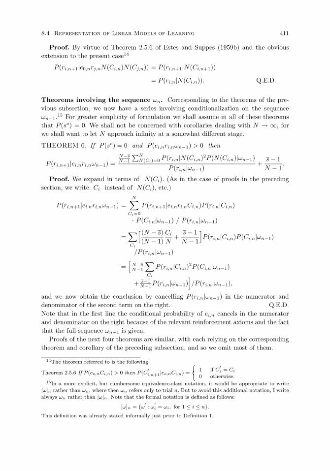
8.4 Representation of Linear Models of Learning 411

Proof. By virtue of Theorem 2.5.6 of Estes and Suppes (1959b) and the obviousextension to the present case14

P (ri,n+1|e0,nrj,nN(Ci,n)N(Cj,n)) = P (ri,n+1|N(Ci,n+1))

= P (ri,n|N(Ci,n)). Q.E.D.

Theorems involving the sequence ωn. Corresponding to the theorems of the pre-vious subsection, we now have a series involving conditionalization on the sequenceωn−1.15 For greater simplicity of formulation we shall assume in all of these theoremsthat P (so) = 0. We shall not be concerned with corollaries dealing with N → ∞, forwe shall want to let N approach infinity at a somewhat different stage.

THEOREM 6. If P (so) = 0 and P (ei,nri,nωn−1) > 0 then

P (ri,n+1|ei,nri,nωn−1) =N−sN−1

∑NN(Ci)=0 P (ri,n|N(Ci,n)2P (N(Ci,n)|ωn−1)

P (ri,n|ωn−1)+

s− 1N − 1

.

Proof. We expand in terms of N(Ci). (As in the case of proofs in the precedingsection, we write Ci instead of N(Ci), etc.)

P (ri,n+1|ei,nri,nωn−1) =N∑

Ci=0

P (ri,n+1|ei,nri,nCi,n)P (ri,n|Ci,n)

· P (Ci,n|ωn−1) / P (ri,n|ωn−1)

=∑Ci

[ (N − s)(N − 1)

Ci

N+

s− 1N − 1

]P (ri,n|Ci,n)P (Ci,n|ωn−1)

/P (ri,n|ωn−1)

=[

N−sN−1

∑Ci

P (ri,n|Ci,n)2P (Ci,n|ωn−1)

+ s−1N−1P (ri,n|ωn−1)

]/P (ri,n|ωn−1),

and we now obtain the conclusion by cancelling P (ri,n|ωn−1) in the numerator anddenominator of the second term on the right. Q.E.D.Note that in the first line the conditional probability of ei,n cancels in the numeratorand denominator on the right because of the relevant reinforcement axioms and the factthat the full sequence ωn−1 is given.

Proofs of the next four theorems are similar, with each relying on the correspondingtheorem and corollary of the preceding subsection, and so we omit most of them.

14The theorem referred to is the following:

Theorem 2.5.6 If P (eo,nCi,n) > 0 then P (C′i,n+1|eo,nCi,n) =

1 if C

′i = Ci

0 otherwise.15In a more explicit, but cumbersome equivalence-class notation, it would be appropriate to write

[ω]n rather than ωn, where then ωn refers only to trial n. But to avoid this additional notation, I write

always ωn rather than [ω]n. Note that the formal notation is defined as follows:

[ω]n = ω′: ω

′i = ωi, for 1 ≤ i ≤ n.

This definition was already stated informally just prior to Definition 1.

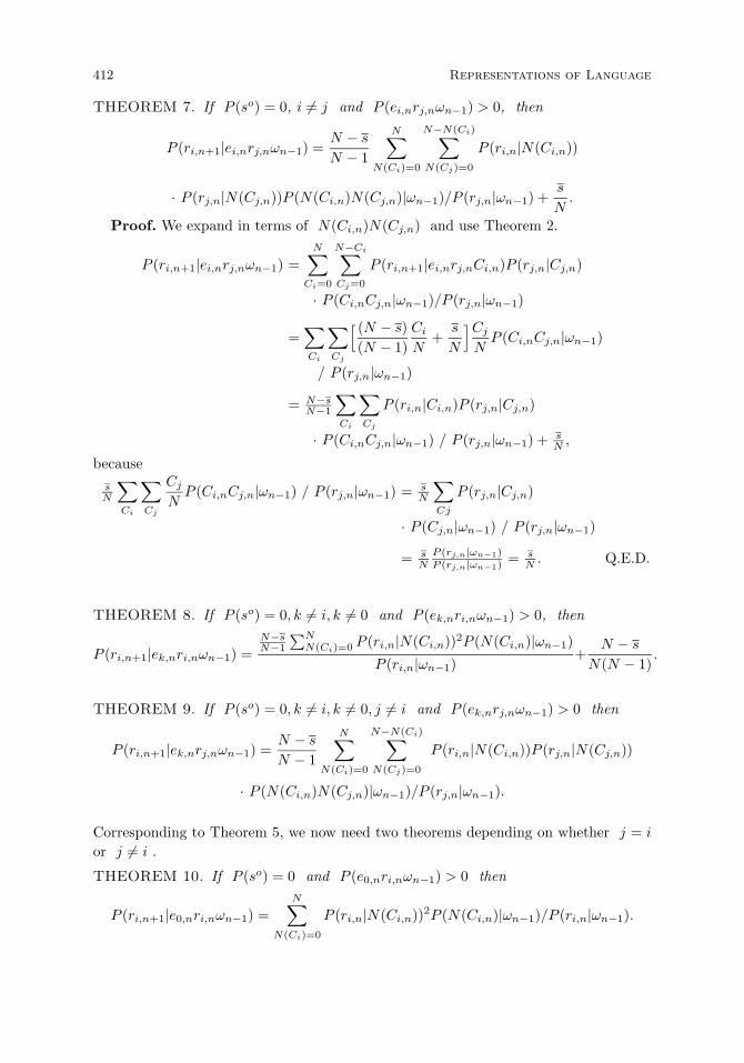
412 Representations of Language

THEOREM 7. If P (so) = 0, i = j and P (ei,nrj,nωn−1) > 0, then

P (ri,n+1|ei,nrj,nωn−1) =N − s

N − 1

N∑N(Ci)=0

N−N(Ci)∑N(Cj)=0

P (ri,n|N(Ci,n))

· P (rj,n|N(Cj,n))P (N(Ci,n)N(Cj,n)|ωn−1)/P (rj,n|ωn−1) +s

N.

Proof. We expand in terms of N(Ci,n)N(Cj,n) and use Theorem 2.

P (ri,n+1|ei,nrj,nωn−1) =N∑

Ci=0

N−Ci∑Cj=0

P (ri,n+1|ei,nrj,nCi,n)P (rj,n|Cj,n)

· P (Ci,nCj,n|ωn−1)/P (rj,n|ωn−1)

=∑Ci

∑Cj

[ (N − s)(N − 1)

Ci

N+

s

N

]Cj

NP (Ci,nCj,n|ωn−1)

/ P (rj,n|ωn−1)

= N−sN−1

∑Ci

∑Cj

P (ri,n|Ci,n)P (rj,n|Cj,n)

· P (Ci,nCj,n|ωn−1) / P (rj,n|ωn−1) + sN ,

becausesN

∑Ci

∑Cj

Cj

NP (Ci,nCj,n|ωn−1) / P (rj,n|ωn−1) = s

N

∑Cj

P (rj,n|Cj,n)

· P (Cj,n|ωn−1) / P (rj,n|ωn−1)

= sN

P (rj,n|ωn−1)P (rj,n|ωn−1)

= sN . Q.E.D.

THEOREM 8. If P (so) = 0, k = i, k = 0 and P (ek,nri,nωn−1) > 0, then

P (ri,n+1|ek,nri,nωn−1) =N−sN−1

∑NN(Ci)=0 P (ri,n|N(Ci,n))2P (N(Ci,n)|ωn−1)

P (ri,n|ωn−1)+

N − s

N(N − 1).

THEOREM 9. If P (so) = 0, k = i, k = 0, j = i and P (ek,nrj,nωn−1) > 0 then

P (ri,n+1|ek,nrj,nωn−1) =N − s

N − 1

N∑N(Ci)=0

N−N(Ci)∑N(Cj)=0

P (ri,n|N(Ci,n))P (rj,n|N(Cj,n))

· P (N(Ci,n)N(Cj,n)|ωn−1)/P (rj,n|ωn−1).

Corresponding to Theorem 5, we now need two theorems depending on whether j = i

or j = i .

THEOREM 10. If P (so) = 0 and P (e0,nri,nωn−1) > 0 then

P (ri,n+1|e0,nri,nωn−1) =N∑

N(Ci)=0

P (ri,n|N(Ci,n))2P (N(Ci,n)|ωn−1)/P (ri,n|ωn−1).

8.4 Representation of Linear Models of Learning 413

THEOREM 11. If P (so) = 0, j = i and P (e0,nrj,nωn−1) > 0 then

P (ri,n+1|e0,nrj,nωn−1) =∑N

N(Ci)=0

∑N−N(Ci)N(Cj)=0 P (ri,n|N(Ci,n))P (rj,n|N(Cj,n))

· P (N(Ci)N(Cj)|ωn−1)/P (rj,n|ωn−1).

As the form of the six theorems just stated suggests, the next step is to prove thatas N → ∞

N∑N(Ci)=0

P (ri,n|N(Ci,n))2P (N(Ci,n)|ωn−1) = P (ri,n|ωn−1)2 (11)

andN∑

N(Ci)=0

N−N(Ci)∑N(Cj)=0

P (ri,n|N(Ci,n))P (rj,n|N(Cj,n))P (N(Ci,n)N(Cj,n)|ωn−1) (12)

= P (ri,n|ωn−1)P (rj,n|ωn−1)

for i = j. For this purpose it is convenient to define certain variances and covariances.

σ2iω(N,n) =

N∑N(Ci)=0

[P (ri,n|N(Ci,n)ωn−1) − P (ri,n|ωn−1)]2 (13)

· P (N(Ci,n)|ωn−1),

σijω(N,n) =N∑

N(Ci)=0

N−N(Ci)∑N(Cj)=0

[P (ri,n|N(Ci,n)ωn−1) − P (ri,n|ωn−1)] (14)

· [P (rj,n|N(Cj,n)ωn−1) − P (rj,n|ωn−1)]P (N(Ci,n)N(Cj,n)|ωn−1).

It is easy to show that

σ2iω(N,n) =

N∑N(Ci)=0

P (ri,n|N(Ci,n))2P (N(Ci,n)|ωn−1) − P (ri,n|ωn−1)2, (15)

and

σijω(N,n) =N∑

N(Ci)=0

N−N(Ci)∑N(Cj)=0

P (ri,n|N(Ci,n))P (rj,n|N(Cj,n)) (16)

· P (N(Ci,n)N(Cj,n)|ωn−1) − P (ri,n|ωn−1)P (rj,n|ωn−1).

From (15) and (16) it is clear that if

limN→∞

σ2iω(N,n) = 0 (17)

andlim

N→∞σijω(N,n) = 0, (18)

then (11) and (12) will be established, provided the limits exist of the individual termson the right-hand sides of (15) and (16). And this existence does follow from our otherresults. Before we proceed to establish (17) and (18), we review our limit assumptionsas N → ∞.

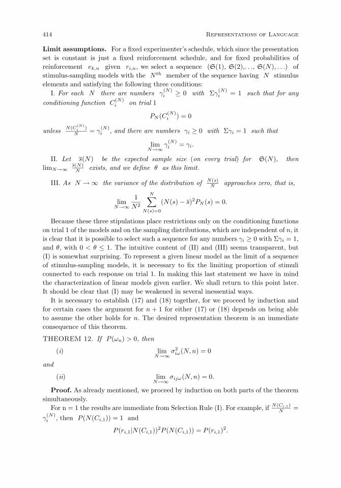
414 Representations of Language

Limit assumptions. For a fixed experimenter’s schedule, which since the presentationset is constant is just a fixed reinforcement schedule, and for fixed probabilities ofreinforcement ek,n given ri,n, we select a sequence (S(1), S(2),. . ., S(N), . . .) ofstimulus-sampling models with the N th member of the sequence having N stimuluselements and satisfying the following three conditions:

I. For each N there are numbers γ(N)i ≥ 0 with Σγ(N)

i = 1 such that for anyconditioning function C

(N)i on trial 1

PN (C(N)i ) = 0

unless N(C(N)i )

N = γ(N)i , and there are numbers γi ≥ 0 with Σγi = 1 such that

limN→∞

γ(N)i = γi.

II. Let s(N) be the expected sample size (on every trial) for S(N), thenlimN→∞

s(N)N exists, and we define θ as this limit.

III. As N → ∞ the variance of the distribution of N(s)N approaches zero, that is,

limN→∞

1N2

N∑N(s)=0

(N(s) − s)2PN (s) = 0.

Because these three stipulations place restrictions only on the conditioning functionson trial 1 of the models and on the sampling distributions, which are independent of n, itis clear that it is possible to select such a sequence for any numbers γi ≥ 0 with Σγi = 1,and θ, with 0 < θ ≤ 1. The intuitive content of (II) and (III) seems transparent, but(I) is somewhat surprising. To represent a given linear model as the limit of a sequenceof stimulus-sampling models, it is necessary to fix the limiting proportion of stimuliconnected to each response on trial 1. In making this last statement we have in mindthe characterization of linear models given earlier. We shall return to this point later.It should be clear that (I) may be weakened in several inessential ways.

It is necessary to establish (17) and (18) together, for we proceed by induction andfor certain cases the argument for n + 1 for either (17) or (18) depends on being ableto assume the other holds for n. The desired representation theorem is an immediateconsequence of this theorem.

THEOREM 12. If P (ωn) > 0, then

(i) limN→∞

σ2iω(N,n) = 0

and

(ii) limN→∞

σijω(N,n) = 0.

Proof. As already mentioned, we proceed by induction on both parts of the theoremsimultaneously.

For n = 1 the results are immediate from Selection Rule (I). For example, if N(Ci,1)N =

γ(N)i , then P (N(Ci,1)) = 1 and

P (ri,1|N(Ci,1))2P (N(Ci,1)) = P (ri,1)2.

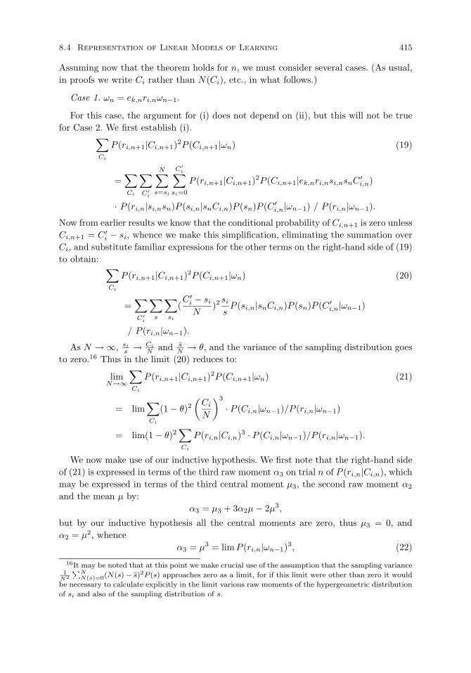
8.4 Representation of Linear Models of Learning 415

Assuming now that the theorem holds for n, we must consider several cases. (As usual,in proofs we write Ci rather than N(Ci), etc., in what follows.)

Case 1. ωn = ek,nri,nωn−1.

For this case, the argument for (i) does not depend on (ii), but this will not be truefor Case 2. We first establish (i).∑

Ci

P (ri,n+1|Ci,n+1)2P (Ci,n+1|ωn) (19)

=∑Ci

∑C′

i

N∑s=si

C′i∑

si=0

P (ri,n+1|Ci,n+1)2P (Ci,n+1|ek,nri,nsi,nsnC′i,n)

· P (ri,n|si,nsn)P (si,n|snCi,n)P (sn)P (C ′i,n|ωn−1) / P (ri,n|ωn−1).

Now from earlier results we know that the conditional probability of Ci,n+1 is zero unlessCi,n+1 = C ′

i − si, whence we make this simplification, eliminating the summation overCi, and substitute familiar expressions for the other terms on the right-hand side of (19)to obtain: ∑

Ci

P (ri,n+1|Ci,n+1)2P (Ci,n+1|ωn) (20)

=∑C′

i

∑s

∑si

(C ′

i − si

N)2si

sP (si,n|snCi,n)P (sn)P (C ′

i,n|ωn−1)

/ P (ri,n|ωn−1).

As N → ∞, si

s → Ci

N and sN → θ, and the variance of the sampling distribution goes

to zero.16 Thus in the limit (20) reduces to:

limN→∞

∑Ci

P (ri,n+1|Ci,n+1)2P (Ci,n+1|ωn) (21)

= lim∑Ci

(1 − θ)2(Ci

N

)3

· P (Ci,n|ωn−1)/P (ri,n|ωn−1)

= lim(1 − θ)2∑Ci

P (ri,n|Ci,n)3 · P (Ci,n|ωn−1)/P (ri,n|ωn−1).

We now make use of our inductive hypothesis. We first note that the right-hand sideof (21) is expressed in terms of the third raw moment α3 on trial n of P (ri,n|Ci,n), whichmay be expressed in terms of the third central moment µ3, the second raw moment α2

and the mean µ by:α3 = µ3 + 3α2µ− 2µ3,

but by our inductive hypothesis all the central moments are zero, thus µ3 = 0, andα2 = µ2, whence

α3 = µ3 = limP (ri,n|ωn−1)3, (22)

16It may be noted that at this point we make crucial use of the assumption that the sampling variance1

N2

PNN(s)=0(N(s)− s)2P (s) approaches zero as a limit, for if this limit were other than zero it would

be necessary to calculate explicitly in the limit various raw moments of the hypergeometric distribution

of si and also of the sampling distribution of s.

416 Representations of Language

and combining (21) and (22), we have:

lim∑Ci

P (ri,n+1|Ci,n+1)2P (Ci,n+1|ωn) = (1 − θ)2 limP (ri,n|ωn−1)2. (23)

We now apply the fact that by virtue of our inductive hypothesis α2 = µ2 to Theorem8 as N → ∞ and obtain:

limP (ri,n+1|ωn) = (1 − θ) limP (ri,n|ωn−1). (24)

Equation (i) follows for Case 1 immediately from (23) and (24).We now turn to (ii), and use the same arguments which took us from (19) to (20).

α(i, j, ω, n+ 1) =∑Ci

∑Cj

P (ri,n+1|Ci,n+1)P (rj,n+1|Cj,n+1) (25)

· P (Ci,n+1Cj,n+1|ωn)

=∑Ci

∑Cj

∑s

∑si

∑sj

(Ci − si)N

(Cj − sj)N

si

sP (si,nsj,n|snCi,nCj,n)

· P (sn)P (Ci,nCj,n|ωn−1) / P (ri,n|ωn−1).

Now again as N → ∞, si

s → Ci

N ,sj

s → Cj

N and sN → θ, and 1

N2

∑s(s − s)2P (s) → 0,

whence in the limit (25) reduces to:

limα(i, j, ω, n+ 1) = (1 − θ)2 lim∑Ci

∑Cj

(Ci

N)2(

Cj

N)P (Ci,nCj,n|ωn−1) (26)

/ P (ri,n|ωn−1)

= (1 − θ)2 lim∑Ci

∑Cj

P (ri,n|Ci,n)2P (rj,n|Cj,n)

· P (Ci,nCj,n|ωn−1) / P (ri,n|ωn−1).

We now use our inductive hypothesis to compute the raw cross-moment on trial n, whichis denoted by the expression on the right-hand side of (26). Thus, dropping notation forω and n, let

α(i2, j) =∑Ci

∑Cj

P (ri,n|Ci,n)2P (rj,n|Cj,n)P (Ci,nCj,n|ωn−1), (27)

µ(i2, j) =∑Ci

∑Cj

[P (ri,n|Ci,n) − µ(i)]2[P (rj,n|Ci,n) − µ(j)] (28)

· P (Ci,nCj,n|ωn−1)

where µ(i) is the mean of P (ri,n|Ci,n), and similarly for µ(j). And the definition ofα(i, j) should be obvious. Now by explicit computation

µ(i2, j) = α(i2, j) − α(i2)µ(j) − 2α(i, j)µ(i) + 2µ(i)2µ(j) (29)

+ µ(i)2µ(j) − µ(i)2µ(j).

It easily follows from our induction that the central cross-moment µ(i2, j) = 0. Also byour inductive hypothesis µ(i2) = σ2

i = 0, whence

α(i2) = µ(i)2.

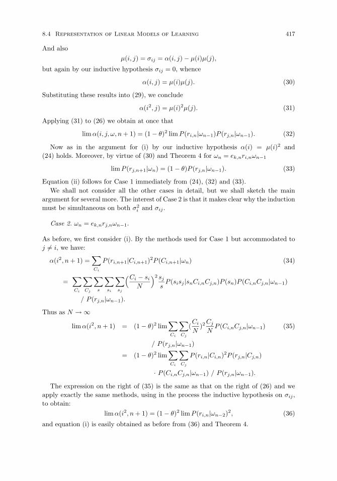
8.4 Representation of Linear Models of Learning 417

And alsoµ(i, j) = σij = α(i, j) − µ(i)µ(j),

but again by our inductive hypothesis σij = 0, whence

α(i, j) = µ(i)µ(j). (30)

Substituting these results into (29), we conclude

α(i2, j) = µ(i)2µ(j). (31)

Applying (31) to (26) we obtain at once that

limα(i, j, ω, n+ 1) = (1 − θ)2 limP (ri,n|ωn−1)P (rj,n|ωn−1). (32)

Now as in the argument for (i) by our inductive hypothesis α(i) = µ(i)2 and(24) holds. Moreover, by virtue of (30) and Theorem 4 for ωn = ek,nri,nωn−1

limP (rj,n+1|ωn) = (1 − θ)P (rj,n|ωn−1). (33)

Equation (ii) follows for Case 1 immediately from (24), (32) and (33).We shall not consider all the other cases in detail, but we shall sketch the main

argument for several more. The interest of Case 2 is that it makes clear why the inductionmust be simultaneous on both σ2

i and σij .

Case 2. ωn = ek,nrj,nωn−1.

As before, we first consider (i). By the methods used for Case 1 but accommodated toj = i, we have:

α(i2, n+ 1) =∑Ci

P (ri,n+1|Ci,n+1)2P (Ci,n+1|ωn) (34)

=∑Ci

∑Cj

∑s

∑si

∑sj

(Ci − si

N

)2 sj

sP (sisj |snCi,nCj,n)P (sn)P (Ci,nCj,n|ωn−1)

/ P (rj,n|ωn−1).

Thus as N → ∞

limα(i2, n+ 1) = (1 − θ)2 lim∑Ci

∑Cj

(Ci

N)2Cj

NP (Ci,nCj,n|ωn−1) (35)

/ P (rj,n|ωn−1)

= (1 − θ)2 lim∑Ci

∑Cj

P (ri,n|Ci,n)2P (rj,n|Cj,n)

· P (Ci,nCj,n|ωn−1) / P (rj,n|ωn−1).

The expression on the right of (35) is the same as that on the right of (26) and weapply exactly the same methods, using in the process the inductive hypothesis on σij ,to obtain:

limα(i2, n+ 1) = (1 − θ)2 limP (ri,n|ωn−2)2, (36)

and equation (i) is easily obtained as before from (36) and Theorem 4.

418 Representations of Language

Turning now to (ii), we have by the usual methods:

α(i, j, n+ 1) =∑Ci

∑Cj

∑s

∑si

∑sj

(Ci − si)N

(Cj − sj)N

sj

s(37)

· P (si,nsj,n|snCi,nCj,n)P (sn)P (Ci,nCj,n|ωn−1) / P (ri,n|ωn−1)

but the right-hand side of (37) is just like the right-hand side of (25) with i and j

interchanged, and the argument proceeds in identical fashion.

Case 3. ωn = ek,nrj′,nωn−1.

The proof of (i) is the same as for Case 2 with j′ replacing j. The situation is differentwith respect to the proof of (ii), for a new kind of raw cross-moment must be considered,namely α(i, j, j′) which, however, may be treated in the same fashion as α(i2, j).

α(i, j, j′, n+ 1) =∑Ci

∑Cj

∑s

∑si

∑sj

∑sj′

(Ci − si)N

(Cj − sj)N

sj′

s(38)

· P (si,nsj,nsj′,n|snCi,nCj,nCj′,n)P (sn)P (Ci,nCj,nCj′,n|ωn−1)

/ P (rj′,n|ωn−1).

Thus as N → ∞limα(i, j, j′, n+ 1) = (1 − θ)2 limα(i, j, j′, n) / µ(j′, n). (39)

But the central cross-moment (on trial n) is:

µ(i, j, j′) = α(i, j, j′) − α(i, j)µ(j′) − α(i, j′)µ(j) − α(j, j′)µ(i) (40)

−2µ(i)µ(j)µ(j′).

By our inductive hypothesis µ(i, j, j′) = 0, and α(i, j) = µ(i)µ(j), etc., whence

α(i, j, j′) = µ(i)µ(j)µ(j′), (41)

as would be expected from earlier results. From (39) and (41) we have

limα(i, j, j′, n+ 1) = (1 − θ)2 limµ(i, n)µ(j, n), (42)

and the remainder of the argument moves along standard lines.The other six cases are proved in a similar way and consequently will be omitted. It

should be clear that the argument always hinges on establishing a result like (30), (31)or (41). Q.E.D.

We now have as a consequence of the theorems in this section the following repre-sentation theorem for linear models.

THEOREM 13. (Representation Theorem). Given any single parameter linear model(R,E,Ω, P, θ) there exists a sequence (S(1),. . . ,S(N), . . .) of stimulus-sampling modelssuch that for every ω and n

P (ωn) = limN→∞

PN (ωn),

where PN is the probability measure of S(N) .

Proof. We use selection rules (I), (II), and (III), the preceding theorems of thissection, and proceed by induction on n. For n = 1, we use selection rule (I). Assuming

8.5 Learning Comprehension Grammars 419

the theorem holds for n, we then use the fact that in the limit the axioms hold for thesequence of stimulus-sampling models. The remainder of the simple inductive proof isexactly analogous to that of Theorem 4.1 in Estes and Suppes (1959a) on linear models,and will not be repeated here.

As can be seen from the dates of the principal articles referred to in these two sec-tions, the main results were obtained more than thirty years ago. I still like them asexamples of representation theorems in mathematical psychology. The proof of Theo-rem 13 can, with some work, probably be simplified, but even if so, it will remain astestimony to the technical problems of proving exact reduction theorems even for rela-tively simple scientific theories. A new area of application, with possibly some changesin the theorem and its proof, may be to the reinforcement learning models now beingused in experimental economics. At least in the recent past, economists have been moreinterested than psychologists in representation theorems.

8.5 Robotic Machine Learning of Comprehension Grammars forTen Languages17

Without going into all the details, I want to convey a rather clear intuitive sense of theprocess of learning of natural language in terms of the various events that happen whenan utterance is given to a robot. (But it should be understood that the basic programof machine learning would apply without serious modification to other applications, forexample, machine learning of physics word problems, which I briefly consider later.)Also, following standard learning usage, I shall often speak of trials where, of course, Imean that the trial begins with a command in the form of an utterance to be executedby the robot.

The most important way to describe conceptually the learning process the programembodies is in the description of the state of memory of a robot at the beginning ofeach trial. There are four aspects of this memory that are changed due to learning. Thefirst is the association relation between words of a given language and internal symbolsthat have as denotations actions, objects, properties and relations in the robot’s world.A central problem is to learn in each language what word is properly associated with agiven internal symbol. A second aspect of the memory that changes is the denotationalvalue of a given word, which will affect its probability of being associated. The third partthat changes is the short-term memory that holds a given verbal command for the periodof the trial on which it is effective. This memory content decays and is not availablefor access after the trial on which a particular command is given. This means that atthe beginning of the trial, before a command is given, this short-term buffer is empty.What we have said thus far, could, with some stretching, fit into classical theories ofassociation, but for language learning it is quite evident that this semantically restrictedassociation relation and some simple features of short-term memory are certainly notenough.

The fourth aspect is the important one of learning grammatical forms. Consider

17This section is based on Suppes, Bottner and Liang (1996), and Suppes and Liang (1996). Two

prior papers describing the approach, first presented at two conferences in 1991, are Suppes, Liang and

Bottner (1992) and Suppes, Bottner and Liang (1995).

420 Representations of Language

the verbal command Get the nut. This would be an instance of the grammatical formA the O, where A is the category of actions and O is the category of objects. Thisform actually represents a mild oversimplification, because we do not have just a singlecategory of actions. There are several subcategories, depending upon the number ofarguments required, and certain other natural semantical requirements as well. Theexample will illustrate how things work, however. The grammatical forms are derivedby generalization only from actual instances of verbal commands given to the robot.No prior knowledge of any sort of the grammar of the natural language to be learned isavailable to the robot. Also important is the fact that associated with each grammaticalform as it arises from generalization are the associations of the words which have beenthe basis for the generalization, along with their internal representations. For example,if Get the nut were the occurrence in which the grammatical form just stated wasgenerated, then also stored with that grammatical form would be the associations get ∼$g and nut ∼ $n, where $g and $n are internal symbols whose denotations are known tothe robot. When incorrect associations are deleted by further learning, the grammaticalforms based on such associations are also deleted.

Comprehension grammar. Most linguistic analysis is concerned with grammars detailedenough to produce natural utterances of the language being studied. A comprehensiongrammar, in contrast, as we characterize it here, can generate a superset of utterances.The rules are required only to lead to the correct semantic interpretation of an utteranceof the language. Robots, like very young children, can easily have the capacity to under-stand language before they can produce it. Although it is difficult and subtle to collectaccurate and anything like complete data on the comprehension grammar generated byvery young children, the evidence is overwhelming that they comprehend much morethan they can produce.

Problem of denotation. In the probabilistic theory of machine learning of naturallanguage which we have been developing, we have encountered in a new form a standardproblem in the analysis of the semantics of natural language, namely, how to handlewords that are nondenoting. We do not mean nondenoting in some absolute sense, butrelative to a fixed set of semantic categories. These categories in the robotic case are,roughly speaking, the categories of actions, objects, properties and relations. It may wellbe that in some elaborate set-theoretical semantics of natural language, nondenotingwords like the definite article the denote a complicated set-theoretical function, butthe relevance of such an elaborate semantics to language learning is doubtful. In therobotic context, we have something simpler and closer to the common man’s view ofwhat denotations are. We take, as denoting words, color and object words, commonnouns, familiar concrete action words, etc. We take ordinary prepositions in English,and sometimes other devices in other languages, to denote relations in most cases. Onthe other hand, our computational semantics centered on physics word problems, withan internal equational language of physical quantities, is further removed from common-sense ideas.

When a child learning a first language, or an older person learning a second language,

8.5 Learning Comprehension Grammars 421

first encounters utterances in that new language, there is no uniform way in whichnondenoting words are marked. There is some evidence that various prosodic features areused in English and other languages to help the child. For example, in many utterancesaddressed to very young children, the definite or indefinite article is not stressed butrather the common noun it modifies, as in the expression Hand me the cup. But suchdevices do not seem uniform, and in any case are not naturally available to us in ourmachine-learning research, where we use written input of words without additionalprosodic notation.

As has already been made clear, a central feature of our approach to machine learningis the probabilistic association between words of the natural language being learned anddenoting symbols of the internal language. It is appropriate that at the beginning allwords are treated equally, and so the associations are formed from sampling based ona uniform distribution. On the other hand, after many words have been learned anda good deal of language has been acquired by the robot, it is very unnatural, andalso inefficient, if the robot is now given, for example, the esoteric command Get theastrolabe, to have the internal symbol $ast be associated with equal probability with thedefinite article the and astrolabe—we assume here that the association of get is alreadycorrectly fixed. After much linguistic experience, there should be very little chance ofthe robot’s associating the definite article the with any denoting symbol.

To incorporate such learning many variant models are easily formulated. We haverestricted ourselves to one which brings out the most salient distinctions to consider.

Background cognitive and perceptual assumptions. Before explicitly formulat-ing the learning principles of association and denotation used, I first state informallyassumptions we make about the cognitive and perceptual capacities of the class ofrobots, albeit as yet quite limited, we work with.

Internal language. The robot has a fully developed internal language, which it does notlearn. It is technically important, but not conceptually fundamental, that in our casethis language is Lisp. When we speak here of the internal language we refer only tothe language of the internal representation, which is itself a language at a higher levelof abstraction, relative to the concrete movements and perceptions of the robot. It isthe language of the internal representations held in memory that provides the directinterface to the natural-language learning. In fact, most of the machine learning of agiven natural language can take place through simulation of the robot’s behavior byusing just the language of the internal representation. The first associations learned arebetween the internal representation in memory of a coerced action and a contiguousverbal utterance in the natural language being learned.

The fundamental importance of this internal representation of a coerced action canbe recognized by considering a parallel case of animal learning. When a dog is trained toGet the paper or Get the ball by being led through the desired action or by some relatedtechnique, the residue in memory of what we term the coerced action is surely drasticallyabstracted from the perceptually rich context of the demonstrated action desired, andit is that abstracted internal representation in memory that must be associated to the

422 Representations of Language

verbal stimulus in order for the dog later to perform the desired action upon hearingthe verbal command. We are a long way from knowing even the general structure of thedog’s internal representation in memory of the action. In this limited sense, life with arobot is much easier, for we ourselves create the form of its internal representation.

Objects, relations and properties. We furthermore assume the robot begins its natural-language learning with all the basic cognitive and perceptual concepts it will have. Inother words, our first-language learning experiments are pure language learning. Anylearning of new concepts is delayed to another phase. For example, we have assumedthat the spatial relations frequently referred to in all, or at least all the languages weconsider in detail, are already known to the robot. This is quite contrary to humanlanguage learning. For example, probably in no widely used natural language at least,do children at the age of thirty-six months use or fully understand the relations of leftand right. To avoid misunderstanding, we emphasize that we consider it an importantfuture task to have the robot also learn the familiar spatial and temporal relations.

Actions. What was just said about objects and relations applies also to actions, repre-sented in English by such verbs as pick up, get, place, etc. The English, of course, mustbe learned, but not the underlying actions.

Associations and grammatical forms. Before stating any formal principles of learning,I describe as informally and intuitively as possible the learning setup used. Consider theEnglish command Pick up the screw, no part of which has as yet been learned by therobot. The learning steps may be roughly schematized as follows:

(i) By coercion, or simulation of coercion, the robot creates in memory an internalrepresentation of the coerced action of picking up the screw. For statement oflearning principles we show this internal representation, not as a Lisp expression,but just as a schematic function I(...) of the denoting terms in the Lisp expression.Here, by denoting terms we mean the names in the internal language of the actions,objects, properties and relations mentioned. The internal representation of Pick upthe screw is then I($p,$u,$s), where $p = the action of picking, $u = the directionup and $s = screw.

(ii) By contiguity the robot associates the verbal utterance and the internal represen-tation

Pick up the screw ∼ I($p,$u,$s),

where ‘∼’ is the symbol used for association.(iii) By probabilistic association, the robot associates the internal denotations with the

English words, with one possibility the following incorrect result:

pick ∼ $s, up ∼ $p, screw ∼ $u.

We need to observe the following:(a) We assume from the beginning the robot knows word boundaries, as delin-

eated by the typed input. This is an example of an assumption that is natural

8.5 Learning Comprehension Grammars 423

for robots, but clearly false for very young children.(b) For our simple example, there are twenty-four possible ways of associating the

three internal symbols to the four denoting words in the English utterance.We initially assign to each of these twenty-four possibilities equal probabil-ity, but as trials continue, modify the probability by dynamic changes indenotational values, as is explained later in detail.

(iv) After the associations are made, by the principle of generalization, which we callcategory generalization, each word is assigned the category of its associated inter-nal symbol. In the present case pick ∈ O—the category of objects, up ∈ A—thecategory of actions and screw ∈ R—the category of relations. A grammaticalform is then also generalized from the verbal command:

O A the R

which, like the assigned categories is wrong for English, but remember that thisis just the starting point of learning. With this grammatical form is associated itsinternal representation I(A, R, O) which characterizes its meaning.

(v) A new command is presented as the next step, say Pick up the nut. By coercionthe internal representation I($p, $u, $n) is created (see (i) above). The robot thenfirst searches its memory to see if any of the words uttered are associated to one ofthe internal denotations. Here the result is up ∼ $p, and also the classification ofthe as a nondenoting word is found. There are then six possibilities of probabilisticassociation for pick, the and nut. Note that the earlier incorrect association of pickwith $s does not appear here, which means that at this stage of learning it will bechanged. So, let us suppose the new associations are

pick ∼ $u, nut ∼ $n.

We also have as a new grammatical form

R A the O

which though incorrect, now has only the confusion of the associations of pickand up as its source. To correct these associations we must separate the constantpairing of pick and up, which is what we do. In any case, we form at once theassociation to the internal representation:

R A the O ∼ I(A, R, O).

(vi) Learning stops whenever the following steps of interpretation can be successfullycompleted upon giving the robot a verbal command:

(a) An association to an internal denotation or a nondenoting classification isfound in memory for each word.

(b) The category of each word is found in memory.(c) The grammatical form resulting from (b) is found with an associated internal

representation in memory.(d) The command is correctly executed on the basis of the internal representa-

tion.

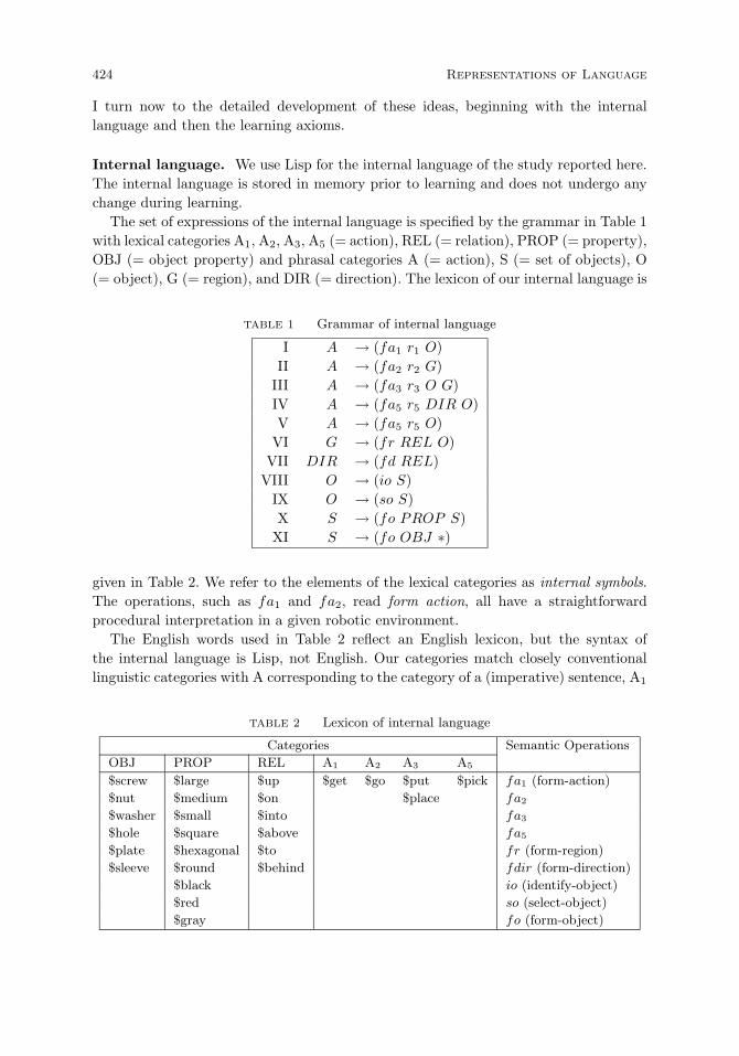
424 Representations of Language

I turn now to the detailed development of these ideas, beginning with the internallanguage and then the learning axioms.

Internal language. We use Lisp for the internal language of the study reported here.The internal language is stored in memory prior to learning and does not undergo anychange during learning.

The set of expressions of the internal language is specified by the grammar in Table 1with lexical categories A1, A2, A3, A5 (= action), REL (= relation), PROP (= property),OBJ (= object property) and phrasal categories A (= action), S (= set of objects), O(= object), G (= region), and DIR (= direction). The lexicon of our internal language is

TABLE 1 Grammar of internal language

I A → (fa1 r1 O)II A → (fa2 r2 G)

III A → (fa3 r3 O G)IV A → (fa5 r5 DIR O)V A → (fa5 r5 O)

VI G → (fr REL O)VII DIR → (fd REL)

VIII O → (io S)IX O → (so S)X S → (fo PROP S)

XI S → (fo OBJ ∗)

given in Table 2. We refer to the elements of the lexical categories as internal symbols.The operations, such as fa1 and fa2, read form action, all have a straightforwardprocedural interpretation in a given robotic environment.

The English words used in Table 2 reflect an English lexicon, but the syntax ofthe internal language is Lisp, not English. Our categories match closely conventionallinguistic categories with A corresponding to the category of a (imperative) sentence, A1

TABLE 2 Lexicon of internal language

Categories Semantic Operations

OBJ PROP REL A1 A2 A3 A5

$screw $large $up $get $go $put $pick fa1 (form-action)

$nut $medium $on $place fa2

$washer $small $into fa3

$hole $square $above fa5

$plate $hexagonal $to fr (form-region)

$sleeve $round $behind fdir (form-direction)

$black io (identify-object)

$red so (select-object)

$gray fo (form-object)

8.5 Learning Comprehension Grammars 425

corresponding to the category of transitive verbs, REL corresponding to the category ofprepositions, PROP to the category of adjectives, OBJ corresponding to the categoryof a common noun, DIR to the category of adverbs, G to the category of prepositionalphrases, O to the category of (determined) noun phrases, and S to the category ofa nominal group. We chose, however, not to refer to these categories by their usuallinguistic labels, since we think of them as semantic categories.

The grammar of the internal language would derive the following Lisp structure forthe internal representation of the action corresponding to the English command Get ascrew, where the asterisk ∗ refers to the set of objects that are present in a certain visualenvironment:

(fa1 $get (so (fo $screw ∗))). (1)

Let γ = (fo $screw ∗). Then γ itself is the minimal Lisp expression in (1) containingonly the internal symbol $screw, and (so (fo $screw ∗)) is the maximal Lisp expressionin (1) containing only the internal symbol $screw. We use this distinction later.

General learning axioms. We now turn to our learning axioms, which naturally fallinto two groups, those for computations using working memory and those for changesin the state of long-term memory. We use, as is obvious, a distinction about kinds ofmemory that is standard in psychological studies of human memory, but the details ofour machine-learning process are not necessarily faithful to human learning of language,and we make no claim that they are. On the other hand, our basic processes of associa-tion, generalization, specification and rule-generation almost certainly have analogues inhuman learning, some better understood than others at the present time. In the generalaxioms formulated in this section we assume rather little about the specific languageof the internal representation, although the examples that illustrate the axioms use theinternal language just described.

Notation. Concerning notation used in the axioms, we generally use Latin letters forsentences or their parts, whatever the natural language, and we use Greek letters to referto internal representations of sentences or their parts. Turning now to specific notation,the letters a, b, ... refer to words in a sentence, and the Greek letters α, β, ... refer tointernal symbols. The symbol s refers to an entire sentence, and correspondingly σ to anentire internal representation. Grammatical forms—either sentential or term forms—aredenoted by g or also g(X) to show a category argument of a form; correspondingly theinternal representations of a grammatical form are denoted by γ or γ(X). We violate ourGreek-Latin letter convention in the case of semantic categories or category variablesX, X ′, Y , etc. We use the same category symbols in both grammatical forms and theirinternal representations.

To insure the proper semantic meaning is carried from a natural-language sentenceto its internal representation, or vice versa, we index, as needed, multiple occurrences ofthe same category in a given sentence and the corresponding occurrences in its internalrepresentation. An example of this indexing is given later.

426 Representations of Language

Computations Using Working Memory.18

W1. Probabilistic Association. On any trial, let s be associated to σ, let a be in the setof words of s not associated to any internal symbol of σ, and let α be in the set ofinternal symbols not currently associated with any word of s. Then pairs (a, α) aresampled, possibly using the current denotational value, and associated, i.e., a ∼ α.

The probabilistic sampling in the case Get the screw could lead to the incorrect asso-ciations get ∼ $screw, the ∼ $get and no association for screw, for there are only twosymbols to be associated to in the internal representation.

W2. Form Generalization.19 If g(g′i) ∼ γ(γ′i), g′i ∼ γ′i, and γ′ is derivable from X, then

g(Xi) ∼ γ(Xi), where i is the index of occurrence.

From the associations given after Axiom W1 we would derive the incorrect generalization

OBJ A1 screw ∼ (fa1 A1 (io (fo OBJ ∗))). (2)

The correct one is

A1 the OBJ ∼ (fa1 A1 (io (fo OBJ ∗))). (3)

W3. Grammar-Rule Generation. If g ∼ γ and γ is derivable from X, then X → g.

Corresponding to W3, we now get the incorrect rule

A → OBJ A1 screw. (4)

The correct one isA → A1 the OBJ. (5)

W4. Form Association. If g(g′) ∼ γ(γ′) and g′ and γ′ have the corresponding indexedcategories, then g′ ∼ γ′.

We get from (2) the incorrect form association

OBJ ∼ (io (fo OBJ ∗)). (6)

The correct one—to be learned from more trials—is derived from (3)

the OBJ ∼ (io (fo OBJ ∗)). (7)

W5. Form Specification. If g(Xi) ∼ γ(Xi), g′ ∼ γ′, and γ is derivable from X, theng(g′i) ∼ γ(γ′i).

As can be easily seen, Axiom W5 on form specification is essentially the converse ofAxiom W2 on form generalization.

W6. Content Deletion. The content of working memory is deleted at the end of eachtrial.

18The learning program has a short-term working memory for processing the command it is presented.

The memory holds its content for the time period of a single trial. The first group of learning axioms

describe the association computations that take place in working memory during the course of a trial.19A distinct principle of generalization generates grammatical forms and their associated semantic

forms. The methods used combine those of context-free grammars and model-theoretic semantics for

formal languages. The concept of generalization is widely used in psychological theories of learning. The

kind of generalization used here is restricted to the generation of grammatical forms and grammatical

rules from concrete utterances. For example, the phrase the nut generalizes to the grammatical form

the O, where O is the category of objects.

8.5 Learning Comprehension Grammars 427

We now turn to the axioms governing long-term memory.

Changes in State of Long-term Memory20

L1. Denotational Value Computation. If at the end of trial n a word a in the pre-sented verbal stimulus is associated with some internal symbol α, then d(a), thedenotational value of a, increases and if a is not so associated d(a) decreases.Moreover, if a word a does not occur on a trial, then d(a) stays the same unlessthe association of a to an internal symbol α is broken on the trial, in which cased(a) decreases.

Because this axiom is conceptually less familiar, we give a more detailed example later.

L2. Form Factorization. If g ∼ γ and g′ is a substring of g that is already in long-termmemory and g′ and γ′ are derivable from X, then g and γ are reduced to g(X) andγ(X). Also g(X) ∼ γ(X) is stored in long-term memory, as is the correspondinggrammatical rule generated by Axiom W4.

We illustrate this axiom by an example, which is really simple. It seems complex, becausethe premises take three lines, and we have two conclusions, an association and thecorresponding grammatical rule. Let

g ∼ γ : A1 the OBJ ∼ (fa1 A1 (io (fo OBJ ∗)))g′ ∼ γ′ : the OBJ ∼ (io (fo OBJ ∗))

X : O → the OBJ

ThenA1 O ∼ (fa1 A1 O)

A → A1 O.

L3. Form Filtering. Associations and grammatical rules are removed from long-termmemory at any time if they can be generated.

In the previous example, g ∼ γ can now be removed from long-term memory, and socan A → A1 the OBJ , learned as an example of Axiom W3.

L4. Congruence Computation.21 If w is a substring of g, w′ is a substring of g′ andthey are such that(a) g ∼ γ and g′ ∼ γ,(b) g′ differs from g only in the occurrence of w′ in place of w,(c) w and w′ contain no words of high denotational value,

then w′ ≈ w and the congruence is stored in long-term memory.20This memory can also change from trial to trial, but it stores associations and grammatical forms

which remain unchanged when they are correct for the application being considered. The way the state

of long-term memory changes from trial to trial is described in this second part of the learning axioms.21By using a concept of semantic congruence restricted to nondenoting words, we simplify the gram-

mars and at the same time permit direct comparisons across languages. The intuitive idea of such

congruence is simple. Two strings of a natural language are congruent when they have identical repre-

sentations in the internal language.

Various strong and weak concepts of congruence can be used to get varying degrees of closeness of

meaning. The idea is not to be caught in the search for a single concept of synonymy, just as in modern

geometry we are not caught in a single concept of congruence. We have in affine geometry, for example, a

weaker sense of congruence than in Euclidean geometry but it is also easy to get a commonsense notion

of congruence that is stronger than the Euclidean one, namely congruence that requires sameness of

orientation.

428 Representations of Language

Using Axiom L4, reduction of the number of grammatical rules for a given naturallanguage is further achieved by using congruence of meaning (Suppes 1973b, 1991).Consider the following associations of grammatical forms:

die Schraube ∼ (io (fo $screw ∗)) (8)

der Schraube ∼ (io (fo $screw ∗)). (9)

Association (8) and (9) differ only with respect to the article. The article in (8) is inthe nominative and accusative case, the article in (9) is in the genitive and dative case.What is important here is that there is no difference in the respective internal repre-sentations. We therefore call (8) congruent with (9) and collect the differing elementsinto a congruence class [DA] = die, der where DA = definite article. This allows usto reduce the two grammatical forms (8) and (9) into one:

[DA] Schraube ∼ (io (fo $screw ∗)). (10)

Notice that reduction by virtue of congruence is risky in the following way. We maylose information about the language to be learned. For instance, collapsing the genderdistinction exhibited by the difference between (8) and (9) will make us incapable ofdistinguishing between the following sentences:

Steck die Schraube in das Loch. (11)

Steck die Schraube in die Loch. (12)

Whereas (11) is grammatical, (12) is not. As long as our focus is on comprehensiongrammar, a command like (12) will probably not occur, but for purposes of production,congruence in the present form should not be used.

L5. Formation of Memory Trace. The first time a form generalization, grammaticalrule or congruence is formed, the word associations on which the generalization,grammatical rule or congruence is based are stored with it in long-term memory.

Using our original example after W3, the incorrect associations would be stored inlong-term memory, but with more learning, later deleted (L6 (a)).

L6. Deletion of Associations.22

(a) When a word in a sentence is given a new association, any prior associationof that word is deleted from long-term memory.

(b) If a ∼ α at the beginning of a trial, a appears in the utterance s given onthat trial but α does not appear in the internal representation σ of s, thenthe association a ∼ α is deleted from long-term memory.

(c) If no internal representation is generated from the occurrence of a sentences, σ is then given as the correct internal representation, and there are severalwords in s associated to an internal symbol α of σ such that the number of

22For wider applications, this axiom is too strong. In many familiar uses of natural language, a

variety of associations are significant. Here we drastically simplify the associations to strict semantic

ones. This highly restrictive simplification is in contrast to the general use of associations for many

kinds of computations in the earlier sections of this chapter. The only justification of the restricted

simplification is to make, at this early stage of development, the work in machine learning easier.

8.5 Learning Comprehension Grammars 429

occurrences of these words is greater than the number of occurrences of α inσ, then these associations are deleted.

L7. Deletion of Form Association or Grammatical Rule. If a ∼ α is deleted, then anyform generalization, grammatical rule or congruence for which a ∼ α is a memorytrace is also deleted from long-term memory.

Comments on Axioms. Of the thirteen axioms, only three need to be more specific tothe study reported here. These three are (W1) Probabilistic association, (W4) Formassociation, and (L1) Denotational value computations, which are given a more specifictechnical formulation in the next subsection. Axiom W2, especially, is given a muchmore detailed formulation. Examples of these more specific axioms are also given.

Specialization of certain axioms and initial conditions.

Probabilistic Association. (Axiom W1′) On any trial n, let s be associated to σ, letA be the set of words of s not associated to any internal symbol of σ, let dn(a) be thecurrent denotational value of each such a in A and let A be the set of internal symbolsnot currently associated with any word of s. Then

1. An element α is uniformly sampled without replacement from A.

2. At the same time an element a is sampled without replacement from A with thesampling probability

p(a) =dn(a)∑A dn(a)

.

3. The sampled pairs are associated, i.e., a ∼ α.

4. Sampling continues until either the set A or the set A of internal symbols is empty.

Due to the probabilistic nature of this procedure (Axiom W1), there are severalpossible outcomes. Consider, for example, Get the screw, which has the internal rep-resentation (fa1 $get (io (fo $screw ∗))). The sampling process might generate anyone of six different possible pairs, like, for instance, get ∼ $screw and screw ∼ $get.Since there are three words occurring in the verbal command, there are in principle sixways to associate the three words of the command to the two symbols of the internalexpression.

Form Association. (Axiom W4′) Let g ∼ γ at any step of an association computationon any trial.

1. If X occurs in g and (fo X ∗) occurs in γ, then X ∼ (fo X ∗).

2. If (i) wX is a substring of g with g ∼ γ such that w = a, which is a word withlow denotational value, or if X is preceded by a variable, or is the first symbolof g, w = ε, the empty symbol, and (ii) γ′(X) is the maximal Lisp form of γcontaining the occurrence of X and no other occurrence of categories, then

wX ∼ γ′(X).

430 Representations of Language

3. If (i) X1w1 · · ·wm−1Xm is a substring of g, where the Xi, i = 1, . . . ,m are notnecessarily distinct category names and wi are substrings, possibly empty, orwords that have no association to internal symbols on the given trial, and (ii)γ′(Xπ(1), . . . , Xπ(m)) is the minimal Lisp form of γ containing Xπ(1), . . . , Xπ(m),then

X1w1 · · ·wm−1Xm ∼ τ(Xπ(1), . . . , Xπ(m)),

where π is a permutation of the numbers 1, . . . ,m.

To show how Axiom W4′ works, assume we have arrived at the following associationof grammatical forms:

A1 the PROP OBJ ∼ (fa1 A1 (io (fo PROP (fo OBJ ∗)))) (13)

which could be obtained as a generalization, for instance, from the command Get the redscrew with the words correctly associated. To analyze this example, we make referenceto Table 1.

From Axiom W4′.1, we may infer

OBJ ∼ (fo OBJ ∗). (14)

From Axiom W4′.2, we infer

PROP OBJ ∼ (fo PROP (fo OBJ ∗)). (15)

From Axiom W4′.3, we infer

the PROP OBJ ∼ (io (fo PROP (fo OBJ ∗))). (16)

Using grammar-rule generation(Axiom W3), and the grammar of the internal lan-guage (Table 1), we infer from (14) and Rule XI of Table 1

S → OBJ. (17)

From (15), Rule X of Table 1 and form generalization (Axiom W2)

PROP S ∼ (fo PROP S), (18)

and finally from grammar-rule generation (Axiom W3)

S → PROP S (19)

as a rule of English grammar. We also derive from (16), (15) and the internal grammarusing Axiom W2

the S ∼ (io S) (20)

and then again by grammar-rule generation

O → the S (21)

as a rule for our English grammar.Before the introduction of the axioms I promised to give an example of indexing of

categories to preserve meaning. Such indexing can be avoided for the restricted corporahere, but is needed for more general purposes. Here is an example from the corpusshowing how it works. Consider the sentence

Put the nut on the screw.

8.5 Learning Comprehension Grammars 431

The correct grammatical form and associated internal representation would, with in-dexing, look like this

A3 the OBJ1 REL the OBJ2 ∼ (fa3 A3 (io (fo OBJ1 ∗))(fr REL (io (fo OBJ2 ∗))))

where postscript numerals are used for indexing OBJ .

Denotational Value Computations. (Axiom L1′) If at the end of trial n a word a inthe presented verbal stimulus is associated with some internal symbol α of the internalrepresentation σ of s, then23

dn+1(a) = (1 − θ)dn(a) + θ,

and if a is not associated with some denoting internal symbol α of the internal repre-sentation

dn+1(a) = (1 − θ)dn(a).

Moreover, if a word a does not occur on trial n, then

dn+1(a) = dn(a),

unless the association of a to an internal symbol α is broken on trial n, in which case

dn+1(a) = (1 − θ)dn(a).

To show how the computation of denotational value (Axiom L1) works, let us assumethe associations given are get ∼ $screw, the ∼ $get. Let us further assume that at theend of this trial

d(get) = 0.900d(screw) = 0.950d(the) = 0.700.

On the next trial the verbal command is

Get the nut.

As a result, we end this trial with

get ∼ $get, nut ∼ $nut

and with the association of the deleted (Axiom L6 (a)). Using θ = 0.03, as we usuallydo, we now have

d(get) = 0.903d(the) = 0.679.

After, let us say, three more occurrences of the without any association being formedthe denotational value would be further reduced to 0.620. If the command Get the sleeveis given and sleeve has not previously occurred and get ∼ $get, then we may see howsleeve has a higher probability of being associated to $sleeve than the. For under thehypotheses given, the sampling probabilities for the and sleeve would be:

p(the) =d(the)

d(the) + d(sleeve)=

0.6200.620 + 1

= 0.383

23The learning model used here is just the linear learning model introduced at the beginning of the

preceding section (4).

432 Representations of Language

and

p(sleeve) =d(the)

d(the) + d(sleeve)=

11.620

= 0.617.

The dynamical computation of denotation value continues after initial learning evenwhen no mistakes are being made. As a consequence high-frequency words like a andthe in English and ba in Chinese have their denotational values approach zero ratherquickly, as can be seen from the learning curves in Figures 1 and 2 given later. (From aformal point, it is useful to define a word as nondenoting if its asymptotic denotationalvalue is zero, or, more realistically, below a certain threshold.)

This particular linear learning model with two parameters, d1(a), and θ, could easilybe replaced by more elaborate alternatives.

Initial conditions. At the beginning of trial 1, the association relation ∼, the congruencerelation ≈ and the set of grammatical rules is empty. Moreover, the initial denotationalvalue d1(a) is the same for all words a.

The Corpora. In order to test our system we applied it to ten corpora, each of adifferent language. These languages were: English, Dutch, German, French, Spanish,Catalan, Russian, Chinese, Korean, Japanese.24 The size of our corpora varied from400 to 440 sentences. The corpora in the 10 languages cover an almost identical setof internal structures. They could not be made completely identical for the followingreason: an internal language word that was translated by one word in one language,say L, might require two or more words (depending on context) in another languageL′. As a consequence, L′ might not be learnable from the corpus of 400. To arrive ata complete learning of all the words, we therefore either added sentences as, e.g., inSpanish, or removed sentences, as in Japanese.

The most important variation requirement on the various corpora was that two wordsof a given language, which were intended to correspond to two internal symbols, mustnot always co-occur if the correct meaning were to be learned. For example, if nimmand Schraube only occurred in the single command Nimm die Schraube! there wouldbe no assurance that the intended associations Schraube ∼ $screw and nimm ∼ $getwould ever be learned, no matter how many learning trials there were.

We also note that in the Japanese case we deleted all the sentences translating $aboveas an internal symbol, because in Japanese above and on are expressed by the same wordue. So this means that we deleted ten sentences from the basic corpus in the case ofJapanese.

Despite careful instruction of our translators we are not sure whether the translationssound natural in all cases and would really get used in a robotic working environment.To check this would however go much beyond what can be done by standard translationmethods and requires field studies of language use in a working environment. In cases of a

24This ordering reflects qualitative judgments about the nearness of the languages, as may be seen

explicitly in Table 5 below showing the comprehension-grammar rules for each language. For example,

Chinese, Korean and Japanese are grouped together, because of the placement of an imperative verb

of action in final position.

8.5 Learning Comprehension Grammars 433

lexical gap we used very simple devices: e.g., French has no single idiomatic word for thenonspatial meaning of the English adjective medium, so we used the circumlocutionaryphrase de taille moyenne. In some cases we avoided technical language where a singleword consists of two morphemes and expresses two internal denoting symbols. Thisoccurs, as might be expected, often in German. For example, Rundschraube expressesthe idea of round screw that is the property round and the object screw.

In the case of Catalan, we set in advance the denotational value for a few wordsas different from initial value of one. The reason for this is that there were so manynondenoting words in our sense, and these nondenoting words uniformly co-occurredwith certain action verbs, so that within our limited corpus the intuitively correct de-notational value could be learned only with a probability less than one. So we set theinitial denotational value for the words d and de at 0.05.

In order to obtain a successful learning performance on a corpus, it is often useful tomake some modifications in the corpus. In the final tests of a theory such changes are,of course, undesirable. The changes we did make are described below.

The introduction of pick up created many problems because of the special nature ofthis verb and relation in English. In many languages the notion of picking somethingup is expressed by a single action verb with no additional preposition required. Theproblems created by this particular action, as expressed in various languages, led to animportant problem. Individual words in the corpus of a given natural language some-times denoted more than one internal symbol. Our solution, which was artificial, but theonly really artificial solution we had to adopt, was to split such words into two parts:

French: ramasse into ra and masse

Spanish: recoge into rec and oge

Catalan: recull into re and cull

Russian: podnimi into pod and nimi

Korean: cip&ela into cip and &ela

Japanese: toriagero into tori and agero.

This absence of isomorphism of the semantic categories of words across languages is notsurprising, as has been observed in Bowerman (1996) and Choi and Bowerman (1991).What is identified as the same action and different relations in one language may beidentified as different actions and the same relation in another language.

Empirical results. In summarizing our results in this subsection, we first presentsome learning curves, followed by the congruence classes of nondenoting words in oursense. We then use these abstract classes to simplify and facilitate the summary ta-ble of semantically based grammatical rules of comprehension generated from the tenlanguages.

Lexicon. In Table 3 we specify for each natural language the number of words learned.We count as different words different inflected forms of what according to dictionaryusage is the same word. As might be expected, Russian has the largest number of internalsymbols with more than one association, just because of its rich inflectional patterns.

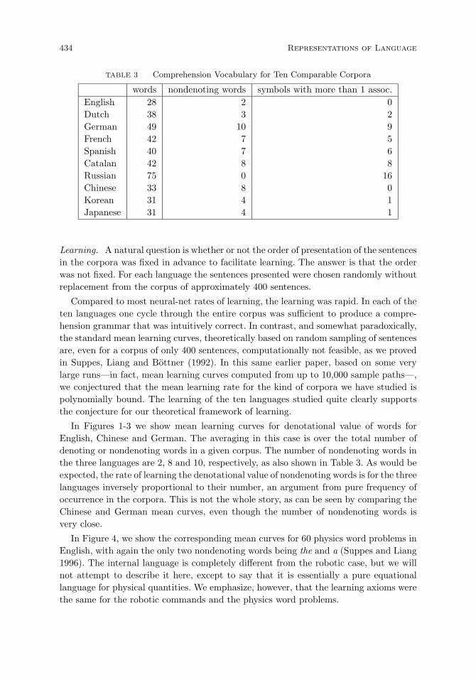
434 Representations of Language

TABLE 3 Comprehension Vocabulary for Ten Comparable Corpora

words nondenoting words symbols with more than 1 assoc.English 28 2 0Dutch 38 3 2German 49 10 9French 42 7 5Spanish 40 7 6Catalan 42 8 8Russian 75 0 16Chinese 33 8 0Korean 31 4 1Japanese 31 4 1

Learning. A natural question is whether or not the order of presentation of the sentencesin the corpora was fixed in advance to facilitate learning. The answer is that the orderwas not fixed. For each language the sentences presented were chosen randomly withoutreplacement from the corpus of approximately 400 sentences.

Compared to most neural-net rates of learning, the learning was rapid. In each of theten languages one cycle through the entire corpus was sufficient to produce a compre-hension grammar that was intuitively correct. In contrast, and somewhat paradoxically,the standard mean learning curves, theoretically based on random sampling of sentencesare, even for a corpus of only 400 sentences, computationally not feasible, as we provedin Suppes, Liang and Bottner (1992). In this same earlier paper, based on some verylarge runs—in fact, mean learning curves computed from up to 10,000 sample paths—,we conjectured that the mean learning rate for the kind of corpora we have studied ispolynomially bound. The learning of the ten languages studied quite clearly supportsthe conjecture for our theoretical framework of learning.

In Figures 1-3 we show mean learning curves for denotational value of words forEnglish, Chinese and German. The averaging in this case is over the total number ofdenoting or nondenoting words in a given corpus. The number of nondenoting words inthe three languages are 2, 8 and 10, respectively, as also shown in Table 3. As would beexpected, the rate of learning the denotational value of nondenoting words is for the threelanguages inversely proportional to their number, an argument from pure frequency ofoccurrence in the corpora. This is not the whole story, as can be seen by comparing theChinese and German mean curves, even though the number of nondenoting words isvery close.

In Figure 4, we show the corresponding mean curves for 60 physics word problems inEnglish, with again the only two nondenoting words being the and a (Suppes and Liang1996). The internal language is completely different from the robotic case, but we willnot attempt to describe it here, except to say that it is essentially a pure equationallanguage for physical quantities. We emphasize, however, that the learning axioms werethe same for the robotic commands and the physics word problems.

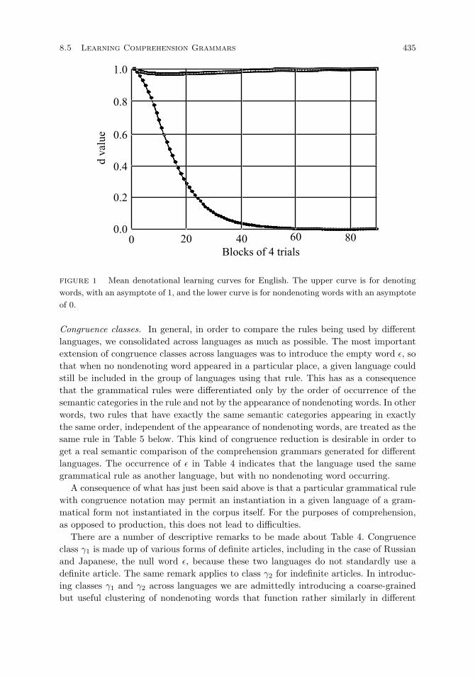
8.5 Learning Comprehension Grammars 435

FIGURE 1 Mean denotational learning curves for English. The upper curve is for denoting

words, with an asymptote of 1, and the lower curve is for nondenoting words with an asymptote

of 0.

Congruence classes. In general, in order to compare the rules being used by differentlanguages, we consolidated across languages as much as possible. The most importantextension of congruence classes across languages was to introduce the empty word ε, sothat when no nondenoting word appeared in a particular place, a given language couldstill be included in the group of languages using that rule. This has as a consequencethat the grammatical rules were differentiated only by the order of occurrence of thesemantic categories in the rule and not by the appearance of nondenoting words. In otherwords, two rules that have exactly the same semantic categories appearing in exactlythe same order, independent of the appearance of nondenoting words, are treated as thesame rule in Table 5 below. This kind of congruence reduction is desirable in order toget a real semantic comparison of the comprehension grammars generated for differentlanguages. The occurrence of ε in Table 4 indicates that the language used the samegrammatical rule as another language, but with no nondenoting word occurring.

A consequence of what has just been said above is that a particular grammatical rulewith congruence notation may permit an instantiation in a given language of a gram-matical form not instantiated in the corpus itself. For the purposes of comprehension,as opposed to production, this does not lead to difficulties.

There are a number of descriptive remarks to be made about Table 4. Congruenceclass γ1 is made up of various forms of definite articles, including in the case of Russianand Japanese, the null word ε, because these two languages do not standardly use adefinite article. The same remark applies to class γ2 for indefinite articles. In introduc-ing classes γ1 and γ2 across languages we are admittedly introducing a coarse-grainedbut useful clustering of nondenoting words that function rather similarly in different

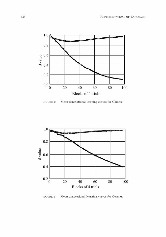
436 Representations of Language

FIGURE 2 Mean denotational learning curves for Chinese.

FIGURE 3 Mean denotational learning curves for German.

8.5 Learning Comprehension Grammars 437

TABLE 4 Congruence Classes

E D G F S C R Ch K J

γ1 the het die le el el ε nage ku ε

de das l l l zhege ε ε

der la la la

dem

den

γ2 a een ein un un ε ε yige han −eine une una ε

einem

einen

einer

γ3 − − − de taille ε ε − − − −ε

γ4 ε ε ε ε − − ε ε ε no

ε

γ5 − − − − − − − ε ε no tokoro

no

γ6 ε ε ε de de d ε ε − −ε ε de

ε

γ7 − − − − − − − − − o

γ8 − − − − − − − ba ε ε

γ9 − − − − − − − − ul o

lul

γ10 − − − − − − − − ε ni

γ11 − − − − − − − zai − −ε

γ12 − − − − − − − chao ε ε

ε

γ13 − − − − − − − na4 ε ni

na4liε

γ14 ε ε ε ε junto a l ε − − −ε ε

438 Representations of Language

FIGURE 4 Mean denotational learning curves for 60 physics word problems in English.

languages. More refinements of congruence of meaning and use could lead to divisionsof γ1 and also γ2 into several smaller classes.

The class γ3 is special for French because several words are required to expressthe idea of medium as in medium screw, namely the phrase de taille moyenne. Werecognize the resulting analysis is a distortion of the natural semantics of the French.The distortion arises from the English lexical bias, but not grammatical bias, built intoour fixed set of denoting words in the internal language.

Given that Chinese is not an inflected language, as German is, the number of non-denoting words in Table 4 is large. We cannot discuss in detail all of these particles.The particle ba occurs before noun phrases describing direct objects of actions. Theparticle zai occurs before noun phrases describing objects of relations. We note that thegrammar for Chinese given in Table 5 has the following two rules:

A → [γ8] O A3 [γ11] G

andG → REL [γ6] O

But to put zai before a relation word is not correct Chinese. This superset causes noproblem for comprehension, and the correct instances are when ε is used rather thanzai. Remarks very similar to those for zai apply to chao. The difference in their usereflects a semantic distinction we do not need for comprehension but would need forproduction. The particle zai is used mainly in connection with relations of position suchas on and under. In contrast chao is used in connection with the direction of motion.

Grammatical rules. An overview of the resulting grammars for the ten languages isgiven in Table 5. The table has eleven columns. In the first column we list the grammat-

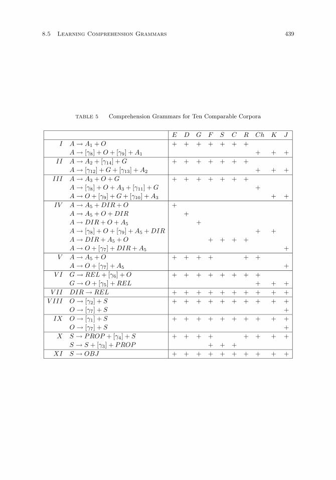
8.5 Learning Comprehension Grammars 439

TABLE 5 Comprehension Grammars for Ten Comparable Corpora

E D G F S C R Ch K J

I A → A1 +O + + + + + + +A → [γ8] +O + [γ9] +A1 + + +

II A → A2 + [γ14] +G + + + + + + +A → [γ12] +G+ [γ13] +A2 + + +

III A → A3 +O +G + + + + + + +A → [γ8] +O +A3 + [γ11] +G +A → O + [γ9] +G+ [γ10] +A3 + +

IV A → A5 +DIR+O +A → A5 +O +DIR +A → DIR+O +A5 +A → [γ8] +O + [γ9] +A5 +DIR + +A → DIR+A5 +O + + + +A → O + [γ7] +DIR+A5 +

V A → A5 +O + + + + + +A → O + [γ7] +A5 +

V I G → REL+ [γ6] +O + + + + + + + +G → O + [γ5] +REL + + +

V II DIR → REL + + + + + + + + + +V III O → [γ2] + S + + + + + + + + + +

O → [γ7] + S +IX O → [γ1] + S + + + + + + + + + +

O → [γ7] + S +X S → PROP + [γ4] + S + + + + + + + +

S → S + [γ3] + PROP + + +XI S → OBJ + + + + + + + + + +

440 Representations of Language

ical rules in the order of internal-language grammatical rules, cf. Table 1. In the nextcolumns we list the languages in the following order: English, Dutch, German, French,Spanish, Catalan, Russian, Chinese, Korean, Japanese. To each internal grammaticalrule corresponds in general a set of language specific rules. In the case of Rules VIIand XI the set is a unit set for the obvious reason that no variation can arise in ourlimited internal language. Clearly in a more general setting, in the case of Rule VII,e.g., relations could have modifying properties.

The most important contrast between the Indo-European and Asian languages is thatin the Indo-European languages the imperative verb expressing action is usually at thebeginning of an utterance, but in the Asian languages it is usually in final position. See,for example, the two rules derived from Rule II. The first is for the seven Indo-Europeanlanguages and the second for the three Asian languages. Similar remarks hold for thethree rules derived from Rule III.

This well-known contrast between the two groups of languages leads to a more sys-tematic question about the rules given in Table 5. Does the set of rules corresponding toeach rule of the internal language exhaust the possible permutations of the order of thesemantic categories? Surprisingly the answer is affirmative except for the set generatedby Rule III, which has only three members rather than six.

However, reflecting only on the three languages controlled as native speakers bymy two collaborators and me, we can give simple examples within the vocabulary andconceptual framework of our various corpora exhibiting two of the missing permutations:

A3 G O

E Put near the washer a screw.

G Leg neben die Scheibe eine Schraube.

G A3 O

E Near the washer put a screw.

G Neben die Scheibe leg eine Schraube

Ch Zai nage dianquan fujin fang yige luosiding.

For the third missing permutation, our Korean informant gave us the following example:

G O A3

K Ku nasapati yephey (han) nasa-lul nohala.

The washer near (one) screw put.

The close correspondence between Tables 1 and 5 is, as a matter of principle, mis-leading. Although the grammatical rules of Table 5 are derived via Axiom W3 directlyfrom the primitive grammatical rules of the internal language, as given in Table 1, thisneed not be the case. The larger corpus that is a superset of the one studied here forEnglish, Chinese and German has examples requiring derived internal grammatical rulesin applying Axiom W3. A German example of this phenomenon, taken from Suppes,Bottner and Liang (1995), is

A → A4 [einen] S D [der] PROP ist.

An instance of this rule is:

Heb eine Mutter hoch, die nicht groß ist.

8.5 Learning Comprehension Grammars 441

Related work and unsolved problems. By far the most extensive research onlanguage learning has been on children’s learning their first language. Rather extensivetheoretical treatments are to be found in Wexler and Culicover (1980) and in Pinker(1984, 1989). Some of this work is related to ours, but not in a central way in terms ofthe details of theoretical ideas. For example, Wexler and Culicover assume the learneralready has a deep context-free grammar of the language in question, and learning iscentered on the learning of transformations. In contrast, we begin with no grammar ofthe language to be learned. We make no detailed claims of the relevance of our work tochildren’s learning, but connections undoubtedly exist at a certain level.

In the past decade or so there has been a relatively small number of articles orbooks on machine learning of natural language. Langley and Carbonell (1987) providean excellent overview as of the date of their publication. Within the framework of thiswork, ours is more semantically than syntactically driven. This semantic commitmentis also shared by the work of Feldman et al. (1990, 1996) and Siskind (1992, 1994),which is also the work closest to our own. Feldman et al. (1990) describe in directand simple terms their original idea. First, the learning system is presented pairs ofpictures and true natural language statements about the pictures. Second, the systemis to learn the language well enough to determine whether or not a new sentence is trueof the accompanying picture. Feldman et al. (1996)’s approach to language learningseparates the learning of the grammar from the learning of the lexical concepts. Thegrammar is learned by use of Bayesian inference over a set of possible grammars andmodel merging. Siskind’s original work (1992), his dissertation, was in the context ofnaive physics, but focused also on the algorithms children may use in learning language.This work is continued in Siskind (1994), but with any assumption of prior languageknowledge eliminated. The concentration is on lexical acquisition via possible internalrepresentations of meaning. Although Siskind (1994) concentrates entirely on lexicalmeaning, his 7-step procedure, which constitutes a learning algorithm, bears resemblanceat the top level but not in detail to our procedure. Siskind (1991) has a concept that iscertainly different but similar in certain respects to our concept of denotational valueequal to 0 in the limit for nondenoting words. His ideas are, however, not probabilistic,and he does not present any learning curves. He does offer in his concept of temperature(1994) a treatment of homonymy, which we do not.

In spite of our considering ten languages, the present test of our theory must beregarded as very preliminary in character. The theory needs to be extended to solvea variety of pressing unsolved problems. We restrict ourselves to four problems, but itis a mark of the still primitive character of theoretical developments in this area, oursand others, that any informed reader can quickly double or triple this list. In our view,large-scale experimentation is premature for the kind of theory we are developing untilmore conceptual problems are solved:

. Learning of anaphora. Even very restricted and sometimes rather artificial uses ofnatural language are usually saturated with uses of anaphora. Physics word problemsare a good example.

. Learning temporal features. The ordinary use of language marks temporal sequences ofevents in a rich variety of ways. Much systematic discourse in science and technology

442 Representations of Language

requires continual time and tense distinctions that must be learned.. Learning multiple meanings. Troublesome examples already exist in robotic use, e.g.,

screw as both a noun and a verb in English. Much more exotic are the many meaningsof washer in English: ring of metal (our robotic case), a machine for washing, araccoon, and so forth.

. Learning concepts as well as words. It can well be claimed that concepts should belearned, not just words that stand for them. At present our theory offers nothing inthis respect, although we have begun some systematic work involving multivariatenetwork models (Suppes and Liang 1998).

Final remarks on learning. The importance of the general idea of association or condi-tioning, the mechanism at the heart of learning in Sections 3-5, is undiminished. Now inthe context of current neuroscience a main challenge is to find its physical embodiment.For this purpose many classical conditioning experiments with animals from aplysiaup the evolutionary tree are essential for identifying when and where conditioning hasoccurred. Philosophers caught up in the rhetoric about behaviorism often do not realizethat in developed theories of conditioning as axiomatized in Sections 3 and 5 the con-cept of association, conditioning state or even that of stimulus has a mainly theoreticalstatus, not observable directly and only possible to estimate indirectly from behavioralresponse data.

On the other hand, it seems clear that highly specific mechanisms are used for dif-ferent kinds of learning. It is almost certainly the case, for example, that a new wordmust be learned by a rather large population of neurons and never simply by a singleneuron. This learning, it is also likely, takes the form of learning frequencies of givenamplitudes and phases to represent words in the cortex. For other brain activity dif-ferent representations can also be envisaged for learning by single neurons, as has nowbeen demonstrated in a number of important cases, but not for human language, thesubject to which I now turn.

8.6 Language and the Brain.

Some historical background. Aristotle said that the distinguishing feature of manas an animal is that he is a rational animal, but, in more biological and psychologicalterms, it is that of being a talking animal. Language is, in ways that we have not yet fullyexplored, the most distinguishing mark of man as an animal. Its processing is centered,above all, in the brain, not just for the production of speech, but for the intentionalformation of what is to be said, or for the comprehension of what has been heard orread. So it is the brain’s processing of language that is the focus of this section. I beginwith a historical sketch of the discovery of electrical activity in the brain.

An early reference to electricity being generated by muscles or nerves of animalscomes from a study by Francesco Redi (1671), who describes in this way an experimenthe conducted in 1666: “It appeared to me as if the painful action of the torpedine(electric ray) was located in these two sickle-shaped bodies, or muscles, more than inany other part.” Redi’s work was done in Florence under the Medici’s. These electricalobservations were fragmentary and undeveloped. But the idea of electrical activity in the

8.6 Language and the Brain. 443

muscles or nerves of various animals became current throughout the eighteenth century(Whittaker 1910). Yet it was more than 100 years after Redi before the decisive step wastaken in Bologna by Luigi Galvani. He describes his first steps in the following manner:

The course of the work has progressed in the following way. I dissected a frog and pre-

pared it . . . Having in mind other things, I placed the frog on the same table as an electric

machine. When one of my assistants by chance lightly applied the point of a scalpel to

the inner crural nerves of the frog, suddenly all the muscles of the limbs were seen so

to contract that they appeared to have fallen into violent tonic convulsions. Another

assistant who was present when we were performing electrical experiments thought he

observed that this phenomenon occurred when a spark was discharged from the conduc-

tor of the electrical machine. Marvelling at this, he immediately brought the unusual

phenomenon to my attention when I was completely engrossed and contemplating other

things. Hereupon I became extremely enthusiastic and eager to repeat the experiment

so as to clarify the obscure phenomenon and make it known. I myself, therefore, applied

the point of the scalpel first to one then to the other crural nerve, while at the same time

some one of the assistants produced a spark; the phenomenon repeated itself in precisely

the same manner as before. (Galvani 1791/1953, pp. 45–46)

Galvani’s work of 1791 was vigorously criticized by the well-known Italian physicistAlessandro Volta (1745–1827), who was born in Como and was a professor of physicsat the University of Pavia. Here are his words of criticism, excerpted from a letter byVolta to Tiberius Cavallo, read at the Royal Society of London:

The name of animal electricity is by no means proper, in the sense intended by Galvani,

and by others; namely, that the electric fluid becomes unbalanced in the animal organs,

and by their own proper force, by some particular action of the vital powers. No, this is

a mere artificial electricity, induced by an external cause, that is, excited originally in a

manner hitherto unknown, by the connexion of metals with any kind of wet substance.

And the animal organs, the nerves and the muscles, are merely passive, though easily

thrown into action whenever, by being in the circuit of the electric current, produced in

the manner already mentioned, they are attacked and stimulated by it, particularly the

nerves. (Volta 1793/1918, pp. 203–208)

Galvani was able to meet these criticisms directly and in 1794 published anonymouslya response containing the detailed account of an experiment on muscular contractionwithout the use of metals (Galvani 1794). The original and important nature of Galvani’swork came to be recognized throughout Europe. The prominent German physicist EmilDu Bois-Reymond summarized in the following way Galvani’s contribution:

1. Animals have an electricity peculiar to themselves, which is called Animal Electric-

ity.

2. The organs to which this animal electricity has the greatest affinity, and in which

it is distributed, are the nerves, and the most important organ of its secretion is

the brain.

3. The inner substance of the nerve is specialized for conducting electricity, while the

outer oily layer prevents its dispersal, and permits its accumulation.

4. The receivers of the animal electricity are the muscles, and they are like a Leyden

jar, negative on the outside and positive on the inside.

444 Representations of Language

5. The mechanism of motion consists in the discharge of the muscular fluid from the

inside of the muscle via the nerve to the outside, and this discharge of the muscular

Leyden jar furnishes an electrical stimulus to the irritable muscle fibres, which

therefore contract. (Du Bois-Reymond 1848/1936, p. 159)

A next event of importance was the demonstration by Carlo Matteucci (1844) thatelectrical currents originate in muscle tissue. It was, however, about 100 years after Gal-vani, that Richard Caton (1875) of Liverpool detected electrical activity in an exposedrabbit brain, using the Thomson (Lord Kelvin) reflecting telegraphic galvanometer. In1890, Adolf Beck of Poland detected regular electrical patterns in the cerebral cortex ofdogs and rabbits. Beginning at the end of the nineteenth century Villem Einthoven, aDutch physician and physiologist, developed a new electrocardiograph machine, basedon his previous invention of what is called the string galvanometer, which was simi-lar to the device developed to measure telegraphic signals coming across transatlanticcables. Using Einthoven’s string galvanometer, significant because of its sensitivity, in1914, Napoleon Cybulsky and S. Jelenska Macieszyna, of the University of Cracow inPoland, recorded a dog’s epileptic seizures. Beginning about 1910, Hans Berger in Jena,Germany began an extensive series of studies that detected electrical activity throughintact skulls. This had the great significance of being applicable to humans. His ob-servations were published in 1929, but little recognized. Recognition came, however,when his findings were confirmed by Edward Douglas Adrian and B. H. C. Matthews ofthe University of Cambridge, who demonstrated Berger’s findings at the PhysiologicalSociety in Cambridge in 1934, and the International Congress of Psychology in 1937.In the late 1930s and the early 1940s, research on electrical activity in brains, or whatwe now call electroencephalography (EEG), moved primarily to North America—W. G.Lennox and Erna and F. A. Gibbs at the Harvard Medical School, H. H. Jasper andDonald Linsley at Brown University, and Wilder Penfield at McGill University. One ofthe first English-language reports to verify Berger’s work was by Jasper and Carmichael(1935). Nearly at the same time, Gibbs et al. (1935) began using the first ink-writingtelegraphic recorder for EEG in the United States, built by Garceau and Davis (1935).25

By the 1950s, EEG was widely used clinically, especially for the study of epilepsy, andfor a variety of research on the nature of the electrical activity in the brain. This is notthe place to summarize in any serious detail the work by a wide variety of scientistsfrom 1950 to the present, but an excellent review of EEG, that is, of electrical activity,pertinent especially to cognition, is to be found in Rugg and Coles (1995).

Observing the brain’s activity. The four main current methods of observing thebrain are easy to describe. The first is the classical electroencephalographic (EEG)observations already mentioned, which,—and this is important—, have a time resolutionof at least one millisecond. The second is the modern observation of the magnetic fieldrather than the electric field, which goes under the title of magnetoencephalography(MEG). This also has the same time resolution of approximately one millisecond. Thethird is positron emission tomography (PET), which has been widely used in the lastseveral decades and is good for observing location, in some cases, of brain activity, but

25I obtained these last references from Geddes (2001).

8.6 Language and the Brain. 445

has a time resolution of only one second. Finally, the most popular current method isfunctional magnetic resonance imaging (fMRI), which does an excellent job of observingabsorption of energy in well-localized places in the brain, but unfortunately, also has atime resolution of no less than a second.

Although many excellent things can be learned from PET and fMRI, they are notreally useful if one wants to identify brain waves representing words or sentences, forthe processing, although slow by modern computer standards, is much too fast to beable to accomplish anything with the time resolution of observation no better than onesecond. The typical word, for example, whether listened to or read, will be processed innot more than 4 or 5 hundred milliseconds, and often faster. My own serious interest,focused on the way the brain processes language, began from the stimulus I received byhearing a brilliant lecture in 1996 on MEG, by Sam Williamson, a physicist who has beenprominent from the beginning in the development of MEG. I was skeptical about whathe said, but the more I thought about it, the more I realized it would be interesting andimportant to try using MEG to recognize the processing of individual words. This ideasuggested a program of brain-wave recognition, as recorded by MEG, similar in spiritto speech recognition. I was familiar with the long history of speech recognition fromthe 1940s to the present, and I thought maybe the same intense analytical effort couldyield something like corresponding results. So, in 1996, assisted especially by Zhong-LinLu, who had just taken a Ph.D. with Sam Williamson and Lloyd Kaufman at New YorkUniversity, we conducted an MEG experiment at the Scripps Institute of Research inSan Diego, California. When we proceeded to analyze the results of the first experiment,the problem of recognizing which one of seven words was being processed on the basisof either having heard the word or having read it on a computer screen, we were notable to get very good recognition results from the MEG recordings. Fortunately, it wasa practice at the Scripps MEG facility, which is technically very much more expensiveand complicated to run than standard EEG equipment, to also record the standard 20EEG sensors used for many years. We proceeded to analyze the EEG data as well, andhere we had much better recognition results (Suppes, Lu and Han 1997).

In the standard EEG system, widely used throughout the world for observing elec-trical activity in the brain, sensors to record the electrical activity are arranged in whatare commonly called the 10-20 system, as shown in Figure 5, with the location on thesurface of the skull of the head shown in the approximate form of a circle, with ears leftand right and eyes at the top in the figure. The first letters of the initials used in thelocations correspond to references to the location in the part of the brain, for example,F for frontal, C for center, T for temporal, P for parietal, O for occipital. Second, youwill note that the odd-numbered sensors are located on the skull on top of the lefthemisphere and the even-numbered sensors are located over the right hemisphere, withthree sensors located approximately along the center line. There are more opinions thandeeply articulated and established facts about what takes place in the left hemisphereor in the right hemisphere, possibly both, in the processing of language. My own viewis that there is probably more duality than has been generally recognized, but I will nottry to make an empirical defense of that view in the present context, although I havepublished data supporting duality (Suppes, Han and Lu 1998, Table 2).

446 Representations of Language

FIGURE 5 The 10-20 system of EEG sensors.

Figure 6 shows a typical trial, in which the subject was given a visual, i.e., printed,sentence, one word at a time, on a computer screen. The trial lasted for over 3000milliseconds, with an observation of an amplitude of the observed wave plotted on they-coordinate in microvolts every millisecond. Given that so much data are observedin a little over three seconds, just from one sensor, out of 20, it is easy to see thatEEG recordings of language activity are rich in data and, in fact, we might almost say,swamped by data. It is not difficult to run an experiment with several subjects, eachwith a number of hours of recording, and have at the end between five and ten gigabytesof data of the kind to be seen in Figure 6. This means that the problem of trying tofind waves corresponding to particular words and sentences is not going to be a simplematter. It is very different from behavioral experiments dealing with language, in whichthe observed responses of subjects are easily recorded in a few megabytes and thenanalyzed without anything like the same amount of computation.

Methods of data analysis. There is no royal road to finding words and sentencesin the kind of data just described, so I will outline here the approach that I and mycolleagues have used with some success in the past few years. The basic approach is verymuch taken from digital signal processing, but the application is a very different onefrom what is ordinarily the focus of electrical engineers or others using the extensive

8.6 Language and the Brain. 447

FIGURE 6 Unanalyzed EEG data from one trial and one sensor.

mathematical, quantitative and statistical techniques that have been developed in thelast 50 years in digital signal processing. An excellent general reference is Oppenheimand Schafer (1975).

The approach is easily sketched, although the technical details are more complicatedand will only be outlined. Generally, but with important exceptions to be noted, thefirst thing to do is to average the data, for example, for a given condition, a typicalcase being the brain response to a particular verbal stimulus, given either auditorily orvisually. The purpose of this averaging is to eliminate noise, especially high-frequencynoise, on the assumption that the signal is of much lower frequency. The next step isthen to perform a Fourier transform on the averaged data, passing from the time domainto the frequency domain, perhaps the most characteristic feature of signal processinganalysis. The third step, which can be done simultaneously with the second step, isto filter in the frequency domain, to reduce still further the bandwidth of the signalused for identifying the word or sentence being processed. An alternative, which wehave explored rather thoroughly in some work, is to select in the frequency domainthe frequencies with the highest energies, as measured by the absolute value of theiramplitudes, and then to superpose the sine functions in the time domain.26 In eithercase, by filtering or superposition, we get a much simpler signal as we pass by an inverseFourier transform back to the time domain.

Speaking now of filtering, and ignoring for the moment the superposition approach,we go back to the time domain with a bandpass filter fixed by two parameters, the lowfrequency L and the high frequency H of the filter. We now select two more parameters

26Actually, in ‘selecting a frequency ωi with amplitude Ai’, we are in fact selecting a sine wave

Ai sin(ωit + ϕi), where ϕi is its phase. More on this on the next page.

448 Representations of Language

that are of importance. Namely, what should we take to be the beginning s and theending e of the signals for the words or sentences in a given experimental condition. Asin other brain matters, it is not at a glance obvious from the recorded brain wave whenthe representation of a particular word or sentence begins or ends in the continuallyactive electrical waves that are observed. When a quadruple (L,H, s, e) is selected, wethen use that quadruple of parameters to make a classification of the brain waves of thewords or sentences that are the stimuli in a given experimental condition.

Our aim is to optimize or maximize the number of brain waves correctly classified.We keep varying the quadruple of parameters until we get what seems to be the bestresult that can be found. We are doing this in a four-dimensional grid of parameters,but I show in Figure 7 the optimal surface for two parameters of the filter, althoughhere what is used as a measure on the ordinate or y-axis is the difference between thehigh-frequency and low-frequency filter rather than the high filter itself. So we haveon the abscissa the low filter measured in Hz and on the ordinate the difference W ,which is the width in Hz of the bandpass filter. The smoothness of the surface shownin Figure 7 is characteristic of what we always observe, and would be expected ofobservations, of an electrical field outside the skull, the place where we are observingthem. (We are of course very fortunate that the electrical fields are strong enough to beobserved without complete contamination by noise.) This isocontour map is for the firstexperiment with 48 geography sentences discussed in more detail below, but the mapshows clearly that the best recognition rate was 43 of the 48 sentences (approximately90%). As the parameters of the bandpass filter are changed, the contour map showsdefinitely lower recognition rates.

Fourier analysis of EEG data. In the background of the Fourier analysis is the standardtheory of the Fourier integral, but in practice our data are finite. The finite-impulse datathat we are interested in observing usually last for no more than a few seconds. Forexample, the sentences studied will ordinarily last not more than three or four secondswhen spoken at a natural rate. To analyze frequencies with given amplitudes and phases,we use the discrete Fourier transform. As indicated, our goal is to find the frequenciesthat contain the signal and eliminate the noise. (The artifacts generated by eye blinksor other such events are discussed at the end of this section.)

Let N be the number of observations, equally spaced in time, usually one millisecondapart. We then represent the finite sequence of observations x(n), 0 ≤ n ≤ N − 1 byFourier series coefficients X(k) as a periodic sequence of period N , so we have the dualpair

X(k) =N−1∑n=0

x(n)e−i( 2πN )kn (1)

x(n) =1N

N−1∑k=0

X(k)ei( 2πN )kn. (2)

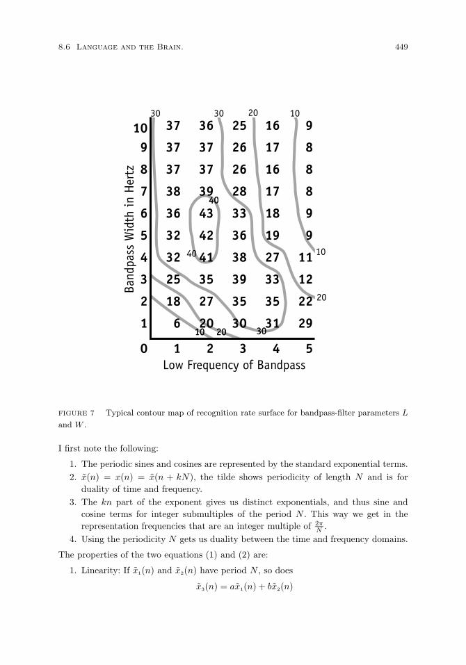
8.6 Language and the Brain. 449

FIGURE 7 Typical contour map of recognition rate surface for bandpass-filter parameters L

and W .

I first note the following:

1. The periodic sines and cosines are represented by the standard exponential terms.2. x(n) = x(n) = x(n + kN), the tilde shows periodicity of length N and is for

duality of time and frequency.3. The kn part of the exponent gives us distinct exponentials, and thus sine and

cosine terms for integer submultiples of the period N . This way we get in therepresentation frequencies that are an integer multiple of 2π

N .4. Using the periodicity N gets us duality between the time and frequency domains.

The properties of the two equations (1) and (2) are:

1. Linearity: If x1(n) and x2(n) have period N , so does

x3(n) = ax1(n) + bx2(n)

450 Representations of Language

andX3(k) = aX1(k) + bX2(k).

2. Invariance under shift of a sequence

n → n+m.

3. Various symmetry properties, e.g., |X(k)| = |X(−k)|.4. Convolution of x1 and x2 of period N has period N :

x3(n) =N−1∑m=0

x1(m)x2(n−m).

Of importance is the efficient fast discrete Fourier transform, an algorithm due to Cooleyand Tukey (1965) and others, a variant of which was used in the computations reportedbelow.

Filters. The principle of filter construction is simple. Details are not. A bandpassfilter, e.g., 1-20 Hz simply “filters all the frequencies below 1 Hz and above 20 Hz”.There are many developments in the electrical engineering literature on the theory andart of designing filters, which it is not possible to survey here. The important point isalways to design a filter with some criterion of optimality.

If the signal is known, then the engineering objective is to optimize its transmission.Our problem, as already mentioned, is that in our experiments, the signal carrying theword or sentence in question is unknown. So our solution is to optimize the filter topredict the correct classification. The parameters we used have been discussed above. Inaddition we often make a smoothing correction around the edges of the filter by usinga 4th-order Butterworth filter, although in the work reported here, something simplerwould serve the purpose just about as well.27

Three experimental results. I turn now to three of the most important results wehave obtained so far.

Invariance between subjects. In the first experiment, we presented 48 sentences aboutthe geography of Europe to 9 subjects. The subjects were asked to judge the truth orfalsity of the sentences, and while they were either listening to or reading the sentencesdisplayed one word at a time on a computer screen, we made the typical EEG recordings.The semantic task was simple, but because the sentences were separated by only fourseconds, the task of judging their truth or falsity was not trivial. Typical sentenceswere of the form The capital of Italy is not Paris, and Warsaw is the largest city inAustria. Taking now the data from five subjects to form prototypes of the 48 sentences,by averaging the data from the five subjects, and taking the other four subjects to formcorresponding averaged test samples of each sentence, we applied the Fourier methodsdescribed above and found an optimal bandpass filter from a predictive standpoint.28

We were able to recognize correctly 90% of the test samples, using as a criterion for

27Butterworth filters are well described in Oppenheim and Schafer (1975, pp. 211–218).28The data are for the visual condition of reading the sentences, one displayed word at a time.

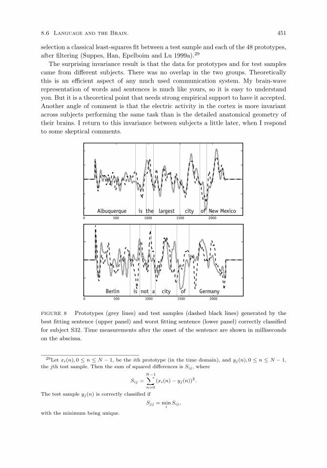
8.6 Language and the Brain. 451

selection a classical least-squares fit between a test sample and each of the 48 prototypes,after filtering (Suppes, Han, Epelboim and Lu 1999a).29

The surprising invariance result is that the data for prototypes and for test samplescame from different subjects. There was no overlap in the two groups. Theoreticallythis is an efficient aspect of any much used communication system. My brain-waverepresentation of words and sentences is much like yours, so it is easy to understandyou. But it is a theoretical point that needs strong empirical support to have it accepted.Another angle of comment is that the electric activity in the cortex is more invariantacross subjects performing the same task than is the detailed anatomical geometry oftheir brains. I return to this invariance between subjects a little later, when I respondto some skeptical comments.

FIGURE 8 Prototypes (grey lines) and test samples (dashed black lines) generated by the

best fitting sentence (upper panel) and worst fitting sentence (lower panel) correctly classified

for subject S32. Time measurements after the onset of the sentence are shown in milliseconds

on the abscissa.

29Let xi(n), 0 ≤ n ≤ N − 1, be the ith prototype (in the time domain), and yj(n), 0 ≤ n ≤ N − 1,

the jth test sample. Then the sum of squared differences is Sij , where

Sij =

N−1Xn=0

(xi(n) − yj(n))2.

The test sample yj(n) is correctly classified if

Sjj = mini

Sij ,

with the minimum being unique.

452 Representations of Language

One hundred sentences. I now turn to a second more recent experiment in which sub-jects were visually presented 100 different geography sentences (Suppes, Wong et al., toappear). I concentrate here only on the remarkable result of correct recognition of 93 ofthe 100 sentences for one subject (S32). Using the methods described, the best recog-nition rate achieved for a single subject (S32) was 93%, i.e., 93 of the 100 test samples.These results were achieved with L = 1.25 Hz, W = 21.25 Hz, s = 180 ms after onsetof the visual presentation of the first word of each sentence, and e = 2200 ms, markingthe ending of the recordings used for the least-squares criterion of fit. The best bipolarsensor was C4-T6. In Figure 8 we show at the top the best and at the bottom the worstfit, as measured by the least-squares criterion, for the 93 sentences correctly recognized.The sum of squares for the worst was more than three times that for the best.

Invariance between visual images and their names. The third experiment showed thatthe visual images generated on a computer screen, of a familiar shape, such as a circleor triangle, were very similar to the brain images generated by the corresponding word(Suppes, Han, Epelboim and Lu 1999b). This surprising result very much reinforceda classical solution of how the mind has general concepts. It is a famous episode inthe history of philosophy in the eighteenth century that Berkeley and Hume stronglycriticized Locke’s conception of abstract or general ideas. Berkeley has this to say in ANew Theory of Vision (1709/1901):

It is indeed a tenet, as well of the modern as the ancient philosophers, that all general

truths are concerning universal abstract ideas; without which, we are told, there could

be no science, no demonstration of any general proposition in geometry. But it were no

hard matter, did I think it necessary to my present purpose, to shew that propositions

and demonstrations in geometry might be universal, though they who make them never

think of abstract general ideas of triangles or circles.

After reiterated efforts and pangs of thought to apprehend the general idea of a triangle,

I have found it altogether incomprehensible. And surely, if any one were able to let that

idea into my mind, it must be the author of the Essay Concerning Human Understanding:

he, who has so far distinguished himself from the generality of writers, by the clearness

and significancy of what he says. Let us therefore see how this celebrated author describes

the general or which is the same thing, the abstract idea of a triangle. ‘It must be,’ says

he, ‘neither oblique nor rectangle, neither equilateral, equicrural, nor scalenum; but all

and none of these at once. In effect it is somewhat imperfect that cannot exist; an idea,

wherein some parts of several different and inconsistent ideas are put together.’ (Essay

on Human Understanding, B. iv. ch. 7. s. 9.) This is the idea which he thinks needful

for the enlargement of knowledge, which is the subject of mathematical demonstration,

and without which we could never come to know any general proposition concerning

triangles. Sure I am, if this be the case, it is impossible for me to attain to know even

the first elements of geometry: since I have not the faculty to frame in my mind such an

idea as is here described. (Berkeley, pp. 188–189.)

Hume, in a brilliant exposition and extension of Berkeley’s ideas, in the early pages ofA Treatise of Human Nature, (1739/1951) phrased the matter beautifully in the openingparagraph of Section VII, entitled Of Abstract Ideas:

8.6 Language and the Brain. 453

A very material question has been started concerning abstract or general ideas, whether

they be general or particular in the mind’s conception of them. A great philosopher has

disputed the receiv’d opinion in this particular, and has asserted, that all general ideas are

nothing but particular ones, annexed to a certain term, which gives them a more extensive

signification, and makes them recall upon occasion other individuals, which are similar

to them. As I look upon this to be one of the greatest and most valuable discoveries that

has been made of late years in the republic of letters, I shall here endeavour to confirm

it by some arguments, which I hope will put it beyond all doubt and controversy.

(Hume, Treatise, p. 17.)

Although not discussed by Berkeley and Hume, we also confirmed that the same istrue of simple patches of color. In other words, a patch of red and the word ‘red’ generatesimilar brain images in the auditory part of the cortex.

The specific significant results were these. By averaging over subjects as well astrials, we created prototypes from brain waves evoked by stimuli consisting of simplevisual images and test samples from brain waves evoked by auditory or visual wordsnaming the visual images. We correctly recognized from 60% to 75% of the test-samplebrain waves. Our general conclusion was that simple shapes and simple patches of colorgenerate brain waves surprisingly similar to those generated by their verbal names. Thisconclusion, taken together with extensive psychological studies of auditory and visualmemory, support the solution conjectured by Berkeley and Hume. The brain, or, ifyou prefer, the mind, associates individual visual images of triangles, e.g., to the wordtriangle. It is such an associative network that is the likely procedural replacement forthe mistaken attempt by Locke to introduce abstract ideas.

Comparisons of averaged and filtered brain waves generated by visual images andspoken names of the images are shown in Figure 9. Time after the onset of the stimulus(visual image or word) is shown in milliseconds on the abscissa. In the upper panel thesolid curved line is the prototype brain wave generated by the color blue displayed as ablank computer screen with a blue background. The dotted curved line is the test-samplebrain wave generated by the spoken word blue. In the lower panel are the prototype brainwave (solid line), generated by display of a triangle on the screen, and the test-samplebrain wave (dotted line), generated by the spoken word triangle. In neither case is thematch perfect, for even when the same stimulus is repeated, the filtered brain waves donot match exactly, since the brain’s electric activity continually changes from momentto moment in numerous ways. But, all the same, there are many invariances necessaryfor human communication, and even at this early stage we can identify some of them.

Criticisms of results and response. I first sketch the general nature of the criti-cisms. In many brain imaging experiments the data are very rich and complex. Conse-quently, a complicated procedure may also be used to find, for given conditions, an op-timal value. The search for this optimal value, which here is the best correct recognitionrate, is analogous to computing an extreme statistic for a given probability distribution.The basis of the analogy is that the search corresponds to possibly many repetitionsof a null-hypothesis experiment. These repetitions require computation of the appro-priate extreme statistic. Moreover, if several parameters are estimated in finding such

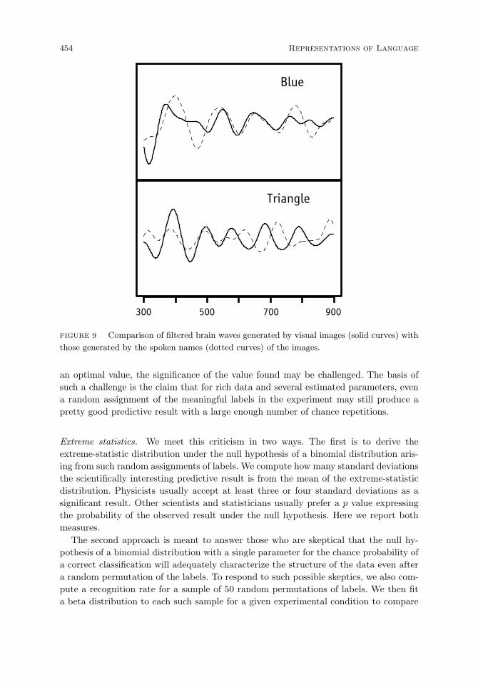
454 Representations of Language

FIGURE 9 Comparison of filtered brain waves generated by visual images (solid curves) with

those generated by the spoken names (dotted curves) of the images.

an optimal value, the significance of the value found may be challenged. The basis ofsuch a challenge is the claim that for rich data and several estimated parameters, evena random assignment of the meaningful labels in the experiment may still produce apretty good predictive result with a large enough number of chance repetitions.

Extreme statistics. We meet this criticism in two ways. The first is to derive theextreme-statistic distribution under the null hypothesis of a binomial distribution aris-ing from such random assignments of labels. We compute how many standard deviationsthe scientifically interesting predictive result is from the mean of the extreme-statisticdistribution. Physicists usually accept at least three or four standard deviations as asignificant result. Other scientists and statisticians usually prefer a p value expressingthe probability of the observed result under the null hypothesis. Here we report bothmeasures.

The second approach is meant to answer those who are skeptical that the null hy-pothesis of a binomial distribution with a single parameter for the chance probability ofa correct classification will adequately characterize the structure of the data even aftera random permutation of the labels. To respond to such possible skeptics, we also com-pute a recognition rate for a sample of 50 random permutations of labels. We then fita beta distribution to each such sample for a given experimental condition to compare

8.6 Language and the Brain. 455

with the corresponding extreme statistic distribution arising from the null hypothesis.We first derive the extreme statistic under the null hypothesis.Let p = probability of a success, a correct classification in our case, on a single trial,

and q = 1 − p. Let X be the random variable whose value is the number k of successesin n independent trials. The probability of at least k successes is:

P (X ≥ k) =n∑

j=k

P (X = j) =n∑

j=k

(n

j

)pjqn−j . (3)

Now we repeat the experiment governed by a binomial distribution. So we have r in-dependent repetitions of the n independent trials. For r repetitions (r = 21, 000 in the100-sentences experiment), the random variable representing the extreme statistic is

Y = max(X1, . . . ,Xr). (4)

Let P (Y ≥ k) be the probability that Y is at least k in at least one of the r repetitions,the extreme statistic of interest. Then clearly

P (Y ≥ k) = 1 − P (X < k)r, (5)

= 1 −[

k−1∑j=0

(n

j

)pjqn−j

]r

.

We also need the theoretical density distribution of Y, to compare to various empiricalresults later. This is easy to compute from (3).

P (Y = k) = P (Y ≥ k) − P (Y ≥ k + 1), (6)

= P (X < k + 1)r − P (X < k)r,

=

[k∑

j=1

(n

j

)pjqn−j

]r

−[

k−1∑j=1

(n

j

)pjqn−j

]r

.

From (4) we can compute the mean and standard deviation of the extreme statistic Y.Second, we report results for the beta distribution on (0, 1) fitted to the empirical

sample of extreme statistics. The density f(x) of the beta distribution is:

f(x) =

Γ(a+b)Γ(a)Γ(b)x

a−1(1 − x)b−1, a, b > 0, 0 < x < 1,0 otherwise,

(7)

where Γ(a) is the gamma function. If Z is a random variable with a beta distribution,then its mean and variance are given as simple functions of the parameters a and b.

µZ = E(Z) =a

a+ b, (8)

σ2Z = Var(Z) =

ab

(a+ b)2(a+ b+ 1). (9)

The probability that the random variable Z has a value equal to or greater than kn is:

P (Z ≥ k

n) =

Γ(a+ b)Γ(a)Γ(b)

∫ 1

kn

xa−1(1 − x)b−1dx. (10)

The computation of P (Z ≥ kn ) is difficult for the extreme tail of the distribution. In

some cases we use a mathematically rigorous upper bound that is not the best possible,

456 Representations of Language

FIGURE 10 Cumulative mean and standard deviation of the recognition rate of the sample

of random permutations.

but easy to compute, namely, just the area of the rectangle with height f( kn ) containing

the tail of the distribution to the right of f( kn ):

P (Z ≥ k

n) ≤ f(

k

n)(1 − k

n), (11)

where f( kn ) is defined by (5).

Computation of extreme statistics. I begin with the second experiment using 100sentences. As a check on the null hypothesis, we constructed an empirical distributionof the extreme statistic by sampling 50 random permutations. Several points are to benoted.

1. A permutation of the 100 sentence “labels” is randomly drawn from the populationof 100! possible permutations, and the sentence test samples are relabeled usingthis permutation.

2. Exactly the same grid of parameters (L,W, s, e) is now run for each bipolar pairof sensors, as for the correct labeling on the data of subject S32, to obtain, byFourier analysis, filtering and selection of temporal intervals (s, e), a best rate ofrecognition or classification for the random label assignment. For the 100-sentencesexperiment, the number of points on the grid tested for each random permutationis 7 × 10 = 70 for L× W , 5 × 4 = 20 for s× e and 15 for the number of sensors,so the number of repetitions r, from the standpoint of the null hypothesis, is70 × 20 × 15 = 21, 000.

3. This random sampling of label permutations is repeated, and the recognition re-sults computed, until a sample of 50 permutations has been drawn.

In Figure 10, I show the cumulative computation of the mean m and standarddeviation s for the sample of 50 label permutations for the data of subject S32. For thefull sample of 50 the mean m = 6.04 and the standard deviation s = 0.77. In Figure11, I show: (i) the frequency distribution of the null-hypothesis extreme statistic Ywith n = 100, p = 0.01 and r = 21, 000, (ii) the empirical histogram of the maximumnumber of successes obtained for the 50 sample points with r = 21, 000, and (iii) thefitted beta distribution as well. From Figure 11 it is visually obvious that the correct

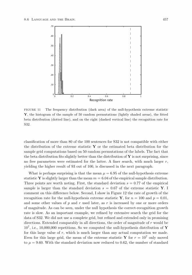
8.6 Language and the Brain. 457

FIGURE 11 The frequency distribution (dark area) of the null-hypothesis extreme statistic

Y, the histogram of the sample of 50 random permutations (lightly shaded areas), the fitted

beta distribution (dotted line), and on the right (dashed vertical line) the recognition rate for

S32.

classification of more than 80 of the 100 sentences for S32 is not compatible with eitherthe distribution of the extreme statistic Y or the estimated beta distribution for thesample grid computations based on 50 random permutations of the labels. The fact thatthe beta distribution fits slightly better than the distribution of Y is not surprising, sinceno free parameters were estimated for the latter. A finer search, with much larger r,yielding the higher result of 93 out of 100, is discussed in the next paragraph.

What is perhaps surprising is that the mean µ = 6.95 of the null-hypothesis extremestatistic Y is slightly larger than the meanm = 6.04 of the empirical sample distribution.Three points are worth noting. First, the standard deviation s = 0.77 of the empiricalsample is larger than the standard deviation s = 0.67 of the extreme statistic Y. Icomment on this difference below. Second, I show in Figure 12 the rate of growth of therecognition rate for the null-hypothesis extreme statistic Y, for n = 100 and p = 0.01,and some other values of p and r used later, as r is increased by one or more ordersof magnitude. As can be seen, under the null hypothesis the correct-recognition growthrate is slow. As an important example, we refined by extensive search the grid for thedata of S32. We did not use a complete grid, but refined and extended only in promisingdirections. Extended comparably in all directions, the order of magnitude of r would be107, i.e., 10,000,000 repetitions. So we computed the null-hypothesis distribution of Yfor this large value of r, which is much larger than any actual computation we made.Even for this large grid, the mean of the extreme statistic Y for r = 107 only movedto µ = 9.60. With the standard deviation now reduced to 0.62, the number of standard

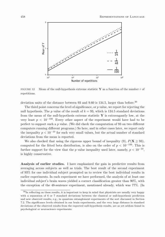
458 Representations of Language

FIGURE 12 Mean of the null-hypothesis extreme statistic Y as a function of the number r of

repetitions.

deviation units of the distance between 93 and 9.60 is 134.5, larger than before.30

The third point concerns the level of significance, or p value, we report for rejecting thenull hypothesis. The p value of the result of k = 93, which is 134.5 standard deviationsfrom the mean of the null-hypothesis extreme statistic Y is extravagantly low, at thevery least p < 10−100. Every other aspect of the experiment would have had to beperfect to support such a p value. (We did check the computation of 93 on two differentcomputers running different programs.) So here, and in other cases later, we report onlythe inequality p < 10−10 for such very small values, but the actual number of standarddeviations from the mean is reported.

We also checked that using the rigorous upper bound of inequality (9), P (X ≥ 93),computed for the fitted beta distribution, is also on the order of p < 10−100. This isfurther support for the view that the p value inequality used later, namely, p < 10−10,is highly conservative.

Analysis of earlier studies. I have emphasized the gain in predictive results fromaveraging across subjects as well as trials. The best result of the second experimentof 93% for one individual subject prompted us to review the best individual results inearlier experiments. In each experiment we have performed, the analysis of at least oneindividual subject’s brain waves yielded a correct classification greater than 90%, withthe exception of the 48-sentence experiment, mentioned already, which was 77%. (In

30In reflecting on these results, it is important to keep in mind that physicists are usually very happy

with a separation of 6 or 7 standard deviations between the classical or null-hypothesis prediction

and new observed results, e.g., in quantum entanglement experiments of the sort discussed in Section

7.2. The significance levels obtained in our brain experiments, and the very large distance in standard

deviations of the observed results from the expected null-hypothesis results, are as yet seldom found in

psychological or neuroscience experiments.

8.6 Language and the Brain. 459

Suppes, Han, Epelboim and Lu (1999a), this 77% was reported as 79%, because a finergrid was used.) Results for the best subject in the various experiments are summarizedin Table 6.

With one exception, the p values shown in Table 6 are highly significant, by moststandards of experimental work, extravagantly so. The exception is for the visual-imageexperiment in which 8 simple visual images were presented as stimuli. For four of thesubjects, as shown in Table 6, we were able to classify all 8 brain waves correctly, butthis perfect result of 100 percent was significant only at the level of p < 0.01 for the nullhypothesis, because with enough repetitions the best guesses under the null hypothesisdo pretty well also, with µ = 6.28.

The lesson for experimental design of this last point is obvious. If the data are massiveand complex, as in the brain experiments described, and extensive search for optimalparameters is required, then the probability p of a correct response under the nullhypothesis should be small. Figure 12 graphically makes the point. When p is small thenumber of repetitions can be very large, without affecting very much the mean of Y,the extreme statistic of r repetitions. As can be seen also, from Table 6, when p = 0.01,the binomial parameter of the 100-sentences experiment, even 10,000,000 repetitionsunder the null hypothesis of 100 trials, increases E(Y) only slightly to 9.60. To putthe argument dramatically, at the rate of 1 second per trial, it would take more timethan the present estimated age of the universe to have enough repetitions to obtainE(Y) ≥ 93.

I say in the preceding paragraph that p should be small, but that is too simple. Theother way out, used in the first two experimental conditions of Table 6, 7 visual wordsand 7 auditory words, is to increase the number of test samples. In those two conditions,p = 1

7 , but the number of test samples was 35, and, as can be seen from the table, thenull hypothesis was rejected at a level better than 10−10. Reanalysis of the data from thevisual-image experiment with p = 1

8 , in a similar approach by increasing the number oftest samples from 8 to 24 yielded some better levels of rejection of the null hypothesis.The details are reported below.

More skeptical questions. As in all regimes of detailed experimentation, there is nosharp point after which further experiments need not be conducted, because all relevantquestions have been answered. Galison (1987) made a detailed study of several importantresearch programs of experimentation in physics. It seems likely that the main aspectsof his analysis apply to many other areas of science. He says:

Amidst the varied tests and arguments of any experimental enterprise, experimentalists

must decide, implicitly or explicitly, that their conclusions stand ceteris paribus: all other

factors being equal. And they must do so despite the fact that the end of an experimen-

tal demonstration is not, and cannot be, based purely on a closed set of procedures.

. . . Certain manipulations of apparatus, calculations, assumptions, and arguments give

confidence to the experimentalist: what are they? . . . When do experimentalists stake

their claim on the reality of an effect? When do they assert that the counter’s pulse or

the spike in a graph is more than an artifact of the apparatus or environment? In short:

How do experiments end? (Galison, pp. 3–4.)

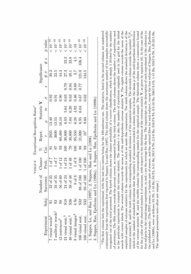
TA

BLE

6E

xce

pti

onalR

ecognit

ion

Rate

sa

Num

ber

ofC

hanc

e%

Rep

et.

Stat

isti

cY

Sign

ifica

nce

Exp

erim

ent

Subj.

Succ

esse

sP

rob.

Cor

.r

µm

σs

#σ

#s

pva

lue

7vi

sual

wor

ds1

S132

of35

1of

791

2925

13.4

00.

9220

.2<

10−

10

7au

dito

ryw

ords

1S3

34of

351

of7

9736

0013

.55

0.91

22.5

<10

−10

12se

nten

ces2

S856

of60

1of

1293

60,4

8016

.10

0.90

44.3

<10

−10

24vi

sual

sent

.3S1

824

of24

1of

2410

030

,800

6.83

5.64

0.63

0.79

27.3

23.2

<10

−10

48vi

sual

sent

.3S2

638

of48

1of

4879

30,8

007.

046.

200.

630.

9449

.133

.8<

10−

10

8vi

sual

imag

es4

4Ss

8of

81

of8

100

95,5

506.

284.

920.

460.

693.

74.

5<.0

110

0vi

sual

sent

.S3

288

of10

01

of10

088

21,0

006.

956.

040.

670.

7712

1.0

106.

4<

10−

10

100

visu

alse

nt.

S32

93of

100

1of

100

9310

79.

600.

6213

4.5

<10

−10

1.Su

ppes

,Lu,

and

Han

(199

7);

2.Su

ppes

,H

anan

dLu

(199

8)3.

Supp

es,H

an,E

pelb

oim

and

Lu

(199

9a);

4.Su

ppes

,H

an,E

pelb

oim

and

Lu

(199

9b)

aT

he

firs

tco

lum

nlist

sth

eex

per

imen

t,w

ith

the

last

two

entr

ies

bei

ng

for

the

100-s

ente

nce

one.

The

subje

cts,

list

edin

the

seco

nd

colu

mn,are

num

ber

ed

continuousl

yfr

om

the

exper

imen

tsfirs

tre

port

edin

Suppes

,Lu

and

Han

(1997).

The

third

colu

mn

show

sth

em

axim

um

num

ber

ofte

stsa

mple

ssu

cces

sfully

reco

gniz

edout

ofth

eto

talpre

sente

d.T

he

fourt

hco

lum

nsh

ow

sth

ech

ance

pro

bability

ofa

corr

ect

class

ifica

tion,w

hic

his

sim

ply

1div

ided

by

the

num

ber

ofpro

toty

pes

.T

he

fift

hco

lum

nre

cord

sth

eper

cent

corr

ect,

as

com

pute

dfr

om

the

third

colu

mn.T

he

sixth

colu

mns

show

sth

enum

ber

rofre

pet

itio

ns

use

d

inth

epart

icula

rex

per

imen

tto

com

pute

the

extr

eme

statist

ic.

The

num

ber

ris

als

oth

enum

ber

of

repet

itio

ns

origin

ally

use

din

the

grid

for

the

initia

l

searc

hw

ith

corr

ect

label

s.T

he

seven

thco

lum

nre

cord

sth

em

ean

µofth

enull-h

ypoth

esis

extr

eme

statist

icY

.T

he

eighth

colu

mn

reco

rds

the

mea

nofth

e

empir

icalsa

mple

sofex

trem

est

atist

ics

for

the

exper

imen

tsfo

rw

hic

hw

em

ade

this

com

puta

tion.T

he

nin

thco

lum

nsh

ow

sth

est

andard

dev

iation

σofth

e

extr

eme

statist

icY

,and

the

tenth

colu

mn

the

corr

espondin

gst

andard

dev

iation

softh

eem

pir

icalsa

mple

s.T

he

elev

enth

colu

mn

reco

rds

the

num

ber

k−

µσ

,

whic

his

the

num

ber

ofst

andard

dev

iations

that

the

num

ber

kofsu

cces

ses

reco

rded

inco

lum

nth

ree

isfr

om

the

mea

nµ

ofth

enull-h

ypoth

esis

dis

trib

ution

ofth

eex

trem

est

atist

icY

,and

the

twel

fth

colu

mn

the

corr

espondin

gnum

ber

for

the

empir

icalsa

mple

.T

he

thir

teen

thco

lum

nsh

ow

sa

conse

rvative

bound

for

the

pvalu

eofth

eobse

rved

num

ber

kofsu

cces

ses,

with

resp

ect

toth

edis

trib

ution

ofth

eex

trem

est

atist

icY

,as

giv

enby

equation

(6).

Inth

eca

seofth

e

four

subje

cts

inth

evis

ual-im

age

exper

imen

t,m

and

sare

the

aver

age

for

the

four.

The

super

scri

pt

on

the

des

crip

tion

ofea

chex

per

imen

tis

the

refe

rence

to

the

publish

edst

udy.

(The

EE

Gse

nso

r,or

bip

ola

rpair

ofse

nso

rs,and

the

optim

alfilt

erfo

rea

chsu

bje

ct,ex

cept

the

four

subje

cts

ofSuppes

,H

an,E

pel

boim

and

Lu

(1999b),

wer

eas

follow

s:S1:T

6,1-1

0H

z;S3:T

3,3-1

1H

z;S8:C

4-T

6,2.5

-9H

z;S18:P

4-T

6,0.5

-10

Hz;

S26:C

4-C

6,1-1

5H

z;S32:C

4-T

6,1.2

5-2

2.5

Hz.

The

optim

alpara

met

ers

wer

eoft

ennot

uniq

ue.

)

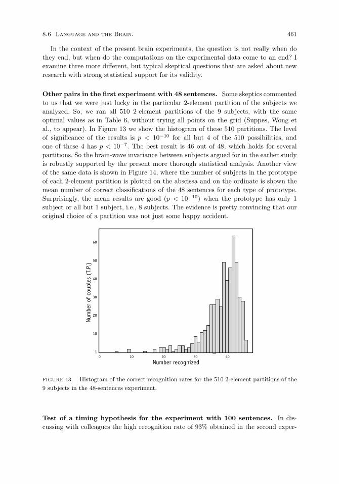
8.6 Language and the Brain. 461

In the context of the present brain experiments, the question is not really when dothey end, but when do the computations on the experimental data come to an end? Iexamine three more different, but typical skeptical questions that are asked about newresearch with strong statistical support for its validity.

Other pairs in the first experiment with 48 sentences. Some skeptics commentedto us that we were just lucky in the particular 2-element partition of the subjects weanalyzed. So, we ran all 510 2-element partitions of the 9 subjects, with the sameoptimal values as in Table 6, without trying all points on the grid (Suppes, Wong etal., to appear). In Figure 13 we show the histogram of these 510 partitions. The levelof significance of the results is p < 10−10 for all but 4 of the 510 possibilities, andone of these 4 has p < 10−7. The best result is 46 out of 48, which holds for severalpartitions. So the brain-wave invariance between subjects argued for in the earlier studyis robustly supported by the present more thorough statistical analysis. Another viewof the same data is shown in Figure 14, where the number of subjects in the prototypeof each 2-element partition is plotted on the abscissa and on the ordinate is shown themean number of correct classifications of the 48 sentences for each type of prototype.Surprisingly, the mean results are good (p < 10−10) when the prototype has only 1subject or all but 1 subject, i.e., 8 subjects. The evidence is pretty convincing that ouroriginal choice of a partition was not just some happy accident.

FIGURE 13 Histogram of the correct recognition rates for the 510 2-element partitions of the

9 subjects in the 48-sentences experiment.

Test of a timing hypothesis for the experiment with 100 sentences. In dis-cussing with colleagues the high recognition rate of 93% obtained in the second exper-

462 Representations of Language

FIGURE 14 Histogram of mean number of the correct recognition rate for the 510 2-element

partitions, indexed from 1-8 for the number of subjects in the prototype. So, e.g., 1 on the

abscissa corresponds to all the 2-element partitions having exactly one subject used for the

prototype.

iment reported above, and the earlier results summarized in Table 6, several personsskeptically suggested that perhaps our recognition rates are just coming from the dif-ferent timing of the visual presentation of words in different sentences. Sentences werepresented one word at a time in the center of the computer screen, with the onset timeof each visual word the same as the onset time of the corresponding auditory presenta-tion of the sentence. Visually displaying one word at a time avoids many troublesomeeye movements that can disrupt the brain waves, and it has also been shown to bean effective fast way to read for detailed content (Rubin and Turano 1992). The dura-tion of each visual word of a sentence also matched the auditory duration within a fewmilliseconds.

To test this timing idea, which is supported by the presence of an evoked responsepotential at the onset of most visual words, we used a recognition model that dependedonly on an initial segment of the brain-wave response to each word in a sentence (Suppes,Wong et al., to appear). The model replaces the two parameters s and e for the temporalinterval by two different parameters. The first is α, which is the estimated time lagbetween the onset of each word in every sentence and the beginning of the correspondingbrain wave in the cortex. The second is β, which is the proportion of the displayed lengthof each word, starting from its onset, used in the prototype for recognition after the delaytime α for the signal to reach the cortex. Because of the variable length of words andsentences, we normalized the least squares computation by dividing by the number ofobservations used. If only timing, and not the full representation of the word, mattersin recognition, then only a small portion of the initial segment of a word is needed,essentially the initial segment containing the onset-evoked response potential. On theother hand, if the full representation of the word is used in successful recognition, interms of our least squares criterion, then the larger β is, the better for recognition. To

8.6 Language and the Brain. 463

adjust β to the temporal length of each word displayed, we expressed β as a decimalmultiple of the temporal display length of word i of each sentence. The best predictiveresult was for α = 200 ms and β = 1.25, with a recognition rate of 92%. The recognitionrate as a function of 0.125 ≤ β ≤ 2.00 is shown in Figure 15. The rate of correctrecognition increases monotonically with β up to β = 1.25 and then declines slowlyafter β = 1.50. These results support two conclusions. First, timing is important. Therecognition rate of 45% for β = 0.125 is much greater than a chance outcome. But,second, the more complete the brain-wave representation of the words in a sentence, thebetter for recognition purposes.

FIGURE 15 Classification results using different initial segments of brain-wave data after

onset of each word in a sentence. Segment i begins after α ms following onset of word i in a

sentence and segment i ends after β · li ms, where li is the length in ms of the visual display of

word i.

Censoring data in the visual-image experiment. One kind of skeptical questionthat keeps the computations going is about artifacts. Perhaps the remarkable levels ofstatistical significance are due to some artifacts in the data.31 Now there is a long historyof the problems of artifacts in EEG research. A main source is eye blinks and saccadicor pursuit eye movements, another is ambient current in the environment, mainly dueto the 60 Hz oscillation of the standard alternating current in any building in whichexperiments are ordinarily conducted, and still another source is in the instrumentationfor observing and recording the electric brain waves. This list is by no means exhaustive.There is a large literature on the subject from several different angles, but it would betoo much to survey it here.

31Given that the extreme statistics of the random permutations had a mean close to the low mean of

the null hypothesis for the second experiment, it is extremely unlikely that any artifacts could account

for the correct classification of 93% in the second experiment, or, in fact, in any of the others with

p < 10−10. But artifact removal remains an important topic, not so much to meet ill-informed skeptical

questions, but to improve the classification results, as is the case for an example that follows.

464 Representations of Language

I restrict myself to describing how we used a rather familiar statistical approach,rather than any visual inspection of the recorded data for eye blinks or other artifacts.32

The approach was to censor the data, but to introduce a free parameter to optimize thecensoring—optimize in the sense already described of maximizing the correct recognitionrate.

Let Xik = observation i on trial k, and let ω be the number of trials averaged tocreate a prototype or test sample. Then

mi = Xi =1ω

ω∑k=1

Xik.

In similar fashion, we compute the variance s2i . Let α be the free parameter for censoringsuch that if

|Xik −mi| > αsi

eliminate observation i of trial k from the data being averaged. The computational taskis to find the α that optimizes classification. In the example reported here, we ran aone-dimensional grid of 20 values of si to approximate the best value α.

The experiment for which the extreme statistics were not highly significant was thevisual-image one already described, the one that was relevant to the eighteenth-centurycontroversy about abstract ideas. The data, as I said earlier, supported in a direct waythe skeptical views of Berkeley and Hume, but the statistical support was not verystrong. So we reanalyzed the data, creating 24 rather than 8 test samples, and we alsoran the experiment with four monolingual Chinese (Mandarin) speakers to confirm theverbal part, with auditory or visual words, in Chinese as well as English. The detailsare reported in Suppes, Wong et al. (to appear).

Table 7 shows the significant results for cross-modal classification. The first twoconditions are for the original experiment using English. For the feminine-auditory-voice representing brain waves (AWF) as prototypes and the visual-image brain wavesas test samples, 15 of the 24 test samples were correctly classified after censoring, animprovement from 11 of 24 without censoring, for a resulting significance level of p <0.016. When the roles of prototype and test sample were reversed the results of censoringwere better, 16 of the 24 test samples correctly classified after censoring, with p < 0.001.Note that the significance levels here are conservative, based on the complete grid searchequal to r = 1, 470, 000, the number of repetitions under the extreme-statistic nullhypothesis.

In the case of the Chinese, the best results were in the comparison of the auditory andvisual presentation of the eight words, with the best result being for the visual Chinesewords (VW) as prototypes and the auditory Chinese words (AW) as test samples, in thecensored case, 17 of 24 correctly classified, with p approximately 0.0001, and with, asbefore, the number of repetitions r, under the null hypothesis, greater than a million. Sowe end by strengthening the case for Berkeley and Hume, without claiming the evidenceis as yet completely decisive.

An appropriate stopping point for this analysis is to emphasize that censoring does

32In our larger experiments with more than 40,000 trials it is impractical to try to use traditional

observational methods to detect artifacts.

8.7 Epilogue: Representation and Reduction in Science 465

TABLE 7 Cross-modal results in visual-image experiment with censored data

R Y SignificanceExper. µ σ #σ p-valueEnglishAWF/VI 11 11.57 .692 0.8 ≈ .500censor 15 13.01 .642 3.1 < .016VI/AWF 11 11.57 .692 0.8 ≈ .500censor 16 13.01 .642 4.7 < .001ChineseAW/VW 9 11.42 .690censor 16 12.86 .662 4.7 < .001VW/AW 13 11.42 .690 2.3 ≈ .05censor 17 12.86 .662 6.3 ≈ .0001

not guarantee improvement in classification. Most of the other results in Table 6 showedlittle improvement from censoring, but then for all of the experiments reported there,except for the visual-image one, the results were highly significant without censoring.

As in many areas of science, so with EEG recordings, statistical and experimentalmethods for removing artifacts and other anomalies in data constitute a large subjectwith a complicated literature. I have only reported a common statistical approach here,but I am happy to end with this one example of a typical method of “cleaning up”data. It is such censored data that should be used to form a representation suitable forserving as a test of some theory or, as is often the case, some congerie of theoreticalideas.

8.7 Epilogue: Representation and Reduction in Science33

The theme of reduction is as old as philosophy. Already in the 5th century BC, Leu-cippus and especially his student, Democritus, stated in clear general terms the atomicideas for which they are justly famous. Matter is nothing but solid atoms moving inempty space. The weight, density and hardness of a physical object depends only onthe arrangements of its atoms in the void, as the Greeks described empty space. Butalso, according to Democritus, nothing happens randomly, but according to law andby necessity. Although much criticized by Aristotle and his followers over the centuries,this reductionist mechanical view of nature was once again brought to the fore with thedevelopment of physics, or, as it was known then, natural philosophy, in the seventeenthand eighteenth centuries.

But the two most famous ancient atomists to come after Democritus added to thismechanical picture the effects of chance. Here is a well-known quotation from Epicurus,taken from his letter to Herodotus, written probably in the 4th century BC (Oates 1940,p. 5):

And the atoms move continuously for all time, some of them falling straight down, others

swerving, and others recoiling from their collisions. And of the latter, some are borne

33The remarks in this section supplement those on reductionism in Suppes (1984, pp. 120-125).

466 Representations of Language

on, separating to a long distance from one another, while others again recoil and recoil,

whenever they chance to be checked by the interlacing with others, or else shut in by

atoms interlaced around them. For on the one hand the nature of the void which separates

each atom by itself brings this about, as it is not able to afford resistance, and on the

other hand the hardness which belongs to the atoms makes them recoil after collision to

as great a distance as the interlacing permits separation after the collision. And these

motions have no beginning, since the atoms and the void are the cause.

And this is was Lucretius had to say in De Rerum Natura, written in the first centuryBC (Oates 1940, p. 95):

This point too herein we wish you to apprehend: when bodies are borne downwards sheer

through void by their own weights, at quite uncertain times and uncertain spots they

push themselves a little from their course: you just and only just can call it a change of

inclination. If they were not used to swerve, they would all fall down, like drops of rain,

through the deep void, and no clashing would have been begotten nor blow produced

among the first-beginnings: thus nature never would have produced aught.

So Epicurus and Lucretius represent reduction of nature to probabilistic mechanics, adiscipline not really well developed scientifically until the twentieth century. Of course,these atomists did not get a good press from Aristotle to Newton, with a few notableexceptions. A justly quotable passage from Newton is to be found in his well-knownletter of February 25, 1692/3, written to Richard Bentley.

It is inconceivable, that inanimate brute matter should, without the mediation of some-

thing else, which is not material, operate upon and affect other matter without mutual

contact, as it must be, if gravitation, in the sense of Epicurus, be essential and inherent

in it. And this is one reason why I desired you would not ascribe innate gravity to me.

That gravity should be innate, inherent, and essential to matter, so that one body may

act upon another at a distance through a vacuum, without the mediation of anything

else, by and through which their action and force may be conveyed from one to another,

is to me so great an absurdity, that I believe no man, who has in philosophical matters

a competent faculty of thinking, can ever fall into it. Gravity must be caused by an

agent acting constantly according to certain laws; but whether this agent be material or

immaterial, I have left to the consideration of my readers.

From Newton onward the great contributors to the development of physics were, al-most without exception, quite clear on the difference between establishing a thesis ofreduction scientifically, as opposed to speculative ideas about it. About two hundredyears after Newton, Maxwell states this view very clearly in his little book Matter andMotion.

Of course if we begin by assuming that the real bodies are systems composed of matter

which agrees in all respects with the definitions we have laid down, we may go on to assert

that all phenomena are changes of configuration and motion, though we are not prepared

to define the kind of configuration and motion by which the particular phenomena are to

be explained. But in accurate science such asserted explanations must be estimated, not

by their promises, but by their performances. The configuration and motion of a system

are facts capable of being described in an accurate manner, and therefore, in order that

the explanation of a phenomenon by the configuration and motion of a material system

may be admitted as an addition to our scientific knowledge, the configurations, motions,

8.7 Epilogue: Representation and Reduction in Science 467

and forces must be specified, and shown to be consistent with known facts, as well as

capable of accounting for the phenomenon.”

Maxwell, Matter and Motion, 1877/1920, pp. 70-71

Maxwell makes clear enough the need to distinguish between reductions that arefirmly established from those that are not. This does not mean that all speculation is abad thing. We might even maintain that in most cases in science, the “next big thing”is preceded by speculation that it is out there to be discovered or invented. What isimportant to the modern temperament is that scientific speculations be taken straightas conjectures, not mixed and served in metaphysical cocktails of suspect ingredients.So one of the puritanical themes of this book is that scientific reduction is hard work. Tofinish it off with detailed and explicit representation theorems is even harder. In spiteof the many pages in this book and the continual focus on representation theorems, nota single really significant representation theorem providing the stiff backbone for someimportant claim about reduction of one part of science to another has been proved oreven stated. The reader who has missed some of my earlier remarks on this topic mayask, Why not?

The answer is obvious. The problem was too difficult for me. Perhaps the most fa-mous case to consider is the reduction of thermodynamics to statistical mechanics. Ata general conceptual level this is one of the great triumphs of what used to be calledthe mechanical philosophy. And at a general level of analysis a famous article on thetopic was published by Ernest Nagel in 1949. But Nagel fully realized he was not ableto give the full details or to begin to offer a rigorous mathematical proof of an appro-priate representation theorem. Ruelle (1978) is one of the best examples of a rigorousmathematical approach, but his idealization requires that the physical systems to whichit directly applied be actually infinite in all directions, i.e., completely space filling, inorder to exhibit sharp phase transitions. The detailed explanation of phase transitionsin macroscopic thermodynamic systems is one of the main objectives of classical equilib-rium statistical mechanics. I also want to emphasize that phase transitions are amongthe most obvious systematic changes in natural phenomena that we would naturallywant to explain. For example, we would like to derive from fundamental physical princi-ples the result that under ordinary atmospheric pressure liquid water turns into steamat about 100 degrees Celsius. To derive this result rigorously from first principles forthe kitchen tea kettle is still not possible. The same goes for the other dramatic phasetransition, the freezing of a glass of water.

The absence of rigorous representation theorems for these everyday dramatic phe-nomena does not mean physicists are doing a bad job of analysis. It is just that we havecome to realize in a very explicit way how difficult it is to give rigorous mathematical re-sults for all kinds of ordinary natural phenomena. And physicists, clever problem solversthat they are, have gone ahead and learned much about such phenomena, including howto calculate, without rigorous justification, a large number of quantitative results.

Given how much this case generalizes to other important phenomena, with examplesranging from the weather to the stock market, it is, as in other matters, philosophicallyimportant to have a pluralistic approach to what can be accomplished. Weather predic-tions are much better now than they were forty years ago, even though we now realize

468 Representations of Language

that detailed predictions a month in advance are hopeless within our current theoriesand computing regimes for analyzing weather data. Physicists are adept at deriving use-ful and highly accurate equations explaining many phenomena that cannot be analyzedrigorously from a general mathematical standpoint. From such work we derive insightsand intuitions about what representations and reductions are probably approximatelycorrect, even though new surprises may be lurking in as yet undiscovered byways. Andit is important for philosophers of science to have an understanding and overview ofwhat is currently believed by physicists to be true of many physical phenomena, or, ofother phenomena such as market behavior or language use by other scientists. In fact,in many areas of science, necessarily mainly empirical results on representation maybe the only results that can be currently obtained. The brain-wave representations forlanguage reported in Section 6 are an example.

But it is also part of such a pluralistic view to keep a place for rigorous results aboutrepresentation and reduction. I have tried to give some sufficiently simple manageableexamples in various areas of science in the last four chapters. I include in this list ofexamples the extended analysis of representations or interpretations of probability inChapter 5. It is also evident that not all kinds of representation immediately suggestreduction. For example, the many representation theorems provable in the theory ofmeasurement, of which I gave elementary examples in Chapter 3, do not conceptuallysuggest we are substantively reducing physical or psychological properties to numbers,but rather are using numbers to refine our analysis of the properties. In other words, thiskind of representation is not like the physical reduction of the concept of temperatureto the mean motion of particles.

On the other hand, the representation of computable functions by register machinesor Turing machines, as stated in Chapter 3, or the representation of finite automata orregister machines by stimulus-response models in Chapter 8, do suggest rather directphysical realizations of computational processes, and these realizations have at bot-tom much simpler mechanisms than were thought possible a hundred years earlier. Theexistence of such simple mechanisms for many complex phenomena—and thus their re-duction in one sense—is a point much emphasized and exemplified in the recent lengthytome A New Kind of Science (2002) by the theoretical physicist Stephen Wolfram. ButWolfram properly stresses, as he has in earlier publications, that many such processesare computationally irreducible, meaning that there is no simpler way to study theirbehavior than to observe the processes themselves.

Without entering into new technical complexities, it is evident that a concept likecomputational irreducibility is useful in helping to explain why accepted cases of reduc-tion often do not result in any drastic change of concepts in our descriptions of ordinaryphenomena. There are, of course, other reasons for there being little change in the faceof what seems like a conceptual revolution. We will, I am sure, still talk in a hundredyears about tables and chairs as we now do. And this holds for countless other familiarobjects and processes.

On the other hand, to hold the thesis that such reductions have no impact on ordinarythought and talk is also a mistake. Numerical representations of time and temperatureare now used by ordinary folk in ways that would have seemed strange and out of place

8.7 Epilogue: Representation and Reduction in Science 469

in the not too distant past. Some similar changes seem likely as we come to understandin ever more physical detail just how our minds and bodies work, but forecasting whichrepresentations of the future and their invariants will become the basis of new naturalidioms is, even if not computationally irreducible, too difficult to attempt.

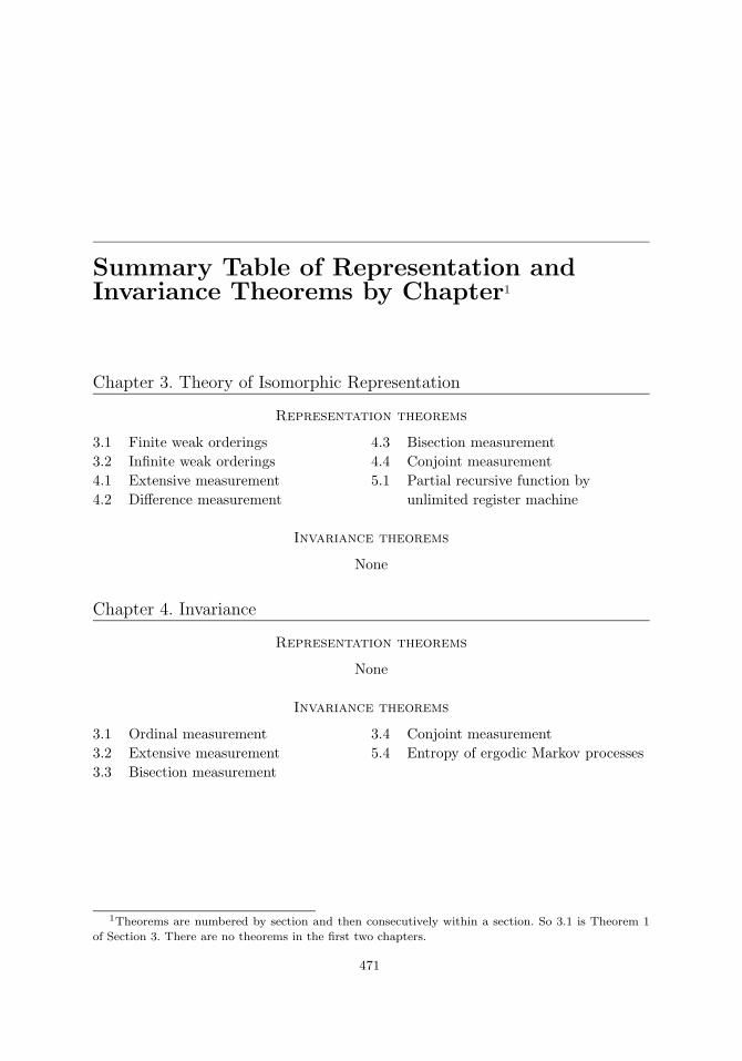
Summary Table of Representation andInvariance Theorems by Chapter1

Chapter 3. Theory of Isomorphic Representation

Representation theorems

3.1 Finite weak orderings 4.3 Bisection measurement3.2 Infinite weak orderings 4.4 Conjoint measurement4.1 Extensive measurement 5.1 Partial recursive function by4.2 Difference measurement unlimited register machine

Invariance theorems

None

Chapter 4. Invariance

Representation theorems

None

Invariance theorems

3.1 Ordinal measurement 3.4 Conjoint measurement3.2 Extensive measurement 5.4 Entropy of ergodic Markov processes3.3 Bisection measurement

1Theorems are numbered by section and then consecutively within a section. So 3.1 is Theorem 1

of Section 3. There are no theorems in the first two chapters.

471

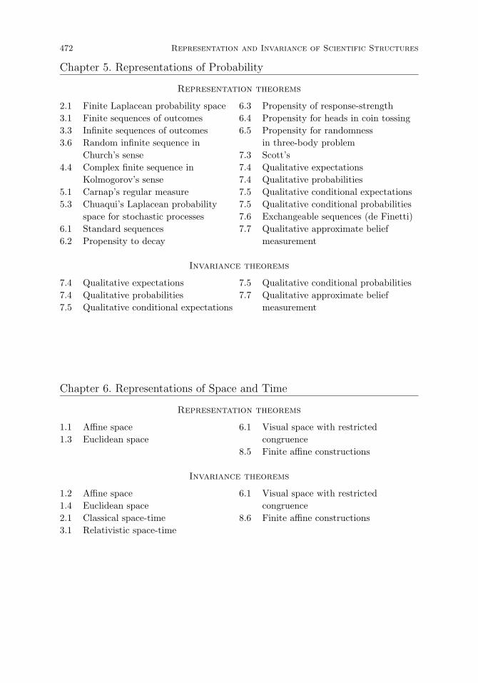
472 Representation and Invariance of Scientific Structures

Chapter 5. Representations of Probability

Representation theorems

2.1 Finite Laplacean probability space 6.3 Propensity of response-strength3.1 Finite sequences of outcomes 6.4 Propensity for heads in coin tossing3.3 Infinite sequences of outcomes 6.5 Propensity for randomness3.6 Random infinite sequence in in three-body problem

Church’s sense 7.3 Scott’s4.4 Complex finite sequence in 7.4 Qualitative expectations

Kolmogorov’s sense 7.4 Qualitative probabilities5.1 Carnap’s regular measure 7.5 Qualitative conditional expectations5.3 Chuaqui’s Laplacean probability 7.5 Qualitative conditional probabilities

space for stochastic processes 7.6 Exchangeable sequences (de Finetti)6.1 Standard sequences 7.7 Qualitative approximate belief6.2 Propensity to decay measurement

Invariance theorems

7.4 Qualitative expectations 7.5 Qualitative conditional probabilities7.4 Qualitative probabilities 7.7 Qualitative approximate belief7.5 Qualitative conditional expectations measurement

Chapter 6. Representations of Space and Time

Representation theorems

1.1 Affine space 6.1 Visual space with restricted1.3 Euclidean space congruence

8.5 Finite affine constructions

Invariance theorems

1.2 Affine space 6.1 Visual space with restricted1.4 Euclidean space congruence2.1 Classical space-time 8.6 Finite affine constructions3.1 Relativistic space-time

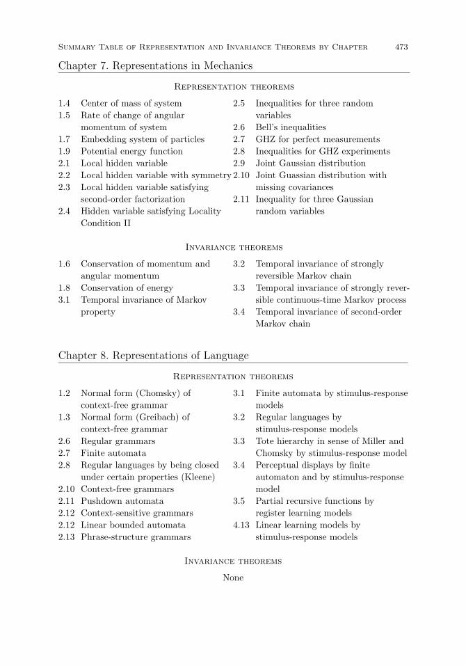
Summary Table of Representation and Invariance Theorems by Chapter 473

Chapter 7. Representations in Mechanics

Representation theorems

1.4 Center of mass of system 2.5 Inequalities for three random1.5 Rate of change of angular variables

momentum of system 2.6 Bell’s inequalities1.7 Embedding system of particles 2.7 GHZ for perfect measurements1.9 Potential energy function 2.8 Inequalities for GHZ experiments2.1 Local hidden variable 2.9 Joint Gaussian distribution2.2 Local hidden variable with symmetry 2.10 Joint Guassian distribution with2.3 Local hidden variable satisfying missing covariances

second-order factorization 2.11 Inequality for three Gaussian2.4 Hidden variable satisfying Locality random variables

Condition II

Invariance theorems

1.6 Conservation of momentum and 3.2 Temporal invariance of stronglyangular momentum reversible Markov chain

1.8 Conservation of energy 3.3 Temporal invariance of strongly rever-3.1 Temporal invariance of Markov sible continuous-time Markov process

property 3.4 Temporal invariance of second-orderMarkov chain

Chapter 8. Representations of Language

Representation theorems

1.2 Normal form (Chomsky) of 3.1 Finite automata by stimulus-responsecontext-free grammar models

1.3 Normal form (Greibach) of 3.2 Regular languages bycontext-free grammar stimulus-response models

2.6 Regular grammars 3.3 Tote hierarchy in sense of Miller and2.7 Finite automata Chomsky by stimulus-response model2.8 Regular languages by being closed 3.4 Perceptual displays by finite

under certain properties (Kleene) automaton and by stimulus-response2.10 Context-free grammars model2.11 Pushdown automata 3.5 Partial recursive functions by2.12 Context-sensitive grammars register learning models2.12 Linear bounded automata 4.13 Linear learning models by2.13 Phrase-structure grammars stimulus-response models

Invariance theorems

None

References

Abelson, R. M. and R. A. Bradley (1954). A 2x2 factorial with paired comparisons. Biometrics

10(4):487–502.

Aczel, J. (1961). Uber die Begrundung der Additions- und Multiplikationsformeln von be-

dingten Wahrscheinlichkeiten. Magyar Tudomanyos Akademia Matematikai Kutato Int.

Kozlemenyei 6:110–122.

Aczel, J. (1966). Lectures on functional equations and their applications. New York: Academic

Press.

Aho, A. V. and J. D. Ullman (1972). The theory of parsing, translation, and compiling , vol. 1.

Englewood Cliffs, NJ: Prentice Hall.

Alekseev, V. M. (1968–1969a). Quasirandom dynamical systems I, II, III. Math. USSR Sbornik

5,6,7:505–560 and 1–43.

Alekseev, V. M. (1969b). Quasirandom dynamical systems. (Russian). Mat. Zametki 6(4):489–

498. English translation in Math. Notes 6 (1969), 749–753.

Alexandrov, A. D. (1950). On Lorentz transformations. (Russian). Uspekhi Matematichekikh

Nauk 5, 3(37):187.

Alexandrov, A. D. (1975). Mapping of spaces with families of cones and space-time transfor-

mations. Annali di Matematica Pura ed Applicata 103:229–257.

Ames Jr., A. (1946). Binocular vision as affected by relations between uniocular stimulus

patterns in common place environments. American Journal of Psychology 59:333.

Anderson, J. R. (1976). Language, memory, and thought . Hillsdale, NJ: Lawrence Erlbaum.

Angell, R. B. (1974). The geometry of visibles. Nous 8:87–117.

Appell, P. (1941). Traite de mecanique rationelle. Tome I: Statique, dynamique du point . Paris:

Gauthier-Villars, sixth edn.

Aquinas, T. (1944). Summa theologica. In A. C. Regis, ed., Basic writings of Saint Thomas

Aquinas, vol. 1. New York: Random House.

Arbib, M. A. (1969). Memory limitations of stimulus-response models. Psychological Review

76:507–510.

Archimedes (1897). On the equilibrium of planes. In T. L. Heath, ed., The works of Archimedes,

edited in modern notation with introductory chapters, pages 189–220. Cambridge, England:

Cambridge University Press. Translation by T. L. Heath.

475

476 Representation and Invariance of Scientific Structures

Aristotle (1960). De Caelo (On the heavens). Cambridge, MA: Harvard University Press.

English translation by W. K. C. Guthrie. First published in 1939.

Aristotle (1975). De Anima (On the soul). Cambridge, MA: Harvard University Press, 4th

edn. English translation by W. S. Hett. First published in 1936.

Arnold, V. I. (1978). Mathematical methods of classical mechanics. New York: Springer.

Arrow, K. J. (1951). Social choice and individual values. New York: Wiley.

Attias, H. (1999). Independent factor analysis. Neural Computation 11:803–852.

Balzer, W. (1978). Empirische Geometrie und Raum-Zeit-Theorie in Mengentheoretischer

Darstellung . Konigstein/Ts.: Scriptor Verlag.

Bayes, T. (1763). An essay towards solving a problem in the doctrine of chances. Philosophical

Transactions of the Royal Society 53:370–418. Reprinted in Facsimiles of two papers by

Bayes with a commentary by W. Edwards Deming, New York, Hafner Pub. Co., 1940.

Beck, A. (1890). Die Strome der Nervencentren. Centralblatt fur Physiologie 4:572–573.

Bell, J. S. (1964). On the Einstein-Podolsky-Rosen paradox. Physics 1:195–200.

Bentham, J. (1789/1907). The principles of morals and legislation. Oxford: Clarendon Press.

First published in 1789.

Berger, H. (1929). Uber das Elektroenkephalogram des Menschen. Archiv fur Psychiatrie

Nervenkrankheiten 87(4):527–570. Translated by P. Gloor in Electroencephalography Clinic

Neurophysiology, Supplement 28, 37–73, 1969.

Berkeley, G. (1709/1901). An essay towards a new theory of vision. In A. C. Fraser, ed.,

Berkeley’s complete works, vol. 1, pages 93–210. New York: Oxford University Press. First

published in 1709.

Bernoulli, D. (1738). Specimen theoriae novae de mensura sortis. Comentarii academiae

scientiarum imperiales petropolitanae 5:175–192. Translation by L. Sommer in Econometrica

1954, 22, 23–26.

Bernoulli, J. (1713). Ars conjectandi . Basileae: Impensis Thurnisiorum fratrum. Reprinted on

pp. 106-286 in Vol. 3 of Die Werke von Jakob Bernoulli, Birkhauser Verlag, Basel, 1975.

Bertrand, J. L. (1888). Calcul des probabilities. Paris: Gauthier-Villars.

Bever, T. G., J. Fodor, and M. Garrett (1968). A formal limitation of associationism. In T. R.

Dixon and D. L. Horton, eds., Verbal behavior and general behavior theory . Englewood Cliffs:

Prentice-Hall.

Blank, A. A. (1953). The Luneburg theory of binocular visual space. Journal of the Optical

Society of America 43:717–727.

Blank, A. A. (1957). The geometry of vision. British Journal of Physiological Optics l4:154–169.

Blank, A. A. (1958a). Analysis of experiments in binocular space perception. Journal of the

Optical Society of America 48:911–925.

Blank, A. A. (1958b). Axiomatics of binocular vision: The foundations of metric geometry in

relation to space perception. Journal of the Optical Society of America 48:328–334.

Blank, A. A. (1961). Curvature of binocular visual space: An experiment. Journal of the

Optical Society of America 51:335–339.

Blumenfeld, W. (1913). Untersuchungen uber die scheinbare Grosse in Sehraume. Zeitschrift

fur Psychologie und Physiologie der Sinnesorgane 65:241–404.

References 477

Bohm, D. (1965). The special theory of relativity . New York: W. A. Benjamin.

Borsuk, K. and W. Szmielew (1960). Foundations of geometry . Amsterdam: North Holland.

Bourbaki, N. (1950). The architecture of mathematics. American Mathematical Monthly

57:231–232.

Bouwmeester, D., J. W. Pan, M. Daniell, H. Weinfurter, and A. Zeilinger (1999). Observa-

tion of three-photon Greenberger-Horne-Zeilinger entanglement. Physical Review Letters

82(7):1345–1349.

Bowerman, M. (1989). Learning a semantic system. What role do cognitive predispositions

play? In M. L. Rice and R. L. Schiefelbusch, eds., The teachability of language, pages 133–

169. Baltimore: Paul H. Brookes.

Bowerman, M. (1996). The origin of children’s spatial semantic categories: Cognitive vs. linguis-

tic determinants. In J. J. Gumperz and S. C. Levinson, eds., Rethinking linguistic relativity ,

pages 145–176. Cambridge, England: Cambridge University Press.

Bradley, R. A. (1954a). Rank analysis of incomplete block designs, II. Additional tables for

the method of paired comparisons. Biometrika 41:502–537.

Bradley, R. A. (1954b). Incomplete block rank analysis: On the appropriateness of the model

for a method of paired comparisons. Biometrics 10:375–390.

Bradley, R. A. (1955). Rank analysis of incomplete block designs, III. Some large-sample results

on estimation and power for a method of paired comparisons. Biometrika 42:450–470.

Bradley, R. A. and M. E. Terry (1952). Rank analysis of incomplete block designs, I. The

method of paired comparisons. Biometrika 39:324–345.

Breiman, L. (1999). Prediction games and arcing algorithms. Neural Computation 11:1493–

1518.

Bresnan, J. (1982). The passive in lexical theory. In J. Bresnan, ed., The mental representation

of grammatical relations, pages 3–86. Cambridge, MA: MIT Press.

Bronte, C. (1847/1971). Jane Eyre, an authoritative text, backgrounds, criticism, edited by

Richard J. Dunn. New York: W. W. Norton & Company. First published in 1847.

Bruns, H. (1887). Uber die Integrale des Vielkorper-Problems. Acta Mathematica 11:25–96.

Brush, S. G. (1976). The kind of motion we call heat: A history of the kinetic theory of gases

in the 19th century . Amsterdam: North-Holland Publishing Co.

Buffon, G. L. (1733). Communication. Actes de l’academie des sciences - Paris pages 43–45.

Buffon, G. L. (1777). Essai d’arithmetique morale.

Busemann, H. (1955). The geometry of geodesics. New York: Academic Press.

Bush, R. R. and W. K. Estes, eds. (1959). Studies in mathematical learning theory . Stanford,

CA: Stanford University Press.

Bush, R. R. and F. Mosteller (1955). Stochastic models for learning . New York: Wiley.

Campbell, N. R. (1920). Physics, the elements. Cambridge University Press.

Campbell, N. R. (1928). An account of the principles of measurement and calculation. New

York: Longmans, Green and Co.

Cantor, G. (1895). Beitrage zur Begrundung der transfiniten Mengenlehre. Mathematische

Annalen 46:481–512. Translation by P. E. B. Jourdain in Contributions to the founding of

the theory of transfinite numbers, Dover, New York 1952, pp. 85–136 and pp. 137–201, with

original pagination indicated.

478 Representation and Invariance of Scientific Structures

Carnap, R. (1945). On inductive logic. Philos. Sci. 12:72–97.

Carnap, R. (1950). The logical foundations of probability . Chicago, IL: University of Chicago

Press.

Carnap, R. (1952). The continuum of inductive methods. Chicago, IL: The University of

Chicago Press.

Cartwright, N. (1999). The dappled world: A study of the boundaries of Science. Cambridge,

England: Cambridge University Press.

Caton, R. (1875). The electric currents of the brain. British Medical Journal 2:278. Abstract

only.

Chaitin, G. J. (1966). On the length of programs for computing finite binary sequences. Journal

of the ACM 13(4):547–569.

Chaitin, G. J. (1969). On the length of programs for computing finite binary sequences. Journal

of the ACM 16(1):145–159.

Choi, S. and M. Bowerman (1991). Learning to express motion events in English and Korean:

The influence of language-specific lexicalization patterns. Cognition 41(1):83–121.

Chomsky, N. (1957). Syntactic structures. The Hague: Mouton.

Chomsky, N. (1959). On certain formal properties of grammars. Information and Control

2:137–167.

Chuaqui, R. (1977). A semantical definition of probability. In A. I. Arruda and N. C. A.

da Costa, eds., Non classical logic, model theory and computability , pages 135–168. Amster-

dam: North Holland.

Chuaqui, R. (1991). Truth, possibility, and probability . Amsterdam: North Holland.

Chuaqui, R. and P. Suppes (1990). An equational deductive system for the differential and

integral calculus. In P. Martin-Lof and G. Mints, eds., Lecture notes in computer science,

Proceedings of COLOG-88 International Conference on Computer Logic, pages 25–49. Berlin:

Springer.

Chuaqui, R. and P. Suppes (1995). Free-variable axiomatic foundations of infinitesimal analysis:

A fragment with finitary consistency proof. The Journal of Symbolic Logic 60:122–159.

Church, A. (1936). An unsolvable problem of elementary number theory. American Journal of

Mathematics 58:345–363.

Church, A. (1940). On the concept of a random sequence. Bulletin of American Mathematical

Society 46(2):130–135.

Clagett, M. (1959). The science of mechanics in the middle ages. Madison, WI: University of

Wisconsin Press.

Compton, A. H. (1923). A quantum theory of the scattering of X-rays by light elements.

Physical Review 21:483–502.

Cooley, J. W. and J. W. Tukey (1965). An algorithm for the machine computation of complex

Fourier series. Math. Computation 19:297–301.

Copeland, A. H. (1928). Admissible numbers in the theory of probability. Amer. Jour. Math.

50(4):535–552.

Coren, S. and J. S. Girgus (1978). Seeing is deceiving : the psychology of visual illusions.

Hillsdale, NJ: Lawrence Erlbaum.

References 479

Cover, T. M., P. Gacs, and R. M. Gray (1989). Kolmogorov’s contribution to information

theory and algorithmic complexity. Annals of Probability 17:840–863.

Cover, T. M. and J. A. Thomas (1991). Elements of information theory . New York: Wiley.

Crangle, C. and P. Suppes (1989). Geometrical semantics for spatial prepositions. In P. A.

French, T. E. Uehling, Jr., and H. K. Wettstein, eds., Midwest studies in philosophy , vol. 14,

pages 399–422. Notre Dame, IN: University of Notre Dame Press.

da Costa, N. C. A. and R. Chuaqui (1988). On Suppes’ set theoretical predicates. Erkenntnis

29:529–589.

Daniels, N. (1972). Thomas Reid’s discovery of a non-Euclidean geometry. Philosophy of

Science 39:219–234.

David, F. N. (1962). Games, gods and gambling: The origins and history of probability and

statistical ideas from the earliest times to the Newtonian era. London: Charles Griffin.

Davidson, D. and P. Suppes (1956). A finitistic axiomatization of subjective probability and

utility. Econometrica 24:264–275.

Davidson, D., P. Suppes, and S. Siegel (1957). Decision making: An experimental approach.

Stanford, CA: Stanford University Press. Midwahy Reprint, Chicago, IL: University of

Chicago, Press, 1977.

Davis, M. (1958). Computability and unsolvability . New York: McGraw–Hill.

Davis, R. L. (1953). The number of structures of finite relations. Proceedings of the American

Mathematical Society 4:486–495.

Dawid, A. P. (1986). Probability forecasting. In S. Kotz, N. L. Johnson, and C. B. Read, eds.,

Encyclopedia of statistical sciences, vol. 7, pages 210–218. New York: Wiley.

de Barros, A. J. and P. Suppes (2000). Inequalities for dealing with detector inefficiencies in

Greenberger-Horne-Zeilinger-type experiments. Physical Review Letters 84:793–797.

de Finetti, B. (1931). Sul significato della probabilita. Fundamenta Mathematicae 17:298–329.

de Finetti, B. (1937/1964). La prevision: ses lois logiques, ses sources subjectives. Annales de

l’Institut Henri Poincare 7:1–68. Translation in Kyburg and Smokler (1964), 93–158.

de Finetti, B. (1951). Recent suggestions for the reconciliation of theories of probability. In

J. Neyman, ed., Proceedings of the second Berkeley symposium on mathematical statistics

and probability . Berkeley: University of California Press.

de Finetti, B. (1974). Theory of probability , vol. 1. New York: Wiley. Translated by A. Machi

and A. Smith.

de Finetti, B. (1975). Theory of probability , vol. 2. New York: Wiley. Translated by A. Machi

and A. Smith.

de Moivre, A. (1718/1756). The doctrine of chances. London: Chelsea, 3rd edn. First published

in 1718.

Dedekind, R. (1872). Stetigkeit und Irrationale Zahlen. Vieweg: Braunschweig. Translated by

W. W. Beman, Continuity and irrational numbers, in ’Essays on the theory of numbers’,

1-27, New York: Dover, 1963.

Dembowski, P. (1968). Finite geometries. New York: Springer.

Dempster, A. P. (1967). Upper and lower probabilities induced by a multivalued mapping.

Ann. Math. Statist. 38:325–340.

480 Representation and Invariance of Scientific Structures

Descartes, R. (1637/1954). La Geometrie. New York: Dover. Translated from the French and

Latin by D. E. Smith and M. L. Latham. First published in 1637.

Descartes, R. (1644/1983). Principia philosophiae. Amsterdam: Ludovicum Elzevirium. Trans-

lation by V. R. Miller and R. P. Miller, Principles of philosophy, Reidel, Dordrecht, 1983.

First published 1644.

Descartes, R. (1649/1927). Passions of the soul. In R. M. Eaton, ed., Descartes selections,

pages 361–403. New York: Charles Scribner’s sons. First published in 1649.

Diaconis, P. (1977). Finite forms of de Finetti’s theorem on exchangeability. Synthese 36:271–

281.

Diaconis, P. and D. Freedman (1980). Finite exchangeable sequences. The Annals of Probability

8(4):745–764.

Dijksterhius, E. J. (1957). Archimedes. New York: Humanities Press.

Dirac, P. A. M. (1947). The principles of quantum mechanics. Oxford: Clarendon Press, 3rd

edn. First published in 1930.

Domotor, Z. (1969). Probabilistic relational structures and their applications. Tech. Rep. 144,

Stanford University, Institute for Mathematical Studies in the Social Sciences, Stanford, CA.

Domotor, Z. (1972). Causal models and space-time geometries. Synthese 24:5–57.

Doob, J. L. (1941). Probability as measure. Ann. Math. Stat. 12:206–214, 216–217.

Doob, J. L. (1960). Some problems concerning the consistency of mathematical models. In R. E.

Machol, ed., Information and Decision Processes, pages 27–33. New York: McGraw–Hill.

Drosler, J. (1966). Das beidaeugige Raumsehen. In W. Metzger, ed., Handbuch der Psychologie,

pages 590–615. Goettingen: Hogrefe.

Drosler, J. (1979a). Foundations of multi-dimensional metric scaling in Cayley-Klein geome-

tries. British Journal of Mathematical and Statistical Psychology 32:185–211.

Drosler, J. (1979b). Grundlegung einer mehrdimensionalen metrischen Skalierung. Zeitschrift

fuer experimentelle und angewandte Psychologie 26:1–36.

Drosler, J. (1979c). Relativistic effects in visual perception of real and apparent motion. Arch.

Psychol. 131:249–266.

Drosler, J. (1987). Experimentelle untersuchung der Geometrie des monokularen Sehraumes.

Zeitschrift fuer experimentelle und angewandte Psychologie 3:351–369.

Drosler, J. (1988). The psychophysical function of binocular space perception. Journal of

Mathematical Psychology 32:285–297.

Drosler, J. (1992). Eine untersuchung des perspektivischen Sehens. Zeitschrift fuer experi-

mentelle und angewandte Psychologie 34:515–532.

Du Bois-Reymond, E. (1848). Untersuchungen uber thierische Elektricitat . Berlin: Verlang

von G. Reiner. Passage quoted translated by Hebbel E. Hoff, Galvani and the pre-Galvanic

electrophysiologists, Annals of Science, 1 (1936), 157–172.

Einstein, A. (1905/1923). Zur electrodynamik bewegter Korper. Annalen der Physik 17.

Translation in Lorentz et al. (1923).

Einstein, A. (1934). On the method of theoretical physics. Philosophy of Science 1:163–169.

Einstein, A. (1949). Remarks to the essays appearing in this collective volume. In P. A.

Schilpp, ed., Albert Einstein: Philosopher-scientist , Library of Living Philosophers, Vol. 7,

pages 663–688. Chicago: Open Court Publishing.

References 481

Epelboim, J. and P. Suppes (2001). A model of eye movements and visual working memory

during problem solving in geometry. Vision Research 41:1561–1574.

Epicurus (1940). Epicurus to Herodotus. In Oates (1940), pages 3–15.

Estes, W. K. (1959a). Component and pattern models with Markovian interpretations. In

Bush and Estes (1959).

Estes, W. K. (1959b). The statistical approach to learning theory. In S. Koch, ed., Psychology:

A Study of a Science. New York: McGraw–Hill.

Estes, W. K. and P. Suppes (1959a). Foundations of linear models. In Bush and Estes (1959),

pages 137–179.

Estes, W. K. and P. Suppes (1959b). Foundations of statistical learning theory, II. The stimulus

sampling model. Tech. Rep. 26, Institute for Mathematical Studies in the Social Sciences,

Stanford University.

Estes, W. K. and P. Suppes (1974). Foundations of stimulus sampling theory. In D. H. Krantz,

R. C. Atkinson, R. D. Luce, and P. Suppes, eds., Contemporary developments in mathemat-

ical psychology, Vol. 1: Learning, memory and thinking , pages 163–183. San Francisco, CA:

Freeman.

Euclid (1926). Elements. The thirteen books of Euclid’s Elements. New York: Dover, 2nd edn.

Translated from the text of Heiberg, with introduction and commentary, by Sir Thomas L.

Heath.

Euclid (1945). Optics. Journal of the Optical Society of America 35. Translated by H. E.

Burton.

Euclid (1996). Euclid’s Phaenomena: A translation and study of a Hellenistic treatise in spher-

ical astronomy . New York: Garland Publishing. Translated by J. L. Berggren and R. S. D.

Thomas.

Euler, L. (1842). Lettres de Euler a une Princesse d’Allemagne, sur divers sujets de physique

et de philosophie. Paris: L. Hachette.

Fagin, R. (1976). Probabilities on finite models. Journal of Symbolic Logic 41:50–58.

Feldman, J. A., G. Lakoff, D. Bailey, S. Narayanan, T. Regier, and A. Stolcke (1996). L0: The

first five years. Artificial Intelligence Review 10:103–129.

Feldman, J. A., G. Lakoff, A. Stolcke, and S. Hollbach Weber (1990). Miniature language

acquisition: A touchstone for cognitive science. In Proceedings of the 12th Annual Conference

of the Cognitive Science Society , pages 686–693. Cambridge, MA: MIT Press.

Feller, W. (1950). An introduction to probability theory and its applications, vol. 1. New York:

Wiley.

Feller, W. (1966). An introduction to probability theory and its applications, vol. 2. New York:

Wiley.

Fine, A. (1982). Hidden variables, joint probability, and the Bell inequalities. Physical Review

Letters 48:291–295.

Fine, T. L. (1973). Theories of probability . New York: Academic Press.

Finke, R. A. (1989). Principles of mental imagery . Cambridge, MA: MIT Press.

Fishburn, P. C. (1970). Utility theory for decision making . New York: Wiley.

482 Representation and Invariance of Scientific Structures

Fitelson, B. (2001). Studies in Bayesian Confirmation Theory . Ph.D. thesis, University of

Wisconsin-Madison, Ann Arbor, MI.

FitzGerald, G. F. (1889). The ether and the Earth’s atmosphere. Science 13(328):390.

Fock, V. A. (1931/1978). Fundamentals of quantum mechanics. Moscow: Mir Publishers.

Translated from the Russian by E. Yankovsky.

Fodor, J. and Z. Pylyshyn (1988). Connectionism and cognitive architecture: A critical analysis.

Cognition 28:3–71.

Foley, J. M. (1964). Desarguesian property in visual space. Journal of the Optical Society of

America 54:5:684–692.

Foley, J. M. (1965). Visual space: A scale of perceived relative direction. Proceedings of the

73rd Annual Covention of the American Psychological Association 1:49–50.

Foley, J. M. (1966). Locus of perceived equidistance as a function of viewing distance. Journal

of the Optical Society of America 56:822–827.

Foley, J. M. (1969). Distance in stereoscopic vision: The three-point problem. Vision Research

9:1505–1521.

Foley, J. M. (1972). The size-distance relation and intrinsic geometry of visual space: Implica-

tions for processing. Vision Research 12:323–332.

Foley, J. M. (1978). Distance perception. In R. Held, H. Leibowitz, and H. L. Teuber, eds.,

Handbook of sensory physiology, Vol. 8: Perception, pages 181–213. New York: Springer.

Ford, L. R., Jr. (1957). Solution of a ranking problem from binary comparisons. American

Mathematical Monthly pages 28–33.

Frank, P. (1909). Die Stellung des Relativitatsprinzips in System der Mechanik und der Elektro-

dynamik. Sitzungsberichte der Akademie der Wissenschaften in Wien. Mathemat. Naturw.

Klasse 118(2a):373–446.

Frege, G. (1899). Letter to Hilbert. In Frege (1980), pages 35–36.

Frege, G. (1900). Letter to Hilbert. In Frege (1980), page 43.

Frege, G. (1903a). Uber die Grundlagen der Geometrie. Jahresbericht der Deutschen

Mathematiker-Vereinigung 12:319–324. Translation in Frege (1971).

Frege, G. (1903b). Uber die Grundlagen der Geometrie II. Jahresbericht der Deutschen

Mathematiker-Vereinigung 12:368–375. Translation in Frege (1971).

Frege, G. (1906a). Uber die Grundlagen der Geometrie I. Jahresbericht der Deutschen

Mathematiker-Vereinigung 15:293–309. Translation in Frege (1971).

Frege, G. (1906b). Uber die Grundlagen der Geometrie (Fortsetzung) II. Jahresbericht der

Deutschen Mathematiker-Vereinigung 15:377–403. Translation in Frege (1971).

Frege, G. (1906c). Uber die Grundlagen der Geometrie (Schluss) III. Jahresbericht der

Deutschen Mathematiker-Vereinigung 15:423–430. Translation in Frege (1971).

Frege, G. (1971). On the foundations of geometry and formal theories of arithmetic. London

and New Haven: Yale University Press. Translation by E. H. Kluge.

Frege, G. (1980). Philosophical and mathematical correspondence. Chicago, IL: University of

Chicago Press. Edited by G. Gabriel.

Freudenthal, H. (1965). Lie groups in the foundations of geometry. Advances in Mathematics

1:145–190.

References 483

Friedman, J., T. Hastie, and R. Tibshirani (2000). Additive logistic regression: A statistical

view of boosting. Annals of Statistics 28:337–407.

Fu, K. S. (1974). Syntactic methods in pattern recognition. New York: Academic Press.

Gaifman, H. (1964). Concerning measures in first order calculi. Israel J. Math. 2:1–18.

Gaifman, H. and M. Snir (1982). Probabilities of rich languages, testing and randomness.

Journal of Symbolic Logic 47:495–548.

Galavotti, M. C. (1987). Comments on Patrick Suppes ”Propensity interpretations of proba-

bility”. Erkenntnis 26:359–368.

Galavotti, M. C. (In press). Between logicism and subjectivism: Harold Jeffreys’s probabilistic

epistemology. British Journal for the Philosophy of Science.

Galison, P. (1987). How experiments end . Chicago: University of Chicago Press.

Galvani, L. (1791/1953). De viribus electricitatis in motu musculari. De Bononiensi Scien-

tiarum et Artium Instituto atque Academia, Comm. 7:363–418. Translated by Margaret

Glover Foley, in Luigi Galvani, Commentary on the Effects of Electricity on Muscular Mo-

tion. Notes and introduction by I. Bernard Cohen. Norwalk, CT: Burndy Library, 1953.

Galvani, L. (1794). Dell’uso, e dell’attivita, dell’arco conduttore nelle contrazioni dei muscoli .

Bologna: A. S. Tommaso d’Aquino. Published anonymously. Portion translated in: B. Dibner,

Galvani-Volta: A controversy that led to the discovery of useful electricity. Norwalk, CT:

Burndy Library, 1952.

Garceau, L. and H. Davis (1935). An ink-writing electroencephalogram. Archives of Neurology

and Psychiatry 34:1292–1294.

Gazdar, G., E. Klein, G. Pullum, and I. Sag (1985). Generalized phrase structure grammar .

Cambridge, MA: Harvard University Press.

Geddes, L. A. (2001). Contributions of the vacuum tube to early electrophysiological research.

IEEE Engineering in Medicine and Biology pages 118–126.

Gibbs, F. A., H. Davis, and W. G. Lennox (1935). The electroencephalogram in epilepsy as a

condition of impaired consciousness. Archives of Neurology and Psychiatry 34(6):1135–1148.

Giere, R. N. (1973). Objective single-case probabilities and the foundations of statistics. In

P. Suppes, L. Henkin, G. C. Moisil, and A. Joja, eds., Logic, methodology and philosophy of

science, vol. 4, pages 467–483. Amsterdam: North-Holland Publishing Co.

Godel, K. (1949). A remark about the relationship between relativity theory and idealistic

philosophy. In P. A. Schilpp, ed., Albert Einstein: Philosopher-scientist , Library of Living

Philosophers, Vol. 7, pages 555–562. Chicago: Open Court Publishing.

Gogel, W. C. (1956a). Relative visual direction as a factor in relative distance perceptions.

Psychological Monographs 70(11). Whole No. 418.

Gogel, W. C. (1956b). The tendency to see objects as equidistant and its inverse relation to

lateral separation. Psychological Monographs 70(4). Whole No. 411.

Gogel, W. C. (1963). The visual perception of size and distance. Vision Research 3:101–120.

Gogel, W. C. (1964a). The perception of depth from binocular disparity. Journal of Experi-

mental Psychology 67:379–386.

Gogel, W. C. (1964b). Size cue to visually perceived distance. Psychological Bulletin 62:217–

235.

484 Representation and Invariance of Scientific Structures

Gogel, W. C. (1965). Equidistance tendency and its consequences. Psychological Bulletin

64:153–163.

Goldblatt, R. (1987). Orthogonality and space-time geometry . New York: Springer.

Goldreich, O., S. Goldwasser, and S. Micali (1986). How to construct random functions. Journal

of the ACM 33(4):792–807.

Good, I. J. (1962). Subjective probability as the measure of a non-measurable set. In E. Nagel,

P. Suppes, and A. Tarski, eds., Logic, methodology and philosophy of science: Proceedings of

the 1960 International Congress, pages 319–329. Stanford: Stanford University Press.

Good, I. J. (1983). Good thinking: The foundations of probability and its applications. Min-

neapolis: University of Minnesota Press.

Green, G. (1958). An essay on the application of mathematical analysis to the theories of

electricity and magnetism. Goteborg, Sweden: Wezata-Melins Aktiebolag. Facsimile reprint

of the 1828 ed., printed for the author, by T. Wheelhouse, Nottingham.

Greenberger, D. M., M. A. Horne, A. Shimony, and A. Zeilinger (1990). Bell’s theorem without

inequalities. Amer. J. Phys. 58:1131–1143.

Greenberger, D. M., M. A. Horne, and A. Zeilinger (1989). Going beyond Bell’s theorem. In

M. Kafatos, ed., Bell’s theorem, quantum theory, and conceptions of the universe. Dordrecht:

Kluwer Academic Press.

Greenspan, D. G. (1973). Discrete models. Reading, MA: Addison–Wesley.

Greibach, F. A. (1965). A new normal form theorem for context-free phrase-structure gram-

mars. Journal of ACM 12:42–52.

Griffith, R. M. (1949). Odds adjustment by American horse-race bettors. American Journal

of Psychology 62:290–94.

Grunbaum, A. (1963). Philosophical problems of space and time. New York: Knopf.

Hacking, I. (1975). The emergence of probability: A philosophical study of early ideas about

probability, induction and statistical inference. Cambridge, England: Cambridge University

Press.

Hahn, R. (1967). Laplace’s first formulation of scientific determinism in 1773. Actes du XIe

Congres International d’Histoire des Sciences 1965 2:167–171.

Hamel, G. (1958). Die Axiome der Mechanik. In Handbuch der Physik , vol. 5, pages 1–42.

Berlin: Springer.

Hardy, L. H., G. Rand, M. C. Rittler, A. A. Blank, and P. Boeder (1953). The geometry of

binocular space perception. Elizabeth, NJ: Schiller.

Harre, R. (1999). Models and type-hierarchies: Cognitive foundations for iconic thinking. In

R. C. Paton and I. Neilson, eds., Visual representations and interpretations, pages 97–111.

London: Springer.

Harrison, M. A. (1965). Introduction to switching and automata theory . New York: McGraw–

Hill.

Hastie, T., R. Tibshirani, and J. Friedman (2001). The elements of statistical learning . New

York: Springer.

Helmholtz, H. (1868). Uber die Tatsachen, die der Geometrie zugrunde liegen. Wis-

senschaftliche Abhandlungen 2:618–637.

References 485

Henkin, L., P. Suppes, and A. Tarski, eds. (1959). The axiomatic method with special reference

to geometry and physics. Amsterdam: North-Holland Publishing Co. Proceedings of an

international symposium held at the University of California, Berkeley, December 16, 1957–

January 4, 1958.

Hermes, H. (1938). Eine Axiomatisierung des allgemeinen Mechanik. Forschungen zur Logik

und zur Grundlegung der exakten Wissenschaften, Neue Folge 3.

Hilbert, D. (1897/1930). Grundlagen der Geometrie. Leipzig and Berlin: B. G. Teubner,

seventh edn. First published in 1897.

Hilbert, D. (1899). Letter to Frege. In Frege (1980), pages 39–40.

Hintikka, J. (1966). A two-dimensional continuum of inductive logic. In Hintikka and Suppes

(1966), pages 113–132.

Hintikka, J. and P. Suppes, eds. (1966). Aspects of inductive logic. Amsterdam: North-Holland

Publishing Co.

Holland, P. W. and P. R. Rosenbaum (1986). Conditional association and unidimensionality

in monotone latent trait models. Annals of Statistics 14:1523–1543.

Hopcroft, J. E. and J. D. Ullman (1969). Formal languages and their relation to automata.

Reading, MA: Addison–Wesley.

Hopf, E. (1934). On causality, statistics and probability. Journal of Mathematics and Physics

17:51–102.

Huddleston, R. and G. Pullum (2002). The Cambridge grammar of the English language.

Cambridge, England: Cambridge University Press.

Hudgin, R. H. (1973). Coordinate-free relativity. In P. Suppes, ed., Space, time and geometry ,

pages 366–382. Dordrecht: Reidel.

Hume, D. (1739/1951). A treatise of human nature. London: John Noon. Quotations taken

from L. A. Selby-Bigge’s edition, Oxford University Press, London, 1951.

Humphreys, P. (1985). Why propensities cannot be probabilities. Philosophical Review 94:557–

570.

Huygens, C. (1657). De ratiociniis in ludo aleae. Ludg. Batav., Ex officinia J. Elsevirii.

Huygens, C. (1673/1986). The pendulum clock, or geometrical demonstration of pendula as

applied to clocks. Ames, IA: Iowa State University Press. First published in 1673. Translated

by R. J. Rockwell.

Indow, T. (1967). Two interpretations of binocular visual space: Hyperbolic and Euclidean.

Annals of the Japan Association for Philosophy of Science 3:51–64.

Indow, T. (1968). Multidimensional mapping of visual space with real and simulated stars.

Perception and Psychophysics 3:45–53.

Indow, T. (1974a). Applications of multidimensional scaling in perception. In E. C. Carterette,

ed., Handbook of perception: Vol. 2. Psychophysical judgment and measurement , pages 493–

531. New York: Academic Press.

Indow, T. (1974b). On geometry of frameless binocular perceptual space. Psychologia 17:50–63.

Indow, T. (1975). An application of MDS to study of binocular visual space. In Theory,

methods and applications of multidimensional scaling and related techniques. University of

California, San Diego. U.S.-Japan Seminar (sponsored by the National Science Foundation

and Japan Society for the Promotion of Science).

486 Representation and Invariance of Scientific Structures

Indow, T. (1979). Alleys in visual space. Journal of Mathematical Psychology 19:221–258.

Indow, T. (1982). An approach to geometry of visual space with no a priori mapping func-

tions: Multidimensional mapping according to Riemannian metrics. Journal of Mathematical

Psychology 26:204–236.

Indow, T., E. Inoue, and K. Matsushima (1962a). An experimental study of the Luneburg

theory of binocular space perception (1): The 3- and 4-point experiments. Japanese Psycho-

logical Research 4:6–16.

Indow, T., E. Inoue, and K. Matsushima (1962b). An experimental study of the Luneburg

theory of binocular space perception (2): The alley experiments. Japanese Psychological

Research 4:17–24.

Indow, T., E. Inoue, and K. Matsushima (1963). An experimental study of the Luneburg

theory of binocular space perception (3): The experiments in a spacious field. Japanese

Psychological Research 5:10–27.

James, W. (1890/1950). Principles of psychology . New York: Dover. First published in 1890.

Jamison, D., D. Lhamon, and P. Suppes (1970). Learning and the structure of information.

In J. Hintikka and P. Suppes, eds., Information and inference, pages 197–259. Dordrecht:

Reidel.

Jammer, M. (1961). Concepts of mass in classical and modern physics. Cambridge, MA:

Harvard University Press.

Jasper, H. H. and L. Carmichael (1935). Electrical potentials from the intact human brain

(special article). Science 81:51–53.

Jaynes, E. T. (1978). Where do we stand on maximum entropy? In Rosenkrantz (1983), pages

211–314.

Jaynes, E. T. (1979). Concentration of distributions at entropy maxima. In Rosenkrantz (1983),

pages 315–336.

Jeffrey, R. C. (1965). The logic of decision. New York: McGraw-Hill.

Jeffreys, H. (1948). Theory of probability . Oxford: Clarendon Press, 2nd edn. First published

in 1939.

Jeffreys, H. (1957). Scientific inference. Cambridge, England: Cambridge University Press,

2nd edn.

Jeffreys, H. and D. Wrinch (1919). On certain aspects of the theory of probability. Philosophical

Magazine 38:715–731.

Jones, A. (2000). Pappus’ notes to Euclid’s Optics. In P. Suppes, J. M. Moravcsik, and

H. Mendell, eds., Ancient and mediaeval traditions in the exact sciences, pages 49–58. Stan-

ford, CA: CSLI Publications.

Jones, O. (1867). Examples of Chinese ornament selected from objects in the South Kensington

Museum and other collections. London: S. & T. Gilbert.

Joyce, J. (1934). Ulysses. New York: Random House.

Kac, M. (1959). Probability and related topics in the physical sciences. New York: Interscience.

Kandel, E. R. (1985). Cellular mechanisms of learning and the biological basis of individuality.

In E. R. Kandel and J. H. Schwartz, eds., Principles of neural science. Amsterdam: Elsevier,

2nd edn.

References 487

Kant, I. (1781/1997). Critique of pure reason. New York: Cambridge University Press. First

published in 1781. Translated by P. Guyer and A. W. Wood.

Kant, I. (1786/1970). Metaphysical foundations of natural science. New York: Bobbs-Merrill

Company, Inc. First published in 1786. Translated, with introduction and essay, by J.

Ellington.

Kaplan, R. M. and J. Bresnan (1982). Lexical-functional grammar: A formal system for gram-

matical representation. In J. Bresnan, ed., The Mental representation of grammatical rela-

tions, pages 173–281. Cambridge, MA: MIT Press.

Kaufmann, S. A. (1982). The crystallization and selection of dynamical order in the evolution

of metazoan gene regulation. In H. Haken, ed., Evolution of order and chaos in physics,

chemistry, and biology , page 28. New York: Springer.

Keller, J. B. (1986). The probability of heads. American Mathematical Monthly 93:191–197.

Kelly, F. P. (1979). Reversibility and stochastic networks. New York: Wiley.

Kelvin (1846). On the mathematical theory of electricity in equilibrium. Cambridge and Dublin

Mathematical Journal 1:75–96. (Lord Kelvin, also W. Thomson).

Keynes, J. M. (1921). A Treatise on probability . London: Macmillan.

Khinchin, A. I. (1949). Statistical mechanics. New York: Dover.

Kieras, D. E. (1976). Finite automata and S-R models. Journal of Mathemathical Psychology

13:127–147.

Kleene, S. C. (1936). Lambda-definability and recursiveness. Duke Mathematical Journal

2:340–353.

Kleene, S. C. (1956). Representation of events in nerve nets and finite automata. In C. E.

Shannon and J. McCarthy, eds., Automata studies, pages 3–41. Princeton, NJ: Princeton

University Press.

Klein, F. (1893). A comparative review of recent researches in geometry. Bulletin of the New

York Mathematical Society 2:215–249.

Knorr, W. R. (1975). The evolution of the Euclidean elements. Dordrecht: Reidel.

Knorr, W. R. (1986). The ancient tradition of geometric problems. Boston, MA: Birkhauser.

Kolmogorov, A. N. (1933/1950). Foundations of the theory of probability . New York: Chelsea

Publishing Company. Translated by N. Morrison. First published in German in 1933. The

transcription of Russian into English for the last syllable of Kolmogorov’s name was generally

changed from -off to -ov around 1970.

Kolmogorov, A. N. (1959). Entropy per unit time as a metric invariant of automorphisms

(Russian). Doklady Akademii Nauk SSSR 124:754–755.

Kolmogorov, A. N. (1963). On tables of random numbers. Sankhya: The Indian Journal of

Statistics: Series A 25:369–376.

Kolmogorov, A. N. (1965). Three approaches to the quantitative definition of information.

Problemy Peredaci Informacii 1:4–7.

Kolmogorov, A. N. (1968). Logical basis for information theory and probability theory. IEEE

Trans. Information Theory IT-14:662–664.

Koopman, B. O. (1940a). The axioms and algebra of intuitive probability. Annals of Mathe-

matics 41(2):269–292.

488 Representation and Invariance of Scientific Structures

Koopman, B. O. (1940b). The bases of probability. Bulletin of the American Mathematical

Society 46:763–774. Reprinted in Kyburg and Smokler (1964), 159–172.

Koopman, B. O. (1941). Intuitive probabilities and sequences. Annals of Mathematics

42(1):169–187.

Kosslyn, S. M. (1973). Scanning visual images: Some structural implications. Perception &

Psychophysics 14:90–94.

Kosslyn, S. M. (1975). Information representation in visual images. Cognitive Psychology

7:341–370.

Kosslyn, S. M. (1976). Can imagery be distinguished from other forms of internal representa-

tion? Evidence from studies of information retrieval times. Memory & Cognition 14:93–111.

Kosslyn, S. M. (1978). Measuring the visual angle of the mind’s eye. Cognitive Psychology

10:356–389.

Kosslyn, S. M. (1980). Image and mind . Cambridge, MA: Harvard University Press.

Kosslyn, S. M., B. J. Reiser, M. J. Farah, and F. S. L. (1983). Generating visual images: Units

and relation. Journal of Experimental Psychology, general 112:278–303.

Kraft, C. H., J. W. Pratt, and A. Seidenberg (1959). Intuitive probability on finite sets. The

Annals of Mathematical Statistics 30:408–419.

Krantz, D. H., R. D. Luce, P. Suppes, and A. Tversky (1971). Foundations of measurement

Vol. I: Additive and polynomial representations. New York: Academic Press.

Krauss, P. H. (1969). Representation of symmetric probability models. J. Symbolic Logic

34:183–193.

Kuratowski, C. (1921). Sur la notion de l’ordre dans la theorie des ensembles. Fundamenta

Mathematicae 2:161–171.

Kyburg Jr., H. E. (1974). The logical foundations of statistical inference. Dordrecht: Reidel.

Kyburg Jr., H. E. and H. E. Smokler, eds. (1964). Studies in subjective probability . New York:

Wiley.

Lagrange, J. L. (1873). Oeuvres de Lagrange, vol. 6. Paris: Gauthier-Villars. Edited by J. A.

Serret.

Lamb, H. (1919). The kinematics of the eye. Philosophical Magazine 38:685–695.

Lamperti, J. and P. Suppes (1959). Chains of infinite order and their application to learning

theory. Pacific Journal of Mathematics 9:739–754.

Langley, P. and J. G. Carbonell (1987). Language acquisition and machine learning. In

B. MacWhinney, ed., Mechanisms of language acquisition, pages 115–155. Hillsdale, NJ:

Lawrence Erlbaum.

Laplace, P. S. (1773/1776). Recherches, 1 sur l’integration des equations differentielles aux

differences finies, et sur leur usage dans la theorie des hasards. 2, sur le principe de la gravi-

tation universelle, et sur les inegalites seculaires des planetes qui en dependent. Memoires de

mathematique et de physique presentes a l’Academie Royale des Sciences par divers Scavans,

annee 1773 (often cited as Savants etrangers) 7:37–232.

Laplace, P. S. (1774a). Memoire sur les suites recurro-recurrentes et sur leurs usages dans

la theorie des hasards. Memoires de mathematique et de physique presentes a l’Academie

Royale des Sciences par divers Scavans (often cited as Savants etrangers) 6:353–371.

References 489

Laplace, P. S. (1774b). Memoire des la probabilite des causes par les evenements. Memoires de

mathematique et de physique presentes a l’Academie Royale des Sciences par divers Scavans

(often cited as Savants etrangers) 6:621–656.

Laplace, P. S. (1799/1966). Mecanique celeste. Bronx, N.Y.: Chelsea Pub. Co. Vols. 1-4 is a

reprint of the English translation by Nathaniel Bowditch of the edition published in Boston,

1829-1839.

Laplace, P. S. (1812). Theorie analytique des probabilites. Paris.

Laplace, P. S. (1951). A philosophical essay on probabilities. New York: Dover, sixth edn.

Introduction of his Theorie analytique des probabilites (Laplace 1812), translated by F. W.

Truscott and F. L. Emory.

Latzer, R. W. (1972). Nondirected light signals and the structure of time. Synthese 24:236–280.

Leibniz, G. W. (1692/1966). Essay de dynamique. In G. H. Pertz, ed., Gesammelte Werke.

Hildesheim, Germany: George Olms. First published in 1692.

Leibniz, G. W. (1695). Specimen dynamicum. Acta Eruditorum 14:145–157. Translation by R.

Francks and R.S. Woolhouse in G.W. Leibniz, Philosophical texts, Oxford University Press,

New York, 1998.

Levelt, W. J. M. (1982). Cognitive styles in the use of spatial direction terms. In R. J. Jarvella

and W. Klein, eds., Speech, place, and action, pages 251–268. New York: Wiley.

Levelt, W. J. M. (1984). Some perceptual limitations on talking about space. In A. J.

Van Doorn, W. A. van de Grand, and K. J., eds., Limits in perception, pages 323–358.

Utrecht: VNU Press.

Levi, I. (1980). The enterprise of knowledge. Cambridge, MA: MIT Press.

Lewes, G. H. (1847). The reality of Jane Eyre. Fraser’s Magazine pages 690–693. Reprinted

in ”Jane Eyre”, by Charlotte Bronte (1971), Richard J. Dunn’s edition, p. 448.

Li, M. and P. B. M. Vitanyi (1993). An introduction to Kolmogorov complexity and its appli-

cations. New York: Springer.

Lindberg, D. C., ed. (1970). John Pecham and the science of optics: Perspectiva communis.

Madison, WI: University of Wisconsin Press.

Lindenbaum, A. and A. Tarski (1934-35/1983). On the limitations of the means of expression

of deductive theories. In A. Tarski, ed., Logic, semantics, metamathematics: Papers from

1923 to 1938 , pages 384–392. Indianapolis, IN: Hackett Pub. Co. First published in 1934-35

as Uber die Beschranktheit der Ausdrucksmittel deduktiven Theorien, in Ergebnisse eines

mathematischen Kolloquiums, 7, pp. 15-22.

Lindley, D. V. (1971). Bayesian statistics: A review . Philadelphia: Soc. For Industrial and

Applied Mathematics.

Lindsay, R. B. and H. Margenau (1936). Foundations of physics. New York: Wiley.

Loeve, M. (1978). Probability theory II . New York: Springer, 4th edn.

Lorentz, H. A. (1892). The relative motion of the earth and the ether. Versl. K. Ak. W.

Amsterdam 1:74. Also in H. A. Lorentz Collected papers, Vol. 4 p. 219–223, Nijhoff, the

Hague, 1937.

Lorentz, H. A. (1895). Versuch einer Theorie der elektrischen und optischen Erscheinungen

in bewegten Korpern. Leiden: E. J. Brill. Also in H.A. Lorentz Collected papers, Vol. 5 p.

1–138, Nijhoff, the Hague, 1937.

490 Representation and Invariance of Scientific Structures

Lorentz, H. A., A. Einstein, H. Minkowski, and H. Weyl (1923). The principle of relativity.

A collection of original memoirs on the special and general theory of relativity . New York:

Dover. With notes by A. Sommerfeld. Translated by W. Perrett and G. B. Jeffery.

Luce, R. D. (1959). Individual choice behavior . New York: Wiley.

Luce, R. D. (1968). On the numerical representation of qualitative conditional probability.

Annals of Mathematical Statistics 39:481–491.

Luce, R. D. (2000). Utility of gains and losses: Measurement, theoretical and experimental

approaches. Mahwah, NJ: Erlbaum Associates.

Luce, R. D., D. H. Krantz, P. Suppes, and A. Tversky (1990). Foundations of measurement

Vol. III: Representation, axiomatization, and invariance. San Diego, CA: Academic Press.

Luce, R. D. and P. Suppes (1965). Preference, utility and subjective probability. In R. D. Luce,

R. R. Bush, and E. H. Galanter, eds., Handbook of mathematical psychology , vol. 3, pages

249–410. New York: Wiley.

Lucretius (1940). De rerum natura. In Oates (1940), pages 69–219.

Luneburg, R. K. (1947). Mathematical analysis of binocular vision. Princeton, NJ: Princeton

University Press.

Luneburg, R. K. (1948). Metric methods in binocular visual perception. In Studies and essays

presented to R. Courant on his 60th birthday , pages 215–240. New York: Wiley(Interscience).

Luneburg, R. K. (1950). The metric of binocular visual space. Journal of the Optical Society

of America 40:627–642.

Mach, E. (1883/1942). The science of mechanics, a critical and historical account of its de-

velopment . Chicago: Open Court Publishing, 5th edn. First published in 1883. Translated

from the German by Thomas J. McCormack, containing additions and alterations up to the

ninth (final) edition, with two hundred and fifty cuts and illustrations.

MacLane, S. and G. D. Birkhoff (1967). Algebra. New York: Macmillan.

Makridakis, S., A. Andersen, R. Carbone, R. Fildes, M. Hilbon, R. Lewandowski, J. Newton,

E. Parzen, and R. Winkler (1984). The forecasting accuracy of major time series methods.

Chichester: Wiley.

Markov, A. A. (1951). The theory of algorithms (Russian). Trudy Matematicheskogo Instituta

imeni V. A. Steklova 38:176–189.

Martin-Lof, P. (1966). The definition of random sequences. Information and Control 9:606–619.

Martin-Lof, P. (1969). Literature on Von Mises’ kollektivs revisited. Theoria 35:12–37.

Matsushima, K. and H. Noguchi (1967). Multidimensional representation of binocular visual

space. Japanese Psychological Research 9:85–94.

Matteucci, C. (1844). Traite des phenomenes electrophysiologiques des animaux . Paris: Fortin

Masson.

Maxwell, J. C. (1860). Illustrations of the dynamical theory of gases. Philosophical Magazine

Reprinted in Maxwell (1890), Vol. 1, 377–409.

Maxwell, J. C. (1861-1862). On physical lines of force. Philosophical Magazine, Series 4 21,

23:161–175, 281–291 and 338–348, 12–24, 85–95. Reprinted in Maxwell (1890), Vol. 1, 451–

513.

References 491

Maxwell, J. C. (1867). On the dynamical theory of gases. Philosophical Transactions 157:49–88.

Reprinted in Maxwell (1890), Vol. 2, 26–78.

Maxwell, J. C. (1877). Matter and motion. London. Reprinted by Macmillian, London, in

1920.

Maxwell, J. C. (1890). The scientific papers of James Clerk Maxwell . Cambridge, England:

Cambridge University Press. Edited by W. D. Niven. Reprinted by Dover, New York, in

1965.

Mayo, D. G. (1996). Error and the growth of experimental knowledge. Chicago: University of

Chicago Press.

McGlothlin, W. H. (1956). Stability of choices among uncertain alternatives. American Journal

of Psychology 69:604–615.

McKinsey, J. C. C., A. C. Sugar, and P. Suppes (1953). Axiomatic foundations of classical

particle mechanics. Journal of Rational Mechanics and Analysis 2:253–272.

McKinsey, J. C. C. and P. Suppes (1953). Transformations of systems of classical particle

mechanics. Journal of Rational Mechanics and Analysis 2:273–289.

Mehlberg, H. (1935). Essai sur la theorie causale du temps. I. Studia Philosophica 1:119–260.

Mehlberg, H. (1937). Essai sur la theorie causale du temps. II. Studia Philosophica 2:111–231.

Mellor, D. H. (1971). The matter of chance. Cambridge, England: Cambridge University Press.

Mermin, N. D. (1990a). Quantum mysteries revisited. American Journal of Physics 58(8):731–

734.

Mermin, N. D. (1990b). Extreme quantum entanglement in a superposition of macroscopically

distinct states. Physical Review Letters 65(15):1838–1840.

Mermin, N. D. (1993). Hidden variables and the two theorems of John Bell. Reviews of Modern

Physics 65(3):803–815.

Michelson, A. A. and E. W. Morley (1887). On the relative motion of the earth and the

luminiferous ether. American Journal of Science 34:333–336.

Millenson, J. R. (1967). An isomorphism between stimulus-response notation and information

processing flow diagrams. The Psychological Record 17:305–319.

Miller, G. A. and N. Chomsky (1963). Finitary models of language users. In R. D. Luce, R. R.

Bush, and E. Galanter, eds., Handbook of Mathematical Psychology , vol. 2. New York: Wiley.

Miller, G. A., E. Galanter, and K. H. Pribram (1960). Plans and the structure of behavior .

New York: Holt.

Milne, E. A. (1948). Kinematic relativity . London: Oxford University Press.

Montgomery, R. (2001). A new solution to the three-body problem. Notices of the American

Mathematical Society 48:471–481.

Moody, E. A. and M. Clagett, eds. (1952). The medieval science of weights (Scientia de

ponderibus). Madison, WI: The University of Wisconsin Press.

Moser, J. (1973). Stable and random motions in dynamical systems with special emphasis on

celestial mechanics. Herman Weyl Lectures, the Institute for Advanced Study. Princeton,

NJ: Princeton University Press.

Mosteller, F. and D. L. Wallace (1964/1984). Applied Bayesian and classical inference: The

case of the federalist papers. Springer Series in Statistics. New York: Springer.

492 Representation and Invariance of Scientific Structures

Moulines, C. U. (1975). A logical reconstruction of classical equilibrium thermodynamics.

Erkenntnis 9:101–130.

Moulines, C. U. (1976). Approximate application of empirical theories: A general explication.

Erkenntnis 10:201–227.

Moulines, C. U. and J. D. Sneed (1979). Suppes’ philosophy of physics. In R. J. Bogdan, ed.,

Patrick Suppes, pages 59–91. Dordrecht: Reidel.

Mundy, B. (1986a). Optical axiomatization of Minkowski space-time geometry. Philosophy of

Science 37:1–30.

Mundy, B. (1986b). The physical content of Minkowski geometry. British Journal for the

Philosophy of Science 37:25–54.

Murray, N. and M. Holman (2001). The role of chaotic resonances in the solar system. Nature

410:773–779.

Nagel, E. (1939a). The formation of modern conceptions of formal logic in the development of

geometry. Osiris 7:142–224. Reprinted in E. Nagel Teleology revisited, New York, Columbia

University Press, 1979, pp. 195–259.

Nagel, E. (1939b). Principles of the theory of probability. In International Encyclopedia of

Unified Science, vol. 1 (6). Chicago, IL: University of Chicago Press.

Nagel, E. (1949). The meaning of reduction in the natural sciences. In R. C. Stauffer, ed.,

Science and civilization, pages 99–135. Madison, WI: University of Wisconsin Press.

Neimark, E. D. and W. K. Estes, eds. (1967). Stimulus sampling theory . Holden-Day series in

Psychology. San Francisco: Holden-Day.

Nelson, E. (1987). Radically elementary probability theory . Princeton, NJ: Princeton University

Press.

Neugebauer, O. (1957). The exact sciences in antiquity . Providence, RI: Brown University

Press, 2nd edn.

Newton, I. (1687/1946). Principia. Berkeley, CA: University of California Press. First published

in 1687. Translation by F. Cajori.

Newton, I. (1704/1931). Opticks. London: Bell. Reprinted from the 4th edition. First published

in 1704.

Neyman, J. (1971). Foundations of behavioristic statistics. In V. Godambe and D. Sprott,

eds., Foundations of statistical inference, pages 1–19. Toronto: Holt, Rinehart and Winston

of Canada.

Nishikawa, Y. (1967). Euclidean interpretation of binocular visual space. Japanese Psycholog-

ical Research 9:191–198.

Noether, E. (1918). Invariante Variationsprobleme. Nachr. Konig. Gesell. Wissen. Gottingen,

Math.-Phys. Klasse 2 pages 235–257. Reprinted in Noether Collected papers, Springer, New

York 1983.

Noll, W. (1955). Die Herleitung der Grundgleichungen der Thermomechanik der Kontinua aus

der statistischen Mechanik. Journal of Rational Mechanics and Analysis 4:627–646.

Noll, W. (1974). The foundations of mechanics and thermodynamics: Selected papers by W.

Noll . New York: Springer. With a preface by C. Truesdell.

Norman, M. F. (1972). Markov processes and learning models. New York: Academic Press.

References 493

Oates, W. J., ed. (1940). The Stoic and Epicurean philosophers: The complete extant writings of

Epicurus, Epictetus, Lucretius, Marcus Aurelius. New York: Random House, by arrangement

with Oxford University Press.

Oppenheim, A. V. and R. W. Schafer (1975). Digital signal processing . Englewood Cliffs, NJ:

Prentice-Hall.

Ornstein, D. S. (1970). Bernoulli shifts with the same entropy are isomorphic. Advances in

Mathematics 4:337–352.

Ornstein, D. S. and B. Weiss (1991). Statistical properties of chaotic systems. Bull. Am. Math.

Soc.(New Series) 24:11–116.

Padoa, A. (1902). Un nouveau systeme irreductible de postulats pour l’algebre. C. R. Deuxieme

Congres International des Mathematiciens, Paris pages 249–256.

Pais, A. (1982). ’Subtle is the Lord ...’ The science and life of Albert Einstein. New York:

Oxford University Press.

Palladio, A. (1570/1965). The four books of architecture. New York: Dover. Unabridged and

unaltered republication of the work first published by Isaac Ware in 1738.

Pappus (1876-1878). Pappi Alexandrini collectionis quae supersunt . Berlin: Weidman. Edited

by F. Hultsch.

Pasch, M. (1882). Vorlesungen uber Neuere Geometrie. Leipzig: Verlag von Julius Springer.

Peacocke, C. (1983). Sense and content : Experience, thought, and their relations. London:

Oxford University Press.

Pecham, J. (1970). Perspectiva communis. In Lindberg (1970).

Peres, Y. (1992). Finite violation of a Bell inequality for arbitrarily large spin. Physical Review

A 46:4413–4414.

Pinker, S. (1984). Language learnability and language development . Cambridge, MA: Harvard

University Press.

Pinker, S. (1989). Learnability and cognition: The acquisition of argument structure. Cam-

bridge, MA: MIT Press.

Plato (1892). Meno. In The dialogues of Plato. London: Macmillian. Translated by B. Jowett.

Reprinted in 1937, Random House, New York.

Poincare, H. C. (1898). The measuring of time. Revue de Metaphysique et de Morale 6:1–13.

Poincare, H. C. (1905). Sur la dynamique de l’electron. Comptes Rendus de l’Academie des

Sciences Paris 140:1504. Reprinted in Oeuvre de Henry Poincare, Vol. 9, p. 489, Paris,

Gauthier-Villars, 1954.

Poincare, H. C. (1906). Sur la dynamique de l’electron. Rendiconti del Circolo Matematico

di Palermo 21:129–175. Reprinted in Oeuvre de Henry Poincare, Vol. 9, p. 494, Paris,

Gauthier-Villars, 1954.

Poincare, H. C. (1910). Sechs Vortrage aus der Reinen Mathematik und Mathematishen Physic.

Leipzig: Teubner.

Poincare, H. C. (1912). Calcul des probabilites. Paris: Gauthier-Villars, 2nd edn.

Poisson, S. D. (1833). Traite de mecanique. Paris: Bachelier, 2nd edn.

Poisson, S. D. (1837). Recherches sur la probabilite des jugements en matiere criminelle et en

matiere civile. Paris.

494 Representation and Invariance of Scientific Structures

Poncelet, J. V. (1865). Traite des proprietes projectives de figures. Paris: Gauthier-Villars, 2nd

edn. First published in 1822.

Popper, K. R. (1957). The propensity interpretation of the calculus of probability and the

quantum theory. In S. Korner, ed., Observation and interpretation in the philosophy of

physics. London: Butterworth.

Popper, K. R. (1959). The propensity interpretation of probability. British Journal for the

Philosophy of Science 10:26–42.

Popper, K. R. (1974). Replies to my critics. In P. A. Schilpp, ed., The philosophy of Karl

Popper , vol. 2 of Library of Living Philosophers, Vol. 14 . Chicago: Open Court Publishing.

Portugal, F. H. and J. S. Cohen (1977). A century of DNA, a history of the discovery of the

structure and function of the genetic substance. Cambridge, MA: MIT Press.

Post, E. L. (1936). Finite combinatory processes. Formulation I. Journal of Symbolic Logic

1:103–5.

Preston, M. G. and P. Baratta (1948). An experimental study of the auction value of an

uncertain outcome. American Journal of Psychology 61:183–193.

Ptolemy, C. (1984). The almagest . New York: Springer. Translated and annotated by G. J.

Toomer. Written about 150 A.D.

Rabin, M. O. (1963). Probabilistic automata. Information and Control 6:230–245.

Rabin, M. O. and D. Scott (1959). Finite automata and their decision problems. IBM Journal of

Research and Development 3:114–125. Reprinted in E. F. Moore (Ed.), Sequential machines.

Reading MA, Wesley, 1964, 98-114.

Ramsey, F. P. (1931). Truth and probability. In R. B. Braithwaite, ed., The foundations of

mathematics and other logical essays, pages 156–198. London: Kegan Paul, Trench, Trubner

& Co.

Redi, F. (1686). Esperienze intorno a diverse cose naturali, e particolarmente a quelle, che ci

son portate dall’Indie. Florence: Piero Matini. First published in 1671.

Reichenbach, H. (1924). Axiomatik der relativistichen Raum-Zeit-Lehre. Braunschweig: Vieweg

and Sons.

Reichenbach, H. (1932). Axiomatik der wahrscheinlichkeitsrechnung. Math. Zs. 34:568–619.

Reid, T. (1764/1967). Inquiry into the human mind. In Philosophical works, vol. 1. Hildesheim,

Germany: George Olms. First published in 1764.

Riemann, B. (1866–1867). Uber die Hypothesen, welche der Geometrie zu Grunde liegen.

Gesellschaft der Wissenschaften zu Gottingen: Abhandlungen 13:133–152. Habilitationss-

chrift, Gottingen, 1854. Translation: ”On the hypotheses which lie at the basis of geometry”,

Nature VIII, 14-17, 36f (May 1873).

Robb, A. A. (1911). Optical geometry of motion: A new view of the theory of relativity .

Cambridge, England: Heffer.

Robb, A. A. (1914). A theory of time and space. New York: Cambridge University Press.

Robb, A. A. (1921). The absolute relations of time and space. New York: Cambridge University

Press.

Robb, A. A. (1928). On the connexion of a certain identity with the extension of conical order

to n dimensions. Proceedings of the Cambridge Philosophical Society 24:357–374.

References 495

Robb, A. A. (1930). On a symmetrical analysis of conical order and its relation to time-space.

Proceedings of the Royal Society of London, Series A 129:549–579.

Robb, A. A. (1936). Geometry of time and space. New York: Cambridge University Press.

Roberts, F. S. and P. Suppes (1967). Some problems in the geometry of visual perception.

Synthese 17:173–201.

Rogers Jr., H. (1967). Theory of recursive functions and effective computability . New York:

McGraw–Hill.

Rollins, M. (1989). Mental imagery: On the limits of cognitive science. New Haven: Yale

University Press.

Rosenkrantz, R. D. (1977). Inference, method and decision. Dordrecht: Reidel.

Rosenkrantz, R. D., ed. (1983). E. T. Jaynes: Papers on probability, statistics and statistical

physics. Dordrecht: Reidel.

Rouanet, H., J. M. Bernard, M. C. Bert, B. Lecoutre, M. P. Lecoutre, and B. Le Roux (1998).

New ways in statistical methodology: From significance tests to Bayesian inference. European

University Studies, Series VI-Psychology, Vol. 618. Berne: Peter Lang.

Rubin, G. S. and K. Turano (1992). Reading without saccadic eye movements. Vision Research

32(5):895–902.

Rubin, H. and P. Suppes (1954). Transformations of systems of relativistic particle mechanics.

Pacific Journal of Mathematics 4:563–601.

Rubin, H. and P. Suppes (1955). A note on two-place predicates and fitting sequences of

measure functions. Journal of Symbolic Logic 20:121–122.

Ruelle, D. (1969). Statistical mechanics: Rigorous results. New York: W. A. Benjamin.

Ruelle, D. (1978). Thermodynamic formalism. Reading, MA: Addison–Wesley. Encyclopedia

of mathematics and its application, Vol. 5.

Rugg, M. D. and M. G. Coles, eds. (1995). Electrophysiology of mind: Event-related brain

potentials and cognition. New York: Oxford University Press.

Salmon, W. (1979). Propensities: A discussion review. Erkenntnis 14:183–216.

Sambursky, S. (1956). On the possible and probable in ancient Greece. Osiris 12:35–48.

Savage, L. J. (1954). The foundations of statistics. New York: Wiley. Revised edition printed

in 1972, Dover, New York.

Schelling, H. (1956). Vision. Journal of the Optical Society of America 46:309–315.

Schilpp, P. A., ed. (1963). The philosophy of Rudolf Carnap. Library of Living Philosophers,

Vol. 11. Chicago: Open Court Publishing.

Schutz, J. W. (1973). Foundations of special relativity: Kinematik axioms for Minkowski space-

time. New York: Springer.

Schutz, J. W. (1979). An axiomatic system for Minkowski space-time. Tech. Rep. MPI-

PAE/Astro 181, Max-Plank-Institut fur Physik und Astrophysik, Munich.

Scott, D. (1964). Measurement structures and linear inequalities. Journal of Mathematical

Psychology 1:233–247.

Scott, D. and P. Krauss (1966). Assigning probabilities to logical formulas. In Hintikka and

Suppes (1966), pages 219–264.

496 Representation and Invariance of Scientific Structures

Scott, D. and P. Suppes (1958). Foundational aspects of theories of measurement. Journal of

Symbolic Logic 23:113–128.

Shepard, R. N. (1966). Learning and recall as organization and search. Journal of Verbal

Learning and Verbal Behavior 5:201–204.

Shepard, R. N. and L. A. Cooper (1982). Mental images and their transformations. Cambridge,

MA: MIT Press/Bradford.

Shepard, R. N. and J. Metzler (1971). Mental rotation of three-dimensional objects. Science

171:701–703.

Shepherdson, J. C. and H. E. Sturgis (1963). Computability of recursive functions. Journal of

the ACM 10:217–255.

Shuford, E. H. (1959). A comparison of subjective probabilities for elementary and compound

events. Tech. Rep. 20, The Psychometric Lab., University of North Carolina.

Siacci, F. (1878). Del moto per una linea piana. Atti della Reale Accademia di Torino 14:750–

766.

Sierpenski, W. (1958). Cardinal and ordinal numbers. Warsaw: Polska Akademia Nauk, Mono-

grafie Matematyczne. Tom. 34 Panstwowe Wydawnictwo Naukowe.

Simon, H. A. (1957). Models of man. New York: Wiley.

Sinai, Y. G. (1959). On the concept of entropy of a dynamical system. Dokl. Akad. Nauk.

SSSR 124:768–771.

Siskind, J. M. (1991). Dispelling myths about language bootstrapping. In Proceedings of the

AAAI Spring Symposium Workshop on Machine Learning of Natural Language and Ontol-

ogy .

Siskind, J. M. (1992). Naive physics, event perception, lexical semantics, and language acqui-

sition. Ph.D. thesis, Elec. Eng. & Comp. Sci., MIT, Cambridge, MA.

Siskind, J. M. (1994). Lexical acquisition in the presence of noise and homonymy. In Proceedings

of the 12th National Conference on Artificial Intelligence, AAAI-94 , pages 760–766.

Sitnikov, K. (1960). Existence of oscillating motions for the three-body problem. Doklady

Akademii Nauk, USSR 133(2):303–306.

Smith, C. A. B. (1961). Consistency in statistical inference and decision. J. R. Statist. Soc.,

B 23:1–25.

Smoluchowski, M. (1918). Uber den Begriff des Zufalls und den Ursprung der Wahrschein-

lichkeitsgesetze in der Physik. Die Naturwissenschaften pages 253–263.

Snapper, E. and R. J. Troyer (1971). Metric affine geometry . New York: Academic Press.

Sneed, J. D. (1971). The logical structure of mathematical physics. Dordrecht: Reidel.

Soare, R. I. (1987). Recursively enumerable sets and degrees. New York: Springer.

Solomonoff, R. J. (1964). A formal theory of inductive inference. Information and Control

7:1–22, 224–254.

Sommer, R. and P. Suppes (1996). Finite models of elementary recursive nonstandard analysis.

Notas de la Sociedad Matematica de Chile 15:73–95.

Sommer, R. and P. Suppes (1997). Dispensing with the continuum. Journal of Mathematical

Psychology 41:3–10.

References 497

Stegmuller, W. (1976). The structure and dynamics of theories. New York: Springer. Trans-

lation of Theorienstrukturen und Theoriendynamik, originally published as V. 2, Pt. 2 of

the author’s Probleme und Resultate der Wissenschaftstheorie und analytischen Philosophie,

1973.

Stegmuller, W. (1979). The structuralist view of theories: A possible analogue of the Bourbaki

programme in physical science. Berlin: Springer.

Stein, W. (1930). Der Begriff des Schwerpunktes bei Archimedes. Ouellen und Studien zur

Geschichte der Mathematik, Physik und Astronomie 1:221–224.

Stevens, S. S. (1946). On the theory of scales of measurement. Science 103:677–680.

Strawson, P. F. (1966). The bounds of sense: An essay on Kant’s Critique of Pure Reason.

London: Methuen.

Suppe, F., ed. (1974). The structure of scientific theories. Urbana: University of Illinois Press.

Suppes, P. (1956). The role of subjective probability and utility in decision-making. In Proceed-

ings of the Third Berkeley Symposium on Mathematical Statistics and Probability, 1954-1955 ,

vol. 5, pages 61–73.

Suppes, P. (1957/1999). Introduction to logic. New York: Van Nostrand. Reprinted in 1999 by

Dover, New York.

Suppes, P. (1959). Axioms for relativistic kinematics with or without parity. In Henkin et al.

(1959), pages 291–307.

Suppes, P. (1960a). A comparison of the meaning and uses of models in mathematics and the

empirical sciences. Synthese 12:287–301.

Suppes, P. (1960b). Axiomatic set theory . New York: Van Nostrand. Slightly revised edition

published by Dover, New York, 1972.

Suppes, P. (1962). Models of data. In E. Nagel, P. Suppes, and A. Tarski, eds., Logic, method-

ology and philosophy of science: Proceedings of the 1960 International Congress, pages 252–

261. Stanford: Stanford University Press.

Suppes, P. (1969a). Studies in the methodology and foundations of science: Selected papers

from 1951 to 1969 . Dordrecht: Reidel.

Suppes, P. (1969b). Stimulus-response theory of finite automata. Journal of Mathematical

Psychology 6:327–355.

Suppes, P. (1969c). Stimulus-response theory of finite automata and TOTE hierarchies: A

reply to Arbib. Psychological Review 76:511–514.

Suppes, P. (1970a). A probabilistic theory of causality . Amsterdam: North-Holland Publishing

Co.

Suppes, P. (1970b). Probabilistic grammars for natural languages. Synthese 22:95–116.

Suppes, P. (1972). Finite equal-interval measurement structures. Theoria 38:45–63.

Suppes, P. (1973a). New foundations of objective probability: Axioms for propensities. In

P. Suppes, L. Henkin, G. C. Moisil, and A. Joja, eds., Logic, methodology, and philosophy

of science IV: Proceedings of the Fourth International Congress for Logic, Methodology and

Philosophy of Science, Bucharest, 1971 , pages 515–529. Amsterdam: North-Holland Pub-

lishing Co.

Suppes, P. (1973b). Congruence of meaning. Proceedings and Addresses of the American

Philosophical Association 46:21–38.

498 Representation and Invariance of Scientific Structures

Suppes, P. (1974a). Popper’s analysis of probability in quantum mechanics. In P. A. Schilpp,

ed., The philosophy of Karl Popper , pages 760–774. Chicago: Open Court Publishing.

Suppes, P. (1974b). The structure of theories and the analysis of data. In F. Suppe, ed., The

structure of scientific theories, pages 266–283. Urbana, IL: University of Illinois Press, 2nd

edn.

Suppes, P. (1974c). Aristotle’s concept of matter and its relation to modern concepts of matter.

Synthese 28:27–50.

Suppes, P. (1974d). The measurement of belief. Journal of the Royal Statistical Society (Series

B) 36:160–191.

Suppes, P. (1975). From behaviorism to neobehaviorism. Theory and Decision 6:269–285.

Suppes, P. (1976). Testing theories and the foundations of statistics. In W. L. Harper and C. A.

Hooker, eds., Foundations of probability theory, statistical inference, and statistical theories

of science, vol. 2, pages 437–455. Dordrecht: Reidel.

Suppes, P. (1977a). Is visual space Euclidean? Erkenntnis 36:397–421.

Suppes, P. (1977b). Learning theory for probabilistic automata and register machines. In

H. Spada and W. F. Kempf, eds., Structural models of thinking and learning , pages 57–79.

Bern: Hans Huber Publisher. Proceedings of the 7th IPN-Symposium on formalized theories

of thinking and learning and their implications for science instruction.

Suppes, P. (1979). The logic of clinical judgment: Bayesian and other approaches. In H. T.

Engelhardt, Jr., S. F. Spicker, and B. Towers, eds., Clinical judgment: A critical appraisal ,

pages 145–159. Dordrecht: Reidel.

Suppes, P. (1980). Limitations of the axiomatic method in ancient Greek mathematical sciences.

In J. Hintikka, D. Gruender, and E. Agazzi, eds., Pisa Conference Proceedings, vol. 1, pages

197–213. Dordrecht: Reidel.

Suppes, P. (1983). Arguments for randomizing. In P. D. Asquith and T. Nickles, eds., PSA

1982 , pages 464–475. Lansing, MI: Philosophy of Science Association.

Suppes, P. (1984). Probabilistic metaphysics. Oxford: Blackwell.

Suppes, P. (1987). Propensity representations of probability. Erkenntnis 26:335–358.

Suppes, P. (1988). Empirical structures. In E. Scheibe, ed., The role of experience in science,

proceedings of 1986 conference of the Academie Internationale de Philosophie des Sciences

(Bruxelles), pages 23–33. New York: Walter de Gruyter.

Suppes, P. (1989). Current directions in mathematical learning theory. In E. E. Roskam, ed.,

Mathematical Psychology in Progress, pages 3–28. New York: Springer.

Suppes, P. (1991). Language for humans and robots. Oxford: Blackwell.

Suppes, P. (1995). Some foundational problems in the theory of visual space. In R. D. Luce,

M. D’Zmura, D. Hoffman, G. J. Iverson, and A. K. Romney, eds., Geometric representations

of perceptual phenomena: Papers in honor of Tarow Indow on his 70th birthday , pages 37–45.

Mahwah, NJ: Erlbaum Associates.

Suppes, P. (1998). Pragmatism in physics. In P. Weingartner, G. Schurz, and G. Dorn, eds.,

The role of pragmatics in contemporary philosophy , pages 236–253. Vienna: Holder, Pichler,

Tempsky.

Suppes, P. (2000). Quantifier-free axioms for constructive affine plane geometry. Synthese

125:263–281.

References 499

Suppes, P. (2001a). Finitism in geometry. Erkenntnis 54:133–144.

Suppes, P. (2001b). Weak and strong reversibility of causal processes. In M. C. Galavotti,

P. Suppes, and D. Costantini, eds., Stochastic causality , pages 203–220. Stanford, CA: CSLI

Publications.

Suppes, P. and R. C. Atkinson (1960). Markov learning models for multiperson interactions.

Stanford, CA: Stanford University Press.

Suppes, P., M. Bottner, and L. Liang (1995). Comprehension grammars generated from machine

learning of natural language. Machine Learning 19:133–152.

Suppes, P., M. Bottner, and L. Liang (1996). Machine learning comprehension grammars for

ten languages. Computational Linguistics 22:329–350.

Suppes, P. and R. Chuaqui (1993). A finitarily consistent free-variable positive fragment of

infinitesimal analysis. Notas de Logica Matematica 38:1–59. Proceedings of the IX Latin

American Symposium on Mathematical Logic, held at Bahia Blanca, Argentina, August

1992.

Suppes, P., A. J. de Barros, and G. Oas (1998). A collection of probabilistic hidden-variable

theorems and counterexamples. In R. Pratesi and L. Ronchi, eds., Waves, information and

foundations of physics. Conference proceedings, Vol. 60 , pages 267–291. Bologna: Societa

Italiana Di Fisica.

Suppes, P., B. Han, J. Epelboim, and Z. L. Lu (1999a). Invariance between subjects of brain

wave representations of language. Proceedings of the United States National Academy of

Sciences 96:12953–12958.

Suppes, P., B. Han, J. Epelboim, and Z. L. Lu (1999b). Invariance of brain-wave representations

of simple visual images and their names. Proceedings of the United States National Academy

of Sciences 96:14658–14663.

Suppes, P., B. Han, and Z. L. Lu (1998). Brain-wave recognition of sentences. Proceedings of

the National Academy of Sciences 95:15861–15866.

Suppes, P., D. H. Krantz, R. D. Luce, and A. Tversky (1989). Foundations of measurement vol-

ume II: Geometrical, threshold, and probabilistic representations. San Diego, CA: Academic

Press.

Suppes, P. and L. Liang (1996). Probabilistic association and denotation in machine learn-

ing of natural language. In A. Gammerman, ed., Computational learning and probabilistic

reasoning , pages 87–100. New York: Wiley.

Suppes, P. and L. Liang (1998). Concept learning rates and transfer performance of several

multivariate neural network models. In C. E. Dowling, F. S. Roberts, and P. Theuns, eds.,

Recent progress in mathematical psychology , pages 227–252. Mahwah, NJ: Erlbaum Asso-

ciates.

Suppes, P., L. Liang, and M. Bottner (1992). Complexity issues in robotic machine learning of

natural language. In L. Lam and V. Naroditsky, eds., Modelling complex phenomena, pages

102–127. New York: Springer.

Suppes, P., Z. L. Lu, and B. Han (1997). Brain-wave representations of words. Proceedings of

the United States National Academy of Sciences 94:14965–14969.

Suppes, P. and W. Rottmayer (1974). Automata. In E. C. Carterette and M. P. Friedman,

eds., Handbook of perception, Vol. 1: Historical and philosophical roots of perception, pages

335–362. New York: Academic Press.

500 Representation and Invariance of Scientific Structures

Suppes, P. and M. Winet (1955). An axiomatization of utility based on the action of utility

differences. Journal of Management Science 1:259–270.

Suppes, P., D. K. Wong, M. Perreau-Guimaraes, E. T. Uy, and W. Yang (to appear). High

statistical recognition rates for some persons’ brain-wave representations of sentences .

Suppes, P. and M. Zanotti (1976). Necessary and sufficient conditions for existence of a unique

measure strictly agreeing with a qualitative probability ordering. Journal of Philosophical

Logic 5:431–438.

Suppes, P. and M. Zanotti (1980). A new proof of the impossibility of hidden variables using

the principles of exchangeability and identity of conditional distribution. In P. Suppes,

ed., Studies in the foundations of quantum mechanics, pages 173–191. East Lansing, MI:

Philosophy of Science Association.

Suppes, P. and M. Zanotti (1981). When are probabilistic explanations possible? Synthese

48:191–199.

Suppes, P. and M. Zanotti (1982). Necessary and sufficient qualitative axioms for conditional

probability. Zeitschrift fur Wahrscheinlichkeitstheorie und verwandte Gebiete 60:163–169.

Suppes, P. and M. Zanotti (1996). Mastery learning of elementary mathematics: Theory and

data. In Foundations of probability with applications: Selected papers, 1974–1995 , pages

149–188. New York: Cambridge University Press.

Suppes, P. and J. L. Zinnes (1963). Basic measurement theory. In R. D. Luce, R. R. Bush, and

E. H. Galanter, eds., Handbook of mathematical psychology , vol. 1, pages 3–76. New York:

Wiley.

Swerdlow, N. M. (1998). The Babylonian theory of the planets. Princeton: Princeton University

Press.

Szekeres, G. (1968). Kinematic geometry: An axiomatic system for Minkowski space-time.

Journal of Australian Mathematical Society 8:134–160.

Szmielew, W. (1983). From affine to Euclidean geometry: An axiomatic approach. Warszawa,

Poland and Dordrecht, Holland: PWN-Polish Scientific Publishers and D. Reidel.

Tait, W. W. (1959). A counterexample to a conjecture of Scott and Suppes. Journal of Symbolic

Logic 24:15–16.

Tarski, A. (1935). Der Wahrheitsbegriff in den formalisierten Sprachen. Studia Philosophica

1:261–405.

Tarski, A. (1953). Undecidable theories. Amsterdam: North-Holland Publishing Co.

Tarski, A. and S. Givant (1987). A formalization of set theory without variables. Providence,

RI: American Mathematical Society.

Toda, M. (1951). Measurement of intuitive-probability by a method of game. Japan. J. Psychol.

22:29–40.

Toda, M. (1958). Subjective inference vs. objective inference of sequential dependencies. Japan.

Psychol. Res. 5:1–20.

Todhunter, I. (1865/1949). A history of the mathematical theory of probability from the time

of Pascal to that of Laplace. New York: Chelsea Publishing Company. First published in

1865.

Toth, L. F. (1964). Regular figures. New York: Macmillan.

References 501

Truesdell, C. (1968). Essays in the history of mechanics. New York: Springer.

Tulving, E. and F. I. M. Craik, eds. (2000). The Oxford handbook of memory . New York:

Oxford University Press.

Turing, A. M. (1936). On computable numbers, with an application to the Entscheidungsprob-

lem. Proc. London Math. Soc. Ser. 2 42:230–265. A correction, Vol. 43 (1936), 544–546.

Tye, M. (1991). The imagery debate. Representation and mind. Cambridge, MA: MIT

Press/Bradford.

van der Waerden, B. L., ed. (1968). Sources of quantum mechanics. New York: Dover.

van Fraassen, B. C. (1980). The scientific image. Oxford: Clarendon Press.

van Lambalgen, M. (1987a). Random sequences. Amsterdam: Dutch Foundation for Scientific

Research.

van Lambalgen, M. (1987b). Von Mises’ definition of random sequences reconsidered. Journal

of Symbolic Logic 52(3):725–755.

van Lambalgen, M. (1990). The axiomatization of randomness. Journal of Symbolic Logic

55(3):1143–1167.

van Lambalgen, M. (1992). Independence, randomness and the axiom of choice. Journal of

Symbolic Logic 57(4):1274–1304.

van Lambalgen, M. (1996). Randomness and foundations of probability: Von Mises’ axioma-

tisation of random sequences. In T. S. Ferguson, L. S. Shapley, and J. B. MacQueen, eds.,

Statistics, probability and game theory. Papers in honor of David Blackwell , Lecture Notes

- Monograph Series, Volume 30, pages 347–367. Hayward, CA: Institute of Mathematical

Statistics.

Vaught, R. (1954). Remarks on universal classes of relational systems. Indagationes Matemat-

icae 16:589–591.

Veblen, O. (1904). A system of axioms for geometry. Transaction of the American Mathematical

Society 5:343–384.

Veblen, O. and J. W. Young (1910). Projective geometry - Vol. 1 . Boston, MA: Ginn. Reprinted

by Blaisdell, New York, 1938.

Veblen, O. and J. W. Young (1918). Projective geometry - Vol. 2 . Boston, MA: Ginn. Reprinted

by Blaisdell, New York, 1938.

Ville, J. (1939). Etude critique de la notion de collectif . Paris: Gauthiers-Villars.

Vitruvius (1960). The ten books on architecture. New York: Dover. Originally published by

Harvard University Press in 1914. Translated by Morris Hicky Morgan.

Voigt, W. (1887). Uber das Doppler’sche Prinzip. Nachr. Ges. Wiss. Gottingen 41.

Volta, A. (1793/1918). Letter to Tiberius Cavallo, 22 May 1793. In Le opere di Alessandro

Volta, vol. 1, pages 203–208. Milan: Ulrico Hoepli.

von Mises, R. (1919). Grundlagen der Wahrscheinlichkeitsrechnung. Mathematische Zeitschrift

5:52–99.

von Mises, R. (1941). On the foundations of probability and statistics. Ann. Math. Stat.

12:191–205, 215–216.

von Neumann, J. (1932/1955). Mathematical foundations of quantum mechanics. Princeton,

NJ: Princeton University Press. Translated from the German edition of 1932 by R. T. Byer.

502 Representation and Invariance of Scientific Structures

von Plato, J. (1983). The method of arbitrary functions. The British Journal for the Philosophy

of Science 34:37–47.

Wagner, M. (1985). The metric of visual space. Perceptions & Psychophysics 38:483–495.

Wald, A. (1936). Sur la notion de collectif dans le calcul des probabilites. C. R. Acad. Sci.

Paris 202:180–183.

Walker, A. G. (1948). Foundations of relativity. Parts I and II. Proceedings of the Royal Society

of Edimburgh, Section A, Mathematical and Physical Sciences 62:319–335.

Walker, A. G. (1959). Axioms for cosmology. In Henkin et al. (1959), pages 308–321.

Wexler, K. and P. W. Culicover (1980). Formal principles of language aquisition. Cambridge,

MA: MIT Press.

Weyl, H. (1928/1931). The theory of groups and quantum mechanics. London: Methuen &

Co. Ltd. Translation from the second (revised) German edition of Gruppentheorie und

Quantenmechanik, 1928.

Whittaker, E. T. (1904/1937). A treatise on the analytical dynamics of particles and rigid

bodies. Cambridge, England: Cambridge University Press, 4th edn. First published in 1904.

Whittaker, E. T. (1910). A history of the theories of aether and electricity . London: Longmans,

Green and Co.

Wiener, N. (1914). A simplification of the logic of relations. Proceedings of the Cambridge

Philosophical Society 17:387–390.

Wilson, E. B. and G. N. Lewis (1912). The space-time manifold of relativity. The non-Euclidean

geometry of mechanics and electromagnetics. Proceedings of the American Academy of Arts

and Sciences 48:389–507.

Winnie, J. A. (1977). The causal theory of space-time. In J. Earman, C. Glymour, and

J. Stachel, eds., Foundations of space-time theories, pages 134–205. Minneapolis: University

of Minnesota Press.

Wittgenstein, L. (1922). Tractatus logico-philosophicus. New York: Routledge. English and

German.

Wolfram, S. (2002). A new kind of science. Champaign, IL: Wolfram Media Inc.

Wussing, H. (1984). The genesis of the abstract group concept . Cambridge, MA: MIT Press.

Zajaczkowska, A. (1956). Experimental test of Luneburg’s theory: Horopter and Alley experi-

ments. Journal of the Optical Society of America 46:514–527.

Zeeman, E. C. (1964). Causality implies the Lorentz group. Journal of Mathematical Physics

5:490–493.

Zeeman, E. C. (1967). The topology of Minkowski space. Topology 6:161–170.

Zvonkin, A. K. and L. A. Levin (1970). The complexity of finite objects and the development of

the concepts of information and randomness by means of the theory of algorithms. Russian

Mathematical Surveys 25:83–124.

Author Index

Abelson, R., 213

Ackermann, W., 75

Aczel, J., 234

Adrian, E. D., 444

Agatharchus, 304

Aho, A. V., 360

Alekseev, V. M., 220

Alexandrov, A. D., 281

Ames Jr., A., 293

Anaxagoras, 304

Andersen, A., 244

Anderson, J. R., 391n

Angell, R. B., 290, 291

Apollonius, 40

Appell, P., 321n

Aquinas, T., 82, 83, 329n

Arbib, M. A., 387–391

Archimedes, 36n, 37–40, 43, 44, 48, 205,

208, 232, 235

Aristotle, 35, 36, 36n, 43, 44, 54n, 81–83,

86, 93, 102, 102n, 103–105, 107, 108,

265, 272, 273, 273n, 328, 329n, 442,

465, 466

Arnold, V. I., 317

Arrow, K. J., 19, 23

Atkinson, R. C., 8n, 381

Attias, H., 286

Bailey, D., 441

Bain, A., 91

Balzer, W., 34

Baratta, P., 246–248

Bayes, T., 140, 140n, 141–144, 159, 166,

183, 193, 199, 223, 226, 242–244

Beck, A., 444

Bell, J. S., 332, 335–338, 342, 343

Bentley, R., 466

Berger, H., 444

Berkeley, G., 289, 290, 293, 302, 452, 453,

464

Berlyne, C., 388

Bernard, J. M., 183, 263

Bernoulli, D., 167

Bernoulli, J., 124, 158

Bernstein, S., 145

Bert, M. C., 183, 263

Bertrand, J. L., 163–165

Bever, T. G., 389

Birkhoff, G. D., 35, 220n

Blank, A. A., 291, 293

Blumenfeld, W., 290–292, 296

Boeder, P., 291, 293

Bohm, D., 273n

Boltzmann, L., 241, 257, 349

Bolyai, J., 45

Borsuk, K., 46, 310

Bose, S., 224

Bottner, M., 419n, 434, 440

Bourbaki, N., 33, 34

Bouwmeester, D., 342

Bowerman, M., 105, 110, 433

Bradley, R. A., 213

Brahe, T., 274n

Breiman, L., 286

Bresnan, J., 361

Bronte, C., 51n

Brouwer, L. E. J., 303

Bruns, H., 328

Brush, S. G., 257

Burks, A., 190

Busemann, H., 285

Bush, R. R., 20, 24, 403

503

504 Representation and Invariance of Scientific Structures

Campbell, N. R., 63

Cantor, G., 61n, 160

Carbone, R., 244

Carbonell, J. G., 441

Carmichael, L., 444

Carnap, R., 129, 190–200

Cartwright, N., 262n

Caton, R., 444

Cauchy, A. L., 12, 149

Cayley, A., 57, 296

Chaitin, G. J., 180

Chasles, M., 47

Choi, S., 433

Chomsky, N., 13, 354, 358, 359, 361, 387,

391

Chuaqui, R., 33, 190, 200, 201, 311

Church, A., 74n, 76, 168, 173, 176, 176n,

177, 178, 220, 360

Clagett, M., 43, 273, 273n

Clauser, J. F., 337

Cohen, J. S., 19

Coles, M. G., 444

Compton, A. H., 328

Condorcet, M. J., 160

Cooley, J. W., 450

Cooper, L. A., 94

Copeland, A. H., 176n

Coren, S., 300

Costantini, D., 224

Cover, T. M., 182

Craik, F. I. M., 86

Crangle, C., 105

Culicover, P. W., 441

Cybulsky, N., 444

da Costa, N. C. A., 33

D’Alembert, J., 160

Daniell, M., 342

Daniels, N., 290, 291

David, F. N., 158

Davidson, D., 28, 239

Davis, H., 444

Davis, M., 81

Davis, R. L., 196

Dawid, A. P., 244

de Barros, A. J., 13, 332n, 340, 341

Dedekind, R., 46

de Finetti, B., 129, 155, 190, 226, 228, 230,

232, 238, 239, 239n, 240–242, 242n,

244, 245, 245n, 248, 250, 253, 254

Dembowski, P., 284, 285, 303

Democritus, 304, 465

de Moivre, A., 158, 187

Dempster, A. P., 253

Desargues, G., 294n

Descartes, R., 44, 52, 53, 65n, 83, 274, 274n,

323n, 327

Diaconis, P., 240n

Dijksterhius, E. J., 38

Diocles, 40

Dirac, P. A. M., 224, 256, 257

Domotor, Z., 234, 281

Donders, F. C., 302

Doob, J. L., 20, 22, 24, 178

Drosler, J., 296

Du Bois-Reymond, E., 443, 444

Duhem, P., 43

Ehrenfest, P., 349

Einstein, A., 19, 23, 49, 224, 274, 278, 278n,

279–281, 284, 328

Einthoven, V., 444

Epelboim, J., 95n, 451, 452, 459, 460, 460n

Epicurus, 52, 53, 465, 466

Estes, W. K., 20, 24, 377, 381, 403–406,

408–411, 419

Euclid, 10, 35, 36, 36n, 37, 37n, 39–41, 42n,

43–46, 106, 109, 186, 288, 289, 291

Eudoxus, 35, 35n

Euler, L., 159, 323, 323n, 327

Fagin, R., 195

Farah, M. J., 95

Feldman, J. A., 441

Feller, W., 177, 344

Fermat, P., 158

Fermi, E., 224

Fildes, R., 244

Fine, A., 337

Fine, T. L., 262n

Finke, R. A., 94, 95

Fishburn, P. C., 248

Fisher, R. A., 184, 187

Fitelson, B., 198n

FitzGerald, G. F., 278, 279, 281

Fliegel, S. L., 95

Author Index 505

Fock, V. A., 257–259, 262

Fodor, J., 93, 389

Foley, J. M., 266, 285, 291, 294, 295, 297,

299, 300, 302

Ford Jr., L. R., 213

Fraenkel, A. A. H., 30

Frank, P., 274n

Freedman, D., 240n

Frege, G., 47, 48, 303

Freudenthal, H., 285

Friedman, J., 263n, 286

Fu, K. S., 286

Gacs, P., 182

Gaifman, H., 190, 200

Galanter, E., 387

Galavotti, M. C., 185n, 220–224

Galen, 42n

Galilei, G., 44, 273

Galison, P., 459

Galvani, L., 443, 444

Garceau, L., 444

Garrett, M., 389

Gauss, J. C. F., 12, 45

Gazdar, G., 361

Geddes, L. A., 444n

Gibbs, E., 444

Gibbs, F. A., 444

Gibbs, W., 22, 187, 241, 257

Giere, R. N., 202, 221

Girgus, J. S., 300

Givant, S., 102, 155

Godel, K., 49, 360

Gogel, W. C., 291, 293

Goldblatt, R., 282

Goldreich, O., 179

Goldwasser, S., 179

Good, I. J., 129, 245n, 253, 254

Gray, R. M., 182

Green, G., 330

Greenberger, D. M., 332, 339

Greenspan, D. G., 20

Greibach, F. A., 359

Griffith, R. M., 247, 248

Grunbaum, A., 291, 297

Hacking, I., 158, 184n

Hahn, R., 160n

Hamel, G., 322, 323

Han, B., 445, 451, 452, 459, 460, 460n

Hardy, L. H., 291, 293

Harre, R., 22

Harrison, M. A., 391, 392

Hastie, T., 263n, 286

Heath, T. L., 36, 37, 37n

Heisenberg, W., 256, 257

Helmholtz, H., 285, 286, 290, 293, 301

Hermes, H., 319

Hilbert, D., 46–49, 303

Hilbon, M., 244

Hintikka, J., 190, 198, 199

Holland, P. W., 333

Hollbach Weber, S., 441

Holman, M., 220n

Hopcroft, J. E., 360, 371

Hopf, E., 214

Horne, M. A., 332, 337, 339

Huddleston, R., 361

Hudgin, R. H., 281

Hume, D., 83–91, 93, 94, 202n, 238n, 452,

453, 464

Humphreys, P., 223, 224

Huygens, C., 44n

Ictinus, 304

Indow, T., 291, 295, 296

Inoue, E., 291, 296

Jacob, R. L., 174

James, W., 88–92, 94

Jamison, D., 394

Jammer, M., 329n

Jasper, H. H., 444

Jaynes, E. T., 241, 242

Jeffrey, R. C., 226

Jeffreys, H., 129, 185, 185n, 186–188, 188n,

189, 189n, 190, 200, 238

Jones, A., 304n

Jones, O., 98

Jordanus, 43

Joyce, J., 17

Kac, M., 349

Kandel, E. R., 398

Kant, I., 86–88, 91, 265, 297

Kaplan, R. M., 361

Kaufman, L., 445

Kaufmann, S. A., 19

506 Representation and Invariance of Scientific Structures

Keller, J. B., 214–216

Kelly, F. P., 346

Kelvin (W. Thomson), 22, 22n, 444

Kemeny, J., 190

Kendler, H. H., 388

Kendler, T. S., 388

Kepler, J., 274n, 322

Keynes, J. M., 131, 184, 185, 185n, 238

Khinchin, A. I., 5, 18, 22

Kieras, D. E., 391

Kirchhoff, G., 257

Kleene, S. C., 13, 74n, 76, 370

Klein, E., 361

Klein, F., 98–100, 102, 156, 290, 296, 303

Knorr, W. R., 35, 35n

Kolmogorov, A. N., 12, 125, 126, 129–131,

144, 165n, 177, 178, 178n, 179, 180,

182, 184, 200, 202, 220

Koopman, B. O., 185n, 230, 234, 248, 250,

253

Kosslyn, S. M., 94, 95

Kraft, C. H., 228, 229

Krantz, D. H., 28, 29n, 63, 69, 71n, 106,

204, 205, 230, 232, 234, 236, 248, 269,

288, 298, 306

Krauss, P. H., 190, 200

Kuratowski, C., 34

Kyburg Jr., H. E., 190, 200, 226

Lagrange, J. L., 12, 159, 330

Lakoff, G., 441

Lamb, H., 302

Lamperti, J., 348

Langley, P., 441

Laplace, P. S., 12, 129, 158–160, 160n, 161–

163, 166, 183, 184, 187, 201, 225, 242,

284

Latzer, R. W., 281, 282

Lecoutre, B., 183, 263

Lecoutre, M. P., 183, 263

Leibniz, G. W., 184, 184n, 329, 329n, 331

Lennox, W. G., 444

Le Roux, B., 183, 263

Leucippus, 465

Levelt, W. J. M., 105

Levi, I., 226

Levin, L. A., 182

Levy, P., 177n

Lewandowski, R., 244

Lewes, G. H., 51n

Lewis, G. N., 281

Lhamon, D., 394

Li, M., 182

Liang, L., 419n, 434, 440, 442

Lie, S., 285, 286, 301

Lindberg, D. C., 289

Lindenbaum, A., 102, 106

Lindley, D. V., 129, 245n

Lindsay, R. B., 18, 21

Lindstrom, P., 29

Linsley, D., 444

Lobachevski, N. I., 45

Loeve, M., 342

Lorentz, H. A., 49, 104, 278–281

Loschmidt, J. J., 257, 349

Lowenheim, L., 252

Lu, Z. L., 445, 451, 452, 459, 460, 460n

Luce, R. D., 28, 29n, 63, 69, 71n, 106, 204,

205, 212, 227, 230, 232, 234, 236, 246,

248, 254, 269, 288, 298, 306

Lucretius, 52, 53, 466

Luneburg, R. K., 285, 291–297, 299, 301,

302

Mach, E., 40, 274

Macieszyna, S. J., 444

MacLane, S., 35

Makridakis, S., 244

Maltzman, I., 388

Margenau, H., 18

Markov, A. A., 74n, 76, 124, 139, 353

Martin-Lof, P., 177, 179, 182, 220

Matsushima, K., 291, 296

Matteucci, C., 444

Matthews, B. H. C., 444

Maxwell, J. C., 12, 22, 22n, 241, 256, 279–

281, 348, 466, 467

Mayo, D. G., 184n

McGlothlin, W. H., 247, 248

McKinsey, J. C. C., 316, 321, 344

Mehlberg, H., 282

Mellor, D. H., 202, 221, 222, 224

Mermin, N. D., 339

Metzler, J., 94

Micali, S., 179

Michelson, A. A., 279

Author Index 507

Mill, J., 88

Millenson, J. R., 387

Miller, G. A., 387, 391

Milne, E. A., 281

Minkowski, H., 49, 282

Montgomery, R., 324n

Moody, E. A., 43

Morley, E. W., 279

Moser, J., 219, 220

Mosteller, F., 262, 263, 403

Moulines, C. U., 34

Mundy, B., 282

Murray, N., 220n

Nagel, E., 46, 190, 467

Narayanan, S., 441

Neimark, E. D., 377

Nelson, E., 201

Neugebauer, O., 35, 35n

Newton, I., 12, 37, 44, 44n, 45, 45n, 48, 83,

87, 121, 214, 218, 239, 270n, 274, 289,

316, 322, 322n, 323, 324, 327, 328, 330,

331, 466

Newton, J., 244

Neyman, J., 184, 184n

Nishikawa, Y., 291, 296

Noether, E., 104, 329n

Noguchi, H., 291, 296

Noll, W., 322n

Norman, M. F., 403

Oas, G., 13, 332n

Oates, W. J., 52, 465, 466

Oppenheim, A. V., 447, 450n

Ornstein, D. S., 123n, 126

Osgood, C. E., 388

Padoa, A., 54n

Pais, A., 274n, 278n

Palladio, A., 98, 304

Pan, J. W., 342

Pappus, 304n

Parzen, E., 244

Pascal, B., 158

Pasch, M., 46–48, 267

Peacocke, C., 92, 93

Peano, G., 46, 161

Pearson, E., 184

Pearson, K., 184

Pecham, J., 289

Penfield, W., 444

Peres, Y., 338

Perreau-Guimaraes, M., 452, 461, 462, 464

Philoponus, J., 104

Pieri, M., 46

Pinker, S., 441

Planck, M., 257

Plato, 35, 35n, 42, 54n

Poincare, H. C., 164, 214, 257, 278–281

Poisson, S. D., 137, 137n, 328

Poncelet, J. V., 45, 47, 47n

Popper, K. R., 202, 221

Portugal, F. H., 19

Post, E. L., 74n, 76

Pratt, J. W., 228, 229

Preston, Malcolm G., 246–248

Pribram, K. H., 387

Proclus, 36, 42

Ptolemy, C., 41, 42, 44, 45n, 107, 108, 272,

273, 304n, 322

Pullum, G., 361

Putnam, H., 190

Pylyshyn, Z., 93

Rabin, M. O., 361, 364, 369, 391, 392

Ramsey, F. P., 239, 239n, 248

Rand, G., 291, 293

Redi, F., 442, 443

Regier, T., 441

Reichenbach, H., 176n, 281

Reid, T., 288–291, 302

Reiser, B. J., 95

Riemann, B., 214, 218, 285

Rittler, M. C., 291, 293

Robb, A. A., 49, 275, 281, 282

Roberts, F. S., 302

Rogers Jr., H., 81

Rollins, M., 93

Rosenbaum, P. R., 333

Rosenkrantz, R. D., 241, 241n, 242

Rottmayer, W., 286, 392, 397

Rouanet, H., 183, 263

Rubin, G. S., 462

Rubin, H., 170, 196, 277, 344

Ruelle, D., 5, 403n, 467

Rugg, M. D., 444

Russell, B., 303, 388

508 Representation and Invariance of Scientific Structures

Sag, I., 361

Salmon, W., 224

Sambursky, S., 158

Savage, L. J., 129, 226, 228, 230, 248–252

Schafer, R. W., 447, 450n

Schelling, H., 291, 293

Schutz, J. W., 282

Scott, D., 29, 29n, 67, 118, 190, 200, 229,

230, 234, 235, 252, 254, 361, 364, 391,

392

Seidenberg, A., 228, 229

Shepard, R. N., 93, 94

Shepherdson, J. C., 76, 79, 81

Shimony, A., 337, 339

Shuford, E. H., 247, 248

Siacci, F., 121n

Siegel, S., 28, 239

Sierpenski, W., 61n

Simon, H. A., 19, 23

Simpson, T., 12

Sinai, Y. G., 126

Siskind, J. M., 441

Sitnikov, K., 220

Skolem, A. T., 252

Smith, C. A. B., 253

Smokler, H. E., 226

Smoluchowski, M., 214

Snapper, E., 317

Sneed, J. D., 34

Snir, M., 200

Soare, R. I., 81

Solomonoff, R. J., 180

Sommer, R., 311

Stegmuller, W., 34

Stein, W., 39

Steiner, J., 47

Stevens, S. S., 117

Stolcke, A., 441

Strawson, P. F., 291, 297

Sturgis, H. E., 76, 79, 81

Sugar, A. C., 316, 321

Suppe, F., 30n

Swerdlow, N. M, 37n

Szekeres, G., 282

Szmielew, W., 47, 308, 310

Tait, W. W., 29n

Tarski, A., 18, 20, 21, 25n, 26, 34, 102, 106,

155, 156, 179, 200, 252

Taylor, B., 311

Terry, M. E., 213

Thales, 35

Thomas, J. A., 182

Thomson, W. (Lord Kelvin), 22, 22n, 444

Tibshirani, R., 263n, 286

Toda, M., 247

Todhunter, I., 158

Toth, L. F., 102

Troyer, R. J., 317

Truesdell, C., 322n, 328

Tukey, J. W., 450

Tulving, E., 86

Turano, K., 462

Turing, A. M., 51, 74n, 76, 360, 373

Tversky, A., 28, 29n, 63, 69, 71n, 106, 204,

205, 230, 232, 234, 236, 248, 269, 288,

298, 306

Tye, M., 93

Ullman, J. D., 360, 371

Uy, E. T., 452, 461, 462, 464

van der Waerden, B. L., 257

van Fraassen, B. C., 27, 30n

van Lambalgen, M., 177, 178, 204

Vaught, R., 29

Veblen, O., 49, 284, 285n

Venn, J., 129, 187, 188

Veronese, G., 46

Ville, J., 177, 177n

Vitanyi, P. B. M., 182

Vitruvius, 303, 304

Voigt, W., 278

Volta, A., 443

von Mises, R., 129, 171–173, 177–179, 187,

188

von Neumann, J., 49, 161, 260, 261, 345

von Plato, J., 214

von Staudt, C., 47

Vuillemin, J., 47n

Wagner, M., 266, 296, 297, 299

Wald, A., 176

Walker, A. G., 281, 282

Wallace, D. L., 262, 263

Weinfurter, H., 342

Author Index 509

Weiss, B., 123n

Wexler, K., 441

Weyl, H., 259, 260

Whittaker, E. T., 121n, 274, 443

Wiener, N., 34

Williamson, S., 445

Wilson, E. B., 281

Winet, M., 28

Winkler, R., 244

Winnie, J. A., 281

Wittgenstein, L., 193, 197

Wolfram, S., 468

Wong, D. K., 452, 461, 462, 464

Wrinch, D., 238

Wussing, H., 100n

Yang, W., 452, 461, 462, 464

Young, J. W., 285n

Zajaczkowska, A., 291, 293

Zanotti, M., 8n, 230, 234, 236, 254, 333–335

Zeeman, E. C., 281

Zeilinger, A., 332, 339, 342

Zermelo, E., 30, 257, 349

Zinnes, J. L., 28, 61n, 66

Zvonkin, A. K., 182

Index

abstract ideas

– Berkeley, 452–453, 464

– Hume, 452–453, 464

additive

– conjoint measurement, 69

– conjoint structure, 70

– displacement operation, 317

– group, 55, 317

– vs. multiplicative, 55

– measure, 65, 231

– probability measure, 123

– countably, 135

– probability space, 134, 135, 139, 161,

168, 169, 212, 227

– property, 131

– representation, 55, 69

– σ-additive, 200

additivity, 69, 191, 227, 232, 298

– axiom, 232

– countable, 139

– de Finetti’s axiom, 232

– theorem on finite, 140

adequacy

– of axioms, 63

– of mechanics, 330

affine

– congruence, 269

– geometry, 267n

– construction, 306

– group of transformations, 268

– parallelogram, 280

– plane, 297

– bisection construction, 307

– doubling construction, 307

– space, 268n, 321

– axioms for, 267

– dimensionality, 267

– four-dimensional, 105, 318

– invariance theorem, 268

– ordered, 266

– real, 313, 316–318

– structure, 265

– transformations, see transformation

algebra(s), 32, 134, 143, 162, 170, 179, 314

– abstract, 285

– axiomatization, 4

– Boolean, 359

– homomorphism, 58, 58n

– isomorphism, 54

– linear, 213

– of events, 133–134, 162, 225, 230, 233,

234

– of functions, 234

– of indicator functions, 230, 231, 234

– partial extended, 234

– of operations, 114

– of sets, 64, 133, 134, 136, 165, 253, 387

– qualitative, 231–233

– reduction of geometry to, 52

– σ-algebra, 123, 133–135, 209

– subalgebra, 62, 125, 254, 255

algorithm, 139, 176, 179, 180, 182,

359–362, 367, 374, 441, 450

– complexity of, 180

– for constructing grammars, 358

– learning, 441

alphabet, 80, 177, 361, 362, 364, 365, 374,

376, 380, 383, 384, 396, 402

ambiguity, 357, see grammar(s),ambiguous

– theorem on, 360

511

512 Representation and Invariance of Scientific Structures

apperception, 88

Archimedean

– axiom, 205, 208, 232, 235

– mathematical tradition, 37

association(s), 14, 442

– and grammatical forms, 422–424, 428

– and human learning, 425

– and memory, 95

– deletion of, 428–429

– form, 429–430

– in Hume, 83–84, 86, 87

– in James, 88–92

– in Kant, 88

– incorrect, 420

– laws of, 88

– learning principles, 421

– of ideas, 15

– of words and internal symbols, 419,

420

– probabilistic, 421, 423, 426, 429

– axiom, 429

– stimulus-response, 13, 389

astronomy, 42, 44, 45n, 284

– ancient, 42, 42n, 43, 44, 157, 322

automata, 13, see also machine, 392

– and stimulus-response, see

stimulus-response theory

– connected, 365, 384

– equivalence, 365

– weak, 393

– finite, 361–364, 394

– and regular grammar, 367–371

– and stimulus-response models,

380–387

– deterministic, 361, 367

– isomorphism, 363–364

– languages accepted, 364–367, 369

– languages accepted infinite, 366

– nondeterministic, 367

– representation theorem, 370

– representation theorem by

stimulus-response models, 384

– with output, 363

– isomorphism, 365

– linear bounded, 374

– and context-sensitive grammars, 374

– probabilistic, 367–370

– pushdown, 371

– and context-free grammars, 371–373

– representation theorem, 373

– representation

– in terms of languages, 353

– theory of, 13, 389

– transition function, 362

– two-state, 380

automaton, see automata

automorphism, 99, 122, 303

axiom(s)

– adequacy, 63

– and postulates, 36

– Archimedean, 38, 205, 208, 232, 235

– associativity, 78

– bisection, 307

– completeness, 267

– congruence, 268

– construction, 306

– creative, 53

– de Finetti’s qualitative, 226–230, 238,

250, 252

– dimensionality, 267

– doubling, 307

– dynamical, 320

– elementary, 252

– Euclidean, 105, 109, 287

– first-order, 29

– for cardinal numbers, Tarski’s, 34

– free, 54

– Good’s, 254

– grammar-rule generation, 426, 430

– group, 102

– impenetrability, 323

– in Aristotle, 35

– independence of, 48, 285

– invariance, see invariance

– Keynes’, 184, 238

– kinematical, 320

– Kolmogorov’s, 200

– Koopman’s, 250

– linear learning models, 404–405

– linearity, 307

– Luce’s choice, 212, 213

– machine learning, 425–432

– long-term memory, 427

– working memory, 426

– necessity, 238

– of choice, 40, 305

Index 513

– of free mobility, 286

– of Jeffreys and Wrinch, 238

– of motion, see law(s) of, motion

– of set theory, 30

– Pasch’s, 46, 267

– Peano’s, 161

– principle of sufficient reason, 159

– probability, 134–136, 203

– qualitative, 230–233, 238

– qualitative, of probability, 188

– quantifier-free, 305, 306

– Ramsey’s, 239

– rationality, 250–252

– rationality vs. structure, 250

– register learning models, 398–399

– program construction, 398

– program execution, 399

– register structure, 398

– reinforcement, 399

– response, 399

– stimulus encoding, 398

– reinforcement, 405

– Savage’s, 249–252

– Schutz’s, 282

– Scott’s, 235

– stimulus-response theory, 379–380

– conditioning, 379

– response, 380

– sampling, 379

– structure, 250–252

– sufficiency, 238

– waiting-time, 208–210

– Walker’s, 282

axiomatizability, 5

– criterion for, 29

– of theory of measurement, 28

axiomatization (of)

– a group, 31

– a theory, 5–7, 10, 17, 26

– by set-theoretical predicate, 30, 55

– affine plane, 306–308

– affine space, 266–267

– with restricted congruence, 298–300

– algebra, see algebra(s), axiomatization

– and definition, 30–33

– classical particle mechanics, 6, 21–22,

112, 316, 319–323

– classical space-time, 269–272

– decision-making, 250

– Euclidean space, 268

– extrinsic-intrinsic, see characterization

(of a theory), intrinsic vs. extrinsic

– finite, 28

– geometry, 4, 46, 48, 106

– verticality, 107

– independent, 33

– measurement

– bisection, 68

– conjoint, 69–70

– difference, 66–67

– extensive, 64–65

– hyperordinal, 28–30

– ordinal, 25–27

– methods of, 10

– partial qualitative expectation

structure, 234–235

– probability, 12, 27, 130–157, 203

– qualitative conditional, 234

– subjective, 239

– real affine space, 316–318

– register learning models, 397

– restricted relativistic space-time, see

axiomatization (of), special

relativity

– semiorders, 254

– special relativity, 275–276, 281–282

– qualitative, 280–282

– theory of conditioning, 442

– theory of utility, 239

– vector spaces, 314

– visual space, 292

Bayesian, 184, 185, 189n, 198, 200, 245n,

248, 251, 261, 262

– Bayes’ postulate, 141–144

– Bayes’ theorem, 140

– inference, 441

– methods, 263

– objective position, 241, 242

– rule of behavior, 141, 143, 144

– subjective position, 242

behavior

– and conditioned reflex, 387

– and stimulus-response theory, 353,

375, 388

– Bayesian rule of, 141, 143, 144

514 Representation and Invariance of Scientific Structures

behavior (continued)

– equivalence, 393

– experiments, 446

– language, 375

– learning, 13

– rational, 19

– response data, 442

– robot’s, 421

– science, 20, 23, 24

behaviorism, 9, 10, 13, 442

behavioristic

– approach to theories, 10

– psychology, 377

– theory of language, 1, 9

belief

– and decision, 245

– and epistemic probability, 183

– and subjective probability, 155, 231,

239, 252

– and utility, 234

– convergence and reasonableness,

243–245

– degrees of reasonable, 185–226

– in Hume, 84

– measurement, 248–252

– finite approximate, 253

– mistaken, 244

– quantity of, 239

Bell’s inequalities, 336–338

– theorem, 337

– CHSH form, 337

– three values, 338

Bernoulli process, 124, 125, 127, 182, 241n

betting, see gambling

betweenness, 68, 100, 103, 107, 121, 122,

266, 267, 270, 275, 280, 282, 287, 316n

brain

– activity, 88, 90, 287, 442

– electrical, 442–444, 451

– observation, 444–446, 463

– and computer, 390

– and language, 354, 442–465

– brain-wave, 8, 10, 14, 448, 453

– classification, 448, 458

– prototypes, 453

– recognition, 445

– discovery of electrical activity, 442–444

– experimental results, 450–453

– censoring data, 463–465

– criticism, 453–461

– extreme statistics, 454–458

– invariance between images and

words, 452–453, 464–465

– invariance between subjects,

450–451, 461

– table of results, 460

– test of a timing hypothesis, 461–463

– Fourier analysis of data, 448–450

– optimal filters, 450

– images, 452, 453

– methods of data analysis, 446–450

– processes, 89

– processing of language, 445

– representation of response, 383

calculus

– formal, see calculus, logical

– integral, 42

– logical, 2, 3, 5, 7

– semantics for, see semantics

– of probability, 160

cardinality, 29, 30, 56, 59, 60, 142, 160,

225, 228, 252, 256, 384, 385, 404

– infinite, 305

categorical, 226, 268

– theory, see theory, categorical

causal

– account of the mind, 88

– chain, 313

– deterministic stance in classical

physics, 260

– dispositional phenomena, 221

– explanation, 83, 170

– law, 322

– processes, 13, 260, 343

– and noncausal, 260

– reversibility, see reversibility

causality, 89, 90, 351

– common cause as hidden variable, 313,

332, 333

– in propensity theory, 221

– probabilistic, 222

– theory of, 222

censoring (statistical), 463–465

chain

– causal chain, 313

Index 515

– Markov, see Markov chain

– of infinite order, 348

characterization (of a theory), 3

– as theory of measurement, 29

– axiomatic, see axiomatization

– intrinsic vs. extrinsic, 5–6, 28, 29

– of the models, 57

– set-theoretical, 48

choice

– axiom of, 40, 212, 249, 305

– Luce’s, 212, 213

– of a unit of measurement, 112

– of coordinate system, 121

– of measure function, 196, 197

– probability, 212, 213

– rational, 19, 23

– set of, 213

– subjective, 199

– theory of, 251

classical particle mechanics, see mechanics

closure

– condition, 303, 307

– of a language, 370

– of invariant frames, 270, 276

– property, 29, 79, 100, 133

– under submodels, 29, 29n, 251

coin tossing, 130–131, 136, 137, 147, 390

– mechanics of, 214

– possibly biased, 240

– pre-image of heads, 216

– propensity theory of, 214–218

– representation theorem, 217

collinearity, 266–268, 298, 308

complexity, 221

– and propensity, 221

– Kolmogorov’s definition, 129, 177–182

computer, see also automata

– and the brain, 390

– learning, see machine, learning

– program, 74, 177, 286, 304, 354, 375

– universal, 62, see also machine,

Turing, universal, see also machine,

unlimited register, 181

concept(s)

– children’s mastery, 401

– formation, 398, 400

– geometric, meaning of, 46

– of a model, 21

– primitive, see primitive concepts

– register-machine learning, 398, 401

conditioning, see also association(s), 353,

378, 381, 386, 388–391, 393, 399, 401,

442

– and automata, 374, 376

– axioms, 379

– classical, 375–377

– experiments, 376, 442

– function, 377, 414

– of pigeons, 388

– parameters, 381

– pattern, 382

– probability of, see probability

– states of, 374, 381, 382, 442

– stimulus-response, 374–377

confirmation

– degree of, 190, 198

– function, 192

– theory, 165, 190–198

– set-theoretical formulation, 196

congruence, 100, 105, 107, 121, 122, 268,

270, 280, 294, 428, 429, 432

– affine, 269

– axioms for, 268, 300

– class, 428, 433, 435–438

– computation, 427

– meaning, 428, 438

– of parallel segments, 103

– of segments, 275, 283, 287

– perceived, 297

– proper time, see time, proper

– restricted

– axioms for, 298–299

– semantic, 427n

constant(s)

– logical, 24

– nonlogical, 24

continuum mechanics, 22, 322n

– Newton, 322n

correlation, 153, 332–334, 336, 337, 342

– GHZ-type, 341, 342

– matrix, 342, 343

– prediction on, 339

covariant, 122–123

creative definition, see definition

516 Representation and Invariance of Scientific Structures

criterion (of)

– closure under submodels, 251

– definition, 187

– eliminability, 53, 78

– noncreativity, 53, 78

– for a ’pure’ state, 259

– for axiomatizability, 29

– for hidden variables, 343

– for joint distribution, 334

– least-squares, 450n, 452, 462

– optimality, 450

– probability spaces generation, 141, 165

– representational consequence, 251

– simultaneity, 343

– Vaught, 29

data

– analysis, 262, 284, 446–450, 459

– and model, 21, 24, 284

– and theory, 7

– auditory, 109

– behavioral response, 442

– brain-wave, 445, 446, 453

– canonical form, 7, 130

– censoring, 463–465

– empirical, 130, 197, 204, 321

– experimental, 144, 198, 284, 287, 377,

461

– haptic, 109

– model of, 66

– observational, 186

– reduction, 144

– relative-frequency, 226, 243

– sensory, 396

– visual, 109

decision

– and subjective probability, 245–248

– behavioral aspects of, 226

– function, 234, 251

– mechanical procedure, 27, 360

– Tarski’s procedure, 179

– theory, 226, 250, 251

– and utility, see utility

– statistical, 8–10

– under uncertainty, 248–256

definability, 53n

definition

– and axiomatization, 30–33

– as axiom or premise, 53

– as representation, 53–54

– coordinating, 3, 4, 6–8

– creative, 34

– eliminability, see eliminability

– in a theory, 53

– noncreativity, see noncreativity

– recursive, 24, 25

– set-theoretical, 33

– set-theoretical predicate, 32

– theory of, 78

denotation

– denotational-value computation, 427,

431–432

– problem of, 420–421

density, 147, 148

– and distribution, 148, 150n, 210

– asymptotic, 347

– Bernoulli, 136, 150

– binomial, 136, 150

– Cauchy, 149

– conditional, 217

– conditional discrete, 210

– continuous, 149, 216

– discrete, 148, 150, 241

– properties of, 210

– discrete qualitative, 210–211

– geometric, 138, 150, 151, 211

– of random variable, 148

– piecewise continuous, 148–149

– Poisson, 137, 150, 152

– stationary, 348, 349

– uniform, 150, 210

derivation, see grammar(s), derivation

determinism

– and randomness, 223

– and reversibility, 349–351

– and the three-body problem, 218–220,

223

– and unpredictability, 220

– indeterminism, 90

– and classical mechanics, 223

– and propensity, 222–223

– Laplace, 160n

distribution, see also probability,

distribution, see also density, 137, 147,

148, 165, 180, 197, 222, 235, 258, 349,

455–457

Index 517

– a priori, 193, 197

– and density, 148, 150n, 210

– asymptotic, 125, 346

– beta, 454–458

– binomial, 137, 454, 455

– continuous, 152

– cumulative, 147

– discrete, 369

– exponential, 153, 157

– extreme-statistic, 453–455

– Gaussian, 153, 342, 343

– geometric, 157, 203, 204, 207, 209,

399, 400

– hypergeometric, 406–409, 415n

– joint, 123, 124, 153–155, 332–334, 337,

339–342, 345

– and simultaneous observation, 343

– maximum-entropy, 242

– mean, 346

– normal, 153, 218

– null-hypothesis, 456, 457

– of random variable, 155, 201, 225

– parameter of, 248, 402

– piecewise continuous, 148–149, 152

– Poisson, 135n, 137

– prior, 188, 198, 241

– improper, 188n

– random, 180

– rational, 192

– sampling, 414, 415, 415n

– spatial of retinal stimulation, 294

– symmetric, 223

– uniform, 152, 163–165, 201, 400, 402,

421

– unique, 208, 235

Ehrenfest model, 348–349

eliminability

– criterion for subroutines, 78

– criterion of definition, 53, 78

embedding, 62–63, 100, 283, 284, 286, 301,

384

– homomorphic, 62

– isomorphic, 329

– theorem, 62, 329–330

entropy, 123–125, 241n, 349

– and ergodic theory, 14, 97, 123–127

– and isomorphism, 126, 127

– as complete invariant, 97, 123–127,

155, 241

– for Bernoulli processes, 126

– for Markov processes, 126

– as measure of uncertainty, 123–127,

241n

– as objective prior distribution, 241

– for a Bernoulli process, 124

– for a Markov process, 124

– for discrete-time processes, 123

– maximum entropy, 242

– of a random variable, 123

– principle of maximum, 241, 242

ergodic

– and stationary, 124, 346

– Markov chain, 125, 346

– process, 97, 124–127, 156, 211, 260

– birth and death, 348

– theory, 123, 123n

– and entropy, see entropy

– fundamental theorem of, 125

– transformation, 124

ergodicity, 124–125

error, 306, 392, 398

– experimental, 340, 341

– in observation, 12

– of approximation, 306

– of measurement, see measurement,

error of

event(s), 130

– language of, 131–133

– set-theoretical representation, 130, 131

evidence, 2, 3, 9, 35, 35n, 107, 108, 141,

184, 185, 190, 198, 226, 243, 244, 292,

293, 300, 345

– and hypothesis, 192

– experimental, 186

– theory as organization of, 9

– with zero probability, 202

exchangeability, 156–157, 211

– exchangeable events, 240

– for infinite sequences, 240–241

expectation, 124, 166, 249

– comparison, 234

– conditional, 204n, 236, 334

– function, 232, 233, 235, 236, 238

– mathematical, 166

– moral, see utility, expected

518 Representation and Invariance of Scientific Structures

expectation (continued)

– of random variable, 149–153, 233, 235,

336–338, 340

– partial qualitative structure, 235–236

expected

– loss, 8

– utility, see utility, expected

– value, 149, 230, 407

– of random variable, 149, 150, 230,

231

experiment(s), see also data

– and theory, 7

– as infinite sequence of trials, 377

– as random variable, 146

– as set of possible outcomes, 64

– behavioral, 446

– brain, 458–465

– canonical form of data, 130

– classical conditioning, 375, 376, 442

– classical discrimination, 376

– conditioned reflex, 387

– design, 197, 459

– experimenter partition, 405

– Gedanken, 332

– Gestalt, 95

– GHZ, see GHZ experiments

– in physics, 23

– in probability, 144–146

– independence of, 144–146

– learning, 183, 403

– MEG, 445

– models, 7

– null-hypothesis, 453

– on hidden variables, 332

– on imagery, 94, 95

– on subjective probability, 246

– on visual space

– Blumenfeld, 290–292

– Foley, 266, 294–295, 299

– Gogel, 293

– Indow, 295–296

– Luneburg, 292–293

– Wagner, 266, 296–297, 299

– quantum entanglement, 458n

– theory of the, 7

– visual-image, 450–451, 459

– with biased mechanism, 162

explanation, 87, 90, 140

– causal, 83, 170

– qualitative, 90

exponential decay, 157

exterior product, see vector product

finitism, 266, 303–311

first-order

– logic, see logic, first-order

formal method, 35n

– as set-theoretical method, 1

– role of, 1–2

formula(s), 24

– atomic, 24

– molecular, 24

– recursive definition, 25

– validity, 27, 360

– well-formed, 191

Fourier

– analysis, 456

– experimental results, 450–453

– filters, 450

– properties, 448–450

– transformation, 447, 448, 450

frequency

– single-case vs. long-run, 222

function

– clock time, 318

– computable, 74, 76

– conditioning, 377

– confirmation, 192

– decision, 234

– effectively calculable, 74

– extended indicator, 230

– force, 22

– external, 319

– internal, 319

– kinetic energy, 331

– mass, 21

– partial recursive, 74, 74n, 75–76, 394

– over finite alphabet, 80–81

– place-selection, 171

– position, 21, 319

– potential energy, 330, 331

– primitive recursive, 74–75

– utility, see utility

– vector-valued, 319

gambling, 157, 158, 174, 246

– and place-selection rule, 171, 172

Index 519

– auction game, 246

– betting, 172–174, 245

– and random sequence, 171

– fair, 177

– martingale, 177

– principle excluding gambling systems,

171, 172

– race track, 246–247

– unfair sequence, 177

game

– auction, 246

– of chance, 158, 161, 167, 178, 242

– problem of points, 158

– two-person, 247

generalization, 426n

geometry, 35, 35n, 36, 39

– absolute, 105, 106, 287, 298

– affine, 103, 105, 267n, 287, 306

– ancient Greek, 38

– and finitism, 266, 303–311

– and use of prepositions, 105

– applications of, 305

– as set-theoretical structure, 98

– axiomatization of, 46, 48

– contextual, 294, 295, 300–301

– demonstrations, 452

– differential, 296

– elliptic, 287, 290

– Euclidean, 40, 43, 48, 103, 105, 106,

121, 287

– foundations of, 45, 48, 285

– group-theoretic, 102

– hyperbolic, 46, 105, 299

– invariants in, 100

– Minkowski, 282

– modern, 45–47

– non-Euclidean, 45

– of visual space, see visual space

– ordered, 287

– perceptual, 300

– phenomenal, 297

– projective, 46, 89, 103, 287, 294n

– reduction to algebra, 52

– spherical, 107, 290

– static spatial, 106

– synthetic, 316n

– transformational, 102

– two-dimensional, 289

GHZ experiments, 154n, 338–342

– detector inefficiencies, 339–342

– inequalities, 339–342

grammar(s)

– ambiguous, 360–361

– and automata, 13, 370

– comprehension, 354, 420, 435

– learning, 419–442

– rules, 432n

– context-free, 356, 359, 360

– and pushdown automata, 371–373

– representation theorem, 372

– context-sensitive, 356, 361

– and linear bounded automata, 374

– recursive property, 374

– representation theorem, 374

– derivation, 355–356

– leftmost, 360

– tree, 356, 361, 382

– for internal language, 424, 425

– learning, 376, 441

– lexical-functional, 357, 361

– normal form, 357–359

– Chomsky, 358

– Greibach, 359

– of internal language, 430

– phrase-structure, 354, 356, 357, 359,

361

– and Turing machines, 374

– generalized, 361

– representation theorem, 374

– picture, 286–287

– probabilistic, 389

– production, 355

– recursive, 374

– regular, 356, 357, 361

– and finite automata, 367–371

– representation theorem, 369

– representation theorems, 361–374

– rule generation, see axiom(s),

grammar-rule generation

– type-0, see grammar, phrase-structure

– types of, 356–357

– weak equivalence, 355

hidden variable(s), 130, 260, 313

– and quantum mechanics, 332–343

– common cause, 313, 332, 333

520 Representation and Invariance of Scientific Structures

hidden variable(s) (continued)

– conditional independence, 333

– deterministic, 333

– existence, 332, 333

– Bell’s inequalities, 336–338

– GHZ inequalities, 338–342

– factorization, 333–334

– locality, 335

– Bell, 335

– representation theorems, 332–343

hierarchy

– of formal languages, see language,

formal

– of geometries, 287–288

– of grammars, see grammar, types of

– of theories, 8

– role in learning, 401–403

homogeneity, 259

homomorphism, 28–30, 58–62, 111

– and isomorphism, 58, 62, 114n

– for algebras, 58

hypothesis testing

– authorship of Federalist Papers, 262

– brain representations, 442–465

– extreme statistics, 454–458

– GHZ-type experiments, see GHZ-type

experiments

– machine learning, 433–440

– mental representations, see mental,

representations

– visual space, 282–288

impenetrability

– axiom of, 323

impetus, 273

independence (of)

– and exchangeability, 240

– axioms, 48, 68, 284

– condition, 70

– conditional, 333

– distributions, 125, 346

– events, 166, 168, 178

– experiments, 144–146

– irrelevant alternatives, 251

– path, 310

– predicates, 191, 196

– primitive concepts, 320

– Padoa’s principle, 54n

– random variables, 153–154, 156

– scale or units, 213

– the past, 208

– trials, 154, 455

– vectors, linear, 316

indeterminism, see determinism

induction, see inference, inductive

inertial frame(s)

– classical invariance axioms, 270

– definition, 269

– relativistic invariance axioms, 276

inference, 53

– Bayesian, 441

– deductive, 192, 193

– in Hume, 83–85

– inductive, 129, 185, 242n

– principles of, 8

– and theories, 8, 9

– material, 8

– statistical, 129, 222, 253

inner product, see scalar product

instrumentalism, see theory, instrumental

view of

intention, 387

intentional, 91

– component of language, 442

interpretation

– empirical, 3

– vs. models, see model

– procedural, 424

– semantic, 420

invariance, 11, 109, 110, 127, 274

– absolute convergence, 323

– as constancy, 97

– axioms

– for classical space-time, 270–271

– for restricted relativistic space-time,

276

– covariance and, 123, 280n

– empirical meaning and, 111

– entropy in ergodic theory, see entropy

– flatness of space, 105

– geometric, 110, 156

– groups and, 100

– in Hume, 84

– in neural processing, 354

– in perception, 12, 105, 108, 109

– in physics, 103, 120

Index 521

– in theories of measurement, 110,

112–114

– logic and, 102

– mathematical notion, 114

– meaningfulness and, 110–112

– ordinal transformation, 111

– principle of, 85

– probabilistic, 155–157

– exchangeability, 156

– exponential decay, 157

– independence, 156

– propensity to decay, 208

– proper time, 275, 276

– proper time as a complete invariant,

104

– relativity and, 11, 275

– representation, 97, 111, 112

– in the brain, 461

– in the brain, between images and

words, 452–453, 464–465

– in the brain, between subjects,

450–451, 461

– of language in the brain, 354

– size-distance hypothesis, 285, 295

– spatial preposition, 109

– speed of light, 275, 276

– symmetry and, 11, 97–105

– theorem, see invariance theorem (for)

– time and, 313, 343, 344

– under a group of transformations, 6,

104, 105

– under a theory, 104, 104n

– under a time shift, 211

invariance theorem (for), 121

– affine space, 268

– classical space-time, 271

– conservation of energy, 332

– conservation of momentum and

angular momentum, 327

– entropy of ergodic Markov processes,

126

– Euclidean space, 269

– finite affine constructions, 310

– Galilean, 271

– measurement

– bisection, 119

– conjoint, 119

– difference, 118

– extensive, 118

– measurement theories, 112

– qualitative approximate belief

measurement, 255

– qualitative conditional expectations,

236

– qualitative conditional probabilities,

236

– qualitative expectations, 232

– qualitative probabilities, 232

– relativistic space-time, 277

– temporal invariance of

– continuous-time Markov process, 348

– Markov property, 345

– random-variable distribution, 347

– second-order Markov chain, 348

– visual space with restricted

congruence, 299

isomorphism, 30, 54–58, 82, 84, 86, 91–93,

364, 391

– absence of, in semantic categories, 433

– and association, 91

– and automata, 363, 365

– and equivalence, 329

– and ergodic processes, 125–127

– and homomorphism, see

homomorphism

– and mental representation, 81, 86, 89

– and resemblance, 84, 85

– difficulties about, 58

– for algebras, 54

– for groups, 55

– for simple relation structures, 56

– in mental imagery, 95

– in stochastic processes, 126

– of models, 10, 403n

– of models of a theory, 4, 51, 54–57

– of structures, 364

– structural, 74, 111

– types, 28

language

– and automata, 364–367

– and brain, 442–465

– and stimulus-response, see

stimulus-response theory

– behavior, 375

522 Representation and Invariance of Scientific Structures

language (continued)

– behavioristic theories of, 2, 9

– brain’s processing, 445

– categories of words, 425

– closure, 370

– closure under operations, 359–360

– context-free, 358–360

– context-sensitive, 357, 374

– encoding, 395

– first-order, 200

– for degree of confirmation, 190

– formal, 93, 196, 200, 354, 355, 357,

358, 426n

– hierarchy, 354–361

– inflected, 438

– internal, 395, 420–422, 424–425, 427n,

430, 432, 434, 438, 440

– learning, see learning

– machine, see machine

– natural, 13, 110, 355, 361, 419, 420,

427, 428n, 433, 441

– neural processing of, 354

– neural theories of, 2

– of a theory, 24, 25, 30

– of events, 131–133

– phrase-structure, 357, 359

– programming, 177, 375

– recursive/nonrecursive, 361

– recursively enumerable, 361

– regular, 359, 369–371, 387

– representation

– brain-wave, 8, 10, 446

– in terms of automata, 353

– in the brain, 354

– set-theoretical approach to, 2, 357

– set-theoretical operations on, 359–360

– type-0, see language, phrase-structure

– unsolvable problems, 360–361

law(s) (of)

– association, see association

– causal, 322

– conservation, 104, 122, 327–329, 332

– Aquinas, 329n

– Aristotle, 328

– Bruns, 328

– Compton effect, 328

– Descartes, 327

– Newton, 328

– Donders’, 302

– electrodynamics, 279

– expression of, 188

– gravitation, 218

– gravitational attraction, 88

– habit, 90

– inductive, 345

– inertial, 274

– invariant exponential, 157

– linear momentum, 325

– logic, see logic, laws of

– mechanics, 345

– motion, 44–45, 121, 321, 323

– nature, 87, 222, 259

– Newton’s

– first, 323

– second, 323

– third, 330

– physics, 122, 123, 329

– probability, 123

– reproduction, 87

– the motion of the planets, 322

– vector, 317

learning

– children’s mastery of simple concepts,

401

– discrimination, 377

– language, 388, 393, 420, 441

– and reinforcement, 394

– by humans, 110, 354, 383, 420, 422,

425, 441

– by machines, see machine learning,

language

– by robots, 419–442

– natural, 354, 419, 420

– probabilistic, 421

– stimulus-response theory, 389

– without prior knowledge, 441

– linear models, 403, 404, 432

– and stimulus-sampling models,

403–419

– Luce’s alpha model of, 212, 213

– machine, see machine learning

– of concepts, 403, 422, 441

– parameter, 404

– register-machine models, 401

– axiomatization, 397–401

– primitive concepts, 397

Index 523

– program construction axioms, 398

– program execution axioms, 399

– register structure axioms, 398

– reinforcement axioms, 399

– response axioms, 399

– stimulus encoding axiom, 398

– reinforcement models, 419

– role of hierarchies, 401–403

– stochastic models, 130

– theories of, 426n

lexicon

– for internal language, 424

light line, 277, 278

likelihood, 141, 142

– principle of maximum, 143

logic, see also calculus, logical, 10, 200

– and probability, 184–201

– deductive, 185, 186

– elementary, 62

– first-order, 4–6, 17, 25, 62, 252, 360

– formal, 1

– inductive, 185, 198

– laws of, 140

– mathematical, 20, 21, 23

– modal, 155

– of inference, 53

– probability logic, 200

– propositional, 359

– two-valued, 245

– undecidable in, 360

machine, see also automata, 362, 371

– finite, 370

– internal states, 375

– language, 78, 375

– learning, see machine learning

– register, 394–398

– instructions, 398

– single, 80

– unlimited, 51, 74, 76–80, 181, 353,

395

– representation, 14

– of partial recursive functions, 74–81

– sequential, 391

– single register, 395

– transition table, 381

– Turing, 79, 80, 373–374, 394

– universal, 51, 76, 180, 181, 390

– vs. register machine, 394

machine learning, 13, 396–403

– axioms, 425–432

– denotational-value, 427

– form association, 426

– grammatical form generalization,

426

– long-term memory, 427

– using working memory, 426

– congruence computation, 427

– corpora of ten languages, 432–440

– curves, 433–438

– empirical results, 433–440

– language, 354, 421, 425, 434, 441

– by robots, 419–442

– natural, 354, 419, 420

– probabilistic, 420

– problem of denotation, 420–421,

427, 431–432

– unsolved problems, 441–442

Markov chain, 124, 346, 347, 381

– deterministic, 125

– ergodic, 125, 346

– first-order, 139, 344

– nonergodic, 124

– second-order

– and strongly reversible, 348

– states of, 381, 382

– stationary, 346

– strongly reversible, 344, 346

– weakly reversible, 344

Markov process, 126, 241n, 345

– and entropy as a complete invariant,

see entropy, as a complete invariant

– aperiodic, 346

– continuous-time, 346, 348

– second-order, 348

– ergodic, 126, 127

– homogeneous, 345

– irreducible, 345

mathematics, 10, 22, 27, 30, 38–41, 46, 48,

53, 57, 102, 120, 161, 305, 375, 389

– and models, 21, 23

– and reduction, 5

– and set-theory, 161

– applied, 20, 33, 311

– finitistic, 303, 311

– in physics, 305, 311

524 Representation and Invariance of Scientific Structures

mathematics (continued)

– Babylonian and Egyptian, 35

– Bourbaki approach, 33–34

– foundations of, 1, 13, 74, 74n, 186, 303

– Greek, 35, 36n, 121, 157

– in Aristotle, 35

– learning of, 394

– non-axiomatic, 42

– of measurement, 63

– philosophy of, 266

– pure, 3–6, 33, 37, 40, 58, 180, 186, 303

matrix, 247

– correlation, 342, 343

– decision, 249

– Galilean, 271

– identity, 271, 278

– Lorentz, 276–278

– non-negative definite, 343

– nonsingular, 271

– rotation, 268

– similarity, 269

– transition, 139

meaning, 430

– and internal representation, 423, 425,

441

– and symmetry, 102–103

– and use, 21

– closeness of, 427n

– congruence of, 428, 438

– constancy of, 21

– empirical, 45, 112, 321

– and invariance, 111

– geometrical, 110

– intuitive, 39

– learning, 432

– meaningfulness

– and invariance, 110–112

– of empirical hypothesis, 110

– multiple, 442

– objective, in physics, 103–105, 318

– of geometric concepts, 46

– of symbols in a theory, 53

– of the concept of a model, 21

– physical, 104

measure

– -theoretic, 177, 178, 182, 201

– additive, 65, 231

– Bernoulli, 183

– complexity of sequence

(Kolmogorov’s), 129, 177–182

– degree of belief, 248–252

– function, 192, 196, 197

– inner and outer, 253

– on set of stimuli, 377

– probability, 136, 155, 203–205, 210,

225, 228, 229, 233, 234, 244, 378, 404

– a priori, 200

– additive, 123

– conditional, 238

– countably additive, 135

– for first-order languages, 200

– measure-theoretic, 178n

– numerical, 185, 226, 230

– standard, 227

– subjective, 231

– regular (Carnap), 191, 194, 197

– response strength, 212

– state-symmetric, 192, 193

– structure-symmetric, 194

– symmetric, 193

– uncertainty, see entropy

– upper and lower, 253

– Wittgenstein, 193, 197

measurement (of)

– bisection, 67–68

– conjoint, 69–70

– theory of, 39

– difference, 66–67

– distance, 55, 115, 275

– empirical process of, 4

– error of, 12, 157, 284

– extensive, 63–66, 232, 236, 247

– extensive quantities, 55

– finite approximate for beliefs, 253

– hardness, 110

– hyperordinal, 28

– instruments, 65, 104

– intelligence, 110

– intensive, 66–67

– intensive quantities, 63

– length, 63, 64

– mass, 11, 55, 63, 64, 110, 113–115

– mathematics of, 63

– methods of, 269

– of distance, 113

– ordinal, 25, 26, 110, 114n

Index 525

– physical, 68

– precision in, 20

– probability, 110

– procedure, 4, 52, 65, 104, 112, 114,

186, 260

– process, 260, 345

– in quantum mechanics, 260

– psychological, 68

– racial prejudice, 110

– scales of, see scale

– sensation intensities, 117

– simultaneous of momentum and

position, 258

– space-time frame, 269

– speed of light, 276

– structures, 63

– subjective probability, 63, 245, 246,

248

– temperature, 110, 113, 116

– theory of, 4, 5, 11, 28, 55, 58, 59, 62,

95, 112, 120, 226, 403

– and finite relational structure, 118

– and weak orderings, 58

– axiomatizability, 28, 29

– elementary, 65

– equal-interval, 97

– invariance, see invariance, in

theories of measurement

– time, 271, 321

– unit of, 11, 110–112, see also scale,

113, 120, 269

– utility, 114, 117, 231

mechanics, 27, 38, 40, 43, 104, 223, 279,

324

– adequacy of, 330

– celestial, 284

– classical particle, 6, 12, 13, 21, 111,

122, 203, 214, 222, 223, 265, 272,

313–332, 334

– and determinism, 324

– and indeterminism, 223

– and reversibility, 344

– axioms, 319–323

– primitive concepts, 21, 319–320

– representation theorems, 329–332

– system, see systems of particle

mechanics

– continuum, 22, 322n

– Newton, 322n

– fluid, 12, 45n, 322n

– medieval, 273, 273n

– of coin tossing, 214–218

– quantum, see quantum mechanics

– relativistic, 111, 343

– and reversibility, 344

– relativistic (nonquantum), 328

– standard formalization, 27

– statistical, 12, 187, 241, 242, 260, 322n

– and probability, 256

– and thermodynamics, see

thermodynamics

– Ehrenfest model, 348–349

– foundations of, 22

– model of, 22–23

– stationarity, 211

– three-body problem, 218–220

mental

– images, 89, 92–95

– rotation of, 94

– representations, 63, 81–95

– and isomorphism, 81, 86, 89

method (of)

– asymptotic, 322n

– axiomatic, 10, 35–49

– Bayesian, 263

– constructive, 305, 309

– data analysis, 446–450

– deductive, 48

– finitistic, 311

– formal, 1–2, 35n

– measurement, 269

– model-theoretic, 201

– multidimensional scaling (MDS), 296

– nonconstructive, 176, 178

– nonfinitistic, 305

– reinforcement, 393, 399

– sampling, 243

– set-theoretical, 1, 364

– statistical, 7, 187, 222, 465

model(s), 290

– algebraic, 212

– and data, 284

– and frame of reference, 6

– and reductionism, see reduction in

science

– and submodel, 62

526 Representation and Invariance of Scientific Structures

model(s) (continued)

– as abstraction, 17

– as design standard, 17

– as exemplar, 17

– as linguistic entity, 20

– as set-theoretical entity, 21

– class of, 5, 6, 57, 385, 404

– concept of, 21

– fundamental, see model, in

mathematical logic

– construction of, 23

– embedding, see embedding

– empirical, 4, 4n, 5, 58

– finite, 252, 311

– homomorphism, see homomorphism

– in biology, 23

– in mathematical logic, 21, 23, 24

– in mathematical statistics, 24

– in physics, 23

– in the social sciences, 23

– infinite, 252

– isomorphism, see isomorphism

– learning, see learning

– meanings of, 17–24

– as class of models, 20

– multivariate network, 442

– numerical, 4, 5, 11, 58, 114

– of a theory, 3–5, 10, 51, 57, 104, 112,

225, 403

– and abstraction, 58

– of choice, 212

– of classical particle mechanics, 22

– of electromagnetic phenomena, 22

– of probability, 129

– of rational choice, 19, 23

– of response strength, 211, 214

– of science, 87

– of statistical mechanics (Ehrenfest),

348–349

– of the experiment, 7

– vs. model of the theory, 7–8

– of theory of measurement, 55

– physical, 17, 21, 22, 24

– physical vs. set-theoretical, 22

– plurality of, 6

– recognition, 462

– related by Galilean transformations, 6

– response strength, 212

– set-theoretical, 21, 22, 24, 54

– stimulus-response, see

stimulus-response theory

– stimulus-sampling, 403, 407, 414, 418,

419

– submodel, 251

– subset of, 11

– theory of, 5, 20, 190, 200, 228

– vs. empirical interpretations, 3–5

model-theoretic, 200

– approach to probability, 200

– semantics, 426n

momentum, 104, 122, 258, 259, 325–327

– angular, 326

– laws of conservation, see law(s), of

conservation

– linear, 325

– space, 258

moral expectation, see utility, expected

neuroscience, 10, 12, 383, 442–465

noncreativity

– criterion for subroutines, 78

– criterion of definition, 53, 78

normative, 184, 192

observable(s), 144, 332, 333

– and primitive symbols, 3

– as random variables, 332, 333, 339

– data, 321

– expectation of, 338

– Gaussian, 332

– in reinforcement, 392, 394, 405

– in stimulus presentation, 405

– joint distribution of, 334

– mean values of, 257

– normalized, 338

– Peres’ definition, 338

– probability, 212

operations, 21, 89, 225, 251, 281, 306, 308,

314, 424

– algebra of, 114

– arithmetical, 4, 52, 111, 362, 363

– binary, 315

– Boolean, 251

– empirical, 4, 111, 113, 114

– set-theoretical, 64, 357

– on languages, see language

optimality, 450

Index 527

orbital theory, 21

ordering, 5, 6, 33, 59n, 60, 61n, 68, 69, 71,

73, 231, 234, 253, 323

– betweenness, 68

– binary, 68, 251

– bisection, 68

– ternary, 68

– empirical, 111

– lexicographical, 60, 191, 193

– of preferences, 239, 250–252

– partial, 118

– probability, 230

– qualitative, 210, 211

– quaternary, 28, 66, 67, 234, 268, 282,

283, 308

– Robb’s, 281

– semiorder, 254

– separation, 103

– temporal, 306, 378

– weak, 39, 55, 56, 58–61, 61n, 62, 64,

67–70, 73, 111, 211, 227, 253

paradox, 258, 266

– and set theory, 30

– Bertrand, 163–164

– Bertrand’s random chord, 164–166

– Buffon’s needle, 164

– Pascal, 158

parameter, 258, 335, 398, 402, 447, 448,

450, 453, 455–457, 462, 464

– conditioning, 381

– decay, 210

– distribution, 204

– estimation of, 7, 8, 24, 183, 203, 401

– learning, 404, 407

– of a distribution, 248

– optimal or unique, 459, 460n

– physical, 210

– single, 404, 454

– value unknown, 188

path, 281

– independence of, see theorem

– inertial, 265, 271

– sample, 123–125, 127, 434

payoff, 247

perception, 86, 89, 92, 109, 286, 421

– and distinguished points, 301

– and identity of objects, 84

– and memory, 86

– and metric spaces, 288

– binocular space, 296

– constancy of, 84

– distance, 289, 300

– eye motion, 289, 301–302

– experiments, 297

– in Aristotle, 81, 83, 86

– in Descartes, 83

– in Hume, 83, 84

– in Kant, 87

– invariance in, see invariance

– minimum visible, 289

– optical angles, 289

– spatial, 110

– semantics of, 110

– subjective, 261

– tactile, 289

– theory of, 286

– visual, 83, 97, 105, 282, 289, 301, 302

philosophy of science (and)

– characterization, 1

– formal method, 1, 2, 28, 49

– meaningfulness, 104n

– probability, 14

– reductionism, 5

– set-theoretical models, 24

– structure of scientific theories, 51

pragmatism, 10, 183

– about probability, 256–263

– in physics, 261–262

prediction, 222, 244

– classical or null-hypothesis, 458n

– on correlation, 339

– quantum mechanical, 339

– unpredictability, 220

preference, 66, 249

– comparing, 234

– ordering of, 250, 251

– relation, 239, 249, 252

– theory of, 28

primitive concepts, 53

– Euclidean geometry, 106

– betweenness, see betweenness

– congruence, see congruence

– independence, 320

– Padoa’s principle, 54n

– interpretation, 64

528 Representation and Invariance of Scientific Structures

primitive concepts (continued)

– of classical particle mechanics, see

mechanics

– physics, 112

– probability, 130

– projective geometry, 287

– register learning model, 397

– set membership, 54, 78

– stimulus-response theory, 377–378

primitive notions, see primitive concepts

probabilistic

– association, 421, 423, 426, 429

– axiom, 429

– automata, see automata

– behavior, 146

– causality, see causality

– grammar, see grammar

– invariance, see invariance

– machine learning, see machine,

learning

– sampling, 426

probability, 12, 14

– a posteriori, 199

– a priori, 198–200

– and conditioning, 379, 380, 382, 385,

387

– and legal reasoning, 184n

– and modality, 154–155

– axioms of, 134–136, 203

– choice, see choice

– classical definition, 157–167, 242, 243

– concepts, 64, 123n, 155, 176, 192, 197,

200, 225, 256

– in quantum mechanics, 224, 257, 260

– in statistical mechanics, 256

– conditional, 138, 139, 157, 166, 190,

202, 211, 217, 234, 333, 406, 411, 415

– density, 123, 136, 191, 258, 338, 371

– distribution, 125, 157, 188, 189n, 200,

204, 223, 226, 235, 240, 248, 257, 371

– in coin tossing, 216

– epistemic, 183

– estimation, 245–248, 250

– foundations of, 14, 129, 130, 159, 161,

177, 184n, 200, 222, 226, 257, 261,

263

– frequentist, 183

– guessing, 386, 398, 399

– interpretations, see probability,

representations

– inverse, 188, 223

– laws, 123

– logic, 200

– logical theory of, 184–201, 238, 241

– measure or measurement, see measure

– model-theoretic approach, 200

– nature of, 11, 49, 129, 183

– objective, 170, 183, 185, 202, 221, 241,

246

– objective priors, 241–242

– of response, 405

– of sampling, 399, 429, 431

– posterior, 141, 141n, 142, 189, 198, 243

– pragmatic view of, 256–263

– prior, 141–143, 164, 185, 188, 189, 243

– propensity representations of, 202–225

– qualitative, 185n, 188, 203–205, 210,

211, 226, 228, 232, 249, 250, 254

– conditional, 204, 208

– structure, definition, 227

– quantitative, 250

– random finite sequences, 178–184

– relative-frequency theory, 129,

167–179, 224

– representations, 8, 129, 143, 202

– semantic definition of, 200

– single-case, 202, 203

– space, 123, 129, 130, 131n, 134–135,

141–143, 161, 162, 165, 167, 168,

234, 397

– additive, 134, 135, 139

– categoricity, 225

– finite, 196, 201, 210, 235

– generation, 140

– infinite, 165n

– Laplacean, 161, 162

– standard formal theory of, 12, 27, 200

– statistical, 198

– stopping, 399

– subjective, 63, 64, 155, 184, 198, 204,

208, 210, 211, 224–256, 261

– symmetry principles in, see symmetry

– theory, 126, 129, 140, 141, 158, 166,

177, 178, 184, 186, 207, 223–225,

306, 332, 344, 378

– second-order, 334

Index 529

– transition, 345–347, 367, 369

– universal, 182

– upper and lower, 252–256

process

– Bernoulli, see Bernoulli process

– birth and death, 348

– brain, 89

– ergodic, see ergodic

– stationary, 211

– stochastic, 201

– continuous-time continuous-state,

201

– continuous-time discrete-state, 201

– Laplacean representation, 201

propensity

– and indeterminism, 222–223

– and objective probability, 221

– concept of, 202, 221

– in three-body problem, 218–220

– interpretation, 178

– of coin-tossing, 214–218

– of radioactive decay, 207–210

– of response strength, 211–214

– representation, 202–225

property, 91, 116, 123, 133, 168, 192, 254

– additive, 131

– associative, 233

– closure, see closure

– Desarguesian, 294, 294n

– irreflexivity, 196

– measurement, 111

– memoryless, 211

– order, 68, 211

– symmetry, 100

– weakly reversible, 344

proposition, 21, 34, 41, 131, 184, 297, 452

– a priori, 186

– derivation from assumptions, 40

– Desarguesian, 294n

– in geometry, 452

– primitive, 186

– proposition-like account of mental

activity, 95

– vs. event in probability, 131, 184

– vs. sentence, 184

psychology, 28, 203, 211, 239, 296, 383,

387

– associationist, 89

– behavioristic, 10, 377

– experiments

– brain representation of language,

445–453, 458–465

– on mental imagery, 92–95

– subjective probability, 246–248

– visual space, 290–297

– mathematical, 419

– mental representations, see mental,

representations

– of imagery, 89, 93, 95

– of perception, 286

– of vision, 83, 265, 266, 282–297

– visual space, see visual space

– reduction of, 5

– stimulus-response theory, see

stimulus-response theory

quantum mechanics, 4, 12, 23, 48, 258,

259, 313, 328

– absence of a converse, 154n

– and causal processes, 343

– and homogeneity, 259

– and measurement, 260

– and probability, 224, 256–261

– and propensity, 202

– and reversibility, 345

– and subjectivity of observation, 260

– and testing, 261

– Bell’s inequalities, see Bell’s

inequalities

– GHZ experiments, see GHZ

experiments

– hidden variables, see hidden variable

random

– chord paradox, see paradox

– function, 179

– poly-random function, 179

– procedure, 178

– quantity, 155, 240

– sampling, 200, 434, 456

– sequence, 168, 171–173, 176–178, 220,

222, 224

– definition, see randomness,

definition

– exchangeable, 240

– finite, 178–179, 182, 214

530 Representation and Invariance of Scientific Structures

random (continued)

– variable, 14, 123, 124, 146–153, 189,

201, 229, 230, 268n, 306, 332–334,

342, 397, 455

– and experiment, 146

– continuous, 149

– correlation, 153

– covariance, 153

– discrete, 148

– expectation, see expectation

– expected value (or mean), see

expected

– family of, 155

– independence, 153–154, 156

– inequalities, 337

– observable, see observable

– piecewise continuous, 148

– with infinite range, 164

randomness, 172

– definition, 168–183, 262

– Church’s, 173–177

– Kolmogorov’s, 179–182

– Martin-Lof’s, 179

– von Mises’, 171–173

– for finite sequences, 168

– in a deterministic system, 223

– propensity for, 218, 222

rational

– behavior, see behavior

– choice, see choice

– decision, 248, 250, 251

– distribution, see distribution

rationality, 248, 251, 252, 442

– axioms, 250–252

– vs. structure axioms, 250

– conditions of, 243–244

recursive

– definition, 25

– partial recursive functions, 75–81

– primitive recursive functions, 74–75

reduction in science, 52–53, 353, 354,

403n, 419, 465–469

– computational irreducibility, 468

– of geometry to algebra, 52

– pluralism about, 53, 467

– reductionism, 5, 53, 467–469

– representation theorems, 5

– thermodynamics, 467

– to particles or atoms

– Democritus, 465

– Epicurus and Lucretius, 52, 465

– Maxwell, 466

– Newton, 466

reinforcement, 13, 353, 377, 378, 410

– axiom, 405, 411

– concept of, 394

– determinate, 392–394, 401

– learning, 419

– methods of, 393, 399

– nondeterminate, 392–394

– partial, 393

– schedule of, 374, 376, 381, 385, 403,

414

– set of, 385, 404

relative-frequency theory, 129, 167–179

relativity

– contraction factor, 276, 279

– principle of, 279, 280

– restricted, 282

– space and time functions, 269

– space-time, see space-time, restricted

relativistic

representation

– additive, 55, 69

– analytic, 121

– and definition, 53–54

– and invariance, 97, 111, 112

– and reduction, 112

– brain-wave, 10, 14, 354, 442–465

– Cartesian, 284

– construction, 119n

– events, see event

– homomorphic, 58–62

– in memory, 421

– internal, 420, 421

– and meaning, 423, 425, 441

– isomorphic, 54–57

– language, see language

– Laplacean for stochastic processes, 201

– machine, see machine

– mental, see mental

– multiplicative, 55

– nature of, 51–54

– numerical, 59, 111, 118n, 281, 284

– finitistic, 311

Index 531

– of probability, see probability,

representations

– representational consequence, 251

– response, 383

– space, see space

– time, see time

representation theorem (for), 4, 57

– affine space, 268

– and reductionism, see reduction in

science

– automata

– finite, 370

– finite, by stimulus-response models,

384

– linear bounded, 374

– pushdown, 373

– Bell’s inequalities, 337

– Cayley’s, 57

– center of mass of system, 326

– embedding system of particles, 330

– Euclidean space, 269

– finite affine constructions, 309

– GHZ for perfect measurements, 339

– grammars

– context-free, 372

– context-sensitive, 374

– normal form (Chomsky), 358

– normal form (Greibach), 359

– phrase-structure, 374

– regular, 369

– hidden variable satisfying Locality

Condition II, 335

– inequalities for GHZ experiments, 340

– inequalities for three random

variables, 335

– inequality for three Gaussian random

variables, 343

– joint Gaussian distribution, 342

– joint Gaussian distribution with

missing covariances, 342

– linear learning models by

stimulus-response models, 418–419

– local hidden variable, 333

– local hidden variable satisfying

second-order factorization, 334

– local hidden variable with symmetry,

334

– measurement

– bisection, 68

– conjoint, 70

– difference, 67

– extensive, 65

– nature of, 223–225, 305

– partial recursive function by register

learning model, 400

– partial recursive function by unlimited

register machine, 79–80

– perceptual displays, 393

– potential energy function, 332

– probability (by)

– Carnap’s regular measure, 194

– complex finite sequence in

Kolmogorov’s sense, 182

– exchangeable sequences (De

Finetti), 240

– finite Laplacean probability space,

161

– propensity for heads in coin tossing,

217

– propensity for randomness in

three-body problem, 220

– propensity in terms of

response-strength, 212

– propensity to decay, 208

– qualitative approximate belief

measurement, 255

– qualitative conditional expectations,

236

– qualitative conditional probabilities,

236

– qualitative expectations, 232

– qualitative probabilities, 232

– random infinite sequence in

Church’s sense, 176

– Scott’s, 229

– sequences of outcomes finite, 167

– sequences of outcomes infinite, 169

– stochastic processes, Chuaqui’s, 201

– stochastic processes, Nelson’s, 201

– rate of change of angular momentum

of system, 327

– regular languages (Kleene), 370

– regular languages by

stimulus-response models, 387

– standard sequences, 205

– tote hierarchy, 387

532 Representation and Invariance of Scientific Structures

representation theorem (for) (continued)

– visual space with restricted

congruence, 299

– weak orderings

– finite, 59

– infinite, 61

reversibility, 13, 130, 313, 343–351

– and deterministic systems, 349–351

– of Markov chains, see Markov chain

– strong, 344, 346–349

– harmonic oscillator, 350

– weak, 343–346

risk

– and expected utility, 250

– and truth, 8

sampling, 374, 377, 378, 388, 402, 421

– axioms, 379

– distribution, 414, 415, 415n

– postulate of simple randomness of, 142

– probabilistic, 426

– probability of, see probability

– random, 434, 456

– sample space, see probability, space

– theorem, 408n

– variance, 415n

scalar product, 315, 319

– bilinearity, 315

– Euclidean metric, 315

– Euclidean norm, 315

– positive definite, 315

– symmetry, 315

scale, 112

– absolute, 112

– classification, 114

– hyperordinal, 117

– interval, 114

– ordinal, 69, 114n, 115–117

– ratio, 112

semantic

– association, 428n

– category, 420, 425, 433, 435, 440

– comparison, 435

– congruence, 427n

– definition of probability, 200

– distinction, 438

– form, 426n

– grammatical rule, 433

– interpretation, 420

– meaning, 425

– operation, 424

– overlapping, 110

– restriction, 419

semantics, 21, 354, 384, 420

– computational, 420

– for logical calculus, 3

– modal, 155

– model-theoretic, 426n

– of spatial perception, 110

– set-theoretical, 420

– vs. syntax, 184, 441

semiorder, see ordering

sentential

– connectives, 4, 24, 25

set-theoretical, 161, 172

– approach, 1, 2, 27, 33, 46, 48, 60, 62

– to language, see language

– concepts, 197

– confirmation theory, 196

– definitions, 33, 39

– methods, 1, 364

– model, see model

– notation, 132, 133

– operations, 64, 357

– predicate, 10, 17, 30, 32, 34, 55, 130,

320, 357

– representation of events, 131, 133

– semantics, 420

– structure

– as geometry, 98

– sample space, 146

– vector space, 314

– structure of groups, 32

space

– absolute, 270n, 274, 298

– affine, see affine

– and finitism, see finitism

– constant curvature, 266, 285, 292, 296

– decision, 250, 251

– Euclidean, 268, 318

– flatness of, 105

– geometry of, see geometry

– Hilbert, 49

– metric, 103, 288

– momentum, 258

– oriented physical, 105–110

Index 533

– probability, see probability

– projective, 103, 267n

– separation, 103

– representation of, 265, 266

– sample, 131n, 146, 155, 207, 225, 377

– finite, 156

– non-numerical discrete, 146

– transformations, see transformations

– vector, see vector

– visual, see visual space

space-time, 106, 301

– affine, 280

– classical, 265, 269–272

– axioms for, 270–271

– Galilean transformations, 271

– historical background, 272–274

– invariance theorem, 271

– classical structure, 313, 316, 318–319

– coordinates, 122

– frame of reference, 269

– point, 272

– qualitative approach, 270

– restricted relativistic, 265, 276–282

– axioms for, 276

– Galilean matrix, 271

– historical background, 278–281

– invariance theorem, 277

– Lorentz matrix, 276

– Lorentz transformations, 276

– proper time, see time, proper

standard deviation, 454–458, 458n, 460n

standard formalization, see theory,

formalization

stationarity, 123–125, 211, 346

statistics

– authorship of Federalist Papers, 262

– extreme, 8, 454–458

– foundations of, 9, 130

– mathematical, 20, 24

– practice, 262–263

stimulus-response theory, 374–380, 386,

388

– and complex behavior, 353, 375,

387–390

– and theory of plans, 387

– association, 13

– connections, 396

– finite automata representation, 353,

380–387, 393

– response to criticism, 387–394

– hierarchies, 391

– infinite automata representation, 353,

394–403

– insufficiency of, see and complex

behavior

– language representation, 353, 375, 387,

388, 395

– learning models representation, 353,

403–419

– model, 13, 379, 381, 383–385, 387,

388, 391, 392, 400, 404

– nondeterminate reinforcement, 392,

397

– table, 388

– unlimited register machines

representation, 394–403

stimulus-sampling theory, 377, 404

– axioms, 399

– models, 407, 414, 418, 419

– and linear models, 403–419

stochastic

– approach, 179

– learning model, 130

– process, 13, 123–126, 130, 178, 201,

306, 344–346

– continuous-time continuous-state,

201

– continuous-time discrete-state, 201

– Laplacean representation, 201

– standard concepts, 345

strategy

– minimax, 247

strongly reversible, see reversibility

structure(s)

– -symmetric measure, 194

– algebra of sets, 134

– axioms, 250–252

– basic, 33

– biological, 23

– classes of, 33

– concept of, 35

– constituent, 361

– description, Carnap’s, 193–195

– event, 162

– finite relational, 118, 283

534 Representation and Invariance of Scientific Structures

structure(s) (continued)

– functional, 361

– generation, 33

– group, 32

– homomorphism of, 58

– in econometrics, 20

– information, 394

– isomorphism of, 4, 10, 54, 55, 95, 364

– logical, 3

– measurement, 63

– additive conjoint, 69

– bisection, 67

– difference, 66

– extensive, 63

– memoryless waiting-time, 208

– mother, 33

– natural language, 355

– of a theory, 3, 10, 27, 29, 51, 112

– order, 33

– representing, 370

– set-theoretical

– geometry, 98

– of measurement, 55

– simple relation, 56

– syntactic, 51

– topological, 33

– unified of visual space, 300

subjective probability, see probability,

subjective

symbolic dynamics, 220, 220n

symmetry, 11, 34, 100, 102, 109, 122, 194,

197–199, 217, 219, 223, 299–301, 337,

450

– absolute convergence, 323

– and invariance, see invariance, 98

– and meaning, see meaning

– antisymmetric relation, 30

– bilateral, 98

– condition, 335

– in probability, 162–163

– on conditional expectations, 334

– principle of indifference or, 163

– principles of, 105, 165, 167

– state, 198

– state-symmetric, 192, 193

– structure-symmetric, 194

syntax, see grammar(s)

system of particle mechanics

– conservative, 330–331

systems of particle mechanics, 320

– axiom of impenetrability, 323

– constant energy, 332

– dynamical axioms, 320

– equivalent, 329

– kinematical axioms, 320

– kinetic energy, 331

– Newton’s First Law theorem, 323

– potential energy, 330

– single particle, 331

– subsystem, 329

– theorem on determinism, 324

theory

– as linguistic entity, 4

– as major premises, 8

– as method of organizing evidence, 9

– as principles of inference, 8, 9

– categorical, 10, 57, 225

– of probability, 225

– confirmation, 165, 190–198

– formalization in first-order logic

(standard formalization), 4, 24–30

– instrumental view of, 8–10

– logical structure of, 3

– noncategorical, 10, 57, 58

– noncausal, 322n

– of categories, 35

– of groups, 21

– (Ω,)-categorical, 225

– possible realization, 21

– primitive concepts, see primitive

concepts

– quantitative, 24

– scientific theories, 2–10

– description of, 2

– semicategorical, 225

– set of rules of, 3

thermodynamics, 4, 22, 33

– and statistical mechanics, 224

– reduction to statistical mechanics, 5,

403, 467

three-body problem, 222, 223, 225, 324,

328, 331

– propensity representation, 218–220

time, see also space-time

– -function, 318

Index 535

– and invariance, 313

– beginning of, 104, 105, 265

– continuous or discrete, 306

– coordinate, 275

– direction of, 271, 276, 281

– reversibility, see reversibility

– evolution, 260

– measurement of, 271

– observer-independent, 104

– proper, 104, 275, 275n, 280

– as a complete invariant, 104

– invariance, 275, 276

– representation of, 12, 265

– shift, 123

– translation of, 124, 277

transformation(s), 57, 99, 100, 110, 111,

114, 121, 122, 212, 285, 344, 345

– affine, 265, 268, 269, 271, 299

– Galilean, 6, 111, 122, 265, 269, 271

– Lorentz, 104, 111, 122, 265, 266,

269, 275, 276, 278–281

– nonsingular, 277

– directional, 107

– ergodic, 124

– group of, 57, 100, 104, 105, 111

– hypermonotone, 117

– identity, 115

– in grammar, 361

– learning of, 441

– in physics, 343

– linear, 115, 118, 119, 119n, 213

– metrically isomorphic, 285

– monotone, 116

– monotone-increasing, 111

– nonlinear, 164

– numerical, 114, 118

– of mental images, 94

– ordinal, 111

– projective, 47, 93

– similarity, 114, 115, 118, 232, 269

– space-, 99

– stationary, 124

tree, see grammar(s), derivation, tree

trial(s)

– and subtrial, 393

– as ordered pair, 404

– Bernoulli, 124, 136, 138, 154

– conditioning, 386, 393

– discrete, 138

– finite sequence, 168, 180

– in conditioning, 377, 378

– infinite sequence, 187, 188, 240, 377,

404

– learning, 139, 393, 397, 419

– number, 168

– permutation, 211

– randomization, 183

– reinforcement, 377

– partial, 394

– sampling on, 380

– sequence of, 139

truth, 131, 160, 162, 245, 450

– and probability, 239

– and risk, 8

– general, 452

– L-true, 191

– necessary, 87

– role in evaluation of theories, 8–9

– Tarski’s definition, 26

– value, 110, 111

– vs. usefulness, 8

uncertainty

– and decision-making, 248–256

– Heisenberg relations, 257

– measure of, see entropy

uniqueness

– of probability measure, 235

unpredictability, see prediction

utility, 9, 66, 117, 141n, 239, 249

– and decision theory, 231, 234, 249

– cardinal, 114

– expected, 167, 212, 239, 248, 250

– maximization, 249

– theory, 234, 236

– function, 249

– numerical, 252

– of outcomes, 231

utterance, 286, 355, 419, 421, 423, 440

– and internal representation, 422

– production, 420

– semantic interpretation, 420

– superset of, 420

variance, 150

vector product, 316, 319, 323, 326

– bilinearity, 316

536 Representation and Invariance of Scientific Structures

vector product (continued)

– inner or scalar, see scalar product

– Jacobi identity, 316

– orthogonality, 316

– skew symmetry, 316

vector(s), 259, 269, 271, 277

– -velocity, 279

– acceleration, 122

– addition for points, 317

– binary operation on, 315

– in physics, 315

– infinite series, 319

– linearly independent, 316

– of direction of force, 219

– of response strength, 213

– position, 325

– product

– exterior, see vector product

– inner or scalar, see scalar product

– radius, 121n

– spaces, 121, 213, 281, 282, 314–318

– action on a set of points, 317

– axioms for, 314

– basis, 316

– Cartesian, 315

– dimensionality, 316

– real, 315

– set-theoretical structure, 314

– standard concepts, 316

– translation, 268

– vector-valued function, 319

– velocity, 122

velocity, 104, 214, 222, 258, 259, 279, 324,

344

– as covariant, 122

– constant, 103, 215, 270n

– relative, 270

– escape, 220

– in coin tossing, 216

– of light, 275, 280

– relative, 276

– uniform, 328

– vector, 122

vision, see also visual space

– binocular, 292

– monocular, 288, 290

– psychology of, 83, 265, 266, 282–297

– visual space, see visual space

– theory of

– Berkeley’s, 289

– Euclidean, 40–41, 288

– Luneburg’s, 293

visual space, 8, 282–302

– as not Euclidean, 292

– constant curvature, 285, 292

– contextual, 300

– contextual effects, 293

– distance perception, see perception

– double elliptic, 290

– elliptic, 287

– equidistance tendency, 293

– Euclidean, 283, 288

– experiments, see experiments, visual

space

– geometry of, 289, 290, 294–296,

300–302

– Helmholtz-Lie problem, 285

– hierarchy of geometries, 287–288

– hyperbolic, 287, 288, 292, 293

– hypothesis testing, 282–287

– kinematics of eye motion, 302

– Luneburg’s theory, 292

– nature of, 288–297

– Berkeley’s Essay, 289

– Euclid’s Optics, 288

– Newton’s Opticks, 289

– Reid’s Inquiry, 289

– Reid’s spherical geometry, 290

– objects of, 302

– partial axioms, 297–300

– affine plane, 297

– congruence, 298

– three distinguished points, 297

– spherical, 290

weakly reversible, see reversibility