Ecole Centrale de Nantes - Université de Nantes - Conservatoire National Supérieur de Musique et de Danse de Paris

MASTER AUTOMATIQUE ROBOTIQUE ET INFORMATIQUE APPLIQUEE

SPÉCIALITY : ASI

Year 2015 / 2016

Final Year Project

Presented by :

Christian EL HAJJ

16/09/2016

Nantes

TITLE

Search by audible features in a huge database by applying the scattering transform

JURY

President : E. Le Carpentier Jury : J.F. Petiot, S. Moussaoui, S. Bourguignon Supervisor : M. Lagrange Laboratory : IRCCYN

Acknowledgment

This project would have not been possible without the collaboration between theCNSMDP ("Conservatoire National Supérieur de Musique et de Danse de Paris") andthe laboratory of IRCCYN ("Institut de Recherche en Communications et Cybernétique

de Nantes "). I would like to thank especially Dr. Mathieu Lagrange who has put histrust in me on completing this project, for his guidance all along my internship andhis suggestions that helped me achieve the results reported here.I would also like to thank Vincent Lonstanlen, for his guidance on how to use theMatlab toolbox Scatnet, and for his suggestions during the progress of my internship.

Contents

1 Introduction 1

1.1 Data mining for music . . . . . . . . . . . . . . . . . . . . . . . . . . . 1

1.2 CNSMDP and TICEL Project . . . . . . . . . . . . . . . . . . . . . . . 1

1.3 The SOL database . . . . . . . . . . . . . . . . . . . . . . . . . . . . . 2

1.4 Human interpretation and timber . . . . . . . . . . . . . . . . . . . . . 2

1.4.1 The mechanics of hearing . . . . . . . . . . . . . . . . . . . . . 3

1.4.2 The psychology of hearing . . . . . . . . . . . . . . . . . . . . . 4

1.5 What do we know about timbre ? . . . . . . . . . . . . . . . . . . . . . 4

1.6 De�ning the problem . . . . . . . . . . . . . . . . . . . . . . . . . . . . 5

1.6.1 Ranking against the instrument class and the playing technique 5

1.6.2 Acoustical description against perceptual judgments . . . . . . . 6

1.7 Solving the problem . . . . . . . . . . . . . . . . . . . . . . . . . . . . . 6

1.8 The ranking metrics . . . . . . . . . . . . . . . . . . . . . . . . . . . . 7

1.8.1 Computing the distances . . . . . . . . . . . . . . . . . . . . . . 7

1.8.2 The mean average precision . . . . . . . . . . . . . . . . . . . . 7

1.8.3 The precision at k . . . . . . . . . . . . . . . . . . . . . . . . . . 8

2 Ranking against the instrument class and the playing technique 9

2

2.1 Clustering the samples . . . . . . . . . . . . . . . . . . . . . . . . . . . 9

2.2 Experimental procedure . . . . . . . . . . . . . . . . . . . . . . . . . . 10

2.3 Feature extraction . . . . . . . . . . . . . . . . . . . . . . . . . . . . . 10

2.3.1 Mel Frequency Cepstral Coe�cients MFCC . . . . . . . . . . . 11

2.3.2 The Scattering transform . . . . . . . . . . . . . . . . . . . . . . 15

3 Optimizing an acoustical representation against perceptual judgments 22

3.1 Introduction . . . . . . . . . . . . . . . . . . . . . . . . . . . . . . . . . 22

3.2 Metric learning . . . . . . . . . . . . . . . . . . . . . . . . . . . . . . . 23

3.2.1 K-NN vs search query . . . . . . . . . . . . . . . . . . . . . . . 23

3.2.2 Large Margin Nearest Neighbors . . . . . . . . . . . . . . . . . . 24

3.2.3 LMNN applied to optimize the acoustical description againstphysical labels . . . . . . . . . . . . . . . . . . . . . . . . . . . . 27

3.2.4 LMNN applied to optimize the acoustical description against per-ceptual judgments . . . . . . . . . . . . . . . . . . . . . . . . . 30

3.3 Conclusion . . . . . . . . . . . . . . . . . . . . . . . . . . . . . . . . . . 36

List of Figures

1.1 Musical octave study of sol database . . . . . . . . . . . . . . . . . . . 3

1.2 Scheme of the cochlear taken from medel.com website . . . . . . . . . . 3

1.3 Example to demonstrate the average precision . . . . . . . . . . . . . . 8

2.1 Experimental procedure . . . . . . . . . . . . . . . . . . . . . . . . . . 11

2.2 Mel scale . . . . . . . . . . . . . . . . . . . . . . . . . . . . . . . . . . 12

2.3 Procedure of MFCC feature extraction . . . . . . . . . . . . . . . . . . 12

2.4 Scheme of the scattering transform procedure . . . . . . . . . . . . . . 16

2.5 [a.] Variation of amplitude in time of two samples one with smoothattack and the second one with sharp attack. [b.] scattering of order 1of both signals [c.] scattering of order 2 of both signals . . . . . . . . . 18

2.6 [a.] Variation of amplitude in time of two samples one without vibratoand the second one with vibrato. [b.] scattering of order 1 of bothsignals [c.] scattering of order 2 of both signals . . . . . . . . . . . . . 19

3.1 An example showing the motivation behind the use of the LMNN . . . 24

3.2 LMNN applied on two di�erent labeling opinion . . . . . . . . . . . . . 32

List of Tables

2.1 Results of the study performed on the MFCC features. Labels takenas 16 class of instruments, 32 classes of instruments with variation, 498classes of techniques of play . . . . . . . . . . . . . . . . . . . . . . . . 14

2.2 Comparison between MFCC before and after standardization for the16 classes of instruments, 32 classes of instruments with variation, 498classes of playing techniques . . . . . . . . . . . . . . . . . . . . . . . . 15

2.3 Table comparing the results of applying metric ranking to di�erent win-dow length for the scattering transform. . . . . . . . . . . . . . . . . . 19

2.4 Table comparing the results of applying metric ranking to di�erent tech-nique of preprocessing on a scattering with T=250ms considering 16 classof instruments . . . . . . . . . . . . . . . . . . . . . . . . . . . . . . . . 20

3.1 Results of applying the MFCC and the scattering to the perpectualmapping. . . . . . . . . . . . . . . . . . . . . . . . . . . . . . . . . . . . 23

3.2 Comparison between the P@5 before and after LMNN for feature ex-tracted using the MFCC and the scattering with T=250ms . . . . . . . 28

3.3 Comparison between the MAP before and after LMNN for feature ex-tracted using the MFCC and the scattering with T=250ms . . . . . . . 28

3.4 Results of the MAP for the division of the space into a part for trainand a part for test . . . . . . . . . . . . . . . . . . . . . . . . . . . . . 29

3.5 Results of the P@5 for the division of the space into a part for train anda part for test . . . . . . . . . . . . . . . . . . . . . . . . . . . . . . . . 29

3.6 Table showing the comparison between the scattering and the MFCCwith the same number of features (666) before and after applying theLMNN . . . . . . . . . . . . . . . . . . . . . . . . . . . . . . . . . . . . 30

5

3.7 Results of summing the distances and summing the projection matrix L 31

3.8 Results of weigthing the sum . . . . . . . . . . . . . . . . . . . . . . . . 34

3.9 Results of normalizing the distances . . . . . . . . . . . . . . . . . . . . 35

3.10 Results of applying class matching before using LMNN . . . . . . . . . 35

Chapter 1

Introduction

1.1 Data mining for music

In a daily basis, a big amount of musical data is being uploaded to the web. Thisdata can take many form, and include a lot of information. Some example of whatinformation can be taken from those data are the genre of the music, the gender of theartist, the lyrics of songs, the instruments being played ...

With the increase of those data comes a challenge of identifying and classifying themusical data on the web. Data mining refers to a process of automatically extractingimportant information from �les in a database. In music, data mining has got a lotof attention of the musical and machine learning community in the past years. Thispaper shows the work done in extracting information related to instruments and playingtechniques.

1.2 CNSMDP and TICEL Project

The CNSMDP ("Conservatoire National Supérieur de Musique et de Danse de Paris")o�ers a high level training in the domain of music,dance and sound technologies. Placedunder the tutelage of the French Ministry of Culture and Communication, the conser-vatory o�ers to its 1300 students a cutting edge study programmes. Also, to keep upwith the new technologies and help in its advancement, a lot of projects are launchedto bene�t from the digital advancement in the musical and dance domains.The project TICEL ("Traité instrumental collaboratif en ligne") falls directly in thatperspective. It was launched in collaboration between the CNSMDP, "'Ecole normale

1

supérieure de Paris" and "Ecole centrale de Nantes". The project was thus supervisedby Dr. Mathieu Lagrange at the laboratory of IRCCYN ("Institut de Recherche en

Communications et Cybernétique de Nantes") in the city of Nantes. I was asked aspart of my �nal year project to conduct an internship on the project.

The purpose of the internship is to study the sounds played by di�erent instrumentswith di�erent playing techniques. The music samples are thus represented in a space ofdescriptors that enables the discrimination between two instruments and their relativeplaying techniques. This discrimination is done by �nding a space where an euclideandistance is maximum for inter-class observations and minimum for intra-class obser-vations. The goodness of �t of the space is evaluated using two ranking metrics: themean average precision (MAP) and the precision at k (P@k). The study is done onthe SOL database that is presented in the next paragraph.

1.3 The SOL database

The SOL database is provided as part of the Orchids orchestration system by theteam IRCAM. It contains 25119 audio �les stored in the 24 bits / 44.1 kHz format.The sounds are played by 16 di�erent instruments which can be subdivided into 32di�erent classes. There are 498 di�erent combination of instrument with di�erent play-ing techniques. The database contains three types of instruments varying from strings(Violin, Viola, ...), woodwind (Flute, Oboe...) and Brass (Trumpet, Trombone,...).The techniques of playing on each instruments vary from instrument to another andinclude techniques such as Aeolian, crescendo, �atterzunge... A full list of instrumentsand playing techniques is provided in [7]. Figure 2.1 shows the distribution of the SOLdatabase along 6 octaves and one non acoustic class. The biggest part is octave 4 whereall the instruments are represented in it (with di�erent proportions).

1.4 Human interpretation and timber

Before presenting the work done in this internship it is interesting to look on howthis discrimination between sounds is naturally done by human.

2

Figure 1.1: Musical octave study of sol database

Figure 1.2: Scheme of the cochlear taken from medel.com website

1.4.1 The mechanics of hearing

Our brain processes sounds by analyzing both the frequency components of thosesignals and the temporal change of amplitude. To better understand this phenomena,the �gure 1 shows a scheme of the cochlea located inside the ear. On the right partof the picture, the �gure shows that the cochlea contains hair resonating at di�erentfrequencies. Those small hair will trigger a nerve. this nerve will inform the brain onwhich frequencies is being heard by the ear. The brain will thus have three informationto process, the frequencies, their relative loudness and the time they are being heard.Based on those three information the sound will be constructed, allowing us to recognizethe loudness, pitch and timbre of the sounds we are hearing. Other perception factors

3

can help in recognizing the spacial coordinates of that sound.

1.4.2 The psychology of hearing

In our daily interaction with our environment, our brain processes the sound thatis being heard by the ear. This processing is what gives the sound a meaning .Forexample, hearing the sound of a train behind us is directly correlated with fear. Anotherexample more relevant to our study, a french person hearing an arabic song will reactto it di�erently from a native person. To fully understand how we interpret sound,the mechanical factors inside the ear are not enough. Just as all the other senses, apsychological aspect should be taken into account to build the whole picture of ourinterpretation of reality. This aspect can not be explained with equations yet, ratherit is better understood with experiences or with functional study of the brain. Thelast section of this paper will be dealing with one similar problem of understanding thepsychology of interpreting instrument sounds.

This report perform studies on the similarity between di�erent audio recordingscoming from the same or from di�erent instruments with di�erent playing technique,and since timber by its most general de�nition is what allows us to experience, thesame note played with the same loudness, in a di�erent way for each instrument.Let us �rst start by talking about timbre, then present the problem and its proposedsolution.

1.5 What do we know about timbre ?

Since the �rst explanation of sounds put by Helmholtz in 1863 [4], the de�nitionof timbre has changed, especially with the inability of modern day synthesizers toreproduce the same auditory experience of an instrument based on a primal de�nitionof timbre. After a lot of studies done on the subject by physicists, biologists andmusicians we have a clear de�nition of what timbre is not rather than what it really is.For instance, the American National Standard Institute ANSI in the American NationalStandard on Acoustical Terminology (ANSI S1.1-1994 ) de�nes timbre as follows :

"Timbre is that attribute of auditory sensation in terms of which a listener

can judge that two sounds similarly presented and having the same loudness

and pitch are dissimilar." ANSI 1994

This de�nition clearly states that timbre is not related to the loudness, pitch or theduration of the tune being played (or spoken). This being said, There are still many

4

factors that help us distinguish between two notes played with the same loudness, pitchand duration, those factors are considered as part of the structure of timbre. Someexample of those factors:

• The di�erence in amplitude of the harmonics.

• Change in harmonics during the attack.

• The deviation of the harmonics from the perfect n ∗ f location where f is thefundamental note and n is an integer.

• The vibrato of the note.

• The sustain and the decay of the note.

The notion of timbre is still an abstract one, thus it will be an obvious step to try to�nd another solution to solve the problem.

1.6 De�ning the problem

To try and achieve the best results, the project was divided into two parts. The �rstpart is based on the true labeling of the data and the second part is based on a groundtruth experiment conducted on 78 samples.

1.6.1 Ranking against the instrument class and the playing

technique

In the �rst section of the project, the complete Sol database is studied by dividingit into classes. Three type of classes are studied :

1. classes of instruments.

2. classes of instruments with variation(with mute, without mute...).

3. classes of instruments with di�erent playing techniques.

In this part, the labeling is taken from the physical nature of the instrument, and nohuman opinion a�ects the decision of the labeling. The problem being thus faced is oneof discriminating between instruments based on the physical aspect of the instruments

5

or playing techniques. It should be noted that the di�culty of the problem incrementwith the number of classes. For example, it easier to di�erentiate between two instru-ments than between the playing techniques.The anticipated end result is to �nd the space where the �ve nearest neighbors to eachsample are from the same class.

1.6.2 Acoustical description against perceptual judgments

In the second part of the project, a similarity study was conducted and 32 di�erentsubjects. it subject gave labeling based on their interpretation of 78 samples takenfrom the complete database. This time the labeling is a�ected by the psychologicalway each person hear the sound. The similarity between two samples is not only basedon the true nature of the sound but also on how each subject interpret the sound.The objective in this section is that the �ve nearest samples are from the same classbased on the average opinion of all the test subjects.

1.7 Solving the problem

In both cases, the �rst step is to identify the space in which the study of the datashould be made and proceed to proper feature extraction. Two ways of looking atthe feature extraction problem can be considered: perceptual or taxonomic [6]. Theperceptual approach is motivated by the biological aspect of the problem, and it aims toexplain how we hear the sound by �nding a space where the descriptors axis explains thenotion of timbre. This aspect will not be discussed in this paper, rather the taxonomicapproach will be studied. In the taxonomic approach the best feature space is the onethat helps in getting the most discrimination between classes.

A state of the art study was done on the subject of features extraction for audiosamples. Based on that study, two space representations are considered; the �rst one isthe MFCC and the other is the scattering [2]. In both cases the highest precision basedon the Mean-Average-Precision and Precision-At-5 should be achieved using techniquesof data treatment and metric learning.

6

1.8 The ranking metrics

1.8.1 Computing the distances

To evaluate the performance of each space, the pair wise euclidean distance betweeneach two instrument samples in that space is computed. For n number of �les an n*nsymmetric matrix of distances is thus obtained. The 5 smaller distances to each �leare extracted. For each �le 5 other suggestions are kept. This method is usually usedto evaluate search engine. Thus our problem can be looked at as being a search enginebased on instrument or playing techniques. A success would be to give 5 suggestionsthat are from the same class (same instrument or same playing technique).

1.8.2 The mean average precision

The MAP is a single evaluation number of the whole search system performance.This is the most used number in the domain of search systems. In the mean averageprecision, the mean stands for averaging on the entire di�erent queries results. Theaverage precision or AP stands for the average precision of each query result alone. Inbrief, for each query, the average precision and then average on the entire query spaceare computed. Let us now de�ne the average precision.

Average precision

To better understand the average precision Let us consider an example in �g 1.3.Let us take the �ve nearest samples to the yellow sample inside the square. And letus denote By 1 if the other sample is in the same class and 0 if not. the �ve nearestsamples would be evaluated as [1 0 0 1 1]. The precision of each sample is given by thefollowing equation :

precision =relevant retrieved

retrieved

. The precision of the samples would thus be equal to :

[1/1 1/2 1/3 2/4 3/5] = [1 0.5 0.33 0.5 0.6]

the average precision would then be equal to the sum of those samples divided by thenumber of samples.

AP =1 + 0.5 + 0.33 + 0.5 + 0.6

5= 0.586

7

Figure 1.3: Example to demonstrate the average precision

The same computation will be done for all the samples in the space. and at the end wesum all the AP and divide them by the number of samples to obtain the mean averageprecision. As we can see the mean average precision put more weight on having the�rst result as a relevant sample(same class) than the second result and so on.

1.8.3 The precision at k

The precision at k is another ranking metric that is used to evaluate the result of asearch query. As its name indicates we are only interested of the precision at a givenrank k. in our example we take the precision at 5 as a metric to evaluate the data. Thismetric is very useful to indicate if the user will get a relevant document in the 5 �rstresult. A major disadvantage of this metric is that it does not take into considerationthe position of that �le in the result, meaning that, for a certain search query, if wehave n out 5 relevant �les it doesn't matter if the �rst one is relevant result or not.The precision at k is the average of all the precision of each sample alone.

8

Chapter 2

Ranking against the instrument class

and the playing technique

2.1 Clustering the samples

In the �rst part of the study, the following ranking problem was studied. 25119musical extraction are provided of di�erent solo instruments played with di�erent tech-niques. Those samples are clustered in three di�erent ways:

1. 16 classes of instruments.

In the �rst labeling type the samples are classi�ed based on the instruments theyare played with. Since the database provided contains 16 di�erent instruments,the samples are divided in 16 di�erent clusters.

2. 32 classes of instruments with variation.

To add some complexity to the instrument clustering and to further test thestability of the code, an additional variation to the instruments clustering isconsidered. So for example, a sample played without mute is given di�erent labelthan a sample played by the same instrument with mute.

3. 498 classes of instrument with di�erent playing techniques. The lastclustering and the most complex ranking problem to solve, is considering thattwo samples played with di�erent techniques will have di�erent labels even if theyare being played by the same instrument. Thus there is 498 di�erent labels inthis clustering.

9

2.2 Experimental procedure

The experimental procedure is composed of two parts. The �rst one computes thefeatures based on one of the two representations: MFCC or scattering (with di�erentparameters). In the second part the ranking metrics are computed before and afterprocessing the data in the feature space.

In the �rst part, the use of the two representations is done as follows : using a �xedlength window of calculation a certain number of temporal features are obtained basedon the length of the signal. Then, by averaging along the time axis, only one vector offeatures by audio �le is left.For the second step, the distance computation is done using pairwise Euclidean distancemeasure. Many form of processing in the feature space are tested and only the onethat proves e�cient is shown here and presented in further details in later sections:

• Standardization.

• High or low variance �ltering.

• Projecting into symmetrical data by whitening.

• Large Margin Nearest Neighbor.[8]

The evolution of the data is done in the Euclidean space after preprocessing thedata. The two ranking metrics, MAP and P@5, are used for the evaluation.

The following sections follows the same scheme presented in �gure 2.1. First thefeature extraction procedure is presented, following are the methods of processing in thefeature space. At the end, The performance is analyzed using the distance computationand ranking metrics.

2.3 Feature extraction

In this section the two methods of feature extraction studied in this report arepresented alongside the motivation and the algorithm of computation. First the MelFrequency Cepstral Coe�cients are presented followed by the scattering representation.

10

Figure 2.1: Experimental procedure

2.3.1 Mel Frequency Cepstral Coe�cients MFCC

The MFCC (Mel Frequency Cepstral Coe�cients) became famous with the rise ofspeech recognition systems. The MFCC are able to mcast a spoken stream in a compactand meaningful space. Those coe�cients contains most of the information needed forprocessing spoken audio streams. They are still found in most of the audio processingapplications. In the musical domain MFCC has been widely used for music genreclassi�cation.The biggest limitation of the MFCC, as we will see in details, is its inability to encodelarge time scale variation.

Algorithm and motivation

The extraction of the MFCC features is divided into 5 steps as presented in �gure2.3. In this part, Each step is presented along with the motivation and the limitation

11

Figure 2.2: Mel scale

Figure 2.3: Procedure of MFCC feature extraction

it provides.

1. Frame division

The �rst step is to divide the waveform into equal spaced frames in the timedomain. The split is obtained by applying a windowing function at �xed time in-tervals. This step is motivated by the fact that audio signals (music and speech)can be considered a statistically stationary for a short period of time. The limi-tation of this step is related to the length of the windowing function. It is proventhat the best results are obtained for a window function length between 25 and40ms. The longer the frame the bigger the variation of the signal in each frameand this will lead to a loss of information.

2. DFT or FFT computation

The discrete Fourier transform (or fast Fourier transform) is used to project fromthe time domain to the frequency domain. By using the Fourier transform theamplitude of the spectrum is taken inducing a loss of knowledge on the phase.The motivation of computing the MFCC, is that the information provided to thebrain by the cochlear is the amplitude of the frequencies(1.3.1).

3. LOG of amplitude spectrum computation

The log of the spectrum amplitude obtained by the Fourier transform is taken.This step is motivated by the human perception of the sound loudness. The

12

loudness of the sound is perceived by human in a logarithmic way : 8 time moreenergy should be put into a sound loudness to double the hearing experience.

4. Mel scale projection This step is done to reduce the space and smooth thespectrum by applying a mapping from the log amplitude spectrum to the Melfrequency scale. This mapping is logarithmic for high frequencies(higher than1KHZ) and linear for low frequencies(below 1KHZ). The scale is motivated bythe fact that human do not perceive pitch in a linear way. The mapping allowhuman to reduce the space to n features space, where n can vary up to 40.

5. DCT computation Now 40 highly correlated features are left and most of themcontaining unnecessary information. To achieve the decorrelation and to extractthe interesting features a Discrete Cosine Transform is applied and only the �rst12 of the 27 features are kept.

MFCC parameter choice

Before applying preprocessing techniques to the MFCC, a tuning on the values ofdi�erent parameters should be tested. the default factors for the MFCC were provento be the best.

The results are shown in the table below. Divided into three parts with the numberof class varying from 16,32 to 498. Two variations of the mfcc are shown with the�rst one is by taking 12 features out of the 27 and the other is with taking all the 27features. The last one is by taking the features in the mel space without applying theDCT(40 features).

13

features map pat5

16 classes of instrumentsmfcc 12/27 22.66 85.93mfcc 27/27 19.72 85.24mel 16.48 62.9032 classes of instruments with variationmfcc 12/27 20.84 83.98mfcc 27/27 17.87 82.85mel 14.72 60.26498 classes of playing techniquesmfcc 8.24 43.95mfcc 27/27 8.85 43.96mel 5.74 32.90

Table 2.1: Results of the study performed on the MFCC features. Labels taken as 16class of instruments, 32 classes of instruments with variation, 498 classes of techniquesof play

The best results were proven to be by taking 12 out of the 27 MFCC coe�cients,this is due to the fact that those coe�cients better represent the physical aspect of theinstruments used.

MFCC features preprocessing

When dealing with a big space of data, Usually a preprocessing technique should beapplied before proceeding to use a learning algorithm. This usually proves to be e�-cient, and there are di�erent techniques of normalization that can be tested for example: The e�ect of preprocessing the MFCC features was tested using the standardizationtechnique.Feature standardization : In feature standardization, each feature is taken inde-pendently and treated in the following way :for each dimension,

• Compute the mean.

• Substract the resulting mean.

• Compute the standard deviation.

• Divide by the standard deviation.

14

This technique is widely used as a preprocessing for MFCC, since it removes the ef-fect of the DC component that overshadows the space. The result of applying thestandardization is shown in the table below.

features map pat5

16 classes of instrumentsraw 22.66 85.93standardize 24.22 86.8932 classes of instruments with variationraw 20.84 83.98standardize 22.29 85.12498 classes of playing techniquesraw 8.24 43.95standardize 8.78 45.19

Table 2.2: Comparison between MFCC before and after standardization for the 16classes of instruments, 32 classes of instruments with variation, 498 classes of playingtechniques

As it is shown in the tables, the results indicate that standardization yields to a slightperformance while performed in the MFCC feature space. This improvement is dueto the fact that some of the features in the MFCC will be highly weighted and a�ectsthe other features. By standardizing this e�ect will be reduced. Since the space iscompact, and the MFCC itself contains preprocessing techniques such as decorrelationthe improvement is in the order of 1%.

2.3.2 The Scattering transform

The second feature extraction method that was studied is the scattering transform.This method achieves signal decomposition using multiple wavelet transform alongsidemodulus operators. Figure 2.4 shows a scheme of how the procedure of extracting thescattering coe�cients works.

This method �rst proposed by Stephan Mallat in [5] is relatively new. A lot ofresearch are being made on its application in di�erent domains such as image andaudio. In this paper a study on its e�ectiveness for music classi�cation problems ispresented.

1. First divide the audio samples into frames by using a windowing function. Those

15

Figure 2.4: Scheme of the scattering transform procedure

windows can vary from multiples of 10 milliseconds to the order of multiples of100 milliseconds.

2. Apply to the frames a low pass �lter. The output of that �lter will be thescattering of order n.

3. Apply to the frames a wavelet �lter bank. Take the modulus of the output andreplace the frames with the output of this step.

4. Repeat the step 2 and 3 n times. For audio signals scattering of order 2 is enoughto represent the data.

Reducing variance of the representation

Audio signals contains information that does not alter the perception of sounds byhuman. And for tasks such as instrument identi�cation, those information are notimportant. Such information are :

• Translating an audio signal in time will not alter the perception of this soundby humans. Audio signals perception are thus largely time invariant.Indded ,discarding the information of time location will not alter the identi�cation ofinstruments or playing techniques. The representation Φ will thus have the fol-lowing property Φ(x(t− c)) = Phi(x(t)).

• Other information that can be discarded are the one related to time warping.Time warping can be considered as shifting the signal by a factor that is timedependent. Audio signals are invariant to small scale time warping. What isneeded from the representation is not to be time warping invariant Φ(x(t−c(t))) =

16

Φ(x(t)) rather to be stable to time warping. This can be seen as a lipschitzcontinuity condition :

||Φ(x(t− c(t)))− Φ(x(t))|| ≤ C||x||||c′||∞

The scattering transform is based on a wavelet transform. To better understand howthe time shifting and stability to deformation are obtained, let us look at each of the�gure 2.4 block alone.

Low pass �lter : To achieve stability to time shifting, an average in time is ap-plied. This average is achieved by applying a low pass �lter. At the �rst step all theinformation is lost by this low pass �lter, and the result is 0 for scattering of order 0.This same averaging will be applied again before the output of each order to insuretime invariance.

Wavelet �lter bank: Since a lot of the information is lost in the low pass �lter, Aseries of high pass �lters is applied to encode the lost information. To ensure stabilityto time warping, The high pass �lters used are wavelet functions. The use of waveletis motivated by the fact that at low frequency they have high frequency resolution andat high frequency the have low frequency resolution. This will guarantee overlappingat high frequencies between a signal warped in time and a signal not warped.

Take the modulus By applying a low pass �lter again to the output of the highpass �lters, again an average of 0 is obtained. To avoid this, a non linearity should beintroduced. In the scattering transform, the best non linearity to be considered is bytaking the modulus.

Cascading At each step, only the output of the low pass �lter is taken. This meansthat at each step, a loss of high frequency information is forced. To obtain thoseinformation again, a cascade High pass �lter and low pass �lter is done until the lossof information is not signi�cant anymore. To further demonstrate the importance ofsecond order coe�cients the following examples is discussed.

Examples presenting the importance of second order

In the �gure 2.5 two audio samples are presented of an accordion playing the note A3.The �rst sample is with a soft attack and the second one is with a sharp attack. Sincein the �rst order coe�cient, the resolution of high frequency is low, no informationrelated to the attack can be found easily and the two samples can be confused.By looking at one of the second order coe�cients corresponding to one of the highfrequencies. The attack can be clearly found. And the di�erence between the twosamples can be easily done.

17

Figure 2.5: [a.] Variation of amplitude in time of two samples one with smooth attackand the second one with sharp attack. [b.] scattering of order 1 of both signals [c.]scattering of order 2 of both signals

In the �gure 2.6 the same analysis can be made. This time The �rst sample presentan audio without vibrato, while the other one present the same audio with vibrato.Since the �rst order coe�cients does not have high resolution for high frequencies, thefrequency of the vibrato is lost. By taking the second coe�cient of one of the �rstorder feature, the frequency of the vibrato is clearly visible as a frequency not varyingin time.

Results of varying the length of the windowing function T

The impact of taking smaller window time on the output of the ranking metrics istested. The test was performed on the 16,32 and 498 labeling variations. The resultsare given in the following table.

18

Figure 2.6: [a.] Variation of amplitude in time of two samples one without vibrato andthe second one with vibrato. [b.] scattering of order 1 of both signals [c.] scattering oforder 2 of both signals

features map pat5

16 classes of instrumentsscattering T=25ms 18.07 72.79scattering T=128ms 16.79 70.47scattering T=250ms 16.49 70.4032 classes of instruments with variationscattering T=25ms 16.29 70.17scattering T=128ms 15.18 67.21scattering T=250ms 14.89 67.05498 classes of playing techniquesscattering T=25ms 7.79 40.17scattering T=128ms 6.66 37.38scattering T=250ms 6.46 37.07

Table 2.3: Table comparing the results of applying metric ranking to di�erent windowlength for the scattering transform.

19

As presented in the tables, the bigger the windowing time the lower the precision.This is due to the fact that the scattering will be discarding information related tothe small time variation. In the next part, the e�ect of preprocessing on the biggestwindowing time is presented.

Preprocessing the scattering features

As for the MFCC, the normalization that was tested on the scattering features isthe standardization. Another type of preprocessing was applied, that will be referredto as std and median method.

Std and median method : The scattering features present a lot of variability inits factors, with some of the factors being irrelevant to the process. To remove thosefactors and reduce the space, a study of variance should be done. The variance of eachfeature alone is computed, and sorted by growing values. The accumulated sum is thencomputed and either the high or the low variances will be discarded. In both cases animprovement was noticed but the best result was achieved with only leaving 83% ofthe high variances. This is the std part of the method.The second part is to divide by the vector of median (the median of each feature iscomputed alone). The feature space is then divided by the median. This will make thedistribution of the features symmetrical and close to Gaussian.The e�ect of the standardization and the std and median method is represented in thetable below.

features map pat516 classes of instrumentsraw 16.49 70.40standarize 19.31 78.98stdandmedian 30.73 93.8732 classes of instrumentsraw 14.89 67.05standarize 17.52 75.13stdandmedian 28.07 90.94498 classes of playing techniquesraw 6.46 37.07standarize 10.69 47.01stdandmedian 20.41 57.98

Table 2.4: Table comparing the results of applying metric ranking to di�erent techniqueof preprocessing on a scattering with T=250ms considering 16 class of instruments

20

For the scattering, the preprocessing technique that will be taken into account is thestd and median. By considering the table, applying the std and median technique isproved to be bene�cial. It is to be noted that the std and median can not be appliedto the MFCC since the coe�cients taken are already in a very compact space(space of12 features).

In the next chapter, we shall see the results of applying the feature extraction onthe ground truth labeling problem.

21

Chapter 3

Optimizing an acoustical

representation against perceptual

judgments

3.1 Introduction

In this second part of the study, 78 samples are selected from the SOL databaseand labeled using a perceptual study performed with 32 subjects. Each subject givesdi�erent labels based on her/his opinion on which two samples are similar or not.

1. Feature extraction

In this part, the same feature extraction method is applied to the samples. TheMFCC is extracted and then the standardization is applied. For the scattering,the features are extracted and then the std and median method of preprocessingis applied.

2. The metric ranking

To start the study of this method, the two ranking metrics used in the �rst partshould be generalized. The new MAP and P@5 that are used are obtained in thefollowing way :

• Compute the metric ranking for each label provided by each subject.

• Compute the average of the ranking metrics over the 32 set of labels corre-sponding to each subject.

3. Results.

22

features MAP P@5mfcc 50.74 55.66scattering 40.17 44.01

Table 3.1: Results of applying the MFCC and the scattering to the perpectual mapping.

The table shows the results of the ranking metrics applied to the features extractedusing the MFCC and the scattering. The MFCC outperforms the scattering even withthe preprocessing applied.

3.2 Metric learning

In the �rst part of the study, the problem was treated without the need of methodsof learning. In this part however, the problem is more complicated as labelings areestablished for each subject di�erently based on how she/he experiences those sounds.The problem is to �nd a space that is not just representative to the physical aspect ofthe sound but that takes into account the opinion of di�erent subjects. This problemwould be very complicated to solve without considering techniques of learning.

3.2.1 K-NN vs search query

For each query, the space of interest are the closest �ve samples. This evaluationindicates that beyond those 5 samples, there is no change of precision based on theaccuracy of those samples. Thus the evaluation of a search query is highly related tothe k nearest neighbors classi�cation.In a k nearest neighbors classi�cation, the euclidean distance is computed betweeneach new sample and the entire samples of the space. For each new sample, a decisionis made based on the classes of the the �ve nearest neighbors. If the majority of thenearest neighbors correspond to a certain class, the new sample will be assigned thisclass.In both cases (K-NN and search query), an ideal case is that the k nearest neighborof each sample corresponds to the real class of that sample. However in the K-NNclassi�er, it is enough to have the majority of the samples assigned with the exact classof the sample where in the search query it is needed to have the k �rst results from thesame class of the search query.

The LMNN short for "Large Margin Nearest Neighbor" is a supervised learningmethod applied to the features space.It is designed to optimize the K-NN classi�cation

23

Figure 3.1: An example showing the motivation behind the use of the LMNN

problem by reprjocting into a space of same dimension by altering the descriptorsvectors. Its concept however is well suited for the problem of search query addressedin this paper.

3.2.2 Large Margin Nearest Neighbors

The learning technique that is considered in this paper is the large margin nearestneighbors [8]. In the LMNN the ideal space would be one where each observation hasthe same class of its K nearest neighbors. This is done in the following way :

• Compute the pair wise Euclidean distance of the space.

• Attract the K nearest neighbors corresponding to the same class(Shrink the dis-tance between the observation and the k nearest corresponding to the same class).

• Set a margin based on the farthest nearest neighbor from the same class.

• Push all observations from di�erent classes outside this margin (expand the dis-tance between the observation and other samples that violate the margin.)

To better understand this idea, let us have a look at the following example in �gure3.1. Consider a space of �ve samples that are divided in two classes. The blue classcorresponds to samples played by a violin and the yellow class corresponds to samples

24

played by a guitar. Let us focus on the e�ect of applying LMNN on the blue sampleat the center. The settings of the LMNN will be tuned to a problem of three nearestneighbors classi�cation. As showed in the �rst part of the �gure 3.1 that the threenearest neighbors to the blue sample in the middle are as follows : [Violin, Guitar,Violin]. The LMNN algorithm will thus aim to attract the two other samples thatcorrespond to the violin class. To ensure that the guitar will not be one of the nearestneighbors of that sample a margin will be set and the yellow sample should be pushedoutside the margin. If the LMNN is applied with success the result will be similar tothe second part of the �gure 3.1. The same process will be applied to each sample ofthe space.

Learning a Mahalanobis distance

To perform the process explained above, the LMNN uses a projection of the spaceby computing a Mahalanobis distance. A Mahalanobis distance is de�ned as follows :

DM(~xi, ~xj) = (~xi − ~xj)TM(~xi − ~xj)

By considering M as a positive semide�nite matrix M can be decomposed as follows :

M = LTL

. Thus the Mahalanobis distance can be looked at as being a projection from aneuclidean space to another euclidean space using the operator L :

DL(~xi, ~xj) = ||L(~xi − ~xj)||

. By using this projection, the same process can be applied to obtain the rankingmetrics (MAP and P@5).

The Model

The model to solve this distance learning problem is based on three di�erent opti-mization problems :

1. Mahalanobis metric for clustering(MMC). [9]

2. Pseudometric Online Learning Algorithm(POLA) . [10]

3. Neighborhood Component Analysis(NCA). [11]

25

The model formulates the parameter estimation as a convex optimization over thespace of positive semide�nite matrices similar to the MMC. The margin by which theclassi�er is accurate for labeled examples will be maximized similar to POLA. And itis build to learn a Mahalanobis distance for optimization of K-NN classi�er accuracysimilar to the NCA.

The loss function

The end result of applying LMNN would be to e�ciently attract the k nearestneighbors and push impostors outside a certain margin. This formulations leads toa two termed loss function. The penalization is de�ned as follows :

1. Impose penalty on large distances between each sample and the k nearest neigh-bors with the same class label.

2. Impose penalty on small distances between each sample and samples correspond-ing to di�erent classes.

Before presenting the equations of the two terms of the loss function lets �rst give thenotation that will be used.

A target neighbor is one of the k nearest neighbors for each sample that correspondto the same class of that sample. The notation for such neighbor is the following :j i indicates that ~xj is a target neighbor of ~xi.An impostor is a neighbor that violates the marge set by the distance of each sample.This impostor will have a di�erent label than the observation : ~yl 6= ~yi.The equation will be presented in terms of the linear transformation L of the inputspace.

Now that the terminology is presented, let us start by giving the equation of the �rstterm of the loss function. This term is the one responsible of pulling the K-nearestneighbors corresponding to the same class as the observation and is given by :

εpull(L) = Σj i||L(~xi − ~xj)||2

The �rst term of the loss function is thus being put on the sum of the distancesbetween the observation and the k nearest neighbors corresponding to the same classin the projected space.

The second term of the loss function will push the impostors outside a de�ned margin.It is de�ned as follows :

26

εpush(L) =∑i,j i

∑l

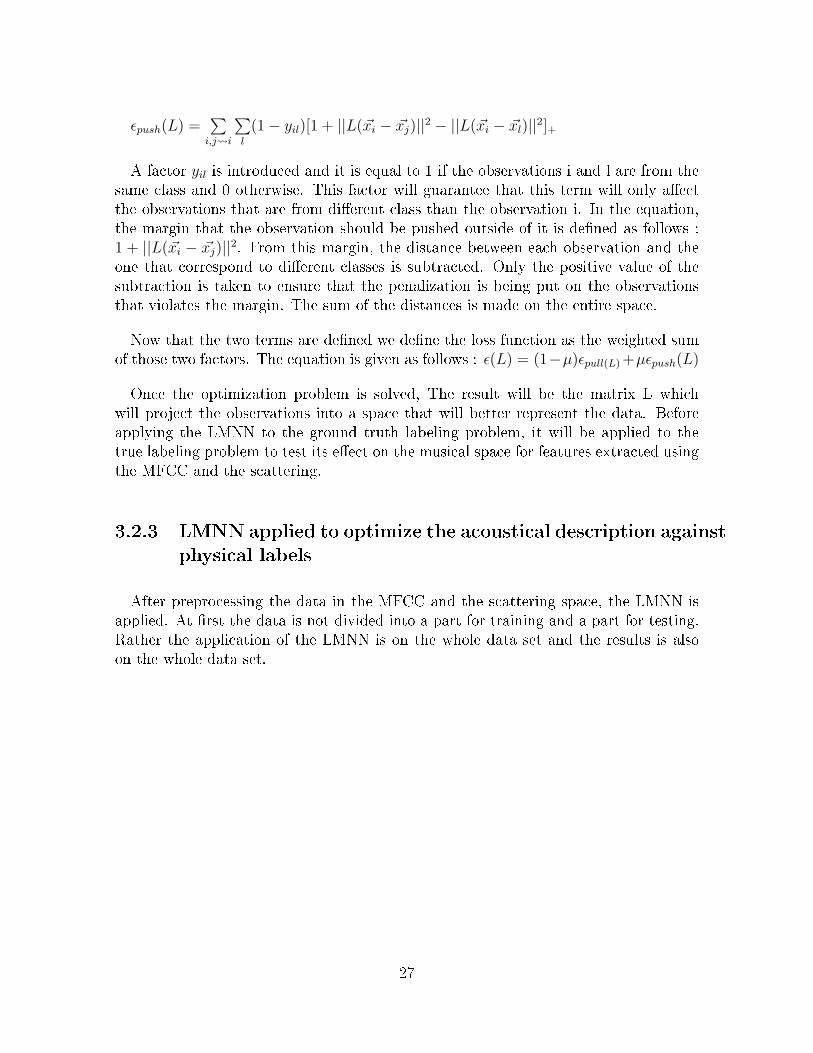
(1− yil)[1 + ||L(~xi − ~xj)||2 − ||L(~xi − ~xl)||2]+

A factor yil is introduced and it is equal to 1 if the observations i and l are from thesame class and 0 otherwise. This factor will guarantee that this term will only a�ectthe observations that are from di�erent class than the observation i. In the equation,the margin that the observation should be pushed outside of it is de�ned as follows :1 + ||L(~xi − ~xj)||2. From this margin, the distance between each observation and theone that correspond to di�erent classes is subtracted. Only the positive value of thesubtraction is taken to ensure that the penalization is being put on the observationsthat violates the margin. The sum of the distances is made on the entire space.

Now that the two terms are de�ned we de�ne the loss function as the weighted sumof those two factors. The equation is given as follows : ε(L) = (1−µ)εpull(L)+µεpush(L)

Once the optimization problem is solved, The result will be the matrix L whichwill project the observations into a space that will better represent the data. Beforeapplying the LMNN to the ground truth labeling problem, it will be applied to thetrue labeling problem to test its e�ect on the musical space for features extracted usingthe MFCC and the scattering.

3.2.3 LMNN applied to optimize the acoustical description against

physical labels

After preprocessing the data in the MFCC and the scattering space, the LMNN isapplied. At �rst the data is not divided into a part for training and a part for testing.Rather the application of the LMNN is on the whole data set and the results is alsoon the whole data set.

27

features p@5 before LMNN p@5 after LMNN16 class of instrumentsmfcc 86.89 87.09scattering 93.87 99.9932 class of instruments with variationmfcc 85.12 86.16scattering 90.94 99.92498 class of playing techniquesmfcc 45.19 46.38scattering 57.98 88.08

Table 3.2: Comparison between the P@5 before and after LMNN for feature extractedusing the MFCC and the scattering with T=250ms

The �rst table shows the comparison between the P@5 before and after applyingthe LMNN. An improvement is noted for all the di�erent type of classes for bothfeatures extracted using the MFCC and the scattering. The scattering continue tooutperform the MFCC after the LMNN. For the two type instruments the scatteringafter the LMNN gives almost a perfect result. And for the last type of classes of playingtechniques, the scattering after gives a remarkable improvement of 30.1%.

features MAP before LMNN MAP after LMNN16 class of instrumentsmfcc 24.22 24.73scattering 30.73 60.0732 class of instruments with variationmfcc 22.29 25.27scattering 28.07 56.88498 class of playing techniquesmfcc 8.78 9.61scattering 20.41 44.42

Table 3.3: Comparison between the MAP before and after LMNN for feature extractedusing the MFCC and the scattering with T=250ms

Again for the MAP, The scattering continues to outperform the MFCC. with a bigimprovement after applying the LMNN. This shows that the scattering contains thenecessary variability for the problem of music search query.

To further show the importance of the LMNN, two division of train / test datasets

28

are made and the results are shown in the following tables for the 32 class of instrumentwith variation:

features MAP before LMNN MAP after LMNNDivision into 80% for train and 20% for testmfcc 23.24 24.54scattering 31.00 60.70Division into 50% for train and 50% for testmfcc 22.74 24.02scattering 30.70 62.98

Table 3.4: Results of the MAP for the division of the space into a part for train and apart for test

The �rst table shows that for both the mfcc and the scattering an improvement wasnoted even with a split of 50/50 between train and test. However for the scattering theimprovement was greater and it provided the same improvement without the divisioninto train test.

features P@5 before LMNN P@5 after LMNNDivision into 80% for train and 20% for testmfcc 73.90 75.14scattering 83.05 98.44Division into 50% for train and 50% for testmfcc 81.17 81.86scattering 90.02 99.31

Table 3.5: Results of the P@5 for the division of the space into a part for train and apart for test

The same can be noted for the P@5. The division was made on the entire space bytaking 80% of each class for train and 20% for test(50% for train and 50% for test fromeach class).

Now that the e�ect of LMNN have been proven to be very e�ective on the scatteringwhile it provides slight improvement for the MFCC, one last test should be made. Thistest is to prove that the e�ectiveness of the LMNN on the scattering is not due to thespace volume rather than the variability this space contains.The MFCC was extended in the following way :

• add the delta coe�cients (a total of 12 coe�cients)

29

• add the delta delta coe�cients (a total of 12 coe�cients)

• Multiply the pair wise coe�cients, the total will 666 coe�cients

((36 ∗ 35)/2) + 36 = 666

Then the same number of coe�cients is taken from the scattering. The results aregiven in the following table :

features MAP before LMNN map after LMNN p@5 before LMNN p@5 after LMNNmfcc 10.38 13.35 58.01 77.80scattering 28.43 51.35 92.85 99.85

Table 3.6: Table showing the comparison between the scattering and the MFCC withthe same number of features (666) before and after applying the LMNN

The results shown in the table above were anticipated. The scattering transformoutperformed the MFCC after applying the LMNN even when the space of MFCCfeatures was expended. The MFCC precision degraded with the additional features.The LMNN could not rise the precision of the MFCC even with a high space of features.

Now that the LMNN has proven to be e�cient for the musical search query problembased on the physical labeling of the observation, it is time to see its e�ect on theground truth problem.

3.2.4 LMNN applied to optimize the acoustical description against

perceptual judgments

To apply the LMNN to a series of multiple labelings some adaptation shall be madeas, to the best of our knowledge this issue has not been addressed in the literature.Some methods are now proposed and tested to take advantage of the LMNN to optimizethe acoustical description against perceptual judgments:

1. Summing the distances

The �rst method that was proposed is to sum over the distances. Two ways ofsumming the distances was used :

The �rst one is to sum directly over the resulting distances and the second is tosum over the matrices L of projection obtained by the LMNN. To better under-stand the di�erence between this approach and summing directly the distances

30

let us see the equations below :Summing the projection matrices L can be written as :

L =nobs∑k=1

Lk

Thus the new distances will be :

(~xi − ~xj)T

nobs∑k=1

LTk

nobs∑k=1

Lk(~xi − ~xj)

= (~xi − ~xj)T

nobs∑k=1,w=1

LTkLw(~xi − ~xj)

= (~xi − ~xj)T (

nobs∑k=1,w=1,k=w

LTkLw +

nobs∑k=1,w=1,k 6=w

LTkLw)(~xi − ~xj)

= (~xi − ~xj)T

nobs∑k=1,w=1,k=w

LTkLw(~xi − ~xj) + (~xi − ~xj)

T

nobs∑k=1,w=1,k 6=w

LTkLw(~xi − ~xj)

nobs∑k=1

dMk(~xi − ~xj) +

nobs∑k=1,w=1,k 6=w

(Lk ~xi − Lk ~xj)T (Lw ~xi − Lw ~xj) eq.1

The �rst part of eq.1 is the same as summing the distances directly, the secondpart however do not have a physical explanation. A sum over the distance isbetter understood. However a comparison is provided for further study since italso achieved good results.

features Sum MAP MAP after LMNN p@5 p@5 after LMNNmfcc Sum over L 50.74 55.02 55.66 60.99mfcc Sum over distances 50.74 54.24 55.66 60.04scattering Sum over L 40.17 49.63 44.01 61.85scattering Sum over distances 40.17 51.46 44.01 65.57

Table 3.7: Results of summing the distances and summing the projection matrix L

Lets look at all the di�erent cases that might be encountered to better understandthe improvement provided by the sum over the distances. In the following study,the focus is only on two di�erent labeling opinions from the 32. The �gure 3.2show an example of applying LMNN on two di�erent labeling opinion for thesame samples with three nearest neighbors considered. The pairwise distancematrix before applying the LMNN is given by :

31

Figure 3.2: LMNN applied on two di�erent labeling opinion

1 d12 d13 d14 d15d21 1 d23 d24 d25d31 d32 1 d34 d35d41 d42 d43 1 d45d51 d52 d53 d54 1

After applying the LMNN with sum over distances Four di�erent cases can bepresented :

(a) The two labeling opinion agrees on the similarity.The application of LMNN will conduct to a smaller distance if the labelsare similar. If the observations are target neighbors both distances will besmaller in the new space for both labeling provided by the two di�erentusers. Observation 3 and 4 in �gure 1 illustrate that idea. In this case thetwo distances DM1 and DM2 will be smaller than the original distance in thespace before the application of LMNN. Let us now go back to update ournew pair wise distance matrix:

DM134 < d34 and DM234 < d34

32

the sum of those two terms is thus :

DM134 +DM234 < 2d34

.

(b) The two labeling opinion agrees on the non similarity.The same analogy can be made for the case were both opinion agree thatthe two observation belongs to di�erent classes. If we take for example theobservations 1 and 3 we will have at the end

DM134 +DM234 > 2d34

.

(c) The two labeling opinion dos not agrees on the similarity.If the two labeling opinion disagree on the similarity between two observa-tion, in one space we will have smaller distance while in the second we willhave bigger distance. For example if we look at samples 2 and 4 in �gure 1,we can see that in the new spaces distance between those two observationsis bigger for the new space with LMNN based on labeling opinion 1, andbigger in the space with LMNN based on labeling opinion 2. we will thushave :

DM124 > d24 and DM224 < d24

. Let us introduce two factors α > 1 and β < 1 this implies :

DM124 = αd24 and DM224 = βd24

Dsum24 = αd24 + βd24

.

(d) An observation is not a�ected in both spaces by LMNN.If the distance between two observations that are not target neighbors forthe LMNN is bigger than a certain margin the distance will not be a�ecteddirectly. This distance will slightly change because the observation them-selves have been displaced in their own small margin. We can thus makethe assumption that the variation in distance in the new space is negligibleand the for example the distance between observation 1 and 5 will be

Dsum15 = 2d15

Now that we have formulated all the factors we can construct our new matrixbased on the sum of the projection matrix L. To simplify the notation we will takeon factor to represent the di�erent factors in case 3, for example let 2A = α+ β.

1 2Ad12 > 2d13 > 2d14 2d152Ad21 1 2Cd23 2Bd24 2d25> 2d31 2Cd32 1 < 2d34 2d35> 2d41 2Bd42 < 2d43 1 2d452d51 2d52 2d53 2d54 1

33

Let us now examine two cases, one where we have an agreement and one werewe have a disagreement :

(a) Case were we have agreement between di�erent opinions.It should be noted again that we are searching to compare distances andnot the exact value of the distances. So let us take two distances were inthe �rst both users agree that two samples belongs to the same class and inthe other they agree that they don't. for example we can take d13 and d34.In the space before the application of LMNN we had : d13 − d34 in the newspace we will have a di�erence between a value that is twice bigger thanthe �rst distance and a value that is twice smaller than the second distance.So we have been able to have a space that make the di�erence in distancesbigger if we have two exact opinions on labeling. And for both labelingopinions the error will be minimized.

(b) Case were we have disagreement between opinions. Let us take again dis-tance d13 but this time let us compare it with d21. Let us take F as a valuethat is bigger than 1 to represent the factor by which in the new space thedistance between samples 1 and 3 is bigger. we will thus have in the newspace 2Fd13 − 2Add21. We now that the �rst distance is going to be biggerthan the original distance between samples 1 and 2. On the other handthe distance between 1 and 2 in the new space will depend on the originaldistance between 1 and 2. So if the distance in the new space is smaller thanin the original space, labeling based on �rst user will have smaller error thanlabeling based on second user. But since the �rst factor is well optimizedwe will have optimization in both case.This idea that the "winner" between the two opinion is based on the rep-resentation in the original space is very important. And it will be essentialin a case were we have more than two opinions, since the probability thattwo samples will be considered similar by the users is related to the physicalaspect of the sound.

2. Weighting the sum over distances

In this case, the sum is weighted based on a factor of relevance of each labelingopinion relatively to the other labeling opinions. The success is based on aprecision factor obtained by applying the normalized mutual information (NMI)[12]. The distances is thus multiplied each one by the precision of the labelingopinion over the entire labeling opinion space. The results are as follows :

features MAP MAP after LMNN P@5 p@5 after LMNNmfcc 50.74 54.35 55.66 60.51scattering 40.17 52.61 44.01 66.89

Table 3.8: Results of weigthing the sum

34

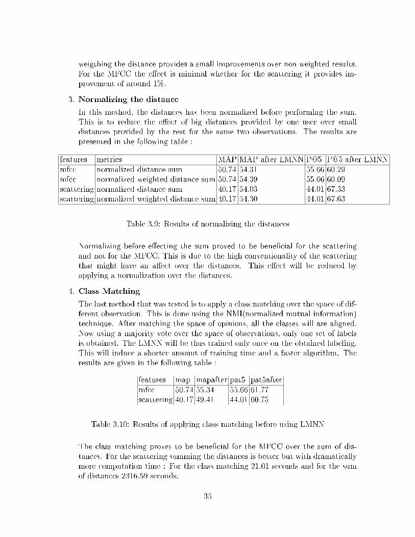
weigthing the distance provides a small improvements over non weighted results.For the MFCC the e�ect is minimal whether for the scattering it provides im-provement of around 1%.

3. Normalizing the distance

In this method, the distances has been normalized before performing the sum.This is to reduce the e�ect of big distances provided by one user over smalldistances provided by the rest for the same two observations. The results arepresented in the following table :

features metrics MAP MAP after LMNN P@5 P@5 after LMNNmfcc normalized distance sum 50.74 54.31 55.66 60.29mfcc normalized weighted distance sum 50.74 54.39 55.66 60.09scattering normalized distance sum 40.17 54.03 44.01 67.33scattering normalized weighted distance sum 40.17 54.30 44.01 67.63

Table 3.9: Results of normalizing the distances

Normalizing before e�ecting the sum proved to be bene�cial for the scatteringand not for the MFCC. This is due to the high conventionality of the scatteringthat might have an a�ect over the distances. This e�ect will be reduced byapplying a normalization over the distances.

4. Class Matching

The last method that was tested is to apply a class matching over the space of dif-ferent observation. This is done using the NMI(normalized mutual information)technique. After matching the space of opinions, all the classes will are aligned.Now using a majority vote over the space of observations, only one set of labelsis obtained. The LMNN will be thus trained only once on the obtained labeling.This will induce a shorter amount of training time and a faster algorithm. Theresults are given in the following table :

features map mapafter pat5 pat5aftermfcc 50.74 55.34 55.66 61.77scattering 40.17 49.41 44.01 60.75

Table 3.10: Results of applying class matching before using LMNN

The class matching proves to be bene�cial for the MFCC over the sum of dis-tances. For the scattering summing the distances is better but with dramaticallymore computation time : For the class matching 21.01 seconds and for the sumof distances 2316.59 seconds.

35

3.3 Conclusion

This paper provided a study of two problems of music search query. The �rst onebased on the physical aspect of the sound. The results obtained for this part andthe preprocessing technique for the scattering are novel work. The precision obtainedon the search query for musical purposes proved that the standard deviation of thescattering should be studied in order to achieve state of the art results. This techniqueof preprocessing should be tested for di�erent problems in the domain of audio andimages. In the second part, the problem of studying multiple user opinion in order to�nd a space that respects all the opinions was addressed. This novel work has studiedinteresting research avenues for solving the problem.

36

Bibliography

[1] Beth Logan Mel Frequency Cepstral Coe�cients for Music Modeling. 2000

[2] J. Andén and S. Mallat. Multiscale scattering for audio classi�cation.. ISMIR 2011

[3] J. Andén Time and frequency scattering for audio classi�cation. January 7, 2014

[4] Hermann Ludwig Ferdinand von Helmholtz On the sensations of tone as a physio-

logical basis. 1895

[5] Stephan Mallat Recursive interferometric Representations 18th European SignalProcessing Conference 2010

[6] Perfecto Herrera-Boyer and al. Automatic Classi�cation of Musical Instrument

Sounds. Journal of New Music Research 2003

[7] Yan Maresz and al. Ircam solo instruments UltimateSoundBank reference guide

[8] K. Q. Weinberger, L. K. Saul. Distance Metric Learning for Large Margin Nearest

Neighbor Classi�cation. Journal of Machine Learning Research (JMLR) 2009

[9] P. Xing, A. Y. Ng, M. I. Jordan, and S. Russell Distance metric learning, with

application to clustering with side-information. Cambridge, MA, 2002.

[10] Shalev-Shwartz, Y. Singer, and A. Y. Ng. Online and batch learning of pseudo-

metrics Ban�, Canada, 2004.

[11] Goldberger, S. Roweis, G. Hinton, and R. Salakhutdinov. Neighbourhood compo-

nents analysis Cambridge, MA, 2005

[12] Kraskov Alexande and al. , Hierarchical Clustering Based on Mutual Information

Grassberger, Peter (2003)

37