REPORT RESUMESED 017 006 24 CG 001 S56.

EFFECT OF ERROR OF MEASUREMENT ON THE POWER OF STATISTICAL

TESTS. FINAL REPORT.BY- CLEARY, T. A. LINN, ROBERT L.EDUCATIONAL TESTING SERVICE, PRINCETON, N.J.REPORT NUMBER BR -G -$574 PUB DATE SEP 61

GRANT OEG1-1-06074-2632EDRS PRICE KF -$0.25 HC -$2.08 50P.

DESCRIPTORS- *STATISTICAL ANALYSIS, MENTAL TESTS,*RELIABILITY, TEST CONSTRUCTION, *TESTS OF SIGNIFICANCE:

ANALYSIS OF VARIANCE, *MEASUREMENT TECHNIQUES,

THE PURPOSE OF THIS RESEARCH WAS TO STUDY THE EFFECT OF

ERROR OF MEASUREMENT UPON THE POWER OF STATISTICAL TESTS.

.ATTENTION-WS FOCUSED ON THE F-TEST OF THE SINGLE FACTOR

ANALYSIS OF VARIANCE. FORMULAS WERE DERIVED TO SHOW THE

RELATIONSHIP BETWEEN THE NONCENTRALITY PARAMETERS FOR

ANALYSES USING TRUE SCORES AND THOSE USING OBSERVED SCORES.

THE EFFECT OF THE RELIABILITY OF THE MEASUREMENT AND THE

SAMPLE SIZE WERE THUS DEMONSTRATED. THE ASSUMPTIONS OF

CLASSICAL TEST THEORY WERE USED TO DEVELOP FORMULAS RELATING

TEST LEN(STH TO THE NONCENTRALITY PARAMETERS. THREE METHODS OF

ESTIMATIMG POWER FOR DIFFERENT CONDITIONS OF SAMPLE SIZE AND

TEST LENGTH WERE STUDIED. THE COST OF AN EXPERIMENT WAS

ANALYZED IN TERMS OF A FIXED COST PER SUBJECT AND A VARIABLE.COST DEPENDENT UPON TEST LENGTH. COMPUTER PROGRAMS WERE

WRITTEN TO USE THE LEAST SQUARES APPROXIMATION AND THE

APPROXIMATION BASED ON PATNAIK TO ESTIMATE THE POWER UNDER

ALL PERMISSIBLE ALLOCATIONS Of RESOURCES TO SAMPLE SIZE AND

.TEST LENGTH. THE PROGRAM RESULTS INDICATE WHICH OF THE .

PERMISSIBLE ALLOCATIONS WILL RESULT IN MAXIMUM POWER. TO

DEMONSTRATE EMPIRICALLY THE EFFECT OF ERROR OF MEASUREMENT ON

THE POWER OF STATISTICAL TESTS, SAMPLES OF PERSONS AND ITEMS

WERE RANDOMLY DRAWN FROM A LARGE FOOL OF DATA. TESTS Of 10,

.20, AND 40 RANDOMLY DRAWN ITEMS WERE SCORED FOR SAMPLES WITH

:,;1- FOUR AND EIGHT PERSONS PER GROUP. THE EXPECTED TRENDS WEREPRESENT BUT NOT DEFINITIVE. (AUTHOR)

4' '7r -t

_rwev

Project No. 6-85/4.- .--111FINAL REPORT

Contract No. 0EG-1-7-068574-2632

EFFECT OF ERROR OF MEASUREMENT ON

THE POWER OF STATISTICAL TESTS

September 1967

U.S. DEPARTMENT OF HEALTH,

EDUCATION, AND WELFARE

Office of EducationBureau of Research

it* Zev-tit.S.,-.06Z7,1

Effect of Error of Measurement on the

Power of Statistical Tests

Project No. 6-8574

Contract No. 0EG-1-7-068574-2632

T. Anne Cleary and Robert L. Linn

September 1967

The research reported herein was performed pursuant to

a grant with the Office of Education, U.S. Department

of Health, Education, and Welfare. Contractors under-

taking. such projects under Government sponsor-Ship

are encouraged to express freely their professional.

judgment in.the conduct of the project. Points .of

view or opinions stated do not, therefore, necessarily

represent official Office of Education position or

policy.

Educational Testing .Service

Princeton, New Jersey

The services of Dr. Cleary were subcontracted with

the University of Wisconsin.

..),4:"4,044,14kt:wr4A141464

Contents

OOOOOOOO 0

Page

IntroductionProblemPurpose

Part I: Theoretical Development

112

2Test Theory

. 2Statistical Tests

t 4The Power Function 8Cost of an Experiment

15Allocation of Resources . 16Conclusions

18

Part II: Empirical Demonstration 21Purpose 21Method 21Results

22Discussion

4) 27Conclusions

284

Summary28

References .

30

Appendix AAl -

Appendix 13B-1

APt

ft

Problem

Introduction

Discussions of the power of statistical tests can be found in

almost all basic statistics books. The power function, which gives

the probability of rejecting a hypothesis, depends upon the dif-

ferences expected in random samples from the same population, that

is, upon sampling error. Implicit in the usual discussion of

power is the assumption that the observations are errorless or

"true" measurements. Sampling error rather than measurement error

is considered.

The test theory literature, on the other hand, is concerned

primarily with the error of measurement (4). Observations are

considered fallible and repeated measures of the same object are

expected to vary about the "true" measurement, the expected value

of the repeated measures.

Sutcliffe (10) has attempted to consider tne two types of

error simultaneously. Sutcliffe elaborated the implications of

measurement error for the F test of differences between means and

demonstrates how measurement error decreases the sensitivity of a

test of significance. More specifically, Sutcliffe compared the

ratios of the expected mean square between groups to the expected

mean square within groups for a single factor analysis of vari-

ance in two cases: the case of no measurement error and the case

where observed scores were assumed to include measurement error

as defined in classical test theory. Sutcliffe showed that the

power of the test is always greater for the error-free case.

Lord (6) has given extensive consideration to the implica-

tions ofian item sampling model for mental test theory. Lord has

shown that item sampling methods can improve the efficiency of the

experimental design of a study particularly one concerned with

group means.

(i) If only a limited amount of time can be demanded

of each research subject, the total amount of infor-

mation obtained from a given number of subjects may

be greatly increased by item sampling. (ii) If a

test can be administered to only one examinee at a

time, the examiner's time may be the limiting factor;

more information about a group of examinees maybeObtained by giving a few items to each examinee in-

stead of giving the entire test to just a few examin-

ees. (iii) With certain tests, scoring costs may be

the limiting factor; in this case, it would be better

to score a few items from the answer sheet of each

examinee than to score all items on the answer sheets

of a few examinees. (6, p. 23)

-1-

.

_ t

4

The item-sampling model has strong advantages in many group-

comparison situations such as frequently occur in the evaluations

of educational programs. However, practical administrative con-

siderations such as the need for common instructions and testing

time, the economy of being able to use a single scoring key, and

the fact that test data must frequently serve several purposes,

often make it desirable to administer the same test to all examinees.

In such situations, one is faced with the problem of deciding

whether it is more efficient to improve the sensitivity of a

planned statistical test by increasing the number of examinees or

by increasing the test length as a means of reducing the error of

measurement.

Overall and Dalai (7).discussed the problem of choosing a

research design which maximizes power relative to cost. They

concluded that no matter how unreliable the measurement, it is

better to use more-subjects and obtain a single measurement per

subject than to obtain several measures on each of fewer subjects.

As 'Overall and Dalai pointed out, the above conclusion is based

on the assumption that there is a fixed cost per measurement

unit, and this cost is the same 'whether the units are obtained

for the same subject or different subjects.

Purpose

The purpose of this research was to develop, from the assump-

tions of classical test theory, formulas demonstrating the effect

of error of measurement on. the power of somecommonly used statis-

ticaltests. An important aspect of the research was the develop-

ment of a procedure that would enable the educational researcher

to estimate whether an attempt to reduce measurement error by in-

creasing, accuracy of observations or to reduce sampling error by

increasing the number of observations would be the more effective

strategy. The implications that various assumptions concerning

the fixed and variable costs of testing have for-the choice of a

strategy, were investigated.also. Since the assumptions of -classi-

cal theory cannot be expected to hold exactly in real data, the

effects on statistical tests of increasing reliability and the

number of observations were demonstrated empirically.

Part 1: Theoretical Development

Test Theory

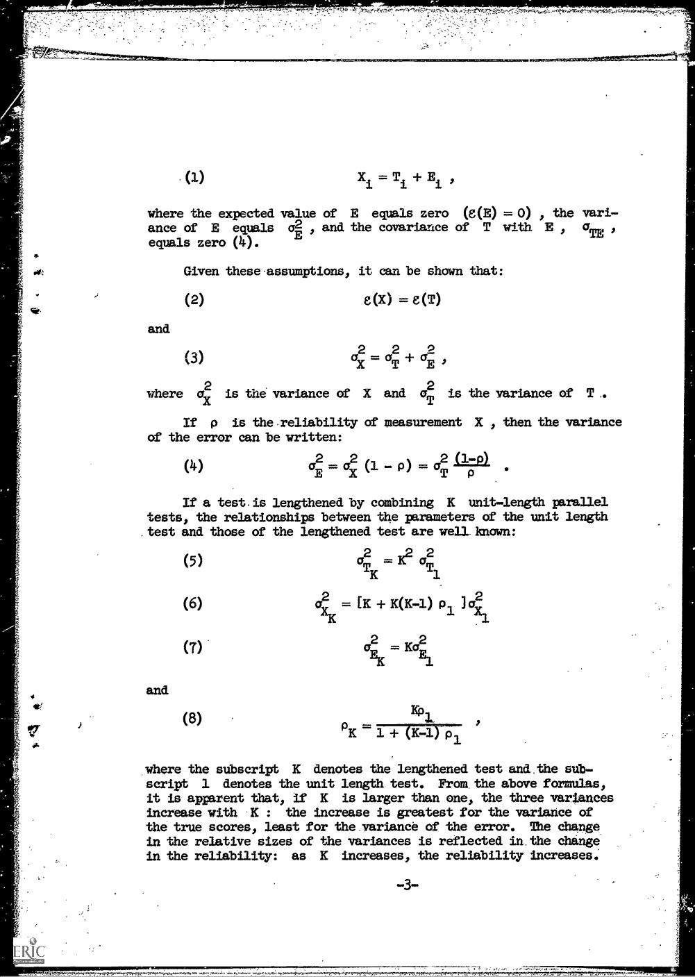
In classical test theory, it is assumed that an observation,

Xi , for individual i is equal to his true score, Ti , plus

an error score, Ei :

-2-

t.

(1)

2.'";,-0e,,t-tr=.^,4'1:-47,--:4,-7-:% ..3`

Xi = Ti Ei

where the expected value of E equals zero (e(E) = 0) , the vari-ance of E equals ai , and the covariance of T with. E 1 a

TEequals zero (4).

and

Given these. assumptions, it can be shown that:

(2) e(X) = e(T)

2 2(3) a

X= a

T+ a

E2

where a2X

is the variance of X and a2

is the variance of T

If p is the. reliability of measurement X , then the varianceof the error can be written:

(4)E02 a2

X=a2

T(1P -p)

If a test. is lengthened by combining K unit-length paralleltests, the relationships between the parameters of the unit length.test and those of the lengthened test are well known:

and

(5)

(6)

(7)

(8)

2 ,2 2(ITK= OTi

= tit K(K-1) P1 Q411t

a2

= Ka2

EK El

PK 1 -1=1T7t-1 c.3:

,where the subscript K denotes the lengthened test and.the sub-script 1 denotes the unit length test. From, the above formulas,it is apparent that, if K is larger than one, the three variancesincrease with 'K : the increase is greatest for the variance ofthe true scores, least for the .variance of the error. The change_

in the relative sizes of the variances is reflected in. the changein the reliability: as K increases, the reliability increases.

.3.

Statistical Tests

In the derivation and interpretation of statistical tests, the

Observations are generally considered to be free of error of mea-

surement, that is, in the language of test theory, the observations

are true scores. The application of statistical tests to observed

scores subject to error of measurement is in no sense incorrect or

even necessarily inappropriate: the assumptions of the statistical

tests may be satisfied by the observed scores. However; if the

hypotheses are formulated in terms of true scores and tested with

observed scores, the noncentrality parameter and-therefore the

power can be quite different from what would be expected with true

scores. Failure to reject the null hypothesis with observed scores

is not equivalent to a failure to reject the null hypothesis with

true scores.

Perhaps, one of the most commonly used statistical tests in

educational research is the F test of the analysis of variance.

In addition to being commonly used, it is well known that the F

test with one and v2 degrees of freedom is equivalent to the

two t test. If v2 approaches infinity, the F distri-

bution approaches a chi-square distribution.

Consider a single-factor analysis of variance. The model for

this analysis is

where

(9) Tig = M + g.+ Big

g = 1, . G

= ," 12

Tig is the .true score for individual" i in group g

M is the population true-score mean,

A is the component of the true score which is due to the

effect of treatment. g , and

Big is the deviation of an individual's score from the group

mean, the error of analysis-of-variance model..

The Bi

are assumed to be independently-and normally diStri-.

buted with expected value of zero and common variance all3

2Over

all possible treatments, g , the sum of the A is zero and the

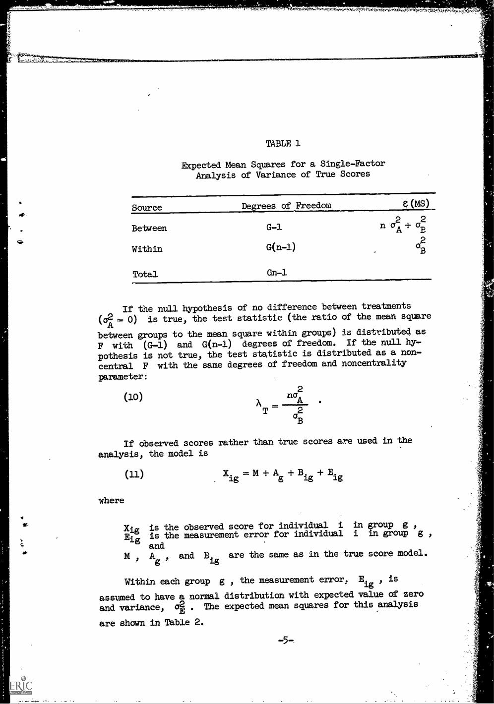
variance is QA . Table 1 presents the expected mean squares for

thIS

44-

,

TABLE 1

Expected Mean Squares for a Single-Factor

Analysis of Variance of True Scores

Source Degrees of Freedom

Between G-1

Within G(n-1)

Total Gn-1

e (MS)

2n o'A + aB

2

a2

If the null hypothesis of no difference between treatments

A = CI) is true, the test statistic (the ratio of the mean square

between groups to the mean square within groups) is distributed as

F with (G-1) and G(n-1) degrees of freedom. If the null hy-

pothesis is not true, the test statistic is distributed as a non-

central F with the same degrees of freedom and noncentrality

parameter:

(10)

T

ria2A

a2B

If observed scores rather than true scores are used in the

analysis, the model is

(U)

where

X. = M + A + B. + Eg ig

Xig is the observed score for individual i in group gEig is the measurement error for individual i in group g ,

andM 1 A and B

igare the same as in the true score model.

Within each group g , the measurement error, E'

is

assumed to have a normal distribution with expected value of zero

and variance, 4 . The expected mean squares for this analysis

are shown in Table 2.

For fixed n , the relationship be.tween power and error of

measurement can be seen by noting that the ratio of the meansquares divided by their expected values,

TABLE 2

Expected. Mean Squares for a Single-FactorAnalysis of Variance of Observed Scores

Source

Between

Within

Total

Drees of Freedom g MS

G-1 n a2 + a2 + a2A B E

G(n-1)(7B (YE

2

Gn-1

If the null hypothesis (all.2= 0) is true, the test statistic

has the same distribution as in the error-free case. however, ifthe null hypothesis is false, the test statistic is distributed asnoncentral F with the same degrees of freedom but with noncentral-ity parameter,

(12)

2nciA

2 2Ba +

(YE

For a,s2

greater than zero, the noncentrality parameter for

the observed score analysis, Ax , will be smaller than the non-

centrality parameter for the true score analysis, AT . Since

power for the test with given degrees of freedom is a nondec,-easing

function of the noncentrality parameter, the power for the true-score analysis is always ueater than the power for the observed

score analysis.

MS 2 2Between aB + aE

'Within nag + a + a2B E

is distributed as Central F . Power can then be expressed as

113Between 1Pr F j_--Within 1 +

Clearly, the larger A , the smaller the term to the right of theinequality sign and the greater the power. As mentioned earlierthis result was obtained previously by Sutcliffe (10).

The relationship between power and A is, of course, dependentupon the degrees of freedom. For fixed degrees of freedom the poweris a negatively accelerated function of A . As the degrees of free-dom in the denominator (or number of persons per cell) increases,the initial slope increases and also the rate of negative accelera-tion.

The noncentrality parameter can be usefully expressed in termsof p , the reliability of the measure and the variances of thetrue score components. From fOrmulas.4 and 12

2(13)

Apn a4

Xa + a2A

since

aT= a

A + aB .

The relationship between the noncentrality parameters for theobserved score and true-score analyses can be seen by substitutingformula 10 into 13:

(l5) np AAX -'n + (1-47;

For fixed , and n , 11( is a positivelyaccelerated function

of p , the reliability of the scores: as p increases by equalunits from zero, the increase in AX is at first quite small buteach successive increase in p results in a slightly lamer in-crease in Ax . The rate of positive acceleration increases to 7)L, .

If the test length is increased by a factor of K , thereliability and therefore the noncentrality parameter will increase.If pl denotes the reliability of the unit length test, the ob-served scores noncentrality parameter can be expressed:

-7-

I

4

4-

(16)nEplAT

7'. X + nT

The effect of n and K on the noncentrality parameter, XX '

can be seen more clearly if equation 16 is expressed in terms of

Twhere

(ler)

Thus' XT "(1)T

(i8)

22 crA,

T=

2gB

and:

2

niCP 14)T

43. + (1-P) 4T2 +

The noncentrality parameter, Xx is a strictly increasing

function of both K and n . However, the effect of increasingn is relatively greater than the effect of increasing K sinceK influences both the numerator, and the denominator whereas ninfluences only the numerator. In addition, the effect of n uponpower is increased by the change in degrees of freedom.

The Power Function

The power function for a statistical test gives the probabilitythat the null hypothesis will be rejected given different alternative values of the parameter. To determine the power of the Ftest of the analysis of variance, one needs to determine the proportion of the area of the noncentral F distribution that falls inthe critical region. In the single factor analysis of variance,the test statistic, F

o, is:

(19) NSBe tw een

N3Within

and the critical region is defined by

F > Faa

where a is the significance level of the test. The power functionfor a given X is then given by

(20)

co

Power =2

(Fax) dF'

-7-7; "..": 4,14,

where Fa

is the percentage point of the F distribution with

degrees of freedom v1 1

v2 and the integration is over the den-

sity function of the noncentral F distribution, F' , withv1

and v2

degrees of freedom and noncentrality parameter % .

The evaluation of the power function is not simple. Methodsof evaluating the probability integral have been worked out byWishart (12) and Tang (11)1 but the amount of labor involved gen-

.

erally limits consideration to a few alternative hypotheses. Severalauthors have presented power function curves (2, 3, 5, 8, 9)These curves enable one to determine quickly, if approximately, thepower for a limited number of sets of degrees of freedom and non-centrality parameters. The most relevant of these charts for thedesign of experiments are those of Feldt and Mahmoud (2) whichpresent curves of constant power, for power equal to .5, .7, .9,

as a function of n , the number of persons per cell, and 43 ,

the noncentrality parameter. The charts are designed to permit thespecification of sample size for the testing of main effects inthe analysis of variance. The limited number of power curvesrestricts the use of the charts to situations in which only a rough

estimate of power is required.

Overall and Dalai (7) proposed a method of approximating thepower of an F test which is very appealing because of its greatsimplicity. Their approximation can be denoted as F / Fa where9 is the ratio of the expected mean square between to the expectedmean square within and Fa is the critical value of the F/zatiowith a significance level of a. It should be noted that F is

not the same as the expected of F since in general the expectedvalue of a ratio is not equal to the ratio of the expected values.

Nevertheless, F / Fa is very simple to compute and can be readilyexpressed in terms of the noncentrality parameter X since

(21)AF = 1 + X.

Overall and Dalai have shown that for a particular example the;ratio / F a has a good linear relationship with the true power

correlation equal .988) for a range of true power between .10 and

.60. They concluded that f/ Fa is a good index of power which. . . should provide an adequate basis for comparing alternative

permissible experiments." (7, p. 349). However, for values ofthe true power less than .10 or greater than .80 the linear fit isnot very good. For example, the correlation between true power andl / Fa for v1 = 2 , v = 2, 3, 4, 5, 6, 8, 10, 12, 18, 30, and

60, and X= 0 , 3, 4, 5, 6, 8, 10, 12, and 18 is .966 which repre-sents a fit that is considerably less adequate than the one repre-sented by the correlation of .988 reported in the example byOverall and Dalal.

ar , ,-.1gfit,22V;.';

."' ..!,'if

,t,,,

',6-z4 .4

,,.! i:''':ke) -X.,,,,

P.

The tabled values of power given by Overall and Dalai (7) and the

calculated values of ft / Fa are presented in columns three and

six respectively of Table 3.

Use of the index F / Fa in place of the true power can lead

to erroneous conclusions about the best allocation of resources.

However, the errors will not be serious since an allocation of re-

sources.which yields an optimal value of 'P/ will yield a true

power which will be among the highest possible although it may not

be the absolute maximum. In general, F / Fa appears to be a

useful index: it is easy to calculate and provides a reasonable

approximation to power.

The index C, / Fa does have two minor disadvantages: the

Obtained values do not have the same scale as power, so the un-

modified index does not indicate the actual power level; the index

requires only simple hand calculations, but the calculations are

based on the tabled values of Fa , so the procedure is not well

suited to the computer.

Patnaik (8) has developed an approximation to the noncentral

F which fits to the noncentral F , F' , a central F distri-

bution with the same first two moments:

where

and

4.

(22) I Pv v (F" I A.) dF,

120

(23)

(24)

1.0

g:/wPv1v2 (F) dF

0

v _v1+ 2%

v1 + X

x2

The accuracy of the approximation appears to be quite good.

4For those values of power for which Patnaik compares his approxima-

tion to the Tang (11) tables, the approximation is generally ac-

curate to two decimal places and the error in the third decimal

place appears to be small near the tails. Fatnaik's approximation

is useful only to the extent that it is possible to evaluate the

integral of the appropriate central F distribution. A computer

program written by Holloway and Capp provides one method of evalu-

ating the central F integral. This program is presented in

Appendix A as Subroutine FDIST.

-10-

Table 3

Comparison of Methods of Estimating Power forv1

= 2

Overall Curve-* & ralal Patnaik Fitting

11/Fv2Power Approximation Estimate a

o

o 2 .05 .05 -.04 .05o 3 .05 .05 -.02 .10o 4 .05 .05 -.00 .14o 5 .05 .05 .02 .17o 6 .05 .05 .04 .20o 8 .05 .05 .06 .22o 3.0 .05 .05 .08 .24o 12 .05 .05 .10 .26o 18 .05 .05 .13 .28O 3o .05 .05 .16 .30O 6o .05 .05 .15 .32

3 .2 .12 .12 .13 .20-! .15 .15 .17 .423

3

.18 .18 .19 .583 5 .19 .19 .21 .703 6 .21 .21 .23 .783 8 .23 .23 .25 .903 10 .24 .24 .27 .983 12 .25 .25 .29 1.033 18 .27 .27 .31 1.133 30 .28 .28 .34 1.203 6o .3o .3o .32 1.27

4 2 .14 .144 3 .19 .184 4 .22 .224 5 .24 .214.4 6 .26 .264 8 .3o .294 10 .31 .314 12 .33 .334 18 .35 .354 3o .374 60 .39

.37

.39

.17 .26

.21 .52.24 .72.26 .86.28 .98.31 1.12.33 1.22.34 1.2837 1.41.39 1.50.38 1.58

eer'r?"-etree. re. r"re -Yere"'''''rreerre- le,oempr. "rrer-r

-

4,1

Table 3 (Cont'd)

Overall. Curve8c Dalai Patnaik Fitting

Xv Power Apaoxix-Gation Estimate__

5 25 35 45 55 65 85 105 125 18.5 305 60

6 26 .36 46 56 66 86 106 126 3.86 306 6o

8 28 38 48 58 68 88 108 128 188 3o8 60

.16 .L6

.22 .22

.26 .26

.29 .3o

.32 .32

.36 .36

.38 .38

.40 .40

.43 .43

.45 .45

.47 .47

.18 .18

.25 .25

.31 .31

.35 .35

.38 .38

.42 .42

.45 .45

.47 .47

.53. .51

.54. .514.

.56 .56

.22 .22

.32 .32

.39 .39

.4 .45

.49 .49

.54 .54

.58 .58

.60 .60

.65 .64

.68 .68

.7o .70

-12-

Ariir

.20 .33.

.25 .63

.28 .86

.33. 1.04

.33 1.17

.36 1.34

.38 1.46

.40 1.54

.43 1.69

.45 1.8143 1.90

.22 .36

.28 .71'-

.32 1.01

.35 1.21

.37 1.36

.43. 1.57

.43 1.71

.45 1.80

.48 1.97

.51 2.13.

.48 2.22

., 27 .4634 .94

.39 1.30

.43 1.56

.46 1.76

.50 2.02

.53 2.20

.55 2.33.

.59 2.54

.62 2.71

.6o 2.85

.4"

4

.11

- a

a,. -1166,5.

Table 3 (Conted)

v

Overall& DalaiPower

2 .26

3 .38

4 .47

5 .53

6 .588 .65

10 .68

12 .71

18 7530 .79

6o .81

Curve

Patnaik Fitting ;iF

t.Approximation Estimate ----2-.

.26 .31 .56

.38 .39 1.6

.47 .45 1.58

.54 .5o 1.90

.58 .53 2.14

.65 .59 2:46

.68 .62 2.68

.71 .64 2.83

.75.7o 3410

.79 .73 3.31

.81 .71 3.49

30 .30 .34 .66

12 2 .

12 3 .44 .44 .44 1.36

12 4 .54 .54 .51 1.87

12 5 .61 .62 .57 2.25

12 6 .67 .67 .61 2.54

12 8 .73 .73 .67 .2.91

12 10 .77 .77 .7i. 3.17

.12 12 .79 .8o .74 3.34

12 18 .83 .84 .eo 3.67

.12 30 .86 .86 .84 3.91

12 60 .88 .89 .82 4.12

18.2 .39 .40 .41 .97

18 3 .59 .59 .57 2.00

18 4 .71 .72 .68 2.74

18 5 .79 .79.76 3.29

18 6 .84 .84 .82 370

18 8 .89 .89 .91 4.26

18 io 92 .92 .97 4.64

12 .94 .94 1.02 4.881818 18 .96 .96 1.09 5.36

4 18 30 .97 .97 1.15 5.72

4 18 60 .98 .98 1.15 6.02

1010.10

1010lo1010101010

-13-

ry

le

4

'.V,;eO'>i<

The Patnaik approximation and Subroutine FDIST were used toObtain the power estimates reported in column four of Table 3. Inonly 12 of the 99 power estimates based on the Patnaik approximationin Table 3 is there a difference between these values and thetabled values given by Overall and Dalai (7) as large as .01. Con-sidering that both the tabled values and these estimates have beenrounded to the nearest hundredth there is for all practical purposesno difference between the estimates and the tabled values in (7).

It should be noted that the value of v which was calculatedby formula 24 was rounded to the nearest integer before evaluatingthe integral of the. central F distribution. Presumably, theaccuracy of the power estimates would be slightly improved byusing fractional values of v, however, in view of the accuracyobtained for the example in Table 3 this may be unnecessary forpractical purposes.

In an attempt to determine an easily manipulated functionrelating power to degrees of freedom and noncentrality parameter,the least-squares method was used to fit power values to functionsof the parameters. Primary attention was devoted to the powerfunction for v

1= 2 . A total of 99 Dower values were used: the

88 values tabled by Overall and Dalal (7) for A = 3, 4: 5, 6, 8,10, 12, and 18 and for v2 = 2, 3, 4, 5, 6, 8, 10, 12, 18, 30, and

60; and 11 values of .05 for which A = 0 where v2 was thesame as the tabled values.

For the curve fitting, $2

and n were substituted forv2

and A:

(25)

(26)

v2

n = v + 1 + 11

$2 = Ain .

Then various functions of n and $2

were used in the least-

squares equations: powers of the parameters ranging from 1/2to 3, cross-products, and natural logarithms.

The simplest equation with the fewest terms which resultedin the highest correlation with the tabled values was

(21) Power = .10.57 - 1.15n - 8.54+2 + 5.4302 +, 16.23 log

in(f2+1)]

-14-

4

MY, .44,4414.44,^44.111/ ..144 l'4,4,44,,441,4,41,0544 44.4147

I

,

fr

4

The above equation resulted in power estimates that had a

correlation of .9812 with the tabled values of-Overall and Dalai

that are presented in Table 3. These estimates are reported in

column five of Table 3. In addition the same equation provided a

reasonable fit to the Overall and Dalai power values for vi

(r = .959) and vl = 1 and 2(r =..961).

Using this equation for the values for vl =2 the largest

discrepancies between predicted and true values occurred for large

values of n and .2 where the estimated power was greater than

one. If a value of 1.0 is substituted for the estimated power

values larger than 1.0, the largest discrepancy between predicted

and true is .106. This degree of accuracy might be sufficient for

some purposes. The accuracy evaluated by the correlation is greater

than that of Overall and Dalalis / Fa within the range studied,

and the scale is the same as power. However, the computation of

the function is far more difficult than 1!/1P;E although many

values of the function can be quickly computed-by a very simple

computer program.

Curve fitting as an approach to the power function should not

be abandoned. The power functions are not complex curves and there

is every reason to believe that a reasonable function can be ob-

tained. Minimizing the squares of the residuals is perhaps not

the most appropriate criterion; other criteria should be considered.

In addition, future work should use more power values for large

n and .2 so that the .asymptote of the power function has better

representation.

Cost of an Diperiment

It is obvious that an experimenter can always increase power

by increasing K and/or n . However, in any practical situation,

the experimenter has only limited resources -at his command and

would like to be able to design the experiment so that the power

is maximized within the constraints imposed by the available re-

sources. Generally, the experimenter cannot increase both n

and K : if K is increased n must be decreased.

Let C denote the total cost per group of the experiment and

assume that this cost is the same for all groups. Following the

lead of Cronbach and Gleser (1), it is useful to assume that the

cost is the same for all subjects and that this cost per subject

consists of a fixed cost, Co

, which is independent of test

length and a cost per test unit, C1 . The cost per group, C ,

is then given by:

(28) C = n (Co + KCl)

-15-

ti

^ro_.

-

s.

- z

where n is the number of people per group and K is the length

of the test. Factors which contribute to the fixed cost, Co

might be length of time required to give instructions and cost of

bringing the subject to the testing center. The variable cost,

C1

, would be dependent upon factors such as the per-item scoring

costs and costs of subject time. There is no real provision inthis model for test development costs which would be a functiononly of K , the test length. This cost model implies that for aconstant cost per cell a change in test length, from K.-to K*must be accompanied by a change in the number of subjects per cellfrom n to n* where

(29) n*Co+ K*C

1

n (Co + KC 1)

For any given n , one can solve formula 24 for the maximum

allowable K 0

(30)C - n Co

K=Cl

In the special but rather unrealistic case where Co is

equal to zero, the most efficient allocation of resources willalways be achieved by setting K equal to one regardless of thetest reliability. This conclusion was drawn by Overall and Dala

(7). This can be seen by noting that for Co = 0 , the cost per

cell, C , is a constant as long as the product nK is a constant,

and for a fixed product, nK , not only is the noncentralityparameter maximized for K =1 but so are the degrees of freedom.

Allocation of Resources

To provide the researcher with a method of evaluating therelative effectiveness of increasing sample size and increasingtest length, two computer programs were written in FORTRAN IV.Listings of the programs are presented in Appendix A. These

programs handle only the limited case of asingle factor analysis

of variance.

Each program reads six parameters:

1 PHITRU -- the ratio of the variance of the effects tothe variance within. This parameter has been denoted

above as 41 ,

2 COST -- the total allowable cost per group, denoted Cabove,

'"11."1"'

-

r.

t.

3 CZERO -- the fixed cost per test, denoted Co above,

4 CONE the variable cost, that is, the cost per testunit, denoted C1 ,

5 EEL -- the reliability of-the unit-length test denoted

P16 VI -- the degrees of freedom for the numerator of the F

ratio (number of groups minus one), denotedv1

Each of the two programs then computes the maximum numberof persons per cell permissible within the cost constraints. Foreach sample size from two to the maximum, the corresponding maxi-mum K is calculated. The A

x is estimated by using formula 18.

Both programs then estimate the power for each of the permissiblecombinations of n and K . All of the power estimates areprinted to permit the identification of the combination of It

and K which yields the maximum power.

The first program, "Allocation of resources based on least.squares fit of power function," uses the approximation given byequation 27. This is extremely rapid and can compute power esti-mates for many combinations in a few seconds. The output of thisprogram consists of the input parameters and At 1 n , v2A2wx ,

Alc , and power. Sample computer printouts can be seen in

Appendix B.

The second program, "Allocation of resources using thePatnaik approximation," is based upon the noncentral F ap-proximation developed by Patnaik (8) and presented in equations22, 23, and 24 above. A subroutine MUST, written by Hollowayand Capp and revised. by McKelvey (See Appendix A) was used toobtain both the critical F value ( Fa ) and to evaluate theintegral of the central F distribution employed in Patnaik'sapproximation of the noncentral. F distribution. Sample outputfrom this program can also be seen in Appendix B. In addition tothe output of the first program, the values or v in equation24 and Fa for each permissible combination of n and K areprinted. This second program takes significantly more time thanthe first program: each of the estimated power values requiresabout four seconds to compute on the IBM 7044.

A comparison of the two methods of estimating power is pro-vided in Table 3. Table 3 also includes the values of power givenby Overall and Dalai (7) and the values of F / Fa p the power ap.proximation suggested by Overall and Dalai (7). As noted befores,the scale for 1? /Fa is not the same as scale for power. If a

-17-

......; ilAn.V:14,74,c

ti

4-

ft

correlation is used as the measure of the goodness of the approxi-

mation, the methods of power can be ordered: k / FG , r = .966;

least-squares, r = .981; and Patnaik, r = .9999 . Considering

the size of the discrepancies between the est-'zated and true values,

the Patnaik approximation is clearly superior to the least squares.

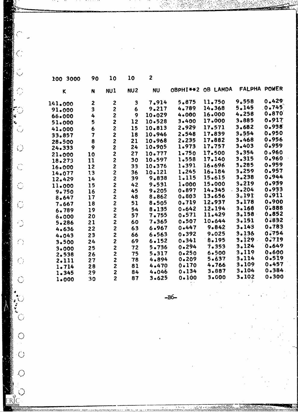
Table 4 presents the power estimates computed by the two pro-

grams under three different cost conditions. The total cost, 1-3 0

is 3000 P1 = .10 and vi= 2 in all cases. Under the first condi-

tion Co=0 , and C

1= 100.. Under these conditions, power is

maximized by increasing sample size to the maximum allowable given

the cost constraints, which for all cases represented in TaLle 4

is 30, The estimates based on the Patnaik approximation accurately

reflect this fact. On the other hand, the least-squares estimates

erroneously decrease for the largest values of n but the errors

in the estimated power are not large. It is interesting to note

that the maximum power in this first, cost condition is much lower

than in the other two cases: the large cost per test unit (C1 = 100)

does not permit the use of a very reliable instrument.

In the second and third cost conditions, the maximum power is

achieved with a smaller sample size than in the first condition.

In these two cases the differences between the allocations based

on the two approximations are minimal. However, the differences

in the power estimates are not necessarily trivial.

Conclusions

Of the three approximations to the power function that were

investigated, the one based on the Patnaik approximation and using

the FDIST program to compute integrals of central F distributions

was by far the most accurate procedure. The only disadvantage of

this method is that it requires considerably more computational

time than the other two estimations methods considered.

The least-squares approximation to the power function which

was developed has the advantage of great computatf.onal speed.

However, the method has two major disadvantages in its present'

state of development; the approximation is limited to the case

of two degrees of freedom in'the numerator, and the power esti.

mates are not sufficiently accurate for zany purposes. In view

of the computationtil ease of this approach, it is considered to

be a potentially useful line of future research. If sufficiently

accurate estimates could be obtained with a relatively simple

function, a major advantage of this approach would be that the

function could be dealt with analytically more readily than the

integrals of the noncentral F distribution.

--7-77700mammag44,

AridekiiiitiL.Aft*wdvityoft.te

Table 4.

Estimated Power for C = 3000

pti.= .10, vl = 2

Least-Squares Estimates based on

Estimates Patnaik Approximation

Co 0 80 90 0 80 90

nc1 100 20 10 100 20 10

2 .15 .35 .43 .14 .33 .43

3 .22 .52 .69 .19 .55 .74

4 .25 .61 .86 .22 .67 .87

5 .28 .67 .97 .24 .73 .92

6 .30 .7o 1.04 .25 .76 .94

7 .31 .72 1.09 .26 .77 .95

8 .32 .73 1.11 .27 .78 .96

9 .33 zu 1.12 .27 ..... .96

10 .33 .72 1.12 .28 8 ,2611 .33 .71 1.11 .28 .7 -.6

12 .34 .70 1.09 .28 .75 .9

13 4211. .69 1.06 .28 .74 .96

14 4 .67 La .29 .73 .94

15 3 .65 1.00 .29 .72 .94

16 .33 .63 .97 .29 .71 .93

17 .33 .61 .93 .29 .69 .91

18 .33 .59 .89 .29 .65 .yo

19 .33 .56 .84 .29 .63 .89

20 .32 .54 .80 .29 .61 .85

21 .32 .52 .75 .30 .59 .83

22 .31 .49 .70 .30 .57 .78

23 .31 .46 .65 .30 .52 .75

24 .31 .44 .6o .3o .5o .72

25 .3o .41 .54 .3o .47 .65

26 .3o .38 .49 .3o .44 .6o

27 .29 .36 .44 .30 .41 .52

28 .29 .33 .38 .30 .36 .46

29 .28 .30 .33 .30 .33 .38

3o .27 .27 .27 al .3o .30

aThe maximum value (based on three decimal places) in each

% column is 'inderlined.

-19-

The Overall and Dalai (7) method of estimating power, re/ Fa, is

computationally most simple and is the only one of the three methods

that is well suited to hand calculations. As previously noted, this

approach does not yield the same scale as power, and the estimates

are much less accurate than those based on the Patnaik approximation.

It would be feasible, of course, to write a computer program which

uses a subroutine such as FDIST to compute F a, and then computeand rescale F / F a as a means of obtaining power estimates. Such

a wogram presumably would have about twice the speed of the Patnaikapproximation program since it would involve only half as many

integral evaluations, however, the accuracy of these estimates would

not match the accuracy of the Patnaik approximation.

Computer programs were written to determine the most efficient

allocation of resources. The two programs are based on the Patnaik

and least-squares approximations, and the Patnaik approximation is

distinctly superior to the least-squares approximation. It is clear

from the sample problems presented that differences in the relative

magnitude of fixed and variable cost result in different optimum

allocation of resources to test length and sample size. The results

are in agreement with the conclusion of Overall and Dalal (7) that

the maximum power under conditions of zero fixed cost is always

obtained by increasing the sample size to the maximum permissible.

Under the more realistic condition of nonzero fixed cost, however,

the maximum power is generally obtained with less than maximum

permissible sample and corresponding test length which is greater

than the minimum unit length test.

-20-

Ne/1,<Ye ,-*,.;:tt---;

Part II: Empirical Demonstration

Purpose

The preceding theoretical development has been based upon theassumptions of classical test theory. Because the assumptions ofclassical test theory cannot be expected to hold exactly in realdata, the effects on the power of statistical tests of changing sam-ple size and test length were demonstrated empirically.

Method

Subjects: The subjects were 4885 eleventh-grade students whohad participated in "A Study of Academic Prediction and Growth" anationwide study sponsored by the Educational Testing Service.

The subjects were divided into groups to permit the study ofgroup comparisons. A two-group division was provided by sex: 2293

males and 2362 females. A three-group division was arbitrarilymade by dividing subjects into three groups of approximately equalsize on the basis of the mean scores of students in different typesof schools. (Schools were divided into nine types for the originalstudy.) The type of school, itself, would have provided a moreinteresting set of groups for study, but the differences in meanscores were too small. The sizes of the three groups were: low-scoring, 2105; middle-scoring, 1276; high-scoring; 1489. The

totals for the two-group and three -group divisions are not thesame: subjects with a missing or inappropriate group designationfor sex or type of school were eliminated from that analysis.

Measures: In 1961, the subjects responded to 190 verbaltype items of the School and College Ability Test (SCAT) and theSequential Tests of Educational Progress (STEP). These itemsmeasure verbal aptitude, reading achievement, and writing achieve-ment. These items were considered to belong to a single itempool.

Procedure: The 190 items were scored to provide each sub-

ject with a "true" score. All of the subjects in each of thegroups defined above were considered to form a population of

interest. The distributions of the true scores were then analyzedfor these populations.

To show the effect of the error of measurement on the distri-bution of the test statistic, items and persons were sampled fromthe populations according to the scheme presented in Figure 1.

-21-

4

ft

Ft4

"ta

to

.<

FIGURE 1

Sampling Matrix:

(Number of Samples Drawn for Each Test Length and Sample Size)

PersonsPerGroup

10

Items

20 40

200 200 200

100 100 100

Tests were created by randomly sampling 10, 20, or 40 items

from the total of 190. Samples of persons were created by randomly

drawing four or eight persons from each group. For each sample

of persons, the items that comprised a single randomly generated

test were scored. For each of the designs involving four persons

per group, a total of 200 samples were drawn and for each of the

designs involving eight persons per groupla total of WO were drawn.

After the randomly generated tests were scored analyses of variance

were performed and the distributions of the F statistics were

plotted.

Results

Population parameters for each group are presented in Table 5.

TABLE 5

Group True-Score Parameters

Sex

.10Mean Standard Skewness Kurtosis

Deviation

Male 105.2 33.0 -.335 -.759

Female 112.6 31.2 -.026 -.933

Low

Scores Middle

High

99.4

108.4

122.2

31.0

32.2

30.5

.125

-.100

-.484

-.764

-.880

-.484

Within each set, the two-group and the three-group, the means are

different, the standard deviations comparable, and the measures of

-22-

411

r.

skewness and kurtosis appropriate for the assumption of a normalpopulation distribution. The measures reported for skewness andkurtosis are:

(31) Skewness =(T - 3

NaT

(32) and Kurtosis = E (T 1")4

NT-3

where: T is the score on all 190 items for a given subject,

T is the group mean, andaT is the group standard deviation.

For a normal population these measure of skewness and kurtosis shouldbe zero.

The results of the analyses of variance are presented inTable 6.

TABLE 6

Population True-Score Analyses of Variance

Two-Group Analysis

Source df SS MS F

Between 1 64,025 64,025 62.07Within 4,653 4,799,809 1,031Total 4,654 4,863,834

Three-Group Analysis

Between 2 453,338 266,691 232.96Within 4,867 4,735,485 972Total 4,869 5,188,823

For the two-group analysis (sex) an F ratio of 62.07 with one and4653 degrees of freedom was obtained. Although in a sample thiswoad obviously be a highly significant F value, the value of qis only .0133. Thus the values of AT are only .0532 for the

designs with four persons per group and .1064 for the designs witheight persons per group.

-23-

"),% f ";"/-

.........*WOMMNI*.....

rFi

The F-ratio for the three-group analysis of variance was 232.96

with two and 4867 degrees of freedom. This corresponds to a value

of 4)

2equal to .0957. The values of

Tare .3828 and .7656 for

designs with four and eight persons per group respectively.

The distributions of the observed F ratios for the two-groupanalyses are presented in Figure 2. For two groups and four persons

per group there are one and six degrees of freedom and for a= .05

the critical F value is 5.99. With two groups and eight persons

per group there are one and 14 degrees of freedom and the critical

F value for a= .05 is 4.60.

The six distributions shown in Figure 2 do not differ markedlyfrom each other. AU six distributions are "J" shaped. For the

four-person design there is a steady decrease in the number of Fratios at the low end of the scale as the number of items is increased.In the distributions for eight people the decrease in low values

of observed F ratios appears when the number of items increasesfrom 10 to 20 but for 40 items the unusually large number of casesin the lowest interval destroys this trend.

In Figure 3 the comparable distributions of observed Fratios for the three-group analyses are 4.26 and 3.47 for designs

with four and eight persons per group respectively. The degrees

of freedom for these analyses are two and nine for four personsper group and two and 21 for eight persons per group.

The distributions in Figure 3 are much less "J" shaped,

more nearly symmetrical, than their counterparts in Figure 2.

The distributions do not change systematically in the four-persondesigns as the number of items is increased. In the eight-persondesigns there is some tendency toward larger F ratios as thenumber of items is increased. The most noticeable difference is

between the four- and eight-person designs: larger F ratios areobserved in the eight- person designs.

In Table 7, the proportion of observed F ratios that exceed

the critical value (a = .05) for each experimental design are

reported. In all but one of the 12 experimental designs the "ob-

served power" is greater than .05. The observed power is greater

in the three-group design than in the two-group design. Within

each design there is generally greater observed power for the eight-than for the four-person designs and observed power tends to in-

crease as the number of items is increased.

24

40 30

go 43 g20

0 a.10

FIG

UR

E.2

PER

CE

NT

AG

E D

IST

RIB

UT

ION

S O

F F

RA

TIO

S FO

R 2

GR

OU

PS

10 I

tem

s

40 30co to os g20

14 a.10

10 I

tem

s

0 LA

1.0

2.0

3.0

4.0

5.0

4 People (F.05

5.99)

20 Items

40 Items

0 LA 0 8

IIIl

lt111

111,

1."

1.0

2.0

2.0

4.0

5.0

8 Pe

ople

(F1

05=

4.6

0)

20 I

tem

s

6

LA

0

1.0

2.0

3.0

4.0

5.0

40 I

tem

s

1.0

2.0

3.0

4.0

5.0

01.

02.

03.

04.

05.

0

,..'

$,A

.--Z

sika

rcf

0

Ar

4

.1.,4

%.4

1'V

W%

.-00

.'',4

FIGURE ,a

,

PERCENTAGE D/STRIBUT/ONS OF F RATIOS FOR

3GROUPS

4 People (P.05 = 4.26)

'-4-

41,`

'11

4s\

20 -

10 Items

20 It

40 Item

go

0

111

4-

4)

UN..

C)

00

15 -

km

1IA

kP

k

10

.ji

gO

6

1 1.0

2.0

3.0

4.0

510

1.0

2.0

3.0

4.0

5.0

10 I

tem

s

8 Pe

ople

(P.

05 @

3.4

7)

110

1.0

2.0

3.0

4.0

5.0

20 Items

40 Items

00

0tr

:84

;

LD 6

6

5 0H

I 11

1111

1111

111

10

1.0

2.0

3.0

4.0

540

f.f

Ifou

rtr,

VM

im

-1

i111111:1111li I

1

01.0

.

2.0

3.0

4.0

5:0

.0

2,0

3.0

4.0

5:0

I

..

h,#4

,

TABLE 7

Observed Power

Two -Group Analyses

4

Persons8

Three -Group Analyses

Persons8

Items

10 20 40

.055 .085 .085

.080 .080

.080 .105 .130

.150 .160 .150

Discussion

The empirical distributions of the F ratios presented inFigures 2 and 3 do not contain enough data points to provide verysmooth or very stable results. It is clear, however, that theprobability of detecting a population true score difference by themethods used is not great.

For the tvio-group analyses, the population true score non-

centrality parameters, AT , are only .0532 and .1064 for the

four- and eight-person analyses respectively. The values of A

are even smaller. The variance of the group effects, api2

1 is in

each case 13.75. Relative to the within group variance of 1031,this variance is very small and in view of the AT values one

would not expect the power to be much greater than .05 and it wasnot.

For the three-group analyses, the population true score non-centrality parameters, AT are .3828 and .7656 for the four-

and eight-person analyses respectively. While not large , thesevalues are on the order of eight times as large as the correspondingxir values in the two-group analyses and the degrees of freedom for

both numerator and denominator are larger for.the three-group analyses

47- 4

A

than they are for the two-group analyses. The variance of the group

effects,Ao2

, is in each case, 93.01. The theoretical power for

the three-group analyses would be greater than for the two-groupanalyses, but it would still be less than .10. The observed powerwhich is reported in Table 7 was greater for the three-group analysesthan for the two-group analyses.

Although the true score population differences were small inboth examples, the differences could be of psychological or educa-tional importance. But it is clear that differences of this magni-tude are not likely to be detected with samples of the size usedin these examples.

Conclusions

The empirical demonstration of the effect of error of measure-ment of the power of statistical tests was limited by the smallpopulation true score differences among the groups. The expectedtrends were not clearly demonstrated but some indication of in-creasing power with increasing reliability of the instrument andwith increasing sample size were observed. The effect of increasingn appeared to be relatively greater than the effect of increasingK which is in agreement with theoretical expectations.

The most striking feature of the demonstration, however, wasthat the population mean differences which are reported in Table 4and which appear to reflect the magnitude of differences in whichthe educational researcher is often interested have little chanceof being detected with the four- or eight-person designs studiedhere.

Summary

The purpose of this research was to study the effect of errorof measurement upon the power of statistical tests. Attention wasfocused on the F test of the single factor analysis of variance.Formulas were derived to show the relationship between the non-centrality parameters for analyses using true scores and thoseusing observed scores. The effect of the reliability of themeasurement and the sample size were thus demonstrated. The as-sumptions of classical test theory were used to develop formulasrelating test length to the noncentrality parameters.

-28-

Three methods of estimating power for different conditions of

sample size and test length were studied. The three methods were:

/ Fa suggested by Overall and Dalai (7), a least-squares approxi-

mation, and an approximation based on the work of Patnaik (8).

The approximation based on Patnaik's work was significantly more

accurate than the other two methods but required more computational

time.

The cost of an experiment was analyzed in terms of a fixed

cost per subject and a variable cost dependent upon test length.

Computer programs were written to use the least-squares approxi-

mation and the approximation based on Patnaik to estimate the

power under all permissible allocations of resources to sample

size and test length. The program results indicate which of the

permissible allocations will result in maximum power.

To demonstrate empirically the effect of error of measure-

ment on the power of statistical tests, samples of persons and

items were randomly drawn from a large pool of data. Tests of

10, 20, and 40 randomly drawn items were scored for samples with

four- and eight-persons per group. The expected trends were

present but not definitive.

-29--

rt

rur

.

References

4=m61.410=v==w411=malOcArd,ZJI.1411Mal4VW;11,

1. Cronbach, L, J.; and Gleser, Goldine C. Psydholgaisgheataand Personnel Decisions. (2nd ,;(1.) Urbana, Illinois:University of Illinois Press 1965.

2. Feldt, L. S., and Mahmoud, M. W. "Power Function Charts forSpecification of Sample Size in Analysis of Variance:,"Psychometrika. XXIII, September 1958. p. 201-210.

3. Fox, M. "Charts for the Power of the F.Test." Annals ofMathematical Statistics. XXVII, June 1956.497.

4. Gulliksen, H. Themc31'MentalTests. New York: John Wiley& Sons, Inc. 1950.

5. Lebmer, Emma. "Inverse Tables of Pr(Jbabilities of Errors ofthe Second Kind." Annals of Mathematical Statistics.XV, December 1944. p. 388-398.

6. Lord, F. M. Item Sam li in Test Theory and in ResearchDesign. Research Bulletin 5-22, Princeton, N. J.,Edumtional Testing Service, 1965.

7. Overall, J. E., and Dalai, S. N. "Design of Experiments toMaximize Power Relative to Cost," Ps cfrialBula,e.LXIV, November 1965. p. 339-350.

8. Patnaik, P. B. "The Non-Central X2- and F-Distributions andTheir Applications," Biometrika. 12XVII June 1949.p. 202-232.

9, Pearson, E. S., and Hartley, H. O. "Charts of the PowerFunction for Analysis of Variance Tests, Derived fromthe Non-Central F-Distribution," Biometrika. XXXVIII,June 1951. p. 112-130.

10. Sutcliffe, J. P. "Error of Measurement and the Sensitivity ofa Test of Significance," Psychometrika. XXIII, March 1958.p. 9-17.

U. Tang, P. C. "The Power Function of the Analysis of VarianceTest," Statistical Research Memoirs. II, 1938. p. 126-149

12. Wishart, J. "A Note on the Distribution of the CorrelationRatio," Biometrika. XXIV, November 1932. p. 441-456.

-30-

APPINDIX A

FORTRAN Program Lists

Program using least-squaresapproach Ap-1

Program based on Patnaikapproximation A.2

Subroutine FDIST A.3

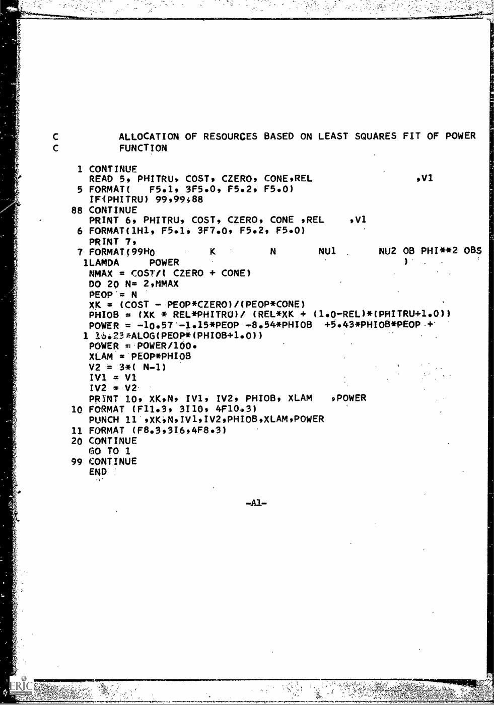
C ALLOCATION OF RESOURCES BASED ON LEAST SQUARES FIT OF POWERC FUNCTION

1 CONTINUEREAD 5, PHITRUs COSTS CZEROs CONEsREL sV1

5 FORMAT( F5.1s 3F5.0, F5.2, F5.0)IF(PHITRU) 9999908

88 CONTINUEPRINT 6, PHITRU, COST, CZEROs CONE sREL ,V1

6 FORMATC1H1s F5.1i 3F7.0, F5.2, F5.0)PRINT 7,

7 FORMAT(99H0 K N NU1 . NU2 OB PHI**2 OBS1LAMDA POWER )-

NMAX = COSTft CZERO + CONE)DO 20 N= 2,NMAXPEOP'= NXK = (COST PEOP *CZERO) /(PEOP *CONE)PHIOB = (XK * REL*PHITRU)/ IREL*XK + (1.0REL)*(PHITRU+1.0))POWER = 10.57'-14,15*PEOP -,-8.54*PHIOB +5.43*PHIOB*PEOP.+*

1 IS.2S*ALOG(PEOP*(PHIOB+1.0))POWER =-POWER/160.XLAM ='PEOP*PHIOBV2 = 3 *( N-.1)IV1 = V1IV2 =1/2.PRINT 10, XKOs IVls IV2s PHIOBs XLAM sPOWER

10 FORMAT (F11.3, 3110s 4F10.3)PUNCH 11"sXKiNsIV1IIV2sPHIOB,XLAM,POWER

11 FORMAT (F8.9,3I6,4F8s3)20 CONTINUE

GO To 199 CONTINUE

END

ti

C ALLOCATION OF RESOURCES USING THE PATNAIK APPROXIMATION

1 CONTINUEREAD 5, PHITRU, COST* CZERO, CONE,REL *V1

5 FORMAT( F5.1* 3F5.0* F5.2, F5.0)IF(PHITRU) 99,99,88

88 CONTINUEPRINT 6, PHITRU* COST, CZERO, CONE ,REL

6 FORMAT(1H1, F5.1, 3F7*0* F5e2)PRINT 7,

7 FORMAT (90H0 K N NU1 NU2 NU ops1PHI**2 085 LAMDA FALPHA POWERNMAX = COST/i CZERO + CONE)DO 20'.N= 2,NMAXPEOP = NXK = (COST PEOP*CZER0)/(PEOP*CONE)PHIOB =' (XK * REL*PHITRU)/ (REL*XK + (1.0REL)*(PHITRU+10))XLAM = PEOP*PHIOSV2 = 3 *( 111-1)PHI.= SORT (PHIOB)IV2'= V2FALPHA.= O.CALL FDIST(2*IV2*FALPHA*05)GALPHA = FALPHAPHIOB ='PEOP*PHIO8SCALE =.(24+PHIOB)/ 2*FALPHA = FALPHA/'SCALEV=A( 2. + PH108)**2)/ (2.+2. *PHIOB)V= V+ .5".IV = VPROB =0..CALL FDIST (IV*IV2* FALPHA* PROB)PROB = 1.0 PROBIV1 st- V1

1V2 = V2XYLAM = PHIOBPHIOB ='PHIOB/PEOPPRINT 70, XK,N* IV1,'1V2* V* PHIOB, MAN* GALPHA, PROB

70 FORMAT (F10.5,311005F1003)PUNCH 710(K.N9IV1tIV2*VOH108,XYLAM.GALPHA,PROB

71 FORMAT (F8.3,316,5F8.3)20 CONTINUE

GO TO 199 CONTINUE

END

.7..41.1"4,77,1"4","*".1.,4

a -

41,

'1;1

C

SUBROUTINE FDIST (MM,NN,FX,PROBX)

C CLARK HOLLOWAY AND W.B.CAPP, AUGUST 31,1959C REVISED APRIL 1,1961 R.J.MCKELVEY

DIMENSION B(2)NOUT=6SF = 0.0SPROB =0.0F=FXPROB=PROBXM=MMN =NN

IF('F) 76,106,100100 SF=. F

IFAF..1.0) 1010 101,105101 XM=M

102DELTA=FLO/500.0GO TO 21

105 FLO=1.0/FXM= NXN= MLOW = 0GO TO 102

106 SPROB = PROBIF(PROB)76,76,107

107 IF (PROB-... 0.5) 1080108,110108 XM=M

XN=NLOW= 1PLO = PROB

109 01.0 = 0.0.DELTA=PLO/200.0GO TO 21

110 IF(PROBa10111,76076111' XM=N"

XN=MIOW = 0PLO = 1.0 PRO8GO:TO 109

21 FACTL =O.O215 FACT=1.0

8(1)=004...e2.3)/2.08(2)=(XN2.0)/2.0

24 A =(XM +XN- 2.0)/2.0

XN= NLOW = 1FLO = FPLO = 0.0

241 IF(A-0.2)400,76.242400 FACT = 0.31630989

GO TO 283242 IF(A-0.7)410,769243410 FACT=0.5

GO TO 2133243 DO 245 Ix1,2

IF(8(I)-0.7)261.76,245261 IF(B(1)-..0.2)264.76,262

- 262 FACT=FACT/0.886226925263 B(I)=110

GO TO 245264 /F(B(I)+0.2)265.76,263265 FACT=FACT/1.772453850

GO TO 263w..

245 CONTINUE244 IF(A-0.7)281976.251251 FACT=FACT*AMB(1)*(3(2))

IF(FACT99999999.)830.283.283830 IF(FACTL.100E-8)283.283.26

26 A=A-1.0

S I

8(1)113(1)-1.0B(2)=8(2)-1:0GO TO 243

281 IF(A-0.2)283.76.282282 FACT=FACT*0.886226925283 FACTL=FACTL+ALOG(FACT)

FACT=1.0IF(A.;-0.7)284,76.26

284 Y1=FACTL+((M/2.0)*ALOG(XMIXN)Y2=(X1-2.0)/20Y3=(XM+XN)/2:0

36 F=DELTA/24,0CUM =O.0

C37 HFDL=Y1+112*ALOG(F)-Y3*ALOG(1.0+XM*F/XN)+ALOG(DELTA)

IF(HFDL+20.)50951.5150 HFD=0,0

GO TO 52.51 HOD=EXP (HMI.),52 CUM=CUM+MFD

F=F+DELTA375 IF(F-FLO)37.37.3838 IF(PLO)76,39.381381 IF(HFD)76,384,382382 IF(ALOW*LO)HFDL-4.604)383,384.384383 DELTA=DELTA/2.0

GO TO 36. . I. .

384 IF(CUMPLO)37,39.3939 FLO=FDELTA

IF(SF) 76,43,4040 F = SF

IF(LOW) 76.42.4141 PROS = CUM

GO TO 4942 PROS = 1.0 CUM

GO TO 4943 PROB = SPROB

IF(LOW) 76,45,4444 F = FLO

GO TO 4945 F = 1.0/FLO49 PROBX=PROB

FX=F1000 RETURN76 WRITE (6,176) MM,NN,FX,PROBX176 FORMAT (10X,36HCOULD NOT WORK F DISTRIBUTION WITH

1(I6,1H0691H,E131.6,1H,E13.6.1H))GO TO 1000END

A5

4

s.

,:11.7f1,Iaf',4tIf44;11:/tp

100 3000 0 100 10 2

K N NU1 NU2 OBPHI**2 OB LAMDA POWER

I,

15.000 2 2 3 1.316 2.632 0.151

10.000 3. 2 6 0.917 2.752 0.215

7.500 4 2 9 0.704 2.817 0.253

6.000 5 2 12 0.571 2.857 0.278

5.000 6 2 15 0.481 2.885 0.295

4.286 7 2 18 0.415 2.905 0.308

3.750 8 2 21 0.365 2.920 0.318

3.333 9 2 24 0.326 2.932 0.325

3.000 10 2 27 0.294 2.941 0.329

2.727 11 2 30 0.268 2.949 0.3332.500 12 2 33 0.246 2.956 0.335

2.308 13 2 36 0.228 2.961 0.336

2.143 14 2 39 0.212 2.966 0.336

2.000 15 2 42 0.198 2.970 0.335

1.875 16 2 45 0.186 2.974 0.334

1.765 17 2 48 0.175 2.977 0.332

1.667 18 2 51 0.166 2.980 0.329

1.57 19 2 54 0.157 2.983 0.326

1.500 20 2 57 0.149. 2.985 0.522

1e429 21 2 60 0.142 2.987 0.319

1.364 22 2 63 0.136 2.989 0.314

1.304 23 2 66 0.130 2.991 0.310

1.250 24 2 69 0.125 2.993 0.305

1.200 25 2 72 0.120 2.994 0.300

1.154 26 2 75 0.115 2.995 0.295

1.111 27 2 78 0.111 2.997 0.289

1.071 28 2 81 0.107 2.998 0.283

1+:084 29 2 84 0.103 2.999 0.277

1.000 30 2 87 0.100 3.000 0.271

100 3000

K

80

N

20

NU1

10 2

NU2 OBPHI**2 OB LAMDA POWER

71.000 2 2 3 4.176 8.353 0.34846.000 3 2 6 3.172 9.517 0.51633.500 4 2 9 2.528 10.113 0.61126.000 5 2 12 2.080 10.400 0.66821.000 6 2 15 1.756 10.500 0.70117.429 7 2 18 1.497 10.479 0.71914.750 8 2 21 1.297 10.374 0.72712.667 9 2 24 1.134 10.209 0.72811.000 1Q 2 27 1.000 10.000 0.7239.636 11 2 30 0.887 99757 0.7148.500 12 2 33 0.791 '9.480 0o7027.538 13 2 36 0.708 9.199 0.6876.714 14 2 39 0.635 8.892 0.6706.000 15 2 42 0.571 8.571 0.6515.375 16 2 45 0.518 8.240 0.6314.824 17 2 48 0.465 7.898 0.6104.333 18 2 51 0.419 7.548 0.5873.895 19 2 54 0.379 7.192 0.5643.500 20 2 57 0.341 6.829 0.5403.143 21 2 60 0.308 6.462 0.5152.818 22 2 63 0.277 6.089 0.4902.522 23 2 66 0.248 5.713 0.4642.250 24 2 69 0.222 5.333 0:4372.000 25 2 72 0.198 4.950 0.4101.769 26 2 75 0.176 4.565 0.3631.556 27 2 78 0.155 4.177 0.3561.357 28 2 81 0.135 3.786 0.3281.172 29 2 84 0.1/7 3.394 0.3001.000 30 2 87 0.100 3.000 0.271

100 3000

K

90

N

10

NU1

10 2

NU2 OBPHI**2 08 LAMA POWER

141.000 2 2 3 5.875 11.750 0.43391.000 3 2 6 4.789 14.368 0.69466.000 4 2 9 4.000 16.000 0.86251.000 5 2 12 3.400 17.000 0.97141.000 6 2 15 2.929 17.571 1.0421 33.857 7 2 18 2.548 17.839 1.08628.500 8 2 21 2.235 17.882 1.110C.

24.333 9 2 24 1.973 17.757 1.12021.000 10 2 27 1.750 17.500 1.11818.273 11 2 30 1.558 17.140 1.10716.000 12 2 33 1.391 16e696 1.089 .t14.077 13 2 36 1.245 16.184 1.06512.429 14 2 39 1.115 15.615 1.03611.000 15 2 42 1.000 15.600 1.0039.750 16 2 45 0.897 14.345 0.96?8.647 17 2 48 0.803 13.656 0.9277.667 18 2 51 0.719 12.937 0.8856.789 19 2 54 0.642 12.194 0.841/-

6.000 20 2 57 0.571 11.429 0./965.286 21 2 60 0.507 10.644 0.7484.636 22 2 63 0.447 '9.842 0.6994.043 23 2 66 0.392 9.025 0.649.3.500 24 2 69 0.341 8.195 0.5983.000 25 2 72 0.294 7.353 0.5454.. 2.538 26 2 75 0.250 6.500 0.4922.111 27 2 78 0.209 5.637 0.4381.714 28 2 81 0.170 4.766 0.3831.345 29 2 84 0.134 3.887 0.3271.000 30 2 87 0.100 3.000 0.271

r

4

N",tit

-B3-

7r,

100 3000 0 100 10 2

'n--.,..

r s,

k../

'C;) ....B4-

N. NU1 NU2 NU OBPHI**2 OB LAMDA FALPHA POWER

15.000 2 2 3 3.45310.000 3 2 6 3.5097.500 4 2 9 3.5396.000 5 2 12 3.5585.000 6 2 15 3.5714.286 7 2 18 3.5803.750 8 2 21 3.5873.333 9 2 24 3.5933.000 10 2 27 3.5972.727 11 2 SO 3.6012040 12 2 33 3.6042.308 13 2 36 3.6072.143 14 2 39 3.6092.000 15 2 42 3.011.875 16 2 45 3.6131.765 17 2 48 3.6141.667 18 2 51 3.6161.579 19 2 54 3.6171.500 20 2 57 3.6181.429 -21 2 60 3.6191.364 22 2 63 3.6201.304 23 2 66 3.6211.250 24 2 69 3.6211e200 25 2 72 3.6:2 21.154 26 2 75 3.6231.111 27 2 78 3.6231.071 28 2 81 3.6241.034 29 2 84 3.6251.000 30 2 87 3.625

1.316 2.632 9.5580.917 2.752 5.1450.704 2.817 4.2580.571 2.857 3.8850.481 2.885 3.6820.415 2.905 3.5540.365 2.920 3.4680.326 2.932 3.4030.294 2.941 3.3540.268 2.949 3.3150.246 2.956 3.2850.228 2.061 3.2590.212 2.966 3.2380.198 2.970 3.21:90.186 2.974 3.2040.175 2.977 3.1910.166 2.980 3.1780.157 2.903 3.1680.149 2.985 3.1580.142 2.987 3.1510.136 2.989 3.1430.130 2.001 3.1360.125 2.903 3.129Q.120 2.014 3.1240.115 2.105 3.1190.111 2.997 301140.107 2.098 3.109Q.103 2.999 3.1040.100 3.000 3.102

0.1370.1930.2230.2410.2530.2620.2680.2730.2770.2800.2830.285D.2870.2890.2900.2910.2920.2930.2040.2950.2960.2960.297'402980.2980.2990.2990.3000.300

0

C

4.

74,..1!",!!!!!'",..ower.;;Ireomftosnftwome~evionwero.m.....r.,..

e".

100 3000 80 20 10 2

K N NU1 NU2 NU OBPH "2 OB LAMDA FALPHA POWER;

71.000 2 2 3 6.230 4.176 8.353 9.558 0.329.et ,

46.00033.500

34

22

69

6.8067.102

3.1722.528

9.51710.113

5.1454.258

0.5530.672

26.000 5 2 12 7.244 2.080 10.400 3.885 0.7264. 21.000 6 2 15 7.293 1.750 10.500 3.682 0.755

."" 17.429 2 18 7.283 1.497 10.479 3.554 0.77114.750 8 2 21 7.231 1.297 10.374 3.468 0.77912.667 9 2 24 7.149 1.134 10.209 3.403 0.78211.000 10 2 27 7.045 1.000 10.000 3.354 0.78x29.636 11 2 30 6.925 0.887 9.757 3.315 0.7558.500 12 2 33 6.792 0.791 9.488 3.285 0.7507.538 13 2 36 6.648 0.708 9.199 3.259 0.7426.714 14 2 39 6.496 0.635 8.892 3.236 0.7336.000 15 2 42 6.338 0.571 8.571 3.219 0.722

U 5.375 16 2 45 6.174 0.515 8.240 3.204 0.7094.824 17 2 48 6.005 0.465 7.898 3.191 0.6944.333 18 2 51 5.833 0.419 7/8548 3.178 0.6513.895 19 2 54 5.657 0.379 7.192 3.168 046343.500 20 2 57 5.478 0.341 6.629 3.158 0.6143.143 21 2 60 5.298 0.308 6.462 3.151 0.5932.818 22 2 63 5.115 0.277 6.089 3.143 0.5702.522 23 2 66 4.931 0.248 5.713 3.136 0.5212.250 24 2 69 4.746 0.222 5.333 3.12.9 0.49-2.000 25 2 72 4.559 0.198 4.950 3.124 0.4691.769 26 2 75 4.372 0.176 4.565 3.119 0.4401.556 27 2 78 4.185 0.155 4.177 3.114 0.408

. 1.357 28 2 81 3.998 0.135 3.786 3.109 0.3651.172 29 2 84 3.611 0.117 3.394 3.104 0.3331.000 30 2 87 3.625 0.100 3.000 3.102 0.300

f 'a

.435-

r

.5-

C.;

/00 3000

K

90

N

10

NU1

10

NU2

2

NU OBPHI * *2 OB LAMDA FALPHA POWER

141.000 2 2 3 7.914 5.875 11.750 90558 0.429'91.000 3 2 6 9.217 4e789 14.368 5.145 0.745

66.000 4 2 9 10.029 4.000 16.000 4.258 6.870'

51.000 5 2 12 10.528 3.400 17.000 3.885 009172

41.000 6 2 15 10.813 2.929 17.571 3.682 0.938

33.857 7 2 18 10.946 2.548 17.839 3,554 0.950

28.500 8 2 21 10.968 2.235 17.882 3.468 0.956

24.333 9 2 24 10.905 1.973 17.757 3.403 0-6959

21.000 10 2 27 10.777 1.750 17.500 3.354 0.960

18.273 11 2 30 10.597 1.558 17./40 3.315 0.960

16.000 12 2 33 10.376 1.391 16.696 3.285 0.959

14.077 13 2 36 10.121 1.245 16.184 3.259 0.957

12.429 14 2 39 9.838 1.115 15.615 3.238 0.944

11.0009.750

1516

2

2

4245

9.5319.205

1.0000.897

15.00014.345

3.2193.204

6:93,90.91a

8.647 17 2 48 8.862 0.803 13.656 30191 0.911

7.667 18 2 51 8.505 0.719 12.917 3.178 94900

6.789 19 2 54 8.135 0.642 12.194 3:160 (4888

6.000 20 2 57 7.755 0.571 11.429 3.158 6.852

5.286 21 2 60 7.365 0.507 10.644 3.151 0.832

4.636 22 2 63 6.967 0.447 9.842 3.143 0.783

4.043 23 2 66 6.563 0.392 9.025 3.136 0:754

3.500 24 2 69 6.152 0.341 8.195 3.129 0:719

3.000 25 2 72 5.736 0.294 7.353 3.124 6.649

2.538 26 2 75 5.317 0.250 6.500 3.119 0.600

2.111 27 2 78 4.894 0.209 5.637 3.114 0.519

1.714 28 2 81 4.470 0.170 4.766 3.109 0.457

1.3451.000

2930

2

2

8487

4.0463.625

0.1340.100

308873.000

3.1043.102

0.584,0.300

"; r--,v--r-5-,,,,-.44.--tuo-,v.-;44---.(.--,Irtnt4-: 4-,.--#^4-_21ttl---i-ert--,

0160CD (11sw.9-46)

INSTRUCTIONS FOR COMPUTING EEC WORT SWUM

The resume is used to identify summary data and information about each document acquired, processed,and stored within the URIC system. In addition to serving as a permanent record of the document 11 the col.landau, the resume is also a means of dissemination. MI fields of the Sato must be completed in the allottedspaces, but inapplicable fields should be left blank. The following instructions are hayed to the lint numbersappearing in the left margin of the form:

TOP UNL ERIC ACC11601k No. Leave blank. A permanent EDnumber still be assigned to each resume and its correspondingdocument ea they are processed into the ERIC system.

UN 001. use Accession Net For use only by ERICClearinghouses. the alpha code and &digit documentnumber.

jimagmllit In numeric form, enter month, day, and yearthat resume ii completed. (Swap: 07 14 66)

LA Lave blank.1,A, Leave blank.

coMit. Check appropriate block to denote presence ofTamed.' within the document.

ERIC Rmschmtlooldesse. Check appropriate block to WU-cal; MIMI.. has permission to reproduce the document andits resume form.

100 -103. Mg, Enter the complete document dtle, in-dueling =Ws) if they add significant information. Whereapplicable, also ester volume number or part number, and thetype ofdocunseits (Friar Report, labia &Sit, Thesis, els.).

;!`..4E 200. Personal Au i . Enter personal author(s), lastname first. : , ran 3.) If two authors are given,enter both. (Eke*: bee, jest 3. Swish, Tel). If there arethree or more suitors, list only one followed by "and others."

UNE 300. InatiniOn Marcel Enter the name of the ergs:dra-ke which originated the report. Include the address (dos tadStile) and the subredinate unit of the organisation. ( ixessfrk:Iknori Uaw., Centiige, Mat, Sant of Eatestiost.)

Source Code. Liave blank.

124E 310. Report/Sides No. Enter any unique number assignedto the document by th-eiiiirtutional source. (Exexple: SC-1234)

UNE 320. Other Source. Use only when a second source isassociated ZW-the document. Follow instructions for Line 300above.

Source Cbde. Leave blank.

we 330. Other t No. Eater document number assignedby the seeon source.

UNE 340. Otberiource. Use only when a third source is aro-elated with the document. Follow Instructions for Line 300 above.

Source Cade. Leave blank.

UN! 350. Other Report No. Enter document amid= **maib} the third source.

UNE 400. Publication Date. Enter the chiy, monk, and year ofthe document: (Fohmhie: 12 Jan 66)

Contract/Grant Number. Applicable only for documents *a-erated from research sponsored by the U.S Office of Educr-tion.Eater appropriate contract or grant number and its prefix.(Example: Oft-1-6-061234-003n

UNES 500-501. Pagination, etc. Eater the total number ofpages of the document, including inuotratios s. and appendixes.(Egan* lisp.) USE THIS SPACE FOR ADDITIONAL IN-FORMATION PERTINENT TO THE DOCUMENT, such aspublisher, journal citation, lad other contract numbers.

UNES 600-606. Reuieval Terms. Enter the Important subjectterms (dnaifteess) which, taken as a group, adequately describethe =nests of the document.

UNE 607. Idea . Enter any additional important tarns,mere specific than descriptors, such as trade names, equipmentmodel names and numbers, organization and project maw&discussed in the document.

UNES 100422. Abstract. Enter an informative abstract of thedocument. Its style and content mint be suitable for publicannouncement and dissemination.

114. 11011111014UT ,arms irict a 1111111411141111

Z.37MtriloolicalePa ---

cm 6000 (nu 948)Cl...7traCESSION NO.

"etrAinTantriir"ACCESSION NUMBER

DEPARTMENT OF HEALTH. EDUCATION. AND WELFAREOFFICE OR EDUCATION

100101

102103

320330

500501

600601602603604605606

607

800801802803804805806807808889816811812813814815816817818819820821

822

09-27- 67

ERIC REPORT RESUME

IS DOCUMENT COPYRIGHTED?

ERIC REPRODUCTION RELEASE?

vasYes to

Noe3P400

TITLE

EFFECT OF ERROR OF MEASUREMENT ON THE POWER OF STATISTICAL TESTS.

Final Report.

PERSONAL. AUTNORIII)

Cleary, T. Anne and Linn, Robert L.INSTITUTION lsouRCtlEducational Test .: Service Princeton New Jers

SOURCE CODE

REPORT /SERIES NO.0 PI R SOU CE

University of Wisconsin, Madison, Wisconsin

...SOURCE CODE

OMNI

L41411P1 REPORT P40.

0 NEN SOURCE SOURCE ODE

OTHER REPORT NO.

PLUM. DATE 09'" 2T CONTRACT/GRANT NUMBER 03a...1 0.00 _,/3.-MImam

PAGINATION. ETC.

i. + 43 pp.

,RETRIEVAL TERMS t .

Statistics

Mental Test TheoryPowerReliabilityError of Measurement

IDENTIFIERS

4ABSTRACT

The purpose of this research was to study the effect of error of measure-ment upon the power of-statistical tests. Attention was focused on the F testof the single factor analysis of variance. Formulas were derived to show therelationship between the noncentrality parameters for analyses using true scoresand those using observed scores. The effect of the reliability of the measurement and the sample size were thus demonstrated. The assumptions of classicaltest theory were used to develop formulas relating test length to the noncentrality parameters. .

Three methods of estimating power for different conditions of sample sizeand test length were studied. The cost of an experiment was analyzed in termsof a fixed cost per subject and a variable cost dependent upon test length.Computer programs were written to use the least squares approximation and theapproximation based on Ettnaik to estimate the power under all immissibleallocations of- resources to sample size and test length. The program resultsindicate which of the permissible allocations will result in maximum power.

To demonstrate empirically the effect of error of measurement on thepower of statistical tests, samples of persons and items were randady drawnfrom a large pool of data. Tests of 10, 20, and 40 randomly drawn items werescored for samples with four and eight persons per group. The expected trendswere present but not definitive. .