report: net load forecasting with distributed · pdf file12/16/2014 · net load...

NET LOAD

Report:

Net Load Forecasting with Distributed Generation

Green Power Labs Inc

One Research Drive,

Dartmouth, Nova Scotia,

Canada, B2Y 4M9

Phone: (902) 466-6475

Fax: (902) 466-6889

2014-12-16

of 35

This report was prepared by Green Power Labs Inc.

(GPLI) in part by a grant provided by the California

Public Utilities Commission’s (CPUC) California Solar

Initiative (CSI) R&D program. The materials in this

report reflect GPLI’s best judgment based on the

information available to the company at the time of

report preparation. Any use of this report by a third

party, or any reliance on or decisions made based

on it, are the responsibility of such third parties. GPLI

accepts no responsibility for damages, if any,

suffered by any third party as a result of decisions

made or actions based on this report.

of 35

Contents

Contents ........................................................................................................................................................ 3

1. Executive Summary ............................................................................................................................ 4

2. Introduction ........................................................................................................................................ 6

3. Data Sources ....................................................................................................................................... 7

3.1. Study Locations ........................................................................................................................... 7

3.2. Load and Weather Data .............................................................................................................. 9

4. Methodology ...................................................................................................................................... 9

4.1. GHI and Cloudiness Index ........................................................................................................... 9

4.2. Distributed PV Generation .......................................................................................................... 9

4.3. Net Load and Consumption Data .............................................................................................. 10

4.4. Calibration of data to December 31st, 2012 .............................................................................. 11

4.4.1. Load .................................................................................................................................... 11

4.4.2. Distributed Generation ...................................................................................................... 12

4.4.3. Data set for analysis ........................................................................................................... 12

5. Results ............................................................................................................................................... 13

5.1.1. Hourly average net load ..................................................................................................... 13

5.1.2. Hourly average distributed generation .............................................................................. 16

5.1.3. Hourly average consumption, net load and generation .................................................... 17

5.1.4. Variability in net load ......................................................................................................... 23

5.1.5. Variability in distributed generation .................................................................................. 28

5.2. Distributed generation in relation to net load .......................................................................... 29

5.2.1. Existing DG penetration ..................................................................................................... 29

5.2.2. Increased DG penetration .................................................................................................. 30

6. Conclusions ....................................................................................................................................... 33

7. Recommendations ............................................................................................................................ 34

of 35

1. Executive Summary

A public private partnership of UC San Diego, San Diego Gas & Electric, Clean Power Research and Green

Power Labs was established under the California Solar Initiative Research, Demonstration and

Deployment Program Grant Solicitation #3 to “improve and demonstrate solar forecasting models to

facilitate PV grid integration”. Green Power Labs role includes the provision of distributed generation

forecasts for five feeders selected in the SDGE service territory, and collaboration with the project

partners for the development of net load forecasting.

This report summarizes Green Power Labs investigation of net load, distributed generation and electrical

consumption at five substations in SDGE’s service territory.

The study simulates power generation in the circuits served by the substations using a model developed

from a sample of 1012 PV installations from the Net Energy Metering (NEM) San Diego data base to

determine average power generation under clear-sky conditions.

Hourly consumption, distributed generation and net load data were calibrated over a three year

evaluation period to account for the changes in load and build-out of DG assets over time.

The load profiles of the five substations show considerable variation, and the timing of peak load also

varies considerably.

The report discusses the impact of variability of consumption within a circuit, and the extent of DG

build-out on risks to system stability. The report presents the frequency distribution of the DG-to-

consumption ratio at one substation for the DG build-out at the end of the evaluation period, and

presents equivalent frequency distribution plots for 25%, 50% and 75% DG penetration. The linear

relationship of these values may be used to extrapolate the impact of DG build-out on risk factors

related to distribution management.

At the levels of DG studied, distributed generation may smooth out the daily peaks and shift the

timing of the daily maximum load. However, as DG is deployed well beyond the 10% level of

penetration characterized in this study, the daily load profile may include a sharp ramp upward as

distributed generation declines and consumption increases.

In the absence of demand-side management, consumption is more fundamental than (net) load in

representing the underlying, behind-the-the-meter load parameter present in a circuit. Accordingly,

of 35

in forecasting load flow in circuits with considerable DG deployed, there may be merit to forecasting

distributed generation and consumption separately to obtain the net load forecast.

The report recommends:

- circuit-level forecasting of consumption, distributed generation and net load where net load

monitoring is available in order to evaluate the relative precision of consumption-and-

generation forecasts relative to direct net load forecasting at varied levels of DG penetration,

- Comparison of circuit-level or substation forecasts with system-level forecasts where there is a

variety of micro-climates, load profile related to customer class, and DG penetration, and

- Further evaluation of parameters which affect distribution system stability, e.g., the distribution

of energy use and DG within the circuit, the location and relative size of commercial-scale PV

sites or other DG concentration in the circuit, and the distance of DG concentration from the

substation’s secondary bus.

of 35

2. Introduction

A public private partnership of UC San Diego (UCSD), San Diego Gas & Electric (SDGE), Clean Power

Research and Green Power Labs (GPL) was established under the California Solar Initiative Research,

Demonstration and Deployment Program Grant Solicitation #3 to “improve and demonstrate solar

forecasting models to facilitate PV grid integration”. Included in this initiative is granular distribution

feeder forecasting, including total sky imagery, power flow modeling for real-time voltage profiles,

identification of reverse power flows or voltage sags that can cause inverter tripping, and control of utility

voltage regulation equipment. Green Power Labs’ role includes the provision of distributed generation

forecasts for five substations selected in the SDGE service territory, and collaboration with the project

partners for the development of net load forecasting.

Specifically, Green Power Labs are to report on (a) gross load characterization and forecasting at the circuit

level, and (b) the impact of DG on gross gen and CAISO Load Forecast submission logistics.

This report summarizes Green Power Labs investigation of net load, distributed generation and electrical

consumption at five feeders in SDGE’s service territory, and makes recommendations for future research

in net load forecasting.

of 35

3. Data Sources

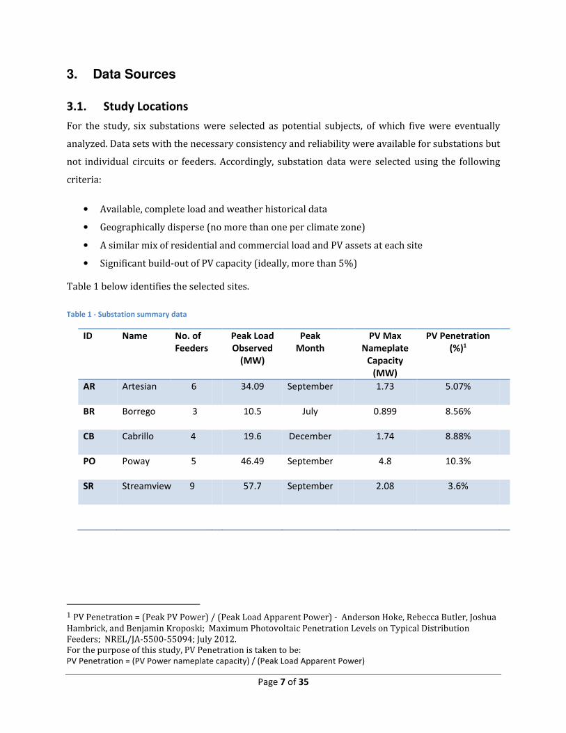
3.1. Study Locations

For the study, six substations were selected as potential subjects, of which five were eventually

analyzed. Data sets with the necessary consistency and reliability were available for substations but

not individual circuits or feeders. Accordingly, substation data were selected using the following

criteria:

• Available, complete load and weather historical data

• Geographically disperse (no more than one per climate zone)

• A similar mix of residential and commercial load and PV assets at each site

• Significant build-out of PV capacity (ideally, more than 5%)

Table 1 below identifies the selected sites.

Table 1 - Substation summary data

ID Name No. of

Feeders

Peak Load

Observed

(MW)

Peak

Month

PV Max

Nameplate

Capacity

(MW)

PV Penetration

(%)1

AR Artesian 6 34.09 September 1.73 5.07%

BR Borrego 3 10.5 July 0.899 8.56%

CB Cabrillo 4 19.6 December 1.74 8.88%

PO Poway 5 46.49 September 4.8 10.3%

SR Streamview 9 57.7 September 2.08 3.6%

1 PV Penetration = (Peak PV Power) / (Peak Load Apparent Power) - Anderson Hoke, Rebecca Butler, Joshua

Hambrick, and Benjamin Kroposki; Maximum Photovoltaic Penetration Levels on Typical Distribution

Feeders; NREL/JA-5500-55094; July 2012.

For the purpose of this study, PV Penetration is taken to be:

PV Penetration = (PV Power nameplate capacity) / (Peak Load Apparent Power)

of 35

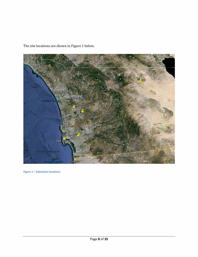
The site locations are shown in Figure 1 below.

Figure 1 – Substation locations

of 35

3.2. Load and Weather Data

For each site, three years of load data (MW), from January, 2010 through December, 2012, were

gathered via SDGE’s supervisory control and data acquisition system, and were provided as 15-

minute average values. SDGE also provided the distributed PV nameplate capacity concurrent with

load data.

Weather data sets were compiled by GPL for the same time period as the load data. These values

included temperature, wind speed and direction, and relative humidity. The data sets were extracted

from ground weather stations on the MesoWest network. In addition to the compiled data, GPL used

satellite images from the Geostationary Satellite system (GOES), operated by the United

States National Environmental Satellite, Data, and Information Service (NESDIS), visible spectrum, to

generate values of total cloud cover and solar irradiance.

The most significant data gaps include several months of power generation data at Poway Substation

in 2011, and a 35 days of load data in Borrego, from mid-July to mid-August 2012.

4. Methodology

4.1. GHI and Cloudiness Index

In the absence of ground-sourced irradiance data from some or all of the distribution areas served

by the substations, the cloudiness index (CI) and global horizontal irradiance (GHI) was simulated

using satellite imagery at ½ hour resolution. The values were derived using GOES satellite images of

brightness at the location of the substation: the observed pixel brightness of the image at the desired

location was compared with the brightness of bare ground at the location and time to derive

cloudiness, for each location over the three-year evaluation period. Solar irradiance was determined

from cloudiness using Sandia National Laboratories’ SPA model. For the purposes of this analysis, the

process was carried out hourly for each substation location over the study period (2010-2012).

4.2. Distributed PV Generation

The distributed PV power generated in each circuit is, in general, not measured directly and is

therefore not necessarily available for net load calculations. Accordingly, simulated PV generation

values were derived using the calculated GHI values using a model developed by GPLI. The theoretical

of 35

direct and diffuse components of irradiance were derived using NREL’s DISC model2, then fed into a

model of a simulated PV plant together with data from local ground weather stations, to calculate the

theoretical power output.

The simulated plant uses generic PV panel models along with a developed distribution of panel slopes

and azimuths to overcome the lack of actual known values.

The size of the simulated plant is defined as the sum of the nameplate capacities connected to the

circuit or substation, as provided by SDGE.

The PV panel simulation was derived using a sample of 1012 PV installations from the Net Energy

Metering (NEM) San Diego data base. The installations were examined in various GIS and global

monitoring packages available via the internet. It was found that the majority of the installations have

orientations facing due south or close to due south. The azimuth and slope of the PV modules were

estimated and applied together with nameplate capacity to form a general model of the relationship

between time of day and year, and power generation under clear-sky conditions.

4.3. Net Load and Consumption Data

For the purpose of this report we define consumption as:

consumption = net load + distributed generation

For consumption at the circuit level and the purpose of this analysis, distribution losses may be

considered as included with consumption. Steady-state voltage or current violations are not

considered.

The consumption consists of the load plus the PV generation at that point in time; this value is meant

to represent the actual power consumption in a circuit, including the effects of any behind-the-meter

generation (in this case PV).

• 2 Maxwell, E. L., A Quasi-Physical Model for Converting Hourly Global Horizontal to Direct Normal

Insolation, Technical Report No. SERI/TR-215-3087, Golden, CO: Solar Energy Research Institute, 1987.

of 35

Hourly consumption data were derived from average load data and distributed generation derived

from instantaneous satellite data.

4.4. Calibration of data to December 31st, 2012

4.4.1. Load

The net load data was reviewed to identify changes in consumption over the evaluation period.

The data sets used for this analysis consisted of three years (from January 1st, 2010, till December

31st, 2012). Over the course of three years there are natural changes in the build-out of feeders at

each substation. Monthly and 3-year average load in five substation can be seen in Figure 2 below.

Figure 2 - Annual average load by substation and year

Notes: The average load, consumption and generation energy units, e.g., MWh/h, are abbreviated to power units, e.g., MW.

The figure presents measured (net) load data, which includes circuit losses, consumption and distributed generation.

As shown in Figure 2 there were upward and downward trends in load at each substation of as much

as 20% over the three year period.

The average monthly data were also examined to detect sudden changes in load which may be relate

to changes in feeder connections: none was observed.

of 35

The hourly load data for 2010 and 2011 were factored in relation to the change in average annual

load relative to year 2012, to approximate conditions in 2012.

4.4.2. Distributed Generation

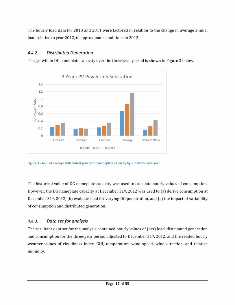
The growth in DG nameplate capacity over the three-year period is shown in Figure 3 below.

Figure 3 - Annual average distributed generation nameplate capacity by substation and year

The historical value of DG nameplate capacity was used to calculate hourly values of consumption.

However, the DG nameplate capacity at December 31st, 2012 was used to (a) derive consumption at

December 31st, 2012, (b) evaluate load for varying DG penetration, and (c) the impact of variability

of consumption and distributed generation.

4.4.3. Data set for analysis

The resultant data set for the analysis contained hourly values of (net) load, distributed generation

and consumption for the three-year period adjusted to December 31st, 2012, and the related hourly

weather values of cloudiness index, GHI, temperature, wind speed, wind direction, and relative

humidity.

of 35

5. Results

5.1.1. Hourly average net load

Hourly and seasonal variations in net load are described in the following (figures), which depict

average hourly net load in January, April, July and October for the respective substations, including

all days (week-days, week-end days and holidays).

Figure 4: Artesian seasonal net load average daily profile

of 35

Figure 5: Borrego seasonal net load average daily profile

Figure 6: Cabrillo seasonal net load average daily profile

of 35

Figure 7: Poway seasonal net load average daily profile

Figure 8: Stream View seasonal net load average daily profile

of 35

With the exception of the site in the desert (BR), the substations typically have small peaks in the

morning and larger ones in the afternoon or evening. There is, however, considerable variation in the

daily profiles between circuits. The timing of peak load varies considerably, as shown in the following

Table 2.

Table 2 - Winter and summer peak consumption values and time-of-day, by substation

ID Name Winter Peak Consumption

(MW)

Summer

Peak

Consumption

(MW)

AR Artesian 1800h 15.0 2100h3 15.0

BR Borrego 0700h 5.5 1700h 6.5

CB Babrillo 1800h 13.5 2000h 11.6

PO Poway 1800h 23 1700h 23.5

SR Streamview 1800h 36 2000h 35

Summer and winter peak values were similar for each substation, with seasonal variation of less than

20%.

Consumption peaks in the summertime may be attributed to air conditioning. At two of the

substations the largest peaks occurred in the afternoon in the summertime: in these cases the net

load is reduced by concurrent DG.

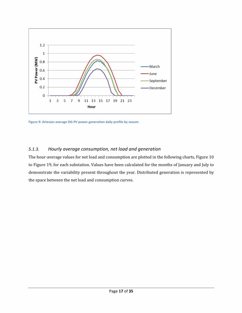
5.1.2. Hourly average distributed generation

The PV-DG generation for the five substations are very similar to the typical “Bell Shape” PV power

daily profile, as it can be seen below in Figure 9.

3 Local time (Pacific Daylight Time)

of 35

Figure 9: Artesian average DG-PV power generation daily profile by season

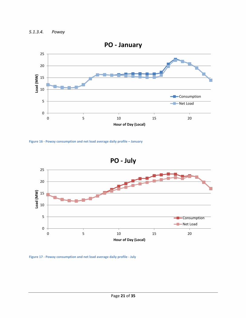
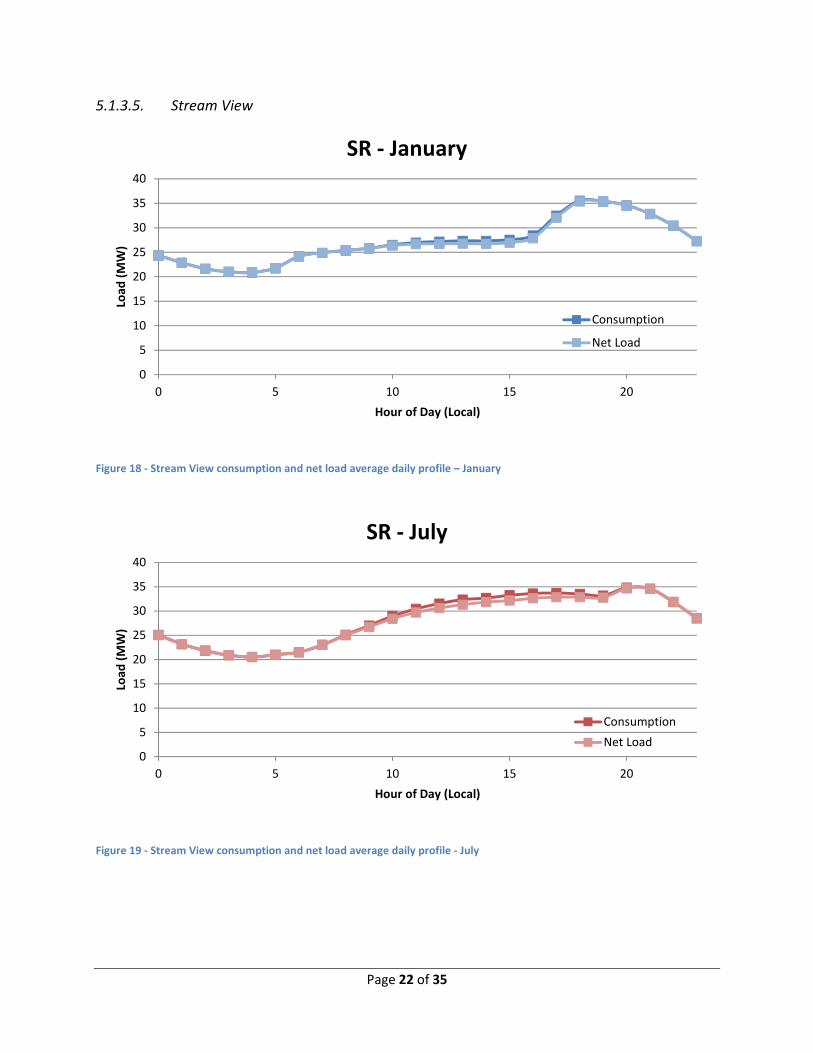
5.1.3. Hourly average consumption, net load and generation

The hour-average values for net load and consumption are plotted in the following charts, Figure 10

to Figure 19, for each substation. Values have been calculated for the months of January and July to

demonstrate the variability present throughout the year. Distributed generation is represented by

the space between the net load and consumption curves.

of 35

5.1.3.1. Artesian

Figure 10 - Artesian consumption and net load average daily profile - January

Figure 11 - Artesian consumption and net load average daily profile - July

0

2

4

6

8

10

12

14

16

0 5 10 15 20

Loa

d (

MW

)

Hour of Day (Local)

AR - January

Consumption

Net Load

0

2

4

6

8

10

12

14

16

0 5 10 15 20

Loa

d (

MW

)

Hour of Day (Local)

AR - July

Consumption

Net Load

of 35

5.1.3.2. Borrego

Figure 12 - Borrego consumption and net load average daily profile - January

Figure 13 - Borrego consumption and net load average daily profile - July

0

1

2

3

4

5

6

0 5 10 15 20

Loa

d (

MW

)

Hour of Day (Local)

BR - January

Consumption

Net Load

0

1

2

3

4

5

6

7

0 5 10 15 20

Loa

d (

MW

)

Hour of Day (Local)

BR - July

Consumption

Net Load

of 35

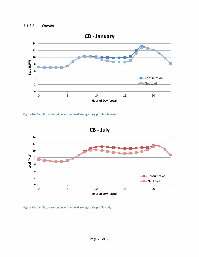
5.1.3.3. Cabrillo

Figure 14 - Cabrillo consumption and net load average daily profile – January

Figure 15 - Cabrillo consumption and net load average daily profile - July

0

2

4

6

8

10

12

14

0 5 10 15 20

Loa

d (

MW

)

Hour of Day (Local)

CB - January

Consumption

Net Load

0

2

4

6

8

10

12

14

0 5 10 15 20

Loa

d (

MW

)

Hour of Day (Local)

CB - July

Consumption

Net Load

of 35

5.1.3.4. Poway

Figure 16 - Poway consumption and net load average daily profile – January

Figure 17 - Poway consumption and net load average daily profile - July

0

5

10

15

20

25

0 5 10 15 20

Loa

d (

MW

)

Hour of Day (Local)

PO - January

Consumption

Net Load

0

5

10

15

20

25

0 5 10 15 20

Loa

d (

MW

)

Hour of Day (Local)

PO - July

Consumption

Net Load

of 35

5.1.3.5. Stream View

Figure 18 - Stream View consumption and net load average daily profile – January

Figure 19 - Stream View consumption and net load average daily profile - July

0

5

10

15

20

25

30

35

40

0 5 10 15 20

Loa

d (

MW

)

Hour of Day (Local)

SR - January

Consumption

Net Load

0

5

10

15

20

25

30

35

40

0 5 10 15 20

Loa

d (

MW

)

Hour of Day (Local)

SR - July

Consumption

Net Load

of 35

5.1.4. Variability in net load

5.1.4.1. Maximum and minimum hourly values

The variability in net load is presented in Figure 20 to Figure 24 below. The minimum and maximum

hourly record is indicated, by hour, for the substation and month noted. The data set includes the

month referenced over three years, including weekdays, weekends and holidays. Mean values are

presented as a curve in these figures.

Figure 20 - Artesian load variability – June: hourly minimum, average and maximum load (MWh/h)

Figure 21 - Borrego load variability - June: hourly minimum, average and maximum load (MWh/h)

0

2

4

6

8

10

12

1 2 3 4 5 6 7 8 9 10 11 12 13 14 15 16 17 18 19 20 21 22 23 24

Ne

t Lo

ad

(M

W)

Hour

of 35

Figure 22 - Cabrillo load variability - June: hourly minimum, average and maximum load (MWh/h)

Figure 23 - Poway load variability - June: hourly minimum, average and maximum load (MWh/h)

of 35

Figure 24 - Stream View load variability - June: hourly minimum, average and maximum load (MWh/h)

The hourly variation presented above is for the 90 days of data available in June, 2010-2012. (The

data sets for July, which may be a more representative month for summer maxima in DG as well as

load, were not complete at all locations.)

There is a large range of variability in hourly net load estimates. The variability of net load comprises

from approximately 40 to 200% of the mean hourly load with highest hourly variability in Borrego,

which is the substation with the smallest peak load. While the cause is not speculated, the impact is

that solutions to load flow control in grids with high penetration DG may require individual

substation or circuit data to be effective.

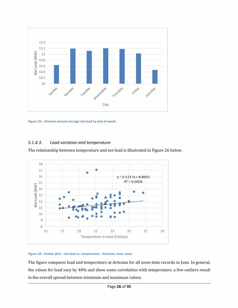
5.1.4.2. Load variation by day-of-week

As illustrated in Figure 25 below there is variation in the total power used by day-of-week. The figure

indicates a variation in average daily energy consumption of 7% at the Artesian Substation, which is

characteristic of all substations in the study. There is also a variation in the hourly profile between

weekdays and weekends. These effects contribute in a relatively minor way to the hourly variations

described in sub-section 5.1.4.1 above.

of 35

Figure 25 - Artesian annual average net load by day-of-week

5.1.4.3. Load variation and temperature

The relationship between temperature and net load is illustrated in Figure 26 below.

Figure 26 - Scatter plot - net load vs. temperature - Artesian, June, noon

The figure compares load and temperature at Artesian for all noon-time records in June. In general,

the values for load vary by 40% and show some correlation with temperature; a few outliers result

in the overall spread between minimum and maximum values.

of 35

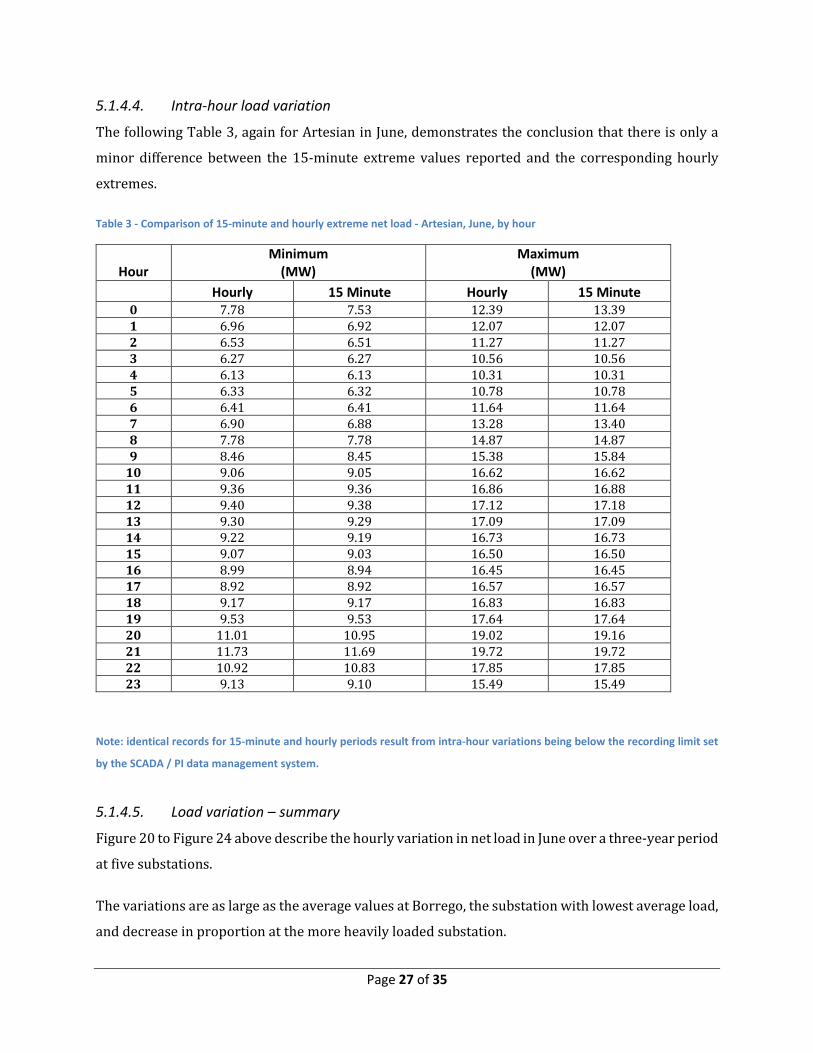
5.1.4.4. Intra-hour load variation

The following Table 3, again for Artesian in June, demonstrates the conclusion that there is only a

minor difference between the 15-minute extreme values reported and the corresponding hourly

extremes.

Table 3 - Comparison of 15-minute and hourly extreme net load - Artesian, June, by hour

Hour

Minimum

(MW)

Maximum

(MW)

Hourly 15 Minute Hourly 15 Minute

0 7.78 7.53 12.39 13.39

1 6.96 6.92 12.07 12.07

2 6.53 6.51 11.27 11.27

3 6.27 6.27 10.56 10.56

4 6.13 6.13 10.31 10.31

5 6.33 6.32 10.78 10.78

6 6.41 6.41 11.64 11.64

7 6.90 6.88 13.28 13.40

8 7.78 7.78 14.87 14.87

9 8.46 8.45 15.38 15.84

10 9.06 9.05 16.62 16.62

11 9.36 9.36 16.86 16.88

12 9.40 9.38 17.12 17.18

13 9.30 9.29 17.09 17.09

14 9.22 9.19 16.73 16.73

15 9.07 9.03 16.50 16.50

16 8.99 8.94 16.45 16.45

17 8.92 8.92 16.57 16.57

18 9.17 9.17 16.83 16.83

19 9.53 9.53 17.64 17.64

20 11.01 10.95 19.02 19.16

21 11.73 11.69 19.72 19.72

22 10.92 10.83 17.85 17.85

23 9.13 9.10 15.49 15.49

Note: identical records for 15-minute and hourly periods result from intra-hour variations being below the recording limit set

by the SCADA / PI data management system.

5.1.4.5. Load variation – summary

Figure 20 to Figure 24 above describe the hourly variation in net load in June over a three-year period

at five substations.

The variations are as large as the average values at Borrego, the substation with lowest average load,

and decrease in proportion at the more heavily loaded substation.

of 35

The variations are typically greatest during daytime, particularly in the afternoon hours.

Variations may be expected to relate more to local use patterns for smaller service areas and loads.

However, the sites selected are in areas with a residential / commercial mix. For the summer month

presented, the load variations relate, in part, to temperature (air conditioning load) and, to a lesser

extent, day of week. The reason for this variability was not investigated; however the observation

demonstrates the need for data from individual substations or circuits to develop solutions to load

flow control in grids with high penetration levels of DG.

The hourly results for min/max values were similar to 15-minute values and are considered to be an

effective metric for analysing the impact of distributed generation and other factors, e.g., demand

management and storage, on power flow in individual circuits.

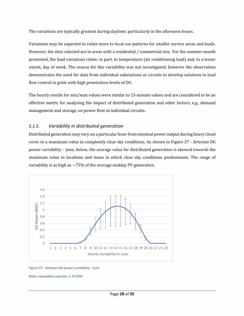
5.1.5. Variability in distributed generation

Distributed generation may vary on a particular hour from minimal power output during heavy cloud

cover to a maximum value in completely clear sky conditions. As shown in Figure 27 - Artesian DG

power variability – June, below, the average value for distributed generation is skewed towards the

maximum value in locations and times in which clear sky conditions predominate. The range of

variability is as high as ~75% of the average midday PV generation.

Figure 27 - Artesian DG power variability – June

Note: nameplate capacity: 1.74 MW

of 35

Similar ranges in variability as illustrated in the figure above were observed at all other sites.

5.2. Distributed generation in relation to net load

5.2.1. Existing DG penetration

The data were examined to characterize conditions which may threaten distribution system stability,

e.g., voltage rise, frequency control, control of power flow reversals. The determinants for these

conditions include: the extent of DG penetration relative to energy use in the circuit; the extent to

which DG assets are concentrated, e.g., at commercial-scale PV sites; the location of DG concentration

in the circuit, e.g., distance from the substation’s secondary bus; and the location and energy use of

consumers. This report evaluates the impact of increasing DG penetration on the total net load at the

study substations only.

For illustration, data is presented for the Artesian substation. At December 31st, 2012, DG nameplate

capacity was 5.07% of the maximum net load supplied to the system. Adjusting for growth in

consumption and DG assets over the three-year evaluation period, the annual net load was

94.8 GWh/year, DG was 2.53 GWh/year and consumption was 97.4 GWh/year by the end of the

period.

Figure 28 - Frequency distribution of the ratio of distributed generation to consumption – Artesian

(day-time)Figure 28 below shows a frequency distribution of the ratio of distributed generation to

consumption during daylight hours, calculated hourly over the evaluation period.

of 35

Figure 28 - Frequency distribution of the ratio of distributed generation to consumption – Artesian (day-time)

The frequency peak in the figure above at low levels of distributed generation includes start-of-day,

end-of-day and heavily overcast conditions. The distribution of the broader peak is a function of the

variability of both consumption and distributed generation through the day. A maximum

DG/consumption ratio of 12.3% was recorded on May 19th, 2012.

These data may be used to describe the probability of exceeding specific DG/consumption ratios, or

to present the DG/consumption ratios at specified probability intervals, e.g., 1% probability of

excedence occurs at a DG/consumption ratio of 9.9%

5.2.2. Increased DG penetration

The impact of increasing DG penetration at Artesian is described in

Figure 29 - Frequency distribution of distributed generation-to-consumption for 50% PV penetration

scenario, Artesian, below.

Figure 29 - Frequency distribution of distributed generation-to-consumption for 50% PV penetration scenario, Artesian

of 35

As illustrated in the figure above, the measured frequency distribution may be scaled directly

(whereas an abscissa of “PV / Net Load” would not be directly scalable).

The following Table 4 for DG nameplate capacities of 25%, 50% and 75% shows the maximum and

P99 ratios at Artesian in June, for daylight hours.

Table 4 - P99 and maximum values of generation-to-consumption by DG penetration, Artesian

DG penetration4 (%) hourly PV/consumption ratio (%)

Maximum value P99 value

5 12 9.9

25 60 49

50 119 99

75 179 147

(note: net load is zero when PV/Consumption = 1)

The data may be used to interpolate, e.g., that for the load and distributed generation profiles and

variability at Artesian, there is a 1% hourly probability that generation will exceed consumption (net

load will be zero at the substation) during daylight hours when the DG nameplate capacity reaches

50.5% of peak consumption.

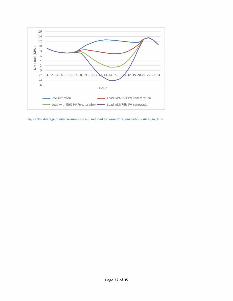
The average data for consumption, distributed generation and net load at Artesian in June is

illustrated in Figure 30 below.

4 PV Penetration = (PV Power nameplate capacity, kW) / (Peak Consumption, kWh/h)

of 35

Figure 30 - Average hourly consumption and net load for varied DG penetration - Artesian, June

of 35

6. Conclusions

Load data from five substations in the San Diego Gas and Electric service territory were studied. The

data was compiled in 15-minute average values over a period of three years (January 2010 to

December 2012). The substations included between three and nine distribution circuits or feeders.

Peak loads observed over the evaluation period ranged from 10.5 MW to 57.7 MW, and occurred in

July, September or December.

The photovoltaic solar power distributed generation (PV DG, or DG) assets related to each substation

varied in nameplate capacity from 3.6% to 10.3% of the peak load. The installations were

predominantly residential-scale.

Hourly weather data for the period were extracted from ground weather stations on the MesoWest

network; GOES-West satellite images were used to generate hourly values of total cloud cover and

solar irradiance.

Hourly values of solar power generation were derived for each substation using irradiance and

nameplate capacity information. To simulate power generation, a sample of 1012 PV installations

from the Net Energy Metering (NEM) San Diego data base were evaluated and modeled to form a

general model of the relationship between time of day and year, and power generation under clear-

sky conditions. The model was used to calculate generation and consumption hourly related to each

substation over the evaluation period.

The hourly consumption, distributed generation and net load data were calibrated over the three

year evaluation period to account for the changes in load and build-out of DG assets over time.

Net load data are presented by hour of day for each substation: the load profiles show considerable

variation between locations. The timing of peak load also varies considerably. Two of the five

substations have afternoon peaks in the summer months: these peaks are reduced by distributed

generation.

The report illustrates the variability in net load by summer-time hourly profiles including minimum

and maximum values at each substation. Variation by day-of-week, temperature and the time-step of

the record are discussed.

The report characterizes the relationship between consumption, distributed generation and net load

in terms of variables which affect the operation and management of power distribution systems; it

of 35

discusses the impact of variability of consumption within a circuit, and the extent of DG build-out on

risks to system stability. The report presents the frequency distribution of the DG-to-consumption

ratio at one substation for the DG build-out at the end of the evaluation period, and presents

equivalent frequency distribution plots for 25%, 50% and 75% DG penetration. The linear

relationship of these values may be used to extrapolate the impact of DG build-out on risk factors

related to distribution management.

Distributed generation plays a noticeable role in the daily load profile of the substations which were

studied. Consumption related to these substations can have a different profile from that of the net

load. At the levels of DG studied, distributed generation may smooth out the daily peaks and shift the

timing of the daily maximum load. However, as DG is deployed well beyond the 10% level of

penetration characterized in this study, the daily load profile may include a sharp ramp upward as

distributed generation declines and consumption increases.

In the absence of demand-side management, consumption is more fundamental than (net) load in

representing the underlying, behind-the-the-meter load parameter present in a circuit. Accordingly,

in forecasting load flow in circuits with considerable DG deployed, there may be merit to forecasting

distributed generation and consumption separately to obtain the net load forecast.

7. Recommendations

1. An evaluation is recommended of the precision of consumption-and-generation forecasts

relative to direct net load forecasts, at various substations or circuits and at varied levels of

DG penetration. The evaluation will inform strategic approaches to load forecasting and

distribution management systems in an environment of high-level DG penetration and

increasing ability to monitor load at high resolution.

2. Circuit-level or substation forecasts may be aggregated and compared with system-level

forecasts. With the variety of micro-climates and load profiles related to customer class in the

service territory, it may be possible to develop forecasts of detailed areas and aggregate the

results to improve system-level day-ahead forecasting.

3. Conditions which may threaten distribution system stability, e.g., voltage rise, frequency

control, control of power flow reversals, require simulation using load flow models. This

report evaluated the impact of increasing DG penetration on the total net load at the study

of 35

substations. Other parameters include the distribution of energy use and DG within the

circuit, the location and relative size of commercial-scale PV sites or other DG concentration

in the circuit, and the distance of DG concentration from the substation’s secondary bus.

report: net load forecasting with distributed · pdf file12/16/2014 · net load...

Documents