CONTRACT NO. 92-303. · . FINAL · REPORT

·_ , . JUNE 1995

Determination.of Variability in Leaf Biomass Densi_ties

of Conifers and Mixed Conifers Under Different Environmental Conditions·

in the San Joaquin Valley Air Basin

Determination of Variability in Leaf Biomass Densities of Conifers and Mixed Conifers Under Different Environmental

Conditions in the San Joaquin Valley Air Basin

Final Report

Contract No. 92-303

Prepared for:

California Air Resources Board Research Division

P.O.Box 2815 Sacramento, California 95812

Prepared by:

Patrick J. Temple Randall J. Mutters

Carol Adams Justin Greene

Randa11 Jackson Michael Guzy

Statewide Air Pollution Research Center University of California

Riverside, California 92521

June 1995

Disclaimer

The statements and conclusions in this report are those of the contractor and not

necessarily those of the California Air Resources Board. The mention of

commercial products, their source, or their use in connection with material

reported herein is not to be construed as actual or implied endorsement of such

products.

ii

Acknowledgments

We express our appreciation to Patricia Velasco and Robert Grant of the California Air

Resources Board for all their assistance towards completion of this project. Thanks also to Chris

LaClaire for manuscript preparation.

This report was submitted in fulfillment of ARB Contract Number 92-303,

"Determination of Variability in Leaf Biomass Densities of Conifers and Mixed Conifers Under

Different Environmental Conditions in the San Joaquin Valley Air Basin," by the Statewide Air

Pollution Research Center, University of California, Riverside, under the sponsorship of the

California Air Resources Board. Work was completed as of March 1995.

iii

Abstract

Biogenic emissions of reactive hydrocarbons from vegetation constitute a significant, but

as yet undefined, fraction of total hydrocarbon emissions in the San Joaquin Valley Air Basin

(SJV AB). Uncertainties in the amounts of reactive hydrocarbons emitted by vegetation have

contributed to uncertainties in models of regional ozone formation in the SNAB. The objective

of this research was to provide accurate estimates of foliar biomass per unit area, and the

variability associated with those estimates, for the dominant native vegetation of the western

slopes of the Sierra Nevada portion of the SNAB. Biomass sampling plots were established at

29 locations within the do~inant vegetation zones of the study area. All of the trees on each

500 m2 plot were measured for stem and canopy dimensions and branch samples were collected

from representative trees. Measurements of intercepted light and soil samples were collected

at each plot. Estimates of foliar biomass were made for each plot by three independent methods:

I. regression of tree diameter with leaf biomass; 2. light interception relative to leaf area index;

3. scaling from branch leaf area and biomass to whole canopy leaf area and biomass.

Multivariate regression analysis was used to relate these foliar biomass estimates for oak and for

conifer plots to a suite of independent predictor variables, including elevation, slope, aspect,

temperature, precipitation, and soil chemical characteristics. Results of the regression analyses

showed that elevation was the single most useful parameter to predict foliar biomass of conifer­

dominated plots. Regression equations for oak plots were generally not significant, possibly

because of lack of variability among the oak plots. Based on these results, GIS techniques were

employed to calculate foliar biomass of conifer and mixed conifer forest types in 2 x 2 km grid

cells across elevational gradients along the western slopes of the Sierras.

iv

Table of Contents

Page

Disclaiiner . . . . . . . . . . . . . . . . . . . . . . . . . . . . . . . . . . . . . . . . . . . . . . . . . ii

Acknowledgments . . . . . . . . . . . . . . . . . . . . . . . . . . . . . . . . . . . . . . . . . . . . iii

Abstract . . . . . . . . . . . . . . . . . . . . . . . . . . . . . . . . . . . . . . . . . . . . . . . . . . iv

List of Figures . . . . . . . . . . . . . . . . . . . . . . . . . . . . . . . . . . . . . . . . . . . . . . vii

List of Tables . . . . . . . . . . . . . . . . . . . . . . . . . . . . . . . . . . . . . . . . . . . . . . ix

INTRODUCTION AND STATEMENT OF THE PROBLEM .................. 1

A. The Role of Biogenic Hydrocarbon Emissions . . . . . . . . . . . . . . . . . . . 1

B. Dominant Vegetation Types of the Sierras ..................... 1

C. Methods for Estimating Foliar Biomass . . . . . . . . . . . . . . . . . . . . . . . 4

1. Allometric Relationships . . . . . . . . . . . . . . . . . . . . . . . . . . . . 4

2. Proportional Relationships . . . . . . . . . . . . . . . . . . . . . . . . . . 4

3. Light Interception . . . . . . . . . . . . . . . . . . . . . . . . . . . . . . . . 5

4. Remote Sensing Techniques ......................... 5

D. Objectives . . . . . . . . . . . . . . . . . . . . . . . . . . . . . . . . . . . . . . . . . 6

TASK 1. SELECTION OF VEGETATION SAMPLING SITES THAT REFLECT THE VARIABILITY OF THE ENVIRONMENTAL CONDITIONS THAT INFLUENCE TREE GROWTH ....................... 7

A. Methodology . . . . . . . . . . . . . . . . . . . . . . . . . . . . . . . . . . . . . . . 7

B. Results .......................................... 15

TASK 2. MEASUREMENT OF LEAF BIOMASS DENSITIES AND ENVIRONMENTAL VARIABLES IN THE FIELD .............. 21

A. Methodology .................................. 21

1. Tree Mensuration and Collection of Branch Samples . . . . . 21

2. Measurement of Intercepted Light ................ 22

B. Results ..................................... 22

TASK 3. ST A TISTICAL ANALYSES AND COMPILATION OF FOLIAR BIOMASS DATA ................................... 23

A. Methodology - Determination of Foliar Biomass . . . . . . . . . . . . 23

1. Allometric Relationships . . . . . . . . . . . . . . . . . . . . . . 23

2. Branch Volume to Crown Volume Relationships . . . . . . . 30

3. Light Interception Method for Estiinating Foliar Biomass 31

V

31 B. Estimates of Foliar Biomass . . . . . . . . . . . . . . . . . . . . . .

TASK 4. EXTRAPOLATION OF BIOMASS ESTIMATES FROM SAMPLING PLOTS TO GRIDDED COVERAGE ACROSS THE STUDY AREA ... 37

A. Methodology .................................. 37

1. Multivariate Regression Analyses . . . . . . . . . . . . . . . . . 37

2. Description of Independent Variables . . . . . . . . . . . . . . 38

3. Multivariate Regression Analyses . . . . . . . . . . . . . . . . . 40

B. Results ..................................... 41

1. Multivariate Regression Equations . . . . . . . . . . . . . . 41

2. GIS Analysis of Foliar Biomass . . . . . . . . . . . . . . . . 46

Appendices

Appendix 1. Tree mensuration data from biomass sampling plots

Appendix 2. Branch sample data from biomass sampling plots

Appendix 3. Light intercept data from each biomass sampling plot

Appendix 4. Soil samp]e analyses from each biomass sampling p]ot

Appendix 5. Foliar biomass on 2 x 2 km grid cells in the SNAB portion of the Sierras

Appendix 6. Procedures for ca1culating the foliated volume (V) of a tree

CONCLUSIONS AND RECOMMENDATIONS ......................... 49

REFERENCES . . . . . . . . . . . . . . . . . . . . . . . . . . . . . . . . . . . . . . . . . . . . . 51

Glossary of Terms, Abbreviations and Symbols .......................... 53

vi

List of Figures

Figure 1. Major vegetation types in the Sierra Nevada in relation to moisture and elevational gradients . . . . . . . . . . . . . . . . . . . . . . . . . . . 3

Figure 2. Dominant vegetation types of the SNAB, based upon CAL VEG as modified by the Desert Research Institute . . . . . . . . . . . . . . . . . . . . . 10

Figure 3. Forest zones of the lower and middle slopes of the SNAB portion of the Sierras, dominated by oak savannas and woodlands (foothills), ponderosa pine zone (lower slopes), and white fir dominated mixed conifer forests (middle slopes) . . . . . . . . . . . . . . . . . 11

Figure 4. Two x two kilometer grid coverages of ponderosa pine dominated areas located between 2000 to 2500 m elevation on south-facing O to 12 degree slopes in the Sierras . . . . . . . . . . . . . . . . . 12

Figure 5. Two x two kilometer grid coverages of white fir dominated areas located between 1500 to 2000 m elevation on south-facing O to 12 degree slopes . . . . . . . . . . . . . . . . . . . . . . . . . . . . . 13

Figure 6. Two x two kilometer grid coverages of white fir dominated areas located between 2000 to 2500 m elevation on south-facing O to 12 degree slopes . . . . . . . . . . . . . . . . . . . . . . . . . . . . . 14

Figure 7. Location of biomass sampling plots within the SNAB (outline) relative to elevational gradients in the Sierras ....... 20

Figure 8. Allometric relationship between leaf area and leaf dry weight for incense cedar (Calocedrus decu"ens), based upon branch samples collected from biomass sampling plots in the Sierras .......................................... 25

Figure 9. Allometric relationship between leaf area and leaf dry weight for white fir (Abies concolor), based upon branch samples collected from biomass sampling plots in the Sierras . . . . . . . . . 26

Figure 10. Allometric relationship between leaf area and leaf dry weight for California black oak (Quercus kelloggiz), based upon branch samples collected from biomass sampling plots in the Sierras ...................................... 27

vii

Figure 11. Allometric relationship betweer. leaf area and leaf dry weight for all pine species (Pinus spp.), based upon branch samples collected from biomass sampling plots in the Sierras . . . . . . . . . . . . . . 28

Figure 12. Elevational contour map of the SJVAB constructed from high-resolution DEM coverages .............................. 47

Figure 13. Foliar biomass estimates per 2 km grid cells of conifer and mixed conifer forest types in the SJVAB portion of the Sierras . . . . . . . . 48

viii

Table 1.

Table 2.

Table 3.

Table 4.

Table 5.

Table 6.

Table 7.

Table 8.

Table 9.

Table 10.

List of Tables

Summary of plot characteristics used in the classification of potential biomass sampling sites in the Sierras . . . . . . . . . . . . . . . . . . . 8

Location of biomass sampling plots and a description of the dominant and understory vegetation at each plot . . . . . . . . . . . . . . . . . 16

Site characteristics for biomass sampling plots in the SNAB . . . . . . . . . 19

Allometric relationships between leaf area and leaf dry weight, based upon branch samples collected on the biomass plots ............................................ 24

Allometric regression equations between foliar biomass and tree diameter (DBH) used to estimate leaf biomass for dominant trees in the Sierras . . . . . . . . . . . . . . . . . . . . . . . . . . . . . 29

Foliar biomass for tree species on biomass sampling plots, estimated by three independent techniques: 1. DBH; 2. crown volume; 3. light interception . . . . . . . . . . . . . . . . . . . ...... 32

Average foliar biomass (Mg ha·1) of dominant tree species of the western Sierra Nevada, estimated by three independent techniques; mean ±1 standard deviation ...................... 36

List of independent variables used in multivariate regression calculations . . . . . . . . . . . . . . . . . . . . . . . . . . .. . ....... 39

Summary list of coefficients for multivariate regression equations. Parameter coefficients a.re listed with ±1 standard error . . . . . 42

Multivariate regression equations between estimates of foliar biomass on sampling plots in the Sierras and environmental variables . . . . 44

ix

INTRODUCTION AND STATEMENT OF THE PROBLEM

A. The Role of Biogenic Hydrocarbon Emissions

Biogenic emissions of reactive hydrocarbons from naturally-occurring vegetation

constitute a significant but as yet undefined fraction of total volatile hydrocarbons in the San

Joaquin Valley Air Basin (SNAB). These biogenic hydrocarbons can contribute to

photochemically-generated oxidant air pollution in both urban and rural areas (Altschuller 1983;

Chameides et al. 1988; Dimitriades 1981). Inventories of biogenic hydrocarbon emissions are

crucial to complete emission source inventories in the SNAB and to assist in modeling studies

of photochemical oxidant pollution formation and dispersion in the SNAB. Compilation of a

complete inventory of biogenic hydrocarbon emissions for an air basin has two key components:

1. Field and laboratory studies of rates of reactive hydrocarbon emissions

from the dominant vegetation types in the area.

2. Estimates of foliar biomass densities across environmental gradients of the

dominant vegetation types, so that rates of natural hydrocarbon emissions

can be converted to amounts of hydrocarbon emitted on a temporal and

regional scale.

This report wiH address the need for a detailed inventory of leaf biomass densities by

providing estimates of the variability of foliar biomass for major vegetation types across

environmental gradients.

B. Dominant Vegetation Types of the Sierras

Previous studies of hydrocarbon emissions from natural vegetation have shown that oaks

(Quercus spp.) and conifers, particularly pines (Pinus spp.) are major sources of volatile reactive

hydrocarbons (Lamb et al. 1985). The principal hydrocarbon emitted from oaks and other

hardwoods is isoprene while a- and ~-pinene are the major components of hydrocarbon

emissions from conifers (Lamb et al. 1985). This suggests that the oak woodlands of the Sierra

foothills and the conifer and mixed conifer forest zones on the western slopes of the Sierra

1

Nevada may be significant sources of reactive hydrocarbons that may influence photochemical

oxidant formation in the SJV AB. Other major types of vegetation coverages that could also

contribute to biogenic hydrocarbon emissions, such as agricultural crops, urban landscaping, and

grasslands (Winer et al. 1990) will not be considered in this report.

The conifer and mixed conifer forest zones in the Sierras extend from approximately

1500 m to 2500 m in elevation. Within the broad conifer and mixed conifer zones, the

distribution and density of individual tree species are controlled by elevational and soil moisture

gradients (Fig. 1). Slope, aspect, soil edaphic properties, fire history, logging and other

disturbances also play major roles in determining plant distribution and biomass (Rundel et al.

1977). The lower dryer slopes of the Sierras are dominated by ponderosa pine (Pinus ponderosa

Laws.). In much of the ponderosa pine zone logging and other disturbances have led to

considerable replacement of pine with other tree species, including white fu [Abies concolor (G.

& G.) Lindi.] and incense cedar [Ca/ocedrus decurrens (Torr.) Florin]. On the more mesic

upper slopes, the mixed conifer forest type prevails, whose dominant species include ponderosa

pine, sugar pine (P. lambertiana Doug.), white fir, incense cedar, and California black oak

(Quercus kelloggii Newb.). Groves of giant sequoia [Sequoiadendron giganteum (Lindi.)

Buckh. Jdominate slopes or draws where soil moisture is abundant, and Jeffrey pine (P. jeffreyi

Grev. & Balf.) dominate exposed, rocky ridge crests. Above the mixed conifer zone, areas of

red fir (Abies magnijica Murr.) occupy more mesic sites and lodgepole pine [P. contorta var.

murryana (G. & B.) Critch.] are found on the rocky, exposed sites (Sudworth 1967).

Although the original scope of work of this project was confined to the conifer and mixed

conifer zones on the western slopes of the Sierras, the oak woodlands of the foothills, below the

ponderosa pine belt, were also surveyed. The oak woodlands were included because of the

importance of isoprene emissions from oaks and other hardwoods. Isoprene emission rates from

oaks can be 10 or more times greater than rates of terpene emissions from pines (Tanner and

Zielinska 1994). So, in consultation with ARB personnel, the original scope of work was

expanded to include estimates of foliar biom_ass from oak savannas and oak woodlands in the

foothills. The pristine oak woodlands of the Sierra foothills have mostly been converted to

grazing lands, but the remaining dominant trees include blue oak (Quercus douglasii Hook. &

Am.), canyon oak (Q. chrysolepis Liebm.), and gray pine (P. sabiniana Doug.). Several other

2

THE SIElU NEVADA

-~-~ ~ :> w -' w

4000--------------. Alp.ne Convnurwties

3000

2500

2000

1500

lodgepole Pine FOfest

Ponderosa Pine Forest

Mes.: Xeric MOISTURE GRADIENT

Figure 1. Major vegetation types in the Sierra Nevada in relation to moisture and elevational gradients [adapted from Rundel et al. (1977)].

3

species of oaks, including valley oak (Q. lobatt' Nee) and interior live oak (Q. wislizeni A.

deC.), are now highly localized in distribution.

C. Methods for Estimating Foliar Biomass

1. Allometric Relationships

The only technique for the direct measurement of foliar biomass and leaf area is

the destructive harvesting of the tree, removal of all the foliage, measuring the leaf area and

weighing the mass of leaves. This method is clearly impractical for the measurement of large

numbers of trees, so foresters have devised sampling techniques that rely on non-destructive

measurements of standing trees. The traditional technique involves the establishment of

allometric relationships between tree diameter or sapwood area and leaf mass (Brown 1978,

Westman 1987). This relationship is determined by the destructive harvesting of a limited

number of trees over a wide range of diameters and measurement of leaf area and leaf biomass

for the entire crown or for representative branches. Regression equations between tree diameter

at breast height (DBH) and leaf area and mass have been published for a number of tree species,

including several species in the study zone in the Sierras (Brown 1978, Westman 1987). The

primary advantages of this technique are that it is based on actual tree measurements and that

measurement of DBH is quick and accurate so that large numbers of trees can be sampled. The

major disadvantage of this procedure is that the regression equation between DBH and leaf

biomass is based upon a limited number of trees from a specific geographical area. Thus the

equations may not represent the unique characteristics of the trees from a particular sampling

plot nor do the allometric regression equations capture the potential variability of the relationship

between DBH and leaf biomass across environmental gradients.

2. Proportional Relationships

This technique employs the proportional relationship between the volume of

foliage on branches sampled from individual trees and the volume of foliage in the tree crown

as a whole. The leaf mass and area from the branch samples are measured and the percent of

the whole tree crown represented by the branch is calculated, and the data from the branch

samples are scaled up to estimate the tree crown as a whole. The advantage of this procedure

is that it is based upon easily-obtainable measurements of crown volumes from large numbers

4

of trees. The major disadvantage is that very large trees cannot be ,.;ampled because even the

lowest branches cannot be reached. In addition, tree crown geometry is assumed to be

symmetrical, which may not be valid for high density plots with overlapping crowns. Further

details of this technique are given in Task 2, Section A.

3. Light Interception

This technique for estimation of foliar biomass involves measurement of the

amount of incident photosynthetically-active solar radiation transmitted through the tree canopy,

in comparison with the amount of light measured in an open area. The amount of light

intercepted by the tree canopy has been shown to be proportional to the projected and total leaf

area of the canopy (Lang 1991, Pierce and Running 1988). Leaf area and leaf area index (LAI)

can be calculated from published equations and leaf biomass can be calculated from the

relationship between specific leaf area and leaf dry weight. Specific details of this technique

will be given in Task 2, Section A. This method has the advantage that measurements of

transmitted light can be made relatively quickly, so a large number of sample points can be

measured over a range of environmental conditions. Second, estimates of foliar biomass based

upon transmitted light can be directly compared with biomass estimates derived from reflected

light, as in Thematic Mapper data (see Section C.4. in Introduction). The major disadvantage

of this technique is that leaf area estimates are derived from equations using extinction

coefficients that have not been completely validated either theoretically or empirically (Lang and

Xiang 1986). The advantages and limitations of the light intercept method for estimating LAI

have been discussed in a number of recent publications (Norman and Campbell 1989).

4. Remote Sensing Techniques

Two previous estimates of foliar biomass in the SNAB (Engineering-Science

1990, Tanner et al. 1992) relied primarily on remote sensing data derived from satellite imagery

supplemented with aerial photography and existing vegetation classification databases. Data

from the Landsat Thematic Mapper was processed using a vegetation band ratio called the

Normalized Difference Vegetation Index (NDVI). The NDVI has been shown to differentiate

vegetation types and to provide estimates of growth and productivity based upon chlorophyll

reflectance measurements (Becker and Chandury 1988, Teng 1990). Once the boundaries and

geographical extent of the different classes of vegetation were delineated, a specific location

5

within a vegetation classification unit was selected and the foliar biomass was estimated for the

major plant species within the unit.

The major disadvantage of this technique is that biomass estimates within a

vegetation type were based upon samples not necessarily collected within that unit, so that

significant discrepancies were reported between leaf biomass estimates from the model and actual

measurements of leaf biomass from sampling in the field (Tanner et al. 1992). In addition, the

remote sensing data cannot be used to provide estimates of the variability of foliar biomass as

influenced by environmental factors. Environmental gradients can vary widely over relatively

short distances, particularly in mountainous terrain where slope, aspect, soil water, and soil type

can change rapidly with short changes in elevation. Estimates of foliar biomass based upon

"typical" units of a vegetation classification type cannot be used to estimate the error associated

with these rapidly-changing environmental gradients.

D. Objectives

The objective of this research was to provide estimates of foliar biomass per unit area,

and the variability associated with those estimates, for the dominant vegetation of the foothills

and western slopes of the Sierras in the SNAB portion of Tulare, Madera, Fresno, and Kem

Counties. Within each sampling plot foliar biomass was measured by three independent

techniques, which provided an estimate of the error associated with the biomass data. Foliar

biomass data from the sampling plots were aggregated on a regional scale using a multivariate

regression model that related foliar biomass to a suite of environmental variables. The

regression analysis provided confidence limits on the foliar biomass estimates and indicated the

statistical significance of the various environmental parameters as predictors of variations in

biomass densities across the study area.

6

TASK 1 SELECTION OF VEGETATION SAMPLING SITES THAT REFLECT THE

VARIABILITY OF THE ENVIRONMENT AL CO!\'DITIONS THAT INFLUENCETREEGRO~TH

A. Methodology

The initial criteria used in the process of site selection are listed in Table 1. These

criteria were selected by reference to the literature on the distribution of dominant vegetation

types in the Sierras, by reference to silvicultural manuals which describe the range of growing

conditions for each tree species, and by consultation with members of the US Forest Service

with extensive field experience in the Sierras. Toe primary attributes of each site were the

dominant vegetation type, and the slope, aspect, and elevation. The slope, aspect, and elevation

define to a large extent the environmental conditions under which the vegetation is growing and

thus define the potential biomass of the vegetation.

Specific criteria for the preliminary site selection process included the dominant

vegetation types of ponderosa pine, Jeffrey pine, and white fir, elevation ranges of 1500 to 3000

m at 500 m increments, slopes of O to 12 and 12 to 24 degrees, and northern (0 to 90, 270 to

360 degrees) and southern (90 to 270 degrees) aspects. Potential candidate sampling plots were

generated using ARC/INFO spatiaJ analysis techniques on the following databases: the California

Digital Elevation Model (DEM) at a resolution of 250 m, Desert Research lnstitute's enhanced

version of CALVEG, and coordinates of county lines, the outline of the San Joaquin Valley Air

Basin, and major roads from the Teale Data Center. All coverages were projected to Lambert

coordinates.

The California DEM was resampled at a resolution of 2000 m to generate a master grid,

2 km by 2 km, whose coverage was compatible with Radian's Biogenic Emission Inventory

Model. Missing cell values originating from missing USGS data points for some areas were

estimated using focal point mean procedures calculated from all adjoining grid cells with data

values. Polygon coverage was generated from the 2 x 2 km grid for intersection with other

databases for subsequent site selection. The polygon coverage was resampled and additional

coverages were generated based upon specified ranges in elevation for each vegetation type.

7

Table 1. Summary of plot characteristics used in the classification of potential biomass sampling sites in the Sierras.

1. Confine sampling sites to the San Joaquin Valley Air Basin portion of the western Sierras in Tulare, Madera, Fresno, and Kem Counties.

2. Dominant vegetation types:

a. Ponderosa pine/mixed conifer forest - CALVEG type no. 8

b. White fir/mixed conifer forest - CALVEG type no. 15

c. Jeffrey pine forest - CALVEG type no. 34

3. Elevation:

a. Ponderosa type:

i. 1500-2000 m ii. 2000-2500 m

b. White fir type:

i. 1500-2000 m ii. 2000-2500 m

c. Jeffrey pine type:

i. 2000-2500 m

4. Slope:

a. Flat to moderate: 0-12 degrees

b. Moderate to severe: 12-24 degrees

5. Aspect:

a. North-facing: 270 W - 90 E

b. South-facing: 90 E - 270 W

6. Accessible by roads or trails; not on private lands or in wilderness areas.

8

Aspect was determined for each grid by calcu:ating the down-slope direction of maximum

rate of change from each cell to its neighbors. The values of the output grid were the compass

directions of the aspect, in which O degrees = north, and which progressed to 360 degrees in

a clockwise direction. A polygon coverage was generated from the grid and then the grid was

resampled to determine the location of north and south-facing aspects.

An output slope grid was calculated as degree of slope, in which O degrees = level and

90 degrees = vertical. The range of mean slope values for individual 2 x 2 km cells within the

study area varied from O to 24 degrees. The steeper slopes expected within a mountainous

region were not expressed within the mean slope values because averaging over a 2 x 2 km grid

cell masked these extreme slope values. A polygon coverage was generated from the grid and

resampled to identify areas with slopes of O to 12 and 12 to 24 degrees.

To produce the final selection of potential sampling sites the reduced coverages described

above, representing the geographic distribution of the dominant vegetation types and the

specified elevations, slopes, and aspects, were intersected to compute the specific grid cells

common to the specified parameters. These cells have been displayed in a series of figures,

representing the geographical range within the study area of potential sampling sites that share

a specified set of parameters. In Figure 2 the dominant vegetation of the entire SNAB is shown

and the overall coverage of ponderosa pine, Jeffrey pine, and white fir are shown throughout

their range in the southern Sierras. The dominant vegetation types of the Sierra Nevada portion

of the SNAB are shown iI.1 Figure 3. The clear elevational gradient, from the oak-dominated

foothills, to ponderosa pine-dominated lower slopes, to white fir-dominated mixed conifer forests

on middle slopes, is well-illustrated in this figure. Figure 4 shows the distribution of the 2 x

2 km grid cells representing ponderosa pine growing at elevations between 2000 to 2500 m, on

0 to 12 degree slopes with south facing aspects. Figure 5 represents white fir growing between

1500 to 2000 m, on Oto 12 degree slopes with south-facing aspects. Figure 6 shows white fir

growing between 2000 to 2500 m on O to 12 degree slopes with south-facing aspects. Similar

maps were prepared for all other combinations of vegetation type, elevation, slope, and aspect.

In the original Request for Proposals and in the Technical Plan submitted in response to

that RFP, the scope of the project was confined to conifer and mixed conifer forest types of the

9

• Al&nual Grrmlad

• Mountain llnuh

• PtnUl,ro1t1 PIM

■ l•/frq PIM

ffldt,Fir•

□ ~•,un, • Yhld Dai Woodla"4

• BllU Oak Woodland

■ Afric,llbln t[ill OOur

0 6D Mi

• 51 1.00 Km

Figure 2. Dominant vegetation types of the SJVAB, based upon CALVEG as modified by the Desert Research Institute.

Reference Map

Po1Ukro,a PllU-0 3IJ 60Mi -

Mixed Oak Woodland I 511 100 X,,,

Figure 3. Forest zones of the lower and middle slopes of the SJVAB portion of the -Sierras, dominated by oak savannas and woodlands (foothills), ponderosa pine zone (lower slopes), and white fir dominated mixed conifer forests (middle slopes).

] l

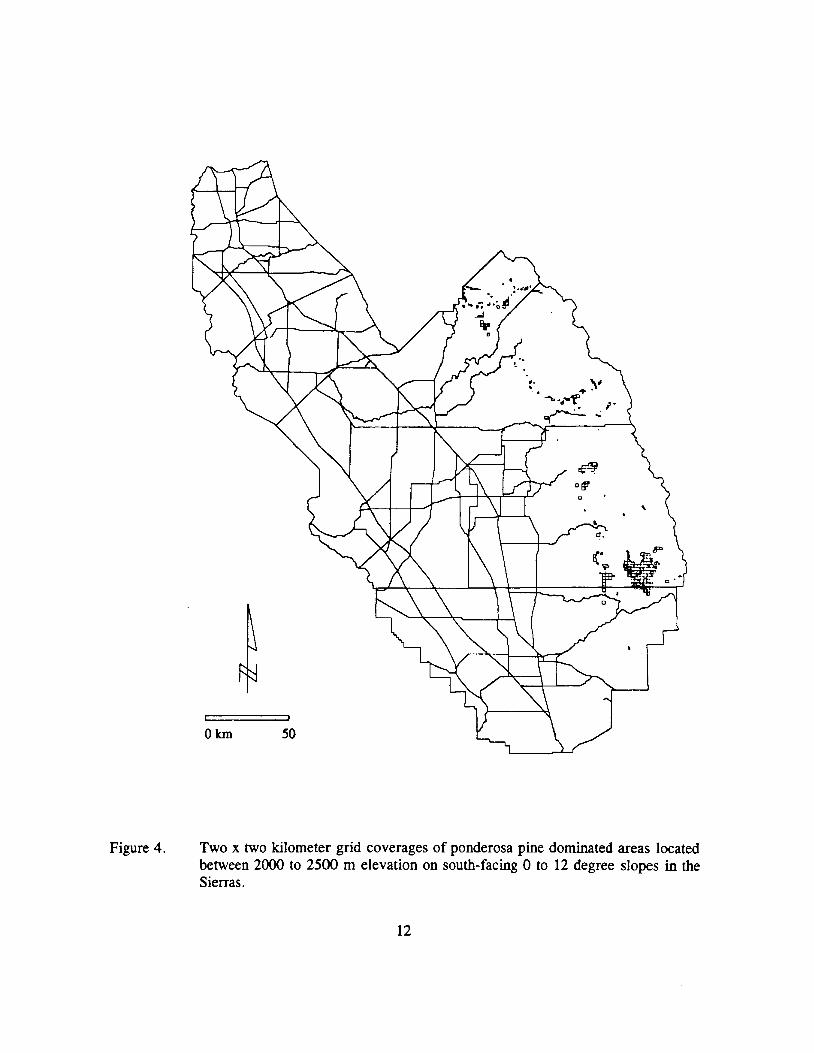
Figure 4. Two x two kilometer grid coverages of ponderosa pine dominated areas located between 2000 to 2500 m elevation on south-facing O to 12 degree slopes in the Sierras.

12

0km 50

Figure 5. Two x two kilometer grid coverages of white fir dominated areas located between 1500 to 2000 m elevation on south-facing Oto 12 degree slopes.

13

Figure 6. Two x two kilometer grid coverages of white fir dominated areas located between 2000 to 2500 m elevation on south-facing Oto 12 degree slopes.

14

western slopes of the Sierras. The initial protocol for selection of sites (n.ble 1) reflected this

restriction. Later, in consultation with CARB, the scope of work was expanded to include

biomass sampling plots in the mixed oak woodland vegetation type of the Sierra foothills (Fig.

2). This vegetation type has largely been converted to agricultural use, primarily orchards and

pasturelands, so only a limited number of plots were located in the oak zone.

B. Results

Between 7 July and 7 September 1993, a total of 29 vegetation sampling plots were

established from the Kernville/Lake Isabella area at the southern end of the Sierras to the

Madera/Mariposa county line at the northern limit of the SJV AB. The locations and a brief

description of each plot is given in Table 2. The site characteristics for each plot, including

dominant vegetation type, GIS coordinates, elevation, slope, and aspect are given in Table 3.

The location of each sample plot relative to its position on an elevational gradient from the

foothills to the middJe slopes of the western Sierras is shown in Figure 7.

15

Table 2. Location of biomass sampling plots and a description of the dominant ar.d understory vegetation at each plot.

Plot 1. Greenhorn Mts., 2.2 mi. S of Alta Sierra on Rancheria Rd., S facing slope dominated by second-growth incense cedar, white fir, and California black oak, with a few scattered large ponderosa pine; understory is mostly seedling incense cedar.

Plot 2. Greenhorn Mts. 1.3 mi. SE of Alta Sierra, N facing slope dominated by incense cedar and white fir, similar to Plot 1.

Plot 3. NE of KernvilJe, S facing. Jeffrey pine dominated, also incense cedar and white fir; understory is composed of a few California black oak.

Plot 4. Similar to plot 3, N facing. Jeffrey pines, white fir, and incense cedar.

Plot 5. Camp Nelson area, dirt road 1.4 mi. E of Redwood Drive on Hwy. 190. Ponderosa pine and Jeffrey pine dominated; understory mostly seedling and sapling incense cedar.

Plot 6. Holby Meadow Road, along Western Divide Hwy. above 2000 m, wide, flat ridge-top dominated by white fir; understory consists of white fir seedlings.

Plot 7. Balch Park Rd. 8.3 mi. E of intersection with Yokohl Rd. at 1500 m. Ponderosa pine dominated, mixed with black oak and incense cedar; understory is also incense cedar seedlings.

Plot 8. Hospital Rock Picnic Area, along Hwy. 198 in Sequoia National Park; S facing slope at 1000 min oak zone, dominated by valley oak (Quercus chrysolepis) with buckeye (Aesculus califomica) sub-dominant; understory consists of grasses and annual plants.

Plot 9. Hwy 198, 2.2 mi. E of Plot 8 at 1050 m. Open oak plot dominated by valley oak, black oak and scattered blue oak (Quercus douglasil); understory is scattered buckeye, Rhamnus sp. and Umbellularia californica.

Plot 10. White fir dominated; 6.0 mi N of plot 9 on General's Highway; S facing, mid­slope. Understory is western flowering dogwood (Camus Nuttalliz).

Plot 11. Wolverton Ski Area; Pack Animal Corral; 1.2 mi N of Gen Sherman parking lot. SW facing slope dominated by large white fir; understory is white fir saplings.

16

Table 2 (continued)

Plot 12. Montecito-Sequoia Lodge road; just past bridge over fust creek, 100 m S of road. Red fir (Abies magnifica) dominated. Red fu has dark reddish bark, much darker than white fu; red fir needles have two faint white lines on upper surface, white fir lacks these lines. One large lodgepole pine (Pinus contona) has "com flakes" bark. Understory is seedling white and red fus and Ribes (currants).

Plot 13. Lodgepole pine. Big Meadows road, 100 m E of "Starlight Trail" road 14S14. 100% lodgepole pine, understory is sparce lodgepole pine. Flat ridge-top.

Plot 14. Pack animal saddle area, 0.15 mi N of turnoff to Gen. Grant tree; S-facing, flat ridge-top. Large sugar pines (Pinus lambeniana) mixed with red fu and sapling sugar pines; understory is Rosa sp.

Plot 15. Jeffrey pine (Pinus jeffreyl), 0.1 mi S of turnoff to Stony Creek Lodge. 100% Jeffrey pine, sparce understory is also Jeffrey pine.

Plot 16. Mackenzie Ridge, Ponderosa pine dominated. Plot has large ponderosa pines and smaller incense cedar, understory is young white fir and also Ceanothus and Ribes. N-facing, near ridge top. 3.9 mi from Hwy 180, along left fork of turnoff to YMCA Sequoia Lake Camp, along road 13S67 until int. with 13S78, 50 m down 13S78, then 10 m down slope (over rocky ledge).

Plot 17. Mt. Home State Forest. Giant Sequoia/white fu dominated. Understory is a few white fu seedlings and Ribes. 20.3 mi from int. of Balch Park Rd. and Yokohl Rd. 200 m upslope, NW facing, mid-slope.

Plot 18. Shaver Lake, junction of Peterson Road and Big Creek Road. Ponderosa pine dominated, with mixture of sugar pine, incense cedar and California black oak; understory of pine and oak saplings and manzanita.

Plot 19. Shaver Lake, Soaproot Saddle Road, 2.6 mi E of Plot 18. Dense ponderosa pine stand; understory mostly manzanita ..

Plot 20. Hwy 168 N of Shaver Lake, at road 8S12. Mixture of large red and white fus on N facing slope; understory of fir saplings.

Plot 21. Hwy 168 at Tamarisk Ridge. Mixture of red and white firs on S facing slope.

Plot 22. Shaver Lake, Dinkey Creek Rd. at road 10S87. Dense Jeffrey pine stand; understory is Ribes spp. and manzanita.

17

Table 2 (continued)

Plot 23. Dinkey Creek Rd., 0.4 mi along road 10S76. Mixed conifer forest, ponderosa and sugar pines, incense cedar and a few white firs; understory of white fir and incense cedar seedlings.

Plot 24. Bass Lake. Ponderosa pine dominated, with understory of incense cedar and manzanita.

a few California black oak;

Plot 25. Hwy 41 at Madera/Mariposa county line. Mixed conifer forest, ponderosa and sugar pines; understory of incense cedar and white fir saplings.

Plot 26. San Joaquin Experimental Range, California State University, Fresno, 1.2 miles E of Highway 41 on Rd. 8063, 75 m S of road, S facing slope (3 °), rolling topography. Savannah dominated by scattered canyon oak (Quercus chrysolepis), blue oak (Quercus douglasil), and occasional grey pine (Pinus sabiniana) with an understory of perennial grasses.

Plot 27. E of Bakersfield on Breckenridge Rd, tum north on Democrat Rd, 1.1 mi., 100 E of road, SW facing 13° slope, rolling topography. Savannah dominated by blue oak (Quercus douglasil) with an understory of perennial grasses.

Plot 28. 3.5 mi E of California Hot Springs Rd on M-56, then Non Mtn Rd #52 for 2.3 mi., 50 m W of road, N facing 18° slope, rolling topography. Savannah dominated by blue oak (Quercus douglasil) with an understory of perennial grasses.

Plot 29. 0.5 mi. S of Ruth Hill Rd. on Ennis Rd. on E side of the road, S facing 14° slope, rocky rolling topography. Ruth Hill Rd. intersects with Highway 180 1 mi. E of Highway 63 in the Squaw Valley area. Savannah dominated by blue oak (Quecus douglasiz) with an understory of perennial grasses.

18

Table 3. Site characteristics for biomass sampling ;,lots in the SNAB.

Plot No. Dominant Lat. Elevation, Slope, Aspect, Vegetation meters degrees degrees

1 cedar/white fir 35.7 1950 9 160 2 cedar/white fir 35.7 1650 12 35 3 mixed conifer 35.9 2060 18 245 4 white fir 35.9 2150 17 0 5 cedar/white fir 36.2 1750 18 190 6 white fir 36.1 2200 6 50 7 ponderosa pine 36.3 980 15 180 8 oak woodland 36.5 950 24 45 9 oak woodland 36.6 1400 20 180

10 white fir 36.6 1500 17 0 11 white fir 36.6 2200 10 230 12 red fir 36.7 2150 5 130 13 lodgepole pine 36.7 2300 5 180 14 red fir 36.7 2200 8 195 15 Jeffrey pine 36.7 2100 10 150 16 ponderosa pine 36.7 1600 15 40 17 mixed conifer 36.2 1900 16 330 18 ponderosa pine 37.0 1375 0 210 19 ponderosa pine 37.0 1325 2 145 20 red/white fir 37.2 2200 10 220 21 red/white fir 37.2 2275 12 195 22 Jeffrey pine 37.1 2000 2 200 23 ponderosa pine 37.1 1800 8 215 24 ponderosa pine 37.3 1100 18 30 25 ponderosa pine 37.3 1400 11 180 26 oak woodland 37.1 450 3 210 27 oak woodland 35.4 950 13 120 28 oak woodland 35.9 700 18 0 29 oak woodland 36.7 400 14 200

19

, • fl MJ

.--===::i.-a::::=:,JII b

Figure 7. Location of biomass sampling plots within the SJVAB (outline) relative to elevational gradients in the Sierras.

20

TASK 2 l\1EASUREME!'.1 OF LEAF BIOMASS DENSITIES AND

ENVIRONMENTAL VARIABLES IN THE FIELD

A. Methodology

1. Tree Mensuration and Collection of Branch Samples

At each of the vegetation sampling sites a 500 m2 plot was established in areas

that were least disturbed and which most represented the mix of tree species, sizes, and crown

conditions that typified the plant community. At most sites this was accomplished by laying out

a plot 10 m wide by 50 m long, using a tape measure to ensure accuracy. The plots were

oriented with the long axis parallel to the main slope. At one site, Plot 15, a grid 20 x 25 m

was used. At each plot, the latitude, longitude, and elevation were measured using a portable

Global Positioning System (GPS) instrument (Model AVD-55, Garmin Inst. Co, Kansas City,

MO). Slope and aspect and other distinguishing characteristics were also recorded. A soil pit

was dug in each plot and the soil characteristics were recorded. Composited soil samples from

the A and B horizons were collected and submitted to the Soils Laboratory at UC Davis for

analysis of pH, total N, SO4 , and P, and exchangeable cations, including Ca, Mg, and K. The

A horizon is the surface soil layer, containing the highest amounts of organic material and in

which biological and microbial activity is maximum. The B horizon is the sub-surface layer

characterized by the accumulation of transformed organic and mineral materials leached from

the A horizon.

All the trees in the plot > 10 cm DBH were identified, tagged and numbered,

and the DBH was recorded for each. Tree heights and the length of the crown (from the top

of the tree to the point of the lowest foliated branch) was measured with a clinometer (Model

PM-5/1520, Suunto Corp., Finland). The crown base of each tree was measured along N-S and

E-W directions. Notes were also taken that recorded unusual conditions in the size or

irregularity of the tree crown. Branch samples were collected from six positions within the tree

crown, lower, middle, and top on the N and S sides of the tree. Branch samples were collected

with pruning poles to a maximum height of 6 m. For each branch, diameter at the base, total

length, foliated length, and height and width of the foliated portion were recorded in the field.

21

The branches were then returned to the laboratory where leaf areas, fresh weight and oven dry

weights of the foliage were recorded.

2. Measurement of Intercepted Light

Measurements of light transmitted through the canopy were taken at 10 locations

within each sampling plot with a PAR ceptometer (Decagon Devices, Inc., Seattle, WA). At

each point, the intensity of photosynthetically-active wavelengths of light (PAR) was measured

at 8 compass points (N, NE, E, SE, S, SW, W, NW), and the measurements were averaged to

produce a mean PAR for each of the 10 points within the plot. Similar measurements were

made in a clearing or open area nearby, to establish the total incident PAR at that time. In

addition, zenith angles to the horizon surrounding the plot were measured with a clinometer and

these data were recorded for each plot.

In addition to these measurements on the biomass sampling plots, an intensive

program of light transmittance measurements was conducted from 20 September to 8 October

1993 at 60 sites in the Huntington Lakes area east of Fresno. Thirty points were sampled on

both the south-facing and north-facing slopes of the watershed. Associate site variables, such

as tree species composition, elevation, slope, aspect, and angles to surrounding peaks were also

recorded. The objective of this feasibility study was to assess the variability of foliar biomass

over a small scale using the light-intercept technique.

B. Results

Tree mensuration data for all 29 biomass sampling plots are given in Appendix 1.

Branch sample data, including foliar volumes, leaf area, and leaf fresh and dry weights, are

given in Appendix 2. Light intercept data for all plots are given in Appendix 3, and soil sample

analyses for all plots are given in Appendix 4. The data in these Appendices were delivered to

the ARB on a 3. 5" disk, included in the Final Report.

22

TASK 3 STATISTICAL ANALYSES MTJl COMPILATION OF FOLIAR BIOMASS DATA

A. Methodology - Determination of Foliar Biomass

1. Allometric Relationships

Allometric relationships between leaf area and leaf fresh and dry weights were

established for each of the major tree species on the biomass plots by means of regression

analysis of foliage from the branch samples collected on the plots. These regression equations

are given in Table 4. Leaf area and leaf dry weights were highly correlated in these species and

regression coefficients typically were O. 90 or greater. The leaf area and leaf dry weight data

used in these calculations are shown graphically for incense cedar (Fig. 8), white fir (Fig. 9),

California b1ack oak (Fig. 10), and for four species of pines (Fig. 11). Insufficient numbers of

samples were available for the other tree species encountered on the biomass sampling plots to

establish regressions between leaf area and leaf dry weight for all species. Equations for

closely-related species were used instead. For example, the equation for canyon live oak

(Quercus chrysolepis) (Table 4) was used to relate leaf area to leaf dry weight for blue oak

(Quercus douglasil).

The regression equations between tree diameter (DBH) and foliar biomass used

in this study were taken from the literature. For white fir, red fir, ponderosa and Jeffrey pines,

and black and canyon oaks, the equations were derived from destructive harvesting of trees from

the immediate area of the study, either in Sequoia/Kings Canyon National Park or from the

western slopes of the southern Sierras. For the other species, the closest possible geographical

reference or substitute species was used. The regression equations used to calculate foliar

biomass from tree DBH used in this study are given in Table 5, together with the reference to

the original report in the literature. The DBH data were also used to calculate the basal area

for each species of tree on each plot. The basal area is a measure of the relative importance of

each species in the tree community.

23

Table 4. Allometric relationships between leaf area and leaf dry weight, based upon branch samples collected on the biomass plots.

Abies concolor (White fir)

Leaf area (cm2) = 1.9625 + 23.9515 (leaf d.w., g)

Abies magnifica (Red fu)

LA (m2) = -0.0695 + 0.0041 (leaf d.w., g)

Calocedrus decurrens (Incense cedar)

LA (cm2) = 15.0424 + 33.0870 (leaf d. w., g)

Quercus ch,ysolepis (Canyon live oak)

LA (cm2) = 127.43 + 40.2074 (leaf d.w., g)

Quercus kelloggii (California black oak)

LA (m2) = 0.2655 + 0.0156 (leaf d.w., g)

Pinus contona (Lodgepole pine)

LA (cm2) = -400.50 + 41.09 (leaf d.w., g)

Pinus jeffreyi (Jeffrey pine)

LA (cm2) = 90.60 + 29.36 (leaf d.w., g)

Pinus lambeniana (Sugar pine)

LA (cm2) = 180.37 + 50.20 (leaf d. w., g)

Pinus ponderosa (Ponderosa pine)

LA (cm2) = 451.42 + 34.21 (Jeaf d.w., g)

R2 = 0. 91

R2 = 0.92

R2 = 0. 99

R2 = 0.99

R2 = 0.83

R2 = 0.98

R2 = 0.99

R2 = 0.99

R2 = 0.96

24

rncense cedar

25000

• 20000

- 15000NE 0-(0

~ 10000(0-(0

a, ...J

5000

0

0 100 200 300 400 500 600 700

Leaf dry wt. (g)

Leaf area (cm2) = 15.0424 + 33.0870 (leaf d.w.) r2 = 0.99

Figure 8. Allometric relationship between leaf area and leaf dry weight for incense cedar (Calocedrus decurrens), based upon branch samples col1ected from biomass sampling plots in the Sierras; n = 19.

25

45

40

35

NE - 30 0 ......... ro 25Q)

ro '--Q) ro 20

....J

15

10

5

White Fir

0

0

0 1 2 3

Leaf dry wt (g)

Leaf area (cm2) = 1.9625 + 23.9515 (leaf dry wt.) r2 = 0.91

Figure 9. Allometric relationship between leaf area and leaf dry weight for white fir (Abies concolor), based upon branch samples collected from biomass sampling plots in the Sierras; n = 66.

26

••

Cal. Black Oak

5-.---------------------------,

4 • -NE ......., 3 ro

-~ ro ro a, -' 2

1

0 ~----~-----,-----,-----.,....----------

0 50 100 150 200 250

Leaf dry wt. (g}

Leaf area (m2) = -0.2655 + 0.0156 (leaf dry wt.) r2 = 0.83

Figure 10. Allometric relationship between leaf area and leaf dry weight for California black oak (Quercus kelloggil), based upon branch samples collected from biomass sampling plots in the Sierras; n = 14.

27

All pine spp.

0 100 200 300 400 500 600 700 800

Leaf dry wt. (g)

Figure 11. Allometric relationship between leaf area and leaf dry weight for all pine species (Pinus spp.), based upon branch samples collected from biomass sampling plots in the Sierras; n = 32.

28

35000 ---------------------,

D

30000

25000 -NE 0 ......... 20000 (0

~ ,.._ (0

15000 (0 a,

...J

10000

5000

0

Table 5. Allometric regression equations between foliar biomass and tree diameter (DBH) used to estimate leaf biomass for dominant trees in the Sierras.

Species Location Reference

Abies concolor: Sierras Westman (1987)

In (biomass, g) = 1.89 (In DBH, cm) + 3.82

Abies magnifica: Sierras Westman ( 1987)

In (biomass, g) = 2.93 (In DBH, cm) - 0.13

Calocedrus decurrens, no equation in literature; substituted Thuja plicata: Montana Kendall Snell and Brown (1978)

In (biomass, g) = 1.36 (In DBH, cm) + 5.31

Pinus contorta. jefjreyi, lambertiana, ponderosa; for all Pinus spp. used P. ponderosa: Sierras Kittridge (1944)

log (biomass, kg) = 1.67 (log DBH, in) - 0. 73

Quercus chrysolepis, douglasii, lobata; used Q. chrysolepis: Sierras Kittridge ( 1944)

log (biomass, kg) = 2.66 (log DBH, in) - 1.36

Quercus kelloggii, no equation in literature; substituted Q. velutina: Tennessee Rothacker et al. (1954)

log (N) = 1.86 (log DBH, in) + 2.44 N = no. of leaves; each leaf weighed 0.53 ± 0.28 g

Camus nuttallii, no equation in literature; substituted C. florida: Tennessee Rothacker et al. (1954)

log (N) = 2.05 (log DBH, in) + 2.86 N = no. of leaves; each leaf weighed 0.15 ± 0.05 g

Aesculus califomicus, no equation in literature; substituted Carya tomentosa: Tennessee Rothacker et al. (1954)

log (N) = 1.52 (log DBH, in) + 2.31 N = no. of leaves; each leaf weighed 0.82 ± 0.65 g

29

2. Branch Volume to Crown Volume Relationships

This method for calculating foliar biomass used the relationship between the

volume of foliage on branches sampled from individual trees and the volume of foliage in the

tree crown as a whole. For those species whose shape approximated a cone, such as pines, firs,

and incense cedar, the total volume in the tree crown was calculated by the hollow cone method;

i.e., volume = outer cone volume - inner cone volume. The outside dimensions of the cone

were the major and minor axes at the base of the canopy and the canopy height. The inside

dimensions of the hollow cone were derived from measurements of branch samples, using the

unfoliated length of the branch and the DBH of the trunk to determine the internal volume of

the canopy not occupied by foliage. Thus, volume of foliage in a conical tree crown:

V = 1/12 1r abh - 1/3 1r r2h

in which a and b are the lengths of the major and minor axes at the base of the canopy, h is

canopy height, and r is the average length of the unfoliated branches plus the average radius of

the trunk. Calculations for spherically-shaped canopies, such as the oaks, were similar, except

that formulae for volumes of ellipsoids were substituted for those of cones.

Foliar volume of a branch sample was calculated from measurements of foliated

branch length, width, and height:

V (branch) = 1r abh

Total foliage density within a branch was calculated as the total leaf surface area per foliated

volume. The leaf surface area as measured by the leaf area meter was multiplied by 1r for

cylindrical leaves, such as pine needles, or by 2 for flat leaves, such as the oaks. The mean

foliage density per species was calculated from all available branch samples for that species and

this mean foliage density was applied to the trees for which no branch samples had been

collected. Total leaf area for each tree was calculated using the mean foliar density and the total

foliated crown volume. Total leaf area was converted to biomass using the regression equations

30

for leaf area/leaf biomass given in Table 4. These individual tree foliar biomasses were summed

to produce a total foliar biomass for each species on each plot.

3. Light Interception Method for Estimating Foliar Biomass

Foliar biomass was estimated from light interception data using the method

outlined by Nonnan (1988). Measurements of intercepted PAR under the tree canopy and PAR

measurements at full sunlight were related to the total leaf area of the canopy using the

relationship:

LAI = ( (tb (1 - cos 0) - 1) In ( Ea/Ei) I 0.72 - 0.337 tb)

in which LAI is leaf area index, Ea = PAR outside the canopy, Ead = Par outside the canopy

with the light sensor shaded, Ei = average PAR under the canopy, tb = (Ea-Ead)/Ea, and

e = zenith angle. LAI was converted to leaf area by multiplying by the area of the plot (500

m2). This total plot leaf area was proportioned to the individual tree species on the plots based

upon the percent basal area for each species on the plot. The leaf area was converted to foliar

biomass using the regression equations given in Table 4.

B. Estimates of Foliar Biomass

Biomass of foliage for all the trees on the sampling plots, estimated by the three

independent techniques described above, is given in Table 6. Analysis of the data in Table 6

by individual tree species showed that for most species the three methods gave biomass estimates

that were generally comparable (Table 7), although the method based upon crown volume

relationships (Method 2) averaged higher than Method 1 (DBH) or Method 3 (light interception).

For two species, however, these estimation techniques appeared to produce anomalous results.

The crown volume method overestimated biomass of Jeffrey pine, particularly on Plot 15, where

the Jeffrey pines constituted a small number (n = 9) of large, open-grown trees. The DBH

method appeared to overestimate the biomass of red fir on those plots in which red fir was the

dominant or co-dominant tree species, particularly on Plots 12, 20, and 21 (Table 6). Further

analysis of the biomass data from Table 6 proceeded with the entire data set and also with the

data from these plots estimated by these particular techniques removed from the data set.

31

Tab]e 6. Fc1iar biomass for tree species on biomass sampling plots, estimated by three independent techniques: 1. DBH; 2. crown vo]ume;

3. light interception.

Foliar biomass (kg)

Plot

No. Species

No.

trees DBH Volume Light

1 C. decurrens 25 590.3 1076.2 220.9

A. concolor 6 39.7 97.0 20.5

P. jeffreyi 1 48.5 62.9 20.4

Q. kelloggii 3 85.1 32.1 6.8

2 A. conco]or 2 42.0 69.8 44.2

C. decurrens 34 596.5 436.9 454.8

P. ponderosa 2 75.2 61.0 55.4

Q. kelloggii 5 144.5 48.9 23.4

3 A. concolor 11 246.9 391.9 270.7

C. decurrens 10 174.7 124.9 138.7

P. jeffreyi 6 360.8 1847.7 322.8

Q. kelloggii 6 41.1 15.6 6.9

4 A. conco]or

P. Jeffreyi

12

23

222.2

269.6

280.0

447.9

515.4

510.1

5 A. concolor 6 237.3 259.4 199.0

C. decurrens 34 866.8 333.2 526.2

P. Jambertiana 1 11.2 5.2 4.5

P. ponderosa 1 62.9 41.6 36.9

Q. chrysolepis 3 52.4 9.2 26.2

Q. kelloggii 7 110.2 40.8 14.2

32

Foliar biomass (kg)

6 A. concolor 28 2323.7 1813.5 1270.4

7 C. decurrens 1 17.7 57.8 22.0

P. ponderosa 27 436.1 167.6 523.7

Q. chrysolepis 1 3.4 8.9 3.5

Q. kelloggii 17 66.7 62.9 17.6

8 A. californica

Q. chrysolepis

25

20

85.6

777.2

- -

886.8 484.2

9 A. californica

Q. chrysolepis

Q. kelloggii

8

5

44

22.5

16.6

431.5

-53.0

850.9

-15.2

101.9

10 A. concolor 15 1334.7 2057.1 910.4

C. decurrens 6 159.9 604.9 79.0

C. nuttallii 5 12.7 - -

P. lambertiana 1 123.0 282.3 40.0

11 A. concolor 19 2659.0 1549.9 883.7

12 A. magnifica

P. contorta

48

1

9949.8

88.0

4670.8

47.0

723.4

6.3

13 A. concolor

P. contorta

1

43

10.2

680.2

6.6

755.9

10.7

416.3

14 A. magnifica

C. decurrens

P. lambertiana

38

1

5

382.2

28.9

319.4

631.6

37.8

742.1

392.2

36.4

265.1

15 P. jeffreyi 9 289.3 210.6 259.0

33

Foliar biomass (kg)

16 A. concolor

C. decurrens

P. ponderosa

1

7

18

74.1

186.2

609.4

89.0

533.5

314.7

95.5

173.7

549.9

17 A. concolor

P. ponderosa

S. gigantea

6

3

12

338.2

7.4

-

643.5

3.6

-

855.4

13.1

-

18 C. decurrens 1 12.9 24.8 27.3

P. lambertiana 2 31.5 22.7 44.0

P. ponderosa 10 210.9 285.5 432.1

Q. chrysolepis 1 0.2 0.9 0.3

Q. kelloggii 1 19.7 67.7 8.9

19 C. decurrens

P. ponderosa

7

24

14.5

326.5

98.9

164.1

28.2

613.9

20 A. concolor

A. magnifica

42

4

1908.8

2508.6

2577.5

497.4

503.0

390.0

21 A. concolor

A. magnifica

8

13

510.4

4326.6

694.5

614.5

56.2

280.9

22 C. decurrens

P. jeffreyi

1

27

6.0

479.3

10.5

361.6

8.6

774.1

23 A. concolor 10 111.2 173.5 193.3

C. decurrens 13 284.2 1576.1 357.6

P. lambertiana 10 169.0 200.8 140.2

P. ponderosa 6 366.1 447.4 445.5

34

Foliar biomass (kg)

C. decurrens 4 143.424 86.2 298.1

P. ponderosa 11 224.0 182.2 360.3

Q. kelloggii 4 178.6 164.3 63.0

117.5C. decurrens 5 77.8 168.625

P. lambertiana 73.5 43.32 43.5

P. ponderosa 395.714 478.6 699.1

P. sabiniana 226 51.8 - -

Q. chrysolepis 7 219.2 142.6202.4

178.3Q. douglasii 5 176.5 124.4

7 537.7 133.6Q. douglasii 89.427

557.4Q. douglasii 12 464.0 120.928

541.9 1189.5Q. douglasii 10 113.529

35

Table 7. Average foliar biomass (Mg ha- 1) of dominant tree species of the

western Sierra Nevada, estimated by three independent techniques; mean ±1 standard deviation.

Foliar biomass (Mg ha-1)

Species n DBH volume light interception

White fir 167 14.36 (18.48) 15 .28 (17 .20) 8.32 (8.26)

Incense cedar 149 4.42 (5.40) 7.92 (9.06) 3.34 (3.34)

Jeffrey pine 66 5.80 (3.16) 19.30 (18.78) 7.54 (5.66)

Black oak 43 2. 70 (2.62) 3.22 (5.66) 0.60 (0.68)

Ponderosa 103 5.60 (3. 96) 4.12 (3.02) 7.46 (5.04)

Sugar pine 21 2.32 (2.32) 4.42 (5.54) 1.80 (1.94)

Canyon oak 19 3.50 (6.08) 3.92 (6.96) 2.24 (3.80)

Red fir 103 85.84 (82.04) 32.06 (40.92) 8.94 (3.84)

Lodgepole 47 7.68 (8.38) 8.02 (10.02) 4.22 (5.80)

Blue oak 34 8.60 (3.46) 10.30 (9.76) 2.24 (0.32)

36

TASK4 EXTRAPOLATION OF BIOMASS ESTTh1ATES FROM SAMPLING PLOTS TO

GRIDDED COVERAGE ACROSS THE STUDY AREA

A. Methodology

1. Multivariate Regression Analyses

The final phase of the biomass project involved the calculation of multivariate

regression equations linking foliar biomass estimates on the sampling plots to GIS and

environmental parameters that were associated with those estimates. The multivariate regression

equations were then used to extrapolate foliar biomass across environmental gradients in forested

areas of the foothills and mountains in the San Joaquin Valley Air Basin.

In the initial phase of data analysis scatter graphs were made for the biomass estimates,

both on a per plot and on a per tree per species per plot basis. These scatter graphs were used

to check for outliers and to look for patterns that would suggest curvilinear or multiple

polynomial relationships. Some outlier data were identified as a result of this preliminary

screening, and several plots were revisited and trees resampled to increase the precision of the

original data set. In addition, plot 17 was eliminated from the data set. This plot was

dominated by Giant Sequoia but as no biomass estimates could be made for this species, the data

set from this plot could not be used. Preliminary data analyses also showed large variations in

biomass among plots, due largely to variability in site quality across environmental gradients.

A natural log transfonnation of the biomass data was used to equalize variances, to normalize

distribution of residuals, and to enhance linear relationships between biomass and independent

variables.

Preliminary statistical analyses using estimates of biomass for individual tree species to

develop equations for the prediction of foliar biomass on a per species basis showed that this was

not possible for this data set. First, the different tree species were present in only a limited

subset of biomass sampling plots. White fir was present in the highest number of plots, 14.

Ponderosa pine was found in only 10 plots. Red fir was present in only three plots. Second,

the number of individual trees of each species sampled on each plot was highly variable. For

example, white fir was the only species present on plot 6, where 28 trees were sampled. On

plot 16, 26 trees were sampled, but only one white fir was found on the plot. Because of the

37

high degree of variability in number of trees of e1ch species per plot and because of the limited

number of sampling plots in which the individual species were represented, regression equations

between foliar biomass and independent variables were generally not significant. Data analysis

proceeded using total foliar biomass per plot as the dependent variable.

The preliminary data screening also showed that the biomass estimates across plots

differed significantly between conifer-dominated plots and oak-dominated plots. Environmental

variables also divided along similar lines, as the oak-dominated plots were confined to the

warmer, drier foothills and lower slopes of the Sierras. For these reasons, separate multivariate

equations were fit for the conifer plots and for the oak plots.

2. Description of Independent Variables

The independent variables used in the preliminary data analyses are listed in Table 8.

The variable list included site descriptors such as latitude, longitude, elevation, slope and aspect,

maximum and minimum temperatures for each of the four seasons, and average precipitation for

the last 10 years. Temperature and precipitation data were collected from the nearest long-term

climatological station to the plot. Also included were site-specific soil characteristics, such as

depth of litter layer, depth of A horizon, and soil chemical analyses for S, N, P, K, Ca, and

Mg. These variables were of two types: (1) The site descriptors were derived from GIS

coverages and thus can be accessed remotely for any point within the coverage area. (2) The

site-specific soil characteristics were determined from soil samples collected on-site, and thus

cannot be derived from GIS coverages. This distinction was maintained in the data analyses,

so that two different sets of independent variables were included in the multivariate calculations:

(1) the "GIS" set; (2) the complete set, including GIS and soil characteristics. Additional

independent variables were derived from this original set by calculating interaction terms, such

as precipitation by temperature, precipitation by N, or precipitation by the ratio of Ca to Mg.

A final list of independent variables was determined by preliminary analyses of the data and by

reference to the literature for potential interactions among variables. This list included

approximately 75 variables, comprising original independent variables, curvilinear (quadratic)

terms, and multiple interaction terms.

38

Table 8. List of independent variables used in multivariate regression calculations.

A. GIS- Derived:

Temperature: spring, summer, fall, winter max and min T (C) Precipitation: mean annual ppt for last 10 years (cm) Latitude, longitude, elevation (m), slope (degrees), aspect (degrees, N or S)

B. Site-Specific Soil Samples:

Litter depth (cm), depth of A horizon (cm) Chemical analyses for A and B horizons: N, SO4 , available P, K, Ca, Mg

C. Calculated Ratios and Interactions:

Ppt x temp Ppt X N Ppt x Ca/Mg etc.

The independent variables were analyzed for principal components and factors to

determine if the large number of variables could be replaced by a significantly reduced number

of components or factors, or by a smaller sub-set of variables, one for each component or factor.

This analysis showed that relationships among the independent variables were generally not

strong enough to select representative components or factors. The exception was temperature,

in which all independent temperature variables could be represented by a single factor.

However, some initial regression analyses bad shown that higher correlation coefficients were

obtained with specific seasonal temperatures, relative to yearly mean temperature. Because of

the loss of sensitivity to this key predictor variable for biomass if a factor were substituted, the

original set of independent temperature variables was retained in the final multivariate regression

analyses.

39

3. Multivariate Regression Analyses

Because of the large number of independent variables, backwards elimination regression

could not be used. Consequently, stepwise regression analysis was used, with some restrictions

on the maximum number of variables included in each equation. For the conifer plots, in which

n = 22, a maximum of seven independent variables was allowed. For the oak plots, in which

n = 6, only two variables were permitted to enter the equations. These restrictions were

imposed to prevent overparameterization of the models. Three runs were conducted for each

data set, at p = 0.05, 0.10, and 0.15; where p is the probability for entry or removal of a

variable from the model. This analysis was conducted to identify potential candidate variables

for inclusion in the multivariate model. In the final equation, each variable included was

significant at p = 0.05 or lower. The final model was selected to meet all the following

criteria: (1) all variables included were significant at p = 0.05 or lower; (2) the number of

variables included did not exceed the limit imposed by the overparameterization restriction; (3)

the model had the highest coefficient of determination (r2); i.e,. had the highest predictive

potential.

Multivariate regression models were computed using SAS for each of eight biomass data

sets, including the three methods of biomass estimation and the geometric mean of the three

biomass data sets, calculated separately for oak plots and conifer plots. In addition, separate

equations were calculated using only the GIS variables, and the complete variable set including

soil analyses. As a measure of the precision of the regression estimates, 95 %confidence limits

were calculated for all multiple regression equations that were statistically significa_nt. The SAS

statistical library provides 95 % confidence limits for individual data points in a regression

model. These confidence limits are equivalent to 95 % confidence bands around a simple linear

regression equation, and should be interpreted similarly. That is, 95 % of the time the predicted

biomass of a new plot randomly sampled from the same population of plots used in the original

analyses will fall within these confidence limits.

40

B. Resu'ts

1. Multivariate Regression Equations

The coefficients of regression equations for predicting foliar biomass of conifers

and oaks across environmental gradients in the SNAB portion of the Sierras are listed in Table

9. Regression equations based upon the coefficients listed in Table 9 are given in Table 10.

Separate equations are given for each method of biomass estimation and for the geometric

mean of the three methods. For conifers, elevation, temperature and precipitation interactions,

and Ca to Mg ratios in the A horizon were the most significant variables for predicting biomass.

As expected, the sites at higher elevations had higher precipitation and lower temperatures,

which reduced evapotranspiration and increased the amount of water available for tree growth.

This association between elevation and foliar biomass was most clearly demonstrated in the GIS

regressions, in which elevation was the most significant variable, and in some cases the only

significant variable, for prediction of biomass. Method 1, based on DBH, appeared to produce

the best estimates of biomass relative to the other procedures and to the geometric mean of the

three methods. The "best fit" regression equation, including all variables, accounted for 90%

of the variability in foliar biomass across the conifer plots. The "best fit" regression equation

based only on GIS variables accounted for 70% of the variability in biomass across the plots.

Although the regression equation relating foliar biomass as estimated by Method 1 to the

GIS data sets had an R2 of 0. 703 (Table 9), the ability of this equation to predict foliar biomass

in areas outside the original sample set was not known. An approximate test of the predictive

ability of the regression equation, known as the "jackknife," was used to assess the predictive

powers of the relationship between foliar biomass and GIS variables (L. Larsen, CARB, personal

communication). The first step of the jackknife process consisted of calculations of new

regression equations between Method 1 foliar biomass and GIS variables for each sub-set of 21

plots out of the total of 22 conifer plots. Thus, in tum, one plot of the 22 was left out of the

biomass data set, and 22 new regression equations were calculated using the remaining 21 data

sets. Each of these regression models was then used to calculate a predicted value for the

excluded plot. The observed values for foliar biomass for the excluded plots were then

correlated with the predicted values from the new regression equations. The correlation

41

Table 9. Summary list of ;oefficients for multivariate regression equations. Parameter coefficients are listed with ±1 standard error.

A. Conifer plots (n = 22}

Y = In (total plot biomass, kg)

Method p > F

1 (DBH) 0.904 0.0001

3 (Volume) 0.609 0.0006

4 (Light) 0.815 0.0003

Geometric 0. 829 0.0001 mean

Y = In (total plot biomass)

0. 703 0.0008

X = total variable list

Significant variables

aspect summer max T ppt x spring min T ppt x fall max T (ppt)2 x Ca/Mg (A) intercept

elevation (ppt)2 X N (A) (ppt)2 x N (B) intercept

aspect depth of (A) PIK (A) Ca/Mg (A) winter min T ppt x fall min T (ppt)2 x (winter min T)2 intercept

elevation K (B) PIK (A) Ca/Mg (A) (ppt)2 x winter min T intercept

- 0.69 - 0.10

0.001 - 0.004

6x10-6 11.03

0.002 - 0.002

0.004 3.13

- 0.39 - 0.05 - 0.0006

0.06 0.113

- 0.003 - lxl0-7

7.85

0.001 0.99

- 5xl0-5

0.075 - lxlo-6

3.63

X = GIS variables list

elevation ppt x fall max T (spring min T)2 (ppt)2 x winter min T (ppt)2 x spring min T intercept

0.001 - 0.0044 - 0.044 - 9xlo-6

0.0002 5.88

Coefficients

(0.10) (0.04) (0.0005) (0.001) (5x10-6) (0.92)

(0.0004) (0.0001) (0.001) (0.74)

(0.13) (0.016) (0.0001) (0.015) (0.03) (0.0008) (5xl0·8)

(0.32)

(0.0002) (0.29) (2xl0·5)

(0.018) (3xl0·7)

(0.44)

(0.0004) (0.0015) (0.018) (2x10-6) (4x10-6) (0.92)

42

1

Table 9 (continued)

3 0.306

4 n.s.

Geometric 0.260 mean

B. Oak plots (n

1 0.947

3 0.985

4 0.912

Geometric 0.979 mean

1 n.s.

3 0.968

4 n.s.

Geometric 0.679

0.008

0.015

= 6)

0.012

0.002

0.026

0.003

0.006

0.044

elevation 0.001 (0.0004) intercept 4.88 (0.72)

mean 6.50 (0.093)

elevation 0.0008 (0.0003) intercept 5.39 (0.54)

X = total variable list

slope 0.02 (0.004) S04-S (A) - 0.125 (0.023) intercept 7.10 (0.22)

P(B) - 0.015 (0.003) spring max T 1.31 (0.27) intercept - 30.40 (7.63)

litter depth 1.26 (0.37) K (A) - 4.68 (0.84) intercept 6.69 (0.46)

K (A) - 2.10 (0.21) S04-S (B) 0.068 (0.012) intercept 6.74 (0.18)

X = GIS variable list

mean 6.28 (0.10)

spring max T 1.84 (0.29) (fall min n2 0.03 (0.01) intercept - 46.89 (8.24)

mean 5.14 (0.29)

spring min T 0.44 (0.15) intercept 0.67 (l.81)

43

Table 10. Multivariate regression equations between estimates of foI:ar biomass on sampling plots in the Sierras and environmental variables. Y = In (total foliar biomass, kg).

A. Conifer plots (n = 22)

I. Total variable list, including soil analyses

Method 1 (DBH) Y = 11.03 - 0.69 (aspect)- 0.10 (summer max n + 0.001 (ppt x spring min n -0.004 (ppt x fall max T) + 6x10-6 [(ppt)2 x Ca/Mg(A)].

Method 2 (volume) Y = 3.13 + 0.002 (elevation - 0.002 [(ppt)2 x N(A)] + 0.004 (ppt)2 x N(B).

Method 3 (light) Y = 7.85 - 0.39(aspect) - 0.05 [depth of (A)) - 0.0006 [PIK (A)) + 0.06 [Ca/Mg (A)) + 0.l 13(winter min n -0.003 (ppt x fall min T)- 1 x 10·1 [(ppt)2 x (winter min

n2J.

Geometric mean Y = 3.63 + 0.001 (elevation) + 0.99 [K (B)] - 5 x 10-s [PIK (A)) + 0.075 [Ca/Mg (A)) - 1 x 10-6 [(ppt)2 x winter min T].

2. GIS variables list

Method 1 Y = 5.88 + 0.001 (elevation) - 0.0044 (ppt x fall max T) - 0.044 [spring min T)2] - 9 x J0-6 [(ppt)2 x winter min T] + 0.0002 [(ppl)2 x spring min T].

Method 2 Y = 4.88 + 0.001 (elevation)

Method 3 n.s.

Geometric mean Y = 5.39 + 0.0008 (elevation)

B. Oak plots (n = 6)

l. Total variable list

Method 1 Y = 7.10 + 0.02 (slope) - 0.125 [SO4 (A)].

Method 2 Y = - 30.40 - 0.oI5 [P (B)) + 1.31 (spring max T).

Method 3 Y = 6.69 + 1.26 (litter depth) - 4.68 [K (A)].

Geometric mean Y = 6.74 - 2.10 [K (A)J + 0.068 rso. (B)J.

2. GIS variables list

Method 1 n.s.

Method 2 Y = -46.89 + 1.84 {spring max T) + O.o3 [(fall min T)2]

Method 3 n.s.

Geometric mean Y = 0.67 + 0.44 (spring min T).

44

coefficient for observed vs. predicted biomass values was 0.242, indicating relatively poor ability

of the full GIS model to predict foliar biomass of a plot not in the original data set.

The jackknife procedure also provided valuable information on the stability of the

independent variables included in the multivariate regression equations. Elevation appeared in

17 of the 22 models, and various precipitation by temperature interactions appeared in 19 of the

22 models. These results showed the importance of elevation by itself or in combination with

temperature and precipitation as the principal environmental determinants of variations in conifer

foliar biomass. The precise elevation of the biomass sampling plots, or of any other point in

the Sierras, can be determined with great accuracy, using standard GIS techniques. However,

temperature and precipitation data must be extrapolated from scattered meteorological stations

and may not accurately reflect conditions at the sampling sites. These results suggest that until

future research provides greater understanding of the interactive effects of temperature and

precipitation on foliar biomass, the simplest and most stable predictor of variability in conifer

foliar biomass in the Sierras is elevation. The best-fit regression equation between conifer foliar

biomass on sampling plots and elevation was:

Y (In foliar biomass, kg) = 4.88 + 0.001 (elevation, m).

This regression had an R2 of 0.306, indicating that elevation by itself explained approximately

31 % of the variability in foliar biomass across conifer sampling plots.

Regression equations for prediction of oak biomass are more difficult to interpret because

only six plots were sampled and because environmental parameters did not vary substantially

among the oak plots. Method 3. based upon crown to 'branch volume relationships, appeared

to give the best estimates of biomass, particularly for the list of GIS variables. Soil parameters

were the most significant variables in regression equations calculated from the total variable list.

This may have occurred because these soil parameters had a greater range of variability across

the oak plots than did temperature or precipitation parameters. When the soil characteristics

were excluded, in the GIS regressions, oak biomass showed only a weak relationship to spring

temperatures. Because of this relative lack of variability across oak plots, the best predictor of

oak foliar biomass may be the mean biomass of the six oak plots.

45

2. GIS Analysis of Foliar Biomass

GIS was used to construct a digital database containing the relevant geographical

information pertaining to the study area. GIS was also used for spatial analysis of the data and

to construct maps of foliar biomass displaying the variability of biomass across elevational

gradients in the Sierras. The multivariate regression analysis had shown that elevation was the

principal GIS parameter that best predicted foliar biomass, so a high-resolution elevational grid

map of the SNAB was extracted from the DEM (Fig. 12). The resolution of the original grid

was 250 m. Linear extrapolation techniques were then used to construct a new elevational grid

with a resolution of 100 m that covered the study area in the Sierras. Foliar biomass in

kilograms per hectare for each l00 m by 100 m cell within the grid was then calculated using

the regression model Y = 4.88 + 0.001 (elevation). These biomass estimates in kg ha·1 were

then summed over the 400 ha in each 2 x 2 km cell in the grid to produce an estimate of foliar

biomass per 2 km cell. The geographical coordinates (latitude and longitude) of the centroid of

each 2 km cell were attached to the foliar biomass estimates, and were used to construct a "look

up" table, which listed the geographical coordinates and the estimated foliar biomass for each

2 km grid cell in the study area. A map showing the distribution of conifer foliar biomass per

2 x 2 km grid cell was constructed by classification of biomass estimates into a graded sequence

from low ( < 2 kg x H>6) to high ( > 25 kg x 106) across elevational gradients in the Sierras (Fig.

13). Foliar biomass on the lower slopes generally averaged 2 to 5 million kg per cell, increasing

to 5 to 10 million kg per ceJI in the mixed conifer zone of mid-slopes, and 10 to 20 million kg

per cell on the white and red fir dominated upper slopes.

These foliar biomass estimates for coniferous forest zones are higher than those

previously reported for use in natural hydrocarbon emissions modeJling in the SNAB. The

present research, based on broad-scale sampling of forest types across a range of environmental

conditions, found that current forestry practices such as fire prevention and selective cutting of

pines relative to less valuable species, have increased foliar density in these forests. In addition,

biomass sampling in forests above 2000 to 2500 m indicated that these plots were largely

dominated by dense white and red fir stands, with high foliar biomass density, rather than by

mixed-conifer forest types of lower foliar density. Increased sampling of foliar biomass across

a larger range of elevations and environmental conditions is needed to confinn these

observations.

46

N 41}()() Ill

3IJOO ..N ,A..,.., 2000 Ill ' \

1000 IllN

• 60 Mi

, se 100 Km Figure 12. Elevational contour map of the SJVAB constructed from high-resolution

DEM coverages. 47

Re/erenee Map

,!•,.~'{:• ·. . ~i' ..

":' . -.~·,..t

·• -4. ... ,

... • !

Biollum (111ill1Mu of ig 1¥' 2 bl ull) ••f

■ >25 ■ 21os ■ 201o2S ■ <2 ■ isto20 ■ 10 to 15

□ 5 to 10 0 30 60 Mi

• 50 100 Km

Figure 13. Foliar biomass estimates per 2 km grid cells of conifer and mixed conifer forest types in the SJVAB portion of the Sierras.

➔ 8

CONCLUSIONS AJ.1) RECOI\1MENDATIONS

1. Multivariate regression analysis was used to correlate foliar biomass on 22 conifer-dominated

and six oak-dominated sampling plots in the SNAB portion of the Sierras with a suite of GIS,

environmental, and soil variables.

2. Foliar biomass on the sampling plots was estimated by three independent techniques: a.

allometric relationship between tree diameter (DBH) and foliar biomass; b. ratio of branch

sample volume, leaf area and biomass to whole crown volume, leaf area and biomass; c. light

interception by the tree canopy. Biomass estimates among the three techniques were in general

agreement, although on some plots one or more of the methods appeared to over or under

estimate biomass by a significant amount.

3. The best-fit regression equations for foliar biomass of conifer-dominated plots included

elevation, aspect, precipitation by temperature interactions, and soil fertility as significant

variables in the equations. When soil fertility variables were excluded, elevation and various

precipitation by temperature interactions were the significant variables in the equations.

4. Statistical analysis of the "best-fit" regression equation between foliar biomass on conifer­

dominated plots and GIS variables using the "jackknife" technique suggested that this regression

equation was a poor predictor of foliar biomass for plots not in the original data set. This

procedure also showed that elevation was the most stable variable in the regression equations,

along with various temperature and precipitation interaction terms.

5. Based upon these statistical analyses, the best available predictor of foliar biomass in conifer­

dominated areas of the Sierras is elevation. The "best-fit" regression equation: Y {In, foliar

biomass, kg) = 4.88 + 0.001 (elevation, m) accounted for 31 % of the variability in foliar

biomass on conifer-dominated sampling plots.

49

6. The relation between biomass of conifer-dominated plots and elevation was used to construct

a GIS-based map and "look up" table of the distribution of conifer foliar biomass per 2 x 2 km

grid cell in the SNAB portion of the western slopes of the Sierras.

7. Regressions between foliar biomass on oak plots and independent variables were generally

not statistically significant because of the small number of plots (n = 6) and because the oaks

occupy a relatively homogeneous habitat in the Sierra foothills, with little variability in

meteorological parameters. The mean foliar biomass of the oak plots, estimated by DBH, was

11040 (±3180) kg ha· 1•

8. Future research to improve the accuracy of models of foliar biomass in relation to

environmental variables should focus on better quantification of the effects of temperature and

precipitation interactions on foliar biomass. This could be achieved by sampling in plots located

over a wider range of temperatures and low, medium, and high average precipitation. More

precise measurements of temperature and precipitation at the biomass sampling plots are also

needed to improve the accuracy of these models of foliar biomass variability. Models of foliar

biomass of individual tree species could also be obtained by sampling larger numbers of

individual species across the complete range of their distribution in the Sierras.

50

REFERENCES

Altschuller, A.P. 1983. Review: natural volatile organic substances and their effect on air quality in the United States. Atmos. Environ. 17: 2131-2165.

Becker, F. and B.J. Choudhury. 1988. Relative sensitivity of normalized difference vegetation index (NOVI) and microwave polarization difference index (MPDI) for vegetation desertification monitoring Remote Sens. Environ. 24: 297-311.

Brown, J.K. 1978. Weight and Density of Crowns of Rocky Mountain Conifers. US Forest Service Res. Paper INT-197. Int. For. Range Exp. Sta.

Chameides, W.L., R.W. Lindsay, J. Richardson, and C.S. Kiang. 1988. The role of biogenic hydrocarbon emissions in urban photochemical smog: Atlanta as a case study. Science 241: 1473-1475.

Dimitriaides, B. 1981. The role of natural organics in photochemical air pollution issues and research needs. J. Air Pollut. Control Assoc. 31: 229-235.

Engineering-Science 1990 Leaf Biomass Density and Land Use Data for Estimating Vegetative Emissions. US Environmental Protection Agency Contract No. 68-02-4348, Berkeley, CA.

Kendall Snell, J.A. and J.K. Brown. 1978. Comparison of tree biomass estimators - DBH and sapwood area. Forest Science 24: 455-457.

Kittredge J. 1944. Estimation of the amount of foliage of trees and stands. J. Forestry 42: 905-912.

Lamb, B., H. Westberg, and G. Allwine. 1985. Biogenic hydrocarbon emissions from deciduous and coniferous trees in the United States. J. Geophys. Res. 90: 2380-2390.

Lang, A.R.G. and Y. Xiang. 1986. Estimation of leaf area index from transmission of direct sunlight in discontinuous canopies. Agric. Forest Met. 37: 229-243.

Norman, J.M. and G.S. Campbell. 1989. Canopy structure. pp. 301-325. In: Plant Physiological Ecology, Field Methods and Instrumentation. R.E. Pearcy, J.R. Ehleringer, H.A. Mooney, and P.W. Rundel, eds., Chapman and Hall, London.

Rothacker, J.S., F.E. Blow, and S.M. Potts. 1954. Estimating the quantity of tree foliage in oak stands in the Tennessee Valley. J. Forestry 52: 169-173.

51

Runde}, P.W., D.J. Parsons, and D.T. Gordon. 1977. Montane and sub-alpine vegetation of the Sierra Nevada and Cascade Ranges. pp. 559-600. In: Terrestrial Vegetation of California, M.G. Barbour and J. Major, eds. J. Wiley & Sons, NY.

Sudworth, G.B. 1967. Forest Trees of the Pacific Slope. Dover Publ. Inc., NY.

Tanner, R.L. 1992. Development of a Natural Source Emissions Inventory. ORI Draft Report No. 8303-009. 1 F 1, Desert Research Inst. , Reno, NV.

Tanner, R.L. and B. Zelinska. 1994. Determination of the biogenic emission rates of species contributing to VOC in the San Joaquin Valley of California. Atmos. Environ. 28: 1113-1120.

Teng, W.L. 1990. AVHRR monitoring of U.S. crops during the 1988 drought. Photogram. Eng. Remote Sens. 56: 1143-1146.

Westman, W.E. 1987. Aboveground biomass, surface area, and production relations of red fir (Abies magnijica) and white fir (Abies concolor). Can. J. For. Res. 17: 311-319.

Winer, A.M., J. Arey, S.M. Ashmann, R. Atkinson, W.D. Long, C.L. Morrison, and D.M. Olszyk. 1990. Hydrocarbon emissions from vegetation found in California's Central Valley. Final Report, CARB Contract No. A732-155. Statewide Air Pollution Research Center, University of California, Riverside.

52

Allometric

Ceptometer

Clinometer

Edaphic

Extinction coefficient

lsoprene

Lambert coordinate

Polygon coverages

Sapwood

Terpene

Zenith angle

ARC/INFO

CALVEG

DBH

DEM

GIS

OPS

LAI

Glossary of Terms, Abbreviatiom and Symbols

The numerical relationships among size and biomass of plant parts.

Instrument for measuring intercepted light beneath a plant canopy.

Instrument for measuring angles; used to measure tree heights.

Site quality, with particular reference to soil conditions.

The relative proportion of light intercepted by canopy leaf area.

Reactive hydrocarbon emitted primarily by deciduous leaves.

Map coordinates corrected for the curvature of the earth.

Vector-based digital catalog of coordinates for geographic data base.

Area of tree stem used to conduct water and nutrients.

Reactive hydrocarbon emitted primarily by coniferous foliage.

Angle of the sun above the horizon.

Program for manipulating databases in a GIS system.

Map of California vegetation zones developed by California Department of Forestry and Fire Protection.

Diameter Breast Height, position at which tree diameters are measured.

Digital Elevation Model.

Geographic Information System.

Global Positioning System.

Leaf Area Index, ratio of ground area to canopy leaf area above.

53

NOVI Norma]ized Difference Vegetation Index, ratio of spect:-a] bands from sate1lite imagery used to differentiate vegetation types and to estimate productivity, based upon chlorophy11 reflectance measurements.

SNAB San Joaquin Val1ey Air Basin.

PAR Photosynthetica11y Active Radiation.

Abies concolor

Abies magnifica

Aesculus califomica

Calocedrus decu"ens

Comus nuttallii

Pinus contorta

Pinus Jeffreyi

Pinus lambertiana

Pinus ponderosa

Pinus sabiniana

Quercus chrysolepis

Quercus douglasii

Quercus kelloggii

Quercus lobata

Sequoiadendron giganteum

White fir

Red fir

California buckeye

Incense cedar

Western dogwood

Lodgepole pine

Jeffrey pine

Sugar pine

Ponderosa pine

Gray pine

Canyon oak

Blue oak

California black oak

Va11ey oak

Giant sequoia

54

Appendices

Appendices 1 to 5 are contained on two 3.5" disks that are attached to this report.

Appendix 1 is the file TREE. WBl, which contains the complete tree measurement data set

for each biomass sampling plot. Appendix 2 is the file BRANCH. WBl, which contains the

complete data set on all branch samples collected on the plots. Appendix 3 is the file

CEPTODAT.WBl, which contains the light interception measurements from each plot.

Appendix 4 is the file SITESOIL.XLS, which contains the results from the chemical analyses

of soil samples collected from each plot. A more complete description of each plot is

contained in the file SITEDATA.WBl. These files are in Quattro Pro 1.0 format. Appendix

5 is the file GRIDBIOM.DOC, which is the look-up table of foliar biomass estimates for

each 2 km by 2 km grid cell in the study area. Each cell is identified by precise latitude and

longitude coordinates. This is a text file in Word for Windows 6.0 format.

Appendix 6 is a complete description of the technique for calculating the foliated

volume of a tree crown from measurements of tree height, crown length and width, DBH,

and foliated length of branch samples.

Appendix 1

Tree mensuration data from biomass sampling plots

(TREE.WBl)

Appendix 2

Branch sample data from biomass sampling plots

(BRANCH.WBl)

Appendix 3

Light intercept data from each biomass sampling plot

(CEPTODAT.WBl)

Appendix 4

Soil sample analyses from each biomass sampling plot

(SITESOIL.XLS)

Appendix 5

Foliar biomass on 2 x 2 km grid cells in the SNAB portion of the Sierras

(GRIDBIOM.DOC)

Appendix 6

Procedures for calculating the foliated volume (V) of a tree.

I. Conically-shaped tree crown (Fig. 1).

1. Calculate volume of whole tree crown (V1) using fonnula for an elliptical cone:

V1 = 1/3 1r (a/2 • b/2) h = ,r/12 (a•b•h),

where V1 = volume, a = width of base of crown, N-S, b = width of base of crown, E-W, and b = crown height.

2. Calculate internal crown volume (VJ not occupied by foliage, using formula for right circular cone:

where V2 = volume of unfoliated crown, r = average unfoliated branch length in crown, and h = crown height.

3. Substract V 2 from V1:

V = 1r/12 a•b•h - 1r/3 r2 h

II. Elliptically-shaped tree crown (Fig. 2).

1. Calculate volume of whole tree crown (V1) using fonnula for an ellipsoid:

where a = maximum crown width N-S, b = maximum crown width E-W, and h1 = crown height.

2. Calculate internal crown volume (V2) not occupied by foliage, using formula for an ellipsoid:

where r = average unfoliated length of branches, and bi = unfoliated crown height.

/ I

i I

,,,,,., r I I

i

Figure 1. Diagram of conically-shaped tree crown showing dimensions used to calculate foliated volume.

I,----

T

Figure 2o Diagram of elliptically-shaped tree crown showing dimensions use~ to calculate foliateJ vol..i.J.e.