renewal, recurrence and regeneration · preface use the template preface.tex together with the...
TRANSCRIPT

Gerold Alsmeyer
Renewal, Recurrence andRegeneration
February 16, 2010
Springer


For Sylviane, Melanie and Daniel


Preface
Use the template preface.tex together with the Springer document class SVMono(monograph-type books) or SVMult (edited books) to style your preface in theSpringer layout.
A preface is a book’s preliminary statement, usually written by the author or ed-itor of a work, which states its origin, scope, purpose, plan, and intended audience,and which sometimes includes afterthoughts and acknowledgments of assistance.
When written by a person other than the author, it is called a foreword. Thepreface or foreword is distinct from the introduction, which deals with the subjectof the work.
Customarily acknowledgments are included as last part of the preface.
Place(s), Firstname Surnamemonth year Firstname Surname
vii

Acknowledgements
Use the template acknow.tex together with the Springer document class SVMono(monograph-type books) or SVMult (edited books) if you prefer to set your ac-knowledgement section as a separate chapter instead of including it as last part ofyour preface.
ix


Contents
1 Introduction . . . . . . . . . . . . . . . . . . . . . . . . . . . . . . . . . . . . . . . . . . . . . . . . . . . 11.1 The renewal problem: a simple example to begin with . . . . . . . . . . . . 21.2 The Poisson process: a nice example to learn from . . . . . . . . . . . . . . . 51.3 Markov chains: a good example to motivate . . . . . . . . . . . . . . . . . . . . 71.4 Branching processes: a surprising connection . . . . . . . . . . . . . . . . . . . 121.5 Collective risk theory: a classical application . . . . . . . . . . . . . . . . . . . . 141.6 Queuing theory: a typical application . . . . . . . . . . . . . . . . . . . . . . . . . . 191.7 Record values: yet another surprise . . . . . . . . . . . . . . . . . . . . . . . . . . . . 24
2 Random walks and stopping times: classifications and preliminaryresults . . . . . . . . . . . . . . . . . . . . . . . . . . . . . . . . . . . . . . . . . . . . . . . . . . . . . . . . 292.1 Preliminaries and classification of random walks . . . . . . . . . . . . . . . . 29
2.1.1 Lattice-type of random walks . . . . . . . . . . . . . . . . . . . . . . . . . . 292.1.2 Making life easier: the standard model of a random walk . . . 312.1.3 Classification of renewal processes: persistence vs.
termination . . . . . . . . . . . . . . . . . . . . . . . . . . . . . . . . . . . . . . . . . 322.1.4 Random walk and renewal measure: the point process view . 33
2.2 Random walks and stopping times: the basic stuff . . . . . . . . . . . . . . . 342.2.1 Filtrations, stopping times and some fundamental results . . . 352.2.2 Wald’s identities for stopped random walks . . . . . . . . . . . . . . 382.2.3 Ladder variables, a fundamental trichotomy, and the
Chung-Fuchs theorem . . . . . . . . . . . . . . . . . . . . . . . . . . . . . . . . 402.3 Recurrence and transience of random walks . . . . . . . . . . . . . . . . . . . . 452.4 The renewal measure in the transient case: cyclic decompositions
and basic properties . . . . . . . . . . . . . . . . . . . . . . . . . . . . . . . . . . . . . . . . . 502.4.1 Uniform local boundedness . . . . . . . . . . . . . . . . . . . . . . . . . . . . 512.4.2 A useful connection with first passage times . . . . . . . . . . . . . . 522.4.3 Cyclic decomposition via ladder epochs . . . . . . . . . . . . . . . . . 55
2.5 The stationary delay distribution . . . . . . . . . . . . . . . . . . . . . . . . . . . . . . 572.5.1 What are we looking for and why? . . . . . . . . . . . . . . . . . . . . . . 572.5.2 The derivation . . . . . . . . . . . . . . . . . . . . . . . . . . . . . . . . . . . . . . . 58
xi
xii Contents
2.5.3 The infinite mean case: restricting to finite horizons . . . . . . . 602.5.4 And finally random walks with positive drift via ladder
epochs . . . . . . . . . . . . . . . . . . . . . . . . . . . . . . . . . . . . . . . . . . . . . 61
3 Blackwell’s renewal theorem . . . . . . . . . . . . . . . . . . . . . . . . . . . . . . . . . . . . 653.1 Statement of the result and historical account . . . . . . . . . . . . . . . . . . . 653.2 The easy part first: the behavior of U at −∞ . . . . . . . . . . . . . . . . . . . . . 673.3 A coupling proof . . . . . . . . . . . . . . . . . . . . . . . . . . . . . . . . . . . . . . . . . . . 68
3.3.1 Shaking off technicalities . . . . . . . . . . . . . . . . . . . . . . . . . . . . . 683.3.2 Setting up the stage: the coupling model . . . . . . . . . . . . . . . . . 703.3.3 Getting to the point: the coupling process . . . . . . . . . . . . . . . . 713.3.4 The final touch . . . . . . . . . . . . . . . . . . . . . . . . . . . . . . . . . . . . . . 72
3.4 Feller’s analytic proof . . . . . . . . . . . . . . . . . . . . . . . . . . . . . . . . . . . . . . . 733.5 The Fourier analytic proof by Feller and Orey . . . . . . . . . . . . . . . . . . . 76
3.5.1 Preliminaries . . . . . . . . . . . . . . . . . . . . . . . . . . . . . . . . . . . . . . . . 763.5.2 Proof of the nonarithmetic case . . . . . . . . . . . . . . . . . . . . . . . . 803.5.3 The arithmetic case: taking care of periodicity . . . . . . . . . . . . 81
3.6 Back to the beginning: Blackwell’s original proof . . . . . . . . . . . . . . . . 823.6.1 Preliminary lemmata . . . . . . . . . . . . . . . . . . . . . . . . . . . . . . . . . 823.6.2 Getting the work done . . . . . . . . . . . . . . . . . . . . . . . . . . . . . . . . 863.6.3 The two-sided case: a glance at Blackwell’s second paper . . 88
4 The key renewal theorem and refinements . . . . . . . . . . . . . . . . . . . . . . . . 894.1 Direct Riemann integrability . . . . . . . . . . . . . . . . . . . . . . . . . . . . . . . . . 904.2 The key renewal theorem . . . . . . . . . . . . . . . . . . . . . . . . . . . . . . . . . . . . 934.3 Spread out random walks and Stone’s decomposition . . . . . . . . . . . . . 95
4.3.1 Nonarithmetic distributions: Getting to know the good ones . 954.3.2 Stone’s decomposition . . . . . . . . . . . . . . . . . . . . . . . . . . . . . . . . 96
4.4 Exact coupling of spread out random walks . . . . . . . . . . . . . . . . . . . . . 994.4.1 A clever device: Mineka coupling . . . . . . . . . . . . . . . . . . . . . . 994.4.2 A zero-one law and exact coupling in the spread out case . . . 1004.4.3 Blackwell’s theorem once again: sketch of Lindvall &
Rogers’ proof . . . . . . . . . . . . . . . . . . . . . . . . . . . . . . . . . . . . . . . 1024.5 The minimal subgroup of a random walk . . . . . . . . . . . . . . . . . . . . . . . 1034.6 Uniform renewal theorems in the spread out case . . . . . . . . . . . . . . . . 110
5 The renewal equation . . . . . . . . . . . . . . . . . . . . . . . . . . . . . . . . . . . . . . . . . . . 1135.1 Classification of renewal equations and historical account . . . . . . . . . 1135.2 The standard renewal equation . . . . . . . . . . . . . . . . . . . . . . . . . . . . . . . . 116
5.2.1 Preliminaries . . . . . . . . . . . . . . . . . . . . . . . . . . . . . . . . . . . . . . . . 1165.2.2 Existence and uniqueness of a locally bounded solution . . . . 1175.2.3 Asymptotics . . . . . . . . . . . . . . . . . . . . . . . . . . . . . . . . . . . . . . . . 119
5.3 The renewal equation on the whole line . . . . . . . . . . . . . . . . . . . . . . . . 1245.4 Approximating solutions by iteration schemes . . . . . . . . . . . . . . . . . . 1275.5 Deja vu: two applications revisited . . . . . . . . . . . . . . . . . . . . . . . . . . . . 128

Contents xiii
5.6 The renewal density . . . . . . . . . . . . . . . . . . . . . . . . . . . . . . . . . . . . . . . . 1285.7 A second order approximation for the renewal function . . . . . . . . . . . 128References . . . . . . . . . . . . . . . . . . . . . . . . . . . . . . . . . . . . . . . . . . . . . . . . . . . . . 128
6 Stochastic fixed point equations and implicit renewal theory . . . . . . . . 131
A Chapter Heading . . . . . . . . . . . . . . . . . . . . . . . . . . . . . . . . . . . . . . . . . . . . . . . 133A.1 Conditional expectations: some useful rules . . . . . . . . . . . . . . . . . . . . 133A.2 Uniform integrability: a list of criteria . . . . . . . . . . . . . . . . . . . . . . . . . 135A.3 Convergence of measures . . . . . . . . . . . . . . . . . . . . . . . . . . . . . . . . . . . . 135
A.3.1 Vague and weak convergence . . . . . . . . . . . . . . . . . . . . . . . . . . 135A.3.2 Total variation distance and exact coupling . . . . . . . . . . . . . . . 136A.3.3 Subsection Heading . . . . . . . . . . . . . . . . . . . . . . . . . . . . . . . . . . 140
Glossary . . . . . . . . . . . . . . . . . . . . . . . . . . . . . . . . . . . . . . . . . . . . . . . . . . . . . . . . . . 143
Solutions . . . . . . . . . . . . . . . . . . . . . . . . . . . . . . . . . . . . . . . . . . . . . . . . . . . . . . . . . . 145
Index . . . . . . . . . . . . . . . . . . . . . . . . . . . . . . . . . . . . . . . . . . . . . . . . . . . . . . . . . . . . . 147


Acronyms
Use the template acronym.tex together with the Springer document class SVMono(monograph-type books) or SVMult (edited books) to style your list(s) of abbrevia-tions or symbols in the Springer layout.
Lists of abbreviations, symbols and the like are easily formatted with the help ofthe Springer-enhanced description environment.
cdf (cumulative) distribution functionchf characteristic functionCLT central limit theoremdRi directly Riemann integrableFT Fourier transformiff if, and only ifiid independent and identically distributedmgf moment generating functionMRW Markov random walkRP renewal processRW random walkSLLN strong law of large numbersSRP standard renewal process = zero-delayed renewal processSRW standard random walk = zero-delayed random walkui uniformly integrableWLLN weak law of large numbers
xv


Chapter 1Introduction
What goes around, comes around.
In Applied Probability, one is frequently facing the task to determine the asymptoticbehavior of a real-valued stochastic processes (Rt)t∈T in discrete (T = N0) or con-tinuous (T = R≥) time which bears a regeneration scheme in the following sense:for an increasing sequence 0 < ν1 ≤ ν2, ... either
• Rνk+t : 0≤ t < νk+1−νk, k ≥ 1 [type A]or• Rνk+t −Rνk : 0≤ t < νk+1−νk, k ≥ 1 [type B]
are independent and identically distributed (iid) random elements, often called cy-cles hereafter. The νk, which may be random or deterministic, are called regenera-tion epochs and constitute a so-called renewal process, that is a nondecreasing se-quence of nonnegative random variables with iid increments. The last assertion is anecessary consequence of each of the two above regeneration properties. Intuitivelyspeaking, regeneration means that (Rt)t∈T, possibly after being reset to 0 (type B),restarts or regenerates at ν1,ν2, ... in a distributional sense. For example, if Rt de-notes the number of waiting customers at time t in a queuing system, then (undersuitable model assumptions) a regeneration scheme of type A is obtained with thehelp of the epochs νk where an arriving customer finds the system idle. For anotherexample, let Rt be the stock level at time t in an (s,S)-inventory model with maximalstock level S and critical level 0 < s < S. Whenever incoming demands cause thestock level to fall below s, denote these epochs as ν1,ν2, ..., the stock is immediatelyrefilled to go back to S. If the times between demands and the demand sizes are iid,then it is not difficult to verify that the νk are regeneration epochs for (Rt). Simplesymmetric random walk (Rn)n≥0 on the integer lattice provides a more theoreticalexample. Here Rn denotes the position at time n of a particle which in each stepmoves to one of the two neighboring sites with probability 1
2 each. It is known andwill in fact be shown in ??????? that with probability one this particle visits any sitek ∈ Z infinitely often. Hence, the epochs ν1,ν2, ... where it returns to 0 provide aregeneration scheme of type A for (Rn)n≥0. A regeneration scheme of type B canalso be given for this sequence by letting νk be the first time where the particle hits kfor any k ∈ N. In a similar vein, Brownian motion (Rt)t≥0 with positive drift µ , i.e.
1

2 1 Introduction
a Gaussian process with stationary independent increments, continuous trajectories,R0 = 0, ERt = µt and VarRt = σ2t for some σ2 > 0, regenerates in the sense oftype B at the consecutive hitting epochs of the line x 7→ µx.
Drawing conclusions from the existence of a regeneration scheme for a givenstochastic process may be viewed as the ultimate goal of renewal theory, but ina narrower and more classical sense it deals with the analysis of those sequencesthat are at the bottom of such schemes, namely sums of iid real-valued randomvariables, called random walks, including the afore-mentioned renewal sequencesas a special case by having nonnegative increments. However, unlike classical limittheorems which provide information on the asymptotic behavior of a random walkafter a suitable normalization, renewal theory strives for the fine structure of randomwalks by exploring its ubiquitous regenerative pattern. The present text puts a strongemphasis on this latter....
1.1 The renewal problem: a simple example to begin with
Despite its simplistic nature, the following example provides a good framework tomotivate some of the most basic questions in connection with a renewal process.Suppose we are given an infinite supply of light bulbs which are used one at a timeuntil they fail. Their lifetimes are denoted as X1,X2, ... and assumed to be iid randomvariables with positive mean µ . If the first light bulb is installed at time S0 := 0, then
Sn :=n
∑k=1
Xk for n≥ 1
denotes the time at which the nth bulb fails and is replaced with a new one. In otherwords, each Sn marks a renewal epoch. Some of the natural problems that come tomind for this model are the following:
(Q1) Is the number of renewals up to time t, denoted as N(t), almost surely finitefor all t > 0? And what about its expectation EN(t)?
(Q2) What is the asymptotic behavior of t−1N(t) and its expectation as t → ∞,that is the long run average (expected) number of renewals per unit of time?
(Q3) What can be said about the long run behavior of E(N(t +h)−N(t)) for anyfixed h > 0?
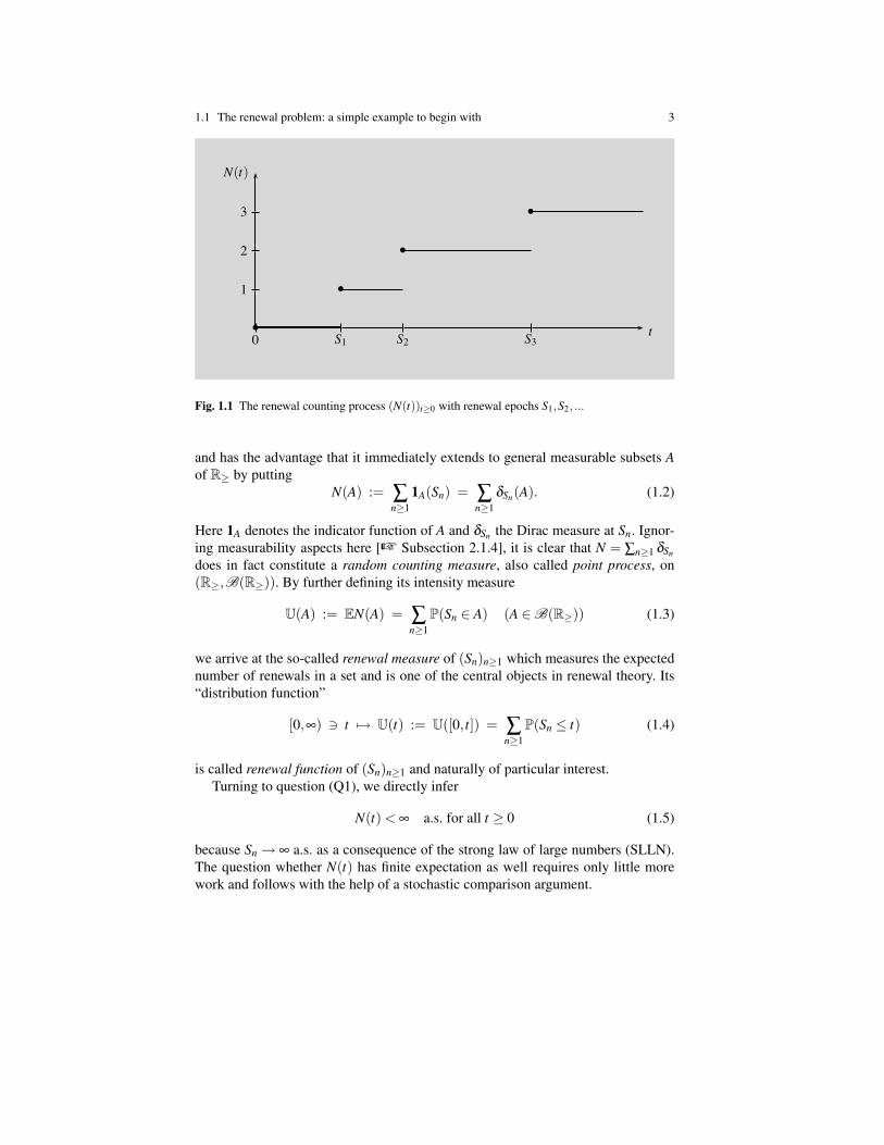
The stochastic process (N(t))t≥0 is called the renewal counting process associatedwith (Sn)n≥1 and may be formally defined as
N(t) := supn≥ 0 : Sn ≤ t for t ≥ 0. (1.1)
An equivalent definition is
N(t) := ∑n≥1
1[0,t](Sn)
1.1 The renewal problem: a simple example to begin with 3
0 S1 S2 S3t
N(t)
1
2
3
•
•
•
•
Fig. 1.1 The renewal counting process (N(t))t≥0 with renewal epochs S1,S2, ...
and has the advantage that it immediately extends to general measurable subsets Aof R≥ by putting
N(A) := ∑n≥1
1A(Sn) = ∑n≥1
δSn(A). (1.2)
Here 1A denotes the indicator function of A and δSn the Dirac measure at Sn. Ignor-ing measurability aspects here [+ Subsection 2.1.4], it is clear that N = ∑n≥1 δSn
does in fact constitute a random counting measure, also called point process, on(R≥,B(R≥)). By further defining its intensity measure
U(A) := EN(A) = ∑n≥1
P(Sn ∈ A) (A ∈B(R≥)) (1.3)
we arrive at the so-called renewal measure of (Sn)n≥1 which measures the expectednumber of renewals in a set and is one of the central objects in renewal theory. Its“distribution function”
[0,∞) 3 t 7→ U(t) := U([0, t]) = ∑n≥1
P(Sn ≤ t) (1.4)
is called renewal function of (Sn)n≥1 and naturally of particular interest.Turning to question (Q1), we directly infer
N(t) < ∞ a.s. for all t ≥ 0 (1.5)
because Sn→ ∞ a.s. as a consequence of the strong law of large numbers (SLLN).The question whether N(t) has finite expectation as well requires only little morework and follows with the help of a stochastic comparison argument.

4 1 Introduction
Theorem 1.1.1. If (Sn)n≥1 is a renewal process, then its renewal function iseverywhere finite, i.e. U(t) < ∞ for all t ≥ 0.
Proof. The essence of the subsequent argument leads back to old work by STEIN[42]. Since P(X1 = 0) < 1 there exists a constant c > 0 such that p := P(X1 ≤ c) < 1.Consider the renewal process (S′n) with increments defined as X ′n := c1Xn>c forn≥ 1, thus S′n = ∑
nk=1 X ′k for n≥ 1. This process moves as follows: Each jump of size
c is preceded by a random number of zeroes having a geometric distribution withparameter 1− p = P(X ′1 = c). Consequently, if N′, U′ have the obvious meaning,then N′(nc) equals n plus the sum of n+1 (actually independent) geometric randomvariables with parameter p giving
U′(nc) = EN′(nc) = n+(n+1)p
1− p=
n+ p1− p
for all n ∈ N.
The assertion now follows because X ′n ≤ Xn for each n ∈ N clearly implies N(t) ≤N′(t) and hence U(t)≤ U′(t) for all t ≥ 0. ut
With the previous result at hand we can turn to question (Q2) on the long runaverage number of renewals per time unit, also called renewal rate. Ignoring therandom oscillations in the replacement scheme it is natural to expect that this rateshould be µ−1, as every installed light bulb is expected to burn for a time interval oflength µ . The following result provides a positive answer for t−1N(t) and is basedon a neat probabilistic argument that goes back to DOOB [18]. The correspondingassertion for t−1U(t) is also valid, but its proof requires more work and will be givenlater [+ Thm. 2.4.3].
Theorem 1.1.2. If (Sn)n≥1 is a renewal process with mean interrenewal time0 < µ ≤ ∞, then
limt→∞
N(t)t
=1µ
a.s.
with the usual convention that ı−1 := 0.
Proof. Using N(t)→∞ a.s. in combination with the SLLN for (Sn)n≥1 we infer thatboth, N(t)−1SN(t) and N(t)−1SN(t)+1 converge a.s. to µ as t → ∞. Moreover, (1.1)implies SN(t) ≤ t < SN(t)+1 for all t ≥ 0. Consequently,
SN(t)
N(t)≤ t
N(t)≤ SN(t)+1
N(t)for all t ≥ 0
provides the assertion upon letting t tend to infinity. ut

1.2 The Poisson process: a nice example to learn from 5
Asking for the expected number of renewals in a bounded interval of length h(question (Q3)) the heuristic argument given before the previous result suggests thatit should be approximately equal to µ−1h, that is
U((t, t +h]) = U(t +h)−U(t) ≈ hµ
(1.6)
at least for large values of t. On the other hand, it should not take by surprise thatfor this to show the random fluctuations of N(t +h)−N(t) must be considered morecarefully. In fact, an answer to (Q3) cannot be provided at this point and is one ofthe highly nontrivial blockbuster results to be derived in Chapter 3.
1.2 The Poisson process: a nice example to learn from
So far we have not addressed the question whether the distribution of N(t) or itsexpectation U(t) may be computed explicitly in closed form. Let F and Fn denotethe cdf of X1 and Sn, respectively, hence F1 = F and Fn = F∗n for each n ∈N, whereF∗n denotes the n-fold covolution of F defined recursively as
F∗n(t) =∫
[0,t]F∗(n−1)(t− x) F(dx) for all t ≥ 0.
Now observe that, by (1.1),
N(t) = n = Sn ≤ t < Sn+1 = Sn ≤ t\Sn+1 ≤ t
and thus
P(N(t) = n) = P(Sn ≤ t)−P(Sn+1 ≤ t) = Fn(t)−Fn+1(t). (1.7)
for all n ∈ N0 and t ≥ 0. Furthermore, by (1.4)
U(t) = ∑n≥1
P(Sn ≤ t) = ∑n≥1
Fn(t) for all t ≥ 0. (1.8)
This shows that closed form expressions require an explicit knowledge of all Fn(t) aswell as of their infinite sum which is true only in very few cases. The most importantone of these will be discussed next.
Suppose that F is an exponential distribution with parameter θ > 0, that is
F(t) = 1− e−θ t (t ≥ 0).
It is well-known that Sn then has a Gamma distribution with parameters n and θ , thedensity of which (with respect to Lebesgue measure λλ0) is

6 1 Introduction
fn(x) =θ nxn−1
(n−1)!e−θx (x≥ 0)
for each n ∈ N. In order to find P(N(t) = n), we consider gn(t) := eθ t P(N(t) = n)for t ≥ 0 and any fixed n ∈ N. A conditioning argument yields
gn(t) = eθ t P(Sn ≤ t < Sn +Xn+1)
= eθ t∫ t
0P(X1 > t− x) fn(x) dx
=∫ t
0eθx fn(x) dx
=∫ t
0
θ nxn−1
(n−1)!dx for all t ≥ 0,
whence
P(N(t) = n) =(θ t)n
n!e−θ t for all t ≥ 0 and n ∈ N.
For n = 0 we obtain more easily
P(N(t) = 0) = P(S1 > t) = 1−F(t) = e−θ for all t ≥ 0.
We have thus shown
Theorem 1.2.1. If (Sn)n≥1 is a renewal process having exponential incre-ments with parameter θ , then N(t) has a Poisson distribution with parameterθ t for each t > 0, in particular
U(t) = EN(t) = θ t for all t ≥ 0, (1.9)
that is, U equals Lebesgue measure on R>.
We thus see that for the exponential case question (Q3) has an explicit answer inthat (1.6) becomes an exact identity:
U(t +h)−U(t) =hµ
for all t ≥ 0, h > 0.
The previous result allows us also to find the cdf of Sn (n ∈ N), namely
Fn(t) = P(N(t)≥ n) = e−θ t∑k≥n
(θ t)k
k!for all t ≥ 0. (1.10)
As for the renewal counting process N(t) : t ≥ 0, the fact that N(t) d= Poisson(θ t)is actually a piece only of the following more complete result.

1.3 Markov chains: a good example to motivate 7
Theorem 1.2.2. If (Sn)n≥1 is a renewal process having exponential incre-ments with parameter θ , then the associated renewal counting process(N(t))t≥0 forms a homogeneous Poisson process with intensity (rate) θ , thatis:
(PP1) N(0) = 0.(PP2) (N(t))t≥0 has independent increments, i.e.,
N(t1), N(t2)−N(t1), ..., N(tn)−N(tn−1)
are independent random variables for each choice of n ∈ N and0 < t1 < t2 < ... < tn < ∞.
(PP3) (N(t))t≥0 has stationary increments, i.e., N(s+t)−N(s) d= N(t) forall s, t ≥ 0.
(PP4) N(t) d= Poisson(θ t) for each t ≥ 0.
We refrain from providing a proof of the result at this point [+ ??????] andjust mention that the crucial fact behind it is the lack of memory property of theexponential distribution.
1.3 Markov chains: a good example to motivate
A good motivation for the theoretical relevance of renewal theory in connection withstochastic processeses with inherent regeneration scheme is provided by a look atan important subclass, namely finite irreducible Markov chains.
A stochastic sequence (Mn)n≥0 such that all Mn take values in a finite set S iscalled finite Markov chain if it satisfies the Markov property, viz.
P(Mn+1 = j|Mn = i,Mn−1 = in−1, ...,M0 = i0) = P(Mn+1 = j|Mn = i)
for all n ∈ N0 and i0, ..., in−1, i, j ∈S , and is temporally homogeneous, viz.
P(Mn+1 = j|Mn = i) = P(M1 = j|M0 = i) =: pi j
for all n ∈ N0 and i, j ∈ S . The set S is called the state space of (Mn)n≥0 andP = (pi j)i, j∈S its (one-step) transition matrix. We continue with a summary ofsome basic properties of such chains. A more detailed exposition will be providedin ????????
First of all, if τ is a stopping time for (Mn)n≥0, i.e. τ takes values in N0 ∪∞and τ = n ∈ σ(M0, ...,Mn) for all n∈N0, then the Markov property persists in thesense that

8 1 Introduction
P(Mτ+1 = j|Mτ = i,Mτ−1, ...,M0,τ < ∞) = P(Mτ+1 = j|Mτ = i) = pi j
for all i, j ∈S . This is called the strong Markov property. For any path i0→ i1→...→ in in S its probability is easily obtained by multiplying one-step transitionprobabilities, viz.
P(M1 = i1, ...,Mn = in|M0 = i0) = λi0 pi0i1 · ... · pin−1in ,
where λ = λi : i ∈S denotes the distribution of M0, called initial distribution ofthe chain. In the following, we make use of the common notation Pi := P(·|M0 = i)and Pλ := ∑i∈S Pi for any distribution λ = λi on S . Hence (Mn)n≥0 starts at iunder Pi and has initial distribution λ under Pλ .
Not surprisingly, temporal homogeneity extends to all n-step transition probabil-ties (n ∈ N), i.e. p(n)
i j := P(Mn = j|M0 = i) = P(Mk+n = j|Mk = i) for all k ∈ N0.Moreover, they satisfy the Chapman-Kolmogorov equations
p(n)i j = ∑
k∈Sp(m)
ik p(n−m)k j for all i, j ∈S and m,n ∈ N0, (1.11)
where p(0)i j := δi j. If P(n) := (p(n)
i j )i, j∈S denotes the n-step transition matrix, thenthese equations may be restated in matrix form as
P(n) = P(m)P(n−m) for all m,n ∈ N0. (1.12)
Consequently P(n) = Pn for each n ∈ N0, i.e. the transition matrices form a semi-group generated by P. Let us note that, under Pλ , the distribution of Mn is given byλPn for every n ∈ N0.
The chain (Mn)n≥0 and its transition matrix P are called irreducible if all statescommunicate with respect to P, where i, j ∈ S are said to be communicating ifthere exist m,n ∈ N0 such that p(m)
i j > 0 and p(n)ji > 0. In other words, the chain
can reach any state from any other state in a finite number of steps with positiveprobability. As a further prerequisite, some state properties must be defined. LetT (i) := infn≥ 1 : Mn = i denote the first return time to i ∈S , where inf /0 := ∞.Then i is called
• recurrent if Pi(T (i) < ∞) = 1.• transient if Pi(T (i) = ∞) > 0.• positive recurrent if i is recurrent and EiT (i) < ∞.• null recurrent if i is recurrent and EiT (i) = ∞.• aperiodic if Pi(T (i) ∈ dN) < 1 for any integer d ≥ 2.
It will be shown in ?????? that each of these properties is a solidarity property whichmeans that it is shared by communicating states and thus by all states if the chain isirreducible. In the latter case we can therefore attribute any property to the chain aswell. Putting f (n)
i j := Pi(T ( j) = n), it is an easy exercise to verify that

1.3 Markov chains: a good example to motivate 9
p(n)i j =
n
∑k=1
f (k)i j p(n−k)
j j for all i, j ∈S and n ∈ N. (1.13)
Now consider, for any state i ∈ S , the sequence Tn(i) of successive returntimes, i.e. T1(i) := T (i) and
Tn(i) :=
infk > Tn−1(i) : Mk = i, if Tn−1(i) < ∞,
∞, otherwisefor n≥ 2.
The next lemma provides a first indication of how renewal theory enters in Markovchain analysis. A stochastic sequence with iid increments taking values in R≥∪∞and having positive mean is called proper renewal process if the increments are a.s.finite, and terminating renewal process otherwise.
Lemma 1.3.1. For any i ∈S , the sequence (Tn(i))n≥1 forms a renewal pro-cess under Pi. It is proper if i is recurrent and terminating otherwise.
Proof. Fix any i ∈S , write Tn for Tn(i) and put β := Pi(T1 < ∞). Use the Markovproperty and temporal homogeneity to find that
Pi(T1 = m,T2−T1 = n)= Pi(T1 = m,Mm = i,T2−T1 = n)= P(Mm+n = i,Mm+k 6= i for 1≤ k < n|Mm = i)Pi(T1 = m)= Pi(Mn = i,Mk 6= i for 1≤ k < n)Pi(T1 = m)= Pi(T1 = m)Pi(T1 = n)
for all n,m ∈N and then also, after summation over m,n ∈N, that Pi(T2 < ∞) = β 2.This shows conditional independence and identical distribution (under Pi) of T1 andT2−T1 given T2 < ∞. For arbitrary n ∈ N, it follows by an inductive argument thatT1,T2−T1, ...,Tn−Tn−1 are conditionally iid given Tn < ∞ as well as Pi(Tn < ∞) =β n. The assertions of the lemma are now easily concluded. ut
As an immediate consequence, we now obtain the following zero-one law.
Lemma 1.3.2. If i ∈S is recurrent, then
Pi(Mn = i infinitely often) = 1,
whileP j(Mn = i infinitely often) = 0
for all j ∈S if i is transient.

10 1 Introduction
Proof. Observe that Mn = i infinitely often= Tn(i) < ∞ for all n ∈N. Now usethe previous lemma to infer that
Pi(Tn(i) < ∞ for all n ∈ N) = limn→∞
Pi(T (i) < ∞)n
which clearly equals 1 if i is recurrent and 0 otherwise. If i is transient, the strongMarkov property further implies
P j(Mn = i infinitely often) = P j(T (i) < ∞)Pi(Mn = i infinitely often) = 0
for all j ∈S . utWe see from the previous result that any finite Markov chain has at least one re-
current state because otherwise all i ∈S would be visited only finitely often whichis clearly impossible if |S |< ∞. Adding irreducibility as a further assumption, sol-idarity now leads to the following important conclusion:
Theorem 1.3.3. Every irreducible finite Markov chain is recurrent.
We can now turn to the most interesting question about the long run behavior ofan irreducible finite Markov chain (Mn)n≥0. Since Mn moves around in S visitingevery state infinitely often and since, by the Markov property, the chain has nomemory, one can expect Mn to converge in distribution to some limit law π = πi :i ∈S which does not depend on the initial distribution P(M0 ∈ ·). An importantinvariance property of any such limit law π is stated in the following lemma. PutPλ := ∑i∈S λiPi for any distribution λ = (λi)i∈S on S and notice that (Mn)n≥0has initial distribution λ under Pλ .
Lemma 1.3.4. Suppose that, for some initial distribution λ = (λi)i∈S on S ,
πi := limn→∞
Pλ (Mn = i) (1.14)
exists for all i ∈S , i.e., Mnd→ π = (πi)i∈S . Then π is a left eigenvector of P
for the eigenvalue 1, i.e. π = πP, and
Pπ(Mn ∈ ·) = π for all n ∈ N0.
Any such π is called invariant or stationary distribution of (Mn)n≥0. If thechain is irreducible then all πi are positive.
Proof. Since πPn equals the distribution of Mn under Pπ as stated earlier, it sufficesto prove the first assertion and the positivity of π in the irreducible case. But withS being finite condition (1.14) implies

1.3 Markov chains: a good example to motivate 11
π j = limn→∞
Pλ (Mn+1 = j) = ∑i∈S
limn→∞
Pλ (Mn = i)pi j = ∑i∈S
πi pi j
for all j ∈S which is the same as π = πP. Now suppose that (Mn)n≥0 is irreducible.As π = πPn for all n ∈ N0, we see that, if π j = 0 for some j ∈S , then
0 = π j = ∑i∈S
πi p(n)i j for all n ∈ N
and thus p(n)i j = 0 for all π-positive i and all n ∈ N. But this means that j cannot be
reached from any π-positive i which is impossible by irredubility. utIn view of the previous lemma we are now facing two questions for a given
irreducible finite Markov chain (Mn)n≥0:
(Q1) Does (Mn)n≥0 always have a stationary distribution π?(Q2) Does (1.14) hold true for any choice of λ and with the same limit π?
Of course, a positive answer to (Q1) follows from a positive answer to (Q2) which,however, is not generally true and brings in fact aperiodicity into play. Namely, if thechain is not aperiodic, then it can be shown that (by solidarity) it has a unique periodd ≥ 2 in the sense that d is the maximal integer such that Pi(T (i) ∈ dN) = 1 for alli ∈S . This further entails p(n)
ii = 0 for all i ∈S and all n ∈ N\dN [+ ??????? forfurther details]. On the other hand, if (1.14) held true for any λ , we inferred uponchoosing λ = δi that
πi = limn→∞
p(n)ii = liminf
n→∞p(n)
ii = 0
which contradicts that all πi must be positive.Based on the previous observations we further confine ourselves now to aperi-
odic finite Markov chains (Mn)n≥0. Then, for (Q2) to be answered affirmatively, itsuffices to show that
π j = limn→∞
p(n)i j for all i, j ∈S .
But with the help of (1.13) and the dominated convergence theorem, this reduces to
π j = limn→∞
∑k≥1
11,...,n(k) f (k)i j p(n−k)
j j = limn→∞
p(n)j j for all j ∈S
and finally makes us return to renewal theory via the following observation: SinceMn = j= ∑k≥1Tk( j) = n, where the summation indicates as usual the union ofpairwise disjoint events, we infer that
p(n)j j = ∑
k≥1P j(Tk( j) = n) = U j(n), for all j ∈S and n ∈ N (1.15)

12 1 Introduction
where U j denotes the renewal measure of the discrete renewal process (Tk( j))k≥1.Consequently, in order to find the limiting behavior of p(n)
j j we must find the limitingbehavior of the renewal measure U j along singleton sets tending towards infinity.This is in perfect accordance with (Q3) of Section 1.1 once observing that, due tothe fact that the Tk( j) are integer-valued, U j(n) = U j(n)−U j(n−1) for all n∈N.
1.4 Branching processes: a surprising connection
In this section, we will take a look at a very simple branching model of cell division.It may be surprising at first glance that branching as a typically exponential-typephenomenon can be studied with the help of renewal theory which rather deals withstochastic phenomena of linear type. Let it be said to all weisenheimers that this isnot accomplished by just using a logarithmic transformation.
We consider a population of cells having independent lifetimes with a standardexponential distribution. At the end of its lifetime, each cell either splits into twonew cells with probability p or dies with probability 1− p independent of all othercells alive. Suppose that at time t = 0 the evolution starts with one cell having life-time T and number of offspring Y , thus P(Y = 2) = p = 1−P(Y = 0), and Y isindependent of T . Let Z(t) be the number of cells alive at time t ∈ R≥. Then
Z(t) = 1T>t + 1T≤t,X=2(Z1(t−T )+Z2(t−T )) (1.16)
where Zi(t−T ) denotes the size at time t of the subpopulation of cells stemmingfrom the i th daughter cell born at T ≤ t (i = 1,2). As following from the modelassumptions, the (Zi(t))t≥0 are mutually independent copies of (Z(t))t≥0 and furtherindependent of (T,Y ).
Our goal is to find the expected population size M(t) := EZ(t). Since T is inde-
pendent of Y and T d= Exp(1), we infer from (1.16)
M(t) = P(T > t)+∫
[0,t]M(t− s)2p P(T ∈ ds)
= e−t +∫ t
0M(t− s)2pe−s ds for all t ≥ 0
which is an integral equation of convolutional type that may be rewritten as
M = F +M ∗Q, (1.17)
here with F(t) := e−t for t ≥ 0 and Q(ds) := 2pe−s1(0,∞)(s)ds. An equation of thistype can be solved with the help of renewal theory as we will see in a moment andis therefore called renewal equation. Notice first that Q has total mass
‖Q‖ = 2p∫
∞
0e−s ds = 2p = EY

1.4 Branching processes: a surprising connection 13
and is thus a probability distribution only if EY = 1. On the other hand, a look at themgf of Q, viz.
φQ(t) =∫
est Q(ds) = 2p∫
∞
0e(t−1)s ds =
2p1− t
(−∞ < t < 1),
shows the existence of a unique θ such that φQ(θ) = 1, namely θ = 1− 2p. Nowobserve that
eθ tM(t) = e(θ−1)t +∫ t
0eθ(t−s)Mθ (t− s)2pe(θ−1)s ds for all t ≥ 0
which may be rewritten as
Mθ = Fθ +Mθ ∗Qθ , (1.18)
where Mθ (t) := eθ tM(t), Fθ (t) := e−2pt and Qθ (ds) := 2pe−2ps1(0,∞)(s)ds. Since‖Qθ‖= φQ(θ) = 1 (by choice of θ ), we see that a change of measure turns the orig-inal renewal equation (1.17) into an equivalent so-called proper renewal equationwith a probability distribution as convolution measure, in fact Qθ = Exp(2p). Let(Sn)n≥1 be a renewal process with this increment distribution. Then (1.18) becomes
Mθ (t) = Fθ (t) + EMθ (t−S1) for all t ≥ 0
and upon n-fold iteration
Mθ (t) =n−1
∑k=0
EFθ (t−Sk) + EMθ (t−Sn) for all t ≥ 0 and n ∈ N.
It is intuitively clear and taken for granted here that M is continuous on R≥ and thusbounded on compact subintervals. Consequently,
limn→∞
EMθ (t−Sn) ≤ limn→∞
P(Sn ≤ t) maxs∈[0,t]
Mθ (s) = 0
because Sn→ ∞ a.s., and we therefore conclude
Mθ (t) = ∑k≥0
EFθ (t−Sk) = Fθ (t)+Fθ ∗U(t),
where U := ∑n≥1 P(Sn ∈ ·) denotes the renewal measure of (Sn)n≥1. But the latterhas exponentially distributed increments with parameter 2p and so U = 2pλλ0 onR> by Thm. 1.2.1. This finally allows us to compute Fθ ∗U(t) explicitly leading to
Mθ (t) = e−2pt +∫ t
02pe−2p(t−s) ds = 1 for all t ≥ 0
and thereforeM(t) = e(2p−1)t for all t ≥ 0 (1.19)
14 1 Introduction
The parameter 2p− 1 thus giving the exponential rate of mean growth or decay ofthe population is called its Malthusian parameter.
Astute readers will have noticed that for this particularly nice example of a cellsplitting model (1.19) could have been obtained far more easily by showing with thehelp of the memoryless property of the exponential distribution that (eθ tZ(t))t≥0is a martingale with Z(0) = 1 and thus having constant expectation equal to one.However, if we replace the exponential lifetime distribution with an arbitrary dis-tribution F with finite mean µ , then this latter argument breaks down while therenewal argument still works. In fact, we may even additionally assume an arbitraryoffspring distribution pk to arrive at the following general renewal equation forM(t) = EZ(t):
M(t) = F(t) +∫
[0,t]M(t− s) Q(ds) for all t ≥ 0 (1.20)
where Q(ds) = µF(ds). If µ 6= 1 and thus Q is not a probability distribution, thena transformation of (1.20) into a proper one requires the existence of a (necessarilyunique) θ such that φQ(θ) = µφF(θ) = 1 which may fail if µ < 1. In the case whereθ exists the result is as before that
Mθ (t) = Fθ (t)+Fθ ∗U(t) (1.21)
where U denotes the renewal measure of a renewal process with increment distri-bution Qθ (ds) = µeθsF(ds). Unlike the exponential case, however, this does notgenerally lead to an explicit formula for M(t) because U is not known explicitly.Instead, one must resort once again to asymptotic considerations as t → ∞. For afurther discussion of these aspects in this more general situation, we refer to Chap-ter 5.
1.5 Collective risk theory: a classical application
This application is a relative of the previous one in that it eventually leads to arenewal equation that must be solved in order to gain information on the quantity ofinterest.
In collective risk theory, a part of nonlife insurance mathematics, the followingproblem is of fundamental interest: An insurance company earns premiums at aconstant rate c∈R> from a portfolio of insurance policies and faces negative claimsfrom these of absolute sizes X1,X2, ... at successive random epochs 0 < T1 < T2 < ...Given an initial risk reserve R(0), the risk reserve R(t) at time t, i.e., the availablecapital at t to cover incurred future claims, is given by
R(t) = R(0)+ ct−N(t)
∑k=1
Xk for all t ≥ 0,

1.5 Collective risk theory: a classical application 15
where N(t) := ∑n≥1 1Tn≤t denotes the number of claims up to time t. If R(t) be-comes negative, so-called technical ruin occurs. It is therefore a main concern of theinsurance company to choose R(0) and c in such a way that the probability for thisevent, called ruin probability, is small. Plainly, this requires a computation of thisprobability after the specification of a stochastic model for the bivariate sequence(Tn,Xn)n≥1. Again, we do not strive for greatest generality in this introductory sec-tion but will instead discuss the problem in the framework of what is known today asthe Cramer-Lundberg model which has its origin in a dissertation by F. LUNDBERG[34]:
(CL1) (N(t))t≥0 is a homogeneous Poisson process with intensity λ or, equivalent-
ly, T1,T2−T1, ... are iid with T1d= Exp(λ ).
(CL2) X1,X2, ... are iid with common distribution F and finite positive mean µ .(CL3) (Tn)n≥1 and (Xn)n≥1 are independent.
Put Yn := Tn−Tn−1 for n ∈ N (with T0 = 0) and let (X ,Y ) denote a generic copy of(Xn,Yn) hereafter. Defining the epoch of technical ruin, viz.
Λ := inft ≥ 0 : R(t) < 0 (inf /0 := ∞),
the task is to compute for a fixed premium rate c
Ψ(r) := P(Λ < ∞|R(0) = r) for r > 0.
T1 T2 T3 Λ = T4
X1X2
X3
X4
t
R(t)
Fig. 1.2 The risk reserve process (R(t))t≥0 with ruin epoch Λ
Let us begin with the observation that technical ruin can only occur at the epochsTn, that is (given R(0) = r)

16 1 Introduction
Λ = Tτ , where τ := infn≥ 1 : r + cTn−Sn < 0
and (Sn)n≥1 denotes the renewal process with increments X1,X2, ... Hence
Ψ(r) = P(τ < ∞|R(0) = r) for r ≥ 0.
In the following considerations we keep R(0) = r fixed and simply write P insteadof P(·|R(0) = r). Rewriting τ as
τ = infn≥ 1 : Sn− cTn > r
we see that ν is a so-called first passage time for the random walk (Sn− cTn)n≥1with drift ν := E(X− cY ) = µ− cλ−1. Hence
Ψ(r) = 1 for all r > 0
if ν ≥ 0, because Sn− cTn → ∞ a.s. by the SLLN if ν > 0, and limsupn→∞ Sn−cTn = ∞ a.s. by the Chung-Fuchs theorem [+ Thm. 2.2.11] in the case ν = 0. Theinteresting case to be discussed hereafter is therefore when
(CL4) ν = E(X− cY ) = µ− cλ
< 0
which means that the mean premium earned between two claim epochs is largerthan the expected claim size. We first prove a renewal equation for Ψ := 1−Ψ .
Lemma 1.5.1. Assuming (CL1–4), Ψ satisfies the renwal equation
Ψ(r) = Ψ(0) +∫ r
0Ψ(r− x) Q(dx) for all r ≥ 0. (1.22)
where Q(dx) := λ
c P(X > x)dx on R≥.
Proof. Since X and Y are independent with X d= F and Y d= Exp(λ ), a conditioningargument leads to
Ψ(r) = P(Sn ≤ r + cTn for all n≥ 1)
=∫(x,y):x≤r+cy
P(x+Sn ≤ r + c(y+Tn) for all n≥ 1) P(X ∈ dx,Y ∈ dy)
=∫
∞
0
∫[0,r+cy]
Ψ(r− x+ cy)λe−λy F(dx) dy
=∫
∞
r
λ
ce−(λ/c)(y−r)
∫[0,y]
Ψ(y− x) F(dx) dy
and thus shows the differentiability of Ψ with

1.5 Collective risk theory: a classical application 17
Ψ′(r) = −λ
c
∫[0,r]
Ψ(r− x) F(dx) +∫
∞
r
λ 2
c2 e−(λ/c)(y−r)∫
[0,y]Ψ(y− x) F(dx) dy
= −λ
c
∫[0,r]
Ψ(r− x) F(dx) +λ
cΨ(r)
for all r ≥ 0. Consequently, we obtain upon integration
Ψ(r)−Ψ(0) =λ
c
(∫ r
0
(Ψ(y)−
∫[0,y]
Ψ(y− x) F(dx))
dy)
which leaves us with the verification of∫ r
0
(Ψ(y)−
∫[0,y]
Ψ(y− x) F(dx))
dy =∫ r
0Ψ(r− x)P(X > x) dx
for r ≥ 0. But this follows from∫ r
0
∫[0,y]
Ψ(y− x) F(dx) dy =∫
[0,r]
∫ r−x
0Ψ(y) dy F(dx)
=∫ r
0Ψ(y)P(X ≤ r− y) dy =
∫ r
0Ψ(r− y)P(X ≤ y) dy
and∫ r
0 Ψ(y)dy =∫ r
0 Ψ(r− y)dy. ut
Notice that Q as defined in the lemma has total mass ‖Q‖= λ
c EX = λ µ
c < 1 be-cause ν < 0. This means that (1.22) is a so-called defective renewal equation. Since‖Q∗n‖ = ‖Q‖n→ 0, we infer that the renewal measure UQ := ∑n≥1 Q∗n associatedwith Q is a finite measure with total mass (1−‖Q‖)−1‖Q‖ and
Ψ ∗Q∗n(r) =∫
[0,r]Ψ(r− x) Q∗n(dx) ≤ ‖Q‖n → 0 as n→ ı
Hence, by a similar iteration argument as in the previous section we find that
Ψ(r) = Ψ(0)+Ψ(0)∗UQ(r) = Ψ(0)+∫ r
0Ψ(0) UQ(dx) = Ψ(0)(1+UQ(r))
and thereupon that
limr→∞
Ψ(r) = Ψ(0)(1+‖UQ‖) =Ψ(0)
1−‖Q‖ =cΨ(0)c−λ µ
. (1.23)
On the other hand, we have Sn− cTn→−∞ a.s. if ν < 0 and therefore Ψ(r)→ 1 asr→ ∞. By combining this with (1.23) and solving for Ψ(0) yields
Ψ(0) =c−λ µ
c= 1− λ µ
c= 1−‖Q‖. (1.24)

18 1 Introduction
Naturally, this is not the end of the story when striving for the asymptotic behav-ior of Ψ(r) beyond the quite trivial statement that limr→∞Ψ(r) = 0 if ν < 0. As inthe branching example of the previous section, we will now make use of a changeof measure argument which, however, requires an additional condition on the distri-bution F of X . As before, let φF be the mgf of F . Note that Qθ (dx) = eθxQ(dx) hastotal mass [+ formula ????? in Appendix ?]
‖Qθ‖ =λ
c
∫∞
0eθx P(X > x) dx =
λ
cθ(φF(θ)−1)
which is less than ‖Q‖ < 1 for all θ < 0 because φF is increasing on R≤. In orderfor finding a θ such that ‖Qθ‖ = 1, this θ must therefore be positive if it exists atall. Therefore we introduce as a further condition:
(CL5) There exists θ > 0 such that φF(θ) = 1+cθ
λ.
With the extra condition (CL5) the ruin probability Ψ(r) after multiplication witheθr satisfies a proper renewal equation as stated in the next theorem. In the casewhere X is also exponentially distributed this can be converted into an explicit for-mula for Ψ(r), while in the general case a statement on its asymptotic behavior asr→ ∞ is possible but must wait until Section ???
Theorem 1.5.2. Assuming (CL1–5), the ruin probability Ψθ (r) := eθrΨ(r)satisfies the proper renewal equation
Ψθ (r) = eθrQ((r,∞)) +∫
[0,r]Ψθ (r− x) Qθ (dx) for all r ≥ 0 (1.25)
and thus
Ψθ (r) = eθrQ((r,∞)) +∫
[0,r]eθ(r−x)Q((r− x,∞)) Uθ (dx), (1.26)
where Q is as in Lemma 1.5.1 and Uθ := ∑n≥1 Q∗nθ
denotes the renewal mea-sure associated with Qθ .
Proof. Rewriting (1.22) with the help of (1.24), we obtain
Ψ(r) = 1−(
Ψ(0) +∫ r
0Ψ(r− x) Q(dx)
)= Ψ(0)−Q(r) +
∫[0,r]
Ψ(r− x) Q(dx)
= Q((r,∞)) + +∫
[0,r]Ψ(r− x) Q(dx) for all r ≥ 0

1.6 Queuing theory: a typical application 19
and then (1.25) after multiplication with eθr. Validity of (1.26) follows now in thesame manner as in the previous section when using that Ψθ is bounded on compactsubintervals of R≥ in combination with Q∗n
θ(r) = P(Sn ≤ r)→ 0 as n→ ∞, where
(Sn)n≥1 denotes a renewal process with increment distribution Qθ . utFinally looking at the special case where F = Exp(1/µ), we first note that then
Qθ (dx) =λ
ce−((1/µ)−θ)x dx
and thus equals an exponential distribution (with parameter λ/c) if
θ =1µ− λ
c> 0
which is easily seen to be an equivalent version of (CL4). Hence (CL5) does auto-matically hold here once (CL4) is valid. Now use Uθ = λ
c λλ0 and Q = λ µ
c Exp(1/µ)to infer with the help of Thm. 1.5.2 that
Ψθ (r) =λ µ
ce−(λ/c)r +
λ
c
∫ r
0
λ µ
ce−(λ/c)x dx =
λ µ
cfor all r ≥ 0
and therefore
Ψ(r) =λ µ
ce−((1/µ)−(λ/c))r for all r ≥ 0 (1.27)
1.6 Queuing theory: a typical application
Queuing theory as an important branch of Applied Probability deals with the per-formance analysis of service facilities which are subject to random input. Here weconsider a single server station who is facing (beginning at time T0 = 0) arrivals ofcustomers at random epochs 0 < T1 < T2 < ... with service requests of (temporal)size B1,B2, ... Customers who find the server busy join a queue and are served in theorder they have arrived (first in, first out). Typical performance measures are quan-tities like workload, queue length or sojourn times of customers in the system. Theymay be studied over time (transient analysis) or in the long run (steady state analy-sis). Typically, the complexity of queuing systems does not allow a transient analysiswhence one usually resorts to a steady state analysis. Like for finite Markov chains,the idea is that after a relaxation period the system is approximately in stochasticequilibrium so that relevant quantities may be approximated by their value underthe stationary distribution. The computation of such approximations often requiresthe use of renewal theory as we will briefly demonstrate in this section.
We consider the so-called M/G/1-queue specified by the following assumptions:
(M/G/1-1) The arrival process (N(t))t≥0, where N(t) := ∑n≥1 1Tn≤t for t ≥ 0,is a homogeneous Poisson process with intensity λ (Poisson input).

20 1 Introduction
(M/G/1-2) The service times B1,B2, ... are iid with common distribution G andfinite positive mean µ .
(M/G/1-3) The sequences (Tn)n≥1 and (Bn)n≥1 are independent.(M/G/1-4) There is one server and a waiting room of infinite capacity.(M/G/1-5) The queue discipline is FIFO (“first in, first out”).
The Kendall notation “M/G/1”, which may be expanded by further symbols whenreferring to more complex systems, has the following meaning:
“M”: The first letter refers to the arrival pattern, and “M” stands for “Marko-vian”. This means that the interarrival times An := Tn−Tn−1 are iid with anexponential distribution which renders (N(t))t≥0 a homogeneous Poissonprocess and, in particular, a continuous time Markov process.
“G”: The second letter refers to the sequence of service times, and “G” standsfor “general”. This means that the service times Bn are iid with an arbitrarydistribution on R≥ with positive mean.
“1”: The number in the third position refers to the number of servers (or coun-ters).
In the following, we will focus on the analysis of the queue length in steady state.Suppose for simplicity that at time T0 = 0 the system is empty. For t ≥ 0, let Q(t) bethe queue length at t, i.e. the number of waiting customers in the system at this timeincluding the one currently in service. This is a stochastic process with Q(0) = 0(due to our previous assumption) and trajectories that are right continuous with lefthand limits. It is also a pure jump process with jumps being of size +1 at an arrivalepoch and −1 at a departure epoch. On the other hand, it is not a Markov processunless the Bn are also exponentially distributed because the future evolution of theprocess at any time t does not only depend on the past through Q(t) but also thetime the customer currently in service already spent at the counter. The classicalway out of this dilemma is a resort to an embedded discrete Markov chain in thesense defined in Section 1.3 but with countable state space N0. It is obtained bylooking at
Qn := Q(Dn) (n ∈ N0)
where D0 := 0 and the Dn for n ≥ 1 denote the successive departure epochs ofcustomers in the system (thus D1 = T1 +B1). As one can easily see, the Qn and Dnsatisfy the recursive relations
Qn = (Qn−1−1)+ +Kn and (1.28)Dn = (Dn−1∨Tn)+Bn for n ∈ N, (1.29)
where Kn is the number of customers that enter the system during the service of thenth customer (with service time Bn), thus
Kn = N(Dn)−N(Dn−1∨Tn) for n ∈ N.
By using the model assumptions, notably (M/G/1-3) and the properties of a Poissonprocess, it is not difficult to verify that the Kn are iid with distribution κ j : j ∈ N0
1.6 Queuing theory: a typical application 21
given by
κ j :=∫
R>
P(N(y) = j) G(dy) =∫
R>
e−λy (λy) j
j!G(dy).
In particular,
EK1 = ∑j≥1
jκ j =∫
R>
EN(y) G(dy) =∫
R>
λy G(dy) = λ µ =: ρ. (1.30)
Moreover, Kn is independent of Q0, ...,Qn−1 which in combination with (1.28) easilyproves:
Lemma 1.6.1. The queue length process (Qn)n≥0 at departure epochs consti-tutes an irreducible and aperiodic discrete Markov chain with state space N0and transition matrix
P = (pi j)i, j∈N0 =
κ0 κ1 κ2 κ3 . . .κ0 κ1 κ2 κ3 . . .0 κ0 κ1 κ2 . . .0 0 κ0 κ1 . . ....
......
.... . .
.
Let us continue by finding the necessary and sufficient condition under whichthe queuing system is stable or, equivalently, the chain (Qn)n≥0 is positive recurrent.Here we should mention that all notions introduced in Section 1.3 for finite Markovchains like irreducibility, recurrence and aperiodicity carry over without changes tothe case of countable state space. Observe that ρ as defined in (1.30) satisfies
ρ =EB1
ET1=
mean service timemean interarrival time
. (1.31)
It is called the traffic intensity of the system because it provides a measure of itsthroughput rate. Intuitively, one can expect stability of the system if ρ is less than 1because then, on the average, the server works at a faster rate than customers enterthe system. The following renewal theoretic analysis will confirm this assertion.
For the random walk Sn := ∑nj=1(K j − 1) (n ∈ N0), we define the associated
sequence σn of so-called descending ladder epochs by σ0 := 0 and, recursively,
σn :=
infk > σn−1 : Sk < Sσn−1, if σn−1 < ∞,
∞, otherwisefor n≥ 1.
Since (Sn)n≥1 can obviously make downward jumps of size−1 only, we infer Sσn =−n if σn < ∞. Furthermore, as ES1 = EK1− 1 = ρ − 1, we see that σn < ∞ a.s.

22 1 Introduction
for all n ∈ N and thus liminfn→∞ Sn = −∞ a.s. requires ρ ≤ 1 [by the SLLN orthe Chung-Fuchs theorem 2.2.11]. More precisely, we will show in Thm. 2.2.9 thatρ < 1 implies Eσ1 < ∞, while ρ = 1 implies σ1 < ∞ a.s. and Eσ1 = ∞. Furthermore,in any of these two cases, the σn have iid increments [+ Thm. 2.2.7] and hence forma discrete renewal process. Let U = ∑n≥1 P(σn ∈ ·) denote its renewal measure withrenewal counting density
un := U(n) for n ∈ N0.
With the help of the previous facts we are now able to prove the following resultabout Qn.
Theorem 1.6.2. The queue length process at departure epochs (Qn)n≥0 is arecurrent Markov chain iff ρ ≤ 1, and it is positive recurrent iff ρ < 1. Fur-thermore ρ ≤ 1 implies
P(Qn = j) = P(Qn = j,σ1 > n) +n
∑k=0
P(Qk = j,σ1 > k)un−k (1.32)
for all j,n ∈ N0, in particular P(Qn = 0) = un.
Proof. Recall that Q0 = 0 is assumed, i.e. P = P(·|Q0 = 0). It suffices to studythe recurrence of state 0 as (Qn)n≥0 is irreducible. The crucial observation is thatσ1 = infn≥ 1 : Qn = 0 and that Qn = Sn for 0≤ n < σ1. Indeed, if ρ ≤ 1 and thusP(σ1 < ∞) = 1, the recurrence of 0 follows just by definition. On the other hand,if ρ > 1 and thus P(σ1 = ∞) > 1, then there is a positive chance of never hitting 0again after time 0 so that 0 must be transient. As mentioned above, ρ < 1 furtherensures Eσ1 < ∞ and thus the positive recurrence of the chain. Finally,
P(Qn = j) = P(Qn = j,σ1 > n) + ∑m≥1
P(Qn = j,σm ≤ n < σm+1)
= P(Qn = j,σ1 > n) +n
∑k=0
∑m≥1
P(Qn = j,σm = n− k,σm+1−σm > k)
= P(Qn = j,σ1 > n) +n
∑k=0
P(Qk = j,σ1 > k) ∑m≥1
P(σm = n− k)
for all j,n ∈ N0 shows (1.32). Here we have used for the last line that, with Fn :=σ((Qk,Sk) : 0≤ k ≤ n),
1.6 Queuing theory: a typical application 23
P(Qn = j,σm = n− k,σm+1−σm > k)
=∫σm=n−k
P(Qn = j,σm+1−σm > k|Fn−k) dP
=∫σm=n−k
P(Qk = j,σ1 > k|Q0) dP
= P(Qk = j,σ1 > k)P(σm = n− k)
for all j,m,n ∈ N0 and 0≤ k ≤ n. utIt should be observed that (1.32) may be restated as P(Qn = j) = g j ∗U(n), where
g j(k) := P(Qk = j,σ1 > k) for j,k ∈ N0,
and that this could have also been deduced as in the previous two examples fromthe fact that P(Qn = j) (as a function of n for fixed j) satisfies the discrete renewalequation
P(Qn = j) = g j(n) +n
∑k=0
P(Qn−k = j)P(σ1 = k) for all n ∈ N0.
So we have a similar result for a quantity of interest as in the previous two sec-tions [+ (1.21) and (1.26)], here in a discrete setup because the renewal processpertaining to U is integer-valued. Owing to this fact an application of the domi-nated convergence theorem to (1.32) immediately leads to the following result onthe asymptotic behavior of Qn once the convergence of un as n→∞ has been proved,the limit actually being (Eσ1)−1.
Theorem 1.6.3. If ρ < 1, then
π j := limn→∞
P(Qn = j) =1
Eσ1∑k≥0
P(Qk = j,σ1 > k) (1.33)
for all j ∈ N0.
It should not take by surprise that π = (π j) j≥0, which obviously forms a proba-bility distribution, is the unique stationary distribution of (Qn)n≥0. Using
P(Qk = j,σ1 > k) = ∑n>k
P(Qn = j,σ1 = n)
in (1.33), we further obtain after interchanging the order of summation that
π j =1
Eσ1E
(σ1−1
∑n=0
1Qn= j
)for all j ∈ N0, (1.34)

24 1 Introduction
which is the occupation measure representation of π having the very intuitive in-terpretation that the stationary probability for a queue length of j (at departures ofcustomers) is just the expected number of epochs this value is attained during acycle, defined as a (discrete) time interval between two epochs where the systembecomes idle (busy period).
1.7 Record values: yet another surprise
Consider a sequence (Xn)n≥1 of iid nonnegative random variables with a continuousdistribution F . We say that a record occurs at time n if Xn exceeds all precedingvalues of the sequence, i.e., if Xn > max1≤k<n Xk. In this case n is a record epochand Xn a record value. More formally, define σ1 := 1, R1 := X1 and then, recursively,
σn := infk > σn−1 : Xk > Rn−1 and Rn := Xσn for n≥ 2.
Clearly, the σn are the record epochs and the Rn the record values of the sequence(Xn)n≥1. Our main concern here is to get information on how the Rn spread onthe nonnegative halfline. At first glance this seems to be quite unrelated to renewaltheory, for record values do not generally show the pattern of a renewal process. Forinstance, if F is the uniform distribution on (0,1) so that all Xn take values in thisinterval, then it is quite clear that the Rn accumulate at 1 from below. On the otherhand, and this is the crucial observation, information on the Rn may be gained alsoafter the application of a function G to the Xn that leaves their order unchanged.
Lemma 1.7.1. Under the stated assumptions, let G : R≥ → R≥ be a nonde-creasing function such that
P(G(X1) < G(X2)|X1 < X2) = 1.
Then the record epochs for (Xn)n≥1 and (G(Xn))n≥1 are a.s. the same, and(G(Rn))n≥1 is the sequence of record values associated with (G(Xn))n≥1.
Proof. Easy. utAs on can easily see, the lemma particularly applies to F itself (viewed as a cdf),
and since F is continuous, the iid F(Xn) are uniformly distributed on (0,1). By thenapplying the transformation x 7→ − log(1− x), we arrive at the sequence
Yn :=− log(1−F(Xn)) (n ∈ N)
of iid standard exponentials, for
P(Y1 > t) = P(F(X1) > 1− e−t) = e−1 for all t > 0.

1.7 Record values: yet another surprise 25
Consequently, the problem of studying record epochs and values of iid continuousrandom variables may be reduced to the study of the corresponding variables for iidstandard exponentials, for which we have the following result based on the lack ofmemory property of the exponential distribution.
Theorem 1.7.2. Let (Xn)n≥1 be a sequence of iid standard exponentials withcanonical filtration (Fn)n≥1, associated record epochs σn and record valuesRn for n ∈ N. Then the following assertions hold true:
(a) (Rn)n≥1 is a renewal process with standard exponential increments.(b) For each n ≥ 2, the conditional distribution of the nth interrecord time
τn := σn−σn−1 given Fσn−1 is geometric on N with parameter e−r ifRn−1 = r. Moreover,
P(τn = k) =∫
∞
0(1− e−r)k−1e−2r rn−2
(n−2)!dr
for all k ∈ N.
Proof. Put Yn := Rn−Rn−1 for n ∈ N, where R0 := 0.
(a) Clearly, T1 = Y1d= Exp(1). Suppose now that we have already shown that
Y1, ...,Yn are iid with a standard exponential distribution. As one can easily verify,the sequence (Xσn+k)k≥1 is independent of Fσn and a copy of (Xk)k≥1 [+ Thm.2.2.1]. Putting Ek := τn+1 = k for k ∈ N, we infer for each t ≥ 0
P(Yn+1 > t|Fσn) = ∑k≥1
P(Xσn+k > Rn + t,Xσn+ j ≤ Rn for 1≤ j < k|Rn)
= ∑k≥1
E(P(Xσn+k > Rn + t|Rn,Ek)1Ek |Rn) a.s.
and since Xσn+k is independent of Rn and Ek for each k, we further obtain by invok-
ing Lemma A.1.1 and using Xσn+kd= Exp(1) that
P(Xσn+k > Rn + t|Rn,Ek) = e−t 1Ek a.s.
Consequently,
P(Yn+1 > t|Fσn) = e−t∑k≥1
P(Ek|Rn) = e−t a.s.
for all t ≥ 0 which proves that Yn+1 is independent of Fσn , particularly of R1, ...,Rn,and has a standard exponential distribution. Hence the assertion follows by inductionover n.

26 1 Introduction
(b) As (Xσn−1+k)k≥1 is independent of Fσn−1 , it is clear that the conditional dis-tribution of τn given Fσn−1 only depends on the current record at σn−1, i.e. Rn−1,and has a geometric distribution with parameter e−r if Rn−1 = r. The formula forthe unconditional probabilities P(τn = k) then follows by integrating agains the dis-tribution of Rn−1 which, by (a), is a Gamma law with parameters n−1 and 1. ut
With the help of the previous result we infer from Theorem 1.2.2 that the recordcounting process
N(t) := ∑n≥1
1Rn≤t (t ≥ 0)
forms a homogeneous Poisson process with intensity 1, also called standard Poissonprocess, if the underlying Xn are standard exponentials. It is now straightforward toconclude a similar result in the general case by drawing on Lemma 1.7.1 and thesubsequent discussion.
Theorem 1.7.3. Let (Xn)n≥1 be a sequence of iid nonnegtive random vari-ables with continuous cdf F and associated record values (Rn)n≥1. Let furtherb := infx ∈ R : F(x) = 1 and ν be the measure on R≥, defined by
Λ((s, t]) := log(
1−F(s)1−F(t)
)for 0≤ s < t < b,
and vanishing outside [0,b]. Then the record counting process (N(t))t≥0 formsa nonhomogeneous Poisson process with intensity measure Λ , that is
(NPP1) N(0) = 0.(NPP2) (N(t))t≥0 has independent increments.
(NPP3) N(t)− N(s) d= Poisson(Λ((s, t])) for all 0 ≤ s < t < ∞, wherePoisson(0) := δ0.
If F has λλ0-density f , then so does Λ , viz. λ (t) = f (t)1−F(t) 1(0,b)(t), which is
then called the intensity function of (N(t))t≥0.
Proof. As before, put G(t) := − log(1−F(t)) and let N(t) be the record count-ing process of the iid standard exponentials (G(Xn))n≥1, hence a standard Poissonprocess by Thm. 1.7.2. Now all assertions are immediate consequences of this facttogether with the observation that
N(t) = N(G(t)) for all t ≥ 0.
All further details can therefore be left to the reader. utSo we have arrived at the very explicit result that the record counting process
of a sequence of iid nonnegtive random variables with continuous cdf F is alwaysa nonhomogeneous Poisson process, and its “renewal function” U(t) = EN(t) just

1.7 Record values: yet another surprise 27
equals Λ([0, t]) = − log(1−F(t)) for t ≥ 0. Notice that in the case where F has aλλ0-density f the intensity function λ (t) of (N(t))t≥0 is nothing but the failure orhazard rate of the sequence (Xn)n≥1, that is
λ (t) = limh↓0
P(X1 ∈ (t, t +h]|X1 > t) for λλ0-almost all t ≥ 0.


Chapter 2Random walks and stopping times:classifications and preliminary results
Our motivating examples have shown that renewal theory is typically concernedwith sums of iid nonnegative random variables, i.e. renewal processes, the goal be-ing to describe the implications of their regenerative properties. On the other hand,it then appears to be quite natural and useful to choose a more general frameworkby considering also sums of iid real-valued random variables, called random walks.Doing so, the regenerative structure remains unchanged while monotonicity is lost.However, this will be overcome by providing the concept of ladder variables, there-fore introduced and studied in Subsection 2.2.3. The more general idea behind thisconcept is to sample a random walk along a sequence of stopping times that rendersa renewal process as a subsequence. This in turn is based on an even more gen-eral result which, roughly speaking, states that any finite stopping time for a randomwalk may be formally copied indefinitely over time and thus always leads to anotherimbedded random walk. The exact result is stated as Theorem 2.2.3 in Subsection2.2.2. Further preliminary results besides some basic terminology and classificationinclude the (topological) recurrence of random walks with zero-mean increments,some basic properties of renewal measures of random walks with positive drift, theconnection of the renewal measure with certain first passage times including ladderepochs, and the definition of the stationary delay distribution.
2.1 Preliminaries and classification of random walks
2.1.1 Lattice-type of random walks
As already mentioned, any sequence (Sn)n≥0 of real-valued random variables withiid increments X1,X2, ... and initial value S0 independent of these is called randomwalk (RW) hereafter, and S0 its delay. If µ := EX1 exists, then µ is called the driftof (Sn)n≥0. In the case where all Xn as well as S0 are nonnegative and µ is positive(possibly infinite), (Sn)n≥0 is also called a renewal process (RP). Finally, a RW
29

30 2 Random walks and stopping times: classifications and preliminary results
or RP (Sn)n≥0 is called trivial if X1 = 0 a.s., zero-delayed or standard if S0 = 0a.s. (abbreviated as SRW, respectively SRP), and delayed otherwise.
An important characteristic of a RW (Sn)n≥0 in the context of renewal theory isits lattice-type. Let F denote the distribution of the Xn and F0 the distribution of S0.Since (Sn)n≥0 forms an additive sequence with state space G0 := R, and since G0has closed subgroups Gd := dZ := dn : n ∈ Z for d ∈ R> and G∞ := 0, it isnatural to ask for the smallest closed subgroup on which the RW is concentrated.Namely, if all the Xn as well as S0 take only values in a proper closed subgroup G ofR, that is, F(G) = F0(G) = 1, then the same holds true for all Sn and its accumula-tion points. The following classifications of F and (Sn)n≥0 reflect this observation.
Definition 2.1.1. For a distribution F on R, its lattice-span d(F) is defined as
d(F) := supd ∈ [0,∞] : F(Gd) = 1.
Let Fx : x∈R denote the translation family associated with F , i.e., Fx(B) :=F(x+B) for all Borel subsets B of R. Then F is called
– nonarithmetic, if d(F) = 0 and thus F(Gd) < 1 for all d > 0.– completely nonarithmetic, if d(Fx) = 0 for all x ∈ R.– d-arithmetic, if d ∈ R> and d(F) = d.– completely d-arithmetic, if d ∈ R> and d(Fx) = d for all x ∈Gd .
If X denotes any random variable with distribution F , thus X−x d= Fx for eachx ∈R, then the previous attributes are also used for X , and we also write d(X)instead of d(F) and call it the lattice-span of X .
For our convenience, a nonarithmetic distribution is sometimes referred to as0-arithmetic hereafter, for example in the lemma below. A random variable X isnonarithmetic iff it is not a.s. taking values only in a lattice Gd , and it is completelynonarithmetic if this is not the case for any shifted lattice x + Gd , i.e. any affineclosed subgroup of R, either. As an example of a nonarithmetic, but not completelynonarithmetic random variable we mention X = π +Y with a standard Poisson vari-able Y . Then d(X−π) = d(Y ) = 1. If X = 1
2 +Y , then d(X) = 12 and d(X− 1
2 ) = 1. Inthis case, X is 1
2 -arithmetic, but not completely 12 -arithmetic. The following simple
lemma provides the essential property of a completely d-arithmetic random variable(d ≥ 0).
Lemma 2.1.2. Let X ,Y be two iid random variables with lattice-span d ≥ 0.Then d ≤ d(X−Y ) with equality holding iff X is completely d-arithmetic.
Proof. Let F denote the distribution of X ,Y . The inequality d ≤ d(X−Y ) is trivial,and since (X +z)−(Y +z) = X−Y , we also have d(X +z)≤ d(X−Y ) for all z∈R.

2.1 Preliminaries and classification of random walks 31
Suppose X is not completely d-arithmetic. Then d(X + z) > d for some z ∈Gd andhence also c := d(X−Y ) > d. Conversely, if the last inequality holds true, then
1 = P(X−Y ∈Gc) =∫
Gd
P(X− y ∈Gc) F(dy)
impliesP(X− y ∈Gc) = 1 for all F-almost all y ∈Gd
and thus d(X − y) ≥ c > d for F-almost all y ∈ Gd . Therefore, X cannot be com-pletely d arithmetic. ut
We continue with a classification of RW’s based on Definition 2.1.1.
Definition 2.1.3. A RW (Sn)n≥0 with increments X1,X2, ... is called
– (completely) nonarithmetic if X1 is (completely) nonarithmetic.– (completely) d-arithmetic if d > 0, P(S0 ∈ Gd) = 1, and X1 is (com-
pletely) d-arithmetic.
Furthermore, the lattice-span of X1 is also called the lattice-span of (Sn)n≥0 inany of these cases.
The additional condition on the delay in the d-arithmetic case, which may berestated as d(S0) = kd for some k ∈ N∪∞, is needed to ensure that (Sn)n≥0 isreally concentrated on the lattice Gd . The unconsidered case where (Sn)n≥0 has d-arithmetic increments but non- or c-arithmetic delay for some c 6∈Gd ∪∞ will notplay any role in our subsequent analysis.
2.1.2 Making life easier: the standard model of a random walk
Quite common in the theory of Markov chains and also possible and useful here invarious situations (as any RW is also a Markov chain with state space R) is the useof a standard model for a RW (Sn)n≥0 with a given increment distribution. In such amodel we may vary the delay (initial) distribution by only changing the underlyingprobability measure and not the delay or the whole sequence itself.
Definition 2.1.4. Let P(R) be the set of all probability distributions on R.We say that a RW (Sn)n≥0 is given in a standard model
(Ω ,A,(Pλ )λ∈P(R),(Sn))
32 2 Random walks and stopping times: classifications and preliminary results
if each Sn is defined on (Ω ,A) and, for each Pλ , has delay (initial) distributionλ and increment distribution F , that is Pλ (Sn ∈ ·) = λ ∗F∗n for each n ∈ N0.If λ = δx, we also write Px for Pλ .
A standard model always exists: Let B(R) denote the Borel σ -field over R andfix any distribution F on R. By choosing the coordinate space Ω := RN0 with co-ordinate mappings S0,X1,X2, ..., infinite product Borel σ -field A = B(R)N0 andproduct measure Pλ = λ ⊗FN0 for λ ∈P(R), we see that (Sn)n≥0 forms a RWwith delay distribution λ and increment distribution F under each Pλ and is thusindeed given in a standard model, called canonical or coordinate model.
2.1.3 Classification of renewal processes: persistence vs.termination
Some applications of renewal theory lead to RP’s having an increment distributionthat puts mass on ∞. This has been encountered in Section 1.3 when defining the se-quence of successive hitting times of a transient state of a finite Markov chain. Froman abstract point of view, this means nothing but to consider sums of iid random vari-ables taking values in the extended semigroup R≥ ∪ ∞. Following FELLER[+[21, footnote on p. 115]], any distribution F on this set with F(∞) > 0 and thuslimx→∞ F(x) < 1 is called defective. A classification of RP’s that accounts for thispossibility is next.
Definition 2.1.5. A RP (Sn)n≥0 with almost surely finite delay S0 and incre-ments X1,X2, ... having distribution F and mean µ is called
– proper (or persistent, or recurrent) if F is nondefective, i.e. F(∞) = 0.– terminating (or transient) if F is defective.
In the proper case, (Sn)n≥0 is further called
– strongly persistent (or positive recurrent) if µ < ∞.– weakly persistent (or null recurrent) if µ = ∞.
Clearly, the terms “recurrent” and “transience” reflect the idea that any renewalprocess may be interpreted as sequence of occurrence epochs for a certain eventwhich is then recurrent in the first, and transient in the second case. In the transientcase, all Sn have a defective distribution and
P(Sn < ∞) = P(X1 < ∞, ...,Xn < ∞) = P(X1 < ∞)n for all n ∈ N.

2.1 Preliminaries and classification of random walks 33
Moreover, there is a last renewal epoch, defined as ST with
T : = supn≥ 0 : Sn < ∞ (2.1)
giving the number of finite renewal epochs. For the latter variable the distribution iseasily determined.
Lemma 2.1.6. Let (Sn)n≥0 be a terminating renewal process with incrementdistribution F. Then the number of finite renewal epochs T has a geometricdistribution with parameter p := F(∞), that is, P(T = n) = p(1− p)n forn ∈ N0.
Proof. This follows immediately from P(T = 0) = P(X1 = ∞) = p and
P(T = n) = P(X1 < ∞, ...,Xn < ∞,Xn+1 = ∞) = (1− p)n p
for all n ∈ N. ut
2.1.4 Random walk and renewal measure: the point process view
Although this is not a text on point processes, we will briefly adopt this viewpointbecause it appears to be quite natural, in particular for a general definition of therenewal measure of a RW to be presented below. So let (Sn)n≥0 be a RW given in astandard model and consider the associated random counting measure on (R,B(R))
N := ∑n≥0
δSn
which more explicitly means that
N(ω,B) := ∑n≥0
δSn(ω)(B) for all ω ∈Ω and B ∈B(R).
By endowing the set M of counting measures on (R,B(R)) with the smallest σ -field M that renders measurability of all projection mappings
πB : M → N0∪∞, µ 7→ µ(B),
i.e. M := σ(πB : B ∈ B(R)), we have that N : (Ω ,A,Pλ )→ (M ,M) defines ameasurable map and thus a random element in M , called point process. For eachB ∈B(R), N(B) is an ordinary random variable which counts the number of pointsSn in the set B. Taking expectations we arrive at the so-called intensity measure ofthe point process N under Pλ , namely

34 2 Random walks and stopping times: classifications and preliminary results
Uλ (B) := Eλ N(B) = ∑n≥0
Pλ (Sn ∈ B) for B ∈B(R).
The following definition extends those already given in the Introduction to generalRW’s on the real line.
Definition 2.1.7. Given a RW (Sn)n≥0 in a standard model, the intensity mea-sure Uλ of the associated point process N under Pλ is called renewal measureof (Sn)n≥0 under Pλ and
Uλ (t) := Uλ ((−∞, t]) for t ∈ R
the pertinent renewal function. If λ = δx for some x ∈ R, we write Ux forUδx . Finally, the stochastic process (N(t))t∈R defined by N(t) := N((−∞, t])is called renewal counting process of (Sn)n≥0.
A detail we should comment on at this point is the following: In all examples ofthe Introduction we have defined the renewal measure on the basis of the epochs Snfor n≥ 1, whereas here we also account for S0 even if S0 = 0. The reason is that bothdefinitions have their advantages. On the other hand, the general definition aboveforces us from now on to clearly state that U is the renewal measure of (Sn)n≥1 andnot (Sn)n≥0 in those instances where S0 is not to be accounted for. Fortunately, thiswill only be necessary occasionally, one example being the Poisson process whichby definition has N(0) = 0.
Owing to the fact that Pλ = λ ∗F∗n for each n≥ 0 and λ ∈P(R), where F is asusual the distribution of the Xn and F∗0 := δ0, we have that
Uλ = ∑n≥0
λ ∗F∗n = λ ∗∑n≥0
F∗n = λ ∗U0 for all λ ∈P(R). (2.2)
Natural questions on Uλ to be investigated are:
(Q1) Is Uλ locally finite, i.e. Uλ (B) < ∞ for all bounded B ∈B(R)?(Q2) Is Uλ (t) < ∞ for all t ∈ R if Sn→ ∞ a.s.?
For a RP (Sn)n≥0, the two questions are equivalent as Uλ (t) = 0 for t < 0, and wehave already given a positive answer in Section 1.1 [+ Thm. 1.1.1]. In the situationof a RW, it may therefore take by surprise that the answer to both questions is notpositive in general.
2.2 Random walks and stopping times: the basic stuff
This section is devoted to some fundamental results on RW’s and stopping timesincluding the important concept of ladder variables that will allow us to study RW’s

2.2 Random walks and stopping times: the basic stuff 35
with the help of embedded RP’s. Since stopping often involves more than just agiven RW (Sn)n≥0, due to additionally observed processes or randomizations, it isreasonable to consider stopping times with respect to filtrations that are larger thanthe one generated by (Sn)n≥0 itself.
2.2.1 Filtrations, stopping times and some fundamental results
In the following, let (Sn)n≥0 be a RW in a standard model with increments X1,X2, ...and increment distribution F . For convenience, it may take values in any Rd , d ≥ 1.We will use P for probabilities that do not depend on the distribution of S0. Letfurther (Fn)n≥0 be a filtration such that
(F1) (Sn)n≥0 is adapted to (Fn)n≥0, i.e., σ(S0, ...,Sn)⊂Fn for all n ∈ N0.(F2) Fn is independent of (Xn+k)k≥1 for each n ∈ N0.
Let also F∞ be the smallest σ -field containing all Fn. Condition (F2) ensures that(Sn)n≥0 is a temporally homogeneous Markov chain with respect to (Fn)n≥0, viz.
P(Sn+1 ∈ B|Fn) = P(Sn+1 ∈ B|Sn) = F(B−Sn) Pλ -a.s.
for all n ∈ N0, λ ∈P(Rd) and B ∈B(Rd). A more general, but in fact equivalentstatement is that
P((Sn+k)k≥0 ∈C|Fn) = P((Sn+k)k≥0 ∈C|Sn) = P(Sn,C) Pλ -a.s.
for all n ∈ N0, λ ∈P(R) and C ∈B(Rd)N0 , where
P(x,C) := Px((Sk)k≥0 ∈C) = P0((Sk)k≥0 ∈C− x) for x ∈ Rd .
Let us recall that, if τ is any stopping time with respect to (Fn)n≥0, also called(Fn)-time hereafter, then
Fτ = A ∈F∞ : A∩τ ≤ n ∈Fn for all n ∈ N0,
and the random vector (τ,S0, ...,Sτ)1τ<∞ is Fτ -measurable. The following basicresult combines the strong Markov property and temporal homogeneity of (Sn)n≥0as a Markov chain with its additional spatial homogeneity owing to its iid incre-ments.
Theorem 2.2.1. Under the stated assumptions, let τ be a (Fn)-time. Then, forall λ ∈P(Rd), the following equalities hold Pλ -a.s. on τ < ∞:

36 2 Random walks and stopping times: classifications and preliminary results
P((Sτ+n−Sτ)n≥0 ∈ ·|Fτ) = P((Sn−S0)n≥0 ∈ ·) = P0((Sn)n≥0 ∈ ·). (2.3)P((Xτ+n)n≥1 ∈ ·|Fτ) = P((Xn)n≥1 ∈ ·). (2.4)
If Pλ (τ < ∞) = 1, then furthermore (under Pλ )
(a) (Sτ+n−Sτ)n≥0 and Fτ are independent.
(b) (Sτ+n−Sτ)n≥0d= (Sn−S0)n≥0.
(c) Xτ+1,Xτ+2, ... are iid with the same distribution as X1.
Proof. It suffices to prove (2.4) for which we pick any k ∈ N0, n ∈ N, B1, ...,Bn ∈B(Rd) and A ∈ Fτ . Using A∩ τ = k ∈ Fk and (F2), it follows for each λ ∈P(Rd) that
Pλ (A∩τ = k,Xk+1 ∈ B1, ...,Xk+n ∈ Bn)= Pλ (A∩τ = k)P(Xk+1 ∈ B1, ...,Xk+n ∈ Bn)= Pλ (A∩τ = k)P(X1 ∈ B1, ...,Xn ∈ Bn),
and this clearly yields the desired conclusion. utAssuming S0 = 0 hereafter, let us now turn to the concept of formally copying a
stopping time τ for (Sn)n≥1. The latter means that there exist Bn ∈B(Rnd) for n≥ 1such that
τ = infn≥ 1 : (S1, ...,Sn) ∈ Bn, (2.5)
where as usual inf /0 := ∞. With the help of the Bn we can copy this stopping rule tothe post-τ process (Sτ+n−Sτ)n≥1 if τ < ∞. For this purpose put Sn,k := Sn+k−Sn,
Sn,k := (Sn+1−Sn, ...,Sn+k−Sn) = (Sn,1, ...,Sn,k) andXn,k := (Xn+1, ...,Xn+k)
for k ∈ N and n ∈ N0.
Definition 2.2.2. Let τ be a stopping time for (Sn)n≥1 as in (2.5). Then thesequences (τn)n≥1 and (σn)n≥0, defined by σ0 := 0 and
τn :=
infk ≥ 1 : Sσn−1,k ∈ Bk, if σn−1 < ∞
∞, if σn−1 = ıand σn :=
n
∑k=1
τk
for n ≥ 1 (thus τ1 = τ) are called the sequence of formal copies of τ and itsassociated sequence of copy sums, respectively.

2.2 Random walks and stopping times: the basic stuff 37
The following theorem summarizes the most important properties of the τn,σnand Sσn1σn<∞.
Theorem 2.2.3. Given the previous notation, put further β := P(τ < ∞) andZn := (τn,Xσn−1,τn) for n ∈ N. Then the following assertions hold true:
(a) σ0,σ1, ... are stopping times for (Sn)n≥0.(b) τn is a stopping time with respect to (Fσn−1+k)k≥0 and Fσn−1 -
measurable for each n ∈ N.(c) P(τn ∈ ·|Fσn−1) = P(τ < ∞) a.s. on σn−1 < ∞ for each n ∈ N.(d) P(τn < ∞) = P(σn < ∞) = β n for all n ∈ N.(e) P(Zn ∈ ·,τn < ∞|Fσn−1) = P(Z1 ∈ ·,τ1 < ∞) a.s. on σn−1 < ∞ for
all n ∈ N.(f) Given σn < ∞, the random vectors Z1, ...,Zn are conditionally iid with
the same distribution as Z1 conditioned upon τ1 < ∞.(g) If G := P((τ,Sτ) ∈ ·|τ < ∞), then P((σn,Sσn) ∈ ·|σn < ∞) = G∗n a.s.
for all n ∈ N.
In the case where τ is a.s. finite (β = 1), this implies further:
(h) Zn and Fσn−1 are independent for each n ∈ N.(i) Z1,Z2, ... are iid.(j) (σn,Sσn)n≥0 forms a SRW taking values in N0×Rd .
Proof. The simple proof of (a) and (b) is left to the reader. Assertion (c) and (e)follow from (2.3) when observing that, on σn−1 < ∞,
τn = ∑k≥0
1τn>k = ∑k≥0
k
∏j=1
1Bcj(Sσn−1, j) and Zn 1τn<∞
are measurable functions of (Sσn−1,k)k≥0. Since P(τn < ∞) = P(τ1 < ∞, ...,τn < ∞),we infer (d) by an induction over n and use of (c). Another induction in combinationwith (d) gives assertion (f) once we have proved that
P((Z1, ...,Zn) ∈ An,Zn+1 ∈ B,σn+1 < ∞)= P((Z1, ...,Zn) ∈ An,σn < ∞)P(Z1 ∈ B,τ < ∞)
for all n ∈ N and An,B from the σ -fields obviously to be chosen here. But with thehelp of (e), this is inferred as follows:

38 2 Random walks and stopping times: classifications and preliminary results
P((Z1, ...,Zn) ∈ An,Zn+1 ∈ B,σn+1 < ∞)= P((Z1, ...,Zn) ∈ An,Zn+1 ∈ B,σn < ∞,τn+1 < ∞)
=∫(Z1,...,Zn)∈An,σn<∞
P(Zn+1 ∈ B,τn+1 < ∞|Fσn) dP
= P((Z1, ...,Zn) ∈ An,σn < ∞)P(Z1 ∈ B,τ < ∞).
Assertion (g) is a direct consequence of (f), and the remaining assertion (h),(i) and(j) in the case β = 1 are just the specializations of (e),(f) and (g) to this case. ut
Notice that, for a finite Markov chain, any sequence (Tn(i))n≥0 of successivereturn times to a recurrent state i forms a sequence of copy sums, namely the oneassociated with T1(i), and it provides us with a cyclic decomposition of the chainas demonstrated in Section 1.3. For a RW (Sn)n≥0 even more is true owing to itstemporal and spatial homogeneity, namely, that every finite stopping time τ and itsassociated sequence of copy sums leads to a cyclic decomposition. This allows usto analyze intrinsic features of the RW by choosing τ in an appropriate manner.
2.2.2 Wald’s identities for stopped random walks
Returning to the situation where (Sn)n≥0 is a real-valued zero-delayed random walk,the purpose of this section is to provide two very useful identities originally due toA. WALD [46] for the first and second moment of stopped sums Sτ for finite meanstopping times τ .
Theorem 2.2.4. [Wald’s identity] Let (Sn)n≥0 be a SRW adapted to a filtra-tion (Fn)n≥0 satisfying (F1) and (F2). Let further τ be an a.s. finite (Fn)-timeand suppose that µ := EX1 exists. Then
ESτ = µ Eτ
provided that either the Xn are a.s. nonnegative, or τ has finite mean.
Proof. Since τ is a.s. finite, we have that
Sτ = ∑n≥1
Xn1τ≥n a.s. (2.6)
Observe that, by (F2), Xn and τ ≥ n ∈Fn−1 are independent for all n∈N. Hence,if the Xn are nonnegative, we infer
ESτ = ∑n≥1
EXn1τ≥n = EX1 ∑n≥1
P(τ ≥ n) = µ Eτ

2.2 Random walks and stopping times: the basic stuff 39
as claimed. If τ has finite mean then so does at least one of ∑τn=1 X−n or ∑
τn=1 X+
n .Consequently, under the latter assumption we get the assertion for real-valued Xn aswell when observing that Sτ = ∑
τn=1 X+
n −∑τn=1 X−1 . ut
A little more difficult, though based on the same formula (2.6) for Sτ , is thederivation of Wald’s second identity for E(Sτ −µτ)2.
Theorem 2.2.5. [Wald’s second identity] Let (Sn,Fn)n≥0 be as in Theorem2.2.4 and suppose that the Xn have finite variance σ2. Then (with µ as before)
E(Sτ −µτ)2 = σ2 Eτ
for any (Fn)-time τ with finite mean.
Proof. W.l.o.g. let µ = 0. By (2.6), we have Sτ∧n = ∑nk=1 Xk1τ≥k and therefore
S2τ∧n =
(n
∑k=1
Xk1τ≥k
)2
=n
∑k=1
X2k 1τ≥k+
n
∑k=1
XkSk−11τ≥k
for each n ∈ N. Now use the independence of Xk and Sk−1,1τ≥k together withµ = 0 to infer EXkSk−11τ≥k = 0 and EX2
k 1τ≥k = σ2P(τ ≥ k) which provides uswith
ES2τ∧n = σ
2 E(τ ∧n) for all n ∈ N.
As Sτ∧n→ Sτ a.s., it follows with Fatou’s lemma that
ES2τ ≤ liminf
n→∞ES2
τ∧n = σ2Eτ < ∞. (2.7)
This proves integrability of Sτ and hence uniform integrability of the Doob-typemartingale (E(S2
τ |Fτ∧n))n≥0. Moreover,
E(S2τ |Fτ∧n)−S2
τ∧n = E(S2τ −S2
τ∧n|Fτ∧n)= E((Sτ −Sτ∧n)(Sτ +Sτ∧n)|Fτ∧n)
= 2Sτ∧n E(Sτ −Sτ∧n|Fτ∧n) + E((Sτ −Sτ∧n)2|Fτ∧n)≥ 0 a.s.,
because E(Sτ−Sτ∧n|Fτ∧n) = 0 a.s. for all ∈N [+ Lemma A.1.3]. But this impliesthat (S2
τ∧n)n≥0 is also uniformly integrable and thus equality must hold in (2.7). utWe remark for the interested reader that the proof just given differs slightly
from the one usually found in the literature [+ e.g. GUT [23]] which shows that(Sτ∧n)n≥0 forms a Cauchy sequence in the space L2 of square integrable randomvariables and thus converges in square mean to Sτ . Let us further note that Wald-type identities for higher integral moments of Sτ may also be given. We refer to[12].

40 2 Random walks and stopping times: classifications and preliminary results
2.2.3 Ladder variables, a fundamental trichotomy, and theChung-Fuchs theorem
We will now define the most prominent sequences of copy sums in the theory ofRW’s which are obtained by looking at the record epochs and record values of aRW (Sn)n≥0, or its reflection (−Sn)n≥0.
Definition 2.2.6. Given a SRW (Sn)n≥0, the stopping times
σ> := infn≥ 1 : Sn > 0, σ
≥ := infn≥ 1 : Sn ≥ 0,σ
< := infn≥ 1 : Sn < 0, σ≤ := infn≥ 1 : Sn ≤ 0,
are called first strictly ascending, weakly ascending, strictly descending andweakly descending ladder epoch, respectively, and
S>1 := Sσ>1σ><∞, S≥1 := Sσ≥1σ≥<∞,
S<1 := Sσ<1σ<<∞, S≤1 := Sσ≤1σ≤<∞
their respective ladder heights. The associated sequences of copy sums(σ>
n )n≥0, (σ≥n )n≥0, (σ<n )n≥0 and (σ≤n )n≥0 are called sequences of strictly as-
cending, weakly ascending, strictly descending and weakly descending ladderepochs, respectively, and
S>n := Sσ
>n
1σ>n <∞, n≥ 0, S≥n := S
σ≥n
1σ≥n <∞, n≥ 0,
S<n := Sσ
<n
1σ<n <∞, n≥ 0, S≤n := S
σ≤n
1σ≤n <∞, n≥ 0
the respective sequences of ladder heights.
Plainly, if (Sn)n≥0 has nonnegative (positive) increments, then σ≥n = n (σ>n = n)
for all n ∈N. Moreover, σ≥n = σ>n and σ≤n = σ<
n a.s. for all n ∈N in the case wherethe increment distribution is continuous, for then P(Sm = Sn) = 0 for all m,n ∈ N.
The following theorem provides some basic information on the ladder variablesand is a consequence of the SLLN and Thm. 2.2.3.
Theorem 2.2.7. Let (Sn)n≥0 be a nontrivial SRW. Then the following asser-tions are equivalent:
(a)(σα
n ,Sσαn
)n≥0 is a SRW taking values in N0×R for any α ∈ >,≥
(resp. <,≤).(b) σα < ∞ a.s. for α ∈ >,≥ (resp. <,≤).

2.2 Random walks and stopping times: the basic stuff 41
(c) limsupn→∞ Sn = ∞ a.s. (resp. liminfn→∞ Sn =−∞ a.s.)
Proof. It clearly suffices to prove equivalence of the assertions outside parenthe-ses. The implications “(a)⇒(b)” and “(c)⇒(b)” are trivial, while “(b)⇒(a)” followsfrom Thm. 2.2.3(j). This leaves us with a proof of “(a),(b)⇒(c)”. But ES> > 0 incombination with the SLLN applied to (S>
n )n≥0 implies
limsupn→∞
Sn ≥ limn→∞
S>n = ∞ a.s.
and thus the assertion. ut
!<1 2 !>
1 !>2 5 6 !<
2 8 9 !>3 11 !<
3
n
Sn
Fig. 2.1 Path of a RW with strictly ascending ladder epochs σ>1 = 3, σ
>2 = 4 and σ
>3 = 10, and
strictly descending ladder epochs σ<1 = 1, σ
<2 = 5 and σ
<3 = 12.
If EX1 > 0 (resp. < 0) we thus have that σ>,σ≥ (resp. σ<,σ≤) are a.s. finitewhence the associated sequences of ladder epochs and ladder heights each consti-tute nondecreasing (resp. nonincreasing) zero-delayed RW’s. Much deeper informa-tion, however, is provided by the next result disclosing a quite unexpected dualitybetween ascending and descending ladder epochs that will enable us to derive afurther classification of RW’s as to their asymptotic behavior including the Chung-Fuchs theorem on the asymptotic behavior of a RW with drift zero.

42 2 Random walks and stopping times: classifications and preliminary results
Theorem 2.2.8. Given a SRW (Sn)n≥0 with first ladder epochs σ≥, σ>, σ≤,σ<, the following assertions hold true:
Eσ≥ =
1P(σ< = ∞)
and Eσ> =
1P(σ≤ = ∞)
, (2.8)
P(σ≤ = ∞) = (1−κ)P(σ< = ∞), (2.9)
where
κ := ∑n≥1
P(S1 > 0, ...,Sn−1 > 0,Sn = 0) = ∑n≥1
P(σ≤ = n,S≤1 = 0).
Proof. Define
An1 = S1 ≤ S2, ...,S1 ≤ Sn,Ank = S1 > Sk, ...,Sk−1 > Sk,Sk ≤ Sk+1, ...,Sk ≤ Sn for 2≤ k ≤ n−1
and Ann = S1 > Sn, ...,Sn−1 > Sn.
Using (Sk−Si)1≤i<kd= (Sk−i)1≤i<k and (S j−Sk)k< j≤n
d= (S j)1≤ j≤n−k for each 1 <k < n, we then obtain
P(Ank) = P(Sk−Si < 0,1≤ i < k,S j−Sk ≥ 0,k < j ≤ n)= P(Sk−Si < 0,1≤ i < k)P(S j−Sk ≥ 0,k < j ≤ n)= P(Si < 0,1≤ i < k)P(S j ≥ 0,1≤ j ≤ n− k)
= P(σ≥ ≥ k)P(σ< > n− k),
(2.10)
and a similar result for k = 1 and k = n. It follows for all n≥ 2
1 =n
∑k=1
P(Ank) =n
∑k=1
P(σ≥ ≥ k)P(σ< > n− k) ≥ P(σ< = ∞)n
∑k=1
P(σ≥ ≥ k).
and thereupon by letting n tend to ∞ (∞ ·0 = 0 · ı := 0).
P(σ< = ∞)Eσ≥ = P(σ< = ∞) ∑
k≥1P(σ≥ ≥ k) ≤ 1.
Hence P(σ< = ∞) > 0 entails Eσ≥ < ∞.
Assuming conversely Eσ≥ < ∞, we infer with the help of (2.10)
1 ≤m
∑k=1
P(σ≥ ≥ k)P(σ< > n− k) +n
∑k=m
P(σ≥ ≥ k),
2.2 Random walks and stopping times: the basic stuff 43
and then upon letting n tend to ∞
1 ≤ P(σ< = ∞)m
∑k=1
P(σ≥ ≥ k) + ∑k≥m
P(σ≥ ≥ k).
By finally taking the limit m→ ∞, we arrive at
1 ≤ P(σ< = ∞)Eσ≥
which proves the equivalence of Eσ≥ < ∞ and P(σ< = ∞) > 0, and also the firstpart of (2.8). But the second part follows analogously when replacing each “>” with“≥” and each “≤” with “<” in the definition of theAnk. For the proof of (2.9), wenote that
P(σ< = ∞)−P(σ≤ = ∞) = P(σ< = ∞,σ≤ < ∞)
= ∑n≥1
P(S1 > 0, ...,Sn−1 > 0,Sn = 0,S j ≥ 0, j > n)
= ∑n≥1
P(S1 > 0, ...,Sn−1 > 0,Sn = 0)P(S j ≥ 0, j ≥ 1)
= P(σ< = ∞) ∑n≥1
P(S1 > 0, ...,Sn−1 > 0,Sn = 0)
= κ P(σ< = ∞),
which obviously gives the desired result. utBy considering (−Sn)n≥0 in the previous result, the relations (2.8) and (2.9) with
the roles of σ>,σ≤ and σ<,σ≥ interchanged are immediate consequences. This inturn justifies to call each of (σ>,σ≤) and (σ<,σ≥) a dual pair.
The previous result leads also to the following trichotomy that is fundamental fora deeper analysis of RW’s.
Theorem 2.2.9. Let (Sn)n≥0 be a nontrivial SRW. Then exactly one of the fol-lowing three cases holds true:
(i) σ≤,σ< are both defective and Eσ≥,Eσ> are both finite.(ii) σ≥,σ> are both defective and Eσ≤,Eσ< are both finite.(iii) σ≥,σ>,σ≤,σ< are all a.s. finite with infinite expectation.
In terms of the asymptotic behavior of Sn as n→ ∞, these three alternativesare characterized as follows:
(i) limn→∞ Sn = ∞ a.s.(ii) limn→∞ Sn =−∞ a.s.(iii) liminfn→∞ Sn =−∞ and limsupn→∞ Sn = ∞ a.s.

44 2 Random walks and stopping times: classifications and preliminary results
Finally, if µ := EX1 exists, thus EX+ < ∞ or EX− < ∞, then (i), (ii), and (iii)are equivalent to µ > 0, µ < 0, and µ = 0, respectively.
Proof. Notice first that P(X1 = 0) < 1 is equivalent to κ < 1, whence (2.9) ensuresthat σ>,σ≥ as well as σ<,σ≤ are always defective simultaneously in which casethe respective dual ladder epochs have finite expectation by (2.8). Hence, if neither(a) nor (b) holds true, the only remaining alternative is that all four ladder epochsare a.s. finite with infinite expectation. By combining the three alternatives for theladder epochs just proved with Thm. 2.2.7, the respective characterizations of thebehavior of Sn for n→ ∞ are immediate.
Suppose now that µ = EX1 exists. In view of Thm. 2.2.7 it then only remains toverify that (iii) holds true in the case µ = 0. But any of the alternatives (i) or (ii)would lead to the existence of a ladder epoch σ such that Eσ < ∞ and Sσ is a.s.positive or negative. On the other hand, ESσ = µ Eσ = 0 would follow by an appealto Wald’s identity 2.2.4 which is impossible. Hence µ = 0 entails (iii). ut
The previous result calls for a further definition that classifies a RW (Sn)n≥0 withregard to the three alternatives (i), (ii) and (iii).
Definition 2.2.10. A RW (Sn)n≥0 is called
– positive divergent if limn→∞ Sn = ∞ a.s.– negative divergent if limn→∞ Sn =−∞ a.s.– oscillating if liminfn→∞ Sn =−∞ and limsupn→∞ Sn = ∞ a.s.
While for nontrivial RW’s with finite drift Theorem 2.2.9 provides a satisfactoryanswer in terms of a simple condition on the increment distribution as to wheneach of the three alternatives occurs, this is not possible for general RW’s. Thecase of zero mean increments is the Chung-Fuchs theorem and stated as a corollarybelow. Another simple criterion for being in the oscillating case is obviously that theincrement distribution is symmetric, for then σ> and σ< are identically distributedand hence both a.s. finite.
Corollary 2.2.11. [Chung-Fuchs theorem] Any nontrivial RW (Sn)n≥0 withdrift zero is oscillating.

2.3 Recurrence and transience of random walks 45
2.3 Recurrence and transience of random walks
Every nontrivial arithmetic RW (Sn)n≥0 with lattice-span d is also a discrete Markovchain on Gd = dZ. It is therefore natural to ask under which condition on the incre-ment distribution it also recurrent, i.e.
P(Sn = x infinitely often) = 1 for all x ∈Gd . (2.11)
Plainly, this is possible only in the oscillating case, but the question remains whetherthis is already sufficient. Moreover, the same question may be posed for the cased = 0, i.e. nonarithmetic (Sn)n≥0, however, with the adjustment that condition (2.11)must weakened to
P(|Sn− x|< ε infinitely often) = 1 for all x ∈Gd and ε > 0, (2.12)
because otherwise continuous RW’s satisfying P(Sn = x) = 0 for all n ∈ N andx ∈ R would be excluded right away. The more general condition (2.12) is calledtopological recurrence because it means that open neighborhoods of any x ∈Gd arevisited infinitely often. The purpose of this section, which follows the presentation in[9], is to show that any RW (Sn)n≥0 satisfying n−1Sn
P→ 0 is topologically recurrent[+ Thm. 2.3.5]. We start by defining topological recurrence for individual states.
Definition 2.3.1. Given a sequence (Sn)n≥0 of real-valued random variables,a state x ∈ R is called (topologically) recurrent for (Sn)n≥0 if
P(|Sn− x|< ε infinitely often) = 1 for all ε > 0
and transient otherwise. If supn≥0 P(|Sn− x| < ε) > 0 for all ε > 0, then thestate x is called possible.
Plainly, every recurrent state is possible, and in the case where (Sn)n≥0 is con-centrated on a lattice dZ we may take ε = 0 in the definition of a recurrent state thusleading to the usual one also used for discrete Markov chains.
In the following, let (Sn)n≥0 be a nontrivial SRW,
R := x ∈ R : x is recurrent for (Sn)n≥0
its recurrence set and E its set of possible states. If (Sn)n≥0 is d-arithmetic (d > 0),then naturally R ⊂ E ⊂ dZ holds true. In fact, if (Sn)n≥0 has lattice-span d ≥ 0,then Gd is the smallest closed subgroup of R containing E as one can easily verify.Further information on the structure of R is provided by the next theorem.

46 2 Random walks and stopping times: classifications and preliminary results
Theorem 2.3.2. The recurrence set R of a nontrivial SRW (Sn)n≥0 is eitherempty or a closed subgroup of R. In the second case, R = Gd if (Sn)n≥0 haslattice-span d, thus R = R in the nonarithmetic case and R = dZ in the d-arithmetic case.
Proof. Suppose that R 6= /0. Let (xk)k≥1 be a sequence in R with limit x and pickm ∈ N such that |xm− x|< ε for any fixed ε > 0. Then
P(|Sn− x|< 2ε infinitely often) ≥ P|Sn− xm|< ε infinitely often) = 1.
Hence x ∈R, i.e., R is closed. The next step is to verify that x− y ∈R wheneverx∈R and y∈ E . To this end, fix any ε > 0 and choose m∈N such that P(|Sm−y|<ε) > 0. Then
P(|Sm− y|< ε)P(|Sn− (x− y)|< 2ε finitely often)= P(|Sm− y|< ε, |Sm+n−Sm− (x− y)|< 2ε finitely often)≤ P(|Sn− x|< ε finitely often) = 0
showing P(|Sn− (x− y)|< 2ε finitely often) = 0 and thus x− y ∈R. In particluar,x− y ∈ R for x,y ∈ R so that R is a closed additive subgroup of R. Moreover,R = E , for 0 ∈ R,x ∈ E implies −x = 0− x ∈ R and thus x ∈ R. By what hasbeen pointed out before this theorem, we finally conclude R = E = Gd if d is thelattice-span of (Sn)n≥0. ut
Although Thm. 2.3.2 provides complete information about the structure of therecurrence set R of a RW (Sn)n≥0, the more difficult problem of finding sufficientconditions ensuring R 6= /0 remains. A crucial step in this direction is to relate theproblem to the behavior of the renewal measure U of (Sn)n≥0 which in the presentcontext should be viewed as an occupation measure. Notice that x ∈ R impliesN(I) = ∑n≥0 1I(Sn) = ∞, in particular U(I) = EN(I) = ∞ for any open interval Icontaining x. That the converse is also true, will be shown next.
Theorem 2.3.3. Let (Sn)n≥0 be a nontrivial SRW. If there exists an open in-terval I such that
0 < ∑n≥0
P(Sn ∈ I) = U(I) < ∞,
then (Sn)n≥0 is transient, that is R = /0. Conversely, if U(I) = ∞ for somebounded interval I, then (Sn)n≥0 is recurrent.
Proof. Clearly, U(I) > 0 implies I 6= /0, while U(I) < ∞ in combination with theBorel-Cantelli lemma implies P(Sn ∈ I infintely often) = 0 and thus I ⊂Rc as I is

2.3 Recurrence and transience of random walks 47
open. Consequently, R = /0 if the RW is nonarithmetic. In the d-arithmetic case, thesame follows from I∩dZ 6= /0 which in turn is a consequence of U(I) > 0.
Now suppose that U(I) = ∞ for some bounded and w.l.o.g. open interval I. Itsuffices to prove 0 ∈R. Fix an arbitrary ε > 0. Since I may be covered by finitelymany intervals of length 2ε , we have U(J) = ∞ for some J = (x− ε,x+ ε). Let
T (J) := supn≥ 1 : Sn ∈ J [sup /0 := 0].
denote the last time≥ 1 where the RW visits J and put An := T (J) = n for n∈N0.It follows that
Sn ∈ J finitely often = T (J) < ∞ = ∑k≥0
Ak
and, furthermore,
Ak ⊃ Sk ∈ J, |Sk+n−Sk| ≥ 2ε for all n≥ 1 for all k ∈ N0.
Consequently, by using the independence of Sk and (Sk+n− Sk)n≥0 in combination
with (Sk+n−Sk)n≥0d= (Sn)n≥0, we infer
P(Ak) ≥ P(Sk ∈ J)P(|Sn| ≥ 2ε for all n≥ 1) for all k ∈ N0
and thereby via summation over k ≥ 0
P(Sn ∈ J finitely often) ≥ P(|Sn| ≥ 2ε for all n≥ 1)U(J)
which showsP(|Sn| ≥ 2ε for all n≥ 1) = 0, (2.13)
because U(J) = ∞. Notice that this holds for any ε > 0.
Defining Jδ := (−δ ,δ ), J := Jε and An := T (J) = n for n ∈ N0, we have
P(Ak) = limδ↑ε
P(Sk ∈ Jδ ,Sk+n 6∈ J for all n≥ 1) for all k ∈ N.
Now, (2.13) implies
P(A0) = P(Sn 6∈ J for all n≥ 1) = 0
and for k ≥ 1, δ < ε
P(Sk ∈ Jδ ,Sk+n 6∈ J for all n≥ 1)
≤ P(Sk ∈ Jδ , |Sk+n−Sk| ≥ ε−δ for all n≥ 1)
≤ P(Sk ∈ Jδ )P(|Sk+n−Sk| ≥ ε−δ for all n≥ 1) = 0
so that P(Ak) = 0 for all k ∈ N0. We have thus proved that

48 2 Random walks and stopping times: classifications and preliminary results
P(|Sn|< ε finitely often) = P(T (J) = ∞) = ∑k≥0
P(Ak) = 0
for all ε > 0, that is 0 ∈R. utThe following equivalences are direct consequences of the result just shown.
Corollary 2.3.4. Given a nontrivial SRW (Sn)n≥0, the following assertionsare equivalent:
(a1) (Sn)n≥0 is recurrent.(a2) N(I) = ∞ a.s. for all open intervals I such that I∩ℜ 6= /0.(a3) U(I) = ∞ for all open intervals I such that I∩ℜ 6= /0.(a4) U(I) = ∞ for some finite interval I.
By contraposition, equivalence of
(b1) (Sn)n≥0 is transient.(b2) N(I) < ∞ P-f.s. for all finite intervals I.(b3) U(I) < ∞ for all finite intervals I.(b4) 0 < U(I) < ∞ for some finite open interval I.
holds true.
We are now ready to prove the main result of this section.
Theorem 2.3.5. Any nontrivial SRW (Sn)n≥0 which satisfies n−1SnP→ 0 or, a
fortiori, has drift zero is recurrent.
Proof. In view of the previous result it suffices to show U([−1,1]) = ∞. Defineτ(x) := infn≥ 0 : Sn ∈ [x,x+1] for x ∈R. Since τ is a stopping time for (Sn)n≥0,we infer with the help of Thm. 2.2.1 that
U([x,x+1]) =∫τ(x)<∞ ∑
n≥01[x,x+1](Sτ+n) dP
≤∫τ(x)<∞ ∑
n≥01[−1,1](Sτ+n−Sτ) dP
= P(τ(x) < ∞) ∑n≥0
P(Sn ∈ [−1,1])
= P(τ(x) < ∞)U([−1,1]).
(2.14)
Therefore
2.3 Recurrence and transience of random walks 49
U([−n,n]) ≤n−1
∑k=−n
U([k,k +1]) ≤ 2nU([−1,1]) for all n ∈ N. (2.15)
Fix now any ε > 0 and choose m ∈ N so large that P(|Sk| ≤ εk) ≥ 12 for all k > m,
which is possible by our assumption n−1SnP→ 0. As a consequence,
P(|Sk| ≤ n) ≥ 12
for all m < k ≤ nε
and therefore
U([−n,n]) ≥ ∑m<k≤n/ε
P(|Sk| ≤ n) ≥ 12
(nε−m−1
).
This yields in combination with (2.15)
U([−1,1]) ≥ 12n
U([−n,n]) ≥ 14ε− m+1
4nfor all n ∈ N
so that, by letting n tend to infinity, we finally obtain
U([−1,1]) ≥ limsupn→∞
12n
U([−n,n]) ≥ 14ε
which gives the desired conclusion, for ε > 0 was arbitrary. utRemark 2.3.6. (a) Since any recurrent RW is oscillating, the previous result partic-ularly provides an extension of the Chung-Fuchs theorem in that EX1 = 0 may bereplaced with the weaker assumption that the WLLN n−1Sn
P→ 0 holds true.
(b) All previous results are easily extended to the case of arbitrary delay distribu-tion λ as long as λ (Gd) = 1 in the d-arithmetic case. In fact, assuming a standardmodel (Ω ,A,(Pλ )λ∈P(R),(Sn)n≥0) and letting R(λ ) denote the recurrence set of(Sn)n≥0 under Pλ , it suffices to observe for R(λ ) = R(δ0) that
Pλ (|Sn− x|< ε infinitely often) =∫
Gd
P0(|Sn− (x− y)|< ε infinitely often) λ (dy)
holds true if λ (Gd) = 1. For a transient RW the local finiteness of the renewalmeasure Uλ as stated in Cor. 2.3.4 for λ = δ0 even extends to all initial distributionsλ as is readily seen.
(c) Dealing with the recurrence of RW’s as Markov chains it is worth mentioningthat Lebesgue measure λλ0 in the nonarithmetic case and d times counting measureλλd on Gd in the d-arithmetic case provides a stationary measure for a RW (Sn)n≥0,no matter whether it is recurrent or not. This follows from

50 2 Random walks and stopping times: classifications and preliminary results
Pλλd(Sn ∈ B) : =
∫Gd
Px(Sn ∈ B) λλd(dx)
=∫
P0(Sn ∈ B− x) λλd(ds)
=∫∫
1B(x+ s) λλd(dx) P0(Sn ∈ ds)
=∫
λλd(B− s) P0(Sn ∈ ds) = λλd(B) for all B ∈B(R)
where the translation invariance of λλd on Gd has been utilized.
(d) The condition n−1SnP→ 0 in Thm. 2.3.5 is not sharp for the recurrence. Inde-
pendent work by ORNSTEIN [37] and STONE [44] showed that, if ℜ(z) denotes thereal part of a complex number z and ϕ is the Fourier transform of the increments ofthe RW, then ∫
ε
−ε
ℜ
(1
1−ϕ(t)
)dt = ı
provides a necessary and sufficient condition for the recurrence of (Sn)n≥0. We willreturn to this in ????????
(e) In view of the fact that any recurrent RW is oscillating, it might be temptingto believe that these two properties are actually equivalent. However, this holds trueonly if EX1 exists [+ final part of Thm. 2.2.9]. In the case where EX−1 = EX+
1 = ∞
the RW may be oscillating , so that every finite interval is crossed infinitely often,and yet be transient. KESTEN [26] further showed the following trichotomy whichis stated here without proof.
Theorem 2.3.7. [Kesten] Given a RW (Sn)n≥0 with EX−1 = EX+1 = ∞, exactly
one of the following three cases holds true:
(a) limn→∞ n−1Sn = ∞ a.s.(b) limn→∞ n−1Sn =−∞ a.s.(c) liminfn→∞ n−1Sn =−∞ and limsupn→∞ n−1Sn = ∞ a.s.
2.4 The renewal measure in the transient case: cyclicdecompositions and basic properties
As shown in the previous section, the renewal measure Uλ of a transient RW (Sn)n≥0is locally finite for any initial distribution λ [+ Cor. 2.3.4 and Rem. 2.3.6(b)].This section is devoted to further investigations in the transient case that are alsoin preparation of one of the principal results in renewal theory, viz. Blackwell’srenewal theorem to be derived in the next chapter.
2.4 The renewal measure in the transient case: cyclic decompositions and basic properties 51
2.4.1 Uniform local boundedness
We have seen in the Introduction that the renewal measure of a RW with exponentialincrements with mean µ equals exactly µ−1 times Lebesgue measure if the initialdistribution is the same as for the increments. In view of this result and also intu-itively, it is quite plausibel that for a general RW with drift µ and renewal measureUλ the behavior of the renewal measure should at least be of a similar kind in thesense that
Uλ (I) ≈ λλ0(I)µ
for any bounded interval I and any initial distribution λ . What is indeed shown nextis uniform local boundedness of Uλ .
Lemma 2.4.1. Let (Sn)n≥0 be a transient RW in a standard model. Then
supt∈R
Pλ (N([t, t +a])≥ n) ≤ P0(N([−a,a])≥ n) (2.16)
for all a > 0, n ∈ N0 and λ ∈P(R). In particular,
supt∈R
Uλ ([t, t +a]) ≤ U0([−a,a]) (2.17)
and N([t, t +a]) : t ∈R is uniformly integrable under each Pλ for all a > 0.
Proof. If (2.16) holds true, then the uniform integrability of N([t, t +a]) : t ∈R is adirect consequence, while (2.17) follows by summation over n. So (2.16) is the onlyassertion to be proved. Fix t ∈ R, a > 0, and define τ := infn≥ 0 : Sn ∈ [t, t +a].Then
N([t, t +a]) =
∑k≥0 1[t,t+a](Sτ+k), if τ < ∞,
0, otherwise.
The desired estimate now follows by a similar argument as in (2.14), viz.
Pλ (N([t, t +a])≥ n) = Pλ
(τ < ∞, ∑
k≥01[t,t+a](Sτ+k)≥ n
)
≤ Pλ
(τ < ∞, ∑
k≥01[−a,a](Sτ+k−Sτ)≥ n
)= Pλ (τ < ∞)P0(N([−a,a])≥ n)
for all n ∈ N and λ ∈P(R). ut

52 2 Random walks and stopping times: classifications and preliminary results
2.4.2 A useful connection with first passage times
In the case of a RP (Sn)n≥0, there is a very useful connection between its renewalfunction t 7→ Uλ (t) and the first passage times
τ(t) := infn≥ 0 : Sn > t for t ∈ R≥.
These are clearly stopping times for (Sn)n≥0, arise in many applications and will bestudied in greater detail in ???????? Furthermore, as the RP has a.s. nondecreasingtrajectories, we see that, for all t ∈ R≥ and n ∈ N0,
τ(t) > n =
max0≤k≤n
Sk ≤ t
= Sn ≤ t
and further
τ(t) =τ(t)−1
∑n=0
1[0,t](Sn) = ∑n≥0
1[0,t](Sn) = N(t) a.s., (2.18)
that is, (τ(t))t≥0 also equals the renewal counting process associated with (Sn)n≥0.The following result is now immediate.
Lemma 2.4.2. Let (Sn)n≥0 be a RP in a standard model. Then its renewalfunction satisfies
Uλ (t) = Eλ τ(t) for all t ∈ R≥0 and λ ∈P(R≥).
Provided that (Sn)n≥0 has also finite drift µ , the previous result may be combinedwith Wald’s identity 2.2.4 to infer
∞ > U0(t) = E0τ(t) =1µ
E0Sτ(t) =tµ
+E0(Sτ(t)− t)
µ(2.19)
for all t ∈ R≥, the finiteness of U0(t) following from Thm. 1.1.1 or Cor. 2.3.4. Thenonnegative random variable
R(t) : = Sτ(t)− t for t ∈ R≥
provides the amount by which the RP exceeds the level t at the first passage epochτ(t) [+ Fig. 2.2]. It plays an important role in renewal theory and has been givena number of different names, depending on the context in which it is discussed:overshoot, excess (over the boundary), forward recurrence time, or residual waitingtime. Clearly, the first two names express the afore-mentioned exceedance property
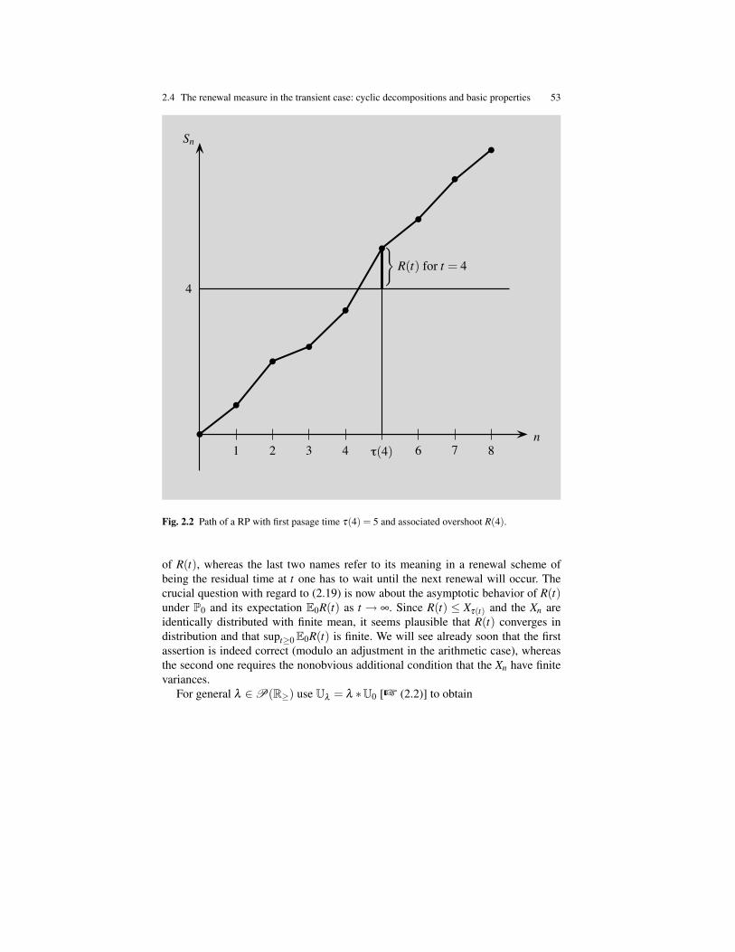
2.4 The renewal measure in the transient case: cyclic decompositions and basic properties 53
1 2 3 4 !(4) 6 7 8
!R(t) for t = 4
n
Sn
4
Fig. 2.2 Path of a RP with first pasage time τ(4) = 5 and associated overshoot R(4).
of R(t), whereas the last two names refer to its meaning in a renewal scheme ofbeing the residual time at t one has to wait until the next renewal will occur. Thecrucial question with regard to (2.19) is now about the asymptotic behavior of R(t)under P0 and its expectation E0R(t) as t → ∞. Since R(t) ≤ Xτ(t) and the Xn areidentically distributed with finite mean, it seems plausible that R(t) converges indistribution and that supt≥0 E0R(t) is finite. We will see already soon that the firstassertion is indeed correct (modulo an adjustment in the arithmetic case), whereasthe second one requires the nonobvious additional condition that the Xn have finitevariances.
For general λ ∈P(R≥) use Uλ = λ ∗U0 [+ (2.2)] to obtain

54 2 Random walks and stopping times: classifications and preliminary results
Uλ (t) =∫
[0,t]U0(t− x) λ (dx) =
∫[0,t]
E0τ(t− x) λ (dx)
=1µ
∫[0,t]
(t− x+E0R(t− x)) λ (dx)(2.20)
A combination of (2.19) and (2.20) now leads to the following result, called elemen-tary renewal theorem, which complements Thm. 1.1.2 in Section 1.1 and completesthe answer to question (Q2) posed there. It was first proved by FELLER [20] bymaking use of a Tauberian theorem for Laplace integrals [+ also his textbook [21]]and later by DOOB [18] via probabilistic arguments.
Theorem 2.4.3. [Elementary renewal theorem] Let (Sn)n≥0 be a RP in astandard model. Then
limt→∞
Uλ (t)t
=1µ
(2.21)
and limt→∞
τ(t)t
=1µ
Pλ -a.s. (2.22)
for all λ ∈P(R≥).
Strictly speaking, the elementary renewal theorem is just (2.21), but we haveincluded (2.22) because it can be viewed as its pathwise analog and also providesthe extension of Thm. 1.1.2 to arbitrary initial distributions λ when recalling from(2.18) that τ(t) = N(t) for all t ∈ R≥.
Proof. Since (Sn)n≥0 satisfies the SLLN under each Pλ and Sτ(t)−1 ≤ t < Sτ(t),Doob’s argument used in the proof of Thm. 1.1.2 works here as well to give (2.22).Left with the proof of (2.21), we infer from (2.20) with the help of Fatou’s lemma
liminft→∞
Uλ (t)t≥ 1
µ
∫limt→∞
(t− x
t1[0,t](x)
)λ (dx) =
1µ
.
for any λ ∈P(R≥). For the reverse inequality we must work a little harder andconsider the RP (Sc,n)n≥0 with truncated increments Xn∧ c for some c > 0. Denoteby τc(t) the corresponding first passage time and note that Sc,n ≤ Sn for all n ∈ N0implies τ(t)≤ τc(t). Also, Rc(t) := Sc,τc(t)− t ≤ c for all t ∈ R≥. Consequently, byanother appeal to (2.19),
E0τ(t) ≤ E0τc(t) =t +E0Rc(t)
µc≤ t + c
µcfor all t ∈ R≥
where µc := E(X1∧c). By using this in (2.20), the dominated convergence theoremensures that, for any λ ∈P(R≥),
2.4 The renewal measure in the transient case: cyclic decompositions and basic properties 55
limsupt→∞
Uλ (t)t≤∫
limt→∞
(t− x+ c
µct1[0,t](x)
)λ (dx) =
1µc
.
But this holds true for all c > 0 and limc→∞ µc = µ . Therefore we finally obtain
limsupt→∞
Uλ (t)t≤ 1
µ
which completes the proof. utIt is to be emphasized that all results and identities in this subsection have been
obtained only for the case of RP’s, that is for RW’s with nonnegative positive meanincrements. This may also be taken as a transitional remark so as to motivate theconsideration of general RW’s (Sn)n≥0 with a.s. finite ladder epoch σ> in the nextsubsection, the main focus being on the case where the RW has positive drift.
2.4.3 Cyclic decomposition via ladder epochs
Here we consider a nontrivial SRW (Sn)n≥0 with renewal measure U. Let σ beany a.s. finite stopping time for (Sn)n≥0 with associated sequence (σn)n≥0 of copysums. Denote by U(σ) the renewal measure of the RW (Sσn)n≥0 and define the pre-σoccupation measure of (Sn)n≥0 by
V(σ)(A) := E
(σ−1
∑n=0
1A(Sn)
)for A ∈B(R), (2.23)
which has total mass ‖V (σ)‖= Eσ and is hence finite if σ has finite mean. The nextlemma provides us with a useful relation between U and U(σ),V(σ).
Lemma 2.4.4. Under the stated assumptions,
U = V(σ) ∗U(σ)
for any a.s. finite stopping time σ for (Sn)n≥0.
Proof. Using cyclic decomposition with the help of the σn, we obtain

56 2 Random walks and stopping times: classifications and preliminary results
U(A) = E
(∑k≥0
1A(Sk
)= ∑
n≥0E
(σn+1−1
∑k=σn
1A(Sk)
)
= ∑n≥0
∫R
E
(σn+1−1
∑k=σn
1A−x(Sk−Sσn)
∣∣∣∣∣Sσn = x
)P(Sσn ∈ dx)
= ∑n≥0
∫R
V(σ)(A− x) P(Sσn ∈ dx)
= V(σ) ∗U(σ)(A) for all A ∈B(R),
where (2.3) of Thm. 2.2.1 has been utilized in the penultimate line. utNow, if (Sn)n≥0 has a.s. finite ladder epoch σ = σα for some α ∈ >,≥,<,≤,
we write Uα and V α for U(σ) and V(σ), respectively. Note that Uα is the renewalmeasure of the ladder height process (Sα
n )n≥0. As a trivial but important conse-quence of the previous lemma, we note that
U = V α ∗Uα if P(σα < ∞) = 1. (2.24)
In the case where σ> < ∞ a.s. (and thus also σ≥ < ∞ a.s.), we thus have a convolu-tion formula for the renewal measure U that involves the renewal measure of a RP,namely U> or U≥. This will allow us in various places to reduce a problem for RW’swith positive drift to those that have a.s. nonnegative or even positive increments.
If (Sn)n≥0, given in a standard model, has arbitrary initial distribution λ , thenLemma 2.4.4 in combination with Uλ = λ ∗U0 immediately implies
Uλ = λ ∗V(σ) ∗U(σ) = V(σ) ∗U(σ)λ
(2.25)
where V(σ),U(σ) are defined as before under P0.Returning to the zero-delayed situation, let us finally note that a simple compu-
tation shows thatV(σ) = ∑
n≥0P(σ > n,Sn ∈ ·), (2.26)
and that, for any real- or complex-valued function f
∫f dV(σ) = ∑
n≥0
∫σ>n
f (Sn) dP = E
(σ−1
∑n=0
f (Sn)
)(2.27)
whenever one of the three expressions exist.

2.5 The stationary delay distribution 57
2.5 The stationary delay distribution
2.5.1 What are we looking for and why?
In order to motivate the derivation of what is called the stationary delay distribu-tion of a RP (Sn)n≥0, let us first dwell on some heuristic considerations that embarkon the results in Section 1.2. We saw there that, if (Sn)n≥0 has exponential incre-ment distribution with parameter θ and the same holds true for S0, then the renewalmeasure U equals θλλ0 on R≥ which means that U([t, t + h]) for any fixed h istemporally invariant. In fact, we further found that the associated renewal countingprocess N := (N(t))t≥0 is a homogeneous Poisson process and as such a stationarypoint process in the sense that
ΘsN := (N(s+ t)−N(s))t≥0d= N for all s ∈ R≥. (2.28)
This follows immediately from the fact that a Poisson process has stationary andindependent increments [+ Thm. 1.2.2]. Cleary, N is a functional of the renewalprocess (Sn)n≥0 or, equivalently, of S0,X1, ..., i.e. N = h(S0,X1, ...) for some mea-surable function h. For the same reason
ΘsN = h(Sτ(s)− s,Xτ(s)+1, ...) = h(R(s),Xτ(s)+1, ...) for all s ∈ R≥,
where R(s) is the overshoot at s [see Fig. 2.3]. After this observation, the validityof (2.28) can be explained as follows. Even without providing a rigorous argument,the memoryless property of the exponential distribution is readily seen to imply thatR(s) d= Exp(θ) for all s ∈ R≥. By Thm. 2.2.1, R(s) is further independent of the iid
sequence (Xτ(s)+n)n≥1 with Xτ(t)+1d= X1. But this is all it takes to conclude (2.28).
Now let us turn to the general case, the question being whether an appropriatechoice of the delay distribution Fs of a RP (Sn)n≥0 with increment distribution F
renders R(t) d= Fs for all t ∈ R≥. If yes then by the same reasoning as before weshould obtain a stationary associated renewal counting process N = (N(t))t≥0 underPFs in the sense of (2.28) and in particular a translation invariant renewal measureUFs on R≥. But the translation invariance entails that UFs equals θλλ0 on R≥ forsome θ > 0, while the elementary renewal theorem 2.4.3 gives θ = 1/EX1. It willbe shown in ??????? that (R(t))t≥0 constitutes a continuous time Markov processfor which Fs, if it exists, forms a stationary distribution. However, the way Fs isderived hereafter, does not use this fact.
The question not addressed so far is why we should strive for Fs. The short replyis that its existence provides strong evidence that for arbitrary delay distributionsλ the behavior of ΘtN under Pλ and particularly of Uλ ([t, t + h]) is expected to bethe same as in the stationary situation if t tends to infinity. However, what we arereally hoping for and in fact going to deliver later is to turn this into a rigorous resultby a suitable construction of two RP’s on the same probability space with the same

58 2 Random walks and stopping times: classifications and preliminary results
0 1 2 3
1 2 3 4 !(4) 6 7 8
!R(4) = S!(4)!4
n
Sn S!(4)+n!4
4
Fig. 2.3 Path of a RP with first pasage time τ(4) = 5 and associated overshoot R(4).
increment distribution but different delay distributions λ and Fs, such that theirrenewal counting processes N and N′, say, are asymptotically equal in the sensethat limt→∞ ρ(ΘtN,ΘtN′) = 0, where ρ denotes a suitable distance function. Thetechnique behind this idea is well-known under the name coupling in the theory ofstochastic processes.
2.5.2 The derivation
If λ denotes any measure on R, let λ+ := λ (·∩R>) be its restriction to R> hereafterin the sense that its mass on R≤ has been removed. Having outlined what we arelooking for, let us now turn to the derivation of the stationary delay distribution Fs
for a RP (Sn)n≥0 with increment distribution F , finite mean µ and given as usual in

2.5 The stationary delay distribution 59
a standard model. The first thing to note is that Uλ = λ ∗U0 satisfies the convolutionequation
Uλ = λ + F ∗Uλ for all λ ∈P(R≥)
which in terms of the renewal function becomes a renewal equation as encounteredin Section 1.4, namely
Uλ (t) = λ (t) +∫
[0,t]F(t− x) Uλ (dx) for all λ ∈P(R≥) (2.29)
The goal is to find a λ such that Uλ (t) = µ−1t for all t ∈ R≥ (thus Uλ = µ−1λλ+0 )
and we will now do so by simply plugging the result into (2.29) and solving forλ (t). Then, with F := 1−F
λ (t) =tµ− 1
µ
∫ t
0F(t− x) dx
=1µ
∫ t
0F(t− x) dx =
1µ
∫ t
0F(x) dx for all t ≥ 0.
We thus see that there is only one λ , now called Fs, that gives the desired propertyof Uλ , viz.
Fs(t) :=1µ
∫ t
0F(x) dx =
1µ
∫ t
0P(X1 > x) dx for all t ≥ 0,
which is continuous and requires that µ is finite. To all those who prematurely leanback now let is be said that this is not yet the end of the story because there arequestions still open like “What about the infinite mean case?” and “Is this really theanswer we are looking for if the RP is arithmetic?”
If (Sn)n≥0 is d-arithmetic, w.l.o.g. suppose d = 1, then indeed a continuous delaydistribution gives a continuous renewal measure which is in sharp contrast to thezero-delayed situation where the renewal measure is concentrated on N0. The pointto be made here is that an appropriate definition of stationarity of the associatedrenewal counting process N must be restricted to those times at which renewalsnaturally occur in the 1-arithmetic case, namely integer epochs. In other words, thestationary delay distribution Fs to be defined must now be concentrated on N, butonly give (2.28) for t ∈ N0 under PFs . This particularly implies U+
Fs = µ−1λλ+1 and
thus U+Fs(n) = UFs(1, ...,n) = µ−1n for n ∈ N, where λλ1 is counting measure on
the set of integers Z. By pursuing the same argument as above, but for t ∈ N0 only,we then find that Fs must satisfy
Fs(n) =nµ− 1
µ
n
∑k=1
F(n− k) for all n ∈ N
and therefore

60 2 Random walks and stopping times: classifications and preliminary results
Fs(n) =1µ
n−1
∑k=0
F(k) dx =1µ
n
∑k=1
P(X1 ≥ k) for all n ∈ N
as the unique solution among all distributions concentrated on N. We summarizeour findings as follows.
Theorem 2.5.1. Let (Sn)n≥0 be a RP in a standard model with finite drift µ
and lattice-span d ∈ 0,1. Define its stationary delay distribution Fs on R≥by
Fs(t) :=
1µ
∫ t0 P(X1 > x) dx, if d = 0,
1µ ∑
n(t)k=1 P(X1 ≥ k), if d = 1
(2.30)
for t ∈ R≥, where n(t) := btc= supn ∈ Z : n≤ t. Then UFs = µ−1λλ+d .
Now observe that the integral equation (2.29) remains valid if λ is any locallyfinite measure on R≥ and Uλ is still defined as λ ∗U0. This follows because (2.29)is linear in λ . Hence, if we drop the normalization µ−1 in the definition of Fs, weobtain without further ado the following extension of the previous theorem.
Corollary 2.5.2. Let (Sn)n≥0 be a RP in a standard model with lattice-spand ∈ 0,1. Define the locally finite measure ξ on R≥ by
ξ (t) :=
∫ t0 P(X1 > x) dx, if d = 0,
∑n(t)k=1 P(X1 ≥ k), if d = 1
(2.31)
for t ∈ R≥ and n(t) as in Thm. 2.5.1. Then Uξ = λλ+d .
2.5.3 The infinite mean case: restricting to finite horizons
There is no stationary delay distribution if (Sn)n≥0 has infinite mean µ , but Cor.2.5.2 helps us to provide a family of delay distributions for which stationarity stillyields when restricting to finite horizons, that is to time sets [0,a] for a ∈ R>. Asa further ingredient we need the observation that the renewal epochs in [0,a] of(Sn)n≥0 and (Sa,n)n≥0, where Sa,n := S0 + ∑
nk=1(Xk ∧ a), are the same. As a trivial
consequence they also have the same renewal measure on [0,a], whatever the delaydistribution is. But by choosing the latter appropriately, we also have a dominationresult on (a,∞) as the next result shows.
2.5 The stationary delay distribution 61
Theorem 2.5.3. Let (Sn)n≥0 be a RP in a standard model with drift µ = ∞
and lattice-span d ∈ 0,1. With ξ given by (2.31) and for a > 0, define dis-tributions Fs
a on R≥ by
Fsa (t) :=
ξ (t ∧a)ξ (a)
for t ∈ R≥. (2.32)
Then, for all a ∈ R>, UFsa ≤ ξ (a)−1λλ
+d with equality holding on [0,a].
Proof. Noting that Fsa can be written as Fs
a = ξ (a)−1ξ −λa, where λa ∈P(R≥) isgiven by
λa(t) :=ξ (t)−ξ (a∧ t)
ξ (a)= 1(a,∞)(t)
ξ (t)−ξ (a)ξ (a)
for all t ∈ R≥,
we infer with the help of Cor. 2.5.2 that
UFsa = ξ (a)−1Uξ −λa ∗U0 ≤ ξ (a)−1Uξ = ξ (a)−1
λλd on R≥
as claimed. ut
2.5.4 And finally random walks with positive drift via ladder epochs
A combination of the previous results with a cyclic decomposition via ladder epochsallows us to further extend these results to the situation where (Sn)n≥0 is a RWwith positive drift µ and lattice-span d ∈ 0,1 and thus may also take on negativevalues. This is accomplished by considering Fs,Fs
a and ξ as defined before, but forthe associated ladder height RP (S>
n )n≥0. Hence we put
ξ (t) :=
∫ t0 P(S>
1 > x) dx, if d = 0,
∑n(t)k=1 P(S>
1 ≥ k), if d = 1(2.33)
for t ∈ R≥ (with n(t) as in Thm. 2.5.1) and then again Fsa by (2.32) for a ∈ R>. If
S>1 has finite mean µ> and hence ξ is finite, then let Fs be its normalization, i.e.
Fs = (µ>)−1ξ . In order to be able to use the results from the previous section wemust first verify that S>
1 and X1 are of the same lattice-type.
Lemma 2.5.4. Let (Sn)n≥0 be a nontrivial SRW and σ an a.s. finite first ladderepoch. Then d(X1) = d(Sσ ).

62 2 Random walks and stopping times: classifications and preliminary results
Proof. If X1 is nonarithmetic the assertion follows directly from the obvious in-equality d(Sσ )≤ d(X1) = 0. Hence it suffices to consider the case when d(X1) > 0.W.l.o.g. suppose d(Sσ ) = 1 and σ = σ>, so that d(X1) = 1 must be verified. Ifd(X1) < 1, then p := P(X1 = c) > 0 for some c 6∈ Z. Define Wn := Sn+1− S1 forn ∈ N0, clearly a copy of (Sn)n≥0 and independent of X1. Then
S>1 = X11X1>0+(X1 +Wτ(−X1))1X1≤0,
where τ(t) := infn ≥ 0 : Wn > t. Consequently, if c > 0, then P(S>1 = c) ≥ p >
0 which is clearly impossible as c 6∈ Z. If c < 0, then use that Wτ(t) is a strictlyascending ladder height for (Wn)n≥0 and thus integer-valued for any t ∈ R≥ to inferthat
P(S>1 ∈ c+Z) ≥ pP(c+Wτ(−c) ∈ c+Z) = pP(Wτ(−c) ∈ Z) > 0
which again contradicts our assumption d(S>1 ) = 1, for (c+Z)∩Z = /0. ut
Theorem 2.5.5. Let (Sn)n≥0 be a RW in a standard model with positive driftµ and lattice-span d ∈ 0,1. Then the following assertions hold with ξ ,Fs
aand Fs as defined in (2.33) and thereafter.
(a) U+ξ
= Eσ> λλ+d .
(b) U+Fs
a≤ ξ (a)−1Eσ> λλ
+d for all a ∈ R>.
(c) If µ is finite, then U+Fs = µ−1λλ
+d .
Proof. First note that µ > 0 implies Eσ> < ∞ [+ Thm. 2.2.9] and µ> = ES>1 =
µ Eσ> by Wald’s identity. By (2.25), Uλ = V> ∗U>λ
for any distribution λ , where
V>(A) = E0
(σ>−1
∑n=0
1A(Sn)
)for A ∈B(R)
is the pre-σ> occupation measure and thus concentrated on R≤ with ‖V>‖= Eσ>.Of course, (2.25) extends to arbitrary locally finite measures λ . Therefore,
Uξ (A) = V> ∗U>ξ(A) =
∫R≤
U>ξ(A− x) V>(dx)
=∫
R≤λλ
+d (A− x) V>(dx) = V>(R≤)λλ
+d (A)
= Eσ>
λλ+d (A) for all A ∈B(R≥)
where Cor. 2.5.2, the translation invariance of λλd and A−x⊂R≥ for all x∈R≤ havebeen utilized. Hence assertion (a) is proved. As (b) and (c) are shown in a similarmanner, we omit supplying the details again and only note for (c) that, if µ < ∞,

2.5 The stationary delay distribution 63
U+Fs = (µ>)−1 Eσ> λλ
+d really equals µ−1λλ
+d because µ> = µ Eσ> as mentioned
above. utRemark 2.5.6. (a) Replacing the strictly ascending ladder height S>
1 with the weaklyascending one S≥1 in the definition (2.33) of ξ leads to Uξ = Eσ≥λλd and thus to aproportional, but different result if S>
1 and S≥1 are different. On the other hand, it isclear that, for some β ∈ (0,1],
P(S≥1 ∈ ·) = (1−β )δ0 + β P(S>1 ∈ ·) (2.34)
where µ≥ = β µ> gives β = µ≥/µ>. Consequently, a substitution of S>1 for S≥1 in
(2.33) changes ξ merely by a factor and thus has the same normalization in the caseµ < ∞, namely Fs. In other words, the stationary delay distributions of (S>
n )n≥0 and(S≥n )n≥0 are identical.
(b) Given a RP (Sn)n≥0 with finite drift µ , we have already mentioned that theforward recurrence times R(t) form a continuous time Markov process with station-ary distribution π(dt) := µ−1P(X1 > t)dt, and we have found that Uπ = µ−1λλ
+0 ,
no matter what the lattice-type of (Sn)n≥0 is. On the other hand, if the latter is 1-arithmetic, then the stationary delay distribution Fs that gives UFs = µ−1λλ
+1 is dis-
crete and thus differs from π . In terms of the forward recurrence times this canbe explained as follows: The Markov process (R(t))t≥0 has continuous state spaceR> regardless of the lattice-type of the underlying RP and as such the continu-ous stationary distribution π . As a consequence, its subsequence (R(n))n≥0 forms aMarkov chain with the same state space and the same stationary distribution. How-ever, in the 1-arithmetic case N forms a closed subclass of states in the sense thatP(Rn ∈ N for all n ≥ 0) = 1 if P(R0 ∈ N) = 1. Hence (R(n))n≥0 may also be con-sidered as a discrete Markov chain on N and as such has stationary distribution Fs.
(c) The positive forward recurrence time R(t) = Sτ(t)− t, τ(t) = infn : Sn > t,has been used in the previous derivations as a motivation for the stationary de-lay distribution. As an alternative, one may also consider the nonnegative variantV (t) := Sν(t)− t with ν(t) := infn : Sn ≥ t. In the nonarithmetic case, this doesnot lead to anything different because stopping on the boundary, i.e. V (t) = 0, hasasymptotic probability zero. However, if (Sn)n≥0 is 1-arithmetic, then the stationarydelay distribution on R≥ instead of R> is obtained, namely
Fs(t) :=1
µ>
n
∑k=0
P(S>1 > k)1[n,n+1)(t) for t ∈ R≥.
As a consequence, UFs equals µ−1λλ1 on R≥ instead of R> only. Similar adjust-ments apply to the definitions of ξ and Fs
a when dealing with V (t), but we refrainfrom a further discussion.


Chapter 3Blackwell’s renewal theorem
Blackwell’s renewal theorem may be rightfully called the mother of all deeper re-sults in renewal theory. Not only it provides an answer to question (Q3) stated inthe first section on the expected number of renewals in a finite remote interval butis also the simpler, yet equivalent version of the key renewal theorem discussed inthe next chapter that allows us to determine the asymptotic behavior of many in-teresting quantities in applied stochastic models some of which we have alreadyseen in the Introduction. The present chapter is devoted exclusively to this resultand its derivation via four quite different proofs, the first and most recent one be-ing based on probabilistic arguments, notably the coupling method, the second oneon an analytic argument in combination with the Choquet-Deny equation, the thirdone on Fourier analysis, and the last one on Blackwell’s original 1948 proof payingobeisance to the eponymous mathematician.
3.1 Statement of the result and historical account
We are now going to state Blackwell’s theorem for RW’s with positive drift whichis often called the two-sided version of the original result that only considers RP’s(nonnegative or one-sided case). But with the concept of ladder variables at hand,a proof of the general version is easily reduced to the nonnegative case as we willdemonstrate below. The following notation is introduced so as to facilitate a unifiedformulation of subsequent results for the arithmetic and the nonarithmetic case. Ford ≥ 0, define
d-limt→∞
f (t) :=
limt→∞
f (t), if d = 0,
limn→∞
f (nd), if d > 0.
Recall that λλ0 denotes Lebesgue measure, while λλd for d > 0 is d times countingmeasure on dZ. The factor d is actually chosen for convenience in the followingtheorem.
65

66 3 Blackwell’s renewal theorem
Theorem 3.1.1. [Blackwell’s renewal theorem] Let (Sn)n≥0 be a RW in astandard model with lattice-span d ≥ 0 and positive drift µ . Then
d-limt→∞
Uλ ([t, t +h]) = µ−1
λλd([0,h]) and (3.1)
limt→−∞
Uλ ([t, t +h]) = 0 (3.2)
for all λ ∈P(R), where µ−1 := 0 if µ = ∞.
The result has a long history dating back, as pointed out in [14], [15] and [6], toold work from 1936 by KOLMOGOROV [28] on discrete Markov chains from whichthe theorem for arithmetic RP’s is deducible. In 1949 this case was explicitly settledby ERDOS, FELLER & POLLARD [19], while BLACKWELL [6] in 1948 providedthe first proof for nonarithmetic RP’s. The latter case was also treated by DOOB [18,Thm. 12] under the additional restriction that some Sn is nonsingular with respectto λλ0 (such distributions will later be called spread out, + Section 4.3). Proofs inthe general case of RW’s with positive drift had not to wait long. The arithmeticcase was settled in 1952 by CHUNG & WOLFOWITZ [15], the nonarithmetic oneagain by BLACKWELL [7] in 1953, although a version under the afore-mentionedspread out assumption was given one year earlier by CHUNG & POLLARD [14].BLACKWELL’s work, which mentions a further unpublished proof by HARRIS, isalso remarkable for the fact that the concept of ladder variables is introduced andused there for the first time. Nevertheless all proofs that had been published until themid fifties appeared to be quite technical and did not meet the intuitive appeal of theresult itself. The following quote of SMITH [41] from his 1958 survey on renewaltheory and its ramifications describes it accurately:
Blackwell’s renewal theorem has a strong intuitive appeal and it is surprising that its proofshould be so difficult. We suspect that no one has yet thought on the “right” mode but thatwhen this mode is ultimately realized a simple proof will emerge.
After further proofs by FELLER & OREY [22] in 1961 via Fourier analysis [+ Sec-tion 3.5], by FELLER in his 1971 textbook [21] using the Helly-Bray theorem inconnection with the Choquet-Deny equation [+ Section 3.4], by MCDONALD [35]in 1975 via harmonic analysis of the forward recurrence time process, and by scChan [10] using a constructive method, a breakthrough towards a more natural andreally probabilistic approach had to wait until the advent of the coupling method,first introduced as early as 1938 by the ingenious mathematician DOEBLIN [16],[17] in his study of discrete Markov chains but unnoticed or forgotten afterwardsfor more than 30 years due to his untimely and tragic death in 1940. Until today,four coupling proofs of Blackwell’s renewal theorem have been published, the firstones by LINDVALL [30] in 1977 for RP’s with finite drift and by ATHREYA, MC-DONALD & NEY [4] one year later for RW’s with finite positive drift. In 1987,THORISSON [45] provided a third proof that “improved” on the former two ones bygiving a self-contained argument for successful coupling where those had utilized

3.2 The easy part first: the behavior of U at −∞ 67
the Hewitt-Savage zero-one law or the topological recurrence of RW’s with driftzero. The coupling proof we are going to present in Section 3.3 may be viewed as ablend of these three contributions. Yet another, very short proof was finally given in1996 by LINDVALL & ROGERS [32] and is inspired by a special coupling that hadbeen christened Mineka coupling by the first author in his monography [31] on thecoupling method (referring to [36]). We will describe it in Section 4.4 including ashort account of how it may be used to prove Blackwell’s theorem [+ Subsection4.4.3].
We close this section with a brief classification of Blackwell’s renewal theoremin a measure-theoretic context. Recall that a sequence (Qn)n≥1 of locally finite mea-sures in R converges vaguely ( v→) to a locally finite measure Q, in short Qn
v→Q, iffor every continuous function g : R→ R with compact support (g ∈ C0(R))
limn→∞
∫g dQn =
∫g dQ
holds true. Since any g ∈ C0(R) may be approximated pointwise by primitive func-tions of the form h = ∑
kj=1 a j1I j with bounded intervals I j and conversely indicators
of such intervals are pointwise limits of functions in C0(R), an equivalent conditionis
limn→∞
Qn(I) = Q(I)
for all Q-continuous intervals I, that is, whose endpoints have no mass under Q.Now it is easily seen that the two assertions in Blackwell’s renewal theorem mayalso be stated as
Uλ (t + ·) v→ µ−1
λλd as t→ ∞ (through dZ if d > 0) and (3.3)
Uλ (t + ·) v→ 0 as t→−∞ (3.4)
for every λ ∈P(R). It is worth mentioning that, once the convergence of Uλ (t + ·)has been established, the translation invariance of the limiting measure Λ , say, onGd immediately follows from
Λ(I) = d-limt→∞
Uλ (t + I) = d-limt→∞
Uλ (s+ t + I) = Λ(s+ I)
for all bounded intervals I and all s ∈ Gd . Hence, Λ must be a multiple of λλd , forthis is the unique (up to scaling) translation invariant measure (Haar measure) onGd .
3.2 The easy part first: the behavior of U at −∞
The renewal measure of any RW with positive drift vanishes at −∞. This is thesecond and less interesting assertion (3.2) of Blackwell’s theorem. Since it is also

68 3 Blackwell’s renewal theorem
easily verified with the help of Lemma 2.4.1, we treat this part of the theorem firstso as to focus exclusively on the nontrivial part thereafter, i.e. on (3.1).
Given a RW (Sn)n≥0 with drift µ > 0 and arbitrary delay distribution, it followsfrom Sn→ ∞ a.s. that N(0) = N((−∞,0]) < ∞ a.s. and thus
limt→−∞
N([t, t +h]) = limt→−∞
∑n≥0
1[t,t+h](Sn) = 0 a.s.
for each h > 0. This yields the desired conclusion (3.2) because, by Lemma 2.4.1,the family N([t, t +h] : t ∈ R is further uniformly integrable.
Plainly, (3.2) is equivalent to
limt→−∞
U(t +B) = 0 for all bounded B ∈B(R), (3.5)
but even more can be said without further ado. As N(0) < ∞ a.s. further implies
limt→−∞
N(t) = 0 a.s.
and this convergence is monotone, we infer with the help of the monotone conver-gence theorem that
limt→−∞
U(t) = 0 if U(0) = EN(0) < ∞. (3.6)
However, the question remains and will so for a further while under which conditionon the RW we have that U(0) < ∞. We refer to ???????
3.3 A coupling proof
We now proceed with a presentation of the first proof of (3.1) which is purely prob-abilistic and based on the coupling technique. To disenthrall the ensuing argumentsfrom distracting technicalities we begin with a couple of preliminary considerations.
3.3.1 Shaking off technicalities
1st reduction: S0 = 0.It is no loss of generality to prove (3.1) for zero-delayed RW’s only. Indeed, if S0has distribution λ , then
Uλ ([t, t +h]) =∫
U0([t− x, t− x+h]) λ (dx)

3.3 A coupling proof 69
together with supt∈R U0([t, t +h])≤ U0([−h,h]) < ∞ [+ Lemma 2.4.1] implies byan appeal to the dominated convergence theorem that (3.1) is valid for Uλ if so forU0.
2nd reduction: (Sn)n≥0 is a RP.The cyclic decomposition via ladder variables described in Subsection 2.4.3 furtherallows us to reduce the proof to the case where (Sn)n≥0 has nonnegative increments.To see this recall first that, by Lemma 2.5.4, the ladder height process (S>
n )n≥0 isof same lattice-type as (Sn)n≥0 and suppose that its renewal measure U> satisfies(3.1). Then U = V> ∗U>, ‖V>‖ = Eσ> < ∞, µ> = µEσ> and another appeal tothe dominated convergence theorem yield
d-limt→∞
U([t, t +h]) =∫
d-limt→∞
U>([t− x, t− x+h]) V>(dx)
= (µ>)−1
λλd([0,h])‖V>‖
=
µ−1λλd([0,h]), if µ < ∞,
0, if µ = ∞
(3.7)
for all h > 0, i.e. validity of (3.1) for U as well.
3rd reduction: (Sn)n≥0 is completely d-arithmetic (d ≥ 0).The final reduction that will be useful hereafter is to assume that the incrementdistribution is completely d-arithmetic so that, by Lemma 2.1.2, its symmetrizationhas the the same lattice-span.
Lemma 3.3.1. Let (Sn)n≥0 be a nontrivial SRW with lattice-span d ≥ 0 andrenewal measure U. Let (ρn)n≥0 a SRP independent of (Sn)n≥0 and with ge-ometric increments, viz. P(ρ1 = n) = (1− θ)n−1θ for some θ ∈ (0,1) andn∈N. Then (Sρn)n≥0 is a completely d-arithmetic SRW with renewal measureU(ρ) satisfying U(ρ) = (1−θ)δ0 +θ U.
Proof. First of all, let (In)n≥1 be a sequence of iid Bernoulli variables with param-eter θ independent of (Sn)n≥0. Each In may be interpreted as the outcome of a cointossing performed at time n. Let (Jn)n≥0 be the SRP associated with (In)n≥1 and let(ρn)n≥0 be the sequence of copy sums associated with ρ = ρ1 := infn≥ 1 : In = 1.Then (ρn)n≥0 satisfies the assumptions of the lemma, and since ρ is a stopping timefor the bivariate SRW (Sn,Jn)n≥0, we infer by invoking Thm. 2.2.3(j) that (Sρn)n≥0forms a SRW. Next observe that, for each A ∈B(R),
U(ρ)(A)−δ0(A) = E
(∑n≥1
In1A(Sn)
)= EI1 (U(A)−δ0(A))
which proves the relation between U(ρ) and U, for EI1 = θ .

70 3 Blackwell’s renewal theorem
It remains to show that (Sρn)n≥0 is completely d-arithmetic. Let (S′n,ρ ′n)n≥0 be anindependent copy of (Sn,ρn)n≥0 and put ρ := ρ1 and ρ ′ := ρ ′1. By Lemma 2.1.2, itsuffices to show that the symmetrization Sρ −S′
ρ ′ is d-arithmetic. Since c := d(Sρ −S′
ρ ′)≥ d, we must only consider the case c > 0 and then show that P(X1 ∈ cZ) = 1.But
1 = P(Sρ −S′ρ ′ ∈ cZ) = ∑
m,n≥1θ
2(1−θ)m+n−2 P(Sm−S′n ∈ cZ)
clearly implies P(Sm−S′n ∈ cZ) = 1 for all m,n ∈ N. Hence
0 < P(S1−S′1 = 0) = P(S2−S′1 ∈ cZ,S1−S′1 = 0) = P(X1 ∈ cZ)P(S1−S′1 = 0)
giving P(X1 ∈ cZ) = 1 as asserted. utWith the relation between U(ρ) and U at hand it is clear that it suffices to show
(3.1) for the first of these measures. Alternatively, we could rely on cyclic decom-position as in the 2nd reduction, viz. U = Vρ ∗U(ρ) with V(ρ) denoting the pre-ρoccupation measure.
3.3.2 Setting up the stage: the coupling model
Based on the previous considerations, we now assume that (Sn)n≥0 is a zero-delayedcompletely d-arithmetic RP with drift µ . As usual, the increment distribution isdenoted by F . The starting point of the coupling construction is to consider thissequence together with a second one (S′n)n≥0 such that the following conditions aresatisfied:
(C1) (Sn,S′n)n≥0 is a bivariate RW with iid increments (Xn,X ′n), n≥ 1.
(C2) (S′n−S′0)n≥0d= (Sn)n≥0 and thus X ′1
d= X1.
(C3) S′0d= Fs if µ < ∞, and S′0
d= Fsa for some a ∈ R> if µ = ∞.
Here Fs and Fsa denote the stationary delay distribution and its truncated variant
defined in (2.30) and (2.32), respectively. By the results in Section 2.5, the renewalmeasure U′ of (S′n)n≥0 satisfies U′([t, t + h]) = µ−1λλd([0,h]) for all t,h ∈ R> ifµ < ∞, and U′([t, t + h]) ≤ ξ (a)−1λλd([0,h]) for all t,h ∈ R> if µ = ∞ where ξ (a)tends to ∞ as a → ∞. Hence U′ satisfies (3.1) in the finite mean case and doesso approximately for sufficiently large a if µ = ∞. The idea is now to construct athird RP (S′′n)n≥0 from the given two which is a copy of (S′n)n≥0 and such that S′′nis equal or at least almost equal to Sn for all n ≥ T , T an a.s. finite stopping timefor (Sn,S′n)n≥0, called coupling time. This entails that the coupling process (S′′n)n≥0has renewal measure U′ while simultaneously being close to U on remote intervalsbecause with high probability such intervals contain only renewal epochs S′′n forn≥ T .
Having outlined the path towards the asserted result we must now complete thespecification of the above bivariate model so as to facilitate a successful coupling.
3.3 A coupling proof 71
But the only unspecified component of the model is the joint distribution of (X1,X ′1)for which the following two alternatives will be considered:
(C4a) X1, X ′1 are independent or, equivalently, (Sn)n≥0 and (S′n)n≥0 are indepen-dent.
(C4b) X ′1 = Y11[0,b](|X1−Y1|)+ X11(b,∞)(|X1−Y1|), where Y1 is an independentcopy of X1 an b is chosen so large that Gb := P(X1−Y1 ∈ ·||X1−Y1| ≤ b)is d-arithmetic (and thus nontrivial).
The existence of b with d(Gb) = d follows from the fact that G := P(X1−Y1 ∈ ·) isd-arithmetic together with Gb
w→ G.Condition (C4a) is clearly simpler than (C4b) and will serve our needs in the
finite mean case because then it is sufficient to guarantee that the symmetrizationX1−X ′1 is integrable with mean zero. Since the latter is also d-arithmetic, we inferfrom Thm. 2.3.5 that (Sn−S′n)n≥0 is (topologically) recurrent on Gd .
On the other hand, if µ = ∞, the difference of two independent X1,X ′1 fails to beintegrable, while under (C4b) we have X1−X ′1 = (X1−Y1)1[−b,b](X1−Y1) which isagain symmetric with mean zero and d-arithmetic by choice of b. Once again wehence infer the recurrence of the symmetric RW (Sn−S′n)n≥0 on Gd .
A coupling of two independent processes with identical transition mechanism butdifferent initial distributions is what DOEBLIN realized in [16] for Markov chainsand is therefore called Doeblin coupling hereafter. The construction with (X1,X ′1)as specified in (C4b) goes back to ORNSTEIN [37] and is thus named Ornsteincoupling.
3.3.3 Getting to the point: the coupling process
In the following suppose that (C1–3) and (C4a) are valid if µ < ∞, while (C4a) isreplaced with (C4b) if µ = ∞. Fix any ε > 0 if F is nonarithmetic, while ε = 0if F has lattice-span d > 0. Since (Sn− S′n)n≥0 is recurrent on Gd (recall that thedelay distribution of S′0 is also concentrated on Gd) we infer the a.s. finiteness of theε-coupling time
T := infn≥ 0 : |Sn−S′n| ≤ εand define the coupling process (S′′n)n≥0 by
S′′n :=
S′n, if n≤ T,
Sn− (ST −S′T ), if n≥ Tfor n ∈ N0, (3.8)
which may also be stated as
S′′n :=
S′n, if n≤ T,
S′T +∑nk=T+1 Xk, if n > T
for n ∈ N0. (3.9)
72 3 Blackwell’s renewal theorem
The subsequent lemma accounts for the intrinsic properties of this construction.
Lemma 3.3.2. Under the stated assumptions, the following assertions holdtrue for the coupling process (S′′n)n≥0:
(a) (S′′n)n≥0d= (S′n)n≥0.
(b) |S′′n −Sn| ≤ ε for all n≥ T .
Proof. We only need to show (a) because (b) is obvious from the definition of thecoupling process and the coupling time. Since T is a stopping time for the bivariateRW (Sn,S′n)n≥0, we infer from Thm. 2.2.1 that XT+1,XT+2, ... are iid with the samedistribution as X1 and further independent of T,(Sn,S′n)0≤n≤T . But this easily seento imply assertion (a), namely
P(S′′0 ∈ B0,X ′′j ∈ B j for 1≤ j ≤ n)
=n
∑k=0
P(T = k,S′0 ∈ B0,X ′j ∈ B j for 1≤ j ≤ k)P(X j ∈ B j for k < j ≤ n)
+P(T > n,S′0 ∈ B0,X ′j ∈ B j for 1≤ j ≤ n)
=n
∑k=0
P(T = k,S′0 ∈ B0,X ′j ∈ B j for 1≤ j ≤ k)P(X ′j ∈ B j for k < j ≤ n)
+P(T > n,S′0 ∈ B0,X ′j ∈ B j for 1≤ j ≤ n)
= P(S′0 ∈ B0,X ′j ∈ B j for 1≤ j ≤ n)
for all n ∈ N and B1, ...,Bn ∈B(R≥). utBefore moving on to the finishing argument, let us note that a coupling with
a.s. finite 0-coupling time is called exact coupling, while we refer to an ε-couplingotherwise.
3.3.4 The final touch
As usual, let N(I) denote the number of renewals Sn in I, and let N′′(I) be thecorresponding variable for the coupling process (S′′n)n≥0. Define further Nk(I) :=∑
kj=0 1I(Sn) and N′′k (I) in a similar manner. Fix any h > 0, ε ∈ (0,h/2), and put I :=
[0,h], Iε := [ε,h− ε], and Iε := [−ε,h + ε]. The following proof of (3.1) focusseson the slightly more difficult nonarithmetic case, i.e. d = 0 hereafter. We first treatthe case µ < ∞.
A. The finite mean case. By Lemma 3.3.2(a), (S′′n)n≥0 has renewal measure U′which in turn equals µ−1λλ
+0 by our model assumption (C3). It follows from the

3.4 Feller’s analytic proof 73
coupling construction that
S′′n ∈ t + Iε ⊂ Sn ∈ t + I ⊂ S′′n ∈ t + Iε
for all t ∈ R≥ and n≥ T . Consequently,
N′′(t + Iε)−NT (t + I) ≤ N(t + I) ≤ N′′(t + Iε)+NT (t + I)
and therefore, by taking expectations,
U′(t + Iε)−ENT (t + I) ≤ U(t + I) ≤ U′(t + Iε)+ENT (t + I) (3.10)
for all t ∈ R≥. But U′(t + Iε) = µ−1(h− 2ε) and U′(t + Iε) = µ−1(h + 2ε) for allt > ε . Moreover, the uniform integrability of N(t + I) : t ∈ R [+ Lemma 2.4.1]in combination with NT (t + I)≤ N(t + I) and limt→∞ NT (t + I) = 0 a.s. entails
limt→∞
ENT (t + I) = 0.
Therefore, upon letting t tend to infinity in (3.10), we finally arrive at
h−2ε
µ≤ liminf
t→ıU(t + I) ≤ limsup
t→ıU(t + I) ≤ h+2ε
µ.
As ε can be made arbitrarily small, we have proved (3.1).
A. The infinite mean case. Here we have U′ ≤ ξ (a)−1λλ+0 where a may be chosen
so large that ξ (a)−1 ≤ ε . Since validity of (3.10) remains unaffected by the driftassumption, we infer by just using the upper bound
limsupt→ı
U(t + I) ≤ ξ (a)−1(h+2ε) ≤ ε(h+2ε)
and thus again the assertion, for ε can be made arbitrarily small. This completes ourcoupling proof of Blackwell’s theorem.
3.4 Feller’s analytic proof
The following analytic proof of (3.1), given for nonarithmetic SRW with finite mean,is largely due to FELLER as given in his textbook [21, p. 264–266] and embarks onthe following lemma by CHOQUET & DENY [11]. An adaptation to the arithmeticcase is easily provided and left to the interested reader.

74 3 Blackwell’s renewal theorem
Lemma 3.4.1. [Choquet-Deny] Given a nonarithmetic distribution F on Rwith finite mean, any bounded continuous function ϕ : R→ R satisfying ϕ =ϕ ∗F is necessarily constant.
Proof. Start by observing that, for any t ∈ R, the sequence Mn(t) := ϕ(t−Sn), n ∈N0, constitutes a martingale w.r.t. the natural filtration (Fn)n≥0 of (Sn)n≥0 because
E(ϕ(t−Sn)|Fn−1) = E(ϕ(t−Sn)|Sn−1)
=∫
ϕ(t− x−Sn−1) F(dx)
= ϕ ∗F(t−Sn−1) = ϕ(t−Sn−1) f.s.
for all n ∈ N. As (Mn(t))n≥0 is also bounded, we infer that Mn(t)→M∞(t) a.s. andin second mean, and the limit is a.s. constant by an appeal to the Hewitt-Savagezero-one law, the constant being EM∞(t) = EM0(t) = ϕ(t). But as an L2-martingaleit further satisfies
0 = E(M∞(t)−M0(t))2 = ∑n≥1
E(Mn(t)−Mn−1(t))2
and thus ϕ(t) = ϕ(t− Sn) a.s. for all n ∈ N0. Now let (Wn)n≥0 := (Sρn)n≥0 be theembedded completely nonarithmetic RW according to Lemma 3.3.1 and denote byν its finite drift. Then
ϕ(t) = ϕ(t−Wn) = ϕ(t +nν−Wn) a.s. for all n ∈ N0 and t ∈ R. (3.11)
Use the recurrence of the zero-mean RW (nν−Wn)n≥0 on R to infer
nν−Wn : n ∈ N0= R a.s.
Combining this with the continuity of ϕ in (3.11) finally shows ϕ ≡ ϕ(0). utWith the help of this lemma, we will now proceed to show the vague convergence
of U(t + ·) to µ−1λλ0 as t→∞ which is equivalent to (3.1) as pointed out at the end ofthe first section of the present chapter. The uniform local boundedness of U, statedas supt∈R U([t, t +a])≤ U([−a,a]) < ∞ for all a ∈ R> in (2.17), obviously ensuresthat supt∈R U(t + K) < ∞ for all compact K ⊂ R and thus the vague compactnessof the family ΘtU : t ∈ R where ΘtU := U(t + ·). Hence, by invoking the Helly-Bray theorem [+ e.g. [9, p. 160f]], every sequence (ΘtkU)k≥1 with tk→∞ containsa vaguely convergent subsequence. In order to prove ΘtU
v→ µ−1λλ0 as t → ∞, ittherefore suffices to verify that any vaguely convergent subsequence has the samelimit µ−1λλ0.
To this end, suppose that tk→ ∞ and ΘtkUv→ λ , so that
ϕ(x) := limk→∞
g∗ΘtkU(x) = limk→∞
∑n≥0
Eg(x+ tk−Sn) = g∗λ (x)

3.4 Feller’s analytic proof 75
for every g∈C0(R). Plainly, ΘtkUv→ λ implies Θtk+xU
v→Θxλ for all x∈R. We willshow next that Θtk+xU
v→ λ for all x ∈ R holds true as well whence the uniquenessof the vague limit implies the translation invariance of λ and thus λ = cλλ0 for somec ∈ R≥.
Lemma 3.4.2. Under the stated assumptions, Θtk+xUv→ λ for all x ∈ R.
Proof. Fix any such g, let a > 0 be such that supp(g)⊂ [−a,a], and put
ω(g,ε) := supx,y∈R:|x−y|≤ε
|g(x)−g(y)|
As g is uniformly continuous, limε↓0 ω(g,ε) = 0. With the help of the dominatedconvergence theorem, we infer
ϕ(x) = limk→∞
(g(x+ tk)+
∫g∗U(x− y+ tk) F(dy)
)=∫
limk→∞
g∗U(x− y+ tk) F(dy)
= ϕ ∗F(x) for all x ∈ R,
that is, ϕ satisfies the Choquet-Deny equation. Furthermore, by another use of (2.17)of Lemma 2.4.1, we find that ϕ is a uniformly continuous function because
|ϕ(x)−ϕ(y)| ≤ supk≥1
∫[x+tk−a−ε,x+tk+a+ε]
|g(x−u+ tk)−g(y−u+ tk)| U(du)
≤ ω(g, |x− y|) supt∈R
U([t−a− ε, t +a+ ε])
≤ ω(g, |x− y|)U([−2a−2ε,2a+2ε]) for all x,y ∈ R.
Hence the Choquet-Deny lemma implies that ϕ ≡ ϕ(0). Now we have that
g∗Θxλ (y) = limk→∞
g∗Θtk+xU(y)
= limk→∞
g∗ΘtkU(x+ y) = ϕ(x+ y) = ϕ(0) for all x ∈ R
and since this is true for all g ∈ C0(R), we infer Θxλ = λ for all x and thereby theassertion of the lemma. ut
It remains to verify that ΘtUv→ cλλ0 holds with c = µ−1. But the the fact that
UFs([t, t +h]) = µ−1h for all t,h∈R> if Fs denotes the stationary delay distributionof (Sn)n≥0 yields by the dominated convergence theorem
µ−1h = lim
t→∞
∫U([t− x, t− x+h]) Fs(dx) = ch

76 3 Blackwell’s renewal theorem
and thus c = µ−1.
3.5 The Fourier analytic proof by Feller and Orey
In this section, we will give a proof of Blackwell’s theorem under the assumptionthat (Sn)n≥0 is a SRW with increment distribution F , lattice-span d ∈ 0,1, andfinite positive drift µ . Levy’s continuity theorem is a powerful tool to show the weakconvergence of finite measures on R but fails to work in the present context wherethe vague convergence must be verified for the locally finite measures ΘtU = U(t + ·)as t →±∞. The subsequent Fourier-analytic approach that embarks on a study ofthe finite measures
Vs(B) := ∑n≥0
sn(F∗n(B)+F∗n(−B)) for B ∈B(R) and s ∈ (0,1),
obtained from U by symmetrization and discounting, is essentially due to FELLER& OREY [22]. Here we follow closely the nice adaptation by BREIMAN [9, Section10.3] [+ also [47]]. His textbook and the one by CHOW & TEICHER [13] shouldalso be consulted for a number of Fourier-analytic results that are taken hereafter asknown facts. Since we are going to make use of complex numbers, let i :=
√−1 andℜz,ℑz,z = ℜz− iℑz denote the real part, imaginary part and conjugate-complex ofa complex number z, respectively.
3.5.1 Preliminaries
Let φ(t) = EeitX1 denote the Fourier transform (FT) of X1. Since Sn has FT φ n forall n ∈ N0, the finite discounted renewal measure Us = ∑n≥0 snF∗n has FT
Ψs := ∑n≥0
snφ
n =1
1− sφ
which converges to Ψ := (1− φ)−1 on Dφ := t ∈ R : φ(t) 6= 1. The latter setequals R\0 in the nonarithmetic case (d = 0) and R\2πZ in the 1-arithmeticcase. Note further that Us ↑ U and Vs ↑ V := V1 as s ↑ 1. Using the already provedfact limt→−∞ U(t + I)→ 0 for all bounded intervals I, we see that
limt→∞
(U(t + I)−V(t + I)) = limt→∞
U(−t− I) = 0
and thus that it suffices to prove
ΘtVv→ µ
−1λλd for t→ ∞ through Gd . (3.12)

3.5 The Fourier analytic proof by Feller and Orey 77
Since −X1 has distribution F(−·) and FT φ = ℜφ − iℑφ , we see that F∗n +F∗n(−·) has FT ℜ(φ n) for all n ∈ N0. Hence, the FT of Vs equals
ℜΨs = ℜ
(1
1− sφ
)=
1− sℜφ
|1− sφ |2 ≥ 0.
As s ↑ 1, it converges pointwise on Dφ to
ℜΨ = ℜ
(1
1−φ
)=
1−ℜφ
|1−φ |2 . (3.13)
The following lemma provides a key to our attempted result and describes the be-havior of ℜΨs as s ↑ 1.
Lemma 3.5.1. Let b > 0 be such that φ(t) 6= 1 for all t ∈ [−b,b]\0. ThenℜΨ is λλ0-integrable on [−b,b], and
lims↑1
∫ b
−bf (t)ℜΨs(t) dt =
π f (0)µ
+∫ b
−bf (t)ℜΨ(t) dt (3.14)
for all f ∈ C0(R), that is
ℜΨs 1[−b,b] λλ0v→ πg(0)
µδ0 + ℜΨ 1[−b,b] λλ0 (s ↑ 1).
Proof. We begin with the proof of the λλ0-integrability of ℜΨ on [−b,b]. Since ℜΨ
is continuous on [−b,b]\0, it suffices to prove local integrability at 0. We chooseε ∈ (0,b] so small that |1−φ(t)| ≥ µt/2 for t ∈ [−ε,ε], which is possible becauseφ ′(0) = µ . After these observations and recalling (3.13) it suffices to verify that∫
ε
−ε
1−ℜφ(t)t2 dt = 2
∫ε
0
1−Ecos(tX1)t2 dt < ∞.
But with the help of Fubini’s theorem, we obtain∫ε
0
1−Ecos(tX1)t2 dt = E
(∫ε
0
1− cos(tX1)t2 dt
)= E
(|X1|
∫ε|X1|
0
1− cos tt2 dt
)≤ E|X1|
∫∞
0
1− cos tt2 dt
with the last estimate clearly being finite.Turning to the proof of (3.14), we first write, for any given f ∈ C0(R),

78 3 Blackwell’s renewal theorem∫ b
−bf (t)(
ℜΨs(t)−ℜΨ(t))
dt =∫ b
−bf (t)ℜ
(1
1− sφ(t)− 1
1−φ(t)
)dt
=∫ b
−bf (t)
(s−1)φ(t)|1− sφ(t)|2 ℜ
(φ(t)(1− sφ(t))
1−φ(t)
)dt =: I(s,b).
On [−b,b]\[−ε,ε], the integrand of I(s,b) remains bounded and converges to 0 ass ↑ 1. Hence we must examine I(s,ε) for sufficiently small ε > 0. To this end write
I(s,ε) = I1(s,ε)− I2(s,ε) with
I1(s,ε) : =∫
ε
−ε
f (t)(s−1)φ(t)|1−φ(t)|2 ℜ
(φ(t)(1− sφ(t))
1−φ(t)
)dt and
I2(s,ε) : =∫
ε
−ε
f (t)(s−1)2φ(t)|1−φ(t)|2 |φ(t)|2ℜΨ(t) dt
and notice that the integrand of I2(s,ε) is bounded by a multiple of ℜΨ , for |1−sφ | ≥ 1− s. Hence, by the dominated convergence theorem,
lims↑1
I2(s,ε) = 0 for all 0 < ε ≤ b.
Left with the critical term I1(s,ε), fix any η ∈ (0,1) and ε ∈ (0,b] sufficiently smallsuch that, for φ(t) = 1+φ ′(t∗)t, t∗ ∈ [−t, t], we have
(1−η)((1− s)2 + µ
2t2) ≤ |1− sφ(t)|2 ≤ (1+η)((1− s)2 + µ
2t2)and therefore the continuity of
g(s, t) :=|1− sφ(t)|2
(1− s)2 + µ2t2
for (s, t) ∈ (0,1]× [−ε,ε] with 1−η ≤ g(s, t)≤ 1+η . Furthermore,
g(t) := lims↑1
g(s, t) =|1−φ(t)|2
µ2t2 for all t 6= 0
with continuous extension at 0, defined by
g(0) := limt→0
|1−φ(t)|2µ2t2 =
|φ ′(0)|2µ
= 1.
In a similar manner, we find that
h(t) := − f (t)ℜ
(φ(t)(1−φ(t))
1−φ(t)
)for t 6= 0
is continuous on [−ε,ε] after setting h(0) := f (0). Just note that

3.5 The Fourier analytic proof by Feller and Orey 79
limt→0
1−φ(t)1−φ(t)
=φ ′(0)φ ′(0)
= −1.
Possibly after further diminishing ε such that
1−η
1+ηh(0) ≤ h(t)
g(s, t)≤ 1+η
1−ηh(0) for all (s, t) ∈ [1− ε,1)× [−ε,ε],
we finally conclude
lims↑1
I1(s,ε) = lims↑1
∫ε
−ε
h(t)g(s, t)
(1− s)(1− s)2 + µ2t2 dt
= lims↑1
∫ε/(1−s)
−ε/(1−s)
h(t(1− s))g(s, t(1− s))
11+ µ2t2 dt
Q1±η
1∓η
h(0)µ
∫∞
−∞
dt1+ t2
=1±η
1∓η
πh(0)µ
and thereupon (3.14) as h(0) = f (0) and η can be made arbitrarily small. utInstead of proving (3.12) we will prove the equivalent assertion [+ Thm. ??]
that
h(x)ΘaV(dx) v→ h(x)µ
λλd(dx) for a→ ∞ through Gd (3.15)
for some positive continuous and λλd-integrable function h. As will be seen soon,a convenient choice is a function h that is the FT of a symmetric distribution withλλ0-density h∈C0(R). The next lemma shows that such a choice is actually possible.
Lemma 3.5.2. For each α > 0, the triangular distribution Gα with continuousλλ0-density hα(x) := (2α−|x|)1(−2α,2α)(x) has the FT
hα(t) =sin2
αtα2t2 ,
and for any α,β > 0 with α/β 6∈Q the FT hα + hβ of Gα +Gβ is everywherepositive.
Proof. The first assertion follows from the well-known fact that Gα is the con-volution square of a uniform distribution on (−α,α), the latter having real FTsinαt
αt = hα(t)1/2. For the second assertion it is to be observed that hα = 0 equalsα−1πZ and is disjoint from β−1πZ whenever α,β have irrational ratio. ut

80 3 Blackwell’s renewal theorem
3.5.2 Proof of the nonarithmetic case
Assuming the nonarithmetic case, we will show now (3.15) for a positive functionh = hα + hβ as in the above lemma. In fact, we will even show weak convergencethere which, by Levy’s continuity theorem, amounts to the verification of
lima→∞
∫eitx h(x) ΘaV(dx) =
1µ
∫eitx h(x) dx for all t ∈ R. (3.16)
Note thatΘaVs = ∑
n≥0sn ((F∗n(a+ ·)+F∗n(a−·)))
and has FT 2e−iat ℜΨs(t) for a ∈ R and s ∈ (0,1). Since, for a suitable constantc ∈ R>,
h∗n := maxn−1≤x≤n
h(|x|) ≤ cn−2 for all n ∈ N
and V is uniformly locally bounded, we also have
sups∈(0,1]
∫h dΘaVs =
∫h dΘaV ≤ 2c sup
xV([x,x+1]) ∑
n≥1
1n2 < ∞
andlims↑1
∫eitx h(x) ΘaVs(dx) =
∫eitx h(x) ΘaV(dx) (3.17)
for all a ∈ R. Now use that eitx h(x) is the FT (at x) of h(y− t)λλ0(dy) (with h =hα +hβ as in the above lemma) together with Fubini’s theorem to obtain the crucialequation ∫
eitx h(x) ΘaVs(dx) =∫∫
eixyh(y− t) dy ΘaVs(dx)
=∫∫
eixyh(y− t)ΘaVs(dx) dy
=∫ b
−b2e−iay
ℜΨs(y)h(y− t) dy
(3.18)
for all t ∈ R, where b = b(t) is such that supp(h)(·− t) ⊂ [−b,b]. The last integralis perfectly tailored to an application of Lemma 3.5.1, which yields
lims↑1
∫ b
−b2e−iay
ℜΨs(y)h(y− t) dy =2π
µh(−t) +
∫ b
−b2e−iay
ℜΨ(y)h(y− t) dy
for all t ∈R if φ(t) 6= 1 for t ∈ [−b,b]\0. But the latter holds because F is nonar-ithmetic. Moreover, the Riemann-Lebesgue lemma [+ [9, p. 216]] implies
lima→∞
∫ b
−b2e−iay
ℜΨ(y)h(y− t) dy = 0

3.5 The Fourier analytic proof by Feller and Orey 81
while Fourier inversion [+ [9, Thm. 8.39]] gives
h(−t) =1
2π
∫eitx h(x) dx.
By combining these facts with (3.17) and (3.18), we finally arrive at the desiredconclusion (3.16).
3.5.3 The arithmetic case: taking care of periodicity
Now assume that F is 1-arithmetic and thus its FT 2π-periodic which necessitatessome adjustments of the previous arguments because ℜΨ has singularities at allintegral multiples of 2π . Instead of (3.16), we must verify now
1-lima→∞
∫eitx h(x) ΘaV(dx) =
1µ
∑n∈Z
eitn h(n) for all t ∈ R. (3.19)
As one can readily see, eqs. (3.17) and (3.18) remain valid in the present situationbut an application of Lemma 3.5.1 requires to write the last integral in (3.18) in theform ∫
π
−π
2e−ikyℜΨs(y)g(y− t) dy, where g(y) := ∑
n∈Zh(y+2πn)
and the 2π-periodicity of ℜΨs has been utilized. Note also that the defining sum forg always ranges over finitely many n only because h has compact support. We theninfer
lims↑1
∫π
−π
2e−ikyℜΨs(y)g(y− t) dy =
2π
µg(−t) +
∫π
−π
2e−ikyℜΨ(y)g(y− t) dy
for all t ∈R and k ∈ Z. As k→∞, the last integral converges to 0 by another appealto the Riemann-Lebesgue lemma. Moreover, the 2π-periodic continuous function ghas Fourier coefficients
g∗n =1
2π
∫π
−π
e−inx g(x) dx
=1
2π
∫π
−π
e−inx∑
m∈Zh(x+2πm) dx
=1
2π
∫∞
−∞
e−inxh(x) dx =h(−n)
2πfor n ∈ Z
which are absolutely summable so that [+ [29, Thm. 9.1]]
g(−t) = ∑n∈Z
e−intg∗n =1
2π∑n∈Z
eint h(n) for all t ∈ R.

82 3 Blackwell’s renewal theorem
Putting the stated facts together we obtain (3.19).
3.6 Back to the beginning: Blackwell’s original proof
Let us finally present the proof of (3.1) that was originally provided by the epony-mous mathematician DAVID BLACKWELL in 1948 for a nonarithmetic zero-delayedRP (Sn)n≥0 with drift µ . Albeit keeping the order of his arguments, we take thefreedom of streamlining some of them and of using our notation from the previoussections. As a particular difference we should note that BLACKWELL considers therenewal measure that does not include the renewal S0.
3.6.1 Preliminary lemmata
Referring to STEIN [42] for a proof, BLACKWELL embarks on the result [Lemma 1in [6]] that U((t, t + h]) is finite for all t,h ∈ R≥, followed by two further lemmatastated next.
Lemma 3.6.1. Let Nk((t, t + h]) := ∑n≥k 1(t,t+h](Sk+n − Sk) and Fk :=σ(S0, ...,Sk) for k ∈ N0. Then∫
ANk((T,T +h]) dP =
∫A
U((T,T +h]) dP
for all A ∈Fk, h, t ∈ R≥, and any nonnegative Fk-measurable random vari-able T .
Proof. This is immediate from∫A
Nk((T,T +h]) dP =∫
AE(Nk((T,T +h])|Fk) dP
and the fact that the point process Nk is independent of Fk and thus of T , whence
E(Nk((T,T +h])|Fk) = E(Nk((T,T +h])|T ) = U((T,T +h]) a.s.
for h, t ∈ R≥. ut
Lemma 3.6.2. We have U((t, t +h]) ≤ U((0,h]) or all h, t ∈ R>.

3.6 Back to the beginning: Blackwell’s original proof 83
Proof. Fix positive h, t and put Ak := Sk−1≤ t < Sk for k∈N. Then N((t, t +h]) =N0((t, t +h])≤ Nk((0,h])+1 on Ak. Hence
U((t, t +h]) = ∑k≥1
∫Ak
N((t, t +h]) dP ≤ ∑k≥1
∫Ak
Nk((0,h]) dP + 1
= ∑k≥1
∫Ak
U((0,h]) dP + 1 = U((0,h])+1,
where Lemma 3.6.1 has been used for the last line. utThe reader will have noticed that the previous lemma is just a slightly weaker
variant of (2.17) the proof of which avoids the definition of a stopping time. Ofcourse, it still shows uniform local boundedness of U. Defining
d(h) := liminft→∞
U((t, t +h]) and D(h) := limsupt→∞
U((t, t +h]),
and choosing an,bn→ ∞ such that
limn→∞
U((an,an +h]) = d(h) and limn→∞
U((bn,bn +h]) = D(h),
BLACKWELL takes the next step by proving the following result for any h > 0.
Lemma 3.6.3. For all k ∈ N0,
Yk,n := U((an−Sk,an +h−Sk])P→ d(h) and
Zk,n := U((bn−Sk,bn +h−Sk])P→ D(h)
as n→ ∞.
Proof. Put I := (0,h] for any fixed h > 0. By observing
N(t + I)
= Nk(t−Sk + I), if Sk ≤ t,≤ k +Nk(I), if Sk > t
we infer with the help of Lemma 3.6.2 (first inequality)∫U(t−Sk + I) dP − (1+U(I))P(Sk > t) ≤
∫Sk≤t
U(t−Sk + I) dP
≤ U(t + I) ≤∫Sk≤t
U(t−Sk + I) dP + (k +U(I))P(Sk > t).
and thus in particular

84 3 Blackwell’s renewal theorem∫Yk,n dP + (1+U(I))P(Sk > an) ≥ U(an + I), (3.20)∫Zk,n dP + (1+U(I))P(Sk > bn) ≤ U(bn + I). (3.21)
Now (3.20) and (3.21) imply
limsupn→∞
EYk,n ≥ d(h) and liminfn→∞
EZk,n ≤ D(h)
for all k ∈ N0. Furthermore,
liminfn→∞
Yk,n ≤ d(h) and limsupn→∞
Zk,n ≤ D(h) a.s.
A combination of these facts easily leads to the desired conclusions. ut
Corollary 3.6.4. The sequences (an)n≥1 and (bn)n≥1 can be chosen in such away that Yk,n→ d(h) and Zk,n→ D(h) a.s. for all k ∈ N0.
Proof. For each k, the sequences (Yk,n)n≥1 and (Zk,n)n≥1 as convergent in proba-bility contain an a.s. convergent subsequence which amounts to picking suitablesubsequences (an(k))n≥1 and (bn(k))n≥1. By replacing the original an,bn with thediagonal sequence ak(k),bk(k) gives the result. ut
The fact that (Sn)n≥0 is nonarithmetic enters in the next lemma.
Lemma 3.6.5. For each ε > 0 there is a number tε such that for all t ≥ tεthere exists c ∈ (t − ε, t + ε) such that U((an − c,an − c + h])→ d(h) andU((bn− c,bn− c+h])→ D(h) as n→ ∞.
Proof. The crucial ingredient following from the lattice-type of (Sn)n≥0 is that, if Hdenotes the set of possible states of (Sn)n≥0 [+ Def. 2.3.1], viz.
H = x ∈ R : supn≥0
P(|Sn− x|< ε) > 0 for all ε > 0,
then H is asymptotically dense at ∞ in the sense that for all ε > 0 there exists t0 suchthat (t− ε, t + ε)∩H 6= /0 for all t ≥ t0. A proof of this will be given at the end ofthis subsection. Now fix any ε and then any t ≥ tε . The definition of H ensures thatP(|Sk− t|< ε) > 0 for some k ∈ N0. Hence, by invoking the previous corollary, wecan pick any c = Sk(ω) with ω from
|Sk− t|< ε,Yk,n→ d(h),Zk,n→ D(h)
to obtain the desired conclusion. ut
3.6 Back to the beginning: Blackwell’s original proof 85
Lemma 3.6.6. For all s, t,h ∈ R>, the inequalities
P(N((t, t +h] > 0)P(X1 > 0)
≤ U((t, t +h]) ≤ P(N((t, t +h] > 0)P(X1 > h)
, (3.22)
P(X1 > s+h)P(X1 > 0)
≤ P(N((t, t +h] > 0,N((t +h, t +h+ s] = 0)P(N((t, t +h] > 0)
≤ P(X1 > s)P(X1 > h)
. (3.23)
hold true.
Proof. For brevity we write N := N((t, t + h]) and N′ := N((t + h, t + h + s]). Asearlier, let τ(t) denote the first passage time of (Sn)n≥0 beyond t and R(t) = Sτ(t)− tthe associated overshoot. Put Ek := τ(t) = k,R(t)≤ h for k∈N0. These are clearlypairwise disjoint with ∑k≥0 Ek = N > 0. Furthermore,
Ei∩Xi+ j = 0, j < k ⊂ Ei∩N ≥ k ⊂ Ei∩Xi+ j ≤ h, j < k
so that
P(Ei)P(X1 = 0)k−1 ≤ P(Ei∩N ≥ k) ≤ P(Ei)P(X1 ≤ h)k−1.
Summing over i≥ 0 we obtain
P(N > 0)P(X1 = 0)k−1 ≤ P(N ≥ k) ≤ P(N > 0)P(X1 ≤ h)k−1,
and a summation over k yields (3.22) as U((t, t +h]) = EN = ∑k≥1 P(N ≥ k).Turning to the proof of (3.23), define
σ j := infk > j : Xk > h and τ j := infk > j : Xk > 0
and A j := Xσ j > s, B j := Xτ j > h+ s for j ∈N0. Then E j∩B j ⊂ E j∩N′ = 0⊂ E j ∩A j, and
P(A j) =P(X1 > s)P(X1 > h)
, P(B j) =P(X1 > h+ s)
P(X1 > 0).
Using the independence of E j from A j,B j, we infer
P(E j)P(B j) ≤ P(E j ∩N′ = 0) ≤ P(E j)P(A j) for all j ∈ N0
and thereupon (3.23) when summing over j. ut
86 3 Blackwell’s renewal theorem
Lemma 3.6.7. Let (Sn)n≥0 be a nonarithmetic RW with limsupn→∞ Sn = ∞
a.s. and associated set of possible states
H :=
x ∈ R : supn≥0
P(|Sn− x|< ε) > 0 for all ε > 0
.
Then H is a closed semigroup and asymptotically dense at ∞ in the sense thatlimx→∞ ρ(x,H) = 0 where ρ(x,H) := miny∈H |x− y|.
Proof. To verify that H forms a closed semigroup of R is an easy exercise left tothe reader. Possibly after switching to the ladder height process (S>
n )n≥0 of the samelattice-type [+ Lemma 2.5.4], we may assume w.l.o.g. that (Sn)n≥0 is a RP and thusH ⊂ R≥. The lattice-type asumption implies that, for any fixed ε > 0, there existpositive θ1, ...,θm ∈ H and α1, ...,αm ∈ Z\0 satisfying κ := ∑
mi=1 αiθi ∈ (0,ε].
Denote by Hε the subsemigroup of H generated θ1, ...,θm and put z := ∑mi=1 |αi|θi.
Then zN⊂Hε . Now, if n ∈ N is such that nκ ≤ z < (n+1)κ , then for all k ≥ n and1≤ j ≤ n
kz+ jκ =m
∑i=1
(k|θi|+ jθi)︸ ︷︷ ︸∈N
θi ∈ Hε
holds true and thus ρ(x,Hε)≤ κ ≤ ε for all x≥ nz. ut
3.6.2 Getting the work done
To finish the proof of (3.1), we will show now that D(h)≤ µ−1h≤ d(h) or, equiva-lently,
D(h) :=D(h)
h≤ 1
µ≤ d(h)
h=: d(h) for all h > 0.
It follows from
U((t, t +h]) =n
∑k=1
U((
t +(k−1)h
n, t +
khn
])that nd(h/n) ≤ d(h) and nD(h/n) ≥ D(h). Hence D(h/n) ≥ D(h) and d(h/n) ≤d(h). It is therefore sufficient to show
limsuph↓0
D(h) ≤ 1µ≤ liminf
h↓0d(h). (3.24)
To this end, fix any h > 0 and any ε ∈ (0,h). By Lemma 3.6.5, we can picknumbers ci,di for which

3.6 Back to the beginning: Blackwell’s original proof 87
h− ε < ci+1− ci < h < di+1−di < h+ ε,
U((an−di,an−di +h])→ D(h), U((bn− ci,bn− ci +h])→ d(h)
for all i ∈ N0. Notice that this implies ci ↑ ∞ as well as di ↑ ∞.BLACKWELL starts by investigating d(h). Fix n ∈ N and then m such that
cm < an ≤ cm+1. Put Nm := N((0,an − cm]) and Ni := N((an − ci+1,an − ci]) fori = 0, ...,m−1 with expectations Ui. Then N((0,an− c0]) = ∑
mi=0 Ni and
1 = P(N((0,an− c0]) = 0) + P(N((0,an− c0]) > 0)
= P(X1 > an− c0) +m
∑i=0
P(Ni > 0,N((an− ci,an− c0] = 0)
≤ P(X1 > an− c0) +m
∑i=0
P(X1 > ci− c0)P(X1 > ci+1− ci)
P(Ni > 0) (by (3.23))
≤ P(X1 > an− c0) +m
∑i=0
P(X1 > ci− c0)P(X1 > ci+1− ci)
P(X1 > 0)Ui (by (3.22))
≤ P(X1 > an− c0) +m
∑i=0
P(X1 > i(h− ε))P(X1 > h)
P(X1 > 0)Ui.
By letting n→ ∞ (entailing m→ ∞) and rearranging terms, we arrive at
P(X1 > h)P(X1 > 0)
≤ hd(h)∑i≥0
P(X1 > i(h− ε)) ≤ hd(h)(
µ
h− ε+1)
having utilized the standard inequality EX ≤ ∑i≥0 P(X > i) ≤ EX + 1 for any ran-dom variable X ≥ 0. Consequently, if µ is finite, then by first letting ε and then htend to 0, we obtain 1≤ µ liminfh↓0 d(h) as desired.
A similar argument works for D(h). Let N′i ,Ui be the analogs of Ni,Ui whensubstituting an for bn and the ci for di. Let m this time be such that dm < bn ≤ dm+1.Then N((0,bn− c0]) = ∑
qi=0 Ni and, by another use of Lemma 3.6.6,
1 ≥m
∑i=0
P(N′i > 0,N((bn−di,an−d0] = 0)
≥m
∑i=0
P(X1 > di+1−d0)P(X1 > 0)
P(N′i > 0)
≥m
∑i=0
P(X1 > di+1−d0)P(X1 > 0)
P(X1 > di+1−di)U′i
≥m
∑i=0
P(X1 > (i+1)(h+ ε))P(X1 > 0)
P(X1 > h)U′i.
Letting n (and thus m) go to infinity and making rearrangements as before, we obtain
88 3 Blackwell’s renewal theorem
P(X1 > 0)P(X1 > h)
≥ hD(h)l
∑i=0
P(X1 > (i+1)(h+ ε)) for all l ∈ N (3.25)
and therefore in the case µ < ∞
P(X1 > 0)P(X1 > h)
≥ hD(h)(
µ
h+ ε−1)
.
With ε and then h going to 0, we arrive at 1≥ µ limsuph↓0 D(h) which is the desiredconclusion.
If µ = ∞, the sum on the right-hand side of (3.25) approaches ∞ as l→∞ and soD(h) must be 0 for all h > 0. This shows the desired result in this case as well.
3.6.3 The two-sided case: a glance at Blackwell’s second paper
As BLACKWELL [7] provided also the first complete proof of (3.1) for nonarithmeticRW’s with positive drift µ , we close this section with a brief account of its majoringredients. Probably the most interesting one is the use of ladder variables whichoccur here for the very first time in the literature. Given a SRW (Sn)n≥0 with positivedrift, the first result shown is that
U((t, t +h]) =∫
[0,∞)(H(x− t)−H(x− t−h)) U>(dx) (3.26)
[+ [7, Thm. 2]], where U> is the renewal measure of the ladder height process(S>
n )n≥0 and H(t) := ∑n≥0 P(σ> > n,−t < Sn ≤ 0) for t ∈ R≥. Further ingredientsare (3.1) for U>, i.e., U>((t, t + h])→ h/µ> as t → ∞, and Wald’s equation whichgives µ> = µ Eσ>. The proof itself mainly consists of a careful analysis of the in-tegral on the right-hand side of (3.26), however, without observing that it actuallycoincides with U> ∗V>(t) =
∫(−∞,0] U>((t − x, t + h− x])V>(dx), the cyclic de-
composition formula stated in (2.24). As seen in 3.3.1, this observation would haveled directly to the desired conclusion by an appeal to the dominated convergencetheorem, for U> is uniformly locally bounded and satisfying (3.1).

Chapter 4The key renewal theorem and refinements
Given a RW (Sn)n≥0 in a standard model with positive drift µ and lattice-span d, thesimple observation
Uλ ([t−h, t]) =∫
1[0,h](t− x) Uλ (dx) = 1[0,h] ∗Uλ (t)
for all t ∈ R, h ∈ R> and λ ∈P(R) shows that the nontrivial part of Blackwell’srenewal theorem may also be stated as
d-limt→∞
1[0,h] ∗Uλ (t) =1µ
∫1[0,h] dλλd (4.1)
for all h ∈R> and λ ∈P(Gd), in other words, as a limiting result for convolutionsof indicators of compact intervals with the renewal measure. This raises the ques-tion, supported further by numerous applications [+ e.g. (1.21) (1.26)], to whichclass R of functions g : R→ R an extension of (4.1) in the sense that
d-limt→∞
g∗Uλ (t) =1µ
∫g dλλd for all g ∈R (4.2)
is possible. Obviously, all finite linear combinations of indicators of compact inter-vals are elements of R. By taking monotone limits of such step functions, one canfurther easily verify that R contains any g that vanishes outside a compact intervalI and is Riemann integrable on I. On the other hand, in view of applications a re-striction to functions with compact support appears to be undesirable and calls forappropriate conditions on g that are not too difficult to check in concrete examples.In the nonarithmetic case one would naturally hope for λλ0-integrability as being asufficient condition, but unfortunately this is not generally true. The next sectionspecifies the notion of direct Riemann integrability, first introduced and thus namedby Feller [21], and provides also a discussion of necessary and sufficient conditionsfor this property to hold. Assertion (4.2) for functions g of this kind, called key re-newal theorem, is proved in Section 4.2. We then proceed with a longer treatment ofan important special class of nonarithmetic RW’s which are called spread out and
89

90 4 The key renewal theorem and refinements
are characterized by having a renewal measure which is nonsingular with respect toLebesgue measure λλ0. Stone’s decomposition of such renewal measures, stated andproved in Section 4.3, will provide us with the key to enlarge the class of functionssatisfying (4.2) and to even infer uniform convergence [+ Section 4.6]. Naturallyrelated to these improvements is exact coupling of spread out RW’s which is there-fore studied in Section 4.4. A further discussion of this problem for general RW’sforms the topic of Section 4.5 and leads to the notion of the minimal subgroup of aRW.
4.1 Direct Riemann integrability
Definition 4.1.1. Let g be a real-valued function on R and define, for δ > 0and n ∈ Z,
In,δ := (δn,δ (n+1)],mn,δ := infg(x) : x ∈ In,δ, Mn,δ := supg(x) : x ∈ In,δσ(δ ) := δ ∑
n∈Zmn,δ and σ(δ ) := δ ∑
n∈ZMn,δ .
The function g is called directly Riemann integrable (dRi) if σ(δ ) and σ(δ )are both absolutely convergent for all δ > 0 and
limδ→0
(σ(δ )−σ(δ )) = 0.
The definition reduces to ordinary Riemann integrability if the domain of g isonly a compact interval instead of the whole line. In the case where
∫∞
−∞g(x)dx
may be defined as the limit of such ordinary Riemann integrals∫ b−a g(x)dx with a,b
tending to infinity, the function g is called improperly Riemann integrable. An ap-proximation of g by upper and lower step functions having integrals converging to acommon value is then still only taken over compact intervals which are made biggerand bigger. However, in the above definition such an approximation is required tobe possible directly over the whole line and therefore of a more restrictive type thanimproper Riemann integrability.
The following lemma, partly taken from [3, Prop. V.4.1], collects a whole bunchof necessary and sufficient criteria for direct Riemann integrability.
Lemma 4.1.2. Let g be an arbitrary real-valued function on R. Then the fol-lowing two conditions are necessary for direct Riemann integrability:

4.1 Direct Riemann integrability 91
(dRi-1) g is bounded and λλ0-a.e. continuous.(dRi-2) g is λλd-integrable for all d ≥ 0.
Conversely, any of the following conditions is sufficient for g to be dRi:
(dRi-3) For some δ > 0, σ(δ ) and σ(δ ) are absolutely convergent, and gsatisfies (dRi-1).
(dRi-4) g has compact support and satisfies (dRi-1).(dRi-5) g satisfies (dRi-1) and f ≤ g≤ h for dRi functions f ,h.(dRi-6) g vanishes on R<, is nonincreasing on R≥ and λλ0-integrable.(dRi-7) g = g1− g2 for nondecreasing functions g1,g2 and f ≤ g ≤ h for
dRi functions f ,h.(dRi-8) g+ and g− are dRi.
Proof. (a) Suppose that g is dRi. Then the absolute convergence of σ(1) and σ(1)ensures that g is bounded, for
supx∈R|g(x)| ≤ sup
n∈Z(|m1
n|+ |M1n |) < ∞.
That g must also be λλ0-a.e. continuous is a standard fact from Lebesgue integrationtheory but may also be quickly assessed as follows: If g fails to have this propertythen, with g∗(x) := liminfy→x g(y) and g∗(x) := limsupy→x g(y), we have
α := λλ0(g∗ ≥ g∗+ ε) > 0 for some ε > 0.
As mn,δ ≤ g∗(x) ≤ g∗(x) ≤ Mn,δ for all x ∈ (nδ ,(n + 1)δ ), n ∈ Z and δ > 0, itfollows that
σ(δ )−σ(δ ) ≥∫
(g∗(x)−g∗(x)) λλ0(dx) ≥ εα for all δ > 0
which contradicts direct Riemann integrability. We have thus proved necessity of(dRi-1).
As for (dRi-2), it suffices to note that, with
φ(δ ) := δ ∑n∈Z|mn,δ | and δφ(δ ) := ∑
n∈Z|Mn,δ |,
we have∫ |g(x)|λλ0(dx)≤ φ(1)+φ(1) and
∫ |g(x)|λλd(dx)≤ φ(d)+φ(d) for eachd > 0.
(b) Turning to the sufficient criteria, put
gδ := ∑n∈Z
mn,δ 1In,δand gδ := ∑
n∈ZMn,δ 1In,δ
for δ > 0. (4.3)
92 4 The key renewal theorem and refinements
If (dRi-3) holds true, then gδ ↑ g and gδ ↓ g λλ0-a.e. as δ ↓ 0 by the λλ0-a.e. conti-nuity of g. Hence the monotone convergence theorem implies (using −∞ < σ(δ )≤σ(δ ) < ∞)
σ(δ ) =∫
gδ dλλ0 ↑∫
g dλλ0 and σ(δ ) =∫
gδ dλλ0 ↑∫
g dλλ0
proving that g is dRi.Since each of (dRi-4) and (dRi-5) implies (dRi-3), there is nothing to prove under
these conditions.Assuming (dRi-6), the monotonicity of g on R≥ gives
Mn,δ = g(nδ+) and mn,δ = g((n+1)δ )≥Mn,δ for all n ∈ N0, δ > 0.
Consequently,
0 ≤ σ(δ ) ≤∫
∞
0g(x) dx ≤ σ(δ )
≤ δg(0)+σ(δ ) ≤∫
∞
0g(x) dx + δg(0) < ∞
and therefore σ(δ )− σ(δ )≤ δg(0)→ 0 as δ → 0.Assuming (dRi-7) the monotonicity of g1 and g2 ensures that g has at most count-
ably many discontinuities and is thus λλ0-a.e. continuous. g is also bounded becausef ≤ g≤ h for dRi function f ,h. Hence (dRi-5) holds true.
Finally assuming (dRi-8), note first that g−,g+ both satisfy (dRi-1) because thisis true for g. Moreover,
0 ≤ g± ≤ (gδ )+ +(gδ )− ≤ ∑n∈Z
(|Mn,δ |+ |mn,δ |)
1In,δfor all δ > 0
whence g−,g+ both satisfy (dRi-5). utFor later purposes, we give one further criterion for direct Riemann integrability.
Lemma 4.1.3. Let g be a function on R that vanishes on R< and is nonde-creasing on R≥. Then gθ (x) := eθxg(x) is dRi for any θ ∈ R such that gθ isλλ0-integrable.
Proof. Clearly, g must be nonnegative. For θ ≤ 0 the assertion follows directly from(dRi-6) because gθ is nondecreasing on R≥. Hence suppose θ > 0 and let δ > 0 bearbitrary. Then we have
Mn,δ := supgθ (x) : x ∈ In,δ ≤ eθδ (n+1)g(δn)
= e2θδ (eθδ (n−1)g(δn)) ≤ e2θδ
δ
∫δn
δ (n−1)gθ (y) dy

4.2 The key renewal theorem 93
for all n ∈ N and similarly
mn,δ := infgθ (x) : x ∈ In,δ ≥ eθδng(δ (n+1)) ≥ e−2θδ
δ
∫δ (n+2)
δ (n+1)gθ (y) dy
for all n ∈ N0. Consequently,
σ(δ )−σ(δ ) = δM0,δ + δ ∑n≥1
(Mn,δ −mn−1,δ )
≤ δgθ (0) + (e2θδ − e−2θδ )∫
R≥gθ (y) dy → 0 as δ → 0
which proves the assertion. ut
4.2 The key renewal theorem
We are now ready to formulate the announced extension of Blackwell’s renewaltheorem, called key renewal theorem. The name was given by Smith [41] in allusionto its eminent importance in applications.
Theorem 4.2.1. [Key renewal theorem] Let (Sn)n≥0 be a RW with positivedrift µ , lattice-span d and renewal measure U. Then
d-limt→∞
g∗U(t) =1µ
∫g dλλd and (4.4)
limt→−∞
g∗U(t) = 0 (4.5)
for every dRi function g : R→ R.
Listing non- and d-arithmetic case separately, (4.4) takes the form
d-limt→∞
g∗U(t) =1µ
∫∞
−∞
g(x) dx (4.6)
if d = 0 where the right-hand integral is meant as an improper Riemann integral. Inthe case d > 0, we have accordingly
limn→∞
g∗U(nd) =dµ
∑n∈Z
g(nd) (4.7)
and, furthermore, for any a ∈ R,

94 4 The key renewal theorem and refinements
d-limt→∞
g∗U(nd +a) =dµ
∑n∈Z
g(nd +a), (4.8)
because g(·+a) is clearly dRi as well.
Proof. We restrict ourselves to the more difficult nonarithmetic case. Given a dRifunction g, let gδ ,gδ be as in (4.3) for δ > 0 and recall that
gδ ≤ g≤ gδ , σ(δ ) =∫
∞
−∞
gδ (x) dx and σ(δ ) =∫
∞
−∞
gδ (x) dx.
Fix any δ ∈ (0,1) and m ∈N large enough such that ∑|n|>m |Mn,δ |< δ . Then, usinginequality (2.17), we infer
gδ ∗U(t) = ∑n∈Z
Mn,δ U(t− In,δ ) ≤ ∑|n|≤m
Mn,δ U(t−nδ − I0,δ ) + δ U([−1,1])
and therefore with Blackwell’s theorem
limsupt→∞
gδ ∗U(t) ≤ ∑|n|≤m
Mn,δ limt→∞
U(t−nδ − I0,δ ) + δ U([−1,1])
=δ
µ∑|n|≤m
Mn,δ + δ U([−1,1])
≤ 1µ
∫∞
−∞
gδ (x) dx +δ 2
µ+ δ U([−1,1])
=1µ
σ(δ ) +δ 2
µ+ δ U([−1,1]).
(4.9)
Consequently, as g∗U≤ gδ ∗U for all δ > 0,
limsupt→∞
g∗U(t) ≤ limδ↓0
limsupt→∞
gδ ∗U(t) ≤ 1µ
∫∞
−∞
g(x) dx.
Replace g with −g in the above estimation to obtain
liminft→∞
g∗U(t) ≥ 1µ
∫∞
−∞
g(x) dx.
This completes the proof of (4.4). But if we let t tend to −∞ in (4.9), use the trivialhalf of Blackwell’s theorem and let then δ go to 0, we arrive at
limsupt→−∞
g∗U(t) ≤ 0.
The reverse inequality for the lower limit is again obtained by substituting g for −gin this derivation. Hence (4.5) is proved completing the proof of the theorem. ut
The first proof of the key renewal theorem was given by SMITH [38, Thm. 1 andCor. 1.1] for the case of nonarithmetic RP’s and λλ0-integrable functions that are

4.3 Spread out random walks and Stone’s decomposition 95
either zero on R≤ and nonincreasing on R>, or of bounded variation on compactintervals. In a second paper [39], he also pointed out how this result may be de-duced from Blackwell’s theorem, as did KESTEN & RUNNENBURG [27]. The proofpresented here is essentially due to FELLER [21] for nonarithmetic RP’s and dRifunctions and was later extended to the case of nonarithmetic RW’s with positivedrift by ATHREYA, MCDONALD & NEY [5], however using a different argument.
Remark 4.2.2. In the d-arithmetic and thus discrete case, the convolution g∗U mayactually be considered as a function on the discrete group dZ and thus requiresg to be considered on this set only which reduces it to a sequence (gn)n∈Z. Do-ing so merely absolute summability, i.e. ∑n∈Z |gn| < ∞, is needed instead of directRiemann integrability. With this observation the result reduces to a straightforwardconsequence of Blackwell’s renewal theorem and explains that much less attentionhas been paid to it in the literature.
Remark 4.2.3. The following counterexample shows that in the nonarithmetic caseλλ0-integrability of g does not suffice to ensure (4.4). Consider a distribution F on Rwith positive mean µ =
∫xF(dx) and renewal measure U = ∑n≥0 F∗n. The function
g := ∑n≥1 n1/21[n.n+n−2) is obviously λλ0-integrable, but
g∗U(n) = ∑k≥0
g∗F∗k(n) ≥ g∗F∗0(n) = g(n) = n1/2
diverges to ∞ as n→ ∞. Here the atom at 0 that any renewal measure of a SRWpossesses already suffices to demonstrate that g(x) must not have unbounded oscil-lations as x→ ∞. But there are also examples of renewal measures with no atomat 0 (thus pertaining to a delayed RW) such that the key renewal theorem failsto hold for λλ0-integrable g. FELLER [21, p. 368] provides an example of a λλ0-continuous distribution F with finite positive mean such that U = ∑n≥1 F∗n satisfieslimsupt→∞ g∗U(t) = ∞ for some λλ0-integrable g.
4.3 Spread out random walks and Stone’s decomposition
4.3.1 Nonarithmetic distributions: Getting to know the good ones
Whenever striving for limit theorems for RW’s as time goes to infinity, there is afundamental difference between the arithmetic and the nonarithmetic case as forthe way these processes are forgetting their initial conditions. This becomes appar-ent most clearly when trying to couple two completely d-arithmetic (d ≥ 0) RW’s(Sn)n≥0 and (S′n)n≥0 with the same increment distribution but different delays S0 andS′0. As has been seen in the coupling proof of Blackwell’s theorem in Section 3.3,such RW’s, if arithmetic, may be defined on a common probability space in such away that exact coupling holds true, i.e., the coupling time

96 4 The key renewal theorem and refinements
T := infn≥ 0 : Sn = S′n
is finite with probability one. In other words, after a nonanticipative random time Tthe two RW’s meet exactly. Hence, the observation of any of the two RW’s after Tdoes not provide information on where they came from (complete loss of memory).This property does not generally persist when moving to the (completely) nonar-ithmetic case. More precisely, there are situations, and these will be characterizedsoon, where T is infinite with positive probability however the joint distribution of(Sn,S′n)n≥0 is chosen. As a consequence we had to resort in Section 3.3 to a weakercoupling, called ε-coupling, where only
T (ε) := infn≥ 0 : |Sn−Sn| ≤ ε′
is finite with probability one. In such a situation a loss of memory merely holdstrue up to a (small) error ε . On the other hand, it is natural to ask whether there existnonarithmetic increment distributions that do allow exact coupling of two associatedRW’s. The good news is: Yes, there are and they can be precisely defined.
Definition 4.3.1. A distribution F on R is called spread out if F∗n is nonsin-gular with respect to λλ0 for some n ∈ N, that is, if there are a λλ0-continuousmeasure F1 6= 0 and a measure F2 such that F∗n = F1 +F2 for some n ∈ N. Arandom variable X (RW (Sn)n≥0) is called spread out if this holds true for itsdistribution (increment distribution).
Plainly, we have the following implications:
λλ0-continuous⇒ spread out⇒ completely nonarithmetic⇒ nonarithmetic.
With regard to the renewal measure of a spread out RW the basic observation is thefollowing.
Lemma 4.3.2. A SRW (Sn)n≥0 is spread out if, and only if, its renewal measureU is nonsingular with respect to λλ0.
Proof. Obvious. ut
4.3.2 Stone’s decomposition
In view of the last lemma it is natural to ask for more information on the renewalmeasure of a spread out SRW (Sn)n≥0. The result to be presented hereafter goes back

4.3 Spread out random walks and Stone’s decomposition 97
to STONE [43] [+ also [3, Section VII.1]] but will be derived here in a different andmore probabilistic manner based on cyclic decomposition.
Let us start by considering the particularly simple case first, when the incrementdistribution F has a continuous λλ0-density f with compact support ( f ∈ C0(R)).
Lemma 4.3.3. Let (Sn)n≥0 be a SRW with positive drift µ and λλ0-continuousincrement F having a density of the form f ∗λ for some f ∈ C0(R) and λ ∈P(R). Then its renewal measure U can be written as U = δ0 + uλλ0, wherethe renewal density u is bounded and continuous (u ∈ Cb(R)) and satisfieslimx→−∞ u(x) = 0 and limx→∞ u(x) = µ−1.
Proof. Suppose first that F = f λλ0 for some f ∈ C0(R), that is λ = δ0. Then F ∗Uhas density u := f ∗U. Hence the asserted decomposition of U follows from U =δ0 + F ∗U, which leaves us with the proof of the asserted properties of u. Choosea > 0 so large that [−a,a]⊃ supp( f ). Then ‖u‖∞ = ‖ f‖∞ supx∈R U([−2a,2a) < ∞,where ‖ · ‖∞ denotes the supremum norm and (2.17) has been utilized. Moreover,we infer with the help of the dominated convergence theorem
limh→0|u(x+h)−u(x)| ≤
∫[x−2a,x+2a]
limh→0| f (x+h− y)− f (x− y)| U(dx) = 0
and thus u ∈ Cb(R). Finally, the limiting assertions follow from the key renewaltheorem, for f is dRi by (dRi-4) of Lemma 4.1.2.
Now suppose the general case that F = ( f ∗λ )λλ0. Then the same decompositionU = δ0 +uλλ0 holds true with u = ( f ∗λ )∗U = ( f ∗U)∗λ . But the asserted prop-erties for u are then easily inferred from the fact fact that f ∗U has these properties(by the first part). ut
Proceeding to the general case, we first need the following smoothing lemma forconvolutions of functions also stated in [3, Section VII.1].
Lemma 4.3.4. If F is spread out, there exists a convolution power F∗m havinga nontrivial λλ0-continuous component with density in C0(R).
Proof. As F is spread out, we have F∗n ≥ f λλ0 for some f ∈L1(R) and n ∈N. Wemay further assume that f is bounded with compact support. Now choose functionsfk ∈ Cb(R) such that ‖ f − fk‖1 → 0. Then f ∗ fk ∈ Cb(R) for all k ∈ N followsby a similar argument as in the previous lemma using the dominated convergencetheorem. Furthermore,
‖ f ∗2− f ∗ fk‖∞ ≤ ‖ f‖∞ ‖ f − fk‖1 → 0 as k→ ∞

98 4 The key renewal theorem and refinements
showing the continuity of f ∗2 as a uniform limit of continuous functions. Finally,since F∗2n ≥ f ∗2 λλ0 the proof is complete (with m = 2n) because f ∗ maybe replacedwith a minorant in C0(R). ut
After these preparations we are ready to present the general decomposition resultfor renewal measures of spread out RW’s.
Theorem 4.3.5. [Stone’s decomposition] Let (Sn)n≥0 be a spread out RW ina standard model with positive drift µ . Then, for each λ ∈P(R), its renewalmeasure Uλ under Pλ has the decomposition Uλ = U′
λ+U′′
λ, where U′
λis a
finite measure and U′′λ
= uλ λλ0 with uλ ∈Cb(R) satisfying limx→−∞ uλ (x) = 0and limx→∞ uλ (x) = µ−1.
Proof. Since Uλ = λ ∗U0 it suffices to prove the result for the zero-delayed caseas one can easily verify. So let (Sn)n≥0 be a spread out SRW and suppose first thatits increment distribution F satisfies F = α f λλ0 +(1−α)G for some α > 0, somedensity function f ∈ C0(R), and some G ∈P(R). In this case we may assume thatXn = ηnYn + (1−ηn)X ′n for each n ∈ N, where (ηn)n≥1, (Yn)n≥1 and (X ′n)n≥1 areindependent sequences of iid random variables with
(i) η1d= B(1,α), i.e. P(η1 = 1) = 1−P(η1 = 0) = α ,
(ii) Y1d= f λλ0, and
(iii) X ′1d= G.
Put S′n := ∑nj=1 X ′j for n∈N0 and let U′1−α = ∑n≥0 α(1−α)nG∗n ∈P(R) denote its
normalized (1−α)-discounted renewal measure. Let (σn)n≥0 be the SRP definedby the successive times when the ηk’s equal 1. Plainly, this is the sequence of copysums associated with σ := infn≥ 1 : ηn = 1 and has geometrically distributed in-crements with parameter α . As usual let V(σ) be the pre-σ occupation measure andU(σ) be the renewal measure of (Sσn)n≥0. By Lemma 2.4.4 (cyclic decomposition),we have U = V(σ) ∗U(σ). Observe that
P(Sσ ∈ ·) = ∑n≥0
α(1−α)n P(S′n +Yn+1 ∈ ·) = U′1−α ∗ ( f λλ0) = ( f ∗U′1−α)λλ0
to infer from Lemma 4.3.3 that U(σ) = δ0 + u(σ)λλ0 for some u(σ) ∈ Cb(R) withlimx→−∞ u(σ)(x) = 0 and limx→∞ u(σ)(x) = (ESσ )−1 = (µ Eσ)−1. Consequently,
U = V(σ) ∗ (δ0 +u(σ)λλ0) = V(σ) +(u(σ) ∗V(σ))λλ0.
Using ‖V(σ)‖ = Eσ < ∞ it is easily verified that u := u(σ) ∗V(σ) has all assertedproperties.
To finish the proof is now easy use Lemma 4.3.4 to infer for general spread outF that F∗m satisfies the condition of the previous part. Then, with V(m) := ∑
m−1k=0 F∗k
and U(m) := ∑n≥0 F∗mn, we infer that
4.4 Exact coupling of spread out random walks 99
U = V(m) ∗U(m) = V(m) ∗(U(m)′+u(m)
λλ0
)= V(m) ∗U(m)′+(u(m) ∗V(m))λλ0
where ‖U(m)′‖< ∞ and u(m) ∈Cb(R) with limx→−∞ u(m)(x)= 0 and limx→∞ u(m)(x)=(mµ)−1. Hence, U′ := V(m)∗U(m)′ and U′′ := (u(m)∗V(m))λλ0 are easily seen to haveall required properties. ut
4.4 Exact coupling of spread out random walks
Returning to the motivating discussion at the beginning of the previous section wewill now proceed to show that two spread out random walks with common incrementdistribution do always allow exact coupling. Our derivation is based on the work byLINDVALL & ROGERS [32] but confines to the case of one-dimenisonal RW’s whichis our main concern here.
4.4.1 A clever device: Mineka coupling
Let (Sn)n≥0 be an arbitrary RW in a standard model with increment distributionF . For the moment we do not assume that F is spread out. The reader is referred toA.3.2 for a collection of some basic facts on the total variation distance and the max-imal coupling of probability measures F,G on a measurable space (X,A ) includingthe definition of F ∧G.
Lemma 4.4.1. [Mineka coupling] Let F be a distribution on R such that1−α := ‖F−δx ∗F‖< 1. Then there exist random variables X ,Y on a com-
mon probability space (Ω ,A,P) such that X d= F, Y d= F, and X −Y has asymmetric distribution on −x,0,x with P(X−Y = x) = α/2.
Proof. Notice that α = ‖F−δx ∗F‖= ‖F−δ−x ∗F‖. Hence, by (A.6) in A.3.2, wehave
‖F ∧δx ∗F‖ = ‖F ∧δ−x ∗F‖ = α.
Now let (X ,η) be a pair of random variables on some probability space (Ω ,A,P)with distribution defined by
P(X ∈ A,η = i) =
(F ∧δx ∗F)(A)/2, if i = 1,
(F ∧δ−x ∗F)(A)/2, if i =−1,
F(A)− ((F ∧δx ∗F)(A)+(F ∧δ−x ∗F)(A))/2, if i = 0

100 4 The key renewal theorem and refinements
for A ∈B(R). Then X d= F and η is symmetric on −1,0,1 with P(η = 1) = α/2as one can easily verify. Hence, putting Y := X −ηx, we see that X −Y has theasserted distribution and leaves us with a proof of Y d= F . To this end, we obtain forany A ∈B(R)
P(Y ∈ A) = P(X− x ∈ A,η = 1)+P(X + x ∈ A,η =−1)+P(X ∈ A,η = 0)
=12
(δ−x ∗ (F ∧δx ∗F)(A)+δx ∗ (F ∧δ−x ∗F)(A))
+F(A)− 12((F ∧δx ∗F)(A)+(F ∧δ−x ∗F)(A))
= F(A)
because δ±x ∗ (F ∧δ±x ∗F) = F±x∧F . ut
4.4.2 A zero-one law and exact coupling in the spread out case
With the help of a Mineka coupling we are now able to prove the following zero-one law about the total variation distance between two random walks with equalincrement distributions but different delays.
Theorem 4.4.2. Let (Sn)n≥0 be a RW in a standard model with increment dis-tribution F and, for n ∈ N and x ∈ R,
∆n(x) := ‖Px(Sn ∈ ·)−P0(Sn ∈ ·)‖= ‖δx ∗F∗n−F∗n‖.
Then exactly one of the following two alternatives holds true for any x ∈ R:
(i) ∆n(x) = 1 for all n ∈ N.(ii) ∆n(x)→ 0 as n→ ∞.
Proof. Fix x ∈R\0 and suppose that (i) does not hold, thus ‖F∗m−δx ∗F∗m‖< 1for some m ∈N. By Lemma 4.4.1, we can define iid random vectors (Y ′n,Y ′′n ), n≥ 1,
such that Y ′1d= Y ′′1
d= Sm and the distribution of Y ′1−Y ′′1 is symmetric on −x,0,xwith P(Y ′1−Y ′′1 = x) = (1−∆m(x))/2. Hence, putting (U ′n,U ′′n ) := ∑
nk=1(Y
′k ,Y′′k ) for
n ∈ N0, the sequence (U ′n −U ′′n )n≥0 forms a symmetric SRW on xZ and is thusrecurrent on this set. As a consequence, the stopping time
Tx := infn≥ 0 : U ′n = x+U ′′n
is a.s. finite whence by the coupling inequality [+ Lemma A.3.8]
‖P(U ′n ∈ ·)−P(x+U ′′n ∈ ·)‖ ≤ P(Tx > n) → 0 as n→ ∞.

4.4 Exact coupling of spread out random walks 101
Since U ′nd= F∗mn and x +U ′′n
d= δx ∗F∗mn, this shows ∆mn(x)→ 0 as n→ ∞. But∆n(x) is nonincreasing in n by the Contraction lemma A.3.7 and thus converges to0 as well. ut
Turning to the question of exact coupling of two RW’s with increment distribu-tion F , the following result is now straightforward. For our convenience, an exactcoupling (S′n,S′′n)n≥0 of two RW’s (S′n)n≥0 and (S′′n)n≥0 with increment distributionF and (S′0,S
′′0) = (0,x) is called exact (F,x)-coupling hereafter. Here it should be
noticed that any such coupling with (S′0,S′′0) = (x,y) for (x,y) ∈ R2 may be viewed
as an exact (F,y− x)-coupling by redefining (S′0,S′′0) := (0,y− x).
Corollary 4.4.3. In the situation of Thm. 4.4.2, an exact (F,x)-coupling existsif ∆m(x) < 1 for some m ∈ N.
Proof. Given a RW (Sn)n≥0 with increment distribution F , we have for any m ≥ 1that
P((Xmn+1, ...,Xm(n+1)) ∈ ·|(Smk)k≥0) = Qm(Sm(n+1)−Smn, ·),where Qm(s, ·) denotes the conditional distribution of (X1, ...,Xm) given Sm = s.Hence, if x ∈ R is such that ∆m(x) < 1 for some m ∈ N, then (U ′n,x + U ′′n )n≥0as defined in the proof of the previous result provides an exact (F,x)-couplingif m = 1. In the case m > 1 we must first define X′n := (X ′mn+1, ...,X
′m(n+1)) and
X′′n := (X ′′mn+1, ...,X′′m(n+1)) (possibly on an enlarged probability space) such that
P((X′n,X′′n) ∈ ·|(U ′k,U ′′k )k≥0) = Q(U ′n+1−U ′n, ·)⊗Q(U ′′n+1−U ′′n , ·)
for each n ∈ N0. An exact (F,x)-coupling of is then obtained by setting (S′0,S′′0) :=
(0,x) and
(S′n,S′′n) := (X ′1 + ...+X ′n,x+X ′′1 + ...+X ′′n ) for n ∈ N,
hence (S′mn,S′′mn) = (U ′n,x+U ′′n ) for all n ∈ N0. ut
Finally, we will show that in the spread out case a coupling of the above typeexists for every x ∈ R.
Theorem 4.4.4. If F is spread out, then only case (ii) in Thm. 4.4.2 occurs,i.e. ∆n(x)→ 0 for all x ∈R. As a consequence, an exact (F,x)-coupling existsfor all x ∈ R.
Proof. It suffices to verify that, for any x ∈ R, we have ‖F∗m− δx ∗F∗m‖ < 1 forsome m ∈ N. By Lemma 4.3.4, there exists m ∈ N and a nontrivial g ∈ C0(R)

102 4 The key renewal theorem and refinements
such that F∗m ≥ gλλ0. Since every such g is bounded from below by α1(a,b) forsuitable α ∈ (0,1] and a < b, we infer F∗m ≥ α1(a,b)λλ0, in other words, F∗mcontains the uniform distribution on (a,b) as a λλ0-continuous component, that isF∗m ≥ βUnif (a,b) for some β ∈ (0,1] (in fact β := α(b−a) will do). As a conse-quence, F∗mn ≥ β nUnif(a,b)∗n for each n ∈N, and since Unif(a,b)∗n has a positivedensity on (na,nb) it is clear that ‖Unif(a,b)∗n− δx ∗Unif(a,b)∗n‖ < 1 for somen = n(x) ∈ N implying
‖F∗mn−δx ∗F∗mn‖ ≤ (1−βn)+β
n‖Unif(a,b)∗n−δx ∗Unif(a,b)∗n‖ < 1
as asserted. utRemark 4.4.5. Let us point out that the previous result is easily used to show thatin the spread out case an exact coupling exists for any initial distribution λ , i.e.,we may construct a bivariate RW (S′n,S′′n)n≥0 such that both components are RW’s
with a given spread out increment distribution F and (S′0,S′′0) d= δ0 ⊗ λ . This is
accomplished by a Mineka coupling conditioned upon (S′0,S′′0) = (0,x) for x ∈ R.
In this case the X ′n as well as the X ′′n are still independent of (S′0,S′′0), but the pairs
(X ′n,X ′′n ) are not. Further details are left to the reader.
4.4.3 Blackwell’s theorem once again: sketch of Lindvall &Rogers’ proof
Let (Sn)n≥0 be a nonarithmetic SRW with finite positive drift µ , increment distribu-tion F and renewal measure U. In order for a proof of (3.1), Lindvall & Rogersconfine themselves to an argument that proves a successful ε-coupling (for anyε > 0) with a delayed version (S′n)n≥0 having the stationary delay distribution Fs
and thus renewal measure µ−1λλ0 on R>. Their point is to avoid making use of anymore advanced result like the Chung-Fuchs theorem or the Hewitt-Savage zero-onelaw. What they do need is the fact that the support of the completely nonarithmeticF := ∑n≥1 2−nF∗n, given by
supp(F) := x ∈ R : F((x− ε,x+ ε)) > 0 for all ε > 0
contains elements that are arbitarily close, i.e.
∀ ε > 0 ∃ x,y ∈ supp(F) : |x− y|< ε. (4.10)
But this follows directly from Lemma 3.6.7. Furthermore, by Lemma 3.3.1, therenewal measure U := ∑n≥0 F∗n is related to U through the relation U = (δ0 +U)/2.Hence it is no loss of generality to assume that F itself satisfies the support condition(4.10).
Turning to the coupling argument, let (X ′′n )n≥1 be an independent copy of (Xn)n≥1and S′0 be a further independent random variable with distribution Fs. For any fixed

4.5 The minimal subgroup of a random walk 103
ε > 0, define
X ′n := X ′′n 1|Xn−X ′′n |≤ε + Xn 1|Xn−X ′′n |>ε for n ∈ N,
where (4.10) ensures that P(X1−X ′1 6= 0) > 0. This is an Ornstein coupling as intro-duced in Subsection 3.3.2, however with a small ε instead of a large b. As a conse-quence, (Sn− S′n)n≥0 constitutes a RW with symmetric increments that are furtherbounded by ε > 0. Any x ∈ R that is crossed infinitely often is thus missed at eachcrossing time by at most ε . Here is a simple argument that shows that (Sn−S′n)n≥0 isoscillating and hence crosses every x∈R infinitely often. By symmetry, we have thatits first strictly ascending and descending ladder epochs are identically distributedand thus either both a.s. finite or both defective. Since the last possibility is excludedby the fact that limsupn→∞ |Sn− S′n| = ∞ a.s., we arrive at the desired conclusion.Finally noting that now the ε-coupling time
T (ε) := infn≥ 0 : |Sn−S′n| ≤ ε
has been shown to be a.s. finite we can refer to Subsection 3.3.4 for the remainingargument that proves Blackwell’s theorem with the help of this coupling.
Albeit an Ornstein rather than a Mineka coupling, the previous construction ismore inspired by the latter one in that the RW (Sn− S′n)n≥0 is “almost simple” byhaving ε-bounded increments.
4.5 The minimal subgroup of a random walk
This section may be skipped upon first reading. Returning to Thm. 4.4.2, a naturalquestion to be addressed hereafter is the following: Given a nontrivial distributionF on R with lattice-span d ≥ 0, what can be said about the sets
G(F) := x ∈ R : ∆n(x) < 1 for some n ∈ N = x ∈ R : ∆n(x)→ 0
and G(F), where as before ∆n(x) = ‖δx ∗ F∗n − F∗n‖ and F = ∑n≥1 2−nF∗n?Obviously, 0 ⊂ G(F) ⊂ G(F) ⊂ Gd and, by what has been shown in 4.4.2,G(F) = G(F) = R in the spread out case. Since all F∗n are equivalent as one caneasily verify we have ∆n(x) := ‖δx ∗ F∗n− F∗n‖ < 1 for some n ∈ N iff ∆1(x) < 1.Consequently,
G(F) = x ∈ R : ∆1(x) < 1. (4.11)
Lemma 4.5.1. G(F) is a measurable subgroup of R for any F ∈P(R).
Proof. We show first that G(F) is a group for which we must verify that x,y∈G(F)implies x− y ∈ G(F). But this follows immediately from the general fact that the

104 4 The key renewal theorem and refinements
total variation distance is shift-invariant on P(R), i.e. ‖λ −µ‖= ‖δx ∗λ −δx ∗µ‖for all x ∈ R. Namely, if x,y ∈G(F), it yields
∆n(x− y) = ‖δx ∗F∗n−δy ∗F∗n‖ ≤ ∆n(x)+∆n(y) → 0
and thus the required x− y ∈G(F).In order to see that G(F) is measurable, it suffices to prove measurability of
Gn(F) := x ∈ R : ∆n(x) < 1 for n ∈ N, for G(F) =⋃
n≥1 Gn(F). We will do sofor n = 1 only because the general case is treated analogously. Let Bn be the σ -fieldgenerated by the pairwise disjoint dyadic intervals In,k := (k/2n,(k + 1)2n], k ∈ Z.Then (Bn)n≥0 forms a filtration with B(R) = σ(Bn : n≥ 0). Furthermore, definingthe function fn : (R2,B(R2)→ ([0,1],B([0,1]))
fn(x,y) := ∑k∈Z
1In,k(y)(
F(In,k)F(In,k)+δx ∗F(In,k)
)(with the convention 0
0+0 := 0), it is easily seen that fn(x, ·) is a density of F |Bn,the restriction of F to Bn, with respect to (F + Fx)|Bn. Next observe that fn(x, ·)also equals the conditional expectation of dF/d(F + Fx) with respect to Bn underνx := (F +δx ∗F)/2 and thus defines a bounded martingale which converges to
f (x,y) := liminfn→∞
fn(x,y)
outside the νx-null set
Nx :=
liminfn→∞
fn(x,y) < limsupn→∞
fn(x,y)
for each x ∈ R. By the dominated convergence theorem,
F(In,k) = limm→∞
∫In,k∩Nc
x
fm+n(x,y) (2νx)(dy)
=∫
In,k∩Ncx
f (x,y) (2νx)(dy) =∫
In,k
f (x,y) (2νx)(dy)
for all n ∈ N, k ∈ Z and x ∈ R showing that
f (x, ·) =dF
d(2νx)and thus 1− f (x, ·) =
dFx
d(2νx)
for all x∈R because the In,k generate B(R) and are closed under intersections. Nowobserve that ∆1(x) < 1 iff F(x : f (x, ·)(1− f (x, ·)) > 0> 0. Moreover, f (x, ·) > 0F-a.s. for all x ∈ R. Consequently,
G1(F) = x ∈ R : F( f (x, ·) < 1) > 0, (4.12)

4.5 The minimal subgroup of a random walk 105
which together with the joint measurability of f (x,y) in x and y implies the measur-ability of G1(F). ut
The previous measurability argument is from [1] where the groups G(F) andG(F) have emerged from the attempt to solve a different problem, namely, to definethe smallest measurable subgroup G∗ of R (not necessarily closed) on which a SRW(Sn)n≥0 with increment distribution F is concentrated in the sense that
(G1) P(Sn ∈G∗ for all n≥ 0) = 1.(G2) If P(Sn ∈ G) for all n ≥ 0) = 1 for a measurable subgroup G of R, then
G∗ ⊂G.
It is immediate from the definition of lattice-type that, if (Sn)n≥0 has lattice-spand ≥ 0, then G∗, the closure of G∗, equals Gd . However, in general G∗ ( Gd . Take,for example, a SRW on the rationals such that its increment distribution puts positiveprobability on every q ∈Q. Then G∗ = Q, whereas G∗ = R.
Definition 4.5.2. The measurable subgroup G∗ of R satisfying (G1) and (G2)is called the minimal subgroup of (Sn)n≥0.
Two theorems derived hereafter collect all relevant information about G := G(F)and G := G(F). As usual, let d(F) denote the lattice-span of F , and denote by Fthe symmetrization of F , that is the distribution of X−Y if X ,Y are two independentrandom variables with distribution F . We also write Fn for F∗n, and Fn,x for δx ∗F∗n.
Theorem 4.5.3. Let (Sn)n≥0 be a nontrivial SRW with increment distributionF and F = ∑n≥1 2−nF∗n. Then the following assertions hold true:
(a) G is the minimal subgroup of (Sn)n≥0.(b) G = x ∈ R : ‖Fm+n−Fm,x‖< 1 for some m ∈ N,n ∈ N0.(c) If G 6= G, then F(G) = 0 or, equivalently, P(Sn ∈G) = 0 for all n ∈ N.
Proof. (a) In order to show that G := G(F) satisfies (G1) we first show F(G) > 0.Put νx := (F +δx ∗ F)/2 and infer from (4.11) and (4.12) that
G = x ∈ R : F( f (x, ·) < 1) > 0, where f (x, ·) :=dF
d(2νx).
It follows that f (x, ·)≡ 1 F-a.s. for all x ∈ Gc.Next, let X be a random variable with distribution F . Then the calculation

106 4 The key renewal theorem and refinements
∫B
E
(1
f (X ,y)
)F(dy) =
∫∫B
1
f (x,y)F(dy) F(dx)
=∫ (
F(B)+δx ∗ F(B))
F(dx)
= F(B)+ F2(B) (B ∈B(R))
with
F2 = F∗2 = ∑m,n≥1
2−(m+n)Fm+n
shows that F + F2 has F-density E(1/ f (X ,y)). If F(Gc) = 1, we infer f (X , ·) ≡ 1a.s. from above and thereby
F(Gc)+ F2(Gc) = F(Gc) = 1,
i.e. F2(G) = 1. But this is impossible because F2 is dominated by F . Hence F(G) > 0must hold.
Next, suppose that F(G) < 1 or, equivalently, α := F(Gc) > 0. Consider thedistribution F ′ := α−1F(·∩Gc) and use the previous part to infer that G′ := G(F ′)has positive probability under F ′ = ∑n≥1 2−nF ′n, that is
0 < F ′(G′) = F ′(G′∩ Gc)
and so G′∩Gc 6= /0. Pick any x from this set which must be nonzero because 0 6∈ Gc.It follows ‖F ′−δx ∗ F ′‖< 1. On the other hand, Fn ≥ αnF ′n for all n ∈ N implies
F = ∑n≥1
2−nFn ≥ ∑n≥1
(α/2)nF ′n =:α
2−αH
with H ∈P(R) being equivalent to F ′. But the last fact clearly implies ‖H−Hx‖<1 and therefore
‖F−δx ∗ F‖ ≤(
1− α
2−α
)+
α
2−α‖H−δx ∗H‖ < 1,
which is impossible for x ∈ Gc. We conclude F(G) = 1 and thus (G1) for G.
In order to see that G also satisfies (G2) we must derive Gc ⊂ Gc for anymeasurable subgroup G of R with F(G) = 1. But x ∈ Gc for any such G entails−x+G⊂Gc and therefore
Fx(G) = P(X ∈ −x+G) ≤ F(Gc) = 0.
As a consequence, ‖F−δx ∗ F‖= 1, that is x ∈ Gc as desired.
4.5 The minimal subgroup of a random walk 107
(b) Here it suffices to note that
F ∧δx ∗ F =
(∑n≥1
2−nFn
)∧(
∑n≥1
2−nFn,x
)6= 0
holds iff Fm∧Fn,x 6= 0 for some m,n ∈ N.
(c) Suppose F(G) > 0 and thus Fn(G) > 0 for all n ∈N. Pick any x ∈ G and thenn ∈ N, r ∈ N0 such that ‖Fn+r,x−Fn‖< 1. Since
‖Fn+r−Fn‖ ≤∫‖Fn−Fn,y‖ Fr(dy)
≤∫
G‖Fn−Fn,y‖ Fr(dy) + Fr(Gc) < 1
we infer with the help of Lemma A.3.4 that
∆2n+r(x) = ‖F2n+r−F2n+r,x‖ = 1− (1−‖Fn+r−Fn‖)(1−‖Fn+r,x−Fn‖) < 1
and thus x ∈G. Hence G = G and F(G) = 1. utBefore providing a characterization of G := G(F), the following auxiliary result
is needed about the structure of the sets
Sx :=
r ∈ Z : infn≥0‖Fn+r−Fn,x‖< 1
=
r ∈ Z : limn→∞‖Fn+r−Fn,x‖< 1
for x ∈ G and the corresponding ones Sx for the symmetrization F and x ∈ G :=G(F). Let us also define G := G(F) with F := ∑n≥1 2−nFn . By the previoustheorem, G forms the minimal subgroup of a SRW (Sn)n≥0 with increment distri-bution F, i.e., a symmerization of (Sn)n≥0.
Lemma 4.5.4. The following assertions hold for the previously defined setsSx and Sx .
(a) S0 is a subgroup of Z, thus S0 = s0Z for some s0 ∈ N.(b) r +S0 ⊂ Sx for all r ∈ Sx and all x ∈ G.(c) F(G) = 1 and hence G = G holds iff S0 = Z (and thus Sx = Z for all
x ∈G by (b)).(d) There exists x ∈ G such that 1 ∈ Sx.(e) If F is symmetric, i.e. F = F−, then S0 = Z if F(G) = 1, and S0 = 2Z
otherwise.(f) Sx = Z for all x ∈G and hence G = G (by (c)).
Proof. (a) We have S0 6= /0 because 0 ∈ S0. Given any r,s ∈ S0, pick m,n ∈ N suchthat ‖Fm+r−Fm‖< 1 and ‖Fn+s−Fn‖< 1. It then follows from Lemma A.3.4 that

108 4 The key renewal theorem and refinements
‖Fm+n+r−Fm+n+s‖ = ‖Fm+r ∗Fn−Fm ∗Fn+s‖= 1− (1−‖Fm+r−Fm‖)(1−‖Fn+s−Fn‖) < 1
This shows r− s ∈ S0 and thus the asserted group property of S0.
(b) Given x∈ G\0, Thm. 4.5.3(b) implies Sx 6= /0. Now, given r ∈ Sx and s∈ S0,pick m,n ∈ N such that ‖Fm+r−Fm,x‖< 1 and ‖Fn+s−Fn‖< 1. By another appealto Lemma A.3.4, we obtain
‖Fm+n+r+s−Fm+n,x‖ = 1− (1−‖Fm+r−Fm,x‖)(1−‖Fn+s−Fn‖) < 1
and thus r + s ∈ Sx as claimed.
(c) If F(G) = 1, then 1 ∈ S0 and thus Sx = S0 = Z for all x ∈ G (by (b)) followsfrom
limn→∞‖Fn+1−Fn‖ = lim
n→∞
∥∥∥∥∫G(Fn,x−Fn) F(dx)
∥∥∥∥≤∫
Glimn→∞
∆n(x) F(dx) = 0.
For the reverse conclusion it suffices to note that Sx = Z and thus 0∈ Sx for all x∈ Gimplies limn→∞ ‖Fn−Fn,x‖< 1 for all x ∈ G, that is G = G.
(d) If F(G) = 1, the assertion follows directly from part (c). Hence supposeF(G) = 0 and put
Gk,r := x ∈ G : ‖Fk+r,x−Fk‖< 1 for k ∈ N0, r ∈ Z, k ≥−r.
Then G =⋃
k,r≥0 Gk,r (by Thm. 4.5.3(b)), G =⋃
k≥0 Gk,0 and F(G) = 1 imply theexistence of k ∈ N and r ∈ Z\0 such that F(Gk,r) > 0. Since ‖Fk+r,x − Fk‖ =‖Fk+r−Fk,−x‖, we have −r ∈ Sx. Furthermore,
‖Fk+r+1−Fk+r‖ ≤∫‖Fk+r,x−Fk‖ F(dx)
≤ F(Gck,r) +
∫Gk,r
‖Fk+r,x−Fk‖ F(dx) < 1(4.13)
gives r +1 ∈ S0, which in combination with −r ∈ Sx and (b) shows 1 ∈ S−x for allx ∈Gk,r.
(e) By (c) it suffices to consider the case when F is symmetric and F(G) = 0.Use Lemma A.3.6 (first equality below) and the symmetry of F to obtain
‖Fk+r−Fk,x‖ = ‖F−k+r− (Fk,x)−‖ = ‖F−k+r−F−k,−x‖= ‖F−k+r,x−F−k ‖ = ‖Fk+r,x−Fk‖
(4.14)
4.5 The minimal subgroup of a random walk 109
for all k,r ∈ N and x ∈ R. Consequently, if r ∈ Sx then −r ∈ Sx = −S−x entailingSx =−Sx = S−x for all x ∈ R.
Now choose k ∈ N, r ∈ Z\0 as in the previous part. Then, by another appealto (4.14), ‖Fk+r−Fk,x‖= ‖Fk+r,x−Fk‖= ‖Fk+r−Fk,−x‖ showing Gk,r = Gk+r,−r =−Gk,r. It is therefore no loss of generality to assume r ≥ 1. By (4.13), we haver+1 ∈ S0 which together with r ∈ Sx implies 1 ∈ Sx for all x ∈Gk,r and thus Gk,r ⊂⋃
m≥1 Gm,1, in particular F(Gl,1) > 0 for some l. Another application of (4.13), nowwith k = l, r = 1, shows 2 ∈ S0 and thus S0 = 2Z, for S0 6= Z by what has beenshown in (b).
(f) By (d), we can choose x ∈ G such that
‖Fk+1−Fk,x‖ = ‖F−k+1− (Fk,x)−‖ < 1 for some k ∈ N.
Observe that (Fk,x)− = δ−x ∗F−k = F−k,−x, so that Fk,x ∗ (Fk,x)− = Fk . By a furtherappeal to Lemma A.3.4, we infer
‖Fk+1−Fk ‖ = ‖Fk+1 ∗F−k+1−Fk,x ∗ (Fk,x)−‖ < 1
which shows 1 ∈ S0, i.e. S0 = Z since S0 forms a group. Now use (c) to finallyconclude that F(G) = 1 and G = G. ut
Furnished by the last part of the previous lemma, we are now able to prove quiteeasily that G = G(F) forms the subgroup of the symmetrization (Sn)n≥0 of (Sn)n≥0.
Theorem 4.5.5. Under the assumptions of Thm. 4.5.3, G is the minimal sub-group of the symmetrization (Sn)n≥0 with increment distribution F, that isG = G.
Proof. We keep the notation from before. Since G = G by Lemma 4.5.4(f), itremains to verify that G = G. But Lemma A.3.4 provides us with
‖Fk ∧Fk,x‖ = ‖(Fk ∗F−k )∧ (Fk,x∧F−k )‖ = ‖Fk ∧Fk,x‖‖Fk‖ = ‖Fk ∧Fk,x‖
for all x ∈ R and k ∈ N, whence x ∈G, i.e. ‖Fk ∧Fk,x‖> 0 form some k, holds iffx ∈G, i.e. ‖Fk ∧Fk,x‖> 0 for some k. ut
Our final result in this section provides a characterization of the lattice-type of adistribution F in terms of G and G.
Theorem 4.5.6. Let (Sn)n≥0 be a nontrivial SRW with increment distributionF and renewal measure U.

110 4 The key renewal theorem and refinements
(a) If F is nonarithmetic, then the following assertions are equivalent:(a1) F is spread out.(a2) G = R.(a3) G = R.
(b) If F is d-arithmetic for some d > 0, then the following assertions areequivalent:(b1) F is completely d-arithmetic.(b2) G = dZ.(b3) G = G.
Proof. (a) We must only verify “(a3)⇒(a1)”, because “(a1)⇒(a2)” has been shownas Thm. 4.4.4 and “(a2)⇒(a3)” is a trivial consequence of G ⊂ G. Let (Sn)n≥0 bea SRW with increment distribution F . Then G = R ensures that an exact (F ,x)-coupling exists for each x ∈ R [+ proof of Thm. 4.4.4]. As has been pointed out inRemark 4.4.5, this further entails the existence of an exact coupling (S′n, S′′n)n≥0 such
that S′0 = 0 and S′′0d= λ for any λ ∈P(R). Here we choose any λ with a λλ -density
implying that all S′′n have a λλ -continuous distribution. Let T := infn≥ 0 : S′n = S′′nbe the a.s. finite coupling time and n ∈ N so large that P(T ≤ n) > 0. Then
F∗n ≥ P(S′n ∈ ·,T ≤ n) = P(S′′n ∈ ·,T ≤ n)
shows that F∗n, and thus F itself by equivalence, has a λλ -continuous component.Hence F is spread out.
(b) If F is darithmetic for d > 0, then G and G are necessarily closed subgroupsof dZ. Consequently, any d-arithmetic RW has minimal subgroup dZ. By Lemma2.1.2, F is completely d-arithmetic iff the symmetrization (Sn)n≥0 is d-arithmeticand thus has minimal subgroup dZ. But the latter also equals G by Thm. 4.5.5,hence (b1) implies (b2) which in turn trivially implies (b3) because G ⊂ G. But(b3) also implies (b1) because it first implies G = G = dZ as pointed out aboveand thereby that F is d-arithmetic. By another appeal to Lemma 2.1.2 we finallyconclude (b1). ut
4.6 Uniform renewal theorems in the spread out case
Returning to renewal theory, we will now derive stronger versions of Blackwell’stheorem and the key renewal theorem for spread out random walks by making useof exact coupling and Stone’s decomposition.

4.6 Uniform renewal theorems in the spread out case 111
Theorem 4.6.1. Let (Sn)n≥0 be a spread out RW in a standard model withpositive drift µ . Then, for all a ∈ R> and λ ∈P(R),
limt→∞
∥∥Uλ (·∩ [t, t +a])−µ−1
λλ0(·∩ [t, t +a])∥∥ = 0 (4.15)
or, equivalently,
limt→∞
supA∈B([0,a])
∣∣Uλ (t +A)−µ−1
λλ0(A)∣∣ = 0. (4.16)
Proof. In view of the results in Section 4.4, notably Thm. 4.4.4 and Remark 4.4.5,we may assume that (Sn)n≥0 is given together with a second RW (S′n)n≥0 havingthe same increment distribution and such that (Sn,S′n)n≥0 forms a bivariate RW in astandard model with a.s. finite coupling time T = infn ≥ 0 : Sn = S′n under eachPλ1,λ2 , where Pλ1,λ2((S0,S′0) ∈ ·) = λ1⊗λ2 for any λ1,λ2 ∈P(R). Now choose anarbitrary λ1 = λ and λ2 such that U+
λ2= µ−1λλ
+0 if µ < ∞, and U+
λ2≤ ελλ
+0 for any
given ε > 0 if µ = ∞. Since exact coupling occurs at T we infer with the help of astandard coupling argument that for any fixed a∈R> and all bounded A∈B([0,a])
∣∣Uλ1(t +A)−Uλ2(t +A)∣∣ ≤ Eλ1
(T−1
∑n=0
1[t,t+a](Sn)
)+Eλ2
(T−1
∑n=0
1[t,t+a](S′n)
).
But the right-hand side converges to 0 because ∑T−1n=0 1[t,t+a](Sn)→ 0 a.s. and the
family ∑T−1n=0 1[t,t+a](Sn) : t ∈ R is uniformly integrable under every Pλ [+ Sub-
section 3.3.4]. By the choice of λ2, this yields the asserted result (by additionallyletting ε tend to 0 in the case µ = ∞). ut
Turning to the key renewal theorem, the following version extends the classicalone in two ways. The asserted convergence first is uniform within suitable func-tion classes and second does not require direct Riemann integrability but only λλ0-integrability together with boundedness and asymptotic evanescence at ±∞. Thecrucial ingredient is Stone’s decomposition [+ Thm. 4.3.5].
Theorem 4.6.2. Under the same assumptions as in the previous theorem, leth : R→R≥ be a bounded, λλ0-integrable function satisfying lim|t|→∞ h(t) = 0.Then
limt→∞
sup|g|≤h
∣∣∣∣g∗Uλ (t)−µ−1∫
Rg(x) λλ0(dx)
∣∣∣∣ = 0, and (4.17)
limt→∞
sup|g|≤h
|g∗Uλ (t)| = 0 (4.18)

112 4 The key renewal theorem and refinements
for all λ ∈P(R).
Proof. We restrict ourselves to the proof of (4.17). Stone’s decomposition statesthat, for any fixed λ ∈P(R),
Uλ = uλ λλ0 + U′λ,
where ‖U ′λ‖< ∞ and uλ ∈ Cb(R) satisfies
limx→∞
uλ (x) = µ−1 and lim
x→−∞uλ (x) = 0.
It follows that, for any g,h as claimed in the theorem,∣∣∣∣g∗Uλ (t)− 1µ
∫R
g(x) λλ0(dx)∣∣∣∣
≤∫
R|g(x)| ∣∣uλ (t− x)−µ
−1∣∣ λλ0(dx) + |g| ∗U′λ(t)
≤∫
Rh(x)
∣∣uλ (t− x)−µ−1∣∣ λλ0(dx) + h∗U′
λ(t).
But the last two expressions converge to 0 as t→ ∞ by the dominated convergencetheorem. This is easily seen by using the assumptions about h, the properties of uλ
and the finiteness of U′λ
. utThe main assertion (4.17) of Thm. 4.6.2 has been obtained by ARJAS, NUM-
MELIN & TWEEDIE [2] although an earlier version without uniformity was givenmuch earlier by SMITH [38] (with a correction in [40]) but hardly recognized for along time. Thm. 4.6.1 is also stated in [2]. For λλ0-continuous F it was first provedby BREIMAN [8].
Let us finally note that in the d-arithmetic case the counterparts of the previoustwo results are easily seen to be equivalent to the seemingly weaker Blackwell’s the-orem and the key renewal theorem. We therefore refrain from an explicit statementof these extensions. As for key renewal theorem in the d-arithmetic case, recall fromRemark 4.2.2 that the condition of direct Riemann integrability for the consideredfunction g may be replaced with the condition ∑n∈Z |g(nd)|< ∞ which particularlyimplies the boundedness of g on dZ as well as lim|n|→∞ g(nd) = 0. In other words,g must exactly satisfy the conditions of Thm. 4.6.2, but on the lattice dZ.

Chapter 5The renewal equation
This chapter is devoted to a systematic treatment of the so-called renewal equation,an integral equation of Volterra-type we have already encountered in various of theintroductory examples in Chapter 1. This is not surprising because almost everyrenewal quantity may in fact be described as the solution Ψ to a renewal equationof the general form
Ψ = ψ + Ψ ∗Q, (5.1)
where Q is a given locally finite measure and ψ a given locally bounded functionon R≥ (standard case) or R (general case). If ψ = 0, then (5.1) is also a well-knownobject in harmonic analysis where its solutions are called Q-harmonic functions. Ithas been studied in the more general framework of Radon measures on separablelocally compact Abelian groups by CHOQUET & DENY [11] and is therefore alsoknown as the Choquet-Deny equation. It has already been encountered in Section3.4 as an ingredient to Feller’s analytic proof of Blackwell’s renewal theorem [+Lemma 3.4.1].
The next section provides a short historical account and a classification of (5.1)with regard to the domain of ψ,Q and the total mass of Q. We then study existence,uniqueness and asymptotic behavior of solutions in the various cases in Sections5.2–??. ???????????
5.1 Classification of renewal equations and historical account
The problem of solving a renewal equation of the form
Ψ(x) = ψ(x) +∫ x
0Ψ(x− y) f (y) dy, x ∈ R≥ (5.2)
for suitable given functions ψ, f : R≥ → R≥ leads back to the origins of renewaltheory. As LOTKA, one of the pioneers in this area, writes in his 1939 paper [33]:
113

114 5 The renewal equation
The analysis of problems of industrial replacement forms part of the more general analysisof problems presented by “self-renewing aggregates”1... Historically, the investigation of anactuarial problem came first. L. HERBELOT [24] examined the number of annual accessionsrequired to maintain a body of N policyholders constant, as members drop out by death. Heassumes an initial body of N “charter” members at time t = 0, all of the same age, which forsimplicity may be called age zero, since this merely amounts to fixing an arbitrary origin ofthe age scale. He further assumes the same uniform age at entry for each “new” member.
Let q(s) denote the rate per head at which members drop out by death at times, being then immediately replaced by a new member of the fixed age of entry. Letfurther P(t) be the probability at the age of entry of surviving t years and p(t) itsderivative (thus assumed to exist). Note that P(0) = 1. Then the expected number ofsurvivors of charter members at time t equals NP(t), while N
∫ t0 q(s)P(t−s) ds gives
the expected number of survivors at time t of “new” members. Hence, the conditionfor a constant membership N is
N p(t) + N∫ t
0q(s)P(t− s) ds = N for all t ∈ R≥
and leads to the equation
p(t) +∫ t
0q(s)p(t− s) ds + q(t) = 0 for all t ∈ R≥
after dividing by N and differentiating with respect to t. But the last equation isclearly equivalent to
q(t) = −p(t) −∫ t
0q(t− s)p(s) ds for all t ∈ R≥
and therefore a renewal equation of type (5.2) with Ψ = q and ψ = f = −p. AsLotka further points out in [33]
... there is nothing in Herbelot’s treatment to limit its application to living organisms. It isdirectly applicable to the problem of industrial replacement of an equipment comprising Noriginal units installed at time t = 0, and maintained constant by the replacement of disusedunits with new.
His paper also contains a good account of the relevant literature between 1907 and1939. Beginning with a further quote from this source, we finally give an exampleof (5.2) that arises in a biological context.
A population of living organisms, unlike industrial equipment, has practically no begin-ning. We know its existence only as a continuing process. Accordingly, the equation for itsdevelopment is most naturally framed without explicit reference to any ‘charter members”.
The basis of the analysis is as follows: In a population growing solely by excess ofbirths over deaths (i.e. in the absence of immigration and emigration), the annual femalebirths B(t) at time t are the daughters of mothers a years old, born at time t− a when theannual female births were B(t − a). If fertility and mortality are constant and such that a
1 chosen by Lotka as a translation of the German phrase “sich erneuernde Gesamtheiten” used bySwiss actuaries.
5.1 Classification of renewal equations and historical account 115
fraction p(a) of all births survive to age a, and are then reproducing at an average rate m(a)daugthers per head per annum, then, evidently,
B(t) =∫
∞
0B(t−a)p(a)m(a) da.
Lotka then points out that this equation, though not referring explicitly to any initialstate, may be written as an equation of type (5.2), namely
B(t) = b(t) +∫ t
0B(t−a)p(a)m(a) da
where b(t) :=∫
∞
t B(t − a)p(a)m(a)da denotes the number of annual births ofdaughters at t whose mothers where born before time zero.
Until 1941 a fairly large numbers of articles had dealt with the renewal equationin various applied contexts, but as FELLER [20] wrote in that year:
Unfortunately most of this literature is of a heuristic nature so that the precise conditions forthe validity of different methods or statements are seldom known. This literature is, more-over, abundant in controversies and different conjectures which are sometimes supported ordisproved by unnecessarily complicated examples.
In the very same paper, he provided, with the help of Laplace transforms, the firstrigorous proof of the existence and uniqueness of a nondecreasing solution of (5.1)in the standard case with nondecreasing ψ . His result is contained in our Theorem5.2.2.
In order for a systematic analysis of equation (5.1), which in more explicit formreads
Ψ(x) = ψ(x) +∫
RΨ(x− y) Q(dy), x ∈ R, (5.3)
we first provide a classification with respect to the given data ψ and Q. The goal is todetermine all solutions Ψ within a reasonable class of functions. If Q is concentratedon R≥, i.e. Q(0−) = Q((−∞,0)) = 0, and only solutions Ψ vanishing on R< areconsidered, then (5.3) simplifies to
Ψ(x) = ψ(x) +∫
[0,x]Ψ(x− y) Q(dy), x ∈ R. (5.4)
Obviously, such solutions can only exist if ψ vanishes on R< as well. We call thissituation the standard case and (5.4) a standard renewal equation because it is theone encountered in most applications. For its analysis to be provided in the nextsection we may restrict right away to the domain R≥.
In the case where Q has lattice-span d > 0, w.l.o.g. d = 1, it is further to be notedthat (5.3) may also be stated as a system of uncoupled discrete renewal equationson Z (or N0 in the standard case), viz.
Ψ(a)
n = ψ(a)n + ∑
n∈ZΨ
(a)n−k qk, n ∈ Z (5.5)
116 5 The renewal equation
for 0 ≤ a < d, where Ψ(a)
n := Ψ(a + n), ψ(a)n := ψ(a + n) and qn := Q(n). This
equation may then be analyzed separately for each a, the given data being the se-quence (ψ(a)
n )n∈Z and the measure Q on Z.
Regarding the total mass of Q, a renewal equation is called defective if ‖Q‖< 1,proper if ‖Q‖= 1, and excessive if ‖Q‖> 1. Equation (5.2) constitutes a special caseof a proper standard renewal equation where the convolving probability measure Qon R≥ has a λλ0-density. ?????????????????????
5.2 The standard renewal equation
5.2.1 Preliminaries
Some further notation is needed hereafter and therefore introduced first. Recall thatQ is assumed to be locally finite, thus Q(t) = Q([0, t]) < ∞ for all t ∈R≥. We denoteits mean value by µ(Q) and its mgf by φQ, that is
µ(Q) :=∫
R≥x Q(dx)
andφQ(θ) :=
∫R≥
eθx Q(dx).
The latter function is nondecreasing and convex on its natural domain
DQ := θ ∈ R : φQ(θ) < ∞
for which one of the four alternatives
DQ = /0, (−∞,θ ∗), (−∞,θ ∗], or R
with θ ∗ ∈ R must hold. If DQ has interior points, then φQ is infinitely often differ-entiable on int(DQ) with nth derivative given by
φ(n)Q (θ) =
∫R≥
xneθx Q(dx) for all n ∈ N.
In the following we will focus on measures Q on R≥, called admissible, for whichµ(Q) > 0, Q(0) < 1 and DQ 6= /0 holds true. Note that the last condition is par-ticularly satisfied if ‖Q‖ < ∞ or, more generally, Q is uniformly locally bounded,i.e.
supt≥0
Q([t, t +1]) < ∞.

5.2 The standard renewal equation 117
Moreover, φQ is increasing and strictly convex for such Q. Hence, there exists atmost one value ϑ ∈DQ such that φQ(ϑ) = 1. It is called the characteristic exponentof Q hereafter.
Let U := ∑n≥0 Q∗n with Q∗0 := δ0 be the renewal measure of Q. Put further
Qθ (dx) := eθx Q(dx)
again a locally finite measure for any θ ∈ R, and let Uθ be its renewal measure.Then
Uθ (dx) = ∑n≥0
Q∗nθ (dx) = ∑n≥0
eθx Q∗n(dx) = eθx U(dx). (5.6)
Moreover, φQθ= φQ(·+θ) and φUθ
= φU(·+θ).
Lemma 5.2.1. Given an admissible measure Q on R≥, the following asser-tions hold true for any θ ∈ R:
(a) Q∗nθ
is admissible for all n ∈ N.(b) Uθ is locally finite, that is Uθ (t) < ∞ for all t ∈ R≥.(c) limn→∞ Q∗n(t) = 0 for all t ∈ R≥.
Proof. Assertion (a) is trivial when noting that Q∗nθ
(0) = Q∗n(0) = Q(0)n for allθ ∈ R and n ∈ N. As for (b), it clearly suffices to show that Uθ is locally finite forsome θ ∈R. To this end note that DQ 6= /0 implies φQ(t)→ 0 as t→−∞ and thus theexistence of θ ∈ R such that ‖Qθ‖= φQ(θ) < 1. Hence Uθ is the renewal measureof the defective probability measure Qθ and thus finite, for
‖Uθ‖ = ∑n≥0‖Q∗nθ ‖ = ∑
n≥0‖Qθ‖n =
11−φQ(β )
< ∞.
Finally, the local finiteness of U = U0 gives U(t) = ∑n≥0 Q∗n(t) < ∞ for all t ∈ R≥from which (c) directly follows. ut
5.2.2 Existence and uniqueness of a locally bounded solution
We are now ready to prove the fundamental theorem about existence and uniquenessof solutions in the standard case (5.4) under the assumption that the measure Q isregular and the function ψ is locally bounded on R≥, i.e.
supx∈[0,t]
|ψ(x)| < ∞ for all t ∈ R≥.
Before stating the result let us note that n-fold iteration of equation (5.4) leads to

118 5 The renewal equation
Ψ(x) =n
∑k=0
ψ ∗Q∗k(x) + Ψ ∗Q∗(n+1)(x)
which in view of part (c) of the previous lemma suggests that Ψ = ψ ∗U forms theunique solution of (5.4).
Theorem 5.2.2. Let Q be an admissible measure on R≥ and ψ : R≥ → R alocally bounded function. Then there exists a unique locally bounded solutionΨ of the renewal equation (5.4), viz.
Ψ(x) = ψ ∗U(x) =∫
[0,x]ψ(x− y) U(dy), x ∈ R≥
where U denotes the renewal measure of Q. Moreover, Ψ is nondecresing ifthe same holds true for ψ .
Proof. Since U is locally finite, the local boundedness of ψ entails the same for thefunction ψ ∗U, and the latter function satisfies (5.4) as
ψ ∗U = ψ ∗δ0 +
(∑n≥1
ψ ∗Q∗(n−1)
)∗Q = ψ + (ψ ∗U)∗Q.
Moreover, ψ ∗U is nondecreasing if ψ has this property.Turning to uniqueness, suppose we have two locally bounded solutions Ψ1,Ψ2 of
(5.4). Then its difference ∆ , say, satisfies the very same equation with ψ ≡ 0, that is∆ = ∆ ∗Q. By iteration,
∆ = ∆ ∗Q∗n for all n ∈ N.
Since ∆ is locally bounded, it follows upon setting ∆ ∗(x) := supy∈[0,x] |∆(x)| and anappeal to Lemma 5.2.1(c) that
|∆(x)| = limn→∞|∆ ∗Q∗n(x)| ≤ ∆
∗(x) limn→∞
Q∗n(x) = 0 for all x ∈ R≥
which proves Ψ1 = Ψ2. utThe following version of the Choquet-Deny lemma is a direct consequence of
the previous result [+ also Lemma 3.4.1].
Corollary 5.2.3. If Q is an admissible measure on R≥, then Ψ ≡ 0 is the onlylocally bounded solution to the Choquet-Deny equation Ψ = Ψ ∗Q.

5.2 The standard renewal equation 119
5.2.3 Asymptotics
Continuing with a study of the asymptotic behavior of solutions ψ ∗U a distinctionof the cases ‖Q‖< 1, Q‖= 1, and ‖Q‖> 1 is required. Put Id := 0 if d = 0, andId := [0,d) if d > 0.
We begin with the defective case when φQ(0) = ‖Q‖< 1 and thus U is finite withtotal mass ‖U‖= (1−φQ(0))−1.
Theorem 5.2.4. Given a defective renewal equation of the form (5.4) withlocally bounded ψ such that ψ(∞) := limx→∞ ψ(x) ∈ [−∞,∞] exists, the sameholds true for Ψ = ψ ∗U, namely
Ψ(∞) =ψ(∞)
1−φQ(0).
Proof. If ψ(∞) = ∞, then the local boundedness of ψ implies infx≥0 ψ(x) > −∞.Consequently, by an appeal to Fatou’s lemma,
liminfx→∞
Ψ(x) = liminfx→∞
∫[0,x]
ψ(x− y) U(dy)
≥∫
R≥liminf
x→∞1[0,x](y)ψ(x− y) U(dy)
= ψ(∞)‖U‖ = ∞.
A similar argument shows limsupx→∞Ψ(x) = −∞ if ψ(∞) = −∞. But if ψ(∞) isfinite then ψ necessarily bounded and we obtain by the dominated convergencetheorem that
limx→∞
Ψ(x) =∫
R≥limx→∞
1[0,x](y)ψ(x− y) U(dy) = ψ(∞)‖U‖ =ψ(∞)
1−φQ(0)
as claimed. utTurning to the case where Q 6= δ0 is a probability distribution on R≥ (proper
case) a statement about the asymptotic behavior of solutions ψ ∗U can be directlydeduced with the help of the key renewal theorem 4.2.1 or its refinement Thm. 4.6.2if Q is spread out.
Theorem 5.2.5. Given a proper renewal equation of the form (5.4) with dRifunction ψ , it follows for all a ∈ Id that

120 5 The renewal equation
d-limx→∞
Ψ(x+a) =1
µ(Q)
∫R≥
ψ(x+a) λλd(dx), (5.7)
where d denotes the lattice-span of Q. If Q is spread out, then (5.7) persists tohold with d = 0 for all bounded, λλ0-integrable ψ with limx→∞ ψ(x) = 0.
Our further investigations will rely on the subsequent lemma which shows thata renewal equation preserves its structure under an exponential transform Q(dx) 7→Qθ (dx) = eθxQ(dx) for any θ ∈R. Plainly, Qθ is a probability measure iff θ equalsthe characteristic exponent of Q. This fact has already been used in our introductoryexamples on branching [+ Section 1.4] and collective risk theory [+ Section 1.5]to be reconsidered in the next section. Given a function ψ on R≥, put
ψθ (x) := eθxψ(x), x ∈ R≥
for any θ ∈ R.
Lemma 5.2.6. Let Q be an admissible measure on R≥, ψ : R≥→R a locallybounded function and Ψ any solution to the pertinent renewal equation (5.4).Then, for any θ ∈ R, Ψθ forms a solution to (5.4) for the pair (ψθ ,Qθ ), i.e.
Ψθ = ψθ +Ψθ ∗Qθ . (5.8)
Moreover, if Ψ = ψ ∗U, then Ψθ = ψθ ∗Uθ is the unique locally boundedsolution to (5.8).
Proof. For the first assertion, it suffices to note that Ψ = ψ +Ψ ∗Q obviously im-plies (5.8), for
eθxΨ(x) = eθx
ψ(x) +∫
[0,x]eθ(x−y)
Ψ(x− y) eθy Q(dy)
for all x ∈ R≥. Since Qθ is admissible for any θ ∈ R, the second assertion followsby Thm. 5.2.2. ut
With the help of this lemma we are now able to derive the following generalresult on the asymptotic behavior of ψ ∗U for a standard renewal equation of theform (5.4). It covers the excessive as well as the defective case.

5.2 The standard renewal equation 121
Theorem 5.2.7. Given a renewal equation of the form (5.4) with admissible Qwith lattice-span d and locally bounded function ψ , the following assertionshold true for its unique locally bounded solution Ψ = ψ ∗U:
(a) If θ ∈ R is such that ‖Qθ‖< 1 and ψθ (∞) exists, then
limx→∞
eθxΨ(x) =
ψθ (∞)1−φQ(θ)
(5.9)
(b) If Q possesses a characteristic exponent ϑ , then
d-limx→∞
eϑxΨ(x+a) =
1µ(Qϑ )
∫R≥
eϑxψ(x+a) λλd(dx) (5.10)
for all a ∈ Id if ψϑ is dRi. If Q and thus Qϑ is spread out, then(5.10) extends to all ψ such that ψϑ is bounded and λλ0-integrable withψϑ (∞) = 0.
Proof. All assertions are direct consequences of the previous results. utRemark 5.2.8. If 1 < ‖Q‖< ∞ in the previous theorem, then DQ ⊃ (−∞,0] and thecontinuity φQ together with limθ→−∞ φQ(θ) = 0 always ensures the existence ofϑ < 0 with φQ(ϑ) = ‖Qϑ‖ = 1 by the intermediate value theorem. On the otherhand, if Q is an infinite admissible measure, then it is possible that φQ(θ) < 1 forall θ ∈ DQ.
There is yet another situation uncovered so far where further information on theasymptotic behavior of ψ ∗U may be obtained. Suppose that, for some θ ∈R, ψθ (∞)exists but is nonzero and that Qθ is defective. Then Thm. 5.2.4 provides us with
Ψθ (∞) = limx→∞
eθxΨ(x) =
ψθ (∞)1−φQ(θ)
6= 0
which in turn raises the question whether the rate of convergence of Ψθ (x) to Ψθ (∞)may be studied by finding a renewal equation satisfied by the difference Ψ 0
θ:=
Ψθ (∞)−Ψθ . An answer is given by the next theorem for which θ = 0 is assumedwithout loss of generality. For d ∈ R≥ and θ ∈ R, let us define
e(d,θ) :=
θ , if d = 0,
(eθd−1)/d, if d > 0.(5.11)
which is a continuous function on R≥×R.

122 5 The renewal equation
Theorem 5.2.9. Given a defective renewal equation of the form (5.4) withlocally bounded ψ such that ψ(∞) 6= 0, it follows that Ψ 0 :=Ψ(∞)−Ψ formsthe unique locally bounded solution to the renewal equation Ψ 0 = ψ +Ψ 0 ∗Qwith
ψ(x) := ψ0(x)+ψ(∞)
Q((x,∞))1−φQ(0)
, x ∈ R.
Furthermore, if Q has characteristic exponent ϑ (necessarily positive) andlattice-span d, then
d-limx→∞
Ψ0
ϑ (x+a) =eϑa
µ(Qϑ )
(ψ(∞)
e(d,ϑ)+∫
R≥eϑy
ψ0(y+a) λλd(dy)
)(5.12)
for any a ∈ Id provided that either ψϑ is dRi, or Q is spread out and ψϑ abounded, λλ0-integrable function.
Proof. A combination of
Ψ(∞)−∫
[0,x]Ψ(∞) Q(dx) = Ψ(∞)Q((x,∞)) =
ψ(∞)Q((x,∞))1−φQ(0)
= ψ(x)−ψ0(x)
and Ψ = ψ +Ψ ∗Q shows the asserted renewal equation for Ψ 0. By the previousresults, we then infer under the stated conditions on ψ and Q that
d-limx→∞
Ψ0
ϑ (x+a) =1
µ(Qϑ )
∫R≥
ψϑ (y+a) λλd(dy) for any a ∈ [0,d).
Hence it remains to verify that the right-hand side equals the right-hand side of(5.12).
Let us first consider the case d = 0: Using φQ(ϑ) = 1, we find that∫R≥
eϑy(ψ(y)−ψ0(y)) λλ0(dy) =
ψ(∞)1−φQ(0)
∫R≥
eϑyQ((y,∞)) λλ0(dy)
=ψ(∞)
ϑ(1−φQ(0))
∫R≥
(eϑy−1) Q(dy) =ψ(∞)
ϑ
which is the desired result.If d > 0 and a ∈ [0,d), use Q((y+a,∞)) = Q((y,∞)) for any y ∈ dZ to see that

5.2 The standard renewal equation 123∫dN0
eϑy(ψ(y+a)−ψ0(y+a)) λλd(dy) =
ψ(∞)1−φQ(0)
∫dN0
eϑyQ((y,∞)) λλd(dy)
=dψ(∞)
1−φQ(0) ∑n≥0
∑k>n
eϑndQ(kd)
=dψ(∞)
1−φQ(0) ∑k≥1
Q(kd)k−1
∑n=0
eϑnd
=dψ(∞)
1−φQ(0) ∑k≥1
eϑkd−1eϑd−1
Q(kd)
=ψ(∞)
(1−φQ(0))e(d,ϑ) ∑k≥0
(eϑkd−1)Q(kd) =ψ(∞)
e(d,ϑ).
The proof is herewith complete. utIt is worthwile to give the following corollary that provides information on the
behavior of the renewal function U(t) pertaining to an admissible measure Q thatpossesses a characteristic exponent ϑ 6= 0. The proper renewal case ϑ = 0 will beconsidered more carefully later [+ Section 5.7].
Corollary 5.2.10. Let Q be an admissible measure on R≥ with lattice-span dand characteristic exponent ϑ . Then its renewal function U(x) satisfies
(a) in the defective case (ϑ > 0):
d-limx→∞
eϑx(
11−φQ(0)
−U(x))
= d-limx→∞
U((x,∞)) =1
µ(Qϑ )e(d,ϑ).
(b) in the excessive case (ϑ < 0):
d-limx→∞
eϑx U(x) =1
µ(Qϑ )|e(d,ϑ)|
Proof. Since U(x) = I(x) + U ∗Q(x) for x ∈ R≥ with I := 1[0,∞), we infer fromThm. 5.2.9 that in the defective case U0(x) = ‖U‖−U((x,∞)) satisfies the renewalequation
U0(x) = I(x)+U0 ∗Q(x) with I(x) := ‖U‖Q((x,∞)).
The function Iϑ is dRi by Lemma 4.1.3 because I is nondecreasing on R≥ and∫∞
0 ϑeϑyQ((y,∞))dy = φQ(ϑ)−φQ(0) < ∞. Hence we obtain the asserted result byan appeal to (5.12) of Thm. 5.2.9.
In the excessive case, ϑ < 0 implies that Iϑ (x) = eϑx1[0,∞)(x) is dRi so that, by(5.10) of Thm. 5.2.7(b),

124 5 The renewal equation
d-limx→∞
eϑxU(x) =1
µ(Qϑ )
∫R≥
eϑxλλd(dx) =
1µ(Qϑ )|e(d,ϑ)|
as claimed. utExample 5.2.11. For α > 0, consider the infinite admissible measure
Q(α)(dx) := xα−1λλ
+0 (dx)
with associated renewal measure U(α) and mgf φ (α). Then
φ(α)(θ) =
∫∞
0xα−1eθx dx =
1|θ |α
∫∞
0xα−1e−x dx =
Γ (α)|θ |α
for all θ < 0, where Γ (x) denotes Euler’s gamma function. This shows in partic-ular that Q(α) has characteristic exponent ϑα = −Γ (α)1/α . Using the functionalequation Γ (x+1) = xΓ (x), we further obtain
µ(Q(α)ϑα
) =∫
∞
0xα eϑα x dx =
Γ (α +1)|ϑα |α+1 =
α
Γ (α)1/α.
Consequently, Cor. 5.2.10 provides us with
limx→∞
eϑα x U(α)(x) =α
Γ (α)2/α. (5.13)
The case α = 1 where Q := Q(1) = λλ+0 even allows an explicit computation of
U = U(1): By induction over n we find that
Q∗n(x) =xn
n!for all x≥ 0 and n ∈ N0.
Consequently,
U(x) = ∑n≥0
xn
n!= ex for all x≥ 0 (5.14)
or, equivalently,U(dx) = δ0(dx) + ex
λλ+0 (dx). (5.15)
This may alternatively be derived from the fact that, by (5.6), U(dx) = exV(dx),where V denotes the renewal measure of the standard exponential distributione−xλλ
+0 (dx) which, by Thm. 1.2.1, equals δ0 +λλ
+0 .
5.3 The renewal equation on the whole line
Proceeding to the general renewal equation (5.3) of the form
5.3 The renewal equation on the whole line 125
Ψ(x) = ψ(x) +∫
RΨ(x− y) Q(dy), x ∈ R
the situation becomes more difficult, not least owing to the unbounded range ofintegration that necessitates a further restriction with regard to the functions ψ forwhich a solution exists at all. In the following, we will briefly discuss extensions ofthe results obtained for standard renewal equations but limit ourselves to the caseswhere Q is a defective or a proper probability distribution on R.
Beginning again with the defective case we see that the expected solution
ψ ∗U(x) =∫
Rψ(x− y) U(dy), x ∈ R
is still well defined if ψ is bounded (instead of merely locally bounded), for U isfinite with total mass (1−‖Q‖)−1. Indeed, under this stronger condition on ψ thefollowing result looks almost the same as in the standard case.
Theorem 5.3.1. Given a defective distribution Q on R and a bounded mea-surable function ψ : R→ R, the following assertions hold true:
(a) There exists a unique bounded solution Ψ to equation (5.3), namelyΨ := ψ ∗U.
(b) For each α ∈ −∞,∞, the existence of ψ(α) = limx→α ψ(x) entailsthe same for Ψ(α) = limx→α Ψ(x), and
Ψ(α) =ψ(α)
1−‖Q‖ . (5.16)
Proof. Essentially the same as for Thm. 5.2.4 in the standard case and therefore leftto the reader. ut
Now let Q be a proper distribution on R with positive mean and consider first(5.3) with ψ ≡ 0. The obvious fact that any constant function Ψa ≡ a for a ∈R thenconstitutes a bounded solution marks a drastic change to the previous case in thatuniqueness is lost. Moreover, as U is now only locally finite the canonical solutioncandidate ψ ∗U is not necessarily well defined even for bounded functions ψ andthus calls for a stronger condition to be imposed on these functions. In view of thekey renewal theorem such a condition appears to be the direct Riemann integrability.
Theorem 5.3.2. Let Q be a distribution on R with positive mean µ = µ(Q)and lattice-span d and let ψ : R → R be a dRi function. Then any Ψa :=a+ψ ∗U, a ∈ R, forms a bounded solution to equation (5.3). Furthermore,

126 5 The renewal equation
d-limx→∞
Ψ0(x+a) =1µ
∫R
ψ(x+a) λλd(dx) for all a ∈ [0,d), (5.17)
limx→−∞
Ψ0(x) = 0, (5.18)
and Ψ0 is the unique solution to (5.3) that vanishes at −∞. If Q is spread out,then all previous assertions remain valid for any bounded, λλ0-integrable ψ
with lim|x|→∞ ψ(x) = 0.
Proof. It suffices to prove the uniqueness assertion for Ψ0 or, equivalently, that Ψ ≡0 is the only bounded solution of the Choquet-Deny equation on the line (equation(5.3) with ψ ≡ 0) that vanishes at −∞. To this end, let (Sn)n≥0 be a SRW withincrement distribution Q. Then Ψ = Ψ ∗Q may be restated as Ψ(x) = EΨ(x− S1)for all x ∈ R which upon iteration yields
Ψ(x) = EΨ(x−Sn) for all x ∈ R and n ∈ N.
Since Q has positive mean, we have Sn → ∞ a.s. which in combination withΨ(−∞) = 0 and the boundedness of Ψ implies by an appeal to the dominated con-vergence theorem that
Ψ(x) = E(
limn→∞
Ψ(x−Sn))
= Ψ(−∞) = 0 for all x ∈ R
as required. utBy what has just been verified we can finally state the following version of the
Choquet-Deny lemma [+ also Lemma 3.4.1 and Cor. 5.2.3].
Corollary 5.3.3. If Q is a distribution on R with positive mean µ = µ(Q),then any bounded solution Ψ to the Choquet-Deny equation Ψ = Ψ ∗Q forwhich Ψ(−∞) exists must be constant.
The renewal equation on the whole line has attracted much less interest than itsone-sided counterpart. KARLIN [25] in an old paper studied the general case underthe assumption that Q is an arithmetic or spread out distribution on R with µ(Q) 6= 0.He also gave a discussion of an abstract generalization. In his textbook [21], FELLERproves a result for the case when ψ is continuous with compact support [+ his Thm.VI.10.2] but only for the purpose of giving a proof of Blackwell’s theorem in thegeneral case.
5.4 Approximating solutions by iteration schemes 127
5.4 Approximating solutions by iteration schemes
Returning to the standard case, more precisely equation (5.4) for a locally boundedfunction ψ and a distribution Q 6= δ0 on R≥, this section wants to provide a briefdiscussion of how the unique locally bounded solution Ψ = ψ ∗U may be obtainedvia appropriate approximation sequences (Ψn)n≥0. A natural approach, also takenby XIE in [48], is to consider iteration schemes of the form
Ψn+1(x) = ψ(x) +∫
[0,x]Ψn(x− y) Q(dy), x ∈ R≥ (5.19)
for suitable choices of the initialization Ψ0. He embarks on the following simpleobservation.
Lemma 5.4.1. Let t ∈ R>, Ψ = ψ ∗U and Ψ0 a locally bounded function sat-isfying
Ψ0(x) ≤ [≥] Ψ(x) for x ∈ [0, t].
Then Ψn(x)≤ [≥]Ψ(x) for all x ∈ [0, t] and n ∈ N.
Proof. This is shown by induction over n. By assumption the assertion holds truefor n = 0, and if it is assumed for general n, then it follows for n+1 from
Ψn+1(x) =∫
[0,x]Ψn(x− y) Q(dy) ≤ [≥]
∫[0,x]
Ψ(x− y) Q(dy) = Ψ(x)
for x ∈ [0, t] as Ψ forms a solution of (5.4). utAs shown by the next theorem, any iteration scheme (5.19) with locally bounded
initialization Ψ0 exhibits geometric convergence towards the unique locally boundedsolution Ψ = ψ ∗U on any bounded interval [0, t].
Theorem 5.4.2. Let t ∈ R>, Ψ = ψ ∗U and (Ψn)n≥0 be an iteration schemeas in (5.19) with bounded initialization Ψ0 on [0, t]. Then
‖Ψn−Ψ‖t,∞ ≤ ‖Ψ0−Ψ‖t,∞ Q∗k(t)m
for all k ∈N, m ∈N0 and mk≤ n < (m+1)k, where ‖·‖t,∞ denotes the supre-mum norm on [0, t].
Proof. Put ∆n := Ψn−Ψ for n ∈ N0. Note that (5.19) implies
∆n(x) =∫
[0,x]∆n−1(x− y) Q(dy), x ∈ R≥

128 5 The renewal equation
and thus ∆n = ∆k ∗Q∗(n−k) for all 0 ≤ k < n as well as ‖∆n‖t,∞ ≤ ‖∆0‖t,∞ for alln ∈ N. Moreover, Q∗nk(t) ≤ Q∗k(t)n for all k ∈ N and n ∈ N0. By combining thesefacts, we obtain
∆mk+r(x) ≤∫
[0,x]|∆r(x− y)| Q∗mk(dy) ≤ ‖∆0‖t,∞ Q∗k(t)m
for all x ∈ [0, t], k ∈N, m∈N0 and r ∈ 0, ...,k−1 which is the asserted result. utOf course, if Q(t) < 1, then the theorem provides us with the geometrically de-
creasing estimate
‖Ψn−Ψ‖t,∞ ≤ ‖Ψ0−Ψ‖t,∞ Q(t)n for all n ∈ N0 (5.20)
which is the result given in [48].
5.5 Deja vu: two applications revisited
5.6 The renewal density
5.7 A second order approximation for the renewal function
References
1. Alsmeyer, G.: The minimal subgroup of a random walk. J. Theoret. Probab. 15(2), 259–283(2002)
2. Arjas, E., Nummelin, E., Tweedie, R.L.: Uniform limit theorems for non-singular renewal andMarkov renewal processes. J. Appl. Probability 15(1), 112–125 (1978)
3. Asmussen, S.: Applied probability and queues, 2nd edn. Springer-Verlag, New York (2003)4. Athreya, K., McDonald, D., Ney, P.: Coupling and the renewal theorem. Amer. Math. Monthly
85(10), 809–814 (1978)5. Athreya, K.B., McDonald, D., Ney, P.: Limit theorems for semi-Markov processes and renewal
theory for Markov chains. Ann. Probab. 6(5), 788–797 (1978)6. Blackwell, D.: A renewal theorem. Duke Math. J. 15, 145–150 (1948)7. Blackwell, D.: Extension of a renewal theorem. Pacific J. Math. 3, 315–320 (1953)8. Breiman, L.: Some probabilistic aspects of the renewal theorem. In: Trans. Fourth Prague
Conf. on Information Theory, Statistical Decision Functions, Random Processes (Prague,1965), pp. 255–261. Academia, Prague (1967)
9. Breiman, L.: Probability. Addison-Wesley Publishing Company, Reading, Mass. (1968)10. Chan, Y.K.: A constructive renewal theorem. Ann. Probability 4(4), 644–655 (1976)11. Choquet, G., Deny, J.: Sur l’equation de convolution µ = µ ∗σ . C. R. Acad. Sci. Paris 250,
799–801 (1960)12. Chow, Y.S., Robbins, H., Teicher, H.: Moments of randomly stopped sums. Ann. Math. Statist.
36, 789–799 (1965)13. Chow, Y.S., Teicher, H.: Probability theory. Independence, interchangeability, martingales, 3rd
edn. Springer Texts in Statistics. Springer-Verlag, New York (1997)
References 129
14. Chung, K.L., Pollard, H.: An extension of renewal theory. Proc. Amer. Math. Soc. 3, 303–309(1952)
15. Chung, K.L., Wolfowitz, J.: On a limit theorem in renewal theory. Ann. of Math. (2) 55, 1–6(1952)
16. Doeblin, W.: Expose de la theorie des chaınes simples constantes de markoff a un nombre finid’etats. Rev. Math. Union Interbalkan. 2, 77–105 (1938)
17. Doeblin, W.: Elements d’une theorie generale des chaınes simples constantes de markoff. Ann.Sci. c. Norm. Supr., III. Ser. 57, 61–111 (1940)
18. Doob, J.L.: Renewal theory from the point of view of the theory of probability. Trans. Amer.Math. Soc. 63, 422–438 (1948)
19. Erdos, P., Feller, W., Pollard, H.: A property of power series with positive coefficients. Bull.Am. Math. Soc. 55, 201–204 (1949)
20. Feller, W.: On the integral equation of renewal theory. Ann. Math. Statistics 12, 243–267(1941)
21. Feller, W.: An introduction to probability theory and its applications. Vol. II. Second edition.John Wiley & Sons Inc., New York (1971)
22. Feller, W., Orey, S.: A renewal theorem. J. Math. Mech. 10, 619–624 (1961)23. Gut, A.: Stopped random walks. Limit theorems and applications., 2nd edn. Springer Series in
Operations Research and Financial Engineering. Springer, New York (2009)24. Herbelot, L.: Application d’un theoreme d’analyse a l’etude de la repartition par age. Bull.
Trimestriel de l’Inst. des Actuaires Francais 19, 293 (1909)25. Karlin, S.: On the renewal equation. Pacific J. Math. 5, 229–257 (1955)26. Kesten, H.: The limit points of a normalized random walk. Ann. Math. Statist. 41, 1173–1205
(1970)27. Kesten, H., Runnenburg, J.T.: Some elementary proofs in renewal theory with applications to
waiting times. Afdeling Rep. S 203. Math. Centrum Amsterdam. Statist. (1956)28. Kolmogoroff, A.: Anfangsgrunde der Theorie der Markoffschen Ketten mit unendlich vielen
moglichen zustanden. Rec. Math. Moscou, n. Ser. 1, 607–610 (1936)29. Korner, T.W.: Fourier analysis, 2nd edn. Cambridge University Press, Cambridge (1989)30. Lindvall, T.: A probabilistic proof of Blackwell’s renewal theorem. Ann. Probability 5(3),
482–485 (1977)31. Lindvall, T.: Lectures on the coupling method. Wiley Series in Probability and Mathematical
Statistics: Probability and Mathematical Statistics. John Wiley & Sons Inc., New York (1992).A Wiley-Interscience Publication
32. Lindvall, T., Rogers, L.C.G.: On coupling of random walks and renewal processes. J. Appl.Probab. 33(1), 122–126 (1996)
33. Lotka, A.J.: A contribution to the theory of self-renewing aggregates, with special referenceto industrical replacement. Ann. Math. Stat. 10, 1–25 (1939)
34. Lundberg, F.: Approximated presentation of the probability function. Reinsurance of collec-tive risk. (Approximerad framstallning af sannolikhetsfunctionen. Aterforsakring af kollek-tivristiker.) (1904)
35. McDonald, D.: Renewal theorem and Markov chains. Ann. Inst. H. Poincare Sect. B (N.S.)11(2), 187–197 (1975)
36. Mineka, J.: A criterion for tail events for sums of independent random variables. Z. Wahr-scheinlichkeitstheorie und verw. Gebiete 25, 163–170 (1973)
37. Ornstein, D.S.: Random walks. I, II. Trans. Amer. Math. Soc. 138 (1969), 1-43; ibid. 138,45–60 (1969)
38. Smith, W.L.: Asymptotic renewal theorems. Proc. Roy. Soc. Edinburgh. Sect. A. 64, 9–48(1954)
39. Smith, W.L.: Extensions of a renewal theorem. Proc. Cambridge Philos. Soc. 51, 629–638(1955)
40. Smith, W.L.: Regenerative stochastic processes. Proc. Roy. Soc. London. Ser. A. 232, 6–31(1955)
41. Smith, W.L.: Renewal theory and its ramifications. J. Roy. Statist. Soc. Ser. B 20, 243–302(1958)

130 5 The renewal equation
42. Stein, C.: A note on cumulative sums. Ann. Math. Statistics 17, 498–499 (1946)43. Stone, C.: On absolutely continuous components and renewal theory. Ann. Math. Statist. 37,
271–275 (1966)44. Stone, C.J.: On the potential operator for one-dimensional recurrent random walks. Trans.
Amer. Math. Soc. 136, 413–426 (1969)45. Thorisson, H.: A complete coupling proof of Blackwell’s renewal theorem. Stochastic Process.
Appl. 26(1), 87–97 (1987)46. Wald, A.: Sequential Analysis. John Wiley & Sons Inc., New York (1947)47. Woodroofe, M.: Nonlinear renewal theory in sequential analysis, CBMS-NSF Regional Con-
ference Series in Applied Mathematics, vol. 39. Society for Industrial and Applied Mathemat-ics (SIAM), Philadelphia, Pa. (1982)
48. Xie, M.: Some results on renewal equations. Comm. Statist. Theory Methods 18(3), 1159–1171 (1989)
Chapter 6Stochastic fixed point equations and implicitrenewal theory
131


Appendix AChapter Heading
A.1 Conditional expectations: some useful rules
In this section we collect some useful results on conditional expectations used inthis text, in particluar those that might not immediately be seen.
Lemma A.1.1. Let X ,Y be nonnegative random variables and E be an eventsuch that P(E ∩X > Y) > 0. Let further F denote the cdf of X. Then
P(X > Y + x|Y,E ∩X > Y) =P(X > Y + x|Y,E)
P(X > Y |Y,E)1E∩X>Y a.s.
for all x ≥ 0, and the right-hand ratio simplifies to 1−F(Y+x)1−F(Y ) if X is indepen-
dent of Y and E.
Proof. The result follows from∫E∩Y∈B,X>Y
P(X > Y + x|Y,E)P(X > Y |Y,E)
dP
=∫
E∩Y∈B1X>YP(X > Y + x|Y,E)
P(X > Y |Y,E)dP
=∫
E∩Y∈BP(X > Y |Y,E)P(X > Y + x|Y,E)
P(X > Y |Y,E)dP
=∫
E∩Y∈BP(X > Y + x|Y,E) dP
=∫
E∩Y∈B,X>Y1X>Y+x dP
for all measurable B⊂ R≥. If X and Y,E are independent, then the asserted simpli-fication follows from
133

134 A Chapter Heading
P(X > Y + x|Y = y,E) = P(X > x+ y|Y = y,E) = 1−F(x+ y)
for all x,y≥ 0. ut
Lemma A.1.2. Let (Fn)n≥0 be a filtration, τ a (Fn)-time and X a real-valuedrandom variable such that EX exists. Then
E(X |Fτ) = ∑n∈N0∪∞
1τ=nE(X |Fn) a.s. (A.1)
If τ is a.s. finite and (Xn)n≥0 a sequence of random variables adapted to(Fn)n≥0, then particularly (choose X = g(Xτ))
E(g(Xτ)|Fτ) = ∑n≥0
1τ=nE(g(Xn)|Fn) a.s. (A.2)
for any measurable real function g such that Eg(Xτ) exists.
As a consequence of the previous lemma we note the following result:
Lemma A.1.3. Let (Fn)n≥0 be a filtration, τ an a.s. finite (Fn)-time and(Sn)n≥0 an adapted sequence of real valued integrable random variables withS0 = 0 and increments X1,X2, ... Suppose further that Sτ is integrable. Then
E(Sτ −Sτ∧n|Fτ∧n) = ∑k>n
E(Xk1τ≥k|Fn) a.s.
for all n∈N. In the special case where Eτ < ∞ and (Sn)n≥0 is a RW with driftzero, this gives E(Sτ −Sτ∧n|Fτ∧n) = 0 a.s. for all n ∈ N.
Proof. The assumptions ensure that Sτ−Sτ∧n = ∑k>n Xk1τ≥k is integrable for eachn ∈ N. Now use (A.1) to infer for any n ∈ N
E(Sτ −Sτ∧n|Fτ∧n) = E
(∑k>n
Xk1τ≥k
∣∣∣∣Fτ∧n
)
=n
∑j=1
1τ∧n= j ∑k>n
E(Xk1τ≥k|F j)
= 1τ≥n ∑k>n
E(Xk1τ≥k|Fn)
= ∑k>n
E(Xk1τ≥k|Fn) a.s.

A.3 Convergence of measures 135
as claimed. The result in the special case follows easily from τ ≥ k ∈Fk−1 and
E(Xk1τ≥k|Fn) = E(E(Xk|Fk−1)1τ≥k|Fn)) = 0 a.s.
for all k > n. ut
A.2 Uniform integrability: a list of criteria
A.3 Convergence of measures
A.3.1 Vague and weak convergence
A sequence (Qn)n≥1 of locally finite measures on (R,B(R)) converges vaguely toa locally finite measure Q (Qn
v→ Q) if
limn→∞
∫g dQn =
∫g dQ for all g ∈ C0(R). (A.3)
In the case where Q,Q1, ... are finite and (A.3) extends to all g∈Cb(R), the sequenceis said to be weakly convergent to Q (Qn
w→ Q). Clearly, weak convergence impliesvague convergence. More precise information is stated in the following proposition.
Proposition A.3.1. Let Q,Q1, ... be finite measures on (R,B(R)) such thatQn
v→ Q. Then the following assertions are equivalent:
(a) Qnw→ Q.
(b) (Qn)n≥1 is tight, i.e. lima→∞ supn≥1 Qn([−a,a]c) = 0.(c) limn→∞ ‖Qn‖= ‖Q‖.
The next result is tailored to an application in the Fourier analytic proof of Black-well’s renewal theorem in Section 3.5.
Proposition A.3.2. Let (Qn)n≥1 be a sequence of locally finite measures on(R,B(R)). Then the following assertions are equivalent.
(a) Qnv→ Q for a locally finite measure Q.
(b) There exists a positive continuous function h (h ∈ C (R)) such thathQn
v→ Q′ for a locally finite measure Q′.

136 A Chapter Heading
Proof. Since hC0(R) := hg : g ∈ C0(R)= C0(R), we have
limn→∞
∫g dQn =
∫g dQ for all g ∈ C0(R)
if, and only if,
limn→∞
∫gh dQn =
∫gh dQ for all g ∈ C0(R).
Hence Qnv→Q holds iff hQn
v→ hQ for some h ∈ C (R). But hQnv→Q′ may always
be restated as hQnv→ hQ with Q := (1/h)Q′, for h is everywhere positive. The
continuity of h and thus 1/h ensures that Q remains locally finite if this is the casefor Q′. ut
A.3.2 Total variation distance and exact coupling
Let M± = M±(X,A ) denote the space of finite signed measures on a given a mea-surable space (X,A ), i.e. the vector space of all differences λ−µ of finite measuresλ ,µ on this space. Endowed with the supremum norm ‖ · ‖, that is
‖λ‖ := supA∈A|λ (A)|,
(M±,‖ · ‖) becomes a complete normed space (Banach space). The induced metricis called total variation distance. Clearly, convergence in total variation of λn to λ
means uniform convergence, that is
limn→∞
supA∈A|λn(A)−λ (A)| = 0.
By a standard extension argument the latter condition is further equivalent to
limn→∞
supg∈bA :‖g‖∞≤1
∣∣∣∣∫ g dλn−∫
g dλ
∣∣∣∣ , (A.4)
where bA denotes the space of bounded A -measurable functions g : X→ R.Confining to probability distributions λ ,µ , we have
‖λ −µ‖ =∫ f >g
( f −g) dν =∫ f <g
(g− f ) dν =12
∫| f −g| dν , (A.5)
where f ,g are the densities of λ ,µ with respect to an arbitrary dominating measureν (e.g. λ + µ). In the discrete case, where X is countable, this implies

A.3 Convergence of measures 137
‖λ −µ‖ =12 ∑
x∈X|λx−µx‖
when choosing f ,g as counting densities and setting λx = λ (x). Note further thatλ ,µ are mutually singular if, and only if, ‖λ −µ‖ = 1 or, equivalently, λ ∧µ = 0,where
λ ∧µ(dx) := ( f ∧g)(x)ν(dx).
In general, we have by (A.5) that
‖λ −µ‖ =∫ f >g
( f − f ∧g) dν =∫
( f − f ∧g) dν = 1−‖λ ∧µ‖. (A.6)
A pair (X ,Y ) of random variables, defined on a probability space (Ω ,A,P), is called
a coupling for λ and µ if X d= λ and Y d= µ . It satisfies the coupling inequality
‖λ −µ‖ ≤ P(X 6= Y ), (A.7)
because, for all A ∈A ,
|λ (A)−µ(A)| = |P(X ∈ A)−P(Y ∈ A)|= |P(X ∈ A,X 6= Y )−P(Y ∈ A,X 6= Y )| ≤ P(X 6= Y ).
The following lemma shows that there is always a coupling that provides equalityin (A.7).
Lemma A.3.3. (Maximal coupling lemma) Given two distributions λ ,µ ona measurable space (X,A ) there exist random variables X ,Y on a common
probability space (Ω ,A,P) such that X d= λ , Y d= µ and
‖λ −µ‖ = P(X 6= Y ).
The pair (X ,Y ) is called a maximal coupling of λ and µ .
Proof. Put α := ‖λ ∧µ‖, ϕ := α−1(λ ∧µ) ∈P(X) and observe that
λ = αϕ +(1−α)λ ′ and µ = αϕ +(1−α)µ′
with obviously defined λ ′,µ ′ ∈P(X). Now let η ,X ′,Y ′ and Z be independent ran-
dom variables on a common probability space (Ω ,A,P) such that X ′ d= λ ′, Y ′ d= µ ′,Z d= ϕ and P(η = 1) = 1−P(η = 0) = α . Defining
X :=
Z, if η = 1,
X ′, if η = 0and Y :=
Z, if η = 1,
Y ′, if η = 0

138 A Chapter Heading
it is easily seen that X d= λ , Y d= µ , and
P(X 6= Y ) = P(η = 0) = 1−α = 1−‖λ ∧µ‖
which, by (A.6), proves the assertion. utIn connection with the convolution of distributions the following result is an im-
mediate consequence of the maximal coupling lemma.
Lemma A.3.4. For any λ1,λ2,µ1,µ2 ∈P(R),
(λ1⊗λ2)∧ (µ1⊗µ2) = (λ1∧λ2)⊗ (µ1∧µ2) (A.8)
and therefore
‖(λ1⊗λ2)∧ (µ1⊗µ2)‖ = ‖λ1∧λ2‖‖µ1∧µ2‖. (A.9)
Furthermore,
‖(λ1 ∗λ2)∧ (µ1 ∗µ2)‖ = ‖λ1∧µ1‖‖λ2∧µ2‖ (A.10)
or, equivalently,
‖λ1 ∗λ2−µ1 ∗µ2‖ = 1− (1−‖λ1−µ1‖)(1−‖λ2−µ2‖). (A.11)
Proof. Let f1, f2,g1,g2 be the densities of λ1,λ2,µ1 and µ2, respectively, with re-spect to some ν ∈P(R). Then (A.8) follows from
(λ1⊗λ2)∧ (µ1⊗µ2)(dx,dy) = ( f1(x)g1(y))∧ ( f2(x)g2(y)) ν2(dx,dy)
= ( f1(x)∧ f2(x)) · (g1(y)∧g2(y)) ν2(dx,dy)
= (λ1∧λ2)⊗ (µ1∧µ2)(dx,dy).
while all subsequent assertions are straightforward consequences. We therefore omitfurther details. utRemark A.3.5. The maximal coupling lemma shows that we can define indepen-dent pairs (X1,Y1) and (X2,Y2) on a common probability space which are max-imal couplings of (λ1,µ1) and (λ2,µ2), respectively. Then (A.8) together with
(X1,X2)d= λ1⊗λ2 and (Y1,Y2)
d= µ1⊗µ2 confirms the intuitively obvious fact thatthe coupling ((X1,X2),(Y1,Y2)) of (λ1⊗λ2,µ1⊗µ2) is maximal.
As a another useful property of the total variation distance we point put its invari-ance under bimeasurable transformations, a case of particular interest for us beingthe reflection x 7→ −x on (R,B(R)).

A.3 Convergence of measures 139
Lemma A.3.6. Let λ ,µ be two probability measures on a measurable space(X,A ) and T : X→X a bijective map such that T and T−1 are both measur-able. Then
‖λ (T ∈ ·)−µ(T ∈ ·)‖ = ‖λ −µ‖.In particular, if λ ,µ ∈P(R) and λ−(B) := λ (−B) for B ∈B(R), then
‖λ−−µ−‖ = ‖λ −µ‖.
An important fact about the total variation distance in connection with Markovprocesses is the following contraction property, formulated in terms of a Markovpair (X ,Y ) in a standard model (Ω ,A,(Pλ )λ∈P(X),(X ,Y )). This means that X ,Yare defined on (Ω ,A), take values in (X,A ) and, for a transition kernel P, satisfy
Pλ (X ∈ A,Y ∈ B) =∫
AP(x,B)λ (dx) for all A,B ∈A and λ ∈P(X).
Of course, if (Xt)t≥0 is a Markov process (in discrete or continuous time), then any(Xs,Xt) with s < t forms a Markov pair.
Lemma A.3.7. (Contraction lemma) Let (X ,Y ) be a Markov pair in a stan-dard model with transition kernel P. Then
‖Pλ (Y ∈ ·)−Pµ(Y ∈ ·)‖ ≤ ‖Pλ (X ∈ ·)−Pµ(X ∈ ·)‖ = ‖λ −µ‖
for all λ ,µ ∈P(X).
Proof. Since, for any g ∈ bA , we have that Pg(x) :=∫
g(y)P(x,dy) ∈ bA andPg‖∞ ≤ ‖g‖∞, we infer
‖Pλ (Y ∈ ·)−Pµ(Y ∈ ·)‖ = supg∈bA :‖g‖∞≤1
|Eλ g(Y )−Eµ g(Y )| (by (A.4))
= supg∈bA :‖g‖∞≤1
|Eλ Pg(X)−Eµ Pg(X)|
≤ suph∈bA :‖h‖∞≤1
|Eλ h(X)−Eµ h(X)|
= ‖Pλ (X ∈ ·)−Pµ(X ∈ ·)‖
and thus the asserted inequality. utThe following coupling inequality is tailored to the study of couplings of tempo-
rally homogeneous Markov chains and thus particularly RW’s with the same transi-tion kernel but arbitrary initial distributions. Given a transition kernel P on a measur-able space (X,A ), a bivariate sequence (Xn,Yn)n≥0 with natural filtration (Fn)n≥0

140 A Chapter Heading
is called a Markov coupling (for P) if both, (Xn)n≥0 and (Yn)n≥0, are Markov chainsw.r.t. (Fn)n≥0 with transition kernel P.
Lemma A.3.8. (Coupling inequality) Let (Xn,Yn)n≥0 be a Markov couplingwith associated coupling time T := infn ≥ 0 : Xn = Yn. For n ∈ N0, putλn := P(Xn ∈ ·) and µn := P(Yn ∈ ·). Then
‖λn−µn‖ ≤ P(T > n) for all n ∈ N0.
Proof. Defining the coupling process
Zn := Xn1T>n+Yn1T≤n for n ∈ N0,
it follows with the help of the strong Markov property that (Zn)n≥0 is a copy of(Xn)n≥0, and it coincides with the Y -process after time T . Now
|P(Zn ∈ A)−P(Yn ∈ A)| = |P(Xn ∈ A,T > n)−P(Yn ∈ A,T > n)| ≤ P(T > n)
for each measurable A and n ∈ N0 yields the assertion. ut
A.3.3 Subsection Heading
Instead of simply listing headings of different levels we recommend to let everyheading be followed by at least a short passage of text. Furtheron please use theLATEX automatism for all your cross-references and citations as has already beendescribed in Sect. A.1.
For multiline equations we recommend to use the eqnarray environment.
a×b = ca×b = c (A.12)
A.3.3.1 Subsubsection Heading
Instead of simply listing headings of different levels we recommend to let everyheading be followed by at least a short passage of text. Furtheron please use theLATEX automatism for all your cross-references and citations as has already beendescribed in Sect. A.3.3.
Please note that the first line of text that follows a heading is not indented,whereas the first lines of all subsequent paragraphs are.

A.3 Convergence of measures 141
Fig. A.1 Please write yourfigure caption here
Table A.1 Please write your table caption here
Classes Subclass Length Action Mechanism
Translation mRNAa 22 (19–25) Translation repression, mRNA cleavageTranslation mRNA cleavage 21 mRNA cleavageTranslation mRNA 21–22 mRNA cleavageTranslation mRNA 24–26 Histone and DNA Modification
a Table foot note (with superscript)

Glossary
Use the template glossary.tex together with the Springer document class SVMono(monograph-type books) or SVMult (edited books) to style your glossary in theSpringer layout.
glossary term Write here the description of the glossary term. Write here the de-scription of the glossary term. Write here the description of the glossary term.
glossary term Write here the description of the glossary term. Write here the de-scription of the glossary term. Write here the description of the glossary term.
glossary term Write here the description of the glossary term. Write here the de-scription of the glossary term. Write here the description of the glossary term.
glossary term Write here the description of the glossary term. Write here the de-scription of the glossary term. Write here the description of the glossary term.
glossary term Write here the description of the glossary term. Write here the de-scription of the glossary term. Write here the description of the glossary term.
143


Solutions
Problems of Chapter 1
?? The solution is revealed here.
?? Problem Heading(a) The solution of first part is revealed here.(b) The solution of second part is revealed here.
145


Index
acronyms, list of, xv
canonical model, 32Chapman-Kolmogorov equations, 8characteristic exponent, 116convergence
total variation, 132vague, 131weak, 131
coordinate model, 32coupling, 58
ε-, 72, 96Doeblin, 71exact, 72, 95exact (F,x)-, 101inequality, 133Markov, 136maximal, 133Mineka, 67, 99Ornstein, 71, 103process, 70, 71time, 70, 71
directly Riemann integrable, 90distribution
0-arithmetic, 30arithmetic/nonarithmetic, 30
completely, 30defective, 32initial, 8invariant, 10lattice-span, 30spread out, 96stationary, 10stationary delay, 57
drift, 29
equationChoquet-Deny-, 113defective renewal, 17discrete renewal, 23proper renewal, 13renewal, 12, 59
excess (over the boundary), 52
failure rate, 27first passage time, 52forward recurrence time
+ excess, 52
glossary, 139
hazard rate, 27
intensity, 7function, 26measure, 3, 26
intensity measure, 33
ladder epochdescending, 21dual pair, 43strictly/weakly ascending, 40strictly/weakly descending, 40
ladder height, 40lemma
Choquet-Deny, 74, 118, 126contraction, 135maximal coupling, 133
Malthusian parameter, 14Markov chain
finite, 7irreducible, 8
147

148 Index
Markov property, 7strong, 8
measureadmissible, 116
characteristic exponent, 116intensity, 3, 33locally finite, 34occupation, 24
pre-σ , 55random counting, 3, 33renewal, 3, 34
discounted, 76uniform local boundedness, 51
occupation measure, 24pre-σ , 55
overshoot+ excess, 52
Poisson processhomogeneous, 7nonhomogeneous, 26standard, 26
preface, viiproblems, 141process
homogeneous Poisson, 7nonhomogeneous Poisson, 26point, 3, 33
stationary, 57record counting, 26renewal, 1, 29
delayed, 30null recurrent, 32persistent, 32positive recurrent, 32proper, 9, 32recurrent, 32standard, 30strongly persistent, 32terminating, 9, 32transient, 32weakly persistent, 32
renewal counting, 2standard Poisson, 26
queueM/G/1-, 19
random walk, 29d-arithmetic/nonarithmetic, 31
completely, 31delayed, 30lattice-span, 31
minimal subgroup, 105negative divergent, 44oscillating, 44positive divergent, 44spread out, 96standard, 30stationary measure, 49trivial, 30
recordcounting process, 26epoch, 24value, 24
recurrencetopological, 45
renewalcounting density, 22counting process, 2, 34density, 97equation, 12, 59
defective, 17, 115discrete, 23excessive, 115proper, 13, 115standard, 115
function, 3, 34measure, 3, 34
discounted, 76uniform local boundedness, 51
renewal process, 1, 29delayed, 30null recurrent, 32persistent, 32positive recurrent, 32proper, 9, 32recurrent, 32standard, 30strongly persistent, 32terminating, 9, 32transient, 32weakly persistent, 32
residual waiting time+ excess, 52
ruin probability, 15
solidarity property, 8solutions, 141standard model, 31state
aperiodic, 8communicating, 8null recurrent, 8positive recurrent, 8possible, 45recurrent, 8, 45

Index 149
transient, 8, 45Stone’s decomposition, 98stopping time
copy sums, 36formal copy, 36
symbols, list of, xv
temporally homogeneous, 7theorem
Blackwell’s renewal, 66
Chung-Fuchs, 41, 44elementary renewal, 54key renewal, 93
total variation distance, 132traffic intensity, 21transition matrix, 7
Wald’s identity, 38Wald’s second identity, 39