renewable energy technology cost · pdf file2 renewable energy technology cost review –...
TRANSCRIPT
Renewable Energy Technology Cost Review Melbourne Energy Institute
Technical Paper Series
March 2011
Lead Authors:
Patrick Hearps
Dylan McConnell
Review:
Professor Mike Sandiford
Dr Roger Dargaville

1 Renewable Energy Technology Cost Review – Melbourne Energy Institute, March 2011
Executive Summary - Renewable Energy Technology Cost Review
This paper has undertaken a review of current and future costs of three forms of renewable energy
technology, comparing data from a range of international and Australian-specific studies, taking care
to compare data on the same basis of financial assumptions (discount rates) and resource quality.
The purpose was to compare both the current costs, along with the rate of decrease, and the reason
for differences between the studies. The Australian-specific datasets are the ‘Australian Energy
Generation Technology Costs’ report by EPRI, and the 2010 dataset used by the Australian Energy
Market Operator (AEMO), largely based on the EPRI data with a review from ACIL Tasman.
The assessment reviewed technical and economic parameters of wind, photovoltaic and solar
thermal energy generation technologies, considering technology specific learning rates and cost
reduction potentials. It includes a detailed exploration of the factors contributing to the learning
rates and cost reductions.
Common financial assumptions (in particular discounting rates) are used, to provide a common basis
of comparisons and analysis. These parameters were utilized in Levelised Cost of Energy (LCOE)
calculations to develop cost outlooks, and compare the outlooks to other projections. Where
relevant, LCOE is calculated from capital & operating cost data at a common renewable resource
level, and includes the revenue generated from the sale of Renewable Energy Certificates, priced
under a simplified assumption at an unchanging $50/MWh.
The international analyses tended to indicate cheaper costs for all of the solar and wind technologies
than the AEMO dataset. Some of this difference can be attributed to the AEMO dataset’s focus on
the Australian-specific context of the technologies. However, especially in the case of the solar
technologies (both PV and thermal), the rate of cost reduction expected from the global analyses is
faster than that in the AEMO dataset. In both cases, AEMO costs in 2030 were higher than, and
outside the range of, the 2020 costs from the international analyses.
The renewable technologies of PV and wind have historically shown that a large proportion of cost
reductions have come from the learnings and economies of scale associated with large-scale global
deployment, and not just improvements in technical efficiency. This is made particularly apparent
when displaying a technology learning curve as a function of cumulative installed capacity, rather
than time. Therefore any projection of a cost curve over time has an inherent assumption, whether
explicit or not, of the expected growth in deployment of the technology.
With this in mind, when considering scenarios for new energy technology development and
deployment, especially in the context of shifting away from greenhouse gas emitting energy sources,
initial higher costs of renewable energy should not be considered a barrier to deployment. Rather,
the focus should be on whether learning curves can give confidence that the technology is able to
achieve desirable cost reductions within an acceptable timeframe, and how much the rate of
deployment is expected to change the rate of cost reduction.
The key findings of this assessment are summarised below for each of the three technologies.

2 Renewable Energy Technology Cost Review – Melbourne Energy Institute, March 2011
Photovoltaic
The installed capacity of photovoltaic has grown at rate of 40% over the last decade. As the industry
has grown PV module prices declined along a well established learning curve, which has seen cost
reductions of 22% for each doubling of cumulative capacity, over the last few decades. An excursion
from this historical rate occurred due to supply bottlenecks and market dynamics from 2003 to the
end of 2008. The learning curve has since returned towards the historic, and the global installation
capacity increased to 10 Gigawatt-peak (GWp)/annum in 2010.
The International Energy Agency (IEA) and the EPIA expect further cost reduction with increased
production capacities, improved supply chains and economies of scale. China has experienced a 20-
fold increase in production capacity in four years, increased expansion of global production
capacities for key components (including modules and inverters) and is continuing to exert
downwards pressure on prices. A surge in silicon production capacity (a key commodity) has both
alleviated supply constraints, and continued to increase. Technological cost reduction opportunities
include improvements in efficiency for the different cell types. Based on these drivers, the IEA and
EPIA have made cost projections using learning rates of 18%, slightly lower than the historical
average of 22%.
Figure 1: Solar photovoltaic cost projections (Direct Normal Irradiation = 2445 kWh/m2/yr)
The key findings are:
The EPRI & AEMO data has higher starting costs compared to international studies
The international studies, with the exception of the EPIA reference scenario, have slightly
higher rates of cost reduction base on continuation of historical learning rates.
$0
$50
$100
$150
$200
$250
$300
$350
$400
$450
2005 2010 2015 2020 2025 2030 2035
LCO
E (
$/M
Wh
)
EPRI AEMO (ACIL Tasman) EPIA (reference) EPIA (moderate)
EPIA (advanced) IEA (PCEG) IEA (RoadMap)

3 Renewable Energy Technology Cost Review – Melbourne Energy Institute, March 2011
Wind
Wind energy generation has expanded rapidly in the previous decade 2000-2010, with installed
capacity growing at 28% and doubling every 3 years. Wind capital costs have tracked along a
learning curve as this capacity has grown, and the expectation of all of the studies reviewed is for the
trend to continue as the expansion of the wind industry continues. Key commodity constraints and
supply chain bottle necks have hampered cost reductions in the past few years. With larger scale
(and largely automated) manufacturing, these bottlenecks have been alleviated. More recent
developments have seen wind technology costs continue along historic learning rates. Incremental
technological improvements represent a significant potential for cost reductions, with anticipated
improvements resulting in larger, more efficient turbines.
The IEA and the Global Wind Energy Council (GWEC) expect that modest cost reductions will
continue, due to economies of scale (as a result of continuing industry expansion, especially Chinese
manufacturing), alongside stronger supply chains and technological improvements. The major
technical cost reduction opportunities include increasing turbine size, hub height, and the
elimination gearbox losses via the use of direct drive turbines.
Figure 2: Wind power cost projections
The key findings are:
- The starting costs for the AEMO and EPRI results are higher than the international analyses.
Some of this could likely be attributed to the Australian-specific context of these studies.
- The rate of cost decrease over time is similar for the studies, with the EPRI data showing the
fastest rate of reduction, albeit from the highest starting point.
A useful next step of analysis would be to compare these costs against data available from current
Australian wind power projects.
$0
$20
$40
$60
$80
$100
$120
$140
$160
2005 2010 2015 2020 2025 2030 2035
LCO
E ($
/MW
h)
EPRI AEMO (ACIL Tasman) GWEC Ref GWEC Mod GWEC Adv IEA (PGEC)
4 Renewable Energy Technology Cost Review – Melbourne Energy Institute, March 2011
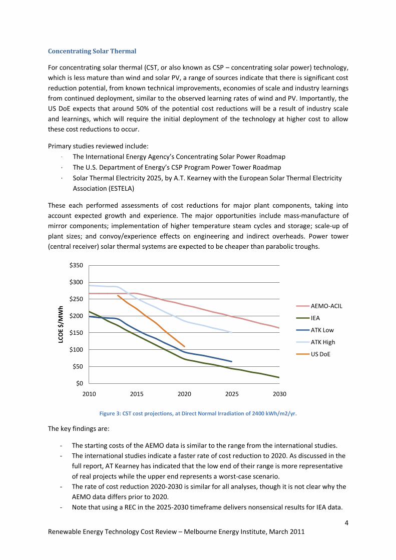
Concentrating Solar Thermal
For concentrating solar thermal (CST, or also known as CSP – concentrating solar power) technology,
which is less mature than wind and solar PV, a range of sources indicate that there is significant cost
reduction potential, from known technical improvements, economies of scale and industry learnings
from continued deployment, similar to the observed learning rates of wind and PV. Importantly, the
US DoE expects that around 50% of the potential cost reductions will be a result of industry scale
and learnings, which will require the initial deployment of the technology at higher cost to allow
these cost reductions to occur.
Primary studies reviewed include:
The International Energy Agency’s Concentrating Solar Power Roadmap
The U.S. Department of Energy’s CSP Program Power Tower Roadmap
Solar Thermal Electricity 2025, by A.T. Kearney with the European Solar Thermal Electricity
Association (ESTELA)
These each performed assessments of cost reductions for major plant components, taking into
account expected growth and experience. The major opportunities include mass-manufacture of
mirror components; implementation of higher temperature steam cycles and storage; scale-up of
plant sizes; and convoy/experience effects on engineering and indirect overheads. Power tower
(central receiver) solar thermal systems are expected to be cheaper than parabolic troughs.
Figure 3: CST cost projections, at Direct Normal Irradiation of 2400 kWh/m2/yr.
The key findings are:
- The starting costs of the AEMO data is similar to the range from the international studies.
- The international studies indicate a faster rate of cost reduction to 2020. As discussed in the
full report, AT Kearney has indicated that the low end of their range is more representative
of real projects while the upper end represents a worst-case scenario.
- The rate of cost reduction 2020-2030 is similar for all analyses, though it is not clear why the
AEMO data differs prior to 2020.
- Note that using a REC in the 2025-2030 timeframe delivers nonsensical results for IEA data.
$0
$50
$100
$150
$200
$250
$300
$350
2010 2015 2020 2025 2030
LCO
E $/
MW
h AEMO-ACIL
IEA
ATK Low
ATK High
US DoE

5 Renewable Energy Technology Cost Review – Melbourne Energy Institute, March 2011
Table of Contents
Executive Summary - Renewable Energy Technology Cost Review ................................................... 1
Table of Contents .............................................................................................................................. 5
1. Introduction .............................................................................................................................. 6
2. The Levelised Cost of Energy ..................................................................................................... 7
2.1. Introduction to LCOE .......................................................................................................... 7
2.2. Discount Rate: .................................................................................................................... 7
2.3. Other Financial Assumptions .............................................................................................. 8
3. Context: Fossil Fuel Levelised Costs Of Energy & Renewable Energy Certificates ................... 10
4. Learning curves of energy generation technologies: an in-depth analysis .............................. 11
4.1. Learning rates .................................................................................................................. 11
4.2. The Experience Curve and Learning Rate .......................................................................... 12
5. Photovoltaic Technology ......................................................................................................... 13
5.1. Introduction ..................................................................................................................... 13
1.1.1. Generation costs for PV Solar Power ........................................................................ 14
5.2. Historical Cost Reductions ................................................................................................ 15
5.2.1. PV Module................................................................................................................ 15
5.2.2. Balance of System (BOS) ........................................................................................... 20
5.3. Cost Projections ............................................................................................................... 22
5.3.1. Key findings .............................................................................................................. 23
6. Wind Power ............................................................................................................................ 24
6.1. Introduction ..................................................................................................................... 24
6.1.1. Generation Costs for Wind Power............................................................................. 25
6.2. Cost Reductions ............................................................................................................... 26
6.2.1. Technology ............................................................................................................... 28
6.2.2. Wind Resource Assessment ...................................................................................... 30
6.2.3. Economies of Scale and Volume Effects .................................................................... 31
6.3. Cost Projections ............................................................................................................... 32
6.3.1. Key findings .............................................................................................................. 33
7. Concentrating solar power (CSP) ............................................................................................. 34
7.1. Comparison of projected costs of CSP from several analyses ............................................ 34
7.2. Solar thermal power – introduction.................................................................................. 35
7.3. Potential for cost reductions by component ..................................................................... 40
7.4. International Energy Agency (IEA) – Technology Roadmap – Concentrating Solar Power .. 43
7.5. ESTELA and AT Kearney Associates ................................................................................... 44
7.6. AEMO dataset .................................................................................................................. 46
8. Appendix I: LCOE Model Verification ...................................................................................... 47
9. Appendix II: Photovoltaic ........................................................................................................ 48
10. Appendix III: Wind ............................................................................................................... 49
11. Appendix IV: Concentrating Solar Thermal.......................................................................... 52
12. Appendix V: Solar Resource ................................................................................................ 55
13. References .......................................................................................................................... 56
6 Renewable Energy Technology Cost Review – Melbourne Energy Institute, March 2011
1. Introduction
This report assesses the recent developments in renewable energy generation technology, based on
a range of analyses and reports from international sources. The primary objective is to review
current cost outlooks, and compare the outlooks with those currently used by the Australian energy
industry, in particular the dataset currently used by the Australian Energy Market Operator (AEMO),
based on a the ‘Australian Electricity Generation Technology Costs – Reference Case 2010’ study
carried out by EPRI for the Federal Department of Resources, Energy & Tourism. This study uses the
‘Levelised Cost of Energy’ metric to determine cost outlooks, and compare different cost projections.
The primary studies reviewed containing detailed cost information were:
Solar Photovoltaic
International Energy Agency – Projected Costs of Generating Electricity 2010
International Energy Agency – Technology Roadmap – Solar Photovoltaic Energy (2010)
European Photovoltaic Industry Association – Solar Generation 6 (2011)
Wind
International Energy Agency – Projected Costs of Generating Electricity 2010
Global Wind Energy Council – Global Wind Energy Outlook 2010
Concentrating Solar Thermal
International Energy Agency – Technology Roadmap - Concentrating Solar Power (2010)
Sandia National Laboratories (US Department of Energy) – Power Tower Cost Reduction Roadmap
(2011)
AT Kearney Consulting with European Solar Thermal Electricity Association (ESTELA) – Solar Thermal
Electricity 2025
Sargent & Lundy Consulting – Assessment of Parabolic Trough and Power Tower Solar Technology
Cost and Performance Forecasts (2003)

7 Renewable Energy Technology Cost Review – Melbourne Energy Institute, March 2011
2. The Levelised Cost of Energy
2.1. Introduction to LCOE
The Levelised Cost Of Energy (LCOE) is the most transparent metric used to measure electric power
generating costs, and is widely used as a tool to compare the generation costs from differing
sources. The LCOE is a measure of the marginal cost (the cost of producing one extra unit) of
electricity, over an extended period, and is sometimes referred to as Long Run Marginal Cost or
LRMC.
The LCOE is representative of the electricity price that would equalize cashflows (inflows and
outflows) over the economic life time of an energy generating asset. It is the average electricity price
needed for a Net Present Value (NPV) of zero when performing a discounted cash flow (DCF)
analysis. With the average electricity price equal to the LCOE, an investor would breakeven and so
receive a return equal to the discount rate on the investment.
The LCOE is determined by the point where the present value of the sum discounted revenues is
equivalent to the discounted value of the sum of costs1:
Where:
n = Project lifetime (yrs) t = Year in which sale or cost is incured r = Discount rate (%) By definition this is the point at which the Net Present Value (summation of the Present Values, PV,
of the cashflows) for a project is zero2:
Where:
And:
EBIT = Earnings Before Interest and Tax DEP = Depreciation CAPEX = Capital Expenditure T = Corporate Tax rate (%)
2.2. Discount Rate:
One of the most important assumptions and input parameters is the discount rate. This input
represents an appraisal of the time value of the money used in the investment. This value is
dependent on the type of investor and their respective financial market, and is representative of the
return expected (or the cost) of the particular capital. Money from the risk averse debt market

8 Renewable Energy Technology Cost Review – Melbourne Energy Institute, March 2011
maybe available at a nominal rate of 8%, where as the equity market, which takes on higher risk, will
be available at a higher nominal rate of, say, 13%.
This discount rate is particularly important in the context of renewable energy generating assets,
due to their inherent capital intensity. This can be contrasted with technologies with higher
operating costs (for example open cycle gas turbines). Whilst the LCOE for these technologies is
affected by the choice of discount rate, the impact is less pronounced and they are less sensitive to
variations in the discount rate.
Typically, the initial investment comprises of a combination of both debt financing and equity
financing. When this is the case, it is appropriate to use the Weighted Average Cost of Capital
(WACC) as the effective discount rate. The WACC is calculated by weighting the individual costs by
the proportion of each funding type2:
Where: D = Amount of Debt kd = Cost of Debt E = Amount of Equity ke = Cost of Equity T = Corporate Tax Rate
Tax is considered in our cash flow analysis, and all the cash flows are considered to be in real 2010
Australian Dollars. As such, a post-tax, real WACC is used. We use a discount rate of 8.1% to comply
with the ATSE analysis, which assumes a 75-25 debt-equity split, and a real debt cost of 7.3% and a
real, pre-tax equity cost of 17%. Given the sensitive nature of the discount rate, the same rate as
ATSE analysis was used to enable a consistent basis, for comparison.
2.3. Other Financial Assumptions
Global Assumptions
Tax: The corporate tax rate is assumed to be 30% for the purposes of all cash-flow analysis.
Depreciation: The electric utility industry typically uses the straight-line method, which was used in
this analysis. For a 25 year lifetime, the annual depreciation is 4%, and for a 30 year lifetime,
the annual depreciation is 3.33%.
Exchange Rates: In line with the Mid Year Economic Financial Outlook approach, the exchange rate
is assumed to remain around the levels seen at the time the forecasts were prepared3. As of
March 01 2011, a US$ exchange rate was $0.9853 used, and an EU€ exchange rate of $0.70
was used4.

9 Renewable Energy Technology Cost Review – Melbourne Energy Institute, March 2011
Construction Period and Economic Lifetime
The construction period and economic lifetime can have a considerable affect on the levelised cost
of generation. This is particularly important for protracted construction periods (lead times). The
economic and lifetimes and construction periods used are presented in Table 1, and are based on
the AEMO dataset5. The IEA reports wind construction periods of 1 year1 (unlike AEMO), and the
effects of this are explored in Appendix III.
Table 1: Construction periods and Economic Lifetimes
Technology Construction Period Economic Life Time
Wind 2 year 30 years Solar PV 1 year 30 years
Solar Thermal 2 years 30 years
The Capacity Factor
In the case of renewable energy generators the assumed capacity factor of a facility has a significant
impact on the LCOE. For renewable energy generators, the capacity factor is generally dependant on
the quality of the renewable resource. In the interests of a consistent approach, constant capacity
factors were used for each technology type. These capacities were based on reasonable resource
qualities for Australian conditions, summarized below in Table 2, as used in the EPRI study6.
Table 2: Capacity Factors
Technology Resource Quailty Capacity Factor
Wind 6.8 m/s 30% Solar PV 2445 kWh/m2/yr 20%
Solar Thermal 2400 kWh/m2/yr Varied by plant storage configuration
Technology Specific Inputs
The remaining parameters are specific to the technology type. These include capital cost, operation
and maintenance costs, which are explored in the report.
To demonstrate the modelling, Appendix I shows the levelised costs calculated, and compares
against the ATSE modelling results. The results for different technologies (Wind and CST), including
the technology specific inputs, are included in the appendix.
10 Renewable Energy Technology Cost Review – Melbourne Energy Institute, March 2011
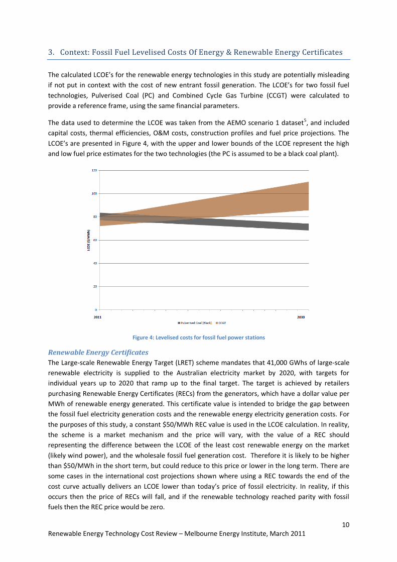
3. Context: Fossil Fuel Levelised Costs Of Energy & Renewable Energy Certificates
The calculated LCOE’s for the renewable energy technologies in this study are potentially misleading
if not put in context with the cost of new entrant fossil generation. The LCOE’s for two fossil fuel
technologies, Pulverised Coal (PC) and Combined Cycle Gas Turbine (CCGT) were calculated to
provide a reference frame, using the same financial parameters.
The data used to determine the LCOE was taken from the AEMO scenario 1 dataset5, and included
capital costs, thermal efficiencies, O&M costs, construction profiles and fuel price projections. The
LCOE’s are presented in Figure 4, with the upper and lower bounds of the LCOE represent the high
and low fuel price estimates for the two technologies (the PC is assumed to be a black coal plant).
Figure 4: Levelised costs for fossil fuel power stations
Renewable Energy Certificates
The Large-scale Renewable Energy Target (LRET) scheme mandates that 41,000 GWhs of large-scale
renewable electricity is supplied to the Australian electricity market by 2020, with targets for
individual years up to 2020 that ramp up to the final target. The target is achieved by retailers
purchasing Renewable Energy Certificates (RECs) from the generators, which have a dollar value per
MWh of renewable energy generated. This certificate value is intended to bridge the gap between
the fossil fuel electricity generation costs and the renewable energy electricity generation costs. For
the purposes of this study, a constant $50/MWh REC value is used in the LCOE calculation. In reality,
the scheme is a market mechanism and the price will vary, with the value of a REC should
representing the difference between the LCOE of the least cost renewable energy on the market
(likely wind power), and the wholesale fossil fuel generation cost. Therefore it is likely to be higher
than $50/MWh in the short term, but could reduce to this price or lower in the long term. There are
some cases in the international cost projections shown where using a REC towards the end of the
cost curve actually delivers an LCOE lower than today’s price of fossil electricity. In reality, if this
occurs then the price of RECs will fall, and if the renewable technology reached parity with fossil
fuels then the REC price would be zero.

11 Renewable Energy Technology Cost Review – Melbourne Energy Institute, March 2011
4. Learning curves of energy generation technologies: an in-depth analysis
The analysis considers the factors and trends for learning rates in several renewable energy
generation technologies. A useful forecast tool for the cost reductions of energy technologies is the
‘Grubb’ curve. At initial stages of technology conception, costs tend to be underestimated. As they
reach the point of commercialisation and deployment, the costs tend to increase with
comprehensive engineering assessments and real-world implementation. After the point of
commercialisation, costs tend to reduce due to a combination of factors, and eventually cost
reduction rates reduce as technologies mature. Different technologies can be mapped onto
different segments of the curve.
Figure 5: Grubb curve for renewable energy technologies, from EPRI (2010)
4.1. Learning rates
In many high-level analyses, the generic term ‘learning rate’ is used to describe the rate of costs
reductions during commercial deployment. A range of specific factors contribute to reducing costs.
These can be divided into two broad categories
Technological improvements – changes to the basic design of the technology.
‘Learning by doing’ – refers to the technical and management experience gained during the
construction and operation of power plants leading to more streamlined, efficient methods of
building and operating plants. A relevant example, is from SENER (Spanish engineering company)
who has developed a type of parabolic trough mirror support strut that is simpler to manufacture
and assemble, leading to a four-fold increase in the speed of mirror assembly for concentrating solar
plants.
Technical efficiency – refers to Research & Development. Upgrading to state-of-the-art
components, experience pushing operational envelopes or otherwise, the technology becomes
overall more efficient by increasing output or decreasing wasted energy or materials. Upgrading
12 Renewable Energy Technology Cost Review – Melbourne Energy Institute, March 2011
from subcritical to supercritical steam turbines in thermal power plants, and incremental gains in the
efficiency of photovoltaic cells are examples of technically efficiency improvements.
Economies of scale – increase in the size or volume of units results in lower costs per unit.
Economies of scale in the physical size of components – refers to the efficiency gains in
construction, attributed to increased scale of industrial units. A 50 MW steam turbine requires the
same complexity of piping, condensers, control systems and pressure relief systems as a 250MW
turbine, with the main difference being the larger size of components for the larger turbine. On a
per-MW basis, larger turbines are generally cheaper, the wind industry has demonstrated this with
today’s wind turbines an order of magnitude larger in output than 20 years ago. The effect is
particularly important where the costs of design and construction are large relative to the raw
material cost.
Economies of scale through large-volume manufacturing – refers to manufacturing efficiency
gains achieved by producing very high volumes. When an industry reaches a scale where dedicated
component factories can be built with the certainty of an ongoing market, unit costs come down
significantly, as has been the case with solar PV and wind.
4.2. The Experience Curve and Learning Rate
The development and economics of renewable energy is sometimes illustrated by the use of the
experience curve. Experience curves show that cumulative quantitative development of a product
relates to the development of the specific costs.
Experience curves reflect the reduction in the cost of energy achieved with each doubling of capacity
– known as the progress ratio. If the cumulative deployment of a technology doubles, the learning
rate represents the achieved reduction in costs. The graph of the log of the costs versus the log of
cumulative installed capacity will follow a straight line. This is well demonstrated by photovoltaic
industry.
The progress ratio (P) is related to the Learning rate (L) by the following expression:
Historic data with steady learning rates allow for extrapolation into the future, and allow estimations
of when a technology will reach as certain price level. It demonstrates the development that may be
seen if the existing trends continue in the future.
The learning rate represents the effect of mass production (economies of scale) and the effect upon
production costs without taking other causal relationships into account, such as the cost of raw
materials or the demand-supply balance in a particular market (seller’s or buyer’s market).
13 Renewable Energy Technology Cost Review – Melbourne Energy Institute, March 2011
5. Photovoltaic Technology
5.1. Introduction
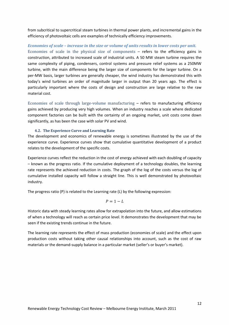
Photovoltaic (PV) capacity has exhibited an average annual growth rate of 40% over the last decade
(see Figure 6). The installed capacity almost increased by 50% between 2008 and 2009 from 15.7GW
to 22.9 GW7. The EPIA expects the total installed capacity at the end of 2010 is to be between 32 and
38 GW.
Figure 6: World Cumulative PV power installed7
Solar PV generates electricity through the direct conversion of sunlight. The basic building block of
the PV system is the cell, which is a semi-conductor device which converts solar energy into direct
current electricity. PV cells are interconnected to form the PV module.
There are many different types of PV cells. Single crystalline silicon and multi-crystalline silicon
represent 85-90% of the PV market. Thin film PV cells represent 10%-15% of the PV market, and
have many several different categories. Thin film cells less efficient, but cheaper, and crystalline
silicon cell are more expensive.
Utility scale PV systems are generally built directly on the ground, and are typically between 1MW
and 50MW in size. The module is combined with a ground based, mounting system, to create the
solar collector array. The modules within the array are connected to an inverter, which converts the
DC power into AC power, which is then transformed at a substation, for distribution in a high voltage
transmission line.
0
5000
10000
15000
20000
25000
30000
35000
40000
45000
2000 2002 2004 2006 2008 2010
Cu
mu
lati
ve In
stal
late
d C
apac
ity
(MW
)
Year
Historical 2010 High Estimate 2010 Low Estimate
14 Renewable Energy Technology Cost Review – Melbourne Energy Institute, March 2011
1.1.1. Generation costs for PV Solar Power
The key parameters that govern the cost of PV power are the capital costs the solar resource and the
discount rate. Other costs are the variable costs including operations and maintenance costs. Of
these parameters, the capital cost is the most significant and provides the largest opportunity for
cost reduction.
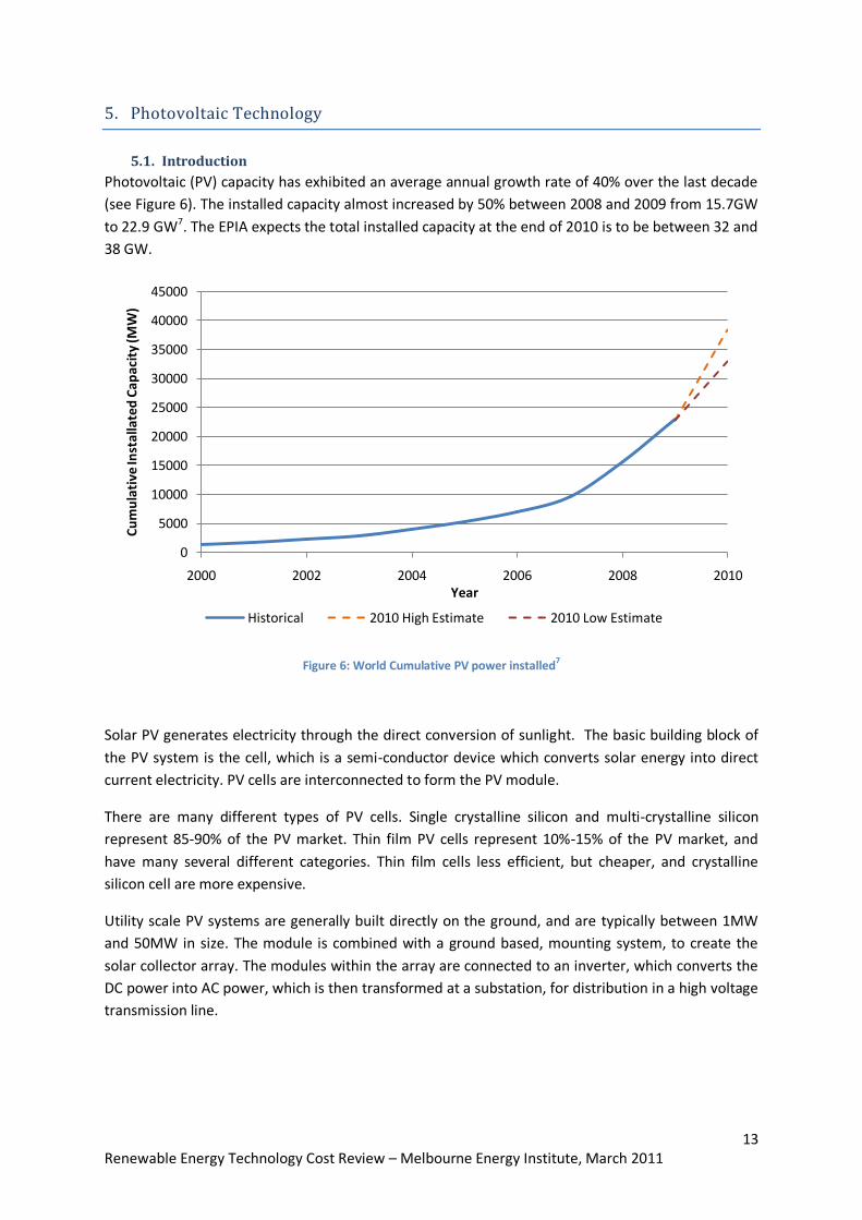
The capital costs themselves fall into one of two broad categories; the module and the balance of
system (BOS). The module is the interconnected array of PV cells and incorporates feedstock silicon
prices, cell processing and module assembly costs. The BOS includes structural system costs
(structural installation, racks, site preparation and other attachments) and electrical system costs
(the inverter, wiring and transformer and electrical installation costs). A breakdown of the costs for
a ground mounted system as suggested by the Rocky Mountain Institute is illustrated below in
Figure 78,9.
0
5
10
15
20
25
30
35
40
45
Balance of System
Structural Installation
Racking
Site Preparation
Electrical Installation
Wiring, Transformer etc
Inverter
0%
10%
20%
30%
40%
50%
60%
70%
80%
90%
100%
Photovoltaic Solar System
0
10
20
30
40
50
60
70
Module
Cell Processing
Module Assemble
Silicon
Mod.
BOS
Figure 7: PV Solar System Cost Breakdown8,9
15 Renewable Energy Technology Cost Review – Melbourne Energy Institute, March 2011
5.2. Historical Cost Reductions
As summarised by the EPIA, increase capacity has been associated with cost reductions. These
reductions are a result of both technological improvements and the economies of scale. Both the
module and balance of system components have experienced, or have the potential to experience,
reductions as a result of both of these factors.
According to EPIA the general industry trend to fewer and larger vertically integrated multinationals
has increased competition and price pressure7, and lead to synergies between different parts of the
supply chain.
The following analysis explores the cost reduction potentials for both module and balance of system
components. Both technological and economies of scale effects are covered.
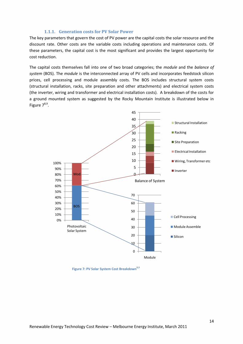
5.2.1. PV Module
The module cost reportedly represents 60% of the capital cost for a ground mounted system8.
Experience curves for the module price display a historic learning rate of 22% (capital costs have
reduced by 22% for each doubling of capacity), for the period from 1976 -200310 (Figure 8).
Figure 8: Historic Experience Curve for PV, with 22% Learning rate10
Departures from the historic learning rate from, 2003 to 2008, and have been attributed to varying
PV industry market dynamics, supply chain issues and profit margins10. Since 2009 learning rates
have approached the historic rates.
1.0
10.0
100.0
0 1 10 100 1000 10000 100000
PV
Mo
du
le P
rice
(20
10 $
/W)
Cummulative PV Capacity (MW)

16 Renewable Energy Technology Cost Review – Melbourne Energy Institute, March 2011
Technological Developments
Technological progress plays a large role in the development of PV technology, the chief focus being
the improvement in the efficiency of conversion of sunlight to electricity. There is a range of PV
devices, from low cost low efficiency cells to high cost high efficiency cells. Commercial PV modules
fall broadly into two categories; wafer based crystalline silicon (c-Si) and thin film. Other emerging
technologies, including concentrating PV and organic solar cells have a significant potential for
performance increase and cost reduction, but are not explored here. Figure 9 below illustrates the
different cost and performance of differing PV technologies11.
Figure 9: Performance and Price of different PV modules11
Module efficiencies range from 10% for thin film cells to as high 20% single crystalline cells and have
an important impact on the cost through the entire module value chain and so are critical to
determining module pricing12. Higher efficiencies result in higher power outputs per square meter,
which is a significant consideration, given that many module cost inputs are priced on a per meter
squared basis (e.g. glass).
A wide subset of technologies falls within the categories of Thin Film and Crystalline Silicon,
characterised by the underlying physical properties of the semi-conductor used. Within these
technologies, there is a further range of efficiencies, ranging from the theoretical, to the lab scale
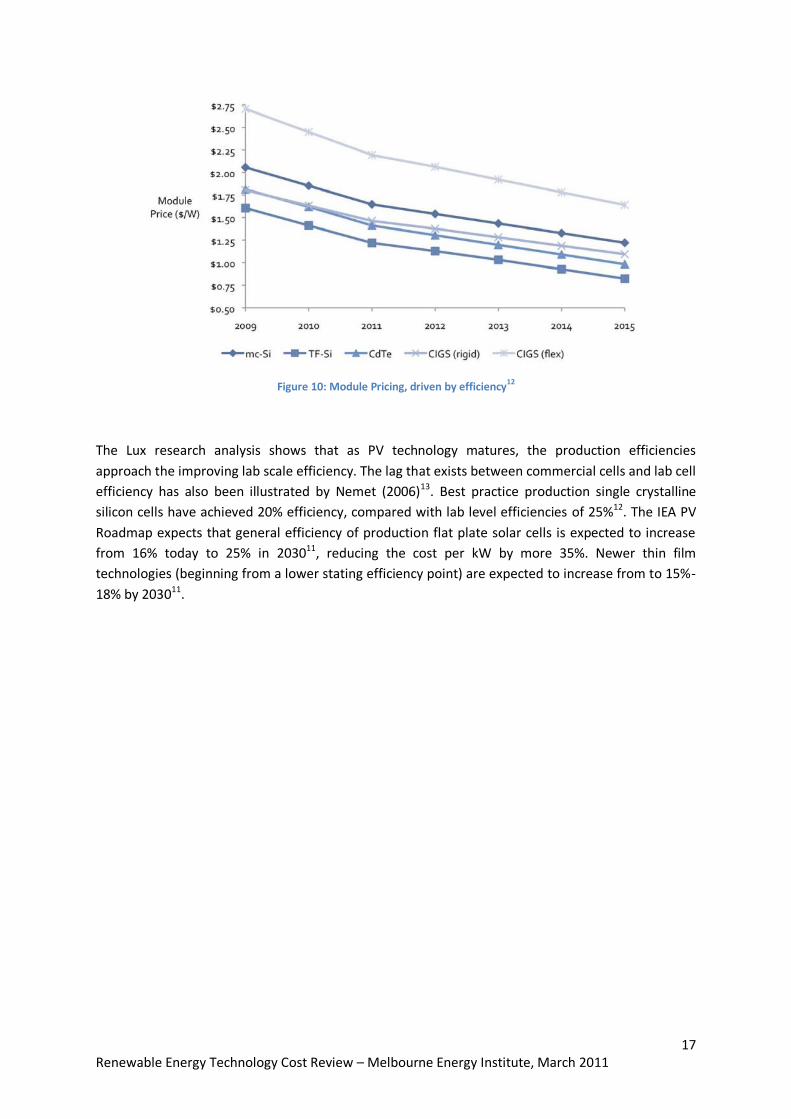
and finally production efficiencies. Figure 10 illustrates the module price reductions, that Lux
Research expect to occur as a result of efficiency measures12 for some of PV technologies. It should
be noted that the relative apparent additional expense of the multi crystalline silicon technology
(mc-Si), is partially offset by the lower area related system costs due to the higher conversion12.
17 Renewable Energy Technology Cost Review – Melbourne Energy Institute, March 2011
Figure 10: Module Pricing, driven by efficiency12
The Lux research analysis shows that as PV technology matures, the production efficiencies
approach the improving lab scale efficiency. The lag that exists between commercial cells and lab cell
efficiency has also been illustrated by Nemet (2006)13. Best practice production single crystalline
silicon cells have achieved 20% efficiency, compared with lab level efficiencies of 25%12. The IEA PV
Roadmap expects that general efficiency of production flat plate solar cells is expected to increase
from 16% today to 25% in 203011, reducing the cost per kW by more 35%. Newer thin film
technologies (beginning from a lower stating efficiency point) are expected to increase from to 15%-
18% by 203011.
18 Renewable Energy Technology Cost Review – Melbourne Energy Institute, March 2011
Economies of Scale and Volume Effects
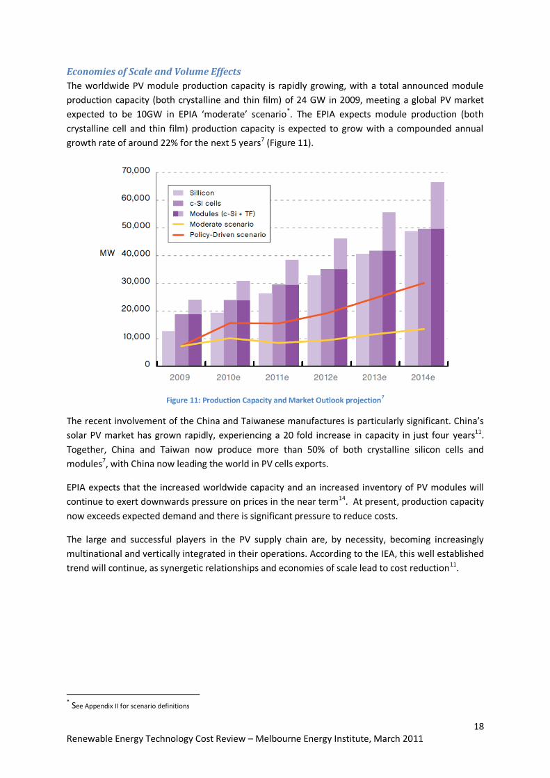
The worldwide PV module production capacity is rapidly growing, with a total announced module
production capacity (both crystalline and thin film) of 24 GW in 2009, meeting a global PV market
expected to be 10GW in EPIA ‘moderate’ scenario*. The EPIA expects module production (both
crystalline cell and thin film) production capacity is expected to grow with a compounded annual
growth rate of around 22% for the next 5 years7 (Figure 11).
Figure 11: Production Capacity and Market Outlook projection7
The recent involvement of the China and Taiwanese manufactures is particularly significant. China’s
solar PV market has grown rapidly, experiencing a 20 fold increase in capacity in just four years11.
Together, China and Taiwan now produce more than 50% of both crystalline silicon cells and
modules7, with China now leading the world in PV cells exports.
EPIA expects that the increased worldwide capacity and an increased inventory of PV modules will
continue to exert downwards pressure on prices in the near term14. At present, production capacity
now exceeds expected demand and there is significant pressure to reduce costs.
The large and successful players in the PV supply chain are, by necessity, becoming increasingly
multinational and vertically integrated in their operations. According to the IEA, this well established
trend will continue, as synergetic relationships and economies of scale lead to cost reduction11.
* See Appendix II for scenario definitions

19 Renewable Energy Technology Cost Review – Melbourne Energy Institute, March 2011
Upstream (Silicon Production) Trends
The current main source of silicon feedstock is virgin polysilicon. During early 2008 polysilicon
production capacity lagged behind the rising demand, resulting in a significant price spike (to
$500/kg)15.
Silicon production capacity expanded in response to the production lag, according to the NREL15.
EPIA and also attributes the growth to a response to the previous silicon shortages. The shortage
was overcorrected, as a result of capacity expansions that were already in the pipeline, as new
capacity was constructed. Production capacity outpaced demand in 2009 and the contract and
forward prices for polysilicon declined to around $100 per kg. EPIA expects silicon production
continue to grow at 30%.
Production of PV grade silicon feed stock was dominated by Germany, the US, Japan and Korea in
2009. However, there are many new entrants in the market (including numerous companies in
China). This is expected to provide a more competitive supply / demand situation14.
Figure 12: Forward Contract Prices for Polysilicon as charted by NREL study15
The NREL expects the price of silicon to decline continually in the near future15, at a rate of about
12% per year from 2009 (see Figure 12). The current spot price is tracking below the contract prices,
currently at $76 per kg, with $60/kg expected by the end of 201116. Silicon production capacity is
expected to continue growing at 30% p.a. from 2010 to 20147, putting further pressure on prices, as
more competitive capacity is brought on line.
Novel methods of silicon production have achieved progress during recent years with several pilot
plants being put into operation. Whilst these new production methods have not yet been introduced
to the market, the IEA expects successful deployment will realise further cost reductions11.

20 Renewable Energy Technology Cost Review – Melbourne Energy Institute, March 2011
5.2.2. Balance of System (BOS)
The BOS costs largely depend on the nature of the installation, and can vary between 20% (for a
simplified grid-connected system) to 70% (for an off-grid system)14, with 40% representative of a
standard ground mounted system8. The BOS costs and products are therefore an integral part to
achieving system cost reductions.
The BOS cost reductions are arguably more complicated than Module cost reductions, as the costs
are incurred by many different parties (installers, suppliers, regulators, utilities, building owners etc).
The BOS industry is less vertically integrated and more fragmented than the module and upstream
production industries. Because of this fragmented approach, there are literally hundreds of potential
cost reduction pathways8, and potential synergies available between the different BOS costs.
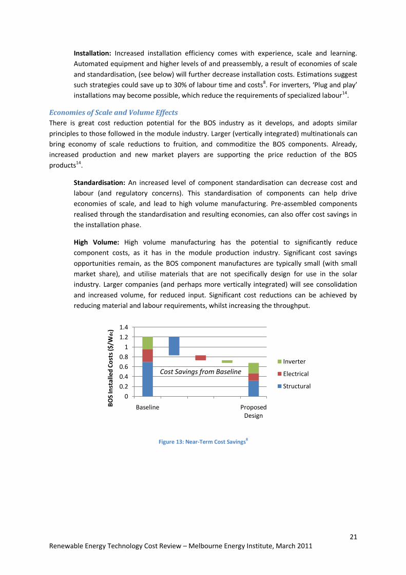
Figure 13 illustrates the potential cost savings, for the different BOS components according to the
Rocky Mountain Institute.
Technological Developments
There is much potential for technological developments to optimise physical design and reduce BOS
costs. There are many design strategies already being considered, however these strategies have not
been widely taken up, and in some case have not been combined in an optimal manner.
Electrical Systems: The inverters remain a key development point. The DC-AC inverters,
which can contribute up to 10% to the system costs, offer a significant opportunity for
breakthrough in technical design8. Inverters have been developed with larger rated
capacities for the utility scale PV systems. New units simplify system design and installation
and can help to increase energy yield11, but are not yet being widely deployed.
For some electrical systems, increasing integration between inverter processes and module
electronics is possible. Specially designed BOS components may reduce cost downsizing or
eliminating some components8. That is, BOS components can also reduce module
components cost (with increased cooperation and integration between the module
manufacturers and BOS manufacturers).
Structural Improvements: Downsizing of the structural components enables considerable
cost reductions. The structure cost, in particular the racking, can contribute up to 40% of
BOS costs8.
Exposure to the wind forces is one of the factors affecting structural design; reducing
exposure to wind can reduce the structural requirements. Efficient wind design (including
spacing, spoiling and deflection could result in a 30% reduction in the system structural
costs8.
Alternative approaches to reducing structural cost involve using the actual module as a
structure. Racking systems could be significantly reduced by using the rigid glass as a part of
the structural system14.
21 Renewable Energy Technology Cost Review – Melbourne Energy Institute, March 2011
Installation: Increased installation efficiency comes with experience, scale and learning.
Automated equipment and higher levels of and preassembly, a result of economies of scale
and standardisation, (see below) will further decrease installation costs. Estimations suggest
such strategies could save up to 30% of labour time and costs8. For inverters, ‘Plug and play’
installations may become possible, which reduce the requirements of specialized labour14.
Economies of Scale and Volume Effects
There is great cost reduction potential for the BOS industry as it develops, and adopts similar
principles to those followed in the module industry. Larger (vertically integrated) multinationals can
bring economy of scale reductions to fruition, and commoditize the BOS components. Already,
increased production and new market players are supporting the price reduction of the BOS
products14.
Standardisation: An increased level of component standardisation can decrease cost and
labour (and regulatory concerns). This standardisation of components can help drive
economies of scale, and lead to high volume manufacturing. Pre-assembled components
realised through the standardisation and resulting economies, can also offer cost savings in
the installation phase.
High Volume: High volume manufacturing has the potential to significantly reduce
component costs, as it has in the module production industry. Significant cost savings
opportunities remain, as the BOS component manufactures are typically small (with small
market share), and utilise materials that are not specifically design for use in the solar
industry. Larger companies (and perhaps more vertically integrated) will see consolidation
and increased volume, for reduced input. Significant cost reductions can be achieved by
reducing material and labour requirements, whilst increasing the throughput.
Figure 13: Near-Term Cost Savings8
0
0.2
0.4
0.6
0.8
1
1.2
1.4
Baseline Proposed Design
BO
S In
stal
led
Co
sts
($/W
dc)
Inverter
Electrical
Structural
Cost Savings from Baseline
22 Renewable Energy Technology Cost Review – Melbourne Energy Institute, March 2011
5.3. Cost Projections
Based on these key costs drivers and cost reductions, projections of capital cost and hence levelised
costs can be made. The EPIA and IEA have made cost projections based on these cost reductions out
to 2030 and 2050 respectively. Each has multiple capital cost projections, corresponding to different
scenarios with differing conditions (see Appendix II for details). Both the IEA and EPIA assume an
18% learning rate, which is less than the 22% learning rate experienced in the past.
The IEA reports the 2010 capital cost for utility scale PV facilities as $4060/kW and expects the
capital costs of PV to drop by 70% to between $1220 and $1830 a kW1. It is with projected by the IEA
that reductions in capital cost of 40% by 2015, and 50% by 2020 will occur.
EPIA reports the 2010 capital cost as being $3600/kW. They expect capital costs of $1380/kW in
their moderate scenario, and $1060/kW in the more optimistic scenario by 2030. A capital cost
reduction of 50% by 2020 will occur according to EPIA17.
The EPRI analysis suggests the 2015 costs of PV are over $8000/kW for flat plate collector. A 35%
reduction in capital costs $5500 / kW in 20306 is assumed to occur by EPRI (with the reduction to
begin occurring in 2015). The EPRI report included qualitative discussion around the cost reduction;
however there was no specific justification of 35% rate. This 2030 capital cost is within the range of
the 2010 costs from IEA and EPIA.
The AEMO data was taken from Scenario 1 of input assumptions to the 2010 NTNDP5 modelling,
representing the best-case data in the range of scenarios modelled. The AEMO data assumes that
the capital cost for flat plat photovoltaics begins at $5118/kW in 2010 and linearly decreases
(starting from 2015) to $3581/kW in 2030. The AEMO dataset is based on the EPRI analysis.
Residential scale PV installations are currently available in Australia at between approximately
$4500/kW and $6500/kW18. This value excludes RECs and any other subsidies, and is in line with the
international residential scale prices. As suggested by EPIA, utility scale investments are in a position
to leverage volumes and lower negotiate prices17. Both the IEA and EPIA report lower prices for
utility scale systems.
The projected LCOE for the different outlooks is presented in Figure 14.
23 Renewable Energy Technology Cost Review – Melbourne Energy Institute, March 2011
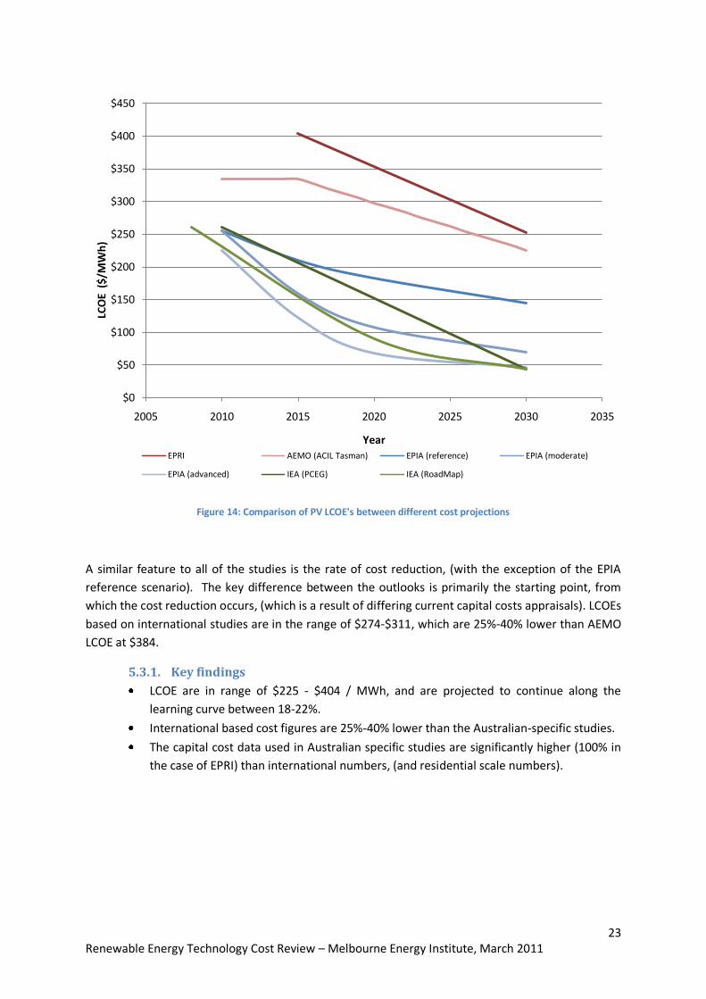
Figure 14: Comparison of PV LCOE's between different cost projections
A similar feature to all of the studies is the rate of cost reduction, (with the exception of the EPIA
reference scenario). The key difference between the outlooks is primarily the starting point, from
which the cost reduction occurs, (which is a result of differing current capital costs appraisals). LCOEs
based on international studies are in the range of $274-$311, which are 25%-40% lower than AEMO
LCOE at $384.
5.3.1. Key findings
LCOE are in range of $225 - $404 / MWh, and are projected to continue along the
learning curve between 18-22%.
International based cost figures are 25%-40% lower than the Australian-specific studies.
The capital cost data used in Australian specific studies are significantly higher (100% in
the case of EPRI) than international numbers, (and residential scale numbers).
$0
$50
$100
$150
$200
$250
$300
$350
$400
$450
2005 2010 2015 2020 2025 2030 2035
LCO
E (
$/M
Wh
)
YearEPRI AEMO (ACIL Tasman) EPIA (reference) EPIA (moderate)
EPIA (advanced) IEA (PCEG) IEA (RoadMap)

24 Renewable Energy Technology Cost Review – Melbourne Energy Institute, March 2011
6. Wind Power
6.1. Introduction
The industry has experience an average growth rate of 28% over the past decade, and has doubled
on average every 3 years. The total installed capacity was almost 160 GW at the end of 2009, and
Global Wind Energy Council (GWEC) estimates that a further 30 GW was installed in 201019 (Figure
15).
Figure 15: Cumulative Wind Power Installed Globally
Modern utility scale wind turbines are typically deployed in arrays of 50 – 150 turbines, known as
‘wind farms’. The turbines generally have three-bladed rotors, between 80m – 125m in diameter, on
top of a tower, typically between 80m – 130m high.
The wind force applied to the turbine blades drives a generator housed in the ‘nacelle’ on top of the
tower. The rotor drive shaft is either directly connected to an annually generator (direct-drive
turbine) or, more commonly, the shaft is connected to a gearbox. Transformers within the nacelle
transform the power for distribution to the power collection system.
The individual turbines are connected to a power collection system (generally at medium voltage)
and control system. At a substation the medium voltage power is transformed and connected to a
high voltage transmission network. The land in between turbines may be used for other purposes;
however road access, for both construction and O&M are required.
Turbine power is controlled by modifying the blade pitch (the angle of attack with respect to the
relative wind) as the blades spin around the rotor hub, and the turbine is pointed into wind by
rotating the nacelle around the tower.
0
50
100
150
200
250
2000 2002 2004 2006 2008 2010
Cu
mu
lati
ve In
stal
led
Cap
acit
y (G
W)
Year
Historical GWEC High Estimate GWEC Low Estimate

25 Renewable Energy Technology Cost Review – Melbourne Energy Institute, March 2011
6.1.1. Generation Costs for Wind Power
The key parameters that govern the cost for wind power are the capital costs, wind resource quality
and the discount rate. Other costs are the variable costs including operations and maintenance
costs. Of these parameters, the capital cost is the most significant and presents the largest potentials
for cost reductions.
The capital costs of a wind power project are broken into several categories. These categories
include the turbine cost, construction costs, grid connection costs and other capital cost. The
construction costs include foundation work, road construction and buildings, and grid connection
costs include cabling and substations. The turbine cost includes the production transportation and
installation of the turbine itself (e.g. blades, transformer). A breakdown of the cost distribution can
be found in Figure 1620.
The turbine cost can be further categorized into the major components. The EWEA have suggested a
turbine cost breakdown representative of a gearbox driven turbine (as opposed to direct drive) in a
European setting (Figure 16). The major cost items include the rotor blade, the tower and gearbox.
The ‘Balance of Tower’ category includes other minor cost associated with the tower, such as the
rotor hub, cabling, and rotor shaft.
0%
10%
20%
30%
40%
50%
60%
70%
80%
90%
100%
Capital Cost Distribution
Other Capital Costs
Civil Works
Grid Connection
Turbine ex works
Figure 16: Capital Cost Distribution for a Wind Turbine (gearbox drive)20
0%
10%
20%
30%
40%
50%
60%
70%
80%
90%
100%
Turbine Cost Distribution
Generator
Transformer
Power Converter
Gearbox
Rotor Blades
Tower
Other

26 Renewable Energy Technology Cost Review – Melbourne Energy Institute, March 2011
6.2. Cost Reductions
Wind power has experienced cost reductions as capacities have expanded. Experience curves have
been developed and learning rates of 10%21 have been observed (based on historic records). The
experience curve is for wind power capital cost is shown below in Figure 17, for European
installations (with the data sets spanning roughly between 1990 and 2008).
Figure 17: Historic Wind Experience curve, with Learning rate22,23
Supply-imbalances increased turbine prices from around 2004 according to Berkeley Labs. This
imbalance occurred at the same time as a surge in steel and other base commodity prices, (and
prices rose as cumulative capacity increased)24. According to the EWEA, some supply chain issues
have resolved, and the learning rate has been returned to more historic values.
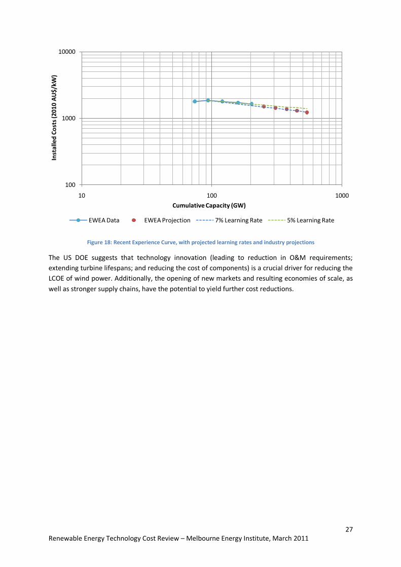
Figure 18 illustrates the cost data and projections, alongside two different learning rates (7% and
5%). The IEA projections incorporate a 7% learning rate1, whilst the EWEA suggests a learning rate of
10% will occur (in line with historic observations21).
100
1000
10000
1 10 100
Cap
ital
Co
st (
2010
AU
$/kW
)
Cumulative Capacity (GW)
EWEA Data M. Junginger Learning Rate (10%)
27 Renewable Energy Technology Cost Review – Melbourne Energy Institute, March 2011
Figure 18: Recent Experience Curve, with projected learning rates and industry projections
The US DOE suggests that technology innovation (leading to reduction in O&M requirements;
extending turbine lifespans; and reducing the cost of components) is a crucial driver for reducing the
LCOE of wind power. Additionally, the opening of new markets and resulting economies of scale, as
well as stronger supply chains, have the potential to yield further cost reductions.
100
1000
10000
10 100 1000
Inst
alle
d C
ost
s (2
010
AU
$/kW
)
Cumulative Capacity (GW)
EWEA Data EWEA Projection 7% Learning Rate 5% Learning Rate
28 Renewable Energy Technology Cost Review – Melbourne Energy Institute, March 2011
6.2.1. Technology
Technology remains a key driver for the reduction in levelised electricity costs for wind, and is
characterized by incremental reductions in the cost of energy, rather than by single leap. According
to the US DOE, there is a general focus on the development of:
o Stronger and lighter materials
o Super conductor materials, for better electrically efficient generators
o Larger, more flexible rotors.
There is a long-term drive to develop larger turbines, which is a direct result of the desire to improve
energy capture by accessing the stronger winds at higher elevations. Currently, the largest turbines
are 7.5MW, and the IEA suggests 20MW turbines will be available by 202025. The EPRI analysis in
contrast assumes there will be an ultimate turbine size limit in the range 3-5MW6. Both the IEA and
US DOE expect improvements through using advanced towers, advanced rotors, reduced energy
losses and improvements to the drive train25,26.
Throughout the past 20 years, average wind turbine ratings have grown almost linearly26. Each group
of wind turbine designers has predicted that its latest machine is the largest that a wind turbine will
ever be. However, turbine size has grown along the linear curve and has achieved reductions in life-
cycle cost of energy14. According to the IEA Wind Roadmap, the key development points are the
rotors, the blade, the tower and the drive train.
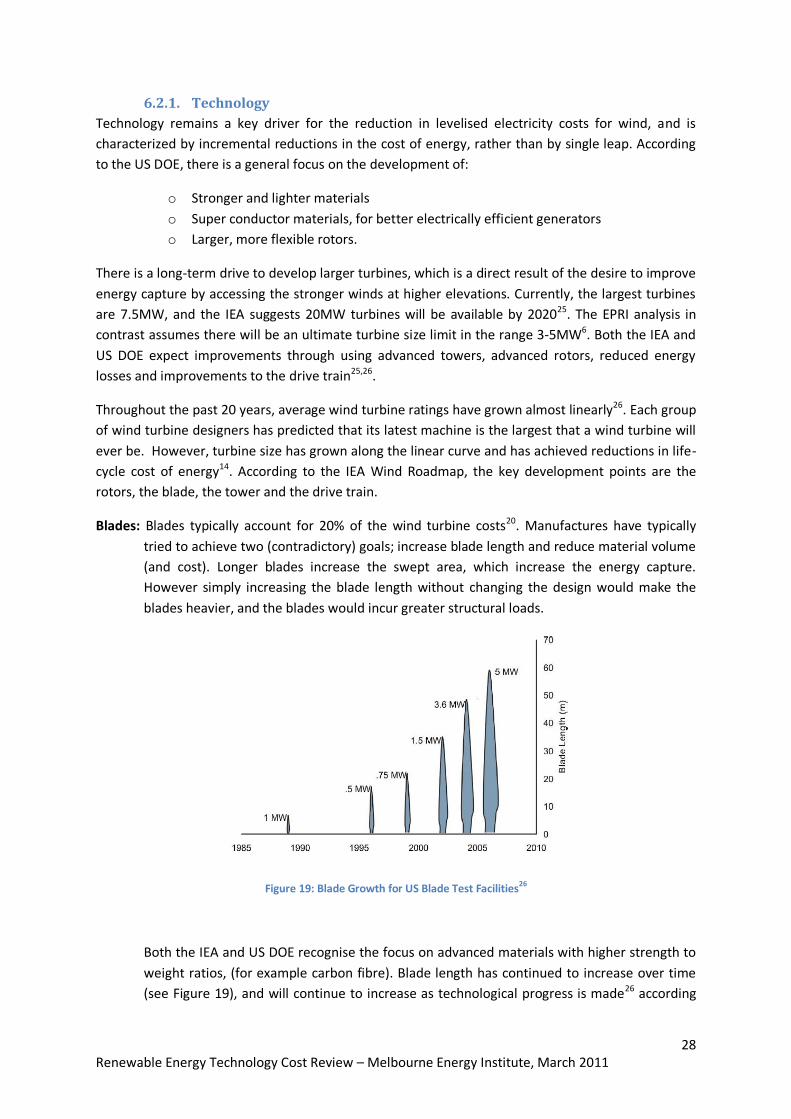
Blades: Blades typically account for 20% of the wind turbine costs20. Manufactures have typically
tried to achieve two (contradictory) goals; increase blade length and reduce material volume
(and cost). Longer blades increase the swept area, which increase the energy capture.
However simply increasing the blade length without changing the design would make the
blades heavier, and the blades would incur greater structural loads.
Figure 19: Blade Growth for US Blade Test Facilities26
Both the IEA and US DOE recognise the focus on advanced materials with higher strength to
weight ratios, (for example carbon fibre). Blade length has continued to increase over time
(see Figure 19), and will continue to increase as technological progress is made26 according
29 Renewable Energy Technology Cost Review – Melbourne Energy Institute, March 2011
to US DOE. According to both the EWEA and IEA, blade lengths are anticipated to increase to
approximately 125m by 2020.
Drive Train: Improvements that remove or reduce the fixed losses during low power generation are
likely to have an important impact on raising the capacity factor and reducing cost. Parasitic
losses when summed over the entire add up to significant numbers. These improvements
include innovative power-electronic architectures and large-scale use of permanent-magnet
generators. The IEA has identified the gearbox as a key development area (and efficiency
loss point), and EWEA has noted clear a trend towards a simplification of the gearbox
component, (e.g, one-stage gearboxes), and direct-drive turbines.
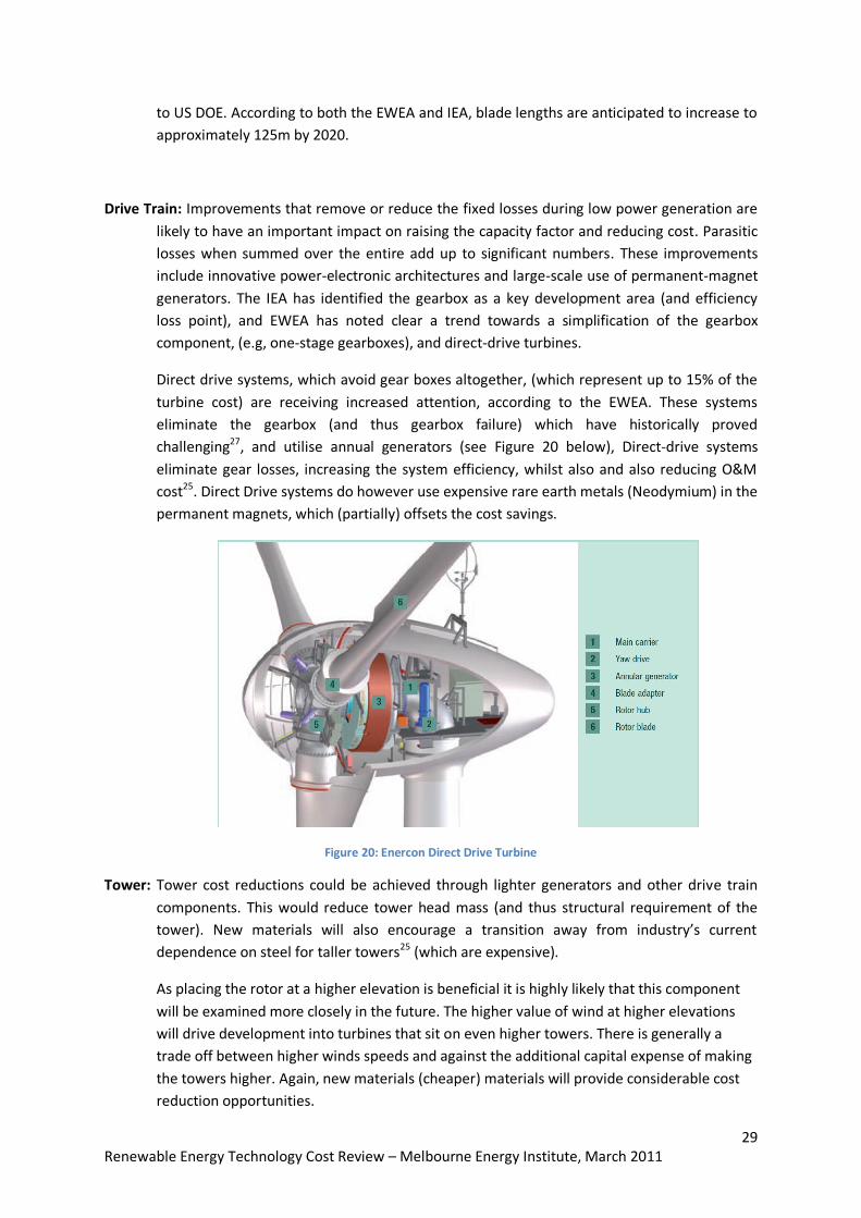
Direct drive systems, which avoid gear boxes altogether, (which represent up to 15% of the
turbine cost) are receiving increased attention, according to the EWEA. These systems
eliminate the gearbox (and thus gearbox failure) which have historically proved
challenging27, and utilise annual generators (see Figure 20 below), Direct-drive systems
eliminate gear losses, increasing the system efficiency, whilst also and also reducing O&M
cost25. Direct Drive systems do however use expensive rare earth metals (Neodymium) in the
permanent magnets, which (partially) offsets the cost savings.
Figure 20: Enercon Direct Drive Turbine
Tower: Tower cost reductions could be achieved through lighter generators and other drive train
components. This would reduce tower head mass (and thus structural requirement of the
tower). New materials will also encourage a transition away from industry’s current
dependence on steel for taller towers25 (which are expensive).
As placing the rotor at a higher elevation is beneficial it is highly likely that this component
will be examined more closely in the future. The higher value of wind at higher elevations
will drive development into turbines that sit on even higher towers. There is generally a
trade off between higher winds speeds and against the additional capital expense of making
the towers higher. Again, new materials (cheaper) materials will provide considerable cost
reduction opportunities.

30 Renewable Energy Technology Cost Review – Melbourne Energy Institute, March 2011
New tower erection technologies might play a role in O&M costs which will also help drive
down the system cost of energy25.
The US DOE quantifies the effects of the improvement in technology by determining the
effective increase in capacity factor expected, (using a constant resource as a basis for
comparison). For example, as hub heights increase, the energy extracted from an identical
wind resource will also increase. The EWEA expects that the capacity factor achieved for a
particular quality will increase over time, as a result of all the technological improvements21.
A summary of the US DOE expected performance improvements for wind turbine, expressed
in terms of capacity factors, is in Table 326.
Table 3: Potential improvements in capacity factor from advances in wind26
Technology % increase of existing capacity factors
Best Case Expected Worst Case
Advanced tower concepts +11% +11% +11%
Advanced rotors +35% +25% +10%
Reduced energy losses and improved availability
+7% +5% +0%
Drive-train (gearboxes, generators and
power electronics)
+8% +4% +0%
Capacity Factor: Previous studies (including the ACIL Tasman Review), estimate the capacity factor
of successive wind deployments to continually decline over time, as the better wind
resources are exhausted preferentially. Whilst this phenomenon is a reality, this simple
analysis fails to incorporate the improvement in capacity factors as a result of technological
improvements. These improvements will partially or completely offset the reduction in
capacity that occurs as wind resources are depleted, according to the EWEA21.
6.2.2. Wind Resource Assessment
Models are needed to predict wind patterns in difficult terrain and also wake effects for large wind
farms. These factors can have serious implications for wind energy capture, and improved modelling
is likely to better optimize the wind resource, and thus decrease levelised costs25. Increasing
forecasting accuracy is also likely to improve the value of the wind energy (by helping produces
meeting delivery targets).
31 Renewable Energy Technology Cost Review – Melbourne Energy Institute, March 2011
6.2.3. Economies of Scale and Volume Effects
Industry growth over the past decades has given rise to bottlenecks in supply of key components,
including labour24. The IEA reports that these issues have been addressed by accelerate automated,
localised, large-scale manufacturing for economies of scale, (with an increased number of recyclable
components)25. Now, overcapacity in the supply chain is putting considerable price pressures on
manufacturers28, according to the Bloomberg Wind Turbine Price analysis. Manufactures are
continuing to reduce costs, and are displaying aggressive pricing, with recent decreases in wind
turbine costs driven by new US manufacturing capacity28.
An important development is the performance of China’s wind sector, which managed to surprise
even optimists in the industry. By the end of 2009, China had more than 80 wind turbine
manufacturing business, and is readying itself to enter the international market19, which GWEC
expects to put further downward pressures on the wind turbine pricing.
On-site Manufacturing: To reduce transportation costs, concepts such as on-site manufacturing and
segmented blades are also being explored. It might also be possible to segment moulds and
move them into temporary buildings close to the site of a major wind installation so that
the blades can be made close to, or actually at, the wind site.
Commodity Constraints: The use of rare-earth permanent magnets in generator rotors instead of
wound rotors has several advantages (high energy density c.f. copper). However, according
to the EWEA it increases the exposure to rare earth metal availability and supply
constraints.
Installation experience: Installation experience of a country or jurisdiction can have a large impact
on the development of wind projects. The EWEA reports that ‘early’ projects are often very
time-consuming to establish, and it usually takes several years to adapt regulatory and
administrative systems to deal with these new challenges. Grid connection procedures or
multi-level spatial planning permission procedures tend to be both inefficient and
unnecessarily costly in new wind energy markets21. Experience suggests that the
“administration experience” curve is particularly steep for the first 1000MW installed, and
that once authorities and grid operators have the experience and are used to the
procedures, development can happen very fast21. This is a particularly relevant observation
in the Australian context, has approximately only 2000MW of wind currently installed.
32 Renewable Energy Technology Cost Review – Melbourne Energy Institute, March 2011
6.3. Cost Projections
GWEC and IEA have made cost projections based on these cost reductions. Each organisation has
multiple projections, corresponding to different scenarios with differing conditions, and levelised
cost projections were made based on these capital cost projections (see Appendix III for details).
The EWEA assumes that the cost trajectory will continue along an optimistic 10% learning rate for
the next 5 year21. More conservative estimates were used but GWEC and the IEA, which assumes
the cost trajectory will continue along at a 7% learning rate.
The IEA reports current capital cost for wind power to be $1725 /kW, and predicts capital cost to
decline to $1420/kW by 20301.
The GWEC is reporting current capital cost of $1890/kw , and predict $1590/kW will occur by 2030 in
their moderate scenario. The capital cost is expected to have reduced to $1790 by 2020.
The EPRI data suggests the 2015 capital costs for wind power is more than $3500/kW. It is assumed
that capital costs will decrease by 35% by to around $2300 by 20306. Again, The EPRI report included
qualitative discussion around the cost reduction; however there was no specific justification of 35%
rate (or the capital costs). The 2030 EPRI estimate is higher than all the GWEC and IEA estimates for
2010 capital costs.
The EPRI analysis is also basis for the AEMO dataset used (Scenario 1 of input assumptions to the
2010 NTNDP modelling)5. AEMO assume that the current capital cost for wind is $3018, which
reduces to $2415 by 2030. The cost reductions occur after year 2015.
A recent media release from AGL suggests that the installed cost for McCarthur Wind Farm was
around $2400/kW29. This is falls between the international and Australian specific studies. It is
however roughly as low as (and in fact slightly lower than) the capital cost that AEMO project to be
realised in 2030. However, further analysis of current data from Australian wind power projects is
required and would be a useful next step.
The projected LCOE for the different outlooks is presented in Figure 21.

33 Renewable Energy Technology Cost Review – Melbourne Energy Institute, March 2011
Figure 21: Comparison of Wind LCOE’s between different cost projections
The cost of wind energy is at record lows. For the purposes of context, it should be noted that some
projects in high wind resource areas (US, Brazil, Sweden and Mexico) are already displaying LCOE’s
of below $68/MWh28 (2010 AUD). However, these projects would have high capacity factors, and
cannot therefore be directly compared with the LCOE’s presented above.
A similar feature to all of the studies is the rate of cost reduction, (with the exception of the EPRI
analysis). Again, the key difference between the outlooks is primarily the current LCOE, which is a
result of the different current capital costs used. LCOEs based on international studies are in the
range of $90-$110, which are roughly 45%-50% lower than AEMO LCOE at $158.
6.3.1. Key findings
LCOE are in range of $45-$135 / MWh, and are projected to continue along the learning
curve at roughly 7%.
International based LCOE figures are 50% lower than the Australian-specific studies.
The capital cost data used in Australian specific studies are significantly higher than
international numbers.
$0
$20
$40
$60
$80
$100
$120
$140
$160
2005 2010 2015 2020 2025 2030 2035
LCO
E ($
/MW
h)
EPRI AEMO (ACIL Tasman) GWEC Ref GWEC Mod GWEC Adv IEA (PGEC)
34 Renewable Energy Technology Cost Review – Melbourne Energy Institute, March 2011
7. Concentrating solar power (CSP)
Comparison of solar thermal costs for the purpose of this review has primarily focused on towers,
which while less mature than troughs, are considered by several independent analyses to have the
greatest potential for lowest cost production of electricity. Sources of data have included:
U.S. Department of Energy CSP Program: Power Tower Technology Roadmap and Cost
Reduction Plan
International Energy Agency: Technology Roadmap Concentrating Solar Power
European Solar Thermal Electricity Association & A.T. Kearney Associates: Solar Thermal
Electricity 2025
Sargent & Lundy: Assessment of Parabolic Trough and Power Tower Solar Technology Cost
and Performance Forecasts
SolarReserve, tower developer (publications and personal communications)
Abengoa Solar, tower developer (publications and personal communications)
SENER/Torresol Energy, tower developer (publications and personal communications)
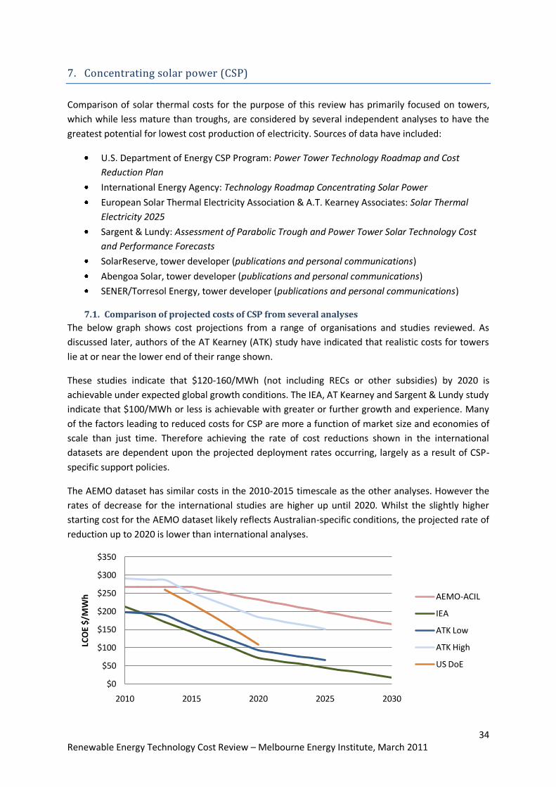
7.1. Comparison of projected costs of CSP from several analyses
The below graph shows cost projections from a range of organisations and studies reviewed. As
discussed later, authors of the AT Kearney (ATK) study have indicated that realistic costs for towers
lie at or near the lower end of their range shown.
These studies indicate that $120-160/MWh (not including RECs or other subsidies) by 2020 is
achievable under expected global growth conditions. The IEA, AT Kearney and Sargent & Lundy study
indicate that $100/MWh or less is achievable with greater or further growth and experience. Many
of the factors leading to reduced costs for CSP are more a function of market size and economies of
scale than just time. Therefore achieving the rate of cost reductions shown in the international
datasets are dependent upon the projected deployment rates occurring, largely as a result of CSP-
specific support policies.
The AEMO dataset has similar costs in the 2010-2015 timescale as the other analyses. However the
rates of decrease for the international studies are higher up until 2020. Whilst the slightly higher
starting cost for the AEMO dataset likely reflects Australian-specific conditions, the projected rate of
reduction up to 2020 is lower than international analyses.
$0
$50
$100
$150
$200
$250
$300
$350
2010 2015 2020 2025 2030
LCO
E $
/MW
h AEMO-ACIL
IEA
ATK Low
ATK High
US DoE

35 Renewable Energy Technology Cost Review – Melbourne Energy Institute, March 2011
Figure 22: Comparison of LCOEs (with RECs) for CST from a range of studies. All calculated for DNI = 2400kWh/m2/year
7.2. Solar thermal power – introduction
Figure 23: Diagram of solar thermal central receiver power tower - note in real plants there are hundreds to thousands of heliostats (Image: Sharon Wong 2010)
Solar thermal power, at its simplest, uses mirrors to concentrate the sun’s rays to achieve
temperatures in the order of several hundred degrees, hot enough to boil water, generate
superheated steam and drive a conventional steam turbine in the same way that a fossil or nuclear
thermal power plant works.
There are a number of different mirror configurations available, such as parabolic troughs and
paraboloidal dishes. This analysis however, will mainly focus on power towers, or central receiver
plants, unless otherwise mentioned, as several analyses point towards power towers having the
greatest potential for low cost power out of the solar thermal technologies†.
The key components of a central receiver or power tower system are:
Central receiver tower – a concrete or steel tower, over 100m tall. At the top of the tower is
a receiver, consisting of rows of vertical tubes made out of a high-temperature alloy, in
which heat is absorbed from rays of concentrated sunlight into a heat transfer fluid,
commonly water (steam) or molten salt).
Heliostat field – a heliostat has flat mirrors mounted on a pedestal which tracks the sun on
both axes, reflecting the sun’s light onto the receiver. A single heliostat can be up to 150m2
in area, and a tower will have hundreds to thousands of heliostats, in the case of large
systems fully surrounding the tower in 360o.
† E.g. Sargent & Lundy LLC, 2003, IEA CSP Roadmap, 2010, discussion and full references in main report body.
36 Renewable Energy Technology Cost Review – Melbourne Energy Institute, March 2011
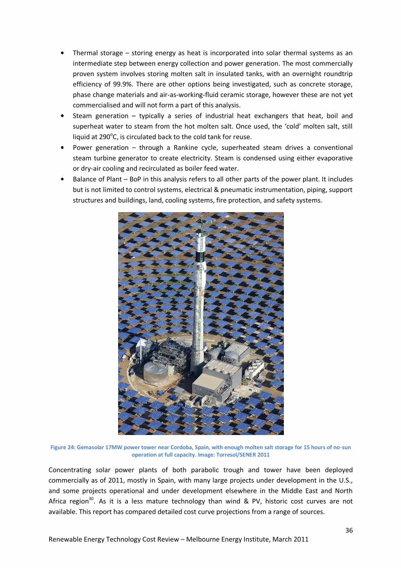
Thermal storage – storing energy as heat is incorporated into solar thermal systems as an
intermediate step between energy collection and power generation. The most commercially
proven system involves storing molten salt in insulated tanks, with an overnight roundtrip
efficiency of 99.9%. There are other options being investigated, such as concrete storage,
phase change materials and air-as-working-fluid ceramic storage, however these are not yet
commercialised and will not form a part of this analysis.
Steam generation – typically a series of industrial heat exchangers that heat, boil and
superheat water to steam from the hot molten salt. Once used, the ‘cold’ molten salt, still
liquid at 290oC, is circulated back to the cold tank for reuse.
Power generation – through a Rankine cycle, superheated steam drives a conventional
steam turbine generator to create electricity. Steam is condensed using either evaporative
or dry-air cooling and recirculated as boiler feed water.
Balance of Plant – BoP in this analysis refers to all other parts of the power plant. It includes
but is not limited to control systems, electrical & pneumatic instrumentation, piping, support
structures and buildings, land, cooling systems, fire protection, and safety systems.
Figure 24: Gemasolar 17MW power tower near Cordoba, Spain, with enough molten salt storage for 15 hours of no-sun operation at full capacity. Image: Torresol/SENER 2011
Concentrating solar power plants of both parabolic trough and tower have been deployed
commercially as of 2011, mostly in Spain, with many large projects under development in the U.S.,
and some projects operational and under development elsewhere in the Middle East and North
Africa region30. As it is a less mature technology than wind & PV, historic cost curves are not
available. This report has compared detailed cost curve projections from a range of sources.
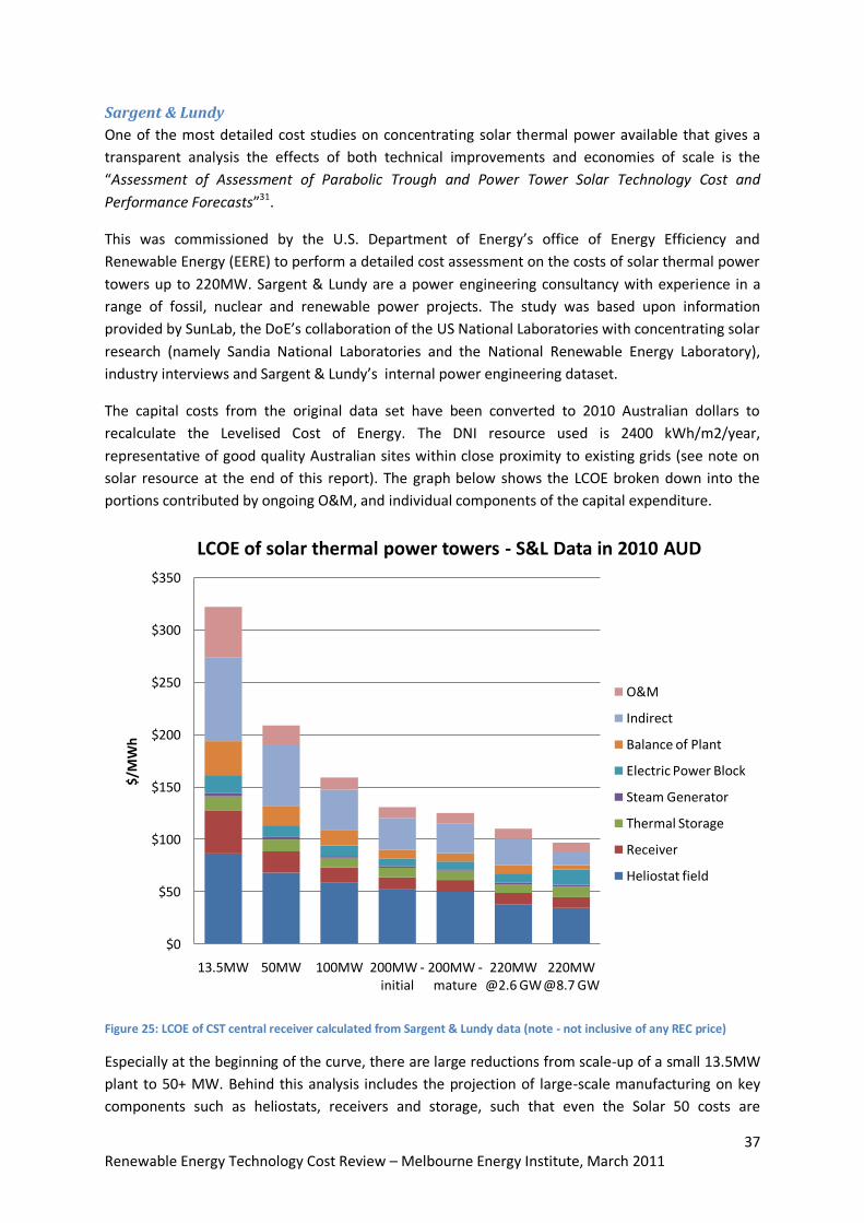
37 Renewable Energy Technology Cost Review – Melbourne Energy Institute, March 2011
Sargent & Lundy
One of the most detailed cost studies on concentrating solar thermal power available that gives a
transparent analysis the effects of both technical improvements and economies of scale is the
“Assessment of Assessment of Parabolic Trough and Power Tower Solar Technology Cost and
Performance Forecasts”31.
This was commissioned by the U.S. Department of Energy’s office of Energy Efficiency and
Renewable Energy (EERE) to perform a detailed cost assessment on the costs of solar thermal power
towers up to 220MW. Sargent & Lundy are a power engineering consultancy with experience in a
range of fossil, nuclear and renewable power projects. The study was based upon information
provided by SunLab, the DoE’s collaboration of the US National Laboratories with concentrating solar
research (namely Sandia National Laboratories and the National Renewable Energy Laboratory),
industry interviews and Sargent & Lundy’s internal power engineering dataset.
The capital costs from the original data set have been converted to 2010 Australian dollars to
recalculate the Levelised Cost of Energy. The DNI resource used is 2400 kWh/m2/year,
representative of good quality Australian sites within close proximity to existing grids (see note on
solar resource at the end of this report). The graph below shows the LCOE broken down into the
portions contributed by ongoing O&M, and individual components of the capital expenditure.
Figure 25: LCOE of CST central receiver calculated from Sargent & Lundy data (note - not inclusive of any REC price)
Especially at the beginning of the curve, there are large reductions from scale-up of a small 13.5MW
plant to 50+ MW. Behind this analysis includes the projection of large-scale manufacturing on key
components such as heliostats, receivers and storage, such that even the Solar 50 costs are
$0
$50
$100
$150
$200
$250
$300
$350
13.5MW 50MW 100MW 200MW -initial
200MW -mature
220MW @2.6 GW
220MW @8.7 GW
$/M
Wh
LCOE of solar thermal power towers - S&L Data in 2010 AUD
O&M
Indirect
Balance of Plant
Electric Power Block
Steam Generator
Thermal Storage
Receiver
Heliostat field
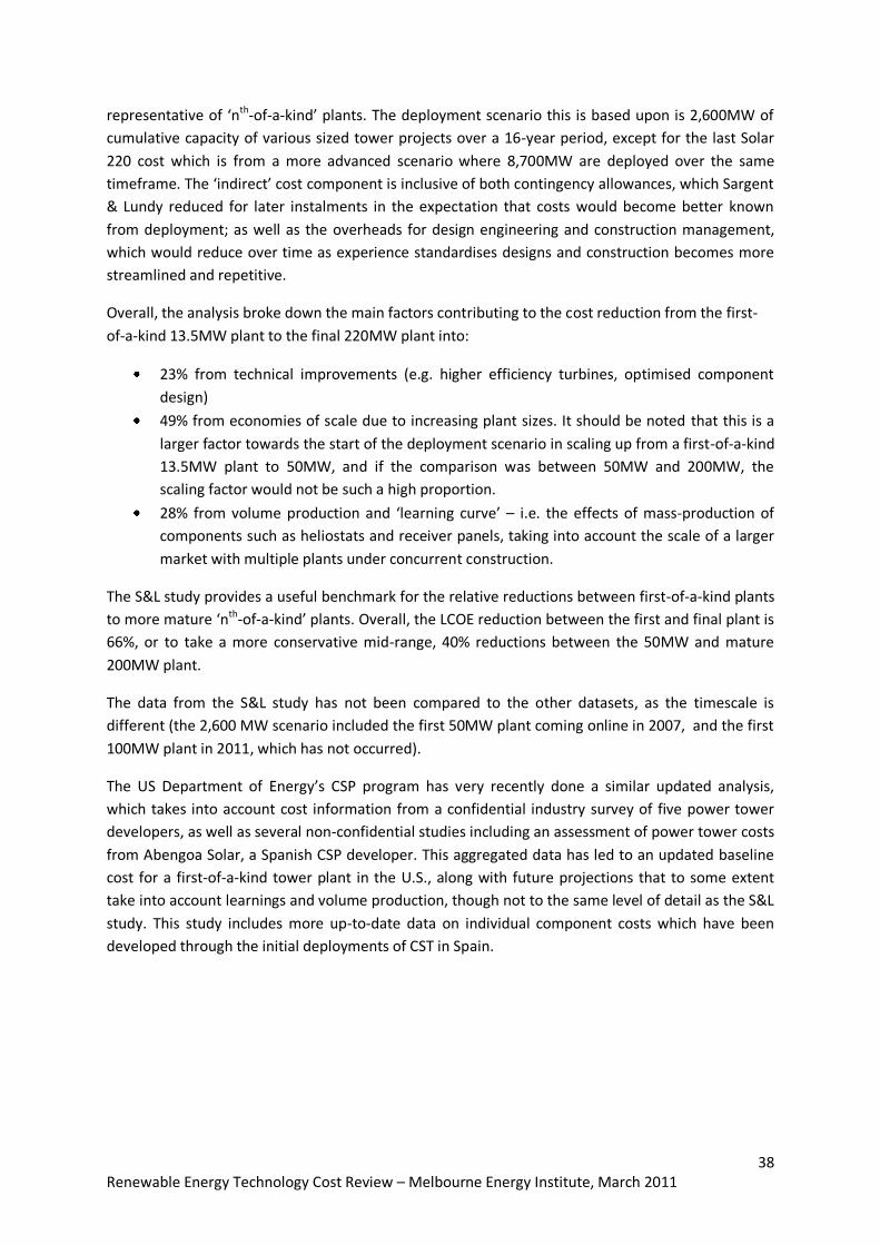
38 Renewable Energy Technology Cost Review – Melbourne Energy Institute, March 2011
representative of ‘nth-of-a-kind’ plants. The deployment scenario this is based upon is 2,600MW of
cumulative capacity of various sized tower projects over a 16-year period, except for the last Solar
220 cost which is from a more advanced scenario where 8,700MW are deployed over the same
timeframe. The ‘indirect’ cost component is inclusive of both contingency allowances, which Sargent
& Lundy reduced for later instalments in the expectation that costs would become better known
from deployment; as well as the overheads for design engineering and construction management,
which would reduce over time as experience standardises designs and construction becomes more
streamlined and repetitive.
Overall, the analysis broke down the main factors contributing to the cost reduction from the first-
of-a-kind 13.5MW plant to the final 220MW plant into:
23% from technical improvements (e.g. higher efficiency turbines, optimised component
design)
49% from economies of scale due to increasing plant sizes. It should be noted that this is a
larger factor towards the start of the deployment scenario in scaling up from a first-of-a-kind
13.5MW plant to 50MW, and if the comparison was between 50MW and 200MW, the
scaling factor would not be such a high proportion.
28% from volume production and ‘learning curve’ – i.e. the effects of mass-production of
components such as heliostats and receiver panels, taking into account the scale of a larger
market with multiple plants under concurrent construction.
The S&L study provides a useful benchmark for the relative reductions between first-of-a-kind plants
to more mature ‘nth-of-a-kind’ plants. Overall, the LCOE reduction between the first and final plant is
66%, or to take a more conservative mid-range, 40% reductions between the 50MW and mature
200MW plant.
The data from the S&L study has not been compared to the other datasets, as the timescale is
different (the 2,600 MW scenario included the first 50MW plant coming online in 2007, and the first
100MW plant in 2011, which has not occurred).
The US Department of Energy’s CSP program has very recently done a similar updated analysis,
which takes into account cost information from a confidential industry survey of five power tower
developers, as well as several non-confidential studies including an assessment of power tower costs
from Abengoa Solar, a Spanish CSP developer. This aggregated data has led to an updated baseline
cost for a first-of-a-kind tower plant in the U.S., along with future projections that to some extent
take into account learnings and volume production, though not to the same level of detail as the S&L
study. This study includes more up-to-date data on individual component costs which have been
developed through the initial deployments of CST in Spain.

39 Renewable Energy Technology Cost Review – Melbourne Energy Institute, March 2011
Sandia National Laboratories: Power Tower Technology Roadmap and Cost Reduction Plan
This report, produced by Sandia National Laboratories for the US Department of Energy (DoE)’s CSP
Program and currently available in draft form, is the product of a joint DoE-industry working group
which has collected cost data from a number of solar thermal power tower developers32. It has been
aggregated to a standard set of component cost data, and an analysis on the potential for cost
reduction for each key component has been carried out. The Roadmap has identified opportunities
falling into the full range of learning rate factors that have the potential to reduce the LCOE from
power towers by almost 50% by 2020:
Figure 26: Projected LCOE breakdown from Sandia (2011) (note – not inclusive of any REC price)
Due to differences in the underlying plant designs shown, the ‘100MW’ plant shown for 2013 is
actually equivalent in size by mirror field and annual electricity output to a plant roughly halfway
between the 50 and 100MW plants from the S&L study. Due to a range of factors, including
increases in the costs of components such as power block and receiver, the updated costs are more
expensive than prior projections. However it is also using component costs more suited to ‘first-of-a-
kind’ plants with no factors for manufacturing volume and learnings, and a high factor for indirect
costs and engineering overheads. Later plants take into account both improved efficiencies (such as
supercritical steam turbines) and learning/volume effects on components.
$0
$50
$100
$150
$200
$250
$300
$350
2013 - 100MW2017 - 150MW2020 - 150MW
$/M
Wh
US DoE CSP Program Power Tower Roadmap
O&M
Indirect
Balance of Plant
Electric Power Block
Steam generator
Thermal storage
Receiver
Heliostat field
40 Renewable Energy Technology Cost Review – Melbourne Energy Institute, March 2011
7.3. Potential for cost reductions by component
Unique Components
Heliostats - Heliostats (mirrors) are the single largest outlay in a solar thermal power plant. As they
are modular in nature, they are able to benefit from the effects of manufacturing volume reducing
unit costs.
The graph in Figure 27 is data from a detailed bottom-up heliostat cost study performed by Sandia
National Laboratories, based on data from a number of vendors at different rates of production. One
representative 75-150MW CST tower plant will have just over 1 million square metres of heliostat
area33.
Figure 27: Heliostat cost curve as a function of production volume. Data from Sandia National Laboratories 'Heliostat Cost Reduction Study' via Power Tower Roadmap
Due to both reduced costs per unit and reduced field requirements due to higher efficiency plant
operation, the US DoE Power Tower Roadmap expects that the contribution of heliostats to the
levelised cost of electricity will almost halve by 2020.
Receiver – the high temperature receivers used for solar towers are the most unique component of
the technology (and therefore is the main factor of technical risk), currently only produced by two
companies – SENER (Spain) and Pratt & Whitney Rocketdyne (USA). Given the relatively small
deployment of these components so far, it is reasonable to expect reductions in cost from learning
and more regular manufacturing. Sargent & Lundy’s original analysis indicated that a 10-15%
learning rate on the receiver component in isolation is expected with a market of multiple plants per
year31. This is in part due to the repetitive assembly of the receiver, which basically consists of
dozens of panels each made of several dozen individual high-temperature metal tubes. It is also
noted that the values of $200-150/kWt used for the 2013 receiver cost in the Power Tower
Roadmap is higher than estimates from Abengoa ($125/kWt).
Storage – The potential for salt storage to become cheaper would mainly come from the technical
improvement of expanding to higher temperatures, which requires less salt for a given amount of
$0
$50
$100
$150
$200
$250
100,000 1,000,000 10,000,000
$/m
2
Total m2/year production
Heliostat cost reduction due to volume

41 Renewable Energy Technology Cost Review – Melbourne Energy Institute, March 2011
energy storage. In addition, some developers are actively pursuing and demonstrating thermocline
storage systems which use a single tank instead of two, where the hot salt is layered on top of the
cold salt. This has only been demonstrated experimentally, and needs to overcome a number of
technical hurdles such as temperature gradient degradation, thermal ratcheting and scaleability. If it
is proven at commercial scale, this has the potential to reduce storage costs by over 30%34.
Generation components -
Components such as the steam turbine and power block are relatively standard thermal power
equipment readily available from companies such as Siemens, GE and Alstom, which would not be
expected to benefit further from learning-through-experience type effects. However due to the
complexity of the design and assembly of the associated infrastructure of heat exchangers, piping,
these components benefit from economies of scale of construction – i.e. the cost of power
generation components does not scale linearly with the output of the plant35.
It should be noted that when comparing the size of a solar thermal plant, the annual output
(MWh/year) is a more useful measure than the size of the turbine, which can vary considerably
depending on the desired operating regime. The US DoE Roadmap expects that power towers will be
able to increase in thermal size at least double the current baseline size, which could result in capital
savings per unit output of over 15%.
Figure 28: Capital cost reduction as a multiple of reference plant output. Source: AT Kearney & ESTELA (2010), data from industry sources and ATK analysis. Note this refers to all technologies – trough, tower, linear Fresnel, dish.
42 Renewable Energy Technology Cost Review – Melbourne Energy Institute, March 2011
Technical improvements
Known improvements to the base technology used in power towers include:
Supercritical steam turbines - Expanding to higher operating temperatures for the salt and steam
inlet conditions. Currently, the standard operating temperature for a tower is 540oC superheated
steam. Superheated and supercritical steam turbines are operational in conventional fossil plants at
temperatures of 600-610oC 36. Reaching 600oC operating temperatures is expected for standard CSP
development by 2020. It is possible that further R&D into higher temperature materials may push
this to 640oC and above. As indicated by EPRI and the Sandia/US DoE Roadmap, this is expected to
push gross steam turbine efficiencies as high as 48%6.
Raising the temperature and operating regime (superheated to supercritical) of the steam turbines
increases the efficiency of the power conversion cycle. As this is one of the largest sources of energy
losses, an increase of 1-2% leads to significant performance improvement. However, in the current
market supercritical turbines are not available under 400MW37, approximately double the size
required by a single large solar thermal tower. If the market for towers grows, there may be a
greater incentive to produce supercritical turbines at these lower sizes. Standardisation of these
products would then help reduce unit costs.
Indirect costs
Indirect costs consist of the extra fees and charges associated with developing and constructing a
project on top of the ‘hard’ costs attributed to labour, materials and components. As the CST
technology matures, contractors become more familiar with the construction process, and more
modular standardised designs are used repeatedly, the indirect costs are expected to reduce31. It
should also be pointed out that engineering, development and planning costs are mostly
independent from the size of the plant, scaling non-linearly38.
Engineering, procurement and construction management fees along with other project-related
expenses can typically add another 30-35% or more on top of direct capital costs of a CST project,
which ends up being a significant contributor to the levelised cost of electricity. This is most
apparent for today’s projects which are being conducted on one-off bases, with many projects still
being first-of-a-kind for individual companies and contractors. It is expected that through learnings
and modular design, indirect costs could be reduced to 20-25% of direct costs, which is what some
power tower developers are expecting for near-term projects already32,37,39. If deployment occurs in
an ad-hoc, non-continuous fashion, this has the potential to keep indirect costs high.
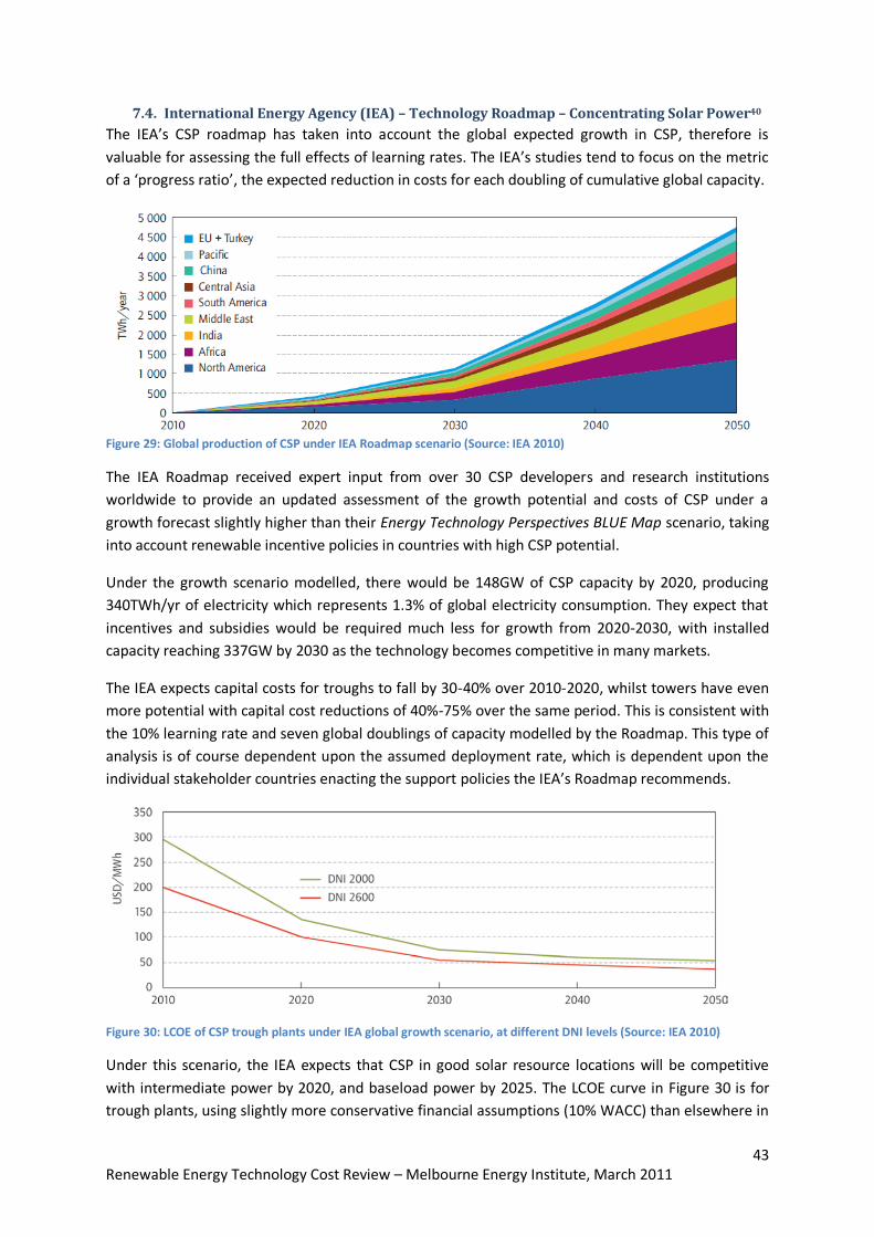
43 Renewable Energy Technology Cost Review – Melbourne Energy Institute, March 2011
7.4. International Energy Agency (IEA) – Technology Roadmap – Concentrating Solar Power40
The IEA’s CSP roadmap has taken into account the global expected growth in CSP, therefore is
valuable for assessing the full effects of learning rates. The IEA’s studies tend to focus on the metric
of a ‘progress ratio’, the expected reduction in costs for each doubling of cumulative global capacity.
Figure 29: Global production of CSP under IEA Roadmap scenario (Source: IEA 2010)
The IEA Roadmap received expert input from over 30 CSP developers and research institutions
worldwide to provide an updated assessment of the growth potential and costs of CSP under a
growth forecast slightly higher than their Energy Technology Perspectives BLUE Map scenario, taking
into account renewable incentive policies in countries with high CSP potential.
Under the growth scenario modelled, there would be 148GW of CSP capacity by 2020, producing
340TWh/yr of electricity which represents 1.3% of global electricity consumption. They expect that
incentives and subsidies would be required much less for growth from 2020-2030, with installed
capacity reaching 337GW by 2030 as the technology becomes competitive in many markets.
The IEA expects capital costs for troughs to fall by 30-40% over 2010-2020, whilst towers have even
more potential with capital cost reductions of 40%-75% over the same period. This is consistent with
the 10% learning rate and seven global doublings of capacity modelled by the Roadmap. This type of
analysis is of course dependent upon the assumed deployment rate, which is dependent upon the
individual stakeholder countries enacting the support policies the IEA’s Roadmap recommends.
Figure 30: LCOE of CSP trough plants under IEA global growth scenario, at different DNI levels (Source: IEA 2010)
Under this scenario, the IEA expects that CSP in good solar resource locations will be competitive
with intermediate power by 2020, and baseload power by 2025. The LCOE curve in Figure 30 is for
trough plants, using slightly more conservative financial assumptions (10% WACC) than elsewhere in
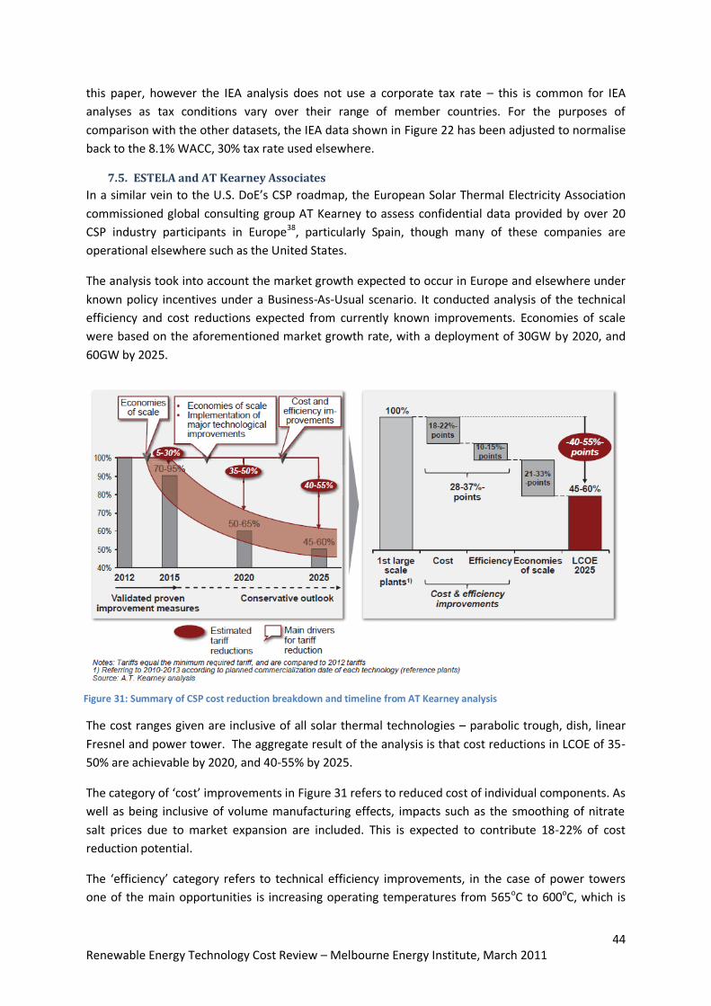
44 Renewable Energy Technology Cost Review – Melbourne Energy Institute, March 2011
this paper, however the IEA analysis does not use a corporate tax rate – this is common for IEA
analyses as tax conditions vary over their range of member countries. For the purposes of
comparison with the other datasets, the IEA data shown in Figure 22 has been adjusted to normalise
back to the 8.1% WACC, 30% tax rate used elsewhere.
7.5. ESTELA and AT Kearney Associates
In a similar vein to the U.S. DoE’s CSP roadmap, the European Solar Thermal Electricity Association
commissioned global consulting group AT Kearney to assess confidential data provided by over 20
CSP industry participants in Europe38, particularly Spain, though many of these companies are
operational elsewhere such as the United States.
The analysis took into account the market growth expected to occur in Europe and elsewhere under
known policy incentives under a Business-As-Usual scenario. It conducted analysis of the technical
efficiency and cost reductions expected from currently known improvements. Economies of scale
were based on the aforementioned market growth rate, with a deployment of 30GW by 2020, and
60GW by 2025.
The cost ranges given are inclusive of all solar thermal technologies – parabolic trough, dish, linear
Fresnel and power tower. The aggregate result of the analysis is that cost reductions in LCOE of 35-
50% are achievable by 2020, and 40-55% by 2025.
The category of ‘cost’ improvements in Figure 31 refers to reduced cost of individual components. As
well as being inclusive of volume manufacturing effects, impacts such as the smoothing of nitrate
salt prices due to market expansion are included. This is expected to contribute 18-22% of cost
reduction potential.
The ‘efficiency’ category refers to technical efficiency improvements, in the case of power towers
one of the main opportunities is increasing operating temperatures from 565oC to 600oC, which is
Figure 31: Summary of CSP cost reduction breakdown and timeline from AT Kearney analysis

45 Renewable Energy Technology Cost Review – Melbourne Energy Institute, March 2011
possible with today’s technology but not implemented in initial plants in the interest of keeping
initial deployment low-risk39. As discussed earlier, higher temperatures both increasing the steam
turbine efficiency, and lower the unit cost of salt storage by allowing greater storage of energy per
unit volume of salt. Improved mirror efficiency is also a factor included in this analysis.
The ‘economies of scale’ portion takes into account both larger sizes for single plants, in the case of
power towers up to 200MW, as well as the reduced engineering, construction management and
planning cost overheads associated with larger plants, or multiple plants of a smaller size rolled out
on a modular basis.
The actual Levelised Cost of Energy
projection range out to 2025 in Figure 32 is
given for a reference solar thermal plant in
Spain.
For the purposes of comparison in Figure 22,
several adjustments have been made as
outlined in the appendix IV.
The Eurocent/kWh figures shown have been
converted to Australian dollars at the
exchange rate of 1 AUD = 0.7 EUR, slightly
below today’s exchange rate. The financial
parameters used a lifetime of 25 years, but a
lower WACC of 6.9% post-tax, largely due to
a low Return on Equity rate. Using the
common WACC of 8.1% used elsewhere in
this report would result in an LCOE 11-12%
higher over the range shown, this
adjustment has also been made (See
Appendix 4 for further details).
Lastly, adjustment has been made to take into account the relatively low solar resource of the base
plant that these calculations are derived from in Spain with 2084 kWh/m2/year. Australia’s higher
solar resource would result in approximately 13-15% lower LCOE from the same capital cost plant
(comparison using DNI=2400).
Due to the nature of the AT Kearney-ESTELA study analyzing cost data from over 20 industry
participants, exact data is confidential and not available for release, and the cost range shown
represents all solar thermal technologies. However, updated information from the AT Kearney
authors indicates that the upper range of costs shown represent a worst-case scenario, and that
some solar thermal projects on the market are tracking at or even below the low end of the range
given, indicating that this is the more realistic end of the cost projection. This seems to be especially
the case for some current power tower technology projects41.
Figure 32: LCOE for solar thermal in Spain (Source: AT Kearney analysis)

46 Renewable Energy Technology Cost Review – Melbourne Energy Institute, March 2011
7.6. AEMO dataset
For comparison, the cost data and future cost reduction projection currently used by the Australian
Energy Market Operator has been used for a central receiver solar thermal plant with 6 hours of
storage.
The capital cost quoted is $6,410/kW from 2010-2015, with an assumed capital cost reduction of
35% by 2030 to $4,166/kW. This is taken from Scenario 1 of input assumptions to the 2010 NTNDP
modelling, representing the best-case data in the range of scenarios modelled5. It is based upon data
from the EPRI report commissioned by the Department of Resource, Energy & Tourism6, and
reviewed by ACIL Tasman. The underlying data between AEMO and EPRI for this particular
technology case are the same, therefore separate analysis for EPRI data has not been included as it
would not give a different cost curve.
The factors of O&M and overall plant efficiency were constant over this period, with no allowance
for reduction given in the data. The performance data from EPRI (capacity factors and annual solar-
electric efficiency of 15.5%) have been used to calculate capacity factor for DNI = 2400
kWh/m2/year, to allow the same basis of comparison with the other datasets in this report.
DNI (kWh/m2/year) Daily average DNI (kWh/m2/day) Capacity Factor
1825 5 26.4%
2190 6 31.6%
2400 6.6 34.7%
2555 7 36.9%

47 Renewable Energy Technology Cost Review – Melbourne Energy Institute, March 2011
8. Appendix I: LCOE Model Verification
The following two tables compare a sample of the model outputs against ATSE modeling results. A
sample of four different sets of input variables, for the two different technologies, and can be found
below.
CST Sample Calculations (not inclusive of RECs):
Capex Opex CF LCOE - MEI LCOE-ATSE Difference
$6,410 $73 35% $309.90 $309 0.291%
$5,662 $73 35% $276.54 $276 0.196%
$4,914 $73 35% $243.19 $243 0.078%
$4,166 $73 35% $209.83 $209 0.397%
Wind Sample Calculations (not inclusive of RECs):
Capex Opex CF LCOE - MEI LCOE-ATSE Difference
$3,018 $37 30% $169.57 $169 0.337%
$2,817 $37 30% $159.22 $159 0.138%
$2,616 $37 30% $148.86 $148 0.581%
$2,415 $37 30% $138.51 $138 0.370%
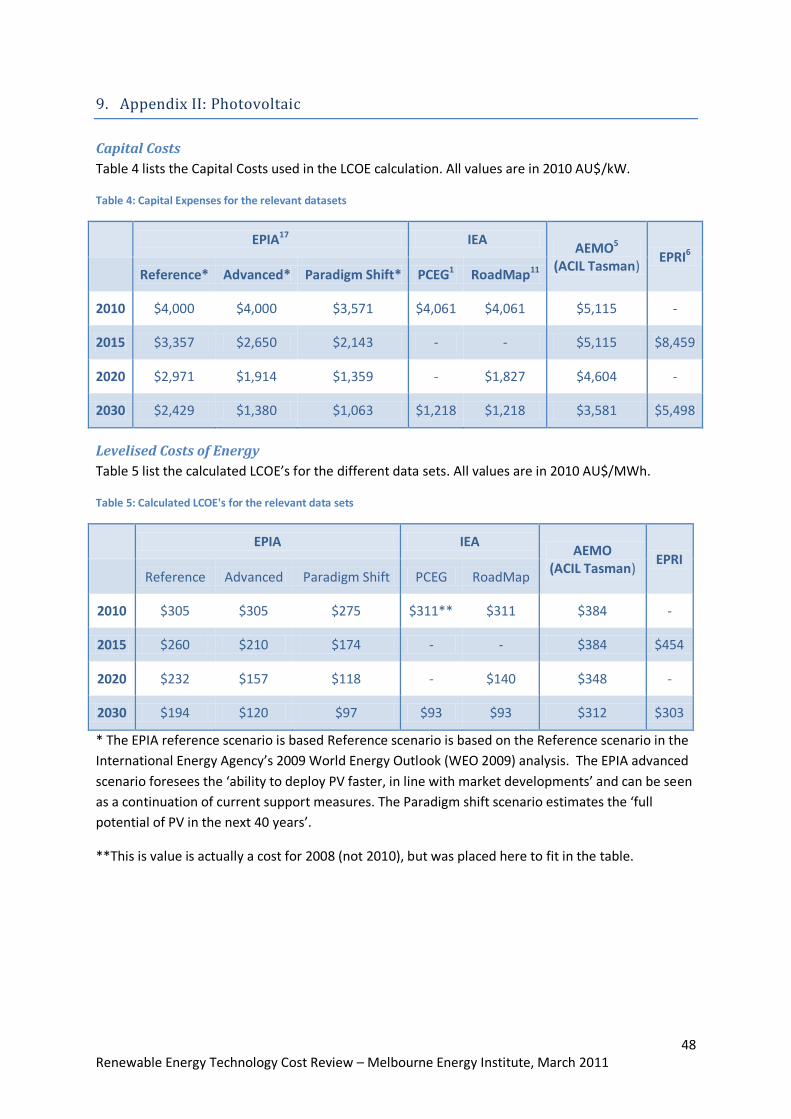
48 Renewable Energy Technology Cost Review – Melbourne Energy Institute, March 2011
9. Appendix II: Photovoltaic
Capital Costs
Table 4 lists the Capital Costs used in the LCOE calculation. All values are in 2010 AU$/kW.
Table 4: Capital Expenses for the relevant datasets
EPIA17 IEA
AEMO5 (ACIL Tasman)
EPRI6
Reference* Advanced* Paradigm Shift* PCEG1 RoadMap11
2010 $4,000 $4,000 $3,571 $4,061 $4,061 $5,115 -
2015 $3,357 $2,650 $2,143 - - $5,115 $8,459
2020 $2,971 $1,914 $1,359 - $1,827 $4,604 -
2030 $2,429 $1,380 $1,063 $1,218 $1,218 $3,581 $5,498
Levelised Costs of Energy
Table 5 list the calculated LCOE’s for the different data sets. All values are in 2010 AU$/MWh.
Table 5: Calculated LCOE's for the relevant data sets
EPIA IEA
AEMO (ACIL Tasman)
EPRI
Reference Advanced Paradigm Shift PCEG RoadMap
2010 $305 $305 $275 $311** $311 $384 -
2015 $260 $210 $174 - - $384 $454
2020 $232 $157 $118 - $140 $348 -
2030 $194 $120 $97 $93 $93 $312 $303
* The EPIA reference scenario is based Reference scenario is based on the Reference scenario in the
International Energy Agency’s 2009 World Energy Outlook (WEO 2009) analysis. The EPIA advanced
scenario foresees the ‘ability to deploy PV faster, in line with market developments’ and can be seen
as a continuation of current support measures. The Paradigm shift scenario estimates the ‘full
potential of PV in the next 40 years’.
**This is value is actually a cost for 2008 (not 2010), but was placed here to fit in the table.

49 Renewable Energy Technology Cost Review – Melbourne Energy Institute, March 2011
10. Appendix III: Wind
1.1.1. Experience Curves
The wind experience curve was constructed from two sets of data; an ‘historic’ set based on the
installation of wind farms in Spain between 1990 and 200122, and a ‘current’ set based on
aggregated numbers from the European Wind Energy Agency between 2000 and 201023. The historic
set was reported in 2001 Euro’s, whilst the EWEA set was report in 2005 Euro’s. The data was
inflated and converted to 2010 Australian dollars to provide a consistent and relevant basis of
comparison. The original data can be found below:
Historic Data22 Current Data23
Cumulative Capacity (MW)
Cost (2010 $/kWh) Cumulative Capacity
(MW) Cost (2010 $/kWh)
4966 2467 16357 1540
5709 2342 24448 1286
6271 2127 31248 1143
7443 1962 39431 1286
8975 1752 47620 1429
10960 1654 59091 1643
12449 1686 74133 1786
13848 1628 93802 1857
15561 1543 120791 1786
17434 1493 159134 1714
19058 1473
Log-Log plots of the transformed data were constructed to represent the experience curves. The
progress ratios and hence learning rates can be derived from this plot.
The most recent EWEA data, and EWEA projections for the medium term were also plotted
alongside two different learning rates (5% and 7%). This illustrates how the EWEA projections fit in
with different learning rate projections (e.g. the IEA projection of a learning rate of 7%1). It should be
noted that a different (but more aggressive) EWEA projection suggests a 10% learning rate could be
achieved.
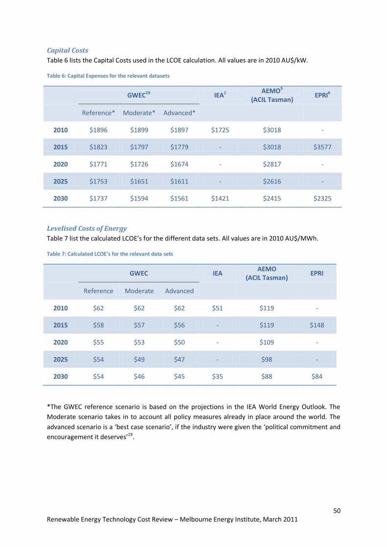
50 Renewable Energy Technology Cost Review – Melbourne Energy Institute, March 2011
Capital Costs
Table 6 lists the Capital Costs used in the LCOE calculation. All values are in 2010 AU$/kW.
Table 6: Capital Expenses for the relevant datasets
GWEC19 IEA1
AEMO5 (ACIL Tasman)
EPRI6
Reference* Moderate* Advanced*
2010 $1896 $1899 $1897 $1725 $3018 -
2015 $1823 $1797 $1779 - $3018 $3577
2020 $1771 $1726 $1674 - $2817 -
2025 $1753 $1651 $1611 - $2616 -
2030 $1737 $1594 $1561 $1421 $2415 $2325
Levelised Costs of Energy
Table 7 list the calculated LCOE’s for the different data sets. All values are in 2010 AU$/MWh.
Table 7: Calculated LCOE's for the relevant data sets
GWEC IEA
AEMO (ACIL Tasman)
EPRI
Reference Moderate Advanced
2010 $62 $62 $62 $51 $119 -
2015 $58 $57 $56 - $119 $148
2020 $55 $53 $50 - $109 -
2025 $54 $49 $47 - $98 -
2030 $54 $46 $45 $35 $88 $84
*The GWEC reference scenario is based on the projections in the IEA World Energy Outlook. The
Moderate scenario takes in to account all policy measures already in place around the world. The
advanced scenario is a ‘best case scenario’, if the industry were given the ‘political commitment and
encouragement it deserves’19.
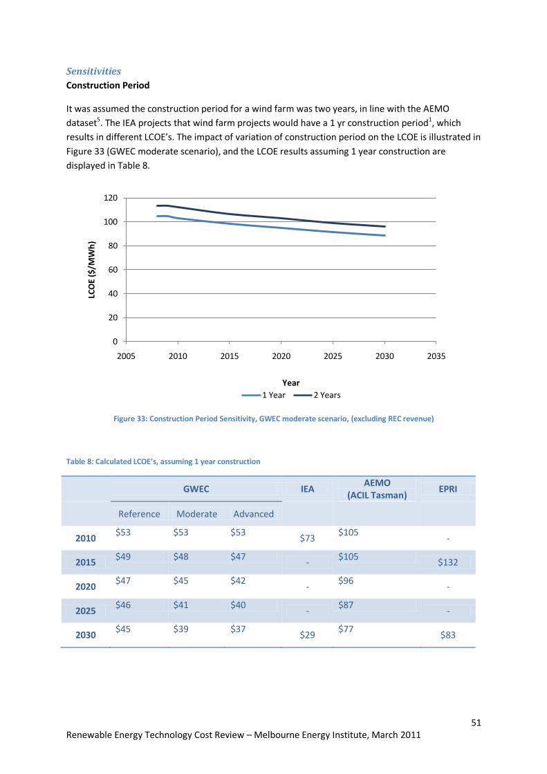
51 Renewable Energy Technology Cost Review – Melbourne Energy Institute, March 2011
Sensitivities
Construction Period
It was assumed the construction period for a wind farm was two years, in line with the AEMO
dataset5. The IEA projects that wind farm projects would have a 1 yr construction period1, which
results in different LCOE’s. The impact of variation of construction period on the LCOE is illustrated in
Figure 33 (GWEC moderate scenario), and the LCOE results assuming 1 year construction are
displayed in Table 8.
Figure 33: Construction Period Sensitivity, GWEC moderate scenario, (excluding REC revenue)
Table 8: Calculated LCOE’s, assuming 1 year construction
GWEC IEA
AEMO (ACIL Tasman)
EPRI
Reference Moderate Advanced
2010 $53 $53 $53
$73 $105
-
2015 $49 $48 $47
- $105
$132
2020 $47 $45 $42
- $96
-
2025 $46 $41 $40
- $87
-
2030 $45 $39 $37
$29 $77
$83
0
20
40
60
80
100
120
2005 2010 2015 2020 2025 2030 2035
LCO
E ($
/MW
h)
Year
1 Year 2 Years

52 Renewable Energy Technology Cost Review – Melbourne Energy Institute, March 2011
11. Appendix IV: Concentrating Solar Thermal
1.1.1. Costs
The tables below list the costs used in the LCOE calculations. All values are in 2010 AU$/kW unless
explicitly stated otherwise, converted at foreign exchange rates of 1USD = 0.985AUD, and 1EUR =
0.7AUD. LCOEs are inclusive of $50/MWh REC.
AEMO 2010 (ACIL Tasman) – Scenario 1
Capex ($/kW) O&M ($/kW/yr)
Annual Solar-Electric Efficiency
LCOE ($/MWh)
2010 $6,410 $73 15.5% $267
2015 $6,410 $73 15.5% $267
2020 $5,662 $73 15.5% $233
2025 $4,914 $73 15.5% $198
2030 $4,166 $73 15.5% $164
US DoE Power Tower Roadmap
Capex ($/kW) O&M ($/kW/yr)
Annual Solar-Electric Efficiency
LCOE ($/MWh)
2013 $7,540 $66 14.8% $260
2017 $7,516 $58 15.7% $179
2020 $5,763 $51 17.8% $109
International Energy Agency data was available as a final LCOE. It has been converted to Australian
dollars taking into account factors to allow for different tax rates and WACC used.
IEA CSP Roadmap – DNI 2400
LCOE (US$/MWh, no REC) LCOE (AU$/MWh adjusted, with REC)
2010 $295 $213
2020 $136 $72
2030 $76 $18
WACC 10% 8.1%
Tax Rate 0 30%
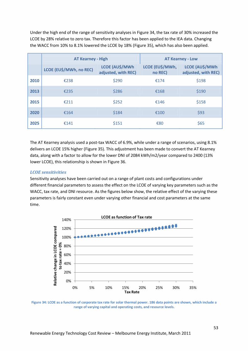
53 Renewable Energy Technology Cost Review – Melbourne Energy Institute, March 2011
Under the high end of the range of sensitivity analyses in Figure 34, the tax rate of 30% increased the
LCOE by 28% relative to zero tax. Therefore this factor has been applied to the IEA data. Changing
the WACC from 10% to 8.1% lowered the LCOE by 18% (Figure 35), which has also been applied.
AT Kearney - High AT Kearney - Low
LCOE (EU$/MWh, no REC)
LCOE (AU$/MWh adjusted, with REC)
LCOE (EU$/MWh, no REC)
LCOE (AU$/MWh adjusted, with REC)
2010 €238 $290 €174 $198
2013 €235 $286 €168 $190
2015 €211 $252 €146 $158
2020 €164 $184 €100 $93
2025 €141 $151 €80 $65
The AT Kearney analysis used a post-tax WACC of 6.9%, while under a range of scenarios, using 8.1%
delivers an LCOE 15% higher (Figure 35). This adjustment has been made to convert the AT Kearney
data, along with a factor to allow for the lower DNI of 2084 kWh/m2/year compared to 2400 (13%
lower LCOE), this relationship is shown in Figure 36.
LCOE sensitivities
Sensitivity analyses have been carried out on a range of plant costs and configurations under
different financial parameters to assess the effect on the LCOE of varying key parameters such as the
WACC, tax rate, and DNI resource. As the figures below show, the relative effect of the varying these
parameters is fairly constant even under varying other financial and cost parameters at the same
time.
Figure 34: LCOE as a function of corporate tax rate for solar thermal power. 186 data points are shown, which include a range of varying capital and operating costs, and resource levels.
0%
20%
40%
60%
80%
100%
120%
140%
0% 5% 10% 15% 20% 25% 30% 35%
Rel
ativ
e ch
ange
in L
CO
E co
mp
are
d
to t
ax r
ate
= 0
%
Tax Rate
LCOE as function of Tax rate

54 Renewable Energy Technology Cost Review – Melbourne Energy Institute, March 2011
Figure 35: LCOE as a function of varying WACC for solar thermal power. 186 data points are shown, which also include a range of varying capital and operating costs, and resource levels.
Figure 36: LCOE as a function of DNI. 20 different cases are shown which also include varying capital and operating costs, and annual solar-to-electric efficiencies.
0%
20%
40%
60%
80%
100%
120%
140%
160%
180%
200%
0% 2% 4% 6% 8% 10% 12% 14%
Ch
ange
in L
CO
E (r
elat
ive
to
6%
W
AC
C)
WACC (%)
LCOE as a function of WACC (Discount rate)
0%
20%
40%
60%
80%
100%
120%
2,000 2,100 2,200 2,300 2,400 2,500 2,600 2,700 2,800 2,900 3,000
LCO
E re
lati
ve t
o D
NI 2
000
DNI (kWh/m2/year)
LCOE as function of Direct Normal Irradiation

55 Renewable Energy Technology Cost Review – Melbourne Energy Institute, March 2011
12. Appendix V: Solar Resource
The available solar radiation at any given location has a significant effect on the LCOE for solar
technologies, as this essentially governs the total energy output and capacity factor for a given
installation. There are several ways of measuring solar resource:
- Global Horizontal Irradiation (GHI) measures the energy received on a surface parallel to the
surface of the Earth (i.e. flat on the ground).
- Direct Normal Irradiation (DNI) measures the energy received on a surface angled at a
normal (i.e. perpendicular) to the sun at any point in time.
For assessing solar energy technologies, DNI is the relevant resource type to use. When calculating
output, factors such as the angle of a fixed collector or the tracking of a moving collector can be
taken into account.
Figure 37: Direct Normal Irradiation resource for Australia. Adapted from DLR42
For Australia, as can be seen from Figure 37, the DNI over most of Australia is over 2000
kWh/m2/year (5.48 kWh/m2/day average). There are many areas in central NSW, central QLD,
South Australia and Western Australia with average DNI around 2400, whilst still in close proximity
to the existing electricity grid. Therefore for the purposes of the solar thermal power analysis in this
report, all calculations have been done on the basis of DNI = 2400 kWh/m2/year.

56 Renewable Energy Technology Cost Review – Melbourne Energy Institute, March 2011
13. References
1 International Energy Agency and Nuclear Energy Agency (2010), Projected Costs of Generating Electricity 2010 Edition,
Organization for Economic Cooperation & Development, France.
2 Higgins R.C (2008), Analysis for financial management, 9th edition, McGraw-Hill Irwin.
3 Australian Government, Mid Year Economic and Fiscal Outlook, http://www.budget.gov.au/2010-11/content/myefo/html/part_2-01.htm. Accessed 01 March 2011.
4 Reserve Bank of Australia, RBA Exchange Rates, http://www.rba.gov.au/statistics/frequency/exchange-rates.html. Accessed 01 March 2011.
5 Australian Energy Market Operator (2010), NTNDP Modelling Assumptions: Supply Input Spreadsheets, Available from: http://www.aemo.com.au/planning/ntndp2010consult.html, Accessed 11 Feb 2011.
6 Electric Power Research Institute, (2010), Australian Electricity Generation Technology Costs – Reference Case 2010, Department of Resources, Energy and Tourism, Available at: http://www.ret.gov.au/energy/Documents/facts-stats-pubs/AEGTC%202010.pdf, Accessed 10 Dec 2010.
7 European Photovoltaic Industry Association, (2010), Global Market Outlook for Photovoltaics until 2014, European Photovoltaic Industry Association. Available at: http://www.epia.org/fileadmin/EPIA_docs/public/Global_Market_Outlook_for_Photovoltaics_until_2014.pdf, Accessed 4th Feb 2011.
8 Rocky Mountain Institute (2010), Achieving Low-Cost Solar PV: Balance of System Cost Reductions, Rocky Mountain Institute. Available at: http://www.rmi.org/Content/Files/BOSReport.pdf. Accessed Feb 24th 2011.
9 CrystalClear (2008), The Crystal Clear Integrated Project, Proceedings of the 23rd European PV Solar Energy Conference
2008, Valencia.
10 C. Breyer and A. Gerlach (2010), Global Overview on Grid-Parity Event Dynamics, in Proceedings 25th European Photovoltaic Solar Energy Conference, Valencia.
11 International Energy Agency (2010), Technology Roadmap - Solar Photovoltaic Energy, International Energy Agenc.
Available at: http://www.iea.org/papers/2010/pv_roadmap.pdf, Accessed 31 Jan 2011.
12 Lux Research (2010), Module Cost Structure Breakdown. Lux Research Inc. Available at: http://www.luxresearchinc.com/component/content/article/7/83-lux-researchmodule-cost-structure-breakdown.html
13 G. F Nemet (2006), Beyond the learning curve: factors influencing cost reductions in photovoltaics, Energy Policy 34, no. 17: 3218–3232.
14 International Energy Agency (2009, Trends in Photovoltaic Applications. International Energy Agency. Available at:
http://www.iea-pvps.org/fileadmin/dam/public/report/statistics/tr_2009_neu.pdf
15 National Renewable Energy Laboratories (2009), The Effects of the Financial Crisis on Photovoltaics: An Analysis of Changes in Market Forecasts from 2008 to 2009, US Department of Energy, Available at: http://www.nrel.gov/docs/fy10osti/46713.pdf
16 Standard & Poor’s Equity Solar Research Analysts, December 2010.
17 European Photovoltaic Industry Association (2011), Solar Generation 6: Solar Photovoltaic Energy Empowering the World, European Photovoltaic Industry Association. Available at: http://www.epia.org/index.php?eID=tx_nawsecuredl&u=0&file=fileadmin/EPIA_docs/documents/Solar_Generation_6__2011_Full_report_Final.pdf&t=1300329404&hash=5d631347c2643d74d99567bec466ceda
18 Personal Communications, Damien Moyse, Energy Projects & Policy Manager - Alternative Technology Association (March 2011)
19 Global Wind Energy Council (2010), Global Wind Energy Outlook 2010, Global Wind Energy Council, Available at: http://www.gwec.net/fileadmin/documents/Publications/GWEO%202010%20final.pdf
20 M. I Blanco (2009), The economics of wind energy, Renewable and Sustainable Energy Reviews 13, no. 6-7: 1372–1382.
21 European Wind Energy Association (200 9), Economics of Wind Main Report, European Wind Energy Association. Available at: http://www.ewea.org/fileadmin/ewea_documents/documents/publications/reports/Economics_of_Wind_Main_Report_FINAL-lr.pdf

57 Renewable Energy Technology Cost Review – Melbourne Energy Institute, March 2011
22M. Junginger, A. Faaij, and W. C. Turkenburg (2005), Global experience curves for wind farms, Energy Policy 33, no. 2: 133-150.
23 European Wind Energy Association (2009), Pure Power - A report by the European Wind Energy Association - 2009 update, European Wind Energy Associaton.
Available at: http://www.ewea.org/fileadmin/ewea_documents/documents/publications/reports/Pure_Power_Full_Report.pdf
24 Bolinger, M.A. (2009), Wind Power Price Trends in the United States: Struggling to Remain Competitive in the Face of
Strong Growth, Lawrence Berkeley National Laboratory, California.
25 International Energy Agency (2009), Wind Roadmap. International Energy Agency. Available at:
http://www.iea.org/papers/2009/Wind_Roadmap.pdf
26 US Department of Energy (2008), 20% Wind Energy by 2030, Increasing Wind Energy’s Contribution
to U.S. Electricity Supply, US Department of Energy, Available at: http://www1.eere.energy.gov/windandhydro/pdfs/41869.pdf
27 European Wind Energy Association, Wind Energy – The Facts. Available at: http://www.ewea.org/fileadmin/ewea_documents/documents/publications/WETF/WETF.pdf
28Bloomberg New Energy Finance 2011, Wind Turbine Prince Index, Bloomberg, Available at: http://bnef.com/Download/pressreleases/139/pdffile/
29 AGL, (2010), Media Release. Available at: http://www.agl.com.au/about/ASXReleases/Pages/$1billionwindfarminVictoriassouthwesttobebiggestinsouthernhemisphere.aspx
30 National Renewable Energy Laboratories (2010), Concentrating Solar Power Projects, US Department of Energy, Available
at: http://www.nrel.gov/csp/solarpaces/by_country.cfm, Accessed: 1 Mar 2011
31 Sargent & Lundy Consulting LLC, (2003), Assessment of Assessment of Parabolic Trough and Power Tower Solar Technology Cost and Performance Forecasts, National Renewable Energy Laboratories & US Department of Energy, Available at: http://www.nrel.gov/csp/pdfs/34440.pdf, Accessed: 10 Jan 2010
32 Kolb, G. J., Ho, C. K., Mancini, T. R. & Gary, J. A., 2011, Power Tower Technology Roadmap and Cost Reduction Plan, Sandia National Laboratories, Alberqurque
33 Solar Reserve, (2009), Tonopah Crescent Dunes Plan of Development, Available at: http://www.tonopahsolar.com/pdfs/Tonopah_Crescent_Dunes_POD_2009_11_23.pdf, accessed 1 Feb 2011
34 Libby, C. Et al, (2010), Solar Thermocline Storage Systems, Electric Power Research Institute, Palo Alto
35 Lipman, E. (2010), Reducing CSP plant LCOE with precise engineering, synergies and R&D, Siemens AG, Proceedings of the
16th SolarPACES conference, Perpignan
36 Cziesla, F. Et al (2009), Lunen – State-Of-The Art Ultra Supercritical Steam Power Plant under construction, Available at: http://www.energy.siemens.com/us/pool/hq/power-generation/power-plants/steam-power-plant-solutions/coal-fired-power-plants/Luenen.pdf, Accessed 1 Mar 2011
37 Kelly, B. et al (2010), Advanced Thermal Energy Storage For Central Receivers With Supercritical Coolants, Proceedings of the 16th SolarPACES conference, Perpignan
38 AT Kearney Consulting (2010), Solar Thermal Electricity 2025, Available at: http://www.estelasolar.eu/fileadmin/ESTELAdocs/documents/Cost_Roadmap/2010-06%20-%20Solar%20Thermal%20Electricity%202025%20-%20ENG.pdf, Accessed 1 Feb 2011
39 Personal communication. Solar Reserve, 2011
40 International Energy Agency, (2010), Technology Roadmap: Concentrating Solar Power, International Energy Agency.
Available at: http://www.iea.org/papers/2010/csp_roadmap.pdf, Accessed 1 Feb 2011
41 Personal communications, AT Kearney, Mar 2011
42 Trieb, F., et al, (2009), Global Concentrating Solar Power Potentials, DLR (German Aerospace Centre), Available at: http://www.dlr.de/tt/desktopdefault.aspx/tabid-2885/4422_read-16596/, Accessed: 2 Jan 2010