The International Association for the Properties of Water and Steam

Niagara Falls, Canada July 2010

Guideline on an Equation of State for Humid Air in Contact with Seawater and Ice,

Consistent with the IAPWS Formulation 2008 for the Thermodynamic Properties of Seawater

© 2010 International Association for the Properties of Water and Steam

Publication in whole or in part is allowed in all countries provided that attribution is given to the International Association for the Properties of Water and Steam

President:

Dr. Daniel G. Friend Thermophysical Properties Division

National Institute of Standards and Technology 325 Broadway

Boulder, Colorado 80305, USA

Executive Secretary: Dr. R. B. Dooley

Structural Integrity Associates, Inc. 2616 Chelsea Drive

Charlotte, North Carolina 28209, USA email: bdooley@structint.com

This Guideline contains 21 pages, including this cover page.

This Guideline has been authorized by the International Association for the Properties of Water and Steam (IAPWS) at its meeting in Niagara Falls, Canada, 18-23 July, 2010, for issue by its Secretariat. The members of IAPWS are: Britain and Ireland, Canada, the Czech Republic, Denmark, France, Germany, Greece, Japan, Russia, the United States of America, and associate members Argentina and Brazil, Italy, and Switzerland.

The equation of state provided in this Guideline is a fundamental equation for the specific Helmholtz energy as a function of air mass fraction, temperature and density; details can be found in the article “Thermodynamic Properties of Sea Air” by R. Feistel et al. [1]. This equation is rigorously consistent with the IAPWS Releases on fluid water, ice and seawater [2, 3, 4] and can be used for the computation of the properties of arbitrary mutual phase transitions and composites thereof.

Further information about this Guideline and other documents issued by IAPWS can be obtained from the Executive Secretary of IAPWS or from http://www.iapws.org.

2

Contents

1 Nomenclature 2

2 Introductory Remarks and Special Constants 5

3 The Equation of State 5

4 Relations of the Thermodynamic Properties to the Specific Helmholtz Energy 8

5 Colligative Properties 11

6 Range of Validity and Brief Discussion 17

7 Estimates of Uncertainty 17

8 Computer-Program Verification 18

9 References 18

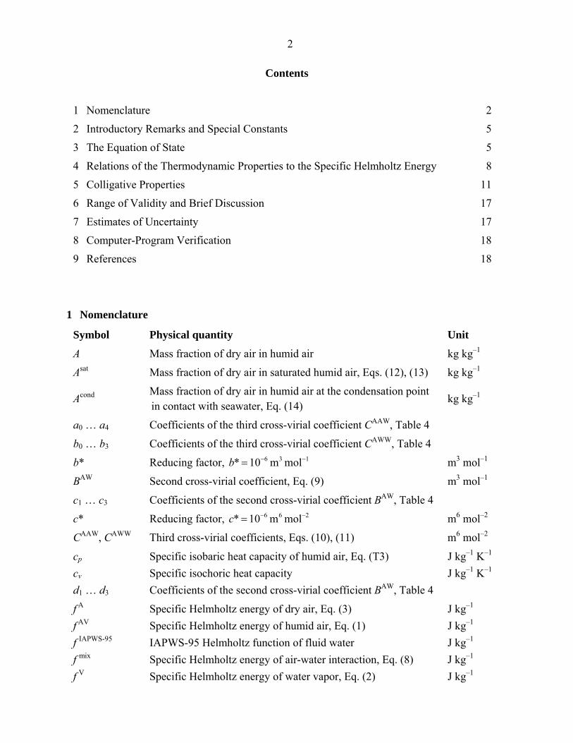
1 Nomenclature

Symbol Physical quantity Unit

A Mass fraction of dry air in humid air kg kg–1

Asat Mass fraction of dry air in saturated humid air, Eqs. (12), (13) kg kg–1

Acond Mass fraction of dry air in humid air at the condensation point

in contact with seawater, Eq. (14) kg kg–1

a0 … a4 Coefficients of the third cross-virial coefficient CAAW, Table 4

b0 … b3 Coefficients of the third cross-virial coefficient CAWW, Table 4

b* Reducing factor, 136 molm10* −−=b m3 mol–1

BAW Second cross-virial coefficient, Eq. (9) m3 mol–1

c1 … c3 Coefficients of the second cross-virial coefficient BAW, Table 4

c* Reducing factor, 266 molm10* −−=c m6 mol–2

CAAW, CAWW Third cross-virial coefficients, Eqs. (10), (11) m6 mol–2

cp Specific isobaric heat capacity of humid air, Eq. (T3) J kg–1 K–1 cv Specific isochoric heat capacity J kg–1 K–1 d1 … d3 Coefficients of the second cross-virial coefficient BAW, Table 4

f A Specific Helmholtz energy of dry air, Eq. (3) J kg–1 f AV Specific Helmholtz energy of humid air, Eq. (1) J kg–1 f

IAPWS-95 IAPWS-95 Helmholtz function of fluid water J kg–1 f mix Specific Helmholtz energy of air-water interaction, Eq. (8) J kg–1 f

V Specific Helmholtz energy of water vapor, Eq. (2) J kg–1

3

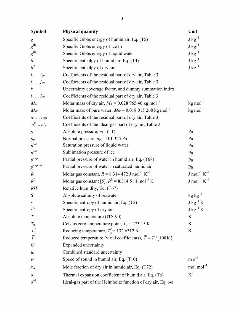
Symbol Physical quantity Unit

g Specific Gibbs energy of humid air, Eq. (T5) J kg–1 gIh Specific Gibbs energy of ice Ih J kg–1 gliq Specific Gibbs energy of liquid water J kg–1 h Specific enthalpy of humid air, Eq. (T4) J kg–1 hA Specific enthalpy of dry air J kg–1 i1 … i19 Coefficients of the residual part of dry air, Table 3 j1 … j19 Coefficients of the residual part of dry air, Table 3 k Uncertainty coverage factor, and dummy summation index l1 … l19 Coefficients of the residual part of dry air, Table 3 MA Molar mass of dry air, MA = 0.028 965 46 kg mol–1 kg mol–1 MW Molar mass of pure water, MW = 0.018 015 268 kg mol–1 kg mol–1 n1 … n19 Coefficients of the residual part of dry air, Table 3

01n … 0

13n Coefficients of the ideal-gas part of dry air, Table 2 p Absolute pressure, Eq. (T1) Pa p0 Normal pressure, p0 = 101 325 Pa Pa psat Saturation pressure of liquid water Pa psubl Sublimation pressure of ice Pa pvap Partial pressure of water in humid air, Eq. (T68) Pa pvap,sat Partial pressure of water in saturated humid air Pa R Molar gas constant, R = 8.314 472 J mol–1 K–1 J mol–1 K–1 RL Molar gas constant [5], RL = 8.314 51 J mol–1 K–1 J mol–1 K–1 RH Relative humidity, Eq. (T67) S Absolute salinity of seawater kg kg–1 s Specific entropy of humid air, Eq. (T2) J kg–1 K–1 sA Specific entropy of dry air J kg–1 K–1 T Absolute temperature (ITS-90) K T0 Celsius zero temperature point, T0 = 273.15 K K

*AT Reducing temperature, *

AT = 132.6312 K K T Reduced temperature (virial coefficients), ( )/ 100 KT T= U Expanded uncertainty uc Combined standard uncertainty w Speed of sound in humid air, Eq. (T10) m s–1

xA Mole fraction of dry air in humid air, Eq. (T72) mol mol–1

α Thermal expansion coefficient of humid air, Eq. (T6) K–1 αid Ideal-gas part of the Helmholtz function of dry air, Eq. (4)

4

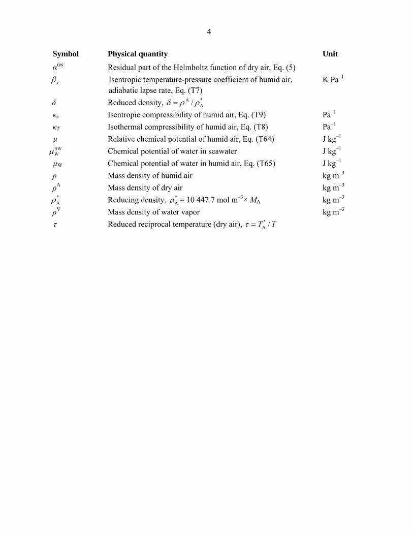
Symbol Physical quantity Unit

αres Residual part of the Helmholtz function of dry air, Eq. (5) sβ Isentropic temperature-pressure coefficient of humid air,

adiabatic lapse rate, Eq. (T7) K Pa–1

δ Reduced density, *A

A / ρρδ = κs Isentropic compressibility of humid air, Eq. (T9) Pa–1 κT Isothermal compressibility of humid air, Eq. (T8) Pa–1 µ Relative chemical potential of humid air, Eq. (T64) J kg–1 SWWμ Chemical potential of water in seawater J kg–1 µW Chemical potential of water in humid air, Eq. (T65) J kg–1 ρ Mass density of humid air kg m–3 ρA Mass density of dry air kg m–3

*Aρ Reducing density, *

Aρ = 10 447.7 mol m–3× MA kg m–3 ρV Mass density of water vapor kg m–3 τ Reduced reciprocal temperature (dry air), TT /*

A=τ

5

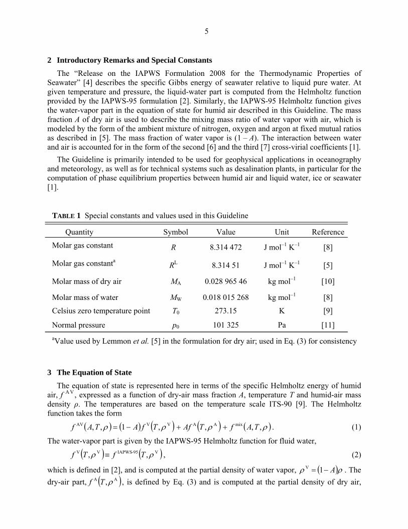
2 Introductory Remarks and Special Constants The “Release on the IAPWS Formulation 2008 for the Thermodynamic Properties of

Seawater” [4] describes the specific Gibbs energy of seawater relative to liquid pure water. At given temperature and pressure, the liquid-water part is computed from the Helmholtz function provided by the IAPWS-95 formulation [2]. Similarly, the IAPWS-95 Helmholtz function gives the water-vapor part in the equation of state for humid air described in this Guideline. The mass fraction A of dry air is used to describe the mixing mass ratio of water vapor with air, which is modeled by the form of the ambient mixture of nitrogen, oxygen and argon at fixed mutual ratios as described in [5]. The mass fraction of water vapor is (1 – A). The interaction between water and air is accounted for in the form of the second [6] and the third [7] cross-virial coefficients [1].

The Guideline is primarily intended to be used for geophysical applications in oceanography and meteorology, as well as for technical systems such as desalination plants, in particular for the computation of phase equilibrium properties between humid air and liquid water, ice or seawater [1].

TABLE 1 Special constants and values used in this Guideline

Quantity Symbol Value Unit Reference

Molar gas constant R 8.314 472 J mol–1 K–1 [8]

Molar gas constanta RL 8.314 51 J mol–1 K–1 [5]

Molar mass of dry air MA 0.028 965 46 kg mol–1 [10]

Molar mass of water MW 0.018 015 268 kg mol–1 [8]

Celsius zero temperature point T0 273.15 K [9]

Normal pressure p0 101 325 Pa [11] aValue used by Lemmon et al. [5] in the formulation for dry air; used in Eq. (3) for consistency

3 The Equation of State The equation of state is represented here in terms of the specific Helmholtz energy of humid

air, f A V, expressed as a function of dry-air mass fraction A, temperature T and humid-air mass density ρ. The temperatures are based on the temperature scale ITS-90 [9]. The Helmholtz function takes the form

( ) ( ) ( ) ( ) ( )ρρρρ ,,,,1,, mixAAVVAV TAfTAfTfATAf ++−= . (1)

The water-vapor part is given by the IAPWS-95 Helmholtz function for fluid water,

( ) ( )V95-IAPWSVV ,, ρρ TfTf ≡ , (2)

which is defined in [2], and is computed at the partial density of water vapor, ( )ρρ A−= 1V . The dry-air part, ( )AA , ρTf , is defined by Eq. (3) and is computed at the partial density of dry air,

6

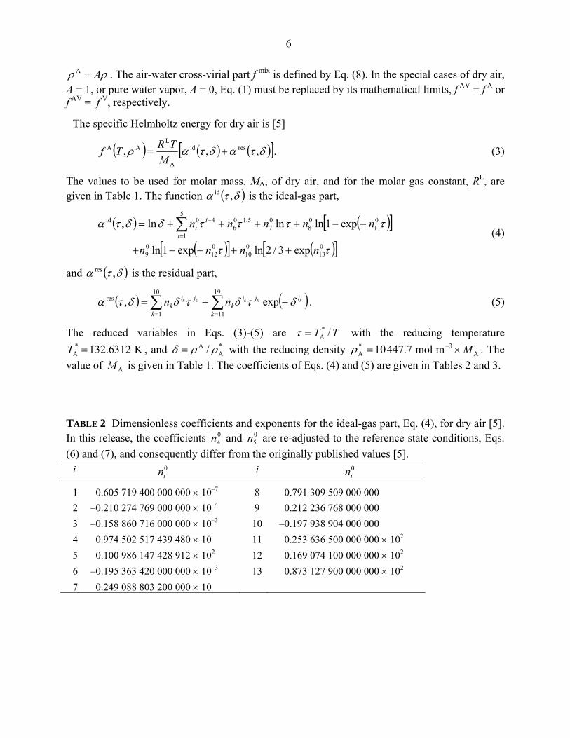
ρρ A=A . The air-water cross-virial part f mix is defined by Eq. (8). In the special cases of dry air,

A = 1, or pure water vapor, A = 0, Eq. (1) must be replaced by its mathematical limits, f AV = f A or f AV = f

V, respectively.

The specific Helmholtz energy for dry air is [5]

( ) ( ) ( )[ ]δταδταρ ,,, resid

A

LAA +=

MTRTf . (3)

The values to be used for molar mass, MA, of dry air, and for the molar gas constant, RL, are given in Table 1. The function ( )δτα ,id is the ideal-gas part,

( ) ( )[ ]( )[ ] ( )[ ]ττ

ττττδδτα

013

010

012

09

011

08

07

5.106

5

1

40id

exp3/2lnexp1ln

exp1lnlnln,

nnnn

nnnnni

ii

++−−+

−−++++= ∑=

−

(4)

and ( )δτα ,res is the residual part,

( ) ( )∑∑==

−+=19

11

10

1

res exp,k

ljik

k

jik

kkkkk nn δτδτδδτα . (5)

The reduced variables in Eqs. (3)-(5) are TT /*A=τ with the reducing temperature

K6312.132*A =T , and *

AA / ρρδ = with the reducing density A

3*A mmol7.44710 M×= −ρ . The

value of AM is given in Table 1. The coefficients of Eqs. (4) and (5) are given in Tables 2 and 3.

TABLE 2 Dimensionless coefficients and exponents for the ideal-gas part, Eq. (4), for dry air [5]. In this release, the coefficients 0

4n and 05n are re-adjusted to the reference state conditions, Eqs.

(6) and (7), and consequently differ from the originally published values [5]. i 0

in i 0in

1 0.605 719 400 000 000 × 10–7 8 0.791 309 509 000 0002 –0.210 274 769 000 000 × 10–4 9 0.212 236 768 000 0003 –0.158 860 716 000 000 × 10–3 10 –0.197 938 904 000 0004 0.974 502 517 439 480 × 10 11 0.253 636 500 000 000 × 102 5 0.100 986 147 428 912 × 102 12 0.169 074 100 000 000 × 102 6 –0.195 363 420 000 000 × 10–3 13 0.873 127 900 000 000 × 102 7 0.249 088 803 200 000 × 10

7

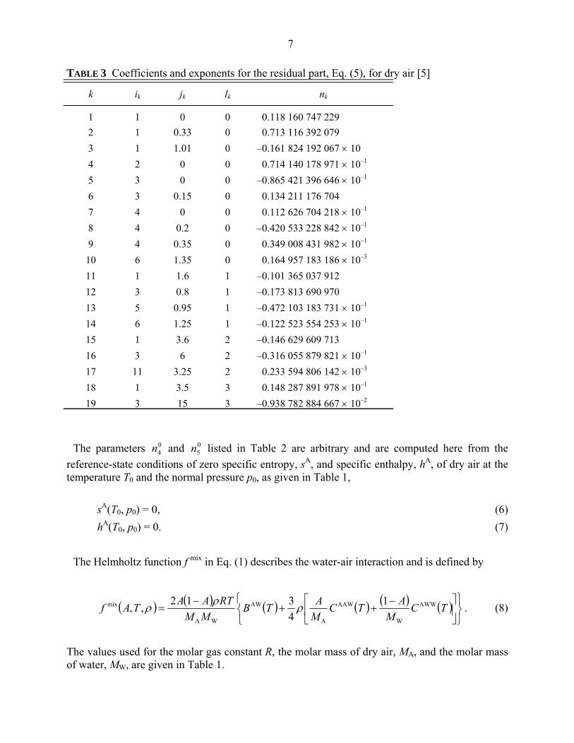
TABLE 3 Coefficients and exponents for the residual part, Eq. (5), for dry air [5]

k ik jk lk nk

1 1 0 0 0.118 160 747 2292 1 0.33 0 0.713 116 392 0793 1 1.01 0 –0.161 824 192 067 × 104 2 0 0 0.714 140 178 971 × 10–1

5 3 0 0 –0.865 421 396 646 × 10–1

6 3 0.15 0 0.134 211 176 7047 4 0 0 0.112 626 704 218 × 10–1

8 4 0.2 0 –0.420 533 228 842 × 10–1

9 4 0.35 0 0.349 008 431 982 × 10–1

10 6 1.35 0 0.164 957 183 186 × 10–3

11 1 1.6 1 –0.101 365 037 91212 3 0.8 1 –0.173 813 690 97013 5 0.95 1 –0.472 103 183 731 × 10–1

14 6 1.25 1 –0.122 523 554 253 × 10–1

15 1 3.6 2 –0.146 629 609 71316 3 6 2 –0.316 055 879 821 × 10–1

17 11 3.25 2 0.233 594 806 142 × 10–3

18 1 3.5 3 0.148 287 891 978 × 10–1

19 3 15 3 –0.938 782 884 667 × 10–2

The parameters 04n and 0

5n listed in Table 2 are arbitrary and are computed here from the reference-state conditions of zero specific entropy, sA, and specific enthalpy, hA, of dry air at the temperature T0 and the normal pressure p0, as given in Table 1,

sA(T0, p0) = 0, (6) hA(T0, p0) = 0. (7)

The Helmholtz function f mix in Eq. (1) describes the water-air interaction and is defined by

( ) ( ) ( ) ( ) ( ) ( )⎭⎬⎫

⎩⎨⎧

⎥⎦

⎤⎢⎣

⎡ −++

−= TC

MATC

MATB

MMRTAATAf AWW

W

AAW

A

AW

WA

mix 14312,, ρρρ . (8)

The values used for the molar gas constant R, the molar mass of dry air, MA, and the molar mass of water, MW, are given in Table 1.

8

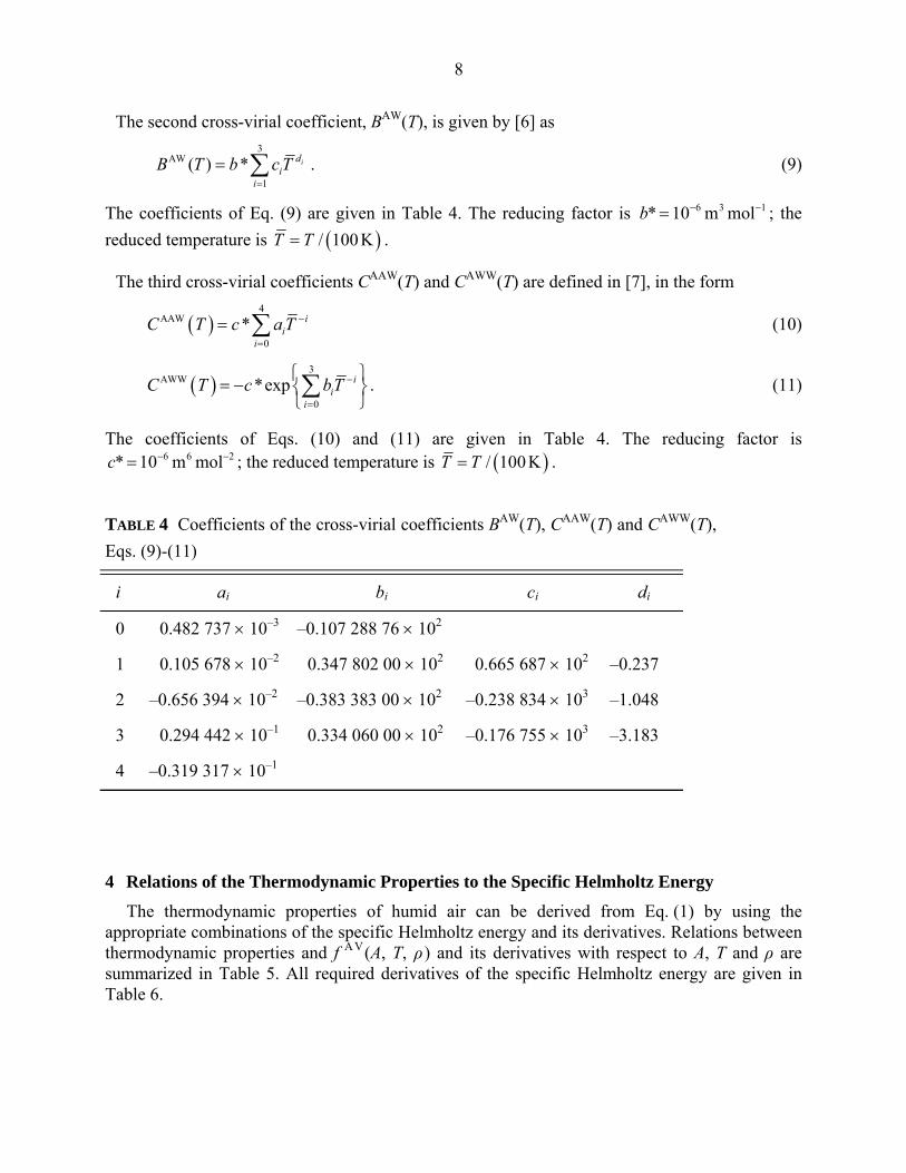
The second cross-virial coefficient, BAW(T), is given by [6] as 3

AW

1( ) * id

ii

B T b c T=

= ∑ . (9)

The coefficients of Eq. (9) are given in Table 4. The reducing factor is 136 molm10* −−=b ; the reduced temperature is ( )/ 100 KT T= .

The third cross-virial coefficients CAAW(T) and CAWW(T) are defined in [7], in the form

( )4

AAW

0* i

ii

C T c a T −

=

= ∑ (10)

( )3

AWW

0*exp i

ii

C T c bT −

=

⎧ ⎫= − ⎨ ⎬

⎩ ⎭∑ . (11)

The coefficients of Eqs. (10) and (11) are given in Table 4. The reducing factor is 266 molm10* −−=c ; the reduced temperature is ( )/ 100 KT T= .

TABLE 4 Coefficients of the cross-virial coefficients BAW(T), CAAW(T) and CAWW(T), Eqs. (9)-(11)

i ai bi ci di

0 0.482 737 × 10–3 –0.107 288 76 × 102

1 0.105 678 × 10–2 0.347 802 00 × 102 0.665 687 × 102 –0.237

2 –0.656 394 × 10–2 –0.383 383 00 × 102 –0.238 834 × 103 –1.048

3 0.294 442 × 10–1 0.334 060 00 × 102 –0.176 755 × 103 –3.183

4 –0.319 317 × 10–1

4 Relations of the Thermodynamic Properties to the Specific Helmholtz Energy

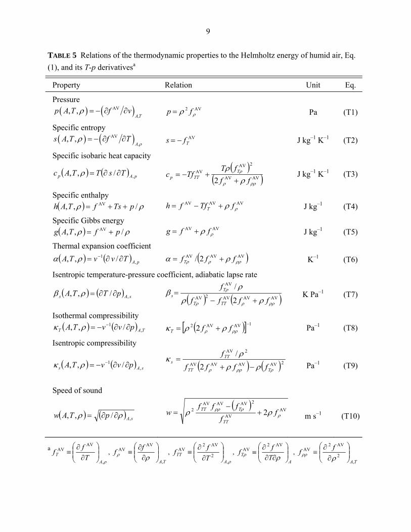
The thermodynamic properties of humid air can be derived from Eq. (1) by using the appropriate combinations of the specific Helmholtz energy and its derivatives. Relations between thermodynamic properties and f

A V(A, T, ρ) and its derivatives with respect to A, T and ρ are summarized in Table 5. All required derivatives of the specific Helmholtz energy are given in Table 6.

9

TABLE 5 Relations of the thermodynamic properties to the Helmholtz energy of humid air, Eq. (1), and its T-p derivativesa

Property Relation Unit Eq.

Pressure ( ) ( )AV, ,

A,Tp A T f vρ = − ∂ ∂ AV2

ρρ fp = Pa (T1)

Specific entropy ( ) ( )AV, ,

A,s A T f T

ρρ = − ∂ ∂ AV

Tfs −= J kg–1 K–1 (T2)

Specific isobaric heat capacity

( ) ( ) pAp TsTTAc ,/,, ∂∂=ρ ( )( )AVAV

2AVAV

2 ρρρ

ρ

ρρ

fffT

Tfc TTTp +

+−= J kg–1 K–1 (T3)

Specific enthalpy ( ) ρρ /,, AV pTsfTAh ++= AVAVAV

ρρ fTffh T +−= J kg–1 (T4)

Specific Gibbs energy ( ) ρρ /,, AV pfTAg += AVAV

ρρ ffg += J kg–1 (T5)

Thermal expansion coefficient ( ) ( ) pATvvTA ,

1 /,, ∂∂= −ρα ( )AVAVAV 2/ ρρρρ ρα fffT += K–1 (T6)

Isentropic temperature-pressure coefficient, adiabatic lapse rate

( ) ( ) sAs pTTA ,/,, ∂∂=ρβ ( ) ( )AVAVAV2AV

AV

2

/

ρρρρ

ρ

ρρ

ρβ

ffff

f

TTT

Ts

+−= K Pa–1 (T7)

Isothermal compressibility ( ) ( ) TAT pvvTA ,

1 /,, ∂∂−= −ρκ ( )[ ] 1AVAV2 2 −+= ρρρ ρρκ ffT Pa–1 (T8)

Isentropic compressibility

( ) ( ) sAs pvvTA ,1 /,, ∂∂−= −ρκ ( ) ( )2AVAVAVAV

2AV

2

/

ρρρρ ρρ

ρκ

TTT

TTs

ffff

f

−+=

Pa–1 (T9)

Speed of sound

( ) ( ) sApTAw ,/,, ρρ ∂∂= ( ) AV

AV

2AVAVAV2 2 ρ

ρρρ ρρ ff

fffw

TT

TTT +−

=

m s–1 (T10)

a

ρ,

AVAV

AT T

ff ⎟⎟⎠

⎞⎜⎜⎝

⎛

∂∂

≡ , TA

ff,

AVAV

⎟⎟⎠

⎞⎜⎜⎝

⎛∂

∂≡

ρρ , ρ,

2

AV2AV

ATT T

ff ⎟⎟⎠

⎞⎜⎜⎝

⎛

∂∂

≡ , A

T Tff ⎟⎟

⎠

⎞⎜⎜⎝

⎛∂∂

∂≡

ρρ

AV2AV ,

TA

ff,

2

AV2AV

⎟⎟⎠

⎞⎜⎜⎝

⎛

∂∂

≡ρρρ

10

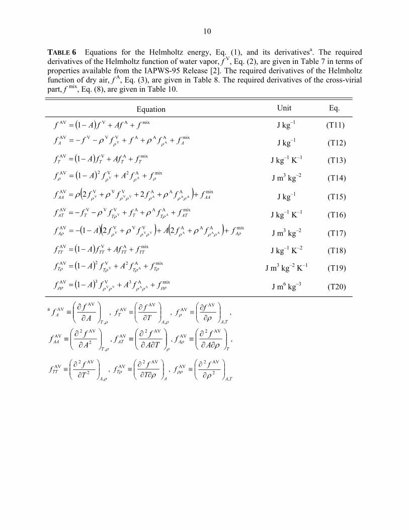
TABLE 6 Equations for the Helmholtz energy, Eq. (1), and its derivativesa. The required derivatives of the Helmholtz function of water vapor, f

V, Eq. (2), are given in Table 7 in terms of

properties available from the IAPWS-95 Release [2]. The required derivatives of the Helmholtz function of dry air, f A, Eq. (3), are given in Table 8. The required derivatives of the cross-virial part, f mix, Eq. (8), are given in Table 10.

Equation Unit Eq.

( ) mixAVAV 1 fAffAf ++−= J kg–1 (T11) mixAAAVVVAV

AV AA ffffff +++−−=ρρ

ρρ J kg–1 (T12)

( ) mixAVAV 1 TTTT fAffAf ++−= J kg–1 K–1 (T13)

( ) mixA2V2AVAV1 ρρρρ ffAfAf ++−= J m3 kg–2 (T14)

( ) mixAAAVVVAVAAAVVV 22 AAAA ffffff ++++=

ρρρρρρρρρ J kg–1 (T15)

mixAAAVVVAVAV ATTTTTAT ffffff +++−−=

ρρρρ J kg–1 K–1 (T16)

( )( ) ( ) mixAAAVVVAVAAAVVV 221 ρρρρρρρρ ρρ AA fffAffAf ++++−−= J m3 kg–2 (T17)

( ) mixAVAV 1 TTTTTTTT fAffAf ++−= J kg–1 K–2 (T18)

( ) mixA2V2AVAV1 ρρρρ TTTT ffAfAf ++−= J m3 kg–2 K–1 (T19)

( ) mixA3V3AVAAVV1 ρρρρρρρρ ffAfAf ++−= J m6 kg–3 (T20)

a

ρ,

AVAV

TA A

ff ⎟⎟⎠

⎞⎜⎜⎝

⎛∂

∂≡ ,

ρ,

AVAV

AT T

ff ⎟⎟⎠

⎞⎜⎜⎝

⎛

∂∂

≡ , TA

ff,

AVAV

⎟⎟⎠

⎞⎜⎜⎝

⎛∂

∂≡

ρρ ,

ρ,2

AV2AV

TAA A

ff ⎟⎟⎠

⎞⎜⎜⎝

⎛∂

∂≡ ,

ρ⎟⎟⎠

⎞⎜⎜⎝

⎛∂∂

∂≡

TAff AT

AV2AV ,

TA A

ff ⎟⎟⎠

⎞⎜⎜⎝

⎛∂∂

∂≡

ρρ

AV2AV ,

ρ,2

AV2AV

ATT T

ff ⎟⎟⎠

⎞⎜⎜⎝

⎛

∂∂

≡ , A

T Tff ⎟⎟

⎠

⎞⎜⎜⎝

⎛∂∂

∂≡

ρρ

AV2AV ,

TA

ff,

2

AV2AV

⎟⎟⎠

⎞⎜⎜⎝

⎛

∂∂

≡ρρρ

11

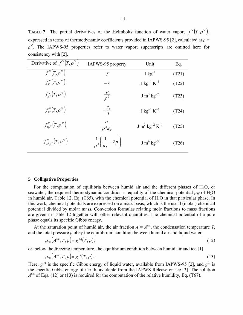
TABLE 7 The partial derivatives of the Helmholtz function of water vapor, ( )VV , ρTf ,

expressed in terms of thermodynamic coefficients provided in IAPWS-95 [2], calculated at ρ = ρV. The IAPWS-95 properties refer to water vapor; superscripts are omitted here for consistency with [2].

Derivative of ( )VV , ρTf IAPWS-95 property Unit Eq.

( )VV , ρTf f J kg–1 (T21)

( )VV , ρTfT s− J kg–1 K–1 (T22)

( )VV ,V ρρ

Tf 2ρp J m3 kg–2 (T23)

( )VV , ρTfTT Tcv− J kg–1 K–2 (T24)

( )VV ,V ρρ

TfT Tκρ

α2 J m3 kg–2 K–1 (T25)

( )VV ,VV ρρρ

Tf ⎟⎟⎠

⎞⎜⎜⎝

⎛− p

T

2113 κρ

J m6 kg–3 (T26)

5 Colligative Properties For the computation of equilibria between humid air and the different phases of H2O, or

seawater, the required thermodynamic condition is equality of the chemical potential μW of H2O in humid air, Table 12, Eq. (T65), with the chemical potential of H2O in that particular phase. In this work, chemical potentials are expressed on a mass basis, which is the usual (molar) chemical potential divided by molar mass. Conversion formulas relating mole fractions to mass fractions are given in Table 12 together with other relevant quantities. The chemical potential of a pure phase equals its specific Gibbs energy.

At the saturation point of humid air, the air fraction A = Asat, the condensation temperature T, and the total pressure p obey the equilibrium condition between humid air and liquid water,

( ) ( )pTgpTA ,,, liqsatW =μ , (12)

or, below the freezing temperature, the equilibrium condition between humid air and ice [1], ( ) ( )pTgpTA ,,, Ihsat

W =μ . (13) Here, gliq is the specific Gibbs energy of liquid water, available from IAPWS-95 [2], and gIh is the specific Gibbs energy of ice Ih, available from the IAPWS Release on ice [3]. The solution Asat of Eqs. (12) or (13) is required for the computation of the relative humidity, Eq. (T67).

12

The equilibrium between humid air and seawater obeys the condition [1], ( ) ( )pTSpTA ,,,, SW

Wcond

W μμ = . (14)

Here, Acond is the air fraction at the condensation point in contact with seawater, S is the absolute salinity and SW

Wμ is the chemical potential of water in seawater, available from the IAPWS Release on seawater [4]. Humid air in equilibrium with seawater, S > 0, is always subsaturated, Acond > Asat, if no ice is present, i.e., if the temperature is higher than the freezing temperature of seawater.

In Eqs. (12) and (14), the dissolution of the constituents of air in the liquid phase is neglected.

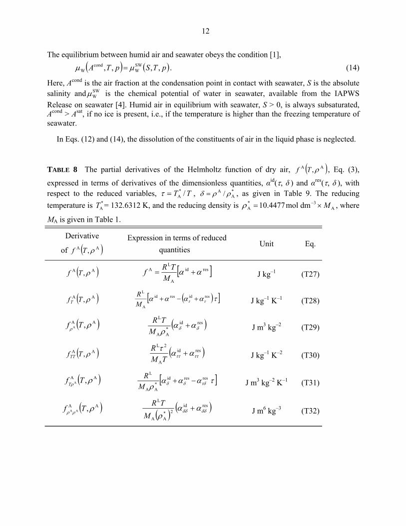
TABLE 8 The partial derivatives of the Helmholtz function of dry air, ( )AA , ρTf , Eq. (3),

expressed in terms of derivatives of the dimensionless quantities, αid(τ, δ ) and αres(τ, δ ), with respect to the reduced variables, TT /*

A=τ , *A

A / ρρδ = , as given in Table 9. The reducing temperature is *

AT = 132.6312 K, and the reducing density is A3*

A dmmol4477.10 M×= −ρ , where

MA is given in Table 1.

Derivative

of ( )AA , ρTf Expression in terms of reduced

quantities Unit Eq.

( )AA , ρTf [ ]resid

A

LA αα +=

MTRf J kg–1 (T27)

( )AA , ρTfT ( )[ ]ταααα ττresidresid

A

L

+−+MR J kg–1 K–1 (T28)

( )AA ,A ρρ

Tf ( )resid*AA

L

δδ ααρ

+M

TR J m3 kg–2 (T29)

( )AA , ρTfTT ( )resid

A

2L

ττττ αατ+

TMR J kg–1 K–2 (T30)

( )AA ,A ρρ

TfT [ ]ταααρ τδδδ

resresid*AA

L

−+M

R J m3 kg–2 K–1 (T31)

( )AA ,AA ρρρ

Tf ( ) ( )resid2*

AA

L

δδδδ ααρ

+M

TR J m6 kg–3 (T32)

13

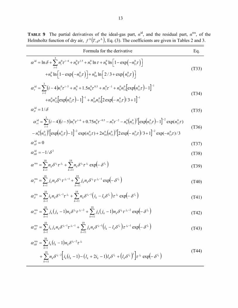
TABLE 9 The partial derivatives of the ideal-gas part, αid, and the residual part, αres, of the Helmholtz function of dry air, ( )AA , ρTf , Eq. (3). The coefficients are given in Tables 2 and 3.

Formula for the derivative Eq.

( )

( ) ( )

5id 0 4 0 1.5 0 0 0

6 7 8 111

0 0 0 09 12 10 13

ln ln ln 1 exp

ln 1 exp ln 2 / 3 exp

ii

in n n n n

n n n n

α δ τ τ τ τ

τ τ

−

=

⎡ ⎤= + + + + − −⎣ ⎦

⎡ ⎤ ⎡ ⎤+ − − + +⎣ ⎦ ⎣ ⎦

∑ (T33)

( ) ( )[ ]

( )[ ] ( )[ ] 1013

013

010

1012

012

09

1011

011

08

107

5.006

05

3

1

50id

13/exp21exp

1exp5.14

−−

−−

=

−

+−+−+

−++++−= ∑

ττ

ττττατ

nnnnnn

nnnnnnnii

ii

(T34)

δαδ /1id = (T35)

( )( ) ( ) ( )[ ]

( ) ( )[ ] ( ) ( )[ ] 3/)exp(13/exp22)exp(1exp

)exp(1exp75.054

013

2013

2013

010

012

2012

2012

09

011

2011

2011

08

207

5.006

3

1

60id

ττττ

ττττταττ

nnnnnnnn

nnnnnnniii

ii

−+−+−−

−−−+−−=

−−

−−−

=

−∑ (T36)

0id =τδα (T37)2id /1 δαδδ −= (T38)

( )∑∑==

−+=19

11

10

1

res expk

ljik

k

jik

kkkkk nn δτδτδα (T39)

( )∑∑=

−

=

− −+=19

11

110

1

1res expk

ljikk

k

jikk

kkkkk njnj δτδτδατ (T40)

( ) ( )∑∑=

−

=

− −−+=19

11

110

1

1res expk

ljlkk

ik

k

jikk

kkkkkk linni δτδδτδαδ (T41)

( ) ( ) ( )∑∑=

−

=

− −−+−=19

11

210

1

2res exp11k

ljikkk

k

jikkk

kkkkk njjnjj δτδτδαττ (T42)

( ) ( )∑∑=

−−

=

−− −−+=19

11

1110

1

11res expk

ljlkk

ikk

k

jikkk

kkkkkk linjnji δτδδτδατδ (T43)

( )

( ) ( ) ( )[ ] ( )∑

∑

=

−

=

−

−+−+−−+

−=

19

11

22

10

1

2res

exp121

1

k

ljlk

lkkkkk

ik

k

jikkk

kkkkk

kk

lliliin

nii

δτδδδ

τδαδδ

(T44)

14

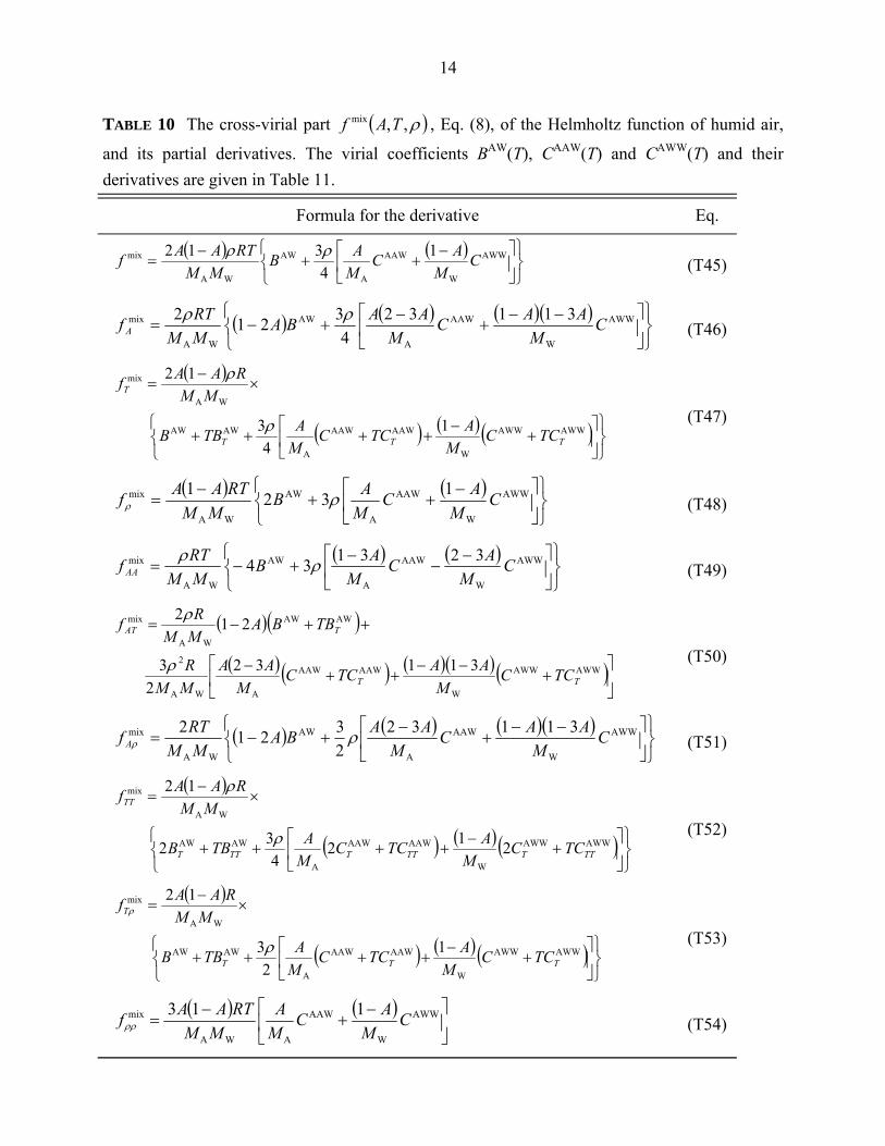
TABLE 10 The cross-virial part ( )ρ,,mix TAf , Eq. (8), of the Helmholtz function of humid air,

and its partial derivatives. The virial coefficients BAW(T), CAAW(T) and CAWW(T) and their derivatives are given in Table 11.

Formula for the derivative Eq.

( ) ( )⎭⎬⎫

⎩⎨⎧

⎥⎦

⎤⎢⎣

⎡ −++

−= AWW

W

AAW

A

AW

WA

mix 14

312 CM

ACMAB

MMRTAAf ρρ (T45)

( ) ( ) ( )( )⎭⎬⎫

⎩⎨⎧

⎥⎦

⎤⎢⎣

⎡ −−+

−+−= AWW

W

AAW

A

AW

WA

mix 311324

3212 CM

AACM

AABAMMRTf A

ρρ (T46)

( )

( ) ( ) ( )⎭⎬⎫

⎩⎨⎧

⎥⎦

⎤⎢⎣

⎡+

−++++

×−

=

AWWAWW

W

AAWAAW

A

AWAW

WA

mix

14

3

12

TTT

T

TCCM

ATCCMATBB

MMRAAf

ρ

ρ

(T47)

( ) ( )⎭⎬⎫

⎩⎨⎧

⎥⎦

⎤⎢⎣

⎡ −++

−= AWW

W

AAW

A

AW

WA

mix 1321 CM

ACMAB

MMRTAAf ρρ (T48)

( ) ( )⎭⎬⎫

⎩⎨⎧

⎥⎦

⎤⎢⎣

⎡ −−

−+−= AWW

W

AAW

A

AW

WA

mix 323134 CM

ACM

ABMMRTf AA ρρ (T49)

( )( )

( ) ( ) ( )( ) ( )⎥⎦

⎤⎢⎣

⎡+

−−++

−

++−=

AWWAWW

W

AAWAAW

AWA

2

AWAW

WA

mix

311322

3

212

TT

TAT

TCCM

AATCCM

AAMMR

TBBAMMRf

ρ

ρ

(T50)

( ) ( ) ( )( )⎭⎬⎫

⎩⎨⎧

⎥⎦

⎤⎢⎣

⎡ −−+

−+−= AWW

W

AAW

A

AW

WA

mix 3113223212 C

MAAC

MAABA

MMRTf A ρρ (T51)

( )

( ) ( ) ( )⎭⎬⎫

⎩⎨⎧

⎥⎦

⎤⎢⎣

⎡+

−++++

×−

=

AWWAWW

W

AAWAAW

A

AWAW

WA

mix

2124

32

12

TTTTTTTTT

TT

TCCM

ATCCMATBB

MMRAAf

ρ

ρ

(T52)

( )

( ) ( ) ( )⎭⎬⎫

⎩⎨⎧

⎥⎦

⎤⎢⎣

⎡+

−++++

×−

=

AWWAWW

W

AAWAAW

A

AWAW

WA

mix

12

3

12

TTT

T

TCCM

ATCCMATBB

MMRAAf

ρ

ρ

(T53)

( ) ( )⎥⎦

⎤⎢⎣

⎡ −+

−= AWW

W

AAW

AWA

mix 113 CM

ACMA

MMRTAAfρρ (T54)

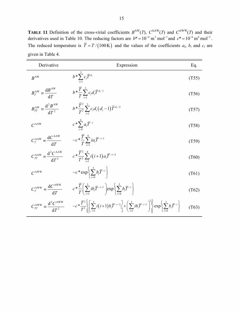
15

TABLE 11 Definition of the cross-virial coefficients BAW(T), CAAW(T) and CAWW(T) and their derivatives used in Table 10. The reducing factors are 136 molm10* −−=b and 266 molm10* −−=c . The reduced temperature is ( )/ 100 KT T= and the values of the coefficients ai, bi and ci are

given in Table 4.

Derivative Expression Eq.

AWB 3

1* id

ii

b c T=∑ (T55)

TBBT d

d AWAW ≡

31

1* id

i ii

Tb c d TT

−

=∑ (T56)

2

AW2AW

dd

TBBTT ≡ ( )

2 32

21

* 1 idi i i

i

Tb c d d TT

−

=

−∑ (T57)

AAWC 4

0* i

ii

c a T −

=∑ (T58)

TCCT d

d AAWAAW ≡

41

1* i

ii

Tc ia TT

− −

=

− ∑ (T59)

2

AAW2AAW

dd

TCCTT ≡ ( )

2 42

21

* 1 ii

i

Tc i i a TT

− −

=

+∑ (T60)

AWWC 3

0*exp i

ii

c bT −

=

⎧ ⎫− ⎨ ⎬

⎩ ⎭∑ (T61)

TCCT d

d AWWAWW ≡

3 31

1 0* expi i

i ii i

Tc ibT bTT

− − −

= =

⎛ ⎞ ⎧ ⎫⎨ ⎬⎜ ⎟

⎝ ⎠ ⎩ ⎭∑ ∑ (T62)

2

AWW2AWW

dd

TCCTT ≡ ( )

22 3 3 32 1

21 1 0

* 1 expi i ii i i

i i i

Tc i i bT ibT bTT

− − − − −

= = =

⎧ ⎫⎡ ⎤ ⎛ ⎞ ⎧ ⎫⎪ ⎪− + +⎨ ⎬ ⎨ ⎬⎜ ⎟⎢ ⎥⎣ ⎦ ⎝ ⎠ ⎩ ⎭⎪ ⎪⎩ ⎭∑ ∑ ∑ (T63)

16

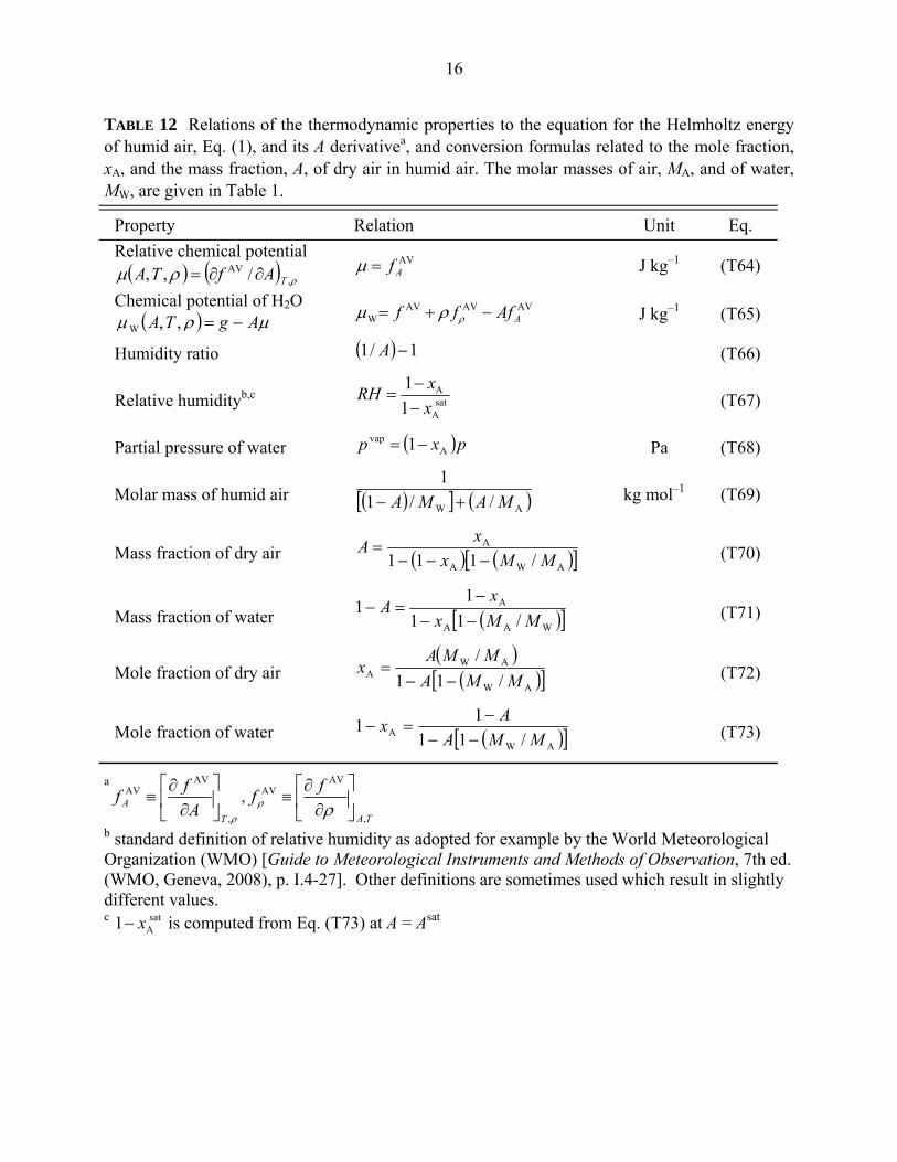
TABLE 12 Relations of the thermodynamic properties to the equation for the Helmholtz energy of humid air, Eq. (1), and its A derivativea, and conversion formulas related to the mole fraction, xA, and the mass fraction, A, of dry air in humid air. The molar masses of air, MA, and of water, MW, are given in Table 1.

Property Relation Unit Eq. Relative chemical potential

( ) ( ) ρρμ ,AV /,, TAfTA ∂∂=

AVAf=μ J kg–1 (T64)

Chemical potential of H2O ( ) μρμ AgTA −=,,W

AVAVAVW AAfff −+= ρρμ J kg–1 (T65)

Humidity ratio ( ) 1/1 −A (T66)

Relative humidityb,c Asat

A

11

xRHx

−=

− (T67)

Partial pressure of water ( )pxp Avap 1−= Pa (T68)

Molar mass of humid air ( )[ ] ( )AW //11

MAMA +− kg mol–1 (T69)

Mass fraction of dry air ( ) ( )[ ]AWA

A

/111 MMxxA−−−

= (T70)

Mass fraction of water ( )[ ]WAA

A

/111

1MMx

xA

−−−

=− (T71)

Mole fraction of dry air ( )

( )[ ]AW

AWA /11

/MMA

MMAx

−−= (T72)

Mole fraction of water ( )[ ]AWA /11

11MMA

Ax−−

−=− (T73)

a

ρ,

AVAV

TA A

ff ⎥⎦

⎤⎢⎣

⎡∂

∂≡ ,

TA

ff,

AVAV

⎥⎦

⎤⎢⎣

⎡∂

∂≡

ρρ

b standard definition of relative humidity as adopted for example by the World Meteorological Organization (WMO) [Guide to Meteorological Instruments and Methods of Observation, 7th ed. (WMO, Geneva, 2008), p. I.4-27]. Other definitions are sometimes used which result in slightly different values. c sat

A1 x− is computed from Eq. (T73) at A = Asat

17

6 Range of Validity and Brief Discussion

The equation of state, Eq. (1), is valid for humid air within the temperature and pressure range 193 K ≤ Τ ≤ 473 K and 0 < p ≤ 5 MPa.

The pressure is computed from Eq. (T1). All validity regions of the formulas combined in Eq. (1), including the Helmholtz functions of water vapor and dry air, as well as the cross-virial coefficients, overlap only in this range. The separate ranges of validity of the individual components are wider, for some of them significantly. Therefore, Eq. (1) will also provide reasonable results outside of the T-p range given above if one component dominates numerically in Eq. (1) and is evaluated within its particular range of validity.

The air fraction A can take any value between 0 and 1 provided that the partial pressure of water, pvap, Eq. (T68), does not exceed its saturation value, i.e.,

0 < Α < 1 and Asat(T, p) ≤ A. The exact value of the air fraction Asat(T, p) of saturated humid air is given by equal chemical

potentials of water in humid air and of either liquid water, Eq. (12), if the temperature is above the freezing point, or of ice, Eq. (13), if the temperature is below the freezing point. At low density, the partial pressure pvap,sat of saturated humid air can be estimated by either the correlation function for the vapor pressure, psat(T), of liquid water [12], or for the sublimation pressure, psubl(T), of ice [13], to obtain ( ) ( ) ( )[ ]AW

satvap,satvap,sat /1/, MMpppppTA −−−= , from Eq. (T70) as a sufficient practical approximation.

This formulation for the thermodynamic properties of humid air was developed in cooperation with the SCOR/IAPSO Working Group 127 on Thermodynamics and Equation of State of Seawater.

7 Estimates of Uncertainty

Here, estimated combined standard uncertainties uc [14] are reported, from which expanded uncertainties U = k uc can be obtained by multiplying with the coverage factor k = 2, corresponding to a 95% confidence level. The term “uncertainty” used in the following refers to combined standard uncertainties or to relative combined standard uncertainties.

Uncertainty estimates are not directly available for the full Helmholtz function of humid air, Eq. (1), or the properties derived from it. Rather, comprehensive uncertainty estimates are available only for the formulations of its parts, dry air [5] and water vapor [2]. In the range considered here, the dry-air uncertainty of the density is 0.1%, of the sound speed is 0.2% and of the heat capacity is 1%.

The uncertainties of the second cross-virial coefficient BAW(T) and of its enthalpy coefficient, BAW – T dBAW/dT, as functions of the temperature are tabulated in [6]. They decrease monotonically from about 8 and 24 cm3 mol–1 at 150 K, to 2 and 5 cm3 mol–1 at 300 K, and to 0.3 and 0.5 cm3 mol–1, respectively, at 2000 K. The agreement of values computed from Eq. (T68) with experimental data for the partial pressure of water in saturated air is better than 0.5% up to densities of 50 kg m–3 and about 1% at 100 kg m–3 [1].

18

8 Computer-Program Verification

To assist the user in computer-program verification, Tables 13, 14 and 15 with test values are given for specified parameter values of saturated air. They contain values for the specific Helmholtz energy, f

A V(A, T, ρ), and its parts together with their first and second derivatives, as well as some thermodynamic properties.

9 References

[1] Feistel, R., Wright, D.G., Kretzschmar, H.-J., Hagen, E., Herrmann, S., and Span, R., Ocean Sci. 6, 91 (2010). Available at http://www.ocean-sci.net/6/91/2010/

[2] IAPWS, Revised Release on the IAPWS Formulation 1995 for the Thermodynamic Properties of Ordinary Water Substance for General and Scientific Use (2009). Available from http://www.iapws.org

[3] IAPWS, Revised Release on the Equation of State 2006 for H2O Ice Ih (2009). Available from http://www.iapws.org

[4] IAPWS, Release on the IAPWS Formulation 2008 for the Thermodynamic Properties of Seawater (2008). Available from http://www.iapws.org

[5] Lemmon, E.W., Jacobsen, R.T, Penoncello, S.G., and Friend, D.G., J. Phys. Chem. Ref. Data 29, 331 (2000).

[6] Harvey, A.H., and Huang, P.H., Int. J. Thermophys. 28, 556 (2007).

[7] Hyland, R.W., and Wexler, A., ASHRAE Transact. 89, 520 (1983).

[8] IAPWS, Guideline on the Use of Fundamental Physical Constants and Basic Constants of Water (2005). Available from http://www.iapws.org

[9] Preston-Thomas, H., Metrologia 27, 3 (1990).

[10] Picard, A., Davis, R.S., Gläser, M., and Fujii, K., Metrologia 45, 149 (2008).

[11] ISO, ISO Standards Handbook: Quantities and Units (International Organization for Standard-ization, Geneva, 1993).

[12] IAPWS, Revised Supplementary Release on Saturation Properties of Ordinary Water Substance (1992). Available from http://www.iapws.org

[13] IAPWS, Revised Release on the Pressure along the Melting and Sublimation Curves of Ordinary Water Substance (2011). Available from http://www.iapws.org

[14] ISO, Guide to the Expression of Uncertainty in Measurement (International Organization for Standardization, Geneva, 1993). Available at http://www.bipm.org/utils/common/documents/jcgm/JCGM_100_2008_E.pdf

19

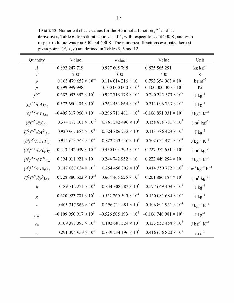
TABLE 13 Numerical check values for the Helmholtz function f

AV and its derivatives, Table 6, for saturated air, A = Asat, with respect to ice at 200 K, and with respect to liquid water at 300 and 400 K. The numerical functions evaluated here at given points (A, T, ρ) are defined in Tables 5, 6 and 12.

Quantity Value Value Value Unit

A 0.892 247 719 0.977 605 798 0.825 565 291 kg kg–1 T 200 300 400 K ρ 0.163 479 657 × 10–4 0.114 614 216 × 10 0.793 354 063 × 10 kg m–3 p 0.999 999 998 0.100 000 000 × 106 0.100 000 000 × 107 Pa

f AV –0.682 093 392 × 106 –0.927 718 178 × 105 0.240 345 570 × 105 J kg–1

(∂f AV/∂A)T,ρ –0.572 680 404 × 106 –0.263 453 864 × 103 0.311 096 733 × 106 J kg–1

(∂f AV/∂T )A,ρ –0.405 317 966 × 104 –0.296 711 481 × 103 –0.106 891 931 × 104 J kg–1 K–1

(∂f AV/∂ρ)A,T 0.374 173 101 × 1010 0.761 242 496 × 105 0.158 878 781 × 105 J m3 kg–2

(∂2f AV/∂A2)T,ρ 0.920 967 684 × 106 0.624 886 233 × 107 0.113 786 423 × 107 J kg–1

(∂2f AV/∂A∂T )ρ 0.915 653 743 × 104 0.822 733 446 × 104 0.702 631 471 × 104 J kg–1 K–1

(∂2f AV/∂A∂ρ)T –0.213 442 099 × 1010 –0.450 004 399 × 105 –0.727 972 651 × 104 J m3 kg–2

(∂2f AV/∂T 2)A,ρ –0.394 011 921 × 10 –0.244 742 952 × 10 –0.222 449 294 × 10 J kg–1 K–2

(∂2f AV/∂T∂ρ)A 0.187 087 034 × 108 0.254 456 302 × 103 0.414 350 772 × 102 J m3 kg–2 K–1

(∂2f AV/∂ρ2)A,T –0.228 880 603 × 1015 –0.664 465 525 × 105 –0.201 886 184 × 104 J m6 kg–3

h 0.189 712 231 × 106 0.834 908 383 × 105 0.577 649 408 × 106 J kg–1

g –0.620 923 701 × 106 –0.552 260 595 × 104 0.150 081 684 × 106 J kg–1

s 0.405 317 966 × 104 0.296 711 481 × 103 0.106 891 931 × 104 J kg–1 K–1

μW –0.109 950 917 × 106 –0.526 505 193 × 104 –0.106 748 981 × 106 J kg–1

cp 0.109 387 397 × 104 0.102 681 324 × 104 0.123 552 454 × 104 J kg–1 K–1

w 0.291 394 959 × 103 0.349 234 196 × 103 0.416 656 820 × 103 m s–1

20

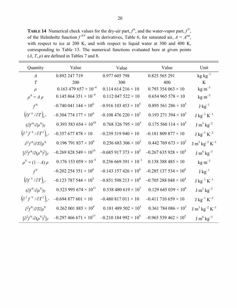
TABLE 14 Numerical check values for the dry-air part, f A, and the water-vapor part, f V,

of the Helmholtz function f AV and its derivatives, Table 6, for saturated air, A = Asat, with respect to ice at 200 K, and with respect to liquid water at 300 and 400 K, corresponding to Table 13. The numerical functions evaluated here at given points (A, T, ρ) are defined in Tables 7 and 8.

Quantity Value Value Value Unit

A 0.892 247 719 0.977 605 798 0.825 565 291 kg kg–1 T 200 300 400 K ρ 0.163 479 657 × 10–4 0.114 614 216 × 10 0.793 354 063 × 10 kg m–3

ρA = A ρ 0.145 864 351 × 10–4 0.112 047 522 × 10 0.654 965 578 × 10 kg m–3

f A –0.740 041 144 × 106 –0.916 103 453 × 105 0.895 561 286 × 105 J kg–1

( ) A/AρTf ∂∂ –0.304 774 177 × 104 –0.108 476 220 × 103 0.193 271 394 × 103 J kg–1 K–1

(∂f A/∂ρA)T 0.393 583 654 × 1010 0.768 326 795 × 105 0.175 560 114 × 105 J m3 kg–2

( ) A2A2 / ρTf ∂∂ –0.357 677 878 × 10 –0.239 319 940 × 10 –0.181 809 877 × 10 J kg–1 K–2

∂2 f A/∂T∂ρA 0.196 791 837 × 108 0.256 683 306 × 103 0.442 769 673 × 102 J m3 kg–2 K–1

[∂2f A/∂(ρA)2]T –0.269 828 549 × 1015 –0.685 917 373 × 105 –0.267 635 928 × 104 J m6 kg–3

ρV = (1 – A) ρ 0.176 153 059 × 10–5 0.256 669 391 × 10–1 0.138 388 485 × 10 kg m–3

f V –0.202 254 351 × 106 –0.143 157 426 × 106 –0.285 137 534 × 106 J kg–1

( ) V/VρTf ∂∂ –0.123 787 544 × 105 –0.851 598 213 × 104 –0.705 288 048 × 104 J kg–1 K–1

(∂f V/∂ρV)T 0.523 995 674 × 1011 0.538 480 619 × 107 0.129 645 039 × 106 J m3 kg–2

( ) V2V2 / ρTf ∂∂ –0.694 877 601 × 10 –0.480 817 011 × 10 –0.411 710 659 × 10 J kg–1 K–2

∂2f V/∂T∂ρV 0.262 001 885 × 109 0.181 489 502 × 105 0.361 784 086 × 103 J m3 kg–2 K–1

[∂2f V/∂(ρV)2]T –0.297 466 671 × 1017 –0.210 184 992 × 109 –0.965 539 462 × 105 J m6 kg–3

21

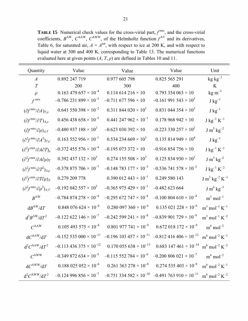
TABLE 15 Numerical check values for the cross-virial part, f mix, and the cross-virial coefficients, BAW, CAAW, CAWW, of the Helmholtz function f

AV and its derivatives, Table 6, for saturated air, A = Asat, with respect to ice at 200 K, and with respect to liquid water at 300 and 400 K, corresponding to Table 13. The numerical functions evaluated here at given points (A, T, ρ) are defined in Tables 10 and 11.

Quantity Value Value Value Unit

A 0.892 247 719 0.977 605 798 0.825 565 291 kg kg–1 T 200 300 400 K ρ 0.163 479 657 × 10–4 0.114 614 216 × 10 0.793 354 063 × 10 kg m–3

f mix –0.786 231 899 × 10–3 –0.711 677 596 × 10 –0.161 991 543 × 103 J kg–1

(∂f mix/∂A)T,ρ 0.641 550 398 × 10–2 0.311 844 020 × 103 0.831 044 354 × 103 J kg–1

(∂f mix/∂T)A,ρ 0.456 438 658 × 10–5 0.441 247 962 × 10–1 0.178 968 942 × 10 J kg–1 K–1

(∂f mix/∂ρ)A,T –0.480 937 188 × 102 –0.623 030 392 × 10 –0.223 330 257 × 102 J m3 kg–2

(∂2f mix/∂A2)T,ρ 0.163 552 956 × 10–1 0.534 234 669 × 103 0.135 814 949 × 104 J kg–1

(∂2f mix/∂A∂T)ρ –0.372 455 576 × 10–4 –0.195 073 372 × 10 –0.916 854 756 × 10 J kg–1 K–1

(∂2f mix/∂A∂ρ)T 0.392 437 132 × 103 0.274 155 508 × 103 0.125 834 930 × 103 J m3 kg–2

(∂2f mix/∂T2)A,ρ –0.378 875 706 × 10–7 –0.148 783 177 × 10–3 –0.536 741 578 × 10–2 J kg–1 K–2

(∂2f mix/∂T∂ρ)A 0.279 209 778 0.390 012 443 × 10–1 0.249 580 143 J m3 kg–2 K–1

(∂2f mix/∂ρ2)A,T –0.192 042 557 × 102 –0.365 975 429 × 10–1 –0.482 623 664 J m6 kg–3

BAW –0.784 874 278 × 10–4 –0.295 672 747 × 10–4 –0.100 804 610 × 10–4 m3 mol–1

dBAW/dT 0.848 076 624 × 10–6 0.280 097 360 × 10–6 0.135 021 228 × 10–6 m3 mol–1 K–1

d2BAW/dT 2 –0.122 622 146 × 10–7 –0.242 599 241 × 10–8 –0.839 901 729 × 10–9 m3 mol–1 K–2

CAAW 0.105 493 575 × 10–8 0.801 977 741 × 10–9 0.672 018 172 × 10–9 m6 mol–2

dCAAW/dT –0.152 535 000 × 10–11 –0.196 103 457 × 10–11 –0.812 416 406 × 10–12 m6 mol–2 K–1

d2CAAW/dT 2 –0.113 436 375 × 10–12 0.170 055 638 × 10–13 0.683 147 461 × 10–14 m6 mol–2 K–2

CAWW –0.349 872 634 × 10–5 –0.115 552 784 × 10–6 –0.200 806 021 × 10–7 m6 mol–2

dCAWW/dT 0.188 025 052 × 10–6 0.261 363 278 × 10–8 0.274 535 403 × 10–9 m6 mol–2 K–1

d2CAWW/dT 2 –0.124 996 856 × 10–7 –0.751 334 582 × 10–10 –0.491 763 910 × 10–11 m6 mol–2 K–2